Introduction to Astronomical Photometry
452
-
Upload
sergio-alejandro-fuentealba-zuniga -
Category
Documents
-
view
241 -
download
2
Transcript of Introduction to Astronomical Photometry

7/21/2019 Introduction to Astronomical Photometry
http://slidepdf.com/reader/full/introduction-to-astronomical-photometry 1/451

7/21/2019 Introduction to Astronomical Photometry
http://slidepdf.com/reader/full/introduction-to-astronomical-photometry 2/451
This page intentionally left blank
7/21/2019 Introduction to Astronomical Photometry
http://slidepdf.com/reader/full/introduction-to-astronomical-photometry 3/451
Introduction to Astronomical Photometry, Second Edition
Completely updated, this Second Edition gives a broad review of astronomical photometry to provide an understanding of astrophysics from adata-based perspective. It explains the underlying principles of theinstruments used, and the applications and inferences derived frommeasurements. Each chapter has been fully revised to account for the latestdevelopments, including the use of CCDs.
Highly illustrated, this book provides an overview and historicalbackground of the subject before reviewing the main themes withinastronomical photometry. The central chapters focus on the practical designof the instruments and methodology used. The book concludes by discussingspecialized topics in stellar astronomy, concentrating on the information thatcan be derived from the analysis of the light curves of variable stars andclose binary systems. This new edition includes numerous bibliographicnotes and a glossary of terms. It is ideal for graduate students, academic
researchers and advanced amateurs interested in practical and observationalastronomy.
Edwin Budding is a research fellow at the Carter Observatory, NewZealand, and a visiting professor at the Çanakkale University, Turkey.
Osman Demircan is Director of the Ulupınar Observatory of ÇanakkaleUniversity, Turkey.

7/21/2019 Introduction to Astronomical Photometry
http://slidepdf.com/reader/full/introduction-to-astronomical-photometry 4/451
7/21/2019 Introduction to Astronomical Photometry
http://slidepdf.com/reader/full/introduction-to-astronomical-photometry 5/451
Cambridge Observing Handbooks for Research Astronomers
Today’s professional astronomers must be able to adapt to use telescopesand interpret data at all wavelengths. This series is designed to provide themwith a collection of concise, self-contained handbooks, which covers thebasic principles peculiar to observing in a particular spectral region, or tousing a special technique or type of instrument. The books can be used as anintroduction to the subject and as a handy reference for use at the telescope,
or in the office.
Series editors
Professor Richard Ellis, Astronomy Department, California Institute of
Technology
Professor John Huchra, Center for Astrophysics, Smithsonian Astrophysical
Observatory
Professor Steve Kahn, Department of Physics, Columbia University,
New YorkProfessor George Rieke, Steward Observatory, University of Arizona, TucsonDr Peter B. Stetson, Herzberg Institute of Astrophysics, Dominion Astrophys-
ical Observatory, Victoria, British Columbia

7/21/2019 Introduction to Astronomical Photometry
http://slidepdf.com/reader/full/introduction-to-astronomical-photometry 6/451
7/21/2019 Introduction to Astronomical Photometry
http://slidepdf.com/reader/full/introduction-to-astronomical-photometry 7/451
Introduction to Astronomical
Photometry
Second Edition
E D W I N B U D D I N G & O S M A N D E M I R C A NÇanakkale University, Turkey
7/21/2019 Introduction to Astronomical Photometry
http://slidepdf.com/reader/full/introduction-to-astronomical-photometry 8/451
CAMBRIDGE UNIVERSITY PRESS
Cambridge, New York, Melbourne, Madrid, Cape Town, Singapore, São Paulo
Cambridge University PressThe Edinburgh Building, Cambridge CB2 8RU, UK
First published in print format
ISBN-13 978-0-521-84711-7
ISBN-13 978-0-511-33503-7
© E. Budding and O. Demircan 2007
Information on this title: www.cambridge.org/9780521847117
This publication is in copyright. Subject to statutory exception and to the provision ofrelevant collective licensing agreements, no reproduction of any part may take place without the written permission of Cambridge University Press.
ISBN-10 0-511-33503-2
ISBN-10 0-521-84711-7
Cambridge University Press has no responsibility for the persistence or accuracy of urlsfor external or third-party internet websites referred to in this publication, and does notguarantee that any content on such websites is, or will remain, accurate or appropriate.
Published in the United States of America by Cambridge University Press, New York
www.cambridge.org
hardback
eBook (NetLibrary)eBook (NetLibrary)
hardback
7/21/2019 Introduction to Astronomical Photometry
http://slidepdf.com/reader/full/introduction-to-astronomical-photometry 9/451
Contents
Preface to first edition page xi
Preface to second edition xv
1 Overview 1
1.1 Scope of the subject 11.2 Requirements 21.3 Participants 51.4 Targets 61.5 Bibliographical notes 8
References 10
2 Introduction 11
2.1 Optical photometry 11
2.2 Historical notes 142.3 Some basic terminology 272.4 Radiation: waves and photons 322.5 Bibliographical notes 34
References 37
3 Underlying essentials 39
3.1 Radiation field concepts 39
3.2 Black body radiation 423.3 The Sun seen as a star 443.4 The bolometric correction 493.5 Stellar fluxes and temperatures 513.6 Broadband filters: essential points 563.7 Surface flux and colour correlations 633.8 Absolute parameters of stars 65
vii
7/21/2019 Introduction to Astronomical Photometry
http://slidepdf.com/reader/full/introduction-to-astronomical-photometry 10/451
viii Contents
3.9 Bibliographical notes 68References 70
4 Themes of astronomical photometry 724.1 Extinction 724.2 Broadband filters: data and requirements 804.3 Photometry at intermediate bandwidths 924.4 Narrowband photometry 1034.5 Fast photometry 1104.6 Photometry of extended objects 1164.7 Photopolarimetry 1384.8 Bibliographical notes 151
References 157
5 Practicalities 161
5.1 Overview of basic instrumentation 1615.2 Detectors 1705.3 Conventional measurement methods 192
5.4 Bibliographical notes 200References 202
6 Procedures 204
6.1 The standard stars experiment 2046.2 Differential photometry 2216.3 Application of CCD cameras 2316.4 Light curves of variable stars 237
6.5 Bibliographical notes 242References 245
7 Basic light curve analysis 247
7.1 Light curve analysis: general outline 2477.2 Eclipsing binaries: basic facts 2497.3 Hand solution of light curves 2577.4 Computer-based analysis 262
7.5 Bibliographical notes 272References 276
8 Period changes in variable stars 279
8.1 Variable stars and periodic effects 2798.2 Complexities in O – C diagrams 2848.3 Period changes: observational aspects 288
7/21/2019 Introduction to Astronomical Photometry
http://slidepdf.com/reader/full/introduction-to-astronomical-photometry 11/451
Contents ix
8.4 Period changes: theoretical aspects 2988.5 Statistical data on Algol binaries 3018.6 Bibliographical notes 303
References 307
9 Close binary systems 310
9.1 Coordinate transformation 3109.2 Orbital eccentricity 3129.3 Proximity effects 3169.4 The 16-parameter curve fitter 3209.5 Frequency domain analysis 325
9.6 Narrowband photometry of binaries 3279.7 Bibliographical notes 335
References 338
10 Spotted stars 341
10.1 Introductory background 34110.2 The photometric effects of starspots 344
10.3 Application to observations 34810.4 Starspots in binary systems 35810.5 Analysis of light curves of RS CVn-like stars 36110.6 Bibliographical notes 370
References 373
11 Pulsating stars 375
11.1 Introductory background 375
11.2 The Baade–Wesselink procedure 38311.3 Six-colour data on classical cepheids 38811.4 Pulsational radii 40011.5 Bibliographical notes 406
References 409
Appendix 411
Author index 413
Subject index 421

7/21/2019 Introduction to Astronomical Photometry
http://slidepdf.com/reader/full/introduction-to-astronomical-photometry 12/451

7/21/2019 Introduction to Astronomical Photometry
http://slidepdf.com/reader/full/introduction-to-astronomical-photometry 13/451
7/21/2019 Introduction to Astronomical Photometry
http://slidepdf.com/reader/full/introduction-to-astronomical-photometry 14/451
xii Preface to first edition
A particular concept, which may become increasingly significant in thefuture development of astronomy, is that of the ‘PC-observatory’. Much of the more routine side of observational data collection can be put under the
control of a personal computer. Automatic photometric telescopes (APTs),of up to half-metre aperture class, have been developed and operated byamateurs in their backyards. Data can be gathered by the tended robot,while the human designer has the freedom to ponder and relax in the waythat humans are wont. I have seen this in action right here in Wellington,but do not doubt that at least similar capabilities exist in very many otherplaces.
In the early eighties I started a correspondence with Professor M. Zeilikof the University of New Mexico, who shared my interest in the photometryand analysis of eclipsing binary systems. This later developed into exchangevisits, and in the environment of Dr Zeilik’s active research and educationprogramme, at Albuquerque and Capilla Peak, I began to appreciate morefully the momentum of the electronics revolution and its impact on opticalastronomy and the propagation of information.
Enthusiasm and capabilities are thus already nascent in good measure, and
against this background the appearance of a book with entry-point information,guidelines on equipment and methodology, astronomical purposes – generaland specific, leading, it is hoped, towards definite new contributions in thefield – seems opportune.
Introduction to Astronomical Photometry is then a textbook on astronom-ical photometry (essentially in the optical domain) intended for universitystudents, research starters, advanced amateurs or others with this special
interest. It avoids jumping directly into technical or formally presentedinformation without some preparation. Each chapter is rounded off with asection of bibliographical notes. The book starts with an overview, and moveson through a historical background and glossary of terms. Then comes achapter on the underlying physical principles of radiative flux measurement.Colour determinations and temperature and luminosity relationships arealso examined here. From this base more wide-ranging questions in currentastronomical photometry are approached. The central two chapters deal
with principles of photometer design, including recent advances, and somecommon data-handling techniques for system calibration from standard starobservation and the generation of light curves. The remainder of the bookpresents applications of photometry to selected topics of stellar astrophysics.Curve fitting techniques for various kinds of light curve from variable stars,including close binary stars, spotted and pulsating stars, are followed through.Inferences drawn from such investigations are then advanced.
7/21/2019 Introduction to Astronomical Photometry
http://slidepdf.com/reader/full/introduction-to-astronomical-photometry 15/451
Preface to first edition xiii
There is a large number of people to whom I feel thankful for helpingthis book to be realized. Some of them I have mentioned already, but evenif I didn’t, I am sure the formative influence of Zdenek Kopal would soon
become clear to readers of the subsequent pages. Indeed, many of them werewritten whilst I shared his welcoming office during my sabbatical leave of 1990. Professor F. D. Kahn was principal host during my stay in Manchester,and his hospitality and that of his department helped make that year veryspecial for me.
That period of leave, which gave me the time to collect things together, wasessentially enabled through the generous support of the Carter Observatory
Board, and approved by its Director, Dr R. J. Dodd, who also helped withremarks on the text. Useful comments were also provided by Dr J. Dyson(Manchester), Dr J. Hearnshaw (Christchurch) and Mr J. Priestley (CarterObservatory). Interest and encouragement were expressed by Dr M. Zeilik,and his colleagues and students at UNM, Albuquerque, with whom my leavestarted in 1990, by Drs B. Szeidl and K. Oláh during my August sojournat the Konkoly Observatory (Budapest), and as well by Drs M. de Grootand C. J. Butler of the Armagh Observatory, where I similarly visited later
that year.Among the many others who I would like to acknowledge, though space
unfortunately restricts, Mr T. Hewitt of the Computer Centre at ManchesterUniversity, who introduced me to the wonderful world of PCTEX, surelydeserves mention. He helped this text materialize in a very real sense. I alsothank John Rowcroft and Carolyn Hume for help with the diagrams.
Last, but not least, to my family and wife Patricia – thanks.

7/21/2019 Introduction to Astronomical Photometry
http://slidepdf.com/reader/full/introduction-to-astronomical-photometry 16/451
7/21/2019 Introduction to Astronomical Photometry
http://slidepdf.com/reader/full/introduction-to-astronomical-photometry 17/451
Preface to second edition
Some years ago professional colleagues suggested that a new edition of An
Introduction to Astronomical Photometry could be useful and timely. Thedecision to act upon this did not come, however, until the warm and conducivesummer of 2003, in the stimulative environment of north-west Anatolia, oncehome to great forefathers of astronomy, such as Anaxagoras and Hipparchos.The former set up his school at the surely appropriately named Lampsakos,
just a few miles from where the present authors are working: the latterhailed originally from what is now the Iznik district of neighbouring Bythinia.Eudoxus too, after learning his observational astronomy in Heliopolis, movedback to Mysia to found the institute at Cyzicus (today’s Kapu Dagh), whileAristotle’s thoughts on the heavens must have also been developing around thetime of his sojourn in the Troad, after the death of Plato. In such surroundingsit is difficult to resist thinking about the brightness of the stars.
But that was just the beginning. It quickly became clear that the proposedtask could not be lightly undertaken. There were at least three main questionsto clarify: (1) what branches of modern astronomy can be suitably associatedwith photometry; (2) what level of explanation can be set against the intentionof an introduction; and (3) who could become involved with what aspect of the subject? An approximate size and scope were originally based on themodel of the first edition. Improvable aspects of that were known from thestart; however, what was not then realized very clearly was just how much
development had taken place in astronomical photometry over the last decadeor so. This concerns not just the specific headings of the original text, but thegrowth of a large number of related new topics.
Among the striking new developments has been the increasing size andnumber of automated telescopes: up to the one metre class and beyond, andalso the widening use of computer controlled CCD detectors, together withcontinued development and application of purpose-oriented filter systems.
xv
7/21/2019 Introduction to Astronomical Photometry
http://slidepdf.com/reader/full/introduction-to-astronomical-photometry 18/451
xvi Preface to second edition
Data accumulation has increased tremendously, while millimagnitude preci-sion is regularly achieved in many observatories. The fantastic rise in capacityof modern data processors has allowed huge new surveys to be undertaken,
with a consequent pressure for swift and effective analysis procedures basedon realistic models.
As always, compromises are entailed; but, in response to such challenges,one entirely new chapter was produced, dealing with the timing of variablestar phenomena and the astrophysical implications of such information. Aswell, four new sections and 14 subsections were added to other chapters of theoriginal. Other parts, although listed under their original headings, have all
been amended to some extent: in a few cases by almost complete rewriting.A deliberate choice was made from the outset to give the content a moredecidedly academic orientation than the first edition, although the aim of outreach is still present. It is hoped that many of the active amateurs makinga real and recognized contribution to modern astronomical photometry willstill find the balance helpful, even if only for consultation. In professionalcontexts, it is well to note that the book is still described as an Introduction.Chapter 4 tries to sketch some of the broad and exciting scope of current
astronomical photometry, but of necessity, discussion of many worthy topicsis very curtailed. The final five chapters select particular questions of stellarastrophysics for introductory analysis.
It is a pleasure to feel gratitude to the people who have helped the prepara-tion of the second edition, though it is hard to list all their names. The rector,staff and students of the University of Çanakkale, Turkey, deserve gratefulacknowledgement. In particular, members of the Physics Department have
provided warm and collegiate help. Especially we thank Volkan and HicranBakıs for very much appreciated practical assistance.In New Zealand, Dr Denis Sullivan gave welcome support, especially
through his facilitation of library and computer facilities at the VictoriaUniversity of Wellington. That university’s library staff were invariablyhelpful in searching out information and resources. Drs Murray Forbes andTim Banks, former Physics Department students, have also been helpful withinformation. The Carter Observatory’s Honorary Research Fellowship to EB
is recognized with thanks.Last, but not least, to our families and close friends – many thanks.
7/21/2019 Introduction to Astronomical Photometry
http://slidepdf.com/reader/full/introduction-to-astronomical-photometry 19/451
1
Overview
1.1 Scope of the subject
This book is aimed at laying groundwork for the purposes and methodsof astronomical photometry. This is a large subject with a large range of connections. In the historical aspect, for example, we retain contact with theearliest known systematic cataloguer of the sky, at least in Western sources,
i.e. Hipparchos of Nicea (∼160–127 BCE): the ‘father of astronomy’, forhis magnitude arrangements are still in use, though admittedly in a muchrefined form. A special interest attaches to this very long time baseline,and a worthy challenge exists in getting a clearer view of early records andprocedures.
Photometry has points of contact with, or merges into, other fields of obser-vational astronomy, though different words are used to demarcate particularspecialities. Radio-, infrared-, X-ray-astronomy, and so on, often concernmeasurement and comparison procedures that parallel the historically well-known optical domain. Spectrophotometry, as another instance, extends andparticularizes information about the detailed distribution of radiated energywith wavelength, involving studies and techniques for a higher spectralresolution than would apply to photometry in general. Astrometry and stellarphotometry form limiting cases of the photometry of extended objects. Sincestars are, for the most part, below instrumental resolution, a sharp separa-
tion is made between positional and radiative flux data. But this distinctionseems artificial on close examination. Thus, accurate positional surveys onstars take the small spread of light that a telescope forms as a stellar image,microscopically sample it and analyse the flux distribution, allowing statisticalprocedures to fix the position of the light centroid.
If photometry merges into more specialized fields at one side, it remainsconnected to simple origins at another. This has been a feature of the
1
7/21/2019 Introduction to Astronomical Photometry
http://slidepdf.com/reader/full/introduction-to-astronomical-photometry 20/451
2 Overview
continuous overall growth of the subject over the last few centuries. Thus,when Fabricius noticed the variability of Mira in 1596 it was the beginningof the study of long period variable stars. Several thousand Miras are now
known, each with their own peculiar vagaries of period and amplitude. TheMiras are just one group among a score of different kinds of variable star. If we look into the vast and developing body of data on variable stars we willnotice the special role in astronomical science for the amateur, particularlywhen his or her efforts are organized and collated. The human eye still playsa key part, especially in those dramatic initial moments of discovery, whetherit be of a new supernova, an ‘outburst’ of a cataclysmic variable, or a sudden
drop of a star of the R Coronæ Borealis type. An effort is made in thisbook to retain contact with this basic type of support: photometric quantitiesare related back to their origins in eye-based measurement, for example. Weencounter also useful data sets that are within the reach of small observatories,amateur groups, or well-endowed individuals to provide.
On the other hand, a scientific discipline gives active motivation to seriouseffort, so long as frontier areas can be identified within its ambit. The laterchapters address themselves to areas of variable star research where tech-
niques are still being developed, and answers still unresolved. Although, inprinciple, all stars will change their output luminosity if one takes the timeinterval long enough, we think of variable stars as a subclass that showsintriguing effects over timescales usually much less than a human lifetime,and typically over the range from seconds (‘fast’) to years (‘slow’). Restric-tions to the areas of research follow naturally by the implied concentration.These chapters expose this process, starting from fairly mainstream topics in
astronomical photometry. They should pave the way towards more technicalor specialized research.
1.2 Requirements
The remarkable spread of personal computers (PCs) and the electronicnetworks linking them over the last few decades open up all sorts of
interesting activities, of which the control of astronomical equipment, theaccessing of relevant information, the logging and processing of observa-tional data, and the fitting of adequate physical model predictions are just afew – but a special few from our present point of view. High-quality opticaltelescopes that can be used for astronomical photometry are also increasinglyavailable at competitive prices. Modern technology has thus placed withinreach of a large number of potential enthusiasts the means of dealing with
7/21/2019 Introduction to Astronomical Photometry
http://slidepdf.com/reader/full/introduction-to-astronomical-photometry 21/451
1.2 Requirements 3
observation and analysis that would have been frontline a generation ago.For the reasons indicated in the preceding section these are additive to theoverall course of astronomical science.
This point can be made more quantitatively. Detailed considerations will bepresented in later chapters, but one of the most important specifiers is the ratioof signal to noise (S/N ): the measure of information of interest comparedwith irrelevant disturbances of the measurement. ‘Good’ measurements areassociated with S/N values of 100 or over. This quality of measurement canbe attained in stellar photometry for a large number of stars with relativelymodest sized telescopes. Consider, for example, the few hundred thousand
stars included in famous great catalogues, such as the Henry Draper Cata-logue or the Bonner Durchmusterung. Optical monitoring of such stars ispossible at S/N
>∼ 100, in good weather conditions at a dark sky observatorywith a ‘small’ 25-cm aperture telescope. Such facilities could be consideredat the minimal end of a range whose upper limit advances with the latesttechnological strides of the Space Age.
Generally speaking, differential photometry of variable stars, in order tostimulate attempts at detailed modelling, looks persuasive at S/N
∼100,
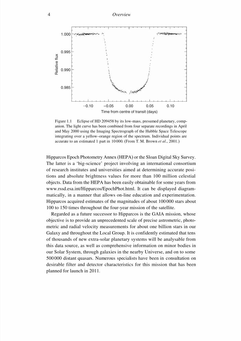
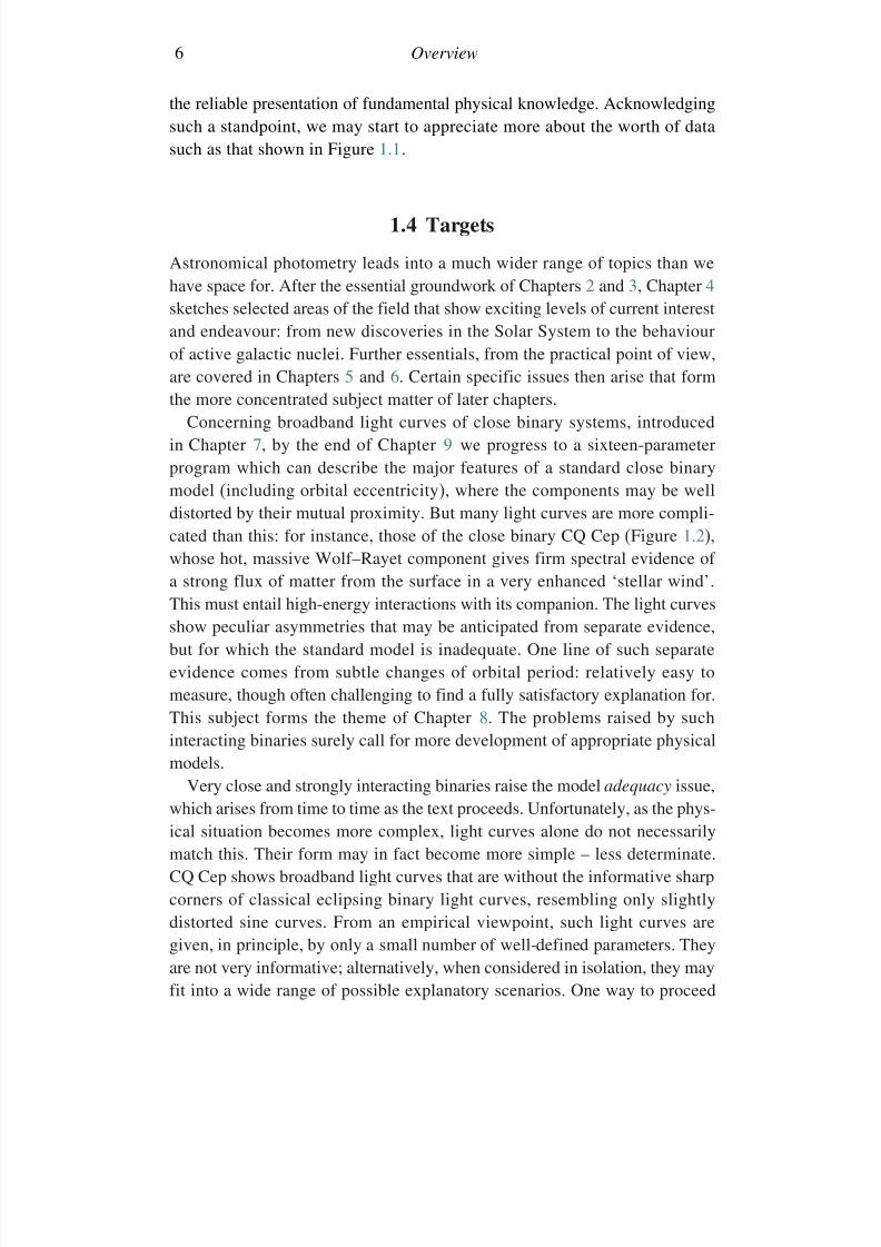
though this is a rather crude overall guide. Variable stars are known whoseentire variation is only of order a hundredth of a magnitude. A particularlynotable example came to light in 1999 with the photometric identificationof the planetary companion to HD 209458 (Figure 1.1). More such caseshave followed and many more can be confidently expected in future years.Clearly, such low amplitude ‘light curves’ require the utmost in achievableaccuracy, as will be explained presently. On the other hand, traditional eye-
based estimation of stellar brightness is usually thought to be doing very wellat 10% accuracy. There are many variables of large amplitude where data of this accuracy are still useful, particularly when coverage is extensive, so thatobservations can be averaged.
It can be shown that accuracy to one part in a thousand is achievable evenwith a 0.6 m telescope and 2 min integrations from a ground-based site,provided that site is suitably located, for example at a few thousand metresaltitude like the summit of Mauna Kea. On this basis, hour-long integrations
with a >1 m telescope from similar locations should allow mag accuracy tobe approachable for brighter stars such as HD 209458. This star, also knownas V376 Pegasi, turns out to be among the nearest of stars showing eclipses.This point alone suggests a likely high relative frequency of low light loss(planetary?), yet-to-be-discovered eclipses cosmically.
The availability of internet access to large-scale monitorings of cosmiclight sources offers a range of new possibilities, for example, with the
7/21/2019 Introduction to Astronomical Photometry
http://slidepdf.com/reader/full/introduction-to-astronomical-photometry 22/451
4 Overview
1.000
0.995
0.990 R e l a t i v e f l u x
0.985
– 0.10 – 0.05 0.05 0.100.00
Time from centre of transit (days)
Figure 1.1 Eclipse of HD 209458 by its low-mass, presumed planetary, comp-anion. The light curve has been combined from four separate recordings in Apriland May 2000 using the Imaging Spectrograph of the Hubble Space Telescopeintegrating over a yellow–orange region of the spectrum. Individual points are
accurate to an estimated 1 part in 10 000. (From T. M. Brown et al., 2001.)
Hipparcos Epoch Photometry Annex (HEPA) or the Sloan Digital Sky Survey.The latter is a ‘big-science’ project involving an international consortiumof research institutes and universities aimed at determining accurate posi-tions and absolute brightness values for more than 100 million celestialobjects. Data from the HEPA has been easily obtainable for some years fromwww.rssd.esa.int/Hipparcos/EpochPhot.html. It can be displayed diagram-matically, in a manner that allows on-line education and experimentation.Hipparcos acquired estimates of the magnitudes of about 100 000 stars about100 to 150 times throughout the four-year mission of the satellite.
Regarded as a future successor to Hipparcos is the GAIA mission, whoseobjective is to provide an unprecedented scale of precise astrometric, photo-metric and radial velocity measurements for about one billion stars in our
Galaxy and throughout the Local Group. It is confidently estimated that tensof thousands of new extra-solar planetary systems will be analysable fromthis data source, as well as comprehensive information on minor bodies inour Solar System, through galaxies in the nearby Universe, and on to some500 000 distant quasars. Numerous specialists have been in consultation ondesirable filter and detector characteristics for this mission that has beenplanned for launch in 2011.
7/21/2019 Introduction to Astronomical Photometry
http://slidepdf.com/reader/full/introduction-to-astronomical-photometry 23/451
1.3 Participants 5
1.3 Participants
The foregoing indicates several levels of potential support to astronomical
photometry. Eye-based data from skilled observers continues to have a signif-icant place, especially with certain kinds of irregular or peculiar variable star,and appears likely to do so for the foreseeable future. Many of these observersare working with telescopes of the 10-inch class.
When a person or group has the skills and resources to combine PC capa-bilities with a telescope of this size, a photometer utilizing photoelectricdetection principles, particularly an areal CCD-type camera, and sufficientawareness of procedures, an order of magnitude or more of detail is addedto the information content of data obtained in a given spell of observing.There are also good organizations to support the growth in value of suchwork: like, for example, the International Amateur–Professional Photoelec-tric Photometry association, the long-established Vereinigung der Sternfre-unde, or the Center for Backyard Astrophysics. Relatively small and lowcost, highly automated photometric telescopes (APTs) have also appearedin this context, offering very interesting avenues for future developments in
photometry.The main components – telescope, photometry-system and PC – can, of
course, be separated. Apart from instrument control and data management,a computer is also directed to archiving and analysis. It is in this latter areawhere one main thrust of this book lies. The analysis of data provides theessential link between observational production and theoretical interpretation,which can seem like two halves of a driving cycle. Naturally, each side isin a continual process of growth and development, but it is hoped that thisbook will be helpful to students and enthusiasts, interested in catching holdof relevant procedures and helping develop them.
Astronomical photometry will then be seen to have an important bearing onour knowledge of the natural Universe. Recognition of the deep significanceof such knowledge to general human understanding and culture gives riseto a professional position about the subject. People taking up such a profes-sion will be generally seeking to make new and original contributions, of a
standard that can be critically read and accepted by colleagues similarly moti-vated, in a global context. Considerable efforts, with due periods of specialisttraining in suitably equipped environments that incur consequent signifi-cant expenses, are usually required to achieve this. The acceptance of suchimplications, together with high standards of checking and review, fosters acommon professionalism among persons thus involved. On this basis, profes-sional astronomy should serve the wider community well; especially regarding
7/21/2019 Introduction to Astronomical Photometry
http://slidepdf.com/reader/full/introduction-to-astronomical-photometry 24/451
6 Overview
the reliable presentation of fundamental physical knowledge. Acknowledgingsuch a standpoint, we may start to appreciate more about the worth of datasuch as that shown in Figure 1.1.
1.4 Targets
Astronomical photometry leads into a much wider range of topics than wehave space for. After the essential groundwork of Chapters 2 and 3, Chapter 4sketches selected areas of the field that show exciting levels of current interest
and endeavour: from new discoveries in the Solar System to the behaviourof active galactic nuclei. Further essentials, from the practical point of view,are covered in Chapters 5 and 6. Certain specific issues then arise that formthe more concentrated subject matter of later chapters.
Concerning broadband light curves of close binary systems, introducedin Chapter 7, by the end of Chapter 9 we progress to a sixteen-parameterprogram which can describe the major features of a standard close binarymodel (including orbital eccentricity), where the components may be well
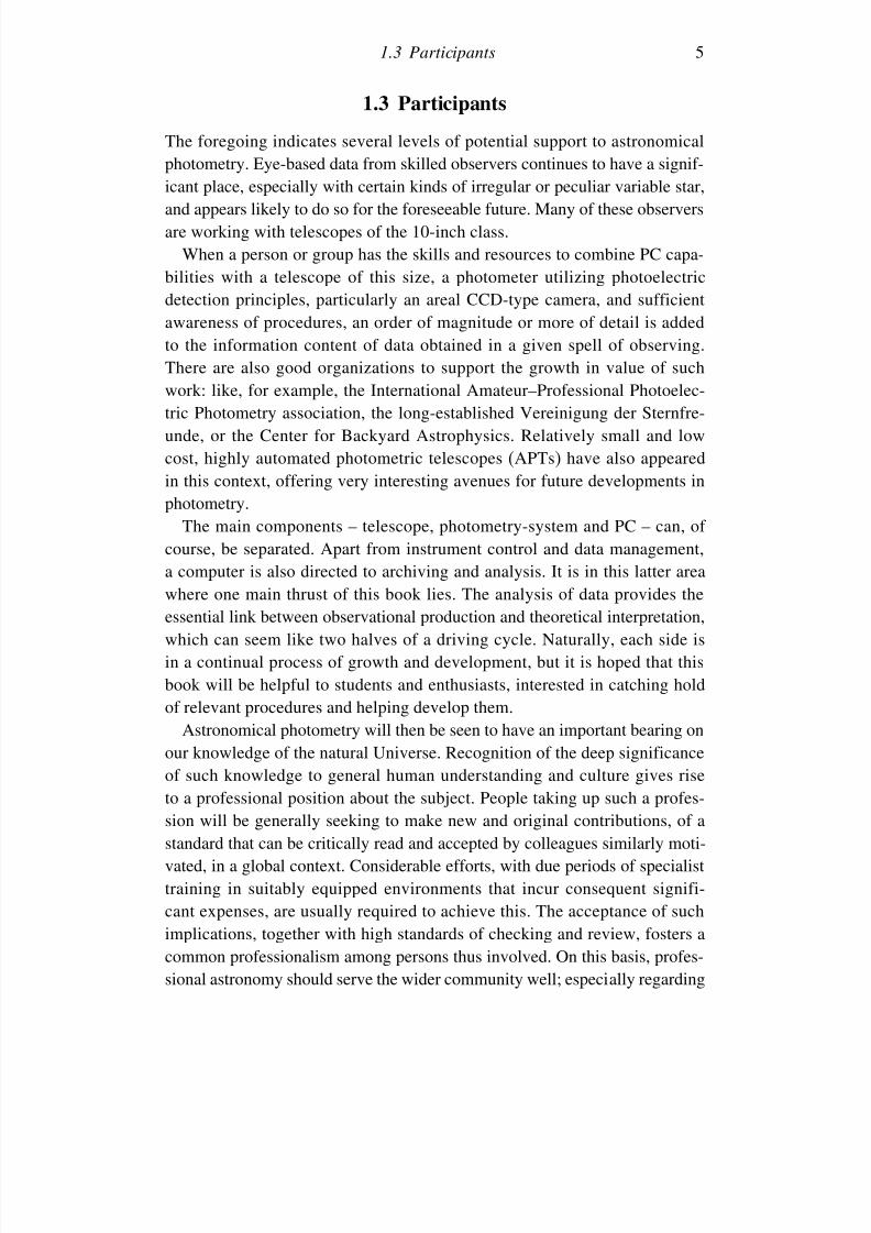
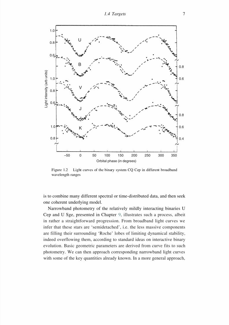
distorted by their mutual proximity. But many light curves are more compli-cated than this: for instance, those of the close binary CQ Cep (Figure 1.2),whose hot, massive Wolf–Rayet component gives firm spectral evidence of a strong flux of matter from the surface in a very enhanced ‘stellar wind’.This must entail high-energy interactions with its companion. The light curvesshow peculiar asymmetries that may be anticipated from separate evidence,but for which the standard model is inadequate. One line of such separate
evidence comes from subtle changes of orbital period: relatively easy tomeasure, though often challenging to find a fully satisfactory explanation for.This subject forms the theme of Chapter 8. The problems raised by suchinteracting binaries surely call for more development of appropriate physicalmodels.
Very close and strongly interacting binaries raise the model adequacy issue,which arises from time to time as the text proceeds. Unfortunately, as the phys-ical situation becomes more complex, light curves alone do not necessarily
match this. Their form may in fact become more simple – less determinate.CQ Cep shows broadband light curves that are without the informative sharpcorners of classical eclipsing binary light curves, resembling only slightlydistorted sine curves. From an empirical viewpoint, such light curves aregiven, in principle, by only a small number of well-defined parameters. Theyare not very informative; alternatively, when considered in isolation, they mayfit into a wide range of possible explanatory scenarios. One way to proceed
7/21/2019 Introduction to Astronomical Photometry
http://slidepdf.com/reader/full/introduction-to-astronomical-photometry 25/451
1.4 Targets 7
1.0
0.8
0.6
1.0
0.8
0.6
0.8
–50 0 50 100 150
Orbital phase (in degrees)
L i g h t i n t e n s i t y ( a r b u n i t s )
200 250 300 350
0.8
0.8
0.6
0.6
0.4
1.0
U
B
V
J
K
Figure 1.2 Light curves of the binary system CQ Cep in different broadbandwavelength ranges
is to combine many different spectral or time-distributed data, and then seekone coherent underlying model.
Narrowband photometry of the relatively mildly interacting binaries UCep and U Sge, presented in Chapter 9, illustrates such a process, albeit
in rather a straightforward progression. From broadband light curves weinfer that these stars are ‘semidetached’, i.e. the less massive componentsare filling their surrounding ‘Roche’ lobes of limiting dynamical stability,indeed overflowing them, according to standard ideas on interactive binaryevolution. Basic geometric parameters are derived from curve fits to suchphotometry. We can then approach corresponding narrowband light curveswith some of the key quantities already known. In a more general approach,
7/21/2019 Introduction to Astronomical Photometry
http://slidepdf.com/reader/full/introduction-to-astronomical-photometry 26/451
8 Overview
one seeks a simultaneous or concomitant explanation of concurrent data sets,with information feeding across from one curve-fitting to another.
Something like this happens in the successive approximations analysis we
carry out for the spotted RS CVn type stars. In Chapter 10, great increasesin observational surveillance of these ‘extensions to the solar laboratory’ areanticipated, with the exploitation of automated photometric telescopes andother techniques. But the fitting of the wave distortions in these systemsis notoriously imprecise. Basically, we face a stringent information limit if we rely only on broadband photometry. Either we admit to a frustratingsmallness of derivable parameter sets, or give in to the temptation to advance
plausible models that can match the data well, but actually specify moreinformation than it really contains. Again the answer will be to combine asmany data sets as possible, spectroscopic as well as photometric, to uncovera unified picture. Increased combinatorial use of new techniques, such asZeeman Doppler Imaging, or multi-band stellar radio astronomy, should allowvaluable progress to be made in this context.
The Baade–Wesselink technique, outlined in Chapter 11, is another areawhere the temptation to derive and utilize numerical parameters may exceed
proper caution. Even so, the suggested dangers are perhaps not that serious.Those inferences in the method which are prone to unreliability are wellknown, and continue to be investigated to find firmer versions. Fortunately,there are also quite independent means of testing the overall reliability of Baade–Wesselink results.
Whether or not present techniques will remain useful, we can find in themviable approaches to a fuller appreciation of the meaning of photometric data.
1.5 Bibliographical notes
The 1998 edition of A. A. Henden and R. H. Kaitchuk’s Astronomical Photom-
etry (Willmann-Bell) recognizes much of the same scope of the subject asour overview, and addresses comparable requirements and participants. Itsspecial usefulness regarding practical details will become apparent in the bibli-
ographic notes of later chapters. Willmann-Bell (www.willbell.com/) haveproduced a selection of other textbooks in the field, including a re-edition(1998) of D. S. Hall and R. M. Genet’s useful Photoelectric Photometry of
Variable Stars that features the work of the remarkable amateur astronomerLouis Boyd. Other earlier publications of the Fairborn Press throw light onthe development of the productive interaction of small telescope and personalcomputer, while the groundwork of C. Sterken and J. Manfroid’s Astronomical
7/21/2019 Introduction to Astronomical Photometry
http://slidepdf.com/reader/full/introduction-to-astronomical-photometry 27/451
1.5 Bibliographical notes 9
Photometry: A Guide (Kluwer, 1992) and V. Straizys’s Multicolor Stellar
Photometry (Pachart, 1995) should not be missed.More recently, C. Sterken and C. Jaschek have compiled an overview of
variable star photometry in their Light Curves of Variable Stars: A Pictorial
Atlas (Cambridge University Press, 1996). The earlier C. and M. Jascheks’Classification of the Stars (Cambridge University Press, 1989) was also auseful broad-based text reviewing the role played by photometry in developingunderstanding for stars of all types. That book, in turn, cited M. Golay’s Intro-
duction to Astronomical Photometry (Reidel, 1974) as an important seminalwork on astronomical photometric science. Although the present text aims at
a reasonably complete introduction, references are made, from time to time,to such comprehensive backgrounders.
Concerning the aim of broad outreach indicated in Section 1.1, the contin-uous network of communications organized by observers’ societies and groupsin many countries should be consulted. These include the British Astronom-ical Association (Variable Star Section: www.britastro.org/vss/), the AmericanAssociation of Variable Star Observers (www.aavso.org/), the AssociationFrançaise des Observateurs d’Etoiles Variables (cdsweb.u-strasbg.fr/afoev/),the Variable Star Observers League in Japan (vsolj.cetus-net.org/), the GermanVereinigung der Sternfreunde (www.vds-astro.de/), relevant sections of theRoyal Astronomical Society of New Zealand (www.rasnz.org.nz/) and theirvarious equivalents in other countries. Most of the above websites givelinks to similar organizations; or, in any case, relevant information could beaccessed through the International Astronomical Union (IAU – www.iau.org/ Organization/), probably via its Divisions V and XII. A good backgrounder
for such activities was provided in G. A. Good’s Observing Variable Stars, inPatrick Moore’s practical astronomy series (Springer-Verlag, 2003). A nicereview of the role of visual monitoring in variable star studies was given byAlbert Jones in Austral. J. Astron. (6, 81, 1995).
Specific short contributions on astronomical photometry appear in the Infor-mation Bulletin on Variable Stars, whose production has arisen from a back-ground of efforts through Commissions 27 and 42 of the IAU, and is published
by the Konkoly Observatory (www.konkoly.hu/IBVS), Budapest, Hungary.The International Amateur–Professional Photoelectric Photometry organiza-tion (www.iappp.vanderbilt.edu/) also addresses itself across national bound-aries (T.D. Oswalt, D.S. Hall & R.C. Reisenweber, I.A.P.P.P. Commun.
42, 1, 1990), while Peremeniye Zvezdiy records comparable activities in theRussian language. A useful set of papers relevant to this context also appearedin The Study of Variable Stars Using Small Telescopes, ed. J.R. Percy
7/21/2019 Introduction to Astronomical Photometry
http://slidepdf.com/reader/full/introduction-to-astronomical-photometry 28/451
10 Overview
(Cambridge University Press, 1986). The Center for Backyard Astrophysicscan be accessed via cba.phys.columbia.edu/.
Quantitative data on S/N values for real photometers appear in the Optec
(tradename) Manual, as well towards the end of A. A. Henden and R. H.Kaitchuck’s Astronomical Photometry, where a full explanation of the under-lying principles is given. Figure 1.1 comes from the paper of T.M. Brownet al. ( Astrophys. J., 552, 699, 2001). This remarkable light curve of a roughlyJupiter-like planet transiting a stellar disk was brought about after photometricattention was directed to HD 209458 following the precise measurementof small variations of radial velocity (cf. Mazeh et al., 2000). Figure 1.2
appeared in D. Stickland et al. ( Astron. Astrophys., 134, 45, 1984). Informa-tion on Hipparcos photometry is available from astro.estec.esa.nl/Hipparcos/,similarly on the SDSS at www.sdss.org/ and the GAIA mission at astro.estec.esa.nl/GAIA/.
References
Brown, T. M., Charbonneau, D., Gilliland, R. L., Noyes, R. W. & Burrows, A., 2001, Astrophys. J ., 552, 699.
Golay, M., 1974, Introduction to Astronomical Photometry, Reidel.Good, G. A., 2003, Observing Variable Stars, Springer-Verlag, 2003.Hall, D.S. & Genet, R.M., 1998, Photoelectric Photometry of Variable Stars,
Willmann-Bell.Henden, A. A. & Kaitchuk, R. H., 1998, Astronomical Photometry, Willmann-Bell.Jaschek, C. & Jaschek, M., 1989, Classification of the Stars, Cambridge University
Press.
Jones, A., 1995, Austral. J. Astron., 6, 81.Mazeh, T., Naef, D., Torres, G. et al., 2000, Astrophys. J., 532, 55.Oswalt, T. D., Hall, D. S. & Reisenweber, R. C., 1990, I.A.P.P.P. Commun., 42, 1.Percy, J. R., 1986, The Study of Variable Stars Using Small Telescopes, Cambridge
University Press.Sterken, C. & Manfroid, J., 1992, Astronomical Photometry: A Guide, Kluwer.Sterken, C. & Jaschek, C., 1996, Light Curves of Variable Stars: A Pictorial Atlas,
Cambridge University Press.Stickland, D., Bromage, G. E., Burton, W. M., Budding, E., Howarth, I. D., Willis,
A. J., Jameson, R. & Sherrington, M. R., 1984, Astron. Astrophys., 134, 35.Straizys, V., 1995, Multicolor Stellar Photometry, Pachart.
7/21/2019 Introduction to Astronomical Photometry
http://slidepdf.com/reader/full/introduction-to-astronomical-photometry 29/451
2
Introduction
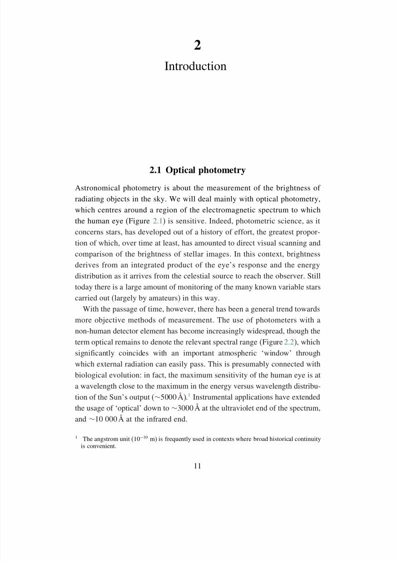
2.1 Optical photometry
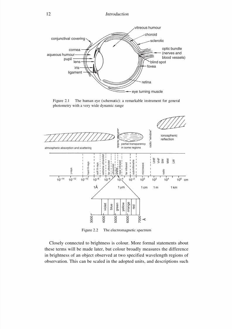
Astronomical photometry is about the measurement of the brightness of radiating objects in the sky. We will deal mainly with optical photometry,which centres around a region of the electromagnetic spectrum to whichthe human eye (Figure 2.1) is sensitive. Indeed, photometric science, as it
concerns stars, has developed out of a history of effort, the greatest propor-tion of which, over time at least, has amounted to direct visual scanning andcomparison of the brightness of stellar images. In this context, brightnessderives from an integrated product of the eye’s response and the energydistribution as it arrives from the celestial source to reach the observer. Stilltoday there is a large amount of monitoring of the many known variable starscarried out (largely by amateurs) in this way.
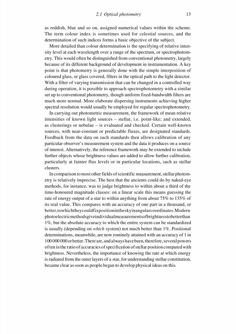
With the passage of time, however, there has been a general trend towardsmore objective methods of measurement. The use of photometers with anon-human detector element has become increasingly widespread, though theterm optical remains to denote the relevant spectral range (Figure 2.2), whichsignificantly coincides with an important atmospheric ‘window’ throughwhich external radiation can easily pass. This is presumably connected withbiological evolution: in fact, the maximum sensitivity of the human eye is at
a wavelength close to the maximum in the energy versus wavelength distribu-tion of the Sun’s output (∼5000 Å).1 Instrumental applications have extendedthe usage of ‘optical’ down to ∼3000 Å at the ultraviolet end of the spectrum,and ∼10 000 Å at the infrared end.
1 The angstrom unit (10−10 m) is frequently used in contexts where broad historical continuityis convenient.
11
7/21/2019 Introduction to Astronomical Photometry
http://slidepdf.com/reader/full/introduction-to-astronomical-photometry 30/451
12 Introduction
conjunctival covering
corneaaqueous humour
pupillens
irisligament
vitreous humour
choroid
sclerotic
optic bundle(nerves andblood vessels)
blind spotfovea
retina
eye turning muscle
Figure 2.1 The human eye (schematic): a remarkable instrument for generalphotometry with a very wide dynamic range
v i o l e
t
b l u
e
g r e e n
y e
l l o w
o r a n g e
r e d
o p t i c a l
“ w i n d o w
”
10–14 10–12 10–10 10–8 10–6 10–4 10–2 100 102 104 106
h a r d
X - r a y s
s o
f t X - r a y s
e x
t r e m e u
l t r a v
i o l e t
u l t r a v
i o l e t
f a r u
l t r a v
i o l e t
v i s i b l e
f a r
i n f r a r e
d
s u
b m
i l l i m e
t r e
m i c r o w a v e
r a d i o
V H F
U H F
S W
M W
L W
1 cm1 µm1Å
Å
1 m 1 km
cm
atmospheric absorption and scattering
ionosphericreflection
γ - r a y s
n e a r i n f r a r e d
3 0 0 0
4 0 0 0
5 0 0 0
6 0 0 0
7 0 0 0
partial transparencyin some regions r a
d i o “ w i n d o w ”
Figure 2.2 The electromagnetic spectrum
Closely connected to brightness is colour. More formal statements aboutthese terms will be made later, but colour broadly measures the differencein brightness of an object observed at two specified wavelength regions of observation. This can be scaled in the adopted units, and descriptions such
7/21/2019 Introduction to Astronomical Photometry
http://slidepdf.com/reader/full/introduction-to-astronomical-photometry 31/451
2.1 Optical photometry 13
as reddish, blue and so on, assigned numerical values within the scheme.The term colour index is sometimes used for celestial sources, and thedetermination of such indices forms a basic objective of the subject.
More detailed than colour determination is the specifying of relative inten-sity level at each wavelength over a range of the spectrum, or spectrophotom-etry. This would often be distinguished from conventional photometry, largelybecause of its different background of development in instrumentation. A keypoint is that photometry is generally done with the simple interposition of coloured glass, or glass covered, filters in the optical path to the light detector.With a filter of varying transmission that can be changed in a controlled way
during operation, it is possible to approach spectrophotometry with a similarset up to conventional photometry, though uniform fixed-bandwidth filters aremuch more normal. More elaborate dispersing instruments achieving higherspectral resolution would usually be employed for regular spectrophotometry.
In carrying out photometric measurement, the framework of mean relativeintensities of known light sources – stellar, i.e. point-like; and extended,as clusterings or nebulae – is evaluated and checked. Certain well-knownsources, with near-constant or predictable fluxes, are designated standards.
Feedback from the data on such standards then allows calibration of anyparticular observer’s measurement system and the data it produces on a sourceof interest. Alternatively, the reference framework may be extended to includefurther objects whose brightness values are added to allow further calibration,particularly at fainter flux levels or in particular locations, such as stellarclusters.
In comparison to most other fields of scientific measurement, stellar photom-
etry is relatively imprecise. The best that the ancients could do by naked-eyemethods, for instance, was to judge brightness to within about a third of thetime-honoured magnitude classes: on a linear scale this means guessing therate of energy output of a star to within anything from about 75% to 135% of its real value. This compares with an accuracy of one part in a thousand, orbetter,towhichtheycouldfixpositionintheskyinangularcoordinates.Modernphotoelectricmethodsgiveindividualmeasurementsofbrightnesstobetterthan1%, but the absolute accuracy to which the entire system can be standardized
is usually (depending on which system) not much better than 1%. Positionaldeterminations, meanwhile, are now routinely attained with an accuracy of 1 in100 000 000 orbetter.There are,and always havebeen, therefore,severalpowersof ten in the ratio of accuracies of specification of stellar position compared withbrightness. Nevertheless, the importance of knowing the rate at which energyis radiated from the outer layers of a star, for understanding stellar constitution,became clear as soon as people began to develop physical ideas on this.
7/21/2019 Introduction to Astronomical Photometry
http://slidepdf.com/reader/full/introduction-to-astronomical-photometry 32/451
14 Introduction
The side of photometry dealing with calibration issues is sometimes seenas playing a supporting role to a more attention-catching activity connectedwith variable stars. Alternative purposes again appear in this connection.
Some information retrieval and processing is to check, or further refine ourknowledge of, the underlying physics, such as with ‘classical’ variables,e.g. cepheids, or normal eclipsing binary systems. On the other hand, certainobservations are made with some expectation of discovery; either by findingvariability in a hitherto unsuspected object, or by monitoring seeminglyunpredictable types of irregularity, for instance with flare stars, cataclysmicvariables, BL Lacerate type objects and such-like.
Astronomical photometry was originally largely concerned with the rela-tive brightness values of stars, and the magnitude system in which theseare expressed. Stellar surfaces are below the eye’s limit of resolution, eventhrough the world’s largest telescopes, and are thus point-like. Some of themost familiar astronomical objects – the Sun, the Moon, the Milky Wayor the sky itself – are extended, however. Their local brightness can beexpressed, in traditional units, as ‘n stars of magnitude m per unit squareangular measure’, with the meaning that the light received from e.g. an area
of surface subtending 1 arcmin by 1 arcmin (about the limit of resolutionof a typical human eye) would be the same as if coming from n of mthmagnitude stars (m = 10 might be used for this), or, alternatively, simplyas magnitude x per square arcsec, say. There are many extended sources,but usually with relatively faint surface brightness values. With improvedlinear areal detectors and more large telescopes there continue to be impres-sive developments in the detailed surface photometry of faint nebulae and
galaxies.Photometry has thus a range of important roles to play in astrophysics.By providing basic reference data on stellar brightness and colour, such asvia the well-known colour–magnitude diagrams, fundamental tests to ideas of stellar structure and evolution have been provided. The continual discoveryof new kinds of photometric phenomena in objects as varied as members of the solar system to active galactic nuclei, regions of nebulosity, supernovae,spotted stars, cataclysmic variables or high-energy bursters all helps build
up and develop physical theory.
2.2 Historical notes
The historical basis for stellar brightness determinations centres on the mag-nitude system in which they are evaluated. This system goes back at least
7/21/2019 Introduction to Astronomical Photometry
http://slidepdf.com/reader/full/introduction-to-astronomical-photometry 33/451
2.2 Historical notes 15
as far as that ancient compilation of data on stars, the catalogue of Hippar-chos,2 completed by about 130 BCE. Just how the system originated appears‘lost in the mists of time’. It is known that Hipparchos, along with earlier
Greek astronomers, referred to still earlier Babylonian star and constellationidentifications, but the details in such information transfer are no longer clear.In any case, the magnitudes of Hipparchos, as conveyed to posterity throughClaudius Ptolemy’s great Megali Syntaxis tis Astronomias, are essentiallysimilar to present-day values for the 1000 or so brightest stars.
During the cultural flowering of the Abbasid caliphate the astronomicalworks of the Greeks became known and studied in a new setting. Translated
into the Kitab al Majisti
(the Almagest), Ptolemy’s treatise stimulated notonly the attention of Islamic scholars but also their active experimental inves-tigation. The enlightened Abdullah al Mamun, in the early part of the ninthcentury of our era, founded the renowned observatory at Baghdad, whereastronomy was supported by new and improved instrumentation, as well asadvances in theory and methods of calculation. It was from this background,for example, that Al Battani (Albategnius), on the basis of new observations(mainly at Ar Raqqah), substantially improved on Ptolemy’s value for the
precession constant.Also benefitting from the Almagest, Abd al Rahman Sufi, at Isfahan in
the tenth century, decided that not only the positional determinations of thestars as given in the Almagest, but also their magnitudes, could be checked,or reassessed. Sufi published a new list of magnitudes of all the thousand orso stars of the Almagest he could actually observe, adding also a hundred ormore new ones of his own. There is no doubt that Sufi’s magnitudes represent
an improvement in precision over the run of values attributed to Ptolemy.Magnitude values given in Ptolemy’s catalogue have an average accuracy of not less than half a magnitude division, which becomes about a third of adivision in Sufi’s work (magnitude units were divided into three subdivisionsin these ancient catalogues). The scholar of ancient astronomy, E. Knobel,pointed out that Sufi also appears to have been the first astronomer to takeaccount of a galaxy external to our own, i.e. his was the first map to indicatethe Andromeda Nebula.
The differences that existed between Sufi’s and Ptolemy’s magnitude valueswere not overemphasized. Presumably, Sufi and his followers supposed thatthe earlier observers had just not been assiduous enough, after all shortcom-ings in some of Ptolemy’s positional work had already come to light. Thepossibility of inherent variation of starlight, while it may well have occurred
2 sometimes spelled Hipparchus.
7/21/2019 Introduction to Astronomical Photometry
http://slidepdf.com/reader/full/introduction-to-astronomical-photometry 34/451
16 Introduction
to Sufi, would probably have been regarded with some demur, for the trend of opinion among the ancients, epitomized by no less an authority than Aristotle,was that the sphere of the fixed stars was something eternal and invariable
(‘incorruptible’). Apparent short-term variation of starlight (i.e. twinkling)could be put down to shortcomings of human eyesight. Sufi’s improvedmagnitudes were therefore accepted as definitive in Ulugh Beg’s recompi-lation of the classical stellar catalogue for the epoch 1437 AD: nearly fivecenturies after Sufi’s time.
The idea of a permanent, invariably rotating outer sphere of the stars was inharmony with prevalent philosophical concepts of the Middle Ages in Europe;
but a certain shakiness to this model was introduced by the sudden appearancein 1572 of a bright ‘new star’ (nova), which captured the attention of TychoBrahe, then a 26-year-old Danish nobleman, with scientific interests, lookingfor his calling in life. As with Hipparchos himself, who, according to Pliny,had been stimulated to compile his catalogue by just such an event some 1700years previously, Tycho was to go on to produce his own new catalogue of the stars; though, apparently, he did not live to see the work brought to a finalpublished form.
Another important, but rather fortuitous, event in the life of Tycho wasthe appearance of a bright comet in 1577, not long after the astronomer hadestablished himself in his new observatory at Uraniborg, on a small islandbetween Zealand and Sweden. From his series of observations of the cometTycho was able, at last, to bring firm evidence to deny the Aristoteliancontention that no substantial changes have effect beyond the sphere of theMoon. We know also that, in his meticulous way, Tycho was marking in
his catalogue manuscripts the magnitude values of some stars by dots, wherehe believed there was some discrepancy between previously recorded values.Tycho would not have been dismayed, therefore, by the announcement in1596 by David Fabricius of the new appearance of what was later called Mira:the first known variable star in the more normally used sense.3 Fabricius wasin correspondence with Johannes Kepler, then about the same age as Tychohad been at the time of the new star of 1572. The following year (1597)
both he and the now middle-aged Tycho, who had left his native land, wereworking together in Prague.Tycho died in 1601, a year after W. Janszoon Blaeu found another famous
variable of the northern skies – P Cygni – and three years before Kepler saw
3 Of course, we now know that the novae are also variables, i.e. stars, normally too faint to beseen, that suddenly become very much brighter, so sometimes allowing temporary naked eyevisibility.
7/21/2019 Introduction to Astronomical Photometry
http://slidepdf.com/reader/full/introduction-to-astronomical-photometry 35/451
2.2 Historical notes 17
his own bright new star in the form of the supernova of 1604. So it was that bythe seventeenth century the concept of new or variable stars became accepted:catalogued magnitudes were checked again, more variables were discovered
and Aristotle’s immutable outer sphere began to fade into oblivion. Tycho’scatalogue was eventually published in comprehensive form by Kepler in the
Rudolphine Tables, but already by 1603 his work was attracting attentionthrough its artistic rendering in the form of the star charts of Johann Bayer’sUnranometria. These famous maps included the 48 classical constellations of the ancients drawn by the Renaissance artist Albrecht Dürer. Janszoon Blaeuand Bayer also recognized 12 new constellations not among those listed in
the Almagest. These were in the far southern parts of the sky, invisible toancient astronomers of the Near East. Data on these stars had come fromearly explorers, but particularly through the tabulations of the Dutch sailorsP. D. Keyzer and F. de Houtman.
This period of growth in astronomy occurred side by side with the devel-opment of the telescope as a scientific instrument; championed in those earlydays, of course, by Galileo. Galileo gave attention to stars fainter than sixthmagnitude – the faintest class of Hipparchos’ subdivisions – and decided on a
simple extension to seventh, eighth and so on, so as to follow in a consistentprogression. The system was kept by Flamsteed and others, indeed right up toour own day when, since, in principle, the zero point of the magnitude scalecoincides with a certain average originally based on the Ptolemaic values, westill maintain an observational link with that first compilation of Hipparchos(which itself may have been influenced by earlier sources) more than 2000years ago.
Some of the stars catalogued by Ptolemy were very far to the south of his Alexandrian sky, and, with the additional apparent displacement resultingfrom the precession and nutation of the equinoxes, apart from the generallyhigher latitudes of observers, dropped from the attention of the mediævalEuropean astronomers. Some of these stars (e.g. and Sagittarii) attractedthe notice of young Edmond Halley, who, from his observations on the islandof St Helena, published in 1679, provided another of the early cataloguesof stars of the southern sky. Halley, still trustful of the Almagest writings,
and pondering over the two magnitudes or so discrepancies, speculated onthe possibility of inherent variations of this scale in the fifteen hundred yearssince Ptolemy had recorded their magnitudes.
Early in the eighteenth century a further important development to astro-nomical photometry came with the introduction of specific instrumentationby Pierre Bouguer, who might be regarded as a patron of much of thesubject matter of this book. Bouguer was, for instance, the first to make

7/21/2019 Introduction to Astronomical Photometry
http://slidepdf.com/reader/full/introduction-to-astronomical-photometry 36/451
18 Introduction
a systematic study of the extinction of light from celestial bodies by theintervening atmosphere, and showed that the increase in magnitude (diminu-tion in brightness) thus caused was directly proportional to the mass of
intervening air. He is credited with the more basic establishing of the inversesquare law diminution of light flux (in vacuo) (proposed by Kepler). He alsoquantified that effect, which may well have been noticed in earlier times,known as the limb darkening of the Sun, i.e. the tendency of the surfacebrightness to fade towards the edge of the solar disk. The effect has been asource of extensive astrophysical interest, aspects of which will be met laterin this text.
Bouguer’s methodology appears to have been neglected through the centurythat followed, though this is mollified by its ultimate dependence on that rathernon-impersonal element the human eye, whatever the intervening instrumen-tation; up until the advent of photographic methods, at least. So even by themid nineteenth century when Argelander and his associates were engaged withthe very large undertaking of the Durchmusterungen, ultimately recordingaround half a million magnitude estimates, a very simple eye-based proce-dure was considered expedient; though it is also true to say that a careful,
instrument-based approach, such as that followed in the more intensive workof John Herschel, had its reward in terms of a much better scale of internalself-consistency.
It had been during the earlier years of the astronomical career of JohnHerschel’s father, William, that an important class of variable star, theeclipsing binary system, was discovered with the memorable work of youngJohn Goodricke. Binary systems, or double stars as they are also known,
were a strong interest of W. Herschel at the time, but though he gave Algol,the binary whose eclipsing pattern was first recognized by Goodricke, closeattention with the large telescopes at his disposal, he could not discern twocomponents by eye. The period of the binary’s orbital revolution is relativelyshort – less than three days – so that with a few inferences about the conse-quent likely angular size of the orbit at an expectable distance, Herschel’sfailure to resolve the components becomes not surprising. Herschel’s intro-duction of more powerful light collectors, and his interest in the ability to
resolve detail, particularly in faint and diffuse patches of light, paved the wayfor the photometry of extended sources; though more quantitative work onthis had to await the appearance of purpose-built photometric equipment.
Living in the same county as Goodricke, not more than 40 km away, wasanother astronomer of the eighteenth century, the significance of whose workseems to have been largely overlooked for a century or more after his deathin 1793. This was John Michell, who was the first to recognize the probable
7/21/2019 Introduction to Astronomical Photometry
http://slidepdf.com/reader/full/introduction-to-astronomical-photometry 37/451
2.2 Historical notes 19
gravitational binding of many double stars on the basis of reasoned statisticalargument. He also conjectured on the existence of ‘black holes’ (as theyare now called): highly condensed stars with gravity so strong as to confine
photons to a surrounding bound region. Michell seems to have encounteredHerschel in Yorkshire already in the 1760s, and it is likely that later heat least came to know of Goodricke. Among his achievements was anotherremarkable result published in 1767: a determination of the ‘photometricparallax’ of Vega at 0.45 arcsec. The corresponding distance, of the right orderof magnitude but only around a quarter of modern values, results from theassumption of an equal inherent luminosity for Vega and the Sun, with some
additional estimates about the apparent brightness of Saturn as an intermediatestep in his calculation. Interactions with the work of Herschel, as it happened,around the same time as Goodricke’s discovery, supported Michell’s laterrealization that stars must come in inherently different luminosities and indeedhe would have understood the full circumstances of Goodricke’s eclipsingbinary hypothesis as well as Herschel’s failure to resolve it.
More advanced astronomical photometer designs, utilizing the null principlefor brightness comparison, and incorporating controlled diminution of source
brightness, e.g. by the use of polarizing agents, appeared by the middle of thenineteenth century, notably that of J. K. F. Zöllner, who based his photometeron a design of François Arago.
It became apparent by about the middle 1800s that the traditional magnitudescale should be not too far from logarithmic in the received fluxes of visiblestarlight; a point related to the physiology of sensation as investigated byG. T. Fechner and E. H. Weber. The formal rule for stellar magnitudes which
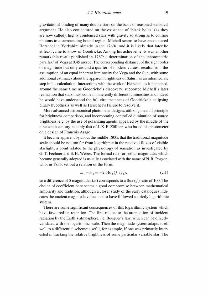
became generally adopted is usually associated with the name of N. R. Pogson,who, in 1856, set out a relation of the form:
m1 − m2 = −25logf 1/f 2 (2.1)
so a difference of 5 magnitudes (m) corresponds to a flux (f ) ratio of 100. Thechoice of coefficient here seems a good compromise between mathematicalsimplicity and tradition, although a closer study of the early catalogues indi-cates the ancient magnitude values not to have followed a strictly logarithmic
system.There are some significant consequences of this logarithmic system which
have favoured its retention. The first relates to the attenuation of incidentradiation by the Earth’s atmosphere, i.e. Bouguer’s law, which can be directlyvalidated with the logarithmic scale. Then the magnitude system adapts itself well to a differential scheme; useful, for example, if one was primarily inter-ested in tracking the relative brightness of some particular variable star. The
7/21/2019 Introduction to Astronomical Photometry
http://slidepdf.com/reader/full/introduction-to-astronomical-photometry 38/451
20 Introduction
overall changes of brightness, associated with variations in the atmosphere’stransparency from night to night or secular drifts in the response of thereceiver easily drop out as zero constants on a logarithmic scale. Only when
one wishes to tie in measurements with an absolute system of units (not neces-sarily an immediate objective) does it become required to evaluate just what(in watts per square metre, say) would correspond to the radiation from a zeromagnitude star. These matters will be considered in more detail in the nextchapter. Colour too, defined as a difference of magnitudes at different wave-lengths, lends itself well to some quasi-empirical relationships of a simpleform relating to the temperature of the radiation emitting surface.
In the nineteenth century efforts started to be made for a more system-atic basis to magnitude determination through the medium of photography.For various reasons this proved not to be so straightforward, however, anduntil relatively recently photographic magnitude determinations were notgreatly superior in accuracy to eye-based measures of a trained observer usingspecially prepared equipment. This was the case with the meridian visualphotometer, developed towards the end of the nineteenth century at HarvardCollege Observatory by E. C. Pickering and his associates. Thus, if the ancient
catalogue of Sufi listed stellar magnitudes to an internal accuracy of abouta third of a magnitude, the skilled observers using the Harvard meridianphotometer could improve on this so that their amplitude of uncertainty wasno worse than half that of Sufi, while a tenth of a magnitude accuracy char-acterized photographic determinations of better quality in the first half of thetwentieth century.
Despite its objective nature, there are a number of complicating and often
non-linear effects which take place between the original incidence of starlightand the final forms of darkened grain stellar images in the emulsion over theexposed plate (or film). These complications make reliable extraction of acorresponding set of magnitude values a difficult exercise. A number of theearly investigators, e.g. Bond, Kapteyn, Pickering, Scheiner, Bemporad (andothers), looked for some empirical formula to relate magnitude with somethingeasily measured, such as image diameter, but there was no uniformity of opinion as to what the formula should be, each worker generally preferring
his own.In the early years of the twentieth century the theory of photographic
image formation was explored more fully by K. Schwarzschild, and moreelaborate procedures for calibration were devised, involving things like objec-tive partial-covering screens, plate holders capable of easy movement forrepeated exposures, image plane filters, tube sensitometers and the densit-ometry of extrafocal images. Methods generally required the setting up of
7/21/2019 Introduction to Astronomical Photometry
http://slidepdf.com/reader/full/introduction-to-astronomical-photometry 39/451
2.2 Historical notes 21
Telescope
Objective
Diaphragm
Fabry lens Photocathode
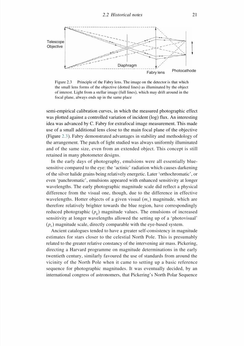
Figure 2.3 Principle of the Fabry lens. The image on the detector is that whichthe small lens forms of the objective (dotted lines) as illuminated by the object
of interest. Light from a stellar image (full lines), which may drift around in thefocal plane, always ends up in the same place
semi-empirical calibration curves, in which the measured photographic effectwas plotted against a controlled variation of incident (log) flux. An interestingidea was advanced by C. Fabry for extrafocal image measurement. This madeuse of a small additional lens close to the main focal plane of the objective(Figure 2.3). Fabry demonstrated advantages in stability and methodology of
the arrangement. The patch of light studied was always uniformly illuminatedand of the same size, even from an extended object. This concept is stillretained in many photometer designs.
In the early days of photography, emulsions were all essentially blue-sensitive compared to the eye: the ‘actinic’ radiation which causes darkeningof the silver halide grains being relatively energetic. Later ‘orthochromatic’, oreven ‘panchromatic’, emulsions appeared with enhanced sensitivity at longer
wavelengths. The early photographic magnitude scale did reflect a physicaldifference from the visual one, though, due to the difference in effectivewavelengths. Hotter objects of a given visual (mv) magnitude, which aretherefore relatively brighter towards the blue region, have correspondinglyreduced photographic (pg) magnitude values. The emulsions of increasedsensitivity at longer wavelengths allowed the setting up of a ‘photovisual’(pv) magnitude scale, directly comparable with the eye-based system.
Ancient catalogues tended to have a greater self-consistency in magnitude
estimates for stars closer to the celestial North Pole. This is presumablyrelated to the greater relative constancy of the intervening air mass. Pickering,directing a Harvard programme on magnitude determinations in the earlytwentieth century, similarly favoured the use of standards from around thevicinity of the North Pole when it came to setting up a basic referencesequence for photographic magnitudes. It was eventually decided, by aninternational congress of astronomers, that Pickering’s North Polar Sequence
7/21/2019 Introduction to Astronomical Photometry
http://slidepdf.com/reader/full/introduction-to-astronomical-photometry 40/451
22 Introduction
(which originally consisted of some 47 stars) should define the basic photo-graphic (pg) magnitude scale. This was to be linked with the pre-existingvisual scale by the requirement that the mean of all pg magnitudes for stars of
spectral type A0 in the magnitude range 5.5–6.5 be equal to the mean of thevisual magnitudes for those same stars, as determined by Harvard meridianphotometry. In 1912 Pickering published the photographic magnitudes of thechosen North Polar Sequence, which had by then grown in number to 96 stars.
Although difficulties with the use of the North Polar Sequence beganto be found when it was used to calibrate magnitudes in other parts of the sky, after careful cross-checks, notably by F. Seares at Mt Wilson, the
system was eventually shown to be relatively accurate internally (probableerrors of standards generally less than five hundredths of a magnitude) andprobably represented an adequate basic reference for a number of years inthe photographic photometry era. A large number of secondary sequenceswere set up in time, with particular attention being paid to specially selectedregions, such as those associated with the name of J.C. Kapteyn of theGroningen Observatory (Holland), or the ‘Harvard Standard Regions’. Theselatter are arranged in declination bands from
+75 to
−75 labelled A to F.
Calibrations then moved to the southern hemisphere, including a South PolarSequence, and photographic photometry of the Magellanic Clouds.
Developments also occurred in the method of magnitude determinationfrom photographic plates. Popular for a time was the Schilt type photometer,which allows a fine pencil of light from a standard lamp to be directed throughthe plate to be studied. The small spot of light passing through the platecould have its diameter varied, and would normally have been set as small as
conveniently possible for the range of magnitudes to be measured. The beamwas directed to the centre of a stellar image, where its attenuation would bemaximized. The beam, thus reduced in intensity, would then be transmitted toa suitable detective device, such as a photocell and galvanometer combination.
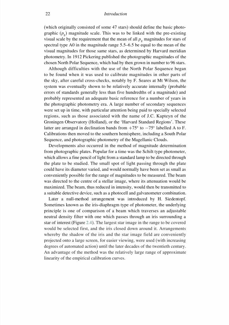
Later a null-method arrangement was introduced by H. Siedentopf.Sometimes known as the iris-diaphragm type of photometer, the underlyingprinciple is one of comparison of a beam which traverses an adjustableneutral density filter with one which passes through an iris surrounding a
star of interest (Figure 2.4). The largest star image in the range to be coveredwould be selected first, and the iris closed down around it. Arrangementswhereby the shadow of the iris and the star image field are convenientlyprojected onto a large screen, for easier viewing, were used (with increasingdegrees of automated action) until the later decades of the twentieth century.An advantage of the method was the relatively large range of approximatelinearity of the empirical calibration curves.
7/21/2019 Introduction to Astronomical Photometry
http://slidepdf.com/reader/full/introduction-to-astronomical-photometry 41/451
2.2 Historical notes 23
reference beam
neutral density filter
differencecurrent
stepper motor
filter position
display
neutral densitywedge
measuring beamgroundglass screen
iris control
platecarriage
condenser
standard lamp source
photometer and
servomechanism
Figure 2.4 General arrangement (schematic) of an iris type photographic photometer
While work was underway to set up the North Polar Sequence referencesystem for photographic magnitudes, efforts were already being made in thedevelopment of a photoelectric approach. The selenium cell was introducedinto astronomy by G. M. Minchin, who first performed photometry of Venusand Jupiter with it at the home observatory of W. H. S. Monck of Dublin in1892. Among the first to obtain ‘well-marked’ effects with this device (from
the Moon) was G. F. Fitzgerald, whose name is perpetuated by his originalproposal for the spatial contraction of moving objects now associated withspecial relativity.
The Irish pioneers of photoelectric photometry had to contend with thevagaries of their climate, relatively small telescopes and, seemingly mosttroublesome, electrometry of the signal, which depended on an older gener-ation of quadrant electrometers of notorious instability. By opting for the
alternative of measuring the photoconductive decline of resistance of an illu-minated (and refrigerated) selenium cell in a Wheatstone bridge arrangementJoel Stebbins began to achieve a more continuous success in the early years of the twentieth century at Urbana, Illinois. By 1910, Stebbins had secured thefirst photoelectric light curve of a variable star – that of the famous eclipsingbinary system Algol (Figure 2.5) – with a probable error of no greater than0.02 magnitudes, an exceedingly accurate set of data for its time. Indeed,
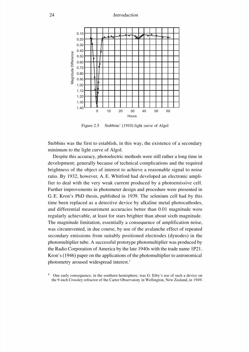
7/21/2019 Introduction to Astronomical Photometry
http://slidepdf.com/reader/full/introduction-to-astronomical-photometry 42/451
24 Introduction
0.10
0.20
0.30
0.40
0.50
0.60
0.70
0.80
0.90
1.00
1.10
1.201.30
1.400 10 20 30
Hours
M a g n i t u d e D i f f e r e n c e
40 50 60
Figure 2.5 Stebbins’ (1910) light curve of Algol
Stebbins was the first to establish, in this way, the existence of a secondaryminimum to the light curve of Algol.
Despite this accuracy, photoelectric methods were still rather a long time indevelopment; generally because of technical complications and the requiredbrightness of the object of interest to achieve a reasonable signal to noiseratio. By 1932, however, A. E. Whitford had developed an electronic ampli-fier to deal with the very weak current produced by a photoemissive cell.Further improvements in photometer design and procedure were presented inG. E. Kron’s PhD thesis, published in 1939. The selenium cell had by thistime been replaced as a detective device by alkaline metal photocathodes,and differential measurement accuracies better than 0.01 magnitude wereregularly achievable, at least for stars brighter than about sixth magnitude.The magnitude limitation, essentially a consequence of amplification noise,was circumvented, in due course, by use of the avalanche effect of repeatedsecondary emissions from suitably positioned electrodes (dynodes) in the
photomultiplier tube. A successful prototype photomultiplier was produced bythe Radio Corporation of America by the late 1940s with the trade name 1P21.Kron’s (1946) paper on the applications of the photomultiplier to astronomicalphotometry aroused widespread interest.4
4 One early consequence, in the southern hemisphere, was G. Eiby’s use of such a device onthe 9-inch Crossley refractor of the Carter Observatory in Wellington, New Zealand, in 1949.
7/21/2019 Introduction to Astronomical Photometry
http://slidepdf.com/reader/full/introduction-to-astronomical-photometry 43/451
2.2 Historical notes 25
This type of tube was used by H.L. Johnson and W.W. Morgan in theearly 1950s when they set up the three-colour UBV photoelectric system,which, despite certain well-known limitations, has been in general use up
to present times. In effect, the UBV magnitudes, because they have beenapplied to so many stars, at present probably represent the de facto mostgenerally used basic reference for stellar magnitudes, though other physicallyadvantageous schemes, notably the uvby system, are increasingly met with.In setting up the UBV system, Johnson and Morgan returned to photovisualmagnitudes traceable to North Polar Sequence values, and the principle of letting the relatively common A0 type stars locate, by their average, the zero
point of the B − V and U − B colour scales. Since the system was one of essentially improved accuracy, however, ultimately it defined the magnitudescale, though in essential agreement with earlier representations.
A key point here is the use of specifically designed filters in the definitionof a magnitude system. In this connection, a significant problem with theearlier photographic procedures came to light after the introduction of mirroraluminization techniques in the 1930s. The more effective reflectivity of aluminized over silvered reflectors, particularly in the ultraviolet, showed up
as significant differences in photographic magnitudes from plates taken withdifferent types of mirror surface. By the time of World War II, it was clearthat the key to more reliable magnitudes lay in a better definition of theoptical transmission properties of the entire photometer, i.e. the combinationof objective, intermediate reflecting and refractive media and the responsefunction of the detector itself. Postwar professional stellar photometry hasessentially taken careful definition of an adopted set of filters as axiomatic to
procedure. The process of defining a magnitude scale then becomes one of continued persistent checks and rechecks of measurements of selected starswith such filters: slowly weeding out slightly variable or peculiar stars andbuilding up increasingly reliable averages for the remaining standards. Certainmeritorious photometrists, in both hemispheres, have devoted considerableefforts to this aim. The broadband photoelectric photometry based on that of Johnson and Morgan is perhaps most well known in this respect. But anyparticular photometric system of n filters can be regarded as well defined,insofar as an ample number of reference stars are secured, each within itssufficiently precise box of n-dimensional space – the Golay box.5
A kind of complementarity existed in the middle years of the twentiethcentury, in which the precision and speed advantages of a single-channel
5 This oft-cited term comes from M. Golay’s informative Introduction to AstronomicalPhotometry, Reidel, 1974.
7/21/2019 Introduction to Astronomical Photometry
http://slidepdf.com/reader/full/introduction-to-astronomical-photometry 44/451
26 Introduction
photoelectric detector were balanced by the multi-channel and compactinformation storage advantages of photographic media. One 36 cm squareplate from the UK Schmidt Telescope (UKST), for example, could register
of the order of a million stars and galaxies over a 6.6deg square regionof sky. During the 1970s and 80s, the UKST was operated by the RoyalObservatory, Edinburgh, and carried out deep sky surveys of the southernhemisphere. Elaborate machines were built to carry out automatized digitalrecording of the vast amount of information that could be recorded onsuch plates.
Various groups later attempted to combine these information capabilities in
electronographic areal detectors of one form or another. Astronomy-specificimage tubes tended to be expensive and cumbersome. Adaptations of thewidely produced television type electron-gun scanning devices, on the otherhand, lacked suitable image storage and control facilities or precision. Butin 1970 the charge coupled device (CCD) was introduced at Bell Labora-tories. By 1975, the CCD camera had been placed at the focal plane of some large telescopes and their diffusion through observational astronomyhas continued ever since.
Although the information management requirements imposed by the neces-sities of digital sampling and recording of images at or near the resolutionlimit still entails relatively small areal coverage compared with, say, Schmidtcamera plates, CCDs are effective in both precision and object multiplicity.Moreover, individual chips can be arranged in mosaic form to cover largerareas of sky, as in large-scale surveys. Lower work functions associatedwith the photoconductive property of semiconductors generally entails more
reach into longer wavelength spectral regions (i.e. into the IR) than theearlier photoemissive detectors. In turn, this has required filter redesigns, sothat broadband magnitude systems can be continuous through the change of detection media, but such issues were generally in hand by the early 1990s.Colour–magnitude diagrams for star clusters that reach to twentieth or moremagnitude are now commonplace, even with telescopes of less than 1 metreaperture: there has thus been something of an information ‘explosion’ sincethe arrival of CCDs.
Fortunately, the concomitant growth of speed and data storage capabili-ties of small computers has permitted this explosion to remain manageable.In turn, this has allowed various large new ground-based surveys to beinitiated towards the end of the twentieth century. These have often beenprimarily motivated by specific research aims, e.g. the MACHO project’ssearches for gravitational lens effects, but they have yielded very interestingby-products through the collection of regular photometric data on millions of
7/21/2019 Introduction to Astronomical Photometry
http://slidepdf.com/reader/full/introduction-to-astronomical-photometry 45/451
2.3 Some basic terminology 27
stars. Large numbers of new variables were thus discovered, often in previ-ously unstudied areas, such as among the fainter parts of globular clusters orexternal galaxies.
Keeping pace with and contributing to such large information growthhas characterized ground-based optical photometry through the late yearsof the twentieth century, but a new era opened up with the launch of theHipparcos satellite in 1989. This ESA supported mission regularly includedestimates of Johnson V magnitudes of each of its ∼120 000 programmestars around 100–150 times throughout the four-year mission. Subsequentsystematic analysis enabled existing light curves of known variable stars to
be checked and also brought to light several thousand previously unknownvariables. The satellite’s on-board Tycho experiment aimed at providingmore precise two-colour (B and V ) data for at least 400000 stars. Usefulinformation on Hipparcos photometry has been publicly available fromthe ‘Hipparcos Epoch Photometry Annex’ of the programme’s educationwebpage (astro.estec.esa.nl/Hipparcos/education.html). At the present timethere are plans to follow Hipparcos with comparable, but more extensiveand precise, new space-based surveys to collect more detailed photometric
knowledge, from faint members of the Solar System to remote galaxies andquasars.
A useful marrying of space-based astronomy with the extensive amountof earlier photographic material came with the electronic digitization of suchdata, as carried out by the Catalogs and Surveys Branch of the Space TelescopeScience Institute. The first such catalogue (GSC I) was published in 1989,mainly as a support for positional needs in satellite control systems, but its
widespread availability proved a valuable scientific resource for astronomersgenerally. The later version (GSC II) is based on 1 arcsec resolution scans,and records of the order of a billion objects at two epochs and three wideband,photographic emulsion-based bandpasses.
2.3 Some basic terminology
A short glossary of frequently encountered terms is presented next, but manyof these are subjects of more detailed discussion in later chapters.
absolute magnitude M
This takes out the distance dependence of brightness, and thereforereflects the intrinsic amount of light put out by the source. It is definedas the apparent magnitude (see below) that the source (in the absence of
7/21/2019 Introduction to Astronomical Photometry
http://slidepdf.com/reader/full/introduction-to-astronomical-photometry 46/451
28 Introduction
light loss in the intervening space) would have if situated at a distanceof 10 parsecs.6 M then satisfies:
m − M = 5log − 5 (2.2)where is the distance to the source in parsecs. If interstellar extinction(see below) reduces the brightness of the source, i.e. adds A magnitudesinto the apparent magnitude value, then this quantity must similarly beadded to the right hand side of (2.2).
apparent magnitude m
This is the brightness of a star in the traditional system as it has evolved
to its modern form. The basic formula has been given already as (2.1).Balmer decrement measures D, c1
The discontinuity at the end of the Balmer series of hydrogen absorptionlines is a conspicuous feature in the near ultraviolet of stellar spectra.It is sensitive to surface gravity as well as temperature, consequentlyvarious photometric systems include some monitoring on either side of the discontinuity, to determine the size of the jump in energy terms, or
the decrement value D. In the intermediate bandwidth uvby system thecolour index combination u − v − v − b is found to correlate withthe Balmer decrement D. This has been given the special symbol c1.
bolometric magnitude mbol and correction BCBolometric magnitudes go beyond the restriction of magnitude at someparticular wavelength, or range of wavelengths, and refer to the totalpower of the source integrated over all wavelengths. The bolometriccorrection is then the quantity that must be added to the visual magnitudeto obtain the bolometric one. In general, it is negative in value.
brightness
This directly perceived datum is closely associated with the apparentmagnitude for point-like sources, i.e. stars. For extended objects furtherspecification is required. More physical details, connecting also withthe related term ‘intensity’, are given in Chapters 3 and 4.
colour excess
Due to the strong correlation between colour index and surface temper-ature, if the temperature of a certain star is known a priori it shouldbe possible to predict its normal colour index. Sometimes, however,stars or other astronomical sources produce anomalous effects, such as
6 1 parsec (pc) is the distance at which the mean Earth–Sun distance would subtend an angleof 1 arcsecond.
7/21/2019 Introduction to Astronomical Photometry
http://slidepdf.com/reader/full/introduction-to-astronomical-photometry 47/451
2.3 Some basic terminology 29
a violet or red excess, the proper interpretation of which is not alwaysobvious.
colour index C or CI
This is expressed as the difference of two magnitude values (in a givensystem) at different wavelengths: e.g. B (∼4400Å) – V (∼5500 Å) inthe UBV system.
effective temperature T eff
It is often desirable to characterize the overall emission of unit area of a radiation source by a suitable parameter. The effective temperatureis that of a Planckian radiation field (Section 3.1) having the same
integrated emission per unit area.effective wavelength eff
Observation of a radiation source extends over a range of wavelengthsabout some nominal value. The effective wavelength is a representationof this value that can usefully characterize the magnitude for compara-tive spectral studies. There are alternative measures, such as mean orisophotal wavelength. More specific statements about these are given
in Chapter 3.extinction k, A
Light from stars does not reach the detector directly, but passes throughabsorbing or scattering media – the Earth’s own atmosphere, as well asthe interstellar medium – whereby its intensity decreases. The extinctionis related to a coefficient, which depends on the medium and wave-length of transmission. For the Earth’s atmosphere k usually denotes
the extinction coefficient at the observation wavelength. A is used (witha slightly different physical meaning) for the interstellar medium.
flux , f
This measures the power of a radiative field passing through some unitof area, but in conventional physical units, and is thus more suitablethan the magnitude value for general physical analysis. It is sometimesconvenient to distinguish between emitted, , and received, f , fluxes.
gradient , GThe magnitude difference at two given wavelengths divided by thedifference of the two wavelengths’ reciprocals, , gives a usually fairlyconstant quantity over optical wavelength ranges, due to approximateblack-body-like behaviour. Even closer to a constant is the differencebetween two such ‘absolute’ gradients for two radiation sources – the‘relative’ gradient G.
7/21/2019 Introduction to Astronomical Photometry
http://slidepdf.com/reader/full/introduction-to-astronomical-photometry 48/451
30 Introduction
illuminance, irradiance f
The meaning is practically the same as flux, but the usage is gener-ally reserved for a surface illuminated by a remote source, such as a
unit area above the Earth’s atmosphere illuminated by starlight. Thewords illuminance and irradiance are used more or less interchangeably,although the usage of the latter may be more in the context of speci-fying received flux per unit wavelength f or frequency range f . Termssuch as spectral illuminance or irradiance are also used to make thisapplication clear.
interstellar reddening E
The extinction of light due to interstellar matter gives rise to its ownspecialized study. The reddening E measures an increase in magnitude(dimming) as one passes to shorter wavelengths, e.g. from V to B,beyond what would be appropriate for a star of the given spectral type,and after having taken account of the normal effect of the Earth’satmosphere to produce reddening.
line index e.g. ,
The underlying idea is again that of a magnitude difference. In this case,however, the context is narrowband photometry, and the narrowbandfilter is centred on a particular spectral line, e.g. H, H. The value 2.5log (flux) thus measured is subtracted from a similar measure, madewith an intermediate bandwidth filter of the surrounding continuum, toform the line index.
luminosity L
Also a measure of the radiative power of a source, it relates to the entire
output, and thus can be directly connected with absolute bolometricmagnitude. The relevant formula, scaling to the solar luminosity L, is
M bol = 475−25log L/L (2.3)
magnitude bandwidth
Real observations must inevitably cover some finite wavelength range.
Conventionally, optical photometry is subdivided into ‘narrow’, ‘inter-mediate’ and ‘broad’ bandwidth types, depending on the order of magni-tude of the ratio /, the effective transmission range divided byits mean wavelength. Narrowband photometry uses filters for which/ 10−2. For intermediate-band photometry the ratio is around, orsomewhat less than, 10−1, while for broadband photometry we typicallyfind / ∼ 1
4 .
7/21/2019 Introduction to Astronomical Photometry
http://slidepdf.com/reader/full/introduction-to-astronomical-photometry 49/451
2.3 Some basic terminology 31
metallicity index m1
Stellar spectra are dependent on the proportion of elements heavierthan helium (metals) in their radiating atmospheres (as well as other
parameters). Certain photometric systems allow a suitable combina-tion of magnitude values from different filters to monitor the relativeabundance of metals (metallicity). In the uvby system this is referredto as m1 = v − b− b − y.
monochromatic magnitude m
Standard magnitudes represent the integrated product of a responsefunction with a light flux distribution. For a monochromatic magnitude
the response function is an ideal one (-function), having unit integralover a vanishingly small wavelength (or frequency) interval at thewavelength (or frequency) specified, and zero elsewhere. The conceptis used in the analysis of magnitude systems.
sequence
An orderly arrangement of a group of stars according to magnitudes orcolours.
spectral resolutionThis is the inverse of the bandwidth measure given above, i.e. /,the number of times the effective transmission range will divide intoa representative wavelength. The term photometry is generally appliedto relatively low spectral resolution observations, although some spec-troscopic observations are made at very low resolution (e.g. objectivegrating surveys), while certain photometric type techniques are made atvery high resolution (e.g. solar chromospheric monitoring).
spectral type
Stars are classified on the basis of their observed spectral energy distri-bution, particularly with regard to the appearance or disappearance of certain discrete features. The types have been arranged, after pioneeringwork at Harvard College Observatory in the late nineteenth and earlytwentieth centuries, into groups designated with capital letters: thusO, B, A, F, G, K, M represent the main types in order of decreasing
temperature. These are then further subdivided into typically eight orso subtypes (e.g. G0, G2, , G8; note, not necessarily successive inte-gers). There is a strong correlation between colour index and spectraltype, since surface temperature is the main underlying variable. Theconnection is not unequivocal, however, since both spectral type andcolour index may be affected separately by other physical variables. Thesystem was later extended by W. Morgan, P. Keenan and E. Kellman
7/21/2019 Introduction to Astronomical Photometry
http://slidepdf.com/reader/full/introduction-to-astronomical-photometry 50/451
32 Introduction
to include the effects of varying gravity, or luminosity (see above), onspectra. This (MKK) system is now in general use.
standard magnitude e.g. V, B, U
The term apparent magnitude is too imprecise for scientific use. Themagnitude system has been more precisely defined over the last severaldecades, allowing different workers, using their local measurements,advantageously to convert to a generally recognized scale: for example,that of the standard V (for visual) magnitude.
standard star
A magnitude system is progressively defined by reference to standard
stars; starting usually with relatively bright and well-known ones, suchas Vega or the ten primary standards of the UBV system.
2.4 Radiation: waves and photons
Though this book centres largely around photometric procedure and anal-ysis, with certain practical applications well to the fore, the nature of light
underlies these and certain basic concepts should be clear. This is not reallya very straightforward matter, however. In Newton’s time a ‘corpuscular’or particle-like theory was considered able to account for the evidence of experiments. On the other hand, a wave theory had also been advanced andhad some proponents, so that a kind of rivalry of explanations existed forsome time.
Nowadays both points of view are regarded as tenable and complementary,
and either one or the other may be advantageous in different contexts. Forexample, interferometry of two beams of radiation emanating from a star,directed through two mirrors of known separation, but within the ‘coherencelength’ of that radiation, in principle, enables information on the size of thestar to be determined. On the other hand, the existence of such a coherencelength itself testifies to some finiteness of structure within the propagatingwave trains.
In the last half of the nineteenth century ideas on the wave propagation
of light became clarified after a number of convincing experiments. In 1878James Clerk Maxwell produced a set of equations describing the interactionof magnetic and electric fields, as a result of which it was shown that awave motion, involving these fields, will sustain itself, provided this motionis characterized by a certain velocity, equal to the reciprocal of the squareroot of the product of the magnetic permeability and electrical permittivity of the medium in which the wave propagates. This wave motion was identified
7/21/2019 Introduction to Astronomical Photometry
http://slidepdf.com/reader/full/introduction-to-astronomical-photometry 51/451
2.4 Radiation: waves and photons 33
with light and, since free space also has magnetic permeability and electricalpermittivity, light propagates through it, with an ‘absolute’ velocity.
Maxwell himself, along with his contemporaries, accepted the idea of a
universal medium (the ‘æther’) permeating all space and supporting the wavemotion. However, later this concept was found to be superfluous – misleadingeven. At any rate, the notion of some material entity at absolute rest, to whichthe motions of objects can be directly referred, which the existence of thesupposed medium suggests might be possible, is not in keeping with the resultsof physical experiments. It is well known that Einstein’s famous theories of relativity, which revolutionized subsequent physics, grew out of this back-
ground. Many remarkable developments of modern astronomy have providedobservational supports for relativity, and striking examples of progressiveinteraction between physical theory and observational practice.
Einstein, in another basic contribution to modern physics, gave a discussionof the photoelectric effect, whose implications are central to photoelectricphotometry. This presentation, in which a given discrete energy of radiationcorresponds with an energy change of a fundamental particle (e.g. an electron),leads to a view of radiation interacting with matter in a particle-like way. This
view is already seen in Planck’s idea that the energy emitted by a radiatingbody emerges in certain tiny packets or quanta. The quantum theory, whichhas grown out of this, associates wave properties with fundamental particles,such as electrons; as well as the reverse with photons: the modern ‘corpuscles’of light.
It was known already towards the end of the nineteenth century that certainclean metal surfaces could be induced to lose negative electrical charge
under the influence of ultraviolet light. Einstein’s photoelectric theory neatlysummarizes this effect by the equation
h = h0 + 12
mv2 (2.4)
where the product of Planck’s constant h with the frequency of the impingingphoton gives the input energy of the quantum. If this is greater than aparticular threshold work function, associated with the frequency 0, and
characteristic of the particular metal, or electron-yielding surface involved,then an electron can emerge with kinetic energy 1
2 mv2, as specified by thelast term on the right hand side.
A circuit can be set up so that electrons liberated from a suitably preparedand illuminated cathode surface are attracted to a nearby positive electrode,where their arrivals are registered. In this way, a light-responsive surface ismade to form the detective element (photocathode) of a photometer. In the
7/21/2019 Introduction to Astronomical Photometry
http://slidepdf.com/reader/full/introduction-to-astronomical-photometry 52/451
34 Introduction
basic form of the photoemission theory, then, the energy of the emittedelectron depends only on the frequency of the incident radiation and not on itsintensity. However, the number of electrons emitted per second, or (negative)
current, from the photoresponsive surface, does vary in direct proportion tothe photon incidence rate. This proportionality is at the root of photometricmethods utilizing the photoelectric effect.
Even without surface emission, the photo-energization of electrons mayresult in measurable effects. This is an area of technology that has seenconsiderable advances in the era of solid state electronics. In particular,the greater ease with which photo-energized electrons can move through a
semiconductor, or the photoconductive effect, allows them to be collected inmicroscopic potential wells in numbers that are linearly proportional to localflux values, at least for some range of brightness values. Many collectionsites, of microscopic size, set up over an electronically controllable area, canthen be used as a linearly responsive sensitive photometric imaging system,such as the charge coupled devices (CCDs) that continue to see increasedapplications in astronomical research.
2.5 Bibliographical notes
Many interesting points were made about the role of the eye in observingcelestial objects in M. Minnaert’s book The Nature of Light and Colour in the
Open Air (Dover, 1954). A more detailed text on the eye, exposing its opticalbehaviour in relation to photometry, is Fundamentals of Visual Science, by
M. L. Rubin and G. L. Wells (C. C. Thomas, Illinois, 1972), but a more recentsource is S. E. Palmer’s Vision Science: Photons to Phenomenology (BradfordBooks, 1999). Articles on eye-based astronomical photometry can be foundamong the annals of organizations such as the AAVSO or the RASNZ’sVariable Stars Section, and others mentioned in the previous chapter’s bibli-ographical notes. A well-regarded summary of visual methods was given byF. M. Bateson in South. Stars (13, 23, 1947).
J. B. Hearnshaw’s The Measurement of Starlight (Cambridge University
Press, 1996) provides a very thorough and valuable source to consult onthe historical development of astronomical photometry, including over1800 literature references in its purview. Volume 13 of Mem. R. Astron.
Soc. (1843) contained a compilation of the old catalogues of Ptolemy,Ulugh Beg and others, by F. Baily. E. Knobel assembled a chronologicallisting of information on old astronomical catalogues back to the time of Eudoxus in Volume 43 (1876) of the same publication. Aspects of the
7/21/2019 Introduction to Astronomical Photometry
http://slidepdf.com/reader/full/introduction-to-astronomical-photometry 53/451
2.5 Bibliographical notes 35
tumultuous Renaissance period of astronomy are readably recounted inC. A. Ronan’s The Astronomers (Evans Bros., 1964) or A. Koestler’s bookThe Sleepwalkers (Penguin Books, 1990). A biography of P. Bouguer may
be found in La Grande Encyclopédie (H. Lamirault, 1902) and some of hiscontributions are recalled in, for example, the short biographies given byH. Ludendorff in Populäre Astronomie (Wilhelm Engelmann, 1921). Thediscovery of the regularity of Algol’s variability and the inferences placedthereon by John Goodricke were reviewed by Z. Kopal in Mercury (19, 88,1990). Z. Kopal provided further background on the lives of John Michelland the Herschel family in his autobiography Of Stars and Men (Adam
Hilger, 1986, Chapters 6 & 7). Consideration of the early observationalbackground on Algol’s variability was given by E. Budding in South. Stars
(32, 180, 1988).A seminal article covering the whole early development of stellar photo-
metry is that of K. Lundmark in Handbuch der Astrophysik (5, 210, 1932) (seealso G. Eberhard in the same series, 7, 90, 1936), while H. F. Weaver’s seriesof papers in Popular Astron. (54, 211, 1946 and subsequent issues) providesalternative, more descriptive, reading. The stars of the North Polar Sequence
are listed in the Trans. Int. Astron. Union, 1, 71, 1922. Background on thedevelopment of photographic photometry is covered in such sources, thoughalternative, technically oriented material is available in reference manualsissued by some of the larger companies dealing with photographic materials.A review of the iris-diaphragm technique was given by B. E. Schaefer, Publ.
Astron. Soc. Pac. (93, 253, 1981), while more information can be soughtin Modern Techniques in Astronomical Photography, eds. R.M. West and
J. L. Heudier (ESO, 1978).Minchin’s early experiments in photoelectric photometry were recorded byC. J. Butler, in the Ir. Astron. J. (17, 373, 1986), and G. E. Kron recalled thepioneering work of Joel Stebbins in Chapter 2 of Photoelectric Photometry of
Variable Stars, eds. D. S. Hall and R. M. Genet (Willmann-Bell Inc., 1988).His cited paper was published in Astrophys. J . (103, 326, 1946). Stebbins’light curve shown in Figure 2.5 was published in Astrophys. J . (32, 185,1910). G. Eiby’s MSc thesis was submitted to the Victoria University of
Wellington in October, 1949.The Johnson and Morgan era (see Astrophys. J., 117, 313, 1953) was
covered in a number of still useful papers in Astronomical Techniques, ed.W. A. Hiltner (University of Chicago Press, 1962) in articles such as thoseof A. Lallemand, H. L. Johnson and R. H. Hardie. The similar Basic Astro-
nomical Data of the same series (ed. K. A. Strand) contains seminal papersby B. Strömgren, H. L. Johnson, S. Sharpless, W. Becker and others. The
7/21/2019 Introduction to Astronomical Photometry
http://slidepdf.com/reader/full/introduction-to-astronomical-photometry 54/451
36 Introduction
little Astronomical Photoelectric Photometry, ed. F. B. Wood (AAAS, 1953),is also a good source book on the early development of the subject.
A compact description of the application of the COSMOS machine
measuring UKST plates at the Royal Observatory Edinburgh for UBV surveyphotometry was given by R. J. Dodd and L. Ellery in the Proceedings of the1st Asian-Pacific Regional Meeting of the IAU in Wellington, New Zealand,
NZ Journ. Sci. (22, 457, 1979) (eds. W. Davidson & B.M. Lewis). Anexample of the data application is that of Dodd, Andrews and MacGillivray(1986) to the distribution properties of galaxies in a selected field of theSouthern Sky Survey: Second Epoch Survey (M. Longair, 1985). A general
list of astronomical survey work, including those involving large-angle photo-graphic plates, is presented at www.vilspa.esa.es/astroweb/yp_survey.html.The MACHO project, one of the first bulk CCD-based stellar data-processingendeavours was presented by A. Gould in Astrophys. J . (404, 451, 1993),and subsequently discussed in many presentations to the AAS, e.g. Bull.
Amer. Astron. Soc. (25 and 26, 1993, 1994, etc). Updated information can beaccessed via wwwmacho.mcmaster.ca/. Information on the comparable OGLEand MOA projects is similarly found at bulge.astro.princeton.edu/ogle/,and www.physics.auckland.ac.nz/moa/, respectively. Information on theGuide Star Catalog is available from chart.stsci.edu/gsc/GSChome.htm.As one example of its application to astrophysical aims we may citeR.L. Smart et al., Ultracool Dwarfs: New Spectral Types L and T (Springer,2001), p. 119. The Sloan Digital Sky Survey maintains the webpagewww.sdss.org/. The Hipparcos Epoch Photometry Annex can be accessedfrom www.rssd.esa.int/Hipparcos/EpochPhot.html.
Many of the basic terms and formulae of Section 2.3 appear in C. W. Allen’s Astrophysical Quantities, whose 4th edition (ed. A. N. Cox) was publishedby AIP Press in 2000. H. J. Gray and A. Isaacs’ A New Dictionary of Physics
(Longman, 1975) provides an extensive source of related definitions.Further general reading on modern theories of light and the photoelectric
effect is to be found in, for example, R. Baierlein’s Newton to Einstein:
The Trail of Light (Cambridge University Press, 2001); or Light (Vol. 1) by
H. Haken (North Holland Publ. Co., 1981), while basic questions of relevanceto Section 2.4 are reviewed in What is Light? by A. C. S. van Heel and C. H. F.Velzel (World University Library, London, Weidenfeld and Nicolson, 1968),or The Ethereal Æther , by L.S. Swenson Jr. (University of Texas Press,1972). P. Léna’s Observational Astrophysics (Springer-Verlag, 1988) includesan in-depth treatment of radiation, which it relates to general astrophysicalcontexts.
7/21/2019 Introduction to Astronomical Photometry
http://slidepdf.com/reader/full/introduction-to-astronomical-photometry 55/451
References 37
References
Allen, C. W., 2000, Astrophysical Quantities, 4th edn., ed. A. N. Cox, AIP Press.Baily, F., 1843, Mem. R. Astron. Soc., 13, 1.Baierlein, R., 2001, Newton to Einstein: The Trail of Light , Cambridge University
Press.Bateson, F. M., 1947, South. Stars, 13, 23.Becker, W., 1963, Stars and Stellar Systems, III , Basic Astronomical Data, ed. K.A.
Strand, University of Chicago Press, p. 241.Budding, E., 1988, South. Stars, 32, 180.Butler, C. J., 1986, Ir. Astron. J., 17, 373.Eberhard, G., 1936, Handbuch der Astrophysik , Springer, 7, 90.
Dodd, R. J. & Ellery, L., 1979, NZ Journ. Sci., 22, 457.Dodd, R.J., Andrews, F.P. & MacGillivray, H.T., 1986, Astrophys. Space Sci.,123, 145.
Eiby, G., 1949, MSc thesis, Victoria University, Wellington, New Zealand.Golay, M., 1974, Introduction to Astronomical Photometry, Reidel.Gould, A., 1993, Astrophys. J ., 404, 451.Gray, H. J. & Isaacs, A., 1975, A New Dictionary of Physics, Longman.Haken, H., 1981, Light , I, North Holland.Hardie, R. H., 1962, Stars and Stellar Systems, II, Astronomical Techniques, ed. W. A.
Hiltner, University Chicago Press, p. 178.Hearnshaw, J. B., 1996, The Measurement of Starlight , Cambridge University Press.IAU, 1922, Transactions, 1, 71.Johnson, H.L., 1962, Stars and Stellar Systems, II, Astronomical Techniques, ed.
W. A. Hiltner, University of Chicago Press, p. 157.Johnson, H. L., 1963, Stars and Stellar Systems, III, Basic Astronomical Data, ed.
K. A. Strand, University of Chicago Press, p. 204.Johnson, H. L. & Morgan, W. W., 1953, Astrophys. J. 117, 313.Knobel, E. B., 1876, Mem. R. Astron. Soc., 43, 1.
Koestler, A., 1990, The Sleepwalkers, Penguin Books.Kopal, Z., 1986, Of Stars and Men, Adam Hilger.Kopal, Z., 1990, Mercury, 19, 88.Kron, G. E., 1946, Astrophys. J ., 103, 326.Kron, G. E., 1988, Photoelectric Photometry of Variable Stars, ed. D.S. Hall and
R. M. Genet, Chapter 2, Willmann-Bell Inc.Lallemand, A., 1962, Stars and Stellar Systems, II, Astronomical Techniques, ed.
W. A. Hiltner, University of Chicago Press, p. 126.Lamirault, H., 1902, La Grande Encyclopédie (1886-1902), ed. M. Berthelot, Paris.
Léna, P., 1988, Observational Astrophysics, Springer-Verlag.Longair, M. S., 1985, Southern Sky Survey: Second Epoch, Royal Observatory
Edinburgh, Research & Facilities (see also www.roe.ac.uk/ifa/wfau/cosmos/).Ludendorff, H., 1921, Populäre Astronomie, Wilhelm Engelmann.Lundmark, K., 1932, Handbuch der Astrophysik , J. Springer, 5, 210.Minnaert, M. 1954, The Nature of Light and Colour in the Open Air , Dover.Palmer, S. E., 1999, Vision Science: Photons to Phenomenology, Bradford Books.Ronan, C. A., 1964, The Astronomers, Evans Bros.
7/21/2019 Introduction to Astronomical Photometry
http://slidepdf.com/reader/full/introduction-to-astronomical-photometry 56/451
38 Introduction
Rubin, M. L. & Wells, G. L., 1972, Fundamentals of Visual Science, C. C. Thomas.Schaefer, B. E., 1981, Publ. Astron. Soc. Pac., 93, 253.Sharpless, S., 1963, Stars and Stellar Systems, III, Basic Astronomical Data, ed. K. A.
Strand, University of Chicago Press, p. 225.Smart, R. L., Carollo, D., Lattanzi, M. G., McLean, B. & Spagna, A., 2001, Ultracool
Dwarfs: New Spectral Types L and T , eds. H. R. A. Jones & I. A. Steele, Springer,p. 119.
Stebbins, J., 1910, Astrophys. J ., 32, 185.Strömgren, B., 1963, Stars and Stellar Systems, III, Basic Astronomical Data, ed.
K. A. Strand, University of Chicago Press, p. 123.Swensen Jr., L. S., 1972, The Ethereal Æther , University of Texas Press.Van Heel, A. C .S. & Velzel, C. H. F., 1968, What is Light?, World University Library,
Weidenfeld and Nicolson.Weaver, H. F., 1946, Popular Astron., 54, 211.West, R. M. & Heudier, J. L., 1978, Modern Techniques in Astronomical Photography,
European Southern Observatory.Wood, F. B., 1953, Astronomical Photoelectric Photometry, AAAS.

7/21/2019 Introduction to Astronomical Photometry
http://slidepdf.com/reader/full/introduction-to-astronomical-photometry 57/451
3
Underlying essentials
3.1 Radiation field concepts
Consider a thermally insulated ‘black’ enclosure, maintained at a constanttemperature, T . The enclosure has a characteristic radiation field in isolationfrom other sources, which depends only on T . The maintenance of thisconstant temperature implies an equilibrium in internal thermal emissions and
absorptions. Let there be an aperture s to the enclosure, which we take tobe so small that the radiation field characterizing the interior is essentiallyunaffected. Radiation emerging from the aperture is detected by a receiverpresenting an area A normal to the radius r joining the centre of the apertureto that of the detector. The external medium is regarded as transparent. Theangle between the normal to s and r is .
The luminous power L picked up by the detector (Figure 3.1) is found tobe proportional to A/r 2, s and cos , so that
L ∝ s cos (3.1)
where we have abbreviated slightly by writing = A/r 2 – the ‘solid angle’subtended by A. The unit of solid angle is the steradian, defined so thatan entire sphere subtends 4 steradians at an internal point, so a cone of semiangle 328 subtends close to 1 steradian at its apex. Sometimes the
expression ‘luminous flux’ is met for L, but the term power is appropriate,since L can be measured in watts, while flux has the more restricted meaningof power passing through unit area.
The constant of proportionality in (3.1) is the intensity I , sometimes calledspecific brightness, so that
L = I s cos (3.2)
39
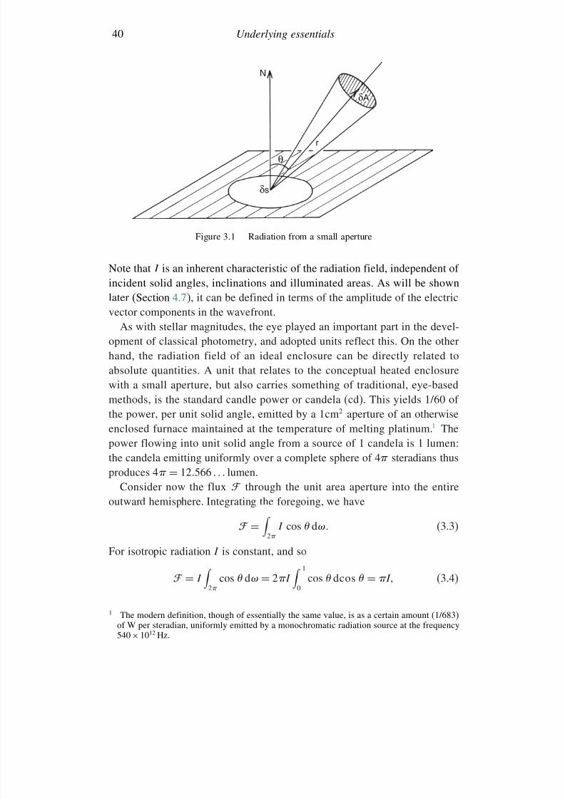
7/21/2019 Introduction to Astronomical Photometry
http://slidepdf.com/reader/full/introduction-to-astronomical-photometry 58/451
40 Underlying essentials
N
θ
r
δs
δA
Figure 3.1 Radiation from a small aperture
Note that I is an inherent characteristic of the radiation field, independent of incident solid angles, inclinations and illuminated areas. As will be shownlater (Section 4.7), it can be defined in terms of the amplitude of the electricvector components in the wavefront.
As with stellar magnitudes, the eye played an important part in the devel-opment of classical photometry, and adopted units reflect this. On the otherhand, the radiation field of an ideal enclosure can be directly related toabsolute quantities. A unit that relates to the conceptual heated enclosurewith a small aperture, but also carries something of traditional, eye-basedmethods, is the standard candle power or candela (cd). This yields 1/60 of the power, per unit solid angle, emitted by a 1cm2 aperture of an otherwiseenclosed furnace maintained at the temperature of melting platinum.1 Thepower flowing into unit solid angle from a source of 1 candela is 1 lumen:the candela emitting uniformly over a complete sphere of 4 steradians thusproduces 4 = 12566 lumen.
Consider now the flux through the unit area aperture into the entireoutward hemisphere. Integrating the foregoing, we have
= 2 I cos d (3.3)
For isotropic radiation I is constant, and so
= I
2 cos d = 2I
1
0cos dcos = I (3.4)
1 The modern definition, though of essentially the same value, is as a certain amount (1/683)of W per steradian, uniformly emitted by a monochromatic radiation source at the frequency540 × 1012 Hz.
7/21/2019 Introduction to Astronomical Photometry
http://slidepdf.com/reader/full/introduction-to-astronomical-photometry 59/451
3.1 Radiation field concepts 41
so that the 1cm2 aperture of the considered isotropic furnace emits altogether60 lumens. This turns out to be equivalent to about 0.276 watts in the visibleregion of the spectrum.
Flux is here seen to be the cosine-weighted integral of the intensity. It is,in this way, sometimes termed the first moment of the intensity. A zerothmoment is defined by
4J =
4 I d (3.5)
J is easily seen to denote the mean intensity. Here we have integrated overthe entire sphere. The corresponding expression for flux gives the differ-
ence between the outward hemisphere integration and the inward one (tacitlyassumed to be zero in equations (3.3) and (3.4)).
A second moment, known as the ‘pressure’ of a radiation field, given by
4K =
4 I cos2 d (3.6)
is also found with flux and mean intensity in analyses of radiation fields. Ina radiating stellar atmosphere, where there is a steady radiative flow without
sources or sinks of energy, can be shown to be proportional to the gradientof K with respect to the variable ‘optical depth’, which is the integral of local opacity over distance in the direction of the net flow. This relationshipbetween radiation pressure and flux is one way to express the transportof energy by radiation in steady conditions. Its form points to a diffusionprocess.
A variety of other units appear in photometry, associated with its visualbackground and the characterization of light levels or brightness values of illuminated surfaces. Partly this stems from the replacement of CGS nomen-clature by SI units – for instance, with the phot and the lux . The formerindicates a luminous power passing through 1cm2 of 0.00146 watts (i.e.1lumencm2), the latter corresponds to the same net rate of watts, but spreadover 1m2. The lumen and candela were conserved in value as basic unitswith the CGS → SI transfer. The phot, a relatively large unit, is then 104×the lux in value. These units can be applied to the power per unit area above
the atmosphere received from a star of given magnitude (Section 3.3).2
A unit quantitatively similar to the lux for measuring the apparent brightnessof an extended surface is the apostilb. If light illuminates a white surfaceso that 1 lux is perfectly diffused by each square metre it is said to have abrightness, or sometimes intensity, of 1 apostilb. Intensity is more properly
2 Note also the jansky = 10−26 W m−2 Hz−1, a unit of irradiance used in radioastronomy.
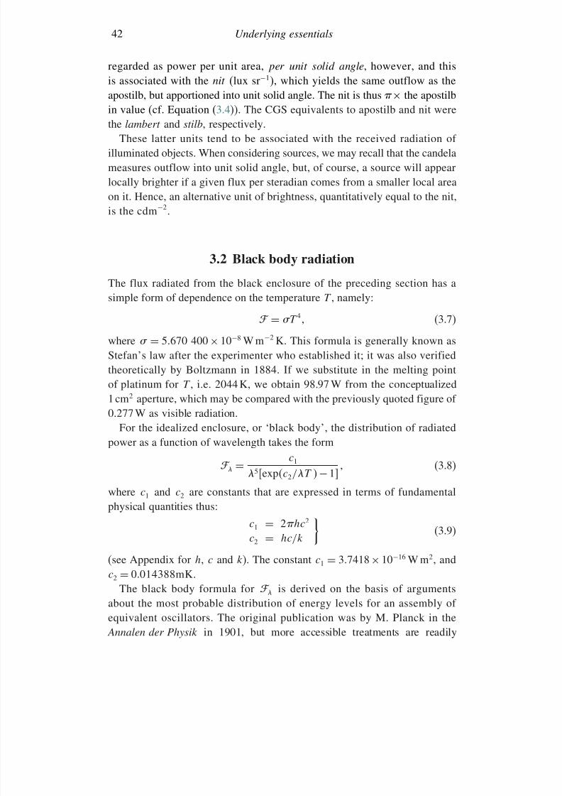
7/21/2019 Introduction to Astronomical Photometry
http://slidepdf.com/reader/full/introduction-to-astronomical-photometry 60/451
42 Underlying essentials
regarded as power per unit area, per unit solid angle, however, and thisis associated with the nit (lux sr−1), which yields the same outflow as theapostilb, but apportioned into unit solid angle. The nit is thus
×the apostilb
in value (cf. Equation (3.4)). The CGS equivalents to apostilb and nit werethe lambert and stilb, respectively.
These latter units tend to be associated with the received radiation of illuminated objects. When considering sources, we may recall that the candelameasures outflow into unit solid angle, but, of course, a source will appearlocally brighter if a given flux per steradian comes from a smaller local areaon it. Hence, an alternative unit of brightness, quantitatively equal to the nit,is the cdm−2.
3.2 Black body radiation
The flux radiated from the black enclosure of the preceding section has asimple form of dependence on the temperature T , namely:
=T 4 (3.7)
where = 5670 400 × 10−8 W m−2 K. This formula is generally known asStefan’s law after the experimenter who established it; it was also verifiedtheoretically by Boltzmann in 1884. If we substitute in the melting pointof platinum for T , i.e. 2044 K, we obtain 98.97 W from the conceptualized1 cm2 aperture, which may be compared with the previously quoted figure of 0.277 W as visible radiation.
For the idealized enclosure, or ‘black body’, the distribution of radiatedpower as a function of wavelength takes the form
= c1
5expc2/T −1 (3.8)
where c1 and c2 are constants that are expressed in terms of fundamentalphysical quantities thus:
c1 = 2hc2
c2 = hc/k (3.9)
(see Appendix for h, c and k). The constant c1 = 37418× 10−16 W m2, andc2 = 0014388mK.
The black body formula for is derived on the basis of argumentsabout the most probable distribution of energy levels for an assembly of equivalent oscillators. The original publication was by M. Planck in the
Annalen der Physik in 1901, but more accessible treatments are readily
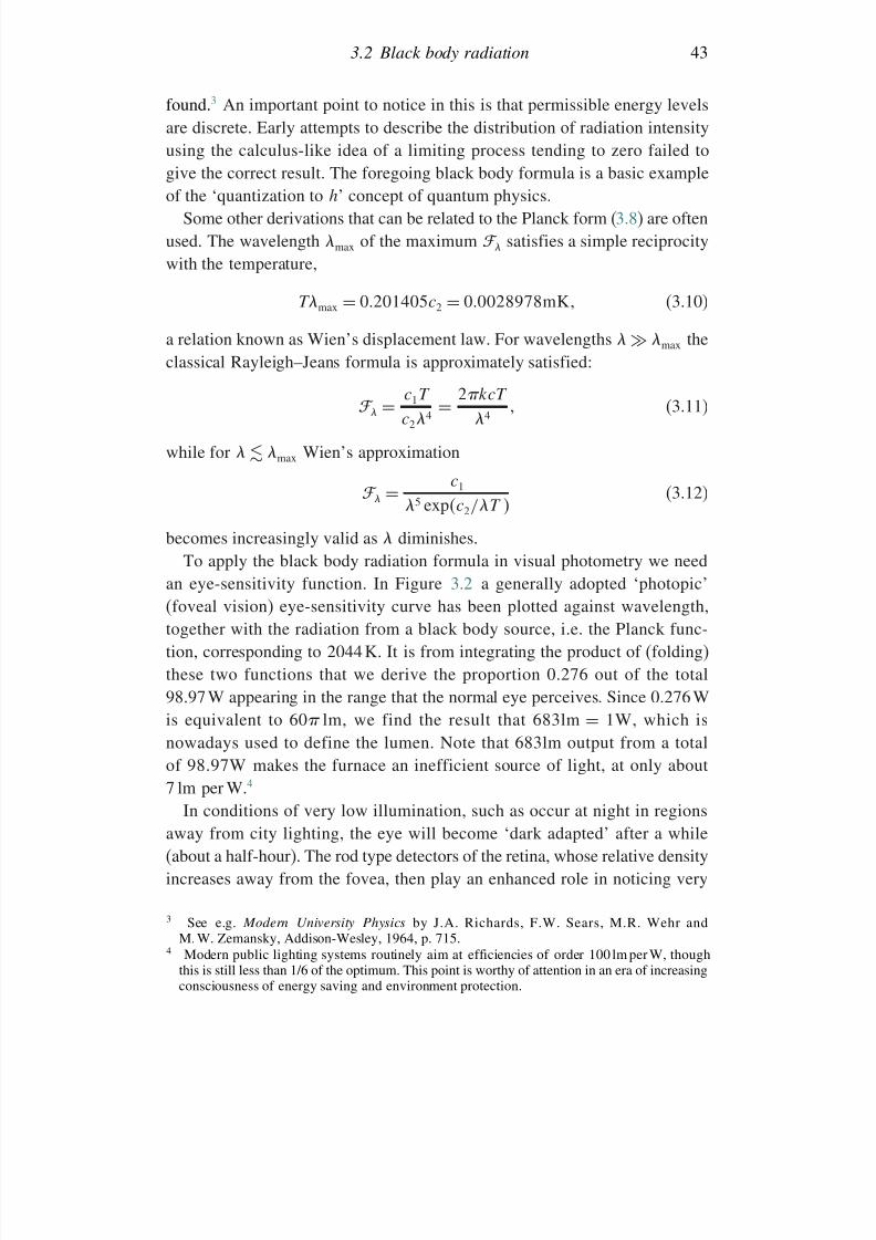
7/21/2019 Introduction to Astronomical Photometry
http://slidepdf.com/reader/full/introduction-to-astronomical-photometry 61/451
3.2 Black body radiation 43
found.3 An important point to notice in this is that permissible energy levelsare discrete. Early attempts to describe the distribution of radiation intensityusing the calculus-like idea of a limiting process tending to zero failed to
give the correct result. The foregoing black body formula is a basic exampleof the ‘quantization to h’ concept of quantum physics.
Some other derivations that can be related to the Planck form (3.8) are oftenused. The wavelength max of the maximum satisfies a simple reciprocitywith the temperature,
Tmax = 0201405c2 = 00028978mK (3.10)
a relation known as Wien’s displacement law. For wavelengths max theclassical Rayleigh–Jeans formula is approximately satisfied:
= c1T
c24 = 2kcT
4 (3.11)
while for max Wien’s approximation
= c1
5 expc2/T
(3.12)
becomes increasingly valid as diminishes.To apply the black body radiation formula in visual photometry we need
an eye-sensitivity function. In Figure 3.2 a generally adopted ‘photopic’(foveal vision) eye-sensitivity curve has been plotted against wavelength,together with the radiation from a black body source, i.e. the Planck func-tion, corresponding to 2044 K. It is from integrating the product of (folding)
these two functions that we derive the proportion 0.276 out of the total98.97 W appearing in the range that the normal eye perceives. Since 0.276 Wis equivalent to 60 lm, we find the result that 683lm = 1W, which isnowadays used to define the lumen. Note that 683lm output from a totalof 98.97W makes the furnace an inefficient source of light, at only about7 lm per W.4
In conditions of very low illumination, such as occur at night in regionsaway from city lighting, the eye will become ‘dark adapted’ after a while(about a half-hour). The rod type detectors of the retina, whose relative densityincreases away from the fovea, then play an enhanced role in noticing very
3 See e.g. Modern University Physics by J.A. Richards, F.W. Sears, M.R. Wehr andM. W. Zemansky, Addison-Wesley, 1964, p. 715.
4 Modern public lighting systems routinely aim at efficiencies of order 100 lm per W, thoughthis is still less than 1/6 of the optimum. This point is worthy of attention in an era of increasingconsciousness of energy saving and environment protection.
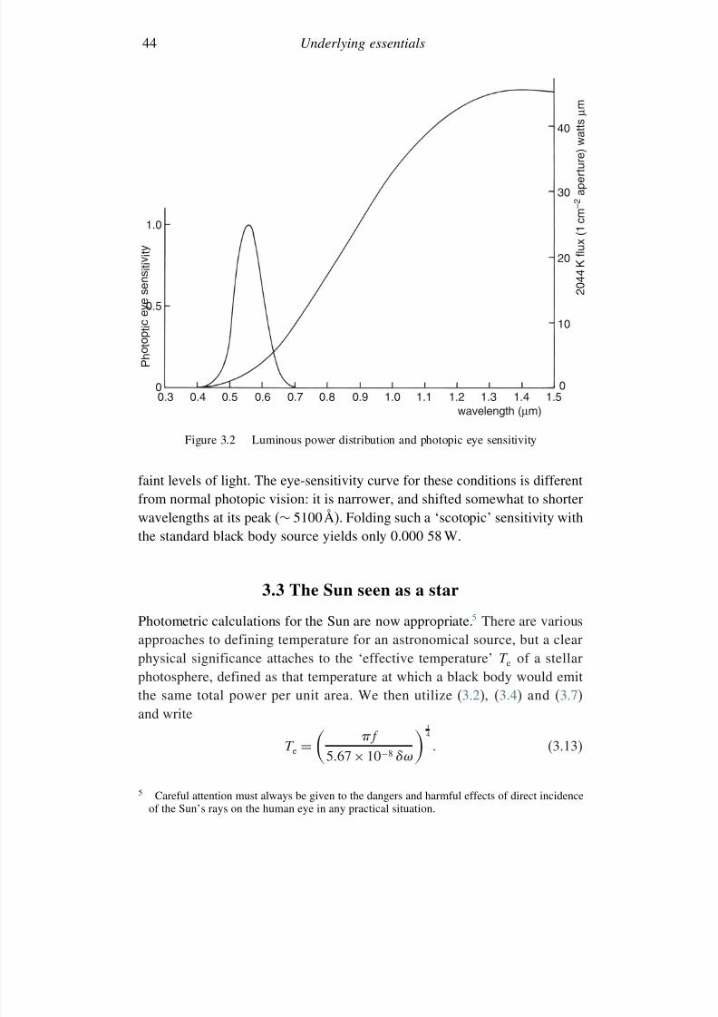
7/21/2019 Introduction to Astronomical Photometry
http://slidepdf.com/reader/full/introduction-to-astronomical-photometry 62/451
44 Underlying essentials
P h o t o p
t i c e y e
s e n s i t i v i t
y
0.30
0.4 0.6 0.7 0.8 0.9 1.0 1.1 1.2 1.3 1.4 1.5
wavelength (µm)
00.5
40
10
20
30
1.0
0.5 2 0 4 4 K f l u x ( 1 c m – 2 a
p e r t u r e ) w a t t s µ m
Figure 3.2 Luminous power distribution and photopic eye sensitivity
faint levels of light. The eye-sensitivity curve for these conditions is differentfrom normal photopic vision: it is narrower, and shifted somewhat to shorterwavelengths at its peak (∼ 5100Å). Folding such a ‘scotopic’ sensitivity withthe standard black body source yields only 0.000 58 W.
3.3 The Sun seen as a star
Photometric calculations for the Sun are now appropriate.5 There are variousapproaches to defining temperature for an astronomical source, but a clearphysical significance attaches to the ‘effective temperature’ T e of a stellarphotosphere, defined as that temperature at which a black body would emit
the same total power per unit area. We then utilize (3.2), (3.4) and (3.7)and write
T e =
f
567× 10−8
14
(3.13)
5 Careful attention must always be given to the dangers and harmful effects of direct incidenceof the Sun’s rays on the human eye in any practical situation.

7/21/2019 Introduction to Astronomical Photometry
http://slidepdf.com/reader/full/introduction-to-astronomical-photometry 63/451
3.3 The Sun seen as a star 45
The Sun’s mean semi-diameter is some 959.63 arcsec, i.e. its disk subtends,on average, a solid angle of 6800 × 10−5 sr. The quantity f denotes themean flux, or illuminance, received by unit area normal to the Sun’s rays at
a point above the Earth’s atmosphere, where we neglect the effects of anyintervening absorption and take f/ to be the representative intensity of thewhole solar surface. Space-based measures for f (the solar ‘constant’) averagearound 1365±10Wm−2 (Fig 3.4). Although not so different from pre-satellitevalues, the determination used to require careful allowances for atmosphericabsorptive effects, as well as finiteness of the sensitivity bandwidth of thereceiver. In any case, application of (3.13) then shows the Sun’s effective
temperature to be about 5775 ± 10K. Hence, 1m2
of the solar photosphereemits (on average) some 63.1 MW. The distribution of the Sun’s averagedenergy spectrum with wavelength, together with that of an equivalent blackbody, is shown in Figure 3.3. Folded with the eye-sensitivity function the netpower comes to 8.49 MW. Black body fluxes over a range of stellar surfacetemperatures are given in Table 3.1.
Wavelength (µm)
0.1
0
0.2
I r r a d i
a n c e ( w a t t s c m – 2
µ m – 1 )
0.40.2 0.6 0.8 1.0 1.2 1.4 1.6 1.8 2.0 2.42.2 2.6 2.8
Figure 3.3 Solar spectrum (dashed) and 5770 K black body (full)
7/21/2019 Introduction to Astronomical Photometry
http://slidepdf.com/reader/full/introduction-to-astronomical-photometry 64/451
46 Underlying essentials
With radius 696×108 m, and the foregoing representative temperature, theluminous output of the entire Sun amounts to 353×1028 lm, or 281×1027 cd.How much of this light is received at the Earth? In the usually adopted
conditions of no temporal build-ups or losses in the energy flow, i.e. a steadystate, the uniform flow of radiation entering a sphere of radius r 1 arounda central source all subsequently passes through a second concentric sphereof radius r 2r 1 < r 2, so that the flux falls off as r 1
2/r 22. The flux f above
the atmosphere at the distance of the Earth, in terms of that at the solarphotosphere , is thus simply given by
f =R2
r 2 (3.14)
where R is the Sun’s mean radius and r is the Sun–Earth distance. (Thisconservation argument underlies the inverse square dependence on r implicitin (3.1).) With a value of 1496 × 1011 m for r , we then obtain 126 ×105 lm m−2 (lux) for the photopic illuminance (= 184Wm−2).
If the Sun were removed to a distance of 10pc it would appear as
a star of visual magnitude 4.82 (i.e. its absolute visual magnitude M v).The implied increase in distance is 1/(01 in radians) = 2062648, sothat the solid angle decreases accordingly. The corresponding increase of 31.57213 magnitudes follows very precisely, but the actual value of the Sun’s magnitude at its true mean distance from the Earth involves thetechnically awkward matter of putting the Sun on the stellar magnitudescale. The value for this, mv = −2675, has been determined by a number of experimenters using different methods: it is probably known to an accuracyof about 0.02 mag. The v suffix (for visual) here refers to the eye’s range of photopic sensitivity.
Imagine the Sun moved out further, dropping a further two magnitudes,say, to 6.82, i.e. corresponding to a flux of 469×10−9 lx. Such a star wouldstill be just visible to a good, dark-adapted eye on a clear moonless night.We thus notice the remarkable range in sensitivity of the eye, which canaccommodate incident light flux levels, from identifiable sources, over a
range of 14 orders of magnitude! Fluxes from individual visible stars varyover about three powers of ten brighter than ∼ 5 × 10⁻⁹ lx. A dark-adaptedeye can detect still fainter sources, but this would be from diffuse patches,noticed predominantly in the ‘averted vision’ of the rods, and of unclearoutline.
The energy radiated by the Sun is distributed over a wide range of wave-lengths, from the -ray domain (somewhat irregularly) at 0.1 Å or less, to
7/21/2019 Introduction to Astronomical Photometry
http://slidepdf.com/reader/full/introduction-to-astronomical-photometry 65/451
3.3 The Sun seen as a star 47
detectable radio emissions at wavelengths 12 orders of magnitude or moregreater; however, 96% of the energy is in the decade 03–3 m, and indeedabout 40% over the small photopic range. Determinations of the net output
of radiation are important to a wide variety of studies, especially within thecompass of earth sciences. It is notable, therefore, that until relatively recentlythe value of so basic a quantity as the solar mean flux was not known toan accuracy higher than 1%. Of course, ground-based measurements of thetotal radiation from astronomical sources are always influenced by the vari-able, energy-attenuating medium of the atmosphere. There is the powerfulultraviolet absorbing component of ozone at the short-wave end, and strong
absorption bands due to water vapour in the infrared. Dusts and aerosolsintroduce some extinction throughout the spectrum to an extent difficult toaccount for precisely, which adds to the contribution of classical Rayleighscattering (−4 law) by atmospheric molecules.
Space-based measures of the total radiative output of the Sun have beenunderway since the late 1970s. One well-known series of studies was centredon an instrument called the Active Cavity Radiometer Irradiance Monitor(ACRIM), developed by NASA. Results from such monitoring are shown in
Figure 3.4. It is clear from the outputs of the various missions that, apart fromcalibration problems, the solar irradiance does vary, i.e. the Sun is a variablestar at the level of at least a few tenths of a percent. This variation has bothshort- and long-term components and is probably related to the ‘activity’known to characterize the Sun. Stars, in general, with effective tempera-tures below about 6500 K develop significant convective regions below theirphotospheres and, particularly if they have rapid rotation rates, will tend to
show evidence of such activity. This will be discussed in more detail inChapter 10.The determination of the apparent visual magnitude of the Sun, combined
with a knowledge of its spectral energy distribution and the response of the detector – the eye for the present, say – allow us to put the magnitudescale on an absolute footing, or determine the zero point value in watts persquare metre, in other words. Thus, if 184Wm−2 over the visual range,above the atmosphere, corresponds to magnitude
−2675, magnitude 0.0
will correspond to 184 × 10−04×2675 = 367 × 10−9 W m−2. Similarly, theabsolute visual magnitude of the Sun being 4.82, and its total luminosityemitted in visual light taken to be 4r 2 × 184 = 5175× 1025 W, we deducethat M v = 00 would be equivalent to 438 × 1027 watts of isotropic visualradiation.
For bolometric magnitudes an equivalent comparison can be made. The totalluminosity, using the previously quoted temperature and radius, is found to be
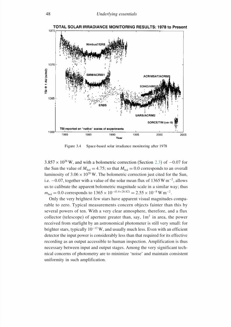
7/21/2019 Introduction to Astronomical Photometry
http://slidepdf.com/reader/full/introduction-to-astronomical-photometry 66/451
48 Underlying essentials
Figure 3.4 Space-based solar irradiance monitoring after 1978
3857× 1026 W, and with a bolometric correction (Section 2.3) of −007 forthe Sun the value of M bol = 475; so that M bol = 00 corresponds to an overallluminosity of 306
×1028 W. The bolometric correction just cited for the Sun,
i.e. −007, together with a value of the solar mean flux of 1365W m−2, allowsus to calibrate the apparent bolometric magnitude scale in a similar way; thusmbol = 00 corresponds to 1365× 10−04×2682 = 255× 10−8 W m−2.
Only the very brightest few stars have apparent visual magnitudes compa-rable to zero. Typical measurements concern objects fainter than this byseveral powers of ten. With a very clear atmosphere, therefore, and a fluxcollector (telescope) of aperture greater than, say, 1m2 in area, the power
received from starlight by an astronomical photometer is still very small: forbrighter stars, typically 10−12 W, and usually much less. Even with an efficientdetector the input power is considerably less than that required for its effectiverecording as an output accessible to human inspection. Amplification is thusnecessary between input and output stages. Among the very significant tech-nical concerns of photometry are to minimize ‘noise’ and maintain consistentuniformity in such amplification.
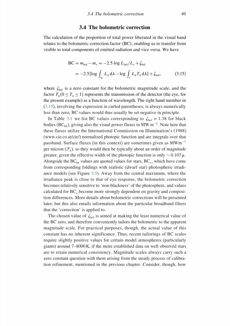
7/21/2019 Introduction to Astronomical Photometry
http://slidepdf.com/reader/full/introduction-to-astronomical-photometry 67/451
3.4 The bolometric correction 49
3.4 The bolometric correction
The calculation of the proportion of total power liberated in the visual band
relates to the bolometric correction factor BC, enabling us to transfer fromvisible to total components of emitted radiation and vice versa. We have
BC = mbol − mv = −25 log Lbol/Lv + bol
= −25log
L d − log
vLT d + bol (3.15)
where bol is a zero constant for the bolometric magnitude scale, and thefactor T 0 ≤ T ≤ 1 represents the transmission of the detector (the eye, forthe present example) as a function of wavelength. The right hand member in(3.15), involving the expression in curled parentheses, is always numericallyless than zero; BC values would thus usually be set negative in principle.
In Table 3.1 we list BC values corresponding to bol = 138 for blackbodies (BCbb), giving also the visual power fluxes in MW m−2. Note here thatthese fluxes utilize the International Commission on Illumination’s (1988)(www.cie.co.at/cie/) normalized photopic function and are integrals over thatpassband. Surface fluxes (in this context) are sometimes given as MWm−2
per micron ( ), so they would then be typically about an order of magnitudegreater, given the effective width of the photopic function is only ∼ 0107 .Alongside the BCbb values are quoted values for stars, BC∗, which have comefrom corresponding foldings with realistic (dwarf star) photospheric irradi-ance models (see Figure 3.5). Away from the central maximum, where the
irradiance peak is close to that of eye response, the bolometric correctionbecomes relatively sensitive to ‘non-blackness’ of the photosphere, and valuescalculated for BC∗ become more strongly dependent on gravity and composi-tion differences. More details about bolometric corrections will be presentedlater, but this also entails information about the particular broadband filtersthat the ‘correction’ is applied to.
The chosen value of bol is aimed at making the least numerical value of
the BC zero, and therefore conveniently tailors the bolometric to the apparentmagnitude scale. For practical purposes, though, the actual value of thisconstant has no inherent significance. Thus, recent tailorings of BC scalesrequire slightly positive values for certain model atmospheres (particularlygiants) around 7–8000 K, if the more established data on well observed starsare to retain numerical consistency. Magnitude scales always carry such azero constant question with them arising from the steady process of calibra-tion refinement, mentioned in the previous chapter. Consider, though, how
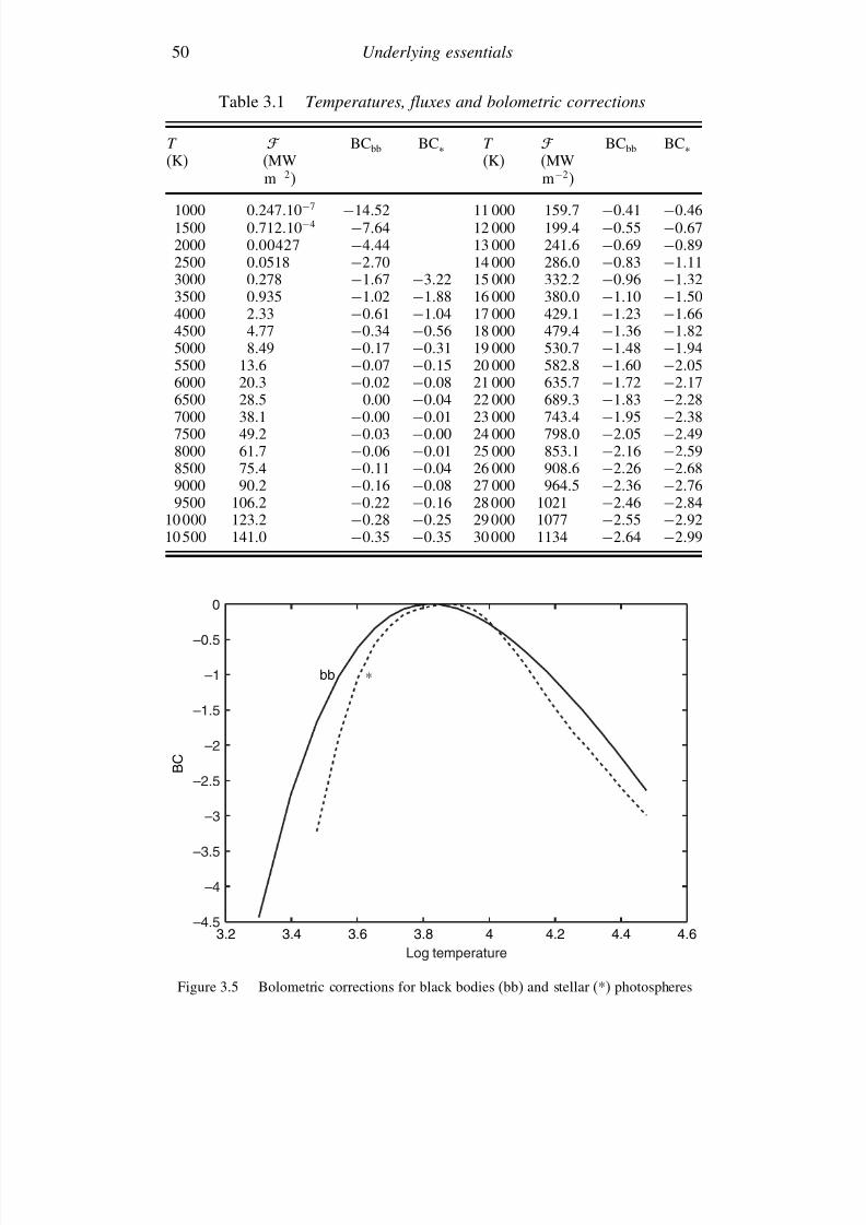
7/21/2019 Introduction to Astronomical Photometry
http://slidepdf.com/reader/full/introduction-to-astronomical-photometry 68/451
50 Underlying essentials
Table 3.1 Temperatures, fluxes and bolometric corrections
T BCbb BC∗ T BCbb BC∗
(K) (MW (K) (MWm−2) m−2)
1000 024710−7 −1452 11 000 1597 −041 −0461500 071210−4 −764 12 000 1994 −055 −0672000 000427 −444 13 000 2416 −069 −0892500 00518 −270 14 000 2860 −083 −1113000 0278 −167 −322 15 000 3322 −096 −1323500 0935 −102 −188 16 000 3800 −110 −1504000 233 −061 −104 17 000 4291 −123 −166
4500 477 −034 −056 18 000 4794 −136 −1825000 849 −017 −031 19 000 5307 −148 −1945500 136 −007 −015 20 000 5828 −160 −2056000 203 −002 −008 21 000 6357 −172 −2176500 285 0.00 −004 22 000 6893 −183 −2287000 381 −000 −001 23 000 7434 −195 −2387500 492 −003 −000 24 000 7980 −205 −2498000 617 −006 −001 25 000 8531 −216 −2598500 754 −011 −004 26 000 9086 −226 −2689000 902
−016
−008 27 000 9645
−236
−276
9500 1062 −022 −016 28 000 1021 −246 −28410 000 1232 −028 −025 29 000 1077 −255 −29210 500 1410 −035 −035 30 000 1134 −264 −299
B C
bb ∗
3.2 3.4 3.6 3.8 4 4.2 4.4 4.6Log temperature
0
–0.5
–1
–1.5
–2
–2.5
–3
–3.5
–4
–4.5
Figure 3.5 Bolometric corrections for black bodies (bb) and stellar (*) photospheres
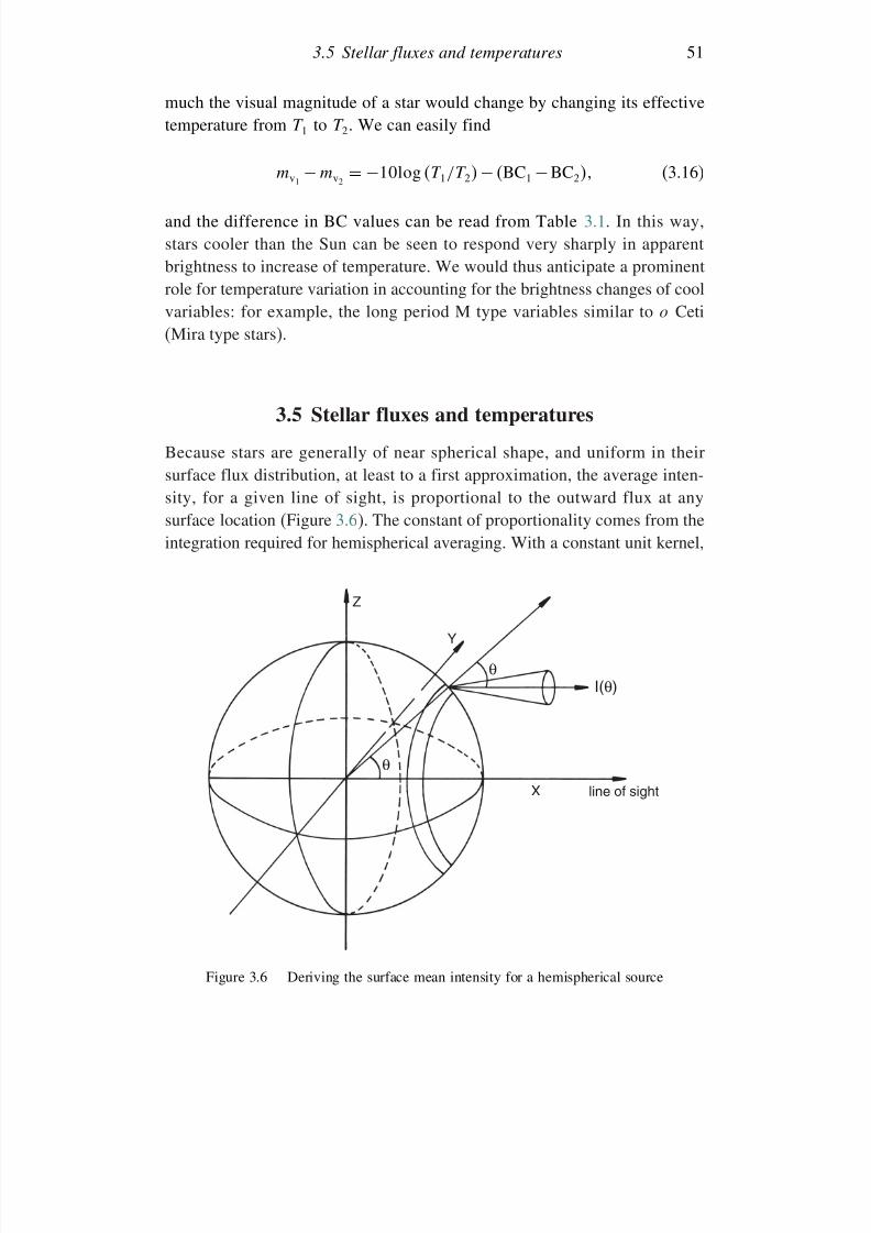
7/21/2019 Introduction to Astronomical Photometry
http://slidepdf.com/reader/full/introduction-to-astronomical-photometry 69/451
3.5 Stellar fluxes and temperatures 51
much the visual magnitude of a star would change by changing its effectivetemperature from T 1 to T 2. We can easily find
mv1 − mv2 = −10log T 1/T 2 − BC1 −BC2 (3.16)
and the difference in BC values can be read from Table 3.1. In this way,stars cooler than the Sun can be seen to respond very sharply in apparentbrightness to increase of temperature. We would thus anticipate a prominentrole for temperature variation in accounting for the brightness changes of coolvariables: for example, the long period M type variables similar to o Ceti
(Mira type stars).
3.5 Stellar fluxes and temperatures
Because stars are generally of near spherical shape, and uniform in theirsurface flux distribution, at least to a first approximation, the average inten-
sity, for a given line of sight, is proportional to the outward flux at anysurface location (Figure 3.6). The constant of proportionality comes from theintegration required for hemispherical averaging. With a constant unit kernel,
Z
X line of sight
Y
θ I(θ)
θ
Figure 3.6 Deriving the surface mean intensity for a hemispherical source
7/21/2019 Introduction to Astronomical Photometry
http://slidepdf.com/reader/full/introduction-to-astronomical-photometry 70/451
52 Underlying essentials
this is 2 1
0 cos dcos = ; i.e. the projected area of unit sphere. Now wecan write the outward (local) flux as
= 2 1
0I cos dcos
= say (3.17)
Hence, here corresponds to the ‘surface mean intensity’: the average of intensity weighted by each local unit surface area projected in the line of sight.
In the case of a non-spherical source, the corresponding areal averagingno longer involves a constant unit kernel and the local intensity function
varies over the surface, so the formal resemblance to a local flux integralloses strictness, though an expression corresponding to (3.17) could still bedevised, with representing an equivalent hemisphere average of the surfaceintensity for a given projection.
This averaging is done automatically in stellar photometry, since stellarimages are, in general, much too small to be resolved even with the world’slargest telescopes. A practical angular diameter , subtending solid angle
, is then taken to be a circular mean. For the power influx normally incidenton 1 m2 at the above-atmosphere level we have an expression, correspondingto (3.2), of the form
f ∗ = T (3.18)
Here, f ∗ can be regarded as directly determinable. In this satellite era, forinstance, an appropriate bolometric detector could be located at the consideredposition, above the atmosphere. Practical difficulties would still be present,
since real detectors always have some finite range of sensitivity, for example.The difficulties are compounded on the Earth’s surface, where one has theadditional problems of climatic and transparency vagaries with which tocontend. Such problems, though, did not prevent E. Pettit and S. Nicholsonfrom carrying out their classic series of bolometric measurements of stellarradiation in the 1920s, when from measurements of temperature increase (aslittle as 0.000 009 K from Boss 4342) they were able to determine represen-
tative stellar fluxes.The right hand side of (3.18) can be dealt with in two ways: firstly, if theangular diameter of the star can be determined, we can rewrite (3.13) as
T e = 4f ∗/214 (3.19)
and thus determine the temperature of the stars in a direct way. This hasbeen the main objective of a number of experiments to determine the scale
7/21/2019 Introduction to Astronomical Photometry
http://slidepdf.com/reader/full/introduction-to-astronomical-photometry 71/451
3.5 Stellar fluxes and temperatures 53
of stellar temperature; starting with Pettit and Nicholson, and continuing bya process of steady refinement up to the present.
It is also possible to use Equation (3.18) to determine stellar size. For stars
whose temperature is relatively close to that of the Sun this can be done onthe basis of a Taylor type linearization. We will consider a more generalapproach later. First let us use (3.19) to write
f ∗f
=
T ∗T
4∗
2
with ∗ and denoting the star and Sun, respectively. We then have
∗
= R∗r r ∗R
= 1002m−m∗
T T ∗
2 (3.20)
where we have converted the luminosity ratio to a bolometric magnitudedifference. So now
R∗ = R1002m−m∗
sin 1
T T ∗
2
(3.21)
where stands for the star’s parallax in arcseconds.In the vicinity of the Sun’s temperature (∼ 5000–7000 K) the bolometric
correction varies relatively slowly, and since the difference in bolometriccorrections is multiplied by 0.2, the effect of the correction on the visualmagnitude difference turns out to be considerably less than the accuracy withwhich we can specify this difference. For such stars we can use mv valuesdirectly in (3.21).
For the temperature ratio T /T ∗ we make use of an approximation, some-times called the ‘linear gradient’. For this we convert the Planck form (3.8)to a monochromatic magnitude scale, so that
mT = −25log c1 +125log +1086c2/T
+25 log 1− exp−c2/T+ T (3.22)
where T is a constant for the particular magnitude scale chosen. The final
logarithmic term in T is small and relatively slowly varying at opticalwavelengths and temperatures in the considered range; we neglect it for thepresent purpose. Differentiating the remaining expression, first with respectto reciprocal temperature, and then with respect to reciprocal wavelength, wefind
2mT
1/T1/ = constant = 1086c2 (3.23)
7/21/2019 Introduction to Astronomical Photometry
http://slidepdf.com/reader/full/introduction-to-astronomical-photometry 72/451
54 Underlying essentials
This expression shows up the linear gradient idea just referred to. It has anintegral of the form
mT
1/ = 1086c
2T + (3.24)
where is an arbitrary function of . The proportionality of the right handside to reciprocal temperature directly leads to a useful interpretation for thegradient of the spectral irradiance. The difference between this function fora given star and that of a reference continuum, such as the Sun’s, i.e. therelative gradient, permits photometric comparisons of temperatures.
Now integrate (3.24) over an interval corresponding to the difference −1
in the two reciprocal wavelengths associated with the definition of a colourC , and do this at the two temperatures to be compared, T and T ∗, and, aftera little manipulation, it emerges that
C − C ∗ = 1086c2
T 1− T /T ∗−1 (3.25)
Taking these colours to refer to conventional B − V values, we rearrange
(3.25) to findT /T ∗ 1− B − V /1206 (3.26)
which can be used in (3.21).Consider, for an example, 1 Cen A, a star whose apparent magnitude
and parallax are well known at mv = −001 and = 0742arcsec. Its valueof B − V is 0.69,6 implying a somewhat cooler surface temperature than theSun’s, i.e. T
=5590 K. Equation (3.21) now yields R
∗ =12R
– in essential
agreement with generally cited values.The temperature measure in this example was taken from the observed
colour: the ‘colour temperature’. A ‘brightness temperature’ may be obtainedby inverting the Planck formula for the flux (3.8) at a given wavelength,and there are other approaches to temperature derivation which do not neces-sarily yield the same result for the same star. It is the effective temperature,however, which is the one referred to in connection with Equation (3.19),
dealing with integrated power and angular diameter, which has the mostcomprehensive role. Colour or brightness temperatures can play a supportingrole, for example, over a restricted range of effective temperatures, whereproportionality between the various temperature scales can be used. The estab-lishing of dependable values of effective temperatures for stars has been a
6 Such data can be easily accessed from the SIMBAD database at simbad.u-strasbg.fr/sim-fid.pl.
7/21/2019 Introduction to Astronomical Photometry
http://slidepdf.com/reader/full/introduction-to-astronomical-photometry 73/451
3.5 Stellar fluxes and temperatures 55
fundamental task of modern astrophysics. In fact, suitably defined and care-fully measured colours have proved to have very useful applications in thiscontext, as discussed in Section 3.7.
Apart from the direct use of Equation (3.19), or some equivalent, progressin finding effective temperatures has come from the development of sophis-ticated model atmospheres for stars, based on computer calculations. Thesepredict, for a given atmospheric composition, a spectral distribution of fluxwhich is uniquely determined at a given effective temperature (and surfacegravity, on which there is a weaker dependence). Although such modelscan fit observed relative stellar irradiance data to theoretical distributions
parametrized by effective temperatures, this is not the same as direct temper-ature determination. Thus, ultimately, such calculations have to be checkedon whether their predicted effective temperatures agree with observedones for those relatively few stars whose fluxes and angular diameters arewell known.
There have been three general approaches to the determination of angulardiameters: (a) direct measurement by an interferometer; (b) from the diffrac-tion pattern observed at an occultation of a star from an intermediate ‘sharp
edge’, notably the Moon’s limb; and (c) from eclipsing binaries whichare double lined spectroscopic binaries (so that absolute parameters canthen be determined), and which also have known parallax, enabling us totransfer the derived radii to angular measure. There has been a markedimprovement in the knowledge of stellar parallaxes, particularly since theresults of the Hipparcos Space Astrometry Mission were published in 1997,allowing a greater role for (c). Eclipsing binaries with known absolute param-
eters are often associated with the inverse ‘eclipse method’ of distancedetermination, however, to be discussed later. Data on a few of the bestknown reference stars, selected from a variety of sources, are presented inTable 3.2.
The bolometric magnitude for a given flux f is easily derived from thepreviously given calibration of the bolometric scale. If the measured apparentmagnitude is subtracted from this value, for a given star, then the corre-sponding BC is obtained. In Table 3.2 we have listed BC values corresponding
to the V magnitude of the Johnson (1951) UBV system. We also tabulatesome corresponding theoretical values, which, as mentioned before, dependon atmospheric composition, effective temperature and surface gravity. Thedifferences between theoretical and observed values here can be regarded asresulting from the cumulative effects of errors, either in the determinationsof or f , in the application of the temperature, gravity and composi-tion parameters, or in the model atmospheres themselves. Clearly there are
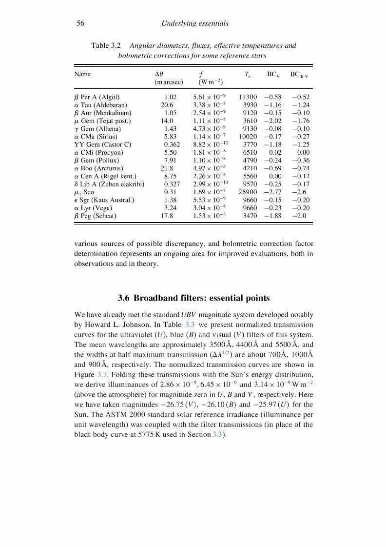
7/21/2019 Introduction to Astronomical Photometry
http://slidepdf.com/reader/full/introduction-to-astronomical-photometry 74/451
56 Underlying essentials
Table 3.2 Angular diameters, fluxes, effective temperatures and
bolometric corrections for some reference stars
Name f T e BCV BCthV(m arcsec) W m−2
Per A (Algol) 102 561 ×10−9 11300 −058 −052 Tau (Aldebaran) 206 338 ×10−8 3930 −116 −124 Aur (Menkalinan) 105 254×10−9 9120 −015 −010 Gem (Tejat post.) 140 111 ×10−8 3610 −202 −176 Gem (Alhena) 143 473 ×10−9 9130 −008 −010 CMa (Sirius) 583 114 ×10−7 10020 −017 −027YY Gem (Castor C) 0362 882
×10−12 3770
−118
−125
CMi (Procyon) 550 181 ×10−8 6510 002 000 Gem (Pollux) 791 110 ×10−8 4790 −024 −036 Boo (Arcturus) 218 497 ×10−8 4210 −069 −074 Cen A (Rigel kent.) 875 226×10−8 5560 000 −012 Lib A (Zuben elakribi) 0327 299×10−10 9570 −025 −0171 Sco 031 169 ×10−8 26900 −277 −26 Sgr (Kaus Austral.) 138 553 ×10−9 9660 −015 −020 Lyr (Vega) 324 304 ×10−8 9660 −023 −020 Peg (Scheat) 178 153
×10−8 3470
−188
−20
various sources of possible discrepancy, and bolometric correction factordetermination represents an ongoing area for improved evaluations, both inobservations and in theory.
3.6 Broadband filters: essential points
We have already met the standard UBV magnitude system developed notablyby Howard L. Johnson. In Table 3.3 we present normalized transmissioncurves for the ultraviolet (U ), blue (B) and visual (V ) filters of this system.The mean wavelengths are approximately 3500 Å, 4400 Å and 5500 Å, andthe widths at half maximum transmission (1/2) are about 700Å, 1000Åand 900 Å, respectively. The normalized transmission curves are shown in
Figure 3.7. Folding these transmissions with the Sun’s energy distribution,we derive illuminances of 286 × 10−9 645 × 10−9 and 314 × 10−9 W m−2
(above the atmosphere) for magnitude zero in U , B and V , respectively. Herewe have taken magnitudes −2675 V , −2610 B and −2597 U for theSun. The ASTM 2000 standard solar reference irradiance (illuminance perunit wavelength) was coupled with the filter transmissions (in place of theblack body curve at 5775 K used in Section 3.3).
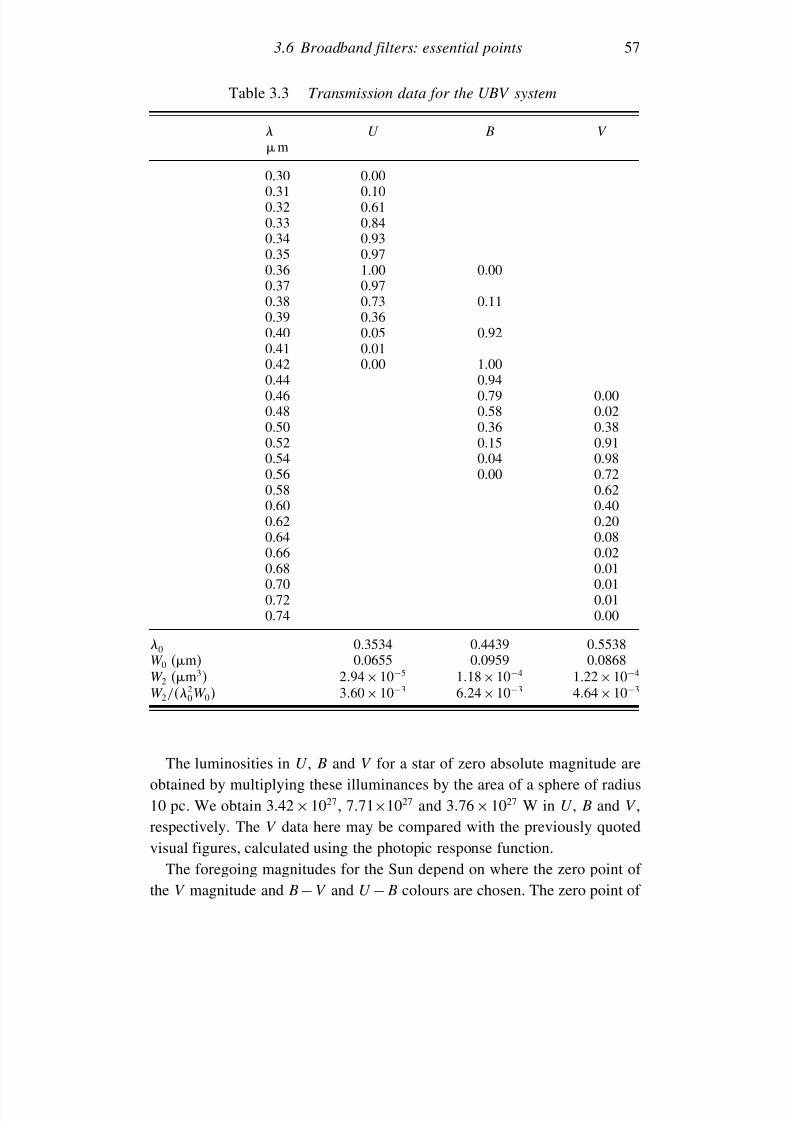
7/21/2019 Introduction to Astronomical Photometry
http://slidepdf.com/reader/full/introduction-to-astronomical-photometry 75/451
3.6 Broadband filters: essential points 57
Table 3.3 Transmission data for the UBV system
U B V
m0.30 0.000.31 0.100.32 0.610.33 0.840.34 0.930.35 0.970.36 1.00 0.000.37 0.97
0.38 0.73 0.110.39 0.360.40 0.05 0.920.41 0.010.42 0.00 1.000.44 0.940.46 0.79 0.000.48 0.58 0.020.50 0.36 0.380.52 0.15 0.91
0.54 0.04 0.980.56 0.00 0.720.58 0.620.60 0.400.62 0.200.64 0.080.66 0.020.68 0.010.70 0.010.72 0.010.74 0.00
0 0.3534 0.4439 0.5538W 0 (m) 0.0655 0.0959 0.0868W 2 (m3) 294×10−5 118×10−4 122 ×10−4
W 2/20W 0 360 ×10−3 624×10−3 464 ×10−3
The luminosities in U , B and V for a star of zero absolute magnitude areobtained by multiplying these illuminances by the area of a sphere of radius10 pc. We obtain 342 × 1027, 7.71×1027 and 376× 1027 W in U , B and V ,respectively. The V data here may be compared with the previously quotedvisual figures, calculated using the photopic response function.
The foregoing magnitudes for the Sun depend on where the zero point of the V magnitude and B − V and U −B colours are chosen. The zero point of
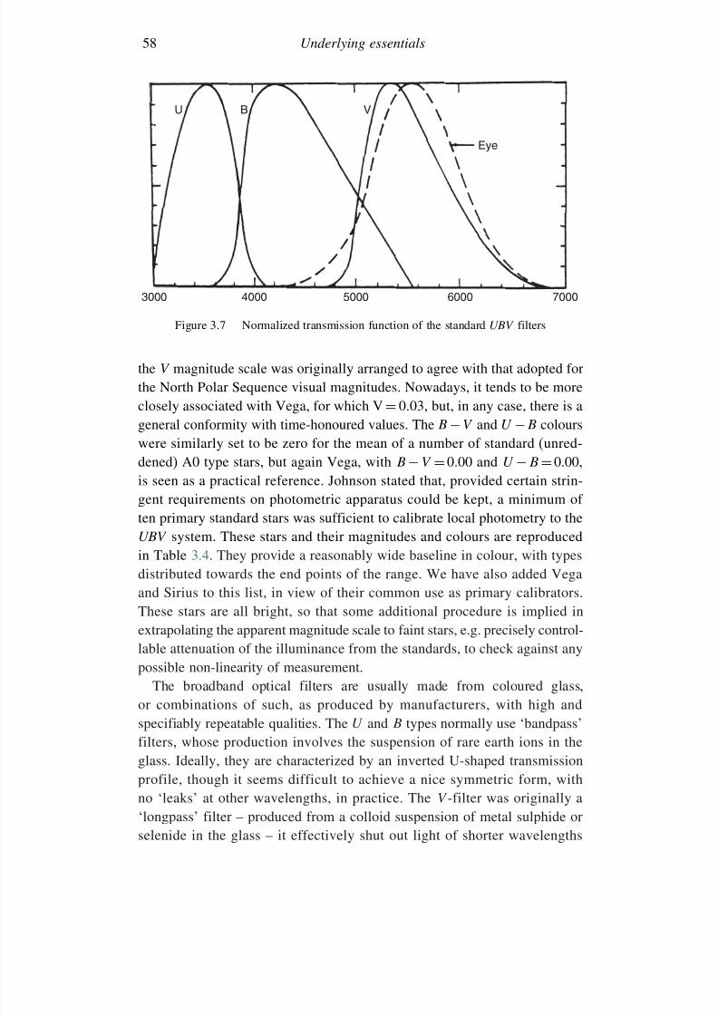
7/21/2019 Introduction to Astronomical Photometry
http://slidepdf.com/reader/full/introduction-to-astronomical-photometry 76/451
58 Underlying essentials
3000 4000 5000 6000
Eye
VU B
7000
Figure 3.7 Normalized transmission function of the standard UBV filters
the V magnitude scale was originally arranged to agree with that adopted forthe North Polar Sequence visual magnitudes. Nowadays, it tends to be moreclosely associated with Vega, for which V
=0.03, but, in any case, there is a
general conformity with time-honoured values. The B −V and U −B colourswere similarly set to be zero for the mean of a number of standard (unred-dened) A0 type stars, but again Vega, with B − V =0.00 and U − B =0.00,is seen as a practical reference. Johnson stated that, provided certain strin-gent requirements on photometric apparatus could be kept, a minimum of ten primary standard stars was sufficient to calibrate local photometry to theUBV system. These stars and their magnitudes and colours are reproduced
in Table 3.4. They provide a reasonably wide baseline in colour, with typesdistributed towards the end points of the range. We have also added Vegaand Sirius to this list, in view of their common use as primary calibrators.These stars are all bright, so that some additional procedure is implied inextrapolating the apparent magnitude scale to faint stars, e.g. precisely control-lable attenuation of the illuminance from the standards, to check against anypossible non-linearity of measurement.
The broadband optical filters are usually made from coloured glass,or combinations of such, as produced by manufacturers, with high andspecifiably repeatable qualities. The U and B types normally use ‘bandpass’filters, whose production involves the suspension of rare earth ions in theglass. Ideally, they are characterized by an inverted U-shaped transmissionprofile, though it seems difficult to achieve a nice symmetric form, withno ‘leaks’ at other wavelengths, in practice. The V -filter was originally a‘longpass’ filter – produced from a colloid suspension of metal sulphide or
selenide in the glass – it effectively shut out light of shorter wavelengths
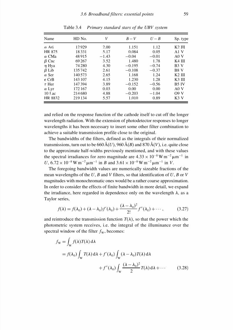
7/21/2019 Introduction to Astronomical Photometry
http://slidepdf.com/reader/full/introduction-to-astronomical-photometry 77/451
3.6 Broadband filters: essential points 59
Table 3.4 Primary standard stars of the UBV system
Name HD No. V B −V U − B Sp. type
Ari 12 929 200 1151 112 K2 IIIHR 875 18 331 517 0084 005 A1 V CMa 48 915 −143 −004 −001 A0 V Cnc 69 267 352 1480 178 K4 III Hya 74 280 430 −0195 −074 B3 V Lib 135 742 261 −0108 −037 B8 V Ser 140 573 265 1168 124 K2 III CrB 143 107 415 1230 128 K3 III Her 147 394 389 −0152 −056 B5 IV
Lyr 172 167 003 000 000 A0 V10 Lac 214 680 488 −0203 −104 O9 VHR 8832 219 134 557 1010 089 K3 V
and relied on the response function of the cathode itself to cut off the longerwavelength radiation. With the extension of photodetector responses to longerwavelengths it has been necessary to insert some other filter combination to
achieve a suitable transmission profile close to the original.The bandwidths of the filters, defined as the integrals of their normalizedtransmissions, turn out to be 660 Å(U ), 960 Å(B) and 870 Å(V ), i.e. quite closeto the approximate half-widths previously mentioned, and with these valuesthe spectral irradiances for zero magnitude are 433 × 10−8 W m−2 m−1 inU , 672× 10−8 W m−2 m−1 in B and 361× 10−8 W m−2 m−1 in V .
The foregoing bandwidth values are numerically sizeable fractions of themean wavelengths of the U , B and V filters, so that identification of U , B or V
magnitudes with monochromatic ones would be a rather coarse approximation.In order to consider the effects of finite bandwidth in more detail, we expandthe irradiance, here regarded in dependence only on the wavelength , as aTaylor series,
f = f0 + − 0f 0 + − 02
2! f 0 +· · · (3.27)
and reintroduce the transmission function T, so that the power which the
photometric system receives, i.e. the integral of the illuminance over thespectral window of the filter f W, becomes:
f W =
WfT d
= f0
WT d + f 0
W
− 0T d
+ f 0
W
−02
2 T d+· · · (3.28)
7/21/2019 Introduction to Astronomical Photometry
http://slidepdf.com/reader/full/introduction-to-astronomical-photometry 78/451
60 Underlying essentials
Neglecting second and higher power terms in this expansion, we find simply
f W = f0W 0 (3.29)
Here we have put
0 =
WT d/
W
T d
which makes the first order term in (3.28) vanish, and thus defines the meanwavelength of the filter 0. We have also put
W0 = W T d
the ‘bandwidth’ of the filter.While 0 does not depend on the spectrum of the illuminance of the source,
it is precisely representative only where the filter bandwidth is negligible incomparison to that. The transmission profile can be characterized by momentsof the transmission function higher than the zeroth. The first moment W 1 iszero by definition of the mean wavelength 0. The second moments W 2, for
the UBV filters, are given below Table 3.3. The square roots of the ratiosW 2/W 0 are comparable to the half-bandwidths of normal inverted U-shapedtransmission profile filters.
The effect of the source power distribution over a given broadband filteris included in its ‘effective’ wavelength eff , given as
eff
= WfT d
W fT d
(3.30)
Expanding numerator and denominator in (3.30) according to (3.27), it canbe shown, with a little reduction, that
eff = 0 + f 0W 2f0W 0
(3.31)
where W 2
= W
−02 T d The mean wavelengths, zeroth and second
moments (W 0 and W 2), listed below Table 3.3, have been determined fromSimpson quadrature of the data in the table.
If 0 is not far from the wavelength max of the maximum of the energydistribution, f 0 0, so that eff 0. We have already noted that thiscondition is roughly satisfied for the Sun in the visual region. On the basisof a general accord between Wien’s displacement law and real stellar energydistributions, stars significantly hotter than the Sun have a downward sloping
7/21/2019 Introduction to Astronomical Photometry
http://slidepdf.com/reader/full/introduction-to-astronomical-photometry 79/451
3.6 Broadband filters: essential points 61
continuum in the visual (negative relative gradient), while the cool ‘late’ typestars are still increasing their spectral irradiance through the visual region(positive relative gradient), to a maximum somewhere in the red, or infrared.
Hence, the difference eff − 0, taking the same sign as f 0/f0, ordlog f/d0
, can be related to equation (3.24), which we rewrite inslightly amended form as
dlog f
−2d1/ = −5 −
2 (3.32)
From (3.24) we deduce the gradient term to be of the form 1086c2/T .However, from (3.32) it can be seen that may also be written as 5max.
Several approximations have been invoked here: for a start the underlyingPlanck function is only an approximate representation to the spectral illumi-nance of a real star (see Figure 3.3). The gradient could be defined to be1086c2/T , following (3.24), but such a gradient should not be exactly equalto 5max, as can be easily seen by comparison with Wien’s displacementlaw (3.10). Finally, the effective wavelength (3.31) results from truncating aTaylor series after only its first order term. Even so, the relationship
eff − 0 = 5max − 0W 22
0 W 0
is sufficiently accurate to allow a reasonable estimation of the differenceeff − 0 in dependence on the spectral gradient.
In any case, the effective wavelength, as defined by (3.30), is not necessarilythat of the best representative wavelength for the irradiance folded with thetransmission function. The wavelength at which the flux multiplied by the
filter’s bandpass equals this integrated product is the ‘isophotal’ wavelengthi, i.e.
fi = f W/W 0 (3.33)
It can be shown, in a similar way to the derivation of (3.31), that
i = 0 + f 0W 22f 0W 0
(3.34)
which is reasonably valid so long as f 0 = 0, corresponding to 0 appre-ciably different from max. In the case of f 0 ∼ 0 the fluxes at all threewavelength measures, 0, eff and i, are sufficiently close that the effect of finite bandwidth loses significance.
Since we can writef
f = f
f + f d2 log f
f d2

7/21/2019 Introduction to Astronomical Photometry
http://slidepdf.com/reader/full/introduction-to-astronomical-photometry 80/451
62 Underlying essentials
we find that
f
f 0
= 5max − 0
20
+ 2max − 0
00
−max
(3.35)
Hence, for hot stars, for which 0 > max, we deduce that the second termon the right hand side in (3.35) will be rather smaller, in absolute value,than the first, and so i − 0 → 3
5 eff − 0 < 0. For cool stars for which0 < max the second term is of low influence ∼ −2/0 compared to the first5max/2
0, so that i −0 → 12 eff −0 > 0. These differences appear to
become large for large max, but, in practice, max would seldom be greaterthan
∼3
0 for optical filters and visible stars. Stars for which
max −
0∼
0can be seen to introduce differences eff − 0 ∼ 001 m, using the data
given in Table 3.3.The similar trend of the more accessible eff toward i throughout the range
of observed spectral types at optical wavelengths is thus evident. Numer-ical quadratures for real stars and broadband filters have shown that thediscrepancies between these various wavelength representations are such thata difference of 001 magnitudes could occur if the monochromatic magni-
tude at the mean wavelength 0 were simply used, regardless of the combinedeffect of finite bandwidth and spectral gradient. If eff is used as the equiv-alent monochromatic wavelength, reductional errors drop to only around atenth of this.
Using the foregoing formula for eff , in combination with the data belowTable 3.3 and the adopted temperature of Vega from Table 3.2, we derivethe effective wavelengths of the U , B and V filters for a star of zero U − B
and B − V to be 3524Å, 4394Å and 5479Å, respectively. Hence, the previ-ously calculated spectral irradiances (433 × 10−12 W m−2 Å−1, U ; 672 ×10−12 W m−2Å−1, B; and 361 × 10−12 W m−2Å−1, V ), if for a reference starat zero magnitude and colour, should apply at these wavelengths. The use of the angstrom unit here eases direct comparisons with literature-quoted data.For example, the power emitted in discrete line features in a spectrum isoften represented as of ‘equivalent width’ to so many angstroms of nearbycontinuum radiation (see Section 4.4).
In Table 3.5, the previously derived illuminance data are applied to tele-scopes of different diameters (D) and stars of different magnitudes in orderto have a ‘feel’ for what representative photon counts should compare within a real system. Due to the reciprocity between illuminance and area for agiven total count, the first two entries in each column can be simply trans-ferred: as the illuminance drops by a factor 25122 (2 mag), the tabulated areacorrespondingly increases by approximately the same amount. If we were
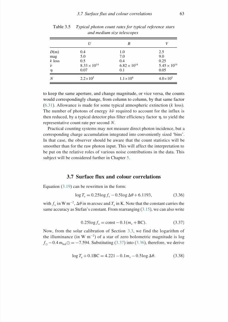
7/21/2019 Introduction to Astronomical Photometry
http://slidepdf.com/reader/full/introduction-to-astronomical-photometry 81/451
3.7 Surface flux and colour correlations 63
Table 3.5 Typical photon count rates for typical reference stars
and medium size telescopes
U B V
D(m) 0.4 1.0 2.5mag 5.0 7.0 9.0k loss 0.5 0.4 0.25 833 ×1014 682 ×1014 545× 1014
0.07 0.1 0.05
N 2.2×10⁵ 1.1×10⁶ 4.0×10⁵
to keep the same aperture, and change magnitude, or vice versa, the countswould correspondingly change, from column to column, by that same factor(6.31). Allowance is made for some typical atmospheric extinction (k loss).The number of photons of energy h required to account for the influx isthen reduced, by a typical detector plus filter efficiency factor , to yield therepresentative count rate per second N .
Practical counting systems may not measure direct photon incidence, but acorresponding charge accumulation integrated into conveniently sized ‘bins’.In that case, the observer should be aware that the count statistics will besmoother than for the raw photon input. This will affect the interpretation tobe put on the relative roles of various noise contributions in the data. Thissubject will be considered further in Chapter 5.
3.7 Surface flux and colour correlations
Equation (3.19) can be rewritten in the form:
log T e = 025log f ∗ −05log + 61193 (3.36)
with f ∗ in W m−2, in m arcsec and T e in K. Note that the constant carries thesame accuracy as Stefan’s constant. From rearranging (3.15), we can also write
025log f ∗ = const −01mv +BC (3.37)
Now, from the solar calibration of Section 3.3, we find the logarithm of the illuminance (in W m−2) of a star of zero bolometric magnitude is logf −04 mbol = −7594. Substituting (3.37) into (3.36), therefore, we derive
log T e + 01BC = 4221−01mv −05log (3.38)
7/21/2019 Introduction to Astronomical Photometry
http://slidepdf.com/reader/full/introduction-to-astronomical-photometry 82/451
64 Underlying essentials
The usefulness of this relationship has been stressed in the work of T. G.Barnes, D. S. Evans and others. The right hand side is a potentially measurablequantity,7 at least for nearer or larger stars, or certain eclipsing binary
components.From (3.19), and the fundamental relationship between illuminance and the
magnitude scale (2.1), we deduce that this right hand side, F V say, is equal to025× the logarithm of the surface flux in V light, together with some additiveconstant. The left hand side is dependent on essentially the temperature only,and should show a tight relationship to an appropriately chosen colour; suchas Equation (3.26), for instance, suggests for B −V . In fact, Barnes and Evans
found a particularly well-correlated and stable relationship of the form:F V = a + bV − R (3.39)
where R denotes the magnitude corresponding to a red filter, which is one of a group extending the UBV system to longer wavelengths (R, I , J , K , L, M ,N ) introduced by Johnson in 1965. a and b are constants, having values asfollows:
−017 < V − R < 000 a = 3977 b = −1390000 < V − R < 126 a = 3977 b = −0429
126 < V − R < 420 a = 3837 b = −0320
With these calibrations in place, the value of F V can be derived for a starfrom the relatively easily measured value of V − R. This is now, in turn,equated to the right hand side of (3.38), allowing the angular diameter to beevaluated. This would clearly be useful when either a star’s distance, or its
size, is known: application of the angular diameter value then allowing thedetermination of the other quantity – size or distance.In an early application of the foregoing to the Mira type variable R Tri,
for example, Barnes and Evans, using a distance derived from an adoptedperiod–absolute magnitude relationship, determined the actual radius valuesat several points through the light cycle from corresponding angular diametervalues. In Chapter 11 a similar idea will be pursued for a classical cepheidtype variable star.
The correlation (3.39) has an essentially empirical nature. As it happens,Barnes and Evans found the V − R index to be a reasonably stable colourmonitor of surface flux in the visual over a wide range of stellar types andluminosity classes. Generally speaking, however, we should not expect one
7 The constant term is different in different sources, presumably reflecting different adoptedvalues of the solar constant and bolometric magnitude.
7/21/2019 Introduction to Astronomical Photometry
http://slidepdf.com/reader/full/introduction-to-astronomical-photometry 83/451
3.8 Absolute parameters of stars 65
simple linear formula relating a particular colour and effective temperatureto remain valid over a wide range of spectral classes or surface gravitieswithout losing significant accuracy. But it may be possible to use higher order
formulae that are applicable over limited ranges. For example, the dependenceof F V on B −V , found by Popper (1998), is well represented by the following:
F V early = 3957−0311B − V +0586B − V 2 −5713B − V 3 (3.40)
−02 < B − V ≤ 01 and
F V late = 3958 −0361B − V +0103B − V 2 −0076B − V 3 (3.41)
01 < B − V ≤ 12
3.8 Absolute parameters of stars
Eclipsing binary stars offer a ‘royal road’ for the determination of basic stellarparameters, to use a phrase of Henry Norris Russell. Photometrically well-
monitored eclipsing binaries that also have well-determined pairs of radialvelocity curves directly furnish masses and radii of the component stars.We will detail how this is done in Chapters 7 and 9. But stellar absoluteluminosities are of equal physical significance as the masses. From the defi-nition given in Section 2.3, in order to determine luminosities for stars of known radii we must also know their temperatures. These can be derived fromcolour–temperature relations, such as those of the preceding section. Clearly,
the relationship of absolute luminosities to observed brightness values mustdepend on the distance of the stars. Hence parallaxes can also be derivedfrom the study of normal eclipsing binaries.
Although this route to parallax determinations – the ‘eclipse method’ –has been increasingly recognized, particularly since the work of Barnes andEvans, Lacy and others, it is, of course, not as direct as astrometric measure-ments. These have become significantly more accurate since the results of the astrometric satellite Hipparcos were published in the late nineties. Even
so, I. Semeniuk (2000), following a Barnes–Evans flux calibration, pointedout that parallaxes obtained by the eclipse method could have an accuracysurpassing that of the Hipparcos programme if care was taken about theselection of suitable binaries. Of course, only one star in ∼1000 shows cleareclipses, but the fact that the effect can be discerned, in principle, out to as faras stars can be individually monitored gives the method a cosmic significancenot shared by astrometric work of the present generation.
7/21/2019 Introduction to Astronomical Photometry
http://slidepdf.com/reader/full/introduction-to-astronomical-photometry 84/451
66 Underlying essentials
The application of eclipsing binary data to the direct checking of basicstellar parameters was the subject of a number of seminal publications of D. M. Popper. The paper already cited (Popper, 1998) examined the prop-
erties of 14 well-studied systems within 125 pc with low scatter Hipparcosparallaxes. The thrust of that paper was towards establishing the foregoingflux–colour relations for Main Sequence (MS) like stars and the commonlyused filters (V and B), for which purpose the choice of relatively near starsrendered insignificant the potential complication of interstellar absorption.Having derived such relations, the results can be applied to absolute parameterderivation.
Let us rewrite (3.14), generalized for surface and received fluxes from anystar, in terms of the parallax (= 1/ r , when r is in pc and is in arcsec), thus:
log = const − log R +05log f V −05log F V
In more usual astronomical format this becomes
log = 7454− log R −02log mV −2F V (3.42)
The value of the constant here comes from using data for the Sun, which at a
parallax of 0.1 arcsec would have V = 4.82 from the definition of its absolutemagnitude, and for which F V = 3.755 from the definition in (3.38).For a group of stars differing only in mass, say, all at essentially the same
distance compared with their distance to the Earth, as in a cluster, (3.42)expresses a relationship between mV and colour (i.e. through the colour depen-dent term F V ), in which the radius appears as a parameter. If this parameter isnot really independent, but has some functional relationship to the effectivetemperature as a result of an equilibrium structure adopted by a star of a given
mass, then (3.42) can be seen as a two-dimensional mapping of this relation-ship in the colour–magnitude plane. Individual stars in the mapping form a‘sequence’. The existence of such colour–magnitude sequences (for dwarf andgiant stars) was first noticed by E. Hertzsprung in 1911, and later interpretedby H. N. Russell in terms of stellar structure and evolution. Dwarfs, beingspatially more frequent, conform to the most well known of these mappings,generally known as the Main Sequence. The sequence for giants becomesmore distinct for stars of spectral type G and later, where it forms what isusually called the Giant Branch, although the giant luminosity class persiststhrough to early type stars. Other sequences have been identified, with differentdegrees of clarity, in colour–magnitude plots of different groups of stars, oftenwhen they have some linking characteristic, such as belonging to a cluster.
Table 3.6 provides empirical data on the Main Sequence, obtainedfrom running smooth curves through combined eclipse method analysis,Barnes–Evans type applications or parallax, magnitude and angular diameter
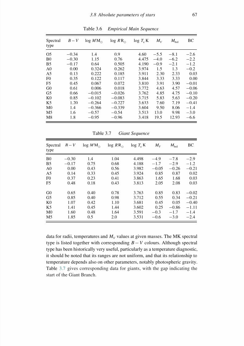
7/21/2019 Introduction to Astronomical Photometry
http://slidepdf.com/reader/full/introduction-to-astronomical-photometry 85/451
3.8 Absolute parameters of stars 67
Table 3.6 Empirical Main Sequence
Spectral
type
B − V log M M log R R log T e K M V M bol BC
O5 −034 14 09 460 −55 −81 −26B0 −030 115 076 4475 −40 −62 −22B5 −017 064 0505 4190 −09 −21 −12A0 000 0324 0262 3974 15 13 −02A5 013 0222 0185 3911 230 233 003F0 035 0122 0117 3844 333 333 000F5 045 0067 0072 3810 391 390 −001G0 061 0006 0018 3772 463 457 −006
G5 066 −0015 −0026 3762 485 475 −010K0 085 −0102 −0083 3715 583 563 −020K5 120 −0264 −0227 3633 760 719 −041M0 14 −0366 −0339 3604 950 806 −14M5 16 −057 −054 3513 130 998 −30M8 18 −095 −096 3418 195 1293 −66
Table 3.7 Giant Sequence
Spectraltype
B −V log M M log R R log T e K M V M bol BC
B0 −030 1.4 1.04 4.498 −49 −78 −29B5 −017 0.75 0.68 4.188 −17 −29 −12A0 000 0.43 0.56 3.982 −005 −026 −021A5 014 0.33 0.45 3.924 085 087 002F0 037 0.23 0.41 3.863 165 168 003F5 048 0.18 0.43 3.813 205 208 003
G0 065 0.40 0.78 3.763 085 083 −002G5 085 0.40 0.98 3.712 055 034 −021K0 107 0.42 1.10 3.681 045 005 −040K5 141 0.45 1.44 3.602 025 −086 −111M0 160 0.48 1.64 3.591 −03 −17 −14M5 185 0.5 2.0 3.531 −06 −30 −24
data for radii, temperatures and M V values at given masses. The MK spectraltype is listed together with corresponding B − V colours. Although spectraltype has been historically very useful, particularly as a temperature diagnostic,it should be noted that its ranges are not uniform, and that its relationship totemperature depends also on other parameters, notably photospheric gravity.Table 3.7 gives corresponding data for giants, with the gap indicating thestart of the Giant Branch.
7/21/2019 Introduction to Astronomical Photometry
http://slidepdf.com/reader/full/introduction-to-astronomical-photometry 86/451
68 Underlying essentials
3.9 Bibliographical notes
Fundamentals of photometry related to the vision based units are covered
in the Handbook of Applied Photometry, ed. C. De Cusatis (AIP Press,1997). (The SI system of units was expounded in S. Dresner’s Units of
Measurement , Harvey, Miller and Medcalf, 1971.) The moment integrals of the intensity are also covered in numerous astrophysical texts that discussradiative transfer: e.g. V. Kourganoff’s Basic Methods in Transfer Problems
(Clarendon Press, 1952).The original references on black body radiation laws are: A.J. Stefan
(Wien Ber., 79, 397, 1879); L. Boltzmann ( Ann. Physik (ser. 3), 31, 291,1884); M. Planck ( Ann. Physik (ser. 4), 4, 553, 1901); W. Wien (Phil. Mag.
(ser. 5), 43, 214, 1894); Lord Rayleigh (Phil. Mag., 49, 539, 1900); J.H.Jeans (Phil. Mag. (ser. 6), 17, 229, 1905). A variety of useful formulae aregiven in Allen’s Astrophysical Quantities, ed. A. N. Cox (AIP Press, 2000).
For a recent review of measurements of the total solar luminosity, seeR. C. Willson & A. V. Mordvinor (Geophys. Research Lett., 30, 1199, 2003),or R. B. Lee, R. S. Wilson & S. Thomas (Proc. Amer. Met. Soc., 13th Confer-ence, paper P6.31, 2004). It is now known that the mean total solar irradiance(after taking out the effects of orbital geometry) varies on the order of ∼0.1%.This is ascribed mainly to solar activity effects.
A well-cited version of the solar irradiance distribution was that of H. Neckel and D. Labs (Sol. Phys., 90, 205, 1984) (see also G. Thuillieret al., Science, 225, 182, 1987; and E. A. Makarova et al., Astron. Zh., 66,583, 1989. This was updated by L. Colina et al., 1996, Astron. J., 112, 307;
see also G. Cayrel de Strobel, 1996, Astron. Astrophys. Rev., 7, 243). In thisconnection, the BASS solar spectrum at bass2000.obspm.fr/solar spect.phpcan also be usefully consulted.
Absolute calibration of the magnitude scale formed the subject of IAU Symp. 54, ed. B. Hauck and B. E. Westerlund (Reidel, 1973), and hasgiven rise to many papers since: see, for example, M. S. Bessell, F. Castelliand B. Plez’ (1998) review (Astron. Astrophys., 333, 231), which includes
many other references. The classic papers on stellar bolometry and angulardiameters of E. Pettit and S. Nicolson ( Astrophys. J., 68, 279, 1928) andG.P. Kuiper ( Astrophys. J., 88, 429, 1938) were discussed by D. L. Harrisin Basic Astronomical Data, ed. K. A. Strand (University of Chicago Press,1963, p. 273). But, particularly since the use of colour-based fluxes of the ‘Barnes–Evans’ type (see T. G. Barnes & D. S. Evans, Mon. Not. Roy.
Astron. Soc., 174, 489, 1976, and T. G. Barnes, D. S. Evans & T. J. Moffett,
7/21/2019 Introduction to Astronomical Photometry
http://slidepdf.com/reader/full/introduction-to-astronomical-photometry 87/451
3.9 Bibliographical notes 69
Mon. Not. Roy. Astron. Soc., 183, 285, 1978), there have been increasedefforts to check fundamental stellar parameters through photometric measures.
An increased supply of data from above the absorbing layers of the
atmosphere, or through windows in the infrared region, has also enabledimproved net flux determinations, leading to calibrations such as thatof A.D. Code et al. ( Astrophys. J., 203, 417, 1976) and D.S. Hayes,
IAU Symp. 80: The H–R Diagram (Reidel, 1978, p. 65). D.M. Popper( Ann. Rev. Astron. Astrophys., 18, 115, 1980, updated in Publ. Astron Soc.
Pacific, 110, 919, 1998) provided empirical data from analysis of binarystars to compare with such scales. Stellar temperature data were reviewed
by E. Böhm-Vitense ( Ann. Rev. Astron. Astrophys., 19, 295, 1981) andmore recently by G.P. Di Benedetto ( Astron. Astrophys., 339, 858, 1998).Information on the reduction of photoelectric lunar occultation data wasgiven by G.L. Blow ( IAPPP, 10, 1, 1982). The stellar bolometric correc-tions (BC∗) of Table 3.1 have come from combining the information inmore recent sources (particularly that of Bessell et al., 1998) and takingappropriate averages to smooth trends. The more comprehensive data inTable 3.2 is influenced by that in the catalogue of D.E. Blackwell andA.E. Lynas-Gray ( Astron. Astrophys., 282, 899, 1994). This, and otherrelevant data (e.g. D. E. Blackwell & A. E. Lynas-Gray, Astron. Astrophys.
Suppl. Ser., 129, 505, 1998) can be usefully accessed from the SIMBADdatabase at simbad.u-strasbg.fr/.
The UBV filter transmission coefficients whose normalized forms havebeen presented in Table 3.3 originally appeared in Astrophys. J., 114, 522,1951. The system’s primary standards (Table 3.4) are from H. L. Johnson’s
article in Basic Astronomical Data, ed. K. A. Strand (University of ChicagoPress, 1963, p. 204). Reference should also be made to the paper of M. Bessell(Publ. Astron. Soc. Pacific, 102, 1181, 1990) in the era of photoconductivedetectors. More detailed discussions of the UBV system can be found ine.g. M. Golay’s Introduction to Astronomical Photometry (Reidel, 1974) andV. Straizys’ Multicolour Stellar Photometry (Mokslas Publ., 1977). Muchof Section 3.6 has been adapted from Chapter 2 of Golay’s text with some
differences of treatment and application.Many papers have discussed Barnes–Evans type relations. Increased detec-
tive capability in the infrared has allowed fuller integration of the flux distri-bution, giving rise to the ‘infrared flux method’ of D. E. Blackwell et al.
( Mon. Not. Roy. Astron. Soc., 221, 427, 1986), so that the process of stellartemperature determination continues to be checked and refined (see Bessellet al., 1998, cited above).
7/21/2019 Introduction to Astronomical Photometry
http://slidepdf.com/reader/full/introduction-to-astronomical-photometry 88/451
70 Underlying essentials
Much of Section 3.8 derives from the contribution of E. Budding,M. Rhodes & D.J. Sullivan to IAU Coll. 196, ed. D. Kurtz (CambridgeUniversity Press, 2005). Tables like 3.6 and 3.7 appear in various sources.
The format came originally from E. Budding’s article in Investigating theUniverse, ed. F. D. Kahn (Reidel, 1982, p. 271), but the present values areinfluenced by those of P. Harmanec ( Bull. Astron. Inst. Czech., 39, 329,1988) and V. Straizys (Vilnius Astron. Obs. Biul., 76, 17, 1987), as well asthe data of D. M. Popper referenced above and I. Semeniuk ( Acta Astron.,50, 381, 2000). Comparable theoretical results can be found in, for example,Eggleton, Fitchett & Tout (1989) or Tout et al. (1996) (see reference list).
References
Allen, C.W., 2000, Astrophysical Quantities, ed. A. N. Cox, AIP Press.Barnes, T. G. & Evans, D.S., 1976, Mon. Not. Roy. Astron. Soc., 174, 489.Barnes, T. G., Evans, D. S. & Moffett, T. J., 1978, Mon. Not. Roy. Astron. Soc., 183,
285.
Bessell, M., 1990, Publ. Astron. Soc. Pacific, 102, 1181.Bessell, M. S., Castelli F. & Plez, B., 1998, Astron. Astrophys., 333, 231.Blackwell, D. E. & Lynas-Gray, A. E., 1994, Astron. Astrophys., 282, 899.Blackwell, D. E. & Lynas-Gray, A. E., 1998, Astron. Astrophys. Suppl. Ser., 129, 505.Blackwell, D. E., Booth, A. J., Petford, A. D., Leggett, S. K., Mountain, C. M. & Selby,
M.J., 1986, Mon. Not. Roy. Astron. Soc., 221, 427.Blow, G. L., 1982, IAPPP, 10, 1.Böhm-Vitense, E., 1981, Ann. Rev. Astron. Astrophys., 19, 295.Boltzmann, L., 1884, Ann. Physik (ser. 3), 31, 291.
Budding, E., 1982, Investigating the Universe, ed. F. D. Kahn, Reidel, p. 271.Budding, E., Rhodes, M. & Sullivan, D., 2005, IAU Coll. 196 , ed. D. Kurtz, Cambridge
University Press, p. 386.Cayrel de Strobel, G., 1996, Astron. Astrophys. Rev., 7, 243.Code, A. D., Bless, R. C., Davis, J. & Brown, R. H., 1976, Astrophys. J., 203, 417.Colina, L., Bohlin, R. C. & Castelli, F., 1996, Astron. J., 112, 307.De Cusatis, C., 1997, Handbook of Applied Photometry, AIP Press.Di Benedetto, G. P., 1998, Astron. Astrophys., 339, 858.Dresner, S., 1971, Units of Measurement , Harvey, Miller & Medcalf.
Eggleton, P. P., Fitchett, M. J. & Tout, C. A., 1989, Astrophys. J ., 347, 998.Golay, M., 1974, Introduction to Astronomical Photometry, Reidel.Harmanec, P., 1988, Bull. Astron. Inst. Czech., 39, 329.Harris, D. L., 1963, Basic Astronomical Data, ed. K. A. Strand, University of Chicago
Press, p. 273.Hayes, D. S.,1978, IAU Symp. 80: The H–R Diagram, Reidel, p. 65.Jeans, J. H., 1905, Phil. Mag. (ser. 6), 17, 229.Johnson, H. L., 1951, Astrophys. J., 114, 522.
7/21/2019 Introduction to Astronomical Photometry
http://slidepdf.com/reader/full/introduction-to-astronomical-photometry 89/451
References 71
Johnson, H.L., 1963, Basic Astronomical Data, ed. K.A. Strand, University of Chicago Press, p. 204.
Kourganoff, V., 1952, Basic Methods in Transfer Problems, Clarendon Press.Kuiper, G. P., 1938, Astrophys. J., 88, 429.Lee, R. B., Wilson, R. S. & Thomas, S., 2004, Proc. Amer. Met. Soc., 13th Conf.,
paper P6.31.Lord Rayleigh (J. W. Strutt), 1900, Phil. Mag., 49, 539.Makarova, E. A., Knyazeva, L. N. & Kharitonov, A.V., 1989, Astron. Zh., 66, 583.Neckel, H. & Labs, D., 1984, Sol. Phys., 90, 205.Pettit, E. and Nicolson, S., 1928, Astrophys. J., 68, 279.Planck, M., 1901, Ann. Physik (ser. 4), 4, 553.Popper, D. M., 1980, Ann. Rev. Astron. Astrophys., 18, 115.
Popper, D. M., 1998, Publ. Astron Soc. Pacific, 110, 919.Richards, J.A., Sears, F.W., Wehr, M.R. & Zemansky, M.W., 1964, Modern
University Physics, Addison–Wesley, p. 715.Semeniuk, I., 2000, Acta Astron., 50, 381.Stefan, A. J., 1879, Wien Ber., 79, 397.Straizys, V., 1977, Multicolour Stellar Photometry, Mokslas Publ.Straizys, V., 1987, Vilnius Astron. Obs. Biul., 76, 17.Thuillier, G., Goutail, J. P., Simon, P. C., Pastiels, R., Labs, D. & Neckel, H., 1984,
Science, 225, 182.
Tout, C. A., Pols, O. R., Eggleton, P. P. & Han, Z., 1996, Mon. Not. R. Astron. Soc.,281, 257.Wien, W., 1894, Phil. Mag. (ser. 5), 43, 214.Willson, R. C. & Mordvinor, A. V., 2003, Geophys. Research Lett., 30, 1199.
7/21/2019 Introduction to Astronomical Photometry
http://slidepdf.com/reader/full/introduction-to-astronomical-photometry 90/451
4
Themes of astronomical photometry
4.1 Extinction
Extinction, or the attenuation of light as it passes through a medium, can beexplained on the basis of the equation for the transport of radiation, written as
dI
ds = −I
+j (4.1)
where I represents the intensity (see (3.2)) at wavelength and in thedirection arccos to the outward direction of spatial coordinate s, while
denotes a general extinction coefficient per unit mass of the medium, of density , through which the radiation is passing. Emission of intensity j addsinto the beam in this formulation, but in the usual situation for photometry of optical transmission from a remote source to a local detector j is effectively
zero for the intervening space. The intensity then has the simple form:I = I 0
exp− s
0 ds/ (4.2)
4.1.1 Atmospheric extinction
We can apply (4.2) to the illuminance f above and below the Earth’s atmo-sphere to find the radiation intercepted by a real detector at an Earth-based
observatory. The illuminance will be the star’s surface mean intensity multi-plied by the solid angle which its disk subtends, (3.18), and we write
f = f 0 exp−kX (4.3)
or in magnitudes,
m = m0 +25log10 e kX (4.4)
72
7/21/2019 Introduction to Astronomical Photometry
http://slidepdf.com/reader/full/introduction-to-astronomical-photometry 91/451
4.1 Extinction 73
where the extinction coefficient k is regarded as a function of wavelength,usually taken to be independent of direction through the atmosphere, andX represents the mass of air through which the radiation penetrates from
the source at zenith distance ; m0 denotes the apparent magnitude abovethe atmosphere. Models for atmospheric extinction deal mainly with Rayleighscattering on molecules, aerosol scattering and molecular absorption. Each of these contributors has its own form of wavelength dependence and distributionwith height, and also variation with time.
Equation (4.4) is sometimes called Bouguer’s law – its convenient linearform in the magnitude scale has already been mentioned: though, strictly
speaking, this linearity only applies for the monochromatic magnitudem. In applying (4.4) to broadband, e.g. UBV , photometry, account hasto be taken of finiteness of the passband of the filters. Departures from a strictlinearity will rise with increasing bandwidth of the filter, with a significancewhich depends on the accuracy standards set or required. The human eye,for example, although essentially a broadband detector, would normally haveaccuracy limitations allowing the preceding linear form to be quite adequate.
In order to take account of the finite passband effects at a given mean
wavelength 0, we rewrite Equation (3.27) as
f W = f0W 0 + 12
f 0W 2
We substitute from (4.3) for f0 in this, and then convert from thelinear scale of fluxes to the logarithmic scale of magnitudes, using naturallogarithms multiplied by −1086 = −25log10 e. This allows the convenientapproximation ln1
+x
x, valid for small x, and enables the exponential
terms to be directly simplified. After a little manipulation we find
m0 = m0
0 +1086Xk
+ W 2 kdlog f 0
W 0 d + W 2k
2W 0
=0
−
1086k02X2W 2
2W 0
(4.5)
where m00 is not quite the same as m00 would be in (4.4), since it refers
to a finite bandwidth filter centred at 0, and so has absorbed a small term(of order W 2/W 0) in f 0 , which does not depend on the air mass.
We have seen in (3.32) that dlog f/d can be approximated, at wave-length 0, as 5max − 0/2
0, which, using (3.24) and (3.25), we are able torewrite using a colour index (say, B − V ). A form, ideal or observationally
7/21/2019 Introduction to Astronomical Photometry
http://slidepdf.com/reader/full/introduction-to-astronomical-photometry 92/451
74 Themes of astronomical photometry
obtained, for the dependence of extinction coefficient k on wavelength isalso useful. A power-law is often adopted, e.g.
k = const −n
(4.6)where, for the Rayleigh law of scattering on atmospheric molecules, n = 4.Such a form may be more or less valid in practice, depending on observingand climatic conditions during the observations, but we can thereby analyse(4.5); k can be replaced by −nk/, and k by nn +1k/2.
We may now examine the various contributions on the right hand side in(4.5).
(i) The principle term ∼ kX, which shows the approximate validityof Bouguer’s law, as expected.
(ii) The colour-dependent term ∼ 5nmax −0W 2/30W 0. Over the range of
encountered surface temperatures of stars max − 0/0 is, in general,of order unity. W 2/W 02
0 is typically of order 5 ×10⁻³ for filters like theUBV ones (Table 3.3). Hence, this term is of order a few hundredths of a magnitude, and not negligible for detailed work.
(iii) The term in k works out to be of order nn + 1W 2/220W 0, which,though not negligible, only appears as a constant factor multiplying theair mass, and thus may be absorbed into the main extinction term.
(iv) Finally, the second order term in the air mass, though amplified by thecoefficient n from the power-law k ∼ −n, nevertheless is also multipliedby k2, in addition to the small term W 2/2
0W 0. Since k is of order 10−1, thisterm will be of order 10−3 for broadband filters, and so probably negli-
gible in general, though not if the most precise reductions are pursued.
An empirical test on real data is likely to show the extent of non-linearityof Bouguer’s law. What is often found, though, are irregularities of a greaterscale than the minor contributions (ii)–(iv), due to an atmosphere which hasmore complicated properties than those of our simplified model. Apart fromthe primary extinction effects already mentioned, there are often thin cloudsor hazes with their own quasi-chaotic variations in position and time. Practical
approaches for dealing with the extinction are discussed in Chapter 6.
4.1.2 The atmospheric mass
The mass of air through which starlight passes should, at least for lower valuesof the zenith angle , be proportional to sec . This is based on regardingthe atmosphere as made up of plane stratified layers. The approximation is
7/21/2019 Introduction to Astronomical Photometry
http://slidepdf.com/reader/full/introduction-to-astronomical-photometry 93/451
4.1 Extinction 75
tolerable for zenith angles up to 60. To account for the effects of curvatureof the atmospheric layers use is frequently made of ‘Bemporad’s formula’
X = sec −00018167sec −1−0002875sec −12
−0000808sec −13 −· · · (4.7)
which is correct (at sea level) to within 0.001 for X up to about 6.8, andhas at least 1% accuracy for X < 10, i.e. surpassing the requirements of allnormal observing situations of practical photometry. More recently, Kasten
and Young’s formula X = 1/cos + 050572 × 9607995 − −16364
( in degrees) is cited.How do we determine ? Here we outline some general procedures for
coordinate transformations that will be used in this and other sections of thetext. Readers already familiar with such details may proceed directly to theresult (4.9).
Three rotation matrices are introduced which take the form:
R x =
1 0 00 cos sin
0 − sin cos
R y =
cos 0 − sin
0 1 0sin 0 cos
R z = cos sin 0
− sin cos 00 0 1
where represents a positive (anticlockwise) rotation about the positive axisgiven as the suffix to R. These matrices operate on a three-coordinate setxyz, representing some fixed point, arranged as a vector x. The result of the matrix vector product is a new three-coordinate set corresponding to newaxes, transformed as a result of the operation R about whichever of the three
axes was chosen to rotate about. A succession of n operations corresponds torepeated multiplications of the type Rn
.Rn−1…R1
.x.We carry out a sequence of rotations which takes us from the west-line
to the line of sight to the star, via the celestial equator, as an example(Figure 4.1). We start with an alt-azimuth system of axes and the origin isidentified with the observer’s position. The z-axis points to the zenith, thex-axis points horizontally to the west, and the y-axis, by the requirement of
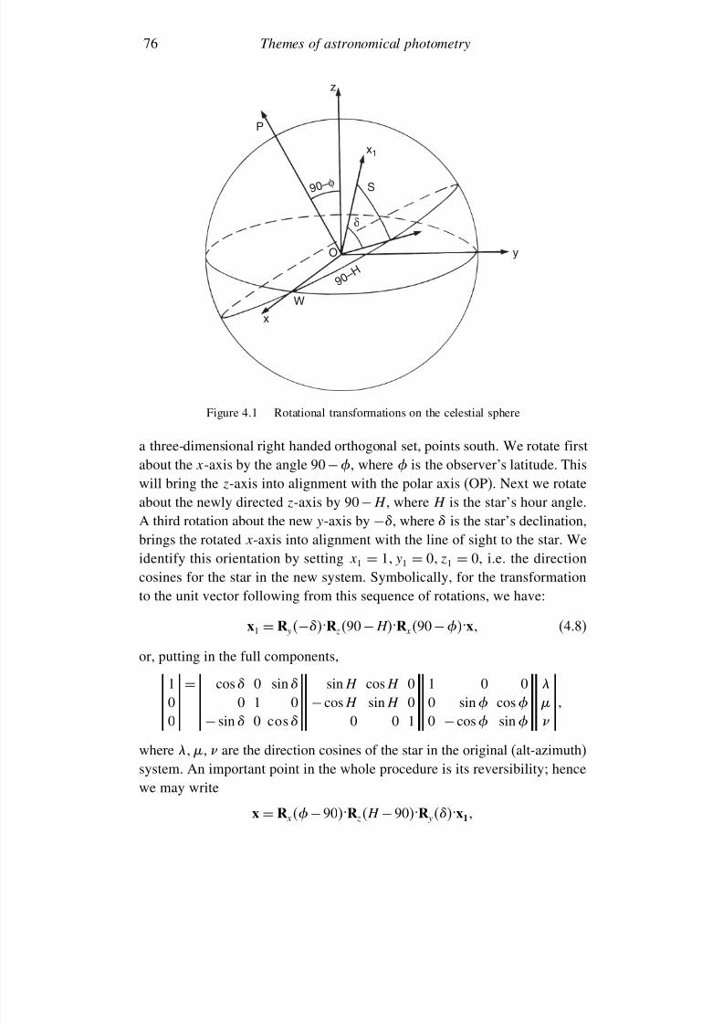
7/21/2019 Introduction to Astronomical Photometry
http://slidepdf.com/reader/full/introduction-to-astronomical-photometry 94/451
76 Themes of astronomical photometry
z
y
P
x
W
O
S
δ
x1
9 0 – φ
9 0 – H
Figure 4.1 Rotational transformations on the celestial sphere
a three-dimensional right handed orthogonal set, points south. We rotate firstabout the x-axis by the angle 90 −, where is the observer’s latitude. Thiswill bring the z-axis into alignment with the polar axis (OP). Next we rotateabout the newly directed z-axis by 90− H , where H is the star’s hour angle.A third rotation about the new y-axis by −, where is the star’s declination,brings the rotated x-axis into alignment with the line of sight to the star. We
identify this orientation by setting x1 = 1 y1 = 0 z1 = 0, i.e. the directioncosines for the star in the new system. Symbolically, for the transformationto the unit vector following from this sequence of rotations, we have:
x1 = R y−.R z90 − H.R x 90− .x (4.8)
or, putting in the full components,
1
= cos 0 sin sin H cos H 0 1 0 0
0 0 1 0 − cos H sin H 0 0 sin cos 0 − sin 0 cos 0 0 1 0 − cos sin
where are the direction cosines of the star in the original (alt-azimuth)system. An important point in the whole procedure is its reversibility; hencewe may write
x = R x −90.R zH − 90.R y.x1
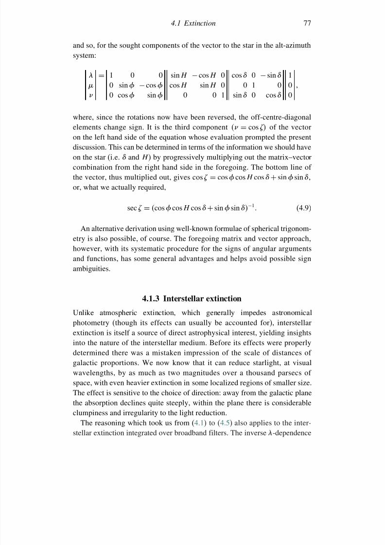
7/21/2019 Introduction to Astronomical Photometry
http://slidepdf.com/reader/full/introduction-to-astronomical-photometry 95/451
4.1 Extinction 77
and so, for the sought components of the vector to the star in the alt-azimuthsystem:
= 1 0 0 sin H − cos H 0 cos 0 − sin 1 0 sin − cos cos H sin H 0 0 1 0 0 0 cos sin 0 0 1 sin 0 cos 0
where, since the rotations now have been reversed, the off-centre-diagonalelements change sign. It is the third component = cos of the vectoron the left hand side of the equation whose evaluation prompted the present
discussion. This can be determined in terms of the information we should haveon the star (i.e. and H ) by progressively multiplying out the matrix–vectorcombination from the right hand side in the foregoing. The bottom line of the vector, thus multiplied out, gives cos = cos cos H cos + sin sin
or, what we actually required,
sec = cos cos H cos + sin sin −1 (4.9)
An alternative derivation using well-known formulae of spherical trigonom-etry is also possible, of course. The foregoing matrix and vector approach,however, with its systematic procedure for the signs of angular argumentsand functions, has some general advantages and helps avoid possible signambiguities.
4.1.3 Interstellar extinction
Unlike atmospheric extinction, which generally impedes astronomicalphotometry (though its effects can usually be accounted for), interstellarextinction is itself a source of direct astrophysical interest, yielding insightsinto the nature of the interstellar medium. Before its effects were properlydetermined there was a mistaken impression of the scale of distances of galactic proportions. We now know that it can reduce starlight, at visual
wavelengths, by as much as two magnitudes over a thousand parsecs of space, with even heavier extinction in some localized regions of smaller size.The effect is sensitive to the choice of direction: away from the galactic planethe absorption declines quite steeply, within the plane there is considerableclumpiness and irregularity to the light reduction.
The reasoning which took us from (4.1) to (4.5) also applies to the inter-stellar extinction integrated over broadband filters. The inverse -dependence
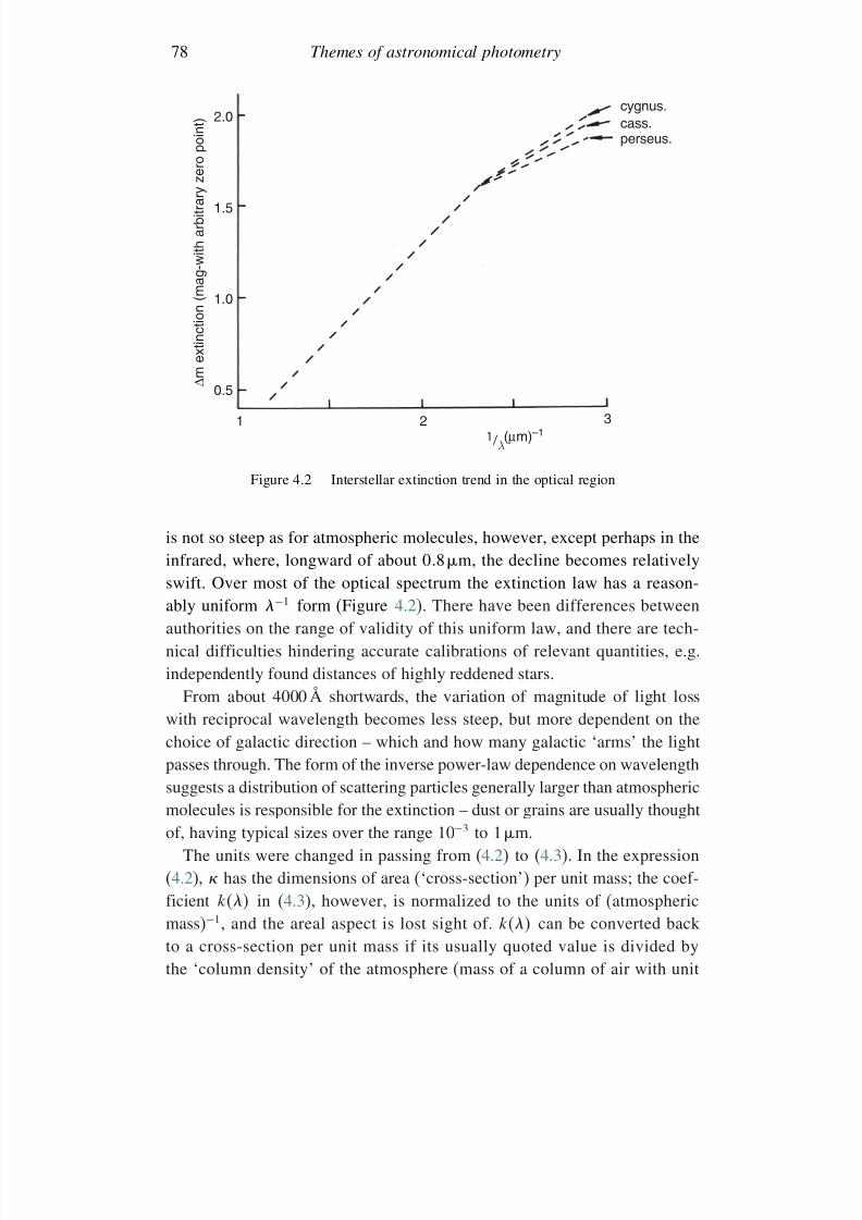
7/21/2019 Introduction to Astronomical Photometry
http://slidepdf.com/reader/full/introduction-to-astronomical-photometry 96/451
78 Themes of astronomical photometry
1 2 31 /λ
(µm)–1
cygnus.cass.perseus.
2.0
1.5
1.0
0.5 ∆ m e x t i n c
t i o n ( m a g - w i t h a r b i t r a r y z e r o p o i n t )
Figure 4.2 Interstellar extinction trend in the optical region
is not so steep as for atmospheric molecules, however, except perhaps in theinfrared, where, longward of about 08 m, the decline becomes relativelyswift. Over most of the optical spectrum the extinction law has a reason-ably uniform −1 form (Figure 4.2). There have been differences betweenauthorities on the range of validity of this uniform law, and there are tech-nical difficulties hindering accurate calibrations of relevant quantities, e.g.
independently found distances of highly reddened stars.From about 4000 Å shortwards, the variation of magnitude of light loss
with reciprocal wavelength becomes less steep, but more dependent on thechoice of galactic direction – which and how many galactic ‘arms’ the lightpasses through. The form of the inverse power-law dependence on wavelengthsuggests a distribution of scattering particles generally larger than atmosphericmolecules is responsible for the extinction – dust or grains are usually thought
of, having typical sizes over the range 10−3 to 1 m.The units were changed in passing from (4.2) to (4.3). In the expression
(4.2), has the dimensions of area (‘cross-section’) per unit mass; the coef-ficient k in (4.3), however, is normalized to the units of (atmosphericmass)−1, and the areal aspect is lost sight of. k can be converted backto a cross-section per unit mass if its usually quoted value is divided bythe ‘column density’ of the atmosphere (mass of a column of air with unit
7/21/2019 Introduction to Astronomical Photometry
http://slidepdf.com/reader/full/introduction-to-astronomical-photometry 97/451
4.1 Extinction 79
cross-sectional area and length equal to the mean height of the atmosphere≈ 10350kgm−2).1 In the interstellar context there is no real equivalent toatmospheric mass – the corresponding part of the extinction exponent reverts
to a column density. A possible unit for this is solar masses per squareparsec along the direction to a given star, of determinable interstellar extinc-tion. The interstellar equivalent to k (extinction per unit column density,thus expressed) would then typically turn out to be of order ∼ 001–01at optical wavelengths. In any case, interstellar extinction follows the form(4.5) to increase the apparent magnitude of the source. It is made up of aprincipal term – a product of cross-section per unit mass, column density of
the interstellar matter and the scaling constant 1.086 – together with smallcontributions (of order W 2/W 0) proportional to the colour and the square of the column density.
Photometric information is often sought for a group of cosmogonicallyrelated objects, e.g. a cluster of stars, in the form of a colour–magnitude (ortwo-colour) diagram. For practical purposes, the individual cluster membersare regarded as all at essentially the same distance from Earth, with someintervening interstellar matter. If there were a uniform extinction law, then
every star would be displaced from a position corresponding to its intrinsicmagnitude m1
, and colour C 12, by an amount depending on the extinction
A1, and the excess E 12
of extinction at the shorter wavelength over that atthe longer. This displacement, the same (to first order) for all the stars in thecluster, fixes the cluster’s ‘reddening line’.
This suggests a method of probing the interstellar medium to obtain columndensities to particular clusters. Turning to the two-colour diagram, the additive
term 5log to apparent magnitude m1 , (Equation (2.2)), is subtracted out;colour–colour diagrams of various clusters can thus be directly compared.Given the direction of the reddening line, which, in the first approximationcharacterizes all interstellar space, the amount of movement required to super-pose one cluster’s distribution of points on another of similar type fixes therelative amount of interstellar matter. If k for the interstellar medium weresimply proportional to −1, then the slope of the reddening line would be−1
1
−−1
2 /−13
−−1
4 , where 1 and 2 are the wavelengths characterizing
the magnitudes whose difference defines one of the two colours; 3 and 4
are similarly associated with the other colour. For the frequently used UBV
system this approximation for the ratio E UB/E BV is about 1.3. This slope isappreciably greater than typical values found in practice ∼ 08. In actuality,
1 For a typical value of kV = 025, for example, V = 24 × 10−5 m2 kg−1, or ∼ 12 ×10−30 m2 per atmospheric molecule.

7/21/2019 Introduction to Astronomical Photometry
http://slidepdf.com/reader/full/introduction-to-astronomical-photometry 98/451
80 Themes of astronomical photometry
though, extinction effects applying to real UBV observations of clusters aremore complicated than would be apparent from such a prima facie approach.
In the first place, the form of the extinction law shortward of about 4000 Å
no longer varies simply like −1, and there is a clear dependence on direction.Such effects are better interpreted against a three-dimensional map of thegalactic environment through which we are observing. Looking along thegalactic arm in which the Sun is located, for example, close to the disk inthe direction of the constellation Cygnus, the relative increase of extinctionwith decreasing wavelength maintains itself rather well compared with otherdirections. In a roughly opposite galactic longitude, towards Orion, distinct
fall-offs from the law beyond 4000 Å are observed, particularly near regionsof nebulosity. Furthermore, second order effects in the extinction, which affectwide bandwidth filters, can be seen from (4.5) to introduce terms that wouldalter the linear prescription by a few per cent.
As a practical approach, relationships of the type:
A1
E 12
= R + a1C 12+ a2E 12
or E 34
E 12
= S + b1C 12+ b2E 12
(4.10)
are sought, where R, S , a1, a2, b1 and b2 are constants. A frequently quotedversion of (4.10), for instance, is
E U −B/E B−V = 072+ 005E B−V
(b1, in this case, being small compared with S and b2). In a similar way,RV = AV /E B−V = 31 is frequently cited as a generally representative valuefor the interstellar medium. Analysis of Equations (4.10), on the basis of general expressions for extinction of the type (4.5), leads to a quantitativeunderstanding of the properties of the interstellar medium. In principle, RV
could be as low as ∼1.2 for a Rayleigh scattering regime, or it could tend toa larger number (> 5, say) for a large grain population (‘grey’ extinction).
4.2 Broadband filters: data and requirements
4.2.1 The UBV system
The most well known of the broadband photometric systems, i.e. UBV ,evolved, with the addition of U , from one in which eye responses to starlight
7/21/2019 Introduction to Astronomical Photometry
http://slidepdf.com/reader/full/introduction-to-astronomical-photometry 99/451
4.2 Broadband filters: data and requirements 81
were compared with the more blueward actinic reaction of a photographicemulsion. From the start it was realized that the difference in magnitudes of stars in these two regions – what has come down to us as B
−V – should
correlate with some physical variable: surface temperature being the mostlikely.
It was also realized early on that stars of a given colour and located at asimilar distance, e.g. by being components of gravitationally bound systems,could have quite a large difference in intrinsic brightness, and so stars mustcome in inherently different sizes regardless of their surface temperature.The most basic subdivision is between ‘giants’ and ‘dwarfs’. Dwarfs are
much more commonly occurring stars spatially; it is dwarfs which make upthe well-known Main Sequence on colour magnitude diagrams (see Sections(2.3), (3.8)). For stars of a surface temperature similar to the Sun, and cooler,however, there are far too many relatively bright examples in the galacticfield than can be accounted for by the known proportion of cool dwarfs. Thegiants, indeed, on a sequence of their own, become very conspicuous in thegalactic field for the later spectral types G to M.
Giants and dwarfs occupy categories in another scheme based on size rather
than surface temperature – the ‘luminosity’ classification. This classificationreflects much more directly on stellar structure than inherent mass: both giantsand dwarfs may exist for stars of a given mass. The scheme developed fromthe spectroscopic work of W. W. Morgan, P. C. Keenan and E. Kellman in the1940s. Giants are assigned luminosity class III; dwarfs are class V. Besidesthese, there are supergiant stars (classes I and II), subgiants (class IV), as wellas subdwarfs and occasional ‘stragglers’ that don’t seem to fit easily into any
clear luminosity class type.One of the more prominent issues in the development of stellar astrophysicshas concerned that very noticeable ultraviolet feature of spectra – the limitof the Balmer series of hydrogen lines at 3760 Å and the formation of theBalmer continuum shortward of this limit. The spectrum in this region issensitive to the surface gravity of the source. It is not difficult to visualize,qualitatively, why this should be – it is a consequence of a reduced pressure,or more specifically electron pressure, in the atmospheres of giants relative
to dwarfs. Simple arguments can be advanced as to why the pressure near thevisible surface of a star should decline rather swiftly with increasing stellarradius at a given overall mass (e.g. a dimensional argument suggests pressure∝ radius−4).
The populations of the various levels of excitation and the proportions of ionized atoms in the photospheric sources of the radiation will be influencedin their probable arrangement by the ambient electron concentration. These
7/21/2019 Introduction to Astronomical Photometry
http://slidepdf.com/reader/full/introduction-to-astronomical-photometry 100/451
82 Themes of astronomical photometry
gravity-dependent populations determine the relative strengths of spectralfeatures. This gives a reason to monitor photometric behaviour at the Balmerseries limit; to measure the Balmer ‘jump’ or ‘decrement’ which occurs there.
The U filter, whose maximum transparency lies on the other side of the jump to that of the B filter, thus made a natural entrance to a developingobservational programme for rapid retrieval of useful information from alimited input of photon flux.
This leads on to questions about what information can be delivered froma given photometric system, what can be sought, and how these questionsrelate to each other. Temperature and size (luminosity) have been seen to
be among the more basic targets of a three-filter system – the interstellarextinction is also a potential derivable, as well as information on the densityand composition of the interstellar medium. Stellar population type, metallicityor element abundance ratios reflect more or less detailed information onthe chemical composition of a given star. Quantities which measure thesecan be sought from a suitably chosen filter set, but more output derivablesimply more input specifiers. Other facts of interest, e.g. masses, structure orevolution, may be not so immediately derived from photometry alone, but
inferred when other kinds of data are added.If the UBV system arose in a natural way from preceding methods and
available resources, that, unfortunately, is no guarantee of its optimal suitingto physical requirements. Drawbacks which are often commented on includethe fact that it is the Earth’s atmosphere, and thus something outside thedesirable laboratory-control concept, which defines the short-wave cutoff of the U filter. The B and U filters overlap each other in their response curves,
and indeed both overlap the Balmer jump itself, thus a main underlying targetof the U −B colour measure appears not so efficiently achieved. In the originalsetting up of the UBV system it was the photoelectric cathode responsefunction which determined the long wavelength cutoff, and the astronomerwas then subject to somewhat unknown factors within manufacturing.
But to see what the UBV system can achieve in practice consider the threediagrams which make up Figure 4.3. These diagrams have been constructedfrom data accumulated over many different investigations of field stars of
known parallax, eclipsing binaries and clusters. They represent the generaltrends for stars of similar composition to the Sun, though they are not exactfor particular cases.
Figure 4.3(a) is the basic schematic colour (B−V ) versus magnitude (abso-lute) M V diagram. This diagram, or a theoretical version of it, is often called aHertzsprung–Russell, or simply H–R, diagram after the two astronomers whofirst brought it to light. It has been found to be an extremely useful way of
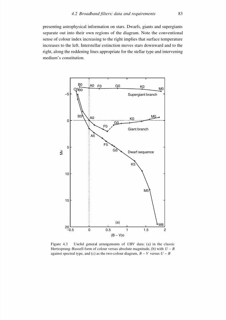
7/21/2019 Introduction to Astronomical Photometry
http://slidepdf.com/reader/full/introduction-to-astronomical-photometry 101/451
4.2 Broadband filters: data and requirements 83
presenting astrophysical information on stars. Dwarfs, giants and supergiantsseparate out into their own regions of the diagram. Note the conventionalsense of colour index increasing to the right implies that surface temperature
increases to the left. Interstellar extinction moves stars downward and to theright, along the reddening lines appropriate for the stellar type and interveningmedium’s constitution.
–5
0
5
10
15
20–0.5 0 0.5 1 1.5 2
M v
(B – V)o
Dwarf sequence
Giant branch
Supergiant branch
B0 A0 F0 G0 K0 M0B0
A0
F0G0
K0 M0
O5
B5
A5
F5
G5
K5
M5
M8(a)
Figure 4.3 Useful general arrangements of UBV data: (a) in the classicHertzsprung–Russell form of colour versus absolute magnitude, (b) with U − B
against spectral type, and (c) as the two-colour diagram, B − V versus U − B
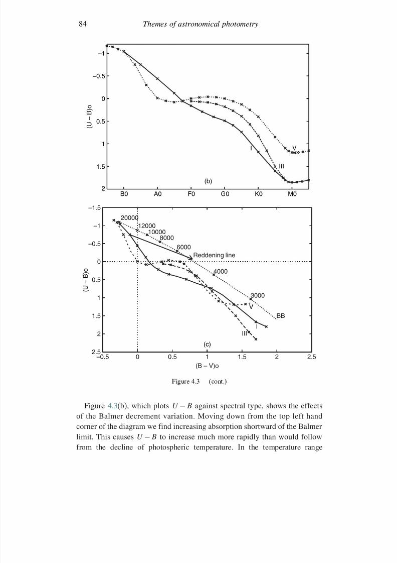
7/21/2019 Introduction to Astronomical Photometry
http://slidepdf.com/reader/full/introduction-to-astronomical-photometry 102/451
84 Themes of astronomical photometry
–1
–0.5
0
0.5
1
1.5
2G0 K0 M0B0 A0 F0
I V
III
( U –
B ) o
(b)
–0.5
( U – B ) o
V
0 0.5 1 1.5 2 2.5(B – V)o
–1.5
–1
0
–0.5
1
0.5
2
1.5
2.5
IIII
BB
3000
4000
Reddening line6000
80001000012000
20000
(c)
Figure 4.3 (cont.)
Figure 4.3(b), which plots U − B against spectral type, shows the effectsof the Balmer decrement variation. Moving down from the top left handcorner of the diagram we find increasing absorption shortward of the Balmerlimit. This causes U − B to increase much more rapidly than would followfrom the decline of photospheric temperature. In the temperature range
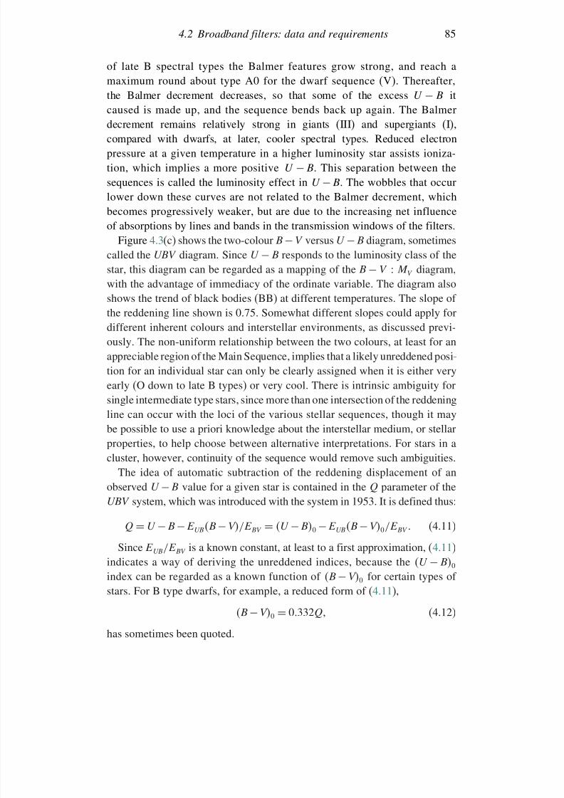
7/21/2019 Introduction to Astronomical Photometry
http://slidepdf.com/reader/full/introduction-to-astronomical-photometry 103/451
4.2 Broadband filters: data and requirements 85
of late B spectral types the Balmer features grow strong, and reach amaximum round about type A0 for the dwarf sequence (V). Thereafter,the Balmer decrement decreases, so that some of the excess U
−B it
caused is made up, and the sequence bends back up again. The Balmerdecrement remains relatively strong in giants (III) and supergiants (I),compared with dwarfs, at later, cooler spectral types. Reduced electronpressure at a given temperature in a higher luminosity star assists ioniza-tion, which implies a more positive U − B. This separation between thesequences is called the luminosity effect in U − B. The wobbles that occurlower down these curves are not related to the Balmer decrement, whichbecomes progressively weaker, but are due to the increasing net influenceof absorptions by lines and bands in the transmission windows of the filters.
Figure 4.3(c) shows the two-colour B − V versus U − B diagram, sometimescalled the UBV diagram. Since U − B responds to the luminosity class of thestar, this diagram can be regarded as a mapping of the B − V : M V diagram,with the advantage of immediacy of the ordinate variable. The diagram alsoshows the trend of black bodies (BB) at different temperatures. The slope of the reddening line shown is 0.75. Somewhat different slopes could apply for
different inherent colours and interstellar environments, as discussed previ-ously. The non-uniform relationship between the two colours, at least for anappreciable region of the Main Sequence, implies that a likely unreddened posi-tion for an individual star can only be clearly assigned when it is either veryearly (O down to late B types) or very cool. There is intrinsic ambiguity forsingle intermediate type stars, since more than one intersection of the reddeningline can occur with the loci of the various stellar sequences, though it maybe possible to use a priori knowledge about the interstellar medium, or stellarproperties, to help choose between alternative interpretations. For stars in acluster, however, continuity of the sequence would remove such ambiguities.
The idea of automatic subtraction of the reddening displacement of anobserved U − B value for a given star is contained in the Q parameter of theUBV system, which was introduced with the system in 1953. It is defined thus:
Q = U − B − E UBB − V/E BV = U − B0 − E UBB − V0/E BV (4.11)
Since E UB/E BV is a known constant, at least to a first approximation, (4.11)indicates a way of deriving the unreddened indices, because the U − B0
index can be regarded as a known function of B − V0 for certain types of stars. For B type dwarfs, for example, a reduced form of (4.11),
B − V0 = 0332Q (4.12)
has sometimes been quoted.
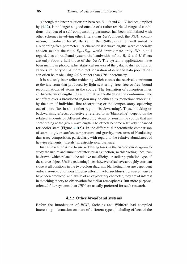
7/21/2019 Introduction to Astronomical Photometry
http://slidepdf.com/reader/full/introduction-to-astronomical-photometry 104/451
86 Themes of astronomical photometry
Although the linear relationship between U −B and B −V indices, impliedby (4.12), is no longer so good outside of a rather restricted range of condi-tions, the idea of a self-compensating parameter has been maintained with
other schemes involving other filters than UBV . Indeed, the RGU combi-nation, introduced by W. Becker in the 1940s, is rather well suited toa reddening-free parameter. Its characteristic wavelengths were especiallychosen so that the ratio E UG/E GR would approximate unity. While stillregarded as a broadband system, the bandwidths of the R, G and U filtersare only about a half those of the UBV . The system’s applications havebeen mainly in photographic statistical surveys of the galactic distributions of
various stellar types. A more direct separation of disk and halo populationscan often be made using RGU rather than UBV photometry.It is not only interstellar reddening which causes the received continuum
to deviate from that produced by light scattering, free–free or free–boundrecombinations of atoms in the source. The formation of absorption linesat discrete wavelengths has a cumulative feedback on the continuum. Thenet effect over a broadband region may be either flux reduction: ‘blocking’by the sum of individual line absorptions; or the compensatory squeezing
out of more flux in some other region: ‘backwarming’. These blocking orbackwarming effects, collectively referred to as ‘blanketing’, depend on therelative amounts of different absorbing atoms or ions in the source that arecontributing at the given wavelength. The effects become relatively enhancedfor cooler stars (Figure 4.3(b)). In the differential photometric comparisonof stars, at given surface temperature and gravity, measures of blanketingthus trace composition, particularly with regard to the relative abundances of
heavier elements: ‘metals’ in astrophysical parlance.Just as it was possible to use reddening lines in the two-colour diagram tostudy the nature and amount of interstellar extinction, so ‘blanketing lines’ canbe drawn, which relate to the relative metallicity, or stellar population type, of the source object. Unlike reddening lines, however, that have a roughly constantslope at all positions in the two-colour diagram, blanketing lines are dependentonlocalsourceconditions.Empiricalformulaeforsuchlinesingivensequenceshave been produced, and, while of an exploratory character, they are of interest
in matching theory to observation for stellar atmospheres. But more purpose-oriented filter systems than UBV are usually preferred for such research.
4.2.2 Other broadband systems
Before the introduction of RGU , Stebbins and Whitford had compiledinteresting information on stars of different types, including effects of the
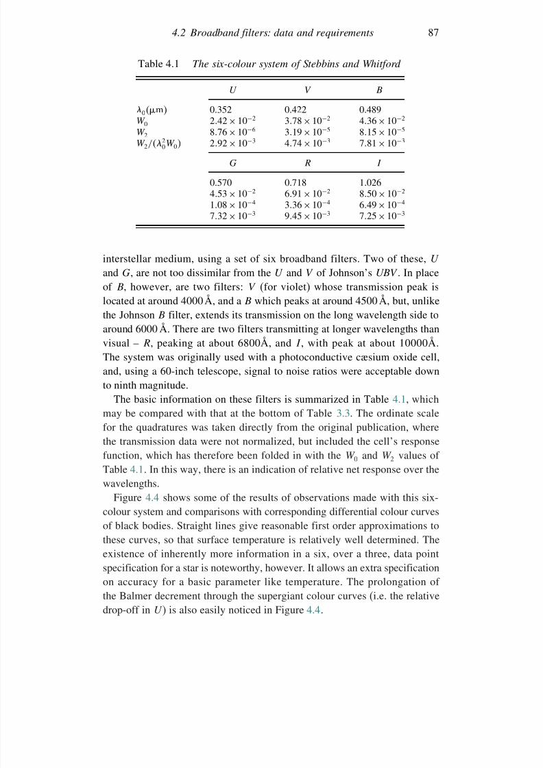
7/21/2019 Introduction to Astronomical Photometry
http://slidepdf.com/reader/full/introduction-to-astronomical-photometry 105/451
4.2 Broadband filters: data and requirements 87
Table 4.1 The six-colour system of Stebbins and Whitford
U V B
0m 0.352 0.422 0.489W 0 242 ×10−2 378×10−2 436×10−2
W 2 876 ×10−6 319×10−5 815×10−5
W 2/20W 0 292 ×10−3 474 ×10−3 781×10−3
G R I
0.570 0.718 1.026453 ×10⁻² 691×10−2 850 ×10−2
108 ×10−4
336×10−4
649×10−4
732 ×10−3 945×10−3 725×10−3
interstellar medium, using a set of six broadband filters. Two of these, U
and G, are not too dissimilar from the U and V of Johnson’s UBV . In placeof B, however, are two filters: V (for violet) whose transmission peak islocated at around 4000 Å, and a B which peaks at around 4500 Å, but, unlike
the Johnson B filter, extends its transmission on the long wavelength side toaround 6000 Å. There are two filters transmitting at longer wavelengths thanvisual – R, peaking at about 6800Å, and I , with peak at about 10000Å.The system was originally used with a photoconductive cæsium oxide cell,and, using a 60-inch telescope, signal to noise ratios were acceptable downto ninth magnitude.
The basic information on these filters is summarized in Table 4.1, whichmay be compared with that at the bottom of Table 3.3. The ordinate scalefor the quadratures was taken directly from the original publication, wherethe transmission data were not normalized, but included the cell’s responsefunction, which has therefore been folded in with the W 0 and W 2 values of Table 4.1. In this way, there is an indication of relative net response over thewavelengths.
Figure 4.4 shows some of the results of observations made with this six-colour system and comparisons with corresponding differential colour curves
of black bodies. Straight lines give reasonable first order approximations tothese curves, so that surface temperature is relatively well determined. Theexistence of inherently more information in a six, over a three, data pointspecification for a star is noteworthy, however. It allows an extra specificationon accuracy for a basic parameter like temperature. The prolongation of the Balmer decrement through the supergiant colour curves (i.e. the relativedrop-off in U ) is also easily noticed in Figure 4.4.
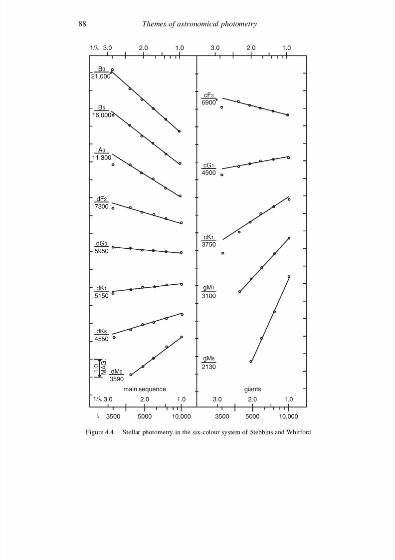
7/21/2019 Introduction to Astronomical Photometry
http://slidepdf.com/reader/full/introduction-to-astronomical-photometry 106/451
88 Themes of astronomical photometry
3500
3.0 2.0 1.0 3.0 2.0
giantsmain sequence
1.0
3.0 2.0 1.0 3.0 2.0 1.0
λ
1/ λ
1/ λ
5000 10,000 5000 10,0003500
B0
21,000
cF3
6900
cG1
4900
cK1
3750
gM1
3100
gM6
2130
B5
16,000
A011,300
dF2
7300
dG0
5950
dK1
5150
dK5
4550
dM0 1 . 0
M A G
.
3590
Figure 4.4 Stellar photometry in the six-colour system of Stebbins and Whitford
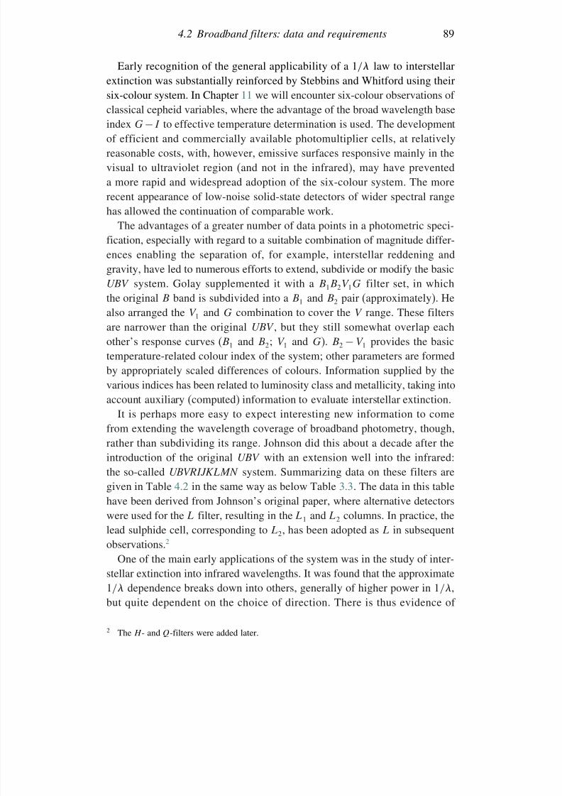
7/21/2019 Introduction to Astronomical Photometry
http://slidepdf.com/reader/full/introduction-to-astronomical-photometry 107/451
4.2 Broadband filters: data and requirements 89
Early recognition of the general applicability of a 1/ law to interstellarextinction was substantially reinforced by Stebbins and Whitford using theirsix-colour system. In Chapter 11 we will encounter six-colour observations of
classical cepheid variables, where the advantage of the broad wavelength baseindex G− I to effective temperature determination is used. The developmentof efficient and commercially available photomultiplier cells, at relativelyreasonable costs, with, however, emissive surfaces responsive mainly in thevisual to ultraviolet region (and not in the infrared), may have preventeda more rapid and widespread adoption of the six-colour system. The morerecent appearance of low-noise solid-state detectors of wider spectral range
has allowed the continuation of comparable work.The advantages of a greater number of data points in a photometric speci-fication, especially with regard to a suitable combination of magnitude differ-ences enabling the separation of, for example, interstellar reddening andgravity, have led to numerous efforts to extend, subdivide or modify the basicUBV system. Golay supplemented it with a B1B2V 1G filter set, in whichthe original B band is subdivided into a B1 and B2 pair (approximately). Healso arranged the V 1 and G combination to cover the V range. These filters
are narrower than the original UBV , but they still somewhat overlap eachother’s response curves (B1 and B2; V 1 and G). B2 − V 1 provides the basictemperature-related colour index of the system; other parameters are formedby appropriately scaled differences of colours. Information supplied by thevarious indices has been related to luminosity class and metallicity, taking intoaccount auxiliary (computed) information to evaluate interstellar extinction.
It is perhaps more easy to expect interesting new information to come
from extending the wavelength coverage of broadband photometry, though,rather than subdividing its range. Johnson did this about a decade after theintroduction of the original UBV with an extension well into the infrared:the so-called UBVRIJKLMN system. Summarizing data on these filters aregiven in Table 4.2 in the same way as below Table 3.3. The data in this tablehave been derived from Johnson’s original paper, where alternative detectorswere used for the L filter, resulting in the L1 and L2 columns. In practice, thelead sulphide cell, corresponding to L2, has been adopted as L in subsequent
observations.2
One of the main early applications of the system was in the study of inter-stellar extinction into infrared wavelengths. It was found that the approximate1/ dependence breaks down into others, generally of higher power in 1/,but quite dependent on the choice of direction. There is thus evidence of
2 The H - and Q-filters were added later.
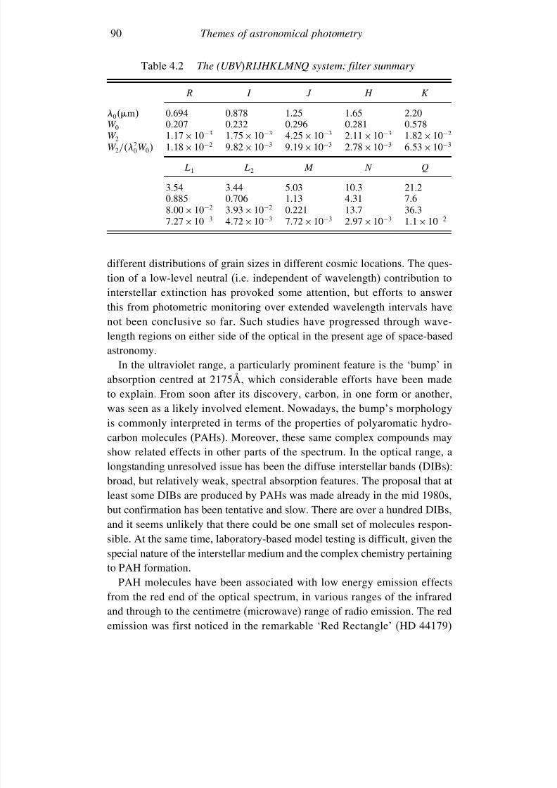
7/21/2019 Introduction to Astronomical Photometry
http://slidepdf.com/reader/full/introduction-to-astronomical-photometry 108/451
90 Themes of astronomical photometry
Table 4.2 The (UBVRIJHKLMNQ system: filter summary
R I J H K
0m 0.694 0.878 1.25 1.65 2.20W 0 0.207 0.232 0.296 0.281 0.578W 2 117×10−3 175× 10−3 425 ×10−3 211×10−3 182 ×10−2
W 2/20W 0 118×10−2 982 ×10−3 919×10−3 278×10−3 653 ×10−3
L1 L2 M N Q
3.54 3.44 5.03 10.3 21.20.885 0.706 1.13 4.31 7.6
800 ×10−2
393× 10−2
0.221 13.7 36.3727×10⁻³ 472 ×10−3 772 ×10−3 297×10−3 11× 10−2
different distributions of grain sizes in different cosmic locations. The ques-tion of a low-level neutral (i.e. independent of wavelength) contribution tointerstellar extinction has provoked some attention, but efforts to answerthis from photometric monitoring over extended wavelength intervals have
not been conclusive so far. Such studies have progressed through wave-length regions on either side of the optical in the present age of space-basedastronomy.
In the ultraviolet range, a particularly prominent feature is the ‘bump’ inabsorption centred at 2175Å, which considerable efforts have been madeto explain. From soon after its discovery, carbon, in one form or another,was seen as a likely involved element. Nowadays, the bump’s morphologyis commonly interpreted in terms of the properties of polyaromatic hydro-carbon molecules (PAHs). Moreover, these same complex compounds mayshow related effects in other parts of the spectrum. In the optical range, alongstanding unresolved issue has been the diffuse interstellar bands (DIBs):broad, but relatively weak, spectral absorption features. The proposal that atleast some DIBs are produced by PAHs was made already in the mid 1980s,but confirmation has been tentative and slow. There are over a hundred DIBs,and it seems unlikely that there could be one small set of molecules respon-
sible. At the same time, laboratory-based model testing is difficult, given thespecial nature of the interstellar medium and the complex chemistry pertainingto PAH formation.
PAH molecules have been associated with low energy emission effectsfrom the red end of the optical spectrum, in various ranges of the infraredand through to the centimetre (microwave) range of radio emission. The redemission was first noticed in the remarkable ‘Red Rectangle’ (HD 44179)
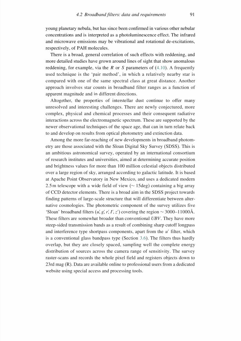
7/21/2019 Introduction to Astronomical Photometry
http://slidepdf.com/reader/full/introduction-to-astronomical-photometry 109/451
4.2 Broadband filters: data and requirements 91
young planetary nebula, but has since been confirmed in various other nebularconcentrations and is interpreted as a photoluminescence effect. The infraredand microwave emissions may be vibrational and rotational de-excitations,
respectively, of PAH molecules.There is a broad, general correlation of such effects with reddening, and
more detailed studies have grown around lines of sight that show anomalousreddening, for example, via the R or S parameters of (4.10). A frequentlyused technique is the ‘pair method’, in which a relatively nearby star iscompared with one of the same spectral class at great distance. Anotherapproach involves star counts in broadband filter ranges as a function of
apparent magnitude and in different directions.Altogether, the properties of interstellar dust continue to offer many
unresolved and interesting challenges. There are newly conjectured, morecomplex, physical and chemical processes and their consequent radiativeinteractions across the electromagnetic spectrum. These are supported by thenewer observational techniques of the space age, that can in turn relate backto and develop on results from optical photometry and extinction data.
Among the more far-reaching of new developments in broadband photom-etry are those associated with the Sloan Digital Sky Survey (SDSS). This isan ambitious astronomical survey, operated by an international consortiumof research institutes and universities, aimed at determining accurate positionand brightness values for more than 100 million celestial objects distributedover a large region of sky, arranged according to galactic latitude. It is basedat Apache Point Observatory in New Mexico, and uses a dedicated modern
2.5 m telescope with a wide field of view (∼ 15deg) containing a big arrayof CCD detector elements. There is a broad aim in the SDSS project towardsfinding patterns of large-scale structure that will differentiate between alter-native cosmologies. The photometric component of the survey utilizes five‘Sloan’ broadband filters (u g r I z) covering the region ∼ 3000–11000Å.These filters are somewhat broader than conventional UBV . They have moresteep-sided transmission bands as a result of combining sharp cutoff longpass
and interference type shortpass components, apart from the u filter, whichis a conventional glass bandpass type (Section 3.6). The filters thus hardlyoverlap, but they are closely spaced, sampling well the complete energydistribution of sources across the camera range of sensitivity. The surveyraster-scans and records the whole pixel field and registers objects down to23rd mag (R). Data are available online to professional users from a dedicatedwebsite using special access and processing tools.

7/21/2019 Introduction to Astronomical Photometry
http://slidepdf.com/reader/full/introduction-to-astronomical-photometry 110/451
92 Themes of astronomical photometry
4.3 Photometry at intermediate bandwidths
The broadband systems discussed hitherto are characterized by several key
points. Firstly, they have had a fairly clear development from historic photom-etry performed by such basic devices as the photographic plate or eye.Secondly, the filters associated with these broad transmissions are usually,at least in the optical domain, made from coloured glass, or coloured glasscombinations, with broad, but not necessarily symmetric, transmission func-tions. Thirdly, such broad transmission characteristics allow the integratedTaylor expansion (3.27) to have reasonable validity for foldings with a realstellar irradiance function. At high resolution this irradiance has numerous
discrete irregularities, which make the Taylor expansion derivatives awkwardto define. In any case, narrow wavelength sampling, in general, would bemore likely to cause a particular brightness temperature, in the case of onefilter, or colour temperature, in the case of two, to deviate from the closerapproximation to source effective temperature, which such measures tend toat broader passbands.
The special peculiarities of high-resolution sampling can be avoided, whilst
also escaping difficulties coming from the second order terms in the Taylordevelopment (3.27), with an appropriate choice of intermediate bandwidthfilters. Such methods touch on the foregoing points in the following respects.Firstly, they have been led by astrophysical requirements, rather than histor-ical continuity. Secondly, while it is still possible to devise an intermediatebandpass filter from a suitable overlap of shortpass and longpass edges ina combination of coloured glasses, it is generally much more convenientto employ filters of the interference type. Modern manufacturing techniquesallow passbands with stringent requirements on transmissions and mean wave-lengths to be effectively realizable over a wide optical range. Thirdly, partof this stringency in requirements is concerned with the positioning of thebands in relation to strong spectral features. These should be absent fromthe transmission range of any intermediate-band filter intended for deter-mining a temperature scale; or, at least, such effects, if present in onefilter, should be removed in an appropriate difference of magnitudes from
two filters.
4.3.1 The uvby system
The most well-known intermediate-band system is the uvby four-filter combi-nation, introduced following the published ideas of B. Strömgren, and theobservational work of D. Crawford starting in the late 1950s. Essentially all
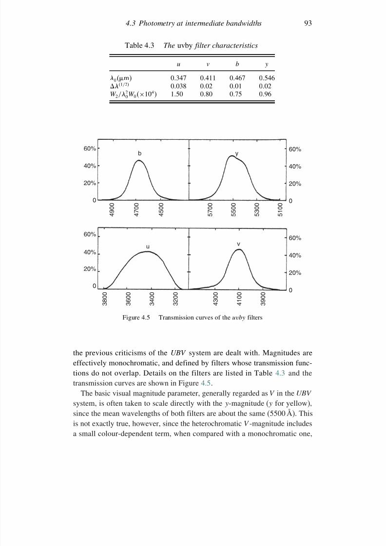
7/21/2019 Introduction to Astronomical Photometry
http://slidepdf.com/reader/full/introduction-to-astronomical-photometry 111/451
4.3 Photometry at intermediate bandwidths 93
Table 4.3 The uvby filter characteristics
u v b y
0m 0347 0411 0467 05461/2 0038 002 001 002W 2/2
0W 0×104 150 080 075 096
60%
40%
20%
0
60%
u
b y
v40%
20%
3 8 0
0
3 6 0
0
3 4 0
0
3 2 0
0
4 3 0
0
4 1 0
0
3 9 0
0
4 9 0 0
4 7 0 0
4 5 0 0
5 7 0 0
5 5 0 0
5 3 0 0
5 1 0 0
0
60%
40%
20%
0
60%
40%
20%
0
Figure 4.5 Transmission curves of the uvby filters
the previous criticisms of the UBV system are dealt with. Magnitudes areeffectively monochromatic, and defined by filters whose transmission func-
tions do not overlap. Details on the filters are listed in Table 4.3 and thetransmission curves are shown in Figure 4.5.
The basic visual magnitude parameter, generally regarded as V in the UBV
system, is often taken to scale directly with the y-magnitude (y for yellow),since the mean wavelengths of both filters are about the same (5500 Å). Thisis not exactly true, however, since the heterochromatic V -magnitude includesa small colour-dependent term, when compared with a monochromatic one,
7/21/2019 Introduction to Astronomical Photometry
http://slidepdf.com/reader/full/introduction-to-astronomical-photometry 112/451
94 Themes of astronomical photometry
as can be inferred from (3.28) or (4.5). Using again the magnitude scale, atmean wavelength 0, we obtain
−25log
10f
W = −1086ln f
W
= −1086ln
f0W 0
1+ f 0W 2
2f0W 0
(4.13)
to terms in the second order of small quantities.Applying this to the V -filter, we have, to a sufficient accuracy,
V = v −1086lnf0W 0 − 0543f 0 W 2f0 W 0
(4.14)
where v denotes an appropriate zero constant to tie in the scale with anadopted calibration (Section 3.3). For the y-filter we can simply write
y = y −1086lnf0W y (4.15)
where 0 is the same (055 m) in both cases, and W y represents the integralof the flux multiplied by the corresponding transmission of the y-filter. (Sinceonly the zeroth moment need be considered for this filter for the present
purpose, there is no loss of generality in dropping the zero suffix.)Combining the foregoing, we have
V = y −1086ln W 0W y
−0543W 2f 0
W 0f0 + v − y (4.16)
Using the Planck formula, from the discussion that follows (3.32), with a littlemanipulation we find f 0/f0 5max − 0/2
0, and f 0/f0 30max
−02/4
0. Combining the first of these with the definition of the
magnitude scale, we obtain5max − 0
20
0921b − y
+ c (4.17)
where the b to y wavelength difference = 008 m. The quantity carises from the somewhat arbitrary fixing of b − y to be zero at a certainspectral type of dwarf star, or, in other words, a certain value for max.Since max
0
5500 Å for stars whose b
−y is around 0.55, it follows
that c −0921×055/008 = −633. Therefore, removing the various zeroterms in (4.16) by taking the V and y scales to be coincident for stars of colour b − y = 055, we can find,
V = y − 012b − y −0552 (4.18)
This formula shows the expected scale of departure of y from strict V
over a range of b − y values on the basis of a Planck-like approximation to
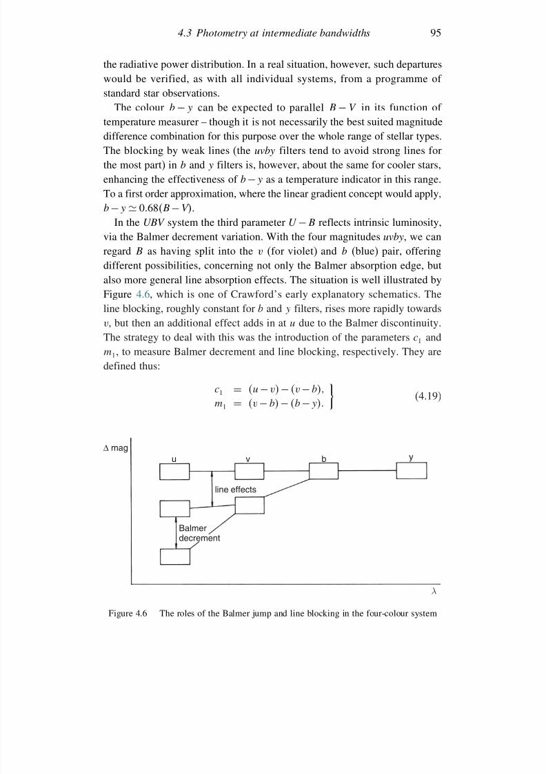
7/21/2019 Introduction to Astronomical Photometry
http://slidepdf.com/reader/full/introduction-to-astronomical-photometry 113/451
4.3 Photometry at intermediate bandwidths 95
the radiative power distribution. In a real situation, however, such departureswould be verified, as with all individual systems, from a programme of standard star observations.
The colour b − y can be expected to parallel B − V in its function of temperature measurer – though it is not necessarily the best suited magnitudedifference combination for this purpose over the whole range of stellar types.The blocking by weak lines (the uvby filters tend to avoid strong lines forthe most part) in b and y filters is, however, about the same for cooler stars,enhancing the effectiveness of b − y as a temperature indicator in this range.To a first order approximation, where the linear gradient concept would apply,
b − y 068B − V.In the UBV system the third parameter U − B reflects intrinsic luminosity,via the Balmer decrement variation. With the four magnitudes uvby, we canregard B as having split into the v (for violet) and b (blue) pair, offeringdifferent possibilities, concerning not only the Balmer absorption edge, butalso more general line absorption effects. The situation is well illustrated byFigure 4.6, which is one of Crawford’s early explanatory schematics. Theline blocking, roughly constant for b and y filters, rises more rapidly towardsv, but then an additional effect adds in at u due to the Balmer discontinuity.The strategy to deal with this was the introduction of the parameters c1 andm1, to measure Balmer decrement and line blocking, respectively. They aredefined thus:
c1 = u − v − v − b
m1 = v − b− b − y
(4.19)
∆ magu v b y
λ
line effects
Balmerdecrement
Figure 4.6 The roles of the Balmer jump and line blocking in the four-colour system
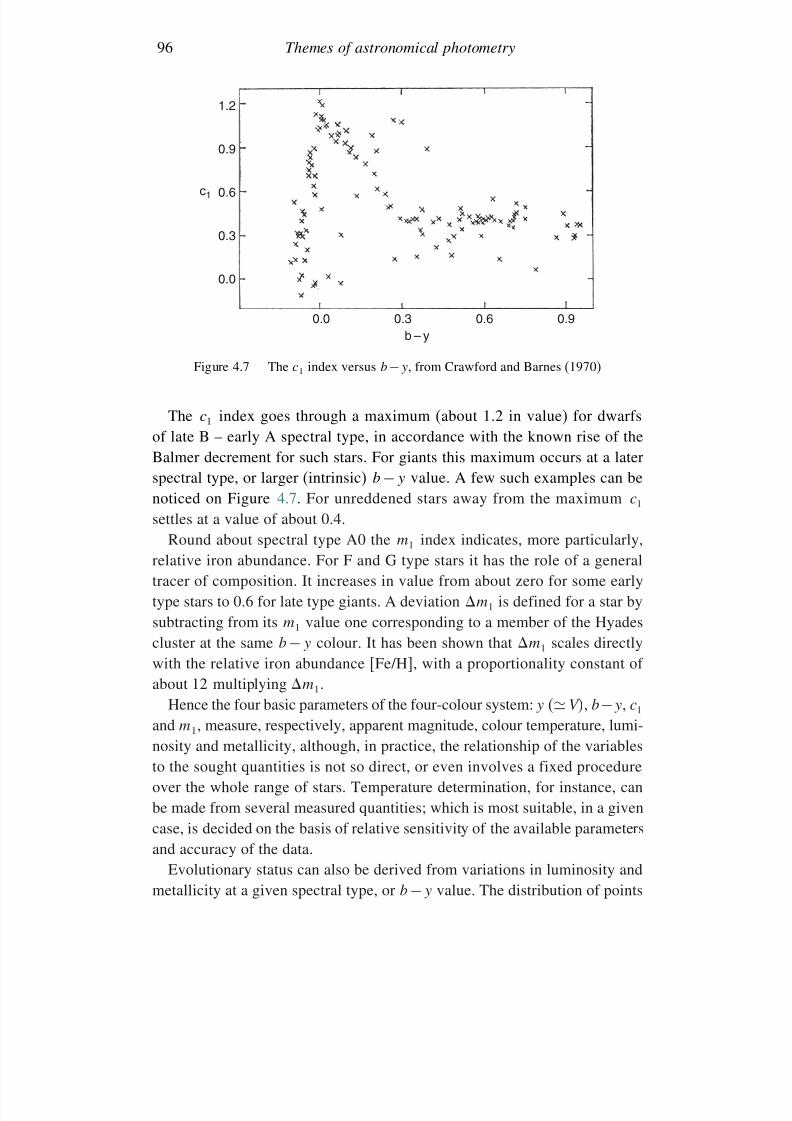
7/21/2019 Introduction to Astronomical Photometry
http://slidepdf.com/reader/full/introduction-to-astronomical-photometry 114/451
96 Themes of astronomical photometry
1.2
0.9
0.6c1
0.3
0.0
0.0 0.3b – y
0.6 0.9
Figure 4.7 The c1 index versus b − y, from Crawford and Barnes (1970)
The c1 index goes through a maximum (about 1.2 in value) for dwarfsof late B – early A spectral type, in accordance with the known rise of the
Balmer decrement for such stars. For giants this maximum occurs at a laterspectral type, or larger (intrinsic) b − y value. A few such examples can benoticed on Figure 4.7. For unreddened stars away from the maximum c1
settles at a value of about 0.4.Round about spectral type A0 the m1 index indicates, more particularly,
relative iron abundance. For F and G type stars it has the role of a generaltracer of composition. It increases in value from about zero for some earlytype stars to 0.6 for late type giants. A deviation m
1
is defined for a star bysubtracting from its m1 value one corresponding to a member of the Hyadescluster at the same b − y colour. It has been shown that m1 scales directlywith the relative iron abundance [Fe/H], with a proportionality constant of about 12 multiplying m1.
Hence the four basic parameters of the four-colour system: y V, b−y, c1
and m1, measure, respectively, apparent magnitude, colour temperature, lumi-nosity and metallicity, although, in practice, the relationship of the variables
to the sought quantities is not so direct, or even involves a fixed procedureover the whole range of stars. Temperature determination, for instance, canbe made from several measured quantities; which is most suitable, in a givencase, is decided on the basis of relative sensitivity of the available parametersand accuracy of the data.
Evolutionary status can also be derived from variations in luminosity andmetallicity at a given spectral type, or b − y value. The distribution of points
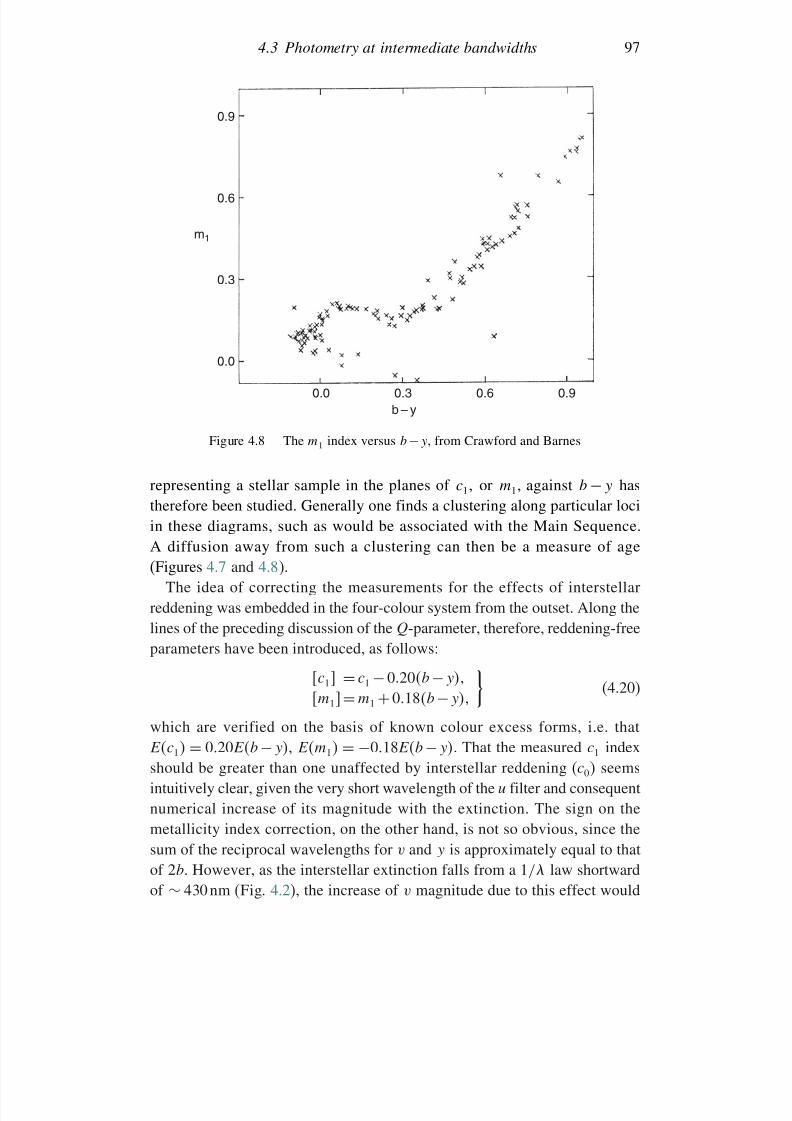
7/21/2019 Introduction to Astronomical Photometry
http://slidepdf.com/reader/full/introduction-to-astronomical-photometry 115/451
4.3 Photometry at intermediate bandwidths 97
0.9
0.6
m1
0.3
0.0
0.0 0.3b – y
0.6 0.9
Figure 4.8 The m1 index versus b − y, from Crawford and Barnes
representing a stellar sample in the planes of c1, or m1, against b − y hastherefore been studied. Generally one finds a clustering along particular lociin these diagrams, such as would be associated with the Main Sequence.A diffusion away from such a clustering can then be a measure of age(Figures 4.7 and 4.8).
The idea of correcting the measurements for the effects of interstellar
reddening was embedded in the four-colour system from the outset. Along thelines of the preceding discussion of the Q-parameter, therefore, reddening-freeparameters have been introduced, as follows:
c1 = c1 − 020b − y
m1 = m1 + 018b − y
(4.20)
which are verified on the basis of known colour excess forms, i.e. thatEc1
=020Eb
−y, Em1
= −018Eb
−y. That the measured c1 index
should be greater than one unaffected by interstellar reddening (c0) seemsintuitively clear, given the very short wavelength of the u filter and consequentnumerical increase of its magnitude with the extinction. The sign on themetallicity index correction, on the other hand, is not so obvious, since thesum of the reciprocal wavelengths for v and y is approximately equal to thatof 2b. However, as the interstellar extinction falls from a 1/ law shortwardof ∼ 430 nm (Fig. 4.2), the increase of v magnitude due to this effect would
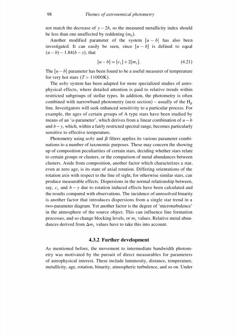
7/21/2019 Introduction to Astronomical Photometry
http://slidepdf.com/reader/full/introduction-to-astronomical-photometry 116/451
98 Themes of astronomical photometry
not match the decrease of y − 2b, so the measured metallicity index shouldbe less than one unaffected by reddening (m0).
Another modified parameter of the system u
−b has also been
investigated. It can easily be seen, since u − b is defined to equalu − b− 184b − y, that
u− b = c1 +2m1 (4.21)
The u−b parameter has been found to be a useful measurer of temperaturefor very hot stars T > 11000K.
The uvby system has been adapted for more specialized studies of astro-
physical effects, where detailed attention is paid to relative trends withinrestricted subgroups of stellar types. In addition, the photometry is oftencombined with narrowband photometry (next section) – usually of the H
line. Investigators will seek enhanced sensitivity to a particular process. Forexample, the ages of certain groups of A type stars have been studied bymeans of an ‘a-parameter’, which derives from a linear combination of u−b
and b−y, which, within a fairly restricted spectral range, becomes particularlysensitive to effective temperature.
Photometry using uvby and filters applies its various parameter combi-nations to a number of taxonomic purposes. These may concern the showingup of composition peculiarities of certain stars, deciding whether stars relateto certain groups or clusters, or the comparison of metal abundances betweenclusters. Aside from composition, another factor which characterizes a star,even at zero age, is its state of axial rotation. Differing orientations of therotation axis with respect to the line of sight, for otherwise similar stars, can
produce measurable effects. Dispersions in the normal relationship between,say, c1 and b − y due to rotation induced effects have been calculated andthe results compared with observations. The incidence of unresolved binarityis another factor that introduces dispersions from a single star trend in atwo-parameter diagram. Yet another factor is the degree of ‘microturbulence’in the atmosphere of the source object. This can influence line formationprocesses, and so change blocking levels, or m1 values. Relative metal abun-dances derived from m1 values have to take this into account.
4.3.2 Further development
As mentioned before, the movement to intermediate bandwidth photom-etry was motivated by the pursuit of direct measurables for parametersof astrophysical interest. These include luminosity, distance, temperature,metallicity, age, rotation, binarity, atmospheric turbulence, and so on. Under
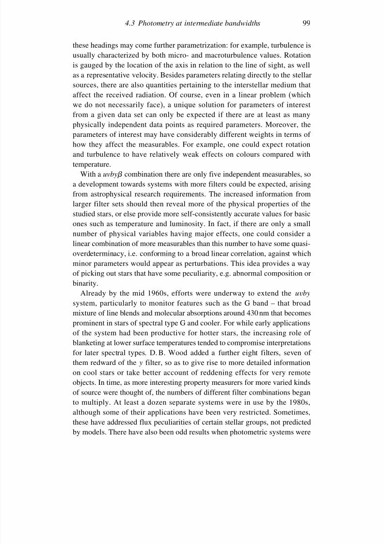
7/21/2019 Introduction to Astronomical Photometry
http://slidepdf.com/reader/full/introduction-to-astronomical-photometry 117/451
4.3 Photometry at intermediate bandwidths 99
these headings may come further parametrization: for example, turbulence isusually characterized by both micro- and macroturbulence values. Rotationis gauged by the location of the axis in relation to the line of sight, as well
as a representative velocity. Besides parameters relating directly to the stellarsources, there are also quantities pertaining to the interstellar medium thataffect the received radiation. Of course, even in a linear problem (whichwe do not necessarily face), a unique solution for parameters of interestfrom a given data set can only be expected if there are at least as manyphysically independent data points as required parameters. Moreover, theparameters of interest may have considerably different weights in terms of
how they affect the measurables. For example, one could expect rotationand turbulence to have relatively weak effects on colours compared withtemperature.
With a uvby combination there are only five independent measurables, soa development towards systems with more filters could be expected, arisingfrom astrophysical research requirements. The increased information fromlarger filter sets should then reveal more of the physical properties of thestudied stars, or else provide more self-consistently accurate values for basic
ones such as temperature and luminosity. In fact, if there are only a smallnumber of physical variables having major effects, one could consider alinear combination of more measurables than this number to have some quasi-overdeterminacy, i.e. conforming to a broad linear correlation, against whichminor parameters would appear as perturbations. This idea provides a wayof picking out stars that have some peculiarity, e.g. abnormal composition orbinarity.
Already by the mid 1960s, efforts were underway to extend the uvbysystem, particularly to monitor features such as the G band – that broadmixture of line blends and molecular absorptions around 430 nm that becomesprominent in stars of spectral type G and cooler. For while early applicationsof the system had been productive for hotter stars, the increasing role of blanketing at lower surface temperatures tended to compromise interpretationsfor later spectral types. D. B. Wood added a further eight filters, seven of them redward of the y filter, so as to give rise to more detailed information
on cool stars or take better account of reddening effects for very remoteobjects. In time, as more interesting property measurers for more varied kindsof source were thought of, the numbers of different filter combinations beganto multiply. At least a dozen separate systems were in use by the 1980s,although some of their applications have been very restricted. Sometimes,these have addressed flux peculiarities of certain stellar groups, not predictedby models. There have also been odd results when photometric systems were
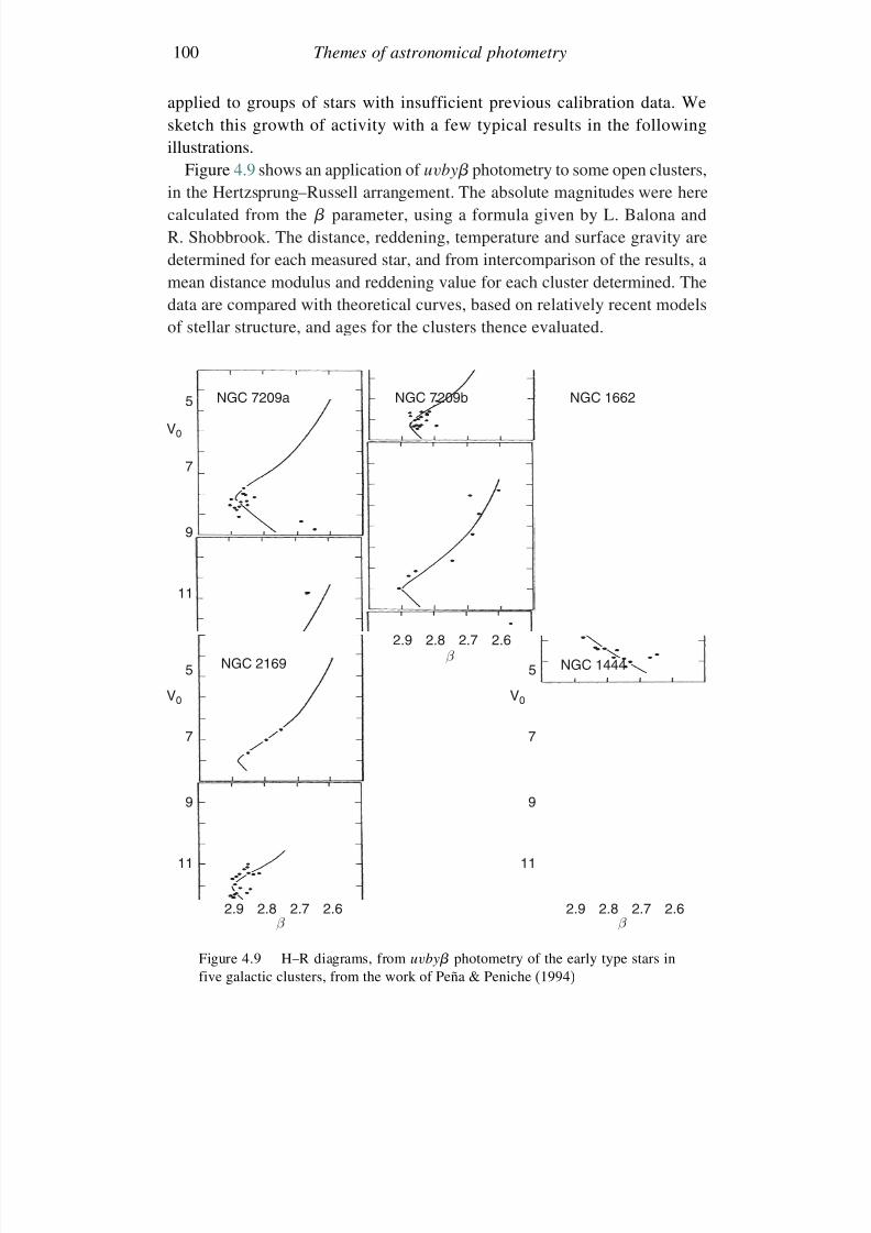
7/21/2019 Introduction to Astronomical Photometry
http://slidepdf.com/reader/full/introduction-to-astronomical-photometry 118/451
100 Themes of astronomical photometry
applied to groups of stars with insufficient previous calibration data. Wesketch this growth of activity with a few typical results in the followingillustrations.
Figure 4.9 shows an application of uvby photometry to some open clusters,in the Hertzsprung–Russell arrangement. The absolute magnitudes were herecalculated from the parameter, using a formula given by L. Balona andR. Shobbrook. The distance, reddening, temperature and surface gravity aredetermined for each measured star, and from intercomparison of the results, amean distance modulus and reddening value for each cluster determined. Thedata are compared with theoretical curves, based on relatively recent models
of stellar structure, and ages for the clusters thence evaluated.
5 NGC 7209a NGC 7209b
NGC 2169 NGC 1444
2.9 2.8 2.7β
2.6
2.9 2.8 2.7β
2.62.9 2.8 2.7β
2.6
NGC 1662
V0
7
9
11
5V0
7
9
11
5V0
7
9
11
Figure 4.9 H–R diagrams, from uvby photometry of the early type stars infive galactic clusters, from the work of Peña & Peniche (1994)
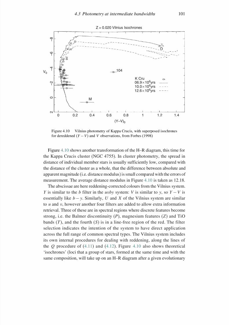
7/21/2019 Introduction to Astronomical Photometry
http://slidepdf.com/reader/full/introduction-to-astronomical-photometry 119/451
4.3 Photometry at intermediate bandwidths 101
Z = 0.020 Vilnius Isochrones
– 8
– 6
– 4
– 2
0
20 0.2 0.4
M
104
D
K Cru06.9 × 106yrs10.0 × 106yrs12.6 × 106yrs
0.6
(Y–V)0
0.8 1 1.2 1.4
V0
Figure 4.10 Vilnius photometry of Kappa Crucis, with superposed isochronesfor dereddened (Y − V ) and V observations, from Forbes (1998)
Figure 4.10 shows another transformation of the H–R diagram, this time forthe Kappa Crucis cluster (NGC 4755). In cluster photometry, the spread indistance of individual member stars is usually sufficiently low, compared withthe distance of the cluster as a whole, that the difference between absolute andapparent magnitude (i.e. distance modulus) is small compared with the errors of measurement. The average distance modulus in Figure 4.10 is taken as 12.18.
The abscissae are here reddening-corrected colours from the Vilnius system.Y is similar to the b filter in the uvby system: V is similar to y, so Y − V isessentially like b − y. Similarly, U and X of the Vilnius system are similarto u and v, however another four filters are added to allow extra informationretrieval. Three of these are in spectral regions where discrete features becomestrong, i.e. the Balmer discontinuity (P ), magnesium features (Z) and TiO
bands (T ), and the fourth (S ) is in a line-free region of the red. The filterselection indicates the intention of the system to have direct applicationacross the full range of common spectral types. The Vilnius system includesits own internal procedures for dealing with reddening, along the lines of the Q procedure of (4.11) and (4.12). Figure 4.10 also shows theoretical‘isochrones’ (loci that a group of stars, formed at the same time and with thesame composition, will take up on an H–R diagram after a given evolutionary
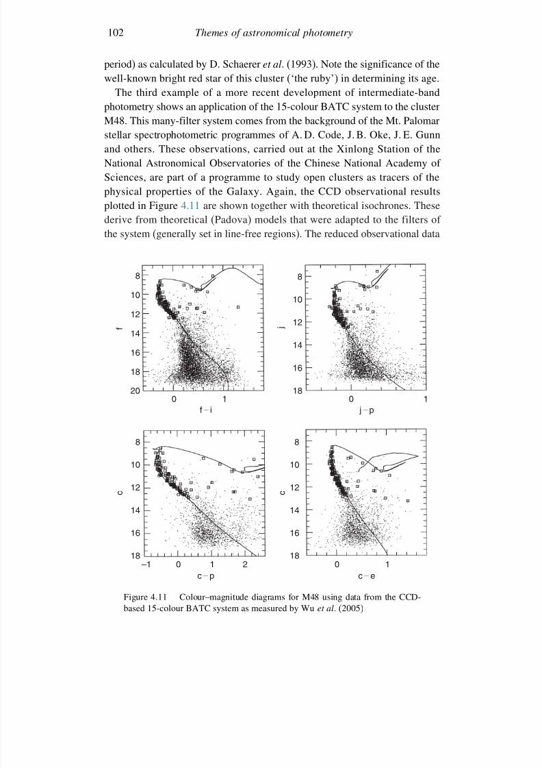
7/21/2019 Introduction to Astronomical Photometry
http://slidepdf.com/reader/full/introduction-to-astronomical-photometry 120/451
102 Themes of astronomical photometry
period) as calculated by D. Schaerer et al. (1993). Note the significance of thewell-known bright red star of this cluster (‘the ruby’) in determining its age.
The third example of a more recent development of intermediate-band
photometry shows an application of the 15-colour BATC system to the clusterM48. This many-filter system comes from the background of the Mt. Palomarstellar spectrophotometric programmes of A. D. Code, J. B. Oke, J. E. Gunnand others. These observations, carried out at the Xinlong Station of theNational Astronomical Observatories of the Chinese National Academy of Sciences, are part of a programme to study open clusters as tracers of thephysical properties of the Galaxy. Again, the CCD observational results
plotted in Figure 4.11 are shown together with theoretical isochrones. Thesederive from theoretical (Padova) models that were adapted to the filters of the system (generally set in line-free regions). The reduced observational data
8
10
12
14 f
16
18
200 1
0 10 1 2–1
8
10
12
14
j
16
18
8
10
12
14
16
18
8
10
12
14
16
18
0 1f – i
c – p
c c
c – e
j – p
Figure 4.11 Colour–magnitude diagrams for M48 using data from the CCD-based 15-colour BATC system as measured by Wu et al. (2005)
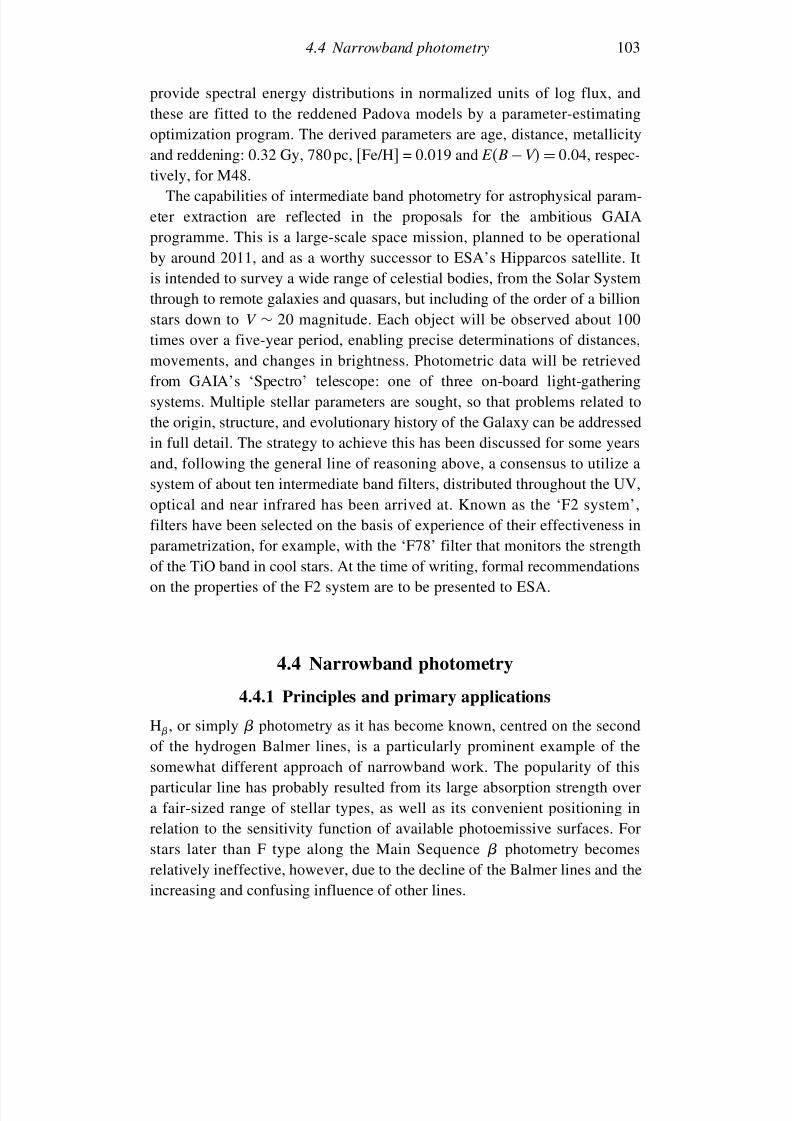
7/21/2019 Introduction to Astronomical Photometry
http://slidepdf.com/reader/full/introduction-to-astronomical-photometry 121/451
4.4 Narrowband photometry 103
provide spectral energy distributions in normalized units of log flux, andthese are fitted to the reddened Padova models by a parameter-estimatingoptimization program. The derived parameters are age, distance, metallicity
and reddening: 0.32 Gy, 780 pc, [Fe/H] = 0.019 and EB −V = 004, respec-tively, for M48.
The capabilities of intermediate band photometry for astrophysical param-eter extraction are reflected in the proposals for the ambitious GAIAprogramme. This is a large-scale space mission, planned to be operationalby around 2011, and as a worthy successor to ESA’s Hipparcos satellite. Itis intended to survey a wide range of celestial bodies, from the Solar System
through to remote galaxies and quasars, but including of the order of a billionstars down to V ∼ 20 magnitude. Each object will be observed about 100times over a five-year period, enabling precise determinations of distances,movements, and changes in brightness. Photometric data will be retrievedfrom GAIA’s ‘Spectro’ telescope: one of three on-board light-gatheringsystems. Multiple stellar parameters are sought, so that problems related tothe origin, structure, and evolutionary history of the Galaxy can be addressedin full detail. The strategy to achieve this has been discussed for some years
and, following the general line of reasoning above, a consensus to utilize asystem of about ten intermediate band filters, distributed throughout the UV,optical and near infrared has been arrived at. Known as the ‘F2 system’,filters have been selected on the basis of experience of their effectiveness inparametrization, for example, with the ‘F78’ filter that monitors the strengthof the TiO band in cool stars. At the time of writing, formal recommendationson the properties of the F2 system are to be presented to ESA.
4.4 Narrowband photometry
4.4.1 Principles and primary applications
H, or simply photometry as it has become known, centred on the secondof the hydrogen Balmer lines, is a particularly prominent example of the
somewhat different approach of narrowband work. The popularity of thisparticular line has probably resulted from its large absorption strength overa fair-sized range of stellar types, as well as its convenient positioning inrelation to the sensitivity function of available photoemissive surfaces. Forstars later than F type along the Main Sequence photometry becomesrelatively ineffective, however, due to the decline of the Balmer lines and theincreasing and confusing influence of other lines.
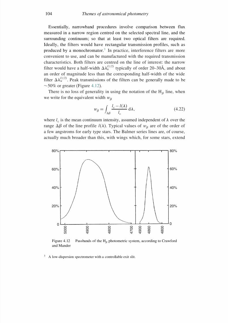
7/21/2019 Introduction to Astronomical Photometry
http://slidepdf.com/reader/full/introduction-to-astronomical-photometry 122/451
104 Themes of astronomical photometry
Essentially, narrowband procedures involve comparison between fluxmeasured in a narrow region centred on the selected spectral line, and thesurrounding continuum; so that at least two optical filters are required.
Ideally, the filters would have rectangular transmission profiles, such asproduced by a monochromator.3 In practice, interference filters are moreconvenient to use, and can be manufactured with the required transmissioncharacteristics. Both filters are centred on the line of interest: the narrowfilter would have a half-width
1/2n typically of order 20–30Å, and about
an order of magnitude less than the corresponding half-width of the widefilter
1/2w . Peak transmissions of the filters can be generally made to be
∼50% or greater (Figure 4.12).There is no loss of generality in using the notation of the H line, whenwe write for the equivalent width w
w =
lc − l
lc
d (4.22)
where lc is the mean continuum intensity, assumed independent of over therange of the line profile l. Typical values of w are of the order of
a few angstroms for early type stars. The Balmer series lines are, of course,actually much broader than this, with wings which, for some stars, extend
80%
60%
40%
20%
0
5 0 0 0
4 9 0 0
4 8 0 0
4 7 0 0
4 9 0 0
4 8 6 0
4 8 0 0
80%
60%
40%
20%
0
Figure 4.12 Passbands of the H photometric system, according to Crawfordand Mander
3 A low-dispersion spectrometer with a controllable exit slit.
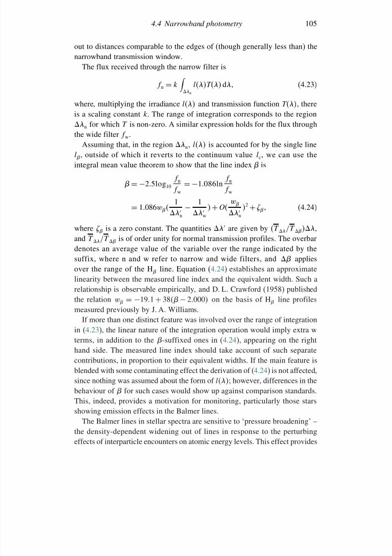
7/21/2019 Introduction to Astronomical Photometry
http://slidepdf.com/reader/full/introduction-to-astronomical-photometry 123/451
4.4 Narrowband photometry 105
out to distances comparable to the edges of (though generally less than) thenarrowband transmission window.
The flux received through the narrow filter is
f n = k
n
lT d (4.23)
where, multiplying the irradiance l and transmission function T, thereis a scaling constant k. The range of integration corresponds to the regionn for which T is non-zero. A similar expression holds for the flux throughthe wide filter f w.
Assuming that, in the region n, l is accounted for by the single linel, outside of which it reverts to the continuum value lc, we can use theintegral mean value theorem to show that the line index is
= −25log10
f nf w
= −1086ln f nf w
= 1086w 1
n
− 1
w
+ Ow
n
2 + (4.24)
where is a zero constant. The quantities are given by T /T ,and T /T is of order unity for normal transmission profiles. The overbardenotes an average value of the variable over the range indicated by thesuffix, where n and w refer to narrow and wide filters, and appliesover the range of the H line. Equation (4.24) establishes an approximatelinearity between the measured line index and the equivalent width. Such arelationship is observable empirically, and D. L. Crawford (1958) published
the relation w = −191 + 38 − 2000 on the basis of H line profilesmeasured previously by J. A. Williams.If more than one distinct feature was involved over the range of integration
in (4.23), the linear nature of the integration operation would imply extra wterms, in addition to the -suffixed ones in (4.24), appearing on the righthand side. The measured line index should take account of such separatecontributions, in proportion to their equivalent widths. If the main feature isblended with some contaminating effect the derivation of (4.24) is not affected,
since nothing was assumed about the form of l; however, differences in thebehaviour of for such cases would show up against comparison standards.This, indeed, provides a motivation for monitoring, particularly those starsshowing emission effects in the Balmer lines.
The Balmer lines in stellar spectra are sensitive to ‘pressure broadening’ –the density-dependent widening out of lines in response to the perturbingeffects of interparticle encounters on atomic energy levels. This effect provides
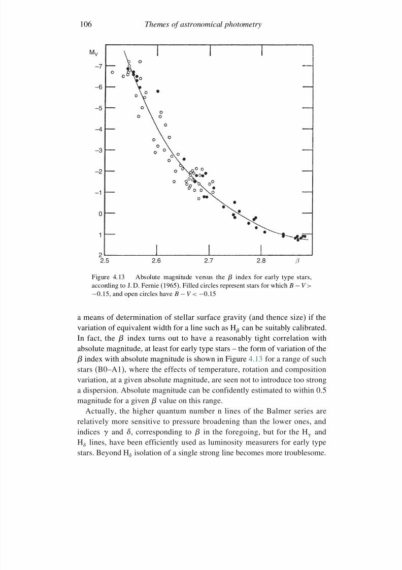
7/21/2019 Introduction to Astronomical Photometry
http://slidepdf.com/reader/full/introduction-to-astronomical-photometry 124/451
106 Themes of astronomical photometry
MV
–7
–6
–5
–4
–3
–2
–1
0
1
22.5 2.6 2.7 2.8 β
Figure 4.13 Absolute magnitude versus the index for early type stars,according to J. D. Fernie (1965). Filled circles represent stars for which B − V >
−015, and open circles have B − V < −015
a means of determination of stellar surface gravity (and thence size) if thevariation of equivalent width for a line such as H can be suitably calibrated.In fact, the index turns out to have a reasonably tight correlation withabsolute magnitude, at least for early type stars – the form of variation of the index with absolute magnitude is shown in Figure 4.13 for a range of suchstars (B0–A1), where the effects of temperature, rotation and compositionvariation, at a given absolute magnitude, are seen not to introduce too strong
a dispersion. Absolute magnitude can be confidently estimated to within 0.5magnitude for a given value on this range.
Actually, the higher quantum number n lines of the Balmer series arerelatively more sensitive to pressure broadening than the lower ones, andindices and , corresponding to in the foregoing, but for the H andH lines, have been efficiently used as luminosity measurers for early typestars. Beyond H isolation of a single strong line becomes more troublesome.
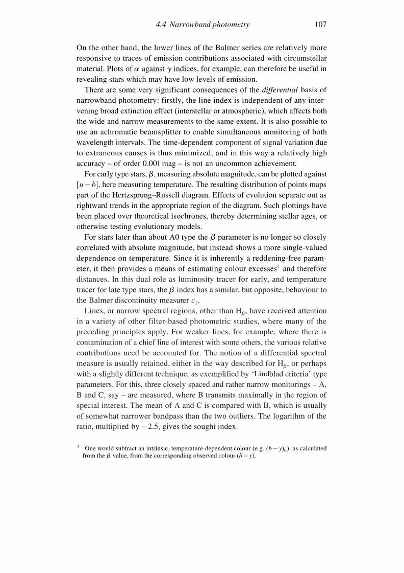
7/21/2019 Introduction to Astronomical Photometry
http://slidepdf.com/reader/full/introduction-to-astronomical-photometry 125/451
4.4 Narrowband photometry 107
On the other hand, the lower lines of the Balmer series are relatively moreresponsive to traces of emission contributions associated with circumstellarmaterial. Plots of against indices, for example, can therefore be useful in
revealing stars which may have low levels of emission.There are some very significant consequences of the differential basis of
narrowband photometry: firstly, the line index is independent of any inter-vening broad extinction effect (interstellar or atmospheric), which affects boththe wide and narrow measurements to the same extent. It is also possible touse an achromatic beamsplitter to enable simultaneous monitoring of bothwavelength intervals. The time-dependent component of signal variation due
to extraneous causes is thus minimized, and in this way a relatively highaccuracy – of order 0.001 mag – is not an uncommon achievement.For early type stars, , measuring absolute magnitude, can be plotted against
u−b, here measuring temperature. The resulting distribution of points mapspart of the Hertzsprung–Russell diagram. Effects of evolution separate out asrightward trends in the appropriate region of the diagram. Such plottings havebeen placed over theoretical isochrones, thereby determining stellar ages, orotherwise testing evolutionary models.
For stars later than about A0 type the parameter is no longer so closelycorrelated with absolute magnitude, but instead shows a more single-valueddependence on temperature. Since it is inherently a reddening-free param-eter, it then provides a means of estimating colour excesses4 and thereforedistances. In this dual role as luminosity tracer for early, and temperaturetracer for late type stars, the index has a similar, but opposite, behaviour tothe Balmer discontinuity measurer c1.
Lines, or narrow spectral regions, other than H, have received attentionin a variety of other filter-based photometric studies, where many of thepreceding principles apply. For weaker lines, for example, where there iscontamination of a chief line of interest with some others, the various relativecontributions need be accounted for. The notion of a differential spectralmeasure is usually retained, either in the way described for H, or perhapswith a slightly different technique, as exemplified by ‘Lindblad criteria’ typeparameters. For this, three closely spaced and rather narrow monitorings – A,B and C, say – are measured, where B transmits maximally in the region of special interest. The mean of A and C is compared with B, which is usuallyof somewhat narrower bandpass than the two outliers. The logarithm of theratio, multiplied by −25, gives the sought index.
4 One would subtract an intrinsic, temperature-dependent colour (e.g. b − y0), as calculatedfrom the value, from the corresponding observed colour (b − y).
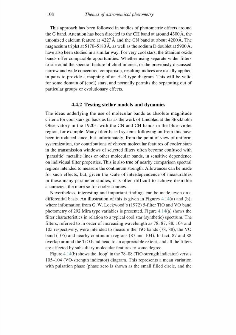
7/21/2019 Introduction to Astronomical Photometry
http://slidepdf.com/reader/full/introduction-to-astronomical-photometry 126/451
108 Themes of astronomical photometry
This approach has been followed in studies of photometric effects aroundthe G band. Attention has been directed to the CH band at around 4300 Å, theunionized calcium feature at 4227 Å and the CN band at about 4200 Å. The
magnesium triplet at 5170–5180 Å, as well as the sodium D doublet at 5900 Å,have also been studied in a similar way. For very cool stars, the titanium oxidebands offer comparable opportunities. Whether using separate wider filtersto surround the spectral feature of chief interest, or the previously discussednarrow and wide concentred comparison, resulting indices are usually appliedin pairs to provide a mapping of an H–R type diagram. This will be validfor some domain of (cool) stars, and normally permits the separating out of
particular groups or evolutionary effects.
4.4.2 Testing stellar models and dynamics
The ideas underlying the use of molecular bands as absolute magnitudecriteria for cool stars go back as far as the work of Lindblad at the StockholmObservatory in the 1920s: with the CN and CH bands in the blue–violetregion, for example. Many filter-based systems following on from this have
been introduced since, but unfortunately, from the point of view of uniformsystemization, the contributions of chosen molecular features of cooler starsin the transmission windows of selected filters often become confused with‘parasitic’ metallic lines or other molecular bands, in sensitive dependenceon individual filter properties. This is also true of nearby comparison spectralregions intended to measure the continuum strength. Allowances can be madefor such effects, but, given the scale of interdependence of measurables
in these many-parameter studies, it is often difficult to achieve desirableaccuracies; the more so for cooler sources.Nevertheless, interesting and important findings can be made, even on a
differential basis. An illustration of this is given in Figures 4.14(a) and (b),where information from G. W. Lockwood’s (1972) 5-filter TiO and VO bandphotometry of 292 Mira type variables is presented. Figure 4.14(a) shows thefilter characteristics in relation to a typical cool star (synthetic) spectrum. Thefilters, referred to in order of increasing wavelength as 78, 87, 88, 104 and
105 respectively, were intended to measure the TiO bands (78, 88), the VOband (105) and nearby continuum regions (87 and 104). In fact, 87 and 88overlap around the TiO band head to an appreciable extent, and all the filtersare affected by subsidiary molecular features to some degree.
Figure 4.14(b) shows the ‘loop’ in the 78–88 (TiO-strength indicator) versus105–104 (VO-strength indicator) diagram. This represents a mean variationwith pulsation phase (phase zero is shown as the small filled circle, and the
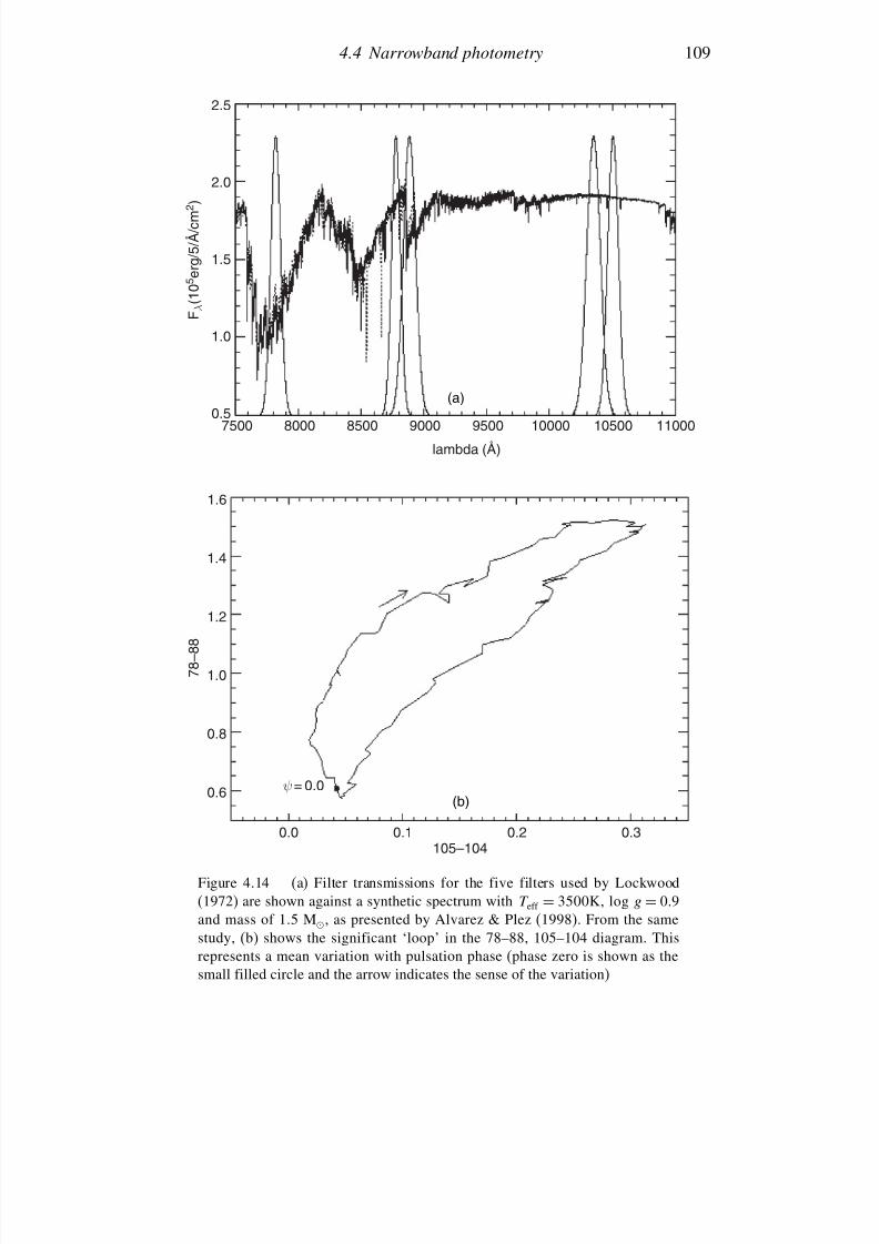
7/21/2019 Introduction to Astronomical Photometry
http://slidepdf.com/reader/full/introduction-to-astronomical-photometry 127/451
4.4 Narrowband photometry 109
2.5
2.0
1.5
F λ ( 1 0 5 e r g / 5 / Å / c m
2 )
1.0
0.57500 8000 8500 9000
lambda (Å)
9500 10000 10500 11000
(a)
1.6
1.4
1.2
1.0 7 8 – 8 8
0.8
0.6
0.0
ψ = 0.0
0.1
105–104
0.2 0.3
(b)
Figure 4.14 (a) Filter transmissions for the five filters used by Lockwood(1972) are shown against a synthetic spectrum with T eff = 3500K, log g = 09and mass of 1.5 M, as presented by Alvarez & Plez (1998). From the samestudy, (b) shows the significant ‘loop’ in the 78–88, 105–104 diagram. Thisrepresents a mean variation with pulsation phase (phase zero is shown as thesmall filled circle and the arrow indicates the sense of the variation)
7/21/2019 Introduction to Astronomical Photometry
http://slidepdf.com/reader/full/introduction-to-astronomical-photometry 128/451
110 Themes of astronomical photometry
sense of the phase change indicated by the arrow) from a sample of 256Miras. Since the VO bands increase in depth at cooler temperatures than theTiO bands, the loop gives persuasive evidence of a relative phase lag as a
pulsational wave emerges through cooler layers of the atmosphere.Another generally narrowband set of filters that has been applied to cool
stars is that of Dickow et al. (1970), sometimes called the Copenhagen system.These include eight filters, the shortest wavelength one of which resembles u
of the uvby system, but the other seven have narrow transmission windows inthe range 391 to 497 nm. The system involves six indices, five being simplelinear differences of magnitude and the other being a difference of two differ-
ences, similar to the metallicity index of the uvby system. Expressing the meanwavelengths in nm, the five linear indices are: g = [mag(427) – mag(439)],measuring the G band; n =[mag(417) – mag(429)], measuring a CN band;k = [mag(406) – mag(391)], measuring the Ca II K line; f = [mag(406) –mag(497)], measuring a violet to green colour; and u = [mag(344) – mag(406)],measuring an ultraviolet to violet colour. The index m is the differencebetween the [mag(406) – mag(452)] and [mag(452) – mag(497)] colours.
A quasi-overdeterminacy argument was applied for these six indices in
relation to the major parameters of temperature, gravity and composition.These are independently known from the R−I , M V and [Fe/H] values of somecalibration stars. Giant and dwarf stars were then found to separate neatlyinto two clear groups on either side of an empirical linear formula involvingm and f . Also, residuals in plots of the k index, which can be expected toassociate closely with M V through a well-known empirical formula linkingabsolute magnitude with the strength of the Ca II H K line (the Wilson–Bappu
effect), were found to give a strong indicator of stellar duplicity.Later work has allowed a broadband V magnitude to be derived – mainlyfrom mag(497), together with smaller terms in n and f . Distance modulithence follow, given the determinability of M V . Low metallicity (populationII) stars can be thus identified and their ages compared with those of metal-licity comparable to younger field stars (population I) by isochrone fitting.Such studies, directed to selected groups of stars (e.g. cool giants), havebeen aimed at probing stellar characteristics as a function of galactic latitude,
thereby checking kinematic properties of the Galaxy.
4.5 Fast photometry
The transition from photographic to photoelectric approaches to astronomicalphotometry, which became widespread around the middle years of the
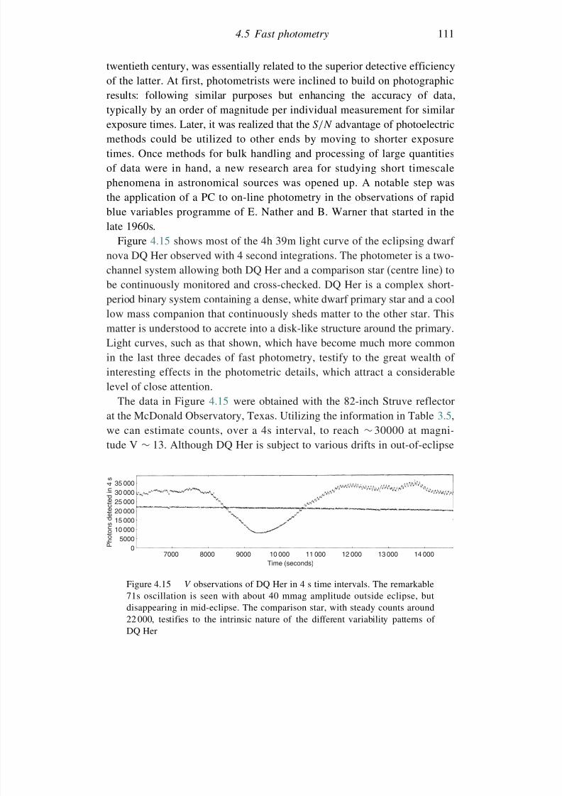
7/21/2019 Introduction to Astronomical Photometry
http://slidepdf.com/reader/full/introduction-to-astronomical-photometry 129/451
4.5 Fast photometry 111
twentieth century, was essentially related to the superior detective efficiencyof the latter. At first, photometrists were inclined to build on photographicresults: following similar purposes but enhancing the accuracy of data,
typically by an order of magnitude per individual measurement for similarexposure times. Later, it was realized that the S/N advantage of photoelectricmethods could be utilized to other ends by moving to shorter exposuretimes. Once methods for bulk handling and processing of large quantitiesof data were in hand, a new research area for studying short timescalephenomena in astronomical sources was opened up. A notable step wasthe application of a PC to on-line photometry in the observations of rapid
blue variables programme of E. Nather and B. Warner that started in thelate 1960s.Figure 4.15 shows most of the 4h 39m light curve of the eclipsing dwarf
nova DQ Her observed with 4 second integrations. The photometer is a two-channel system allowing both DQ Her and a comparison star (centre line) tobe continuously monitored and cross-checked. DQ Her is a complex short-period binary system containing a dense, white dwarf primary star and a coollow mass companion that continuously sheds matter to the other star. This
matter is understood to accrete into a disk-like structure around the primary.Light curves, such as that shown, which have become much more commonin the last three decades of fast photometry, testify to the great wealth of interesting effects in the photometric details, which attract a considerablelevel of close attention.
The data in Figure 4.15 were obtained with the 82-inch Struve reflectorat the McDonald Observatory, Texas. Utilizing the information in Table 3.5,
we can estimate counts, over a 4s interval, to reach ∼ 30000 at magni-tude V ∼ 13. Although DQ Her is subject to various drifts in out-of-eclipse
35 00030 000
P h o t o n s d e t e c t e d i n 4 s
25 00020 00015 00010 000
50000
7000 8000 9000 10 000Time (seconds)
11 000 12 000 13 000 14 000
Figure 4.15 V observations of DQ Her in 4 s time intervals. The remarkable71s oscillation is seen with about 40 mmag amplitude outside eclipse, butdisappearing in mid-eclipse. The comparison star, with steady counts around22 000, testifies to the intrinsic nature of the different variability patterns of DQ Her
7/21/2019 Introduction to Astronomical Photometry
http://slidepdf.com/reader/full/introduction-to-astronomical-photometry 130/451
112 Themes of astronomical photometry
brightness, this may be considered brighter, by a little over a magnitude, thantypically quoted values. Including sky background, then, the ordinate scale inFigure 4.15 seems plausible, and indicates 0.005 mag as the limiting accuracy
from just the counting statistics of the ‘shot noise’ distribution of photonarrivals. The apparent variations of the comparison star appear somewhatgreater than this, pointing to the likely role of atmospheric effects, e.g. scin-tillation. This is the well-known rapid variation of starlight associated withrefractive effects of moving density variations in the light path through theatmosphere. Scintillation depends on various circumstantial parameters, but(using a formula given by A. T. Young) a ∼3 mmag dispersion could be esti-mated for 4 s integrations with a 2.1 m aperture in ‘good observing’ conditions.The upshot is that the ∼40 mmag oscillation is clearly discernible on the datarecord of Figure 4.15, without the need for special micro-variability-searchingprocedures.
Concerning this latter point, Figure 4.16 is instructive. Here we see a graph-ical presentation of periodicity effects derived from analysis of photometriccounts, in dependence on frequency in mHz, for the white dwarf G 29 – 38.5
The original observations were made by J. T. McGraw and E. L. Robinson
using the 2.08m Struve telescope at McDonald Observatory. This popularmethod of display is the power spectrum: usually obtained by squaring andadding amplitudes of the Fourier components of the original time-series data.There is a cluster of periodicities around 15 minutes, with another group atabout half this timescale. Such oscillations are associated with the non-radialpulsation modes of white dwarfs. They are explained in terms of buoyancyeffects in the star’s outer layers, possibly including regions of non-uniform
ionization and stratified composition.Clearly, in interpreting spectra such as Figure 4.16, attention has to be paidto the relative scale of features against the background and possible contrib-utory sources at any particular frequency. It can be shown, for instance, thatthe Poissonian distribution of photon counts, mentioned above, has a ‘white’spectrum: at any particular frequency the variance in the power spectrum isn/2N , where n is the total number of collected photons in the time seriesand N is the number of uniform time intervals into which it is subdivided for
Fourier analysis. This is not necessarily the same with atmospheric scintilla-tion (depending on telescope aperture and wind speed) nor variations of trans-parency. The latter often show wave-like effects over timescales of minutes:comparable to some of those shown in Figure 4.16, however, such variationsare strongly correlated over telescope fields of view. With areal detectors
5 The name derives from H. Giclas’ survey work at the Lowell Observatory.
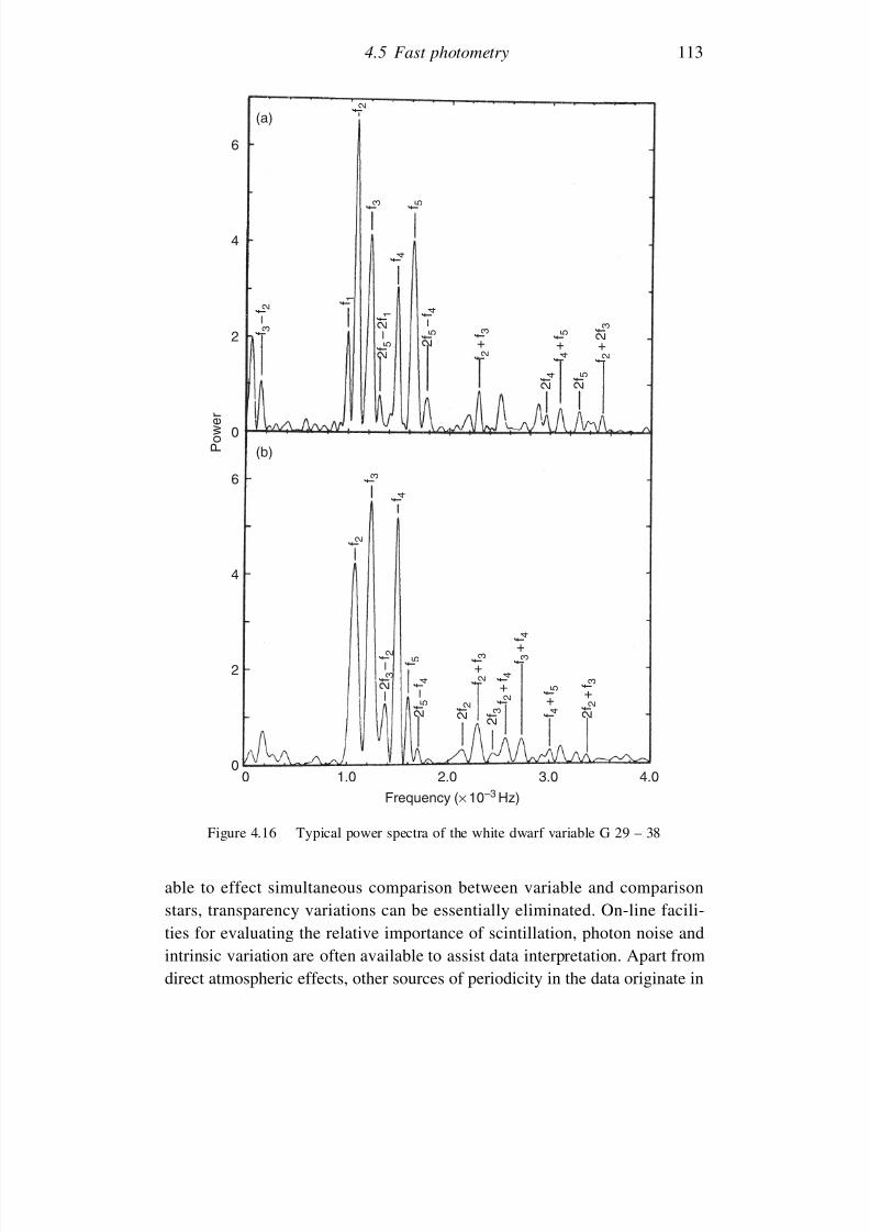
7/21/2019 Introduction to Astronomical Photometry
http://slidepdf.com/reader/full/introduction-to-astronomical-photometry 131/451
4.5 Fast photometry 113
(a)
(b)
6
4
2 f 3 – f 2
2 f 5 –
2 f 1
2 f 3 – f 2
f 2 +
f 3
f 2 + f 4
f 3 + f 4
f 4 + f 5
2 f 2 + f 3
2 f 5 – f 4
2 f 5 – f 4
f 2 + f 3
f 4 + f 5
f 2 + 2
f 3
2 f 4
2 f 2
2 f 3
2 f 5
f 2
f 3 f 5
f 4
f 1
f 2
f 3
f 4
f 5
0 P o w e r
6
4
2
00 1.0 2.0
Frequency (× 10–3 Hz)
3.0 4.0
Figure 4.16 Typical power spectra of the white dwarf variable G 29 – 38
able to effect simultaneous comparison between variable and comparisonstars, transparency variations can be essentially eliminated. On-line facili-ties for evaluating the relative importance of scintillation, photon noise andintrinsic variation are often available to assist data interpretation. Apart fromdirect atmospheric effects, other sources of periodicity in the data originate in
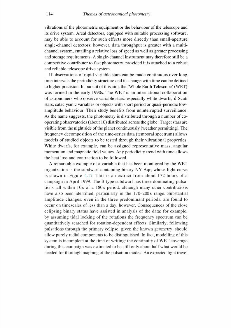
7/21/2019 Introduction to Astronomical Photometry
http://slidepdf.com/reader/full/introduction-to-astronomical-photometry 132/451
114 Themes of astronomical photometry
vibrations of the photometric equipment or the behaviour of the telescope andits drive system. Areal detectors, equipped with suitable processing software,may be able to account for such effects more directly than small-aperture
single-channel detectors; however, data throughput is greater with a multi-channel system, entailing a relative loss of speed as well as greater processingand storage requirements. A single-channel instrument may therefore still be acompetitive contributor to fast photometry, provided it is attached to a robustand reliable telescope drive system.
If observations of rapid variable stars can be made continuous over longtime intervals the periodicity structure and its change with time can be definedto higher precision. In pursuit of this aim, the ‘Whole Earth Telescope’ (WET)was formed in the early 1990s. The WET is an international collaborationof astronomers who observe variable stars: especially white dwarfs, Scutistars, cataclysmic variables or objects with short period or quasi-periodic low-amplitude behaviour. Their study benefits from uninterrupted surveillance.As the name suggests, the photometry is distributed through a number of co-operating observatories (about 10) distributed across the globe. Target stars arevisible from the night side of the planet continuously (weather permitting). The
frequency decomposition of the time-series data (temporal spectrum) allowsmodels of studied objects to be tested through their vibrational properties.White dwarfs, for example, can be assigned representative mass, angularmomentum and magnetic field values. Any periodicity trend with time allowsthe heat loss and contraction to be followed.
A remarkable example of a variable that has been monitored by the WETorganization is the subdwarf-containing binary NY Aqr, whose light curveis shown in Figure 4.17. This is an extract from about 172 hours of acampaign in April 1999. The B type subdwarf has three dominating pulsa-tions, all within 10 s of a 180 s period, although many other contributionshave also been identified, particularly in the 170–200 s range. Substantialamplitude changes, even in the three predominant periods, are found tooccur on timescales of less than a day, however. Consequences of the closeeclipsing binary status have assisted in analysis of the data: for example,by assuming tidal locking of the rotations the frequency spectrum can be
quantitatively searched for rotation-dependent effects. Similarly, followingpulsations through the primary eclipse, given the known geometry, shouldallow purely radial components to be distinguished. In fact, modelling of thissystem is incomplete at the time of writing: the continuity of WET coverageduring this campaign was estimated to be still only about half what would beneeded for thorough mapping of the pulsation modes. An expected light travel
7/21/2019 Introduction to Astronomical Photometry
http://slidepdf.com/reader/full/introduction-to-astronomical-photometry 133/451
4.5 Fast photometry 115
3
counts (×105)
2
0 4000 8000 seconds
12000 16000 20000 seconds
3
2
Figure 4.17 A light curve (after Kilkenny et al., 2003) resulting from a WETcampaign on the eclipsing binary system NY Aqr (PG 1336-018), whose primaryis a hot pulsating subdwarf that is accompanied by a cool Main Sequence star.
Both stars have radii of only about 1/6 R, and the orbital sequence is completedin around 2.424 hours. The data shown are most of a single run from one of the WET sites, using a 5 s integration time. The pulsation amplitude (maximum∼3% of the total flux) can be seen to vary in this data sample. This is interpretedas the beating of components of different frequency
time effect in the oscillation phases was also shown to be consistent with thedata, although an independent firm determination of the orbital size was not
possible with the given coverage. Nevertheless, the undoubted improvementin knowledge of the system’s frequency structure should stimulate furtherdetailed efforts in the future.
Fast photometry has developed as a more specialist branch of astronom-ical photometry, but its target objects are drawn from across more or lessthe same wide range of objects. Apart from stellar objects like those alreadymentioned, there are interesting applications in solar system contexts, particu-
larly lunar and planetary occultations. On the other hand, high time resolutiondata are relevant to the energetics of active galaxy nuclei, quasars, blazars andcomparable objects containing massive collapsed cores. Given the continueddevelopment of high speed data-handling electronics and the relatively inex-pensive supply of bulk storage, fast photometry seems likely to increase itsrole as a productive field of astronomical research.
7/21/2019 Introduction to Astronomical Photometry
http://slidepdf.com/reader/full/introduction-to-astronomical-photometry 134/451
116 Themes of astronomical photometry
4.6 Photometry of extended objects
It was mentioned that astronomical photometry often deals with the luminous
flux from a celestial source overall, i.e. a certain magnitude is relatedto a certain luminosity (see Section (3.6)). Certainly for general stellarphotometry, we are not usually concerned with the local surface brightnessvariation, or illumination geometry, though information on these may comefrom specific kinds of observation of variable stars. Stellar photometry,notwithstanding its historic role in the development of the subject, thusprovides a special subset of conditions for analysis. The flux emanating fromthe point-like source is essentially independent of the photometer’s aperture,
the main purpose of which is then to cut out extraneous input to the systemfrom a background of no direct interest.
In the case of an extended object, though, such matters characterize thestudy from the outset, thereby introducing extra dimensions of potentialcomplexity. From the observing point of view, greater stringency in instrumentpositioning as well as aperture control are required. We continue our broadreview of underlying themes by considering a few topics within extended
object photometry: at first by some basic visual examples, followed by casesdrawn from Solar System, nebular and galactic contexts.
4.6.1 Visual photometry
A flux of 126×105 lx from the Sun was derived in Section 3.3. Dividing thisby the 68×10−5 sr that the Sun subtends at the Earth, we obtain the intensitywhich, from (3.2), characterizes the radiation field in visual wavelengths,above the Earth’s atmosphere from the Sun’s photosphere (averaged over thevisible hemisphere and assuming the intervening space to be absorption free).The value is 185×109 cd m−2 (or nt, see Section 3.1). On a clear day with theSun at the zenith, the brightness would be reduced, by atmospheric extinction,to about 14×109 cd m−2 as an average over the entire disk, reaching a valueof about 18× 109 cd m−2 at its centre.
A generally comparable brightness would characterize Cen A if the eye
could resolve its disk. When the size of an object sinks below the eye’s diskof resolution, though, the sensation of brightness no longer corresponds tointensity in the sense of (3.2), but rather with the net flux. When more than justone or two ‘pixels’ (picture cells) of the eye’s retina become illuminated, theflux per pixel essentially corresponds to the surface brightness of the precedingparagraph. In this context, we meet Olbers’ famous gedanken experiment,that if, in any direction, the line of sight sooner or later were to encountera Sun-like star, then the entire sky should become of comparable brightness
7/21/2019 Introduction to Astronomical Photometry
http://slidepdf.com/reader/full/introduction-to-astronomical-photometry 135/451
4.6 Photometry of extended objects 117
to the surface of the Sun! Solutions offered for this ‘paradox’ usually involvefiniteness and expansion of the Universe, taking into account the total starnumbers that the premise requires. Full consideration of the details would
take us beyond our present course, but the photometric premises on which itis based are straightforward enough.
With Rougier’s value for the difference (14.29) in the magnitude of Sunand full Moon we derive the full Moon magnitude −1246, which correspondsto 0.24 lx on the scale just cited. The Moon’s apparent semi-diameter varies,depending on its orbital position and where the terrestrial observer is located,but on average it is slightly less than that of the Sun at ∼ 940, or 659 ×
10−5
sr. This implies a mean surface brightness of about 2500nt for theterrestrial observer of the full, high altitude Moon on a clear night. This isof comparable brightness to the mean daytime sky, which subtends a solidangle almost 105 bigger than the solar disk itself. With some inferences aboutthe fractions of sunlight scattered by the Moon’s surface and atmosphericmolecules at given incidence angles and in particular directions of viewing,this comparability of brightness can be understood in a general way, but amore detailed exposition would be required to show why it is that the Mooncan sometimes be bright enough to stand out against the daytime sky, andat other times not. The problem of first visibility of the lunar crescent, forinstance, of ceremonial significance to Muslims, is potentially one of greatcomplexity to treat in full detail. Approximate formulae are usually referredto for practical convenience.
The light from a mV = 0 star spread over a patch of sky of size, say, 1‘square degree’
=304617
· · ·×10−4 sr, represents a number (823
×10−2)
of lux per steradian, and is thus a unit of brightness. This unit is relevantfor an object like the Milky Way, whose apparent brightness derives fromthe net effect of a large number of unresolved faint stars. A more generallyapplicable unit for faint sources, however, could be twentieth magnitude starsper square arcminute (mag 20 stars arcmin−2 = 296× 10−7 cd m−2).
The brightness of the daytime sky falls, on a clear moonless night in anisolated area, by a factor of several millions to, typically, ∼ 3×10⁻⁴ cd m−2,
the residual light being due to the net effect of airglow, zodiacal light, auroraland faint unresolved, or scattered, starlight contributions. Light ‘pollution’ intowns can enhance this by at least an order of magnitude, depending on thearrangement of local lighting.6 The faint light of the Milky Way has to be at
6 According to information from the International Dark-sky Association, city-environment nightsky brightness is typically 10 000 times greater than this value and has generally shown asteady increase with time. It would be difficult for the average unaided eye to make outanything fainter than a third magnitude star in such a sky.
7/21/2019 Introduction to Astronomical Photometry
http://slidepdf.com/reader/full/introduction-to-astronomical-photometry 136/451
118 Themes of astronomical photometry
least comparable to 10−4 cd m−2 in order to be distinguished,7 and typicallyturns out to be ∼750 mag 20 stars arcmin−2 (∼2×10⁻⁴ cd m−2). If the MilkyWay covers around
∼107 arcmin2 of sky, we quickly form some feeling for
what numbers of Sun-like stars are required to account for its light in thissimplistic way, keeping in mind that mV = 20 compares with what the Sunwould be at the distance of the centre of the Galaxy, and neglecting the effectsof interstellar extinction.
Standing out against the background of the Milky Way are a few clusters,for example h and Persei, both of area around 100 arcmin2. Their total illu-minances are comparable to that from a fourth magnitude star, which implies a
brightness of about 1 mag 10 star arcmin−2
. The clusters are known to containa few hundred bright stars, but they are located at distances of somewhat over2000 pc. We deduce directly, therefore, that these stars must be of essentiallygreater visual luminosity than the Sun, by around 6 mag, on average.
An alternative to the number of stars of given magnitude per square angularunit is to put one star of equivalent light output. Thus 750mag 20 starsarcmin−2 = 1281mag arcmin−2, or 21.70 mag arcsec−2. This latter represen-tation is frequently used to mark contour levels in mapping the surface bright-
ness distribution of galaxies, i.e. a given locus corresponds to mag arcsec−2.Galaxies external to the Milky Way, like the Magellanic Clouds, or the
Andromeda Galaxy, which are visible as extended objects, still appear tohave a comparable local brightness to the Milky Way, despite their muchgreater distances. This can be understood if the galaxies are composed of comparable column densities of stars in a similar inherent luminosity distri-bution. The decline in received flux from each individual star type with
increasing distance squared is then counterbalanced by a proportional increasein numbers per unit area of sky. Regions of relatively greater stellar (column)density, like the bar region of the Large Magellanic Cloud, appear corre-spondingly brighter.
4.6.2 Solar System photometry
The Solar System presents a particular subset of conditions for photometry.
Thus, there is only one predominating source of illumination, i.e. the Sun, anddistances and angles involved in the configuration can be determined withprecision. The illuminating pencil may be regarded, with sufficient accuracy,as a parallel beam. Attention is then directed to the nature of the reflecting
7 Note also the ‘nanolambert’ (nL) = 3183 × 10−6 cd m−2, sometimes used for visually faintbrightness levels.
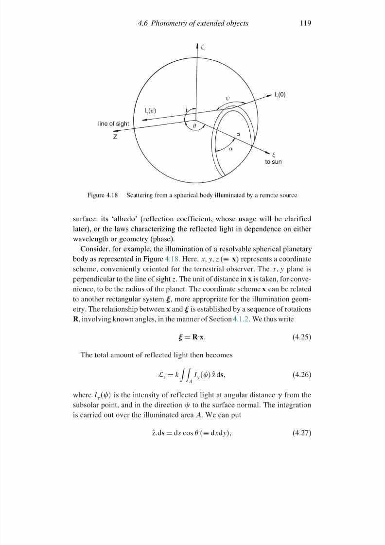
7/21/2019 Introduction to Astronomical Photometry
http://slidepdf.com/reader/full/introduction-to-astronomical-photometry 137/451
4.6 Photometry of extended objects 119
ζ
line of sight
Z
Iγ (ψ )
Iγ (0)
P
i
ψ
θ
α ξ
to sun
Figure 4.18 Scattering from a spherical body illuminated by a remote source
surface: its ‘albedo’ (reflection coefficient, whose usage will be clarifiedlater), or the laws characterizing the reflected light in dependence on eitherwavelength or geometry (phase).
Consider, for example, the illumination of a resolvable spherical planetarybody as represented in Figure 4.18. Here, x y z ≡ x represents a coordinatescheme, conveniently oriented for the terrestrial observer. The x y plane isperpendicular to the line of sight z. The unit of distance in x is taken, for conve-nience, to be the radius of the planet. The coordinate scheme x can be related
to another rectangular system , more appropriate for the illumination geom-etry. The relationship between x and is established by a sequence of rotationsR, involving known angles, in the manner of Section 4.1.2. We thus write
= R.x (4.25)
The total amount of reflected light then becomes
r = k
AI z ds (4.26)
where I is the intensity of reflected light at angular distance from thesubsolar point, and in the direction to the surface normal. The integrationis carried out over the illuminated area A. We can put
zds = ds cos ≡ dxdy (4.27)
7/21/2019 Introduction to Astronomical Photometry
http://slidepdf.com/reader/full/introduction-to-astronomical-photometry 138/451
120 Themes of astronomical photometry
where z is the unit vector in the direction parallel to the line of sight, and d s
is an increment of area on the surface of the planet. The constant k allows theunits of r to be appropriately expressed in (4.26). The simplest reradiation
formula is that of completely uniform diffusion of the reradiated (scattered)flux (‘Lambert’s law’). In this case I = I = const.
More generally we can use a limb-darkened (cosine law) form, i.e.
I = I 01− u + u cos (4.28)
where u is the limb-darkening coefficient. I 0 can be written in the form
I 0
=I 0f (4.29)
Spelling out the first row of the direction cosine matrix R, we have
l1x + l2y + l3z = (4.30)
where we set to lie in the direction of the centre of the Sun. We choosethe x y orientation such that l2 = 0, and then l1 and l3 are sin and cos ,respectively, where is the angle indicated in Figure 4.18. Alternatively, wecould write l
3 =cos sin i, where measures the angle between Earth and
Sun in the plane perpendicular to the axis (phase), which is inclined atangle i to the line of sight.
We then combine (4.30) and (4.29), insert into (4.26), using also (4.27)and (4.28), and we find,
r = kI 0
A
C 1fl1x + l3z + C 2fl1xz + l3z2 dx dy (4.31)
where C 1 and C 2 are constants, dependent on u, that normalize the integration,so that the net returned light remains constant with different assigned valuesof u. The suffix A denotes the projection of the illuminated area in the lineof sight.
Writing I 0 = L/ for the intensity of the illuminating beam, the appro-priate value for k becomes r 2p R2
se/R2spR2
ep, where r p is the planetary body’sradius, Rse the distance between Sun and Earth, Rsp the solar–planet distance,and Rep that between the planet and the Earth. For convenience, we make the
Sun–Earth separation to be the unit of distance (i.e. 1 a.u.), so that Rse dropsout of the formula for k.
At least for a conservative bolometric radiation field, we now have suitablyarranged formulae to scale the brightness seen by an observer at the Earth tothe solar luminosity. For, if there is no build up or loss of radiative energyin the considered process, all incoming radiation will be reradiated by theilluminated surface (though usually with some redistribution in wavelength)
7/21/2019 Introduction to Astronomical Photometry
http://slidepdf.com/reader/full/introduction-to-astronomical-photometry 139/451
4.6 Photometry of extended objects 121
and the bolometric albedo abol is unity. Over some particular wavelengthrange, however, this does not normally hold, and k should include a non-unityalbedo a. This can be regarded as an empirical scaling factor multiplying the
returned sunlight, in the given wavelength range, that makes the calculatedreflected light agree with the observed level, after appropriate allowance fordirectional effects in the scattering.
This observed level is studied in its dependence on the orbital angularargument – the ‘phase law’. Since the integral in (4.31) takes different valuesat a given phase in dependence on the form of f, however, the formof the phase law will be similarly dependent. Hence, we must perform the
integration (4.31) in order to study such phase laws for different f. Thisintegration introduces a class of integral of the following type:
mn =
Ac
xmzn dxdy (4.32)
where Ac represents the area A enclosed by some perimeter c on a sphere.The integrals fall into three classes, depending on whether the perimeter curvelies entirely within the circular boundary of the sphere (‘annular’), as seen
from a great distance along the z-axis; whether it intersects with this outercircular boundary (‘partial’); or whether this outer boundary itself delimitsthe area over which the double integration is carried out (‘total’).
In this book we meet two types of integral of this kind, whose differencelies in the different perimeter curves c. The presently arising kind we identifyas mn . In this case, the curve c is a circle formed by the intersection of a plane, at an arbitrary orientation, with the sphere. Seen from a distancealong the z-axis this circle appears as an elliptical curve, unless it crossesover the outer boundary (partial case). The other kind of integral we denotem
n . In that case, the perimeter is formed by the sphere’s intersection with acylinder whose axis is parallel to the z-axis. Its outline, in the line of sight,then appears circular.
In the case of a near parallel illuminating beam, an appropriate form forf is f = ≥ 0, and f = 0 < 0. We can then find C 1 =31 − u/3 − u and C 2 = 3u/3 − u. Using the -integral notation, we
rewrite (4.31) as
r = ar 2p
R2spR2
epLC 1l1 10 + l3 01 + C 2l1 11 + l3 02 (4.33)
The -integrals in this expression will be defined in terms of two parameters:the angular extent m of the illuminated region, and the distance z0 of thesubsolar point above the plane z = 0. In the geometrical arrangement under
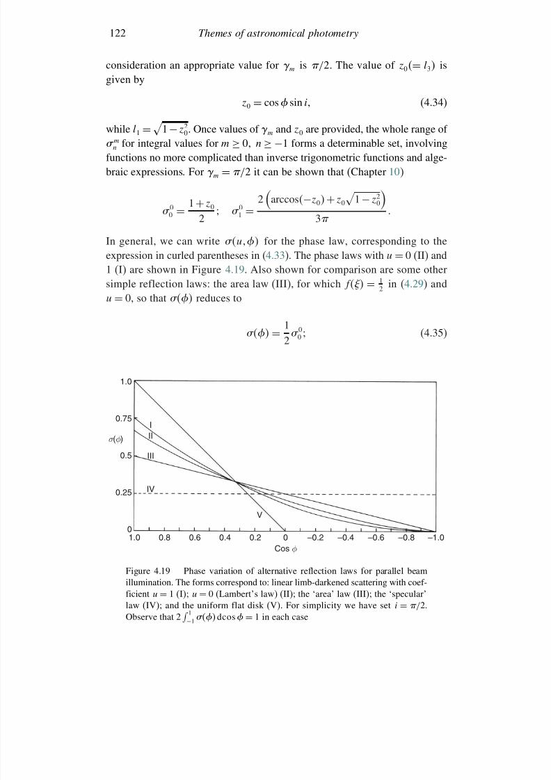
7/21/2019 Introduction to Astronomical Photometry
http://slidepdf.com/reader/full/introduction-to-astronomical-photometry 140/451
122 Themes of astronomical photometry
consideration an appropriate value for m is /2. The value of z0= l3 isgiven by
z0 = cos sin i (4.34)
while l1 =
1− z20. Once values of m and z0 are provided, the whole range of
mn for integral values for m ≥ 0 n ≥ −1 forms a determinable set, involvingfunctions no more complicated than inverse trigonometric functions and alge-braic expressions. For m = /2 it can be shown that (Chapter 10)
00 =
1+
z0
2 01 =
2arccos
−z0
+z0 1−
z20
3
In general, we can write u for the phase law, corresponding to theexpression in curled parentheses in (4.33). The phase laws with u = 0 (II) and1 (I) are shown in Figure 4.19. Also shown for comparison are some othersimple reflection laws: the area law (III), for which f = 1
2 in (4.29) andu = 0, so that reduces to
= 12
00 (4.35)
1.0
0.75
III
III
IV
V
0.5
σ (φ )
0.25
01.0 0.8 0.6 0.4 0.2 0Cos φ
–0.2 –0.4 –0.6 –0.8 –1.0
Figure 4.19 Phase variation of alternative reflection laws for parallel beamillumination. The forms correspond to: linear limb-darkened scattering with coef-ficient u = 1 (I); u = 0 (Lambert’s law) (II); the ‘area’ law (III); the ‘specular’law (IV); and the uniform flat disk (V). For simplicity we have set i = /2.Observe that 2
1−1 dcos = 1 in each case
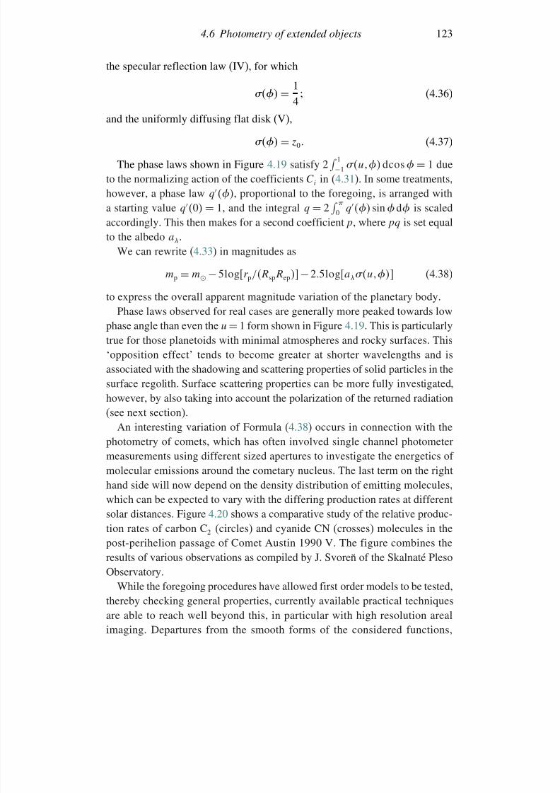
7/21/2019 Introduction to Astronomical Photometry
http://slidepdf.com/reader/full/introduction-to-astronomical-photometry 141/451
4.6 Photometry of extended objects 123
the specular reflection law (IV), for which
= 14
(4.36)
and the uniformly diffusing flat disk (V),
= z0 (4.37)
The phase laws shown in Figure 4.19 satisfy 2 1
−1 u dcos = 1 dueto the normalizing action of the coefficients C i in (4.31). In some treatments,however, a phase law q , proportional to the foregoing, is arranged witha starting value q 0
=1, and the integral q
=2
0
q sin d is scaledaccordingly. This then makes for a second coefficient p, where pq is set equalto the albedo a.
We can rewrite (4.33) in magnitudes as
mp = m − 5logr p/RspRep −25logau (4.38)
to express the overall apparent magnitude variation of the planetary body.Phase laws observed for real cases are generally more peaked towards low
phase angle than even the u = 1 form shown in Figure 4.19. This is particularlytrue for those planetoids with minimal atmospheres and rocky surfaces. This‘opposition effect’ tends to become greater at shorter wavelengths and isassociated with the shadowing and scattering properties of solid particles in thesurface regolith. Surface scattering properties can be more fully investigated,however, by also taking into account the polarization of the returned radiation(see next section).
An interesting variation of Formula (4.38) occurs in connection with thephotometry of comets, which has often involved single channel photometermeasurements using different sized apertures to investigate the energetics of molecular emissions around the cometary nucleus. The last term on the righthand side will now depend on the density distribution of emitting molecules,which can be expected to vary with the differing production rates at differentsolar distances. Figure 4.20 shows a comparative study of the relative produc-tion rates of carbon C2 (circles) and cyanide CN (crosses) molecules in the
post-perihelion passage of Comet Austin 1990 V. The figure combines theresults of various observations as compiled by J. Svoren of the Skalnaté PlesoObservatory.
While the foregoing procedures have allowed first order models to be tested,thereby checking general properties, currently available practical techniquesare able to reach well beyond this, in particular with high resolution arealimaging. Departures from the smooth forms of the considered functions,
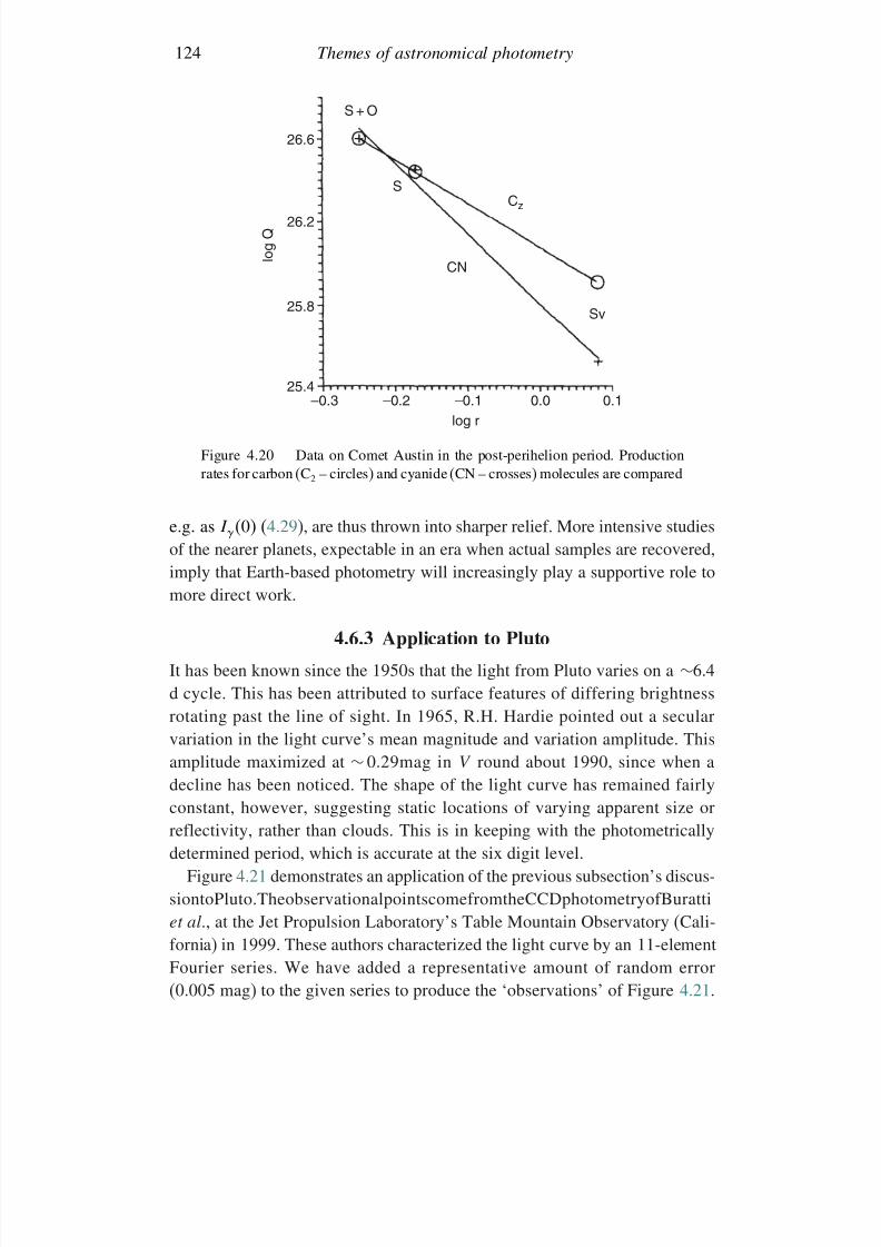
7/21/2019 Introduction to Astronomical Photometry
http://slidepdf.com/reader/full/introduction-to-astronomical-photometry 142/451
124 Themes of astronomical photometry
–0.3 –0.2 –0.1 0.0 0.1
l o g Q
log r
26.6
26.2
25.8
25.4
S + O
SCz
CN
Sv
Figure 4.20 Data on Comet Austin in the post-perihelion period. Productionrates for carbon (C2 – circles) and cyanide (CN – crosses) molecules are compared
e.g. as I 0 (4.29), are thus thrown into sharper relief. More intensive studiesof the nearer planets, expectable in an era when actual samples are recovered,imply that Earth-based photometry will increasingly play a supportive role tomore direct work.
4.6.3 Application to Pluto
It has been known since the 1950s that the light from Pluto varies on a ∼
6.4d cycle. This has been attributed to surface features of differing brightnessrotating past the line of sight. In 1965, R.H. Hardie pointed out a secularvariation in the light curve’s mean magnitude and variation amplitude. Thisamplitude maximized at ∼ 029mag in V round about 1990, since when adecline has been noticed. The shape of the light curve has remained fairlyconstant, however, suggesting static locations of varying apparent size orreflectivity, rather than clouds. This is in keeping with the photometrically
determined period, which is accurate at the six digit level.Figure 4.21 demonstrates an application of the previous subsection’s discus-
siontoPluto.TheobservationalpointscomefromtheCCDphotometryofBurattiet al., at the Jet Propulsion Laboratory’s Table Mountain Observatory (Cali-fornia) in 1999. These authors characterized the light curve by an 11-elementFourier series. We have added a representative amount of random error(0.005 mag) to the given series to produce the ‘observations’ of Figure 4.21.
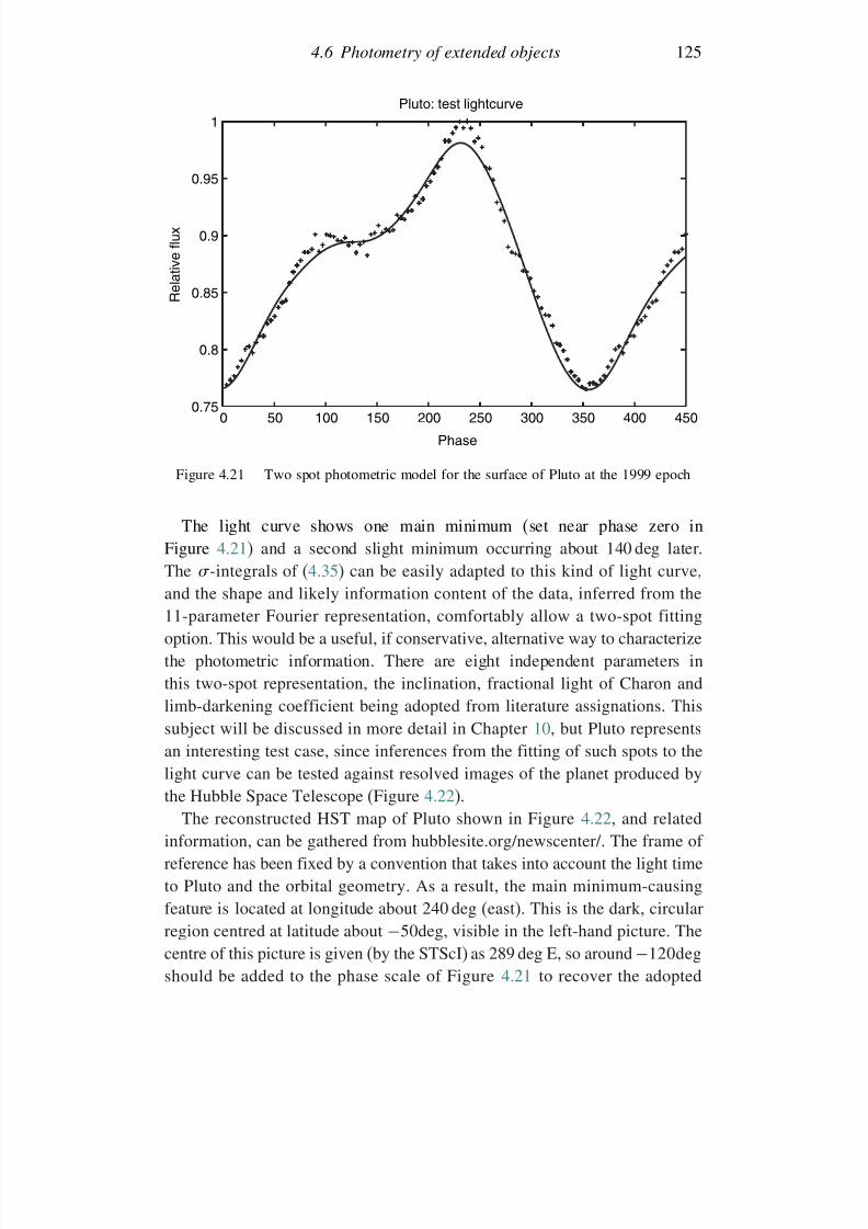
7/21/2019 Introduction to Astronomical Photometry
http://slidepdf.com/reader/full/introduction-to-astronomical-photometry 143/451
4.6 Photometry of extended objects 125
1
0.95
0.9
0.85
0.8
0.750 50 100 150 200 250 300 350 400 450
R e l a t i v e f l u x
Phase
Pluto: test lightcurve
Figure 4.21 Two spot photometric model for the surface of Pluto at the 1999 epoch
The light curve shows one main minimum (set near phase zero inFigure 4.21) and a second slight minimum occurring about 140 deg later.The -integrals of (4.35) can be easily adapted to this kind of light curve,and the shape and likely information content of the data, inferred from the11-parameter Fourier representation, comfortably allow a two-spot fittingoption. This would be a useful, if conservative, alternative way to characterizethe photometric information. There are eight independent parameters inthis two-spot representation, the inclination, fractional light of Charon andlimb-darkening coefficient being adopted from literature assignations. Thissubject will be discussed in more detail in Chapter 10, but Pluto representsan interesting test case, since inferences from the fitting of such spots to thelight curve can be tested against resolved images of the planet produced bythe Hubble Space Telescope (Figure 4.22).
The reconstructed HST map of Pluto shown in Figure 4.22, and related
information, can be gathered from hubblesite.org/newscenter/. The frame of reference has been fixed by a convention that takes into account the light timeto Pluto and the orbital geometry. As a result, the main minimum-causingfeature is located at longitude about 240 deg (east). This is the dark, circularregion centred at latitude about −50deg, visible in the left-hand picture. Thecentre of this picture is given (by the STScI) as 289 deg E, so around −120degshould be added to the phase scale of Figure 4.21 to recover the adopted
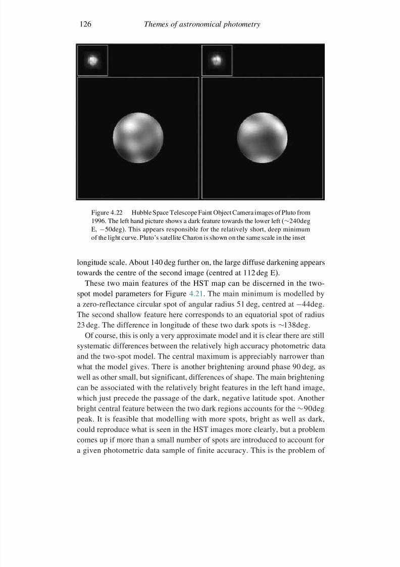
7/21/2019 Introduction to Astronomical Photometry
http://slidepdf.com/reader/full/introduction-to-astronomical-photometry 144/451
126 Themes of astronomical photometry
Figure 4.22 Hubble Space Telescope Faint Object Camera images of Pluto from1996. The left hand picture shows a dark feature towards the lower left (∼240deg
E, −50deg). This appears responsible for the relatively short, deep minimumof the light curve. Pluto’s satellite Charon is shown on the same scale in the inset
longitude scale. About 140 deg further on, the large diffuse darkening appearstowards the centre of the second image (centred at 112 deg E).
These two main features of the HST map can be discerned in the two-spot model parameters for Figure 4.21. The main minimum is modelled bya zero-reflectance circular spot of angular radius 51 deg, centred at
−44deg.
The second shallow feature here corresponds to an equatorial spot of radius23 deg. The difference in longitude of these two dark spots is ∼138deg.
Of course, this is only a very approximate model and it is clear there are stillsystematic differences between the relatively high accuracy photometric dataand the two-spot model. The central maximum is appreciably narrower thanwhat the model gives. There is another brightening around phase 90 deg, aswell as other small, but significant, differences of shape. The main brightening
can be associated with the relatively bright features in the left hand image,which just precede the passage of the dark, negative latitude spot. Anotherbright central feature between the two dark regions accounts for the ∼90degpeak. It is feasible that modelling with more spots, bright as well as dark,could reproduce what is seen in the HST images more clearly, but a problemcomes up if more than a small number of spots are introduced to account fora given photometric data sample of finite accuracy. This is the problem of
7/21/2019 Introduction to Astronomical Photometry
http://slidepdf.com/reader/full/introduction-to-astronomical-photometry 145/451
4.6 Photometry of extended objects 127
over-specification: i.e. trying to specify more photometric information fromthe data than they actually contain. In this situation, alternative combinationsof parameters can produce essentially similar shapes of light curve. On the
positive side, this same two-spot model has been used to represent, in a moreor less similar way, various light curves of Pluto, coming from differentepochs. Even if the accuracy for detailed representation is low, the similarityof parameter values for the main features at different epochs is an indicationof the relative stability of at least some real surface features of Pluto.
Small differences in the light curve shape of Pluto have been seen fromone epoch to another, however, and this has been discussed in terms of
different levels of atmospheric and solid-state methane, in response to thehighly varying degrees of insolation. In this respect, Pluto’s orbital geometry,particularly its high eccentricity and the 122 deg obliquity of its rotation, arenoteworthy. Buratti et al., who produced the broadband data discussed above,also observed the planet in the region of the methane band at 8900Å with a50Å narrowband filter. They noted a significant inverse correlation betweenmethane band strength (i.e. light absorption from the gaseous phase) and thedarkening, suggesting that the light regions contain more methane ice. In
that connection, then, the difference between the light curves of Tholen andTedesco for the 1980–83 period and those of Buratti et al. are interesting,since the diffuse equatorial region is brighter at the earlier (pre-equinox)epoch. Although Buratti et al. showed that most of the light curve’s majorcharacteristics can be explained by the varying aspect of some relatively fixedregions of different intrinsic brightness, certain features may be related tothe changing state (solid or gaseous) of methane: ‘volatile transport’ as it
is usually termed. The study of Pluto thus demonstrates the interesting andpenetrative applicability of combining broad and narrowband photometry.
4.6.4 Photometry of galactic nebulae
The word nebula (Latin for mist) is used to represent a wide range of extendedcelestial sources, involving a variety of different physical situations. Thebright, glowing nebulae range from quite symmetrical, quasi-spherical ‘plan-
etary’ sources, to irregular, clumpy or fragmented clouds which may spread,in extreme cases, to over a hundred parsecs or more in linear extent. Thereare also dark nebulae, conspicuous by the special extinction they producein the light from stars behind them. The topic is thus big and multi-faceted,and data often lack a fully comprehensive quality of necessity. Nevertheless,the astrophysical problems posed by these objects are deep and exciting, andcontinue to raise new challenges.
7/21/2019 Introduction to Astronomical Photometry
http://slidepdf.com/reader/full/introduction-to-astronomical-photometry 146/451
128 Themes of astronomical photometry
Within the present broad review we will raise some of the more obviousquestions, such as where does the light come from – or how is a brightnebula’s energy budget balanced, to put it in a more structured way. Among
the primary photometric tasks is then to determine the net radiative energylosses. The well-known Crab Nebula (Messier 1), in the constellation of Taurus, provides an instructive general example.
The integrated magnitude of the ∼5 arcmin diameter (continuum) source isabout mV = 86. The distance of the source has been determined to be about2200 pc, implying a linear size of ∼3pc. The large distance also results in asignificant interstellar extinction (Section 4.1.3), so that the intrinsic apparent
magnitude of the source would be around mV = 71. Using the calibrationof Section 3.6, this yields some 24 × 10−6 W m−2 at the source, with theforegoing size and distance, or ∼7× 1028 W altogether in the visual region.This is already more than 100 times greater than the Sun’s bolometric output,but it is not all. The non-thermal continuum power of the nebula declineswith a low negative power of the frequency, extending from the radio up tothe X-ray region, where individual photon energies are two (or more) ordersof magnitude greater than in the optical. An appropriate integration will show
∼1031 W to be a fair estimate for the entire rate of radiation loss of the Crabin its predominating synchrotron continuum emission.
The rotational energy of the nebula’s central pulsar can be estimated tobe on the order of 1043 J, so if we suppose that the magnetic fields involvedin the synchrotron emission derive from this energy reserve, we can quicklyestimate an e-folding time for the energy loss on the order of tens of thousandsof years. This would imply a measurable slow-down trend in the pulsar’s
rotation rate over a few years of observation and this, in fact, has beenobserved to be of the corresponding order of magnitude (10−23 s per second).Many bright nebulae shine mainly in discrete emission lines rather than
a continuum. Two-dimensional photometry, particularly with high resolutionscanners or array type detectors, are increasingly revealing more complexityof structural detail in such sources, requiring more fine tuning of the many-parameter models that address themselves to the data. As an illustration of howphotometry can approach this process, we consider a procedure for evaluation
of the effective temperature of the central star of a planetary nebula, alongthe lines proposed originally by H. Zanstra in the 1920s.
We suppose that the radiative emission from the hydrogen atoms, of whichthe nebula is largely composed, arises from a cascade recombination process,giving rise, in the emergent radiation field, to the Balmer lines, together withLyman – the first level to ground transition of atomic hydrogen associ-ated with photons of wavelength 1215 Å. The Ly transition’s upper state is
7/21/2019 Introduction to Astronomical Photometry
http://slidepdf.com/reader/full/introduction-to-astronomical-photometry 147/451
4.6 Photometry of extended objects 129
supplied from Balmer line recombinations through the nebula. Attention thenfixes on these Balmer lines, which derive, in this picture, from an input photonstream coming originally from beyond the Lyman limit of the central star’s
radiation field.A quantity that can be observationally determined is the ratio of the net
illuminance from the nebula LB integrated over a Balmer line, to the irradi-
ance per unit frequency from the central star H s, at frequency 1, say, in agiven line-free region of its optical spectrum. We shall express this ratio asBAB
. Now, H s can be written as a fraction of the entire illuminance beyondthe Lyman limit (912Å), to an extent which depends on the temperature
of the photosphere – a simple Planckian form was assumed in the originalpresentations. It is more relevant, however, to relate H s to the integral of the distribution of numbers of photons per second with wavelengths shorterthan 912 Å, using E = h (Chapter 2). This is because the main underlyingpremise is that the total rate of photon production in all the Balmer recombi-nation lines of the nebula can be set equal to this integral. The sum S A of thevalues of AB
for all the Balmer line images of the nebula then results in animplicit equation for the temperature. This is of the form
S A =
x0
x2 dx
ex − 1/
x31
ex1 −1
where x = h/kT x0 corresponds to the Lyman limit and x1 to 1.The AB
values are probably best determined using high-dispersion spec-trophotometric techniques and areal detectors. Single-beam photometry couldbe considered, however, by means of a photometer equipped with a controllable
‘iris’typeentranceaperture.Thestellarcontinuumfluxismeasuredwiththeirisstopped right down around the central star, using a filter which avoids nebularlines as much as possible, but is of sufficient width to allow a good continuumsignal. The total light from the nebula through each of a set of narrowbandfilters centred on the principal Balmer lines is then measured. The initially smallaperture is progressively widened until the recorded level reaches a constantlimit taken to be that of the nebula as a whole. The observed photon incidencerates in the various lines are converted into above-the-atmosphere values, by
taking account of the net transmission and detector response functions, i.e. therelevant and k-loss terms referred to in Section 3.6. A similar procedureapplies also to the continuum measurement, though this has to be divided bythe frequency bandwidth of the used filter to obtain the spectral irradiance at 1.
It seems likely that only a few Balmer line narrowband filters would beavailable for a convenient and practical arrangement – and, fortunately, thisusually suffices, since the relatively rapid decline of intensity of the Balmer
lines with n for many planetary nebulae permits an acceptable extrapolation
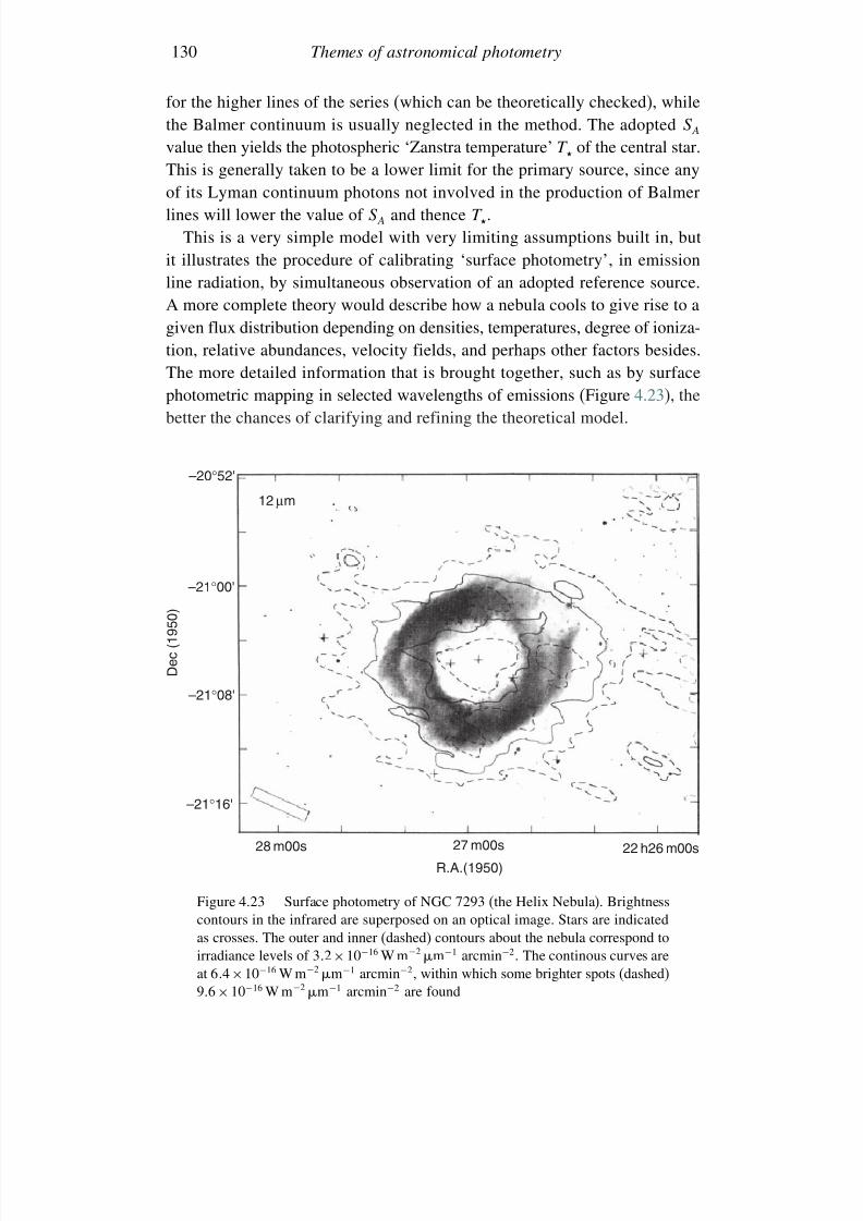
7/21/2019 Introduction to Astronomical Photometry
http://slidepdf.com/reader/full/introduction-to-astronomical-photometry 148/451
130 Themes of astronomical photometry
for the higher lines of the series (which can be theoretically checked), whilethe Balmer continuum is usually neglected in the method. The adopted S Avalue then yields the photospheric ‘Zanstra temperature’ T of the central star.
This is generally taken to be a lower limit for the primary source, since anyof its Lyman continuum photons not involved in the production of Balmerlines will lower the value of S A and thence T .
This is a very simple model with very limiting assumptions built in, butit illustrates the procedure of calibrating ‘surface photometry’, in emissionline radiation, by simultaneous observation of an adopted reference source.A more complete theory would describe how a nebula cools to give rise to a
given flux distribution depending on densities, temperatures, degree of ioniza-tion, relative abundances, velocity fields, and perhaps other factors besides.The more detailed information that is brought together, such as by surfacephotometric mapping in selected wavelengths of emissions (Figure 4.23), thebetter the chances of clarifying and refining the theoretical model.
28 m00s 27 m00s 22 h26 m00sR.A.(1950)
12 µm
–21°00'
–20°52'
–21°08'
–21°16'
D e c ( 1 9 5 0 )
Figure 4.23 Surface photometry of NGC 7293 (the Helix Nebula). Brightnesscontours in the infrared are superposed on an optical image. Stars are indicatedas crosses. The outer and inner (dashed) contours about the nebula correspond toirradiance levels of 32×10−16 W m−2 m−1 arcmin−2. The continous curves areat 64×10−16 W m−2 m−1 arcmin−2, within which some brighter spots (dashed)96
×10
−16 W m−2 m
−1 arcmin
−2 are found
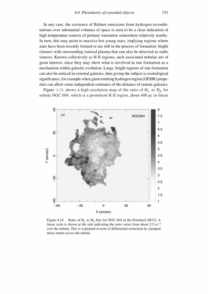
7/21/2019 Introduction to Astronomical Photometry
http://slidepdf.com/reader/full/introduction-to-astronomical-photometry 149/451
4.6 Photometry of extended objects 131
In any case, the existence of Balmer emissions from hydrogen recombi-nations over substantial volumes of space is seen to be a clear indication of high temperature sources of primary ionization somewhere relatively nearby.
In turn, this may point to massive hot young stars, implying regions wherestars have been recently formed or are still in the process of formation: brightclusters with surrounding ionized plasma that can also be detected as radiosources. Known collectively as H II regions, such associated nebulae are of great interest, since they may show what is involved in star formation as amechanism within galactic evolution. Large, bright regions of star formationcan also be noticed in external galaxies, thus giving the subject a cosmological
significance, for example when giant emitting hydrogen region (GEHR) prope-rties can allow some independent estimates of the distance of remote galaxies.Figure 4.24 shows a high resolution map of the ratio of H to H for
nebula NGC 604, which is a prominent H II region, about 400 pc in linear
6 0
3 0
0
– 3 0
– 6 0
–60 –30 0
X (arcsec)
Y ( a r c s e c )
30 60
8
7.5NGC604
6.5
5.5
4.5
3.5
2.5
1.5
1
2
3
4
5
6
7
Figure 4.24 Ratio of H to H flux for NGC 604 in the Pinwheel (M33). Alinear scale is shown at the side indicating the ratio varies from about 2.5 to 7over the nebula. This is explained in term of differential extinction by clumpeddusty matter across the nebula
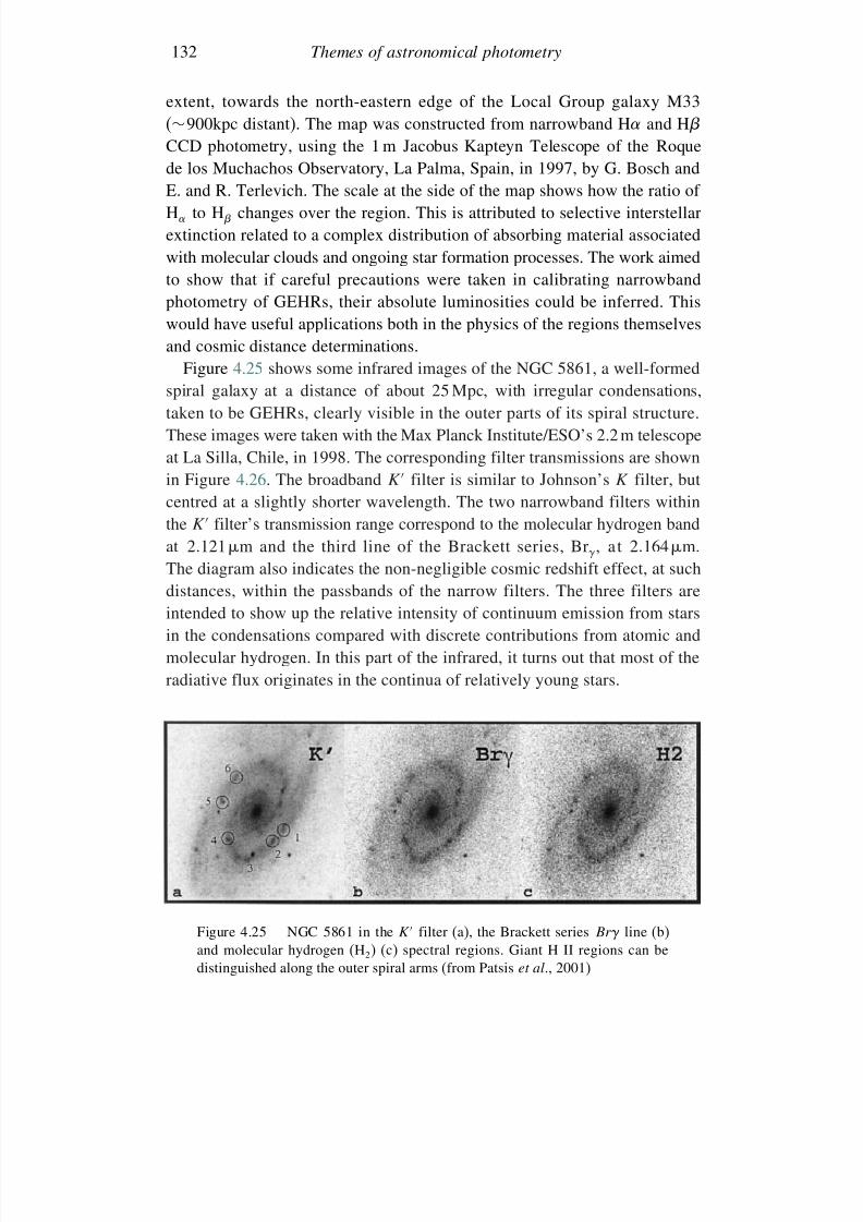
7/21/2019 Introduction to Astronomical Photometry
http://slidepdf.com/reader/full/introduction-to-astronomical-photometry 150/451
132 Themes of astronomical photometry
extent, towards the north-eastern edge of the Local Group galaxy M33(∼900kpc distant). The map was constructed from narrowband H and H
CCD photometry, using the 1 m Jacobus Kapteyn Telescope of the Roque
de los Muchachos Observatory, La Palma, Spain, in 1997, by G. Bosch andE. and R. Terlevich. The scale at the side of the map shows how the ratio of H to H changes over the region. This is attributed to selective interstellarextinction related to a complex distribution of absorbing material associatedwith molecular clouds and ongoing star formation processes. The work aimedto show that if careful precautions were taken in calibrating narrowbandphotometry of GEHRs, their absolute luminosities could be inferred. Thiswould have useful applications both in the physics of the regions themselvesand cosmic distance determinations.
Figure 4.25 shows some infrared images of the NGC 5861, a well-formedspiral galaxy at a distance of about 25 Mpc, with irregular condensations,taken to be GEHRs, clearly visible in the outer parts of its spiral structure.These images were taken with the Max Planck Institute/ESO’s 2.2 m telescopeat La Silla, Chile, in 1998. The corresponding filter transmissions are shownin Figure 4.26. The broadband K filter is similar to Johnson’s K filter, but
centred at a slightly shorter wavelength. The two narrowband filters withinthe K filter’s transmission range correspond to the molecular hydrogen bandat 2121 m and the third line of the Brackett series, Br , at 2164 m.The diagram also indicates the non-negligible cosmic redshift effect, at suchdistances, within the passbands of the narrow filters. The three filters areintended to show up the relative intensity of continuum emission from starsin the condensations compared with discrete contributions from atomic andmolecular hydrogen. In this part of the infrared, it turns out that most of theradiative flux originates in the continua of relatively young stars.
Figure 4.25 NGC 5861 in the K filter (a), the Brackett series Br line (b)and molecular hydrogen (H2) (c) spectral regions. Giant H II regions can bedistinguished along the outer spiral arms (from Patsis et al., 2001)
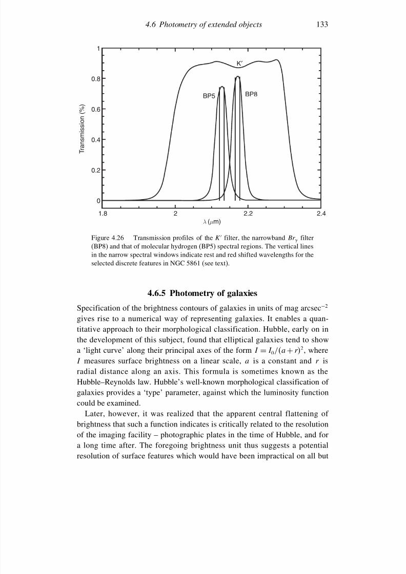
7/21/2019 Introduction to Astronomical Photometry
http://slidepdf.com/reader/full/introduction-to-astronomical-photometry 151/451
4.6 Photometry of extended objects 133
1
0.8
BP5 BP8
K′
0.6
0.4
T r a n s m i s s i o n ( % )
0.2
0
1.8 2 2.2 2.4λ (µ m)
Figure 4.26 Transmission profiles of the K filter, the narrowband Br filter(BP8) and that of molecular hydrogen (BP5) spectral regions. The vertical linesin the narrow spectral windows indicate rest and red shifted wavelengths for theselected discrete features in NGC 5861 (see text).
4.6.5 Photometry of galaxies
Specification of the brightness contours of galaxies in units of mag arcsec−2
gives rise to a numerical way of representing galaxies. It enables a quan-titative approach to their morphological classification. Hubble, early on inthe development of this subject, found that elliptical galaxies tend to showa ‘light curve’ along their principal axes of the form I = I 0/a + r2, whereI measures surface brightness on a linear scale, a is a constant and r isradial distance along an axis. This formula is sometimes known as theHubble–Reynolds law. Hubble’s well-known morphological classification of
galaxies provides a ‘type’ parameter, against which the luminosity functioncould be examined.
Later, however, it was realized that the apparent central flattening of brightness that such a function indicates is critically related to the resolutionof the imaging facility – photographic plates in the time of Hubble, and fora long time after. The foregoing brightness unit thus suggests a potentialresolution of surface features which would have been impractical on all but
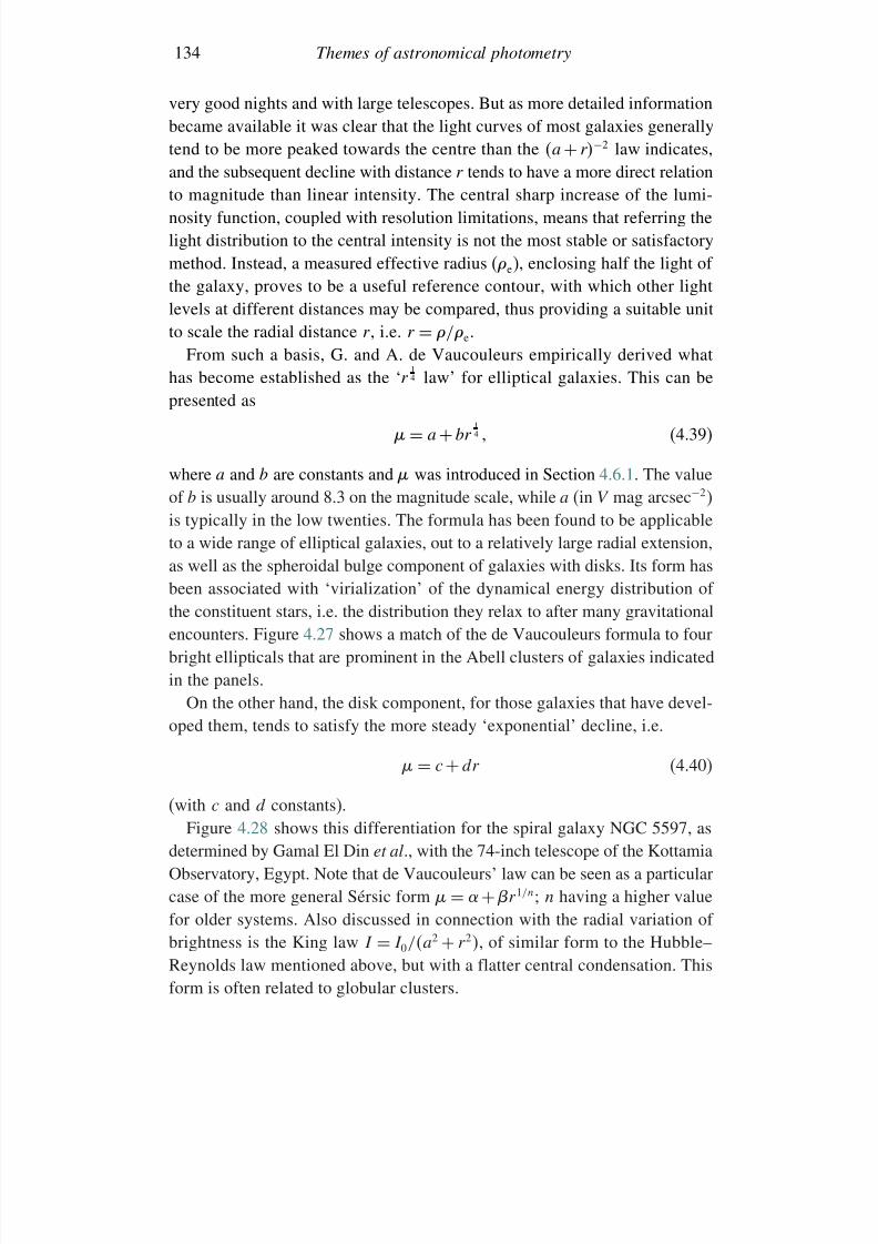
7/21/2019 Introduction to Astronomical Photometry
http://slidepdf.com/reader/full/introduction-to-astronomical-photometry 152/451
134 Themes of astronomical photometry
very good nights and with large telescopes. But as more detailed informationbecame available it was clear that the light curves of most galaxies generallytend to be more peaked towards the centre than the a
+r−2 law indicates,
and the subsequent decline with distance r tends to have a more direct relationto magnitude than linear intensity. The central sharp increase of the lumi-nosity function, coupled with resolution limitations, means that referring thelight distribution to the central intensity is not the most stable or satisfactorymethod. Instead, a measured effective radius (e), enclosing half the light of the galaxy, proves to be a useful reference contour, with which other lightlevels at different distances may be compared, thus providing a suitable unit
to scale the radial distance r , i.e. r = /e.From such a basis, G. and A. de Vaucouleurs empirically derived whathas become established as the ‘r
14 law’ for elliptical galaxies. This can be
presented as
= a + br 14 (4.39)
where a and b are constants and was introduced in Section 4.6.1. The valueof b is usually around 8.3 on the magnitude scale, while a (in V mag arcsec−2)is typically in the low twenties. The formula has been found to be applicableto a wide range of elliptical galaxies, out to a relatively large radial extension,as well as the spheroidal bulge component of galaxies with disks. Its form hasbeen associated with ‘virialization’ of the dynamical energy distribution of the constituent stars, i.e. the distribution they relax to after many gravitationalencounters. Figure 4.27 shows a match of the de Vaucouleurs formula to fourbright ellipticals that are prominent in the Abell clusters of galaxies indicated
in the panels.On the other hand, the disk component, for those galaxies that have devel-
oped them, tends to satisfy the more steady ‘exponential’ decline, i.e.
= c + dr (4.40)
(with c and d constants).Figure 4.28 shows this differentiation for the spiral galaxy NGC 5597, as
determined by Gamal El Din et al., with the 74-inch telescope of the KottamiaObservatory, Egypt. Note that de Vaucouleurs’ law can be seen as a particularcase of the more general Sérsic form = +r 1/n; n having a higher valuefor older systems. Also discussed in connection with the radial variation of brightness is the King law I = I 0/a2 + r 2, of similar form to the Hubble–Reynolds law mentioned above, but with a flatter central condensation. Thisform is often related to globular clusters.
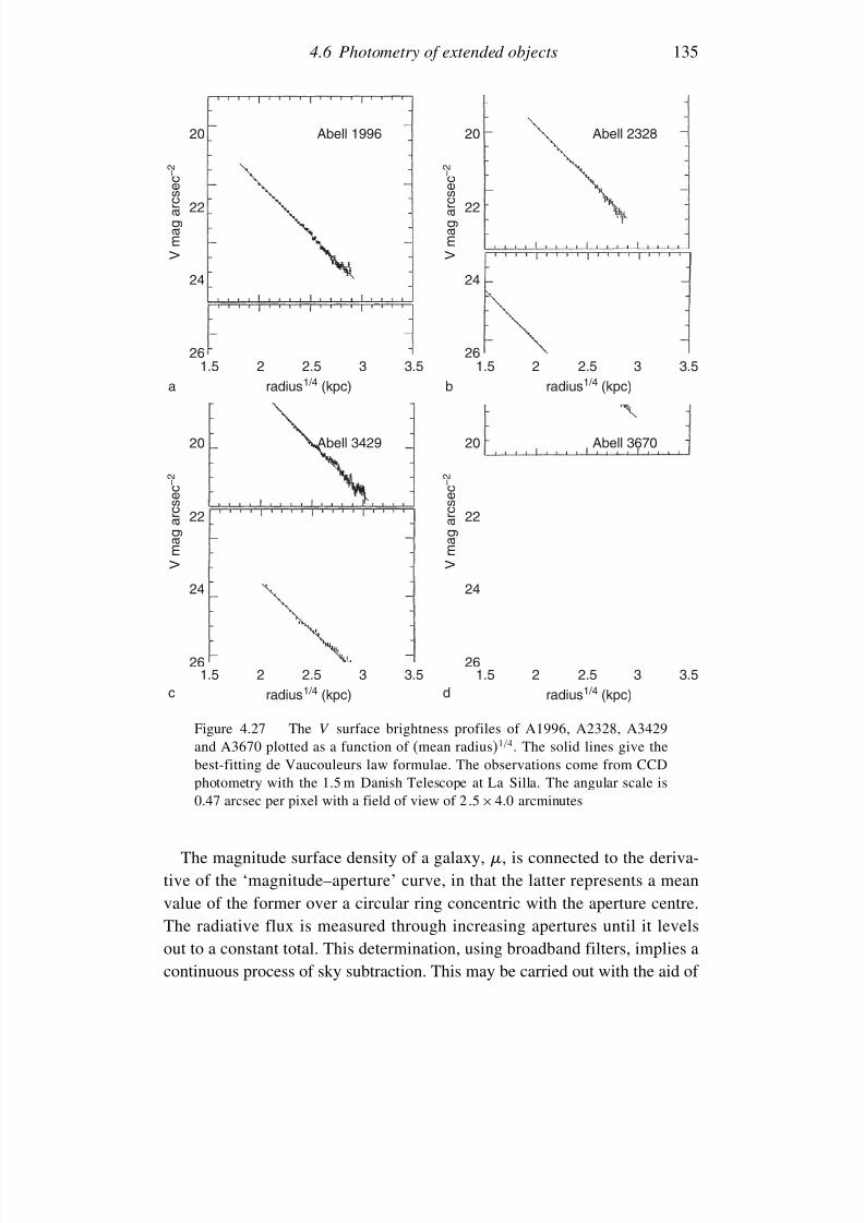
7/21/2019 Introduction to Astronomical Photometry
http://slidepdf.com/reader/full/introduction-to-astronomical-photometry 153/451
4.6 Photometry of extended objects 135
1.5 2 2.5 3 3.5 1.5 2 2.5 3 3.5radius1/4 (kpc) radius1/4 (kpc)
26
24
22
20
V m a g a r c s e c – 2
26
24
22
20
V m a g a r c s e c – 2
26
24
22
20
V m a g a r c s e c – 2
26
24
22
20
V m a g a r c s e c – 2
Abell 1996 Abell 2328
Abell 3429 Abell 3670
ba
c d
1.5 2 2.5 3 3.5 1.5 2 2.5 3 3.5
radius1/4 (kpc) radius1/4 (kpc)
Figure 4.27 The V surface brightness profiles of A1996, A2328, A3429and A3670 plotted as a function of (mean radius)1/4. The solid lines give thebest-fitting de Vaucouleurs law formulae. The observations come from CCDphotometry with the 1.5 m Danish Telescope at La Silla. The angular scale is0.47 arcsec per pixel with a field of view of 2 5× 40 arcminutes
The magnitude surface density of a galaxy, , is connected to the deriva-tive of the ‘magnitude–aperture’ curve, in that the latter represents a meanvalue of the former over a circular ring concentric with the aperture centre.The radiative flux is measured through increasing apertures until it levelsout to a constant total. This determination, using broadband filters, implies acontinuous process of sky subtraction. This may be carried out with the aid of
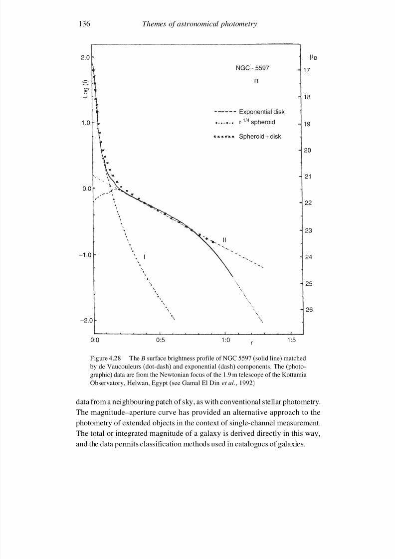
7/21/2019 Introduction to Astronomical Photometry
http://slidepdf.com/reader/full/introduction-to-astronomical-photometry 154/451
136 Themes of astronomical photometry
NGC - 5597
B
Exponential disk
r 1/4 spheroid
Spheroid + disk
17
18
19
20
21
22
23
24
25
26
µB
II
I
0:0 0:5 1:0 1:5r
2.0
1.0
0.0
–2.0
–1.0
L o g ( I )
Figure 4.28 The B surface brightness profile of NGC 5597 (solid line) matchedby de Vaucouleurs (dot-dash) and exponential (dash) components. The (photo-graphic) data are from the Newtonian focus of the 1.9 m telescope of the Kottamia
Observatory, Helwan, Egypt (see Gamal El Din et al., 1992)
data from a neighbouring patch of sky, as with conventional stellar photometry.The magnitude–aperture curve has provided an alternative approach to thephotometry of extended objects in the context of single-channel measurement.The total or integrated magnitude of a galaxy is derived directly in this way,and the data permits classification methods used in catalogues of galaxies.
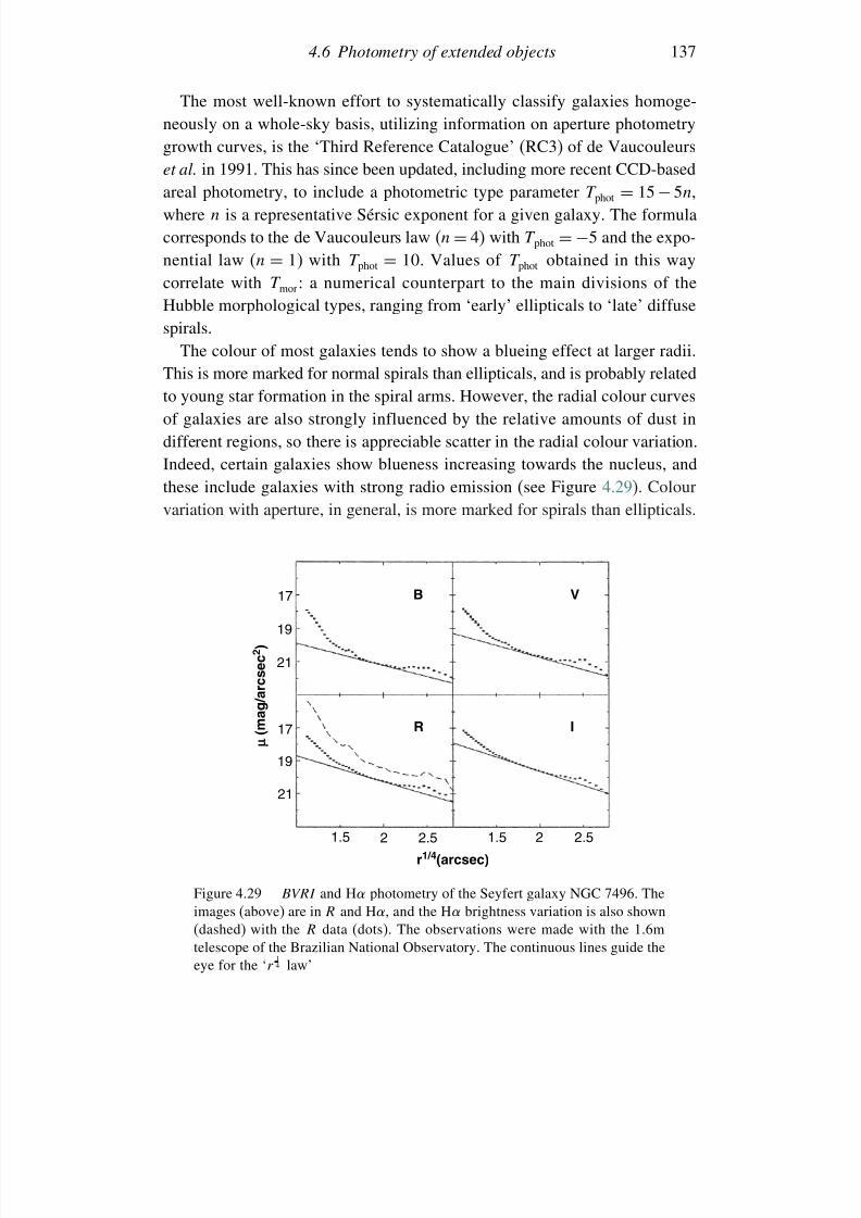
7/21/2019 Introduction to Astronomical Photometry
http://slidepdf.com/reader/full/introduction-to-astronomical-photometry 155/451
4.6 Photometry of extended objects 137
The most well-known effort to systematically classify galaxies homoge-neously on a whole-sky basis, utilizing information on aperture photometrygrowth curves, is the ‘Third Reference Catalogue’ (RC3) of de Vaucouleurs
et al. in 1991. This has since been updated, including more recent CCD-basedareal photometry, to include a photometric type parameter T phot = 15 − 5n,where n is a representative Sérsic exponent for a given galaxy. The formulacorresponds to the de Vaucouleurs law (n = 4) with T phot = −5 and the expo-nential law (n = 1) with T phot = 10. Values of T phot obtained in this waycorrelate with T mor: a numerical counterpart to the main divisions of theHubble morphological types, ranging from ‘early’ ellipticals to ‘late’ diffuse
spirals.The colour of most galaxies tends to show a blueing effect at larger radii.This is more marked for normal spirals than ellipticals, and is probably relatedto young star formation in the spiral arms. However, the radial colour curvesof galaxies are also strongly influenced by the relative amounts of dust indifferent regions, so there is appreciable scatter in the radial colour variation.Indeed, certain galaxies show blueness increasing towards the nucleus, andthese include galaxies with strong radio emission (see Figure 4.29). Colourvariation with aperture, in general, is more marked for spirals than ellipticals.
1.5 2 2.5 1.5 2 2.5
21
19
17
21
19
17 B V
R I
r1/4(arcsec)
µ
( m a g / a r c s e c
2 )
Figure 4.29 BVRI and H photometry of the Seyfert galaxy NGC 7496. Theimages (above) are in R and H, and the H brightness variation is also shown(dashed) with the R data (dots). The observations were made with the 1.6mtelescope of the Brazilian National Observatory. The continuous lines guide theeye for the ‘r
14 law’
7/21/2019 Introduction to Astronomical Photometry
http://slidepdf.com/reader/full/introduction-to-astronomical-photometry 156/451
138 Themes of astronomical photometry
The growth of high-sensitivity areal detectors has allowed investigators tobuild on the systematics of previous techniques, but with the advantages of linear detection, digital recording and computer-based image reduction more
detailed features of galactic morphology are opened up. Knowledge has beenenhanced still further in the present era of high-resolution space telescopes.
4.7 Photopolarimetry
Conventional photometry, concerning itself with the intensity I of an incident
light beam, addresses only part of the information that the light contains.The wave properties of light can be summarized by referring to four ‘Stokesparameters’ I , Q, U and V . These contain information not only about theintensity I , which is closely related to the subject matter hitherto, but alsoabout the two perpendicular components into which the electric vector of anelectromagnetic vibration is resolvable: their relative magnitudes and orienta-tion with respect to a frame of reference specified by the observer, and their
separations along the axis of propagation (phase difference). An input streamof wave packets from a source normally shows some prevailing tendencieswith these properties, though we also find a good deal of randomization whenthe wave packets have passed through turbulent inhomogeneous media andare collected over a wide range of frequencies.
The omission of data on three of the four basic parameters characterizingthe input could be seen as rather a negligence, were it not for the usuallymuch greater information yield, for a given amount of observational effort,
from I than the other three parameters. In order to obtain reliable data onrepresentative values for Q, U and V , along with I , particularly in stellaroptical photometry, very significant improvements in equipment and operationare necessary. Nevertheless, it is appropriate to include a brief discussion of this subject, which, in the optical domain at least, has developed as an offshootfrom conventional photometry.
We approach the Stokes parameters via the solutions of Maxwell’s equa-
tions for a single electromagnetic wave propagation involving componentsE x and E y of the electric vector, i.e.,
E x = E 1 cost −2z/ + x
E y = E 2 cost −2z/ + y
(4.41)
where we have put the vector components in the x and y directions at timet, for angular frequency , and wavelength , at position z along the axis
7/21/2019 Introduction to Astronomical Photometry
http://slidepdf.com/reader/full/introduction-to-astronomical-photometry 157/451
4.7 Photopolarimetry 139
of propagation (z-axis), where there are phase advancements x and y atz t = 0.
Let us now introduce the Stokes parameters, I Q U V , as
I = E 21 + E 22
Q = E 21 − E 22
U = 2E 1E 2 cos
V = 2E 1E 2 sin
(4.42)
where expresses the phase difference y −x, and E 1 and E 2 are the ampli-tudes of the wave motions in the x and y directions.
The foregoing expressions (4.41) for E x and E y satisfyE xE 1
2
+
E y
E 2
2
− 2E xE y
E 1E 2cos = sin2 (4.43)
which is the equation of an ellipse in the E x E y plane. From consideringthe general form of the equation of second degree, the sum of squares of the principal axes of this ellipse is seen to equal the sum of the squares of the amplitudes E 21 + E 22 . This is I by the preceding definition and invariant
against a rotational transformation of the axes x y. The (signed) product of these principal axes, E 2E 1 sin , is a similar invariant, proportional to the areaof the ellipse, and turns out to be 1
2 V in the foregoing notation. The ratioV/I is thus a measure of the nearness of the ellipse to a circle – the ‘circularpolarization’ of the wave, sometimes denoted by q , which varies in the range−1 ≤ q ≤ 1.
The remaining two quantities relate to the difference of the squares of theprincipal axes. Averaged over a suitable time interval, to allow representative
statistics for a large number of received wave packets, they indicate anytendency towards a linear polarization prevalence in the radiation – the twoquantities fix not only the ‘degree of linear polarization’ p as
p =
Q2 + U 2
I (4.44)
but also the orientation of the major axis with respect to the x-axis as
= 12 arctanU/Q (4.45)
A ‘degree of total polarization’ p =
Q2 + U 2 + V 2/I is also sometimesused.
A specification of any systematic polarization in the illuminance in termsof the four Stokes parameters calls for the insertion of an ‘analyser’ into theoptical train, which monitors the linear polarization in at least two orientations,
7/21/2019 Introduction to Astronomical Photometry
http://slidepdf.com/reader/full/introduction-to-astronomical-photometry 158/451
140 Themes of astronomical photometry
as well as a ‘depolarizer’, to account for any net instrumental effects havingnothing to do with the source under study. A ‘quarter-wave plate’ retarderplaced at different orientations in the wave train introduces an effect in the
photometric output whose coefficient is V . It is thus possible to have asuitable arrangement of rotatable optical components – a ‘Stokes-meter’ –where all four parameters are monitored together. The relative accuracy of determination is, however, then spread more thinly, and in practice manyobservers, particularly in the stellar context, have settled for concentrating onthe linear polarization in their data.
The effect of any particular piece of polarizing, or optically ‘active’, mate-
rial on a given beam, specified by a vector S with four components corre-sponding to the four Stokes parameters, can be studied by means of a ‘Muellermatrix’ M, whose form specifies the action of the optical agent. The outputbeam S satisfies
S = M.S (4.46)
The net effect of a combination of n components – analysers, retarders or
whatever – is examined as the result of the sequence of operations Sout =Mn
.Mn−1 M1.Sin. Operating with such a Mueller calculus one gains a
fuller understanding of the design and action of a photopolarimeter. Twobasic forms of such matrices can be set out. For a perfect analyser, we have
Ma =
1 cos 2 sin2 0cos2 cos2 2 1
2 sin 4 0sin2 1
2 sin 4 sin2 2 0
0 0 0 0
where measures the orientation of the principal plane of the analyser withrespect to the initial axis. For a perfect retarder of retardance with the axisof optical activity at position angle , we write Mr as
Mr = 1 0 0 00 G
+H cos4 H sin4
−sin sin2
0 H sin4 G − H cos4 sin cos2
0 sin sin2 − sin cos2 cos
where G = 12 1+ cos and H = 1
2 1− cos .8
8 For more details on this, the reader is referred to Shurcliff and Ballard’s Polarized Light , vanNostrand, 1964.
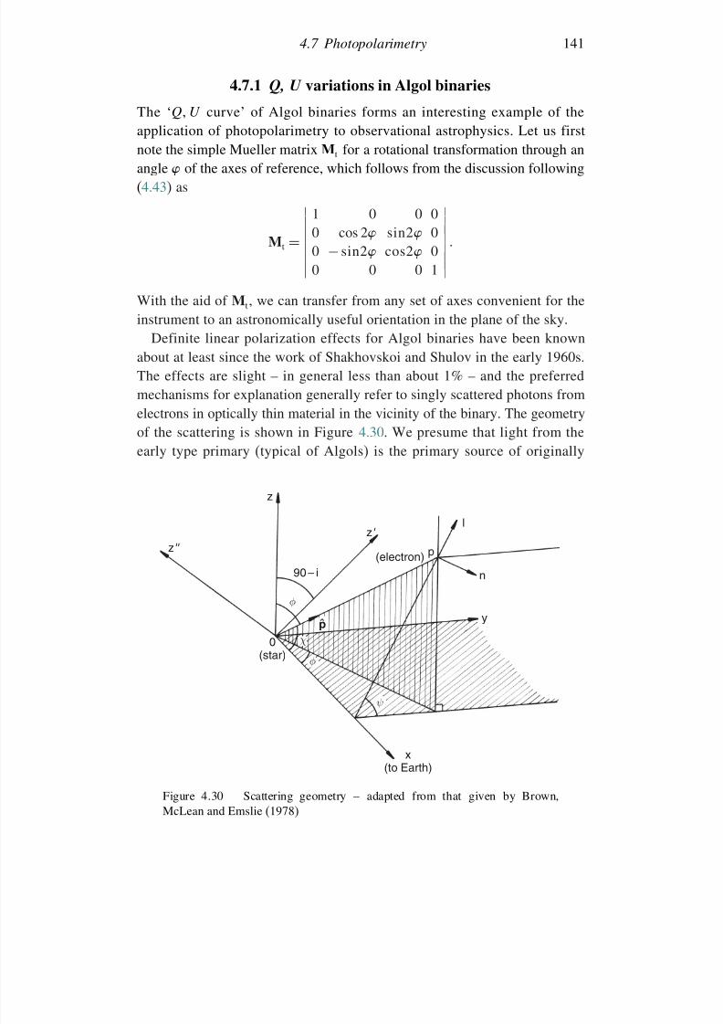
7/21/2019 Introduction to Astronomical Photometry
http://slidepdf.com/reader/full/introduction-to-astronomical-photometry 159/451
4.7 Photopolarimetry 141
4.7.1 Q, U variations in Algol binaries
The ‘Q U curve’ of Algol binaries forms an interesting example of theapplication of photopolarimetry to observational astrophysics. Let us firstnote the simple Mueller matrix Mt for a rotational transformation through anangle of the axes of reference, which follows from the discussion following(4.43) as
Mt =
1 0 0 00 cos 2 sin2 00 − sin2 cos2 00 0 0 1
With the aid of Mt, we can transfer from any set of axes convenient for theinstrument to an astronomically useful orientation in the plane of the sky.
Definite linear polarization effects for Algol binaries have been knownabout at least since the work of Shakhovskoi and Shulov in the early 1960s.The effects are slight – in general less than about 1% – and the preferredmechanisms for explanation generally refer to singly scattered photons from
electrons in optically thin material in the vicinity of the binary. The geometryof the scattering is shown in Figure 4.30. We presume that light from theearly type primary (typical of Algols) is the primary source of originally
x(to Earth)
0(star)
z''
z
z'
90 – i(electron)
p
l
n
y
ψ
φ
φ
p ›
χ
Figure 4.30 Scattering geometry – adapted from that given by Brown,McLean and Emslie (1978)
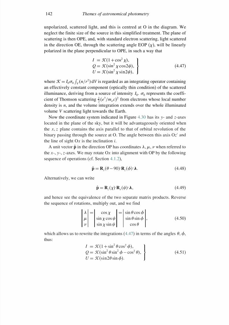
7/21/2019 Introduction to Astronomical Photometry
http://slidepdf.com/reader/full/introduction-to-astronomical-photometry 160/451
142 Themes of astronomical photometry
unpolarized, scattered light, and this is centred at O in the diagram. Weneglect the finite size of the source in this simplified treatment. The plane of scattering is then OPE, and, with standard electron scattering, light scattered
in the direction OE, through the scattering angle EOP ( ), will be linearlypolarized in the plane perpendicular to OPE, in such a way that
I = 1+ cos2
Q = sin2 cos2
U = sin2 sin2
(4.47)
where = I 0 0 V n/r 2 dV is regarded as an integrating operator containing
an effectively constant component (optically thin condition) of the scatteredilluminance, deriving from a source of intensity I 0. 0 represents the coeffi-cient of Thomson scattering 1
2 e2/mec2 from electrons whose local numberdensity is n, and the volume integration extends over the whole illuminatedvolume V scattering light towards the Earth.
Now the coordinate system indicated in Figure 4.30 has its y- and z-axeslocated in the plane of the sky, but it will be advantageously oriented whenthe x z plane contains the axis parallel to that of orbital revolution of the
binary passing through the source at O. The angle between this axis Oz andthe line of sight Ox is the inclination i.
A unit vector p in the direction OP has coordinates when referred tothe x-, y-, z-axes. We may rotate Ox into alignment with OP by the followingsequence of operations (cf. Section 4.1.2),
p = R y −90.R z. (4.48)
Alternatively, we can write
p = R z.R x . (4.49)
and hence see the equivalence of the two separate matrix products. Reversethe sequence of rotations, multiply out, and we find
= cos = sin cos
sin cos sin sin
sin sin cos
(4.50)
which allows us to rewrite the integrations (4.47) in terms of the angles ,thus:
I = 1+ sin2 cos2
Q = sin2 sin2 − cos2
U = sin2 sin
(4.51)
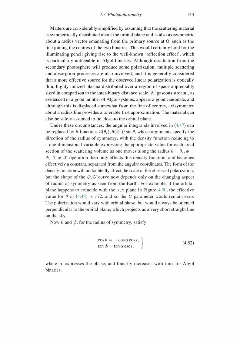
7/21/2019 Introduction to Astronomical Photometry
http://slidepdf.com/reader/full/introduction-to-astronomical-photometry 161/451
4.7 Photopolarimetry 143
Matters are considerably simplified by assuming that the scattering materialis symmetrically distributed about the orbital plane and is also axisymmetricabout a radius vector emanating from the primary source at O, such as the
line joining the centres of the two binaries. This would certainly hold for theilluminating pencil giving rise to the well-known ‘reflection effect’, whichis particularly noticeable in Algol binaries. Although reradiation from thesecondary photosphere will produce some polarization, multiple scatteringand absorption processes are also involved, and it is generally consideredthat a more effective source for the observed linear polarization is opticallythin, highly ionized plasma distributed over a region of space appreciably
sized in comparison to the inter-binary distance scale. A ‘gaseous stream’, asevidenced in a good number of Algol systems, appears a good candidate, andalthough this is displaced somewhat from the line of centres, axisymmetryabout a radius line provides a tolerable first approximation. The material canalso be safely assumed to lie close to the orbital plane.
Under these circumstances, the angular integrands involved in (4.47) canbe replaced by -functions r r / sin , whose arguments specify the
direction of the radius of symmetry, with the density function reducing toa one-dimensional variable expressing the appropriate value for each arealsection of the scattering volume as one moves along the radius = r =r . The operation then only affects this density function, and becomeseffectively a constant, separated from the angular coordinates. The form of thedensity function will undoubtedly affect the scale of the observed polarization,but the shape of the Q U curve now depends only on the changing aspect
of radius of symmetry as seen from the Earth. For example, if the orbitalplane happens to coincide with the x y plane in Figure 4.30, the effectivevalue for in (4.48) is /2, and so the U parameter would remain zero.The polarization would vary with orbital phase, but would always be orientedperpendicular to the orbital plane, which projects as a very short straight lineon the sky.
Now and , for the radius of symmetry, satisfy
cos = −cos cos i
tan = tan csc i
(4.52)
where expresses the phase, and linearly increases with time for Algolbinaries.
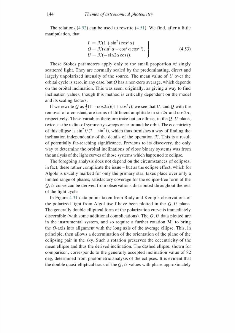
7/21/2019 Introduction to Astronomical Photometry
http://slidepdf.com/reader/full/introduction-to-astronomical-photometry 162/451
144 Themes of astronomical photometry
The relations (4.52) can be used to rewrite (4.51). We find, after a littlemanipulation, that
I =
1+ sin
2
i cos
2
Q = sin2 − cos2 cos2 i
U = − sin2 cos i
(4.53)
These Stokes parameters apply only to the small proportion of singlyscattered light. They are normally scaled by the predominating, direct andlargely unpolarized intensity of the source. The mean value of U over theorbital cycle is zero, in any case, but Q has a non-zero average, which dependson the orbital inclination. This was seen, originally, as giving a way to findinclination values, though this method is critically dependent on the modeland its scaling factors.
If we rewrite Q as 12 1 − cos21 + cos2 i, we see that U , and Q with the
removal of a constant, are terms of different amplitude in sin 2 and cos 2,respectively. These variables therefore trace out an ellipse, in the Q U plane,twice, as the radius of symmetry sweeps once around the orbit. The eccentricityof this ellipse is sin2 i/2
−sin2 i, which thus furnishes a way of finding the
inclination independently of the details of the operation . This is a resultof potentially far-reaching significance. Previous to its discovery, the onlyway to determine the orbital inclinations of close binary systems was fromthe analysis of the light curves of those systems which happened to eclipse.
The foregoing analysis does not depend on the circumstances of eclipses;in fact, these rather complicate the issue – but as the eclipse effect, which forAlgols is usually marked for only the primary star, takes place over only a
limited range of phases, satisfactory coverage for the eclipse-free form of theQ U curve can be derived from observations distributed throughout the restof the light cycle.
In Figure 4.31 data points taken from Rudy and Kemp’s observations of the polarized light from Algol itself have been plotted in the Q U plane.The generally double elliptical form of the polarization curve is immediatelydiscernible (with some additional complications). The Q U data plotted arein the instrumental system, and so require a further rotation Mt to bring
the Q-axis into alignment with the long axis of the average ellipse. This, inprinciple, then allows a determination of the orientation of the plane of theeclipsing pair in the sky. Such a rotation preserves the eccentricity of themean ellipse and thus the derived inclination. The dashed ellipse, shown forcomparison, corresponds to the generally accepted inclination value of 82deg, determined from photometric analysis of the eclipses. It is evident thatthe double quasi-elliptical track of the Q U values with phase approximately
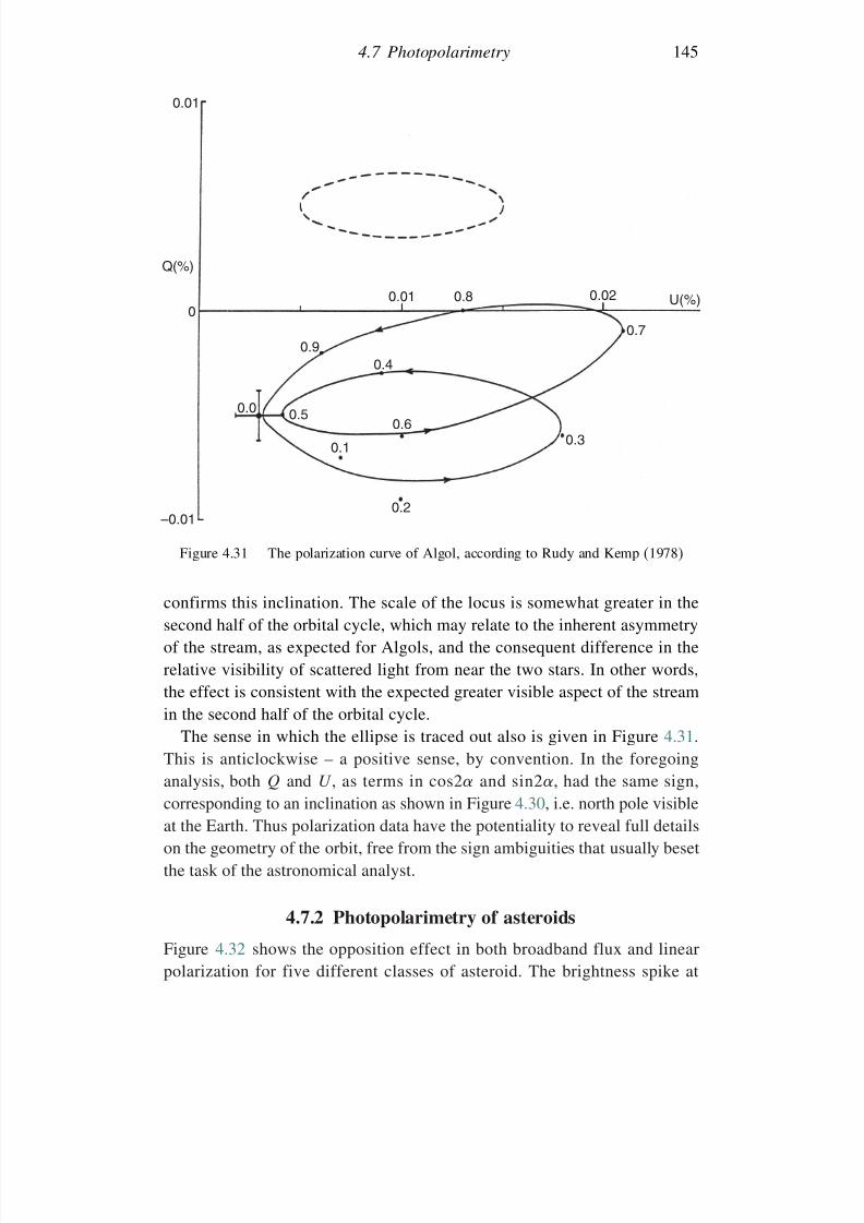
7/21/2019 Introduction to Astronomical Photometry
http://slidepdf.com/reader/full/introduction-to-astronomical-photometry 163/451
4.7 Photopolarimetry 145
0.01 0.8 0.02 U(%)
0.7
0.3
0.4
0.6
0.1
0.2
0.50.0
0.9
0.01
0
–0.01
Q(%)
Figure 4.31 The polarization curve of Algol, according to Rudy and Kemp (1978)
confirms this inclination. The scale of the locus is somewhat greater in thesecond half of the orbital cycle, which may relate to the inherent asymmetryof the stream, as expected for Algols, and the consequent difference in the
relative visibility of scattered light from near the two stars. In other words,the effect is consistent with the expected greater visible aspect of the streamin the second half of the orbital cycle.
The sense in which the ellipse is traced out also is given in Figure 4.31.This is anticlockwise – a positive sense, by convention. In the foregoinganalysis, both Q and U , as terms in cos2 and sin2, had the same sign,corresponding to an inclination as shown in Figure 4.30, i.e. north pole visible
at the Earth. Thus polarization data have the potentiality to reveal full detailson the geometry of the orbit, free from the sign ambiguities that usually besetthe task of the astronomical analyst.
4.7.2 Photopolarimetry of asteroids
Figure 4.32 shows the opposition effect in both broadband flux and linearpolarization for five different classes of asteroid. The brightness spike at
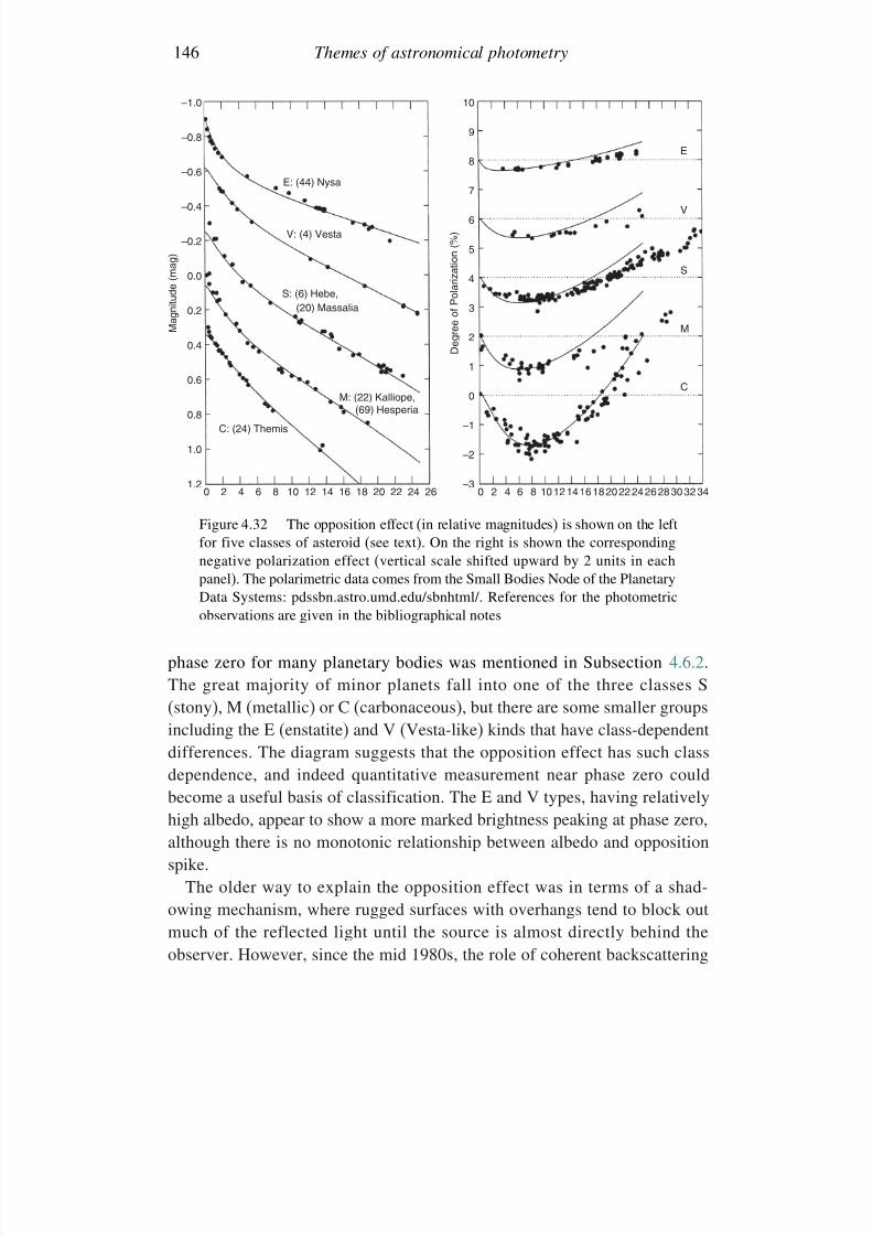
7/21/2019 Introduction to Astronomical Photometry
http://slidepdf.com/reader/full/introduction-to-astronomical-photometry 164/451
146 Themes of astronomical photometry
M a g n i t u d e ( m a g )
D e g r e e o f P o l a r i z a t i o n ( % )
1.0
0.8
0.6
0.4
0.2
0.0
–0.2
–0.4
–0.6
–0.8
–1.0
E: (44) Nysa
V: (4) Vesta
S: (6) Hebe,(20) Massalia
M: (22) Kalliope,
C: (24) Themis
(69) Hesperia
1.2
–2
–1
0
1
2
3
4
5
6
7
8
9
10
–30 2 4 6 8 10 12 14 16 18 20 22 24 26 0 2 4 6 8 10121416182022242628303234
C
M
S
V
E
Figure 4.32 The opposition effect (in relative magnitudes) is shown on the leftfor five classes of asteroid (see text). On the right is shown the correspondingnegative polarization effect (vertical scale shifted upward by 2 units in eachpanel). The polarimetric data comes from the Small Bodies Node of the PlanetaryData Systems: pdssbn.astro.umd.edu/sbnhtml/. References for the photometricobservations are given in the bibliographical notes
phase zero for many planetary bodies was mentioned in Subsection 4.6.2.The great majority of minor planets fall into one of the three classes S(stony), M (metallic) or C (carbonaceous), but there are some smaller groupsincluding the E (enstatite) and V (Vesta-like) kinds that have class-dependentdifferences. The diagram suggests that the opposition effect has such classdependence, and indeed quantitative measurement near phase zero couldbecome a useful basis of classification. The E and V types, having relativelyhigh albedo, appear to show a more marked brightness peaking at phase zero,
although there is no monotonic relationship between albedo and oppositionspike.
The older way to explain the opposition effect was in terms of a shad-owing mechanism, where rugged surfaces with overhangs tend to block outmuch of the reflected light until the source is almost directly behind theobserver. However, since the mid 1980s, the role of coherent backscattering
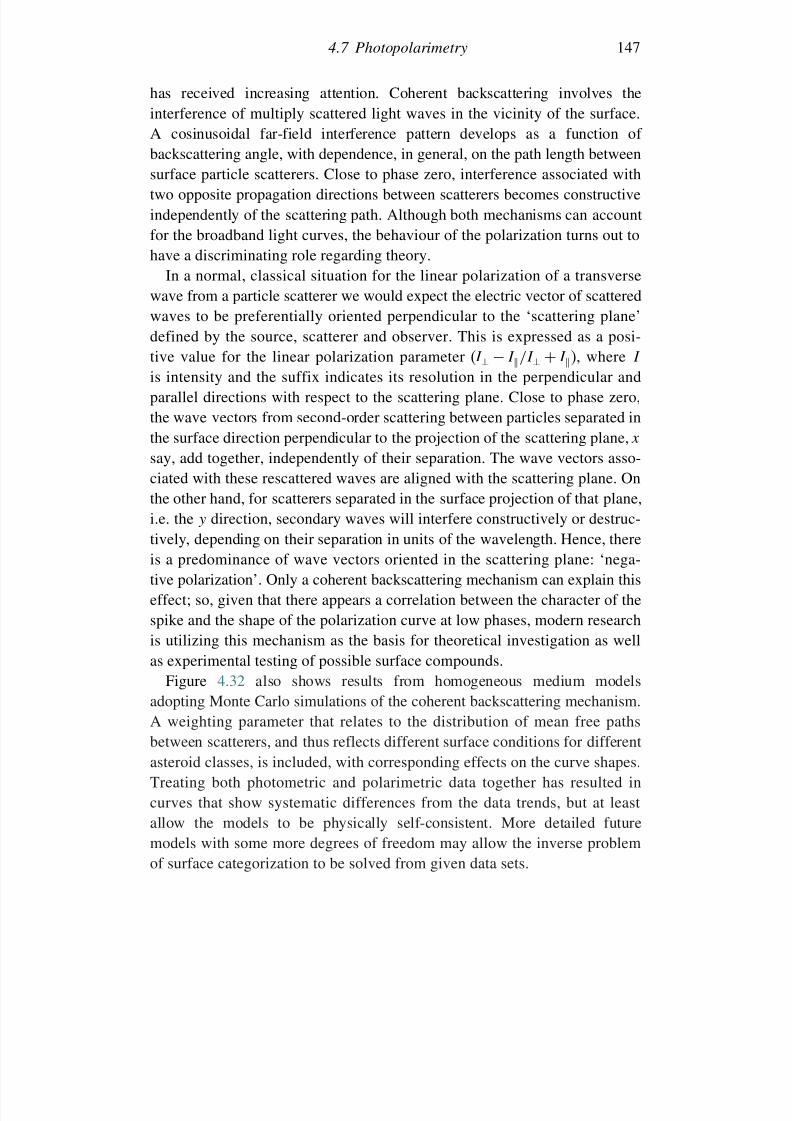
7/21/2019 Introduction to Astronomical Photometry
http://slidepdf.com/reader/full/introduction-to-astronomical-photometry 165/451
4.7 Photopolarimetry 147
has received increasing attention. Coherent backscattering involves theinterference of multiply scattered light waves in the vicinity of the surface.A cosinusoidal far-field interference pattern develops as a function of
backscattering angle, with dependence, in general, on the path length betweensurface particle scatterers. Close to phase zero, interference associated withtwo opposite propagation directions between scatterers becomes constructiveindependently of the scattering path. Although both mechanisms can accountfor the broadband light curves, the behaviour of the polarization turns out tohave a discriminating role regarding theory.
In a normal, classical situation for the linear polarization of a transversewave from a particle scatterer we would expect the electric vector of scatteredwaves to be preferentially oriented perpendicular to the ‘scattering plane’defined by the source, scatterer and observer. This is expressed as a posi-tive value for the linear polarization parameter (I ⊥ − I /I ⊥ + I ), where I
is intensity and the suffix indicates its resolution in the perpendicular andparallel directions with respect to the scattering plane. Close to phase zero,the wave vectors from second-order scattering between particles separated inthe surface direction perpendicular to the projection of the scattering plane, x
say, add together, independently of their separation. The wave vectors asso-ciated with these rescattered waves are aligned with the scattering plane. Onthe other hand, for scatterers separated in the surface projection of that plane,i.e. the y direction, secondary waves will interfere constructively or destruc-tively, depending on their separation in units of the wavelength. Hence, thereis a predominance of wave vectors oriented in the scattering plane: ‘nega-tive polarization’. Only a coherent backscattering mechanism can explain thiseffect; so, given that there appears a correlation between the character of thespike and the shape of the polarization curve at low phases, modern researchis utilizing this mechanism as the basis for theoretical investigation as wellas experimental testing of possible surface compounds.
Figure 4.32 also shows results from homogeneous medium modelsadopting Monte Carlo simulations of the coherent backscattering mechanism.A weighting parameter that relates to the distribution of mean free pathsbetween scatterers, and thus reflects different surface conditions for different
asteroid classes, is included, with corresponding effects on the curve shapes.Treating both photometric and polarimetric data together has resulted incurves that show systematic differences from the data trends, but at leastallow the models to be physically self-consistent. More detailed futuremodels with some more degrees of freedom may allow the inverse problemof surface categorization to be solved from given data sets.
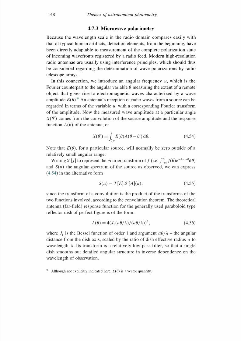
7/21/2019 Introduction to Astronomical Photometry
http://slidepdf.com/reader/full/introduction-to-astronomical-photometry 166/451
148 Themes of astronomical photometry
4.7.3 Microwave polarimetry
Because the wavelength scale in the radio domain compares easily withthat of typical human artifacts, detection elements, from the beginning, havebeen directly adaptable to measurement of the complete polarization stateof incoming wavefronts registered by a radio feed. Modern high-resolutionradio antennae are usually using interference principles, which should thusbe considered regarding the determination of wave polarizations by radiotelescope arrays.
In this connection, we introduce an angular frequency u, which is theFourier counterpart to the angular variable measuring the extent of a remote
object that gives rise to electromagnetic waves characterized by a waveamplitude E.9 An antenna’s reception of radio waves from a source can beregarded in terms of the variable u, with a corresponding Fourier transformof the amplitude. Now the measured wave amplitude at a particular angleX comes from the convolution of the source amplitude and the responsefunction A of the antenna, or
X=
2
EA−
d (4.54)
Note that E, for a particular source, will normally be zero outside of arelatively small angular range.
Writing f to represent the Fourier transform of f (i.e.
− fe−2 iud)and Su the angular spectrum of the source as observed, we can express(4.54) in the alternative form
Su= E Au (4.55)
since the transform of a convolution is the product of the transforms of thetwo functions involved, according to the convolution theorem. The theoreticalantenna (far-field) response function for the generally used paraboloid typereflector dish of perfect figure is of the form:
A = 4J 1a//a/2 (4.56)
where J 1 is the Bessel function of order 1 and argument a/ – the angulardistance from the dish axis, scaled by the ratio of dish effective radius a towavelength . Its transform is a relatively low-pass filter, so that a singledish smooths out detailed angular structure in inverse dependence on thewavelength of observation.
9 Although not explicitly indicated here, E is a vector quantity.
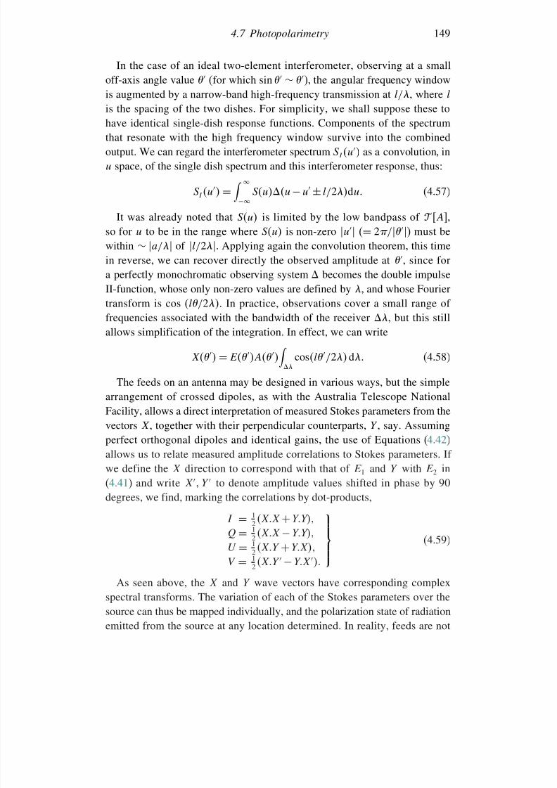
7/21/2019 Introduction to Astronomical Photometry
http://slidepdf.com/reader/full/introduction-to-astronomical-photometry 167/451
4.7 Photopolarimetry 149
In the case of an ideal two-element interferometer, observing at a smalloff-axis angle value (for which sin ∼ ), the angular frequency windowis augmented by a narrow-band high-frequency transmission at l/, where l
is the spacing of the two dishes. For simplicity, we shall suppose these tohave identical single-dish response functions. Components of the spectrumthat resonate with the high frequency window survive into the combinedoutput. We can regard the interferometer spectrum S I u as a convolution, inu space, of the single dish spectrum and this interferometer response, thus:
S I u =
−Suu − u ± l/2du (4.57)
It was already noted that Su is limited by the low bandpass of A,so for u to be in the range where Su is non-zero u (= 2/) must bewithin ∼ a/ of l/2. Applying again the convolution theorem, this timein reverse, we can recover directly the observed amplitude at , since fora perfectly monochromatic observing system becomes the double impulseII-function, whose only non-zero values are defined by , and whose Fouriertransform is cos (l/2. In practice, observations cover a small range of
frequencies associated with the bandwidth of the receiver , but this stillallows simplification of the integration. In effect, we can write
X = EA
cosl/2 d (4.58)
The feeds on an antenna may be designed in various ways, but the simplearrangement of crossed dipoles, as with the Australia Telescope NationalFacility, allows a direct interpretation of measured Stokes parameters from the
vectors X , together with their perpendicular counterparts, Y , say. Assumingperfect orthogonal dipoles and identical gains, the use of Equations (4.42)allows us to relate measured amplitude correlations to Stokes parameters. If we define the X direction to correspond with that of E 1 and Y with E 2 in(4.41) and write X Y to denote amplitude values shifted in phase by 90degrees, we find, marking the correlations by dot-products,
I = 12 XX + YY
Q = 1
2 XX − YYU = 12 XY + YX
V = 12 XY − YX
(4.59)
As seen above, the X and Y wave vectors have corresponding complexspectral transforms. The variation of each of the Stokes parameters over thesource can thus be mapped individually, and the polarization state of radiationemitted from the source at any location determined. In reality, feeds are not
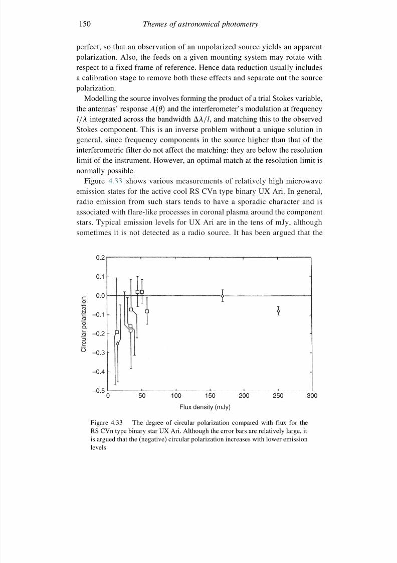
7/21/2019 Introduction to Astronomical Photometry
http://slidepdf.com/reader/full/introduction-to-astronomical-photometry 168/451
150 Themes of astronomical photometry
perfect, so that an observation of an unpolarized source yields an apparentpolarization. Also, the feeds on a given mounting system may rotate withrespect to a fixed frame of reference. Hence data reduction usually includes
a calibration stage to remove both these effects and separate out the sourcepolarization.
Modelling the source involves forming the product of a trial Stokes variable,the antennas’ response A and the interferometer’s modulation at frequencyl/ integrated across the bandwidth /l, and matching this to the observedStokes component. This is an inverse problem without a unique solution ingeneral, since frequency components in the source higher than that of the
interferometric filter do not affect the matching: they are below the resolutionlimit of the instrument. However, an optimal match at the resolution limit isnormally possible.
Figure 4.33 shows various measurements of relatively high microwaveemission states for the active cool RS CVn type binary UX Ari. In general,radio emission from such stars tends to have a sporadic character and isassociated with flare-like processes in coronal plasma around the componentstars. Typical emission levels for UX Ari are in the tens of mJy, although
sometimes it is not detected as a radio source. It has been argued that the
0 50 100 150 200 250 300
Flux density (mJy)
0.2
0.1
0.0
–0.1
–0.2
–0.3
–0.4
–0.5
C i r c u l a r p o l a r i z a t i o n
Figure 4.33 The degree of circular polarization compared with flux for theRS CVn type binary star UX Ari. Although the error bars are relatively large, itis argued that the (negative) circular polarization increases with lower emissionlevels
7/21/2019 Introduction to Astronomical Photometry
http://slidepdf.com/reader/full/introduction-to-astronomical-photometry 169/451
4.8 Bibliographical notes 151
flare outbursts are associated with very large concentrations of magnetic fluxthat tend to stay in relatively fixed locations on the stars. The fact that thecircular polarization state retains its sense over intervals of several years can
be taken to support this idea. The decrease of circular polarization with flareintensity was interpreted to indicate that the most intense flares are in morecompact, optically thick regions, while lesser intensity outbursts may arisefrom more extensive regions emitting by a gyrosynchrotron process furtherout in the corona.
4.8 Bibliographical notes
The treatment of atmospheric extinction is standard, and a summaryis given in M. Golay’s Introduction to Astronomical Photometry (Reidel,1974, Chapter 2). Formula (4.7) is attributed to Bemporad (see E. Schoen-berg, Handbuch der Astrophysik , Springer, 2, 268, 1929). The more recentalternative cited comes from F. Kasten and A. T. Young ( Appl. Opt., 28,4735, 1989). A.T. Young gives further background in Meth. Exp. Phys.
(12A, Optical and Infrared, ed. M.L. Meeks, Academic Press (p. 123),1976); and also Icarus (11, 1, 1969) (see also Hayes, D.S. & Latham,D.W., Astrophys. J ., 197, 593, 1975).
Orthogonal matrix transformations and their application to the rotationaltransformation of coordinate axes are discussed in, for example, Elementary
Matrices, R. A. Frazer, W. J. Duncan & A. R. Collar (Cambridge UniversityPress, 1946, Chapter 8).
A summary on interstellar extinction is provided in Chapter 4 of C. andM. Jaschek’s Classification of the Stars (Cambridge University Press, 1987).The mean formula
Ar = A0 sec b
1− exp
−r sin b
where A0 is a constant, b is the galactic latitude and the thickness of theextinction providing layer, is provided there, though clear evidence is also
given to show the marked local variations which occur in particular directions.The form of the interstellar extinction law (Figure 4.2) is also discussed invarious places in the Symposium to honour K. Nandy (Q. J. R. Astr. Soc., 28,207 (et seq), 1987). An up-to-date summary of likely causes of the extinctionwas given by B.T. Draine ( Ann. Rev. Astron. Astrophys., 41, 241, 2003),while the diffuse interstellar bands (DIBs) were reviewed by G. H. Herbig( Ann. Rev. Astron. Astrophys., 33, 19, 1995).
7/21/2019 Introduction to Astronomical Photometry
http://slidepdf.com/reader/full/introduction-to-astronomical-photometry 170/451
152 Themes of astronomical photometry
The purposes behind the choice of optical filters have stimulated verymany papers and discussions. Significant sections of IAU Symp. 24 (ed. K.Lodén, L. O. Lodén & U. Sinnerstad), Academic Press, London, 1966, 50 (ed.
C. Fehrenbach & B. E. Westerlund, Reidel, 1973), and 54 (ed. B. Hauck &B. E. Westerlund, Reidel, 1975) were dedicated largely to this subject. Morerecent relevant IAU Symposia are nos. 111 (eds. D. S. Hayes, L. E. Pasinetti& A. G. Davis Phillip, Reidel, 1985) and 189 (eds. T. Bedding, A. J. Booth &J. Davis, Kluwer, 1997). The general forms shown in Figure 4.3 appear inmany places: they accord with the typical numerical values tabulated in C. W.Allen’s Astrophysical Quantities, ed. A. N. Cox (AIP Press, 2000) (see also
H. L. Johnson, Ann. Rev. Astron. Astrophys., 4, 193, 1966; Tables 3.6 and 3.7herein, and also listings such as those of B. Nicolet, Astron. Astrophys. Suppl.,34, 1, 1978 and T. Lanz, Astron. Astrophys. Suppl., 65, 195, 1986). TheQ parameter of Equation (4.11) appeared in Johnson and Morgan’s originalpaper ( Astrophys. J., 117, 313, 1953).
The respective merits of UBV and RGU (W. Becker, Veröff. Univ. Sternw.
Göttingen, No. 80, 1946), as well as various other filter systems, were thor-oughly reviewed in Golay’s Introduction to Astronomical Photometry. The
extension to the seven-colour UBVB1 B2 V 1 G (Geneva system) is discussedin Golay’s paper in Vistas in Astronomy (24, 141, 1980). Figure 4.4 comesfrom J. Stebbins & A.E. Whitford ( Astrophys. J., 98, 20, 1943). H. L.Johnson introduced the RIJKLMN extension to the UBV system in Astro-
phys. J. (141, 923, 1965). Later H and Q filters were added: the formercovering a near-IR region relatively free from water-vapour absorption;the latter, at ∼21m, permitting longer wavelength checking of satellite
data, notably that of the IRAS (Neugebauer et al., Astrophys. J ., 278, L1,1984; – see, for instance, S. J. Kenyon & L. Hartmann, Astrophys. J. Suppl.,101, 117, 1995). Uniformity of IR filter systems has been discussed byA.T. Young, E.F. Milone and C.R. Stagg ( Astron. Astrophys., 105, 259,1994).
Information on the Sloan Digital Sky Survey was given by J.E. Gunnand G.R. Knapp in Astron. Soc. Pacific Conf. Ser. (ed. T. Soifer 43, 267,1992), and also R. G. Kron, in Progress in Telescope and Instrumentation
Technologies, ESO Conference and Workshop Proceedings No. 42, ed. M. H.Ulrich (ESO, p. 635, 1992). Details of the photometric system were givenby M. Fukugita et al. ( Astron. J ., 111, 1748, 1996). Further information,including how to access data, is available from www.sdss.org/.
The original papers on the intermediate-band uvby set were B. Ström-gren’s ( Ann. Rev. Astron. Astrophys., 4, 443, 1966), and D.L. Crawford’sarticle ( IAU Symp. 24, p. 170). Some of the basic diagrams in this
7/21/2019 Introduction to Astronomical Photometry
http://slidepdf.com/reader/full/introduction-to-astronomical-photometry 171/451
4.8 Bibliographical notes 153
photometric system have been shown in the text. Thus, Figures 4.7 and 4.8come from D. L. Crawford and J. V. Barnes’ article in Astron. J., 75, 978,1970, which also discusses the reduction of observations in this system, as
well as presenting lists of standard stars. Figure 4.6 was shown in Crawford’spedagogic summary in Stellar Astronomy (eds. H.-Y. Chiu, R. L. Warasilaand J. L. Remo, Gordon and Breach, 1969). Useful programs for extractingstellar parameters from Strömgren photometry were published by T. T. Moon(Commun. Univ. London Obs., 78, 1985).
D.B. Wood’s extension to the uvby system was presented in Astron. J.
(74, 177), 1969. Figure 4.9 is taken from J.H. Peña & R. Peniche ( Rev.
Mex. Astron. Astrofis., 28, 139, 1994), which cites the work of L. Balonaand R.R. Shobbrook ( Mon. Not. Roy. Astron. Soc., 211, 375, 1984). TheVilnius system was introduced by V. L. Straizys ( Bull. Vilnius Astron. Obs.,28, 1970), and M. C. Forbes’ application of this, shown in Figure 4.10, comesfrom his Ph.D. thesis (Victoria University, Wellington, New Zealand, 1996).The model calculations of D. Schaerer et al. are in Astron. Astrophys. Suppl.
Ser. (98, 53, 1993). Z.-Y. Wu et al.’s paper (Publ. Astron. Soc. Pacific,117, 32, 2005) has developed from the multi-band system of J. B. Oke and
J. E. Gunn ( Astrophys. J ., 260, 713, 1983), originally discussed by J. B. Okein Proc. IAU Symp. 26 (Academic Press, ed. H. Hubenet, p. 3, 1966). Itsdevelopment can be traced to the work of A.D. Code, ed. J.L. Greenstein(University of Chicago Press, 1960, p. 50); see also J. B. Oke ( Astrophys. J .,131, 358, 1960). A large variety of different photometric systems, with corre-sponding standard star data, is available from cdsweb.u-strasbg.fr/cats/II.htx.The Padova models were presented by G. Bertelli et al. ( Astron. Astrophys.
Suppl., 106, 275, 1994).The H transmission diagram is from D. L. Crawford and J. Mander( Astron. J., 71, 114, 1966). The analysis which is followed through inEquations (4.22–4.24) was given by E. Budding and N. Marngus ( Astrophys.
Space Sci., 67, 477, 1980). J. D. Fernie’s paper ( Astron. J., 70, 575, 1965) isreferred to in Figure 4.13, while a u − b plot can be found in B. Ström-gren’s cited review of 1966. The idea of measuring hydrogen line strengths asan indicator of luminosity is older than this, and the principle of comparison
of the flux in spectral features with the surrounding continuum is discussedin the classic paper of B. Lindblad ( Astrophys. J., 55, 85, 1922). The narrow-band filter containing ‘Copenhagen system’ was presented by P. Dickowet al. ( Astron. Astrophys. Suppl. Ser ., 2, 1, 1970). G.W. Lockwood’s dataare in Astrophys. J. Suppl. (24, 375, 1972), as used by R. Alvarez & B. Plez( Astron. Astrophys., 330, 1109, 1998). The ‘Wilson–Bappu’ relation wasgiven in Wilson, O.C. & Bappu, M.K.V. ( Astrophys. J., 125, 661, 1957).
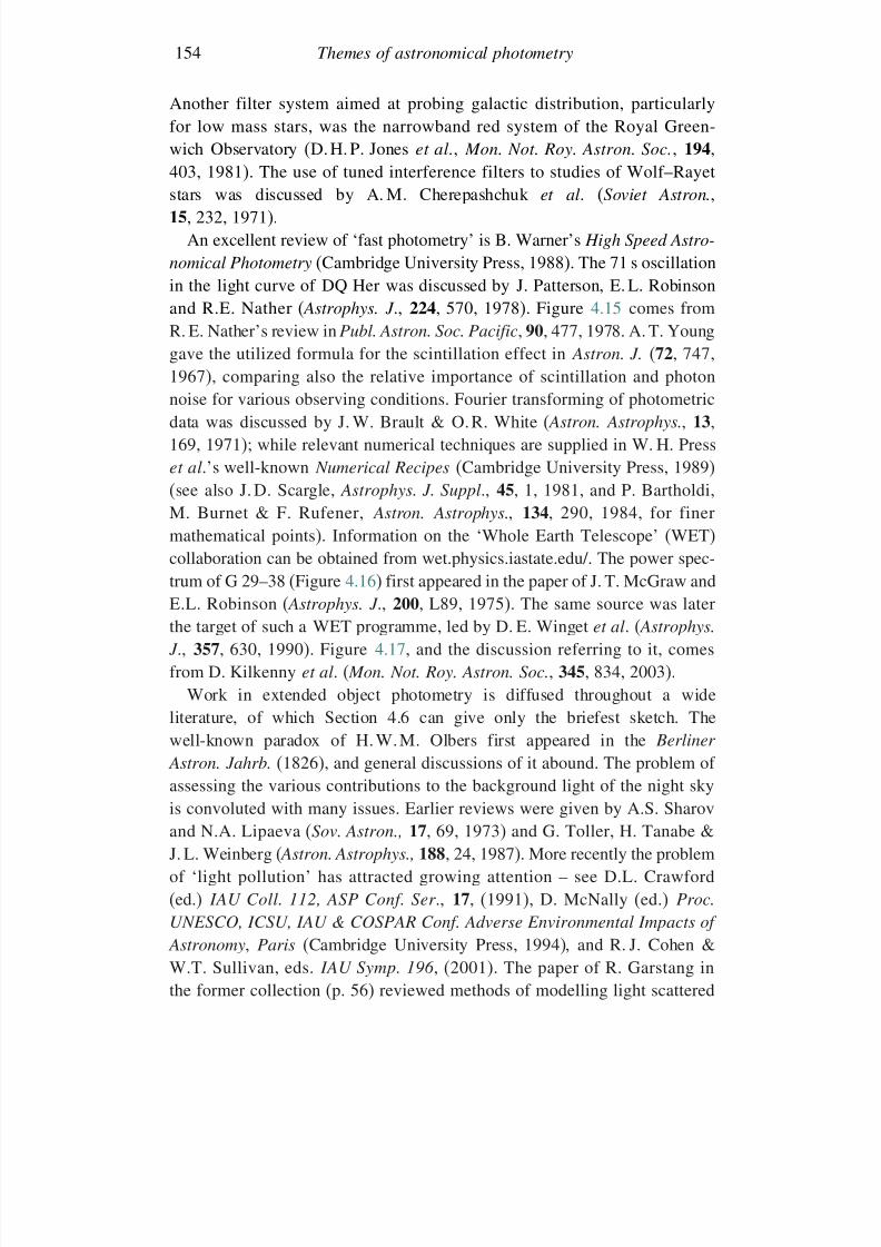
7/21/2019 Introduction to Astronomical Photometry
http://slidepdf.com/reader/full/introduction-to-astronomical-photometry 172/451
154 Themes of astronomical photometry
Another filter system aimed at probing galactic distribution, particularlyfor low mass stars, was the narrowband red system of the Royal Green-wich Observatory (D. H. P. Jones et al., Mon. Not. Roy. Astron. Soc., 194,
403, 1981). The use of tuned interference filters to studies of Wolf–Rayetstars was discussed by A. M. Cherepashchuk et al. (Soviet Astron.,15, 232, 1971).
An excellent review of ‘fast photometry’ is B. Warner’s High Speed Astro-
nomical Photometry (Cambridge University Press, 1988). The 71 s oscillationin the light curve of DQ Her was discussed by J. Patterson, E. L. Robinsonand R.E. Nather ( Astrophys. J ., 224, 570, 1978). Figure 4.15 comes from
R. E. Nather’s review in Publ. Astron. Soc. Pacific, 90, 477, 1978. A. T. Younggave the utilized formula for the scintillation effect in Astron. J. (72, 747,1967), comparing also the relative importance of scintillation and photonnoise for various observing conditions. Fourier transforming of photometricdata was discussed by J. W. Brault & O. R. White ( Astron. Astrophys., 13,169, 1971); while relevant numerical techniques are supplied in W. H. Presset al.’s well-known Numerical Recipes (Cambridge University Press, 1989)(see also J. D. Scargle, Astrophys. J. Suppl., 45, 1, 1981, and P. Bartholdi,
M. Burnet & F. Rufener, Astron. Astrophys., 134, 290, 1984, for finermathematical points). Information on the ‘Whole Earth Telescope’ (WET)collaboration can be obtained from wet.physics.iastate.edu/. The power spec-trum of G 29–38 (Figure 4.16) first appeared in the paper of J. T. McGraw andE.L. Robinson ( Astrophys. J ., 200, L89, 1975). The same source was laterthe target of such a WET programme, led by D. E. Winget et al. ( Astrophys.
J ., 357, 630, 1990). Figure 4.17, and the discussion referring to it, comes
from D. Kilkenny et al. ( Mon. Not. Roy. Astron. Soc., 345, 834, 2003).Work in extended object photometry is diffused throughout a wideliterature, of which Section 4.6 can give only the briefest sketch. Thewell-known paradox of H. W. M. Olbers first appeared in the Berliner
Astron. Jahrb. (1826), and general discussions of it abound. The problem of assessing the various contributions to the background light of the night skyis convoluted with many issues. Earlier reviews were given by A.S. Sharovand N.A. Lipaeva (Sov. Astron., 17, 69, 1973) and G. Toller, H. Tanabe &
J. L. Weinberg ( Astron. Astrophys., 188, 24, 1987). More recently the problemof ‘light pollution’ has attracted growing attention – see D.L. Crawford(ed.) IAU Coll. 112, ASP Conf. Ser ., 17, (1991), D. McNally (ed.) Proc.
UNESCO, ICSU, IAU & COSPAR Conf. Adverse Environmental Impacts of
Astronomy, Paris (Cambridge University Press, 1994), and R. J. Cohen &W.T. Sullivan, eds. IAU Symp. 196 , (2001). The paper of R. Garstang inthe former collection (p. 56) reviewed methods of modelling light scattered
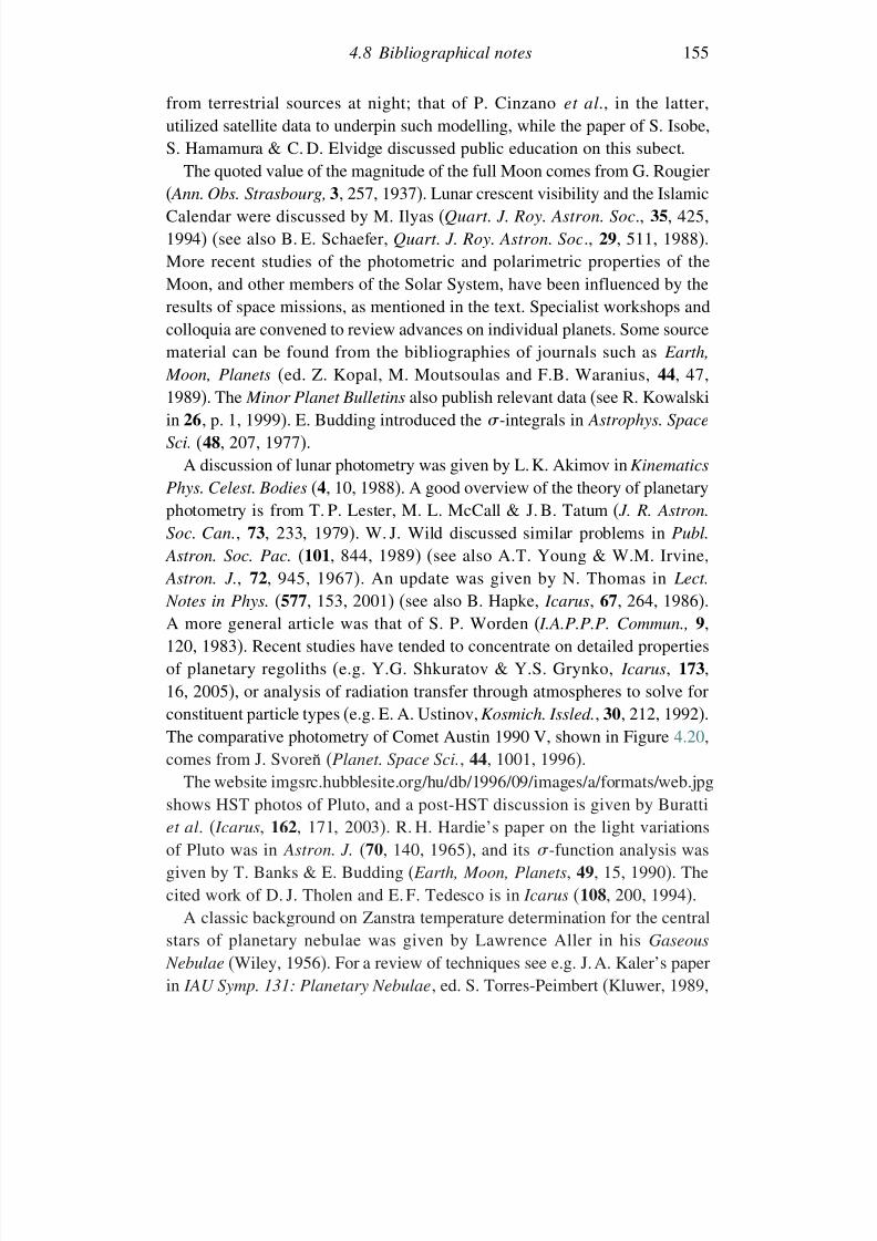
7/21/2019 Introduction to Astronomical Photometry
http://slidepdf.com/reader/full/introduction-to-astronomical-photometry 173/451
4.8 Bibliographical notes 155
from terrestrial sources at night; that of P. Cinzano et al., in the latter,utilized satellite data to underpin such modelling, while the paper of S. Isobe,S. Hamamura & C. D. Elvidge discussed public education on this subect.
The quoted value of the magnitude of the full Moon comes from G. Rougier( Ann. Obs. Strasbourg, 3, 257, 1937). Lunar crescent visibility and the IslamicCalendar were discussed by M. Ilyas (Quart. J. Roy. Astron. Soc., 35, 425,1994) (see also B. E. Schaefer, Quart. J. Roy. Astron. Soc., 29, 511, 1988).More recent studies of the photometric and polarimetric properties of theMoon, and other members of the Solar System, have been influenced by theresults of space missions, as mentioned in the text. Specialist workshops and
colloquia are convened to review advances on individual planets. Some sourcematerial can be found from the bibliographies of journals such as Earth,
Moon, Planets (ed. Z. Kopal, M. Moutsoulas and F.B. Waranius, 44, 47,1989). The Minor Planet Bulletins also publish relevant data (see R. Kowalskiin 26, p. 1, 1999). E. Budding introduced the -integrals in Astrophys. Space
Sci. (48, 207, 1977).A discussion of lunar photometry was given by L. K. Akimov in Kinematics
Phys. Celest. Bodies (4, 10, 1988). A good overview of the theory of planetary
photometry is from T. P. Lester, M. L. McCall & J. B. Tatum ( J. R. Astron.Soc. Can., 73, 233, 1979). W. J. Wild discussed similar problems in Publ.
Astron. Soc. Pac. (101, 844, 1989) (see also A.T. Young & W.M. Irvine, Astron. J., 72, 945, 1967). An update was given by N. Thomas in Lect.
Notes in Phys. (577, 153, 2001) (see also B. Hapke, Icarus, 67, 264, 1986).A more general article was that of S. P. Worden ( I.A.P.P.P. Commun., 9,120, 1983). Recent studies have tended to concentrate on detailed properties
of planetary regoliths (e.g. Y.G. Shkuratov & Y.S. Grynko, Icarus, 173,16, 2005), or analysis of radiation transfer through atmospheres to solve forconstituent particle types (e.g. E. A. Ustinov, Kosmich. Issled., 30, 212, 1992).The comparative photometry of Comet Austin 1990 V, shown in Figure 4.20,comes from J. Svoren (Planet. Space Sci., 44, 1001, 1996).
The website imgsrc.hubblesite.org/hu/db/1996/09/images/a/formats/web.jpgshows HST photos of Pluto, and a post-HST discussion is given by Burattiet al. ( Icarus, 162, 171, 2003). R. H. Hardie’s paper on the light variations
of Pluto was in Astron. J. (70, 140, 1965), and its -function analysis wasgiven by T. Banks & E. Budding ( Earth, Moon, Planets, 49, 15, 1990). Thecited work of D. J. Tholen and E. F. Tedesco is in Icarus (108, 200, 1994).
A classic background on Zanstra temperature determination for the centralstars of planetary nebulae was given by Lawrence Aller in his Gaseous
Nebulae (Wiley, 1956). For a review of techniques see e.g. J. A. Kaler’s paperin IAU Symp. 131: Planetary Nebulae, ed. S. Torres-Peimbert (Kluwer, 1989,
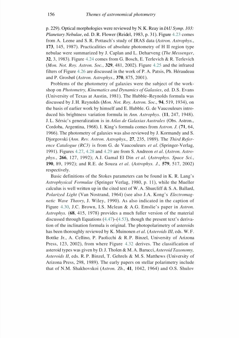
7/21/2019 Introduction to Astronomical Photometry
http://slidepdf.com/reader/full/introduction-to-astronomical-photometry 174/451
156 Themes of astronomical photometry
p. 229). Optical morphologies were reviewed by N. K. Reay in IAU Symp. 103:
Planetary Nebulae, ed. D. R. Flower (Reidel, 1983, p. 31). Figure 4.23 comesfrom A. Leene and S. R. Pottasch’s study of IRAS data ( Astron. Astrophys.,
173, 145, 1987). Practicalities of absolute photometry of H II region typenebulae were summarized by J. Caplan and L. Deharveng (The Messenger ,32, 3, 1983). Figure 4.24 comes from G. Bosch, E. Terlevich & R. Terlevich( Mon. Not. Roy. Astron. Soc., 329, 481, 2002). Figure 4.25 and the infraredfilters of Figure 4.26 are discussed in the work of P. A. Patsis, Ph. Héraudeauand P. Grosbøl ( Astron. Astrophys., 370, 875, 2001).
Problems of the photometry of galaxies were the subject of the work-
shop on Photometry, Kinematics and Dynamics of Galaxies, ed. D.S. Evans(University of Texas at Austin, 1981). The Hubble–Reynolds formula wasdiscussed by J. H. Reynolds ( Mon. Not. Roy. Astron. Soc., 94, 519, 1934), onthe basis of earlier work by himself and E. Hubble. G. de Vaucouleurs intro-duced his brightness variation formula in Ann. Astrophys. (11, 247, 1948).J. L. Sérsic’s generalization is in Atlas de Galaxias Australes (Obs. Astron.,Cordoba, Argentina, 1968). I. King’s formula comes from Astron. J. (71, 64,1966). The photometry of galaxies was also reviewed by J. Kormandy and S.
Djorgovski ( Ann. Rev. Astron. Astrophys., 27, 235, 1989). The Third Refer-ence Catalogue (RC3) is from G. de Vaucouleurs et al. (Springer-Verlag,1991). Figures 4.27, 4.28 and 4.29 are from S. Andreon et al. ( Astron. Astro-
phys., 266, 127, 1992); A.I. Gamal El Din et al. ( Astrophys. Space Sci.,190, 89, 1992); and R.E. de Souza et al. ( Astrophys. J., 579, 517, 2002)respectively.
Basic definitions of the Stokes parameters can be found in K. R. Lang’s
Astrophysical Formulae (Springer Verlag, 1980, p. 11), while the Muellercalculus is well written up in the cited text of W. A. Shurcliff & S. A. Ballard,Polarized Light (Van Nostrand, 1964) (see also J.A. Kong’s Electromag-
netic Wave Theory, J. Wiley, 1990). As also indicated in the caption of Figure 4.30, J.C. Brown, I.S. Mclean & A.G. Emslie’s paper in Astron.
Astrophys. (68, 415, 1978) provides a much fuller version of the materialdiscussed through Equations (4.47)–(4.53), though the present text’s deriva-tion of the inclination formula is original. The photopolarimetry of asteroids
has been thoroughly reviewed by K. Muinonen et al. ( Asteroids III , eds. W. F.Bottke Jr., A. Cellino, P. Paolicchi & R. P. Binzel, University of ArizonaPress, 123, 2002), from where Figure 4.32 derives. The classification of asteroid types was given by D. J. Tholen & M. A. Barucci, Asteroid Taxonomy,
Asteroids II , eds. R. P. Binzel, T. Gehrels & M. S. Matthews (University of Arizona Press, 298, 1989). The early papers on stellar polarimetry includethat of N.M. Shakhovskoi ( Astron. Zh., 41, 1042, 1964) and O.S. Shulov
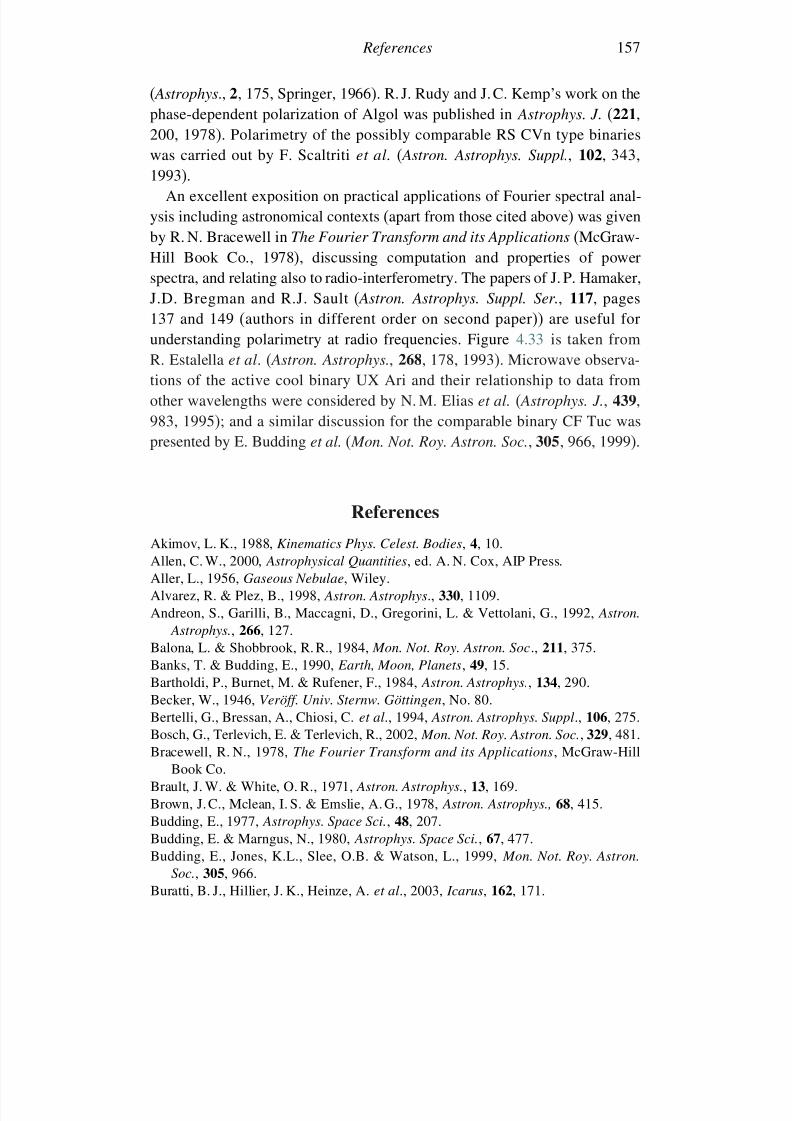
7/21/2019 Introduction to Astronomical Photometry
http://slidepdf.com/reader/full/introduction-to-astronomical-photometry 175/451
References 157
( Astrophys., 2, 175, Springer, 1966). R. J. Rudy and J. C. Kemp’s work on thephase-dependent polarization of Algol was published in Astrophys. J . (221,200, 1978). Polarimetry of the possibly comparable RS CVn type binaries
was carried out by F. Scaltriti et al. ( Astron. Astrophys. Suppl., 102, 343,1993).
An excellent exposition on practical applications of Fourier spectral anal-ysis including astronomical contexts (apart from those cited above) was givenby R. N. Bracewell in The Fourier Transform and its Applications (McGraw-Hill Book Co., 1978), discussing computation and properties of powerspectra, and relating also to radio-interferometry. The papers of J. P. Hamaker,
J.D. Bregman and R.J. Sault ( Astron. Astrophys. Suppl. Ser., 117, pages137 and 149 (authors in different order on second paper)) are useful forunderstanding polarimetry at radio frequencies. Figure 4.33 is taken fromR. Estalella et al. ( Astron. Astrophys., 268, 178, 1993). Microwave observa-tions of the active cool binary UX Ari and their relationship to data fromother wavelengths were considered by N. M. Elias et al. ( Astrophys. J., 439,983, 1995); and a similar discussion for the comparable binary CF Tuc waspresented by E. Budding et al. ( Mon. Not. Roy. Astron. Soc., 305, 966, 1999).
References
Akimov, L. K., 1988, Kinematics Phys. Celest. Bodies, 4, 10.Allen, C. W., 2000, Astrophysical Quantities, ed. A. N. Cox, AIP Press.Aller, L., 1956, Gaseous Nebulae, Wiley.Alvarez, R. & Plez, B., 1998, Astron. Astrophys., 330, 1109.
Andreon, S., Garilli, B., Maccagni, D., Gregorini, L. & Vettolani, G., 1992, Astron. Astrophys., 266, 127.
Balona, L. & Shobbrook, R. R., 1984, Mon. Not. Roy. Astron. Soc., 211, 375.Banks, T. & Budding, E., 1990, Earth, Moon, Planets, 49, 15.Bartholdi, P., Burnet, M. & Rufener, F., 1984, Astron. Astrophys., 134, 290.Becker, W., 1946, Veröff. Univ. Sternw. Göttingen, No. 80.Bertelli, G., Bressan, A., Chiosi, C. et al., 1994, Astron. Astrophys. Suppl., 106, 275.Bosch, G., Terlevich, E. & Terlevich, R., 2002, Mon. Not. Roy. Astron. Soc., 329, 481.Bracewell, R. N., 1978, The Fourier Transform and its Applications, McGraw-Hill
Book Co.Brault, J. W. & White, O. R., 1971, Astron. Astrophys., 13, 169.Brown, J. C., Mclean, I. S. & Emslie, A. G., 1978, Astron. Astrophys., 68, 415.Budding, E., 1977, Astrophys. Space Sci., 48, 207.Budding, E. & Marngus, N., 1980, Astrophys. Space Sci., 67, 477.Budding, E., Jones, K.L., Slee, O.B. & Watson, L., 1999, Mon. Not. Roy. Astron.
Soc., 305, 966.Buratti, B. J., Hillier, J. K., Heinze, A. et al., 2003, Icarus, 162, 171.
7/21/2019 Introduction to Astronomical Photometry
http://slidepdf.com/reader/full/introduction-to-astronomical-photometry 176/451
158 Themes of astronomical photometry
Caplan, J. & Deharveng, L., 1983, The Messenger , 32, 3.Cherepashchuk, A. M., Martynov, D. Y., Korolev, F. A., Klement’eva, A. Y.,
Meshcheryakova, T. F. & Esipov, V. F., 1971, Soviet Astron., 15, 232.Cinzano, P., Falchi, F., Elvidge, C.D. & Baugh, K.E., 2001, IAU Symp. 196 , eds.
R. J. Cohen and W. T. Sullivan, p. 95.Code, A. D., 1960, Stellar Atmospheres, ed. J. L. Greenstein, University of Chicago
Press, p. 50.Crawford, D. L., 1958, Astrophys. J., 128, 190.Crawford, D. L., 1966, IAU Symp. 24, ed. K. Lodén, L. O. Lodén and U. Sinnerstad,
Academic Press, p. 170.Crawford, D. L., 1969, Stellar Astronomy, eds. H.-Y. Chiu, R. L. Warasila &
J. L. Remo, Gordon & Breach, p. 73.
Crawford, D. L. & Mander, J., 1966, Astron. J., 71, 114.Crawford, D. L. & Barnes, J. V., 1970, Astron. J., 75, 978.de Souza, R. E., Viegas, S. M. & Gruenwald, R., 2002, Astrophys. J., 579, 517.de Vaucouleurs, G., 1948, Ann. Astrophys., 11, 247.de Vaucouleurs, G., de Vaucouleurs, A., Corwin, Jr., H. G., Buta, R. J., Paturel, G.
& Fouque, P., 1991, Third Reference Catalogue (RC3), Springer-Verlag.Dickow, P., Gyldenkerne, K., Hansen, L. Jacobsen, P. L., Johanson, K. T.,
Kjaergaard, P. & Olsen, E. H., 1970, Astron. Astrophys. Suppl. Ser ., 2, 1.Draine, B. T., 2003, Ann. Rev. Astron. Astrophys., 41, 241.
Elias, N. M., Quirrenbach, A., Witzel, A., Naundorf, C. E., Wegner, R., Guinan, E. F.& McCook, G. P., 1995, Astrophys. J., 439, 983.Estalella, R., Paredes, J.M., Rius, A., Marti, J. & Peracaula, M., 1993, Astron.
Astrophys., 268, 178.Evans, D. S. (ed.), 1981, Photometry, Kinematics and Dynamics of Galaxies, Univer-
sity of Texas, Austin.Fernie, J. D., 1965, Astron. J., 70, 575.Forbes, M. C., 1996, Ph.D. thesis, Victoria University, Wellington, New Zealand.Frazer, R. A., Duncan, W. J. & Collar, A. R., 1946, Elementary Matrices, Cambridge
University Press.Fukugita, M., Ichikawa, T., Gunn, J. E., Doi, M., Shimasaku, K. & Schneider, D. P.,
1996, Astron. J ., 111, 1748.Gamal El Din, A.I., Issa, I.A., Osman, A.M.I. & Kamal, F.Y., 1992, Astrophys.
Space Sci., 190, 89.Garstang, R., 1991, IAU Coll. 112, ASP Conf. Ser ., 17, ed. D. L. Crawford, p. 56.Golay, M., 1974, Introduction to Astronomical Photometry, Reidel.Golay, M., 1980, Vistas in Astronomy, 24, 141.Gunn, J.E. & Knapp, G.R., 1992, Astron. Soc. Pacific Conf. Ser., ed. T. Soifer,
43, 267.Hamaker, J. P., Bregman, J. D. & Sault, R. J., 1996, Astron. Astrophys. Suppl. Ser.,
117, 137.Hapke, B., 1986, Icarus, 67, 264.Hardie, R. H., 1965, Astron. J., 70, 140.Hayes, D. S. & Latham, D. W., 1975, Astrophys. J ., 197, 593.Herbig, G. H., 1995, Ann. Rev. Astron. Astrophys., 33, 19.Ilyas, M., 1994, Quart. J. Roy. Astron. Soc., 35, 425.
7/21/2019 Introduction to Astronomical Photometry
http://slidepdf.com/reader/full/introduction-to-astronomical-photometry 177/451
References 159
Isobe, S., Hamamura, S. & Elvidge, C. D., 2001, IAU Symp. 196 , eds. R. J. Cohen &W. T. Sullivan, p. 363.
Jaschek, C. & Jaschek, M., 1987, Classification of the Stars, Cambridge UniversityPress.
Johnson, H. L., 1965, Astrophys. J., 141, 923.Johnson, H. L., 1966, Ann. Rev. Astron. Astrophys., 4, 193.Johnson, H. L. & Morgan, W. W., 1953, Astrophys. J., 117, 313.Jones, D. H. P., Sinclair, J. E. & Alexander, J. B., 1981, Mon. Not. Roy. Astron. Soc.,
194, 403.Kaler, J.A., 1989, in IAU Symp. 131: Planetary Nebulae, ed. S. Torres-Peimbert,
Kluwer, p. 229.Kasten, F. & Young, A. T., 1989, Appl. Opt., 28, 4735.
Kenyon, S. J. and Hartmann, L., 1995, Astrophys. J. Suppl., 101, 117.Kilkenny, D., Reed, M. D., O’Donoghue, D. et al. (49 coauthors), 2003, Mon. Not.
Roy. Astron. Soc., 345, 834.King, I., 1966, Astron. J., 71, 64.Kong, J. A., 1990, Electromagnetic Wave Theory, J. Wiley.Kormandy, J. & Djorgovski, S., 1989, Ann. Rev. Astron. Astrophys., 27, 235.Kopal, Z., Moutsoulas, M. & Waranius, F. B., 1989, Earth, Moon, Planets, 44, 47.Kowalski, R., 1999, Minor Planet Bulletins, 26, 1.Kron, R.G., 1992, Progress in Telescope and Instrumentation Technologies, ESO
Conf. & Workshop Proceedings No. 42, ed. M. H. Ulrich, ESO, p. 635.Lang, K. R., 1980, Astrophysical Formulae, Springer-Verlag.Lanz, T., 1986, Astron. Astrophys. Suppl., 65, 195.Leene, A. & Pottasch, S. R., 1987, Astron. Astrophys., 173, 145.Lester, T. P., McCall, M. L. & Tatum, J. B., 1979, J. R. Astron. Soc. Can., 73, 233.Lindblad, B., 1922, Astrophys. J., 55, 85.Lockwood, G. W., 1972, Astrophys. J. Suppl., 24, 375.McGraw, J. T. & Robinson, E. L., 1975, Astrophys. J ., 200, L89.McNally, D. (ed.), 1994, Proc. UNESCO, ICSU, IAU & COSPAR Conf. Adverse
Environmental Impacts of Astronomy, Paris, Cambridge University Press.Moon, T. T., 1985, Commun. Univ. London Obs., No 78.Muinonen, K., Piironen, J., Shkuratov Yua. et al., 2002, Asteroids III , eds. W. F. Bottke
Jr., A. Cellino, P. Paolicchi & R. P. Binzel, University of Arizona Press, 123.Nather, R. E., 1978, Publ. Astron. Soc. Pacific, 90, 477.Neugebauer, G., Habing, H.J., Van Dainen, R. et al., 1984, Astrophys. J ., 278, L1.Nicolet, B., 1978, Astron. Astrophys. Suppl., 34, 1.Oke, J. B., 1960, Astrophys. J ., 131, 358.Oke, J. B., 1966, Proc. IAU Symp. 26 , ed. H. Hubenet, Academic Press, p. 3.
Oke, J. B. & Gunn, J. E., 1983, Astrophys. J ., 260, 713.Olbers, H. W. M., 1826, Berliner Astron. Jahrb., ed. C. F. E. Späthen, 110.Patsis, P. A., Héraudeau, Ph. & Grosbøl, P., 2001, Astron. Astrophys., 370, 875.Patterson, J., Robinson, E. L. & Nather, R. E., 1978, Astrophys. J ., 224, 570.Peña, J. H. & Peniche, R., 1994, Rev. Mex. Astron. Astrofis., 28, 139.Press, W. H., Flannery, B. P., Teukolsky, S. A. & Vetterling, W. T., 1989, Numerical
Recipes, Cambridge University Press.Reay, N. K., 1983, IAU Symp. 103, Planetary Nebulae, ed. D. R. Flower, Reidel, p. 31.
7/21/2019 Introduction to Astronomical Photometry
http://slidepdf.com/reader/full/introduction-to-astronomical-photometry 178/451
160 Themes of astronomical photometry
Reynolds, J. H., 1934, Mon. Not. Roy. Astron. Soc., 94, 519.Rougier, G., 1937, Ann. Obs. Strasbourg, 3, 257.Rudy, R. J., & Kemp, J. C., 1978, Astrophys. J ., 221, 200.Sault, R.J., Hamaker, J.P. & Bregman, J.D., 1996, Astron. Astrophys. Suppl. Ser.,
117, 149.Scaltriti, F., Piirola, V., Coyne, G. V., Koch, R. H., Elias, N. M. & Holenstein, B. D.,
1993, Astron. Astrophys. Suppl., 102, 343.Scargle, J. D., 1981, Astrophys. J. Suppl., 45, 1.Schaefer, B. E., 1988, Quart. J. Roy. Astron. Soc., 29, 511.Schaerer, D., Meynet, G., Maeder, A. et al., 1993, Astron. Astrophys. Suppl. Ser.,
98, 523.Schoenberg, E., 1929, Handbuch der Astrophysik , J. Springer, Berlin, 2, 268.
Sérsic, J. L., 1968, Atlas de Galaxias Australes, Obs. Astron., Cordoba, Argentina.Shakhovskoi, N. M., 1964, Astron. Zh., 41, 1042.Sharov, A. S. & Lipaeva, N. A., 1973, Sov. Astron., 17, 69.Shkuratov, Y. G. & Grynko, Y. S., 2005, Icarus, 173, 16.Shulov, O. S., 1966, Astrophysics, 2, 175, Springer.Shurcliff, W. A. & Ballard, S. A., 1964, Polarized Light , Van Nostrand.Stebbins, J. & Whitford, A. E., 1943, Astrophys. J., 98, 20.Straizys, V. L., 1970, Bull. Vilnius Astron. Obs., 28.Strömgren, B., 1966, Ann. Rev. Astron. Astrophys., 4, 443.
Svoren, J., 1996, Planet. Space Sci., 44, 1001.Tholen, D. J. and Barucci, M. A., 1989, Asteroid Taxonomy, Asteroids II , eds.R. P. Binzel, T. Gehrels, and M. S. Matthews, University of Arizona Press, 298.
Tholen, D. J. & Tedesco, E. F., 1994, Icarus, 108, 200.Thomas, N., 2001, Lect. Notes Phys., 577, 153.Toller, G., Tanabe, H. & and Weinberg, J. L., 1987, Astron. Astrophys., 188, 24.Ustinov, E. A., 1992, Kosmich. Issled., 30, 212.Warner, B., 1988, High Speed Astronomical Photometry, Cambridge University Press.Wilson, O.C. & Bappu, M.K.V., 1957, Astrophys. J., 125, 661.
Wild, W. J., 1989, Publ. Astron. Soc. Pac., 101, 844.Winget, D. E., Nather, R. E., Clemens, J. C. et al., 1990, Astrophys. J ., 357, 630.Wood, D. B., 1969, Astron. J , 74, 177.Worden, S. P., 1983, I.A.P.P.P. Commun., 9, 120.Wu, Z.-Y., Zhou, X., Ma, J., Jiang, Z.-J. & Chen, J.-S., 2005, Publ. Astron. Soc.
Pacific, 117, 32.Young, A. T., 1967, Astron. J., 72, 747.Young, A. T., 1969, Icarus, 11, 1.Young, A. T., 1976, Meth. Exp. Phys., 12A (Optical and Infrared, ed. M. L. Meeks),
Academic Press, p. 123.Young, A. T. & Irvine, W. M., 1967, Astron. J., 72, 945.Young, A. T., Milone, E. F. and Stagg, C. R., 1994, Astron. Astrophys., 105, 259.
7/21/2019 Introduction to Astronomical Photometry
http://slidepdf.com/reader/full/introduction-to-astronomical-photometry 179/451
5
Practicalities
5.1 Overview of basic instrumentation
Figure 5.1 schematizes the essential optical photometric system in its obser-vatory setting. At the heart of the system is the detector. The excitationof electrons responding to incident photons, whose acquired energy thenallows them to be registered in some way, forms the basis for practical flux
measurement in more or less all photometric systems. With this there hasbeen a continued trend towards more reliably linear, efficient and informativedetectors. The photocathode (photomultiplier) tube, a single channel, spatiallynon-resolving device, has been the simplest type of linear detector in generaluse. However, the advent of efficient areal detectors, bulk data-handlingfacilities and software improvements that can efficiently control observinginstruments, as well as process raw data into manageable form, have revo-lutionized ground-based astronomical photometry in the last decade or so.This was already evident from the widening new horizons of the previouschapter’s review, and will be reinforced as we progress. But our more imme-diate purpose is to draw out the practical groundwork on which useful datarelies. Overviewing this allows us to see how common elements in photon fluxmeasurement have developed, sometimes along new and separate paths, butwith generally parallel aims, often involving the same or similar principles.
Referring to the scheme of Figure 5.1, the optical arrangements in front
(foreoptics) are designed to direct suitably selected fluxes from astronomicalsources to the detector element. After electrons have been photo-energized,their activity is to be registered by appropriate electronics. As well as acounting operation, this involves dealing with and minimizing extraneouselectron activity not arising from the source of interest (‘noise’). We canexpect the whole photometer, foreoptics, detector and signal electronics, tobe in close communication with a computer.
161
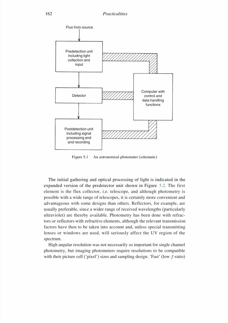
7/21/2019 Introduction to Astronomical Photometry
http://slidepdf.com/reader/full/introduction-to-astronomical-photometry 180/451
162 Practicalities
Postdetection unit
including signalprocessing andand recording
Detector
Predetection unitincluding lightcollection and
input
Flux from source
Computer withcontrol and
data handlingfunctions
Figure 5.1 An astronomical photometer (schematic)
The initial gathering and optical processing of light is indicated in theexpanded version of the predetector unit shown in Figure 5.2. The firstelement is the flux collector, i.e. telescope, and although photometry ispossible with a wide range of telescopes, it is certainly more convenient andadvantageous with some designs than others. Reflectors, for example, areusually preferable, since a wider range of received wavelengths (particularlyultraviolet) are thereby available. Photometry has been done with refrac-
tors or reflectors with refractive elements, although the relevant transmissionfactors have then to be taken into account and, unless special transmittinglenses or windows are used, will seriously affect the UV region of thespectrum.
High angular resolution was not necessarily so important for single channelphotometry, but imaging photometers require resolutions to be compatiblewith their picture cell (‘pixel’) sizes and sampling design. ‘Fast’ (low f -ratio)
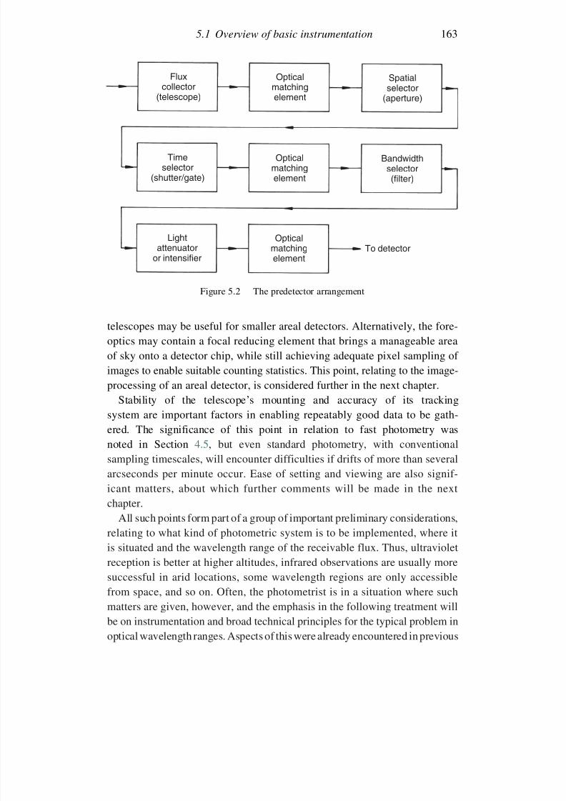
7/21/2019 Introduction to Astronomical Photometry
http://slidepdf.com/reader/full/introduction-to-astronomical-photometry 181/451
5.1 Overview of basic instrumentation 163
Fluxcollector
(telescope)
Opticalmatchingelement
Spatialselector
(aperture)
Bandwidthselector(filter)
Opticalmatchingelement
Timeselector
(shutter/gate)
Lightattenuator
or intensifier
Opticalmatchingelement
To detector
Figure 5.2 The predetector arrangement
telescopes may be useful for smaller areal detectors. Alternatively, the fore-optics may contain a focal reducing element that brings a manageable areaof sky onto a detector chip, while still achieving adequate pixel sampling of images to enable suitable counting statistics. This point, relating to the image-processing of an areal detector, is considered further in the next chapter.
Stability of the telescope’s mounting and accuracy of its trackingsystem are important factors in enabling repeatably good data to be gath-ered. The significance of this point in relation to fast photometry wasnoted in Section 4.5, but even standard photometry, with conventionalsampling timescales, will encounter difficulties if drifts of more than severalarcseconds per minute occur. Ease of setting and viewing are also signif-icant matters, about which further comments will be made in the nextchapter.
All such points form part of a group of important preliminary considerations,relating to what kind of photometric system is to be implemented, where it
is situated and the wavelength range of the receivable flux. Thus, ultravioletreception is better at higher altitudes, infrared observations are usually moresuccessful in arid locations, some wavelength regions are only accessiblefrom space, and so on. Often, the photometrist is in a situation where suchmatters are given, however, and the emphasis in the following treatment willbe on instrumentation and broad technical principles for the typical problem inoptical wavelength ranges. Aspects of this were already encountered in previous
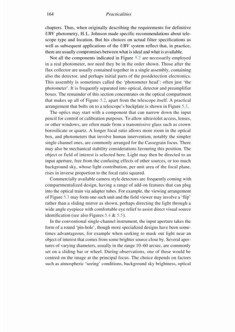
7/21/2019 Introduction to Astronomical Photometry
http://slidepdf.com/reader/full/introduction-to-astronomical-photometry 182/451
164 Practicalities
chapters. Thus, when originally describing the requirements for definitiveUBV photometry, H. L. Johnson made specific recommendations about tele-scope type and location. But his choices on actual filter specifications as
well as subsequent applications of the UBV system reflect that, in practice,there are usually compromises between what is ideal and what is available.
Not all the components indicated in Figure 5.2 are necessarily employedin a real photometer, nor need they be in the order shown. Those after theflux collector are usually contained together in a single assembly, containingalso the detector, and perhaps initial parts of the postdetection electronics.This assembly is sometimes called the ‘photometer head’: often just ‘the
photometer’. It is frequently separated into optical, detector and preamplifierboxes. The remainder of this section concentrates on the optical compartmentthat makes up all of Figure 5.2, apart from the telescope itself. A practicalarrangement that bolts on to a telescope’s backplate is shown in Figure 5.3.
The optics may start with a component that can narrow down the inputpencil for control or calibration purposes. To allow ultraviolet access, lenses,or other windows, are often made from a transmissive glass such as crownborosilicate or quartz. A longer focal ratio allows more room in the optical
box, and photometers that involve human intervention, notably the simplersingle channel ones, are commonly arranged for the Cassegrain focus. Theremay also be mechanical stability considerations favouring this position. Theobject or field of interest is selected here. Light may then be directed to aninput aperture, free from the confusing effects of other sources, or too muchbackground sky, whose light contribution, per unit area of the focal plane,rises in inverse proportion to the focal ratio squared.
Commercially available camera style detectors are frequently coming withcompartmentalized design, having a range of add-on features that can pluginto the optical train via adapter tubes. For example, the viewing arrangementof Figure 5.3 may form one such unit and the field viewer may involve a ‘flip’rather than a sliding mirror as shown, perhaps directing the light through awide angle eyepiece with comfortable eye relief to assist direct visual sourceidentification (see also Figures 5.4 & 5.5).
In the conventional single-channel instrument, the input aperture takes the
form of a round ‘pin-hole’, though more specialized designs have been some-times advantageous, for example when seeking to mask out light near anobject of interest that comes from some brighter source close by. Several aper-tures of varying diameters, usually in the range 10–60 arcsec, are commonlyset on a sliding bar or wheel. During observations, one of these would becentred on the image at the principal focus. The choice depends on factorssuch as atmospheric ‘seeing’ conditions, background sky brightness, optical
7/21/2019 Introduction to Astronomical Photometry
http://slidepdf.com/reader/full/introduction-to-astronomical-photometry 183/451
5.1 Overview of basic instrumentation 165
1
3
2
4
5
6
7
1. Filter wheel2. Field eyepiece3. Diaphragm slide4. Microscope eyepiece
5. Fabry lens6. Photomultiplier housing7. Filter wheel control box
Figure 5.3 Optical arrangement of a working photometer (as used on the 41cmRuthCrisp telescope of Caster Observatory, New Zealand; see Nield, 1987).
quality of the flux collector, accuracy of its tracking, or other circumstances,
but 20–30 arcsec is typical. Another form of controllable aperture is of theiris type. In stellar photometry it can be adjusted to suit varying seeing orbackground levels. It has also been very successfully applied to extendedsources (Section 4.5).
Single channel input may be subsequently analysed by more than onedetector in a ‘multi-beam’ arrangement (Figure 5.4). This differs from ‘multi-channel’ photometry, because there is more than one source aperture in the
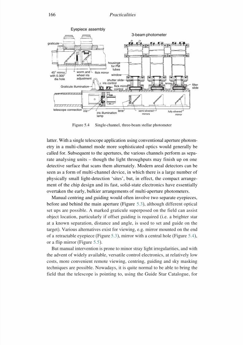
7/21/2019 Introduction to Astronomical Photometry
http://slidepdf.com/reader/full/introduction-to-astronomical-photometry 184/451
166 Practicalities
Eyepiece assembly3-beam photometer
45° mirrorwith 0.300"
dia hole
worm andwheel irisadjustment
flick mirror
housingsfor PMtubes
window
shutter slideiris control
flick mirrorcontrol
lenses filterslide
telescope connection
Graticule illumination
irisiris illuminationlamp
lens
graticule
semi-silveredmirrors
fully silveredmirror
Figure 5.4 Single-channel, three-beam stellar photometer
latter. With a single telescope application using conventional aperture photom-etry in a multi-channel mode more sophisticated optics would generally becalled for. Subsequent to the apertures, the various channels perform as sepa-rate analysing units – though the light throughputs may finish up on onedetective surface that scans them alternately. Modern areal detectors can beseen as a form of multi-channel device, in which there is a large number of physically small light-detection ‘sites’, but, in effect, the compact arrange-ment of the chip design and its fast, solid-state electronics have essentiallyovertaken the early, bulkier arrangements of multi-aperture photometers.
Manual centring and guiding would often involve two separate eyepieces,before and behind the main aperture (Figure 5.3), although different opticalset ups are possible. A marked graticule superposed on the field can assistobject location, particularly if offset guiding is required (i.e. a brighter starat a known separation, distance and angle, is used to set and guide on thetarget). Various alternatives exist for viewing, e.g. mirror mounted on the end
of a retractable eyepiece (Figure 5.3), mirror with a central hole (Figure 5.4),or a flip mirror (Figure 5.5).
But manual intervention is prone to minor stray light irregularities, and withthe advent of widely available, versatile control electronics, at relatively lowcosts, more convenient remote viewing, centring, guiding and sky maskingtechniques are possible. Nowadays, it is quite normal to be able to bring thefield that the telescope is pointing to, using the Guide Star Catalogue, for
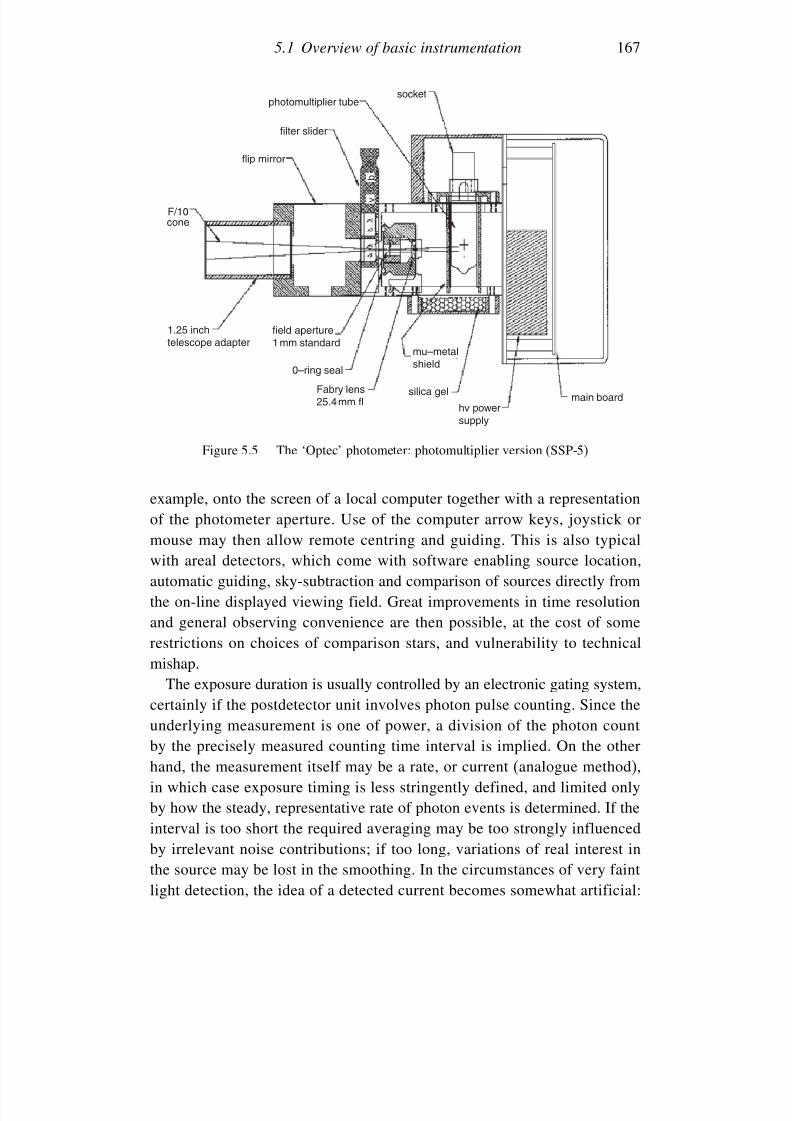
7/21/2019 Introduction to Astronomical Photometry
http://slidepdf.com/reader/full/introduction-to-astronomical-photometry 185/451
5.1 Overview of basic instrumentation 167
socketphotomultiplier tube
filter slider
flip mirror
F/10cone
1.25 inchtelescope adapter
field aperture1 mm standard
0–ring seal
mu–metalshield
silica gel
hv powersupply
main boardFabry lens25.4 mm fl
b
v
Figure 5.5 The ‘Optec’ photometer: photomultiplier version (SSP-5)
example, onto the screen of a local computer together with a representationof the photometer aperture. Use of the computer arrow keys, joystick ormouse may then allow remote centring and guiding. This is also typicalwith areal detectors, which come with software enabling source location,automatic guiding, sky-subtraction and comparison of sources directly fromthe on-line displayed viewing field. Great improvements in time resolutionand general observing convenience are then possible, at the cost of somerestrictions on choices of comparison stars, and vulnerability to technicalmishap.
The exposure duration is usually controlled by an electronic gating system,certainly if the postdetector unit involves photon pulse counting. Since theunderlying measurement is one of power, a division of the photon countby the precisely measured counting time interval is implied. On the other
hand, the measurement itself may be a rate, or current (analogue method),in which case exposure timing is less stringently defined, and limited onlyby how the steady, representative rate of photon events is determined. If theinterval is too short the required averaging may be too strongly influencedby irrelevant noise contributions; if too long, variations of real interest inthe source may be lost in the smoothing. In the circumstances of very faintlight detection, the idea of a detected current becomes somewhat artificial:
7/21/2019 Introduction to Astronomical Photometry
http://slidepdf.com/reader/full/introduction-to-astronomical-photometry 186/451
168 Practicalities
solid state detectors revert to the idea of storing collected photoelectrons inthe vicinity of an electrostatic anode, or potential well. Measurement issuesstill concern linearity of response and a sufficient scale of counts to enable
satisfactory signal to noise ratios from the statistics, however.The determination of an optimum gate becomes a critical matter in fast
photometry, where sources may be both rapidly varying and intrinsicallyfaint. In this particular context, the general information advantages of arealimaging are not so relevant. In fact, since areal read-outs inevitably takeconsiderably more time than single channel devices, their direct applica-tion to high-speed stellar monitoring would be non-optimal and relatively
inefficient.There are other tasks, however, e.g. (bright) standard star calibration, where
the selection of a gate time interval becomes less important. The neces-sary time-of-day specification can be conveniently signalled by the exposurestarter. A controlling computer would usually provide a stable and accuratereference clock, but a gate timer can be modified to yield elapsed timeafter a given initial signal. An external DC recorder can be similarly cali-brated against a reference clock, though nowadays it is much more normal tofind all data-handling operations centralized on a PC, equipped with suitablesoftware.
Frequently adopted integration times for general work are of the order of several seconds, though in fast photometry the interval may drop to f −1
s ,where f s is the rate of measurable photon events per second divided by aquantity related to the desired signal to noise ratio, i.e. S/N2 for Poissonianstatistics. This subject was discussed in Section 4.5, where it was mentioned
that the noise need not be simply Poissonian, and should involve more detailedconsiderations about the role of the atmosphere for planned programmesof fast photometry. Values of f −1
s as little as 10−3 seconds are found withbright stars and intermediate-sized telescopes. Of course, such a rate of datacollection quickly puts large demands on storage, as well as efficient highspeed data transfer, particularly if from an areal detector, so that appropriateelectronic arrangements to cover this point are required when rapid events
are being monitored (e.g. lunar occultations of stars).Optical matching beyond the aperture in Figure 5.2 means, for example,
beam collimation, since narrowband filters are designed to work with aparallel beam. Beam-splitting can also be performed here. The time reso-lution of narrowband photometry is optimized by simultaneous monitoringin the different spectral regions, i.e. two-beam photometry. The same argu-ment applies to photopolarimetry, where simultaneous comparison of different
7/21/2019 Introduction to Astronomical Photometry
http://slidepdf.com/reader/full/introduction-to-astronomical-photometry 187/451
5.1 Overview of basic instrumentation 169
polarization components of the light input is highly desirable, in view of theusually small scale of effects.
Recommendations on bandwidth selection, i.e. filter designs, are normally
provided in the original papers of system initiators, though, of course, thenet response functions are products of those of all agents involved in thelight throughput, including the atmosphere, flux collector and, particularly,the detector’s own spectral efficiency curve. In the case of well-used sets, likethe UBV , a great body of additional experience and alternative filter/detectorcombinations now exist. Developments in solid state detectors, for example,with their enhanced red sensitivity, have required extensive redesign of filters,
notably for the U , where the well-known red leak (mentioned in Section 3.6)introduces complications. Filters commonly come in sets of at least three units,and often the number is a half-dozen or more. For ease of computer controland light-tight optics, an internally mounted wheel, equipped with a position-registering switch, or encoder, is preferable. Six typical sized (25 mm) filtersare easily accommodated on a wheel of order 10 cm in diameter.
Apart from the different types of filter already discussed, a neutral densityfilter is sometimes employed, for example, to reduce the signal from bright
standard stars to manageable proportions compared to a programme star, orto test linearity of the measurement system. Conversely, it is also possible toarrange for photoelectronic image intensification prior to the main measuringcomponent for very faint objects. Care is required with either of these intro-ductions, which may lead to loss of accuracy. Light diminution, thoughperhaps convenient in some operations, must inevitably reduce the signal,and though the gross photon input S/N ratio may still be acceptable, some
component of potential interest may not be. Moreover, the signal reduction,or the form of its dependence on wavelength, may be imprecisely known.On the other hand, intensification, which essentially means re-imaging andtherefore implies areal detection, usually brings in some extra noise andperhaps loss of linearity, focusing, or other disadvantage. It would usuallybe implicit, however, that such disadvantage is offset by sky noise (or other)variation during the long integration period required for the measurement of unenhanced very faint sources.
The final optical matching element in the scheme of Figure 5.2 is the Fabrylens. Its purpose, usually applying to non-field-imaging or single channeldevices, is to image the entrance pupil of the flux collector on the detectorsurface (Section 2.2). A fixed patch of illumination is then maintained onthis surface. A wandering image on the detector surface, even if containing aconstant flux, would only produce a constant signal if the response functionwere perfectly constant over the surface. This is difficult to achieve for real
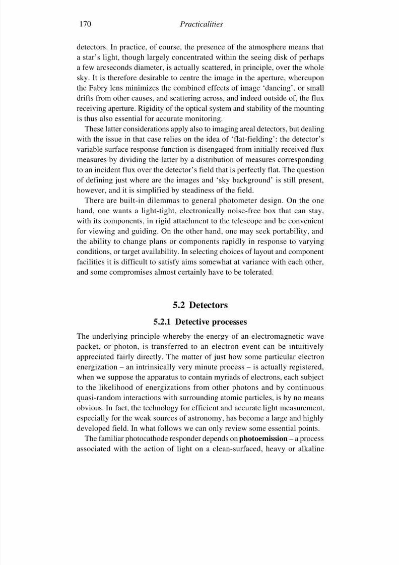
7/21/2019 Introduction to Astronomical Photometry
http://slidepdf.com/reader/full/introduction-to-astronomical-photometry 188/451
170 Practicalities
detectors. In practice, of course, the presence of the atmosphere means thata star’s light, though largely concentrated within the seeing disk of perhapsa few arcseconds diameter, is actually scattered, in principle, over the whole
sky. It is therefore desirable to centre the image in the aperture, whereuponthe Fabry lens minimizes the combined effects of image ‘dancing’, or smalldrifts from other causes, and scattering across, and indeed outside of, the fluxreceiving aperture. Rigidity of the optical system and stability of the mountingis thus also essential for accurate monitoring.
These latter considerations apply also to imaging areal detectors, but dealingwith the issue in that case relies on the idea of ‘flat-fielding’: the detector’svariable surface response function is disengaged from initially received fluxmeasures by dividing the latter by a distribution of measures correspondingto an incident flux over the detector’s field that is perfectly flat. The questionof defining just where are the images and ‘sky background’ is still present,however, and it is simplified by steadiness of the field.
There are built-in dilemmas to general photometer design. On the onehand, one wants a light-tight, electronically noise-free box that can stay,with its components, in rigid attachment to the telescope and be convenient
for viewing and guiding. On the other hand, one may seek portability, andthe ability to change plans or components rapidly in response to varyingconditions, or target availability. In selecting choices of layout and componentfacilities it is difficult to satisfy aims somewhat at variance with each other,and some compromises almost certainly have to be tolerated.
5.2 Detectors5.2.1 Detective processes
The underlying principle whereby the energy of an electromagnetic wavepacket, or photon, is transferred to an electron event can be intuitivelyappreciated fairly directly. The matter of just how some particular electronenergization – an intrinsically very minute process – is actually registered,when we suppose the apparatus to contain myriads of electrons, each subject
to the likelihood of energizations from other photons and by continuousquasi-random interactions with surrounding atomic particles, is by no meansobvious. In fact, the technology for efficient and accurate light measurement,especially for the weak sources of astronomy, has become a large and highlydeveloped field. In what follows we can only review some essential points.
The familiar photocathode responder depends on photoemission – a processassociated with the action of light on a clean-surfaced, heavy or alkaline
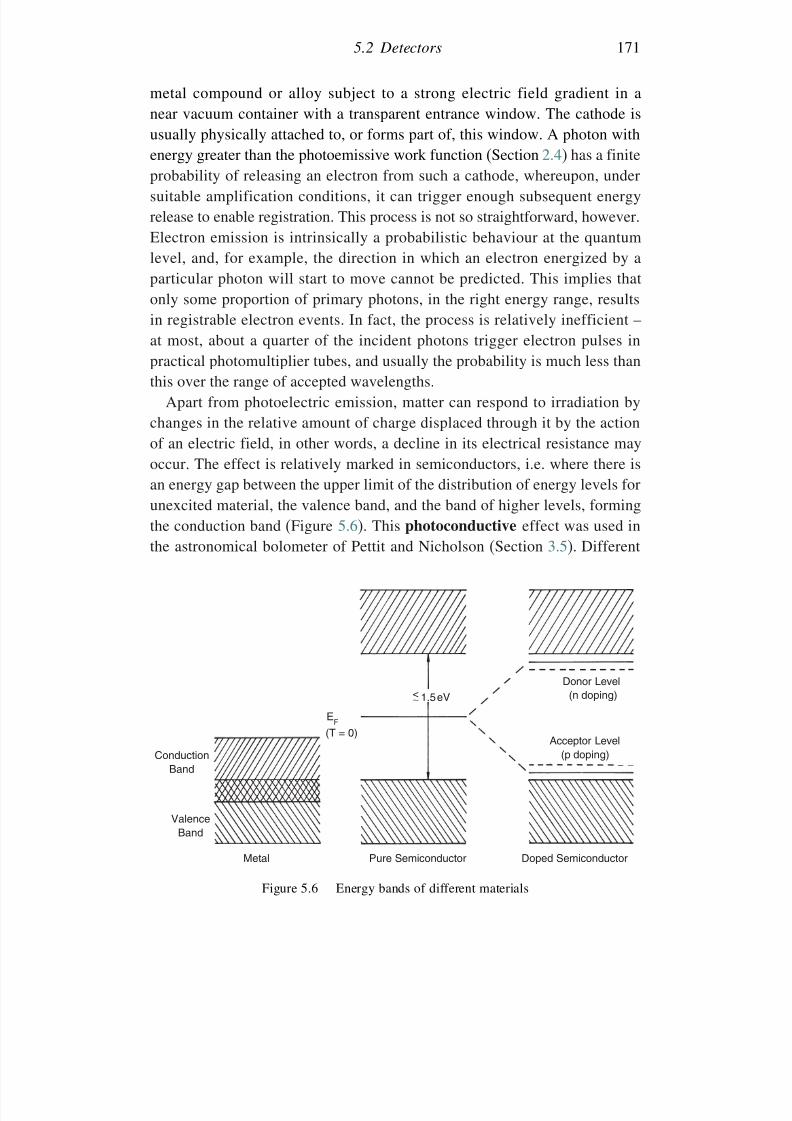
7/21/2019 Introduction to Astronomical Photometry
http://slidepdf.com/reader/full/introduction-to-astronomical-photometry 189/451
5.2 Detectors 171
metal compound or alloy subject to a strong electric field gradient in anear vacuum container with a transparent entrance window. The cathode isusually physically attached to, or forms part of, this window. A photon with
energy greater than the photoemissive work function (Section 2.4) has a finiteprobability of releasing an electron from such a cathode, whereupon, undersuitable amplification conditions, it can trigger enough subsequent energyrelease to enable registration. This process is not so straightforward, however.Electron emission is intrinsically a probabilistic behaviour at the quantumlevel, and, for example, the direction in which an electron energized by aparticular photon will start to move cannot be predicted. This implies that
only some proportion of primary photons, in the right energy range, resultsin registrable electron events. In fact, the process is relatively inefficient –at most, about a quarter of the incident photons trigger electron pulses inpractical photomultiplier tubes, and usually the probability is much less thanthis over the range of accepted wavelengths.
Apart from photoelectric emission, matter can respond to irradiation bychanges in the relative amount of charge displaced through it by the actionof an electric field, in other words, a decline in its electrical resistance may
occur. The effect is relatively marked in semiconductors, i.e. where there isan energy gap between the upper limit of the distribution of energy levels forunexcited material, the valence band, and the band of higher levels, formingthe conduction band (Figure 5.6). This photoconductive effect was used inthe astronomical bolometer of Pettit and Nicholson (Section 3.5). Different
Conduction
Band
ValenceBand
Metal Pure Semiconductor Doped Semiconductor
EF
(T = 0)
Donor Level(n doping)
Acceptor Level(p doping)
<∼ 1.5 eV
Figure 5.6 Energy bands of different materials
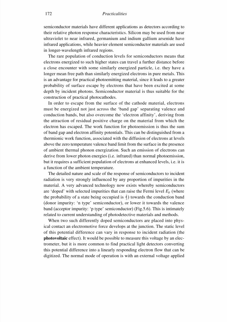
7/21/2019 Introduction to Astronomical Photometry
http://slidepdf.com/reader/full/introduction-to-astronomical-photometry 190/451
172 Practicalities
semiconductor materials have different applications as detectors according totheir relative photon response characteristics. Silicon may be used from nearultraviolet to near infrared, germanium and indium gallium arsenide have
infrared applications, while heavier element semiconductor materials are usedin longer-wavelength infrared regions.
The rare population of conduction levels for semiconductors means thatelectrons energized to such higher states can travel a further distance beforea close encounter with some similarly energized particle, i.e. they have alonger mean free path than similarly energized electrons in pure metals. Thisis an advantage for practical photoemitting material, since it leads to a greater
probability of surface escape by electrons that have been excited at somedepth by incident photons. Semiconductor material is thus suitable for theconstruction of practical photocathodes.
In order to escape from the surface of the cathode material, electronsmust be energized not just across the ‘band gap’ separating valence andconduction bands, but also overcome the ‘electron affinity’, deriving fromthe attraction of residual positive charge on the material from which theelectron has escaped. The work function for photoemission is thus the sum
of band gap and electron affinity potentials. This can be distinguished from athermionic work function, associated with the diffusion of electrons at levelsabove the zero temperature valence band limit from the surface in the presenceof ambient thermal phonon energization. Such an emission of electrons canderive from lower photon energies (i.e. infrared) than normal photoemission,but it requires a sufficient population of electrons at enhanced levels, i.e. it isa function of the ambient temperature.
The detailed nature and scale of the response of semiconductors to incidentradiation is very strongly influenced by any proportion of impurities in thematerial. A very advanced technology now exists whereby semiconductorsare ‘doped’ with selected impurities that can raise the Fermi level E F (wherethe probability of a state being occupied is 1
2 ) towards the conduction band(donor impurity: ‘n type’ semiconductor), or lower it towards the valenceband (acceptor impurity: ‘p type’ semiconductor) (Fig.5.6). This is intimatelyrelated to current understanding of photodetective materials and methods.
When two such differently doped semiconductors are placed into phys-ical contact an electromotive force develops at the junction. The static levelof this potential difference can vary in response to incident radiation (thephotovoltaic effect). It would be possible to measure this voltage by an elec-trometer, but it is more common to find practical light detectors convertingthis potential difference into a linearly responding electron flow that can bedigitized. The normal mode of operation is with an external voltage applied
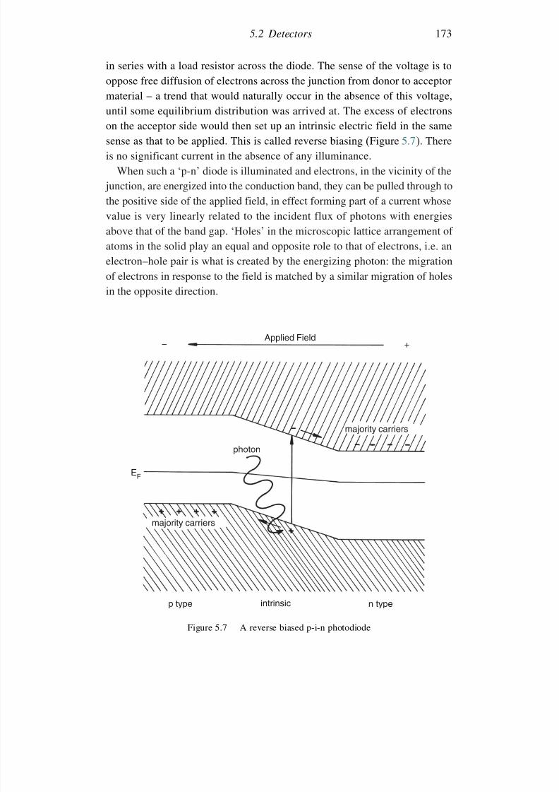
7/21/2019 Introduction to Astronomical Photometry
http://slidepdf.com/reader/full/introduction-to-astronomical-photometry 191/451
5.2 Detectors 173
in series with a load resistor across the diode. The sense of the voltage is tooppose free diffusion of electrons across the junction from donor to acceptormaterial – a trend that would naturally occur in the absence of this voltage,
until some equilibrium distribution was arrived at. The excess of electronson the acceptor side would then set up an intrinsic electric field in the samesense as that to be applied. This is called reverse biasing (Figure 5.7). Thereis no significant current in the absence of any illuminance.
When such a ‘p-n’ diode is illuminated and electrons, in the vicinity of the junction, are energized into the conduction band, they can be pulled through tothe positive side of the applied field, in effect forming part of a current whose
value is very linearly related to the incident flux of photons with energiesabove that of the band gap. ‘Holes’ in the microscopic lattice arrangement of atoms in the solid play an equal and opposite role to that of electrons, i.e. anelectron–hole pair is what is created by the energizing photon: the migrationof electrons in response to the field is matched by a similar migration of holesin the opposite direction.
Applied Field
majority carriers
majority carriers
photon
EF
p type intrinsic n type
– +
Figure 5.7 A reverse biased p-i-n photodiode
7/21/2019 Introduction to Astronomical Photometry
http://slidepdf.com/reader/full/introduction-to-astronomical-photometry 192/451
174 Practicalities
The inclusion of a layer of intrinsic or undoped semiconductor materialbetween acceptor and donor (n type) regions results in a ‘p-i-n’ diode. Thishas an effectively extended energization cross-section over the simple junc-
tion, particularly at longer wavelengths, as well as a relatively faster responsetime. Such diodes, as robust, light-weight and inexpensive detectors, notrequiring high voltages, have been usefully applied to astronomical photom-etry. However, though they give better access to the near infrared, they tendto be relatively noisy as visible region detectors compared with photomulti-plier tubes. This is essentially because of the inherent information advantageproduced by the secondary emission cascade gain.
If the reverse bias voltage is made high enough an electron that crosses tothe acceptor material may, through the energy of its impact, trigger a flowdown the potential slope of the bias field or an ‘avalanche’ effect, reminiscentof the cascade effect in photomultipliers. The gain, typically in the orderof hundreds, increases with increasing applied voltage, resulting in higherphoton sensitivity. Greater stringency then applies in limiting the input to lowfluxes and efficient temperature control systems are required to maintain highperformance.
Still higher gains are possible, though still in solid-state detectors, fromphototransistors. In the bipolar version, it is the base-collector junction thatis the light-sensitive element. Owing to the inherent current gain, whichthe transistor derives on the base current, high light sensitivity ensues. The‘field effect phototransistor’ (photo-FET) utilizes the photovoltaic effect inthe channel region as the basis of its amplification. Extremely high (‘singlephoton’) detections can then be enabled.
Practical photocathodes in tube photoemission devices are often made of p type material, i.e. with the Fermi level closer to the valence band, whichnow has additional acceptor levels above it. The population of these acceptorlevels can give rise to a noticeable red-leak in the cathode response function.This population is strongly temperature dependent, as well as critically relatedto impurity concentration. This entails individual variation in red responsefrom cathode to cathode depending on operating temperature – a point of significance to photoemission-based photometry at longer wavelengths and
its reduction procedure.Electron energization in semiconductor material is also basic to electronic
areal detection, or imaging. This may take the form of a suitably contrivedarray of small photodetection sites formed on a demarcated and controllablesubstrate, as in a charge coupled device (CCD), or it may involve the rapidsequential scanning of the electric potential distribution on a photoresponsivetarget, as with a television camera. In either case one seeks a low-noise
7/21/2019 Introduction to Astronomical Photometry
http://slidepdf.com/reader/full/introduction-to-astronomical-photometry 193/451
5.2 Detectors 175
mapping of an areal flux distribution into a corresponding, linearly dependentdistribution of electron concentrations that can be faithfully read out. Althoughconsiderable complexity may then be introduced in dealing with the greatly
increased amount of data, the underlying detection principles are basicallysimilar to those of single channel units.
5.2.2 Detector characteristics
The practicalities of astronomical (weak) signal detection raise the questionof detector quantum efficiency. This may be defined as,
Q = number of registered events/incident photon (5.1)We commonly find a Poissonian distribution of registrations, so that the noisein either input or output signals is proportional to the square root of the signal,which is thus also proportional to the signal to noise ratio S/N. A similarefficiency measure to Q is sometimes called responsivity R. This gives thedetector output per unit of input power, generally in non-quantized unitssuch as amperes/watt or volts/watt, depending on the nature of the output.
In comparing Q and R, the frequency dependence of the energy of a photonh, cf. (2.3), should be kept in mind, i.e. Q ∝ R.
Another useful parameter of performance may be introduced, which wecall the information transfer efficiency E , given as
E = S/N2out/S/N2
in (5.2)
In an ideal situation, one would find S/Nout = QS/√
QSin, and so E = Q
for the detective process. In practice, E ≤
Q, because additional processes,irrelevant to detection, add into the output noise N out, and correspondinglyreduce S/Nout. A reduction of E from Q also results from non-uniformityin the weighting of registered photon events from a uniform input.
A more direct indicator of noise is the noise equivalent power N EP, definedas the optical power producing an output equal to the noise level of thedetector. Noise depends on the square root of the receiver’s bandwidth , sothe N EP may be given as so many watts per (root) Hz. The relevant equation
can be seen to beN EP = fA
S/N1/2 (5.3)
where f is the incident flux on a detector area A. From (5.3) it follows thatthe lower the value of the N EP, the better the detection of low signals.
For convenient detection one seeks a linear responder, i.e. linearity.Although the photoelectric effect is at the root of the silver halide grain
7/21/2019 Introduction to Astronomical Photometry
http://slidepdf.com/reader/full/introduction-to-astronomical-photometry 194/451
176 Practicalities
darkening that takes place in photographic emulsions, the variety of additionalprocesses leading to the final state of a photographic plate or film tendsto make the net registration rather non-linear. In general, we characterize
linearity as the slope of the curve of accumulated registered events versusthe number of accumulated incident photon events at the same surface.Where there is a continuous, quasi-instantaneous registration of events (e.g.a photocathode) any particular registration will be independent of previousones, and thus tend to produce linear detection. Where an accumulation of events can interact at a detection site prior to final registration, as with aphotographic emulsion or CCD, the likelihood of non-linearities increases.
In any case, there will be some lower level, below which noise impedesperformance. Above this level we may ask about the event capacity of a detection site, i.e. how many events can be usefully accumulated beforesome saturation effect, either from the detector itself or from the associatedregistration system, starts to impede linearity? Also there is the working range
(sometimes called dynamic range) – essentially the same as event capacityfor a noiseless accumulative single detector, but more generally interpretedas the difference between useful maximum and minimum event counts.
Quasi-instantaneous detection was mentioned, but, in fact, it takes a finitetime for the output from a device to reach a steady registration sequence. Theterm response time usually refers to the time it takes a detector current torise to a value of 1 − 1/e (632%) of its steady-state value. A recovery time
similarly measures a fall to 1/ e of the steady-state value after the removal of illumination. Alternatively, a rise time may refer to the time interval between10% and 90% of peak response, when a detector receives an illumination step
function. There is a corresponding fall time involving the same fractions afterlight removal, though fall and rise times may be different numerically. Thesetimes are associated with the movements of photon-energized charge carrierswithin the detector material and the capacitance and resistance associated withthe measuring circuit. A low load resistance will allow fast response times,while high measurement sensitivity requires a high load resistance, hencethe choice depends on what application the arrangement is designed for. We
consider some numerical values in Section 5.3. Manufacturers may quoteoptimum rise times that relate to minimal circuit stray capacitance and lowcomponent resistance values. Maximum usable signal (i.e. before damagemay occur) is another manufacturer’s datum that a user should be aware of.
The role of spectral response was already met in previous chapters. Asmentioned above, different detector materials will be responsive in differentregions of the spectrum, according to their work-functions. The properties of
7/21/2019 Introduction to Astronomical Photometry
http://slidepdf.com/reader/full/introduction-to-astronomical-photometry 195/451
5.2 Detectors 177
particular types, e.g. S20, GaAs, InGaAs, should be consulted in connectionwith planned observation programmes.
For areal detectors, such as CCDs, one seeks information on pixel size that
should be comparable to telescopic resolution in the focal plane, and the totalnumber of pixels and their geometric organization by the controlling software.A distinction can be made between pixel size, as determined by the software,and detection-site size, which is less than or equal to pixel size. Aspects of image software control relevant to photometry will be dealt with later.
Detector parameters such as quantum efficiency, linearity, event capacityand so on, are often characterized by figures of merit, which manufacturers
quote about their products. Such data may, however, be cited in relation tovery specific technical applications, such as laser light detection in scanningmachines, so a prospective user or buyer should keep the envisaged applicationin mind in perusing data. N EP, for instance, includes the detector area: onedetector may have lower N EP than another simply because of a lower area,regardless of the basic detective quality of the material per unit area.
5.2.3 Photomultiplier tubesThe advance in design of photomultiplier tubes over pre-existent cell typesessentially concerns the multiplier system of secondary emission electrodes,mounted in the same near-vacuum container as the cathode and anode. Thesecondary dynodes are arranged in a series, each one at an electrostaticpotential of around 100 V higher than its predecessor. The first dynode, at whichspecial arrangements are sometimes included to maximize photometric effi-
ciency, is at a similar potential above the cathode. It attracts electrons releasedfrom the cathode, but after impinging on the dynode surface with sufficientkinetic energy each such electron releases several more toward the followingdynode. The process is repeated perhaps a dozen times along the dynode chain.In this way, large numbers of electrons are produced as pulses in responseto photon incidence, and are thus significantly more measurable against thebackground of quasi-random thermal energizations in the measuring system.SomeexamplesofdifferentdesignsofphotomultipliersareshowninFigure5.8.
The voltages along the dynode chain are maintained by a divider, usuallyin the form of a series of high-quality resistors mounted across relevantpins of the photomultiplier base. This resistive chain, in parallel with thedynamic resistance of the tube itself, involves a compromise on the choiceof component values. Too high resistances in the chain would mean that thecurrent could start to become comparable to that of the tube at high photonincidence. Hence the dynode voltages would be reduced somewhat, leading
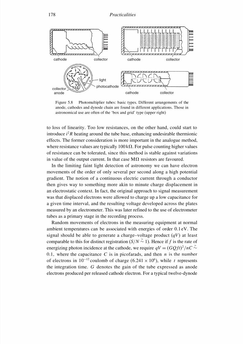
7/21/2019 Introduction to Astronomical Photometry
http://slidepdf.com/reader/full/introduction-to-astronomical-photometry 196/451
178 Practicalities
cathode cathode
cathode
collector collector
collector
collector
anode
light
photocathode
Figure 5.8 Photomultiplier tubes: basic types. Different arrangements of theanode, cathodes and dynode chain are found in different applications. Those inastronomical use are often of the ‘box and grid’ type (upper right)
to loss of linearity. Too low resistances, on the other hand, could start tointroduce i2R heating around the tube base, enhancing undesirable thermionic
effects. The former consideration is more important in the analogue method,where resistance values are typically 100 k. For pulse counting higher valuesof resistance can be tolerated, since this method is stable against variationsin value of the output current. In that case M resistors are favoured.
In the limiting faint light detection of astronomy we can have electronmovements of the order of only several per second along a high potentialgradient. The notion of a continuous electric current through a conductorthen gives way to something more akin to minute charge displacement inan electrostatic context. In fact, the original approach to signal measurementwas that displaced electrons were allowed to charge up a low capacitance fora given time interval, and the resulting voltage developed across the platesmeasured by an electrometer. This was later refined to the use of electrometertubes as a primary stage in the recording process.
Random movements of electrons in the measuring equipment at normalambient temperatures can be associated with energies of order 0.1 eV. The
signal should be able to generate a charge–voltage product (qV ) at leastcomparable to this for distinct registration (S/N
>∼ 1). Hence if f is the rate of energizing photon incidence at the cathode, we require qV = GQft2/nC
>∼01 where the capacitance C is in picofarads, and then n is the numberof electrons in 10−12 coulomb of charge (6241 × 106), while t representsthe integration time. G denotes the gain of the tube expressed as anodeelectrons produced per released cathode electron. For a typical twelve-dynode
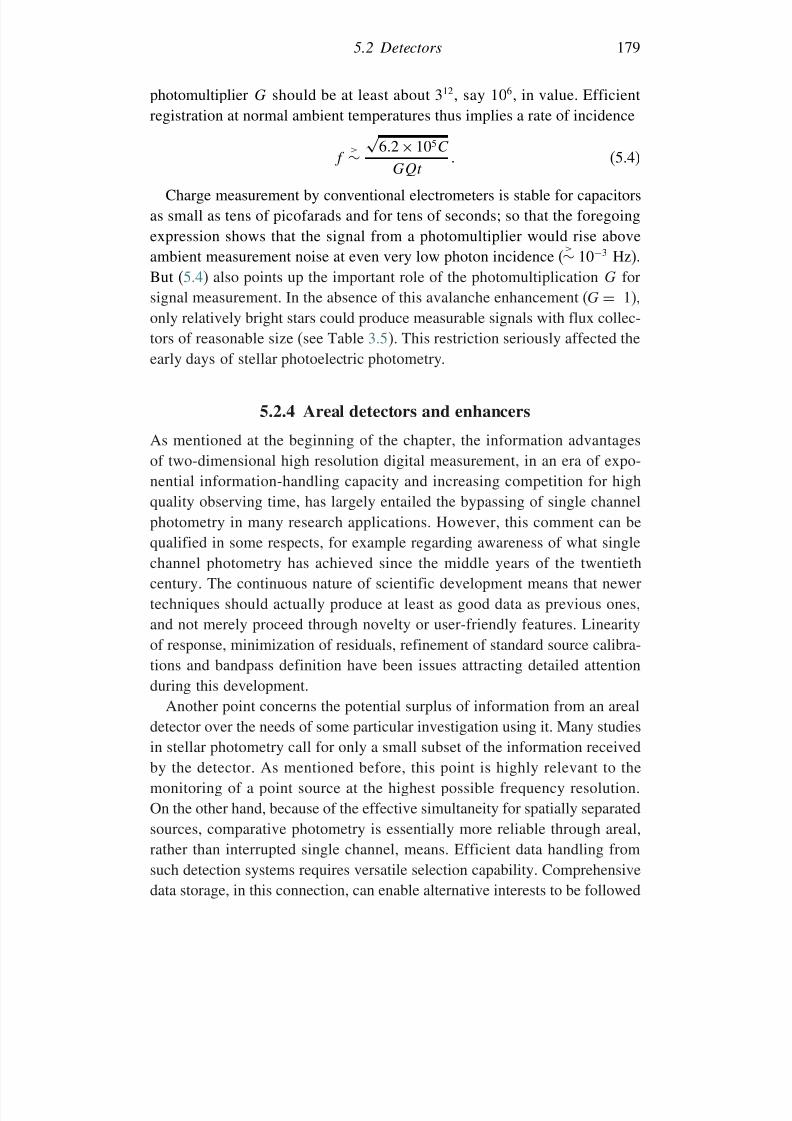
7/21/2019 Introduction to Astronomical Photometry
http://slidepdf.com/reader/full/introduction-to-astronomical-photometry 197/451
5.2 Detectors 179
photomultiplier G should be at least about 312, say 106, in value. Efficientregistration at normal ambient temperatures thus implies a rate of incidence
f >∼√
62 × 105
C GQt
(5.4)
Charge measurement by conventional electrometers is stable for capacitorsas small as tens of picofarads and for tens of seconds; so that the foregoingexpression shows that the signal from a photomultiplier would rise aboveambient measurement noise at even very low photon incidence (
>∼ 10−3 Hz).But (5.4) also points up the important role of the photomultiplication G for
signal measurement. In the absence of this avalanche enhancement (G = 1),only relatively bright stars could produce measurable signals with flux collec-tors of reasonable size (see Table 3.5). This restriction seriously affected theearly days of stellar photoelectric photometry.
5.2.4 Areal detectors and enhancers
As mentioned at the beginning of the chapter, the information advantages
of two-dimensional high resolution digital measurement, in an era of expo-nential information-handling capacity and increasing competition for highquality observing time, has largely entailed the bypassing of single channelphotometry in many research applications. However, this comment can bequalified in some respects, for example regarding awareness of what singlechannel photometry has achieved since the middle years of the twentiethcentury. The continuous nature of scientific development means that newer
techniques should actually produce at least as good data as previous ones,and not merely proceed through novelty or user-friendly features. Linearityof response, minimization of residuals, refinement of standard source calibra-tions and bandpass definition have been issues attracting detailed attentionduring this development.
Another point concerns the potential surplus of information from an arealdetector over the needs of some particular investigation using it. Many studiesin stellar photometry call for only a small subset of the information received
by the detector. As mentioned before, this point is highly relevant to themonitoring of a point source at the highest possible frequency resolution.On the other hand, because of the effective simultaneity for spatially separatedsources, comparative photometry is essentially more reliable through areal,rather than interrupted single channel, means. Efficient data handling fromsuch detection systems requires versatile selection capability. Comprehensivedata storage, in this connection, can enable alternative interests to be followed
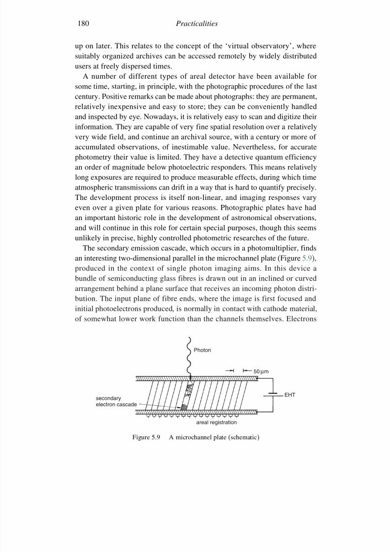
7/21/2019 Introduction to Astronomical Photometry
http://slidepdf.com/reader/full/introduction-to-astronomical-photometry 198/451
180 Practicalities
up on later. This relates to the concept of the ‘virtual observatory’, wheresuitably organized archives can be accessed remotely by widely distributedusers at freely dispersed times.
A number of different types of areal detector have been available forsome time, starting, in principle, with the photographic procedures of the lastcentury. Positive remarks can be made about photographs: they are permanent,relatively inexpensive and easy to store; they can be conveniently handledand inspected by eye. Nowadays, it is relatively easy to scan and digitize theirinformation. They are capable of very fine spatial resolution over a relativelyvery wide field, and continue an archival source, with a century or more of
accumulated observations, of inestimable value. Nevertheless, for accuratephotometry their value is limited. They have a detective quantum efficiencyan order of magnitude below photoelectric responders. This means relativelylong exposures are required to produce measurable effects, during which timeatmospheric transmissions can drift in a way that is hard to quantify precisely.The development process is itself non-linear, and imaging responses varyeven over a given plate for various reasons. Photographic plates have hadan important historic role in the development of astronomical observations,
and will continue in this role for certain special purposes, though this seemsunlikely in precise, highly controlled photometric researches of the future.
The secondary emission cascade, which occurs in a photomultiplier, findsan interesting two-dimensional parallel in the microchannel plate (Figure 5.9),produced in the context of single photon imaging aims. In this device abundle of semiconducting glass fibres is drawn out in an inclined or curvedarrangement behind a plane surface that receives an incoming photon distri-
bution. The input plane of fibre ends, where the image is first focused andinitial photoelectrons produced, is normally in contact with cathode material,of somewhat lower work function than the channels themselves. Electrons
Photon
secondaryelectron cascade
areal registration
EHT
50 µm
Figure 5.9 A microchannel plate (schematic)
7/21/2019 Introduction to Astronomical Photometry
http://slidepdf.com/reader/full/introduction-to-astronomical-photometry 199/451
5.2 Detectors 181
liberated by the photon incidence then avalanche down the fibre, in responseto an accelerating field of typically several kilovolts, and repeated incidenceson the fibre wall. Gains in excess of 106 can be produced in this way. The
anode array at the other end of the fibres may drive a two-dimensional photon-counting logger, or a phosphor screen upon which an intensified image isproduced. The technical requirements of the microchannel plate, particularlywith regard to channel evacuation and the application of high voltages, makefor a somewhat delicate and expensive device.
Image intensifiers, in general, need not employ the secondary emissionfeature of the microchannel plate. They may simply utilize the energizationof photoelectrons by a strong electric field in a focused flight from cathode toanode (Figure 5.10). The accelerated electrons impinge upon a phosphor screentarget where the intensified image is formed. Optical fibres may be used toreproduce this image, normally formed on a curved surface, into a convenientlyflat format. Commercially available intensifiers can be made quite robust, andare able to be cascaded in several stages. Operating voltages are inevitablyhigh, however, since this provides the basic source of intensification. This cangive rise to operational awkwardness in typical dome observing conditions.
The development and availability of television type cameras raises interestin their application to astronomical work, where various related instrumen-tation appeared – for example, the Image Photon Counting System (IPCS),developed at University College, London. Photons incident on a front-mounted photocathode resulted in electron emission events whose detectionwas assisted by a Thorne-EMITM image intensifier utilizing a cascade ampli-fication principle. The IPCS has been used for observations of limiting S/N
conditions, particularly with high dispersion spectroscopy of faint objects.It was employed at the Isaac Newton Telescope on the island of La Palma
Photocathode
InputFibreOptic Anode
Phosphor
OutputFibreOptic
Figure 5.10 An electrostatically focused image tube

7/21/2019 Introduction to Astronomical Photometry
http://slidepdf.com/reader/full/introduction-to-astronomical-photometry 200/451
182 Practicalities
in the Canary Islands from 1984 until 1992. The arrangement for recordingthe areal structure of an image employed a Vidicon camera and a digitalimage processing unit based on a 15 m pixel size. A later version involved
a CCD back-end that could process an area of up to 2400×3200 pixels, of size 12 m. Another version, employing a microchannel plate front-end, wasused with the Queens University of Belfast échelle spectrograph, also at LaPalma observatory. A full discussion of this technology is outside the scopeof this book: there are a couple of points that can be made here, however.
Firstly, vacuum tube imaging detection necessitates two stages of electroninformation transfer, firstly in the image production on the target, and secondly
in the sampling of the read-out beam. Although suitable cooling of the cameramay allow noise fluctuations in the read-out beam to be reduced to acceptablelevels, there is inevitably a limit to the extent to which strong local variationsof intensity on the target can be faithfully reproduced in the statistics of thereturn beam. In short, precision in the read-out process appears inherentlymore difficult to achieve than in the direct charge relocation procedure of solid-state charge coupled devices.
Secondly, whilst sophisticated electronic cameras become increasingly
within general reach, their basic purposes usually differ from those of astro-nomical photometry. Whilst it may be interesting to record a varying star ona video tape, for example, it is the digitization of the photometric data thatis required for analysis. Such data may be available by suitable decoding of the relevant frames, but the process of removing information used to create avisual impression, which was not the main aim of the observation, introducesirrelevances.
5.2.5 Charge coupled devices (CCDs)
Charge coupled devices, or CCDs, are ultra-sensitive, semiconductor, chip-based areal detectors that have been increasingly used as the detector elementin astronomical instruments (Figure 5.11). Large observatories were devel-oping their use in the mid seventies. By the late eighties CCD usage haddiffused through to quite small establishments and amateurs. By now high
quality robust cameras are relatively easy to obtain from commercial suppliers,with specifiable characteristics and extra features for specialist applications.In the future line of development, phototransistor ‘quantum dots’ may beenvisaged, whose high internal gain may allow on-chip single photon detec-tion at very high spatial resolution.
Each individual CCD detection site can be regarded as a minute photo-responsive metal oxide semiconductor (MOS) capacitor (Figure 5.11c), wherea polysilicon electrode is separated by an insulating layer of silicon dioxide
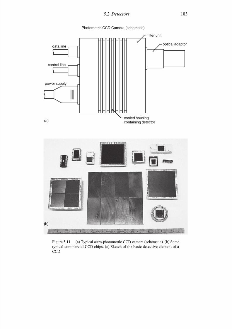
7/21/2019 Introduction to Astronomical Photometry
http://slidepdf.com/reader/full/introduction-to-astronomical-photometry 201/451
5.2 Detectors 183
Photometric CCD Camera (schematic)
filter unit
optical adaptor
cooled housingcontaining detector
power supply
control line
data line
(a)
(b)
Figure 5.11 (a) Typical astro-photometric CCD camera (schematic). (b) Sometypical commercial CCD chips. (c) Sketch of the basic detective element of aCCD
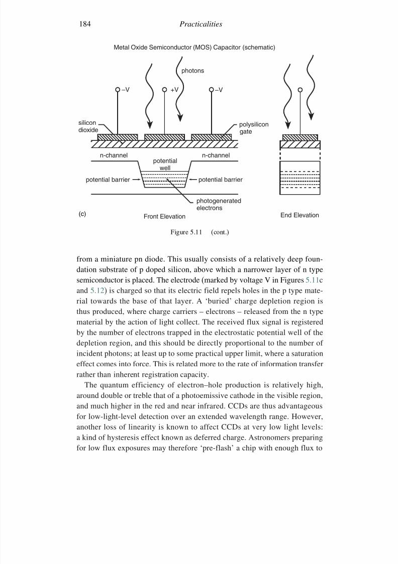
7/21/2019 Introduction to Astronomical Photometry
http://slidepdf.com/reader/full/introduction-to-astronomical-photometry 202/451
184 Practicalities
Metal Oxide Semiconductor (MOS) Capacitor (schematic)
photons
–V +V –V
silicondioxide
polysilicongate
n-channel n-channelpotentialwell
potential barrier potential barrier
photogeneratedelectrons
Front Elevation End Elevation(c)
Figure 5.11 (cont.)
from a miniature pn diode. This usually consists of a relatively deep foun-dation substrate of p doped silicon, above which a narrower layer of n typesemiconductor is placed. The electrode (marked by voltage V in Figures 5.11cand 5.12) is charged so that its electric field repels holes in the p type mate-rial towards the base of that layer. A ‘buried’ charge depletion region is
thus produced, where charge carriers – electrons – released from the n typematerial by the action of light collect. The received flux signal is registeredby the number of electrons trapped in the electrostatic potential well of thedepletion region, and this should be directly proportional to the number of incident photons; at least up to some practical upper limit, where a saturationeffect comes into force. This is related more to the rate of information transferrather than inherent registration capacity.
The quantum efficiency of electron–hole production is relatively high,around double or treble that of a photoemissive cathode in the visible region,and much higher in the red and near infrared. CCDs are thus advantageousfor low-light-level detection over an extended wavelength range. However,another loss of linearity is known to affect CCDs at very low light levels:a kind of hysteresis effect known as deferred charge. Astronomers preparingfor low flux exposures may therefore ‘pre-flash’ a chip with enough flux to
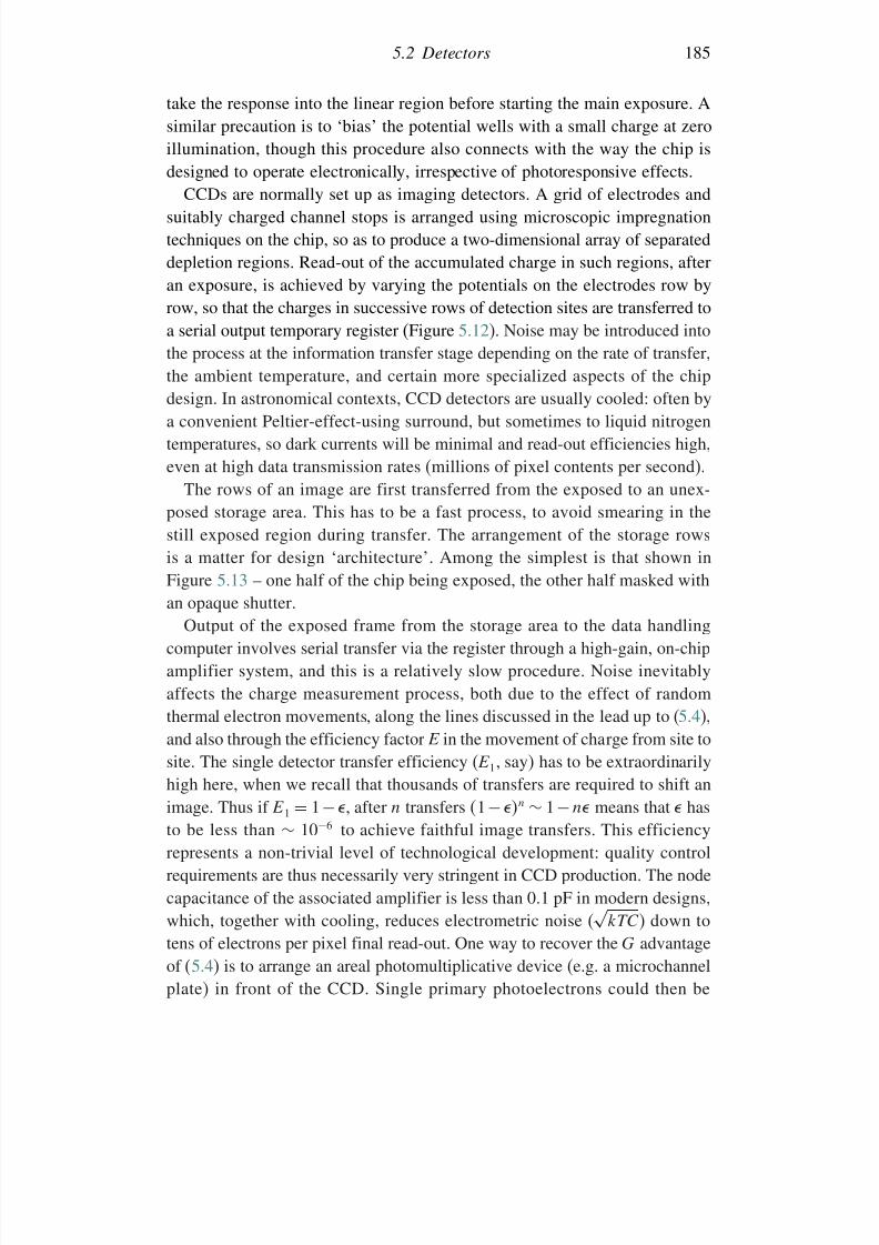
7/21/2019 Introduction to Astronomical Photometry
http://slidepdf.com/reader/full/introduction-to-astronomical-photometry 203/451
5.2 Detectors 185
take the response into the linear region before starting the main exposure. Asimilar precaution is to ‘bias’ the potential wells with a small charge at zeroillumination, though this procedure also connects with the way the chip is
designed to operate electronically, irrespective of photoresponsive effects.CCDs are normally set up as imaging detectors. A grid of electrodes and
suitably charged channel stops is arranged using microscopic impregnationtechniques on the chip, so as to produce a two-dimensional array of separateddepletion regions. Read-out of the accumulated charge in such regions, afteran exposure, is achieved by varying the potentials on the electrodes row byrow, so that the charges in successive rows of detection sites are transferred to
a serial output temporary register (Figure 5.12). Noise may be introduced intothe process at the information transfer stage depending on the rate of transfer,the ambient temperature, and certain more specialized aspects of the chipdesign. In astronomical contexts, CCD detectors are usually cooled: often bya convenient Peltier-effect-using surround, but sometimes to liquid nitrogentemperatures, so dark currents will be minimal and read-out efficiencies high,even at high data transmission rates (millions of pixel contents per second).
The rows of an image are first transferred from the exposed to an unex-
posed storage area. This has to be a fast process, to avoid smearing in thestill exposed region during transfer. The arrangement of the storage rowsis a matter for design ‘architecture’. Among the simplest is that shown inFigure 5.13 – one half of the chip being exposed, the other half masked withan opaque shutter.
Output of the exposed frame from the storage area to the data handlingcomputer involves serial transfer via the register through a high-gain, on-chip
amplifier system, and this is a relatively slow procedure. Noise inevitablyaffects the charge measurement process, both due to the effect of randomthermal electron movements, along the lines discussed in the lead up to (5.4),and also through the efficiency factor E in the movement of charge from site tosite. The single detector transfer efficiency (E 1, say) has to be extraordinarilyhigh here, when we recall that thousands of transfers are required to shift animage. Thus if E 1 = 1−, after n transfers 1−n ∼ 1−n means that hasto be less than
∼10−6 to achieve faithful image transfers. This efficiency
represents a non-trivial level of technological development: quality controlrequirements are thus necessarily very stringent in CCD production. The nodecapacitance of the associated amplifier is less than 0.1 pF in modern designs,which, together with cooling, reduces electrometric noise (
√ kTC ) down to
tens of electrons per pixel final read-out. One way to recover the G advantageof (5.4) is to arrange an areal photomultiplicative device (e.g. a microchannelplate) in front of the CCD. Single primary photoelectrons could then be
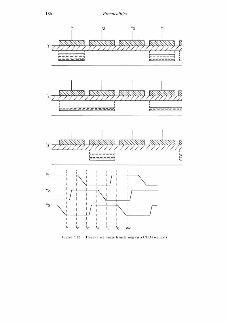
7/21/2019 Introduction to Astronomical Photometry
http://slidepdf.com/reader/full/introduction-to-astronomical-photometry 204/451
186 Practicalities
t2
t4 t6t5t2t1
t3
t3
t1
v1
v1
v3
v3
v1v2
v2
etc.
Figure 5.12 Three-phase image transferring on a CCD (see text)
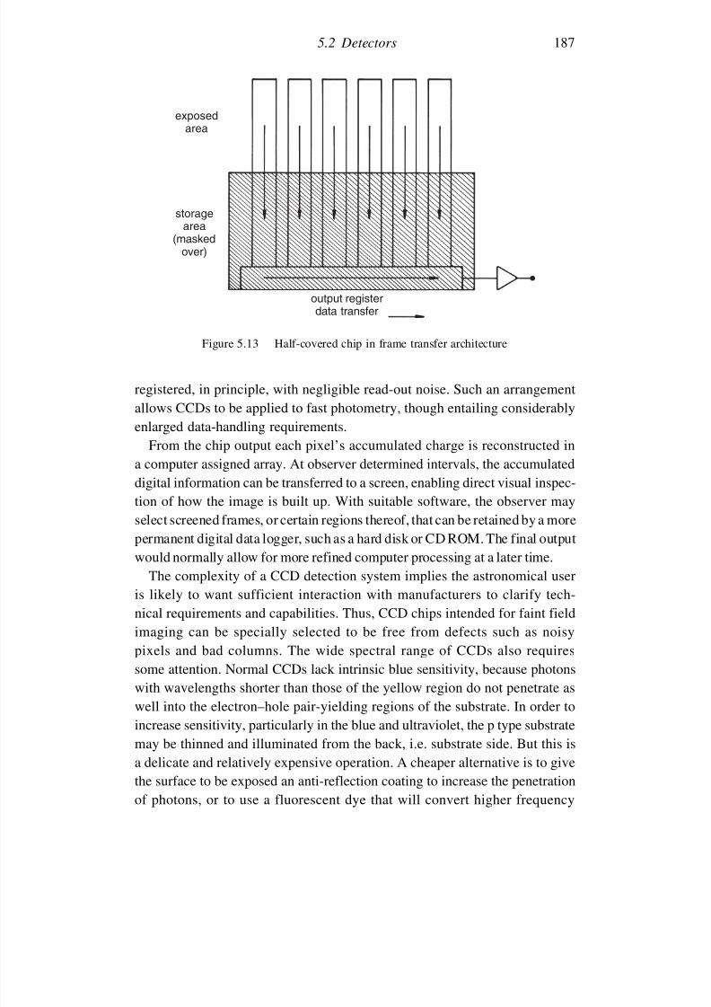
7/21/2019 Introduction to Astronomical Photometry
http://slidepdf.com/reader/full/introduction-to-astronomical-photometry 205/451
5.2 Detectors 187
exposedarea
storagearea
(maskedover)
output registerdata transfer
Figure 5.13 Half-covered chip in frame transfer architecture
registered, in principle, with negligible read-out noise. Such an arrangement
allows CCDs to be applied to fast photometry, though entailing considerablyenlarged data-handling requirements.From the chip output each pixel’s accumulated charge is reconstructed in
a computer assigned array. At observer determined intervals, the accumulateddigital information can be transferred to a screen, enabling direct visual inspec-tion of how the image is built up. With suitable software, the observer mayselect screened frames, or certain regions thereof, that can be retained by a morepermanent digital data logger, such as a hard disk or CD ROM. The final outputwould normally allow for more refined computer processing at a later time.
The complexity of a CCD detection system implies the astronomical useris likely to want sufficient interaction with manufacturers to clarify tech-nical requirements and capabilities. Thus, CCD chips intended for faint fieldimaging can be specially selected to be free from defects such as noisypixels and bad columns. The wide spectral range of CCDs also requiressome attention. Normal CCDs lack intrinsic blue sensitivity, because photons
with wavelengths shorter than those of the yellow region do not penetrate aswell into the electron–hole pair-yielding regions of the substrate. In order toincrease sensitivity, particularly in the blue and ultraviolet, the p type substratemay be thinned and illuminated from the back, i.e. substrate side. But this isa delicate and relatively expensive operation. A cheaper alternative is to givethe surface to be exposed an anti-reflection coating to increase the penetrationof photons, or to use a fluorescent dye that will convert higher frequency
7/21/2019 Introduction to Astronomical Photometry
http://slidepdf.com/reader/full/introduction-to-astronomical-photometry 206/451
188 Practicalities
photons to lower energy ones. But since those photons are then re-emitted inall directions there is inevitably some loss of efficiency. In the red region of a CCD’s response, associated with the greater penetration of photons, there
is also a relative loss of spatial resolution.Operation of a CCD involves much more than obtaining an effective chip.
The chip is potentially a very large data generator, as can easily be seen fromconsidering the information content of, say, a 1000 by 1000 array, each pixelof which may have an event capacity of ∼104. The whole may be recordingexposures in a matter of seconds. It is not surprising, given this level of datageneration, that a considerable proportion of time and effort in working with
a CCD camera relates to the design of efficient image handling software.A key task is the selection from the total amount of data generated thatrelevant to what is finally sought. With the photometry of variable stars,for example, one may proceed along lines parallel to single channel aper-ture photometry by selecting those pixel regions on the frame that containstars of interest, i.e. the variable and its comparison(s), sample some nearbybackground sky level, and utilize only that data subset. On-line reductions,performed in an efficient system, allow the presentation of a preliminary form
of light curve, more or less as it is observed. It is still useful, though, toback-up full data sets of raw observations, both as a security and for lessimmediate purposes.
The CCD-using astronomer can be helped by extensive technical experi-ence of manufacturers, and commercially obtainable specialized equipment.Modern observatories generally make available convenient software facili-ties with special user-oriented computer command sequences; such as, for
example, the Munich Image Data Analysis System (MIDAS) of the EuropeanSouthern Observatory. Convenient as this may be, an increasing techno-logical separation between the data acquisition system and its user carriessome danger of discrepancies in unfamiliar or unseen parts of the processingcreeping through to the end results unnoticed. More discussion about howCCDs are applied to stellar photometric data retrieval, including a typicalexample of variable star monitoring, is given in the next chapter.
5.2.6 Noise in photometry
It is instructive first to follow through the disturbances to signal registrationthat occur for a basic detector such as a photomultiplier. There is a statisticalnoise due to the inherently non-steady photon influx. This is sometimes calledshot noise, or the primary detection noise. A Poissonian distribution is normalfor the arrival of the primary photon stream from a source of constant emissive
7/21/2019 Introduction to Astronomical Photometry
http://slidepdf.com/reader/full/introduction-to-astronomical-photometry 207/451
5.2 Detectors 189
power. This gives rise to the familiar √
n concept for the S/N ratio of theprimary signal (∝ n). This becomes the predominant noise source for higherincident fluxes.
The multiplicative effect of the secondary emission process in a photomul-tiplier should follow a similar pattern. The final form is quasi-Poissonian,but with some usually significant departure, the full explanation for which iscomplex, but has been connected with non-uniformity of response over thedynode surfaces, or the fact that some electrons fail either to reach the nextdynode or produce secondary electrons if they do arrive there. Multiplicationnoise can be characterized by a second moment parameter = q 2/q 2, where q
is the observed output charge in each pulse. increases over an ideal value of unity in dependence on the gain at each electrode and its unevenness, as wellas the small fraction of original photodetection pulses that fail to propagate.
These two inherent sources of noise, i.e. shot and multiplication, are supple-mented by various other contributions, increasingly significant for fainter illu-mination. They are reducible by careful design and operation, but, as with giantpulses due to cosmic ray incidence, for example, cannot be eliminated entirely.
The most commonly encountered source ofadditional noise is ‘dark current’ –the background of low energy pulses present in the absence of cathode illumina-tion. For sufficiently low illuminance this dark current can become comparableto the signal: a condition referred to as dark current limited detection. It mayarise in astronomical contexts with a very dark sky, low scintillation and smallentrance aperture, depending rather critically on ambient temperature.
The dark current is usually regarded as mainly thermionic emission fromthe cathode and perhaps some dynodes, but this is not the whole story. Dark
current is indeed normally reduced with a reduction in ambient temperature,but sometimes low work function materials used for certain emissive surfacescan, at a given temperature, give rise to a lower dark current than that foundfrom other tubes employing higher work function electrodes. Contaminationof the near vacuum tube interiors by residual gas particles released fromadsorption to components, or possible diffusion of helium traces from theatmosphere, secondary cosmic ray effects, residual radioactivity or electro-
luminescence in the glass envelope, field emission from sharp corners onelectrodes, or trapped charge from previous exposures to light have all beenrelated to such non-thermionic contributions to the dark current. The cathode’sphotoemissivity is also reduced by lowering the temperature, so it is notobvious what the optimum working temperature will be for any particulartube – such data can usually be supplied by the manufacturer, however, frominformation determined during production.
7/21/2019 Introduction to Astronomical Photometry
http://slidepdf.com/reader/full/introduction-to-astronomical-photometry 208/451
190 Practicalities
Voltages in the range 1000–2000 V between cathode and anode are typicallyrequired to operate a photomultiplier as a faint light detector. For any particulartubean S/N experiment should be performed, measuring dark current and signal
from a faint source against applied voltage, to determine the optimum workingvoltage. Such experiments show that tubes have a quite sensitive responseto voltage variation, due to multiplicative secondary emission. For example,according to the manufacturer’s specifications for the EMI 9558 tube that wasrecommendedforastronomicalphotometry,increasingthevoltagefrom1000to1200 V changes the sensitivity typically from 70 to 400 A lm−1. The behaviouris approximately that of a power law with an exponent of about 8. In other
words, if tube output currents for a constant source are to be kept constant towithin 01%, the voltage must be regulated to within a factor 10−4. This israther a stringent limit, and calls for a high quality of voltage supply, keepingin mind that observatories are often located in remote sites, where it may bedifficult to ensure a well-regulated basic supply. The strong recommendationfor limiting drawn current (usually to a few milliamperes) in a unit capable of supplying several thousands of volts is also worth noting.
Tubes have a variety of operating idiosyncrasies, associated with ‘warm-
up’ or ‘fatigue’ effects, dampness, the action of the background magneticfield or other effects. Some new designs have been particularly well suited tolow-light-level pulse counting; though there is also an argument for stayingwith tube types already tested by extensive pioneering research.
The dark current proportion of detector noise is much less with a photo-diode, because of both increased detective quantum efficiency (which may beat least 2–3 times greater in the visible, and much greater towards the infrared),
and the responsive surface being small and entirely illuminated. Thoughnoise in the subsequent measurement system is relatively much greater forphotodiode than photomultiplier systems, as a result of the G factor differ-ence in (5.4), this does not necessarily cause the greatest loss of informationin all photometric conditions. At a sufficiently bright level where inherentshot noise predominates, for example, the quantum advantage of photodiodedetection can outweigh the then relatively negligible addition of measurementnoise. With an areal array of solid state detectors there are also normally a
number of separate pixels sampling the light distribution from a source, sothat the well-known regression to the mean principle applies in combiningtheir separate estimations of the flux.
Noise in a CCD thus has both a temporal and a spatial aspect. In addi-tion to the already considered primary shot noise, the temporal aspect has acomponent that is associated with continual resetting of the zero illuminationreference level after read-outs. This reset noise has the
√ kTC form referred
7/21/2019 Introduction to Astronomical Photometry
http://slidepdf.com/reader/full/introduction-to-astronomical-photometry 209/451
5.2 Detectors 191
to in the previous section in relation to electrometric measurement. In orderto estimate its relative importance, it can be compared with the static biascharge of normally a few hundred counts. The noise related to pixel charge
measurement involves the behaviour of the amplifier, which we consider inthe next section, but clearly effects related to temperature will be reduced bycooling, as with photodiode dark current.
The noise associated with dark current in a CCD is regarded as having aspatial dependence, in that it arises mainly from over the surface of the chipand relates to minor irregularities in the solid state molecular bonding lattice,associated with material interfaces and impurities. Each pixel generates a
slightly different level of dark current, so the noise depends on non-uniformityof response over the surface as well as the dark current’s inherent quasi-Poissonian contribution to the electron counts. Dark current, following agenerally Richardson law type dependence on temperature, could fill thepotential wells of an uncooled CCD at 20 C in, typically, a few seconds,but cooling to −50 C say, reduces this to a tolerable few electrons per pixelper second. The standard approach to spatial non-uniformity of response inCCDs is through flat fielding, although it should be remembered that there is
an additional shot noise contribution to the adopted flat-field distribution.Aside from the pixel transfer efficiency, which was already seen to have
to be very high, another potential component to image noise comes fromthe various high frequency oscillators involved in the gating circuitry. This‘clocking noise’ rises with signal load and clocking frequency, but it cannormally be controlled by manufacturers to a negligible level for astronom-ical applications. Although information from suppliers is thus a prerequisite
to effective CCD use, as with photomultipliers, there is still an individualcharacter to each camera, regarding, for example, the locations of ‘dead spots’or faulty columns in the array.
Problems of instrumental variation are not necessarily too serious,depending on the nature of the observations. Differential photometry, forexample, is quite stable against slow ‘creep’ effects. Fast photometry doesnot concern itself with variation on such timescales (hours). Instrumentalcalibration by reference to standard stars, on the other hand, really calls for
the most stable of conditions, both externally and internal to the equipment.The total noise of detection is then not just that of the photoelectric
responder, since the signal has already been deteriorated by the atmosphere.The existence of static atmospheric extinction can be dealt with by well-knownprocedures of intercomparisons between different stars. But the atmospherehas also dynamic extinction properties on a wide range of timescales. At thehigh-frequency end these are covered by the term scintillation (twinkling).
7/21/2019 Introduction to Astronomical Photometry
http://slidepdf.com/reader/full/introduction-to-astronomical-photometry 210/451
192 Practicalities
This can be conveniently characterized as a modulation of the signal, of whichit is some proportion, m say, for a given night and integration period. Scin-tillation is a complex result of atmospheric inhomogeneities on the incoming
wavefront, as sampled by the telescope’s aperture; but, from the practicalstandpoint, can be treated as an empirical parameter adding mS into the noise(see Section 4.5).
The atmosphere also scatters light from all other sources, some of which arevariable on short timescales. Even the steady component of this backgroundlight of the sky introduces a secondary noise, through its shot noise from thedetector. On the best quality nights, when transparency is high, scintillation islow and adequate precautions have been taken to reduce inherent instrumentalnoise to a minimum, the background sky noise represents a final limiting foraccurate measurement of weak astronomical sources – ‘sky limited’ detection.
5.3 Conventional measurement methods
5.3.1 Analogue method
Early measuring and recording techniques for photoelectric photometry,beyond simple electrometry, involved amplification of the photocurrent upto the point where it could be logged on a pen recorder. This is the analogue,often called DC, procedure, and it is still used in some measurement tech-niques, or its principles apply when analogue amplification arises, for examplein the transferring of voltage proportional to the photon produced chargein a CCD’s detection sites prior to digitization. An example of a schematic
circuit that can perform the very large amplifications often required is shownin Figure 5.14. This circuit involves an operational amplifier arranged with aresistive negative feedback loop, in the manner nicely explained in Hendenand Kaitchuck’s (1982) book.
Let us consider the information transfer efficiency E from a tube typedetector through the DC amplifier. We regard the cathode, responding to aconstant light input, as a current generator of a mean signal I , onto which anoise component denoted i2
= I − ¯
I2
is added. Independent additive
noise sources a and b satisfy
a + b2 = a2+b2 (5.5)
Now the ratio of detector output signal to input signal was specified to beG. Hence, if the thermal agitation of electrons in the amplifier’s load resistorR generates an additional source of noise (‘Johnson noise’) iR
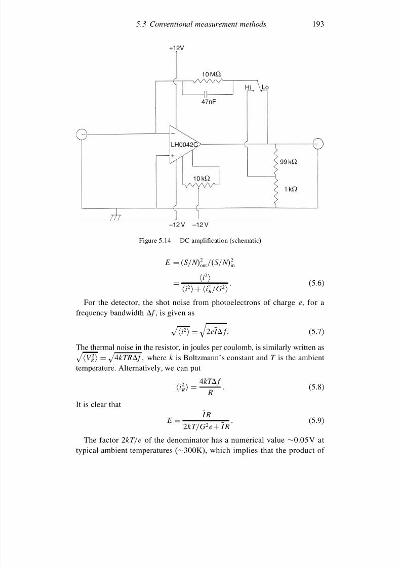
7/21/2019 Introduction to Astronomical Photometry
http://slidepdf.com/reader/full/introduction-to-astronomical-photometry 211/451
5.3 Conventional measurement methods 193
+12V
10 MΩ
47nF
LH0042C
10 kΩ
99 kΩ
1 kΩ
Hi Lo
–12 V –12 V
–
+
Figure 5.14 DC amplification (schematic)
E = S/N2out/S/N2
in
= i2i2+i2
R/G2 (5.6)
For the detector, the shot noise from photoelectrons of charge e, for a
frequency bandwidth f , is given as i2 =
2eIf (5.7)
The thermal noise in the resistor, in joules per coulomb, is similarly written as V 2R =
4kTRf where k is Boltzmann’s constant and T is the ambient
temperature. Alternatively, we can put
i2R = 4kTf
R (5.8)
It is clear that
E = IR
2kT/G2e + IR (5.9)
The factor 2kT/e of the denominator has a numerical value ∼005V attypical ambient temperatures (∼300K), which implies that the product of
7/21/2019 Introduction to Astronomical Photometry
http://slidepdf.com/reader/full/introduction-to-astronomical-photometry 212/451
194 Practicalities
detector current and load resistance must be greater than 005/G2 to preventserious information loss from this measurement noise. Again we see theimportance of the internal gain G in minimizing the effects of thermal noise.
The load resistance R couples with stray capacitance of the tube C s tointroduce a response time = RC s, so that if f is the mean frequency of arrival of electrons at the anode, we can rewrite (5.9) as
E = f
31× 105C s/G2 + f (5.10)
where C s is in picofarads, and the time unit is seconds. This equation gives
a limit on available time resolution for a detector of given internal gain G
and stray capacitance C s. The stray capacitance of a photomultiplier tubeassembly is typically of the order of a picofarad, so f ≥ 10−6 to avoidserious signal degradation from amplification noise. This condition would becomfortably satisfied in any feasible application of DC amplification, becausefor the faintest signals, where the largest resistors would be used, would belarge enough (
>∼ 10−3 s) that other more significant sources of noise would
constrain f long before the low incidence (∼ 10−3
) corresponding to thisJohnson noise limiting was reached. Bright sources (f ∼ 106 in Table 3.5)will correspondingly admit very high time resolution.
The gain issue was underlying the comparison between photomultipliers(G ∼ 106) and photodiodes (G = 1) in Section 5.2.6, though other factors areinvolved, apart from those previously mentioned. Firstly, improvements incomponent manufacturing have allowed stable resistances of very high values(
>
∼109 ) to become more easily available, with corresponding improve-
ments to the ratio (5.9). Secondly, this ratio can also be reduced with effec-tive cooling of components. With areal detectors, spatially distributed finesampling of the flux offers an additional means to recover net S/N . Suchpoints significantly bear on the choice of detector and the requirement forinternal gain prior to measurement.
As mentioned, a common output medium for this analogue approach, insingle channel mode, has been the strip chart, or pen recorder. This allows
a visible, simple and permanent record of a photometric observing session.With a reliable strip chart, the run of the data, relative quality of the night,any special or spurious events or commentary that the observer may havewritten alongside the pen’s track, can be quickly ascertained. Recent designsof pen recorders have more advanced features including accurate linearity;constant, user-selected speeds; smooth and continuous pen action; as well asparallel digital display that can communicate with a computer. Their prices
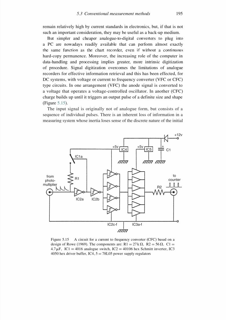
7/21/2019 Introduction to Astronomical Photometry
http://slidepdf.com/reader/full/introduction-to-astronomical-photometry 213/451
5.3 Conventional measurement methods 195
remain relatively high by current standards in electronics, but, if that is notsuch an important consideration, they may be useful as a back-up medium.
But simpler and cheaper analogue-to-digital converters to plug into
a PC are nowadays readily available that can perform almost exactlythe same function as the chart recorder, even if without a continuoushard-copy permanence. Moreover, the increasing role of the computer indata-handling and processing implies greater, more intrinsic digitizationof procedure. Signal digitization overcomes the limitations of analoguerecorders for effective information retrieval and this has been effected, forDC systems, with voltage or current to frequency converter (VFC or CFC)
type circuits. In one arrangement (VFC) the anode signal is converted toa voltage that operates a voltage-controlled oscillator. In another (CFC)charge builds up until it triggers an output pulse of a definite size and shape(Figure 5.15).
The input signal is originally not of analogue form, but consists of asequence of individual pulses. There is an inherent loss of information in ameasuring system whose inertia loses sense of the discrete nature of the initial
IC1a
IC2a IC2b
IC2c-f IC3a-f
R1fromphoto-
multiplier
+5vIC4
+5vIC5 C1
+12v
+
tocounter
R2
Figure 5.15 A circuit for a current to frequency converter (CFC) based on adesign of Rowe (1969). The components are: R1 = 27 k R2 = 56 C1 =47 F IC1 = 4016 analogue switch, IC2 = 40106 hex Schmitt inverter, IC34050 hex driver buffer, IC4 5 = 78L05 power supply regulators
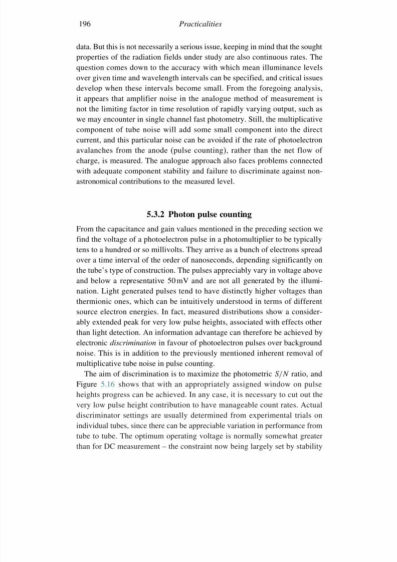
7/21/2019 Introduction to Astronomical Photometry
http://slidepdf.com/reader/full/introduction-to-astronomical-photometry 214/451
196 Practicalities
data. But this is not necessarily a serious issue, keeping in mind that the soughtproperties of the radiation fields under study are also continuous rates. Thequestion comes down to the accuracy with which mean illuminance levels
over given time and wavelength intervals can be specified, and critical issuesdevelop when these intervals become small. From the foregoing analysis,it appears that amplifier noise in the analogue method of measurement isnot the limiting factor in time resolution of rapidly varying output, such aswe may encounter in single channel fast photometry. Still, the multiplicativecomponent of tube noise will add some small component into the directcurrent, and this particular noise can be avoided if the rate of photoelectron
avalanches from the anode (pulse counting), rather than the net flow of charge, is measured. The analogue approach also faces problems connectedwith adequate component stability and failure to discriminate against non-astronomical contributions to the measured level.
5.3.2 Photon pulse counting
From the capacitance and gain values mentioned in the preceding section wefind the voltage of a photoelectron pulse in a photomultiplier to be typicallytens to a hundred or so millivolts. They arrive as a bunch of electrons spreadover a time interval of the order of nanoseconds, depending significantly onthe tube’s type of construction. The pulses appreciably vary in voltage aboveand below a representative 50 mV and are not all generated by the illumi-nation. Light generated pulses tend to have distinctly higher voltages thanthermionic ones, which can be intuitively understood in terms of differentsource electron energies. In fact, measured distributions show a consider-ably extended peak for very low pulse heights, associated with effects otherthan light detection. An information advantage can therefore be achieved byelectronic discrimination in favour of photoelectron pulses over backgroundnoise. This is in addition to the previously mentioned inherent removal of multiplicative tube noise in pulse counting.
The aim of discrimination is to maximize the photometric S/N ratio, and
Figure 5.16 shows that with an appropriately assigned window on pulseheights progress can be achieved. In any case, it is necessary to cut out thevery low pulse height contribution to have manageable count rates. Actualdiscriminator settings are usually determined from experimental trials onindividual tubes, since there can be appreciable variation in performance fromtube to tube. The optimum operating voltage is normally somewhat greaterthan for DC measurement – the constraint now being largely set by stability
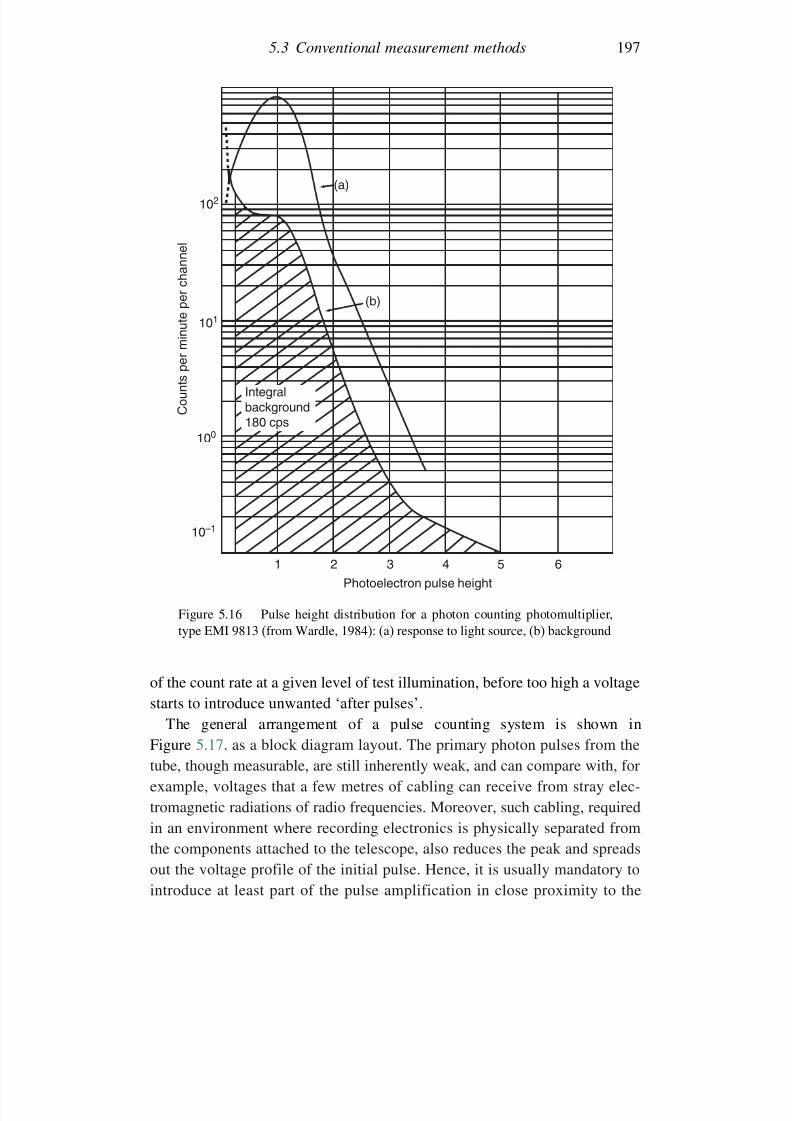
7/21/2019 Introduction to Astronomical Photometry
http://slidepdf.com/reader/full/introduction-to-astronomical-photometry 215/451
5.3 Conventional measurement methods 197
1
C o u n t s p e r m i n u t e p
e r c h a n n e l
(a)
102
101
100
10–1
(b)
2 3
Photoelectron pulse height
4 5 6
Integralbackground180 cps
Figure 5.16 Pulse height distribution for a photon counting photomultiplier,type EMI 9813 (from Wardle, 1984): (a) response to light source, (b) background
of the count rate at a given level of test illumination, before too high a voltagestarts to introduce unwanted ‘after pulses’.
The general arrangement of a pulse counting system is shown inFigure 5.17. as a block diagram layout. The primary photon pulses from the
tube, though measurable, are still inherently weak, and can compare with, forexample, voltages that a few metres of cabling can receive from stray elec-tromagnetic radiations of radio frequencies. Moreover, such cabling, requiredin an environment where recording electronics is physically separated fromthe components attached to the telescope, also reduces the peak and spreadsout the voltage profile of the initial pulse. Hence, it is usually mandatory tointroduce at least part of the pulse amplification in close proximity to the
7/21/2019 Introduction to Astronomical Photometry
http://slidepdf.com/reader/full/introduction-to-astronomical-photometry 216/451
198 Practicalities
HIGH VOLTAGE RATEMETER
DETECTOR PULSE AMPLIFIER DISCRIMINATOR
SCALER CLOCK COMPUTER
CHART RECORDER
Figure 5.17 Postdetection photon counting system: general arrangement
anode, often as a small preamplifier unit on the photometer head. The subse-quent main pulse amplifier, which may be combined with the discriminatorin a single unit, outputs pulses that are as linearly responsive to the originalphoton pulses as possible. These output pulses, having a definite shape andsize, typically ∼1 V, are sent to a counter that needs to have a bandwidth atleast as high as the amplifier and is frequently an order of magnitude higherto ensure full time resolution. The counter would often take the form of aninsertable board inside the controlling and data-logging computer.
The counting of pulses encounters time resolution (bandwidth) limitationfor bright sources. This can be appreciated in terms of ‘pulse pile-up’ – thedefinite chance that a pulse may indistinguishably merge with its neighbourwhen incidence becomes high enough. Measured count rates are thus system-atically in error to some extent. This will be slight when the true incidencefrequency f is much less than the inverse time resolution (1/ d), or ampli-fier bandwidth frequency f b (= 1/2 d), but it becomes progressively more
significant as f → f b.The systematic underestimation of pulse incidence can be related to the nettime resolution, or ‘dead time’ value d, as follows. In unit time interval thenumber of incident pulses is f , while the number counted will be f c. Each of these f c events is associated with a dead time d, so that the effective countingtime is shortened by f c d, and so
f c =
f1−
f c
d=
f1−
f c/2f
b (5.11)
7/21/2019 Introduction to Astronomical Photometry
http://slidepdf.com/reader/full/introduction-to-astronomical-photometry 217/451
5.3 Conventional measurement methods 199
The distribution in electron arrival times at the anode can be as smallas 10−9 s in modern tube designs with beam focusing. Hence, the basicdata-generator is potentially a high bandwidth (GHz) device. However, high
measurement bandwidth f b (low d) brings with it more stringent require-ments for well-screened, low-stray-impedance amplifier components, pushingup either likely costs or physical stability requirements. This need not benecessary for many astronomical programmes, where event incidence couldbe typically around several thousand hertz, as in, say, intermediate-bandphotometry of tenth mag stars with a
<∼ 1 m class telescope (see Table 3.5).From (5.11) we require only f b
>∼ 103f c to achieve 0.1% accuracy in standard
photometric reductions (without a dead time correction), and in a differentialphotometry context even greater precision would be inferred. It implies thatf b ∼ 10MHz would be adequate for many practical situations.
For the most accurate work, and, in any case, for full awareness of instru-mental parameters, it is desirable to have some knowledge of the operatingdead time for any given photometer. This is sometimes arrived at from manu-facturer’s specifications, or by an error minimization technique on standardstar data. It is preferable to have an independent empirical option for this,however, and one simple technique is to use two light emitting diodes (LEDs)mounted in such a way that all other light except theirs can be excluded fromthe photometer. Their light should be able to be maintained at an accuratelyconstant level, perhaps by means of a battery source, and they should emitenough light that some significant level of non-linearity will occur. Their lightoutput could be usefully made to be comparable to a pair of bright (nakedeye) stars, set within the telescope with the cover tightly on.
We write f 1 for the count rate observed with the first LED on by itself,and f 2 for that with the second. When both LEDs are switched on togetherthe count rate is f 3. In the absence of a dead time effect, we would havef 3 = f 1 + f 2, but in practice we should find that f 3 = f 1 + f 2 − , where isa relatively small number.
Making use of (5.11), we have
f 31− f 3 d= f 11− f 1 d
+ f 21− f 2 d (5.12)
This can be solved for d, to yield
d =
1−
f 3 − f 1f 3 − f 2
f 1f 2
/f 3 (5.13)
7/21/2019 Introduction to Astronomical Photometry
http://slidepdf.com/reader/full/introduction-to-astronomical-photometry 218/451
200 Practicalities
from which, for small ,
d
2f f 3 (5.14)
where f is the harmonic mean f 1f 2/f 1 + f 2.Any device (aperture stops, neutral density filters, etc.) that allows a
constant, reasonably bright light source to be divided into constant propor-tions may be used as an alternative to summing different LEDs – it is onlyrequired that f 1 f 2 and f 3 be accurately measurable and the true incidencerates exactly additive.
5.4 Bibliographical notes
The practical side of astronomical photometry was well covered, in a veryreadable style, in A. A. Henden & R. H. Kaitchuck’s Astronomical Photometry
(Van Nostrand Reinhold, 1982) (a re-edited version of which appeared fromWillmann-Bell in 1998, who have published much other comparable sourcematerial on photometry, see Section 1.5). This publisher has responded well
to the rise of areal solid state detectors with a number of well-cited practicalprimers, such as C. Buil’s CCD Astronomy: Construction and Use of an Astro-
nomical CCD Camera (1991); Choosing and Using a CCD camera, R. Berry(1992); The CCD Camera Cookbook , R. Berry, V. Kanto & J. Munger (1994);and Handbook of Astronomical Image Processing, R. Berry & J. Burnell(2000). Some of these books come with software to assist in camera assemblyand usage. C. Sterken & J. Manfroid’s Astronomical Photometry: A Guide
(Kluwer, 1992) also contained much useful practical information, with impor-tant considerations given to telescope and foreoptics arrangements.There have been numerous technical symposia on the electronics of solid
state areal detectors: an example of a general introduction from such ameeting can be found in D. J. Burt’s Basic Operation of the Charge Coupled
Device, from the (first) International Conference on Technology and Appli-cations of Charge Coupled Devices, University of Edinburgh, 1974. Anothergeneral article is Charge Coupled Devices by D. E. Weisner, McGraw-Hill
Encyclopedia of Science and Technology, 7th edn. (McGraw-Hill Inc.,1992). From a professional astronomy standpoint, CCD detectors werereviewed by C.D. Mackay ( Ann. Rev. Astron. Astrophys., 24, 255, 1986),and discussed in I. S. Mclean’s Electronic and Computer-aided Astronomy
(Ellis Horwood, 1989), updated as Electronic Imaging in Astronomy –
Detectors and Instrumentation (Wiley Praxis, 1997). Subsequently, inthe Practical Astronomy Handbook series of Cambridge University Press,
7/21/2019 Introduction to Astronomical Photometry
http://slidepdf.com/reader/full/introduction-to-astronomical-photometry 219/451
5.4 Bibliographical notes 201
S. B. Howell’s Handbook of CCD Astronomy (2000), appeared, which,together with P. Lena’s A Practical Guide to CCD Astronomy (CambridgeUniversity Press, 1998), give a wealth of background information. J. R.
Janesick’s Scientific Charge-Coupled Devices (SPIE Press, 2001) takes asomewhat broader perspective on applications, as does G. C. Holst’s CCD
Arrays, Cameras and Displays (JCD Publishing, 1996). A compendiumof source information, referring to books, magazine articles, equipmentand software suppliers, user groups, email lists and websites, with generalaccessibility, is provided at www.stargazing.net/david/. Figure 5.11 isfrom introductory technical material of Molecular ExpressionsTM (see
micro.magnet.fsu.edu/primer/digitalimaging/concepts/moscapacitor.html).A number of books containing designs and possibilities for astronomicalphotometry instrumentation were produced by the Fairborn Press, AutoscopeCorporation, in the 1980s, e.g. The Photoelectric Photometry Handbook , eds.D. R. and R. M. Genet I and II (1989); Microcomputers in Astronomy, eds.R.M. and K.A. Genet I (1983) and II (1984); and Robotic Observatories,eds. R.M. Genet and D.S. Hayes, (1989). The 3rd New Zealand Confer-
ence on Photoelectric Photometry (Blenheim, 1989), eds. J. Richard and
E. Budding, also published by Fairborn Press (1991), contained other refer-ences on automatic telescopes and CCDs, then a field of nascent development.
The section on detectors (5.2) draws a lot from material provided, orcited, by manufacturers. For example, the electron tubes division of ThorneEMI have detailed booklets on the properties of photomultiplier tubes, imageintensifiers and the like. These cite special studies, such as R. Wardle’s Test
Parameters and General Operating Rules for Photomultipliers (Thorne EMI
R/P 067, 1984), from where Figure 5.16 comes; or C. J. Oliver’s paper in thesame series (Thorne EMI R/P 066, 1984), which discusses part of Section 5.2.6in detail. Similarly, information on the properties of particular CCD imagesensor types may be found from Kodak at www.kodak.com/global/plugins/ acrobat/en/digital/ccd/applicationNotes/noiseSources.pdf or Roper Scientific(GmbH Germany) at www.roperscientific.de/CCD% 20primer.html. Informa-tion on the IPCS was given by A. Boksenberg (Phil. Trans. Roy. Soc. London
A, 307, 531, 1982); and J. L. A. Fordham, D. A. Bone and A. R. Jorden (SPIE
Proc., 627, 206, 1986).Information transfer efficiency, as presented in Section 5.3, was exposed
in detail in the article of A. Lallemande in Astronomical Techniques, ed.W. A. Hiltner (University Press, Chicago, 1962, p. 126), but it is also dealtwith in Henden and Kaitchuck’s book. More technical details are to be foundin texts such as Detection and Spectrometry of Faint Light , by J. Meaburn(Reidel, 1976) and M. J. Eccles, M. E. Sim and K. P. Tritton’s Low Light Level
7/21/2019 Introduction to Astronomical Photometry
http://slidepdf.com/reader/full/introduction-to-astronomical-photometry 220/451
202 Practicalities
Detectors in Astronomy (Cambridge University Press, 1983), which providedsource material for some of this chapter. Henden and Kaitchuck’s book hasgood information on the recording techniques of Section 5.3. This includes
the proper accounting for dead time, as discussed at the end of this section.C. Rowe’s CFC circuit first appeared in South. Stars (23, 63, 1969).
A number of the diagrams used in this chapter (and the next) derivefrom students’ theses. Thus, versions of Figures 5.1, 5.2 and 5.4 appear inA. R. Sadik’s Ph.D. thesis (University of Manchester, 1978), 5.3 and 5.14 arein K. M. Nield’s M.Sc. thesis (University of Waikato, 1987), and Figure 5.15is from the M.Sc. thesis of M. C. Forbes (University of Wellington, 1990).
References
Berry, R., 1992, Choosing and Using a CCD camera, Willmann-Bell.Berry, R. & Burnell, J., 2000, Handbook of Astronomical Image Processing,
Willmann-Bell.Berry, R., Kanto, V. & Munger, J., 1994, The CCD Camera Cookbook , Willmann-Bell.
Boksenberg, A., 1982, Phil. Trans. Roy. Soc. London A, 307, 531.Buil, C., 1991, CCD Astronomy: Construction and Use of an Astronomical CCD
Camera, Willmann-Bell.Burt, D. J., 1974, Basic Operation of the Charge Coupled Device, International Confer-
ence on Technology and Applications of Charge Coupled Devices, (I), Universityof Edinburgh.
Eccles, M.J., Sim, M.E. & Tritton, K.P., 1983, Low Light Level Detectors in
Astronomy, Cambridge University Press.Forbes, M. C., 1990, M.Sc. thesis, University of Wellington.
Fordham, J. L. A., Bone, D. A. & Jorden, A. R., 1986, SPIE Proc., 627, 206.Genet, D. R. & Genet, R. M., 1989, The Photoelectric Photometry Handbook (I & II)
Fairborn Press, Autoscope Corporation.Genet, R.M. & Genet, K.A., 1983, Microcomputers in Astronomy (I); 1984, (II),
Fairborn Press, Autoscope Corporation.Genet, R. M. & Hayes, D. S., 1989, Robotic Observatories, Fairborn Press, Autoscope
Corporation.Henden, A.A. & Kaitchuck, R.H., 1982, Astronomical Photometry, Van Nostrand
Reinhold (1998 re-edition by Willmann-Bell).
Holst, G. C., 1996, CCD Arrays, Cameras and Displays, JCD Publishing.Howell, S. B., 2000, Handbook of CCD Astronomy, Cambridge University Press.Janesick, J. R., 2001, Scientific Charge-Coupled Devices, SPIE Press.Lallemande, A., 1962, Astronomical Techniques, ed. W. A. Hiltner, University Press,
Chicago, p. 126.Lena, P., 1998, A Practical Guide to CCD Astronomy, Cambridge University Press.Mackay, C. D., 1986, Ann. Rev. Astron. Astrophys., 24, 255.McLean, I. S., 1989, Electronic and Computer-aided Astronomy, Ellis Horwood.

7/21/2019 Introduction to Astronomical Photometry
http://slidepdf.com/reader/full/introduction-to-astronomical-photometry 221/451
References 203
McLean, I. S., 1997, Electronic Imaging in Astronomy: Detectors and Instrumentation,Wiley Praxis.
Meaburn, J., 1976, Detection and Spectrometry of Faint Light , Reidel.Nield, K. M., 1987, M.Sc. thesis, University of Waikato.Oliver, C. J., 1984, Thorne EMI R/P 066 , Thorne EMI.Richard, J. & Budding, E., 1989, 3rd New Zealand Conference on Photoelectric
Photometry (Blenheim), Fairborn Press, Autoscope Corporation.Rowe, C., South. Stars, 23, 63, 1969.Sadik, A. R., 1978, Ph.D. thesis, University of Manchester.Sterken, C. & Manfroid, J., 1992, Astronomical Photometry: A Guide, Kluwer.Wardle, R., 1984, Thorne EMI R/P 067 , Thorne EMI.Weisner, D. E., 1992, Charge Coupled Devices, McGraw-Hill Encyclopedia of Science
and Technology, 7th edn., McGraw-Hill Inc.
7/21/2019 Introduction to Astronomical Photometry
http://slidepdf.com/reader/full/introduction-to-astronomical-photometry 222/451
6
Procedures
This chapter is about the essential procedures for setting up and using anastronomical photometric system, and processing its data. The first twosections deal with two basic calibration experiments. There is then a sectiondealing with observational particulars in the application of a CCD camera. Abrief introduction to variable star photometry, including an overview of thetiming of photometric phenomena, follows. The treatment and interpretation
of data is concentrated on.
6.1 The standard stars experiment
The purpose of this is to calibrate a given local photometric system to astandard or reference system, based on detailed comparisons of published
magnitude and colour values of standard stars, with corresponding measure-ments made with local equipment. The experiment is sometimes related tothe terms absolute, or all-sky photometry. To do it well normally requiresvery good, i.e. transparent and stable, sky conditions, but these nights are notso common at most observing locations. They are sometimes described as‘photometric nights’, though certain kinds of high quality, differential photom-etry have been carried out (notably with multi-channel or areal photometers)in nights of lesser quality, even where light clouding is present.
The choice and finding of particular standard stars is related to observingexperience and particulars of the task. Specialist programmes are underwaythat continue to produce improved and more extended lists of standardsin various photometric systems. But there are also certain well-acceptedprimaries (Section 3.6), which are normally bright stars and easy to find.Nowadays, it is very easy to access lists of standard stars from internetsources. These would be often associated with the work of A. U. Landolt,
204
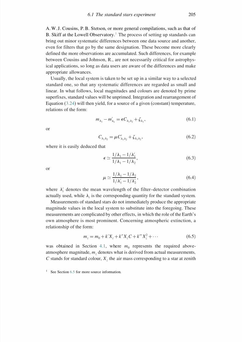
7/21/2019 Introduction to Astronomical Photometry
http://slidepdf.com/reader/full/introduction-to-astronomical-photometry 223/451
6.1 The standard stars experiment 205
A. W. J. Cousins, P. B. Stetson, or more general compilations, such as that of B. Skiff at the Lowell Observatory.1 The process of setting up standards canbring out minor systematic differences between one data source and another,
even for filters that go by the same designation. These become more clearlydefined the more observations are accumulated. Such differences, for examplebetween Cousins and Johnson, R., are not necessarily critical for astrophys-ical applications, so long as data users are aware of the differences and makeappropriate allowances.
Usually, the local system is taken to be set up in a similar way to a selectedstandard one, so that any systematic differences are regarded as small and
linear. In what follows, local magnitudes and colours are denoted by primesuperfixes, standard values will be unprimed. Integration and rearrangement of Equation (3.24) will then yield, for a source of a given (constant) temperature,relations of the form:
m1− m
1 = C 12
+ 1 (6.1)
or
C 12 =
C 12 +
12
(6.2)
where it is easily deduced that
1/1 −1/1
1/1 −1/2
(6.3)
or
1/1 −1/2
1/1
−1/
2
(6.4)
where i denotes the mean wavelength of the filter–detector combination
actually used, while i is the corresponding quantity for the standard system.Measurements of standard stars do not immediately produce the appropriate
magnitude values in the local system to substitute into the foregoing. Thesemeasurements are complicated by other effects, in which the role of the Earth’sown atmosphere is most prominent. Concerning atmospheric extinction, arelationship of the form:
mz = m0 + kX z + kX zC + kX 2z +· · · (6.5)
was obtained in Section 4.1, where m0 represents the required above-atmosphere magnitude, mz denotes what is derived from actual measurements,C stands for standard colour, X z the air mass corresponding to a star at zenith
1 See Section 6.5 for more source information.
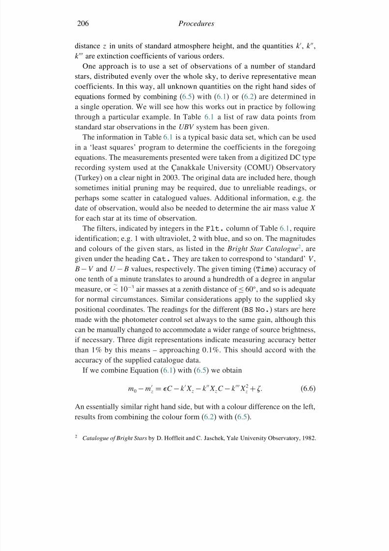
7/21/2019 Introduction to Astronomical Photometry
http://slidepdf.com/reader/full/introduction-to-astronomical-photometry 224/451
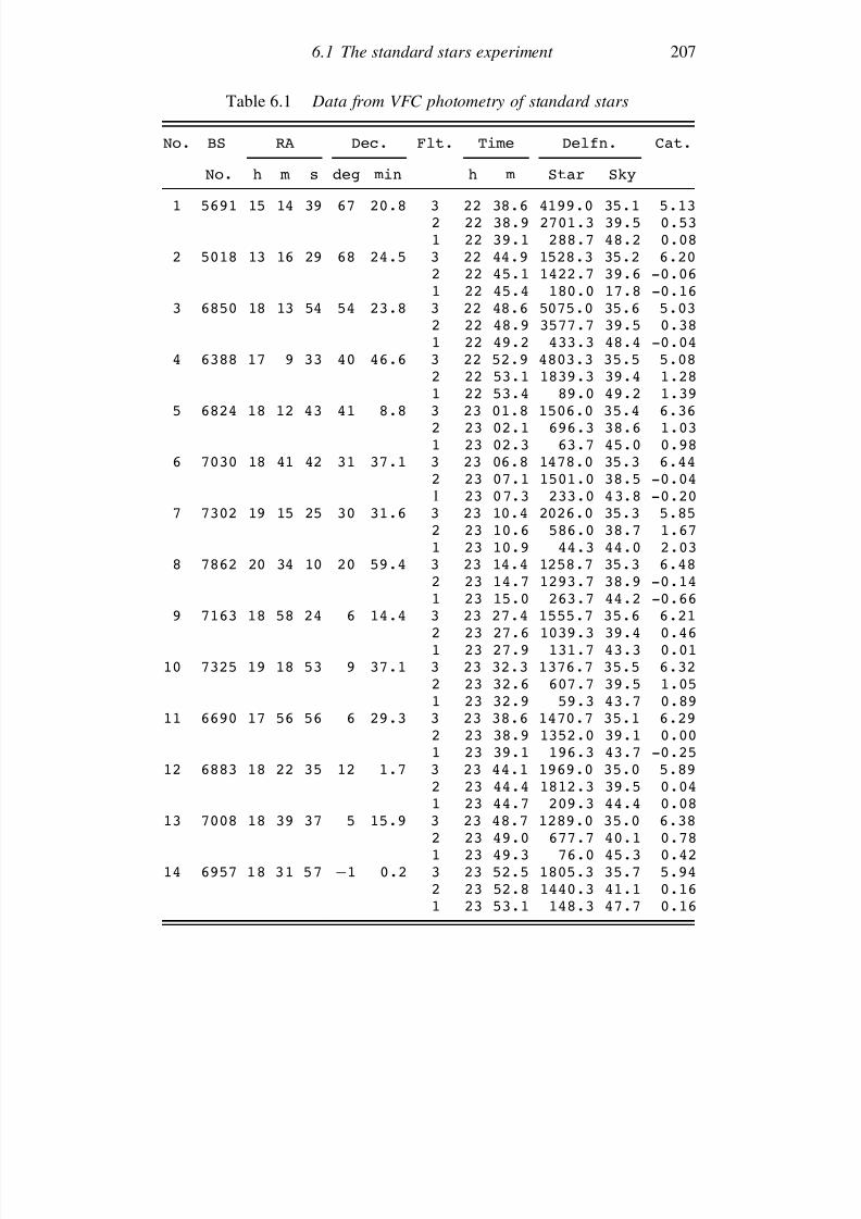
7/21/2019 Introduction to Astronomical Photometry
http://slidepdf.com/reader/full/introduction-to-astronomical-photometry 225/451
6.1 The standard stars experiment 207
Table 6.1 Data from VFC photometry of standard stars
No. BS RA Dec. Flt. Time Delfn. Cat.
No. h m s deg min h m Star Sky
1 5691 15 14 39 67 20.8 3 22 38.6 4199.0 35.1 5.132 22 38.9 2701.3 39.5 0.531 22 39.1 288.7 48.2 0.08
2 5018 13 16 29 68 24.5 3 22 44.9 1528.3 35.2 6.202 22 45.1 1422.7 39.6 -0.061 22 45.4 180.0 17.8 -0.16
3 6850 18 13 54 54 23.8 3 22 48.6 5075.0 35.6 5.03
2 22 48.9 3577.7 39.5 0.381 22 49.2 433.3 48.4 -0.044 6388 17 9 33 40 46.6 3 22 52.9 4803.3 35.5 5.08
2 22 53.1 1839.3 39.4 1.281 22 53.4 89.0 49.2 1.39
5 6824 18 12 43 41 8.8 3 23 01.8 1506.0 35.4 6.362 23 02.1 696.3 38.6 1.031 23 02.3 63.7 45.0 0.98
6 7030 18 41 42 31 37.1 3 23 06.8 1478.0 35.3 6.442 23 07.1 1501.0 38.5 -0.04
1 23 07.3 233.0 43.8 -0.207 7302 19 15 25 30 31.6 3 23 10.4 2026.0 35.3 5.852 23 10.6 586.0 38.7 1.671 23 10.9 44.3 44.0 2.03
8 7862 20 34 10 20 59.4 3 23 14.4 1258.7 35.3 6.482 23 14.7 1293.7 38.9 -0.141 23 15.0 263.7 44.2 -0.66
9 7163 18 58 24 6 14.4 3 23 27.4 1555.7 35.6 6.212 23 27.6 1039.3 39.4 0.461 23 27.9 131.7 43.3 0.01
10 7325 19 18 53 9 37.1 3 23 32.3 1376.7 35.5 6.322 23 32.6 607.7 39.5 1.051 23 32.9 59.3 43.7 0.89
11 6690 17 56 56 6 29.3 3 23 38.6 1470.7 35.1 6.292 23 38.9 1352.0 39.1 0.001 23 39.1 196.3 43.7 -0.25
12 6883 18 22 35 12 1.7 3 23 44.1 1969.0 35.0 5.892 23 44.4 1812.3 39.5 0.041 23 44.7 209.3 44.4 0.08
13 7008 18 39 37 5 15.9 3 23 48.7 1289.0 35.0 6.382 23 49.0 677.7 40.1 0.781 23 49.3 76.0 45.3 0.42
14 6957 18 31 57 −1 0.2 3 23 52.5 1805.3 35.7 5.942 23 52.8 1440.3 41.1 0.161 23 53.1 148.3 47.7 0.16
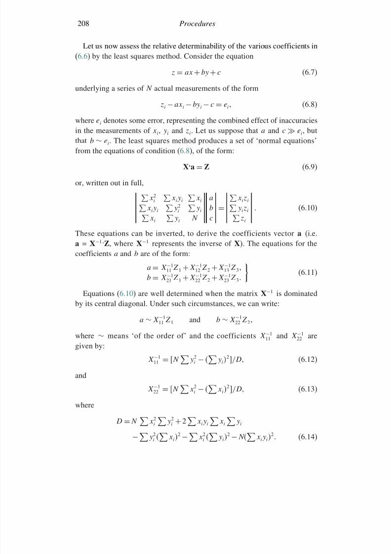
7/21/2019 Introduction to Astronomical Photometry
http://slidepdf.com/reader/full/introduction-to-astronomical-photometry 226/451
208 Procedures
Let us now assess the relative determinability of the various coefficients in(6.6) by the least squares method. Consider the equation
z = ax + by + c (6.7)underlying a series of N actual measurements of the form
zi − axi − byi − c = ei (6.8)
where ei denotes some error, representing the combined effect of inaccuraciesin the measurements of xi, yi and zi. Let us suppose that a and c ei, butthat b ∼ ei. The least squares method produces a set of ‘normal equations’
from the equations of condition (6.8), of the form:
X.a = Z (6.9)
or, written out in full,x2
i
xiyi
xi a
xizi
xiyi
y2
i
yi b =
yizi
xi yi N c zi
(6.10)
These equations can be inverted, to derive the coefficients vector a (i.e.a = X−1.Z, where X−1 represents the inverse of X). The equations for thecoefficients a and b are of the form:
a = X −111 Z1 + X −1
12 Z2 + X −113 Z3
b = X −121 Z1 + X −1
22 Z2 + X −123 Z3
(6.11)
Equations (6.10) are well determined when the matrix X−1 is dominated
by its central diagonal. Under such circumstances, we can write:
a ∼ X −111 Z1 and b ∼ X −1
22 Z2
where ∼ means ‘of the order of’ and the coefficients X −111 and X −1
22 aregiven by:
X −111 = N
y2
i −
yi
2/D (6.12)
andX −1
22 = N
x2i −
xi
2/D (6.13)
where
D = N
x2i
y2
i + 2
xiyi
xi
yi
−
y2i
xi
2 −
x2i
yi
2 − N
xiyi
2 (6.14)
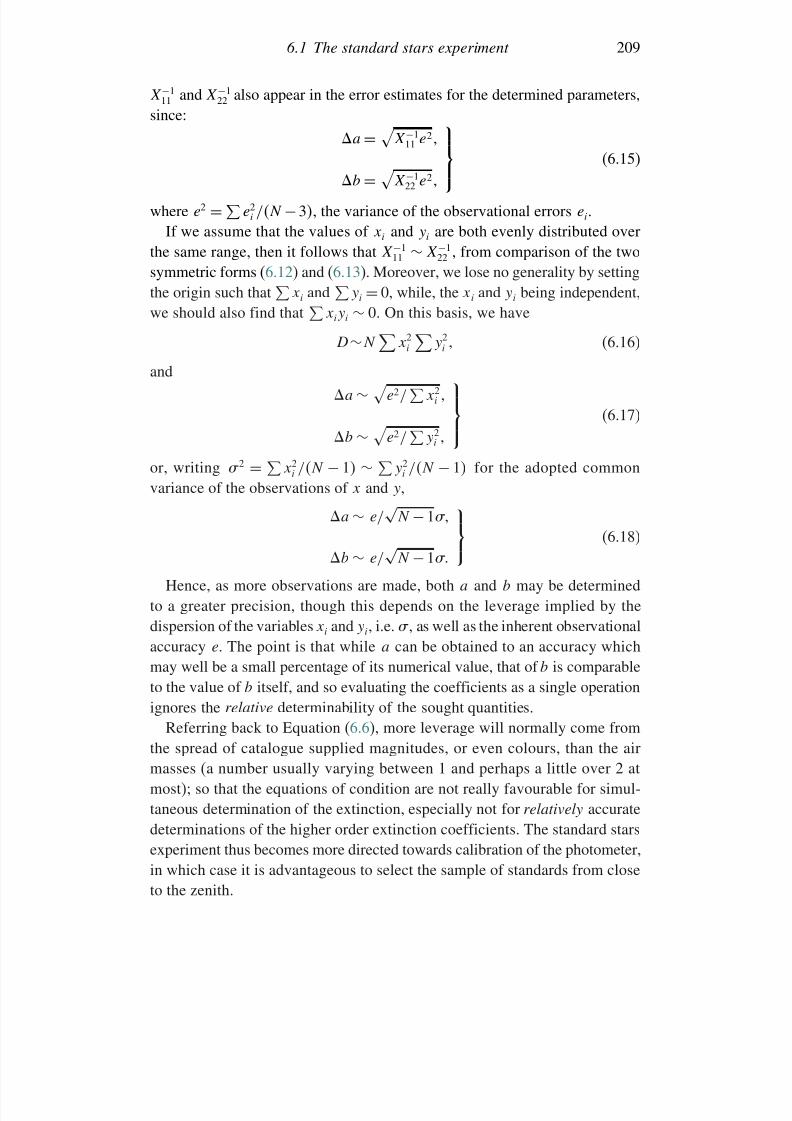
7/21/2019 Introduction to Astronomical Photometry
http://slidepdf.com/reader/full/introduction-to-astronomical-photometry 227/451
6.1 The standard stars experiment 209
X −111 and X −1
22 also appear in the error estimates for the determined parameters,since:
a
= X −111 e2
b =
X −122 e2
(6.15)
where e2 =e2
i /N −3, the variance of the observational errors ei.If we assume that the values of xi and yi are both evenly distributed over
the same range, then it follows that X −111 ∼ X −1
22 , from comparison of the twosymmetric forms (6.12) and (6.13). Moreover, we lose no generality by settingthe origin such that xi and yi
=0, while, the xi and yi being independent,
we should also find that
xiyi ∼ 0. On this basis, we have
D∼N
x2i
y2
i (6.16)
and
a ∼
e2/
x2i
b ∼ e2/y2i
(6.17)
or, writing 2 = x2
i /N − 1 ∼ y2
i /N − 1 for the adopted commonvariance of the observations of x and y,
a ∼ e/√
N −1
b ∼ e/√
N −1
(6.18)
Hence, as more observations are made, both a and b may be determined
to a greater precision, though this depends on the leverage implied by thedispersion of the variables xi and yi, i.e. , as well as the inherent observationalaccuracy e. The point is that while a can be obtained to an accuracy whichmay well be a small percentage of its numerical value, that of b is comparableto the value of b itself, and so evaluating the coefficients as a single operationignores the relative determinability of the sought quantities.
Referring back to Equation (6.6), more leverage will normally come fromthe spread of catalogue supplied magnitudes, or even colours, than the air
masses (a number usually varying between 1 and perhaps a little over 2 atmost); so that the equations of condition are not really favourable for simul-taneous determination of the extinction, especially not for relatively accuratedeterminations of the higher order extinction coefficients. The standard starsexperiment thus becomes more directed towards calibration of the photometer,in which case it is advantageous to select the sample of standards from closeto the zenith.
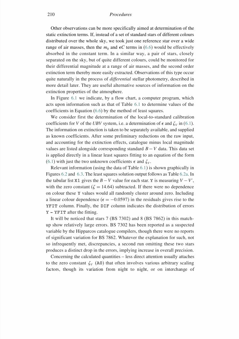
7/21/2019 Introduction to Astronomical Photometry
http://slidepdf.com/reader/full/introduction-to-astronomical-photometry 228/451
210 Procedures
Other observations can be more specifically aimed at determination of thestatic extinction terms. If, instead of a set of standard stars of different coloursdistributed over the whole sky, we took just one reference star over a wide
range of air masses, then the m0 and C terms in (6.6) would be effectivelyabsorbed in the constant term. In a similar way, a pair of stars, closelyseparated on the sky, but of quite different colours, could be monitored fortheir differential magnitude at a range of air masses, and the second orderextinction term thereby more easily extracted. Observations of this type occurquite naturally in the process of differential stellar photometry, described inmore detail later. They are useful alternative sources of information on the
extinction properties of the atmosphere.In Figure 6.1 we indicate, by a flow chart, a computer program, which
acts upon information such as that of Table 6.1 to determine values of thecoefficients in Equation (6.6) by the method of least squares.
We consider first the determination of the local-to-standard calibrationcoefficients for V of the UBV system, i.e. a determination of and V in (6.1).The information on extinction is taken to be separately available, and suppliedas known coefficients. After some preliminary reductions on the raw input,and accounting for the extinction effects, catalogue minus local magnitudevalues are listed alongside corresponding standard B − V data. This data setis applied directly in a linear least squares fitting to an equation of the form(6.1) with just the two unknown coefficients and V .
Relevant information (using the data of Table 6.1) is shown graphically inFigures 6.2 and 6.3. The least squares solution output follows as Table 6.2a. Inthe tabular list X1 gives the B
−V value for each star. Y is measuring V
−V ,
with the zero constant ( = 1464) subtracted. If there were no dependenceon colour these Y values would all randomly cluster around zero. Includinga linear colour dependence ( = −00597) in the residuals gives rise to theYFIT column. Finally, the DIF column indicates the distribution of errorsY - YFIT after the fitting.
It will be noticed that stars 7 (BS 7302) and 8 (BS 7862) in this match-up show relatively large errors. BS 7302 has been reported as a suspected
variable by the Hipparcos catalogue compilers, though there were no reportsof significant variation for BS 7862. Whatever the explanation for such, notso infrequently met, discrepancies, a second run omitting these two starsproduces a distinct drop in the errors, implying increase in overall precision.
Concerning the calculated quantities – less direct attention usually attachesto the zero constant V (A0) that often involves various arbitrary scalingfactors, though its variation from night to night, or on interchange of
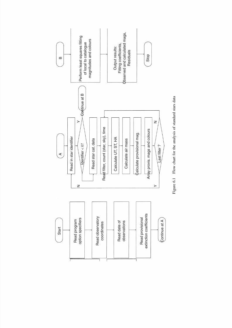
7/21/2019 Introduction to Astronomical Photometry
http://slidepdf.com/reader/full/introduction-to-astronomical-photometry 229/451
B
P e r f o r m l e a s t s q u a r e s f i t t i n g
o f l o c a l t o c a t a l o g u e
m a g n i t u d e s a n d c o l o u r s
O u t p u t r e s u l t s :
F i t t i n g c o e f f i c i e n t s ,
O b s e r v e d a n d c a l c u l a t e d
m a g s ,
R e s i d u a l s
S t o p
S t a r t
R e a d p r o g r a
m
o p t i o n s p e c i f i e r s
R e a d o b s e r v a
t o r y
c o o r d i n a t e s
R e a d d a t e o f
o b s e r v a t i o n
s
R e a d p r o v i s i o
n a l
e x t i n c t i o n c o e f f i c i e n t s
C o n t i n u e a t
A
A
R e a d i n s t a r i d e n t i f i e r
I d e n t i f i e r <
0 ?
R e a d s t a r c a t . d a t a
R
e a d f i l t e r , c o u n t ( s t a r , s k y ) , t i m e
C a l c u l a t e U T ,
S T ,
H A
C a l c u l a t e a i r m a s s
C a l c u l a t e p r o v i s i o n a l m a g
.
A
r r a y p r o v i s . m a g s a n d c o l o u r s
L a s t f i l t e r ?
Y
Y N
N
C o n t i n u e a t B
F i g u r e 6 . 1
F l o w c h a r t f o r t h e a n a l y s i s o f s t a n d a r d s t a r s d a t a
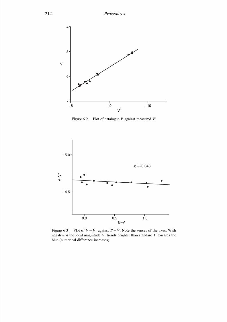
7/21/2019 Introduction to Astronomical Photometry
http://slidepdf.com/reader/full/introduction-to-astronomical-photometry 230/451
212 Procedures
–8 –9 –10V′
4
5
6
7
V
Figure 6.2 Plot of catalogue V against measured V
0.0 0.5
14.5
15.0
V – V
′
ε = –0.043
1.0B–V
Figure 6.3 Plot of V − V against B − V . Note the senses of the axes. Withnegative the local magnitude V trends brighter than standard V towards theblue (numerical difference increases)
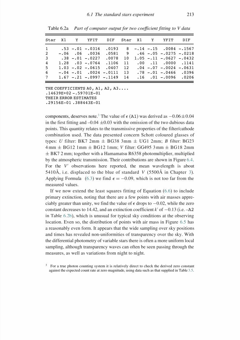
7/21/2019 Introduction to Astronomical Photometry
http://slidepdf.com/reader/full/introduction-to-astronomical-photometry 231/451
6.1 The standard stars experiment 213
Table 6.2a Part of computer output for two coefficient fitting to V data
Star X1 Y YFIT DIF Star X1 Y YFIT DIF
1 .53 -.01 -.0316 .0193 8 -.14 -.15 .0084 -.15672 -.06 .06 .0036 .0581 9 .46 -.05 -.0275 -.02183 .38 -.01 -.0227 .0078 10 1.05 -.11 -.0627 -.04324 1.28 .03 -.0764 .1106 11 .00 .11 .0000 .11415 1.03 -.02 -.0615 .0407 12 .04 -.07 -.0024 -.06316 -.04 -.01 .0024 -.0111 13 .78 -.01 -.0466 .03967 1.67 -.21 -.0997 -.1149 14 .16 .01 -.0096 .0206
THE COEFFICIENTS A0, A1, A2, A3....
.14639E+02 -.59701E-01THEIR ERROR ESTIMATES.29156E-01 .388443E-01
components, deserves note.3 The value of (A1) was derived as −006±004in the first fitting and –0.04 ±0.03 with the omission of the two dubious datapoints. This quantity relates to the transmissive properties of the filter/cathodecombination used. The data presented concern Schott coloured glasses of
types: U filter: BK7 2mm ± BG38 3mm ± UG1 2mm; B filter: BG234 mm ± BG12 1mm ± BG12 1mm; V filter: GG495 3 mm ± BG18 2mm± BK7 2 mm; together with a Hamamatsu R6358 photomultiplier, multipliedby the atmospheric transmission. Their contributions are shown in Figure 6.4.For the V observations here reported, the mean wavelength is about5410Å, i.e. displaced to the blue of standard V (5500Å in Chapter 3).Applying Formula (6.3) we find = −009, which is not too far from the
measured values.If we now extend the least squares fitting of Equation (6.6) to includeprimary extinction, noting that there are a few points with air masses appre-ciably greater than unity, we find the value of drops to −0.02, while the zeroconstant decreases to 14.42, and an extinction coefficient k of −0.13 (i.e. –A2
in Table 6.2b), which is unusual for typical sky conditions at the observinglocation. Even so, the distribution of points with air mass in Figure 6.5 hasa reasonably even form. It appears that the wide sampling over sky positionsand times has revealed non-uniformities of transparency over the sky. Withthe differential photometry of variable stars there is often a more uniform localsampling, although transparency waves can often be seen passing through themeasures, as well as variations from night to night.
3 For a true photon counting system it is relatively direct to check the derived zero constantagainst the expected count rate at zero magnitude, using data such as that supplied in Table 3.5.
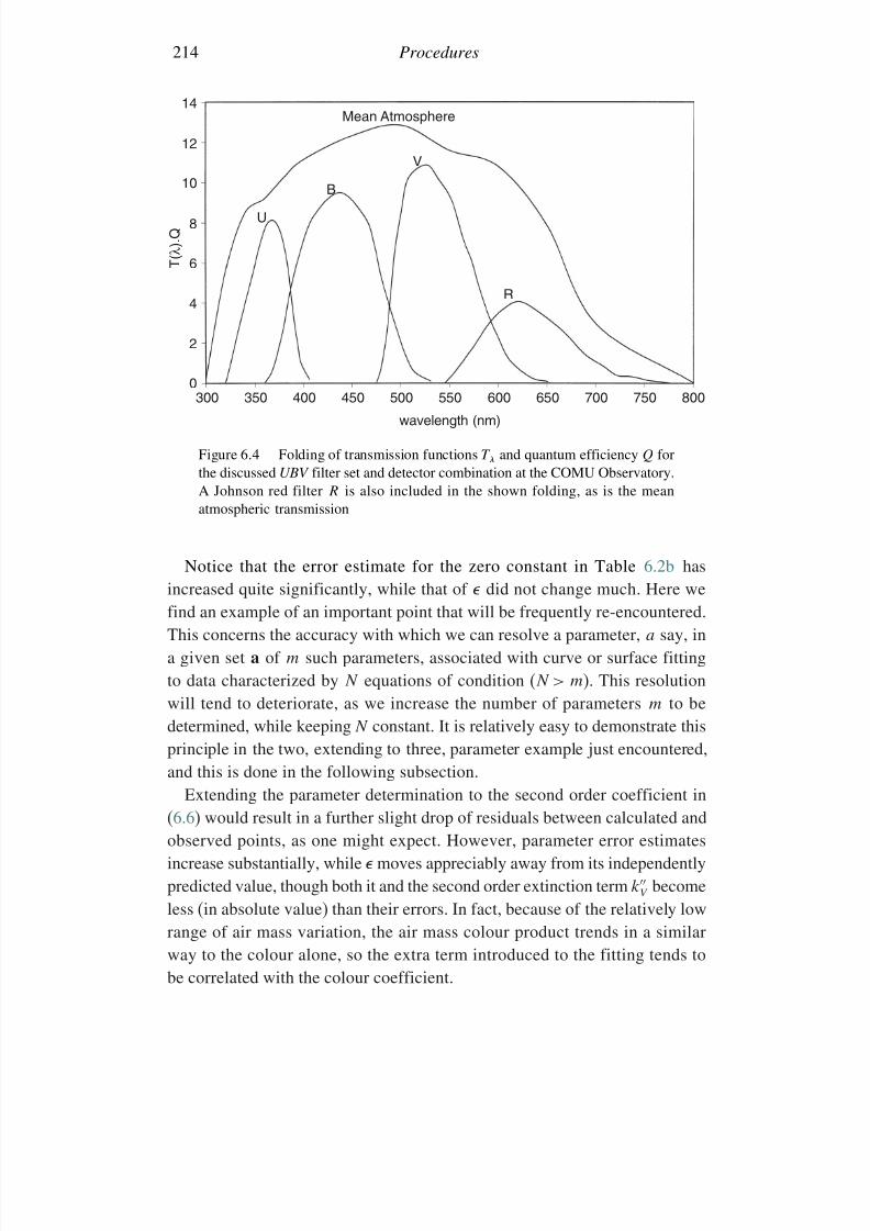
7/21/2019 Introduction to Astronomical Photometry
http://slidepdf.com/reader/full/introduction-to-astronomical-photometry 232/451
214 Procedures
14
12
10
8
T ( λ ) . Q
6
4
2
0300 350 400 450 500 550
wavelength (nm)
600
R
VB
U
Mean Atmosphere
650 700 750 800
Figure 6.4 Folding of transmission functions T and quantum efficiency Q forthe discussed UBV filter set and detector combination at the COMU Observatory.A Johnson red filter R is also included in the shown folding, as is the mean
atmospheric transmission
Notice that the error estimate for the zero constant in Table 6.2b hasincreased quite significantly, while that of did not change much. Here wefind an example of an important point that will be frequently re-encountered.This concerns the accuracy with which we can resolve a parameter, a say, ina given set a of m such parameters, associated with curve or surface fittingto data characterized by N equations of condition (N > m). This resolutionwill tend to deteriorate, as we increase the number of parameters m to bedetermined, while keeping N constant. It is relatively easy to demonstrate thisprinciple in the two, extending to three, parameter example just encountered,and this is done in the following subsection.
Extending the parameter determination to the second order coefficient in(6.6) would result in a further slight drop of residuals between calculated and
observed points, as one might expect. However, parameter error estimatesincrease substantially, while moves appreciably away from its independentlypredicted value, though both it and the second order extinction term k
V becomeless (in absolute value) than their errors. In fact, because of the relatively lowrange of air mass variation, the air mass colour product trends in a similarway to the colour alone, so the extra term introduced to the fitting tends tobe correlated with the colour coefficient.
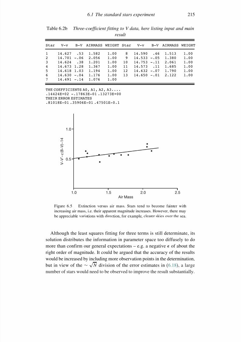
7/21/2019 Introduction to Astronomical Photometry
http://slidepdf.com/reader/full/introduction-to-astronomical-photometry 233/451
6.1 The standard stars experiment 215
Table 6.2b Three-coefficient fitting to V data, here listing input and main
result
Star V-v B-V AIRMASS WEIGHT Star V-v B-V AIRMASS WEIGHT
1 14.627 .53 1.582 1.00 8 14.590 .46 1.513 1.002 14.701 -.06 2.056 1.00 9 14.533 -.05 1.380 1.003 14.624 .38 1.201 1.00 10 14.753 -.11 2.061 1.004 14.673 1.28 1.367 1.00 11 14.573 .11 1.685 1.005 14.618 1.03 1.194 1.00 12 14.632 -.07 1.790 1.006 14.630 -.04 1.176 1.00 13 14.650 -.01 2.122 1.007 14.491 -.14 1.076 1.00
THE COEFFICIENTS A0, A1, A2, A3....
.14424E+02 -.17863E-01 .13273E+00THEIR ERROR ESTIMATES.81018E-01 .35906E-01 .47501E-0.1
1.0
0.5
1.0
V –
V ′ – ε ( B –
V ) – 1 4
1.5Air Mass
2.0 2.5
Figure 6.5 Extinction versus air mass. Stars tend to become fainter withincreasing air mass, i.e. their apparent magnitude increases. However, there maybe appreciable variations with direction, for example, clearer skies over the sea.
Although the least squares fitting for three terms is still determinate, itssolution distributes the information in parameter space too diffusely to domore than confirm our general expectations – e.g. a negative of about theright order of magnitude. It could be argued that the accuracy of the resultswould be increased by including more observation points in the determination,but in view of the ∼ √
N division of the error estimates in (6.18), a largenumber of stars would need to be observed to improve the result substantially.
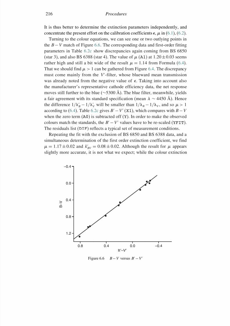
7/21/2019 Introduction to Astronomical Photometry
http://slidepdf.com/reader/full/introduction-to-astronomical-photometry 234/451
216 Procedures
It is thus better to determine the extinction parameters independently, andconcentrate the present effort on the calibration coefficients , in (6.1), (6.2).
Turning to the colour equations, we can see one or two outlying points in
the B − V match of Figure 6.6. The corresponding data and first-order fittingparameters in Table 6.2c show discrepancies again coming from BS 6850(star 3), and also BS 6388 (star 4). The value of (A1) at 120±003 seemsrather high and still a bit wide of the result = 114 from Formula (6.4).That we should find > 1 can be gathered from Figure 6.4. The discrepancymust come mainly from the V -filter, whose blueward mean transmissionwas already noted from the negative value of . Taking into account also
the manufacturer’s representative cathode efficiency data, the net responsemoves still further to the blue (∼5300 Å). The blue filter, meanwhile, yieldsa fair agreement with its standard specification (mean ∼ 4450 Å). Hencethe difference 1/
B − 1/V will be smaller than 1/B − 1/V , and so > 1
according to (6.4). Table 6.2c gives B −V (X1), which compares with B −V
when the zero term (A0) is subtracted off (Y). In order to make the observedcolours match the standards, the B −V values have to be re-scaled (YFIT).The residuals list (DIF) reflects a typical set of measurement conditions.
Repeating the fit with the exclusion of BS 6850 and BS 6388 data, and asimultaneous determination of the first order extinction coefficient, we find = 117 ± 002 and k
BV = 008 ± 002. Although the result for appearsslightly more accurate, it is not what we expect; while the colour extinction
1.2
0.8
0.4
0.0
–0.4
0.8 0.4 –0.40.0Β′–V′
B – V
Figure 6.6 B − V versus B − V
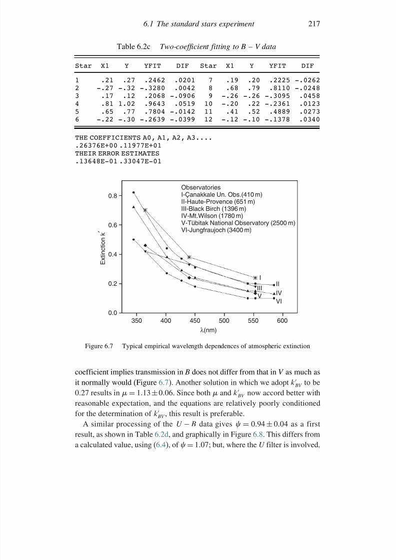
7/21/2019 Introduction to Astronomical Photometry
http://slidepdf.com/reader/full/introduction-to-astronomical-photometry 235/451
6.1 The standard stars experiment 217
Table 6.2c Two-coefficient fitting to B – V data
Star X1 Y YFIT DIF Star X1 Y YFIT DIF
1 .21 .27 .2462 .0201 7 .19 .20 .2225 -.02622 -.27 -.32 -.3280 .0042 8 .68 .79 .8110 -.02483 .17 .12 .2068 -.0906 9 -.26 -.26 -.3095 .04584 .81 1.02 .9643 .0519 10 -.20 .22 -.2361 .01235 .65 .77 .7804 -.0142 11 .41 .52 .4889 .02736 -.22 -.30 -.2639 -.0399 12 -.12 -.10 -.1378 .0340
THE COEFFICIENTS A0, A1, A2, A3.....26376E+00 .11977E+01
THEIR ERROR ESTIMATES.13648E-01 .33047E-01
0.8
0.6
0.4
0.2
0.0350 400 450 500 550 600
IIIIV
IIIV
VI
λ (nm)
E x t i n c t i o n k ′
ObservatoriesI-Çanakkale Un. Obs.(410 m)II-Haute-Provence (651 m)III-Black Birch (1396 m)IV-Mt.Wilson (1780 m)V-Tubitak National Observatory (2500 m)
VI-Jungfraujoch (3400 m)
..
Figure 6.7 Typical empirical wavelength dependences of atmospheric extinction
coefficient implies transmission in B does not differ from that in V as much as
it normally would (Figure 6.7). Another solution in which we adopt kBV to be0.27 results in = 113±006. Since both and k
BV now accord better withreasonable expectation, and the equations are relatively poorly conditionedfor the determination of k
BV , this result is preferable.A similar processing of the U − B data gives = 094 ± 004 as a first
result, as shown in Table 6.2d, and graphically in Figure 6.8. This differs froma calculated value, using (6.4), of = 107; but, where the U filter is involved,
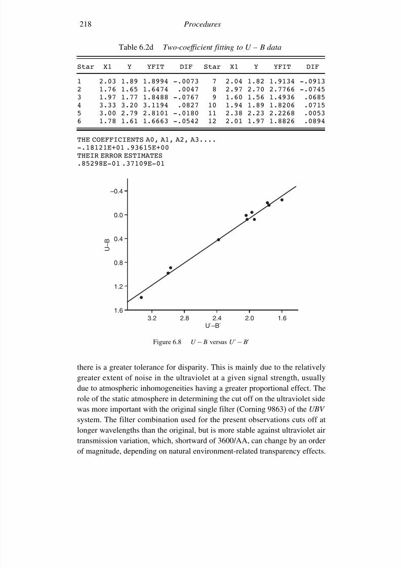
7/21/2019 Introduction to Astronomical Photometry
http://slidepdf.com/reader/full/introduction-to-astronomical-photometry 236/451
218 Procedures
Table 6.2d Two-coefficient fitting to U – B data
Star X1 Y YFIT DIF Star X1 Y YFIT DIF
1 2.03 1.89 1.8994 -.0073 7 2.04 1.82 1.9134 -.09132 1.76 1.65 1.6474 .0047 8 2.97 2.70 2.7766 -.07453 1.97 1.77 1.8488 -.0767 9 1.60 1.56 1.4936 .06854 3.33 3.20 3.1194 .0827 10 1.94 1.89 1.8206 .07155 3.00 2.79 2.8101 -.0180 11 2.38 2.23 2.2268 .00536 1.78 1.61 1.6663 -.0542 12 2.01 1.97 1.8826 .0894
THE COEFFICIENTS A0, A1, A2, A3....-.18121E+01 .93615E+00
THEIR ERROR ESTIMATES.85298E-01 .37109E-01
–0.4
0.0
U – B
U′–B′
0.4
0.8
1.2
1.63.2 2.8 2.4 2.0 1.6
Figure 6.8 U − B versus U − B
there is a greater tolerance for disparity. This is mainly due to the relativelygreater extent of noise in the ultraviolet at a given signal strength, usually
due to atmospheric inhomogeneities having a greater proportional effect. Therole of the static atmosphere in determining the cut off on the ultraviolet sidewas more important with the original single filter (Corning 9863) of the UBV
system. The filter combination used for the present observations cuts off atlonger wavelengths than the original, but is more stable against ultraviolet airtransmission variation, which, shortward of 3600/AA, can change by an orderof magnitude, depending on natural environment-related transparency effects.
7/21/2019 Introduction to Astronomical Photometry
http://slidepdf.com/reader/full/introduction-to-astronomical-photometry 237/451
6.1 The standard stars experiment 219
Another potential difficulty affecting U observations could occur if abroadband detector is used, arising from the red-leak of some UV-transmittingbandpass filters, mentioned in Section 5.1. Under such circumstances, spurious
additions to the signal could become serious for cool star observations. Sincefilter design for the CCD era became more well-discussed, however, improvedspecifications have largely disposed of this issue.
The irregularities of U data have fed back into catalogued sources of information, so that, for instance, the large compilation of UBV photometryof the SIMBAD database shows a significantly greater scatter in U −B valuescompared with corresponding V and B −V for (presumably) constant sources.Proposals have been made on how the U
−B indices can be straightened out,
but, for the most part, users of the UBV system appear to have been readyto live with some level of inaccuracy when traded off against the system’sbroadband light grasp for faint objects, and its general familiarity.
A fitting in which the effect of atmospheric extinction was taken tobe unknown (rather than assigned a typical value) produced the result = 098±003, and k
UB = 014±005, but without significant improvementin the overall goodness of fit, although, in fact, the second value (0.98)
is closer to the theoretically determined value of = 107 for the COMUObservatory photometer.
We have thus followed through the processing of observations of standardstars in detail. The calibration of other systems follows along essentially similarlines, whether broad, intermediate or narrow band filters are used. The inclusionof higher terms in (6.6) would not normally be needed in other than broadbandwork; however, this remark should be qualified, since, due to known difficul-ties of definition, the UBV system is itself not a particularly accurate one (seeSections 4.1–4.3). More recently introduced photometric systems carry inher-ently higher precision. The use of higher order terms in the expansion (6.6)has then to be examined against available accuracy of standards before one cansay where truncations should be made. In Section 4.1.1 we found that thesehigher order terms (in k, k) are of order W 2/2
0W 0. If the standard systemis aiming at 0.001 mag accuracy, therefore, this bandwidth related ratio hasto be less than 10−3 to justify neglect of the second order terms (cf. Table 4.3).
6.1.1 Parameter determinacy and set size: a simple case
Let us write the normal matrix X which determines a, as in (6.9), in thetwo-parameter case simply as
X ≡ x u
u y
7/21/2019 Introduction to Astronomical Photometry
http://slidepdf.com/reader/full/introduction-to-astronomical-photometry 238/451
220 Procedures
The error variance a2 = A2e22, where A2 is given by (6.15), using the
inverse of X, by
A
2
= y
xy − u2 (6.19)
and e22 is the variance of the residuals in this two-parameter fit. Note that the
real determinacy of the normal equations implies that X is a positive definite,symmetric matrix, which means, in effect, that x > 0, y > 0 and xy > u2.
Now when we introduce a third, still determinable, parameter into thederivation, then X becomes X, still positive definite, where
X ≡ x u vu y w
v w z
and so
a2 → A2e23 = yz − w2e2
3
xy − u2z − xw − uvw − yv − uwv (6.20)
From (6.20) we can write, after a little rearrangement,
A2 = A2
1− w2/yz
1− H/zX
(6.21)
where H satisfies X = zX − H > 0, and X , X denote the determinants of X,X, so that H = xw2 +yv2 −2uvw > 0, since
√ xw −√
yv2 > 0, and xy > u2.Note also that 0 < w2/yz < 1, so that (6.21) is of the form
A2
= A2 1
−2
1− 3
(6.22)
where 0 < 2 3 < 1.Thus, A2 ≥ A2 if 3 ≥ 2, i.e. if H/X ≥ w2/y. But, multiplying out H and
X , we find
yH − w2X = yv − uw2 ≥ 0 (6.23)
so the required inequality is established. The result can be generalized to the
m → m + 1 extension in a similar, but more protracted, manner. Hence, theerror factor A2 never decreases with the addition of new parameters. Whetherthe standard deviation error a increases or not depends on whether the netimprovement in the overall fitting (decrease of e2) overrides the deteriorationin a due to the increase of A2. This tends not to occur, in curve-fittings weencounter, after the specification of a few major determinable parameters of the model.
7/21/2019 Introduction to Astronomical Photometry
http://slidepdf.com/reader/full/introduction-to-astronomical-photometry 239/451
6.2 Differential photometry 221
6.2 Differential photometry
The second procedure of this chapter is that in which an object of partic-
ular interest is compared with some reference source or sources. This oftenleads on to the production of light curves. The need to know about the relia-bility of equipment and its calibration by accepted standards, though, makesperformance of the first procedure a practical prerequisite.
The difference in brightness to be measured is usually that of one star fromanother at essentially the same time. But it can refer to one and the same star,as with narrowband spectral intercomparison, or in fast photometry of short-term fluctuations. Slow drifts of background sky brightness or transparencyare then neglected against the scale of fast intrinsic variation. This idea carriesover to more general differential photometry, if relative variation of thebackground can be neglected, or suitably taken into account, against the mainvariation being investigated. In practice, this issue boils down to the nearness,in the relevant respects, between the object and its comparison source. Thisdepends on ambient conditions at the time and location of observation, thenature of the object, and the manner in which the comparisons are made.
Near simultaneous comparison of one star with another similar one locatedclose by in the sky implies a relaxation of the stringency on atmospheric condi-tions, compared with standard stars’ photometry. If simultaneous comparisonis possible, i.e. using a more-than-single channel, or areal, photometer, thenuseful data may still be gathered through quite hazy or variable sky condi-tions. Atmospheric stability through at least a few stellar observation cycletimes (typically several minutes each) would be the minimum requirementfor single-channel photometry.
Traditional visual observations involved a sequence of reference stars. Thisdeveloped, with instrumental photometry, into the selection and adoptionof one main comparison star for a particular object. This star is, at somefavourable time, compared with a standard sequence, so that its magnitudecan be standardized. Its magnitude is also checked for constancy duringthe observations – usually against another reference ‘check’ star. Since anyvariability of the comparison would be inherently independent of the check,
under normal circumstances, constancy of the comparison/check ratio is asufficient guarantee that both stars are constant within some prescribed limitof precision. Any variability of this ratio (corrected for non-intrinsic effects)would require extending the comparison process to more stars, and replacingwhatever original reference was found to vary with a suitable alternative.The choice of a main comparison usually results from a compromise betweenvarious kinds of suitable nearness to the object, i.e. nearness in the sky,
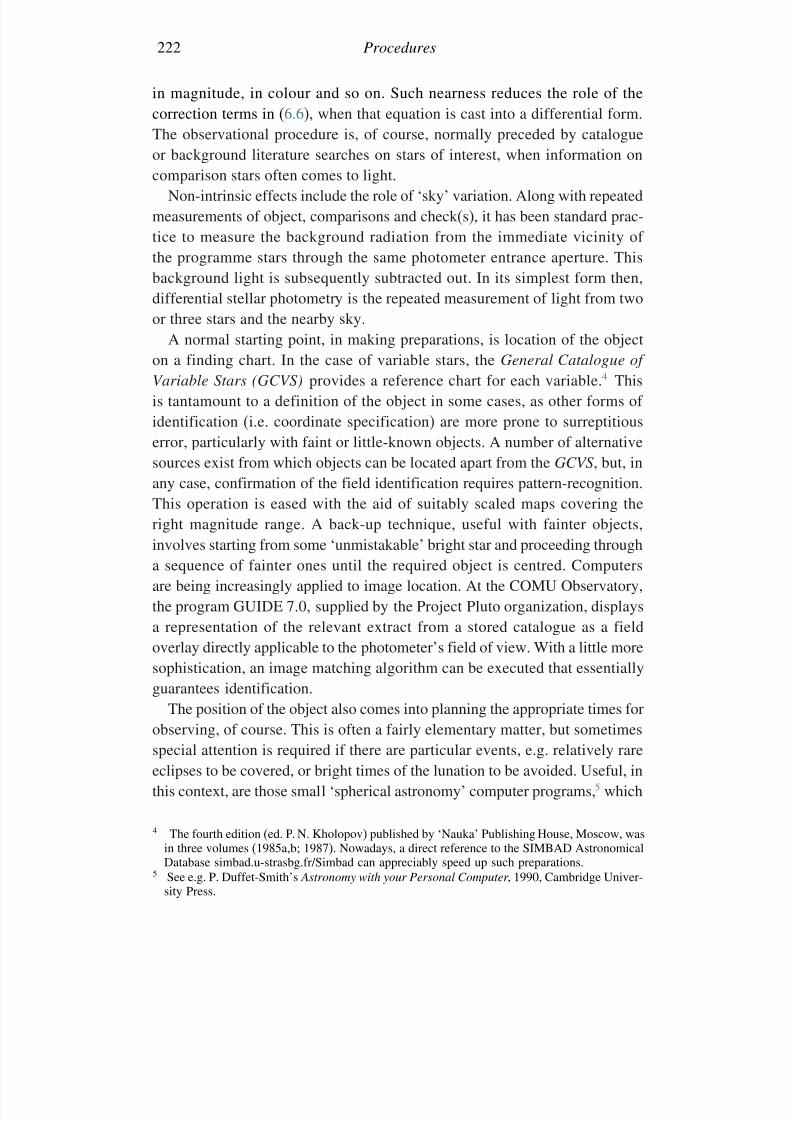
7/21/2019 Introduction to Astronomical Photometry
http://slidepdf.com/reader/full/introduction-to-astronomical-photometry 240/451
222 Procedures
in magnitude, in colour and so on. Such nearness reduces the role of thecorrection terms in (6.6), when that equation is cast into a differential form.The observational procedure is, of course, normally preceded by catalogue
or background literature searches on stars of interest, when information oncomparison stars often comes to light.
Non-intrinsic effects include the role of ‘sky’ variation. Along with repeatedmeasurements of object, comparisons and check(s), it has been standard prac-tice to measure the background radiation from the immediate vicinity of the programme stars through the same photometer entrance aperture. Thisbackground light is subsequently subtracted out. In its simplest form then,
differential stellar photometry is the repeated measurement of light from twoor three stars and the nearby sky.A normal starting point, in making preparations, is location of the object
on a finding chart. In the case of variable stars, the General Catalogue of
Variable Stars (GCVS) provides a reference chart for each variable.4 Thisis tantamount to a definition of the object in some cases, as other forms of identification (i.e. coordinate specification) are more prone to surreptitiouserror, particularly with faint or little-known objects. A number of alternative
sources exist from which objects can be located apart from the GCVS , but, inany case, confirmation of the field identification requires pattern-recognition.This operation is eased with the aid of suitably scaled maps covering theright magnitude range. A back-up technique, useful with fainter objects,involves starting from some ‘unmistakable’ bright star and proceeding througha sequence of fainter ones until the required object is centred. Computersare being increasingly applied to image location. At the COMU Observatory,
the program GUIDE 7.0, supplied by the Project Pluto organization, displaysa representation of the relevant extract from a stored catalogue as a fieldoverlay directly applicable to the photometer’s field of view. With a little moresophistication, an image matching algorithm can be executed that essentiallyguarantees identification.
The position of the object also comes into planning the appropriate times forobserving, of course. This is often a fairly elementary matter, but sometimesspecial attention is required if there are particular events, e.g. relatively rare
eclipses to be covered, or bright times of the lunation to be avoided. Useful, inthis context, are those small ‘spherical astronomy’ computer programs,5 which
4 The fourth edition (ed. P. N. Kholopov) published by ‘Nauka’ Publishing House, Moscow, wasin three volumes (1985a,b; 1987). Nowadays, a direct reference to the SIMBAD AstronomicalDatabase simbad.u-strasbg.fr/Simbad can appreciably speed up such preparations.
5 See e.g. P. Duffet-Smith’s Astronomy with your Personal Computer , 1990, Cambridge Univer-sity Press.
7/21/2019 Introduction to Astronomical Photometry
http://slidepdf.com/reader/full/introduction-to-astronomical-photometry 241/451
6.2 Differential photometry 223
Table 6.3 A typical segment of raw data produced by the data-logger
program. The extract after 20h 46m (only B and V listed) is used to
demonstrate the differential magnitude calculation in 6.2.1
:PROGRAM VAROBS 3.1 by Varol Keskin (2001) .....:Application ÇOMÜ Gözlemevi:File Name ⇒ 011004.dat:Observation Begins at 19:21:48:Observer(s) ⇒ HB,VB:Star Name ⇒ EM Cep:Date ⇒ 1/ 2 October 2004:Julian Date ⇒ 2453280:Local Time
⇒ GMT + 3h [ Times are LOCAL ]
:Moon Phase ⇒ full ( 17. day ):Scale ⇒ 10:Integration Time ⇒ 6 seconds:Sun set ⇒ 18:56:Twilight end ⇒ 20:26:Twilight start ⇒ 05:41:Sun rise ⇒ 07:11C2 U 1483 1500 20:36:18C2 B 5239 5259 20:36:31
C2 V 6044 6041 20:36:44C2S U 387 387 20:38:30C2S B 479 485 20:38:43C2S V 549 547 20:38:56. . . . ...C1 B 13316 13365 20:46:28C1 V 17418 17506 20:46:41C1S B 524 508 20:47:47C1S V 592 596 20:48:00V B 10275 10241 20:49:25
V V 13400 13363 20:49:39VS B 531 528 20:51:26VS V 616 615 20:51:40V B 10306 10347 20:52:37V V 13455 13397 20:52:50C1 B 13400 13355 20:54:19C1 V 17465 17347 20:54:32C1S B 559 551 20:56:51C1S V 651 642 20:57:04. . . .
can, for example, arrange for plots of altitudes for the object corresponding toparticular times of night on particular dates, or give background on the lunarphase, or twilight duration.
We show in Table 6.3 the beginning of a typical raw data file produced by amicrocomputer carrying out the data-logging and control functions indicated
7/21/2019 Introduction to Astronomical Photometry
http://slidepdf.com/reader/full/introduction-to-astronomical-photometry 242/451
224 Procedures
in Figure 5.1 for differential photometry of the variable star EM Cephei.6 Thephotometer was operating as a single-channel VFC instrument (Section 5.3.1)taking all its targets sequentially. Apart from some header type information,
which specifies extra particulars on the observations to be collected, thebulk of the data file consists of sets of four basic pieces of information, i.e.count, time (when the count was registered), filter used and target (object,comparison, check or sky). The reduction program which operates on thisinformation carries out essentially the same task as the one done by hand inthe measurement of pen recorder charts.
The basic arithmetic task is to put
m = −25log
object − skycomparison − sky
(6.24)
for the differential magnitude m. This equation has the magnitude difference(object – comparison) positive when the object is fainter than the comparison.Light-curve data are sometimes presented in the opposite sense, i.e. negativem values when the object is fainter.
The reduction program determines the appropriate set of numbers for object,comparison and sky to substitute into (6.24), and what time, and filter iden-tifier, to affix to the set. Having found the initial, raw data m values, theprogram corrects them for differential extinction and local to standard differ-ences. This is conveniently carried out as a two-stage operation. We firstwrite, using (6.6), to sufficient accuracy,
m0 = m − k
mX z − km X zC (6.25)
to determine the differential magnitude outside the atmosphere m0. Here
X z is positive if there is a greater air mass to the object than the comparison,keeping the same convention for m as (6.24). X z denotes the mean of object and comparison air masses. With successive filter wheel positions,
corresponding data sets are processed, so that the extinction-corrected localcolours C 0 are derived in turn. Corrections to the standard system are thenapplied as
C 0 = C 0 (6.26)
6 This, and subsequent similar data on EM Cep in this section, have been freely quoted fromthe work of Hicran Bakıs, a Ph.D. student of COMU.
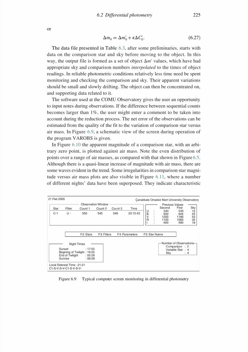
7/21/2019 Introduction to Astronomical Photometry
http://slidepdf.com/reader/full/introduction-to-astronomical-photometry 243/451
6.2 Differential photometry 225
or
m0 = m0 + C 0 (6.27)
The data file presented in Table 6.3, after some preliminaries, starts withdata on the comparison star and sky before moving to the object. In thisway, the output file is formed as a set of object m values, which have hadappropriate sky and comparison numbers interpolated to the times of objectreadings. In reliable photometric conditions relatively less time need be spentmonitoring and checking the comparison and sky. Their apparent variationsshould be small and slowly drifting. The object can then be concentrated on,and supporting data related to it.
The software used at the COMU Observatory gives the user an opportunityto input notes during observations. If the difference between sequential countsbecomes larger than 1%, the user might enter a comment to be taken intoaccount during the reduction process. The net error of the observations can beestimated from the quality of the fit to the variation of comparison star versusair mass. In Figure 6.9, a schematic view of the screen during operation of the program VAROBS is given.
In Figure 6.10 the apparent magnitude of a comparison star, with an arbi-trary zero point, is plotted against air mass. Note the even distribution of points over a range of air masses, as compared with that shown in Figure 6.5.Although there is a quasi-linear increase of magnitude with air mass, there aresome waves evident in the trend. Some irregularities in comparison star magni-tude versus air mass plots are also visible in Figure 6.11, where a numberof different nights’ data have been superposed. They indicate characteristic
21 Feb 2005
Star
C-1 U - 550 545
F2: Stars F3: Filters F4: Parameters F5: Star Name
Night Times Number of ObservationsComparison : 2
: 4Variable Star: 4Sky
: 17:55Sunset: 19:25Begining of Twilight: 05:28End of Twilight: 06:58Sunrise
Local Sidereal Time : 21:21C1-S-V-S-V-C1-S-V-S-V-
548 23:15:43
Second First SkyU : 540 530 15
Previous Values
650 645 25:B1200 1186 43:V1100 1060 35:R
600 580 18:I
Filter Count 1 Count 2 Count 3 TimeObservation Window
Çanakkale Onsekiz Mart University Observatory
Figure 6.9 Typical computer screen monitoring in differential photometry
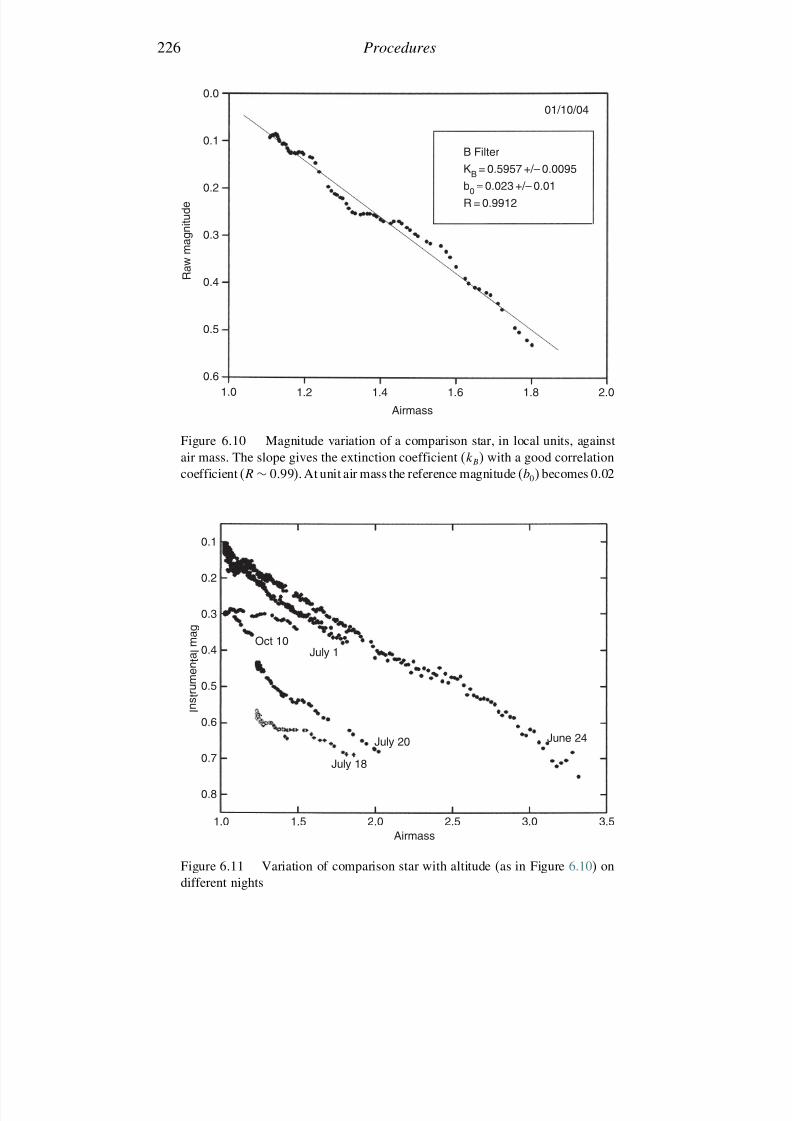
7/21/2019 Introduction to Astronomical Photometry
http://slidepdf.com/reader/full/introduction-to-astronomical-photometry 244/451
226 Procedures
0.0
0.1
0.2
0.3
0.4
0.5
0.61.0 1.2 1.4 1.6 1.8 2.0
01/10/04
B FilterKB = 0.5957 +/– 0.0095
b0 = 0.023 +/– 0.01
R = 0.9912
Airmass
R a w
m a g n i t u d e
Figure 6.10 Magnitude variation of a comparison star, in local units, against
air mass. The slope gives the extinction coefficient (kB) with a good correlationcoefficient (R ∼ 099). At unit air mass the reference magnitude (b0) becomes 0.02
0.1
0.2
0.3
0.4
0.5
0.7
0.8
0.6
1.0 1.5 2.0 2.5 3.0 3.5
July 18
July 20
July 1Oct 10
June 24
Airmass
I n s
t r u
m e n
t a l m
a g
Figure 6.11 Variation of comparison star with altitude (as in Figure 6.10) ondifferent nights
7/21/2019 Introduction to Astronomical Photometry
http://slidepdf.com/reader/full/introduction-to-astronomical-photometry 245/451
6.2 Differential photometry 227
transparency waves, reflecting the inherently dynamic behaviour of the realterrestrial atmosphere. Although linear approximation would be an oversim-plification for representation of such a trend as a whole, it can be adequate to
determine the differential extinction at normal sampling rates. Even the mainstatic term in the atmospheric extinction typically only introduces correctionsin the third significant digit in m. Taking into account time-dependentproperties of the transparency would, in typical sampling conditions for thistype of (single channel) observation, i.e. comparison readings at ∼10–15minute intervals, cause alterations to the derived ms of less than the shotnoise fluctuation from point to point, and so would be lost in subsequent
smoothing.The Earth’s orbital motion should be considered in comparing astronomicalobservations carried out at different times of the year. If we consider a vari-able star situated close to the ecliptic then, at opposition, the light from thestar reaches the Earth about 8 minutes (0.0058 d) earlier than it will reach theSun. At quadrature the time difference disappears and towards conjunction adelay will occur. Clearly there is a dependence in the timing of a celestialevent on just where the Earth happens to be in the ecliptic plane. Times of
observations are thus normally standardized to a heliocentric (or barycentric)coordinate system. This is particularly important for timings such as thoseof epochs of minimum light of eclipsing binary systems, which are oftencited to around 0.0001 d (∼10s) precision. The correction would normallybe included as part of the same data reduction program as that alreadydiscussed.
In order to determine the heliocentric (or similar) correction applied to
remove this light-time effect in observations of stars, we refer again to therotation-matrix formulae of Chapter 4. The task is to find the x-coordinateof the centre of terrestrial motion, when the x-axis points to the object. Forconvenience here, we take the centre to be that of the Sun: it can be shownthat the barycentric correction (i.e. referring to the centre of the Solar System)is always within about 2 seconds of this approximation. Corrections for theeffects of the Moon on the Earth’s position, or the other planets on thebarycentre, could be added for very precise work. Starting with a coordinate
system whose x-axis points to the Sun, we transfer to the object by thefollowing sequence of rotations (see Figure 6.12):
x = Ry−.Rz.Rx−.Rz−.x (6.28)
where the object has equatorial coordinates , while the Sun lies at longi-tude along the ecliptic plane, which is inclined at angle to the equator(Figure 6.12). The vector for the Sun’s coordinates in the starting system
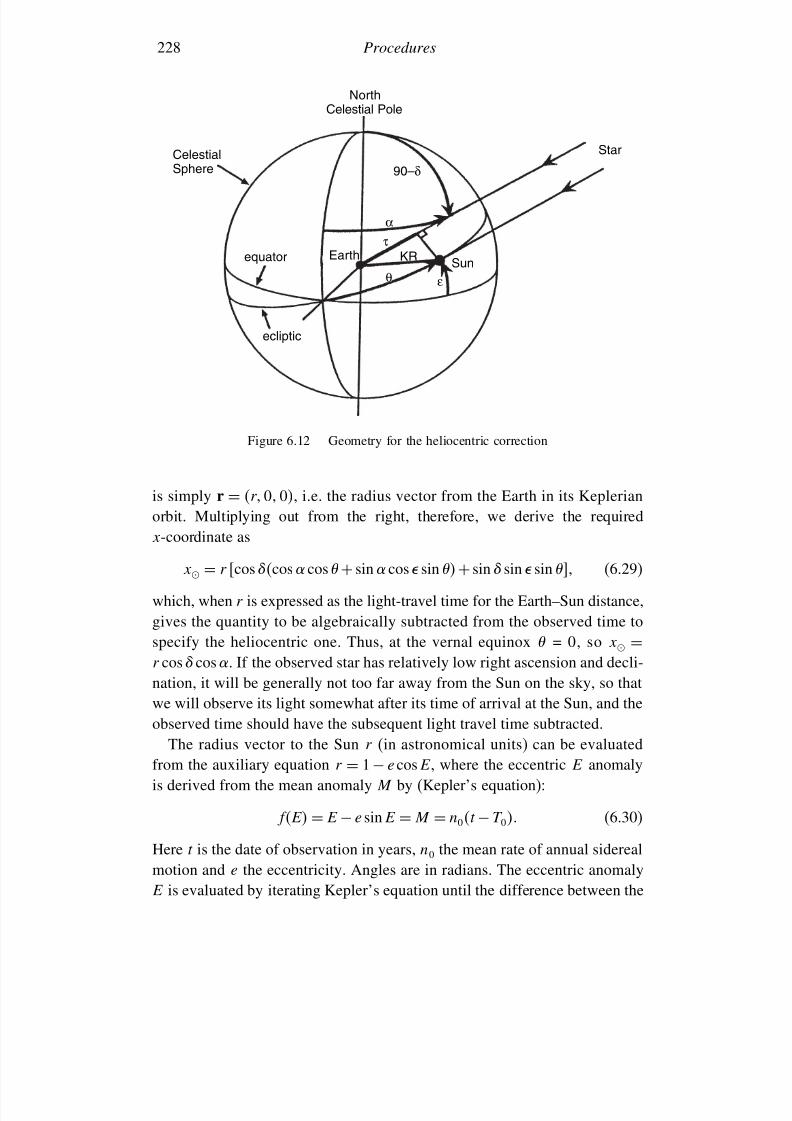
7/21/2019 Introduction to Astronomical Photometry
http://slidepdf.com/reader/full/introduction-to-astronomical-photometry 246/451
228 Procedures
NorthCelestial Pole
CelestialSphere
equator
ecliptic
SunKR
Star
Earth
α
εθ
τ
90–δ
Figure 6.12 Geometry for the heliocentric correction
is simply r = r 0 0, i.e. the radius vector from the Earth in its Keplerianorbit. Multiplying out from the right, therefore, we derive the requiredx-coordinate as
x = r cos cos cos + sin cos sin + sin sin sin (6.29)
which, when r is expressed as the light-travel time for the Earth–Sun distance,gives the quantity to be algebraically subtracted from the observed time tospecify the heliocentric one. Thus, at the vernal equinox = 0, so x =r cos cos . If the observed star has relatively low right ascension and decli-nation, it will be generally not too far away from the Sun on the sky, so thatwe will observe its light somewhat after its time of arrival at the Sun, and theobserved time should have the subsequent light travel time subtracted.
The radius vector to the Sun r (in astronomical units) can be evaluated
from the auxiliary equation r = 1 − e cos E , where the eccentric E anomalyis derived from the mean anomaly M by (Kepler’s equation):
fE = E − e sin E = M = n0t − T 0 (6.30)
Here t is the date of observation in years, n0 the mean rate of annual siderealmotion and e the eccentricity. Angles are in radians. The eccentric anomalyE is evaluated by iterating Kepler’s equation until the difference between the
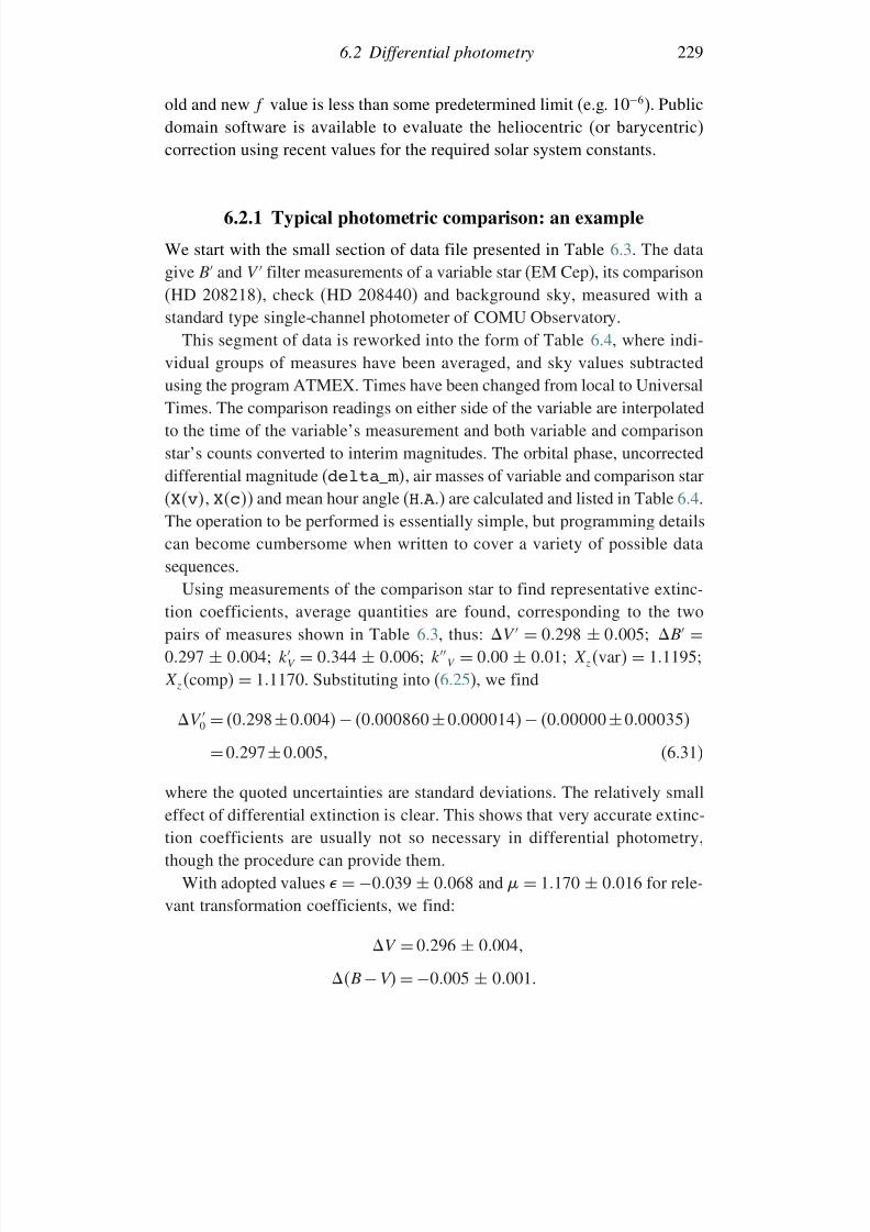
7/21/2019 Introduction to Astronomical Photometry
http://slidepdf.com/reader/full/introduction-to-astronomical-photometry 247/451
6.2 Differential photometry 229
old and new f value is less than some predetermined limit (e.g. 10−6). Publicdomain software is available to evaluate the heliocentric (or barycentric)correction using recent values for the required solar system constants.
6.2.1 Typical photometric comparison: an example
We start with the small section of data file presented in Table 6.3. The datagive B and V filter measurements of a variable star (EM Cep), its comparison(HD 208218), check (HD 208440) and background sky, measured with astandard type single-channel photometer of COMU Observatory.
This segment of data is reworked into the form of Table 6.4, where indi-vidual groups of measures have been averaged, and sky values subtractedusing the program ATMEX. Times have been changed from local to UniversalTimes. The comparison readings on either side of the variable are interpolatedto the time of the variable’s measurement and both variable and comparisonstar’s counts converted to interim magnitudes. The orbital phase, uncorrecteddifferential magnitude (delta_m , air masses of variable and comparison star
(Xv Xc) and mean hour angle (HA ) are calculated and listed in Table 6.4.The operation to be performed is essentially simple, but programming detailscan become cumbersome when written to cover a variety of possible datasequences.
Using measurements of the comparison star to find representative extinc-tion coefficients, average quantities are found, corresponding to the twopairs of measures shown in Table 6.3, thus: V = 0298 ± 0005 B =0297
±0004 k
V
=0344
±0006 k
V
=000
±001 X zvar
=11195
X zcomp = 11170. Substituting into (6.25), we find
V 0 = 0298±0004 − 0000860 ±0000014 − 000000 ±000035
=0297±0005 (6.31)
where the quoted uncertainties are standard deviations. The relatively smalleffect of differential extinction is clear. This shows that very accurate extinc-
tion coefficients are usually not so necessary in differential photometry,though the procedure can provide them.With adopted values = −0039 ± 0068 and = 1170 ± 0016 for rele-
vant transformation coefficients, we find:
V = 0296 ± 0004
B − V = −0005 ± 0001
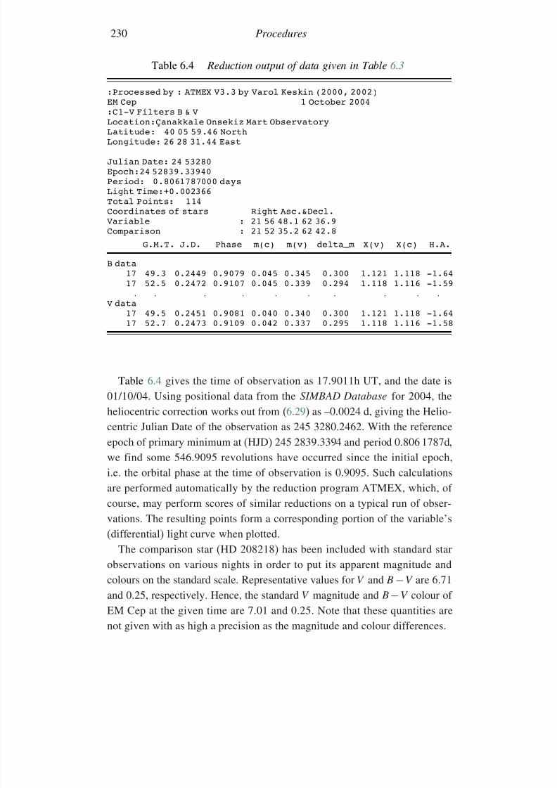
7/21/2019 Introduction to Astronomical Photometry
http://slidepdf.com/reader/full/introduction-to-astronomical-photometry 248/451
230 Procedures
Table 6.4 Reduction output of data given in Table 6.3
:Processed by : ATMEX V3.3 by Varol Keskin (2000, 2002)EM Cep 1 October 2004:C1-V Filters B & VLocation:Çanakkale Onsekiz Mart ObservatoryLatitude: 40 05 59.46 NorthLongitude: 26 28 31.44 East
Julian Date: 24 53280Epoch:24 52839.33940Period: 0.8061787000 daysLight Time:+0.002366Total Points: 114
Coordinates of stars Right Asc.&Decl.Variable : 21 56 48.1 62 36.9Comparison : 21 52 35.2 62 42.8
G.M.T. J.D. Phase m(c) m(v) delta_m X(v) X(c) H.A.
B data17 49.3 0.2449 0.9079 0.045 0.345 0.300 1.121 1.118 -1.6417 52.5 0.2472 0.9107 0.045 0.339 0.294 1.118 1.116 -1.59
. . . . . . . . . .V data
17 49.5 0.2451 0.9081 0.040 0.340 0.300 1.121 1.118 -1.64
17 52.7 0.2473 0.9109 0.042 0.337 0.295 1.118 1.116 -1.58
Table 6.4 gives the time of observation as 17.9011h UT, and the date is01/10/04. Using positional data from the SIMBAD Database for 2004, theheliocentric correction works out from (6.29) as –0.0024 d, giving the Helio-
centric Julian Date of the observation as 245 3280.2462. With the referenceepoch of primary minimum at (HJD) 245 2839.3394 and period 0.806 1787d,we find some 546.9095 revolutions have occurred since the initial epoch,i.e. the orbital phase at the time of observation is 0.9095. Such calculationsare performed automatically by the reduction program ATMEX, which, of course, may perform scores of similar reductions on a typical run of obser-vations. The resulting points form a corresponding portion of the variable’s
(differential) light curve when plotted.The comparison star (HD 208218) has been included with standard starobservations on various nights in order to put its apparent magnitude andcolours on the standard scale. Representative values for V and B −V are 6.71and 0.25, respectively. Hence, the standard V magnitude and B −V colour of EM Cep at the given time are 7.01 and 0.25. Note that these quantities arenot given with as high a precision as the magnitude and colour differences.
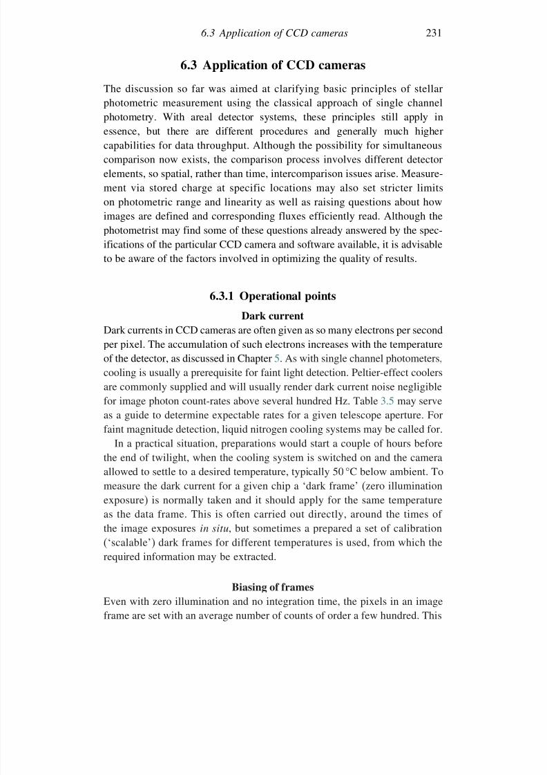
7/21/2019 Introduction to Astronomical Photometry
http://slidepdf.com/reader/full/introduction-to-astronomical-photometry 249/451
6.3 Application of CCD cameras 231
6.3 Application of CCD cameras
The discussion so far was aimed at clarifying basic principles of stellar
photometric measurement using the classical approach of single channelphotometry. With areal detector systems, these principles still apply inessence, but there are different procedures and generally much highercapabilities for data throughput. Although the possibility for simultaneouscomparison now exists, the comparison process involves different detectorelements, so spatial, rather than time, intercomparison issues arise. Measure-ment via stored charge at specific locations may also set stricter limitson photometric range and linearity as well as raising questions about how
images are defined and corresponding fluxes efficiently read. Although thephotometrist may find some of these questions already answered by the spec-ifications of the particular CCD camera and software available, it is advisableto be aware of the factors involved in optimizing the quality of results.
6.3.1 Operational points
Dark currentDark currents in CCD cameras are often given as so many electrons per secondper pixel. The accumulation of such electrons increases with the temperatureof the detector, as discussed in Chapter 5. As with single channel photometers,cooling is usually a prerequisite for faint light detection. Peltier-effect coolersare commonly supplied and will usually render dark current noise negligiblefor image photon count-rates above several hundred Hz. Table 3.5 may serveas a guide to determine expectable rates for a given telescope aperture. Forfaint magnitude detection, liquid nitrogen cooling systems may be called for.
In a practical situation, preparations would start a couple of hours beforethe end of twilight, when the cooling system is switched on and the cameraallowed to settle to a desired temperature, typically 50 °C below ambient. Tomeasure the dark current for a given chip a ‘dark frame’ (zero illuminationexposure) is normally taken and it should apply for the same temperatureas the data frame. This is often carried out directly, around the times of
the image exposures in situ, but sometimes a prepared a set of calibration(‘scalable’) dark frames for different temperatures is used, from which therequired information may be extracted.
Biasing of frames
Even with zero illumination and no integration time, the pixels in an imageframe are set with an average number of counts of order a few hundred. This
7/21/2019 Introduction to Astronomical Photometry
http://slidepdf.com/reader/full/introduction-to-astronomical-photometry 250/451
232 Procedures
is partly to permit a ready linear response to input photons and partly relatedto read-out software. There will be a further pixel to pixel noise around thisoffset (‘bias structure’) but no pixel should register a count of zero as this
can cause difficulties for subsequent statistical image analysis procedure.Information on the biasing is extracted experimentally. Since it does not
involve any exposure time, taking a ‘bias frame’ is essentially an immediateoperation that can be combined into regular procedure during observations aswell as with preparatory field calibration. It is often desirable to combine anumber of such bias frames into one representative (median) set of numbers.
Intercalibration of areal elements – flat fieldingThere will be inherent pixel to pixel variation across any real areal detector,apart from whatever variation arises across the image field. This is partlydue to intrinsic sensitivity change with position and partly due to the wayoptical conditions in the telescope and foreoptics affect the illumination of thechip. The latter variations often arise from dust particles on optical elements,or perhaps from vignetting. The standard approach is to expose the chip toan essentially uniform low level of illumination (low-level twilight is often
used) and examine the resultant pixel to pixel variation across the image.Sometimes, a diffusely illuminated white board (‘dome flat’) is used as analternative to twilight, although questions about the exact comparability of the field illumination to that of the sky may then arise and should be checkedexperimentally.
In taking a flat field there should be a sufficient level of filling for eachpixel well to enable good signal to noise ratios in the collected data without
risking loss of response linearity: somewhat less than half saturation level isgenerally recommended as a desirable count range for a flat field. Saturationlevel counts can be obtained from manufacturer’s data for particular chips, butthey generally run into tens of thousands for common types of CCD cameraat typical gain settings.
In order to increase further the S/N ratio for a mean flat field, it is commonto add the read-outs from a number of separate exposures. Since the resultof flat fielding is a file of ratios of pixel responses, compared with the field
mean, the actual counts are arbitrary, so long as they have been gatheredwithin the range of linear performance of the chip. Here, it should be kept inmind that certain contributors to flat field variation across a CCD frame maybe of a temporary nature. This leads to the precaution of nightly flat fielding.In fact, it is not unusual for flat field images to change during a single night,so it may be desirable to use different flat fields for evening and morningobservations.
7/21/2019 Introduction to Astronomical Photometry
http://slidepdf.com/reader/full/introduction-to-astronomical-photometry 251/451
6.3 Application of CCD cameras 233
The foregoing three topics are usually dealt with together in a CCD obser-vation programme. Typically several dark, flat and bias frames are takenduring a run and later stacked and averaged or median frames selected for
data reduction.
Linearity and well capacity
The relationship between the count registered for a particular pixel and theactual local photon flux is much more complicated in detail than it mayseem. It involves a ‘transfer function’ that incorporates multi-stage electronics,including analogue processes, before the local response is finally digitized.
The aim of good CCD design is that this transfer function produce an outputthat is linearly proportional to the photon input over a definable workingrange. Different CCD manufacturers report on this in different ways, but it iscommon to present a graph of pixel count against exposure time, extendingto a given maximum, known as the full well capacity of the chip. Countsmay be expressed as a relative digital number (DN) or in analogue-to-digitalunits (ADU), which relate to the signal converter used to measure the voltagecreated in the substrate by the stored electrons. Deviations from the best-fit
straight line are found and non-linearity can be expressed in terms of thesedeviations as a percentage.
Regular image processing software requires linearity of response. Hencethere arises a camera quality factor: high-performance CCDs have very goodlinearity over a wide signal range compared to lesser quality devices. CCDcameras intended for professional photometry may have non-linearity of lessthan ∼0.1% over a signal range of up to 10 magnitudes. With such cameras
the small deviations from linearity are constant, and can be determined fromsupplied data. Even with a high quality chip, non-linearity will occur locallynear the full well condition. Beyond this condition the response tends tosaturate. ‘Blooming’ then occurs: this is the overflowing of charge from fullpixels to surrounding ones across the array.
The usual procedure to avoid non-linearity from brighter objects is toreduce exposure times so that collected counts are typically around half-wellcapacity. Multiple short-exposures can be subsequently added, though it may
be necessary to take into account variation of conditions if such additionscover enough time.
Read-out noise
Read-out noise is associated with the analogue to digital conversion process inthe substrate, as well as additional variations that occur during signal transfer.Manufacturers often specify a figure for this contribution in electrons, and

7/21/2019 Introduction to Astronomical Photometry
http://slidepdf.com/reader/full/introduction-to-astronomical-photometry 252/451
234 Procedures
report it for both the sensor element and the entire counting system. Theseparate components are added as squares, and the root mean square specifiedfor the system. At the present time, manufacturers give figures of the order
of ten electrons per read-out as satisfactory for typical use, but astronomersmay press for special designs offering lower levels. The effect of the countingsystem component can be reduced by lowering the gain (expressed as elec-trons per count), but this may also lower the well capacity to an unde-sirable level. In practice, the read-out noise of CCDs intended for astro-nomical use is usually comfortably below acceptable noise levels from thesource; except, perhaps, at high altitude observatories in very clear and stable
conditions.
Measuring stellar fluxes – the PSF and local sky level
The images of stars that appear in a CCD frame can be regarded as a convo-lution of the telescope’s ideal Airy image with a number of other things –arising from tracking irregularities, non-optimal focus, atmospheric ‘seeing’or other blurring effects. The result is usually approximated by an empiricalpoint spread function (PSF), intended to give the observed distribution of flux
over the group of pixels making up a stellar image. Practical stellar PSFs aregenerally of Gaussian form, with two variances for the two dimensions of theframe (‘elliptical Gaussian’). Image processing software exists that can checkthe flux distribution in a designated stellar image and match a PSF to it by asuitable optimizing procedure.
It is well known that convolutions can be usefully processed in thefrequency domain, where the awkwardness of a convolution integral passes
over to the relative simplicity of products of the Fourier transforms of theseparate functions involved. Hence, if we can find suitable forms for theFourier transforms of these disturbing functions they can be divided into thatof the PSF to produce a ‘cleaned’ image of the original source field. Thesuccessful carrying out of this procedure involves some savoir-faire in thechoice and management of relevant software. However, such image improve-ment is not so important for photometry, as can be understood from thecomparable single channel process. In principle, the counts within a selected
‘aperture’ can be simply summed, and compared with a correspondingnearby area of image-free sky. Certain simple photometry applications inCCD data processing software packages follow such a direct analogy withthe single channel procedure. It was seen in Section 4.5, however, that,for precise work, there can be a real issue concerning flux spillage outsidesome pre-assigned aperture. This is an issue that the use of a PSF bypasses,since the fitting of the function’s lower limit, above the dark plus bias level,
7/21/2019 Introduction to Astronomical Photometry
http://slidepdf.com/reader/full/introduction-to-astronomical-photometry 253/451
6.3 Application of CCD cameras 235
defines, in effect, both the local sky level and, through the PSF’s integral,the flux from the star.
Some other practical pointsIt may be necessary to check telescope focusing prior to regular data runs.Wide angle (low depth of focus) systems might encounter sufficient temper-ature variation to affect image quality, or there may be flexure effects forlow-weight telescopes. Apart from possible complications for a uniform PSF,out-of-focus images may cause problems for a field recognition program.Similar difficulties arise from tracking irregularities.
Care is also required at the end of an observing session to make surethe camera returns smoothly to ambient temperature. Failure on this pointcould result in thermal shock and permanent damage to the CCD. Generally,convenient camera software will usually guide the user through a safe parkingsequence for the equipment after use.
6.3.2 Example of CCD-based stellar photometry
A CCD camera is usually operated through a suitable software packageprovided with the instrument or acquired from other sources. These oftenfollow the form of a ‘user-friendly menu’. In what follows, for example, werefer to a few features of MaxIm DLTM. We also describe some operationsof C-Munipack. The observer is still required to set out certain circumstantialinformation (e.g. exposure time, filters).
After opening up MaxIm DLTM and the image to be processed, a ‘process-
calibration wizard’ will conveniently guide the observer. The desired temper-ature and camera model are first given. MaxIm DLTM will assume that thedark image has the same exposure length as the field image unless otherwiseinformed. It will also look for a file in which relevant flat-field images arestored. The wizard then attempts to improve the exposure’s image definition,but, as indicated above, this is not guaranteed to work every time. Finally,adopted images should be saved under a new name, but it is also desirable tosave all raw images. After the wizard has completed image preparation, the
user should be able to obtain the magnitudes of stars of interest. This can, of course, also be done by various alternative packages: IRAF, MIDAS, IDL,and C-Munipack are well-known examples.
C-Munipack7 uses P. B. Stetson’s DAOPHOT procedure for the aperturephotometry of stars in CCD frames. On applying it to images we must first
7 Refer to integral.sci.muni.cz/cmunipack/.
7/21/2019 Introduction to Astronomical Photometry
http://slidepdf.com/reader/full/introduction-to-astronomical-photometry 254/451
236 Procedures
set up data files in a work-folder. Assuming the bias, dark and flat correc-tions were already completed, ‘photometry options’, under the photometrymenu, can be opened. In the options submenu, stellar FWHM (full width at
half maximum) and threshold values relate to the objects of interest in theframes, so these parameters need to be known or estimated before runningthe option. FWHMs of stellar images can be determined from MaxIm DLTM
by positioning a software aperture, using a mouse, onto an object. The infor-mation window in MaxIm DLTM allows multiple measurements of an objectto be stored, so this process can be done with sufficient images to allowrepresentative FWHM values to be utilized. The threshold parameter is set
by the user: by increasing the threshold the number of stars to be included inthe frame processing decreases, so to study faint stars one must set its valuelow enough. The required inner and outer sky reference measures can also bederived from MaxIm DLTM. They are determined from the profiles of objectsof interest.
With such preliminaries assigned, C-Munipack’s photometry option canbe applied. This package delivers magnitudes and positions of objects in theframes and saves them in relevant files. After the photometric determina-
tions, matching of the frames should be performed. This procedure is usefulfor checking observations where there may have been imperfect telescopetracking or field drifting. In the plotting options menu, the user can choosewhether instrumental or differential magnitudes will be displayed. Differentaperture options are also possible in this submenu. Once the desired resultsare found, the data can be saved for future use.
In Table 6.5, partially reduced instrumental magnitudes of V745 Cas
(MAG0) and the comparison star HD 1743 (MAG1) are given with their errors.The Aperture value is the appropriate number from the C-Munipackapertures option. C-Munipack does not actually list explicit air mass(Xv, Xc) and Heliocentric Julian Date (HJD) calculations in the samepackage. These values were obtained from separate computer calculationsand are included in the table for illustration. Once instrumental magnitudesare obtained, using the transformation coefficients, standard differentialmagnitude and colours of V745 Cas can be derived as in Section 6.2.1.
Following the same steps as before, we have: V = −0274 ± 0002B = −0326 ± 0003 k
V = 0259 ± 0009 kV = 000 ± 001 X zvar =
14070 X zcomp = 14047. Substituting again into (6.24), we similarlyfind
V 0 = −0274 ± 0002 − 0000596 ± 0000021 − 000000 ± 000064
= −0274 ± 0002 (6.32)
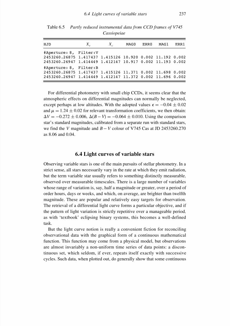
7/21/2019 Introduction to Astronomical Photometry
http://slidepdf.com/reader/full/introduction-to-astronomical-photometry 255/451
6.4 Light curves of variable stars 237
Table 6.5 Partly reduced instrumental data from CCD frames of V745
Cassiopeiae
HJD X v X c MAG0 ERR0 MAG1 ERR1
#Aperture: 8, Filter:V2453260.26875 1.417437 1.415126 10.920 0.002 11.192 0.0022453260.26947 1.414449 1.412147 10.917 0.002 11.193 0.002
#Aperture: 8, Filter:B2453260.26875 1.417437 1.415126 11.371 0.002 11.698 0.0022453260.26947 1.414449 1.412147 11.372 0.002 11.696 0.002
For differential photometry with small chip CCDs, it seems clear that theatmospheric effects on differential magnitudes can normally be neglected,except perhaps at low altitudes. With the adopted values = −004 ± 002and = 124 ± 002 for relevant transformation coefficients, we then obtain:V = −0272 ± 0006, B − V = −0064 ± 0010. Using the comparisonstar’s standard magnitudes, calibrated from a separate run with standard stars,we find the V magnitude and B
−V colour of V745 Cas at JD 2453260.270
as 8.06 and 0.04.
6.4 Light curves of variable stars
Observing variable stars is one of the main pursuits of stellar photometry. In astrict sense, all stars necessarily vary in the rate at which they emit radiation,
but the term variable star usually refers to something distinctly measurable,observed over measurable timescales. There is a large number of variableswhose range of variation is, say, half a magnitude or greater, over a period of order hours, days or weeks, and which, on average, are brighter than twelfthmagnitude. These are popular and relatively easy targets for observation.The retrieval of a differential light curve forms a particular objective, and if the pattern of light variation is strictly repetitive over a manageable period,as with ‘textbook’ eclipsing binary systems, this becomes a well-defined
task.But the light curve notion is really a convenient fiction for reconciling
observational data with the graphical form of a continuous mathematicalfunction. This function may come from a physical model, but observationsare almost invariably a non-uniform time series of data points: a discon-tinuous set, which seldom, if ever, repeats itself exactly with successivecycles. Such data, when plotted out, do generally show that some continuous
7/21/2019 Introduction to Astronomical Photometry
http://slidepdf.com/reader/full/introduction-to-astronomical-photometry 256/451
238 Procedures
curve can be constructed to which the measurements approximate, to withina specifiable error. If this constructed curve is that of a model-dependenttheoretical function, the way is open to interpreting the data in terms of the
parameters of the model. Light curves thus form a useful basis for anal-ysis, particularly as such analysis can usually separate out differential effectsfrom the mean reference level of light. Physical quantities of interest arethence derived from the differential data alone. If the mean light level canbe accurately fixed, it will yield additional information, of course. Theseideas will be explored in more detail later. Even before looking for compre-hensive mathematical models for stellar light variations, though, the more
direct task of noting characteristic features of the variation, notably repeti-tive maxima and minima, forms an informative procedure that can now bediscussed.
6.4.1 Estimation of times of stationary light
The epoch of a minimum (or maximum) light of a close binary system, orsingle star, corresponds to a fixed position of the orbital cycle of a binary
system, or perhaps rotation or pulsation of a single star. Such epochs are usedin finding the periods of cyclic variation. They are essential in the study of changes in the measured periods. It is important to determine these times asaccurately as possible. Different methods are used in determining such timesof stationary light from observations containing N pairs of magnitude andtime values about both sides of a standstill. An overview of some well-knownmethods follows. The principles discussed, in practice, will often be found instandard observatory computer programs.
Kwee and Van Woerden’s method
This (KVW) method is probably the most widely used analytical procedureby observers. It essentially replaced the old tracing paper technique that reliedon graphical estimates. In KVW, (2n + 1) magnitudes equally spaced bythe same time interval T are required as input data. Because observationsdo not necessarily come as an odd number of equally spaced observations,
the points used are usually found by linear interpolation from the raw data.A preliminary estimate T , say, of the time of minimum T m is set up asa central value among the equidistant times. This defines a reflection axisfor the remaining set of n magnitudes. Let mk be the difference betweena pair of initial and reflected magnitudes. The summation m2
k, whichcan be regarded as a function of the chosen time, that we denote as T,provides an estimate of the closeness of the branches’ superposition about the
7/21/2019 Introduction to Astronomical Photometry
http://slidepdf.com/reader/full/introduction-to-astronomical-photometry 257/451
6.4 Light curves of variable stars 239
reflection axis. The reflection axis is shifted successively to T + T/2 andto T − T/2 and the magnitude pairs reassigned. If T was properly chosen,T < T
+T/2 and T < T
−T/2; otherwise, the reflection axis
has to be re-positioned to the time giving the smallest summation and theprocess repeated, keeping the same number of points on either side.
Now, T may be represented by the quadratic formula
T = aT 2 + bT + c (6.33)
where the coefficients a, b and c are evaluated from the three summations(left, centre, right) by elimination. The parabola (6.33) has its lowest value,
T m = c − b2/4a (6.34)
at what can now be taken as the correct epoch of minimum:
T m = −b/2a (6.35)
The measure of error of T m is given by:
T m = 4ac − bT 2
4a2 −1 (6.36)
where is the number of independent magnitude pairs. This would be n if the used points happened to be equidistantly spaced to start with: if obtainedby interpolation = n/2.
KVW is based on the assumption of light curve symmetry, but it may be still
used even if slight asymmetries are present. In this case, the algorithm maytake some time to reach a suitable reflection axis and if there are oscillations inthis process a poor estimate of the epoch of minimum may result. Redefiningthe range of steps may avoid this possibility and save calculation time.
Best fit method
This method is based on optimally fitting a suitable polynomial to the
minimum (or maximum) region of the observations. It may require repeatedapplication of the least squares method for different forms of the polynomial.If mi, T i, i = 1 2 N are the observed values of magnitude and time,residuals Ri are evaluated from:
Ri = mi − T i = mi −n
j =0
aj T j i i = 1 2 N (6.37)
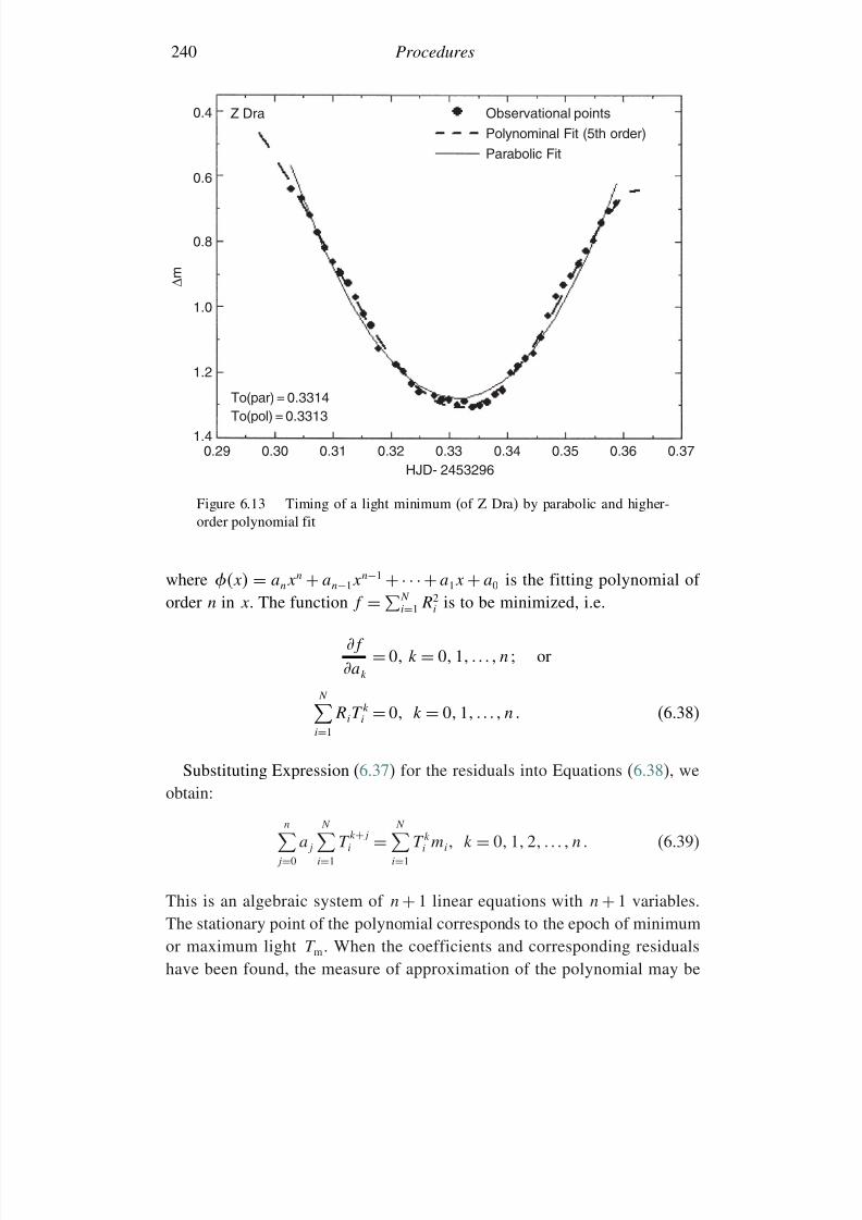
7/21/2019 Introduction to Astronomical Photometry
http://slidepdf.com/reader/full/introduction-to-astronomical-photometry 258/451
240 Procedures
0.4
0.6
0.8
1.0
∆ m
1.2
1.40.29 0.30 0.31 0.32 0.33
HJD- 2453296
To(par) = 0.3314
Z Dra
To(pol) = 0.3313
0.34
Observational points
Polynominal Fit (5th order)
Parabolic Fit
0.35 0.36 0.37
Figure 6.13 Timing of a light minimum (of Z Dra) by parabolic and higher-order polynomial fit
where x = anxn + an−1xn−1 +· · ·+ a1x + a0 is the fitting polynomial of order n in x. The function f =N
i=1 R2i is to be minimized, i.e.
f
ak =0 k
=0 1 n or
N i=1
RiT ki = 0 k = 0 1 n (6.38)
Substituting Expression (6.37) for the residuals into Equations (6.38), weobtain:
nj =0
aj
N i=1
T k+j i =
N i=1
T ki mi k = 0 1 2 n (6.39)
This is an algebraic system of n + 1 linear equations with n + 1 variables.The stationary point of the polynomial corresponds to the epoch of minimumor maximum light T m. When the coefficients and corresponding residualshave been found, the measure of approximation of the polynomial may be
7/21/2019 Introduction to Astronomical Photometry
http://slidepdf.com/reader/full/introduction-to-astronomical-photometry 259/451
6.4 Light curves of variable stars 241
estimated from the standard deviation:
n=
N i=1 R2
i
N − n +1
(6.40)
The best fit method allows one to identify the most suitable order n forthe polynomial that optimally approximates the observations. This entailsrepeated applications of the least squares method until n does not showappreciable change from one fitting to the next, whereupon the sought polyno-mial can be considered found. The epoch of minimum T m may be computed,in the range of times between T 1 and T N , as the root xm of the deriva-
tive: P x = nanxn−1 + n − 1an−1xn−2 + · · · + 2a2x + a1. The bisectionalgorithm provides an iterative way to find this root.
A somewhat developed version of this method occurs when, instead of an arbitrary polynomial, the selected fitting function corresponds to a phys-ical model for the light variation. The fitting function will normally includeparameters ensuring that stationary points on the light curve do occur, but theformulation is usually implicit and non-linear, rather than explicit and linear
as with the polynomial. A least-squares minimization principle still applies,and though it may not be possible to spell out the corresponding time estimateexplicitly, the numerical approach of the computer gives an equivalent result.We will encounter more about this technique in subsequent chapters.
Polygonal line method
Devised by A. Guarnieri, A. Bonifazi and P. Battistini in 1975, this methodmay be considered as an analytical implementation of the tracing papermethod. It is particularly suitable for inhomogeneous distributions of observa-tions along two branches that cannot be correctly processed by KVW. In theapplication, the two branches of the minimum (or maximum) are folded on avertical axis, perpendicular to the time axis, and the length L of the polygonalline connecting the points, in the sense of increasing times, evaluated withoutdistinction between real and reflected points. The length L is thus a functionof the position of the reflection axis L
=LT r and it will be minimized when
T r is effectively the axis of symmetry.The method is carried out, in a systematic way, by shifting the reflection
axis according to a procedure of selected steps and calculating LT r for eachstep. The uncertainty T m
of the minimum position for the function L may beestimated by repeating the summation with data points displaced according tothe mean errors of their values. The abscissae TLmin ± T m
give the epochof minimum T m and corresponding error interval.
7/21/2019 Introduction to Astronomical Photometry
http://slidepdf.com/reader/full/introduction-to-astronomical-photometry 260/451
242 Procedures
Middle line method
This algorithm was developed in order to overcome the influence of appre-ciable asymmetries on the evaluation of the epoch of minimum of eclipsing
binary systems. The foregoing methods are all based on an initial assumptionof a symmetric light curve, and therefore a vertical axis of reflection forthe two branches. Their results will be affected by appreciable departuresfrom symmetry. The issue is dealt with by evaluating a middle line for theminimum and performing a transformation of coordinates so that the middleline becomes a vertical line in the new coordinate system. A conventionalsecond-order polynomial regression will then provide a reference time, and a
transformation back to the original coordinate system yields the correspondingepoch of minimum. This algorithm thus follows the plan of the other methods,where branch superposition has been modified by the rotation of the mid-axis.
Sliding integrations method
Introduced by S. Ghedini, this method is based on the principle of a parabolicdistribution defining the minimum (or maximum) light: m = a 2 +b +c.Each observation is thus a measure of the function m at a given time.
Integration of m allows filtering out of possible superposed variations of higher frequencies. On this basis, the time of stationary light may be estimatedby evaluating the integral difference:
fT = T 0+T/2
T 0
md − T 0+T
T 0+T/2md = −1
2T 2
aT 0 + aT + b
2
(6.41)
which defines the function fT for a given initial time T 0 and total integrationinterval T . In practice, the integrals can be formed by a suitable quadrature,e.g. Simpson’s rule. Given T 0, allowing T to slide along the time axis, in thesense of increasing , will, at some point, produce the zero fT = T z = 0,which satisfies
T z = − b
a−2T 0 (6.42)
The time of minimum T m follows as T m = T 0 + T z/2 = −b/2a.
6.5 Bibliographical notes
The classic reference for much of the subject matter of this chapter is thepaper of R. H. Hardie in Astronomical Techniques, ed. W. A. Hiltner (Univer-sity Press, Chicago, p. 178, 1962). The procedures discussed there wereelaborated on in A. A. Henden and R. H. Kaitchuk’s Astronomical Photometry
7/21/2019 Introduction to Astronomical Photometry
http://slidepdf.com/reader/full/introduction-to-astronomical-photometry 261/451
6.5 Bibliographical notes 243
(Van Nostrand Reinhold, 1982), C. Kitchin’s Astrophysical Techniques
(Adam Hilger, 1984) and W.A. Cooper and E.N. Walker’s Getting the
Measure of the Stars (Adam Hilger, 1988). Henden and Kaitchuck produced
their Astronomical Photometry Software for the IBM-PC (Willmann-Bell,1989), complete with three computer diskettes, enabling the user to applysuch procedures directly to data. Indeed, the impact of computers on dataprocessing is a major change that has occurred since the time of Hardie’spaper. This development continues everywhere, and indications about codingincluded with the present chapter are intended to be illustrative only.Programmers are continually introducing more efficient, user-friendly algo-
rithms, in purpose-oriented computer languages, to deal with data reductionand analysis of the kind presented. Examples of such techniques applied tosingle channel photometry are in the I.A.P.P.P. Commun. and Fairborn Pressliterature mentioned in Section 5.4, or R. Elston & M. Zeilik (Publ. Astron.
Soc. Pac., 94, 729, 1982).A.U. Landolt of Louisiana State University has spent much of the last
several decades on the improvement and definition of broadband, particularlyUBVRI, photometric standard star data, producing careful measurements of
selected regions near clusters or field concentrations. Papers in Astron. J.(78, 959, 1973 through to 104, 340, 1992) encompass a series of studies.Similar work has been done by A. W. Cousins, particularly regardingSouthern Hemisphere standards, ranging from Mon. Not. Astr. Soc. South
Africa (24, 120, 1965) to Mon. Not. Astron. Soc. S. Africa (40, 37, 1981)and S. Africa Astron. Obs. Circ. (8, 69, 1984); see also Cousins, A.J. &Menzies, J.W. in Precision Photometry, eds. D. Kilkenny et al. (p. 240,
1993). P.B. Stetson listed some sources for (CCD) standard stars in hisreview in Proc. IAU Coll. 136: Stellar Photometry: Current Techniques
and Future Developments, eds. C. J. Butler and I. Elliott (CambridgeUniversity Press, 1992, p. 291), and provided further background in Publ.
Astron. Soc. Pacific (112, 925, 2000). Stetson’s standard star data can beaccessed from cadcwww.hia.nrc.ca/cadcbin/wdbi.cgi/astrocat/stetson/query.B. Skiff’s compilation is known as the LONEOS catalogue and can beaccessed from ftp.lowell.edu/pub/bas/starcats/loneos.phot. Recommendations
on filter design for the CCD era were made by M. Bessell (Publ. Astron.Soc. Pacific 102, 1181, 1990). For further general information consultwww.phys-astro.sonoma.edu/observatory/observers/standards/standards.html.An interesting brief review of the Johnson and Cousins filter systemswas produced by G. Persha of Optec Inc. and is accessible fromcompany7.com /library/optec/filtermono.html. The SIMBAD database facilityshould also be referred to for extensive reference coverage on particular stars.
7/21/2019 Introduction to Astronomical Photometry
http://slidepdf.com/reader/full/introduction-to-astronomical-photometry 262/451
244 Procedures
Detailed considerations for approaching 0.001 mag accuracies in calibratinga photometric system were given in A. T. Young’s paper in Automated Tele-
scopes for Photometry and Imaging, ed. S.J. Adelmann et al. ( ASP Conf.
Ser., 28, p. 73). Young argued for a greater degree of spectral sampling tobe achieved with a more complete filter set than just UBV , and more auto-mated actions to streamline procedure. Practical experience along these lineswas reported by C. Sterken and J. Manfroid at the same conference (p. 57)(see also J. Tinbergen, Proc. IAU Coll. 136 , eds. C.J. Butler & I. Elliott,Cambridge University Press, 1992, p. 264; T. Oja, Astron. Astrophys., 286,1006, 1994) and G.W. Henry & D.S. Hall in Robotic Observatories, ed.
M. F. Bode (Wiley, 1995, p. 41). Submillimag accuracy is clearly achiev-able from suitably equipped satellites (see Figure 1.1), and is a prerequisiteof GAIA photometry (refer to Section 1.5), but it can be approached evenwith standard terrestrial photometric equipment, provided that it is suitablylocated (E. Budding, D. Sullivan & M. Rhodes, Transits of Venus: New
Views of the Solar System and Galaxy; Proc. IAU Coll. 196 , ed. D. W. Kurtz,Cambridge University Press, 2005, p. 386) at least regarding differentialphotometry.
With regard to calculations required in preparing for observations, besidesthe book by P. Duffet-Smith mentioned in the text, the similar one byJ. Meeus, Astronomical Algorithms (Willmann-Bell, 2nd edn., 1998) couldbe cited. A number of such sources of information were reviewed byBill McClain at www.salamander.com/ ∼wmmcclain/astro_calc_old.html,including sources for the astronomical constants used in such calculations.
Data showing the properties of atmospheric extinction at an astronomical
observatory appear from time to time distributed throughout the literature, e.g.W. J. Schuster ( Rev. Mex. Astron. Astrofis., 5, 149, 1982); T. S. Yoon & S. W.Lee ( J. Korean Astron. Soc., 15, 59, 1982); A. W. Cousins ( Mon. Not. Astron.
Soc. S. Africa, 44, 10, 1985); A. Jimenez, H. Gonzalez Jorge & M. C. Rabello-Soares ( Astron. Astro-Phys. Suppl., 129, 413, 1998); H. Sung & M. S. Bessell(Publ. Astron. Soc. Austral., 17, 244, 2000); Z. Mikulasek, J. Svoren & J.Ziznovsky (Contrib. Astron. Obs. Skalnate Pleso, 33, 21, 2003) and others.The significance of dynamical extinction effects was studied by E. Poretti &
F. Zerbi ( Astron. Astrophys., 268, 369, 1993). A classic review was given byJ. Stock in Vistas Astron. (11, 127, 1969). A selection of references dealingwith CCDs and their applications to astronomical photometry is given inSection 5.4.
The method of timing minima due to K. K. Kwee and H. van Woerden waspublished in Bull. Astron. Inst. Netherlands (12, 327, 1956). The polygonalline method appears in A. Guarnieri, A. Bonifazi & P. Battistini ( Astron.
7/21/2019 Introduction to Astronomical Photometry
http://slidepdf.com/reader/full/introduction-to-astronomical-photometry 263/451
References 245
Astrophys. Suppl., 20, 199, 1975). The sliding integrations method was givenby S. Ghedini, in Mem. Soc. Astron. Ital. (52, 633, 1981). Ghedini alsoreviewed other methods in his book Software for Photometric Astronomy,
Willmann-Bell (1982).
References
Bessell, M., 1990, Publ. Astron. Soc. Pacific, 102, 1181.Budding, E., Sullivan, D. & Rhodes, M., 2005, Proc. IAU Coll. 196 , ed. D. W. Kurtz,
Cambridge University Press, 2005, p. 386.
Cooper, W. A. & Walker, E. N., 1988, Getting the Measure of the Stars, Adam Hilger.Cousins, A. W., 1965, Mon. Not. Astron. Soc. S. Africa, 24, 120.Cousins, A. W., 1981, Mon. Not. Astron. Soc. S. Africa, 40, 37.Cousins, A. W., 1984, S. Africa Astron. Obs. Circ., 8, 69.Cousins, A. W., 1985, Mon. Not. Astron. Soc. S. Africa, 44, 10.Cousins, A.J. & Menzies, J.W., 1993, Precision Photometry, eds. D. Kilkenny,
E. Lastovicia & J. W. Menzies, SAAO, p. 240.Duffet-Smith, P., 1990, Astronomy with your Personal Computer , Cambridge Univer-
sity Press.
Elston, R. & Zeilik, M., 1982, Publ. Astron. Soc. Pac., 94, 729.Ghedini, S., 1981, Mem. Soc. Astron. Ital., 52, 633.Ghedini, S., 1982, Software for Photometric Astronomy, Willmann-Bell.Guarnieri, A., Bonifazi, A. & Battistini, P., 1975, Astron. Astrophys. Suppl., 20, 199.Hardie, R.H., 1962, Astronomical Techniques, ed. W. A. Hiltner, University Press,
Chicago, p. 178.Henden, A.A. & Kaitchuk, R.H., 1982, Astronomical Photometry, Van Nostrand
Reinhold.Henden, A. A. & Kaitchuk, R. H., 1989, Astronomical Photometry Software for the
IBM-PC , Willmann-Bell.Henry, G.W. & Hall, D.S., 1995, Robotic Observatories, ed. M.F. Bode, Wiley,
p. 41.Hoffleit, D. & Jaschek, C., 1982, Catalogue of Bright Stars, Yale University
Observatory.Jimenez, A., Gonzalez Jorge, H. & Rabello-Soares, M. C., 1998, Astron. Astrophys.
Suppl., 129, 413.Kholopov, P. N., 1985a,b & 1987 (3 vols.), General Catalogue of Variable Stars,
‘Nauka’ Publishing House, Moscow.
Kitchin, C., 1984, Astrophysical Techniques, Adam Hilger.Kwee, K. K. & van Woerden, H., 1956, Bull. Astron. Inst. Netherlands, 12, 327.Landolt, A. U., 1973, Astron. J., 78, 959.Landolt, A. U., 1992, Astron. J., 104, 340.McClain, W., 2006, www.salamander.com/ ∼wmmcclain/astro_calc_old.html.Meeus, J., 1998, Astronomical Algorithms, Willmann-Bell (2nd edn.).Mikulasek, Z., Svoren, J. & Ziznovsky, J., 2003, Contrib. Astron. Obs. Skalnate Pleso,
33, 21.
7/21/2019 Introduction to Astronomical Photometry
http://slidepdf.com/reader/full/introduction-to-astronomical-photometry 264/451
246 Procedures
Oja, T., 1994, Astron. Astrophys., 286, 1006.Persha, G., 2006, company7.com/library/optec/filtermono.html.Poretti, E. & Zerbi, F., 1993, Astron. Astrophys., 268, 369.Schuster, W. J., 1982, in Rev. Mex. Astron. Astrofis., 5, 149, 1982.SIMBAD, 2006, simbad.u-strasbg.fr/Simbad.Skiff, B., 2006, ftp.lowell.edu/pub/bas/starcats/loneos.phot (LONEOS catalogue).Sterken, C. & Manfroid, J., Automated Telescopes for Photometry and Imaging, ed.
S. J. Adelmann et al., ASP Conf. Ser., 28, p. 57.Stetson, P. B., 1992, Proc. IAU Coll. 136: Stellar Photometry: Current Techniques &
Future Developments, eds. C. J. Butler and I. Elliott, Cambridge University Press,p. 291.
Stetson, P. B., 2000, Publ. Astron. Soc. Pacific, 112, 925.
Stetson, P. B., 2006, cadcwww.hia.nrc.ca/cadcbin/wdbi.cgi/astrocat/stetson/query.Stock, J., 1969, Vistas Astron., 11, 127.Sung, H. & Bessell, M. S., 2000, Publ. Astron. Soc. Austral., 17, 244.Tinbergen, J., 1992, Proc. IAU Coll. 136 , eds. C. J. Butler and I. Elliott, Cambridge
University Press, p. 264.Yoon, T.S. & Lee, S.W., 1982, J. Korean Astron. Soc., 15, 59.Young, A. T., 1992, Automated Telescopes for Photometry and Imaging, ed.
S. J. Adelmann et al., ASP Conf. Ser., 28, p. 73.
7/21/2019 Introduction to Astronomical Photometry
http://slidepdf.com/reader/full/introduction-to-astronomical-photometry 265/451
7
Basic light curve analysis
7.1 Light curve analysis: general outline
In this chapter we approach some classic problems of photometric analysis.We start with the light curves of eclipsing binary stars. These reduce,in their simplest form, to regular patterns of variation which can beunderstood by reference to relatively simple models of stars in a simple
geometrical arrangement. First estimates for key parameters can often bedirectly made from inspection of the salient features of a light curve. Thisis a useful preliminary to more detailed analysis. The main issue under-lying this and subsequent chapters, however, concerns the setting out of acomprehensive procedure for parameter value estimation. This represents asubsection of the field of optimization analysis, or the optimal curve-fittingproblem.
In the version of this problem that faces us, we are given a set of N discrete observations loti, i = 1 N , in a data space, which have aprobabilistic relationship to an underlying physical variation, dependent in asingle-valued way on time t. This real variation, whatever its form, is approx-imated by a fitting function, lcaj t, say, which is, formally, some functionof the independent variable t, and a set of n parameters aj , j = 1 n.In general, we regard a subset m of these parameters as determinable from
the data.The object is to transfer the loti information from data space to the aj
information in parameter space. Different sets of parameters map differentversions of the fitting function, approaching more or less closely to the datavalues, so the net probability of such versions varies in response to the chosenparameter set. An optimal solution to the curve-fitting problem is providedby a set of m parameters which maximizes this probability. It can be shown
247
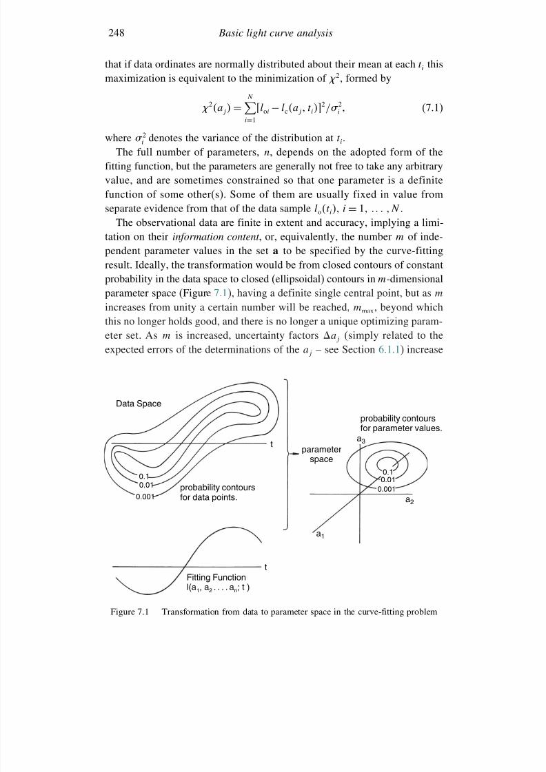
7/21/2019 Introduction to Astronomical Photometry
http://slidepdf.com/reader/full/introduction-to-astronomical-photometry 266/451
248 Basic light curve analysis
that if data ordinates are normally distributed about their mean at each ti thismaximization is equivalent to the minimization of 2, formed by
2aj =N
i=1loi − lcaj ti2/ 2i (7.1)
where 2i denotes the variance of the distribution at ti.The full number of parameters, n, depends on the adopted form of the
fitting function, but the parameters are generally not free to take any arbitraryvalue, and are sometimes constrained so that one parameter is a definitefunction of some other(s). Some of them are usually fixed in value from
separate evidence from that of the data sample loti, i = 1 N .The observational data are finite in extent and accuracy, implying a limi-tation on their information content , or, equivalently, the number m of inde-pendent parameter values in the set a to be specified by the curve-fittingresult. Ideally, the transformation would be from closed contours of constantprobability in the data space to closed (ellipsoidal) contours in m-dimensionalparameter space (Figure 7.1), having a definite single central point, but as m
increases from unity a certain number will be reached, mmax, beyond whichthis no longer holds good, and there is no longer a unique optimizing param-eter set. As m is increased, uncertainty factors aj (simply related to theexpected errors of the determinations of the aj – see Section 6.1.1) increase
Data Space
0.10.01
0.001
0.10.01
0.001
a2
a1
t
t a3
probability contoursfor data points.
Fitting Functionl(a1, a2 . . . . an; t )
parameterspace
probability contoursfor parameter values.
Figure 7.1 Transformation from data to parameter space in the curve-fitting problem
7/21/2019 Introduction to Astronomical Photometry
http://slidepdf.com/reader/full/introduction-to-astronomical-photometry 267/451
7.2 Eclipsing binaries: basic facts 249
progressively, until, at some point just beyond mmax (the ‘information limit’),such factors, for one or more aj , formally pass through a singularity wherethe solution becomes indeterminate, or non-unique. In simple words, a finite
data sample can only yield a finite amount of model information.Below the information limit, a single best set of parameters generally exists.
This is consonant with the idea of a ‘light curve solution’: a term encounteredmore in older literature. As time has progressed, data has improved in quantity,quality and scope, and this has been accompanied by corresponding advancesin theory and the range and detail of models. Nowadays, it would be morecommon to speak of models, or certain aspects of models, being supported by
data – with some given level of confidence, rather than emphasizing a single,distinct interpretation that the word solution suggests.There are three fairly distinct aspects to the curve-fitting problem: (1) speci-
fication of the initial data set in an appropriate form, loti; (2) specification of a physically reasonable and mathematically tractable fitting function, laj t;and (3) the optimization of the match of lc to lo. The procedure is relativelyclear for standard eclipsing binary data, with potentially important yields inastrophysical information.
7.2 Eclipsing binaries: basic facts
Eclipsing binaries are essentially a subset of ‘close binary systems’ – pairsof stars whose separation is typically an order of magnitude greater than a
component mean radius. There are some known cases where the companionsare relatively well separated (e.g. Coronae Borealis), though the likelihoodof observing eclipses in binary systems will clearly drop with increasingdisplacement of the pair relative to their sizes.
It can also be easily seen that component radii of more easily recognizedeclipsing binaries will not, in general, be extremely dissimilar, because if onestar were very much larger than the other (by an order of magnitude or more,say), then the system’s light would tend to be dominated by that larger star.
The eclipse of the small star by the large one (an ‘occultation’), or the passageof the small star in front of the large disk (a ‘transit’), would then have onlya slight effect, evading easy discovery, unless the small star were relativelyvery bright, per unit area of its surface, at the wavelength of observation.1
1 This point is relevant to the new field of ‘planetary’ eclipses: very precise monitoring of starlight can reveal the presence of relatively small and faint companions (see Figure 1.1).
7/21/2019 Introduction to Astronomical Photometry
http://slidepdf.com/reader/full/introduction-to-astronomical-photometry 268/451
250 Basic light curve analysis
Eclipsing binaries are thus pairs of stars showing a regular cycle of variationin apparent brightness, due to their orbital motions lying in a plane inclined ata small angle to the line of sight. The term orbital inclination means the angle
between the axis of the orbit and the line of sight; so that for eclipsing binaries,the numerical value of this angle is usually not far from 90, and in any casecan be shown to be greater than about arcsin 0.85. There is then a successionof alternating photometric minima, transit followed by occultation, and so on.The eclipses are described as complete when the outline of the smaller diskprojects entirely within that of the greater one: a total eclipse if an occultation,or an annular one if a transit. If an eclipse is not complete it is partial.
During the course of an orbital cycle of an eclipsing pair there are twophotometric minima; however, one of these can involve a fairly low lossof light. The deeper eclipse minimum, caused by the eclipse of the starhaving greater brightness per unit area, associated with a higher temperaturephotosphere, is usually called the ‘primary’ minimum, and the star eclipsedat this minimum referred to as the primary star. Similarly, the shallowerminimum is known as the ‘secondary’ one and corresponds to the eclipse of the secondary star.
An interesting observational atlas of light curves of eclipsing binary systemswas produced some years ago by M. G. Fracastoro (1972), including exam-ples that show distinct effects of orbital eccentricity. In the great majority of cases, however, orbits are effectively circular, and there are physical reasonsfor this. Hence, circular orbits represent a practical and convenient simpli-fication for common analysis. Some elementary deductions can be made atonce on this basis: thus, the durations of both eclipses are the same. The
same photospheric areas are in eclipse at corresponding phases through eitherminimum of the light curve, and so the ratio of light lost at such phasesyields a corresponding ratio of surface flux averaged over these eclipsed areas,approximately measuring the surface brightness ratio of the two photospheres.
The matter of which star is called the primary can be occasionally confusing.In spectroscopic contexts, the primary would normally be regarded as thecomponent putting out more light altogether – not necessarily the same thingas the star of greatest brightness per unit area – so the spectroscopic primary
can differ from the photometric one. Also, when stellar evolution of a binaryis considered, the term primary usually refers to the originally more massivestar, though it need not always remain so. There is compelling evidence thatstars lose appreciable mass during the course of their evolution, at a rate thatdepends on the initial mass of the star. In addition to this general effect, massmay be transferred between the components in ‘interactive’ binary evolution.The originally more massive primary may then become the secondary star.
7/21/2019 Introduction to Astronomical Photometry
http://slidepdf.com/reader/full/introduction-to-astronomical-photometry 269/451
7.2 Eclipsing binaries: basic facts 251
Concerning derivable information on eclipsing binaries, it is necessary tocombine observational data – photometric, spectroscopic and other types –to maximize what can be retrieved; but light curves do provide a reasonably
self-contained branch of the subject. There have been, conventionally, threebasic categories in the empirical classification of light curve types: the ‘Algol’(EA) type, the ‘ Lyrae’ (EB) type and the ‘W Ursa Majoris’ (EW) type(Figure 7.2). These prototype names are, at least in the first two cases, some-what inappropriate, and simple letter designations, EA etc., are preferable,and will be used in what follows.
The EA type light curves have roughly constant light levels – to within
∼01mag – outside of the eclipses, which are thus clearly marked, or atleast the primary minimum usually is. It is possible to subdivide this light
curve type further, and the designations EAD and EAS2 have been used forthis. The EAD light curves, for orbital periods of a few days, usually resultfrom the mutual eclipses of a pair of fairly separated normal Main Sequencestars. (Eclipsing systems composed of pairs of normal giants are relativelyrare, and involve much longer periods.) Both minima can be discerned, andtheir depths have a simple relationship to each other if the spectral types,
and therefore approximate surface effective temperatures, are known. Theprimary minimum depth cannot exceed little more than one magnitude atoptical wavelengths, due to the Main-Sequence-like properties of the stars.
The EAS type light curve is exemplified by Algol itself, but perhaps moreobviously by such completely eclipsing Algol systems as U Cep or U Sge.The primary eclipse is deep because of the relatively large size but coolphotosphere of the ‘subgiant’ secondary. The relatively low mass of this star
can be inferred from the low scale of proximity-induced tidal distortion of the bright primary, so that the light curve shows little of the inter-minimumcurvature, at least at optical wavelengths, associated with such effects. AnEAS light curve is distinguished, then, by a deep primary minimum, generallydeeper than 1 mag, and the secondary minimum being so shallow as to standapart clearly from the trend of secondary to primary depth ratios predictablefor Main Sequence pairs. Note that it is not necessary for an Algol-like systemto show an EAS type light curve, even if an EAS light curve were always
produced by an Algol-like pair of stars.The EB type light curve shows a continuous pattern of variability including
the rounded inter-minimum regions associated with more pronounced tidalinteractions. It is more frequently associated with earlier type binaries, andgenerally closer relative separations. There are some early type binaries having
2 Sometimes EA1 and EA2 were alternatively applied.
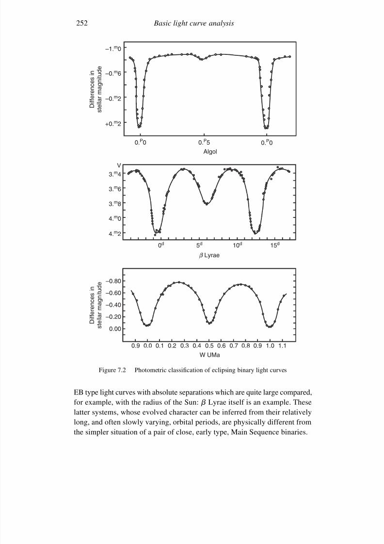
7/21/2019 Introduction to Astronomical Photometry
http://slidepdf.com/reader/full/introduction-to-astronomical-photometry 270/451
252 Basic light curve analysis
–1.m0
–0.m6
Differencesin
stellarmagnitude
Differences
in
stellarmagnitude
–0.m2
0.P0 0.P5
Algol
0.P0
+0.m2
3.m4
3.m6
3.m8
4.m0
4.m2
0d
–0.80
–0.60
–0.40
–0.20
0.00
0.9 0.0 0.1 0.2 0.3 0.4
W UMa
0.5 0.6 0.7 0.8 0.9 1.0 1.1
5d
β Lyrae
10d 15d
V
Figure 7.2 Photometric classification of eclipsing binary light curves
EB type light curves with absolute separations which are quite large compared,for example, with the radius of the Sun: Lyrae itself is an example. Theselatter systems, whose evolved character can be inferred from their relativelylong, and often slowly varying, orbital periods, are physically different fromthe simpler situation of a pair of close, early type, Main Sequence binaries.
7/21/2019 Introduction to Astronomical Photometry
http://slidepdf.com/reader/full/introduction-to-astronomical-photometry 271/451
7.2 Eclipsing binaries: basic facts 253
With EW type light curves the proximity-induced inter-minimum roundingreaches such a scale as to merge imperceptibly into the eclipse minima,which can thus no longer be clearly separated out. It is a fact, which is
not yet perfectly understood, that the EW binaries also show more or lessequal depths of primary and secondary minima. Hence, a light curve showingvery pronounced out-of-eclipse rounding, but with minima depths differingby more than one or two tenths of a magnitude, should be assigned an EBclassification. In fact, such a light curve is rarely encountered, EB binariesbeing preferentially found among systems of somewhat longer period andearlier type than the EW systems. Genuine W UMa type binaries all appear
to have periods appreciably less than one day in duration. They are alsopredominantly made up of late type pairs, by far the largest proportion, byspectral class, being G type primaries and secondaries.
Thus, EAD and ‘normal’ (short-period) EB binaries can be usually clearlyinterpreted in terms of unevolved, Main-Sequence-like pairs. Among the EAS,long-period EB and EW binaries, however, we encounter a range of propertiesof varying awkwardness for explanation, which have sometimes been termedparadoxes. Perhaps the most well known is the ‘Algol paradox’ of the EAS
binaries. This can be readily sensed from the photometry, as indicated above.The deep primary minimum would imply a more evolutionarily advanced,and therefore, presumably, more massive companion. But the absence of tidalproximity effects shows the large companion to have a relatively low mass.A second Algol paradox has been considered in more recent years, connectedwith the difficulty which standard interactive binary evolution theory has ingetting Algols into their observed ‘gentle’ configurations, without drastic ‘run-
away mass-loss’ or ‘spiral-in’ effects. The critical role of angular momentumloss in such evolution has become more evident in this connection. This isrelevant to the O – C studies to be discussed in the next chapter.
A ‘ Lyrae paradox’ exists for longer period EB stars. In order to avoidextremely large masses in the explanations of spectroscopic data on thesebinaries, it is necessary to suppose that the more massive components areactually not seen, but buried in a ‘thick disk’.
Finally, there is a ‘W UMa paradox’ for the EW binaries. This is associated
with these stars being so close as to make ‘contact’ with each other’s surfaces,or indeed share a common photospheric envelope. A star in such a situa-tion would have its outer boundary conditions fixed by dynamical constraintsimposed by the contact configuration. But stars of given mass and composi-tion fix their own outer boundaries, by the Vogt–Russell theorem of classicalstellar structure. The ratio of masses to radii fixed by the contact configura-tion is, in general, incompatible with that of pairs of single stars of the same
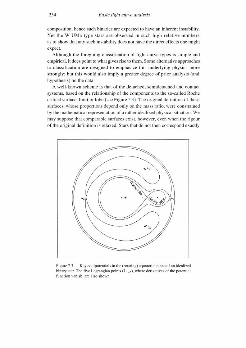
7/21/2019 Introduction to Astronomical Photometry
http://slidepdf.com/reader/full/introduction-to-astronomical-photometry 272/451
254 Basic light curve analysis
composition, hence such binaries are expected to have an inherent instability.Yet the W UMa type stars are observed in such high relative numbersas to show that any such instability does not have the direct effects one might
expect.Although the foregoing classification of light curve types is simple and
empirical, it does point to what gives rise to them. Some alternative approachesto classification are designed to emphasize this underlying physics morestrongly; but this would also imply a greater degree of prior analysis (andhypothesis) on the data.
A well-known scheme is that of the detached, semidetached and contact
systems, based on the relationship of the components to the so-called Rochecritical surface, limit or lobe (see Figure 7.3). The original definition of thesesurfaces, whose proportions depend only on the mass ratio, were constrainedby the mathematical representation of a rather idealized physical situation. Wemay suppose that comparable surfaces exist, however, even when the rigourof the original definition is relaxed. Stars that do not then correspond exactly
L4
+
R o c h
e l o b e
R o c h e L2
L1
L5
L3
l o b
e
Figure 7.3 Key equipotentials in the (rotating) equatorial plane of an idealizedbinary star. The five Lagrangian points (L1−5), where derivatives of the potentialfunction vanish, are also shown
7/21/2019 Introduction to Astronomical Photometry
http://slidepdf.com/reader/full/introduction-to-astronomical-photometry 273/451
7.2 Eclipsing binaries: basic facts 255
to the circumstances imposed by the mathematical formulation (e.g. they maynot be rotating perfectly uniformly or in perfectly circular orbits) still facean essentially similar physical situation if they continue to expand beyond
a certain point. In common parlance, the term ‘Roche lobe’ is used, ratherloosely, in this context, though for precise analysis an appropriate stringencyof formulation should be applied. Of course, the Roche lobe can also beapplied to a real situation, using the relevant mass ratio from observations,on the basis that some degree of approximation is implied.
If a binary component, having expanded up to such a surface, were tocontinue still further a dynamical instability, entailing mass loss, would ensue.
Detached pairs, not yet having evolved to this stage, can be largely identifiedin this way with the EAD type light curves, and also some shorter period EBbinaries. EAS type light curves are similarly closely associated with semide-tached systems, where one component is up against this limit, though thelatter need not always produce a light curve free from significant intermin-imum rounding if the evolved secondary happens to be of earlier than usualtype – u Her is a frequently cited example of this.
As suggested before, EW light curves and contact binaries are fairly well
identified with each other, though it is possible to produce an EW typelight curve from a very close, but not actually in-contact, pair. But, due tothe relatively comparable luminosities, many EW systems are double-linedspectroscopic binaries, i.e. they have two radial velocity curves from whicha mass ratio can be independently derived. When these mass ratios are usedto infer the locations of the Roche lobes, and the results compared withphotometric analysis, there can be little doubt that the components have to be
relatively close to the surfaces of limiting stability. Actually, the term contactpair has frequently given way to that of a ‘common envelope’ binary. In thispicture, a common photospheric surface is considered to lie between the innerand outer critical Roche surfaces. This model, though not without theoreticaldifficulties, offers advantages in accounting for the EW type light variation,as well as other properties of these stars.
Apart from these more basic classifications of the eclipsing binaries, certainother groups have been identified. One such group, the RS CVn binaries,
has attracted much attention in recent years. Though not all of these binariesundergo eclipses, as RS CVn itself, most of the originally identified membersof the group came from studies of eclipsing binaries with peculiarly distortedlight curves. The RS CVn stars show a general range of phenomena paral-lelling the magnetodynamic activity of the Sun but on a very much enhancedscale. Dwarf novae are another group now regarded as binary systems, andinterpreted through interactive binary evolution. Some of them eclipse, and
7/21/2019 Introduction to Astronomical Photometry
http://slidepdf.com/reader/full/introduction-to-astronomical-photometry 274/451
256 Basic light curve analysis
the resulting light variation can provide very useful information on physicalaspects of the configuration. In a more extreme physical condition are X-raybinaries, believed, like dwarf novae, to have resulted from interactive binary
evolution involving initially massive stars. For some of these systems eclipsesare observed for the X-ray radiation itself, while others show very enhancedscales of proximity effects in the optical domain. Qualitatively similar effectshave recently been recognized in ‘symbiotic stars’; while other kinds of stellar peculiarity, e.g. old novae, Be stars, or the ‘barium star’ syndrome, areincreasingly related to the effects of binarity.
The fraction of all stars originating in binary systems is of first order.
Among these, an appreciable fraction, perhaps about 5%, are formed as pairshaving orbital periods less than 10d.3 A fifth of these could be expected toshow noticeable eclipses. It suggests that of the order of 1% of all stars maybe in eclipsing binary systems. This coarse estimate appears borne out by thedata on the few thousand brightest and most well-studied stars. Of about 5000stars brighter than magnitude 6.0, for example, around 50 eclipsing systemsare known. However, among older populations of stars, such as are found in
globular clusters, evolution effects alter the number of detected close binariesabove a given magnitude, compared with the generally younger populationof the nearby galactic field. If searches are continued to the faint, low mass,relatively unevolved stars of globular clusters, close pairs begin to show upagain. But, in fact, ‘evolution effects’ here refer not just to the physical condi-tions and interactions of the binary components themselves, but to dynamicaleffects peculiar to the dense stellar environment of globular clusters. The
incidence of close binary systems in these environments is connected to arange of interesting astrophysical problems. Capture processes can result inthe formation of otherwise unexpected high-energy sources, whilst binaryincidence in the core is strongly related to the dynamical evolution of thecluster as a whole.
Eclipsing binaries are also detected in the galactic field of the nearergalaxies. As noted in Section 3.8, eclipsing binaries offer a direct means for
retrieving precise empirical information on stars over very large tracts of space, hence there has been a developing interest, particularly with increas-ingly faint star study capabilities of more recent years, in checking thecosmological distance ‘ladder’ (at least over its lower rungs) by the eclipsemethod.
3 see E. Guenther et al. (2002).
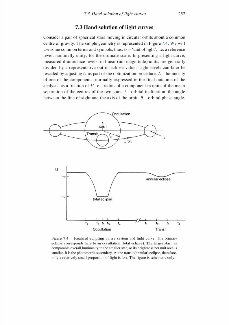
7/21/2019 Introduction to Astronomical Photometry
http://slidepdf.com/reader/full/introduction-to-astronomical-photometry 275/451
7.3 Hand solution of light curves 257
7.3 Hand solution of light curves
Consider a pair of spherical stars moving in circular orbits about a common
centre of gravity. The simple geometry is represented in Figure 7.4. We willuse some common terms and symbols, thus: U – ‘unit of light’, i.e. a referencelevel, nominally unity, for the ordinate scale. In presenting a light curve,measured illuminance levels, in linear (not magnitude) units, are generallydivided by a representative out-of-eclipse value. Light levels can later berescaled by adjusting U as part of the optimization procedure. L – luminosityof one of the components, normally expressed in the final outcome of theanalysis, as a fraction of U . r – radius of a component in units of the meanseparation of the centres of the two stars. i – orbital inclination: the anglebetween the line of sight and the axis of the orbit. – orbital phase angle.
Occultation
cos i
Orbit
Transit
total eclipse
t1 t3 t4t2 t1 t3 t4t2t0
Occultation Transit
U
∧tr
∧oc
annular eclipse
rg rs
Figure 7.4 Idealized eclipsing binary system and light curve. The primaryeclipse corresponds here to an occultation (total eclipse). The larger star hascomparable overall luminosity to the smaller star, so its brightness per unit area issmaller. It is the photometric secondary. At the transit (annular) eclipse, therefore,only a relatively small proportion of light is lost. The figure is schematic only.
7/21/2019 Introduction to Astronomical Photometry
http://slidepdf.com/reader/full/introduction-to-astronomical-photometry 276/451
258 Basic light curve analysis
This is usually reckoned from a time of primary mid-minima using publishedinformation about the observed epoch of the minimum and period of thebinary, but allowance can be made for a zero phase correction, 0, to be
added to the values of to improve the curve-fit.Let us write to denote light levels regarded as effectively constant for
some range of phases, and we set suffixes for , L or r , thus: tr or oc forthat star which is in transit or occultation; g or s for greater or smaller size;1 or 2 for the star being eclipsed or eclipsing. A flat region at the bottom of one of the minima would correspond to the total eclipse of the smaller star.This level is then denoted oc. If only two stars contribute to the observed
light and its variation, we have, for this simple model:between minima = U
oc/U = Lg
U − oc/U = Ls
(7.2)
Quantities relevant to the abscissal scale are: mean period P ; times of beginning and end of eclipses (‘first and fourth contacts’) t1 t4; times of beginning and end of totality t2oc t3oc; times of beginning and end of annularphase t2tr t3tr.
We can set up a right-handed rectangular coordinate frame (xyz), suchthat the z-axis coincides with the line of sight, and the y-axis lies in the planeformed by the z-axis and the axis of orbital revolution passing through thecentre of the primary star – the plane whose intersection with the orbit marksthe zero point of the phase . The unit of distance is the orbit’s semi-diameter.We then find, for the coordinates of the secondary star:
x = sin
y =− cos cos i
By squaring and adding we obtain a basic equation for the separation of thetwo star centres projected onto the tangent plane of the sky, conventionallydenoted , i.e.:
2
=cos2 i
+sin2 sin2 i (7.3)
The orbital phase is calculated from the primary mid-eclipse t0, at time t, as = 2t − t0/P , where the epoch t0 satisfies:
t0 = t1 + t2 + t3 + t4/4 (7.4)
though a more elaborate method would be used in practice for this determina-tion. The ‘tracing paper’ method (Section 6.4) in which observations during a
7/21/2019 Introduction to Astronomical Photometry
http://slidepdf.com/reader/full/introduction-to-astronomical-photometry 277/451
7.3 Hand solution of light curves 259
minimum are plotted out on a transparent sheet, which is then folded so thatthe two halves of the minimum curve are superposed, has been a commonsimple approach.
P is deduced from observed times of minima, and can be expressed withconsiderable accuracy when observations have covered many light cycles.Thus, if we determine t0 to an accuracy t, then P , if constant, is known toan accuracy t/N ; where N is the number of complete cycles of the lightvariation covered. For many of the well-known eclipsing binaries N runs intoseveral thousands or tens of thousands, which would justify the quoting of P values sometimes up to eight decimal places in days, as seen in published
data. Some systems do not have a sensibly constant period, however, and thespecification needs to be qualified by an awareness of this.The orbit size is so small in comparison with the distance of the observer
that perspective effects are negligible. Regarding the two stars as disks in theplane of the sky, in which the orbit projects as an ellipse (Figure 7.4), thenshows
cos i ≤ r g − r s (7.5)
to be the condition that total–annular eclipses occur. If complete eclipsesoccur, and we compare corresponding points within the total and annularlimits, the area eclipsed is that of the disk of the smaller star. If the surfacemean intensity of this star is F s, we can write:
1− oc
1− tr
= F sF g
(7.6)
where F g represents a mean surface brightness of the greater star, averagedover the area of the smaller star’s disk.Let us neglect, for the present, the known tendency of the surface intensity
to decrease from centre to limb, or the limb-darkening effect as it is called.On that basis, we deduce that if the primary minimum corresponds to atransit then the greater star is intrinsically brighter, and vice versa for anoccultation. Transit primary minima normally occur for pairs of stars on theMain Sequence. More generally, we can write
U − tr/U = Lgr s/r g2 (7.7)
where is a factor introduced to account for the limb-darkening effect, but itis usually fairly insensitive to its value and would normally be close to unity.
Since oc/U = Lg, if we put k = r s/r g we will have
k = U − tr/oc U − tr/oc (7.8)
7/21/2019 Introduction to Astronomical Photometry
http://slidepdf.com/reader/full/introduction-to-astronomical-photometry 278/451
260 Basic light curve analysis
Hence, the light levels at the completion of the two eclipses, if available, givean approximate value for the ratio of radii of the two stars.
In the idealized light curve of Figure 7.4 at the external tangencies (t1 t4)
the projected separation of centres 1 is
1 = r g1+ k (7.9)
and at the internal tangencies (t2, t3) the corresponding separation 2 is
2 = r g1− k (7.10)
Taking (7.8), (7.9) and (7.10), and using (7.3), we can approximately evaluatethe three geometric unknowns: r g, r s and i. The two luminosity quantities, U
and Lg (Ls is constrained by (7.2) in this model), together with the epoch of primary mid-minimum t0, make up the list of basic parameters to six. Takingthings a step or two further, we encounter a coefficient of limb darkening ug
as an argument of the function in (7.7), which influences the curvature atthe bottom of the transit minimum. There is a corresponding parameter us
for the smaller star, though its effects are less discernible in the occultation
ingress and egress. In any case, eight parameters correspond to a reasonablycomplete specification for the simple ‘spherical model’ light curve underconsideration.
This analysis is essentially equivalent to that first discussed long ago byHenry Norris Russell, one of the great fact-finders of stellar properties in thefirst half of the twentieth century, and founder of this ‘royal road’, as he putit, to astrophysical knowledge (see Section 3.8). Of course, there are variousshortcomings in this deliberately simplified approach, but it is instructive totest things out on an actual example.
For this, G. E. Kron’s photoelectric data for the fifth magnitude eclipsingbinary YZ Cas, obtained on the 36-inch refractor of the Lick Observatory inthe late 1930s, provide a classic case. Although Kron’s photometer did nothave the same low noise detective efficiency as those of more recent type,the exemplary quality of the data is probably due to: (i) the star (V = 565)is relatively bright, (ii) the telescope aperture (0.91 m) was large for the
magnitude of object being monitored, and (iii) Kron was persistently carefulin his observations of minima, of which he observed a few dozen between1937 and 1940. The object is a textbook example of a pair of Main Sequencestars in a circular orbit, whose plane lies very close to the line of sight.Proximity effects are very slight, and there are no significant variations tothe light curve apart from the eclipses themselves. Kron averaged out small,randomly distributed errors in the large quantity of individual data points,
7/21/2019 Introduction to Astronomical Photometry
http://slidepdf.com/reader/full/introduction-to-astronomical-photometry 279/451
7.3 Hand solution of light curves 261
which were reduced to some 27 ‘normal points’ in each minimum of his bluelight curve; and 22 and 20 in the primary and secondary minima, respectively,of the red filter observations.
Reading from Kron’s (1942) red (6700 Å) light curve, we haveU = 1000
trinner contacts = 0745
trcentre = 0733
oc = 0898
Taking the average of the two transit levels as representative to substituteinto (7.8), we find k = 0539. The internal and external tangencies occur atphases 35 and 123, respectively. Using Equation (7.3) with (7.9) and(7.10), and the foregoing value of k, we derive the three geometric elements,as follows:
r g = 0139
r s=
0075
i = 889
Although obtained in such a simple way, these results compare tolerably withthose of much more elaborate analysis. Such methods have a place, then, inproviding initial estimates for more detailed procedures.
If the light curve showed only partial eclipses, i.e. no identifiable internaltangency, a starting point is still possible using the equality condition of (7.5).
This would give an upper limit for i and lower limits for the component radii.A procedural development was already made in the days of Russell by theintroduction of a function , giving the fraction of a star’s light lost duringeclipse. depends on the projected separation of centres , the ratio of theradii k, and some parameter (or parameters), determining the limb darkeningover the disk of the star being eclipsed. As we have seen, if the eclipsesare complete, it is possible to determine directly from the light levels duringannular and total phases approximate values for both fractional luminosities
L, and the ratio of radii k. With an appropriate value of L1, the light lossof a star being eclipsed could be listed as a set of empirical values forobservations of a given minimum.
Russell and Merrill’s classical method depended on having tables of calcu-lated values for a comprehensive range of values of k and a convenientlynormalized measure of projected separation, p say, over a range of plausiblevalues of the limb-darkening coefficient u. These tables were inverted to
7/21/2019 Introduction to Astronomical Photometry
http://slidepdf.com/reader/full/introduction-to-astronomical-photometry 280/451
262 Basic light curve analysis
provide separate sets of tables of p for given , k and u. Hence, with u set,and determined k and values, the corresponding p values were looked up.Equation (7.3), for varying values of the phase during eclipses, would then
provide a set of equations of condition for the radius of the eclipsed star (usedin scaling the s to the normalized p values) and the orbital inclination i.
This approach provided a reasonably manageable method of analysing eclip-sing binary light curves in the pre-computer era. Nowadays, the use of tablesin this way seems very dated. Apart from that, there were certainother restrictive assumptions, glossed over here in order to provide a generaloverview.
7.4 Computer-based analysis
The use of Equation (7.3) for certain special points on the light curveformed the traditional approach developed by Russell, Merrill and others.Such methods were sometimes called ‘indirect’, so as to distinguish a ‘direct’procedure that concentrates on the equation of the light curve. This directapproach turns out to be well suited to computers, and has the advan-tage of using all available data. It exemplifies the curve-fitting problem of Section 7.1.
Data preparation
Firstly, it is required to present the data in a suitable format. Time can besaved in parameter space exploration if the number of data points can be
reduced without significant loss of information. This has become less of anissue with the enormous speeds and bulk data handling capabilities of modernmachines, although the point is somewhat counterbalanced by correspondingincreases of input volumes. Preliminary data set reduction was encounteredwith Kron’s presentation for YZ Cas, where normal points were used. Theconstruction of a program to ‘bin’ data,4 is relatively commonplace, withready-made software widely available.
The optimum arrangement is difficult to specify strictly. Some regions of alight curve may be intrinsically more informative than others for the quantitiessought. In order to avoid information loss, any error in the assumption of linearvariation of light over the small interval whose data are averaged should be
4 i.e. a program that subdivides the range of abscissae into suitably sized intervals and performsstandard statistical tasks, such as determining the mean and standard deviation within eachinterval.
7/21/2019 Introduction to Astronomical Photometry
http://slidepdf.com/reader/full/introduction-to-astronomical-photometry 281/451
7.4 Computer-based analysis 263
less than the error of the mean in that interval. Note here that small variationsin the magnitude scale, which, at this stage, would be the usual form forthe ordinates, are proportional to linear changes of flux with a constant of
proportionality of about 1.09. Hence, if l is the first order (linear) variationof light for a small change of phase , while el denotes the accuracy withwhich the variation can be specified, we require the second order variationl < el. (Much greater intrinsic accuracy attaches to the phasedetermination than the light level.) For most of the eclipsing binary lightcurves normally encountered we can expect the second order variation l
10−3 2d, for a phase bin d degrees. Failure of the condition is more likely
near the tangencies, where sudden changes of slope occur. We have alreadyseen that such points can be especially informative, so that bin size should bekept as small as conveniently possible in their vicinity. The foregoing estimatesuggests that phase intervals of around 0.01 would be adequate for eclipseminima binning when normal point accuracy (el) is about 1%. Modern lightcurves are making significant improvements on this nominal accuracy, andfiner bin steps should be considered. The suitability of the chosen bin sizescan be checked a posteriori from any significant variation of parameter valueswith an increase in the number of data points. This would be a useful testonce an acceptable parameter set has been found for a given data set. Thereare some light curves which show sudden rapid variations, flash effects orfluctuations. Clearly, in these and similar situations the normal points ideawould have to be used carefully, if at all.
After data-binning, the light curve is generally shifted so that the constantdifference between the comparison star and mean out-of-eclipse light is taken
out of the reductions, or this latter level of light set to zero magnitude.Care must be taken to ensure that the given magnitude differences are of the expected sign, i.e. the eclipse minima being fainter would normally beexpected to have positive differential magnitude, although they are not alwaysgiven with this sign convention. The light curve now takes the form of a setof observed magnitude differences moi against phase i, of order 100, witha maximum at phase zero and reducing to around zero outside of the eclipse
phase ranges. A conversion to the scale of relative flux can then be easilygiven by loi = 10−04×moi .
Formulae and tables for values were originally provided by Russell andMerrill (1952) at Princeton, and Tsesevich in the Soviet Union. In order tocombine the transit and occultation forms of the older sources, however, wecan write k = r 2/r 1 regardless of which star is larger, so allowing 0 < k < .The separation argument d = /r 1, i.e. normalized to the radius of the eclipsed
7/21/2019 Introduction to Astronomical Photometry
http://slidepdf.com/reader/full/introduction-to-astronomical-photometry 282/451
264 Basic light curve analysis
star, is also convenient, so that = u1kd is the fractional light loss of the eclipsed component in this notation. We can then write
lc = U − L1u1kd (7.11)as the basic equation of the light curve in the spherical model. The dependenceof d on comes through (7.3) and the above definition of d. The quantitiesu, L, k and d are different for primary (pr) or secondary (se) minimum region,though the latter three have very simple interconnections, i.e. L1se = U −L1pr,kse = 1/kpr, dse = d/kpr. Equation (7.11) can be substituted into (7.1) for eachobservation at phase i and compared with the corresponding observed loi.
For a linear law of limb darkening, in which the photospheric intensity I ata direction to the outward normal is of the form I = I 01− u + u cos ,it can be easily shown that
= 31− u
3− u 0
0 + 3u
3− u0
1 (7.12)
where integrals of the type mn have appeared. These are defined as
m
n = A x
m
zn
dx dy (7.13)
where A denotes the eclipsed area (cf. (4.32)). The function for a spher-ical star, with limb darkening expressed as a series in powers of cos
(≡ z-coordinate of the corresponding surface point), being eclipsed by aspherical companion, is then given by a corresponding series in terms of 0
n
integrals.The more general integrals m
n appear when departures from sphericity are
included. Recursion formulae are available that enable the whole range of mn
integrals to be evaluated, provided only two and four auxiliary integralsare given. This range of integrals can be computer generated and applied tolight curves which show proximity effects.
integrals
The two basic integrals – 00 and 0
1 – take the following forms:
(i) Annular case d ≤ 1− k k < 1
00 = k2 (7.14)
01 = 2
3 a
− 1
3 1− d − k2
d2d2 −2dk −5+8k2
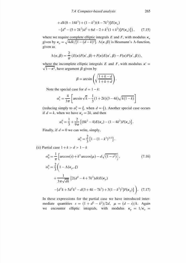
7/21/2019 Introduction to Astronomical Photometry
http://slidepdf.com/reader/full/introduction-to-astronomical-photometry 283/451
7.4 Computer-based analysis 265
+ dk8−14k2 + 1− k24−7k2Ea
−d4 − 5+2k2d2 +6d −2+ k21+ k2Fa (7.15)
where we require complete elliptic integrals E and F , with modulus a
given by a =
4dk/1− d − k2. is Heumann’s -function,given as
= 2
EF + FE − FF
where the incomplete elliptic integrals E and F , with modulus =√ 1−
2, have argument given by
= arcsin
1+ k − d
1+ k + d
Note the special case for d = 1− k:
01 = 4
3
arcsin
√ k − 1
31+ 2k3−4k
k1− k
(reducing simply to 01 = 49 , when d = 14 ). Another special case occursif d = k, when we have a = 2k, and then
01 = 1
3+ 2
9
8k2 −4Ea − 1− 4k2Fa
Finally, if d = 0 we can write, simply,
01
=
23 1−
1
−k23/2
(ii) Partial case 1 + k > d > 1− k
00 = 1
arccoss + k2 arccos − d
1− s2
(7.16)
01 = 2
3
1− p
+ 1
3 √ dk
2d2
−4+ 7k2
dkEp
−d3k +5d2k2 − d3+ 4k − 7k3 +31− k22Fp
(7.17)
In these expressions for the partial case we have introduced inter-mediate quantities s = 1 + d2 − k2/2d, = d − s/k. Againwe encounter elliptic integrals, with modulus p = 1/a =
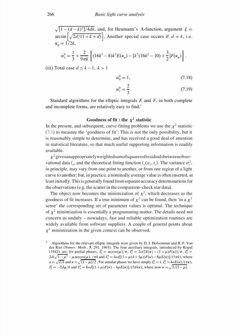
7/21/2019 Introduction to Astronomical Photometry
http://slidepdf.com/reader/full/introduction-to-astronomical-photometry 284/451
266 Basic light curve analysis
1− d − k2/4dk, and, for Heumann’s -function, argument =
arcsin
2d/1+ k + d
. Another special case occurs if d = k, i.e.
p =
1/2k,
01 = 1
3+ 2
9k
16k2 −8k2Ep − k216k2 −10 + 3
2Fp
(iii) Total case d ≤ k − 1 k > 1
00 = 1 (7.18)
0
1 = 2
3 (7.19)Standard algorithms for the elliptic integrals E and F , in both complete
and incomplete forms, are relatively easy to find.5
Goodness of fit : the 2 statistic
In the present, and subsequent, curve-fitting problems we use the 2 statistic(7.1) to measure the ‘goodness of fit’. This is not the only possibility, but it
is reasonably simple to determine, and has received a good deal of attentionin statistical literature, so that much useful supporting information is readilyavailable.
2 givesanappropriatelyweightedsumofsquaresofresidualsbetweenobser-vational data loi and the theoretical fitting function lcaj ti. The variance 2i ,in principle, may vary from one point to another, or from one region of a lightcurve to another; but, in practice, a nominally average value is often inserted, at
least initially. This is generally found from separate accuracy determinations forthe observations (e.g. the scatter in the comparison–check star data).The object now becomes the minimization of 2, which decreases as the
goodness of fit increases. If a true minimum of 2 can be found, then ‘in a 2
sense’ the corresponding set of parameter values is optimal. The techniqueof 2 minimization is essentially a programming matter. The details need notconcern us unduly – nowadays, fast and reliable optimization routines arewidely available from software suppliers. A couple of general points about
2 minimization in the given context can be observed.
5 Algorithms for the relevant elliptic integrals were given by D. J. Hofsommer and R. P. Vander Riet ( Numer. Math., 5, 291, 1963). The four auxiliary integrals, introduced by Kopal(1942), are, for partial phases, I 00 = arccos/ , I 01 = 2a2E − 1 + F/ , I 02 =2d
1− 2 − arccos /k and I 03 = 4ad1+ 4 +3F−8E/3k, where
a = √
d/k and =
1− /2 . For annular phases we have simply I 00 = 1, I 01 = 4aE/,I 02 = −2d/k and I 03 = 8ad1+ F −4E/3k, where now =
2/1 − .
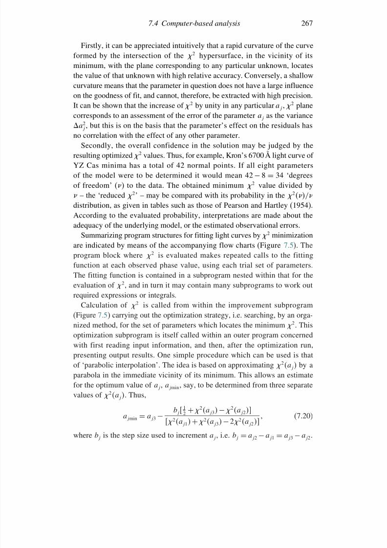
7/21/2019 Introduction to Astronomical Photometry
http://slidepdf.com/reader/full/introduction-to-astronomical-photometry 285/451
7.4 Computer-based analysis 267
Firstly, it can be appreciated intuitively that a rapid curvature of the curveformed by the intersection of the 2 hypersurface, in the vicinity of itsminimum, with the plane corresponding to any particular unknown, locates
the value of that unknown with high relative accuracy. Conversely, a shallowcurvature means that the parameter in question does not have a large influenceon the goodness of fit, and cannot, therefore, be extracted with high precision.It can be shown that the increase of 2 by unity in any particular aj 2 planecorresponds to an assessment of the error of the parameter aj as the variancea2
j , but this is on the basis that the parameter’s effect on the residuals hasno correlation with the effect of any other parameter.
Secondly, the overall confidence in the solution may be judged by theresulting optimized 2 values. Thus, for example, Kron’s 6700 Å light curve of YZ Cas minima has a total of 42 normal points. If all eight parametersof the model were to be determined it would mean 42 − 8 = 34 ‘degreesof freedom’ () to the data. The obtained minimum 2 value divided by – the ‘reduced 2’ – may be compared with its probability in the 2/
distribution, as given in tables such as those of Pearson and Hartley (1954).According to the evaluated probability, interpretations are made about the
adequacy of the underlying model, or the estimated observational errors.Summarizing program structures for fitting light curves by 2 minimization
are indicated by means of the accompanying flow charts (Figure 7.5). Theprogram block where 2 is evaluated makes repeated calls to the fittingfunction at each observed phase value, using each trial set of parameters.The fitting function is contained in a subprogram nested within that for theevaluation of 2, and in turn it may contain many subprograms to work out
required expressions or integrals.Calculation of 2 is called from within the improvement subprogram(Figure 7.5) carrying out the optimization strategy, i.e. searching, by an orga-nized method, for the set of parameters which locates the minimum 2. Thisoptimization subprogram is itself called within an outer program concernedwith first reading input information, and then, after the optimization run,presenting output results. One simple procedure which can be used is thatof ‘parabolic interpolation’. The idea is based on approximating 2aj by a
parabola in the immediate vicinity of its minimum. This allows an estimatefor the optimum value of aj , aj min, say, to be determined from three separatevalues of 2aj . Thus,
aj min = aj 3 − bj 12 + 2aj 3 − 2aj 2
2aj 1 + 2aj 3 −2 2aj 2 (7.20)
where bj is the step size used to increment aj , i.e. bj = aj 2 − aj 1 = aj 3 − aj 2.
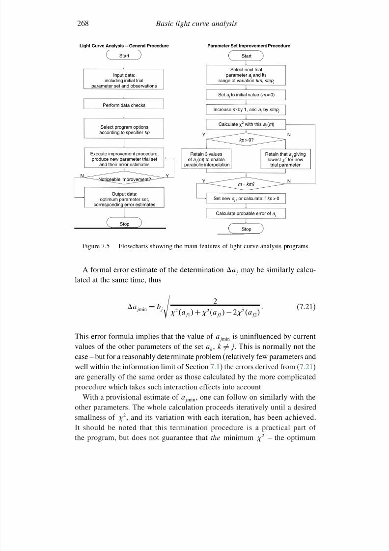
7/21/2019 Introduction to Astronomical Photometry
http://slidepdf.com/reader/full/introduction-to-astronomical-photometry 286/451
268 Basic light curve analysis
Start
Light Curve Analysis – General Procedure
Input data:including initial trial
parameter set and observations
Perform data checks
Select program optionsaccording to specifier kp
Noticeable improvement?
Execute improvement procedure,produce new parameter trial set
and their error estimates
Output data:optimum parameter set,
corresponding error estimates
Stop
N Y
Start
Parameter Set Improvement Procedure
Select next trial
parameter a j and itsrange of variation km , step j
Set a j to initial value (m = 0)
Increase m by 1, and a j by step j
Calculate χ2 with this a j (m )
Retain that a j giving lowest χ2 for new
trial parameter
kp > 0?
m = km ?
Retain 3 valuesof a j (m ) to enable
parabolic interpolation
Set new a j , or calculate if kp > 0
Calculate probable error of a j
Stop
Y N
Y N
Figure 7.5 Flowcharts showing the main features of light curve analysis programs
A formal error estimate of the determination aj may be similarly calcu-lated at the same time, thus
aj min = bj
2
2aj 1 + 2aj 3 −2 2aj 2 (7.21)
This error formula implies that the value of aj min is uninfluenced by currentvalues of the other parameters of the set ak, k = j . This is normally not thecase – but for a reasonably determinate problem (relatively few parameters andwell within the information limit of Section 7.1) the errors derived from (7.21)
are generally of the same order as those calculated by the more complicatedprocedure which takes such interaction effects into account.
With a provisional estimate of aj min, one can follow on similarly with theother parameters. The whole calculation proceeds iteratively until a desiredsmallness of 2, and its variation with each iteration, has been achieved.It should be noted that this termination procedure is a practical part of the program, but does not guarantee that the minimum 2 – the optimum
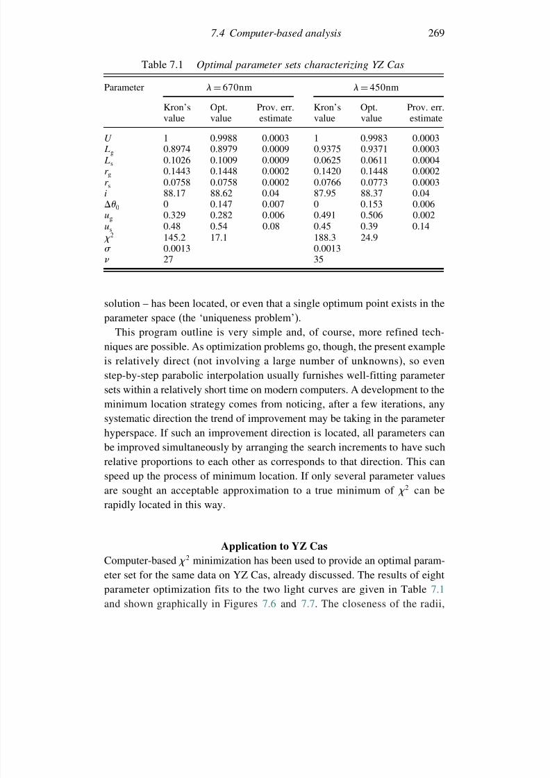
7/21/2019 Introduction to Astronomical Photometry
http://slidepdf.com/reader/full/introduction-to-astronomical-photometry 287/451
7.4 Computer-based analysis 269
Table 7.1 Optimal parameter sets characterizing YZ Cas
Parameter = 670nm = 450nm
Kron’s Opt. Prov. err. Kron’s Opt. Prov. err.value value estimate value value estimate
U 1 0.9988 0.0003 1 0.9983 0.0003Lg 0.8974 0.8979 0.0009 0.9375 0.9371 0.0003Ls 0.1026 0.1009 0.0009 0.0625 0.0611 0.0004r g 0.1443 0.1448 0.0002 0.1420 0.1448 0.0002r s 0.0758 0.0758 0.0002 0.0766 0.0773 0.0003i 88.17 88.62 0.04 87.95 88.37 0.040 0 0.147 0.007 0 0.153 0.006ug 0.329 0.282 0.006 0.491 0.506 0.002us 0.48 0.54 0.08 0.45 0.39 0.14 2 145.2 17.1 188.3 24.9 0.0013 0.0013 27 35
solution – has been located, or even that a single optimum point exists in the
parameter space (the ‘uniqueness problem’).This program outline is very simple and, of course, more refined tech-
niques are possible. As optimization problems go, though, the present exampleis relatively direct (not involving a large number of unknowns), so evenstep-by-step parabolic interpolation usually furnishes well-fitting parametersets within a relatively short time on modern computers. A development to theminimum location strategy comes from noticing, after a few iterations, anysystematic direction the trend of improvement may be taking in the parameterhyperspace. If such an improvement direction is located, all parameters canbe improved simultaneously by arranging the search increments to have suchrelative proportions to each other as corresponds to that direction. This canspeed up the process of minimum location. If only several parameter valuesare sought an acceptable approximation to a true minimum of 2 can berapidly located in this way.
Application to YZ Cas
Computer-based 2 minimization has been used to provide an optimal param-eter set for the same data on YZ Cas, already discussed. The results of eightparameter optimization fits to the two light curves are given in Table 7.1and shown graphically in Figures 7.6 and 7.7. The closeness of the radii,
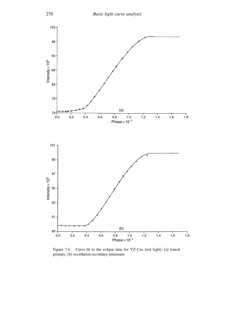
7/21/2019 Introduction to Astronomical Photometry
http://slidepdf.com/reader/full/introduction-to-astronomical-photometry 288/451
270 Basic light curve analysis
103
98
93
88
I n t e n s i t y × 1 0 2
83
78
730.0 0.2 0.4 0.6 0.8 1.0
Phase × 10–11.2 1.4 1.6 1.8
101
99
97
95
I n t e n s i t y × 1 0 2
93
91
890.0 0.2 0.4 0.6 0.8 1.0
Phase × 10–11.2 1.4 1.6 1.8
(a)
(b)
Figure 7.6 Curve-fit to the eclipse data for YZ Cas (red light): (a) transitprimary, (b) occultation secondary minimum.
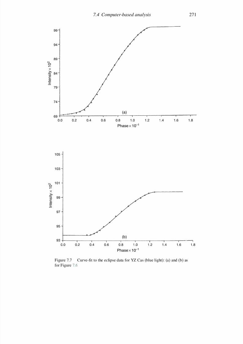
7/21/2019 Introduction to Astronomical Photometry
http://slidepdf.com/reader/full/introduction-to-astronomical-photometry 289/451
7.4 Computer-based analysis 271
99
94
89
84
I n t e n s i t y × 1 0 2
79
74
690.0 0.2 0.4 0.6 0.8 1.0
Phase × 10–1
1.2 1.4 1.6 1.8
105
103
101
99
I n t e n s i t y × 1 0 2
97
95
93
0.0 0.2 0.4 0.6 0.8 1.0
Phase × 10–1
1.2 1.4 1.6 1.8
(a)
(b)
Figure 7.7 Curve-fit to the eclipse data for YZ Cas (blue light): (a) and (b) asfor Figure 7.6
7/21/2019 Introduction to Astronomical Photometry
http://slidepdf.com/reader/full/introduction-to-astronomical-photometry 290/451
272 Basic light curve analysis
inclination and fractional luminosities to the previous simple derivations canbe seen.
From the relative smallness of the provisional error estimates it follows that
the 2 hypersurface sweeps down relatively sharply onto most of the solutionparameters, at least when treated in isolation from each other. This must reflecton the unusually high accuracy of the normal points (∼0001mag). The fittingto the primary minimum in blue is slightly better than the corresponding redlight curve, but the net goodness of fit measures for both pairs of minima arecomparable.
There is a noticeable difference between the derived values of k for the light
curve in the two colours, which is greater than the given error estimate. Thisresult was also obtained by Kron, though he did not lay much weight on it. Thepossibility of some measurable real difference of size, for physical reasons,at the two wavelengths must be very slight if the two stars’ photospheresare anything like those of normal stars. The inclination values also appearrather more different than their quoted errors – about the same for both lightcurves – would suggest.
Such discrepancies question the simple use of (7.21) for error estimates.
In fact, when the correlated errors are properly worked out, we find(Section 6.1.1) that the estimates grow with an increase in the number of sought parameters. This is the effect which limits the number of independentparameters that can be determined. Well-fitting parameter sets may bedirectly derivable from the illustrated procedure, but then one should notmistake accuracy of the curve-fit with accuracy of parameter values. Thus,the derived limb-darkening coefficients, except that of the smaller star at
4500 Å, are in reasonable accord with recent theoretical predictions for thetypes of stars in question (Main Sequence A0 and F5) when the effects of interdependence on error estimation are taken into account. The errors givenin Table 7.1 are, in general, far too low.
7.5 Bibliographical notes
The generalities of the initial section recall much from P. R. Bevington’spopular Data Reduction and Error Analysis for the Physical Sciences
(McGraw-Hill Book Co., 1969), though there is a number of more recenttexts, in wide distribution, dealing with optimization techniques and curve-fitting problems (e.g. E. K. P. Chong and S. H. Zak’s Introduction to
Optimization, 2nd edn., John Wiley, 2001, or P. Venkataraman’s Applied
Optimization with MATLAB Programming, John Wiley, 2002). Practical
7/21/2019 Introduction to Astronomical Photometry
http://slidepdf.com/reader/full/introduction-to-astronomical-photometry 291/451
7.5 Bibliographical notes 273
computational methods are included in the Numerical Recipes of W. H. Presset al. (Cambridge University Press, 1986). I. J. D. Craig and J. C. Brown’s
Inverse Problems in Astronomy (Adam Hilger, 1986), and the Konechno
parametricheskie obratnyie zadachi astrofiziki (Russian) (Izd. Moskov.Univ.) of A. V. Goncharski, S. Y. Romanov and A. M. Cherepashchuk,1991, discuss a general range of data-to-parameter conversion issues, withastrophysical contexts in mind.
With regard to eclipsing binary light curves, whose discussion starts inSection 7.2, there are broad reviews of the subject, in the context of variablestars, in C. Hoffmeister, G. Richter and W. Wenzel’s Variable Stars (Springer
Verlag, 1984); and V. P. Tsesevich’s Eclipsing Variable Stars (John Wileyand Sons, 1973), from which Figure 7.2 derives. A. H. Batten’s Binary and
Multiple Stars (Pergamon Press, 1973) gives a good background to physicalinterpretations, as does J. Sahade and F. B. Wood’s Interacting Binary Stars
(Pergamon Press, 1978), which contains a very full bibliography up to theyear of publication. A comprehensive set of physical reviews appeared alsounder the title Interacting Binary Stars, eds. J.E. Pringle and R.A. Wade(Cambridge University Press, 1985).
The atlas referred to is that of M. G. Fracastoro, An Atlas of Light Curves of Eclipsing Binaries (Oss. Astron. Torino, 1972). Another usefulobservational compilation is that of M. Zejda of the Brno Observatory,accessible from var.astro.cz/brno. This includes a section devoted to eclipsingbinaries without known light elements (BRKA 1999). Extensive bibli-ographic information on over 3500 eclipsing binaries was given in theFinding List for Observers of Interacting Binary Stars of F.B. Wood,
J. P. Oliver, D. R. Florkowski and R. H. Koch (University of PennsylvaniaPress, Astron. Series, 12, 1980, fifth edition). A very large amount of factual information on close binary systems was also compiled by M.A.Svechnikov, of the Ural State University, whose Catalogue (1990, withE. F. Kuznetsova) contains, at least approximate, parameter sets for thegreat majority of known examples. Parts of this have been updated, forexample with the Catalogue of Orbital Elements, Masses and Luminosities
of Detached Main Sequence Type Eclipsing Binaries of M.A. Svechnikov
& E. L. Pervozkina (Ural University, Ekaterinbourg, 1999). The catalogueof A. H. Batten et al. (Publ. Dominion Astrophys. Obs., 17, 1, 1989) or thestatistical review of Z. T. Kraicheva et al. ( Astron. Zh., 55, 1176, 1978); aresimilarly noteworthy. A pictorial atlas of model light curves of close binarysystems was produced by D. Terrell, J. Mukherjee and R. E. Wilson (Krieger,1992). A large amount of comparable material, are accessible from theCatalogue Selection webpage at cdsweb.u-strasbg.fr/cats/V.htx: for example,
7/21/2019 Introduction to Astronomical Photometry
http://slidepdf.com/reader/full/introduction-to-astronomical-photometry 292/451
274 Basic light curve analysis
a catalogue of Algol binaries, prepared by the present authors, together withA. Erdem, C. Ciçek, I. Bulut, F. & E. Soydugan and V. Bakıs, can be foundthere.
Figure 7.3, showing the key equipotentials of the close binary configura-tion, was adapted, via the M.Sc. thesis of M. C. Forbes (Victoria University,Wellington, 1990), from a diagram presented by R. L. Bowers and T. Deemingin their Astrophysics I (Jones and Bartlett, 1984, their Figure 17.5). Althoughthe present book concentrates mainly on the ‘classical’ eclipsing binary types,the physical connections of binarity to other groups of stars is well knownand was reviewed among the many contributions to Close Binary Stars: IAU
Symp. 88, eds. M. J. Plavec, D. M. Popper & R. K. Ulrich (Reidel, 1980); The Nature of Symbiotic Stars; IAU Coll. 70, eds. M. Friedjung & R. Viotti (Reidel,1982); Cataclysmic Variables and Related Objects; IAU Coll. 72,eds.M.Livio& G. Shaviv (Reidel, 1983); Evolutionary Processes in Interacting Binary
Stars; IAU Symp. 151, eds. Y. Kondo, R. Sistero & R. S. Polidan (Kluwer,1992); Wolf–Rayet Stars: Binaries, Colliding Winds, Evolution; IAU Symp.
163,eds.K.A.vanderHucht&P.M.Williams(Kluwer,1995); Compact Stars
in Binaries; IAU Symp. 165, eds. J. van Paradijs, E. P. J. van den Heuvel & E.
Kuulkers (Kluwer, 1996); The Formation of Binary Stars; IAU Symp. 200, eds.H. Zinnecker & R. Mathieu ( Astron. Soc. Pacific, 2001); Compact Binaries
in the Galaxy and Beyond; IAU Coll. 194, ed. G. Tovmassian & E. Sion ( Rev.
Mex. Astron. Astrofís., Conf. Ser., 20, 2004); The Environment and Evolution of
Double and Multiple Stars; IAU Coll. 191,eds.C.Allen&C.Scarfe( Rev. Mex.
Astron. Astrofís., Conf. Ser., 21, 2004); and by others.The interesting subject of binary incidence in globular clusters was exam-
ined by P. Hut et al. (Publ. Astron. Soc. Pacific, 981, 104, 1992), includingboth theoretical and observational considerations. Early reported examplesof such binaries, e.g. by H.S. Hogg (Publ. David Dunlap Obs., 3, No. 6,1973) were later rejected; however, the discovery of X-ray binaries (and laterpulsars) in globular clusters led to some exciting new ideas on the issue, e.g.J.I. Katz ( Nature, 253, 698, 1975); A.C. Fabian, J.E. Pringle & M.J. Rees( Mon. Not. Roy. Astron. Soc., 172, 15, 1975); D. C. Heggie, Proc. IAU Symp.
No. 69., ed. A. Hayli (Reidel, p. 73, 1975); V. Trimble ( Mon. Not. Roy. Astron.
Soc., 178, 335, 1977); J. G. Hills ( Astron. J., 82, 626, 1977); W. H. Press &S. A. Teukolsky ( Astrophys. J., 213, 183, 1977); S. L. Shapiro ( Astrophys. J.,217, 261, 1977); M. E. Alexander & E. Budding ( Astron. Astrophys., 73, 227,1979); L. Spitzer Jr. & R. D. Mathieu ( Astrophys. J., 241, 618, 1980); L. M.Ozernoi & V. I. Dokuchaev ( Astron. Astrophys., 111, 1, 1982); H. Zinnecker( Astrophys. Space Sci., 99, 41, 1984); J.H. Krolik ( Astrophys. J., 282, 452,
7/21/2019 Introduction to Astronomical Photometry
http://slidepdf.com/reader/full/introduction-to-astronomical-photometry 293/451
7.5 Bibliographical notes 275
1984); S. Inagaki, Dynamics of Star Clusters; Proc. Symp. Princeton (Reidel,p. 189, 1985); D. C. Heggie & A. J. Aarseth ( Mon. Not. Roy. Astron. Soc., 257,513, 1992); G. Meylan & D. C. Heggie ( Astron. Astrophys. Rev., 8, 1, 1997),
and others. Photographic surveys to identify photometric binaries had someadvantages of areal coverage, but clear identification of faint or low ampli-tude variables from such sources was difficult and relatively unrewardingfor various reasons (see e.g. H. M. H. El-Worfaly & E. Budding, Astrophys.
Space Sci., 94, 253, 1983). The introduction of CCD arrays had increasedthe detection rate of binaries among the Main Sequence component of theglobulars by 1990, to the point where Hut et al.’s review (1992) considered
the incidence there could compare with that in the regular galactic field.However, recent detailed studies (see e.g. N. Ivanova et al., Mon. Not. Roy.
Astron. Soc., 358, 572, 2005) have indicated a clear decrement in the closebinary population of globular clusters, to around an order of magnitude lessthan that of the galactic field. Such studies indicate alignment of the statisticswith more recent theoretical expectations.
Light curves of eclipsing binaries in the nearest galaxies (the Magellanic
Clouds) were presented already by H. Shapley & V. M. Nail (Proc. Nat. Acad.
Sci. USA, 39, 1, 1953) and pursued more intensively by S. L. Gaposchkin inthe Smithsonian Astrophys. Obs. Spec. Rep., nos. 310 & 380 (1970, 1977).The increased quantum efficiency of CCD detectors was brought to bearon such remote systems (K. S. Jensen, J. V. Clausen & A. Gimenez, Astron.
Astrophys. Suppl., 74, 331, 1988); particularly after studies such as that of J.A. Graham, IAU Symp. 108, eds. S. Van den Bergh & K.S. De Boere(Reidel, 1983, p. 414). A new chapter was opened with the direction of
such sensitive high-technology spectrophotometric systems as the HubbleSpace Telescope to this field (see E.F. Guinan et al., Astrophys. J., 509,21, 1998), or other deep-sky capabilities, and it continues to develop apace(E. L. Fitzpatrick et al., Astrophys. J., 587, 605, 2003; R. W. Hilditch et al.,
Mon. Not. Roy. Astron. Soc., 357, 304, 2005; I. Ribas et al., Astrophys. J., 635,37, 2005).
Sections of Z. Kopal’s (1959) Close Binary Systems (Chapman and Hall,
1959) have been updated and rewritten, firstly in Language of the Stars(Reidel, 1979), and more recently in Mathematical Theory of Stellar Eclipses
(Kluwer Academic Publ., 1990); though the 1959 book contains most, if notall, of the basic formulae utilized in Section 7.3, as well as full reviews of the classical approaches of H. N. Russell ( Astrophys. J., 35, 315, 1912); andH. N. Russell and J. E. Merrill (Contrib. Princeton Univ. Obs., No. 26, 1952);
7/21/2019 Introduction to Astronomical Photometry
http://slidepdf.com/reader/full/introduction-to-astronomical-photometry 294/451
276 Basic light curve analysis
and other early studies. J.B. Irwin’s article in Astronomical Techniques
(see Chapter 2 bibliography) p. 584 is still useful, e.g. by showing the broadeffects of main parameter variation on light curve morphology.
Early values of the limb-darkening coefficient were tabulated in Kopal’s(1959) book, but these have been improved on with further developments of stellar atmosphere modelling, for example, H. M. K. Al Naimiy ( Astrophys.
Space Sci., 53, 181, 1978) compiled a comprehensive set of linear coeffi-cients at different wavelengths for a wide range of surface temperatures andgravities, using the data of D. F. Carbon & O. Gingerich, Theory and Obser-
vations of Normal Stellar Atmospheres (MIT Press, 1969); see also W. vanHamme ( Astron. J., 106, 2096, 1993); or A. Claret ( Astron. Astrophys., 363,1081, 2000).
Section 7.4 is largely drawn from E. Budding’s 1973 analysis of YZ Cas( Astrophys. Space Sci., 22, 87). Kron’s original data on YZ Cas were givenin Lick Obs. Bull. (No. 499, 1939), and Astrophys. J. (96, 173, 1942). Alater discussion of this star, using precise radial velocities, was given byC. H. Lacy ( Astrophys. J., 261, 612, 1981). A practical procedure for evalua-tion of any integral of the type m
n , or any of the related class of I -integrals,
and auxiliary forms, was spelled out in E. Budding ( Astrophys. Space Sci., 29,17, 1974).
References
Alexander, M. E. & Budding, E., 1979, Astron. Astrophys., 73, 227.Allen, C. & Scarfe, C., eds., 2004, The Environment and Evolution of Double and
Multiple Stars; IAU Coll. 191, Rev. Mex. Astron. Astrofís., Conf. Ser., 21.Al Naimiy, H. M. K., 1978, Astrophys. Space Sci., 53, 181.Batten, A. H., 1973, Binary and Multiple Stars, Pergamon Press.Batten, A. H., Fletcher, J. M. and MacCarthy, D. G., 1989, Public Dominion Astrophys.
Obs., 17, 1.Bevington, P. R., 1969, Data Reduction and Error Analysis for the Physical Sciences,
McGraw-Hill Book Co.Bowers, R. L. & Deeming, T., 1984, Astrophysics I , Jones & Bartlett.Budding, E., 1973, Astrophys. Space Sci., 22, 87.
Budding, E., 1974, Astrophys. Space Sci., 29, 17.Carbon, D.F. & Gingerich, O., 1969, Theory and Observation of Normal Stellar
Atmospheres, ed. O. Gingerich, MIT Press, p. 377.Centre de Données Stellaires (CDS), 2006, (Catalogue Selection) cdsweb.
u-strasbg.fr/cats/V.htx.Chong, E.K.P. & Zak, S.H., 2001, Introduction to Optimization, 2nd edn., John
Wiley.Claret, A., 2000, Astron. Astrophys., 363, 1081.
7/21/2019 Introduction to Astronomical Photometry
http://slidepdf.com/reader/full/introduction-to-astronomical-photometry 295/451
References 277
Craig, I. J. D. & Brown, J. C., 1986, Inverse Problems in Astronomy, Adam Hilger.El-Worfaly, H. M. H. & Budding, E., 1983, Astrophys. Space Sci., 94, 253.Fabian, A. C., Pringle, J. E. & Rees, M. J., 1975, Mon. Not. Roy. Astron. Soc., 172, 15.Fitzpatrick, E. L., Ribas, I., Guinan, E. F., Maloney, F. P. & Claret, A., 2003, Astrophys.
J., 587, 605.Forbes, M. C., 1990, R Arae: an interacting, eclipsing binary star system, M.Sc.
Thesis, Victoria University, Wellington.Fracastoro, M. G., 1972, An Atlas of Light Curves of Eclipsing Binaries, Oss. Astron.
Torino.Friedjung, M., & Viotti, R., eds., 1982, The Nature of Symbiotic Stars; IAU Coll. 70,
Reidel.Gaposchkin, S. L., 1970, Smithsonian Astrophys. Obs. Spec. Rep., No. 310.
Gaposchkin, S. L., 1977, Smithsonian Astrophys. Obs. Spec. Rep., No. 380.Goncharski, A. V., Romanov, S. Y. & Cherepashchuk, A. M., 1991, Konechno para-
metricheskie obratnyie zadachi astrofiziki, Izd. Moskov. Univ., Moscow.Graham, J. A., 1983, IAU Symp. 108, eds. S. Van den Bergh & K. S. De Boere, Reidel,
p. 414.Guenther, E., Viki, J., Torres, G., Neuhäuser, R., Fernández, M. & Mundt, R., 2002,
The Origins of Stars and Planets: Proc. ESO Workshop, Garching, p. 431.Guinan, E. F., Fitzpatrick, E. L., Dewarf, L. E. etal., 1998, Astrophys. J., 509, 21.Heggie, D. C., 1975 Proc. IAU Symp. No. 69., ed. A. Hayli, Reidel, p. 73.
Heggie, D. C. & Aarseth, A. J., 1992, Mon. Not. Roy. Astron. Soc., 257, 513.Hilditch, R. W., Howarth, I. D. & Harries, T. J., 2005, Mon. Not. Roy. Astron. Soc.,357, 304.
Hills, J. G., 1977, Astron. J., 82, 626.Hogg, H. S., 1973, Publ. David Dunlap Obs., 3, No 6.Hoffmeister, C., Richter, G. & Wenzel, W., 1984, Variable Stars, Springer-Verlag.Hofsommer, D. J. and Van der Riet, R. P., 1963, Numer. Math., 5, 291.Hut, P., McMillan, S., Goodman, J. etal., 1992, Publ. Astron. Soc. Pacific, 981, 104.Inagaki, S., 1985, Dynamics of Star Clusters; Proc. Symp. Princeton, Reidel,
p. 189.Irwin, J. B., 1962, Astronomical Techniques, ed. W. A. Hiltner, University of Chicago
Press, p. 584.Ivanova, N., Belczynski, K., Fregeau, J.M. & Rasio, F.A., 2005, Mon. Not. Roy.
Astron. Soc., 358, 572.Jensen, K. S., Clausen, J. V. & Gimenez, A., 1988, Astron. Astrophys. Suppl., 74, 331.Katz, J. I., 1975, Nature, 253, 698.Kondo, Y., Sistero, R. & Polidan, R. S., eds., 1992, Evolutionary Processes in Inter-
acting Binary Stars; IAU Symp. 151, Kluwer.
Kopal, Z., 1942, Proc. Amer. Phil. Soc., 85, 399.Kopal, Z., 1959, Close Binary Systems, Chapman and Hall.Kopal, Z., 1979, Language of the Stars, Reidel.Kopal, Z., 1990, Mathematical Theory of Stellar Eclipses, Kluwer Academic Publ.Kraicheva, Z. T., Popova, E. I., Tutukov, A. V. & Yungelson, L. R., 1978, Astron. Zh.,
55, 1176.Krolik, J. H., 1984, Astrophys. J., 282, 452.Kron, G. E., 1939, Lick Obs. Bull. No. 499.
7/21/2019 Introduction to Astronomical Photometry
http://slidepdf.com/reader/full/introduction-to-astronomical-photometry 296/451
278 Basic light curve analysis
Kron, G. E., 1942, Astrophys. J., 96, 173.Lacy, C. H., 1981, Astrophys. J., 261, 612.Livio, M. & Shaviv, G., eds., 1983, Cataclysmic Variables and Related Objects; IAU
Coll. 72, Reidel.Meylan, G. & Heggie, D. C., 1997, Astron. Astrophys. Rev., 8, 1.Ozernoi, L. M. & Dokuchaev, V. I., 1982, Astron. Astrophys., 111, 1.Pearson, E. S. & Hartley, H. O., 1954, Biometreia Tables for Statisticians, I, Cambridge
University Press.Plavec, M. J., Popper, D. M. & Ulrich, R. K., eds., 1980, Close Binary Stars: IAU
Symp. 88, Reidel.Press, W. H. & Teukolsky, S. A., 1977, Astrophys. J., 213, 183.Press, W. H., Flannery, B. P, Teukolsky, S. A. & Vetterling, W. T., 1986, Numerical
Recipes, Cambridge University Press, 1986.Pringle,J.E.&Wade,R.A., Interacting Binary Stars,CambridgeUniversityPress,1985.Ribas, I., Jordi, C., Vilardell, F., Fitzpatrick, E. L., Hilditch, R. W. & Guinan, E. F.,
2005, Astrophys. J., 635, 37.Russell, H. N., Astrophys. J., 35, 315, 1912.Russell, H. N. & Merrill, J. E., Contrib. Princeton Univ. Obs., No. 26, 1952.Sahade, J. & Wood, F. B., 1978, Interacting Binary Stars, Pergamon Press.Shapiro, S. L., 1977, Astrophys. J., 217, 261.Shapley, H. & Nail, V. M., 1953, Proc. Nat. Acad. Sci. USA, 39, 1.
Spitzer, L. Jr. & Mathieu, R. D., 1980, Astrophys. J., 241, 618.Svechnikov, M. A. & Kuznetsova, E. F., 1990, Catalogue of Approximate Photometric
and Absolute Elements of Eclipsing Binary Stars, ed. T.V. Strernin, Ural StateUniversity, Sverdlovsk.
Svechnikov, M. A. & Pervozkina, E. L., 1999, Catalogue of Orbital Elements, Masses
and Luminosities of Detached Main Sequence Type Eclipsing Binaries, UralUniversity, Ekaterinbourg.
Terrell,D.,Mukherjee,J.&Wilson,R.E.,1992, Binary Stars: a Pictorial Atlas,Krieger.Tovmassian, G. & Sion, E., eds., 2004, Compact Binaries in the Galaxy and Beyond;
IAU Coll. 194, Rev. Mex. Astron. Astrofís., Conf. Ser., 20.Trimble, V., 1977, Mon. Not. Roy. Astron. Soc., 178, 335.Tsesevich, V. P., 1973, Eclipsing Variable Stars, John Wiley & Sons.Van der Hucht, K.A. & Williams, P.M., eds., 1995, Wolf–Rayet Stars: Binaries,
Colliding Winds, Evolution; IAU Symp. 163, Kluwer.Van Hamme, W., 1993, Astron. J., 106, 2096.Van Paradijs, J., Van den Heuvel, E.P.J. & Kuulkers, E., 1996, Compact Stars in
Binaries; IAU Symp. 165, Kluwer.Venkataraman, P., 2002, Applied Optimization with MATLAB Programming, John
Wiley.Wood, F. B., Oliver, J. P., Florkowski, D. R. & Koch, R. H., 1980, Finding List for
Observers of Interacting Binary Stars, 5th edn., University of Pennsylvania Press, Astron. Series, 12.
Zejda, M., 1999, BRKA, var.astro.cz/brno.Zinnecker, H., 1984, Astrophys. Space Sci., 99, 41.Zinnecker, H. & Mathieu, R., eds., 2001, The Formation of Binary Stars; IAU Symp.
200, Astron. Soc. Pacific.
7/21/2019 Introduction to Astronomical Photometry
http://slidepdf.com/reader/full/introduction-to-astronomical-photometry 297/451
8
Period changes in variable stars
8.1 Variable stars and periodic effects
The times of observed features, usually minima or maxima, on the lightcurves of variable stars (single or binary), can often be accurately determined.Many classes of variable star have a repetitive, cyclic behaviour regardingsuch features and time, which is understood in terms of their basic physical
properties. Thus, timing data are applied to measuring rotation, pulsation,or orbital periods (P ) of the different kinds of variable. It follows fromangular momentum considerations that any change in the velocity field and/ormass distribution within or nearby a star, or binary system component, willcause a change in rotational or orbital motion. There will then result shiftsof corresponding minima (or maxima) times that have relevance to physicalchanges of the object in question. The ‘O – C’ method is commonly used inmeasuring shifts in the observed times of photometric features.
8.1.1 The O – C method
Defining terms: The O – C – ‘observed minus calculated’ datum (regardedas a single item) – indicates any time difference between the epoch of anobserved phenomenon, presumed periodic, and its prediction, based on anephemeris formula. Eclipses are a typical example. In this case, O – C analysis
often allows identification of the possible cause of period variation. Thesemay arise from orbital eccentricity effects, mass loss from the system orexchange between the components, magnetic effects, the presence of a thirdbody or other reasons.
The normal unit of time for this context is heliocentric Julian days. TheJulian date (JD) is counted in mean solar days (i.e. 24 hours of UniversalTime) elapsed since noon UT on January 1, 4713 BCE on the Julian calendar.
279
7/21/2019 Introduction to Astronomical Photometry
http://slidepdf.com/reader/full/introduction-to-astronomical-photometry 298/451
280 Period changes in variable stars
This date is thought sufficiently early to provide a reasonable zero point fordating human astronomical observations in a general and uniform way. Thepresent date is getting on for two and a half million days in this system.
Julian dates are widely used within astronomical computation, where a 64-bitfloating point (double precision) variable can represent an epoch expressedas a Julian date to about 1 millisecond precision.
Time–phase conversion
The observations of periodic phenomena in variable stars may be referred bothto time and phase scales. By using a phase scale one can combine observations
from different cycles and obtain a mean light curve of a variable star. Forthis, the phase of each observational time is conveniently expressed as afraction of the period P . We apply the formula
Q = T − T 0/P = ET + (8.1)
where Q has both integer and fractional parts as ET and , respectively.ET is the whole number of cycles of the phenomena (e.g. primary eclipses)since the epoch T 0, while is the corresponding phase. The observed time
of minimum light for an eclipsing binary star may provide an O – C residualthat can be converted to a displaced phase in this way.
Sometimes O – C study may include inter-period phenomena, such as thesecondary minimum of an eclipsing system. Let ex be the theoretical phaseof such an event (i.e. time difference between the inter-period and principalphenomenon, as a fraction of the period), as predicted by the ephemeris.A secondary O – C value then follows as:
O − C2 = T ob − T 0 + EP + Pex (8.2)
for the observed secondary minimum T ob.O – C values are plotted against a measure of time to form the ‘O – C
diagram’. It is relatively easy to notice period changes from this diagram, butit may be difficult to explain them through a valid astrophysical model.
Determination of the light elements
The light elements T 0 and P of a periodic variable are derived as follows.Given a number of observed minima (or maxima), we write down the seriesof their Julian dates of occurrence in a column, often with a note on the timingreliability, and take the differences between consecutive times. These differ-ences should be close to integer multiples of the period, i.e. nP , wheren = 1 2 3 For long period variables, like Miras, it can frequently benoticed that n = 1, that is, the period length can be seen immediately in the
7/21/2019 Introduction to Astronomical Photometry
http://slidepdf.com/reader/full/introduction-to-astronomical-photometry 299/451
8.1 Variable stars and periodic effects 281
differences. With rapidly varying stars, determination of the period is moredifficult, but we proceed by beginning with the smallest differences. In thecase of RR Lyrae stars, it is known that, in the great majority of cases,
the period lies between 0.3 and 0.6 days. The procedure is then to choosewell-established small time differences, and try to discover a reasonably clearperiod that will give the least scattered light curve. If this procedure givesno definite single value, then further differences can be tried, or one mayrecourse to a computer-based period search algorithm.
In any case, the immediate aim is to obtain a good initial approximation forP , which may then be further refined. It may be possible to fit the whole series
of epochs in this way, although, in general, small variations of period can beanticipated from one group of epochs to another. For T 0, it is normal to adoptone of the well-determined minimum (or maximum) times in the list, usuallyfrom a publication, if available. A preliminary ephemeris that matches onefairly well-established group of minima (or maxima) is used to form O – Cdifferences for the whole series, which are then usually plotted graphicallyas ordinates against the epoch number.1 This O – C diagram can be usedto make further adjustments to find the most appropriate light elements (i.e.
those that produce the least scatter) for the whole series. It may be necessaryto include secular changes to the period in this process, but sudden, large orunphysical changes cannot normally be admitted.
O – C diagrams – basic forms
The O – C diagram has an important role in astronomical photometry, becauseit allows the identification of errors in the reference elements P and T 0 as
well as the study of period changes of the observed star. Let us considersome examples.
Case a The estimated O – C residuals align with the time axis. In this case,there is no need for corrections. The period is effectively constantduring the considered time interval. The dispersion of points isattributed to observational errors.
Case b The O – Cs form a straight line parallel to the time axis, but at a
vertical displacement a. In this case, the period is correct, but notthe reference epoch. Therefore, T 0 should be revised according to:T 0new = T 0old + a, or a new reference time adopted.
Case c The O – Cs form a straight line crossing the origin, with positiveslope. The supposed period P must be shorter than the true one, so
1 O – C values may also be plotted against the time (EP ), but this is not common.
7/21/2019 Introduction to Astronomical Photometry
http://slidepdf.com/reader/full/introduction-to-astronomical-photometry 300/451
282 Period changes in variable stars
each event occurs progressively later than prediction. The slope s,given by
O
−C
=sE (8.3)
i.e. the linear regression, can be found – by the least squares method,for example. A new period P then follows as:
P = P + s (8.4)
If the O – Cs show a negative slope, the assigned period is then toolong, and should be revised according to (8.4) with s < 0.
Case d The regression line is inclined and does not cross the origin. In this
case, both P and T 0 are incorrect. The O – C relation will be of theform
O − C = sE + b (8.5)
so that the reference elements must be revised according to:
T 0 = T 0 + b P = P + s (8.6)
When the elements T 0 and P have been thus revised, the new O – Cdiagram should revert to the form of case a.O – C diagrams of the foregoing basic types (Figure 8.1) show no
intrinsic period variation, just incorrect linear elements.Case e The O – C residuals form a parabola. In this interesting situation,
whether the parabola be apex up or down, the star is showing acontinuous variation of period. The light elements are expressed bythe second order relationship:
T ex = T 0 + P 0E + cE 2 (8.7)
This equation derives from the continuous variation of the period:P = P 0 +cE , where P 0 is the period at time T 0. The coefficients of thesecond-order regression polynomial for the O – C residuals providethe elements for predicting the phenomena, and thus the means forsubsequent checks and revisions. If c < 0 the parabola is downward
and the period is decreasing linearly with time, while the opposite,of course, holds if c > 0. The new element c is generally quite smallwhen compared to the other two, hence its precise evaluation requiresobservations from a great number of cycles.
Case f The residuals curve is sinusoidal: the period is changing, but notlinearly. In this case, the prediction formula is written as:
T ex = T 0 + P 0E + kE sinE + 0 (8.8)
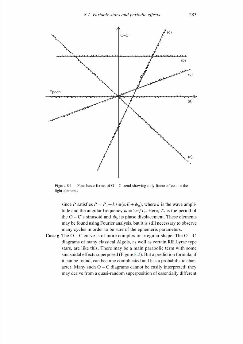
7/21/2019 Introduction to Astronomical Photometry
http://slidepdf.com/reader/full/introduction-to-astronomical-photometry 301/451
8.1 Variable stars and periodic effects 283
(d)O–C
(b)
(c)
(a)
(c)
Epoch
Figure 8.1 Four basic forms of O – C trend showing only linear effects in thelight elements
since P satisfies P = P 0 +k sinE +0, where k is the wave ampli-tude and the angular frequency = 2/T 2. Here, T 2 is the period of the O – C’s sinusoid and 0 its phase displacement. These elementsmay be found using Fourier analysis, but it is still necessary to observemany cycles in order to be sure of the ephemeris parameters.
Case g The O – C curve is of more complex or irregular shape. The O – Cdiagrams of many classical Algols, as well as certain RR Lyrae typestars, are like this. There may be a main parabolic term with somesinusoidal effects superposed (Figure 8.2). But a prediction formula, if it can be found, can become complicated and has a probabilistic char-acter. Many such O – C diagrams cannot be easily interpreted: theymay derive from a quasi-random superposition of essentially different
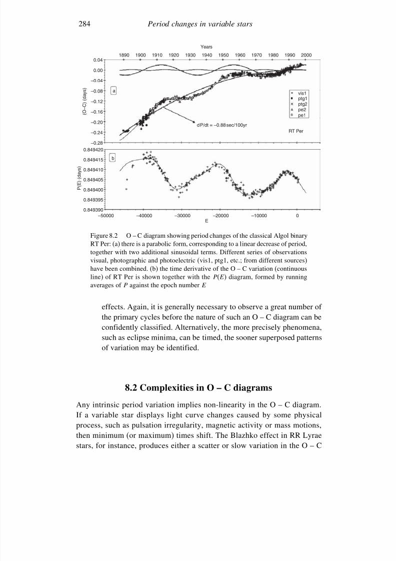
7/21/2019 Introduction to Astronomical Photometry
http://slidepdf.com/reader/full/introduction-to-astronomical-photometry 302/451
284 Period changes in variable stars
Years
d P/dt = –0.88 sec/100yrRT Per
vis1ptg1ptg2pe2pe1
18900.04
0.00
–0.04
–0.08 a
b
( O – C ) ( d a y s )
P ( E ) ( d a y s )
–0.12
–0.16
–0.20
–0.24
–0.280.849420
0.849415
0.849410
0.849405
0.849400
0.849395
0.849390–50000 –40000 –30000 –20000 –10000 0
1900 1910 1920 1930 1940 1950 1960 1970 1980 1990 2000
E
Figure 8.2 O – C diagram showing period changes of the classical Algol binaryRT Per: (a) there is a parabolic form, corresponding to a linear decrease of period,together with two additional sinusoidal terms. Different series of observationsvisual, photographic and photoelectric (vis1, ptg1, etc.; from different sources)have been combined. (b) the time derivative of the O – C variation (continuousline) of RT Per is shown together with the P (E ) diagram, formed by runningaverages of P against the epoch number E
effects. Again, it is generally necessary to observe a great number of the primary cycles before the nature of such an O – C diagram can beconfidently classified. Alternatively, the more precisely phenomena,such as eclipse minima, can be timed, the sooner superposed patternsof variation may be identified.
8.2 Complexities in O – C diagrams
Any intrinsic period variation implies non-linearity in the O – C diagram.If a variable star displays light curve changes caused by some physicalprocess, such as pulsation irregularity, magnetic activity or mass motions,then minimum (or maximum) times shift. The Blazhko effect in RR Lyraestars, for instance, produces either a scatter or slow variation in the O – C
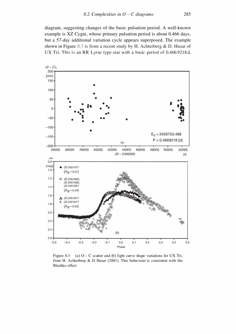
7/21/2019 Introduction to Astronomical Photometry
http://slidepdf.com/reader/full/introduction-to-astronomical-photometry 303/451
8.2 Complexities in O – C diagrams 285
diagram, suggesting changes of the basic pulsation period. A well-knownexample is XZ Cygni, whose primary pulsation period is about 0.466 days,but a 57-day additional variation cycle appears superposed. The example
shown in Figure 8.3 is from a recent study by H. Achterberg & D. Husar of UX Tri. This is an RR Lyrae type star with a basic period of 0.466 9218 d,
E0 = 2450753.488
P = 0.4669218 [d]
34000–200
–150
–100
–50
50
100
150
200(0 – C )1
[min]
0
36000 38000 40000 42000 44000 46000JD – 2400000
48000 50000 52000[d]
(a)
x
–0.5
1.0[mag]
0.8∆ m
1.2
1.4
1.6
1.8
2.0
2.2
2.4
2.6
–0.4 –0.3 –0.2 –0.1 0.0
(b)
Phase
0.1 0.2 0.3 0.4 0.5
JD 2451471
(Φ B ≈ 0.01)
JD 2451840,
JD 2451926,JD 2451927
(Φ B ≈ 0.44)
JD 2451817
(Φ B ≈ 0.93)
JD 2451817
Figure 8.3 (a) O – C scatter and (b) light curve shape variations for UX Tri,from H. Achterberg & D. Husar (2001). This behaviour is consistent with theBlazhko effect
7/21/2019 Introduction to Astronomical Photometry
http://slidepdf.com/reader/full/introduction-to-astronomical-photometry 304/451
286 Period changes in variable stars
on to which a Blazhko period of about 40 d is superposed. The amplitude of the light pulsation varies by a few tenths of a magnitude over this timescale,together with the phase of maximum light. A plot of the O – C difference
using a mean period against the phase of the Blazhko period gives what maybe called a ‘Blazhko diagram’. The Blazhko period is itself found to be notconstant in this example.
At present, in favourable circumstances, deviations of times of minima assmall as 10 s can be measured for regular binaries with sharp eclipses. Theminimum detectable variation on an O – C diagram depends on the timespanof the data. Thus, on the basis of a 10 s timing accuracy, a continuous period
change P/P as small as about 10−9
, in systems with periods around 1 day,would be observable over a timespan of a century. Even so, (i) the use of oldervisual and photographic data, (ii) an uneven, inhomogeneous distribution of data points, (iii) large gaps in the data set, (iv) using normal points to representlight curves (averaging together local groups of individual observations) and(v) an insufficiently long time base to the data set, all reduce the accuracyand usefulness of O – C diagrams. There is thus sometimes confusion whendeciding on the essential character of the variation: abrupt or continuous,
linear or quadratic, parabolic or sinusoidal, or otherwise. In order to decideproperly, one may have to wait for a century or more of good timing data todevelop real confidence.
In a general way, if one has an O – C diagram with a time span of about10 y, the discernible character of the diagram would tend to be linear. If
is longer, say 10 < < 30y, then a parabolic effect may become clear. For30 < < 50y, an alternating quality may emerge, and if > 50y, then we
may start to see real ‘complexities’. Note that part of a sinusoidal variationcould seem parabolic, while part of a more complicated variation could seemsinusoidal over a shorter interval. Present-day O – C data for many eclipsingbinaries cover less than one complete run of a possible long term cycle: orthe expected form of variation does not repeat in a later cycle.
It is well known that any arbitrary continuous non-linear function – suchas the underlying trend of an O – C diagram – can be represented to anydesired degree of accuracy by a series of trigonometric functions of increasing
frequency, i.e. a Fourier series. This is perhaps the basis for an apparentconfidence about functional representation of the variation. However, uponexamining a large number of O – C diagrams, many cases emerge where theyseem simply to follow a succession of linked straight lines. From a physicalpoint of view this would mean that now and then the periods are subject tosudden changes, and at unpredictably irregular intervals. What is happeninghere is that observers use instantaneous elements in the prediction of future
7/21/2019 Introduction to Astronomical Photometry
http://slidepdf.com/reader/full/introduction-to-astronomical-photometry 305/451
8.2 Complexities in O – C diagrams 287
times of minima (or maxima). The epoch and period are taken to satisfycurrent behaviour of the star, but then changed if later observations indicatedeviations.
A somewhat surprising aspect to this topic was introduced by T. E. Sternein 1934, and more recently revived by F. Lombard & C. Koen (1993). Theyasserted that apparent period changes of Miras, and certain other variables,did not have to be real, as they could be explained as the effects of cumulativeerror. It can be shown, from throws of dice, for example, that one can drawup artificial O – C curves that look very similar to those of variable stars, butwhich do not reflect any intrinsic physical effect. In many cases, these curves
also seem to follow a succession of linked straight lines.We can explain this briefly, in a qualitative manner. If there are two dice,
then the smallest throw is 2, the greatest 12, and the mean of all possiblevalues 7. This latter value is the analogue of the mean period of the star. If wewere able to throw the mean value on all occasions then, adding the numbers,we would obtain the series 0, 7, 14, 21, 28, etc. The numbers actually thrownwill deviate from this: in other words, they will fall around the mean inaccordance with pure chance.
If we now assume that, at some time, a very small value (2, say) has beenthrown after a previously fairly regular series, then the sum will be less thanexpected, so the O – C will be negative. For a following throw there wouldbe three possibilities: (i) again very small, (ii) fairly close to 7, or (iii) wellabove average. The latter case would compensate for the deficit incurred bythe preceding throw. Possibility (i) increases the deficit, while (ii) leaves itunchanged. One thus has an approximate 2/3 probability that the following
O – C value will again be negative. Hence, there is a certain tendency for anylarge chance deviation from the average value to be maintained, at least for atime. With a very long series, a compensation tends to occur, such that groupsof deviations of opposite sign follow each other having a similar probabilityof occurrence.
It is well to keep in mind, then, that this commonly used tool – theO – C diagram – may suggest effects that are not real: occasional random
errors of timing may cause accumulated changes in the times of minima (ormaxima), resulting in false indications of period changes. However, this isless likely in the case of regular eclipsing binary systems, where periodsare generally found to a few significant digits better accuracy than times of minima. So, at least for close binary systems, O – C diagrams provide agood basis for studying secular period changes and inferring related physicalprocesses.
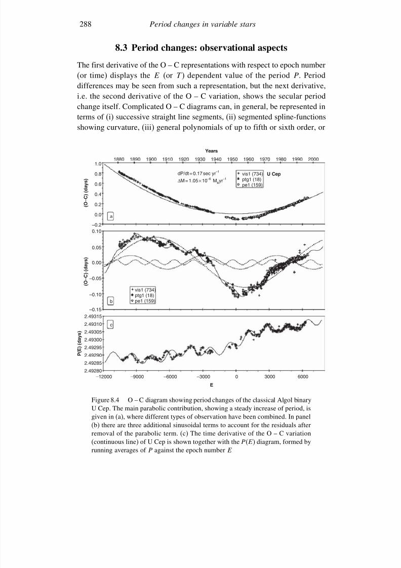
7/21/2019 Introduction to Astronomical Photometry
http://slidepdf.com/reader/full/introduction-to-astronomical-photometry 306/451
288 Period changes in variable stars
8.3 Period changes: observational aspects
The first derivative of the O – C representations with respect to epoch number
(or time) displays the E (or T ) dependent value of the period P . Perioddifferences may be seen from such a representation, but the next derivative,i.e. the second derivative of the O – C variation, shows the secular periodchange itself. Complicated O – C diagrams can, in general, be represented interms of (i) successive straight line segments, (ii) segmented spline-functionsshowing curvature, (iii) general polynomials of up to fifth or sixth order, or
Years
dP/dt = 0.17 sec yr–1
∆M = 1.05 × 10⁻⁶ Mxyr–1U Cepvis1 (734)
ptg1 (18)pe1 (159)
vis1 (734)ptg1 (18)pe1 (159)
189018801.0
0.8
0.6
a
b
c
( O – C ) ( d a y s )
( O – C ) ( d a y s )
P ( E ) ( d a y s )
0.4
0.2
0.0
–0.2
2.49315–0.15
–0.10
–0.05
0.00
0.05
0.10
2.49310
2.49305
2.49300
2.49295
2.49285
2.49290
2.49280–12000 –9000 –3000–6000 0 3000 6000
1900 1910 1920 1930 1940 1950 1960 1970 1980 1990 2000
E
Figure 8.4 O – C diagram showing period changes of the classical Algol binaryU Cep. The main parabolic contribution, showing a steady increase of period, isgiven in (a), where different types of observation have been combined. In panel(b) there are three additional sinusoidal terms to account for the residuals afterremoval of the parabolic term. (c) The time derivative of the O – C variation(continuous line) of U Cep is shown together with the P (E ) diagram, formed byrunning averages of P against the epoch number E
7/21/2019 Introduction to Astronomical Photometry
http://slidepdf.com/reader/full/introduction-to-astronomical-photometry 307/451
8.3 Period changes: observational aspects 289
(iv) a parabola plus a trigonometric series involving up to four terms (see e.g.Figures 8.2, 8.4, 8.6). The direct representation by straight line sections hassometimes been popular, where interpretations are given in terms of abrupt
period changes due to short episodes of mass transfer and loss from thesystem. It is difficult, however, to provide a convincing physical mechanismfor such period jumps in alternating directions.
8.3.1 Period changes in pulsating variables
Alternating period changes of RR Lyrae type variables have been known for
a long time. B. Szeidl (1976) identified period variations in all RR Lyraevariables showing the Blazhko effect in their light curves (see Figure 8.3).This is particularly noticeable from globular cluster studies, where manyRR Lyrae variables are found. Their multi-periodic photometric phenomenacould be modelled by star spots, associated with a solar type cyclic magneticfield. It was then thought that such a cyclic magnetic field might account,physically (apart from just the empirical photometric effect), for variablepulsation periods.
All types of period changes (increasing, decreasing, gradual or abrupt, andalternating) are observed in the giant cepheid type variables. In fact, monotonicperiod changes are expected in these stars as a response to evolution throughthe Hertzsprung gap: monotonic period increases for those moving redward,monotonic decreases for those moving blueward. L. Szabados showed thatthose cepheids with longer pulsation periods exhibit relatively more rapidperiod variations, due to their faster evolution. In order to explain the alter-
nating changes in pulsation period of cepheids, some authors suggested bina-rity and a light travel time effect. However, the O – C cycles in cepheidvariables are found not to repeat exactly. D. S. Hall (1989) has examined theO – C diagrams of 106 cepheids. He found that 42 have no sign of periodchange, 20 have period increases or decreases consistent with expected evolu-tionary effects, and 38 have alternating period changes. The median cyclelength for the alternating period changes was about 50 years, and the medianperiod change for those 38 stars was P/P
=9
×10−5.
8.3.2 Period changes in eclipsing binaries
Parabolic changes of O – C diagrams for binary systems indicate a mono-tonic increase or decrease of the orbital period and these have often beeninterpreted in terms of mass transfer between the component stars or massloss from the system. Cyclic O – C changes were seen as effects related to
7/21/2019 Introduction to Astronomical Photometry
http://slidepdf.com/reader/full/introduction-to-astronomical-photometry 308/451
290 Period changes in variable stars
orbital eccentricity, or gravitationally bound, though not directly observed,component stars producing motion of the binary in a wide orbit. The observedtimes of successive minima would then be advanced or retarded as a result
of changes in the time that light from the system would take to reach theobserver: the ‘light travel time effect’. Cyclic changes of internal structure forone or both components have also been invoked. Gravitational radiation willaffect eclipsing binary periods to a usually negligible extent (of the order of hours in millions of years) in comparison to the other effects to be consideredhere. A galactic acceleration effect, depending statistically on the locationof the binary in our Galaxy relative to the Sun, has also been sought. With
dependence on direction, this could start to affect the seventh digit in themean period value after some tens of years, but no very clear evidence waspresented so far.
Algol systems
Among the more complicated O – C diagrams are those of certainAlgol binaries. These are usually composed of a hot (A or B spectral type)more massive Main-Sequence-like primary well within its Roche lobe and
a cooler (G or K spectral type) less massive subgiant secondary, filling itsRoche lobe to the point of overflow (Section 7.2). Gas streams from the lessmassive secondary to the primary and attendant hydrodynamic effects areexpected. A fraction of the overflowing matter may be lost from the systementirely, together with some continuous stellar wind material from bothcomponents. The transferred and lost mass and associated angular momentaare expected to be on such a scale as to cause measurable changes of orbital
period over some decades.Early studies on the period changes of Algols were initiated before the startof the twentieth century, but attention was called to the importance of theseeffects in relation to dynamical evolution by G. Kuiper, F. B. Wood and othersin the 1940s and 50s. Relatively large period changes had sometimes beennoticed. By the 1960s there appeared observational evidence for circumstellarmaterial, in the form of an accretion ring or disk around the more massiveprimary, together with an understanding of how mass transfer could resolve
the Algol paradox.For the classical Algols, conservative mass transfer, i.e. overflowing mass
and its angular momentum remaining within the system, implies that P shouldsteadily increase. The O – C diagrams should then take the form of anupward parabola. Mass loss from the system as a whole may cause eitheran increase or decrease of P , depending on the vectorial geometry of theoutflow. We could perhaps expect the net effect of mass transfer and loss
7/21/2019 Introduction to Astronomical Photometry
http://slidepdf.com/reader/full/introduction-to-astronomical-photometry 309/451
8.3 Period changes: observational aspects 291
to make the O – C diagram take the form of the sum of two parabolas (i.e.another parabola), however, O – C diagrams of Algols are often much morecomplicated than this.
Cyclic changes of period can be interpreted in terms of a light time effect,as mentioned. In this case, the times of both primary and secondary eclipsesshould trace out the same sinusoidal O – C diagram. A purely sinusoidalO – C diagram would become tilted over for a binary revolving in an eccentricorbit around the mass centre of a triple system. But if the eccentric orbit of the binary is itself rotating, the quasi-sinusoidal O – C diagrams formed bythe primary and secondary minima shift separately. The rotation involved is
that of the location of the peri- and apastra, i.e. the line of apsides of theellipse: it is thus called apsidal motion. We consider this and the light traveltime effect in more detail below.
Classical Algols with periods less than about ten days are expected tohave effectively circular orbits and thus should not exhibit apsidal motionin their O – C diagrams, but, until recently, explanations for many unclearor incomplete O – C diagrams were offered that referred to third bodies orapsidal motion. In many instances concerning the light travel time predictions,
it was later found that either (i) the period changes were not strictly periodic,or (ii) the inferred third body mass was too large to avoid detection inthe composite spectrum, (iii) the inferred orbit required significant velocitychanges that were not observed, or sometimes (iv) an unreasonably largenumber of companion stars was required to explain the effects.
Further developments regarding period changes of Algols have been madeby introducing a magnetic braking effect from their cool secondaries. Magnet-
ically coupled stellar wind mass loss, associated with the Alfvén radius atusually an order of magnitude larger than that of the mass-losing star, extractsa relatively large amount of angular momentum and should thus rapidly spindown the star. From data on single late type stars in well-studied galacticclusters, it was found that the rotation rate, or spin, decreases with measuredstellar age, and relatively rapidly for younger stars. The situation is differentfor binary systems, however, because of ‘spin–orbit coupling’. Here, compo-nents are not able to spin down their rotation by systemic angular momentum
loss. Instead, enhanced angular momentum loss from a stellar wind is accom-panied by an orbital angular momentum interaction, involving tidal friction.Shrinkage of the orbit occurs and its period decreases, i.e. the rotation thenbecomes more rapid.
Late type Roche-lobe filling secondaries of Algols are known to showmagnetic activity effects, so a similar magnetic braking process can beexpected as with the RS CVn and EW type binaries. Both systemic mass loss
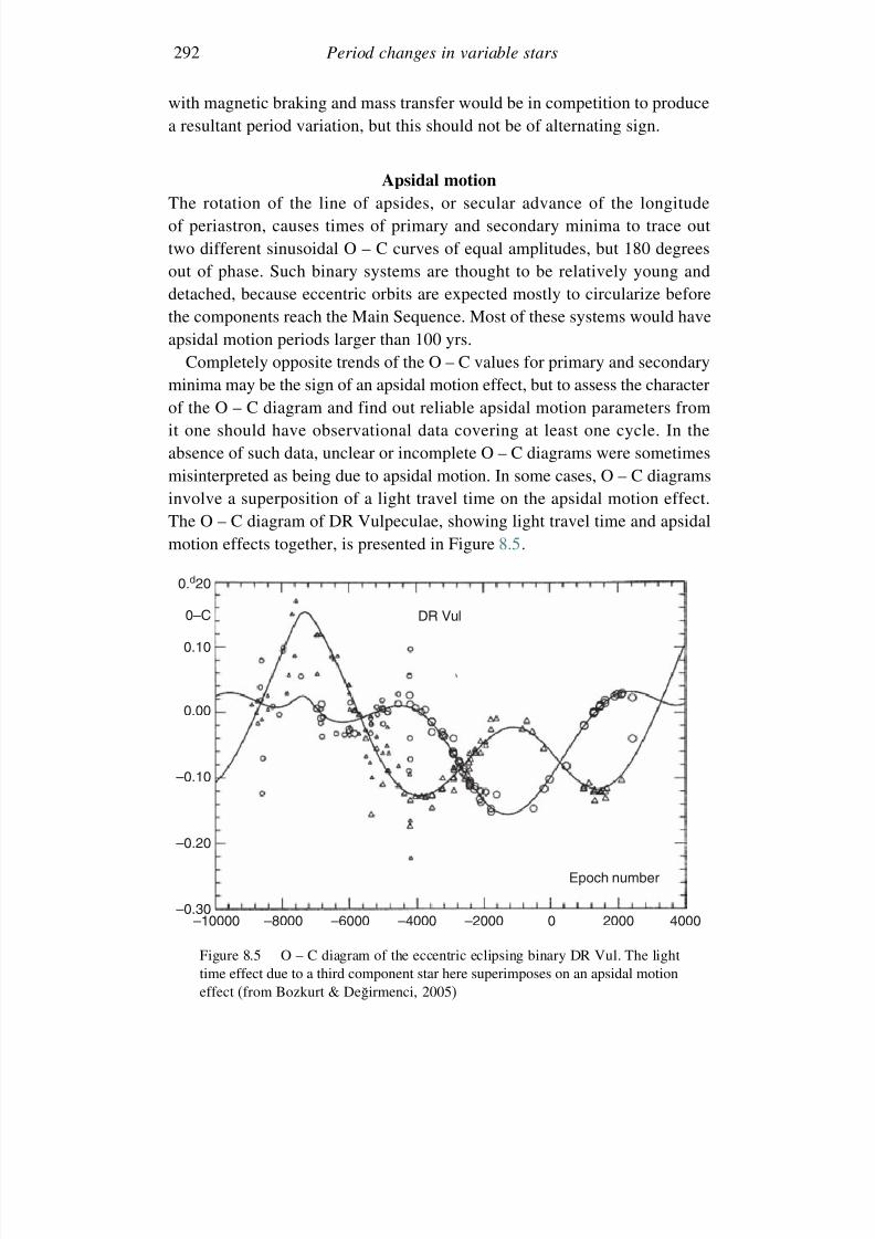
7/21/2019 Introduction to Astronomical Photometry
http://slidepdf.com/reader/full/introduction-to-astronomical-photometry 310/451
292 Period changes in variable stars
with magnetic braking and mass transfer would be in competition to producea resultant period variation, but this should not be of alternating sign.
Apsidal motion
The rotation of the line of apsides, or secular advance of the longitudeof periastron, causes times of primary and secondary minima to trace outtwo different sinusoidal O – C curves of equal amplitudes, but 180 degreesout of phase. Such binary systems are thought to be relatively young anddetached, because eccentric orbits are expected mostly to circularize beforethe components reach the Main Sequence. Most of these systems would have
apsidal motion periods larger than 100 yrs.Completely opposite trends of the O – C values for primary and secondary
minima may be the sign of an apsidal motion effect, but to assess the characterof the O – C diagram and find out reliable apsidal motion parameters fromit one should have observational data covering at least one cycle. In theabsence of such data, unclear or incomplete O – C diagrams were sometimesmisinterpreted as being due to apsidal motion. In some cases, O – C diagrams
involve a superposition of a light travel time on the apsidal motion effect.The O – C diagram of DR Vulpeculae, showing light travel time and apsidalmotion effects together, is presented in Figure 8.5.
0.d20
0–C
0.10
0.00
–0.10
–0.20
–0.30–10000 –8000 –6000 –4000 –2000
Epoch number
DR Vul
0 2000 4000
Figure 8.5 O – C diagram of the eccentric eclipsing binary DR Vul. The lighttime effect due to a third component star here superimposes on an apsidal motioneffect (from Bozkurt & Degirmenci, 2005)
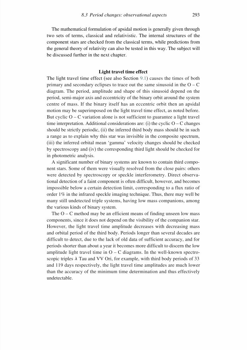
7/21/2019 Introduction to Astronomical Photometry
http://slidepdf.com/reader/full/introduction-to-astronomical-photometry 311/451
8.3 Period changes: observational aspects 293
The mathematical formulation of apsidal motion is generally given throughtwo sets of terms, classical and relativistic. The internal structures of thecomponent stars are checked from the classical terms, while predictions from
the general theory of relativity can also be tested in this way. The subject willbe discussed further in the next chapter.
Light travel time effect
The light travel time effect (see also Section 9.1) causes the times of bothprimary and secondary eclipses to trace out the same sinusoid in the O – Cdiagram. The period, amplitude and shape of this sinusoid depend on the
period, semi-major axis and eccentricity of the binary orbit around the systemcentre of mass. If the binary itself has an eccentric orbit then an apsidalmotion may be superimposed on the light travel time effect, as noted before.But cyclic O – C variation alone is not sufficient to guarantee a light traveltime interpretation. Additional considerations are: (i) the cyclic O – C changesshould be strictly periodic, (ii) the inferred third body mass should be in sucha range as to explain why this star was invisible in the composite spectrum,
(iii) the inferred orbital mean ‘gamma’ velocity changes should be checkedby spectroscopy and (iv) the corresponding third light should be checked forin photometric analysis.
A significant number of binary systems are known to contain third compo-nent stars. Some of them were visually resolved from the close pairs: otherswere detected by spectroscopy or speckle interferometry. Direct observa-tional detection of a faint component is often difficult, however, and becomesimpossible below a certain detection limit, corresponding to a flux ratio of order 1% in the infrared speckle imaging technique. Thus, there may well bemany still undetected triple systems, having low mass companions, amongthe various kinds of binary system.
The O – C method may be an efficient means of finding unseen low masscomponents, since it does not depend on the visibility of the companion star.However, the light travel time amplitude decreases with decreasing massand orbital period of the third body. Periods longer than several decades are
difficult to detect, due to the lack of old data of sufficient accuracy, and forperiods shorter than about a year it becomes more difficult to discern the lowamplitude light travel time in O – C diagrams. In the well-known spectro-scopic triples Tau and VV Ori, for example, with third body periods of 33and 119 days respectively, the light travel time amplitudes are much lowerthan the accuracy of the minimum time determination and thus effectivelyundetectable.
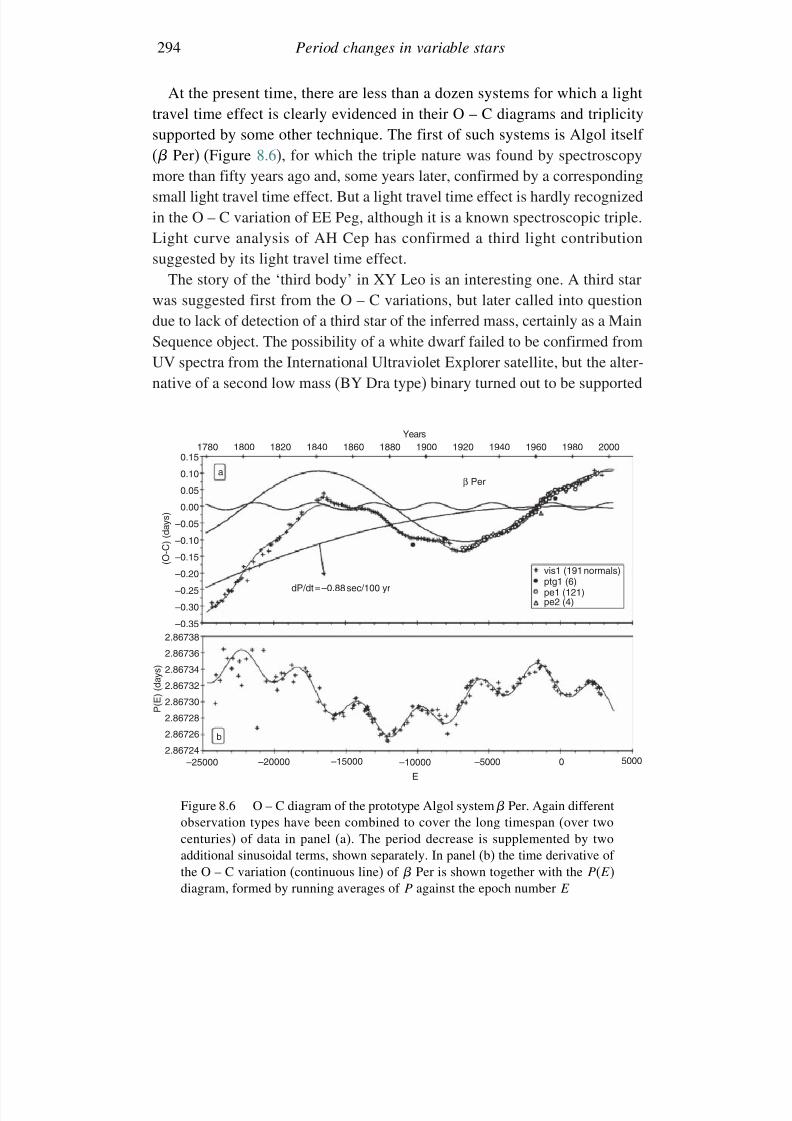
7/21/2019 Introduction to Astronomical Photometry
http://slidepdf.com/reader/full/introduction-to-astronomical-photometry 312/451
294 Period changes in variable stars
At the present time, there are less than a dozen systems for which a lighttravel time effect is clearly evidenced in their O – C diagrams and triplicitysupported by some other technique. The first of such systems is Algol itself
( Per) (Figure 8.6), for which the triple nature was found by spectroscopymore than fifty years ago and, some years later, confirmed by a correspondingsmall light travel time effect. But a light travel time effect is hardly recognizedin the O – C variation of EE Peg, although it is a known spectroscopic triple.Light curve analysis of AH Cep has confirmed a third light contributionsuggested by its light travel time effect.
The story of the ‘third body’ in XY Leo is an interesting one. A third star
was suggested first from the O – C variations, but later called into questiondue to lack of detection of a third star of the inferred mass, certainly as a MainSequence object. The possibility of a white dwarf failed to be confirmed fromUV spectra from the International Ultraviolet Explorer satellite, but the alter-native of a second low mass (BY Dra type) binary turned out to be supported
Years
dP/dt = –0.88 sec/100 yr
vis1 (191 normals)ptg1 (6)pe1 (121)pe2 (4)
18001780
0.150.10
0.05
0.00
–0.05
–0.10
–0.15
–0.20
–0.25
–0.30–0.35
a
b
( O - C ) ( d a y s )
P ( E ) ( d a y s )
2.86738
2.86736
2.86734
2.86732
2.86730
2.86726
2.86728
2.86724
–25000 –20000 –10000–15000 0–5000 5000
1820 1840 1860 1920 19601900 19401880 1980 2000
E
β Per
Figure 8.6 O – C diagram of the prototype Algol system Per. Again differentobservation types have been combined to cover the long timespan (over twocenturies) of data in panel (a). The period decrease is supplemented by twoadditional sinusoidal terms, shown separately. In panel (b) the time derivative of the O – C variation (continuous line) of Per is shown together with the P (E )diagram, formed by running averages of P against the epoch number E
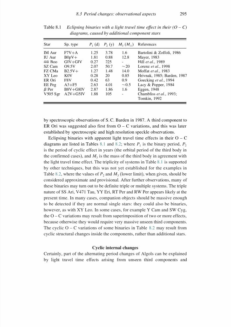
7/21/2019 Introduction to Astronomical Photometry
http://slidepdf.com/reader/full/introduction-to-astronomical-photometry 313/451
8.3 Period changes: observational aspects 295
Table 8.1 Eclipsing binaries with a light travel time effect in their (O – C)
diagrams, caused by additional component stars
Star Sp. type P 1 (d) P 2 (y) M 3 (M ) ReferencesIM Aur F7V+A 125 3.78 1.6 Bartolini & Zoffoli, 1986IU Aur B0pV+ 181 0.88 12.8 Mayer, 198344i Boo GIV+GIV 027 225 - Hill et al., 1989SZ Cam O9.5V 207 50.7 ∼20 Lorenz et al., 1998FZ CMa B2.5V+ 127 1.48 14.0 Moffat et al., 1983XY Leo K0V 028 20 0.85 Hrivnak, 1985; Barden, 1987ER Ori F8V 042 63 0.9 Goecking et al., 1994EE Peg A3
+F5 263 4.01
∼05 Lacy & Popper, 1984
Per B8V+G8IV 287 1.86 1.6 Eggen, 1948V505 Sgr A2V+G5IV 188 105 - Chambliss et al., 1993;Tomkin, 1992
by spectroscopic observations of S. C. Barden in 1987. A third component toER Ori was suggested also first from O – C variations, and this was later
established by spectroscopic and high resolution speckle observations.Eclipsing binaries with apparent light travel time effects in their O – Cdiagrams are listed in Tables 8.1 and 8.2; where P 1 is the binary period, P 2is the period of cyclic effect in years (the orbital period of the third body inthe confirmed cases), and M 3 is the mass of the third body in agreement withthe light travel time effect. The triplicity of systems in Table 8.1 is supportedby other techniques, but this was not yet established for the examples inTable 8.2, where the values of P 2 and M 3 (lower limit), when given, should be
considered approximate and provisional. After further observations, many of these binaries may turn out to be definite triple or multiple systems. The triplenature of SS Ari, V471 Tau, YY Eri, RT Per and RW Per appears likely at thepresent time. In many cases, companion objects should be massive enoughto be detected if they are normal single stars: they could also be binaries,however, as with XY Leo. In some cases, for example Y Cam and SW Cyg,the O – C variations may result from superimposition of two or more effects,
because otherwise they would require very massive unseen third components.The cyclic O – C variations of some binaries in Table 8.2 may result fromcyclic structural changes inside the components, rather than additional stars.
Cyclic internal changes
Certainly, part of the alternating period changes of Algols can be explainedby light travel time effects arising from unseen third components and
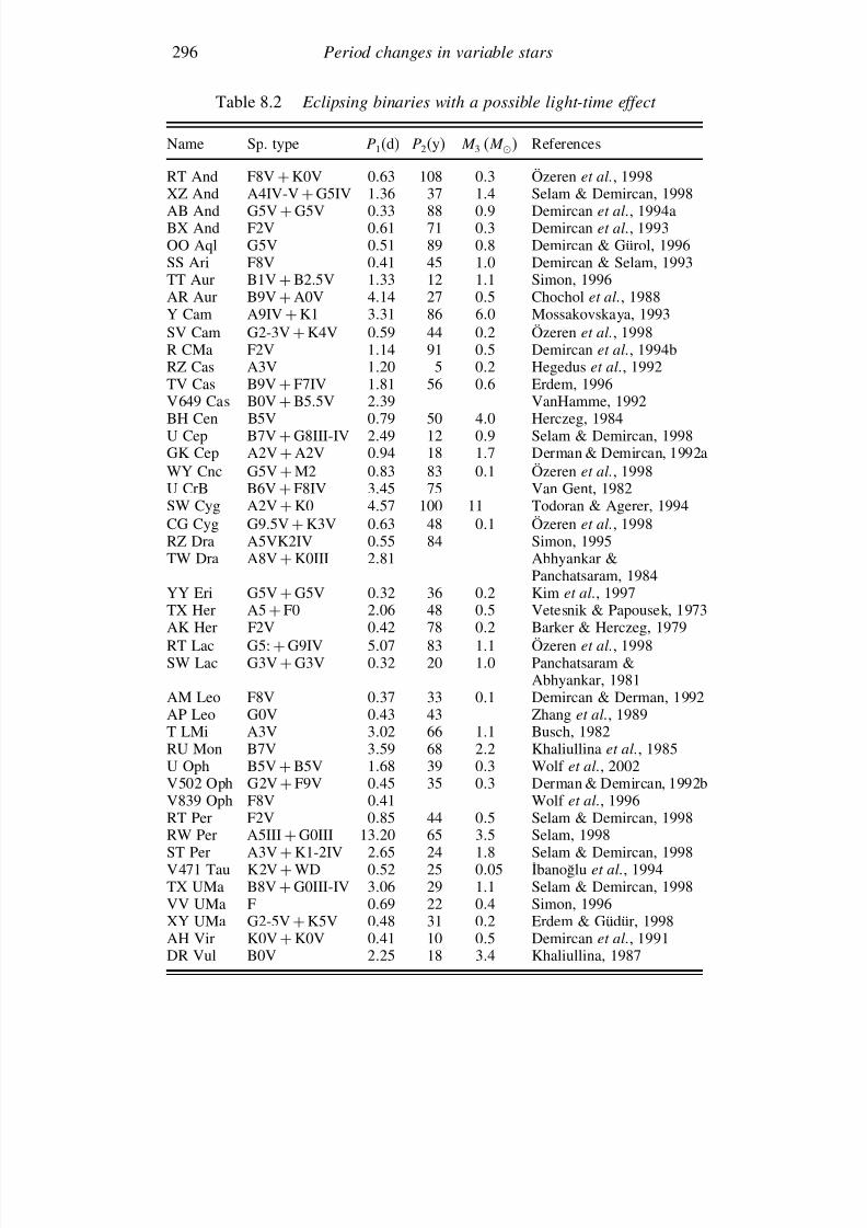
7/21/2019 Introduction to Astronomical Photometry
http://slidepdf.com/reader/full/introduction-to-astronomical-photometry 314/451
296 Period changes in variable stars
Table 8.2 Eclipsing binaries with a possible light-time effect
Name Sp. type P 1(d) P 2(y) M 3 (M ) References
RT And F8V + K0V 063 108 03 Özeren et al., 1998XZ And A4IV-V + G5IV 136 37 14 Selam & Demircan, 1998AB And G5V + G5V 033 88 09 Demircan et al., 1994aBX And F2V 061 71 03 Demircan et al., 1993OO Aql G5V 051 89 08 Demircan & Gürol, 1996SS Ari F8V 041 45 10 Demircan & Selam, 1993TT Aur B1V + B2.5V 133 12 11 Simon, 1996AR Aur B9V + A0V 414 27 05 Chochol et al., 1988Y Cam A9IV + K1 331 86 60 Mossakovskaya, 1993
SV Cam G2-3V + K4V 059 44 02 Özeren et al., 1998R CMa F2V 114 91 05 Demircan et al., 1994bRZ Cas A3V 120 5 02 Hegedus et al., 1992TV Cas B9V + F7IV 181 56 06 Erdem, 1996V649 Cas B0V + B5.5V 239 VanHamme, 1992BH Cen B5V 079 50 40 Herczeg, 1984U Cep B7V + G8III-IV 249 12 09 Selam & Demircan, 1998GK Cep A2V + A2V 094 18 17 Derman & Demircan, 1992aWY Cnc G5V + M2 083 83 01 Özeren et al., 1998U CrB B6V
+F8IV 345 75 Van Gent, 1982
SW Cyg A2V + K0 457 100 11 Todoran & Agerer, 1994CG Cyg G9.5V + K3V 063 48 01 Özeren et al., 1998RZ Dra A5VK2IV 055 84 Simon, 1995TW Dra A8V + K0III 281 Abhyankar &
Panchatsaram, 1984YY Eri G5V + G5V 032 36 02 Kim et al., 1997TX Her A5 + F0 206 48 05 Vetesnik & Papousek, 1973AK Her F2V 042 78 02 Barker & Herczeg, 1979RT Lac G5: + G9IV 507 83 11 Özeren et al., 1998
SW Lac G3V + G3V 032 20 10 Panchatsaram &Abhyankar, 1981AM Leo F8V 037 33 01 Demircan & Derman, 1992AP Leo G0V 043 43 Zhang et al., 1989T LMi A3V 302 66 11 Busch, 1982RU Mon B7V 359 68 22 Khaliullina et al., 1985U Oph B5V + B5V 168 39 03 Wolf et al., 2002V502 Oph G2V + F9V 045 35 03 Derman & Demircan, 1992bV839 Oph F8V 041 Wolf et al., 1996RT Per F2V 085 44 05 Selam & Demircan, 1998
RW Per A5III + G0III 1320 65 35 Selam, 1998ST Per A3V + K1-2IV 265 24 18 Selam & Demircan, 1998V471 Tau K2V + WD 052 25 005 Ibanoglu et al., 1994TX UMa B8V + G0III-IV 306 29 11 Selam & Demircan, 1998VV UMa F 069 22 04 Simon, 1996XY UMa G2-5V + K5V 048 31 02 Erdem & Güdür, 1998AH Vir K0V + K0V 041 10 05 Demircan et al., 1991DR Vul B0V 225 18 34 Khaliullina, 1987
7/21/2019 Introduction to Astronomical Photometry
http://slidepdf.com/reader/full/introduction-to-astronomical-photometry 315/451
8.3 Period changes: observational aspects 297
apsidal motion, but these models seem hard pressed to account for allthe observed effects. One significant constraint came from a study byD. S. Hall of period changes in a sample of 101 Algols, where alternating
changes were found only in systems with late-type secondaries. Lateranalysis confirmed that period changes in earlier type Algols (containingtwo radiative-envelope components) really have less complicated effects,rarely showing cyclic changes in their O – C diagrams. The absence of alternating period changes in radiative Algols strengthens the case foran important dynamic role for envelope convection in the secondaries of classical Algols.
In order to explain the apparent alternating period changes of classicalAlgols, D. S. Hall and P. Biermann introduced a model where the secon-daries undergo episodes of sudden mass transfer. The transferred mass orbitsthe primary in a disk, as a temporary store of orbital angular momentumthat would cause P to decrease. Some time later, this angular momentum isreturned via an accretion process, so P should again increase. The concomi-tant physical processes were not fully confirmed by observation, however.In another construction, a localized magnetically driven strong wind from
the cool component was proposed. This model has also not been substanti-ated from the observed locations of active region longitudes compared withcontemporaneous P changes.
More recent development has produced the idea of cyclic effects associatedwith changes of envelope structure involving convection and magnetic fieldinteraction. Cyclic changes in the magnetic field of one star would, throughthe action of magnetic pressure, cause cyclical changes in the radius of
gyration and hence the internal rotation rate. Spin–orbit coupling, in turn,forces the orbital motion of the binary to follow the activity cycle of theactive component.
Summary
The simplest linear forms of O – C diagram tend to be observed for EAD typebinaries, especially when both stars have radiative envelopes. No significantchange of period would be expected for a pair of Main Sequence stars for at
least a few hundred years if the orbit is circular and there is no gravitationallybound third star. For EAS binaries with radiative components, monotonicperiod changes tend to be observed, and these are interpreted in terms of mass transfer and loss. With classical Algols having late type secondaries,additional magnetic braking effects may be present, but there still seems noclear proof about how any particular model can specify the more complicatedalternating O – C changes of these systems.
7/21/2019 Introduction to Astronomical Photometry
http://slidepdf.com/reader/full/introduction-to-astronomical-photometry 316/451
298 Period changes in variable stars
Parabola and trigonometric series representations for the more complexO – C diagrams of a few well-known examples have been shown inFigures 8.2, 8.4, 8.5 and 8.6. Even the most complicated variations can
be empirically represented by the sum of a parabola and two, or at mostthree, sine curves. Period changes for these Algols are also illustrated byP (E ) diagrams, using local average P values from time of minima data.The time derivatives of best-fit continuous functions to the O – C diagramscan be shown on the P (E ) diagrams. Such simple empirical forms will fitobservational P (E ) diagrams to a satisfactory level of agreement, at leastover limited time intervals.
Mass transfer has the predominating effect on the period changes of U Cep(Figure 8.4),whilesystemicmasslossmaydominateinthecaseofRTPerand
Per(Figures 8.2& 8.6).Someoftheremainingcyclicvariations,butnotall,couldbe caused by unseen third or fourth bodies. For the well-known Per system,astrometric observations showed that the inferred 32 and 180 y periods do notcorrespond to orbital motions, nor have they been explained in terms of apsidalmotion. S. Söderhjelm (1980) speculated that the 32 y periodicity could be duetoa cyclicmagneticeffect of the coolsecondary. The 180 y ‘periodicity’ has also
been thought to be an artifact of two abrupt changes of the orbital period in 1944and 1950. Improvements in precision resulting from astrometric measurementsof planned missions, such as FAME, DIVA, SIM and GAIA, should establishwhether cyclic changes in the O – C diagram may be caused by unseen objectsaround this and other comparable binary systems.
8.4 Period changes: theoretical aspects8.4.1 Angular momentum in single and binary stars
The rotational, or spin, angular momentum H s of a single star with mass m,radius R, and spin period P s is given by
H s = k2R2mP −1s (8.9)
where k is the gyration coefficient. It typically varies between 0.07 and 0.15,
depending on the density distribution inside the star.The orbital angular momentum H o of a binary with component masses m1,
m2 and orbital period P o is given by
H o =
G2
2
1/3m1m2
m1 + m21/3 P 1/3o (8.10)
where G is the gravitation constant.
7/21/2019 Introduction to Astronomical Photometry
http://slidepdf.com/reader/full/introduction-to-astronomical-photometry 317/451
8.4 Period changes: theoretical aspects 299
Angular momentum of a single star may be lost via stellar winds originatingfrom surface regions. However, for cool stars with convection taking place intheir outer envelopes, a significant proportion of mass loss occurs not from
the photosphere itself but from the outer parts of magnetic loops, which canbe located at an ‘Alfven radius’ RA. If the angular momentum H of such astar is differentiated with respect to P s at the surface, and m at the Alfvenradius, arguing that the stellar wind emerges there, we find
dH
dt = −k2R2mP −2
s
dP
dt = k2R2
AP −1s
dm
dt (8.11)
This corresponds with magnetic braking for single cool stars, which can thusbe written:
dP
dt = −
RA
R
2P
m
dm
dt (8.12)
A key point here is that RA is an order of magnitude larger than R and so
a low rate of mass loss may spin down cool stars appreciably in a relativelyshort time. This argument has been supported by a considerable amount of observational data on single cool star rotation rates.
8.4.2 Angular momentum evolution of cool binaries
In Chapter 10 we will encounter examples of RS CVn type binaries. Theyare composed of late type – mostly G or K – stars, often in a somewhatevolved, though not semi detached, state and are characterized by strongsurface magnetic fields. These binaries are expected to undergo secularangular momentum loss from the component stars, primarily via a brakingprocess like that just considered. This angular momentum loss, however, canbe fed from the reservoir of orbital angular momentum H o, through a processof tidal friction. The result should be the spiralling in of the binary, eventually
to form a contact binary system, unless some other process intervenes.To follow through this scenario, a semi-empirical model for the numerical
value of the mass loss rate was constructed, using relevant observational dataon the period changes of 40 RS CVn binaries, thus:
dm
dt = 0068
m1m2
m1 + m21 / 3P −2/3 dP
dt (8.13)
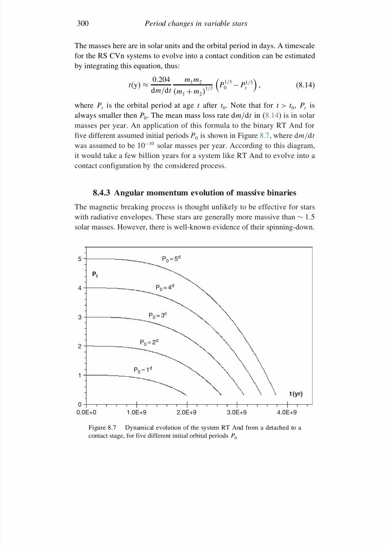
7/21/2019 Introduction to Astronomical Photometry
http://slidepdf.com/reader/full/introduction-to-astronomical-photometry 318/451
300 Period changes in variable stars
The masses here are in solar units and the orbital period in days. A timescalefor the RS CVn systems to evolve into a contact condition can be estimatedby integrating this equation, thus:
ty ≈ 0204dm/dt
m1m2
m1 + m21/3
P
1/30 − P 1/3
t
(8.14)
where P t is the orbital period at age t after t0. Note that for t > t0, P t isalways smaller then P 0. The mean mass loss rate dm/dt in (8.14) is in solarmasses per year. An application of this formula to the binary RT And forfive different assumed initial periods P 0 is shown in Figure 8.7, where dm/dt
was assumed to be 10−10 solar masses per year. According to this diagram,it would take a few billion years for a system like RT And to evolve into acontact configuration by the considered process.
8.4.3 Angular momentum evolution of massive binaries
The magnetic breaking process is thought unlikely to be effective for starswith radiative envelopes. These stars are generally more massive than
∼15
solar masses. However, there is well-known evidence of their spinning-down.
5
Pt
P0 = 5d
P0 = 4d
P0 = 3d
P0 = 2d
P0 = 1d
4
3
2
1
00.0E+0 1.0E+9 2.0E+9 3.0E+9 4.0E+9
t (yr)
Figure 8.7 Dynamical evolution of the system RT And from a detached to acontact stage, for five different initial orbital periods P 0
7/21/2019 Introduction to Astronomical Photometry
http://slidepdf.com/reader/full/introduction-to-astronomical-photometry 319/451
8.5 Statistical data on Algol binaries 301
A high rate of stellar wind flow is implied, perhaps with the aid of somemechanism to stiffen wind material out to a distance appreciably greater thanthat of the photosphere. Massive close binary components cannot lose angular
momentum due to the action of tides alone, but a non-conservative process,like friction, can give rise to a braking torque, causing the orbits to shrink, aswith cool binaries.
We would generally expect the angular momentum evolution of closebinary systems to be towards smaller orbits. For this process to be effective,spin–orbit coupling (P s ≈ P orb is necessary. In this way, relatively long period(P 0 ≥ 10d) binaries that remain detached are not expected to evolve into
shorter period systems over timescales comparable to the age of the Galaxy.On the other hand, the more massive component of a short period binary mayfill its Roche lobe and start transferring mass to the other component while thesystem is evolving towards shorter periods. Once Roche lobe overflow starts,it would tend to take over as the predominant effect in subsequent angularmomentum evolution of the binary. In the fast lead up to primary/secondarymass-ratio reversal, the orbital period would decrease, but thereafter it wouldtend to increase again.
8.5 Statistical data on Algol binaries
There are 719 eclipsing binaries with EA-type light curves in the Atlas of
O – C Diagrams of Eclipsing Binary Stars of J. M. Kreiner, C.-H. Kim andI.-S. Nha (2001). These binaries, forming 63% of all the stars included,
contain both EAD and EAS types, which may be considered together. Forsome 217 (30%) of these systems, the O – C diagrams are indefinite, due toinsufficient number and time coverage of the data points. Of the remaining502 Algols, 221 (44%) display no measurable period variation; 47 (9.4%)display an upward parabola; 31 (6.2%) show a downward parabola; 14 (2.8%)have a periodic variation superimposed on the parabola; 87 (17.3%) havecyclic O – C diagrams; 72 (14.3%) show apsidal motion; and 30 (6.0%) indi-cate more complicated variations of period. Those Algols with increasing,
decreasing or more complicated period variations are listed, together withsome system parameters, in Tables 8.3, 8.4 and 8.5. The system parame-ters in these tables (spectral types of the component stars (sp), mass ratios(q = m2/m1) and orbital periods P , are from the Catalogue of Algols producedrecently by the present authors and their colleagues.
In general, those period increasing systems in Table 8.3 showing upward(i.e. apex down) parabolae are expected to result from (present) secondary to
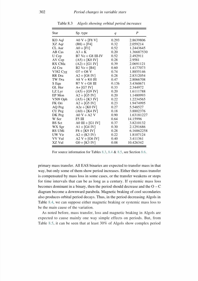
7/21/2019 Introduction to Astronomical Photometry
http://slidepdf.com/reader/full/introduction-to-astronomical-photometry 320/451
302 Period changes in variable stars
Table 8.3 Algols showing orbital period increases
Star Sp. type q P
KO Aql A0 V + [F8 V] 0293 28639806XZ Aqr (B8) + [F4] 032 2059214CL Aur A0 + [F1] 052 12443645AB Cas A3 + K 020 136687530U Cep B7 Ve + G8 III-IV 052 2492911AV Cep (A5) + [K0 IV] 028 29581RX CMa (A2) + [G1 IV] 039 20691121AI Cru B2 Ve + [B4] 060 14177073V382 Cyg O7 + O8 V 074 18855146
RR Dra A2 + [G8 IV] 028 28312054TW Dra A8 V + K0 III 047 28066708S Equ B7 V + G8 III 0126 34360671GL Her A+ [G7 IV] 033 2344972LZ Lyr (A5) + [G9 IV] 020 16111788EP Mon A2 + [G5 IV] 020 11480993V509 Oph (A5) + [K3 IV] 022 12234565FK Ori A2 + [G5 IV] 023 19474995AQ Peg A2e + [K0 IV] 027 5548527CU Peg (A0)
+[K4 IV] 018 38802376
DK Peg A0 V + A2 V 090 163181227W Ser F5 III 064 1415996BS Sct A0 III + [G1 IV] 037 38210132WX Sgr A1 + [G4 IV] 030 21291686RS UMi F8 + [K9 IV] 028 616862258UW Vir A2 + (K3 IV) 022 18107124VV Vul A2 V + [G6 IV] 040 3411361XZ Vul G0 + [K3 IV] 008 10426342
For source information for Tables 8.3, 8.4 & 8.5, see Section 8.6.
primary mass transfer. All EAS binaries are expected to transfer mass in thatway, but only some of them show period increases. Either their mass transferis compensated by mass loss in some cases, or the transfer weakens or stopsfor time intervals that can be as long as a century. If systemic mass lossbecomes dominant in a binary, then the period should decrease and the O – C
diagram become a downward parabola. Magnetic braking of cool secondariesalso produces orbital period decays. Thus, in the period decreasing Algols inTable 8.4, we can suppose either magnetic braking or systemic mass loss tobe the main cause of the variation.
As noted before, mass transfer, loss and magnetic braking in Algols areexpected to cause mainly one way simple effects on periods. But, fromTable 8.5, it can be seen that at least 30% of Algols show complex period
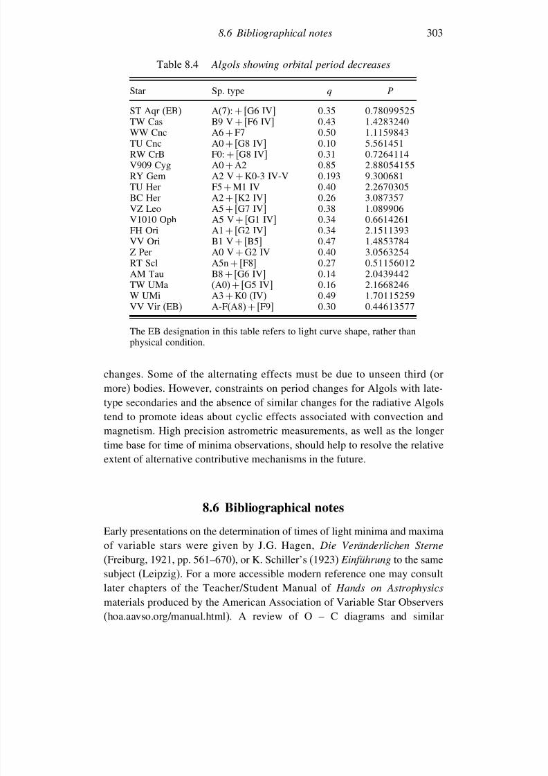
7/21/2019 Introduction to Astronomical Photometry
http://slidepdf.com/reader/full/introduction-to-astronomical-photometry 321/451
8.6 Bibliographical notes 303
Table 8.4 Algols showing orbital period decreases
Star Sp. type q P
ST Aqr (EB) A(7): + [G6 IV] 035 078099525TW Cas B9 V + [F6 IV] 043 14283240WW Cnc A6 + F7 050 11159843TU Cnc A0 + [G8 IV] 010 5561451RW CrB F0: + [G8 IV] 031 07264114V909 Cyg A0 + A2 085 288054155RY Gem A2 V + K0-3 IV-V 0193 9300681TU Her F5 + M1 IV 040 22670305BC Her A2 + [K2 IV] 026 3087357
VZ Leo A5 + [G7 IV] 038 1089906V1010 Oph A5 V + [G1 IV] 034 06614261FH Ori A1 + [G2 IV] 034 21511393VV Ori B1 V + [B5] 047 14853784Z Per A0 V + G2 IV 040 30563254RT Scl A5n + [F8] 027 051156012AM Tau B8 + [G6 IV] 014 20439442TW UMa (A0) + [G5 IV] 016 21668246W UMi A3 + K0 (IV) 049 170115259VV Vir (EB) A-F(A8)
+[F9] 030 044613577
The EB designation in this table refers to light curve shape, rather thanphysical condition.
changes. Some of the alternating effects must be due to unseen third (ormore) bodies. However, constraints on period changes for Algols with late-type secondaries and the absence of similar changes for the radiative Algolstend to promote ideas about cyclic effects associated with convection andmagnetism. High precision astrometric measurements, as well as the longertime base for time of minima observations, should help to resolve the relativeextent of alternative contributive mechanisms in the future.
8.6 Bibliographical notes
Early presentations on the determination of times of light minima and maximaof variable stars were given by J.G. Hagen, Die Veränderlichen Sterne
(Freiburg, 1921, pp. 561–670), or K. Schiller’s (1923) Einführung to the samesubject (Leipzig). For a more accessible modern reference one may consultlater chapters of the Teacher/Student Manual of Hands on Astrophysics
materials produced by the American Association of Variable Star Observers(hoa.aavso.org/manual.html). A review of O – C diagrams and similar
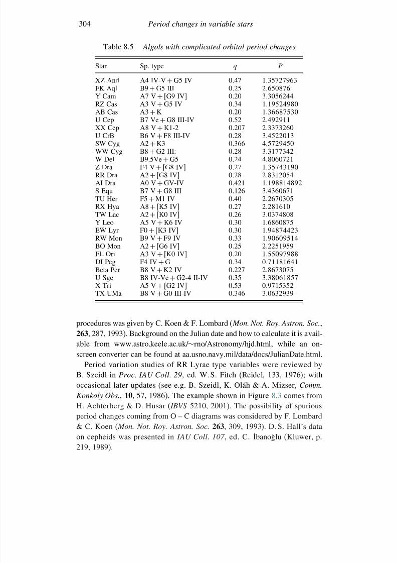
7/21/2019 Introduction to Astronomical Photometry
http://slidepdf.com/reader/full/introduction-to-astronomical-photometry 322/451
304 Period changes in variable stars
Table 8.5 Algols with complicated orbital period changes
Star Sp. type q P
XZ And A4 IV-V + G5 IV 047 135727963FK Aql B9 + G5 III 025 2650876Y Cam A7 V + [G9 IV] 020 33056244RZ Cas A3 V + G5 IV 034 119524980AB Cas A3 + K 020 136687530U Cep B7 Ve + G8 III-IV 052 2492911XX Cep A8 V + K1-2 0207 23373260U CrB B6 V + F8 III-IV 028 34522013SW Cyg A2 + K3 0366 45729450
WW Cyg B8 + G2 III: 028 33177342W Del B9.5Ve + G5 024 48060721Z Dra F4 V + [G8 IV] 027 135743190RR Dra A2 + [G8 IV] 028 28312054AI Dra A0 V + GV-IV 0421 1198814892S Equ B7 V + G8 III 0126 34360671TU Her F5 + M1 IV 040 22670305RX Hya A8 + [K5 IV] 027 2281610TW Lac A2 + [K0 IV] 026 30374808Y Leo A5 V
+K6 IV 030 16860875
EW Lyr F0 + [K3 IV] 030 194874423RW Mon B9 V + F9 IV 033 190609514BO Mon A2 + [G6 IV] 025 22251959FL Ori A3 V + [K0 IV] 020 155097988DI Peg F4 IV + G 034 071181641Beta Per B8 V + K2 IV 0227 28673075U Sge B8 IV-Ve + G2-4 II-IV 035 338061857X Tri A5 V + [G2 IV] 053 09715352TX UMa B8 V + G0 III-IV 0346 30632939
procedures was given by C. Koen & F. Lombard ( Mon. Not. Roy. Astron. Soc.,263, 287, 1993). Background on the Julian date and how to calculate it is avail-able from www.astro.keele.ac.uk/ ∼rno/Astronomy/hjd.html, while an on-screen converter can be found at aa.usno.navy.mil/data/docs/JulianDate.html.
Period variation studies of RR Lyrae type variables were reviewed byB. Szeidl in Proc. IAU Coll. 29, ed. W. S. Fitch (Reidel, 133, 1976); with
occasional later updates (see e.g. B. Szeidl, K. Oláh & A. Mizser, Comm.Konkoly Obs., 10, 57, 1986). The example shown in Figure 8.3 comes fromH. Achterberg & D. Husar ( IBVS 5210, 2001). The possibility of spuriousperiod changes coming from O – C diagrams was considered by F. Lombard& C. Koen ( Mon. Not. Roy. Astron. Soc. 263, 309, 1993). D. S. Hall’s dataon cepheids was presented in IAU Coll. 107 , ed. C. Ibanoglu (Kluwer, p.219, 1989).
7/21/2019 Introduction to Astronomical Photometry
http://slidepdf.com/reader/full/introduction-to-astronomical-photometry 323/451
8.6 Bibliographical notes 305
The simple representation of O – C diagrams by straight line segmentshas been popular and, in the context of binary systems, often interpreted asabrupt period changes due to impulsive events, for example by J. Bergeat
et al. ( Astron. Astrophys., 17, 215, 1972); H. Frieboes-Conde & T. Herczeg( Astron. Astrophys., 12, 1, 1973); E. C. Olson et al. (Publ. Astron. Soc. Pacific,93, 464, 1981); F. van’t Veer & C. Maceroni ( Astron. Astrophys., 199, 183,1988); V. Simon ( Astron. Soc. Pacific Conf. Ser., 130, ed. Kam-Ching Leung,277, 1997, & Proc. 20th Stellar Conf. Czech & Slovak Astron. Inst., ed. J.Dusek, 193, 1998, as well as Astron. Astrophys. Suppl., 134, 1, 1999). See alsoS. Qian ( Mon. Not. Roy. Astron. Soc., 328, 914, 2000, and Astron. J ., 121,
1614, 2001).Studies on the period changes of binary stars were already underway in thenineteenth century (see e.g. Chandler, S. C., Astron. J., 8, 130, 1888). Theeffect of gravitational radiation on period change is spelled out in Lang’s
Astrophys. Formulae (Springer, Ch. 5, 598–601, 1974). The role of accelera-tion with respect to the Galactic Disk was studied by Z. Kordylewski ( Acta
Astron., 15, 133, 1965) and checked by J. M. Kreiner ( Acta. Astron., 21, 365,1971). Although the effect was not confirmed, the compilation has led to the
much fuller Atlas of O – C Diagrams of Eclipsing Binary Stars (WydawnictwoNaukowe Akademii Pedagogicznej Cracow, 2001) of J. M. Kreiner,C. H. Kim & I. S. Nha.
Until recently, many unclear or incomplete O – C diagrams were explainedin terms of third bodies in the systems, i.e. the light travel time or apsidalmotion effects, see Z. Kopal ( Advances in Astron. Astrophys., 3, 39, 1965);also Close Binary Systems (Chapman & Hall, London, 1959, Ch. 2);
K. D. Abhyankar ( Bull. Astron. Soc. India, 9, 99, 1981, and Astrophys. SpaceSci., 99, 355, 1984); also K. D. Abhyankar & T. Panchatsaram ( Mon. Not.
Roy. Astron. Soc., 211, 75, 1984); T. Borkovits & T. Hegedüs ( Astron.
Astrophys. Suppl., 120, 63, 1996). The example of DR Vul, shown inFigure 8.5, is from Z. Bozkurt & O.L. Degirmenci ( Astron. Soc. Pacific
Conf. Ser., 335, 227, 2005).Some of the early papers on binary evolution with mass transfer and
its relation to the Roche surfaces of limiting dynamical stability, referred
to in Section 8.3, were those of K. Walter ( Zeit. Astrofis., 19, 157,1940); G. Kuiper ( Astrophys. J., 93, 133, 1941); O. Struve ( Harvard
Cent. Symp., 3, 211, 1948); F.B. Wood ( Astrophys. J., 112, 196, 1950);J. A. Crawford ( Astrophys. J., 121, 71, 1955); Z. Kopal ( Ann. Astro-
phys., 18, 379, 1955) and S.S. Huang & O. Struve ( Astron. J., 61, 300,1956). F. Hoyle’s ‘dog-eat-dog’ scenario from the popular Frontiers in
Astronomy (Heinemann, London, 1955) is well known. Other references
7/21/2019 Introduction to Astronomical Photometry
http://slidepdf.com/reader/full/introduction-to-astronomical-photometry 324/451
306 Period changes in variable stars
are mentioned in the review literature cited at the end of Chapter 7.Attention was drawn to the role of period changes in the cited papers of Kuiper, and also Wood, who noted the relatively large scale of such effects
for Algols.Early observational evidence on the existence of circumstellar material
related with mass transfer was provided in the Ph.D. thesis of A. B. Wyse(University of California, Berkeley, 1934) and argued to be in the form of an accretion ring or disk by A.H. Joy (Publ. Astron. Soc. Pacific, 54, 21,1942). As shown by S.S. Huang ( Astrophys. J., 138, 471, 1963), periodchanges (in general, changes in the orbital elements) must be the conse-
quence of mass loss or transfer in Algols. Phenomenological effects wereconsidered by S. L. Piotrowski, S. M. Rucinski & I. Semeniuk ( Acta Astron.,24, 389, 1974); while general aspects of the subject were reviewed by E.Budding in Photometric and Spectroscopic Binary Systems, eds. E. B. FinlayCarling & Z. Kopal (Proc. NATO Adv. Study Inst., Maratea, Reidel, 1981,p. 473).
The role of magnetic braking was discussed by E. Schatzman ( Ann.
Astrophys. Suppl., 8, 129, 1959). It was elaborated on by R.P. Kraft &
M. H. Wrubel (Publ. Goethe Link Obs., Indiana University, 64, 703,1965); L. Mestel ( Mon. Not. Roy. Astron. Soc., 140, 177); I. Okomoto( Mon. Not. Roy. Astron. Soc., 166, 683, 1974); F. van’t Veer ( Astron.
Astrophys., 80, 287, 1979); L. Mestel & H. C. Spruit ( Mon. Not. Roy. Astron.
Soc., 226, 57, 1987) and others. Observational support was provided byA. Skumanich ( Astrophys. J., 171, 565, 1972) and A. Uesugi & I. Fukuda,
Revised Catalogue of Stellar Rotational Velocities (Kyoto University,
1982) over a range of spectral type stars. It is believed to be particularlyrelevant to the evolution of RS CVn and W UMa type binaries, see, forexample, E. F. Guinan & D. H. Bradstreet in Formation and Evolution of
Low Mass Stars, eds. A.K. Dupree & M.T.V.T. Lago (Kluwer, p. 345,1988); C. Maceroni & F. van’t Veer ( Astron. Astrophys., 311, 523, 1996) orO. Demircan (Turk. J. Phys., 23, 425, 1999).
Explanations of the cyclical O – C variations in convective cool stars(notably as the secondaries of Algols) have developed, since the early paper
of D. S. Hall & P. Biermann ( Astron. Astrophys., 27, 249, 1973) with contri-butions from J.J. Matese & D.P. Whitmire ( Astrophys. J., 266, 776, 1983and Astron. Astrophys., 117, 7, 1983); D. van Buren & A. Young ( Astrophys.
J., 295, 39, 1985); J.H. Applegate & J. Patterson ( Astrophys. J., 322, 99,1987); C. T. Bolton (Space Sci. Rev., 50, 311, 1989); D. S. Hall in Algols, ed.A. H. Batten (IAU Coll. No. 107, p. 219, 1989); J. H. Applegate ( Astrophys.
J., 385, 621, 1992) and F. van’t Veer ( Astron. Astrophys., 156, 181, 1986 and
7/21/2019 Introduction to Astronomical Photometry
http://slidepdf.com/reader/full/introduction-to-astronomical-photometry 325/451
References 307
Comments Astrophys., 17, 1, 1993). In recent versions, cyclical changes inthe magnetic field of one star, through the action of magnetic pressure, causecyclical changes in the radius of gyration and hence the internal rotation,
through angular momentum conservation. In turn, spin–orbit coupling forcesthe orbital motion of the binary to follow the activity level of the activecomponent star (see also A. F. Lanza, M. Rodono & R. Rosner, Mon. Not.
Roy. Astron. Soc., 296, 893, 1998).Details on the references listed in Table 8.1 are as follows: C. Bartolini &
M. Zoffoli ( Astron. Astrophys., 117, 7, 1983); P. Mayer ( Bull. Astron. Inst.
Czech., 34, 335, 1983); G. Hill, W. A. Fisher & D. Holmgren ( Astron. Astro-
phys., 211, 81, 1989); R. Lorenz, P. Mayer & H. Drechsel ( Astron. Astrophys.,332, 909, 1998); A.F.J. Moffat et al. ( Astron. Astrophys., 120, 278, 1983);B.J. Hrivnak ( Astrophys. J., 290, 696, 1985); S.C. Barden ( Astrophys. J.,317, 333, 1987); K. D. Goecking et al. ( Astron. Astrophys., 289, 827, 1994);C.H. Lacy & D.M. Popper ( Astrophys. J., 281, 268, 1984); O.J. Eggen( Astrophys. J., 108, 1, 1948); C. R. Chambliss et al. ( Astron. J., 106, 2058,1993) and J. Tomkin ( Astrophys. J., 387, 681, 1992). Most of the tabularinformation on Algols in the other tables can be found in the Catalogue of
Algol Type Binary Stars, E. Budding et al. ( Astron. Astrophys., 417, 263,2004: Catalogue 34170263 in the CDS database), or the Katalog orbitalnyich
elementov, mass i svetimosteı tesnyich dvoinyich zvezd (A. M. Gorky Univer-sity of the Urals, Sverdlovsk) of M. A. Svechnikov & E. F. Kuznetsova (1990);with additional information relevant to Table 8.2, including a full list of reference details, in O. Demircan, Variable Stars as Essential Astrophysical
Tools: NATO Science Ser. C , 544, ed. C. Ibanoglu (Kluwer, p. 615, 1999); see
also the paper of S. O. Selam & O. Demircan in the same volume (p. 605);and also the Ph. D. thesis of S.O. Selam (University of Ankara, 1998),Ph. D. thesis of Z. Bozkurt (University of Ege, 2006), and the M.Sc. thesisof V. Bakıs (University of Çanakkale, 2004).
References
Abhyankar, K. D., 1981, Bull. Astron. Soc. India, 9, 99.Abhyankar, K. D., 1984, Astrophys. Space Sci., 99, 355.Abhyankar, K. D. & Panchatsaram, T., 1984, Mon. Not. Roy. Astron. Soc., 211, 75.Achterberg, H. & Husar, D., 2001, IBVS 5210.American Association of Variable Star Observers (AAVSO), 2006 (hoa.aavso.org/
manual.html).Applegate, J. H., 1992, Astrophys. J., 385, 621.Applegate, J. H. & Patterson, J., 1987, Astrophys. J., 322, 99.
7/21/2019 Introduction to Astronomical Photometry
http://slidepdf.com/reader/full/introduction-to-astronomical-photometry 326/451
308 Period changes in variable stars
Bakıs, V., 2004, M.Sc. thesis, University of Çanakkale, Turkey.Barden, S. C. 1987, Astrophys. J., 317, 333.Bartolini, C. & Zoffoli, M., 1983, Astron. Astrophys., 117, 7.Bergeat, J., Lunel, A., Sibille, F. & van’t Veer, F., 1972, Astron. Astrophys., 17, 215.Bolton, C. T., 1989, Space Sci. Rev., 50, 311.Borkovits, T. & Hegedüs, T., 1996, Astron. Astrophys. Suppl., 120, 63.Bozkurt, Z., 2006, Ph. D. thesis, University of Ege, Turkey.Bozkurt, Z. & Degirmenci, O. L., 2005, Astron. Soc. Pacific Conf. Ser., 335, 227.Budding, E., 1981, Photometric and Spectroscopic Binary Systems, eds. E. B. Finlay
Carling & Z. Kopal, Proc. NATO Adv. Study Inst., Maratea, Reidel, p. 473.Budding, E., Erdem, A., Çiçek, C. et al., 2004, Astron. Astrophys., 417, 263 (Catalogue
34170263, CDS database).
Chambliss, C. R., Walker, R. L., Karle, J. H., Snodgrass, H. B. & Vracko, Y. A., 1993, Astron. J., 106, 2058.Chandler, S. C., 1888, Astron. J., 8, 130.Crawford, J. A., 1955, Astrophys. J., 121, 71.Demircan, O., 1999, Turk. J. Phys., 23, 425.Demircan, O., 1999, Variable Stars as Essential Astrophysical Tools: NATO Science
Ser. C , 544, ed. C. Ibanoglu, Kluwer, p. 615.Eggen, O. J., 1948, Astrophys. J., 108, 1.Frieboes-Conde, H. & Herczeg, T., 1973, Astron. Astrophys., 12, 1.
Goecking, K.-D., Duerbeck, H. W., Plewa, T., Kaluzny, J., Schertl, D., Weigelt, G. &Flin, P., 1994, Astron. Astrophys., 289, 827.Guinan, E. F. & Bradstreet, D. H., 1988, Formation and Evolution of Low Mass Stars,
eds. A. K. Dupree & M. T. V. T. Lago, Kluwer, p. 345.Hagen, J. G., 1921, Die Veränderlichen Sterne, Freiburg, p. 561.Hall, D. S., 1989, IAU Coll. 107 , ed. A. H. Batten, Kluwer, p. 219.Hall, D. S., 1990, NATO ASI Ser. C, Vol. 319, Kluwer, p. 95.Hall, D. S. & Biermann, P., 1973, Astron. Astrophys., 27, 249.Hill, G., Fisher, W. A. & Holmgren, D., 1989, Astron. Astrophys., 211, 81.
Hoyle, F., 1955, Frontiers in Astronomy, Heinemann.Hrivnak, B. J., 1985, Astrophys. J., 290, 696.Huang, S. S., 1963, Astrophys. J., 138, 471.Huang, S. S. & Struve, O., 1956, Astron. J., 61, 300.Joy, A.H., 1942, Publ. Astron. Soc. Pacific, 54, 21.Koen, C. & Lombard, F., 1993, Mon. Not. Roy. Astron. Soc., 263, 287.Kopal, Z., 1955, Ann. Astrophys., 18, 379.Kopal, Z., 1959, Close Binary Systems, Chapman & Hall, Chapter 2.Kopal, Z., 1965, Advances Astron. Astrophys., 3, 39.
Kordylewski, Z., 1965, Acta Astron., 15, 133.Kraft, R.P. & Wrubel, M.H., 1965, Publ. Goethe Link Obs., Indiana University,
64, 703.Kreiner, J. M., 1971, Acta. Astron. 21, 365.Kreiner, J. M., Kim, C. H. & Nha, I. S., 2001, Atlas of O – C Diagrams of Eclipsing
Binary Stars, Wydawnictwo Naukowe Akademii Pedagogicznej Cracow.Kuiper, G., 1941, Astrophys. J., 93, 133.Lacy, C. H. & Popper, D. M., 1984, Astrophys. J., 281, 268.
7/21/2019 Introduction to Astronomical Photometry
http://slidepdf.com/reader/full/introduction-to-astronomical-photometry 327/451
References 309
Lang, K., 1974, Astrophys. Formulae, Springer, Chapter 5, 598.Lanza, A. F., Rodono, M. & Rosner, R., 1998, Mon. Not. Roy. Astron. Soc., 296, 893.Lombard, F. & Koen, C., 1993, Mon. Not. Roy. Astron. Soc., 263, 309.Lorenz, R., Mayer, P. & Drechsel, H., 1998, Astron. Astrophys., 332, 909.Maceroni, C. & van’t Veer, F., 1996, Astron. Astrophys., 311, 523.Matese, J. J. & Whitmire, D. P., 1983, Astrophys. J., 266, 776.Matese, J. J. & Whitmire, D. P., 1983, Astron. Astrophys., 117, 7.Mayer, P., 1983, Bull. Astron. Inst. Czech., 34, 335.Mestel, L., 1968, Mon. Not. Roy. Astron. Soc., 140, 177.Mestel, L. & Spruit, H. C., 1987, Mon. Not. Roy. Astron. Soc., 226, 57.Moffat, A.F.J., Vogt, N., Vaz, L.P.R. & Gronbech, B., 1983, Astron. Astrophys.,
120, 278.
Okomoto, I., 1974, Mon. Not. Roy. Astron. Soc., 166, 683.Olson, E. C., Hall, D. S., Louth, H., Markworth, N. L., Piirola, V. & Crawford, R. C.,1981, Publ. Astron. Soc. Pacific, 93, 464.
Piotrowski, S. L., Rucinski, S. M. & Semeniuk, I., 1974, Acta Astron., 24, 389.Qian, S., 2000, Mon. Not. Roy. Astron. Soc., 328, 914.Qian, S., 2001, Astron. J ., 121, 1614.Schatzman, E., 1959, Ann. Astrophys. Suppl., 8, 129.Schiller, K., 1923, Einführung in das Studium der Veränderlichen Sterne, Leipzig,
p. 371.
Selam, S. O., 1998, Ph. D. thesis, University of Ankara, Turkey.Selam, S. O. & Demircan, O., 1999, Variable Stars as Essential Astrophysical Tools:
NATO Science Ser. C , 544, ed. C. Ibanoglu, Kluwer, p. 605.Simon, V., 1997, Astron. Soc. Pacific Conf. Ser., 130, ed. Kam-Ching Leung, 277.Simon, V., 1998, Proc. 20th Stellar Conf. Czech & Slovak Astron. Inst., ed. J. Dusek,
193.Simon, V., 1999, Astron. Astrophys. Suppl., 134, 1.Skumanich, A., 1972, Astrophys. J., 171, 565.Söderhjelm, S., 1980, Astron. Astrophys., 392, 605.
Struve, O., 1948, Harvard Cent. Symp., 3, 211.Svechnikov, M. A. & Kuznetsova, E. F., 1990, Katalog orbitalnyich elementov, mass
i svetimostei tesnyich dvoinyich zvezd , A.M. Gorky University of the Urals,Sverdlovsk.
Szeidl, B., 1976, Proc. IAU Coll. 29, ed. W. S. Fitch, Reidel, 133.Szeidl, B., Olah, K. & Mizser, A., 1986, Comm. Konkoly Obs., 10, 57.Tomkin, J., 1992, Astrophys. J., 387, 681.Uesugi, A. & Fukuda, I., 1982, Revised Catalogue of Stellar Rotational Velocities,
Kyoto University.
Van Buren, D. & Young, A., 1985, Astrophys. J., 295, 39.Van’t Veer, F., 1979, Astron. Astrophys., 80, 287.Van’t Veer, F., 1986, Astron. Astrophys., 156, 181.Van’t Veer, F., 1993, Comments Astrophys., 17, 1.Van’t Veer, F. & Maceroni, C., 1988, Astron. Astrophys., 199, 183.Walter, K., 1940, Zeit. Astrofis., 19, 157.Wood, F. B., 1950, Astrophys. J., 112, 196.Wyse, A. B., 1934, Ph.D. thesis, University of California, Berkeley.
7/21/2019 Introduction to Astronomical Photometry
http://slidepdf.com/reader/full/introduction-to-astronomical-photometry 328/451
9
Close binary systems
In this chapter we proceed to more general effects in close binary lightcurves, with a wider sample of data sets. Although through most of thetwentieth century close pairs formed a distinct subset of double star research,engendering its own data, purposes, methods and outcomes, in present timesthis somewhat artificial separation, mentioned at the beginning of the book,is being bridged. The time is in sight when photometric data can be more
easily joined with astrometry for fuller analysis and information retrieval fromclose binary stars. To proceed with this, we need first to consider the overallgeometry.
9.1 Coordinate transformation
Ambiguities are possible in bringing data on close binary systems into theconventional framework used for double stars, since, for example, the ‘longi-tude of periastron’ used for the radial velocities of spectroscopic binaries isnormally measured inward from the plane of the sky and not the line of nodesin the equator, as in the standard 3-dimensional specification for astrometricbinaries. If, as is usual for close systems, we use the local plane of the skyas the reference, the nodal angle should still refer the line of intersectionof orbital and sky planes to the equatorial coordinate system. This angle has
no effect on radial velocities or photometric effects, though it remains a basicparameter of a binary system.
To quantify this, let us transform from the natural reference frame for anassumed Keplerian reduced orbit – in which the secondary is at r cos , r sin , 0, where r is the radius vector from the centre of the primary(taken as the origin) and is the true anomaly – to a sky reference frame.We may visualize an x axis increasing to the left as with conventional right
310
7/21/2019 Introduction to Astronomical Photometry
http://slidepdf.com/reader/full/introduction-to-astronomical-photometry 329/451
9.1 Coordinate transformation 311
ascension (), y increasing upward like declination () and z the outwardline of sight.1 A positive rotation about the z axis, from this viewpoint, isseen as clockwise on the sky. To do the transformation, rotate first about
the axis by −, where the periastron longitude can be simply regardedas adding to , concerning the secondary’s angular displacement from thenew axis of reference (which we now call x). Then, to transfer from the
axis to the outward line of sight, setting the x axis as that of the ascendingnode, rotate back about this x axis by the complement of the inclination, i.e.− − i. Applying the corresponding rotation matrices Rxi−.Rz− tothe vector , we find
x = r cos +
y = −r sin + cos i
z = r sin + sin i (9.1)
We had originally pictured the sky reference frame x, y, z, with x increasingin the same way as : in practice, there is an additional degree of freedomabout the line of sight, allowing x to be at an arbitrary orientation , say, to
this direction. To move from the orbit on the sky to the equatorial referenceframe X, say, we thus need to rotate back through , i.e. apply R z−,so that X = x cos − y sin , Y = x sin + y cos . The convention normallyadopted for position angle on the sky is clockwise around from the directionof increasing declination, thus = 3/2+ , hence
X = −a1− e2
1
+e cos
cos + sin − sin + cos cos i (9.2)
Y = a1− e2
1+ e cos cos + cos + sin + sin cos i (9.3)
Z = a1− e2
1+ e cos sin + sin i (9.4)
where we have substituted r = a1 − e2/1 + e cos from the standardformulae for elliptic motion.2 Hence, for example, if and = 0 and i = /2,
the ellipse aligns with its periastron apse parallel to increasing declination,if = /2 it is parallel to decreasing RA, and so on. Alternative arrange-ments of the signs and trigonometric functions in the foregoing equationsare possible, of course, depending on adopted conventions: the important
1 Astrometric measures in the direction would here be multiplied by sec to produce thecorresponding changes in .
2 See e.g. W. M. Smart’s Textbook on Spherical Astronomy, Cambridge University Press, 1977.
7/21/2019 Introduction to Astronomical Photometry
http://slidepdf.com/reader/full/introduction-to-astronomical-photometry 330/451
312 Close binary systems
point is that the investigator consistently relates observed data to the adoptedgeometrical arrangement of an applied model.3
The natural reference frame for the binary orbit also allows fairly simple
expressions for the time derivatives as:
= −2a sin
P √
1− e2
= 2acos + e
P √
1− e2
= 0 (9.5)
We may then perform the same transformations on these velocities to obtain:
X = kU 1 sin + U 2 cos cos i (9.6)
Y = −kU 1 sin − U 2 cos cos i (9.7)
Z = kU 2 sin i (9.8)
where U 1 = sin + + e sin , U 2 = cos + + e cos , and k =
2a/P
√ 1− e
2
, P being the orbital period.
4
The Keplerian positions andmotions, in dependence on the parameters a, e, i, , and P , are thussupplied through Equations (9.2–9.4) and (9.6–9.8). To calculate where thesecondary would be at any particular time, relative to the primary, we alsoneed the parameter T 0 that gives the epoch of periastron passage.
9.2 Orbital eccentricity
Eclipsing binary light curves are affected by orbital eccentricity in three mainways. (i) Displacement of the secondary mid-minimum, D, with respect tothe halfway point between successive primary mid-minima. Let D be countedpositive when the secondary occurs after the halfway phase. (ii) Unequalduration of the minima. Let S represent the ratio of secondary to primaryminimum duration. (iii) Asymmetry of the shapes of the minima. Inspection of
thelightcurvefortheseeffects,particularlythefirsttwo,willallowapproximatedeterminations of two additional parameters introduced by orbital eccentricity.
3 In certain treatments one finds measured in the opposite sense to that given here.4 In practice, there is considerable difference in determinable effect, for a given spatial displace-
ment, and the scale of shifts in X , Y and Z . In other words, the accuracy with which modernastrometry can fix the X and Y coordinates (∼ 10−8 in angular measure) is a number of ordersgreater than that with which it can fix the parallax (as are stellar distances orders greater thanthe Astronomical Unit).
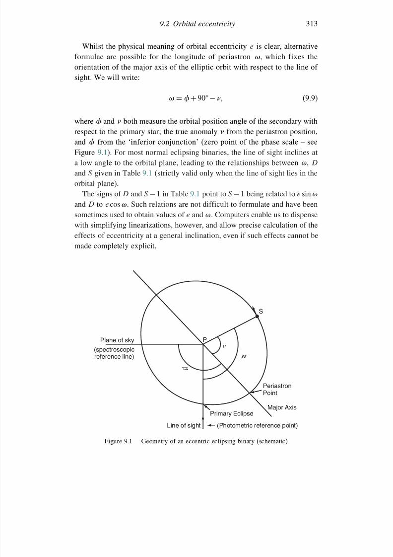
7/21/2019 Introduction to Astronomical Photometry
http://slidepdf.com/reader/full/introduction-to-astronomical-photometry 331/451
9.2 Orbital eccentricity 313
Whilst the physical meaning of orbital eccentricity e is clear, alternativeformulae are possible for the longitude of periastron , which fixes theorientation of the major axis of the elliptic orbit with respect to the line of
sight. We will write:
= + 90 − (9.9)
where and both measure the orbital position angle of the secondary withrespect to the primary star; the true anomaly from the periastron position,and from the ‘inferior conjunction’ (zero point of the phase scale – see
Figure 9.1). For most normal eclipsing binaries, the line of sight inclines ata low angle to the orbital plane, leading to the relationships between , D
and S given in Table 9.1 (strictly valid only when the line of sight lies in theorbital plane).
The signs of D and S −1 in Table 9.1 point to S −1 being related to e sin
and D to e cos . Such relations are not difficult to formulate and have beensometimes used to obtain values of e and . Computers enable us to dispense
with simplifying linearizations, however, and allow precise calculation of theeffects of eccentricity at a general inclination, even if such effects cannot bemade completely explicit.
Plane of sky
(spectroscopicreference line)
Line of sight (Photometric reference point)
Primary EclipseMajor Axis
PeriastronPoint
S
P
φ
ν
β
Figure 9.1 Geometry of an eccentric eclipsing binary (schematic)
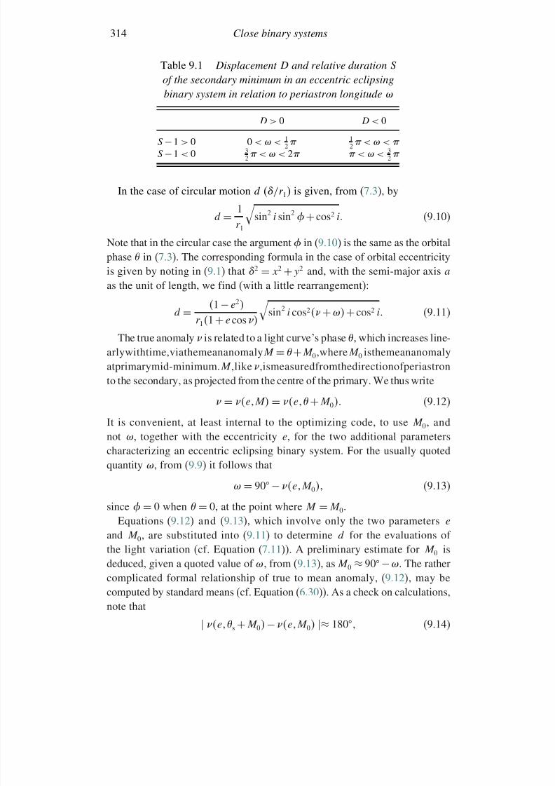
7/21/2019 Introduction to Astronomical Photometry
http://slidepdf.com/reader/full/introduction-to-astronomical-photometry 332/451
314 Close binary systems
Table 9.1 Displacement D and relative duration S
of the secondary minimum in an eccentric eclipsing
binary system in relation to periastron longitude
D > 0 D < 0
S −1 > 0 0 < < 12 1
2 < < S −1 < 0 3
2 < < 2 < < 32
In the case of circular motion d (/r 1) is given, from (7.3), by
d = 1r 1
sin2 i sin2 + cos2 i (9.10)
Note that in the circular case the argument in (9.10) is the same as the orbitalphase in (7.3). The corresponding formula in the case of orbital eccentricityis given by noting in (9.1) that 2 = x2 + y2 and, with the semi-major axis a
as the unit of length, we find (with a little rearrangement):
d
= 1− e2
r 11+ e cos sin2 i cos2
+
+cos2 i (9.11)
The true anomaly is related to a light curve’s phase , which increases line-arlywithtime,viathemeananomalyM = +M 0,whereM 0 isthemeananomalyatprimarymid-minimum.M ,like ,ismeasuredfromthedirectionofperiastronto the secondary, as projected from the centre of the primary. We thus write
= eM = e + M 0 (9.12)
It is convenient, at least internal to the optimizing code, to use M 0, and
not , together with the eccentricity e, for the two additional parameterscharacterizing an eccentric eclipsing binary system. For the usually quotedquantity , from (9.9) it follows that
= 90 − eM 0 (9.13)
since = 0 when = 0, at the point where M = M 0.Equations (9.12) and (9.13), which involve only the two parameters e
and M 0, are substituted into (9.11) to determine d for the evaluations of the light variation (cf. Equation (7.11)). A preliminary estimate for M 0 isdeduced, given a quoted value of , from (9.13), as M 0 ≈ 90 −. The rathercomplicated formal relationship of true to mean anomaly, (9.12), may becomputed by standard means (cf. Equation (6.30)). As a check on calculations,note that
es + M 0 − eM 0 ≈ 180 (9.14)
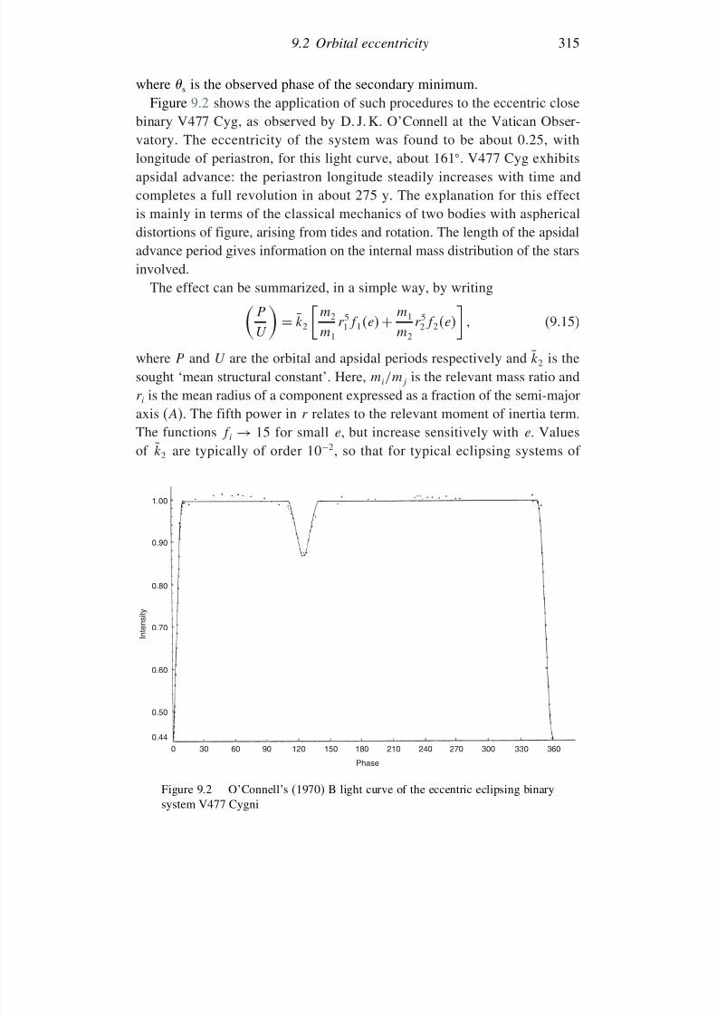
7/21/2019 Introduction to Astronomical Photometry
http://slidepdf.com/reader/full/introduction-to-astronomical-photometry 333/451
9.2 Orbital eccentricity 315
where s is the observed phase of the secondary minimum.Figure 9.2 shows the application of such procedures to the eccentric close
binary V477 Cyg, as observed by D. J. K. O’Connell at the Vatican Obser-
vatory. The eccentricity of the system was found to be about 0.25, withlongitude of periastron, for this light curve, about 161. V477 Cyg exhibitsapsidal advance: the periastron longitude steadily increases with time andcompletes a full revolution in about 275 y. The explanation for this effectis mainly in terms of the classical mechanics of two bodies with asphericaldistortions of figure, arising from tides and rotation. The length of the apsidaladvance period gives information on the internal mass distribution of the stars
involved.The effect can be summarized, in a simple way, by writingP
U
= k2
m2
m1
r 51 f 1e + m1
m2
r 52 f 2e
(9.15)
where P and U are the orbital and apsidal periods respectively and k2 is thesought ‘mean structural constant’. Here, mi/mj is the relevant mass ratio andr i is the mean radius of a component expressed as a fraction of the semi-major
axis (A). The fifth power in r relates to the relevant moment of inertia term.The functions f i → 15 for small e, but increase sensitively with e. Valuesof k2 are typically of order 10−2, so that for typical eclipsing systems of
1.00
0.90
0.80
0.70
0.60
0.50
0.440 30 60 90 120 150 180 210 240 270 300 330 360
Phase
I n t e n s i t y
Figure 9.2 O’Connell’s (1970) B light curve of the eccentric eclipsing binarysystem V477 Cygni
7/21/2019 Introduction to Astronomical Photometry
http://slidepdf.com/reader/full/introduction-to-astronomical-photometry 334/451
316 Close binary systems
low eccentricity we can expect P/U to be around the order of 10−4, butthe sensitivity to the fractional radii r i and eccentricity e may increase this;keeping in mind, though, that very close systems (r i > 02, say) would rarely
show appreciable eccentricity. Further details are given in Section 9.7.There is another effect associated with the general theory of relativity. The
apsidal period from this is of the order of the orbital period multiplied bythe ratio of the energy equivalent of the mass (from Einstein’s well-knownrelation) over the mean potential energy between the peri- and apastronpositions. Again, summarizing by a simple form, we can write
P
U
rel = 3Gm1
+m2
c2A1− e2 (9.16)
This term can be quite significant for fairly eccentric binaries of shortperiod. In the present case, it adds almost thirty years to the terrestri-ally observed apsidal advance period of V477 Cyg. Observations of suchclose eccentric, otherwise normal, binaries provide interesting and importantevidence about this fundamental subject of modern physics.
9.3 Proximity effects
It can be shown that when two stars are sufficiently close to each other thatthe sum of their two mean radii, expressed as fractions of the separation of thetwo mass centres, becomes greater than about 0.75, the pull from sphericityshould become so great as to draw the two photospheric surfaces into contact
in their region of closest proximity. This is taken to be in the vicinity of theinner Lagrangian point L1 (see Figure 7.3). The majority of observed closebinaries, however, are composed of separate bodies, whose departures fromspheres – ‘ellipticity effect’ – together with a radiative interaction – ‘reflectioneffect’ – introduce the photometric proximity effects.
These often can be conveniently dealt with by a linearized approach, inwhich they are regarded as additive perturbations from sphericity. The pertur-bations are expressed in terms of spherical harmonic (Legendre) functions in
the classical manner of analysing the tidal and rotational distortions of celes-tial bodies. The light variation is modelled in a fairly direct way through these(integrable) functions, so long as we include only the separable basic contri-butions of the whole star on its companion; i.e. drop the higher order effectsof the tide on one star affecting that of the other. Such higher order inter-actions start with terms comparable to the square of the principle distortions(i.e. Or 6). They can be included as extended forms of the same treatment,

7/21/2019 Introduction to Astronomical Photometry
http://slidepdf.com/reader/full/introduction-to-astronomical-photometry 335/451
9.3 Proximity effects 317
but their outworking becomes cumbersome. Their contributions to the totalproximity effects would, at most, generally be of the order of 1 or 2 percent for non-contact systems. Other aspects of the underlying description (e.g.
uniform rotation) may well have physical inadequacies at this level of accu-racy. Moreover, more elaborate models, by themselves, do not necessarilyaddress the primary issues of adequacy, uniqueness and determinacy in thefitting of theoretical curves to data of finite accuracy.
The basic idea for the linearized approach can be expressed as follows:
Observed light curve ≡ ‘spherical model’ light curve + ‘distortions’
The spherical model light curve here is that of the eight-parameter modeldescribed in Chapter 7, which is readily extended by another three extraparameters: two (e and M 0) to cover the case of elliptic motion, and onemore in case of a separate ‘third light’ (L3) contribution. In this case, theconstraint U = L1 + L2 is relaxed, L2 is treated as a separate parameter, andthen L3 = U − L1 + L2> 0.
The variation of light due to proximity effects for each star is written in
the form
i = − ell i q i aj Li + −
ref E i aj L3−i
i = 1 2 j = 1 11 (9.17)
(where the mass ratio q ≡ q 1 = m2/m1 = 1/q 2). The expression −
represents an appropriate integration, with the eclipsed part of the distortion
, zero for all phases at which the star is uneclipsed, subtracted out duringeclipses. The paramater dependence of these integrations is indicated by thecontents of the regular parentheses. In addition to the eleven parameters aj
used in the generalized spherical model, five new ones appear – namely: q , 12 and E 12 – making up to 16 the final number of independently specifiableparameters for this ‘standard eclipsing binary’ model. Since in most cases theorbit is essentially circular, only 14 of them usually require specification.
The full treatment of proximity effects, even in the linearized form here
discussed, would take us beyond the scope of the present text, but relevantreferences are given in the bibliography. Nowadays many investigators areprepared to accept and apply already written and reasonably tested softwarethat others have made available, especially where it is possible to check detailsof the coding against source formulae. Programs such as Wood’s WINK,and the Wilson and Devinney (W-D) numerical light curve synthesizer areoften cited in this context. The program CURVEFIT has been documented
7/21/2019 Introduction to Astronomical Photometry
http://slidepdf.com/reader/full/introduction-to-astronomical-photometry 336/451
318 Close binary systems
by M. Rhodes.5 It derives from programming the explicit form of (9.9), andis more particularly relevant to the details of the following discussion.
Concerning the five new parameters, they could be treated as empirically
determinable unknowns. However, in general, observations are not preciseenough to resolve each of the parameters independently, particularly whencorrelation effects are present, that is when photometric effects resultingfrom variation of a certain parameter can be closely simulated by suitablevariations of others. The analytic form of the fitting function suggests thattheory can provide guidelines, or actual values, for some of the pertinentquantities. Also, separate evidence is often available, such as when multi-
wavelength photometry can enable component temperatures to be assessed;or from spectroscopic or perhaps polarimetric data. Spectroscopy can oftenyield a value for the mass ratio q , while polarimetric data may enable anindependent estimate of the inclination i.
The gravity-brightening (sometimes gravity-darkening) coefficients, i,come from classical theory of a star’s outer envelope. If the flux throughthese layers depends only on the temperature gradient (the ‘diffusion’approximation), and the temperature, along with the density and pressure,
is constant along equipotential surfaces (the ‘Clairaut’ stability criterion),then the flux will be inversely proportional to the relative separation of thesesurfaces. But gravity itself has such an inverse proportionality. Hence, wemay deduce that the flux is proportional to gravity ( (integrated light) = 1:the ‘von Zeipel’ law). It is well known that for a physically distorted starthis line of reasoning contains a paradox, in that it leads to a situation wherethe temperature at, say, the pole of a rotating star ought to be the same as
that at the equator (on the same equipotential), though the heating flux inthese two directions is different (i.e. more heating at the pole). More detailedarguments suggest that a restorative circulation sets in to bring down thehorizontal temperature differential, while the difference in gravity-dependentflux remains approximately in place up to the photosphere. At the level of thephotosphere and above a sideways transport of energy would tend to make theflux distribution more uniform than the von Zeipel approximation ( < 1; infact,
∼05 is argued for in some treatments). The relationship of local flux
to gravity depends on assumptions about the distribution of source energygeneration and details of how the circulation mechanism works. Perhaps thewhole approach of applying a global average to the visible regions of thestars would be too simplified for really accurate data. In practice, ≈ 1
5 See home.comcast.net/michael.rhodes/Astronomy.htm. The program can be downloaded fromwww.winsite.com/search/ by typing in CURVEFIT at the prompt.

7/21/2019 Introduction to Astronomical Photometry
http://slidepdf.com/reader/full/introduction-to-astronomical-photometry 337/451
9.3 Proximity effects 319
appears to give a reasonable accord with observations, at least for those starswhose envelopes are dominated by a flux essentially propagated by radiativetransport. For convective heat transport through the subsurface layers the
position is less clear, both theoretically and observationally.The reflection coefficients E i can be derived by assuming that the incident
flux from the companion leads to a local increase of temperature, such that thebolometric emission at the new temperature is equal to the sum of the originalplus received fluxes. The local increase of flux at a particular wavelengthis then approximated by multiplying the temperature derivative of the blackbody expression (3.8) by the calculated local temperature increase. This is
called the black body approximation, and is usually adequate to represent theobserved scale of radiative interactions in normal close binaries to availableaccuracies. It becomes inaccurate when there are very large differences inthe components’ temperatures, e.g. the optical light curves of X-ray binariescontaining cool ‘red’ and hot subdwarf components.
An alternative, and even simpler, scaling factor (i.e. unity) occurs for the‘pure scattering’ approximation, where only the incident flux integration isinvolved in calculating the reflected light. Anisotropy of the reradiation, i.e.
limb darkening of the reflected contribution, has usually been neglected ineclipsing binary light curve contexts, though sometimes an additional, quasi-empirical ‘albedo’ is introduced to scale a derived E i value toward somethingmore in line with observed data.
From the scale of manifest effects, it appears that primary gravity-brightening 1 and secondary reflection E 2 are usually better determinedthan the corresponding quantities 2 and E 1. How well observations support
theory for these parameters has been the subject of many discussions. Fortrial purposes, the diffusion law model for gravity-brightening (i.e. flux ∝temperature gradient, and temperature constant on gravitation equipotentials)in the black body approximation may be followed, while a similar black bodysimplification is supported, in many cases, for the reflection coefficients. Theappropriate formulae at wavelength and primary and secondary unperturbedsurface temperatures T 1 and T 2 then reduce to:
12 = c2
4T 121− exp−c2/T 12 (9.18)
and
E 12 = 12
T 21
T 12
4 expc2/T 21 −1
expc2/T 12 −1 (9.19)
From the practical point of view, there seems little doubt that the fitting of real light curves, involving stars of appreciably different inherent temperatures
7/21/2019 Introduction to Astronomical Photometry
http://slidepdf.com/reader/full/introduction-to-astronomical-photometry 338/451
320 Close binary systems
(notablyclassical Algols), is significantly improved bythe adoption of analbedofactor that reduces E 2 from the value given by this formula, typically by 50%,other parameters being in line with values supportable from other grounds, but
thephysicsofthecompleteenergybudgetinthissituationisnotsoclear.Turbu-lent convection in the subsurface layers of a lower Main Sequence star mayrender the total heat redistribution more uniform, so that only some fractionof the incident flux appears locally ‘reflected’, but it is not easy to see howan implied increase in isotropic luminosity could be verified observationally.
A significant computing economy is achieved by the use of analyticformulae to evaluate the light distortions. Six basic integrals are required:
namely, 0
0, 0
1, and four related, simpler expressions, usually denoted as I
0
−1i,i = 0 3; the rest are determined by recursion formulae. The six involveonly elementary algebraic expressions or elliptic integrals. The latter can beevaluated at a comparable speed to the former (a few dozen cycle times), bythe use of fast and accurate modern algorithms. A typical twenty-iterationoptimization for five or six free parameters with approximately 100 datapoints, involving numerical evaluation of the curvature Hessian at optimum,its inversion and the calculation of its eigenvalues and eigenvectors (relating
to the errors of the parameter values, see below) can be achieved in a fewseconds of computing time on a typical modern desktop or portable computer.
9.4 The 16-parameter curve fitter
Once the fitting function for the standard eclipsing binary model has been
constructed it may be set in a suitable programming environment where aset of optimal parameters is derived, in an essentially parallel way to thatdiscussed for the spherical model and Kron’s light curves of YZ Cas. Aparamount question is how many parameter values can we determine. If thisis not the full sixteen, then we need to supply the underived ones, fromreasonable theory or otherwise.
If one attempts to derive all sixteen parameters of this model from a typicaleclipsing binary light curve one finds it generally not so difficult to produce
a very good fit, provided one starts with a set of parameters near enough to adeep minimum of 2. If this is not the case, then, as the improvement sequenceiterates, one frequently sees the set wandering off into a realm of parameterspace where values become physically unmeaningful; perhaps very large limb-darkening coefficients, or negative luminosities. Such effects can happen evenwith a near minimum 2 starting set – the solution proceeds down a ‘levelvalley’ in the 2-parameters manifold, with a slight change in one parameter
7/21/2019 Introduction to Astronomical Photometry
http://slidepdf.com/reader/full/introduction-to-astronomical-photometry 339/451
9.4 The 16-parameter curve fitter 321
being matched at each step by slight changes in another, or a group of others, 2 being marginally decreased as the correlated parameters drift along, awayfrom the domain of physical feasibility. The corresponding curve-fit may well
look good, but the derived values can contain some embarrassing surprises.The real test, for this context, comes from inverting the ‘curvature Hessian’
of the n parameters ai – the square symmetric matrix formed by the elements2 2/aiaj ij = 1 n – in the vicinity of the optimum, to obtain thecorresponding correlated error matrix. A good explanation of this procedureis given in P. R. Bevington’s (1969) book.6 Almost inevitably, with a sixteenby sixteen matrix (apart from its time-consuming derivation) using typical
photometric data sets for standard close binaries, we would encounter nega-tive elements on the leading diagonal of the error matrix, implying that theminimum is not properly defined; i.e. the contours of 2 in the parameterspace do not close down to a point. It is not a strict minimum, because in itsvicinity there is a level region, where, to the available accuracy, slight changesof one group of parameters, which would increase 2, can be matched by anappropriate combination of others, bringing it back down to numerically thesame value again.
A guide to the number of independent parameters that a given data set of N points can determine comes from considering what the number of coefficientsn would be if the data set was optimally modelled by a set of orthogonalfunctions, e.g. a Fourier series. The unrealistic wobbles of the fitting functionwith insignificant decreases in 2 which come when too many terms areincluded in such a fit are well known in empirical curve-fitting contexts.Since the coefficients of the orthogonal functions, when determined from
uniformly distributed data sets across the full range of phases (0 to 1), are allindependent of each other, the number n required to minimize 2/N − n
specifies, in some sense, the information content of the data.In the general curve-fitting problem the coefficients of the set of orthog-
onal functions have a counterpart in the eigenvalues of the curvature Hessian,evaluated in the vicinity of the optimum. These relate to appropriate linearcombinations of correlated parameter variations whose effects are mutu-ally orthogonal, i.e. numerically independent, in the curve-fitting. Positive
eigenvalues locate, via their corresponding eigenvector set, the 2 mini-mizing principal directions; the largest eigenvalue corresponding to the axisof highest determinacy. In practical curve-fitting problems a finite numbernmax of such positive eigenvalues will be found. This number corresponds
6 Data Reduction and Error Analysis for the Physical Sciences, McGraw-Hill Book Company,1969.
7/21/2019 Introduction to Astronomical Photometry
http://slidepdf.com/reader/full/introduction-to-astronomical-photometry 340/451
322 Close binary systems
to the information content or limit of the data for unique optimal parameterestimation: by increasing the number of parameters beyond this limit thecorrespondingly extended curvature Hessian is found to contain a negative
eigenvalue. Its eigenvectors locate the direction of the local level region whichhas disrupted the determinacy of a uniquely optimizing parameter set.
A complete presentation of the results of a curve-fitting analysis shouldtherefore include information on this optimal curvature Hessian, as well asthe optimal parameter set itself. Of particular interest are the leading diag-onal elements of the inverse of the curvature Hessian – the ‘error matrix’.The square roots of these elements (multiplied by 2) measure directly the
correlated error estimates of the parameter set. The Hessian’s eigenvalue andeigenvector set indicate, by their orientations with respect to the parameteraxes, which parameters, or parameter combinations, may be well determinedfrom the data. The numerical operations on matrices required to perform suchtasks can be readily obtained from computer algorithm distributors – e.g. theNumerical Algorithm Group (NAG).
Application to VV Ori
The fitting function just described has been applied to a set of six ultravi-olet light curves of the relatively bright, early type EB system VV Orionis,published by J. A. Eaton in 1975. The results are shown diagrammatically inFigure 9.3, corresponding to the parameter sets given in Table 9.2. The systemwas reviewed in some detail by H. W. Duerbeck in 1975, and the solutiongiven in Table 9.2 substantiates the generally accepted picture of a pair of relatively massive, unevolved B stars which are members of the Orion’s Belt
Young Star Association. A third, physically related, but lower mass A typestar also contributes slightly to the light L3 of the system. A constant estimatefor the measurement standard deviation l was adopted for all except the1550 Å light curve. The flux ratio J 1/J 2 can be used, in combination withstandard model atmosphere predictions for the emergent flux of early typestars, to estimate the secondary effective temperature for an adopted primaryvalue based on a good spectral type classification for this star. The absoluteparameters which come from combining the solutions of Table 9.2 with the
spectroscopic data given by Duerbeck are presented in Table 9.3.The points to be made here are that the solutions of Table 9.2 are the results
of five-parameter simultaneous optimization runs. The six major parametersof an eclipsing binary light curve were specified in Section 7.3. One of these,the correction to the nominal zero phase position to best fit the minima, is rela-tively independent of all the others, especially for circular orbits (which canbe anticipated in close, strongly tidally interacting binaries, such as VV Ori)
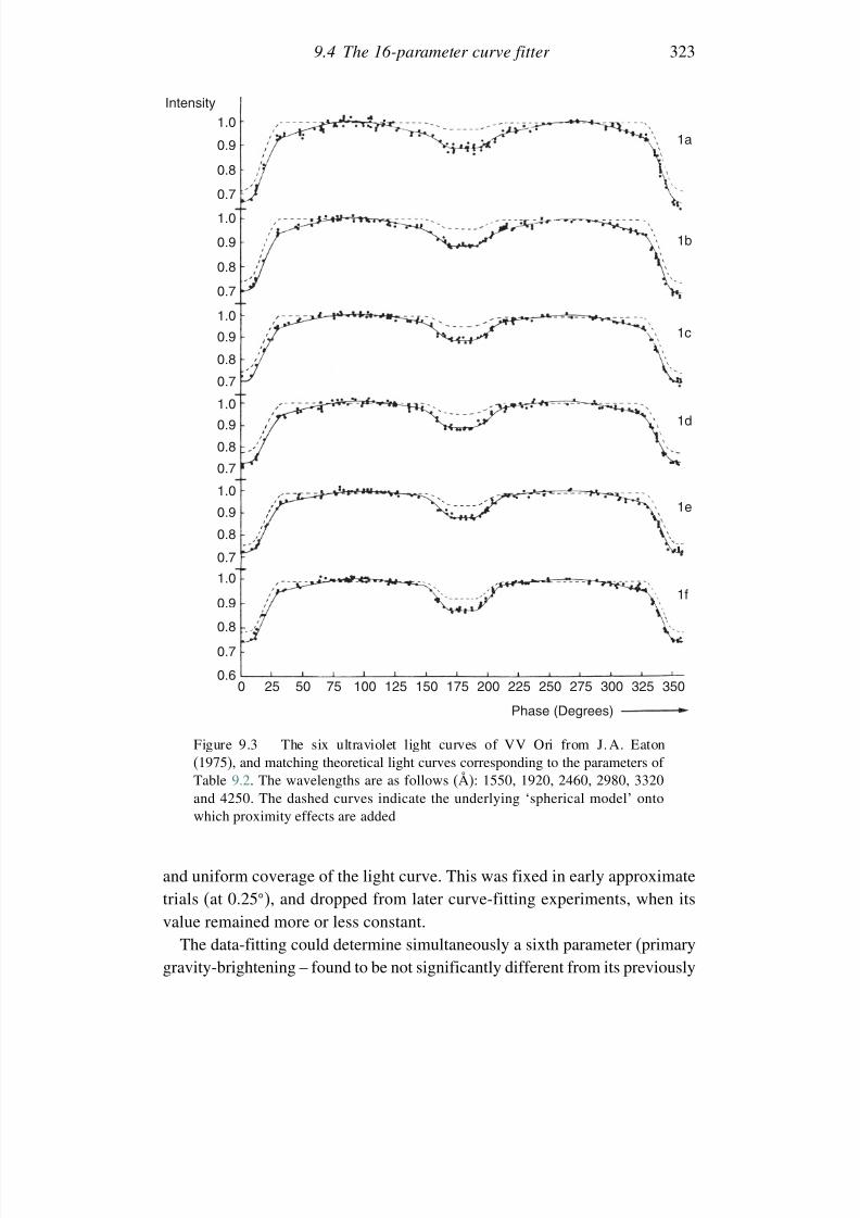
7/21/2019 Introduction to Astronomical Photometry
http://slidepdf.com/reader/full/introduction-to-astronomical-photometry 341/451
9.4 The 16-parameter curve fitter 323
0 25 50 75 100 125 150 175 200 225 250 275 300 325 350
Phase (Degrees)
0.6
0.7
0.8
0.8
0.9
0.9
1.0
0.7
0.7
0.7
0.7
0.8
0.8
0.8
0.8
0.9
0.9
0.9
0.9
1.0
1.0
1.0
1.0
1.0
0.7
Intensity
1f
1e
1d
1c
1b
1a
Figure 9.3 The six ultraviolet light curves of VV Ori from J. A. Eaton(1975), and matching theoretical light curves corresponding to the parameters of Table 9.2. The wavelengths are as follows (Å): 1550, 1920, 2460, 2980, 3320and 4250. The dashed curves indicate the underlying ‘spherical model’ ontowhich proximity effects are added
and uniform coverage of the light curve. This was fixed in early approximatetrials (at 025), and dropped from later curve-fitting experiments, when itsvalue remained more or less constant.
The data-fitting could determine simultaneously a sixth parameter (primarygravity-brightening – found to be not significantly different from its previously
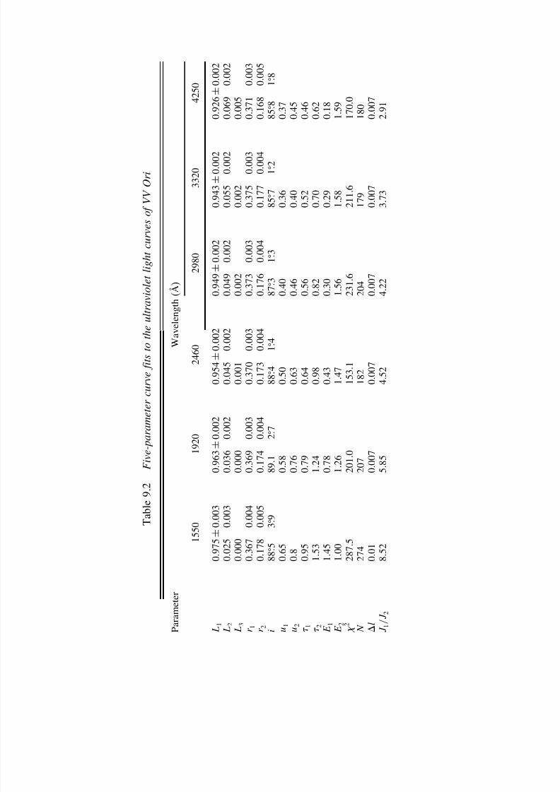
7/21/2019 Introduction to Astronomical Photometry
http://slidepdf.com/reader/full/introduction-to-astronomical-photometry 342/451
T a b l e 9 . 2
F i v e - p a r a
m e t e r c u r v e f i t s t o t h e u l t r a v i o l e t l i g h t c u r v e s o
f V V O r i
P a r a m e t e r
W a v e l e n g t h ( Å )
1
5 5 0
1 9 2 0
2 4 6 0
2 9 8 0
3 3 2 0
4 2 5 0
L 1
0 . 9 7 5
±
0 . 0 0 3
0 . 9 6 3 ± 0 . 0 0 2
0 . 9 5 4 ±
0 . 0 0 2
0 . 9 4 9 ±
0 . 0 0 2
0 . 9 4 3 ±
0 . 0 0 2
0 . 9 2 6 ±
0 . 0 0 2
L 2
0 . 0 2 5
0 . 0 0 3
0 . 0 3 6
0 . 0 0 2
0 . 0 4 5
0 . 0 0 2
0 . 0 4 9
0 . 0 0 2
0 . 0 5 5
0 . 0 0 2
0 . 0 6 9
0 . 0 0 2
L 3
0 . 0 0 0
0 . 0 0 0
0 . 0 0 1
0 . 0 0 2
0 . 0 0 2
0 . 0 0 5
r 1
0 . 3 6 7
0 . 0 0 4
0 . 3 6 9
0 . 0 0 3
0 . 3 7 0
0 . 0 0 3
0 . 3 7 3
0 . 0 0 3
0 . 3 7 5
0 . 0 0 3
0 . 3 7 1
0 . 0 0 3
r 2
0 . 1 7 8
0 . 0 0 5
0 . 1 7 4
0 . 0 0 4
0 . 1 7 3
0 . 0 0 4
0 . 1 7 6
0 . 0 0 4
0 . 1 7 7
0 . 0 0 4
0 . 1 6 8
0 . 0 0 5
i
8 8 5
3 9
8 9 . 1
2 7
8 8 4
1 4
8 7 3
1 3
8 5 7
1 2
8 5
8
1 8
u 1
0 . 6 5
0 . 5 8
0 . 5 0
0 . 4 0
0 . 3 6
0 . 3 7
u 2
0 . 8
0 . 7 6
0 . 6 3
0 . 4 6
0 . 4 0
0 . 4 5
1
0 . 9 5
0 . 7 9
0 . 6 4
0 . 5 6
0 . 5 2
0 . 4 6
2
1 . 5 3
1 . 2 4
0 . 9 8
0 . 8 2
0 . 7 0
0 . 6 2
E 1
1 . 4 5
0 . 7 8
0 . 4 3
0 . 3 0
0 . 2 9
0 . 1 8
E 2
1 . 0 0
1 . 2 6
1 . 4 7
1 . 5 6
1 . 5 8
1 . 5 9
2
2 8 7 . 5
2 0 1 . 0
1 5 3 . 1
2 3 1 . 6
2 1 1 . 6
1 7 0
. 0
N
2 7 4
2 0 7
1 8 2
2 0 4
1 7 9
1 8 0
l
0 . 0 1
0 . 0 0 7
0 . 0 0 7
0 . 0 0 7
0 . 0 0 7
0 . 0 0 7
J 1
/ J 2
8 . 5 2
5 . 8 5
4 . 5 2
4 . 2 2
3 . 7 3
2 . 9 1
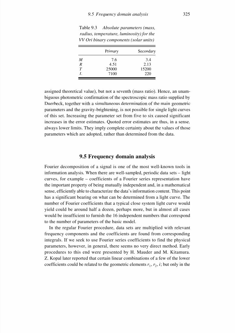
7/21/2019 Introduction to Astronomical Photometry
http://slidepdf.com/reader/full/introduction-to-astronomical-photometry 343/451
9.5 Frequency domain analysis 325
Table 9.3 Absolute parameters (mass,
radius, temperature, luminosity) for the
VV Ori binary components (solar units)
Primary Secondary
M 7.6 3.4R 4.51 2.13T 25000 15200L 7100 220
assigned theoretical value), but not a seventh (mass ratio). Hence, an unam-biguous photometric confirmation of the spectroscopic mass ratio supplied byDuerbeck, together with a simultaneous determination of the main geometricparameters and the gravity-brightening, is not possible for single light curvesof this set. Increasing the parameter set from five to six caused significantincreases in the error estimates. Quoted error estimates are thus, in a sense,always lower limits. They imply complete certainty about the values of those
parameters which are adopted, rather than determined from the data.
9.5 Frequency domain analysis
Fourier decomposition of a signal is one of the most well-known tools ininformation analysis. When there are well-sampled, periodic data sets – lightcurves, for example – coefficients of a Fourier series representation havethe important property of being mutually independent and, in a mathematicalsense, efficiently able to characterize the data’s information content. This pointhas a significant bearing on what can be determined from a light curve. Thenumber of Fourier coefficients that a typical close system light curve wouldyield could be around half a dozen, perhaps more, but in almost all caseswould be insufficient to furnish the 16 independent numbers that correspondto the number of parameters of the basic model.
In the regular Fourier procedure, data sets are multiplied with relevantfrequency components and the coefficients are found from correspondingintegrals. If we seek to use Fourier series coefficients to find the physicalparameters, however, in general, there seems no very direct method. Earlyprocedures to this end were presented by H. Mauder and M. Kitamura.Z. Kopal later reported that certain linear combinations of a few of the lowercoefficients could be related to the geometric elements r 1, r 2, i; but only in the
7/21/2019 Introduction to Astronomical Photometry
http://slidepdf.com/reader/full/introduction-to-astronomical-photometry 344/451
326 Close binary systems
highly idealized circumstances of no photometric proximity effects. In thesecircumstances, a total eclipse minimum, strictly located with respect to axesof phase and intensity (i.e. having been able to set 0
=0, U
=1 after
preliminary inspection), and with a given limb-darkening coefficient (u1) of the eclipsed star, four integrals A2m, given as
A2m =
2
01− l dsin2m m = 0 3
are necessary and sufficient to determine the four remaining parameters of this spherical problem – r 1, r 2, i and L1; the other limb-darkening parameteru
2
being only involved in the annular eclipse. Indeed, the connection betweenthe integrals and the parameters is explicit and fairly direct.
Two other considerations promoted interest in this approach: (i) the ideaof filtering out proximity effects in the general light curve problem, so asto find directly the sought stellar parameters, and (ii) that the integrationprocess smooths out the scatter of data points, so that the resulting parametervalues should be stable against such noise (though they are not necessarilyoptimal, in the 2 minimizing sense). The proximity effects would have
their more sizable components at low multiples of the orbital frequency,whereas noise is associated with the high-frequency end of the spectrum, i.e.at frequencies ∼ 1/, where is the mean spacing of the data points inphase. The significance of these points relates to the orientation of the method,which is towards the application of data from eclipsing binaries to stars ingeneral.
In the general problem, where proximity effects are present, the approachhas been to obtain ‘empirical moments’ A
2m, as given above, from numerical
quadrature of the observational data. From these moments proximity effectintegrals are subtracted to leave residues that can be related to the soughtparameters along the lines of the spherical problem. Determination of theproximity integrals has usually involved representing the light curve in theregions outside eclipse minima as a series in powers of cos . The requiredintegrals then become relatively simple expressions in the coefficients cj of this series. The plan is thus straightforward, with the forementioned points
about separability and noise removal arguing in its favour. Certain complica-tions have been encountered in practice, however, so a detailed exposition of a general method cannot be concisely spelled out here.
One particular source of awkwardness is in the predominating effect of the proximity integrals, because the sin2m weighting couples with the prox-imity effects carrying through all phases, unlike the eclipse effects whichare confined to relatively low phases. Hence, the proximity effect represen-
7/21/2019 Introduction to Astronomical Photometry
http://slidepdf.com/reader/full/introduction-to-astronomical-photometry 345/451
9.6 Narrowband photometry of binaries 327
tation has to be very precise, and though the cosn form has a nice algebraictractability, the corresponding cj s are not well suited to accurate numericalderivation. Alternative strategies have been developed to deal with this, but,
even so, the values of the eclipse residues, and therefore the sought param-eters, remain sensitive to the proximity contributions, particularly with thehigher 2m forms. We need not use integrals higher than A4 to evaluate thebasic geometric parameters if moments of both minima can be combined, and,besides, the use of both minima provides an information advantage, allowingsolution consistency to be checked. Still, the direct connection between eclipsemoments and parameters applies really only for total eclipses. For the annular
case similar approximate expressions can be given, but the procedure defi-nitely loses simplicity when the eclipses remain partial.During the course of frequency domain investigations various interesting
matters have come to light. An interesting example is the uniform expres-sion for the generalized light loss function when expressed as a Hankeltransform of the product of two Bessel functions. One of these latter func-tions arises from the two-dimensional Fourier transform of the light distri-bution over the (presumed circular) outline of the eclipsed star, the other
is the equivalent transform for the opacity of the eclipsing star. A greatsystematization of notation for a wide variety of light loss effects is therebyachieved.
In general, the inherent incommensurability of eclipse and orbital timescalesintroduces complications for frequency-based methods. On the other hand,the greater potential closeness of a Fourier representation to the actual data,which is free of pre-constrained thinking (and, of course, more objective than
simply free-hand drawing), could just be telling us to loosen up our mindsto other possibilities for light curve analysis. For further information on this,as well as detailed treatment of a variety of other procedures relating to thephotometric effects of close binary systems in the frequency domain, thereader is referred to Z. Kopal’s Language of the Stars (1979).
9.6 Narrowband photometry of binaries
Eclipses offer significant opportunities for sensitive narrowband probing of spectral line effects in stellar atmospheres (see Section 4.4). The eclipsingstar, acting as a kind of screen, allows, for example, any difference in thecentre to limb variation between a line and its surrounding continuum tobe monitored. This is particularly effective in cases of Algol type systemsshowing total, or deep partial, eclipses, where one star, though of comparable
7/21/2019 Introduction to Astronomical Photometry
http://slidepdf.com/reader/full/introduction-to-astronomical-photometry 346/451
328 Close binary systems
size to the other, is of very different luminosity. Differential effects in theatmosphere of the brighter star then become detectable.
Algol systems represent a basic, and relatively well-understood, stage in
interactive binary evolution (Section 7.2). There is good evidence that they areaccompanied by sizable amounts of circumbinary matter – in the form of lowdensity plasmas, sometimes associated with gaseous streams, with materialbeing transferred from one star (the ‘loser’) to the other (the ‘gainer’), ormatter being expelled entirely from the system. Narrowband photometry maydiscern particular effects in this context.
We shall explore some curve-fitting and relevant parameter estimation
methods for narrowband data analysis, concentrating here on phases in andnear eclipses for Algol type binaries. For convenience, we continue with thenotation of the frequently used photometry.
For most well-known Algols, Doppler shifts associated with the spatialmotion of the system as a whole – the ‘ -velocity’ – are typically of order1 Å or less at H . This is an order of magnitude less than the half-width of the narrowband H filter, so that the effects of such displacements, whichare present even close to the eclipse phases when orbital radial velocities
are minimal, can be neglected. Rotational Doppler-spread effects, whichdo not alter the equivalent width of line features in normal cases, can besimilarly neglected in the major features of -index light curves of thesebinaries.
Since the measured -index corresponds to the difference of a pair of magnitudes in filters, of which the wider one is still only of intermediatebandwidth, we can deduce (Section 4.4) that different local systems can be
related to a standard system by a linear formula such asstandard = alocal + b (9.20)
where a and b are constants, determined from the measurements of standardstars in the local system.
The linear proportionality of the -index to the equivalent width w (4.24)holds true for a spectrum made up of two or more components, where thenet equivalent width still corresponds to (4.22). This
¯w of the composite
spectrum can be related to the equivalent widths w1, w2, we of individualspectral components by the formula
w = Lc1w11− pc − p −1+ Lc2w2 − Lc3we1− e
Lc11− c + Lc2 + Lc3
(9.21)
where Lc1, Lc2, Lc3 represent fractional continuum luminosities of primary,secondary and circumstellar sources, respectively (Lc1 + Lc2 + Lc3 = 1). The
7/21/2019 Introduction to Astronomical Photometry
http://slidepdf.com/reader/full/introduction-to-astronomical-photometry 347/451
9.6 Narrowband photometry of binaries 329
light loss functions c, are of the same form as specified by (7.11), though requires a quantity u representing a linear limb-darkening coefficient fora spectral region centred on the line centre, whose effective extent is pw1.
p can be defined as Lc1/Lc1 − L1, where L1/Lc1 is the fractional depthof the line centre. In this way, we regard the line as equivalent to a separatelittle spectral region, having its own luminosity L1 and limb darkening u.A typical value for p for early type primaries of Algols is 2.5. In any case, p
and u are not independent. If p is large the line must be shallow, i.e. not sodistinct from the surrounding continuum, so the limb-darkening coefficientsuc, u can be expected to tend to coincide in value.
The third component of the numerator represents an emission contribu-tion of equivalent width we, due to circumstellar plasma. Our method-ology implies that we spell out appropriate forms for the light loss e forsuitable models, using the data to constrain parameter values. The relativecomplexity of such models is measured by the number of parameters neededin the description, but the determinacy of this set depends on the qualityof the available data. In practice, we should expect derivable parameter
sets to correspond to fairly simple models. Effects around eclipses, observ-able with -photometry, corresponding to uniform shell and disk modelsare indicated in Figure 9.4. The disk model is examined in what follows,and applied to -photometry of the interactive Algol systems U Cep andU Sge.
Disk source
In this idealization the emission is associated with a uniform, optically thindisk surrounding the primary equator of extension h in units of the primaryradius R, say, and fractional thickness tR (t 1); tR can be taken to havea value of ∼ vsound/, where is the orbital angular velocity, so typicallytR 106 m, say. This kind of thin accretion structure has been theoreticallyanticipated in the interactive mass-transferring stage of Algol evolution. Its
eclipse can be analysed with -integrals. We will use the uniform intensity0
0, and express it via the intermediate variable s (7.16). In the present case s
represents the projected distance between the shadow cylinder and the centreof the disk, in units of the disk radius (Figure 9.5). It is generally neces-sary to subtract the area Dbs from the underlying star in this treatment,but in the range 1 > s > 1/1 + h only the unocculted edge of the diskis eclipsed.
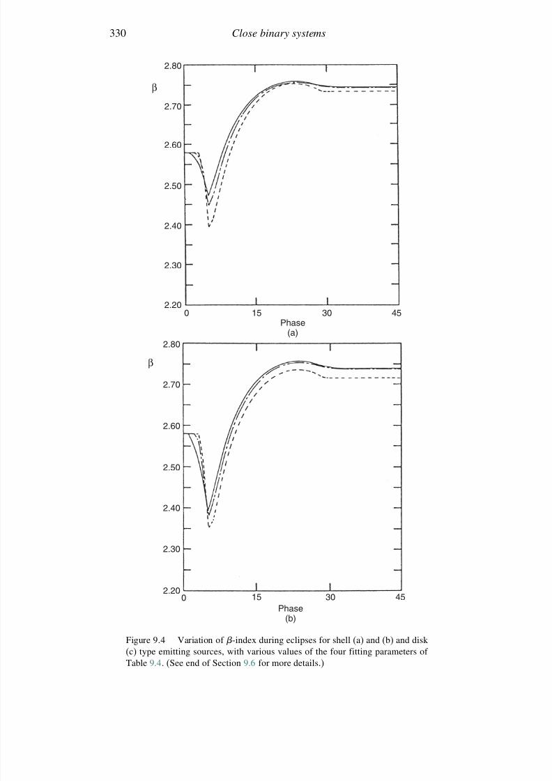
7/21/2019 Introduction to Astronomical Photometry
http://slidepdf.com/reader/full/introduction-to-astronomical-photometry 348/451
330 Close binary systems
0 15 30 45
2.80
2.70
2.60
2.50
2.40
2.30
2.20
β
Phase(a)
0 15 30 45Phase
(b)
β
2.80
2.70
2.60
2.50
2.40
2.30
2.20
Figure 9.4 Variation of -index during eclipses for shell (a) and (b) and disk(c) type emitting sources, with various values of the four fitting parameters of Table 9.4. (See end of Section 9.6 for more details.)

7/21/2019 Introduction to Astronomical Photometry
http://slidepdf.com/reader/full/introduction-to-astronomical-photometry 349/451
9.6 Narrowband photometry of binaries 331
2.80
2.70
2.60
2.50
2.400 15 30 45
Phase(c)
β
Figure 9.4 (cont.)
When the disk is eclipsed by a larger object, of lateral extent k, we havee as
e = 0 d ≥ 1+ h + k
e = s/c 1+ h + k > d ≥ 1+ k
e = s+ s1 − s/1+ h2/2c 1+ k > d > k−1
e = 1− 1− s/c k − 1 ≥ d > k −1− h
e = 1 k − 1− h ≥ d
(9.22)
where the ‘straight edge’ -function s is given by
s = 1
arccos s − s
√ 1− s2
and the other quantities are as follows: d =
sin2 sin2 i + cos2 i/r 1, k = r 2/r 1,s = d − k, s1 = 1/1+ h, so that s = ss1, and c = s1 + 1
2 h2 +2hs21 , for
primary and secondary relative radii r 1, r 2, phase and orbital inclination i.
If i is significantly different from 90, the foregoing formulae are still usable,but k is replaced by k =
r 22 − cos2 i/r 1.
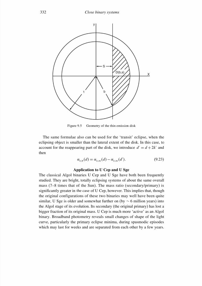
7/21/2019 Introduction to Astronomical Photometry
http://slidepdf.com/reader/full/introduction-to-astronomical-photometry 350/451
332 Close binary systems
S
b
D(b,s)
1
X
y
Figure 9.5 Geometry of the thin emission disk
The same formulae also can be used for the ‘transit’ eclipse, when theeclipsing object is smaller than the lateral extent of the disk. In this case, toaccount for the reappearing part of the disk, we introduce d = d + 2k andthen
etrd = eocd− eocd (9.23)
Application to U Cep and U Sge
The classical Algol binaries U Cep and U Sge have both been frequentlystudied. They are bright, totally eclipsing systems of about the same overallmass (7–8 times that of the Sun). The mass ratio (secondary/primary) issignificantly greater in the case of U Cep, however. This implies that, though
the original configurations of these two binaries may well have been quitesimilar, U Sge is older and somewhat further on (by ∼ 6 million years) intothe Algol stage of its evolution. Its secondary (the original primary) has lost abigger fraction of its original mass. U Cep is much more ‘active’ as an Algolbinary. Broadband photometry reveals small changes of shape of the lightcurve, particularly the primary eclipse minima, during spasmodic episodeswhich may last for weeks and are separated from each other by a few years.
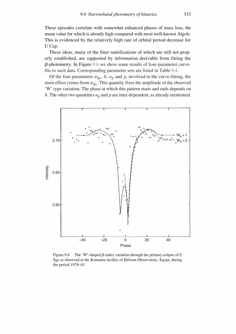
7/21/2019 Introduction to Astronomical Photometry
http://slidepdf.com/reader/full/introduction-to-astronomical-photometry 351/451
9.6 Narrowband photometry of binaries 333
These episodes correlate with somewhat enhanced phases of mass loss, themean value for which is already high compared with most well-known Algols.This is evidenced by the relatively high rate of orbital period decrease for
U Cep.These ideas, many of the finer ramifications of which are still not prop-
erly established, are supported by information derivable from fitting the-photometry. In Figure 9.6 we show some results of four-parameter curve-fits to such data. Corresponding parameter sets are listed in Table 9.4.
Of the four parameters we, h, u and p, involved in the curve-fitting, themain effect comes from we. This quantity fixes the amplitude of the observed
‘W’ type variation. The phase at which this pattern starts and ends depends onh. The other two quantities u and p are inter-dependent, as already mentioned.
2.70
2.65
2.60
–20–40 0 20 40
Phase
I n t e n s i t y
We = 1We = 2
Figure 9.6 The ‘W’-shaped -index variation through the primary eclipse of USge as observed at the Kottamia facility of Helwan Observatory, Egypt, duringthe period 1978–81
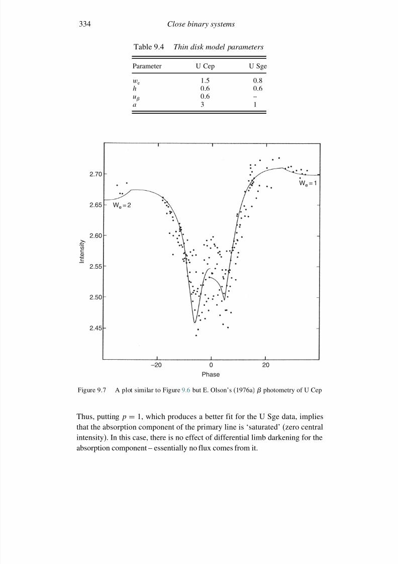
7/21/2019 Introduction to Astronomical Photometry
http://slidepdf.com/reader/full/introduction-to-astronomical-photometry 352/451
334 Close binary systems
Table 9.4 Thin disk model parameters
Parameter U Cep U Sge
we 15 08h 06 06u 06 –a 3 1
2.70
2.65
2.60
2.55
2.50
2.45
–20 0 20
Phase
I n t e n s i t y
We = 1
We = 2
Figure 9.7 A plot similar to Figure 9.6 but E. Olson’s (1976a) photometry of U Cep
Thus, putting p = 1, which produces a better fit for the U Sge data, impliesthat the absorption component of the primary line is ‘saturated’ (zero centralintensity). In this case, there is no effect of differential limb darkening for theabsorption component – essentially no flux comes from it.
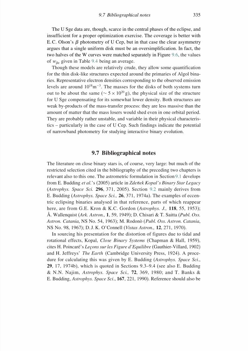
7/21/2019 Introduction to Astronomical Photometry
http://slidepdf.com/reader/full/introduction-to-astronomical-photometry 353/451
9.7 Bibliographical notes 335
The U Sge data are, though, scarce in the central phases of the eclipse, andinsufficient for a proper optimization exercise. The coverage is better withE. C. Olson’s photometry of U Cep, but in that case the clear asymmetry
argues that a single uniform disk must be an oversimplification. In fact, thetwo halves of the W curves were matched separately in Figure 9.6, the valuesof we given in Table 9.4 being an average.
Though these models are relatively crude, they allow some quantificationfor the thin disk-like structures expected around the primaries of Algol bina-ries. Representative electron densities corresponding to the observed emissionlevels are around 1018m−3. The masses for the disks of both systems turn
out to be about the same (∼ 5 × 10
20
g), the physical size of the structurefor U Sge compensating for its somewhat lower density. Both structures areweak by-products of the mass-transfer process: they are less massive than theamount of matter that the mass losers would shed even in one orbital period.They are probably rather unstable, and variable in their physical characteris-tics – particularly in the case of U Cep. Such findings indicate the potentialof narrowband photometry for studying interactive binary evolution.
9.7 Bibliographical notes
The literature on close binary stars is, of course, very large: but much of therestricted selection cited in the bibliography of the preceding two chapters isrelevant also to this one. The astrometric formulation in Section 9.1 developsfrom E. Budding et al.’s (2005) article in Zde ˘ nek Kopal’s Binary Star Legacy
( Astrophys. Space Sci. 296, 371, 2005). Section 9.2 mainly derives fromE. Budding ( Astrophys. Space Sci., 26, 371, 1974a). The examples of eccen-tric eclipsing binaries analysed in that reference, parts of which reappearhere, are from G.E. Kron & K.C. Gordon ( Astrophys. J., 118, 55, 1953);Å. Wallenquist ( Ark. Astron., 1, 59, 1949); D. Chisari & T. Saitta (Publ. Oss.
Astron. Catania, NS No. 54, 1963); M. Rodonò (Publ. Oss. Astron. Catania,NS No. 98, 1967); D. J. K. O’Connell (Vistas Astron., 12, 271, 1970).
In sourcing his presentation for the distortion of figures due to tidal and
rotational effects, Kopal, Close Binary Systems (Chapman & Hall, 1959),cites H. Poincaré’s Leçons sur les Figure d’Equilibre (Gauthier-Villard, 1902)and H. Jeffreys’ The Earth (Cambridge University Press, 1924). A proce-dure for calculating this was given by E. Budding ( Astrophys. Space Sci.,29, 17, 1974b), which is quoted in Sections 9.3–9.4 (see also E. Budding& N.N. Najim, Astrophys. Space Sci., 72, 369, 1980; and T. Banks &E. Budding, Astrophys. Space Sci., 167, 221, 1990). Reference should also be
7/21/2019 Introduction to Astronomical Photometry
http://slidepdf.com/reader/full/introduction-to-astronomical-photometry 354/451
336 Close binary systems
made to the careful paper by S. Söderhjelm ( Astron. Astrophys., 34, 59, 1974).The data on VV Ori comes from J. A. Eaton ( Astrophys. J., 197, 379, 1975).The cited analysis of H. W. Duerbeck was given in Astron. Astrophys. Suppl.
(22, 19, 1975).General reviews of the gravity-brightening effect have been given in a
series of papers by M. Kitamura & Y. Nakamura (Tokyo Astron. Obs. Ann.,
2nd Ser., 22, 31, 1988; Lecture Notes Phys., 305, ed. K. Nomoto, Springer-Verlag, 1988, p. 217; Astrophys. Space Sci., 145, 117, 1988; Space Sci. Rev.,50, 353, 1989) and G. Djurasevic et al. ( Astron. Astrophys., 402, 667, 2003).Surface layer effects were considered by R. Connon-Smith & R. Worley
( Mon. Not. Roy. Astron. Soc., 167, 199, 1974); and further calculations weregiven by A. Claret ( Astron. Astrophys., 359, 289, 2000). L. B. Lucy’s paper in Zeit. Astrofis. (65, 89) is often cited for its numerical derivation of relativelylow ‘convective’ gravity effect coefficients ( ∼ 1/3 in integrated light), but astill lower value (zero) was argued for in L. Anderson & F. H. Shu’s study of contact binary light curves ( Astrophys. J ., 214, 798, 1977). This latter finding,however, is applied to a situation in which lack of complete hydrostaticequilibrium is part of the overall discussion.
In a similar way, S. M. Rucinski’s lowered scale of reflection effect (effec-tive bolometric albedo ∼ 05, Acta Astron., 19, 245, 1969) is also frequentlyused in light-curve fitting programs. This lowered reflection effect was previ-ously noted by Y. Hosokawa (Sendai Rap., Nos. 56 & 70, 1957 & 1959).Apart from the classic sources given in Kopal’s cited text, other studies of thereflection effect in close binary systems include I. Pustyl’nik ( Acta Astron., 27,251, 1977); E. Budding & Y. R. Ardabili 1978, Astrophys. Space Sci., 59, 19,
1978); B. N. G. Guthrie & W. M. Napier ( Nature, 284, 536, 1980); A. Periaiah(Proc. Platinum Jubilee Symp. Nizamiah Obs. Osmania University, 1984,p. 20); L.P.R. Vaz ( Astrophys. Space Sci., 113, 349, 1985); A. Yamasaki(Publ. Astron. Soc. Japan, 38, 449, 1986); M. Tassoul & J.-L. Tassoul ( Mon.
Not. Roy. Astron. Soc., 232, 481, 1988); R.E. Wilson ( Astrophys. J., 356,613, 1990); D.P. Kiurchieva & Vl. G. Shkodrov ( Dokl. B’lgarska Akad.
Nauk., 45, 5, 1992); S. H. Choea & Y. W. Kang ( J. Astron. Space Sci., 9, 30,1992); R. W. Hilditch, T. J. Harries & G. Hill ( Mon. Not. Roy. Astron. Soc.,
279, 1380, 1996); N. T. Kochiashvili & I. B. Pustyl’nik ( Astrophysics, 43, 87,2000); M. Srinivasa Rao ( ASP Conf. Proc., 288, p. 645, 2003); and others.
Section 9.5 is a very brief pointer to a subject which occupied a good deal of Z. Kopal’s Language of the Stars (Reidel, 1979). The Hankel-transform-basedrepresentation of -functions was introduced by him in Astrophys. Space
Sci. (50, 225, 1977). Earlier approaches using Fourier-analysis techniqueswere those of H. Mauder (Kleine Veröff., Bamberg, Remeis-Sternwarte, Nr.
7/21/2019 Introduction to Astronomical Photometry
http://slidepdf.com/reader/full/introduction-to-astronomical-photometry 355/451
9.7 Bibliographical notes 337
38, 1966) and M. Kitamura, Tables of the Characteristic Functions of the
Eclipse (University of Tokyo Press, 1967). See also articles in Zde˘ nek Kopal’s
Binary Star Legacy: Astrophys. Space Sci., 296, 2005: P. Niarchos (p. 359),
O. Demircan (p. 209) and E. Budding (p. 371).Alternative methods of light curve analysis are from A. M. Cherepashchuk,
A. V. Goncharskii & A. G. Yagola (Soviet Astron., 12, 944, 1969) (integralequation solution technique); D. B. Wood ( Astron. J., 76, 701, 1971) (WINK);R. E. Wilson & E. J. Devinney ( Astrophys. J., 166, 605, 1971) (‘W–D’); G.Hill (Publ. Dom. Astrophys. Obs., 15, 297, 1979) (LIGHT); P. Hadrava (Publ.
Astron. Inst. Acad. Sci. Czech. Republic, No. 92, p. 1, 1994) (FOTEL); and
others. The triennial reports of Commission 42 (Trans. Int. Astron. Union(Rep. Astron.)) has given background on the applications of such proceduresfrom time to time. J. Kallrath and E.F. Milone’s Eclipsing Binary Stars:
Modelling and Analysis (Springer, 1999, with a foreword by R. E. Wilson)is also a useful source of information on mathematical models for the lightcurves of eclipsing binary stars, particularly the popular W–D code. Theauthors provide some overview of different approaches to light-curve fittingand their views of future developments.
The great usefulness to astrophysics of accurate information coming fromeclipsing binary light curves, particularly when combined with reliable radialvelocity data so as to provide absolute stellar parameters, was stressed in thepaper of J. Andersen, J. V. Clausen & B. Nordström, in their contributionto the informative IAU Symp. 88: Close Binary Stars, Observations and
Interpretation, eds. M. J. Plavec, D. M. Popper & R. K. Ulrich (Reidel, 1980,p. 81); a theme later developed by J. Andersen ( Astron. Astrophys. Rev.,
3, 91, 1991). The Copenhagen school had by that time produced a largenumber of detailed studies of individual binaries, including a series of papersthat started with K. Gyldenkerne, H. E. Jørgensen and E. Carstensen’s paper( Astron. Astrophys., 42, 303, 1975). These studies went on to check structuralimplications arising from using the absolute stellar parameters of binariesshowing apsidal motion (see previous chapter), for example with papers likeA. Giménez, J. V. Clausen, B. E. Helt & L. P. R. Vaz’ study of the massiveeccentric binary GL Car ( Astron. Astrophys. Suppl. Ser., 62, 179, 1985), and
continue to develop more refined observational tests of astrophysical theory.Section 9.6 is esentially based on material presented by E. Budding in
Close Binary Stars: Observations and Interpretation, in IAU Symp. 88, ed.M.J. Plavec et al. (Reidel, p. 299); E. Budding & N. Marngus ( Astrophys.
Space Sci., 67, 477, 1980); and M. A. Khan & E. Budding ( Astrophys. Space
Sci., 125, 219, 1986). The H data on U Cep come from E. Olson ( Astrophys.
J., 204, 141, 1976a), (see also E. Olson, Astrophys. J. Suppl., 31, 1, 1976b).
7/21/2019 Introduction to Astronomical Photometry
http://slidepdf.com/reader/full/introduction-to-astronomical-photometry 356/451
338 Close binary systems
The desirability of using narrowband photometry to supplement broadbanddata was noted in J. Grygar & B. Horak’s study of Algol ( Bull. Astron.
Inst. Czech., 25, 275, 1975). Narrowband photometry of Lyr, together with
simultaneous spectroscopy, was presented by M. Kiyokawa & S. Kikuchi( NASA STI, Recon. Tech. Report , 75, 20175, 1974). The background to thistopic was reviewed by G. J. Peters in Space Sci. Rev. (50, 9, 1989), since whenfurther relevant studies were given, for example, by M. T. Richards ( Astro-
phys. J., 387, 329, 1992), D. N. Vesper & R. K. Honeycutt (Publ. Astron. Soc.
Pacific, 105, 731, 1993) and others. The cited article of M. T. Richards, infact, developed the analysis beyond the simple kind of geometrical modelling
considered in this section to tomographical procedures, yielding 3-dimensionalrepresentations accounting for detailed spectroscopic data on hydrogen linevariation around the orbit. This has shown interesting results for the brightestAlgols, although underlying information issues of model adequacy, determi-nacy and uniqueness remain, even with the highest quality data. Most of thesemodelling approaches refer back to the seminal study on mass transfer inAlgol binaries of S. H. Lubow & F. H. Shu ( Astrophys. J., 198, 383, 1975).
References
Andersen, J., 1991, Astron. Astrophys. Rev., 3, 91.Anderson, L. & Shu, F. H., 1977, Astrophys. J., 214, 798.Andersen, J., Clausen, J. V. & Nordström, B., 1980, IAU Symp. 88: Close Binary Stars,
Observations and Interpretation, eds. M. J. Plavec, D. M. Popper & R. K. Ulrich,Reidel, p. 81.
Banks, T. & Budding, E., 1990, Astrophys. Space Sci., 167, 221.Bevington, P. R., 1969, Data Reduction and Error Analysis for the Physical Sciences,
McGraw-Hill Book Co.Budding, E., 1974a, Astrophys. Space Sci., 26, 371.Budding, E., 1974b, Astrophys. Space Sci., 29, 17.Budding, E., 1980, IAU Symp. 88, ed. M.J. Plavec, D.M. Popper & R.K. Ulrich,
Reidel, p. 299.Budding, E. & Ardabili, Y. R., 1978, Astrophys. Space Sci., 59, 19.Budding, E. & Marngus, N., 1980, Astrophys. Space Sci., 67, 477.
Budding, E. & Najim, N. N., 1980, Astrophys. Space Sci., 72, 369.Budding, E., Bavis, V., Erdem, A., Demircan, O., Iliev, L., Iliev, I. and Slee, O. B.,
2005, Astrophys. Space Sci., 296, 317.Cherepashchuk, A.M., Goncharskii A.V. & Yagola, A.G., 1969, Sov. Astron., 12,
944.Chisari, D. & Saitta, T., 1963, Publ. Oss. Astron. Catania, NS No. 54.Choea, S.H. & Kang, Y.W., 1992, J. Astron. Space Sci., 9, 30.Claret, A., 2000, Astron. Astrophys., 359, 289.
7/21/2019 Introduction to Astronomical Photometry
http://slidepdf.com/reader/full/introduction-to-astronomical-photometry 357/451
References 339
Commission 42 (Trans. Int. Astron. Union (Rep. Astron.))Connon-Smith, R. & Worley, R., 1974, Mon. Not. Roy. Astron. Soc., 167, 199.Demircan, O., 2005, Astrophys. Space Sci., 296, 209.Djurasevic, G., Rovithis-Livaniou, H., Rovithis, P., Georgiades, N., Erkapic, S. &
Pavlovic, R., 2003, Astron. Astrophys., 402, 667.Duerbeck, H. W., 1975, Astron. Astrophys. Suppl., 22, 19.Eaton, J. A., 1975, Astrophys. J., 197, 379.Giménez, A., Clausen, J.V., Helt, B.E. & Vaz, L.P.R., 1985, Astron. Astrophys.
Suppl. Ser., 62, 179.Grygar, J. & Horak, B., 1974, Bull. Astron. Inst. Czech., 25, 275.Guthrie, B. N. G. & Napier, W. M., 1980, Nature, 284, 536.Gyldenkerne, K., Jørgensen, H. E. & Carstensen, E., 1975, Astron. Astrophys., 42,
303.Hadrava, P., 1994, Publ. Astron. Inst. Acad. Sci. Czech. Republic, 92, 1.Hilditch, R. W., Harries, T. J. & Hill, G., 1996, Mon. Not. Roy. Astron. Soc., 279,
1380.Hill, G., 1979, Publ. Dom. Astrophys. Obs., 15, 297.Hosokawa, Y., 1957, Sendai Rap., No. 56.Hosokawa, Y., 1959, Sendai Rap., No. 70.Jeffreys, H., 1924, The Earth, Cambridge, 1924.Kallrath, J. & Milone, E. F., 1999, Eclipsing Binary Stars: Modelling and Analysis,
Springer.Khan, M. A. & Budding, E., 1986, Astrophys. Space Sci., 125, 219.Kitamura, M., 1967, Tables of the Characteristic Functions of the Eclipse, University
of Tokyo Press.Kitamura, M. & Nakamura, Y., 1988a, Tokyo Astron. Obs. Ann., 2nd Ser., 22, 31.Kitamura, M. & Nakamura, Y., 1988b, Lecture Notes Phys., 305, ed. K. Nomoto,
Springer-Verlag, p. 217.Kitamura, M. & Nakamura, Y., 1988c, Astrophys. Space Sci., 145, 117.Kitamura, M. & Nakamura, Y., 1989, Space Sci. Rev., 50, 353.
Kiurchieva, D. P. & Shkodrov, V. G., 1992, Dokl. B’lgarska Akad. Nauk., 45, 5.Kiyokawa, M. & Kikuchi, S., 1974, NASA STI, Recon. Tech. Report, 75, 20175.Kochiashvili, N. T. & Pustyl’nik, I. B., 2000, Astrophysics, 43, 87.Kopal, Z., 1959, Close Binary Systems, Chapman & Hall.Kopal, Z., 1977, Astrophys. Space Sci., 50, 225.Kopal, Z., 1979, Language of the Stars, Reidel.Kron, G. E. & Gordon, K. C., 1953, Astrophys. J., 118, 55.Lubow, S. H. & Shu, F. H., 1975, Astrophys. J., 198, 383.Lucy, L. B., 1967, Zeit. Astrofis., 65, 89.
Mauder, H., 1966, Kleine Veröff., Bamberg, Remeis-Sternwarte, Nr. 38.Niarchos, P., 2005, Astrophys. Space Sci., 296, p. 359.O’Connell, D. J. K., 1970, Vistas Astron., 12, 271.Olson, E., 1976a, Astrophys. J., 204, 141.Olsen, E., 1976b, Astrophys. J. Suppl., 31, 1.Periaiah, A., 1984, Proc. Platinum Jubilee Symp. Nizamiah Obs. Osmania University,
p. 20.Peters, G. J., 1989, Space Sci. Rev., 50, 9.
7/21/2019 Introduction to Astronomical Photometry
http://slidepdf.com/reader/full/introduction-to-astronomical-photometry 358/451
340 Close binary systems
Poincaré, H., 1903, Leçons sur les Figure d’Equilibre, Paris.Pustyl’nik, I., 1977, Acta Astron., 27, 251.Rhodes., M., 2006, home.comcast.net / ∼michael.rhodes/Astronomy.htm.Richards, M. T., 1992, Astrophys. J., 387, 329.Rodonò, M., 1967, Publ. Oss. Astron. Catania, NS No. 98.Rucinski, S. M., 1969, Acta Astron., 19, 245.Smart, W. M., 1977, Textbook on Spherical Astronomy, Cambridge University Press.Söderhjelm, S., 1974, Astron. Astrophys., 34, 59.Srinivasa Rao, M., 2003, ASP Conf. Proc., 288, eds. I. Hubeny, D. Mihalas &
K. Werner, p. 645.Tassoul, M. & Tassoul, J.-L., 1988, Mon. Not. Roy. Astron. Soc., 232, 481.Vaz, L. P. R., 1985, Astrophys. Space Sci., 113, 349.
Vesper, D. N. & Honeycutt, R. K., 1993, Publ. Astron. Soc. Pacific, 105, 731.Wallenquist, Å., 1949, Ark. Astron., 1, 59.Wilson, R. E., 1990, Astrophys. J., 356, 613.Wilson, R. E. & Devinney, E. J., 1971, Astrophys. J., 166, 605.Wood, D. B., 1971, Astron. J., 76, 701.Yamasaki, A., 1986, Publ. Astron. Soc. Japan, 38, 449.
7/21/2019 Introduction to Astronomical Photometry
http://slidepdf.com/reader/full/introduction-to-astronomical-photometry 359/451
10
Spotted stars
10.1 Introductory background
‘Starspots’ are not a new notion. There was a time when starspots wereoffered as a general explanation of stellar variability. From that extreme, inthe nineteenth century, attention to the hypothesis had dwindled away almostcompletely after the development of stellar spectroscopy, until, in a well-
known pair of papers dealing with the cool binaries AR Lac and YY Gemin the 1950s, the photometrist Gerald Kron revived it. As events have turnedout, there is now a good deal of evidence to support Kron’s conjecture, forcertain groups of cool variable.
The two stars that Kron referred to are good examples of somewhat differentbut related categories of ‘active cool star’ (see Figures 10.1 and 10.2) – starsof spectral type generally later than mid-F, i.e. associated with convectiveouter regions, and usually having a relatively rapid rotational speed. In thecases of AR Lac and YY Gem, both close binary systems, this rapid rotationis a consequence of tidally induced synchronism between rotation and orbitalrevolution. The M type dwarf components of YY Gem are typical flare stars,characterized by Balmer line emissions that on occasions become very strong,reminiscent of solar flares, but with much greater relative intensity. AR Lacalso shows ‘chromospheric’ emission lines, but its particular configuration,G5 and subgiant K0 stars in a
∼2 day period binary, places it as a standard
RS CVn type binary.Active cool stars display a wide range of interrelated phenomena at different
wavelengths, which support the picture of physical processes basically similarto the electrodynamic activity of the Sun, but on a much enhanced scale:activity tracers are typically a couple of orders of magnitude greater. Fromthe accumulation of evidence it would now appear surprising if the broadbandphotometric variations attributed to large spots were not also present. Indeed,
341
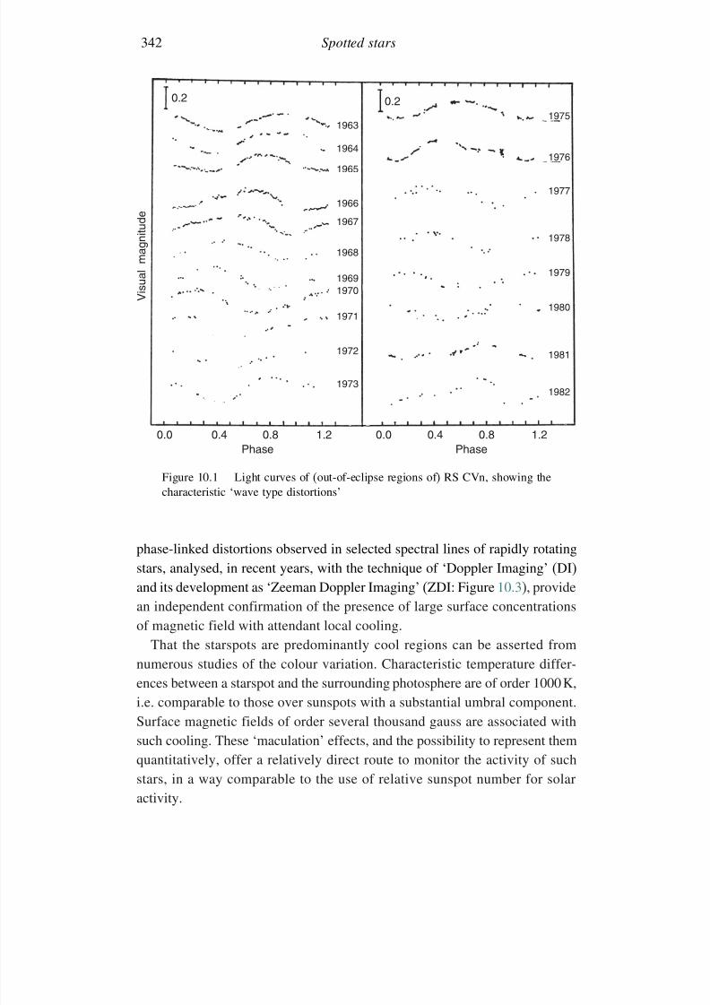
7/21/2019 Introduction to Astronomical Photometry
http://slidepdf.com/reader/full/introduction-to-astronomical-photometry 360/451
342 Spotted stars
0.2 0.2
1963
1964
1965
1966
1967
1968
19691970
1971
1972
1973
0.0 0.4 0.8 1.2 0.0 0.4 0.8 1.2Phase Phase
1975
1976
1977
1978
1979
1980
1981
1982
V i s u a l m a g n i t u d e
Figure 10.1 Light curves of (out-of-eclipse regions of) RS CVn, showing thecharacteristic ‘wave type distortions’
phase-linked distortions observed in selected spectral lines of rapidly rotatingstars, analysed, in recent years, with the technique of ‘Doppler Imaging’ (DI)and its development as ‘Zeeman Doppler Imaging’ (ZDI: Figure 10.3), providean independent confirmation of the presence of large surface concentrationsof magnetic field with attendant local cooling.
That the starspots are predominantly cool regions can be asserted fromnumerous studies of the colour variation. Characteristic temperature differ-
ences between a starspot and the surrounding photosphere are of order 1000 K,i.e. comparable to those over sunspots with a substantial umbral component.Surface magnetic fields of order several thousand gauss are associated withsuch cooling. These ‘maculation’ effects, and the possibility to represent themquantitatively, offer a relatively direct route to monitor the activity of suchstars, in a way comparable to the use of relative sunspot number for solaractivity.
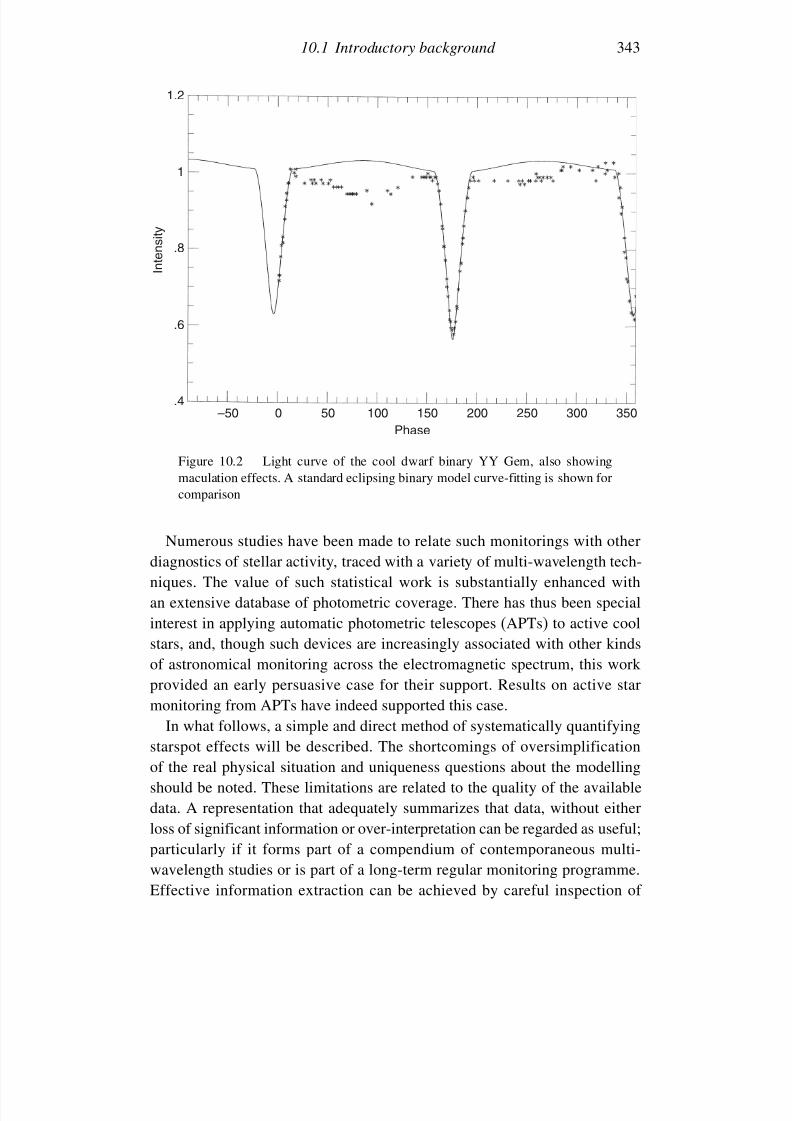
7/21/2019 Introduction to Astronomical Photometry
http://slidepdf.com/reader/full/introduction-to-astronomical-photometry 361/451
10.1 Introductory background 343
–50 0 50 100 150 200 250 300 350Phase
1.2
1
.8
.6
.4
I n t e n s i t y
Figure 10.2 Light curve of the cool dwarf binary YY Gem, also showingmaculation effects. A standard eclipsing binary model curve-fitting is shown forcomparison
Numerous studies have been made to relate such monitorings with otherdiagnostics of stellar activity, traced with a variety of multi-wavelength tech-niques. The value of such statistical work is substantially enhanced withan extensive database of photometric coverage. There has thus been specialinterest in applying automatic photometric telescopes (APTs) to active coolstars, and, though such devices are increasingly associated with other kindsof astronomical monitoring across the electromagnetic spectrum, this workprovided an early persuasive case for their support. Results on active starmonitoring from APTs have indeed supported this case.
In what follows, a simple and direct method of systematically quantifyingstarspot effects will be described. The shortcomings of oversimplification
of the real physical situation and uniqueness questions about the modellingshould be noted. These limitations are related to the quality of the availabledata. A representation that adequately summarizes that data, without eitherloss of significant information or over-interpretation can be regarded as useful;particularly if it forms part of a compendium of contemporaneous multi-wavelength studies or is part of a long-term regular monitoring programme.Effective information extraction can be achieved by careful inspection of
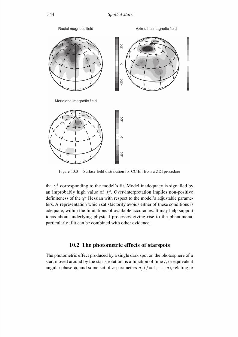
7/21/2019 Introduction to Astronomical Photometry
http://slidepdf.com/reader/full/introduction-to-astronomical-photometry 362/451
344 Spotted stars
Radial magnetic field
Meridional magnetic field
Azimuthal magnetic field
2 0 0
– 2 0 0
0
2 0 0
– 2 0 0
0
Figure 10.3 Surface field distribution for CC Eri from a ZDI procedure
the 2 corresponding to the model’s fit. Model inadequacy is signalled byan improbably high value of 2. Over-interpretation implies non-positivedefiniteness of the 2 Hessian with respect to the model’s adjustable parame-ters. A representation which satisfactorily avoids either of these conditions isadequate, within the limitations of available accuracies. It may help supportideas about underlying physical processes giving rise to the phenomena,particularly if it can be combined with other evidence.
10.2 The photometric effects of starspots
The photometric effect produced by a single dark spot on the photosphere of astar, moved around by the star’s rotation, is a function of time t, or equivalentangular phase , and some set of n parameters aj (j = 1 n), relating to
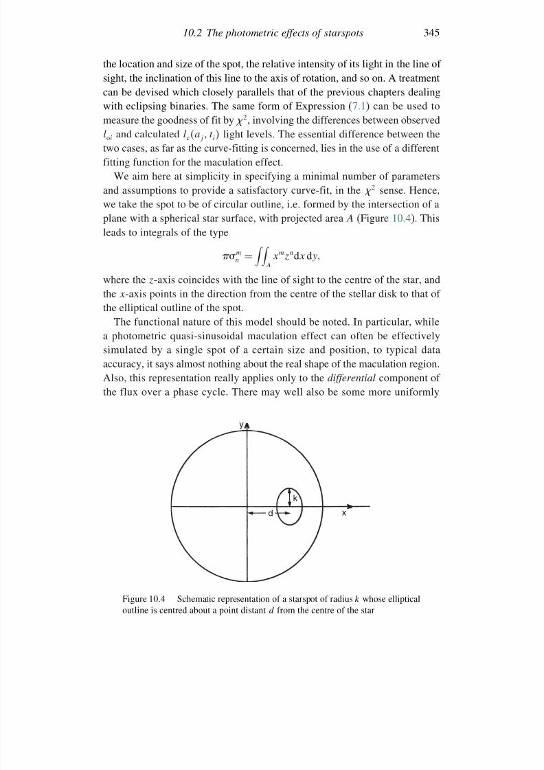
7/21/2019 Introduction to Astronomical Photometry
http://slidepdf.com/reader/full/introduction-to-astronomical-photometry 363/451
10.2 The photometric effects of starspots 345
the location and size of the spot, the relative intensity of its light in the line of sight, the inclination of this line to the axis of rotation, and so on. A treatmentcan be devised which closely parallels that of the previous chapters dealing
with eclipsing binaries. The same form of Expression (7.1) can be used tomeasure the goodness of fit by 2, involving the differences between observedloi and calculated lcaj ti light levels. The essential difference between thetwo cases, as far as the curve-fitting is concerned, lies in the use of a differentfitting function for the maculation effect.
We aim here at simplicity in specifying a minimal number of parametersand assumptions to provide a satisfactory curve-fit, in the 2 sense. Hence,
we take the spot to be of circular outline, i.e. formed by the intersection of aplane with a spherical star surface, with projected area A (Figure 10.4). Thisleads to integrals of the type
mn =
Axmzndx dy
where the z-axis coincides with the line of sight to the centre of the star, andthe x-axis points in the direction from the centre of the stellar disk to that of the elliptical outline of the spot.
The functional nature of this model should be noted. In particular, whilea photometric quasi-sinusoidal maculation effect can often be effectivelysimulated by a single spot of a certain size and position, to typical dataaccuracy, it says almost nothing about the real shape of the maculation region.Also, this representation really applies only to the differential component of the flux over a phase cycle. There may well also be some more uniformly
xd
k
y
Figure 10.4 Schematic representation of a starspot of radius k whose ellipticaloutline is centred about a point distant d from the centre of the star
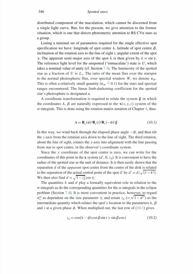
7/21/2019 Introduction to Astronomical Photometry
http://slidepdf.com/reader/full/introduction-to-astronomical-photometry 364/451
346 Spotted stars
distributed component of the maculation, which cannot be discerned froma single light curve. But, for the present, we give attention to the formersituation, which is one that directs photometric attention to RS CVn stars as
a group.Listing a minimal set of parameters required for the single effective spot
specification we have: longitude of spot centre , latitude of spot centre ,inclination of the rotation axis to the line of sight i, angular extent of the spot . The apparent semi-major axis of the spot k is then given by k = sin .The reference light level for the unspotted (‘immaculate’) state is U , whichtakes a nominal value of unity (cf. Section 7.3). The luminosity of the spotted
star as a fraction of U is L1. The ratio of the mean flux over the starspotto the normal photospheric flux, over spectral window W , we denote W .This is often a relatively small quantity (W
<∼ 01) for the stars and spectralranges encountered. The linear limb-darkening coefficient for the spottedstar’s photosphere is designated u.
A coordinate transformation is required to relate the system in whichthe coordinates , are naturally expressed to the xxyz system of the -integrals. This is done using the rotation matrix notation of Chapter 4, thus:
x = R x .R yi.R z−. (10.1)
In this way, we wind back through the elapsed phase angle −, and then tiltthe z-axis from the rotation axis down to the line of sight. The third rotation,about the line of sight, rotates the x-axis into alignment with the line passingfrom star to spot centre, in the observer’s coordinate system.
Since the y coordinate of the spot centre is zero, we can write for thecoordinates of this point in the x system (d, 0, z0). It is convenient to have theradius of the spotted star as the unit of distance. It is then easily shown that theseparation d of the apparent spot centre from the centre of the disk is relatedto the separation of the actual central point of the spot d by d = d/
1− k2.
We then also find d =
1− z2
0 cos .The quantities k and d play a formally equivalent role in relation to the
-integrals as do the corresponding quantities for the -integrals in the eclipseproblem (Section 7.4). It is more convenient in practice, however, to regard mn as dependent on the size parameter , and retain z0 (=
√ 1− d2) as the
intermediate quantity which relates the spot’s location to the parameters , and i at a given phase . When multiplied out, the last row of (10.1) gives
z0 = cos − cos sin i + sin cos i (10.2)
7/21/2019 Introduction to Astronomical Photometry
http://slidepdf.com/reader/full/introduction-to-astronomical-photometry 365/451
7/21/2019 Introduction to Astronomical Photometry
http://slidepdf.com/reader/full/introduction-to-astronomical-photometry 366/451
348 Spotted stars
10.3 Application to observations
10.3.1 Curve fitting
Using (7.1) for 2, we need the form of lcaj . This can be given as
lc = U − L11− W cuz0i (10.9)
where the various parameters aj have been written out as , , i, etc., asdefined above. The light loss term c accounts for the effect, with a givenspot area, of varying light intensity over the photospheric disk. A spot nearthe limb, for example, would remove a greater proportion of light if the stellardisk was of constant brightness, relative to the normal case of some limbdarkening. This entails that c is a linear combination of -integrals with theappropriate limb-darkening coefficients, thus, in the first order form,
c = 3
3− u1− u 00 + u 01 (10.10)
Formula (10.9), which has been usefully applied to data sets from coolstars showing differential maculation effects, builds in an assumption that thelimb darkening in the photosphere is the same as that in the cooler region
of the spot. This will not be exactly true in practice, though in the opticalregion W is usually so small that the difference is not serious. For a betterrendering, however, we could write
lc = U − L1 cupz0 + W L1 cusz0 (10.11)
where we separately subtract the photospheric light loss, darkened with coef-ficient up, and add in the spot’s own contribution, with coefficient us, c
taking the same form as (10.10) in both cases.The conversion of observed time data ti to equivalent phase values i
requires provision of an ephemeris formula, i.e. = t − t0/P , where t0 is aninitial reference time of zero phase, and P is the period. In spotted stars thathappen to be in synchronized binary systems the binary’s orbital ephemeriscan be used for this calculation. Particular data phase ranges showing macu-lation type light loss can then be associated with appropriate spot longitudes.
An alternative procedure, where a sufficiently long and continuous data
set covering an identifiable starspot wave exists, would be to regard thespot longitude as fixed and optimize the corresponding period. This raisesthe subject of differential rotation, which has often been discussed sinceD. S. Hall’s pioneer review of the RS CVn stars in 1975. Investigators havecommonly noted the presence of a ‘migrating wave’, i.e. that a spot effectcentred at a certain longitude would later have drifted, often to greater longi-tude. By analogy with similar effects observed for the Sun it is inferred that the
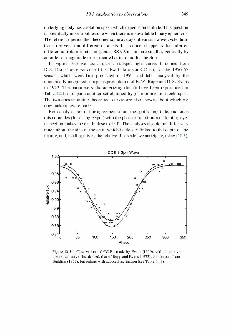
7/21/2019 Introduction to Astronomical Photometry
http://slidepdf.com/reader/full/introduction-to-astronomical-photometry 367/451
10.3 Application to observations 349
underlying body has a rotation speed which depends on latitude. This questionis potentially more troublesome when there is no available binary ephemeris.The reference period then becomes some average of various wave-cycle dura-
tions, derived from different data sets. In practice, it appears that inferreddifferential rotation rates in typical RS CVn stars are smaller, generally byan order of magnitude or so, than what is found for the Sun.
In Figure 10.5 we see a classic starspot light curve. It comes fromD. S. Evans’ observations of the dwarf flare star CC Eri, for the 1956–57season, which were first published in 1959, and later analysed by thenumerically integrated starspot representation of B. W. Bopp and D. S. Evans
in 1973. The parameters characterizing this fit have been reproduced inTable 10.1, alongside another set obtained by 2 minimization techniques.The two corresponding theoretical curves are also shown, about which wenow make a few remarks.
Both analyses are in fair agreement about the spot’s longitude, and sincethis coincides (for a single spot) with the phase of maximum darkening, eye-inspection makes the result close to 150. The analyses also do not differ verymuch about the size of the spot, which is closely linked to the depth of the
feature, and, reading this on the relative flux scale, we anticipate, using (10.3),
0.84
0.86
0.88
0.9
0.92
0.94
0.96
0.98
1
1.02
0 50 100 150 200 250 300 350
R e l a t i v e f l u x
Phase
CC Eri: Spot Wave
Figure 10.5 Observations of CC Eri made by Evans (1959), with alternativetheoretical curve-fits: dashed, that of Bopp and Evans (1973); continuous, fromBudding (1977), but redone with adopted inclination (see Table 10.1)
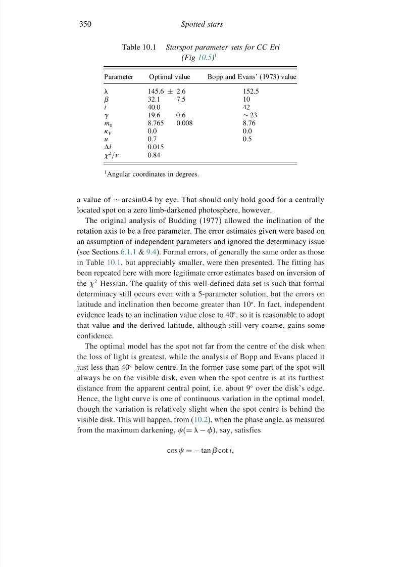
7/21/2019 Introduction to Astronomical Photometry
http://slidepdf.com/reader/full/introduction-to-astronomical-photometry 368/451
350 Spotted stars
Table 10.1 Starspot parameter sets for CC Eri
(Fig 10.5)1
Parameter Optimal value Bopp and Evans’ (1973) value 145.6 ± 2.6 152.5 32.1 7.5 10i 40.0 42 19.6 0.6 ∼ 23m0 8.765 0.008 8.76V 0.0 0.0u 0.7 0.5l 0.015
2/ 0.84
1Angular coordinates in degrees.
a value of ∼ arcsin04 by eye. That should only hold good for a centrallylocated spot on a zero limb-darkened photosphere, however.
The original analysis of Budding (1977) allowed the inclination of the
rotation axis to be a free parameter. The error estimates given were based onan assumption of independent parameters and ignored the determinacy issue(see Sections 6.1.1 & 9.4). Formal errors, of generally the same order as thosein Table 10.1, but appreciably smaller, were then presented. The fitting hasbeen repeated here with more legitimate error estimates based on inversion of the 2 Hessian. The quality of this well-defined data set is such that formaldeterminacy still occurs even with a 5-parameter solution, but the errors onlatitude and inclination then become greater than 10. In fact, independentevidence leads to an inclination value close to 40, so it is reasonable to adoptthat value and the derived latitude, although still very coarse, gains someconfidence.
The optimal model has the spot not far from the centre of the disk whenthe loss of light is greatest, while the analysis of Bopp and Evans placed it just less than 40 below centre. In the former case some part of the spot willalways be on the visible disk, even when the spot centre is at its furthest
distance from the apparent central point, i.e. about 9 over the disk’s edge.Hence, the light curve is one of continuous variation in the optimal model,though the variation is relatively slight when the spot centre is behind thevisible disk. This will happen, from (10.2), when the phase angle, as measuredfrom the maximum darkening, = − , say, satisfies
cos = − tan cot i
7/21/2019 Introduction to Astronomical Photometry
http://slidepdf.com/reader/full/introduction-to-astronomical-photometry 369/451
10.3 Application to observations 351
which acts as a loose constraint on the semi-width of the depressed part of the light curve. From the data in Table 10.1 this yields 140, so the lightcurve should be fairly flat for greater than about 290, or less than
∼10.
More exactly, a spot would cease to have any effect if can satisfy
cos = −sin + sin cos i
cos sin i
which Bopp and Evans’ model does for ±140, i.e. 290, or 10.Keeping in mind the limb-darkening effect, this can be observed on the dashedcurve in Figure 10.5.
In some approaches to starspot parameter estimation, when i can be fixedfrom other evidence (e.g. spectroscopic inferences) and largely influencedby the depth of the minimum, these foregoing relations for can allowa rough estimate for . At least, the value of should give an indica-tion concerning the probable hemisphere, upper or lower in relation to theline of sight, in which a large and distinct concentration of darkening islocated.
The reference level of luminosity, U , when the spot is not present, has been
reconverted to an apparent magnitude scale (m0) in Table 10.1. However,since some part of the spot is always visible in the optimal model, thisreference level is not actually observed, and the amplitude of light variationis slightly reduced from what would be possible with this size of spot. Thedifferent representations of the spot’s shape (rectangular in the numericalintegration) may also have a slight effect on the form of apparent variation.It is this parameter m0, if checked from season to season, that could indicate
a uniform component to the maculation. An alternative approach to this pointwill be considered later.To allow closer comparison with Bopp and Evans’ model, their zero value
of the flux ratio V was adopted. For typical 1000 K temperature differencesbetween spots and surrounding photosphere, the value of V would be about0.05, implying a ∼5% increase in area to recover the same apparent darkening,or ∼2.5% increase of . This would still be within the error range of theestimated value, so setting V
=0 should not be so serious a misrepresentation.
The adopted limb-darkening coefficient does have a small but noticeableeffect. The increase from the earlier value of 0.5 to 0.7, corresponding tomore recent tabulations, gave rise to increases of ∼3% in optimal radius andthe weakly determined latitude parameter.
The reduced 2/ value in Table 10.1 ( being the number of degrees of freedom of the data set, see Section 7.4) indicates an acceptable underlyinghypothesis, at the adopted accuracy of observations (V = 0015), for the

7/21/2019 Introduction to Astronomical Photometry
http://slidepdf.com/reader/full/introduction-to-astronomical-photometry 370/451
352 Spotted stars
optimal model – however, this inference should be regarded cautiously, sinceexactly circular spots are clearly highly idealized as regards shape.
The issue can be regarded in terms of the available information within
the data. If we suppose a minimal photometric resolution of 0.01 mag, thiswould correspond to a spot of about 1% area (not necessarily circular) of the photospheric disk, and around 14 such small darkened areas would beimplied by the overall amplitude of the maculation wave. Each such spotneeds two positional coordinates to locate it, making at least 28 potentiallyfree parameters for an idealized general fitting problem. In fact, the data canonly permit four or five independent parameter estimations, so the information
available from observations is going to be less than what such a general modelcould, in principle, specify. Some additional constraints are therefore requiredif meaningful model parametrization is to remain within the informationcontent of the data. Dark circular spots represent a limiting case of thisconstrained parametrization problem. Because of the concentration into afew determinables, the representative longitude, and perhaps latitude, of amaculation region can be concisely identified in this way.
But there may be other ways to characterize the data, for example, by
having 14 small dark pixels, perhaps initially in a near-circular outline, butadjustable so that they remain contiguous. The adjustment could be doneby a program of additions and subtractions of dark pixels, in such a waythat only changes that reduce 2 are retained in successive stages of therearrangement algorithm. This type of information retrieval program wouldrepresent a generalization of the optimization procedure considered so far.It is an example of what is sometimes referred to by the name ‘maximum
entropy’ methods (MEM).In the transformation from data to information space (Section 7.1), somemodel or ‘image’ is required to formulate the fitting function. The maximumentropy approach allows this form to be as general as possible, within physicalexperience of the effects in question. The entropy of the data representationcan be defined as the natural logarithm of the number of ways it couldbe generated. Thus, if the light curve was without significant features, amaximum entropy maculation model would have a more or less uniform
distribution of spots. The featured light curve of Figure 10.5 contains a fewpoints that appear more scattered from the general trend than others (on thedescending branch near the minimum, for example). If we could be sure thatthe observational accuracy V is actually better than the assigned 0.015, thenthese more scattered points might have their probability of being observedsignificantly enhanced, i.e. the entropy of the model increased, by a spotshape adjustment procedure.
7/21/2019 Introduction to Astronomical Photometry
http://slidepdf.com/reader/full/introduction-to-astronomical-photometry 371/451
10.3 Application to observations 353
An obvious danger with more relaxed models is that of over-interpretation.This would happen in the foregoing procedure if V is not significantlyless than 0.015. 2 could be reduced, but 2/ becomes improbably small
compared to unity. A situation where we try to ask more information fromthe data than it actually contains, i.e. seek more independent parameters thanthere are positive eigenvalues of the 2 curvature Hessian, constitutes whatmay be described as an ill-posed problem. This expression is used when amathematical problem violates one or more of the following conditions: (i) asolution exists; (ii) the solution is unique; (iii) the solution depends contin-uously on the data. Condition (i) is essentially always found with flexible,
multi-parameter fitting functions and the noisy, quasi-sinusoidal photometricwaves associated with data sets from spotted stars. Conditions (ii) and (iii) maywell fail with more relaxed models, however. Generalized fitting algorithmsthus tend to include ‘regularization’ techniques in order to deal with thesepoints. Basically, this comes down to the imposing of judicious constraintsand the restriction of parameter variation becoming large in response to smallvariations of data.
There are also physical questions to consider. The procedure considered
above started from the circular spot as a default low frequency component andretained contiguity of the darkened area as a constraint. Such starting imagesand applied constraints may or may not have clear physical justification. More-over, by using numerical integration and applying more general constraints,the MEM generalization is a bulkier computer operation. The ability to fullysearch parameter space will be necessarily more time-consuming than the useof explicit fitting functions; however, this point can be seen against the scale
of input data. Photometric data sets are relatively compact, compared with theinformation processed in a ZDI operation like that giving rise to Figure 10.3,for example.
Further simple development of the circular spot model (CSM) can bemade by combining -integral-based expressions in the fitting function. Theextension to two or more spots is easily achieved, when we write, in place of (10.9),
lc = U − L11− W
mj =1
cu j z0j j i (10.12)
for the m spots required. Care is needed in ensuring that the spots do notoverlap if is to preserve its distinct meaning in (10.12). This is dealt withby the condition arccos j
. k > j + k j = k, where j , k representthe position vectors to the centres of the j th and kth spots 1 ≤ j k ≤ m,respectively.

7/21/2019 Introduction to Astronomical Photometry
http://slidepdf.com/reader/full/introduction-to-astronomical-photometry 372/451
354 Spotted stars
Such a constraint can be built into the fitting function algorithm, so that apair of close spots are forced not to overlap. This has a physical interpretation,in that spot pairs are often found on the solar photosphere. An alternative
constraint, also with known solar counterpart, is to fix two spots to the samecentre coordinates, such that 2 > 1, say, and that 2 + 1 = u, with u asmall quantity and 2 ∼ 07, say, – i.e. the spot has a ‘penumbral’ perimeterregion. These possibilities point up the difficulty, given the accuracy of typicaldata sets, of resolving detail in a macular region: such experiments as havebeen carried out with close spot pairs have not found significant differencesin consequent light curve forms from those of a single spot of the same
total area.In effect, most available data sets for spotted stars seem to require amaximum of two well-separated spots to match determinability to data accu-racy. This entails a total of eleven parameters, i.e. adding the positionalcoordinates , and radius of the second spot to the preceding eight of Section 10.2. The specification can be set against MEM procedures by refer-ence to Figure 10.6, where we compare two and three spot models to therelatively high accuracy data set for AB Dor of A. Collier Cameron et al.
(1986).
0 50 100 150 200 250 300 350Phase
AB Dor: Spot Wave
0.98
0.99
0.995
1
1.005
1.01
1.015
0.985
R e l a t i v e f l u x
Figure 10.6 Photometry of AB Dor Eri presented by Collier Cameron et al.
(1986), with alternative theoretical curve-fits: continuous, two spot represen-tation; dashed, three spot representation, according to Table 10.2
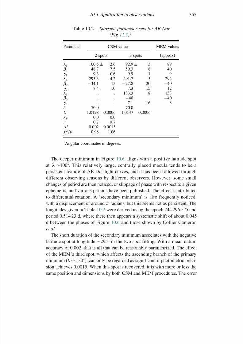
7/21/2019 Introduction to Astronomical Photometry
http://slidepdf.com/reader/full/introduction-to-astronomical-photometry 373/451
10.3 Application to observations 355
Table 10.2 Starspot parameter sets for AB Dor
(Fig 11.5)1
Parameter CSM values MEM values2 spots 3 spots (approx)
1 100.5 ± 2.6 92.9 ± 3 891 48.7 7.5 59.3 8 40 1 9.3 0.6 9.9 1 92 295.3 4.2 291.7 5 2922 −341 15 −278 20 −40 2 7.4 1.0 7.3 1.5 12
3 . . 133.3 8 1383 . . −40 . −40 3 . . 7.1 1.6 8i 70.0 70.0U 1.0128 0.0006 1.0147 0.0006V 0.0 0.0u 0.7 0.7l 0.002 0.0015 2/ 0.98 1.06
1Angular coordinates in degrees.
The deeper minimum in Figure 10.6 aligns with a positive latitude spotat ∼100. This relatively large, centrally placed macula tends to be apersistent feature of AB Dor light curves, and it has been followed throughdifferent observing seasons by different observers. However, some smallchanges of period are then noticed, or slippage of phase with respect to a givenephemeris, and various periods have been published. The effect is attributedto differential rotation. A ‘secondary minimum’ is also frequently noticed,with a displacement of around radians, but this seems not as persistent. Thelongitudes given in Table 10.2 were derived using the epoch 244 296.575 andperiod 0.514 23 d, where there then appears a systematic shift of about 0.045d between the phases of Figure 10.6 and those shown by Collier Cameronet al.
The short duration of the secondary minimum associates with the negativelatitude spot at longitude ∼295 in the two spot fitting. With a mean datumaccuracy of 0.002, that is all that can be reasonably parametrized. The effectof the MEM’s third spot, which affects the ascending branch of the primaryminimum ( ∼ 130), can only be regarded as significant if photometric preci-sion achieves 0.0015. When this spot is recovered, it is with more or less thesame position and dimensions by both CSM and MEM procedures. The error
7/21/2019 Introduction to Astronomical Photometry
http://slidepdf.com/reader/full/introduction-to-astronomical-photometry 374/451
356 Spotted stars
bars shown by Collier Cameron et al. are indeed suggestive of l ∼ 00015.This third spot would tend to weigh against the simple poloidal field arrange-ment suggested by some authors for this star. The main point then boils
down to the accuracy requirement, and hence observing conditions, neededto allow the activity resolution of photometric data into a more productiveresearch phase.
10.3.2 Spot temperatures
The flux ratio parameter is much better determined when there are lightcurves at more than one wavelength – particularly, if one of these is at red
or infrared wavelengths. In this case, we can expect to see maculation effectsof the same general shape in the two wavelength regions, but the amplitudeshould be smaller at the longer wavelength, where the intensity contrast is less(see Figure 10.7). This effect forms good supporting evidence that relativelylarge and concentrated cool surface regions are indeed responsible for theobserved effects, and leads on to enable the mean temperature decrementof the spot region to be determined. The fact that a light curve at a single
wavelength can be explained by bright regions in anti-phase to the darkregions of the adopted hypothesis harks back to the non-uniqueness pointin the introductory section. Coordinated multi-wavelength data are thereforedesirable to resolve this, and help to establish a meaningful interpretation of cool star photometric data in terms of starspots.
One procedure for determining spot temperatures starts by analysing thelight curve with the largest amplitude of variation (due to maculation) usingan assigned (low) value of , i.e. adopted photospheric and spot tempera-
tures, seeking essentially only the positions and sizes of spots. Fixing thederived geometrical parameters into the fitting function, one then uses thelonger wavelength light curve to determine only the best fitting value of its parameter. This enables an improved estimate for the spot temperature –the photospheric temperature being usually fixed from separate evidence,involving spectral information, or the mean colour at light maximum. Onesubstitutes the derived temperature back to get an improved value of to fix
into the fitting function, which can then be re-applied at the shorter wave-length to re-derive the geometric parameters. This completes the first iterativecycle, which may be repeated. One or two iterations usually suffice to bringthe variation of successive spot temperature values well within their probableerrors.
From an operational point of view, one can more directly write, for example,
V − Ic = −25 log lcV − log lcI (10.13)
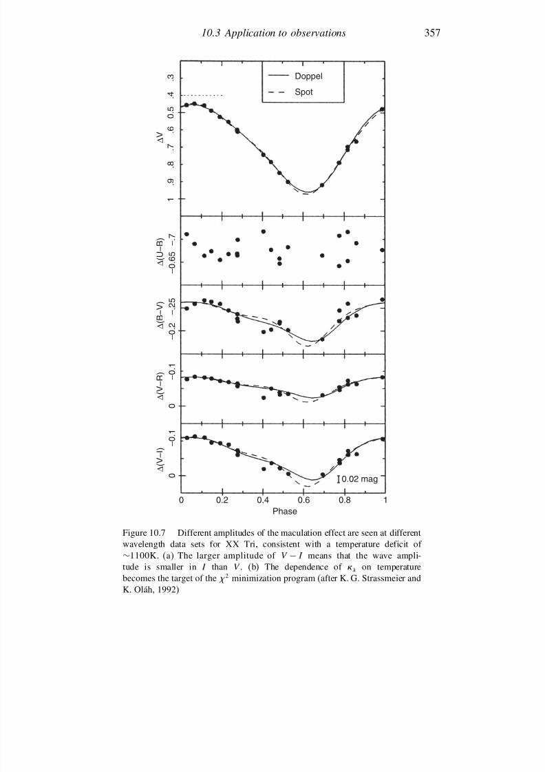
7/21/2019 Introduction to Astronomical Photometry
http://slidepdf.com/reader/full/introduction-to-astronomical-photometry 375/451
10.3 Application to observations 357
Doppel
Spot
. 3
. 4
0 . 5
. 6
. 7 ∆ V
∆ ( U – B )
∆ ( B – V )
∆ ( V – R )
∆ ( V – I )
0
0 0.2 0.4 0.6Phase
0.02 mag
0.8 1
– 0 . 1
0
– 0 . 1
– 0 . 2
– . 2
5
. 8
. 9
1
– 0 . 6
5
– . 7
Figure 10.7 Different amplitudes of the maculation effect are seen at differentwavelength data sets for XX Tri, consistent with a temperature deficit of ∼1100K. (a) The larger amplitude of V − I means that the wave ampli-tude is smaller in I than V . (b) The dependence of on temperaturebecomes the target of the 2 minimization program (after K. G. Strassmeier andK. Oláh, 1992)
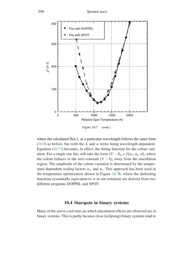
7/21/2019 Introduction to Astronomical Photometry
http://slidepdf.com/reader/full/introduction-to-astronomical-photometry 376/451
358 Spotted stars
0 500 1000 1500 2000
Relative Spot Temperature (K)
0
100
200
300
400
χ 2 ( V
– I )
Fits with DOPPEL
Fits with SPOT
Figure 10.7 (cont.)
where the calculated flux lc at a particular wavelength follows the same form(10.9) as before, but with the L and terms being wavelength dependent.
Equation (10.13) becomes, in effect, the fitting function for the colour vari-ation. For a single star this will take the form V − I0 + fV I , wherethe colour reduces to the zero constant V − I0 away from the maculationregion. The amplitude of the colour variation is determined by the temper-ature dependent scaling factors V and I . This approach has been used inthe temperature optimization shown in Figure 10.7b, where the darkeningfunctions (essentially equivalent to in our notation) are derived from two
different programs DOPPEL and SPOT.
10.4 Starspots in binary systems
Many of the active cool stars on which maculation effects are observed are inbinary systems. This is partly because close (eclipsing) binary systems tend to
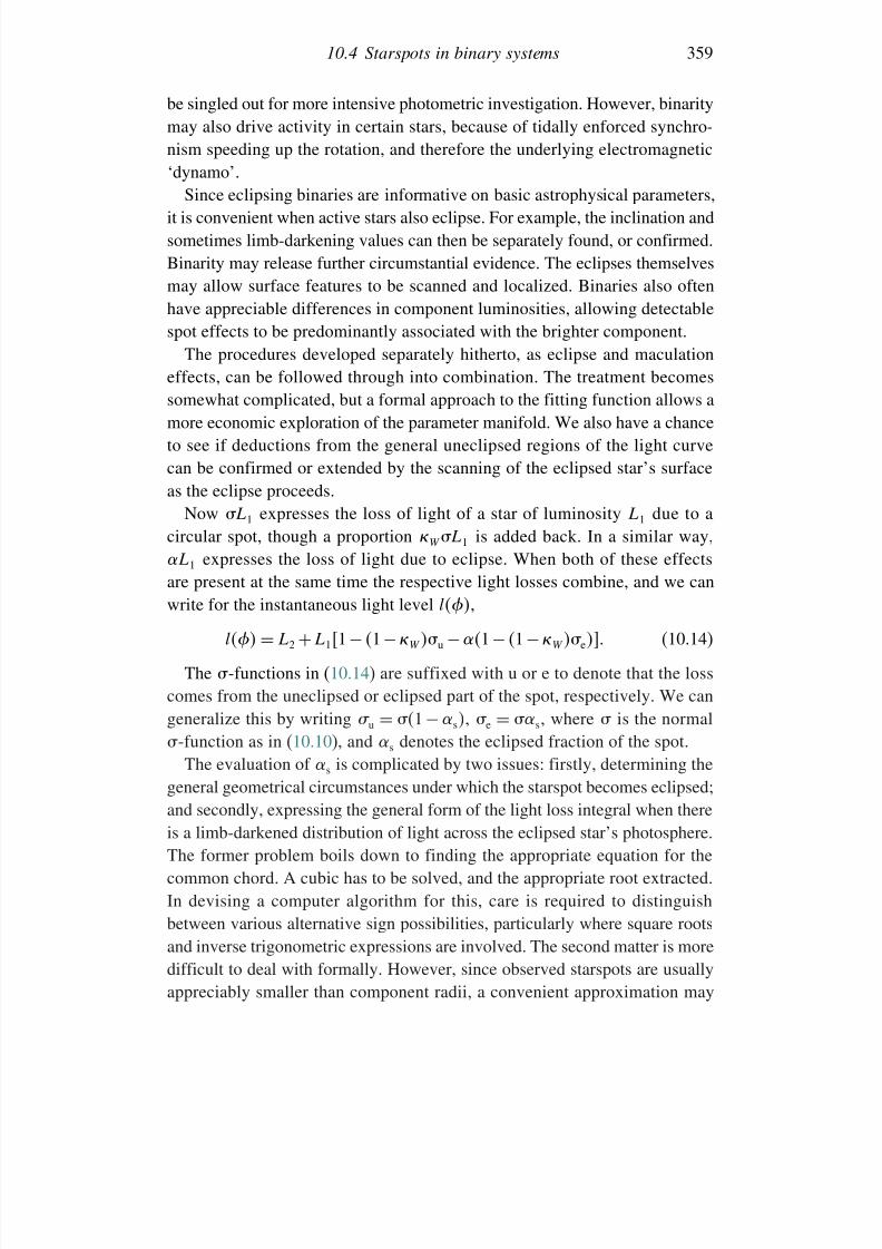
7/21/2019 Introduction to Astronomical Photometry
http://slidepdf.com/reader/full/introduction-to-astronomical-photometry 377/451
10.4 Starspots in binary systems 359
be singled out for more intensive photometric investigation. However, binaritymay also drive activity in certain stars, because of tidally enforced synchro-nism speeding up the rotation, and therefore the underlying electromagnetic
‘dynamo’.Since eclipsing binaries are informative on basic astrophysical parameters,
it is convenient when active stars also eclipse. For example, the inclination andsometimes limb-darkening values can then be separately found, or confirmed.Binarity may release further circumstantial evidence. The eclipses themselvesmay allow surface features to be scanned and localized. Binaries also oftenhave appreciable differences in component luminosities, allowing detectable
spot effects to be predominantly associated with the brighter component.The procedures developed separately hitherto, as eclipse and maculationeffects, can be followed through into combination. The treatment becomessomewhat complicated, but a formal approach to the fitting function allows amore economic exploration of the parameter manifold. We also have a chanceto see if deductions from the general uneclipsed regions of the light curvecan be confirmed or extended by the scanning of the eclipsed star’s surfaceas the eclipse proceeds.
Now L1 expresses the loss of light of a star of luminosity L1 due to acircular spot, though a proportion W L1 is added back. In a similar way,L1 expresses the loss of light due to eclipse. When both of these effectsare present at the same time the respective light losses combine, and we canwrite for the instantaneous light level l,
l = L2 + L11− 1− W u − 1− 1− W e (10.14)
The -functions in (10.14) are suffixed with u or e to denote that the losscomes from the uneclipsed or eclipsed part of the spot, respectively. We cangeneralize this by writing u = 1 − s, e = s, where is the normal -function as in (10.10), and s denotes the eclipsed fraction of the spot.
The evaluation of s is complicated by two issues: firstly, determining thegeneral geometrical circumstances under which the starspot becomes eclipsed;and secondly, expressing the general form of the light loss integral when thereis a limb-darkened distribution of light across the eclipsed star’s photosphere.
The former problem boils down to finding the appropriate equation for thecommon chord. A cubic has to be solved, and the appropriate root extracted.In devising a computer algorithm for this, care is required to distinguishbetween various alternative sign possibilities, particularly where square rootsand inverse trigonometric expressions are involved. The second matter is moredifficult to deal with formally. However, since observed starspots are usuallyappreciably smaller than component radii, a convenient approximation may
7/21/2019 Introduction to Astronomical Photometry
http://slidepdf.com/reader/full/introduction-to-astronomical-photometry 378/451
360 Spotted stars
–80 –60 –40 –20 20 40 60 80 100 1200
1
.9
.8
.7
.6
.5
I n t e n s i t y
Phase
(a)
–80 –60 –40 –20 20 40 60 80 100 1200
1
.9
.8
.7
.6
.5
Phase
(b)
–80 –60 –40 –20 20 40 60 80 100 1200
1
.9
.8
.7
.6
.5
I n t e n s i t y
Phase
(c)
–80 –60 –40 –20 20 40 60 80 100 1200
1
.9
.8
.7
.6
.5
Phase
(d)
–80 –60 –40 –20 20 40 60 80 100 1200
.9
.8
.7
.6
.5
.9
.8
.7
.6
.5
I n t e n s i t y
Phase
(e)
–80 –60 –40 –20 20 40 60 80 100 1200
Phase
(f)
Figure 10.8 The eclipsing binary light curve (upper curve, corresponding toordinate scale) has been based on the parameters of SV Cam (Table 10.2). A spotof radius 20 and at latitude 6 is located at longitude: (a) 1, (b) 10, (c) 20,(d) 30, (e) 50 and (f) 70. The maculation effect is shown below at half scale,and arbitrary height on the intensity axis. The eclipses start at around orbitalphase −32, and the spot starts to be eclipsed about 5 later in (a). It becomescompletely eclipsed by about −8, so that the maculation effect is completely
lost and the primary minimum looks shallower than it otherwise would. With thespot at 20 (c), it starts to emerge about half way through the annular minimum,whereupon the bottom of the primary eclipse drops down. By 50 (e), the mainmaculation minimum is appreciably outside the eclipse, and the effect of theforeshortened spot on the eclipse becomes much less obvious, though the bottomof the minimum still has a steep slope. By 70 (f), though it must still be eclipsedduring the ingress, the net effects of spot eclipse are practically insignificant
7/21/2019 Introduction to Astronomical Photometry
http://slidepdf.com/reader/full/introduction-to-astronomical-photometry 379/451
10.5 Analysis of light curves of RS CVn-like stars 361
be made by computing only the undarkened expression for the light loss,and weighting that with an appropriate z coordinate for the spot to obtain acorresponding limb-darkened form.
The undarkened form for s is made up of two ‘D-shaped’ areas, formedby the common chord and the perimeter of the eclipsed region of the spot andthe boundary of the eclipsing star. These areas are both basically of the form:
D = k2
arccos
c
k
− c
k
1− c2
k2
(10.15)
though the detailed expressions for the integral limit c and, for the ellipticalboundary, the equivalent to the arc radius k are awkward to spell out.
In Figure 10.8 a sequence showing the effects of a relatively large spotpositioned at different longitudes on an eclipse minimum is presented.
10.5 Analysis of light curves of RS CVn-like stars
Many active cool stars are in close binary systems. A group includingnumerous well-known eclipsing binaries showing distorted light curves andspectral emission features, particularly in the H and K lines of ionized calcium,were designated RS CVn stars by D. S. Hall. We will briefly follow througha method for the photometric analysis of such stars.
We first note the important concept of separation of additive contributionsto the net light level. In the previous chapter the photometric effects due to
mutual proximity of components were treated like this. Maculation effects,in general, are also separable. This is firstly because the fitting function fora standard (non-eccentric) eclipsing binary model (Chapter 9) is even aboutphase zero, whereas spots can be centred at any phase. Secondly, the proximityeffects are determined by stellar properties which are also reflected in theeclipse fitting. The standard eclipsing binary model is thus characterized byfive main photometric determinables (U , L1, r 1, k, i), and perhaps also themass ratio q , though this is usually supplied from separate, i.e. spectroscopic,
evidence. This applies also to the the temperatures, needed to fix the scaleof proximity effects through (9.18) and (9.19). The basic parameters are alldetermined by eclipses only in the spherical model (Section 7.3), i.e. theproximity effects, having components at low multiples of the fundamentalperiod of variation, are inter-dependent with the eclipses, which affect onlya relatively narrow range of phases. On the other hand, a spot usually affectsof the order of 90 of phase on either side of its longitude.
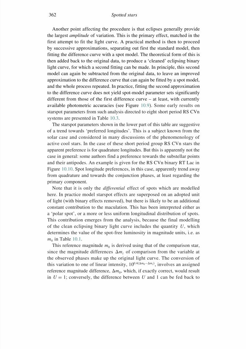
7/21/2019 Introduction to Astronomical Photometry
http://slidepdf.com/reader/full/introduction-to-astronomical-photometry 380/451
362 Spotted stars
Another point affecting the procedure is that eclipses generally providethe largest amplitude of variation. This is the primary effect, matched in thefirst attempt to fit the light curve. A practical method is then to proceed
by successive approximations, separating out first the standard model, thenfitting the difference curve with a spot model. The theoretical form of this isthen added back to the original data, to produce a ‘cleaned’ eclipsing binarylight curve, for which a second fitting can be made. In principle, this secondmodel can again be subtracted from the original data, to leave an improvedapproximation to the difference curve that can again be fitted by a spot model,and the whole process repeated. In practice, fitting the second approximation
to the difference curve does not yield spot-model parameter sets significantlydifferent from those of the first difference curve – at least, with currentlyavailable photometric accuracies (see Figure 10.9). Some early results onstarspot parameters from such analysis directed to eight short period RS CVnsystems are presented in Table 10.3.
The starspot parameters shown in the lower part of this table are suggestiveof a trend towards ‘preferred longitudes’. This is a subject known from thesolar case and considered in many discussions of the phenomenology of
active cool stars. In the case of these short period group RS CVn stars theapparent preference is for quadrature longitudes. But this is apparently not thecase in general: some authors find a preference towards the substellar pointsand their antipodes. An example is given for the RS CVn binary RT Lac inFigure 10.10. Spot longitude preferences, in this case, apparently trend awayfrom quadrature and towards the conjunction phases, at least regarding theprimary component.
Note that it is only the differential effect of spots which are modelledhere. In practice model starspot effects are superposed on an adopted unitof light (with binary effects removed), but there is likely to be an additionalconstant contribution to the maculation. This has been interpreted either asa ‘polar spot’, or a more or less uniform longitudinal distribution of spots.This contribution emerges from the analysis, because the final modellingof the clean eclipsing binary light curve includes the quantity U , whichdetermines the value of the spot-free luminosity in magnitude units, i.e. as
m0 in Table 10.1.This reference magnitude m0 is derived using that of the comparison star,
since the magnitude differences mi of comparison from the variable atthe observed phases make up the original light curve. The conversion of this variation to one of linear intensity, 1004m0−mi, involves an assignedreference magnitude difference, m0, which, if exactly correct, would resultin U = 1; conversely, the difference between U and 1 can be fed back to
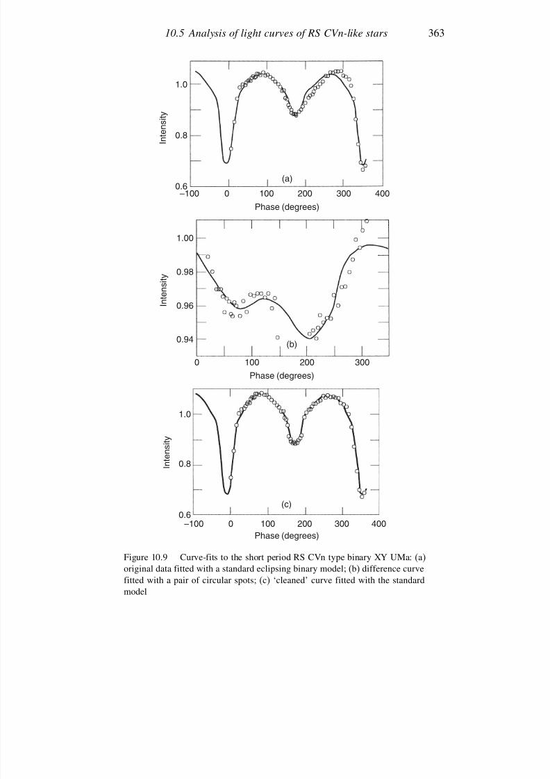
7/21/2019 Introduction to Astronomical Photometry
http://slidepdf.com/reader/full/introduction-to-astronomical-photometry 381/451
10.5 Analysis of light curves of RS CVn-like stars 363
1.0
0.8 I n t e n s i t y
0.6–100 0 100 200
Phase (degrees)
(a)
300 400
1.00
0.98
I n t e n s i t y
0.96
0.94
0 100 200
Phase (degrees)
(b)
300
1.0
I n t e n s i t y
0.8
0.6–100 0 100 200
Phase (degrees)
(c)
300 400
Figure 10.9 Curve-fits to the short period RS CVn type binary XY UMa: (a)original data fitted with a standard eclipsing binary model; (b) difference curvefitted with a pair of circular spots; (c) ‘cleaned’ curve fitted with the standardmodel
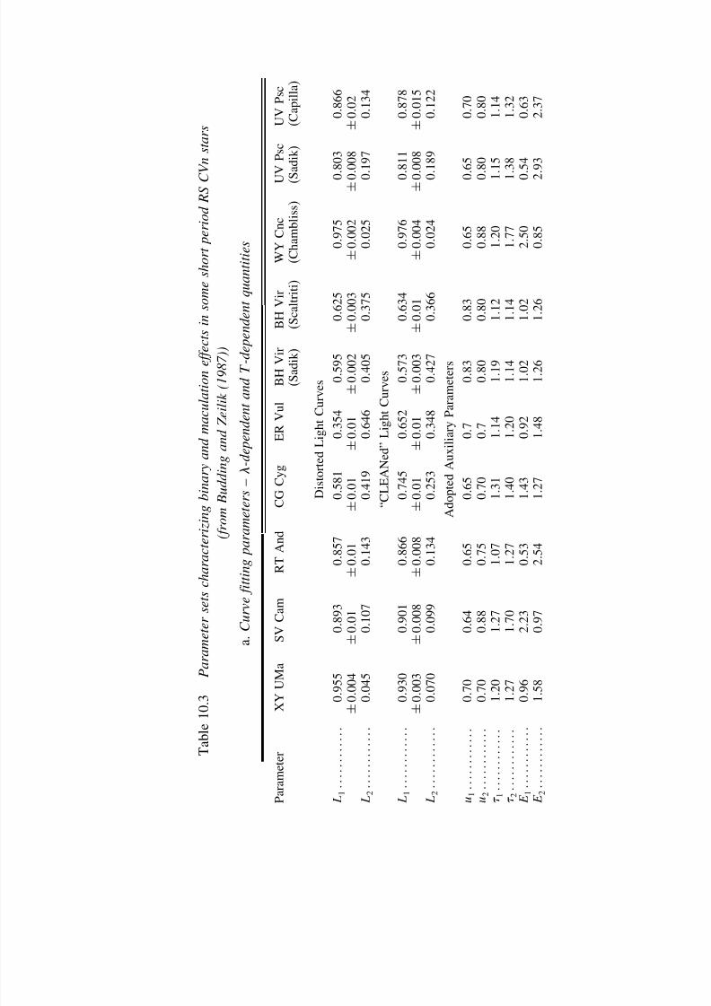
7/21/2019 Introduction to Astronomical Photometry
http://slidepdf.com/reader/full/introduction-to-astronomical-photometry 382/451
T a b l e 1 0 . 3
P a r a m e t e r s e t s c h a r a c t e r i z i n g b i n a r y a n d m a c u
l a t i o n e f f e c t s i n s o m e s h o r t p e r i o d R S C V n s t a r
s
( f r o m B u d d i n g a n d Z e i l i k ( 1 9 8 7 ) )
a . C u r v e f i t t i n g p a
r a m e t e r s – - d e p e n d e n t a n d T - d e p e n d e n t q u a n
t i t i e s
P a r a m e t e r
X Y U
M a
S V C a m
R T A
n d
C G C y g
E R V u
l
B H V i r
B H V i r
W Y C n c
U V P s c
U V P s c
( S a d i k )
( S c a l t r i t i )
( C h a m b l i s s )
( S a d i k )
( C a p i l l a )
D i s t o r t e d L i g h t C
u r v e s
L 1
0 9 5 5
0 8 9 3
0 8 5
7
0 5 8 1
0 3 5 4
0 5 9 5
0 6 2 5
0 9 7 5
0 8 0 3
0 8 6 6
±
0 0 0 4
±
0 0 1
±
0 0 1
±
0 0 1
±
0 0 1
±
0 0 0 2
±
0 0 0 3
±
0 0 0 2
±
0 0 0 8
±
0 0 2
L 2
0 0 4 5
0 1 0 7
0 1 4
3
0 4 1 9
0 6 4 6
0 4 0 5
0 3 7 5
0 0 2 5
0 1 9 7
0 1 3 4
“ C L E A N e d ” L i g h t
C u r v e s
L 1
0 9 3 0
0 9 0 1
0 8 6
6
0 7 4 5
0 6 5 2
0 5 7 3
0 6 3 4
0 9 7 6
0 8 1 1
0 8 7 8
±
0 0 0 3
±
0 0 0 8
±
0 0 0
8
±
0 0 1
±
0 0 1
±
0 0 0 3
±
0 0 1
±
0 0 0 4
±
0 0 0 8
±
0 0 1 5
L 2
0 0 7 0
0 0 9 9
0 1 3
4
0 2 5 3
0 3 4 8
0 4 2 7
0 3 6 6
0 0 2 4
0 1 8 9
0 1 2 2
A d o p t e d A u x i l i a r y P a r a m e t e r s
u 1
0 7 0
0 6 4
0 6 5
0 6 5
0 7
0 8 3
0 8 3
0 6 5
0 6 5
0 7 0
u 2
0 7 0
0 8 8
0 7 5
0 7 0
0 7
0 8 0
0 8 0
0 8 8
0 8 0
0 8 0
1
1 2 0
1 2 7
1 0 7
1 3 1
1 1 4
1 1 9
1 1 2
1 2 0
1 1 5
1 1 4
2
1 2 7
1 7 0
1 2 7
1 4 0
1 2 0
1 1 4
1 1 4
1 7 7
1 3 8
1 3 2
E 1
0 9 6
2 2 3
0 5 3
1 4 3
0 9 2
1 0 2
1 0 2
2 5 0
0 5 4
0 6 3
E 2
1 5 8
0 9 7
2 5 4
1 2 7
1 4 8
1 2 6
1 2 6
0 8 5
2 9 3
2 3 7
7/21/2019 Introduction to Astronomical Photometry
http://slidepdf.com/reader/full/introduction-to-astronomical-photometry 383/451
T a b l e 1 0 . 3
( c o
n t . )
b . C u r v e f i t t i n g s t a t i s t i c s
P a r a m e t e r
X Y
U M a
S V C a m
R T A
n d
C G C y g
E R V u l
B H V i r
B H V i r
W Y C n c
U V P s c
U V P s c
( S a d i k )
( S c a l t r i t i )
( C h a m b l i s s )
( S a d i k )
( C a p i l l a )
D i s t o r t e d L i g h t C
u r v e s
l
0
. 0 1
0 . 0 0 7
0 . 0
1
0 . 0 1
0 . 0 2
0 . 0 1
0 . 0 1 5
0 . 0 1
0 . 0 2
0 . 0 3
l
0 . 0 1 4
0 . 0 2 1
0 . 0
2
0 . 0 3
0 . 0 1
0 . 0 0 7
0 . 0 1 5
0 . 0 1
0 . 0 2
0 . 0 2
N
6 7
9 8
1 0
9
1 2 0
1 3 3
2 6 5
1 5 3
5 6
1 1 5
6 5
2
7
1 . 7
9 6 . 1
0 8 6 . 6
0 9 9 . 6
1 1 8 . 8
1 9 3 . 0
1 7 7 . 9
6 0 . 5
1 6 2 . 1
5 6 . 2
v
6 1
9 3
1 0
3
1 1 4
1 2 7
2 6 0
1 4 7
5 0
1 1 0
6 0
2 / v
1
. 1 8
1 . 0 4
0 . 8
4
0 . 8 7
0 . 9 4
0 . 7 4
1 . 2 1
1 . 2 1
1 . 4 7
0 . 9 4
“ C L E A N e d ” L i g h t
C u r v e s
l
0
. 0 1
0 . 0 1 4
0 . 0 1
4
0 . 0 2
0 . 0 0 7
0 . 0 0 7
0 . 0 1
0 . 0 1
0 . 0 2
0 . 0 2
N
6 7
9 8
1 0
6
1 2 0
1 3 3
2 6 5
1 5 3
5 6
1 1 5
6 5
2
5
1 . 2
8 8 . 3 5
1 1 5 . 3
1 0 8 . 0
1 3 9 . 2
2 0 3 . 9
1 7 3 . 8
3 5 . 8
0 6 9 . 4
4 7 . 0
v
6 1
9 3
1 1
0
1 1 5
1 2 6
2 6 0
1 4 7
5 0
1 1 0
6 0
2 / v
0
. 8 4
0 . 9 5
1 . 1
5
0 . 9 4
1 . 1 0
0 . 7 8
1 . 1 8
0 . 7 2
0 . 6 3
0 . 7 8
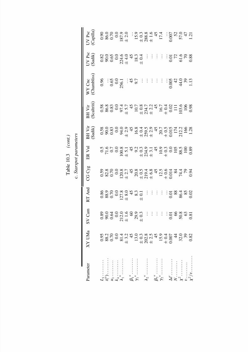
7/21/2019 Introduction to Astronomical Photometry
http://slidepdf.com/reader/full/introduction-to-astronomical-photometry 384/451
T a b l e 1 0 . 3
( c o
n t . )
c . S t a r s p o t p a r a m e t e r s
P a r a m e t e r
X Y U M a
S V C a m
R T A n d
C G C y g
E R V u l
B H V i r
B H V i r
W Y C n c
U V P s c
U V P s c
( S a d i k )
( S c a l t r i t i )
( C h a m b l i s s )
( S a d i k )
( C a p i l l a )
L 1
0
. 9 5
0 . 8 9
0 . 8 6
0 . 5 9
0 . 5
0 . 5 8
0 . 5 8
0 . 9 6
0 . 8 2
0 . 9 0
i
8
8 . 2
9 0 . 0
8 8 . 9
8 2 . 8
7 1 . 6
9 0 . 0
8 6 . 8
…
9 0 . 0
8 6 . 0
u 1
0
. 7 0
0 . 6 4
0 . 7 0
0 . 7 0
0 . 7
0 . 8 3
0 . 8 3
0 . 6 5
0 . 6 5
0 . 7 0
k
0 . 0
0 . 0
0 . 0
0 . 0
0 . 0
0 . 0
0 . 0
0 . 0
0 . 0
0 . 0
1
8
1 . 4
2 1 2 . 0
1 2 7 . 8
1 2 0 . 8
1 0 0 . 8
9 4 . 0
9 7 . 4
2 5 6 . 1
2 2 4 . 6
1 8 7 . 9
±
3 . 2
±
1 . 6
±
8 . 0
±
2 . 7
±
5 . 1
±
2 . 9
±
5 . 7
±
4 . 0
±
2 . 0
1
4 5
6 0
4 5
4 5
4 5
4 5
4 5
4 5
4 5
…
1
1
3 . 0
2 9 . 9
8 . 3
2 0 . 8
9 . 2
1 6 . 8
1 0 . 7
9 . 7
1 8 . 3
1 5 . 9
±
0 . 3
±
0 . 3
±
0 . 1
±
0 . 5
±
0 . 3
±
0 . 4
±
0 . 8
…
±
0 . 4
±
0 . 3
2
2 0
2 . 8
…
…
2 1 9 . 4
2 3 4 . 9
2 5 9 . 5
2 3 4 . 7
…
…
2 8 8 . 8
±
2 . 5
…
…
±
6 . 8
±
3 . 1
±
2 . 9
±
2 . 2
…
…
±
1 . 6
2
4 5
…
…
4 5
4 5
4 5
4 5
…
…
4 5
2
1
5 . 9
…
…
1 2 . 5
1 0 . 9
2 0 . 7
1 6 . 7
…
…
1 7 . 4
±
0 . 4
…
…
±
0 . 6
±
0 . 3
±
0 . 5
±
0 . 4
…
…
…
l
0 . 0
0 7
0 . 0 1
0 . 0 1
0 . 0 1 4
0 . 0
0 . 0 1 5
0 . 0 2
0 . 0 0 5
0 . 0 1
0 . 0 0 7
N
4 4
6 6
8 8
8 4
1 0 5
1 7 4
1 1 1
4 2
7 2
5 2
2
3
2 . 0
5 0 . 8
8 6 . 4
7 4 . 4
8 8 . 5
2 1 2 . 2
1 0 3 . 6
4 4 . 0
6 1 . 6
5 7 . 0
v
3 9
6 3
8 5
7 9
1 0 0
1 6 6
1 0 6
3 9
7 0
4 7
2 / v
0
. 8 2
0 . 8 1
0 . 0 2
0 . 9 4
0 . 8 9
1 . 2 8
0 . 9 8
1 . 1 3
0 . 8 8
1 . 2 1
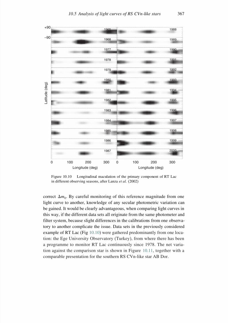
7/21/2019 Introduction to Astronomical Photometry
http://slidepdf.com/reader/full/introduction-to-astronomical-photometry 385/451
10.5 Analysis of light curves of RS CVn-like stars 367
+90
–90
L a t i t u d e ( d
e g )
0 100 200
Longitude (deg) Longitude (deg)
300 100 200 300
2000
1999
1998
1997
1996
1995
1994
1993
1992
1991
1990
1989
1988
1987
1986
1985
1984
1983
1982
1981
1980
1979
1978
1977
1968
1965
0
Figure 10.10 Longitudinal maculation of the primary component of RT Lacin different observing seasons, after Lanza et al. (2002)
correct m0. By careful monitoring of this reference magnitude from onelight curve to another, knowledge of any secular photometric variation canbe gained. It would be clearly advantageous, when comparing light curves inthis way, if the different data sets all originate from the same photometer and
filter system, because slight differences in the calibrations from one observa-tory to another complicate the issue. Data sets in the previously consideredexample of RT Lac (Fig 10.10) were gathered predominantly from one loca-tion: the Ege University Observatory (Turkey), from where there has beena programme to monitor RT Lac continuously since 1978. The net varia-tion against the comparison star is shown in Figure 10.11, together with acomparable presentation for the southern RS CVn-like star AB Dor.
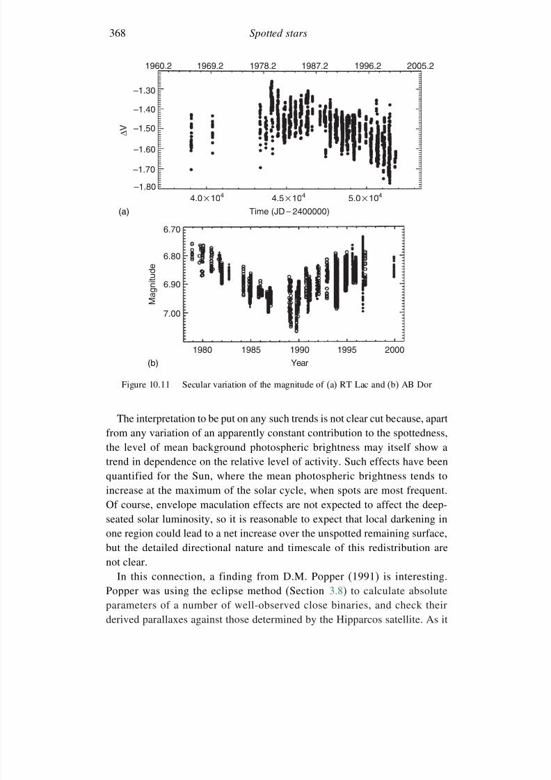
7/21/2019 Introduction to Astronomical Photometry
http://slidepdf.com/reader/full/introduction-to-astronomical-photometry 386/451
368 Spotted stars
–1.80
1960.2 1969.2 1978.2 1987.2 1996.2 2005.2
–1.60
–1.70
–1.50 ∆ V
–1.40
–1.30
4.0 × 10⁴ 4.5 × 10⁴ 5.0 × 10⁴
Time (JD – 2400000) (a)6.70
6.80
6.90
7.00
1980 1985 1990
Year
1995 2000
M a g n i t u d e
(b)
Figure 10.11 Secular variation of the magnitude of (a) RT Lac and (b) AB Dor
The interpretation to be put on any such trends is not clear cut because, apartfrom any variation of an apparently constant contribution to the spottedness,the level of mean background photospheric brightness may itself show atrend in dependence on the relative level of activity. Such effects have beenquantified for the Sun, where the mean photospheric brightness tends toincrease at the maximum of the solar cycle, when spots are most frequent.Of course, envelope maculation effects are not expected to affect the deep-seated solar luminosity, so it is reasonable to expect that local darkening in
one region could lead to a net increase over the unspotted remaining surface,but the detailed directional nature and timescale of this redistribution arenot clear.
In this connection, a finding from D.M. Popper (1991) is interesting.Popper was using the eclipse method (Section 3.8) to calculate absoluteparameters of a number of well-observed close binaries, and check theirderived parallaxes against those determined by the Hipparcos satellite. As it
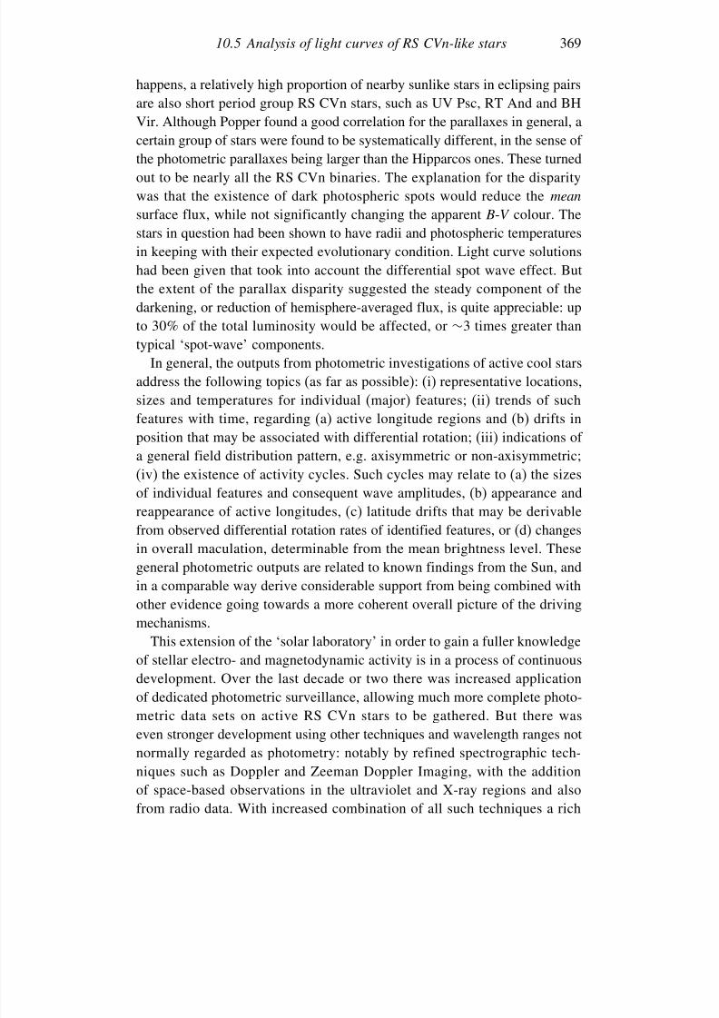
7/21/2019 Introduction to Astronomical Photometry
http://slidepdf.com/reader/full/introduction-to-astronomical-photometry 387/451
10.5 Analysis of light curves of RS CVn-like stars 369
happens, a relatively high proportion of nearby sunlike stars in eclipsing pairsare also short period group RS CVn stars, such as UV Psc, RT And and BHVir. Although Popper found a good correlation for the parallaxes in general, a
certain group of stars were found to be systematically different, in the sense of the photometric parallaxes being larger than the Hipparcos ones. These turnedout to be nearly all the RS CVn binaries. The explanation for the disparitywas that the existence of dark photospheric spots would reduce the mean
surface flux, while not significantly changing the apparent B-V colour. Thestars in question had been shown to have radii and photospheric temperaturesin keeping with their expected evolutionary condition. Light curve solutions
had been given that took into account the differential spot wave effect. Butthe extent of the parallax disparity suggested the steady component of thedarkening, or reduction of hemisphere-averaged flux, is quite appreciable: upto 30% of the total luminosity would be affected, or ∼3 times greater thantypical ‘spot-wave’ components.
In general, the outputs from photometric investigations of active cool starsaddress the following topics (as far as possible): (i) representative locations,sizes and temperatures for individual (major) features; (ii) trends of such
features with time, regarding (a) active longitude regions and (b) drifts inposition that may be associated with differential rotation; (iii) indications of a general field distribution pattern, e.g. axisymmetric or non-axisymmetric;(iv) the existence of activity cycles. Such cycles may relate to (a) the sizesof individual features and consequent wave amplitudes, (b) appearance andreappearance of active longitudes, (c) latitude drifts that may be derivablefrom observed differential rotation rates of identified features, or (d) changes
in overall maculation, determinable from the mean brightness level. Thesegeneral photometric outputs are related to known findings from the Sun, andin a comparable way derive considerable support from being combined withother evidence going towards a more coherent overall picture of the drivingmechanisms.
This extension of the ‘solar laboratory’ in order to gain a fuller knowledgeof stellar electro- and magnetodynamic activity is in a process of continuousdevelopment. Over the last decade or two there was increased application
of dedicated photometric surveillance, allowing much more complete photo-metric data sets on active RS CVn stars to be gathered. But there waseven stronger development using other techniques and wavelength ranges notnormally regarded as photometry: notably by refined spectrographic tech-niques such as Doppler and Zeeman Doppler Imaging, with the additionof space-based observations in the ultraviolet and X-ray regions and alsofrom radio data. With increased combination of all such techniques a rich
7/21/2019 Introduction to Astronomical Photometry
http://slidepdf.com/reader/full/introduction-to-astronomical-photometry 388/451
370 Spotted stars
field of investigation has been opening up: new examples of remarkablephysical behaviour witnessed and worthy challenges to scientific under-standing offered.
10.6 Bibliographical notes
A very extensive literature on spotted stars has developed since D. S. Hall’sreview in the Proc. IAU Colloq. 29: Multiple Periodic Variable Stars, ed.W. Fitch (Reidel, p. 287, 1975). The Cambridge Workshops on Cool Stars,
Stellar Systems and the Sun, held annually in the 1980s, somewhat less regu-larly since, have discussed a great deal of related material, and referencedstill more. Some of the proceedings of these conferences were published inthe Lecture Notes in Physics series of Springer-Verlag, e.g. Vol. 291, 1988,ed. J. L. Linsky & R. E. Stencel; see also Vol. 397, 1992, ed. P. B. Byrne andD. J. Mullan; or within the Conf. Ser. ASP, e.g. 154, eds. R.A. Donahue &J. Bookbinder, 1998. The general reviews of S. Baliunas & A. M. Vaughan( Ann. Rev. Astron. Astrophys., 23, 379, 1985) and L. W. Ramsey ( ASP Conf.
Ser., 9, ed. G. Wallerstein, p. 252, 1990) were also useful. The proceed-ings of IAU Symp. 176: Stellar Surface Structure, eds. K. G. Strassmeier &J. Linsky (Kluwer, 1996) featured many of the related research areas thathave grown up since the introduction of dedicated and automatic photometricmonitoring programmes, DI, ZDI and multi-wavelength techniques; antici-pating also the possibilities for direct imaging that may come with interfer-ometry and large telescope applications. Through such sources the flourishing
research on stellar maculation and related phenomena can be traced over recentdecades.The light curves of RS CVn in Figure 10.1 come from Blanco et al.,
in Activity in Red-Dwarf Stars, eds. P. B. Byrne & M. Rodonò (Reidel,1983, p. 387); that of YY Gem (Figure 10.2) is from a compilation of C. J.Butler (private communication). The ZDI map of CC Eri was provided byM. Semel as part of a multi-wavelength campaign on the star organized in2004. An article analysing the complementary nature of Doppler imaging and
maculation photometry was given by E. Budding & M. Zeilik in Astrophys.Space Sci. (222, 181, 1994).
Sections 10.2 and 10.3 are based primarily on E. Budding ( Astrophys.
Space Sci., 48, 287, 1977). The cited data of B. W. Bopp & D. S. Evans arein Mon. Not. Roy. Astron. Soc. (164, 343, 1973) (see also D. S. Evans, Mon.
Not. Roy. Astron. Soc., 154, 329, 1971). The comparison of CSM and MEMmodelling of the surface of AB Dor develops from E. Budding’s discussion in
7/21/2019 Introduction to Astronomical Photometry
http://slidepdf.com/reader/full/introduction-to-astronomical-photometry 389/451
10.6 Bibliographical notes 371
IAU Symp. 176: Stellar Surface Structure, eds. K. G. Strassmeier & J. Linsky(Kluwer, p. 95, 1996). The reference to A. Collier Cameron et al. is from
Lect. Notes Physics, 254, eds. M. Zeilik & D.M. Gibson, p. 313, 1986.
The presentation in Section 10.3.2 draws from K. G. Strassmeier & K. Oláh( Astron. Astrophys., 259, 595, 1992), from where Figure 10.7 comes. Section10.4 comes originally from E. Budding ( Astrophys. Space Sci., 143, 1, 1988),though with some upgrades.
The studies discussed in Section 10.5 started with those of E. Buddingand M. Zeilik ( Astrophys. J., 319, 827, 1987); and continued with work onindividual RS CVn stars, such as M. Zeilik et al. ( Astrophys. J., 354, 352,
1990) (BH Vir); M. Zeilik et al. ( Astrophys. J., 421, 303, 1994) (CG Cyg);P.A. Heckert et al. ( Astron. J., 115, 1145, 1998) (WY Cnc); but see alsoD.M.Z. Jassur & M.H. Kermani ( Astrophys. Space Sci., 219, 35, 1994)(UV Psc); K. Oláh et al. ( Astron. Astrophys., 291, 110, 1994) (ER Vul);T. Pribulla et al. ( Astron. Astrophys., 362,169, 2000) (RT And); T. A. Lister,A.C. Cameron & R.W. Hilditch ( Mon. Not. Roy. Astron. Soc., 326, 1489,2001) (XY UMa); B. Albayrak et al. ( Astron. Astrophys., 376, 158, 2001)(SV Cam); P. Vivekananda Rao & P. Radhika ( Astrophys. Space Sci., 282,
103, 2002) (UV Psc); D. P. Kjurkchieva, D. V. Marchev & S. Zola ( Astron. Astrophys., 386, 548, 2002) (SV Cam); M. Afsar, P. A. Heckert & C. Ibanoglu( Astron. Astrophys., 420, 595, 2004) (CG Cyg); and others.
The spot modelling technique presented is available as part of the same codereferred to in Chapter 9, i.e. CURVEFIT, see home.comcast.net/ ∼michael.rhodes /Astronomy.htm, downloadable from www.winsite.com/search/. Othercomparable programmes have been around for some time, e.g. D. Bradstreet’s
Binary Maker (Contact Software, 1993); or G. Ribárik’s SML, see G. Ribárik,K. Oláh & K.G. Strassmeier ( Astron. N., 324, 202, 2003); and G. Ribárik(Publ. Astron. Dept. Eötvös University (PADEU), 12, 135, 2002).
The finding of D. M. Popper concerning systematic parallax errors for RSCVn stars (relating to the constant term in the phase decomposition of themaculation effect) was recalled by E. Budding in Proc. IAU Symp. 196 , ed.D. Kurtz (p. 386, 2005); but it also transpires from Popper’s earlier discussionof RT Lac ( Astron. J., 101, 220, 1991) and a similar disparity with UZ Lib
(see M. Grewing et al., Astron. Astrophys., 223, 172, 1989).The ‘maximum entropy’ method mentioned in Section 10.3 and relating to
the work of A.F. Lanza et al. ( Astron. Astrophys., 386, 583, 2002) (shownin Figures 10.10 & 10.11a) has been a popular approach to over-specifiedspot distribution models, since its presentation by S. S. Vogt, G. D. Penrod &A. P. Hatzes in Astrophys. J. (321, 496, 1987). It was used in the above-citedpaper of A. C. Cameron et al. (1986). A comparable alternative approach,
7/21/2019 Introduction to Astronomical Photometry
http://slidepdf.com/reader/full/introduction-to-astronomical-photometry 390/451
372 Spotted stars
using Tikhonov regularization for a generalized fitting procedure, is that of N. E. Piskunov, I. Tuominen & O. Vilhu ( Astron. Astrophys., 230, 363, 1990).These techniques are usually associated with the analysis of DI and ZDI
data sets. K. G. Strassmeier’s paper in Surface Inhomogeneities on Late TypeStars, eds. P.B. Byrne and D.J. Mullan ( Lect. Notes Phys., 397, 50, 1992)compares the results of such different procedures with the same data sets(Figures 10.1 to 10.3), where the extent of high-frequency (probably insignif-icant) differences in the alternative procedures are easy to see. A recent paperof S.V. Jeffers ( Mon. Not. Roy. Astron. Soc., 359, 729, 2005) took a criticallook at starspot parametrization from testing the inverse problem with artifi-
cial data (see also M. Rhodes, E. Budding & M. Zeilik, ASP Conf. Ser., 9,252, 1990). Jeffers noted that two-spot parameter sets characterizing typicalnoisy data sets do not have the same degree of mutual independence as thecoefficients of a Fourier decomposition, although the physical significance of the latter seem even more abstract than circular spot parameters. The inter-relationship of Fourier and circular spot representations was considered inthe review of E. Budding in IAU Symp. 176: Stellar Surface Structure, eds.K.G. Strassmeier & J. Linsky (Kluwer, 1996, p. 95). The book of I.J.D.
Craig & J.C. Brown, Inverse Problems in Astronomy (Adam Hilger, 1986),provides useful mathematical background regarding ill-posed problems, regu-larization and the selection of appropriate constraints when there is a prioriknowledge.
Comprehensive discussions of photometric starspot cycles for a number of RS CVn-like stars were given by K. Oláh, Z. Kollath & K. G. Strassmeier( Astron. Astrophys., 356, 643, 2000) and K. Olah & K. G. Strassmeier ( Astron.
N., 323, 361, 2002). The useful application of APTs to such research wasevident from the paper of M. Rodonò et al. ( Astron. Astrophys., 358, 624,2000). Time intervals covered in such studies are now typically up to 25years. For several RS CVn stars double or even triple cycles have beenfound (e.g. V833 Tau). Caution must be exercised in discussing ‘cycles’longer than a score of years, however, in view of need for at least oneclear repetition with data of sufficient quality to resolve distinct maculationeffects. This may be relevant to the long-term cycle for AB Dor considered by
S. P. Järvinen et al. ( Astron. Astrophys., 432, 657, 2005); although the shortercycle times associated with preferred longitude activation and wave amplitudeseem reasonably clear from the power spectrum of the major maculationeffects. Järvinen et al.’s paper referred to the similar example LQ Hya,for which such derived timescales compare favourably with values obtainedtheoretically from dynamo calculations (V. Holzwarth & M. Schüssler, Astron.
N., 323, 2002). A likely higher Alfvén velocity and shorter range of latitude
7/21/2019 Introduction to Astronomical Photometry
http://slidepdf.com/reader/full/introduction-to-astronomical-photometry 391/451
References 373
variation was inferred for the more active component of CF Tuc, implyinga wave amplitude cycle ∼ 04 that of the Sun, by E. Budding and M. Zeilik( Astrophys. Space Sci., 232, 355, 1995).
References
Afsar, M., Heckert, P. A. & Ibanoglu, C., 2004, Astron. Astrophys., 420, 595.Albayrak, B., Demircan, O., Djurasevic, G., Erkapic, S. & Ak, H., 2001, Astron.
Astrophys., 376, 158.Baliunas, S. & Vaughan, A. M., 1985, Ann. Rev. Astron. Astrophys., 23, 379.
Blanco, C., Catalano, S., Marilli, E. & Rodonò, M., 1983, in Activity in Red-Dwarf Stars, eds. P. B. Byrne & M. Rodonò, Reidel, p. 387.
Bopp, B. W. & Evans, D. S., 1973, Mon. Not. Roy. Astron. Soc., 164, 343.Bradstreet, D., 1993, Binary Maker 2.0, Contact Software.Budding, E., 1977, Astrophys. Space Sci., 48, 287.Budding, E., 1988, Astrophys. Space Sci., 143, 1.Budding, E., 1996, IAU Symp. 176 , eds. K. G. Strassmeier & J. Linsky, Kluwer, p. 95.Budding, E., 2005, Proc. IAU Symp. 196 , ed. D. Kurtz, p. 386.Budding, E. & Zeilik, M., 1987, Astrophys. J., 319, 827.
Budding, E. & Zeilik, M., 1994, Astrophys. Space Sci., 222, 181.Budding, E. & Zeilik, M., 1995, Astrophys. Space Sci., 232, 355.Byrne, P. B. & Mullan, D. J., eds., 1992, Lecture Notes in Physics, Springer, 397.Collier Cameron, A., Bedford, D. K., Evans, T. L., Rucinski, S. M., Vilhu, O. & White,
N. E., 1986, Lect. Notes Physics, 254, eds. M. Zeilik & D. M. Gibson, p. 313.Craig, I. J. D. & Brown, J. C., 1986, Inverse Problems in Astronomy, Adam Hilger.Donahue, R. A. & Bookbinder, J., 1998 Conf. Ser. ASP, 154.Evans, D. S., 1959, Mon. Not. Roy. Astron. Soc., 119, 526.Evans, D. S., 1971, Mon. Not. Roy. Astron. Soc., 154, 329.
Grewing, M., Bianchi, L. & Garrido, R., 1989, Astron. Astrophys., 223, 172.Hall, D.S., 1975, Proc. IAU Colloq. 29: Multiple Periodic Variable Stars, ed.
W. Fitch, Reidel, p. 287.Heckert, P. A., Maloney, G. V., Stewart, M. C., Ordway, J. I., Hickman, A. & Zeilik,
M., Astron. J., 115, 1145.Holzwarth, V. & Schüssler, M., 2002, Astron. N., 323, 2002.Järvinen, S.P., Berdyugina, S.V., Tuominen, I., Cutispoto, G. & Bos, M., 2005,
Astron. Astrophys., 432, 657.Jassur, D. M. Z. & Kermani, M. H., 1994, Astrophys. Space Sci., 219, 35.
Jeffers, S. V., 2005, Mon. Not. Roy. Astron. Soc., 359, 729.Kjurkchieva, D. P., Marchev, D. V. & Zola, S., 2002, Astron. Astrophys., 386, 548.Lanza, A. F., Catalano, S., Rodonó, M. et al., 2002, Astron. Astrophys., 386, 583.Linsky, J. L. & Stencel, R. E., eds., 1987, Lecture Notes in Physics, Springer, 291.Lister, T. A., Cameron, A. C. & Hilditch, R. W., 2001, Mon. Not. Roy. Astron. Soc.,
326, 1489.Oláh, K. & Strassmeier, K. G., 2002, Astron. N., 323, 361.Oláh, K., Budding, E., Kim, H.-L. & Etzel, P. B., 1994, Astron. Astrophys., 291, 110.
7/21/2019 Introduction to Astronomical Photometry
http://slidepdf.com/reader/full/introduction-to-astronomical-photometry 392/451
374 Spotted stars
Oláh, K., Kollath, Z. & Strassmeier, K. G., Astron. Astrophys., 2000, 356, 643.Piskunov, N. E., Tuominen, I. & Vilhu, O., 1990, Astron. Astrophys., 230, 363.Popper, D. M., 1991, Astron. J., 101, 220.Pribulla, T., Chochol, D., Milano, L., Errico, L., Vittone, A.A., Barone, F. &
Parimucha, S., 2000, Astron. Astrophys., 362, 169.Ramsey, L. W., 1990, ASP Conf. Ser., 9, ed. G. Wallerstein, p. 252.Rhodes, M., 2006, CURVEFIT , downloadable from www.winsite.com/search/.Rhodes, M., Budding, E. & Zeilik, M., 1990, ASP Conf. Ser., 9, 252.Ribárik, G., 2002, Publ. Astron. Dept. Eötvös University (PADEU), 12, 135.Ribárik, G., Oláh, K. & Strassmeier, K. G., 2003, Astron. N., 324, 202.Rodonò, M., Messina, S., Lanza, A. F., Cutispoto, G. & Teriaca, L., 2000, Astron.
Astrophys., 358, 624.
Strassmeier, K. G., 1992, Surface Inhomogeneities on Late Type Stars, eds. P. B. Byrne& D.J. Mullan, Lect. Notes Phys., 397, 50.Strassmeier, K. G. & Linsky, J. L., 1996, Stellar Surface Structure: IAU Symp. 176 .Strassmeier, K. G. & Oláh, K., 1992, Astron. Astrophys., 259, 595.Vivekananda Rao, P. & Radhika, P., 2002, Astrophys. Space Sci., 282, 103.Vogt, S. S., Penrod, G. D. & Hatzes, A. P., 1987, Astrophys. J., 321, 496.Zeilik, M., Ledlow, M., Rhodes, M., Arevalo, M. J. & Budding, E., 1990, Astrophys.
J., 354, 352.Zeilik, M., Gordon, S., Jaderlund, E., Ledlow, M., Summers, D. L., Heckert, P. A.,
Budding, E. & Banks, T. S., 1994, Astrophys. J., 421, 303.
7/21/2019 Introduction to Astronomical Photometry
http://slidepdf.com/reader/full/introduction-to-astronomical-photometry 393/451
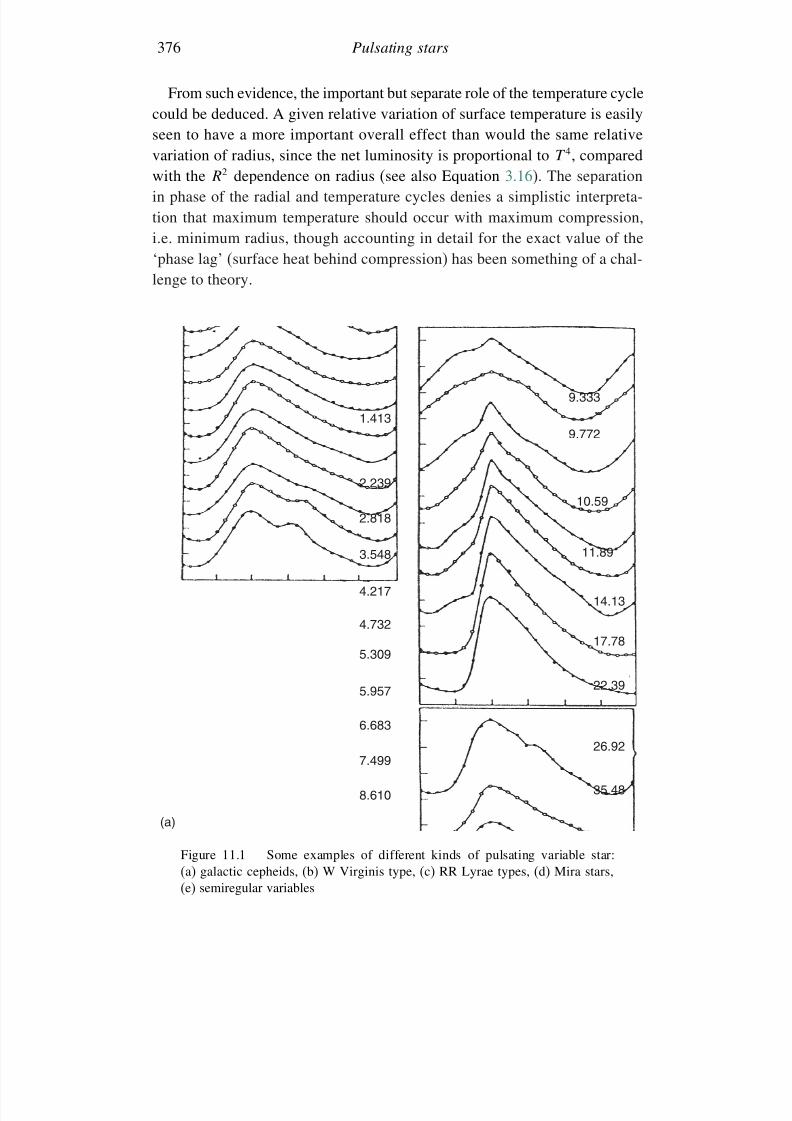
7/21/2019 Introduction to Astronomical Photometry
http://slidepdf.com/reader/full/introduction-to-astronomical-photometry 394/451
376 Pulsating stars
From such evidence, the important but separate role of the temperature cyclecould be deduced. A given relative variation of surface temperature is easilyseen to have a more important overall effect than would the same relative
variation of radius, since the net luminosity is proportional to T 4, comparedwith the R2 dependence on radius (see also Equation 3.16). The separationin phase of the radial and temperature cycles denies a simplistic interpreta-tion that maximum temperature should occur with maximum compression,i.e. minimum radius, though accounting in detail for the exact value of the‘phase lag’ (surface heat behind compression) has been something of a chal-lenge to theory.
1.413
2.239
2.818
3.548
4.217
4.732
5.309
5.957
6.683
7.499
8.610
(a)
35.48
26.92
22.39
17.78
14.13
11.89
10.59
9.772
9.333
Figure 11.1 Some examples of different kinds of pulsating variable star:(a) galactic cepheids, (b) W Virginis type, (c) RR Lyrae types, (d) Mira stars,(e) semiregular variables
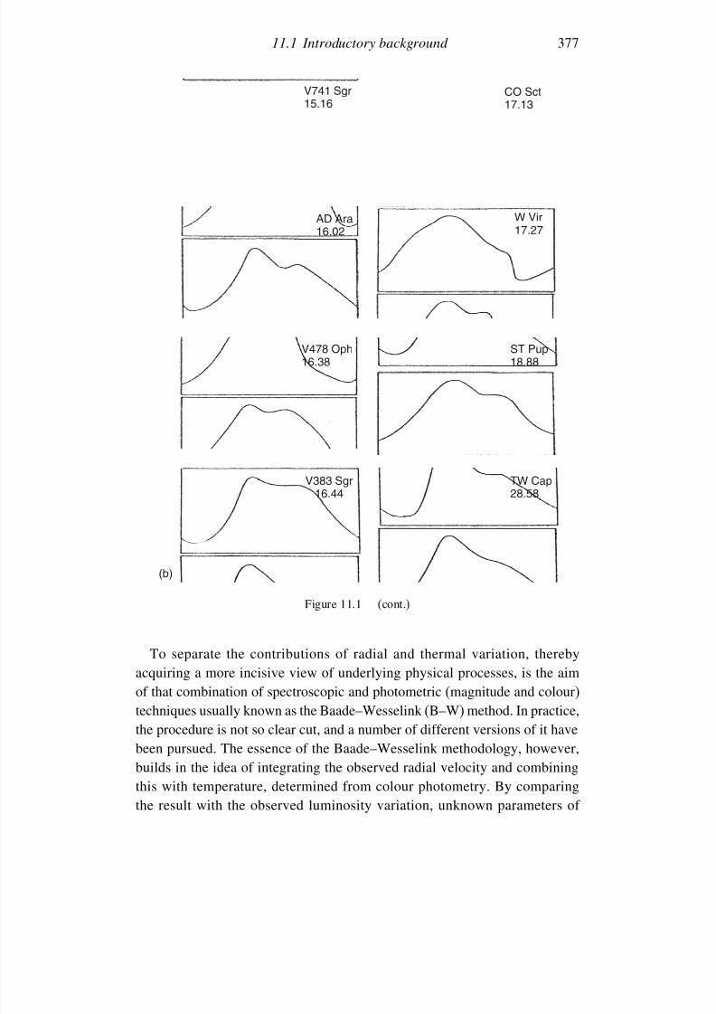
7/21/2019 Introduction to Astronomical Photometry
http://slidepdf.com/reader/full/introduction-to-astronomical-photometry 395/451
11.1 Introductory background 377
V741 Sgr15.16
CO Sct17.13
AD Ara16.02
W Vir17.27
V478 Oph16.38
ST Pup18.88
TW Cap28.58
V383 Sgr16.44
(b)
Figure 11.1 (cont.)
To separate the contributions of radial and thermal variation, therebyacquiring a more incisive view of underlying physical processes, is the aim
of that combination of spectroscopic and photometric (magnitude and colour)techniques usually known as the Baade–Wesselink (B–W) method. In practice,the procedure is not so clear cut, and a number of different versions of it havebeen pursued. The essence of the Baade–Wesselink methodology, however,builds in the idea of integrating the observed radial velocity and combiningthis with temperature, determined from colour photometry. By comparingthe result with the observed luminosity variation, unknown parameters of
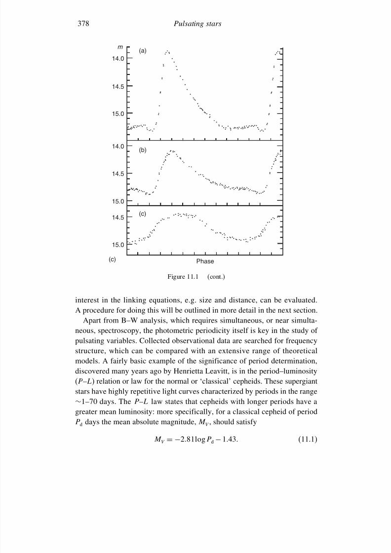
7/21/2019 Introduction to Astronomical Photometry
http://slidepdf.com/reader/full/introduction-to-astronomical-photometry 396/451
378 Pulsating stars
m
14.0
14.5
15.0
14.0
14.5
15.0
14.5
15.0
(c) Phase
(a)
(b)
(c)
Figure 11.1 (cont.)
interest in the linking equations, e.g. size and distance, can be evaluated.A procedure for doing this will be outlined in more detail in the next section.Apart from B–W analysis, which requires simultaneous, or near simulta-
neous, spectroscopy, the photometric periodicity itself is key in the study of pulsating variables. Collected observational data are searched for frequencystructure, which can be compared with an extensive range of theoreticalmodels. A fairly basic example of the significance of period determination,discovered many years ago by Henrietta Leavitt, is in the period–luminosity(P –L) relation or law for the normal or ‘classical’ cepheids. These supergiantstars have highly repetitive light curves characterized by periods in the range∼1–70 days. The P –L law states that cepheids with longer periods have agreater mean luminosity: more specifically, for a classical cepheid of periodP d days the mean absolute magnitude, M V , should satisfy
M V = −281log P d −143 (11.1)
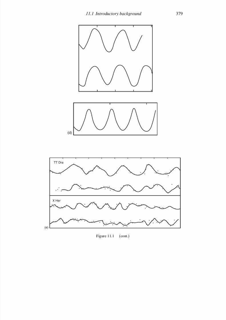
7/21/2019 Introduction to Astronomical Photometry
http://slidepdf.com/reader/full/introduction-to-astronomical-photometry 397/451
11.1 Introductory background 379
(d)
X Her
(e)
TT Dra
Figure 11.1 (cont.)
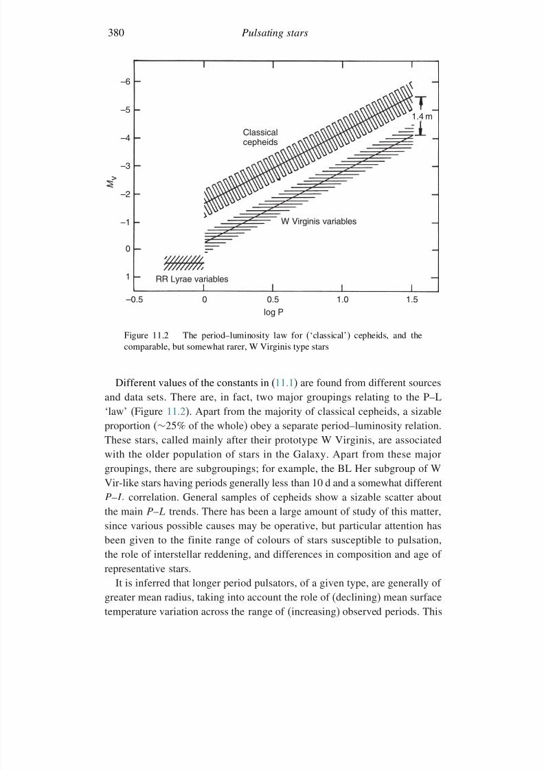
7/21/2019 Introduction to Astronomical Photometry
http://slidepdf.com/reader/full/introduction-to-astronomical-photometry 398/451
380 Pulsating stars
–6
–5
–2
–1
0
1
–0.5
–3
–4
0 0.5 1.0 1.5
log P
RR Lyrae variables
W Virginis variables
Classicalcepheids
1.4 m
M v
Figure 11.2 The period–luminosity law for (‘classical’) cepheids, and thecomparable, but somewhat rarer, W Virginis type stars
Different values of the constants in (11.1) are found from different sourcesand data sets. There are, in fact, two major groupings relating to the P–L‘law’ (Figure 11.2). Apart from the majority of classical cepheids, a sizableproportion (∼25% of the whole) obey a separate period–luminosity relation.These stars, called mainly after their prototype W Virginis, are associatedwith the older population of stars in the Galaxy. Apart from these majorgroupings, there are subgroupings; for example, the BL Her subgroup of WVir-like stars having periods generally less than 10 d and a somewhat differentP –L correlation. General samples of cepheids show a sizable scatter aboutthe main P –L trends. There has been a large amount of study of this matter,
since various possible causes may be operative, but particular attention hasbeen given to the finite range of colours of stars susceptible to pulsation,the role of interstellar reddening, and differences in composition and age of representative stars.
It is inferred that longer period pulsators, of a given type, are generally of greater mean radius, taking into account the role of (declining) mean surfacetemperature variation across the range of (increasing) observed periods. This
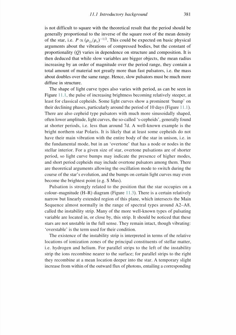
7/21/2019 Introduction to Astronomical Photometry
http://slidepdf.com/reader/full/introduction-to-astronomical-photometry 399/451
11.1 Introductory background 381
is not difficult to square with the theoretical result that the period should begenerally proportional to the inverse of the square root of the mean densityof the star, i.e. P
∝/∗−1/2. This could be expected on basic physical
arguments about the vibrations of compressed bodies, but the constant of proportionality (Q) varies in dependence on structure and composition. It isthen deduced that while slow variables are bigger objects, the mean radiusincreasing by an order of magnitude over the period range, they contain atotal amount of material not greatly more than fast pulsators, i.e. the massabout doubles over the same range. Hence, slow pulsators must be much morediffuse in structure.
The shape of light curve types also varies with period, as can be seen inFigure 11.1, the pulse of increasing brightness becoming relatively steeper, atleast for classical cepheids. Some light curves show a prominent ‘bump’ ontheir declining phases, particularly around the period of 10 days (Figure 11.1).There are also cepheid type pulsators with much more sinusoidally shaped,often lower amplitude, light curves, the so-called ‘s-cepheids’, generally foundat shorter periods, i.e. less than around 7d. A well-known example is thebright northern star Polaris. It is likely that at least some cepheids do not
have their main vibration with the entire body of the star in unison, i.e. inthe fundamental mode, but in an ‘overtone’ that has a node or nodes in thestellar interior. For a given size of star, overtone pulsations are of shorterperiod, so light curve bumps may indicate the presence of higher modes,and short period cepheids may include overtone pulsators among them. Thereare theoretical arguments allowing the oscillation mode to switch during thecourse of the star’s evolution, and the bumps on certain light curves may even
become the brightest point (e.g. S Mus).Pulsation is strongly related to the position that the star occupies on acolour–magnitude (H–R) diagram (Figure 11.3). There is a certain relativelynarrow but linearly extended region of this plane, which intersects the MainSequence almost normally in the range of spectral types around A2–A8,called the instability strip. Many of the more well-known types of pulsatingvariable are located in, or close by, this strip. It should be noticed that thesestars are not unstable in the full sense. They remain intact, though vibrating:
‘overstable’ is the term used for their condition.The existence of the instability strip is interpreted in terms of the relative
locations of ionization zones of the principal constituents of stellar matter,i.e. hydrogen and helium. For parallel strips to the left of the instabilitystrip the ions recombine nearer to the surface; for parallel strips to the rightthey recombine at a mean location deeper into the star. A temporary slightincrease from within of the outward flux of photons, entailing a corresponding
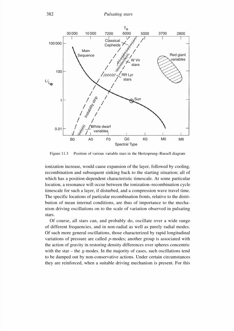
7/21/2019 Introduction to Astronomical Photometry
http://slidepdf.com/reader/full/introduction-to-astronomical-photometry 400/451
382 Pulsating stars
30 000 10 000 7200 6000 5000 3700 2800
100
000
100
1
0.01
MainSequence
Sun
Red giantvariables
RR Lyrstars
W Virstars
Classical
Cepheids
White dwarfvariables
Spectral TypeB0 A0 F0 G0 K0 M0 M8
I n s t a
b i l i t y
s t r i p
Te
L / L
Figure 11.3 Position of various variable stars in the Hertzsprung–Russell diagram
ionization increase, would cause expansion of the layer, followed by cooling,recombination and subsequent sinking back to the starting situation; all of
which has a position-dependent characteristic timescale. At some particularlocation, a resonance will occur between the ionization–recombination cycletimescale for such a layer, if disturbed, and a compression wave travel time.The specific locations of particular recombination fronts, relative to the distri-bution of mean internal conditions, are thus of importance to the mecha-nism driving oscillations on to the scale of variation observed in pulsatingstars.
Of course, all stars can, and probably do, oscillate over a wide range
of different frequencies, and in non-radial as well as purely radial modes.Of such more general oscillations, those characterized by rapid longitudinalvariations of pressure are called p-modes; another group is associated withthe action of gravity in restoring density differences over spheres concentricwith the star – the g-modes. In the majority of cases, such oscillations tendto be damped out by non-conservative actions. Under certain circumstancesthey are reinforced, when a suitable driving mechanism is present. For this
7/21/2019 Introduction to Astronomical Photometry
http://slidepdf.com/reader/full/introduction-to-astronomical-photometry 401/451
11.2 The Baade–Wesselink procedure 383
some ‘negative dissipation’ (Eddington’s term) has to operate. This has beenassociated with appropriately phased withdrawals from the reservoir of ioniza-tion energy, particularly that of doubly ionized helium in the case of classical
radial pulsation. This occurs when the star is in the right evolutionary stageand the layer of encroaching recombination is in the right position. Resonancebetween this component of the total heat flow and the elastic response of thestar then amplifies the vibration: the ‘kappa mechanism’.1
A key task lies in decomposing the more general observed variabilitypatterns in terms of component oscillations of ascribed mode and frequency,and relating the results to stellar models of given net mass, composi-
tion and evolution, confirming, or otherwise, their calculated structures.A number of different approaches to this subject have been reviewed inother sources (Section 11.5) and this topic will not be pursued furtherhere.
11.2 The Baade–Wesselink procedure
We spell out one version of this method of analysis, influenced by the settingof photometric and radial velocity data on classical cepheids in which itoriginated. The procedure is shown as another optimal curve-fitting exercise,comparable to those discussed in previous chapters.
In order to specify the radius at a given phase, we approximate the observedradial velocity curve, consisting of n data points, by a Fourier series,
r a = a0 + hi=1
ai cos2i + hi=1
bi sin2i (11.2)
where the component of the star’s radial motion in the line of sight r a, asmeasured from line shifts, is expressed in terms of the phase , and a0 ai bi
are constants to be determined. This formula should match the observationsto within their quoted accuracy. The number of terms to be retained in thesummations is chosen by minimizing the reduced 2 for the correspondingnumber of degrees of freedom of the data, n − 2h +1.
The radial motion r a in (11.2) is normally given in kilometres per second.It is convenient to multiply this by a scaling factor s, which yields the radialmotion in units of the solar radius R per unit phase. First removing a0, which
1 Kappa is the symbol conventionally used for the stellar absorption coefficient. Its usage herepoints to the role of recombination in the driving mechanism.
7/21/2019 Introduction to Astronomical Photometry
http://slidepdf.com/reader/full/introduction-to-astronomical-photometry 402/451
384 Pulsating stars
simply represents the line of sight spatial motion of the star as a whole, andthen integrating, we obtain for the apparent position of the line-forming layer
Ra = Ra0 + s
hi=1
ai
2i sin 2i − h
i=1
bi
2i cos2i
(11.3)
where Ra measures the radial position of the line-forming layer averagedover the earthward hemisphere at phase , and Ra0 is the mean position of this layer. The scale factor s has the value 86400P/R, where P is the periodof oscillation in days and R is in kilometres.
We now relate (11.3) with the radius of the photosphere Rp. A suitableformula is
Rp = Rp 0 + ps
hi=1
ai
2i sin 2i + −
hi=1
bi
2i cos 2i +
(11.4)
where p represents another scale factor, resulting from the averaging of Ra
over the earthward hemisphere, i.e. the observed radial velocity shifts are
less than the true radial motion. allows for a difference in phase betweenphotometrically detected radial movements of the photosphere and the spec-troscopically derived motion of the line-forming layer. A positive value of implies that the absorption line-forming layer lags behind the photosphere.
When the difference in radii of the photosphere and line-forming layers maybe neglected, and the Doppler shifted spectrum of the radially expanding layerfades from the disk centre according to a linear limb-darkening law, a simple-minded approach yields p
=6
−2u/4
−u, where u is the coefficient of
linear limb darkening. With a standard limb-darkening coefficient of 0.6 wethen find the result p = 24/17, frequently cited in older texts. More thoroughanalysis shows this to be rather an overestimate. The profile is renderedasymmetric by radial motion, the sense of the asymmetry tending to put themeasured shift somewhat greater than the foregoing would predict, to anextent which depends on inherent line broadening, instrumental resolution andmeasuring technique. More detailed calculations led to a common adoption
of p = 131 as the best estimate for this factor for classical cepheids, but inrecent years preferred values of p have tended to increase back towards theolder value.
The photosphere has a certain apparent magnitude m at effective wave-length ,
m = M − 25
2
1+ log
Rp
+ log
F pT p
F T
(11.5)
7/21/2019 Introduction to Astronomical Photometry
http://slidepdf.com/reader/full/introduction-to-astronomical-photometry 403/451
11.2 The Baade–Wesselink procedure 385
where M denotes absolute magnitude, and suffixes and p are applied tosolar and stellar photospheric quantities. The quantity denotes what thedistance to the star would be in the absence of interstellar extinction. If we
take this extinction into account, we have, for the actual distance ,
log = log − A
5 (11.6)
where A is the interstellar extinction at effective wavelength . The fluxratio F p/F involves, in addition to the wavelength , the temperatures T and T p. If these are brightness temperatures, then, by definition, the flux ratiois simply expressed as
F p
F
= exp c2/T −1exp c2/T pfs −1
(11.7)
where c2 has the value 0.014388mK (3.9).We need the value of T p in order to use (11.5) as a fitting function. Contin-
uing with the Baade–Wesselink methodology, we interpret this in terms of theobserved colour of the star, though this step raises difficulties about whethertemperature can be uniquely related to colour for cepheid atmospheres.
Manyinvestigatorsintroduceheretheeffectivetemperature,T e,sinceitformsthe natural independent variable in the study of model stellar atmospheres fromwhich flux values at particular wavelengths, and therefore colours, are deter-mined. Conversely, appropriately chosen observed colours C , defined at wave-lengths 1 and 2, can determine effective temperatures on the basis of givenmodel stellar atmospheres. In practice, one of the wavelengths, 1 say, will bethat of the fitting equation (11.5).
Empirical relationships between colour and effective temperature of the form
e = e0 + aC (11.8)
where we have introduced the conventional reciprocal effective temperaturee = 5040/T e,2 and e0 and a are constants, have been found to be valid overrestricted temperature ranges with selected colour filters for certain equilibriumstellar atmospheres. The form should hold good over most phase ranges forcepheid type variable stars, when thermal response rates for the photosphereare considerably faster than the temperature variation rates associated withthe pulsations, though calculation of the steep rise of temperature just beforebrightness maximum may be flawed if we rely on static atmosphere models
2 5040 log e / k , where k is Boltzmann’s constant in eV. This usage comes from historicapplications of Saha’s equation, see, e.g. Allen (1973).
7/21/2019 Introduction to Astronomical Photometry
http://slidepdf.com/reader/full/introduction-to-astronomical-photometry 404/451
386 Pulsating stars
to provide such a relation. The strong compression pulse during these phasesmay also prevent constancy of the relationship between the spectroscopicand photometric location of the photosphere implied by the use of (11.4);
in fact, spectra are known to show line profile complications during thesephases. From the practical point of view, departures from the linear form(11.8) are likely to be small compared with the probable errors of colourdeterminations. Moreover, the small range of phases associated with steeptemperature (and gravity) variation could be given low weight, or omitted fromthe fitting.
Since the Planck version of the colour–temperature relationship is of thesame form as Equation (11.8) to a close approximation (cf. Equation (3.25)),it suggests relating brightness and effective temperatures by writing, e.g.,b = ke, where k is an empirical constant. The sought relationship betweencolour and brightness temperature is then also of the form
b = b0 + C (11.9)
where
= 504012
25c22 − 1 log10 e (11.10)
If a single brightness temperature value does not hold over the wavelengthsdefining the colour index for a more realistic model, a small change of b
at 1 can still be approximated to a corresponding change of colour by arelationship of the type (11.9) if we write
= 504012
25c2 2 − b2/b1 1 log10 e (11.11)
where b2/b1 is a quantity that can be derived from relevant modelatmosphere calculations. For appropriately chosen broadband filter combina-tions, giving a smooth response in colour to temperature variation, we shouldreasonably expect that b2/b1 ≈ 1, and is slowly varying. Overthe 1000 K or so surface temperature variation typical of cepheid pulsationit may be approximated by a constant.
Keeping in mind the empirical broadband colour temperature relationships
shown in Figure 4.4, we could alternatively expect a more generalized formfor (11.9) as
b = b0 + 1C + 2C 2 +· · ·+ h1g +· · · (11.9a)
where higher order terms in the colour or the term(s) in gravity should besmall compared to the principal colour term.
7/21/2019 Introduction to Astronomical Photometry
http://slidepdf.com/reader/full/introduction-to-astronomical-photometry 405/451
11.2 The Baade–Wesselink procedure 387
Suppose we have a set of N photometric observations of a cepheid attwo wavelengths 1 2; i.e. mi and C i, at assigned phases i. The C is aresubstituted into (11.9), to yield brightness temperatures bi
, which, when
converted into T pi , go into the flux term (11.7). Equation (11.4) is used torepresent photospheric radii Rp at the given i. In this way, the observedmi values are matched by a corresponding set of calculated values mci using(11.5) and the six quantities p Rp0 b0 and , which thus play the roleof parameters in an optimization problem.
These six parameters are not independently determinable solely from (11.5),because p Rp 0 and appear only in the combination p/ and Rp 0/.
However, since the values of Rp 0 and are of particular interest, it isconvenient to keep the foregoing notation and take it that p can be assigneda sufficiently accurate value from theory.
The value of should not be wildly different from that given by (11.10).The constant term b 0 is, in any case, constrained by (11.9) if the colour andbrightness temperature of a source can be independently measured. This isthe case for the Sun, which provides the calibration for (11.5), so a suitabletrial value for b 0 can be given as
b0 = b − C (11.12)
However, it can be argued that a supergiant star of the same colour as theSun, in B − V say, would be emitting a higher surface flux in V , due to theblocking effect in the shorter wavelengths at lower gravity. The V brightnesstemperature is then effectively higher, so b0 should be reduced from (11.12).Allowance may therefore be made for b 0 to be independently adjustable in
fitting (11.5), although this difference may be small when longer wavelengthfilters are used (see Section 3.7).Concerning the value of – real differences in phase between the pulsations
of the continuum and absorption line-forming layers for a cepheid should bebarely detectable (
<∼ 001) according to classical analysis. General calculationsby M. Schwarzschild et al. for the atmosphere of the cepheid Aql indicatedthat a phase lag of up to 3 would be encountered in moving from thecontinuum forming layer up a distance of 1% of the mean radius, i.e. some
100 times the photospheric pressure scale height. This implies no detectableeffect on . Some models of non-classical cepheids (e.g. W Vir), however,indicate that the atmospheric pulsation lag may become quite appreciable(∼ 01×period).
A non-zero value of could be appropriate if the radial velocity andphotometric curves have not been properly reduced to the same epoch andperiod for some reason; but it is also possible that relaxation of the condition
7/21/2019 Introduction to Astronomical Photometry
http://slidepdf.com/reader/full/introduction-to-astronomical-photometry 406/451
388 Pulsating stars
= 0 results in improved curve-fits but with unphysical phase shifts. Ithas been known for a long time, for instance, that a reasonable match tothe observed luminosity variations can be produced, even on the basis of a
black body hypothesis for the observed colour changes, provided the phase of minimum radius is displaced to coincide with that of maximum luminosity.Moving the minimum photospheric radius onto this brightest phase, however,implies a shift in the wrong direction, i.e. that the photospheric minimumoccurs after the radial velocity zero (about its mean).
In this optimization problem, then, we have five independent parameters,of which two only – Rp0 and – can be regarded as entirely free unknowns.
The fitting naturally arranges itself into a two-stage procedure. At first, Rp 0and are determined on the basis of assigned p, , b0 and . In the secondstage, we would relax the values of the latter three parameters; though, since should be effectively zero for a classical cepheid, and b0 tends to dependon through (11.12), the thrust of the procedure lies in finding the optimalvalue of . This is of particular interest in testing model atmospheres, e.g. byformulae such as (11.11).
The role of the temperature variation can be seen from the variation m of
m about its mean value during the course of the pulsation, i.e.,
m = m
C C + m
Rp
Rp (11.13)
m/Rp is simply given by
m
Rp
=
Rp
−5log Rp = −2172Rp
(11.14)
As for m/C , from the reasoning which preceded (11.9) (cf. Section 3.5)we have
m1
C1 2 ≈ 1/1
1/1 − 1/2 (11.15)
11.3 Six-colour data on classical cepheids
We will follow through the foregoing method with some classic observationsof cepheids made in the six-colour system of Stebbins and Whitford. Inparticular, it is the G and I filters of this system which are used to derivetemperatures. This may be compared with the V − R (Johnson) temperaturemeasurer used in the original Barnes–Evans approach (Section 3.7), or the V
minus some infrared magnitude (e.g. K ) used more frequently recently. Note
7/21/2019 Introduction to Astronomical Photometry
http://slidepdf.com/reader/full/introduction-to-astronomical-photometry 407/451
11.3 Six-colour data on classical cepheids 389
that the wavelengths usually quoted for these filters are mean wavelengths.The effective wavelengths are obtained by folding the spectral response of thecell plus filter with the energy distribution of the source. This has little effect
with a star of around solar temperature on the mean wavelength of the G filter(5700 Å), but the effective wavelength of the I filter is significantly displacedto shorter wavelengths, dropping from 0 10300Å to eff 9700 Å. Usingthese values, we find from (11.10) = 0446, and from (11.15) we have
mG
G − I ≈ 243 (11.16)
In place of Equation (11.13) we therefore write
mG 55C − 22Rp
Rp (11.17)
The major features of cepheid optical light variation may be assessedfrom this equation, recalling the phase difference between minimum Rp andminimum C (maximum temperature), the latter occurring typically about 0.1period after the former. In the case of Cep, for example, an apparent
brightness variation of 0.84 mag is observed in the G-filter observations of Stebbins. This is matched by a colour variation G − I of 0.44 mag. Thetemperature variation thus has over four times the effect of the radial variationat visual wavelengths.
From (11.17) it follows that the amplitude of the colour variation, notthe absolute value of the colour, is significant as far as the shape of thelight curve is concerned. Hence, interstellar reddening, which would subtract
a certain, nearly constant, amount from the apparent magnitude observedwith each filter (see Section 4.1.3), should not have any great part to playin the curve-fitting other than fixing the mean light level. On the otherhand, interstellar extinction will, as indicated by (11.6), affect the meaningof the obtained value of . Where the extent of reddening is available fora particular cepheid it can be initially subtracted from the observed coloursC i. The apparent magnitudes mi must then be made correspondingly brighterto obtain a consistent representation. This correction can be determined from
(11.15), i.e. for the six-colour system,
mGred = − mG
G − IG − Ired ≈ −24G − Ired
When such corrections are initially made to the data, the resulting value of is equivalent to the true distance to the star, and the separate calculation(11.6) is not required.
7/21/2019 Introduction to Astronomical Photometry
http://slidepdf.com/reader/full/introduction-to-astronomical-photometry 408/451
390 Pulsating stars
Notice that the amplitude of the magnitude variation will constrain the scaleof radial change for the given range of measured colours. The integral of the radial velocity curve will meanwhile determine how far the photospheric
radius has moved between its lowest and highest points. The combination of these two constraints will tend to fix the mean radius independently of thecombination of mean radius and mean flux that determines the distance for agiven mean apparent magnitude via the absolute calibration of the magnitudescale. In other words, the mean radius, being found from differential measures,can be expected to carry more precision than the distance determination.
A correction for binarity, when known to be present, could also be made
a priori. The proportional contribution of the companion at the wavelengthof each filter requires the addition of corresponding magnitude corrections,rendering data appropriate for the cepheid alone to have magnitudes mc,somewhat greater than those observed mo. This may entail a successiveapproximations procedure, depending on the relative scale of the companion’slight, but if this is small (as would be normally the case), we can write
mc
mo
+1086
×1004mo
LB
LAmax (11.18)
where LB/LAmax is the ratio of the luminosity of the companion to that of thecepheid at maximum. The magnitude differences mo are measured from thatat phase zero, i.e. the lowest mo. The true magnitude variation of the cepheidwould thus be somewhat greater than the apparent.
LB/LAmax will, in general, be different at different wavelengths, so thatanomalous colour variations occur for a cepheid of a given amplitude if this
ratio becomes significant. This would be more likely for early type compan-ions, where, for example, a B −V variation would be less than expected fromthe V variation alone. This point has given rise to some methods of deter-mining binarity, as a result of which it appears that an appreciable proportion –at least ∼30% – of cepheids are in binary systems. The complications therebyintroduced for B–W analysis would tend to lose significance at longer periods,where the cepheid’s luminosity increasingly dominates, in agreement withthe P –L trend. At shorter periods, binarity would introduce something of an
upturn to the lower end of the trend: an effect that does seem noticeable ingeneral P –L type data presentations.
At the initial stage, the parameters b0, p and are fixed at 0.446, 0.951,1.31 and 0, respectively. As noted above, the G light curve is well conditionedto determine a value of Rp0, and the mean G value then constrained to yielda value of . However, Rp0 and directly depend on the adopted value of the scaling parameter p; the real accuracy of their determination by the B–W
7/21/2019 Introduction to Astronomical Photometry
http://slidepdf.com/reader/full/introduction-to-astronomical-photometry 409/451
11.3 Six-colour data on classical cepheids 391
method thus cannot be greater than that with which p can be specified, whichis probably to within 10%.
11.3.1 Application to Cep and Aql
Forpracticalillustration,weturntotwofamousexamplesofcepheidvariables– Cep and Aql – whose variability was discovered in the eighteenth centuryby the young amateur astronomer friends John Goodricke and Edward Piggott.
Radial velocities
Since both stars are quite bright, it is not surprising that relatively good radialvelocity curves were obtained many years ago by T. S. Jacobsen. For Cep,this was published almost twenty years before the six-colour photometry of Stebbins, and so some tailoring of the phases of the two data sets was required.This is complicated by a drift in period of Cep (5.366 282 days at the timeof Stebbins’ photometry), but the shortening has been found to be essentiallylinear, so that phases for the radial velocity on the same ephemeris as thephotometric variation are derived with reasonable confidence. The result is
shown in Figure 11.4(c), which shows the smoothly changing radius withphase. This comes from integrating the Fourier representation (11.2) with thecoefficients (in Jacobsen’s ephemeris) listed in Table 11.1.
In the case of Aql Jacobsen’s data were supplemented by observations byM. Schwarzschild et al., made close to the time of Stebbins et al.’s photometricobservations. An eleven-term Fourier fit gives a very good representation of the radial velocity, the details of which are given in Table 11.2. The radius
of Aql (Figure 11.5(c)) rises to its larger maximum in a more drawn outway than that of Cep, but the location in phase and shape of the minimaare very similar.
Interstellar reddening
The period–luminosity law for cepheids (Figure 11.2) has allowed them toplay an important ‘yardstick’ role in gauging distances, which, since theyare intrinsically very luminous, can be effective over large spatial extents.
It is necessary, though, to have a clear awareness of the role of interstellarreddening, particularly as classical cepheids are, in general, concentratedtowards the galactic plane. A number of studies have been made of this, andthe averages of measured colour excesses, including some in the six-coloursystem itself, and others interpolated to it, turn out as G − Ired = 009 for Cep and G − Ired = 019 for Aql. The corresponding absorptions areAG = 022 for Cep and AG = 048 for Aql.
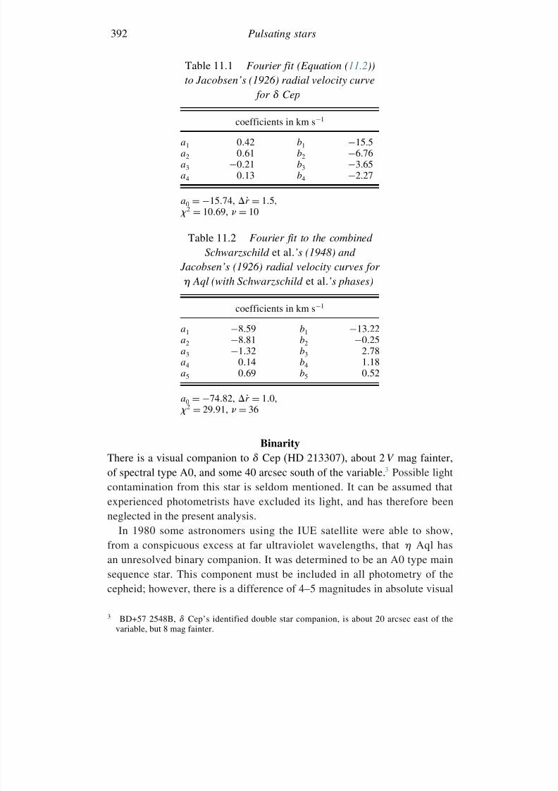
7/21/2019 Introduction to Astronomical Photometry
http://slidepdf.com/reader/full/introduction-to-astronomical-photometry 410/451
392 Pulsating stars
Table 11.1 Fourier fit (Equation (11.2))
to Jacobsen’s (1926) radial velocity curve
for Cep
coefficients in km s−1
a1 042 b1 −15.5a2 061 b2 −6.76a3 −021 b3 −3.65a4 013 b4 −2.27
a0 = −1574, r = 15,
2
= 1069, = 10
Table 11.2 Fourier fit to the combined
Schwarzschild et al.’s (1948) and
Jacobsen’s (1926) radial velocity curves for
Aql (with Schwarzschild et al.’s phases)
coefficients in km s−1
a1 −859 b1 −1322a2 −881 b2 −025a3 −132 b3 278a4 014 b4 118a5 069 b5 052
a0 = −7482, r = 10, 2 = 2991, = 36
Binarity
There is a visual companion to Cep (HD 213307), about 2 V mag fainter,of spectral type A0, and some 40 arcsec south of the variable.3 Possible lightcontamination from this star is seldom mentioned. It can be assumed thatexperienced photometrists have excluded its light, and has therefore beenneglected in the present analysis.
In 1980 some astronomers using the IUE satellite were able to show,from a conspicuous excess at far ultraviolet wavelengths, that Aql hasan unresolved binary companion. It was determined to be an A0 type mainsequence star. This component must be included in all photometry of thecepheid; however, there is a difference of 4–5 magnitudes in absolute visual
3 BD+57 2548B, Cep’s identified double star companion, is about 20 arcsec east of thevariable, but 8 mag fainter.
7/21/2019 Introduction to Astronomical Photometry
http://slidepdf.com/reader/full/introduction-to-astronomical-photometry 411/451
11.3 Six-colour data on classical cepheids 393
magnitude between the two stars, so that its effects can be at most a fewper cent in the G and I ranges. Indeed, its presence was not detected byearlier anomalous colour effect methods, so that neglect of it cannot be too
serious when judged against available photometric accuracy. The derivedcolour temperatures are presumably slightly high, and the required radii wouldbe incremented as a result, but any such variation is within the error arisingfrom other sources of uncertainty.
Optimal photometric parameters
The unreduced photometric data of Stebbins and his colleagues were analysed.
The standard deviation of a single observation is about 0.007 mag. This meansthat the colour determinations correspond to a standard deviation of 0.010,and from (11.17) we therefore expect colour-based luminosity predictions tobe accurate to within m = 0024 mag, neglecting the effect of observationalerrors on the derived radius variations. This quantity, used in the calculationof 2 =N
i=1mi − mci/m2, permits a 2 test on the feasibility of the fit.The comparison star used for Cep was Cep, while Aql was similarly
used for Aql. In order to convert known V apparent magnitudes to the Gscale, the formula G = V − 00099B − V was used. Taking V and B − V
values from the Arizona–Tonantzintla Catalog, we therefore find: G Cep =417 and G Aql = 364. The absolute magnitude of the Sun in the G filterwas similarly found to be 4.81.
With these preliminaries adopted, the results of optimal fittings to theobserved magnitudes are presented in Tables 11.3 and 11.4. Three sets of results are given for each star. These correspond to (i) the single brightnesstemperature hypothesis; (ii) being given by (11.11) and bI/bG
evaluated numerically from model stellar atmosphere data (0.945); and (iii) allowed to be a free parameter. Observed (circles) and calculated (crosses)G magnitudes of Cep and Aql are shown in Figures 11.4(a) and 11.5(a).
Probable errors have been assigned in Table 11.3 and 11.4 for the param-eters corresponding to cases (ii) and (iii). The large 2 value for case (i)demonstrates that this is an unrealistic model, so that formal errors would
here be clearly inappropriate. These errors were determined from the diagonalelements of the error matrix. The extent of correlation between and Rp0 canbe judged from the decreasing precision with which Rp0 is estimated whenwe allow to be a free parameter. In the case of Aql the optimal solutionwith free is only slightly different from the case (ii) solution. The sameis not true for Cep, where the model stellar atmosphere prediction of issignificantly different from the optimal solution.
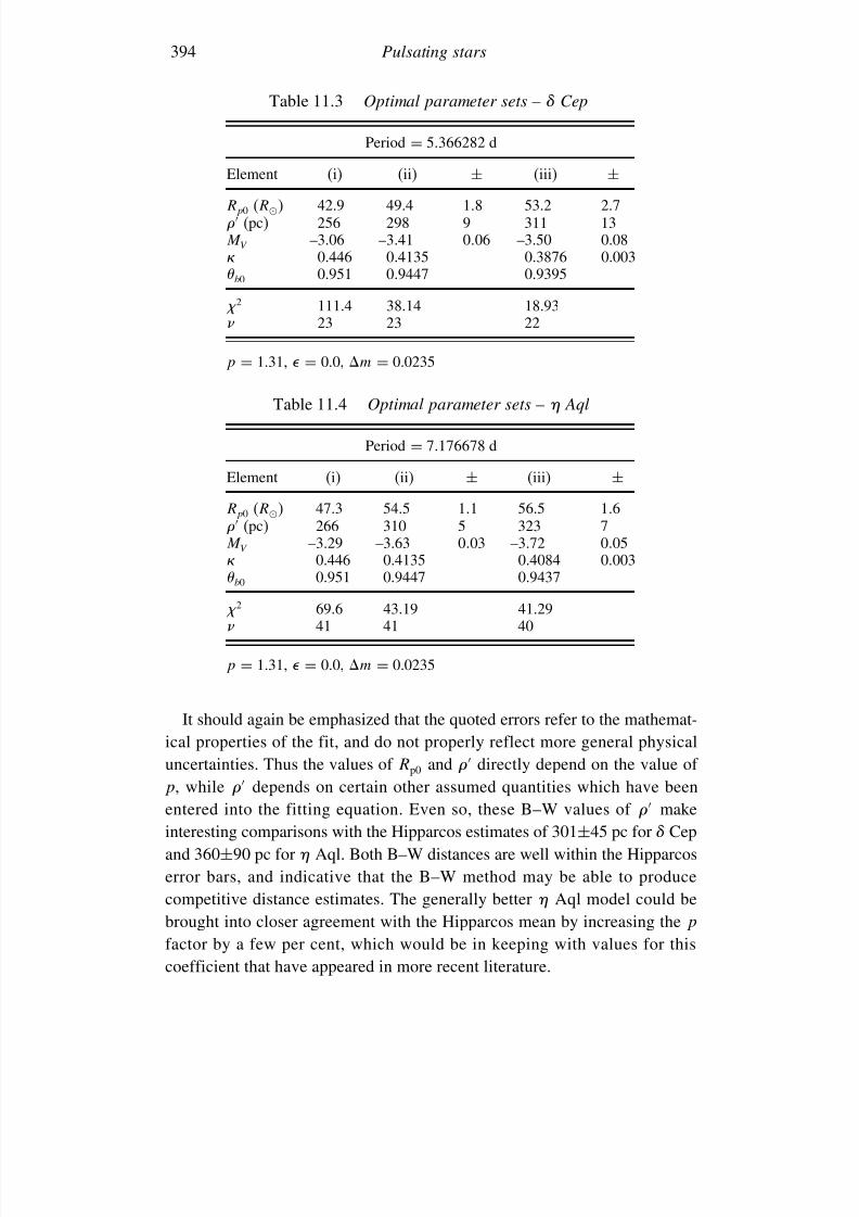
7/21/2019 Introduction to Astronomical Photometry
http://slidepdf.com/reader/full/introduction-to-astronomical-photometry 412/451
394 Pulsating stars
Table 11.3 Optimal parameter sets – Cep
Period = 5.366282 d
Element (i) (ii) ± (iii) ±Rp0 (R) 42.9 49.4 18 53.2 2.7 (pc) 256 298 9 311 13M V –3.06 –3.41 006 –3.50 0.08 0.446 0.4135 0.3876 0.003b0 0.951 0.9447 0.9395
2 111.4 38.14 18.93 23 23 22
p = 1.31, = 0.0, m = 0.0235
Table 11.4 Optimal parameter sets – Aql
Period = 7.176678 d
Element (i) (ii) ± (iii) ±Rp0 (R) 47.3 54.5 11 56.5 16 (pc) 266 310 5 323 7M V –3.29 –3.63 003 –3.72 005 0.446 0.4135 0.4084 0003b0 0.951 0.9447 0.9437
2 69.6 43.19 41.29 41 41 40
p = 1.31, = 0.0, m = 0.0235
It should again be emphasized that the quoted errors refer to the mathemat-ical properties of the fit, and do not properly reflect more general physicaluncertainties. Thus the values of Rp0 and directly depend on the value of p, while depends on certain other assumed quantities which have beenentered into the fitting equation. Even so, these B–W values of make
interesting comparisons with the Hipparcos estimates of 301±45 pc for Cepand 360±90 pc for Aql. Both B–W distances are well within the Hipparcoserror bars, and indicative that the B–W method may be able to producecompetitive distance estimates. The generally better Aql model could bebrought into closer agreement with the Hipparcos mean by increasing the p
factor by a few per cent, which would be in keeping with values for thiscoefficient that have appeared in more recent literature.
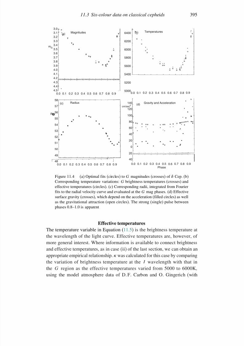
7/21/2019 Introduction to Astronomical Photometry
http://slidepdf.com/reader/full/introduction-to-astronomical-photometry 413/451
11.3 Six-colour data on classical cepheids 395
6400
6200
6000
5800
5600
5400
5200
5000
0.0 0.1 0.2
0.3 0.4 0.5 0.6 0.7 0.8 0.9
0.0 0.1 0.2 0.3 0.4 0.5 0.6 0.7 0.8 0.9 0.0 0.1 0.2 0.3 0.4 0.5 0.6 0.7 0.8 0.9
Magnitudes(a) Temperatures(b)
Phase
Gravity and Acceleration(d)140
120
100
80
60
40
200
20
40
cm/sec2Radius(c)
58
57
56
55
54
53
52
51
50
49
48
R
0.0 0.1 0.2 0.3 0.4 0.5 0.6 0.7 0.8 0.9
3.03.13.23.33.43.53.63.73.83.94.04.14.24.34.44.5
mG
Figure 11.4 (a) Optimal fits (circles) to G magnitudes (crosses) of Cep. (b)Corresponding temperature variations: G brightness temperatures (crosses) and
effective temperatures (circles). (c) Corresponding radii, integrated from Fourierfits to the radial velocity curve and evaluated at the G mag phases. (d) Effectivesurface gravity (crosses), which depend on the acceleration (filled circles) as wellas the gravitational attraction (open circles). The strong (single) pulse betweenphases 0.8–1.0 is apparent
Effective temperatures
The temperature variable in Equation (11.5) is the brightness temperature at
the wavelength of the light curve. Effective temperatures are, however, of more general interest. Where information is available to connect brightnessand effective temperatures, as in case (ii) of the last section, we can obtain anappropriate empirical relationship. was calculated for this case by comparingthe variation of brightness temperature at the I wavelength with that inthe G region as the effective temperatures varied from 5000 to 6000K,using the model atmosphere data of D. F. Carbon and O. Gingerich (with
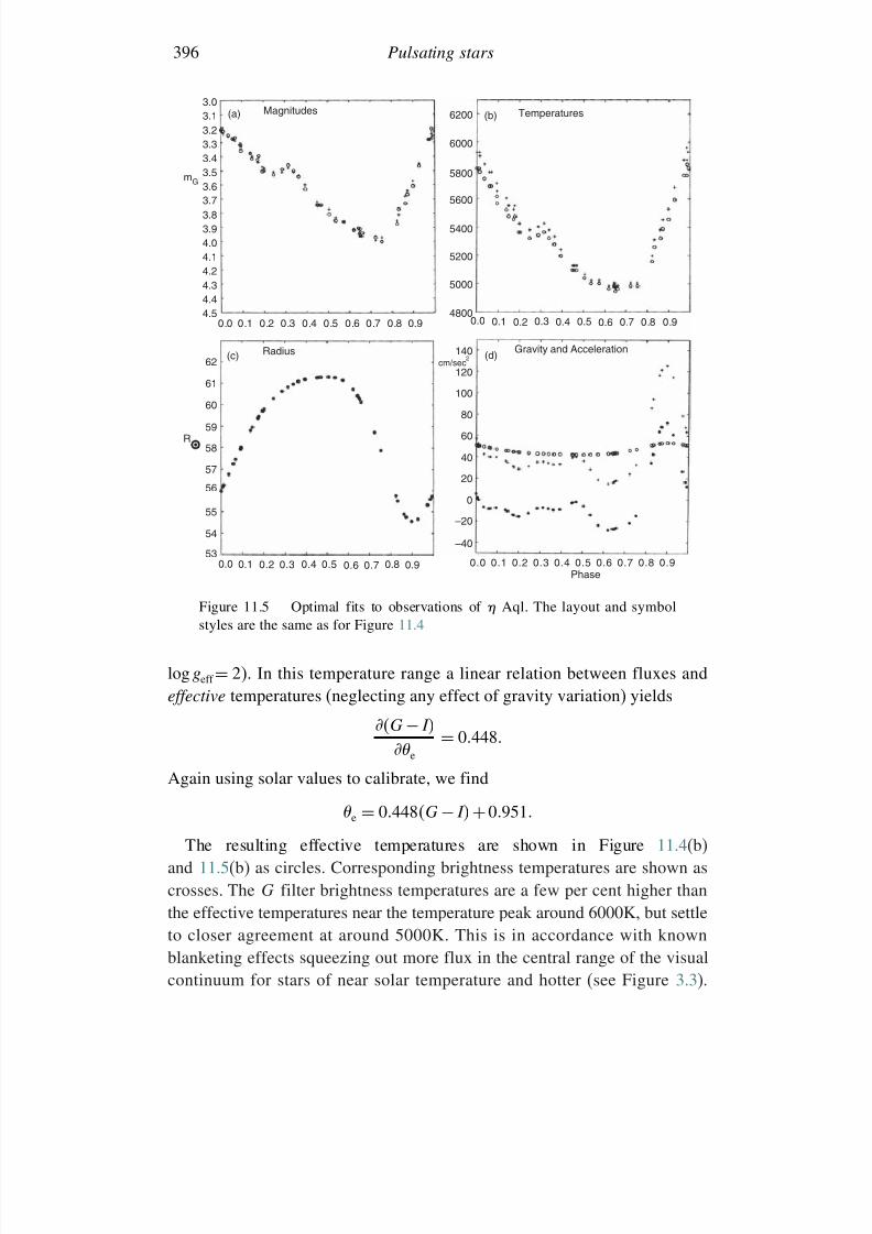
7/21/2019 Introduction to Astronomical Photometry
http://slidepdf.com/reader/full/introduction-to-astronomical-photometry 414/451
396 Pulsating stars
3.0Magnitudes(a)3.1
3.23.33.4
3.53.63.73.83.94.04.1
4.34.44.5
0.0 0.1 0.2 0.3 0.4 0.5 0.6 0.7 0.8
0.0 0.1 0.2 0.3 0.4 0.5 0.6 0.7 0.8
0.9 0.0 0.1 0.2 0.3 0.4 0.5 0.6 0.7 0.8 0.9
0.0 0.1 0.2 0.3 0.4 0.5 0.6 0.7 0.8 0.9
mG
Temperatures6200
6000
5800
5600
5400
5200
5000
4800
Gravity and Acceleration140
120
100
80
60
40
20
0–20
–40
(d)cm/sec
2
Phase
(c) Radius62
61
60
59
58
57
56
55
54
530.9
R
(b)
4.2
Figure 11.5 Optimal fits to observations of Aql. The layout and symbolstyles are the same as for Figure 11.4
log geff = 2). In this temperature range a linear relation between fluxes andeffective temperatures (neglecting any effect of gravity variation) yields
G − I
e
= 0448
Again using solar values to calibrate, we find
e = 0448G − I +0951
The resulting effective temperatures are shown in Figure 11.4(b)and 11.5(b) as circles. Corresponding brightness temperatures are shown ascrosses. The G filter brightness temperatures are a few per cent higher thanthe effective temperatures near the temperature peak around 6000K, but settleto closer agreement at around 5000K. This is in accordance with knownblanketing effects squeezing out more flux in the central range of the visualcontinuum for stars of near solar temperature and hotter (see Figure 3.3).
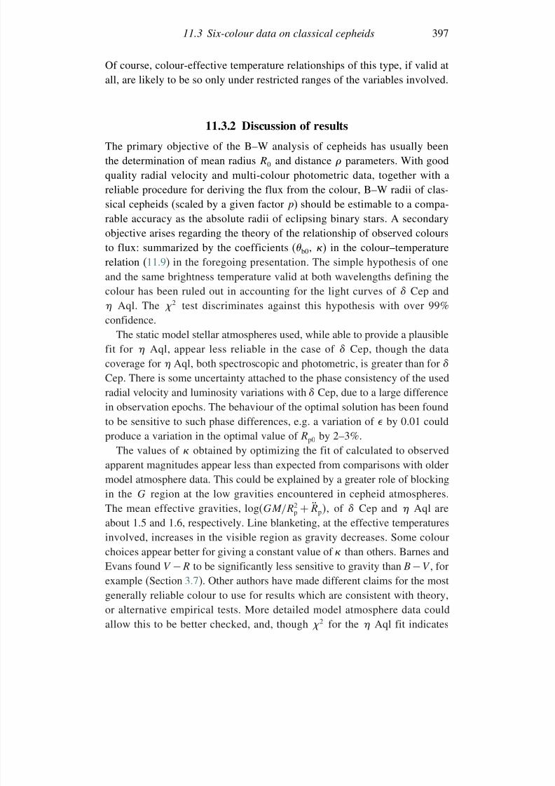
7/21/2019 Introduction to Astronomical Photometry
http://slidepdf.com/reader/full/introduction-to-astronomical-photometry 415/451
11.3 Six-colour data on classical cepheids 397
Of course, colour-effective temperature relationships of this type, if valid atall, are likely to be so only under restricted ranges of the variables involved.
11.3.2 Discussion of results
The primary objective of the B–W analysis of cepheids has usually beenthe determination of mean radius R0 and distance parameters. With goodquality radial velocity and multi-colour photometric data, together with areliable procedure for deriving the flux from the colour, B–W radii of clas-sical cepheids (scaled by a given factor p) should be estimable to a compa-
rable accuracy as the absolute radii of eclipsing binary stars. A secondaryobjective arises regarding the theory of the relationship of observed coloursto flux: summarized by the coefficients (b0, ) in the colour–temperaturerelation (11.9) in the foregoing presentation. The simple hypothesis of oneand the same brightness temperature valid at both wavelengths defining thecolour has been ruled out in accounting for the light curves of Cep and Aql. The 2 test discriminates against this hypothesis with over 99%
confidence.The static model stellar atmospheres used, while able to provide a plausible
fit for Aql, appear less reliable in the case of Cep, though the datacoverage for Aql, both spectroscopic and photometric, is greater than for
Cep. There is some uncertainty attached to the phase consistency of the usedradial velocity and luminosity variations with Cep, due to a large differencein observation epochs. The behaviour of the optimal solution has been foundto be sensitive to such phase differences, e.g. a variation of by 0.01 couldproduce a variation in the optimal value of Rp0 by 2–3%.
The values of obtained by optimizing the fit of calculated to observedapparent magnitudes appear less than expected from comparisons with oldermodel atmosphere data. This could be explained by a greater role of blockingin the G region at the low gravities encountered in cepheid atmospheres.The mean effective gravities, logGM/R2
p + Rp, of Cep and Aql areabout 1.5 and 1.6, respectively. Line blanketing, at the effective temperatures
involved, increases in the visible region as gravity decreases. Some colourchoices appear better for giving a constant value of than others. Barnes andEvans found V −R to be significantly less sensitive to gravity than B −V , forexample (Section 3.7). Other authors have made different claims for the mostgenerally reliable colour to use for results which are consistent with theory,or alternative empirical tests. More detailed model atmosphere data couldallow this to be better checked, and, though 2 for the Aql fit indicates
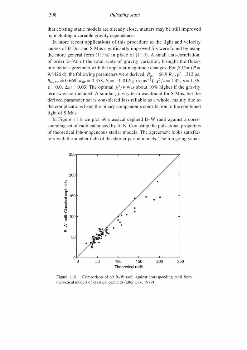
7/21/2019 Introduction to Astronomical Photometry
http://slidepdf.com/reader/full/introduction-to-astronomical-photometry 416/451
398 Pulsating stars
that existing static models are already close, matters may be still improvedby including a variable gravity dependence.
In more recent applications of this procedure to the light and velocity
curves of Dor and S Mus significantly improved fits were found by usingthe more general form (11.9a) in place of (11.9). A small anti-correlation,of order 2–3% of the total scale of gravity variation, brought the fluxesinto better agreement with the apparent magnitude changes. For Dor (P =98426 d), the following parameters were derived: Rp0= 669 R, = 312 pc,b0BV = 0669, BV = 0358 h1 = −0012g in ms−2), 2/= 142, p= 136,= 00, m= 003. The optimal 2/ was about 10% higher if the gravity
term was not included. A similar gravity term was found for S Mus, but thederived parameter set is considered less reliable as a whole, mainly due tothe complications from the binary companion’s contribution to the combinedlight of S Mus.
In Figure 11.6 we plot 69 classical cepheid B–W radii against a corre-sponding set of radii calculated by A. N. Cox using the pulsational propertiesof theoretical inhomogeneous stellar models. The agreement looks satisfac-tory with the smaller radii of the shorter period models. The foregoing values
0
50
100
150
200
250
0 50 100 150 200 250
B – W r
a d i i : C l a s s i c a l c e p
h e i d s
Theoretical radii
Figure 11.6 Comparison of 69 B–W radii against corresponding radii fromtheoretical models of classical cepheids (after Cox, 1979)
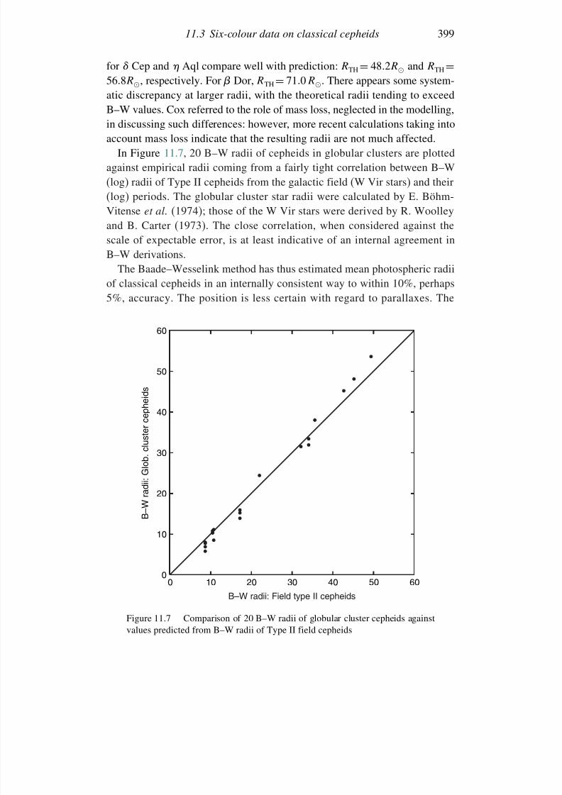
7/21/2019 Introduction to Astronomical Photometry
http://slidepdf.com/reader/full/introduction-to-astronomical-photometry 417/451
11.3 Six-colour data on classical cepheids 399
for Cep and Aql compare well with prediction: RTH = 482R and RTH =568R, respectively. For Dor, RTH= 710 R. There appears some system-atic discrepancy at larger radii, with the theoretical radii tending to exceed
B–W values. Cox referred to the role of mass loss, neglected in the modelling,in discussing such differences: however, more recent calculations taking intoaccount mass loss indicate that the resulting radii are not much affected.
In Figure 11.7, 20 B–W radii of cepheids in globular clusters are plottedagainst empirical radii coming from a fairly tight correlation between B–W(log) radii of Type II cepheids from the galactic field (W Vir stars) and their(log) periods. The globular cluster star radii were calculated by E. Böhm-
Vitense et al. (1974); those of the W Vir stars were derived by R. Woolleyand B. Carter (1973). The close correlation, when considered against thescale of expectable error, is at least indicative of an internal agreement inB–W derivations.
The Baade–Wesselink method has thus estimated mean photospheric radiiof classical cepheids in an internally consistent way to within 10%, perhaps5%, accuracy. The position is less certain with regard to parallaxes. The
0
10
20
30
40
50
60
0 10 20 30 40 50 60
B – W r
a d i i : G l o b . c l u s t e r c e p h e i d s
B–W radii: Field type II cepheids
Figure 11.7 Comparison of 20 B–W radii of globular cluster cepheids againstvalues predicted from B–W radii of Type II field cepheids
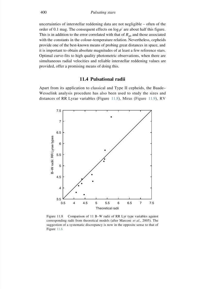
7/21/2019 Introduction to Astronomical Photometry
http://slidepdf.com/reader/full/introduction-to-astronomical-photometry 418/451
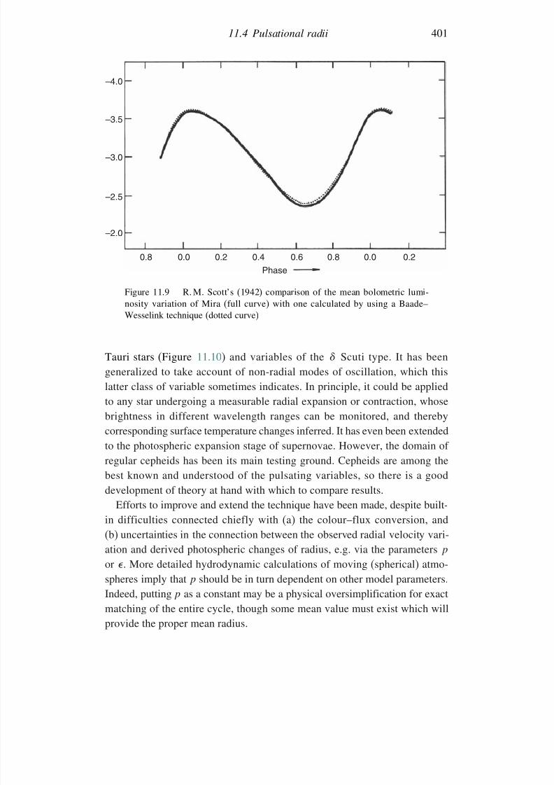
7/21/2019 Introduction to Astronomical Photometry
http://slidepdf.com/reader/full/introduction-to-astronomical-photometry 419/451
11.4 Pulsational radii 401
0.8 0.0 0.2 0.4 0.6 0.8 0.0 0.2
Phase
–4.0
–3.5
–3.0
–2.5
–2.0
Figure 11.9 R. M. Scott’s (1942) comparison of the mean bolometric lumi-nosity variation of Mira (full curve) with one calculated by using a Baade–Wesselink technique (dotted curve)
Tauri stars (Figure 11.10) and variables of the Scuti type. It has beengeneralized to take account of non-radial modes of oscillation, which thislatter class of variable sometimes indicates. In principle, it could be appliedto any star undergoing a measurable radial expansion or contraction, whosebrightness in different wavelength ranges can be monitored, and thereby
corresponding surface temperature changes inferred. It has even been extendedto the photospheric expansion stage of supernovae. However, the domain of regular cepheids has been its main testing ground. Cepheids are among thebest known and understood of the pulsating variables, so there is a gooddevelopment of theory at hand with which to compare results.
Efforts to improve and extend the technique have been made, despite built-in difficulties connected chiefly with (a) the colour–flux conversion, and
(b) uncertainties in the connection between the observed radial velocity vari-ation and derived photospheric changes of radius, e.g. via the parameters p
or . More detailed hydrodynamic calculations of moving (spherical) atmo-spheres imply that p should be in turn dependent on other model parameters.Indeed, putting p as a constant may be a physical oversimplification for exactmatching of the entire cycle, though some mean value must exist which willprovide the proper mean radius.
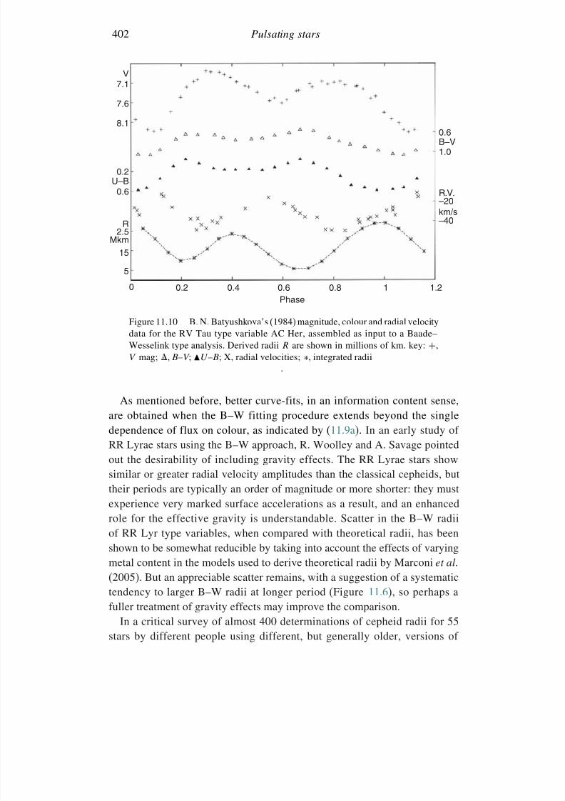
7/21/2019 Introduction to Astronomical Photometry
http://slidepdf.com/reader/full/introduction-to-astronomical-photometry 420/451
402 Pulsating stars
1.0
0 0.2 0.4 0.6 0.8 1 1.2
0.6
–20
–40
V
Phase
7.1
7.6
8.1
0.2U–B
0.6
R2.5
Mkm
15
5
B–V
R.V.
km/s
Figure 11.10 B. N. Batyushkova’s (1984) magnitude, colour and radial velocitydata for the RV Tau type variable AC Her, assembled as input to a Baade–Wesselink type analysis. Derived radii R are shown in millions of km. key: +,V mag; · B–VU –B; X, radial velocities; ∗, integrated radii
.
As mentioned before, better curve-fits, in an information content sense,are obtained when the B–W fitting procedure extends beyond the singledependence of flux on colour, as indicated by (11.9a). In an early study of RR Lyrae stars using the B–W approach, R. Woolley and A. Savage pointedout the desirability of including gravity effects. The RR Lyrae stars showsimilar or greater radial velocity amplitudes than the classical cepheids, buttheir periods are typically an order of magnitude or more shorter: they mustexperience very marked surface accelerations as a result, and an enhancedrole for the effective gravity is understandable. Scatter in the B–W radiiof RR Lyr type variables, when compared with theoretical radii, has been
shown to be somewhat reducible by taking into account the effects of varyingmetal content in the models used to derive theoretical radii by Marconi et al.
(2005). But an appreciable scatter remains, with a suggestion of a systematictendency to larger B–W radii at longer period (Figure 11.6), so perhaps afuller treatment of gravity effects may improve the comparison.
In a critical survey of almost 400 determinations of cepheid radii for 55stars by different people using different, but generally older, versions of
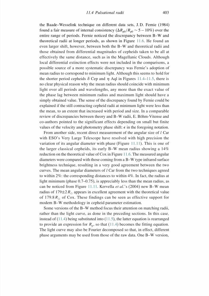
7/21/2019 Introduction to Astronomical Photometry
http://slidepdf.com/reader/full/introduction-to-astronomical-photometry 421/451
11.4 Pulsational radii 403
the Baade–Wesselink technique on different data sets, J. D. Fernie (1984)found a fair measure of internal consistency (Rp0/Rp0 ∼ 5 − 10%) over theentire range of periods. Fernie noticed the discrepancy between B–W and
theoretical radii at longer periods, as shown in Figure 11.6. He found aneven larger shift, however, between both the B–W and theoretical radii andthose obtained from differential magnitudes of cepheids taken to be all ateffectively the same distance, such as in the Magellanic Clouds. Althoughlocal differential extinction effects were not included in the comparisons, apossible source of a more systematic discrepancy was Fernie’s adoption of mean radius to correspond to minimum light. Although this seems to hold for
the shorter period cepheids Cep and Aql in Figures 11.4–11.5, there isno clear physical reason why the mean radius should coincide with minimumlight over all periods and wavelengths, any more than the exact value of the phase lag between minimum radius and maximum light should have asimply obtained value. The sense of the discrepancy found by Fernie could beexplained if the still contracting cepheid radii at minimum light were less thanthe mean, to an extent that increased with period and size. In a comparablereview of discrepancies between theory and B–W radii, E. Böhm-Vitense and
co-authors pointed to the significant effects depending on small but finitevalues of the velocity and photometry phase shift: in the foregoing notation.
From another side, recent direct measurement of the angular size of l Carwith ESO’s Very Large Telescope have resolved with high precision thevariation of its angular diameter with phase (Figure 11.11). This is one of the larger classical cepheids, its early B–W mean radius showing a 14%reduction on the theoretical value of Cox in Figure 11.6. The measured angular
diameters were compared with those coming from a B–W type infrared surfacebrightness technique, resulting in a very good agreement between the twocurves. The mean angular diameters of l Car from the two techniques agreedto within 2%: the corresponding distances to within 4%. In fact, the radius atlight minimum (phase 0.7–0.75), is appreciably less than the mean radius, ascan be noticed from Figure 11.11. Kervella et al.’s (2004) new B–W meanradius of 179±2 R appears in excellent agreement with the theoretical valueof 1798 R
of Cox. These findings can be seen as effective support for
modern B–W methodology in cepheid parameter estimation.Some versions of the B–W method focus their attention on matching radii,
rather than the light curve, as done in the preceding sections. In this case,instead of (11.4) being substituted into (11.5), the latter equation is rearrangedto provide an expression for Rp, so that (11.4) becomes the fitting equation.The light curve may also be Fourier decomposed so that, in effect, differentphase arguments may be used from those of the raw data. One B–W version,
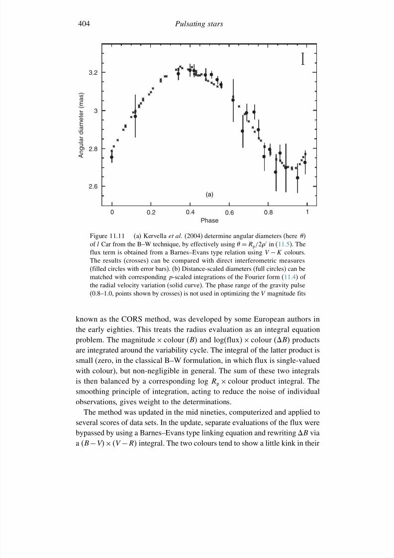
7/21/2019 Introduction to Astronomical Photometry
http://slidepdf.com/reader/full/introduction-to-astronomical-photometry 422/451
404 Pulsating stars
3.2
3
2.8
2.6
0 0.2 0.4 0.6 0.8 1Phase
A n
g u l a r d i a m e t e r ( m a s )
(a)
Figure 11.11 (a) Kervella et al. (2004) determine angular diameters (here )of l Car from the B–W technique, by effectively using = Rp/2 in (11.5). Theflux term is obtained from a Barnes–Evans type relation using V − K colours.The results (crosses) can be compared with direct interferometric measures(filled circles with error bars). (b) Distance-scaled diameters (full circles) can bematched with corresponding p-scaled integrations of the Fourier form (11.4) of the radial velocity variation (solid curve). The phase range of the gravity pulse(0.8–1.0, points shown by crosses) is not used in optimizing the V magnitude fits
known as the CORS method, was developed by some European authors inthe early eighties. This treats the radius evaluation as an integral equationproblem. The magnitude × colour (B) and log(flux) × colour (B) productsare integrated around the variability cycle. The integral of the latter product issmall (zero, in the classical B–W formulation, in which flux is single-valuedwith colour), but non-negligible in general. The sum of these two integrals
is then balanced by a corresponding log Rp × colour product integral. Thesmoothing principle of integration, acting to reduce the noise of individualobservations, gives weight to the determinations.
The method was updated in the mid nineties, computerized and applied toseveral scores of data sets. In the update, separate evaluations of the flux werebypassed by using a Barnes–Evans type linking equation and rewriting B viaa B −V×V −R integral. The two colours tend to show a little kink in their
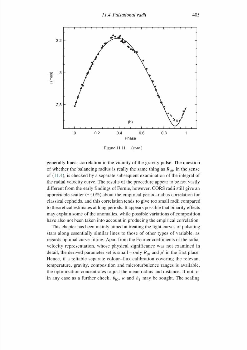
7/21/2019 Introduction to Astronomical Photometry
http://slidepdf.com/reader/full/introduction-to-astronomical-photometry 423/451
11.4 Pulsational radii 405
3.2
3
2.8
0 0.2 0.4Phase
θ
( m a s )
0.6 0.8 1
(b)
Figure 11.11 (cont.)
generally linear correlation in the vicinity of the gravity pulse. The questionof whether the balancing radius is really the same thing as Rp0, in the senseof (11.4), is checked by a separate subsequent examination of the integral of the radial velocity curve. The results of the procedure appear to be not vastlydifferent from the early findings of Fernie, however. CORS radii still give anappreciable scatter (∼10%) about the empirical period–radius correlation forclassical cepheids, and this correlation tends to give too small radii comparedto theoretical estimates at long periods. It appears possible that binarity effectsmay explain some of the anomalies, while possible variations of compositionhave also not been taken into account in producing the empirical correlation.
This chapter has been mainly aimed at treating the light curves of pulsatingstars along essentially similar lines to those of other types of variable, as
regards optimal curve-fitting. Apart from the Fourier coefficients of the radialvelocity representation, whose physical significance was not examined indetail, the derived parameter set is small – only Rp0 and in the first place.Hence, if a reliable separate colour–flux calibration covering the relevanttemperature, gravity, composition and microturbulence ranges is available,the optimization concentrates to just the mean radius and distance. If not, orin any case as a further check, b0, and h1 may be sought. The scaling
7/21/2019 Introduction to Astronomical Photometry
http://slidepdf.com/reader/full/introduction-to-astronomical-photometry 424/451
406 Pulsating stars
factor p cannot be separated out in the B–W procedure as presented: however,if high quality angular diameters, as well as magnitudes, colours and radialvelocities can be added to the simultaneous data set, as with the recent work
of Kervella et al., then p does become independently derivable. This new stepshould then allow empirically determined radii and distances for cepheid andsimilar stars to achieve comparable absolute reliability to those of eclipsingbinaries in the ‘eclipse method’.
11.5 Bibliographical notes
The book on Variable Stars by C. Hoffmeister, G. Richter and W.Wenzel (Springer-Verlag, 1984) provides a comprehensive backgroundto the physical variables considered in this chapter. Other general bookswhich could be referred to are S. Rosseland’s The Pulsation Theory of
Variable Stars (Clarendon Press, 1949), which has a nice chapter on theBaade–Wesselink technique; W. Strohmeier’s Variable Stars (PergamonPress, 1972); Pulsating Stars, ed. B.V. Kukarkin, Keter Publishing House,
Jerusalem, 1975); M. Petit’s Variable Stars (John Wiley, 1987); and W. A.Cooper & E.N. Walker’s book Getting the Measure of the Stars (AdamHilger, 1989).
At a more intensive level, J.P. Cox ( Rep. Prog. Phys., 37, 563, 1974)gives a full review of the linear theory of cepheid-like pulsating stars.The diagrams used in Figures 11.1–11.3 come from that paper. The journal is produced by the Institute of Physics Publishing and further
information is available from www.iop.org/journals/rop. Other sources areS. A. Zhevakin’s Theory of Stellar Pulsation (Leningrad University, 1957);R.F. Christy ( Ann. Rev. Astron. Astrophys., 4, 353, 1966) and A.N. Cox( Ann. Rev. Astron. Astrophys., 18, 15, 1980). More recent developments werecovered in the two reviews of A. Gautschy & H. Saio ( Ann. Rev. Astron.
Astrophys., 33, 75, 1995 & 34, 551, 1996).There were also various relevant proceedings of IAU meetings, including
Symp. 59, Stellar Instability and Evolution, eds. P. Ledoux, A. Noels &
A. W. Rodgers (Reidel, 1974); Colloq. 82, Cepheids: Theory and Observa-tion, ed. J. Madore (Reidel, 1985); Colloq. 111, The Use of Pulsating Stars in
Fundamental Problems of Astronomy, ed. E. G. Schmidt (Cambridge Univer-sity Press, 1989); Colloq. 139, New Perspectives on Stellar Pulsations and
Pulsating Variable Stars, eds. J. M. Nemec & J. M. Matthews (CambridgeUniversity Press, 1993); Colloq. 155, Astrophysical Applications of Stellar
Pulsation, eds. R. S. Stobie & P. A. Whitelock ( ASP Conf. Ser., 83, 1995); and
7/21/2019 Introduction to Astronomical Photometry
http://slidepdf.com/reader/full/introduction-to-astronomical-photometry 425/451
11.5 Bibliographical notes 407
Colloq. 176, The Impact of Large-Scale Surveys on Pulsating Star Research,eds. L. Szabados & D. Kurtz ( ASP Conf. Ser., 203, 2000).
The original reference on the period–luminosity relation is H. S. Leavitt
and E. C. Pickering ( Harv. Circ., 173, 1, 1912). The form cited comes fromM.W. Feast & R.M. Catchpole ( Mon. Not. Roy. Astron. Soc., 286, L1,1997). The classic treatment of A. S. Eddington was given in Mon. Not. Roy.
Astron. Soc. (87, 539, 1927). For recent work on Polaris, referring to overtonepulsation, see V. V. Kovtyukh et al. ( Astron. Astrophys., 401, 661, 2003) andD. G. Turner et al. (Publ. Astron. Soc. Pacific, 117, 207, 2005).
Among the large background of studies of the Baade–Wesselink tech-
nique are: W. Baade ( Astron. Nachr., 228, 359, 1926); K. F. Bottlinger( Astron. Nachr., 232, 3, 1928); W. Becker ( Z. Astrophys., 19, 219, 1940);A. van Hoof (Koninklijke Vlaamsche Acad. Weten., 5, No. 12, 1943);A. J. Wesselink ( Bull. Astron. Inst. Netherland , 10, 91, 1946); J. Grandjeanand P. Ledoux ( Ann. Astrophys., 17, 161, 1954); R. Cavanaggia & J.C.Pecker ( Ann. Astrophys., 18, 151, 1955); C. Whitney ( Astrophys. J., 121,682, 1955); J.B. Oke ( Astrophys. J., 133, 90 and 134, 214, 1961); N.R.Evans ( Astrophys. J ., 209, 135, 1976); L.A. Balona & R.S. Stobie ( Mon.
Not. Roy. Astron. Soc., 189, 659, 1979); B. Caccin et al. ( Astron. Astrophys.,97, 104, 1981); G. R. Ivanov ( Astrophys. Space Sci., 105, 369, 1984); R.B.Hindsley’s Ph.D. Thesis, University of Maryland, 1986; A. Gautschy (Vistas
Astron., 30, 197, 1987); N.R. Simon (Publ. Astron. Soc. Pacific, 99, 868,1987); T.J. Moffet (Proc. IAU Coll. 111, ed. E. G. Schmidt (CambridgeUniversity Press, 1989, p. 191); E. Boehm-Vitense et al. ( Astrophys. J ., 343,343, 1989); B. W. Carney et al. ( Astrophys. J., 386, 663, 1992); Z. Balog,
J. Vinko & G. Kaszas ( Astron. J., 113, 1833, 1997); G.P. Di Benedetto( Mem. Soc. Astron. Ital., 69, 271, 1998); G. Kovács ( Mon. Not. Roy. Astron.
Soc., 342, 58, 2003); J. Storm et al. ( Astron. Astrophys., 415, 531, 2004); &M. A. T. Groenewegen ( Mon. Not. Roy. Astron. Soc., 353, 903, 2004); andothers. The reference to hydrodynamic calculations and line doubling wasC. F. Keller & J. P. Mutschlecner ( Astrophys. J., 167, 127, 1971).
R.M. Scott ( Astrophys. J., 95, 58, 1942) compared radiometrically derived
radial variations of o Ceti by Pettit and Nicholson (see Chapter 3) with thosefrom the Baade–Wesselink technique (Figure 11.9). There has been muchsubsequent discussion on the best IR wavelength to use for reliable colourtemperatures for such cool stars. The subject was reviewed by R. F. Wingin The Study of Variable Stars Using Small Telescopes, ed. J.R. Percy(Cambridge University Press, 1986, p.127). Wing referred to Lockwood’sfilter system, which is noted also in Section 4.4.2.
7/21/2019 Introduction to Astronomical Photometry
http://slidepdf.com/reader/full/introduction-to-astronomical-photometry 426/451
408 Pulsating stars
The B–W technique was extended to RR Lyrae stars in the cited study byR. Woolley and A. Savage ( R. Obs. Bull., No 170, 365, 1971), and manypapers on this class of star have followed, including T. Liu & K. A. Janes
( Astrophys. J. Suppl., 69, 593, 1989); J. G. Cohen ( Astrophys. J., 400, 258,1992); J. Fernley ( Astron. Astrophys., 284, 16, 1994); G. Bono, F. Caputo& R. F. Stellingwerf ( Astrophys. J., 432, 51, 1994); T. E. Nordgren &GR. Schnider ( Astron. Astrophys. Suppl., 205, 540, 2004); as well as someof the references cited above. The study of W Virginis stars referred to inSection 11.4 is that of E. Böhm-Vitense ( Astrophys. J., 188, 571, 1974).
The particular treatment presented for illustration in Sections 11.2 and 11.3
derives from E. Budding ( Astrophys. Space Sci., 48, 249, 1977). The datastudied are from rather old sources (photometry – J. Stebbins, Astrophys.
J., 101, 47, 1945, J. Stebbins et al., Astrophys. J., 115, 292, 1952; radialvelocities – T. S. Jacobsen, Lick Obs. Bull., 12, 138, 1926; M. Schwarzschildet al., Astrophys. J., 108, 207, 1948); but the stars ( Cep and Aql) aresufficiently bright that a relatively high accuracy was obtainable even in theearly days of photometry and radial velocity curve derivation: sufficientlyaccurate to show some shortcomings in the simpler forms of the B–W proce-dure, as seen in the results. The radial velocities used for Dor came fromM.M. Taylor & A.J. Booth ( Mon. Not. Roy. Astron. Soc., 298, 594, 1998).S Mus was discussed by N. R. Evans et al. ( ASP Conf. Ser., 143, 309, 1998;eds. J.C. Brandt et al., p. 309). BV photometry of these stars was providedby H. Williams and W.S.G. Walker of the Photometric Section, RASNZ(New Zealand), and B–W analyses given in that organization’s Communique
(2, Nos. 2 & 3, 2001). The form of colour–temperature relation used harks
back to papers such as R. Cayrel ( Astrophys. J., 151, 997, 1968); and B.Pagel (Proc. IAU Symp., 26, 272, 1966), and these are essentially of the formdiscussed in Section 3.5.
The cited reviews of pulsational radii are from A. N. Cox ( Astrophys. J.,229, 212, 1979) (Figure 11.6); and J.D. Fernie ( Astrophys. J., 282, 641,1984). The compilation of Type II cepheid B–W radii (Figure 11.7) is fromE. Böhm-Vitense, P. Skody & G. Wallerstein ( Astrophys. J., 194, 125, 1974);
supplemented by the field W Vir radii of R. Woolley & B. Carter ( Mon. Not. Roy. Astron. Soc., 162, 379, 1973). The predicted and empirical radii of RRLyr stars (Figure 11.8) is from M. Marconi et al. ( Astrophys. J., 623, L133,2005). B. N. Batyushkova’s data for AC Her (Figure 11.10) come from IBVS
(No. 2505, 1984). P. Kervella et al.’s paper on l Car is in Astrophys. J. (604,L113, 2004). The CORS method was updated by V. Ripepi et al. ( Astron.
Astrophys., 318, 797, 1997).
7/21/2019 Introduction to Astronomical Photometry
http://slidepdf.com/reader/full/introduction-to-astronomical-photometry 427/451
References 409
References
Allen, C.W., 1973, Astrophysical Quantities, Athlone Press, London.Baade, W., 1926, Astron. Nachr., 228, 359.Balog, Z., Vinko, J. & Kaszas, G., 1997, Astron. J., 113, 1833.Balona, L. A. & Stobie, R. S., 1979, Mon. Not. Roy. Astron. Soc., 189, 659.Batyushkova, B. N., 1984, IBVS , No. 2505.Becker, W., 1940, Z. Astrophys., 19, 219.Böhm-Vitense, E., 1974, Astrophys. J., 188, 571.Böhm-Vitense, E., Skody P. & Wallerstein, G., 1974, Astrophys. J., 194, 125.Böhm-Vitense, E., Garnavich, P., Lawler, M., Mena-Werth, J., Morgan, S., Peterson,
E. & Temple, S., 1989, Astrophys. J ., 343, 343.
Bono, G., Caputo, F. & Stellingwerf, R. F., 1994, Astrophys. J., 432, 51.Bottlinger, K. F., 1928, Astron. Nachr., 232, 3.Budding, E., 1977, Astrophys. Space Sci., 48, 249.Caccin, R., Onnembo, A., Russo, G. & Sollazzo, C., 1981, Astron. Astrophys., 97,
104.Carney, B. W., Storm, J. & Jones, R. V., 1992, Astrophys. J., 386, 663.Cavanaggia, R. & Pecker, J. C., 1955, Ann. Astrophys., 18, 151.Cayrel, R., 1968, Astrophys. J., 151, 997.Christy, R. F., 1966, Ann. Rev. Astron. Astrophys., 4, 353.
Cohen, J. G., 1992, Astrophys. J., 400, 258.Cooper, W. A. & Walker, E. N., 1989, Getting the Measure of the Stars, Adam Hilger.Cox, A. N., 1979, Astrophys. J., 229, 212.Cox, A. N., 1980, Annu. Rev. Astron. Astrophys., 18, 15.Cox, J. P., 1974, Rep. Prog. Phys., 37, 563.Di Benedetto, G. P., 1998, Mem. Soc. Astron. Ital., 69, 271.Eddington, A. S., 1927, Mon. Not. Roy. Astron. Soc., 87, 539.Evans, N. R., 1976, Astrophys. J ., 209, 135.Evans, N. R., Böhm-Vitense, E., Beck-Winchatz, B., Carpenter, K. & Robinson, R.,
1998, ASP Conf. Ser. 143, eds. J. C. Brandt, T. B. Ake & C. C. Petersen, p. 309.Feast, M. W. & Catchpole, R. M., 1997, Mon. Not. Roy. Astron. Soc., 286, L1.Fernie, J. D., 1984, Astrophys. J., 282, 641.Fernley, J., 1994, Astron. Astrophys., 284, 16.Gautschy, A., 1987, Vistas Astron., 30, 197.Gautschy, A. & Saio, H., 1995, Ann. Rev. Astron. Astrophys., 33, 75.Gautschy, A. & Saio, H., 1996, Ann. Rev. Astron. Astrophys., 34, 551.Grandjean, J. & Ledoux, P., 1954, Ann. Astrophys., 17, 161.Groenewegen, M. A. T., 2004, Mon. Not. Roy. Astron. Soc., 353, 903.
Hindsley, R. B., 1986, An Investigation of Cephei Variable Stars Using Hydrostatic
Model Atmospheres, Ph.D. Thesis, University of Maryland.Hoffmeister, C., Richter, G. & Wenzel, W., 1984, Variable Stars, Springer-Verlag.Ivanov, G. R., 1984, Astrophys. Space Sci., 105, 369.Jacobsen, T. S., 1926, Lick Obs. Bull., 12, 138.Keller C. F. & Mutschlecner, J. P., 1971, Astrophys. J., 167, 127.Kervella, P., Fouqué, P., Storm, J., et al., 2004, Astrophys. J., 604, L113.Kovács, G., 2003, Mon. Not. Roy. Astron. Soc., 342, 58.
7/21/2019 Introduction to Astronomical Photometry
http://slidepdf.com/reader/full/introduction-to-astronomical-photometry 428/451
410 Pulsating stars
Kovtyukh, V.V., Andrievsky, S.M., Luck, R.E. & Gorlova, N.I., 2003, Astron.
Astrophys., 401, 661.Kukarkin, B. V., ed., 1975, Pulsating Stars, Keter Publishing House.Leavitt, H. S. & Pickering, E. C., 1912, Harv. Circ., 173, 1.Ledoux, P., Noels, A. & Rodgers, A. W., eds., 1974, Symp. 59, Stellar Instability and
Evolution, Reidel.Liu, T. & Janes, K. A., 1989, Astrophys. J. Suppl., 69, 593.Madore, J., ed., 1985, Colloq. 82, Cepheids: Theory and Observation, Reidel.Marconi, M., Nordgren, T., Bono, G., Schnider, G. & Caputo, F., 2005, Astrophys. J.,
623, L133.Moffet, T. J., 1989, Proc. IAU Coll. 111, ed. E. G. Schmidt, Cambridge University
Press, p. 191.
Nemec, J. M. & Matthews, J. M., 1993, IAU Colloq. 139, Cambridge University Press.Nordgren, T. E. & Schnider, G. R., 2004, Astron. Astrophys. Suppl., 205, 540.Oke, J. B., 1961a, Astrophys. J., 133, 90.Oke, J. B., 1961b, Astrophys. J., 134, 214.Pagel, B., 1966, Proc. IAU Symp. 26, 272.Petit, M., 1987, Variable Stars, John Wiley.Ripepi, V., Barone, F., Milano, L. & Russo, G., 1997, Astron. Astrophys., 318, 797.Rosseland, S., 1949, The Pulsation Theory of Variable Stars, Clarendon Press.Schmidt, E.G., ed., 1989, IAU Colloq. 111, Cambridge University Press.
Schwarzschild, M., Schwarzschild, B. & Adams, W. S., 1948, Astrophys. J., 108, 207.Scott, R. M., 1942, Astrophys. J., 95, 58.Simon, N. R., 1987, Publ. Astron. Soc. Pacific, 99, 868.Stebbins, J., 1945, Astrophys. J., 101, 47.Stebbins, J., Kron, G. E. & Smith, J. L., 1952, Astrophys. J., 115, 292.Stobie, R. S. & Whitelock, P. A., 1995, IAU Colloq. 155, ASP Conf. Ser., 83.Storm J., Carney, B. W., Gieren, W. P., Fouqué, P., Latham, D. W. & Fry, A. M., 2004,
Astron. Astrophys., 415, 531.Strohmeier, W., 1972, Variable Stars, Pergamon Press.
Szabados, L. & Kurtz, D., 2000, Colloq. 176 ., ASP Conf. Ser., 203.Taylor, M. M. & Booth, A. J., 1998, Mon. Not. Roy. Astron. Soc., 298, 594.Turner, D. G., Savoy, J., Derrah, J., Abdel-Sabour, A.-L. M. & Berdnikov, L. N., 2005,
Publ. Astron. Soc. Pacific, 117, 207.Van Hoof, A., 1943, Koninklijke Vlaamsche Acad. Weten., 5, No. 12.Wesselink, A. J., 1946, Bull. Astron. Inst. Netherland , 10, 91.Whitney, C., 1955, Astrophys. J., 121, 682.Williams, H., Walker, W. S. G. & Budding, E., 2001, Photom. Section, RASNZ, Comm.,
2, Nos. 2 & 3.
Wing, R. F., 1986, The Study of Variable Stars Using Small Telescopes, ed. J. R. Percy,Cambridge University Press, p. 127.
Woolley, R. & Carter, B., 1973, Mon. Not. Roy. Astron. Soc., 162, 379.Woolley, R. & Savage, A., 1971, R. Obs. Bull., No. 170, 365.Zhevakin, S. A., 1957, Theory of Stellar Pulsation, Leningrad.
7/21/2019 Introduction to Astronomical Photometry
http://slidepdf.com/reader/full/introduction-to-astronomical-photometry 429/451
Appendix
Frequently encountered constants
A few very commonly met with numbers are listed here. Information on math-ematical constants can be found in, e.g., M. Abramowitz and I. A. Stegun’s
Handbook of Mathematical Functions, Dover Publications, 1964. Much moreof the relevant physical and astronomical data can be located in, e.g., C. W.
Allen’s Astrophysical Quantities, 4th edition, 2000, ed. A. N. Cox, AIP Press;G. W. C. Kaye and T. H. Laby’s Tables of Physical and Chemical Constants,Longman, 1986; or the website physics.nist.gov/cuu/Constants/index.html.
Mathematical
3141 592 653 589793 238 462 643/2 1570 796 326 794896 619 231 322
√ 1772 453 850 905516 027 298 1671 radian 57295 779 513 082320 876 798 155e 2718 281 828 459055 235 360 28725log10e 1085 736 204 758129 569 127 822
Physical
Velocity of light c 2997924580
×108 m s−1
Planck’s constant h 6626069×10−34 J sBoltzmann’s constant k 1380651× 10−23 J K−1
Gravitational constant G 6674× 10−11 N m2 kg−2
Electron charge e− 1602177× 10−19 CElectron mass me 9109383×10−31 kgElectron magnetic moment e 928476400 × 10−24 J T−1
Proton mass mp 167262171 × 10−27 kg
411
7/21/2019 Introduction to Astronomical Photometry
http://slidepdf.com/reader/full/introduction-to-astronomical-photometry 430/451
412 Appendix
Unit atomic weight 1660539 ×10−27 kgRadius of first Bohr orbit a0 5291772 ×10−11 mEnergy of 1 eV E 0 1602177
×10−19 J
Corresponding frequency 0 2417989 ×1014 HzCorresponding wavelength 0 1239842 ×10−6 mCorresponding temperature E 0/k 116045 KPhoton energy of wavelength 1986446× 10−25/ J
1239841× 10−6/ eV
Astronomical
Astronomical unit (AU) 149597870 ×1011
m214.94 solar radiiTropical year 315569252× 107 s
365.242 2 mean solar daysSidereal year 315581498 × 107 sMean radius of Earth 637101× 106 mLight year 946053× 1015 mParsec (pc) 3085678
×1016 m
Mass of Sun M 1989×1030 kgRadius of Sun R 69598× 108 mLuminosity of Sun L 3827×1026 WSun’s visual magnitude mv −2675 ≡ 125×105 lxSun’s bolometric magnitude mbol −2682 ≡ 1365Wm−2
Magnitude zero U 286×10−9 B 645×10−9
V 314× 10−9, bol 255× 10−8 W m−2
Mean mags. of Vega U 003 B 003 V 003Parallax of Vega 0.129 arcsecMinimum sky brightness (V)1 25× 10−9 W m−2 sr−1
1 Extragalactic background light in direction of galactic pole.

7/21/2019 Introduction to Astronomical Photometry
http://slidepdf.com/reader/full/introduction-to-astronomical-photometry 431/451
Author index
Aarseth, A. J., 275Abhyankar, K. D., 305Abramowitz, M., 411Achterberg, H., 285, 304Adelmann, S. J., 244Afsar, M., 371Akimov, L. K., 155Al Naimiy, H. M. K., 276
Albayrak, B., 371Alexander, M. E., 274Allen, C., 274Allen, C. W., 36, 68, 152, 411Aller, Lawrence, 155Alvarez, R., 109, 153Andersen, J., 337Anderson, L., 336Andreon, S., 156Andrews, F. P., 36Applegate, J. H., 306Arago, François, 19Ardabili, Y. R., 336
Baade, W., 407Baierlein, R., 36Baily, F., 34Bakis, Hicran, 224nBakis, V., 274, 307
Baliunas, S., 370Ballard, S. A., 140, 156Balog, Z., 407Balona, L. A., 100, 153, 407Banks, T., 155Bappu, M. K. V., 153Barden, S. C., 307Barnes, J. V., 96–7, 153Barnes, T. G., 64–5, 68
Bartholdi, P., 154Bartolini, C., 307Barucci, M. A., 156Bateson, F. M., 34Batten, A. H., 273Battistini, P., 241, 244Batyushkova, B. N., 402, 408Bayer, Johann, 17
Becker, W., 35, 86, 152, 407Bedding, T., 152Bergeat, J., 305Berry, R., 200Bertelli, G., 153Bessell, M. S., 68–9, 243–4Bevington, P. R., 272, 321Biermann, P., 306Binzel, R. P., 156
Blackwell, D. E., 69Blanco, C., 370Blow, G. L, 69Bode, M. F., 244Böhm-Vitense, E., 69, 399, 403, 407–8Boksenberg, A., 201Bolton, C. T., 306Boltzmann, L., 42, 68Bone, D. A., 201Bonifazi, A., 241, 244
Bono, G., 408Bookbinder, J., 370Booth, A. J., 152, 408Bopp, B. W., 349–51, 370Borkovits, T., 305Bosch, G., 132, 156Bottke, W. F., Jr., 156Bottlinger, K. F., 407Bouguer, Pierre, 17, 19, 35
413
7/21/2019 Introduction to Astronomical Photometry
http://slidepdf.com/reader/full/introduction-to-astronomical-photometry 432/451
414 Author index
Bowers, R. L., 274Boyd, Louis, 8Bozkurt, Z., 292, 305Bracewell, R. N., 157
Bradstreet, D. H., 306, 371Brandt, J. C., 408Brault, J. W., 154Bregman, J. D., 157Brown, J. C., 156, 273, 372Brown, T. M., 10Budding, E., 35, 70, 153, 155, 157, 201, 244,
274–6, 305–6, 335–7, 349, 350, 364–6,370–3, 408
as ‘present authors,’ 273Buil, C., 200Bulut, I., 274Buratti, B. J., 124, 127, 155Burnell, J., 200Burnet, M., 154Burt, D. J., 200Butler, C. J., 35, 243–4, 370Byrne, P. B., 370, 372
Caccin, B., 407Cameron, A. C. See Collier Cameron, A.Caplan, J., 156Caputo, F., 408Carbon, D. F., 276, 395Carney, B. W., 407Carstensen, E., 337Carter, B., 399, 408Castelli, F., 68
Catchpole, R. M., 407Cavanaggia, R., 407Cayrel, R., 408Cayrel de Strobel, G., 68Cellino, A., 156Chambliss, C. R., 306Chandler, S. C., 305Cherepashchuk, A. M., 154, 273, 337Chisari, D., 335Chiu, H.-Y., 153
Choea, S. H., 336Chong, E. K. P., 272Christy, R. F., 406Ciçek, C., 274Cinzano, P., 155Claret, A., 276, 336Clausen, J. V., 275, 337Code, A. D., 69, 102, 153Cohen, J. G., 408
Cohen, R. J., 154Colina, L., 68Collar, A. R., 151Collier Cameron, A., 354–6, 371
Connon-Smith, R., 336Cooper, W. A., 242, 406Cousins, A. J., 243Cousins, A. W. J., 205, 243–4Cox, A. N., 68, 152, 398–9, 403, 406, 408,
411Cox, J. P., 406Craig, I. J. D., 273, 372Crawford, D. L., 92, 95–7, 104, 105, 152–4Crawford, J. A., 305
Davis, J., 152Davis Phillip, A. G., 152De Boere, K. S., 275De Cusatis, C., 68de Souza, R. E., 156de Vaucouleurs, A., 134de Vaucouleurs, G., 134, 156Deeming, T., 274
Degirmenci, O. L., 292, 305Deharveng, L., 156Demircan, O., 307, 337
as ‘present authors’, 273Devinney, E. J., 317, 337Di Benedetto, G. P., 69, 407Dickow, P., 110, 153Djorgovski, S., 156Djurasevic, G., 336Dodd, R. J., 36Dokuchaev, V. I., 274Donahue, R. A., 370Draine, B. T., 151Drechsel, H., 306Dresner, S., 68Duerbeck, H. W., 322, 336Duffet-Smith, P., 222n, 244Duncan, W. J., 151Dupree, A. K., 306
Dusek, J., 305
Eaton, J. A., 322, 336Eberhard, G., 35Eccles, M. J., 201Eddington, A. S., 383, 407Eggen, O. J., 306Eiby, G., 24n, 35El-Worfaly, H. M. H., 275

7/21/2019 Introduction to Astronomical Photometry
http://slidepdf.com/reader/full/introduction-to-astronomical-photometry 433/451
Author index 415
Elias, N. M., 157Ellery, L., 36Elliott, I., 243–4Elston, R., 243
Elvidge, C. D., 155Emslie, A. G., 156Erdem, A., 274Estalella, R., 157Evans, D. S., 64–5, 68, 156, 349–51,
370Evans, N. R., 407–8
Fabian, A. C., 274
Fabricius, David, 2, 16Fabry, C., 21Feast, M. W., 407Fechner, G. T., 19Fehrenbach, C., 152Fernie, J. D., 153, 403, 405, 408Fernley, J., 408Finlay-Carling, E. B., 305Fisher, W. A., 306Fitch, W. S., 304, 370
Fitzgerald, G. F., 23Fitzpatrick, E. L., 275Florkowski, D. R., 273Flower, D. R., 156Forbes, M. C., 153, 202, 274Fordham, J. L. A., 201Fracastoro, M. G., 250, 273Frazer, R. A., 151Frieboes-Conde, H., 305Friedjung, M., 274Fukuda, I., 306Fukugita, M., 152
Gamal El Din, A. I., 134, 156Gaposchkin, S. L., 275Garstang, R., 154Gautschy, A., 406–7Gehrels, T., 156Genet, D. R., 201
Genet, K. A., 201Genet, R. M., 8, 35, 201Ghedini, S., 242, 245Gibson, D. M., 371Giménez, A., 275, 337Gingerich, O., 276, 395Goecking, K. D., 306Golay, M., 9, 25n, 69, 89, 151–2Goncharskii, A. V., 273, 337
Gonzalez Jorge, H., 244Good, G. A., 9Gordon, K. C., 335Gould, A., 36
Graham, J. A., 275Grandjean, J., 407Gray, H. J., 36Greenstein, J. L., 153Grewing, M., 371Groenewegen, M. A. T., 407Grosbøl, P., 156Grygar, J., 338Grynko, Y. S., 155
Guarnieri, A., 241, 244Guenther, E., 256nGuinan, E. F., 275, 306Gunn, J. E., 102, 152–3Guthrie, B. N. G., 336Gyldenkerne, K., 337
Hadrava, P., 337Hagen, J. G., 303Haken, H., 36
Hall, D. S., 8–9, 35, 244, 289, 304, 306, 348,361, 370
Hamaker, J. P., 157Hamamura, S., 155Hapke, B., 155Hardie, R. H., 35, 134, 155, 242–3Harmanec, P., 70Harries, T. J., 336Harris, D. L., 68
Hartley, H. O., 267Hartmann, L., 152Hatzes, A. P., 371Hauck, B., 68, 152Hayes, D. S., 69, 151–2, 201Hayli, A., 274Hearnshaw, J. B., 34Heckert, P. A., 371Hegedüs, T., 305Heggie, D. C., 275
Helt, B. E., 337Henden, A. A., 8, 10, 192, 200–2,
242–3Henry, G. W., 244Héraudeau, Ph., 156Herbig, G. H., 151Herczeg, T., 305Hertzsprung, E., 66Heudier, J. L., 35

7/21/2019 Introduction to Astronomical Photometry
http://slidepdf.com/reader/full/introduction-to-astronomical-photometry 434/451
416 Author index
Hilditch, R. W., 275, 336, 371Hill, G., 306, 336–7Hills, J. G., 274Hiltner, W. A., 201, 242
Hindsley, R. B., 407Hoffleit, D., 206nHoffmeister, C., 273Hofsommer, D. J., 266n, 406Hogg, H. S., 274Holmgren, D., 306Holst, G. C., 201Holzwarth, V., 372Honeycutt, R. K., 338Horak, B., 338Hosokawa, Y., 336Howell, S. B., 201Hoyle, F., 305Hrivnak, B. J., 306Huang, S. S., 306Hubble, E., 156Husar, D., 285, 304Hut, P., 274–5
Ibanoglu, C., 307, 371Ilyas, M., 155Inagaki, S., 275Irvine, W. M., 155Irwin, J. B., 276Isaacs, A., 36Isobe, S., 155Ivanov, G. R., 407Ivanova, N., 275
Jacobsen, T. S., 391–2, 408Janes, K. A., 408Janesick, J. R., 201Janszoon Blaue, W., 16–17Järvinen, S. P., 372Jaschek, C., 9, 151, 206nJaschek, M., 9, 151Jassur, D. M. Z., 371Jeans, J. H., 68
Jeffers, S. V., 372Jeffreys, H., 335Jensen, K. S., 275Jimenez, A., 244Johnson, Howard L., 25, 35, 69, 89, 152, 164.
See also UBV systemJones, A., 9Jones, D. H. P., 154Jorden, A. R., 201
Jørgensen, H. E., 337Joy, A. H., 306
Kahn, F. D., 70Kaitchuk, R. H., 8, 10, 192, 200–2, 242–3Kaler, J. A., 155Kallrath, J., 337Kang, Y. W., 336Kanto, V., 200Kapteyn, J. C., 22Kasten, F., 75, 151Kaszas, G., 407Katz, J. I., 274
Kaye, G. W. C., 411Keenan, P. C., 81Keller, C. F., 407Kellman, E., 81Kemp, J. C., 144, 157Kenyon, S. J., 152Kermani, M. H., 371Kervella, P., 403–4, 406, 408Khan, M. A., 337Kholopov, P. N., 222n
Kikuchi, S., 338Kilkenny, D., 115, 154, 243Kim, C.-H., 301, 305King, I., 156Kitamura, M., 325, 337Kitchin, C., 243Kiurchieva, D. P., 336Kiyokawa, M., 338Kjurkchieva, D. P., 371
Knapp, G. R., 152Knobel, E., 15, 34Koch, R. H., 273Kochiashvili, N. T., 336Koen, C., 287, 304Koestler, A., 35Kollath, Z., 372Kondo, Y., 274Kong, J. A., 156Kopal, Z., 35, 155, 266n, 275–6, 305, 325,
327, 335–6Kordylewski, Z., 305Kormandy, J., 156Kourganoff, V., 68Kovács, G., 407Kovtyukh, V. V., 407Kowalski, R., 155Kraft, R. P., 305Kraicheva, Z. T., 273

7/21/2019 Introduction to Astronomical Photometry
http://slidepdf.com/reader/full/introduction-to-astronomical-photometry 435/451
Author index 417
Kreiner, J. M., 301, 305Krolik, J. H., 274Kron, Gerald E., 24, 35, 260–1, 267, 269,
272, 320, 335, 341
Kron, R. G., 152Kuiper, G. P., 68, 290, 305Kukarkin, B. V., 406Kurtz, D. W., 70, 244, 371, 407Kuulkers, E., 274Kuznetsova, E. F., 273, 307Kwee, K. K., 244
Labs, D., 68
Laby, T. H., 411Lacy, C. H., 65, 276, 307Lago, M. T. V. T., 306Lallemand, A., 35, 201Landolt, A. U., 204, 243Lang, K. R., 156, 305Lanz, T., 152Lanza, A. F., 307, 371Latham, D. W., 151Leavitt, H. S., 378, 407
Ledoux, P., 406–7Lee, R. B., 68Lee, S. W., 244Leene, A., 156Léna, P., 36, 201Lester, T. P., 155Leung, Kam-Ching, 305Lindblad, B., 108, 153Linskey, J. L., 370–2Lipaeva, N. A., 154Lister, T. A., 371Liu, T., 408Livio, M., 274Lockwood, G. W., 108–9, 153Lodén, K., 152Lodén, L. O., 152Lombard, F., 287, 304Lorenz, R., 307Lubow, S. H., 338
Lucy, L. B., 336Ludendorff, H, 35Lundmark, K., 35Lynas-Gray, A. E., 69
Maceroni, C., 305, 306MacGillivray, H. T., 36Mackay, C. D., 200Madore, J., 406
Makarova, E. A., 68Mander, J., 104, 153Manfroid, J., 8, 200, 244Marchev, D. V., 371
Marconi, M., 400, 408Marngus, N., 153, 337Matese, J. J., 306Mathieu, R. D., 274Matthews, J. M., 406Matthews, M. S., 156Mauder, H., 325, 336Mayer, P., 307Mazeh, T., 10
McCall, M. L., 155McClain, Bill, 244McGraw, J. T., 112, 154Mclean, I. S., 156, 200McNally, D., 154Meaburn, J., 201Meeks, M. L., 151Meeus, J., 244Menzies, J. W., 243Merrill, J. E., 261–3, 275
Mestel, L., 305Meylan, G., 275Mikulasek, Z., 244Milone, E. F., 152, 337Minnaert, M., 34Mitchell, John, 18–19, 35Mizser, A., 304Moffatt, A. F. J., 307Moffett, T. J., 68, 407Monck, W. H. S., 23
Moon, T. T., 153Mordvinor, A. V., 68Morgan, W. W., 25, 81Moutsoulas, M., 155Muinonen, K., 156Mullan, D. J., 370, 372Munger, J., 200Mutschlecner, J. P., 407
Nail, V. M., 275Najim, N. N., 335Nakamura, Y., 336Napier, W. M., 336Nather, R. E., 111, 154Neckel, H., 68Neild, K. M., 202Nemec, J. M., 406Neugebauer, G., 152

7/21/2019 Introduction to Astronomical Photometry
http://slidepdf.com/reader/full/introduction-to-astronomical-photometry 436/451
418 Author index
Nha, I.-S., 301, 305Niarchos, P., 337Nicholson, S., 52–3, 68, 171Nicolet, B., 152
Noels, A., 406Nomoto, K., 336Nordgren, T. E., 408Nordström, B., 337
O’Connell, D. J. K., 315, 335Oja, T., 244Oke, J. B., 102, 153, 407Okomoto, I., 305
Oláh, K., 304, 357 , 371–2Olbers, H. W. M., 116, 154Oliver, C. J., 201Oliver, J. P., 273Olson, E. C., 305, 334, 335, 337Oswalt, T. D., 9Ozernoi, L. M., 274
Pagel, B., 408Palmer, S. E., 34
Panchatsaram, T., 305Paolicchi, P., 156Pasinetti, L. E., 152Patsis, P. A., 156Patterson, J., 306Pearson, E. S., 267Pecker, J. C., 407Peña, J. H., 100, 153Peniche, R., 100, 153
Penrod, G. D., 371Percy, J. R., 9, 407Periaiah, A., 336Persha, G., 243Pervozkina, E. L., 273Peters, G. J., 338Petit, M., 406Pettit, E., 52–3, 68, 171Pickering, E. C., 20–2, 407Piotrowski, S. L., 305
Piskunov, N. E., 372Planck, Max, 42, 68Plavec, M. J., 274, 337Plez, B., 68, 109, 153Pogson, N. R., 19Poincaré, H., 335Polidan, R. S., 274Popper, D. M., 65–6, 69–70, 274, 307, 337,
368–9, 371
Poretti, E., 244Pottasch, S. R., 156Press, W. H., 154, 273–4Pribulla, T., 371
Pringle, J. E., 273–4Pustyl’nik, I. B., 336
Qian, S., 305
Rabello-Soares, M. C., 244Radhika, P., 371Ramsey, L. W., 370Rayleigh, Lord (J. W. Strutt), 68
Reay, N. K., 156Rees, M. J., 274Reisenweber, R. C., 9Remo, J. L., 153Reynolds, J. H., 156Rhodes, M., 244, 318, 372Ribárik, G., 371Ribas, I., 275Richard, J., 201Richards, J. A., 43n
Richards, M. T., 338Richter, G., 273, 406Ripepi, V., 408Robinson, E. L., 112, 154Rodgers, A. W., 406Rodonò, M., 307, 335, 370, 372Romanov, S. Y., 273Ronan, C. A., 35Rosner, R., 307Rosseland, S., 406Rougier, G., 155Rowe, C., 195, 202Rubin, M. L., 34Rucinski, S. M., 306, 336Rudy, R. J., 144, 157Rufener, F., 154Russell, Henry Norris, 65–6, 260–3,
275
Sadik, A. R., 202Sahade, J., 273Saio, H., 406Saitta, T., 335Sault, R. J., 157Savage, A., 401, 408Scaltriti, F., 157Scarfe, C., 274Scargle, J. D., 154

7/21/2019 Introduction to Astronomical Photometry
http://slidepdf.com/reader/full/introduction-to-astronomical-photometry 437/451
Author index 419
Schaefer, B. E., 35, 155Schaerer, D., 102, 153Schatzman, E., 306Schiller, K., 303
Schmidt, E. G., 406–7Schnider, G. R., 408Schoenberg, E., 151Schüssler, M., 372Schuster, W. J., 244Schwarzschild, K., 20Schwarzschild, M., 387, 391–2, 408Scott, R. M., 401, 407Seares, F., 22
Sears, F. W., 43nSelam, S. O., 307Semel, M., 370Semeniuk, I., 65, 70, 306Sérsic, J. L., 134, 137, 156Shakhovskoi, N. M., 141, 156Shapiro, S. L., 274Shapley, H., 275Sharov, A. S., 154Sharpless, S., 35
Shaviv, G., 274Shkodrov, Vl. G., 336Shkuratov, Y. G., 155Shobbrook, R. R., 100, 153Shu, F. H., 336, 338Shulov, O. S., 141, 156Shurcliff, W. A., 140, 156Siedentopf, H., 22Sim, M. E., 201Simon, N. R., 407Simon, V., 296, 305Sinnerstad, U., 152Sion, E., 274Sistero, R., 274Skiff, B., 205, 243Skody, P., 408Skumanich, A., 306Smart, R. L., 36Smart, W. M., 311n
Söderhjelm, S., 298, 336Soydugan, E., 274Soydugan, F., 274Spitzer, L., Jr., 274Spruit, H. C., 306Srinivasa Rao, M., 336Stagg, C. R., 152Stebbins, Joel, 23–4, 86–9, 152, 388–9, 391,
393, 408
Stefan, A. J., 68Stegun, I. A., 411Stellingwerf, R. F., 408Stencel, R. E., 370
Sterken, C., 8–9, 200, 244Sterne, T. E., 287Stetson, P. B., 205, 235, 243Stickland, D., 10Stobie, R. S., 406–7Stock, J., 244Storm, J., 407Straizys, V. L., 9, 69–70, 153Strand, K. A., 68–9
Strassmeier, K. G., 357 , 370–2Strohmeier, W., 406Strömgren, B., 35, 92, 152–3Strutt, J. W. (Lord Rayleigh), 68Struve, O., 305Sufi, Abd al Rahman, 15–16Sullivan, D., 244Sullivan, W. T., 154Sung, H., 244Svechnikov, M. A., 273, 307
Svoren, J., 123, 155, 244Swenson, L. S., Jr., 36Szabados, L., 289, 407Szeidl, B., 289, 304
Tanabe, W., 154Tassoul, J.-L., 336Tassoul, M., 336Tatum, J. B., 155
Taylor, M. M., 408Tedesco, E. F., 127Terlevich, E., 156Terlevich, R., 132, 156Teukolsky, S. A., 274Tholen, D. J., 127, 155–6Thomas, N., 155Thomas, S., 68Thuillier, G., 68Tinbergen, J., 244
Toller, G., 154Tomkin, J., 307Torres-Peimbert, S., 155Tovmassian, G., 274Trimble, V., 274Tritton, K. P., 201Tsesevich, V. P., 263, 273Tuominen, I., 372Turner, D. G., 407

7/21/2019 Introduction to Astronomical Photometry
http://slidepdf.com/reader/full/introduction-to-astronomical-photometry 438/451
420 Author index
Uesugi, A., 306Ulrich, R. K., 274, 337Ustinov, E. A., 155
van Buren, D., 306van den Bergh, S., 275van den Heuvel, E. P. J., 274van der Hucht, K. A., 274van der Riet, R. P., 266nvan Hamme, W., 276van Heel, A. C. S., 36van Hoof, A., 407van Paradijs, J., 274van Woerden, H., 244van’t Veer, F., 305–6Vaughan, A. M., 370Vaz, L. P. R., 336–7Velzel, C. H. F., 36Venkataraman, P., 272Vesper, D. N., 338Vilhu, O., 372Vinko, J., 407Viotti, R., 274
Vivekananda Rao, P., 371Vogt, S. S., 371
Wade, R. A., 273Walker, E. N., 243, 406Walker, W. S. G., 408Wallenquist, Å., 335Wallerstein, G., 370, 408Walter, K., 305Waranius, F. B., 155
Warasila, R. L., 153Wardle, R., 197 , 201Warner, B., 111, 154Weaver, H. F., 35Weber, E. H., 19Wehr, M. R., 43nWeinberg, J. L., 154Weisner, D. E., 200Wells, G. L., 34Wenzel, W., 273, 406
Wesselink, A. J., 407West, R. M., 35
Westerlund, B. E., 68, 152White, O. R., 154Whitelock, P. A., 406Whitford, A. E., 24, 86–9, 152, 388
Whitmire, D. P., 306Whitney, C., 407Wien, W., 68Wild, W. J., 155Williams, H., 408Williams, J. A., 105Williams, P. M., 274Willson, R. C., 68Wilson, O. C., 153Wilson, R. E., 317, 336–7
Wilson, R. S., 68Wing, R. F., 407Winget, D. E., 154Wood, D. B., 99, 153, 273,
317Wood, F. B., 36, 273, 290, 306Woolley, R., 399, 401, 408Worden, S. P., 155Worley, R., 336Wrubel, M. H., 306Wu, Z.-Y., 102, 153Wyse, A. B., 306
Yagola, A. G., 337Yamasaki, A., 336Yoon, T. S., 244Young, A. T., 75, 151–2, 154–5, 244,
306
Zak, S. H., 272Zanstra, H., 128, 130Zeilik, M., 243, 364–6, 370–3Zejda, M., 273Zemansky, M. W., 43nZerbi, F., 244Zhevakin, S. A., 406Zinnecker, H., 274Ziznovsky, J., 244Zoffoli, M., 307
Zola, S., 371Zöllner, J. K. F., 19
7/21/2019 Introduction to Astronomical Photometry
http://slidepdf.com/reader/full/introduction-to-astronomical-photometry 439/451
Subject index
a-parameter, 98A0 type stars, 22, 392
Balmer decrement and, 85, 96UBV magnitude scale, 25, 58–9
AAVSO (American Association of VariableStar Observers), 9, 34, 303
AB Dor, 354–5, 367–8, 370, 372Abell clusters, 134, 135
absolute magnitude, 27–8 index and, 100, 106–7Ca II H K line and, 110cepheid variables, 378, 385, 393, 400Mira-type variables, 64of the Sun, 46UBV system, 57, 83
absolute photometry, 204absorption lines, 28, 86, 375AC Her, 402, 408accretion disks, 290, 305, 329–32ACRIM (Active Cavity Radiometer
Irradiance Monitor) instrument, 47‘active cool stars,’ 341–3, 358, 361–2, 369
See also spotted starsactive galactic nuclei, 14, 115aether, 33AH Cep, 294air masses
atmospheric extinction and, 73–7, 209–10,213–15
differential photometry, 225, 226 logarithmic magnitude scale and, 19Airy images, 234Albategnius, 15albedo, 119, 146, 319–20Alfvén radius, 291, 299Alfvén velocity, 372Algol ( Per), 18, 35
as an EAS type binary, 251light curve, 23–4
polarization curve, 144–5, 157as a triple system, 294
‘Algol paradox,’ 253, 290Algol-type binaries, 141–5, 251
black body approximation, 319–20evolution, 255–6, 328, 335narrowband photometry, 327O-C diagram, 283–4, 288, 297
period change, 290–1, 302–4statistical data, 301–2
alkali metal photocathodes, 24all-sky photometry, 204Almagest, 15, 17 Cen A, 54, 116 CMa (Sirius), 56, 58–9 CrB, 249 integrals, 264–6, 347 Lyr. See Vegaalt-azimuth, transformations, 75–7altitude variation. See air massesamateurs, scope for, 2amplification
CCD cameras, 185photoelectric photometry, 192–3photoemission detectors, 171pulse counting systems, 197–8telescope photometry and, 48
amplification noise, 194, 196analogue measurement techniques, 192–6
analogue to digital conversion, 195, 233–4Andromeda Nebula, 15, 118ångstrom unit, 11, 62angular diameters, 55–6, 64, 403–6angular frequency, 138, 148–9, 283angular momentum
evolution of eclipsing binaries, 253, 291, 297in single and binary stars, 298–300
apertures, 164–5apostilb (unit), 41–2
421
7/21/2019 Introduction to Astronomical Photometry
http://slidepdf.com/reader/full/introduction-to-astronomical-photometry 440/451
422 Subject index
apparent brightness, 116–17apparent magnitude
bolometric magnitude and, 49cepheids, 384, 389, 397
differential photometry, 225interstellar extinction and, 79spotted stars, 351uvby system and, 96
apsidal motion, 291–2, 305, 315–16APTs (automated photometric telescopes), 5,
343, 370, 372AR Lac, 341area (reflection) law, 122areal detectors, 179–82.
See also charge coupled devices
atmospheric scintillation and, 112–13distinguished from linear, 161electronic, 174–5flat-fielding, 170, 191, 232–3intercalibration, 232–3photographic emulsions as, 180, 275pixel size, 177telescope suitability, 163
Argelander, F. W., 18Aristotle, 16–17Association Française des Observateurs
d’Etoiles Variables, 9asteroids, 145–7, 156ASTM 2000 solar irradiance, 56astrometry
Algol, 297close binary systems, 310–12, 335distinction from spectrometry, 1parallax determination by, 65space missions, 4, 55, 298
ATMEX program, 229–30atmospheric extinction, 72–7, 244
differential extinction, 224–5, 229differential photometry, 237dynamic extinction, 191extinction coefficients, 206, 208–9, 213,
216, 226narrowband photometry and, 107, 151standard star calibration and, 205–6, 209,
215, 217 , 219atmospheric mass. See air massesatmospheric pulsation lag, 387atmospheric ‘window’ for radiation, 11, 47automated photometric telescopes (APTs), 5,
343, 370, 372avalanche enhancement, 179averted vision, 46axial rotation, 98
B – V valuesb – y values and, 95cepheid binarity and, 390
colour temperature and, 25, 54, 65,67, 73
differential photometry, 230H–R diagram derivation, 82
spotted stars, 357 standard stars calibration, 58, 210, 212,216–17, 237
surface temperature correlation, 81U – B versus, 84, 85–6
b – y valuesB – V values and, 95metallicity index and, 97
Baade–Wesselink (B-W) methods, 8, 377–8,383–8, 398–400, 406–7
CORS method, 404–5
background radiation, 222backwarming, 86Balmer decrement, 28, 82, 84–5
index and, 107four-colour system, 95–7six-colour system, 87Vilnius system, 101
Balmer series lines, 103–7, 128–30, 341bandpass filters, 58–9bandwidth types, 30‘barium stars,’ 256
Barnes-Evans approach, 64, 388, 397, 404BASS (BAse de données Solaire Sol), 68BATC system, 102Be stars, 256beam-splitting, 168Bemporad’s formula, 75, 151Bessel functions, 148, 327best fit method, 239–41 Dor, 398–9 index, 106–7, 328–30, 333–4 Lyr, 251–3 Per. See Algol photometry, 103, 329, 333BH Vir, 369bias, CCD camera frames, 231–2bias, semiconductors, 173‘bin’ data, 262–3binarity
cepheid variables, 390, 392–3, 405stellar peculiarities related to, 256unresolved, 98–9
Binary Maker program, 371binary systems
See also close binary systems; coolbinaries; eclipsing binaries; triple starsystems
angular momentum evolution, 298–301dwarf novae as, 255incidence, 256, 274interactive binaries, 7, 250possible third components, 293
7/21/2019 Introduction to Astronomical Photometry
http://slidepdf.com/reader/full/introduction-to-astronomical-photometry 441/451
Subject index 423
spotted stars in, 348, 358–61X-ray binaries, 256
BL Her type stars, 380BL Lac type objects, 14
black body approximation, 318–19black body radiation, 42–4gradient and, 29six-colour system, 87, 388solar spectrum and, 45UBV diagram and, 85
black holes, 19blanketing lines, 86, 99blazars, 115Blazhko effect, 284–5, 289blocking, 86, 95, 98, 387, 397
blooming. See saturation, detectorsblue sensitivity, CCDs, 187bolometric albedo, 120–1bolometric corrections, 28, 30, 48–51, 55–6, 69bolometric luminosity, 401bolometric magnitude, 28, 30, 52
apparent magnitude and, 49, 55Pettit and Nicolson’s technique, 52–3, 68,
171, 407Sun, 47–8, 68
Bonner Durchmusterung, 3
Boss 4342, 42Bouguer’s law, 73–4Brackett series lines, 132
Bright Star Catalogue, 206brightness assessment
accuracy, compared with position, 13apparent magnitude and, 28Sun. Moon etc., 116–17
brightness ratio, eclipsing binaries, 250brightness temperature, 54, 92, 386–7, 395–7British Astronomical Association, 9broadband filters, 56–63, 80–91
colour temperature relationships, 386interstellar extinction and, 77–8magnitude-aperture curve, 135other than UBV, 86–91
broadband photometry, 30CQ Cep, 7 Johnson and Morgan, 25light curve analysis, 6limitations, 8U Cep and U Sge, 332–5
BS 6850 and BS 6388, 216BS 7302 and BS 7862, 210BY Dra type stars, 294
C-Munipack program, 235–6Ca II H K line, 110calibration
CCD cameras, 231, 235differential photometry, 221–30
intercalibration of areal elements, 232–3standard stars experiment, 204–20, 244
Çanakkale Onsekiz Mart University (COMU)Observatory
differential photometry software, 222, 225,229standard star calibrations, 206, 219
candela (unit), 40–2carbon compounds, 90, 123–4cataclysmic variables, 2, 14, 114Catalogue of Algol type Binary stars, 301,
307Catalogue of Bright Stars, 206CC Eri, 349–50, 370CCD cameras, 26, 183, 184, 185, 200.
See also charge coupled devicesapplications, 231–7eclipsing binary detection, 275example photometry, 235–7image frame transfer, 185–7safe parking, 235
Center for Backyard Astrophysics, 5, 10cepheid variables
binarity effects, 390, 392–3distance estimates, 394period change, 289, 304
period-luminosity law, 378six-colour data, 388–400subgroups, 380–1
CF Tuc, 157, 373CFCs (current frequency converters), 195CG Cyg, 371charge coupled devices (CCDs), 26
See also CCD camerasdetectors based on, 182–8linearity, 176noise in, 190–1spectral sensitivity, 187–8
charge-voltage product, 178–9chart recorders, 194–5, 244X2 minimization, 266–9, 272, 320–1, 326
See also curvature Hessianscepheid variables, 383, 393, 397starspot models, 344, 349–50, 357–8
CIE (International Commission onIllumination), 49
circular polarization, 139, 150, 151circular spot model (CSM), 345–7
curve-fitting, 348–51, 363MEM compared to, 355, 370
circumstellar material, 290, 297, 305, 328–32‘Clairaut’ stability criteria, 319‘clocking noise,’ 191close binary systems, 6, 310–35
angular momentum, 300apparent period changes, 286–7coordinate transformation, 310–12
7/21/2019 Introduction to Astronomical Photometry
http://slidepdf.com/reader/full/introduction-to-astronomical-photometry 442/451
424 Subject index
close binary systems (cont.)eclipsing binaries and, 249, 273–4frequency domain analysis, 325–7globular clusters, 256, 275
narrowband photometry, 327–35orbital eccentricity, 312–16proximity effects, 316–20sixteen parameter model, 317, 320–7spotted stars and, 341
clouds, 74, 204clusters of galaxies, 134clusters of stars
brightness of h Per and Per, 116colour-magnitude sequences, 66, 79, 102H-R diagrams of open clusters, 100
NGC 604 in M33, 116–17collimation, 168colour
effective temperature and, 55, 65, 400magnitude scales and, 20surface flux correlations, 63–5wavelength and, 12
colour coefficient, 214colour excess, 28, 97, 107colour index, 13, 29, 73, 386
spectral type and, 31
surface temperature and, 83colour-magnitude diagrams, 26, 66
See also Hertzsprung-Russell diagram;Main Sequence
colour temperature, 54, 92, 96column densities
apparent brightness and, 118interstellar extinction and, 78–9
comets, 16, 123, 124, 155Commission 42 (IAU), 9, 337‘common envelope’ binary systems,
254–5comparison stars. See reference starscomputer languages, 243computer programs, 210
See also data analysisCCD photometry, 235–7data reduction in differential photometry,
225, 227, 229image location, 222light-curve analysis, 262–72, 317, 357–8,
371COMU Observatory. See Çanakkale Onsekiz
Mart Universityconstants, mathematical, physical and
astronomical, 411–12contact binary systems, 254–5, 299, 320,
336convective effects, 320, 336, 341cool binaries, 157, 299, 341
See also active cool stars; spotted stars
coordinate transformations, 75, 119, 242close binary systems, 310–12spotted stars, 346
Copenhagen system, 110, 153
CORS method, 404–5, 408cosmic rays, 189cosmology, 91, 131COSMOS machine, 36CQ Cep, 6, 7 Crab Nebula, 128CSM. See circular spot modelcurrent frequency converters (CFCs), 195curvature Hessians, 321–2, 344, 350, 353curve-fitting problems
Baade–Wesselink (B-W) methods, 383,
387circular spot model (CSM), 348–56eclipsing binary light curves, 247–9, 258,
262, 266, 272, 328five parameter curve fitting, 322, 324four parameter curve fitting, 333sixteen parameter model, 317, 320–7spotted stars, 345, 353–255
CURVEFIT program, 317–18, 371cyanide, 123, 124cyclic changes and O-C diagrams, 297, 301
DAOPHOT procedure, 235dark currents, 189–91, 231data analysis, 243.
See also computer programsCCD cameras, 188data-logger output, differential photometry,
223, 225, 227, 230information content of data, 248–9standard star calibration, 211use of personal computers, 5
data binning, 262–3data space and parameter space, 247–8de Vaucouleurs law, 135–7‘dead time,’ 198–9, 202declination, 76deferred charge, 184 Cep, 389, 391–7, 403
prototype cepheid, 375 Scu type stars, 114, 401detached binary systems, 254–5, 300detectors, photometric, 161–2, 170–92, 201
photon pulse counting, 196–200quantum efficiency and responsivity, 175solid state detectors, 168–75
determinacy issue. See parameterdetermination
DI (Doppler Imaging), 342, 369–70, 372DIBs (diffuse interstellar bands), 90differential extinction, 224–5, 229differential magnitude, 224, 263
7/21/2019 Introduction to Astronomical Photometry
http://slidepdf.com/reader/full/introduction-to-astronomical-photometry 443/451
Subject index 425
differential photometry, 210, 221–30differential rotation, 348–9, 355, 369diffuse interstellar bands (DIBs), 90diffusion approximation, 318
digitization, 195, 233–4discrimination, photoelectron pulses, 196, 198‘dog-eat-dog’ scenario, 305DOPPEL program, 357–8Doppler Imaging (DI), 342, 369–70, 372double stars. See binary systemsDQ Her, 111, 154DR Vul, 292dwarf novae, 111, 255–6dynamic extinction, 191dynamic range, photometric detectors, 176
dynode chains, 177, 189EA type binaries, 251, 255, 297, 301–2Earth-based observations. See ground-based
observationsEarth orbital motion effects, 227EB type binaries, 253, 255, 322–5eclipsing binaries
See also Algol; EA type binariesangular diameter determination, 55discovery, 18
dwarf novae, 111, 255–6geometry of eccentric systems, 313incidence, 256light curve analysis, 6, 247–73, 343, 360narrowband photometry, 327–35NY Aqr, 114, 115orbital inclination, 144period changes, 286–7, 289–97photometric classification, 249–56planetary eclipses, 3, 249nshell and disk sources, 329–32
spotted stars in, 359total and annular eclipses, 259wider utility of, 65–6
Edinburgh, Royal Observatory, 26, 36EE Peg, 294effective radius, galaxies, 134effective temperature, 29, 51, 54–5
a-parameter and, 98cepheid brightness temperature and, 395–6colour and, 55, 65, 385, 397reference stars, 56Sun, 44–5
effective wavelength, 29, 60–2, 384, 388eight parameter model, 260, 267, 269, 317Einstein, Albert, 33electromagnetic spectrum, 11, 12electron mass, charge and magnetic moment,
411electron pressure, 85electrons, photo-ionic, 34
elliptical galaxies, 134EM Cep, 222–3, 229–30EMI 9558, 190EMI 9813, 197
enhancers, areal detectors and, 179–82entropy, maximum entropy methods, 352–5envelope convection, 297ER Ori, 294ER Vul, 371error formulae, 208–9, 268, 272, 322
See also parameter determination Aql, 387, 391–7, 403evolution of binary systems, 255–6, 298–300,
328EW type binaries, 253, 255, 291
extended objects, 14, 46, 116–38, 154extinction. See atmospheric extinction;interstellar extinction
extrafocal image measurement, 21extrasolar planets, 3–4, 10, 249neye-based observations, 34
accuracy, 3, 13bolometric correction, 49extended objects, 116sensitivity of the human eye, 11, 46variable star types, 5
visual object identification, 164, 166eye sensitivity function, 43–4
F2 system, 103Fabry lenses, 21, 165, 169–70fall time, photometric detectors, 176fast photometry, 110–15
CCD cameras, 187Noise, 196solid state detectors, 168telescope stability, 163
Fermi level, 172, 174FETs (field-effect transistors), 174FHWM (full width at half maximum) values,
236field-effect transistors (photo-FETs), 174figures of merit, 177filters, 152, 169, 243
See also broadband filtersCCD cameras and, 26cepheid variable observations, 385,
388–90, 407Cousins and Johnson differences, 205Gaia mission, 103infrared, 152intermediate band photometry, 92–9longpass and bandpass, 58–9magnitude system definition and, 25molecular hydrogen, 133narrowband photometry, 30, 154six-colour system, 386
7/21/2019 Introduction to Astronomical Photometry
http://slidepdf.com/reader/full/introduction-to-astronomical-photometry 444/451
426 Subject index
filters (cont.)spectrometric and spectrophotometric, 13standard star calibrations, 205–6, 213UBV system, 56–63, 69, 169
fitting functionscepheid variables, 385eclipsing binary light curves, 247–9, 266,
320–1spotted stars, 345, 352–4, 356, 359
five parameter curve-fitting, 322, 324Flamsteed, John, 17flare stars, 14, 341, 349flat-fielding, 170, 191, 232–3flow charts, 267–8
See also computer programs
flux, 29–30infrared flux method, 69stellar flux and colour, 66
flux spillage, 234focussing and CCD use, 235foreoptics, 161, 163, 200, 232four-colour system. See uvby systemfour parameter curve fitting, 333–4frame bias; frame transfer. See CCD camerasfrequency domain analysis, 325–7full width at half maximum (FHWM) values,
236
G band, 99, 108GAIA mission, 4, 10, 103, 244, 298gain, detectors, 190, 194, 234galactic acceleration, 290, 305galactic direction
distribution of stellar types, 86interstellar extinction and, 77–8, 80narrowband photometry, 110, 132period change in eclipsing binaries, 289
galaxies, 131–138brightness distribution of, 118catalogues of, 136–8classification of, 133distance estimates, 131eclipsing binary detection in, 256, 275
Galileo Galilei, 17General Catalogue of Variable Stars (GCVS),
222giant branch, (MS) stars, 66–7, 83giant emitting hydrogen region (GEHR),
131–2GL Car, 337globular clusters, 256, 274–5, 289, 399glossary, 27–32Golay box, 25goodness of fit, 266–9, 272, 345
See also curve-fitting problemsGoodricke, John, 18–19, 35, 391gradients, 29, 53–4
gravitational lensing experiments, 26gravity
B–W radii and, 398, 402‘pressure broadening,’ 105
gravity-brightening effect, 318–19, 323, 325,336‘grey’ extinction, 80ground-based observations, 3, 26–7
See also atmospheric extinctionGSC I and GSC II catalogues, 27, 36, 166Guide Star Catalogs (GSC I and II), 27, 36,
166
H II regions, 131–2H–R diagram. See Hertzsprung–Russell
(H–R) diagramH to H ratio, 131–2Halley, Edmund, 17Hamamatsu R6358 photomultiplier, 213hand solutions, light curve analysis, 257–62Hankel transform, 327, 336Harvard Standard Regions, 22H line, narrowband photometry, 103–4HD 1743, 236–7HD 208218, 230HD 209458, 3, 4, 10
HD 208218 and HD 208440, 229HD 44179 nebula, 90–1heliocentric correction, 227–30heliocentric Julian days, 279–80, 304helium, 189Helix nebula, 130hemispherical sources, surface mean
intensity, 51 Henry Draper Catalogue, 3 HEPA (Hipparcos Epoch Photometry Annex),
4, 10, 27, 36Herschel, John and William, 18–19, 35Hertzsprung gap, 289Hertzsprung–Russell (H-R) diagrams
B – V values and, 82instability strip and pulsating stars,
381–2 Cru, 101narrowband photometry and, 107open clusters, 100variable star positions on, 382
Heumann’s -function, 265–6Hipparchos of Nicea, 1, 15–17
Hipparcos Epoch Photometry Annex (HEPA),4, 10, 27, 36
Hipparcos Space Astrometry Mission, 27, 55,65–6, 103, 368–9, 394
historical notes, 14–27, 34–5hour axis, 76Hubble–Reynolds law, 133–4, 156Hubble Space Telescope, 4, 27, 125–6, 275
7/21/2019 Introduction to Astronomical Photometry
http://slidepdf.com/reader/full/introduction-to-astronomical-photometry 445/451
Subject index 427
human eye, 11, 12See also eye-based observations
hydrogen, photometry, 103
ill-posed problems, 353, 372illuminance, 30magnitude scales and, 64Sun, 45telescope diameter and, 62
image frame transfer, 185–7image intensification, 169, 181–2
Information Bulletin on Variable Stars, 9information limit, data analysis, 249information space. See parameter spaceinformation transfer efficiency, 175, 192, 201
infrared flux method, 69infrared radiationinterstellar extinction, 78, 89–90molecular hydrogen in NGC 5861, 132pulsating star observations, 407sensitivity of photometers, 11, 174UBV system extension, 89
instability strip, H-R diagram, 381–2instrumentation, 161–70integrals, evaluation, 264–5, 276, 320, 404
integrals, 264–6
integrals, 346–7intensity, 39–40
hemispherical sources, 51moments of, 41‘Stokes’ parameters and, 138
interactive binaries, 7, 250, 255–6, 328, 335See also close binary systems
interferencecoherent backscattering, 146–7filters, 92, 104
interferometryangular diameter determination, 55, 404microwave polarimetry, 149speckle interferometry, 293theories of light and, 32
intermediate-band photometry, 30, 92–103,199
International Amateur–ProfessionalPhotoelectric Photometry, 5, 9
International Astronomical Union, 9International Commission on Illumination
(CIE), 49interstellar extinction, 29–30, 77–80, 151
cepheid variables, 385, 391–2Crab Nebula, 128infrared studies, 89–90narrowband photometry and, 107six-colour system, 89UBV filters and, 82
interstellar reddening, 30, 97, 389, 391–2, 400inverse-square law, 18, 46
ionization and recombination, 381–3IPCS (Image Photon Counting System), 181,
201IRAS data, 152, 156
iris diaphragm photometers, 11, 22, 23, 35iron abundance, 96irradiance, 30
filter bandwidth and, 59radioastronomy, 41nsolar, 56, 68
irregular variables, 14Isaac Newton Telescope, 181Islam, 15, 117, 155isochrones, 101–2, 107, 110isophotal wavelength, 29, 61
IUE satellite, 392
jansky (unit), 41nJohnson (H. L. Johnson) magnitudes. See
UBV system‘Johnson noise,’ 192, 194Julian dates, 279–80, 304
‘kappa mechanism,’ 383 Cru, 101Kepler, Johannes, 16–18
King law (I. King), 134, 156KVW (Kwee and van Woerden’s) method,
238–9, 241Kwee and van Woerden’s (KVW) method,
238–9, 241
l Car, 403–5, 408Lagrangian points, 254, 316 Tau, 293lambert (unit), 42, 118nLambert’s law, 120, 122light, theories of, 32–4, 36light curve analysis
best fit methods, 239–41broadband light curves, 6close binaries, 310–36computer-based, 262–72displacement of minima, 313–14eclipsing binaries, 247–73, 337Fourier coefficients, 325hand solutions, 257–62KVW method, 238–9middle line method, 241–2polygonal line method, 241sliding integrations method, 242solutions and models, 249
light curvesdifferential photometry, 221eclipsing binaries, 6, 23–4, 250, 257 , 276,
363eight parameter model, 260, 267, 269, 317
7/21/2019 Introduction to Astronomical Photometry
http://slidepdf.com/reader/full/introduction-to-astronomical-photometry 446/451
428 Subject index
light curves (cont.)pulsating stars, 375–9, 381six parameter model, 260, 322sixteen parameter model, 317, 320–7
spherical model, 260–4, 317, 320spotted stars, 342–3, 349–51, 360,361–70
variable stars, 237–42light element determination, 280–2light emitting diodes (LEDs), 199–200light ‘pollution,’ 117–18, 154light travel time effect, 227–8, 290, 292–6,
305limb-darkening
cepheids, 383
eclipsing binaries, 259–61, 264, 319, 326,329, 334Solar System, 120spotted stars, 344, 348, 351, 359the Sun, 18
limb-darkening coefficients, 120, 261, 276,320, 329
Lindblad criteria, 107line blocking, 86, 95, 98, 387, 397line index, 30linear detectors, 161
linear gradients, 53–4linear polarization, 139, 141–5, 147linearity, photodetector, 175
areal detectors, 179CCDs, 184, 231–3pen recorders, 194photographic emulsions, 179photomultipliers, 178solid state detectors, 168
local-to-standard calibration coefficients, 210Lockwood’s system (G. W. Lockwood), 108,
109, 158, 407logarithmic magnitude scale, 19
LONEOS catalogue, 243longitude preferences, 362, 367 longpass filters, 58–9LQ Hya, 372lumen (unit), 40–1, 43luminosity, 30
index and, 107broadband filters and, 81–2, 89solar, 68stars of known radii, 65U – B values and, 85, 95uvby system and, 96, 99
luminosity classification, 81luminous power (luminous flux), 39lunation, timing of observations, 222–3lux (unit), 41Lyman lines, 128–9
MACHO project, 26, 36maculation. See spotted starsMagellanic clouds, 403magnetic braking, 291, 297, 299, 301, 305
magnetic fields and starspots, 342magnetic pressure, 297, 306magnitude-aperture curve, 135–6magnitude bandwidth, 30magnitude scales
calibration, 68Hipparchos of Nicea, 1, 15illuminance and, 64logarithmic basis, 19monochromatic magnitude, 31, 53standard magnitude, 32
the Sun and, 46–7, 412zero constant question, 49Main Sequence (MS) stars, 66–7, 81
in eclipsing binaries, 251, 253, 259–60,272, 275
instability strip and, 381–2mass ratio, 325mass transfer and loss
in Algol-type binaries, 290–1, 297, 301,329, 333, 335–338
cepheid variable radii, 399
period change in variables, 287, 289massive binaries, 300mathematical constants, 411–12mathematical functions for light curves, 237Mauna Kea observatory, 3Maxim DL program, 235maximum entropy methods (MEM), 352–5,
371maximum usable signal, 176Maxwell, James Clerk, 32–3mean structural constant, 315mean wavelength, 29measurement noise, 193–4MEM (maximum entropy methods), 352–5,
371metal oxide semiconductors, 182–4metallicity, 86, 96, 110metallicity index, 31, 82, 97–8microchannel plate, 180–1, 185microwave polarimetry, 148–51MIDAS (Munich Image Data Analysis
System), 188migrating waves, starspots, 348mildly interacting binary systems, 7Milky Way, 117–18
See also galactic directionminor planets, 145–7, 156Mira (o Ceti), 2, 16, 407Mira type stars
apparent period changes, 286B-W analysis, 400–1
7/21/2019 Introduction to Astronomical Photometry
http://slidepdf.com/reader/full/introduction-to-astronomical-photometry 447/451
Subject index 429
light curves, 379light element determination, 280–1radius estimate for R Tri, 64temperature and brightness changes, 51
TiO and VO photometry, 108–10mirror surfaces and magnitude, 25MKK (Morgan, Keenan, Kellman) system, 31MOA project, 36models
stellar atmospheres, 397variable star light curves and, 238
molecular hydrogen, 132monochromatic magnitude, 31, 53, 73, 93monochromators, 104Moon, 116–17, 155, 222–3
Morgan, Keenan, Kellman (MKK) system, 31MS. See Main Sequence starsMueller matrix, 140–1, 156multi-band stellar radio astronomy, 8multi-beam photometry, 166multi-channel photometry, 166multi-wavelength studies, spotted stars, 343,
356–8, 370multiplication noise, 189–90, 196Munich Image Data Analysis System
(MIDAS), 188
naked-eye observations. See eye-basedobservations
narrowband photometry, 103–10close binary systems, 7–8, 327–35, 337–8filters, 30, 154, 168interactive binary evolution, 335Pluto, 127
nebulae, 90–1, 127–32‘negative dissipation,’ 383‘negative’ polarization, 147
Newton, Isaac, 32nit (unit), 42noise
See also signal-to-noise ratioCCD detectors, 185distribution as non-Poissonian, 112, 168,
175in photometry, 188–92read-out noise, 233–4in the ultraviolet, 218
noise equivalent power, 175North Polar Sequence, 21–3, 25, 35, 58novae, 16, 111, 255–6null-method photometers. See iris diaphragm
photometersNY Aqr, 114, 115
O–C (observed-minus-calculated) analysis,279–84, 302
O–C diagrams
basic forms, 281–4, 303complexities, 284–7cyclic changes and, 297, 301period changes and, 289–92
occultationseclipsing binaries, 249–50, 257 , 259, 263lunar and planetary, 55, 69, 115
OGLE project, 36Olbers’ Paradox (H. W. M. Olbers), 116, 154o Ceti. See Mira‘opposition effect,’ 123, 145–5Optec Manual, 10optical depth, 41optical spectrum. See visible spectrumoptimization analysis, 247, 249, 266–7, 272
orbital eccentricity, 250, 279, 290, 312–16orbital inclination, 144, 250, 257 , 262, 331orbital motion and time difference, 227overtone pulsators, 381, 407
P Cyg, 16P-E diagrams, 284, 288, 294, 298p-i-n photodiodes, 173Padova model, 102–3, 153PAHs (polycyclic aromatic hydrocarbons),
90–1
‘parabolic interpolation,’ 267paradoxes, EAS and EW binaries, 253parallaxes, 53, 55
eclipsing binaries, 65–6errors, 368–9, 371photometric, 19
parameter determinationSee also n-parameter curve-fitting/modelsset size and, 219–20, 321spotted stars, 346, 350–3, 372standard star calibrations, 214
parameter space, , 247–8, 262, 320, 352–3parsecs, 28nPeltier effect, 185, 231pen recorders, 194–5, 224periastron longitudes, 310–11, 313perimeter curves, 121period changes, 279–307
in Algol-type binaries, 290–1apparent, 286–7cyclic internal changes, 297eclipsing binaries, 289–97observational aspects, 287–97, 304pulsating variables, 289theoretical aspects, 298–300
period-luminosity laws, 378, 380, 407personal computer use, 2, 5Pettit and Nicolson’s technique, 52–3, 68,
171, 407phase determination, 263‘phase law,’ 121–3

7/21/2019 Introduction to Astronomical Photometry
http://slidepdf.com/reader/full/introduction-to-astronomical-photometry 448/451
430 Subject index
phase scales, 280phot (unit), 41photo-ionisation, 34photocathodes, 170, 172, 174, 181
photoconductive effect, 171–5photodiodes, 173, 190–1, 194photoelectric effect, 33–4, 36photoemission detectors, 170–1photographic emulsions, 20–1, 179–80, 275‘photometer head,’ 164, 165, 198photometers, 161–70
See also detectors; photomultipliersCCD cameras and, 26components of, 162, 165infrared and ultraviolet sensitivity, 11
iris diaphragm, 11, 22, 23measurements, 192–200photoelectric, 23, 110–15Schilt type, 22setting up, 204
photometric parallax, Vega, 19photomultipliers, 24–5, 177–9
efficiency, 171Hamamatsu R6358, 213linearity, 178noise in, 188–90
photon counting, 197use with CCDs, 185voltages, 190
photon countsSee also detectorsIPCS, 181photon pulse counting, 196–200telescope diameter and, 62–3zero constant, 213n
photon noise, 112–13photons, 33
detection processes, 170–92effects on semiconductors, 172–3thermionic work function and, 172
photopic illuminance, 46, 49photopic sensitivity, 43–4, 47photopolarimetry, 138–51, 168–9phototransistors, 174–5photovoltaic effect, 172physical constants, 411–12Piggott, Edward, 391pixel size, 177pixel well capacity, 233–4Planck, Max, 33Planck functions, 61planetary companions, 3–4, 10, 249nplanetary nebulae, 90–1, 128–30Pluto, 124–7point spread function (PSF), 234–5Poissonian distribution and noise, 112, 168,
175
polarimetrySee also circular polarization; linear
polarization; photopolarimetryclose binaries, 318
microwave polarimetry, 148–51polycyclic aromatic hydrocarbons (PAHs),90–1
polygonal line method, 241, 244polynomials, best fit method, 239–41position and brightness assessments, 13postdetection systems, 198power spectra, 112, 113preamplifiers, 198precession of the equinoxes, 15, 17predetector units, 162, 163
‘pressure broadening,’ 105–6primary, in eclipsing binaries, 250primary extinction, 213programs. See computer programsProject Pluto, Guide 7.0 software, 222proximity effects, 264, 316–20proximity integrals, 326PSF (point spread function), 234–5Ptolemy, Claudius, 15, 17, 34pulsars, 128, 274pulsating variables, 375–408
Baade–Wesselink procedures, 383–8light curves, 376–9p-mode and g-mode oscillations, 382period changes, 289six-colour data on Cepheids, 388–400
pulsational radii, 400–6, 408‘pure scattering’ approximation, 319
Q, U curves, 141, 143–5Q parameter, UBV system, 85‘quantization to h,’ 43quantum efficiency, 175, 184, 214quantum theory, 33quasars, 4, 27, 103, 115
r1/4 law, 134, 137
R Tri, 64radial velocity, cepheid variables, 377, 383–4,
387, 391, 408radiation
atmospheric ‘window,’ 11, 47
black body, 42–4nature of, 32–4radiation field concepts, 39–42
radiation intensity, 43radiation pressure, 41radioastronomy
irradiance unit, 41nmicrowave polarimetry, 148–51, 157multi-band, 8of star clusters, 131
7/21/2019 Introduction to Astronomical Photometry
http://slidepdf.com/reader/full/introduction-to-astronomical-photometry 449/451
Subject index 431
Rayleigh scattering, 73–4, 80recorders, pen, 194–5, 224recovery time, photometric detectors, 176red leak, 169, 174, 219
‘Red Rectangle’ (HD 44179), 90–1red sensitivity, detectors, 169, 184, 188reddening
anomalous, 91interstellar, 30, 97, 389, 391–2, 400uvby corrections for, 97, 99
reddening line slope, 79, 85reference stars
See also standard starsbasic photometric data, 56calibration with single, 210
cepheid six-color system, 393differential photometry, 221spotted binaries, 362
reflection axes, light curves, 238–9,241–2
reflection coefficient (albedo), 119, 146,319–320
reflection laws, 122relative gradient, 29, 54, 61relativity, 23, 33, 316remote centring and guiding, 167
reradiation, 120, 143reset noise, 191response functions
broadband filter, 57, 87cathode, 59, 82, 174detector, 25, 129, 148–9, 169–70monochromatic magnitude and, 31
response time, photometric detectors, 176,194
responsivity of detectors, 175reverse biasing, 173–4RGU filter system, 86Richardson law, 191rise time, photometric detectors, 176‘Roche lobe,’ 7, 254–5, 290–1, 301rods, retinal, 43, 46rotation matrices, 75, 151
application to binary systems, 141, 311heliocentric correction, 227–8planetary surfaces, 119spotted stars, 346
Royal Astronomical Society of New Zealand(RASNZ), 9, 34
RR Lyr type starsB–W analysis, 400, 402, 408light curves, 376 period changes, 281, 283–5, 289, 304period-luminosity relationship, 380position on H-R diagram, 382
RS CVn, 370RS CVn type stars
AR Lac as, 341differential rotation, 348–9light curves, 255, 361–70magnetic braking, 291, 299, 307
parallax errors, 368–9polarimetry, 150–1, 157starspot parameters, 346, 362, 366, 372
RT And, 300, 369, 371RT Lac, 362, 367–8, 371RT Per, 284, 298RV Tau type stars, 400–2
s-cepheids, 381S Mus, 381, 398, 408saturation, detectors, 176, 184, 232–3
saturation, U Sge absorption, 334scattering, electrons, 141–2Schilt type photometers, 22Schott filters, 213scintillation, 112–13, 192scotopic sensitivity, 44selenium photoconductors, 23semiconductors
See also charge coupled devicesmicrochannel plate, 180photoconductive effect, 171–5
semidetached binary systems, 254–5, 299sequences, 31, 66
See also Main SequenceSérsic form (J. L. Sérsic), 134, 137, 156set size and parameter determinacy,
219–20Seyfert galaxy NGC 7496, 137 shot noise, 112, 188–93, 227SI units, 41 functions, 155, 331, 336, 359 integrals, 346–7signal-to-noise (S/N) ratio
dark currents and, 191mean flat field, 232photoelectric detection, 24, 196quality of measurements and, 3, 10shot noise and, 189solid state detectors, 168–9, 175
SIMBAD databasepositional data and, 222, 230UBV system values, 54n, 69, 219
single channel photometryamplification noise and, 196areal compared with, 179CCD cameras and, 231, 234design issues, 162, 164, 166, 194differential photometry and, 221, 224
single detector transfer efficiency, 185six-colour system, 87–9, 386–400sky brightness, 234, 412‘sky limited’ detection, 192
7/21/2019 Introduction to Astronomical Photometry
http://slidepdf.com/reader/full/introduction-to-astronomical-photometry 450/451
432 Subject index
‘sky’ variation, 222sliding integrations method, 242, 245Sloan Digital Sky Survey (SDSS), 4, 10, 36,
91, 152
SML program, 371S/N ratio. See signal-to-noise ratiosocieties and groups, 9–10software. See computer programsSolar System photometry, 115, 118–24solid state detectors, 168–9, 200.
See also phototransistors; semiconductorsSouth Polar Sequence, 22southern skies, 17, 26, 243space-based observations, 27
astrometry, 4, 55, 298
solar radiation, 45, 47–8variable stars, 298, 369special relativity, 23specific brightness, 39speckle interferometry, 293spectra. See wavelengthspectral illuminance, 30, 54, 61spectral resolution, 31spectral response, detectors, 176spectral type, 31–2, 62
temperature and, 67
U – B values against, 84spectrophotometry, 1, 13, 129spectroscopic binaries, 55, 255,
310, 318spectroscopy of pulsating stars, 375–6specular reflection law, 122, 123spherical model, 260–4, 317, 320, 323spherical trigonometry, 77sphericity, departures from, 264, 316‘spin–orbit coupling,’ 291, 297, 301, 307SPOT program, 357–8spotted stars, 341–73
in binary systems, 348, 358–61light curve analysis, 360–70parameter sets, 355photometric effects of spots, 344–7RR Lyrae type stars, 289RS CVn type stars, 361–70spot temperatures, 356–8
standard stars.See also reference starscalibration experiment, 204–20, 243differential photometry compared to, 221UVB system, 58Catalogue of Algol type Binary stars, 301,
307Catalogue of Bright Stars, 206General Catalogue of Variable Stars
(GCVS), 222Guide Star Catalogs, 27, 36, 166
Hipparcos Epoch Photometry Annex (HEPA), 4, 10, 27, 36
historical, 3, 15–17, 34 LONEOS catalogue, 243
star charts, 17star clusters, colour-magnitude diagrams, 26star forming regions, 131star spots. See spotted starsstars
See also binary systems; variable starsabsolute parameters of, 65–7distance determination, 64evolutionary models, 107–8giant and dwarf, 81, 96size determination, 53–5, 64
spectral type, 31–2stellar winds, 301Vogt–Russell theorem of structure, 253
stationary light, times of, 238–42Stebbins and Whitford system, 86–9, 152,
388–400Stefan’s constant (A. J. Stefan), 63Stefan’s law, 42, 68stellar temperatures. See surface temperaturessteradians, 39–40stilb (unit), 42
‘Stokes’ parameters, 138–40, 144, 149–50, 156strip charts, 194–5, 224strongly interacting binary systems, 6successive approximations analysis, 8Sun
cepheid colour model and, 387heliocentric correction, 227–30limb darkening, 18photometric characterisation, 44–8spotted star photometry and, 369UBV magnitude, 57visual and bolometric magnitude, 412
supergaints, 83, 87supernova remnants, 128supernovae, 17, 401surface flux, colour correlations, 63–5surface mean intensity, 52surface temperature, 69
correlation with B – V values, 81–2relative gradient and, 61–2six-colour system, 87spectral type and, 31
SV Cam, 360SW Cyg, 295‘symbiotic stars,’ 256
Taylor expansions, 53, 59, 61, 92telescopes, optical
extended source brightness, 14fainter stars revealed by, 17mirror surface effects, 25
7/21/2019 Introduction to Astronomical Photometry
http://slidepdf.com/reader/full/introduction-to-astronomical-photometry 451/451
Subject index 433
photometric use, 2, 5, 48, 162–4, 200photon counts and, 62–3remote centring and guiding, 167
television cameras as detectors, 174–5,
181–2temperature.See also effective temperature; surface
temperatureblack body radiation dependence on, 42cepheid luminosity and, 376cooling CCD cameras, 185, 231, 235flux and bolometric correction, 50spectral type and, 67star spots, 342, 356–8stellar flux and, 51–6
uvby values and, 98–9, 107temperature differences, 319–20temperature effects on noise, 189, 191, 193terminology, 27–32thermal noise, 193–4, 196thermionic effects in photomultipliers, 178,
189thermionic work function, 172Third Reference Catalogue (RC3), 137three-spot fitting option, 354, 372tidal interactions, 251, 299
timedifferences and orbital motion, 227Julian date unit, 279–80light travel time, 227–8, 289–90, 292–6,
305of stationary light, 238–42, 244timing of observations, 222
time-phase conversion, 280time resolution, 115, 167–8, 198
li i 194 196
U Her, 255U Sge, 7, 251, 329, 332–5UBV system
See also B – V values; broadband
photometry;U – B values; V magnitudeclusters, 79–80filters, 56–63, 69, 80–6, 214modifications and extensions, 56–63, 89,
91,152, 244
reddening line slope, 79SIMBAD database, 219standard star calibrations, 206–7telescope type, 164
UBVRIJKLMN system, 89–90UK Schmidt Telescope (UKST), 26, 36ultraviolet radiation
atmospheric absorption, 47, 163, 218CCD camera sensitivity, 187detection of binarity, 392interstellar extinction, 90spotted stars, 369telescope sensitivity, 162, 164VV Ori light curves, 323white dwarf detection, 294
Ulugh Beg, 16, 34uniformly diffusing flat disk, 123units, 40–2UV Psc, 369, 371uvby system, 25, 92–8, 152
See also intermediate band photometry filters and, 98–100Balmer decrement measures, 28extensions to, 99, 101–2, 153
lli i i d 31