Introduction to Artificial Intelligence...Mini-Max Terminology • move: a move by both players •...
74
Adversarial Search Chapter 5 Mausam (Based on slides of Stuart Russell, Andrew Parks, Henry Kautz, Linda Shapiro) 1
Transcript of Introduction to Artificial Intelligence...Mini-Max Terminology • move: a move by both players •...

Adversarial Search Chapter 5
Mausam
(Based on slides of Stuart Russell, Andrew Parks, Henry Kautz,
Linda Shapiro) 1

Game Playing
2
Why do AI researchers study game playing?
1. It’s a good reasoning problem, formal and nontrivial.
2. Direct comparison with humans and other computer
programs is easy.

What Kinds of Games?
Mainly games of strategy with the following characteristics:
1. Sequence of moves to play
2. Rules that specify possible moves
3. Rules that specify a payment for each move
4. Objective is to maximize your payment
3

Games vs. Search Problems
• Unpredictable opponent specifying a move for every possible opponent reply
• Time limits unlikely to find goal, must approximate
4

5
Opponent’s Move
Generate New Position
Generate Successors
Game
Over?
Evaluate Successors
Move to Highest-Valued Successor
Game
Over?
no
no yes
yes
Two-Player Game

Games as Adversarial Search • States:
– board configurations
• Initial state:
– the board position and which player will move
• Successor function:
– returns list of (move, state) pairs, each indicating a legal move and the resulting state
• Terminal test:
– determines when the game is over
• Utility function:
– gives a numeric value in terminal states
(e.g., -1, 0, +1 for loss, tie, win)
6

Game Tree (2-player, Deterministic, Turns)
7
The computer is Max.
The opponent is Min.
At the leaf nodes, the
utility function
is employed. Big value
means good, small is bad.
computer’s
turn
opponent’s
turn
computer’s
turn
opponent’s
turn
leaf nodes
are evaluated

Mini-Max Terminology
• move: a move by both players
• ply: a half-move
• utility function: the function applied to leaf nodes
• backed-up value
– of a max-position: the value of its largest successor
– of a min-position: the value of its smallest successor
• minimax procedure: search down several levels; at the bottom level apply the utility function, back-up values all the way up to the root node, and that node selects the move.
8

Minimax
• Perfect play for deterministic games
• Idea: choose move to position with highest minimax value = best achievable payoff against best play
• E.g., 2-ply game:
9

© Patrick Winston
max
max
min
min
10

© Patrick Winston
max
max
min
min
11

© Patrick Winston
max
max
min
min
12

© Patrick Winston
max
max
min
min
13

© Patrick Winston
max
max
min
min
14

© Patrick Winston
max
max
min
min
15

© Patrick Winston
max
max
min
min
16

© Patrick Winston
max
max
min
min
17

© Patrick Winston
max
max
min
min
18

© Patrick Winston
max
max
min
min
19

max
max
min
min
© Patrick Winston
20

Minimax Strategy
• Why do we take the min value every other level of the tree?
• These nodes represent the opponent’s choice of move.
• The computer assumes that the human will choose that move that is of least value to the computer.
21

Minimax algorithm Adversarial analogue of DFS
22

Properties of Minimax
• Complete? – Yes (if tree is finite)
• Optimal? – Yes (against an optimal opponent)
– No (does not exploit opponent weakness against suboptimal opponent)
• Time complexity? – O(bm)
• Space complexity? – O(bm) (depth-first exploration)
23
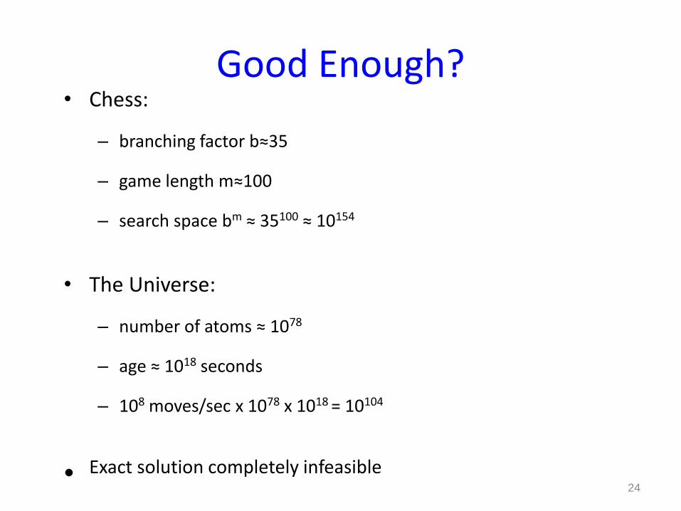
Good Enough? • Chess:
– branching factor b≈35
– game length m≈100
– search space bm ≈ 35100 ≈ 10154
• The Universe:
– number of atoms ≈ 1078
– age ≈ 1018 seconds
– 108 moves/sec x 1078 x 1018 = 10104
• Exact solution completely infeasible 24

Alpha-Beta Procedure
• The alpha-beta procedure can speed up a depth-first minimax search.
• Alpha: a lower bound on the value that a max node may ultimately be assigned
• Beta: an upper bound on the value that a minimizing node may ultimately be assigned
25
v >
v <

max
max
min
min
26

max
max
min
min
27

max
max
min
min
28

© Patrick Winston
max
max
min
min
29
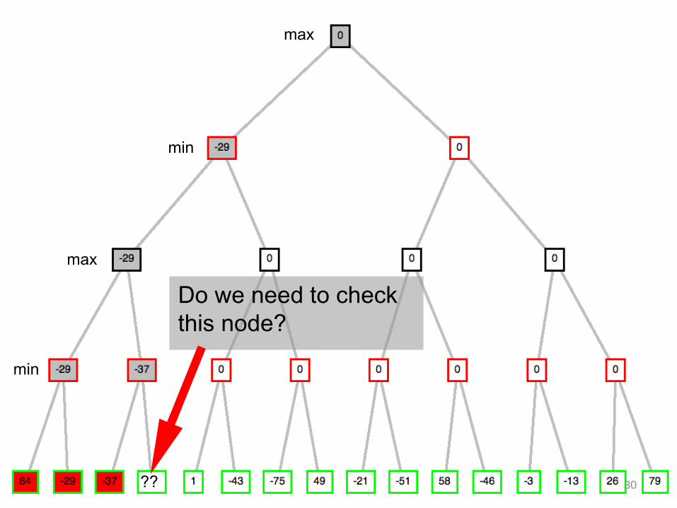
max
max
min
min
Do we need to check
this node?
?? 30

max
max
min
min
X
No - this branch is guaranteed to be
worse than what max already has
31

Alpha-Beta MinVal(state, alpha, beta){
if (terminal(state))
return utility(state);
for (s in children(state)){
child = MaxVal(s,alpha,beta);
beta = min(beta,child);
if (alpha>=beta) return child;
}
return beta; }
alpha = the highest value for MAX along the path
beta = the lowest value for MIN along the path 32

Alpha-Beta MaxVal(state, alpha, beta){
if (terminal(state))
return utility(state);
for (s in children(state)){
child = MinVal(s,alpha,beta);
alpha = max(alpha,child);
if (alpha>=beta) return child;
}
return beta; }
alpha = the highest value for MAX along the path
beta = the lowest value for MIN along the path 33

max
max
min
min α=-∞
β=84
α=-∞
β=∞
α=-∞
β=∞
α=-∞
β=∞ α - the best value
for max along the path
β - the best value
for min along the path
34

max
max
min
min α=-∞
β=-29
α=-29
β=∞
α=-∞
β=∞
α=-∞
β=∞
α=-29
β=∞
α - the best value
for max along the path
β - the best value
for min along the path
35

max
max
min
min α=-∞
β=-29
α=-29
β=∞
α=-∞
β=∞
α=-∞
β=∞
α=-29
β=-37
α - the best value
for max along the path
β - the best value
for min along the path
36

max
max
min
min α=-∞
β=-29
α=-29
β=∞
α=-∞
β=∞
α=-∞
β=∞
α=-29
β=-37
β < α
prune!
X
α - the best value
for max along the path
β - the best value
for min along the path
37

max
max
min
min α=-∞
β=-29
α=-29
β=∞
α=-∞
β=-29
α=-∞
β=∞
α=-29
β=-37
X
α=-∞
β=-29
α=-∞
β=-29
α - the best value
for max along the path
β - the best value
for min along the path
38

max
max
min
min
X
α=-∞
β=-29
α=-29
β=∞
α=-∞
β=-29
α=-∞
β=∞
α=-29
β=-37
α=-∞
β=-29
α=-∞
β=-29
α - the best value
for max along the path
β - the best value
for min along the path
39

max
max
min
min
X
α=-∞
β=-29
α=-29
β=∞
α=-∞
β=-29
α=-∞
β=∞
α=-29
β=-37
α=-43
β=-29
α=-∞
β=-43
α=-43
β=-29
α - the best value
for max along the path
β - the best value
for min along the path
40

max
max
min
min
X
α=-∞
β=-29
α=-29
β=∞
α=-∞
β=-29
α=-∞
β=∞
α=-29
β=-37
α=-43
β=-29
α=-∞
β=-43
α=-43
β=-75
β < α
prune!
X
α - the best value
for max along the path
β - the best value
for min along the path
41

max
max
min
min
X
α=-∞
β=-29
α=-29
β=∞
α=-∞
β=-43
α=-43
β=∞
α=-29
β=-37
α=-43
β=-29
α=-∞
β=-43
α=-43
β=-75
X
α - the best value
for max along the path
β - the best value
for min along the path
42

X X
α=-43
β=∞
α=-43
β=∞
α=-43
β=∞
α=-43
β=-21
α=-43
β=58
max
max
min
min
α - the best value
for max along the path
β - the best value
for min along the path
43

X X
max
max
min
min
α=-43
β=∞
α=-43
β=-46
α=-43
β=∞
α=-43
β=-21
α=-43
β=-46
β < α
prune!
X
X X
X X X X
α - the best value
for max along the path
β - the best value
for min along the path
44

Properties of α-β
• Pruning does not affect final result. This means that it gets the exact same result as does full minimax.
• Good move ordering improves effectiveness of pruning
• With "perfect ordering," time complexity = O(bm/2) doubles depth of search
• A simple example of reasoning about ‘which computations are relevant’ (a form of metareasoning)
45

Shallow Search Techniques
1. limited search for a few levels
2. reorder the level-1 sucessors
3. proceed with - minimax search
46

Good Enough? • Chess:
– branching factor b≈35
– game length m≈100
– search space bm/2 ≈ 3550 ≈ 1077
• The Universe:
– number of atoms ≈ 1078
– age ≈ 1018 seconds
– 108 moves/sec x 1078 x 1018 = 10104
The universe
can play chess
- can we?
47

Cutting off Search
MinimaxCutoff is identical to MinimaxValue except 1. Terminal? is replaced by Cutoff? 2. Utility is replaced by Eval
Does it work in practice? bm = 106, b=35 m=4 4-ply lookahead is a hopeless chess player!
– 4-ply ≈ human novice – 8-ply ≈ typical PC, human master – 12-ply ≈ Deep Blue, Kasparov
48

max
max
min
min
Cutoff
49

Evaluation Functions Tic Tac Toe
• Let p be a position in the game
• Define the utility function f(p) by
– f(p) = • largest positive number if p is a win for computer
• smallest negative number if p is a win for opponent
• RCDC – RCDO
– where RCDC is number of rows, columns and diagonals in which computer could still win
– and RCDO is number of rows, columns and diagonals in which opponent could still win.
50

Sample Evaluations
• X = Computer; O = Opponent
51
O
X
X O
rows
cols
diags
O O X
X X
X O
rows
cols
diags
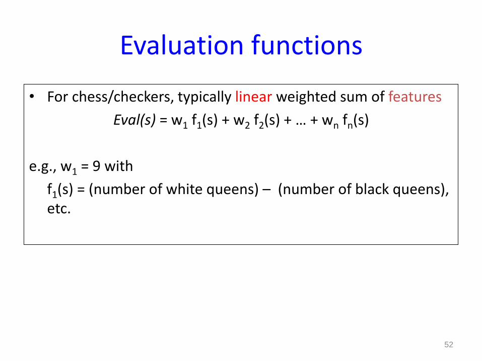
Evaluation functions
• For chess/checkers, typically linear weighted sum of features
Eval(s) = w1 f1(s) + w2 f2(s) + … + wn fn(s)
e.g., w1 = 9 with
f1(s) = (number of white queens) – (number of black queens), etc.
52

Example: Samuel’s Checker-Playing Program
• It uses a linear evaluation function
f(n) = a1x1(n) + a2x2(n) + ... + amxm(n)
For example: f = 6K + 4M + U
– K = King Advantage
– M = Man Advantage
– U = Undenied Mobility Advantage (number of moves that Max where Min has no jump moves)
53

Samuel’s Checker Player
• In learning mode
– Computer acts as 2 players: A and B
– A adjusts its coefficients after every move
– B uses the static utility function
– If A wins, its function is given to B
54

Samuel’s Checker Player
• How does A change its function? 1. Coefficent replacement
(node ) = backed-up value(node) – initial value(node)
if > 0 then terms that contributed positively are given more weight and terms that contributed negatively get less weight
if < 0 then terms that contributed negatively are given more weight and terms that contributed positively get less weight
55

Samuel’s Checker Player
• How does A change its function? 2. Term Replacement 38 terms altogether 16 used in the utility function at any one time Terms that consistently correlate low with the function
value are removed and added to the end of the term queue.
They are replaced by terms from the front of the term
queue.
56

Additional Refinements
• Waiting for Quiescence: continue the search until no drastic change occurs from one level to the next.
• Secondary Search: after choosing a move, search a few more levels beneath it to be sure it still looks good.
• Openings/Endgames: for some parts of the game (especially initial and end moves), keep a catalog of best moves to make.
57

Horizon Effect
The problem with abruptly stopping a search at a fixed
depth is called the 'horizon effect'
58

Chess: Rich history of cumulative ideas
Minimax search, evaluation function learning (1950).
Alpha-Beta search (1966).
Transposition Tables (1967).
Iterative deepening DFS (1975).
End game data bases ,singular extensions(1977, 1980)
Parallel search and evaluation(1983 ,1985)
Circuitry (1987)
59

Chess game tree
60

Problem with fixed depth Searches
if we only search n moves ahead,
it may be possible that the
catastrophy can be delayed by a
sequence of moves that do not
make any progress
also works in other direction
(good moves may not be found)
61

Quiescence Search
This involves searching past the terminal search nodes
(depth of 0) and testing all the non-quiescent or 'violent'
moves until the situation becomes calm, and only then apply
the evaluator.
Enables programs to detect long capture sequences
and calculate whether or not they are worth initiating.
Expand searches to avoid evaluating a position where
tactical disruption is in progress.
62

End-Game Databases
• Ken Thompson - all 5 piece end-games
• Lewis Stiller - all 6 piece end-games
– Refuted common chess wisdom: many positions thought to be ties were really forced wins -- 90% for white
– Is perfect chess a win for white?
63

The MONSTER
White wins in 255 moves (Stiller, 1991)
64

Deterministic Games in Practice
• Checkers: Chinook ended 40-year-reign of human world champion Marion Tinsley in 1994. Used a precomputed endgame database defining perfect play for all positions involving 8 or fewer pieces on the board, a total of 444 billion positions. Checkers is now solved!
• Chess: Deep Blue defeated human world champion Garry Kasparov in a six-game match in 1997. Deep Blue searches 200 million positions per second, uses very sophisticated evaluation, and undisclosed methods for extending some lines of search up to 40 ply. Current programs are even better, if less historic!
• Othello: human champions refuse to compete against computers, who are too good.
• Go: human champions refuse to compete against computers, who are too bad. In Go, b > 300, so most programs use pattern knowledge bases to suggest plausible moves, along with aggressive pruning.
65

Game of Go
human champions refuse to compete against computers, because software is too bad.
Chess Go Size of board 8 x 8 19 x 19
Average no. of
moves per game 100 300
Avg branching
factor per turn 35 235
Additional
complexity
Players can
pass
66

Recent Successes in Go
• MoGo defeated a human expert in 9x9 Go
• Still far away from 19x19 Go.
• Hot area of research
• Leading to development of novel techniques
– Monte Carlo tree search (UCT)
67

Other Games
deterministic chance
perfect
information
chess,
checkers, go,
othello
backgammon,
monopoly
imperfect
information stratego
bridge, poker,
scrabble
68
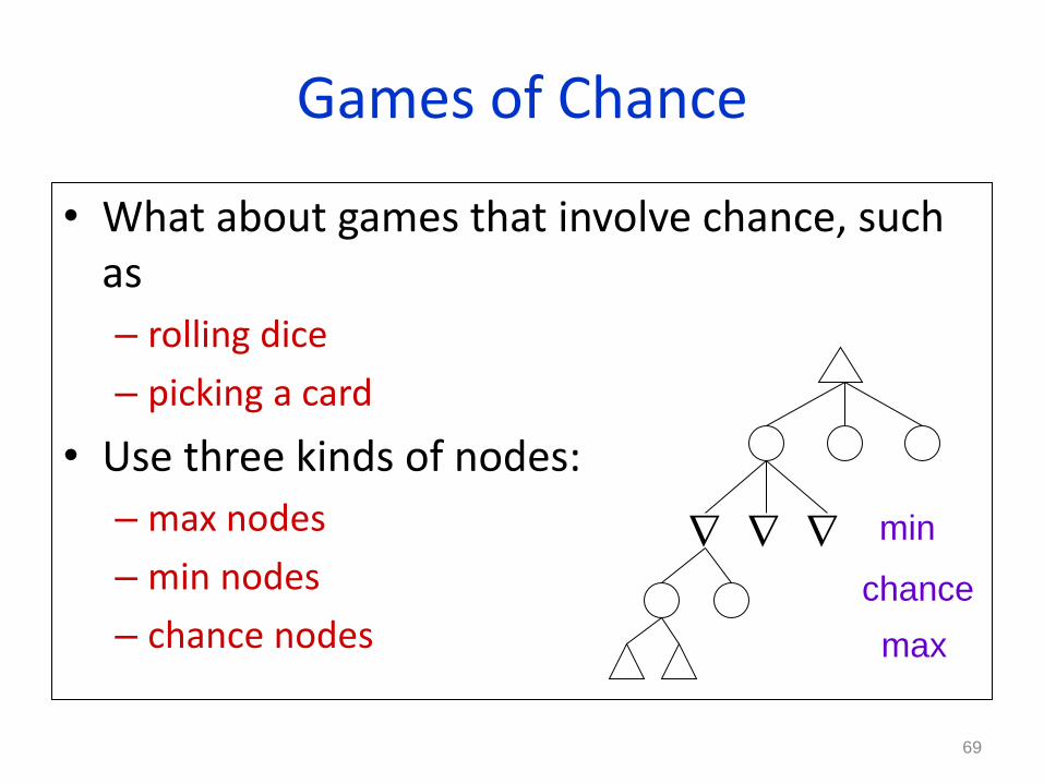
Games of Chance
• What about games that involve chance, such as
– rolling dice
– picking a card
• Use three kinds of nodes:
– max nodes
– min nodes
– chance nodes
69
min
chance
max

Games of Chance Expectiminimax
70
c
d1 di dk
S(c,di)
chance node with
max children
expectimax(c) = ∑P(di) max(backed-up-value(s))
i s in S(c,di)
expectimin(c’) = ∑P(di) min(backed-up-value(s))
i s in S(c,di)

Example Tree with Chance
71
3 5 1 4 1 2 4 5
.4 .6 .4 .6
.4 .6
max
chance
min
chance
max
leaf
1.2

Complexity
• Instead of O(bm), it is O(bmnm) where n is the number of chance outcomes.
• Since the complexity is higher (both time and space), we cannot search as deeply.
• Pruning algorithms may be applied.
72

Imperfect Information
• E.g. card games, where opponents’ initial cards are unknown
• Idea: For all deals consistent with what you can see
–compute the minimax value of available actions for each of possible deals
–compute the expected value over all deals
73

Summary
• Games are fun to work on!
• They illustrate several important points about AI.
• Perfection is unattainable must approximate.
• Game playing programs have shown the world what AI can do.
74