INTRODUCTION TO ALGEBRAIC GEOMETRY Contentsfulger/index_files/AGMAT457.pdfINTRODUCTION TO ALGEBRAIC...
75
INTRODUCTION TO ALGEBRAIC GEOMETRY Contents 1. Affine Geometry 2 1.1. Closed algebraic subsets of affine spaces 2 1.2. Regular functions 4 1.3. Regular maps 5 1.4. Irreducible subsets 8 1.5. Rational functions 10 1.6. Rational maps 11 1.7. Composition of rational maps 12 2. Projective Geometry 15 2.1. Closed subsets of projective space 15 2.2. Example of projective varieties 17 2.3. Regular functions and regular maps on quasiprojective algebraic sets 20 2.4. Rational functions and rational maps for quasiprojective varieties 24 2.5. Projective algebraic sets are universally closed 25 3. Finite maps 29 3.1. Local study of finite maps 31 4. Dimension 34 4.1. Dimension of intersection with a hypersurface 35 4.2. The dimension of the fibers of a regular map 36 4.3. Lines on surfaces 38 5. Nonsingular varieties 41 5.1. Tangent space 41 5.2. Singular points 47 5.3. Codimension one subvarieties 48 5.4. Nonsingular subvarieties of nonsingular varieties 49 6. Blow-ups 51 6.1. The blow-up of P 2 at one point 51 7. Divisors and Class Group 53 8. B´ ezout’s Theorem 55 8.1. Arbitrary smooth projective surfaces 58 9. Appendix 61 9.1. Classical algebraic structures 61 9.2. Commutative algebra 62 9.3. Topology 72 9.4. Categories 73 References 75 1
Transcript of INTRODUCTION TO ALGEBRAIC GEOMETRY Contentsfulger/index_files/AGMAT457.pdfINTRODUCTION TO ALGEBRAIC...

INTRODUCTION TO ALGEBRAIC GEOMETRY
Contents
1. Affine Geometry 21.1. Closed algebraic subsets of affine spaces 21.2. Regular functions 41.3. Regular maps 51.4. Irreducible subsets 81.5. Rational functions 101.6. Rational maps 111.7. Composition of rational maps 122. Projective Geometry 152.1. Closed subsets of projective space 152.2. Example of projective varieties 172.3. Regular functions and regular maps on quasiprojective algebraic sets 202.4. Rational functions and rational maps for quasiprojective varieties 242.5. Projective algebraic sets are universally closed 253. Finite maps 293.1. Local study of finite maps 314. Dimension 344.1. Dimension of intersection with a hypersurface 354.2. The dimension of the fibers of a regular map 364.3. Lines on surfaces 385. Nonsingular varieties 415.1. Tangent space 415.2. Singular points 475.3. Codimension one subvarieties 485.4. Nonsingular subvarieties of nonsingular varieties 496. Blow-ups 516.1. The blow-up of P2 at one point 517. Divisors and Class Group 538. Bezout’s Theorem 558.1. Arbitrary smooth projective surfaces 589. Appendix 619.1. Classical algebraic structures 619.2. Commutative algebra 629.3. Topology 729.4. Categories 73References 75
1
2 INTRODUCTION TO ALGEBRAIC GEOMETRY
1. Affine Geometry
1.1. Closed algebraic subsets of affine spaces. Throughout this course, unless otherwisespecified, we work over an algebraically closed field k = k. Let’s see what space we will workin (for now):
Definition 1.1. The n-dimensional affine space over k is Ank . As a set this is just
kn := k × . . .× k︸ ︷︷ ︸n times
,
but we will put more structure on it: a topology such that the only continuous functionsAnk → A1
k are polynomial. We also ignore the vector space structure on kn.
A polynomial function on Ank is a polynomial P (X1, . . . , Xn) with coefficients in k. The
set of all such is the polynomial ring k[X1, . . . , Xn]. We may also denote by P (X) when wedon’t want to write all indices X1, . . . , Xn.
Definition 1.2. An affine algebraic variety1 or closed subset of affine space is asubset Y ⊂ An
k given by the vanishing of a family of polynomials Pi(X1, . . . , Xn) and wedenote Y = V ((Pi)i).
Similarly we write V (T ) for the common vanishing locus of all polynomials in a set T ⊂ k[X].
We may allow non-algebraically closed fields k in this definition.
Example 1.3. The following are examples of closed algebraic subsets:
• A line in A2 is V (aX + bY + c).• In general, a d-dimensional linear subspace of An is given by the simultaneous van-
ishing of d linear equations.• A curve in the affine plane is the set of zeros of one nonzero polynomial P (X, Y ).• The union of closed subsets in An
k is also closed: If Y1 = V ((Pi)i), and Y2 = V ((Qj)j),then Y1 ∪ Y2 = V ((Pi ·Qj)i,j).• The intersection of close subsets in An
k is also closed: If Y1, Y2 are as above, thenY1 ∩ Y2 = V ((Pi)i, (Qj)j).• If Y = V (f) in An
k is a hypersurface (given by the vanishing of just one polynomial),then
D(f) := Ank \ Y
is also an affine variety... but in An+1k . In fact D(f) = V (Xn+1f − 1). We’ll believe
this more when we learn about morphisms and isomorphisms.• The closed subsets of A1 are:
– ∅.– Finite subsets of points.– A1.
This is because a polynomial of degree n in one variable X has at most n zeros. Also,if Y = x1, . . . , xn are n points in A1
k, then P (X) = (X − x1) · . . . · (X − xn) is apolynomial with Y = V (P ).
Definition/Theorem 1.4. The Zariski topology on Ank is the topology whose closed sets
are all the closed algebraic subsets in Ank .
1Soon, affine algebraic variety will mean irreducible closed algebraic subset

INTRODUCTION TO ALGEBRAIC GEOMETRY 3
Proof. What needs checking is that the union of two closed subsets is closed, the intersection of arbitrarily (indexed by anyfamily, not necessarily finite or countable) many closed subsets is closed, and that the empty set and Ank are both closed. All
are clear.
Question. How can we change the equations of an affine variety without changing the varietyitself?
Example 1.5. Let Y = V ((Pi)i). If we add to the given list of equations of Y one orarbitrarily many equations of the form
∑QjPj, where Qj are finitely many polynomials in
k[X] and Pj are among Pii∈I , then we do not change Y . In particular, if we replace Pii∈Iby the ideal (Pi)i that they generate inside k[X], we still get the same common vanishinglocus Y .
Related to this we make the following definition.
Definition/Theorem 1.6. If Y ⊂ Ank is a subset (usually an affine variety), the ideal of
Y is the ideal I(Y ) k[X] containing all the polynomials P such that P vanishes on Y (i.e.Y ⊆ V (P )).
Proof. All you need to check is that I(Y ) is indeed an ideal, and this is a consequence of the previous example.
Directly from the definition we see Y ⊆ V (I(Y )). In fact equality holds, and several otherstrong results hold as well.
Theorem 1.7.
(i) V (a) = V (√a) for any a k[X].
(ii) I(Y ) is a radical ideal, i.e. P r ∈ I(Y )⇒ P ∈ I(Y ).(iii) If Y1 ⊂ Y2, then I(Y1) ⊃ I(Y2).(iv) If a ⊂ b, then V (a) ⊃ V (b).(v) More generally, I(Y1 ∪ Y2) = I(Y1) ∩ I(Y2) ⊇ I(Y1) · I(Y2).
(vi) If Y ⊂ Ank is an affine variety, then Y = V (I(Y )).
(vii) More generally, if Y ⊂ Ank is just a subset, then V (I(Y )) = Y is the closure of Y in the
Zariski topology on Ank .
(viii) Hilbert Nullstellensatz: If a k[X] is an ideal, then√a = I(V (a)).
Proof. Since (i) through (v) are easy and (vii) → (vi), it remains to prove the Nullstellensatz and (vii). We prove the latter
and leave (viii) for later.
Clearly Y ⊂ V (I(Y )), hence Y ⊆ V (I(Y )). Conversely, let W be closed with W ⊇ Y . The definition of closed sets implies
W = V (a) for some a k[X]. Then V (a) ⊇ Y implies a ⊆ I(V (a)) ⊆ I(Y ) and W = V (a) ⊃ V (I(Y )). In particular V (I(Y )) is
the smallest closed subset containing Y , which is by definition Y .
Corollary 1.8. There is a natural correspondence given by V (·) and I(·) between
closed subsets of Ank radical ideals of k[X].
Corollary 1.9. If T and S are two sets of equations (polynomials in k[X]). Then they
describe the same affine variety Y ⊂ Ank (this means Y = V (T ) = V (S)) iff
√(T ) =
√(S),
where (T ) and (S) are the ideals generated by T and S in k[X].
Question. OK, going the other way: If we have infinitely many equations for an affinevariety Y , can we extract finitely many whose vanishing locus is still exactly Y ? Moreprecisely: If T ⊂ k[X] is a an arbitrary subset of polynomials, does there exist a finite subsetP1, . . . , Pr ⊂ T such that V (P1, . . . , Pr) = V (T )?
The answer is yes, and it comes from the:

4 INTRODUCTION TO ALGEBRAIC GEOMETRY
Theorem 1.10 (Hilbert Basis Theorem). Any ideal I k[X] is generated by finitely manyelements. Equivalently, k[X] is a Noetherian ring.
Proof. See appendix §9.2.5.
Assuming this theorem, then Y = V (T ) = V ((T )) = V (P1, . . . , Pr), where P1, . . . , Pr area finite set of generators of (T ).
The theorem also shows that Ank is a Noetherian space (decreasing sequences of closed
subsets are eventually constant). Indeed if Y1 ⊃ Y2 ⊃ . . . is a decreasing sequence of closedalgebraic subsets, then I(Y1) ⊂ I(Y2) ⊂ . . . is an increasing sequence of ideals of k[X]. Sincethis is a Noetherian ring, this sequence is eventually constant. But Yi = V (I(Yi)) for all iand the conclusion follows.
1.2. Regular functions.
Definition 1.11. Let Y ⊂ Ank be a closed algebraic subset. A function f : Y → k is called
regular if there exists a polynomial F ∈ k[X] such that F (y) = f(y) for all y ∈ Y .
In the above, if we know F then we know f , but if we know f , then usually there areseveral options for F . More precisely, if F |Y = F ′|Y = f , then (F − F ′)|Y = 0, whichmeans that the polynomial F −F ′ vanishes on Y . By definition, this happens precisely when(F − F ′) ∈ I(Y ). So two polynomials give the same regular function on Y when they areequl modulo I(Y ).
Definition/Theorem 1.12. The set of regular functions on the closed Y ⊂ Ank is
k[Y ] :=k[X]
I(Y ),
which is an algebra of finite type over k.
Example 1.13. • k[Ank ] = k[X]
/(0) = k[X] .
• k[∅] = k[X]/
(1) = 0.
• If Y = (1, . . . , 1) is a point in Ank , then k[Y ] = k[X]
/I(Y ). Observe that I(Y ) is
the maximal ideal m1 := (X1 − 1, . . . , Xn − 1), and k[Y ] = k[X]/m1' k. The same
would be true for any other point in Ank .
• If Y is the union of the x and y axes in A2k, then k[Y ] = k[x, y]
/(xy).
• If Y is the hyperbola of equation xy = 1, then k[Y ] = k[x, y]/
(xy − 1). This is
isomorphic to k[x, x−1].
One should look at k[Y ] as an invariant of the affine variety Y . For example the hyperbolaV (xy − 1) ⊂ A2
C (that last time we saw it should be a lot like C∗) is not “the same” as A1C
because their algebras of regular functions C[X,X−1] and C[X] are not isomorphic (Because
any isomorphism C[X,X−1]→ C[X] needs to send X to something invertible, and there are not many options.)In fact k[Y ] is more than an invariant of Y . It actually determines Y . This is a common
instance in mathematics: A space in some category (e.g. topological, differential, holomor-phic, analytic, algebraic) is actually determines by the admissible functions defined on it (e.g.continuous, differentiable, holomorphic, analytic, regular).
Theorem 1.14. There is a one-to-one correspondence between points on a closed subsetY ⊂ An
k and maximal ideals of k[Y ].

INTRODUCTION TO ALGEBRAIC GEOMETRY 5
Proof. Let’s look at Ank first. Here the claim is that the only maximal ideals of k[X] are the ones of form mx, where mx =(X1−x1, X2−x2, . . . , Xn−xn) is the maximal ideal corresponding to the point x = (x1, . . . , xn) ∈ Ank . (this is indeed maximal,
because the k[X] /mx ' k is a field.) So let m k[X] be an arbitrary maximal ideal, and as such radical. Then V (m) is
non-empty (because m 6= (1)). Pick some point x ∈ V (m). Then by the Nullstellensatz, we have I(x) ⊇ I(V (m)) =√m = m,
so mx := I(x) = m by maximality.
For general Y , the maximal ideals of k[Y ] = k[X] /I(Y ) are in a one-to-one correspondence with the maximal ideals of k[X]
that contain I(Y ). And mx ⊃ I(Y ) iff x ∈ Y .
Replacing polynomials with regular functions we see that we can perform the constructionsof today and of last time on Y instead of An. So we can change perspective by changing theambient space:
If Y ⊂ Ank is a closed subset, and T ⊂ k[Y ] is a subset of regular functions, we define
V (T ) = VY (T ) as the common vanishing locus on Y of the functions from T . Then theseV (T )’s are the closed sets of a topology on Y . Let’s test the compatibilities:
Start with a closed subset Z ⊂ Y (with respect to the topology on Y ). Denote by IY (Z)the ideal of regular functions from k[Y ] that vanish on Z. This is a radical ideal. Letϕ : k[X] → k[X] /I(Y ) ' k[Y ] be the quotient map. Then ϕ−1IY (Z) k[X] is also radicaland its vanishing locus in An
k is Z, so Z is also closed in Ank .
Conversely, if Z ⊂ Ank and Y ⊂ An
k are closed subsets such that it happens that Z ⊂ Y ,we show that Z is closed on Y (in Y ’s topology). We have I(Y ) ⊂ I(Z). Then I(Z)/I(Y )is a radical ideal of regular functions from k[Y ] = k[X] /I(Y ) and it vanishes precisely on Z,so Z is closed in Y . We have proved:
• That the Zariski topology on Y is the one induced from Ank .
• That the previous theorem generalizes to a correspondence between closed subsets ofY and radical ideals of k[X] containing I(Y ).
Even more, for Z closed in Y closed in Ank we have k[Z] = k[X]
/I(Z) = k[Y ]
/IY (Z) because
of the Third Isomorphism Theorem (k[Y ]/IY (Z) =
k[X]/I(Y )
I(Z)/I(Y )
' k[X]/I(Z).)
It is not hard to see that an appropriate Nullstellensatz also holds in this case: If a k[Y ]where Y ⊂ An
k is closed, then√a = IY (V (a)). (Let ϕ : k[X] → k[Y ] be the quotient morphism. By the
considerations above and the Nullstellensatz from Ank , we have IY (V (a)) = I(V (ϕ−1a))/I(Y ) =√ϕ−1a/I(Y ). It is an easy
exercise to see that this coincides with√a.)
The analogue of Theorem 1.7 also holds on Y and k[Y ].
1.3. Regular maps. We have learned what a regular function on a closed algebraic subsetis. Now let’s see what functions we allow between two closed algebraic subsets.
Definition 1.15. A function ϕ : X → Y between closed algebraic subsets of An and Am
respectively is a regular map (or morphism) if there exist regular functions f1, . . . , fm ∈k[X] such that
ϕ(x) = (f1(x), . . . , fm(x)),
for any x ∈ X ⊂ Ank (i.e. ϕ is given by polynomial functions).
Example 1.16. A regular function f : X → k is the same as a regular map f : X → A1k.
Example 1.17. If Y ⊂ An is a closed subset, then the inclusion map ı : Y → An is regular.
Example 1.18. The first projection (x, y) 7→ x : V (xy− 1)→ A1 from the hyperbola to theaffine line is a regular map. Note that the image A1 \ 0 is not closed.
6 INTRODUCTION TO ALGEBRAIC GEOMETRY
Example 1.19. The function tϕ7→ (t2, t3) : A1 → V (x3 − y2) is a regular map. It is actually
bijective. Its inverse as a function is (x, y)ϕ−1
7→
yx, if x 6= 0
0, if x = 0.
Let’s see that ϕ−1 is not a regular map. Put Y = V (x3 − y2) and assume there exists
f ∈ k[Y ] such that f(x, y) =
yx, if x 6= 0
0, if x = 0for any (x, y) ∈ Y . Pick F ∈ k[X, Y ] such
that F |Y = f . Multiplying with x (In the rational function field k(X,Y ) if we’re looking for an ambient space),we get (xF (x, y) − y)|Y = 0 when x 6= 0. It is easy to check that it also holds when x = 0(Either becayse x = 0 implies y = 0 on Y , or because xF (x, y)− y must vanish on a closed subset of Y , and Y \ (0, 0) = Y .)Then xF − y ∈ I(V (Y )) = (x3 − y2) (This is because k[X,Y ] is an UFD, and x3 − y2 is irreducible), soxF − y = P · (x3 − y2) for some P ∈ k[X, Y ]. Making x = 0 we get a contradiction.
However, ϕ−1 is continuous: We check that it returns closed sets to closed sets. Since ϕ−1
is invertible, it is equivalent to verify that ϕ is closed (takes closed subsets to closed subsets).Closed subsets of A1 are finite sets of points. They map to finite sets of points, and theseare always closed.
Definition 1.20. If X, Y are closed algebraic subsets (of maybe different affine spaces),then ϕ : X → Y is an isomorphism if it is bijective, and ϕ and ϕ−1 are both regular maps(morphisms).
Example 1.21. The map from the previous example is not an isomorphism even though itis bijective, and actually a homeomorphism for the Zariski topologies. This is because ϕ−1
is not regular.
Example 1.22. The map t 7→ (t, tm) : A1 → V (y − xm) from the affine line to the (general-ized) parabola is an isomorphism. Its inverse is (x, y)→ x.
Regular maps “act” on regular functions. If ϕ : X → Y is a regular map given by regularfunctions f1, . . . , fm in k[X], and g ∈ k[Y ], we define ϕ∗(g) ∈ k[X] as the function
(x1, . . . , xn) = xϕ∗(g)7→ g(f1(x), . . . , fm(x)).
Theorem 1.23. Throughout X ⊂ An and Y ⊂ Am are closed algebraic subsets.
a) If ϕ : X → Y is a regular map, then ϕ∗ : k[Y ]→ k[X] is a morphism of k-algebras.b) If ϕ : X → Y is a regular map, then it is an isomorphism iff ϕ∗ : k[Y ] → k[X] is an
isomorphism of k-algebras.c) X and Y are isomorphic iff k[X] and k[Y ] are isomorphic as k-algebras.d) There is a contravariant equivalence of categories between
closed algebraic subsetsregular maps between them
reduced algebras of finite type over k
morphisms of k-algebras
To go from left to right, send X → k[X] and ϕ → ϕ∗. Conversely, if A is a reduced k-algebra of finite type, then there exists a surjective k-algebra morphism k[X1, . . . , Xn]→ Afor some n ≥ 0. Let I be the kernel. Putting Y := V (I) ⊂ An, we have k[Y ] = A.
Proof. Part a) is a consequence of the fact that if y ∈ Y is a point, then the evaluation at y map g 7→ g(y) : k[Y ] → k is a
k-algebra morphism. For the remaining parts of the problem, the only interesting part is proving that if ψ : k[Y ] → k[X] is amorphism of k-algebras, then there exists ϕ : X → Y a regular map such that ψ = ϕ∗. And this is homework.
We check the functoriality of ϕ∗, i.e. if X,Y, Z are closed algebraic subsets, and ϕ : X → Y and φ : Y → Z are regularmaps, then φ ϕ is also a regular map, and (φ ϕ)∗ = ϕ∗ φ∗. For the regularity, observe that if ϕ is given by regular
functions f1(x), . . . , fm(x) in k[X], and φ by regular functions g1(y), . . . , gp(y) in k[Y ], then φ ϕ is a regular map given by
functions g1(f1(x), . . . , fm(x)), . . . , gp(f1(x), . . . , fm(x)) in k[X]. For the composition rule, take h ∈ k[Z] and observe that

INTRODUCTION TO ALGEBRAIC GEOMETRY 7
(φ ϕ)∗(h) = ϕ∗(φ∗(h)) = h(g1(f1(x), . . . , fm(x)), . . . , gp(f1(x), . . . , fm(x))). In particular, if ϕ is an isomorphism, then so isϕ∗, and (ϕ∗)−1 = (ϕ−1)∗.
Example 1.24. If Y ⊂ An is a closed subset and ı : Y → An is the inclusion map, then ı∗
is the quotient morphism k[X]→ k[X]/I(Y ).
In fact whenever we have a surjective morphism ϕ∗ : k[Y ]→ k[X] is follows that ϕ : X → Yis the inclusion of X as a closed subset of Y . (X = VY (kerϕ∗)).
Example 1.25. The map tϕ→ (t2, t3) from the affine line to the cusp is also not an isomor-
phism because k[X, Y ]/
(X3 − Y 2)ϕ∗→ k[X] is not an isomorphism of k-algebras. (Denoting by
x, y the classes of X,Y modulo (X3 − Y 2), we see that ϕ∗ is determined by ϕ∗(x) = X2 ∈ k[X] and ϕ∗(y) = X3 ∈ k[X]. Then
ϕ∗ sends the maximal ideal (x, y) to the ideal (X2, X3) = (X2) k[X] which is not maximal, so it cannot be an isomorphism.)In fact we saw in class that the affine line and the cusp are not isomorphic by any morphism
between them, because k[X, Y ]/
(X3 − Y 2) and k[X] are not isomorphic via any k-algebra
morphism. This is because every maximal ideal m k[X] has that dimk m/m2 = 1, whilefor (x, y) k[X, Y ]
/(X3 − Y 2) the analogous quotient is 2-dimensional with a basis given by
the classes of x and y modulo (x, y)2.We will see later that m/m2 is the tangent space at the point corresponding to m, so this
construction is not unnatural. In fact it is quite geometric: the affine line and the cusp arenot isomorphic because the line is smooth, while the cusp is singular at (0, 0).
Example 1.26. The k-algebra morphism X 7→ x : k[X]→ k[X, Y ]/
(X3 − Y 2) is ϕ∗ for the
projection onto the first component morphism (x, y)ϕ7→ x from the cusp to the affine line
(seen as the x-axis).Similarly X 7→ y : k[X] → k[X, Y ]
/(X3 − Y 2) corresponds to the second projection
(x, y)→ y from the cusp to the affine line (y-axis this time).Except over 0, the first projection is 2-to-1, while the second is 3-to-1 (even though the
real picture suggests one-to-one, there exist nonreal third roots of unity).
Example 1.27. We saw in Example 1.24 that ϕ∗ surjective corresponds to inclusions ofclosed subsets. What does ϕ∗ injective correspond to?
Let h ∈ k[Y ] and assume ϕ is given by f1, . . . , fm ∈ k[X]. Let’s see what it means forh ∈ k[Y ] to be in the kernel of ϕ∗. Well, ϕ∗(h) = 0 means h(f1(x), . . . , fm(x)) = 0 for allx ∈ X. This happens precisely when h vanishes along ϕ(X) ⊂ Y . If ϕ∗ is injective, this issupposed to imply that h = 0 on Y . But if the only function vanishing along ϕ(X) ⊂ Y is
the zero function, then ϕ(X) = Y , i.e. the image of ϕ is dense in Y (This is the Weak Nullstellensatz).We say that X dominates Y .
The example of the hyperbola projecting to the affine line, shows that the image of aregular map could be dense without the regular map being surjective.
Example 1.28. More generally, every morphism ϕ∗ : k[Y ] → k[X] can be written as thecomposition of a surjection with an inclusion of reduced k-algebras of finite type
k[Y ] Im(ϕ∗) → k[X].
On the geometric side, this corresponds with writing ϕ : X → Y as the composition of adominant map with an inclusion map:
X → ϕ(X) → Y.
8 INTRODUCTION TO ALGEBRAIC GEOMETRY
1.4. Irreducible subsets.
Definition 1.29. If Y ⊂ X is a closed subset, we say that Y is irreducible if whenever Y1
and Y2 are closed subsets of X such that Y = Y1 ∪ Y2, then either Y = Y1 or Y = Y2.If U ⊂ X is any subset, we say that it is irreducible if its closure U ⊂ X is irreducible.If U is not irreducible, we say that it is reducible.If Y ⊂ An is an irreducible closed algebraic subset, we say that Y is an affine variety. In
§1 defined an affine variety to be the same as closed algebraic subset, but now we also ask for irreducibility.
Remark 1.30. The definition looks similar to that of a connected subset, and indeed anirreducible subset is connected, but note that we allow Y1 and Y2 to have nonemty intersection.For example V (xy) = V (x) ∪ V (y) ⊂ A2 is connected, but not irreducible.
Example 1.31. An is irreducible as a closed algebraic subset of itself. Note that here it isimportant that we work with algebraically closed fields. If k is a finite field, then A1 whichcan be identified with k is a finite union of points.
Example 1.32. If U ⊂ X is a nonempty open subset of an affine variety (now irreducible bydefinition), then U is dense in X. (We have X = (X \U)∪U is a union of closed subsets. Now use the definition.)
Example 1.33. If f ∈ k[X] is a reducible polynomial that is not a power of an irreduciblepolynomial, then V (f) ⊂ An is not irreducible. (If f is as above, then we can write f = gh for some
nonconstant polynomials g, h without common factors in the UFD (cf. §9.2.8) k[X]. Then V (f) = V (g) ∪ V (h). We have
V (f) ) V (g) because otherwise g ∈ I(V (f)) implies by the Nullstellensatz gm ∈ (f) for some m ≥ 0, and so there exists l ∈ k[X]
such that gm = fl = ghl which is a contradiction because g and h have no common factors.)
Example 1.34. If ϕ : X → Y is a regular map of closed algebraic subsets and X is irre-ducible, then so is ϕ(X). (If ϕ(X) = V1 ∪ V2 is a union of closed sets, then X = ϕ−1(V1)∪ϕ−1(V2) is also a union of
closed subsets (potentially empty because ϕ is not assumed to be surjective). Since X is irreducible, it is equal to one of them.
Say X = ϕ−1(V1). Then V1 ⊃ ϕ(ϕ−1(V1)) = ϕ(X), hence V1 ⊃ ϕ(X), since V1 is closed.)
Let’s see what is on the algebraic side.
Theorem 1.35. Let Y ⊂ X be a closed subset of a closed subset of the affine space. ThenY is irreducible iff IX(Y ) k[X] is prime, iff k[Y ] is a domain.
Proof. These are simple consequences of the dictionary that we have between geometry and algebra.
Say I(Y ) := IX(Y ) is prime, and write Y = Y1 ∪ Y2 as a union of closed subsets. Then I(Y ) = I(Y1) ∩ I(Y2). But
it is impossible to write a prime ideal as an intersection of two radical ideals unless the prime ideal is one of them: If y1 ∈I(Y1) \ I(Y2) and y2 ∈ I(Y2) \ I(Y1), then y1y2 ∈ I(Y1) · I(Y2) ⊂ I(Y1)∩ I(Y2) = I(Y ) gives a contradiction. Therefore eitherI(Y ) = I(Y1) ⊂ I(Y2) hence Y = Y1, or I(Y ) = I(Y2) ⊂ I(Y1) hence Y = Y2.
Say Y is irreducible, and let fg ∈ IX(Y ). In particular fg|Y = 0. Then Y = VY (f) ∪ VY (g) is a union of closed subsets,and by the definition of irreducibility, Y = VY (f) or Y = VY (g). Then f |Y = 0 or g|Y = 0, hence f or g are in IX(Y ).
The equivalence between IX(Y ) k[X] being prime and k[Y ] = k[X]/IX(Y ) being a domain is a classical algebraic result.
See §9.2.6.
Example 1.36. If X = V (f) ⊂ An for some irreducible f ∈ k[X], then X is irreducible.(We show in §9.2.8 that k[X] is an UFD. In an UFD, irreducible elements are prime, therefore (f) k[X] is prime. In particular
(f) =√
(f) = I(V (f)), hence V (f) is irreducible.)In fact V (f) ⊂ An is irreducible iff f is a power of an irreducible polynomial in k[X]. (Use
the previous paragraph and Example 1.33.)
Example 1.37. It was important that k[X] was an UFD in the previous example. ConsiderR := k[x, y, z]
/(x2 − yz). This is a domain, and it is the ring of regular functions for the
cone Y = V (x2− yz). Furthermore x is irreducible, but not prime (hence R is not an UFD),

INTRODUCTION TO ALGEBRAIC GEOMETRY 9
and VY (x) = VY (x2) = VY (yz) = VY (y)∪ VY (z) is the union of the lines through (0, 0, 1) and(0, 1, 0), hence not an irreducible closed subset. (To see that x is irreducible, use that R is a graded domain.
This is because k[x, y, z] is graded and (x2 − yz) is a homogeneous prime ideal.)
Example 1.38. If I k[X] is a prime ideal, then Y := VX(I) ⊂ X is irreducible. (This is
because if I is prime, then IX(VX(I)) =√I = I, hence IX(Y ) is prime.)
Definition 1.39. A closed subset Z ⊂ Y of a closed algebraic subset of an affine space is anirreducible component of Y if Z is irreducible and Z 6⊂ Y \ Z.
Proposition 1.40. Any closed algebraic subset Y of an affine space has only finitely manyirreducible components Y1, . . . , Yr and Y = ∪ri=1Yi. This decompositions is unique (among
decompositions of Y as a finite union of irreducible closed subsets Wj such that Wj 6⊂Wj′ for j 6= j′).Proof. One can give a proof by contradiction using that Y is a Noetherian topological space as in the book, or we can apply
the primary ideal decompositions from §9.2.7 to the radical ideal I(Y ) to write it uniquely as an intersection of minimal primeideals.
1.4.1. Products. If X ⊂ An and Y ⊂ Am are closed algebraic subsets given by equationsfi ∈ k[X1, . . . , Xn] and gj ∈ k[Y1, . . . , Ym] respectively, then X × Y is a closed algebraicsubset of An+m. It is given by the equations fi and gj seen as polynomials (or regularfunctions) in the bigger ring k[X1, . . . , Xn, Y1, . . . Ym].
Remark 1.41. The Zariski topology on X × Y is the one induced from An+m, and this isdifferent from the product topology as we have seen in homework. For example the diagonalV (x− y) is closed in A1×A1 = A2, but it is not closed in the product topology (Its complement
is not a (finite) union of open subsets of form Ui × U ′i , where Ui, U′i ⊂ A1 are open.)
The ring of regular functions on X × Y ⊂ An+m is
k[X × Y ] ' k[X]⊗k k[Y ] =k[X, Y ]
IAn(X)k[X, Y ] + IAm(Y )k[X, Y ],
where k[X, Y ] = k[X1, . . . , Xn, Y1, . . . , Ym].
The projections (x, y)p17→ x : X × Y → Y and the corresponding p2 : X × Y → Y are
regular maps, and p∗1 is the identification of k[X] with k[X]⊗k 1 in k[X × Y ], while p∗2 is theidentification of k[Y ] with 1⊗k k[Y ].
Any regular map ϕ : X → Y admits a factorization
XΓϕ //
ϕ##G
GGGG
GGGG
G X × Yp2
Y
where Γϕ is the graph morphism x 7→ (x, ϕ(x)) : X → X ×Y and p2 is the second projectionX × Y → Y as above.
Proposition 1.42. If X and Y are irreducible, then so is X × Y .
Proof. Assume X × Y = V1 ∪ V2 is a union of closed subsets. For y ∈ Y , denote Xy = p−12 y. This a copy of Xy sitting over
y ∈ Y inside X ×Y . Since X is irreducible, and Xy = (Xy ∩V1)∪ (Xy ∩V2), we have Xy ⊂ V1 or Xy ⊂ V2 for each y (althoughbeing in V1 or V2 may change as we change y).
Denote Y1 = y ∈ Y | Xy ⊂ V1 and define Y2 analogously. By the remark above, Y = Y1 ∪ Y2. By the irreducibility of Y ,
we have Y = Y 1 or Y = Y 2. Say Y = Y 1. Then V1 contains the open subset X × (Y \ Y \ Y1).
Let f ∈ k[X × Y ] be a polynomial that vanishes along V1. Then it vanishes along X × (Y \ Y \ Y1). In particular for each
x ∈ X, it vanishes along x× (Y \Y \ Y1), hence also along its closure in Y ×X which is Yx. Since this happens for all x ∈ X,
we obtain that f = 0. This implies that V1 is dense in X × Y , and since it was closed to begin with we get X × Y = V1. Thisconcludes the proof.

10 INTRODUCTION TO ALGEBRAIC GEOMETRY
1.5. Rational functions. When X is an affine variety, which since last time also meansirreducible, then k[X] is a domain and we can talk about its fraction field that we denotek(X).
Definition 1.43. A rational function on the affine variety X is an element of k(X).
Every rational function is then a ratio fg
of a regular function f by a nonzero (meaning
not zero everywhere, but maybe somewhere) regular function g.
Remark 1.44. Because they are elements of the field of fractions, fg
= f ′
g′in k(X) if and
only if fg′ = f ′g in k[X].
Example 1.45. 1x
is a rational function on A1.
Observe that rational functions are not necessarily defined over the entire X. In thepreceding example, 1
xis not defined at x = 0. But where is a rational function defined? If we
write h ∈ k(X) as fg, then a temporary answer is that h is defined where g does not vanish,
and indeed it is defined at least at those points.
Definition 1.46. Let h ∈ k(X). We say that h is defined (or regular) at a point x ∈ X ifthere exist f, g ∈ k[X] such that h = f
gand g(x) 6= 0.
There is however an issue that makes finding where rational functions are defined a subtlequestion: The representation h = f
gis not unique. A simple example is x−1
x2−x = 1x, and if we
look at the first formula we are tempted to say that the function is not defined at 0 and 1.But if we use the second formula, then it is defined at 1. In this particular case we would“simplify” as much as possible and then look at where the denominator does not vanish.In general though, more specifically when working with rings that are not UFD, then an“optimal” representation does not exist.
Example 1.47. If X = V (x3 − x2 + y2 − y), then X is irreducible, and y−1x
= x−x2
ybecause
of the formula x3 − x2 + y2 − y = 0. The first formula says that the function h := y−1x
is defined when x 6= 0, which means (x, y) 6∈ (0, 0), (0, 1), while the second formula saysthat the function h (with a different formula) is defined when y 6= 0, which means when (x, y) 6∈(0, 0), (1, 0). Neither of these is optimal. We actually put them together instead of pickingthe larger one to decide that h is defined outside (0, 0).
Definition 1.48. Let h ∈ k(X) be a rational function onX. Then the domain of definitionof h is the union of all open subsets D(g) = X \ V (g), where g varies over all denominatorsof representations h = f
gwith f, g ∈ k[X] and g 6= 0.
A rephrasing is that x ∈ X is in the domain of definition of h if h is defined at x
Remark 1.49. The domain of definition of a rational function is open (because an arbitrary union
of open sets is open in any topological space). Since we are working in a Noetherian topological space,any cover by open sets admits a finite subcover. This means that the domain of h is actuallya union of finitely many D(gi) in the previous definition.
Proposition 1.50. Two rational functions h, h′ ∈ k(X) are equal if and only if they are bothdefined and agree on a nonempty open subset U ⊂ X.
Proof. If r := h− h′ it comes down to showing that if r|U = 0, then r = 0. Write r = fg
. Then r|U = 0 implies f |U = 0, which
in turn means U ⊂ V (f). This implies V (0) = X = U ⊆ V (f). (We saw last time that a nonempty open subset of an irreduciblespace is dense). But V (0) = V (f) implies f = 0 by the Nullstellensatz.

INTRODUCTION TO ALGEBRAIC GEOMETRY 11
The domain of definition gives us a way of testing when a rational function is regular.
Proposition 1.51. Let X be an affine variety. If the domain of definition of h ∈ k(X) is theentire X, i.e. h is defined everywhere, then h is actually a regular function, i.e. h ∈ k[X].The converse is immediate.
Proof. The domain of h is the union of all D(g) with h = fg
for some f, g ∈ k[X], and g 6= 0. The complement of this union
is the intersections of the complements, which means the intersection of all V (g), which we know is V (a), where a is the ideal
generated by all such g. If the domain of h is X, this complement is empty. But V (a) = ∅ only when a = (1). By the definition
of a, there exist finitely many nonzero gi ∈ k[X] and correspondingly finitely many fi ∈ k[X] with h = figi
for all i, but also
finitely many ri ∈ k[X] such that∑i rigi = 1. Multiplying this by h we get h =
∑i rifi. There are no longer any fractions in
this expression, hence h is regular.
Remark 1.52. Given finitely many rational functions hi ∈ k(X), there exists a nonemptyopen subset U ⊂ X where all hi are defined. (The domain of definition of each hi is open and nonempty. It is
enough to show that the intersection finitely many nonempty open subsets is always open nonempty. Indeed if Ui are nonempty
open sets and Vi := X \ Ui are their complements, then if ∩iUi = ∅, then ∪iVi = X. The irreducibility of X then says that X
is one of the Vi’s, which was excluded by the nonemptyness of each Ui)
We were able to understand regular functions on X as polynomial functions restricted toX. Let’s see about rational functions: Say h = f
gwith f, g ∈ k[X] and g 6= 0. Choose
F,G ∈ k[X] polynomial functions that restrict to f, g. The condition g 6= 0 is equivalent to
G 6∈ I(X). So h(x) = F (x)G(x)
whenever x ∈ X, but x 6∈ V (G). Moreover h = 0 if and only if
F |X = 0, i.e. F ∈ I(X). Then we have the following presentation of rational functions:
Proposition 1.53. Let OX be the subring of k(X) generated by elements of form FG
withG 6∈ I(X), and let m be the set of such functions such that F ∈ I(X). Then mOX andk(X) ' OX/m. In particular m is a maximal ideal.
Proof. It is easy to check that OX is a ring and that the function FG7→ F
G|X : OX → k(X) is a ring morphism. Its kernel is all
fractions FG
such that F |X = 0, which is by definition m. Conclude by the first isomorphism theorem.
Localization can help phrase this as k(X) ' k[X](I(X))
/I(X) k[X](I(X))
, where k[X](I(X))
is the localization of k[X] at the prime ideal I(X) (prime because X is irreducible).
1.6. Rational maps. Recall that a regular map was given by finitely many regular functions.We do the same to define rational maps.
Definition 1.54. Let X be an affine variety, and consider f1, . . . , fm ∈ K(X) rational func-tions. They define a rational map ϕ : X 99K Am by the formula ϕ(x) = (f1(x), . . . , fm(x))valid when all fi are defined at x. We say that ϕ is regular at x.
If Y ⊂ Am is a closed subset, a rational map ϕ : X 99K Y is rational map X 99K Am suchthat ϕ(x) ∈ Y for all x ∈ X where ϕ is defined.
Definition 1.55. A rational map f : X 99K A1 is the same as a rational function f ∈ k(X).
Remark 1.52 tells us that a rational map is defined on a nonempty open subset U ⊂ X.For example one can take the intersection of the domains of definition of all fi’s. Recall thatnonempty open subsets of irreducible spaces are dense.
Definition 1.56. The domain of definition of a rational map ϕ = (f1, . . . , fm) is theintersection of the domains of definition of the fi’s.
The image ϕ(X) of ϕ is the set of all ϕ(x), where x is in the domain of definition of ϕ.

12 INTRODUCTION TO ALGEBRAIC GEOMETRY
Example 1.57. Consider the stereographic projection in A2 from the origin (0, 0) to theline x = 1. This is the rational function p : A2 99K A1 that computes slopes of points, i.e.p(x, y) = y
x. Then p is defined at every point except on the line x = 0.
Remark 1.58 (When are rational maps equal?). Say ϕ and ψ are rational maps from theaffine variety X given by rational functions fi and gi in k(X). Then ϕ = ψ if fi = gi forall i as elements of k(X). At the level of functions, using Lemma 1.50, this is the same asasking that there exists U ⊂ X open contained in the domain of definition (e.g. the intersection
of the domain of definition of all fi and gi) of both ϕ and ψ such that ϕ|U = ψ|U as functions, meaningϕ(x) = ψ(x) for all x ∈ U .
Example 1.59. Let X ⊂ Ank be an affine variety and let ϕ : X 99K Y be a rational map.
Then ϕ = 1X as rational maps if and only if ϕ is a regular map and ϕ = 1X as regular maps.
Proof. The other implication being clear, let’s assume that ϕ = 1X as ratinonal maps. By definition ϕ is given by n rational
functions f1, . . . , fn ∈ k(X). By the previous remark, if ϕ = 1X as rational maps, then fi = xi for all i, where xi is therestriction to X of the i-th coordinate function Xi on Ank . Then fi is regular and equal to xi for all i not just as rational
functions, but as regular functions in k[X]. Then ϕ is a regular map and ϕ = 1X .
1.7. Composition of rational maps. Funny things can happen when we have rationalmaps ϕ : X 99K Y and ψ : Y 99K Z. (Note that by the definition of a rational map, this forces both X and Y to
be varieties, i.e. irreducible.) For example the image of ϕ could land outside the domain of ψ, andthen ψ ϕ doesn’t make sense anywhere.
Example 1.60. We cannot compose the stereographic projection from (0, 0) to V (x − 1)with the stereographic projection from (1, 0) to V (x), both seen as rational maps A2 99K A2.Neither of them is defined on the image of the other.
To solve this issue we ask that the domain of ψ meets the image of ϕ. Note that the imageof ϕ is irreducible, in particular the intersection with the domain of ψ is dense under ourassumption that it is nonempty.
Definition 1.61. Let ϕ : X 99K Y and ψ : Y 99K Z be rational maps with X and Y affinevarieties, and Z a closed algebraic subset of some affine space. if ϕ(X) meets the domain ofψ, then we define the composition ψ ϕ : X 99K Z. This is defined on the inverse imagethrough ϕ of the domain of ψ wich is nonempty by assumption.
Recall that if ϕ : X → Y was a regular map, we defined a pullback morphism ϕ∗ : k[Y ]→k[X] by ϕ∗(f)(x) = f(ϕ(x)) for any regular function f : Y → k. This is the same asϕ∗(f) = f ϕ, with f seen now as a regular map (as opposed to function) f : Y → A1.
We try to do the same for a rational function ϕ : X 99K Y . If we want to talk aboutrational functions on Y , then Y must also be irreducible. We would like the compositionf ϕ to be defined for all rational functions f ∈ k(Y ), which means that we want ϕ(X)to meet the domain of definition of every rational function on Y . As the following lemmashows, this is only possible when ϕ(X) is dense in Y .
Lemma 1.62. Let Y be an affine variety. If a subset T ⊂ Y (think ϕ(X) which doesn’t have to be
neither open, nor closed, nor open in its closure) intersects the domain of definition of every rationalfunction f ∈ k(Y ), then T is dense in Y .
Proof. Assume that T is not dense. Then U := Y \ T is open and nonempty. Let g ∈ IX(T ) k[X] be a nonzero function. A
nonzero function exists because IX(T ) = 0 if and only if T = X, and we assumed that this is not the case. Then T ⊂ V (g),hence by passing to complements we have D(g) ⊂ U . Let’s show that D(g) is the domain of definition of some rational functionf . This will show that T does not meet the domain of f , which is a contradiction.

INTRODUCTION TO ALGEBRAIC GEOMETRY 13
The first guess would be f = 1g
, but we know we have to be careful to check that f is not defined (by any other representation
as a fraction) at any point of V (g). Assume that f is defined at x ∈ V (g). Then there exist u, v ∈ k(X) with v(x) 6= 0 such
that 1g
= f = uv
. This means v = ug, and if we evaluate at x we get v(x) = u(x)g(x) = u(x) · 0 = 0, because x ∈ V (g). This is
a contradiction.
Definition 1.63. Let ϕ : X 99K Y be a rational map between affine varieties. We say thatϕ is dominant if ϕ(X) is dense in Y .
Definition 1.64. Let ϕ : X 99K Y be a dominant rational map between affine varieties. Thepullback ϕ∗ : k(Y )→ k(X) is the field morphism defined by ϕ∗(f) = f ϕ for all f ∈ k(Y ).
Since morphisms between fields are injective (actually any morphism of rings from a field is injective, unless
the target is the 0 ring), this means that ϕ∗ is injective. Now that we know what a composition ofrational maps is, we can talk about what “isomorphism” should mean for this kind of maps.
Definition 1.65. The affine varietiesX and Y are birational if there exist dominant rationalmaps ϕ : X 99K Y and ψ : Y 99K X such that ϕ ψ = 1Y and ψ ϕ = 1X .
Then ϕ and ψ are called birational isomorphisms, or just birational, and they areinverses (birationally) of each other.
Example 1.66. i) If X and Y are isomorphic, then they are also birational. The conversemay fail. See examples below.
ii) Let φ : A2 → A1 be the stereographic projection from (0, 0) onto the line V (x−1) ⊂ A2.Let X = V (x3 − y2) be the cusp and let ϕ : X 99K A1 be the restriction ϕ := ψ|X .Then ϕ is birational. An inverse is the morphism (regular map) ψ : A1 → X given byψ(t) = (t2, t3). Observe though that ϕ itself is not regular as it is not defined at theorigin. Also, if ϕ was regular, then X and A1 would be isomorphic, which we know theyare not.
iii) Similarly the node V (x3 − x2 + y2) is birational to A1.
Just like with regular maps, birational isomorphism can be checked with algebra.
Theorem 1.67. Let X and Y be affine varieties and let ϕ : X 99K Y be a dominant rationalmap. Then ϕ is a birational isomorphism if and only if ϕ∗ : k(Y )→ k(X) is an isomorphismof k-algebras (and fields).
Moreover, X and Y are birational if and only if there exists φ : k(Y )→ k(X) an isomor-phism of k-algebras (and fields).
Proof. Just like for regular maps, the first part boils down to checking that the pullback is functorial, meaning that it respectscomposition: if ϕ : X 99K Y and ψ : Y 99K Z are rational maps that can be composed, then (ψ ϕ)∗ = ϕ∗ ψ∗. And also
(1X)∗ = 1k(X). These are proved just like for regular maps.
If Y ⊂ Am, denote the coordinate functions y1, . . . , ym ∈ k[Y ] ⊂ k(Y ). Define ϕ : X 99K Y by ϕ = (φ(y1), . . . , φ(ym)). This
is only a rational map because we don’t know that φ : k(Y )→ k(X) sends k[Y ] to k[X]. One constructs analogously ψ : Y 99K Xfrom φ−1 : k(X)→ k(Y ). To check that ϕ and ψ are birational isomorphisms, inverses to each other, by the composition tricks
in the previous paragraph, it is enough to check that if X = Y , then ϕ = 1X as rational maps if and only if ϕ∗ = 1k(X). This
is easy.
Example 1.68. A2 and A1 are not birational. This is because their function fields k(X) andk(X, Y ) are not isomorphic as k-algebras. (They have different transcendence degrees over k. The first is 1, the
second is 2.)
Example 1.69. i) The map (x, y) 7→ (x, xy) : A2 → A2 is a birational isomorphism. (This
is homework.)ii) t 7→ t2 : A1 → A1 is not birational. (X is not in the image of X 7→ X2 : k(X)→ k(X).)
iii) The elliptic curve V (x3−x+y2) and the affine line A1 are not birational. (Also homework.).

14 INTRODUCTION TO ALGEBRAIC GEOMETRY
Definition 1.70. If X is an affine variety birational to some An, we say that X is rational.
We will see at some point that n in the above definition is uniquely determined if it exists (itis the dimension of X). The motivation for studying rational varieties X is that a birationalisomorphism An 99K X gives a parameterization of X. In fact we are usually happy when thismap is just dominant and then we call X unirational. There exist nonrational unirationalvarieties, but the examples are not that easy.
Example 1.71. i) If f ∈ k[X] is irreducible of total degree 2, then V (f) is rational. (The
stereographic projection from a point x ∈ V (f) to some linear hyperplane in An that does not pass through x restricts to
a birational isomorphism V (f) 99K An−1. This is because lines through x in An intersect V (f) in at most one more point
other than x.)ii) t→ (t2, t3) parameterizes the cusp V (x3 − y2) birationally.iii) t→ (t2 + 1, t(t2 + 1)) parameterizes the node V (x3 − x2 + y2) birationally.iv) t→ t2 parameterizes A1, but not birationally.
Example 1.72. X := V (x3 + y3 + z3− 1) ⊂ A3 is rational if the characteristic of k is not 3.(X contains two skew (not in a same plane) lines `1 := V (x+ y, z) and `2 := V (x+ εy, z − ε), where ε3 = 1, but ε 6= 1 (such ε
exists because x3 − 1 = 0 has nonzero discriminant if the characteristic is not 3).
For any pair of points xi ∈ `i, the line through x1 and x2 intersects X at at most one point (if this line is parameterizedby t → (a1t + b1, a2t + b2, a3t + b3), then to compute the intersection with X, we plug these into the equation of X, and the
result is a polynomial of degree 3 in t which has 3 roots, but sometimes they have multiplicities). This determines a rational
map ϕ : `1 × `299KX.To construct the inverse, recall that if we have two skew lines `1 and `2 in space, then for x in space, not on either of the
lines, there exists a unique line through x that intersects the lines `1 and `2. This way we get a rational map ψ : X 99K `1 × `2that sends x to the intersection of this line through x with the lines `1 and `2 respectively.
The uniqueness of the line in the previous paragraph shows that ϕ and ψ are inverses to each other. We are then done
because `1 × `2 is isomorphic to A1 × A1 ' A2.)
Theorem 1.73. Every affine variety is birational to a hypersurface of some Ad+1.
Proof. Let X ⊂ An be an affine variety, and let K = k(X) be its function field. ThenK is finitely generated over k (for example by x1, . . . , xn, the restrictions of the coordinatefunctions on An to X). Let d be the maximal number of elements in a subset of x1, . . . , xnthat are algebraically independent over k. The Theorem of the Primitive Element then tellsus that there exist t1, . . . , td, td+1 such that t1, . . . , td are algebraically independent over k,and K = k(t1, . . . , td)(td+1) is the finite extension over L := k(t1, . . . , td) generated by thealgebraic (over L) element td+1. In particular td+1 is the root of some irreducible polynomialf ∈ L[T ]. Up to clearing denominators, we can assume that f has coefficients in k[t1, . . . , td],and it is still irreducible. If we include T , then f is an irreducible element of k[t1, . . . , td, T ]which is a polynomial ring in d + 1 variables. Then Y := V (f) is a hypersurface of someaffine space and k(Y ) ' K = k(X).
Remark 1.74. In fact, the ti’s in the previous proof can be chosen as some linear combina-tions (with coefficients in k) of the xj’s. Moreover, the Theorem of the Primitive Elementactually guarantees that td+1 can be chosen to be separable over L, so that the inclusionL ⊂ K is finite and separable.

INTRODUCTION TO ALGEBRAIC GEOMETRY 15
2. Projective Geometry
2.1. Closed subsets of projective space.
Definition 2.1. The projective space Pnk is the set of equivalence classes An+1 \ (0, . . . , 0)/∼,
where (a0, . . . , an) ∼ (b0, . . . , bn) iff there exists λ ∈ k (automatically nonzero) such that bi = λaifor all i.
Remark 2.2. Pn can be identified with
• An+1 \ (0, . . . , 0)/k∗.
• The set of lines in An+1 through the origin (two points are equivalent iff they are on the same line through the origin).
• The set of linear hyperplanes in An+1 through the origin (a hyperplane through the origin is given by an equation
a0x0 + . . .+ anxn, but the coefficients ai are determined only up to multiplication by a nonzero scalar).• The set of one-dimensional quotients kn+1 k up to multiplication by nonzero scalars (the kernel of such is a linear
hyperplane).
Definition 2.3. The class of (a0, . . . , an) from An+1\(0, . . . , 0 in Pn is denoted [a0 : . . . : an].We call these homogeneous coordinates.
We want to treat Pn like we did An. We want to put a Zariski topology on it and talkabout ideals, algebra of regular functions, and fields of rational functions. First we shouldunderstand what V (f) should be. A first problem is that, except for constant polynomials,we cannot evaluate a polynomial f ∈ k[X0, . . . , Xn] at all projective points [a0 : . . . : an].This is because [λa0 : . . . : λan] = [a0 : . . . : an] for any λ ∈ k∗, but for some choice of ai’sand λ, we have f(a0, . . . , an) 6= f(λa0, . . . , λan), unless of course f was constant. But forour specified goal we don’t care as much about evaluating polynomials at points as we careabout deciding whether they are zero or not. With this we have more success if we ask thatf be homogeneous.
Definition 2.4. Say that f ∈ k[X0, . . . , Xn] is homogeneous of degree d if it is a linearcombination of monomials of the same degree d. This is equivalent to f(λ · a) = λd · f(a) forall a ∈ An+1 and λ ∈ k.
Remark 2.5. If f is homogeneous, then we have a clear idea of what it means for f to vanishat a point [a0 : . . . : an] ∈ Pn. This is because f(a) = 0⇔ f(λ · a) = 0 for some λ ∈ k∗.
If f is not homogeneous, then we can break it into finitely many homogeneous pieces:f =
∑i fi, where fi is homogenous of degree i. Then we can also say that f vanishes at
[a0 : . . . : an] if all fi vanish there.
Definition 2.6. Let a k[X] be an ideal generated by (finitely many) homogeneous polyno-mials (of maybe different degrees). We say that a is a homogeneous ideal. Define V (a) ⊂ Pnas the common vanishing locus of every (homogeneous) polynomial f ∈ a.
If a subset X ⊂ Pn is equal to some V (a) for some homogeneous ideal a k[X], we saythat X is a closed algebraic subset in Pn.
Conversely, if X ⊂ Pn is any subset, we define I(X) k[X] as the ideal generated by allhomogeneous polynomials f ∈ k[X] that vanish on X.
Example 2.7. • V (a0x0 + . . .+ anxn) ⊂ Pn is a linear hyperplane of Pn. In generalV (f), where f ∈ k[X] is homogeneous, is a projective hypersurface. Its degree isthe degree of f .• V (f(x, y, z)) ⊂ P2 is called a projective curve.
Remark 2.8. Using that k[X] is a graded ring, one can show the following properties of homogeneous ideals:
(i) An ideal a of a graded ring R is homogeneous iff r ∈ a⇔ ri ∈ a ∀i, where ri is the degree i component of r.

16 INTRODUCTION TO ALGEBRAIC GEOMETRY
(ii) The sum, product, or intersection of homogeneous ideals is homogeneous.(iii) If a is homogeneous, then
√a is also homogeneous.
Remark 2.9. If V (a) ⊂ Pn is closed given by a homogeneous ideal, then V (a) ⊂ An+1 is theaffine cone over it, and also a closed subset.
Just like in An, the sets V (a) are the closed subsets of a topology on Pn that we continueto call the Zariski topology. This relies on showing that the union of finitely many closedalgebraic subsets and that the intersection of finitely many closed algebraic subsets is stillclosed. One can do this with cones.
Since irreducibility was topological, we can continue to talk about that, and define aprojective variety as an irreducible closed algebraic subset of Pn.
We still have analogous results to Theorem 1.7:
(i) V (a) = V (√a) for homogeneous a k[X].
(ii) I(X) is a radical ideal for any subset X ⊂ Pn.(iii) Y1 ⊂ Y2 ⇒ I(Y1) ⊃ I(Y2).(iv) a ⊂ b⇒ V (a) ⊃ V (b).(v) I(Y1 ∪ Y2) = I(Y1) ∩ I(Y2) ⊇ I(Y1) · I(Y2).
(vi) ∩t∈TV (at) = V (∑
t∈T at).
(vii) V (I(Y )) = Y for any subset Y ⊂ Pn.(viii) Homogeneous Strong Nullstellensatz: I(V (a)) =
√a for any homogeneous a k[X].
Something different is theHomogeneous Weak Nullstellensatz: If a k[X] is homogeneous, and a 6= (1), thenV (a) = ∅ ⊂ Pn iff
√a = (X0, . . . , Xn) k[X].
(This is because if a 6= (1), then one always has√a ⊂ (X0, . . . , Xn). Also V (X0, . . . , Xn) = ∅, because Pn does not contain the
point [0 : . . . : 0] by construction. The confusion comes from the fact the the affine cone over ∅ ⊂ Pn is (0, . . . , 0), not ∅ ⊂ An+1)Let I := (X0, . . . , Xn) be the irrelevant ideal of k[X]. This is the only maximal homo-
geneous ideal. For example if x = [1 : 0 : . . . : 0], then its ideal in k[X] is (X1, . . . , Xn) ⊂(X0, . . . , Xn) k[X] (so the first X0 is missing from the ideal). This ideal is not maximal. In generalpoints on X correspond to homogeneous ideals that contain I(X), maximal not among allideals, but among those contained in the irrelevant ideal I and not equal to it.
The geometry of the projective space is a bit different and actually better:
Example 2.10 (Homework). Every two lines in P2 intersect. Looking at the cones over thelines is useful.
The underlying reason is that Pn is a “compactification” of An, and “points at infinity” ofAn are contained in Pn. Let’s see some of these. First observe that since Pn does not contain[0 : . . . : 0], it is covered by the n+ 1 open subsets D(xi) = Pn \ V (xi) for all i ∈ 0, . . . , n.
If x0 6= 0, so if we are on D(x0), then
[x0 : . . . : xn] = [1 :x1
x0
: . . . :xnx0
],
so actually [x] is unambiguously identified with (x1
x0, . . . , xn
x0) ∈ An. Actually more is true:
Proposition 2.11. The identification [x0 : . . . : xn] 7→ (x1
x0, . . . , xn
x0) : D(x0)
ϕ0→ An is a
homeomorphism2 for the Zariski topology. Of course we can replace x0 by any other xi toobtain a different ϕi.
2it will be an isomorphism once we define regular maps between quasiprojective varieties

INTRODUCTION TO ALGEBRAIC GEOMETRY 17
Proof. The map is clearly bijective. To check continuity it is enough to show that ϕ−1(V (f(T1, . . . , Tn))) is closed for anyf ∈ k[T1, . . . , Tn] = k[An]. This is made by “homogenizing” f : Write Ti = xi
x0. Then choose N 0 such that g(x0, . . . , xn) =
xN0 · f(x1x0, . . . , xn
x0) clears the denominators. Observe that g is homogeneous and in Pn we have [a0 : . . . : an] ∈ V (g)∩D(x0)⇔
f(a1a0, . . . , an
a0) = 0⇔ ϕ0([a0 : . . . : an]) = (a1
a0, . . . , an
a0) ∈ V (f) ⊂ An.
We also want to check that ϕ−10 is continuous. It is enough to check that ϕ0 is closed, and for this it is enough to check that
ϕ0(V (f)∩D(x0)) ⊂ An is closed for any homogeneous f ∈ k[X]. This set coincides with V (f(1, x1, . . . , xn)), so it is closed.
This is more in line with what we will eventually call an algebraic variety: Pn is coveredby open subsets that are “isomorphic” to affine varieties.
Remark 2.12. V (x0) ⊂ Pn is identified with Pn−1 with homogeneous coordinates [x1 : . . . :xn]. By iterating we obtain a stratification
Pn = An t An−1 tPn−2︷ ︸︸ ︷
An−2 . . . t A0︸ ︷︷ ︸Pn−1
.
2.2. Example of projective varieties. More details and examples than I am giving inthese notes can be found here.
2.2.1. Veronese subvarieties. Are a nonlinear way of realizing Pn as a subvariety of a largerprojective space. Choose a positive integer d > 0. Then the homogeneous polynomials ofdegree d in k[X0, . . . , Xn] form a k-vector space generated by the monomials of degree d. Anelementary counting argument shows that this space has dimension Nn,d :=
(n+dd
).
Definition 2.13. The Veronese subvariety Vn,d ⊂ PNn,d−1 is the (closure of the) image ofthe Veronese embedding function (no regularity assumptions for now, but eventually it will be the)
[x0 : . . . : xn]ϕn,d7→ [xd0 : xd−1
0 x1 : . . . : xdn].
All monomials in x0, . . . , xn of degree d are supposed to appear in the above expression.
Theorem 2.14. I(Vn,d) k[Ti], where i = (i0, . . . , in) ranges over multi-indices with nonnegative entries and
i0 + . . .+ in = d, so that we have one for Ti each monomial of degree d in the xi’s, is generated by
TiTj − Ti′Tj′
for all i+ j = i′ + j′.
Sketch of proof: Show that the ideal defined by such expressions is the kernel of the algebra morphism k[Ti]→ k[X] which sends
Ti → Xi00 · . . . ·X
inn .
Remark 2.15. The map ϕn,d gives a homeomorphism between Pn and Vn,d. We will latersee that it is an isomorphism.
Example 2.16. ϕ1,2([x : y]) = [x2 : xy : y2] is the Veronese embedding of P1 in P2. Its imageV1,2 is given by the equation xz − y2 = 0.
Corollary 2.17. If f is a homogeneous polynomial of degree d, then D(f) ⊂ Pn is homeo-morphic3 to an affine variety.
Proof. We can look at f as a linear combination of Ti’s. Call this g ∈ k[Ti]. Then ϕn,d identifies D(f) with Vn,d ∩ D(g)
homeomorphically. But since g is linear, D(g) is homeomorphic to some ANn,d−1 and then Vn,d ∩D(g) is homeomorphic to a
(irreducible) closed subset of ANn,d−1, which by definition is an affine variety.
3actually isomorphic once we learn what that is

18 INTRODUCTION TO ALGEBRAIC GEOMETRY
2.2.2. Segre varieties. tell us that products of projective spaces are projective varieties aswell.
Definition 2.18. Let Pn and Pm be projective spaces with homogeneous coordinates [x0 :. . . : xn] and [y0 : . . . : ym] respectively. The Segre variety Sn,m is (the closure of) the image
of the function ([x0 : . . . : xn], [y0 : . . . : ym]) 7→ [x0y0 : x0y1 : . . . : xnym] : Pn × Pm sn,m→ V (I)
Theorem 2.19. Let k[Tij] be a polynomial ring in (n + 1)(m + 1) variables with indicesi ∈ 0, . . . , n and j ∈ 0, . . . ,m + 1. Let I k[Tij] be the ideal generate by elements ofform
TijTkl − TilTkj.The function sn,m : Pn × Pm→V (I) is a bijection4.
Remark 2.20. This will also show that the product of any two projective varieties is aprojective variety.
2.2.3. Grassmann varieties. The Grassmannian G(d, n) is the set of d-dimensional linearsubspaces of kn. We will give it the structure of a projective variety.
Example 2.21. • G(0, n) is just the origin in An.• G(1, n + 1) is the set of lines through the origin in An+1, so we know that we can
identify this with Pn.• G(n, n+1) is the set of hyperplanes through the origin in An+1. This is also identified
with Pn.• G(n, n) is also just a point: An is the only n-dimensional subspace of An.
Things look more interesting for G(2, 4). A plane P ⊂ k4 is the span of two nonzero andnon-collinear vectors ~x and ~y from V := k4. Out of this information we want to obtain a linein some (other) vector space. This line is
∧2P → ∧2V.
As such it is well determined (up to multiplication by scalars) by the “simple wedge” element~x ∧ ~y of ∧2V :
One can look at ∧2V as a(
42
)= 6-dimensional k-vector space (and P is a
(22
)= 1-
dimensional k-vector space). If e1, . . . , e4 is a basis for V , then ei ∧ ej | i < j is a basis for∧2V . We have a function f : V × V → ∧2V that one usually denotes f(v, w) = v ∧ w. If wewant to write this with respect to coordinates ei and ei ∧ ej, then
(1) (a1e1 + . . .+ a4e4)∧ (b1e1 + . . .+ b4e4) = (a1b2− a2b1)e1 ∧ e2 + . . .+ (a3b4− a4b3)e3 ∧ e4,
where the coefficient of ei ∧ ej is det
[ai ajbi bj
]. These all come from asking that f is bilinear,
that f(ei, ej) = ei ∧ ej if i < j, and v ∧ v = 0 for all v ∈ V . This also works when the characteristic is 2.
In this case ei ∧ ej + ej ∧ ej = 0 for all i, j because (ei + ej) ∧ (ei + ej) = 0.
Observe that ~u∧~v = 0 iff ~u and ~v are linearly dependent: From (1) we obtain that ~u∧~v = 0iff[~u ~v
]has rank less than 2 (because the 2 × 2 minors are all 0). This precisely means that ~u and
~v are linearly dependent.
4also isomorphism

INTRODUCTION TO ALGEBRAIC GEOMETRY 19
Linearly independent vectors ~x and ~y span the same plane as the vectors ~x′ and ~y′, if and
only if there exist a, b, c, d ∈ k with
[a bc d
]invertible and
~x′ = a~x+ b~y
~y′ = c~x+ d~y
When these formulas hold, then using the bilinearity of ∧ we have
~x′ ∧ ~y′ = (a~x+ b~y) ∧ (c~x+ d~y) = (ad− bc) · ~x ∧ ~y.Conversely, if ~0 6= ~x′∧~y′ = λ ·~x∧~y for some λ ∈ k∗, then ~x, ~y and ~x′, ~y′ are bases for thesame plane in V : One defines ∧3V similarly to ∧2V , and observes that ~u∧ ~v ∧w = 0 iff ~u,~v, ~w are linearly dependent.
In particular ~x∧~y∧~y′ = 1λ~x′∧~y′∧~y′ = 0 because ~x′, ~y′, ~y′ are linearly dependent. Therefore ~x, ~y, ~y′ are linearly dependent,
so ~y′ is in the plane spanned by ~x and ~y. Similarly ~x′ is also in the plane.
In conclusion the set G(2, 4) of planes in V = k4 is identified with the set of all nonzero~u∧~v ∈ ∧2V up to multiplication by nonzero scalars. This means that G(2, 4) identifies witha subset of P(∧2V ). The thing to pay attention to is that not every element of ∧2V is a“simple wedge”, i.e. of form ~u ∧ ~v. For example e1 ∧ e2 + e3 ∧ e4 is not of this form as weshall see.
If∑
i<j cijei ∧ ej is in the image of f , then there exist ai and bi such that
cij = det
[ai ajbi bj
]for all i < j. The claim that f is not onto suggests that there exist “relations” between these2× 2 determinants. Such a relation is
(2) c12c34 − c13c24 + c14c23 = 0,
which for example e1 ∧ e2 + e3 ∧ e4 does not verify. The relation comes from the Laplaceexpansion using 2 × 2 cofactors for the noninvertible matrix (regardless of the choice of aiand bi)
(3) det
a1 a2 a3 a4
b1 b2 b3 b4
a1 a2 a3 a4
b1 b2 b3 b4
= 0.
Conversely, if (2) is satisfied, then we show that we can find ai and bi such that cij =
det
[ai ajbi bj
]. Because we are “working projectively”, it is enough to solve equations up to
multiplication by scalars. Then WLOG assume c12 = 1, so that
(4) c34 = c13c24 − c14c23
Put a1 = b2 = 1 and a2 = b1 = 0. Then cij are the 2× 2 minors of[1 0 a3 a4
0 1 b3 b4
].
Then
a3 = −c23 b3 = c13
a4 = −c24 b4 = c14

20 INTRODUCTION TO ALGEBRAIC GEOMETRY
This is a solution because it also verifies the equation a3b4 − a4b3 = c34 by (4). A similarargument can use to prove the following:
Theorem 2.22. Assume d ≤ n/2. Then G(d, n) is the projective subvariety of P2(∧dkn)given by the Plucker quadratic equations arising as Laplace expansions (using d×d cofactors)for all the 2d× 2d minors of the 2d× n matrix analogous to the one in (3).G(d, n) is the image of the “wedging” map Pdn−1 → P(∧dkn) that sends d vectors in kn
(up to multiplying all of them by the same scalar) to their wedge product. In coordinates, themap takes a d× n matrix to all its d× d minors.
Remark 2.23. As opposed to the Segre or Veronese embeddings, the map above is not abijection onto its image. This is because a plane has many bases, so the fibers are huge.
When d > n/2, the issue is that (3) does not have any 2d × 2d minors. In this caseone could us an identification G(d, n) ' G(n − d, n) to reduce to the previous case. Forexample one could use the same equations as for G(n − d, n), but the coefficients cI , whereI ⊂ 1, . . . , n is a subset with d elements, refer to the coefficients cI′ for G(n− d, n), whereI ′ is the complement of I, consequently having n− d elements.
2.3. Regular functions and regular maps on quasiprojective algebraic sets. In to-day’s talk we will define regular functions and maps and see examples. The idea to take awayis that as opposed to the affine case, it is hard and not very productive to work with theseas global objects. The most natural way to define things is locally, where you hope to useaffine results, and if the definition was good, local data glues globally.
2.3.1. Functions.
Definition 2.24. A quasiprojective variety is an open subset of a projective variety. Wedefine similarly quasiprojective algebraic subsets by removing the irreducibility assump-tion.
Example 2.25. Affine varieties and open subsets of affine varieties are quasiprojective byidentifying An with D(x0) in Pn.
On Pn, we have seen that we cannot evaluate a nonconstant homogeneous polynomialf ∈ k[X] at any projective point, unless it is zero at that point. The reason was the degreeof homogeneity d = deg f . One can think that things are so great for constants becausethey have degree 0. We cannot find other homogeneous polynomials of degree 0, but wecan find rational functions of degree 0. These are ratios f = g
h, where g, h are homogeneous
polynomials of the same degree d. Then we have f(λ · x) = λdg(x)λdh(x)
= gh(x) for all λ 6= 0. This
means that f is well-defined at the projective point [x0 : . . . : xn].We have a better shot as defining regular functions as rational functions defined every-
where, meaning as functions on X, instead of just elements of a ring defined by algebra. This is supported by theconstructions of §1.5, more specifically Proposition 1.51.
Definition 2.26. A form of degree d is a homogeneous polynomial f ∈ k[X] of degree d.Let X ⊂ Pn be quasiprojective. A regular function at x ∈ X is a ratio f = g
hof forms
of the same degree with h(x) 6= 0. We also say that f is defined in a neighborhood of x. (The
neighborhood could for example be D(h) or any open subset in it.). The set of all functions regular at x isOX,x.
If f is regular at every point x ∈ X, we say that f is regular on X. The set of all suchforms a ring that we denote k[X].

INTRODUCTION TO ALGEBRAIC GEOMETRY 21
Remark 2.27. Two ratios gh
and g′
h′give the same regular function in a neighborhood of x,
if apart from h(x) 6= 0 and h′(x) 6= 0, we have gh′ = g′h on every irreducible component Cxof X that contains x, (i.e. gh′ − g′h ∈ I(Cx)). If X is irreducible, we can of course just look atI(X).
Therefore we identify functions at x if they agree in a neighborhood of x.(To see this, note that if g
h(y) = g′
h′ (y) for every y in a neighborhood U of x, then gh′−g′hhh′ (y) = 0⇒ (gh′ − g′h)(y) = 0 for
all y ∈ U , hence gh′ = g′h on the closure U which is precisely the claimed union (after possibly shrinking U).
The first two examples show that if we look at affine varieties in An as quasiprojective inD(x0), then this sections’s definition of a regular function agrees with the one back in §1.5.
Example 2.28. i) If X = D(x0) ⊂ Pn is the familiar copy of An, then by dehomogenizinga regular function f = g
h, i.e. making x0 = 1, we get a rational function on An in
the sense of §1.5 that is defined everywhere, hence it is regular by Proposition 1.51.Conversely, a polynomail f ∈ k[x1
x0, . . . , xn
x0] of degree d is a ratio f = g
xd0which is defined
at all x ∈ D(x0).ii) The same works if X is closed and irreducible in D(x0). A slight change in the argument
of Proposition 1.51 also shows that a regular function on any closed subset of the affinespace (not necessarily irreducible) in the sense of this section is regular in the sense of§1.3, i.e. an element of k[X]. (The argument is in the book. The idea is to do a “partition of unity” on the
irreducible components of X.)iii) If X = Pn, then k[X] = k. (If f = g
his a ration of forms of the same degree, then f is not defined on D(h).)
We will see that the same is true of any projective variety.iv) k[A2 \ (0, 0)] = k[A2] as you will show.
Caution. The ring of regular functions k[X] for quasiprojective algebraic sets X does not determine X as was the case forclosed affine algebraic sets. For example
• If X is a projective variety, then k[X] = k (as we will see later, but we at least saw it for Pn), so only the constants
are regular, but there are many projective varieties. If X is reducible, then k[X] = kπ0(X), where π0(X) is the (finite)set of connected (not the irreducible ones) components of X.
• If X is closed in D(x0), then k[X] is a finitely generated k-algebra, because it is a closed affine set.
• If X is arbitrary quasiprojective, it may happen that k[X] is not finitely generated. Rees and Nagata constructexamples of such.
For these reasons, particularly the first, we don’t focus on regular functions on the entire X, but rather on functions regular on(affine) open subsets which give us a better grasp on X itself.
Remark 2.29. If X ⊂ Pn is closed, then we can talk about the homogeneous coordinate ring S(X) := k[X]/I(X), where
I(X) k[X] is the ideal generated by the forms vanishing on X.
If X is closed on Pn, then S(X) is the ring of regular functions not on X, but on the affine variety that is the cone in An+1
over X.This is a slightly better invariant of X than k[X]. For example [Har, Theorem 3.4] verifies that if x ∈ X with corresponding
homogeneous maximal ideal (among the homogeneous ideals inside the irrelevant ideal) m, then OX,x = S(X)(m), where the
latter denotes the set of ratios of (classes of) homogeneous forms in the localization S(X)m.
Similarly S(X) determines k[X] and the not yet defined ring of rational functions on X.However S(X) is not intrinsic to X, but depends on the choice of embedding X ⊂ Pn. For example P1 identifies with
V (x0x2 − x11) ⊂ P2 via the second Veronese embedding. However the homogeneous coordinate ring for P1 is k[x, y], but for its
second Veronese it is k[x, y, z]/(xz − y2). These are not isomorphic. The “tangent space” m/m2 is 2-dimensional for every point
in A2, but it is 3-dimensional for (0, 0, 0) on the cone V (xz − y2) ⊂ A3.Another downside of S(X) is that its elements, except for the constants, are not regular functions on X.
2.3.2. Maps.
Definition 2.30. A function ϕ : X → Pm from a quasiprojective algebraic subset of Pn isregular if for every x ∈ X there exists 0 ≤ i ≤ m and a neighborhood x ∈ U ⊂ ϕ−1(D(yi))such that ϕ|U : U → Am = D(yi) is regular, i.e. given by m regular functions from k[U ].
If the image of ϕ is contained in Y , we talk about a regular map X → Y .
22 INTRODUCTION TO ALGEBRAIC GEOMETRY
When X is irreducible, by taking a homogenization we have an alternate definition thatis nicer to work with. The book proves that these are defined well and equivalent in theirreducible case.
Definition 2.31. A regular map ϕ : X → Pm from a quasiprojective variety is an equiv-alence class of m + 1-tuples of homogeneous forms of the same degree f0, . . . , fm, where(f0, . . . , fm) ∼ (g0, . . . , gm) if figj = fjgi for all i, j, meaning that figj − fjgi ∈ I(X) (This is basically
saying that [fi] and [gi] should differ by multiplying all terms by one function.), with an extra regularity condition:For every x ∈ X there exists such an expression where not all fi’s vanish at x. We denoteby ϕ = [f0 : . . . : fm] the equivalence class of the m+ 1-tuple (f0, . . . , fm).
The point of [f0 : . . . : fm] is that [f0(λx) : . . . : fm(λx)] = [λdf0(x) : . . . : λdfm(x)] = [f0(x) : . . . : fm(x)], so when we take
homogeneous coordinates we no longer have the problem that fi themselves are not functions on X.
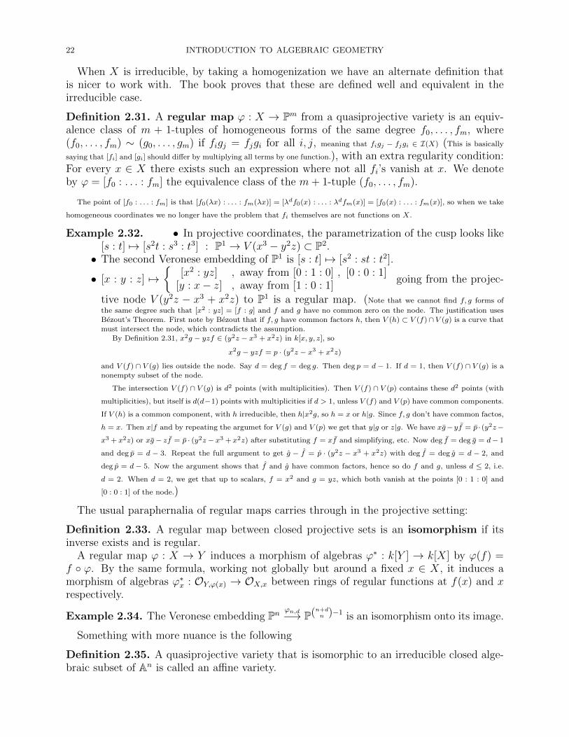
Example 2.32. • In projective coordinates, the parametrization of the cusp looks like[s : t] 7→ [s2t : s3 : t3] : P1 → V (x3 − y2z) ⊂ P2.• The second Veronese embedding of P1 is [s : t] 7→ [s2 : st : t2].
• [x : y : z] 7→
[x2 : yz] , away from [0 : 1 : 0] , [0 : 0 : 1][y : x− z] , away from [1 : 0 : 1]
going from the projec-
tive node V (y2z − x3 + x2z) to P1 is a regular map. (Note that we cannot find f, g forms of
the same degree such that [x2 : yz] = [f : g] and f and g have no common zero on the node. The justification usesBezout’s Theorem. First note by Bezout that if f, g have common factors h, then V (h) ⊂ V (f)∩ V (g) is a curve that
must intersect the node, which contradicts the assumption.
By Definition 2.31, x2g − yzf ∈ (y2z − x3 + x2z) in k[x, y, z], so
x2g − yzf = p · (y2z − x3 + x2z)
and V (f) ∩ V (g) lies outside the node. Say d = deg f = deg g. Then deg p = d − 1. If d = 1, then V (f) ∩ V (g) is anonempty subset of the node.
The intersection V (f) ∩ V (g) is d2 points (with multiplicities). Then V (f) ∩ V (p) contains these d2 points (with
multiplicities), but itself is d(d−1) points with multiplicities if d > 1, unless V (f) and V (p) have common components.
If V (h) is a common component, with h irreducible, then h|x2g, so h = x or h|g. Since f, g don’t have common factos,
h = x. Then x|f and by repeating the argumet for V (g) and V (p) we get that y|g or z|g. We have xg−yf = p · (y2z−
x3 + x2z) or xg− zf = p · (y2z− x3 + x2z) after substituting f = xf and simplifying, etc. Now deg f = deg g = d− 1
and deg p = d − 3. Repeat the full argument to get g − f = p · (y2z − x3 + x2z) with deg f = deg g = d − 2, and
deg p = d − 5. Now the argument shows that f and g have common factors, hence so do f and g, unless d ≤ 2, i.e.
d = 2. When d = 2, we get that up to scalars, f = x2 and g = yz, which both vanish at the points [0 : 1 : 0] and
[0 : 0 : 1] of the node.)
The usual paraphernalia of regular maps carries through in the projective setting:
Definition 2.33. A regular map between closed projective sets is an isomorphism if itsinverse exists and is regular.
A regular map ϕ : X → Y induces a morphism of algebras ϕ∗ : k[Y ] → k[X] by ϕ(f) =f ϕ. By the same formula, working not globally but around a fixed x ∈ X, it induces amorphism of algebras ϕ∗x : OY,ϕ(x) → OX,x between rings of regular functions at f(x) and xrespectively.
Example 2.34. The Veronese embedding Pnϕn,d−→ P(n+d
n )−1 is an isomorphism onto its image.
Something with more nuance is the following
Definition 2.35. A quasiprojective variety that is isomorphic to an irreducible closed alge-braic subset of An is called an affine variety.

INTRODUCTION TO ALGEBRAIC GEOMETRY 23
This yet again improves our definition of affine variety, because now we no longer look atthem as closed in An, but locally closed in some Pm, or even locally closed, but not closed inanother Am.
Example 2.36. If X is a closed subvariety of An and f ∈ k[X] is a regular function, thenD(f) which is quasiprojective as an open subset of X ⊂ An = D(x0) ⊂ Pn is also an affinevariety: It is isomorphic to V (fT − 1) sitting as a closed subset in X × A1 ⊂ An+1 =D(x0) ⊂ Pn+1. (The function x 7→ (x, 1
f(x)) : D(f) → V (fT − 1) is regular on D(f), and its inverse is the regular map
(x, t) 7→ x : V (fT − 1)→ D(f).) D(f) ⊂ X is called a principal affine subset of the affine varietyX.
The ring of regular functions on D(f) is the ring of regular functions on V (fT − 1). Thenk[D(f)] = k[V (fT − 1)] = k[X × A1]
/(fT − 1) = k[X][T ]
/(fT − 1) = k[X][ 1
f] = k[X]f ,
where the latter is the localization of k[X] at the multiplicative system 1, f, f 2, . . ..
Caution. It is not true that every quasiprojective variety is projective or affine. For example A2 \ (0, 0) is not projective(because it is not “compact”), and it is not affine because it is not isomorphic to A2 and they have isomorphic rings of regular
functions.
We will see later that if a quasiprojective variety X ⊂ Pn is isomorphic to a closed subvariety of some Pm, then it was alreadyclosed in Pn.
We will show that regular maps are continuous. The method of proof is to work locally,which shouldn’t be surprising because this is how we work with continuous functions inalmost every other branch of mathematics. But the actual details are more algebraic.
Lemma 2.37. Let X be a quasiprojective subset of Pn. Then the Zariski topology on X hasa basis of open subsets that are affine varieties (isomorphic to closed subvarieties in someaffine space). Equivalently every point x ∈ X has an affine neighborhood.
Proof. Since an open subset of a quasiprojective variety is again quasiprojective, it is enough to check that X itself is coveredby open affine varieties. Then because the sets D(xi)∩X are open in X and cover it, it is enough to check say that D(x0)∩Xis covered by affine varieties.
The new problem is: If X is open in the closure X ⊂ An, then X is covered by affine varieties. The set X \X is closed in X,hence closed in An. There exists a set fi ∈ k[X] of regular functions on X such that X \X = ∩iV (fi). Then X = ∪iD(fi).
Remark 2.38. To work with regular maps ϕ : X → Y , one can cover Y by affines Ui. Thencover each ϕ−1Ui by affines Vij. Then ϕ|UiVij is a regular map between affine varieties in thesense of §1.3, so just given by polynomials.
Corollary 2.39. If ϕ : X → Y is a regular map of quasiprojective subsets of projectivespaces with Y ⊂ Pm. Then ϕ is continuous for the Zariski topology.
Proof. Let Z ⊂ Y be closed. For each x ∈ X there exists an open subset x ∈ U ⊂ X such that ϕ(U) ⊂ D(yi) = Am isregular. By shrinking U around x, we can assume that it is affine. Then ϕ is a regular map between affine varieties, hence it iscontinuous. Then U ∩ ϕ−1Z is closed in U . Since the U ’s cover X, this implies that ϕ−1Z is closed in X.
Yet another definition for regular maps, which is the one that [Har, §1.3] adopts is
Definition 2.40. A regular map ϕ : X → Y is a continuous function such that the inducedpullback ϕ∗x : OY,ϕ(x) → OX,x is a (well-defined) morphism of rings for all x ∈ X.
We practically checked that our initial definition implies this one. Conversely, tf it verifies this one, let x ∈ X and choose
D(yi) = Am such that U := ϕ−1(D(yi)) contains x. Note that U is open by the assumed continuity. Then on a smaller
neighborhood V ⊂ U of x where all gj := ϕ∗x(yjyi
) are regular functions, ϕ : V → Am is given by the formula ϕ(x) =
(g0(x), . . . , gm(x)). The i-th gi is missing. It is one, and it shows up if you write homogeneous coordinates [g0 : . . . : gm].

24 INTRODUCTION TO ALGEBRAIC GEOMETRY
2.4. Rational functions and rational maps for quasiprojective varieties. The thingto take away from this section is that a rational function or map on a quasiprojective varietyX (recall that for us variety means irreducible) is the same as a regular function or map defined on anonempty open (and dense) subset.
We do not have enough regular functions on projective varieties to just say that a rationalfunction is a ratio of regular functions, but things are better if we work with ratios of formsof the same degree.
Definition 2.41. Let X ⊂ Pn be a quasiprojective variety. A rational function on X isa ratio f
gof forms on Pn of the same degree with g|X 6= 0, (i.e. g 6∈ I(X)). We have f
g= f ′
g′iff
fg′ = f ′g on X, (i.e. fg′ − f ′g ∈ I(X)).The set of rational functions forms a field denoted k(X).A rational function f = g
his defined at x ∈ X if h(x) 6= 0.
The domain of definition of f is the dense open subset ∪f= ghD(h). A rational function
is regular on its domain of definition.
Remark 2.42. Two rational functions f1, f2 ∈ k(X) are equal iff they are equal as functionson an open subset contained in the intersection of their domains. (Put f1 = g1
h1and f2 = g2
h2. They
are both regular on U = D(h1) ∩D(h2). The definitions of when two rational functions that are regular on U agree and when
two regular functions on U agree are the same. See Remark 2.27.)
Remark 2.43. Let U be open in X. Then a regular function on U is the same as a rationalfunction on X that is defined (regular) on U .
Remark 2.44. If U ⊂ X is open, then k(U) = k(X). (If a form f vanishes on U , then it vanished on X
and conversely).Moreover, k(X) is the fraction field of OX,x for every x ∈ X. (It is enough to observe that the
obvious map OX,x → k(X) is injective, and every rational function is a ratio of functions regular at x: Let f = gh
be a rational
function. If h(x) 6= 0, then f is regular at x. If not, then choose some form p of degree deg g = deg h that does not vanish at x.
Then f =g/ph/p
is a ratio of regular functions at x.)
Example 2.45. i) If X ⊂ D(x0) ⊂ Pn is an affine variety, then the definition given in thissection for a rational function agrees with the one in §1.5. (This can be seen by (de)homogenizing).
ii) If U ⊂ X is an open affine subset of a quasiprojective variety, then k(X) = k(U) can becomputed as in §1.5. In particular k(P2) = k(x, y) and k(Pn) = k(An).
Definition 2.46. A rational map ϕ : X 99K Pm from a quasiprojective variety is anequivalence class of m+ 1-tuples of homogeneous forms of the same degree f0, . . . , fm, where(f0, . . . , fm) ∼ (g0, . . . , gm) if figj = fjgi for all i, j, meaning that figj−fjgi ∈ I(X) (This is basically saying
that [fi] and [gi] should differ by multiplying all terms by one function.), with the extra condition that not all fivanish on all of X. We denote by ϕ = [f0 : . . . : fm] the equivalence class of the m+ 1-tuple(f0, . . . , fm).
The map ϕ is defined (or regular) at x if for some m + 1-tuple, not all fi vanish at x.The domain of ϕ is the open subset where it is regular. The image of ϕ is the image of thedomain of ϕ.
If Im(ϕ) meets Y ⊂ Pm, we may write ϕ : X 99K Y . We say that ϕ is dominant if itsimage is dense in Y .
If ϕ : X 99K Y is dominant, then we have an induced ϕ∗ : k(Y ) → k(X). This constructionis functorial (respects compositions of dominant rational maps).

INTRODUCTION TO ALGEBRAIC GEOMETRY 25
Remark 2.47. We can also see [f0 : . . . : fm] = [f0
f: . . . : fm
f], where f is a form of the
same degree as the fi’s, and f does not vanish on all of X. In this way we can see rationalfunctions as given by m+ 1 rational functions, not all identically zero on X.
If f = fi for some i such that fi does not vanish on all of X, then we can see the rationalfunction [f0 : . . . : fm] = (f0
fi, . . . , fm
fi) as a rational function to Am = D(yi).
Remark 2.48. To give a rational map X 99K Y is the same as giving a regular map U → Y ,where U ⊂ X is nonempty open (and dense).
In particular, two rational maps agree iff they agree as regular functions on an open subset.
Definition 2.49. ϕ : X 99K Y is a birational isomorphism if it admits an inverse whichis also a rational map. In this case we may also say that X and Y are birational.
Proposition 2.50. Let X and Y be quasiprojective varieties. The following are equivalent
i) X and Y are birational.ii) There exists a birational isomorphism ϕ : X 99K Y .
iii) There exist open subsets U ⊂ X and V ⊂ Y that are isomorphic.iv) There exists a rational map ϕ : X 99K Y and open subsets U ⊂ X such that ϕ is defined
on U and an isomorphism onto its image in Y .v) There exists a dominant rational map ϕ : X 99K Y such that ϕ∗ : k(Y ) → k(X) is an
isomorphism.vi) k(Y ) and k(X) are isomorphic as k-algebras.
vii) There exists a rational map ϕ : X 99K Y such that ϕ∗x : OY,ϕ(x) → OX,x is an isomorphismfor every x in the domain of ϕ.
viii) There exists a rational map ϕ : X 99K Y such that ϕ∗x : OY,ϕ(x) → OX,x is an isomorphismfor one x in the domain of ϕ.
Proof. Only some of the implications are non-trivial.ii)→ iii). Let ψ = ϕ−1. Let U be the domain of ϕ and let V be the domain of ψ. Then U ′ := ϕ−1V ∩U is open because ϕ
is continuous as a function U → Y . Similarly V ′ := ψ−1U ∩ V is open. Then ϕ : U ′ → V ′ is an isomorphism with inverse ψ|U′V ′ .
vi) → ii). From a nonzero morphism f : k(Y ) → k(X) which is automatically injective (because the source is a field),we construct a dominant rational map ϕ : X 99K Y such that f = ϕ∗. The result would then follow by functoriality. Since
k(X) = k(U) for any nonempty open subset U ⊂ X, we may assume that X ⊂ Ap and Y ⊂ Aq are affine varieties. Then k(Y )is generated by the coordinate functions y1, . . . , yq . Define ϕ : X 99K Y by ϕ = (f(y1), . . . , f(yq)). By shrinking X, we can
assume that ϕ is regular, while X is still affine. This is automatically dominant because ϕ∗ : k[Y ]→ k[X] is injective on regular
functions. The claim follows after observing that a (dominant) rational map η : X 99K X for which η∗ = 1k(X) is birational.
This is also handled by restricting to affine subsets (although the one on the left may be different from the one on the right).
2.5. Projective algebraic sets are universally closed. The goal of this section is toprove the following theorem.
Theorem 2.51. Let X ⊂ Pn be a (closed) projective algebraic subset and let f : X → Y bea regular map to a quasiprojective variety. Then f(X) is closed in Y .
Remark 2.52. The projectivity assumption is necessary. For example the image of theregular map (x, y) 7→ x : V (xy − 1)→ A1 is A1 \ (0, 0) which is not closed in A1.
Corollary 2.53. If X is a connected projective algebraic set, then k[X] = k. Consequently,if Y is (quasi)affine and f : X → Y is regular, then f is constant.
Proof. Indeed a regular function f : X → k can be seen as a regular map f : X → A1, or as a regular map f : X → P1 whose
image does not contain the “point at infinity” [1 : 0]. But f(X) ⊂ P1 is closed by the theorem. If it is not everything (because[1 : 0] is not there), then it is just a finite subset of P1. Since X is connected, so is this subset. Therefore f(X) is just a point,meaning that f is constant.
26 INTRODUCTION TO ALGEBRAIC GEOMETRY
Corollary 2.54. If X is simultaneously a closed affine and a closed projective set, then Xis finite.
Proof. Let X′ be a connected component of X. It is still both affine and projective. In particular there exists a regular mapX′ → An for some n, and this map is an isomorphism onto its image. The previous corollary tells us that the image is just a
point, therefore X′ is just a point, and X is finite.
Corollary 2.55. If X ⊂ Pn is an infinite closed subset and f is a nonzero form, then Xintersects the hypersurface V (f).
Proof. By Corollary 2.17, we know that D(f) is affine. By the previous corollary, since X is infinite, it cannot be containedfully in D(f), or else it would also be closed in the affine set D(f). Therefore X and V (f) must intersect.
The proof of the theorem uses an understanding of graphs of regular maps betweenquasiprojective algebraic sets and of products of such sets.
2.5.1. Products and graphs. If X ⊂ Pn and Y ⊂ Pm are quasiprojective algebraic subsets,then X × Y has a structure of qausiprojective set. Here is how it works:
• If X and Y are affine, then X × Y is the affine variety whose algebra of regularfunctions is k[X × Y ] = k[X] ⊗k k[Y ]. (If X ⊂ An is given by equations fi and Y ⊂ Am is given by
equations gj , then X × Y ⊂ An+m is given by equations fi and gj .)• If X and Y are just open subsets of affine varieties, then X × Y = X × Y \ (X \X)× Y ∪X × (Y \ Y ) shows that the product is also open in an affine variety.• If X = Pn and Y = Pm, then X × Y can be seen as a subvariety of P(n+1)(m+1)−1 via
the Segre embedding:
([xi], [yj]) 7→ wij = [xiyj] : Pn × Pm → P(n+1)(m+1)−1.
This map is a bijection onto its image, and its image is closed, given by equationswijwkl = wilwkj for all i, k ∈ 0, . . . , n and j, l ∈ 0, . . . ,m. Therefore Pn × Pm is aprojective variety. The topology on Pn × Pm is the one induced from P(n+1)(m+1)−1.
We should make a little effort to understand the closed subsets of Pn × Pm. Theyare given by vanishing loci of homogeneous forms in wij restricted to Pn × Pm. Butafter restriction, wij = xiyj. Then a monomial of degree d in wij’s is the same as theproduct between a monomial of degree d in xi and one of degree d in yj. Thereforethe closed subsets of Pn×Pm are given by the vanishing of polynomials h(x, y) whichare bihomogeneous, meaning homogeneous in the xi and homogeneous in the yj, fornow of the same degree. But if h(x, y) is bihomogeneous of maybe different degrees
in the xi’s than yj’s, then we can still manage. For example x21y1− 2x2
2y0 vanishes onP2×P1 on the same points as the two polynomials x2
1y0y1− 2x22y
20 and x2
1y21− 2x2
2y0y1
together.• If X ⊂ Pn and Y ⊂ Pm are closed subsets given by equations fi(x) and gj(y), thenX × Y ⊂ Pn × Pm is given inside Pn × Pm by the equations fi and gj which can beseen as bihomogeneous, so X × Y is a closed projective set.• If X and Y are quasiprojective, then we define X × Y as we did for quasiaffine sets.
Remark 2.56. Here are some properties of products:
i) The projections pX : X × Y → X and pY : X × Y → Y are regular.ii) To give morphisms f : Z → X and g : Z → Y is the same as giving one morphism
h : Z → X × Y . Then f and g are recovered by composing with pX and pY . In factX × Y is determined up to isomorphism by this universality property.

INTRODUCTION TO ALGEBRAIC GEOMETRY 27
iii) If f : X → Y is a morphism, then the graph of f is Γf ⊂ X × Y which is the set ofpoints (x, y) ∈ X × Y | y = f(x). Note that Γf ⊂ X× Y is closed (With a bit of work, one
can understand y = f(x) as a set of bihomogeneous equations.)
2.5.2. Proof of Theorem 2.51. Recall that we want to show that if f : X → Y is a regularmap from a projective algebraic subset of Pn to a quasiprojective set, then f(X) is closed inY .
Reduction to projection maps. Since the graph Γf ⊂ X×Y is closed, and pY (Γf ) = f(X),it is enough to show that pY : X × Y → Y maps closed subsets to closed subsets.
Reduction to X = Pn. We have X ⊂ Pn closed. Then our work on products shows thatX × Y ⊂ Pn × Y is also closed and closed subsets of X × Y are closed in Pn × Y . AlsopY : X × Y → Y is the restriction of pY : Pn × Y → Y . If we show that pY : Pn × Y → Ymaps closed subsets to closed subsets, then so did pY : X × Y → Y .
Reduction to Y affine. Let Z ⊂ Pn × Y be closed. The question of pY (Z) being closed inY is local. Then we can cover Y by affine subsets and treat the problem over each of them,i.e. show that pU(Z ∩ Pn × U) ⊂ U is closed if U ⊂ Y is open affine.
Reduction to Y = Am. If Y is affine, then it is isomorphic to a closed subset of Am forsome m. If Z ⊂ Pn × Y is closed, then it is closed in Pn × Am as well, and pY (Z) ⊂ Y isclosed iff it is closed in Am. But pY (Z) = pAm(Z).
We want to show that p := pAm : Pn×Am → Am sends closed subsets to closed subsets. Aclosed subset of Pn×Am is the vanishing locus of polynomials gi(x, y) that are homogeneousin the n+ 1 coordinates x and with no condition on y (by dehomogenizing from Pm to D(y0) = Am.) Wecan assume that gi all have the same degree d by the same trick from §2.5.1 (when we upgraded
from bihomogeneous of the same degree, to bihomogeneous of possibly different degrees in the two sets of variables x and y).A point y0 ∈ Am is not in the image of p iff gi(x, y0) vanish nowhere on Pm × y0. The
Weak Projective Nullstellensatz says that this happens precisely when gi(x, y0) generate anideal Iy0 k[X] that contains a power of the irrelevant (x0, . . . , xn) k[X].
For every positive integer s, put
Ts := y0 ∈ Am | Iy0 6⊃ (x0, . . . , xn)s.Then Im(p) = ∩sTs. It is enough to show that each Ts is closed. Let M be a monomialof degree s in the variables x. Then M ∈ Iy0 means M =
∑i gi(x, y0)Ni,y0(x), where
Ni,y0(x) ∈ k[X]. By looking at the degree s pieces, we can assume that Ni,y0(x) are allhomogeneous polynomials of degree s− d.
Denote by Sd the set of forms of degree d in k[X]. This is a k-vectors space of finite dimension(n+dn
).
Put Gy0 ⊂ Sd the k-subspace generated by the gi(x, y0)’s. The condition Iy0 6⊃ (x0, . . . , xn)s
is thenGy0 · Ss−d ) Ss,
where Gy0 · Ssd is the k-vector subspace of Ss generated by products gi ·N , where N rangesthrough monomials of degree s− d. (If you understand it, this is saying that Gy0 ⊗k Ss−d 6' Ss.)
This is an algebraic condition in y, i.e. given by polynomials: Look at gi as polynomialsin x with coefficients in k[y]. For fixed y and each monomial N of degree s− d, we have thatgi(x, y) · N is a vector in Ss. That for fixed y that these t · dimSs−d vectors, where t is thenumber of gi’s, do not generate Ss means that the matrix that they generate as columns has

28 INTRODUCTION TO ALGEBRAIC GEOMETRY
rank less then dimSs, so all dimSs×dimSs minors vanish. These can be seen as polynomialsin k[y]. Therefore Ts is closed.
Note that when s gets very large, then dimSs > t · Ss−d, so Gy0 · Ss−d 6= Ss for dimensionreasons, and Ts = Am. The proof is interesting for small s and it can actually be implementedin a computer.
2.5.3. Locally projective maps.
Remark 2.57. The same proof can be used to show that if we have a factorization
X ı //
f
##HHH
HHHH
HHH Pn × Y
pYY
,
for some n, where ı is an isomorphism onto a closed subset of Pn × Y (also called a closedembedding), then Im(f) ⊂ Y is closed, without the assumption that X is closed projective.
Morphisms admitting such a factorization are called projective. They are an importantparticular case of a larger class of morphisms called proper that also have the property thatIm(f) ⊂ Y is closed.
If the above factorization exists only locally over Y (meaning that there exists a covering Ui of Y by
open subsets such that f : f−1Ui → Ui is a projective morphism for all i), we say that f is locally projective.
Corollary 2.58. If f : X → Y is locally projective, then f is closed (sends closed subsets of X to
closed subsets of Y ).
Proof. If Z ⊂ X is closed, we want to show that f(Z) ⊂ Y is closed. This is a local question. Let Ui be a cover of Y by
open subsets such if we denote Vi := f−1Ui, then fi := f |UiVi
factors through a closed embedding Vi ⊂ Pni × Ui. The closed
embedding Zi := Z ∩ Vi ⊂ Vi extends to a closed embedding Zi ⊂ Pni × Ui. Then f(Z) ∩ Ui = pUi(Zi) ⊂ Ui is closed.
Remark 2.59. If X is projective, then any regular map f : X → Y to a quasiprojective setis projective. (If X ⊂ Pn is closed, then we have
X Γf //
f
##FFF
FFFF
FFX × Y
pY
ı // Pn × Y
pY
yytttttt
tttt
Y
The composition on the top row is a closed embedding X ⊂ Pn × Y .)

INTRODUCTION TO ALGEBRAIC GEOMETRY 29
3. Finite maps
If f : X → Y is a regular map of quasiprojective varieties such that f−1(y) is a finite setfor all y ∈ Y , then we may think that X and Y are somewhat similar. Algebraic Geometryteaches us to expect an algebraic counterpart for rings which will help with proofs. This isthe concept of a finite extension of rings: If f : A → B is a morphism of rings such that Bis a finite module over A, then we say that f is finite.
Caution. [Sha, §5.3] wants f to be injective, but we don’t. The reason as we will see is that this allows to consider inclusions
of closed subsets as finite maps, which makes sense because they are definitely finite-to-one.
Definition 3.1.
• Affine version: A regular map f : X → Y of closed affine sets is finite if f ∗ : k[Y ]→k[X] is a finite.• Quasiprojective version: A regular map f : X → Y of quasiprojective sets is finite
if Y admits a covering by open affine sets Ui (isomorphic to a closed subset of an affine space, not
necessarily irreducible) such that Vi := f−1Ui is affine and fi := f |UiVi is a finite map of closedaffine sets.
Remark 3.2. Algebra says that a morphism of rings f : A → B such B is of finite type over A is finite iff B is integral over
A, i.e. for every b ∈ B there exists n > 0 and a1, . . . , an ∈ A such that bn +∑i aib
n−i = 0 in B.
Example 3.3. i) If X ⊂ Pn is quasiprojective and Y ⊂ X is the closed subset VX(I) :=V (I) ∩X for some ideal I k[x0, . . . , xn], then the inclusion ı : Y → X is a finite map.(After covering X by affines, we can restrict to the case where X and Y are affine. Then ı∗ : k[X]→ k[Y ] is the quotient
map k[X]→ k[Y ]/IX(Y ).)
ii) Any isomorphism of quasiprojective sets is finite. (In this case f∗i is an isomorphism for all i.)iii) The inclusion A1 \ (0, 0) → A1 is not finite, even though it is one-to-one. (In this case
f∗ is the inclusion k[X] ⊂ k[X,T ]/(XT − 1) and T is not integral over k[X], mainly because XT − 1 is not a monic
polynomial.) For the same reason the projection (x, y) 7→ x : V (xy−1)→ A1 is not finite.iv) The map [x0 : . . . : xn] 7→ [xm0 : . . . : xmn ] : Pn → Pn is finite for any m > 0. More
generally we will see that if fi are m+1 forms of the same degree on a (closed) projectiveset X without common zeros on X, then x 7→ [f0(x) : . . . : fm(x)] : X → Pm is a finitemap.
v) A composition of finite maps is finite.∗ (The algebra statement is that if A → B and B → C are finite,
then so is the induced A→ C. This is clear.)vi) Let f : X → Y and g : Y → Z be regular maps of affine sets. If gf : X → Z is finite,
then so is f . (The algebra statement is that if A→ B → C is such that C is finite over A, then it is also finite over
B.)vii) In particular if f : X → Y is a finite map of affine sets and Z ⊂ X is closed, then f |Z
and f |f(Z)Z are also finite.
∗For now this is clear only for the affine version of Definition 3.1, but we will reconcile the two versions.
Lemma 3.4. Let f : X → Y be a finite map of quasiprojective sets. Then f is locallyprojective over Y (cf. Remark 2.57).
Proof. Since the statement is local, we may work over a cover as in Definition 3.1. Then we may assume that f : X → Y is
a finite map of closed affine sets. We show that f is projective in this case. Let t1, . . . , tn be a finite set of generators of k[X]as a k[Y ] algebra. For example they can be the coordinates from an affine space containing X. Then we have a surjection
k[Y ][t1, . . . , tn] k[X] showing that X is isomorphic to a closed subset of An × Y . We aim to show that X ⊂ Pn × Y is also
closed, where the homogeneous coordinates zi on Pn are such that ti = ziz0
. It is enough to prove that X ∩ (V (z0)× Y ) = ∅, i.e.
X does not meet the hyperplane at infinity over any point of Y .
30 INTRODUCTION TO ALGEBRAIC GEOMETRY
By the finite condition, each ti verifies equations gi(t, y) = 0, where gi(t, y) := tnii +
∑j aij(y)t
ni−ji . If ([0 : z1 : . . . : zn], y) ∈
X, then it verifies the homogenized (with respect to z) equations Gi(z, y) = 0, where
Gi(z, y) = znii +
∑j
aij(y)zj0zni−ji .
But z0 = 0 and Gi(z, y) = 0 for all i clearly implies z0 = . . . = zn = 0 which is not possible in Pn.
Corollary 3.5. If f : X → Y is finite, then f is closed (sends closed subsets of X to closed subsets of
Y ). In particular if f is finite and dominant (f(X) is dense in Y ), then f is surjective.
Proof. Immediate from Corollary 2.58.
Corollary 3.6. Finite maps are finite-to-one.
Proof. We may assume that f : X → Y is a finite map of closed affine subsets. As in the proof of the Lemma, we have that X
is identified with a closed subset of An × Y that is also is also closed in Pn × Y . For every y ∈ Y we have that f−1y is closed
in An and Pn. But the only closed affine and closed projective sets are the finite sets of points.
Remark 3.7. Lemma 3.4 and its proof tell us that if f : X → Y is finite, then the fibers off don’t “disappear to infinity”. For example this gives another reason why the projection ofthe hyperbola V (xy − 1) on the x-axis is not finite.
The next corollary tells us that if X is irreducible, then nonempty open subsets of Xcontain most fibers of f , so these fibers tend to band together.
Corollary 3.8. Let f : X → Y be a finite map of quasiprojective varieties. Then for anyopen subset U ⊂ X there exists an affine open subset V ⊂ Y such that ∅ 6= f−1V ⊂ U .
There is also a converse to Lemma 3.4.
Lemma 3.9. If f : X → Y is a locally projective morphism with finite fibers, then f is finite.
Proof. Without loss of generality we may assume that Y is affine, and that f is projective, i.e. f factors through a closedembedding X ⊂ Pn × Y for some n. For each y ∈ Y , let Hy ∈ Pn be a linear hyperplane such that Hy ∩ Xy = ∅, where
Xy := f−1y (Hy exists since Xy is finite). Then Hy ×Y ⊂ Pn×Y is closed and so is the intersection with X. This intersection
avoids Xy , so its image through the second projection π := pY is a closed (because π is projective) subset Vy ⊂ Y that does notcontain y. Let Uy := Y \ Vy . This is an open subset of Y containing y.
Over Uy , we have that X∩(Pn×Uy) ⊂ (Pn \Hy)×Uy is closed. But Pn \Hy is isomorphic to An−1. Therefore X∩(Pn×Uy)
is isomorphic to a closed subset of An×Uy , also closed in Pn×Uy . Let U ′y be an affine neighborhood of y contained in Uy . Put
Y ′ := U ′y and X′ := X ∩ (Pn × Y ′). We also have that X′ is closed in An × Y ′, in particular it is affine. Put f ′ : X′ → Y ′ the
map induced from f . The goal is to show that k[X′] is finite over k[Y ′], generated by the restrictions t1, . . . , tn of the coordinate
functions on An. In any case the ti’s generate k[X′] as a k[Y ′]-algebra, because X′ is closed in An × Y ′.Let zi be the homogeneous coordinates on Pn so that ti = zi
z0. For ease of notation, assume n = 1. Then X′ is given
in P1 × Y ′ by equations hi(z0, z1, y) = 0 homogeneous in the variables z. We can assume that they have the same degree ofhomogeneity d. We have that X′ ∩ V (z0) = V (z0, (hi)i) = ∅. Working in the affine chart z1 = 1, the Weak Nullstellensatz
implies that (z0, (hi(z0, 1, y))i) = (1) k[Y ′][z0]. In particular there exists a relation on A1z0× Y ′:
1 = z0 · g(z0, y) +∑i
hi(z0, 1, y) · gi(y).
(We have collected everything with z0 that possibly appeared in gi in g.) Setting z0 = 0 we get
1 =∑i
hi(0, 1, y) · gi(y).
On X′ we then have∑i hi(1, t1, y) · gi(y) = 0, because hi(z0, z1, y) = 0 and t1 = z1
z0. Because of the previous formula, this is
monic in t1. Hence t1 is integral over k[Y ′]. And so k[X′] is finite over k[Y ′].
Corollary 3.10. Let X ⊂ Pn be closed projective, and let y ∈ Pn \X. Let ϕ : Pn 99K Pn−1
be the stereographic projection from y. Then ϕ|X is finite (and regular).By iterating, we can replace the point y by a linear subspace L ⊂ Pn that does not meet X.
Then if dimL = d, then the stereographic projection with center L is a map Pn \L→ Pn−d−1.

INTRODUCTION TO ALGEBRAIC GEOMETRY 31
Proof. Note that ϕ is regular outside y, so in particular it is regular on X. Observe that the graph of ϕ|X is closed in Pn×Pn−1.This implies that ϕ|X : X → Pn is a projective morphism. If we show that it has finite fibers, then Lemma 3.9 finishes the
proof. If the fibers are not infinite, then there exists a line ` in Pn through y that meets X at infinitely many points. Since
` ∩X is closed in `, this is only possible if ` ⊂ X. But y ∈ ` \X is a contradiction.
Corollary 3.11 (Noether normalization). Let X ⊂ Pn be a projective variety. Then thereexists a finite dominant map X → Pm for some m.
Similarly if X ⊂ An is an affine variety, then there exists a finite map X → Am for somem.
Proof. Repeat the previous stereographic projection from points until it cannot continue, which is when ϕ(X) = Pm.
Remark 3.12. This seemingly harmless result will give us geometric understanding of thedimension of projective varieties: dimX = m, if the Noether normalization dominates Pm.
Corollary 3.13. If X ⊂ Pn is a projective variety and X → Pm is a Noether normalization,then there exists a linear subspace L ⊂ Pn of dimension n−m− 1 that does not meet X, andevery subspace S of dimension at least n−m meets X.
Proof. L is constructed as the linear span of the points y appearing in the iteration in the proof of Noether normalization. Theprojection from L maps S to a linear subspace of Pm of dimension at least dim s+m− n.
Corollary 3.14. If X ⊂ Pn is a closed projective set and f0, . . . , fs are forms of the samedegree d that do not vanish on X, then f : X → Ps defined by f(x) = [f0(x) : . . . : fs(x)] isfinite.
Proof. The Veronese embedding ν : Pn → P(n+dn
)−1
sends [x] to all degree d monomials in x. It is a closed embedding. Put
N =(n+dn
)−1. On PN , we can see fi as linear forms Fi. Then the rational map PN 99K Ps given by these Fi is for our purposes
a linear projection, and ν(X) is contained in its regular locus. The result is a consequence of Corollary 3.10.
3.1. Local study of finite maps. We are also interested in seeing how finiteness behaveswith respect to open subsets. If f : X → Y is a finite morphism of quasiprojective sets withX and Y affine, then can we reconcile the approaches in Definition 3.1 and show that it wasalready a finite map of affine sets?
Remark 3.15. If ϕ : X → Y is a morphism of affine varieties and f ∈ k[Y ], then ϕ−1D(f) =D(ϕ∗(f)) ⊂ X, i.e. the inverse image of a principal open subset of Y is a principal opensubset of X. It could be empty if f vanishes on ϕ(X).
Proposition 3.16. If f : X → Y is a finite map of affine quasiprojective sets (in the sense of
the second definition), then f ∗ : k[Y ]→ k[X] is finite, i.e. the second definition of 3.1 implies thefirst for morphisms of affine quasiprojective sets.
Proof. Let Y = ∪iUi be an affine open cover of Y such that f−1Ui is an affine open subset of X and f is finite over Ui in theaffine sense (first version of Definition 3.1).
If V ⊂ Ui is a principal open subset corresponding to g ∈ k[Ui], then f−1V is a principal open affine subset of f−1Ui by theprevious remark. Moreover, if k[Ui]→ k[f−1Ui] is finite, then so is k[V ]→ k[f−1V ]. This is because the latter map is just the
localization at g of the previous one, i.e. k[V ] = k[D(g)] = k[Ui]g , which is just rational functions on Ui where the denominatorsare only allowed to range through powers of g.
Cover Ui by principal open subsets of Y . Then they are also principal on Ui by the remark, and f is finite over them in theaffine sense. Without loss of generality we can assume Ui = D(gi) for gi ∈ k[Y ] and that this is a finite cover.
Let hij be generators for k[X]f∗(gi) = k[f−1D(gi)] as a finite algebra over k[Y ]gi = k[D(gi)]. By clearing denominators,
since gi1
is invertible in k[Y ]gi , we can assume that hij =uij
1for some uij ∈ k[X]. (We could write uij = hij if k[X] was a
domain, but we do not assume this).
We claim that uij generate k[X] as a k[Y ]-module: Let x ∈ k[X]. For each i, in k[X]f∗(gi) write x1
=∑jaij
gniji
uij
1for some
aij ∈ k[Y ] and some nij ≥ 0. By clearing denominators, gnii x =
∑a′ijuij for some ni ≥ 0 and a′ij ∈ k[Y ]. Since D(gi) cover Y ,
it follows that ((gi)i) = 1 k[Y ], hence the same is true of ((gnii )i). We can find then bi ∈ k[Y ] such that
∑i big
nii = 1. Then
x =∑i big
nii x is in the k[Y ]-span of uij .

32 INTRODUCTION TO ALGEBRAIC GEOMETRY
Lemma 3.17. Let X be a quasiprojective set and let U and V be open affine subsets. ThenU ∩ V is an open affine. More generally, if f : U → X is a regular map from a closed affineset U to quasiprojective X and V ⊂ X is affine open, then f−1V is affine open in U .
Proof. U × V ⊂ X × X is an open subset and affine, because it is the product of two affines. The diagonal ∆ = (x, y) ∈X × X | x = y is a closed subset of X × X (the graph of the identity morphism). Therefore its intersection with U × V is
closed in U × V in the induced topology. But (U × V ) ∩∆ = U ∩ V , therefore U ∩ V is closed in the affine set U × V , meaningthat itself is affine. The case when the inclusion U ⊂ X is replaced by a regular map is similar.
Proposition 3.18. If f : X → Y is a finite map of quasiprojective sets, then f is affine.This means that if U ⊂ Y is an open affine, then the open f−1U ⊂ X is also affine.
Proof. Cover Y by affines Ui such that f−1Ui is affine and f is finite over Ui in the affine sense. Cover U by open affines Wj
that are each principal in one of Ui. By working over the corresponding Ui, we see as in the previous proposition that f−1Wj
is affine open and f is finite over Wj . Now we are free to assume U = Y .
Up to a further refinement, we can assume that Ui (from Y = ∪iUi) are principal open subsets of Y with f−1Ui ⊂ X affine
open and f finite over Ui. We want to show that X is itself affine.To make writing easier, assume that Y = D(g1) ∪D(g2) for regular functions g1, g2 ∈ k[Y ]. Observe that D(g1) ∩D(g2) =
D(g1g2) is principal in Y , but also in D(g1) and D(g2) (in the first it is the nonvanishing of g2 and in the second of g1. And giis regular on D(gj) because it is regular on Y ). Then X = D(f∗g1) ∪D(f∗g2) and D(f∗g1) ∩D(f∗g2) is principal in each ofthem. Let x be a regular function on D(f∗g1). Then it is regular on the intersection, which is principal in D(f∗g2), given by
the nonvanishing of g1. Since we have arranged for D(f∗g2) to be affine, k[D(f∗(g1g2))] = k[D(f∗g2)]f∗g1 . In particular there
exists x′ ∈ k[D(f∗g2)] such that x = x′
gm1in k[D(f∗g2)]f∗g1 for some m ≥ 0. Then in k[D(f∗g2)], we have
gn1 x′ = gm+n
1 x ∈ k[D(f∗g1)]
for some n ≥ 0 (if X is irreducible, we can choose n = 0). This means that gn+m1 x is regular on the entire X. Similarly, for any
x ∈ k[D(f∗g2)] there exits m ≥ 0 such that gm2 x is regular on X. By working through the algebra, this means that the naturalmaps
(5) k[X]f∗gi → k[D(f∗gi)]
are surjective (they would be isomorphisms if we knew that X was affine). Quite generally these maps are injective: It is enough
to check that if x ∈ k[X], and x|D(f∗g1) = 0, then gm1 x = 0 for some m ≥ 0. But in fact g1x vanishes everywhere, therefore it is
the zero regular function. (Somewhere in here we are using that k[X] is reduced, which is true because the definitions of §2.3.1
do not create nilpotents.)As in the previous proposition, it can be shown that k[X] is finite over k[Y ]. In particular it is of finite type over k. Since
k[X] is also reduced, we can consider Z the closed affine set having k[Z] = k[X]. (We would have Z = X if X was affine.) Using
that Y and Z are affine, the morphisms k[Y ]→ k[Z] = k[X] induce a factorization
Xϕ //
f @@@
@@@@
@ Z
F
Y
(If ti generate k[X] = k[Z] as a k-algebra, then x 7→ (t1(x), . . . , td(x)) : X → Ad always lands in Z because it verifies itsequations. This gives ϕ. Note that ϕ∗ = 1k[Z]. The map F is the only regular map of affine sets with F ∗ = f∗. If yj are
generators for k[Y ], then F (z) = (F ∗(y1)(z), . . . , F ∗(yr)(z)). In particular
F (ϕ(x)) = (F ∗(y1)(ϕ(x)), . . . , F ∗(yr)(ϕ(x))) = (ϕ∗F ∗(y1)(x), . . . , ϕ∗F ∗(yr)(x)) = (f∗(y1)(x), . . . , f∗(yr)(x)) = f(x),
therefore f = F ϕ.)Since F ∗ = f∗, we have that k[Z] is finite over k[Y ] via F ∗, and since Y and Z are affine, F is finite in the affine sense. Then
F−1D(gi) are principal affine open subsets of Z and we have induced regular maps of affine sets ϕi : D(f∗gi)→ D(F ∗gi). Note
that ϕ∗i is the morphism in (5), and in particular is an isomorphism. This implies that the morphism ϕi between affine opensis an isomorphism. Then ϕ restricts to an isomorphism over a cover and therefore it is itself an isomorphism meaning that X
is affine (isomorphic to Z).
Corollary 3.19. a) If f : X → Y is a finite map of quasiprojective sets, then any affinecover of Y has the properties of Definition 3.1.
b) A composition of finite maps between quasiprojective sets is finite.c) If f : X → Y is a finite map of quasiprojective sets, then f |ZX : X → Z is finite for any
closed subset Z ⊂ Y that contains f(X).
INTRODUCTION TO ALGEBRAIC GEOMETRY 33
Proof. a) is immediate from the previous proposition. Using a) one sees that if Ui is an affine cover of Z, then g−1Ui is anaffine cover of Y satisfying the conditions of Definition 3.1 for f , hence Ui verify the same definition for g f .
For c), it is enough to observe that f factors through Z and that an affine cover of Y restricts to an affine cover of Z, since
Z ⊂ Y is closed.
34 INTRODUCTION TO ALGEBRAIC GEOMETRY
4. Dimension
We have been speaking about projective spaces of a certain dimension, and have an in-tuitive understanding that curves should have dimension 1, and that hypersurfaces shouldhave dimension one-less (also called codimension 1). Let’s see what happens for arbitraryquasiprojective sets.
First of all, if X is reducible, then its “dimension” should be the maximal dimension amongits irreducible components, so let’s assume that X is a variety.
Definition/Theorem 4.1. Let X ⊂ Pn be a quasiprojective variety, let X be its closure,let U ⊂ X be an affine open subset, and let x ∈ X. Then the following quantities are allequal:
i) d ≥ 0 such that there exists a Noether normalization X → Pd, i.e. a finite dominant map X → Pd
ii) The transcendence degree of k(X) over k, i.e. the maximal number of elements of k(X) algebraically
independent over k.
iii) The maximal length (i.e. the number of inclusions, or one less than the number of terms) of any chainY0 ( . . . ( Yd = X of irreducible closed subsets of X.
iv) The Krull dimension of k[U ], i.e. the maximal length of any chain of proper (differentfrom (1)) prime ideals 0 = pd ( pd−1 ⊂ . . . ( p0 in k[U ].
v) The Krull dimension of the ring of regular functions OX,x at x.
The number resulting from any of the above is called the dimension of X, denoteddim(X). If Y ⊂ X is a locally closed subset, then its codimension in X is codim(Y,X) =dimX − dimY .
If X is allowed to be reducible, then dimX is the maximal dimension among its compo-nents. If all components have the same dimension we say that X is equidimensional, or ofpure dimension.
Proof. The equivalence between the last four statements is algebra. To relate the first with the second, note that a finite
dominant map X → Pd induces a finite field extension k(x1, . . . , xd) ⊂ k(X). Then trdegkk(X) = trdegkk(x1, . . . , xd) = d. In
particular if X → Pd is a finite dominant map, then d is uniquely determined by X (changing the map doesn’t change d).
Some common sense properties of dimension are the following
Corollary 4.2. • If Y ⊂ X is locally closed, then dimY = dimY . In particular ifU ⊂ X is open and X is irreducible, then dimU = dimX.• dimAd = dimPd = d. For linear subspaces of either of them, the new concept of
dimension agrees with the one from linear algebra.• If f : X → Y is a dominant map, then dimX ≥ dimY .• If f : X → Y is a finite map, then dimX ≤ dimY . Equality holds if f is also
dominant. In particular isomorphisms preserve dimension.• If Y ( X is a proper locally closed subset of X, then dimY < dimX. In particular
if X is irreducible, if Y ⊂ X is closed of codimension 1 and if Y ( Z ⊂ X is a chainwith Z irreducible, then Z = X.• dim(X × Y ) = dimX + dimY .
Proof. For the second to last part note that a chain of irreducible closed subsets of Y can be extended by at least one more byadding X at the end.
For the last part, let’s first treat the case X = Pn and Y = Pm. Then Pn×Pm is irreducible and contains An×Am = An+m
as an open subset, therefore its dimension is n + m. In general, we can assume that X and Y are projective. If X → Pn andY → Pm are Noether normalizations, then X×Y → Pn×Pm is finite and dominant: Clearly it is surjective and has finite fibers.
It is also the product of two locally projective maps, and this is easily seen to be again locally projective as an application ofthe Segre embedding. Conclude by Lemma 3.9. But the corollary then says that dim(X × Y ) = dim(Pn × Pm) = n+m.
INTRODUCTION TO ALGEBRAIC GEOMETRY 35
Example 4.3. The Grassmannian G(d, n) has dimension d(n − d). 5 (Recall that if V = kn,
and W ⊂ V is a d-dimensional linear subspace, then the Plucker embedding sends W ⊂ V to the line ∧dW ⊂ ∧dV , thusdetermining a point in P(∧dV ). The latter has homogeneous coordinates zi1,...,id corresponding to simple wedges ei1 ∧ . . .∧ eidwith 1 ≤ i1 < . . . < id ≤ n. If the coordinate z1...,d is nonzero, then we show that G(d, n) ∩D(z1...,d) ' Ad(n−d): as we did in
(4), for a point ω in the claimed open subset of G(d, n), we can find a unique matrix1 0 . . . 0 a1,1 . . . a1,n−d0 1 . . . 0 a2,1 . . . a2,n−d...
.... . .
......
. . ....
0 0 . . . 1 ad,1 . . . ad,n−d
such that ω = v1 ∧ . . .∧ vd, where vi are the rows of the matrix (This is linear algebra: If w1, . . . , wd is a basis for W , then after
Gauss–Jordan elimination on the matrix whose rows are the wi’s, we get the the matrix whose rows are the vi’s). Conversely
for any such matrix we can find a point in G(d, n) ∩D(z1,...,d). Since there are d(n− d) parameters in the matrix, this defines
the claimed isomorphism.)
4.1. Dimension of intersection with a hypersurface.
Theorem 4.4. Let X ⊂ Pn be an irreducible closed subset. Then X has codimension 1 ifand only if I(X) = (f) for some irreducible nonzero form f on Pn, i.e. X is an irreduciblehypersurface.
Consequently, if X is reducible of codimension 1 and equidimensional, then I(X) = (f)for some (reducible) form f .Proof. Let g be a nonzero form with X ⊂ V (g). Such g exists by the Nullstellensatz, because X 6= Pn. Let g = g1 · . . . · grbe a decomposition of g into irreducible (automatically homogeneous because g is) polynomials of positive degree in the UFDk[X0, . . . , Xn]. Then X ⊂ V (g) = ∪iV (gi). Then the closed sets V (gi) ∩X cover X, and by irreducibility X ⊂ V (gi) for some
i. Put f := gi.
We claim that V (f) is irreducible. Indeed (f) k[X] is a prime ideal because f is irreducible in the UFD k[X]. By the
Nullstellensatz, I(V (f)) =√
(f) = (f) is prime and the claim follows.
If X has codimension 1, since X ⊂ V (f), the previous corollary shows that X = V (f) and the previous paragraph showsI(X) = (f).
Conversely it is clear that if I(X) = (f), then X = V (I(X)) = V (f), so a hypersurface. Let’s show that in this case
dimX = n − 1. In any case, since f 6= 0, we have that X = V (f) 6= Pn. Let p ∈ D(f). By Corollary 3.10, if π : X → Pn−1 isthe restriction to X of the stereographic projection from p, then π is finite. We claim that it is also dominant. Let q ∈ Pn−1.
The line ` through p and q is a closed projective infinite subset, therefore it intersects V (f) = X by Corollary 2.55. If
x ∈ ` ∩X, then π(x) = q, proving that π is in fact surjective. Since π : X → Pn−1 is finite and dominant, it must follow thatdimX = dimPn−1 = n− 1.
Remark 4.5. There are analogous statements in An or Pn1 × . . . × Pnr : The only equidi-mensional closed subsets of codimension one are the hypersurfaces (given by the vanishing ofa polynomial equation in An, or of a multi-homogeneous form on the product of projectivespaces).
However in general if X ⊂ Pn is a projective variety, and Y ⊂ X is an irreducible subsetof codimension 1, then Y is not necessarily of form V (f) ∩X where f is a form on Pn:
For example if we look at P1 × P1 as a quadratic surface X := V (z0z3 − z1z2) ⊂ P3 via the Segre
embedding ([x0 : x1], [y0, y1]) 7→ [x0y0 : x0y1 : x1y0 : x1y1], then there is no form f on P3 such that
X ∩ V (f) is the line ` := X ∩ V (z0, z1) (this is the fiber of the first of [0 : 1] via the first projection P1 × P1 → P1).
Indeed X also contains the line `′ := X ∩ V (z0, z2) (the fiber over [1 : 0]), and ` ∩ `′ = ∅. On the other
hand, V (f) must intersect `′ because it is an infinite projective set (cf. Corollary 2.55) inside P3,
and therefore inside X as well, and them ` = V (f)∩X would also meet `′, which is a contradiction.
Inside Pn, or An, or inside products of projective spaces, sets of form V (f) have codimension1. Let’s see that this holds for all quasiprojective varieties.6
5Since Pn = G(1, n + 1), we don’t get a new formula for dimPn.6Remark 4.5 shows that the converse is not always true, even on products of projective spaces if we change
the projective embedding.
36 INTRODUCTION TO ALGEBRAIC GEOMETRY
Theorem 4.6. Let X ⊂ Pn be a quasiprojective variety. Let f be a nonzero form on Pn andassume that V (f)∩X is a proper closed subset (not ∅ or X). Then V (f)∩X has codimension1 in X. Moreover the same is true for any irreducible component of V (f) ∩X.
Proof. Since dimension can be measured on open subsets, we may assume that X is projective. In this case the intersection is
automatically nonempty by Corollary 2.55. Replacing Pn by a Veronese embedding, we reduce to the case when f is linear.
We do induction on r := codim(X,Pn). The case r = 0, i.e. X = Pn is Theorem 4.4. If r > 0, then there exists p ∈ V (f) \Xby the assumption that V (f) ∩X 6= X. By Corollary 3.10, stereographic projection ϕ : Pn \ p → Pn−1 then maps X finitely
onto its image in Pn−1. Denote the image by X′. Note that dimX′ = dimX, in particular codim(X′,Pn−1) = r − 1. Also
observe that since V (f) is a linear hyperplane passing through p, its image through ϕ is a linear hyperplane V (g) in Pn−1.Again by Corollary 3.10, ϕ maps V (f) ∩ X finitely onto its image, hence dim(V (f) ∩ X) = dim(ϕ(V (f) ∩ X)). We claim
that ϕ(V (f) ∩X) = V (g) ∩X′. The conclusion then follows by induction.
For the claim, the inclusion ϕ(V (f) ∩ X) ⊂ V (g) ∩ X′ is clear. Conversely, let y ∈ V (g) ∩ X′. Then V (f) contains y andp, and since it is linear, it contains the line ` passing through them. Since y ∈ X′, by the construction of the projection, ` ∩Xis nonempty. If x ∈ ` ∩X, then x ∈ V (f) ∩X as well, because ` ⊂ V (f), and we see that ϕ(x) = y, which gives the inclusion
V (g) ∩X′ ⊂ ϕ(V (f) ∩X).The proof in [Sha] is also quite nice.
Iterating the previous result we obtain:
Corollary 4.7. Let r ≤ n. Then any r hypersurfaces in Pn have nonempty intersection.More generally, if X ⊂ Pn is closed projective, and r ≤ dimX, then X has nonemptysimultaneous intersection with any r hypersurfaces in Pn. The case r = 1 is Corollary 2.55. Inparticular r homogeneous equations in Pn always have solutions as long as r ≤ n.
Corollary 4.8. Let X and Y be closed subsets of Pn. Then dim(X∩Y ) ≥ dimX+dimY −n,equivalently codim(X ∩ Y,Pn) ≤ codim(X,Pn) + codim(Y,Pn), and the same is true for anyof its irreducible components.
If X and Y are only quasiprojective, then the conclusion holds only for the nonemptycomponents of X ∩ Y if any.
Proof. Observe that X ∩ Y is isomorphic to (X × Y ) ∩∆, where ∆ is the diagonal in Pn × Pn, i.e. the graph of the identity
morphism Pn → Pn. Consider the Segre embedding Pn × Pn → P(n+1)(n+1)−1. Denote the latter by PN . The diagonal∆ ⊂ Pn×Pn has n equations x0yi = xiy0 for 1 ≤ i ≤ n (at least on the affine open subset D(x0)∩D(y0), but such subsets cover
Pn × Pn, and the question is local on X anyway) which being bihomogeneous of the same degree in the x’s and the y’s, are the
restrictions to Pn × Pn of some forms fi on PN . Then X ∩ Y ' (X × Y )∩∆ = (X × Y )∩ V (f1)∩ . . .∩ V (fn), and by iteratingTheorem 4.6, this has dimension at least dim(X × Y ) − n = dimX + dimY − n. Usually we have equality of dimensions, but
the inquality can be strict if at any step in the iteration we deal with a nonproper intersection.
This is a particular case of the following
Corollary 4.9. Let f : X → Pn be a regular map from a quasiprojective variety X. LetY ⊂ Pn be a quasiprojective subset. Then if Z is a nonemtpy irreducible component of f−1Y ,then dimZ ≥ dimX + dimY − n.
Proof. Observe that f−1Y is isomorphic to (X × Y )∩ Γf , where Γf ⊂ X × Pn is the graph of f . The conclusion is local, so wemay reduce to the affine case. In this case f : X → An has that the graph Γf ⊂ X × An is given by n equations: If f si givenby n regular functions f = (f1, . . . , fn), then Γf is given by equations yi = fi(x). Conclude again by the theorem.
Remark 4.10. When r > 1, it is not true that every equidimensional (or even irreducible)closed subset X ⊂ Pn of codimension r is a set theoretic complete intersection, i.e. theintersection of r hypersurfaces, though simple examples are not that easy to construct andexplain at this point. Many are known when dimX > 1. It is an open question whetherevery irreducible projective curve in P3 is a set theoretic complete intersection.
4.2. The dimension of the fibers of a regular map. If f : V → W is a surjective linearmap of vector spaces, then the fibers of f are all translations of ker f , hence they are all ofthe same dimension, dimV − dimW . It is reasonable to expect at least a similar property

INTRODUCTION TO ALGEBRAIC GEOMETRY 37
from regular maps between algebraic varieties. And indeed we cannot hope that all the fibershave the same dimension in general: think about the blow-up.
The good news comes in the form of the following:
Theorem 4.11. Let f : X → Y be a dominant regular map of quasiprojective varieties. Pute = dimX − dimY . Then
i) If y ∈ Y and Xy := f−1y is nonempty, then every irreducible component of Xy hasdimension at least e.
ii) There exists a nonempty open subset U ⊂ Y such that dimXy = e for all y ∈ U .iii) If x ∈ X, denote by Xx,f the union of the irreducible components of f−1f(x) that
actually contain x. Let Xh := x ∈ X | dimXx,f ≥ h. Then Xh is a closed subset ofX.
iv) If f is locally projective, then Yh := y ∈ Y | dimXy ≥ h is closed in Y .
Proof. For part i). The question is local on Y , so we are free to assume that it is affine. Let g : Y → Am be an affine Noether
normalization with m = dimY . For any y ∈ Y , the fiber Xy is a union of irreducible components of Xg(y), hence we may assume
that Y = Am. Now apply Corollary 4.9 to conclude that since y ∈ f(X) ⊂ Y has codimension m in Pm, the fiber f−1y has
codimension at most m in X.
For part ii). Write X = ∪iXi, where Xi ⊂ X are affine open subsets. For each i we will produce a nonempty open Ui ⊂ Ywith the required property for the restricted map Xi → Y , and then we put U = ∩iUi. (In this way we make sure that when
working in Ui, components of Xy of dimension higher than e do not hide in some other Uj .) We have reduced to the affine case.
Then we do induction on e as in the lemma below. We use the notation in its proof. The case e = 0 follows by homework,since f is finite over a nonempty open subset of Y , and the fibers of a finite map are finite sets of points, hence of dimension 0.
If e > 0, then induction takes care of g. If F ∈ k[Y ][t] and V = D(F ) ⊂ Y ×A1 with V ⊂ g(X), let a ∈ k[Y ] denote the leading
term of F . Then as in the lemma D(a) ⊂ f(X). Moreover, the fiber over y ∈ D(a) is D(F ) ∩ y × A1, which is open in A1, inparticular of dimension 1.
Here is our new setting: g : Xy → C ⊂ A1 = y × A1 is a surjection onto an open subset C of the affine line. We know byinduction that the fibers of g are equidimensional of dimension e− 1. We also know by part i) that every irreducible component
of Xy has dimension at least e. We want to conclude that Xy is equidimensional of dimension e. To see this, first not that if
X′ is a component of Xy , then the conclusion dimX′ ≥ e implies that X′ dominantes C, otherwise X′ maps to a point on C,contradicting the findings on the dimension of fibers of g over C. Hence we may assume that Xy is irreducible. If t0 ∈ C ⊂ A1,
which we can see as an element of k, then the fiber of g over t0 is V (t− t0) ∩Xy , in particular a hypersurface. But as such it
has codimension 1. The conclusion follows.For part iii). The definition of Xh is local (which it wouldn’t be if we just looked at the dimension of the full fiber). Then
we can assume that X and Y are affine varieties. If U ⊂ Y is as in part ii) and Z = Y \U , then Xh ⊂ f−1Z for h ≥ e+ 1. Let
X′ be an irreducible component of f−1Z, and let Y ′ be the closure in Z of f(X′). Furthermore Xh is the union of all X′h. Thestatement follows by induction on dimY , since dimY ′ < dimY , and the conclusion is trivial when Y is a point.
For part iv), observe that Yh = f(Xh), and f is closed since it is locally projective.
Lemma 4.12. Let f : X → Y be a dominant morphism of quasiprojective varieties. Thenthere exists U ⊆ Y open with U ⊂ f(X).
Proof. We may assume that X and Y are affine varieties. Since f : X → Y is dominant, the pullback morphism of rational
functions f∗ : k(Y )→ k(X) is well-defined and injective. We do induction in e := trdegk(Y )k(X). The case e = 0 was homework:
you showed that there exists U ∈ Y nonempty affine open such that f if finite over it. When e > 0, let t ∈ k(X) be transcendentalover k(Y ). We may assume t ∈ k[X] since k(X) is the fraction field of that. Then we have inclusions k[Y ] ⊂ k[Y ][t] ⊂ k[X] and
the composition is f∗. This means that f factors as
Xg //
f##F
FFFF
FFFF
Y × A1
p
Y
where p is the projection on the first component and A1 has coordinate t. Note that g is dominant and trdegk(Y )(t)k(X) = e−1.
By induction the lemma holds for g. Let V ⊂ Y × A1 be an open subset contained in g(X). We may assume that V = D(F ),
with F ∈ k[Y ][t]. Then p(V ) = y ∈ Y | F (y) 6∈ k∗ ⊂ k[t]. Looking at F as a polynomial in t with coefficients in k[Y ], let a be
its leading coefficient. Then D(a) ⊂ p(V ) ⊂ p(g(X)) = f(X) is a nonempty open subset.
Remark 4.13. • The “e” in the theorem is called the relative dimension of f . It isthe expected dimension of the fibers of f .
38 INTRODUCTION TO ALGEBRAIC GEOMETRY
• [Sha, Corollary on p76], stating that the sets Yh are closed without the assumptionthat f is locally projective is incorrect. The correct statement in general is that Yh isconstructible, meaning a finite union of locally closed subsets of Y .
An important corollary of the theorem on the dimension of fibers is a criterion for irre-ducibility.
Corollary 4.14. Let Y be a quasiprojective variety. Let f : X → Y be a locally projectivemap with X quasiprojective. If there exists e ≥ 0 such that the fibers of f are irreducible ofconstant dimension e, then X is also irreducible.
Proof. Let Xi ⊂ X be the irreducible components of X. For each i, let Yi,e := y ∈ Y | dim(Xi)y ≥ e. Since f is locallyprojective, this is a closed subset of Y . Observe that ∪iYi,e = Y . This is because for every y ∈ Y , we have Xy = ∪i(Xi)y ,
and since dimXy = e, at least one term in the union also has dimension e. By the irreducibility of Y , it follows that some
component X1 of X has all fibers of dimension at least e. But since Xy is irreducible and (X1)y ⊂ Xy , it follows that the fibersof X1 and X over Y agree everywhere, meaning X1 = X.
Example 4.15. Let’s give another proof for dimG(d, n) = d(n − d). (We have a regular function
Mn,d,d → G(d, n) that sends an n × d matrix of rank d to its image which is a d-dimensional subspace of kn. The fibers are
isomorphic to GLd(k), since we can use d×d invertible matrices to switch between bases of subspaces, and every invertible matrix
corresponds to a different basis. Since Mn,d,d is open in Mn,d, it follows that d2 = dimGLd(k) = dimMn,d,d − dimG(d, n),
therefore dimG(d, n) = dimMn,d − d2 = nd− d2 = d(n− d).)
4.3. Lines on surfaces.
Example 4.16. If f is a form of degree 3 on P3C, then V (f) contains at least one line (linear
subspace of P3 of dimension 1). (A form of degree 3 on P3 has(63
)= 20 coefficients. Then we can parameterize
forms up to scaling with a P19 by looking at the 20 coefficients as homogeneous coordinates. On the other hand lines in P3
correspond to planes in k4, so to points in G(2, 4).
Let P3 have coordinates [z0 : . . . : z4] and let P19 have coordinates sijkl, where i+ j + j + l = 3 are exponents of monomials
zi0zj1zk2 zl3 of degree 3. Let H ⊂ P3×P19 be the universal hypersuface given by the vanishing of F =
∑i+j+k+l=3 sijklz
i0zj1zk2 zl3.
This is the universal hypersurface of P3 of degree 3, in that all V (f) appear as fibers of the map H → P19 (by assigning explicit
values to the indeterminates sijkl).
Let L ⊂ G(2, 4) × P3 be the universal line. Let’s find equations for it. Let W ⊂ k4 be a 2-dimensional subspace and let
z = [z0 : z1 : z2 : z3] ∈ P3. Then z is in the line in P3 determined by W if and only if z as a vector in k4 is contained in W . An
algebraic-looking condition that is equivalent to this is u ∧ v ∧ z = 0 if u, v is a basis for W . This is equivalent to asking that
the determinants of the 3 × 3 minors in the matrix
uvz
vanish. The determinants of the 2 × 2 minors on the first two rows
give the Plucker coordinates (sij)i<j on G(2, 4) corresponding to W → ∧2W . By Laplace expansion using the last row, we canexpress the 3 × 3 determinants in terms of the zi’s and the sij ’s. We get 4 polynomial equations bihomogneous of degree 1 in
both the zi’s and the sij ’s.
The set of inclusions x ∈ ` and x ∈ V (f) is parameterized by I := (G(2, 4)×H) ∩ (L× P19) inside G(2, 4)× P3 × P19.We are looking for inclusions x ∈ ` ⊂ V (f). Here is how we can fix this: The fiber of the map I → G(2, 4)×P19 over a point
(`, V (f)) is precisely `∩V (f) as a subset of P3. The line ` is contained in V (f) precisely when this fiber has positive dimension.
But Theorem 4.11.iv) tells us that the locus in G(2, 4) × P19 over which all fibers have dimension ≥ 1 is closed. Denote thisclosed set by J ⊂ G(2, 4)× P19. Then V (f) contains some line if and only if f is in the image of J → P19.
Let’s investigate J . The fibers of J → G(2, 4) are hypersurfaces V (f) that contain a fixed line. Up to changes of coordinates,
we may focus on the line z0 = z1 = 0. Then V (f) contains this, if and only if f(0, 0, z2, z3) is identically zero, which happens ifand only if the coefficients s0,0,k,l with k + l = 3 all vanish. There are 4 such, and their vanishing is a linear condition on P19.
Therefore for each ` ∈ G(2, 4), the fiber J` is isomorphic to P 15 (codimension 4 because of the 4 equations which are clearlyindependent). It follows that J is irreducible and of dimension dimG(2, 4) + 15 = 19.
If we can show that the map J → P19 is generically finite (meaning that the fibers are finite over an open subset of the
image), then by Theorem 4.11.ii), it follows that J → P19 is dominant, hence surjective because J is projective. Again byTheorem 4.11.ii), it is enough to check that for one f the fiber Jf is finite nonempty. Let f = z3
0 + z31 + z3
2 + z33 . If ` ⊂ V (f),
then let V (f) 3 [0 : a1 : a2 : a3] := `∩V (z0) and V (f) 3 [b0 : 0 : b1 : b2] := `∩V (z1). Assume that these are two distinct points,
so that any point on ` is of form [tb0 : sa1 : sa2 + tb2 : sa3 + tb3] with s, t arbitrary. Since ` ⊂ V (f), all these points verifyf = 0. Plugging in, this is equivalent to asking that the polynomial in s, t that we get is identically 0, and so all its coefficients
are zero. The coefficients are
a31 + a3
2 + a33 = 0 b30 + b32 + b33 = 0 a2
2b2 + a23b3 = 0 a2b
22 + a3b
23 = 0

INTRODUCTION TO ALGEBRAIC GEOMETRY 39
The conditions that the points a and b were distinct translates into a2 = b3 = 0 or a3 = b2 = 0 and the points are [0 : 1 : 0 : ε]
and [1 : 0 : ε : 0], or [0 : 1 : ε : 0] and [1 : 0 : 0 : ε] as ε, ε range through third roots of −1. If the starting points coincide,
intersect ` with V (z2) or V (z3) instead of V (z1). In any case we obtain only finitely many lines, the lines ` through such pairs
of points.)
Remark 4.17. In fact the Fermat cubic V (z30 + z3
1 + z32 + z3
3) contains 27 lines. They are the9 lines with parameterizations [s : εs : t : εt] as s, t range in C, and ε, ε are cube-roots of −1,and the 18 conjugates under permutations of coordinates.
It can be shown that a general cubic surface contains exactly 27 lines.
Example 4.18. If f is a degree 4 form on P3C, then there exists an irreducible polynomial
P in the coefficients of f seen as indeterminates such that P (f) = 0 if and only if V (f)contains a line (linear subspace of dimension 1). (A form of degree 4 on P3 has
(73
)= 35 coefficients. Then
we can parameterize forms f by P34. The lines in P3 are parameterized by G(2, 4).As before, let J ⊂ G(2, 4) × P34 be the closed subset parameterizing inclusions ` ⊂ V (f). Then V (f) contains some line if
and only if f is in the image of J → P34.
Let’s investigate J . The fibers of J → G(2, 4) are hypersurfaces V (f) that contain a fixed line. Up to changes of coordinates,we may focus on the line z0 = z1 = 0. Then V (f) contains this, if and only if f(0, 0, z2, z3) is identically zero, which happens if
and only if the coefficients s0,0,k,l with k + l = 4 all vanish. There are 5 such, and their vanishing is a linear condition on P34.
Therefore for each ` ∈ G(2, 4), the fiber J` is isomorphic to P 29 (codimension 5 because of the 5 equations which are clearly
independent). It follows that J is irreducible and of dimension dimG(2, 4) + 29 = 33.
Let K be the image of J in P34. We will show that this also has dimension 33. Then it is V (P ) for some P , which is thedesired polynomial.
Since J itself has dimension 33, it is enough to produce one quartic surface that contains only finitely many lines. Then the
map J → K which is surjective by the definition of K, is also generically finite (finite fibers over an open subset) by Theorem4.11. Let f = z4
0 + z41 + z4
2 + z43 . Then one checks explicitly that V (f) contains only finitely many lines: If V (f) contains the
line `, then ` must intersect V (z0) and V (z1) say at points [0 : a1 : a2 : a3] and [b0 : 0 : b2 : b3]. Assume for now that these are
different points. The condition that V (f) ⊃ ` is that f(tb0, sa1, sa2 + tb2, sa3 + tb3) = 0 for all s, t, which after expanding andidentifiying coefficients, leads to
a41 + a4
2 + a43 = 0 b40 + b42 + b43 = 0 a3
2b2 + a33b3 = 0 a2
2b22 + a2
3b23 = 0 a2b
32 + a3b
33 = 0
The solutions are the visible ones: the lines through [0 : 1 : 0 : ε] and [1 : 0 : ε : 0] or through [0 : 1 : ε : 0] and [1 : 0 : 0 : ε] as
ε and ε range through fourth roots of −1. Other similar lines are obtained by looking at the cases when ` intersects V (z0) and
V (zi) at two distinct points with i = 2 or i = 3. )
Definition 4.19. Let C be a projective variety. A family of quartic surfaces in P3 over Cintuitively is a projective set X and a map π : X → C such that the fibers of π are allisomorphic to quartics in P3.
Rigorously, by a family of quartics we mean that there exists ϕ : C → P34 inducing acartesian diagram
C ×P34 H //
π
H
p2
C ϕ
// P34
where H ⊂ P3 × P34 is the universal quartic surface in P3 and
C ×P34 H := (c, (x, V (f))) | ϕ(c) = p2(x, V (f)) = V (f)= p13((Γϕ ×H) ∩ (C × Γp2)) ⊂ C ×H,
where p13 : C × P34 × H → C × H is the projection on the first and last component, andΓϕ ⊂ C × P34 is the graph of ϕ.
We say that π : C × P34 ×H is family of quartic surfaces in P3.Observe that π−1c = p−1
2 ϕ(c). The fibers of p2 are quartic surfaces in P3, so theterminology is justified.

40 INTRODUCTION TO ALGEBRAIC GEOMETRY
We say that π is a nontrivial family if dimϕ(C) > 0.
Corollary 4.20. If π : X → C is a nontrivial family of quartic surfaces in P3, then thereexists c0 ∈ C such that Xc0 = π−1c0 contains at leas one line in P3.
Proof. Since dimϕ(C) > 0, the intersection ϕ(C)∩ V (P ) is nonempty in P34, where P is thepolynomial in the previous example. Let c0 ∈ C such that ϕ(c0) ∈ ϕ(C) ∩ V (P ). Then theexample tells us that Xc0 = Hϕ(c0) contains at least one line.
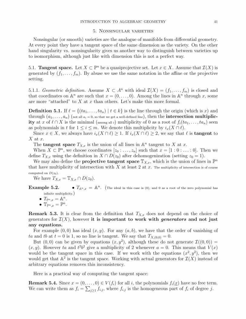
INTRODUCTION TO ALGEBRAIC GEOMETRY 41
5. Nonsingular varieties
Nonsingular (or smooth) varieties are the analogue of manifolds from differential geometry.At every point they have a tangent space of the same dimension as the variety. On the otherhand singularity vs. nonsingularity gives us another way to distinguish between varieties upto isomorphism, although just like with dimension this is not a perfect way.
5.1. Tangent space. Let X ⊂ Pn be a quasiprojective set. Let x ∈ X. Assume that I(X) isgenerated by (f1, . . . , fm). By abuse we use the same notation in the affine or the projectivesetting.
5.1.1. Geometric definition. Assume X ⊂ An with ideal I(X) = (f1, . . . , fm) is closed andthat coordinates on An are such that x = (0, . . . , 0). Among the lines in An through x, someare more “attached” to X at x than others. Let’s make this more formal.
Definition 5.1. If ` = (ta1, . . . , tan) | t ∈ k is the line through the origin (which is x) andthrough (a1, . . . , an) (not all ai = 0, so that we get a well-defined line), then the intersection multiplic-ity at x of ` ∩X is the minimal (among all i) multiplicity of 0 as a root of fi(ta1, . . . , tan) seenas polynomials in t for 1 ≤ i ≤ m. We denote this multiplicity by ix(X ∩ `).
Since x ∈ X, we always have ix(X ∩ `) ≥ 1. If ix(X ∩ `) ≥ 2, we say that ` is tangent toX at x.
The tangent space TX,x is the union of all lines in An tangent to X at x.When X ⊂ Pn, we choose coordinates [z0 : . . . , zn] such that x = [1 : 0 : . . . : 0]. Then we
define TX,x using the definition in X ∩D(z0) after dehomogenization (setting z0 = 1).We may also define the projective tangent space TX,x, which is the union of lines in Pn
that have multiplicity of intersection with X at least 2 at x. The multiplicity of intersection is of course
computed on D(z0).
We have TX,x = TX,x ∩D(z0).
Example 5.2. • TAn,x = An. (The ideal in this case is (0), and 0 as a root of the zero polynomial has
infinite multiplicity.)• TPn,x = An.• TPn,x = Pn.
Remark 5.3. It is clear from the definition that TX,x does not depend on the choice ofgenerators for I(X), however it is important to work with generators and not justany equations.
For example (0, 0) has ideal (x, y). For any (a, b), we have that the order of vanishing ofta and tb at t = 0 is 1, so no line is tangent. We say that TX,(0,0) = 0.
But (0, 0) can be given by equations (x, y2), although these do not generate I((0, 0)) =(x, y). However ta and t2b2 give a multiplicity of 2 whenever a = 0. This means that V (x)would be the tangent space in this case. If we work with the equations (x2, y2), then wewould get that A2 is the tangent space. Working with actual generators for I(X) instead ofarbitrary equations removes this inconsistency.
Here is a practical way of computing the tangent space:
Remark 5.4. Since x = (0, . . . , 0) ∈ V (fi) for all i, the polynomials fi(x) have no free term.We can write them as fi =
∑j≥1 fi,j, where fi,j is the homogeneous part of fi of degree j.

42 INTRODUCTION TO ALGEBRAIC GEOMETRY
If ` is the line through (a1, . . . , an), then fi(ta) =∑
j≥1 fi,j(ta) =∑
j≥1 tjfi,j(a). The
multiplicity ix(X ∩ `) ≥ 2 precisely when fi,1(a) = 0. Therefore
TX,x = V ((fi,1)i)
Recall that we have the formula coming from Taylor expansions, or by checking directly:
fi,1(X) =n∑j=1
Xj∂fi∂xj
(0, . . . , 0).
Here and everywhere else, Xi or Zi are coordinate functions, so indeterminates, whereas xior zi are coordinates of a point x, while ∂xi are notations for directional derivatives. Theequations that describe tangent spaces are always equations in Xi’s.
Remark 5.5. Since fi,1 are all forms of degree 1, the tangent space TX,x is a linear subspaceof An.
Remark 5.6. When we don’t want to change coordinates to make x = (0, . . . , 0), thenx = (x1, . . . , xn) and then we write fi =
∑j≥1 fi,j,x, where fi,j,x is the parts of degree j in
f((X − x1) + x1, . . . , (X − xn) + xn). A formula with partial derivatives:
fi,1,x(X1, . . . , Xn) =n∑j=1
(Xj − xj)∂fi∂xj
(x1, . . . , xn).
This is by definition the differential dxfi(X).Caution: We look at dxfi(X) as linear in the indeterminates Xi − xi, not in Xi. This is
to support looking at (x1, . . . , xn) ∈ An as the origin of TX,x.The differential has the known properties
dx(rf) = rdxf
dx(f + g) = dxf + dxg
(dx(fg))(X) = (dxf)(X) · g(x) + f(x) · (dxg)(X)
where f, g are polynomials and r ∈ k is a scalar. Then
TX,x = V ((dxfi)i)
Example 5.7. i) Let X = V (y− f(x)) with f(0) = 0. Then TX,(0,0) is the line of equation
0 = X ∂(y−f(x))∂x
(0, 0) + Y ∂(y−f(x))∂y
(0, 0) = −Xf ′(0) + Y , which is the line of slope f ′(0)
through (0, 0), meaning what Calculus had us expect it would be.ii) Let X = V (x3− y2). Then TX,(0,0) = A2. This is because both partials of x3− y2 vanish
at (0, 0).iii) Same with X = V (x3 − x2 − y2).iv) However the tangent space at the origin of V (x3 − x− y2) has equation X = 0, so it is
just a line.v) If X = V (x3 − y2, z) ⊂ A3, then TX,(0,0,0) is given by the equation Z ∂z
∂z(0, 0, 0) = 0, i.e.
Z = 0. So the tangent space remembers that X was inside the plane V (z).
Remark 5.8 (Projective case). If X ⊂ Pn is quasiprojective, and x ∈ X, then each equationfi for X is homogeneous. After homogenizing the previous equations, we get that TX,x is

INTRODUCTION TO ALGEBRAIC GEOMETRY 43
given by the vanishing of alln∑j=1
(Zj − xjZ0)∂fi∂zj
(1, x1, . . . , xn),
where where x is the point in D(z0) with homogeneous coordinates [1 : x1 : . . . : xn]. Thisstill has a hint of affineness to it, due to the presence of the xi’s, but we can make it entirelyprojective. In fact a formula of Euler says that if f is homogeneous, then
(deg f) · f =n∑i=0
zi∂f
∂zi.
In particular if [x0 : . . . : xn] ∈ V (f), then∑n
i=0 xi∂f∂zi
(x0, . . . , xn) = 0. Plugging this into theformula for the tangent space, we get that
TX,x is given by the vanishing of alln∑j=0
Zj∂fi∂zj
(z0, . . . , zn)
where now x = [z0 : . . . : zn] doesn’t require an affine chart.
5.1.2. Intrinsic nature of the tangent space. We have defined the tangent space TX,x in termsof an embedding X in Pn or An. However we show that TX,x is intrinsic to X. In particularit does not depend on the projective or affine embedding. We need the following
Theorem 5.9. Let X ⊂ Pn be quasiprojective, and let x ∈ X. Let x ∈ V ⊂ X be an openneighborhood of x with inclusion morphism ı : V → X. Assume there exists ϕ : V → U anisomorphism with U ⊂ Pm quasiprojective. Then
i) ı∗ : OX,x → OV,x is an isomorphism, where OX,x is the ring of regular functions at x(meaning in neighborhoods of x).
ii) ϕ∗ : OU,ϕ(x) → OV,x is an isomorphism.iii) If U ⊂ Am is affine (closed), then OU,ϕ(x) ' k[U ]m, where m is the maximal ideal of k[U ]
corresponding to ϕ(x), and k[U ]m is the localization of k[U ] at the multiplicative systemk[U ] \m.
iv) OX,x is isomorphic to the ring of germs at x, meaning the equivalence classes of pairs (U, f) of a
neighborhood of x and a regular function on U modulo the relation (U, f) ∼ (U ′, f ′) if there exists x ∈ V ⊂ U ∩U ′ another
neighborhood of x such that f |V = f ′|V .
Proof. i) If f is a function regular in a neighborhood of x that is contained in V , then this neighborhood is also contained inX, and it follows that ı∗ is surjective. If a regular function at x vanishes in a neighborhood of x contained in U , then it
also vanishes in a neighborhood of x in X. Hence ı∗ is also injective.ii) This is clear.
iii) We have a map e : k[U ] → OU,ϕ(x) that sends a regular function on U to itself on U seen as a neighborhood of x.
If g ∈ k[U ] \ m, then g(ϕ(x)) 6= 0, hence 1g
is also regular in a neighborhood of x. In particular e(g) is invertible for
every g ∈ k[U ] \ m. The universality property of the fraction ring says that there exists a well-defined induced map
E : k[U ]m → OU,ϕ(x) such that E( fg
) =e(f)e(g)
.
Assume E( fg
) = 0 ∈ OU,ϕ(x). Then e(f) = 0 ∈ OU,ϕ(x), meaning that f vanishes in an open neighborhood ϕ(x) ∈V ⊆ U . Let W = U \ V . This is closed in U and does not contain ϕ(x). Then there exists h ∈ k[U ] a regular functionwith h|W = 0 and h(ϕ(x)) 6= 0. In particular h ∈ k[U ] \ m. The function hf ∈ k[U ] vanishes everywhere on U , therefore
hf = 0 ∈ k[U ]. This precisely means f1
= 0 ∈ k[U ]m, and hence fg
= 0 as well. We have the injectivity of E.
For surjectivity, recall that a regular function at ϕ(x) is a ratio of a priori forms on Pm, but after dehomogenization,
a ratio fg
of polynomials on Am with g(ϕ(x)) 6= 0. Replacing f and g by their restrictions to U , we also recover the
surjectivity of E.iv) This is also clear.

44 INTRODUCTION TO ALGEBRAIC GEOMETRY
Corollary 5.10. The ring OX,x of regular functions at x is independent of the embedding ofX, or of a neighborhood of x in a projective space.
Proof. Use i) and ii).
Corollary 5.11. The ring OX,x is Noetherian and local, meaning it has a unique maximalideal m, which is the ideal of the regular functions at x that vanish at x. FurthermoreOX,x/m ' k.
Proof. Any localization k[U ]m at a prime ideal is a local ring. And a localization of a Noetherian ring is again Noetherian. The
quotient isomorphism is obtained by the remark that we have an evaluation morphism f 7→ f(x) : OX,x → k that is clearly ontobecause k ⊂ OX,x, and whose kernel is by definition m.
Theorem 5.12. Let X be quasiprojective and x ∈ X. Then we have a natural linear iso-morphism
dx : m/m2 → T∨X,x,
where mOX,x is the maximal ideal, and where the RHS is the dual vector space Hom(TX,x, k). Here thevector space structure on m/m2 comes from the isomorphism m/m2 ' m⊗OX,x OX,x/m whichinduces an k ' OX,x/m-module structure on m/m2.
Proof. Let U be an affine neighborhood of x in X. By abuse use use m as notation for the maximal ideal in k[U ] corresponding
to x, as well as for the maximal ideal in the local ring k[U ]m ' OX,x. Then it is easy to show that as k-vector spaces
mk[U ]m/m2k[U ]m ' mk[U ]
/m2k[U ].
In particular we can work in k[U ], instead of OX,x. We have U ⊂ An closed for some n. In this setting we have constructed
(dxf)(X1, . . . , Xn) =
n∑j=1
(Xj − xj)∂f
∂xj(x1, . . . , xn)
for any polynomial f ∈ k[X1, . . . , Xn], where x = (x1, . . . , xn). It is convenient to assume x = (0, . . . , 0), so that we can workwith indeterminates Xi instead of Xi − xi, and so that we get less confused.
The differential is a linear form on kn, and since TX,0 ⊂ kn is a linear subspace, d0f restricts to a linear form on TX,0. We
have a map that we continue to denote
d0 : k[X1, . . . , Xn]→ T∨X,0.
Let f1, . . . , fr be a set of generators for I(X) k[X1, . . . , Xn]. Then
TX,0 = V (d0f1, . . . , d0fr).
If f ∈ I(X), then f =∑ri=1 figi for some gi ∈ k[X]. Then using the product rule, for any v ∈ TX,0 we have
(d0f)(v) =∑i
d0fi(v) · gi(x) +∑i
fi(x) · d0gi(v).
But (d0fi)(v) = 0 for all i because v ∈ TX,0 = V ((d0fi)i), and fi(x) = 0 for all i because 0 ∈ X ⊆ V (I(X)) = V ((fi)i).
Therefore d0f = 0 ∈ T∨X,0 for all f ∈ I(X), meaning I(X) ⊂ ker d0. We get an induced map from the universality property of
quotients that we continue to denote
d0 : k[X]/I(X) = k[U ]→ T∨X,0.
Restricting to m ⊂ k[U ] we get
d0 : m→ T∨X,0.
Note that m k[U ] is generated as an ideal by Xi for all i, these seen as regular functions on X by restriction from An. Usingthis and the product rule again, it is clear that m2 ⊂ ker d0. The universality property for quotients leads to a linear map
d0 : m/m2 → T∨X,0
If the map is not surjective, then it must be contained in some hyperplane in T∨X,0, meaning there exists 0 6= v ∈ (T∨X,0)∨ = TX,0such that Im(d0) ⊂ ker(v), i.e. (d0f)(v) = 0 for all f ∈ m k[U ]. In particular for each i, we have 0 = (d0Xi)(v) = vi, leadingto vi = 0 for all i, i.e. v = 0 ∈ T∨X,0, which contradicts the assumption. Therefore d0 is surjective.
We check injectivity. Recall that m is generated as an ideal (or k[U ]-module) by the classes of Xi modulo I(X) for all
i, hence m/m2 is generated as a k = k[U ]/m-vector space by the classes modulo I(X) + m2 of the same elements. Assume
d0(∑i aiXi) = 0 ∈ T∨X,0 for some ai ∈ k. Then for every v ∈ TX,0
0 =
(d0(∑i
aiXi)
)(v) =
(∑i
aiXi
)(v).

INTRODUCTION TO ALGEBRAIC GEOMETRY 45
This means that∑ni=1 aiXi vanishes on TX,0. By linear algebra, or by the Nullstellensatz, it must be a linear combination of
any given set of linear equations for TX,0. In particular∑i
aiXi ∈ Spank(d0f1, . . . , d0fr).
Since 0 ∈ X = V (f1, . . . , fr), we have fi(0) = 0 for all i and then fi − d0fi =∑j≥2 fi,j ∈ k[X], where fi,j are homogeneous of
degree j in X1, . . . , Xn. In particularfi = d0fi mod (X1, . . . , Xn)2,
leading to ∑i
aiXi = 0 mod I + m2.
Hence ker d0 = 0 for d0 : m/m2 → T∨X,0. Since it is injective, surjective, and linear, d0 is an isomorphism.
Corollary 5.13. TX,x is intrinsic to X, and does not change if we replace X by a neighbor-hood of x.
Definition 5.14. The vector space m/m2 ' T∨X,x is called the cotangent space of X at x.It is denoted ΩX,x.
5.1.3. Differentials for regular maps. Just like we defined differentials for regular functions,we can also define them for maps.
Definition 5.15. Let f : X → Y be a regular map of quasiprojective varieties, and letx ∈ X. Put y = f(x). Then the morphism f ∗ : OY,y → OX,x is local, i.e. f ∗(n) ⊂ m, where nand m are the unique maximal ideals in OY,y and OX,x respectively (The inclusion holds true because
f∗ sends functions that vanish at y to functions that vanish on x). Clearly f ∗(n2) ⊂ m2 as well, therefore itinduces
f ∗ : n/n2 → m/m2.
The differential of f is the dual of this map, which by the theorem above can be writtenas
dxf : TX,x → TY,y.
We can also write this in coordinates. There exist affine open neighborhoods x ∈ U ⊂ Xand y ∈ V ⊂ Y with f(U) ⊂ V . If V ⊂ Am closed, then f = (f1, . . . , fm) for some regularfunctions fi ∈ k[U ]. Then
dxf = (dxf1, . . . , dxfm).
Example 5.16. If X is affine and f is a regular function on it, we can see it as a regularmap f : X → A1. Then dxf should be a linear map from TX,x to TA1,f(x) ' k. But a linearmap TX,x → k is the same as an element of T∨X,x, which is good because that is what dxf wasbefore: an element of T∨X,x.
Remark 5.17. The differential is linear and functorial, i.e. if f : X → Y is regular, andg : Y → Z is regular, and x ∈ X, then we have the chain rule:
(dx(g f))(v) = (df(x)g)(dxf(v)) = (df(x)g dxf)(v),
which is basically d(g f) = dg df .
Example 5.18. Let f : A2 → A2 be the function f : (x, y) = (x + y, (x + y)2), and let’scompute d0f , where 0 = (0, 0). The formula above says
(d0f)(a, b) = ((d0(x+ y))(a, b), (d0(x+ y)2)(a, b)) = (a+ b, 0).
Observe that Im(d0f) = V (y) = TV (y−x2),(0,0). In other words d0f notices that the image of fis contained in the parabola y = x2, which is what functoriality promised: f factors throughthe inclusion of the parabola in A2.

46 INTRODUCTION TO ALGEBRAIC GEOMETRY
Corollary 5.19. If X ⊂ Y , and x ∈ X, then TX,x ⊂ TY,x.
Proof. We can assume that X ⊂ Y ⊂ An. By functoriality, we get maps TX,x → TY,x → TAn,x. The composition is injective,because we have initially defined TX,x as a subspace of TAn,x = kn. Then the first map is automatically also injective.
Corollary 5.20. Let f : X → Y be a regular map, and let x ∈ X. Put y = f(x) and letXy = f−1y. Then
TXy ,x ⊂ ker dxf ⊂ TX,x.
Proof. We can factor
Xf // Y
Xy
⊆
OO
f |Xy
// y
⊂
OO
Then dxf(TXy,x) ⊂ Ty,y = 0.
Example 5.21. However if f : X → Y is surjective, it does not follow that dxf : TX,x →TY,f(x) is surjective for every x ∈ X, although it is surjective for almost all x. Consider for
example (x, y) 7→ y : V (y − x2)f→ A1. This is a finite 2-to-1 map. Given that points on
V (y − x2) all look like (x, x2), we have
TV (y−x2),(x,x2) = V (d(x,x2)(y − x2)) = V ((X − x) · (−2x) + (Y − x2) · 1)
(X, Y ) 7→ Y − x2 : TV (y−x2),(x,x2)
d(x,x2)f→ k
The map d(x,x2)f is going to be surjective, whenever it is not identically zero (since the target is k),meaning whenever Y −x2 is not identically zero for all (X, Y ) ∈ V ((X−x)·(−2x)+(Y −x2)·1).This happens precisely when x 6= 0, i.e. (x, y) = (x, x2) 6= (0, 0).
This respects the geometric intuition: The projection (x, y) 7→ y is linear, so it can beidentified with its differential. The only lines it contracts are those parallel to the x-axis.The only time one of these lines is tangent to the parabola y = x2, is at the origin.
We can also check with algebra. The map f ∗ : k[A1]→ k[V (y − x2)] is the inclusion mapk[y] → k[x, y]
/(y − x2) determined by sending y to y. The maximal ideals we work with
are (y) k[y] for 0 = f(0, 0) ∈ A1, and (x, y) k[x, y]/
(y − x2) for (0, 0) ∈ V (y − x2). The
induced mapf ∗ : (y)
/(y2)→ (x, y)
/(x2, xy, y2)
sends y to (y mod (x2, xy, y2)). However, x2 = y on V (y − x2), so we get that y is sent tozero. On the other hand, y generates (y)
/(y2) as a k-vector space, so we get that the map f ∗
is zero at the level of cotangent spaces, so its dual d(0,0)f is also the zero map, in particularnot surjective.
Example 5.22. Let V = kn+1 as a vector space, so that Pn = P(V ), i.e. the set of lines inV through the origin. We have seen that TPn,x is isomorphic to kn, but how does this relateto V and x?
The point x ∈ P(V ) corresponds to a line ` ⊂ V through the origin by the definition of theprojective space. Let x = [x0, . . . , xn]. Then (x0, . . . , xn) ∈ `. Let f : V \(0, . . . , 0) → P(V )be the map (X0, . . . , Xn) 7→ [X0 : . . . : Xn]. This is regular (because the Xi’s are regular onthe source and don’t have common zeros).
The differential at (x0, . . . , xn) is
d(x0,...,xn)f : TV,(x0,...,xn) → TP(V ),(x0,...,xn).

INTRODUCTION TO ALGEBRAIC GEOMETRY 47
To compute it, we work in an affine D(zi) that contains [x0 : . . . : xn]. Assume x0 6= 0, sothat x ∈ D(z0). On D(z0) ' An we have coordinates zi
z0for all 1 ≤ i ≤ n. Over D(z0),
the function f is (x0, . . . , xn) 7→ (x1
x0, . . . , xn
x0). Given that TV,(x0,...,xn) is V , we get that for
v = (v0, . . . , vn) ∈ V ,
(d(x0,...,xn)f)(v) = ((d(x0,...,xn)x1
x0
)(v)), . . . , (d(x0,...,xn)xnx0
)(v)))
= (−(v0 − x0)x1
x20
+ (v1 − x1)1
x0
, . . . ,−(v0 − x0)xnx2
0
+ (vn − xn)1
x0
)
= (v1x0 − v0x1
x20
, . . . ,vnx0 − v0xn
x20
)
The kernel of this map is those v’s such that vixj = vjxi for all i, j. This is equivalent toasking that the matrix with columns v and x has rank 1, i.e. v and x are proportional,i.e. v ∈ `. So ker d(x0,...,xn)f = `. For dimension reasons and because of the fundamentalisomorphism theorem, it follows that
TPn,x = V /` = Homk(`, V /`)
Remark 5.23. A similar, but of course more involved argument shows that if V = kn andG(d, n) is the Grassmannian of d-dimensional subspaces of V , then for every x ∈ G(d, n)corresponding to a d-dimensional subspace W ⊂ V , we have a natural identification
TG(d,n),x = Homk(W, V /W ).
5.2. Singular points.
Definition 5.24. Let X ⊂ Pn be quasiprojective and let x ∈ X. We define the localdimension at x denoted dimxX or dim(X, x) as any of the following equal quantities:
i) The maximal dimension among the irreducible components of X that contain x.ii) The minimal dimension among all neighborhoods x ∈ U ⊂ X.iii) The Krull dimension (i.e. max length of ascending chain of prime ideals) of OX,x.
Finally we say that x ∈ X is singular if dimTX,x > dim(X, x), and nonsingular orsmooth otherwise. The singular locus of X is the set of all singular points x ∈ X. It isdenoted Sing(X). Its complement is called the nonsingular or smooth locus and denotedXnonsing or Xsm.
Lemma 5.25. Let X1, . . . , Xr be the irreducible components of X that contain x. Then
i) TX,x ⊇ TXi,x for all i. In particular TX,x ⊇∑
i TXi,x, the sum taking place inside TPn,x 'An.
ii) There exists di ≥ 0 such that Ui := x ∈ Xi | dimTXi,x = di is open nonempty anddimTXi,x > di when x ∈ Xi \ Ui.
iii) di = dimXi for all i. In particular dimTX,x ≥ dim(X, x), and x is nonsingular if andonly if equality holds.
Proof. i) This is a consequence of ix(` ∩X) ≥ ix(` ∩Xi) for all i.
ii) We may assume that X = X1 ⊂ An is irreducible closed and we look at An as D(z0) ⊂ Pn. If the ideal of X in Pn isgenerated by homogeneous forms fi, then the set
TX := (x, v) ∈ X × Pn | v ∈ TX,x
48 INTRODUCTION TO ALGEBRAIC GEOMETRY
is closed, given by equations∑nj=0 Zi
∂fi∂zi
(x) = 0 for all i, which are bihomogeneous. The fibers of the first projection
p : TX → X are precisely the tangent spaces TX,x. The map p is projective. The result follows by Theorem 4.11.iv). (With
the notation there, we have Ui = Xdi \Xdi+1 for di = dimTX − dimX.)
iii) When X = Xi is an irreducible (nonempty) hypersurface V (f) ⊂ Pm, where we can assume that f 6= 0 is irreducible, thenTX is given by the equation F = 0 where
F =
m∑i=0
Zm∂f
∂zi(x)
on X × Pm. As such it has dimension dimXi +m− 1 when F 6= 0 and dimX +m when F = 0.
• But F = 0 if and only if ∂f∂zi
vanish everywhere on X. This means that X ⊂ V ( ∂f∂zi
), hence f | ∂f∂zi
for all i. Since the
degree on the right is less than that of f , it follows that ∂f∂zi
= 0 for all i everywhere on Pm (not just on X = V (f)).
Euler’s formula gives
(deg f) · f(x0, . . . , xn) =
m∑i=0
xi∂f
∂zi(x0, . . . , xn),
and since every partial is zero, if follows that f = 0 or deg f = 0. Both contradict assumptions on the hypersurfaceX.
• When F 6= 0, then the first projection p : TX → X is clearly dominant, and then the general fiber has dimension
dimTX − dimX = m− 1 = dimX. But the fibers are precisely the tangent spaces TX,x.In the general case, Xi is birational to a hypersurface, hence up to passing to an open subset, we reduce to the previous
case.
Remark 5.26. The singular locus Sing(X) is closed in X. (If the ideal of X in An is generated by fi,
then inside X, the singular locus is the locus where the matrix ∂fi∂xi
has bigger kernel (lower rank) than dimX. This is described
by the vanishing of the dimX × dimX minors.)
Example 5.27. a) If I(X) = (f) on An and X is closed, then
Sing(X) = VAn( f︸︷︷︸f is here
,∂f
∂x1
, . . . ,∂f
∂xn).
(The vanishing of f at x ∈ An tells us that x ∈ X. The vanishing of all the partial derivatives tells us that dxf is zero at
x, i.e. that kn = ker dxf = TX,x, i.e. that dimTX,x = n > n− 1 = dimX, so x is singular.)b) If I(X) = (f) on Pn, and X is closed, then
Sing(X) = VPn( ︸︷︷︸no f here
∂f
∂z0
, . . . ,∂f
∂zn).
(This is same as before, but with the added bonus that when we work projectively, then Euler’s formula tells us that the
vanishing of the partials of f at x also implies the vanishing of f at x, at least when deg f > 0, which is the case here.)
5.3. Codimension one subvarieties. Nonsingular varieties admit an analogue of Theorem4.4, at least locally.
Definition 5.28. Let X be a quasiprojective variety, and let Y ⊂ X be a closed subset andlet x ∈ Y ⊂ X. We say that f1, . . . , fr are local equations for Y at x if there exists anaffine open neighborhood x ∈ U ⊂ X such that
• fi are defined on U for all i, and• They generate IU(Y ∩ U) k[U ].
Remark 5.29. The definition above seems to depend on the affine neighborhood of x. How-ever if fi are local equations for Y on U , then they are also local equations on any otheraffine neighborhood V with x ∈ V ⊂ U .
Let IX,x(Y ) ⊂ OX,x be the ideal generated by regular functions f at x that in a neigh-borhood Uf of x vanish along Y ∩ Uf . Then IX,x(Y ) is the ideal generated by the image ofIU(Y ∩ U) ⊂ k[U ]→ k[U ]mx ' OX,x for any affine neighborhood x ∈ U ⊂ X.

INTRODUCTION TO ALGEBRAIC GEOMETRY 49
Then any generators f1, . . . , fr of IX,x(Y )OX,x give local equations for Y on some neigh-borhood of x where they are all defined.
Theorem 5.30. If X is a quasiprojective variety and Y ⊂ X is an equidimensional closedsubset of codimension 1, then for any x ∈ X nonsingular point, IX,x(Y ) = (fx)OX,x forsome fx ∈ OX,x. In other words, locally around any x ∈ X, the subset Y is given by one(local) equation (depending on x).
Proof. The proof is analogous to the easier implication in Theorem 4.4. All we need to know is that OX,x is a UFD. This istrue because OX,x is a regular local ring, and then one applies the Auslander–Buchsbaum Theorem.
Corollary 5.31. Let X be a nonsingular quasiprojective variety and let ϕ : X 99K Pm be arational map. Then the complement of the domain of ϕ is a closed subset of X of codimensionat least two.
Proof. Let x ∈ X. In a neighborhood U of x, the rational function ϕ is given by a formula (f0 : . . . : fm), where fi are regular
functions on U . Since OX,x is an UFD, we can divide by any common factor of the fi’s, and get the same rational map. Thuswe can assume that the fi’s don’t have a common factor.
On U , the map ϕ is not defined where fi all vanish. If V (f0, . . . , fm) ∩ U contains an irreducible closed subset Y ⊂ U of
codimension 1, then Y has a local equation gx around x, so that IX,x(Y ) = (gx)OX,x. But then Y ⊂ V (fi) implies gx|fi inOX,x for all i. But we arranged so that the fi’s have no common factor.
Corollary 5.32. Any two birational projective nonsingular curves are isomorphic.
Proof. The previous corollary tells us that a rational map from a nonsingular curve to a projective set is defined except in
codimension 2, hence defined everywhere. If ϕ : C → C′ is a birational map of projective nonsingular curve, we apply this for
ϕ and ϕ−1.
Example 5.33. The nonsingularity of x ∈ X is important in Theorem thrm:smloceq.
• The cusp C = V (y2 − x3), the origin (0, 0) is a subset of codimension 1. It has ideal(x, y) in OC,(0,0), and this is not principal. This is even though (0, 0) can be describedby one equation: either x or y will do. But no equation will generate the ideal (x, y).• Inside the cone over the quadric surface in P3, i.e. the cone over the Segre embedding
of P1 × P1, consider the cone over the line [1 : 0] × P1. Around the vertex of thecone, this cannot even be described by one equation. In particular its ideal is alsonot generated by one element.
5.4. Nonsingular subvarieties of nonsingular varieties. It is natural to wonder whathappens in codimension bigger than 1. It turns out that we are in good shape if we add somenonsingularity condition on Y as well.
Theorem 5.34. Let X be a quasiprojective variety and let Y ⊂ X be a closed subvariety ofcodimension d. Then for any x ∈ X that is nonsingular for both X and Y , the ideal IX,x(Y )is generated by d elements.
Proof. • Case x = Y . Then d = dimX. By the nonsingularity assumption, the cotan-gent space m/m2 is a k-vector space of dimension d = dimX, where m = mx is theideal of functions that vanish at x. Choose generators for this vector space, repre-sented mod m2 by f1, . . . , fd ∈ m. We show that they generate m as an ideal of OX,x.The fi’s are called a system of parameters at x (for X). If a = (f1, . . . , fr), thenthe short exact sequence
0→ a→ m→ m/a→ 0
gives after tensoring with k ' OX,x/m as a OX,x-module the exact sequence:
a/ma→ m/m2 → m/a⊗OX,x k → 0

50 INTRODUCTION TO ALGEBRAIC GEOMETRY
by the right-exactness of tensor products. The map on the left is surjective, therefore
m/a⊗OX,x k = 0.
Nakayama’s Lemma says that this only happens if m/a = 0, i.e. a = m, i.e. the fi’sgenerate m.• In the general case, the inclusion TY,x ⊂ TX,x comes from a surjection
ı∗ : m/m2 → n/n2,
where m is the ideal of x inOX,x, where n is the ideal of x inOY,x, and where ı : Y → Xis the inclusion of Y . Up to changing bases we can then pick f1, . . . , fn+d ∈ mOX,x asystem of parameters at x forX such that ı∗f1+d, . . . , ı
∗fn+d ∈ nOY,x is also a systemof parameters at x, but for Y , and such that f1, . . . , fd generate ker ı∗ = IX,x(Y ) modm2.
We show that there exist local equations g1, . . . , gd for Y ⊂ X at x, i.e. theygenerate IX,x(Y ), such that gi = fi mod m2.
Start by choosing gi ∈ (fi + m2) ∩ IOX,x(Y ). This is possible by the assumptionthat f1, . . . , fd generate IX,x(Y ) mod m2.
Let aOX,x be the ideal generated by the gi’s, and let Y ′ be the closed subset ofX defined by these equations (in a neighborhood of x where all functions involvedare regular). Then we have
√a = IX,x(Y ′) by the Nullstellensatz and Y ⊆ Y ′ since
a ⊂ IX,x(Y )OX,x(Y ). Let hj be generators for IX,x(Y ′). Looking in TX,x, we have
TY,x ⊆ TY ′,x = ker(dxhj)j ⊆ ker(dxgi)i = ker(dxfi)1≤i≤d = TY,x.
Therefore TY,x = TY ′,x. Since dimTY ′,x ≥ dim(Y ′, x) ≥ dim(Y, x) = dimTY,x, itfollows that dim(Y ′, x) = dim(Y, x) and x is a nonsingular point of Y ′. Since Y is anirreducible subset of Y ′ and they have the same dimension (around x), it follows thatY is an irreducible component of Y ′.
If Y ( Y ′, then Y ′ must have another irreducible component through x, and thisimplies that OY ′,x is not a domain. But if x ∈ Y ′ is a nonsingular point, then OY ′,xis a regular local ring , and as such is a domain. Therefore Y = Y ′.
We are not quite done. We still should check that gi generate the ideal of Y ′ = Yaround x, i.e. a = IX,x(Y ′), and not just that they are equations for Y . This followswith a bit of work from the equality ker(dxhj)j = ker(dxgi)i. Intuitively, if instead ofworking with generators, we work with equations, then we get a larger kernel for thedifferentials as in Remark 5.3.

INTRODUCTION TO ALGEBRAIC GEOMETRY 51
6. Blow-ups
The blow-up of a subvariety (or subscheme) is the most important construction of birationalmaps in algebraic geometry. It is used to “resolve” singularities, or maps.
6.1. The blow-up of P2 at one point. This is the map pictured on the cover of thetextbook.
Definition 6.1 (Definition by equations). Let BlpP2 ⊂ P2 × P1 be the closed subset ofequation
z1x2 − z2x1 = 0,
where [z0 : z1 : z2] are coordinates on P2 and [x1 : x2] on P1, and where p = [1 : 0 : 0] is theorigin in D(z0) ' A2. The restriction of the first projection induces a regular map
σ : BlpP2 → P2.
This is called the blow-up of P2 at [1 : 0 : 0].
Remark 6.2. The blow-up at the point [1 : a : b] has equation (z1−az0)x2−(z2−bz0)x1 = 0.
Proposition 6.3. The blow-up map σ : BlpP2 → P2 has the following properties:
i) We can see P1 as a parameter space for lines in P2 through p. To a point [u : v] ∈ P1 wecan associate bijectively the line
`uv := V (z1v − z2u)
which clearly contains p = [1 : 0 : 0]. Then
BlpP2 = (x, `) | x, p ⊂ `.ii) BlpP2 is the closure of the graph of the stereographic projection
[z0 : z1 : z2] 7→ [z1 : z2] : P2ϕp99K P1.
We say that the blow-up at p resolves the indeterminacies of the rational map ϕp, in thatit replaces ϕp with the second projection π : BlpP2 → P1 which is defined everywhere.
iii) Then second projection π : BlpP2 → P1 has the property that
π−1[u : v] = ¯uv = `× [u : v] ⊂ P2 × P1.
iv) If [u : v] 6= [u′ : v′], then ¯uv and ¯
u′v′ are disjoint in BlpP2. We say that the blow-up ofp “separates” the lines `uv through p.
v) BlpP2 is nonsingular.vi) The blow-up map σ is birational and an isomorphism away from p.
vii) σ−1p = p × P1. Denote this curve by E. It is called exceptional.viii) σ−1`uv = E ∪ ¯
uv, where ¯uv = `× [u : v] ⊂ P2 × P1.
ix) E ∩ ¯uv = p× [u : v]. This means that we have a point on E for every line `uv ⊂ P2
through p.x) If f is a reduced form (i.e. no multiple factors) of degree d on P2 and C = V (f), then
σ−1C =
E ∪ C, if C passes through pC, otherise
where C is the closure of σ−1(C \ p) ⊂ P2 \ p × P1 in P2 × P1. The curve C is calledthe strict transform of C.

52 INTRODUCTION TO ALGEBRAIC GEOMETRY
xi) If after dehomogenization in A2 ' D(z0), the form f is written as fk + fk+1 + . . ., wherefi are forms in the coordinates on A2 and fk is the first nonzero one that appears, then
E ∩ C = (p, [u : v]) | fk(u, v) = 0.In other words we have a point in E ∩ C for each line through p in P2 that has highermultiplicity of intersection with C at p than “usual”.
Example 6.4. Consider the cusp C = V (z22z0− z3
1) ⊂ P2C. The singularities are given by the
vanishing of the partials of the equations, which means
Sing(C) = V (z22 , 3z
21 , 2z2z0) = [1 : 0 : 0].
Let’s see that C is smooth.Since the blow-up of P2 at [1 : 0 : 0] is isomorphic to P2 outside p, we only care about what
happens at or around p. This is captured by working over D(z0) ' A2.BlpP2 is covered by D(x1) and D(x2) in P2 × P1.Let’s work in D(x1). Put u = z1
z0, v = z2
z0and x = x2
x1. Then
• C ∩D(z0) is given by the equation v2 − u3 = 0 in D(z0)• BlpP2 inside A2 × A1 is given by v = ux• σ : D(z0x1)→ D(z0) given by the formula σ(u, v, x) = (u, v) can be identified with
(u, x) 7→ (u, ux) : A2 → A2
• With respect to this map, σ−1C is the curve of equation
0 = σ∗(v2 − u3) = (ux)2 − u3 = u2(x2 − 1) = u2(x2 − u)
• Also with respect to this map, the exceptional E is V (u).• Then C ∩ D(x1) is given by the equation x2 − u = 0 inside D(z0x1) ' A2 with
coordinates u, x. But V (x2 − u) is a smooth parabola in A2.
Similarly in D(x2), by putting y = x1
x2, we get that C∩D(x2) has equation 1−y3v = 0, which
is again a smooth curve.

INTRODUCTION TO ALGEBRAIC GEOMETRY 53
7. Divisors and Class Group
Let X ⊂ Pm be a smooth projective variety of dimension n.
Definition 7.1. A divisor on X is an element of the free abelian group generated byirreducible subvarieties of X of codimension 1. Such an irreducible subvariety is also calleda prime divisor. Denote this group by Zn−1(X).
Example 7.2. If X = P1, then Z0(X) is just the set of all possible combinations∑r
i=1 aixi,where ai ∈ Z and r ≥ 0. The sum is purely formal, it is not supposed to return a point inP1 as the result of the linear combination.
Example 7.3. If X ⊂ Pn and f is a form that does not vanish on all of X, then V (f) ∩Xis a divisor on X.
A very important family of examples of divisors are constructed from forms or from rationalfunctions on X.
Definition 7.4. Let f be a form on Pn that does not vanish on all of X. Then we constrcuta divisor
div(f) :=∑i
ordDi(f),
where the Di’s range through the irreducible components of VX(f), and the order ordDi(f)is computed as follows: Let xi be an arbitrary (but fixed) point on Di. Then there existsfi ∈ OX,x such that IX,x(Di) = (fi) and Di = V (fi) in a neighborhood of x (see Theorem
5.30). Then ordDi(f) is the largest ri ≥ 0 such that f
frii
∈ OX,x.If f = g
his a nonzero rational function on X, i.e. a ratio of forms of the same degree that
do not vanish on all of X, then define
div(f) := div(g)− div(h).
In this case when f is a rational function, we say that div(f) is a principal divisor.
Remark 7.5. The principal divisors on X form a subgroup. In fact the map
f 7→ div(f) : (k(X)∗, ·)→ (Zn−1,+)
is a group morphism (turns multiplication into addition). All this uses is that OX,x is anUFD for all x ∈ X, which is true because X is nonsingular/smooth.
Definition 7.6. The class group of X is the quotient
Cl(X) := Zn−1(X)/
principal divisors.
We say that divisors D and D′ are linearly equivalent and write D ∼ D′ if they have thesame class in Cl(X). Equivalently if D−D′ = div(f) for some nonzero rational function onX.
This is typically a huge group. Maybe infinitely generated.
Example 7.7. Cl(Pn) ' Z and a generator is the class of a (any) hyperplane. (Let H be the
class of the hyperplane V (z0) in Cl(Pn). It is enough to show that if D is any divisor, then D ∼ mH for some m. Write
D =∑i aiDi. Since we work on Pn, by Theorem 4.4 we know that Di = V (fi) for some irreducible form fi of degree di. Put
m =∑i aidi. Then D −mH = div(z−m0 ·
∏i faii ), and the latter is readily seen as a ratio of forms of the same degree if we
separate the negative coefficients from the positive ones.)

54 INTRODUCTION TO ALGEBRAIC GEOMETRY
Example 7.8. If C is a smooth projective curve, then Cl(C) ' Z× Jac(C), where Jac(C) isa variety of dimension equal to the genus g(C). It is actually an abelian variety (projectivevariety with a group structure), called the Jacobian of C. It can be identified with thekernel of the degree morphism (Cl(C),+) → (Z,+) which sends D =
∑i aixi to the
integer deg(D) =∑
i ai.Hidden here is the nontrivial result that deg(D) = 0 for all principal divisors on the curve
C, so that deg is well defined modulo principal divisors. For example on a Riemann surface,this says that a meromorphic function has as many zeros as it has poles (when countingmultiplicities/orders).
Remark 7.9. The constructions so far can be adapted for singular quasiprojective varietiesas long as Sing(X) has codimenion two or more in X, i.e. it contains no divisors of X. Thishappens for example for the so called normal varieties. Then for each Di we can pick xi ∈ Di
that is nonsingular in X and repeat the definition of orders.The only result mentioned so far that may fail if quasiprojective replaces projective is that
div(f) = 0 if f ∈ k(C)∗, where C is a curve.With some work, div(f) can be defined even when Sing(X) contains divisors.
Example 7.10. Cl(A1) = 0. This is because every point x ∈ A1 is V (f) for some rationalfunction f ∈ k(A1): Just put f(X) = X − x0.
Somewhat similarly one can show that Cl(An) = 0 for any n ≥ 1.
Example 7.11. Put X = BlpP2. Then Cl(X) = Z2, where p = [1 : 0 : 0]. A set of generatorsis given by H and E, where H = σ−1` is the inverse image (not just the strict transform usually, but
for this particular line they are the same) of the line ` = V (z0) ⊂ P2 via σ : X → P2, and E is theexceptional divisor of the blow-up. (Let’s first show that if T is an irreducible curve inside the blow-up, then
T ∼ dH +mE
for some integers d and E. Look at σ(T ). This is an irreducible curve inside P2, hence T = VP2 (g), where g is a form of somedegree d. Put f = g
zd0. This is a rational function, since it is a ratio of forms of the same degree. We have
divP2 (f) = σ(T )− d`.
Since σ is birational, k(X) = k(P2). Therefore f can also be seen as a rational function on X via σ∗. Let’s compute divX(f).
Since σ : X \E → P2 \ p is an isomorphism, the divisors divX(f) and divP2f are equal except possibly over p. But over p weonly have the divisor E, therefore
divX(f) = σ(T )− d¯−mE = T − dl −mEfor some integer m, where over-lines denote strict transforms, since the irreducibility of T implied T = σ(T ). Finally T −divX(f) = dH +mE.
Next we show that H and E are linearly independent in Cl(X). Assume divX(f) = aH + bE for some integers a, b not both
zero and some nonzero rational function f . Since k(X) = k(P2), we can also see f as rational on P2. It is not hard to show thatdivP2 (f) = aσ(H), since σ(E) = p ⊂ P2 is not a divisor. Therefore aσ(H) is principal on P2, and this only happens if a = 0.Now look inside the copy of A2 ⊂ X which D(z0x1) from last time is isomorphic to. Recall that the coordinates on A2 where
(u, x) with u = z1z0
and x = x2x1
. And E ∩ A2 = VA2 (u). From this and the condition divX(f) = bE, we get that as rational
functions on A2 which is open in X, we have f = cub, where c is a nonzero constant. Therefore
f = czb1zb0
on X and/or P2. But divX(czb1zb0
) = b(VX(z1)− VX(z0)) = b(¯01 + E − ¯) 6= bE. )
INTRODUCTION TO ALGEBRAIC GEOMETRY 55
8. Bezout’s Theorem
Maybe the simplest form of Bezout’s Theorem (BT) is that a linear polynomial has exactlyone solution. It has a famous generalization, the Fundamental Theorem of Algebra (FTA) aparticular case of which says that most polynomials of degree d have exactly d zeroes. Whatdistinguishes most polynomials from any polynomial is that they have nonzero discriminant,meaning that all their zeros have multiplicity one. If we want to obtain a general statement,we count multiplicities, and indeed the FTA says that if we sum the multiplicities of eachzero, we recover the degree of the polynomial.
Let’s see some of these as geometric statements:
Example 8.1. • To intersect V (y) with V (y − ax − b) in A2, we solve the systemy = 0
y = ax+ bBy substitution, this is the same as solving ax+ b = 0.
• Similarly, if f(x) is a polynomial of degree d, then solving f(x) = 0 amounts tointersecting V (y) with V (y − f(x)) in A2. Note that if x0 is a zero of f , then itsmultiplicity as a zero of f is equal to the multiplicity of intersection i(x0,0)(` ∩ C)defined in 5.1, where ` = V (y) and C = V (y − f(x)).
In both cases, we intersect a curve of degree 1 with a curve of degree d (given by oneequation of degree d), and the result is d points in A2, possibly after counting them withtheir multiplicities. We also have that the lines is not an irreducible component of the curve.
• If we intersect the two curves V (y) and V (y−1) in A2, then we get no point, becausethe lines are parallel, or because y = y−1 = 0 is impossible. This seems to contradictthe principle above that when I intersect two curves of degree one I get one point.The culprit for this pathology is not the principle, but the ambient space. We knowintuitively that parallel lines intersect “at infinity” and this can be made precise byworking in the projective space.
Indeed, the projective equations of the two lines are y and y − z, which intersectin the point [1 : 0 : 0] in P2, which is a point in the line at infinity V (z).
By changing coordinates, the second example says that when we intersect any line with anycurve of degree d in P2, we get d points when counting multiplicities, at least when the lineis not a component of the curve.
So how about when we intersect a curve of degree d with a curve of degree e? And whatcan we do when we want to intersect curves that have common components?
Let’s recall how we can justify multiplicities of intersection that are higher than 1. Forexample the line V (y) has multiplicity two of intersection with the parabola y = x2 at (0, 0),because it is the limit of the lines `ε through (0, 0) and (ε, ε2) as ε → 0. Every line `εintersects the parabola at two points (near (0, 0)). We keep this “two” when we pass to thelimit, remembering that the one point we see is actually two points collapsed into one. Weget the following:
Principle: The number of points counted with multiplicity of two curves does not changewhen we deform one or both curves (making sure we don’t get common components).
Example 8.2. We can even use the principle to “intersect” the curve V (y) with itself.Set theoretically, we get the curve, instead of the expected one point. But if instead ofintersecting V (y) and V (y) we intersect V (y) and V (y − εx), then we get one point for all(“small”) nonzero epsilon, so we can say that the curves intersect at one point.

56 INTRODUCTION TO ALGEBRAIC GEOMETRY
Example 8.3. More importantly we can use the principle to intersect curves C and C ′ ofdegrees d and e respectively by deforming C ′ until it becomes a union of e distinct lines noneof which is a component C.
Specifically, if the ideal of C ′ is generated by g, a form of degree e, and f1, . . . , fe aredistinct and nonproportional forms of degree 1, then if we put
gε := (1− ε)g + ε · f1 · . . . · fe,then for each ε ∈ k, we have that gε is a form of degree e. When ε = 0, we get C ′, and whenε approaches 1, we approach ∪ei=1V (fi), a union of e distinct lines. We add together all themultiplicities when we intersect C with each of them, and get de points.
Remark 8.4. It may seem like we could do the gε trick even when we use more or less thane linear forms. However in that case gε itself is no longer a form, so that won’t do.
Still, like we did when we intersected a curve with a line and the set theoretic intersectionwas points, we should be able to assign multiplicities of intersection when we intersect curvesof arbitrary degrees and get only points set theoretically.
Definition 8.5. Let C and D be projective plane curves without common components. Letx ∈ C ∩D. Then the multiplicity of intersection at x is
ix(C ∩D) = dimk OP2,x/IP2,x(C) + IP2,x(D).
Example 8.6. Assume that f ∈ k[x, y] with f(0, 0) = 0 and f irreducible. Let `a be the liney = ax. Let C be the projective closure of V (f) and ¯
a the projective closure of `a. Then forx = (0, 0) = [0 : 0 : 1] belonging to both curves, we get
ix(C ∩ ¯a) = dimk OP2,x/(f, y − ax) = dimk k[x, y](x,y)
/(f, y − ax).
Recall that k[x, y](x,y) is the fraction ring of k[x, y] with multiplicative system k[x, y] \ (x, y):every polynomial f not in (x, y), i.e. with f(0, 0) 6= 0 is invertible in this ring.
We want to see that this multiplicity of intersection agrees with Definition 5.1.Write f = f1 + f2 + . . ., where fi is the homogeneous part of degree i. The old multiplicity
of intersection is the multiplicity of x = 0 as a zero of f(x, ax) =∑
i≥0 fi(x, ax). This is m iffm(x, ax) is the first nonzero term in the sum. Then we can write f(x, ax) = xmga(x), withga(0) 6= 0.
Now use the isomorphisms
k[x, y](x,y)
/(f, y − ax) ' k[x](x)
/(f(x, ax)) ' k[x](x)
/(xmga(x)) ' k[x](x)
/(xm),
where the latter is true since ga(x) is invertible in k[x](x), because it is not in (x). Now the lastquotient is of dimension m, generated by 1, x, . . . , xm−1. So the new multiplicity agrees withthe old one (when we intersect with lines).
Let’s also see a new example
Example 8.7. Let’s intersect the cusp with the node at (0, 0). The ideals are generated byy2 − x3 for the cusp and by y2 − x3 − x2 for the node. Then we compute
k[x, y](x,y)
/(y2 − x3, y2 − x3 − x2) = k[x, y](x,y)
/(y2 − x3, x2) = k[x, y](x,y)
/(y2, x2).
This is generated by 1, x, y, xy, so that the multiplicity of intersection there is equal to 4.The closures in P2 are of equations y2z − x3 = 0 and y2z − x3 − x2z = 0 give another
solution [0 : 1 : 0], which lives on the line at infinity, sitting as the origin in the affine set

INTRODUCTION TO ALGEBRAIC GEOMETRY 57
D(y). In this open subset, the equations are z − x3 and z − x3 − x2z = 0. To compute themultiplicity of intersection at (0, 0) = [0 : 1 : 0], we look at
k[x, z](x,z)/
(z − x3, z − x3 − x2z) = k[x, z](x,z)/
(z − x3, x2z) = k[x](x)
/(x5).
This is generated by 1, x, . . . , x4, so it has dimension 5.So adding the multiplicities at the two points gives 4 + 5 = 3 · 3, so still the products of
degrees.
Remark 8.8. The reason why we work in the local ring at x is that this preserves the “localpicture”. For example if we look at the node given by the equation y2 − x3 − x2, then in thelocal ring of P2 around [0 : 0 : 1], this equation is y2 = x3 + x2 = x2(1 + x). Since 1 + x doesnot vanish at (0, 0) = [0 : 0 : 1], it is invertible in the ring of regular functions around (0, 0).It is not trivial why we can do this, but we can pretend that it is 1. Then the equation lookslike y2 = x2, which is a union of distinct lines y = x and y = −x.
Actually we can compute the multiplicity of intersection between the cusp and the nodeat (0, 0) this way. The cusp has multiplicity of intersection 2 with each of the curves y = ±x,so a total of 4, which is the number we got before.
If you want to make it precise why you can replace y2 = x2(1+x) by y2 = x2, the trick is tosee that the multiplicity of intersection gives the same result whether computed in OP2,[0:0:1]
or in its completion, which in this case is just the ring of power series k[[x, y]]. Then 1 + x
admits a square root r(x) that is invertible and
x 7→ xy 7→ y
r(x)is an automorphism of k[[x, y]]
that turns the node into the union of two lines through (0, 0).
Remark 8.9. As long as both C and D pass through x, we have that IP2,x(C) + IP2,x(D) ⊂mxOP2,x. In particular the class of 1 is nonzero in OP2,x/IP2,x(C) + IP2,x(D), so the mul-
tiplicity of intersection is at least one.
Remark 8.10. If C is singular at x, and x ∈ C ∩ D, then ix(C ∩ D) ≥ 2. (If f and gare the equations of C and D, then the singularity of x implies f ∈ m2
x. Choose an affineneighborhood of x and coordinates so that x = (0, 0). Let g1 be the linear term of g.
• If g1 = 0, then the classes 1, x, y are independent in OP2,x/IP2,x(C) + IP2,x(D) =
k[x, y](x,y)
/(f, g), because the denominator is included in m2
x. In this case the multi-
plicity is at least 3.• If g1 6= 0, then by changing coordinates, we make g1 = y. Then the classes of 1, x are
independent in the quotient, so we get a dimension at least 2, meaning a multiplicityof intersection of at least 2.)
Theorem 8.11 (Plane Bezout). If C and D are curves without common components, thenthe sum of the multiplicities of intersection is degC · degD.
Corollary 8.12. Any irreducible conic in P2 is nonsingular.
Proof. Let f be an irreducible form of degree 2 and C = V (f). Assume p ∈ C is a singularpoint. Let q ∈ C be another point. Let ` be the line through p and q. We have ` ( C, orelse f is reducible. By BT, we get two points of intersection between ` and C when we countmultiplicities. The points p and q are in this intersection, so the multiplicity is at least 1 ateach of them, but the line ` must have multiplicity at least 2 at p, because it is singular, soTpC = P2 ⊃ `. We get the contradiction 2 ≥ 3.

58 INTRODUCTION TO ALGEBRAIC GEOMETRY
Corollary 8.13. A singular irreducible cubic in P2 is rational.
Proof. Let C be a cubic (curve of degree 3) and let p be a singular point. Fix a line ` in P2
that does not pass through p. For each x ∈ `, let `x be the line through p and x. By BTit meets C at 3 points when counting multiplicities. As in the previous corollary, it meetsit at p at least twice, because it is a singular point. Then there is at most one more pointsin C ∩ `x, and we denote this by qx. This defines an actually regular map P1 → C. It isof course not an isomorphism, because C is singular, and P1 is not. But it has a birationalinverse given by q 7→ pq ∩ ` : C \ p → P1, where pq is the line through p and q.
Corollary 8.14. An irreducible plane quartic (curve of degree 4 in P2) cannot have foursingular points.
Proof. Assume C is a quartic and that p1, . . . , p4 are distinct singular points on it. Choosep5 ∈ C different from the previous ones. We show that there exists a conic Q that passesthrough all of them. Then Q ∩ C contains the 4 singular points p1, . . . , p4 with multiplicityat least 2 at each by Remark 8.10 and p5 with multiplicity at least 1, which by BT leads tothe contradiction 4 · 2 ≥ 2 + 2 + 2 + 2 + 1.
Let’s prove the claim. Assume first that 3 of the singular points are on a line `. Then let `′
be the line through the other two. We can put Q = `∪`′. Assume now that no three singularpoints are on a line. The space of conics in P2 is parameterized by a P5 by looking at thecoefficients of the form. The condition that a conic passes through a point p ∈ P2 is linearin the coefficients of the equation of the conic. This means that conics in P2 through a fixedpoint correspond to a hyperplane in P5. If we have 5 points, no three on the same line, thenin P5 we’ll see 5 hyperplanes that meet at one point. (This may require some thinking). Thissays actually that through any 5 general points in P2 there passes exactly one (automaticallysmooth) conic.
8.1. Arbitrary smooth projective surfaces. Let X be a smooth projective surface.
Definition 8.15. If C and D are curves on X that intersect in just points (no common curvecomponents), then by analogy with Definition 8.5, define
C ·D =∑
x∈C∩D
ix(C ∩D)
where ix(C ∩D) = dimk OX,x/(f, g), where f, g are local equations for C and D around x.
The formula is easily seen to be linear in both C and D (so bilinear), thus allowing toassume that C and D are divisors (with possibly negative coefficients).
Assume that D = divX(f), where f is a nonzero rational function on X. So D is a principaldivisor. If C is an irreducible curve in X that does not appear among the components ofD, then we can write f = g
h, where g, h are forms on some Pn containing X such that C
is not a component of V (g) or V (h). This precisely means that f restricts to a nonzerorational function on C. It can be shown that for each x ∈ C ∩ (V (g) ∪ V (h)), we haveix(C ∩ V (g))− ix(C ∩ V (h) = ordx(f |C). Then
deg(div(f |C)) =∑x
ordx(f |C) =∑x
ix(C ∩D) = C ·D.
By abuse C ∩D denotes the set theoretic intersection between the union of components of Cand curves appearing in D with positive or negative coefficient. However last time we agreedthat the degree of a principal divisor on a curve is zero. Therefore C · divX(f) = 0.

INTRODUCTION TO ALGEBRAIC GEOMETRY 59
From the previous paragraph it follows that for any two divisors C and D, the intersectionC · D depends only on their classes in Cl(X), which is divisors modulo principal divisors.We have obtained the following:
Theorem 8.16 (Surface Bezout). If X is a smooth projective surface, then there exists abilinear pairing called an intersection product
(C,D) 7→ C ·D : Cl(X)× Cl(X)→ Zsuch that if C ∩D is just points, then C ·D is the sum of the multiplicities at these points.
Remark 8.17. The intersection product is intrinsic to X. In particular it is preserved byisomorphisms.
Example 8.18. If X = P2, then C ·D = deg(C) · deg(E). This also works if C and D havecomponents in common, because then we can replace one of them by a linearly equivalentdivisor such that we only get points in the intersection.
For example if C = D = V (z0), then D ∼ V (z1), because V (z1)−V (z0) = divP2( z1z0
). Then
C ·D = V (z0) · V (z1) = 1 · 1 = 1.
Example 8.19. If X is the blow-up of P2 at one point p = [0 : 0 : 1], and H ∈ Cl(X) is theclass of the strict transform of a line not passing through p, and E ∈ Cl(X) is the class ofthe exceptional divisor of the blow-up, then the intersection product on X is determined bythe formulas.
H ·H = 1
H · E = 0
E · E = −1
(The three numbers determine the product because Cl(X) is the free abelian group of rank2 generated by the classes of H and E.
The first is true because using divisors on P2 and the fact that X \E ' P2 \p, one showsthat the strict transform of any line in P2 not passing through p is H. The multiplicity ofintersection is local, so we can compute it on P2 away from p, which means it is one.
The second relation is true because the strict transform of a line not through p and theexceptional divisor do not intersect, so there is no point to compute an intersection of mul-tiplicity at.
The third relation may seem unexpected. After all the exceptional divisor is a P1, butwe are not in P2 anymore. Indeed consider the rational function f = z2
z0on P2, which is
birational to X, so f is also rational on X. Then divX(f) = V (z2)− V (z0) = H − (` + E),where ` is the strict transform of V (z0).
Then using the bilinearity and that principal divisors don’t contribute to intersectionnumbers, we get
E · E = (E + divX(f)) · E = (H − `) · E = H · E − ` · E = −` · E.We show that ` · E = 1, which gives E · E = −` · E = −1. In X we have an open subsetA2 such that the blow-up map X → P2 looks like (x, y) 7→ (xy, x) : A2 → A2. Then VP2(z0)corresponds to VA2⊂P2(x), so its inverse image in X is VX(xy) = VX(x) ∪ VX(y). The firstpart, VX(x) is the inverse image of (0, 0), so it is the exceptional divisor E. The second partis the strict transform ` by definition. Furthermore ` and E meet at (0, 0) with multiplicity1, because so do VA2⊂X(y) and VA2⊂X(x). )

60 INTRODUCTION TO ALGEBRAIC GEOMETRY
Example 8.20. Perhaps a simpler example is X = P1 × P1. Here we also have two specialcurve classes: f1 and f2 the classes of the fibers of each projection. Then
i) Cl(X) is isomorphic to Z2, generated by f1 and f2.ii) The intersection product is determined from bilinearity by the following intersection
relations:fi · fj = 1− δij,
with δij the Kronecker delta’s.
(Put coordinates [x0 : x1] on the first copy and [z0 : z1] on the second copy of P1 in the product.Then VX(x0) + divX(x1
x0) = VX(x1), and this argument can be adjusted to show that any two
fibers of the first projection are linearly equivalent. Then f 21 = VX(x0)2 = VX(x0)·VX(x1) = 0,
because they do not intersect. Analogously f 22 = 0.
To compute f1 · f2, we look at V (x1) ∩ V (z1) = ([1 : 0], [1 : 0]) ∈ P1 × P1. This isone point and we want to check the multiplicity of intersection. It lives in the affine openD(x0z0) ' A1 × A1 = A2 with coordinates x = x1
x0and z = z1
z0. In this chart V (x1) = V (x)
and V (z1) = V (z). These are the axes of A2, so they meet with multiplicity 1, because theyhave degree 1.
We show that if C ⊂ P1×P1 is a curve given by an equation g(x0, x1, z0, z1) bihomogeneousof bidegree (n,m), then C ∼ nf1 +mf2. This shows that f1, f2 generate Cl(X). Their linearindependence is a consequence of the intersection relations: If af1 = bf2, then 0 = af 2
1 =bf1f2 = b and a = af1f2 = bf 2
2 = 0, so a = b = 0.Consider g
xn0 zm0
. This is bihomogeneous of bidegree (0, 0), so a rational function on P1×P1.
Then its associated principal divisor has class 0 in Cl(X), but divX( gxn0 z
m0
) = VX(g)−nV (x0)−mV (z0) = C − nf1 −mf2, gives us what we want.)
Remark 8.21. With some work, you can use the previous two examples to show that BlpP2
and P1 × P1 are not isomorphic, because the second contains no irreducible curve of selfintersection -1.
INTRODUCTION TO ALGEBRAIC GEOMETRY 61
9. Appendix
9.1. Classical algebraic structures. Let (G, ·) be a set with a function · : G × G → G.We think of this function as an “operation” on G and denote it a · b := ·(a, b), or just ab.
• The operation is commutative if ab = ba for all (a, b) ∈ G2. We also say that G iscommutative when the operation is clear in context.• (G, ·) is a semigroup if the operation is associative: a(bc) = (ab)c for all a, b, c ∈ G.• (G, ·) is a monoid if it is a semigroup and it contains a unit/neutral element : An
element e ∈ G such that ea = ae = a for all a ∈ G. Sometimes, especially if G iscommutative, this is denoted by 1.N.B. Oftentimes people use semigroup for monoid.• (G, ·) is a group if it is a monoid, and every element has an inverse: There exists a
function −1 : G → G such that a(a−1) = a−1a = e for every a ∈ G. Often, (G, ·) issaid to be a multiplicative group.• When G is a commutative group, the notation (G,+) is sometimes preferred and we
say that G is an additive group. In this case the neutral element is denoted 0 and theinverse of a is −a.• As far as notation goes, for n ∈ N and a ∈ G, denote na = a+ . . .+ a︸ ︷︷ ︸
n times
for additive
structures and an = a·. . .·a for multiplicative structures. For groups, (−n)a := −(na)and a−n := (an)−1.• A subset H ⊂ G is a subsemigroup if H ·H ⊂ H (where H ·H = ab | (a, b) ∈ H ×H and the
operation · is the one on G). If G is a monoid and H a subsemigroup that also contains theunit element, we say that H is a subgroup. If G is a group and H is a submonoidsuch that H−1 ⊂ H, then H is a subgroup of G.• A morphism f : H → G is a function that preserves operations and properties: For
semigroups we want f(ab) = f(a)f(b). For monoids we also want f(1) = 1, for groupswe also want f(a−1) = (f(a))−1.• If H = G, so that f is a self-map f : G→ G, we say that f is an endomorphism.• A monomorphism is an injective (one-to-one) morphism. An epimorphism is a
surjective (onto) morphism.• An isomorphism is a bijective (one-to-one and onto) morphism. Its inverse is then
also a morphism.• If f : H → G is a morphism, then the kernel of f is ker f = h ∈ H | f(h) = 1.
This is a subgroup of H.
Assume now that (R,+, ·) is a set R with two operations (addition and multiplication) on it.
• (R,+, ·) is a semiring if (R,+) is commutative and multiplication is distributive withrespect to addition: a(b+ c) = ab+ ac and (a+ b)c = ac+ bc for all a, b, c ∈ R. It iscommutative if (R, ·) is also commutative.• (R,+, ·) is a ring if it is a semiring, if (R,+) is an additive group, and if (R, ·) is a
monoid (it has a unit 1). In this case a0 = 0a = 0 for all a ∈ R. N.B. Sometimespeople don’t ask that rings contain multiplicative units, and mark the distinction bysaying ring with unit.• (R,+, ·) is a division ring if it is a ring, and if (R∗, ·) is a group, where R∗ := R\0.

62 INTRODUCTION TO ALGEBRAIC GEOMETRY
• (R,+, ·) is a field if it is a commutative division ring. N.B. Sometimes people usefield for division ring and non-commutative field when it is a division ring, but not afield. We have clear notions of subsemiring, subrings, subdivision rings, andsubfields. We also have clear notions of morphisms and isomorphisms.
9.2. Commutative algebra. Let (R,+, ·) be a commutative ring.
9.2.1. Ideals.
• A subset I ⊂ R is an ideal of R if:(i) I is closed under addition: I + I ⊂ I. (i.e. a+ b ∈ I for all a, b ∈ I)(ii) I is closed under taking opposites: −I ⊂ I. (i.e. −a ∈ I for all a ∈ I)
(iii) I is closed under multiplication with elements of R: RI ⊂ I. (i.e. ra ∈ I for allr ∈ R and a ∈ I)
In this case, we denote I R.If xii∈I is a family of elements of R, we denote by (xi)i the ideal generated byxii∈I .
If I = (x) for some x ∈ R, we say that I R is a principal ideal.Example:– An ideal I R is equal to R iff 1 ∈ I.– Even integers form the ideal 2ZZ.– If RX denotes the ring (pointwise operations) of functions f : X → R, where R
is a ring, and if Y ⊂ X is any subset, then the set of functions f ∈ RX such thatf(y) = 0 for all y ∈ Y forms an ideal in RX .
9.2.2. Modules.
• An additive group (M,+) (different + than in R) is an R-module if there exists a functionR ×M → M that we denote (r,m)→ rm called the module action of R on M suchthat(i) r(m+m′) = rm+ rm′. In particular r0 = 0 and r(−m) = (−r)m.(ii) (r + r′)m = rm+ r′m. In particular 0m = 0.
(iii) rs(m) = r(sm).(iv) 1m = m.
N.B. One can define left ideals and left modules with the exact same definitionswhen R is non-commutative. And right ideals or modules are defined by writingthe action of R on the right, and in particular asking m(rs) = (mr)s. When R iscommutative, the distinction is not important.• The free module of rank n is Rn with componentwise R-module action. We denote
by ei the usual “basis” elements. They are the analogue of a basis for vector spaces:every element of Rn can be written uniquely as an R-combination of them.• A subset N ⊂M of an R-module is a submodule if
(i) N is closed under the addition on M .(ii) N is closed under the R-module action.Example: The ideals of R are the only submodules of R.• A morphism of modules is an additive group morphism f : (N,+)→ (M,+) that
preserves the R-module action: f(rn) = rf(n). We have clear notions of monomor-phism, epimorphism, and isomorphism.• An R-module M is finitely generated if there exists a surjective morphism f : Rn →M of R-modules. This is the same as saying that there exist finitely many elements

INTRODUCTION TO ALGEBRAIC GEOMETRY 63
xi ∈ M (they are f(ei)) such that every x ∈ M can be written as an R-combinationof them (though not necessarily unique). We say that the xi generate M .• If f : N →M is a surjective morphism and N is finitely generated, then so is M .• More generally we say that xii∈I generate M if every x ∈M can be written as anR-combination of finitely many of the xii∈I .• If N and M are R-modules, we can form the direct sum N ⊕M . This is the setN ×M with componentwise operations.• If (Ni)i∈I is a family of R-modules, then the direct product ×iNi is the product of
sets with componentwise R-module action.• If (Ni)i∈I is a family of R-modules, then the direct product ⊕iNi is the subset of×iNi consisting of the elements of finite support (i.e. only finitely many componentsare nonzero for each element.)• R×∞ is a ring, but R⊕∞ is not, because there is no unit element (the only viable one
is (1, 1, 1, . . .), and this does not have finite support.)
9.2.3. Kernels, Quotients, Isomorphism Theorems, Snake Lemma.
• If f : N →M is a morphism of R-modules, then the kernel
ker(f) := n ∈ N | f(n) = 0is a submodule of N . And the image
Im(f) := m ∈M | m = f(n) for some n ∈ Nis a submodule of M .
Example: If f : R→ S is a morphism of rings, then ker(f)R is an ideal, whileIm(f) ⊆ S is a subring.• If N ⊂M is a submodule, then
x ∼ y ⇔ x− y ∈ Ndetermines an equivalence relation on M . We may write x = y(mod N). The equiv-alence class of x ∈M is the set of all y ∈M such that x− y ∈ N . We may identifyit with x+N .
The set of all equivalence classes is denoted M/N .It is the quotient of M by N . It inherits the structure of an R-module with the
action given by r(x+N) = rx+N .• The cokernel of f : N →M is
coker(f) := M/Im(f).
• The fundamental homomorphism theorem: If N ⊂M is an R-submodule, thenthe function q : M →M/N given by q(m) = m+N is an epimorphism of R-modules,which is universal in the following sense:
For every morphism f : M → P of R-modules such that N ⊆ ker f (so f(N) = 0),there exists a unique morphism ϕf : M/N → P such that ϕf q = f . With diagrams:
M∀f //
q
N
M/N∃!ϕf
<<yyyyyyyy

64 INTRODUCTION TO ALGEBRAIC GEOMETRY
• The first isomorphism theorem: If f : N →M is a morphism of R-modules, then
Im(f) ' N/ ker(f).
The sign ' means isomorphic.• The second isomorphism theorem: If N,P ⊆M are submodules, then
N + P
N' P
N ∩ Pas R-modules.• The third isomorphism theorem: If P ⊆ N ⊆M is a sequence of R-submodules,
then as R-modules,
M
N' M/P
N/P.
• A sequence of morphisms
. . .→Mifi→Mi+1
fi+1→ Mi+2 → . . .
is called a complex if
ker(fi+1) ⊆ Im(fi)
for all i. If equality holds at Mi+1, we say that the complex (or sequence) is exactthere. If it is exact everywhere, it is said to be exact.• If f : N →M is a morphism of R-modules, then we have an exact sequence:
0→ ker(f)→ Nf→M → coker(f)→ 0.
• If ϕ : M → M/N is a quotient map, and if P ⊂ M is a submodule, then P + N isthe smallest submodule of M containing P and N , and ϕ(P ) ' P+N
N.
If Q ⊂ M/N is a submodule, then ϕ−1Q ⊂ M is a submodule of M containing Nand ϕ(ϕ−1Q) = Q.We have a one-to-one correspondence between submodules of M/N and submodulesof M containing N .• Snake Lemma: Consider a diagram with exact rows and commutative squares
N1//
f
M1//
g
P1//
h
0
0 // N2// M2
// P2
Then there exists a connecting morphism
δ : ker(h)→ coker(f)
that fits into an induced exact sequence
ker(f)→ ker(g)→ ker(h)δ→ coker(f)→ coker(g)→ coker(h).
If one can add a 0 to the left of the first row, or the end of the second row, then theinduced exact sequence also gets a 0 to the left, or to the right respectively.

INTRODUCTION TO ALGEBRAIC GEOMETRY 65
9.2.4. Algebras.
• If f : R→ S is a morphism of rings, we say that S is an R-algebra.• S is finite algebra over R if S is finitely generated as an R-module.• A morphism of R-algebras f : S → S ′ is a morphism of rings and R-modules.• If f : R → S is a morphism of rings, we say that S is an R-algebra of finite type
if there exists a surjective morphism g : R[X1, . . . , Xn] → S of R-algebras. In thiscase there exist elements xi ∈ S (they are g(Xi)) such that every element of S can bewritten as a polynomial in the xi, but maybe not uniquely.• If aR, then the ideal generated by f(a) in S is denoted aS and called the extension
of a in S.• If bS, then the ideal f−1bR, also denoted b ∩ R (even if f is not injective), is the
restriction of b to R.• The restriction of a prime ideal is prime. (If pS is prime, and xy ∈ f−1(p), then f(x)f(y) ∈ p, so
f(x) ∈ p or f(y) ∈ p, i.e. x ∈ f−1(p) or y ∈ f−1(p).)
9.2.5. Noetherianity.
• An R-module M is called Noetherian if it satisfies the ACC condition: Every as-cending chain of submodules N1 ⊂ N2 ⊂ N3 ⊂ . . . becomes constant (there exists isuch that Ni = Ni+1 = . . ..• A ring R is Noetherian if it is Noetherian as a module over itself.• If N ⊂M is a submodule, then N and M/N are both Noetherian iff M is Noetherian.
If M is Noetherian, then every chain in N is a chain in M , so N is Noetherian.
Still if M is Noetherian, then every chain in M/N corresponds naturally to a chain of submodules of M , allcontaining N . Also, two submodules of M containing N are equal iff their images in M/N are equal. Therefore M/N
is Noetherian.
Conversely, if both N and M/N are Noetherian, let N1 ⊂ N2 ⊂ . . . be an ascending chain in M . There exists
i such that Ni ∩ N = Ni+1 ∩ N = . . . and (Ni + N)/N = (Ni+1 + N)/N = . . .. The latter is equivalent to
Ni +N = Ni+1 +N = . . .. Say x ∈ Ni+1. Then x+ n = y + n′ for some n, n′ ∈ N and y ∈ Ni. Then y − x ∈ N and
y − x ∈ Ni+1, so y − x ∈ Ni+1 ∩N = Ni ∩N , so x ∈ Ni. This shows Ni+1 ⊂ Ni, and the other inclusion was there
by construction.
• If f : N →M is a morphism of Noetherian modules, then ker(f), Im(f), and coker(f)are all Noetherian.• A Noetherian module is finitely generated. (Construct a sequence xi ∈M inductively as follows: x1
is nonzero in M . Then xi+1 is an element of M \∑ij=1Rxj . Since the ascending sequence
∑ij=1Rxi must stabilize,
the construction ends after finitely many steps.)Consequently all submodules of a Noetherian module are finitely generated.
• A module is Noetherian iff all its submodules are finitely generated. (One implication
is handled by the above. Assume that all submodules are finitely generated. Let N1 ⊂ N2 ⊂ . . . be an ascending
sequence, and let N = ∪iNi. This is a submodule of M , hence finitely generated. Let x1, . . . , xr be a finite set of
generators. Then there exists i > 0 such that Ni contains them all. Then Ni = Ni+1 = . . . = N .)• Any finitely generated R-module is Noetherian iff R is a Noetherian ring.• R is Noetherian iff all its ideals are finitely generated.• Hilbert Basis Theorem: If R is a Noetherian ring, then R[X] is also a Noetherian
ring. Consequently k[X] is Noetherian for any field k.(Let aR[X], and let ai be the set of leading coefficients of polynomials in a of degree at most i. Observe that
a0 ⊂ a1 ⊂ . . . is an ascending sequence of ideals of R. Let d be such that ad = ad+1 = . . ., and let f1, . . . , fr be a set
of elements of aR[X] of degrees di ≤ d whose leading coefficients generated ad. If f is an arbitrary element of aR,
of degree e ≥ d, then by the definition of ad = ae there exist si ∈ R such that f ′ := f −∑ri=1 siX
e−difi ∈ a and

66 INTRODUCTION TO ALGEBRAIC GEOMETRY
deg f ′ < deg f . We deduce that a is generated by the fi’s and by the polynomials in a of degree at most d− 1. The
latter set can be seen as a sub R-module of Rd. But the Noetherianity of R implies that this is finitely generated. A
finite set of generators of this R-module and the fi’s together form a finite set of generators of a as an R[X]-module.)
9.2.6. More commutative ring and ideal theory. Throughout I R is an ideal.
• x ∈ R \ 0 is a zero divisor if xy = 0 for some y ∈ R \ 0, i.e. f : R→ R definedby f(y) = xy is not injective.• R is a domain if it has no zero divisors.• An ideal I is said to be prime if R/I is a domain. This is the same as xy ∈ I iffx ∈ I or y ∈ I. (If R/I is a domain, then xy ∈ I means xy = 0(mod I), so x = 0(mod I) or y = 0(mod I).
This means precisely x ∈ I or y ∈ I. The converse is similar.)A typical example is pZZ when p is prime, hence the name.
• An ideal I is called proper if it is not R = (1).• A proper ideal I is maximal if it is maximal among the proper ideals of R, i.e. ifJ R and I ⊂ J , then I = J or J = R. Equivalently, I is maximal if R/I is a field.(If R/I is a field, then its only ideals are 0 and (1). This means that the only ideals of R containing I are I and (1).
The converse is similar.)• If I R, then the correspondence between ideals of R/I and ideals of R containing I
respects prime and maximal ideals.• Every proper ideal I R is contained in some maximal ideal mR. (Replacing R by R/I,
we can assume I = 0. One uses Zorn’s Lemma to show that the set of ideals of R, ordered by inclusion admits a
maximal element. Details can be found here.)• A ring R is a domain iff 0 is a prime ideal. It is a field iff 0 is maximal.• The radical of I is
√I := f ∈ R | fn ∈ I for some n > 0.
• I is called radical if√I = I.
• If R is Noetherian, then for any two ideals a, bR such that b ⊂√a, there exists
n > 0 such that bn ⊂ a. (Let x1, . . . , xr be a finite set of generators for b. Since b ⊂√a, there exist ni > 0
such that xni = xnii · x
n−nii ∈ a for all n ≥ ni. Let n′ = maxini. Let’s show that xrn
′ ∈ a for all x ∈ b. Any
element of b is of the form x = p1x1 + . . .+ prxr for some pi ∈ R. Then xrn′
is a linear combination of multiples of
xm11 · . . . · xmr
r with∑imi = rn′. By the pidgeon-hole principle, for each r-tuple (m1, . . . ,mr) with
∑imi = rn′, at
least one of the mi ≥ n′ ≥ ni, and consequently xrn′ ∈ a because a is an ideal.)
• f ∈ R is called nilpotent if fn = 0 for some n > 0.• N :=
√0 is the nilradical of R. It is the set of nilpotents in R.
• If√
0 = 0, then R is said to be reduced. R/I is reduced iff I is a radical ideal.• N is the intersection of all prime ideals of R. (If x ∈ N , then xn = 0 for some n, and then it is
easy to see that x is in every prime ideal. For the converse, one shows that an ideal maximal among those that do
not contain 1, x, x2, . . . is prime. This is again an application of Zorn’s Lemma and details can be found here.)
• If I R, then√I is the intersection of the prime ideals of R that contain I. (The
nilradical of R/I is√I/I. The primes in R/I correspond to the primes in R that contain I.)
• If a, bR, then√a · b =
√a ∩ b =
√a ∩√b. (The only interesting things to prove here are
√a ∩ b ⊂
√ab and
√a ∩√b ⊂√a ∩ b. If x ∈
√a ∩ b, then xn ∈ a ∩ b for some n, and then x2n ∈ ab shows x ∈
√ab.
The other inclusion is easier.)
9.2.7. Primary ideal decomposition for radical ideals.
• An ideal QR is called primary if xy ∈ Q implies x ∈ Q, or yn ∈ Q for some n.• The radical of a primary ideal is prime (If xy ∈
√Q, then xnyn ∈ Q for some n, so xn ∈ Q or ynm ∈ Q
for some m. In both cases, either x or y are in√Q.) If P :=
√Q, we say that Q is P -primary.
INTRODUCTION TO ALGEBRAIC GEOMETRY 67
Look here for an example of an ideal that is not primary, but its radical is prime.• If P R is prime, then it is P -primary.• A strong result that we won’t use, is that in a Noetherian ring every ideal admits a
primary decomposition, i.e. I = ∩ri=1Qi for some r and some primary ideals Qi.But the case of radical ideals is easier and this is what we’ll use.• Let I R. Then
√I is the intersection of the prime ideals that contain it (not finitely
many yet).• An ideal p ⊃ I is minimal prime associated to I if it is minimal (containing
no other) among the prime ideals containing I. Minimal primes exist by the ZornLemma (the set of primes containing I is nonempty because I is contained in some maximal ideal, and it is ordered
by inclusion, though in the other direction now). The minimal primes associated to (0) are calledsimply minimal primes, or the minimal primes associated to R. The minimalprimes of R/I correspond to the minimal primes of I.
• Let I R. Then√I is the intersection of the minimal primes that contain it.
• If R is Noetherian, and I R, then√I is the intersection of finitely many primes.
(Let I be the set of radical ideals that cannot be written as an intersection of finitely many primes, and let R be the
set of radical ideals of R. If R ( I, let b be a maximal element (exists because R is Noetherian). We show that b is
prime, which provides a contradiction. Let xy ∈ b. Then b =√b =
√(b+Rx) · (b+Ry) =
√b+Rx ∩
√c+Rx. The
maximality of b implies that√b+Rx and
√b+Ry are intersections of finitely many primes, hence the same is true
of the intersection, unless x ∈ b or y ∈ b, i.e. b is prime. The conclusion is R = I.)• If R is Noetherian, and I R, then there are only finitely many prime ideals p1, . . . , pr
associated to I, and√I = p1 ∩ . . .∩ pr is the only way (up to permutation) of writing
√I
as a finite intersection of minimal primes associated to I. (Let√I = q1 ∩ . . . ∩ qs be a way
of expressing√I as an intersection of finitely many primes. Let p be a minimal prime associated to I, in particular
p ⊇ ∩iqi. The next result implies p ⊃ qi for some i, hence p = qi by minimality. There may be some qi’s that are not
minimal, but they are now seen to be redundant, and can be removed from the intersection without changing it.)• If pR is prime and p ⊃ ∩si=1qi for some ideals qiR, then p ⊃ qi for some i. (If not
true, then we can pick xi ∈ qi \ p for all i. Then∏i xi ∈ ∩iqi ⊂ p is impossible.)
• If√I = I R is a radical ideal of a Noetherian ring R, and pi are the minimal primes
associated to I, then I = ∩ipi is called the primary ideal decomposition of I.• An element x ∈ R is a zero divisor if xy = 0 for some y 6= 0.• Every element of a minimal prime pR is a zero divisor. (The solution is form here. Let S
be the multiplicative monoid generated by the complement of p and of the zero-divisors of R. Note that 0 6∈ S. Use
Zorn’s Lemma to expand (0) to a maximal ideal I among those that do not meet S. We prove that I is prime, and
then the minimality of p shows p = I ⊂ R \S is a subset of the zero-divisors of R. If xy ∈ I, but x, y 6∈ I, then by the
maximality of I we must have x, y ∈ S. But then xy ∈ I ∩ S is a contradiction. Therefore I is prime.)
9.2.8. Special types of rings. Throughout, R is a commutative ring.PID’s.
• An ideal I R is called principal if I is generated by one element, i.e. there existsx ∈ I such that I = Rx.• If R is a domain whose ideals are all principal, we say that R is a PID (short for
principal ideal domain).• Z and k[X], where k is a field are the easiest examples of PID’s.• Any quotient by a prime ideal and any localization of a PID is again a PID.• Every PID is Noetherian. (Every ideal is finitely generated, actually generated by just one element).

68 INTRODUCTION TO ALGEBRAIC GEOMETRY
• In a PID, every nonzero prime ideal is maximal. (If p = (x) is a nonzero prime ideal, and if
p ( I = (y) for some y ∈ R, then x = yz for some z ∈ R. Then necessarily z ∈ (x), hence z = xt for some t ∈ R.
Therefore x = yxt and 1 = yt, so y is a unit, and in particular (y) = (1). So p is maximal.)
UFD’s.
• An element x ∈ R is called a unit, if it is invertible with respect to multiplication.• An element x ∈ R is called prime if (x)R is a prime ideal.• An element x ∈ R is called irreducible if it is not a product of non-units.• If R is a domain, then any prime element is irreducible. (If p ∈ R is prime, and p = xy, then
x ∈ (p), or y ∈ (p). Say x = pq for some q ∈ R. Then p = pqy implies 1 = qy, so y is a unit.)• There exist domains R and irreducible elements x ∈ R such that x is not prime. For
example 3 in R = Z[√
5] is irreducible, but not prime. A few more details are here.• A domain R is an UFD (short for unique factorization domain) if every elementx ∈ R can be written as a product of primes, and the decomposition is unique up tounits and reordering.• Z is an UFD. This is actually the Fundamental Theorem of Arithmetic.• If R is an UFD, then x ∈ R is prime iff it is irreducible. (One implication is always true.
Conversely, if x is irreducible, then by the definition of UFD it can be written uniquely up to units as a product of
primes. By irreducibility there cannot be more than two primes in this product.)• If x, y are elements of an UFD, then lcm(x, y) and gcd(x, y) are well-defined in R up
to units by factorizing and picking the maximum and minimum respectively betweenexponents of primes.• In fact any PID is an UFD. (We first show that every x in the PID R can be written as a product of
finitely many irreducibles. If this were not true, by Noetherianity we could choose x ∈ R such that (x) is maximalamong the ideals of R generated by elements without finite decomposition as product of irreducibles. By its choice, x
cannot be irreducible. So we can write it as x = yz with y, z both non-units. Consequently (x) ( (y) and (x) ( (z).By the maximality of (x), it follows that y and z are products of finitely many irreducibles, hence so is x. This proves
the first claim.
Second, we show that in a PID every irreducible is prime: Let x be irreducible, and let yz ∈ (x). Since x isirreducible, the ideal (x, y) is either (x), or (1). This is because if (y, x) = (s), then x = ss′ for some s′ ∈ R, so either
s or s′ is a unit by irreducibility. If (x, y) = (x), then y ∈ (x). If (x, y) = 1, then there exist u, v ∈ R such that
ux + vy = 1. Multiplying by z, we get z = (uz) · x + v · (yz) ∈ (x). Therefore (x) is a prime ideal, and x is a primeelement.
Finally, we observe that the uniqueness of the decomposition is a consequence of the primality of the factors.)• If R is a PID, then gcd(x, y) is a generator of the ideal (x, y) and lcm(x, y) is a
generator of (x)∩ (y). In a UFD, we only know for sure that (x, y) ⊂ (gcd(x, y)) andlcm(x, y) ⊂ (x) ∩ (y).• If R is an UFD, then R[X] is also an UFD. Consequently k[X] is an UFD. (Since
R is a domain, R[X] is also a domain, and we have a well-defined notion of degree of polynomials which satisfies
deg(fg) = deg(f) + deg(g).First, observe that a nonconstant (meaning of positive degree) element P ∈ R[X] is irreducible precisely when it
cannot be written as a product of polynomials of smaller degree and when it is primitive, i.e. no non-unit element ofR divides the coefficients of P .
Then it is clear that every element of R[X] is the product of finitely many polynomials as above and an element of
R which is the product of finitely many prime elements of R, which are still prime in R. (If IR, then R[X]/IR[X] '
R/I[X].)
It remains to show that an irreducible nonconstant polynomial is prime. Then primality implies the uniquenessof the factorization up to units. Let P be an irreducible polynomial, and assume FG ∈ (P ), i.e. FG = PQ for some
polynomials F,G,Q. Let c(F ) denote the gcd in R of the coefficients of F . Observe that Fc(F )
is still in R[X], and
it is primitive. Let’s show that c(F · G) = c(F ) · c(G). It is easy to see that the right side divides the left. Then we
can assume that F and G are primitive, and show that F ·G is also primitive. Say a prime element p ∈ R divides allcoefficients of F ·G. Then F ·G = 0 in R
/(p)[X] which is a domain, therefore either F or G is 0 modulo p, and this is
a contradiction. Then in the equality FG = PQ we can assume that all terms are primitive nonconstant polynomials.

INTRODUCTION TO ALGEBRAIC GEOMETRY 69
The equality FG = PQ also holds in K[X], where K is the fraction ring of R. But K[X] is a PID, hence also anUFD. We check that P is still irreducible in K[X] which implies that (P )K[X] is prime, hence F ∈ (P ) or G ∈ (P ).
Say F = PF1 for some F1 ∈ K[X]. Clearing denominators we write rF = PF ′ for some r ∈ R and F ′ ∈ R[X]. Since
P and F are primitive, necessarily c(F ′) = r up to units in R. Then we can divide F ′ by it to get F = PF ′′ wherenow everything is in R[X]. This shows that P is prime in R[X].
See also Gauss’s Lemma )
9.2.9. Tensor products. Let R be a commutative ring and let M , N and P be R-modules.
• A function f : M ×N → P is R-bilinear if for each m ∈M , the map n 7→ f(m,n) :
Nfm→ P is R-linear, and similarly fn : M → P is R-linear for all n ∈ N .
• Observe that a linear function ϕ : M×N → P from the direct product module M×Nis not bilinear unless M = 0 or N = 0. This is because ϕ(r(m,n)) = ϕ(rm, rn) =ϕrn(rm) = rϕrn(m) = rϕ(m, rn) = rϕm(rn) = r2ϕm(n) = ϕ(m,n).• If f : R × R → R is the function f(x, y) = ax2 + bxy + cy2 for some a, b, c ∈ R and
all x, y ∈ R, then f is R-bilinear.• Bilinear maps f : M × N → P are balanced in that f(r · m,n) = f(m, r · n) =r · f(m,n).• The tensor product of the R-modules M and N is an R-module M ⊗R N with anR-bilinear map ϕ : M ×N →M ⊗R N that verifies the following universal property:
For each R-bilinear map F : M×N → P there exists a unique R-module morphismf : M ⊗R N → P such that the following diagram commutes:
M ×N F //
ϕ
P
M ⊗R Nf
::uuuuuuuuuu
• The tensor product is unique up to isomorphism. (Follows from the universality property.)• The tensor product exists. (M ⊗R N ' RM×N
/B, where RM×N is the R-free module on the set M ×N
(much larger than the set M ×N itself), and B is the submodule of this free group generated by the elements of theform (m+m′, n)− (m,n)− (m′, n), (m,n+n′)− (m,n)− (m,n′), (rm, n) = r(m,n), and (m, rn) = r(m,n) for each
(m,m′, n, n′, r) ∈M ×M ×N ×N ×R.
One checks that RM×N/B verifies the universality property of the tensor product with the morphism ϕ(m,n) =
(m,n) mod B ∈ RM×N/B.)
• If m ∈M and n ∈ N , we denote ϕ(m,n) = m⊗ n.• A general element of M ⊗RN looks like
∑si=1mi⊗ ni for some s. In general it is not
possible to write every element of M ⊗R N as m⊗ n. So ϕ is not usually surjective.• M ⊗R N ' N ⊗RM (They both verify the same universality property.)• However if m,m′ ∈ M , then m⊗m′ 6= m′ ⊗m in M ⊗RM . (So the previous isomorphism is
not the identity when M = N .)• M ⊗R R ' R⊗RM 'M .• (M ⊗R N)⊗R P 'M ⊗R (N ⊗R P ).• If S is an R-algebra, then apart from an R-module structure, M⊗RS has the structure
of an S-module with S-action induced by s(m⊗ s′) = m⊗ ss′.• If S is an R-algebra, then S ⊗R R[X] ' S[X].• If I R, then M ⊗R R/I ' M/IM as R/I-modules.• If I,J R, then
J ⊗R R/I ' J /IJ and I ⊗R R/I ' I/I2 as R/I-modules

70 INTRODUCTION TO ALGEBRAIC GEOMETRY
R/J ⊗R R/I ' R/I + J as R/I, R/J , or R−modules
The multiplication map (x, y) 7→ xy : I × J → IJ is bilinear and hence inducesa morphism of R-modules I ⊗R J → IJ R, but while this is surjective (anything
in the product IJ looks like∑si=1 rixiyy for some s and some (ri, xi, yi) ∈ R × I × J , and this is the image of∑s
i=1 rixi ⊗ yi), it is usually not an isomorphism.• The tensor product is a covariant right-exact function from the category of R-modules
to itself. Right-exactness means that if 0 → M1 → M2 → M3 → 0 is a short exactsequence of R-modules and N is an R-module, then
M1 ⊗R N →M2 ⊗R N →M3 ⊗R N → 0
is an exact sequence, but the map on the left may fail to be injective.
• Tensoring the exact sequence 0 → Z ·2→ Z → Z/2Z → 0 by Z/2Z over Z producesthe sequence
Z/2Z0→ Z/2Z
=→ Z/2Z→ 0
which is not exact on the left.
9.2.10. Localization. Let R be a commutative ring.
• A subset S ⊂ R is a multiplicative subset if 1 ∈ S and ab ∈ S whenever a, b ∈ S.The basic examples are
– If pR is a prime ideal, then S = R \ p is a multiplicative set, because a, b 6∈p⇒ ab 6∈ p.A particular case of this is when R is a domain and p = (0). Then S = R∗.
– If f ∈ R, then S = 1, f, f 2, f 3, . . . is clearly a multiplicative set– If S ⊂ R is the set of all nonzero divisors, then S is a multiplicative set.
• On the set R× S we put the equivalence relation (r, s) ∼ (r′, s′) iff there exists t ∈ Ssuch that t(rs′− r′s) = 0. The “t” in the definition is that ∼ is a transitive relation. The equivalenceclass of (r, s) is denoted as expected by r
s.
• The localization or R at S is the set of equivalence classes S−1R := R× S/∼. Ithas a ring structure by copying the fraction operations from Q.• There is a natural map r 7→ r
1: R
u→ S−1R. This map is injective if and only if Scontains no zero divisors. In this case we can remove the “t” from the definition of∼.• The classical examples are
– The localization at a prime ideal Rp when S = R \ p and pR is prime.In particular, if R is a domain, then R(0) is the fraction field of R.
– The localization at an element Rf when S = 1, f, f 2, . . ..– The total fraction ring of R is what we get when S is the set of all nonzero
divisors. In particular we recover the fraction field if R is a domain.These are relevant to Algebraic Geometry in the following way:
– If X is an affine variety, and f ∈ k[X] is a regular function, then k[X]f = k[D(f)],i.e. the set of regular functions on the open subset X \ V (f).
– If X is an affine variety, and Y ⊂ X is a subvariety corresponding to a primeideal p = IX(Y ) k[X], then k[X]p is the set of “germs of rational functions onX, regular in a neighborhood of Y ”, by which we mean
k[X]p = f ∈ k(X) | Domain(f) ∩ Y 6= ∅.

INTRODUCTION TO ALGEBRAIC GEOMETRY 71
– When X is only a closed affine set, then the total fraction ring of k[X] can betaken as a definition for the set of rational functions on X.
• The localization verifies the following universality property: Let S ⊂ R be a multi-plicative set. Then for every ring morphism f : R → T such that f(s) is invertiblein T for all s ∈ S, there exists a unique F : S−1R → T that makes the followingdiagram commute:
Rf //
u
T
S−1R∃! F
<<yyyyyyyy
The map F is then defined as F ( rs) = f(r)
f(s). It makes sense to divide by f(s) precisely because we
imposed the condition that it is a unit.
• If M is an R-module, and S ⊂ R is a multiplicative subset, we can define S−1Mas S ×M/∼, where ∼ is defined just like on S ×M . The localization S−1M is anS−1R-module, and
S−1M ' S−1R⊗RM.
• The ideals of S−1R are all extensions (via u) of ideals of R. Moreover for any bS−1Rwe have b = (b ∩ R)S−1R, i.e. b is the extension of its restriction. (If r
s∈ b, then
b 3 s1rs
= r1⇒ r ∈ b ∩R. Conversely if r ∈ b ∩R, then r
1∈ b, so b 3 1
sr1
= rs
.)• If aR, then the extension aS−1R = x
s| x ∈ a, s ∈ S. (An element in the LHS is of form∑
i xirisi
, with xi ∈ a, ri ∈ R, and si ∈ S. After operations with fractions, using that a is an ideal, we can write this
in the required form. Clearly an element of the RHS is in the LHS.)• If aR, then the extension aS−1R = (1) if and only if a ∩ S 6= ∅.• If pR is a proper (i.e. not (1)) prime ideal and p ∩ S = ∅, then pS−1R is also a
proper prime ideal of S−1R. (If rsr′
s′ ∈ pS−1R, then ss′
1rr′
ss′ ∈ pS−1R, so r1r′
1∈ pS−1R, therefore rr′
1= x
s,
with x ∈ p and s ∈ S, so t(srr − x) = 0 for some t ∈ S. Since 0 ∈ p and p ∩ S = ∅, using the primality of p this
implies srr − x ∈ p, so srr′ ∈ p. Using again that p is prime and p ∩ S = ∅, we get rr′ ∈ p, hence r ∈ p or r′ ∈ p and
rs
= r1
1s∈ pS−1R or r′
s′ = r′
11s′ ∈ pS−1R.)
• There is an order preserving correspondence between proper prime ideals in S−1Rand proper prime ideals in R that do not intersect S.• For example
– The prime ideals of Rp correspond to the prime ideals qR with q ⊆ p.The ring Rp is local, i.e. it has only one maximal ideal, which is pRp.
– The prime ideals of Rf correspond to the prime ideals of R that do not containf .
9.2.11. Integrality. Let f : R→ S be a morphism of rings, not necessarily injective.
• We see S as an R-module with the operation r · s := f(r)s ∈ S for any r ∈ R.• We say that s ∈ S is integral over R if there exists a monic polynomial p(x) =xn + an−1x
n−1 + . . .+ an in R[x] such that p(s) = 0.• Examples:
– x ∈ k[x]/x2 + 1 is integral over k.
– x ∈ Z[x]/
2x+ 1 is not integral over Z.• We can always reduce to the case when f is injective, by replacing R with the imagef(R).• The following are equivalent:

72 INTRODUCTION TO ALGEBRAIC GEOMETRY
– s is integral over R.– R[s], the sub-R-algebra of S generated by s is a finite module over R.– There exists M ⊂ S a finitely generated R-module and such that sM ⊂ M and
AnnS(M) = 0, i.e. there exists no x ∈ S \ 0 such that xm = 0 for all m ∈M .(If s is integral over R and p(x) is a monic polynomial in R[x] of degree n with p(s) = 0, then R[s] is generated by
1, s, . . . , sn−1 as an R-module: we can write sn as a combination of the ones below using p(s) = 0, and that p is
monic. Then we continue by induction, because xkp(x) is also monic for all k ≥ 0.
If R[s] is a finite R-module, we can put M = R[s]. Clearly sM ⊂ M . Moreover AnnSM = 0, because 1 ∈ R ⊂R[s] = M .
If M ⊂ S is a finitely generated R-module such that sM ⊂ M and AnnS(M) = 0, let x1, . . . , xn be a finite set
of generators of M as an R-module. The function y 7→ sy : Mf→ M is an R-linear endomorphism of M . Write
f(xi) =∑j aijxj with aij ∈ R, using that the xi’s generate M as an R-module. Then the n× n matrix A = (aij)ij
satisfies s(∑i rixi) = f(
∑i rixi) = A
r1...
rn
. The matrix A verifies its characteristic polynomial by Hamilton–Cayley
(this proof works over rings too), i.e. there exists p(x) ∈ R[x] monic of degree n such that p(x) = det(xIn − A)
and p(A) = 0n. This is equivalent to p(A) is the zero endomorphism of M . But as an endomorphism of M , p(A) is
multiplication (in S) by p(s). Since AnnS(M) = 0, it follows that p(s) = 0, i.e. s is integral over R.)
• The set of elements in R that are integral over S is a subring, i.e. closed underaddition and multiplication. We denote it R and call it the integral closure of Rin S. (Follows from the equivalence above: If R[s] and R[t] are finite modules over R, then so is R[s, t]. We have
(r + s)R[s, t] ⊂ R[s, t] and rsR[s, t] ⊂ R[s, t].)• If R = S, we say that S is integral over R.• If R = R, we say that R is integrally closed in S.• If R is a domain and S is not specified, we say that R is integrally closed or normal,
if it is integrally closed in its fraction field.• If S is an R-algebra of finite type, then S is integral over R if and only if S is a finitely
generated R-module. In this case we say that S is finite over R. (This is an immediate
consequence of the equivalence above.)
9.3. Topology. A topological space is a set X together with τ ⊂ P(X) a subset of subsetsof X called open subsets of X with the following properties:
• ∅ and X are both in τ .• If U, V ∈ τ , then U ∩ V ∈ τ .• If (Vi)i∈I is a family indexed by an arbitrary set (maybe uncountable) I of elements
of τ , then ∪iVi ∈ τ .
Remark 9.1. The Zariski topology that we work with is quite different from the Euclidiantopology you may be more familiar with. This topology is not given by any norm.
If U ⊂ X is an open set, then we say that V := X \ U is closed. We can also define thetopology on X in terms of closed sets by asking:
• ∅ and X are both closed.• The union of two closed sets is closed.• The intersection of arbitrarily many closed subsets is closed.
If Y ⊂ X is a subset, the closure Y of Y in X is the intersection of all the closed subsetsZ ⊂ X that contain Y . Equivalently, it is the “smallest” closed subset containing Y . We saythat Y is dense if Y = X.

INTRODUCTION TO ALGEBRAIC GEOMETRY 73
A function f : X → Y between topological spaces (X, τ) and (Y, σ) is continuous iff−1(U) ∈ τ for any open set U ∈ σ. Similarly, f is continuous if the preimage through f ofany closed subset of Y is closed in X.
We say that a continuous function f : X → Y is a homeomorphism if f is bijective andf−1 is also continuous.
Caution. It is not usually true that continuous functions send closed sets to closed sets, andsimilarly for opens.
For example the projection on the first component A2 → A1 sends the closed subset whichis the hyperbola xy = 1 to the open nonclosed subset A1 \ 0.
It is also not true that a bijective continuous function is a homeomorphism. For example,let X be the topological space with is R with the Euclidean topology, and let Y be the same R,but with the trivial topology (only Y and ∅ are open). Then the identity f := idR : X → Ywhich sends x → x for all x ∈ R is continuous, but its inverse which is still idR is notcontinuous.
If Y ⊂ X is a subset, the induced topology on Y is that whose open subsets are of formU ∩ Y where U ∈ τ is open on X.
If τ, τ ′ are different topologies on X, we say that τ is coarser than τ ′ if τ ⊂ τ ′, i.e.every open set on τ is also open on τ ′. Note that in this case it is the identity morphismf : (X, τ ′)→ (X, τ) that is continuous, and not the other way around.
For example the Zariski topology is coarser than the Euclidian topology on AnC.
If x ∈ X and U is an open subset of X with x ∈ U , we say that U is a neighborhood ofx in X.
9.4. Categories.
Definition 9.2. A category C is a pair (Ob,Mor) of objects and morphisms (also calledarrows). An object is a set, and a morphism is a function between objects of C. We ask twoconditions of Mor:
• For any object A, the identity function x 7→ x : A1A→ A is a morphism in Mor.
• If f : A → B and g : B → C are morphisms between objects, then g f is also amorphism.
Example 9.3.
• Set is the category of all sets with all functions as morphisms. The objects of Set do not form
a set themselves (see here). Actually this is one of the reasons why categories are studied.
• Gp is the category of groups as objects with group morphisms as morphisms.• Ring is the category of rings.• ModR is the category of modules over a ring R.• V ark is the category of algebraic varieties over k with morphisms given by regular
maps.• Algk is the category of k-algebras.
The appropriate equivalent of a function between categories is the notion of functor. Giventhat we also have morphisms in the categories to be concerned about, there are two types offunctors:
Definition 9.4.
74 INTRODUCTION TO ALGEBRAIC GEOMETRY
• A covariant functor F : C → C ′ associates to each object A ∈ Ob and object F (A) ∈Ob′, and to each morphism f : A→ B from Mor a morphism F (f) : F (A)→ F (B)fromMor′ that respects the composition of morphisms: F (f g) = F (f) F (g) andpreserves identity functions: F (1A) = 1F (A).• A contravariant functor F : C → C ′ similarly associates A from Ob to F (A)
from Ob′, but “reverses arrows”: for each morphism f : A → B, it associates amorphism F (f) : F (B)→ F (A) that respects composition in the sense that F (fg) =F (g) F (f) and preserves identity functions.
Example 9.5. The following are covariant functors:
• The forgetful functor Gp → Set takes a group (G, ·) to the set G, and a morphismto the function that it is. All this does is “forget” the group structure, whence thename. We have forgetful functors to Set from all the other categories.• Sending a set S to the free abelian group ZS (can be seen as functions S → Z) is a
functor from Set to Gp.• Sending a group G to its group algebra Z[G].• Taking the fundamental group of a pointed topological space is a covariant functor
from pointed topological spaces to groups.• The homology groups are functors of topological spaces to abelian groups.
Example 9.6. The following are contravariant functors:
• The cohomology groups from topological spaces to abelian groups.• Taking duals is a functor from vector spaces to vector spaces.• Sending a closed algebraic subset of an affine space to its ring of regular functions
is a functor from the category of such algebraic subsets to the category of reducedalgebras of finite type.• Sending a topological space to the ring of real valued continuous functions is a functor
to Ring.

INTRODUCTION TO ALGEBRAIC GEOMETRY 75
References
[Harr] J. Harris, Algebraic Geometry: A first course[Mil] J.S. Milne, Algebraic Geometry here[Rei] M. Reid, Undergraduate Algebraic Geometry[Sha] I.R. Shafarevich, Basic Algebraic Geometry 1
[GH] P. Griffiths and J. Harris, Principles of Algebraic Geometry[Har] R. Hartshorne, Algebraic Geometry[Mum] D. Mumford, The Red Book of Varieties and Schemes[Vak] R. Vakil, Foundations of Algebraic Geometry here
[AM] M. Atiyah and I.G. MacDonald, Introduction to Commutative Algebra[Eis] D. Eisenbud, Commutative Algebra: With a view towards Algebraic Geometry[Mat] H. Matsumura, Commutative Ring Theory