Rizzi - Modeling and Simulating Aircraft Stability and Control

Introduction to Aircraft Stability and Control
Course Notes for M&AE 5070
David A. Caughey
Sibley School of Mechanical & Aerospace Engineering
Cornell University
Ithaca, New York 14853-7501
2011

2

Contents
1 Introduction to Flight Dynamics 1
1.1 Introduction . . . . . . . . . . . . . . . . . . . . . . . . . . . . . . . . . . . . . . . . . 1
1.2 Nomenclature . . . . . . . . . . . . . . . . . . . . . . . . . . . . . . . . . . . . . . . . 3
1.2.1 Implications of Vehicle Symmetry . . . . . . . . . . . . . . . . . . . . . . . . 4
1.2.2 Aerodynamic Controls . . . . . . . . . . . . . . . . . . . . . . . . . . . . . . . 5
1.2.3 Force and Moment Coefficients . . . . . . . . . . . . . . . . . . . . . . . . . . 5
1.2.4 Atmospheric Properties . . . . . . . . . . . . . . . . . . . . . . . . . . . . . . 6
2 Aerodynamic Background 11
2.1 Introduction . . . . . . . . . . . . . . . . . . . . . . . . . . . . . . . . . . . . . . . . . 11
2.2 Lifting surface geometry and nomenclature . . . . . . . . . . . . . . . . . . . . . . . 12
2.2.1 Geometric properties of trapezoidal wings . . . . . . . . . . . . . . . . . . . . 13
2.3 Aerodynamic properties of airfoils . . . . . . . . . . . . . . . . . . . . . . . . . . . . 14
2.4 Aerodynamic properties of finite wings . . . . . . . . . . . . . . . . . . . . . . . . . . 17
2.5 Fuselage contribution to pitch stiffness . . . . . . . . . . . . . . . . . . . . . . . . . . 19
2.6 Wing-tail interference . . . . . . . . . . . . . . . . . . . . . . . . . . . . . . . . . . . 20
2.7 Control Surfaces . . . . . . . . . . . . . . . . . . . . . . . . . . . . . . . . . . . . . . 20
3 Static Longitudinal Stability and Control 25
3.1 Control Fixed Stability . . . . . . . . . . . . . . . . . . . . . . . . . . . . . . . . . . . 25
v

vi CONTENTS
3.2 Static Longitudinal Control . . . . . . . . . . . . . . . . . . . . . . . . . . . . . . . . 28
3.2.1 Longitudinal Maneuvers – the Pull-up . . . . . . . . . . . . . . . . . . . . . . 29
3.3 Control Surface Hinge Moments . . . . . . . . . . . . . . . . . . . . . . . . . . . . . . 33
3.3.1 Control Surface Hinge Moments . . . . . . . . . . . . . . . . . . . . . . . . . 33
3.3.2 Control free Neutral Point . . . . . . . . . . . . . . . . . . . . . . . . . . . . . 35
3.3.3 Trim Tabs . . . . . . . . . . . . . . . . . . . . . . . . . . . . . . . . . . . . . . 36
3.3.4 Control Force for Trim . . . . . . . . . . . . . . . . . . . . . . . . . . . . . . . 37
3.3.5 Control-force for Maneuver . . . . . . . . . . . . . . . . . . . . . . . . . . . . 39
3.4 Forward and Aft Limits of C.G. Position . . . . . . . . . . . . . . . . . . . . . . . . . 41
4 Dynamical Equations for Flight Vehicles 45
4.1 Basic Equations of Motion . . . . . . . . . . . . . . . . . . . . . . . . . . . . . . . . . 45
4.1.1 Force Equations . . . . . . . . . . . . . . . . . . . . . . . . . . . . . . . . . . 46
4.1.2 Moment Equations . . . . . . . . . . . . . . . . . . . . . . . . . . . . . . . . . 49
4.2 Linearized Equations of Motion . . . . . . . . . . . . . . . . . . . . . . . . . . . . . . 50
4.3 Representation of Aerodynamic Forces and Moments . . . . . . . . . . . . . . . . . . 52
4.3.1 Longitudinal Stability Derivatives . . . . . . . . . . . . . . . . . . . . . . . . 54
4.3.2 Lateral/Directional Stability Derivatives . . . . . . . . . . . . . . . . . . . . . 59
4.4 Control Derivatives . . . . . . . . . . . . . . . . . . . . . . . . . . . . . . . . . . . . . 69
4.5 Properties of Elliptical Span Loadings . . . . . . . . . . . . . . . . . . . . . . . . . . 70
4.5.1 Useful Integrals . . . . . . . . . . . . . . . . . . . . . . . . . . . . . . . . . . . 71
4.6 Exercises . . . . . . . . . . . . . . . . . . . . . . . . . . . . . . . . . . . . . . . . . . 71
5 Dynamic Stability 75
5.1 Mathematical Background . . . . . . . . . . . . . . . . . . . . . . . . . . . . . . . . . 75
5.1.1 An Introductory Example . . . . . . . . . . . . . . . . . . . . . . . . . . . . . 75
5.1.2 Systems of First-order Equations . . . . . . . . . . . . . . . . . . . . . . . . . 79

CONTENTS vii
5.2 Longitudinal Motions . . . . . . . . . . . . . . . . . . . . . . . . . . . . . . . . . . . 81
5.2.1 Modes of Typical Aircraft . . . . . . . . . . . . . . . . . . . . . . . . . . . . . 82
5.2.2 Approximation to Short Period Mode . . . . . . . . . . . . . . . . . . . . . . 86
5.2.3 Approximation to Phugoid Mode . . . . . . . . . . . . . . . . . . . . . . . . . 88
5.2.4 Summary of Longitudinal Modes . . . . . . . . . . . . . . . . . . . . . . . . . 89
5.3 Lateral/Directional Motions . . . . . . . . . . . . . . . . . . . . . . . . . . . . . . . . 89
5.3.1 Modes of Typical Aircraft . . . . . . . . . . . . . . . . . . . . . . . . . . . . . 92
5.3.2 Approximation to Rolling Mode . . . . . . . . . . . . . . . . . . . . . . . . . 95
5.3.3 Approximation to Spiral Mode . . . . . . . . . . . . . . . . . . . . . . . . . . 96
5.3.4 Approximation to Dutch Roll Mode . . . . . . . . . . . . . . . . . . . . . . . 97
5.3.5 Summary of Lateral/Directional Modes . . . . . . . . . . . . . . . . . . . . . 99
5.4 Stability Characteristics of the Boeing 747 . . . . . . . . . . . . . . . . . . . . . . . . 101
5.4.1 Longitudinal Stability Characteristics . . . . . . . . . . . . . . . . . . . . . . 101
5.4.2 Lateral/Directional Stability Characteristics . . . . . . . . . . . . . . . . . . . 102
6 Control of Aircraft Motions 105
6.1 Control Response . . . . . . . . . . . . . . . . . . . . . . . . . . . . . . . . . . . . . . 105
6.1.1 Laplace Transforms and State Transition . . . . . . . . . . . . . . . . . . . . 105
6.1.2 The Matrix Exponential . . . . . . . . . . . . . . . . . . . . . . . . . . . . . . 106
6.2 System Time Response . . . . . . . . . . . . . . . . . . . . . . . . . . . . . . . . . . . 109
6.2.1 Impulse Response . . . . . . . . . . . . . . . . . . . . . . . . . . . . . . . . . 109
6.2.2 Doublet Response . . . . . . . . . . . . . . . . . . . . . . . . . . . . . . . . . 109
6.2.3 Step Response . . . . . . . . . . . . . . . . . . . . . . . . . . . . . . . . . . . 110
6.2.4 Example of Response to Control Input . . . . . . . . . . . . . . . . . . . . . . 111
6.3 System Frequency Response . . . . . . . . . . . . . . . . . . . . . . . . . . . . . . . . 113
6.4 Controllability and Observability . . . . . . . . . . . . . . . . . . . . . . . . . . . . . 113
viii CONTENTS
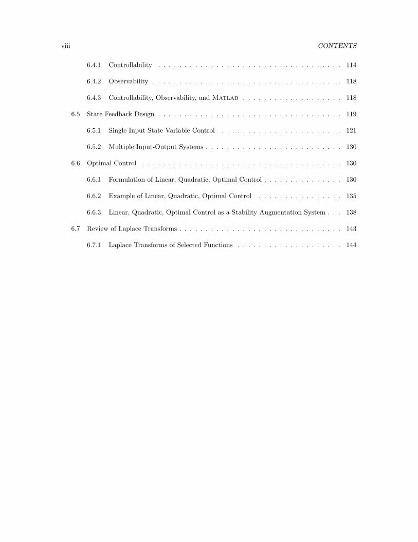
6.4.1 Controllability . . . . . . . . . . . . . . . . . . . . . . . . . . . . . . . . . . . 114
6.4.2 Observability . . . . . . . . . . . . . . . . . . . . . . . . . . . . . . . . . . . . 118
6.4.3 Controllability, Observability, and Matlab . . . . . . . . . . . . . . . . . . . 118
6.5 State Feedback Design . . . . . . . . . . . . . . . . . . . . . . . . . . . . . . . . . . . 119
6.5.1 Single Input State Variable Control . . . . . . . . . . . . . . . . . . . . . . . 121
6.5.2 Multiple Input-Output Systems . . . . . . . . . . . . . . . . . . . . . . . . . . 130
6.6 Optimal Control . . . . . . . . . . . . . . . . . . . . . . . . . . . . . . . . . . . . . . 130
6.6.1 Formulation of Linear, Quadratic, Optimal Control . . . . . . . . . . . . . . . 130
6.6.2 Example of Linear, Quadratic, Optimal Control . . . . . . . . . . . . . . . . 135
6.6.3 Linear, Quadratic, Optimal Control as a Stability Augmentation System . . . 138
6.7 Review of Laplace Transforms . . . . . . . . . . . . . . . . . . . . . . . . . . . . . . . 143
6.7.1 Laplace Transforms of Selected Functions . . . . . . . . . . . . . . . . . . . . 144

Chapter 1
Introduction to Flight Dynamics
Flight dynamics deals principally with the response of aerospace vehicles to perturbationsin their flight environments and to control inputs. In order to understand this response,it is necessary to characterize the aerodynamic and propulsive forces and moments actingon the vehicle, and the dependence of these forces and moments on the flight variables,including airspeed and vehicle orientation. These notes provide an introduction to theengineering science of flight dynamics, focusing primarily of aspects of stability andcontrol. The notes contain a simplified summary of important results from aerodynamicsthat can be used to characterize the forcing functions, a description of static stabilityfor the longitudinal problem, and an introduction to the dynamics and control of both,longitudinal and lateral/directional problems, including some aspects of feedback control.
1.1 Introduction
Flight dynamics characterizes the motion of a flight vehicle in the atmosphere. As such, it can beconsidered a branch of systems dynamics in which the system studies is a flight vehicle. The responseof the vehicle to aerodynamic, propulsive, and gravitational forces, and to control inputs from thepilot determine the attitude of the vehicle and its resulting flight path. The field of flight dynamicscan be further subdivided into aspects concerned with
• Performance: in which the short time scales of response are ignored, and the forces areassumed to be in quasi-static equilibrium. Here the issues are maximum and minimum flightspeeds, rate of climb, maximum range, and time aloft (endurance).
• Stability and Control: in which the short- and intermediate-time response of the attitudeand velocity of the vehicle is considered. Stability considers the response of the vehicle toperturbations in flight conditions from some dynamic equilibrium, while control considers theresponse of the vehicle to control inputs.
• Navigation and Guidance: in which the control inputs required to achieve a particulartrajectory are considered.
1

2 CHAPTER 1. INTRODUCTION TO FLIGHT DYNAMICS
Aerodynamics Propulsion
Flight Dynamics(Stability & Control)
Structures
Aerospace
DesignVehicle
M&AE 3050 M&AE 5060
M&AE 5070M&AE 5700
Figure 1.1: The four engineering sciences required to design a flight vehicle.
In these notes we will focus on the issues of stability and control. These two aspects of the dynamicscan be treated somewhat independently, at least in the case when the equations of motion arelinearized, so the two types of responses can be added using the principle of superposition, and thetwo types of responses are related, respectively, to the stability of the vehicle and to the ability ofthe pilot to control its motion.
Flight dynamics forms one of the four basic engineering sciences needed to understand the designof flight vehicles, as illustrated in Fig. 1.1 (with Cornell M&AE course numbers associated withintroductory courses in these areas). A typical aerospace engineering curriculum with have coursesin all four of these areas.
The aspects of stability can be further subdivided into (a) static stability and (b) dynamic stability.Static stability refers to whether the initial tendency of the vehicle response to a perturbationis toward a restoration of equilibrium. For example, if the response to an infinitesimal increasein angle of attack of the vehicle generates a pitching moment that reduces the angle of attack, theconfiguration is said to be statically stable to such perturbations. Dynamic stability refers to whetherthe vehicle ultimately returns to the initial equilibrium state after some infinitesimal perturbation.Consideration of dynamic stability makes sense only for vehicles that are statically stable. But avehicle can be statically stable and dynamically unstable (for example, if the initial tendency toreturn toward equilibrium leads to an overshoot, it is possible to have an oscillatory divergence ofcontinuously increasing amplitude).
Control deals with the issue of whether the aerodynamic and propulsive controls are adequate totrim the vehicle (i.e., produce an equilibrium state) for all required states in the flight envelope. Inaddition, the issue of “flying qualities” is intimately connected to control issues; i.e., the controlsmust be such that the maintenance of desired equilibrium states does not overly tire the pilot orrequire excessive attention to control inputs.
Several classical texts that deal with aspects of aerodynamic performance [1, 5] and stability andcontrol [2, 3, 4] are listed at the end of this chapter.

1.2. NOMENCLATURE 3
Figure 1.2: Standard notation for aerodynamic forces and moments, and linear and rotationalvelocities in body-axis system; origin of coordinates is at center of mass of the vehicle.
1.2 Nomenclature
The standard notation for describing the motion of, and the aerodynamic forces and moments actingupon, a flight vehicle are indicated in Fig. 1.2.
Virtually all the notation consists of consecutive alphabetic triads:
• The variables x, y, z represent coordinates, with origin at the center of mass of the vehicle.The x-axis lies in the symmetry plane of the vehicle1 and points toward the nose of thevehicle. (The precise direction will be discussed later.) The z-axis also is taken to lie in theplane of symmetry, perpendicular to the x-axis, and pointing approximately down. The y axiscompletes a right-handed orthogonal system, pointing approximately out the right wing.
• The variables u, v, w represent the instantaneous components of linear velocity in the directionsof the x, y, and z axes, respectively.
• The variables X, Y , Z represent the components of aerodynamic force in the directions of thex, y, and z axes, respectively.
• The variables p, q, r represent the instantaneous components of rotational velocity about thex, y, and z axes, respectively.
• The variables L, M , N represent the components of aerodynamic moments about the x, y,and z axes, respectively.
• Although not indicated in the figure, the variables φ, θ, ψ represent the angular rotations,relative to the equilibrium state, about the x, y, and z axes, respectively. Thus, p = φ, q = θ,and r = ψ, where the dots represent time derivatives.
The velocity components of the vehicle often are represented as angles, as indicated in Fig. 1.3. Thevelocity component w can be interpreted as the angle of attack
α ≡ tan−1 w
u(1.1)
1Virtually all flight vehicles have bi-lateral symmetry, and this fact is used to simplify the analysis of motions.

4 CHAPTER 1. INTRODUCTION TO FLIGHT DYNAMICS
x
y
z
V
α
β
u
w
v
Figure 1.3: Standard notation for aerodynamic forces and moments, and linear and rotationalvelocities in body-axis system; origin of coordinates is at center of mass of the vehicle.
while the velocity component v can be interpreted as the sideslip angle
β ≡ sin−1 v
V(1.2)
1.2.1 Implications of Vehicle Symmetry
The analysis of flight motions is simplified, at least for small perturbations from certain equilibriumstates, by the bi-lateral symmetry of most flight vehicles. This symmetry allows us to decomposemotions into those involving longitudinal perturbations and those involving lateral/directional per-turbations. Longitudinal motions are described by the velocities u and v and rotations about they-axis, described by q (or θ). Lateral/directional motions are described by the velocity v and rota-tions about the x and/or z axes, described by p and/or r (or φ and/or ψ). A longitudinal equilibriumstate is one in which the lateral/directional variables v, p, r are all zero. As a result, the side forceY and the rolling moment p and yawing moment r also are identically zero. A longitudinal equilib-rium state can exist only when the gravity vector lies in the x-z plane, so such states correspond towings-level flight (which may be climbing, descending, or level).
The important results of vehicle symmetry are the following. If a vehicle in a longitudinal equilibriumstate is subjected to a perturbation in one of the longitudinal variables, the resulting motion willcontinue to be a longitudinal one – i.e., the velocity vector will remain in the x-z plane and theresulting motion can induce changes only in u, w, and q (or θ). This result follows from thesymmetry of the vehicle because changes in flight speed (V =
√u2 + v2 in this case), angle of attack
(α = tan−1 w/u), or pitch angle θ cannot induce a side force Y , a rolling moment L, or a yawingmoment N . Also, if a vehicle in a longitudinal equilibrium state is subjected to a perturbation inone of the lateral/directional variables, the resulting motion will to first order result in changes onlyto the lateral/directional variables. For example, a positive yaw rate will result in increased lift onthe left wing, and decreased lift on the right wing; but these will approximately cancel, leaving thelift unchanged. These results allow us to gain insight into the nature of the response of the vehicleto perturbations by considering longitudinal motions completely uncoupled from lateral/directionalones, and vice versa.

1.2. NOMENCLATURE 5
1.2.2 Aerodynamic Controls
An aircraft typically has three aerodynamic controls, each capable of producing moments about oneof the three basic axes. The elevator consists of a trailing-edge flap on the horizontal tail (or theability to change the incidence of the entire tail). Elevator deflection is characterized by the deflectionangle δe. Elevator deflection is defined as positive when the trailing edge rotates downward, so, fora configuration in which the tail is aft of the vehicle center of mass, the control derivative
∂Mcg
∂δe< 0
The rudder consists of a trailing-edge flap on the vertical tail. Rudder deflection is characterizedby the deflection angle δr. Rudder deflection is defined as positive when the trailing edge rotates tothe left, so the control derivative
∂Ncg
∂δr< 0
The ailerons consist of a pair of trailing-edge flaps, one on each wing, designed to deflect differentially;i.e., when the left aileron is rotated up, the right aileron will be rotated down, and vice versa. Ailerondeflection is characterized by the deflection angle δa. Aileron deflection is defined as positive whenthe trailing edge of the aileron on the right wing rotates up (and, correspondingly, the trailing edgeof the aileron on the left wing rotates down), so the control derivative
∂Lcg
∂δa> 0
By vehicle symmetry, the elevator produces only pitching moments, but there invariably is somecross-coupling of the rudder and aileron controls; i.e., rudder deflection usually produces some rollingmoment and aileron deflection usually produces some yawing moment.
1.2.3 Force and Moment Coefficients
Modern computer-based flight dynamics simulation is usually done in dimensional form, but thebasic aerodynamic inputs are best defined in terms of the classical non-dimensional aerodynamicforms. These are defined using the dynamic pressure
Q =1
2ρV 2 =
1
2ρSLV 2
eq
where ρ is the ambient density at the flight altitude and Veq is the equivalent airspeed , which is definedby the above equation in which ρSL is the standard sea-level value of the density. In addition, thevehicle reference area S, usually the wing planform area, wing mean aerodynamic chord c, and wingspan b are used to non-dimensionalize forces and moments. The force coefficients are defined as
CX =X
QS
CY =Y
QS
CZ =Z
QS
(1.3)

6 CHAPTER 1. INTRODUCTION TO FLIGHT DYNAMICS
while the aerodynamic moment coefficients are defined as
Cl =L
QSb
Cm =M
QSc
Cn =N
QSb
(1.4)
Note that the wing span is used as the reference moment arm for the rolling and yawing moments,while the mean aerodynamic chord is used for the pitching moment.
Finally, we often express the longitudinal forces in terms of the lift L and drag D, and define thecorresponding lift and drag coefficients as
CL ≡ L
QS= −CZ cos α + CX sin α
CD ≡ D
QS= −CZ sin α − CX cos α
(1.5)
Note that in this set of equations, L represents the lift force, not the rolling moment. It generallywill be clear from the context here, and in later sections, whether the variable L refers to the liftforce or the rolling moment.
1.2.4 Atmospheric Properties
Aerodynamic forces and moments are strongly dependent upon the ambient density of the air at thealtitude of flight. In order to standardize performance calculations, standard values of atmosphericproperties have been developed, under the assumptions that the atmosphere is static (i.e., no winds),that atmospheric properties are a function only of altitude h, that the temperature is given bya specified piecewise linear function of altitude, and that the acceleration of gravity is constant(technically requiring that properties be defined as functions of geopotential altitude. Tables for theproperties of the Standard Atmosphere, in both SI and British Gravitational units, are given on thefollowing pages.

1.2. NOMENCLATURE 7
h (m) T (K) p (N/m2) ρ (kg/m
3) a (m/s)
0 288.15 101325.00 1.225000 340.29500 284.90 95460.78 1.167268 338.37
1000 281.65 89874.46 1.111641 336.431500 278.40 84555.84 1.058065 334.492000 275.15 79495.01 1.006488 332.532500 271.90 74682.29 0.956856 330.563000 268.65 70108.27 0.909119 328.583500 265.40 65763.78 0.863225 326.584000 262.15 61639.91 0.819125 324.584500 258.90 57727.98 0.776770 322.565000 255.65 54019.55 0.736111 320.535500 252.40 50506.43 0.697100 318.486000 249.15 47180.64 0.659692 316.436500 245.90 44034.45 0.623839 314.367000 242.65 41060.35 0.589495 312.277500 239.40 38251.03 0.556618 310.178000 236.15 35599.41 0.525162 308.068500 232.90 33098.64 0.495084 305.939000 229.65 30742.07 0.466342 303.799500 226.40 28523.23 0.438895 301.63
10000 223.15 26435.89 0.412701 299.4610500 219.90 24474.00 0.387720 297.2711000 216.65 22631.70 0.363912 295.0711500 216.65 20915.84 0.336322 295.0712000 216.65 19330.06 0.310823 295.0712500 216.65 17864.52 0.287257 295.0713000 216.65 16510.09 0.265478 295.0713500 216.65 15258.34 0.245350 295.0714000 216.65 14101.50 0.226749 295.0714500 216.65 13032.37 0.209557 295.0715000 216.65 12044.30 0.193669 295.0715500 216.65 11131.14 0.178986 295.0716000 216.65 10287.21 0.165416 295.0716500 216.65 9507.26 0.152874 295.0717000 216.65 8786.45 0.141284 295.0717500 216.65 8120.29 0.130572 295.0718000 216.65 7504.64 0.120673 295.0718500 216.65 6935.66 0.111524 295.0719000 216.65 6409.82 0.103068 295.0719500 216.65 5923.85 0.095254 295.0720000 216.65 5474.72 0.088032 295.07
Table 1.1: Properties of the International Standard Atmosphere; SI units.
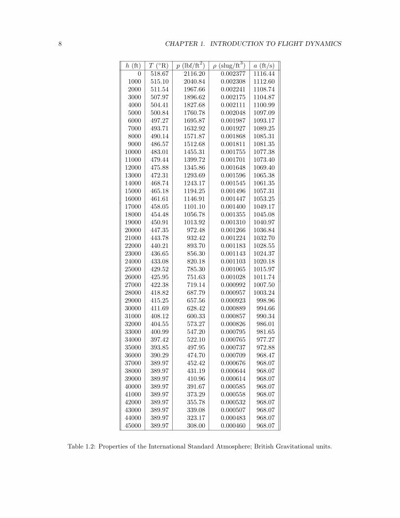
8 CHAPTER 1. INTRODUCTION TO FLIGHT DYNAMICS
h (ft) T (R) p (lbf/ft2) ρ (slug/ft
3) a (ft/s)
0 518.67 2116.20 0.002377 1116.441000 515.10 2040.84 0.002308 1112.602000 511.54 1967.66 0.002241 1108.743000 507.97 1896.62 0.002175 1104.874000 504.41 1827.68 0.002111 1100.995000 500.84 1760.78 0.002048 1097.096000 497.27 1695.87 0.001987 1093.177000 493.71 1632.92 0.001927 1089.258000 490.14 1571.87 0.001868 1085.319000 486.57 1512.68 0.001811 1081.35
10000 483.01 1455.31 0.001755 1077.3811000 479.44 1399.72 0.001701 1073.4012000 475.88 1345.86 0.001648 1069.4013000 472.31 1293.69 0.001596 1065.3814000 468.74 1243.17 0.001545 1061.3515000 465.18 1194.25 0.001496 1057.3116000 461.61 1146.91 0.001447 1053.2517000 458.05 1101.10 0.001400 1049.1718000 454.48 1056.78 0.001355 1045.0819000 450.91 1013.92 0.001310 1040.9720000 447.35 972.48 0.001266 1036.8421000 443.78 932.42 0.001224 1032.7022000 440.21 893.70 0.001183 1028.5523000 436.65 856.30 0.001143 1024.3724000 433.08 820.18 0.001103 1020.1825000 429.52 785.30 0.001065 1015.9726000 425.95 751.63 0.001028 1011.7427000 422.38 719.14 0.000992 1007.5028000 418.82 687.79 0.000957 1003.2429000 415.25 657.56 0.000923 998.9630000 411.69 628.42 0.000889 994.6631000 408.12 600.33 0.000857 990.3432000 404.55 573.27 0.000826 986.0133000 400.99 547.20 0.000795 981.6534000 397.42 522.10 0.000765 977.2735000 393.85 497.95 0.000737 972.8836000 390.29 474.70 0.000709 968.4737000 389.97 452.42 0.000676 968.0738000 389.97 431.19 0.000644 968.0739000 389.97 410.96 0.000614 968.0740000 389.97 391.67 0.000585 968.0741000 389.97 373.29 0.000558 968.0742000 389.97 355.78 0.000532 968.0743000 389.97 339.08 0.000507 968.0744000 389.97 323.17 0.000483 968.0745000 389.97 308.00 0.000460 968.07
Table 1.2: Properties of the International Standard Atmosphere; British Gravitational units.

Bibliography
[1] John Anderson, Introduction to Flight, McGraw-Hill, New York, Fourth Edition, 2000.
[2] Bernard Etkin & Lloyd D. Reid, Dynamics of Flight; Stability and Control, John Wiley& Sons, New York, Third Edition, 1998.
[3] Robert C. Nelson, Flight Stability and Automatic Control, McGraw-Hill, New York,Second Edition, 1998.
[4] Edward Seckel, Stability and Control of Airplanes and Helicopters, Academic Press,New York, 1964.
[5] Richard Shevell, Fundamentals of Flight, Prentice Hall, Englewood Cliffs, New Jersey, Sec-ond Edition, 1989.
9

10 BIBLIOGRAPHY

Chapter 2
Aerodynamic Background
Flight dynamics deals principally with the response of aerospace vehicles to perturbationsin their flight environments and to control inputs. In order to understand this response,it is necessary to characterize the aerodynamic and propulsive forces and moments actingon the vehicle, and the dependence of these forces and moments on the flight variables,including airspeed and vehicle orientation. These notes provide a simplified summary ofimportant results from aerodynamics that can be used to characterize these dependencies.
2.1 Introduction
Flight dynamics deals with the response of aerospace vehicles to perturbations in their flight environ-ments and to control inputs. Since it is changes in orientation (or attitude) that are most important,these responses are dominated by the generated aerodynamic and propulsive moments. For mostaerospace vehicles, these moments are due largely to changes in the lifting forces on the vehicle (asopposed to the drag forces that are important in determining performance). Thus, in some ways,the prediction of flight stability and control is easier than the prediction of performance, since theselifting forces can often be predicted to within sufficient accuracy using inviscid, linear theories.
In these notes, I attempt to provide a uniform background in the aerodynamic theories that can beused to analyze the stability and control of flight vehicles. This background is equivalent to thatusually covered in an introductory aeronautics course, such as one that might use the text by Shevell[6]. This material is often reviewed in flight dynamics texts; the material presented here is derived,in part, from the material in Chapter 1 of the text by Seckel [5], supplemented with some of thematerial from Appendix B of the text by Etkin & Reid [3]. The theoretical basis for these lineartheories can be found in the book by Ashley & Landahl [2].
11

12 CHAPTER 2. AERODYNAMIC BACKGROUND
c(y)
b/2
y
x
ctip
Λ0
rootc
Figure 2.1: Planform geometry of a typical lifting surface (wing).
2.2 Lifting surface geometry and nomenclature
We begin by considering the geometrical parameters describing a lifting surface, such as a wing orhorizontal tail plane. The projection of the wing geometry onto the x-y plane is called the wingplanform. A typical wing planform is sketched in Fig. 2.1. As shown in the sketch, the maximumlateral extent of the planform is called the wing span b, and the area of the planform S is called thewing area.
The wing area can be computed if the spanwise distribution of local section chord c(y) is knownusing
S =
∫ b/2
−b/2
c(y) dy = 2
∫ b/2
0
c(y) dy, (2.1)
where the latter form assumes bi-lateral symmetry for the wing (the usual case). While the spancharacterizes the lateral extent of the aerodynamic forces acting on the wing, the mean aerodynamicchord c characterizes the axial extent of these forces. The mean aerodynamic chord is usuallyapproximated (to good accuracy) by the mean geometric chord
c =2
S
∫ b/2
0
c2 dy (2.2)
The dimensionless ratio of the span to the mean chord is also an important parameter, but insteadof using the ratio b/c the aspect ratio of the planform is defined as
AR ≡ b2
S(2.3)
Note that this definition reduces to the ratio b/c for the simple case of a wing of rectangular planform(having constant chord c).

2.2. LIFTING SURFACE GEOMETRY AND NOMENCLATURE 13
The lift, drag, and pitching moment coefficients of the wing are defined as
CL =L
QS
CD =D
QS
Cm =M
QSc
(2.4)
where
Q =ρV 2
2
is the dynamic pressure, and L, D, M are the lift force, drag force, and pitching moment, respectively,due to the aerodynamic forces acting on the wing.
Conceptually, and often analytically, it is useful to build up the aerodynamic properties of liftingsurfaces as integrals of sectional properties. A wing section, or airfoil , is simply a cut through thelifting surface in a plane of constant y. The lift, drag, and pitching moment coefficients of the airfoilsection are defined as
cℓ =ℓ
Qc
Cd =d
Qc
Cmsect =m
Qc2
(2.5)
where ℓ, d, and m are the lift force, drag force, and pitching moment, per unit span, respectively,due to the aerodynamics forces acting on the airfoil section. Note that if we calculate the wing liftcoefficient as the chord-weighted average integral of the section lift coefficients
CL =2
S
∫ b/s
0
cℓcdy (2.6)
for a wing with constant section lift coefficient, then Eq. (2.6) gives
CL = cℓ
2.2.1 Geometric properties of trapezoidal wings
The planform shape of many wings can be approximated as trapezoidal. In this case, the root chordcroot, tip chord ctip, span b, and the sweep angle of any constant-chord fraction Λn completely specifythe planform. Usually, the geometry is specified in terms of the wing taper ratio λ = ctip/croot; thenusing the geometric properties of a trapezoid, we have
S =croot(1 + λ)
2b (2.7)
and
AR =2b
croot(1 + λ)(2.8)

14 CHAPTER 2. AERODYNAMIC BACKGROUND
camber (mean) line
chord line
V
−α
α
0
chord, c
zero−lift line
Figure 2.2: Geometry of a typical airfoil section.
The local chord is then given as a function of the span variable by
c = croot
[
1 − (1 − λ)2y
b
]
(2.9)
and substitution of this into Eq. (2.2) and carrying out the integration gives
c =2(1 + λ + λ2)
3(1 + λ)croot (2.10)
The sweep angle of any constant-chord fraction line can be related to that of the leading-edge sweepangle by
AR tan Λn = AR tan Λ0 − 4n1 − λ
1 + λ(2.11)
where 0 ≤ n ≤ 1 is the chord fraction (e.g., 0 for the leading edge, 1/4 for the quarter-chord line,etc.). Finally, the location of any chord-fraction point on the mean aerodynamic chord, relative tothe wing apex, can be determined as
xn =2
S
∫ b/2
0
xncdy =2
S
∫ b/2
0
(ncroot + y tan Λn) dy
=3(1 + λ)c
2(1 + λ + λ2)
n +
(
1 + 2λ
12
)
AR tan Λn
(2.12)
Alternatively, we can use Eq. (2.11) to express this result in terms of the leading-edge sweep as
xn
c= n +
(1 + λ)(1 + 2λ)
8(1 + λ + λ2)AR tan Λ0 (2.13)
Substitution of n = 0 (or n = 1/4) into either Eq. (2.12) or Eq. (2.13) gives the axial location of theleading edge (or quarter-chord point) of the mean aerodynamic chord relative to the wing apex.
2.3 Aerodynamic properties of airfoils
The basic features of a typical airfoil section are sketched in Fig. 2.2. The longest straight line fromthe trailing edge to a point on the leading edge of the contour defines the chord line. The lengthof this line is called simply the chord c. The locus of points midway between the upper and lowersurfaces is called the mean line, or camber line. For a symmetric airfoil, the camber and chord linescoincide.

2.3. AERODYNAMIC PROPERTIES OF AIRFOILS 15
For low speeds (i.e., Mach numbers M << 1), and at high Reynolds numbers Re = V c/ν >> 1,the results of thin-airfoil theory predict the lifting properties of airfoils quite accurately for angles ofattack not too near the stall. Thin-airfoil theory predicts a linear relationship between the sectionlift coefficient and the angle of attack α of the form
cℓ = a0 (α − α0) (2.14)
as shown in Fig. 2.3. The theory also predicts the value of the lift-curve slope
a0 =∂cℓ
∂α= 2π (2.15)
Thickness effects (not accounted for in thin-airfoil theory) tend to increase the value of a0, whileviscous effects (also neglected in the theory) tend to decrease the value of a0. The value of a0 forrealistic conditions is, as a result of these counter-balancing effects, remarkably close to 2π for mostpractical airfoil shapes at the high Reynolds numbers of practical flight.
The angle α0 is called the angle for zero lift , and is a function only of the shape of the camber line.Increasing (conventional, sub-sonic) camber makes the angle for zero lift α0 increasingly negative.For camber lines of a given family (i.e., shape), the angle for zero lift is very nearly proportional tothe magnitude of camber – i.e., to the maximum deviation of the camber line from the chord line.
A second important result from thin-airfoil theory concerns the location of the aerodynamic center .The aerodynamic center of an airfoil is the point about which the pitching moment, due to thedistribution of aerodynamic forces acting on the airfoil surface, is independent of the angle of attack.Thin-airfoil theory tells us that the aerodynamic center is located on the chord line, one quarter ofthe way from the leading to the trailing edge – the so-called quarter-chord point. The value of thepitching moment about the aerodynamic center can also be determined from thin-airfoil theory, butrequires a detailed calculation for each specific shape of camber line. Here, we simply note that,for a given shape of camber line the pitching moment about the aerodynamic center is proportionalto the amplitude of the camber, and generally is negative for conventional subsonic (concave down)camber shapes.
It is worth emphasizing that thin-airfoil theory neglects the effects of viscosity and, therefore, cannotpredict the behavior of airfoil stall, which is due to boundary layer separation at high angles of attack.Nevertheless, for the angles of attack usually encountered in controlled flight, it provides a very usefulapproximation for the lift.
Angle of attack,
Thin−airfoil theory
Stall
α 0
Lift
coef
ficie
nt, C
l
α
2π
Figure 2.3: Airfoil section lift coefficient as a function of angle of attack.
16 CHAPTER 2. AERODYNAMIC BACKGROUND
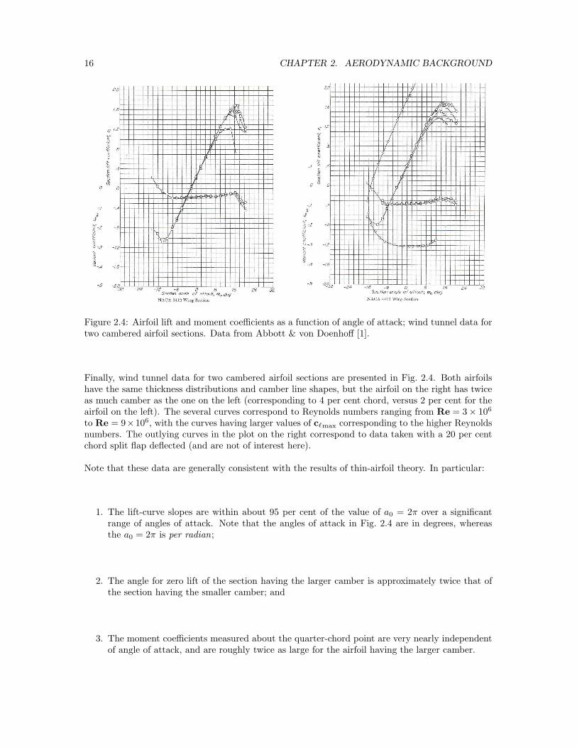
Figure 2.4: Airfoil lift and moment coefficients as a function of angle of attack; wind tunnel data fortwo cambered airfoil sections. Data from Abbott & von Doenhoff [1].
Finally, wind tunnel data for two cambered airfoil sections are presented in Fig. 2.4. Both airfoilshave the same thickness distributions and camber line shapes, but the airfoil on the right has twiceas much camber as the one on the left (corresponding to 4 per cent chord, versus 2 per cent for theairfoil on the left). The several curves correspond to Reynolds numbers ranging from Re = 3 × 10⁶
to Re = 9×10⁶, with the curves having larger values of cℓmax corresponding to the higher Reynoldsnumbers. The outlying curves in the plot on the right correspond to data taken with a 20 per centchord split flap deflected (and are not of interest here).
Note that these data are generally consistent with the results of thin-airfoil theory. In particular:
1. The lift-curve slopes are within about 95 per cent of the value of a0 = 2π over a significantrange of angles of attack. Note that the angles of attack in Fig. 2.4 are in degrees, whereasthe a0 = 2π is per radian;
2. The angle for zero lift of the section having the larger camber is approximately twice that ofthe section having the smaller camber; and
3. The moment coefficients measured about the quarter-chord point are very nearly independentof angle of attack, and are roughly twice as large for the airfoil having the larger camber.

2.4. AERODYNAMIC PROPERTIES OF FINITE WINGS 17
2.4 Aerodynamic properties of finite wings
The vortex structures trailing downstream of a finite wing produce an induced downwash field nearthe wing which can be characterized by an induced angle of attack
αi =CL
πeAR(2.16)
For a straight (un-swept) wing with an elliptical spanwise loading, lifting-line theory predicts thatthe induced angle of attack αi is constant across the span of the wing, and the efficiency factore = 1.0. For non-elliptical span loadings, e < 1.0, but for most practical wings αi is still nearlyconstant across the span. Thus, for a finite wing lifting-line theory predicts that
CL = a0 (α − α0 − αi) (2.17)
where a0 is the wing section lift-curve slope and α0 is the angle for zero lift of the section. SubstitutingEq. (2.16) and solving for the lift coefficient gives
CL =a0
1 + a0
πeAR
(α − α0) = a(α − α0) (2.18)
whence the wing lift-curve slope is given by
a =∂CL
∂α=
a0
1 + a0
πeAR
(2.19)
Lifting-line theory is asymptotically correct in the limit of large aspect ratio, so, in principle,Eq. (2.18) is valid only in the limit as AR → ∞. At the same time, slender-body theory is valid inthe limit of vanishingly small aspect ratio, and it predicts, independently of planform shape, thatthe lift-curve slope is
a =πAR
2(2.20)
Note that this is one-half the value predicted by the limit of the lifting-line result, Eq. (2.19), asthe aspect ratio goes to zero. We can construct a single empirical formula that contains the correctlimits for both large and small aspect ratio of the form
a =πAR
1 +
√
1 +(
πAR
a0
)2(2.21)
A plot of this equation, and of the lifting-line and slender-body theory results, is shown in Fig. 2.5.
Equation (2.21) can also be modified to account for wing sweep and the effects of compressibility. Ifthe sweep of the quarter-chord line of the planform is Λc/4, the effective section incidence is increasedby the factor 1/ cos Λc/4, relative to that of the wing,1while the dynamic pressure of the flow normalto the quarter-chord line is reduced by the factor cos2 Λc/4. The section lift-curve slope is thusreduced by the factor cos Λc/4, and a version of Eq. (2.21) that accounts for sweep can be written
a =πAR
1 +
√
1 +(
πAR
a0 cos Λc/4
)2(2.22)
1This factor can best be understood by interpreting a change in angle of attack as a change in vertical velocity∆w = V∞ ∆α.

18 CHAPTER 2. AERODYNAMIC BACKGROUND
0
0.2
0.4
0.6
0.8
1
0 2 4 6 8 10 12 14 16
Lifting-lineSlender-body
Empirical
Aspect ratio, b2/S
Norm
alize
dlift
-curv
esl
ope,
a
2π
Figure 2.5: Empirical formula for lift-curve slope of a finite wing compared with lifting-line andslender-body limits. Plot is constructed assuming a0 = 2π.
Finally, for subcritical (M∞ < Mcrit) flows, the Prandtl-Glauert similarity law for airfoil sectionsgives
a2d =a0
√
1 − M2∞
(2.23)
where M∞ is the flight Mach number. The Goethert similarity rule for three-dimensional wingsmodifies Eq. (2.22) to the form
a =πAR
1 +
√
1 +(
πAR
a0 cos Λc/4
)2(
1 − M2∞
cos2 Λc/4
)
(2.24)
In Eqs. (2.22), (2.23) and (2.24), a0 is, as earlier, the incompressible, two-dimensional value of thelift-curve slope (often approximated as a0 = 2π). Note that, according to Eq. (2.24) the lift-curveslope increases with increasing Mach number, but not as fast as the two-dimensional Prandtl-Glauertrule suggests. Also, unlike the Prandtl-Glauert result, the transonic limit (M∞ cos Λc/4 → 1.0) isfinite and corresponds (correctly) to the slender-body limit.
So far we have described only the lift-curve slope a = ∂CL/∂α for the finite wing, which is itsmost important parameter as far as stability is concerned. To determine trim, however, it is alsoimportant to know the value of the pitching moment at zero lift (which is, of course, also equal tothe pitching moment about the aerodynamic center). We first determine the angle of attack forwing zero lift. From the sketch in Fig. 2.6, we see that the angle of attack measured at the wingroot corresponding to zero lift at a given section can be written
− (α0)root = ǫ − α0 (2.25)
where ǫ is the geometric twist at the section, relative to the root. The wing lift coefficient can thenbe expressed as
CL =2
S
∫ b/2
0
a [αr − (α0)root] cdy =2a
S
[
S
2αr +
∫ b/2
0
(ǫ − α0) cdy
]
(2.26)

2.5. FUSELAGE CONTRIBUTION TO PITCH STIFFNESS 19
−α
ε
−α0
root chord
local chord
local zero−lift line0 )
root
Figure 2.6: Root angle of attack corresponding to zero lift at a given section.
Setting the lift coefficient to zero and solving for the root angle of attack then yields
(αr)L=0 =2
S
∫ b/2
0
(α0 − ǫ) cdy (2.27)
Now, the wing pitching moment about its aerodynamic center can be determined as the sum ofcontributions from the section values plus the contribution due to the basic lift distribution – i.e.,the distribution of lifting forces at wing zero lift.2These contributions can be expressed as
Cmac =2
Sc
∫ b/2
0
c2 (Cmac)sect dy +
∫ b/2
0
a [(αr)L=0 + ǫ − α0] cx1 dy
(2.28)
where x1 = xac − xMAC is the axial distance between the section aerodynamic center and the wingaerodynamic center. Consistent with these approximations, the wing aerodynamic center is locatedat the chord-weighted quarter-chord location for the wing; i.e.,
xMAC =2
S
∫ b/2
0
xc/4cdy (2.29)
Explicit expressions for this variable can be determined from Eqs. (2.12,2.13) for wings of trapezoidalplanform.
2.5 Fuselage contribution to pitch stiffness
The contribution of the fuselage to the pitching moment is affected by interference effects with thewing flow field. These can be estimated using a simple strip theory (as described, for example,in Example 2.2 of the text by Nelson [4]), but here we will introduce a simple estimate for thedestabilizing effect of the fuselage in the absence of interference effects.
Slender-body theory predicts a distribution of lifting force given by
dL
dx= 2Qα
dSf
dx(2.30)
where Sf = πw2/4 is the equivalent cross-sectional area of the fuselage based on its width w as afunction of the streamwise variable x. For a finite-length fuselage, Eq. (2.30) predicts positive lift on
2The basic lift distribution, of course, sums to zero lift, but is still capable of producing non-zero pitching momentswhen the wing is swept.

20 CHAPTER 2. AERODYNAMIC BACKGROUND
the forward part of the fuselage (where Sf is generally increasing), and negative lift on the rearwardpart (where Sf is generally decreasing), but the total lift is identically zero (since Sf (0) = Sf (ℓf ) = 0,where ℓf is the fuselage length).
Since the total lift acting on the fuselage is zero, the resulting force system is a pure couple, and thepitching moment will be the same, regardless of the reference point about which it is taken. Thus,e.g., taking the moment about the fuselage nose (x = 0), we have
Mf = −∫ ℓf
0
xdL = −2Qα
∫ ℓf
0
xdSf = 2Qα
∫ ℓf
0
Sf dx = 2QαV (2.31)
where V is the volume of the “equivalent” fuselage (i.e., the body having the same planform as theactual fuselage, but with circular cross-sections). The fuselage contribution to the vehicle pitchingmoment coefficient is then
Cm =Mf
QSc=
2VSc
α (2.32)
and the corresponding pitch stiffness is
Cmα =
(
∂Cm
∂α
)
fuse
=2VSc
(2.33)
Note that this is always positive – i.e., destabilizing.
2.6 Wing-tail interference
The one interference effect we will account for is that between the wing and the horizontal tail.Because the tail operates in the downwash field of the wing (for conventional, aft-tail configurations),the effective angle of attack of the tail is reduced. The reduction in angle of attack can be estimatedto be
ε = κCL
πeAR(2.34)
where 1 < κ < 2. Note that κ = 1 corresponds to ε = αi, the induced angle of attack of the wing,while κ = 2 corresponds to the limit when the tail is far downstream of the wing. For stabilityconsiderations, it is the rate of change of tail downwash with angle of attack that is most important,and this can be estimated as
dε
dα=
κ
πeAR(CLα)wing (2.35)
2.7 Control Surfaces
Aerodynamic control surfaces are usually trailing-edge flaps on lifting surfaces that can be deflectedby control input from the pilot (or autopilot). Changes in camber line slope near the trailing edge of alifting surface are very effective at generating lift. The lifting pressure difference due to trailing-edgeflap deflection on a two-dimensional airfoil, calculated according to thin-airfoil theory, is plotted inFig. 2.7 (a) for flap chord lengths of 10, 20, and 30 percent of the airfoil chord. The values plotted

2.7. CONTROL SURFACES 21
0
0.5
1
1.5
2
0 0.2 0.4 0.6 0.8 1
Lifti
ng P
ress
ure,
Del
ta C
p/(2
pi)
Axial position, x/c
Flap = 0.10 cFlap = 0.20 cFlap = 0.30 c
0
0.2
0.4
0.6
0.8
1
0 0.1 0.2 0.3 0.4 0.5
Fla
p ef
fect
iven
ess
Fraction flap chord
(a) Lifting pressure coefficient (b) Control effectiveness
Figure 2.7: Lifting pressure distribution due to flap deflection and resulting control effectiveness.
are per unit angular deflection, and normalized by 2π, so their integrals can be compared with thechanges due to increments in angle of attack. Figure 2.7 (b) shows the control effectiveness
∂Cℓ
∂δ(2.36)
also normalized by 2π. It is seen from this latter figure that deflection of a flap that consists of only25 percent chord is capable of generating about 60 percent of the lift of the entire airfoil pitchedthrough an angle of attack equal to that of the flap deflection. Actual flap effectiveness is, of course,reduced somewhat from these ideal values by the presence of viscous effects near the airfoil trailingedge, but the flap effectiveness is still nearly 50 percent of the lift-curve slope for a 25 percent chordflap for most actual flap designs.
The control forces required to change the flap angle are related to the aerodynamic moments aboutthe hinge-line of the flap. The aerodynamic moment about the hinge line is usually expressed interms of the dimensionless hinge moment coefficient, e.g., for the elevator hinge moment He, definedas
Che≡ He
12ρV 2Sece
(2.37)
where Se and ce are the elevator planform area and chord length, respectively; these are based onthe area of the control surface aft of the hinge line.
The most important characteristics related to the hinge moments are the restoring tendency andthe floating tendency. The restoring tendency is the derivative of the hinge moment coefficient withrespect to control deflection; e.g., for the elevator,
Chδe=
∂Che
∂δe(2.38)
The floating tendency is the derivative of the hinge moment coefficient with respect to angle ofattack; e.g., for the elevator,
Cheαt=
∂Che
∂αt(2.39)
where αt is the angle of attack of the tail.

22 CHAPTER 2. AERODYNAMIC BACKGROUND
0
0.5
1
1.5
2
0 0.2 0.4 0.6 0.8 1
Lifti
ng P
ress
ure,
Del
ta C
p/(2
pi)
Axial position, x/c
Flap deflectionAngle of attack
-0.3
-0.25
-0.2
-0.15
-0.1
-0.05
0
0.05
0.1
0 0.1 0.2 0.3 0.4 0.5
Res
torin
g/F
loat
ing
tend
ency
Hinge position, pct f
Restoring tendencyFloating tendency
(a) Lifting pressure coefficient (b) Hinge moment derivatives
Figure 2.8: Lifting pressure distributions (normalized by 2π) due to flap deflection and to change inangle of attack, and resulting restoring and floating tendencies of control flap. Results of thin-airfoiltheory for 25 percent chord trailing-edge flap.
The restoring and floating tendencies are due primarily to the moments produced about the controlflap hinge line by the lifting pressures induced by changes in either control position or angle of attack.The thin-airfoil approximations to these lifting pressure distributions are illustrated in Fig. 2.8 (a)for a 25 percent chord trailing edge flap. The plotted values of ∆Cp are normalized by 2π, so theaverage value of the ∆Cp due to angle of attack change is unity (corresponding to a lift curve slopeof 2π). Figure 2.8 (b) illustrates the corresponding floating and restoring tendencies as functionsof the hinge line location, measured in fraction of flap chord. It is seen that both tendencies arenegative for hinge lines located ahead of approximately the 33 percent flap chord station. Whilethese results, based on inviscid, thin-airfoil theory are qualitatively correct, actual hinge momentcoefficients are affected by viscous effects and leakage of flow between the flap and the main liftingsurface, so the results presented here should be used only as a guide to intuition.

Bibliography
[1] Ira H. Abbott & Albert E. von Doenhoff, Theory of Wing Sections; Including a Summary
of Data, Dover, New York, 1958.
[2] Holt Ashley & Marten Landahl, Aerodynamics of Wings and Bodies, Addison-Wesley,Reading, Massachusetts, 1965.
[3] Bernard Etkin & Lloyd D. Reid, Dynamics of Flight; Stability and Control, John Wiley& Sons, New York, Third Edition, 1998.
[4] Robert C. Nelson, Flight Stability and Automatic Control, McGraw-Hill, New York,Second Edition, 1998.
[5] Edward Seckel, Stability and Control of Airplanes and Helicopters, Academic Press,New York, 1964.
[6] Richard Shevell, Fundamentals of Flight, Prentice Hall, Englewood Cliffs, New Jersey, Sec-ond Edition, 1989.
23

24 BIBLIOGRAPHY

Chapter 3
Static Longitudinal Stability andControl
The most critical aspects of static longitudinal stability relate to control forces requiredfor changing trim or performing maneuvers. Our textbook [1] treats primarily the situ-ation when the controls are fixed. This is, of course, and idealization, even for the caseof powered, irreversible controls, as the position of the control surfaces can he held fixedonly to the extent of the maximum available control forces. The opposite limit – that offree control surfaces – also is an idealization, limited by the assumptions of zero frictionin the control positioning mechanisms. But, just as the control fixed limit is useful indetermining control position gradients, the control free limit is useful in determining con-trol force gradients. And these latter are among the most important vehicle propertiesin determining handling qualities.
3.1 Control Fixed Stability
Even for the controls-fixed case, our text is a bit careless with nomenclature and equations, so wereview the most important results for this case here. We have seen that for the analysis of longitudinalstability, terms involving products of the drag coefficient and either vertical displacements of thevehicle center-of-gravity or sines of the angle of attack can be neglected. Then, with the axiallocations as specified in Fig. 3.1 the pitching moment about the vehicle c.g. can be written
Cmcg = Cm0w+ CLw
(xcg
c− xac
c
)
− ηSt
SCLt
[
ℓt
c−
(xcg
c− xac
c
)
]
+ Cmf (3.1)
where we assume that Cm0t= 0, since the tail is usually symmetrical. Note that, as is the usual
convention when analyzing static longitudinal stability and control, the positive direction of thex-axis is taken to be aft ;1thus, e.g., the second term on the right-hand side of Eq. (3.1) contributesto a positive (nose-up) pitching moment for positive lift when the c.g. is aft of the wing aerodynamiccenter.
1Also, the origin of the x-axis is taken, by convention, to be at the leading edge of the mean aerodynamic chordof the wing, and distances are normalized by the length of the wing mean aerodynamic chord. Thus, for example, wemight specify the location of the vehicle center-of-gravity as being at 30 per cent m.a.c.
25

26 CHAPTER 3. STATIC LONGITUDINAL STABILITY AND CONTROL
ac
ac
NP
cg
l
FRLi
V
V’
t
w
tw
FRLV
x
ε
α
x − xaccgl tN
i t
Figure 3.1: Geometry of wing and tail with respect to vehicle c.g., basic neutral point, and wingaerodynamic center. Note that positive direction of the x-axis is aft.
Grouping the terms involving the c.g. location, this equation can be written
Cmcg = Cm0w+
(xcg
c− xac
c
)
[
CLw + ηSt
SCLt
]
− ηVHCLt + Cmf (3.2)
where VH = ℓtSt
cS is the tail volume parameter . Note that this definition is based on the distancebetween the aerodynamic centers of the wing and tail, and is therefore independent of the vehiclec.g. location. Note that the total vehicle lift coefficient is
CL =Lw + Lt
QS= CLw + η
St
SCLt (3.3)
where η = Qt/Q is the tail efficiency factor, and this total vehicle lift coefficient is exactly thequantity appearing in the square brackets in Eq. (3.2). Now, we can introduce the dependence ofthe lift coefficients on angle of attack as
CLw = CLαw(αFRL + iw − α0w
)
CLt = CLαt
(
αFRL + it −[
ε0 +dε
dααFRL
])
(3.4)
Note that, consistent with the usual use of symmetric sections for the horizontal tail, we haveassumed α0t
= 0. Introducing these expressions into Eq. (3.3), the latter can be expressed as
CL = CLαw(iw − α0w
) + ηSt
SCLαt
(it − ε0) +
(
CLαw+ η
St
S
[
1 − dε
dα
]
CLαt
)
αFRL (3.5)
This equation has the formCL = CL0 + CLααFRL (3.6)
where the vehicle lift curve slope is
CLα = CLαw+ η
St
S
(
1 − dε
dα
)
CLαt(3.7)
and
CL0 = CLαw(iw − α0w
) + ηSt
SCLαt
(it − ε0) (3.8)
is the vehicle lift coefficient at zero (fuselage reference line) angle of attack. Finally, if we define thevehicle angle of attack relative to the angle of attack for zero vehicle lift, i.e.,
α ≡ αFRL − α0 (3.9)

3.1. CONTROL FIXED STABILITY 27
where
α0 = −CL0
CLα
(3.10)
thenCL = CLαα (3.11)
where CLα is the vehicle lift curve slope, given by Eq. (3.7).
Introducing the angle of attack into Eq. (3.2), the expression for the vehicle pitching moment coef-ficient becomes
Cmcg =Cm0w+
(xcg
c− xac
c
)
[
CLαw(iw − α0w
) + ηSt
SCLαt
(it − ε0)
]
− ηVHCLαt(it − ε0) +
(xcg
c− xac
c
)
[
CLαw+ η
St
S
(
1 − dε
dα
)
CLαt
]
− ηVH
(
1 − dε
dα
)
CLαt+ Cmαf
αFRL
(3.12)
This can be expressed in terms of the angle of attack from zero vehicle lift as
Cmcg = Cm0w+
(xcg
c− xac
c
)
[
CLαw(iw − α0w
) + ηSt
SCLαt
(it − ε0)
]
− ηVHCLαt(it − ε0)
+ Cmαα0 +
(xcg
c− xac
c
)
CLα − ηVHCLαt
(
1 − dε
dα
)
+ Cmαf
α
(3.13)
This equation has the formCm = Cm0 + Cmαα (3.14)
with the vehicle pitching moment coefficient at zero lift
Cm0 = Cm0w+
(xcg
c− xac
c
)
[
CLαw(iw − α0w
) + ηSt
SCLαt
(it − ε0)
]
−ηVHCLαt(it − ε0)+Cmαα0
(3.15)and the vehicle pitch stiffness
Cmα =(xcg
c− xac
c
)
CLα − ηVHCLαt
(
1 − dε
dα
)
+ Cmαf(3.16)
Note that Eq. (3.15) can be simplified (using Eq. (3.16)) to
Cm0 = Cm0w− ηVHCLαt
[
it − ε0 +
(
1 − dε
dα
)
α0
]
+ Cmαfα0 (3.17)
Note that Eq. (3.17) correctly shows that the pitching moment at zero net vehicle lift is independentof the c.g. location, as it must be (since at zero lift the resultant aerodynamic force must sum to apure couple).
The basic (or control-fixed) neutral point is defined as the c.g. location for which the vehicle isneutrally stable in pitch – i.e., the c.g. location for which the pitch stiffness goes to zero. FromEq. (3.16) the neutral point is seen to be located at
xNP
c=
xac
c+ ηVH
CLαt
CLα
(
1 − dε
dα
)
−Cmαf
CLα
(3.18)

28 CHAPTER 3. STATIC LONGITUDINAL STABILITY AND CONTROL
Note that Eq. (3.16) for the pitch stiffness can be expressed as
Cmα =
xcg
c−
[
xac
c+ ηVH
CLαt
CLα
(
1 − dε
dα
)
−Cmαf
CLα
]
CLα (3.19)
where the quantity in square brackets is exactly the location of the basic neutral point, as shown inEq. (3.18). Thus, we can write
Cmα =xcg
c− xNP
c
CLα (3.20)
or, alternatively,∂Cm
∂CL= −
(xNP
c− xcg
c
)
(3.21)
Thus, the pitch stiffness, measured with respect to changes in vehicle lift coefficient, is proportionalto the distance between the c.g. and the basic neutral point. The quantity in parentheses on theright-hand side of Eq. (3.21), i.e., the distance between the vehicle c.g. and the basic neutral point,expressed as a percentage of the wing mean aerodynamic chord, is called the vehicle static margin.2
3.2 Static Longitudinal Control
The elevator is the aerodynamic control for pitch angle of the vehicle, and its effect is described interms of the elevator effectiveness
ae =∂CLt
∂δe(3.22)
where CLt is the lift coefficient of the horizontal tail and δe is the elevator deflection, consideredpositive trailing edge down. The horizontal tail lift coefficient is then given by
CLt =∂CLt
∂αt(α + it − ε) + aeδe (3.23)
and the change in vehicle lift coefficient due to elevator deflection is
CLδe= η
St
Sae (3.24)
while the change in vehicle pitching moment due to elevator deflection is
Cmδe= −η
St
Sae
[
ℓt
c+
xac − xcg
c
]
= −CLδe
[
ℓt
c+
xac − xcg
c
] (3.25)
The geometry of the moment arm of the tail lift relative to the vehicle c.g. (which justifies thesecond term in Eq. (3.25)) is shown in Fig. 3.1.
The vehicle is in equilibrium (i.e., is trimmed) at a given lift coefficient CLtrim when
CLαα + CLδeδe = CLtrim
Cmαα + Cmδeδe = −Cm0
(3.26)
2Again, it is worth emphasizing that the location of the basic neutral point, and other special c.g. locations to beintroduced later, are usually described as fractional distances along the wing mean aerodynamic chord; e.g. we mightsay that the basic neutral point is located at 40 per cent m.a.c.

3.2. STATIC LONGITUDINAL CONTROL 29
These two equations can be solved for the unknown angle of attack and elevator deflection to give
αtrim =−CLδe
Cm0 − CmδeCLtrim
∆
δtrim =CLαCm0 + CmαCLtrim
∆
(3.27)
where∆ = −CLαCmδe
+ CmαCLδe(3.28)
Note that the parameter
∆ = −CLαCmδe+ CmαCLδe
= −CLα
[
−CLδe
(
ℓt
c+
xac − xcg
c
)]
+ CLα
(
xcg − xNP
c
)
CLδe
= CLαCLδe
(
ℓt
c+
xac − xNP
c
)
= CLαCLδe
ℓtN
c
(3.29)
whereℓtN
= ℓt + xac − xNP (3.30)
is the distance from the basic neutral point to the tail aerodynamic center. Thus, the parameter∆ is independent of the vehicle c.g. location, and is seen to be positive for conventional (aft tail)configurations, and negative for canard (forward tail) configurations.
An important derivative related to handling qualities is the control position gradient for trim, whichcan be seen from the second of Eqs. (3.27) to be given by
dδe
dCL
)
trim
=Cmα
∆(3.31)
It is seen from Eq. (3.31) that the control position gradient, which measures the sensitivity of trimmedlift coefficient to control position, is negative for stable, aft tail configurations, and is proportionalto the static margin (since ∆ is independent of c.g. location and Cmα is directly proportional tothe static margin). In fact, using Eq. 3.29, we can see that
dδe
dCL
)
trim
=−1
CLδe
xNP − xc.g.
ℓtN
(3.32)
Thus, the control position gradient is seen to be determined by the static margin, normalized byℓtN
, scaled by the effectiveness of the control deflection at generating lift CLδe.
These results can be used in flight tests to determine the location of the basic neutral point. Foreach of several different c.g. positions the value of lift coefficient CL is determined as a function ofcontrol position (as indicated by the data points in Fig. 3.2 (a).) For each c.g. location the valueof the control position gradient is estimated by the best straight-line fit through these data, andis then plotted as a function of c.g. location. A best-fit straight line to these data, illustrated inFig. 3.2 (b), is then extrapolated to zero control position gradient, which corresponds to the basicneutral point.
3.2.1 Longitudinal Maneuvers – the Pull-up
Another important criterion for vehicle handling qualities is the sensitivity of vehicle normal accel-eration to control input. This can be analyzed by considering the vehicle in a steady pull-up. This

30 CHAPTER 3. STATIC LONGITUDINAL STABILITY AND CONTROL
δetrim
___x cgc = 0.10 0.20 0.30
CLtrim
neutral point
x___cgc
dδe___dCL
0.200.10 0.30
(a) (b)
Figure 3.2: Schematic of procedure to estimate the location of the basic neutral point using controlposition gradient, measured in flight-test.
is a longitudinal maneuver in which the vehicle follows a curved flight path of constant radius R atconstant angle of attack, as sketched in Fig. 3.3. For this maneuver, the pitch rate q is constant,and is given by
q =V
R(3.33)
We define the dimensionless pitch rate
q =q
2Vc
=cq
2V(3.34)
and will need to estimate the additional stability derivatives
CLq ≡ ∂CL
∂q(3.35)
and
Cmq ≡ ∂Cm
∂q(3.36)
V
R
L = nW
W = mg
θ = q = V/R.
Figure 3.3: Schematic of flight path and forces acting on vehicle in a steady pull-up.
3.2. STATIC LONGITUDINAL CONTROL 31
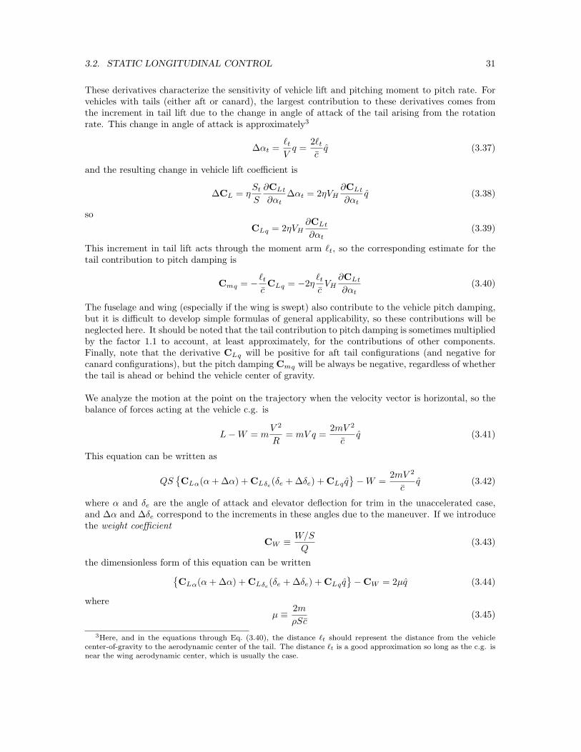
These derivatives characterize the sensitivity of vehicle lift and pitching moment to pitch rate. Forvehicles with tails (either aft or canard), the largest contribution to these derivatives comes fromthe increment in tail lift due to the change in angle of attack of the tail arising from the rotationrate. This change in angle of attack is approximately3
∆αt =ℓt
Vq =
2ℓt
cq (3.37)
and the resulting change in vehicle lift coefficient is
∆CL = ηSt
S
∂CLt
∂αt∆αt = 2ηVH
∂CLt
∂αtq (3.38)
so
CLq = 2ηVH∂CLt
∂αt(3.39)
This increment in tail lift acts through the moment arm ℓt, so the corresponding estimate for thetail contribution to pitch damping is
Cmq = −ℓt
cCLq = −2η
ℓt
cVH
∂CLt
∂αt(3.40)
The fuselage and wing (especially if the wing is swept) also contribute to the vehicle pitch damping,but it is difficult to develop simple formulas of general applicability, so these contributions will beneglected here. It should be noted that the tail contribution to pitch damping is sometimes multipliedby the factor 1.1 to account, at least approximately, for the contributions of other components.Finally, note that the derivative CLq will be positive for aft tail configurations (and negative forcanard configurations), but the pitch damping Cmq will be always be negative, regardless of whetherthe tail is ahead or behind the vehicle center of gravity.
We analyze the motion at the point on the trajectory when the velocity vector is horizontal, so thebalance of forces acting at the vehicle c.g. is
L − W = mV 2
R= mV q =
2mV 2
cq (3.41)
This equation can be written as
QS
CLα(α + ∆α) + CLδe(δe + ∆δe) + CLq q
− W =2mV 2
cq (3.42)
where α and δe are the angle of attack and elevator deflection for trim in the unaccelerated case,and ∆α and ∆δe correspond to the increments in these angles due to the maneuver. If we introducethe weight coefficient
CW ≡ W/S
Q(3.43)
the dimensionless form of this equation can be written
CLα(α + ∆α) + CLδe(δe + ∆δe) + CLq q
− CW = 2µq (3.44)
where
µ ≡ 2m
ρSc(3.45)
3Here, and in the equations through Eq. (3.40), the distance ℓt should represent the distance from the vehiclecenter-of-gravity to the aerodynamic center of the tail. The distance ℓt is a good approximation so long as the c.g. isnear the wing aerodynamic center, which is usually the case.

32 CHAPTER 3. STATIC LONGITUDINAL STABILITY AND CONTROL
is the vehicle relative mass parameter , which depends on ρ, the local fluid (air) density. As a resultof this dependence on air density, the relative mass parameter is a function of flight altitude.
Subtracting the equilibrium values for the unaccelerated case
CLαα + CLδeδe − CW = 0 (3.46)
from Eq. (3.44) gives
CLα∆α + CLδe∆δe =
(
2µ − CLq
)
q (3.47)
Finally, if we introduce the normal acceleration parameter n such that L = nW , then the forcebalance of Eq. (3.41) can be written in the dimensionless form
(n − 1)CW = 2µq (3.48)
which provides a direct relation between the normal acceleration and the pitch rate, so that the liftequilibrium equation can be written
CLα∆α + CLδe∆δe = (n − 1)CW
(
1 − CLq
2µ
)
(3.49)
The pitching moment must also remain zero for equilibrium (since q = 0), so
Cmα∆α + Cmδe∆δe + Cmq q = 0 (3.50)
or
Cmα∆α + Cmδe∆δe = −Cmq
(n − 1)CW
2µ(3.51)
Equations (3.49) and (3.51) provide two equations that can be solved for the unknowns ∆α and ∆δe
to give
∆α =−(n − 1)CW
∆
[(
1 − CLq
2µ
)
Cmδe+
Cmq
2µCLδe
]
∆δe =(n − 1)CW
∆
[(
1 − CLq
2µ
)
Cmα +Cmq
2µCLα
] (3.52)
where
∆ = −CLαCmδe+ CmαCLδe
(3.53)
is the same parameter as earlier (in Eq. (3.28)).
The control position derivative for normal acceleration is therefore given by
dδe
dn=
CW
∆
[(
1 − CLq
2µ
)
Cmα +Cmq
2µCLα
]
(3.54)
Using Eq. (3.20) to express the pitch stiffness in terms of the c.g. location, we have
dδe
dn=
CW
∆
[(
1 − CLq
2µ
)
(xcg
c− xNP
c
)
+Cmq
2µ
]
CLα (3.55)

3.3. CONTROL SURFACE HINGE MOMENTS 33
The c.g. location for which this derivative vanishes is called the basic maneuver point , and itslocation, relative to the basic neutral point, is seen to be given by
xNP
c− xMP
c=
Cmq
2µ
1 − CLq
2µ
≈ Cmq
2µ(3.56)
Since for all configurations the pitch damping Cmq < 0, the maneuver point is aft of the neutralpoint. Also, since the vehicle relative mass parameter µ increases with altitude, the maneuver pointapproaches the neutral point with increasing altitude. If Eq. (3.56) is used to eliminate the variablexNP from Eq. (3.55), we have
dδe
dn= −CW CLα
∆
(
1 − CLq
2µ
)
(xMP
c− xcg
c
)
(3.57)
where(xMP
c− xcg
c
)
(3.58)
is called the maneuver margin.
3.3 Control Surface Hinge Moments
Just as the control position gradient is related to the pitch stiffness of the vehicle when the controlsare fixed, the control force gradients are related to the pitch stiffness of the vehicle when the controlsare allowed to float free.
3.3.1 Control Surface Hinge Moments
Since elevator deflection corresponds to rotation about a hinge line, the forces required to causea specific control deflection are related to the aerodynamic moments about the hinge line. A freecontrol will float, in the static case, to the position at which the elevator hinge moment is zero:
He = 0.
The elevator hinge moment is usually expressed in terms of the hinge moment coefficient
Che =He
QSece(3.59)
where the reference area Se and moment arm ce correspond to the planform area and mean chord ofthe control surface aft of the hinge line. Note that the elevator hinge moment coefficient is definedrelative to Q, not Qt. While it would seem to make more sense to use Qt, hinge moments aresufficiently difficult to predict that they are almost always determined from experiments in whichthe tail efficiency factor is effectively included in the definition of Che (rather than explicitly isolatedin a separate factor).
Assuming that the hinge moment is a linear function of angle of attack, control deflection, etc., wewrite
Che = Che0+ Chαα + Chδe
δe + Chδtδt (3.60)

34 CHAPTER 3. STATIC LONGITUDINAL STABILITY AND CONTROL
V
α
V
eδ(a) (b)
Figure 3.4: Schematic illustration of aerodynamic forces responsible for (a) floating and (b) restoringtendencies of trailing edge control surfaces. Floating (or restoring) tendency represents momentabout hinge line of (shaded) lift distribution acting on control surface per unit angle of attack (orcontrol deflection).
In this equation, α is the angle of attack (from angle for zero vehicle lift), δe is the elevator deflection,and δt is the deflection of the control tab (to be described in greater detail later).
The derivative Chα characterizes the hinge moment created by changes in angle of attack; it iscalled the floating tendency , as the hinge moment generated by an increase in angle of attackgenerally causes the control surface to float upward. The derivative Chδe
characterizes the hingemoment created by a deflection of the control (considered positive trailing edge down); it is calledthe restoring tendency , as the nose-down hinge moment generated by a positive control deflectiontends to restore the control to its original position. The floating tendency in Eq. (3.60) is referredto the vehicle angle of attack, and so it is related to the derivative based on tail angle of attack αt
by
Chα =
(
1 − dǫ
dα
)
Chαt(3.61)
which accounts for the effects of wing induced downwash at the tail. The aerodynamic forcesresponsible for generating the hinge moments reflected in the floating and restoring tendencies aresketched in Fig. 3.4. Only the shaded portion of the lift distribution in these figures acts on thecontrol surface and contributes to the hinge moment.
The angle at which the free elevator floats is determined by the fact that the hinge moment (and,therefore, the hinge moment coefficient) must be zero
Che = 0 = Che0+ Chαα + Chδe
δefree + Chδtδt
or
δefree = − 1
Chδe
(Che0+ Chαα + Chδt
δt) (3.62)
The corresponding lift and moment coefficients are
CLfree = CLαα + CLδeδefree
Cmfree = Cm0 + Cmαα + Cmδeδefree
(3.63)
which, upon substituting from Eq. (3.62), can be written
CLfree = CLα
(
1 − CLδeChα
CLαChδe
)
α − CLδe
Chδe
(Che0+ Chδt
δt)
Cmfree = Cmα
(
1 − CmδeChα
CmαChδe
)
α + Cm0 −Cmδe
Chδe
(Che0+ Chδt
δt)
(3.64)

3.3. CONTROL SURFACE HINGE MOMENTS 35
Thus, if we denote the control free lift curve slope and pitch stiffness using primes, we see from theabove equations that
CL′
α = CLα
(
1 − CLδeChα
CLαChδe
)
Cm′
α = Cmα
(
1 − CmδeChα
CmαChδe
) (3.65)
Inspection of these equations shows that the lift curve slope is always reduced by freeing the controls,and the pitch stiffness of a stable configuration is reduced in magnitude by freeing the controls foran aft tail configuration, and increased in magnitude for a forward tail (canard) configuration (inall cases assuming that the floating and restoring tendencies both are negative).
3.3.2 Control free Neutral Point
The c.g. location at which the control free pitch stiffness vanishes is called the control free neutralpoint . The location of the control free neutral point x′
NP can be determined by expressing the pitchstiffness in the second of Eqs. (3.65)
Cm′
α = Cmα − CmδeChα
Chδe
as
Cm′
α =(xcg
c− xNP
c
)
CLα +ChαCLδe
Chδe
(
ℓt
c+
xac
c− xcg
c
)
=(xcg
c− xNP
c
)
CLα +Chα
Chδe
ηSt
Sae
(
ℓt + xac − xNP
c+
xNP − xcg
c
)
=(xcg
c− xNP
c
)
[
CLα − CLδeChα
Chδe
]
+ ηVHN
Chαae
Chδe
(3.66)
where ae = ∂CLt/∂δe is the elevator effectiveness and
VHN=
(
ℓt
c+
xac
c− xNP
c
)
St
S(3.67)
is the tail volume ratio based on ℓtN, the distance between the tail aerodynamic center and the
basic neutral point, as defined in Eq. (3.30). The quantity in square brackets in the final version ofEq. (3.66) is seen to be simply the control free vehicle lift curve slope CL
′
α, so we have
Cm′
α =(xcg
c− xNP
c
)
CL′
α + ηVHN
Chαae
Chδe
(3.68)
Setting the control free pitch stiffness Cm′
α to zero gives the distance between the control free andbasic neutral points as
xNP
c− x′
NP
c= ηVHN
ae
CL′
α
Chα
Chδe
(3.69)
Finally, if Eq. (3.69) is substituted back into Eq. (3.68) to eliminate the variable xNP , we have
Cm′
α = −(
x′
NP
c− xcg
c
)
CL′
α (3.70)

36 CHAPTER 3. STATIC LONGITUDINAL STABILITY AND CONTROL
Stabilizer
ElevatorTrim tab
Vt
δ
(a) (b)
Figure 3.5: (a) Typical location of trim tab on horizontal control (elevator), and (b) schematicillustration of aerodynamic forces responsible for hinge moment due to trim tab deflection.
showing that the control free pitch stiffness is directly proportional to the control free static margin
(
x′
NP
c− xcg
c
)
3.3.3 Trim Tabs
Trim tabs can be used by the pilot to trim the vehicle at zero control force for any desired speed. Trimtabs are small control surfaces mounted at the trailing edges of primary control surfaces. A linkageis provided that allows the pilot to set the angle of the trim tab, relative to the primary controlsurface, in a way that is independent of the deflection of the primary control surface. Deflection ofthe trim tab creates a hinge moment that causes the elevator to float at the angle desired for trim.The geometry of a typical trim tab arrangement is shown in Fig. 3.5.
Zero control force corresponds to zero hinge moment, or
Che = 0 = Che0+ Chαα + Chδe
δe + Chδtδt
and the trim tab deflection that achieves this for arbitrary angle of attack and control deflection is
δt = − 1
Chδt
(Che0+ Chαα + Chδe
δe) (3.71)
so the tab setting required for zero control force at trim is
δttrim = − 1
Chδt
(Che0+ Chααtrim + Chδe
δetrim) (3.72)
The values of αtrim and δetrim are given by Eqs. (3.27)
αtrim =−CLδe
Cm0 − CmδeCLtrim
∆
δetrim =CLαCm0 + CmαCLtrim
∆
(3.73)

3.3. CONTROL SURFACE HINGE MOMENTS 37
C
c.g. forwardtrimtδ
L trim
Figure 3.6: Variation in trim tab setting as function of velocity for stable, aft tail vehicle.
Substituting these values into Eq. (3.72) gives the required trim tab setting as
δttrim = − 1
Chδt
(
Che0+
Cm0
∆(−ChαCLδe
+ ChδeCLα) +
1
∆(−ChαCmδe
+ ChδeCmα)CLtrim
)
(3.74)Note that the coefficient of CLtrim in this equation – which gives the sensitivity of the trim tabsetting to the trim lift coefficient – can be written as
dδt
dCL= − Chδe
Chδt∆
(
Cmα − ChαCmδe
Chδe
)
= − Chδe
Chδt∆
Cm′
α = − Chδe
Chδt∆
(
x′
NP
c− xcg
c
)
CL′
α (3.75)
and Eq. (3.74) can be written
δttrim = − 1
Chδt
[
Che0+
Cm0
∆(−ChαCLδe
+ ChδeCLα) +
Chδe
∆CL
′
α
(
x′
NP
c− xcg
c
)
CLtrim
]
(3.76)Thus, the tab setting for trim is a linear function of trimmed lift coefficient whose slope is propor-tional to the control free static margin. This variation is shown schematically for a conventional (afttail) configuration in Fig. 3.6.
3.3.4 Control Force for Trim
As mentioned earlier, the most important aspects of stability relating to handling qualities of thevehicle are related to control forces. For longitudinal control, the control force F is related to theelevator hinge moment He through a gearing constant G, so that
F = GHe (3.77)
This equation defines a positive control force as a pull , corresponding to the force required to balancea positive (nose up) elevator hinge moment.4 The units of the gearing constant G are inverse length,which can be interpreted as a mechanical advantage corresponding to radians of control deflectionper unit distance (foot) of control yoke displacement.
4It is important to be careful when reading other books; positive control force is sometimes defined as a push,in which case there is a minus sign inserted on the right hand side of Eq. (3.77) and subsequently throughout theanalysis.

38 CHAPTER 3. STATIC LONGITUDINAL STABILITY AND CONTROL
Expressing the hinge moment in terms of the corresponding dimensionless coefficient, we have
F = GSeceQChe = GSeceQ (Che0+ Chαα + Chδe
δe + Chδtδt) (3.78)
Since this equation is linear in tab deflection, the control force required for a tab setting other thanthe trim value is
F = GSeceQChδt(δt − δttrim) (3.79)
and, substituting the tab setting required for trim from Eq. (3.76), we have
F = GSeceQ
[
Chδtδt + Che0
+Cm0
∆(−ChαCLδe
+ ChδeCLα) +
Chδe
∆CL
′
α
(
xcg − x′
NP
c
)
CLtrim
]
(3.80)Finally, substituting
CLtrim =W/S
Q(3.81)
for level flight with L = W , we have
F =GSece(W/S)Chδe
CL′
α
∆
(
xcg − x′
NP
c
)
+
GSece
[
Chδtδt + Che0
+Cm0
∆(−ChαCLδe
+ ChδeCLα)
]
1
2ρV 2
(3.82)
The dependence of control force on velocity described by this equation is sketched in Fig. 3.7. Notefrom the equation that:
1. The control force F ∝ Sece, i.e, is proportional to the cube of the size of the vehicle; controlforces grow rapidly with aircraft size, and large aircraft require powered (or power-assisted)control systems.
2. The location of the c.g. (i.e., the control free static margin) affects only the constant term inthe equation.
3. The vehicle weight enters only in the ratio W/S.
4. The effect of trim tab deflection δt is to change the coefficient of the V 2 term, and hencecontrols the intercept of the curve with the velocity axis.
If we denote the velocity at which the control force is zero as Vtrim, then Eq. (3.82) gives
GSece
(
Chδtδt + Che0
+Cm0
∆(−ChαCLδe
+ ChδeCLα)
)
1
2ρV 2
trim =
− GSece(W/S)Chδe
CL′
α
∆
(
xcg − x′
NP
c
) (3.83)
so
F = GSece(W/S)Chδe
CL′
α
∆
(
xcg − x′
NP
c
)
[
1 − (V/Vtrim)2]
(3.84)
anddF
dV
)
Vtrim
= − 2
VtrimGSece(W/S)
ChδeCL
′
α
∆
(
xcg − x′
NP
c
)
(3.85)
These last two equations, which also can be interpreted in terms of Fig. 3.7, show that:

3.3. CONTROL SURFACE HINGE MOMENTS 39
V
(pull)F
Increase Vtrim
Decreasestatic
margin
Figure 3.7: Typical variation in control force as function of vehicle velocity for stable configuration.
1. For a given control free static margin (or c.g. position) the control force gradient decreaseswith increasing flight velocity; and
2. At a given trim velocity, the control force gradient decreases as the c.g. is moved aft towardthe control free neutral point (i.e., as the static margin is reduced).
3.3.5 Control-force for Maneuver
Perhaps the single most important stability property of an aircraft, in terms of handling properties,describes the control force required to perform a maneuver. This force must not be too small toavoid over-stressing the airframe, nor too large to avoid making the pilot work too hard.
We will again consider the steady pull-up. The change in control force required to effect the maneuveris
∆F = GSeceQ∆Che (3.86)
where∆Che = Chα∆α + Chδe
∆δe + Chq q (3.87)
where q is the dimensionless pitch rate, as defined in Section 3.2.1. It was also seen in that sectionthat the dimensionless pitch rate for a pull-up could be related directly to the excess load factor(n − 1), so, using Eq. (3.48), we have
∆Che = Chα∆α + Chδe∆δe +
(n − 1)CW
2µChq (3.88)
The derivative Chq arises from the change in hinge moment due to the change in tail angle of attackarising from the pitch rate. Thus
∆Che = Chαt∆αt = Chαt
2ℓt
cq (3.89)
and
Chq ≡ ∂Che
∂q= 2
ℓt
cChαt
(3.90)

40 CHAPTER 3. STATIC LONGITUDINAL STABILITY AND CONTROL
Now, we can use the solution for ∆δe from Eq. (3.52)
∆δe =(n − 1)CW
∆
[(
1 − CLq
2µ
)
Cmα +Cmq
2µCLα
]
(3.91)
along with the lift coefficient equation, Eq. (3.49), which can be written
∆α =1
CLα
[
(n − 1)CW
(
1 − CLq
2µ
)
− CLδe∆δe
]
(3.92)
in the hinge moment equation to give
∆Che = Chα
n − 1
CLα
[(
1 − CLq
2µ
)
CW − CLδe
∆δe
n − 1
]
+ Chδe∆δe +
(n − 1)CW
2µChq (3.93)
which can be rearranged into the form
∆Che
n − 1=
CW
CLα
[(
1 − CLq
2µ
)
Chα +Chq
2µCLα
]
+∆δe
n − 1Chδe
CL′
α
CLα
(3.94)
Finally, using Eq. (3.57) for ∆δe/(n − 1), the equation for the hinge moment increment can bewritten
∆Che
n − 1=
CW CL′
αChδe
∆
(
1 − CLq
2µ
) [
xcg − xMP
c+
∆
CL′
αChδe
(
Chα
CLα
+Chq
2µ − CLq
)]
(3.95)
The control free maneuver point is defined as the c.g. location for which the control force gradient(per g) (or, equivalently, the hinge moment coefficient gradient) vanishes. This is seen from Eq. (3.95)to give
xMP − x′
MP
c=
∆
CL′
αChδe
(
Chα
CLα
+Chq
2µ − CLq
)
(3.96)
Note that this quantity is positive for aft tail configurations, and negative for forward tail (canard)configurations. Substitution of this expression back into Eq. (3.95) then gives
∆Che
n − 1=
CW CL′
αChδe
∆
(
1 − CLq
2µ
)(
xcg − x′
MP
c
)
(3.97)
Finally, the control force gradient (per g) is
∂F
∂n=
∆F
n − 1= GSeceQ
∆Che
n − 1
= GSeceQCW CL
′
αChδe
∆
(
1 − CLq
2µ
)(
xcg − x′
MP
c
) (3.98)
or, since QCW = W/S,
∂F
∂n= GSece(W/S)
CL′
αChδe
∆
(
1 − CLq
2µ
)(
xcg − x′
MP
c
)
(3.99)
The distancex′
MP −xcg
c , seen from the above equation to be directly related to the sensitivity ofnormal acceleration of the vehicle to control force, is called the control free maneuver margin.
Note that the control force gradient (per g) is

3.4. FORWARD AND AFT LIMITS OF C.G. POSITION 41
xx’
Upper limit (maneuverability)
Lower limit (stability)
Allowable rangedF/dn
MP cg
Figure 3.8: Allowable c.g. travel as imposed by limits on control force gradient (per g).
1. Directly proportional to the vehicle wing loading W/S;
2. Directly proportional to the cube of the linear size of the vehicle;
3. Directly proportional to the (control free) maneuver margin (x′
MP − xcg)/c; and
4. Independent of airspeed.
The control force gradient should be neither too small nor too large. If the gradient is too small,the vehicle will be overly sensitive to small control inputs and it will be too easy for the pilot toover stress the airframe. At the same time, the control forces required for normal maneuvers mustnot be larger than the pilot can supply (or so large that the pilot becomes unduly tired performingnormal maneuvers). The lower and upper limits on control force gradient (per g) determine allowablerearward and forward limits on c.g. travel, as sketched in Fig. 3.8. The values of these limits willdepend on the vehicle mission; in general the limits will be higher for transport aircraft, and lowerfor vehicles which require greater maneuverability (such as military fighters or aerobatic aircraft).
3.4 Forward and Aft Limits of C.G. Position
The various control position and force gradients impose limits on the acceptable range of travel ofthe vehicle center of gravity. These include (for most vehicles):
• Rearward limits:
1. The vehicle must be statically stable; i.e., the c.g. must be ahead of the basic and controlfree neutral points.
2. The sensitivity of vehicle velocity to control position must not be too small; i.e., the c.g.must be sufficiently far ahead of the basic neutral point.
3. The sensitivity of vehicle normal acceleration to control force must not be too small; i.e.,the c.g. must be sufficiently far ahead of the control free neutral point.
• Forward limits:

42 CHAPTER 3. STATIC LONGITUDINAL STABILITY AND CONTROL
1. The vehicle must be trimmable at CLmax; i.e., the c.g. must not be so far forward thatthere is insufficient elevator power to trim the vehicle at maximum lift coefficient.
2. The sensitivity of vehicle normal acceleration to control force must not be too high; i.e.,the c.g. must not be so far forward that excessive control force is required to performmaneuvers for which the vehicle is intended.

Bibliography
[1] Robert C. Nelson, Aircraft Stability and Automatic Control, McGraw-Hill, Second edi-tion, 1998.
43

44 BIBLIOGRAPHY
Chapter 4
Dynamical Equations for FlightVehicles
These notes provide a systematic background of the derivation of the equations of motionfor a flight vehicle, and their linearization. The relationship between dimensional stabilityderivatives and dimensionless aerodynamic coefficients is presented, and the principalcontributions to all important stability derivatives for flight vehicles having left/rightsymmetry are explained.
4.1 Basic Equations of Motion
The equations of motion for a flight vehicle usually are written in a body-fixed coordinate system.It is convenient to choose the vehicle center of mass as the origin for this system, and the orientationof the (right-handed) system of coordinate axes is chosen by convention so that, as illustrated inFig. 4.1:
• the x-axis lies in the symmetry plane of the vehicle1and points forward;
• the z-axis lies in the symmetry plane of the vehicle, is perpendicular to the x-axis, and pointsdown;
• the y-axis is perpendicular to the symmetry plane of the vehicle and points out the right wing.
The precise orientation of the x-axis depends on the application; the two most common choices are:
• to choose the orientation of the x-axis so that the product of inertia
Ixz =
∫
m
xz dm = 0
1Almost all flight vehicles have bi-lateral (or, left/right) symmetry, and most flight dynamics analyses take advan-tage of this symmetry.
45

46 CHAPTER 4. DYNAMICAL EQUATIONS FOR FLIGHT VEHICLES
The other products of inertia, Ixy and Iyz, are automatically zero by vehicle symmetry. Whenall products of inertia are equal to zero, the axes are said to be principal axes.
• to choose the orientation of the x-axis so that it is parallel to the velocity vector for an initialequilibrium state. Such axes are called stability axes.
The choice of principal axes simplifies the moment equations, and requires determination of only oneset of moments of inertia for the vehicle – at the cost of complicating the X- and Z-force equationsbecause the axes will not, in general, be aligned with the lift and drag forces in the equilibrium state.The choice of stability axes ensures that the lift and drag forces in the equilibrium state are alignedwith the z and x axes, at the cost of additional complexity in the moment equations and the needto re-evaluate the inertial properties of the vehicle (Ix, Iz, and Ixz) for each new equilibrium state.
4.1.1 Force Equations
The equations of motion for the vehicle can be developed by writing Newton’s second law for eachdifferential element of mass in the vehicle,
d~F = ~a dm (4.1)
then integrating over the entire vehicle. When working out the acceleration of each mass element, wemust take into account the contributions to its velocity from both linear velocities (u, v, w) in each of
the coordinate directions as well as the ~Ω × ~r contributions due to the rotation rates (p, q, r) aboutthe axes. Thus, the time rates of change of the coordinates in an inertial frame instantaneouslycoincident with the body axes are
x = u + qz − ry
y = v + rx − pz
z = w + py − qx
(4.2)
x
z
y
Figure 4.1: Body axis system with origin at center of gravity of a flight vehicle. The x-z plane liesin vehicle symmetry plane, and y-axis points out right wing.

4.1. BASIC EQUATIONS OF MOTION 47
and the corresponding accelerations are given by
x =d
dt(u + qz − ry)
y =d
dt(v + rx − pz)
z =d
dt(w + py − qx)
(4.3)
or
x = u + qz + q(w + py − qx) − ry − r(v + rx − pz)
y = v + rx + r(u + qz − ry) − pz − p(w + py − qx)
z = w + py + p(v + rx − pz) − qx − q(u + qz − ry)
(4.4)
Thus, the net product of mass times acceleration for the entire vehicle is
m~a =
∫
m
[u + qz + q(w + py − qx) − ry − r(v + rx − pz)] ı+
[v + rx + r(u + qz − ry) − pz − p(w + py − qx)] +
[w + py + p(v + rx − pz) − qx − q(u + qz − ry)] k
dm
(4.5)
Now, the velocities and accelerations, both linear and angular, are constant during the integrationover the vehicle coordinates, so the individual terms in Eq. (4.5) consist of integrals of the form
∫
m
dm = m
which integrates to the vehicle mass m, and∫
m
xdm =
∫
m
y dm =
∫
m
z dm = 0, (4.6)
which are all identically zero since the origin of the coordinate system is at the vehicle center ofmass. Thus, Eq. (4.5) simplifies to
m~a = m[
(u + qw − rv) ı + (v + ru − pw) + (w + pv − qu) k]
(4.7)
To write the equation corresponding to Newton’s Second Law, we simply need to set Eq. (4.7) equalto the net external force acting on the vehicle. This force is the sum of the aerodynamic (includingpropulsive) forces and those due to gravity.
In order to express the gravitational force acting on the vehicle in the body axis system, we needto characterize the orientation of the body axis system with respect to the gravity vector. Thisorientation can be specified using the Euler angles of the body axis system with respect to aninertial system (xf , yf , zf ), where the inertial system is oriented such that
• the zf axis points down (i.e., is parallel to the gravity vector ~g);
• the xf axis points North; and
• the yf axis completes the right-handed system and, therefore, points East.

48 CHAPTER 4. DYNAMICAL EQUATIONS FOR FLIGHT VEHICLES
x
x
y
1
f
z , zf 1
f
ψ ψy1 x1
y1
θ
θ
x
zz
2
1
2
, y2
x
z
2
φ
φ
, x
2
z
y
y2
(a) (b) (c)
Figure 4.2: The Euler angles Ψ, Θ, and Φ determine the orientation of the body axes of a flightvehicle. (a) Yaw rotation about z-axis, nose right; (b) Pitch rotation about y-axis, nose up; (c) Rollrotation about x-axis, right wing down.
The orientation of the body axis system is specified by starting with the inertial system, then, inthe following order performing:
1. a positive rotation about the zf axis through the heading angle Ψ to produce the (x1, y1, z1)system; then
2. a positive rotation about the y1 axis through the pitch angle Θ to produce the (x2, y2, z2)system; and, finally
3. a positive rotation about the x2 axis through the bank angle Φ to produce the (x, y, z) system.
Thus, if we imagine the vehicle oriented initially with its z-axis pointing down and heading North,its final orientation is achieved by rotating through the heading angle Ψ, then pitching up throughangle Θ, then rolling through angle Φ. This sequence of rotations in sketched in Fig. 4.2.
Since we are interested only in the orientation of the gravity vector in the body axis system, we canignore the first rotation.2Thus, we need consider only the second rotation, in which the componentsof any vector transform as
x2
y2
z2
=
cos Θ 0 − sin Θ0 1 0
sin Θ 0 cos Θ
xf
yf
zf
(4.8)
and the third rotation, in which the components transform as
xyz
=
1 0 00 cos Φ sinΦ0 − sin Φ cos Φ
x2
y2
z2
(4.9)
2If we are interested in determining where the vehicle is going – say, we are planning a flight path to get us fromNew York to London, we certainly are interested in the heading, but this is not really an issue as far as analysis ofthe stability and controllability of the vehicle are concerned.
4.1. BASIC EQUATIONS OF MOTION 49
Thus, the rotation matrix from the inertial frame to the body fixed system is seen to be
xyz
=
1 0 00 cos Φ sinΦ0 − sin Φ cos Φ
cos Θ 0 − sin Θ0 1 0
sinΘ 0 cos Θ
xf
yf
zf
=
cos Θ 0 − sin ΘsinΘ sin Φ cos Φ cos Θ sin Φsin Θ cos Φ − sin Φ cos Θ cos Φ
xf
yf
zf
(4.10)
The components of the gravitational acceleration in the body-fixed system are, therefore,
gx
gy
gz
=
cos Θ 0 − sin ΘsinΘ sin Φ cos Φ cos Θ sin Φsin Θ cos Φ − sin Φ cos Θ cos Φ
00g0
= g0
− sin Θcos Θ sin Φcos Θ cos Φ
(4.11)
The force equations can thus be written as
XYZ
+ mg0
− sin Θcos Θ sin Φcos Θ cos Φ
= m
u + qw − rvv + ru − pww + pv − qu
(4.12)
where (X,Y,Z) are the components of the net aerodynamic and propulsive forces acting on thevehicle, which will be characterized in subsequent sections.
4.1.2 Moment Equations
The vector form of the equation relating the net torque to the rate of change of angular momentumis
~G =
LMN
=
∫
m
(~r × ~a) dm (4.13)
where (L,M,N) are the components about the (x, y, z) body axes, respectively, of the net aerody-namic and propulsive moments acting on the vehicle. Note that there is no net moment due to thegravitational forces, since the origin of the body-axis system has been chosen at the center of massof the vehicle. The components of Eq.(4.13) can be written as
L =
∫
m
(yz − zy) dm
M =
∫
m
(zx − xz) dm
N =
∫
m
(xy − yx) dm
(4.14)
where x, y, and z are the net accelerations in an inertial system instantaneously coincident with thebody axis system, as given in Eqs. (4.4).
When Eqs. (4.4) are substituted into Eqs. (4.14), the terms in the resulting integrals are eitherlinear or quadratic in the coordinates. Since the origin of the body-axis system is at the vehicle c.g.,
50 CHAPTER 4. DYNAMICAL EQUATIONS FOR FLIGHT VEHICLES
Eqs. (4.6) apply and the linear terms integrate to zero. The quadratic terms can be expressed interms of the moments of inertia
Ix =
∫
m
(
y2 + z2)
dm
Iy =
∫
m
(
z2 + x2)
dm
Iz =
∫
m
(
x2 + y2)
dm
(4.15)
and the product of inertia
Ixz =
∫
m
xz dm (4.16)
Note that the products of inertia Ixy = Iyz = 0, since the y-axis is perpendicular to the assumedplane of symmetry of the vehicle.
Equations (4.14) can then be written as
L = Ixp + (Iz − Iy) qr − Ixz (pq + r)
M = Iy q + (Ix − Iz) rp − Ixz
(
p2 − r2)
N = Iz r + (Iy − Ix) pq − Ixz (qr − p)(4.17)
Note that if principal axes are used, so that Ixz ≡ 0, Eqs. (4.17) simplify to
L = Ixp + (Iz − Iy) qr
M = Iy q + (Ix − Iz) rp
N = Iz r + (Iy − Ix) pq(4.18)
4.2 Linearized Equations of Motion
The equations developed in the preceding section completely describe the motion of a flight vehicle,subject to the prescribed aerodynamic (and propulsive) forces and moments. These equations arenonlinear and coupled , however, and generally can be solved only numerically, yielding relatively lit-tle insight into the dependence of the stability and controllability of the vehicle on basic aerodynamicparameters of the vehicle.
A great deal, however, can be learned by studying linear approximations to these equations. Inthis approach, we analyze the solutions to the equations describing small perturbations about anequilibrium flight condition. The greatest simplification of the equations arises when the equilibriumcondition is chosen to correspond to a longitudinal equilibrium, in which the velocity and gravityvectors lie in the plane of symmetry of the vehicle; the most common choice corresponds to unaccel-erated flight – i.e., to level, unaccelerated flight, or to steady climbing (or descending) flight. Sucha linear analysis has been remarkably successful in flight dynamics applications,3primarily because:
3This statement should be interpreted in the context of the difficulty of applying similar linear analyses to othersituations – e.g., to road vehicle dynamics, in which the stability derivatives associated with tire forces are notoriouslynonlinear.

4.2. LINEARIZED EQUATIONS OF MOTION 51
1. Over a fairly broad range of flight conditions of practical importance, the aerodynamic forcesand moments are well-approximated as linear functions of the state variables; and
2. Normal flight situations correspond to relatively small variations in the state variables; in fact,relatively small disturbances in the state variables can lead to significant accelerations, i.e., toflight of considerable violence, which we normally want to avoid.
Finally, we should emphasize the caveat that these linear analyses are not good approximations insome cases – particularly for spinning or post-stall flight situations.
Thus, we will consider
1. Perturbations from a longitudinal trim condition;
2. Using stability axes;
so we can describe the state variables as
u = u0+ u(t), p = p(t)
v = v(t), q = q(t)
w = w(t), r = r(t)
θ = Θ0+ θ(t), Φ= φ(t) (4.19)
Variables with the subscript 0 correspond to the original equilibrium (trim) state. Note that onlythe axial velocity u and pitch angle θ have non-zero equilibrium values. The trim values of alllateral/directional variables (v, p, r, and Φ) are zero because the initial trim condition correspondsto longitudinal equilibrium; the equilibrium value of w is zero because we are using stability axes;and the equilibrium pitch rate q is assumed zero as we are restricting the equilibrium state to haveno normal acceleration.
The equations for the unperturbed initial equilibrium state then reduce to
X0 − mg0 sinΘ0 = 0
Z0 + mg0 cos Θ0 = 0
M0 = L0 = Y0 = N0 = 0
(4.20)
and we want to solve linear approximations to the equations
X0 + ∆X − mg0 sin (Θ0 + θ) = m (u + qw − rv)
Y0 + ∆Y + mg0 cos (Θ0 + θ) sin φ = m (v + r(u0 + u) − pw)
Z0 + ∆Z + mg0 cos (Θ0 + θ) cos φ = m (w + pv − q(u0 + u))
(4.21)
and
∆L = Ixp + (Iz − Iy) qr − Ixz (pq + r)
∆M = Iy q + (Ix − Iz) rp + Ixz
(
p2 − r2)
∆N = Iz r + (Iy − Ix) pq + Ixz (qr − p)
(4.22)
Since we assume that all perturbation quantities are small, we can approximate
sin (Θ0 + θ) ≈ sinΘ0 + θ cos Θ0
cos (Θ0 + θ) ≈ cos Θ0 − θ sinΘ0
(4.23)

52 CHAPTER 4. DYNAMICAL EQUATIONS FOR FLIGHT VEHICLES
and
sin Φ = sin φ ≈ φ
cos Φ = cos φ ≈ 1(4.24)
Thus, after making these approximations, subtracting the equilibrium equations, and neglectingterms that are quadratic in the small perturbations, the force equations can be written
∆X − mg0 cos Θ0θ = mu
∆Y + mg0 cos Θ0φ = m (v + u0r)
∆Z − mg0 sin Θ0θ = m (w − u0q)
(4.25)
and the moment equations can be written
∆L = Ixp − Ixz r
∆M = Iy q
∆N = Iz r − Ixz p
(4.26)
4.3 Representation of Aerodynamic Forces and Moments
The perturbations in aerodynamic forces and moments are functions of both, the perturbations instate variables and control inputs. The most important dependencies can be represented as follows.The dependencies in the equations describing the longitudinal state variables can be written
∆X =∂X
∂uu +
∂X
∂ww +
∂X
∂δeδe +
∂X
∂δTδT
∆Z =∂Z
∂uu +
∂Z
∂ww +
∂Z
∂ww +
∂Z
∂qq +
∂Z
∂δeδe +
∂Z
∂δTδT
∆M =∂M
∂uu +
∂M
∂ww +
∂M
∂ww +
∂M
∂qq +
∂M
∂δeδe +
∂M
∂δTδT
(4.27)
In these equations, the control variables δe and δT correspond to perturbations from trim in theelevator and thrust (throttle) settings. Note that the Z force and pitching moment M are assumedto depend on both the rate of change of angle of attack w and the pitch rate q, but the dependenceof the X force on these variables is neglected.
Also, the dependencies in the equations describing the lateral/directional state variables can bewritten
∆Y =∂Y
∂vv +
∂Y
∂pp +
∂Y
∂rr +
∂Y
∂δrδr
∆L =∂L
∂vv +
∂L
∂pp +
∂L
∂rr +
∂L
∂δrδr +
∂L
∂δaδa
∆N =∂N
∂vv +
∂N
∂pp +
∂N
∂rr +
∂N
∂δrδr +
∂N
∂δaδa
(4.28)
In these equations, the variables δr and δa represent the perturbations from trim in the rudder andaileron control settings.

4.3. REPRESENTATION OF AERODYNAMIC FORCES AND MOMENTS 53
Note that the representations in Eqs. (4.27) and (4.28) are completely decoupled. That is, theperturbations in longitudinal forces and moments (∆X, ∆Z, and ∆M) depend neither on thelateral/directional perturbations (v, p, and r) nor the lateral/directional control inputs (δr and δa);And the perturbations in lateral/directional forces and moments (∆Y , ∆L, and ∆N) depend neitheron the longitudinal perturbations (u, w, w, and q) nor the longitudinal control inputs (δe and δT ).This is a good approximation for vehicles with left/right symmetry. This decoupling is exact forthe dependence of the lateral/directional forces and moments on the longitudinal state variables,since a change in a longitudinal variable, say angle of attack, cannot produce a change in the sideforce, rolling moment, or yawing moment, for a perfectly symmetric vehicle. The decoupling is onlyapproximate for the dependence of the longitudinal forces and moments on the lateral/directionalstate variables, since a change in a lateral/directional variable, say roll rate, produces no changein axial or vertical force or pitching moment only to within first order for a symmetric vehicle.Consider, for example, the change in lift force due to roll rate. The increased lift on the down-goingwing is canceled by the decreased lift on the upgoing wing only to within the linear approximation.
The final form of the dimensional small-perturbation equations is developed by defining the stabilityderivatives corresponding to force perturbations by dividing them by the vehicle mass, and bydefining the stability derivatives corresponding to moment perturbations by dividing them by thecorresponding moments of inertia of the vehicle. Thus, we define
Xu ≡ 1
m
∂X
∂u, Xw ≡ 1
m
∂X
∂w, . . . XδT
≡ 1
m
∂X
∂δT;
Yv ≡ 1
m
∂Y
∂v, Yp ≡ 1
m
∂Y
∂p, . . . Yδr
≡ 1
m
∂Y
∂δr;
Zu ≡ 1
m
∂Z
∂u, Zw ≡ 1
m
∂Z
∂w, . . . ZδT
≡ 1
m
∂Z
∂δT;
(4.29)
and
Lv ≡ 1
Ix
∂L
∂v, Lp ≡ 1
Ix
∂L
∂p, . . . Lδa
≡ 1
Ix
∂L
∂δa;
Mu ≡ 1
Iy
∂M
∂u, Mw ≡ 1
Iy
∂M
∂w, . . . MδT
≡ 1
Iy
∂M
∂δT;
Nv ≡ 1
Iz
∂N
∂v, Np ≡ 1
Iz
∂N
∂p, . . . Nδa
≡ 1
Iz
∂N
∂δa.
(4.30)
It is important to emphasize that the quantities defined by these equations are not to be interpretedsimply as (the usual mathematical notation for) partial derivatives but, rather, are the expectedpartial derivatives divided by the vehicle mass or appropriate moment of inertia.
When these definitions are substituted back into Eqs. (4.27) and (4.28), and these representationsare then used in Eqs. (4.25) and (4.26), we arrive at the small-disturbance equations for longitudinalmotions:
[
d
dt− Xu
]
u + g0 cos Θ0θ − Xww = Xδeδe + XδT
δT
−Zuu +
[
(1 − Zw)d
dt− Zw
]
w − [u0 + Zq] q + g0 sin Θ0θ = Zδeδe + ZδT
δT
−Muu −[
Mwd
dt+ Mw
]
w +
[
d
dt− Mq
]
q = Mδeδe + MδT
δT
(4.31)

54 CHAPTER 4. DYNAMICAL EQUATIONS FOR FLIGHT VEHICLES
and the small-disturbance equations for lateral/directional motions:[
d
dt− Yv
]
v − Ypp + [u0 − Yr] r − g0 cos Θ0φ = Yδrδr
−Lvv +
[
d
dt− Lp
]
p −[
Ixz
Ix
d
dt+ Lr
]
r = Lδrδr + Lδa
δa
−Nvv −[
Ixz
Iz
d
dt+ Np
]
p +
[
d
dt− Nr
]
r = Nδrδr + Nδa
δa
(4.32)
4.3.1 Longitudinal Stability Derivatives
In order to solve the equations describing longitudinal vehicle motions, we need to be able to evaluateall the coefficients appearing in Eqs. (4.31). This means we need to be able to provide estimates forthe derivatives of X, Z, and M with respect to the relevant independent variables u, w, w, and q.These stability derivatives usually are expressed in terms of dimensionless aerodynamic coefficientderivatives. For example, we can express the stability derivative Xu as
Xu ≡ 1
m
∂X
∂u=
1
m
∂
∂u[QSCX ] =
QS
mu0[2CX0 + CXu] (4.33)
where
CXu ≡ ∂CX
∂(u/u0)(4.34)
is the derivative of the dimensionless X-force coefficient with respect to the dimensionless velocityu/u0. Note that the first term in the final expression of Eq. (4.33) arises because the dynamicpressure Q is, itself, a function of the flight velocity u0 + u. Similar expressions can be developedfor all the required derivatives.
Derivatives with respect to vertical velocity perturbations w are related to aerodynamic derivativeswith respect to angle of attack α, since
α = tan−1(w
u
)
≈ w
u0(4.35)
Then, for example
Zw ≡ 1
m
∂Z
∂w=
1
m
∂
∂(u0α)[QSCZ ] =
QS
mu0CZα (4.36)
Derivatives with respect to pitch rate q are related to aerodynamic derivatives with respect todimensionless pitch rate q ≡ cq
2u0. Thus, for example
Mq ≡ 1
Iy
∂M
∂q=
1
Iy
∂
∂(
2u0qc
) [QScCm] =QSc2
2Iyu0Cmq (4.37)
where
Cmq ≡ ∂Cm
∂q(4.38)
is the derivative of the dimensionless pitching moment coefficient with respect to the dimensionlesspitch rate q. In a similar way, dimensionless derivatives with respect to rate of change of angle ofattack α are expressed in terms of the dimensionless rate of change ˆα = cα
2u0.

4.3. REPRESENTATION OF AERODYNAMIC FORCES AND MOMENTS 55
Variable X Z M
u Xu = QSmu0
[2CX0 + CXu] Zu = QSmu0
[2CZ0 + CZu] Mu = QScIyu0
Cmu
w Xw = QSmu0
CXα Zw = QSmu0
CZα Mw = QScIyu0
Cmα
w Xw = 0 Zw = QSc2mu2
0
CZα Mw = QSc2
2Iyu20
Cmα
q Xq = 0 Zq = QSc2mu0
CZq Mq = QSc2
2Iyu0Cmq
Table 4.1: Relation of dimensional stability derivatives for longitudinal motions to dimensionlessderivatives of aerodynamic coefficients.
Expressions for all the dimensional stability derivatives appearing in Eqs. (4.31) in terms of thedimensionless aerodynamic coefficient derivatives are summarized in Table 4.1.
Aerodynamic Derivatives
In this section we relate the dimensionless derivatives of the preceding section to the usual aerody-namic derivatives, and provide simple formulas for estimating them. It is natural to express the axialand normal force coefficients in terms of the lift and drag coefficients, but we must take into accountthe fact that perturbations in angle of attack will rotate the lift and drag vectors with respect to thebody axes. Here, consistent with Eq. (4.35), we define the angle of attack as the angle between theinstantaneous vehicle velocity vector and the x-axis, and also assume that the propulsive thrust isaligned with the x-axis. Thus, as seen in Fig. 4.3, we have to within terms linear in angle of attack
CX = CT − CD cos α + CL sin α ≈ CT − CD + CLα
CZ = −CD sin α − CL cos α ≈ −CDα − CL
(4.39)
Here the thrust coefficient
CT ≡ T
QS(4.40)
where T is the net propulsive thrust, assumed to be aligned with the x-axis of the body-fixed system.Since all the dimensionless coefficients in Eqs. (4.39) are normalized by the same quantity QS, therepresentations of forces and force coefficients are equivalent.
Speed Derivatives
We first consider the derivatives with respect to vehicle speed u. The derivative
CXu = CT u − CDu (4.41)
represents the speed damping , and
CDu = M∂CD
∂M(4.42)

56 CHAPTER 4. DYNAMICAL EQUATIONS FOR FLIGHT VEHICLES
x
z
V
uw
θα
Θ0V0
L
D
T
Figure 4.3: Orientation of body axes with respect to instantaneous and equilibrium vehicle velocity,illustrating relation between force components in body axes and lift, drag, and thrust forces. Theangle of attack α denotes the angle between the x-axis and the instantaneous velocity vector V , whilethe perturbation in pitch angle θ denotes the angle between the x-axis and the equilibrium velocityvector V0. Lift and drag act perpendicular to, and anti-parallel to, the instantaneous velocity, whilethrust is assumed to act parallel to the x-axis.
represents the contribution of compressibility effects to this derivative.
The contribution of the derivative CT u must be estimated separately for the special cases of constantthrust (appropriate for jet-powered aircraft or for a power-off glide), or constant power (appropriatefor piston-powered aircraft with constant-speed propellers). For the constant thrust case,
CT u =∂
∂(u/u0)
(
T
QS
)
= −2CT 0 (4.43)
And for the constant power case,
CT u =∂
∂(u/u0)
(
P
QSu
)
= −3CT 0 (4.44)
The equilibrium force equations shown in Eqs. (4.20) can be combined to express the equilibriumthrust coefficient as
CT 0 = CD0 + CL0 tan Θ0 (4.45)
which then gives
CXu =
−2CD0 − 2CL0 tan Θ0 − MCDM for constant thrust
−3CD0 − 3CL0 tan Θ0 − MCDM for constant power(4.46)
And, when these expressions are substituted into the equation for the dimensional stability derivativefrom the preceding section, we have
Xu =
− QSmu0
[2CD0 + MCDM] for constant thrust
− QSmu0
[3CD0 + CL0 tan Θ0 + MCDM] for constant power(4.47)
The derivative of the normal force coefficient CZ with respect to vehicle speed u is simply
CZu = −CLu (4.48)

4.3. REPRESENTATION OF AERODYNAMIC FORCES AND MOMENTS 57
since the drag coefficient contribution vanishes when evaluated at the initial trim condition, whereα = 0. The dependence of lift coefficient on speed arises due to compressibility and aeroelasticeffects. We will neglect aeroelastic effects, but the effect of compressibility can be characterized as
CLu = M∂CL
∂M(4.49)
where M is the flight Mach number. The Prandtl-Glauert similarity law for subsonic flow gives
CL =CL|M=0√1 − M2
(4.50)
which can be used to show that∂CL
∂M=
M
1 − M2CL0 (4.51)
whence
CZu = − M2
1 − M2CL0 (4.52)
Use of the corresponding form of the Prandtl-Glauert rule for supersonic flow results in exactly thesame formula. We then have for the dimensional stability derivative
Zu = − QS
mu0
[
2CL0 +M2
1 − M2CL0
]
(4.53)
Finally, the change in pitching moment coefficient Cm with speed u is generally due to effects ofcompressibility and aeroelastic deformation. The latter will again be neglected, so we have only thecompressibility effect, which can be represented as
Cmu = M∂Cm
∂M(4.54)
so we have
Mu =QSc
Iyu0MCmM (4.55)
Angle-of-Attack Derivatives
As mentioned earlier, the derivatives with respect to vertical velocity w are expressed in terms ofderivatives with respect to angle of attack α. Since from Eq. (4.39) we have
CX = CT − CD + CLα (4.56)
we haveCXα = CT α − CDα + CLαα + CL = −CDα + CL0 (4.57)
since we assume the propulsive thrust is independent of the angle of attack, i.e., CT α = 0. Usingthe parabolic approximation for the drag polar
CD = CDp +CL
2
πeAR(4.58)
we have
CDα =2CL
πeARCLα (4.59)

58 CHAPTER 4. DYNAMICAL EQUATIONS FOR FLIGHT VEHICLES
and
Xw =QS
mu0
(
CL0 −2CL0
πeARCLα
)
(4.60)
Similarly, for the z-force coefficient Eq. (4.39) gives
CZ = −CDα − CL (4.61)
whence
CZα = −CD0 − CLα (4.62)
so
Zw = − QS
mu0(CD0 + CLα) (4.63)
Finally, the dimensional derivative of pitching moment with respect to vertical velocity w is givenby
Mw =QSc
Iyu0Cmα (4.64)
Pitch-rate Derivatives
The pitch rate derivatives have already been discussed in our review of static longitudinal stability.As seen there, the principal contribution to pitch damping Cmq is from the horizontal tail and isgiven by
Cmq = −2ηℓt
cVHat (4.65)
Also,
CLq = 2ηVHat (4.66)
so
CZq = −CLq = −2ηVHat (4.67)
The derivative CXq is usually assumed to be negligibly small. In practice, the value given abovefor Cmq is often multiplied by a factor of 1.1 to account for contributions of other components,particularly the wing.
Angle-of-attack Rate Derivatives
The derivatives with respect to rate of change of angle of attack α arise primarily from the timelag associated with wing downwash affecting the horizontal tail. This affects the lift force on thehorizontal tail and the corresponding pitching moment; the effect on vehicle drag usually is neglected.
The wing downwash is associated with the vorticity trailing behind the wing and, since vorticity isconvected with the local fluid velocity, the time lag for vorticity to convect from the wing to the tailis approximately
∆t =ℓt
u0

4.3. REPRESENTATION OF AERODYNAMIC FORCES AND MOMENTS 59
The instantaneous angle of attack seen by the horizontal tail is therefore
αt = α + it − ε = α + it −[
ε0 +dε
dα(α − α∆t)
]
(4.68)
sodαt
dα=
dε
dα∆t =
ℓt
u0
dε
dα(4.69)
The rate of change of tail lift with α is then seen to be
dLt
dα= QtStat
ℓt
u0
dε
dα= ηQStat
ℓt
u0
dε
dα(4.70)
so the change in normal force coefficient with respect to dimensionless α is
CZα ≡ ∂CZ
∂ cα2u0
= −2ηVHatdε
dα(4.71)
The corresponding change in pitching moment is
dMcg
dα= −ℓt
dLt
dα= −ηQStat
ℓ2tu0
dε
dα(4.72)
so the change in pitching moment coefficient with respect to dimensionless α is
Cmα ≡ ∂Cm
∂ cα2u0
= −2ηℓt
cVHat
dε
dα=
ℓt
cCZα (4.73)
4.3.2 Lateral/Directional Stability Derivatives
In order to solve the equations describing lateral/directional vehicle motions, we need to be ableto evaluate all the coefficients appearing in Eqs. (4.32). This means we need to be able to provideestimates for the derivatives of Y , L, and N with respect to the relevant independent variables v,p, and r. As for the longitudinal case, these stability derivatives usually are expressed in terms ofdimensionless aerodynamic coefficient derivatives.
Derivatives with respect to lateral velocity perturbations v are related to aerodynamic derivativeswith respect to angle of sideslip β, since
β = tan−1( v
V
)
≈ v
u0(4.74)
For example, we can express the stability derivative Yv as
Yv ≡ 1
m
∂Y
∂(u0β)=
1
mu0
∂
∂β[QSCy] =
QS
mu0Cyβ (4.75)
where
Cyβ ≡ ∂Cy
∂β(4.76)
is the derivative of the dimensionless Y -force coefficient with respect to the sideslip angle β = v/u0.Similar expressions can be developed for all the required derivatives.

60 CHAPTER 4. DYNAMICAL EQUATIONS FOR FLIGHT VEHICLES
Variable Y L N
v Yv = QSmu0
Cyβ Lv = QSbIxu0
Clβ Nv = QSbIzu0
Cnβ
p Yp = QSb2mu0
Cyp Lp = QSb2
2Ixu0Clp Np = QSb2
2Izu0Cnp
r Yr = QSb2mu0
Cyr Lr = QSb2
2Ixu0Clr Nr = QSb2
2Izu0Cnr
Table 4.2: Relation of dimensional stability derivatives for lateral/directional motions to dimension-less derivatives of aerodynamic coefficients.
Derivatives with respect to roll rate p and yaw rate r are related to aerodynamic derivatives withrespect to the corresponding dimensionless rate, either p ≡ pb
2u0, or r ≡ rb
2u0. Thus, for example, the
roll damping derivative
Lp ≡ 1
Ix
∂L
∂p=
1
Ix
∂
∂(
2u0pb
) [QSbCl] =QSb2
2Ixu0Clp (4.77)
where
Clp ≡ ∂Cl
∂p(4.78)
is the derivative of the dimensionless rolling moment coefficient with respect to the dimensionlessroll rate p.4
Expressions for all the dimensional stability derivatives appearing in Eqs. (4.32) in terms of thedimensionless aerodynamic coefficient derivatives are summarized in Table 4.2.
Sideslip Derivatives
Here we develop approximate expressions for the derivatives of side force and rolling and yawingmoments due to sideslip. The side force derivative Cyβ is dominated by the contribution of thevertical tail. This side force, acting through a horizontal moment arm to the vehicle c.g. is theprincipal stabilizing factor for weathercock stability Cnβ ; the fuselage contribution to weathercockis destabilizing (and is similar to its destabilizing contribution to pitch stiffness). The side force onthe vertical tail, acting through a vertical moment arm to the vehicle c.g. also contributes to thedihedral effect Clβ . Wing geometric dihedral and sweep, as well as wing fuselage interference alsomake important contributions to the dihedral effect. The balance of dihedral effect and weathercockstability plays an important role in the lateral/directional dynamics.
The side force due to sideslip is due primarily to the side force (or “lift”) produced by the verticaltail, which can be expressed as
Yv = −QvSv∂CLv
∂αvαv (4.79)
4Note that the lateral and directional rates are nondimensionalized using the time scale b/(2u0) – i.e., the span di-mension is used instead of the mean aerodynamic chord which appears in the corresponding quantities for longitudinalmotions.

4.3. REPRESENTATION OF AERODYNAMIC FORCES AND MOMENTS 61
where the minus sign is required because we define the angle of attack as
αv = β + σ (4.80)
where positive β = sin−1(v/V ) corresponds to positive v. The angle σ is the sidewash angle de-scribing the distortion in angle of attack at the vertical tail due to interference effects from the wingand fuselage. The sidewash angle σ of the vertical tail is analogous to the downwash angle ε of thehorizontal tail.5
The side force coefficient can then be expressed as
Cy ≡ Y
QS= −Qv
Q
Sv
S
∂CLv
∂αv(β + σ) (4.81)
whence
Cyβ ≡ ∂Cy
∂β= −ηv
Sv
Sav
(
1 +dσ
dβ
)
(4.82)
where
ηv =Qv
Q(4.83)
is the vertical tail efficiency factor .
The yawing moment due to side slip is called the weathercock stability derivative, and is caused byboth, the vertical tail side force acting through the moment arm ℓv and the destabilizing yawingmoment produced by the fuselage. This latter effect is analogous to the destabilizing contributionof the fuselage to the pitch stiffness Cmα, and can be estimated from slender-body theory to be
Cnβ
)
fuse= −2
VSb
(4.84)
where V is the volume of the equivalent fuselage – based on fuselage height (rather than width, asfor the pitch stiffness). The yawing moment contribution due to the side force acting on the verticaltail is
Nv = −ℓvYv
so the corresponding contribution of the vertical tail to the weathercock stability is
Cnβ
)
V= ηvVvav
(
1 +dσ
dβ
)
(4.85)
where
Vv =ℓvSv
bS(4.86)
is the tail volume ratio for the vertical tail.
The sum of vertical tail and fuselage contributions to weathercock stability is then
Cnβ = ηvVvav
(
1 +dσ
dβ
)
− 2VSb
(4.87)
5Note, however, that the sidewash angle is defined as having the opposite sign from the downwash angle. This isbecause the sidewash angle can easily augment the sideslip angle at the vertical tail, while the induced downwash atthe horizontal tail always reduces the effective angle of attack.

62 CHAPTER 4. DYNAMICAL EQUATIONS FOR FLIGHT VEHICLES
Γβu
0
βu0
Figure 4.4: Effect of geometric dihedral angle Γ on angle of attack of the left and right wing panels.View is from behind the wing, i.e., looking along the positive x-axis.
Note that a positive value of Cnβ corresponds to stability, i.e., to the tendency for the vehicle to turninto the relative wind. The first term on the right hand side of Eq. (4.87), that due to the verticaltail, is stabilizing, while the second term, due to the fuselage, is destabilizing. In fact, providingadequate weathercock stability is the principal role of the vertical tail.
The final sideslip derivative describes the effect of sideslip on the rolling moment. The derivativeClβ is called the dihedral effect , and is one of the most important parameters for lateral/directionalstability and handling qualities. A stable dihedral effect causes the vehicle to roll away from thesideslip, preventing the vehicle from “falling off its lift vector.” This requires a negative value of Clβ .
The dihedral effect has contributions from: (1) geometric dihedral; (2) wing sweep; (3) the verticaltail; and (4) wing-fuselage interaction. The contribution from geometric dihedral can be seen fromthe sketch in Fig. 4.4. There it is seen that the effect of sideslip is to increase the velocity normal tothe plane of the right wing, and to decrease the velocity normal to the plane of the left wing, by theamount u0β sin Γ, where Γ is the geometric angle of dihedral. Thus, the effective angles of attack ofthe right and left wings are increased and decreased, respectively, by
∆α =u0β sin Γ
u0= β sin Γ (4.88)
Since the change in angle of attack on the right and left wings is of opposite sign, the correspondingchange in lift on the two wings produces a rolling moment. The corresponding change in rollingmoment coefficient is given by
∆Cl =∆L
QSb= −1
2
(
aw(β sin Γ)y
b+ aw(−β sin Γ)
−y
b
)
= −aw sin Γy
bβ (4.89)
where y is the distance from the c.g. (symmetry plane) to the center of lift for each wing panel.
For an elliptic spanwise load distribution (see Eq. (4.142)), the centroid of lift on the right wing islocated at
y =4
3π
b
2(4.90)
so, combining this result with Eq. (4.89) we have for a wing with an elliptic spanwise loading
Clβ = − 2
3πaw sin Γ (4.91)
The contribution of wing sweep to dihedral effect arises from the change in effective dynamic pressureon the right and left wing panels due to sideslip, as is illustrated in the sketch in Fig. 4.5. According

4.3. REPRESENTATION OF AERODYNAMIC FORCES AND MOMENTS 63
Λ
Λ
ββ
Λ
Figure 4.5: Effect of wing sweep dihedral effect. Sideslip increases the effective dynamic pressure onthe right wing panel, and decreases it by the same amount on the left wing panel.
to simple sweep theory, it is only the components of velocity in the plane normal to the quarter-chordsweep line that contribute to the forces on the wing, so the lift on the each of the wing panels canbe expressed as
(Lift)R = CLS
2Q cos2
(
Λc/4 − β)
(Lift)L = CLS
2Q cos2
(
Λc/4 + β)
(4.92)
The net rolling moment coefficient resulting from this lift is then
Cl =CL
2
y
b
[
cos2(
Λc/4 + β)
− cos2(
Λc/4 − β)]
≈ −CLy
bsin
(
2Λc/4
)
β (4.93)
so the contribution of sweep to dihedral stability is
Clβ = −CLy
bsin
(
2Λc/4
)
(4.94)
Using Eq. (4.90), we have the expression specialized to the case of an elliptic spanwise loading:
Clβ = − 2
3πCL sin
(
2Λc/4
)
(4.95)
Note that the contribution of sweep to dihedral effect is proportional to wing lift coefficient (so itwill be more significant at low speeds), and is stabilizing when the wing is swept back.
The contribution of the vertical tail to dihedral effect arises from the rolling moment generated bythe side force on the tail. Thus, we have
Clβ =z′vb
Cyβ (4.96)
where z′v is the distance of the vertical tail aerodynamic center above the vehicle center of mass.Using Eq. (4.82), this can be written
Clβ = −ηv
(
z′vSv
bS
)
av
(
1 +dσ
dβ
)
(4.97)
At low angles of attack the contribution of the vertical tail to dihedral effect usually is stabilizing.But, at high angles of attack, z′v can become negative, in which case the contribution is de-stabilizing.

64 CHAPTER 4. DYNAMICAL EQUATIONS FOR FLIGHT VEHICLES
low wing
high wing
Figure 4.6: Effect of wing-fuselage interference on dihedral effect; figure corresponds to positivesideslip with vehicle viewed from behind. The presence of the fuselage alters the flow due to sidesliplocally in the vicinity of the wing. Note that the resulting perturbations in angle of attack for a high-wing configuration are opposite in sign to those for a low-wing configuration, with this phenomenoncontributing to stabilizing dihedral effect for the high-wing configuration.
(a) Boeing 747 (b) Lockheed C-5A
Figure 4.7: Illustration of effect of wing-fuselage interference on dihedral effect. The Boeing 747and Lockheed C-5A have wings with nearly the same sweep angle, but the low-wing 747 requiressignificantly more geometric dihedral than the high-wing C-5A. Note: the (smaller) high-wing C-130in the foreground of the photograph on the right requires less negative dihedral (anhedral) than theC-5A because it has an un-swept wing.
The contribution to dihedral effect from wing-fuselage interference will be described only qualita-tively. The effect arises from the local changes in wing angle of attack due to the flow past thefuselage as sketched in Fig. 4.6. As indicated in the figure, for a low-wing configuration the presenceof the fuselage has the effect of locally decreasing the angle of attack of the right wing in the vicinityof the fuselage, and increasing the corresponding angles of attack of the left wing, resulting in anunstable (positive) contribution to Clβ . For a high-wing configuration, the perturbations in angleof attack are reversed, so the interference effect results in a stable (negative) contribution to Clβ .
As a result of this wing-fuselage interaction, all other things being equal, a high-wing configurationneeds less geometric dihedral than a low-wing one. This effect can be seen by comparing the geo-metric dihedral angle of a high-wing aircraft with a similar vehicle having a low-wing configuration.For example, the high-wing Lockheed C-5A actually has negative dihedral (or anhedral), while thelow-wing Boeing 747 has about 5 degrees of dihedral; see Fig. 4.7.
Finally, it is interesting to consider the dihedral stability of the first powered airplane, the Wright

4.3. REPRESENTATION OF AERODYNAMIC FORCES AND MOMENTS 65
Figure 4.8: Three-view drawing of the Wright Flyer. Note the negative geometric dihedral which,in the absence of other significant contributions to dihedral effect, will almost certainly result in anunstable spiral mode.
Flyer; a three-view drawing is shown in Fig. 4.8. The Wright Flyer has virtually no fuselage (and, inany event, the biplane configuration of the wings is nearly symmetric with respect to all the bracing,etc.), so there is no wing-fuselage interference contribution to Clβ . Also, the wing is unswept, sothere is no sweep contribution. In fact, the wings have a slight negative dihedral, so the craft has anet unstable dihedral effect. The Wright brothers did not consider stability a necessary property fora flight vehicle; they started out as bicycle mechanics, and knew that almost anyone could learn toride an unstable bicycle, so they spent much of their time in early experiments learning how to flyunstable aircraft. Recent re-enactments of Wright Flyer flights, in connection with the centennialcelebrations in 2003 of the Wright brothers’ first flight, have confirmed the difficulty in learning tofly a vehicle having an unstable dihedral effect!
Derivatives with Respect to Yaw Rate
Here we develop approximate expressions for the derivatives of side force and rolling and yawingmoments due to yaw rate. The side force derivative Cyr is dominated by the contribution of thevertical tail. This side force, acting through the vertical moment arm to the vehicle c.g. alsocontributes to the derivative Clr, which couples rolling and yawing motions. Differential lift on theleft and right wing panels also is a major contributor to this cross-coupling derivative. The side forceon the vertical tail, acting through the horizontal moment arm to the vehicle c.g. is an importantfactor in yaw damping Cnr, as is the contribution due to differential drag on the left and right wingpanels due to the yaw rate.
The stability derivative describing the side force due to yaw rate is
Yr ≡ 1
m
∂Y
∂r=
QSb
2mu0Cyr (4.98)
where
Cyr ≡ ∂Cy
∂r(4.99)
and r = rb/(2u0) is the dimensionless yaw rate. The side force due to yaw rate arises primarilyfrom the force on the vertical tail; thus the derivative Cyr is analogous to the longitudinal derivative

66 CHAPTER 4. DYNAMICAL EQUATIONS FOR FLIGHT VEHICLES
CZq. The change in angle of attack of the vertical tail due to yaw rate is
∆αv =rℓv
u0= 2
ℓv
br (4.100)
so the change in side force is
∆Y = 2QvSvavℓv
br (4.101)
and the corresponding value of the coefficient derivative is
Cyr = 2ηvVvav (4.102)
Both the wing and the vertical tail contribute to the rolling moment due to yaw rate. The verticaltail contribution is due to the side force acting through the moment arm z′v, the distance the verticaltail aerodynamic center is above the vehicle center of mass. Thus,
Clr)V =z′vb
Cyr = 2ηvz′vb
Vvav (4.103)
The contribution of the wing arises because, as a result of the yaw rate the effective velocity of theleft wing is increased, and that of the right wing is decreased (for a positive yaw rate r). This effectincreases the lift on the left wing, and decreases it on the right wing. The effect is proportional tothe equilibrium lift coefficient and, for an elliptical spanwise loading simple strip theory gives (seeExercise 2)
(Clr)wing =CL0
4(4.104)
The sum of the vertical tail and wing contributions gives the total
Clr =CL0
4+ 2ηv
z′vb
Vvav (4.105)
The yawing moment due to yaw rate is called the yaw damping , and also has contributions fromboth the vertical tail and the wing. The contribution of the vertical tail is due to the side forceacting through the moment arm ℓv, and is analogous to that of the horizontal tail to pitch dampingCmq. Thus, we have
Cnr)V = −ℓv
bCyr = −2ηv
ℓv
bVvav (4.106)
The contribution of the wing to yaw damping is similar to its contribution to rolling moment, exceptnow it is the variation of drag (rather than lift) along the span that generates the moment. Thus, ifthe sectional drag is also assumed to vary elliptically along the span, we find a contribution analogousto Eq. (4.104)
Cnr)wing = −CD0
4(4.107)
and the sum of vertical tail and wing contributions is
Cnr = −CD0
4− 2ηv
ℓv
bVvav (4.108)

4.3. REPRESENTATION OF AERODYNAMIC FORCES AND MOMENTS 67
Derivatives with Respect to Roll Rate
Here we develop approximate expressions for the derivatives of side force and rolling and yawingmoments due to roll rate. The side force derivative Cyp is dominated by the contribution of thevertical tail. This side force, acting through the vertical moment arm to the vehicle c.g. alsocontributes to roll damping Clp, as does differential lift on the left and right wing panels. The sideforce on the vertical tail, acting through the horizontal moment arm to the vehicle c.g. contributesto the cross coupling derivative Cnp, as does the differential drag on the left and right wing panelsdue to the roll rate. The wing drag contribution is complex because the downgoing wing sees anincrease in profile drag, but a decrease in induced drag, so it is useful to consider the two componentsof drag separately.
The derivatives with respect to roll rate p include the side force
Yp ≡ 1
m
∂Y
∂p=
QSb
2mu0Cyp (4.109)
where
Cyp ≡ ∂Cy
∂p(4.110)
where p = pb/(2u0) is the dimensionless roll rate, and the rolling moment
Lp ≡ 1
Ix
∂L
∂p=
QSb2
2Ixu0Clp (4.111)
and yawing moment
Np ≡ 1
Iz
∂N
∂p=
QSb2
2Izu0Cnp (4.112)
The derivative of side force with respect to (dimensionless) roll rate p arises from the linear distri-bution of perturbation angle of attack along the span of the vertical tail
∆α =pz′
u0=
z′
bp (4.113)
where, in this equation, z′ is measured from the vehicle c.g. along the negative z-axis. The sideforce is then given by
∆Y = −ηvQ
∫ bv
0
cv
(
∂cℓ
∂α
)
v
∆α dz′ = −2ηvQ
(
bv
b
)2
bp
∫ 1
0
(
∂ℓ
∂α
)
v
η′ dη′ (4.114)
If the spanwise lift curve slope distribution is approximated as elliptic,(
∂ℓ
∂α
)
v
= ℓ0α
√
1 − η′2 (4.115)
where
av =∂CLv
∂αv=
1
Sv
∫ 1
0
ℓ0α
√
1 − η′2bv dη′ =π
4
bv
Svℓ0α
(4.116)
then the dimensionless side force derivative can be written
Cyp =∆Y
QSp= −2ηvb
S
(
bv
b
)2
ℓ0α
∫ 1
0
η′
√
1 − η′2 dη′ = −2ηvb
3S
(
bv
b
)2
ℓ0α(4.117)
68 CHAPTER 4. DYNAMICAL EQUATIONS FOR FLIGHT VEHICLES
Equation (4.116) can then be used to express this in terms of the vertical tail lift-curve slope av as
Cyp = − 8
3πηv
(
bvSv
bS
)
av (4.118)
In practice, this derivative usually is neglected, but it will be used in the estimation of the yawingmoment due to roll rate later in this section.
The derivative of rolling moment with respect to (dimensionless) roll rate Clp is called roll damping ,and is due almost entirely to the wing. The roll rate imposes a linear variation in angle of attackacross the wing span given, approximately, by
∆α =py
u0=
2y
bp (4.119)
This spanwise distribution in angle of attack produces a spanwise distribution of sectional lift coef-ficient equal to
∆cℓ = aw2y
bp (4.120)
which produces a rolling moment equal to
∆L = −2Q
∫ b/2
0
c∆cℓy dy = −Qb2aw
2p
∫ 1
0
cη2 dη (4.121)
or
Clp =∆L
QSbr= − b
2Saw
∫ 1
0
cη2 dη (4.122)
For an untapered wing,∫ 1
0
cη2 dη =S
3b(4.123)
soClp = −aw
6(4.124)
Note that, for a tapered wing, the roll damping will be somewhat less. In particular, for the ellipticalspanwise loading
c∂cℓ
∂α= ℓ0α
√
1 −(
2y
b
)2
=4S
πbaw
√
1 −(
2y
b
)2
(4.125)
it can be shown6thatClp = −aw
8(4.126)
Also, for angles of attack past the stall , the sign of the lift curve slope is negative, and the rolldamping derivative becomes positive. Thus, any tendency for the vehicle to roll will be augmented,leading to autorotation, or spinning.
The yawing moment induced by roll rate has contributions from both the vertical tail and the wing.The vertical tail contribution comes from the side force induced by roll rate acting through themoment arm ℓv, the distance the vertical tail aerodynamic center is aft of the vehicle center of mass.Thus,
Cnp
)
V= −ℓv
bCyp (4.127)
6See Exercise 3.

4.4. CONTROL DERIVATIVES 69
l
l
∆α
∆α
py
u
∆α
Figure 4.9: Induced drag contribution to yaw due to roll rate; the effect is illustrated for a typicalsection the right wing.
or, using Eq. (4.118), we have
Cnp
)
V=
8
3π
bv
bVvav (4.128)
Note that although the derivative Cyp itself often is neglected, its contribution to Cnp can besignificant.
The contribution of the wing to Cnp has two components: one due to the difference in profile dragon the left and right wing panels and one due to the yawing moment caused by the effective rotationof the lift vector on either wing panel in opposite directions – i.e., to changes in induced drag. Thefirst component depends on the details of the wing sections and the equilibrium angle of attack. Dueto the roll rate, the angle attack of the right wing is increased linearly along the span, and that ofthe left wing is decreased linearly along the span, as shown in Eq. (4.119). Associated with thesechanges in lift is an increase in profile drag on the right wing and a corresponding decrease in dragon the left wing, yielding a positive yawing moment.
The induced drag effect is associated with the rotation of the lift vector at each span station throughthe perturbation angle of attack induced by the roll rate, as illustrated for a typical section of theright wing in Fig. 4.9. As seen in the figure, there is a change in the sectional contribution to theinduced drag given by
∆cd = −cℓ∆α = −cℓpy
u0= −cℓ
(
2y
b
)
p (4.129)
It can be shown that, for an elliptical span loading, simple strip theory integration of this effectacross the span gives7
(
Cnp
)
induced= −CL
8(4.130)
4.4 Control Derivatives
The control derivatives consist of the pitching moment due to elevator deflection
Mδe≡ 1
Iy
∂M
∂δe=
QSc
IyCmδe
(4.131)
7See Exercise 4.

70 CHAPTER 4. DYNAMICAL EQUATIONS FOR FLIGHT VEHICLES
the rolling moment due to aileron deflection
Lδa≡ 1
Ix
∂L
∂δa=
QSb
IxClδa
(4.132)
and the yawing moment due to rudder deflection
Nδr≡ 1
Iz
∂N
∂δr=
QSb
IzCnδr
(4.133)
There also can be significant cross-coupling of the rudder and aileron control moments. The yawingmoment due to aileron deflection
Nδa≡ 1
Iz
∂N
∂δa=
QSb
IzCnδa
(4.134)
is called adverse yaw , since this derivative usually is negative, leading to a tendency to rotate thenose to the left when the vehicle rolls to the right. The rolling moment due to rudder deflection
Lδr≡ 1
Ix
∂L
∂δr=
QSb
IxClδr
(4.135)
also tends to be unfavorable, as it tends to roll the vehicle to the left when trying to turn to theright.
These control derivatives are difficult to predict accurately using simple analyses, and wind-tunneltesting or computational fluid dynamics (CFD) analyses usually are required.
4.5 Properties of Elliptical Span Loadings
It is often useful to estimate lateral/directional stability derivatives and stability coefficients basedon an elliptical spanwise load distribution. Since we usually write
CL =2
S
∫ b/2
0
ccℓ dy (4.136)
it is clear that it is the spanwise distribution of the local chord times the section lift coefficient thatis most important. Thus, we introduce
ℓ ≡ ccℓ (4.137)
and for an elliptical span loading we have
ℓ = ℓ0
√
1 −(
2y
b
)2
(4.138)
The constant ℓ0 is related to the wing lift coefficient by
CL =2
S
∫ b/2
0
ℓ0
√
1 −(
2y
b
)2
dy =bℓ0S
∫ 1
0
√
1 − η2 dη =πbℓ04S
(4.139)
or
ℓ0 =4S
πbCL (4.140)

4.6. EXERCISES 71
The center of lift for a single wing panel having an elliptical span loading is then seen to be
y =2
SCL
∫ b/2
0
yccℓ dy =b2
2SCL
∫ 1
0
ηℓ0√
1 − η2 dη =2b
π
∫ 1
0
η√
1 − η2 dη =2b
3π(4.141)
or2y
b=
4
3π(4.142)
That is, the center of lift of the wing panel is at approximately the 42 per cent semi-span station.
4.5.1 Useful Integrals
When estimating contributions of lifting surfaces having elliptic span loadings to various stabilityderivatives, integrals of the form
∫ 1
0
ηn√
1 − η2 dη (4.143)
often need to be evaluated for various values of non-negative integer n. These integrals can beevaluated in closed form using trigonometric substitution. Thus, we have the following useful results:
∫ 1
0
√
1 − η2 dη =
∫ π/2
0
√
1 − sin2 ξ cos ξ dξ
=
∫ π/2
0
cos2 ξ dξ =
∫ π/2
0
cos 2ξ + 1
2dξ =
π
4
(4.144)
∫ 1
0
η√
1 − η2 dη =
∫ π/2
0
sin ξ
√
1 − sin2 ξ cos ξ dξ
=
∫ π/2
0
sin ξ cos2 ξ dξ =1
3
(4.145)
∫ 1
0
η2√
1 − η2 dη =
∫ π/2
0
sin2 ξ
√
1 − sin2 ξ cos ξ dξ
=
∫ π/2
0
sin2 ξ cos2 ξ dξ =
∫ π/2
0
(
sin 2ξ
2
)2
dξ =
∫ π/2
0
1 − cos 4ξ
8dξ =
π
16(4.146)
4.6 Exercises
1. Show that for a straight, untapered wing (i.e., one having a rectangular planform) having aconstant spanwise load distribution (i.e., constant section lift coefficient), simple strip theorygives the wing contribution to the rolling moment due to yaw rate as
(Clr)wing =CL
3
2. Show that for a wing having an elliptical spanwise load distribution, simple strip theory givesthe wing contribution to the rolling moment due to yaw rate as
(Clr)wing =CL
4
Explain, in simple terms, why this value is smaller than that computed in Exercise 1.

72 CHAPTER 4. DYNAMICAL EQUATIONS FOR FLIGHT VEHICLES
3. Show that the contribution to roll damping of a wing having an elliptical span loading is
Clp = −aw
8
4. Show that for a wing having an elliptical spanwise load distribution, simple strip theory givesthe induced drag contribution of the wing to the yawing moment due to roll rate as
(
Cnp
)
wing= −CL
8

Bibliography
[1] Bernard Etkin & Lloyd Duff Reid, Dynamics of Flight, Stability and Control, McGraw-Hill, Third Edition, 1996.
[2] Robert C. Nelson, Aircraft Stability and Automatic Control, McGraw-Hill, Second edi-tion, 1998.
[3] Louis V. Schmidt, Introduction to Aircraft Flight Dynamics, AIAA Education Series,1998.
73

74 BIBLIOGRAPHY
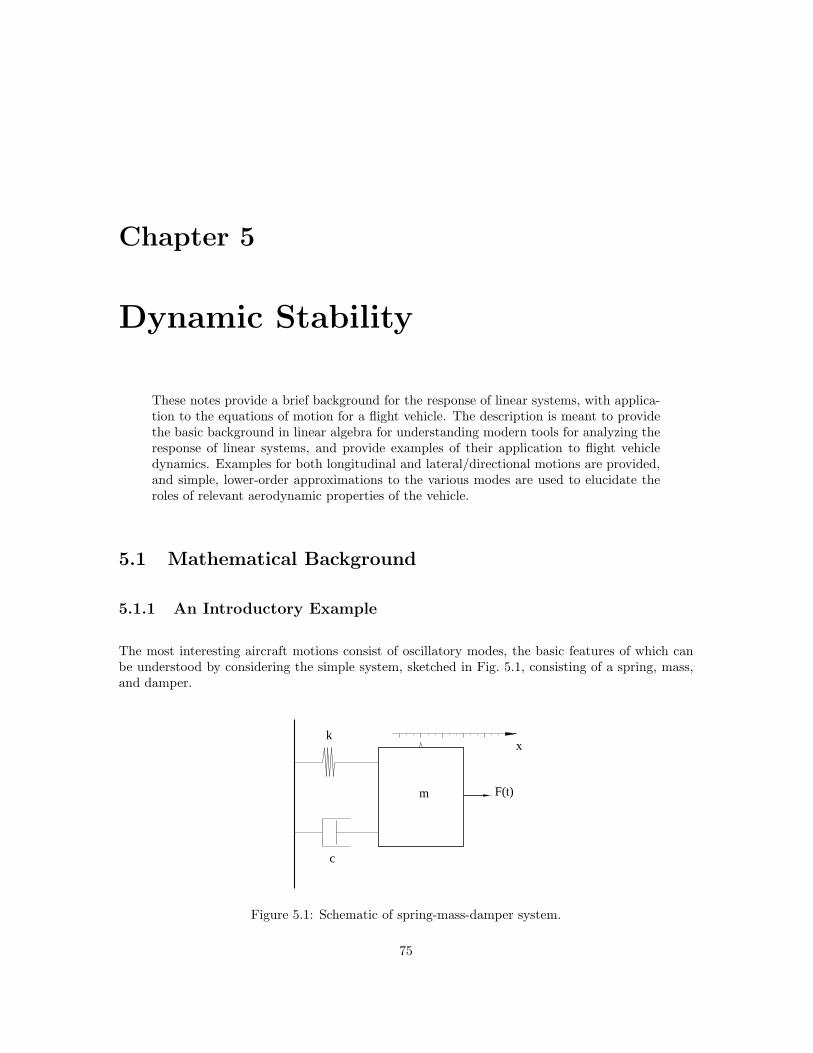
Chapter 5
Dynamic Stability
These notes provide a brief background for the response of linear systems, with applica-tion to the equations of motion for a flight vehicle. The description is meant to providethe basic background in linear algebra for understanding modern tools for analyzing theresponse of linear systems, and provide examples of their application to flight vehicledynamics. Examples for both longitudinal and lateral/directional motions are provided,and simple, lower-order approximations to the various modes are used to elucidate theroles of relevant aerodynamic properties of the vehicle.
5.1 Mathematical Background
5.1.1 An Introductory Example
The most interesting aircraft motions consist of oscillatory modes, the basic features of which canbe understood by considering the simple system, sketched in Fig. 5.1, consisting of a spring, mass,and damper.
m F(t)
k
c
x
Figure 5.1: Schematic of spring-mass-damper system.
75

76 CHAPTER 5. DYNAMIC STABILITY
The dynamics of this system are described by the second-order ordinary differential equation
md2x
dt2+ c
dx
dt+ kx = F (t) (5.1)
where m is the mass of the system, c is the damping parameter, and k is the spring constant ofthe restoring force. We generally are interested in both the free response of the system to an initialperturbation (with F (t) = 0), and the forced response to time-varying F (t). The free response isrelevant to the question of stability – i.e., the response to an infinitesimal perturbation from anequilibrium state of the system, while the forced response is relevant to control response.
The free response is the solution to the homogeneous equation, which can be written
d2x
dt2+
( c
m
) dx
dt+
(
k
m
)
x = 0 (5.2)
Solutions of this equation are generally of the form
x = Aeλt (5.3)
where A is a constant determined by the initial perturbation. Substitution of Eq. (5.3) into thedifferential equation yields the characteristic equation
λ2 +( c
m
)
λ +
(
k
m
)
= 0 (5.4)
which has roots
λ = − c
2m±
√
( c
2m
)2
−(
k
m
)
(5.5)
The nature of the response depends on whether the second term in the above expression is real orimaginary, and therefore depends on the relative magnitudes of the damping parameter c and thespring constant k. We can re-write the characteristic equation in terms of a variable defined by theratio of the two terms in the square root
(
c2m
)2
(
km
) =c2
4mk≡ ζ2 (5.6)
and a variable explicitly depending on the spring constant k, which we will choose (for reasons thatwill become obvious later) to be
k
m≡ ω2
n (5.7)
In terms of these new variables, the original Eq. (5.2) can be written as
d2x
dt2+ 2ζωn
dx
dt+ ω2
nx = 0 (5.8)
The corresponding characteristic equation takes the form
λ2 + 2ζωnλ + ω2n = 0 (5.9)
and its roots can now be written in the suggestive forms
λ =
−ζωn ± ωn
√
ζ2 − 1 for ζ > 1
−ζωn for ζ = 1
−ζωn ± iωn
√
1 − ζ2 for ζ < 1
(5.10)

5.1. MATHEMATICAL BACKGROUND 77
Overdamped System
For cases in which ζ > 1, the characteristic equation has two (distinct) real roots, and the solutiontakes the form
x = a1eλ1t + a2e
λ2t (5.11)
where
λ1 = −ωn
(
ζ +√
ζ2 − 1)
λ2 = −ωn
(
ζ −√
ζ2 − 1) (5.12)
The constants a1 and a2 are determined from the initial conditions
x(0) = a1 + a2
x(0) = a1λ1 + a2λ2
(5.13)
or, in matrix form,(
1 1λ1 λ2
) (
a1
a2
)
=
(
x(0)x(0)
)
(5.14)
Since the determinant of the coefficient matrix in these equations is equal to λ2 − λ1, the coefficientmatrix is non-singular so long as the characteristic values λ1 and λ2 are distinct – which is guaranteedby Eqs. (5.12) when ζ > 1. Thus, for the overdamped system (ζ > 1), the solution is completelydetermined by the initial values of x and x, and consists of a linear combination of two decayingexponentials.
The reciprocal of the undamped natural frequency ωn forms a natural time scale for this problem,so if we introduce the dimensionless time
t = ωnt (5.15)
then Eq. (5.8) can be writtend2x
dt2+ 2ζ
dx
dt+ x = 0 (5.16)
which is seen to depend only on the damping ratio ζ. Figure 5.2 shows the response of overdampedsystems for various values of the damping ratio as functions of the dimensionless time t.
Critically Damped System
When the damping ratio ζ = 1, the system is said to be critically damped , and there is only a singlecharacteristic value
λ1 = λ2 = −ωn (5.17)
Thus, only one of the two initial conditions can, in general, be satisfied by a solution of the form eλt.However, in this special case it is easily verified that teλt = te−ωnt is also a solution of Eq. (5.8), sothe general form of the solution for the critically damped case can be written as
x = (a1 + a2t) e−ωnt (5.18)
The constants a1 and a2 are again determined from the initial conditions
x(0) = a1
x(0) = a1λ1 + a2
(5.19)

78 CHAPTER 5. DYNAMIC STABILITY
0 2 4 6 8 10 12 14 16 18 20−0.2
0
0.2
0.4
0.6
0.8
1
Normalized time, ωn t
Dis
plac
emen
t, x
ζ = 1
ζ = 2
ζ = 5
ζ = 10
0 2 4 6 8 10 12 14 16 18 20−0.1
0
0.1
0.2
0.3
0.4
Normalized time, ωn t
Dis
plac
emen
t, x
ζ = 1
ζ = 2
ζ = 5
ζ = 10
(a) x(0) = 1.0 (b) x(0) = 1.0
Figure 5.2: Overdamped response of spring-mass-damper system. (a) Displacement perturbation:x(0) = 1.0; x(0) = 0. (b) Velocity perturbation: x(0) = 1.0; x(0) = 0.
or, in matrix form,(
1 0λ1 1
)(
a1
a2
)
=
(
x(0)x(0)
)
(5.20)
Since the determinant of the coefficient matrix in these equations is always equal to unity, thecoefficient matrix is non-singular. Thus, for the critically damped system (ζ = 1), the solution isagain completely determined by the initial values of x and x, and consists of a linear combinationof a decaying exponential and a term proportional to te−ωnt. For any positive value of ωn theexponential decays more rapidly than any positive power of t, so the solution again decays, nearlyexponentially.
Figures 5.2 and 5.3 include the limiting case of critically damped response for Eq. (5.16).
Underdamped System
When the damping ratio ζ < 1, the system is said to be underdamped , and the roots of the charac-teristic equation consist of the complex conjugate pair
λ1 = ωn
(
−ζ + i√
1 − ζ2)
λ2 = ωn
(
−ζ − i√
1 − ζ2) (5.21)
Thus, the general form of the solution can be written
x = e−ζωnt[
a1 cos(
ωn
√
1 − ζ2t)
+ a2 sin(
ωn
√
1 − ζ2t)]
(5.22)
The constants a1 and a2 are again determined from the initial conditions
x(0) = a1
x(0) = −ζωna1 + ωn
√
1 − ζ2a2
(5.23)
or, in matrix form,(
1 0
−ζωn ωn
√
1 − ζ2
)(
a1
a2
)
=
(
x(0)x(0)
)
(5.24)

5.1. MATHEMATICAL BACKGROUND 79
0 2 4 6 8 10 12 14 16 18 20−1
−0.8
−0.6
−0.4
−0.2
0
0.2
0.4
0.6
0.8
1
Normalized time, ωn t
Dis
plac
emen
t, x
ζ = 0.1
ζ = 0.3
ζ = 0.6
ζ = 1
0 2 4 6 8 10 12 14 16 18 20−1
−0.8
−0.6
−0.4
−0.2
0
0.2
0.4
0.6
0.8
1
Normalized time, ωn t
Dis
plac
emen
t, x
ζ = 0.1
ζ = 0.3
ζ = 0.6
ζ = 1
(a) x(0) = 1.0 (b) x(0) = 1.0
Figure 5.3: Underdamped response of spring-mass-damper system. (a) Displacement perturbation:x(0) = 1.0; x(0) = 0. (b) Velocity perturbation: x(0) = 1.0; x(0) = 0.
Since the determinant of the coefficient matrix in these equations is equal to ωn
√
1 − ζ2, the systemis non-singular when ζ < 1, and the solution is completely determined by the initial values of x andx. Figure 5.3 shows the response of the underdamped system Eq. (5.16) for various values of thedamping ratio, again as a function of the dimensionless time t.
As is seen from Eq. (5.22), the solution consists of an exponentially decaying sinusoidal motion.This motion is characterized by its period and the rate at which the oscillations are damped. Theperiod is given by
T =2π
ωn
√
1 − ζ2(5.25)
and the time to damp to 1/n times the initial amplitude is given by1
t1/n =lnn
ωnζ(5.26)
For these oscillatory motions, the damping frequently is characterized by the number of cycles todamp to 1/n times the initial amplitude, which is given by
N1/n =t1/n
T=
lnn
2π
√
1 − ζ2
ζ(5.27)
Note that this latter quantity is independent of the undamped natural frequency; i.e., it dependsonly on the damping ratio ζ.
5.1.2 Systems of First-order Equations
Although the equation describing the spring-mass-damper system of the previous section was solvedin its original form, as a single second-order ordinary differential equation, it is useful for later
1The most commonly used values of n are 2 and 10, corresponding to the times to damp to 1/2 the initial amplitudeand 1/10 the initial amplitude, respectively.

80 CHAPTER 5. DYNAMIC STABILITY
generalization to re-write it as a system of coupled first-order differential equations by defining
x1 = x
x2 =dx
dt
(5.28)
Equation (5.8) can then be written as
d
dt
(
x1
x2
)
=
(
0 1−ω2
n −2ζωn
)(
x1
x2
)
+
(
01m
)
F (t) (5.29)
which has the general formx = Ax + Bη (5.30)
where x = (x1, x2)T, the dot represents a time derivative, and η(t) = F (t) will be identified as the
control input.
The free response is then governed by the system of equations
x = Ax (5.31)
and substitution of the general formx = xie
λit (5.32)
into Eqs. (5.31) requires(A − λiI)xi = 0 (5.33)
Thus, the free response of the system in seen to be completely determined by the eigenstructure (i.e.,the eigenvalues and eigenvectors) of the plant matrix A. The vector xi is seen to be the eigenvectorassociated with the eigenvalue λi of the matrix A and, when the eigenvalues are unique, the generalsolution can be expressed as a linear combination of the form
x =
2∑
i=1
aixieλit (5.34)
where the constants ai are determined by the initial conditions. The modal matrix Q of A is definedas the matrix whose columns are the eigenvectors of A
Q =(
x1 x2
)
(5.35)
so the initial values of the vector x are given by
x(0) =
2∑
i=1
aixi = Qa (5.36)
where the elements of the vectora = a1, a2T
correspond to the coefficients in the modal expansion of the solution in the form of Eq. (5.34). Whenthe eigenvalues are complex, they must appear in complex conjugate pairs, and the correspondingeigenvectors also are complex conjugates, so the solution corresponding to a complex conjugate pairof eigenvalues again corresponds to an exponentially damped harmonic oscillation.
While the above analysis corresponds to the second-order system treated previously, the advantage ofviewing is as a system of first-order equations is that, once we have shifted our viewpoint the analysis

5.2. LONGITUDINAL MOTIONS 81
carries through for a system of any order. In particular, the simplest complete linear analyses of eitherlongitudinal or lateral/directional dynamics will lead to fourth-order systems – i.e., to systems offour coupled first-order differential equations. In practice, most of the required operations involvingeigenvalues and eigenvectors can be accomplished easily using numerical software packages, such asMatlab
5.2 Longitudinal Motions
In this section, we develop the small-disturbance equations for longitudinal motions in standardstate-variable form. Recall that the linearized equations describing small longitudinal perturbationsfrom a longitudinal equilibrium state can be written
[
d
dt− Xu
]
u + g0 cos Θ0θ − Xww = Xδeδe + XδT
δT
−Zuu +
[
(1 − Zw)d
dt− Zw
]
w − [u0 + Zq] q + g0 sin Θ0θ = Zδeδe + ZδT
δT
−Muu −[
Mwd
dt+ Mw
]
w +
[
d
dt− Mq
]
q = Mδeδe + MδT
δT
(5.37)
If we introduce the longitudinal state variable vector
x = [u w q θ]T
(5.38)
and the longitudinal control vectorη = [δe δT ]
T(5.39)
these equations are equivalent to the system of first-order equations
Inx = Anx + Bnη (5.40)
where x represents the time derivative of the state vector x, and the matrices appearing in thisequation are
An =
Xu Xw 0 −g0 cos Θ0
Zu Zw u0 + Zq −g0 sin Θ0
Mu Mw Mq 00 0 1 0
In =
1 0 0 00 1 − Zw 0 00 −Mw 1 00 0 0 1
, Bn =
XδeXδT
ZδeZδT
MδeMδT
0 0
(5.41)
It is not difficult to show that the inverse of In is
I−1n =
1 0 0 00 1
1−Zw0 0
0 Mw
1−Zw1 0
0 0 0 1
(5.42)
so premultiplying Eq. (5.40) by I−1n gives the standard form
x = Ax + Bη (5.43)

82 CHAPTER 5. DYNAMIC STABILITY
where
A =
Xu Xw 0 −g0 cos Θ0Zu
1−Zw
Zw
1−Zw
u0+Zq
1−Zw
−g0 sin Θ0
1−Zw
Mu + MwZu
1−ZwMw + MwZw
1−ZwMq +
(u0+Zq)Mw
1−Zw
−Mwg0 sin Θ0
1−Zw
0 0 1 0
B =
XδeXδT
Zδe
1−Zw
ZδT
1−Zw
Mδe+
MwZδe
1−ZwMδT
+MwZδT
1−Zw
0 0
(5.44)
Note that
Zw =QSc
2mu20
CZα = − 1
2µCLα (5.45)
and
Zq =QSc
2mu0CZq = −u0
2µCLq (5.46)
Since the aircraft mass parameter µ is typically large (on the order of 100), it is common to neglectZw with respect to unity and to neglect Zq relative to u0, in which case the matrices A and B canbe approximated as
A =
Xu Xw 0 −g0 cos Θ0
Zu Zw u0 −g0 sinΘ0
Mu + MwZu Mw + MwZw Mq + u0Mw −Mwg0 sinΘ0
0 0 1 0
B =
XδeXδT
ZδeZδT
Mδe+ MwZδe
MδT+ MwZδT
0 0
(5.47)
This is the approximate form of the linearized equations for longitudinal motions as they appear inmany texts (see, e.g., Eqs. (4.53) and (4.54) in [3]2).
The various dimensional stability derivatives appearing in Eqs. (5.44) and (5.47) are related to theirdimensionless aerodynamic coefficient counterparts in Table 5.1; these data were also presented inTable 4.1 in the previous chapter.
5.2.1 Modes of Typical Aircraft
The natural response of most aircraft to longitudinal perturbations typically consists of two under-damped oscillatory modes having rather different time scales. One of the modes has a relativelyshort period and is usually quite heavily damped; this is called the short period mode. The othermode has a much longer period and is rather lightly damped; this is called the phugoid mode.
We illustrate this response using the stability derivatives for the Boeing 747 aircraft at its Mach 0.25power approach configuration at standard sea-level conditions. The aircraft properties and flight
2The equations in [3] also assume level flight, or Θ0 = 0.

5.2. LONGITUDINAL MOTIONS 83
Variable X Z M
u Xu = QSmu0
[2CX0 + CXu] Zu = QSmu0
[2CZ0 + CZu] Mu = QScIyu0
Cmu
w Xw = QSmu0
CXα Zw = QSmu0
CZα Mw = QScIyu0
Cmα
w Xw = 0 Zw = QSc2mu2
0
CZα Mw = QSc2
2Iyu20
Cmα
q Xq = 0 Zq = QSc2mu0
CZq Mq = QSc2
2Iyu0Cmq
Table 5.1: Relation of dimensional stability derivatives for longitudinal motions to dimensionlessderivatives of aerodynamic coefficients. The dimensionless coefficients on which these are based aredescribed in Chapter 4.
condition are given by [2]
V = 279.1 ft/sec, ρ = 0.002377 slug/ft3
S = 5, 500. ft2, c = 27.3 ft (5.48)
W = 564, 032. lb, Iy = 32.3 × 10⁶ slug-ft2
and the relevant aerodynamic coefficients are
CL = 1.108, CD = 0.102, Θ0 = 0
CLα = 5.70, CLα = 6.7, CLq = 5.4, CLM = 0
CDα = 0.66, (5.49)
Cmα = −1.26, Cmα = −3.2, Cmq = −20.8, CmM = 0
(5.50)
These values correspond to the following dimensional stability derivatives
Xu = −0.0212, Xw = 0.0466
Zu = −0.2306, Zw = −0.6038, Zw = −0.0341, Zq = −7.674 (5.51)
Mu = 0.0, Mw = −0.0019, Mw = −0.0002, Mq = −0.4381
and the plant matrix is
A =
−0.0212 0.0466 0.000 −32.174−0.2229 −0.5839 262.472 0.00.0001 −0.0018 −0.5015 0.0
0.0 0.0 1.0 0.0
(5.52)
The characteristic equation is given by
|A − λI| = λ4 + 1.1066λ3 + 0.7994λ2 + 0.0225λ + 0.0139 = 0 (5.53)
and its roots are
λsp = −0.5515 ± ı 0.6880
λph = −0.00178 ± ı 0.1339(5.54)

84 CHAPTER 5. DYNAMIC STABILITY
where, as suggested by the subscripts, the first pair of roots corresponds to the short period mode,and the second pair corresponds to the phugoid mode. The damping ratios of the two modes arethus given by
ζsp =
√
√
√
√
1
1 +(
ηξ
)2
sp
=
√
1
1 +(
0.68800.5515
)2 = 0.6255
ζph =
√
√
√
√
1
1 +(
ηξ
)2
ph
=
√
1
1 +(
0.13390.00178
)2 = 0.0133
(5.55)
where ξ and η are the real and imaginary parts of the respective roots, and the undamped naturalfrequencies of the two modes are
ωnsp=
−ξsp
ζsp=
0.5515
0.6255= 0.882 sec−1
ωnph=
−ξph
ζph=
0.00178
0.0133= 0.134 sec−1
(5.56)
The periods of the two modes are given by
Tsp =2π
ωnsp
√
1 − ζ2sp
= 9.13 sec (5.57)
and
Tph =2π
ωnph
√
1 − ζ2ph
= 46.9 sec (5.58)
respectively, and the numbers of cycles to damp to half amplitude of the respective modes are givenby
N1/2sp=
ln 2
2π
√
1 − ζ2sp
ζsp=
ln 2
2π
√
1 − (0.6255)2
0.6255= 0.1376 (5.59)
and
N1/2ph=
ln 2
2π
√
1 − ζ2ph
ζph=
ln 2
2π
√
1 − (0.0133)2
0.0133= 8.29 (5.60)
Figure 5.4 illustrates the short period and phugoid responses for the Boeing 747 under these condi-tions. These show the time histories of the state variables following an initial perturbation that ischosen to excite only the (a) short period mode or the (b) phugoid mode, respectively.
It should be noted that the dimensionless velocity perturbations u/u0 and α = w/u0 are plottedin these figures, in order to allow comparisons with the other state variables. The plant matrixcan be modified to reflect this choice of state variables as follows. The elements of the first twocolumns of the original plant matrix should be multiplied by u0, then the entire plant matrix shouldbe premultiplied by the diagonal matrix having elements diag(1/u0, 1/u0, 1, 1). The combination ofthese two steps is equivalent to dividing the elements in the upper right two-by-two block of theplant matrix A by u0, and multiplying the elements in the lower left two-by-two block by u0. The
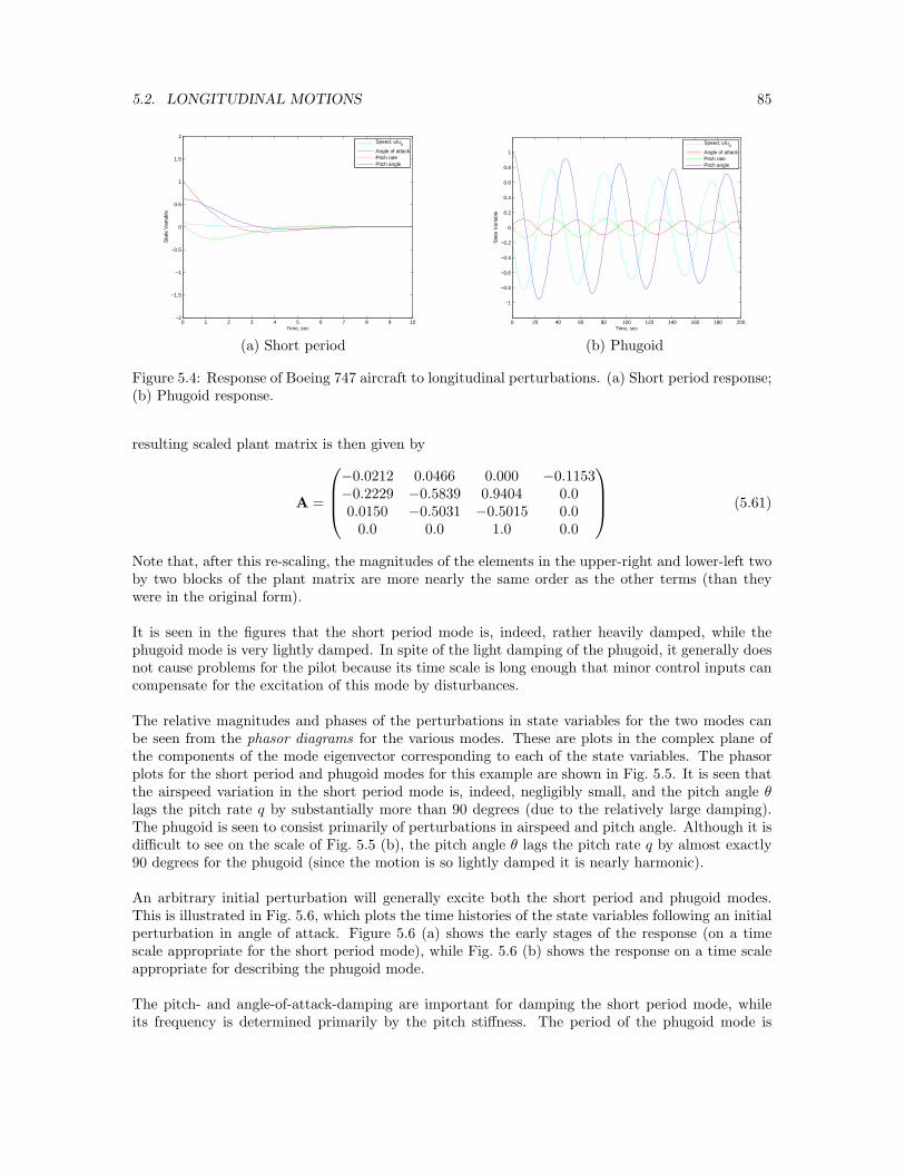
5.2. LONGITUDINAL MOTIONS 85
0 1 2 3 4 5 6 7 8 9 10−2
−1.5
−1
−0.5
0
0.5
1
1.5
2
Time, sec
Sta
te V
aria
ble
Speed, u/u
0
Angle of attackPitch ratePitch angle
0 20 40 60 80 100 120 140 160 180 200
−1
−0.8
−0.6
−0.4
−0.2
0
0.2
0.4
0.6
0.8
1
Time, sec
Sta
te V
aria
ble
Speed, u/u
0
Angle of attackPitch ratePitch angle
(a) Short period (b) Phugoid
Figure 5.4: Response of Boeing 747 aircraft to longitudinal perturbations. (a) Short period response;(b) Phugoid response.
resulting scaled plant matrix is then given by
A =
−0.0212 0.0466 0.000 −0.1153−0.2229 −0.5839 0.9404 0.00.0150 −0.5031 −0.5015 0.0
0.0 0.0 1.0 0.0
(5.61)
Note that, after this re-scaling, the magnitudes of the elements in the upper-right and lower-left twoby two blocks of the plant matrix are more nearly the same order as the other terms (than theywere in the original form).
It is seen in the figures that the short period mode is, indeed, rather heavily damped, while thephugoid mode is very lightly damped. In spite of the light damping of the phugoid, it generally doesnot cause problems for the pilot because its time scale is long enough that minor control inputs cancompensate for the excitation of this mode by disturbances.
The relative magnitudes and phases of the perturbations in state variables for the two modes canbe seen from the phasor diagrams for the various modes. These are plots in the complex plane ofthe components of the mode eigenvector corresponding to each of the state variables. The phasorplots for the short period and phugoid modes for this example are shown in Fig. 5.5. It is seen thatthe airspeed variation in the short period mode is, indeed, negligibly small, and the pitch angle θlags the pitch rate q by substantially more than 90 degrees (due to the relatively large damping).The phugoid is seen to consist primarily of perturbations in airspeed and pitch angle. Although it isdifficult to see on the scale of Fig. 5.5 (b), the pitch angle θ lags the pitch rate q by almost exactly90 degrees for the phugoid (since the motion is so lightly damped it is nearly harmonic).
An arbitrary initial perturbation will generally excite both the short period and phugoid modes.This is illustrated in Fig. 5.6, which plots the time histories of the state variables following an initialperturbation in angle of attack. Figure 5.6 (a) shows the early stages of the response (on a timescale appropriate for the short period mode), while Fig. 5.6 (b) shows the response on a time scaleappropriate for describing the phugoid mode.
The pitch- and angle-of-attack-damping are important for damping the short period mode, whileits frequency is determined primarily by the pitch stiffness. The period of the phugoid mode is

86 CHAPTER 5. DYNAMIC STABILITY
nearly independent of vehicle parameters, and is very nearly inversely proportional to airspeed. Thedamping ratio for the phugoid is approximately proportional to the ratio CD/CL, which is smallfor efficient aircraft. These properties can be seen from the approximate analyses of the two modespresented in the following two sections.
5.2.2 Approximation to Short Period Mode
The short period mode typically occurs so quickly that it proceeds at essentially constant vehiclespeed. A useful approximation for the mode can thus be developed by setting u = 0 and solving
(1 − Zw) w = Zww + (u0 + Zq) q
−Mww + q = Mww + Mqq(5.62)
which can be written in state-space form as
d
dt
(
wq
)
=
(
Zw
1−Zw
u0+Zq
1−Zw
Mw + MwZw
1−ZwMq + Mw
u0+Zq
1−Zw
)
(
wq
)
(5.63)
SinceZq
u0=
QSc
2mu20
CZq = −ηVHat
µ(5.64)
where µ, the aircraft relative mass parameter, is usually large (on the order of one hundred), it isconsistent with the level of our approximation to neglect Zq relative to u0. Also, we note that
Zw =QSc
2mu20
CZα = −ηVHat
µ
dǫ
dα(5.65)
is generally also very small. Thus, Eqs. (5.63) can be further approximated as
d
dt
(
wq
)
=
(
Zw u0
Mw + MwZw Mq + Mwu0
)(
wq
)
(5.66)
The characteristic equation for the simplified plant matrix of Eq. (5.66) is
λ2 − (Zw + Mq + u0Mw) λ + ZwMq − u0Mw = 0 (5.67)
Re
q
Im
w/u0
θ
q
w/u0 Re
Im
u/u0
θ
(a) Short period (b) Phugoid
Figure 5.5: Phasor diagrams for longitudinal modes of the Boeing 747 aircraft in powered approachat M = 0.25. Perturbation in normalized speed u/u0 is too small to be seen in short period mode.

5.2. LONGITUDINAL MOTIONS 87
0 1 2 3 4 5 6 7 8 9 10
−1.5
−1
−0.5
0
0.5
1
1.5
Time, sec
Sta
te V
aria
ble
Speed, u/u
0
Angle of attackPitch ratePitch angle
0 10 20 30 40 50 60 70 80 90 100
−1.5
−1
−0.5
0
0.5
1
1.5
Time, sec
Sta
te V
aria
ble
Speed, u/u
0
Angle of attackPitch ratePitch angle
(a) Short period (b) Phugoid
Figure 5.6: Response of Boeing 747 aircraft to unit perturbation in angle of attack. (a) Time scalechosen to emphasize short period response; (b) Time scale chosen to emphasize phugoid response.
or, if the derivatives with respect to w are expressed as derivatives with respect to α,
λ2 −(
Mq + Mα +Zα
u0
)
λ − Mα +ZαMq
u0= 0 (5.68)
The undamped natural frequency and damping ratio for this motion are thus
ωn =
√
−Mα +ZαMq
u0
ζ = −Mq + Mα + Zα
u0
2ωn
(5.69)
Thus, it is seen that the undamped natural frequency of the mode is determined primarily by thepitch stiffness Mα, and the damping ratio is determined largely by the pitch- and angle-of-attack-damping.
For the example considered in the preceding sections of the Boeing 747 in powered approach we find
ωn =
√
0.54 +(−168.5)(−.4381)
279.1sec−1 = 0.897 sec−1
ζ = −−.4381 − .056 + (−168.5)279.1
2(0.897)= 0.612
(5.70)
When these numbers are compared to ωn = 0.882 sec−1 and ζ = 0.6255 from the more completeanalysis (of the full fourth-order system), we see that the approximate analysis over predicts theundamped natural frequency by only about 1 per cent, and under predicts the damping ratio byless than 2 per cent. As will be seen in the next subsection when we consider approximating thephugoid mode, it generally is easier to approximate the large roots than the small ones, especiallywhen the latter are lightly damped.
88 CHAPTER 5. DYNAMIC STABILITY
5.2.3 Approximation to Phugoid Mode
Since the phugoid mode typically proceeds at nearly constant angle of attack, and the motion is soslow that the pitch rate q is very small, we can approximate the behavior of the mode by writingonly the X- and Z-force equations
u = Xuu + Xww − g0 cos Θ0θ
(1 − Zw) w = Zuu + Zww + (u0 + Zq) q − g0 sin Θ0θ(5.71)
which, upon setting w = w = 0, can be written in the form
d
dt
(
uθ
)
=
(
Xu −g0 cos Θ0
− Zu
u0+Zq
g0 sin Θ0
u0+Zq
)
(
uθ
)
(5.72)
Since, as has been seen in Eq. (5.64), Zq is typically very small relative to the speed u0, it is consistentwith our neglect of q and w also to neglect Zq relative to u0. Also, we will consider only the case oflevel flight for the initial equilibrium, so Θ0 = 0, and Eq. (5.72) becomes
d
dt
(
uθ
)
=
(
Xu −g0
−Zu
u00
) (
uθ
)
(5.73)
The characteristic equation for the simplified plant matrix of Eq. (5.73) is
λ2 − Xuλ − g0
u0Zu = 0 (5.74)
The undamped natural frequency and damping ratio for this motion are thus
ωn =
√
− g0
u0Zu
ζ =−Xu
2ωn
(5.75)
It is useful to express these results in terms of dimensionless aerodynamic coefficients. Recall that
Zu = − QS
mu0[2CL0 + MCLM] (5.76)
and, for the case of a constant-thrust propulsive system,
Xu = − QS
mu0[2CD0 + MCDM] (5.77)
so, if we further neglect compressibility effects, we have
ωn =√
2g0
u0
ζ =1√2
CD0
CL0
(5.78)
Thus, according to this approximation, the undamped natural frequency of the phugoid is a functiononly of the flight velocity, and the damping ratio is proportional to the drag-to-lift ratio. Since the

5.3. LATERAL/DIRECTIONAL MOTIONS 89
latter quantity is small for an efficient flight vehicle, this explains why the phugoid typically is verylightly damped.
For the example of the Boeing 747 in powered approach we find
ωn =√
232.174 ft/sec
2
279.1 ft/sec= 0.163 sec−1
ζ =1√2
0.102
1.108= 0.0651
(5.79)
When these numbers are compared to ωn = 0.134 sec−1 and ζ = 0.0133 from the more completeanalysis (of the full fourth-order system), we see that the approximate analysis over predicts theundamped natural frequency by about 20 per cent, and over predicts the damping ratio by a factor ofalmost 5. Nevertheless, this simplified analysis gives insight into the important parameters governingthe mode.
5.2.4 Summary of Longitudinal Modes
We have seen that the response of a typical aircraft to longitudinal perturbations consists of twooscillatory modes:
1. A short period mode that usually is heavily damped, whose period is determined largely bythe vehicle pitch stiffness Cmα, and which is damped primarily by pitch- and angle-of-attack-damping, Cmq and Cmα, respectively; and
2. A lightly damped, low frequency, phugoid mode whose period is nearly independent of vehicleparameters and inversely proportional to the flight velocity, and for which the damping ratiois proportional approximately to the ratio CD/CL, which is small for efficient vehicles.
We here illustrate the variation in response for a typical vehicle as a function of the vehicle staticmargin – which determines the pitch stiffness. The behavior of the roots of the characteristic equationof the complete fourth-order plant matrix is shown in Fig. 5.7 as a function of the pitch stiffness forour Boeing 747 example. The plot shows the locations of the roots as the static margin is reducedfrom an initial value of 0.22. As the c.g. is moved aft, both the phugoid and short period rootsmove toward the real axis. The short period mode becomes critically damped at a static marginof approximately 0.0158, and the phugoid becomes critically damped at a value of approximately0.0021. One of the phugoid roots then moves toward the right-hand plane, and becomes neutrallystable at a static margin of 0.0. The other phugoid root moves to the left and, at a static margin ofapproximately -.0145, joins one of the short-period roots to create another oscillatory mode, whichis called the third oscillatory mode.
5.3 Lateral/Directional Motions
In this section, we develop the small-disturbance equations for lateral/directional motions in stan-dard state-variable form. Recall that the linearized equations describing small lateral/directional

90 CHAPTER 5. DYNAMIC STABILITY
-0.8
-0.6
-0.4
-0.2
0
0.2
0.4
0.6
0.8
-0.8 -0.6 -0.4 -0.2 0
Imag
inar
y pa
rt o
f roo
t
Real part of root
Short-periodShort-period
Phugoid modePhugoid mode
Figure 5.7: Locus of roots of longitudinal plant matrix for Boeing 747 in level flight at M = 0.25 asstandard seal level conditions as functions of c.g. location for values of static margin ranging from0.22 to -.05. As the static margin is reduced, the roots of both oscillatory modes coalesce on thereal axis; one of the phugoid roots moves to the right and becomes unstable, while the other movesto the left and joins with one of the short period roots to form a third oscillatory mode.
perturbations from a longitudinal equilibrium state can be written
[
d
dt− Yv
]
v − Ypp + [u0 − Yr] r − g0 cos Θ0φ = Yδrδr
−Lvv +
[
d
dt− Lp
]
p −[
Ixz
Ix
d
dt+ Lr
]
r = Lδrδr + Lδa
δa
−Nvv −[
Ixz
Iz
d
dt+ Np
]
p +
[
d
dt− Nr
]
r = Nδrδr + Nδa
δa
(5.80)
If we introduce the lateral/directional state variable vector
x = [v p φ r]T
(5.81)
and the lateral/directional control vector
η = [δr δa]T
(5.82)
these equations are equivalent to the system of first-order equations
Inx = Anx + Bnη (5.83)

5.3. LATERAL/DIRECTIONAL MOTIONS 91
where x represents the time derivative of the state vector x, and the matrices appearing in thisequation are
An =
Yv Yp g0 cos Θ0 Yr − u0
Lv Lp 0 Lr
0 1 0 0Nv Np 0 Nr
In =
1 0 0 00 1 0 −ix0 0 1 00 −iz 0 1
, Bn =
Yδr0
LδrLδa
0 0Nδr
Nδa
(5.84)
where
ix ≡ Ixz
Ix, iz ≡ Ixz
Iz(5.85)
It is not difficult to show that the inverse of In is
I−1n =
1 0 0 00 1
1−ixiz0 ix
1−ixiz
0 0 1 00 iz
1−ixiz0 1
1−ixiz
(5.86)
so premultiplying Eq. (5.83) by I−1n gives the standard form
x = Ax + Bη
where
A =
Yv Yp g0 cos Θ0 Yr − u0Lv+ixNv
1−ixiz
Lp+ixNp
1−ixiz0 Lr+ixNr
1−ixiz
0 1 0 0Nv+izLv
1−ixiz
Np+izLp
1−ixiz0 Nr+izLr
1−ixiz
B =
Yδr0
Lδr +ixNδr
1−ixiz
Lδa+ixNδa
1−ixiz
0 0Nδr +izLδr
1−ixiz
Nδa+izLδa
1−ixiz
(5.87)
For most flight vehicles and situations, the ratios ix and iz are quite small. Neglecting these quantitieswith respect to unity allows us to write the A and B matrices for lateral directional motions as
A =
Yv Yp g0 cos Θ0 Yr − u0
Lv Lp 0 Lr
0 1 0 0Nv Np 0 Nr
B =
Yδr0
LδrLδa
0 0Nδr
Nδa
(5.88)
This is the approximate form of the linearized equations for lateral/directional motions as theyappear in many texts (see, e.g., Eqs. (5.33) in [3]).

92 CHAPTER 5. DYNAMIC STABILITY
Variable Y L N
v Yv = QSmu0
Cyβ Lv = QSbIxu0
Clβ Nv = QSbIzu0
Cnβ
p Yp = QSb2mu0
Cyp Lp = QSb2
2Ixu0Clp Np = QSb2
2Izu0Cnp
r Yr = QSb2mu0
Cyr Lr = QSb2
2Ixu0Clr Nr = QSb2
2Izu0Cnr
Table 5.2: Relation of dimensional stability derivatives for lateral/directional motions to dimension-less derivatives of aerodynamic coefficients.
The various dimensional stability derivatives appearing in Eqs. (5.87) and (5.88) are related to theirdimensionless aerodynamic coefficient counterparts in Table 5.2; these data were also presented inTable 4.2 in the previous chapter.
5.3.1 Modes of Typical Aircraft
The natural response of most aircraft to lateral/directional perturbations typically consists of onedamped oscillatory mode and two exponential modes, one of which is usually very heavily damped.The oscillatory mode has a relatively short period and can be relatively lightly damped, especiallyfor swept-wing aircraft; this is called the Dutch Roll mode, as the response consists of a combinedrolling, sideslipping, yawing motion reminiscent of a (Dutch) speed-skater. One of the exponentialmodes is very heavily damped, and represents the response of the aircraft primarily in roll; it iscalled the rolling mode. The second exponential mode, called the spiral mode, can be either stableor unstable, but usually has a long enough time constant that it presents no difficulty for pilotedvehicles, even when it is unstable.3
We illustrate this response again using the stability derivatives for the Boeing 747 aircraft at its Mach0.25 powered approach configuration at standard sea-level conditions. This is the same vehicle andtrim condition used to illustrate typical longitudinal behavior, and the basic aircraft properties andflight condition are given in Eq. (5.48). In addition, for the lateral/directional response we need thefollowing vehicle parameters
W = 564, 032. lbf, b = 195.7 ft
Ix = 14.3 × 10⁶ slug ft2, Iz = 45.3 × 10⁶ slug ft2, Ixz = −2.23 × 10⁶ slug ft2 (5.89)
and the aerodynamic derivatives
Cyβ = −.96 Cyp = 0.0 Cyr = 0.0
Clβ = −.221 Clp = −.45 Clr = 0.101 (5.90)
Cnβ = 0.15 Cnp = −.121 Cnr = −.30
3This is true at least when flying under visual flight rules and a horizontal reference is clearly visible. Underinstrument flight rules pilots must learn to trust the artificial horizon indicator to avoid entering an unstable spiral.

5.3. LATERAL/DIRECTIONAL MOTIONS 93
These values correspond to the following dimensional stability derivatives
Yv = −0.0999, Yp = 0.0, Yr = 0.0
Lv = −0.0055, Lp = −1.0994, Lr = 0.2468 (5.91)
Nv = 0.0012, Np = −.0933, Nr = −.2314
and the dimensionless product of inertia factors are
ix = −.1559, iz = −.0492 (5.92)
Using these values, the plant matrix is found to be
A =
−0.0999 0.0000 32.174 −279.10−0.0057 −1.0932 0.0 0.2850
0.0 1.0 0.0 0.00.0015 −.0395 0.0 −.2454
(5.93)
The characteristic equation is given by
|A − λI| = λ4 + 1.4385λ3 + 0.8222λ2 + 0.7232λ + 0.0319 = 0 (5.94)
and its roots are
λDR = −.08066 ± ı 0.7433
λroll = −1.2308
λspiral = −.04641
(5.95)
where, as suggested by the subscripts, the first pair of roots corresponds to the Dutch Roll mode,and the real roots corresponds to the rolling and spiral modes, respectively.
The damping ratio of the Dutch Roll mode is thus given by
ζDR =
√
√
√
√
1
1 +(
ηξ
)2
DR
=
√
1
1 +(
0.74330.08066
)2 = 0.1079 (5.96)
and the undamped natural frequency of the mode is
ωnDR=
−ξDR
ζDR=
0.08066
0.1079= 0.7477 sec−1 (5.97)
The period of the Dutch Roll mode is then given by
TDR =2π
ωn
√
1 − ζ2=
2π
0.7477√
1 − 0.10792= 8.45 sec (5.98)
and the number of cycles to damp to half amplitude is
N1/2DR=
ln 2
2π
√
1 − ζ2
ζ=
ln 2
2π
√1 − 0.10792
0.1079= 1.016 (5.99)
Thus, the period of the Dutch Roll mode is seen to be on the same order as that of the longitudinalshort period mode, but is much more lightly damped.

94 CHAPTER 5. DYNAMIC STABILITY
0 1 2 3 4 5 6 7 8 9 10
−1
−0.8
−0.6
−0.4
−0.2
0
0.2
0.4
0.6
0.8
1
Time, sec
Sta
te V
aria
ble
SideslipRoll rateRoll angleYaw rate
0 10 20 30 40 50 60 70 80 90 100−0.2
0
0.2
0.4
0.6
0.8
1
Time, sec
Sta
te V
aria
ble
SideslipRoll rateRoll angleYaw rate
0 2 4 6 8 10 12 14 16 18 20−1.5
−1
−0.5
0
0.5
1
1.5
Time, sec
Sta
te V
aria
ble
SideslipRoll rateRoll angleYaw rate
(a) Rolling mode (b) Spiral mode (c) Dutch Roll
Figure 5.8: Response of Boeing 747 aircraft to unit perturbation in eigenvectors corresponding tothe three lateral/directional modes of the vehicle. (a) Rolling mode; (b) Spiral mode; and (c) DutchRoll mode.
The times to damp to half amplitude for the rolling and spiral modes are seen to be
t1/2roll=
ln 2
−ξroll=
ln 2
1.2308= 0.563 sec (5.100)
and
t1/2spiral=
ln 2
−ξspiral=
ln 2
0.04641= 14.93 sec (5.101)
respectively.
The responses characteristic of these three modes are illustrated in Fig. 5.8. The figure shows thetime histories of the state variables following initial perturbations that are designed to excite onlya single mode. For each of the three subfigures the initial perturbation has unit amplitude for thelargest component and is parallel to the corresponding eigenvector in the state space.
Here the first state variable is again plotted in dimensionless form as β = v/u0. The plant matrixcan be modified to reflect this change in state variable as follows. The first column of the originalplant matrix is first multiplied by u0, then the entire plant matrix is pre-multiplied by the diagonalmatrix having elements diag(1/u0, 1, 1, 1). This is equivalent to dividing all but the first element inthe first row by u0, and multiplying all but the first element in the first column by u0. The firstelement in the first column remains unchanged. With this re-scaling the plant matrix becomes
A =
−0.0999 0.0000 0.1153 −1.0000−1.6038 −1.0932 0.0 0.2850
0.0 1.0 0.0 0.00.4089 −.0395 0.0 −.2454
(5.102)
Note that, after this re-scaling, the magnitudes of the elements in the first row and first column ofthe plant matrix are more nearly the same order as the other terms (than they were in the originalform).
It is seen that the rolling mode consists of almost pure rolling motion (with a very small amountof sideslip). The spiral mode consists of mostly coordinated roll and yaw. And for the the DutchRoll mode, all the state variables participate, so the motion is characterized by coordinated rolling,sideslipping, and yawing motions.
An arbitrary initial perturbation will generally excite all three modes. This is illustrated in Fig. 5.9which plots the time histories of the state variables following an initial perturbation in roll rate. The

5.3. LATERAL/DIRECTIONAL MOTIONS 95
0 2 4 6 8 10 12 14 16 18 20−0.4
−0.2
0
0.2
0.4
0.6
0.8
1
1.2
Time, secS
tate
Var
iabl
e
SideslipRoll rateRoll angleYaw rate
Figure 5.9: Response of Boeing 747 aircraft to unit perturbation in roll rate. Powered approach atM = 0.25 under standard sea-level conditions.
roll rate is seen to be quickly damped, leaving a slowly decaying spiral mode (appearing primarily inthe roll angle anad yaw rate), with the lightly-damped, oscillatory Dutch Roll mode superimposed.
The phasor plots for the rolling and spiral modes are relatively uninteresting, since these correspondto real roots. The eigenvector amplitudes, however, show that the rolling mode is dominated byperturbations in bank angle φ and roll rate p, with a very small amount of sideslip and negligibleyaw rate. The spiral mode is dominated by changes in bank angle. Since the motion is so slow,the roll rate is quite small, and the yaw rate is almost 2.5 times the roll rate, so we would expectsignificant changes in heading, as well as bank angle. The phasor diagram for the Dutch Roll modeis shown in Fig. 5.10. Note that all four state variables participate with significant amplitudes inthe Dutch Roll, and that the bank angle φ lags the roll rate p by almost exactly 90 degrees, as themotion is very lightly damped. Active control, usually to supply additional yaw damping, is oftenrequired on swept-wing transports to bring the damping of this mode to within acceptable limits.
5.3.2 Approximation to Rolling Mode
It has been seen that the rolling mode typically corresponds to almost pure roll. Thus, it is reasonableto neglect all equations except the rolling moment equation, and all perturbations except p. We
φ
β
Im
Re
p
r
Figure 5.10: Phasor diagram for Dutch Roll mode of the Boeing 747 aircraft in powered approachat M = 0.25.

96 CHAPTER 5. DYNAMIC STABILITY
thus approximate the rolling mode by the single first-order equation
p =Lp + ixNp
1 − ixizp (5.103)
for which the characteristic value is
λ =Lp + ixNp
1 − ixiz(5.104)
Since the product of inertia coefficients ix and iz usually are small, the rolling mode is seen to bedominated by roll damping Lp, which is almost always large and negative.
For our example of the Boeing 747 in powered approach at M = 0.25, using the values fromEqs. (5.91) and (5.92), the approximate formula gives
λ =−1.0994 + (−.1559)(−.0933)
1 − (−.1559)(−.0492)sec−1 = −1.093 sec−1 (5.105)
which is a bit more than 10 per cent less than the value of -1.2308 from the analysis for the fullfourth-order system.
5.3.3 Approximation to Spiral Mode
The spiral mode consists of a slow rolling/yawing motion for which the sideslip is relatively small.The roll rate is quite small compared to the yaw rate, so a reasonable approximation is to set
dp
dt= 0 =
Lv + ixNv
1 − ixizv +
Lr + ixNr
1 − ixizr (5.106)
whence
v ≈ −Lr + ixNr
Lv + ixNvr (5.107)
Since ix and iz are generally very small, this can be approximated as
v ≈ −Lr
Lvr (5.108)
The yaw equationdr
dt=
Nv + izLv
1 − ixizv +
Nr + izLr
1 − ixizr (5.109)
upon substitution of Eq. (5.108) and neglect of the product of inertia terms can then be written
dr
dt=
(
Nr −LrNv
Lv
)
r (5.110)
so the root of the characteristic equation for the spiral mode is
λ = Nr −LrNv
Lv(5.111)
Thus, it is seen that, according to this approximation, the spiral mode is stabilized by yaw dampingNr. Also, since stable dihedral effect corresponds to negative Lv and weathercock stability Nv and

5.3. LATERAL/DIRECTIONAL MOTIONS 97
roll due to yaw rate Lr are always positive, the second term in Eq. (5.111) is destabilizing; thusincreasing weathercock destabilizes the spiral mode while increasing dihedral effect stabilizes it.4
For our example of the Boeing 747 in powered approach at M = 0.25, using the values fromEqs. (5.91) and (5.92), the approximate formula gives
λ = −.2314 − 0.2468
−.0055(0.0012) = −.178 (5.112)
which is almost four times the value of -.0464 from the analysis of the full fourth-order system. Thisis consistent with the usual difficulty in approximating small roots, but Eq. (5.111) still gives usefulqualitative information about the effects of weathercock and dihedral stability on the spiral mode.
5.3.4 Approximation to Dutch Roll Mode
The Dutch Roll mode is particularly difficult to approximate because it usually involves significantperturbations in all four state variables. The most useful approximations require neglecting eitherthe roll component or simplifying the sideslip component by assuming the vehicle c.g. travels in astraight line. This latter approximation means that ψ = −β, or
r = − v
u0(5.113)
The roll and yaw moment equations (neglecting the product of inertia terms ix and iz) can then bewritten as
d
dt
(
pr
)
=
(
Lv Lp Lr
Nv Np Nr
)
vpr
(5.114)
Introduction of Eq. (5.113) completes this equation system in the form
d
dt
vpr
=
0 0 −u0
Lv Lp Lr
Nv Np Nr
vpr
(5.115)
The characteristic equation for this system is
λ3 − (Lp + Nr) λ2 + (LpNr + u0Nv − LrNp) λ + u0 (LvNp − LpNv) = 0 (5.116)
This is still a cubic equation, however, for which there is no general closed-form solution. A useful ap-proach to cubic equations that have a lightly damped oscillatory mode is Bairstow’s approximation,which proceeds as follows. If the general cubic
λ3 + a2λ2 + a1λ + a0 = 0 (5.117)
has a lightly damped oscillatory mode, its undamped natural frequency can be approximated as
a2λ2 + a0 ≈ 0 or λ2 ≈ −a0
a2(5.118)
4Even if the spiral mode is unstable, its time constant usually is long enough that the pilot has no trouble counteringit. Unpiloted aircraft, however, must have a stable spiral mode, which accounts for the excessive dihedral usuallyfound on free-flight model aircraft.

98 CHAPTER 5. DYNAMIC STABILITY
This can then be used to write the first term of Eq. (5.117) as
−a0
a2λ + a2λ
2 + a1λ + a0 = 0 (5.119)
giving
a2λ2 +
(
a1 −a0
a2
)
λ + a0 = 0 (5.120)
This quadratic equation can be solved in closed form (or at least the terms contributing to theundamped natural frequency and the damping ratio can be identified directly).
Applying Bairstow’s approximation to Eq. (5.116) yields
λ2 −[
LpNr + u0Nv − LrNp
Lp + Nr+
u0 (LvNp − LpNv)
(Lp + Nr)2
]
λ +u0 (LpNv − LvNp)
Lp + Nr= 0 (5.121)
Thus, the undamped natural frequency is given by
ω2n =
u0 (LpNv − LvNp)
Lp + Nr(5.122)
Since Np is usually negative, both terms in the numerator have the same sign for stable dihedral.Thus, increasing either weathercock stability Nv or dihedral effect Lv increases the natural frequencyof the motion.
The damping ratio is seen to be proportional to
2ζωn =−LpNr − u0Nv + LrNp
Lp + Nr+
u0 (−LvNp + LpNv)
(Lp + Nr)2 (5.123)
For most aircraft, the ratio Nr/Lp is small, and expanding Eq. (5.123) in powers of this parameterand keeping only leading order terms gives
2ζωn ≈ −Nr
(
1 +u0
L2p
Nv
)
+Np
Lp
(
Lr −u0
LpLv
)
(5.124)
Yaw damping is thus seen to contribute to positive ζ and be stabilizing, and weathercock stabilityNv augments this effect. Since both Np and Lp usually are negative, however, the dihedral effect Lv
is seen to destabilize the Dutch Roll mode.5
For our example of the Boeing 747 in powered approach at M = 0.25, using the values fromEqs. (5.91) and (5.92), the approximate formulas give
ωn =
[
(279.1) [(−1.0994)(0.0012) − (−.0055)(−.0933)]
−1.0994 − .2314sec−2
]1/2
= 0.620 sec−1 (5.125)
and
ζ = −(−1.0994)(−.2314)−(.2468)(−.0933)+(279.1)(0.0012)
−1.0994−.2314 + (279.1) (−.0055)(−.0933)−(−1.0994)(0.0012)(−1.0994−.2314)2
2(0.620)
= 0.138
(5.126)
5Recall that there are two contributions from the wing to the yaw-due-to-roll derivative Np; profile drag contributesto positive Np, while induced drag contributes to negative Np. At low values of lift coefficient (i.e., high speeds) theprofile drag contribution can dominate, in which case Np becomes positive. In this case, increased dihedral effect canimprove damping of the Dutch Roll mode. Consistent with this observation is the fact that Dutch Roll tends to be amore serious problem at low speeds.
5.3. LATERAL/DIRECTIONAL MOTIONS 99
The approximation for the undamped natural frequency is only about 15 per cent less than theexact value of 0.748, but the exact damping ratio of 0.1079 is over predicted by almost 30 per cent.Nevertheless, the approximate Eq. (5.124) gives useful qualitative information about the effect ofdihedral and weathercock on the damping of the mode.
5.3.5 Summary of Lateral/Directional Modes
We have seen that the response of a typical aircraft to lateral/directional perturbations consists oftwo exponential modes and one oscillatory mode:
1. A rolling mode that usually is heavily damped, whose time to damp to half amplitude isdetermined largely by the roll damping Lp;
2. A spiral mode that usually is only lightly damped, or may even be unstable. Dihedral effect isan important stabilizing influence, while weathercock stability is destabilizing, for this mode;and
3. A lightly damped oscillatory, intermediate frequency Dutch Roll mode, which consists of acoordinated yawing, rolling, sideslipping motion. For this mode, dihedral effect is generallydestabilizing, while weathercock stability is stabilizing.
Thus, the effects of weathercock and dihedral stability are reversed for the spiral and Dutch Rollmodes, and compromise is required. We here present root locus plots illustrating this behavior forthe full fourth-order system, corresponding to our example Boeing 747 vehicle in powered approachat standard sea level conditions at M = 0.25. Figure 5.11 shows the locus of the roots of the plantmatrix as the dihedral effect Clβ is increased from -.041 to -.561. As the dihedral effect is increased(i.e., made more negative) the spiral and rolling mode roots move to the left, while the complexpair corresponding to the Dutch Roll mode moves to the right. Consistent with our approximateanalysis, increasing the dihedral effect is seen to increase the natural frequency of the Dutch Rollmode.
Figure 5.12 shows the locus of the roots of the plant matrix as the weathercock stability coefficientCnβ is increased from -.07 to 0.69. As the weathercock stability is increased (i.e., made morepositive) the spiral and rolling mode roots move to the right, while the complex conjugate pairof roots corresponding to the Dutch Roll mode moves to the left. Again, consistent with ourapproximate analysis, increasing the weathercock stability increases the natural frequency of theDutch Roll mode.

100 CHAPTER 5. DYNAMIC STABILITY
-1
-0.5
0
0.5
1
-1.4 -1.2 -1 -0.8 -0.6 -0.4 -0.2 0
Imag
inar
y pa
rt o
f roo
t
Real part of root
Rolling modeDutch Roll Dutch Roll
Spiral mode
Figure 5.11: Locus of roots of plant matrix for Boeing 747 aircraft in powered approach at M = 0.25under standard sea-level conditions. Dihedral effect is varied from -.041 to -.561 in steps of -.04, whileall other stability derivatives are held fixed at their nominal values. Rolling and spiral modes becomeincreasingly stable as dihedral effect is increased; spiral mode becomes stable at approximatelyClβ = −.051. Dutch Roll mode becomes less stable as dihedral effect is increased and becomesunstable at approximately Clβ = −.532.
-1
-0.5
0
0.5
1
-1.2 -1 -0.8 -0.6 -0.4 -0.2 0
Imag
inar
y pa
rt o
f roo
t
Real part of root
Rolling modeDutch Roll Dutch Roll
Spiral mode
Figure 5.12: Locus of roots of plant matrix for Boeing 747 aircraft in powered approach at M = 0.25under standard sea-level conditions. Weathercock stability is varied from -.07 to 0.69 in steps of0.04, while all other stability derivatives are held fixed at their nominal values. Rolling and spiralmodes become less stable as weathercock stability is increased; spiral mode becomes unstable atapproximately Cnβ = 0.6567. Dutch roll mode becomes increasingly stable as weathercock stabilityis increased, but is unstable for less than about Cnβ = −.032.

5.4. STABILITY CHARACTERISTICS OF THE BOEING 747 101
5.4 Stability Characteristics of the Boeing 747
5.4.1 Longitudinal Stability Characteristics
In this section we summarize the longitudinal mass distribution and aerodynamic stability charac-teristics of a large, jet transport aircraft, the Boeing 747, at selected flight conditions. Data aresummarized from the report by Heffley et al. [2]. Values for aerodynamic coefficients were scaleddirectly from plots of these variables, except for the derivatives CLq
and CLαfor which no data are
provided. These values were computed from the values of the corresponding dimensional stabilityderivatives Zq and Zw, which are provided in tabular form, with the sign of Zw changed to correcta seemingly obvious error.
Condition numbers correspond to those in the report; Conditions 5-10 are for a clean aircraft,Condition 2 corresponds to a powered approach with gear up and 20 flaps. Angles of attack arewith respect to the fuselage reference line.
Condition 2 5 7 9 10
h (ft) SL 20,000 20,000 40,000 40,000M∞ 0.25 0.500 0.800 0.800 0.900
α (degrees) 5.70 6.80 0.0 4.60 2.40W (lbf) 564,032. 636,636. 636,636. 636,636. 636,636.
Iy (slug-ft2) 32.3 × 10⁶ 33.1 × 10⁶ 33.1 × 10⁶ 33.1 × 10⁶ 33.1 × 10⁶
CL 1.11 0.680 0.266 0.660 0.521CD 0.102 0.0393 0.0174 0.0415 0.0415CLα
5.70 4.67 4.24 4.92 5.57CDα 0.66 0.366 0.084 0.425 0.527Cmα
-1.26 -1.146 -.629 -1.033 -1.613CLα
6.7 6.53 5.99 5.91 5.53Cmα
-3.2 -3.35 -5.40 -6.41 -8.82CLq
5.40 5.13 5.01 6.00 6.94Cmq
-20.8 -20.7 -20.5 -24.0 -25.1CLM
0.0 -.0875 0.105 0.205 -.278CDM
0.0 0.0 0.008 0.0275 0.242CmM
0.0 0.121 -.116 0.166 -.114CLδe
0.338 0.356 0.270 0.367 0.300Cmδe
-1.34 -1.43 -1.06 -1.45 -1.20
Table 5.3: Longitudinal mass properties and aerodynamic stability derivatives for the Boeing 747 atselected flight conditions.

102 CHAPTER 5. DYNAMIC STABILITY
5.4.2 Lateral/Directional Stability Characteristics
In this section we summarize the lateral/directional mass distribution and aerodynamic stabilitycharacteristics of a large, jet transport aircraft, the Boeing 747, at selected flight conditions. Dataare summarized from the report by Heffley et al. [2]. Values for aerodynamic coefficients were scaleddirectly from plots of these variables.
Condition numbers correspond to those in the report; Conditions 5-10 are for a clean aircraft,Condition 2 corresponds to a powered approach with gear up and 20 flaps. Moments and productsof inertia are with respect to stability axes for the given flight condition. Angles of attack are withrespect to the fuselage reference line.
Condition 2 5 7 9 10
h (ft) SL 20,000 20,000 40,000 40,000M∞ 0.25 0.500 0.800 0.800 0.900
α (degrees) 5.70 6.80 0.0 4.60 2.40W (lbf) 564,032. 636,636. 636,636. 636,636. 636,636.
Ix (slug-ft2) 14.3 × 10⁶ 18.4 × 10⁶ 18.2 × 10⁶ 18.2 × 10⁶ 18.2 × 10⁶
Iz (slug-ft2) 45.3 × 10⁶ 49.5 × 10⁶ 49.7 × 10⁶ 49.7 × 10⁶ 49.7 × 10⁶
Ixz (slug-ft2) −2.23 × 10⁶ −2.76 × 10⁶ 0.97 × 10⁶ −1.56 × 10⁶ −.35 × 106
Cyβ-.96 -.90 -.81 -.88 -.92
Clβ -.221 -.193 -.164 -.277 -.095Cnβ
0.150 0.147 0.179 0.195 0.207Clp -.45 -.323 -.315 -.334 -.296Cnp
-.121 -.0687 0.0028 -.0415 0.0230Clr 0.101 0.212 0.0979 0.300 0.193Cnr
-.30 -.278 -.265 -.327 -.333Clδa
0.0461 0.0129 0.0120 0.0137 0.0139Cnδa
0.0064 0.0015 0.0008 0.0002 -.0027Cyδr
0.175 0.1448 0.0841 0.1157 0.0620Clδr
0.007 0.0039 0.0090 0.0070 0.0052Cnδr
-.109 -.1081 -.0988 -.1256 -.0914
Table 5.4: Lateral/Directional mass properties and aerodynamic stability derivatives for the Boeing747 at selected flight conditions.

Bibliography
[1] Bernard Etkin & Lloyd Duff Reid, Dynamics of Flight, Stability and Control, McGraw-Hill, Third Edition, 1996.
[2] R. K. Heffley & W. F. Jewell, Aircraft Handling Qualities Data, NASA CR-2144, December1972.
[3] Robert C. Nelson, Aircraft Stability and Automatic Control, McGraw-Hill, Second edi-tion, 1998.
[4] Louis V. Schmidt, Introduction to Aircraft Flight Dynamics, AIAA Education Series,1998.
103

104 BIBLIOGRAPHY
Chapter 6
Control of Aircraft Motions
These notes provide a brief background in modern control theory and its applicationto the equations of motion for a flight vehicle. The description is meant to provide thebasic background in linear algebra for understanding how modern tools for the analysis oflinear systems work, and provide examples of their application to flight vehicle dynamicsand control. The treatment includes a brief introduction to optimal control.
6.1 Control Response
6.1.1 Laplace Transforms and State Transition
So far, we have investigated only the response of a system to a perturbation, which corresponds tothe homogeneous solution to the system of ordinary differential equations describing the system. Inorder to study the response of the system to control input , it is convenient to use Laplace transforms;see Section 6.7 for a brief review of Laplace transforms.
The Laplace transform of the function y(t), assumed identically zero for t < 0, is
L(y(t)) = Y (s) =
∫
∞
0
y(t)e−st dt (6.1)
and this operation can be applied to each component of a state vector to give the Laplace transformof the state vector
L(x(t)) =
L(x1(t))L(x2(t))
. . .L(xn(t))
=
X1(s))X2(s))
. . .Xn(s))
= X(s) (6.2)
Applying this operation to the terms of the (linear) state space equation (see Eq. (6.233) in Sec-tion 6.7 for the Laplace transform of the derivative of a function)
x = Ax + Bη (6.3)
105
106 CHAPTER 6. CONTROL OF AIRCRAFT MOTIONS
gives−x(0) + sX(s) = AX(s) + Bη(s)
or[sI − A]X(s) = x(0) + Bη(s) (6.4)
Assuming that the inverse [sI − B]−1
exists, this can be written as
X(s) = [sI − A]−1
[x(0) + Bη(s)] (6.5)
The matrix [sI − B]−1
is called the resolvent , and its inverse Laplace transform is called the transitionmatrix
Φ(t) = L−1
(sI − A)−1
(6.6)
Taking the inverse Laplace transform of Eq. (6.5) gives
L−1 (X(s)) = x(t) = L−1(
[sI − A]−1
)
x(0) + L−1(
[sI − A]−1
Bη(s))
(6.7)
The convolution theorem (see Eq. (6.251)) can be used to write the inverse Laplace transform of theproduct appearing in the second term on the right hand side of this equation as
L−1(
[sI − A]−1
Bη(s))
= L−1 (L(Φ)Bη(s)) =
∫ t
0
Φ(t − τ)Bη(τ) dτ (6.8)
whence Eq. (6.7) can be written
x(t) = Φ(t)x(0) +
∫ t
0
Φ(t − τ)Bη(τ) dτ (6.9)
Thus, it is seen that the matrix Φ “transitions” the state vector from its initial state x(0) to itsstate at a later time t, including the effects of control input through the convolution integral in thesecond term on the right-hand side.
6.1.2 The Matrix Exponential
A useful expression for the transition matrix for the case of linear, time-invariant systems – i.e.,those systems that can be described by systems of differential equations of the form of Eqs. (6.3) inwhich the matrices A and B are constants, independent of time – can be written in terms of theso-called matrix exponential .
As motivation, recall that for the case of a single (scalar) equation
x = ax (6.10)
the Laplace transform gives−x(0) + sX(s) = aX(s)
or
X(s) =1
s − ax(0) (6.11)
and we can write
x(t) = L−1
(
1
s − a
)
x(0) (6.12)

6.1. CONTROL RESPONSE 107
Now, recall that (see Eq. (6.239) in the Section 6.7)
L−1
(
1
s − a
)
= eat (6.13)
so the solution to Eq. (6.10) isx(t) = eatx(0) (6.14)
This is, of course, no surprise; we have simply determined the solution to the almost trivial Eq. (6.10)using the very powerful tool of Laplace transforms. But Eq. (6.14) shows us that, for the case of asingle equation the transition matrix is simply
Φ(t) = eat
Now, we can also write
1
s − a=
1
s(1 − a/s)=
1
s+
a
s2+
a2
s3+
a3
s4+ · · · (6.15)
and, since
L(tn) =n!
sn+1or L−1
(
n!
sn+1
)
= tn (6.16)
the series of Eq. (6.15) can be inverted, term by term, to give
L−1
(
1
s − a
)
= 1 + at +(at)2
2!+
(at)3
3!+
(at)4
4!+ · · · (6.17)
Now, it may seem that we’ve just taken the long way around to illustrate the usual power seriesrepresentation of eat. But our goal was to suggest that the matrix analog of Eq. (6.13) is
L−1(
[sI − A]−1
)
= eAt (6.18)
where the matrix exponential is understood to be defined as
eAt ≡ I + At +(At)2
2!+
(At)3
3!+
(At)4
4!+ · · · (6.19)
To verify this conjecture, we note that the matrix analog of Eq. (6.15) is
[sI − A]−1
=I
s+
A
s2+
A2
s3+
A3
s4+ · · · (6.20)
The validity of this equation can be verified by premultiplying by sI − A to give
I = I − A
s+
(
A
s− A2
s2
)
+
(
A2
s2− A3
s3
)
+ · · ·
Successive terms on the right hand side cancel to give the identity I = I, so long as the seriesconverges, which will be assumed here.
Now, taking the inverse Laplace transform of Eq. (6.20) gives
L−1(
[sI − A]−1
)
= I + At +(At)2
2!+
(At)3
3!+ · · · = eAt (6.21)

108 CHAPTER 6. CONTROL OF AIRCRAFT MOTIONS
Thus, we have shown that the state transition matrix for the general linear time-invariant systemcan be expressed as
Φ(t) = eAt (6.22)
where the definition of the matrix exponential appearing here is taken to be Eq. (6.19). The numericalcomputation of the matrix exponential is not always a trivial task, especially if the matrix is largeand ill-conditioned; but most software packages, such as Matlab have standard routines that workwell for most cases of interest.
Using Eq. (6.22), we can express the solution of the state space system as
x(t) = eAtx(0) +
∫ t
0
eA(t−τ)Bη(τ) dτ
or
x(t) = eAt
[
x(0) +
∫ t
0
e−AτBη(τ) dτ
]
(6.23)
Some useful properties of the state transition matrix, which can be seen from its definition in termsof the matrix exponential are:
1. The transition matrix evaluated at t = 0 is the identity matrix; i.e.,
Φ(0) = I (6.24)
2. The transition matrix for the sum of two time intervals is the product of the individual tran-sition matrices in either order; i.e.,
Φ(t1 + t2) = Φ(t1)Φ(t2) = Φ(t2)Φ(t1) (6.25)
This is equivalent to
eA(t1+t2) = eAt1eAt2 = eAt2eAt1 (6.26)
which can be verified directly by substitution into Eq. (6.19).
3. The relation
e−At =[
eAt]−1
(6.27)
can be verified by setting t2 = −t1 in Property 2, then using Property 1.
4. The commutativity property
AeAt = eAtA (6.28)
can be verified directly by pre- and post-multiplying Eq. (6.19) by the matrix A.
5. The differentiation propertyd
dt
(
eAt)
= AeAt (6.29)
can be verified by differentiating Eq. (6.19) term by term.

6.2. SYSTEM TIME RESPONSE 109
6.2 System Time Response
The state vector solution for the homogeneous response of the system
x = Ax + Bη
y = Cx + Dη(6.30)
has been seen to bex(t) = eAtx(0) (6.31)
and hencey(t) = CeAtx(0) (6.32)
We now consider the system response to several typical control inputs.
6.2.1 Impulse Response
For an impulsive input, we defineη(τ) = η0δ(τ) (6.33)
where η0 = [δ10δ20
. . . δp0]T is a constant vector that determines the relative weights of the
various control inputs and δ(t) is the Dirac delta function. Recall that the Dirac delta (or impulse)function has the properties
δ(t − τ) = 0 for t 6= τ∫
∞
−∞
δ(t − τ) dt = 1(6.34)
These properties can be used to see that
∫ t
0
e−AτBη0δ(τ) dτ = Bη0 (6.35)
so the system response to the impulsive input of Eq. (6.33) is seen to be
x(t) = eAtBη0
y(t) = CeAtBη0
(6.36)
Note that since the vector Bη0 can be interpreted as a specified initial perturbation x(0), we seethat the system response to an impulsive input at t = 0 is equivalent to the homogeneous solutionfor the specified x(0) = Bη0.
6.2.2 Doublet Response
A doublet is the derivative of the delta function, so the system response to a doublet control inputis simply the derivative of the analogous impulsive response. Thus, if
η(τ) = η0dδ(τ)
dτ(6.37)

110 CHAPTER 6. CONTROL OF AIRCRAFT MOTIONS
where η0 = [δ10δ20
. . . δp0]T is a constant vector that determines the relative weights of the
various control inputs and δ(t) is the Dirac delta function, the system response will be the derivativeof the impulsive response given by Eq. (6.36), i.e.,
x(t) = eAtABη0
y(t) = CeAtABη0
(6.38)
As for the impulsive response, here the vector ABη0 can be interpreted as a specified initial per-turbation x(0), so we see that the system response to a doublet input at t = 0 is equivalent to thehomogeneous solution for the specified initial perturbation x(0) = ABη0.
6.2.3 Step Response
For a step input, we defineη(τ) = η0H(τ) (6.39)
where the Heaviside step function is defined as
H(τ) =
0, for τ < 0
1, for τ ≥ 0(6.40)
These properties can be used to see that∫ t
0
e−AτBη0H(τ) dτ =
∫ t
0
e−AτBη0 dτ =
(∫ t
0
e−Aτ dτ
)
Bη0 (6.41)
We can evaluate the integral in this expression by integrating the definition of the matrix exponentialterm by term to give
∫ t
0
e−Aτ dτ =
∫ t
0
(
I − Aτ +(Aτ)2
2!− (Aτ)3
3!· · ·
)
dτ
= It − At2
2!+
A2t3
3!− A3t4
4!+ · · ·
=
(
At − (At)2
2!+
(At)3
3!− (At)4
4!+ · · ·
)
A−1
=(
I − e−At)
A−1
(6.42)
so the system response to a step input becomes
x(t) =[
eAt − I]
A−1Bη0
y(t) = C[
eAt − I]
A−1Bη0 + Dη0
(6.43)
For a stable system,1
limt→∞
eAt = 0 (6.44)
so Eq. (6.43) giveslim
t→∞
x(t) = −A−1Bη0 (6.45)
as the steady state limit for the step response.
1The easiest way to see the validity of Eq. (6.44) is to realize that the response to an initial perturbation is shownby Eq. (6.23) to be equal to this matrix exponential times the initial perturbation. For a stable system, this mustvanish in the limit as t → ∞ for any initial perturbation.

6.2. SYSTEM TIME RESPONSE 111
6.2.4 Example of Response to Control Input
We here include two examples of aircraft response to control input. We examine the longitudinalresponse to both, impulsive and step, elevator input for the Boeing 747 in powered approach atM = 0.25 and standard sea level conditions. This is the same equilibrium flight condition studied inthe earlier chapter on unforced response. The aircraft properties and flight condition are given by
V = 279.1 ft/sec, ρ = 0.002377 slug/ft3
S = 5, 500. ft2, c = 27.3 ft (6.46)
W = 564, 032. lb, Iy = 32.3 × 10⁶ slug-ft2
and the relevant aerodynamic coefficients are
CL = 1.108, CD = 0.102, Θ0 = 0
CLα = 5.70, CLα = 6.7, CLq = 5.4, CLM = 0 CLδe= 0.338
CDα = 0.66, (6.47)
Cmα = −1.26, Cmα = −3.2, Cmq = −20.8, CmM = 0 Cmδe= −1.34
These values correspond to the following dimensional stability derivatives
Xu = −0.0212, Xw = 0.0466
Zu = −0.2306, Zw = −0.6038, Zw = −0.0341, Zq = −7.674 Zδe= −9.8175 (6.48)
Mu = 0.0, Mw = −0.0019, Mw = −0.0002, Mq = −0.4381 Mδe= −.5769
and the plant and control matrices are
A =
−0.0212 0.0466 0.0000 −.1153−0.2229 −0.5839 0.9404 0.00000.0150 −0.5031 −0.5015 0.0000
0.0 0.0 1.0 0.0
and B =
0.0000−.0340−.57460.0000
(6.49)
when the state vector is chosen to be2
x =(
u/u0 α q θ)T
(6.50)
The response to an impulsive input is shown in Fig. 6.1. Both short period and phugoid modes areexcited, and the phugoid is very lightly damped and persists for a long time. Ultimately, however,original equilibrium state will be restored, since impulsive input is equivalent to unforced responsewith a particular initial perturbation, as shown if Eq.(6.36).
The response to a one-degree step input is shown in Fig. 6.2. Both short period and phugoid modesare again excited, the short-period less than for the impulsive input as the step input has lesshigh-frequency content. Since the phugoid is very lightly damped it again persists for a long time.
In this case, the system ultimately settles into a new equilibrium state, that given by Eq. (6.45)which, for this case, is found to be
limt→∞
x(t) = −A−1Bη0 = [0.0459 − .0186 0.0 − .0160]T
(6.51)
2Note that this is the form introduced in Chapter 5 in which the velocities have been normalized by the equilibriumflight speed.
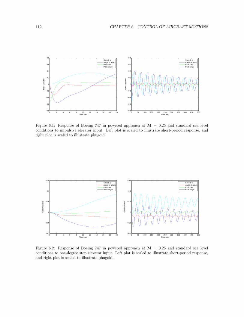
112 CHAPTER 6. CONTROL OF AIRCRAFT MOTIONS
0 2 4 6 8 10 12 14 16 18 20−0.8
−0.6
−0.4
−0.2
0
0.2
0.4
0.6
0.8
Time, sec
Sta
te V
aria
ble
Speed, uAngle of attackPitch ratePitch angle
0 50 100 150 200 250 300 350 400 450 500−0.8
−0.6
−0.4
−0.2
0
0.2
0.4
0.6
0.8
Time, sec
Sta
te V
aria
ble
Speed, uAngle of attackPitch ratePitch angle
Figure 6.1: Response of Boeing 747 in powered approach at M = 0.25 and standard sea levelconditions to impulsive elevator input. Left plot is scaled to illustrate short-period response, andright plot is scaled to illustrate phugoid.
0 2 4 6 8 10 12 14 16 18 20−0.1
−0.05
0
0.05
0.1
0.15
Time, sec
Sta
te V
aria
ble
Speed, uAngle of attackPitch ratePitch angle
0 50 100 150 200 250 300 350 400 450 500−0.1
−0.05
0
0.05
0.1
0.15
Time, sec
Sta
te V
aria
ble
Speed, uAngle of attackPitch ratePitch angle
Figure 6.2: Response of Boeing 747 in powered approach at M = 0.25 and standard sea levelconditions to one-degree step elevator input. Left plot is scaled to illustrate short-period response,and right plot is scaled to illustrate phugoid.
6.3. SYSTEM FREQUENCY RESPONSE 113
for the one-degree value of η0. The new equilibrium state corresponds to an increase in flight speedat a reduced angle of attack. Since the resulting lift coefficient is reduced, the pitch angle becomesnegative – i.e., the aircraft has begun to descend.
The approximations of the preceding analysis are completely consistent with those made in ourearlier study of static longitudinal control, where we found the control sensitivity to be
dδe
dCL
)
trim
=Cmα
∆(6.52)
where∆ = −CLαCmδe
+ CmαCLδe(6.53)
Thus, from the static analysis we estimate for a step input of one degree in elevator
∆CL =δe
Cmα/∆=
π/180
(−1.26)/(7.212)= −.100 (6.54)
The asymptotic steady state of the dynamic analysis gives exactly the same result
∆CL = CLαα + CLδe= 5.70(−.0186) + 0.338(π/180) = −.100 (6.55)
This result illustrates the consistency of the static and dynamic analyses. Note, however, that if thedynamic analysis included compressibility or aeroelastic effects, the results would not have agreedexactly, as these effects were not taken into account in the static control analysis.
6.3 System Frequency Response
The frequency response of a system corresponds to its response to harmonic control input of theform
η(t) = η0eıωtH(t)
= η0 (cos ωt + ı sin ωt)H(t)(6.56)
where H(t) is the Heaviside step function, see Eq. (6.40). This input corresponds to a sinusoidaloscillation of the control at frequency ω, and the system response consists of a start-up transientwhich ultimately evolves into an asymptotically steady-state harmonic response. Plots of the am-plitude of the steady-state harmonic response as a function of the input frequency ω are known asBode plots, and are useful for identifying resonant frequencies of the system.
Frequency response is an important element of classical control theory, and is the principal reasonthat Laplace transforms are such an important tool for control system designers. We will, however,constrain ourselves (at least for now) to dealing with response in the time domain, and not considerfrequency response further.
6.4 Controllability and Observability
Two important properties of a system are its controllability and its observability. Controllabilityrelates to the ability of the control input to influence all modes of the system. For a system having

114 CHAPTER 6. CONTROL OF AIRCRAFT MOTIONS
a single scalar control variable η(t) the system is described by
x = Ax + Bη(t) (6.57)
The system response is related to the eigenvalues of the matrix A, and these are invariant under atransformation of coordinates. The state vector can be transformed to modal coordinates by
v(t) = P−1x(t) (6.58)
where P is the modal matrix of A. That is, the similarity transformation
P−1AP = Λ (6.59)
transforms A to the diagonal matrix Λ. If such a transformation exists,3 then the state equationscan be written as
Pv = APv + Bη(t) (6.60)
or, after pre-multiplying by P−1,v = Λv + P−1Bη(t) (6.61)
Since Λ is a diagonal matrix, this transformation has completely decoupled the equations; i.e.,Eqs. (6.61) are equivalent to
vj = λjvj + fjη(t) (6.62)
where fj are the elements of the vector P−1B. Thus, the evolution of each mode is independent ofall the others, and the j-th mode is affected by the control so long as fj 6= 0. In other words, all themodes are controllable so long as no element of P−1B is zero.
This same transformation process can be applied to the case when η is a vector – i.e., when thereare multiple control inputs. In this case, all modes are controllable so long as at least one elementin each row of the matrix P−1B is non-zero.
6.4.1 Controllability
For cases in which the plant matrix is not diagonalizable a more general procedure must be followedto determine whether the system is controllable. In these cases, we introduce the more specificdefinition of controllability:
Definition: A system is said to be controllable if it is possible by means of an uncon-strained controller to transfer the physical system between any two arbitrarily specifiedstates in a finite time.
The requirement for controllability is well understood for linear, time-invariant systems. For suchsystems we can write
x = Ax + Bη(t) (6.63)
where we assume, for simplicity of presentation, that η(t) represents a single control variable. Thus,if the state vector x has n elements, A is an n × n matrix and B is an n × 1 column vector.
3A diagonalizing transformation will exist if the matrix A has a complete set of linearly independent eigenvectors;in this case the modal matrix P will be non-singular and its inverse will exist. A sufficient condition for the matrixA to have a complete set of linearly independent eigenvectors is that its eigenvalues be real and distinct, but thiscondition is not necessary.

6.4. CONTROLLABILITY AND OBSERVABILITY 115
The system of Eqs. (6.63) has the response
x(t) = eAt
[
x(0) +
∫ t
0
e−AtBη(τ) dτ
]
(6.64)
Since the states are arbitrary, we can choose the final state x(t) = 0 with no loss of generality, inwhich case Eqs. (6.64) become
x(0) = −∫ t
0
e−AtBη(τ) dτ (6.65)
Thus, the question of controllability reduces to whether a control law η(τ) exists that satisfiesEqs. (6.65) for every possible initial state x(0).
Recall that the Cayley-Hamilton theorem tells us that, if the characteristic equation of the plantmatrix is
λn + an−1λn−1 + an−2λ
n−2 + · · · + a1λ + a0 = 0 (6.66)
then we also have
An + an−1An−1 + an−2A
n−2 + · · · + a1A + a0I = 0 (6.67)
This equation can be used to represent any polynomial in the matrix A as a polynomial of ordern − 1. In particular, it can be used to represent the matrix exponential as the finite sum
e−Aτ = I − Aτ +A2τ2
2!− A3τ3
3!+ · · ·
=n−1∑
k=0
fk(τ)Ak(6.68)
The actual process of determining the coefficient functions fk(τ) might be very difficult and tedious,but for our purposes here we don’t need to determine these coefficient functions explicitly, we onlyneed to believe that such a representation is always possible.
Using Eq. (6.68) allows us to write the controllability requirement as
x(0) = −∫ t
0
n−1∑
k=0
fk(τ)AkBη(τ) dτ (6.69)
or
x(0) = −n−1∑
k=0
AkB
∫ t
0
fk(τ)η(τ) dτ (6.70)
Now, for any fk(τ) and η(τ) we can write
∫ t
0
fk(τ)η(τ) dτ = gk for k = 0, 1, 2, . . . , n − 1 (6.71)

116 CHAPTER 6. CONTROL OF AIRCRAFT MOTIONS
so Eqs.(6.70) can be written as
x(0) = −n−1∑
k=0
AkBgk
= −Bg0 − ABg1 − A2Bg2 − · · · − An−1Bgn−1
= −[
B AB A2B · · · An−1B]
g0
g1
g2
.
.
.gn−1
(6.72)
This is a system of equations for the vector g = [g0 g1 g2 . . . gn−1]T
of the form
Vg = −x(0) (6.73)
which will have a solution for any arbitrarily chosen x(0) if the controllability matrix
V =[
B AB A2B · · · An−1B]
(6.74)
has full rank n.
Our analysis here has assumed there is only a single (scalar) control variable, but the analysis followsthrough with no essential change in the case when the control variable η(τ) is a p-element vector.In this case g will be an n · p × 1 vector, and the corresponding controllability matrix will have thesame form as in Eq. (6.74), but since each element there has the same shape as B – an n× p matrix– the controllability matrix will have n rows and n · p columns. The controllability criterion stillrequires that the rank of this matrix be n.
Generally, elevator control alone is sufficient to control all longitudinal modes, and either rudder oraileron control is sufficient to control all lateral/directional modes.
It should be noted that controllability alone says nothing about the quality of the control, sincearbitrarily large control input was assumed to be available. So, it is still important to look atspecific control responses and/or sensitivities to determine if sufficient control action is available toachieve desired motions without saturating the controls.
Example
We consider the example of the system
x = Ax + Bη(t) (6.75)
where
A =
(
0 1−2 −3
)
, and B =
(
01
)
(6.76)
The characteristic equation of the plant matrix is
det(A − λI) = λ2 + 3λ + 2 = 0 (6.77)

6.4. CONTROLLABILITY AND OBSERVABILITY 117
whose roots are λ = −1, −2.
The eigenvectors of A are thus determined from
(A − λ1I)u1 = 0
which gives
u11+ u12
= 0
whence
u1 = [1 − 1]T
Similarly,
(A − λ2I)u2 = 0
gives
2u21+ u22
= 0
whence
u2 = [1 − 2]T
The modal matrix of A and its inverse are then
P =
(
1 1−1 −2
)
and P−1 =
(
2 1−1 −1
)
(6.78)
The characteristic variables are thus
v = P−1x =
(
2 1−1 −1
)(
x1
x2
)
=
(
2x1 + x2
−x1 − x2
)
(6.79)
and
PAP−1 =
(
λ1 00 λ2
)
=
(
−1 00 −2
)
(6.80)
and
P−1B =
(
2 1−1 −1
)
=
(
01
)
=
(
1−1
)
(6.81)
The canonical form of the equations describing the system can thus be written
v =
(
−1 00 −2
)
v +
(
1−1
)
η(t) (6.82)
Both modes are thus seen to be controllable.
Alternatively, since
AB =
(
0 1−2 −3
)(
01
)
=
(
1−3
)
(6.83)
the controllability matrix is
V = [B AB] =
(
0 11 −3
)
(6.84)
The determinant of the controllability matrix det(V) = −1, is non-zero, so its rank must be 2, andthe system is again seen to be controllable.

118 CHAPTER 6. CONTROL OF AIRCRAFT MOTIONS
Note that if the control matrix is changed to
B =
(
−11
)
(6.85)
then
P−1B =
(
2 1−1 −1
)
=
(
−11
)
=
(
−10
)
(6.86)
and the second mode is seen to be uncontrollable. Equivalently, since we now have
AB =
(
0 1−2 −3
) (
−11
)
=
(
1−1
)
(6.87)
the controllability matrix becomes
V = [B AB] =
(
−1 11 −1
)
(6.88)
The determinant of the controllability matrix det(V) = 0, is now zero, so its rank must be less than2, and the modified system is again seen to be uncontrollable.
6.4.2 Observability
The mathematical dual of controllability is observability , which is defined according to:
Definition: A system is observable at time t0 if the output history y(t) in the timeinterval [t0, tf ] is sufficient to determine x(t0).
It can be shown, by a process analogous to that of the preceding section, that, for linear, time-invariant systems, observability is guaranteed when the rank of the observability matrix
U =
C
CA
CA2
···
CAn−1
(6.89)
is equal to n. Note that if the output vector y has q elements, the observability matrix will haveq · n rows and n columns.
6.4.3 Controllability, Observability, and Matlab
Once the plant matrix A, the control matrix B, and the output matrix C have been defined, theMatlab function
V = ctrb(A,B)

6.5. STATE FEEDBACK DESIGN 119
determines the controllability matrix V, and the Matlab function
U = obsv(A,C)
determines the observability matrix U. The rank of either of these matrices can then be determinedusing the Matlab function rank.
6.5 State Feedback Design
A feedback control system can be designed within the state-variable framework to provide a specificeigenvalue structure for the closed-loop plant matrix. Consider the system
x = Ax + Bη
y = Cx(6.90)
It can be shown that, if the system is controllable it is possible to define a linear control law toachieve any desired closed-loop eigenvalue structure. For a single-input system, a linear control lawis given by
η = −kT x + η′ (6.91)
where η′ is the control input in the absence of feedback, and k is a vector of feedback gains. Theblock diagram of this system is illustrated in Fig. 6.3.
Introducing the control law into the state equation system gives
x = Ax + B[
η′ − kT x]
=[
A − BkT]
x + Bη′
= A∗x + Bη′
(6.92)
where the plant matrix describing the behavior of the closed-loop system
A∗ = A − BkT (6.93)
is called the augmented matrix for the system.
For cases in which the plant matrix A of the system has undesirable eigenvalues, the augmentedmatrix A∗ can be made to have more desirable eigenvalues by proper choice of the elements ofthe feedback gain vector k. Note that the effect of state-variable feedback can be interpreted asmodifying the plant matrix of the system; i.e., the effect of the feedback can be interpreted aseffectively changing the properties of the system – the aerodynamic stability derivatives – to achievemore desirable response characteristics.
+ −
ηη ’ x y
C
k
x = Ax + B η.
T
Figure 6.3: Block diagram for system with state-variable feedback.

120 CHAPTER 6. CONTROL OF AIRCRAFT MOTIONS
Example: State Feedback Design
Given the system
x = Ax + Bη
y = Cx(6.94)
with
A =
(
−3 80 0
)
, B =
(
04
)
, C =(
1 0)
(6.95)
we wish to use state-variable feedback to provide closed-loop response having
ωn = 25 sec−1 and ζ = 0.707 (6.96)
Note that the characteristic equation of the original plant matrix is
det(A − λI) = (−3 − λ)(−λ) = λ2 + 3λ = λ(λ + 3) = 0 (6.97)
so the original system has one neutrally stable eigenvalue.
First, the controllability of the system is verified. For this system the controllability matrix is
V = [B AB] =
(
0 324 0
)
(6.98)
so, det(V) = −128, whence V has full rank so the system is controllable. The general form of theaugmented matrix is
A∗ = A − BkT =
(
−3 80 0
)
−(
04
)
(
k1 k2
)
=
(
−3 8−4k1 −4k2
)
(6.99)
The characteristic equation of the augmented matrix A∗ is then
det(A∗ − λI) = (−3 − λ)(−4k2 − λ) + 32k1 = λ2 + (3 + 4k2)λ + 32k1 + 12k2 = 0 (6.100)
Since the desired system response corresponds to the characteristic equation
λ2 + 2ζωnλ + ω2n = 0
λ2 + 2(0.707)(25)λ + (25)2 = 0 = λ2 + 35.35λ + 625(6.101)
a comparison of Eqs. (6.100) and (6.101) shows that we must choose the elements of the gain vectorsuch that
3 + 4k2 = 35.35
32k1 + 12k2 = 625
or
k2 =35.35 − 3
4= 8.09
k1 =625 − 12(8.09)
32= 16.5
(6.102)
The response of the original system and the closed-loop response are compared in Fig. 6.4 for twodifferent initial perturbations. Figure 6.4(a) illustrates the response when the neutrally stable modeis not excited. Figure 6.4(b) illustrates the response when the neutrally stable mode is excited; inthis case the original system never returns to the original equilibrium state. But, in both casesthe closed-loop system returns quickly, with minimal overshoot, to the original equilibrium state.Note, however, that significant excitation of x2 is required in the latter case, even for the first initialcondition.

6.5. STATE FEEDBACK DESIGN 121
0 0.2 0.4 0.6 0.8 1 1.2 1.4 1.6 1.8 2−0.2
0
0.2
0.4
0.6
0.8
1
1.2
Time, sec
Sta
te v
aria
ble
Original system, x
1
Original system, x2
With feedback, x1
With feedback, x2
0 0.5 1 1.5 2 2.5 3 3.5 4 4.5 5−0.2
0
0.2
0.4
0.6
0.8
1
1.2
Time, sec
Sta
te v
aria
ble
Original system, x
1
Original system, x2
With feedback, x1
With feedback, x2
(a) x(0) = [1.0 0.0] (b) x(0) = [1.0 0.1]
Figure 6.4: Response of linear, second-order system, showing effect of state variable feedback. Orig-inal system has λ1 = −3.0, λ2 = 0.0. Modified system has ωn = 25 sec−1 and ζ = 0.707. (a)x(0) = [1.0 0.0]T ; (b) x(0) = [1.0 0.1]T .
6.5.1 Single Input State Variable Control
When the control variable is a single scalar, the feedback gains are uniquely determined by thelocations of the roots of the characteristic equation of the augmented matrix. In this case, thealgorithm of Bass & Gura (see, e.g., [3]) can be used to determine the elements of the gain vector.
We describe the procedure for the system described by
x = Ax + Bη (6.103)
with the control law
η = −kT x + η′ (6.104)
It is desirable to have the plant matrix in the (first) companion form,
A =
−a1 −a2 −a3 · · · −an−1 −an
1 0 0 · · · 0 00 1 0 · · · 0 00 0 1 · · · 0 0
· · ·0 0 0 · · · 1 0
(6.105)
where it is clear from direct calculation of the determinant of A − λI that the elements ai are thecoefficients of the characteristic equation
λn + a1λn−1 + a2λ
n−2 + · · · + an−1λ + an = 0 (6.106)
of the plant matrix A. Note that the homogeneous equations corresponding to the plant matrix of

122 CHAPTER 6. CONTROL OF AIRCRAFT MOTIONS
Eq. (6.105) are of the form
x1 =−a1x1−a2x2−a3x3− · · ·−an−1xn−1−anxn
x2 = x1
x3 = x2 (6.107)
x4 = x3
· · ·xn = xn−1
so the system is equivalent to the single higher-order equation
dny
dtn+ a1
dn−1y
dtn−1+ a2
dn−2y
dtn−2+ · · · + an−1
dy
dt+ any = f(t) (6.108)
where y = xn. Thus, when the equations are in companion form, the control matrix takes the specialform
B = [1 0 0 · · · 0]T
(6.109)
Now, as we have seen, when the control law of Eq. (6.104) is substituted into the Eqs. (6.103), theequations take the form
x = A∗x + Bη′ (6.110)
where
A∗ = A − BkT (6.111)
is the augmented matrix. Because of the special form of the control matrix when the equations arein companion form, the augmented matrix takes the form
A∗ =
−a1 − k1 −a2 − k2 −a3 − k3 · · · −an−1 − kn−1 −an − kn
1 0 0 · · · 0 00 1 0 · · · 0 00 0 1 · · · 0 0
· · ·0 0 0 · · · 0 00 0 0 · · · 1 0
(6.112)
The characteristic equation of the augmented matrix can thus be computed directly as
λn + (a1 + k1) λn−1 + (a2 + k2) λn−2 + · · · (an−1 + kn−1) λ + (an + kn) = 0 (6.113)
Now, once the desired eigenvalues λi have been established, the characteristic equation of the desiredaugmented matrix can also be computed directly from
(
λ − λ1
) (
λ − λ2
) (
λ − λ3
)
· · ·(
λ − λn
)
= 0
λn + a1λn−1 + a2λ
n−2 + a3λn−3 + · · · + an−1λ + an = 0 (6.114)
and the desired gains are determined by equating the coefficients in Eqs. (6.113) and (6.114):
ai + ki = ai , for i = 1, 2, . . . , n
or
ki = ai − ai , for i = 1, 2, . . . , n (6.115)

6.5. STATE FEEDBACK DESIGN 123
Transformation to Companion Form
In order to use the results of the preceding section for a general system, we need to be able totransform an arbitrary plant matrix A to its (first) companion form
A =
−a1 −a2 −a3 · · · −an−1 −an
1 0 0 · · · 0 00 1 0 · · · 0 00 0 1 · · · 0 0
· · ·0 0 0 · · · 1 0
(6.116)
That is, it is necessary to find the matrix T such that
A = TAT−1 (6.117)
where A has the desired form illustrated in Eq. (6.116). It is convenient to represent the neededmatrix as the product of two simpler matrices
T = RS (6.118)
so that
A = RSAS−1R−1 (6.119)
where the intermediate transformation
A = SAS−1 (6.120)
takes the matrix to the (second) companion form
A =
0 0 0 · · · 0 −an
0 1 0 · · · 0 −an−1
0 0 1 · · · 0 −an−2
0 0 0 · · · 0 −an−3
· · ·0 0 0 · · · 1 −a1
(6.121)
We first show that the intermediate transformation
A = SAS−1 (6.122)
is achieved when S is chosen to be the inverse of the controllability matrix V, defined in Eq. (6.74).Thus, we must show that
S−1A = AS−1 (6.123)
or
VA = AV (6.124)
For a single-input system, the controllability matrix takes the form
V =[
b Ab A2b · · · An−1b]
(6.125)

124 CHAPTER 6. CONTROL OF AIRCRAFT MOTIONS
where b is an n-vector and, for A in the (second) companion form, we have
VA =[
b Ab A2b · · · An−1b]
0 0 0 · · · 0 −an
1 0 0 · · · 0 −an−1
0 1 0 · · · 0 −an−2
0 0 1 · · · 0 −an−3
· · ·0 0 0 · · · 0 −a2
0 0 0 · · · 1 −a1
=[
Ab A2b A3b · · · − anb − an−1Ab · · · − a1An−1b
]
(6.126)
The Cayley-Hamilton Theorem can be used to express the final column in the above matrix as
(
−anI − an−1A − an−2A2 − · · · − a1A
n−1)
b = Anb (6.127)
Thus,
VA = A[
b Ab A2b · · · An−1b]
= AV (6.128)
as was to be shown.
For the final transformation, we require
A = RAR−1 (6.129)
to have the desired form, or
R−1A = AR−1 (6.130)
The required matrix R−1 has the form
R−1 =
1 a1 a2 a3 · · · an−2 an−1
0 1 a1 a2 · · · an−3 an−2
0 0 1 a1 · · · an−4 an−3
0 0 0 1 · · · an−5 an−4
· · ·0 0 0 0 · · · 0 1
= W (6.131)
which can be verified by noting that
R−1A =
1 a1 a2 a3 · · · an−2 an−1
0 1 a1 a2 · · · an−3 an−2
0 0 1 a1 · · · an−4 an−3
0 0 0 1 · · · an−5 an−4
· · ·0 0 0 0 · · · 0 1
−a1 −a2 −a3 · · · −an−1 −an
1 0 0 · · · 0 00 1 0 · · · 0 00 0 1 · · · 0 0
· · ·0 0 0 · · · 1 0
=
0 0 0 · · · 0 −an
1 a1 a2 · · · an−2 00 1 a1 · · · an−3 00 0 1 · · · an−4 0
· · ·0 0 0 · · · a1 00 0 0 · · · 1 0
(6.132)
6.5. STATE FEEDBACK DESIGN 125
while
AR−1 =
0 0 0 · · · 0 −an
1 0 0 · · · 0 −an−1
0 1 0 · · · 0 −an−2
0 0 1 · · · 0 −an−3
· · ·0 0 0 · · · 0 −a2
0 0 0 · · · 1 −a1
1 a1 a2 a3 · · · an−2 an−1
0 1 a1 a2 · · · an−3 an−2
0 0 1 a1 · · · an−4 an−3
0 0 0 1 · · · an−5 an−4
· · ·0 0 0 0 · · · 0 1
=
0 0 0 · · · 0 −an
1 a1 a2 · · · an−2 00 1 a1 · · · an−3 00 0 1 · · · an−4 0
· · ·0 0 0 · · · a1 00 0 0 · · · 1 0
= R−1A
(6.133)
as was to be shown.
Now, we have seen for the system in companion form
z = Az + Bη (6.134)
subject to the control law
η = −kT z + η′ (6.135)
the roots of the augmented matrix are driven to those of the characteristic equation
λn + a1λn−1 + a2λ
n−2 + · · · + an−1λ + a0 = 0 (6.136)
by the gain vector having elements
ki = ai − ai (6.137)
where ai are the coefficients of the characteristic equation of the original (open-loop) plant matrix.
The system of Eqs.(6.134) in companion form can be related back to the original system by intro-ducing the transformation
z = Tx (6.138)
to give
Tx = TAT−1Tx + Bη (6.139)
or
x = Ax + T−1Bη (6.140)
The control law then transforms as
η = −kT x = −kT T−1z = −kT z (6.141)
whence
kT T−1 = kT (6.142)
or
k = TT k (6.143)
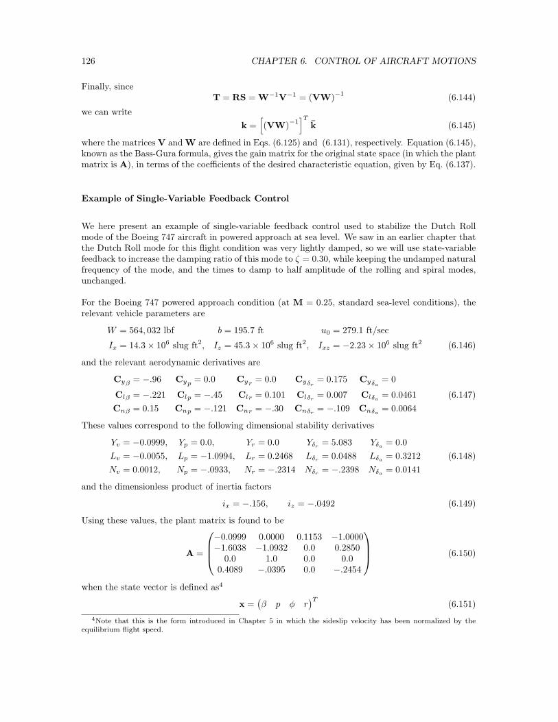
126 CHAPTER 6. CONTROL OF AIRCRAFT MOTIONS
Finally, sinceT = RS = W−1V−1 = (VW)
−1(6.144)
we can write
k =[
(VW)−1
]T
k (6.145)
where the matrices V and W are defined in Eqs. (6.125) and (6.131), respectively. Equation (6.145),known as the Bass-Gura formula, gives the gain matrix for the original state space (in which the plantmatrix is A), in terms of the coefficients of the desired characteristic equation, given by Eq. (6.137).
Example of Single-Variable Feedback Control
We here present an example of single-variable feedback control used to stabilize the Dutch Rollmode of the Boeing 747 aircraft in powered approach at sea level. We saw in an earlier chapter thatthe Dutch Roll mode for this flight condition was very lightly damped, so we will use state-variablefeedback to increase the damping ratio of this mode to ζ = 0.30, while keeping the undamped naturalfrequency of the mode, and the times to damp to half amplitude of the rolling and spiral modes,unchanged.
For the Boeing 747 powered approach condition (at M = 0.25, standard sea-level conditions), therelevant vehicle parameters are
W = 564, 032 lbf b = 195.7 ft u0 = 279.1 ft/sec
Ix = 14.3 × 10⁶ slug ft2, Iz = 45.3 × 10⁶ slug ft2, Ixz = −2.23 × 10⁶ slug ft2 (6.146)
and the relevant aerodynamic derivatives are
Cyβ = −.96 Cyp = 0.0 Cyr = 0.0 Cyδr= 0.175 Cyδa
= 0
Clβ = −.221 Clp = −.45 Clr = 0.101 Clδr= 0.007 Clδa
= 0.0461 (6.147)
Cnβ = 0.15 Cnp = −.121 Cnr = −.30 Cnδr= −.109 Cnδa
= 0.0064
These values correspond to the following dimensional stability derivatives
Yv = −0.0999, Yp = 0.0, Yr = 0.0 Yδr= 5.083 Yδa
= 0.0
Lv = −0.0055, Lp = −1.0994, Lr = 0.2468 Lδr= 0.0488 Lδa
= 0.3212 (6.148)
Nv = 0.0012, Np = −.0933, Nr = −.2314 Nδr= −.2398 Nδa
= 0.0141
and the dimensionless product of inertia factors
ix = −.156, iz = −.0492 (6.149)
Using these values, the plant matrix is found to be
A =
−0.0999 0.0000 0.1153 −1.0000−1.6038 −1.0932 0.0 0.2850
0.0 1.0 0.0 0.00.4089 −.0395 0.0 −.2454
(6.150)
when the state vector is defined as4
x =(
β p φ r)T
(6.151)
4Note that this is the form introduced in Chapter 5 in which the sideslip velocity has been normalized by theequilibrium flight speed.

6.5. STATE FEEDBACK DESIGN 127
(i.e., is based on sideslip angle rather than sideslip velocity).
The roots of the characteristic equation are found to be the same as those in Chapter 5 of the classnotes:
λDR = −.08066 ± ı 0.7433
λroll = −1.2308
λspiral = −.04641
(6.152)
The undamped natural frequency and damping ratio of the Dutch Roll mode are thus
ωnDR= 0.7477 sec−1 and ζDR = 0.1079 (6.153)
The times to damp to half amplitude for the rolling and spiral modes are seen to be
t1/2roll= 0.56 sec and t1/2spiral
= 14.93 sec (6.154)
respectively.
We now determine the gains required, using rudder control only , to increase the damping ratio ofthe Dutch Roll mode to ζ = 0.30, while keeping the other modal properties fixed.
The original plant matrix is the same as that in Eq. (6.150), and its characteristic equation is givenby
λ4 + 1.4385λ3 + 0.8222λ2 + 0.7232λ + 0.0319 = 0 (6.155)
The characteristic equation of the desired system is
(λ − λroll)(λ − λspiral)(λ2 + 2ζωnλ + ω2
n)DR = 0
(λ + 1.2308)(λ + 0.04641)(λ2 + 2ζωnλ + ω2n) = 0
(λ2 + 1.2772λ + 0.05712)(λ2 + 2(0.30)(0.7477)λ + (0.7477)2) = 0
(λ2 + 1.2772λ + 0.05712)(λ2 + 0.4486λ + 0.5591) = 0
λ4 + 1.7258λ3 + 1.1891λ2 + 0.7396λ + 0.0319 = 0
(6.156)
and by construction the roots will be the same as for the original system, except the damping ratiofor the Dutch Roll mode will be increased to
ζ = 0.30
Comparing the coefficients in the characteristic Eqs. (6.155) and (6.156), the gain vector in thecompanion form space is seen to be
k = [1.7258 1.1891 0.7396 0.0319]T − [1.4385 0.8222 0.7232 0.0319]T
= [0.2873 0.3669 0.0164 0.0000]T(6.157)
The control matrix, assuming rudder-only control, is
B = [0.0182 0.0868 0.0 − .2440]T (6.158)
and the gain vector in the original state vector space required to achieve the desired augmentedmatrix is
k =[
(VW)−1
]T
k = [0.1383 0.0943 0.1250 − 1.1333]T (6.159)

128 CHAPTER 6. CONTROL OF AIRCRAFT MOTIONS
0 5 10 15 20 25 30−0.2
−0.15
−0.1
−0.05
0
0.05
0.1
0.15
0.2
Time, sec
Sta
te V
aria
ble
SideslipRoll rateRoll angleYaw rate
0 5 10 15 20 25 30−0.2
−0.15
−0.1
−0.05
0
0.05
0.1
0.15
0.2
Time, sec
Sta
te V
aria
ble
SideslipRoll rateRoll angleYaw rate
(a) (b)
Figure 6.5: Boeing 747 aircraft in powered approach at standard sea level conditions and M = 0.25;response to 5 degree (0.08727 radian) perturbation in sideslip. (a) Original open-loop response; (b)Closed loop response with Dutch Roll damping ratio changed to ζ = 0.30 using rudder state-variablefeedback.
where
V = [B AB A2B A3B] (6.160)
is the controllability matrix and
W =
1 a1 a2 a3
0 1 a1 a2
0 0 1 a1
0 0 0 1
(6.161)
where the element ai is the coefficient of λ4−i in the characteristic equation of the original system.
The augmented plant matrix for the closed-loop system is
A∗ =
−0.1024 −.0017 0.1130 −.9794−1.6158 −1.1014 −.0109 0.3834
0.0 1.0 0.0 0.00.4427 −.0165 0.0305 −.5220
(6.162)
Comparing the augmented plant matrix of Eq. (6.162) with that for the original (open-loop) systemin Eq. (6.150), we see that by far the largest change is in the a4,4 element, indicating that theeffective value of yaw damping has more than doubled. We saw from our approximate analysis thatyaw damping had a stabilizing effect on both, the spiral and Dutch Roll modes.
The response of the closed-loop system to a 5 degree perturbation in sideslip angle is compared tothat of the original open-loop system in Fig. 6.5. The Dutch Roll response of the closed-loop systemis seen, as expected, to be much more heavily damped than that of the original system.
We next determine the gains required, using aileron control only , to increase the damping ratio of theDutch Roll mode to ζ = 0.30, while keeping the other modal parameters unchanged. The originalplant matrix, its characteristic equation, and the characteristic equation of the desired system are

6.5. STATE FEEDBACK DESIGN 129
0 5 10 15 20 25 30−0.2
−0.15
−0.1
−0.05
0
0.05
0.1
0.15
0.2
Time, sec
Sta
te V
aria
ble
SideslipRoll rateRoll angleYaw rate
0 5 10 15 20 25 30−0.2
−0.15
−0.1
−0.05
0
0.05
0.1
0.15
0.2
Time, sec
Sta
te V
aria
ble
SideslipRoll rateRoll angleYaw rate
(a) (b)
Figure 6.6: Boeing 747 aircraft in powered approach at standard sea level conditions and M = 0.25;response to 5 degree (0.08727 radian) perturbation in sideslip. (a) Original open-loop response; (b)Closed loop response with Dutch Roll damping ratio changed to ζ = 0.30 using aileron state-variablefeedback.
all the same as in the previous exercise, so the gain matrix for the companion form system is alsounchanged. The control matrix, however, is now that for aileron-only control, and is given by
B = [0.0000 0.3215 0.0000 − .0017]T (6.163)
The gain vector in the original state vector space required to achieve the desired augmented matrixis then
k =[
(VW)−1
]T
k = [−3.5417 0.8715 0.6746 − 4.0504]T (6.164)
The response of the closed-loop system to a 5 degree perturbation in sideslip angle is comparedwith that of the original system in Fig. 6.6. As for the case of rudder-only control, the closed-loopresponse is seen to be much more heavily damped than that of the open-loop system.
The augmented plant matrix for the closed-loop system in this case is
A∗ =
−0.0999 0.0000 0.1153 −1.0000−0.4651 −1.3734 −.2169 1.5873
0.0 1.0 0.0 0.00.4027 −.0380 .0012 −.2525
(6.165)
Comparing this plant matrix with that for the original (open-loop) system in Eq. (6.150), we seethat by far the largest changes are in the a2,1 and a2,4 elements. The effective dihedral effect hasbeen reduced to less than 30% of its original value, while the effective roll-due-to-yaw rate has beenincreased by more than a factor of five. Thus, it seems that the control algorithm has stabilized theDutch Roll mode by reducing the effective dihedral effect; then, in order to not increase the spiralmode stability it has effectively increased the (positive) roll-due-to-yaw rate derivative.

130 CHAPTER 6. CONTROL OF AIRCRAFT MOTIONS
6.5.2 Multiple Input-Output Systems
For multiple input-output systems having p controls, the feedback control law has the form
η = −Kx + η′ (6.166)
where K is the p × n gain matrix . Thus, there are now p × n gains to be specified, but there arestill only n eigenvalues to be specified.
This additional flexibility can be used to configure the control system in a more optimal way if thecontrol engineer understands the system well enough to make intelligent choices for how to allocatethe gains. But, even for the single-input system, it is not always clear what is the best placementfor the eigenvalues of the augmented matrix. Clearly, more stability is desirable for the less stablemodes, but too much stability can result in a system that requires great effort from the pilot toachieve required maneuvers. Equations (6.137) and (6.145) indicate that more control effort will berequired as the roots of the augmented matrix are moved further and further to the left of those ofthe original plant matrix. Also, it is generally important that the closed-loop frequency response notbe increased too much to avoid exciting modes that have not been modeled, such as those arisingfrom structural deformation due to aeroelasticity.
6.6 Optimal Control
As has been seen in the previous sections, use of the Bass-Gura procedure often is difficult, or resultsin sub-optimal performance for a variety of reasons. These include:
1. The best choice of desired placement for the eigenvalues of the augmented matrix is not alwaysobvious;
2. Particular eigenvalue placement may require more control input than it available; this canresult in saturation of the control action, which introduces non-linearity and can even resultin instability;
3. For multiple input-output systems, we need to develop strategies for deciding on how to allocatethe gains among the n × p elements, since we have only n eigenvalues to place;
4. The process may not be controllable; i.e., if the rank of the controllability matrix V is lessthan n, the method fails since Eq. (6.145) requires determination of the inverse of V.
All these points argue for a control design strategy that, in some sense, optimizes the gain matrixfor stabilizing a given system. This is the goal of what has come to be called optimal control .
6.6.1 Formulation of Linear, Quadratic, Optimal Control
The optimal control of the linear system
x = Ax + Bη(t) (6.167)

6.6. OPTIMAL CONTROL 131
is defined as the control vector η(t) that drives the state from a specified initial state x(t) to adesired final state xd(tf ) such that a specified performance index
J =
∫ tf
t
g(x(τ), η(τ), τ) dτ (6.168)
is minimized. For quadratic optimal control, the performance index is specified in the form
g = xT Qx + ηT Rη (6.169)
where Q and R are symmetric, positive-definite matrices, and the performance index becomes
J =
∫ tf
t
(
xT Qx + ηT Rη)
dτ (6.170)
If the control law is assumed to be linear, i.e., of the form
η = −Kx + η′ (6.171)
then the determination of the gain matrix K that minimizes J is called the linear quadratic regulator(LQR) problem. For this control law the closed-loop response of the system to a perturbation isgiven by
x = [A − BK]x = A∗x (6.172)
whereA∗ = A − BK (6.173)
is the augmented plant matrix.
We usually are interested in cases for which the matrices A, B, and K are independent of time,but the development here is easier if we allow the augmented matrix A∗ to vary with time. In thiscase, we cannot express the solution to Eq. (6.172) in terms of a matrix exponential, but we can stillexpress it in terms of the general state transition matrix Φ∗ as
x(τ) = Φ∗(τ, t)x(t) (6.174)
Equation (6.174) simply implies that the state of the system at any time τ depends linearly on thestate at any other time t. When the control law of Eq. (6.171) is substituted into the performanceindex of Eq. (6.170) and Eq. (6.174) is used to express the evolution of the state variable, the quantityto be minimized becomes
J =
∫ tf
t
xT (τ)[
Q + KT RK]
x(τ) dτ
=
∫ tf
t
xT (t)Φ∗T (τ, t)[
Q + KT RK]
Φ∗(τ, t)x(t) dτ
= xT (t)
(∫ tf
t
Φ∗T (τ, t)[
Q + KT RK]
Φ∗(τ, t) dτ
)
x(t)
(6.175)
orJ = xT (t)Sx(t) (6.176)
where
S(t, tf ) =
∫ tf
t
Φ∗T (τ, t)[
Q + KT RK]
Φ∗(τ, t) dτ (6.177)

132 CHAPTER 6. CONTROL OF AIRCRAFT MOTIONS
Note that, by its construction, the matrix S is symmetric, since the weighting matrices Q and R
are both symmetric.
The simple appearance of Eq. (6.176) belies the complexity of determining S from Eq. (6.177). Infact, if we had to use the latter equation to determine the matrix S, we would face an almost hopelesstask. Our expression of the solution in terms of the general state transition matrix seems to haveresulted in a simple expression for the integral we wish to minimize, but it is almost impossible todevelop a useful expression for the state transition matrix, itself, in general. Instead, in order to findthe gain matrix K that minimizes J , it is convenient to find a differential equation that the matrixS satisfies. To this end, we note that since
J =
∫ tf
t
xT (τ)Lx(τ) dt (6.178)
whereL = Q + KT RK (6.179)
we can writedJ
dt= − xT (τ)Lx(τ)
∣
∣
τ=t= −xT (t)Lx(t) (6.180)
But, from differentiating Eq. (6.176), we have
dJ
dt= xT (t)S(t, tf )x(t) + xT (t)S(t, tf )x(t) + xT (t)S(t, tf )x(t) (6.181)
and, substituting the closed-loop differential equation, Eq. (6.172), for x gives
dJ
dt= xT (t)
[
A∗TS(t, tf ) + S(t, tf ) + S(t, tf )A∗(t)
]
x(t) (6.182)
Thus, we have two expressions for the derivative dJ/dt: Eqs. (6.180) and (6.182). Both are quadraticforms in the initial state x(t), which must be arbitrary . The only way that two quadratic forms inx can be equal for any choice of x is if the underlying matrices are equal; thus, we must have
−L = A∗TS + S + SA∗
or−S = SA∗ + A∗T
S + L (6.183)
Equation (6.183) is a first-order differential equation for the matrix S, so it requires a single initialcondition to completely specify its solution. We can use Eq. (6.177), evaluated at t = tf to give therequired condition
S(tf , tf ) = 0 (6.184)
Once a gain matrix K has been chosen to close the loop, the corresponding performance of thesystem is given by Eq. (6.176), where S(t, tf ) is the solution of Eq. (6.183), which can be written interms of the original plant and gain matrices as
−S = S (A − BK) +(
AT − KT BT)
S + Q + KT RK (6.185)
Our task, then, is to find the gain matrix K that makes the solution to Eq. (6.185) as small aspossible – in the sense that the quadratic forms (Eq. (6.176)) associated with the matrix S areminimized. That is, we want to find the matrix S for which
J = xT Sx < xT Sx (6.186)

6.6. OPTIMAL CONTROL 133
for any arbitrary initial state x(t) and every matrix S 6= S.
We will proceed by assuming that such an optimum exists, and use the calculus of variations to findit. The minimizing matrix S must, of course, satisfy Eq. (6.185)
− ˙S = S
(
A − BK)
+(
AT − KT BT)
S + Q + KT RK (6.187)
and any non-optimum gain matrix, and its corresponding matrix S, can be expressed as
S = S + N
K = K + Z(6.188)
Substituting this form into Eq. (6.185) and subtracting Eq. (6.187) gives
−N = NA∗ + A∗T
N +(
KT R − SB)
Z + ZT(
RK − BT S)
+ ZT RZ (6.189)
where
A∗ = A − BK = A − B(
K + Z)
(6.190)
Note that Eq. (6.189) has exactly the same form as Eq. (6.183) with
L =(
KT R − SB)
Z + ZT(
RK − BT S)
+ ZT RZ (6.191)
so its solution must be of the form of Eq. (6.177)
N(t, tf ) =
∫ tf
t
Φ∗T (τ, t)LΦ∗(τ, t) dτ (6.192)
Now, if J is a minimum, then we must have
xT Sx ≤ xT(
S + N)
x = xT Sx + xT Nx (6.193)
and this equation requires that the quadratic form xT Nx be positive definite (or, at least, positivesemi-definite). But, if Z is sufficiently small, the linear terms in Z (and ZT ) in Eq. (6.191) willdominate the quadratic terms in ZT RZ, and we could easily find values of Z that would make L,and hence N, negative definite. Thus, the linear terms in Eq. (6.191) must be absent altogether .That is, for the gain matrix K to be optimum, we must have
KT R − SB = 0 = RK − BT S (6.194)
or, assuming that the weighting matrix R is not singular,
K = R−1BT S (6.195)
Equation (6.195) gives the optimum gain matrix K, once the matrix S has been determined. Whenthis equation is substituted back into Eq. (6.187) we have
− ˙S = SA + AT S − SBR−1BT S + Q (6.196)

134 CHAPTER 6. CONTROL OF AIRCRAFT MOTIONS
This equation, one of the most famous in modern control theory, is called the matrix Riccati equation,consistent with the mathematical nomenclature that identifies an equation with a quadratic non-linearity as a Riccati equation. The solution to this equation gives the matrix S which, whensubstituted into Eq. (6.195), gives the optimum gain matrix K.
Because of the quadratic nonlinearity in the Riccati equation, it is necessary, except in a few veryspecial cases, to solve it numerically. Since the matrix S is symmetric, Eq. (6.196) representsn(n + 1)/2 coupled, first-order equations. Since the “initial” condition is
S(tf , tf ) = 0 (6.197)
the equation must be integrated backward in time, since we are interested in S(t, tf ) for t < tf .
When the control interval [t, tf ] is finite, the gain matrix K will generally be time-dependent, evenwhen the matrices A, B, Q, and R are all constant. But, suppose the control interval is infinite, sothat we want to find the gain matrix K that minimizes the performance index
J∞ =
∫
∞
t
(
xT Qx + ηT Rη)
dτ (6.198)
In this case, integration of Eq. (6.196) backward in time will either grow without limit or converge
to a constant matrix S. If it converges to a limit, the derivative ˙S must tend to zero, and S must
satisfy the algebraic equation
0 = SA + AT S − SBR−1BT S + Q (6.199)
and the optimum gain in the steady state is given by
K = R−1BT S (6.200)
The single quadratic matrix Eq. (6.199) represents n(n + 1)/2 coupled scalar, quadratic equations,so we expect there will be n(n + 1) different (symmetric) solutions. The nature of these solutionsis, as one might expect, connected with issues of controllability and observability – and a treatmentof these issues is beyond the scope of our treatment here. But, for most design applications, it isenough to know that
1. If the system is asymptotically stable; or
2. If the system defined by (A, B) is controllable, and the system defined by (A, C), where theweighting matrix Q = CT C, is observable,
then the algebraic Riccati equation has an unique positive definite solution S that minimizes J∞
when the control law
η = −Kx = −R−1BT Sx (6.201)
is used.5
5It should be understood that there are still n(n + 1) symmetric solutions; the assertion here is that, of thesemultiple solutions, one, and only one, is positive definite.
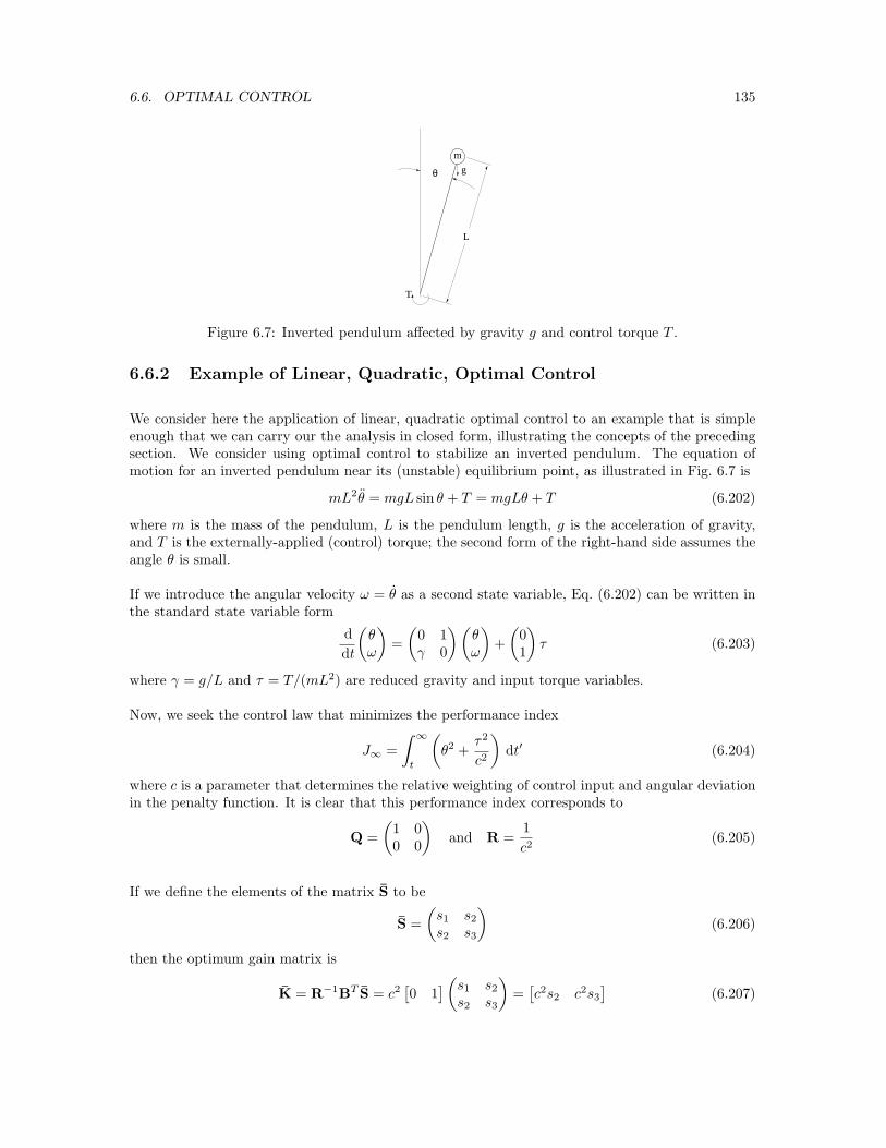
6.6. OPTIMAL CONTROL 135
θ
T
g
L
m
Figure 6.7: Inverted pendulum affected by gravity g and control torque T .
6.6.2 Example of Linear, Quadratic, Optimal Control
We consider here the application of linear, quadratic optimal control to an example that is simpleenough that we can carry our the analysis in closed form, illustrating the concepts of the precedingsection. We consider using optimal control to stabilize an inverted pendulum. The equation ofmotion for an inverted pendulum near its (unstable) equilibrium point, as illustrated in Fig. 6.7 is
mL2θ = mgL sin θ + T = mgLθ + T (6.202)
where m is the mass of the pendulum, L is the pendulum length, g is the acceleration of gravity,and T is the externally-applied (control) torque; the second form of the right-hand side assumes theangle θ is small.
If we introduce the angular velocity ω = θ as a second state variable, Eq. (6.202) can be written inthe standard state variable form
d
dt
(
θω
)
=
(
0 1γ 0
)(
θω
)
+
(
01
)
τ (6.203)
where γ = g/L and τ = T/(mL2) are reduced gravity and input torque variables.
Now, we seek the control law that minimizes the performance index
J∞ =
∫
∞
t
(
θ2 +τ2
c2
)
dt′ (6.204)
where c is a parameter that determines the relative weighting of control input and angular deviationin the penalty function. It is clear that this performance index corresponds to
Q =
(
1 00 0
)
and R =1
c2(6.205)
If we define the elements of the matrix S to be
S =
(
s1 s2
s2 s3
)
(6.206)
then the optimum gain matrix is
K = R−1BT S = c2[
0 1]
(
s1 s2
s2 s3
)
=[
c2s2 c2s3
]
(6.207)

136 CHAPTER 6. CONTROL OF AIRCRAFT MOTIONS
which is seen to be independent of the element s1.
The terms needed for the algebraic Riccati equation
0 = SA + AT S − SBR−1BT S + Q (6.208)
are
SA =
(
s1 s2
s2 s3
)(
0 1γ 0
)
=
(
s2γ s1
s3γ s2
)
(6.209)
AT S =
(
0 γ1 0
) (
s1 s2
s2 s3
)
=
(
s2γ s3γs1 s2
)
(6.210)
and
SBR−1BT S =
(
s1 s2
s2 s3
) (
01
)
c2[
0 1]
(
s1 s2
s2 s3
)
= c2
(
s22 s2s3
s2s3 s23
)
(6.211)
Thus, the Riccati equation is
0 =
(
s2γ s1
s3γ s2
)
+
(
s2γ s3γs1 s2
)
− c2
(
s22 s2s3
s2s3 s23
)
+
(
1 00 0
)
(6.212)
which is equivalent to the three scalar equations
0 = 2s2γ − c2s22 + 1
0 = s1 + s3γ − c2s2s3
0 = 2s2 − c2s23
(6.213)
These equations are simple enough that we can solve them in closed form. The first of Eqs. (6.213)gives
s2 =γ ±
√
γ2 + c2
c2(6.214)
and the third of Eqs. (6.213) gives
s3 = ±1
c
√2s2 (6.215)
Since the elements of S must be real, s2 must be positive (or s3 would be complex). Thus, we mustchoose the positive root in Eq. (6.203). Further, the second of Eqs. (6.213) gives
s1 = c2s2s3 − γs3 = s3
√
γ2 + c2 (6.216)
Thus, elements s1 and s3 have the same sign which, for S to be positive definite, must be positive.Thus,
s2 =γ +
√
γ2 + c2
c2
s3 =1
c
√2s2 =
√2
c2
[
γ +√
γ2 + c2]1/2
(6.217)
represents the unique solution for the corresponding elements for which S is positive definite.
Thus, the gain matrix is seen to be
K =[
c2s2 c2s3
]
=
[
γ +√
γ2 + c2√
2[
γ +√
γ2 + c2]1/2
]
(6.218)

6.6. OPTIMAL CONTROL 137
−5 −4 −3 −2 −1 0 1−5
−4
−3
−2
−1
0
1
2
3
4
5
Real partIm
agin
ary
part
Figure 6.8: Locus of roots of characteristic equation of augmented plant matrix for inverted pen-dulum. Axes are scaled to give roots in units of γ. Open symbols represent roots at values ofc/γ = 0, 1, 10, 100, 1000, with real root corresponding to c/γ = 0. Cyan lines represent asymptotesof root positions in the limit of large c/γ.
The augmented matrix is then given by
A∗ = A − BK =
(
0 1
−√
γ2 + c2 −√
2[
γ +√
γ2 + c2]1/2
)
(6.219)
and its characteristic equation is
λ2 +√
2[
γ +√
γ2 + c2]1/2
λ +√
γ2 + c2 = 0 (6.220)
which has roots
λ =
√2
2
[
−√γ + γ ± ı
√γ − γ
]
(6.221)
where we have introducedγ =
√
γ2 + c2 (6.222)
The locus of these roots is plotted in Fig. 6.8 as the weighting factor c is varied over the range0 < c < 103.
Note that as c/γ becomes large, γ becomes large relative to γ, so
limc/γ→∞
λ = −√
γ√2
(1 ± ı) (6.223)
Thus, as c becomes large, the damping ratio of the system approaches a constant value of
ζ =1√2
while the undamped natural frequency increases as
ωn =√
γ ≈√
c
Large values of c correspond to a performance index in which the weighting of the control term issmall compared to that of the deviations in state variables – i.e., to a situation in which we are
138 CHAPTER 6. CONTROL OF AIRCRAFT MOTIONS
willing to spend additional energy in control to maintain very small perturbations of the state fromits equilibrium position.
On the other hand, as c becomes small, the weighting of the control term in the performance indexbecomes large compared to that of the state variables. This is consistent with the fact that the gainsin Eq. (6.218)
K1 = γ +√
γ2 + c2
K2 =√
2[
γ +√
γ2 + c2]1/2
decrease monotonically with c. In the limit c = 0, however, the gains remain finite, with
limc→0
K1 = 2γ
limc→0
K2 = 2√
γ
since some control is necessary to stabilize this, otherwise unstable, system.
6.6.3 Linear, Quadratic, Optimal Control as a Stability AugmentationSystem
We here present an example of the application of linear, quadratic optimal control to stabilize themotion of the Boeing 747 aircraft in powered approach at M = 0.25 at standard sea level conditions.This is the same aircraft and flight condition for which we used the Bass-Gura procedure to designa feedback control system to stabilize the lateral/directional modes in Section. 6.5.1. In that earliersection, we determined the gains for specific placement of the eigenvalues of the associated augmentedmatrix using only one control, either rudder or ailerons, at a time.
Here, we apply linear, quadratic, optimal control to minimize the steady state performance index
J∞ =
∫
∞
t
(
xT Qx +1
c2ηT Rη
)
dτ (6.224)
where, as in the previous simple example, c is a parameter that determines the relative weightsgiven to control action and perturbations in the state variable in the penalty function. For lat-eral/directional motions at this flight condition, the plant matrix is given by Eq. (6.150), while thecontrol matrix is the union of the two vectors given in Eqs. (6.158) and (6.163)
B =
(
0.0182 0.0868 0.0000 −.24400.0000 0.3215 0.0000 −.0017
)T
(6.225)
where the control vector is
η = [δr δa]T
(6.226)
The weighting matrices in the performance index are taken to be simply
Q = I and R = I (6.227)
where Q is a 4 × 4 matrix and R is a 2 × 2 matrix.

6.6. OPTIMAL CONTROL 139
0 2 4 6 8 10 12 14 16 18 20−2
−1.5
−1
−0.5
0
0.5
1
1.5
2
Time, sec
Sta
te V
aria
ble
SideslipRoll rateRoll angleYaw rate
0 2 4 6 8 10 12 14 16 18 20−2
−1.5
−1
−0.5
0
0.5
1
1.5
2
Time, sec
Sta
te V
aria
ble
SideslipRoll rateRoll angleYaw rateAileronRudder
(a) No feedback (b) c = 0.001
Figure 6.9: Boeing 747 aircraft in powered approach at standard sea level conditions and M = 0.25;response to unit perturbation in sideslip. (a) Original open-loop response; (b) Optimal closed loopresponse with performance parameter c = 0.001.
The Matlab function[S, L, G] = care(A,B,Q,R,T,E);
is used to solve the generalized matrix Riccati equation
ET SA + AT SE −(
ET SB + T)
R−1(
BT SE + TT)
+ Q = 0 (6.228)
which, with the additional input matrices are defined asT = zeros(size(B));
andE = eye(size(A));
reduces to Eq. (6.199). In addition to the solution matrix S, the Matlab function care also returnsthe gain matrix
G = R−1(
BT SE + TT)
(6.229)
and the vectorL = eig(A - BG, E)
containing the eigenvalues of the augmented matrix.
For small values of the parameter c, the control action is weighted heavily in the performance index.Figure 6.9 compares the open-loop response to a unit perturbation in sideslip to the closed-loopsystem response for a value of c = 0.001. This value penalizes control input so heavily that theopen-loop and closed-loop responses are virtually identical. This is a quite different result from thatfor the simple example of Section 6.6.2, and results from the fact that this system is stable, so thenatural (un-forced) return of the system to equilibrium is optimal when control action is heavilypenalized.
Figure 6.10 shows the closed-loop system response for values of c = 0.5, 1.0, and 2.0, respectively.Also plotted in these figures are the time histories of control response required to stabilize themotions, calculated as
η = −Kx (6.230)

140 CHAPTER 6. CONTROL OF AIRCRAFT MOTIONS
0 2 4 6 8 10 12 14 16 18 20−2
−1.5
−1
−0.5
0
0.5
1
1.5
2
Time, sec
Sta
te V
aria
ble
SideslipRoll rateRoll angleYaw rateAileronRudder
0 2 4 6 8 10 12 14 16 18 20−2
−1.5
−1
−0.5
0
0.5
1
1.5
2
Time, sec
Sta
te V
aria
ble
SideslipRoll rateRoll angleYaw rateAileronRudder
0 2 4 6 8 10 12 14 16 18 20−2
−1.5
−1
−0.5
0
0.5
1
1.5
2
Time, sec
Sta
te V
aria
ble
SideslipRoll rateRoll angleYaw rateAileronRudder
(a) c = 0.50 (b) c = 1.0 (c) c = 2.0
Figure 6.10: Boeing 747 aircraft in powered approach at standard sea level conditions and M = 0.25;response to unit perturbation in sideslip illustrating effect of varying weighting parameter c. Optimalclosed-loop responses with (a) c = 0.50; (b) c = 1.0; and (c) c = 2.0. Control deflections required tostabilize the motions are also shown.
This control response is calculated in Matlab simply by defining the matrices C and D definingthe output response as
C = -G;
andD = zeros(2);
and then adding the output variablesy = Cx + Dη (6.231)
to the plots. It is seen in the plots that, as c is increased the motion becomes more heavily damped,but at the cost of significantly greater control input.
The role of the parameter c can be seen more clearly if we examine the behavior of the individualterms in the performance index J∞. Figure 6.11 plots the quadratic forms xT Qx and ηT Rη asfunctions of time for the three values of c illustrated in Fig. 6.10. For greater clarity in the figure,minus the control term is plotted. Thus, for each value of c the optimal control strategy selects thegains that minimize the net area between the two curves. Three trends resulting from increasing care evident in the figure: (1) the value of J∞ – i.e., the area between the two curves – decreases;(2) the return of the system to its equilibrium state is more rapid and heavily damped; (3) most ofthe improvement happens for modest increases in the value of c, with continued increases requiringever larger control inputs for relatively little further improvement in response.
Finally, we illustrate the behavior of the roots of the augmented equation as the parameter c isincreased. Figure 6.12 shows the locations of the roots in the complex plane for selected values ofc. Note that, in this range of values, all roots move to the left as c is increased until the DutchRoll mode becomes critically damped at a value of approximately c = 9.973, as indicated by thejoining of the roots on the real axis. With further increase in c, one of the Dutch Roll roots movesto the right. The value of c required to achieve critical damping of the Dutch Roll mode generallycorresponds to much larger values of c than would ever be used in a practical system.

6.6. OPTIMAL CONTROL 141
-3
-2
-1
0
1
2
0 2 4 6 8 10 12 14
Pen
alty
func
tion
Time, sec.
c = 0.5c = 1.0c = 2.0
Figure 6.11: Penalty functions in performance index for optimal control solution; Boeing 747 aircraftin powered approach at standard sea level conditions and M = 0.25. Upper curves are xT Qx, andlower curves are −ηT Rη, as functions of time for response to unit perturbation in sideslip angle β,so the area between the curves is equal to the performance index J∞.
-1
-0.5
0
0.5
1
-2.5 -2 -1.5 -1 -0.5 0
Imag
inar
y pa
rt o
f roo
t
Real part of root
Rolling Dutch rollSpiral
Figure 6.12: Boeing 747 aircraft in powered approach at standard sea level conditionsand M = 0.25; locus of roots of characteristic equation of augmented matrix as con-trol weighting parameter c is increased. Symbols represent root locations for c =0.001, 0.5, 1.0, 2.0, 5.0, 8.0, 9.0, 9.7, 9.76, 9.7727, 9.7728, 10.0; as c is increased, all roots move to theleft (except for one of the Dutch Roll roots after that mode becomes critically damped between9.7227 < c < 9.7228).

142 CHAPTER 6. CONTROL OF AIRCRAFT MOTIONS

Bibliography
[1] Arthur Bryson & Yu-Chi Ho, Applied Optimal Control: Optimization, Estimation, and
Control, Hemisphere, 1975.
[2] Bernard Etkin & Lloyd Duff Reid, Dynamics of Flight, Stability and Control, McGraw-Hill, Third Edition, 1996.
[3] Bernard Friedland, Control System Design: An Introduction to State-Space Methods,McGraw-Hill, 1986.
[4] Frances B. Hildebrand, Advanced Calculus for Applications, Prentice-Hall, 1962.
[5] Robert C. Nelson, Aircraft Stability and Automatic Control, McGraw-Hill, Second edi-tion, 1998.
[6] Louis V. Schmidt, Introduction to Aircraft Flight Dynamics, AIAA Education Series,1998.
6.7 Review of Laplace Transforms
The Laplace transform of the function f(t), assumed identically zero for t < 0, is defined as
L [f(t)] = F (s) =
∫
∞
0
f(t)e−st dt (6.232)
The Laplace transform F (s) of the function f(t) can be shown to exist, for sufficiently large s, when[4]:
1. The function f(t) is continuous or piecewise continuous in every finite interval t1 ≤ t ≤ T ,where t1 > 0;
2. The function tn|f(t)| is bounded near t = 0 for some number n < 1; and
3. The function e−s0t|f(t)| is bounded for large values of t, for some number s0.
All the functions we normally deal with in stability and control problems satisfy these conditions.
143
144 BIBLIOGRAPHY
6.7.1 Laplace Transforms of Selected Functions
We here review the Laplace transforms of several important functions.
Laplace Transform of a Derivative
If F (s) is the Laplace transform of the function f(t), then the Laplace transform of the derivativedf/dt can be determined as
L[
df
dt
]
=
∫
∞
0
df
dte−st dt = fe−st
∣
∣
∞
0+
∫
∞
0
fse−st dt = −f(0) + s
∫
∞
0
fe−st dt
= −f(0) + sF (s)
(6.233)
Heaviside Step Function
The Heaviside step function is defined as
H(t − τ) =
0, for t < τ
1, for t ≥ τ(6.234)
The Laplace transform of H(t) is thus
H(s) =
∫
∞
0
e−stH(t) dt =
∫
∞
0
e−st dt = − est
s
∣
∣
∣
∣
∞
0
=1
s(6.235)
Dirac Delta Function
The Dirac delta function is defined by the properties
δ(t − τ) = 0 for t 6= τ∫
∞
−∞
δ(t − τ) dt = 1(6.236)
The Laplace transform of δ(t) is thus
δ(s) =
∫
∞
0
e−stδ(t) dt = e0 = 1 (6.237)
The function f(t) = t
The Laplace transform of f(t) = t is
F (s) =
∫
∞
0
te−st dt = − te−st
s
∣
∣
∣
∣
∞
0
+
∫
∞
0
e−st
sdt = −e−st
s2
∣
∣
∣
∣
∞
0
=1
s2(6.238)
6.7. REVIEW OF LAPLACE TRANSFORMS 145
The function f(t) = e−at
The Laplace transform of f(t) = e−at is
F (s) =
∫
∞
0
e−ate−st dt =
∫
∞
0
e−(a+s)t dt = −e−(a+s)t
a + s
∣
∣
∣
∣
∞
0
=1
s + a(6.239)
The Trigonometric Functions, cos ωt and sin ωt
The Laplace transform of f(t) = cos ωt is determined as follows. Since
∫
∞
0
cos ωte−st dt = −cos ωte−st
s
∣
∣
∣
∣
∞
0
− ω
∫
∞
0
sin ωte−st
sdt
=1
s− ω
s
∫
∞
0
sin ωte−st dt =1
s+
ω
s
[
sin ωte−st
s− ω
∫
∞
0
cos ωtte−st
sdt
]
=1
s− ω2
s2
∫
∞
0
cos ωte−st dt
(6.240)
we have(
1 +ω2
s2
)∫
∞
0
cos ωte−st dt =1
s(6.241)
whence
F (s) =
∫
∞
0
cos ωte−st dt =1
s(
1 + ω2
s2
) =s
s2 + ω2(6.242)
Similarly, to determine the Laplace transform of f(t) = sinωt, since
∫
∞
0
sin ωte−st dt = − sinωte−st
s
∣
∣
∣
∣
∞
0
+ω
s
∫
∞
0
cos ωte−st dt
=ω
s
∫
∞
0
cos ωte−st dt =ω
s
[
1
s− ω
s
∫
∞
0
sinωte−st dt
](6.243)
we have(
1 +ω2
s2
)∫
∞
0
sinωte−st dt =ω
s2(6.244)
whence
F (s) =
∫
∞
0
sinωte−st dt =ω
s2(
1 + ω2
s2
) =ω
s2 + ω2(6.245)
The Attenuation Rule
Exponentially damped harmonic functions appear often in linear system dynamics, so the followingattenuation rule is useful.
146 BIBLIOGRAPHY
If F (s) is the Laplace transform of f(t), then the Laplace transform of e−atf(t) is
L[
e−atf(t)]
=
∫
∞
0
e−atf(t)e−st dt =
∫
∞
0
e−(s+a)tf(t) dt
=
∫
∞
0
e−s′tf(t) dt = F (s′) = F (s + a)
(6.246)
Thus, since Eq. (6.242) gives
L [cos ωt] =s
s2 + ω2(6.247)
we have
L[
e−at cos ωt]
=s + a
(s + a)2 + ω2(6.248)
Also, since Eq. (6.245) gives
L [sin ωt] =ω
s2 + ω2(6.249)
we have
L[
e−at sinωt]
=ω
(s + a)2 + ω2(6.250)
The Convolution Integral
The convolution integral
L−1 [F (s)G(s)] =
∫ t
0
f(t − τ)g(τ) dτ (6.251)
where F (s) and G(s) are the Laplace transforms of f(t) and g(t), respectively, can be verifiedformally as follows.
From the definition of the Laplace transform,
F (s)G(s) =
∫
∞
0
e−svf(v) dv
∫
∞
0
e−sug(u) du
=
∫
∞
0
∫
∞
0
e−s(v+u)f(v)g(u) dv du
=
∫
∞
0
g(u)
(∫
∞
0
e−s(v+u)f(v) dv
)
du
(6.252)
Then, with the change of variable
v + u = t (6.253)
we have∫
∞
0
e−s(v+u)f(v) dv =
∫
∞
u
e−stf(t − u) dt (6.254)

6.7. REVIEW OF LAPLACE TRANSFORMS 147
so
F (s)G(s) =
∫
∞
0
(∫
∞
u
e−stf(t − u)g(u) dt
)
du
=
∫
∞
0
(∫ t
0
e−stf(t − u)g(u) du
)
dt
=
∫
∞
0
e−st
(∫ t
0
f(t − u)g(u) du
)
dt = L[∫ t
0
f(t − u)g(u) du
]
(6.255)
which was to be proved. The interchange of order of integration in this last step can be shown to belegitimate, by appropriate limiting procedures, when the Laplace transforms of f(t) and g(t) exist.