introduction - Northwestern Universitylen/photos/pages/vc.pdf · VIEW CAMERA GEOMETRY LEONARD EVENS...
109
c 2008 Leonard Evens VIEW CAMERA GEOMETRY LEONARD EVENS 1. introduction This article started as an exposition for mathematicians of the relation between projective geometry and view camera photography. The two subjects share a com- mon history, and problems in view camera geometry lead to some interesting mathe- matics. In the process of writing the article, I realized that some technical problems in using a view camera could be approached profitably by the projective approach. A considerable part of the article, particularly the section on depth of field, deals with such matters. The article is largely original, but I did receive helpful advice from various sources. In particular, I want to thank Jeff Conrad, who looked at my many earlier drafts and kept bringing me back to the really interesting questions. I’ve also re- ceived help from comments made in the Large Format Forum at www.lfphoto.info. Of course, I am not the first to look into many of the topics considered in this article, and I have tried to include other sources of useful information in the text, mainly in footnotes. I apologize if I’ve left anyone or anything out. 2. Some History Figure 1. Durer Woodcut: Man Drawing a Lute 1523 The history of projective geometry is intimately related to that of representational art. In the 15th and 16th century artists studied how to draw in perspective. (Alberti, della Francesa, Durer, etc.). Imagine a frame through which the artist looks at a scene, and follows a ray from a center of perspective to a point in the Date : June 24, 2011. 1
Transcript of introduction - Northwestern Universitylen/photos/pages/vc.pdf · VIEW CAMERA GEOMETRY LEONARD EVENS...

c©2008 Leonard Evens
VIEW CAMERA GEOMETRY
LEONARD EVENS
1. introduction
This article started as an exposition for mathematicians of the relation betweenprojective geometry and view camera photography. The two subjects share a com-mon history, and problems in view camera geometry lead to some interesting mathe-matics. In the process of writing the article, I realized that some technical problemsin using a view camera could be approached profitably by the projective approach.A considerable part of the article, particularly the section on depth of field, dealswith such matters.
The article is largely original, but I did receive helpful advice from varioussources. In particular, I want to thank Jeff Conrad, who looked at my many earlierdrafts and kept bringing me back to the really interesting questions. I’ve also re-ceived help from comments made in the Large Format Forum at www.lfphoto.info.Of course, I am not the first to look into many of the topics considered in thisarticle, and I have tried to include other sources of useful information in the text,mainly in footnotes. I apologize if I’ve left anyone or anything out.
2. Some History
Figure 1. Durer Woodcut: Man Drawing a Lute 1523
The history of projective geometry is intimately related to that of representationalart. In the 15th and 16th century artists studied how to draw in perspective.(Alberti, della Francesa, Durer, etc.). Imagine a frame through which the artistlooks at a scene, and follows a ray from a center of perspective to a point in the
Date: June 24, 2011.
1

2 LEONARD EVENS
scene. Such a ray intersects the rectangular region bounded by the frame in animage point, and a picture results from transferring those images to paper.
A tool designed to help in this endeavor was the camera obscura, which is Latinfor ‘dark room’.1 Originally, this was indeed a darkened room with a small hole inone side. Rays from the scene through the hole impinge on the opposite wall formingan image of the scene which can be traced on the wall. The image is upside down.If you traced it on paper and rotated the paper through 180 degrees, you wouldfind that left and right are reversed as in a mirror. It has been suggested that 17thcentury Dutch masters such as Vermeer may have used the camera obscura as anaid,2 but this remains controversial. Adding a lens produces a much brighter image,and through the use of various devices, it became possible to view the image outsidethe camera, right side up without the left-right reflection. The camera obscuraplayed an important role in the history of representational art, and photographyarose through efforts to ‘fix’ its image.
Front Standard Rear Standard
Rail
Lens
Bellows
Figure 2. View Camera Schematic
A modern camera employs basically the same principle, with the photographeroutside the camera, and the image recorded by a light sensitive material, either filmor a digital sensor array. View cameras are a special class of camera, usually usingformats such as 4 x 5 inches or larger. Figure 2 shows a scheme for such a camera,which consists of two standards, connected by a bellows, and mounted on a rail.
A lens is mounted in a lensboard attached to the front standard. The rearstandard has a ground glass screen onto which the image is projected, and thephotographer views that image from behind the camera rather than from inside it.It is rotated 180 degrees, but if you rotate it back you will find that left and rightare preserved. The ground glass can be moved out of the way in order to mounta film holder or other recording device. In addition, either standard is capable ofmovements such as rise, fall, and shift to one side as well as rotations about twoperpendicular axes. Through the use of such movements, one can adjust the relativepositions and orientation of the image frame with respect to the lens and both of
1en.wikipedia.org/wiki/Camera obscura.2See www.essentialvermeer.com/camera obscura/co one.html.

VIEW CAMERA GEOMETRY 3
them with respect to the scene. The bellows, which keeps out stray light, and therail, which serves to hold the standards in place, play no role in the geometry, sowe shall largely ignore them.
3. Projective geometry
Parallel lines in a scene receding into the distance appear to the viewer to con-verge to a point, but of course there is no such point in the scene. Like the proverbialpot of gold at the end of a rainbow, it recedes from you as you try to approachit. But the images of such lines in a two-dimensional perspective representationactually do converge to a common point, which is called a vanishing point. So it iseasy to imagine adding to the scene an extra point at infinity to correspond to thevanishing point. The formalization by mathematicians of such ideas in the 17th,18th, and 19th centuries led to the idea of projective space and projective geometry.
In real projective space P3(R), three non-collinear points determine a plane,
two distinct planes intersect in a line, and three non-collinear planes intersect in apoint. There are some other axioms which are necessary to specify the dimensionand characterize the associated field, which in our case is the real number field.3
Those maps of the space which carry points into points, lines into lines, planes intoplanes and also preserve incidence are called projective transformations. (We alsorequire that such a transformation yield the identity on the associated field—ingeneral it may be a field automorphism—but that is always the case for R.)
We also may specify one plane Ω = Ω∞ as the plane at infinity. With thatplane deleted, the resulting space satisfies the axioms of affine geometry, which isconcerned with parallelism. Two planes, a line and a plane, or two lines, assumeddistinct, are parallel if they meet at infinity. If we specify a point O in affine space,
the directed line segments−−→OP from that point may be added and multiplied by
scalars using suitable geometric constructions using parallel lines. The result is avector space, in our case isomorphic to R
3. Given two points O and O′, there is anobvious way to translate the vector space at O to that at O′ via the directed line
segment−−→OO′. (That makes affine space into a flat 3-dimensional real manifold with
an affine connection.) We can use this to define a map A called the antipodal maprelative to O and Ω. Namely just require that A fix O and that the corresponding
directed line segments (vectors) satisfy−−−−→OA(P ) = −−−→OP . (This structure makes
affine space into a symmetric space.) It is not hard to check that if we extend A tothe P
3 by fixing all points in the plane at infinity, the resulting map is a projectivetransformation. Note also that P,O, and A(P ) are always collinear.
There are various models for P3(R). The first is obtained by taking Euclidean
3-space and adjoining an additional plane at infinity by adding one point for everyfamily of parallel lines. Another approach is to take R
4 − (0, 0, 0, 0) and identifyvectors by the equivalence relation which identifies vectors differing by a non-zeroscalar multiplier. The resulting quotient space is P
3(R). A plane through the originin R
4 yields a projective line, and a 3-space through the origin yields a projectiveplane. R
4 has a distinguished canonical basis, but we don’t give it any specialprominence. Projective transformations of P
3 are exactly those that arise fromnonsingular linear transformations of R
4.
3See any good book on projective geometry such as Foundations of Projective Geometry byRobin Hartshorne.

4 LEONARD EVENS
sX
XX
XX
XX
XX
XX
XX
XXz
XX
XX
XX
XX
XX
XX
XXXy
P
O A(P )
Figure 3. Antipodal Map
Any basis in R4 yields a coordinate system and we may attach so called homoge-
neous coordinates (x0, x1, x2, x3) to a point P in P3, except that such coordinates are
only unique up to multiplication by a non-zero scalar. If we arrange the coordinatesso that x0 = 0 is the equation of the specified plane Ω at infinity, then for a point
in the associated affine space, we may take the coordinates to be (1,x1
x0,x2
x0,x3
x0)
which are unique. The last three coordinates are the affine coordinates of the point.We all carry in our heads a model of Euclidean space, which adds a metric to
affine space. This may be specified by attaching consistent inner products to thereal vector spaces at each point. It is surprising how far we will be able to getwithout making use of the Euclidean structure,
Because of gravity, we also carry in our heads a distinction between vertical andhorizontal. This may be formalized as follows. We pick a point called the zenith inthe plane at infinity. Then all lines passing through that point, are called vertical.Similarly, we choose a line in the plane at infinity which we call the horizon. Allplanes containing that line are called horizontal. In the Euclidean context, we alsoassume the horizontal planes are perpendicular to the vertical lines.
4. Pinhole camera geometry
Let us now think of how this framework may be used to study image formation.We shall start just with the case of a“pinhole camera” which is essentially a rect-angular box with a pinhole in one side and the film on the opposite side. Note thatany view camera may be made into a pinhole camera by substituting a plate with asmall hole in it for the lens, and we thereby get the extra flexibility of movements.
The light rays emanating from a point in the scene which pass through the holewill form a solid cone. If we intersect that cone of light with the frame in whichwe capture the image, we will get a small blob of light. If it is small enough, thehuman visual system can’t distinguish it from a point. As a result, we may treatthe pinhole as a point for purposes of geometric ray tracing. That point will becalled the principal point of the camera. It is the center of perspective, also calledthe point of view.
In deciding how large to make the pinhole, one must balance brightness againstsharpness. (If the hole is very small, the image will be sharp, but it will also bevery dim, which may require very long exposures of the photosensitive material.)If the subject point is relatively distant compared to the dimensions of the cameraenclosure, the size of the blob of light won’t vary much over the box, so the imagewill be equally sharp over the course of the light ray, and the sharpness of the

VIEW CAMERA GEOMETRY 5
image won’t depend much on just where you place the film frame, but the size ofthe image will change. Usually, we assume the film frame is in a vertical plane,but it need not be. If you place it closer the image will be smaller, and if youplace it further, it will be larger. The ratio of the image distance v to the subjectdistance u is called the magnification or scale of reproduction. It tells us how muchmeasurements at distance u in the subject space are reduced at the correspondingdistance v in the image space. It is usually less than 1. If the film frame is tilted,the relative positions of vanishing points will change, so shapes will also be affected.
As noted earlier, the image inside the camera when viewed from the front hasorientation reversed. But the process of making an image to be viewed, either bymaking a print or by projection on a screen or showing it on a monitor, reversesthat so the orientation in the final image is correct. The traditional method was tomake a negative image in the film, develop and fix it chemically, and then print itby contact printing or with an enlarger. Darkroom workers had to be careful aboutwhich way they positioned the negative to make sure the resulting print didn’treverse right and left.
We now formalize these concepts as follows. As before, we assume a plane Ωat infinity has been specified (with specified zenith and horizon). In addition, wespecify a different plane Λ called the lens plane—although we don’t yet have alens—with a point O called the principal point. The lens plane and the planeat infinity divide projective space into two compartments. Finally, we specify asimple closed planar curve, not coplanar with the principal point, and we call theplane region it bounds the frame. We shall assume the frame is a rectangle, but itneed not be. We further stipulate that the frame lies entirely in one of these twocompartments which we call the image space. The other compartment is called thesubject space. The plane Π containing the frame is called the image plane or filmplane.
See Figure 4 for a diagrammatic representation. It is important to rememberthat the geometry is three-dimensional, and that a diagram typically only shows atwo-dimensional cross section. So don’t begin to think of the planes as lines. Onthe left we show how it looks conventionally, and on the right how it would lookif we could move ourselves to where we could see the plane at infinity. Note thatalthough it may look as if the two planes divide space into four regions, there areactually only two regions involved.
Consider an affine point P in the subject space. The line determined by O andP intersects the image plane in a unique point P ′ called the corresponding imagepoint. If the image plane is parallel to the lens plane, the image P ′ is in the imagespace. If the image plane is not parallel to the lens plane, then the image point P ′
is in the image space or at infinity. It makes sense also to restrict attention to thosepoints in the subject space with images in the frame , but since in principle theframe may be anywhere in the image space, this is no restriction. For simplicity wehave ignored the camera enclosure, but if we incorporated other bounding planes inaddition to the lens plane, it would further restrict possible positions of the frameand which subject points could have images in the frame. Being able to control theposition of the frame is probably the most useful feature of a view camera.
The map P 7→ P ′ is called a perspective transformation, or just a perspectivitythrough the principal point O. It takes lines into lines and preserves incidence, butof course it is far from being a bijection, so it is not a projective transformation.

6 LEONARD EVENS
Image Space
Frame
Subject Space
Ω→← Ω
O
Π Λ
Ω
Λ
O
Frame
Image Space
Image Space
Subject Space Subject Space
Π
Λ
Normal View View at ∞
Figure 4. Two views of Subject and Image spaces
It is completely determined by the principal point and the position of the imageplane and it is what creates the image.
As noted earlier, if two lines intersect at infinity, their images intersect in avanishing point in the image plane. Generally this is an affine point, but if the linesare parallel to the image plane, the corresponding vanishing point in the image isalso at infinity, which means the affine sections of the image lines are parallel.
This has important implications in photography. Consider a camera pointingupward at a building with vertical sides as sketched in Figure 5. Photographerswill often do that to include the top of the building in the frame.
In Cross Section
VanishingPoint
Subject
Film
O
Picture rotated tonormal view
A B
CD
D′ C′
A′B′
FilmO
Vanishing point
D C
BA
Subject
Three-Dimensional View
Figure 5. Convergence of verticals when film plane is tilted upward

VIEW CAMERA GEOMETRY 7
The camera back, i.e., the image plane, is tilted with respected to the vertical, sothe images of the sides of the building will converge to a vanishing point. It may notbe in the frame, but the sides of the building will still appear to converge, downwardson the ground glass, but, upwards, after we rotate the picture to view it right sideup. (In a conventional SLR or other such camera, this is done for you.) There hasbeen a lot of discussion about what people actually see when they look at such ascene. The human visual system does a lot of processing, and we don’t just“see” theprojected image on the retina. Some have argued that whatever the human visualsystem once expected due to our evolutionary history of hunting and gathering,recently, decades of looking at snapshots with sides of buildings converging, haveconditioned us to find such representations normal. Since structures with verticalsides presumably didn’t play a direct role during our evolution, it is not clear justwhat we expect “naturally”, but I would argue that if you don’t have to turn yourhead too much to see the top of the building, the sides will appear to be parallel. Onthe other hand, if you crane your head a lot, the sides will appear to converge. In anycase, many people do prefer to have verticals appear parallel, and it is consideredessential in most architectural photography. View camera photographers usuallystart with the film plane vertical, and only change that when it is felt to be necessaryfor technical or aesthetic reasons. Of course, users of conventional cameras don’thave that choice, so the problem is ignored, resulting in a multitude of photographswith converging verticals. In the past, when necessary, any correction was donein the darkroom by tilting the print easel in the enlarger, and today it is done bydigital manipulation of the image. But such manipulation, if not done correctly,can produce other distortions of the image.
In a view camera, we make sure verticals are vertical simply by keeping theframe and image plane vertical, which, as noted above, puts the vanishing point atinfinity. If the vertical angle subtended by the frame at the principal point (calledthe vertical angle of view) is large enough, we can ensure that both the top andbottom of the building are included in the frame by moving the frame down farenough, i.e., by dropping the rear standard. If the position of the principal point, inrelation to the scene, is not critical, which is usually the case, then we may insteadraise that principal point by raising the front standard. If we were to leave theframe centered on the horizontal, the top of the building might not be visible andthere might be an expanse of uninteresting foreground in front of the building inthe picture.
The ability of a view camera to perform maneuvers of this kind is one thing thatmakes it so flexible.
5. Adding a Lens
If we add a lens to the mix we gain the advantage of being able to concentratelight. A lens has an opening or aperture, and the rays from a subject point passingthrough the aperture are bent or refracted so they form a cone with vertex at theimage point. The image will be much brighter than anything obtainable in a pinholecamera. In addition, for each subject point, there is a unique image point, on theray through the principal point, which is in focus. In a pinhole camera, as notedearlier, any point on that ray is as much in focus as any other.
Unfortunately the situation is more complicated than this description suggests.First of all, because of inevitable lens aberrations, there is no precise image point,
8 LEONARD EVENS
Λ
O
V(P ) = P
P
V(P )
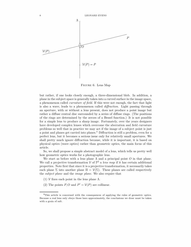
Figure 6. Lens Map
but rather, if one looks closely enough, a three-dimensional blob. In addition, aplane in the subject space is generally taken into a curved surface in the image space,a phenomenon called curvature of field. If this were not enough, the fact that lightis also a wave, leads to a phenomenon called diffraction. Light passing throughan aperture, with or without a lens present, does not produce a point image butrather a diffuse central disc surrounded by a series of diffuse rings. (The positionsof the rings are determined by the zeroes of a Bessel function.) It is not possiblefor a simple lens to produce a sharp image. Fortunately, over the years designershave developed complex lenses which overcome the aberration and field curvatureproblems so well that in practice we may act if the image of a subject point is justa point and planes get carried into planes.4 Diffraction is still a problem, even for aperfect lens, but it becomes a serious issue only for relatively small apertures. Weshall pretty much ignore diffraction because, while it is important, it is based onphysical optics (wave optics) rather than geometric optics, the main focus of thisarticle.
So, we shall propose a simple abstract model of a lens, which tells us pretty wellhow geometric optics works for a photographic lens.
We start as before with a lens plane Λ and a principal point O in that plane.We call a projective transformation V of P
3 a lens map if it has certain additionalproperties. Note first that since it is a projective transformation, it necessarily takeseach plane Σ into another plane Π = V(Σ). These planes are called respectivelythe subject plane and the image plane. We also require that
(1) V fixes each point in the lens plane Λ.
(2) The points P,O and P ′ = V(P ) are collinear.
4This article is concerned with the consequences of applying the rules of geometric optics.Because a real lens only obeys those laws approximately, the conclusions we draw must be takenwith a grain of salt.

VIEW CAMERA GEOMETRY 9
Π = V(Σ) Λ
O
ΣP
P ′ = V(P )
Scheimpflug Line
Figure 7. Scheimpflug Rule
Note that one consequence of (2) is that V carries every plane through O intoitself.
(3) VAV = A where A is the antipodal map in O.
(3) is a symmetry condition, the significance of which we shall explain later. Butnotice for the present that since A is an involution, we have that VAV = A isequivalent to (VA)2 = Id or (AV)2 = Id, i.e., both AV and VA are involutions. Itis also clear by taking inverses that V−1AV−1 = A. These facts will later turn outto have important consequences.
Note that a trivial consequence of (1) is the following rule
(1′) The subject plane Π, the lens plane Λ, and the image plane Π′ = V(Π) arecollinear.
(Note also that (1′) and (2) together imply (1).)(1′) is called the Scheimpflug Rule, and I shall call the common line of intersection
the Scheimpflug line.5
Scheimpflug’s Rule is usually derived as a consequence of the laws of geometricoptics by means of Desargues Theorem in P
3(R).6 One aim of this article is to showyou that it is simpler in many ways to start with (1) or (1′) and derive the laws ofgeometric optics. See Appendix A for a description of Desargues Theorem and aderivation of Scheimpflug’s Rule using geometric optics.
Before proceeding further, let me say a bit about how Scheimplug’s Rule isused in practice. When the camera is set up in standard position with the lensplane and film plane parallel to one another—the only possible configuration for aconventional camera—they intersect at infinity. so that is where the Scheimpflug
5The rule appears in Scheimpflug’s 1904 patent application, but apparently he didn’t claimcredit for it. See
www.trenholm.org/hmmerk/SHSPAT.pdf and www.trenholm.org/hmmerk/TSBP.pdf.6See Wheeler (www.bobwheeler.com/photo/ViewCam.pdf) orLuong (www.largeformatphotography.info/scheimpflug.jpeg).
10 LEONARD EVENS
line is. That means the corresponding subject plane also intersects those planesat infinity and so it is also parallel to them. In some circumstances, it is usefulto have the subject plane oriented differently. For example we might have a fieldof wildflowers extending horizontally away from the camera, and it might not bepossible to get it all in focus by the usual mechanism (stopping down). On the otherhand, we might not care much whether anything significantly above or below thefield was in focus. With a view camera, we can accomplish this by reorienting thefront and rear standards with respect to one another so they are no longer parallel.As a result, they will intersect somewhere within reach, i.e., the Scheimpflug linewill be brought in from infinity. This may be done by tilting the rear standard, butthat may produce undesirable effects on shapes in the scene, as noted previously.So it is often considered better to tilt the front standard. In any case, what turnsout to be important is the line through the lens perpendicular to the rear standard.Tilting the rear standard is the same as rotating the rail (hence that line) and tiltingthe front standard, followed perhaps by shifts of the standards. So, in this article,with a few exceptions, we shall discuss only movements of the front standard.
Note. Strictly speaking the term tilt should be restricted to rotations of thestandard about a horizontal axis. We shall use the term more generally in thisarticle to refer to a rotation of a standard about any axis. In Section 9, we shalldiscuss in greater detail how this is actually done in view cameras.
Let me also emphasize here that I am talking about the exact subject plane Σand the exact image plane Π which correspond to one another via V . If a point Pis not in Σ, its image P ′ won’t be in Π, but it will still produce a blurred extendedimage in Π. If that extended image is small enough, an observer may not be ableto distinguish it from a point. We don’t have the liberty of simultaneously usingmore than one image plane Π, so we have to make do with one exact subject plane.The set of all subject points, such that the extended images in Π are small enough,form a solid region in the subject space called the depth of field. We shall studydepth of field later, but for the moment we just address exact image formation.
Let’s now return to the abstract analysis. Consider the image ΠF = V(Ω) ofthe plane at infinity. By the Scheimpflug Rule, Ω, Λ, and ΠF intersect in a line,necessarily at infinity, i.e., they are parallel. ΠF is called the rear focal plane oroften just the focal plane. A point P at infinity is associated with a family ofparallel lines, all those which intersect at P . One these lines OP passes throughthe principal point O, and P ′ = V(P ), where OP intersects the rear focal plane,is the vanishing point associated with that family of parallel lines. All other lightrays parallel to OP which pass through the lens are refracted to converge on P ′. (Ifyou’ve studied optics before, you will find this configuration in Figure 8 familiar.)
Consider next the subject plane ΣF corresponding to the image plane Ω, i.e.,V(ΣF ) = Ω or ΣF = V−1(Ω). By definition, all rays emanating from a point P inΣF come to focus at infinity. ΣF is called the front focal plane.
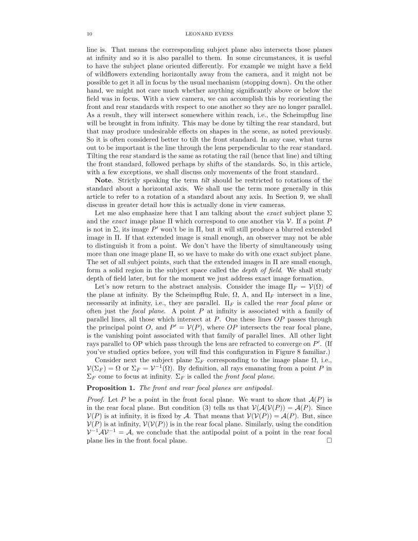
Proposition 1. The front and rear focal planes are antipodal.
Proof. Let P be a point in the front focal plane. We want to show that A(P ) isin the rear focal plane. But condition (3) tells us that V(A(V(P )) = A(P ). SinceV(P ) is at infinity, it is fixed by A. That means that V(V(P )) = A(P ). But, sinceV(P ) is at infinity, V(V(P )) is in the rear focal plane. Similarly, using the conditionV−1AV−1 = A, we conclude that the antipodal point of a point in the rear focalplane lies in the front focal plane.

VIEW CAMERA GEOMETRY 11
ΠF = V(Ω) Λ
O
Figure 8. Rear Focal Plane
ΠF ΣF = V−1(Ω)Λ
O
A(P )
P
Figure 9. Front and Rear Focal Planes
Remark 1. The statement in the Proposition implies condition (3) and so is equiv-alent to it.
Here is an outline of the proof. First show that if the front and rear focal planesare antipodal then VAV and A are the same on the front focal plane. That is nothard to show using the definitions and the fact that P,O, and V(P ) are collinear.Similarly, it is not hard to see that VAV and A fix the plane at infinity. Sincethey also fix the principal point, it follows that we can choose five points, no threeof which are collinear on which both transformations agree. But a theorem inprojective geometry asserts that two projective transformations are the same if andonly if they agree on such a set of points.
As a consequence, we get the following important result.

12 LEONARD EVENS
Proposition 2. The lens map V is completely determined by the lens plane Λ, theprincipal point O, and the focal plane ΠF .
Proof. The (rear) focal plane and the front focal plane are antipodal, so if we knowthe first we know the second and vice versa. Any line through the origin is sentinto itself by a lens map V , since if P1 and P2 are collinear with O, then so areV(P1),V(P2), P1, and P2. Fix such a line L let it intersect the rear focal plane atF , the front focal plane at F ′ and the plane at infinity at F∞. It is easy to see thatQ = AV interchanges F ′ and F∞, and it fixes O.
We now use the concept of the cross ratio, P1, P2;P3, P4, which is a numberdefined for any four collinear points. Given a projective coordinate system, we mayassign an affine coordinate p to each point on such a line, and supposing pi is thecoordinate of Pi, the cross ratio is given by the formula
P1, P2;P3, P4 =p1 − p3
p1 − p4
/p2 − p3
p2 − p4.
(One deals with p = 0 and p = ∞ in this this formula in the obvious ways.) Themost important property of the cross ratio is that it is an invariant preserved byprojective transformations.
Let P be any point on the line OF∞ = OF ′. Assume the coordinate systemon that line has been chosen so that O has coordinate 0, F ′ has coordinate fL,F∞ has coordinate ∞, P has coordinate u and Q(P ) has coordinate v. ThenP,O;F ′, F∞ = Q(P ), O;F∞, F
′.
O
0
F ′
fLF∞
P
u
Q(P )
v
V(P )
In terms of coordinates that means
u− fL
u−∞/−fL
−∞ =v −∞v − fL
/−∞−fL
.
The terms with infinities mutually cancel and we get
u− fL
−fL
=−fL
v − fL
or
(LQ) (u − fL)(v − fL) = (fL)2.
That means that Q(P ) is completely determined by P and F ′ (since Q(F ′) = F∞).Thus Q is completely determined under the hypotheses, which means that V = AQis.
With a bit more algebra, formula (LQ) reduces to
(ALQ)1
u+
1
v=
1
fL
VIEW CAMERA GEOMETRY 13
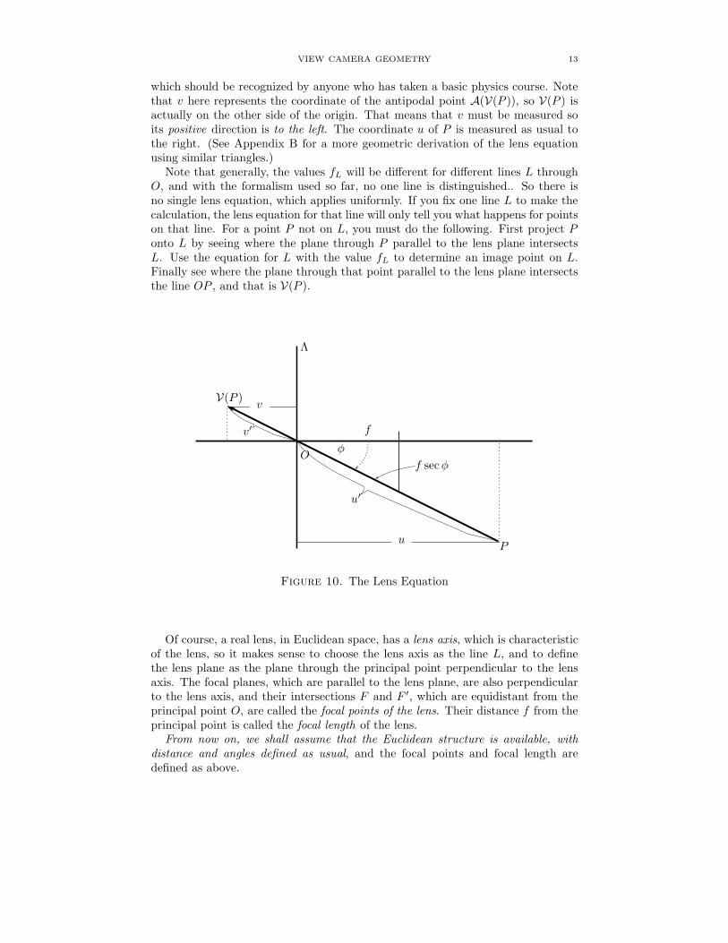
which should be recognized by anyone who has taken a basic physics course. Notethat v here represents the coordinate of the antipodal point A(V(P )), so V(P ) isactually on the other side of the origin. That means that v must be measured soits positive direction is to the left. The coordinate u of P is measured as usual tothe right. (See Appendix B for a more geometric derivation of the lens equationusing similar triangles.)
Note that generally, the values fL will be different for different lines L throughO, and with the formalism used so far, no one line is distinguished.. So there isno single lens equation, which applies uniformly. If you fix one line L to make thecalculation, the lens equation for that line will only tell you what happens for pointson that line. For a point P not on L, you must do the following. First project Ponto L by seeing where the plane through P parallel to the lens plane intersectsL. Use the equation for L with the value fL to determine an image point on L.Finally see where the plane through that point parallel to the lens plane intersectsthe line OP , and that is V(P ).
Λ
Oφ
f
V(P )v
v′
Pu
u′
f secφ
Figure 10. The Lens Equation
Of course, a real lens, in Euclidean space, has a lens axis, which is characteristicof the lens, so it makes sense to choose the lens axis as the line L, and to definethe lens plane as the plane through the principal point perpendicular to the lensaxis. The focal planes, which are parallel to the lens plane, are also perpendicularto the lens axis, and their intersections F and F ′, which are equidistant from theprincipal point O, are called the focal points of the lens. Their distance f from theprincipal point is called the focal length of the lens.
From now on, we shall assume that the Euclidean structure is available, withdistance and angles defined as usual, and the focal points and focal length aredefined as above.
14 LEONARD EVENS
For points on the lens axis, equation (ALQ) holds, with u, v, and fL = f , thefocal distance, measured as Euclidean distances. For points not on the lens axis—see Figure 10—we must apply the more general rule discussed above to obtain
(Lens Equation)1
u+
1
v=
1
f
where u and v refer respectively to the perpendicular distances of the subject pointP and the image point V(P ) to the lens plane, not their Euclidean distances u′
and v′ to the principal point O. People often misunderstand this. To obtain theappropriate equation relating u′ and v′, note that the line L = PV(P ) intersectsthe focal planes at Euclidean distance fL = f secφ, where φ is the angle betweenthe lens axis and PV(P ). Hence,
(GLE)1
u′+
1
v′=
1
f secφ=
cosφ
f
6. The Hinge Line
In a camera without movements, the image plane is parallel to the lens plane, asis the subject plane, and the Scheimpflug line is at infinity. But, in a view camera,when the lens plane is tilted with respect to the image plane, knowing how to usethe Scheimpflug line when focusing is crucial.
Beginning view camera photographers often think that the Scheimpflug Rulecompletely determines the positions of the subject and image planes, and this con-fuses them when trying to apply it. If you specify the image plane, all you know fromScheimpflug is that the subject plane passes through the intersection of the imageplane with the lens plane. But there are infinitely many such planes and withoutfurther information, you don’t know which is the actual subject plane. Similarlygiven the subject plane, there are infinitely many planes with pass through theScheimpflug line and only one is the actual image plane.
Fortunately, Herr Scheimpflug provided us with another rule, which helps todetermine exactly where either plane is, given the other.
Consider a setup where the rear standard is kept vertical and we focus by movingit parallel to itself along the rail, so that all potential image planes Π are parallelto one another. As we do, the line where Π intersects the plane at infinity staysfixed. Call that line I∞. Consider the plane through the principal point O which isparallel to the rear standard. We call that plane the reference plane and generallydenote it by ∆.7 It also passes through that same line I∞ at infinity. See Figure11.
The front focal plane intersects the reference plane ∆ in a line H which we shallcall the hinge line. It is the inverse image of the line I∞ under the lens map. Itdepends only on the lens map and the reference plane. It doesn’t change as wefocus by translating the image plane Π parallel to itself. Let Σ be the subjectplane associated to Π, and consider the line H ′ where it intersects the front focalplane ΣF . That line is carried by V into the intersection of Π with the plane atinfinity, which by our assumptions is I∞. Hence H ′ = H , the hinge line. So allrelevant subject planes pass through the hinge line. In other words, we can envision
7For a real lens, which has physical extent, the location of the reference plane can be tricky.For most lenses used in view camera photography, it will be where the lens axis intersects theplane through the front of the lensboard, or close enough that the difference won’t matter. Forsome telphoto lenses, this can get more complicated. See Section 10 for a bit more discussion.

VIEW CAMERA GEOMETRY 15
the subject plane rotating about the hinge line as we focus, which explains theterminology.
Π ∆ΣF
Σ
Λ
φ
O
v
u
S
f
JTo Horizon
Horizon Image
Hinge Line H
Figure 11. The Hinge Line
The hinge line appears in Scheimpflug’s 1904 patent application, although hedidn’t claim credit for it, and used different terminology. Most photographers,including the current author, first learned about it, its history, and its uses fromMerklinger.8 It is also called the pivot or rotation axis.
Important Note. Figure 11 is typical of the diagrams used in this subject. Itimplicitly suggests that the lens plane is tilted downward, and the image plane isvertical. This is by far the most common situation, but it doesn’t by any meanscover all possible cases. The lens plane could be tilted upward, with the Scheimpflugline and the hinge line above the lens. More to the point, the diagrams also applyto swings to one side or the other, where neither side is distinguished. In thatcase, the standard diagram would show things as they would appear if the observerwere above the camera, looking down, and the lens plane was swung to the right.It gets even more complicated if the lens plane is tilted with respect to a skewaxis, which is neither horizontal nor vertical, or if we tilt the back, hence, thereference plane, in which case, the whole diagram is tilted with respect to thevertical. However, whatever the tilt orientation, we may assume the standarddiagram presents an accurate picture, simply by changing the orientation of theobserver in space. So doing may require some verbal gymnastics. For example, fortilts about a horizontal axis, the horizon provides a reference to which the subjectplane can compared. There is no comparable reference when you swing about avertical axis, but you could look at the vertical plane perpendicular to the imageplane and its intersection with the plane at infinity. (Perhaps it should be called
the ‘verizon’—.|..) In general, assuming the standards are not parallel, consider the
line through the principal point parallel to intersection of the lens plane with theimage plane (determined by the rear standard). The rotation of the front standard
8www.trenholm.org/hmmerk.

16 LEONARD EVENS
about that axis is what we are calling the tilt. Instead of the actual horizon, whichexists independently of the orientation of the camera, you would use the planeperpendicular to the image plane and parallel to the axis of rotation, as well as itsintersection with the plane at infinity. I leave it to the reader to deal with suchmatters. Just keep in mind, in any situation, the positions of image plane, thehinge line, the Scheimpflug line, and the rotation axis will guide you about how tointerpret the words.
Introducing the hinge line simplifies considerably the problem of obtaining adesired subject plane. We first concentrate on where that plane intersects thereference plane, i.e., the desired hinge line. If we get that right, we need only focusthe rear standard until the resulting subject plane swings into place.
With the front standard untitled and parallel to the rear standard, the hingeline is at infinity, but as we tilt the lens plane (forward), the hinge line moves (up)in the reference plane to a finite position.
The perpendicular distance J in the reference plane ∆ from the principal pointO to the hinge line H is called the hinge distance. It is clear geometrically that itcan’t be smaller than the focal length, which would be the case if the lens planewere turned 90 degrees so it was perpendicular to the image plane. In practice younever get anywhere near that, with typical rotation angles being a few degrees andnever exceeding 15 or 20 degrees. From Figure 11, we have
(HD) J =f
sinφ
where φ is the tilt angle, i.e., the angle that the lens plane makes with the referenceplane and the image plane. It follows that the the tilt angle depends only on theposition of the hinge line.
Note also that the distance S from the image of the horizon line to the Scheimpflugline is given by
(SchD) S = v cotφ
But from equation (GLE), we havecosφ
f=
1
v+
1
u. (In Figure 11, u and v are now
the oblique distances to O.) So
v cosφ = (1 +v
u)f = (1 +M)f or
v = f(1 +M) secφ(VE)
where M is the magnification just for objects at distance u at which the subjectplane intersects the reference normal. i.e., the line through O perpendicular to thereference (image) plane.9 Elsewhere in the subject plane, the magnification will bedifferent.
Note that u and M may be negative, which would be the case when the subjectplane tilts away from the reference normal. In that case, there is no subject pointcorresponding to u.
It now follows that
(SchDa) S = v cotφ = vcosφ
sinφ=
(1 +M)f
sinφ= (1 +M)J
9That line is usually drawn as if it were horizontal, the most common case. But as we notedbefore, it need not be.

VIEW CAMERA GEOMETRY 17
Π ΠF
∆
ΣF
Σ
Λ
O
J
J
y
Horizon Image
v
u
To Tilt Horizon
To Horizon
Hinge Line H
Cohinge Line H ′
Figure 12. Cohinge Line
Note one important consequence of equation (VE). Since usually |M | ≪ 1 andφ is pretty small, typically v ≈ f . The exception would be in close-up situationswhen M is can be a fairly large, possibly even larger than 1.
For a given orientation of the lens—which of course fixes the positions of the frontand rear focal planes, any family of parallel subject planes determines a coreferenceplane and its intersection with the rear focal plane should be called the cohingeline. (See Figure 12 again.) It plays a role dual to that of the hinge line, but therearen’t many circumstances in which it remains fixed as you manipulate the camera,so it is not used the same way as the hinge line.
But, the cohinge line can also be thought of as the image of the intersectionof the subject plane with the plane at infinity, which we call the tilt horizon.10
All parallel line pairs, in the subject plane or parallel to the subject plane, havevanishing points on the cohinge line, and every such point is obtainable in that way.This can sometimes be useful as the photographer tries to visualize the placementof the subject plane by looking at the image on the ground glass. Also, nothing inthe image plane below the cohinge line can be exactly in focus, i.e., no point in thesubject above the tilt horizon can be in focus. See Figure 12.
From the diagram and equations (SchDa) and (HD), we get the following equa-tion for the distance of the cohinge line, i.e., the image of the tilt horizon, belowthe image of the horizon.
(TH) y = S − J = (1 +M)J − J = MJ
Note that if M < 0, then y < 0, which means that the tilt horizon image is on theopposite side of the reference normal from where we usually picture it.
We can now begin to see why large tilt angles φ are not common. Namely, except
in close-up situations, |M | ≪ 1, so, unless J =f
sinφis large enough, i.e., φ small
10It should be distinguished from the horizon, which is the intersection with the plane atinfinity with the plane through O, perpendicular to the reference plane, and parallel to the hingeand cohinge lines. Of course, this language only makes sense in case of a pure tilt.

18 LEONARD EVENS
enough, to compensate, y = MJ will be very small. Depth of field—see Section8.3—may allow us to descend a bit further, but usually not by a large amount. Ifthe scene includes expanses, such as open sky, which need not be in focus, thatmay allow the frame to drop further, so it may not matter, but otherwise, the shiftrequired to get the top of the frame where it must be may not be possible becauseof mechanical limitations of the camera. Even if the camera allows for very largeshifts, selecting a portion of the frame far from the observer’s line of sight mayintroduce a bizarre perspective, particularly for wide angle lenses. One can avoidsuch problems by tilting the camera down or by tilting the rear standard, but doingeither may introduce other problems.
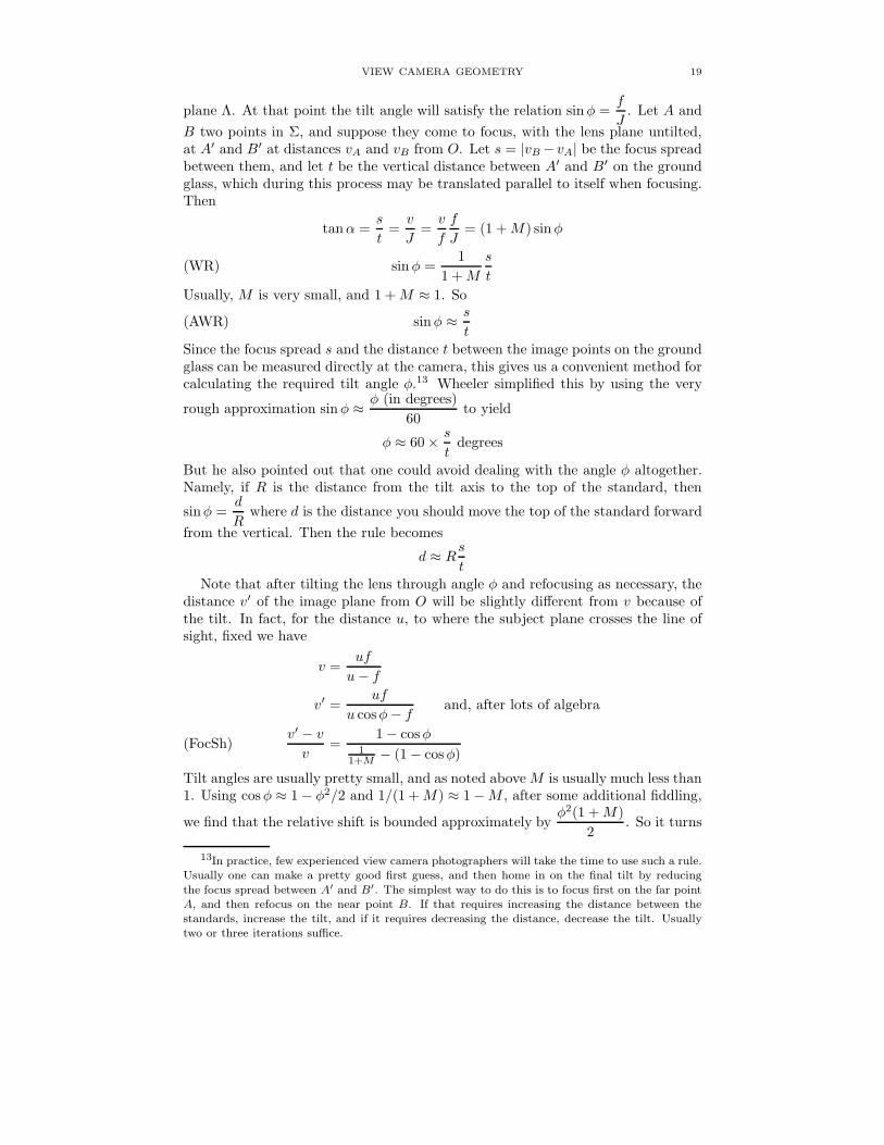
6.1. Wheeeler’s Rule. There is a simple rule discovered by Wheeler11 for calcu-lating the tilt angle on the basis of measurements made on the rail and the groundglass. Refer to Figure 13. Initially, the lens plane Λ is vertical12, and we have
A
A′
B′
ZZ ′
B
Σ
Λ
O
uv
vB
vA
Π
s
t α
α
J
L
Figure 13. Wheeler’s Rule
indicated a prospective subject plane Σ crossing the line of sight at the point Zat distance u from O. (The ground glass, which is not explicitly indicated in thediagram, is also parallel to Λ and will stay so during the process, but it may betranslated by focusing.) If v is the distance of the corresponding image point Z ′ toO, then we have
(EqM)1
u+
1
v=
1
fand
v
f= 1 +M
where M is the magnification at distance u, with no tilt. Let Σ cross Λ in the lineL at distance J from O. By the Scheimpflug Rule, the corresponding image planeΠ also passes through L. As we tilt the lens plane, keeping the prospective subjectplane Σ fixed, the corresponding image plane will tilt (and also move horizontally),until eventually it reaches a position parallel to the original position of the lens
11www.bobwheeler.com/photo/ViewCam.pdf,Section 5.312Of course, the same reasoning works for another initial position of the lens plane, but the
language would have to be adjusted.
VIEW CAMERA GEOMETRY 19
plane Λ. At that point the tilt angle will satisfy the relation sinφ =f
J. Let A and
B two points in Σ, and suppose they come to focus, with the lens plane untilted,at A′ and B′ at distances vA and vB from O. Let s = |vB− vA| be the focus spreadbetween them, and let t be the vertical distance between A′ and B′ on the groundglass, which during this process may be translated parallel to itself when focusing.Then
tanα =s
t=v
J=v
f
f
J= (1 +M) sinφ
sinφ =1
1 +M
s
t(WR)
Usually, M is very small, and 1 +M ≈ 1. So
(AWR) sinφ ≈ s
tSince the focus spread s and the distance t between the image points on the groundglass can be measured directly at the camera, this gives us a convenient method forcalculating the required tilt angle φ.13 Wheeler simplified this by using the very
rough approximation sinφ ≈ φ (in degrees)
60to yield
φ ≈ 60× s
tdegrees
But he also pointed out that one could avoid dealing with the angle φ altogether.Namely, if R is the distance from the tilt axis to the top of the standard, then
sinφ =d
Rwhere d is the distance you should move the top of the standard forward
from the vertical. Then the rule becomes
d ≈ Rst
Note that after tilting the lens through angle φ and refocusing as necessary, thedistance v′ of the image plane from O will be slightly different from v because ofthe tilt. In fact, for the distance u, to where the subject plane crosses the line ofsight, fixed we have
v =uf
u− f
v′ =uf
u cosφ− f and, after lots of algebra
v′ − vv
=1− cosφ
11+M
− (1− cosφ)(FocSh)
Tilt angles are usually pretty small, and as noted aboveM is usually much less than1. Using cosφ ≈ 1− φ2/2 and 1/(1 +M) ≈ 1−M , after some additional fiddling,
we find that the relative shift is bounded approximately byφ2(1 +M)
2. So it turns
13In practice, few experienced view camera photographers will take the time to use such a rule.Usually one can make a pretty good first guess, and then home in on the final tilt by reducing
the focus spread between A′ and B′. The simplest way to do this is to focus first on the far pointA, and then refocus on the near point B. If that requires increasing the distance between thestandards, increase the tilt, and if it requires decreasing the distance, decrease the tilt. Usuallytwo or three iterations suffice.
20 LEONARD EVENS
out that the relative shift, while noticeable, particularly for larger tilts, is prettysmall. For example, for φ = 0.25 radians (about 14.3 degrees) and M = 0.01, therelative shift turns out to be about 0.03 or 3 percent. For f = 150 mm, v = 151.5mm, the shift would be about 5 mm. For a more modest tilt of 0.1 radians (about5.7 degrees), the relative shift would be about 0.005 of 0.5 percent, and for the samef and v, the shift would be about 0.8 mm, which would be just barely detectable.
7. Realizable Points
There are certain forbidden regions which are not available for subject or imagepoints. Look at Figure 12 once more, and concentrate on the two focal planes.
Subject points to the right of the front focal plane ΣF in the diagram map toimage points to the left of the rear focal plane ΠF . As you approach the front focalplane, the image point moves to infinity. Subject points between the front focalplane and the lens plane, even if they are in the subject plane, map to points inthe subject space. Such points cannot be captured by film or a device. Sometimessuch image points are called virtual images. You “see” a magnified virtual imageif you put a magnifying glass closer to a subject than its focal length, but it can’tbe captured without additional optics to turn it into a real image. In effect thatis what your eye does when you use a magnifying glass. In any case, this plays norole in photography. The points to the left of the lens plane get mapped by thelens map to the part of the image space between the lens plane and the rear focalplane. For such points the subject and image points are on the same side of thelens plane, so the light ray would have to double back on itself, and there is noimage which can be captured. We see from this that the region between the focalplanes is forbidden and no point in it corresponds to a realizable subject or imagepoint.
That means that no point between the hinge line and the lens plane produces areal image, and no point between the lens plane and the cohinge line is a real image.In particular, no point in the frame below the cohinge can be exactly in focus, sono subject point above the tilt horizon can produce an image exactly in focus. Butit is possible that some points not in the exact subject plane have slightly blurryimages which are still sharp enough. (See the extensive discussion of depth of fieldin Section 8.3.)
As we shall see later, the finite dimensions of the camera also put further restric-tions on which points can be realized.
8. Depth of Field
As mentioned earlier, we have to put the film (image plane) Π at a specificlocation, so there is one and only one subject plane Σ corresponding to it. Asubject point P not in Σ will produce an image point P ′ not in Π, but it may stillbe close enough that it won’t matter. This effect is called defocus.
The lens is not a point, although, for the purposes of geometric optics, we cantreat it as such. In reality, there is a lens opening or aperture through which lightrays pass. As the diagram shows the light rays which start at a subject point P willemerge from the lens as a solid cone with vertex at the image point P ′, and basethe aperture. The aperture is usually a regular polygon with five or more sides,and it is simplest to assume it is a circular disc, although that is not essential.Under that assumption, the cone will intersect the desired exact image plane Π in

VIEW CAMERA GEOMETRY 21
Π Λ
O
P
P ′
Aperture
CoC
Figure 14. Circle of Confusion
a region, which, if the film plane is parallel to the aperture, will be a circular disc,but in general it will be an ellipse. So we call that region the circle of confusion—abbreviated CoC, whether it is actually a circle or not. If the circle of confusionis not too large, it can’t be distinguished from the point where the axis of thecone intersects Π. For all such points it is as if we were using a pinhole camerawith the pinhole at the center of the aperture. The pinhole image of P ′ will bethe intersection of the line connecting the center of the aperture, i.e., the principalpoint O, to P ′.
Usually we set a criterion for how large the circle of confusion can be and still beindistinguishable from a point. That will depend on factors such as the intendedfinal image, how much it must be enlarged from the image recorded in the camera,and how, and by whom, it is viewed. For a given position of the subject plane (andcorresponding image plane), there will be a region about it, called the depth offield region or, often, just the depth of field. and it is abbreviated ‘DOF’. It shouldbe emphasized that there generally won’t be a sharp cutoff at the boundaries ofdepth of field. Other factors, such as contrast and edge effects, affect perceptionof shaprness, so detail outside the region may still appear sharp. But, at least inprinciple, everything within the region should appear to be in focus, and detailswell outside it should be appear to be out of focus14.
Most of the rest of the article will be concerned with determining the shape ofthis region under different circumstances. It turns out that if the subject plane,lens plane, and image plane are all parallel, i.e., no tilt, the DOF will be containedbetween two planes parallel to both. If the lens plane is tilted, then the region isalmost a wedge shaped region between two bounding planes. By far, the greatestpart of this article will be concerned with quantifying the term ‘almost’, which issomething that is usually ignored.
14Analysis of depth of field usually ignores diffraction, which has an overall burring effect onthe image. See the article by Jeff Conrad atwww.largeformatphotography.info/articles/DoFinDepth.pdf,for a discussion of diffraction.
22 LEONARD EVENS
Before beginning that discussion, it is worthwhile saying something about how aphotographer might approach the problems presented by a given scene. Typically,one wants certain parts of the scene to be in focus and will first try to achieve that,without tilt, by stopping down far enough. If that doesn’t work because the sceneextends from very near in the foreground to the distant background, one will thentry to decide if the situation may be improved by tilting the lens somewhat. Thatmay work provided that the vertical extent one needs in focus close to the lens isnot too great. In the process, one will at some point settle on a narrow range forthe desired subject plane, and that, as we have seen, will determine the tilt anglewithin certain narrow limits. So normally, we will consider the tilt angle essentiallyfixed and proceed from there.
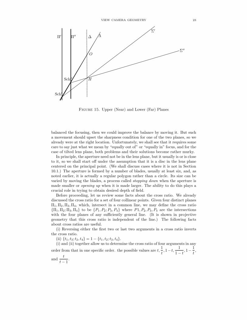
Suppose we specify as before that the image plane Π may only be adjusted bytranslation parallel to itself. Then, all corresponding subject planes meet in thehinge line (which may be at infinity). Suppose we pick two such subject planes, orequivalently, two corresponding image planes. The image plane farther from thelens is called the outer image plane and that closer to the lens is called the innerimage plane. The corresponding subject planes Σ′ and Σ′′ are called respectivelythe upper and lower subject planes or sometimes the near and far subject planes.The latter terminology is more appropriate in the case of zero tilt, for, then all theplanes are parallel and the former plane is indeed nearer to and the latter plane isfurther from the lens plane. But it can be misleading if the tilt is not zero, sincethe upper limit of what can be in focus in the distance is determined by the upperor ‘near’ plane, and the lower limit of what can be in focus in the foreground iscontrolled by the lower or ‘far’ plane. By assumption, the image planes are allparallel, so there is less ambiguity. The outer image plane corresponds to the upper(near) subject plane, and the inner image plane corresponds to lower (far) subjectplane. But, there is still another confusion in terminology. The distances v′, v, v′′ ofthe image planes to the reference plane determine positions on the rail. Dependingon the context, the position v′ should properly be called either the near point orthe upper point, and v′′ should be called the far point or lower point. See Figure15.
In the diagram, we assume we have already tilted the lens plane. Note that whilethe hinge line stays fixed, the Scheimpflug lines differ for the two planes.
There are now two interesting questions to ask.(1) Given Σ′ and Σ′′ (equivalently Π′ and Π′′) as above, where shall we focus,
i.e., place the exact subject plane Σ so that points in Σ′ and Σ′′ are “equally out offocus” in Π in a sense to be discussed. (Some people have argued for favoring oneplane over the other, but we shall not get into that controversy in this article.)
(2) Suppose we have specified a criterion for sharpness, and for whatever reason,we have decided on an exact image plane Π. How far can we place Π′ and Π′′ oneither side of Π so all points between them will satisfy that criterion?
A problem associated with (2) is(2a) Suppose we start with Π′ and Π′′ as in (1) and find the best place to place
Π. How can we control the circles of confusion in Π from points between Π′ andΠ′′ and ensure they satisfy our criterion for sharpness?
Note that if we start with Π and find Π′ and Π′′ solving problem (2), then,intuitively, at least, Π should be the plane solving problem (1) for those two planes.The argument would be that if Π were not already in the position which best
VIEW CAMERA GEOMETRY 23
Π′ Π′′ ∆
Σ′
Σ′′
Λ
O
HSch′′
Sch′
Figure 15. Upper (Near) and Lower (Far) Planes
balanced the focusing, then we could improve the balance by moving it. But sucha movement should upset the sharpness condition for one of the two planes, so wealready were at the right location. Unfortunately, we shall see that it requires somecare to say just what we mean by “equally out of” or “equally in” focus, and for thecase of tilted lens plane, both problems and their solutions become rather murky.
In principle, the aperture need not be in the lens plane, but it usually is or is closeto it, so we shall start off under the assumption that it is a disc in the lens planecentered on the principal point. (We shall discuss cases where it is not in Section10.1.) The aperture is formed by a number of blades, usually at least six, and, asnoted earlier, it is actually a regular polygon rather than a circle. Its size can bevaried by moving the blades, a process called stopping down when the aperture ismade smaller or opening up when it is made larger. The ability to do this plays acrucial role in trying to obtain desired depth of field.
Before proceeding, let us review some facts about the cross ratio. We alreadydiscussed the cross ratio for a set of four collinear points. Given four distinct planesΠ1,Π2,Π3,Π4, which, intersect in a common line, we may define the cross ratioΠ1,Π2; Π3,Π4 to be P1, P2;P3, P4 where P1, P2, P3, P4 are the intersectionswith the four planes of any sufficiently general line. (It is shown in projectivegeometry that this cross ratio is independent of the line.) The following factsabout cross ratios are useful.
(i) Reversing either the first two or last two arguments in a cross ratio invertsthe cross ratio.
(ii) t1, t3; t2, t4 = 1− t1, t2; t3, t4.(i) and (ii) together allow us to determine the cross ratio of four arguments in any
order from that in one specific order. the possible values are t,1
t, 1− t, 1
1− t , 1−1
t,
andt
t− 1.

24 LEONARD EVENS
(iii) Given 5 collinear points (planes) t0, t1, t2, t3, t4, we have
t1, t0; t3, t4t2, t0; t3, t4
= t3, t4; t1, t2.
8.1. Case I. The lens is not tilted with respect to the reference plane. Aswe shall see, things work out very nicely in this case, and both problems have clearsolutions.
Π′ Π Λ
P ′
c
c
v′
v
D
Figure 16. The Basic Diagram
8.1.1. Problem (1). Assume the aperture has diameter D. Choose a plane Π be-tween the outer and inner planes Π′ and Π′′. Fix attention on Π′. Choose a pointP ′ in Π′. and form the solid cone with vertex P ′ and base the aperture. Let Q bethe pinhole image in Π; i.e., the intersection of Π with OP ′. Let c be the diameter
of the disc in which the cone intersects Π. Note that the ratioc
Dremains fixed as
long as the plane Π′ remains fixed. That is clear by considering the similar trianglesin Figure 16, which shows a slice by a p lane through the principal point.
The ratios of corresponding sides in similar triangles are equal. So, we have
(A) Π′,Ω; Π,Λ = v′,∞; v, 0 =v′ − vv′
=c
D
Now let P ′′ be a point on OP ′ in the outer image plane Π′′ on the same side of Πas the lens plane. Clearly, Π will be in the optimum position between Π′ and Π′′
when the circle of confusion produced by P ′′ is identical with that produced by P ′.So we also have
(B) Π′′,Ω; Π,Λ = v′′,∞; v, 0 =v′′ − vv′′
= − c
D.
Hence, by dividing (A) by (B), we obtain
(H) Π,Λ; Π′ Π′′ = v, 0; v′, v′′ =v − v′v − v′′
/ −v′−v′′ = −1

VIEW CAMERA GEOMETRY 25
Π′ Π Π′′ Λ
P ′
cP ′′
v′
v
v′′
D
Figure 17. Balance
It is easy to check that this is true if and only if
(H′)1
v=
1
2
( 1
v′+
1
v′′
)
(H′) by definition says that v is the harmonic mean of v′ and v′′, and similarly wesay that that a plane Π is the harmonic mean of Π′ and Π′′ relative to a plane Π0
if Π,Π0; Π′,Π′′ = −1. Note that this relation doesn’t depend on the order of
Π′,Π′′ since reversing order of either the first two or the last two arguments in across ratio just inverts the cross ratio.
It is sometimes more useful to rewrite equation (H′) as
(H′′) v =2v′v′′
v′ + +v′′
which it reduces to by some simple algebra.In practice, it might be tricky determining the position of the harmonic mean,
but fortunately there is a simple approximation which makes focusing much easier.It is based on the relation (H′), which may also be written
(Ha)v′′ − vv − v′ =
v′′
v′.
For normal photography where all interesting parts of the image are relativelydistant, the values of v′ and v′′ are not much greater than the focal length, andhence are relatively close to one another, so it follows from (Ha) that v′′−v ≈ v−v′,i.e, that we can place the image plane halfway between the near (outer) and far(inner) points on the rail without being very far off, and that simplifies focusingenormously. In fact, detailed calculations show that the error made in so doing isnegligible, even in close-up situations except for very short focal length (wide angle)lenses, a situation almost never met in practice.
8.1.2. Problem(2). Specify the criterion by setting a maximum possible diameter cfor a circle of confusion. We want to determine just how far from Π we may put Π′
26 LEONARD EVENS
and Π′′ so any point between them will yield a circle of confusion in Π of diameternot greater than c.
To this end, we use the same equations (A) and (B). Start at Π and move away
from it in both directions until the two cross ratios are equal to µ =c
Dand −µ
respectively. (Note also that in this case Π will end up being the harmonic meanof Π′ and Π′′ by the same argument as before.) Solving those equations for v′ andv′′ yields
(V) v′ =v
1− µ v′′ =v
1 + µ.
We also see how to solve problem (2b). Namely, the cross ratios in (A) and (B)
are fixed by the positions of the planes, so the ratio µ =c
Dis determined by that
information. Now, given c, simply choose D, by stopping down, so thatc
D= µ or
D = µc.In photography, one seldom uses the actual diameter of the aperture but instead
the f-number N =f
Dwhere f is the focal length.15 (This is because the f-number
is more directly related to the light intensity at P ′.) Hence, it is more useful to
rewrite the crucial ratio µ =Nc
f. So, given a maximum possible diameter c for the
circle of confusion, we need to choose N =fµ
c
On the other hand, when v =2v′v′′
v′ + v′′is chosen as the harmonic mean of v′ and
v′′, we have
µ =v′ − vv′
= 1− v
v′= 1− 2v′′
v” + v′′=v′ − v′′v′ + v′′
,
so
(N) N =v′ − v′′
c
f
v′ + v′′.
But from (E), we get
v′ + v′′ = v( 1
1 + µ+
1
1− µ)
=2v
1− µ2
So
N =v′ − v′′
2c
f
v(1− µ2).
On the other hand, from the lens equation, as in Section 6, we get
v
f=v
u+ 1 = M + 1
15The f-number is usually denoted symbolically as the denominator of a symbolic ‘fraction’ as
in ‘f/32’ for f-number 32. f is not suppose to have a specific value, and you are not supposed toperform a division, but if it were the actual focal length then f/N would be the actual diameterof the aperture, so this terminology can be confusing. We shall abuse the terminology at times inthis article by referring to ‘aperture N ’ when we mean that the f-number is N .

VIEW CAMERA GEOMETRY 27
where M =v
uis the magnification or scale of reproduction at the exact plane of
focus. Hence,
(1) N =v′ − v′′
2c(1 +M)(1− µ2) <
v′ − v′′2c(1 +M)
.
Overestimating N is usually innocuous, so the quantity on the right is a reasonableestimate for the appropriate f-stop. In any case, µ2 is typically small,16 so we maysay
(N′) N ≈ v′ − v′′2c(1 +M)
Except in close-up situations, the scale of reproduction M is quite small and can
be ignored, in which case the estimate becomes N ≈ v′ − v′′2c
. In any case, if we
ignored M , that would just lead us to stop down more than we need to. Usuallythat is innocuous since we are interested in adequate depth of field and don’t careif we get a bit more than we expected17. But there are occasions when one wantsto limit depth of field to precisely what is needed, in which case one would keepthe factor 1 +M .
8.1.3. The Subject Space. What does all this say about what is happening in thesubject space? If we remember that the lens map and its inverse are projectivetransformations and so preserve cross ratios, it follows that Σ,Λ; Σ′,Σ′′ = −1,i.e., the best place to focus is at the harmonic mean of the near and far18 subjectplanes with respect to the lens plane. In particular, if the distances of the near andfar subject planes from the lens plane are respectively u′ and u′′, then you shouldfocus at the harmonic mean u of those distances where
(SH)1
u=
1
2
( 1
u′+
1
u′′
)
.
For scenes in which u′ and u′′ reasonably close, we may use the analogue of equation(Ha)
(SHa)u′′ − uu− u′ =
u′′
u′.
to conclude that u−u′ ≈ u′′−u, i.e., that the front depth of field and the rear depthof field are approximately equal. That holds true not only for close-up photographybut also for normal portraiture. A reasonable estimate for that distance—see 8.2—is
cN(1 +M)
M2
so it depends only on the circle of confusion c , the f-number N and the scale ofreproduction M . In particular, it is essentially independent of the focal length as
16An extreme estimate for µ with N = 64, c = 0.1 and f = 65 isNC
f< 64 × 0.1/65 ≈ 0.1,
so µ2 < .01 or 1 percent. That works for 4 x 5 format. For 8 x 10, with N = 128, c = 0.2 andf = 130 mm, it would be less than 4 percent. Either would amount to an insignificant differencein setting the f-stop.
17Stopping down does require increasing the time setting to maintain exposure, and in somecases that may create problems because of subject movement.
18We switch from ‘upper’ and ’lower’ to ‘near’ and ‘far’ since they are more appropriate in thiscase.
28 LEONARD EVENS
long as the scale of reproduction is kept fixed. One often sees this rule stated asif it held in general, whatever the subject distance, but it clearly fails for subjectssufficiently remote from the lens. In particular, as we see below, the far depth offield is often infinite.
8.1.4. The Hyperfocal Distance. If the far plane is at infinity, i.e., u′′ = ∞, thenequation (SH) tell us that u = 2u′, in other words the correct place to focus is attwice the distance of the near plane.
On the other hand, suppose we stop down to aperture (f-number) N . At whichdistance should we focus so that far plane bounding the depth of field is at infinity?Since the plane at infinity is mapped by the lens map to the focal plane, that
amounts to setting v′′ = f , so equation (B) reduces tov − ff
= µ =c
D=
f
Nc,
which yields v − f = Nc or v = Nc+ f . The corresponding subject plane distancemay be derived from the relation (u− f)(v − f) = f2 which yields
(Hyp) uH = f +f2
Nc≈ f2
Nc
(where the approximation holds as long as Nc is much smaller than f which isalways the case, except for extremely short focal length lenses.) The distance uH iscalled the hyperfocal distance. If you focus at the hyperfocal distance, then infinitywill just barely be in focus. To do so, you place the rear standard back from thefocal plane by the quantity Nc, which is independent of the focal length.
But, as we saw above, u′′ = ∞ implies that u = uH = 2u′, the near distance.In other words, if you focus at the hyperfocal distance, everything from half thatdistance to infinity will be in focus.
Let’s look at a typical example. c = 0.1 mm is a typical value taken for thediameter of the maximum allowable circle of confusion in 4 x 5 photography, andf = 150 mm is a typical “normal” focal length. A typical f-number would beN = 22. So, in this case Nc = 2.2 mm. Similarly, f = 150≫ 2.2, so the hyperfocal
distance is given accurately enough byf2
Nc=
1502
2.2≈ 10227 mm ≈ 10 meters. Half
the hyperfocal distance will be about 5 meters. An extremely short focal length
for such a camera would be f = 50 mm, and in this case502
2.2≈ 1136 mm. In this
case, it might be more accurate to add the focal length to get 1186 = 1.186 meters.Everything from infinity down to about 0.593 meters should be in focus.
Notice that the hyperfocal distance only makes sense given a choice of relativeaperture N . If you stick with the same aperture but focus so that u > uH , you willplace the inner image plane Π′′ in the forbidden region, so ‘image points’ betweenΠ′′ and the focal plane will not correspond to real subject points. (See Section 7.)The result will be that you will lose some far depth of field. See Section 8.2 belowfor formulas which allow you to determine the near depth of field in that case.
It is hard to measure small distances that precisely along the rail, but most viewcameras employ a gearing mechanism which magnifies motions along the rail forfine focusing. Using a scale on the focusing knob in such cases makes it much easier.The alternative is to calculate the hyperfocal distance, or get it from a table, andthen focus on some object in the scene at that distance. Rangefinder devices areavailable for measuring such distances, but it seems overkill to use them, since thecamera itself effectively does it for you.

VIEW CAMERA GEOMETRY 29
8.2. Depth of Field Formulas. Assume we focus at distance u, at aperture (f-
number) N , with circle of confusion c, and let uH = H + f , where H =f2
Nc, be the
hyperfocal distance. Recall formulas (A) and (B)
Π′,Ω; Π,Λ =Nc
f
Π′′,Ω; Π,Λ = −Ncf
As before, since cross ratios are preserved, and V carries the front focal plane ΣF
into the plane at infinity Ω, we obtain
Σ′,ΣF ; Σ,Λ =Nc
f
Σ′′,ΣF ; Σ,Λ = −Ncf
or
u′, f ;u, 0 =Nc
f
u′′, f ;u, 0 = −Ncf
i.e.,
u′ − uu′
=Nc
f
f − uf
u′′ − uu′′
= −Ncf
f − uf
After some algebra, these lead to the equations
u′ =u
1 + Ncuf2 − NC
f
u′′ =u
1− Ncuf2 + NC
f
In each case, multiply the numerator and denominator by the quantity H =f2
NCThis yields
u′ =uH
H + (u − f)(NDOF)
u′′ =uH
H − (u − f)(FDOF)
Since u > f , the denominator in equation (NDOF) is positive, and the formulaalways makes sense. But the denominator in equation (FDOF) may vanish or evenbe negative, so that formula requires a bit of explanation.
If u = H + f , the formula yields u′′ = ∞, which just says the Σ′′ is at infinityas in the previous section (8.1.4).
Suppose on the other hand that u > uH , so the denominator is negative. Inthat case, the formula yields a negative value for u′′. As we saw in the previoussection, that means that v′′ < f , i.e., Π′′ is in the forbidden zone. Restricting

30 LEONARD EVENS
attention to real subject points, we ignore the second equation and conclude thatthe depth of field extends from u′, given by equation (NDOF), to∞. In the extremecase in which one focuses at u = ∞, equation (NDOF) tells us u′ = H , which forall practical purposes is the hyperfocal distances. In other words, if you focus atinfinity, then everything down to the hyperfocal distance will be in focus.
If one’s aim is to maximize depth of field, there is little point in focusing at adistance greater than the hyperfocal distance, so it is common to add the restrictionu ≤ uH .19
If u≫ f , i.e., we are not in a close-up situation, then the above equations yieldthe approximations
u′ ≈ uH
u+H
u′′ ≈ uH
u−HIt is also useful to determine the front and rear depth of field
u− u′ =u(u− f)
H + (u− f)≈ u2
H + u(FDOF)
u′′ − u =u(u− f)
H − (u− f)≈ u2
H − u(RDOF)
where the approximations hold when we are not in a close-up situation. In the caseof close-ups, it is better to divide the numerator and denominator by f2 to obtain
u− u′ =
uf(u
f− 1)
1Nc
+ 1f(u
f− 1)
u′′ − u =
uf(u
f− 1)
1Nc
+ 1f(u
f− 1)
If we use the relationu
f=
1
M+ 1, we obtain after lots of algebra
u− u′ =Nc(1 +M)
M2(1 − NcfM
)
u′′ − u =Nc(1 +M)
M2(1 + NcfM
)
IfNc
fM≪ 1, then, we may ignore the second term in parentheses in the denomina-
tors to obtain
(Ha) u− u′ ≈ u′′ − u ≈ Nc(1 +M)
M2
which we mentioned earlier.
19There may be circumstances in which one wants to favor the background relative to theforeground. In that case, one might sacrifice some or all of the rear depth of field.
VIEW CAMERA GEOMETRY 31
8.3. Case II. Tilted lens plane. In this case, the aperture, which we have as-sumed is in the lens plane, is tilted with respect to the reference plane ∆ , and thiscomplicates everything.20
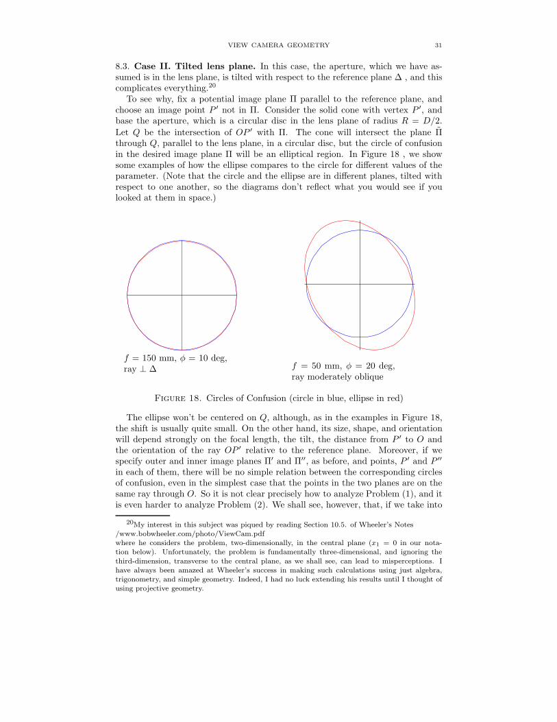
To see why, fix a potential image plane Π parallel to the reference plane, andchoose an image point P ′ not in Π. Consider the solid cone with vertex P ′, andbase the aperture, which is a circular disc in the lens plane of radius R = D/2.
Let Q be the intersection of OP ′ with Π. The cone will intersect the plane Πthrough Q, parallel to the lens plane, in a circular disc, but the circle of confusionin the desired image plane Π will be an elliptical region. In Figure 18 , we showsome examples of how the ellipse compares to the circle for different values of theparameter. (Note that the circle and the ellipse are in different planes, tilted withrespect to one another, so the diagrams don’t reflect what you would see if youlooked at them in space.)
f = 150 mm, φ = 10 deg,ray ⊥ ∆ f = 50 mm, φ = 20 deg,
ray moderately oblique
Figure 18. Circles of Confusion (circle in blue, ellipse in red)
The ellipse won’t be centered on Q, although, as in the examples in Figure 18,the shift is usually quite small. On the other hand, its size, shape, and orientationwill depend strongly on the focal length, the tilt, the distance from P ′ to O andthe orientation of the ray OP ′ relative to the reference plane. Moreover, if wespecify outer and inner image planes Π′ and Π′′, as before, and points, P ′ and P ′′
in each of them, there will be no simple relation between the corresponding circlesof confusion, even in the simplest case that the points in the two planes are on thesame ray through O. So it is not clear precisely how to analyze Problem (1), and itis even harder to analyze Problem (2). We shall see, however, that, if we take into
20My interest in this subject was piqued by reading Section 10.5. of Wheeler’s Notes/www.bobwheeler.com/photo/ViewCam.pdfwhere he considers the problem, two-dimensionally, in the central plane (x1 = 0 in our nota-tion below). Unfortunately, the problem is fundamentally three-dimensional, and ignoring the
third-dimension, transverse to the central plane, as we shall see, can lead to misperceptions. Ihave always been amazed at Wheeler’s success in making such calculations using just algebra,trigonometry, and simple geometry. Indeed, I had no luck extending his results until I thought ofusing projective geometry.

32 LEONARD EVENS
account the limitations imposed by the scene and the mechanical structure of thecamera and remember that the tilt angle φ is almost always relatively small, thenthings don’t get too bad. But the analysis is rather involved, so we now address it.
In all that follows, we assume φ 6= 0, i.e., that the lens plane really is tilted withrespect to the reference plane.
With P ′ and Π as above, consider a plane cross section through P ′ as in Figure19.
Π′ Π
Π
Λ ∆
O
Q
P ′
c
C
v′
v
D
Figure 19. Circle of confusion in Image Plane and Aperture
Here c is the length of the segment of the circle of confusion cut off by the crosssectional plane, and C is the corresponding length cut off in the reference plane∆. v and v′ are as before the perpendicular distances of P ′ and Π to the referenceplane ∆. Π′ is the plane through P ′ parallel to the reference plane.
As in the untilted case, we have the following analogue of equation (A).
(A′) Π′,Ω; Π,∆ = v′,∞; v, 0 =v′ − vv′
=c
C
where C has replaced D and the reference plane ∆ has replaced the lens plane Λ.Note the following crucial fact: the cross sectional plane in the Figure 19 need notcontain O (nor the pinhole image Q). So, C can be any chord in the referenceplane ellipse, and c the corresponding chord of the circle of confusion in Π, andthat includes the major axes of the two ellipses !
The difficulty is that the chord length C depends strongly on both the tilt angle
and the point P ′, so although the ratioc
Cis fixed by the positions of Π and P ′,
unlike the untilted case, the value of c is not.So, to make further progress we have to spend some time analyzing the relation
between the ellipse in the reference plane ∆, and the aperture, which is a circulardisc of diameter D = 2R in the lens plane Λ.
As indicated in the Figure 20, we choose an orthogonal coordinate systemsx1, x2, x3 in the reference plane, and one X1, X2, X3 in the lens plane, which sharethe common origin O and the same x1 = X1-axis, which is the line of intersectionof the reference plane with the lens plane. The x3 and X3 axes are perpendicular

VIEW CAMERA GEOMETRY 33
x1 = X1
X2 x2
φ
x3
X3
P ′
Figure 20. The Basic Coordinate Systems
to the reference plane and lens plane respectively, so the angle φ between them isjust the tilt angle. Note that we have chosen left hand orientations, which is moreappropriate for the image space. In the subject space, we would choose right handorientations by reversing the direction of the x3 and X3 axes. We sometimes alsouse the notations v and u to denote the coordinates along the respective x3 axesin the subject and image spaces respectively, to be consistent with the terminologyused in the lens equation. Both v and u are non-negative in their respective spaces.
Let the point P ′ have coordinates (p1, p2, p3) in the reference plane coordi-
nate system. Put p =√
(p1)2 + (p2)2 + (p3)2 and (p1, p2, p3) = p(j1, j2, j3), soj = (j1, j2, j3) defines the orientation of the ray OP ′, and its components are itsdirection cosines. We must have p3 > 0 (hence j3 > 0), since, otherwise the circleof confusion in the image plane produced by P ′ will be outside the camera. Also, P ′
must be above the lens plane Λ, so for the ray OP ′, we must have j2 > −j3 cotφ.
But using sinφ =j3
√
j22 + j23, this can be rewritten j2 > −
√
1− j21 cosφ. It may
also be rewritten j2 sinφ+ j3 cosφ > 0, and that will be useful below. In fact, thereare much more stringent restrictions on j2 and j3 which we shall get to later.
Since x3 = 0 in the reference plane and X3 = 0 in the lens plane, points in thoseplanes are described by coordinate pairs (x1, x2) and (X1, X2). In Appendix C,we investigate the perspectivity P through P ′ which maps the lens plane to thereference plane and consider how it is expressed in terms of these coordinates.
The following facts follow from that analysis.(a) The point at infinity on the common x1(X1)-axis is fixed since every point
on that axis is fixed. So also are the points O, and (±R, 0).(b) The point at infinity on the X2-axis in the lens plane gets mapped to the
point P∞ = (p1, p2 + p3 cotφ) in the reference plane.(c) Parameterizing the aperture circle by X = (X1 = R cos θ,X2 = R sin θ), 0 ≤
θ ≤ 2π, leads to the following parametrization of the reference ellipse: x = (x1, x2)
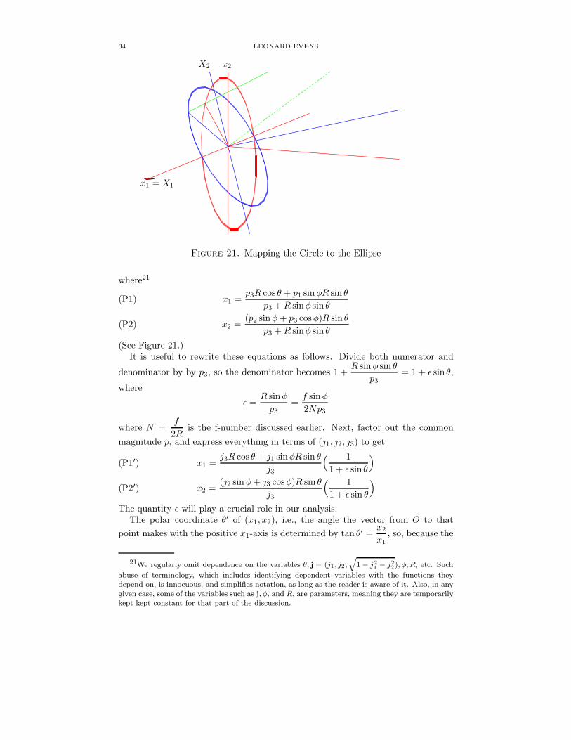
34 LEONARD EVENS
x1 = X1
X2 x2
Figure 21. Mapping the Circle to the Ellipse
where21
x1 =p3R cos θ + p1 sinφR sin θ
p3 +R sinφ sin θ(P1)
x2 =(p2 sinφ+ p3 cosφ)R sin θ
p3 +R sinφ sin θ(P2)
(See Figure 21.)It is useful to rewrite these equations as follows. Divide both numerator and
denominator by by p3, so the denominator becomes 1 +R sinφ sin θ
p3= 1 + ǫ sin θ,
where
ǫ =R sinφ
p3=f sinφ
2Np3
where N =f
2Ris the f-number discussed earlier. Next, factor out the common
magnitude p, and express everything in terms of (j1, j2, j3) to get
x1 =j3R cos θ + j1 sinφR sin θ
j3
( 1
1 + ǫ sin θ
)
(P1′)
x2 =(j2 sinφ+ j3 cosφ)R sin θ
j3
( 1
1 + ǫ sin θ
)
(P2′)
The quantity ǫ will play a crucial role in our analysis.The polar coordinate θ′ of (x1, x2), i.e., the angle the vector from O to that
point makes with the positive x1-axis is determined by tan θ′ =x2
x1, so, because the
21We regularly omit dependence on the variables θ, j = (j1, j2,q
1 − j2
1− j2
2), φ, R, etc. Such
abuse of terminology, which includes identifying dependent variables with the functions theydepend on, is innocuous, and simplifies notation, as long as the reader is aware of it. Also, in anygiven case, some of the variables such as j, φ, and R, are parameters, meaning they are temporarilykept kept constant for that part of the discussion.

VIEW CAMERA GEOMETRY 35
factors involving ǫ cancel, θ′ is independent of ǫ, and we have
tan θ′ =(j2 sinφ+ j3 cosφ) sin θ
j3 cos θ + j1 sinφ sin θ=
(j2 sinφ+ j3 cosφ) tan θ
j3 + j1 sinφ tan θ(T1)
θ′ = arctan( (j2 sinφ+ j3 cosφ) tan θ
j3 + j1 sinφ tan θ
)
− π/2 < θ′ < π/2(T2)
In (T2), θ′, as noted, is returned in the usual range for the arctangent function,so one must correct appropriately for other values. Note also that the factors Rcancelled.
Note, however, that replacing θ by −θ doesn’t replace θ′ by −θ′, so generallyx(−θ) doesn’t have direction opposite to x(θ), but there is one exception, as we
shall see below, θ = ±π2
.
(d) In particular, for θ = ±π/2, the points Q+ = (0,+R) and Q− = (0,−R)
in the lens plane get mapped respectively to the points Q+ = (q+1 , q+2 ) and Q− =
(q−1 , q−2 ) where
q+1 =j1R sinφ
j3
1
1 + ǫ(E1)
q+2 =(j2 sinφ+ j3 cosφ)R
j3
1
1 + ǫ(E2)
and
q−1 = − j1R sinφ
j3
1
1− ǫ(E3)
q−2 = − (j2 sinφ+ j3 cosφ)R
j3
1
1− ǫ(E4)
Note that the line Q+Q− passes through O and has slope
m =j2 sinφ+ j3 cosφ
j1 sinφ
which one easily checks is the same as that of OP∞, so the points P∞, Q+, O,Q−
are collinear. Also, the slope m of this line, is independent of ǫ, i.e., depends onlyon the direction of the ray OP ′ and not on the position of P ′ on it.
Note also that since the numerator in (E2), j2 sinφ + j3 cos > 0, Q+ is in factabove the x1-axis, as indicated in the diagram. So according to (E1), it is in thefirst quadrant if j1 > 0 and in the second quadrant if j1 < 0, and, of course, Q− is inthe opposite quadrant below the x1-axis. (If j1 = 0, Q+ is on the positive x2 axis,and Q− is on the negative x2-axis.) It is geometrically clear that the major axismust be in the same quadrant as Q+, so this leads to the following conclusion: forj1 > 0, the major axis extends from the first quadrant to the third quadrant, andfor j1 < 0, it extends from the second quadrant to the fourth quadrant. In words,the major axis of the reference ellipse extends from closer to the lens plane oppositethe ray to further from the lens plane on the same side as the ray. This holds truewhatever the sign of j2, which is surprising, from a cursory examination of thethree-dimensional geometry, but it does become clear if you look hard enough.
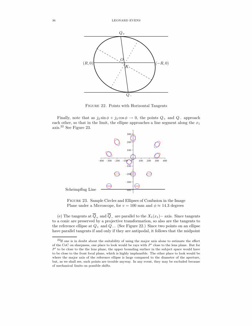
36 LEONARD EVENS
Q+
Q−
(R, 0) (−R, 0)O
K
Figure 22. Points with Horizontal Tangents
Finally, note that as j2 sinφ + j3 cosφ → 0, the points Q+ and Q− approacheach other, so that in the limit, the ellipse approaches a line segment along the x1
axis.22 See Figure 23.
K400 K300 K200 K100 0 100 200 300 400
K400
K300
K200
K100
100
200
300
Scheimpflug Line
Figure 23. Sample Circles and Ellipses of Confusion in the ImagePlane under a Microscope, for v = 100 mm and φ ≈ 14.3 degrees
(e) The tangents at Q+ and Q− are parallel to the X1(x1)− axis. Since tangentsto a conic are preserved by a projective transformation, so also are the tangents tothe reference ellipse at Q+ and Q−. (See Figure 22.) Since two points on an ellipsehave parallel tangents if and only if they are antipodal, it follows that the midpoint
22If one is in doubt about the suitability of using the major axis alone to estimate the effectof the CoC on sharpness, one place to look would be rays with P ′ close to the lens plane. But forP ′ to be close to the the lens plane, the upper bounding surface in the subject space would have
to be close to the front focal plane, which is highly implausible. The other place to look would bewhere the major axis of the reference ellipse is large compared to the diameter of the aperture,but, as we shall see, such points are trouble anyway. In any event, they may be excluded becauseof mechanical limits on possible shifts.

VIEW CAMERA GEOMETRY 37
K = (k1, k2) of Q+Q− is the center of the ellipse. Hence,
k1 =q+1 + q−1
2
=j1R sinφ
2j3
( 1
1 + ǫ− 1
1− ǫ)
= − j1R sinφ
j3
ǫ
1− ǫ2Similarly
k2 = mk1 = − j2 sinφ+ j3 cosφ
j1 sinφ
j1R sinφ
j3
ǫ
1− ǫ2
= − (j2 sinφ+ j3 cosφ)R
j3
ǫ
1− ǫ2Note that although the distance between the principal point O and the center
K of the reference ellipse looks pretty small in Figure 22, it has been exaggeratedfor effect, so typically it is even smaller than indicated. From the above formulas,
sinceǫ
1− ǫ2 ≈ ǫ for small epsilon, it is usually so small that it would not be visible
in a accurate graph, and that was clear in typical examples using Maple to plot thegraphs.
To proceed, we need to see how the reference ellipse varies as we change theprojection point P ′ = (p1, p2, p3) = p(j1, j2, j3). As noted earlier, the parameter
ǫ =f sinφ
2Np3will play an important role. We shall study it and its effect in detail
in Appendices D.1 and D.3, where we consider the various factors which may comeinto play. The worst possible estimate, under plausible assumptions is ǫ ≤ 0.02meaning that if we ignore it, we make an error of at most 2 percent. In practice,it is usually much less than that, but the discussion in the appendices gives us anidea of when it might be large enough to matter.
If we fix the ray and let P ′ go to infinity, then ǫ→ 0. Hence, the reference ellipseapproaches the limiting reference ellipse centered at O, with parametrization
x1 = Rj3 cos θ + j1 sinφ sin θ
j3(L1)
x2 = R(j2 sinφ+ j3 cosφ) sin θ
j3(L2)
In general, it is still not true for the limiting reference ellipse that antipodalpoints on the circle get mapped to antipodal points on the ellipse. But it is true
for θ = ±π2. In that case, the line through O with slope
m =j2 sinφ+ j3 cosφ
j1 sinφ
intersects the limiting ellipse at antipodal points with horizontal tangents and suchthat
q±2 = ±R (j2 sinφ+ j3 cosφ)
j3.
Also, the tangents at (±R, 0) are parallel to this line and so have the same slope.For the limiting ellipse, the equations (T1) and (T2) describing the relation be-
tween the polar angle θ in the lens plane and the polar angle θ′ in the reference

38 LEONARD EVENS
Q+
Q−
(R, 0) (−R, 0)O
Figure 24. The Limiting Reference Ellipse
plane remain true because they were independent of ǫ. Clearly, it suffices to ex-amine that dependence for the upper half of the ellipse, i.e., for 0 ≤ θ ≤ π. It isgeometrically clear that, for j1 > 0, except at 0 = θ = θ′ and π = θ = θ′, we have0 < θ < θ′ < π, and for j1 < 0 the inequality is reversed. With some difficulty itmay also be verified analytically.
For any finite P ′, since ǫ is quite small, the corresponding reference ellipse differsonly slightly from this limit. As we shall see in Appendices D.1 and D.2, thedirection cosines (j1, j2, j3) are severely limited by the possible placement of theimage plane because of bounds on movements of the rear standard and also bythe nature of plausible scenes. But they could vary enough to make a significantdifference in the size and shape of the limiting reference ellipse, and that complicatesthe analysis.
8.3.1. Problem (1). As before, suppose outer and inner image planes Π′ and Π′′,each parallel to the reference plane ∆, are given. Fix a ray with direction cosines(j1, j2, j3) and let that ray intersect the two planes in P ′ and P ′′ respectively.Because of the above analysis, the reference ellipses for P ′ and P ′′ are both quiteclose to the limiting reference ellipse for that ray, so we shall treat them as identicalin all that follows. (See Appendices D.1 and D.3 for a discussion of how much thataffects the calculations.)
Consider now a plane Π between the outer and inner image planes, and look atthe circles of confusion in Π from P ′ and P ′′ respectively, which will be similar tothe limiting reference ellipse, or so close that we can ignore any difference. We mayconclude as in the untilted case, that the circles of confusion will agree just when Πis the harmonic mean of Π′ and Π′′ with respect to the reference plane. See Figure17, entitled “Balance”, but note that D in the diagram gets replaced here by C asin Figure 19.
As before, we have
(C) Π′,Ω; Π,∆ = v′,∞; v, 0 =v′ − vv′
=c
C=v − v′′v′′
= −Π′′,Ω; Π,∆
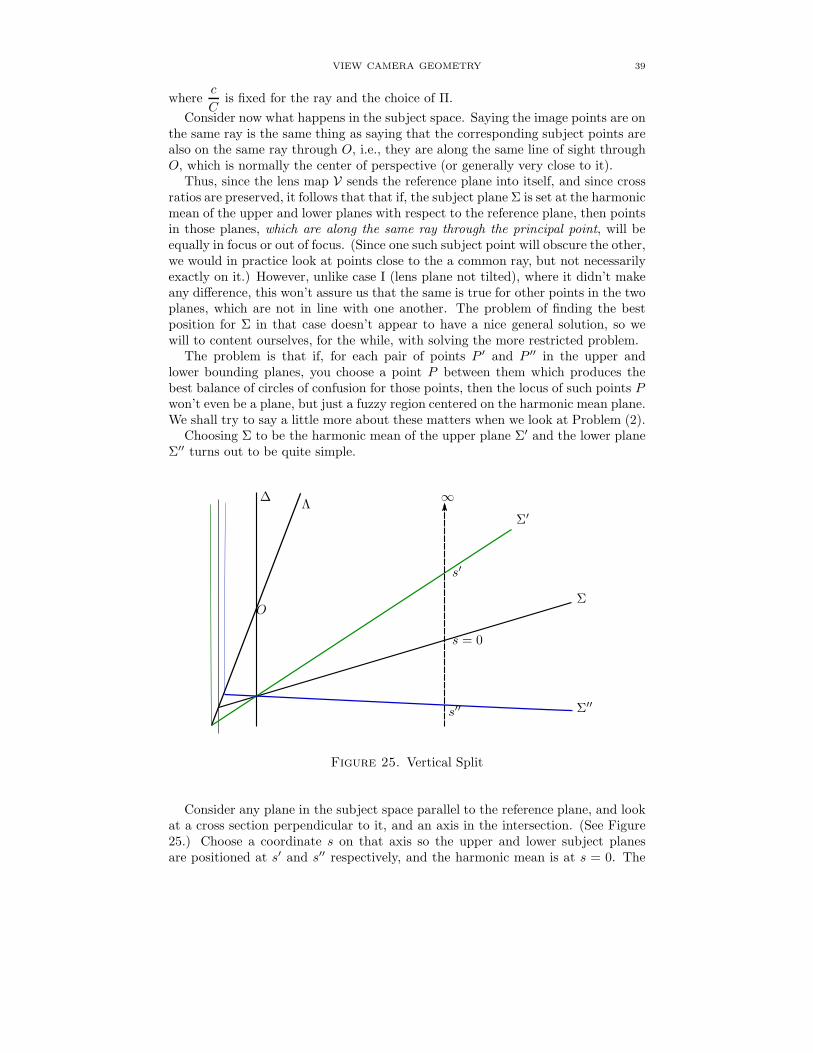
VIEW CAMERA GEOMETRY 39
wherec
Cis fixed for the ray and the choice of Π.
Consider now what happens in the subject space. Saying the image points are onthe same ray is the same thing as saying that the corresponding subject points arealso on the same ray through O, i.e., they are along the same line of sight throughO, which is normally the center of perspective (or generally very close to it).
Thus, since the lens map V sends the reference plane into itself, and since crossratios are preserved, it follows that that if, the subject plane Σ is set at the harmonicmean of the upper and lower planes with respect to the reference plane, then pointsin those planes, which are along the same ray through the principal point, will beequally in focus or out of focus. (Since one such subject point will obscure the other,we would in practice look at points close to the a common ray, but not necessarilyexactly on it.) However, unlike case I (lens plane not tilted), where it didn’t makeany difference, this won’t assure us that the same is true for other points in the twoplanes, which are not in line with one another. The problem of finding the bestposition for Σ in that case doesn’t appear to have a nice general solution, so wewill to content ourselves, for the while, with solving the more restricted problem.
The problem is that if, for each pair of points P ′ and P ′′ in the upper andlower bounding planes, you choose a point P between them which produces thebest balance of circles of confusion for those points, then the locus of such points Pwon’t even be a plane, but just a fuzzy region centered on the harmonic mean plane.We shall try to say a little more about these matters when we look at Problem (2).
Choosing Σ to be the harmonic mean of the upper plane Σ′ and the lower planeΣ′′ turns out to be quite simple.
∆Λ
∞
O
s = 0
s′
s′′
Σ′
Σ
Σ′′
Figure 25. Vertical Split
Consider any plane in the subject space parallel to the reference plane, and lookat a cross section perpendicular to it, and an axis in the intersection. (See Figure25.) Choose a coordinate s on that axis so the upper and lower subject planesare positioned at s′ and s′′ respectively, and the harmonic mean is at s = 0. The

40 LEONARD EVENS
coordinate of the reference plane will be ∞. So we have
−1 = Σ,∆; Σ′,Σ′′ = 0,∞; s′, s′′ =s′
s′′
so s′′ = −s′. In other words,
Proposition 3. The harmonic mean of the upper and lower planes relative to thereference plane bisects the plane region between those planes in any cross sectionalplane parallel to the reference plane.
8.3.2. Problem (2). With the same setup as before, suppose we pick a subject planeΣ and its corresponding image plane Π. Let v be the perpendicular distance from Πto the reference plane, and consider a point P ′ not on Π at perpendicular distancev′ from the reference plane. (v′ is what we called p3 before.) Refer to Figure 26which shows the limiting circle of confusion and the limiting reference ellipse, andcompare it to Figure 19. Here C is the major axis of the limiting reference ellipseand c is the corresponding major axis of the limiting circle of confusion. The centersO′ and Q′ will be shifted slightly from O and Q, but, as noted before, the shiftswill be proportional to ǫ and hence quite small. In all that follows, we shall ignorethe small error made by using the limiting reference ellipse and the limiting circleof confusion.
Π′ Π ∆
O′
P ′
c
C
v′
v
Q′
Figure 26. Limit Circle of confusion and Limit Reference Ellipse
We first consider the case where P ′ is on the far side of Π from the referenceplane, as Figure 26. We have
v′ − vv′
=c
C=
c
D
D
C=Nc
f
D
C=Nc
fκ.
where κ =D
C. Note that the quantity on the left is the cross ratio Π′,Ω; Π,∆
where Π′ is the plane parallel to Π containing P ′. Since c is the major axis of thecircle of confusion, if we make sure that its diameter (i.e., major axis) is always

VIEW CAMERA GEOMETRY 41
small enough, the circle of confusion won’t be distinguishable from a point.23 Letc be the maximum such diameter, and solve for v′ to get
(SN) v′ =v
1− κNcf
.
This equation defines a surface in the image space, which we shall call the outersurface of definition. All points between the plane Π and that surface will producesufficiently sharp images in Π. Points beyond it will appear blurred. Unfortunately,this simple equation hides a lot of complexity. If κ were constant, the surface ofdefinition would be a plane, but, as we saw previously, κ is far from constant, beinghighly dependent on the direction j of the ray OP ′.
So, let us look more carefully at κ =D
C.
Since C is the major axis of the reference ellipse and D is the length of a chord,it follows that κ ≤ 1.24 First suppose that j1 = 0 (so q±1 = 0). In this case thereference ellipse is symmetrical about the x1 = X1-axis, and 2q+2 is its minor axisprovided it is less than D = 2R and otherwise it is its major axis. (When 2q+2 = D,the ellipse is a circle.) So, κ = 1 as long as 2q+2 ≤ D. i.e.,
j2 sinφ+ j3 cosφ
j3≤ 1.
Otherwise,1
κ=j2 sinφ+ j3 cosφ
j3> 1
so κ < 1 and κ→ 0 as j2 → 1, j3 → 0. 25
To see what happens as we move laterally away from the j1 = 0 plane, we lookat where
dx1
dθ= R−j3 sin θ + j1 sinφ cos θ
j3= 0.
This occurs when
tan θ =j3
j1 sinφ
sin θ =j3
√
j23 + j21 sin2 φ
cos θ =j1 sinφ
√
j23 + j21 sin2 φ
23One might question whether the major axis is the right thing to look at. Possibly, someother measure associated with the ellipse might be more appropriate. Presumably, if the minoraxis is much smaller than the major axis, there will be an astigmatic-like effect with a loss ofsharpness along one direction and and an actual improvement transverse to it. Since one neverknows just what kind of detail will be present in a scene, it seems to me that one must worryabout the worst case effects, not some sort of average effect. To settle the matter would requireexperimental investigations beyond the scope of this article. Unless someone show definitivelythat some other measure works better, I will use the major axis.
24If κ = 1, then v′ =v
1 − Nc/fwhich is the estimate which would apply in the untilted case.
25A simple geometric argument shows the dividing point is where the ray (defined by the unit
vector j = (0, j2, j3)) makes an angleφ
2with the x3-axis.

42 LEONARD EVENS
That defines two points on the ellipse, and taking the one with 0 ≤ θ ≤ π, we get
x1 = R
√
j23 + j21 sin2 φ
j3=
√
1 +( j1 sinφ
j3
)2
.
The semi major axis is greater than this quantity, so its reciprocal κ < 1, and κ→ 0as j3 → 0, i.e.,
√
j21 + j22 → 1, as long as j1 6= 0.Similarly, the surface with equation
(SF) v′′ =v
1 + κNcf
.
describes the surface formed by all points on the side closer to the lens for whichthe circles of confusion in Π will have diameter c. We shall call it the inner surfaceof definition. It approaches the plane Π from the other side as the ray becomesmore oblique.
We show some examples of the what the outer surface of definition looks like inFigure 27.
N = 22 N = 45
Figure 27. Outer Surface of Definition, f = 150 mm, c = 0.1mm, φ = 14.3 degrees, approaching exact image plane
As the diagram indicates, these surfaces depend on N as well as c (and of coursef .) As N increases, the surface moves farther away from Π. It approaches theplane Π (in blue in Figure 27) as the ray becomes more oblique.
To measure the effect of κ’s deviation from 1, note that in the fractionNκc
f,
we may always compensate for κ by increasing N appropriately, i.e., by stoppingdown. It is usual to measure changes in the aperture in terms of stops or fractionsof a stop rather than with the f-number. So, in this case, we have
Number of stops =2 log(κ)
log(2).
To proceed further, we must make some estimates for κ in typical situationsencountered in view camera photography. We save the detailed calculations forAppendix D, but we shall outline some of the results below.

VIEW CAMERA GEOMETRY 43
1
00.0
1
0.5
0
1.0
-1-1
Figure 28. κ as a function of the unit vector (j1, j2) for φ = 14.3 degrees
κ may be noticeably less than one if the tilt angle is large and/or the vectorj = (j1, j2, j3) departs significantly from the normal to the reference plane. Figure28 shows the graph of κ as a function of (j1, j2) for the case φ = 0.25 radians ≈ 14.3degrees.26 That is larger than one usually needs in practice, but still, we see thatκ remains fairly close to 1 over much of the range.
In Figure 29, we show the contour curves for κ = 0.9 and κ = 0.8, enclosedwithin the unit circle in the j1, j2-plane.
It is clear from the figure that, for those examples, the smallest values of j =√
j21 + j22 occur on the j2 axis. Solving numerically, we find that the crucial valuesare j2 ≈ 0.5 for κ = 0.9 and j2 ≈ 0.75 for κ = 0.8. The first corresponds to anangle of about 30 degrees with respect to the normal to the reference plane, andthe second to an angle of about 48.6 degrees. To compensate for κ = 0.8, we wouldhave to stop down almost two thirds of a stop, whereas to compensate for κ = 0.9,we would have to stop down less than one third of a stop.27
While it is helpful to know κ as a function of (j1, j2), it is even more enlighteningto understand how it varies as a function of (x1, x2, v) representing a point in theimage plane at distance v from the reference plane. In Section D, I shall proveProposition 5 which asserts the following
26The graph is not entirely accurate since it it includes points for many excluded rays, e.g,
such that j2 < −
q
1 − j2
1cos φ. Also the rate of change of κ at the boundary is too great for
accurate plotting, particularly near (0,−1). Indeed, as j2 approaches −1 along the j2-axis, κ goesfrom 1 at j2 = − cos(φ/2), which is very close to -1, to zero at j2 = −1.
27Despite appearances, each contour curve crosses the j2-axis, not at (0,−1) , but slightly
above it. Also, as above, points such that j2 < −
q
1 − j2
1cos φ, while contributing to the graph,
are associated with excluded rays.

44 LEONARD EVENS
K1.0 K0.5 0 0.5 1.0
K1.0
K0.5
0.5
1.0
Figure 29. Contour Curves for φ = 14.3 degrees, κ = 0.8, 0.9.
(a) If 0 < κ0 < 1, then the projection from the sphere |j| = 1 to the im-age plane, of the contour curve defined by κ = κ0, is an ellipse, centered at theScheimpflug point (0,−S), (S = v cotφ = (1 +M)J), where the x2-axis intersectsthe Scheimpflug line. Its semi-major axis and semi-minor axes are given by
(Mn) d2 = Ssecφ
κ0d1 = d2
√
1− κ20
In particular, the ellipse crosses the positive x2-axis at
S(secφ− κ0
κ0
)
.
(b) If κ0 = 1, the projection is the line segment on the x2-axis from −S(secφ+1)to S(secφ− 1).
(c) For κ0 fixed, the set of all such contour ellipses forms an elliptical conecentered on the line through O in the lens plane, perpendicular to the x1-axis (thetilt axis).
In Figure 30, we show these contour ellipses for φ = 0.25 radians, v = 100mm, and κ0 = 0.6, 0.7, 0.8, 0.9, 1.0.28 As indicated only the portions above theScheimpflug line are shown, since nothing outside the camera is relevant. Actually,nothing below the image of the upper tilt horizon29 is relevant, since such pointswill necessarily have too large CoCs in the image plane. Usually, that line will bewell above the Scheimpflug line, but placing an upper limit on it requires knowingdetails about the scene and plausible small apertures. We shall investigate this insome detail later.
For fixed φ, the contour ellipses scale linearly with v, so to obtain the correspond-ing curves for different positions of the image plane, just leave the curves where
28The view is as it would appear from the vantage point of the lens, since I couldn’t figure outhow to get Maple to reverse the direction of an axis in a plot.
29The upper tilt horizon is where the upper bounding plane Σ′ intersects the plane at infinity.Similarly the lower tilt horizon is where the plane Σ′′ intersects the plane at infinity.

VIEW CAMERA GEOMETRY 45
1.00.7 0.80.6 0.9
K400 K200 0 200 400
K300
K200
K100
100
200
Figure 30. Contour Ellipses in Image plane, φ = 14.3 degrees,v = 100 mm, κ0 = 0.6, 0.7, 0.8.0.9, 1.0 (Only portions aboveScheimpflug line are shown.)
.
they are and multiply the units on the axes by the ratiov
100. The dependence on
the focal length f or the tilt angle φ is more complicated, since they also affect thelikely value of v. We have generally
S = J(1 +M) =f
sinφ(1 +M)
d2 =S secφ
κ 0=
f
κ0 sinφ cosφ(1 +M) =
2f
κ0 sin 2φ(1 +M)
d1 = d2
√
1− κ20
But, for small φ, sinφ ≈ φ and sin 2φ ≈ 2φ, so these equations become
S ≈ f
φ(1 +M)
d2 ≈1
κ 0
f
φ(1 +M)
d1 ≈√
1− κ20
κ0
f
φ(1 +M)
Of course, in the process of changing f and φ, we may also need to change M toaccommodate a particular scene, but except for situations where the subject planerises very steeply, which almost never occur, M is very small, so we may treat itas essentially constant. With that in mind, we can say that the diagram scalesroughly linearly with f and inversely with φ. If we ignore M , v = 100 and φ = 0.25implies that f ≈ 103. So to use the same diagram with different values of f or φ,
leave the contour ellipses where they are and multiply the units on the axes byf
103
and by0.25
φ.

46 LEONARD EVENS
As κ0 → 1, the ellipse approaches the indicated segment on the x2 axis. As κ0
decreases, the ellipses get larger and the ratiod1
d2→ 1. In the limit, as κ0 → 0, the
ellipse approaches a circle of infinite radius.We now begin to see how to attack the problems we have set.We assume that the subject plane has been specified to within fairly narrow
limits, which, as noted previously, will severely restrict the position of the hingeline and the tilt angle φ necessary to achieve it.
For any given position of the rectangular frame, we need only find the smallestvalue κ0 of κ which can occur for rays that pass through that frame. To do thatwe look at the family of contour ellipses in the image plane, as in Figure 30, anddetermine the smallest one containing the frame, thereby setting κ0. We call thecone defined by κ = κ0 the cone of accessibility. It is clear from the geometry thatthe frame will hit that cone at one of the two corners furthest from the Scheimpflugpoint, which simplifies finding the relevant value of κ0.
Physical and optical restrictions place strict bounds on the possible positions ofthe frame . For example, there is a limit to how close the standards can be, whichplaces a lower bound on focal length, which in turn places a lower limit on howclose Π can be to the reference plane, i.e., on the value of v. There is also a limitto how far apart the standards can be, which places an upper limit on the focallength. The region between the reference plane and the rear focal plane is opticallyforbidden. Moreover, for any possible choice of the image plane Π, limitations oncamera movements restrict possible positions of the frame within that plane, andhence on rays passing through the frame. Finally, we can ignore highly implausiblescenes or scenes which would require stopping down beyond what the lens allowsor such that diffraction would dominate considerations from geometric optics.
All of these conditions place a lower bound on κ0, i.e., an upper bound on thesize of the cone of accessibility. Given N, c, and κ0, define
v′0 =v
1− Ncκ0
f
.
It is clear that
v′ =v
1− Ncκ
f
= v′0 ⇐⇒ κ = κ0
so, the plane Π′0 at distance v′0 from the reference plane intersects the outer surface
of definition along its intersection with the cone of accessibility. Similarly, if wedefine
v′′0 =v
1 +Ncκ0
f
and let Π′′0 be the plane at distance v′′0 from the reference plane, the same thing
holds for the intersection of the inner surface of definition with that plane and thecone of accessibility. See Figure 31 which illustrates the situation for the outersurface.
Any point in Π′0 on the cone of accessibility will yield a circle of confusion c in
Π such thatNcκ0
f= 1 − v
v′0, but, if N is fixed, then for a point in Π′
0 inside the

VIEW CAMERA GEOMETRY 47
∆ΠΠ′0
Λv′
κ < κ0
v′0
κ = κ0
v′
κ > κ0
v
O
Figure 31. Cone of Accessibility
cone of accessibility, we will get a circle of confusion c in Π such that
Ncκ
f= 1− v
v′0=Ncκ0
f.
Since κ > κ0 inside the cone, it follows that c < c. In other words, if a sharpnesscriterion is satisfied for points in Π′
0 on the ellipse, it is certainly met for such pointswithin the ellipse. (The interplay between N, c, and κ can be confusing—the authoradmits having had his share of such confusions—and we shall return to it later.)
Similar remarks apply to the inner surface of definition and Π′′0
We may now use the above analysis to address Problems (2) and (2a).Suppose we have a good estimate for κ0 determined by the worst possible case for
the camera, or by the details of the specific scene, or just from what our experiencetells us works.
First we address Problem (2). Suppose an image plane Π has been chosen bysome means, and we give a criterion for sharpness set by a value c for the circle ofconfusion, and also an aperture with f-number N . Then, as above
1− v
v′0=Ncκ0
f=
v
v′′0− 1
v′0 =v
1− Ncκ0
f
v′′0 =v
1 +Ncκ0
f
(VnVf)
tell us how to determine v′0 (Π′0) and v′′0 (Π′′
0 ) and from these the correspondingupper and lower subject planes.
Next consider Problem (2a), in which we can suppose we have specified upperand lower subject planes and the corresponding image planes Π′
0 and Π′′0 , i.e., that
we are given v′0 and v′′0 , which we can determine, as in the untilted case, by thepositions on the rail corresponding to the upper and lower subject planes. ChooseΠ to be their harmonic mean with respect to the reference plane. Then we want

48 LEONARD EVENS
to know how large we need to choose N so that the sharpness criterion set by c ismet everywhere within the cone of accessibility determined by κ0.
To get some idea of the orders of magnitude involved, note that stopping downby one third of a stop corresponds to increasing the f-number by about 12 percent.One third of a stop would not usually be considered significant when making depthof field corrections. Often a photographer will stop down an entire additional stopor more to compensate for the lack of precision inherent in the work.
We shall investigate lower limits on κ in detail in Appendix D.2, but we shalloutline the conclusions below.
From Figure 30, it is clear that κ is going to be larger for rays closer to the tilthorizon, and smaller for rays pointing further from from the tilt horizon, i.e., thoseimaging points in the foreground. Similarly, κ is larger for rays closer to the linex1 = 0, and smaller for rays pointing further from that line. In either case, thesmaller values of κ will require shifting the frame either further in the direction ofpositive x2, i.e., away from the lens plane, or, more to one side or the other. But,limitations of shifts inherent in the structure of the camera will determine just howsmall kappa can be in possible scenes. Moreover, even if the camera allowed verylarge shifts, the resulting scenes which require that everything in the subject planefrom just beyond the lens to infinity be in the frame would be unusual, to say theleast.
If the hinge line is skew, the x1 and x2 axes will be rotated with respect to thesides of the frame, which makes it a bit difficult to interpret all this, but for apure tilt or a pure swing, it is clear what they mean. For example, for a pure tiltdownward, κ may get too small for points in the extreme foreground, either belowthe camera or far to one side. For everything else fixed, limitation on vertical riseof the rear rear standard relative to the lens and limitations on shifts to one side orthe other will limit how small it can get. Similarly, for a pure swing to the right,we may encounter problems for points in the extreme foreground to the right, or,too high or two low, but limitations on shifts of the frame to the left relative to thelens, or, vertical shifts in either direction will limit how small κ can be.
Unfortunately, the position of the frame and how this relates to the focal length,the tilt angle, and the position of the subject plane can be something of a wild card.Let us illustrate by an example. Let f = 90 mm, a common short focal length for4 x 5 photography. Suppose we tilt downward from the horizontal by 0.25 radians(about 14.3 degrees), and suppose the subject plane intersects the reference normalline at distance u = 5 m = 5,000 mm from the lens. The hinge distance would be
J =f
sinφ≈ 364 mm, and the slope of the subject plane would be
J
u≈ 0.0173.
From the lens equation v =fu
u cosφ− f ≈ 94.6 mm, and M =v
u≈ 0.19. Since v is
not much less than 100, Figure 30 gives a pretty accurate rendition of the contourellipses in the image plane. The scale will be reduced by about 5 percent, meaningthat the units at the tick marks on the axes should be about 5 percent smaller,while the curves remain where they are. My view camera in these circumstancewill allow an effective vertical rise of at most 40 mm. (Many cameras, particularlywith a bag bellows, will allow considerably larger shifts.) The 4 x 5 frame hasdimensions just about 96 x 120 mm. Suppose the frame is in landscape orientationand lifted 40 mm, but left symmetric about the line x1 = 0. Then its top will be40 + 48 = 88 mm above the line x2 = 0, and its upper corners will be 60 mm on

VIEW CAMERA GEOMETRY 49
either side of that. Looking at Figure 30, we see that κ will be between 0.8 and0.9, and much closer to the former than the larger in those corners. Taking intoaccount the reduction in scale will reduce κ slightly, so we can guess that it will beabout 0.82 in the corners.30 That would require stopping down about three fifths ofa stop, which, in a critical situation, might be more than one is comfortable with.Of course for most of the frame κ would be much closer to 1, so it would only bean issue if those corners had significant detail.
Note, however, that the scene corresponding to this position of the frame wouldbe somewhat unusual. For one thing, the hinge distance at 364 mm is rather short.For another, the position of the frame is rather unusual. First, it is almost entirelyabove the center of the field, so nothing much above the horizon would be in view.In addition, the questionable corners would correspond to points in the scene veryclose to the lens. Given the data above, since the subject plane slopes so gentlyupward, the corners would be about 364 mm (≈ 14.3 inches) below the lens and88
90364 ≈ 356 mm or (14 inches) into the scene. Such a scene is unusual, but not
entirely implausible.31 Still, this indicates why the plausibility of the scene mightcome into play before the limits of shift were encountered. For example, if oneshifted the frame even higher, thus reducing κ further, the foreground would comeeven closer to the lens. On the other hand, for longer lens, where v typically wouldbe much larger, limitations on shift may play a more important role.
It turns out in the end—see Appendix D.2—that, provided the Scheimpflug dis-tance is large compared to E1 and E2, κ is not much less than 1, and the necessarycorrection is less than one third of a stop. Since S = J(1+M), it usually suffices tolook at the hinge distance, but in some odd situations, we might have to considerthe Scheimpflug distance directly.
The hinge distance is given by J =f
sinφ, so it will be extremely large for very
small tilts. For example, for φ = 1 degree and f ranging from 65 mm to 450 mm,the hinge distance would range from 3.7 meters to over 25 meters. Any plausiblevalues of E1 and E2 would be a very small fraction of that. So we need only considermoderate to large tilts when trying to deide if κ might be small enough to matter.
Usually E1 and E2 are smaller than the dimensions of the frame, but whenextreme shifts are involved, they might be somewhat larger. Usually the camerawon’t support such large shifts, and even it it did, they would only rarely be needed.For example suppose f = 150 mm, often considered the ‘normal’ focal length, andwe have a pure tilt with φ = 0.15 radians (≈ 8.6 degrees), still a substantial tilt.Then J ≈ 1,004 mm, or about 1 meter, and assuming, as usually is the case, thatM is small, v ≈ f secφ ≈ 152 mm. Suppose also that the frame is centered on thehorizontal line of sight and it is in landscape orientation. Then E1 = 60 mm and
30An exact computation using our formulas gives κ ≈ 0.8144, requiring stopping down ≈
0.5925 stops. But such accuracy is overkill, and the graphical method more than suffices for ourneeds.
31For example, the camera might be placed just behind a retaining wall, the top of which
could be that distance below the lens, with the surface beyond the wall starting at the same leveland sloping slightly upward, and we might want everything from a foot or so beyond the lensto a much greater distance in focus. I’ve taken pictures at the Chicago Botanic Garden not toodifferent from this.

50 LEONARD EVENS
E2 = 48 mm,32 which are both small compared to the hinge distance. Calculatingκ from the formula33 yields κ ≈ 0.95 which would require less than one sixth of astop correction. Putting the frame in portrait orientation and raising it by 20 mm,so E1 = 48 mm and E2 = 80 mm, would only reduce κ to about 0.93, and requireabout one fifth of a stop correction. Even reducing the focal length to 90 mm,which would reduce the hinge distance to about 600 mm, would in the latter case,only reduce κ to 0.88, and require a little over one third of an f-stop correction.
Our approach does indicate when κ might be small enough to matter. Thatwould be for large tilts and either when the hinge distance was too short or theframe shifted so much that the relevant quantities were not sufficiently small incomparison to it. This is more likely to occur for very short focal length lenses.This is all subject to the assumption that M is relatively small, which is almostalways the case, except possibly in close-ups.
For cases where the above conditions are not met, e.g., if E1 or E2 are a sizablefraction of S, there is no alternative but to calculate κ for the explicit situationunder consideration. In the example above, we had E1 = 60 and E2 ≈ 90 mm,which are still significant fractions of S ≈ 400 mm, and we found κ might requirea significant f-stop adjustment to compensate.
As we saw, in typical situations, κ only requires stopping down a negligiblefraction of an f-stop, so the whole issue can be ignored. In any case, there aremany other sources of uncertainty in the whole methodology, which may affect thesituation more, thus swamping the effect of κ. First, there is the fact that actuallenses only behave approximately like the ideal lenses discussed in this article.Second, even for an ideal lens, difficulties in positioning the standards, setting thef-number and judging when something is in focus on the ground glass would limitprecision. So, in any event, a prudent photographer may be wise to stop down asmuch as a stop or more than the theory would suggest.
In addition, diffraction, which we have ignored entirely in this article, increas-ingly comes into play as the aperture decreases (f-number increases). This effect isopposite of that of geometric defocus, which decreases as the aperture gets smaller.There is some aperture in between where the two effects are balanced, but charac-terizing it is not easy.34
8.4. Determinng the Proper f-stop in the Tilted Case. To determine theproper f-number in terms of the focus spread, we use essentially the same reasoningas in Section 8.1.2, but to avoid missing some subtle point, we repeat the argument.First, it is easy to see that v is the harmonic mean of v′0 and v′′0 if and only if
1− v
v′0=
v
v′′0− 1 =
Ncκ0
f.
32This means that half the frame will be below that line, which means the frame might extendbelow the image of the upper tilt horizon. But, typically, that part of the scene would be opensky, and so we woudln’t care what was in focus there.
33We could also use Figure 30. Just remember that the numbers at the tick marks must be
multiplied by about150
103
0.25
0.15≈ 2.4.
34There are rules of thumb which try to estimate how to choose the aperture which bestbalances diffraction against geometric defocus, but they are usually based on fairly crude analyses.See Jeff Conrad’s previously referenced article for a nuanced discussion of this issue.

VIEW CAMERA GEOMETRY 51
Using the equality ofNcκ0
fwith either of the two other expressions yields, after
some algebra,
v′0 − v′′0v′0 + v′′0
=Ncκ0
fso
N0 = Nκ0 =v′0 − v′′0
c
f
v′0 + v′′0(NE)
But using v′0 =v
1− (Ncκ0)/fand v′′0 =
v
1 + (Ncκ0)/f, it is easy to see that
v′0 + v′′0 =2v
1− (Ncκ0/f)2≈ 2v
since(Ncκ0
f
)2
is very small, except in highly unusual circumstances, as noted in
Section 8.1.2. Hence,
N0 = Nκ0 ≈v′0 − v′′0
2c
f
v.
So far, this exactly what we got in the untilted case, with κ0 = 1. But there aresome major differences. The first is the factor κ0, and the second is that, from
the lens equation, we obtain, in the tilted case,v
f= (1 + M) secφ, where M is
the magnification for the distance at which the subject plane crosses the referencenormal line. That leads to the estimate
(TK) N0 = Nκ0 ≈v′0 − v′′0
2c(1 +M)cosφ
This can be interpreted as follows. We start by finding the f-number N0 whichwould we get if we assumed κ = 1 were true. This is done by a modification ofthe rule used in the untilted case: divide the focus spread v′0 − v′′0 by twice themaximum acceptable CoC c. Correct this as before by dividing by 1 + M , whereM is the above magnification, but also multiply by cosφ. Finally correct for the
departure of κ from unity to obtain N =N0
κ0. Equivalently, just stop down by an
additional2 logκ0
log 2stops.
Note that we can simplify this rule quite a bit. First note that for typical scenes,M is very small, so it won’t make much difference if we ignore the factor 1 + M .(In any case doing so just overestimates N , which is usually innocuous.) Similarlycosφ is usually very close to 1 because for small φ. cosφ ≈ 1− φ2/2 ≈ 1.
8.4.1. What happens in the subject space. Let Σ be the desired subject plane andlet Π be the corresponding image plane. Fix the f-number N and and a maximalacceptable CoC c. Then, instead of the upper and lower planes Σ′ and Σ′′ wewould get for κ = 1, we get upper and lower surfaces of definition, correspondingto the outer and inner surfaces of definition discussion in the previous section. Theupper surface of definition lies between Σ and the Σ′, and the lower surface ofdefinition lies between Σ and Σ′′. But, as we shall see, the picture, is a bit morecomplicated than that in the image space. See Figure 32. The coordinates are asbefore, except that in the subject space, we have reversed the direction of the x3
axis. The diagram shows a cross-section for the various planes and surfaces for a
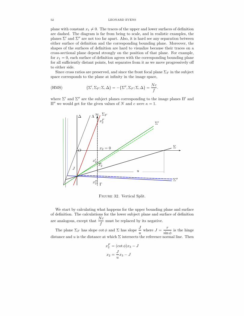
52 LEONARD EVENS
plane with constant x1 6= 0. The traces of the upper and lower surfaces of definitionare dashed. The diagram is far from being to scale, and in realistic examples, theplanes Σ′ and Σ′′ are not too far apart. Also, it is hard see any separation betweeneither surface of definition and the corresponding bounding plane. Moreover, theshapes of the surfaces of definition are hard to visualize because their traces on across-sectional plane depend strongly on the position of that plane. For example,for x1 = 0, each surface of definition agrees with the corresponding bounding planefor all sufficiently distant points, but separates from it as we move progressively offto either side.
Since cross ratios are preserved, and since the front focal plane ΣF in the subjectspace corresponds to the plane at infinity in the image space,
(HMS) Σ′,ΣF ; Σ,∆ = −Σ′′,ΣF ; Σ,∆ =Nc
f.
where Σ′ and Σ′′ are the subject planes corresponding to the image planes Π′ andΠ′′ we would get for the given values of N and c were κ = 1.
∆ ΛΣF∞
O
xF2
x2 = 0
x′2x′2
x′′2
u
Σ′
Σ
Σ′′
Γ
J
Figure 32. Vertical Split.
We start by calculating what happens for the upper bounding plane and surfaceof definition. The calculations for the lower subject plane and surface of definition
are analogous, except thatNc
fmust be replaced by its negative.
The plane ΣF has slope cotφ and Σ has slopeJ
uwhere J =
r
sinφis the hinge
distance and u is the distance at which Σ intersects the reference normal line. Then
xF2 = (cotφ)x3 − J
x2 =J
ux3 − J
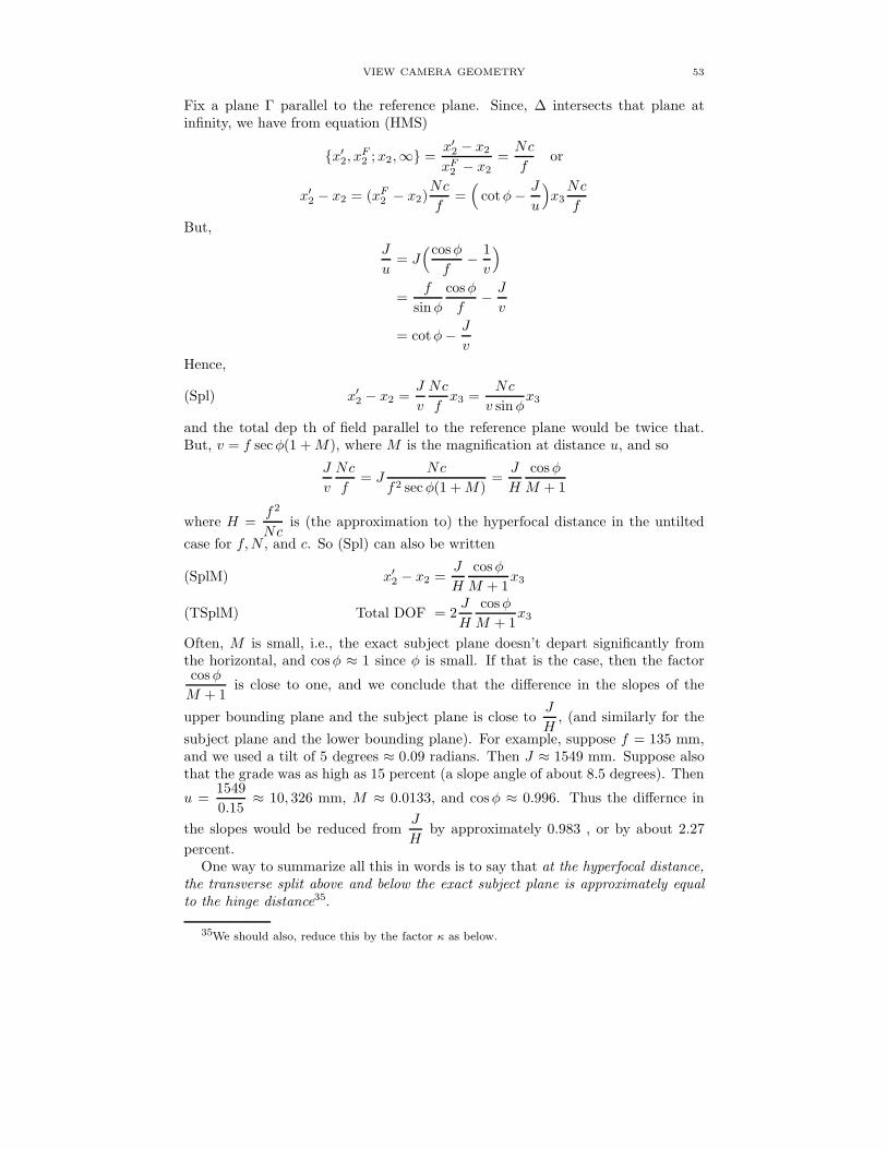
VIEW CAMERA GEOMETRY 53
Fix a plane Γ parallel to the reference plane. Since, ∆ intersects that plane atinfinity, we have from equation (HMS)
x′2, xF2 ;x2,∞ =
x′2 − x2
xF2 − x2
=Nc
for
x′2 − x2 = (xF2 − x2)
Nc
f=
(
cotφ− J
u
)
x3Nc
f
But,
J
u= J
(cosφ
f− 1
v
)
=f
sinφ
cosφ
f− J
v
= cotφ− J
v
Hence,
(Spl) x′2 − x2 =J
v
Nc
fx3 =
Nc
v sinφx3
and the total dep th of field parallel to the reference plane would be twice that.But, v = f secφ(1 +M), where M is the magnification at distance u, and so
J
v
Nc
f= J
Nc
f2 secφ(1 +M)=J
H
cosφ
M + 1
where H =f2
Ncis (the approximation to) the hyperfocal distance in the untilted
case for f,N , and c. So (Spl) can also be written
x′2 − x2 =J
H
cosφ
M + 1x3(SplM)
Total DOF = 2J
H
cosφ
M + 1x3(TSplM)
Often, M is small, i.e., the exact subject plane doesn’t depart significantly fromthe horizontal, and cosφ ≈ 1 since φ is small. If that is the case, then the factorcosφ
M + 1is close to one, and we conclude that the difference in the slopes of the
upper bounding plane and the subject plane is close toJ
H, (and similarly for the
subject plane and the lower bounding plane). For example, suppose f = 135 mm,and we used a tilt of 5 degrees ≈ 0.09 radians. Then J ≈ 1549 mm. Suppose alsothat the grade was as high as 15 percent (a slope angle of about 8.5 degrees). Then
u =1549
0.15≈ 10, 326 mm, M ≈ 0.0133, and cosφ ≈ 0.996. Thus the differnce in
the slopes would be reduced fromJ
Hby approximately 0.983 , or by about 2.27
percent.One way to summarize all this in words is to say that at the hyperfocal distance,
the transverse split above and below the exact subject plane is approximately equalto the hinge distance35.
35We should also, reduce this by the factor κ as below.

54 LEONARD EVENS
Thus, for extremely small tilt angles36, the vertical split will be enormous, andit is only for somewhat larger tilts that this rule becomes useful.
For larger tilts, the rule of thumb is not hard to apply in practice to help estimatedepth of field, provided you know the hyperfocal distance. The hinge distance isusually quite easy to estimate because it involves distances close to the camera. Itis harder to visualize just where in the scene the hyperfocal distance is, but even ifyou make a rough guess, you get a general idea of the extent of the depth of fieldregion. In particular, it helps you avoid overestimating its extent significantly. Thehyperfocal distance f2/Nc is not hard to calculate, but few people are comfortabledoing it in their heads. On the other hand, if you take a small table which gives itfor the focal lengths you have available for one aperture, it is not hard to estimateit for a different aperture by multiplying by the ratio of the f-numbers.
It is instructive to interpret the split distance by describing what happens inthe image plane. To this end, we take Equation (Spl) and multiply it by the
magnificationv
x3from Γ to the image plane. We get
Image of(x′2 − x2) =Nc
sinφ(Spla)
Image of(x′2 − x′′2 ) = 2Nc
sinφ(Splt)
Note that this quantity is independent of the distance x3 in the subject space ofthe plane Γ from O. So, there is a ‘window’ of constant height in the image planewhich moves progressively up in that plane as your attention shifts from backgroundto foreground.
Note that depending on where you look in the DOF wedge, part or all of thiswindow may extend beyond the frame, above it in the foreground and below it inthe background. We shall say more about that in Section 8.4.2.
The window is also what you would see in focus on the ground glass after stop-ping down to that f-number, provided you are looking at the ground glass with theappropriate magnification. For, the maximum acceptable CoC c is chosen on thebasis of what needs to appear sharp in the final image. The standard choice forthat is an 8 x 10 print viewed at 10-12 inches.37 To get the same perspective ona 4 x 5 ground glass, one would have to get proportionately closer, i.e, about 6inches. Very young people or myopes may be able to do that without aids, butmost people will need a 2× loupe. Of course, viewing the ground glass is not thesame as viewing a print, and that might blur the image slightly, but in principle,by stopping down to the taking aperture, and looking at the image on the groundglass, what you see in focus should roughly be what you get.38 However, if you view
36It might be noted that the tilt angle would almost never be exactly zero, but calculationssuch as that above confirm us in our belief that negligible tilts are effectively zero.
3710-12 inches is the normal distance for close viewing. It is generally agreed that viewers aremost comfortable viewing a print at a distance equal to its diagonal, which for an 8 x 10 printis about 12 inches. (The diagonal of an 8 x 10 rectangle is 12.8 inches, but there is usually asmall margin, making the print a bit smaller.) For larger prints, it is assumed viewers will getproportionately further back. There will always be, of course, viewers—‘grain sniffers’—who willtry to get as close as possible, and for them, one would have to adjust c downward.
38Stopping down reduces the brightness of the ground glass image, which makes it harder tojudge what is sharp, and most people won’t be able to see much of anything when stopped downbelow f/16 to f/22.

VIEW CAMERA GEOMETRY 55
the ground glass from further back, you will be effectively increasing the CoC, andthus overestimating what will appear sharp, or, if you use a more powerful loupe,you would be underestimating it. For example, a 4 X loupe in effect reduces theCoC by a factor of two, and the height of the window would be reduced by thesame factor. In most circumstances, it is better to underestimate the depth of fieldvisually than to overestimate it.
Note that for small φ, we have sinφ ≈ φ, so we may approximate (Splt) by 2Nc
φ.
Unfortunately, to use this equation, you have to measure φ in radians. To convertfrom degrees to radians, you divide by 57.3. or very roughly by 60, so a rough
approximation would be 120Nc
φ degrees. For example, if we take c = 0.1 mm, for
φ = 5 degrees and N = 22, we would get12× 22
5≈ 53 mm. (Using sinφ would
give ≈ 50.48 mm.) I doubt if many people would be inclined to make even therough calculation in their heads, but it would be possible to make a short table torefer to in the field.
We now address the upper surface of definition. Assume, as above, x3, i.e, theplane Γ parallel to the reference plane, is fixed. Γ intersects Σ is a line Ls parallel to
the x1-axis. Given a point P = (x1, x2, x3) on that line, let P′= (x1x
′2, x3) be the
corresponding point in the intersection of Γ with the upper surface of definition.Then the same reasoning as that employed above applies except that we must
introduce the factor κ evaluated for the ray −−−→OP in the image space
x′2 − x2 = κNc
v sinφx3
Since the right hand side of this equation also depends on x′2, through κ, to findit exactly we would have to solve a complicated equation. Fortunately, we canavoid that difficulty. Namely, because κ is nonincreasing in the relevant range as j3increases—see Figure 30, for example— we have κ ≥ κ, where the latter is evaluated
for the ray −−−→OP . Hence, we have the inequality
(SplS) x′2 − x2 ≥ κNc
sinφ
x3
v
which will be more than adequate for our needs.To justify these contentions, consider the image Γ′ of the plane Γ in the image
space. As indicated in Figure 33, Γ intersects the lens plane Λ at a line L, and Γ′ isthe plane determined by L and the the image of Li of Ls. Γ′ will intersect the outer
surface of definition at a point Q′, and x′2 is the intersection of the ray determined
by−−→OQ
′with Γ. (As before, the diagram exaggerates the magnitudes significantly.)
Notes. It is also true that κ is bounded above by the value of κ for the ray OP ′
where P ′ = (x1, x′2, x3) is in the upper bounding plane Σ′, so we could use that
information to find an upper bound for x′2−x2, thus constraining it further. In ad-dition, we can obtain exact formulas for the coordinates of the point of intersectionP of the upper surface of definition with the ray OP .(See Appendix E for furtherdiscussion of these matters.) But formula (SplS) will prove adequate for our needshere.
Analogous estimates apply to the lower bounding plane and lower surface ofdefinition. (The reader may be a bit concerned about the estimate κ ≥ κ in that

56 LEONARD EVENS
Γ
Ls
L
Li
Λ
Γ′Σ
Σ′Π′Π
P ′(x′2)
P′(x′2)
P (x2)
Q′
v′
v
O
Figure 33. Finding the Upper Surface of Definition
case, but a careful examination of the relevant diagram show that it works outexactly the same way.)
Finally, we look at how these differences are reflected in the image plane. Tocompare displacements in Γ to those in Π, we must multiply by the magnification
between those planes,v
x3. So, repeating (Splt) for comparison, we get
Image of(x′2 − x′′2 ) =2Nc
sinφ(Splt)
Image of(x′2 − x′′2) ≥ κ 2Nc
sinφ(Spltκ)
As before, the overall height of the window, given by (Splt), is independent of theposition of Γ, but, since κ will vary from foreground to background and from centerto either side, the expression in (Splκ) is not independent of the position of Γ. InFigure 34, we illustrate how this might look on the ground glass in case of a puretilt or pure swing. For a tilt about a skew axis, the frame would be tilted withrespect to the window. On the right is the usual diagram in showing the variousplanes and surfaces in cross section, but keep in mind that these diagrams are notto scale. Everything has been greatly exaggerated to show the relationships. Inreality the surfaces of definition are usually much closer to the bounding planes. Onthe left are two views of the same frame. The top diagram shows a typical in focuswindow for a vertical section in the foreground and the bottom diagram shows sucha window for a section in the background. The curves indicate the limits set by theupper and lower surfaces of definition. In the background, the surfaces of definitionagree with the bounding planes in the center and then move away from them asyou move to either side. In the foreground, the surfaces of definition never coincidewith the bounding planes. Also, although the diagrams do not show it clearly, thedeparture of the surfaces of definition from the bounding planes is not the same forforeground and background, and generally depends on exactly where in the sceneyou look.

VIEW CAMERA GEOMETRY 57
Π ∆ ΛΣF
O Σ′
Σ
Σ′′
Γx3
Upper SD
Lower SD
Frame
WindowForeground
WindowBackground
Figure 34. Windows for Foreground and Background
Let’s look at an example. Suppose we tilt downward from the horizontal 0.25radians (≈ 14.3 degrees), v = 130 mm, f = 125 mm, and so M ≈ 0.0077 mm. Sup-pose the frame is centered on the central line of the field (the x2-axis) in landscapeorientation, so that either corner is 60 mm to the side, and its top is 40 mm abovethe x1-axis. Figure 30, with the tickmarks compressed by 1.3, suggests that theframe will lie just inside the contour curve κ = 0.9. If we stop down to f/32, the
window the image plane will have height2Nc
sinφ≈ 25 mm, and surfaces of definition
would reduce this by at most 10 percent, i.e., by about 1.25 mm, anywhere in awindow, foreground or background. It is questionable whether that would be no-ticeable, except in very special cases, and in any case stopping down an extra onethird of a stop would deal with it. On the other hand, κ as small as 0.7 somewherein the scene would could reduce what is in focus by about 30 percent, which prob-ably would be noticeable. Stopping down a full stop would compensate for that,but it would also require doubling the exposure time, possibly raising difficultiesbecause of subject movement.39
8.4.2. When is it advantagous to use a tilt or swing? The usual wisdom is that youshould use a tilt if by doing so you can obtain the necessary depth of field fromnear to far along the exact subject plane, at a larger aperture (smaller N) withoutrestricting the depth of field about that plane so much that you lose significantdetail. In considering whether that is feasible, attention is usually drawn to the
39It might be argued that the calculations made in this article are irrelevant because you willautomatically incorporate any κ effect as you stop down and observe the result on the groundglass. There are several problems with that argument. First, it is hard under conditions in thefield to examine the ground glass image carefully enough not to be surprised by what appears inthe final print under normal viewing conditions. Second, in order to deal with the dimming of
the image, it may be necessary to use a 4 X or stronger loupe. As noted before, that leads youto overestimate how much you should stop down to get the desired depth of field. Often, you aretrying to balance depth of field against exposure time, and you don’t want to stop down any morethan you really need to. Finally, the more you stop down, the more diffraction becomes an issue.

58 LEONARD EVENS
Π∆ Σ′
Σ
Σ′′
y2
y1Z ′ Z
Y1
Y2
J
U ′ U ′′
Figure 35. Wedge and Pyramid
narrowness of the depth of field in the foreground. If interesting parts of the scenethere extend beyond the DOF wedge, tilting won’t help. But, as we shall see, it isactually a bit more complicated than that.
Figure 35 shows the depth of field wedge, between Σ′ and Σ′′, and how it relatesto the double pyramid determined by the frame. The latter has base the framein the image plane, vertex at the principal point, and extends infinitely out intothe subject space. The planes Y1 and Y2 in the diagram indicate two faces of thepyramid, and its other faces would be to either side. Subject points not in thesolid region formed by intersecting the pyramid with the wedge will either be out offocus or outside the frame. The figure shows what a cross section of this solid regionwould look like for a pure tilt about a horizontal axis. The situation for a swingis similar, but that for a combination of tilt and swing is a bit more complicatedbecause the tilt axis will be skew to the faces of the pyramid.
The scene depicted in the figure is pretty typical. For example, we might have aflat field of flowers starting from the camera and extending out to a hillside in thedistance, and we might want everything between a near plane U ′ and a far planeU ′′ that is in the frame adequately in focus. In this case, we have assumed that U ′
is determined by a near point in the foreground, imaged on the ground glass at thetop of the frame, and U ′′ is determined by a far point at the top of the hill, imagedclose to the bottom of the frame. In using tilt, it would make sense to choose thelower bounding plane at ground level, so that is where the hinge line would be.Similarly, the upper bounding plane would be chosen so it passes through the topof the hill.
Note that there are two regions, marked in red, which are outside the depth offield but could possibly produce images in the frame. So the first requirement forsuccess would be that there not be anything of interest in those regions. The firstregion, that between Σ′ and Y1, is what usually concerns us. Nothing of interest inthe scene should extend into it. But the second region, between Σ′′ and Y2, which

VIEW CAMERA GEOMETRY 59
in this example extends out to infinity, is also of concern. One doesn’t usuallythink about it because typically other elements of the scene—in this example, theground—entirely block it.
Of course, if we didn’t tilt, everything in the frame between the near and farplanes would be in focus, and there would be no such concerns. So the questionis whether or not we can gain an f-stop advantage by tilting. The f-stop to usewithout tilting would be determined from the focus spread s by
N1 ≈s
2c(M + 1)≈ s
2c
where the second approximation holds if we are not in a close-up situation. The
height t of the window40 on the ground glass would be given by t =Nc
sinφ≈ Nc
φ,
so the proper f-stop to use for a given t would be
N2 ≈t
cφ
Hence,
(ADV)N2
N1≈ t
s
φ
M + 1≈ t
sφ
with the last approximation holding if we are not in a close-up situation. For tiltingto make sense, this ratio should be enough less than one to matter. Let’s see howthis might work out in the current example. Suppose as usual we take c = 0.1and suppose the focus spread on the rail were 9 mm. That would require stoppingdown to f/45 without tilting, and, because of subject motion, we might not wantto do that. Under our assumptions, t could be 100 mm or larger. Using a 150 mmlens, and supposing the camera were 1.5 meters above the ground, we would have
φ ≈ 150
1500= 0.1 radians. Hence, we would have
N2
N1≈ 100
9(0.1) ≈ 1.1 > 1 so in this
case, tilting would not give us an advantage. Suppose on the other hand that thetop of the hill were not so high, say t = 50 mm, and although the region betweenΣ′ and Y1 might extend further, there was nothing in it but empty sky. In that
case we would haveN2
N1≈ 50
9(0.1) ≈ .55. so tilting would allow us to use N2 ≈ 25,
a gain of almost two stops.
9. Rotations of the Standard
In this section, we study rotations of the front standard, i.e., the lens plane.(Rotations of the rear standard, are sometime useful, but such movements alsochange the positions of vanishing points. In any case any rotation of the rearstandard is equivalent to a reorientation of the entire camera followed by a rotationof the front standard, so there is no loss of generality in restricting attention to thefront standard.)
Usually, a standard may be rotated only about one of two possible axes, oneperpendicular to the top and bottom of the standard and the other perpendicularto its sides. (This language assumes that initially the camera is level with thestandards perpendicular to the rail, so that top, bottom, and sides make sense,but even in general we can make such distinctions by referring to the rail and the
40Any corrections for κ can be made separately, if necessary.

60 LEONARD EVENS
mechanism whereby the standard is attached to it.) The first type of rotation iscalled a tilt, and the second is called a swing.
There are some differences among view cameras about how tilt and swing aredone. The axis of rotation seldom passes through the principal point, but it canbe very close to it, in which case it is called an axial rotation. Swings are almostalways axial rotations. Tilts, on the other hand may be axial or base, meaning thatthe axis of rotation is below the bottom of the standard and thus far removed fromthe lens. This creates a potential problem because non-axial rotations will changethe position of the principal point. Fortunately, we can compensate for this by acombination of a rise or fall and/or a sideways shift of the standard coupled witha translation of the standard along the rail, in order to return the principal pointto its original position. In addition, it is easy to see that if the relevant elementsof the scene are sufficiently far from the lens, then the change in the position ofthe principal point doesn’t matter very much. We shall assume in what followsthat the principal point stays fixed and all rotation axes pass through it.41 (Thephenomenon called parallax shift, is very sensitive to small changes in the center ofperspective, which for the lens model we have chosen is identical with the principalpoint. But we shall see in Section 10.1, for more complex lens models, which betterdescribe how a real lens behaves, the principal point and center of perspective maybe different.)
There are a variety of view camera mechanisms. If you perform a tilt first, itmay leave the swing axis fixed or it may move it with the standard, and if youswing first, you may or may not move the tilt axis. Such differences can be veryimportant.
Proposition 4. Any rotation of the lens plane (standard) about an axis throughits principal point may be achieved by a combination of a tilt and a swing, in eitherorder.
Proof. To see this consider the normal vectors N and N′ to the original positionand the desired final position of the lens plane. The intersection of the final planewith the original plane is a line in both and to get what we want we just needto rotate N to N′ about that line. Choose a rectangular coordinate system suchthat the tilt axis is the y1-axis, the swing axis is the y2-axis, and the y3-axis isperpendicular to both and hence points along N. (New notation was chosen inorder to avoid confusing these coordinates with x1, x2, and x3 used in Section 8.3.)
First assume that tilting doesn’t affect the swing axis. Project N′ to a vectorM in the y2, y3-plane, and then tilt the lens plane so that N is moved to N′′, amultiple of M. Now swing about the y2-axis so that N′′ is moved to N′ as required.
If tilt does move the swing axis, we must proceed slightly differently. Choosean y′2-axis in the y2, y3 plane which is perpendicular to N′. (That can be done bysolving (si2 + tN) ·N′ = 0, where i2 is a unit vector along the y2-axis, for the ratios : t.) Tilt to move the y2-axis to the y′2-axis, which will move N to a vector N′′ inthe y2, y3 plane which is perpendicular to the y′2-axis. Since both N′′ and N′ arenow perpendicular to the new swing axis, we can swing the former to the latter bya rotation about that axis.
41Another advantage of axial tilt is that the points along the centrally place horizontal lineon the ground glass don’t go very far out of focus. See Equation (FocSh) in Section 6.1 for anestimate of the shift.

VIEW CAMERA GEOMETRY 61
y2 y2 y2
y1 y1y1
N
N′
MN′′
N′
Start Tilt Swing
Figure 36. Rotating the Normal if Swing Axis Stays Fixed in a Tilt
A similar analysis applies if you want to swing first and then tilt.
There is a subtle point about in this procedure that needs explanation. Namely,we know that SO(3,R) is a three-dimensional Lie group since its Lie algebra consistsof all real 3 x 3 skew-symmetric matrices. In general, the best we can do is todecompose a general rotation into three rotations about prescribed axes. So, theabove procedure may need to be supplemented by a rotation of the final position ofthe plane about its normal N′. Fortunately, rotations about an axis perpendicularto the lens plane have no optical effect, so they don’t matter. Thus, the procedureneed only give us what we want up to such a rotation. In other words,we are reallydealing with the homogeneous space SO(3,R)/SO(2,R), which is two-dimensional.
The rotation about N′ is called yaw. As I just noted, it is irrelevant optically,but it can affect the positions of top, bottom and sides of the standard. That canbe important for the rear standard which contains the frame. In that case, oneusually wants to arrange the order of the operations so that the top and bottomremain horizontal. (The term ‘yaw’ comes from navigation where we refer to roll,pitch and yaw of a craft such as an airplane or ship, which correspond to tilt, swingand yaw of the standard, in some order, depending on the conventions.)
The problem of the photographer then is to figure out how to use a combinationof a tilt and swing, in some order, to get the hinge line to coincide with that ofthe desired subject plane. Then by moving the rear standard parallel to itself, thesubject plane may be rotated into the proper position. The above proposition tellsus that this is always possible with an appropriate choice of tilt followed by anappropriate choice of swing, or vice versa.
Unfortunately, the formulas for the respective tilt and swing angles involvetrigonometric and inverse trigonometric functions, so calculating the necessary an-gles in advance is not practical when composing a scene in the field. It is best ifthe operations can be done using what appears in focus on the ground glass. It canalways be done by a sequence of tilt/swing operations, possibly with refocusing,iterated until the photographer is satisfied. But that can be very tedious. It is

62 LEONARD EVENS
best if it can be done by as few such operations as possible, preferably a single tiltfollowed by a single swing, or vice versa, including refocusing as needed.
Whether either of these orders works well without iteration depends on themechanisms for tilt and swing. Assume, as above, that both the tilt and swing axispass through the principal point. If tilting moves the swing axis, but not vice versa,it turns out—see below—that you are better off doing the swing first. Similarly ifswing moves the tilt axis, but not vice versa, you are better off doing the tilt first.Usually, we are in the first case for base tilt and in the second case for axial tilt,but one has to look carefully at how tilt and swing are done. There are also moreelaborate mechanisms which allow for either base or axial tilt and just how theyare arranged can determine what is possible.
To see why it matters which order you do the operations, consider the positionof the desired hinge line H , i.e., where the desired subject plane intersects thereference plane. If H is parallel to the top and bottom of the standard, it is fairlyclear that a single tilt will do. Similarly, if H line is parallel to the sides of thestandard, a single swing will do. So suppose the desired hinge line H is skew, i.e.,parallel to neither. See Figure 37. Since H lies in the reference plane, it will cross
y2
y1
y3
Jh
O
Jv
H
H ′
ls
Q
Q′
S
lv
Figure 37. Effect on Hinge Line
both the original swing and tilt axes in points Jv and Jh respectively. Considerthe line parallel to the tilt (y1) axis through Jv. We may tilt until the hinge linemoves ‘up’ in the reference plane to H ′ passing through Jv. If tilt did not movethe swing axis, Jv will remain on that axis, and hence it will remain fixed with theentire axis when we swing. That means a swing will just rotate H ′ in the referenceplane about the point Jv, and all we need to do is swing until it reaches H . We willalso have to refocus by translating the rear standard in order to move the subjectplane Σ to where we want it, but we won’t have to readjust the tilt.
On the other hand, if tilting does move the swing axis, it will move the pointJv in the reference plane, so the hinge line will be both rotated and translated. Ineffect that means the tilt angle would need to be adjusted after the swing, whichwould require another swing, and so on. In that case, if swinging did not change

VIEW CAMERA GEOMETRY 63
the tilt axis, we would be better of swinging first to move the hinge line, parallelto the sides of the standard, until it reached Jh.
There is one possible point of confusion here, which I should clarify. This iscomplicated to describe, but please bear with me. Let Q′ be the intersection of they3-axis, i.e., the original position of the lens axis, with the desired image plane Π,and let Q be its intersection with the desired subject plane. (Note Q could be atinfinity or even in the image space, which would mean that Q′ is not actually animage of a real point.) Let lv be the line in the image plane, i.e., the rear standard,through Q′ parallel to the y2-axis. Note that lv will be parallel to the sides of theof the rear standard. Let S be the intersection of lv with the desired subject plane.Since it lies in the image plane Π, it lies on the Scheimpflug line. Then the linels = SJvQ in the subject plane is imaged as lv in the image plane. (But keep inmind that ls rotates about the current hinge line as we focus the rear standard.)The aim should be first to tilt so the line ls is in focus on lv and then to swingwithout moving it. We could accomplish this, of course, if we could swing aboutls, but that is not a choice available to us. But, if swing fixes Jv as above, thenwe can readjust the image plane by translating it parallel to itself until the line lsrotates into the desired position.
On the other hand, if the swing axis follows the standard, since it stays fixedwhen you swing, its intersection with the current position of the image plane, i.e.,the current position of S stays fixed. But, since the point Jv will have moved in thereference plane, the line ls won’t stay fixed, and you can’t adjust that by refocusingthe rear standard. So you must, of necessity, readjust the tilt.42
While the above analysis is helpful, neither the hinge line, nor the Scheimpflugline is directly accessible when viewing the image on the ground glass. Instead,one must concentrate on the cohinge line, which is the image of what we calledthe tilt horizon. This line is usually in the frame or can be accessed by movingthe frame. Refer to Figure 38 which has been rotated by 180 degrees, to put theimage right side up, from how it appears on the ground glass. As above, let lvdenote the line through Q′ parallel to the sides of the rear standard, and let lh bethe line through Q′ parallel to the top and bottom of the standard. Let Kv andKh be the respective intersections of the cohinge line with lv and lh. In addition,suppose we choose an image point Q′′ on lv—it could be Q′—which correspondsto a point ls in the desired subject plane, and suppose we tilt so as to bring thesubject points corresponding to Q′′ and Kv simultaneously in focus. If, as above,tilting doesn’t move the swing axis, and the point Jv remains fixed in any ensuingswing, then it is not hard to see that the line ls can be kept in focus along lv, bytranslating the rear standard, as we swing. So all we need to do is to swing untilthe tilt horizon rotates to the desired position. If on the other hand, the tilt axisstays fixed under swings, then we should concentrate instead on the line lh, thepoint Kh and an additional point Q′′′ on lh. There are several variations of thisapproach using points not necessarily on the tilt horizon.
Finally, note that ease in focusing on the desired subject plane and yaw withrespect to the horizontal are separate issues. There is no simple relationship between
42It may be possible to handle the situation by moving the front standard as well as the rearstandard appropriately, without changing the tilt. I haven’t been able to settle to my satisfactionexactly what is possible that way. But that would change the position of the principal pointrelative to the scene, something you usually want to avoid. Since in some cases, that won’t makemuch difference, it might be worth investigating this possibility further.

64 LEONARD EVENS
Q′
Kv
Q′′
Q′′′Kh
lv
lh
Tilt Horizon
Figure 38. View on the Ground Glass
the two. A particular order of operations may be yaw free and behave well opticallyor it may be yaw free and not behave well optically. All four possible combinationscan occur. Unfortunately, the two notions are sometimes mixed up in people’sminds.
10. A more realistic model for a lens
As noted before, a photographic lens is a complex device. There is a standardmodel for how such a lens behaves optically, but it more complicated than whatwe described previously. Instead of a single lens plane, there is a pair of principalplanes perpendicular to the lens axis, front and rear. The points where theseplanes intersect the lens axis are called the front and rear principal points. Thereare in addition two other points on the lens axis called nodal points, but theseonly differ from the principal points when there are different media such as air andwater on different sides of the lens elements. They can be important in underwaterphotography, but not for view cameras, so I won’t discuss the nodal points further.The principal planes and corresponding principal planes control the formation ofimages. We shall show how to modify the scheme we set up previously to describethat process.
Let Λ and Λ′ be the front and rear principal planes, and let O and O′ be thecorresponding front and rear principal points. Let V be a lens transformation with
respect to Λ and O, let TOO′ denote translation by the vector−−→OO′ connecting the
principal points, and define V ′ = TOO′VT−1OO′ . Then V ′ is a lens transformation
with respect to Λ′ and O′. As before there is a front focal plane ΣF and a rearfocal plane ΠF , which are separated respectively from the corresponding principalplanes by the focal length f . We define V = TOO′V = V ′T−1
OO′ . It is a projectivetransformation which describes image formation for the complex lens. In terms oflight rays, this may be described as follows. A ray proceeds from P to the front
principal point O, is translated to O′′ on the rear principal plane via−−→OO′, and a
ray emerges from O′ parallel to PO. Another ray parallel to the lens axis passes

VIEW CAMERA GEOMETRY 65
ΠF Λ′ Λ ΣF
QQ′
P
O′ O
P ′
f f
v u
1
u+
1
v=
1
f
Figure 39. Principal Planes & Points, Focal Planes, and Image Formation
through the front principal plane at Q, is translated to Q′ on the rear principalplane, emerges from Q′ so as to pass through the rear focal point. These two raysthen intersect at the image point P ′. (Alternately, a ray proceeds from P , passesthrough the front focal point to a point on the front principal plane, carries throughparallel to the lens axis to the rear principal plane and from there to the imagepoint P ′.) It is almost (but not quite) as if the region between the two principalplanes did not exist.
Image in blue Subject in green
Ghosts are dotted
Shift vector−−→OO′ in red
Figure 40. Subject, Image, Focal Planes, etc., including Ghosts
There are also ’ghosts’ of these planes. For example, the ghost of the rear focal
plane is obtained by translating it by−−→O′O and that of the rear focal plane by
translating it by−−→OO′. The antipodal plane of the front focal plane relative to O
is the ghost of the rear focal plane, and the antipodal plane of the rear focal planerelative to O′ is the ghost of the front principal plane. Similarly given a subjectand image plane, each has a ghost. Also, we can define reference planes and hingelines as before, and they have ghosts. Much of what we derived previously remains

66 LEONARD EVENS
true if we are careful to keep track of the various planes and their ghosts and keepstraight what should intersect what and where they should intersect. See Figure 40where I attempted to distinguish subject from image planes by color and indicatedghosts using dotted lines. I made no attempt to label anything because the diagramis confusing enough as is. But note that when the lens is tilted with respect to theimage plane, there will be a shift in the center of the image.
In most cases, the displacement−−→O′O will be small enough not to make a major
difference in our previous calculations. But there may be a problem locating justwhere things are in the case of telephoto lenses, where the principal points maybe at some distance along the lens axis from the lens barrel. For example, findingthe distance v between the image plane and the reference plane ∆′—the ‘bellowsextension’—could be tricky.
10.1. Exit and entrance pupils and parallax. In practice, the principal planesare usually so close together than we may ignore the complications raised above.But there is one effect which can be significant.
The transformation V tells us how to find, for each subject point, the correspond-ing image point, but, as noted in Section 8, we have to somehow collect that imagein film (or its digital equivalent), so only one image plane, where we place the film,has points that are exactly in focus for a specified subject plane. For an image pointP not in that plane image, we considered the circle of confusion where a certainsolid cone intersects the film (image) plane. That cone has vertex the image pointP and base the aperture. In our earlier model, we assumed the aperture was in thelens plane. In our new model, the physical aperture would be somewhere betweenthe two principal planes, but this aperture is seen through the lens. The image E ofthe aperture from the front of the lens is called the entrance pupil , and its imageE ′ from the back of the lens is called the exit pupil. We have to use the exit pupilrather than the physical aperture to form the solid cone discussed above. If the exitpupil is in the rear principal plane, then everything works as before. (As we shallsee, that means the entrance pupil is in the front principal plane.) Unfortunately,the entrance and exit pupils need not be in the principal planes. That is typicallytrue for lenses used for smaller formats such as 35 mm. For most normal viewcamera lenses, the entrance and exit pupils are usually in the principal planes, orso close that it doesn’t matter. But, for lenses of telephoto or inverted telephotodesign, which are sometimes used with view cameras, they need not be.
We shall not spend a lot of time here on this subject.43 But we shall outlinesome basic facts. First, the exit pupil is the image under V of the entrance pupil,i.e., E ′ = V(E). It follows by calculations similar to those we did previously thatwe get the lens equation
1
e+
1
e′=
1
fwhere e is the displacement from the front principal plane along the lens axis ofthe entrance pupil, e′ is the displacement of the exit pupil from the rear principalplane, and f is the focal length. As earlier, e must be taken to be positive to theright and e′ positive to the left. But a bit of thought shows how weird the equation
43See the article by Jeff Conrad atwww.largeformatphotography.info/articles/DoFinDepth.pdf,which discusses the subject in great detail. Indeed, the material presented here is a slightlymodified version of what is in that article.
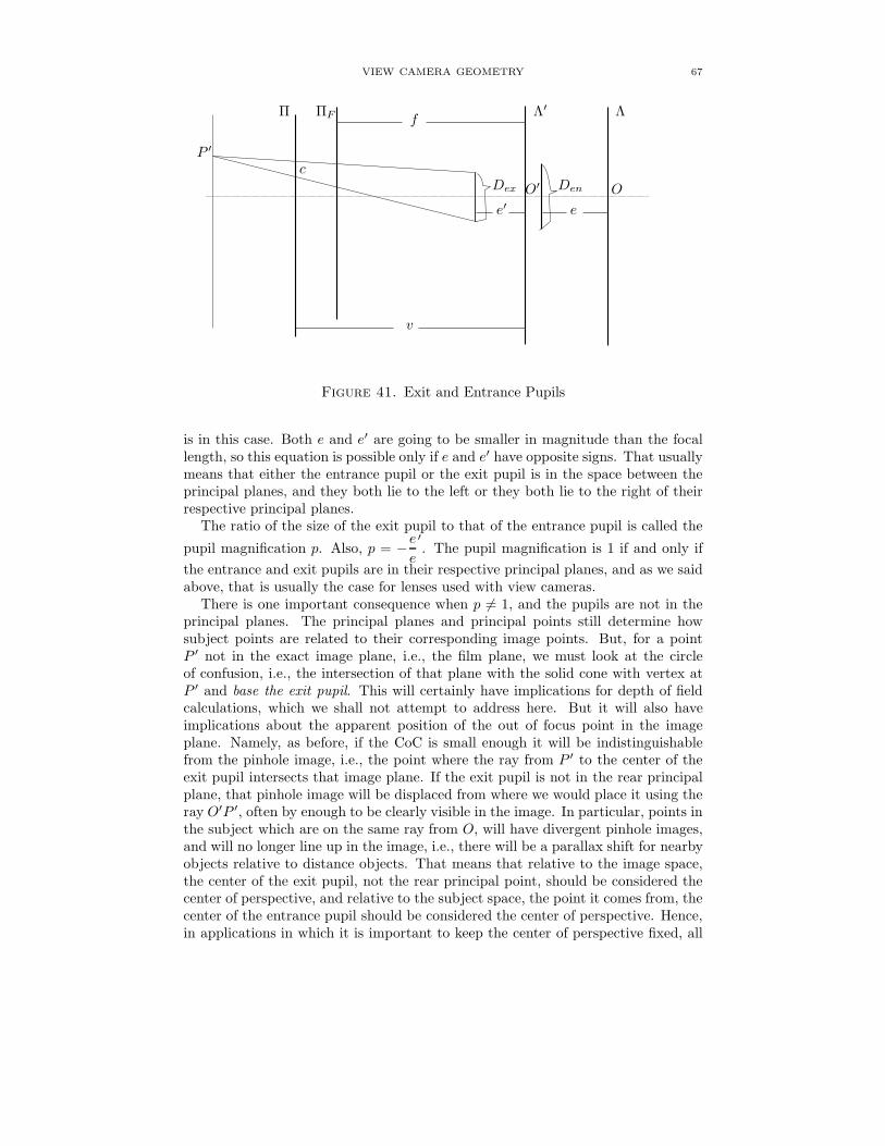
VIEW CAMERA GEOMETRY 67
P ′
Π ΠF Λ′ Λ
cDex Den
f
v
e′ e
O′ O
Figure 41. Exit and Entrance Pupils
is in this case. Both e and e′ are going to be smaller in magnitude than the focallength, so this equation is possible only if e and e′ have opposite signs. That usuallymeans that either the entrance pupil or the exit pupil is in the space between theprincipal planes, and they both lie to the left or they both lie to the right of theirrespective principal planes.
The ratio of the size of the exit pupil to that of the entrance pupil is called the
pupil magnification p. Also, p = −ee
′. The pupil magnification is 1 if and only if
the entrance and exit pupils are in their respective principal planes, and as we saidabove, that is usually the case for lenses used with view cameras.
There is one important consequence when p 6= 1, and the pupils are not in theprincipal planes. The principal planes and principal points still determine howsubject points are related to their corresponding image points. But, for a pointP ′ not in the exact image plane, i.e., the film plane, we must look at the circleof confusion, i.e., the intersection of that plane with the solid cone with vertex atP ′ and base the exit pupil. This will certainly have implications for depth of fieldcalculations, which we shall not attempt to address here. But it will also haveimplications about the apparent position of the out of focus point in the imageplane. Namely, as before, if the CoC is small enough it will be indistinguishablefrom the pinhole image, i.e., the point where the ray from P ′ to the center of theexit pupil intersects that image plane. If the exit pupil is not in the rear principalplane, that pinhole image will be displaced from where we would place it using theray O′P ′, often by enough to be clearly visible in the image. In particular, points inthe subject which are on the same ray from O, will have divergent pinhole images,and will no longer line up in the image, i.e., there will be a parallax shift for nearbyobjects relative to distance objects. That means that relative to the image space,the center of the exit pupil, not the rear principal point, should be considered thecenter of perspective, and relative to the subject space, the point it comes from, thecenter of the entrance pupil should be considered the center of perspective. Hence,in applications in which it is important to keep the center of perspective fixed, all

68 LEONARD EVENS
rotations of the lens should be about the center of the entrance pupil. That isspecially important in panoramic photography, where one rotates the camera tomake exposures of the scene from different angles and then combines the imagesdigitally by making appropriate transformations of those images and merging them.If the center of perspective is not kept fixed in such a rotation, there will be obviousparallax shifts, and it will be impossible, in principle, to merge such elements if theyappear in overlapping exposures. The software for combining panoramic imagesis very sophisticated and may be able deal with such issues in some cases, buteverything works much better if the photographer is careful to locate the center ofperspective and rotate about it. Special tripod heads or attachments are designedwith that in mind.
11. Sources of Error
There are several sources of error which may cause results in the field to differfrom what geometric optics predicts. We mentioned some before. In this section,we attempt to estimate their magnitudes.
The most obvious of these is the fact geometric optics is only an approximationto the actual behavior of a physical lens. As previously noted, because of lensaberrations, the image of a ‘point’ is not a well defined point. With modern lenses,these aberrations are often so well controlled, that the photographer would behard put to see any effect. Perhaps the most significant aberration in practice iscurvature of field, the fact that the image of a plane is a curved surface rather thananother plane. Also, we have to make allowances for the fact that a real lens hassome physical extension, as noted in Section 10, and can’t be described as a single‘principal point’.
Another source of error is possible displacement of the film, where the image isrecorded, from the ground glass image used for focusing. This is similar to errorsin focusing discussed in Section 11.3, and we will discuss the matter in more detailthere. The film’s departure from flatness in the film holder is another source oferror, but we won’t discuss it in this article.
11.1. Errors in focusing—Depth of Focus. Another problem is inaccuracy infocusing, which comes about for two reasons. First, there is bound to be some errorin positioning the standard on the rail. Most view cameras have a fine focusingknob which through gearing converts large movements of the knob into small dis-placements on the rail. Such cameras can be positioned to within 0.1 to 0.2 mm oreven better. Those without gearing can’t focus as precisely.
More serous is the fact that it is not possible to find a definite point at which theimage appears exactly in focus. If you try to focus with the lens at full aperture onsome element of the scene, there will be a point on the rail where it just comes intofocus and beyond that a point where it just goes out of focus. The spread betweenthose points is called the depth of focus . It should be distinguished from depth offield, but the two notions are related, and sometimes it is difficult to disentangleone from the other. Both are based on the same optical effect: a sufficiently smalldisc in the image plane is not distinguishable from a point
The analysis of depth of focus is very similar to that for depth of field. We willdiscuss mainly the case of no tilt, but our basic conclusions will remain valid inthe general case. Suppose the image of a subject point is at distance v from theprincipal point, but in attempting to focus on it, you place the ground glass at
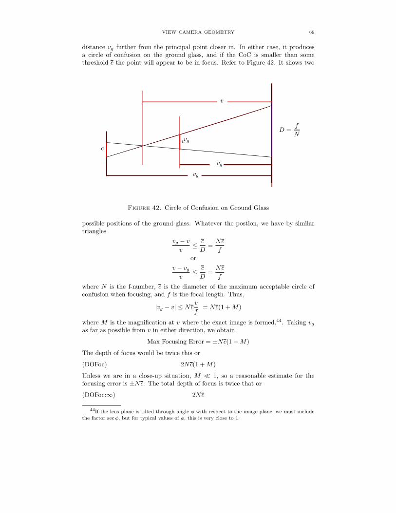
VIEW CAMERA GEOMETRY 69
distance vg further from the principal point closer in. In either case, it producesa circle of confusion on the ground glass, and if the CoC is smaller than somethreshold c the point will appear to be in focus. Refer to Figure 42. It shows two
v
D =f
Nvg
cc
vg
vg
Figure 42. Circle of Confusion on Ground Glass
possible positions of the ground glass. Whatever the postion, we have by similartriangles
vg − vv
≤ c
D=Nc
f
or
v − vg
v≤ c
D=Nc
f
where N is the f-number, c is the diameter of the maximum acceptable circle ofconfusion when focusing, and f is the focal length. Thus,
|vg − v| ≤ Ncv
f= Nc(1 +M)
where M is the magnification at v where the exact image is formed.44. Taking vg
as far as possible from v in either direction, we obtain
Max Focusing Error = ±Nc(1 +M)
The depth of focus would be twice this or
(DOFoc) 2Nc(1 +M)
Unless we are in a close-up situation, M ≪ 1, so a reasonable estimate for thefocusing error is ±Nc. The total depth of focus is twice that or
(DOFoc:∞) 2Nc
44If the lens plane is tilted through angle φ with respect to the image plane, we must includethe factor sec φ, but for typical values of φ, this is very close to 1.

70 LEONARD EVENS
There is one potential problem with this reasoning. M may be determined from
the subject distance u by the formula M =1
u/f − 1. But usually, we find instead
Mg, the magnification at the position of the ground glass, either by measuringthe bellows extension, vg directly, or by determining the ratio of the image size tothe subject size. Using 1 + Mg rather than 1 +M introduces an error in formula(DOFoc). But, we have
|(1 +M)− (1 +Mg)| = |M −Mg| =|v − vg|
u≤ Nc
f
v
u=Nc
fM
and the quantity on the right is going to be miniscule in any practical case.Note There is another way to approach the problem. Namely fix the position
vg of the ground glass and ask how far on either side of it an image point can beand still appear in focus. The total range for which that is true is
2Nc(M + 1)
1− (Nc/f)2= 2Nc(M + 1)(1 + (Nc/f)2 + (Nc/f)4 + . . . )
which, since (Nc)/f)2 is almost always very small, amounts to the same estimate.One almost always focuses with the lens at maximum aperture. For view camera
lenses this can range from f/4.5 to about f/8 or smaller. The proper choice forc depends on a variety of factors. It is related to the value c used for depth offield calculations but is not necessarily the same. In depth of field calculations,one is thinking of a final print viewed at leisure under good lighting. A standardfor comparison is an 8 x 10 print viewed at about 12 inches.45 The CoC for thatis usually taken to be between 0.1 and 0.2 mm, depending on assumptions aboutwho, under what circumstances, is viewing the print. Let’s take the value 0.2 mm.(If you prefer a smaller value, it is clear how to modify the calculations.) Since a 4× 5 negative must be enlarged 2 × to yield an 8 × 10 print, we should reduce theCoC at the level of the film to 0.1 mm.
Let’s think a bit about how this correlates with what you see when looking atthe ground glass. In comparison to the print, you should put your eye about sixinches from the image. Very young people, and some myopic people, with theirglasses off, can do that, but most of us can’t without a loupe or other aid. Solet’s assume that for critical focusing you use a loupe, and to start, let’s assume itmagnfies 2×. Were viewing the ground glass the same thing as viewing the print,then c = 0.1 mm would be an appropriate choice for estimating depth of focus. Atypical aperture would be f/5.6, i.e., N = 5.6. That would yield a focusing errorfor distant subjects of about ±5.6×0.1 = ±0.56 mm, and the depth of focus wouldbe twice that or about 1.12 mm.
But, looking at the ground glass under a dark cloth in the field is not the sameas viewing a print. Even a well made viewing screen has some texture, which,under sufficient magnification, will interfere with resolving fine detail.46 So theproper choice of /c for you is something you must determine experimentally. Youcan do that by measuring the distance as above between where a detail just comes
45A larger print viewed from proportionately further away appears the same. If your viewersinsist on getting very close to a large print, you need to adjust the CoC c accordingly.
46For this reason, it is not wise to use high powered magnifiers to focus. Usually one doesn’twant to go stronger than 4 to 6 ×, and usually 8× is a practical upper limit, to be used onlyunder special circumstances. Even at that level, one may find oneself focusing on viewing screenartifacts rather than on the scene.
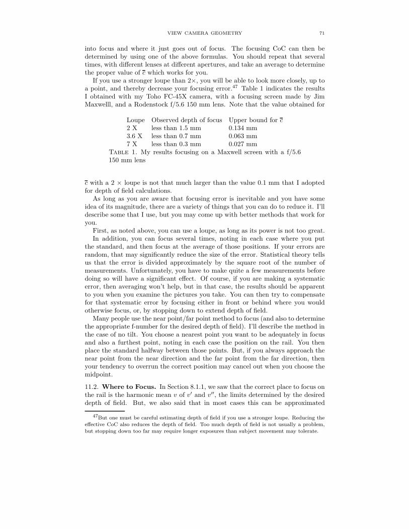
VIEW CAMERA GEOMETRY 71
into focus and where it just goes out of focus. The focusing CoC can then bedetermined by using one of the above formulas. You should repeat that severaltimes, with different lenses at different apertures, and take an average to determinethe proper value of c which works for you.
If you use a stronger loupe than 2×, you will be able to look more closely, up toa point, and thereby decrease your focusing error.47 Table 1 indicates the resultsI obtained with my Toho FC-45X camera, with a focusing screen made by JimMaxwelll, and a Rodenstock f/5.6 150 mm lens. Note that the value obtained for
Loupe Observed depth of focus Upper bound for c2 X less than 1.5 mm 0.134 mm3.6 X less than 0.7 mm 0.063 mm7 X less than 0.3 mm 0.027 mm
Table 1. My results focusing on a Maxwell screen with a f/5.6150 mm lens
c with a 2 × loupe is not that much larger than the value 0.1 mm that I adoptedfor depth of field calculations.
As long as you are aware that focusing error is inevitable and you have someidea of its magnitude, there are a variety of things that you can do to reduce it. I’lldescribe some that I use, but you may come up with better methods that work foryou.
First, as noted above, you can use a loupe, as long as its power is not too great.In addition, you can focus several times, noting in each case where you put
the standard, and then focus at the average of those positions. If your errors arerandom, that may significantly reduce the size of the error. Statistical theory tellsus that the error is divided approximately by the square root of the number ofmeasurements. Unfortunately, you have to make quite a few measurements beforedoing so will have a significant effect. Of course, if you are making a systematicerror, then averaging won’t help, but in that case, the results should be apparentto you when you examine the pictures you take. You can then try to compensatefor that systematic error by focusing either in front or behind where you wouldotherwise focus, or, by stopping down to extend depth of field.
Many people use the near point/far point method to focus (and also to determinethe appropriate f-number for the desired depth of field). I’ll describe the method inthe case of no tilt. You choose a nearest point you want to be adequately in focusand also a furthest point, noting in each case the position on the rail. You thenplace the standard halfway between those points. But, if you always approach thenear point from the near direction and the far point from the far direction, thenyour tendency to overrun the correct position may cancel out when you choose themidpoint.
11.2. Where to Focus. In Section 8.1.1, we saw that the correct place to focus onthe rail is the harmonic mean v of v′ and v′′, the limits determined by the desireddepth of field. But, we also said that in most cases this can be approximated
47But one must be careful estimating depth of field if you use a stronger loupe. Reducing theeffective CoC also reduces the depth of field. Too much depth of field is not usually a problem,but stopping down too far may require longer exposures than subject movement may tolerate.

72 LEONARD EVENS
accurately enough by focusing at the arithmetic mean v =v′ + v′′
2. Let’s see just
how accurate that is. As usual, we have48
v′ =v
1−Nc/fv′′ =
v
1 +Nc/fso
v′ + v′′ =v
1−Nc/f +v
1 +Nc/f=
2v
1− (Nc/f)2
orv′ + v′′
2=
v
1− (Nc/f)2
and v = v(1 − (Nc/f)2)(EF)
In most cases (Nc/f)2 is so small that we can ignore the difference. For example,suppose we choose c = 0.1 mm, f = 150 mm, and N = 22. Then (Nc/f)2 ≈0.000215. In other words, the relative error is a little over 0.02 perecent. Exceptin extreme close-ups, we can assume v ≈ f , so the actual error would be about0.000215× 150 ≈ 0.03 mm. Stopping down to f/45 would double this to 0.06 mm,a distance much less than the normal focusing error. The worst case would be avery short focal length lens using a very small aperture in an extreme close-up.49
For example, if f = 65 mm and N = 64, then (Nc/f)2 ≈ 0.0097, a relative errorof about 1 percent. For v = 2f = 130 mm, this would result in an error of about0.13 mm, which might produce a just barely detectable effect. Of course, at such asmall aperture, diffraction would begin to play a role.
So the conclusion is that it is safe to focus halfway between v′ and v′′ except inextreme clos-ups with very short focal length lenses. In such cases, the harmonicmean will be just a trifle short of the arithmetic mean. Even in such a case, it isunlikely that one needs to be so accurate that the difference between v and v isimportant.
11.3. Depth of focus and Depth of Field. At this point, it may be worthdiscussing how depth of focus affects depth of field. If you are focused slightly offwhere you think you should be, the total size of the depth of field region won’t besignificantly affected, but its location will be. It will be shifted in the direction ofthe error. One way to judge how significant that may be is to compare the depthof focus, which we saw might vary from as little as ±0.2 mm to as much to ±0.7mm, to the focus spread on the rail, which may vary from undetectable up to 2mm on the low end to as much as 10 mm at the high end. Clearly, the focusingerror will be more important when the focus spread is small, so it is in that casethat one should try to focus as best as possible, by using a high power loupe andother measures. Given that there is also a limit to how precisely the standard maybe placed on the rail, a lower limit for what is attainable might be ±0.1 to ± 0.2mm, with the latter being more plausible than the former.
The proper f-stop for a desired depth of field is usually determined, explicitly orimplicitly, from the focus spread s. If, you choose the f-numberN on the assumption
48We can ignore the ‘κ effect’ since at worst it will reduce the error even more.49Except in close-ups, there is normally little need to use very small apertures with very short
focal length lens.

VIEW CAMERA GEOMETRY 73
that the focus position is exactly where it should be, you will have too much depthof field in one direction and not enough in the other, so you should correct for suchan error by increasing s by an amount ds to compensate for the shift, which willresult in a shift dN is the f-number you get. The relation between the f-numberand the focus spread is
N ≈ s cosφ
2c(1 +M)≤ s
2c
and in any case the N you would choose is proportional to s, so we may conclude
dN
N≈ ds
s
The associated increase in the f-stop would be
2
log 2log
(
1 +dN
N
)
≈ 2.89dN
N
where the approximation holds provideddN
Nis small. If s is small and ds is large,
this can result in a significant change in N . It is easy to see that for larger focus
Focus Spread in mm f-number0.9 4.51.12 5.61.6 82.2 113.2 164.4 226.4 329.0 45
Table 2. Focus Spread and Estimate of f-number usings
2c, c = 0.1
spreads, we can tolerate a fairly large focusing error. For example, if s = 6.4
mm, ds = 0.7 mm,dN
N≈ 0.11 which would amount to about one third of a stop
correction. With a focus spread of 0.9 mm or less, we would need a fairly powerfulloupe even to detect it, and even if we could reduce ds to 0.2 mm, the neededcorrection to the f-stop would be about 2.89× 0.22 ≈ 0.64 or two thirds of a stop.
Fortunately, when the focus spread is small, we may want to stop down severalstops in any case. But in cases where that is inadvisable, it is specially importantto focus as carefully as possible. For larger focus spreads, it might be prudent tostop down up an additional one third to one half stop.
A shift of the film plane from the focusing plane on the ground glass will havea similar effect. It will shift the entire depth of field in one direction. Fortunately,it is a systematic error which the photographer can measure and either correct byadjusting the position of the ground glass or compensate for.
The best way to measure such a shift is to focus as carefully as possible on ascale50 at a known distance from the lens and making a 45 degree angle with the line
50Marks on the scale should be placed close enough so that in the image, their separation willbe comparable in magnitude to the CoC. Otherwise, the drop in reolution may not be detectable.

74 LEONARD EVENS
of sight, take a picture, and see how far off the focus is. Focusing should be donewith a high power loupe. The subject distance u should be close enough—perhaps
two to three meters—to be able to calculate the magnification M =f
u− f rea-
sonably accurately. Ideally, the process should be repeated several times, perhapsusing different lenses, and different target distances. The subject distance shouldbe measured from the front principal point, which for most lenses is close to thefront of the lensboard.51
From the lens equation, it is easy to see that the displacement du in subjectdistance u is related to the corresponding displacement dv in image distance v by
(Sh) dv = −M2 du
You should remember to correct for the angle between the target scale and the lineof sight, e.g., for a 45 degree angle, du would be about 70 percent of the distancealong the scale as indicated in the print.
It is impossible to eliminate such a shift entirely, and in some cases it may beas large as 0.1 to 0.2 mm, i.e., comparable in magnitude to normal focusing andpositioning errors.
Of course, systematic errors, whatever their cause, will become apparent withexperience. If you can’t track them down and correct them, you can just compensatewhen focusing or by stopping down a bit more.
11.4. Leveling the Camera. For certain scenes, it is important that the filmplane be plumb. This is particularly important to prevent convergence of verticalsin architectural photography. Leveling is usually done with a level, which dependson centering a bubble between two reference lines. Checking with my carpenter’slevel, I found this could produce an error of about 2–4 mm over a distance of 600mm, which which could result in the rear standard being out of plumb by as muchas ψ = 0.005 radians. Will such a small error be noticeable?
Figure 43 shows the effect of tilting the back on convergence of verticals. In thediagram on the left, Π and Λ indicate the standards of the out of plumb camera,where the angle ψ is greatly exaggerated. Γ indicates a plane through the lensparallel to a vertical building facade. The diagram on the right shows the imagesof the sides of the building converging to the vanishing point P∞. w1 + w2 is thewidth of the image of the building at the center of the field, and χ is the angle theindicated side makes with the center line. We have
tanχ =w1
v cotψ=w1
vtanψ
But because the angles are so small, we may use tanφ ≈ ψ and tanχ ≈ χ, whichleads to
χ ≈ w1
vψ
In most cases, v ≈ f and w1 is bounded by the dimensions of the frame. For
plausible values of f and w1,w1
fis not much larger than 1, and is usually somewhat
smaller. So χ is, at worst, the same order of magnitude as ψ, and usually it issmaller. For ψ ≈ 0.005 radians, the departure from the vertical over 100 mm inthe image would be at worst about 0.5 mm, i.e., it would be undetectable to theunaided eye.
51Avoid telephoto or wide angle lenses unless you know the position of the principal point.

VIEW CAMERA GEOMETRY 75
Π Λ Γ
ψv cotψ
vw1 w2
P∞
χ
Figure 43. Effect on Convergence of Verticals of Tilted Camera
Being out of plumb also slightly affects focus on the building facade because theimage of the facade would be tilted by a very small angle ξ with respect to the rearstandard. Let S be the distance at which plane of the building facade intersectsthe lens plane and, by Scheimpflug’s Rule, the image of that plane. Then
S = u tanψ = v tan ξ whence
tan ξ =v
utanψ = M tanψ and
ξ ≈Mψ
Say M = 0.01, ψ = 0.005 radians, so ξ ≈ 5 × 10⁻⁵. Over a distance of 120 mm,that would move the image of the facade about 6× 10⁻³ mm. But, even at f/4.5,an image point can be as far as about Nc = 4.5 × 0.1 = 0.45 mm on either sideof the film plane and still produce a circle of confusion not distinguishable from apoint. Hence, this effect is truly so insignificant that it need not concern anyone.
11.5. Alignment of the Standards. The above discussion assumes that the stan-dards are exactly parallel, but in practice, that is unlikely to be the case. The lensplane will make a very small angle φ with respect to the film plane. There area couple of methods for checking parallelism. First, one can check the distancebetween the standards at each of the four corners. Without using sophisticatedequipment, a plausible estimate for the error in such a measurement is about ±0.5mm. An estimate for the corresponding tilt angle is obtained by dividing that bythe distance from the center of the lens board to a corner. Depending on the designof the camera, that could range between 50 mm and 100 mm. The correspondingtilt would be between 0.01 and 0.005 radians. Alternately, one might use a level,in which case, as noted in Section 11.4, a tilt as large as 0.005 radians might notbe detectable. So 0.005 radians is the value we shall use in the remainder of thisdiscussion.

76 LEONARD EVENS
A small tilt φ will move the hinge line from infinity to hinge distance J =f
sinφ≈ f
φ. For f = 150, φ = 0.005, this would be about 30 meters, and it might
be significantly shorter for a shorter focal length lens. The corresponding angle
the subject plane makes with the vertical would be γ = arctanu
J, where u is
the distance to the focus point along the line of sight. The value of u would ofcourse depend on the scene, but a rough estimate for a typical scene might be thehyperfocal distance at f/22. That would be about 10 meters for a 150 mm lens. Soinstead of being zero, as would be the case if the standards were exactly parallel,γ ≈ 18 degrees.
Figure 44 shows the presumed region in focus were the standards exactly paralleland the actual region resulting from a slight unintended tilt. The tilt is greatly ex-aggerated, for purposes of illustration, in comparison to what it would be in reality.Don’t be misled by the orientation in the diagram. The hinge line resulting from anunintended tilt, together with the associated subject planes, could be anywhere.
Π ∆ Σ′
Σ
Σ′′
y2
y1 uZ ′ Z
Y1
Y2
u′1 u′′2u′ u′′
J
C′1
C′2
C′′1
C′′2
Figure 44. Comparison of Depth of Field Regions

VIEW CAMERA GEOMETRY 77
We need only consider subject points such that the corresponding image pointslie in the frame, and the red lines indicate planes Y1 and Y2, which set the limitson the depth of field imposed by that restriction. Since the tilt axis will generallybe skew to the sides of the frame, those planes should be assumed to be parallel tothe tilt axis and to pass through opposite corners of the frame. y1 and y2 denotethe distances at which those planes intersect Π, where those distances are measuredfrom the plane, denoted Z ′Z in the diagram, determined by the tilt axis and the lineof sight, the positive direction being that away from the Scheimfplug line. (So inthe diagram y1 would be negative.) The blue lines indicate the near and far limitsof depth of field under the assumption that the standards are parallel, and thegreen lines the limits arising because of the tilt. The actual depth of field overlapsthe presumed depth of field, being greater or less, depending on the position of thesubject point in relation to the plane Z ′Z. Note that the effect of the inadvertenttilt appears to be much more pronounced in the background than in the foreground,but this may be misleading because of compression of distant points as seen on theground glass.
The depth of field will of course depend on the relative aperture (f-number) Nand the CoC c. Note that c is based on what we hope to achieve in the final print,not on the c, the focusing CoC. As noted in Section 11.1, the latter depends stronglyon the characteristics of the focusing screen and the power of the loupe.
Σ′ and Σ′′ intersect Z ′Z at distances u′ and u′′ from the reference plane, whichis also the presumed lens plane. As we shall see, these are essentially the same asthe values determined in Section 8.4.1 under the assumption that the standards(and hence Σ′,Σ, and Σ′′) are parallel. To gauge the effect of the unintended tilt,we need to find the distances, in increasing order, u′2, u
′1, u
′′2 , and u′′1 at the points
C′2, C
′1, C
′′2 , and C′′
1 at which Σ′ and Σ′′ cross Y1 and Y2.If the alignment were perfect, we would expect that everything between two
planes parallel to the image plane Π would be in focus, so it is useful to considerwhat happens in such planes at each of these points. There would be essentiallynothing in focus captured by the frame for such a plane at either of the extremesu′2 (C2) and u′′1 (C′′
1 ). At each of u′ and u′′, the limits which a depth of field tablewould predict, part of of such a plane captured by the frame would be in focus.Finally, at either u′1 (C′
1) or u′′2 , everything captured by the frame would be infocus, or at least the figure suggests that would be the case.
To see why the figure is accurate in this regard, recall from Section 8.4.1 that foreach distance in the subject space, there is a window in Π showing what is in focus
at that distance. That window is of constant heightNc
sinφ≈ Nc
φ, but it moves in
the image plane Π as we move from foreground to background.52 Taking c = 0.1mm, N = 22 and φ = 0.005 radians yields about 880 mm for that height. So ifthe window starts either at C′
1 of C′′2 , the height of the window will be more than
enough to cover the frame. Even if we opened up as far as f/5.6, we would stillhave room to spare.
It follows that if we want to be sure we have identified two planes between whicheverything captured in the frame is in focus, we should use u′1 and u′′2 rather thanu′ and u′′ as the near and far limits of depth of field.
We now derive formulas for the quantities described above.
52As above, we can ignore the‘κ effect.

78 LEONARD EVENS
The relevant formulas describing the planes Σ,Σ′, and Σ′′ were derived in Section8.4.153. We have
x2 =J
ux3 − J = J(
x3
u− 1)
x′2 = x2 +J cosφ
H(M + 1)x3 = J(
x3
u− 1) +
J cosφ
H(M + 1)x3
x′′2 = x2 −J cosφ
H(M + 1)x3 = J(
x3
u− 1)− J cosφ
H(M + 1)x3
where x3 denotes the distance to the reference plane, x2, x′2, and x′′2 denote the
distances from the plane Z ′Z to Σ,Σ′, and Σ′′ at x3, H =f2
Ncis the approximation
to the hyperfocal distance introduced earlier, andM is the magnification at distanceu.54 Hence,
x′2x3
= J(1
u− 1
x3) +
J cosφ
H(M + 1)(SP)
x′′2x3
= J(1
u− 1
x3)− J cosφ
H(M + 1)(MP)
We shall do the calculation for u′1. The calculations for the other quantities aresimilar. Refer to Figure 45. Using similar triangles, and putting x3 = u′1 in equation
Π ∆ Σ′ Σ
Σ′′
u′1
u
J
v
y1
φ
x′2
Figure 45. Effect of Small Tilt on Depth of Field
(SP), we have
−y1v
=x′2u′1
= J(1
u− 1
u′1) +
J cosφ
H(M + 1)
53We may ignore the ‘κ effect’ on the circle of confusion because φ is so small.54Because of the slight tilt, M differs insignificantly from the value that would apply if the
standards were parallel. See the end of this section for the details.
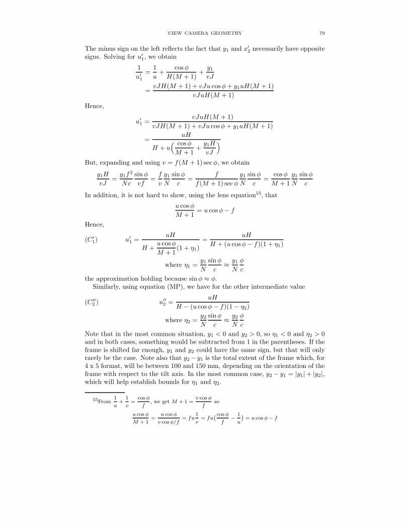
VIEW CAMERA GEOMETRY 79
The minus sign on the left reflects the fact that y1 and x′2 necessarily have oppositesigns. Solving for u′1, we obtain
1
u′1=
1
u+
cosφ
H(M + 1)+y1vJ
=vJH(M + 1) + vJu cosφ+ y1uH(M + 1)
vJuH(M + 1)
Hence,
u′1 =vJuH(M + 1)
vJH(M + 1) + vJu cosφ+ y1uH(M + 1)
=uH
H + u( cosφ
M + 1+y1H
vJ
)
But, expanding and using v = f(M + 1) secφ, we obtain
y1H
vJ=y1f
2
Nc
sinφ
vf=f
v
y1N
sinφ
c=
f
f(M + 1) secφ
y1N
sinφ
c=
cosφ
M + 1
y1N
sinφ
c
In addition, it is not hard to show, using the lens equation55, that
u cosφ
M + 1= u cosφ− f
Hence,
u′1 =uH
H +u cosφ
M + 1(1 + η1)
=uH
H + (u cosφ− f)(1 + η1)(C′
1)
where η1 =y1N
sinφ
c≈ y1N
φ
c
the approximation holding because sinφ ≈ φ.Similarly, using equation (MP), we have for the other intermediate value
u′′2 =uH
H − (u cosφ− f)(1− η2)(C′′
2 )
where η2 =y2N
sinφ
c≈ y2N
φ
c
Note that in the most common situation, y1 < 0 and y2 > 0, so η1 < 0 and η2 > 0and in both cases, something would be subtracted from 1 in the parentheses. If theframe is shifted far enough, y1 and y2 could have the same sign, but that will onlyrarely be the case. Note also that y2− y1 is the total extent of the frame which, for4 x 5 format, will be between 100 and 150 mm, depending on the orientation of theframe with respect to the tilt axis. In the most common case, y2 − y1 = |y1|+ |y2|,which will help establish bounds for η1 and η2.
55From1
u+
1
v=
cos φ
f, we get M + 1 =
v cos φ
fso
u cos φ
M + 1=
u cos φ
v cos φ/f= fu
1
v= fu
` cos φ
f−
1
u
´
= u cos φ − f
80 LEONARD EVENS
The formulas for the two extreme values are
u′2 =uH
H + (u cosφ− f)(1 + η2)(C′
2)
u′′1 =uH
H − (u cosφ− f)(1− η1)(C′′
1 )
If we set η1 = η2 = 0 in the above equations, we get we get the distances atwhich Σ′ and Σ′′ cross the plane Z ′Z.
u′ =uH
H + (u cosφ− f)(T ′)
u′′ =uH
H − (u cosφ− f)(T ′′)
These formulas should be compared to those derived in Section 8.2 under the as-sumptions that the standards are exactly parallel. They are the same except thatu cosφ − f replaces u − f . Since φ is so small, cosφ is essentially equal to 1, andthe results would be indistinguishable in practice.
How the above formulas relate to what one would do in practice is a bit subtle.They certainly indicate what would happen were one to focus on one specific targetpoint at a known distance u and then try to use depth of field tables to estimatehow to set the aperture so that all interesting detail is in focus in the final print.Let’s estimate η1 and η2 for a typical scene to see what might happen in that case.Take φ = 0.005 radians, N = 22, c = 0.1 mm, and y1 = y2 ≈ 50 mm. This yields−η1 = η2 ≈ 0.11. Then with H = 10 meters and u = 8 meters, we would obtainin the foreground u′1 ≈ 4.67 meters and u′ ≈ 4.44 meters, a difference of about 5percent from the expected value. But that large an effect would only be seen atone corner of the frame. We would actually gain depth of field at opposite corner.Similarly, in the background, u′′2 ≈ 27.8 meters, and u′′ ≈ 40 meters for a differenceof about 33 percent from the expected value, a much larger shift.
But, as noted above, because of the compression of the metric in the distance,as seen on the ground glass, the above figures are misleading. There is another wayto look at it, which gives a better idea of what we will see on the ground glass andin the final p0rint.. Divide both numerator and denominator of equation (C′
1) by
1 + η1, and put H ′1 =
H
1 + η1. We get
(D′1) u′1 =
uH ′1
H ′1 + (u cosφ− f)
But H ′1 =
f2
Nc(1 + η1)is just the (approximation) to the hyperfocal distance we
would obtain for f-number N(1 + η1). If we put that value for the f-number in ourdepth of field calculator, rather than the value N that we are actually using, thecalculator will give u′1 for the near limit. Similarly, if we use N(1 − η2) instead ofN , the calculator will give us u′′2 for the far limit. Alternately, provided y1 < 0,
and y2 > 0—by far the most common case—if we set the aperture atN
1− η , where
η is the larger of |η1| and |η2|, we will get near and far limits on the depth of fieldencompassing u′ and u′′, the values we would have got using N , were the standards
VIEW CAMERA GEOMETRY 81
exactly parallel. Thus
(ST) −2log(1− η)
log 2
is an estimate for the amount we need to stop down to compensate for an inadver-tent tilt. In the above example, 1− η = 0.89, and amount we need to stop down isabout one third of a stop.
What happens if you don’t use depth of field tables? There are two possibleapproaches which are commonly used. First, you can just stop down and try tovisually estimate the depth of field on the basis of what you see on the groundglass. Alternately, you can use the near point/far point method: focus on the railhalfway between where specific points in Σ′ and Σ′′ (presumed parallel to Π) comeinto focus, and set the aperture based on the focus spread and the chosen CoC c.Or, you can use some combination of the two approaches.
The major advantage of the purely visual approach is that you can examine theentire frame, both foreground and background to make sure all interesting detail isadequately in focus, so the precise shape of the depth of field region is not relevant.But the approach also has some drawbacks, the most obvious being that the imagemay be too dim at plausible taking apertures to see much of anything. In addition,if you use a powerful loupe in order to deal with dimness, what you see will bedetermined by c, the focusing CoC, which depends on the power of the loupe. Thenet effect is likely to be that you will stop down too far, by up to two stops. Thatcan be a problem if subject movement is an issue because of longer exposure time.
Suppose instead you use the near point/far point method. The near and farpoints, together with the position of the hinge line resulting from the unintendedtilt, will determine the planes Σ′ and Σ′′. The proper aperture is given in terms
of the focus spread s by the formulas
2c(1 +M)cosφ. But, ignoring the term
cosφ ≈ 1, you get the same answer you would get under the assumption of perfectalignment. At that aperture, if the near point were chosen at C′
1 and the far pointat C′′
2 , then everything between the planes through those points, as indicated inFigure 44, would be in focus in the final print. In order to pick those points out,you need to know which plane is Y1 and which is Y2.
Here is one way to do it. At each corner of the frame, focus at infinity or as toclose to infinity as possible. Look at Figure 46. If you focus so that the subjectplane Σ1 is parallel to Y1, the depth of field wedge, at the focusing aperture, willcut across the region between Y1 and Y2, so there will be lots of detail along thediagonal which is in focus all the way up to the opposie corner. On the other hand,if you focus such that so the subject plane Σ2 is parallel to Y2, the wedge will lookvery different. The ‘upper’ bounding plane may intersect Y1 at great distance, butthe ‘lower’ bounding plane won’t intersect it anywhere in the the subject space. Asa result, little, if anything, will remian in focus as you look on the diagonal towardsthe other corner..
There may be a similar but less pronounced effect for the other pair of corners,but the proper choice is that for which the effect is most pronounced. Of course,it may turn out that there is no detectable difference for either pair of corners,but that just means that the inadvertent tilt is too small to worry about and thestandards are exactly parallel as best as can be determined.

82 LEONARD EVENS
Y1
ZZ ′
Σ1
Y2
Σ2
Figure 46. The Difference between focusing at ∞ at Y1 and Y2
To summarize, focus at infinity at each of the four corners and note the cornerfor which the greatest amount remains in focus along the diagonal. That is thecorner in which you should look for the near point, and the opposite corner is theone where you should look for your far point. If you can’t tell the difference, thenyour standards are aligned well enough and it doesn’t matter.
The above analyses also suggest some ways to reduce the magnitude of the error,perhaps to the point that you can ignore it entirely. One should of course do one’sbest to align the standards. It may be possible thereby to reduce φ to as little as0.001–0.002 radians. Also, stopping down will reduce the magnitude of the errorin two ways. First it will reduce η1 and η2, but, in addition, it will increase J ,decrease H , and most likely decrease u, the distance at which you focus, becauseof increased depth of field. On the other hand, being fussier about fine detailby choosing a smaller value for c, paradoxically, will actually make matters worse
because of the quotientφ
cwill have a smaller denominator.
Aside. There are two possible expressions for the magnification at distance u
M =f
u− f
Mφ =f
u cosφ− fwhere the first is calculated on the assumptions that the standards are exactlyparallel and the second incorporates the tilt. Dividing the first by the second anddoing some algebra results in the relation
Mφ = M1
1− (1− cosφ)/(1 − f/u)
But 1 − cosφ ≈ φ2/2 ≤ 0.0052
2= 1.25 × 10⁻⁵. Even in close-ups u ≥ 2f so
1− f/u > 1/2 so at worst that increases the relative error to 2.5× 10⁻⁵ or 0.0025percent. Thuus Mφ is so close to M that we can ignore the difference.
VIEW CAMERA GEOMETRY 83
11.6. Error in Setting the Tilt. Let’s now consider the case of an intentionaltilt, the purpose of which is either to set an explicit exact subject plane Σ, or,more often, a desired depth of field between bounding planes Σ′ and Σ′′. A crucial
parameter is the tilt angle56 φ or equivalently the hinge distance J =f
sinφ.
If our only aim is to establish an exact subject plane, then the error in setting φis essentially irrelevant. If the desired plane looks in focus on the ground glass thenthere is an excellent chance it will look in focus in the final print. That would betrue even if we didn’t use a particularly powerful loupe since the taking apertureis likely to be several stops smaller than the the focusing aperture, thus increasingthe depth of field about the exact subject plane. On the other hand, an error inthe tilt angle may in some cases result in a significant shift in the position of thehinge line. We need to determine if that will result in a significant change in theexpected depth of field, and that is the aim of the analysis below.
Recall Wheeler’s Rule in Section 6.1.
(WR) sinφ =1
1 +M
s
t
where s is the focus spread between the images of two points in the desired subjectplane Σ, t is the vertical57 distance between those points, when each is in focus,on the ground glass, and M is the magnification at the distance u at which theΣ crosses the normal line to the standards. The measurements of s and t and thevalue of M are those that hold before any tilt is applied. It is easy to estimatethe error in φ from formula (WR), and it is clear how it depends on the error inmeasuring the focus spread. But the rule is seldom used in practice, except possiblyto establish an initial guess for the tilt. Instead one tries, visually, to adjust thetilt so that the desired subject plane is entirely in focus. If two selected points inthat plane are not simultaneously in focus, there will be some focus spread betweenthem as one focuses first on one and then on the other. When there is no discerniblefocus spread, the tilt angle is presumed correct. Unfortunately, because of depthof focus considerations, a very small focus spread can’t be distinguished from nofocus spread, and that will lead to an error in φ, J , and the position of the resultingsubject plane.
In Figure 47, we show the relation between the subject plane Σ and the imageplane Π, when the latter is close to being vertical but not quite there. φ is theangle the lens plane makes with the vertical58, and β is the angle the image planemakes with the vertical.
Note that we have chosen the orientations for φ and β opposite to one another,the former being positive in the counterclockwise direction and the latter in theclockwise direction. The tilt will be exactly right when β = 0, but in practice itwill be some small angle. As before, we will have
tanβ =s
t
where s (possibly negative) is the focus spread between two image points and t istheir vertical separation on the ground glass, when each is in focus. If s is smaller
56In most cases, we don’t actually need to know what that angle is, but it still plays a role.57The usual disclaimer applies. The language must be changed if the tilt axis is not horizontal.58This assumes a pure tilt about a horizontal axis. In general, we would measure φ with
respect to the line in the original position of the lens plane perpendicular to the tilt axis.
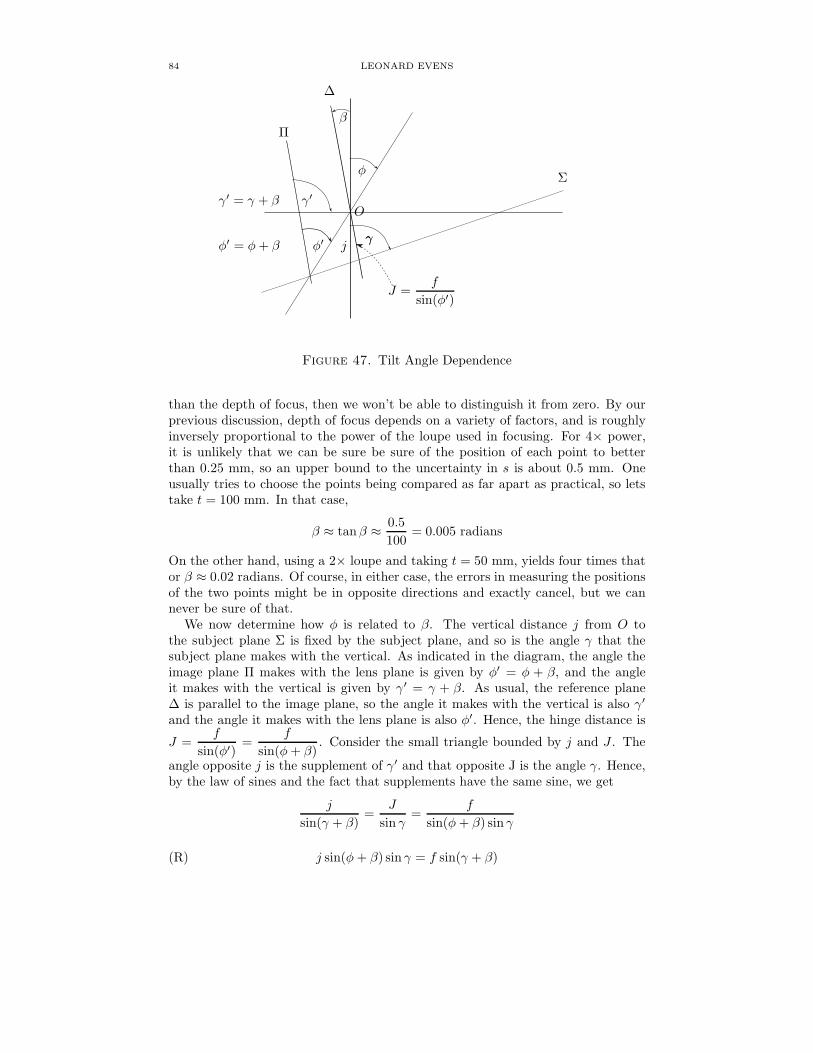
84 LEONARD EVENS
γ
γ′
φ
φ′
β
γφ′ = φ+ β
γ′ = γ + β
j
J =f
sin(φ′)
O
Σ
∆
Π
Figure 47. Tilt Angle Dependence
than the depth of focus, then we won’t be able to distinguish it from zero. By ourprevious discussion, depth of focus depends on a variety of factors, and is roughlyinversely proportional to the power of the loupe used in focusing. For 4× power,it is unlikely that we can be sure be sure of the position of each point to betterthan 0.25 mm, so an upper bound to the uncertainty in s is about 0.5 mm. Oneusually tries to choose the points being compared as far apart as practical, so letstake t = 100 mm. In that case,
β ≈ tanβ ≈ 0.5
100= 0.005 radians
On the other hand, using a 2× loupe and taking t = 50 mm, yields four times thator β ≈ 0.02 radians. Of course, in either case, the errors in measuring the positionsof the two points might be in opposite directions and exactly cancel, but we cannever be sure of that.
We now determine how φ is related to β. The vertical distance j from O tothe subject plane Σ is fixed by the subject plane, and so is the angle γ that thesubject plane makes with the vertical. As indicated in the diagram, the angle theimage plane Π makes with the lens plane is given by φ′ = φ + β, and the angleit makes with the vertical is given by γ′ = γ + β. As usual, the reference plane∆ is parallel to the image plane, so the angle it makes with the vertical is also γ′
and the angle it makes with the lens plane is also φ′. Hence, the hinge distance is
J =f
sin(φ′)=
f
sin(φ+ β). Consider the small triangle bounded by j and J . The
angle opposite j is the supplement of γ′ and that opposite J is the angle γ. Hence,by the law of sines and the fact that supplements have the same sine, we get
j
sin(γ + β)=
J
sin γ=
f
sin(φ+ β) sin γ
(R) j sin(φ+ β) sin γ = f sin(γ + β)
VIEW CAMERA GEOMETRY 85
Differentiate both sides of (R) with respect to φ, keeping in mind that j, J, and γare fixed. We obtain
j cos(φ+ β) sin γ(dφ
dβ+ 1
)
= f cos(γ + β)
which we can solve to obtain
dφ
dβ+ 1 =
f cos(γ + β)
j cos(φ+ β) sin γ
dφ
dβ= −1 +
f cos(γ + β)
j cos(φ+ β) sin γ
= −1 +sinφ0 cos(γ + β)
cos(φ+ β) sin γ(TR)
where we use the fact thatf
j= sinφ0, where φ0 is the tilt angle for which the
image plane is vertical and β = 0.Let’s look carefully at the expression on the right of equation (TR). We already
saw that a reasonable estimate for β is 0.005, and φ will not usually be larger than0.2, so cos(φ + β) ≈ 1, and sinφ0 ≈ 0.2. The subject plane doesn’t usually tiltvery strongly up or down, so it is safe to suppose 1.5 < γ < 1.65 and the same canbe said of γ + β. So −0.08 < cos(γ + β) < 0.08. Putting that all together gives arough estimate
dφ
dβ≈ −1± 0.016
within the relevant range. That tells that over the relevant range, the relationshipbetween φ and β is very close to linear, with slope very close to -1. In particular,when we try to set the tilt angle φ to φ0, the value with β = 0, the differencedφ = φ− φ0 is approximately equal to β.
Note however,that the image will be recorded in the plane Π of rear standard,which is vertical, not in Π. We can presume the standard has been placed tosplit the slight focus spread evenly, as indicated in Figure 48. That will displacethe subject plane slightly from Σ to Σ. The figure does not show the tilt angle
φ0 which we really wanted, but it appears implicitly as j =f
sinφ0, the distance
at which Σ crosses the reference plane. Also, we saw above that dφ = φ − φ0 isapproximately equal to the negative of β, the angle Π makes with the vertical. Inthe figure, β is positive, φ < φ0, whence J > j, and Σ passes under A and aboveB. If β < 0, and φ > φ0, then Σ passes over A and under B.
Corresponding to dφ, we have, using J =f
sinφ,
dJ = − f
sin2 φcosφdφ
dJ
J= −cosφ
sinφdφ = − dφ
tanφ≈ −dφ
φ(Rφ)
Note that dφ ≈ β, being determined by depth of focus considerations, is essen-tially independent of φ, which means that for small values of φ, the relative errordφ
φcould be pretty large. So we should stop to think a bit about how small φ might
be in practice.

86 LEONARD EVENS
φ
jJ
O
Σ
Σ
∆ΠΠ
A
B
B′
A′
β
Figure 48. Subject Plane Error
Refer again to Wheeler’s rule, i.e., formula (WH). If, with the standards parallel,s is less than the depth of focus, you can’t set a tilt on the basis of what you seeon the ground glass.. With the depth of focus between 0.5 mm and 1.0 mm, andt between 50 mm and 100 mm, as we saw above, that means that the minimumpossible value for φ ≈ tanφ could range between 0.005 and 0.02 radians. I’vedone some experiments which suggest that even those estimates are optimistic inpractice. An informal online survey suggested that tilt angles less than 2 degreesor 0.035 radians are rare. So let’s assume φ ≥ 0.03 radians except in specialcircumstances. Clearly, in such cases, we would do our best to minimize dφ so letsassume dφ ≈ 0.005 radians, so the relative error could be as large as 1/6 or about15 percent. On the other hand, for a moderate tilt of 0.1 radians, even if we were abit less careful and dφ ≈ .01 radians, then the relative error would be only 10 percent. By being careful, it could be reduced to 5 percent.
We are now in a position to see if these errors will affect the expected depth offield, or equivalently, the f-stop needed to obtain some desired depth of field.
There are no tables which give the depth of field T above and below the exactplane of focus in terms of the parameters, but we could rely on the formula (SplM)from Section 8.4.1
(SplM) T = 2J
H
cosφ
M + 1x3 =
Nc
f tanφ(M + 1)x3
with the total being twice that. As we saw, the relative change in M is miniscusle,and, except in close-ups, M is small enough to disregard in any case. So we have
dT
T= sec2 φ
dφ
tanφ+dN
N
If we set this to zero on the assumption that N has been adjusted to compensatefor the change if φ, we obtain
dN
N= − sec2 φ
dφ
tanφ= − secφ
dφ
sinφ≈ dφ
φ

VIEW CAMERA GEOMETRY 87
In number of stops of fractions thereof, this amounts to
2
log 2log
(
1 +dφ
φ
)
≈ 2.89dφ
φ
According to the above estimates,dφ
φcan range from 0.05 to 0.17. So the needed
correction to the aperture might range between one sixth to one half a stop, withthe former being more likely in typcial situations.
The above calculation would be useful only if you knew the actual value of T thatyou want at some specific distance x3. But that is unlikely to be the case. Instead,you usually identify target points on either side of the exact subject plane thatyou want to be in focus and then try to adjust the wedge so that it includes thosepoints. There are two basic approaches to doing that after establishing the tilt angleby choosing an exact subject plane: (i) stopping down and visually determining whatis in focus or (ii) calculating the f-number based on the focus spread between thetarget points.
The first approach has the advantage of being entirely visual, and you can alsoadjust the position of the exact subject plane at the same time. It won’t matterif there is an error in setting φ because you can see what is in focus. But you dohave to be careful that your focusing CoC is close to the CoC which is appropriatefor figuring depth of field in the print. Otherwise, you may end up either withtoo little or too much depth of field in the end result. The latter, in particular,can be a problem if you want to limit depth of field or if subject motion becomesapparent because of increased exposure time. It also has the disadvantage that itonly works if you can still see fine detail as you stop down. Many people may havedifficulty seeing well at f/16 and few can see much of anything beyond f/22. Usinga powerful loupe helps, but in effect reduces the focusing CoC, which, as notedabove, may lead you to stop down too much.
Just how an error in φ affects depth of field when using the focus spread methodis more complex. It may depend on the specific scene. Consider a scene such as aflat field of wildflowers receding into the distance with nothing above the groundin the foreground, a tree in the middle ground, and perhaps some mountains inthe far distance. Figure 49 illustrates such a scene schematically. Refer back to
Π ∆ Σ′
Σ
Σ′′
y2
y1 uZ ′ Z
Y1
Y2
u′J
C′1
C′2
C′′2
P (k, h)
Figure 49. Example
Figure 44, and note the differences. Σ′′ has been chosen to lie along the ground,

88 LEONARD EVENS
and Σ′ to pass through P (k, h) at the top of the tree, close C′159. The image of
C′′2 in the foreground would be at the top of the frame on the ground glass, and
the image of high point P (k, h), which is presumed be be below the images of themountain tops, is close to the bottom of the frame. Note that although the scenealmost fills the frame, two regions (marked in red), one between Σ′ and Y1 andthe other between Σ′′ and Y2 could produce images which are in the frame butoutside the depth of field. That could be a problem were there anything of interestin those regions which was not obscured by other parts of the scene. In this case, itis assumed that there is nothing of interest in the first region and that the secondregion is underground. 60
How would you go about setting up the camera for this scene. First, you wouldalmost certainly use the plane Σ′′ to determine the tilt angle, since it would containlots of detail, and most likely you could minimize the error dφ by using it. Youwould then note the position on the rail, refocus on the point P and note its positionon the rail. Next, you would measure the focus spread S in order find the f-stop,using
(NEq) N =S
2c
cosφ
M + 1≈ S
2c(M + 1)≈ S
2c
Finally, you would place the standard halfway between the two reference points onthe rail in order to set the position of of the exact subject plane Σ.
Note that all of this will be done with the actual tilt, whatever it is, and that inturn will determine the focus spread S. If you went to the trouble of independentlymeasuring φ and used the first expression in formula (NEq), then any error inthat measurement would make a difference in the calculated value for N , as notedabove, and you would have to compensate for it. But you are highly unlikely to doanything like that. Instead you would use the second or third expressions which donot involve φ. As a result you might overestimate slightly how much you need tostop down, and in general that would be innocuous.
More serious are the errors which result when focusing either on the low pointor the high point, or, in placing the standard halfway between them. But that wasaddressed in Section 11.3, and the tilt does not signficantly change the conclusionsdrawn there. If the spread S is large, then the necessary correction to the aperturewill probably be less than one third of a stop. But since the point of using a tiltis stop down less than we would without tilting—at the price of dealing with thewedg—the focus spread may be relatively small. If so, you may want to stop downan extra stop or more to be sure. And, as noted before, you should try to determinethe positions of the reference points on the rail a carefully as possible by using aloupe and the other measures discussed before.
There is a related question which is of passing interest, but is unlikely to affectwhat you do. Suppose you go through the process more than once. Since the tiltangle will vary, so also will the resulting focus spread, and hence the value of Nyou end up with. Let’s see by how much.
59The intersection C′
2of Y2 with Σ′ would be in the image space, which in effect means that
the depth of field extends to infinity.60Note also that there are two regions, that bounded by Y2,Σ′ and Σ′′ and that between Y1
and Σ′, which are in the depth of field but outside the frame and hence irrelevant.
VIEW CAMERA GEOMETRY 89
By similar triangles—not drawn in figure 49—we have
k + J
k=J
u′
u′ =J
J + kso
du′ =(J + k) dJ − J dJ
(J + k)2=
k dJ
(J + k)2
Hence
du′
u′=
k
J + k
dJ
J= − k
J + k
dφ
tanφ≈ − k
J + k
dφ
φ
Let’s see how much effect this has on the position of the standard.
v′ =fu′
u′ cosφ− f
dv′ =(u′ cosφ− f)f/, du′ − fu′(du′ cosφ− u′ sinφdφ)
(u′ cosφ− f)2
=−f2 du′ + f(u′)2 sinφdφ
(u cosφ− f)2
Hence
(DRφ)dv′
v′= − v
′
u′du′
u′+v′
fsinφdφ = −M ′du
′
u”+ (M ′ + 1)
dφ
φ
where M ′ is the magnification at the distance u′ at which Σ′ crosses the referencenormal. A similar calculation gives the relative error in v′′ in terms of M ′′, thecorresponding magnification at u′′ where Σ′′ crosses the reference normal. M ′ (and
similarly M ′′) will be very small except in close-ups, and by the abovedu′
u′is the
same order of magnitude asdφ
φ. Also, sinφdφ is miniscule. Hence, the change in
the focus spread due to dφ will be much less than the error in measuring it, andhence can be ignored.
As noted above, this calculation, while confidence building, is not really relevant.
11.7. Conclusion. The above discussions suggest that it would be prudent to stopdown one additional stop or more to compensate for the cumulative errors discussedabove as well as for the ‘κ’ effect discussed previously. In critical situations wherethat is not feasible, one should be as careful as possible in focusing, maintainingalignment, and performing movements.
Appendix A. Relation to Desargues Theorem
We say two triangles are perspective with each other from a point, if the threelines connecting corresponding vertices intersect in that point. In effect the secondtriangle is obtained from the first triangle by the perspectivity from that point.We say that two triangles are perspective with respect to each other from a line ifcorresponding sides are coplanar and the three points of intersection formed thereby

90 LEONARD EVENS
all lie on that line. Desargues Theorem61 says that if two triangles are perspectivefrom a point then then are also perspective from a line. Desargues Theorem isvirtually a tautology in P
3(R) if the two triangles don’t lie in the same plane.(See Figure 50. The line l containing R,S, and T is the intersection of the planescontaining ABC and A′B′C′.)
P
AB
C
A′
B′
C′
R S T l
Figure 50. Desargues Theorem in Space
To prove it when the triangles lie in the same plane, you must construct anappropriate third triangle, not in that plane, which is perspective with each of theoriginal two triangles from appropriate points.62 The dual of Desargues Theoremsays that if two triangles are perspective from a line then they are also perspectivefrom a point. (Figure 50 also makes clear why it is true in space. The point P isthe intersection of the three planes determined by the corresponding sides, which,by assumption, are coplanar.)
We shall derive the Scheimpflug Rule from the law of optics that says that theimage of any point P in the subject plane Σ is formed as follows. (See Figure 52in Appendix B.) Take a ray from P parallel to the lens axis—hence perpendicularto the lens plane—to its intersection Q with the lens plane; refract it so it passesthrough the rear focal point F ; then the lines QF and PO are coplanar, and theirintersection is the image point P ′.
Refer to Figure 51. In the diagram, O is the principal point, F is the rearfocal point, P1 and P2 are arbitrary points in the subject plane Σ, Q1 and Q2 thecorresponding projections on the lens plane Λ, and P ′
1 and P ′2 the corresponding
image points. Consider the triangles P1OP2 and Q1FQ2. By construction,the lines OF,P1Q1, and P2Q2 connecting corresponding vertices are parallel, and
61Some may be tempted to place an apostrophe at the end of ‘Desarges’. That would beappropriate if it were a plural noun, but Girard Desargues (1591 - 1661) was definitely one person.It would be correct to use ‘Desargues’s Theorem’ or ‘the Desargues Theorem’ instead, but eitherseems awkward, so, as is common practice, we shall ignore the problem and omit the apostropheentirely.
62See any good book on projective geometry, e.g., Foundations of Projective Geometry byRobin Hartshorne, for further discussion.

VIEW CAMERA GEOMETRY 91
P1 P2
Q1
Q2O
F
P ′2
P ′1
T
Figure 51. Derivation of the Scheimpflug Rule from Optical Rules
hence they intersect in a common point at infinity. By Desargues Theorem63,the intersections of corresponding sides P ′
1 = OP1 ∩ FQ1, P′2 = OP2 ∩F Q2, and
T = P1P2 ∩Q1Q2 are collinear. Since P1P2 is in the subject plane, and Q1Q2 is inthe lens plane, T is in their intersection. Since it also lies on P ′
1P′2, it is in the image
plane. Since P1 and P2 were arbitrary points of the subject plane, it follows that Tcould be any point on the intersection of the lens plane and the subject plane, andso that line is also contained in the image plane, and the argument is complete.
Note that for the above arguments to work physically, the points P1 and P2 inthe subject plane must be chosen close enough so that the points Q1 and Q2 arein the lens opening. If not, no rays would actually emerge from them on the otherside of the lens plane. There is no problem in accomplishing that, so the proofis valid provided we agree that the lens map takes planes into planes. But it is infact true in general, i.e., given any point P in the subject plane, once we knowthe properties of the lens map, including the Scheimpflug Rule, we saw that wecan prove the rule stated above for image formation holds, even if the lens planeis opaque at Q. Of course, from the perspective of a mathematician who is usedto such things, it is simpler and more elegant just to assume the rules (1), (2) and(3), all of which are quite plausible, and derive any optical principles we need fromthem. Others may find it more appealing physically to derive Scheimpflug’s lawfrom optical principles.
As we noted at the beginning of this article, real lenses don’t actually obey thelaws of geometric optics because of lens defects, but they come prety close becauseof advances in lens design. In principle, the approximations are only supposed tobe valid for rays close to the lens axis, but as we have noted previously, they workmuch more generally. It would be an interesting exercise to determine how well
63Note that this uses only Desargues Theorem in the case where the triangles are not coplanar.
In any event, as noted above, it is inherent in the geometry, so it would hold in any case. Sostatements that imply that the Scheimpflug Rule is a consequence of Desargues Theorem aremisleading. It is actually a consequence of the rules of geometric optics, in fact equivalent tothem, as we have shown.
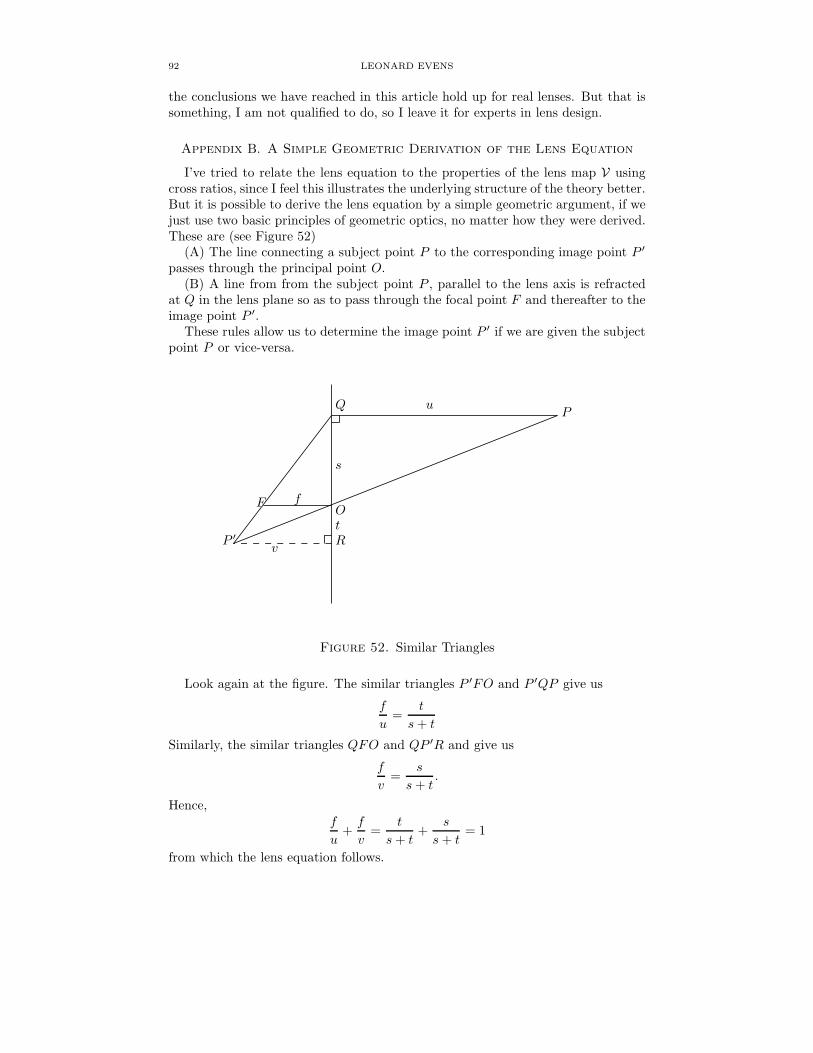
92 LEONARD EVENS
the conclusions we have reached in this article hold up for real lenses. But that issomething, I am not qualified to do, so I leave it for experts in lens design.
Appendix B. A Simple Geometric Derivation of the Lens Equation
I’ve tried to relate the lens equation to the properties of the lens map V usingcross ratios, since I feel this illustrates the underlying structure of the theory better.But it is possible to derive the lens equation by a simple geometric argument, if wejust use two basic principles of geometric optics, no matter how they were derived.These are (see Figure 52)
(A) The line connecting a subject point P to the corresponding image point P ′
passes through the principal point O.(B) A line from from the subject point P , parallel to the lens axis is refracted
at Q in the lens plane so as to pass through the focal point F and thereafter to theimage point P ′.
These rules allow us to determine the image point P ′ if we are given the subjectpoint P or vice-versa.
PQ
O
RP ′
F
v
f
u
s
t
Figure 52. Similar Triangles
Look again at the figure. The similar triangles P ′FO and P ′QP give us
f
u=
t
s+ t
Similarly, the similar triangles QFO and QP ′R and give us
f
v=
s
s+ t.
Hence,f
u+f
v=
t
s+ t+
s
s+ t= 1
from which the lens equation follows.

VIEW CAMERA GEOMETRY 93
Appendix C. Mapping the Lens Plane to the Reference Plane
In this section we derive a coordinate description of the projection through P ′
mapping points in the lens plane Λ to points in the reference plane ∆. We usethe coordinate systems and notation introduced in Section 8.3. See, in particularFigure 20.
A projective transformationP from one projective plane to another is determinedby a 3 x 3 matrix
A =
a00 a01 a02
a10 a11 a12
a20 a21 a22
which is unique up to multiplication by a non-zero scalar. The transformation isdescribed using homogeneous coordinates by multiplying by a 3 x 1 column vectorX, representing a point in Λ, on the left by A, to obtain a 3 x 1 column vector x,representing its image in ∆. We choose the notation, so that X0 = 0 and x0 = 0represent the lines at infinity in each plane. In terms of the affine coordinates(X1, X2) in Λ and (x1, x2) in ∆, the transformation is given by linear fractionaltransformations
(LF) x1 =a10 + a11X1 + a12X2
a00 + a01X1 + a)2X2x2 =
a20 + a21X1 + a22X2
a00 + a01X1 + a02X2
To determine the 9 matrix entries aij up to a nonzero multiple, we need 8 relations.These can be provided by finding the images of 4 points, no three of which arecollinear, or any equivalent information.
We first use the fact that all points on the common x1(X1)-axis are fixed. Thefact that (0, 0) is fixed tells us that a10 = a20 = 0. Then, the fact that (1, 0) is fixedtells us that a11 = a00 + a01 and a21 = 0. Thus, P is described by
(X2) x1 =a11X1 + a12X2
a00 + a01X1 + a02X2x2 =
a21X1 + a22X2
a00 + a01X1 + a02X2.
We next consider the point at infinity on the X2-axis. In Figure 53, the lineP ′P∞ is parallel to the X2-axis, so P∞ is the projection of the point at infinity onthat axis in ∆. It is clear that P∞ has coordinates (p1, p2 + p3 cotφ).
Putting this information in Equation (X2) yields
p1 =a12∞
a00 + a02∞=
a12
a00/∞+ a02=a12
a02
and
p2 + p3 cotφ =a20 + a22∞a00 + a02∞
=a22
a02
so a12 = p1a02 and a22 = (p2 + p3 cotφ)a02.Finally using Figure 54, we see that Q∞ = (p1,−p3 cscφ) in Λ maps to the point
at infinity on the x2-axis. Hence,
0 =a11p1 − a12p3 cscφ
a00 + a01p1 − a02p3 cscφ∞ =
a12p1 − a22p3 cscφ
a00 + a01p1 − a02p3 cscφ
so
a11p1 = a12p3 cscφ a00 + a01p1 = a02p3 cscφ
Now put a02 = 1. From the above relations, we see that a12 = p1, a22 = p2 +p3 cscφ,a11p1 = p1p3 cscφ, and a00 +a01p1 = p3 cscφ. Combining the last equation

94 LEONARD EVENS
x3-axis
x2-axis
x1 = X1-axis
X2-axis‖ X2-axis
P ′
P∞
p3
p1
p2
p3 cotφ
φ φ
Figure 53. Finding P∞
x3-axis
x2-axis
x1 = X1-axis
X2-axis
‖ x2-axis
P ′
Q∞
p3
p1
−p3 cscφ
φ
φ
Figure 54. Finding Q∞
with a11 = a00 + a01, yields a01 = 0 and a11 = a00 = p3 cscφ. It follows that P hasthe form
x1 =p3 cscφX1 + p1X2
p3 cscφ+X2x2 =
(p2 + p3 cotφ)X2
p3 cscφ+X2.
If we multiply through both numerator and denominator by sinφ in each equation,we get
x1 =p3X1 + p1 sinφX2
p3 + sinφX2x2 =
(p2 sinφ+ p3 cosφ)X2
p3 + sinφX2.
If we now put X1 = R cos θ and X2 = R sin θ, we get the parametric representa-tion described in Section 8.3.

VIEW CAMERA GEOMETRY 95
Appendix D. Approximations
In this section we analyze in greater detail the approximations we have used.We shall consider the case for the 4 x 5 inch format, but the results generally holdmore generally since most things tend to scale appropriately with the format size.For example, for 8 x 10 inch format, the dimensions of the camera would be abouttwice as large as would be the acceptable diameter of the circle of confusion andfocal lengths of lenses.64
D.1. How close can the projection point P ′ be to the reference plane?
We now look at estimates for ǫ =f sinφ
2Np3. It depends on p3, which is the distance of
the projection point P ′ to the reference This will clearly occur on the inner surface
defined in equations (SF), by v′′ =v
1 + κNc/ffor rays such that κ = 1, so we may
take p3 = v′′ =v
1 +Nc/f, which in turn depends on v the distance of the image
plane to the reference plane. Look at Figure 55. As in equation (GLE), we have
1
v+
1
J/m=
cosφ
f
so using J =f
sinφ, we obtain
1
v=
cosφ−m sinφ
f
64Not everything simply scales up. For example, if you double both the focal length and the
CoC in the formulaf2
2Nc, you end up doubling the hyperfocal distance, which means roughly
that you halve the depth of field. Similarly, for the same subject distance, magnification M willdiffer according to format, even if one compensates by modifying the degree of enlargement of theresulting image.
φ
O
Π ∆ Λ
v
J
u =J
mΣ
Figure 55. Estimating v from the Slope m of the Subject Plane

96 LEONARD EVENS
so
(Lv) v =f
cosφ−m sinφ.
Note that m can be negative, which means that the subject plane slopes down-ward, away from the lens. (It means that u is negative, and the line of sightintersects the subject plane behind the lens in the image space. But the algebrastill gives the right answer for v.) That situation might arise, for example, if onewere on a hill and wanted the subject plane to follow the downhill slope. But insuch a case, it is rather unlikely that angle would exceed 45 degrees. So it is safeto posit that m ≥ −1. Under that assumption, we get
v ≥ f
cosφ+ sinφ=
f secφ
1 + tanφ.
and
p3 = v′′ ≥ f secφ
(1 + tanφ)(1 + Ncf
)
Putting this in the formula for ǫ, we obtain
ǫ ≤ sinφ cosφ
2N(1 + tanφ)(1 +
Nc
f)
or
ǫ ≤ sin(2φ)(1 + tanφ)
4
( 1
N+c
f
)
.(E1)
A reasonable upper bound for φ as noted before is about 0.25 radians. A typicalvalue for the acceptable circle of confusion in 4 x 5 photography is c = 0.1, anda typical lower bound for the f-number encountered in practice might be N = 8.Finally, while in 4 x 5 inch photography, one might occasionally encounter a focallength of 50 mm or less, a reasonable lower bound is f = 65 mm. Those values giveǫ ≤ 0.01904, which represents an error of about 2 percent. Even taking extremevalues such as φ = 0.5 radians (about 29 degrees), N = 5.6, and f = 50 mm, onlyincreases the bound to 0.059. A more typical scene might have φ = 0.15 radians(about 8.6 degrees), N = 22, and f = 135 mm. Those values decrease the upperbound to 0.004.
It should be noted however that there are other limitations which may place asignificantly smaller lower bound on ǫ. Limits on rise. fall, and shift may force therear standard further back to prevent too much of the region between v′ and v′′
overlapping the optically prohibited zone between the lens plane and the rear focalplane. (No such point can be an image of a real subject point.)
Another factor is the fact that every lens has a limited coverage. That meansthat there is right circular cone centered on the principal point O with axis the lensaxis, outside of which lens aberrations preclude any possibility of sharp images.Even if the camera allows for sufficiently large movements, one would avoid placingthe frame so that it extends outside this cone, and that will further limit how closeP ′ can be to the reference plane.
As a result, in practice we can usually do a lot better than ǫ ≤ 0.02. The caseswhere this might not be the case are lenses with very wide coverage, unusuallylarge rises, falls, or shifts, scenes where the subject plane is strongly tilted, orscenes requiring, for some reason, very large tilt angles.

VIEW CAMERA GEOMETRY 97
D.2. Estimating κ. To get a more precise estimate of κ, we find the semi-majoraxis of the limiting reference ellipse by optimizing x2
1 + x22 as a function of θ. We
start by deriving a convenient expression for r2 = x21+x2
2, the square of the distancefrom O to a point on the reference ellipse. Using Equations (L1) and (L2) in Section8.3, we have
r2 = x21 + x2
2 =1
j33[(j2 cosφ+ j1 sinφ sin θ)2 + (j2 sinφ+ j3 cosφ)2 sin2 θ]
where for convenience we have taken R = 1, i.e., we take the radius of the apertureas the unit of length. (We can put R back in afterwards where necessary.) It turnsout to be more convenient to work with the quantity
j23(r2 − 1) = (j2 cosφ+ j1 sinφ sin θ)2 + (j2 sinφ+ j3 cosφ)2 sin2 θ.
After a couple of pages of algebra and trigonometry, we find this simplifies to
j23(r2 − 1) = sinφ[(1− 2j23) sinφ+ 2j2j3 cosφ] sin2 θ + 2j1j3 sin θ cos θor
r2 − 1 =sinφ
j23
[(1 − 2j23) sinφ+ 2j2j3 cosφ]1− cos 2θ
2+ 2j1j3
sin 2θ
2
Put
A = −[(1− 2j23) sinφ+ 2j2j3 cosφ] = (2j23 − 1) sinφ− 2j2j3 cosφ(DEN)
B = 2j1j3(NUM)
so
(RT) r2 − 1 =sinφ
2j23−A(1− cos 2θ) +B sin 2θ
Differentiating with respect to θ, and setting the derivative to zero yields
−A sin 2θ +B cos 2θ = 0
or
tan 2θ =B
A=
2j1j3(1 − 2j23) sinφ− 2j2j3 cosφ
(TAN)
This condition determines the values of θ for which the maximum and minimumvalues of r2 − 1 occur, but the reader should keep in mind that we may replace thenumerator and denominator by their negatives, since that leaves tan 2θ unchanged.The maximum, the semi-major axis, occurs where r2 − 1 > 0 and the minimum,the semi-minor axis, where r2 − 1 < 0.
Using some simple trigonometry, we get
S = sin 2θ = ±BH
(SIN)
C = cos 2θ = ±AH
(COS)
where
H =√
B2 +A2(HYP)
where, we must choose the ± consistently in both equations, as noted above. Letus choose the + signs. If, as we shall see, r2 − 1 ends up positive, we made the

98 LEONARD EVENS
right choice. Putting these values back in the formula RT, we obtain the followingformula for a, the semi-major axis.
a2 − 1 =sinφ
2j23
−A(1 − A
H) +
B2
H
=sinφ
2j23H−AH +A2 +B2
=sinφ
2j23H−AH +H2
a2 − 1 =sinφ
2j23(H −A)(MAX)
Since H − A ≥ 0, we made the correct choice. Finally, we get for the semi-majoraxis a
a =
√
1 +(H −A) sinφ
2j23(SMA)
κ =1
a=
1
a=
1√
1 + (H−A) sin φ
2j2
3
(KE)
In general, we must multiply the expression in (SMA) by R, the radius of theaperture, but since we would also have to put R in the numerator of the expressionin (KE), we would get the same result in for κ.
O
A′A
M ′M ‖ A′A
B
M ′M
OA = AB = OA′
∠BOA′ = θ′
∠BOA = θ
OM = median, angle bisectorfor vertex O of AOB
OM ′ = median, angle bisectorfor vertex O of A′OB
Figure 56. Consistent Half Angles
Note. There is another more geometric way to derive the expression for a2− 1.Namely, if you set r2 = 1 in (RT), you obtain
0 = −A(1− cos 2θ) +B sin 2θ = −2A sin2 θ + 2B sin θ cos θ
whence
sin θ = 0 or tan θ =B
A
VIEW CAMERA GEOMETRY 99
The first corresponds to the point (±1, 0) (generally (±R, 0)), and the second de-termines which values the parameter θ takes so that the corresponding points onthe ellipse are at the same distance from O. On a non-circular ellipse, there aregenerally four points whose distance from the center has any given value betweenthe semi-minor and semi-major axes, and the major and minor axes bisect the twoangles made by the two chords through O connecting them. That tells us that theangle θ′ in the reference plane that the second chord makes with the x1-axis is twicethat made by the major axis with the x1 axis. In general the relation between theangles θ′ and θ is rather complicated (see Section 8.3, equations (T1) and (T2),and it is not consistent with halving angles. But as Figure 56 indicates, it is in thiscase.
It should be noted further that the above calculations still leave some ambiguityabout the positions of the major and minor axes. Equation (TAN) restricts usto two possible values of 2θ0 between 0 and 2π, and hence two possible values ofθ0 between 0 and π. Also, θ0 is the parameter value in the lens plane, and theabove calculations provide no guidance about how the corresponding angle θ′0, inthe reference plane, is related to it. Fortunately, we have other means to determinethe orientations of major and minor axes, as explained under item (e) in Section8.3.
We can now derive a simplified expression for F (θ). Let θ = θ0 at the semi-majoraxis. Then A = H cos(2θ0), and B = H sin(2θ0). Hence,
F (θ) =sinφ
2j23[−A+A cos(2θ) +B sin(2θ)]
=sinφ
2j23[−A+H cos(2θ0) cos(2θ)) +H sin(2θ0) sin(2θ)]
F (θ) =sinφ
2j23[−A+H cos(2(θ − θ0))](GT)
which shows clearly how F (θ) varies near the maximum.Having attended to the algebra, we are now ready to make estimates for κ. Note
that, were we to write out A,B, and H =√A2 +B2, in equation (KE), we would
obtain a rather complex expression for κ in terms of j = (j1, j2, j3 =√
1− j21 − j22)and φ. But, set up in this way, it is fairly simple to draw graphs and do calculationsusing a symbolic manipulation program. The graphs in Section 8.3.2 were obtainedusing this formulation with Maple.
In Section 8.3, I asserted
Proposition 5. (a) If 0 < κ0 < 1, then the projection from the sphere |j| = 1 to theimage plane, of the contour curve defined by κ = κ0, is an ellipse, centered at theScheimpflug point (0,−S), (S = v cotφ = (1 +M)J , where the x2-axis intersectsthe Scheimpflug line. Its semi-major axis and semi-minor axes are given by
(Mn) d2 = Ssecφ
κ0d1 = d2
√
1− κ20
In particular, the ellipse crosses the positive x2-axis at
S(secφ− κ0
κ0
)
.
(b) If κ0 = 1, the projection is the line segment on the x2-axis from −S(secφ+1)to S(secφ− 1)

100 LEONARD EVENS
(c) For κ0 fixed, the set of all such contour ellipses forms an elliptical conecentered on the line through O in the lens plane with the plane perpendicular to thex1-axis (the tilt axis).
Proof. 65 (a) κ = κ0 where 0 < κ0 ≤ 1 yields
a2 − 1 =sinφ
2j23(H −A) =
1
κ20
− 1 =1− κ2
0
κ20
= K(C0)
H = A+2K
sinφj23 = A+Kj23
B2 +A2 = H2 = A2 + 2Kj23A+K2j43
B2 = 2Kj23A+K2j43(C1)
But, B2 = (2j1j3)2 = 4j21j
23 , so equation (C1) has a common factor of j23 , which we
may assume is non-zero, so we get
4j21 = 2KA+K2j23
4j21 = 2K[(2j23 − 1) sinφ− 2j2j3 cosφ] +K2j23(C2)
If we put j1 =x1
p, j2 =
x2
p, j3 =
v
p, where p2 = x2
1 + x22 + v2, we obtain
2j23 − 1 =2v2 − p2
p2=v2 − x2
1 − x22
p2
Putting all this in (C2), we obtain
4x2
1
p2= 2K
(v2 − x21 − x2
2
p2sinφ− 2
x2v
p2cosφ
)
+K2 v2
p2
4x21 = 2K[(v2 − x2
1 − x22) sinφ− 2x2v cosφ] +K
2v2
(4 + 2K sinφ)x21 + 2K sinφ(x2
2 + 2v cotφx2) = (4K sin2 φ+ 4K2)v2(C3)
But v cotφ = S, 2K = 4K
sin2 φ, 2K sinφ = 4K, and K
2=
4K2
sin2 φ, so
(1 +K)x21 +K(x2
2 + 2Sx2) =(
K +K2
sin2 φ
)
S2 tan2 φ
(1 +K)x21 +K(x2 + S)2 = (K tan2 φ+K2 sec2 φ)S2 +KS2
(1 +K)x21 +K(x2 + S)2 = K(1 +K) sec2 φS2(C4)
This is an ellipse with center at (0,−S) provided K 6= 0, κ0 6= 1. In that case, wealso have
(d1
d2
)2
=K
1 +K= 1− κ2
0 and
d22 =
K(1 +K) sec2 φS2
K= (1 +K) sec2 φS2 =
S2 sec2 φ
κ20
as claimed.
65It is not too hard to see that the points on rays satisfying κ = κ0 satisfy a quadratic equation,so since all those rays pass through O, they form a degenerate quadric, in fact, a cone. But Idon’t see an obvious way to derive the additional facts about its axis and shape. So, the onlyalternative is brute force calculation.

VIEW CAMERA GEOMETRY 101
(b) If K = 0, all equation (C4) tell us is that x1 = 0. But if we go back to
equation (C0), we see that K = 0 implies that H =√A2 +B2 = A, which can
only happen if B = 0 and A ≥ 0. But B = 2j1j3 = 0 tells us that j1 = 0, so x1 = 0.Expressing the second condition in terms of x2 and v yields
(v2 − x22) sinφ− 2x2v cosφ ≥ 0.
Since this is a continuous function of x2 and since it is positive for x2 = 0, we needonly find where it vanishes. But that reduces to the quadratic equation
x22 + 2x2v cotφ− v2 = x2
2 + 2x2S − S2 tan2 φ = 0.
Solving this gives to the two limits −S(1 + secφ) and S(−1 + secφ).Remark. It is worth pointing out that if we put x2 = v sinψ, where ψ is the
angle the ray makes with the x3-axis, then this amounts to saying that ψ ranges
from −π2
+φ
2at the lower end to
φ
2at the upper end.
(c) This is clear from the formulas since S = v cotφ is proportional to v, and allthe Scheimpflug points lie on the indicated line.
It remains to place some limits on how skew the ray j can be, which will setplausible lower bounds for κ0. This is dependent on the maximum possible shift Eof a point in the image plane from its intersection with the x3-axis. This will besubject—as in D.1—to reasonable assumptions about the structure of the cameraand likely scenes.
Forbidden Zone
FrameP
OO′ O′
Π ∆
Λ
Cohinge Line
E
α
v
x1
x′1
x2 x′2
S
Figure 57. Possible Shifts
See Figure 57. The diagram on the left shows the rectangular region withinwhich the frame may be moved, as it would appear from the vantage point of thelens. (The directions of the x1 and x2- axes are chosen consistently with what wedid earlier in the image space.)66 The forbidden zone is outlined in red, and the
66If the standard starts out with sides vertical and horizontal, and the rotation of the standardis closer to being a tilt, then the x1-axis is more horizontal. On the other hand, if the rotation iscloser to being a swing, then the x1-axis is more vertical.
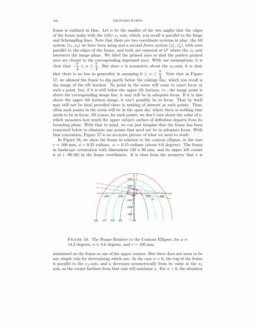
102 LEONARD EVENS
frame is outlined in blue. Let α be the smaller of the two angles that the edgesof the frame make with the (tilt) x1 axis, which, you recall is parallel to the hingeand Scheimpflug lines. Note that there are two coordinate systems in play: the tiltsystem (x1, x2) we have been using and a second frame system (x′1, x
′2), with axes
parallel to the edges of the frame, and both are centered at O′ where the x3 axisintersects the image plane. We label the primed axes so that the positve primedaxes are closest to the corresponding unprimed axes. With our assumptions, it is
clear that −π4≤ α ≤ π
4. But since κ is symmetric about the x2-axis, it is clear
that there is no loss in generality in assuming 0 ≤ α ≤ π
4. Note that in Figure
57, we allowed the frame to dip partly below the cohinge line, which you recall isthe image of the tilt horizon. No point in the scene will come to exact focus atsuch a point, but, if it is still below the upper tilt horizon, i.e., the image point isabove the corresponding image line, it may still be in adequate focus. If it is alsoabove the upper tilt horizon image, it can’t possibly be in focus. That by itselfmay still not be fatal provided there is nothing of interest at such points. Thus,often such points in the scene will be in the open sky, where there is nothing thatneeds to be in focus. Of course, for such points, we don’t care about the value of κ,which measures how much the upper subject surface of definition departs from itsbounding plane. With that in mind, we can just imagine that the frame has beentruncated below to eliminate any points that need not be in adequate focus. Withthat convention, Figure 57 is an accurate picture of what we need to study.
In Figure 58, we show the frame in relation to the contour ellipses, in the casev = 100 mm, φ = 0.25 radians. α = 0.15 radians (about 8.6 degrees). The framein landscape orientation with dimensions 120 x 96 mm, and its upper left corneris at (−90, 60) in the frame coordinates. It is clear from the geometry that κ is
1.00.7 0.80.6 0.9
x1K400 K200 0 200 400
K300
K200
K100
100
200
Figure 58. The Frame Relative to the Contour Ellipses, for φ ≈14.3 degrees, α ≈ 8.6 degrees, and v = 100 mm.
minimized on the frame at one of the upper corners. But there does not seem to beany simple rule for determining which one. In the case α = 0, the top of the frameis parallel to the x1-axis, and κ decreases symmetrically from its value at the x2
axis, so the corner furthest from that axis will minimize κ. For α > 0, the situation
VIEW CAMERA GEOMETRY 103
appears to be more complicated. I have not been able to solve the analytic problemcompletely, but Maple examples provide some insight.
Let (E1, E2) be its coordinates with respect to the frame (primed) system of anupper corner P of the frame as in Figure 57. The values of E1 and E2 dependon the dimensions of the frame and how it has been oriented. Those values willbe limited by possible shifts of the standards. In the diagram E2 ≤ E1, but thatdepends on the orientation of the frame—portrait or landscape—, and the reversecould be true. P has coordinates (p1, p2) with respect to the tilt (unprimed) systemwhere
p1 = E1 cosα− E2 sinα
p2 = E1 sinα+ E2 cosα
The coordinates of P in the (x1, x2, x3) coordinate system will be (p1, p2, v), andthe ray OP will be determined (as in the proof of Proposition 5) by
j1 =p1
p, j2 =
p2
p, and j3 =
v
p(JE)
where
p =√
p21 + p2
2 + v2 =√
E2 + v2, E2 = E21 + E2
2
Look at the dashed line in Figure 58 determined by the top of the frame. It isnot hard to see that its equation is x2 = E2 secα − x1 tanα, and we may graph κalong that line. See Figure 59. The graph rises to a maximum, which appears tobe at x1 = E2 tanα, or close by, but I see no reason why that should be the case.It falls off close to linearly for much of the domain on either side of the maximum,but the fall-off on the left appears to be steeper than that on the right. Maple plotswith different values of the parameters produce similar results. So it does appearthat the corner to the left, i.e., that opposite the x2-axis from the x′1 axis, will yieldthe smaller value of κ. So the conclusion from the graphical data seems to be thefollowing. Look at all potential positions of the frame allowed by the structure of thecamera, and consider the two furthest from the Scehimpflug point. Choose the oneopposite the central axis from the line perpendicular to the tilt axis, and calculateκ0 there. That is the worst possible case for the camera. Conversely, given whatyou consider an acceptable value of κ0, for any given E2 and alpha, find the twopoints where the line x2 = E1 secα− x1 tanα intersects that contour ellipse. If theseparation between those points is large enough to accommodate the frame, the twopoints define the limits of shift to either side which are consistent with that valueof κ0. Otherwise, choose a smaller κ0 and redo the calculation.
We shall now derive another expression for κ which will allow us to see howsensitive it is to the position of the frame. We start with the equation of a typicalcontour ellipse as given in Proposition 5
x21
d21
+(x2 + S)2
d22
= 1
κ2x21
(1− κ2)S2 sec2 φ+κ2(x2 + S)2
S2 sec2 φ= 1
Note that we dropped the subscript from κ. Read this way, these equations can beread as a relation between κ, x1, and x2 for fixed φ and S. If κ is fixed, we get theappropriate contour ellipse. But if we specify (x1, x2) as, for example, at a corner

104 LEONARD EVENS
x1K300 K200 K100 0 100 200 300
0.60
0.65
0.70
0.75
0.80
0.85
Figure 59. κ along the line x2 = E2 secα − x1 tanα, E2 = 60mm, α = 8.6 degrees, and for v = 100 mm and φ = 14.3 degrees.
of the frame, then the equation may be used to find κ in terms of it. Continuing,we get
κ2 x21
S2+ κ2(1− κ2)
(x2 + S)2
S2= (1− κ2) sec2 φ
κ4 (x2 + S)2
S2− κ2
(x21 + (x2 + S)2
S2+ sec2 φ
)
+ sec2 φ = 0
(BQ) κ4 s22
S2− κ2
( s2
S2+ sec2 φ
)
+ sec2 φ = 0
where s2 = x2 + S is the distance of the Scheimpflug point (0,−S) to (0, x2),
and s =√
x21 + s22 is its distance of the point (x1, x2). Put x1 =
x1
S, x2 =
x2
S,
s2 =s2S
= (1 + x2) and s =s
S=
√
x21 + (1 + x2)2. Note that s2 and s are close to
1 provided x1 and x2 are small relative to S. By the quadratic equation formula,
(QSa) κ2 =s2 + sec2 φ±
√
(s2 + sec2 φ)2 − 4s22 sec2 φ
2s22But, by Schwartz’s Inequality
s2 + sec2 φ ≥ 2s secφ ≥ 2s2 secφ > 2s2
which implies first that the quantity under the square root is positive, and secon-darily that the first term in the numerator divided by the denominator is greaterthan 1. Were we to add anything to it, we would get something larger than one,which is not possible since κ2 ≤ 1. Hence, the correct formula is
κ2 =s2 + sec2 φ−
√
(s2 + sec2 φ)2 − 4s22 sec2 φ
2s22
=s2 + sec2 φ−
√
(s2 − sec2 φ)2 + 4(s2 − s22) sec2 φ
2s22
so finally67
(Qκ) κ =
√
x21 + (1 + x2)2 + sec2 φ−
√
(x21 + (1 + x2)2 − sec2 φ)2 + 4x2
1 sec2 φ
2(1 + x2)2
67There is a problem for s2 = 0 in which case the expression becomes indeterminate. We caneither apply L’Hospital’s Rule or just solve equation (BQ), which becomes linear for s2 = 0.

VIEW CAMERA GEOMETRY 105
This expression allows us to see how κ, behaves as a function of the parameters.It is not obvious from the formulas, but, for fixed φ, it is a decreasing function ofthe x1, and x2 when both are small compared to 1. This is clear from Maple plotssuch as the one in Figure 60.68 It is also increasing as a function of φ, if the other
0.00.05
0.81
0.2
0.86
y2
0.10.15
0.91
0.96
y1
0.1 0.150.05 0.20.0
Figure 60. κ as a function of y1 = x1, y2 = x2 for φ = 0.15 radians
two variables are fixed. But recall that φ is essentially pre-determined by the scene,
since sinφ =f
J. f is determined by the desired field of view and what is available
to the photographer, and J is determined by the position of the desired subjectplane. Thus, φ may vary as the photographer composes the scene, but within avery narrow range.69
To proceed further we must make some estimates of the parameters.We start by considering S = J(1 +M), which is approximately J as long as M
is small. It is not much smaller than J , in any event, unless the subject plane tiltsstrongly away from the reference normal, which is rather unlikely. A reasonablelower bound for J would be 1 meter = 1,000 mm.70 For example, for a pure tiltdownward, the camera is at eye level, which can range from about 1.5 to 1.75meters, depending on the height of the photographer, and how far he or she bendsover. The subject plane usually passes well below the lens, even below the ground,so the 1 meter bound is plausible. In cases of pure swing, or even skew tilt axis,the language would be different, but the conclusions would be similar.
Consider next the tilt angle φ. We have been taking φ = 0.25 radians, but thisis a trifle extreme, so let’s assume φ is at most 0.15 radians (about 8.6 degreesinstead. Then 1 < secφ < 1.012, and is essentially fixed by the scene.
Finally, let’s assume that x1, x2 ≤ 100 mm. In the case of a pure tilt, thatwould mean the frame might be largely above the horizon image, even when inportrait mode, and possible well off to one side. Similarly for a pure swing, with
68I’ve also checked it by finding the partial derivatives with respect to x = x2
1, , y = (1 + x2)2,
and z = sec2 φ which are monotonic in the corresponding parameters. But the algebra is a bitmessy and need not be included here given the availability of plots.
69Note also that for fixed f , changing φ entails changing J and S, and so also x1 and x2, sothe actual dependence on φ might be fairly complex. Fortunately we need not worry about that,because, as noted above, φ is essentially constant.
70The most important exception to this would be close-up or table-top photography, which welargely ignore here.

106 LEONARD EVENS
an appropriate change of language. In the extreme case where the tilt axis makesa 45 degree angle with the edges of the frame, this would still place a corner of theframe two thirds of its diameter (≈ 150 mm) above the horizon image, and far offto one side, which would be a highly unlikely situation, to say the least.
Since the right hand side of (Qκ) is decreasing, we can determine a lower bound
by evaluating it for x1 = x2 =100
1000= 0.1. We get κ2 > 0.81 from which we
conclude that κ > 0.9, and, to compensate, that would require a correction of atmost three tenths of a stop, which should be acceptable. Also, the positions of theframes described above are unusual, and, in any event, the worst estimates wouldoccur only in one or two corners. For most of the frame κ would be closer to 1.Note also that even in extremely unlikely scenarios the correction is likely to be atworst something like three quarters of a stop.
D.3. How Displacement from the Limiting Ellipse Changes Things. Thecalculations in the previous sections are based on using the limiting reference ellipsedefined by x = (x1, x2) where, as in Section 8.3 with R = 1,
x1 =j3 cos θ + j1 sinφ sin θ
j3(L1)
x2 =(j2 sinφ+ j3 cosφ) sin θ
j3(L2)
But, as we saw previously, the actual reference ellipse is given by
x = x1
1 + ǫ sin θ
which is perturbed from the limiting ellipse, for each value of θ, by the indicated
factor. We also saw that the center of the perturbed ellipse was at k = −qǫ
1− ǫ2where q = x(π/2) = (q1, q2) and
q1 =j1 sinφ
j3(Q1)
q2 −j2 sinφ+ j3 cosφ
j3(Q2)
So, for the displacement from the center of the perturbed ellipse, we have
y = x− k i.e.,
y =x
1 + ǫ sin θ+
ǫq
1− ǫ2(PEa)
There are two triangle inequalities. The more familiar asserts that the third sideof a triangle is less than or equal to the sum of the other two sides, but it is alsotrue that the third side is greater than or equal to the larger of the two other sidesless the smaller. These yield
|y| ≤ |x|1 + ǫ sin θ
+ǫ|q|
1− ǫ2(TEa)
|y| ≥ |x|1 + ǫ sin θ
− ǫ|q|1− ǫ2(TEb)
Our analysis will depend primarily on inequality (TEa), but first we must digressand use inequality (TEb). Since x ≥ |q|, and sin θ ≤ 1, if we ignore terms of order

VIEW CAMERA GEOMETRY 107
ǫ2 and higher71, we see that a good estimate for the lower bound on |y| is |x|(1−2ǫ).For the moment we shall draw just one conclusion from this estimate, namely, that
(F) |y| attains a maximum for 0 ≤ θ ≤ πIndeed, if both maximum values of |y| occurred for π < θ < 2π, since 1 − 2ǫ > 0,the same would have to be true for |x|, which is obviously false.
We now investigate how equation (PEa) affects the conclusions drawn previouslyabout Problem (1) where we used the limiting reference ellipse. We reasoned thatCoCs for points along the same ray through O in the outer and inner planes wouldmatch provided the focus was set at the harmonic mean. Thus, we have two valuesof ǫ to consider
ǫ′ =f sinφ
2Nv′and ǫ′′ =
f sinφ
2Nv′′
where v′ and v′′ are respectively the distances of the outer and inner image planesfrom the reference plane. (Note that v′ > v′′.) Let y′ and y′′ be the correspondingquantities for the two perturbed ellipses.72 From (PEa) we have
|y′ − y′′| = |x|∣
∣
∣
1
1 + ǫ′ sin θ)− 1
1 + ǫ′′ sin θ
∣
∣
∣
= |x|( (ǫ′′ − ǫ′) sin θ
1 + (ǫ′ + ǫ′′) sin θ + ǫ′ǫ′′ sin2 θ
)
≤ |x||(ǫ′′ − ǫ′) sin θ| ≤ |x||ǫ′′ − ǫ′|since by (F), we may assume without loss of generality that sin θ ≥ 0.
But
|ǫ′′ − ǫ′| = f sinφ
2N
∣
∣
∣
1
v′′− 1
v′
∣
∣
∣
=f sinφ
2N
|v′ − v′′|v′v′′
=f sinφ
Nv
|v′ − v′′|v′ + v′′
so
|y′ − y′′| ≤ 2ǫ|v′ − v′′|v′ + v′′
|x|(PEc)
where ǫ =f sinφ
2Nvis the value of ǫ for the harmonic mean v of v′ and v′′.
The quantity v′− v′′ is what we previously called the focus spread, and we usedit to derive estimates for the f-number needed to produce the desired depth of field.A rough estimate for the focus spread is 2Nc. Lenses used in 4 x 5 photographyseldom can be stopped down beyond f/64, and such a small aperture would raisediffraction issues, even for a perfect lens. Taking c = 0.1 mm, and N = 45 yields afocus spread of 9 mm. So let’s assume the focus spread is not larger than 10 mm.If the inner image distance is approximately the focal length, and we assume thelatter is larger than 50 mm, that means the outer image distance is larger than 60
71We saw earlier that ǫ < 0.02, so ǫ2 < 0.0004. If we incorporated those terms the effect wouldclearly be negligible. The skeptical reader can test this contention by working it all out, but weshall avoid such unnecessary complications here.
72This notation may conflict with the usual notation y′ =dy
dθ, but the context should make
it clear which is intended.

108 LEONARD EVENS
mm, and hencev′ − v′′v′ + v′′
<10
60= 1/6. It follows that a reasonable approximation for
the upper bound for |y′ − y′′| is ǫ|x|3
. If we take 0.02 as the upper bound for ǫ, we
see that the failure to match is less than 0.67 percent. Usually, it would be muchless than that. So, if we place the image plane at the harmonic mean, we wouldbe making a slight error, but it would be so small that it would be undetectable innormal practice.
Next, we address the effect of the perturbation on our estimate of κ, as neededin analysis of Problem (2). From inequality (TEa), and using q| ≤ |x| as well assin θ ≥ 0, we obtain
|y| ≤ |x|(
1 +2ǫ
1− ǫ2)
So, if aǫ is the semi-major axis of the perturbed ellipse, and κǫ its reciprocal, wehave
aǫ ≤ a(1− ǫ2 + 2ǫ
1− ǫ2)
and
κǫ ≥ κ1− ǫ2
1 + 2ǫ− ǫ2 ≈ κ(1− 2ǫ)
where in the last estimate we ignore terms of order ǫ2 or smaller. Taking 0.02 asthe upper bound for ǫ suggests that a reasonable estimate for a lower bound for κǫ
is 0.94 κ. Interpreted as a necessary change in the f-number to compensate, thatwould amount to about 0.12 stops. It would typically be considerably less.
So the general conclusion is that using the limiting ellipse instead of the actualperturbed ellipse whatever the problem under consideration, has such a small effect,that in practice it would be virtually undetectable. In particular, given the otherapproximations inherent in the use of geometric optics, errors in focusing, and thedifficulty in setting the standards or the f-number exactly as we want them, it isnot usually worth worrying about.
Final Note A much more difficult problem is determining where the semi-majoraxis of the perturbed ellipse is in comparison with that of the limiting ellipse. You
do this by relating the quantity y· dydθ
to the corresponding dot product for x, which
we can calculate from the formula we derived previously for x ·x. It turns out thatthe θ displacement, while small, may be considerably larger than the quantities weconsidered above. Fortunately, it doesn’t matter in the analysis.
Appendix E. Exact Calculation for the Upper Surface of Definition
Refer to Figure 33 in Section 8.4.1. The problem is to determine the coordinates
of the point P′on the upper surfaces of definition in the subject space in terms of
the corresponding point Q′on outer surface of definition in the image space. The
latter is given, as usual, by v′ =v
1−Ncκ/f where κ = κ(j, φ). The approach is to
use the lens equation1
s+
1
t=
cos ζ
fwhere s and t represent the respective distances
of Q′and P
′along the ray determined by j and ζ is the angle that the ray makes
with the lens plane. It is a little tricky using this formula. We take the vector j

VIEW CAMERA GEOMETRY 109
pointing into the image space, and what we get for t tells us the distance, againin the image space to a corresponding point. But then we must take the antipodal
point in the subject space to get P′. It is not hard to determine s and cos ζ from
the known data. I omit the calculations, but the final result I got was that P′is
the point antipodal to tj where
(LE) t =(1 +M)f
(1 +M)j2 sinφ+ (M cosφ+Ncκ(j, φ)/f)j3
I have not rechecked my calculations, so I don’t really vouch for the formula. I rec-ommend that any reader who is interested enough in the result redo the calculationsaccording to the scheme outlined above.
Department of Mathematics, Northwestern University, Evanston, Illinois