Introduction - Mr-CFDdl.mr-cfd.com/tutorials/ansys-fluent/20-hot-gas-cooling...Tutorial: Modeling...
22
Tutorial: Modeling Evaporation of Liquid Droplets in a Circular Channel Introduction The purpose of this tutorial is to simulate cooling of a hot air stream by water injection using species transport and discrete phase models of ANSYS Fluent 14.5. Prerequisites This tutorial is written with the assumption that you have completed Tutorial 1 from the ANSYS Fluent 14.5 Tutorial Guide, and that you are familiar with the ANSYS Fluent navigation pane and menu structure. Some steps in the setup and solution procedure will not be shown explicitly. Problem Description The problem to be considered is shown in the Figure 1. Hot air enters through the inlet of a 3D circular pipe. Water droplets are injected at various axial and radial locations by creating Discrete Phase Model injections. Water undergoes a phase change as it comes in contact with hot air, and the mixture of air and vapor flows downstream. The solution will be performed in two stages: 1. Converge the flow without DPM (no evaporation). 2. Start DPM injection and solve the actual phase change problem. c ANSYS, Inc. December 27, 2012 1
Transcript of Introduction - Mr-CFDdl.mr-cfd.com/tutorials/ansys-fluent/20-hot-gas-cooling...Tutorial: Modeling...
Tutorial: Modeling Evaporation of Liquid Droplets in a
Circular Channel
Introduction
The purpose of this tutorial is to simulate cooling of a hot air stream by water injectionusing species transport and discrete phase models of ANSYS Fluent 14.5.
Prerequisites
This tutorial is written with the assumption that you have completed Tutorial 1 fromthe ANSYS Fluent 14.5 Tutorial Guide, and that you are familiar with the ANSYS Fluentnavigation pane and menu structure. Some steps in the setup and solution procedure willnot be shown explicitly.
Problem Description
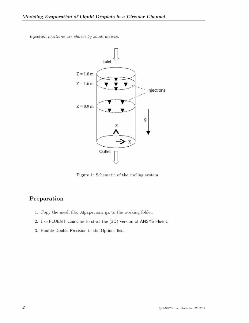
The problem to be considered is shown in the Figure 1. Hot air enters through the inletof a 3D circular pipe. Water droplets are injected at various axial and radial locations bycreating Discrete Phase Model injections. Water undergoes a phase change as it comes incontact with hot air, and the mixture of air and vapor flows downstream.
The solution will be performed in two stages:
1. Converge the flow without DPM (no evaporation).
2. Start DPM injection and solve the actual phase change problem.
c© ANSYS, Inc. December 27, 2012 1
Modeling Evaporation of Liquid Droplets in a Circular Channel
Injection locations are shown by small arrows.
Figure 1: Schematic of the cooling system
Preparation
1. Copy the mesh file, 3dpipe.msh.gz to the working folder.
2. Use FLUENT Launcher to start the (3D) version of ANSYS Fluent.
3. Enable Double-Precision in the Options list.
2 c© ANSYS, Inc. December 27, 2012
Modeling Evaporation of Liquid Droplets in a Circular Channel
Setup and Solution
Step 1: Mesh
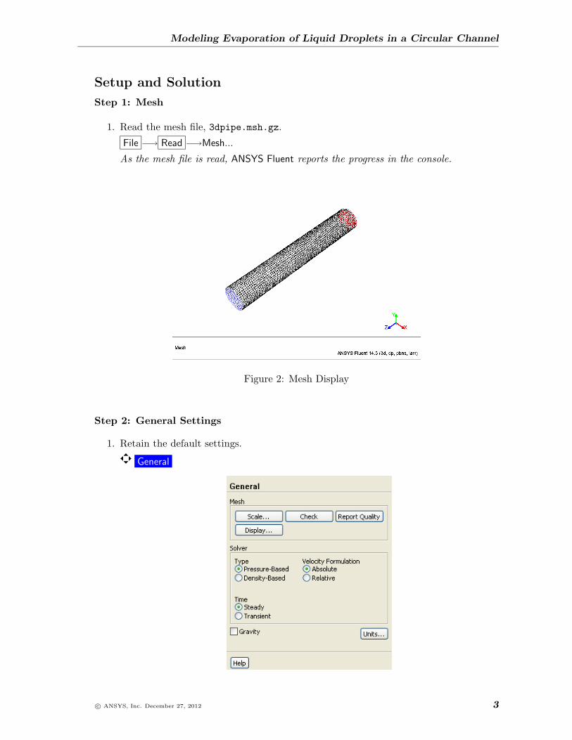
1. Read the mesh file, 3dpipe.msh.gz.
File −→ Read −→Mesh...
As the mesh file is read, ANSYS Fluent reports the progress in the console.
Figure 2: Mesh Display
Step 2: General Settings
1. Retain the default settings.
General
c© ANSYS, Inc. December 27, 2012 3
Modeling Evaporation of Liquid Droplets in a Circular Channel
2. Check the mesh.
General −→ Check
ANSYS Fluent performs various checks on the mesh and reports the progress in theconsole. Pay attention to the minimum volume reported and make sure this is apositive number. Scaling is not required for this case.
Step 3: Models
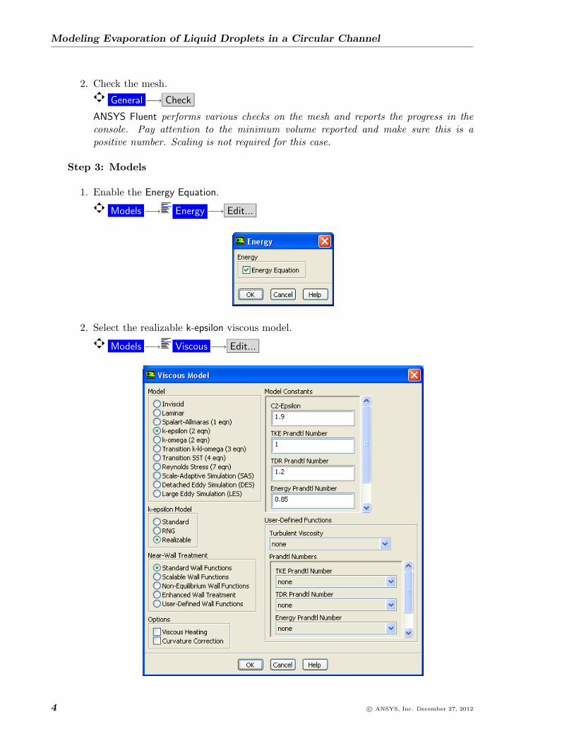
1. Enable the Energy Equation.
Models −→ Energy −→ Edit...
2. Select the realizable k-epsilon viscous model.
Models −→ Viscous −→ Edit...
4 c© ANSYS, Inc. December 27, 2012
Modeling Evaporation of Liquid Droplets in a Circular Channel
(a) Select k-epsilon(2 eqn) from the Model list.
The dialog box will expand after the selection.
(b) Select Realizable from the k-epsilon Model group box.
(c) Retain the default selection of Standard Wall Functions from the Near-Wall Treat-ment group box.
(d) Click OK to close the Viscous Model dialog box.
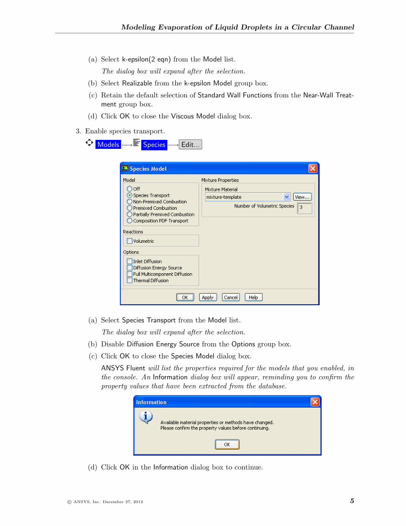
3. Enable species transport.
Models −→ Species −→ Edit...
(a) Select Species Transport from the Model list.
The dialog box will expand after the selection.
(b) Disable Diffusion Energy Source from the Options group box.
(c) Click OK to close the Species Model dialog box.
ANSYS Fluent will list the properties required for the models that you enabled, inthe console. An Information dialog box will appear, reminding you to confirm theproperty values that have been extracted from the database.
(d) Click OK in the Information dialog box to continue.
c© ANSYS, Inc. December 27, 2012 5
Modeling Evaporation of Liquid Droplets in a Circular Channel
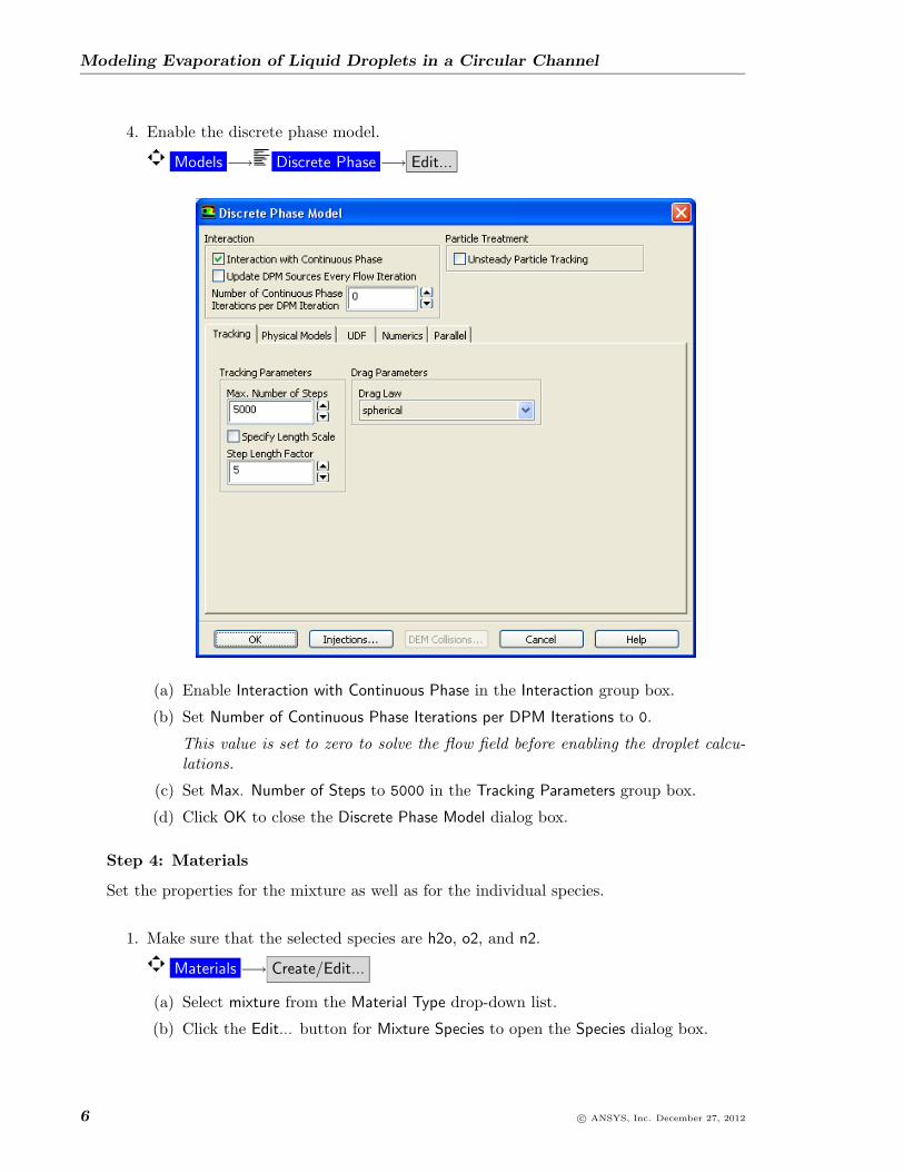
4. Enable the discrete phase model.
Models −→ Discrete Phase −→ Edit...
(a) Enable Interaction with Continuous Phase in the Interaction group box.
(b) Set Number of Continuous Phase Iterations per DPM Iterations to 0.
This value is set to zero to solve the flow field before enabling the droplet calcu-lations.
(c) Set Max. Number of Steps to 5000 in the Tracking Parameters group box.
(d) Click OK to close the Discrete Phase Model dialog box.
Step 4: Materials
Set the properties for the mixture as well as for the individual species.
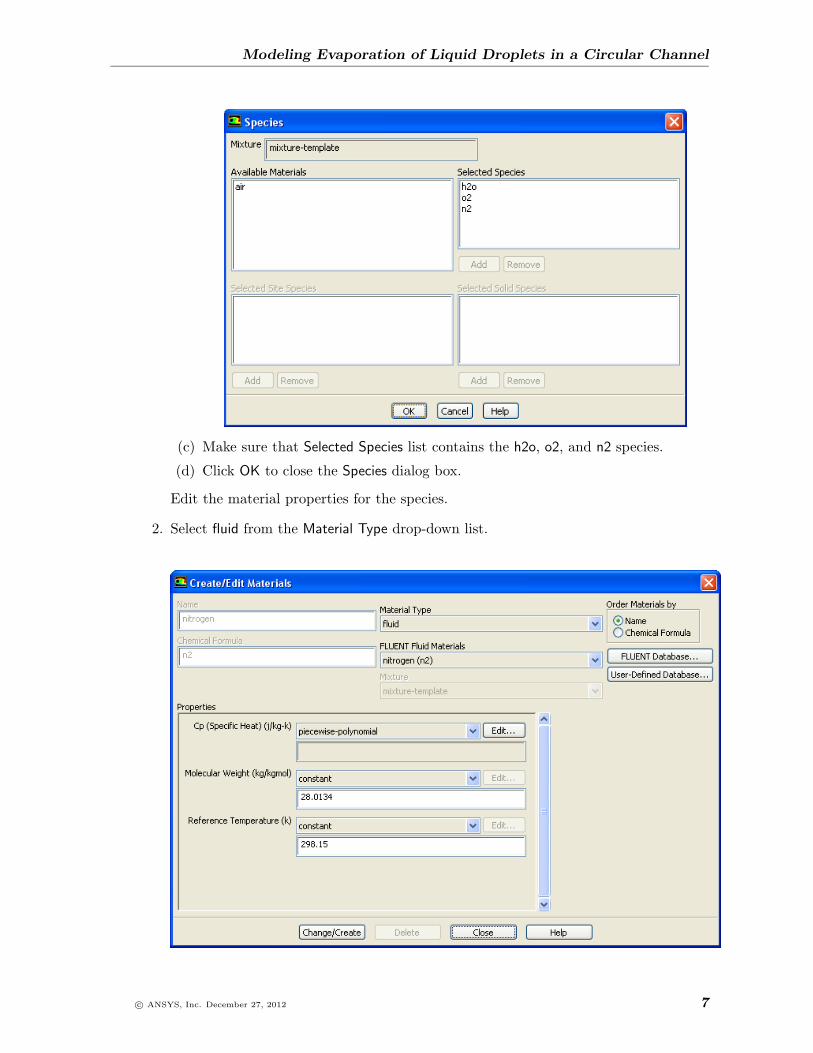
1. Make sure that the selected species are h2o, o2, and n2.
Materials −→ Create/Edit...
(a) Select mixture from the Material Type drop-down list.
(b) Click the Edit... button for Mixture Species to open the Species dialog box.
6 c© ANSYS, Inc. December 27, 2012
Modeling Evaporation of Liquid Droplets in a Circular Channel
(c) Make sure that Selected Species list contains the h2o, o2, and n2 species.
(d) Click OK to close the Species dialog box.
Edit the material properties for the species.
2. Select fluid from the Material Type drop-down list.
c© ANSYS, Inc. December 27, 2012 7
Modeling Evaporation of Liquid Droplets in a Circular Channel
3. Ensure that piecewise-polynomial is selected from the Cp drop-down list for n2, o2, andh2o.
4. Close the Create/Edit Materials dialog box.
Step 5: Boundary Conditions
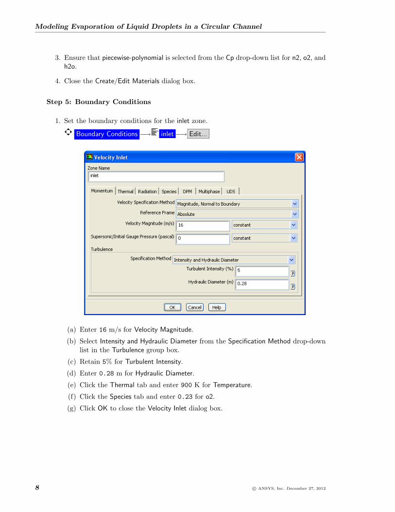
1. Set the boundary conditions for the inlet zone.
Boundary Conditions −→ inlet −→ Edit...
(a) Enter 16 m/s for Velocity Magnitude.
(b) Select Intensity and Hydraulic Diameter from the Specification Method drop-downlist in the Turbulence group box.
(c) Retain 5% for Turbulent Intensity.
(d) Enter 0.28 m for Hydraulic Diameter.
(e) Click the Thermal tab and enter 900 K for Temperature.
(f) Click the Species tab and enter 0.23 for o2.
(g) Click OK to close the Velocity Inlet dialog box.
8 c© ANSYS, Inc. December 27, 2012
Modeling Evaporation of Liquid Droplets in a Circular Channel
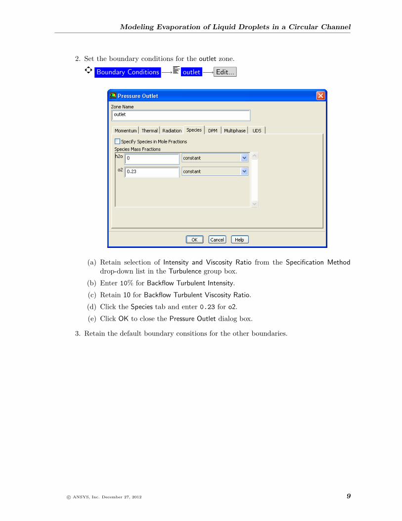
2. Set the boundary conditions for the outlet zone.
Boundary Conditions −→ outlet −→ Edit...
(a) Retain selection of Intensity and Viscosity Ratio from the Specification Methoddrop-down list in the Turbulence group box.
(b) Enter 10% for Backflow Turbulent Intensity.
(c) Retain 10 for Backflow Turbulent Viscosity Ratio.
(d) Click the Species tab and enter 0.23 for o2.
(e) Click OK to close the Pressure Outlet dialog box.
3. Retain the default boundary consitions for the other boundaries.
c© ANSYS, Inc. December 27, 2012 9
Modeling Evaporation of Liquid Droplets in a Circular Channel
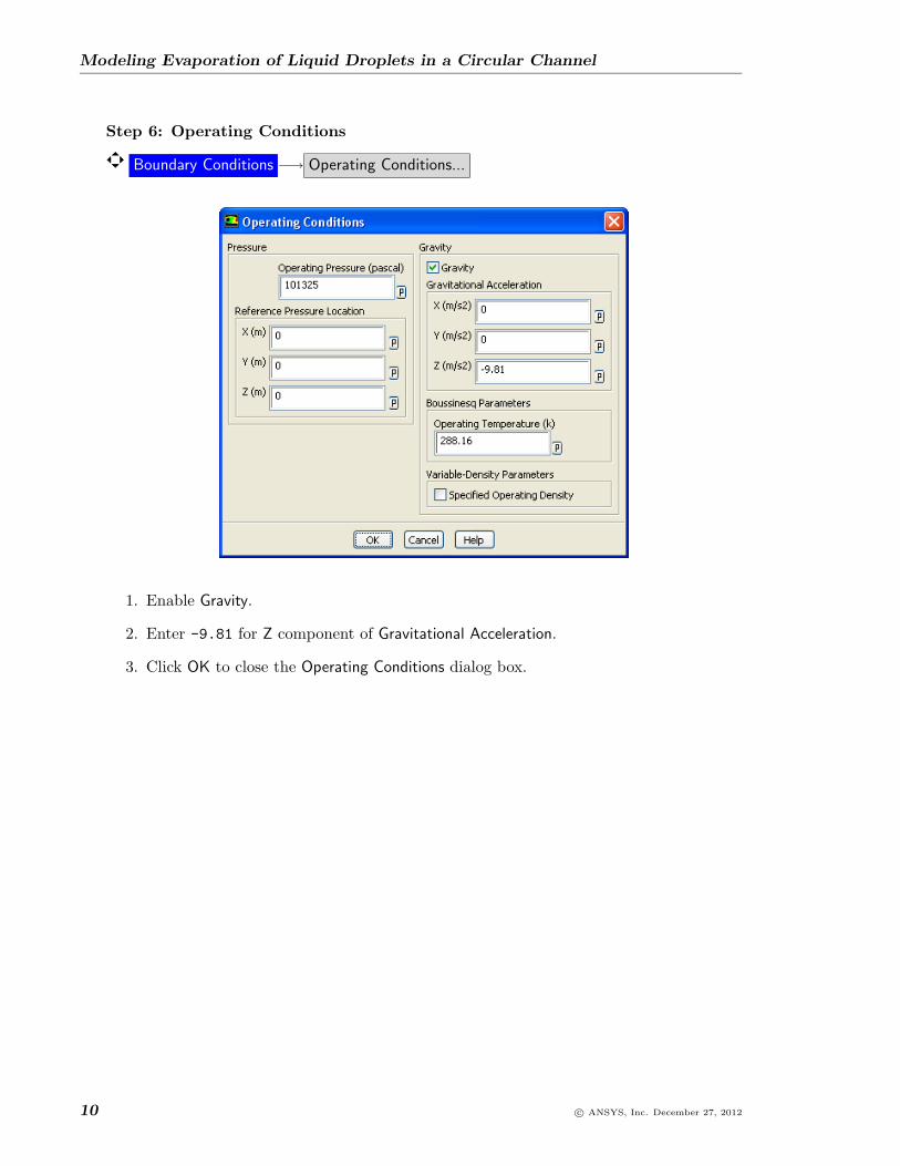
Step 6: Operating Conditions
Boundary Conditions −→ Operating Conditions...
1. Enable Gravity.
2. Enter -9.81 for Z component of Gravitational Acceleration.
3. Click OK to close the Operating Conditions dialog box.
10 c© ANSYS, Inc. December 27, 2012
Modeling Evaporation of Liquid Droplets in a Circular Channel
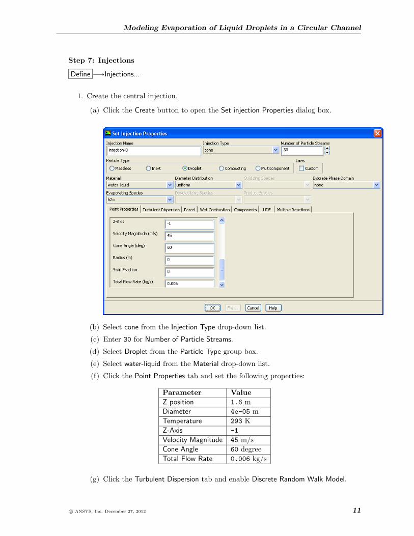
Step 7: Injections
Define −→Injections...
1. Create the central injection.
(a) Click the Create button to open the Set injection Properties dialog box.
(b) Select cone from the Injection Type drop-down list.
(c) Enter 30 for Number of Particle Streams.
(d) Select Droplet from the Particle Type group box.
(e) Select water-liquid from the Material drop-down list.
(f) Click the Point Properties tab and set the following properties:
Parameter ValueZ position 1.6 mDiameter 4e-05 mTemperature 293 KZ-Axis -1Velocity Magnitude 45 m/sCone Angle 60 degreeTotal Flow Rate 0.006 kg/s
(g) Click the Turbulent Dispersion tab and enable Discrete Random Walk Model.
c© ANSYS, Inc. December 27, 2012 11
Modeling Evaporation of Liquid Droplets in a Circular Channel
(h) Enter 40 for Number of Tries.
(i) Click OK to close the Set Injection Properties dialog box.
Click OK in the Information dialog box.
Note: You will create eight more injections at different locations.
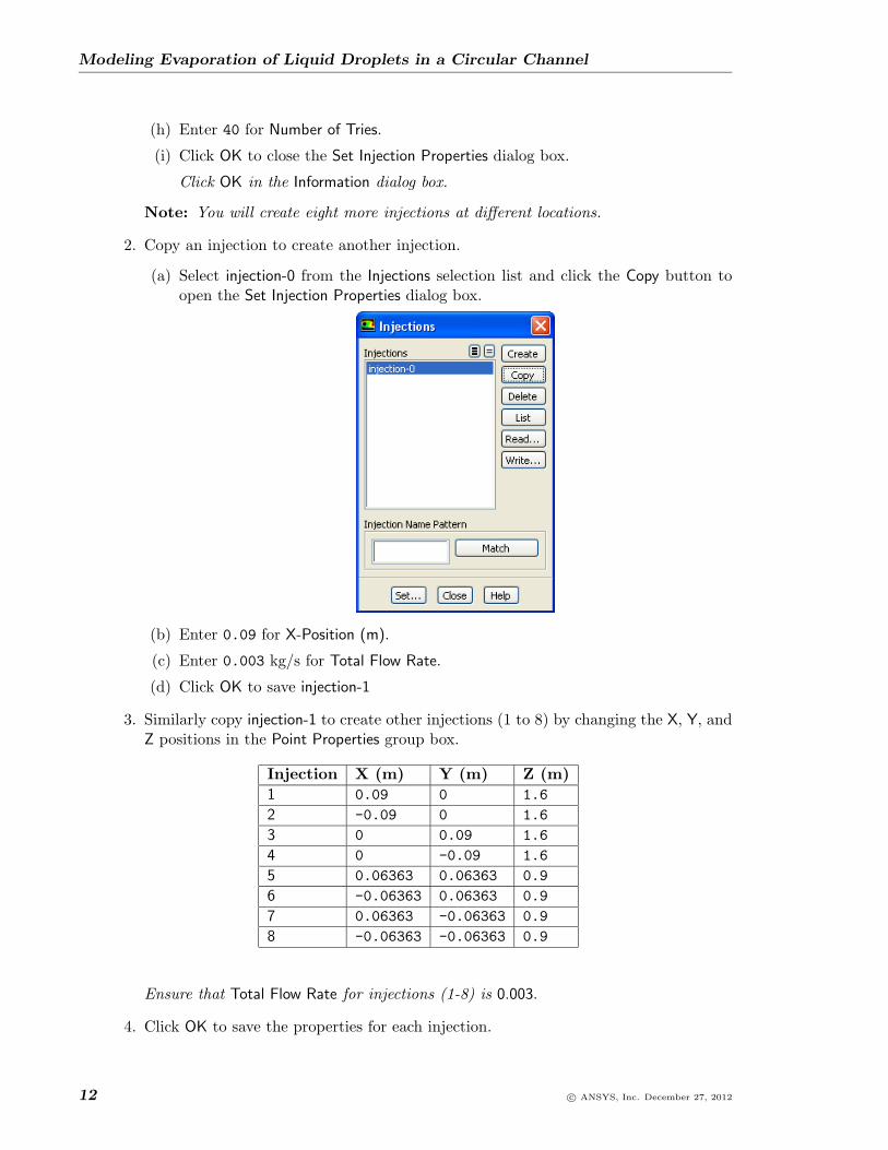
2. Copy an injection to create another injection.
(a) Select injection-0 from the Injections selection list and click the Copy button toopen the Set Injection Properties dialog box.
(b) Enter 0.09 for X-Position (m).
(c) Enter 0.003 kg/s for Total Flow Rate.
(d) Click OK to save injection-1
3. Similarly copy injection-1 to create other injections (1 to 8) by changing the X, Y, andZ positions in the Point Properties group box.
Injection X (m) Y (m) Z (m)1 0.09 0 1.62 -0.09 0 1.63 0 0.09 1.64 0 -0.09 1.65 0.06363 0.06363 0.96 -0.06363 0.06363 0.97 0.06363 -0.06363 0.98 -0.06363 -0.06363 0.9
Ensure that Total Flow Rate for injections (1-8) is 0.003.
4. Click OK to save the properties for each injection.
12 c© ANSYS, Inc. December 27, 2012
Modeling Evaporation of Liquid Droplets in a Circular Channel
5. Close the Injections dialog box.
Step 8: Solution
For DPM cases, it is recommended to establish the flow field before initializing the dropletcalculations.
1. Ensure that residual plotting is enabled.
Monitors −→ Residuals −→ Edit...
2. Initialize the flow field.
Solution Initialization −→ Initialize
Hybrid Initialization is the default Initialization Method in ANSYS Fluent 14.5. Refer tothe section 28.11 Hybrid Initialization, in the ANSYS Fluent 14.5 User’s Guide.
3. Save the case file (pipe-flow.cas.gz).
File −→ Write −→Case...
4. Start the calculation for 100 iterations.
Run Calculation −→ Calculate
The solution converges in approximately 35 iterations.
5. Save the data file (pipe-flow.dat.gz).
File −→ Write −→Data...
Step 9: Solution with DPM
1. Set Number of Continuous Phase Iterations per DPM Iteration to 30.
Models −→ Discrete Phase −→ Edit...
(a) Enter 30 for Number of Continuous Phase Iterations per DPM Iterations.
(b) Click OK to close the Discrete Phase Model dialog box.
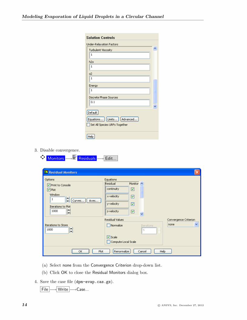
2. Change the under-relaxation factor for Discrete Phase Sources to 0.1.
Solution Controls
c© ANSYS, Inc. December 27, 2012 13
Modeling Evaporation of Liquid Droplets in a Circular Channel
3. Disable convergence.
Monitors −→ Residuals −→ Edit...
(a) Select none from the Convergence Criterion drop-down list.
(b) Click OK to close the Residual Monitors dialog box.
4. Save the case file (dpm-evap.cas.gz).
File −→ Write −→Case...
14 c© ANSYS, Inc. December 27, 2012
Modeling Evaporation of Liquid Droplets in a Circular Channel
5. Perform one DPM track from the TUI.
Enter the following command in the console:
solve > dpm-update
6. Run the calculation for 1500 iterations.
Run Calculation −→ Calculate
7. Save the data file (dpm-evap.dat.gz).
File −→ Write −→Data...
Step 10: Postprocessing
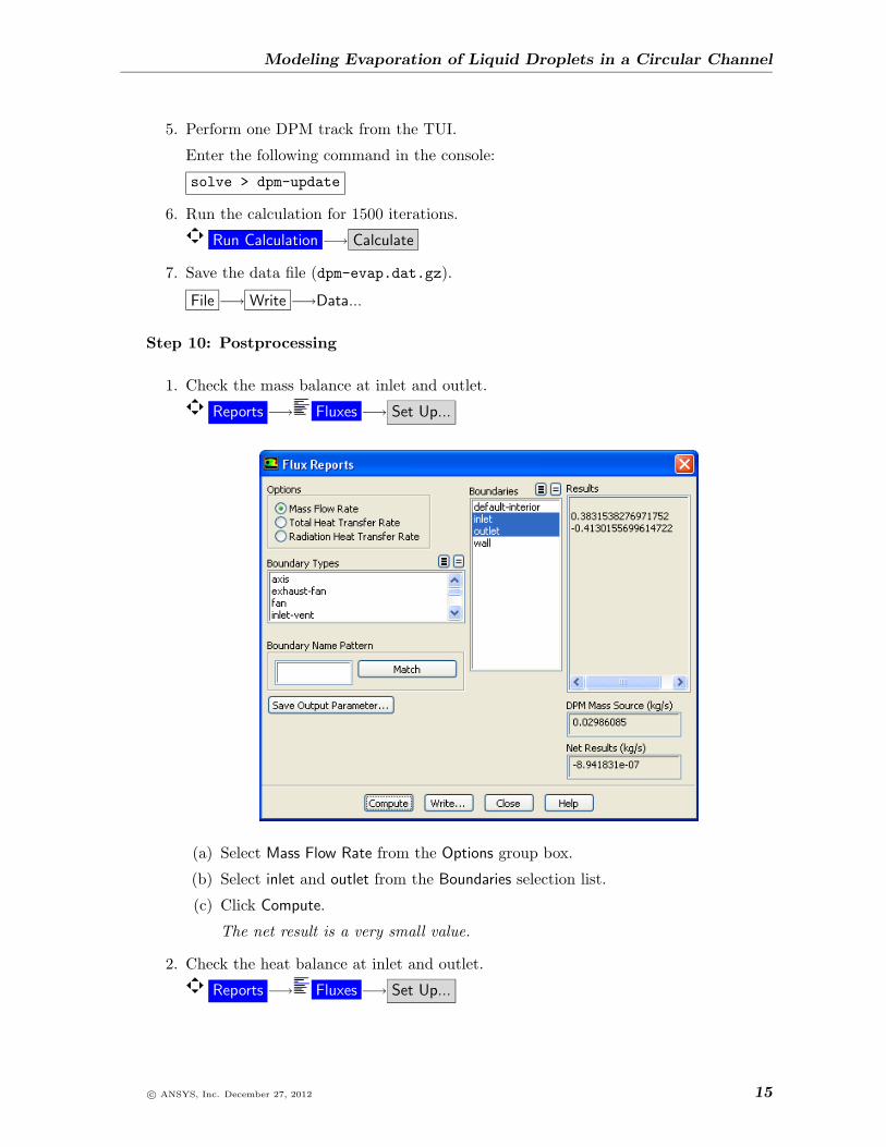
1. Check the mass balance at inlet and outlet.
Reports −→ Fluxes −→ Set Up...
(a) Select Mass Flow Rate from the Options group box.
(b) Select inlet and outlet from the Boundaries selection list.
(c) Click Compute.
The net result is a very small value.
2. Check the heat balance at inlet and outlet.
Reports −→ Fluxes −→ Set Up...
c© ANSYS, Inc. December 27, 2012 15
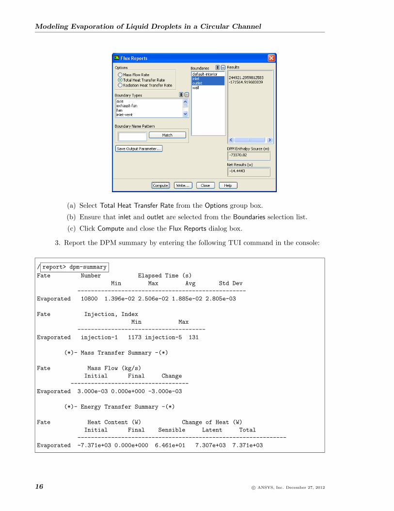
Modeling Evaporation of Liquid Droplets in a Circular Channel
(a) Select Total Heat Transfer Rate from the Options group box.
(b) Ensure that inlet and outlet are selected from the Boundaries selection list.
(c) Click Compute and close the Flux Reports dialog box.
3. Report the DPM summary by entering the following TUI command in the console:
/ report> dpm-summary
Fate Number Elapsed Time (s)Min Max Avg Std Dev
--------------------------------------------------Evaporated 10800 1.396e-02 2.506e-02 1.885e-02 2.805e-03
Fate Injection, IndexMin Max
--------------------------------------Evaporated injection-1 1173 injection-5 131
(*)- Mass Transfer Summary -(*)
Fate Mass Flow (kg/s)Initial Final Change
-----------------------------------Evaporated 3.000e-03 0.000e+000 -3.000e-03
(*)- Energy Transfer Summary -(*)
Fate Heat Content (W) Change of Heat (W)Initial Final Sensible Latent Total
--------------------------------------------------------------Evaporated -7.371e+03 0.000e+000 6.461e+01 7.307e+03 7.371e+03
16 c© ANSYS, Inc. December 27, 2012
Modeling Evaporation of Liquid Droplets in a Circular Channel
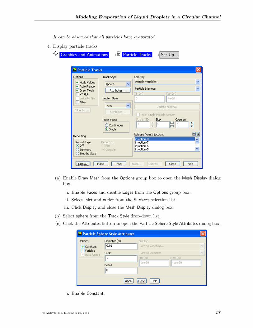
It can be observed that all particles have evaporated.
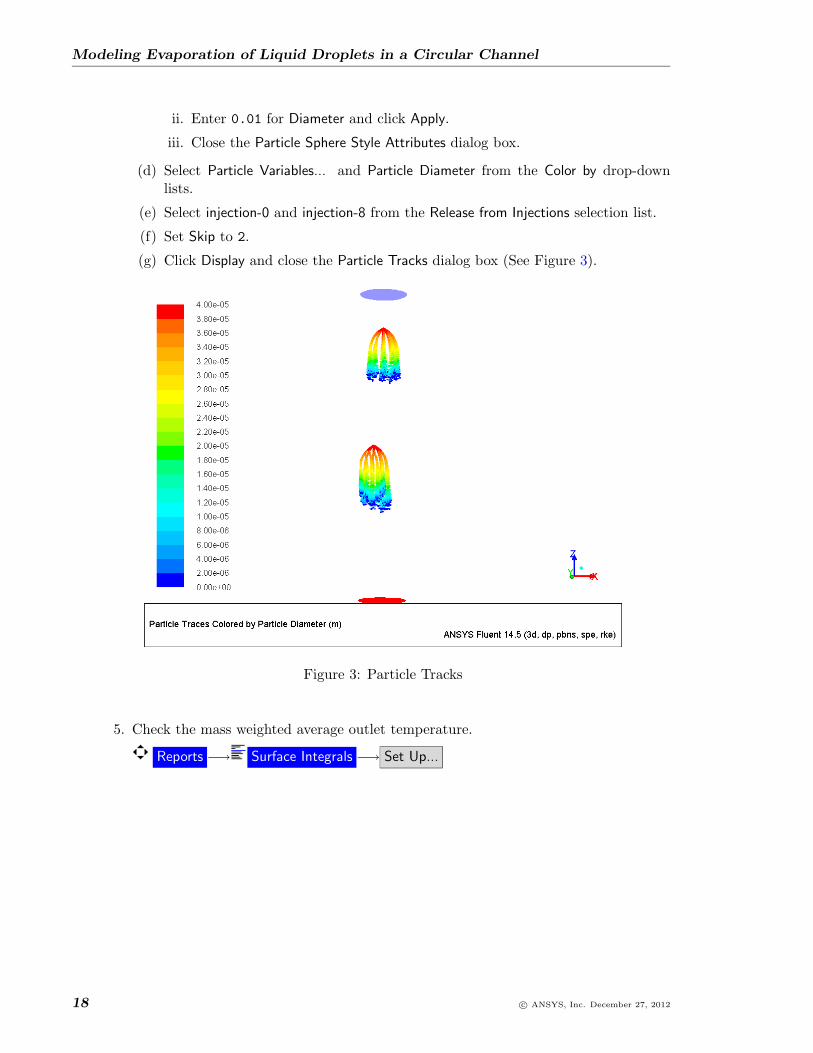
4. Display particle tracks.
Graphics and Animations −→ Particle Tracks −→ Set Up...
(a) Enable Draw Mesh from the Options group box to open the Mesh Display dialogbox.
i. Enable Faces and disable Edges from the Options group box.
ii. Select inlet and outlet from the Surfaces selection list.
iii. Click Display and close the Mesh Display dialog box.
(b) Select sphere from the Track Style drop-down list.
(c) Click the Attributes button to open the Particle Sphere Style Attributes dialog box.
i. Enable Constant.
c© ANSYS, Inc. December 27, 2012 17
Modeling Evaporation of Liquid Droplets in a Circular Channel
ii. Enter 0.01 for Diameter and click Apply.
iii. Close the Particle Sphere Style Attributes dialog box.
(d) Select Particle Variables... and Particle Diameter from the Color by drop-downlists.
(e) Select injection-0 and injection-8 from the Release from Injections selection list.
(f) Set Skip to 2.
(g) Click Display and close the Particle Tracks dialog box (See Figure 3).
Figure 3: Particle Tracks
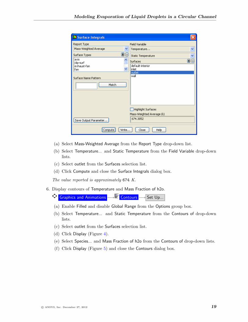
5. Check the mass weighted average outlet temperature.
Reports −→ Surface Integrals −→ Set Up...
18 c© ANSYS, Inc. December 27, 2012
Modeling Evaporation of Liquid Droplets in a Circular Channel
(a) Select Mass-Weighted Average from the Report Type drop-down list.
(b) Select Temperature... and Static Temperature from the Field Variable drop-downlists.
(c) Select outlet from the Surfaces selection list.
(d) Click Compute and close the Surface Integrals dialog box.
The value reported is approximately 674 K.
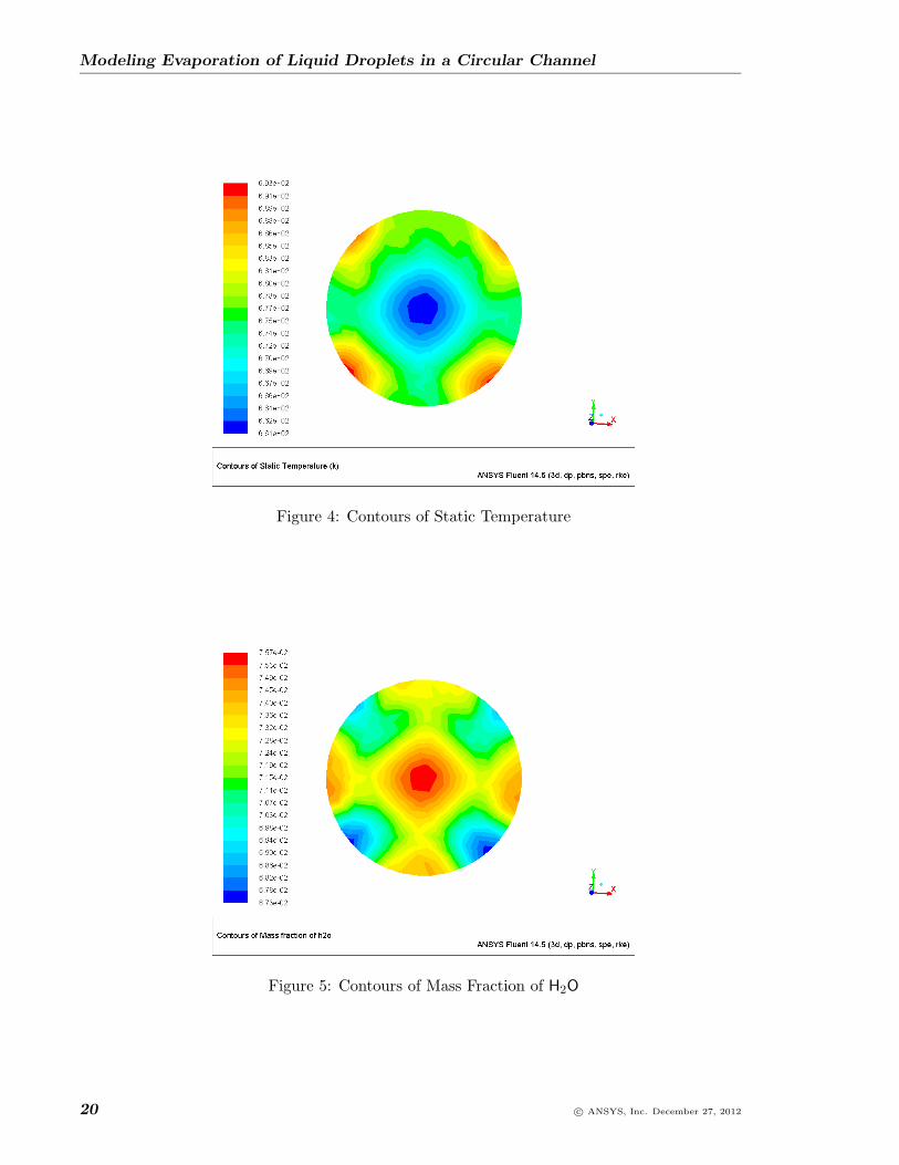
6. Display contours of Temperature and Mass Fraction of h2o.
Graphics and Animations −→ Contours −→ Set Up...
(a) Enable Filled and disable Global Range from the Options group box.
(b) Select Temperature... and Static Temperature from the Contours of drop-downlists.
(c) Select outlet from the Surfaces selection list.
(d) Click Display (Figure 4).
(e) Select Species... and Mass Fraction of h2o from the Contours of drop-down lists.
(f) Click Display (Figure 5) and close the Contours dialog box.
c© ANSYS, Inc. December 27, 2012 19
Modeling Evaporation of Liquid Droplets in a Circular Channel
Figure 4: Contours of Static Temperature
Figure 5: Contours of Mass Fraction of H2O
20 c© ANSYS, Inc. December 27, 2012
Modeling Evaporation of Liquid Droplets in a Circular Channel
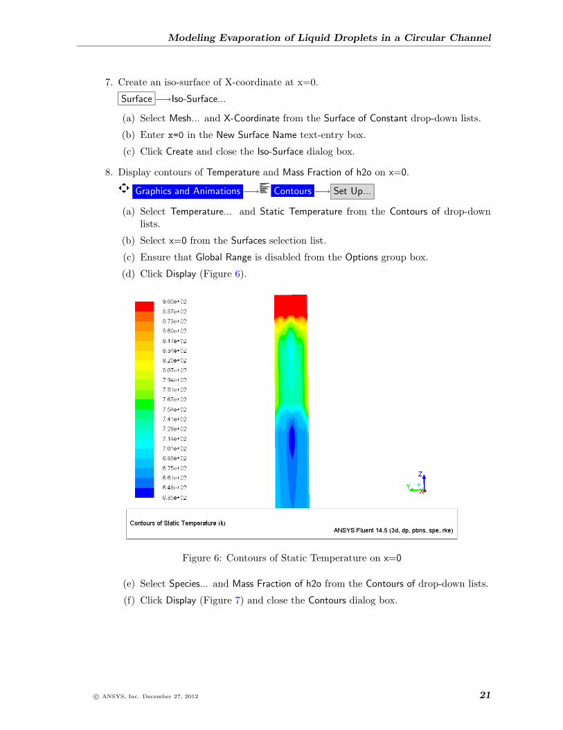
7. Create an iso-surface of X-coordinate at x=0.
Surface −→Iso-Surface...
(a) Select Mesh... and X-Coordinate from the Surface of Constant drop-down lists.
(b) Enter x=0 in the New Surface Name text-entry box.
(c) Click Create and close the Iso-Surface dialog box.
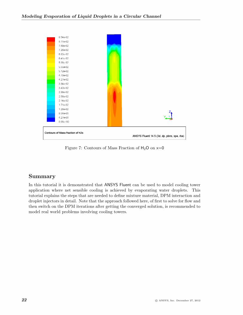
8. Display contours of Temperature and Mass Fraction of h2o on x=0.
Graphics and Animations −→ Contours −→ Set Up...
(a) Select Temperature... and Static Temperature from the Contours of drop-downlists.
(b) Select x=0 from the Surfaces selection list.
(c) Ensure that Global Range is disabled from the Options group box.
(d) Click Display (Figure 6).
Figure 6: Contours of Static Temperature on x=0
(e) Select Species... and Mass Fraction of h2o from the Contours of drop-down lists.
(f) Click Display (Figure 7) and close the Contours dialog box.
c© ANSYS, Inc. December 27, 2012 21
Modeling Evaporation of Liquid Droplets in a Circular Channel
Figure 7: Contours of Mass Fraction of H2O on x=0
Summary
In this tutorial it is demonstrated that ANSYS Fluent can be used to model cooling towerapplication where net sensible cooling is achieved by evaporating water droplets. Thistutorial explains the steps that are needed to define mixture material, DPM interaction anddroplet injectors in detail. Note that the approach followed here, of first to solve for flow andthen switch on the DPM iterations after getting the converged solution, is recommended tomodel real world problems involving cooling towers.
22 c© ANSYS, Inc. December 27, 2012