Introduction - math.ntnu.no fileTRANSPORT-COLLAPSE SCHEME FOR HETEROGENEOUS SCALAR CONSERVATION LAWS...

TRANSPORT-COLLAPSE SCHEME FOR HETEROGENEOUSSCALAR CONSERVATION LAWS

DARKO MITROVIC AND ANDREJ NOVAK

Abstract. We extend Brenier’s transport collapse scheme on heterogeneous

scalar conservation laws with initial and boundary data. It is based on averag-ing out the solution to the corresponding kinetic equation, and it necessarily

converges toward the entropy admissible solution of the considered problem.

We also provide numerical examples.

1. Introduction

Let Ω ⊂ Rd be a bounded smooth domain. We consider the following Cauchyproblem

∂tu+ divxf(t,x, u) = 0, (t,x) ∈ R+ × Ω, (1)

u|t=0 = u0(x), (2)

u|R+×∂Ω = uB(t,x), (3)

where the function f = (f1, . . . , fd) ∈ C2(Rd+1+ ), Rd+1

+ = R+ ×Rd+1. We addi-tionally assume that for some constants a, b ∈ R, it holds

f(t,x, a) = f(t,x, b) = 0 and a ≤ u0, uB ≤ b.

Latter conditions provide the maximum principle for the entropy admissible solutionto (1), (2), (3) (see e.g. [15]).

A typical problem described by (1), (2), (3) arises e.g. in traffic flow models.Namely, if we aim to describe a flow on a finite highway (required to model on andoff ramps) we need to use boundary conditions [18]. For instance, optimization oftravel time and cost between two points can be obtained by controlling incomingand outgoing car densities [2].

Never the less, it is clear that the boundary conditions cannot be prescribedunless characteristics corresponding to equation (1) leave the boundary (those arecharacteristics originating from x = R on Figure 1). This means that one needsto introduce a new concept defining what conditions should satisfy the unknownfunction u in order to be a solution to (1), (2), (3). This was firstly done in [3] viathe following definition which we introduce in the form convenient for us (we alsoinclude the notion of entropy solution for (1), (2)).

Definition 1. A bounded function u is called an entropy admissible solution to

2010 Mathematics Subject Classification. 35L65.Key words and phrases. heterogeneous scalar conservation law; mixed problem; transport-

collapse scheme; kinetic formulation.

1

2 DARKO MITROVIC AND ANDREJ NOVAK

a) (1), (2) if for every convex function V ∈ C2(R), every λ ∈ R and everyϕ ∈ C1

c (R+ ×Rd), it holds∫∫R+×Rd

[V (u)∂tϕ+

∫ u

a

f ′λ(t,x, v)V ′(v)dv · ∇ϕ+∫ u

a

divxf(t,x, v)V ′′(v)dv ϕ]dxdt

(4)

+∫Rd

V (u0(x))ϕ(0,x)dx ≤ 0;

b) (1), (2), (3) if for every convex function V ∈ C2(R), every λ ∈ R and everyϕ ∈ C1

c (R+ × Ω), it holds∫∫R+×Ω

[V (u)∂tϕ+

∫ u

a

f ′λ(t,x, v)V ′(v)dv · ∇ϕ+∫ u

a

divxf(t,x, v)V ′′(v)dv ϕ]dxdt

(5)

+∫R+

∫∂Ω

(ϕ∫ uB

a

f ′λ(t,x, v)V ′(v)dv) · νdsdt+∫

Ω

V (u0(x))ϕ(0,x)dx ≤ 0,

where ν is the unit normal on ∂Ω.

Equivalent and more usual definition of admissible solution is given by theKruzhkov entropies V (u) = |u − λ|, λ ∈ R, and it states that a bounded func-tion u is called an entropy admissible solution to (1), (2), (3) if for every λ ∈ R itholds

∂t|u− λ|+ divx[sgn(u− λ)(f(t,x, u)− f(t,x, λ))] + sgn(u− λ)divxf(t,x, λ) ≤ 0(6)

in the sense of distributions on D′(R+ × Ω), andi) it holds esslimt→0

∫Ω|u(t,x)− u0(x)|dx = 0;

ii) for every λ ∈ R, it holds

(sgn(u− λ)− sgn(uB − λ)) 〈f(t,x, u)− f(t,x, uB), ~ν〉 ≥ 0

on ∂Ω, where ~ν is normal on ∂Ω.The expressions in (i) and (ii) are well defined at least when the flux is genuinely

nonlinear since then, the strong traces of 〈sgn(u− λ)(f(t,x, u)− f(t,x, λ)), ~ν〉 andf(t,x, u), ~ν〉 exist at ∂Ω [1, 17]).

Work in the field of numerical methods for conservation laws is rather intensive.Most of the papers deal with Cauchy problems for conservation laws (scalar conser-vation laws or systems; see e.g. classical books [9, 13] and references therein). Asfor (1), (2), (3) , there are much less results since the interest for this kind of prob-lem has arisen relatively recently. We mention [5] where stability and convergenceresults for monotone (first-order) numerical schemes approximating (homogeneous)scalar conservation laws in several space dimensions were obtained. For results inthe case of systems, one can consult [16] where one can also find thorough overviewof state of the art for the problem.

The aim of the present paper is to extend the transport-collapse scheme [4] forthe initial and initial-boundary value problem for heterogeneous scalar conservationlaws. Originally, the transport collapse scheme was introduced as a mean for solvingthe Cauchy problem (1), (2) in the case when the flux is independent of (t,x) ∈

HETEROGENEOUS TRANSPORT-COLLAPSE SCHEME 3

R+×Rd. Although [14] appeared ten years after [4], the transport-collapse schemeis actually based on the kinetic formulation [14] in the frame of which, using theKruzhkov entropy conditions [11], one reduces the nonlinear equation (1) on thelinear (so called kinetic) equation (see Theorem 2 below). However, derivative ofa measure figures in the equation (see the right-hand side of (7)) and it has onemore variable (so called kinetic or velocity variable). Due to the former reason, thekinetic equation is not convenient for numerical implementation. Never the less, ifwe neglect the derivative of the measure, and then average out the solution to theobtained linear equation with respect to the kinetic variable, we can obtain entropysolution to the considered problem. Details are provided in the next sections.

In conclusion, the power of the method to be presented is in its ability to trans-form nonlinear problem into linear. Linear scalar conservation laws are easy tosolve numerically since there are a lot of robust numerical schemes available. Thecost of that ”transformation” in practical computing is adding one more dimension(see (7)).

The paper is organized as follows. In Section 2, we shall prove convergence ofthe transport-collapse scheme for initial value problems corresponding to (1). InSection 3, we shall introduce a transport-collapse type operator for (1), (2), (3),and the proof of its convergence toward the entropy solution.

2. Initial value problem

In order to extend the transport-collapse in heterogeneous situation, we needappropriate kinetic formulation. It is given in [7] through the following theorem.

Theorem 2. [7] The function u ∈ C([0,∞);L1(Rd))∩L∞loc((0,∞);L∞(Rd)) is theentropy admissible solution to (1), (2) if and only if there exists a non-negativeRadon measure m(t,x, λ) such that m((0, T )×Rd+1) <∞ for all T > 0 and such

that the function χ(λ, u) =

1, 0 ≤ λ ≤ u−1, u ≤ λ ≤ 00, else

, represents the distributional solution

to

∂tχ+ div(x,λ)[F (t,x, λ)χ] = ∂λm(t,x, λ), (t,x) ∈ R+ ×Rd, (7)

χ(λ, u(t = 0,x)) = χ(λ, u0(x)), (8)

where F = (f ′λ,−d∑j=1

∂xjfj).

Let us state properties of the function χ.

Proposition 3. [4, page 1018] It holdsa) ∀u, v ∈ L1(Rd) such that u ≥ v =⇒ χ(λ, u) ≥ χ(λ, v);b) ∀u ∈ L1(Rd), ∀g ∈ L∞(Rd ×R), it holds∫∫

χ(λ, u)g(x, λ)dxdλ =∫ (∫ u

ag(x, λ)dλ

)dx;

In particular, if g = G′λ and G(a) = 0, then∫∫

χ(λ, u)g(x, λ)dxdλ =∫G(x, u)dx

c) TV (u) =∫TV (χ(λ, ·))dλ.

The idea of the transport collapse scheme for the initial value problem (1), (2)is to solve problem (7), (8) when we omit the right-hand side in (7):

∂th+ divx,λ[F (t,x, λ)h] = 0, h|t=0 = χ(λ, u0(x)). (9)


The solution of this equation is obtained via the method of characteristics. Theyare given by

x = f ′λ, x|t=0 = x0,

λ = −d∑j=1

∂xjfj(t,x, λ), λ|t=0 = λ0.(10)

For later purpose, we rewrite this system in the integral formx = x0 +

∫ t0f ′λ(t′,x, λ)dt′

λ = λ0 −∫ t

0

d∑j=1

∂xjfj(t′,x, λ)dt′.

(11)

The solution to (9) has the form

h(t,x, λ) = χ(λ0(t,x, λ), u0(x0(t,x, λ))). (12)

To avoid proliferation of symbols, denote

‖∇xf‖∞ = sup∆x>0

|f(x + ∆x)− f(x)|‖∆x‖

. (13)

We have the following properties of the characteristics.

Proposition 4. The characteristics x0 = x0(t,x, λ) and λ0 = λ0(t,x, λ) satisfythe following continuity properties:

|Rx| := |x0(t,x + ∆x, λ)− x0(t,x, λ)| (14)

≤ ‖∆x‖(

1 +∫ t

0

maxλ‖∇xf

′λ(t′, ·, λ))dt′‖∞

).

|Rλ| := |λ0(t,x + ∆x, λ)− λ0(t,x, λ)| (15)

≤ ‖∆x‖∫ t

0

maxλ‖∇xdivxf(t′, ·, λ))dt′‖∞,

where the norms are given by (13).

Proof: From (11), we have

x = x0(t,x, λ) +∫ t

0

f ′λ(t′,x, λ)dt′

x + ∆x = x0(t,x + ∆x, λ) +∫ t

0

f ′λ(t′,x + ∆x, λ)dt′.

By subtracting those equations, we obtain

|x0(t,x + ∆x, λ)− x0(t,x, λ)| (16)

≤ ∆x +∫ t

0

maxλ‖f ′λ(t′,x + ∆x, λ)− f ′λ(t′,x, λ)‖∞dt′

≤ ∆x + ‖∆x‖∫ t

0

maxλ‖∇xf

′λ(t′, ·, λ)‖∞dt′.

This proves (14).


Inequality (15) is proved analogously. It holds

λ = λ0(t,x + ∆x, λ)−∫ t

0

d∑j=1

∂xjfj(t′,x + ∆x, λ)dt′,

λ = λ0(t,x, λ)−∫ t

0

d∑j=1

∂xjfj(t′,x, λ)dt′

and it is enough to subtract the last two equalities, and to follow the procedurefrom (16). 2

Let us now define the transport-collapse operator T .

Definition 5. The transport collapse operator T (t) is defined for every u ∈ L1(Rd)by

T (t)u(x) =∫χ(λ0(t,x, λ), u(x0(t,x, λ)))dλ. (17)

It satisfies the following properties which are the same as the ones from [4,Proposition 1].

Proposition 6. It holds for every u, v ∈ L1(Rd)

a) u ≤ v a.e. implies T (t)u ≤ T (t)v a.e;b)∫T (t)u(x)dx =

∫u(x)dx;

c) the operator T (t) is non-expansive

‖T (t)u− T (t)v‖L1(Rd) ≤ ‖u− v‖L1(Rd),

and, in particular, ‖T (t)u‖L1(Rd) ≤ ‖u‖L1(Rd);d) TV (T (t)u) ≤ (1 + C1t)TV (u) + tC2, where TV is the total variation and

C1 and C2 are appropriate constants depending on the C2-bounds of theflux f ;

e) ‖T (t)u−u‖L1(Rd) ≤ C2TV (u)t+ tC1 for the constants C1 and C2 from theprevious item;

Proof: Item a) directly follows from the definition of the transport collapse op-erator T (t).

As for the item b), denote by Z = (x, λ) characteristics from (10). Notice that,since div(x,λ)F = 0, it holds ∣∣∣ det

∂Z(t,x0, λ0)∂(x0, λ0)

∣∣∣ = 1. (18)

Therefore, according to Proposition 3,∫T (t)u(x)dx =

∫Rd+1

χ(λ0(t,x, λ), u(x0(t,x, λ))dxdλ

=(

x0(t,x, λ) = yλ0(t,x, λ) = η

)=∫Rd+1

χ(η, u(y))∣∣∣ det

∂Z(t,x0, λ0)∂(x0, λ0)

∣∣∣dydη =∫u(y)dy.

Item c) now follows from a) and b) according to the Crandall-Tartar lemmaabout non-expansive order preserving mappings [6, Proposition 3.1].


Let us now prove item d). We have∫Rd

|T (t)u(x + ∆x)− T (t)(x)|dx

=∫Rd

|∫R

χ(λ0(t,x+∆x, λ), u(x0(t,x+∆x, λ)))−χ(λ0(x0(t,x, λ), u(x0(t,x, λ)))dλ|dx

≤∫

Rd+1

|χ(λ0(t,x+∆x, λ), u(x0(t,x+∆x, λ)))−χ(λ0(x0(t,x, λ), u(x0(t,x, λ)))|dxdλ

We next write x0(t,x + ∆x, λ) = x0(t,x, λ) + Rx(t,x, λ) and λ0(t,x + ∆x, λ) =λ0(t,x, λ) +Rλ(t,x, λ), where Rx and Rλ are estimated in (14), and introduce thechange of variables x0(t,x, λ) = y, λ0(t,x, λ) = η (keep in mind (18)). We obtain∫

Rd

|T (t)u(x + ∆x)− T (t)u(x)|dx

≤∫Rd+1

|χ(η +Rλ, u(y +Rx))− χ(η, u(y))|dydη

≤∫Rd+1

|χ(η +Rλ, u(y +Rx))− χ(η, u(y +Rx))|dydη

+∫Rd+1

|χ(η, u(y +Rx))− χ(η, u(y))|dydη

≤ ‖Rλ‖∞ TV (χ) + ‖Rx‖∞∫R

TV (χ(η, u(·)))dη = 4‖Rλ‖∞ + ‖Rx‖∞TV (u),

since the characteristics are of C1-class, TV (χ) = 4, and since (3), item c) holds.Having in mind Proposition 4, we conclude the proof of d). We remark that

C1 = 4 maxt,λ‖∇xf(t, ·, λ)‖∞, C2 = max

t,λ‖∇xdivxf(t, ·, λ)‖∞.

It remains to prove item e). Using (11), as in to the proof of item d), we have

‖T (t)u− u‖L1(Rd) ≤∫Rd+1

|χ(λ0(t,x, λ), u(x0(t,x, λ)))− χ(λ, u(x))|dxdλ

=∫Rd+1

|χ(λ+Rλ, u(x +Rx))− χ(λ, u(x))|dλdx

≤ C1 t TV (u) + C2 t,

which immediately gives e). 2

We also need the following result.

Proposition 7. For any smooth positive test function ϕ, and Lipschitz functionV : R→ R, we have∫

(V (T (t)u)− V (u))(x)ϕ(x)dx ≤∫ t

0

∫BV (t′,x, u(x))∇ϕdxdt′ (19)

+∫ t

0

∫ ∫ u

a

divxf(t,x, λ)V ′′(λ)dλdt′ + o(t), t→ 0

where BV (t,x, u) =∫ uaf ′λ(t,x, λ)V ′(λ)dλ.


Proof: Remark first that for any fixed (t,x), from the definition of the functionχ, it follows for any C1-function G∫

G′(λ)χ(λ0(t,x, λ), u(x0(t,x, λ)))dλ =2p∑k=0

(−1)kG′(ωk)−G(0), (20)

where the increasing sequence (ωk), k = 0, . . . , 2p, belongs to the set λ ∈ [a, b] :λ0(t,x, λ) = u(x0(t,x, λ)) (since the entropy solution to (1), (2) takes values inthe interval (a, b)). Remark that the set has odd cardinality since the multivaluedsolution is obtained by continuous transformation from the graph of initial value[4, page 1016]. Moreover, due to the mean value theorem, the following relationholds for any convex function V (see e.g. [8, p. 40]):

V (2p∑k=0

(−1)kωk) ≤2p∑k=0

(−1)kV (ωk). (21)

From (20) and (21), it follows

V (T (t)u(x)) = V (∫χ(λ0(t,x, λ), u(t,x0(t,x, λ)))dλ) = V (

2p∑k=0

(−1)kωk)

≤2p∑k=0

(−1)kV (ωk) =∫V ′(λ)χ(λ0(t,x, λ), u(x0(t,x, λ)))dλ+ V (0).

We have from here∫(V (T (t)u(x))− V (u(x)))ϕ(x)dx (22)

≤∫∫

(V ′(λ)χ(λ0(t,x, λ), u(x0(t,x, λ)))− V ′(λ)χ(λ, u(x)))ϕ(x)dxdλ

=∫∫

V ′(λ0(t,x, λ))χ(λ0(t,x, λ), u(x0(t,x, λ)))(ϕ(x)−ϕ(x0(t,x, λ)))dxdλ (23)

+∫∫

(V ′(λ)−V ′(λ0(t,x, λ)))χ(λ0(t,x, λ), u(x0(t,x, λ)))ϕ(x)dxdλ (24)

+(∫∫

V ′(λ0)χ(λ0(t,x, λ), u(x0(t,x, λ)))ϕ(x0(t,x, λ))dxdλ

−∫∫

V ′(λ)χ(λ, u(x))ϕ(x)dxdλ). (25)

The two terms from (25) cancel according to (18). Let us consider the term from(23). Using the Taylor formula∫∫

V ′(λ0(t,x, λ))χ(λ0(t,x, λ), u(x0(t,x, λ)))(ϕ(x0(t,x, λ))− ϕ(x))dxdλ (26)

=∫∫

V ′(λ0(t,x, λ))χ(λ0(t,x, λ), u(x0(t,x, λ)))(x0(t,x, λ)− x) · ∇ϕ(x0(t,x, λ))dxdλ

+∫∫

V ′(λ0(t,x, λ))χ(λ0(t,x, λ), u(x0(t,x, λ)))D2ϕ(x) (x0(t,x, λ)− x)2dxdλ.

From (11), we conclude by expanding the function f ′λ(t′,x, λ) into the Taylor ex-pansion around x0:


x0(t,x, λ)− x =∫ t

0

f ′λ(t′,x, λ)dt′ =∫ t

0

f ′λ(t′,x0(t,x, λ), λ)dt′ (27)

+ (x0(t,x, λ)− x)∫ t

0

∇xf ′λ(t′, x, λ)dt′ =∫ t

0

f ′λ(t′,x0(t,x, λ), λ)dt′ +O(t2),

since clearly x0(t,x, λ)− x =∫ t

0f ′λ(t′,x, λ)dt′ = O(t). Inserting this into (26) and

applying the change of variables from (18), we conclude using item b) from (3):∫∫V ′(λ0)χ(λ, u(x))(ϕ(x0(t,x, λ))− ϕ(x))dxdλ (28)

=∫ t

0

BV (t′,x, u(x))∇ϕdxdt′ +O(t2).

To deal with the remaining term from (24), we shall expand the function V ′ intothe Taylor series around λ0. We have∫∫

(V ′(λ)− V ′(λ0))χ(λ0(t,x, λ), u(x0(t,x, λ)))ϕ(x)dxdλ (29)

=∫∫

V ′′(λ0(t,x, λ))(λ− λ0((t,x, λ)))χ(λ0(t,x, λ), u(x0(t,x, λ)))ϕ(x)dxdλ

+O(‖λ− λ0((t,x, λ))‖2L1(supp(ϕ)×(a,b)))

Applying the procedure as in (27), we reach to the estimate

λ0(t,x, λ)− λ = −∫ t

0

d∑j=1

fj(t′,x0(t,x, λ), λ)dt′ +O(t2). (30)

If we notice that ‖λ−λ0((t,x, λ))‖2L1(supp(ϕ)×(a,b)) = O(t2), from (29) and (30), weconclude∫∫

(V ′(λ)− V ′(λ0))χ(λ0(t,x, λ), u(x0(t,x, λ)))ϕ(x0(t,x, λ))dxdλ (31)

= −∫ t

0

∫ ∫ u

a

d∑j=1

fj(t′,x0(t,x, λ), λ)dt′ ϕ(x)dx +O(t2)

Combining (22), (28), and (31), we conclude the theorem. 2

A consequence of Proposition 6 and Proposition 7 is the following theorem:

Theorem 8. Denote

Sn(t)u = (1− α)T (t

n)ku + αT (

t

n)k+1u, (32)

where

t =(k + α)n

, k ∈ N, α ∈ [0, 1). (33)

For each initial value u0 ∈ L1(Rd) such that a ≤ u0 ≤ b, the unique entropysolution of (1), (2) at time t is given by the formula

u(t, ·) = L1 − limn→∞

Sn(t)u.


Proof: First, fix an arbitrary t > 0. Consider the sequence of functions un(t, ·) =Sn(t)u. We aim to prove that the sequence (un(t, ·)) is strongly precompact inL1(Rd). To this end, we shall use the Kolmogorov criterion stating that a functionalsequence bounded in L1(Rd) is strongly precompact in L1(Rd) if it is uniformlyL1(Rd) continuous. In other words, we need to prove that

a) ‖un(t, ·)‖L1(Rd) ≤ C for every n ∈ N and some constant C;b) for any relatively compact K ⊂⊂ Rd, any ε > 0, there exists ∆x > 0 such

that ‖un(t,x + ∆x)− un(t,x)‖L1(Rd) ≤ ε.Item a) follows from Proposition 6, item c).As for the item b), we shall use property d) from Proposition 6. Taking into

account definition of the total variation and form of the sequence (un(t, ·)), simplecalculations show that (with the notations from Proposition 6)

‖un(t, ·+ ∆x)− un(t, ·)‖L1(Rd) ≤ 2∆x

(1 +tC1

n

)n+C2t

n

n∑j=1

(1 +

tC1

n

)j≤ eCt∆x,

for an appropriate constant C. This clearly implies L1-equicontinuity of the se-quence (un(t, ·)). This means that for every fixed t > 0, we can choose a stronglyconverging subsequence (not relabeled) (un(t, ·)) of the sequence (un(t, ·)). Bytaking a dense countable subset E ⊂ R+, we can choose the same convergingsubsequence (un(t, ·)) for every t ∈ E.

Now, by the continuity property given in item e) from Proposition 6, we concludethat the subsequence (un(t, ·)) strongly converges in C([0, T ];L1(Rd) for every T ∈R+ toward a function u ∈ C([0, T ];L1(Rd).

Now, we need to check that u satisfies the entropy admissibility conditions. First,notice that for every t, as n→∞, it holds that α→ 0. Thus, it is enough to noticethat the main part of the transport-collapse operator given by T ( tn )ku → u asn→∞ along the previously chosen subsequence and to consider

∫Rd

(V (T (t

n)ku)− V (u))ϕ(x)dx =

k−1∑j=0

∫Rd

(V (T (t

n)j+1u)− V (T (

1n

)ju))ϕ(x)dx

(19)

≤k−1∑j=0

∫ (j+1)t/n

jt/n

∫Rd

BV (t′,x, T (t

n)ju(x))∇ϕdxdt′ +O(t/n).

Now, we simply let n → ∞ and keep in mind arbitrariness of t to infer that thefunction u satisfies the entropy admissibility conditions from Definition 1, a).

Remark also that this implies convergence of the entire sequence given by (32)due to uniqueness of entropy solutions to (1), (2). 2

3. Boundary value problem

First, notice that the kinetic formulation from Theorem 2 still holds in the inte-rior of R+ × Ω. This means that in order to adapt the transport collapse schemefor the problem (1), (2), (3) we can apply the same method as in the previous sec-tion. We cannot use the method of characteristics directly since the characteristicsentering the boundary determine the value at the boundary. However, since we are


re-iterating the procedure after a short period of time (see (32) and (38)), we canadjust the (small part of) initial data so that the method of characteristics is welldefined. We provide the details below.

Let us also remark that a kinetic formulation which includes boundary conditionsis derived in [10] but we were not able to use it here.

Accordingly, in order to generalize the transport collapse scheme to the mixedproblem corresponding to (1), let us consider for a short period of time the kineticformulation to (1) augmented with the initial and boundary conditions as follows.

∂thε + divx,λ[F (t,x, λ)hε] = 0, (34)

hε|t=0 = χ(λ, uε0(x)), hε|R+×∂Ω = χ(λ, uB(t,x)). (35)

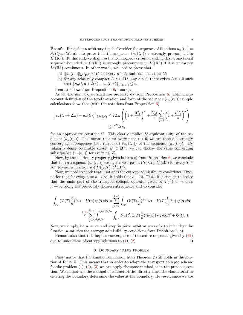
Above, the approximation uε0 satisfy the compatibility conditions with uB in thefollowing sense. We are keeping fixed uB and we adapt u0 so that it coincideswith uB at the edges of ∂Ω × R+. More precisely, denote by ∂Ωε common partof Ω and the ε-neighborhood of ∂Ω. Assume that the characteristics issuing from(0, x0) ∈ t = 0 × ∂Ωε hits the boundary at (t0, y0). Then, we replace the valueu0(x0) of the initial function u0 by uB(t0, y0) (see Figure 1).

Notice that from (10), it follows that t0 ∈ (0, Cε) for any x0 ∈ Ωε where C =maxt,x,λ |F (t,x, λ)|. In the sequel, we shall assume that C = 1

Under such assumptions, for a short period of time, we can solve (34), (35) usingthe method of characteristics where the characteristics will emanate not only fromt = 0, but also from the boundaries. Remark that if a characteristic originatesfrom t = 0, we simply use the system of characteristics (10). If a characteristicoriginates from the boundary, we then write:

t = 1, t(0) = t0

x = f ′λ, x|t=t0 = x0

λ = −d∑j=1

∂xjfj(t,x, λ), λ|t=t0 = λ0

hε = 0, hε|t=0 = χ(λ, uB(t0,x0))

(36)

where (t0,x0) is the point from the boundary.Now, the solution has the same form as for the initial value problem. The value of

the unknown function hε at a point (t,x, λ) is obtained by drawing a characteristicthrough it. By going back along the characteristic, we shall either hit the boundaryor the line t = 0. Thus, the boundary value or the initial value will determine thevalue of hε at (t,x, λ).

To be more precise, denote by WB ⊂ R+t × Ωx ×Rλ set of all points through

which characteristics issuing from the boundary pass, and by WI ⊂ R+t ×Ωx×Rλ

set of all points through which characteristics issuing from the initial plane t = 0pass. We can rewrite the solution in the form

hε(t,x, λ) = χ(λ0(t,x, λ), uε0(x0(t,x, λ))κWI+ uB(x0(t,x, λ))κWB

), (37)

at least in the set [0, ε)×∂Ωε. Now, we can generalize the transport collapse schemeto the initial boundary problem for heterogeneous scalar conservation laws.

Theorem 9. Denote


Figure 1. The characteristics are denoted by dotted lines. Wechoose the correction uε0 of u0 so that uε0(x0) = uB(t0, L).

Tn(t)(u0, uB)(x) =∫h1/n(t,x, λ)dλ.

The entropy admissible solution to the initial boundary value problem (1), (2),(3) is given by the formula

u(t, ·) = L1 − limn→∞

Tn(t

n)n(u1/n

0 , uB). (38)

Remark 10. Notice that after t = 1/n we stop the time and then re-iterate theprocedure. This means that the sequence of functions (un) = (Tn( tn )n(u1/n

0 , uB))is well defined.

Proof: The form of the transport-collapse operator (38) is almost the same asfrom (17). Therefore, the proof that the TV bound of the sequence (un) is finite isthe same. We provide the details below.

TV (Tn(t)(u0, uB)) = TV (∫h1/n(t,x, λ)dλ)

(37)

≤ TV (∫

[χ(λ0(t,x, λ), u1/n0 (x0(t,x, λ))κWI

+ uB(x0(t,x, λ))κWB)dλ]

Prop.6

≤ (1 + C1t) maxTV (u0), TV (uB)+ tC2.

Repeating the procedure from the proof of Theorem 8, we conclude that the se-quence (un) = (Tn( tn )n(u0, uB)) satisfies

TV (un) ≤ eC3t∆x ≤ C4∆x

for some constants C3 and C4.Thus, we conclude that the total variation of the sequence (un) remains uniformly

bounded from where, according to the Kolmogorov criterion, it follows that thesequence (un) is strongly precompact in L1

loc(R+ × Ω) toward a function u. The

limit of the sequence satisfies the entropy admissibility conditions from Definition1 which makes it a unique entropy solution to (1)-(3).


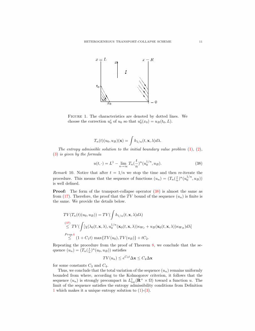
Figure 2. The characteristics are denoted by dotted lines. Theytransform the interval (L,R) into the interval(x(t, L, λ), x(t, R, λ)).

The proof of the latter fact is similar to the proof of Proposition 7 and Theorem8. From there, we see that it is enough to prove that∫

(V (T (t)u)− V (u))(x)ϕ(x)dx ≤∫ t

0

∫BV (t′,x, u(x))∇ϕdxdt′ (39)

+∫ t

0

∫ ∫ u

a

divxf(t,x, λ)V ′′(λ)dλdt′+∫ ∫ t

0

f ′λ(t, L, λ)dt′V ′(λ)χ(λ, ulB)ϕ(L)dλ

+∫ ∫ t

0

f ′λ(t, R, λ)dt′V ′(λ)χ(λ, urB)ϕ(R)dλ+ o(t), t→ 0.

The only difference between the proof of Proposition 7 and the situation thatwe have here is in the term (25) (see relation (22) in Proposition 7). Namely, afterapplying the change of variables (18) the domain of integration is changed for thefirst term from (25) and therefore, the two terms from (25) will not subtract (seeFigure 2). In order to explain technical details more concisely, we shall assume thatx ∈ R (i.e. that we are in the one-dimensional situation) and that the boundaryfunction uB is continuously differentiable. This means that we have the followingboundary conditions for some real numbers L < R

u|x=L = ulB(t), u|x=R = urB(t).

Remark that the change of variables (18) maps the interval (L,R) into the inter-val (x(t, L, λ),x(t, R, λ)), (t, λ) ∈ R+ ×R. We have after the change of variables(18) (in the first integral below):

∫ R

L

∫R

V ′(λ0)χ(λ0(t,x, λ), u(x0(t,x, λ)))ϕ(x0(t,x, λ))dxdλ (40)

−∫ R

L

∫R

V ′(λ)χ(λ, u(x))ϕ(x)dxdλ

=∫R

∫ x(t,R,λ)

x(t,L,λ)

V ′(λ)χ(λ, u(x))ϕ(x)dxdλ−∫ R

L

∫R


=∫ (∫ L

x(t,L,λ)

+∫ x(t,R,λ)

R

)∫R

V ′(λ)χ(λ, u(x))ϕ(x)dxdλ.

Since the boundary data are continuously differentiable and compatible with theinitial data,


(∫ L

x(t,L,λ)

+∫ x(t,R,λ)

R

)∫R


=∫

(x(t, L, λ)− L)V ′(λ)χ(λ, ulB(t))ϕ(L)dλ

+∫

(R− x(t, R, λ))V ′(λ)χ(λ, urB(t))ϕ(R)dλ+ t o(1), t→ 0.

Finally, taking into account (11):

x(t, L, λ)− L =∫ t

0

f ′λ(t′, L, λ)dt′ = O(t),

x(t, R, λ)−R =∫ t

0

f ′λ(t′, R, λ)dt′ = O(t),

we conclude from here and (40):

∫ R

L

∫R

V ′(λ0)χ(λ0(t,x, λ), u(x0(t,x, λ)))ϕ(x0(t,x, λ))dxdλ

−∫ R

L

∫R


=∫ ∫ t

0

f ′λ(t, L, λ)dt′V ′(λ)χ(λ, ulB(t))ϕ(L)dλ

+∫ ∫ t

0

f ′λ(t, R, λ)dt′V ′(λ)χ(λ, urB(t))ϕ(R)dλ+ o(1) +O(t)

Combining this with (22), we conclude that (39) holds. This concludes the theorem.2

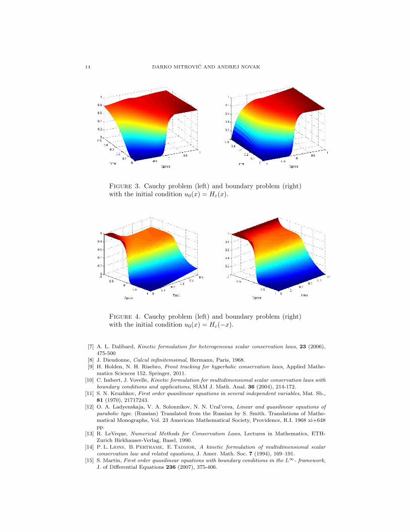
Corresponding numerical examples are given below. It is one-dimensional scalarconservation law defined on [0, 0.5] × [−1, 1] with the flux f(x, u) = Hε(x)(1 −u)(u + 1) + 4Hε(−x)(1 − u)(u + 1), where Hε is a standard regularization of theHeaviside function with ε = 10−4. In the first simulation boundary conditions areu|x=−1 = 0, u|x=1 = 1 and the initial condition is u|t=0 = Hε(x). In the secondsimulation boundary conditions are u|x=−1 = 1, u|x=1 = 0 and the initial conditionis u|t=0 = Hε(−x).

References

[1] J. Aleksic, D. Mitrovic, Strong traces for averaged solutions of heterogeneous ultra-parabolic

transport equations, J. of Hyperbolic Differential Equations 10 (2014), 659–676.[2] F. Ancona, A. Marson On the attainable set for scalar nonlinear conservation laws with

boundary control, SIAM J. Control Optim. 36 (1998), 290172

[3] C. Bardos, A. Y. Le Roux, J.-C. Nedelec, First order quasi-linear equation with boundaryconditions, Comm. Partial Diff. Equations 9 (1979), 1017–1034.

[4] Y. Brenier, Averaged multivalued solutions for scalar conservation laws, SIAM J. on Numer-

ical Analysis 21 (1984), 1013–1037.[5] B Cockburn, F Coquel, PG LeFloch, Convergence of the finite volume method for multidi-

mensional conservation laws, SIAM Journal on Numerical Analysis 32 (1995), 687–705.[6] M. G. Crandall, A. Majda, Monotone difference approximations for scalar conservation laws,

Math. Comput. 34 (1981), 1–21.


Figure 3. Cauchy problem (left) and boundary problem (right)with the initial condition u0(x) = Hε(x).

Figure 4. Cauchy problem (left) and boundary problem (right)with the initial condition u0(x) = Hε(−x).

[7] A. L. Dalibard, Kinetic formulation for heterogeneous scalar conservation laws, 23 (2006),

475-500

[8] J. Dieudonne, Calcul infinitemsimal, Hermann, Paris, 1968.[9] H. Holden, N. H. Risebro, Front tracking for hyperbolic conservation laws, Applied Mathe-

matics Sciences 152, Springer, 2011.

[10] C. Imbert, J. Vovelle, Kinetic formulation for multidimensional scalar conservation laws withboundary conditions and applications, SIAM J. Math. Anal. 36 (2004), 214-172.

[11] S. N. Kruzhkov, First order quasilinear equations in several independent variables, Mat. Sb.,

81 (1970), 21717243.[12] O. A. Ladyenskaja, V. A. Solonnikov, N. N. Ural’ceva, Linear and quasilinear equations of

parabolic type. (Russian) Translated from the Russian by S. Smith. Translations of Mathe-

matical Monographs, Vol. 23 American Mathematical Society, Providence, R.I. 1968 xi+648pp.

[13] R. LeVeque, Numerical Methods for Conservation Laws, Lectures in Mathematics, ETH-

Zurich Birkhauser-Verlag, Basel, 1990.[14] P. L. Lions, B. Perthame, E. Tadmor, A kinetic formulation of multidimensional scalar

conservation law and related equations, J. Amer. Math. Soc. 7 (1994), 169–191.[15] S. Martin, First order quasilinear equations with boundary conditions in the L∞- framework,

J. of Differential Equations 236 (2007), 375-406.


[16] S. Mishra, M. Svard, , Z. Anfew. Math. Phys.

[17] E. Yu. Panov, Existence of strong traces for quasi-solutions of multi-dimensional conserva-

tion laws, J. of Hyperbolic Differential Equations 4 (2007), 729–770.[18] I. S. Strub, A. M. Bayen, Mixed Initial-Boundary Value Problems for Scalar Conservation

Laws: Application to the Modeling of Transportation Networks, Hybrid Systems: Computa-

tion and Control Lecture Notes in Computer Science 3927 (2006), 552–567

Darko MitrovicUniversity of Montenegro, Faculty of Mathematics, Podgorica, Montenegro

E-mail address: [email protected]

Andrej Novak

University of Dubrovnik, Department of Electrical Engineering and Computer Science,

Dubrovnik, CroatiaE-mail address: [email protected]

Introduction - math.ntnu.no fileTRANSPORT-COLLAPSE SCHEME FOR HETEROGENEOUS SCALAR CONSERVATION LAWS...

Documents

Transcript of Introduction - math.ntnu.no fileTRANSPORT-COLLAPSE SCHEME FOR HETEROGENEOUS SCALAR CONSERVATION LAWS...