Introduction à l’analyse en ondelettes et à l’analyse...
191
Introduction à l’analyse en ondelettes et à l’analyse multi- résolution Frédéric Truchetet Le2i, UMR 5158 Université de Bourgogne - CNRS [email protected]
Transcript of Introduction à l’analyse en ondelettes et à l’analyse...
Introduction à l’analyse en ondelettes et à l’analyse multi-résolution
Frédéric TruchetetLe2i, UMR 5158
Université de Bourgogne - [email protected]
Introduction à l’analyse en ondelettes et à l’analyse multi-résolution
� Première partie: une introduction en «images »
� Deuxième partie: un peu plus de rigueur
� Troisième partie: quelques applications
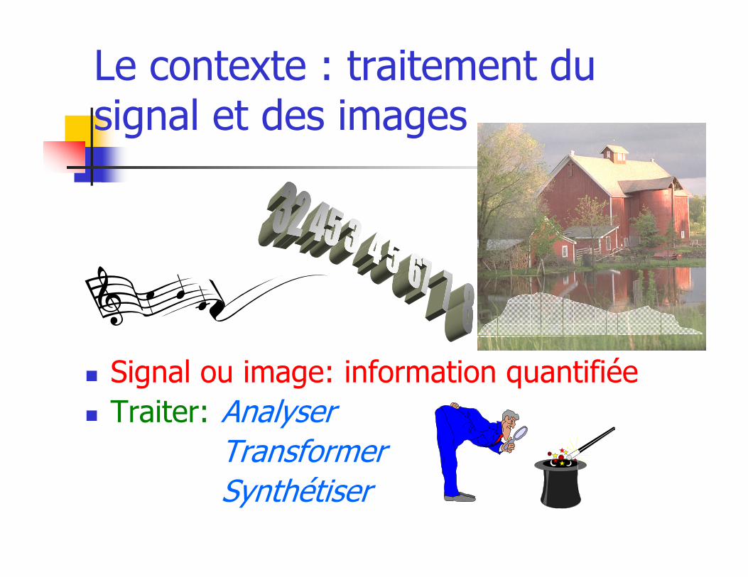
Le contexte : traitement du signal et des images
� Signal ou image: information quantifiée
� Traiter: AnalyserTransformerSynthétiser
Des ondelettes, pourquoi ?
Traitement du signal
Exemple de problème :
Analyse d’une phrase musicale
� Création automatique d’une partition à partir d’un signal sonore
� Reconstruction du morceau de musique à partir de la partition
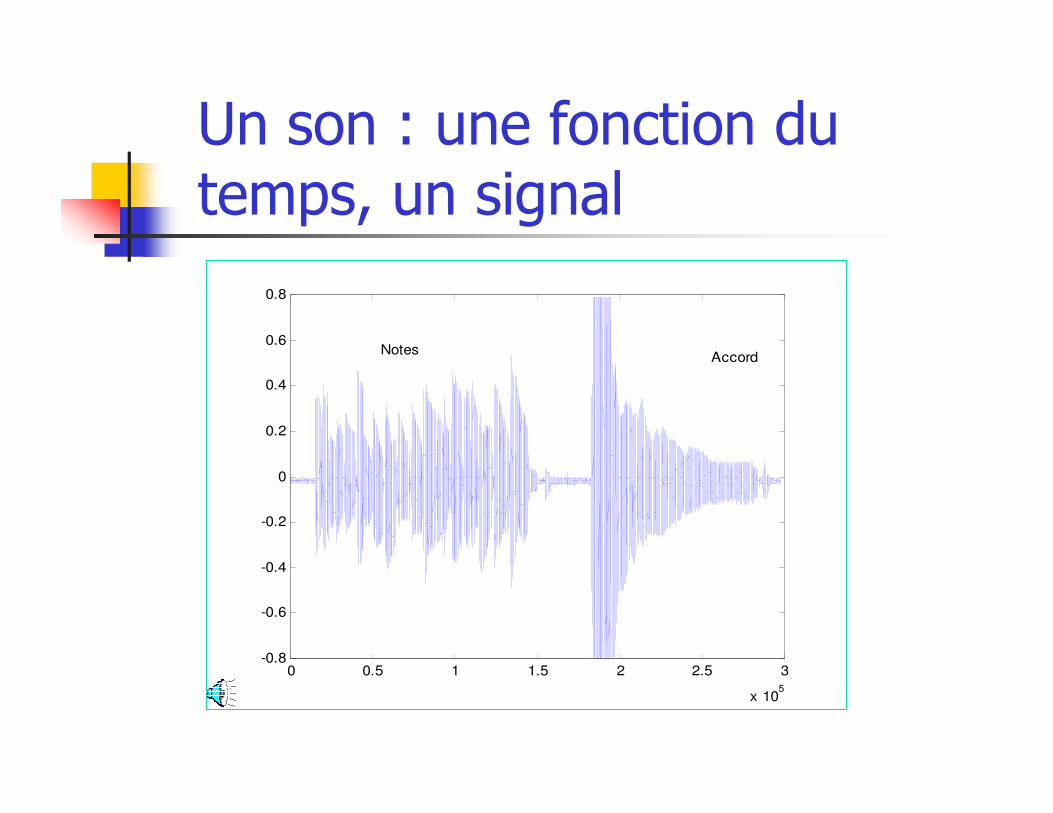
Un son : une fonction du temps, un signal
0 0.5 1 1.5 2 2.5 3
x 105
-0.8
-0.6
-0.4
-0.2
0
0.2
0.4
0.6
0.8
Notes Accord
Des ondelettes, pourquoi ?
La partition décompose la musique en « atomes » ou notes situés en
� Hauteur (do, ré, mi, etc…)
� Durée (ronde, blanche, noire, croche, etc…)
� Position dans le temps (barres de mesure)
c’est une analyse
La partition permet au musicien de reproduire la musique
c’est la synthèse
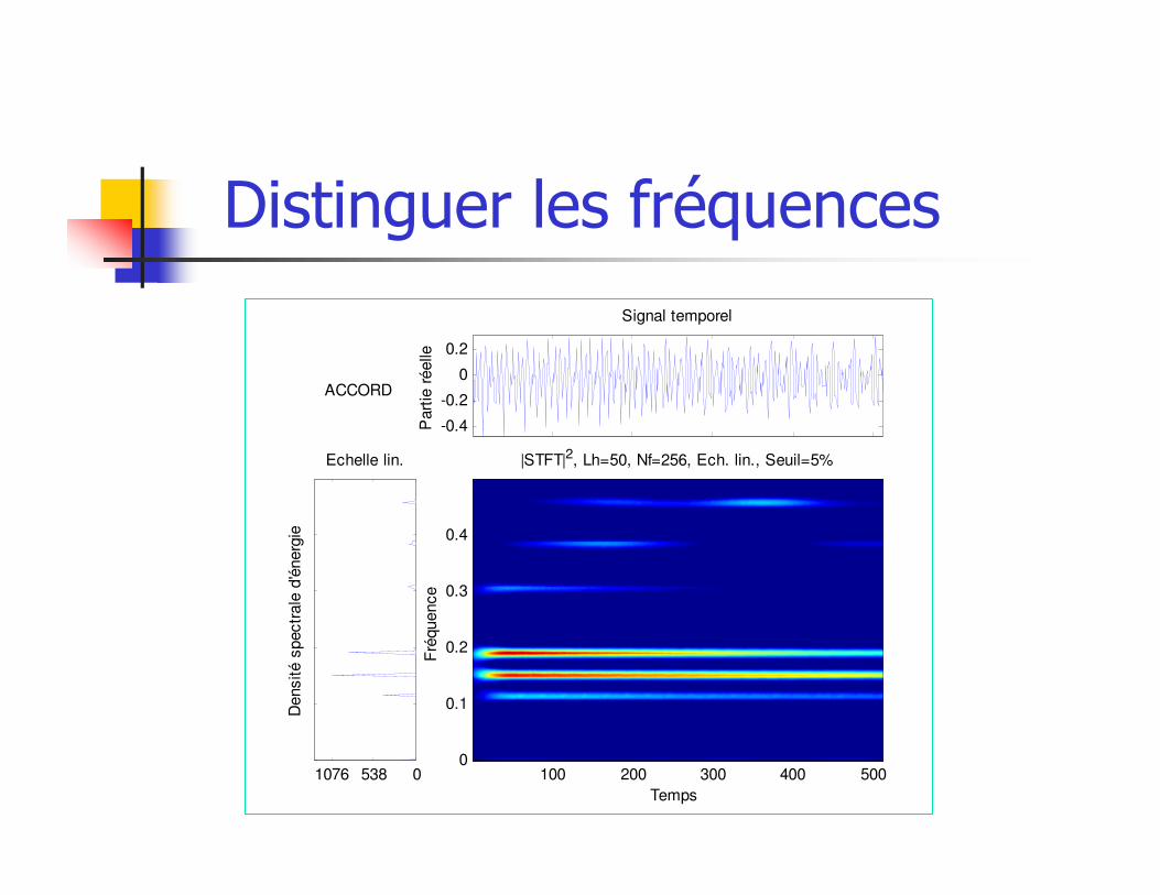
Distinguer les fréquences
-0.4
-0.2
0
0.2
Part
ie r
éelle
Signal temporel
05381076
Echelle lin.
Densité s
pectr
ale
d'é
nerg
ie
|STFT|2, Lh=50, Nf=256, Ech. lin., Seuil=5%
Temps
Fré
quence
100 200 300 400 5000
0.1
0.2
0.3
0.4
ACCORD
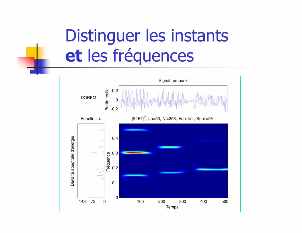
Distinguer les instants et les fréquences
-0.2
0
0.2
Part
ie r
éelle
Signal temporel
072143
Echelle lin.
Densité s
pectr
ale
d'é
nerg
ie
|STFT|2, Lh=50, Nf=256, Ech. lin., Seuil=5%
Temps
Fré
quence
100 200 300 400 5000
0.1
0.2
0.3
0.4
DOREMI
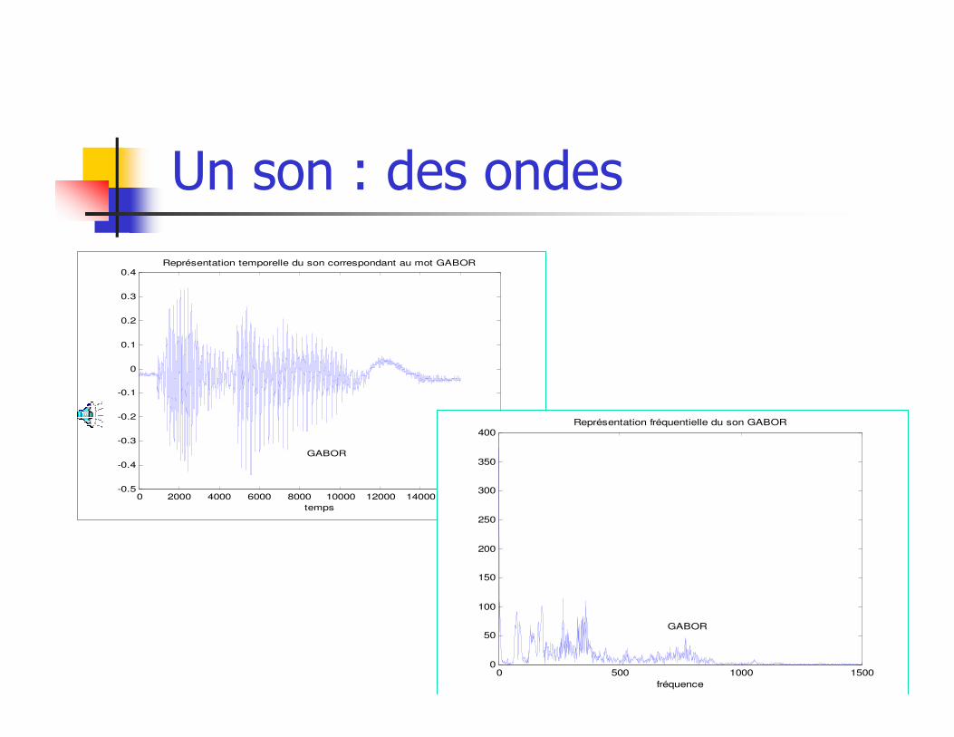
Un son : des ondes
0 2000 4000 6000 8000 10000 12000 14000 16000 18000-0.5
-0.4
-0.3
-0.2
-0.1
0
0.1
0.2
0.3
0.4Représentation temporelle du son correspondant au mot GABOR
temps
GABOR
0 500 1000 15000
50
100
150
200
250
300
350
400Représentation fréquentielle du son GABOR
fréquence
GABOR
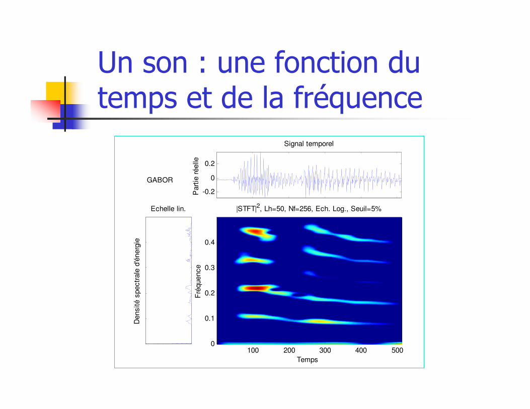
Un son : une fonction du temps et de la fréquence
-0.2
0
0.2
Part
ie r
éelle
Signal temporel
Echelle lin.
Densité s
pectr
ale
d'é
nerg
ie
|STFT|2, Lh=50, Nf=256, Ech. Log., Seuil=5%
Temps
Fré
quence
100 200 300 400 5000
0.1
0.2
0.3
0.4
GABOR
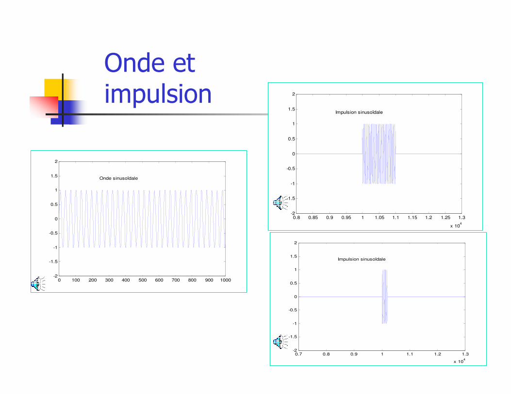
Onde et impulsion
0 100 200 300 400 500 600 700 800 900 1000-2
-1.5
-1
-0.5
0
0.5
1
1.5
2
Onde sinusoïdale
0.8 0.85 0.9 0.95 1 1.05 1.1 1.15 1.2 1.25 1.3
x 104
-2
-1.5
-1
-0.5
0
0.5
1
1.5
2
Impulsion sinusoïdale
0.7 0.8 0.9 1 1.1 1.2 1.3
x 104
-2
-1.5
-1
-0.5
0
0.5
1
1.5
2
Impulsion sinusoïdale
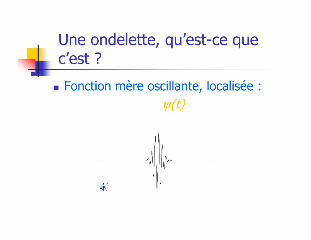
Une ondelette, qu’est-ce que c’est ?
� Fonction mère oscillante, localisée :
ψ(t)
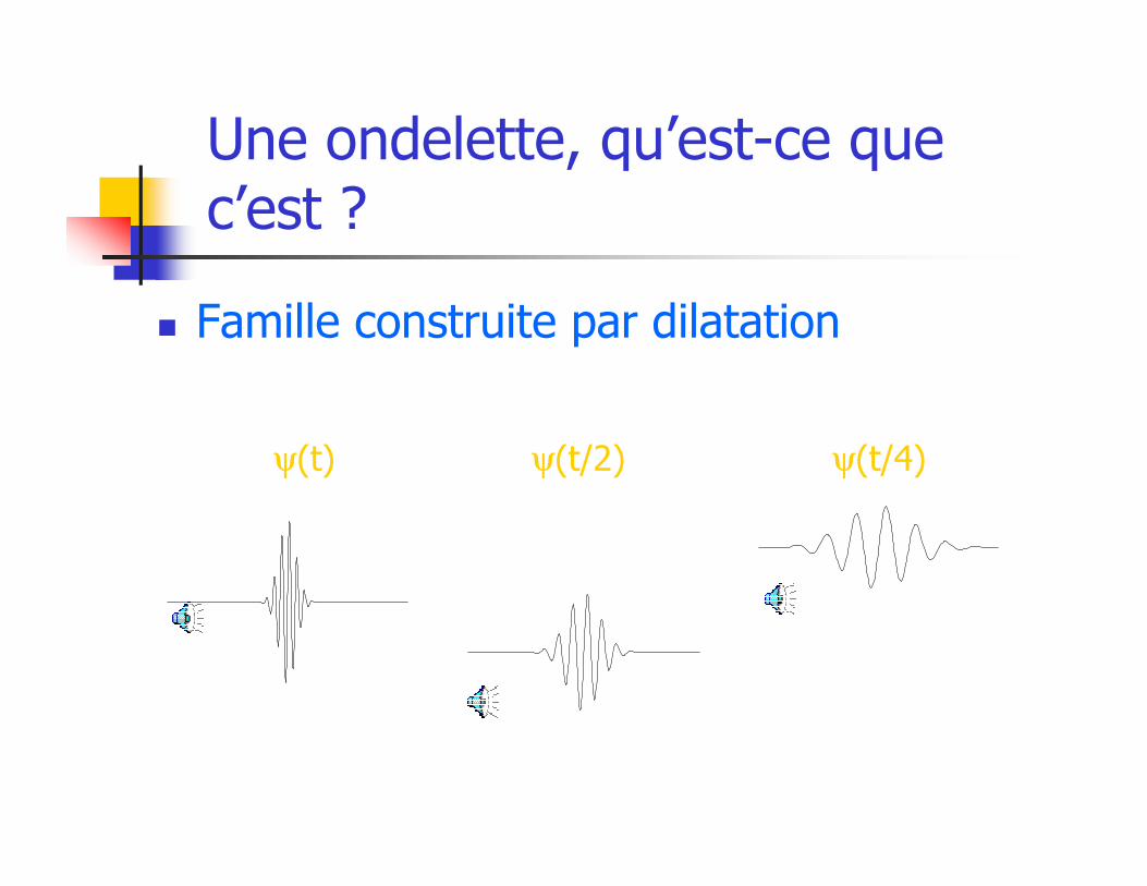
Une ondelette, qu’est-ce que c’est ?
� Famille construite par dilatation
ψ(t) ψ(t/2) ψ(t/4)
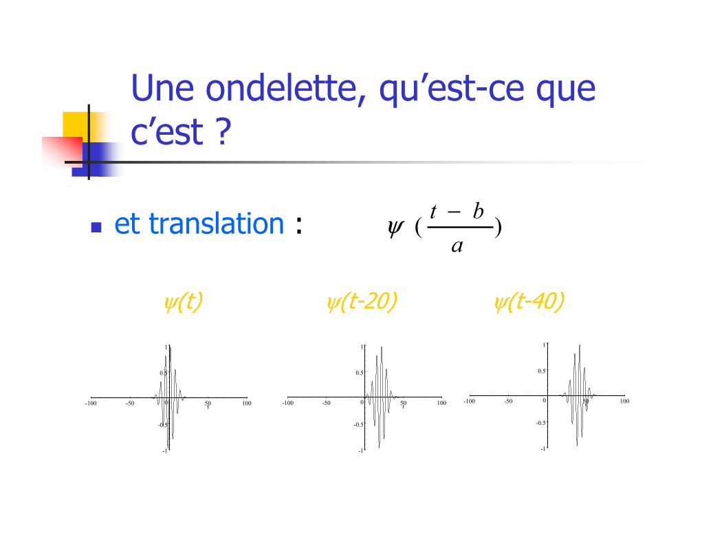
Une ondelette, qu’est-ce que c’est ?
� et translation :
ψ(t) ψ(t-20) ψ(t-40)
-1
-0.5
0
0.5
1
-100 -50 50 100t
-1
-0.5
0
0.5
1
-100 -50 50 100t
-1
-0.5
0
0.5
1
-100 -50 50 100t
)(a
bt −ψ
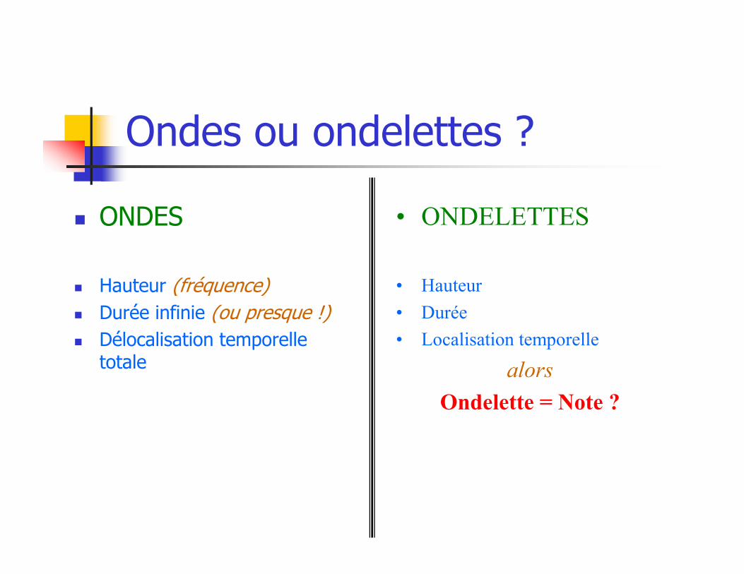
Ondes ou ondelettes ?
� ONDES
� Hauteur (fréquence)
� Durée infinie (ou presque !)
� Délocalisation temporelle totale
• ONDELETTES
• Hauteur
• Durée
• Localisation temporelle
alors
Ondelette = Note ?
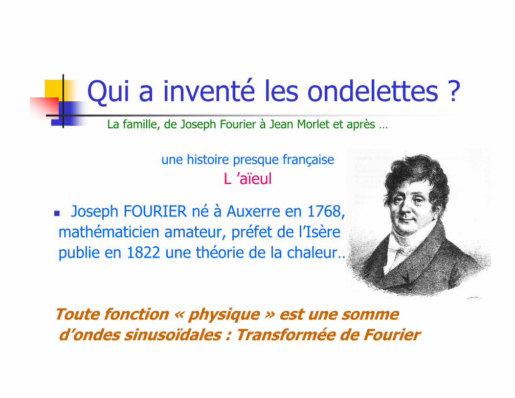
Qui a inventé les ondelettes ?La famille, de Joseph Fourier à Jean Morlet et après …
une histoire presque française
L ’aïeul
� Joseph FOURIER né à Auxerre en 1768,
mathématicien amateur, préfet de l’Isère
publie en 1822 une théorie de la chaleur…
Toute fonction « physique » est une sommed’ondes sinusoïdales : Transformée de Fourier
Qui a inventé les ondelettes ?
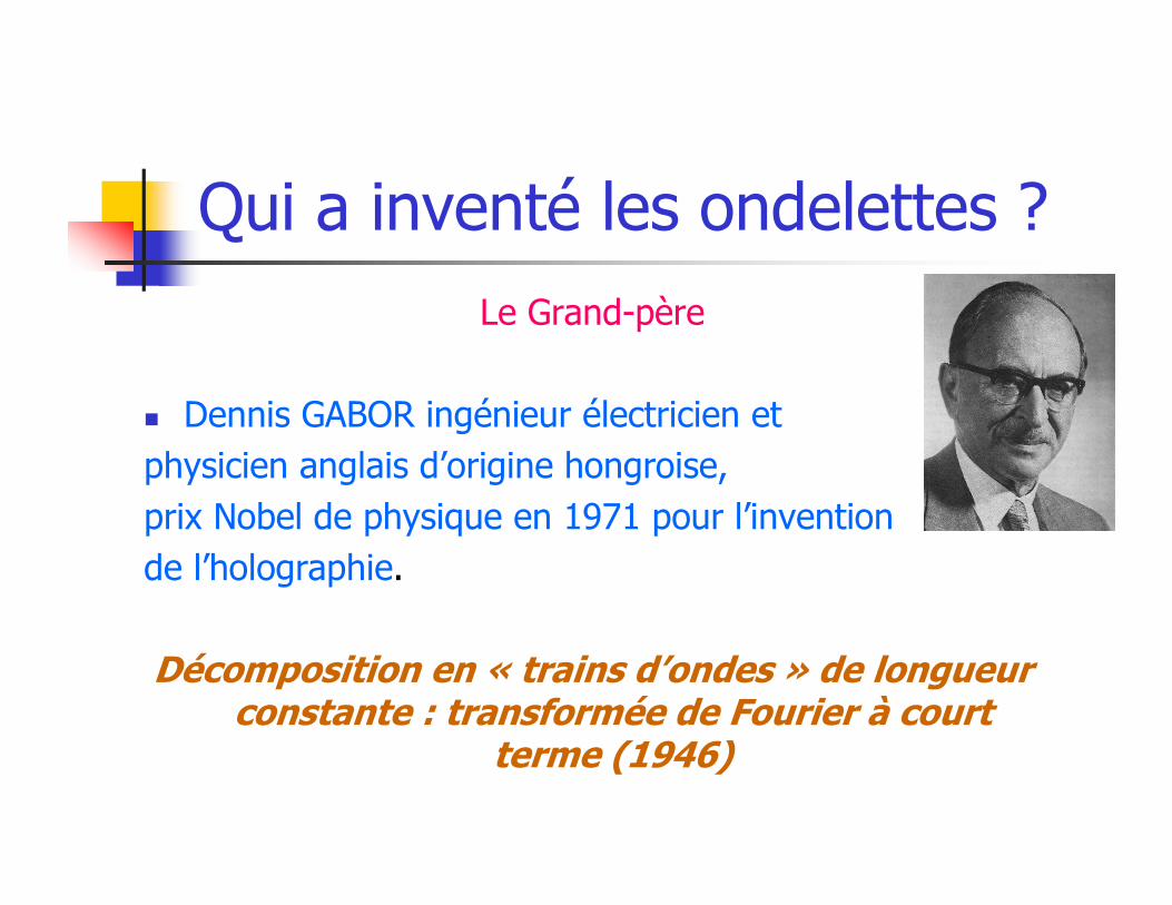
Le Grand-père
� Dennis GABOR ingénieur électricien et
physicien anglais d’origine hongroise,
prix Nobel de physique en 1971 pour l’invention
de l’holographie.
Décomposition en « trains d’ondes » de longueur constante : transformée de Fourier à court
terme (1946)
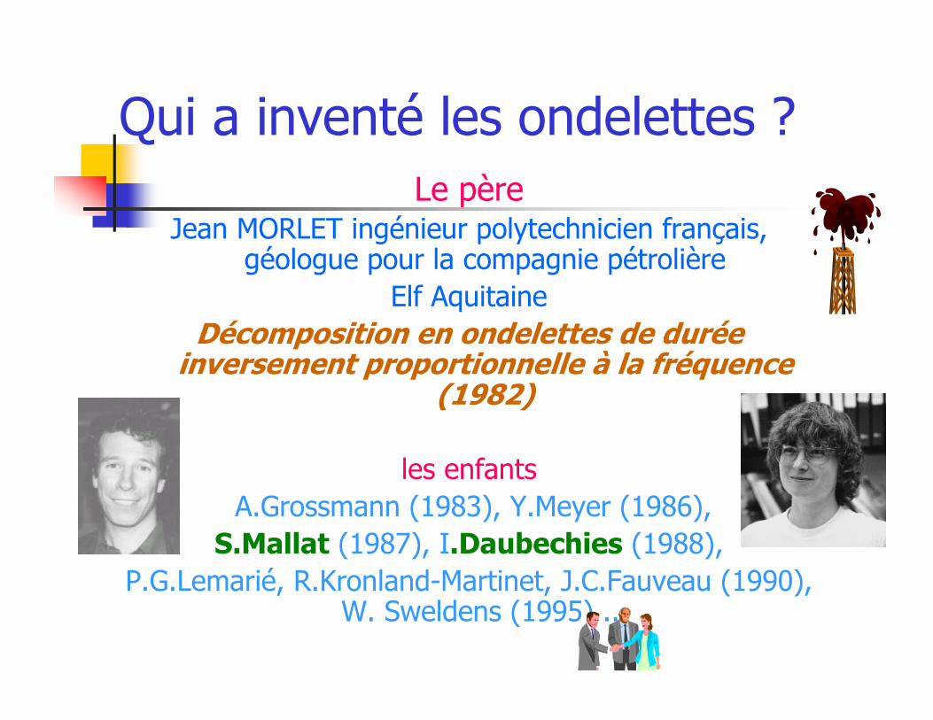
Le pèreJean MORLET ingénieur polytechnicien français,
géologue pour la compagnie pétrolière
Elf Aquitaine
Décomposition en ondelettes de durée inversement proportionnelle à la fréquence
(1982)
les enfants
A.Grossmann (1983), Y.Meyer (1986),
S.Mallat (1987), I.Daubechies (1988),
P.G.Lemarié, R.Kronland-Martinet, J.C.Fauveau (1990), W. Sweldens (1995) ...
Qui a inventé les ondelettes ?
Deuxième partie: un peu plus de rigueur …
… et de mathématiques
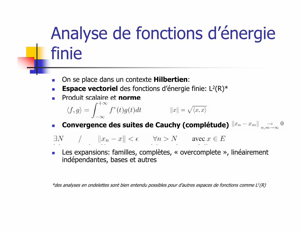
Analyse de fonctions d’énergie finie
� On se place dans un contexte Hilbertien:
� Espace vectoriel des fonctions d’énergie finie: L2(R)*
� Produit scalaire et norme
� Convergence des suites de Cauchy (complétude)
� Les expansions: familles, complètes, « overcomplete », linéairement indépendantes, bases et autres
*des analyses en ondelettes sont bien entendu possibles pour d’autres espaces de fonctions comme L1(R)
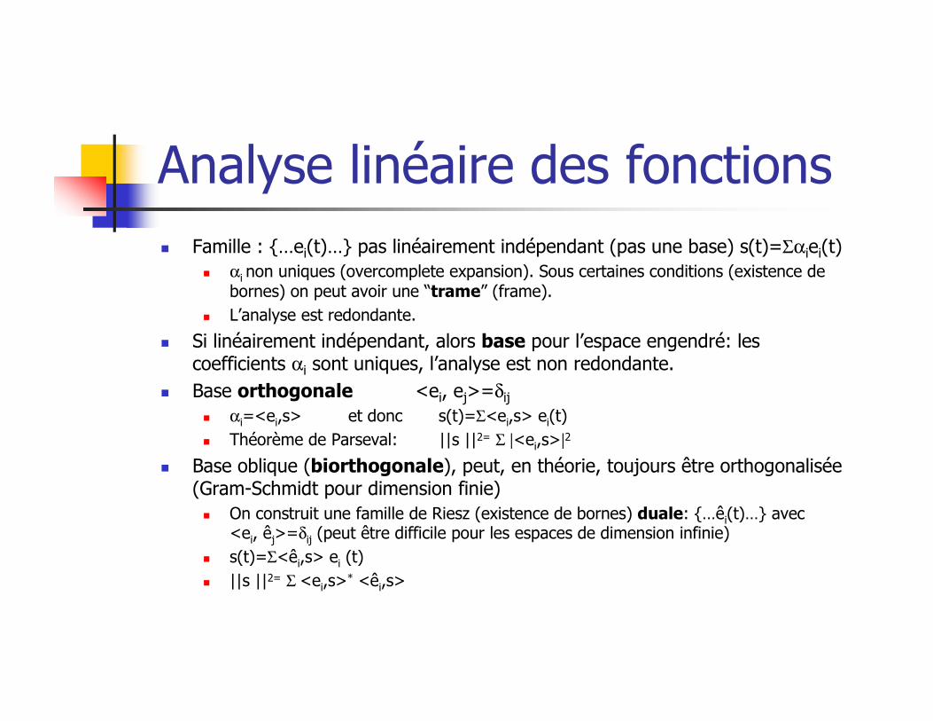
Analyse linéaire des fonctions
� Famille : {…ei(t)…} pas linéairement indépendant (pas une base) s(t)=Σαiei(t)� αi non uniques (overcomplete expansion). Sous certaines conditions (existence de
bornes) on peut avoir une “trame” (frame).
� L’analyse est redondante.
� Si linéairement indépendant, alors base pour l’espace engendré: les coefficients αi sont uniques, l’analyse est non redondante.
� Base orthogonale <ei, ej>=δij� αi=<ei,s> et donc s(t)=Σ<ei,s> ei(t)
� Théorème de Parseval: ||s ||2= Σ |<ei,s>|2
� Base oblique (biorthogonale), peut, en théorie, toujours être orthogonalisée(Gram-Schmidt pour dimension finie)
� On construit une famille de Riesz (existence de bornes) duale: {…êi(t)…} avec <ei, êj>=δij (peut être difficile pour les espaces de dimension infinie)
� s(t)=Σ<êi,s> ei (t)
� ||s ||2= Σ <ei,s>* <êi,s>
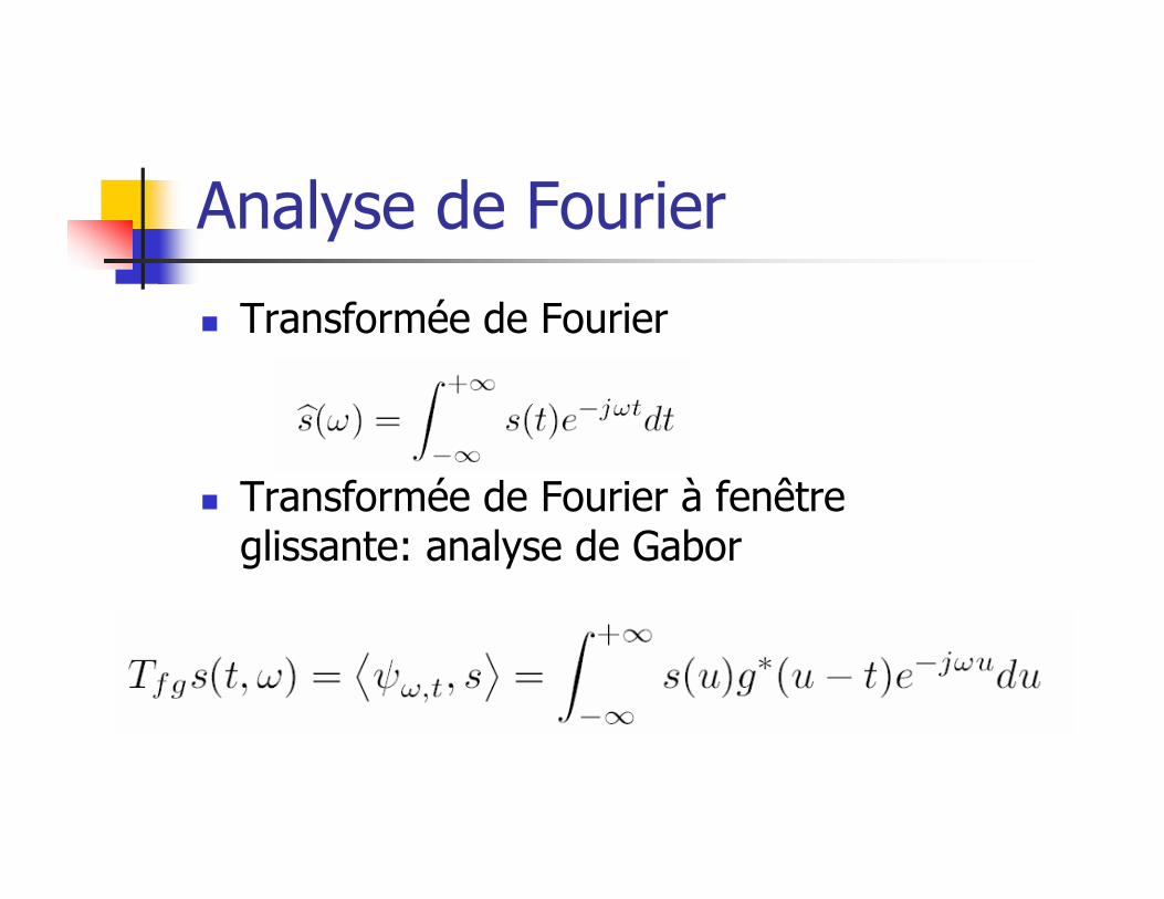
Analyse de Fourier
� Transformée de Fourier
� Transformée de Fourier à fenêtre glissante: analyse de Gabor
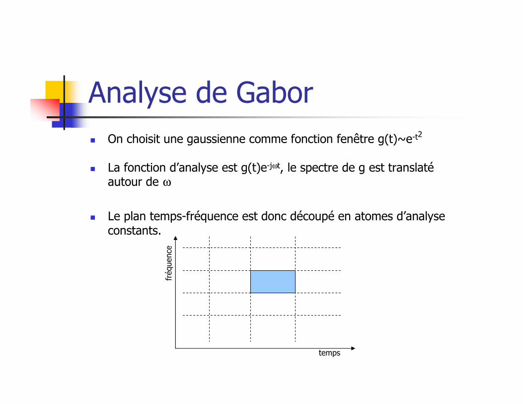
Analyse de Gabor
� On choisit une gaussienne comme fonction fenêtre g(t)~e-t2
� La fonction d’analyse est g(t)e-jωt, le spectre de g est translatéautour de ω
� Le plan temps-fréquence est donc découpé en atomes d’analyseconstants.
temps
fréquence
Ondelettes
� Transformée en ondelettes
� Inversion
� Condition d’admissibilité
� Régularité et moments nuls (CN-1 si N moments
nuls, …)
Ondelettes
Conditions pour parler d’analyse en ondelettes:
� Une ou plusieurs fonctions mères qui engendrent par dilatation (analyse à Q constant) et translation la famille des ondelettes
� Reconstruction possible (condition d’admissibilité)
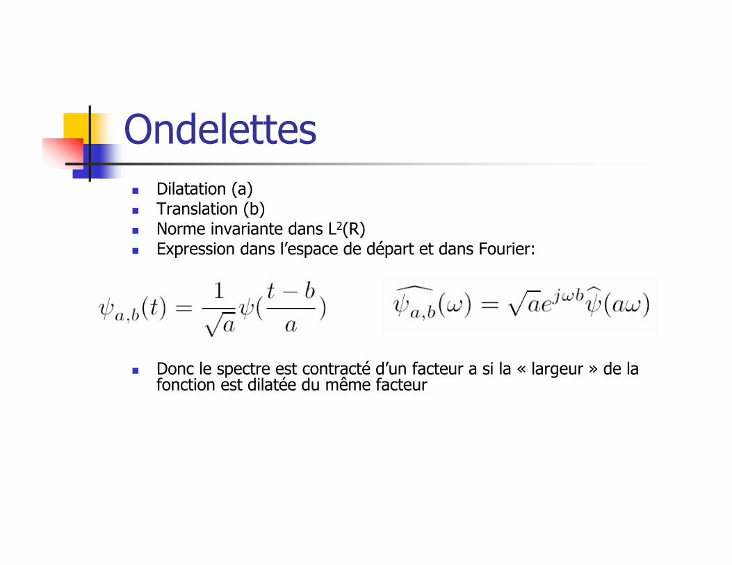
Ondelettes� Dilatation (a)� Translation (b)� Norme invariante dans L2(R)� Expression dans l’espace de départ et dans Fourier:
� Donc le spectre est contracté d’un facteur a si la « largeur » de la fonction est dilatée du même facteur
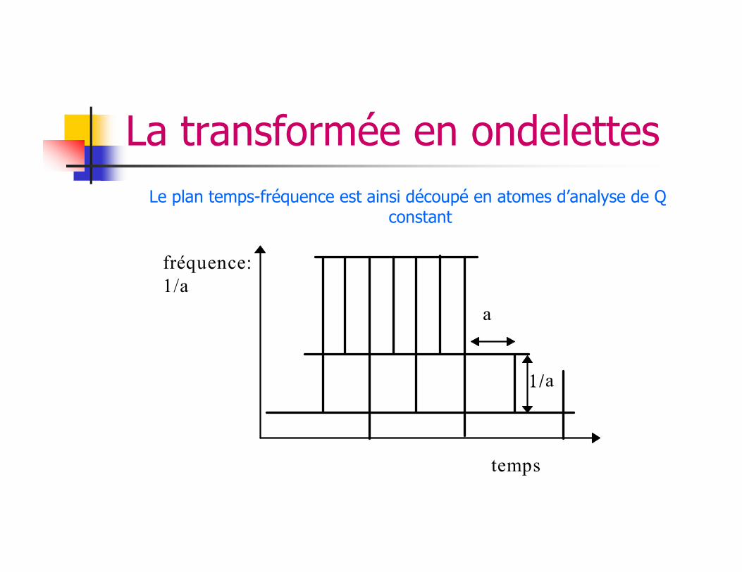
La transformée en ondelettes
Le plan temps-fréquence est ainsi découpé en atomes d’analyse de Q constant
1/a
a
temps
fréquence:
1/a
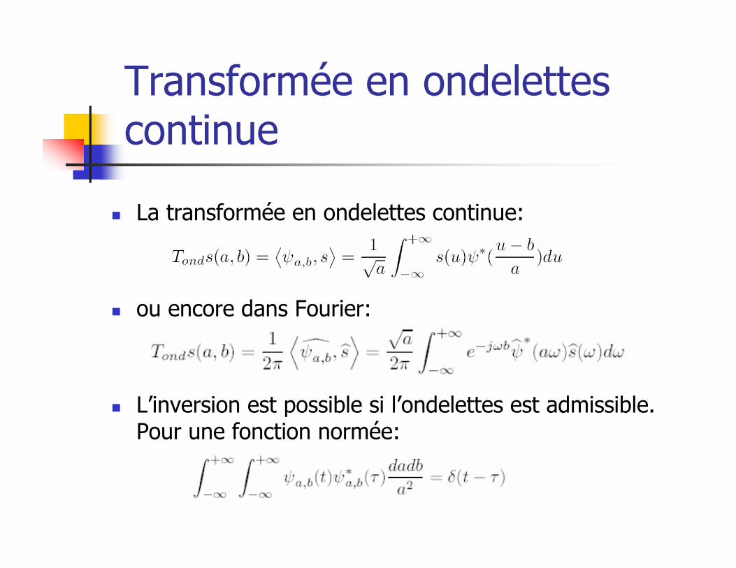
Transformée en ondelettes continue
� La transformée en ondelettes continue:
� ou encore dans Fourier:
� L’inversion est possible si l’ondelettes est admissible. Pour une fonction normée:
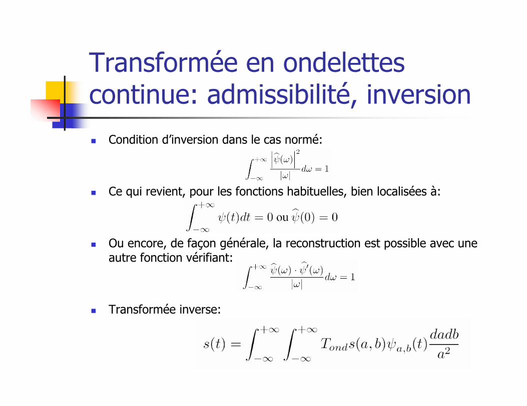
Transformée en ondelettes continue: admissibilité, inversion
� Condition d’inversion dans le cas normé:
� Ce qui revient, pour les fonctions habituelles, bien localisées à:
� Ou encore, de façon générale, la reconstruction est possible avec une autre fonction vérifiant:
� Transformée inverse:
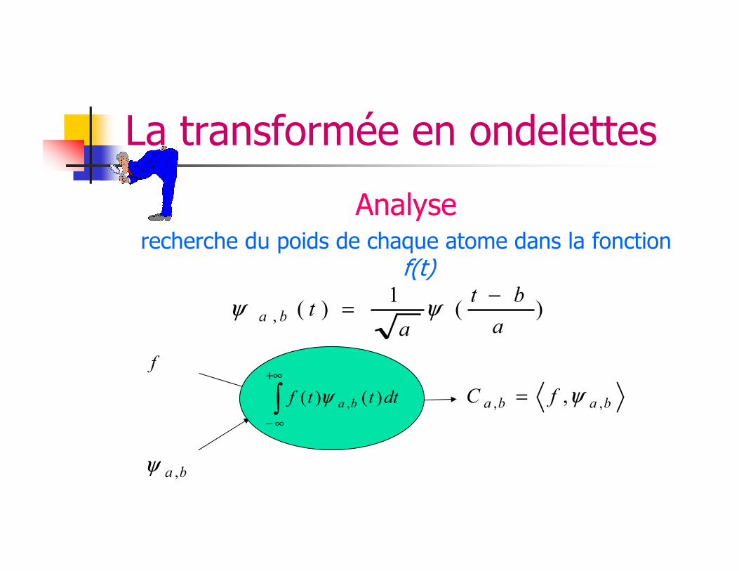
La transformée en ondelettes
Analyserecherche du poids de chaque atome dans la fonction
f(t)
)(1
)(,a
bt
atba
−= ψψ
baba fC ,, ,ψ=
ba ,ψ
f
∫+∞
∞−
dtttf ba )()( ,ψ
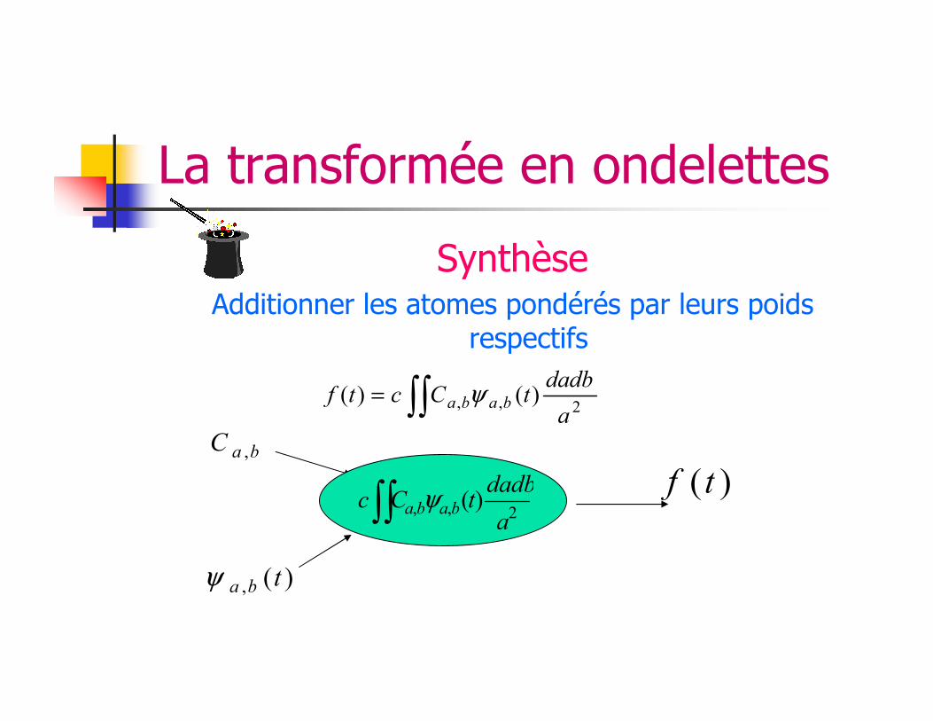
La transformée en ondelettes
SynthèseAdditionner les atomes pondérés par leurs poids
respectifs
∫∫=2,, )()(
a
dadbtCctf baba ψ
baC ,
)(, tbaψ
)(tf∫∫ 2,, )(
a
dadbtCc baba ψ
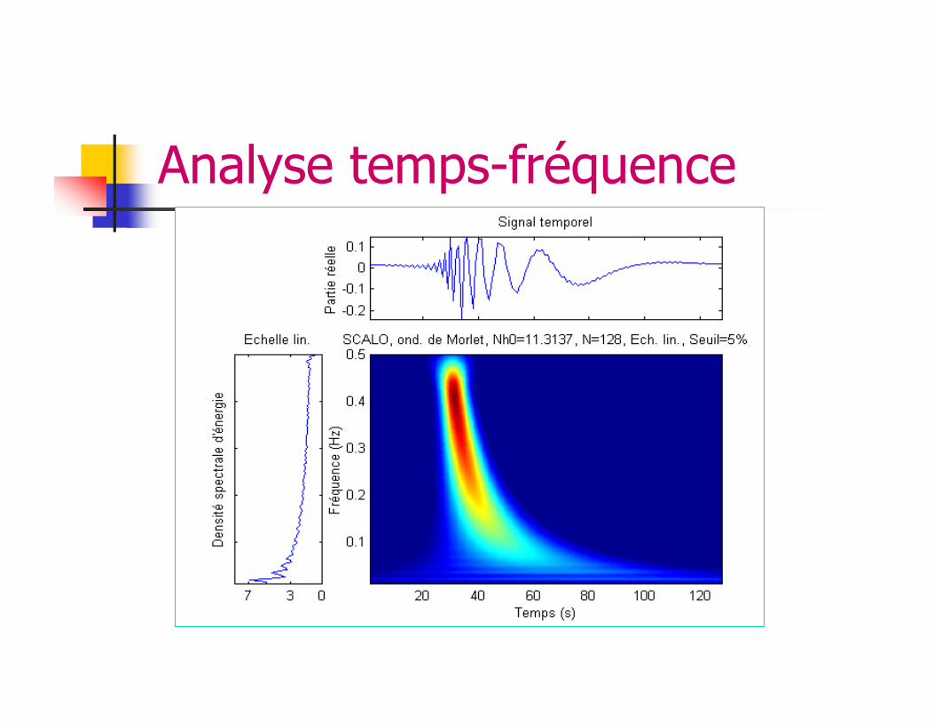
Analyse temps-fréquence
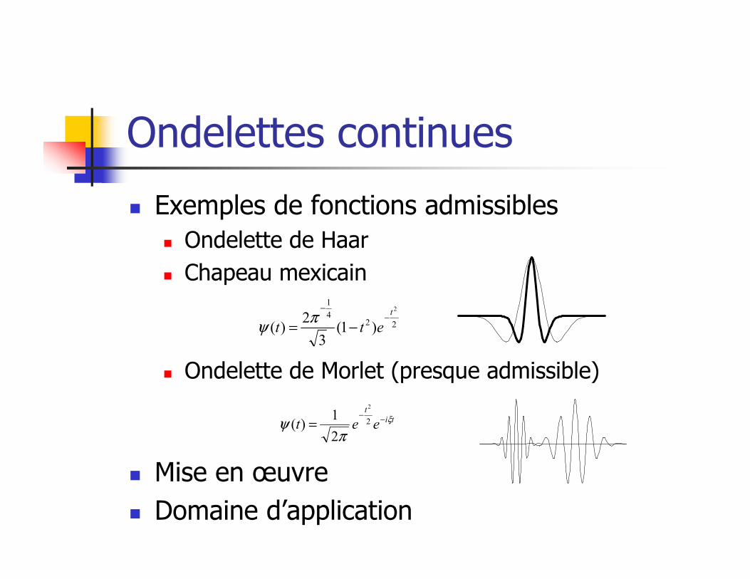
Ondelettes continues
� Exemples de fonctions admissibles� Ondelette de Haar
� Chapeau mexicain
� Ondelette de Morlet (presque admissible)
� Mise en œuvre
� Domaine d’application
ti
t
eet ξ
πψ −−
= 2
2
2
1)(
224
12
)1(3
2)(
t
ett−
−
−=π
ψ
Transformations bilinéaires
Transformations de la classe de Cohen
� Spectrogramme ( carré du module de la STFT): non inversible
� Scalogramme (carré du module de la TO): non inversible
� Wigner-Ville (TF de la « corrélation instantanée »): inversible, mais termes d’intermodulation…
� Pseudo Wigner-Ville
Peu utilisées pour les signaux multidimensionnels
Analyse discrète en ondelettes
� Discrétisation et dépendance translation-dilatation
� Pavage du plan temps-fréquence
Analyse en ondelettes discrète
� Cas général
� Bases dyadiques et autres
� Bases orthogonales
� Bases biorthogonales
� Trames
Analyse multirésolution de Mallat
� Formalisme de base
� Bases orthogonales
� Bases obliques: biorthogonales
� Lifting scheme
� Algorithmes non décimés
� Analyses non-dyadiques
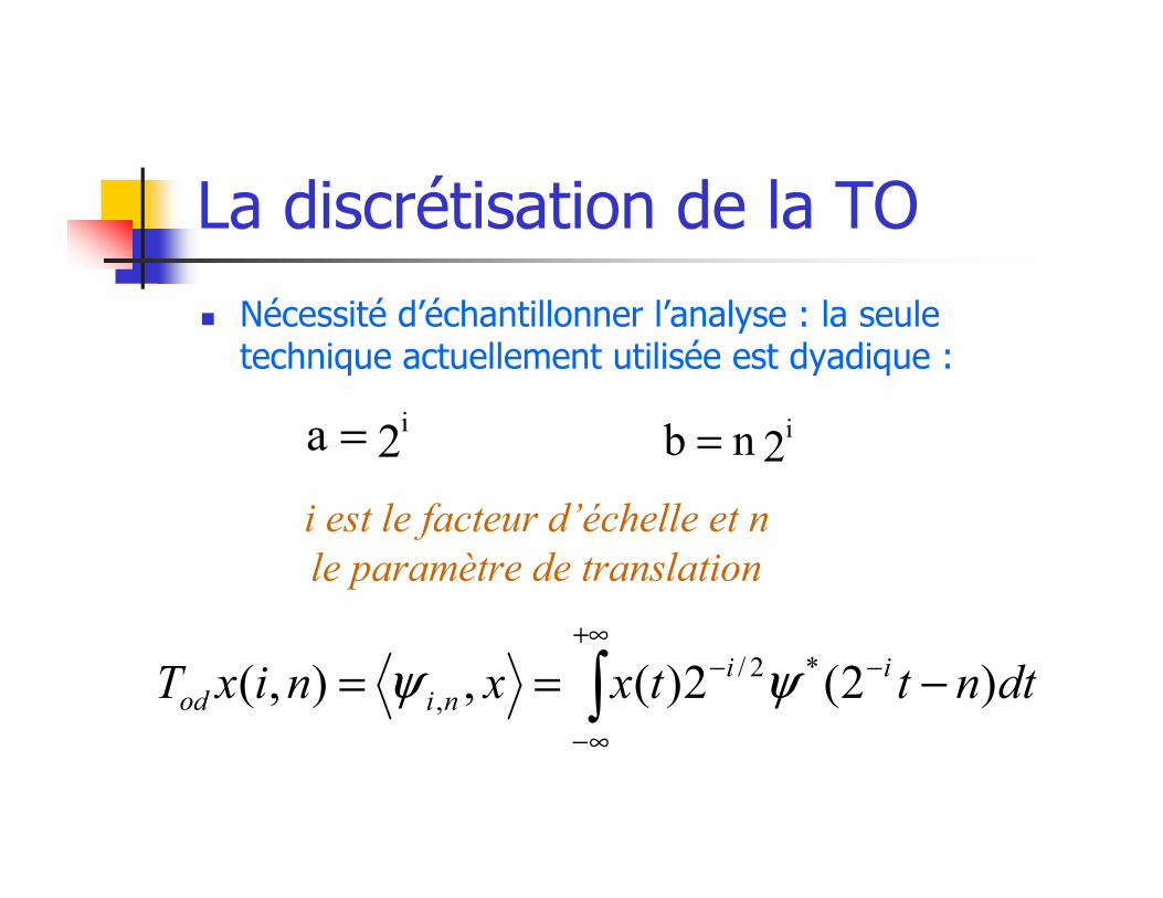
La discrétisation de la TO
� Nécessité d’échantillonner l’analyse : la seule technique actuellement utilisée est dyadique :
2a i= 2nb i=
i est le facteur d’échelle et n
le paramètre de translation
∫+∞
∞−
−− −== dtnttxxnixT ii
niod )2(2)(,),( *2/
, ψψ
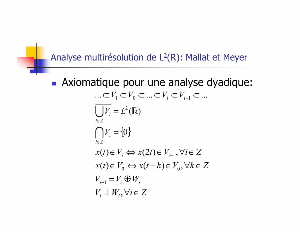
Analyse multirésolution de L2(R): Mallat et Meyer
� Axiomatique pour une analyse dyadique:
{ }
ZiWV
WVV
ZkVktxVtx
ZiVtxVtx
V
LV
VVVV
ii
iii
ii
Zi
i
Zi
i
ii
∈∀⊥
⊕=
∈∀∈−⇔∈
∈∀∈⇔∈
=
=
⊂⊂⊂⊂⊂⊂
−
−
∈
∈
−
,
,)()(
,)2()(
0
)(
.........
1
00
1
2
101
I
U R
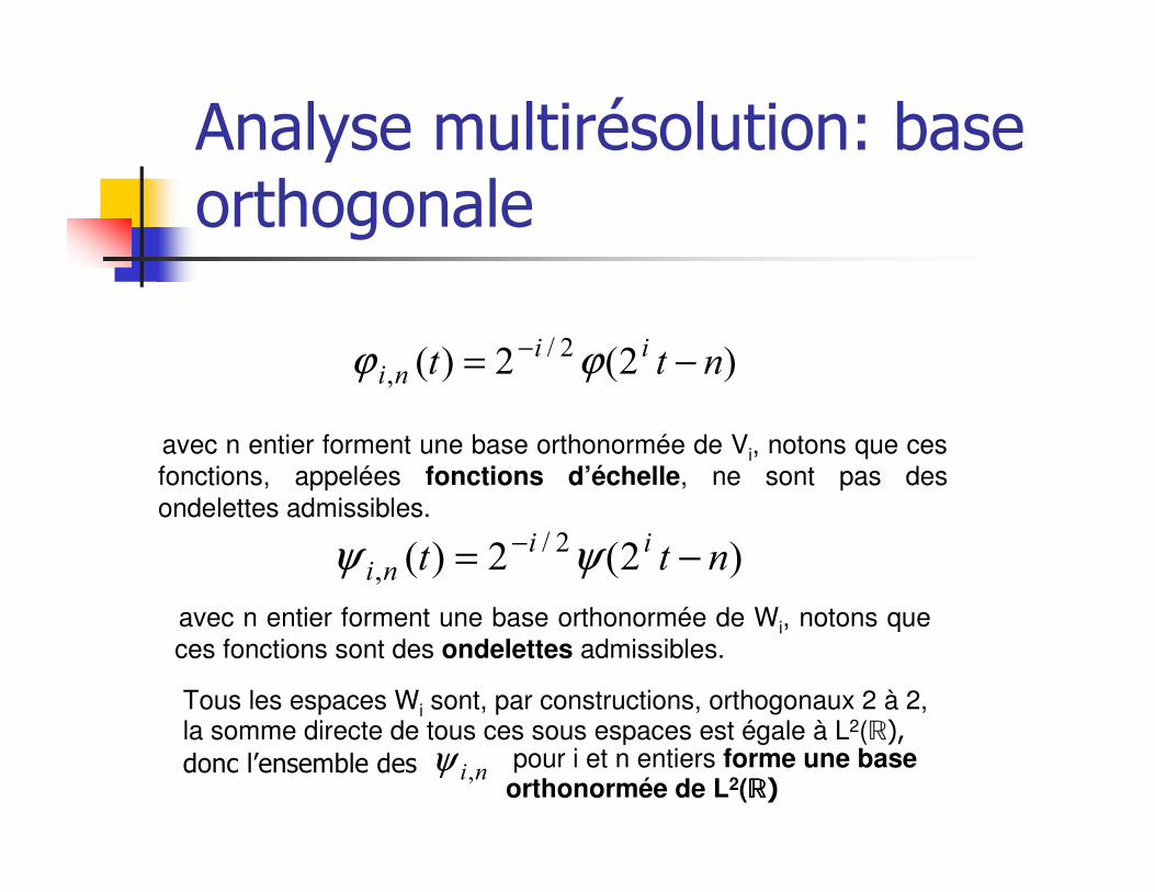
Analyse multirésolution: base orthogonale
)2(2)( 2/, ntt iini −= − ϕϕ
avec n entier forment une base orthonormée de Vi, notons que ces
fonctions, appelées fonctions d’échelle, ne sont pas des
ondelettes admissibles.
)2(2)( 2/, ntt iini −= − ψψ
avec n entier forment une base orthonormée de Wi, notons que
ces fonctions sont des ondelettes admissibles.
Tous les espaces Wi sont, par constructions, orthogonaux 2 à 2, la somme directe de tous ces sous espaces est égale à L2(R), donc l’ensemble des ni,ψ pour i et n entiers forme une base
orthonormée de L2(RRRR)
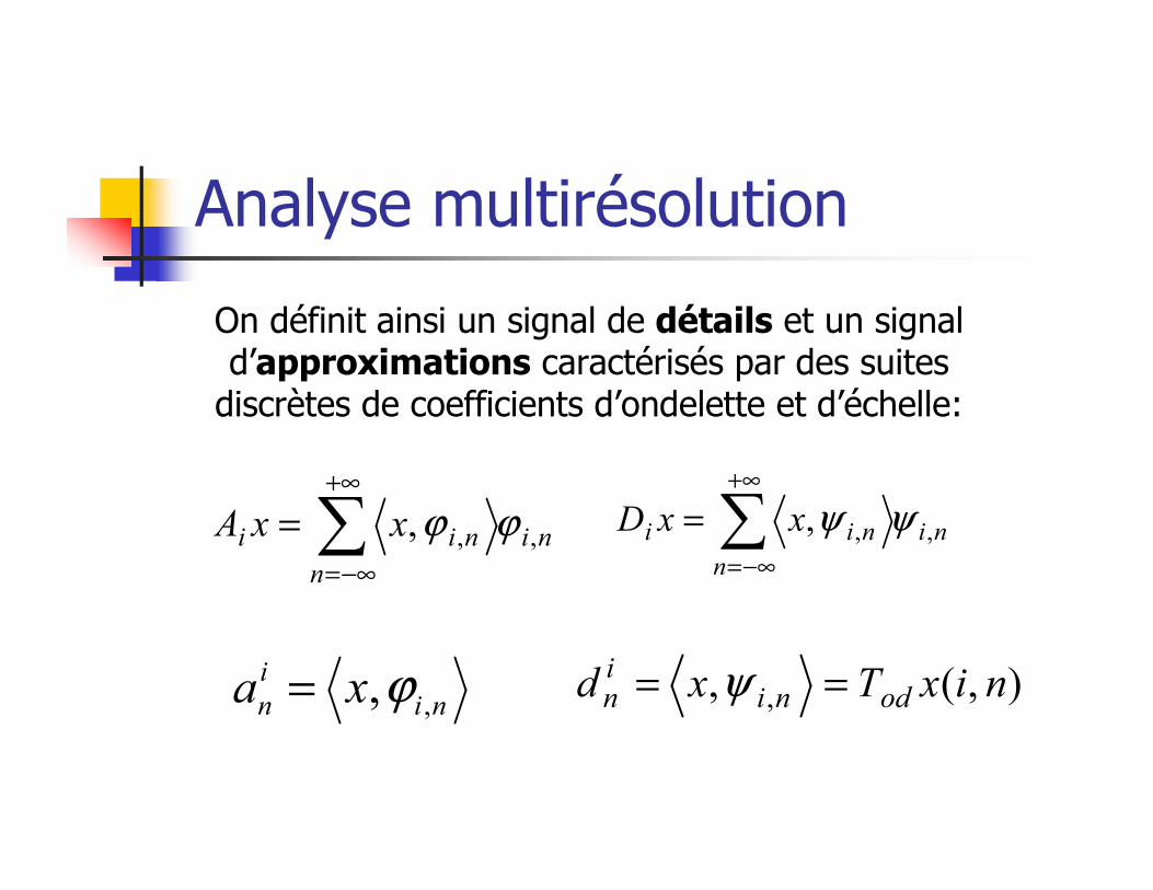
Analyse multirésolution
ni
n
nii xxA ,,, ϕϕ∑+∞
−∞=
= ni
n
nii xxD ,,, ψψ∑+∞
−∞=
=
ni
i
n xa ,,ϕ= ),(, , nixTxd odniin == ψ
On définit ainsi un signal de détails et un signal d’approximations caractérisés par des suites discrètes de coefficients d’ondelette et d’échelle:
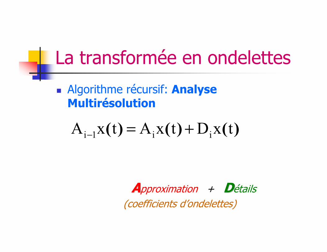
La transformée en ondelettes
� Algorithme récursif: Analyse Multirésolution
AApproximation + DDétails
(coefficients d’ondelettes)
)()()( txDtxAtxA ii1i +=−
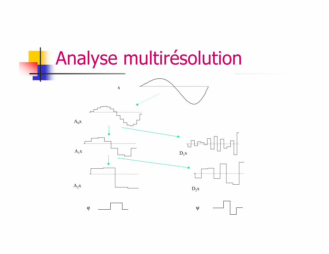
Analyse multirésolution
x
A0x
A1x D1x
A2x D2x
ϕ ψ
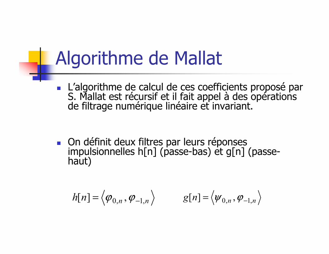
Algorithme de Mallat
� L’algorithme de calcul de ces coefficients proposé par S. Mallat est récursif et il fait appel à des opérations de filtrage numérique linéaire et invariant.
� On définit deux filtres par leurs réponses impulsionnelles h[n] (passe-bas) et g[n] (passe-haut)
nnnh ,1,0 ,][ −= ϕϕ nnng ,1,0 ,][ −= ϕψ
Algorithme de Mallat
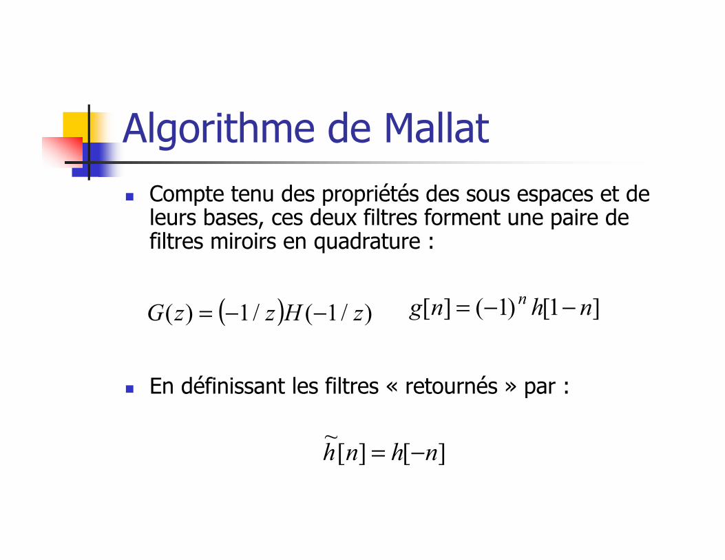
� Compte tenu des propriétés des sous espaces et de leurs bases, ces deux filtres forment une paire de filtres miroirs en quadrature :
� En définissant les filtres « retournés » par :
( ) )/1(/1)( zHzzG −−= ]1[)1(][ nhng n −−=
][][~
nhnh −=
Algorithme de Mallat
anj-1
anj
dnj
h
g
2
2
anj-1
anj
dnj
h
g
2
2
+
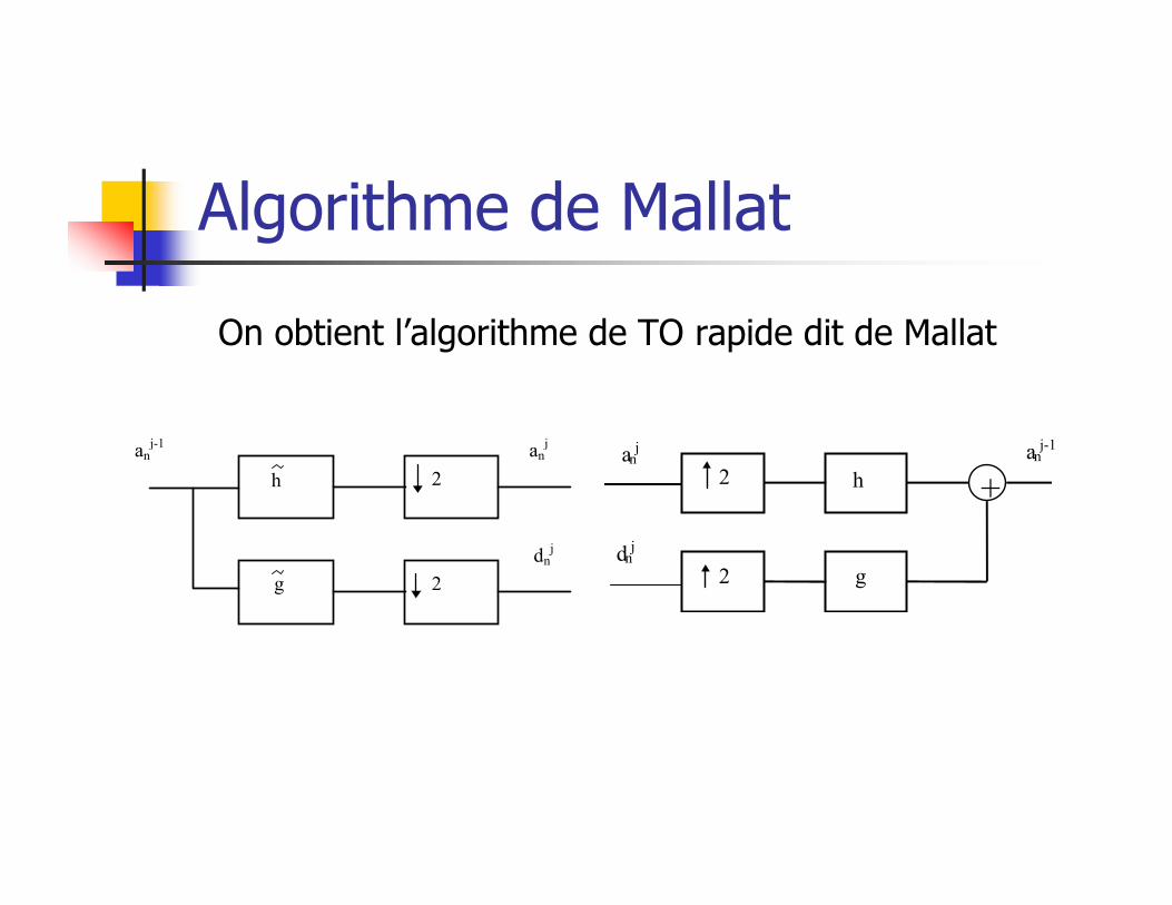
On obtient l’algorithme de TO rapide dit de Mallat
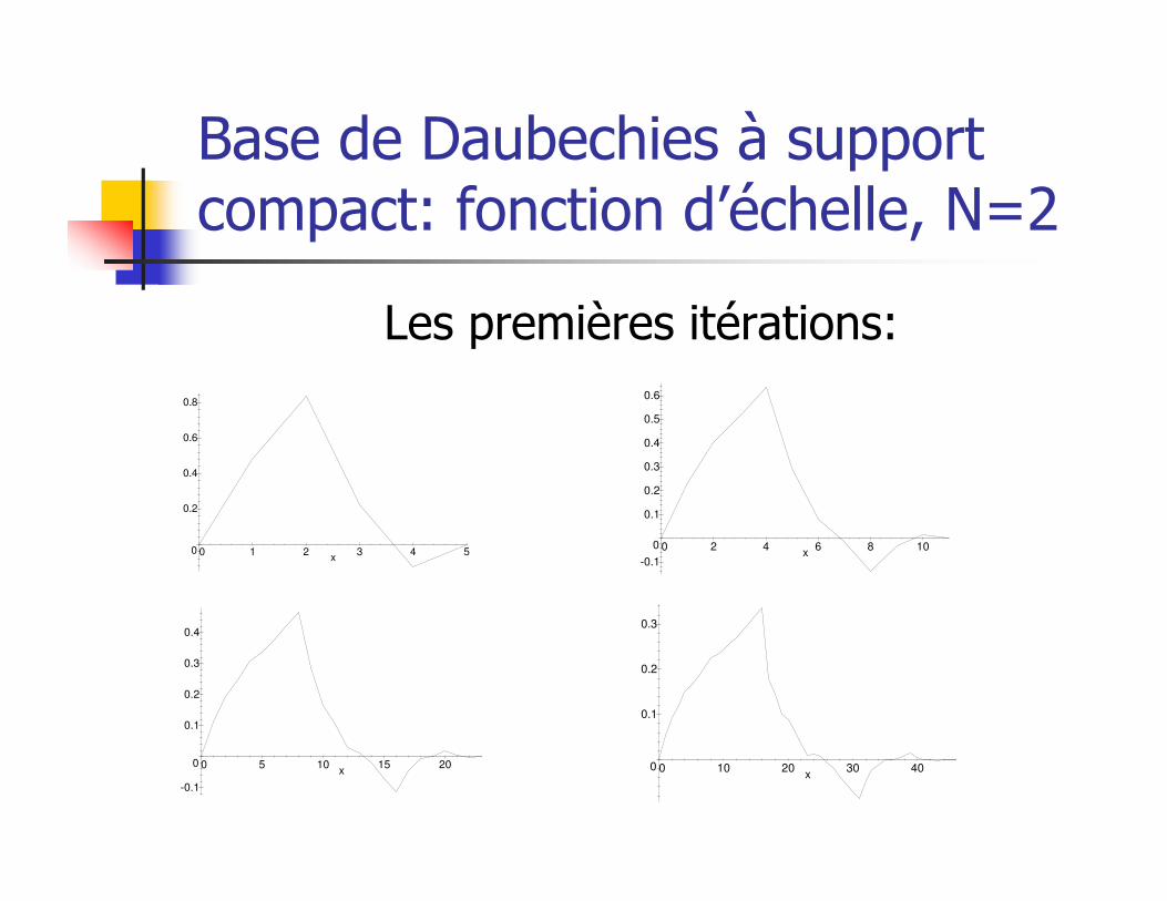
Base de Daubechies à support compact: fonction d’échelle, N=2
Les premières itérations:
x1086420
0.6
0.5
0.4
0.3
0.2
0.1
0
-0.1
x20151050
0.4
0.3
0.2
0.1
0
-0.1x
403020100
0.3
0.2
0.1
0
x543210
0.8
0.6
0.4
0.2
0
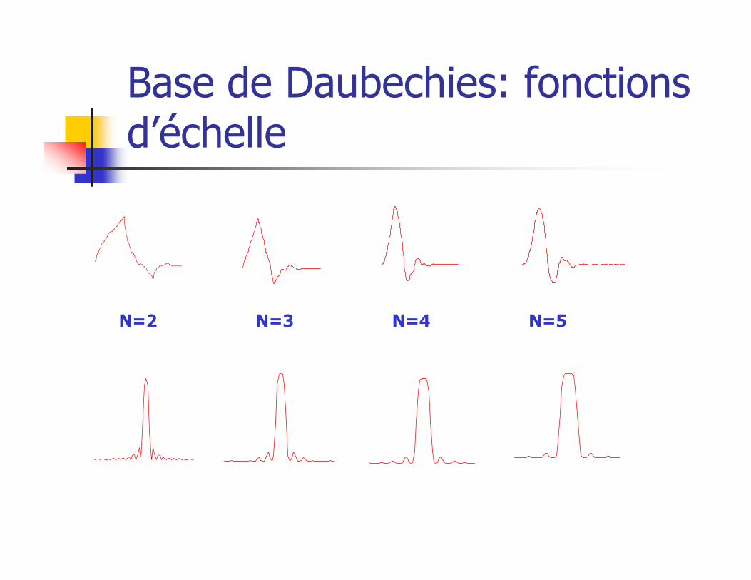
Base de Daubechies: fonctions d’échelle
N=2 N=3 N=4 N=5
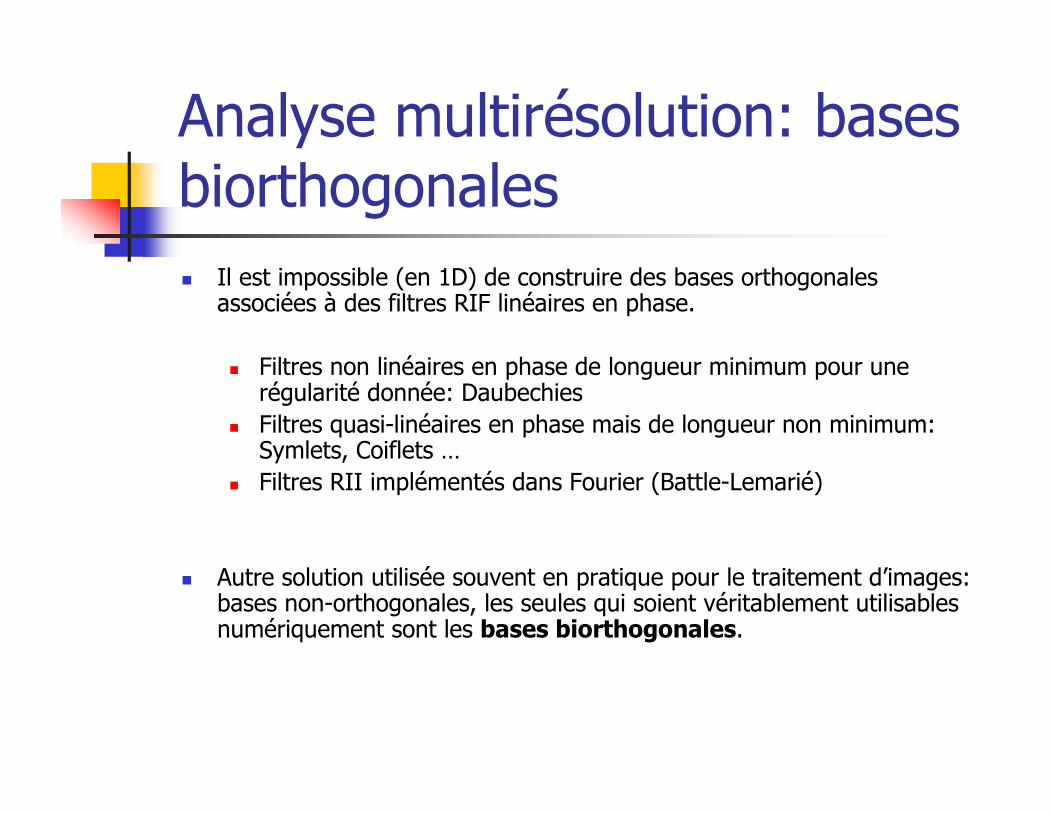
Analyse multirésolution: bases biorthogonales
� Il est impossible (en 1D) de construire des bases orthogonales associées à des filtres RIF linéaires en phase.
� Filtres non linéaires en phase de longueur minimum pour une régularité donnée: Daubechies
� Filtres quasi-linéaires en phase mais de longueur non minimum: Symlets, Coiflets …
� Filtres RII implémentés dans Fourier (Battle-Lemarié)
� Autre solution utilisée souvent en pratique pour le traitement d’images: bases non-orthogonales, les seules qui soient véritablement utilisables numériquement sont les bases biorthogonales.
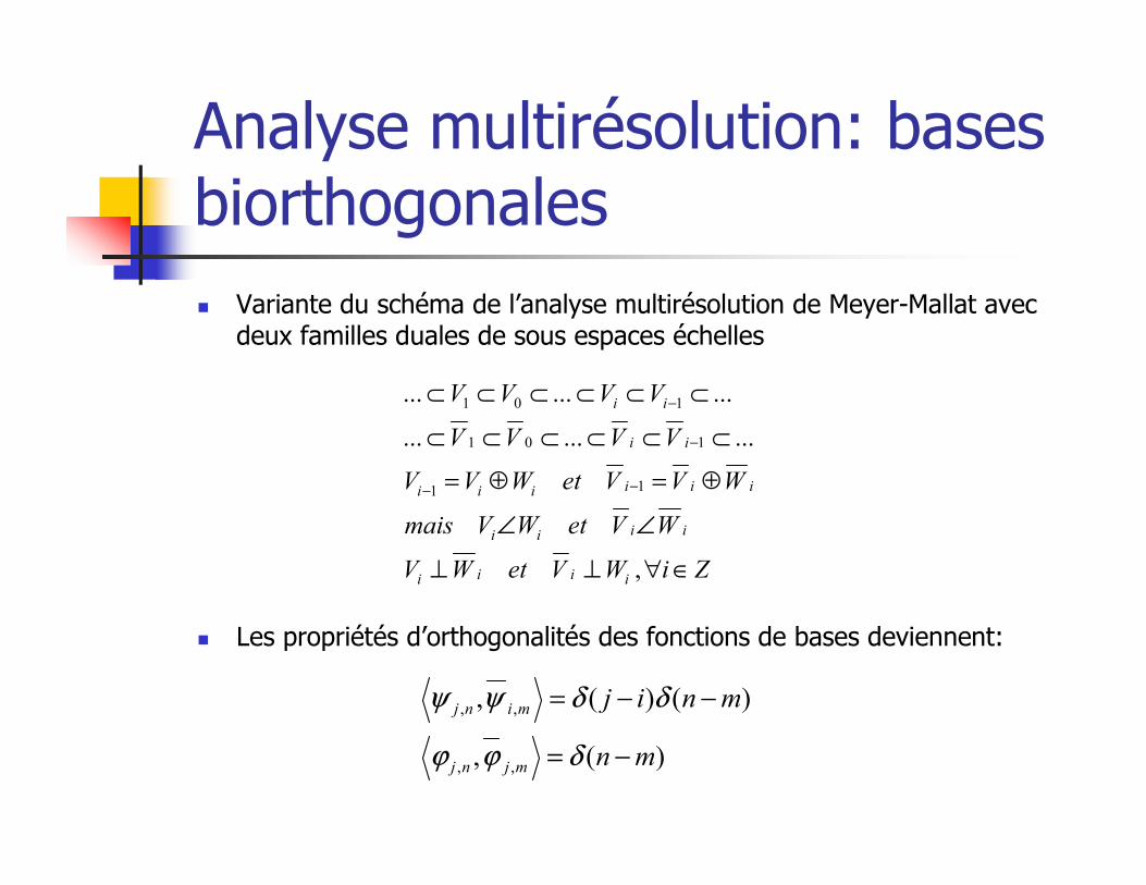
Analyse multirésolution: bases biorthogonales
� Variante du schéma de l’analyse multirésolution de Meyer-Mallat avec deux familles duales de sous espaces échelles
� Les propriétés d’orthogonalités des fonctions de bases deviennent:
ZiWVetWV
WVetWVmais
WVVetWVV
VVVV
VVVV
iiii
iiii
iiiiii
ii
ii
∈∀⊥⊥
∠∠
⊕=⊕=
⊂⊂⊂⊂⊂⊂
⊂⊂⊂⊂⊂⊂
−−
−
−
,
.........
.........
11
101
101
)(,
)()(,
,,
,,
mn
mnij
mjnj
minj
−=
−−=
δϕϕ
δδψψ
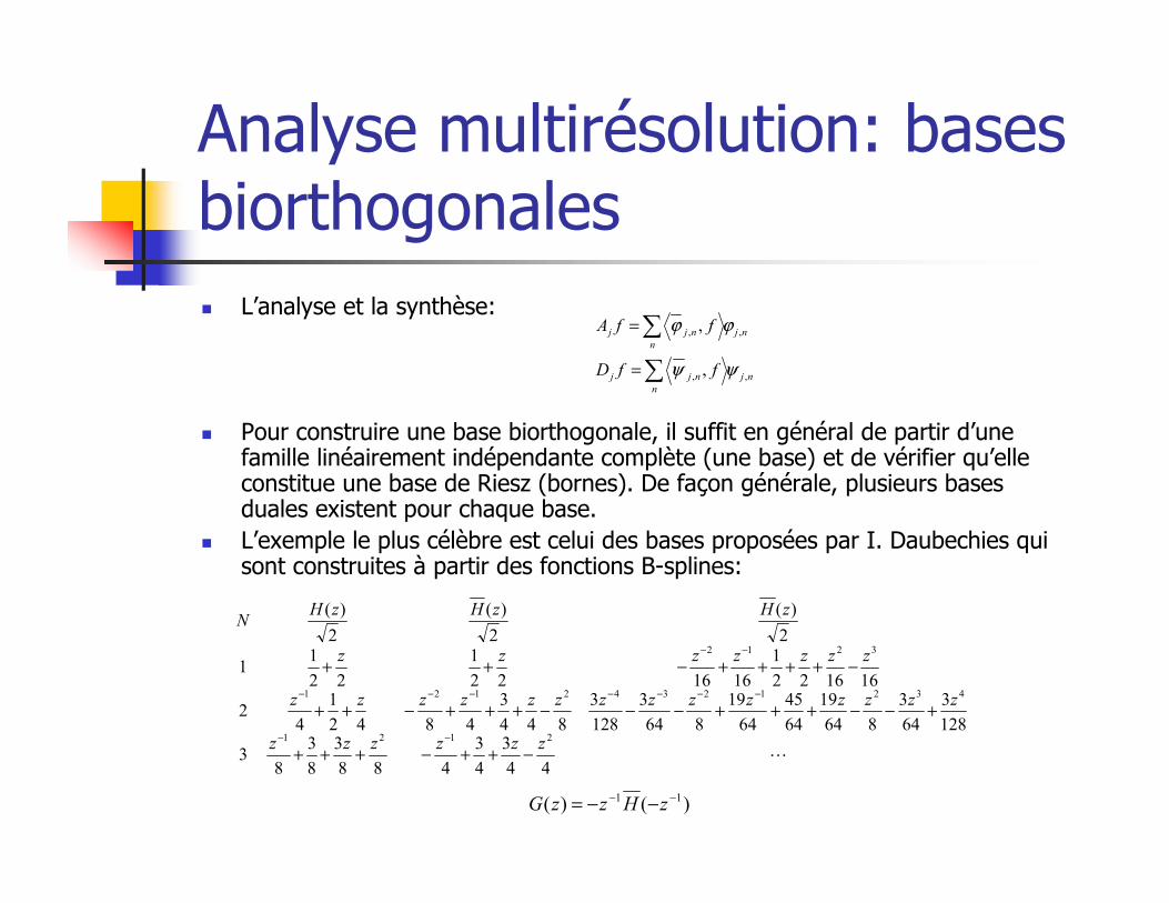
Analyse multirésolution: bases biorthogonales
� L’analyse et la synthèse:
� Pour construire une base biorthogonale, il suffit en général de partir d’une famille linéairement indépendante complète (une base) et de vérifier qu’elle constitue une base de Riesz (bornes). De façon générale, plusieurs bases duales existent pour chaque base.
� L’exemple le plus célèbre est celui des bases proposées par I. Daubechies qui sont construites à partir des fonctions B-splines:
nj
n
njj
nj
n
njj
ffD
ffA
,,
,,
,
,
ψψ
ϕϕ
∑
∑
=
=
)()( 11 −− −−= zHzzG
L44
3
4
3
488
3
8
3
83
128
3
64
3
864
19
64
45
64
19
864
3
128
3
844
3
4842
1
42
161622
1
161622
1
22
11
2
)(
2
)(
2
)(
2121
43212342121
3212
zzzzzz
zzzzzzzzzzzzzz
zzzzzzz
zHzHzHN
−++−+++
+−−+++−−−+++−++
−++++−++
−−
−−−−−−−
−−
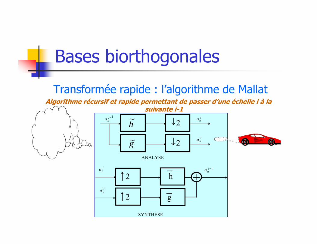
Bases biorthogonales
Transformée rapide : l’algorithme de MallatAlgorithme récursif et rapide permettant de passer d’une échelle i à la
suivante i-1
anj−1 ~
han
j
↓2
~gd n
j
↓2
ANALYSE
anj−1an
j
d nj
SYNTHESE
2
2
h
g
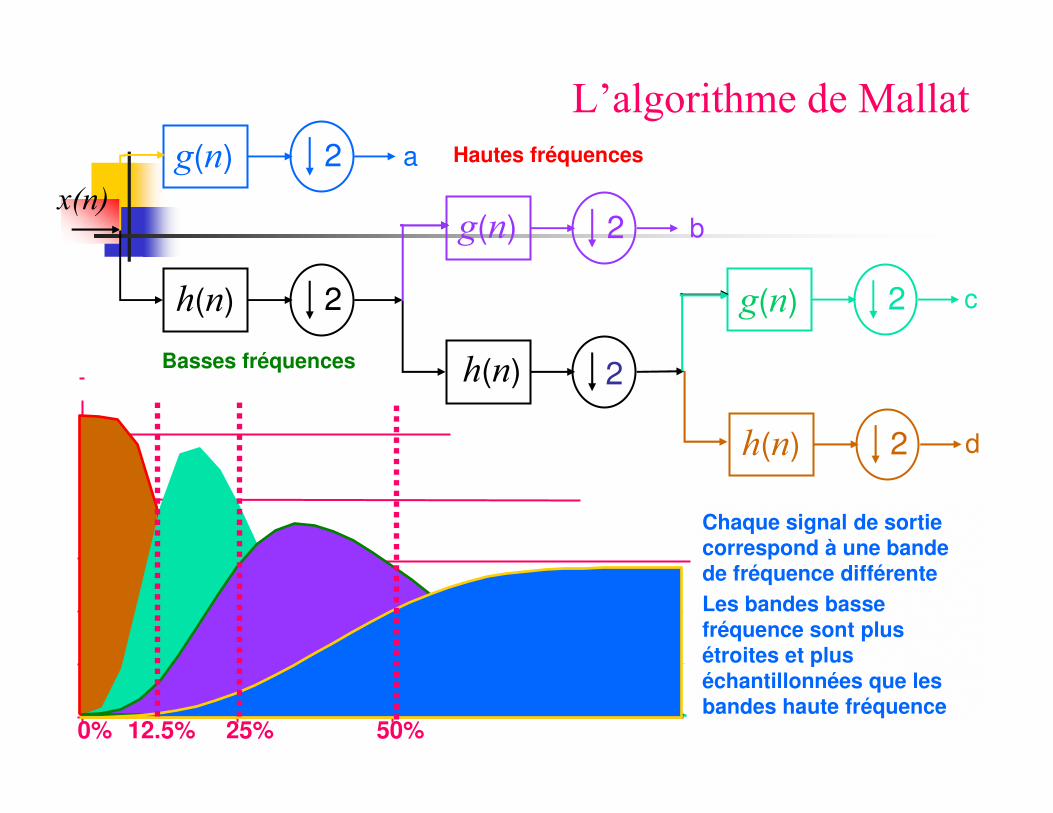
Basses fréquences
Hautes fréquences
x(n)
0%
Chaque signal de sortie correspond à une bandede fréquence différente
Les bandes bassefréquence sont plus étroites et plus échantillonnées que les bandes haute fréquence
25% 50%12.5%
g(n) 2 a
h(n) 2
h(n) 2
g(n) 2 b
h(n) 2 d
g(n) 2 c
L’algorithme de Mallat
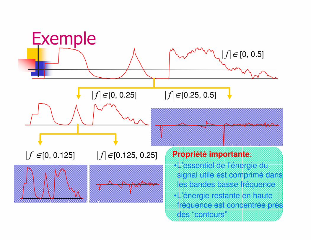
Propriété importante:
•L’essentiel de l’énergie dusignal utile est comprimé dans
les bandes basse fréquence
•L’énergie restante en haute fréquence est concentrée prèsdes “contours”
Exemple| f |∈ [0, 0.5]
| f |∈[0, 0.25] | f |∈[0.25, 0.5]
| f |∈[0, 0.125] | f |∈[0.125, 0.25]
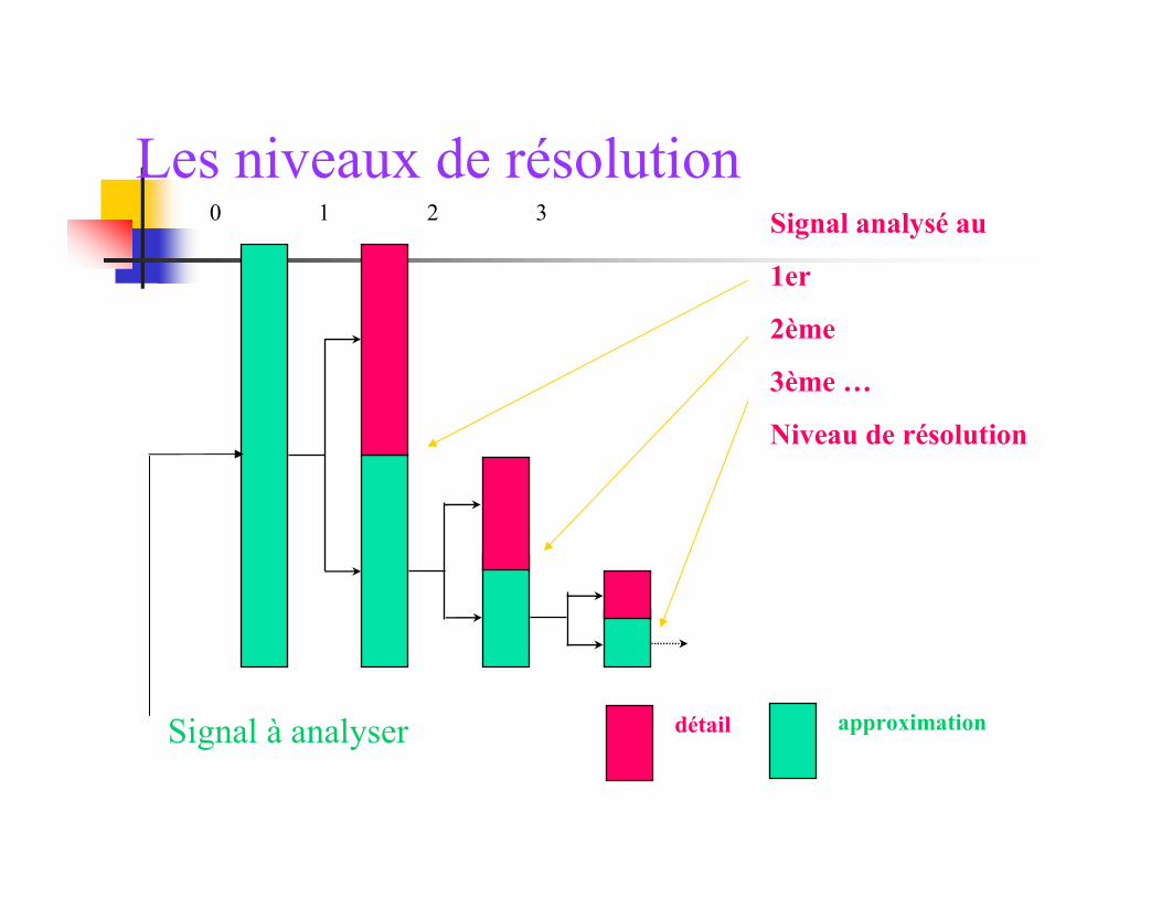
Les niveaux de résolutionSignal analysé au
1er
2ème
3ème …
Niveau de résolution
0 1 2 3
approximationdétailSignal à analyser
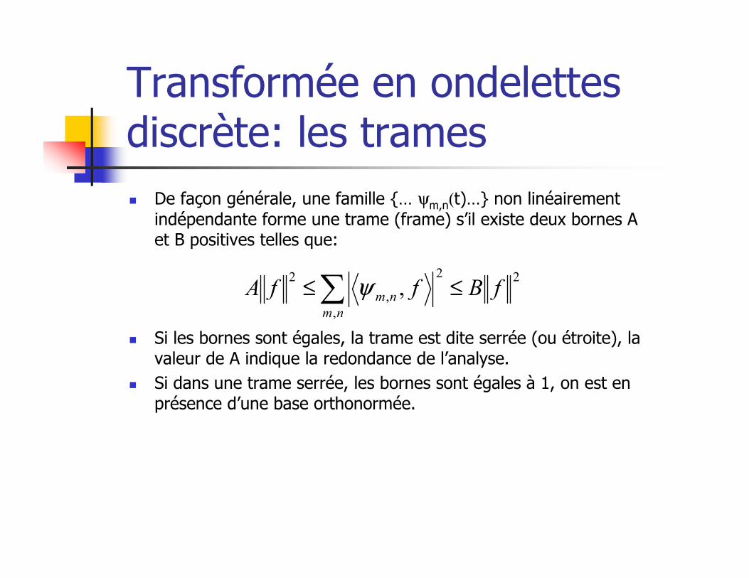
Transformée en ondelettes discrète: les trames
� De façon générale, une famille {… ψm,n(t)…} non linéairement indépendante forme une trame (frame) s’il existe deux bornes A et B positives telles que:
� Si les bornes sont égales, la trame est dite serrée (ou étroite), la valeur de A indique la redondance de l’analyse.
� Si dans une trame serrée, les bornes sont égales à 1, on est en présence d’une base orthonormée.
2
,
2
,
2, fBffA
nm
nm∑ ≤≤ ψ
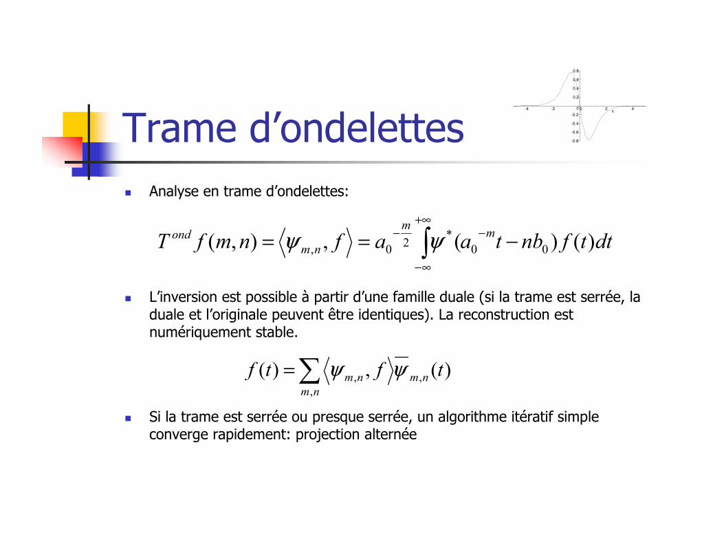
Trame d’ondelettes
� Analyse en trame d’ondelettes:
� L’inversion est possible à partir d’une famille duale (si la trame est serrée, la duale et l’originale peuvent être identiques). La reconstruction est numériquement stable.
� Si la trame est serrée ou presque serrée, un algorithme itératif simple converge rapidement: projection alternée
dttfnbtaafnmfTm
m
nm
ond )()(,),( 00
*2
0, −== −+∞
∞−
−
∫ψψ
)(,)( ,
,
, tftf nm
nm
nm ψψ∑=
x420-2-4
0.8
0.6
0.4
0.2
0
-0.2
-0.4
-0.6
-0.8
Ondelettes discrètes: variantes et extensions
� Paquets d’ondelettes� Multi-ondelettes� Ondelettes rationnelles� Ondelettes multi-dimensionnelles
� Séparables� Non-séparables
� Ondelettes géométriques� Gaborettes…� Ridgelets� Curvelets� …
� Ondelettes multi-valuées� Pseudo, semi, … ondelettes
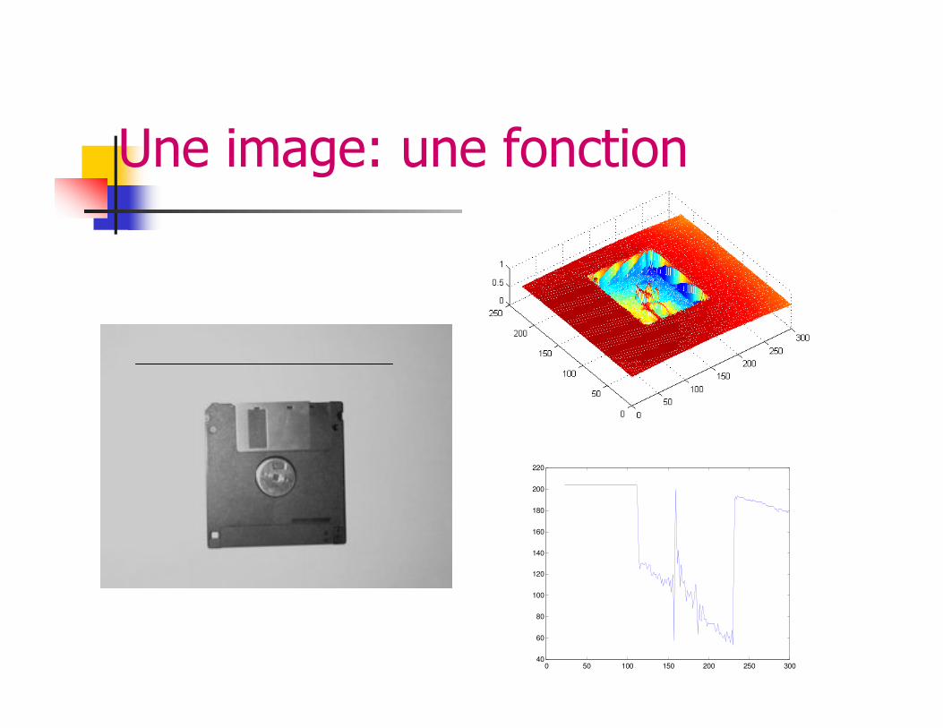
Une image: une fonction
0 50 100 150 200 250 30040
60
80
100
120
140
160
180
200
220
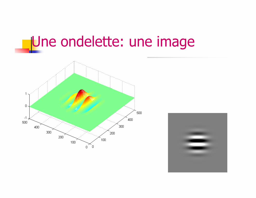
Une ondelette: une image
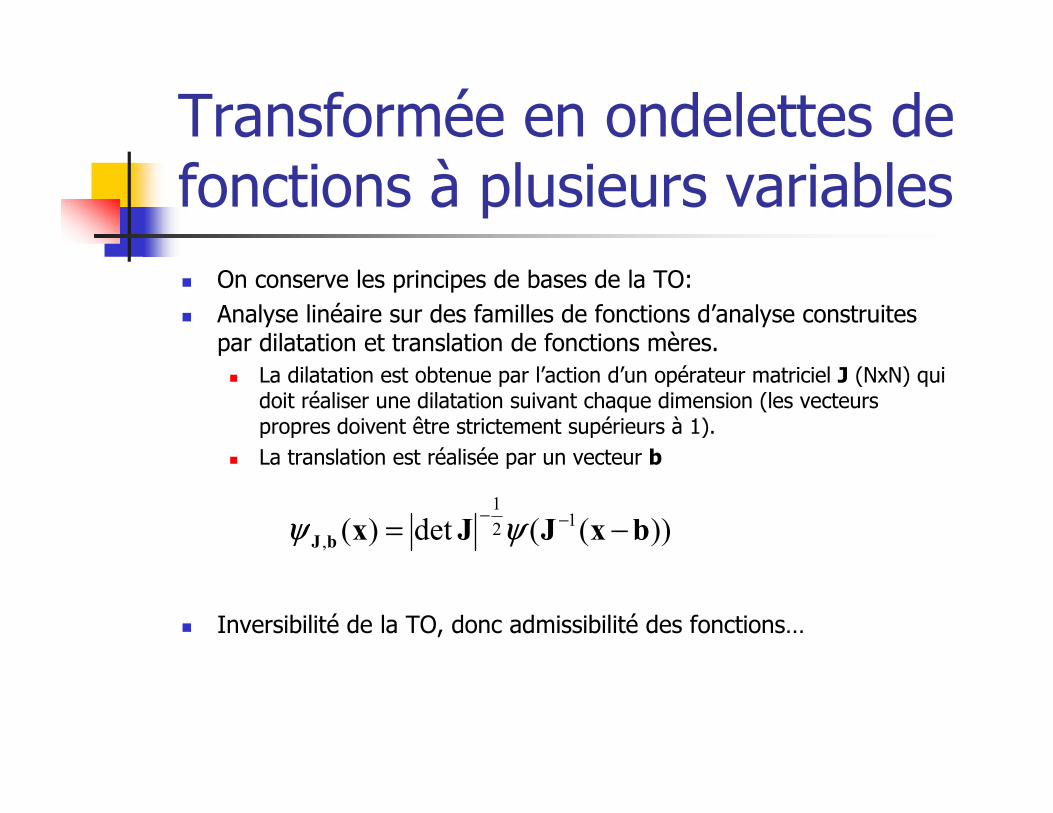
Transformée en ondelettes de fonctions à plusieurs variables
� On conserve les principes de bases de la TO:
� Analyse linéaire sur des familles de fonctions d’analyse construites par dilatation et translation de fonctions mères.
� La dilatation est obtenue par l’action d’un opérateur matriciel J (NxN) qui doit réaliser une dilatation suivant chaque dimension (les vecteurs propres doivent être strictement supérieurs à 1).
� La translation est réalisée par un vecteur b
� Inversibilité de la TO, donc admissibilité des fonctions…
))((det)( 12
1
, bxJJxbJ −= −−ψψ
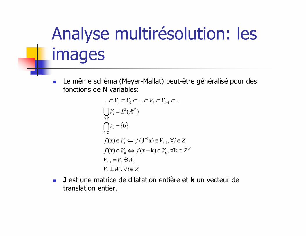
Analyse multirésolution: les images
� Le même schéma (Meyer-Mallat) peut-être généralisé pour des fonctions de N variables:
� J est une matrice de dilatation entière et k un vecteur de translation entier.
{ }
ZiWV
WVV
ZVfVf
ZiVfVf
V
LV
VVVV
ii
iii
N
ii
Zi
i
N
Zi
i
ii
∈∀⊥
⊕=
∈∀∈−⇔∈
∈∀∈⇔∈
=
=
⊂⊂⊂⊂⊂⊂
−
−−
∈
∈
−
,
,)()(
,)()(
0
)(
.........
1
00
1
1
2
101
kkxx
xJx
I
U R
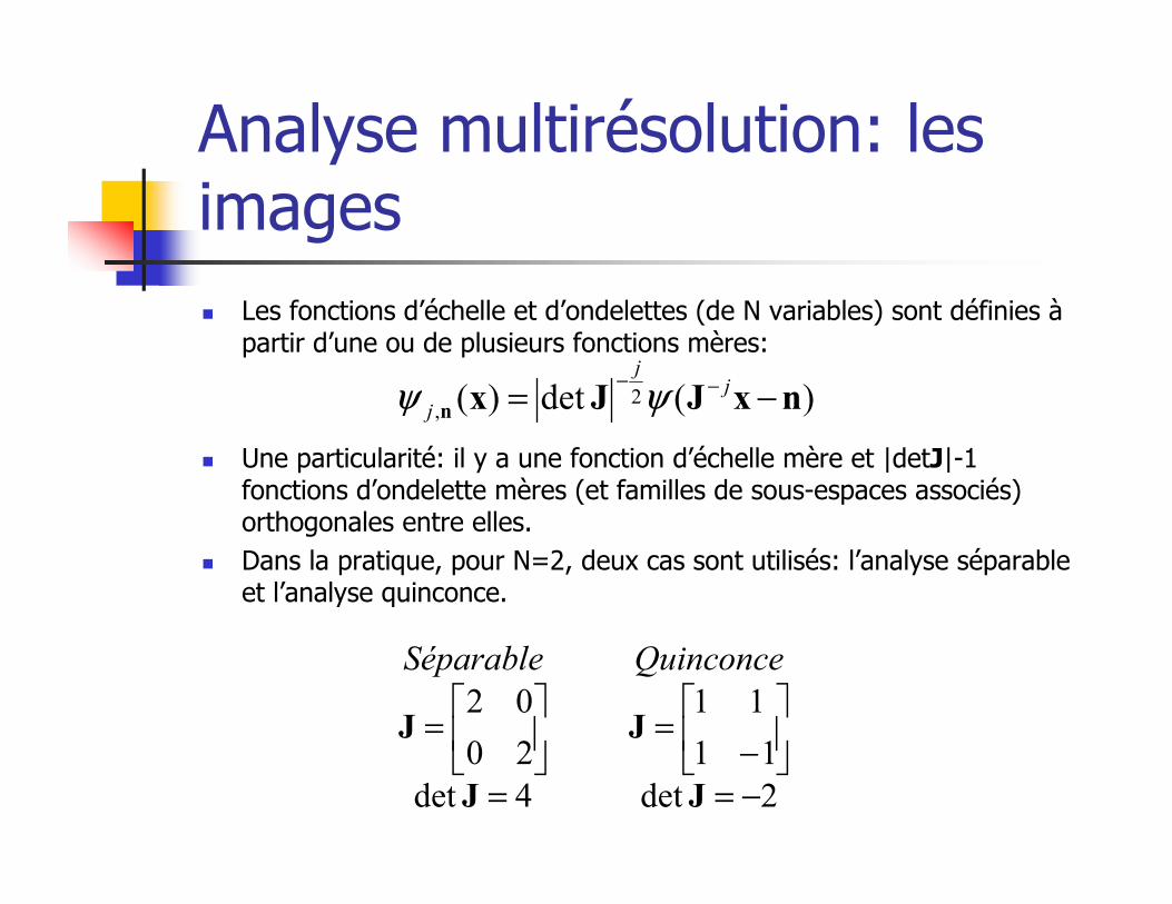
Analyse multirésolution: les images
� Les fonctions d’échelle et d’ondelettes (de N variables) sont définies à partir d’une ou de plusieurs fonctions mères:
� Une particularité: il y a une fonction d’échelle mère et |detJ|-1 fonctions d’ondelette mères (et familles de sous-espaces associés) orthogonales entre elles.
� Dans la pratique, pour N=2, deux cas sont utilisés: l’analyse séparable et l’analyse quinconce.
)(det)( 2, nxJJxn −= −− j
j
j ψψ
2det4det
11
11
20
02
−==
−=
=
JJ
JJ
QuinconceSéparable
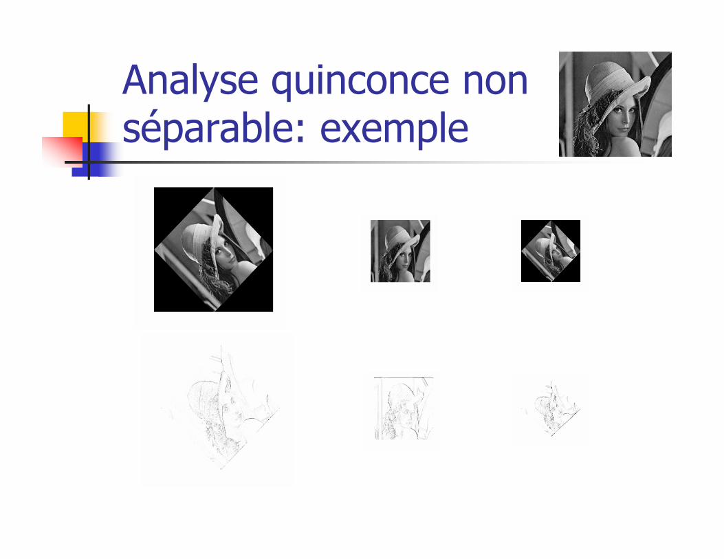
Analyse quinconce non séparable: exemple
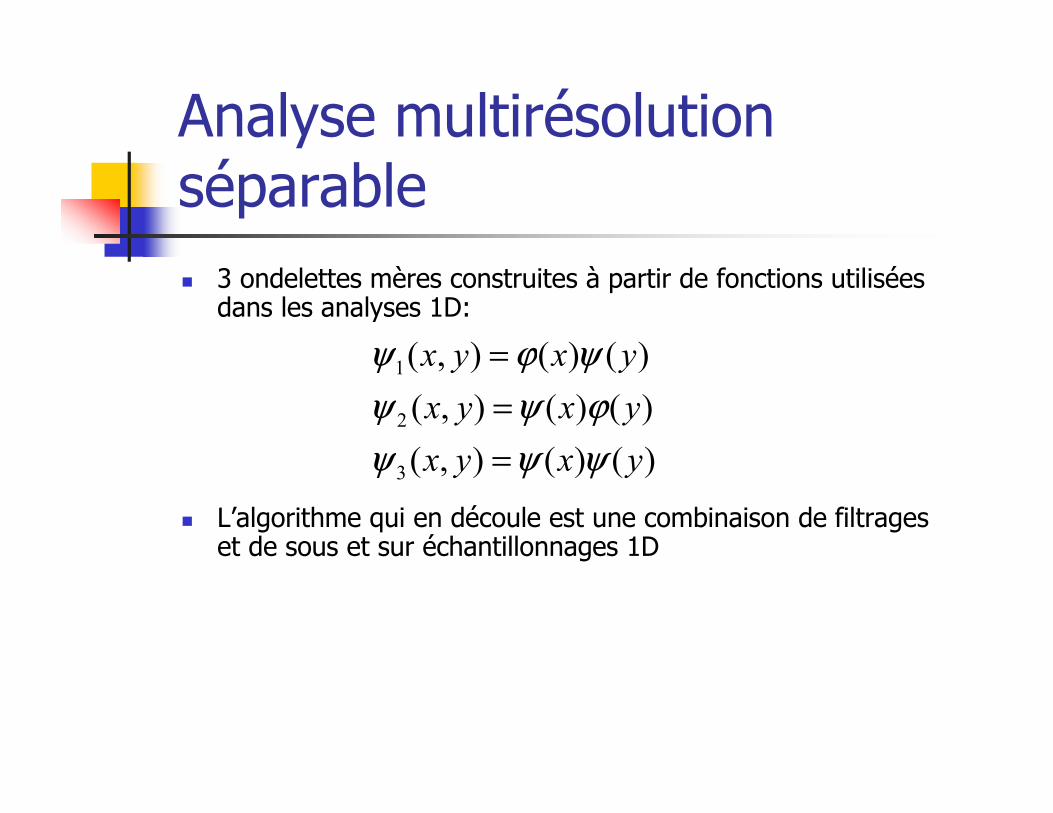
Analyse multirésolutionséparable
� 3 ondelettes mères construites à partir de fonctions utilisées dans les analyses 1D:
� L’algorithme qui en découle est une combinaison de filtrages et de sous et sur échantillonnages 1D
)()(),(
)()(),(
)()(),(
3
2
1
yxyx
yxyx
yxyx
ψψψ
ϕψψ
ψϕψ
=
=
=
h(n)
g(n)
2
2
h(n)
g(n)
2
2
h(n)
g(n)
2
2
h(n)
g(n)
2
2
h(n)
g(n)
2
2
h(n)
g(n)
2
2
h(n)
g(n)
2
2
h(n)
g(n)
2
2
h(n)
g(n)
2
2
h(n)
g(n)
2
2
h(n)
g(n)
2
2
h(n)
g(n)
2
2
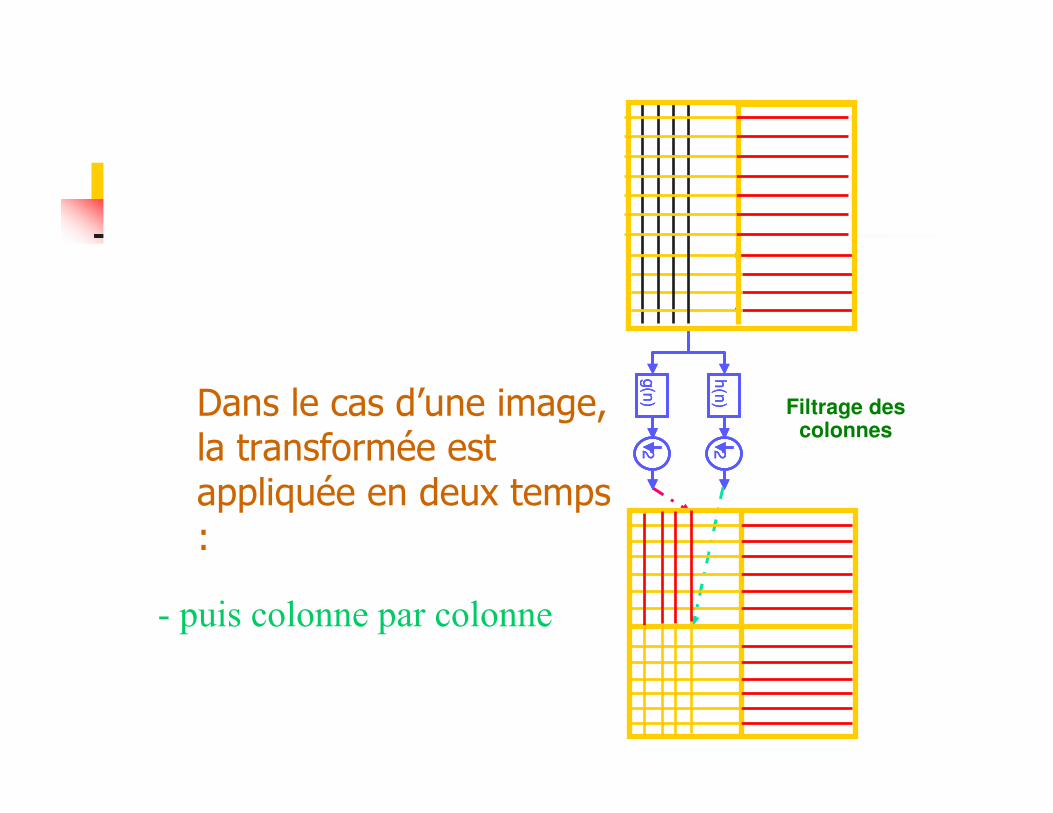
Dans le cas d’une image, la transformée estappliquée en deux temps :
Filtrage des colonnes
h(n
)
g(n
)
22
h(n
)
g(n
)
22
h(n
)
g(n
)
22
Filtrage des lignes
- Ligne par ligne,- puis colonne par colonne
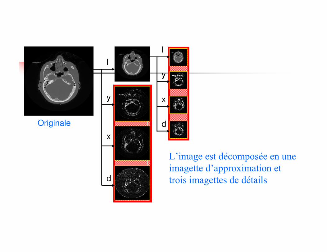
Originale
l
y
x
d
l
y
x
d
L’image est décomposée en une
imagette d’approximation et
trois imagettes de détails
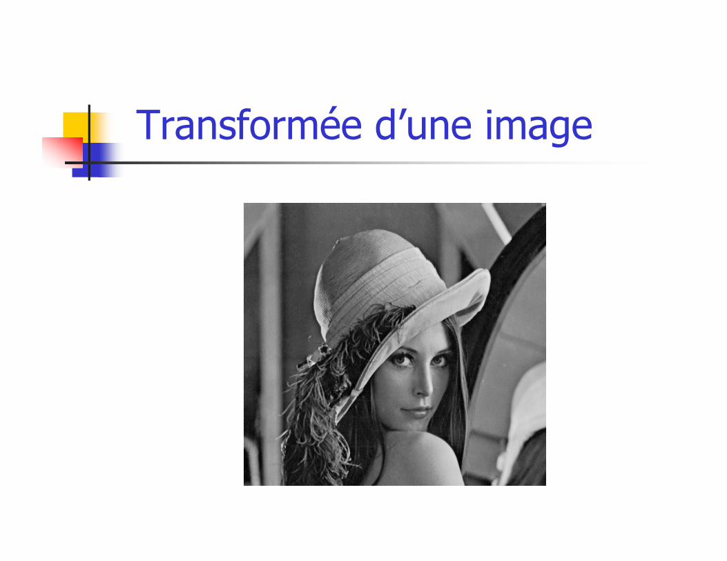
Transformée d’une image
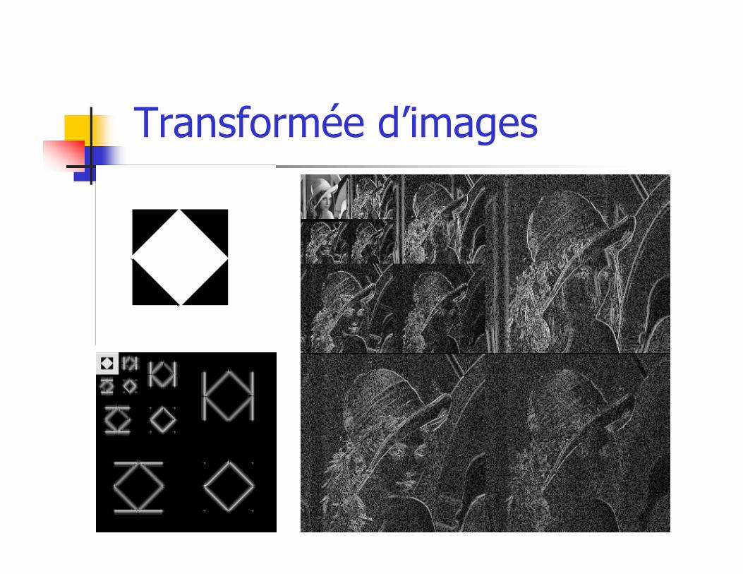
Transformée d’images
Quelles ondelettes
� La liberté de choix est large (admissibilité)� Malédiction ou bénédiction?
� Quels efforts doit-on faire pour ce choix et quelles en sont les conséquences?� N’importe quelle ondelette?
� Quelles propriétés doit on considérer en priorité?
symétrie, régularité, nombre de moments nuls, compacité
Symétrie
Dans quelques applications la fonction doit être symétrique(ou antisymétrique):
Cas des images du monde réel
C’est lié à la linéarité en phase
Symétriques: Haar, Mexican hat, MorletNon symétriques: Daubechies, 1D support compact et orthogonales
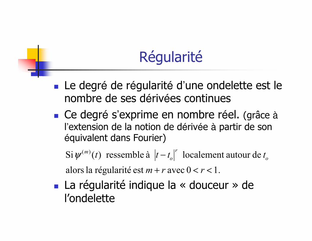
Régularité
� Le degré de régularité d’une ondelette est le nombre de ses dérivées continues
� Ce degré s’exprime en nombre réel. (grâce à
l’extension de la notion de dérivée à partir de son équivalent dans Fourier)
� La régularité indique la « douceur » de l’ondelette
.10 avec est régularitéla alors
deautour localement à ressemble)( Si )(
<<+
−
rrm
tttt o
r
o
mψ
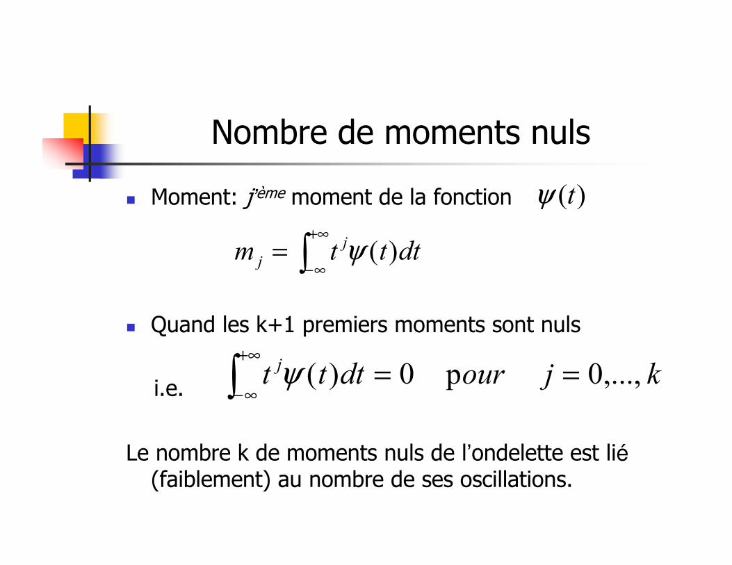
Nombre de moments nuls
� Moment: j’ème moment de la fonction
� Quand les k+1 premiers moments sont nuls
i.e.
Le nombre k de moments nuls de l’ondelette est lié(faiblement) au nombre de ses oscillations.
)(tψ
∫+∞
∞−= dtttm j
j )(ψ
kjourdttt j ,...,0p0)( ==∫+∞
∞−ψ
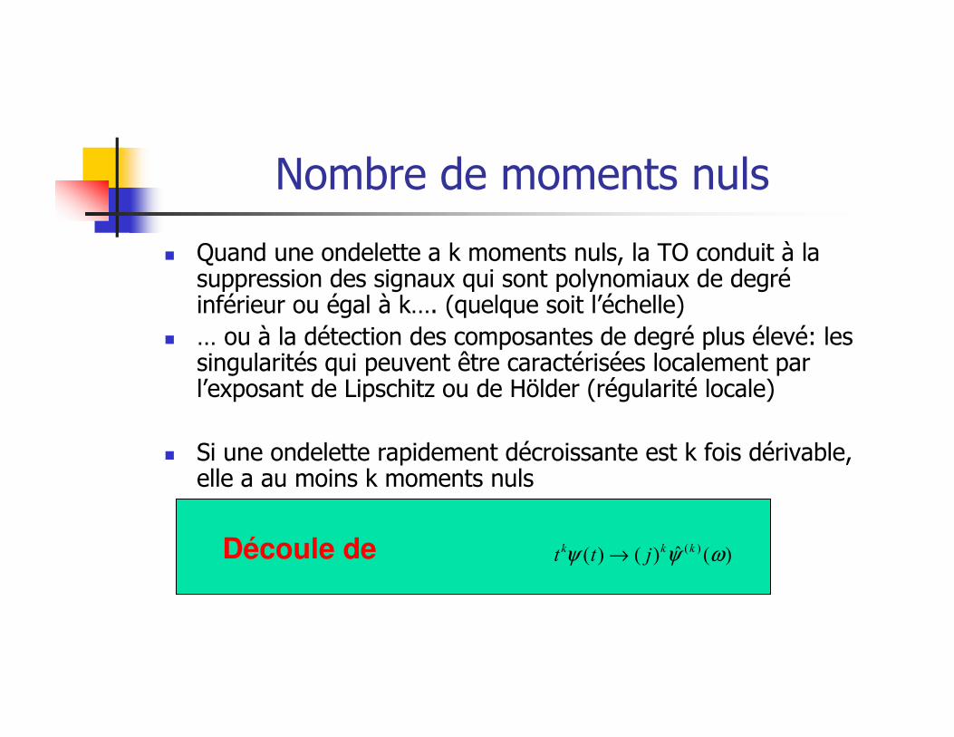
Nombre de moments nuls
� Quand une ondelette a k moments nuls, la TO conduit à la suppression des signaux qui sont polynomiaux de degréinférieur ou égal à k…. (quelque soit l’échelle)
� … ou à la détection des composantes de degré plus élevé: les singularités qui peuvent être caractérisées localement par l’exposant de Lipschitz ou de Hölder (régularité locale)
� Si une ondelette rapidement décroissante est k fois dérivable, elle a au moins k moments nuls
Découle de )(ˆ)()( )( ωψψ kkk jtt →
Compacité (largeur du support)
� Le nombre de coefficients du filtre RIF.
� Le nombre de moments nuls est proportionel à la largeur dusupport.
� Il faut établir un compromis entre le coût de calcul et la précision de l’analyse
� et un compromis entre la résolution temporelle et fréquentielle
� Une ondelette compacte dans une base orthogonale ne peut pas être symétrique en 1D
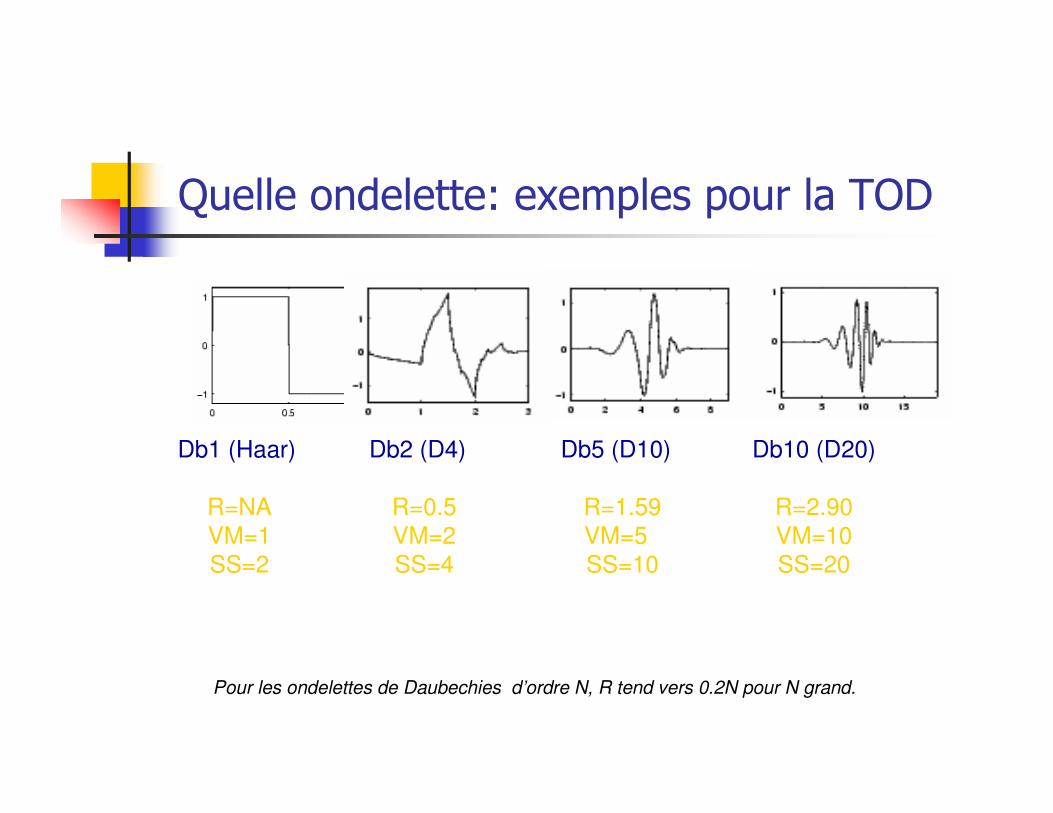
Quelle ondelette: exemples pour la TOD
Db1 (Haar) Db2 (D4) Db5 (D10) Db10 (D20)
R=NA R=0.5 R=1.59 R=2.90
VM=1 VM=2 VM=5 VM=10
SS=2 SS=4 SS=10 SS=20
Pour les ondelettes de Daubechies d’ordre N, R tend vers 0.2N pour N grand.
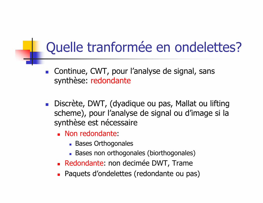
Quelle tranformée en ondelettes?
� Continue, CWT, pour l’analyse de signal, sans synthèse: redondante
� Discrète, DWT, (dyadique ou pas, Mallat ou lifting scheme), pour l’analyse de signal ou d’image si la synthèse est nécessaire
� Non redondante:
� Bases Orthogonales
� Bases non orthogonales (biorthogonales)
� Redondante: non decimée DWT, Trame
� Paquets d’ondelettes (redondante ou pas)
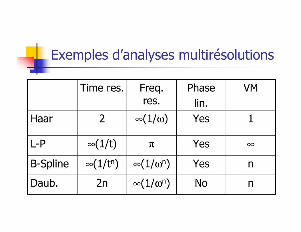
Exemples d’analyses multirésolutions
nNo∞(1/ωn)2nDaub.
nYes∞(1/ωn)∞(1/tn)B-Spline
∞Yesπ∞(1/t)L-P
1Yes∞(1/ω)2Haar
VMPhase
lin.
Freq. res.
Time res.
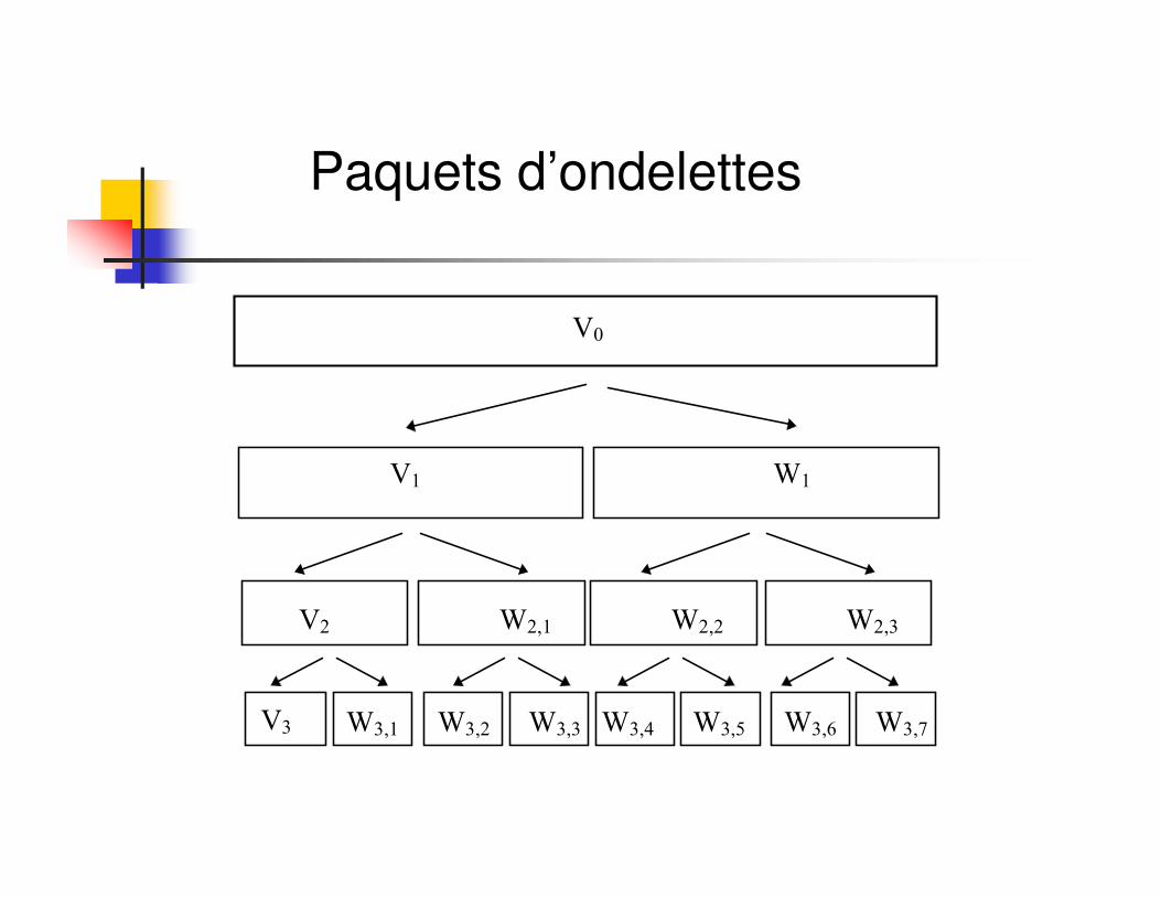
V0
V1 W1
V2 W2,1
V3 W3,1
W2,2 W2,3
W3,2 W3,7W3,6W3,5W3,4W3,3
Paquets d’ondelettes
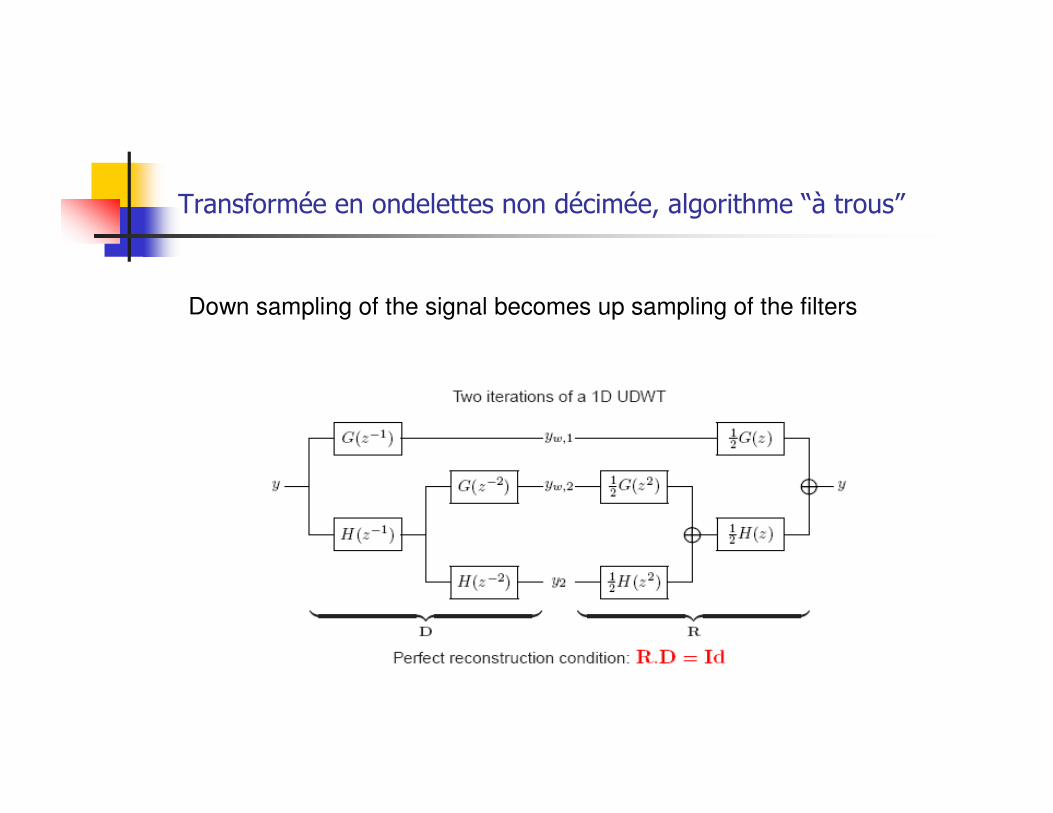
Transformée en ondelettes non décimée, algorithme “à trous”
Down sampling of the signal becomes up sampling of the filters
Analyse en ondelettes rationnelles
F. Truchetet, A. Baussard, F. Nicolier
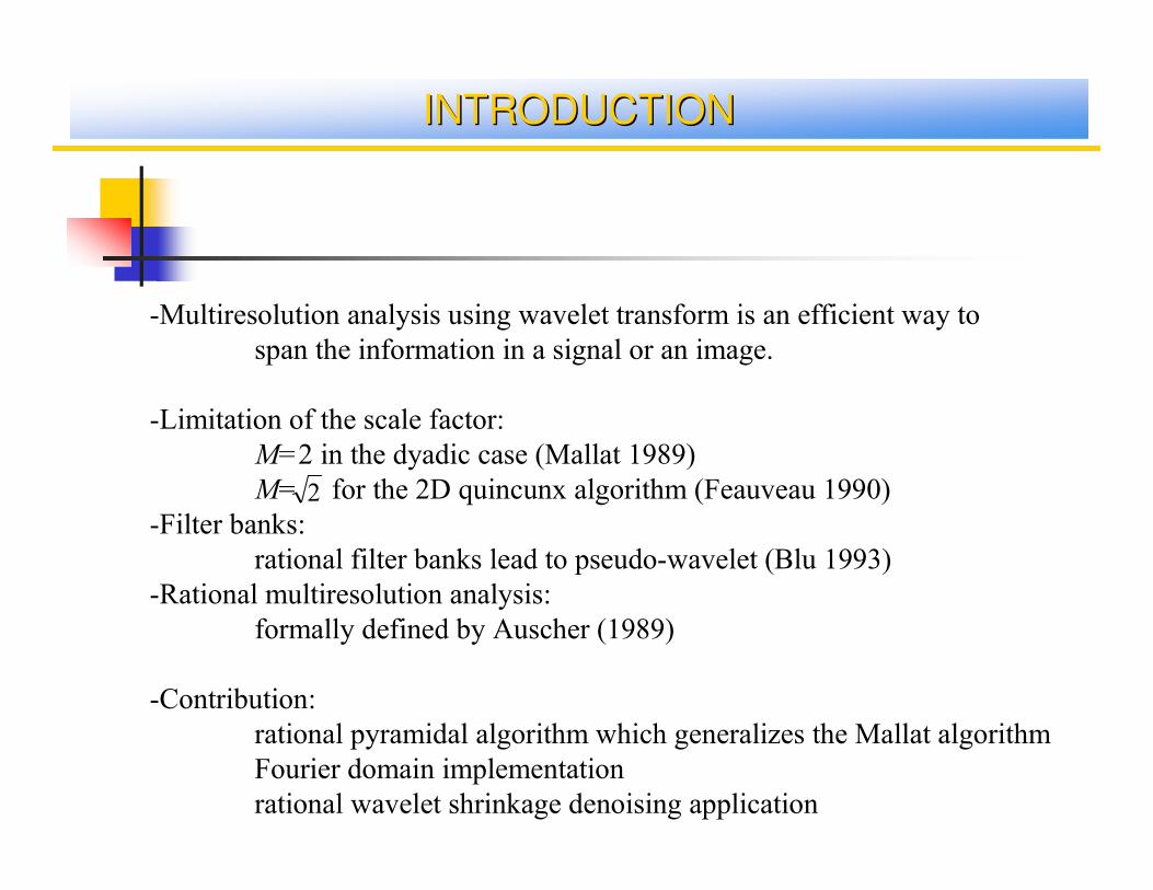
-Multiresolution analysis using wavelet transform is an efficient way to
span the information in a signal or an image.
-Limitation of the scale factor:
M=2 in the dyadic case (Mallat 1989)
M= for the 2D quincunx algorithm (Feauveau 1990)
-Filter banks:
rational filter banks lead to pseudo-wavelet (Blu 1993)
-Rational multiresolution analysis:
formally defined by Auscher (1989)
-Contribution:
rational pyramidal algorithm which generalizes the Mallat algorithm
Fourier domain implementation
rational wavelet shrinkage denoising application
INTRODUCTIONINTRODUCTION
2
RATIONAL MULTIRESOLUTION ANALYSISRATIONAL MULTIRESOLUTION ANALYSIS
( )
{ }( ) ( )( ) ( ) 00
11
2
1
,
,
0
,
VkxfVxfZk
VxMfVxfZj
V
RLV
VVZj
jj
Zj
j
zj
j
jj
∈−⇔∈∈∀∈⇔∈∈∀
=
=⊂∈∀
+−
∈
∈
+
I
U
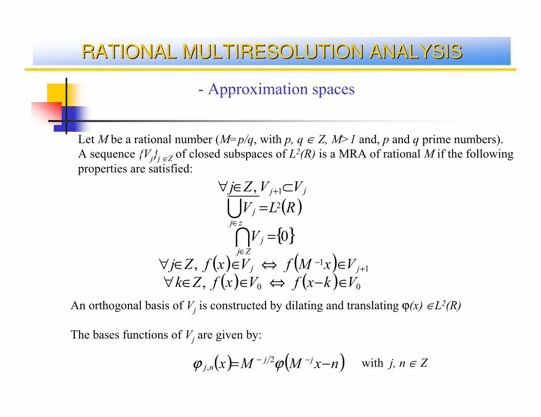
Let M be a rational number (M=p/q, with p, q ∈ Z, M>1 and, p and q prime numbers).
A sequence {Vj}j ∈Z of closed subspaces of L2(R) is a MRA of rational M if the following
properties are satisfied:
An orthogonal basis of Vj is constructed by dilating and translating ϕ(x) ∈L2(R)
The bases functions of Vj are given by:
- Approximation spaces
( ) ( )nxMMx jjnj −= −− ϕϕ 2, with j, n ∈ Z
RATIONAL MULTIRESOLUTION ANALYSISRATIONAL MULTIRESOLUTION ANALYSIS
- Detail spaces
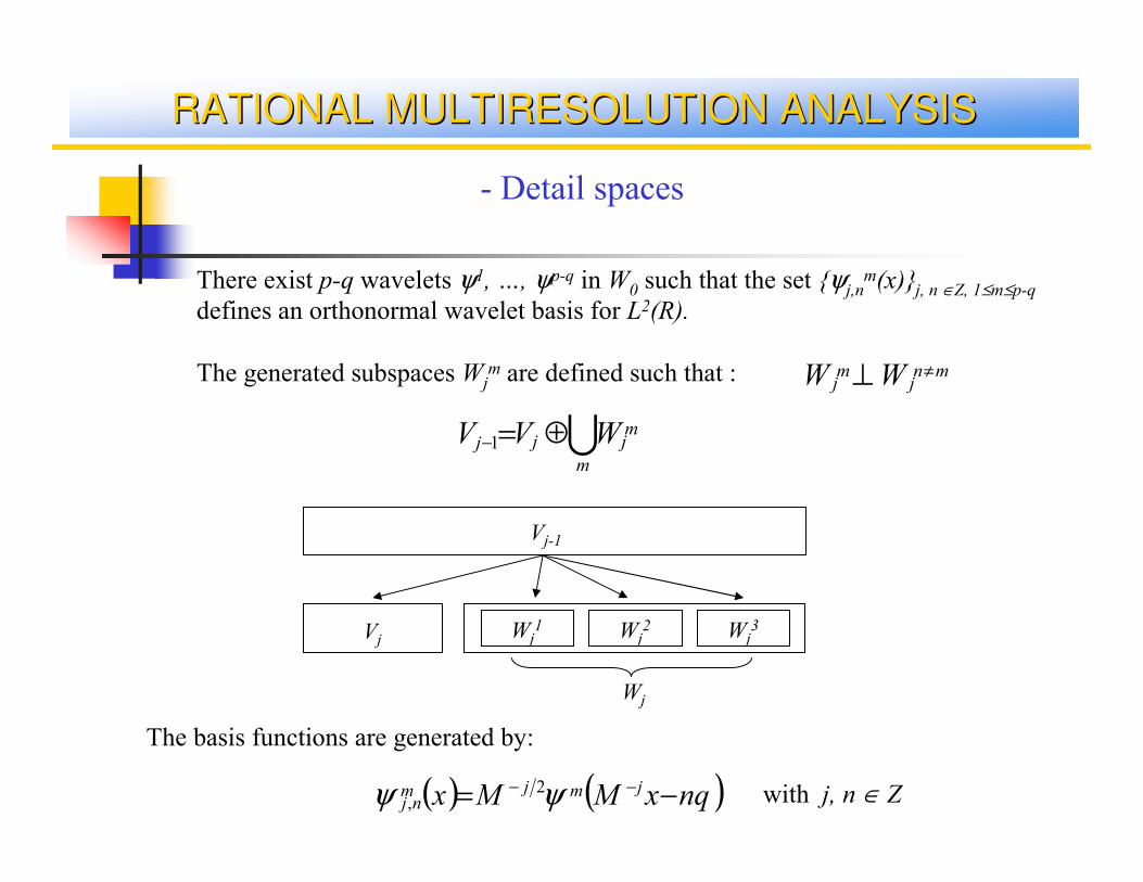
There exist p-q wavelets ψ1, …, ψp-q in W0 such that the set {ψj,nm(x)}j, n ∈Z, 1≤m≤p-q
defines an orthonormal wavelet basis for L2(R).
The generated subspaces Wjm are defined such that :
Um
mjjj WVV ⊕=−1
mnj
mj WW ≠⊥
Vj-1
Vj Wj1 Wj
2 Wj3
Wj
The basis functions are generated by:
( ) ( )nqxMMx jmjmnj −= −− ψψ 2, with j, n ∈ Z
PYRAMIDAL ANALYSIS ALGORITHMPYRAMIDAL ANALYSIS ALGORITHM
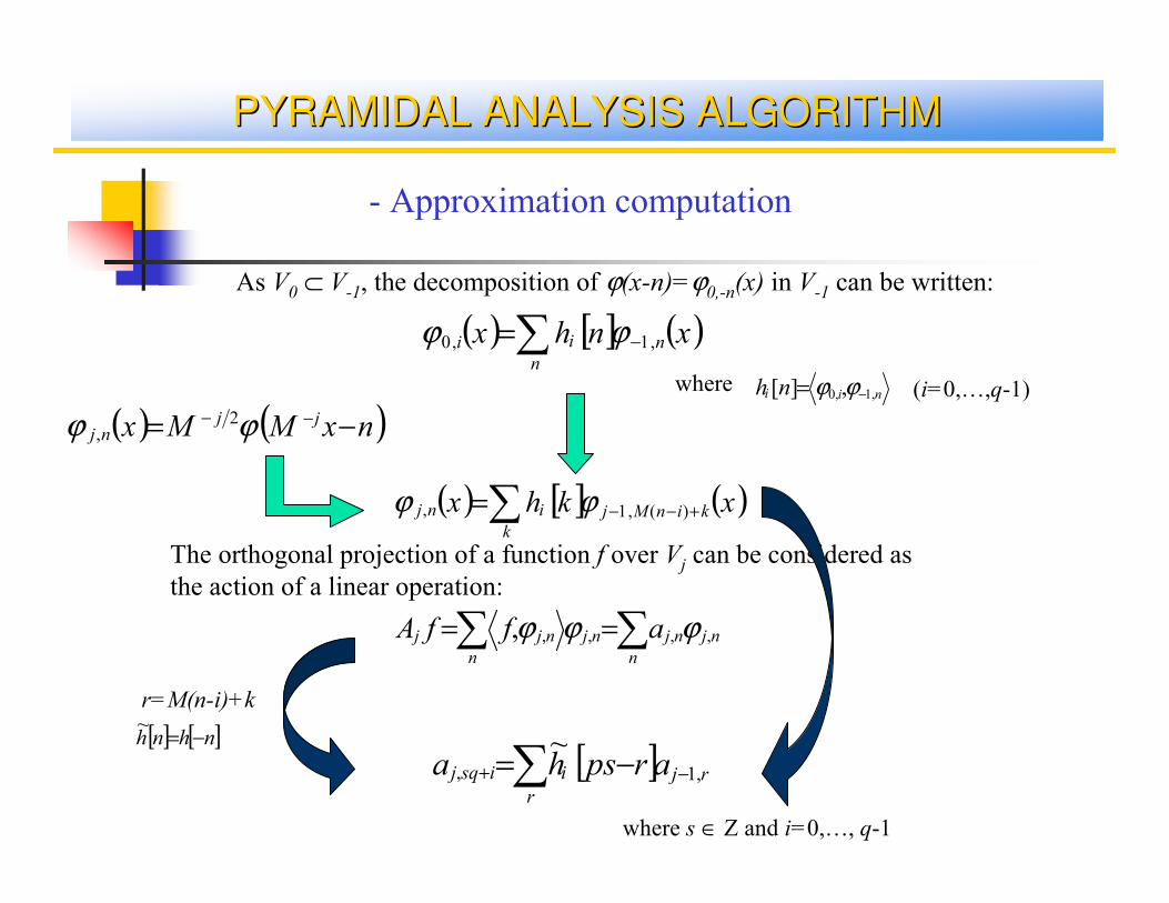
- Approximation computation
( ) [ ] ( )∑ −=n
nii xnhx ,1,0 ϕϕ
As V0 ⊂ V-1, the decomposition of ϕ(x-n)=ϕ0,-n(x) in V-1 can be written:
wherenii nh ,1,0 ,][ −= ϕϕ (i=0,…,q-1)
The orthogonal projection of a function f over Vj can be considered as
the action of a linear operation:
∑∑ ==n
njnjnj
n
njj affA ,,,,, ϕϕϕ
( ) ( )nxMMx jjnj −= −− ϕϕ 2,
( ) [ ] ( )∑ +−−=k
kinMjinj xkhx )(,1, ϕϕ
[ ]∑ −+ −=r
rjiisqj arpsha ,1,
~
r=M(n-i)+k
[ ] [ ]nhnh −=~
where s ∈ Z and i=0,…, q-1
PYRAMIDAL ANALYSIS ALGORITHMPYRAMIDAL ANALYSIS ALGORITHM
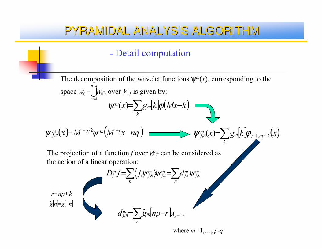
- Detail computation
The decomposition of the wavelet functions ψm(x), corresponding to the
space , over V-1 is given by:Uqp
m
mWW−
=
=1
00
[ ] ( )∑ −=k
mm kMxkgx ϕψ )(
( ) ( )nqxMMx jmjmnj −= −− ψψ 2, [ ] ( )∑ +−=
k
knpjmmnj xkgx ,1, )( ϕψ
The projection of a function f over can be considered as
the action of a linear operation:
mjW
∑∑ ==n
mnj
mnj
mnj
n
mnj
mj dffD ,,,,, ψψψ
r=np+k
[ ] [ ]ngng −=~
[ ]∑ −−=r
rjmmnj arnpgd ,1,
~
where m=1,…, p-q
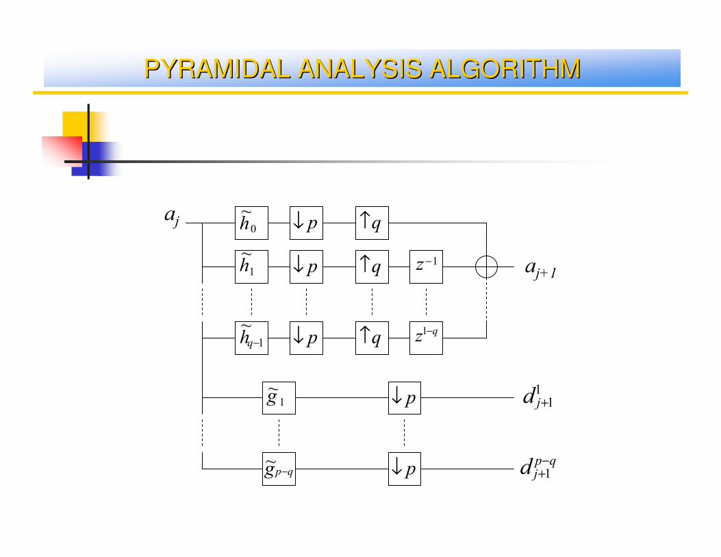
PYRAMIDAL ANALYSIS ALGORITHMPYRAMIDAL ANALYSIS ALGORITHM
0
~h
1
~h
1
~−qh
p↓
p↓
p↓
q↑
q↑
q↑
1−z
qz −1
p↓
p↓
1~g
qpg −~
aj
aj+1
11+jd
qpjd
−+1
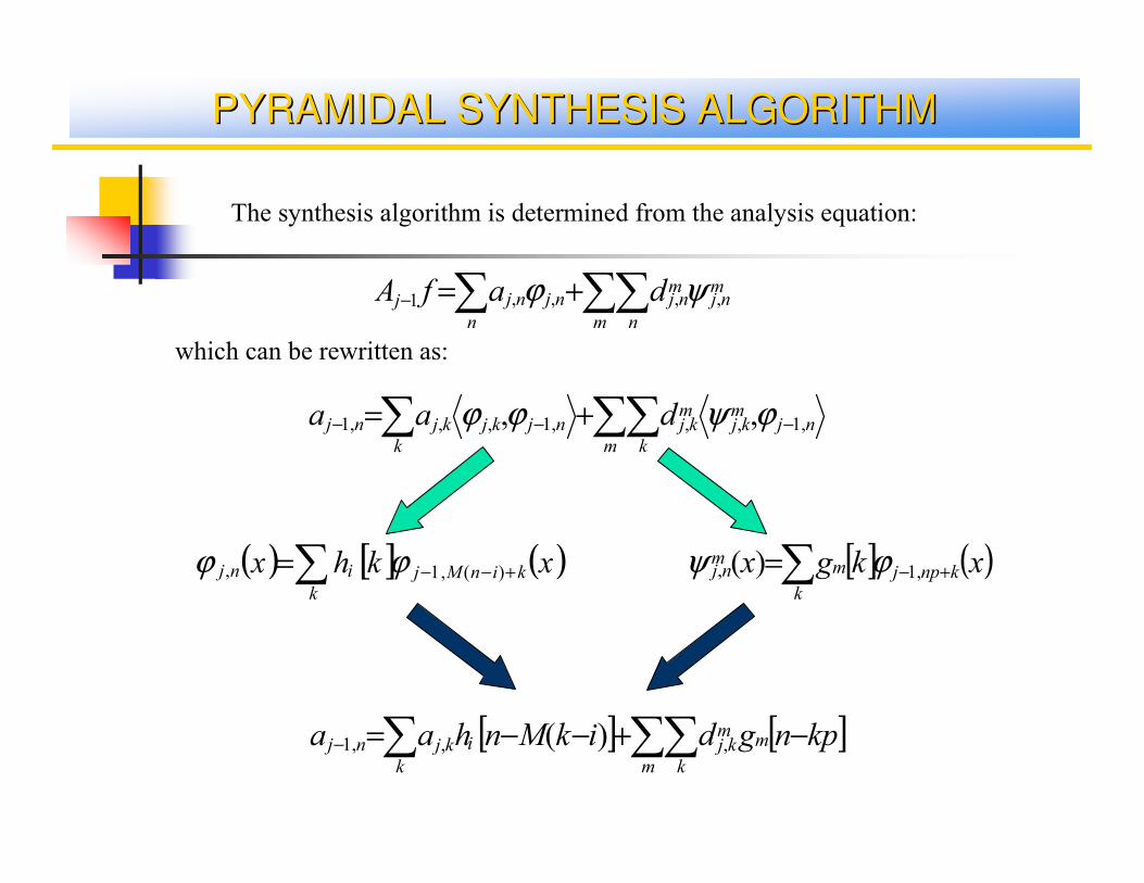
PYRAMIDAL SYNTHESIS ALGORITHMPYRAMIDAL SYNTHESIS ALGORITHM
The synthesis algorithm is determined from the analysis equation:
∑ ∑∑+=−n m n
mnj
mnjnjnjj dafA ,,,,1 ψϕ
∑ ∑∑ −−− +=k m k
njmkj
mkjnjkjkjnj daa ,1,,,1,,,1 ,, ϕψϕϕ
which can be rewritten as:
[ ] ( )∑ +−=k
knpjmmnj xkgx ,1, )( ϕψ( ) [ ] ( )∑ +−−=
k
kinMjinj xkhx )(,1, ϕϕ
[ ] [ ]∑ ∑∑ −+−−=−k m k
mmkjikjnj kpngdikMnhaa ,,,1 )(
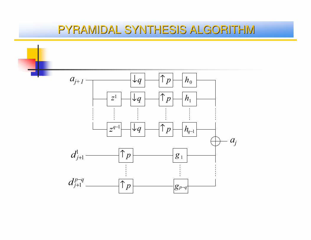
PYRAMIDAL SYNTHESIS ALGORITHMPYRAMIDAL SYNTHESIS ALGORITHM
0h
1h
1−qh
q↓ p↑
1z
1−qz
1g
qpg −
aj
aj+1
11+jd
qpjd
−+1
q↓
q↓
p↑
p↑
p↑
p↑
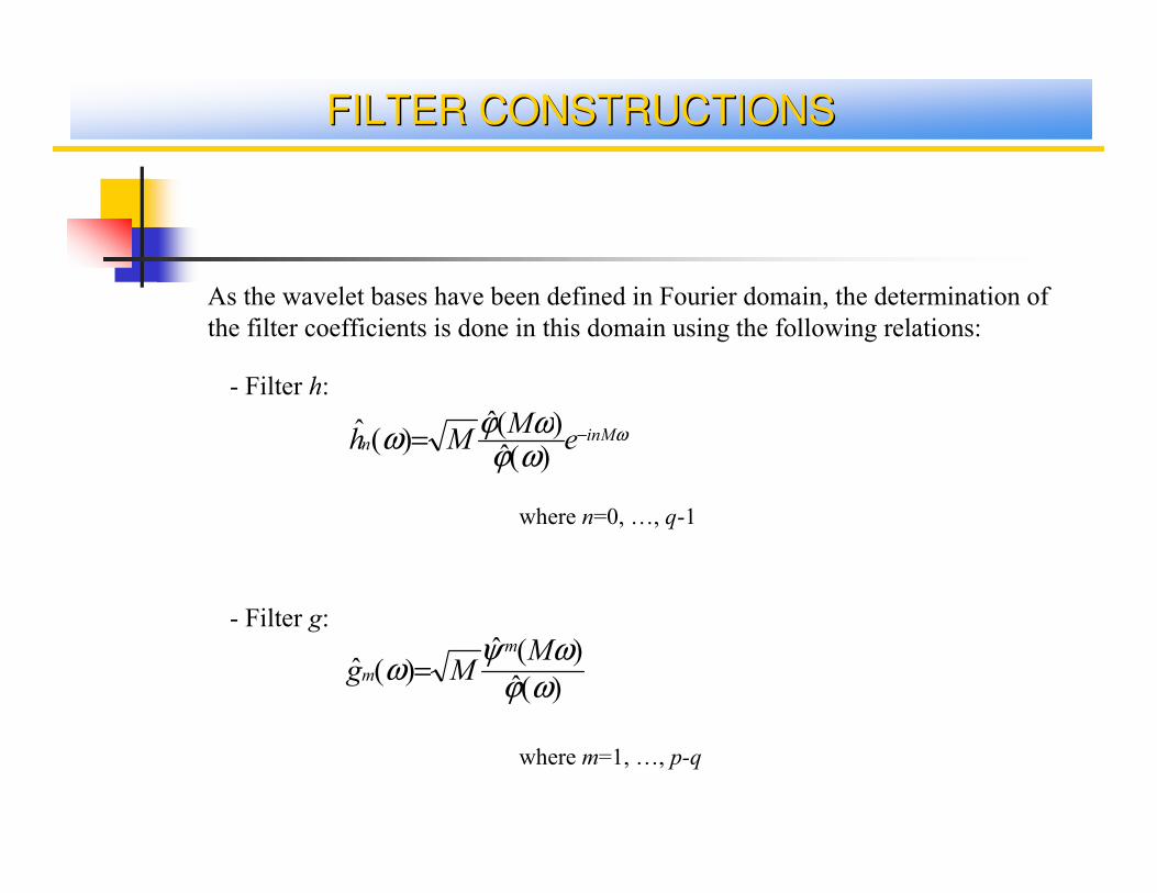
FILTER CONSTRUCTIONSFILTER CONSTRUCTIONS
As the wavelet bases have been defined in Fourier domain, the determination of
the filter coefficients is done in this domain using the following relations:
- Filter h:
ωωϕωϕω inM
n eM
Mh −=)(ˆ)(ˆ
)(ˆ
- Filter g:
)(ˆ
)(ˆ)(ˆ
ωϕωψ
ωM
Mgm
m =
where n=0, …, q-1
where m=1, …, p-q
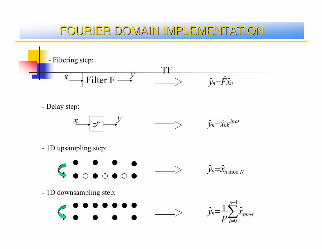
FOURIER DOMAIN IMPLEMENTATIONFOURIER DOMAIN IMPLEMENTATION
- 1D downsampling step:
∑−
=+=
1
0
ˆ1ˆp
l
lpnn xp
y
- 1D upsampling step:
Nnn xy mod ˆˆ =
- Delay step:
zpx y ωipnn exy ˆˆ =
- Filtering step:
Filter Fx y TF
nn xFy ˆˆˆ =
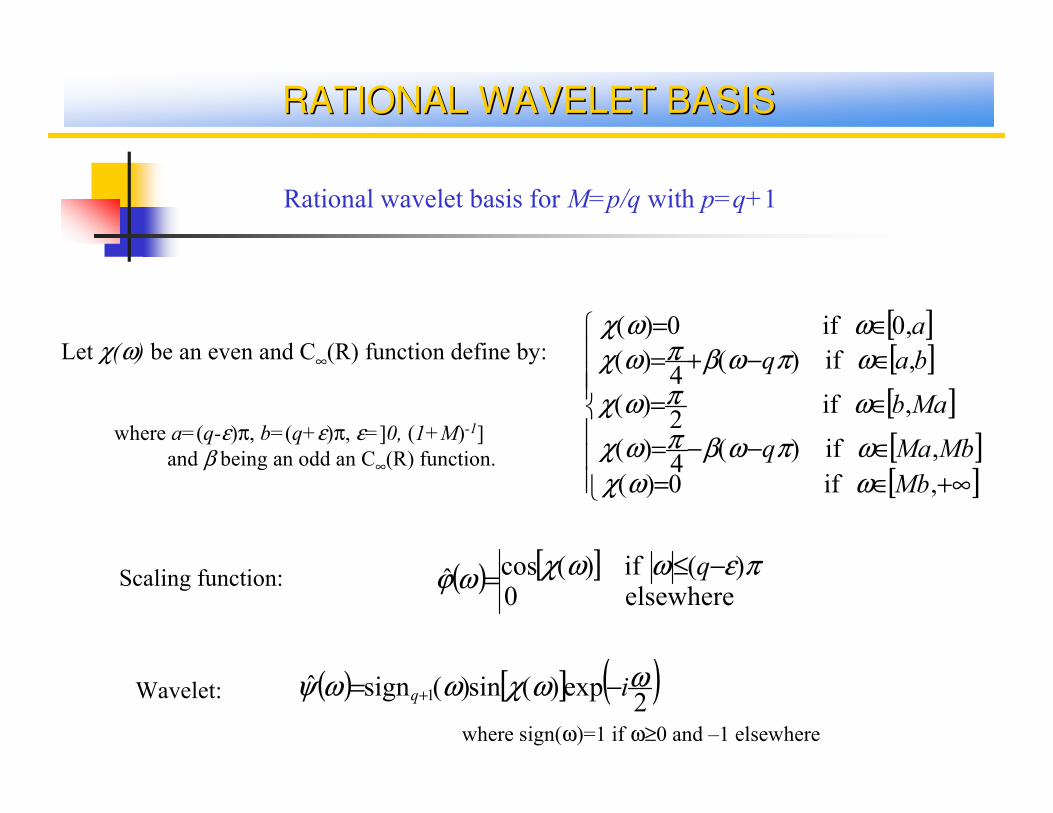
RATIONAL WAVELET BASISRATIONAL WAVELET BASIS
[ ][ ][ ][ ][ ]
+∞∈=∈−−=
∈=
∈−+=∈=
, if 0)(
, if )(4
)(
, if 2
)(
, if )(4
)(
,0 if 0)(
Mb
MbMaq
Mab
baq
a
ωωχωπωβπωχ
ωπωχ
ωπωβπωχωωχ
Rational wavelet basis for M=p/q with p=q+1
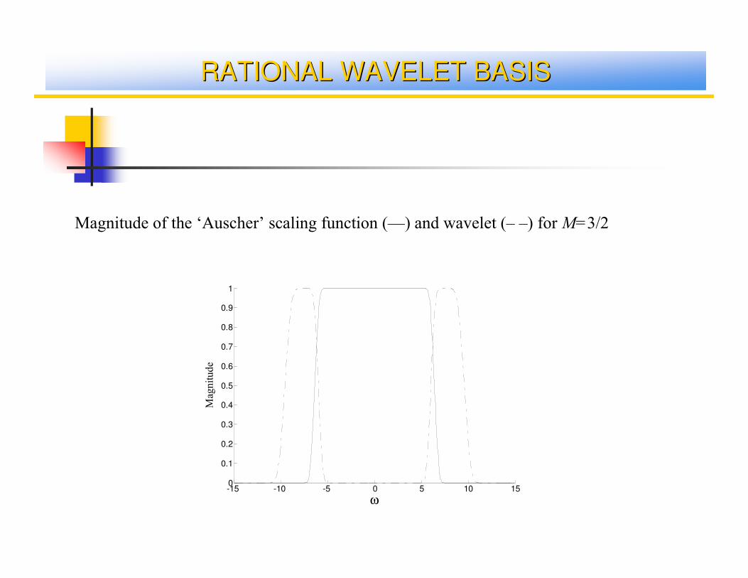
Let χ(ω) be an even and C∞(R) function define by:
where a=(q-ε)π, b=(q+ε)π, ε=]0, (1+M)-1]
and β being an odd an C∞(R) function.
Scaling function:
Wavelet:
( ) [ ] elsewhere 0)( if )(cosˆ πεωωχωϕ −≤= q
( ) [ ] ( )2
exp)(sin)(signˆ 1ωωχωωψ iq −= +
where sign(ω)=1 if ω≥0 and –1 elsewhere
RATIONAL WAVELET BASISRATIONAL WAVELET BASIS
-15 -10 -5 0 5 10 150
0.1
0.2
0.3
0.4
0.5
0.6
0.7
0.8
0.9
1
Mag
nitude
ω
Magnitude of the ‘Auscher’ scaling function (—) and wavelet (– –) for M=3/2
RATIONAL WAVELET BASISRATIONAL WAVELET BASIS
0 100 200 300-0.5
0
0.5
1
0 100 200 300-0.2
0
0.2
0.4
0.6
0.8
1
0 100 200 300-1
-0.5
0
0.5
1
110 120 130 140 150-0.2
0
0.2
0.4
0.6
0.8
110 120 130 140 150-0.2
0
0.2
0.4
0.6
0.8
110 120 130 140 150
-0.6
-0.4
-0.2
0
0.2
0.4
0.6
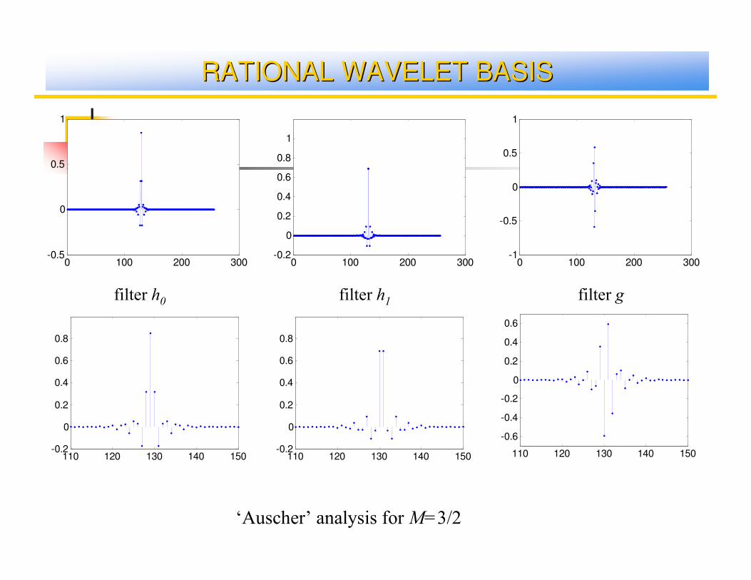
‘Auscher’ analysis for M=3/2
filter h0 filter h1 filter g
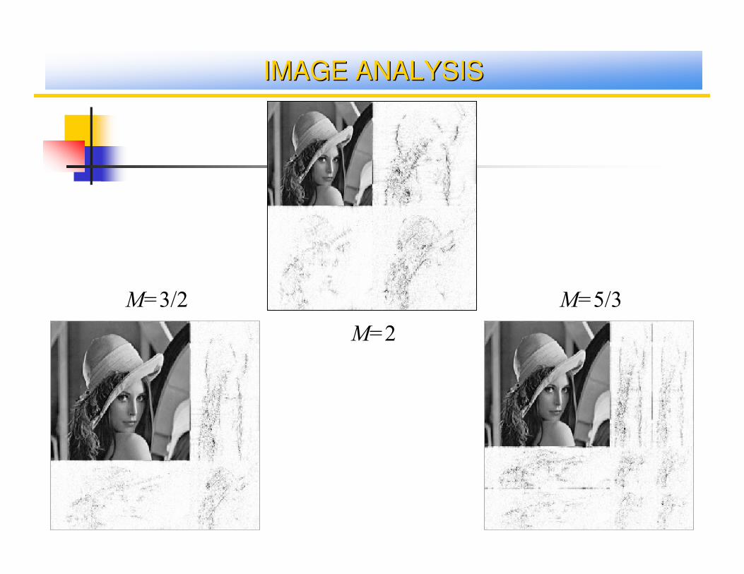
IMAGE ANALYSISIMAGE ANALYSIS
M=2
M=3/2 M=5/3
WAVELET SHRINKAGE DENOISINGWAVELET SHRINKAGE DENOISING
* Wavelet shrinkage based on the Stein’s Umbiased Estimate of Risk (SURE)
method (donoho 1994)
- estimate the variance σ2 of the noise.
- at each scale M j, a threshold Tj is calculated (taking into account σ2).
- perform the thresholding on the different scales.
*Applications:
- signal denoising
- 2D separable image denoising
- white and Gaussian noise centered on high frequency
* Easy extention to the rational case
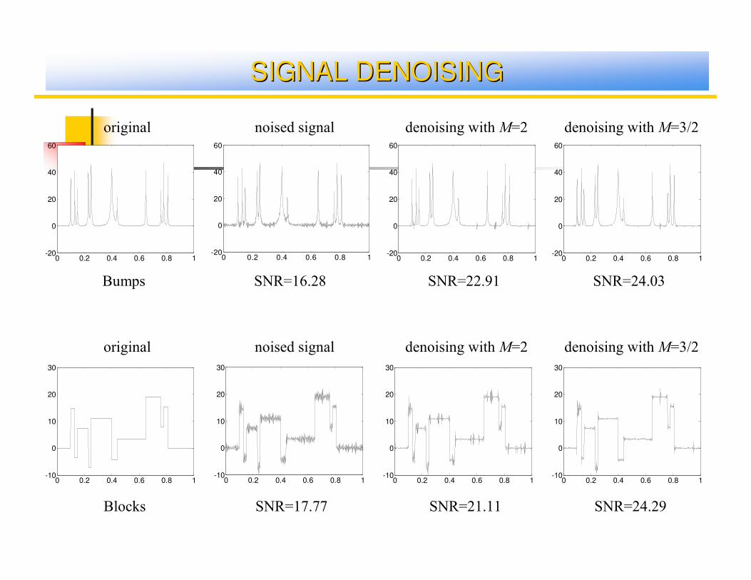
SIGNAL DENOISINGSIGNAL DENOISING
0 0.2 0.4 0.6 0.8 1-20
0
20
40
60
0 0.2 0.4 0.6 0.8 1-20
0
20
40
60
0 0.2 0.4 0.6 0.8 1-20
0
20
40
60
0 0.2 0.4 0.6 0.8 1-20
0
20
40
60
0 0.2 0.4 0.6 0.8 1-10
0
10
20
30
0 0.2 0.4 0.6 0.8 1-10
0
10
20
30
0 0.2 0.4 0.6 0.8 1-10
0
10
20
30
0 0.2 0.4 0.6 0.8 1-10
0
10
20
30
original noised signal denoising with M=2 denoising with M=3/2
original noised signal denoising with M=2 denoising with M=3/2
SNR=16.28 SNR=22.91 SNR=24.03
SNR=17.77 SNR=21.11 SNR=24.29
Bumps
Blocks
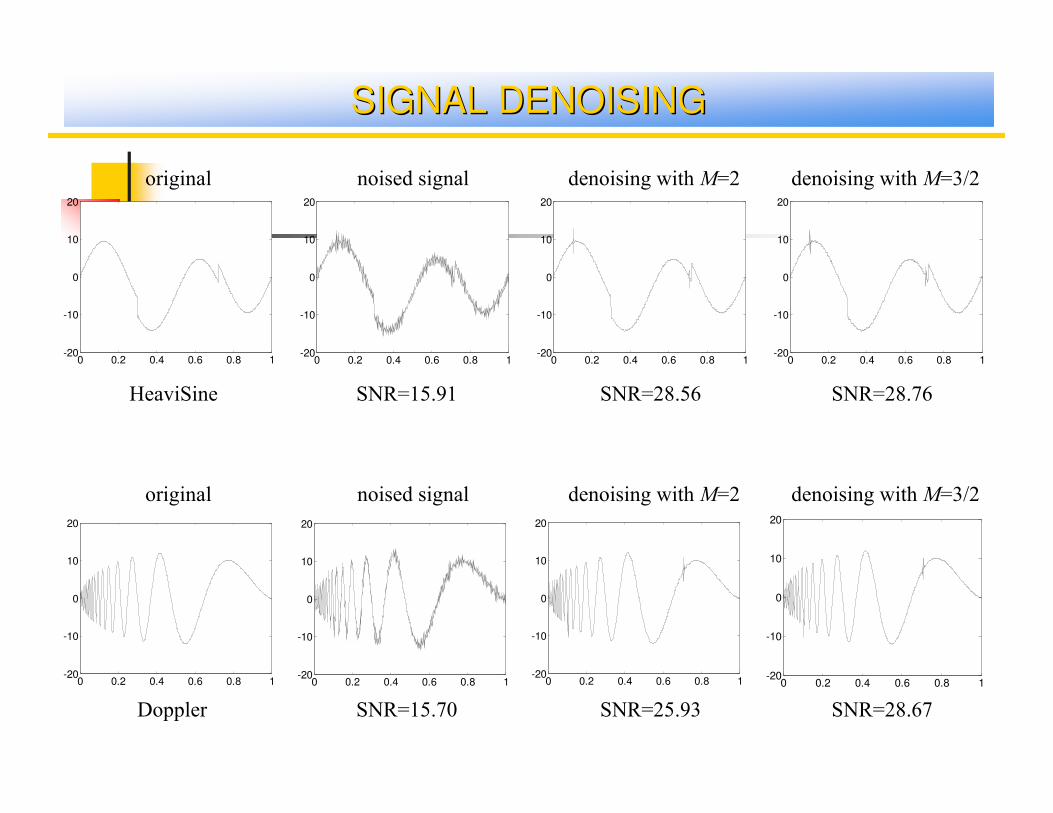
SIGNAL DENOISINGSIGNAL DENOISING
0 0.2 0.4 0.6 0.8 1-20
-10
0
10
20
0 0.2 0.4 0.6 0.8 1-20
-10
0
10
20
original noised signal denoising with M=2 denoising with M=3/2
SNR=15.91 SNR=28.56 SNR=28.76
original noised signal denoising with M=2 denoising with M=3/2
SNR=15.70 SNR=25.93 SNR=28.67
0 0.2 0.4 0.6 0.8 1-20
-10
0
10
20
0 0.2 0.4 0.6 0.8 1-20
-10
0
10
20
0 0.2 0.4 0.6 0.8 1-20
-10
0
10
20
0 0.2 0.4 0.6 0.8 1-20
-10
0
10
20
0 0.2 0.4 0.6 0.8 1-20
-10
0
10
20
0 0.2 0.4 0.6 0.8 1-20
-10
0
10
20
HeaviSine
Doppler
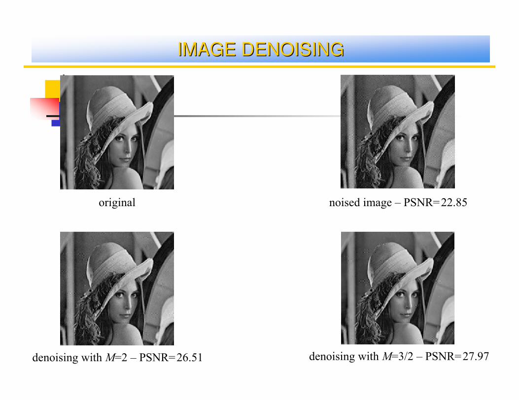
IMAGE DENOISINGIMAGE DENOISING
original noised image – PSNR=22.85
denoising with M=2 – PSNR=26.51 denoising with M=3/2 – PSNR=27.97
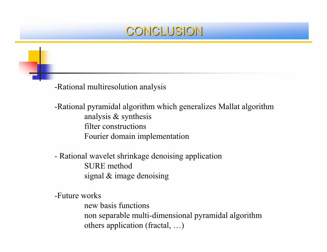
CONCLUSIONCONCLUSION
-Rational multiresolution analysis
-Rational pyramidal algorithm which generalizes Mallat algorithm
analysis & synthesis
filter constructions
Fourier domain implementation
- Rational wavelet shrinkage denoising application
SURE method
signal & image denoising
-Future works
new basis functions
non separable multi-dimensional pyramidal algorithm
others application (fractal, …)
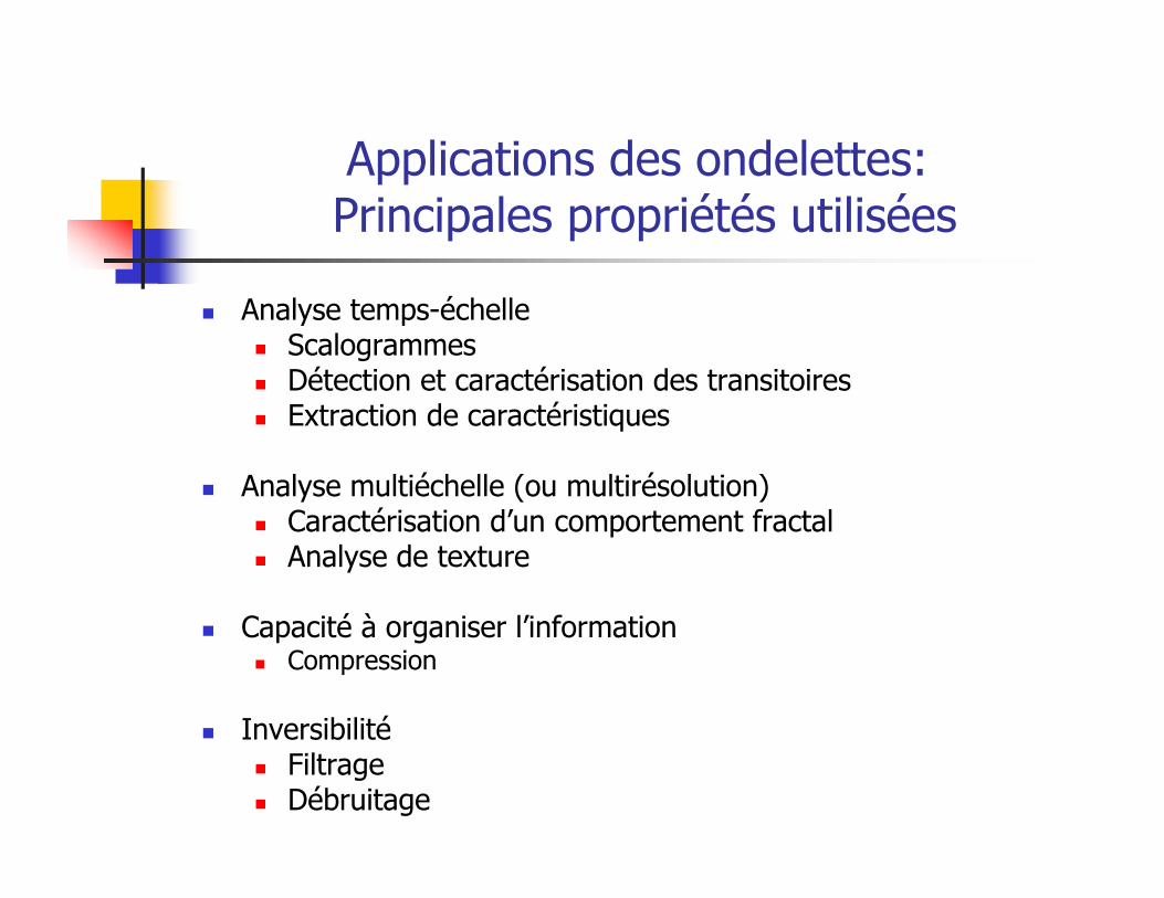
Applications des ondelettes:Principales propriétés utilisées
� Analyse temps-échelle� Scalogrammes� Détection et caractérisation des transitoires� Extraction de caractéristiques
� Analyse multiéchelle (ou multirésolution)� Caractérisation d’un comportement fractal� Analyse de texture
� Capacité à organiser l’information� Compression
� Inversibilité� Filtrage� Débruitage
Quelques applications des ondelettes en traitement des images
� Analyse et caractérisation des images
� Compression des images
� Tatouage
� Débruitage
� Zoom, Codage fractal…
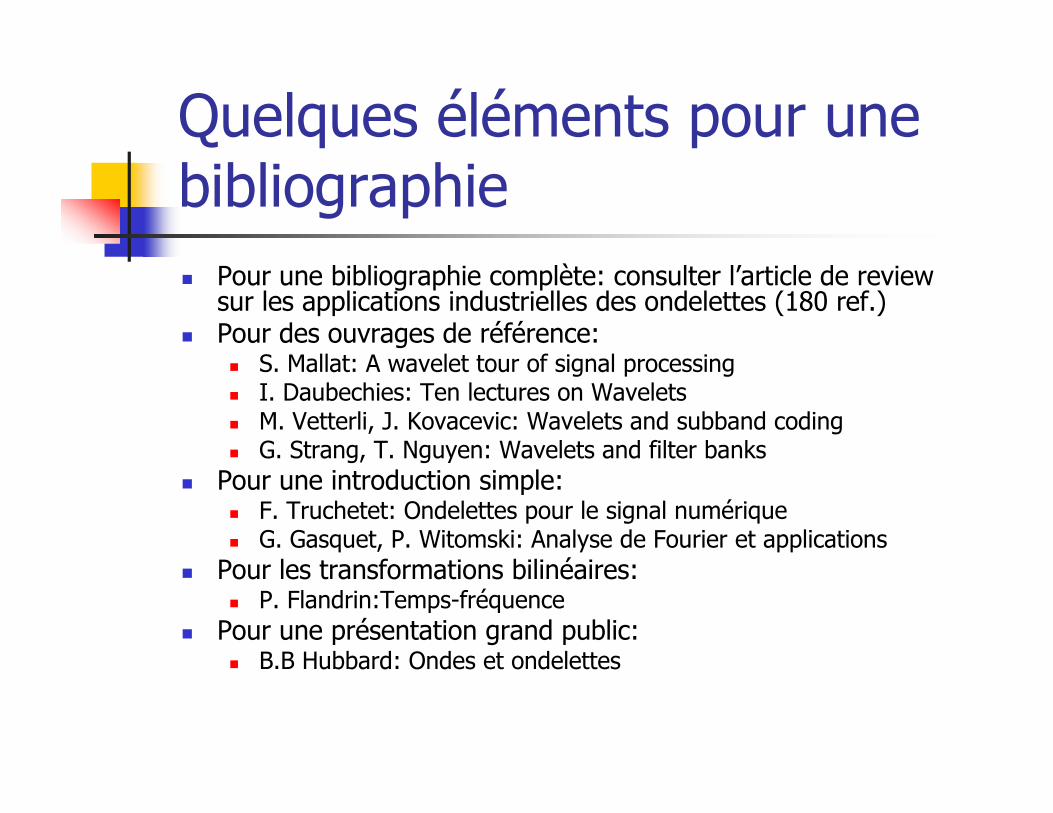
Quelques éléments pour une bibliographie
� Pour une bibliographie complète: consulter l’article de reviewsur les applications industrielles des ondelettes (180 ref.)
� Pour des ouvrages de référence:� S. Mallat: A wavelet tour of signal processing� I. Daubechies: Ten lectures on Wavelets� M. Vetterli, J. Kovacevic: Wavelets and subband coding� G. Strang, T. Nguyen: Wavelets and filter banks
� Pour une introduction simple:� F. Truchetet: Ondelettes pour le signal numérique� G. Gasquet, P. Witomski: Analyse de Fourier et applications
� Pour les transformations bilinéaires:� P. Flandrin:Temps-fréquence
� Pour une présentation grand public:� B.B Hubbard: Ondes et ondelettes
Troisième partie: applications
� Les ondelettes dans l’industrie
Wavelet applications in signal processing
� Acoustical Signal processing
� Ultrasonic Non Destructive Evaluation
� Speech enhancement
Ultrasonic Non Destructive EvaluationAbbate et al., Park et al. (1997)
� WT (Gabor wavelet) applied to the time-frequency
analysis of ultrasonic echo waveform obtained by an
ultrasonic pulse-echo technique
� Noise suppression of ultrasonic flaw signal and NDE of
material degradation using wavelet analysis of
ultrasonic echo waveform
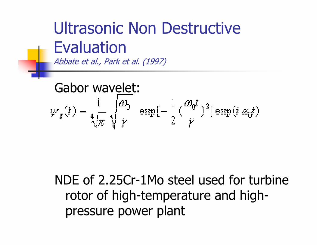
Ultrasonic Non Destructive EvaluationAbbate et al., Park et al. (1997)
Gabor wavelet:
NDE of 2.25Cr-1Mo steel used for turbine rotor of high-temperature and high-pressure power plant
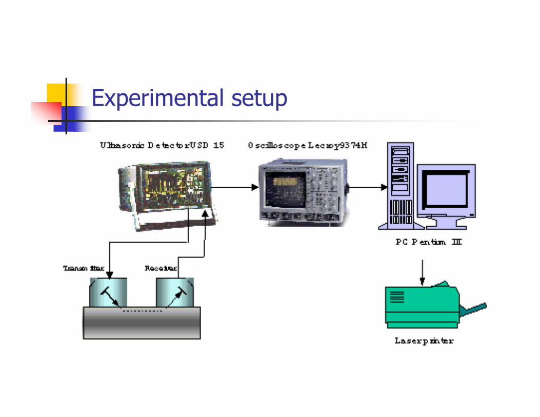
Experimental setup
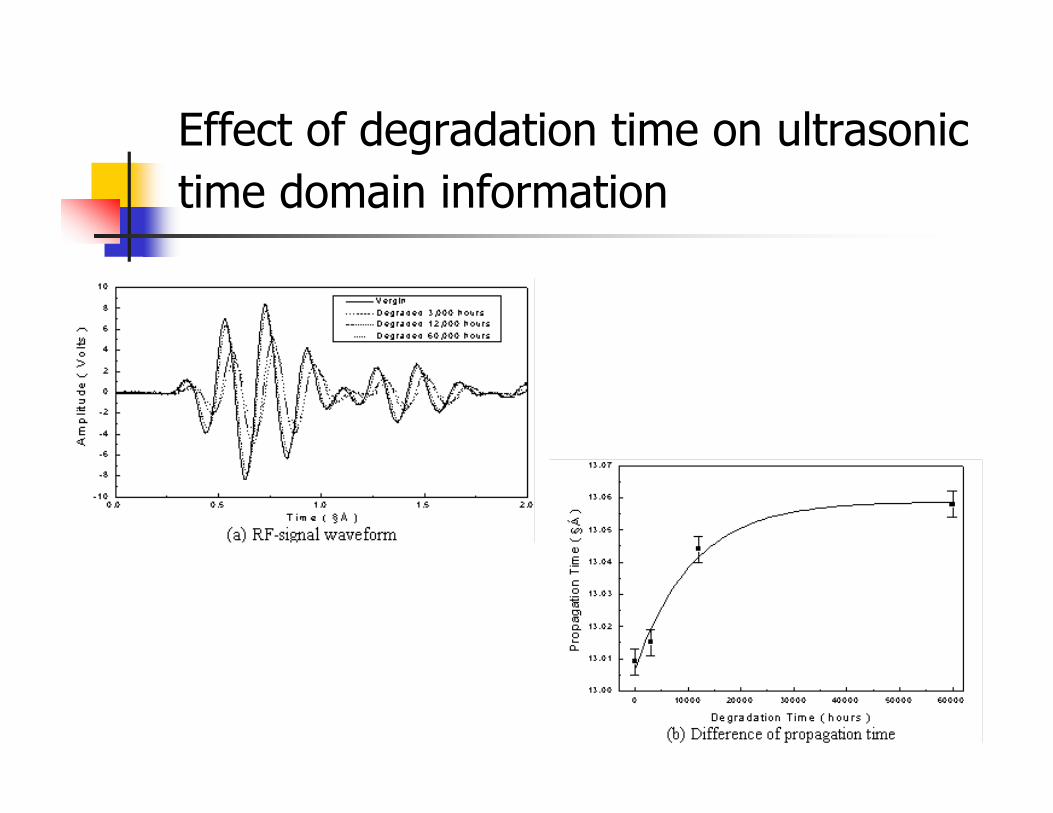
Effect of degradation time on ultrasonic
time domain information
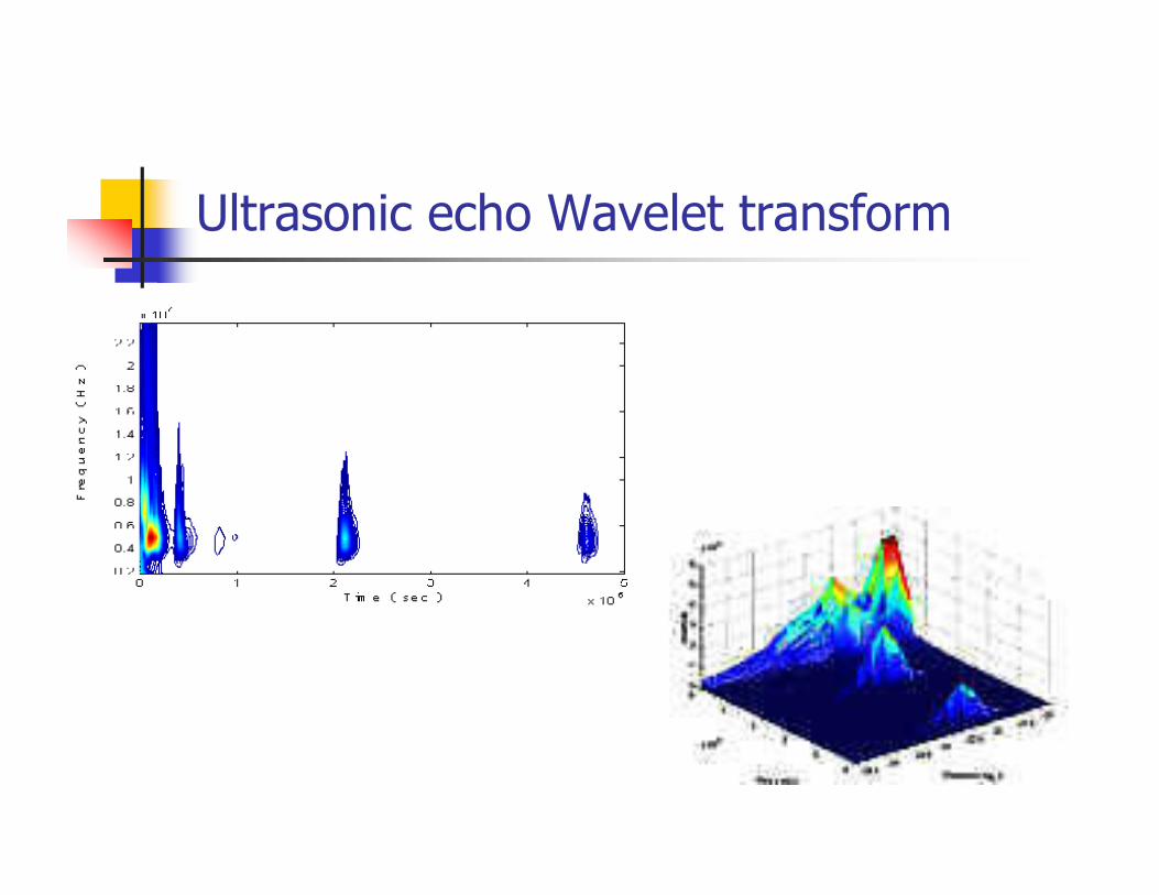
Ultrasonic echo Wavelet transform
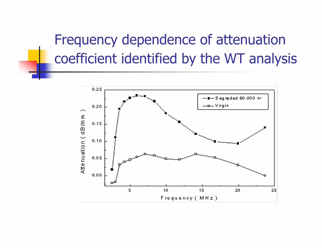
Frequency dependence of attenuation
coefficient identified by the WT analysis
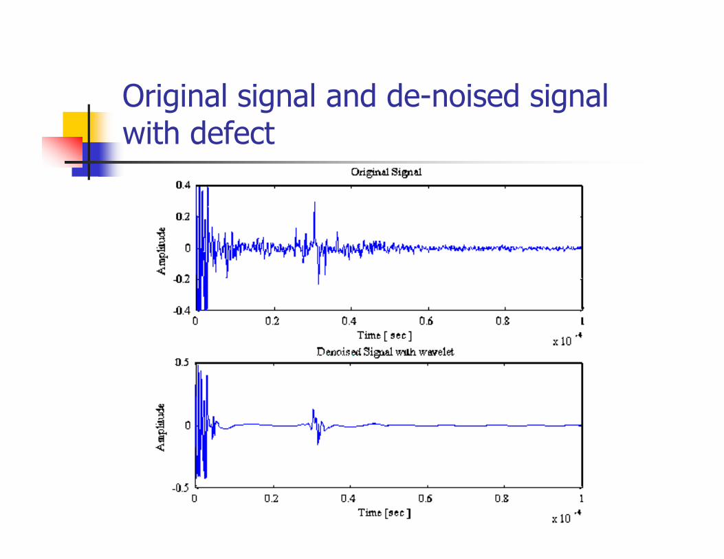
Original signal and de-noised signal with defect
Ultrasonic Examination of Thermal Sprayed Coatings with FrequencyAnalysis Hatanaka et al. (2000)
� Nondestructive methods for evaluating adhesive
strength of thermal sprayed coating and measuring
coating thickness by ultrasonic testing
� Coating thickness measurement: the WT was used
� to analyze the ultrasonic waveform and
� to enhance signal-to-noise ratio of ultrasonic waveforms
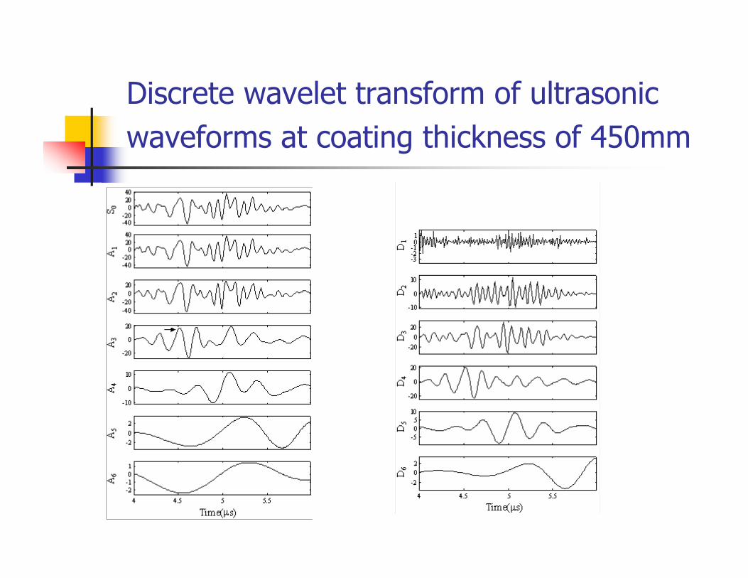
Discrete wavelet transform of ultrasonic
waveforms at coating thickness of 450mm
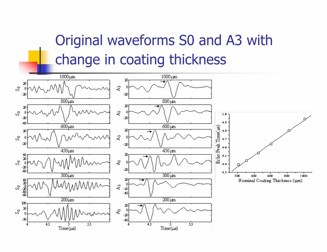
Original waveforms S0 and A3 with
change in coating thickness
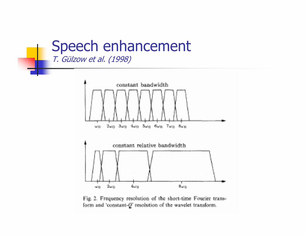
Speech enhancementT. Gülzow et al. (1998)
� Spectral subtraction: a popular method for speech
enhancement, if corrupted by additive noise.
� Based on the manipulation of the magnitude of the noisy-
speech spectrum. Previous realizations used uniformly
spaced frequency transformations.
� Application of filterbank with bark-scaled frequency
bands: a discrete wavelet transformation
� The enhancement results as well as the expenditures are
compared to those obtained with uniform spectral
transformations.
Speech enhancementT. Gülzow et al. (1998)
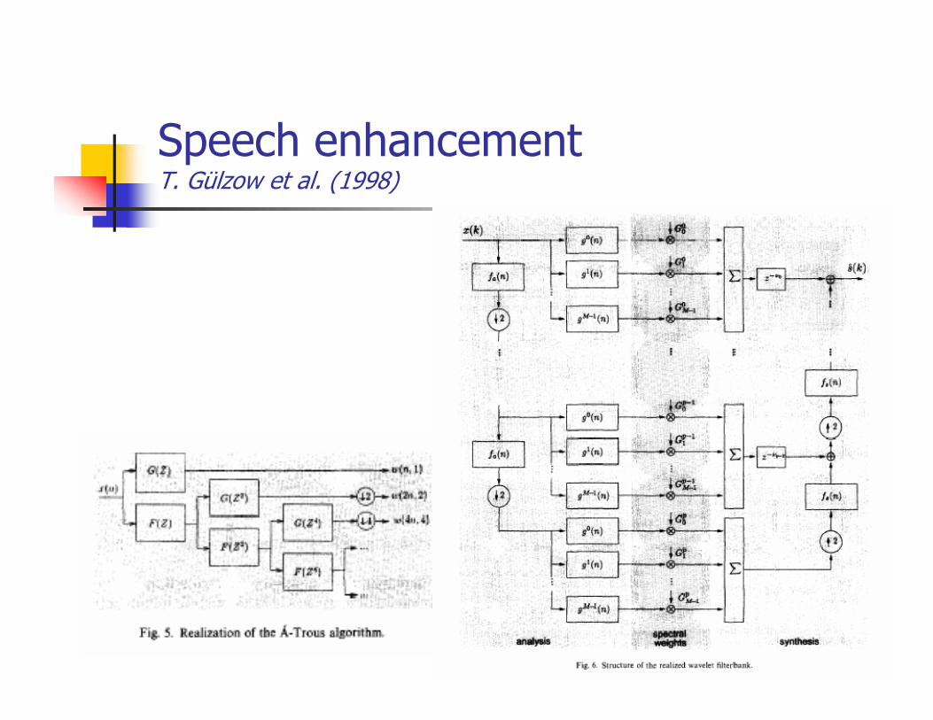
Speech enhancementT. Gülzow et al. (1998)
Wavelet applications in signal processing
� Power production, electrotechnic andpower electronic
� Control of rotating machines
� Power quality monitoring
Sensorless Speed Measurement of AC Machines Using Analytic Wavelet Transform Aller et al. (2002)
� Analytic wavelet transform of the stator current signal
for a direct torque control drive.
� The time–frequency resolution obtained and the
computation time required by the proposed algorithm
are improved in comparison to existing techniques and
the method can be applied over the entire speed range.
� The instantaneous frequency is estimated by ridges
detection in the spectrogram. The spectrogram can be
obtained using any time–frequency transform such as
STFT, AWT or Wigner–Ville.
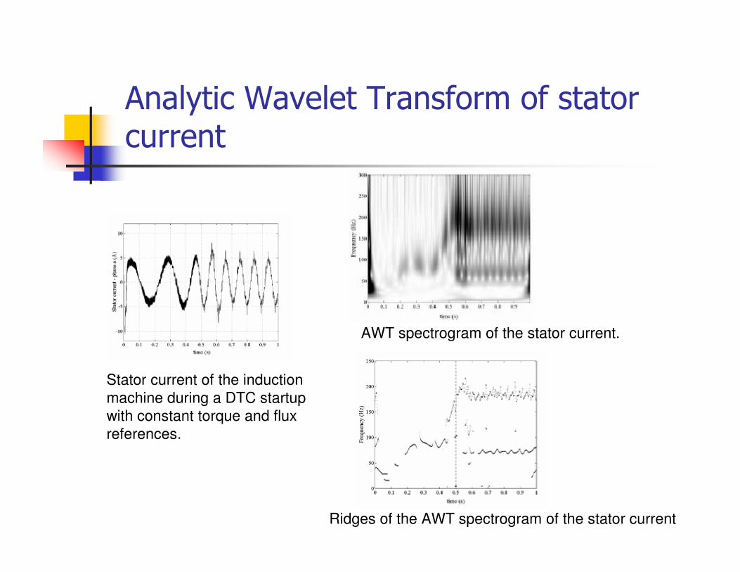
Analytic Wavelet Transform of stator current
AWT spectrogram of the stator current.
Ridges of the AWT spectrogram of the stator current
Stator current of the induction
machine during a DTC startup
with constant torque and flux
references.
Power quality monitoring
� High voltage insulation suffers from aging processes
� Failure of equipment can be sudden and catastrophic,
leading to risk of injury to personnel and damage of
expensive equipment.
� On line monitoring of electrical signals has been
shown to provide useful diagnostic information.
� The processing of such information is a complex problem.
� The wavelet transform can be used to provide a method
of analysis and visualisation of transient electrical signals
obtained from on line monitoring.
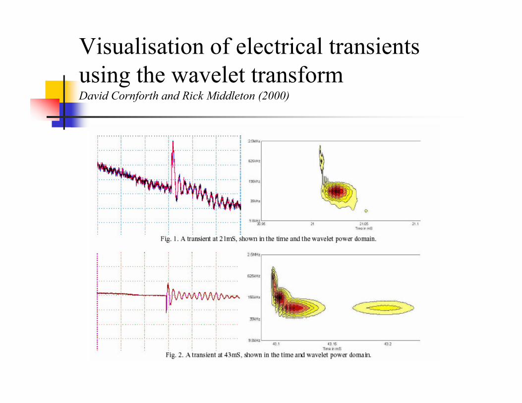
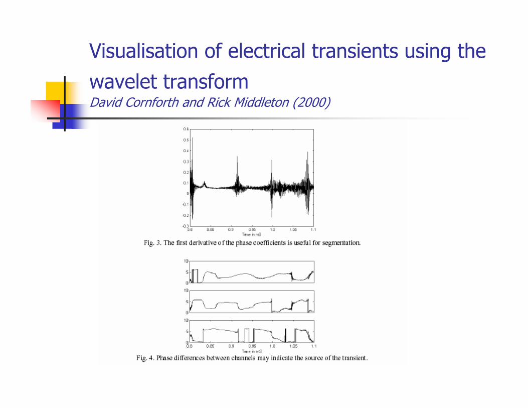
Visualisation of electrical transients
using the wavelet transformDavid Cornforth and Rick Middleton (2000)
Visualisation of electrical transients using thewavelet transformDavid Cornforth and Rick Middleton (2000)
� These results show that the power coefficients may be
useful in the following ways:
· Manual visualisation and inspection of transients
· Noise removal
· Automatic segmentation of the signal to obtain the
segments of interest
· Automatic classification of transients after further
processing
Visualisation of electrical transients using the
wavelet transformDavid Cornforth and Rick Middleton (2000)
Pattern Recognition Applications For Power System Disturbance ClassificationGaouda et al. (1999)
� Automated on-line disturbance classification technique.
� Based on wavelet multiresolution analysis and pattern recognition
� WT is for feature extraction in order to classify different disturbances.
� Minimum Euclidean distance, k-nearest neighbor, and neural network
classifiers are used to evaluate the efficiency of the extracted features.
� Feature vector: The standard deviation at different resolution levels
� Wavelet basis: Daubechies-8
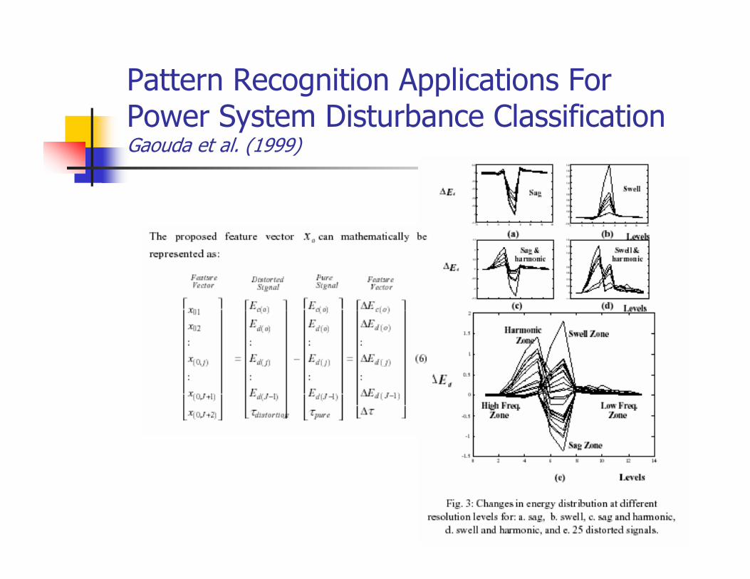
Pattern Recognition Applications For Power System Disturbance ClassificationGaouda et al. (1999)
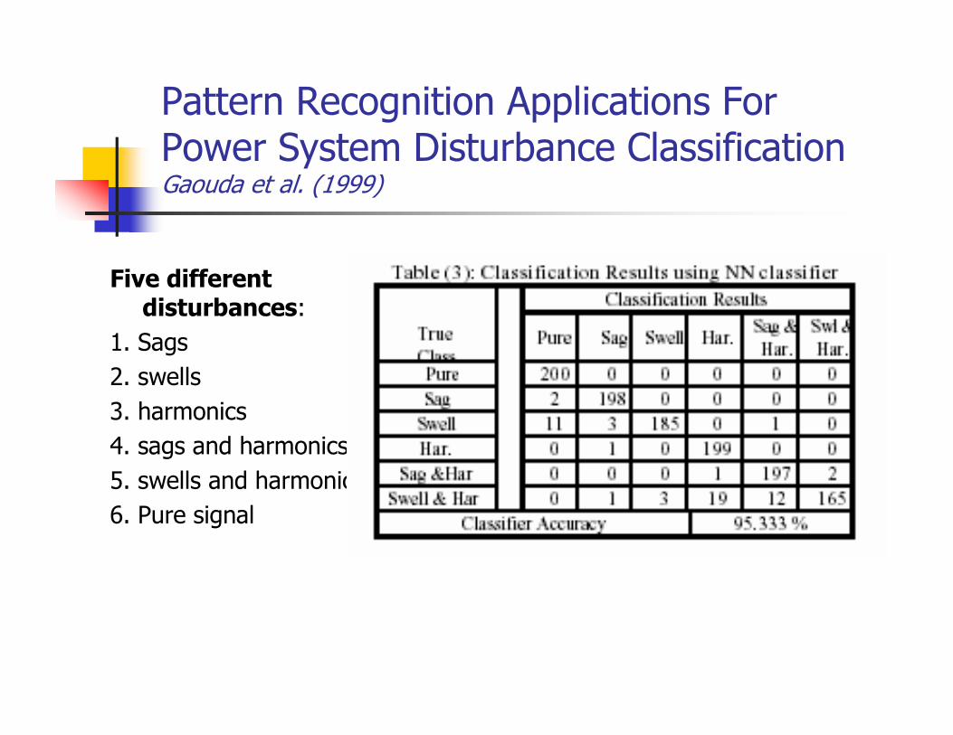
Pattern Recognition Applications For Power System Disturbance ClassificationGaouda et al. (1999)
Five differentdisturbances:
1. Sags
2. swells
3. harmonics
4. sags and harmonics
5. swells and harmonics
6. Pure signal
Wavelet applications in signal processing
� Non destructive testing (NDT)
� Magnetic Flux Leakage (MFL)
� Vibration signal analysis
Wavelet Analysis of MFL Signal for
Steel Wire Rope Testing Barat et al. (2000)
� Inspection is realized by magnetic flux leakage (MFL) method: magnetic
head magnetically saturates a rope passing through magnetic head.
� Discontinuities, like broken wires or strands, pits of corrosion etc., cause
changes in leakage magnetic field.
� Signal analysis: register number and characteristics of broken wires and
measure the loss of metallic cross-section area.
� Problem: strong influence of rope vibrations, gap changes, twisted rope
structure, etc… inducing wide band (white) and narrow band noises
� Magnetostatic transducers (based on Hall-effect sensor) are usually used
for inspection of steel wire ropes. This sensor measures the distribution of
leakage field caused by defect. Using differential measurement scheme,
signal of a typical defect has a form of smooth two-polar impulses with
duration depending on depth and size of the defect.
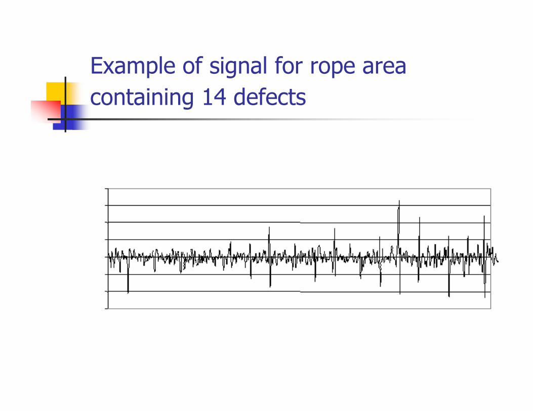
Example of signal for rope area
containing 14 defects
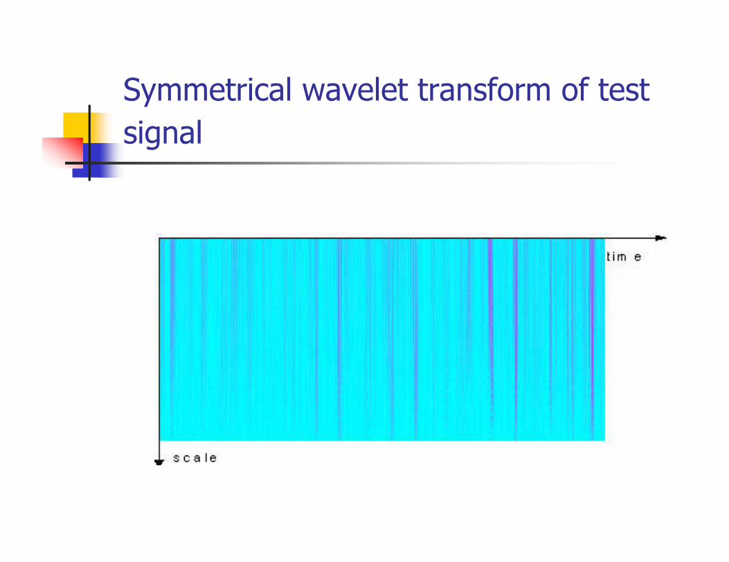
Symmetrical wavelet transform of test
signal
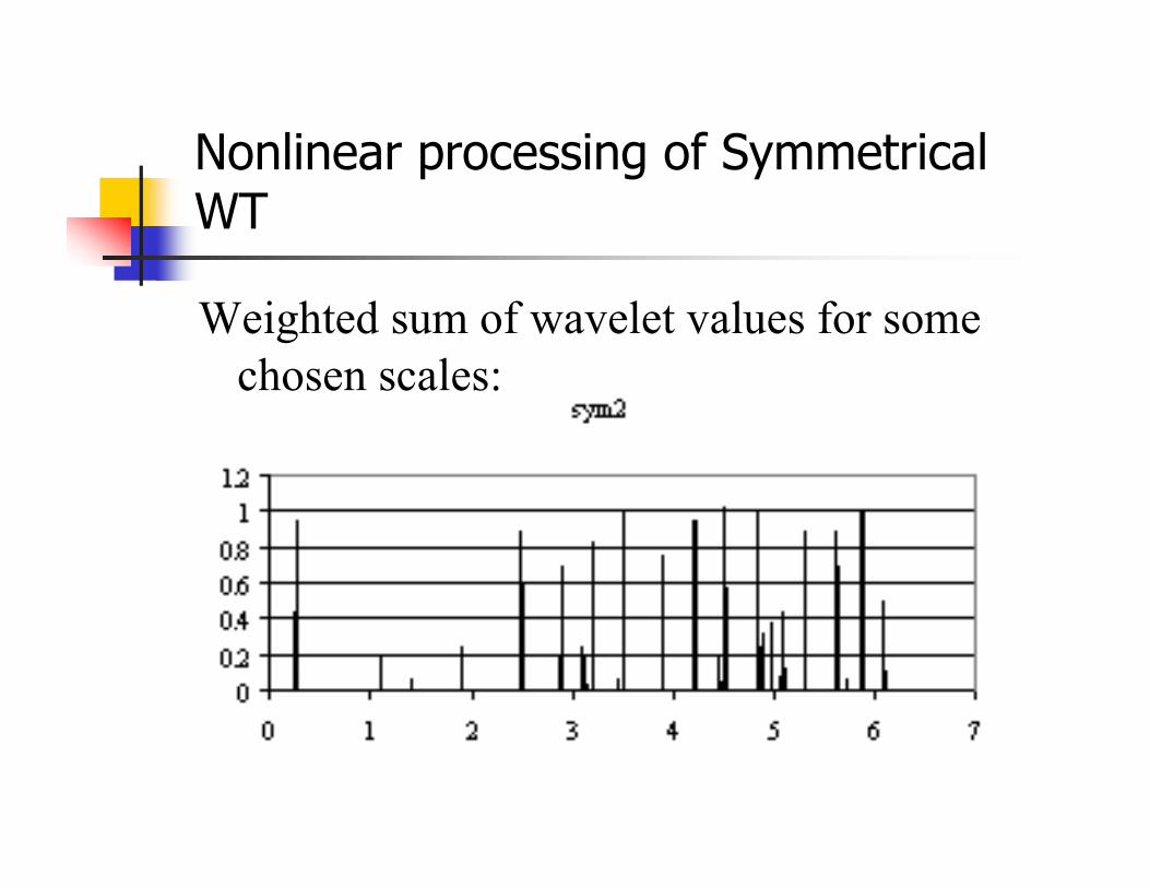
Nonlinear processing of SymmetricalWT
Weighted sum of wavelet values for some
chosen scales:
The application of wavelet transform in magnetic flux leakage test of pipelineYang-Lijian et al. (2001)
� Detecting localized flaws in oil and gas pipeline by
measuring magnetic flux leakage.
� WT is applied to the processing of detected signals.
� Biorthogonal wavelet to decompose actual signals; the
result shows that the wavelet analysis has high
performance in the feature extraction of flux leakage
signals of pipeline.
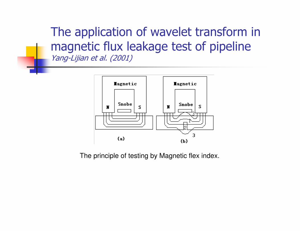
The application of wavelet transform in magnetic flux leakage test of pipelineYang-Lijian et al. (2001)
The principle of testing by Magnetic flex index.
The application of wavelet transform in magnetic flux leakage test of pipelineYang-Lijian et al. (2001)
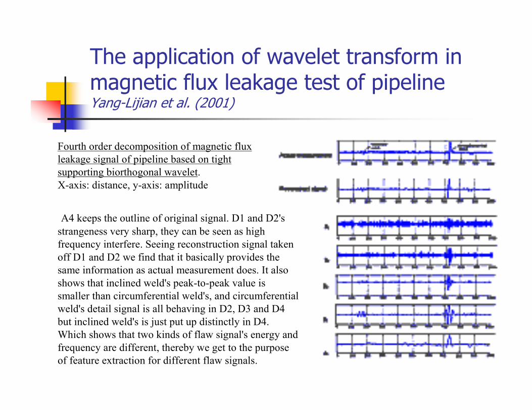
Fourth order decomposition of magnetic flux
leakage signal of pipeline based on tight
supporting biorthogonal wavelet.
X-axis: distance, y-axis: amplitude
A4 keeps the outline of original signal. D1 and D2's
strangeness very sharp, they can be seen as high
frequency interfere. Seeing reconstruction signal taken
off D1 and D2 we find that it basically provides the
same information as actual measurement does. It also
shows that inclined weld's peak-to-peak value is
smaller than circumferential weld's, and circumferential
weld's detail signal is all behaving in D2, D3 and D4
but inclined weld's is just put up distinctly in D4.
Which shows that two kinds of flaw signal's energy and
frequency are different, thereby we get to the purpose
of feature extraction for different flaw signals.
Wavelet applications in signal processing
� Tool wear monitoring
� Chemical process
Real-Time Tool Condition Monitoring in Transfer Machining StationsYa Wu et al. (2001)
� Tool condition monitoring is one of the major concerns in
modern machining operations, especially for the transfer
machining operations in mass production. A misdetected
tool failure such as wear, breakage, chipping, etc.! could
lead to poor product quality and even damage the machine
tool and/or the fixture. On the other hand, a false detected
tool failure may cause the unnecessary breakdown of an
entire production line.
� In the indirect methods, tool condition is predicted based
on various sensor signals such as cutting force, vibration,
temperature, acoustic emission, and motor current. cutting
force signals and vibration signals.
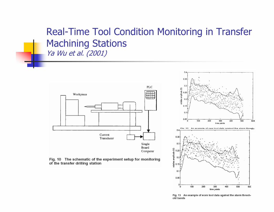
Real-Time Tool Condition Monitoring in TransferMachining StationsYa Wu et al. (2001)
Real-Time Tool Condition Monitoring in TransferMachining Stations Ya Wu et al. (2001)
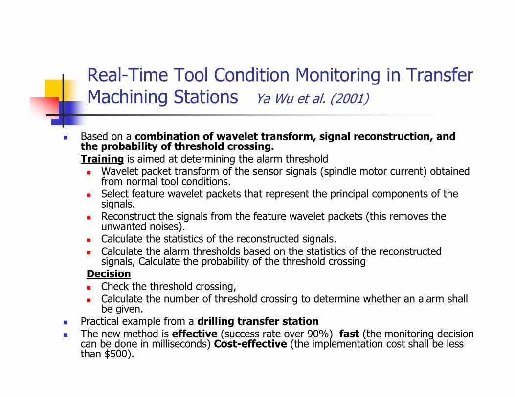
� Based on a combination of wavelet transform, signal reconstruction, andthe probability of threshold crossing. Training is aimed at determining the alarm threshold� Wavelet packet transform of the sensor signals (spindle motor current) obtained
from normal tool conditions. � Select feature wavelet packets that represent the principal components of the
signals. � Reconstruct the signals from the feature wavelet packets (this removes the
unwanted noises). � Calculate the statistics of the reconstructed signals. � Calculate the alarm thresholds based on the statistics of the reconstructed
signals, Calculate the probability of the threshold crossingDecision� Check the threshold crossing,� Calculate the number of threshold crossing to determine whether an alarm shall
be given.� Practical example from a drilling transfer station� The new method is effective (success rate over 90%) fast (the monitoring decision
can be done in milliseconds) Cost-effective (the implementation cost shall be lessthan $500).
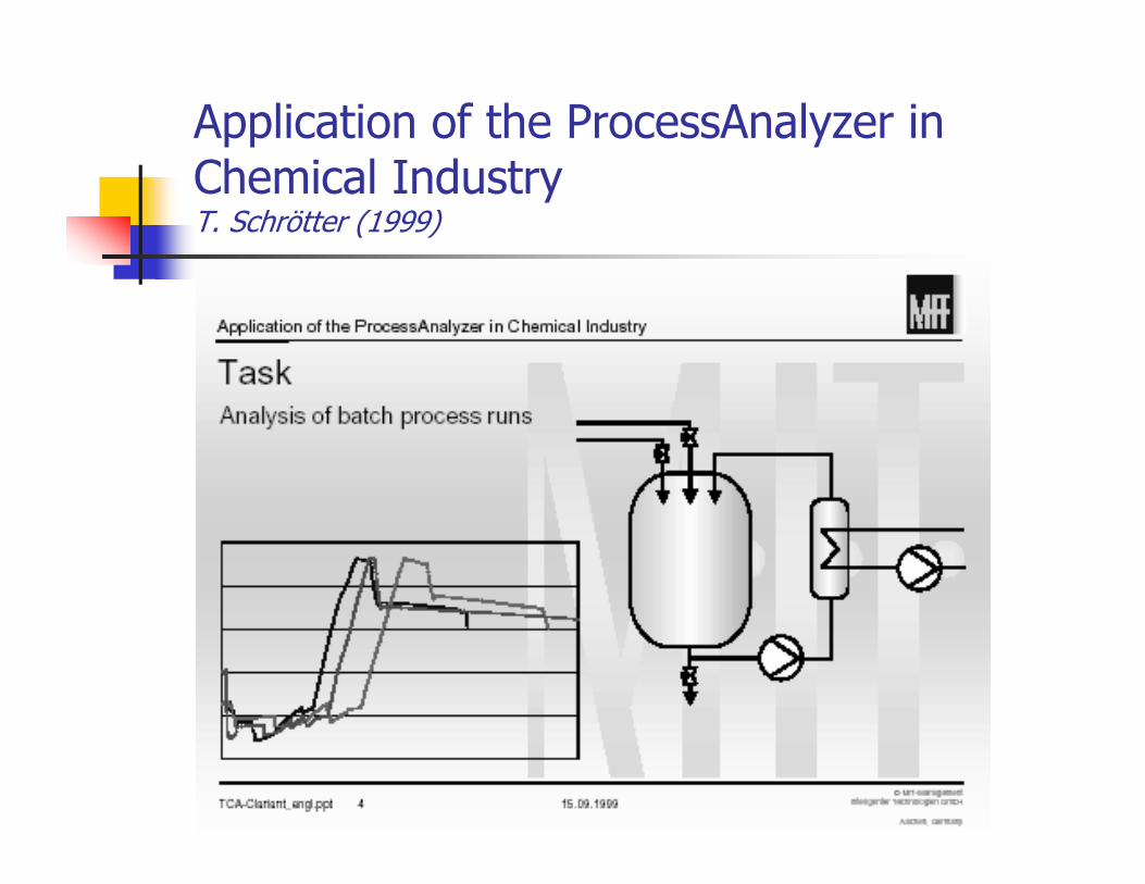
Application of the ProcessAnalyzer inChemical IndustryT. Schrötter (1999)
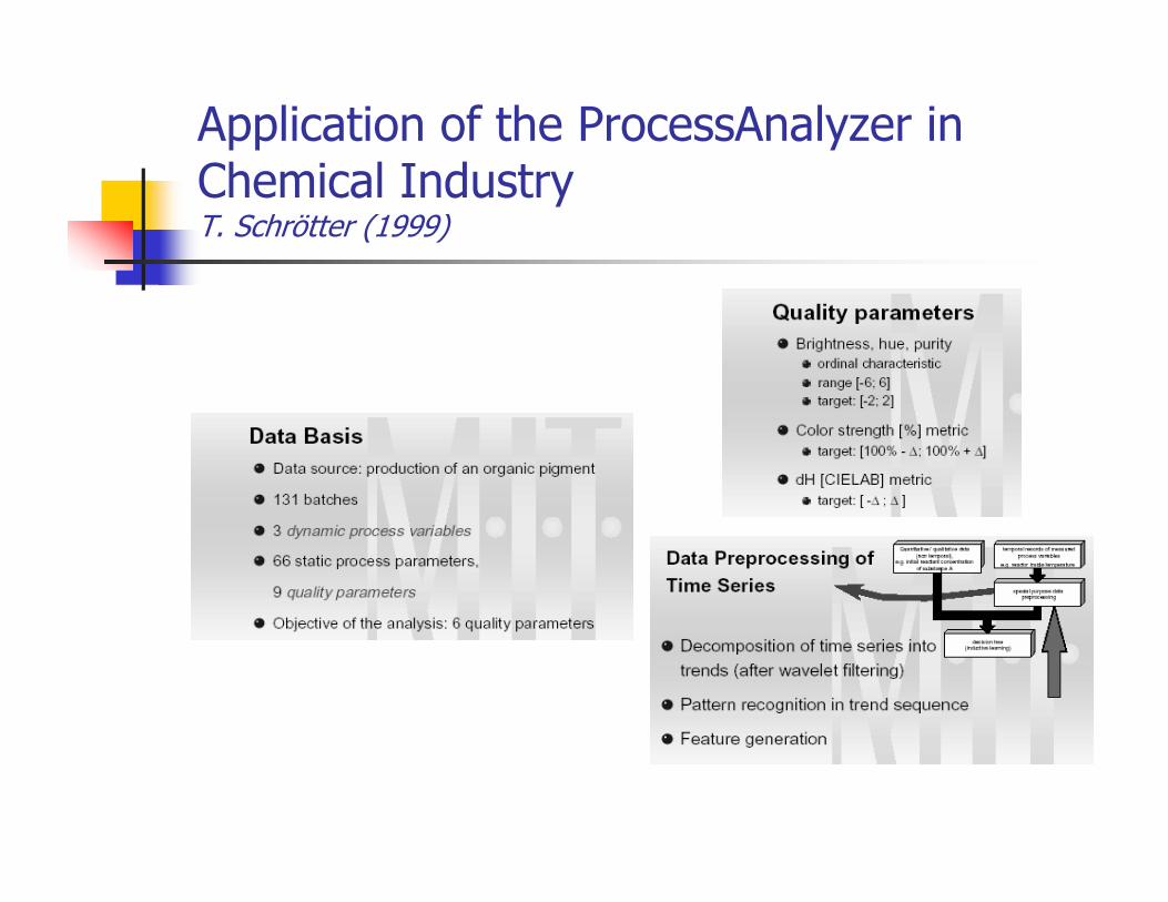
Application of the ProcessAnalyzer inChemical IndustryT. Schrötter (1999)
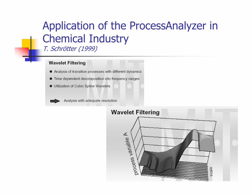
Application of the ProcessAnalyzer inChemical IndustryT. Schrötter (1999)
Wavelet applications in signal processing
� Stochastic signal analysis
� Wind energy
� DNA-sequences
� Computer traffic (cf P.Abry)
Wavelet Packet Transfer FunctionModelling of Nonstationary Time SeriesG. P. Nason et al. (2000)
� How a non-decimated wavelet packet transform (NWPT) can be used to model a response time series, in terms of an explanatory time series
� The proposed computational technique transforms theexplanatory time series into a NWPT representation andthen uses standard statistical modelling methods to identifywhich wavelet packets are useful for modelling theresponse time series.
� Application to an important problem from the wind energyindustry: how to model wind speed at a target location using wind speed and direction from a reference location.
Wavelet Packet Transfer FunctionModelling of Nonstationary Time SeriesG. P. Nason et al. (2000)
� Before construction of a wind farm an analysis is
undertaken to establish whether a particular target site is
suitable.
� One aspect of this analysis involves the prediction of the
long-term mean wind speed at the target site.
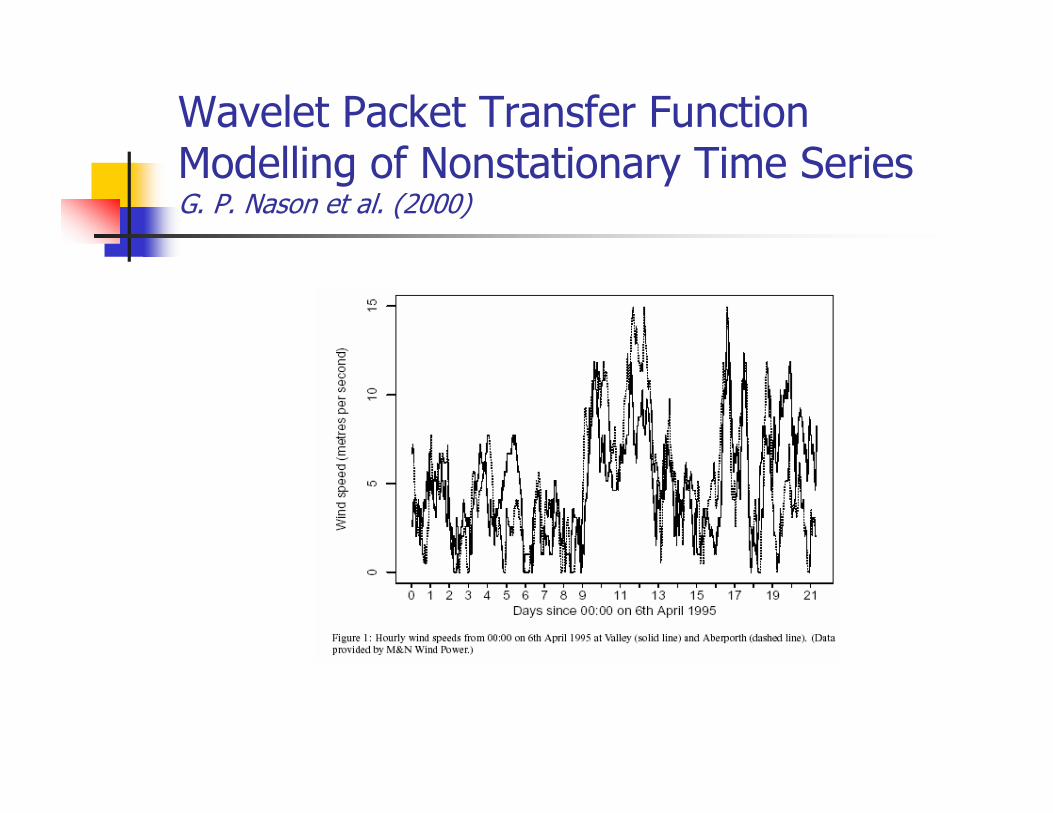
� Typically, wind speeds are measured by a pilot
anemometer at a height of 10m at the target site for several
months.
� A model predicting target from reference speeds is
constructed.
Wavelet Packet Transfer FunctionModelling of Nonstationary Time SeriesG. P. Nason et al. (2000)
Wavelet Packet Transfer FunctionModelling of Nonstationary Time SeriesG. P. Nason et al. (2000)
� Extraction of non-decimated wavelet transform
coefficients at the same dyadic scale for each time series
and then statistically modelling of one set in terms of the
other using linear regression.
� Non-decimated transforms have the same number of
coefficients at each scale and coefficients within each scale
are located according to the same time grid.
� Moreover, wavelet packets can elicit a greater variety of
behaviours than can wavelets alone.
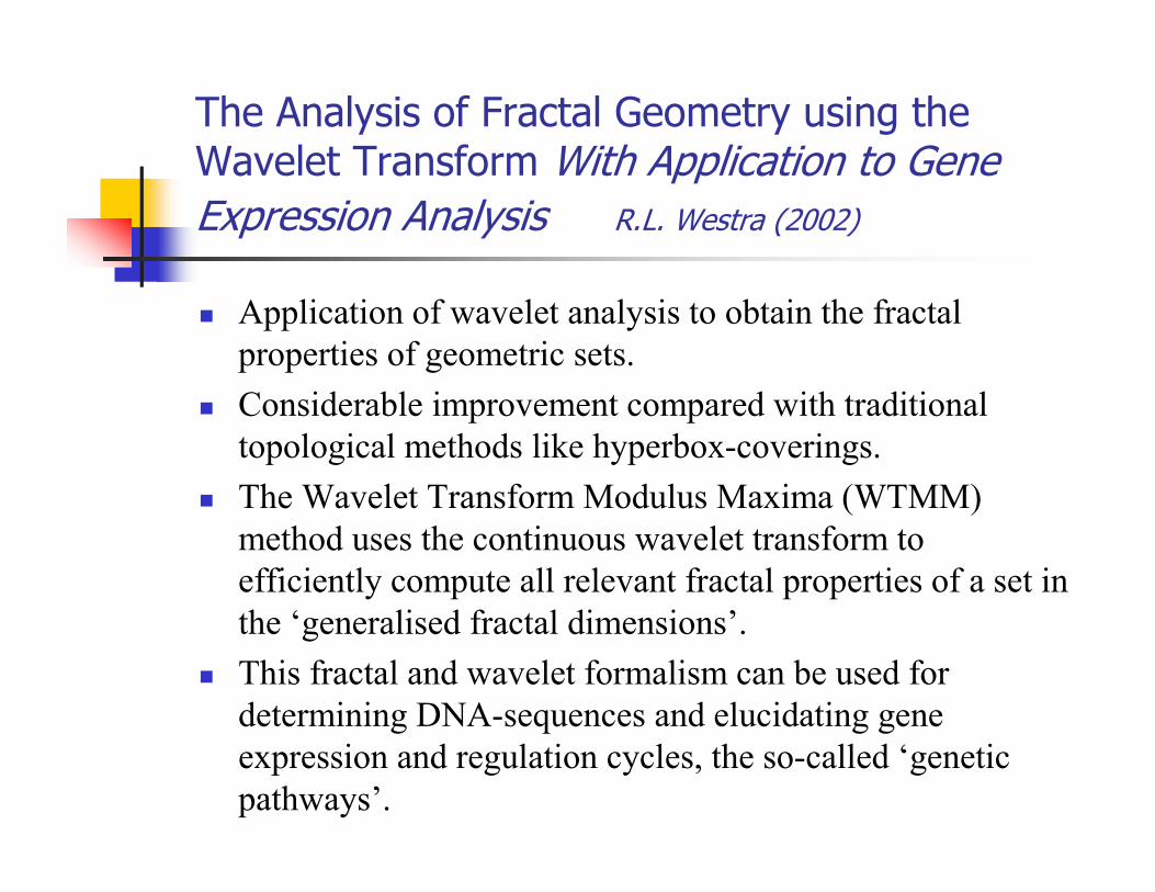
The Analysis of Fractal Geometry using theWavelet Transform With Application to GeneExpression Analysis R.L. Westra (2002)
� Application of wavelet analysis to obtain the fractal
properties of geometric sets.
� Considerable improvement compared with traditional
topological methods like hyperbox-coverings.
� The Wavelet Transform Modulus Maxima (WTMM)
method uses the continuous wavelet transform to
efficiently compute all relevant fractal properties of a set in
the ‘generalised fractal dimensions’.
� This fractal and wavelet formalism can be used for
determining DNA-sequences and elucidating gene
expression and regulation cycles, the so-called ‘genetic
pathways’.
Wavelet applications in image processing
� Image compression
� JPEG
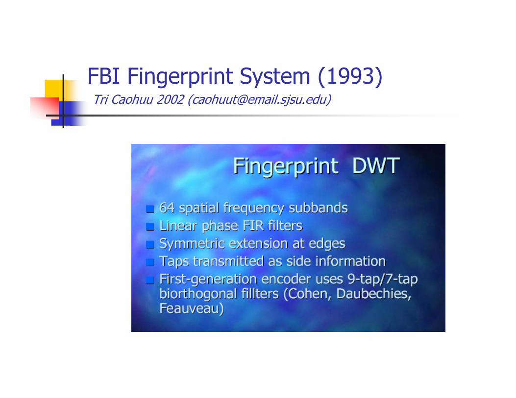
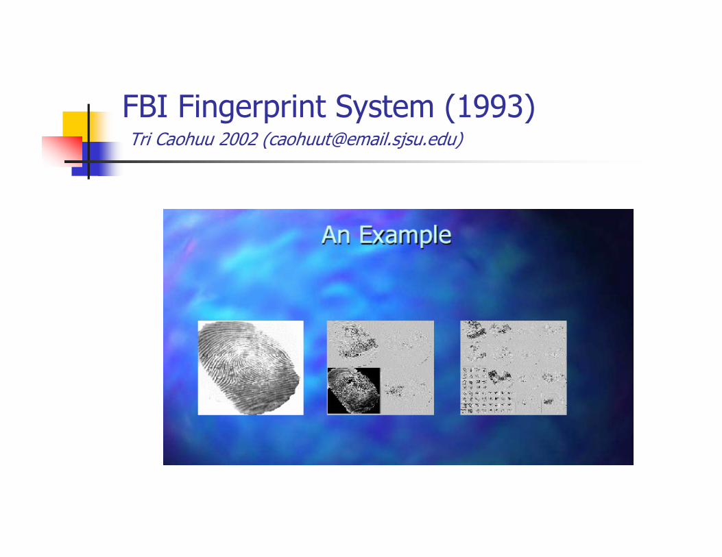
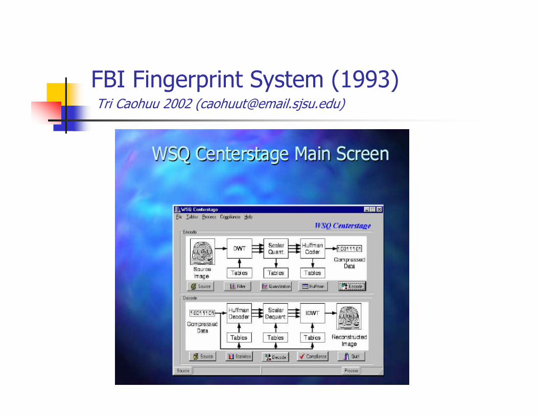
� Finger print
� Color image compression
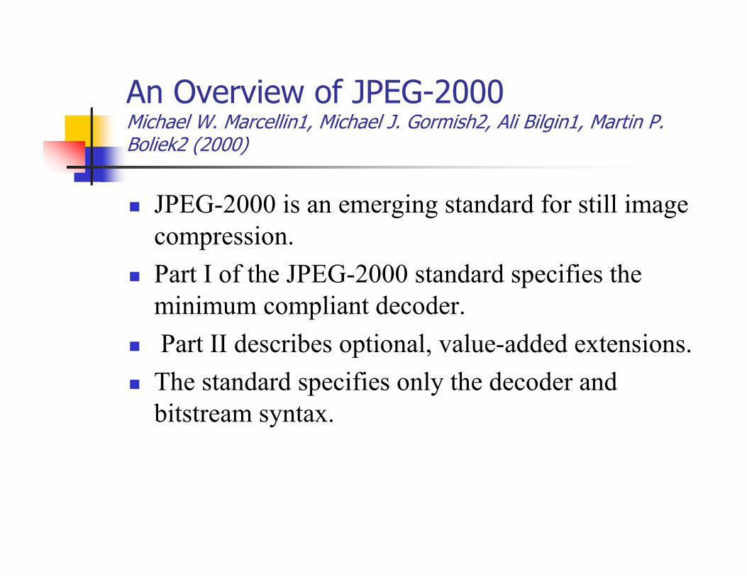
An Overview of JPEG-2000Michael W. Marcellin1, Michael J. Gormish2, Ali Bilgin1, Martin P. Boliek2 (2000)
� JPEG-2000 is an emerging standard for still image
compression.
� Part I of the JPEG-2000 standard specifies the
minimum compliant decoder.
� Part II describes optional, value-added extensions.
� The standard specifies only the decoder and
bitstream syntax.
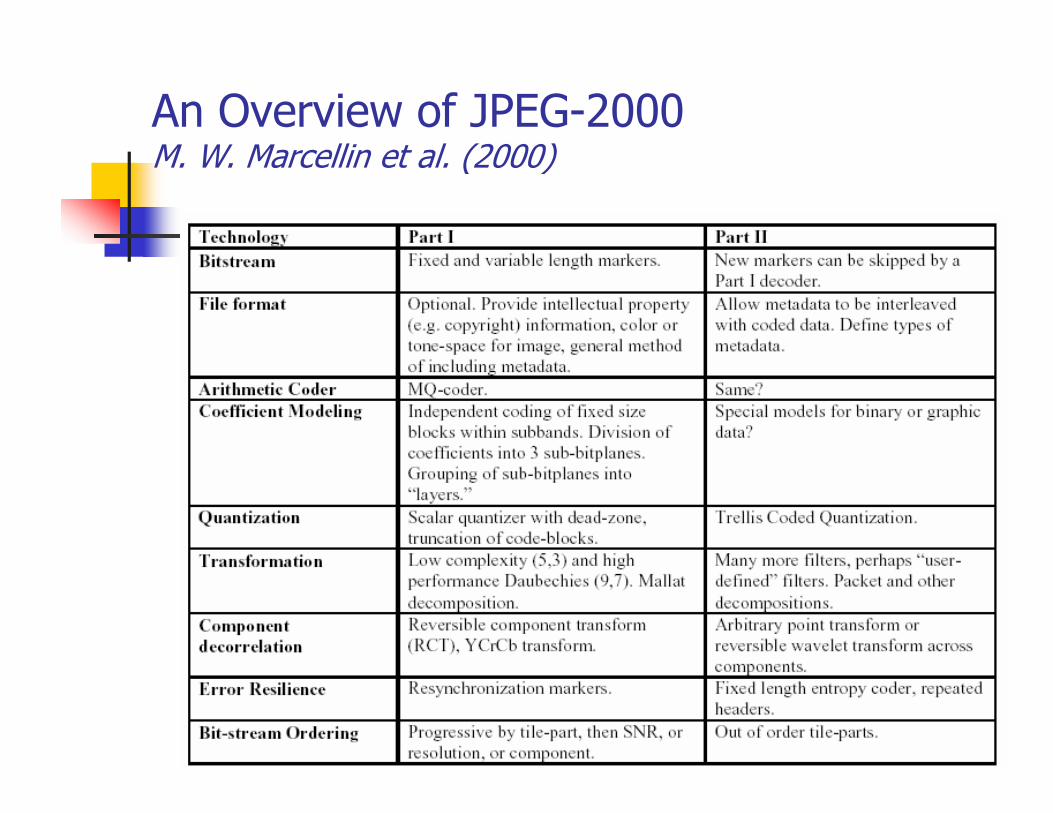
An Overview of JPEG-2000M. W. Marcellin et al. (2000)
An Overview of JPEG-2000M. W. Marcellin et al. (2000)
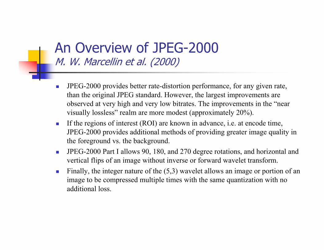
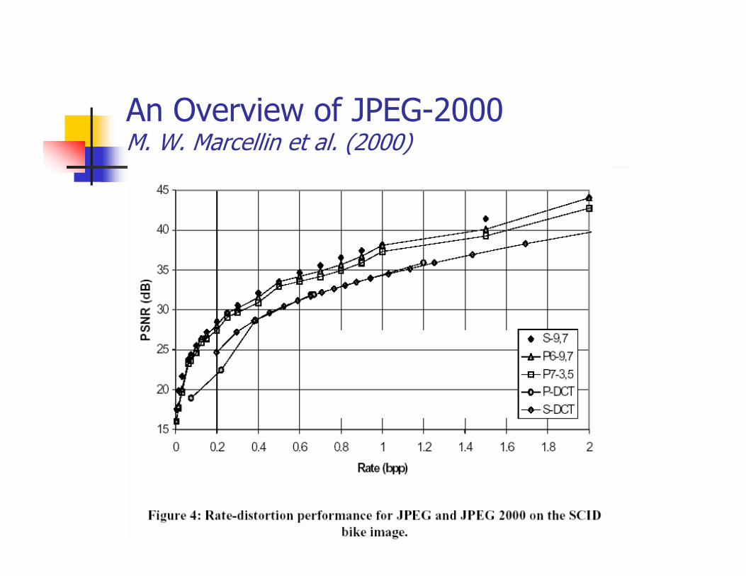
� JPEG-2000 provides better rate-distortion performance, for any given rate,
than the original JPEG standard. However, the largest improvements are
observed at very high and very low bitrates. The improvements in the “near
visually lossless” realm are more modest (approximately 20%).
� If the regions of interest (ROI) are known in advance, i.e. at encode time,
JPEG-2000 provides additional methods of providing greater image quality in
the foreground vs. the background.
� JPEG-2000 Part I allows 90, 180, and 270 degree rotations, and horizontal and
vertical flips of an image without inverse or forward wavelet transform.
� Finally, the integer nature of the (5,3) wavelet allows an image or portion of an
image to be compressed multiple times with the same quantization with no
additional loss.
An Overview of JPEG-2000M. W. Marcellin et al. (2000)
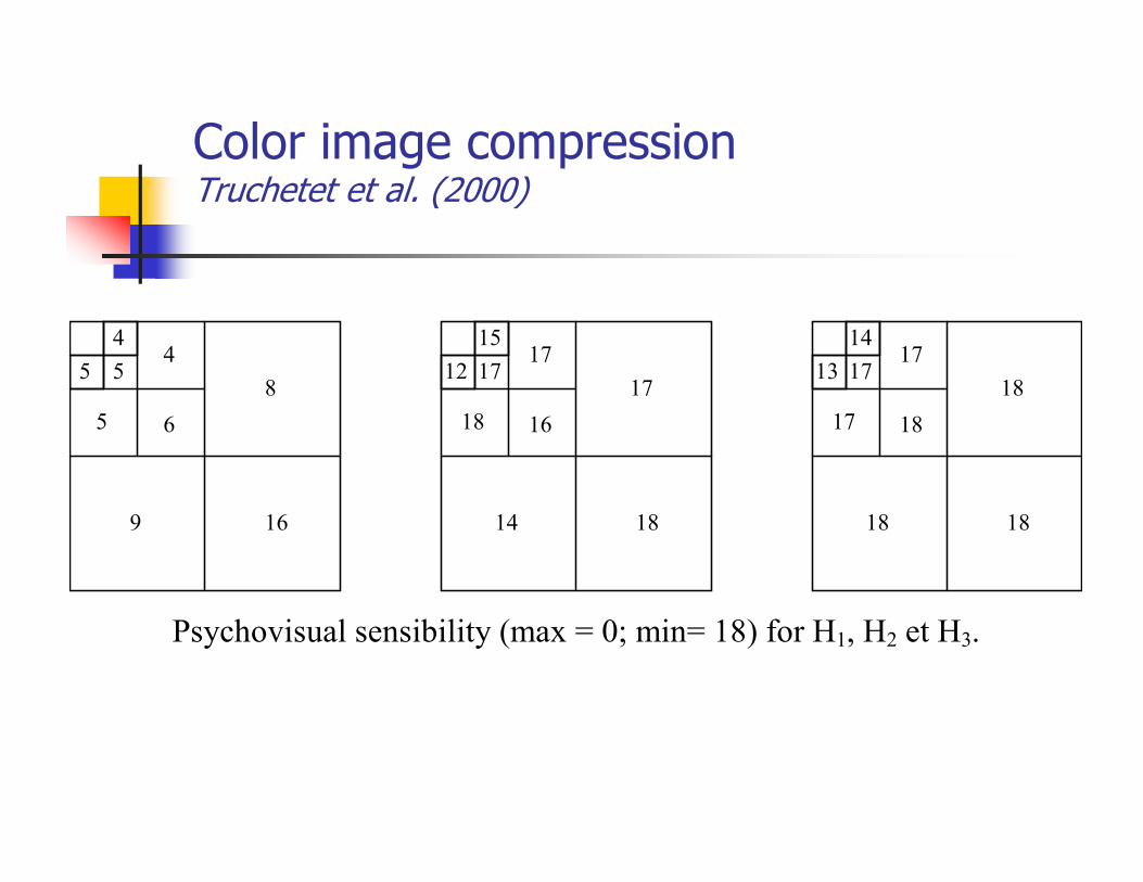
Color image compressionTruchetet et al. (2000)
5
4
5 4
5 6
8
9 16
Psychovisual sensibility (max = 0; min= 18) for H1, H2 et H3.
17
15
1217
18 16
17
14 18
17
14
1317
17 18
18
18 18
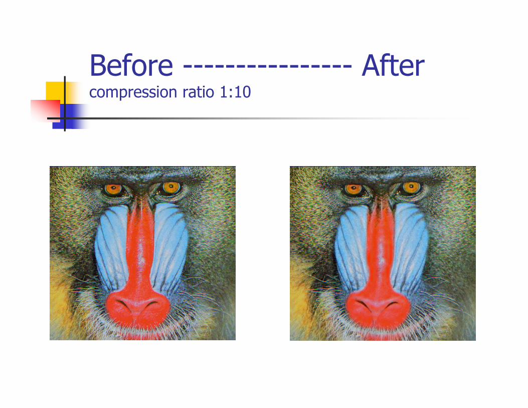
Before ---------------- Aftercompression ratio 1:10
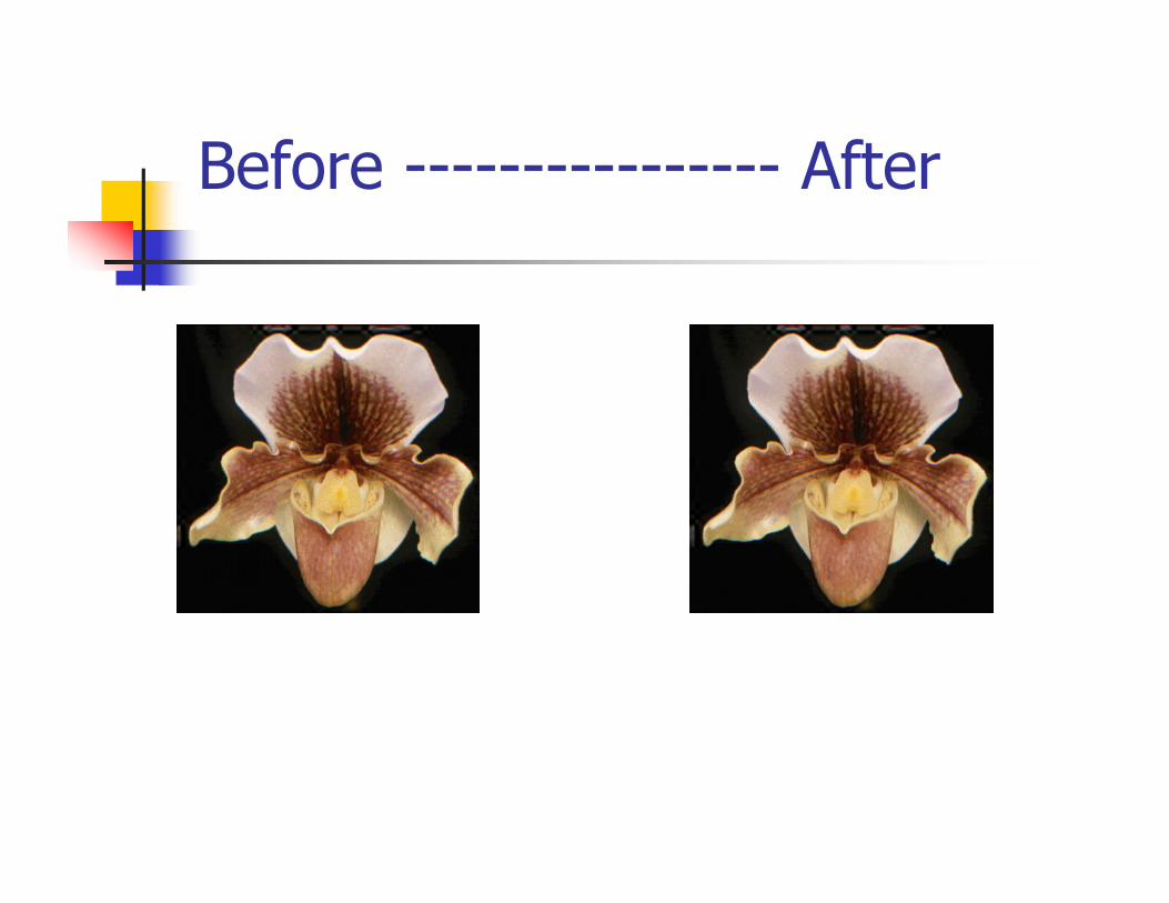
Before ---------------- After
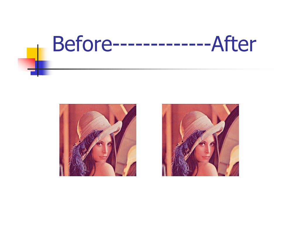
Before-------------After
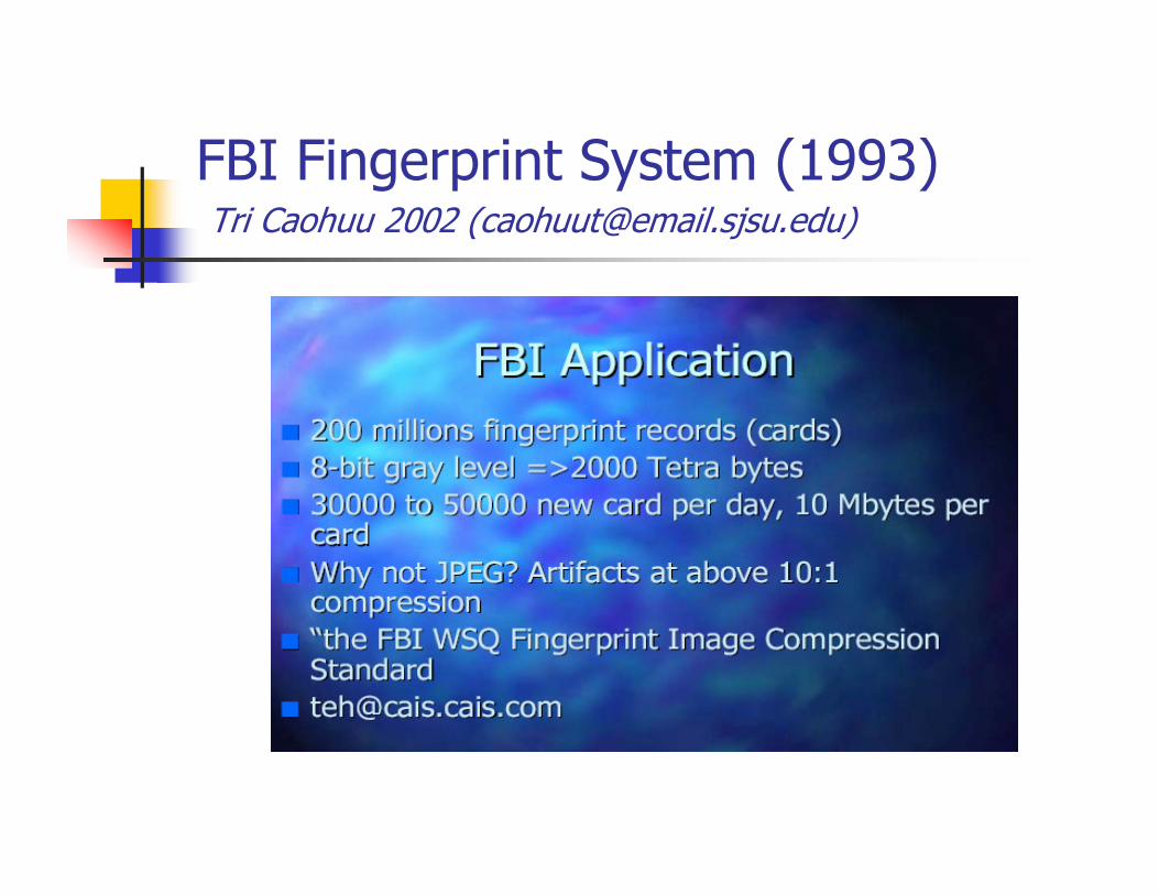
FBI Fingerprint System (1993)Tri Caohuu 2002 ([email protected])
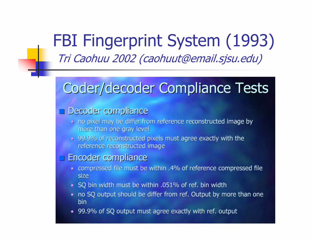
FBI Fingerprint System (1993)Tri Caohuu 2002 ([email protected])
FBI Fingerprint System (1993)Tri Caohuu 2002 ([email protected])
FBI Fingerprint System (1993)Tri Caohuu 2002 ([email protected])
FBI Fingerprint System (1993)Tri Caohuu 2002 ([email protected])
Wavelet applications in image processing
� Machine vision
� Textile and fabric
� Precision farming
Vision system for on-loom fabricinspectionH.Sari-Sarraf et al. (1999)
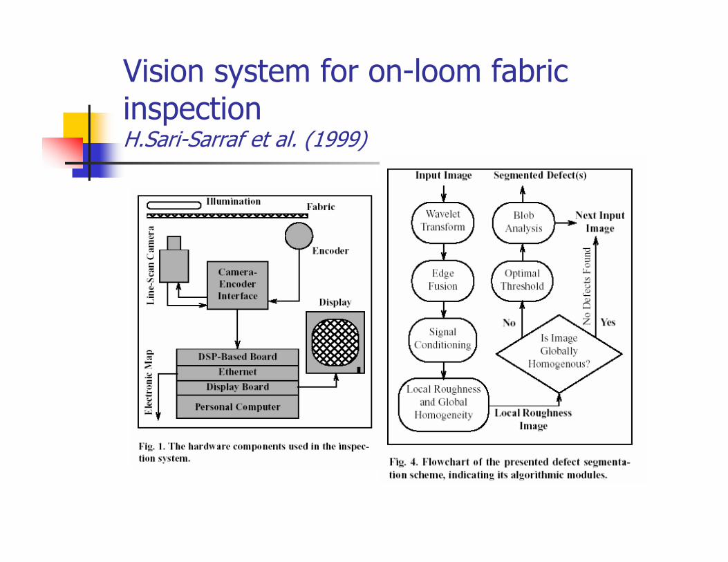
� Fabric inspection system: on-loom inspection of the fabric under construction
with 100% coverage.
� Synchronized to the motion of the loom, the developed system acquires very
high-quality, vibration-free images of the fabric using either front or
backlighting.
� The acquired images are subjected to a defect segmentation algorithm, which
is based on the concepts of wavelet transform, image fusion, and the
correlation dimension.
� Segmentation algorithm based on the localization of those events (i.e., defects)
in the input images that disrupt the global homogeneity of the background
texture.
� The overall detection rate of the presented approach was found to be 89% with
a localization accuracy of 0.2 in. (i.e., the minimum defect size) and a false
alarm rate of 2.5%.
Vision system for on-loom fabricinspectionH.Sari-Sarraf et al. (1999)
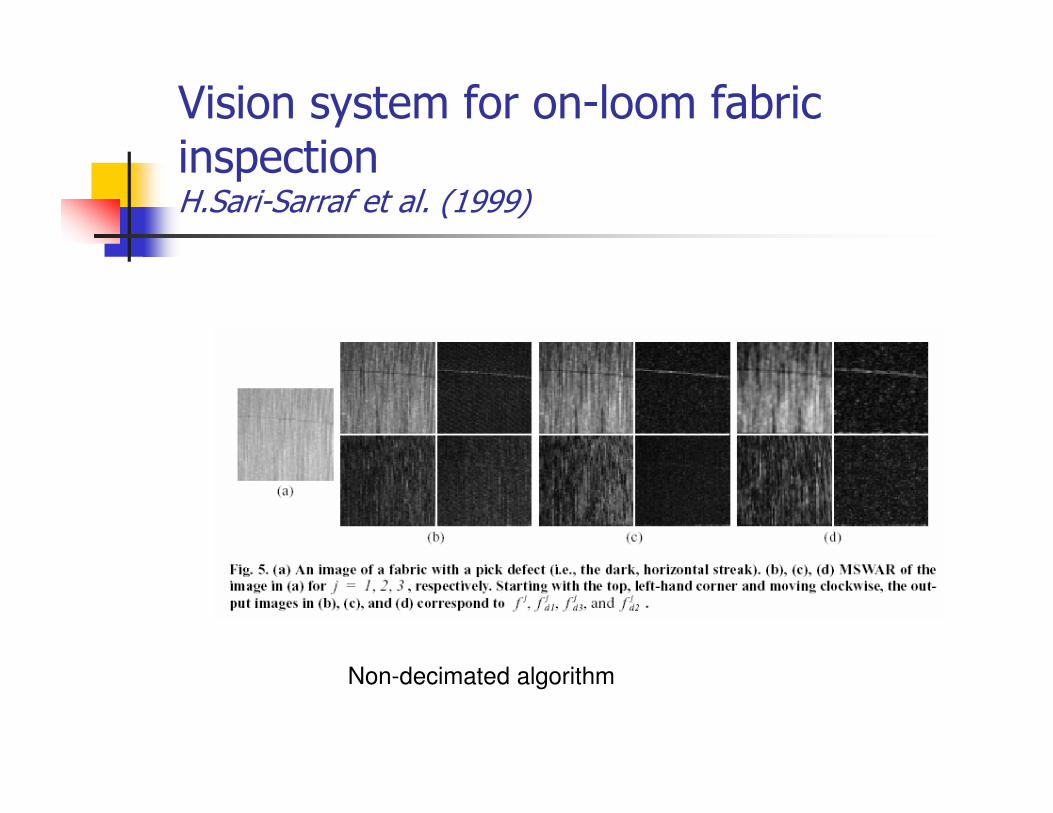
Vision system for on-loom fabricinspectionH.Sari-Sarraf et al. (1999)
Non-decimated algorithm
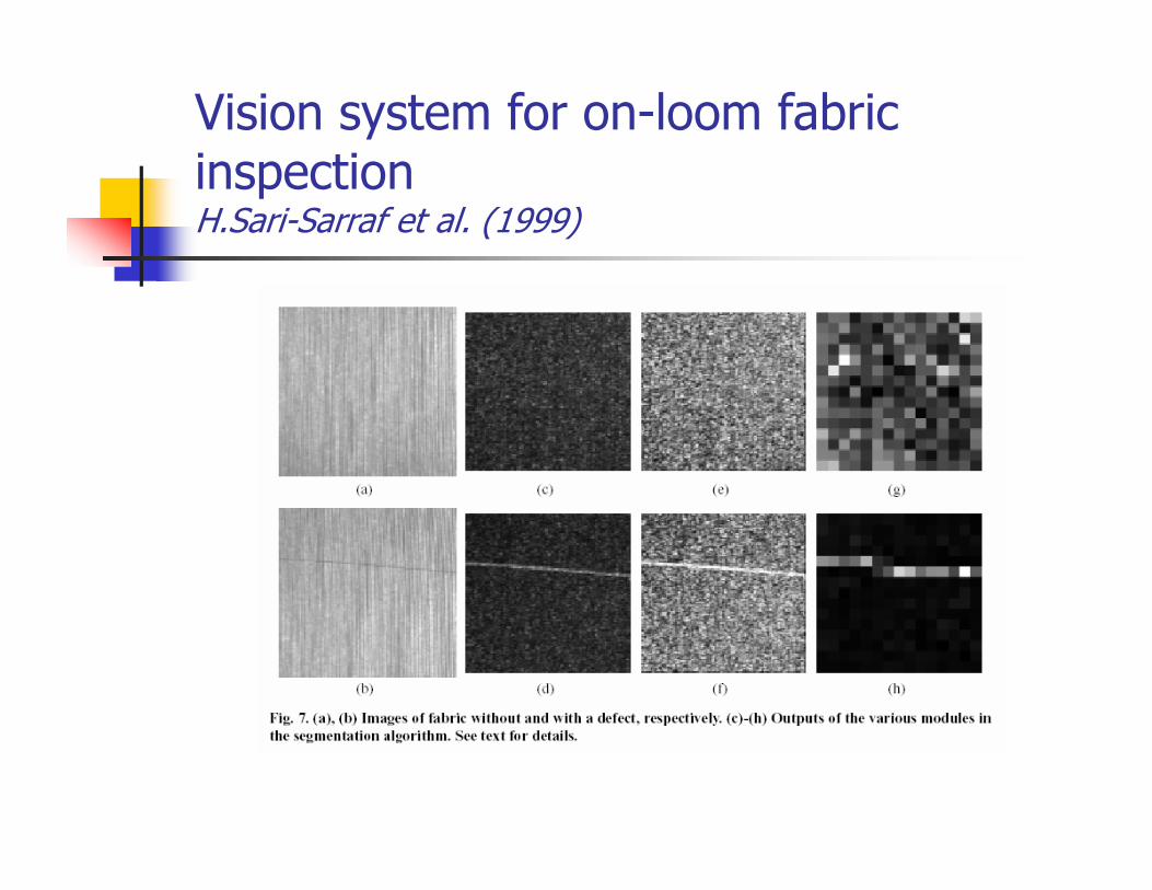
Vision system for on-loom fabricinspectionH.Sari-Sarraf et al. (1999)
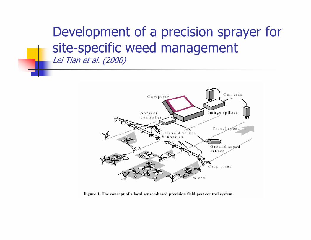
Development of a precision sprayer for site-specific weed managementLei Tian et al. (2000)
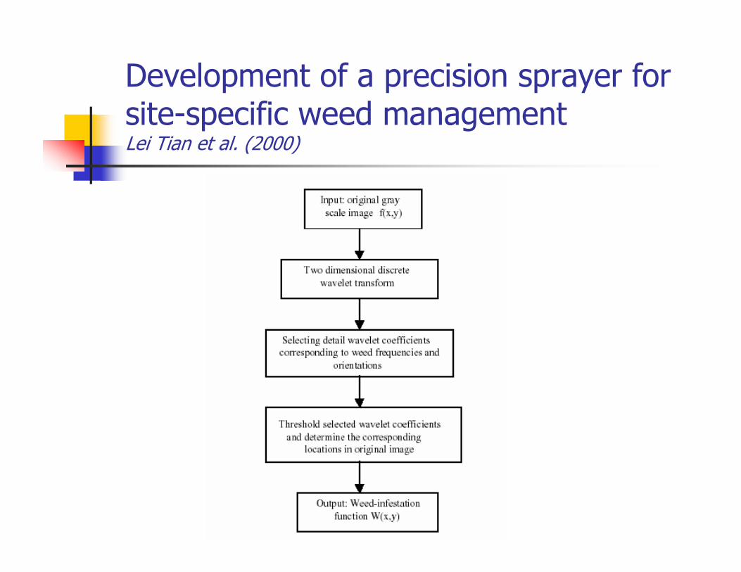
Development of a precision sprayer for site-specific weed managementLei Tian et al. (2000)
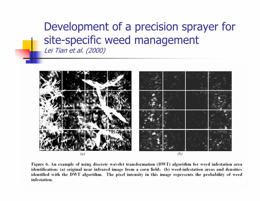
Development of a precision sprayer for site-specific weed managementLei Tian et al. (2000)
Wavelet applications in image processing
� Miscellanous
� Bioinformatics
� GIS
� Satellite imaging
Microarray Image Enhancement by Denoising Using Stationary Wavelet Transform X. H. Wang et al. (2003)
� Microarray imaging is a recent cutting-edge technology in bioinformatics
which can monitor thousand of genes simultaneously. Thousands of
oligonucleotides and cDNAs could be globally viewed at the same time. This
provides a systematic and comprehensive way to survey the DNA and RNA
variations, which could become a standard tool for both molecular biology
research and genomic clinical diagnosis, such as cancer diagnosis, diabetes
diagnosis
� The tasks of image processing focus on two major targets: spot segmentation
and spot intensity extraction. However, the quality of the images from the
experiments is not always perfect.
� The noises introduced during the experiment will greatly affect the accuracy of
the gene expression.
� To denoise the image noises before further image processing with stationary
wavelet transform (SWT).
� The time invariant characteristic of SWT is particularly useful in image
denoising.
Microarray Image Enhancement by DenoisingUsing Stationary Wavelet TransformX. H. Wang et al. (2003)
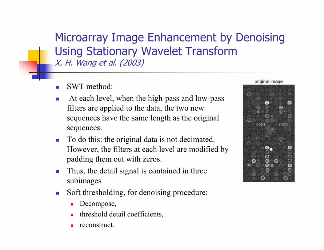
� SWT method:
� At each level, when the high-pass and low-pass
filters are applied to the data, the two new
sequences have the same length as the original
sequences.
� To do this: the original data is not decimated.
However, the filters at each level are modified by
padding them out with zeros.
� Thus, the detail signal is contained in three
subimages
� Soft thresholding, for denoising procedure:
� Decompose,
� threshold detail coefficients,
� reconstruct.
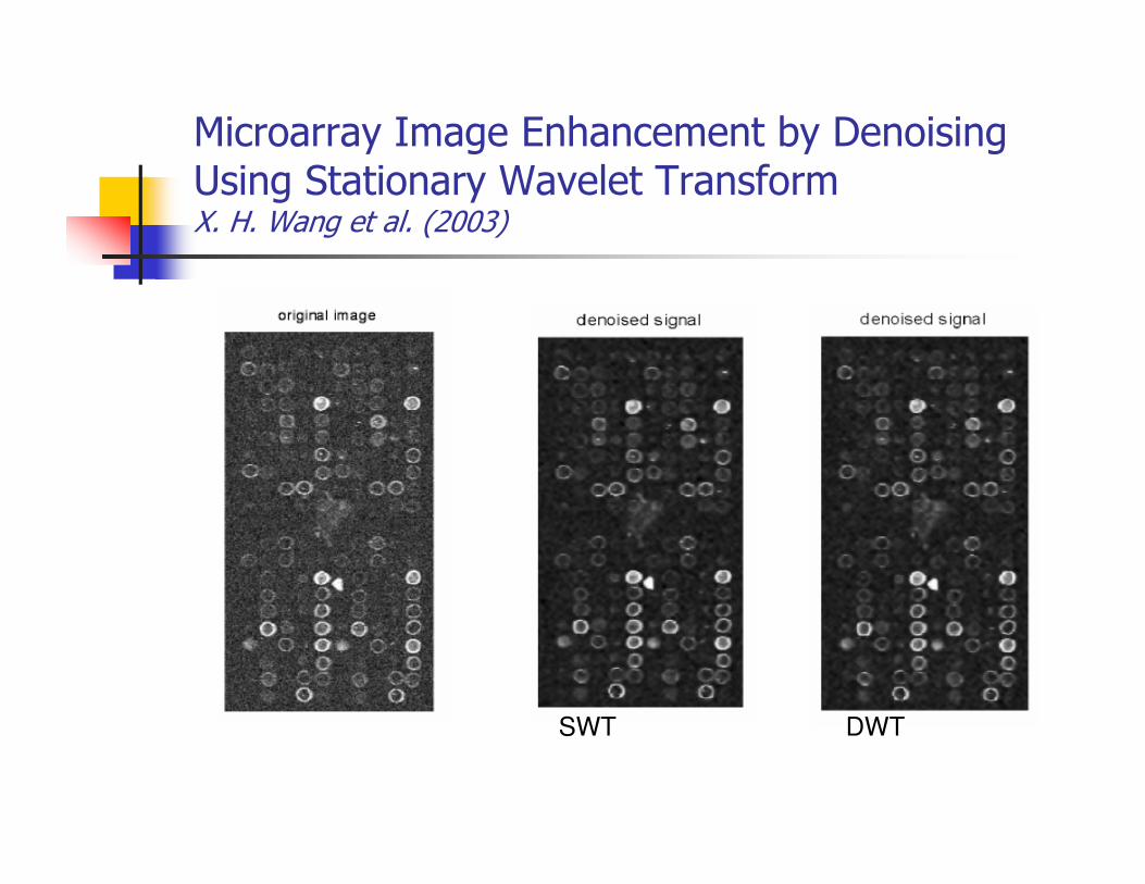
Microarray Image Enhancement by DenoisingUsing Stationary Wavelet TransformX. H. Wang et al. (2003)
SWT DWT
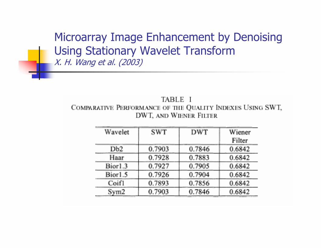
Microarray Image Enhancement by DenoisingUsing Stationary Wavelet TransformX. H. Wang et al. (2003)
Multiresolution spatial analysisMitchell Morehart et al. (1999)
� This paper explores the use of the wavelet transform as a spatial analysis tool
for modeling complex multivariate geographic relationships for Geographic
Information Systems (GIS)
� Wavelet methods: ability to process noisy data with local structures and to
represent discontinuities such as jumps or peaks in a function. This is an
important consideration for estimating geographically-referenced multivariate
surfaces where a high degree of spatial inhomogeneity is expected.
� WT: spatial analysis tool for modeling complex multivariate geographic
relationships
� Examples from agricultural data are used to illustrate the exploratory data
analysis inherent in the wavelet transform. The resulting maps provide a
convenient means of visually conveying tremendous amounts of information.
� The redundant à trous discrete wavelet transform is shown to aid enormously
in feature detection and exploration in the succession of resolution views of
the data.
Multiresolution spatial analysisMitchell Morehart et al. (1999)
� Spatial analysis of relationships between farming and its naturalresource base are carried out using data collected from USDA'sAgricultural Resource Management Study (ARMS).
� The ARMS is a personally enumerated survey, conducted since 1984 by the National Agricultural Statistics Service (NASS) and theEconomic Research Service (ERS) of the U.S. Department ofAgriculture.
� The ARMS is a probability-based multi frame, stratified survey thatuses multiple questionnaire versions to collect information on farmproduction expenses, capital purchases, income, production practices, and other farm operating characteristics.
Multiresolution spatial analysisMitchell Morehart et al. (1999)
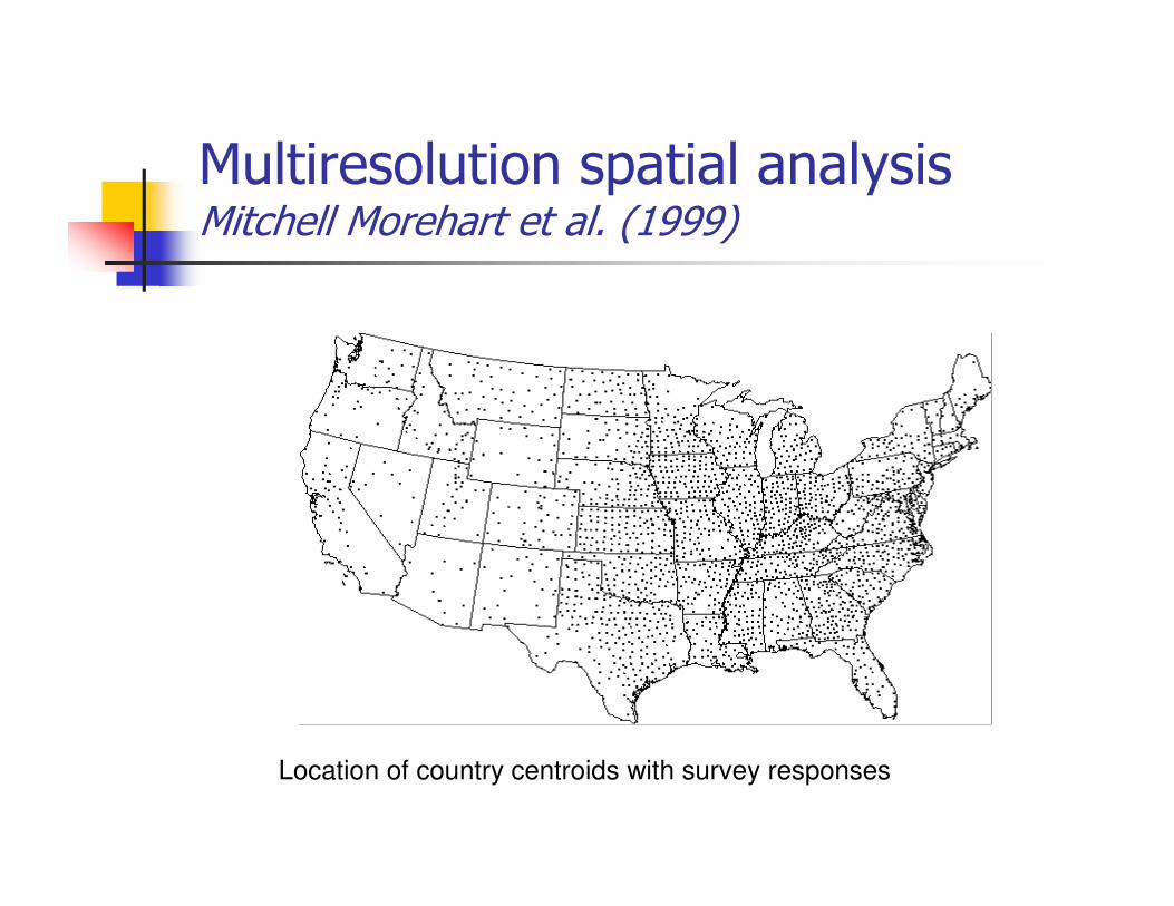
Location of country centroids with survey responses
Multiresolution spatial analysisMitchell Morehart et al. (1999)
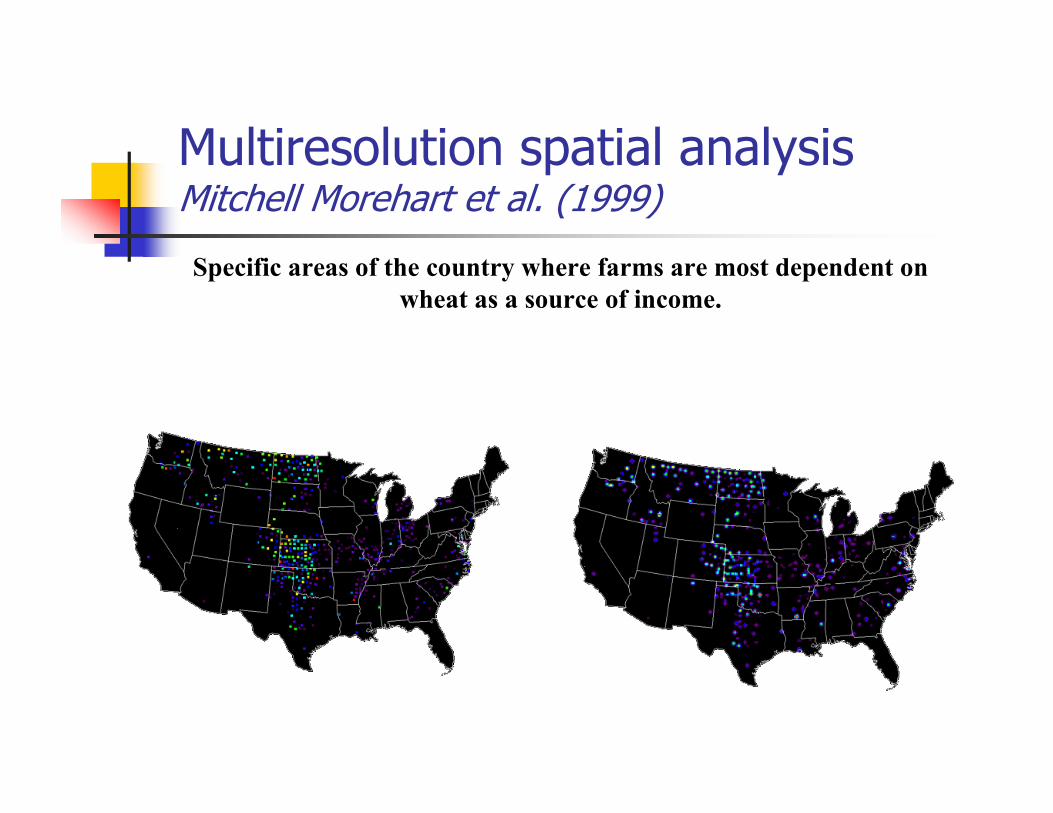
Specific areas of the country where farms are most dependent on
wheat as a source of income.
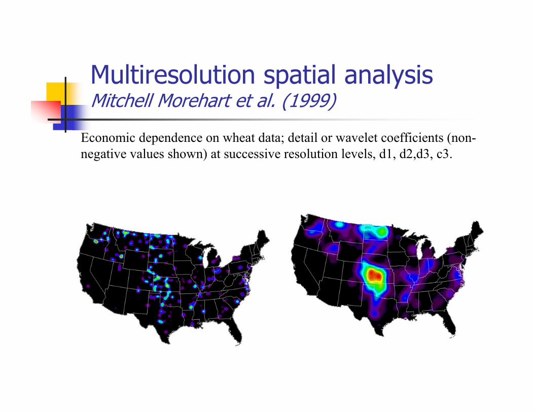
Multiresolution spatial analysisMitchell Morehart et al. (1999)
Economic dependence on wheat data; detail or wavelet coefficients (non-
negative values shown) at successive resolution levels, d1, d2,d3, c3.
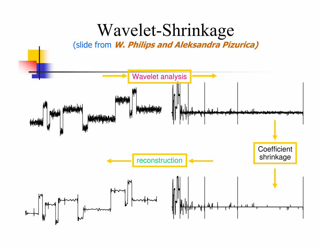
Wavelet-Shrinkage(slide from W. Philips and Aleksandra Pizurica)
Wavelet analysis
Coefficientshrinkagereconstruction
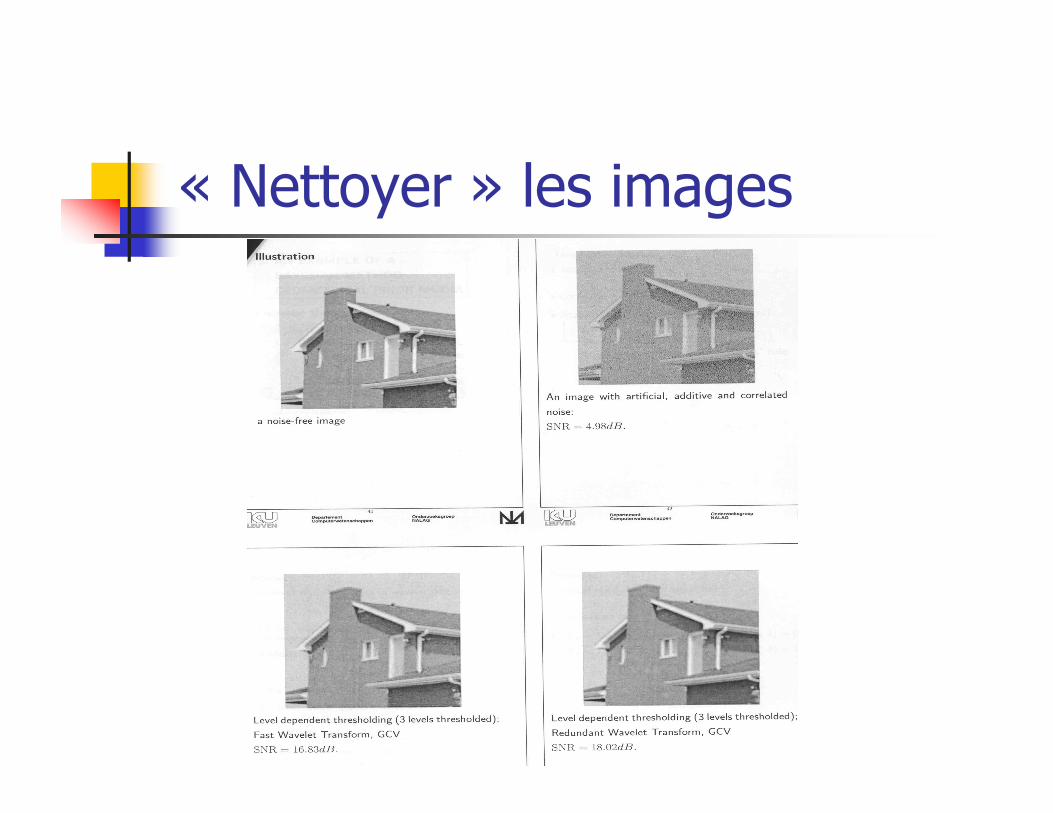
« Nettoyer » les images
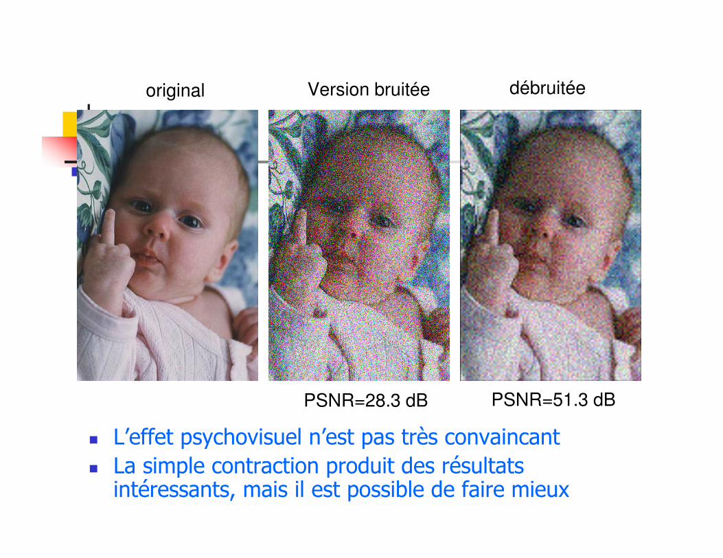
� L’effet psychovisuel n’est pas très convaincant
� La simple contraction produit des résultatsintéressants, mais il est possible de faire mieux
PSNR=28.3 dB PSNR=51.3 dB
original Version bruitée débruitée
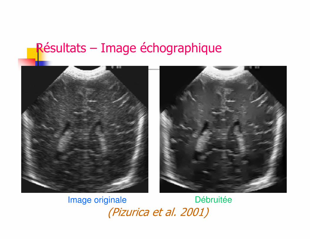
Résultats – Image échographique
(Pizurica et al. 2001)Image originale Débruitée
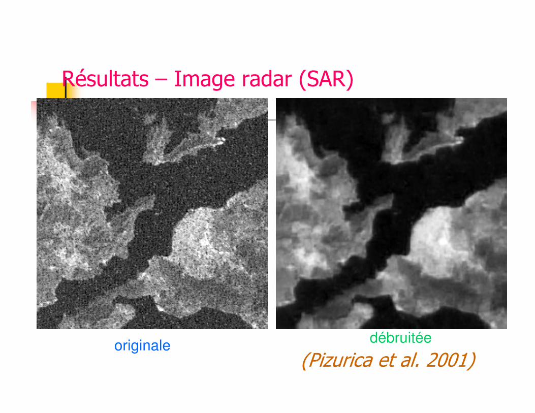
Résultats – Image radar (SAR)
originaledébruitée
(Pizurica et al. 2001)
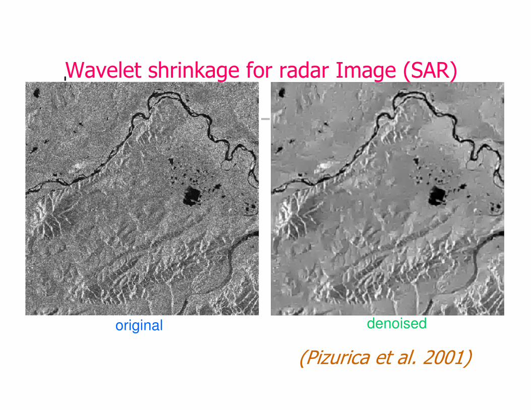
Wavelet shrinkage for radar Image (SAR)
original denoised
(Pizurica et al. 2001)
ConclusionWavelet applications in industrial context are numerous and invade nearly every domain
� However, if one considers only operational devices or software, very few can be really pointed out. And most of them deal with image compression.
� Presently one has to admit that wavelet transform stays essentially a laboratory technique, but with the development of dedicated IC and of efficient software tools the gap is being strode.
� Scale discrimination properties of WT are widely used for practical applications in algorithms of de-noising (wavelet shrinkage), scale filtering, fractal analysis or scalogramvisualization
� Organizing and concentrating information are also amongst the main reasons of WT success in numerous applications and particularly in image compression devices.
ConclusionWavelet cannot solve all the problems and there are still a lot of limitations inherent to WT.
� Decimated WT is not invariant by translation: it induces artifacts and a lack of consistency in some transient detection algorithms and in signal or image enhancement approaches.
� Dyadic DWT has a very limited frequency resolution and sometime the searched feature is spread on two scales and cannot be clearly detected.
� CW or, in a more interesting way, rational wavelet analysis
� Transposing 1D WT to 2D is not easy and the separable approach leads to a non isotropic behavior. Horizontal, vertical and diagonal directions are subject to special attention and if it can be of interest when processing is linked to human psycho-visual system imitation, on the contrary when the treatment aims at extracting exact physical information this anisotropy can be a serious source of errors.
� Non-separable wavelet basis, quincunx analysis or steerable wavelet analysis.
� Wavelets for orthogonal basis (in 1D) cannot be symmetrical with FIR filters. Signal and images to be treated are, most often, symmetric and they need a zero-phase filtering for avoiding artifacts.
� Bi-orthogonal wavelets can be of finite length but they lead to poor de-correlation between scales. Symlets or Coiflet are not of minimum length but they provide a quasi-symmetrical analysis function.
ConclusionFinally, is wavelet a success story?
� Is wavelet transform a fashion?
� A long life-time one!!
� Is wavelet transform a gadget?
� Most of the time it brought very little
� Real industrial appplications are stillscarce
� There is still a lot to do to point out what is worthwhile and what is not
� There is still plenty of room for research
……
� And one must admit that…
LastLast wordword :waveletwavelet isis stillstill a hot spota hot spot
By 1990, more than 1000 scientificpapers have been published on WT.
Even in 2009 several international scientific conferences are specifically dedicated to wavelet transform and itsapplications.
Wavelets are present in almost all the conferences on signal or image processing and in many otherconferences dealing with different topics (quanticphysics, optics, thermodynamic, fluid flowing, geology, acoustic, computer science, etc...)
A journal dedicated to wavelets exists since 1993 (AppliedComputational Harmonic Analysis),
A Wavelet Digest is diffused and updated on the web.
Spend sometime at: http://www.wavelet.org