5

Chapter 1

Introduction and Background

Quantum mechanics forms the basis for our understanding of the behavior of light and matter.

While most day-to-day events we observe can be accurately modeled using classical mechanics and

electromagnetism, many physical systems require a quantum mechanical description. Whether we

are interested in the details of a chemical reaction or the flow of electrons through a semiconductor

inside a computer, or even a system as apparently simple as the interaction of the electromagnetic

field with a single atom, quantum mechanical modeling is both highly accurate and necessary. As

optical networks and computing resources shrink and become faster, they will inevitably encounter

limits set by quantum mechanics. While these limits might impose restrictions on the behavior of a

system, they may also open the door to other uses for the same system. This thesis is dedicated to

examining ways of building simpler models for quantum systems which respect their dynamics, but

may eventually also allow those systems to be more easily developed into useful technology.

Quantum mechanics is an inherently probabilistic model for the physical world. In order to model

the dynamics of quantum systems, we propagate not a single position and momentum as we might

for a classical system, but instead a probability distribution. Undergraduate quantum mechanics

usually introduces the Schrodinger equation, a partial differential equation for the wavefunction of

an isolated physical system, from which we can calculate the possible results of measurements of

certain observable quantities. However, as we work to match this simple model with the physical

world, we encounter limits to the model. First, we are forced to reckon with the difficulty of building

an isolated system, and then measuring it. By definition, the measurement process is an intrusion

from the “outside” into a supposedly isolated system. This is usually dealt with by hand-waving

arguments about an omnipotent experimenter suddenly introducing a measurement apparatus and

making a sharp, projective measurement.

Of course, this model, too, often does not match with the physical reality of a laboratory or

its example quantum system under study. A real physical quantum system is an open system,

unavoidably coupled to the environment surrounding it, making it difficult to define the boundary

of the “system.” Often, the best we can hope for is to shape the coupling of system to environment

6

so that we may retrieve information about the system without disrupting it in ways we do not

want. (If we can do this, then we are justified in our model’s separation between “system” and

“environment.”) A physical measurement process can almost always be modeled not as a direct

measurement of the system, but instead a measurement of the environment interacting with the

system of interest. Measurements also necessarily take time; the instantaneous measurement of

introductory quantum mechanics is as much an approximation as its isolation.

We must also deal with the fact that our measurement may not tell us everything about our

system, because of the limited way in which the environment interacts with the system, or because

our measurement cannot distinguish between different states of the environment or, as a result,

the system. As experimenters, our understanding of the state of our quantum system is shaped

by the system’s history and dynamics (the realm of the Schrodinger equation), and also by the

fallible way we measure the system, noise which may be introduced through the environment or

measurement, or our simple failure to measure all of the parts of the environment which carry

information about the system. We must almost always think of our quantum system as being in a

mixed state, acknowledging our lack of knowledge about the system.

Mixed states cannot be modeled as wavevectors (|ψ〉), and must instead be modeled using density

matrices (∑

i ci|ψi〉〈ψi|), which we propagate in time using the master equation. Density matrices

reside in a much larger space than wavefunctions — they have many more degrees of freedom —

which makes accurate simulations of dynamics a challenge for large systems. In particular, any

system which is coupled with an electromagnetic field can be difficult to simulate because the field,

modeled as a harmonic oscillator, is infinite dimensional (there’s no top to the ladder of states).

It is usually reasonable to define a cut-off energy, but this can still result in very large density

matrices, especially if the system consists of tensor products of this large field space with other

system components. Coupling with a two-level system quadruples the number of elements in the

density matrix.

One way to tackle this challenge is by simulating only fully observed systems. That is, only sys-

tems in which the experimenter measures every output channel. Such systems can be simulated using

a stochastic Schrodinger equation, and their states remain pure, and take the form of wavefunctions.

The quantum simulations (“trajectories”) in this thesis are all of this form. The statistical behavior

of such systems is identical to partially observed systems over long times (or multiple samples of

identical systems). Measurements should not be able to change the fundamental statistics of the

underlying system.

Given a physical system, however, the experimenter often does not have the option of measuring

every output channel. An atom may emit light into all 4π steradians, for example, which cannot all be

covered in detectors. To build her best guess as to the system state, the experimenter is forced to use

the master equation as a “filter” — an equation which propagates her current best guess about the

7

state of the system, with filter input from the output of the measurement process. The experimenter’s

best guess is a mixed state, and propagating the master equation will be computationally intense

(and very difficult to do in real time). Should the experimenter desire to use this filter to decide on

a control signal to drive the system to a particular state, she will be hard pressed to update her best

guess in real time, and the control task will be very challenging. This thesis attempts to develop

techniques to build simple models for quantum systems which capture the dynamics of interest (and

potential utility) and which may also be propagated much more easily, potentially in real time, by

a computer or purpose-built circuit. Such simple models might also provide insight into the system

by elucidating the components which result in particular behavior.

The general technique I use to build simpler models is to find a linear or nonlinear submanifold

of the full space of possible dynamics, in which the particular dynamics of a system are generally

confined. I adapt various techniques for finding such subspaces developed for other applications to

the case of quantum dynamics, and illustrate both their successes and failures.

1.1 Thesis overview

The remainder of this Introduction introduces the example physical system whose dynamics we will

attempt to model with simple dynamical systems: a two-level atom in a high-finesse optical cavity, a

situation known as “cavity quantum electrodynamics” (cavity QED). I review the dominant model

for cavity QED, the Jaynes-Cummings model, give an abbreviated derivation of the Maxwell-Bloch

equations, and a short summary of known interesting dynamics observed in these equations and

in corresponding simulations of cavity QED. I close with a brief introduction to a few topics in

stochastic calculus, to lay the groundwork for the remainder of the thesis.

Chapter 2 provides an overview of the technique of projecting filtering equations onto manifolds.

I then turn to a particular manifold — a linear space of density matrices — and project the stochastic

master equation for cavity QED onto this space, deriving nonlinear dynamical equations for the local

coordinates.

Chapter 3 makes the work of Chapter 2 more concrete by describing a process, Proper Orthogonal

Decomposition, for determining a linear density matrix space onto which to project the dynamics.

I analyze cavity QED dynamics in phase and absorptive bistability regimes, and demonstrate some

successes, and some failures, of this process for generating accurate filters.

Chapter 4 turns away from linear manifolds, and introduces nonlinear manifolds generated with

an algorithm for Local Tangent Space Alignment. We turn again to phase and absorptive bistability

regimes. In the phase bistability case, we are able to fit the manifold coordinates with simple

combinations of expectation values, and derive a set of situation-specific “Maxwell-Bloch” equations,

which I then compare with previously-derived equations for this system, and evaluate as a filter. The

8

absorptive bistability case is more complex, but I lay the groundwork for deriving similar systems

of equations.

The concluding Chapter 5 draws the results together, examines the successes and failures of the

examined model reduction techniques, and suggests directions for future work.

1.2 Model system: Cavity quantum electrodynamics

A single atom in a high-finesse optical cavity constitutes a canonical system in quantum optics.

Experimental work on such systems (such as [3, 4, 5, 6, 7], among many others) has demonstrated

strong coupling between the atom and the optical field, meaning that the presence or absence of a

single photon drastically changes the environment for a single atom, and correspondingly, that the

state of the single atom strongly affects the behavior of the field in the cavity. There are multiple

parameter ranges in which strong coupling occurs. Strong coupling can be identified as a regime in

which the ratio of the square of the atom-field coupling rate to the product of the cavity decay and

atomic spontaneous emission rates is large. This ratio is called the “cooperativity.” Two limits of

interest are the “bad cavity” and “good cavity” limits: for a fixed value of the cooperativity, the

cavity decay rate may be large compared with the spontaneous emission (“bad cavity”), or small

(“good cavity”). We usually scale time by the atomic spontaneous emission rate, so it ends up

dropping out; this means that a small cavity decay rate, for a fixed cooperativity, implies a small

atom-field coupling rate (inside a higher-finesse cavity), and vice versa.

1.2.1 The Jaynes-Cummings model

A simple model for the atom-cavity system is the Jaynes-Cummings model [8]. In this model, the

atom is approximated as a two-level system, there is only one harmonic mode of the field in the

cavity. The two-level atom is equivalent to a single spin, and the operators which act on it are

the Pauli matrices and their linear combinations: σ− lowers the atom into its ground state, while

σ+ = σ†− excites the atom. The field is acted upon by a and a†, the familiar annihilation and creation

operators for a simple harmonic oscillator. We operate in a rotating frame, at the frequency of the

driving field. The Hamiltonian in this model takes the form

H = ∆ca†a + ∆aσ+σ− + ig0

(

a†σ− − aσ+

)

+ iE(

a† − a)

, (1.1)

where ∆c is the detuning between the field and the cavity, ∆a is the detuning between the field and

the atomic transition, g0 is the coupling rate between the atom and the cavity field, and E is the

driving (classical) field strength. Stepping through the terms of the equation:

9

• ∆ca†a accounts for the difference in energy between on- and off-resonant drive of the cavity

by the external field.

• ∆aσ+σ− similarly accounts for the difference in energy between on- and off-resonant drive of

the atom by the external field.

• ig0

(

a†σ− − aσ+

)

is responsible for exchange of energy between the atom and the field at rate

2g0. The first term creates an excitation in the field, while driving the atom to the ground

state; that is, the atom emits a photon into the field. The second is the inverse process, where

the atom absorbs one photon out of the field, and becomes excited.

• iE(

a† − a)

is the external driving field, acting to excite the phase quadrature of the cavity

mode.

A Hamiltonian like (1.1) would suffice if we were concerned only with the unobserved dynamics

of a closed quantum system. However, for useful systems, the “closed” model will not suffice.

Instead, we must extend the picture to include the system’s interaction with its environment, and

the behavior of an observer making measurements on the system. The observer may know the

quantum state fully, or imperfectly, and so we model the dynamics of such an “open quantum

system” with a master equation, which propagates the motion of a density matrix. The interaction

of the system and its environment is governed by probabilities, so that the time at which the atom or

field changes state (such as emitting a photon) is random. We therefore require a stochastic model

for the propagation of the density matrix, which allows for the introduction of noise resulting from

this inherently probabilistic behavior.

The Ito form of the stochastic master equation (SME) which governs the behavior of an atom-

cavity system being observed with homodyne measurements of both the leaking cavity field and the

atomic emission is

dρ = −i[H, ρ]dt + κ(

2aρa† − a†aρ − ρa†a)

dt

+γ (2σ−ρσ+ − σ+σ−ρ − ρσ+σ−) dt

+i√

2κ(

ρa† − aρ − Tr[ρ(

a† − a)

]ρ)

dW1

+i√

2γ (ρσ+ − σ−ρ − iTr[ρ (σ+ − σ−)]ρ) dW2. (1.2)

Here dW1 and dW2 are uncorrelated Wiener processes corresponding to noise on the two different

measurement processes, κ is the rate of field decay out the end of the cavity (usually toward a

detector), and γ is the rate of decay of the atomic state (atomic spontaneous emission) measured by

a second homodyne detection process. γ⊥, not included above, is the atomic transverse relaxation

rate, and we scale time so that this rate is 1. A free atom has a spontaneous emission rate γ = 2, and

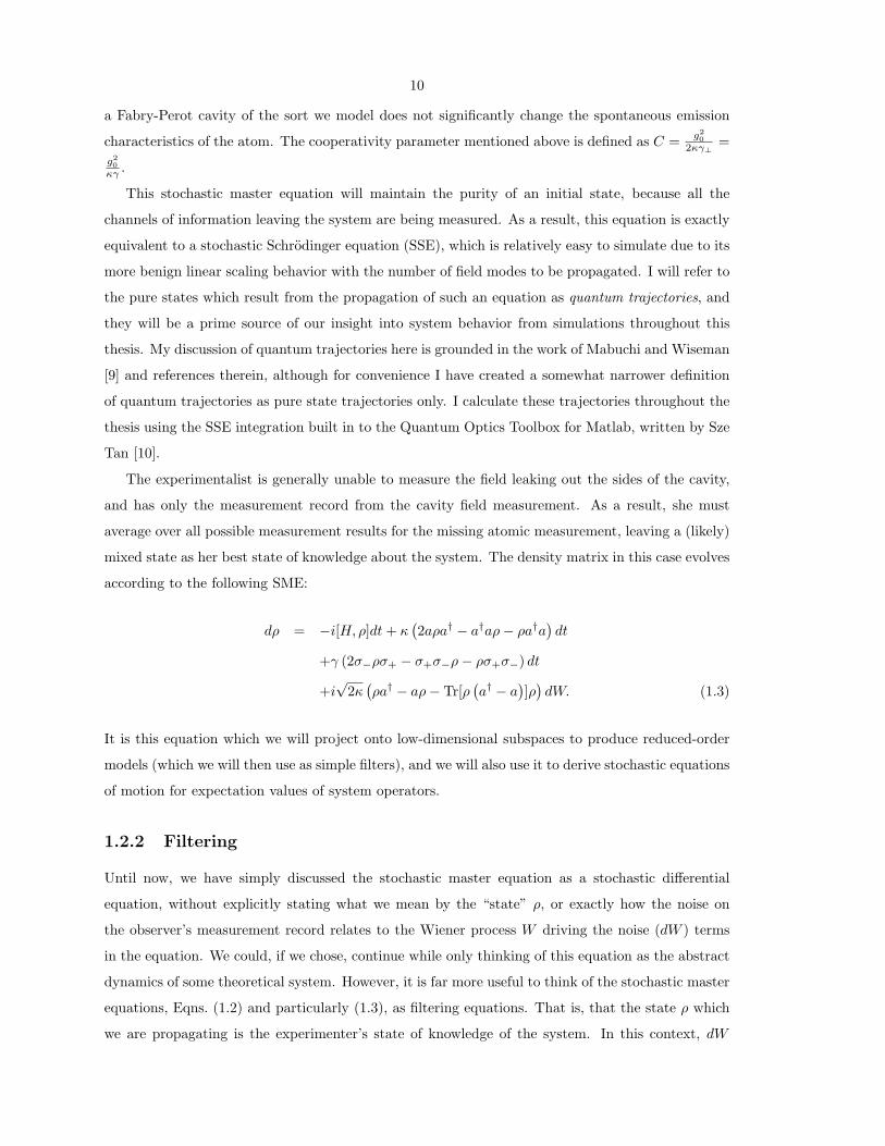
10

a Fabry-Perot cavity of the sort we model does not significantly change the spontaneous emission

characteristics of the atom. The cooperativity parameter mentioned above is defined as C =g2

0

2κγ⊥

=

g2

0

κγ .

This stochastic master equation will maintain the purity of an initial state, because all the

channels of information leaving the system are being measured. As a result, this equation is exactly

equivalent to a stochastic Schrodinger equation (SSE), which is relatively easy to simulate due to its

more benign linear scaling behavior with the number of field modes to be propagated. I will refer to

the pure states which result from the propagation of such an equation as quantum trajectories, and

they will be a prime source of our insight into system behavior from simulations throughout this

thesis. My discussion of quantum trajectories here is grounded in the work of Mabuchi and Wiseman

[9] and references therein, although for convenience I have created a somewhat narrower definition

of quantum trajectories as pure state trajectories only. I calculate these trajectories throughout the

thesis using the SSE integration built in to the Quantum Optics Toolbox for Matlab, written by Sze

Tan [10].

The experimentalist is generally unable to measure the field leaking out the sides of the cavity,

and has only the measurement record from the cavity field measurement. As a result, she must

average over all possible measurement results for the missing atomic measurement, leaving a (likely)

mixed state as her best state of knowledge about the system. The density matrix in this case evolves

according to the following SME:

dρ = −i[H, ρ]dt + κ(

2aρa† − a†aρ − ρa†a)

dt

+γ (2σ−ρσ+ − σ+σ−ρ − ρσ+σ−) dt

+i√

2κ(

ρa† − aρ − Tr[ρ(

a† − a)

]ρ)

dW. (1.3)

It is this equation which we will project onto low-dimensional subspaces to produce reduced-order

models (which we will then use as simple filters), and we will also use it to derive stochastic equations

of motion for expectation values of system operators.

1.2.2 Filtering

Until now, we have simply discussed the stochastic master equation as a stochastic differential

equation, without explicitly stating what we mean by the “state” ρ, or exactly how the noise on

the observer’s measurement record relates to the Wiener process W driving the noise (dW ) terms

in the equation. We could, if we chose, continue while only thinking of this equation as the abstract

dynamics of some theoretical system. However, it is far more useful to think of the stochastic master

equations, Eqns. (1.2) and particularly (1.3), as filtering equations. That is, that the state ρ which

we are propagating is the experimenter’s state of knowledge of the system. In this context, dW

11

represents the new information which the experimenter receives through her measurement, and is

called the innovation. The innovation is defined as the difference between the measurement result

and what the observer expected the result to be. In the case of a homodyne measurement of the

phase quadrature of the cavity field, for example, the innovation is measurement − expectation =

dY − i2

⟨

a† − a⟩

. That this is a Wiener process reflects that the innovation is unbiased — the

experimenter learns as much from a measurement result that is larger than her expectation as from

a result that is smaller [11].

1.3 The Maxwell-Bloch equations

In my efforts to derive simple classical (or semi-classical) models to approximate quantum systems,

the canonical relevant example of such a simplification serves as a constant point of comparison.

The Maxwell-Bloch equations are a set of five, coupled, deterministic differential equations for the

expectation values of the five simplest operators in this system: a, a†, σ−, σ+, and σz. The first

four will be familiar from the Hamiltonian; the last, σz, corresponds to the population difference

between the atomic excited and ground states, and allows the system of equations to close without

stretching any approximations to the breaking point. These operators may be combined to create

the Hermitian operators

x =1

2

(

a + a†)

y =i

2

(

a† − a)

σx = σ+ + σ−

σy = i (σ− − σ+) . (1.4)

These Hermitian operators correspond to possible observables of the atom-cavity system. x is the

cavity field’s amplitude quadrature; y is its phase. Using the spin analogy with a two-level atom,

the Pauli matrix σx is the atomic component along the x axis, and similarly for σy and σz.

In the density matrix formalism, the expectation value of an operator O is given by Tr (Oρ).

Therefore, the equation of motion of that expectation value is d 〈O〉 = Tr (O (dρ)). If we use the

definition of dρ given by Eqn. (1.3) to calculate the equations of motion of the five operators above,

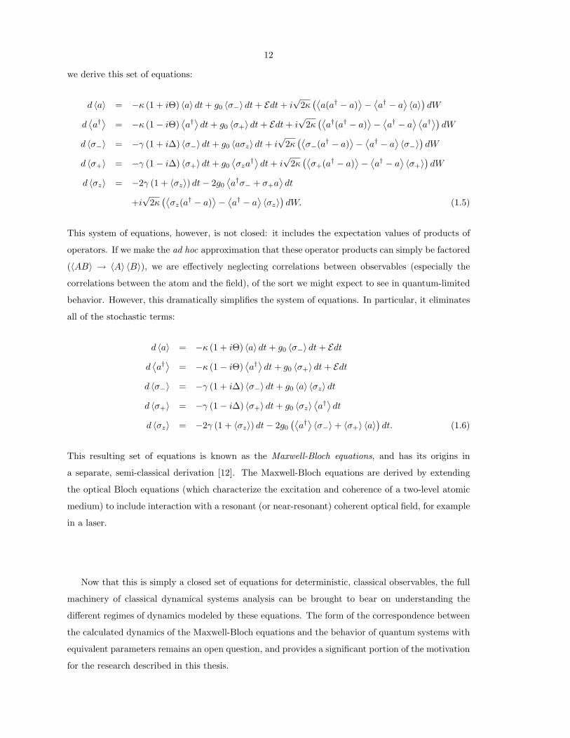
12

we derive this set of equations:

d 〈a〉 = −κ (1 + iΘ) 〈a〉 dt + g0 〈σ−〉 dt + Edt + i√

2κ(⟨

a(a† − a)⟩

−⟨

a† − a⟩

〈a〉)

dW

d⟨

a†⟩

= −κ (1 − iΘ)⟨

a†⟩

dt + g0 〈σ+〉 dt + Edt + i√

2κ(⟨

a†(a† − a)⟩

−⟨

a† − a⟩ ⟨

a†⟩)

dW

d 〈σ−〉 = −γ (1 + i∆) 〈σ−〉 dt + g0 〈aσz〉 dt + i√

2κ(⟨

σ−(a† − a)⟩

−⟨

a† − a⟩

〈σ−〉)

dW

d 〈σ+〉 = −γ (1 − i∆) 〈σ+〉 dt + g0

⟨

σza†⟩

dt + i√

2κ(⟨

σ+(a† − a)⟩

−⟨

a† − a⟩

〈σ+〉)

dW

d 〈σz〉 = −2γ (1 + 〈σz〉) dt − 2g0

⟨

a†σ− + σ+a⟩

dt

+i√

2κ(⟨

σz(a† − a)

⟩

−⟨

a† − a⟩

〈σz〉)

dW. (1.5)

This system of equations, however, is not closed: it includes the expectation values of products of

operators. If we make the ad hoc approximation that these operator products can simply be factored

(〈AB〉 → 〈A〉 〈B〉), we are effectively neglecting correlations between observables (especially the

correlations between the atom and the field), of the sort we might expect to see in quantum-limited

behavior. However, this dramatically simplifies the system of equations. In particular, it eliminates

all of the stochastic terms:

d 〈a〉 = −κ (1 + iΘ) 〈a〉 dt + g0 〈σ−〉 dt + Edt

d⟨

a†⟩

= −κ (1 − iΘ)⟨

a†⟩

dt + g0 〈σ+〉 dt + Edt

d 〈σ−〉 = −γ (1 + i∆) 〈σ−〉 dt + g0 〈a〉 〈σz〉 dt

d 〈σ+〉 = −γ (1 − i∆) 〈σ+〉 dt + g0 〈σz〉⟨

a†⟩

dt

d 〈σz〉 = −2γ (1 + 〈σz〉) dt − 2g0

(⟨

a†⟩

〈σ−〉 + 〈σ+〉 〈a〉)

dt. (1.6)

This resulting set of equations is known as the Maxwell-Bloch equations, and has its origins in

a separate, semi-classical derivation [12]. The Maxwell-Bloch equations are derived by extending

the optical Bloch equations (which characterize the excitation and coherence of a two-level atomic

medium) to include interaction with a resonant (or near-resonant) coherent optical field, for example

in a laser.

Now that this is simply a closed set of equations for deterministic, classical observables, the full

machinery of classical dynamical systems analysis can be brought to bear on understanding the

different regimes of dynamics modeled by these equations. The form of the correspondence between

the calculated dynamics of the Maxwell-Bloch equations and the behavior of quantum systems with

equivalent parameters remains an open question, and provides a significant portion of the motivation

for the research described in this thesis.

13

1.4 Bistability and other interesting dynamics

The quantum dynamical system defined by the master equations (1.2) and (1.3) is known to exhibit

several interesting behaviors, some of which correspond with the behavior of the Maxwell-Bloch

equations (1.6). Of particular interest for this thesis are two parameter regimes in which the dynamics

of both quantum and classical systems are “bistable.” In classical, deterministic dynamics, a bistable

system is one with two stable (or asymptotically stable) equilibria, and the system settles towards

one or the other depending on initial conditions [13]. For the stochastic and quantum cases in this

research, I have adapted this term, and assigned it a more phenomenological definition: a system

is bistable if its dynamics show it to have two zones of phase space in which it is relatively stable.

Noise may drive the system from one stable zone to the other (and back). I will commonly refer

to the two zones as states, although they may not correspond to individual quantum states. The

zones may roughly correspond to the stable points of a bistable deterministic system, or they may

not. A more rigorous definition is likely possible using the techniques and language developed in

stochastic dynamical systems theory (for background and foundations, see [14], [15] and [16]), but I

have chosen this phenomenological definition for simplicity.

Bistability is useful in the engineering of practical devices, in particular for switching and binary

memory. It is intimately related to hysteresis, in which a system prepared through two (or more)

different time-varying processes settles into different stable states for the same set of system pa-

rameters. Static memory for computing makes use of the bistable behavior of magnetic domains —

prepared with strong fields in one direction, they hold that state until actively switched. Most useful

bistable systems are relatively noise-free, which contributes to their utility. As performance demands

increase, however, devices must become smaller and faster, pushing them into the limit where their

behavior is affected by thermal noise, and potentially quantum fluctuations. Current engineered

devices are many orders of magnitude more energetic than the relevant quantum limits, but novel

technologies for communication and computing (such as those developed for quantum computation

and key distribution) may eventually approach it. Stabilizing the two “stable” states of a quantum

bistable system in real time would require a model of the underlying quantum dynamics which can

be computed alongside the system itself. This thesis is, in part, an attempt to examine potential

tools which can be used to make such models, and evaluate their accuracy and utility.

In this thesis, I examine two distinct types of bistability in the cavity QED system: phase

bistability and absorptive bistability. In the phase bistable regime, the field mode maintains a

fixed amplitude, but switches between two states with opposite phase, with the switching events

corresponding to atomic spontaneous emission events [9]. In the absorptive bistable regime, the

field switches between a low-amplitude state, very near the vacuum state, and a high-amplitude

state. For the parameter regime examined here, the upper state (or, perhaps more accurately,

14

02

46

8

-4

-2

0

2

40

0.05

0.10

0.15

(a)

-20

24

68

-5

0

50

0.02

0.04

0.06

0.08

0.1

(b)

Figure 1.1: Q functions for the field modes of two bistable Cavity QED parameter regimes. (a)Phase bistability. (b) Absorptive Bistability.

zone) is much broader than a minimum-uncertainty state, and has significant variation in its phase.

The appearance of the system from the observer’s standpoint, then, is a system whose absorption

changes suddenly between two values, thus “absorptive bistability.” The relative ease of measuring

field amplitude makes absorptive bistability particularly inviting for use as an optical switch or bit

of memory. For both types of bistability, if one does a partial trace over the atomic portion of the

density matrix, the Q function of the resulting field state takes the form of a bimodal distribution

(Figure 1.1).

Phase bistability has been the subject of numerous publications over the course of the past

twenty years. First noted by Alsing and Carmichael [17] and Kilin and Krinitskaya [18], it was further

investigated by Mabuchi and Wiseman [9], who simulated the noisy switching behavior in a quantum

trajectory formulation using the full stochastic master equation with homodyne detection to measure

the phase quadrature directly, and no measurement of the spontaneous emission (following the

example of Carmichael and collaborators [19], who modeled the system with homodyne detection

of the cavity field and direct photo-detection of the atomic decay). Phase bistability occurs for

resonant conditions (driving field, cavity, and atom all resonant), with a large driving field E relative

to the atom-cavity coupling g0, and g0 large compared to the atomic spontaneous emission rate. In

the limit of no atomic spontaneous emission (γ = 0), the Maxwell-Bloch equations have two stable

points [17]

〈a〉± =E + g0 〈σ−〉±

κ

〈σ−〉± =−g0

4E ∓ i

[

1

4−

( g0

4E)2

]1/2

〈σz〉 = 0, (1.7)

(with appropriate conjugate terms). Extending this insight into the case of quantum states, we see

15

that for E ≫ g0, the two stable points become orthogonal quantum states. They now correspond to

two coherent states of the field, each paired with an atomic state in a superposition of the excited

and ground states, but with opposite phases. When we let γ 6= 0, but still small, the resulting

spontaneous emission events correspond to the system switching between the two stable states [19].

Van Handel and Mabuchi [11] examined the phase bistable state from the perspective of pro-

jection filtering. They defined a three-dimensional, nonlinear manifold: one dimension measures

the relative populations of two gaussian field states (paired with the corresponding atomic state

appropriate for their phase), and the other two dimensions reflect the positions of the two gaussians.

After an excellent, clear derivation of the filtering equation and rules for projecting it, they project

the master equation onto this nonlinear manifold and derive a nonlinear set of stochastic differential

equations to use as a simple filter. This filter behaves almost identically to the optimal filter, despite

its simplicity, which implies that the underlying dynamics are fundamentally quite simple. If we

take the two gaussian field modes to be fixed, the resulting 1-dimensional system is identical to the

filter for a stationary Markovian jump process (the Wonham filter). Our analysis of the geometry of

this system in Chapter 4 focuses on the geometry of the switching behavior; we should expect that

the dynamics we derive will require the inclusion of the state position variables to characterize the

transitions.

The Maxwell-Bloch equations may be examined as classical dynamical systems in order to search

for regimes with interesting behavior which may correspond to novel behavior in the related quantum

system. Gang, Ning, and Haken ([20] and [21]; see [21] for a summary of earlier related, but limited,

work by others) undertook a search for these regimes, and Armen and Mabuchi [22] extended

this search and analyzed the behavior of quantum systems in several regimes. They examined

the absorptive bistability regime (which I use as an example system to evaluate model reduction

techniques in this thesis), as well as behavior near both super- and sub-critical Hopf bifurcations,

which lead to classical systems exhibiting limit cycles surrounding stable or unstable fixed points.

Absorptive bistability may be predicted by semi-classical analysis of a saturable absorber in an

optical cavity [23]. Savage and Carmichael [24] were the first to examine the single-atom case using

the model described here, and discuss how quantum fluctuations would affect the system.

Absorptive bistability occurs for a range of parameters, generally with quite low driving field

amplitude. Similar behavior with a non-resonant driving field is referred to as “dispersive bista-

bility.” However, it is simplest to take all the detunings to be zero, and my calculations do so.

The semiclassical system behavior then depends on the driving field strength and the dimensionless

cooperativity. With C = 10, for example, the Maxwell-Bloch equations have two stable, and one

unstable, solutions over a range of driving field strength; see Figure 1.2. The two stable states for

a given driving field exhibit vastly different cavity field amplitude. Notably, the states are defined

by the absolute value of their field amplitude, meaning that we do not gain much insight into the

16

0

1

2

3

4

5

6

7

8

9

10

11

0.35 0.4 0.45 0.5 0.55 0.6

Figure 1.2: Semiclassical intracavity steady state field magnitude as a function of drive field E , from[22]. The dashed portion indicates an unstable equilibrium. The parameter values are: g0 =

√2,

γ = 2, κ = 0.1, Θ = 0, and ∆ = 0 (with γ⊥ = 1 setting the scaling of time). The point used toexamine absorptive bistability in this thesis has E = 0.56.

relative quadrature (phase vs. amplitude) behavior. As [22] demonstrates, absorptive bistability pa-

rameters correspond to a quantum system which exhibits a bimodal Q function for the cavity field

(see Figure 1.1b), and whose quantum trajectory simulations exhibit stochastic switching behavior.

In contrast to the phase bistable regime, however, these two “states” may not be not superficially

identical. For the parameter regime of interest in this research, the lower state’s cavity field is very

similar to a slightly displaced vacuum, while the upper state is much broader than a minimum-

uncertainty coherent state, and may be better characterized as a semi-stable zone rather than a

particular stable state. This shape is not universal. In the regime studied in [24], the two states are

more similar in shape: the higher-amplitude portion of the Q function is only somewhat broader than

the lower, and it lacks the spread in the phase quadrature that is pronounced with our parameters.

For a fixed cooperativity, the shape of the Q function depends on the cavity decay rate, with

more sharply peaked states in the good cavity case. Our trajectory simulations show a phase

quadrature that stays very near zero in the lower state, and fluctuates dramatically in the upper

state, corresponding to a pure state (as required by the quantum trajectory simulation) moving

around significantly within the broad upper region defining the upper state. Making sense of this

behavior, and what makes the upper state appear stable while not being a single state, motivates

the examination of absorptive bistability throughout this thesis. While I find no global answer, I

hope that the insights gained through attempts at model reduction will enable future work to better

17

understand this system.

1.5 An aside on stochastics

I will now give a brief overview of some results from stochastic calculus, to lay the groundwork

for their use later in the thesis. These notes skim only the very surface of the field; I recommend

Gardiner [25] and van Kampen [26] for more information. In stochastic calculus, we commonly have

a Wiener process (usually denoted W ), which is a continuous-time stochastic process which can

be thought of as the integral of white noise. Rigorously, the differential form of writing stochastic

equations of motion is nothing but a shorthand for the integral form. In stochastic differential

equations, however, we write a stochastic increment dW , which is like a stochastic dt. We generally

choose to scale it so that the mean value of dW 2 is dt, or “dW ∼√

dt.”

In classical, deterministic analysis, the integral can be defined as the sum of intervals, and in the

limit of infinitesimal intervals, it does not matter whether we have chosen at each interval to use the

function value at the start, middle, or end of the interval. In defining the stochastic integral, however,

it does matter. We are forced to make a choice regarding which side of the infinitesimal interval to

choose when summing, as they produce different results. The most common choices are those made

by Ito and Stratonovich. Ito chose the start of each interval, while Stratonovich chose the midpoint.

A given stochastic differential equation, therefore, must be accompanied by information about which

kind of SDE it is. I follow the standard practice of writing ◦dW for Stratonovich, and simply dW

for Ito. Almost every equation in this thesis is in Ito form. There are many integrators designed

for stochastic systems (see [27] for a summary), but I have restricted my work to a simple Ito-Euler

integrator. (This is simply an Euler integrator with a stochastic term added.) When numerically

integrating an SDE using this method, you must use the Ito form of the equation, because you are

implicitly choosing the value at the start of each time interval for your integration. Other integrators

use the Stratonovich form, or (like the Milstein integrator) add different correction terms.

Let us assume we have an Ito stochastic differential equation

dR(x, t) = A(x, t)dt + B(x, t)dW. (1.8)

In order to transform this to the equivalent Stratonovich SDE, we must subtract the “Ito correction

term”1

2(DB(x, t)) B(x, t)dt (1.9)

where D indicates the derivative. (If Eqn. (1.8) is a linear equation such as dv = Avdt + BvdW ,

the derivative is simply the matrix B, so you may commonly see the correction term written with

18

B2.) Similarly, if we have a Stratonovich SDE

dR(x, t) = A(x, t)dt + B(x, t) ◦ dW, (1.10)

we add the Ito correction term (1.9) to transform it into Ito form.

The other critical difference between Ito and Stratonovich forms, for the purposes of this thesis,

is how they respond to a transformation of coordinates. Projecting equations of motion, as I will do

in Chapters 2 and 3, is such a transformation of coordinates. Under a transformation x = φ(x), the

coordinates of (1.8) transform into

A(x) = A(x)dφ

dx+

1

2(B(x, t))

2 d2φ

dx2

B(x) = B(x)dφ

dx. (1.11)

In contrast, the coordinates in the Stratonovich form transform like vectors (with no second-order

derivatives):

A(x) = A(x)dφ

dx

B(x) = B(x)dφ

dx. (1.12)

Projection is a geometric process, so we need to be able to treat the stochastic increments in

our equations of motion as vectors. Therefore, when we project equations of motion they will

be Stratonovich equations [11].