Intro Prob and Random Processes 21 Jul 10 Lecture Set 2 Final

8/11/2019 Intro Prob and Random Processes 21 Jul 10 Lecture Set 2 Final

http://slidepdf.com/reader/full/intro-prob-and-random-processes-21-jul-10-lecture-set-2-final 1/19



Relationships Involving Joint, Marginal and ConditionalProbabilities

¨

¨

¨

¨

( ) ( | ) ( ) ( | ) ( ) P AB P A B P B P B A P A

, then (( ) | ) ( | ) ( | ) If AB P A B C P A C P B C

( ) ( ) ( | ) ( | )...... (Chain Rule) P ABC P A P B A P C AB



1 2

1

If , ,......, are a set of mut exc and exh events, then

P(A)= ( | ) ( )

m

m

j j

j

B B B

P A B P B

1

( | ) ( )( | ) ......(Bayes' Rule)

( | ) ( )

j j j m

j j j

P A B P B P B A

P A B P B

Sir Thomas Bayes arrived at the above formula, which is used in many applications,particularly in interpreting the impact of additional information, A on the probability ofsome event B j.Discuss Example 2.2 & 2.3 from Sam Shanmugan



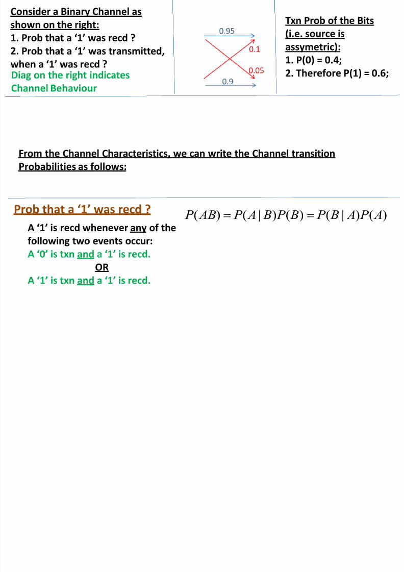
Prob that a ‘1’ was transmitted, when a ‘1’ was recd ?

1

( | ) ( )( | ) ......(Bayes' Rule)

( | ) ( )

j j j m

j j

j

P A B P B P B A

P A B P B



Relationships Involving Joint, Marginal and ConditionalProbabilities (contd)

The term ‘independence’ is more obvious, when we consider the latterequation. The probability of the event A

i remains the same irrespective of

the outcome of event B j i.e. conditioning Ai on B j does not affect the probability of A i .

Also note that the latter equality follows from the first and vice versa.It should be noted that statistical independence is quite different from

mutual exclusiveness. Indeed, if Ai and B j are mutually exclusive, thenP(Ai B j )=0, by definition.

Two events and are said to be statistically independent

if ( ) ( ) ( ) or when P( | )=P( )i j

i j i j i j i

A B

P A B P A P B A B A

Statistical Independence: Suppose that A i and B j are events associated

with the outcomes of two experiments. Suppose that the occurrence of Ai does not affect the occurrence of B j and vice versa, then we say that theevents are statistically independent.



Relationships Involving Joint, Marginal and ConditionalProbabilities (contd)

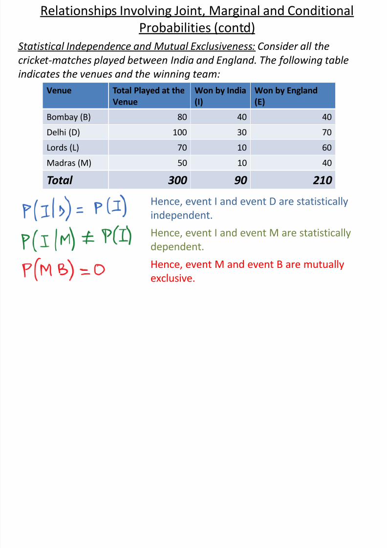
Statistical Independence and Mutual Exclusiveness: Consider all thecricket-matches played between India and England. The following tableindicates the venues and the winning team:

Venue Total Played at theVenue

Won by India(I)

Won by England(E)

Bombay (B) 80 40 40

Delhi (D) 100 30 70Lords (L) 70 10 60

Madras (M) 50 10 40

Total 300 90 210

Hence, event I and event D are statisticallyindependent.

Hence, event I and event M are statisticallydependent.

Hence, event M and event B are mutuallyexclusive.



Introduction to RVs

It is often useful to describe the outcome of an experiment by a number. Fore.g. I can say that a Head corresponds to 1.34 and Tail corresponds to –2.56.We can also have the following assignments for a random variable D, theoutcome of a ‘Dice -throw’ .

Incidentally, if we see the probabilities, we find that in this case, the dice isbiased. It will also be noted that the assignment of numbers to the respectiveoutcomes of the experiment has been made arbitrarily. Once the mapping hasbeen done, it does not change.

{ 1.4, Two 0.3, Three 1.8, Four 2.9, Five 8.96, Six 11.4}

( 1.4) 0.1, ( 0.3) 0.2, (1.8) 0.2, ( 2.9) 0.3, (8.96) 0.1, ( 11.4) 0.1,

which we have got directly from the probability of the oc

Oneand

P P P P P P

currence of the various faces.



Introduction to RVs (contd)• The numerical quantity, associated with the random outcomes ofan experiment is loosely called a RV.

• RV is a function whose domain is the set of outcomes of anexperiment and whose range is R 1, the real line.

• For every outcome of the sample space, the RV assigns a numberon the real line. When we see a RV, we only see a number on thereal line but we should remember that there is an underlyingexperiment in operation and giving rise to certain outcomes.

• The probability of occurrence of each outcome (of the underlyingexperiment) determines the probability of occurrence of each ofthe mapped numbers.

One

Two

Six -11.4

-0.3

-1.4

Domain, thepossibleoutcomes

Range, the realline



Types of Random Variables

• Discrete RVs They take values which belong to a set of finite length .For e.g. the RV representing the top face on a dice will take one out ofmax possible six values. The sample space would be {-2, 3, 4.5, -9.0, 5.6,8}. Similarly, the age of a man (rounded off in years) and the number ofchildren of a couple would also be discrete RVs.

• Continuous RVs A RV which may take infinite number of values or a continuum of values is called a Continuous RV. For e.g. The heightof men in a town, the voltage at the front end of a receiver or the age of

a man (without any rounding-off)



Cumulative Distribution Function (cdf)

(2.0) ( 11.4) ( 2.9) ( 1.4) ( 0.3) (1.8)

( ) ( ) ( ) ( ) ( )

0.1 0.3 0.1 0.2 0.2

0.9

X F P P P P P

P Six P Four P One P Two P Three




Fig2

{ 1.4, Two 0.3, Three 1.8, Four 2.9, Five 8.96, Six 11.4}

( 1.4) 0.1, ( 0.3) 0.2, (1.8) 0.2, ( 2.9) 0.3, (8.96) 0.1, ( 11.4) 0.1,

which we have got directly from the probability of the oc

One

and

P P P P P P

currence of the various faces.

(2.0) ( 11.4) ( 2.9) ( 1.4) ( 0.3) (1.8)

( ) ( ) ( ) ( ) ( )

0.1 0.3 0.1 0.2 0.2

0.9

X F P P P P P

P Six P Four P One P Two P Three




The nature of the cdf can be seen from fig . At times, the cdf is merelycalled the Distribution Function. The cdf has the following properties

( ) 0 X F

( ) 1 X F

1 2 1 2( ) ( ) if X X F x F x x x

1 2 2 1( ) ( ) ( ) X X P x X x F x F x Fig2



Joint Occurrence of many RVs

Let us consider the case of joint occurrence of two or more RVs. Agood example is the position of a satellite in space. The position P is a joint RV of the three co-ordinates X, Y and Z, which themselves arerandom in nature and are therefore RVs. We may be interested in thefollowing probabilities:

What is the probability of the satellite of being in the general volume(2km to 3km, 0 to -1km, 55 to 56km) in space i.e

P(2 X 3, 0 Y -1, 55 Z 56)=?



Joint Occurrence of many RVs

In a country, what is the probability ofa woman having age 30 years and

having two children i.e. P(A=30, C=2)=?

Though the position of the satellite inspace requires three co-ordinates, attimes we may merely be interested inknowing what is the probability of thesatellite being in such a volume in spacethat the Y-co-ord is between –5km and –6km. So here we are interested inextracting the marginal probability ofthe Y-co-ord from the joint probabilityof the 3-D position, P. This aspectwould be discussed soon.

Sr Age(A)

Children(C)

1 32 22 29 1

3 32 3

4 29 1

5 30 1

6 30 2

7 29 2

8 29 1

10,000 32 2



Joint Occurrence of many RVs and their Joint cdfHaving considered joint RVs, we can now talk

about the joint cdf. It is given by:

, ( , ) [( ) ( )] X Y F x y P X x Y y

, , ,

, , ,

( , ) 0, ( , ) 0, ( , ) ( ),

( , ) 0, ( , ) 1, ( , ) ( ) X Y X Y X Y Y

X Y X Y X Y X

F F y F y F y

F x F F x F x

From these definitions, it can be seen that:

Joint Occurrence of many RVs and their Joint cdf



Joint Occurrence of many RVs and their Joint cdf

,

,

1 6(2,3) (1,1) (1, 2) (1,3) (2,1) (2, 2) (2,3) 6*

12 121 6

(1,6) (1,1) (1, 2) (1,3) (1, 4) (1,5) (1,6) 6*12 12

C D

C D

F P P P P P P

F P P P P P P

Fig1

Fig3

Consider the case when C={1,2,3}, a 3- sided coin and D={1,2,3,4}, a ‘4 -sided’ Dice.Discuss the following:

, , ,( , ) 0, ( , ) 0, ( , ) ( ),

( , ) 0, ( , ) 1, ( , ) ( )

X Y X Y X Y Y

X Y X Y X Y X

F F y F y F y

F x F F x F x

Intro Prob and Random Processes 21 Jul 10 Lecture Set 2 Final

Documents

Transcript of Intro Prob and Random Processes 21 Jul 10 Lecture Set 2 Final