Intrinsic finite element modeling of a linearmembrane shell problem

Peter Hansbo ∗ Mats G. Larson †

Abstract

A Galerkin finite element method for the membrane elasticity problem on ameshed surface is constructed by using two-dimensional elements extended into threedimensions. The membrane finite element model is established using the intrinsic ap-proach suggested by Delfour and Zolesio [8].

1 Introduction

Models of thin-shell structures are often established using differential geometry to definethe governing differential equations in two dimensions, cf. Ciarlet [4] for an overview. Asimpler approach is the classical engineering trick of viewing the shell as an assembly offlat elements, in which simple transformations of the two-dimensional stiffness matrices areperformed, cf., e.g., Zienkiewciz [15]. In contrast to these approaches, Delfour and Zolesio[8, 9, 10] established elasticity models on surfaces using the signed distance function, whichcan be used to describe the geometric properties of a surface. In particular, the intrinsictangential derivatives were used for modeling purposes as the main differential geometrictool and the partial differential equations were established in three dimensions. A similarconcept had been used earlier in a finite element setting for the numerical discretization ofthe Laplace-Beltrami operator on surfaces by Dziuk [12], resulting in a remarkably cleanand simple implementation. For diffusion-like problems, the intrinsic approach has becomethe focal point of resent research on numerical solutions of problems posed on surfaces, cf.,e.g., [1, 2, 7, 11, 13, 14]

The purpose of this paper is to begin to explore the possibilities of the intrinsic approachin finite element modeling of thin-shell structures, focusing on the simplest model, thatof the membrane shell without bending stiffness. We derive a membrane model using theintrinsic framework and generalize the finite element approach of [12]. Finally, we givesome elementary numerical examples.

∗Department of Mechanical Engineering, Jonkoping University, SE-55111 Jonkoping, Sweden.†Department of Mathematics and Mathematical Statistics, Umea University, SE-90187 Umea, Sweden

1

arX

iv:1

203.

3292

v1 [

mat

h.N

A]

15

Mar

201

2

2 The membrane shell model problem

2.1 Basic notation

We begin by recalling the fundamentals of the approach of Delfour and Zolesio [8, 9, 10].Let Σ be a smooth two-dimensional surface imbedded in R3, with outward pointing normaln. If we denote the signed distance function relative to Σ by d(x), for x ∈ R3, fulfilling∇d = n, we can define the domain occupied by the membrane by

Ωt = x ∈ R3 : |d(x)| < t/2,

where t is the thickness of the membrane. The closest point projection p : Ωt → Σ is givenby

p(x) = x− d(x)n(x),

the Jacobian matrix of which is

∇p = I − d∇⊗ n− n⊗ n

where I is the identity and ⊗ denotes exterior product. The corresponding linear projectorP Σ = P Σ(x), onto the tangent plane of Σ at x ∈ Σ, is given by

P Σ := I − n⊗ n,

and we can then define the surface gradient ∇Σ as

∇Σ := P Σ∇. (2.1)

The surface gradient thus has three components, which we shall denote by

∇Σ =:

∂

∂xΣ1∂

∂xΣ2∂

∂xΣ3

.

For a vector valued function v(x), we define the tangential Jacobian matrix as

∇Σ ⊗ v :=

∂v1

∂xΣ1

∂v1

∂xΣ2

∂v1

∂xΣ3

∂v2

∂xΣ1

∂v2

∂xΣ2

∂v2

∂xΣ3

∂v3

∂xΣ1

∂v3

∂xΣ2

∂v3

∂xΣ3

and the surface divergence ∇Σ · v := tr∇Σ ⊗ v.

2

2.2 The surface strain and stress tensors

We next define a surface strain tensor

εΣ(u) :=1

2

(∇Σ ⊗ u+ (∇Σ ⊗ u)T

),

which is extensively used in [8, 9, 10], where it is employed to derive models of shells basedon purely mathematical arguments.

From a mechanical point of view, the problem of using εΣ(u) as a fundamental measureof strain on a surface lies in it not being an in-plane tensor, in that εΣ(u)·n 6= 0. The shearstrains associated with the out-of-plane direction are typically neglected in mechanicalmodels, but are present in εΣ(u) (cf. Remark 2.1). To obtain an in-plane strain tensor weneed to use the projection twice to define

εPΣ(u) := P Σε(u)P Σ,

which lacks all out-of-plane strain components. For a shell, where plane stress is assumed,this strain tensor can still be used, since out-of-plane strains do not contribute to the strainenergy.

Remark 2.1 It is instructive to work out the details at a surface point whose surroundingis tangential to the x1x2–plane. In this case n = (0, 0, 1),

P Σ =

1 0 00 1 00 0 0

, ∇Σ ⊗ u =

∂u1

∂x1

∂u2

∂x1

∂u3

∂x1

∂u1

∂x2

∂u2

∂x2

∂u3

∂x2

0 0 0

,

εΣ(u) =

∂u1

∂x1

1

2

(∂u1

∂x2

+∂u2

∂x1

)1

2

∂u3

∂x1

1

2

(∂u1

∂x2

+∂u2

∂x1

)∂u2

∂x2

1

2

∂u3

∂x21

2

∂u3

∂x1

1

2

∂u3

∂x2

0

,

and

εPΣ =

∂u1

∂x1

1

2

(∂u1

∂x2

+∂u2

∂x1

)0

1

2

(∂u1

∂x2

+∂u2

∂x1

)∂u2

∂x2

0

0 0 0

.The terms in εΣ not present in εPΣ are shear strains that are typically neglected for thinstructures, and it is clear that in our case εPΣ is the relevant strain tensor.

3

However, the tensor εPΣ is rather cumbersome to use directly in a numerical implemen-tation; it would be much easier to work with εΣ which can be establish using tangentialderivatives. For this reason, we use the fact that there also holds (as is easily confirmed)

εPΣ(u) = P ΣεΣ(u)P Σ =1

2

(P Σ∇Σ ⊗ uP Σ + (P Σ∇Σ ⊗ uP Σ)T

),

and since n · εΣ(u) · n = 0 we have the following relation:

εPΣ(u) = εΣ(u)− ((εΣ(u) · n)⊗ n+ n⊗ (εΣ(u) · n)) ,

so that, using dyadic double-dot product,

σ : u⊗ v = (σ · u) · v, u⊗ v : σ = u · (v · σ),

where σ is a tensor and u, v are vectors, we arrive at

εPΣ(u) : εPΣ(v) = εΣ(u) : εΣ(v)− 2(εΣ(u) · n) · (εΣ(v) · n), (2.2)

which will be used in the finite element implementation below. We also note that thereholds

tr εPΣ(v) = ∇Σ · v, (2.3)

where trε =∑

k εkk.We shall assume an isotropic stress–strain relation,

σ = 2µε+ λtrε I,

where σ is the stress tensor and I is the identity tensor. The Lame parameters λ and µare related to Young’s modulus E and Poisson’s ratio ν via

µ =E

2(1 + ν), λ =

Eν

(1 + ν)(1− 2ν).

For the in-plane stress tensor we thus assume

σPΣ := 2µεPΣ + λtrεPΣ P Σ,

in the plane strain case and, in the plane stress case, which is appropriate for a thinmembrane,

σPΣ := 2µεPΣ + λ0trεPΣ P Σ, (2.4)

where

λ0 :=2λµ

λ+ 2µ=

Eν

1− ν2.

4

2.3 The membrane shell equations

Consider a potential energy functional given by

Π(ut) :=1

2

∫Ωt

σ(ut) : ε(ut)dΩt −∫

Ωt

f t · ut

where f t is of the form f t = f p. Under the assumption of small thickness, we have∫Ωt

f(x) dΩt ≈∫ t/2

−t/2

∫Σ

f dΣdz

and thus

Π(ut) ≈ ΠPΣ(u) :=

t

2

∫Σ

σPΣ(u) : εPΣ(u)dΣ− t∫

Σ

f · u dΣ

:=t

2(σPΣ(u), εPΣ(u))Σ − t(f ,u)Σ.

Minimizing the potential energy leads to the variational problem of finding u ∈ V ,where V is an appropriate Hilbert space which we specify below, such that

aΣ(u,v) = lΣ(v) ∀v ∈ V (2.5)

where, by (2.2) and (2.3),

aΣ(u,v) = (2µεPΣ(u), εPΣ(v))Σ + (λ0 tr εPΣ(u), tr εPΣ(v))Σ

= (2µεΣ(u), εΣ(v))Σ − (4µεΣ(u) · n, εΣ(v) · n)Σ + (λ0∇Σ · u,∇Σ · v)Σ,

and lΣ(v) = (f ,v)Σ. This variational problem formally coincides with the one analyzedin the classical differential geometric setting by Ciarlet and co-workers [6, 5], as shown in[10].

Splitting the displacement into a normal part un := u · n and a tangential part ut :=u− unn we have the identity

εPΣ(u) = εPΣ(ut) + un∇⊗ n = εPΣ(ut) + unκ,

where κ = ∇ ⊗ ∇d is the Hessian of the distance function d, cf. [10], The bilinear formcan therefore also be written in the form

aΣ(u,v) = (2µ(εPΣ(ut) + unκ), εPΣ(vt) + vnκ)Σ

+ (λ0(tr εPΣ(ut) + untrκ), tr εPΣ(vt) + vntrκ)Σ (2.6)

This means that we do not have full ellipticity in our problem. Based on this observationwe conclude that the natural function space for the variational formulation is

V = v : vn ∈ L2(Σ) and vt ∈ [H1(Σ)]2,

5

cf. [5]. The loss of ellipticity have consequences for the numerics and we comment on thisin the numerical examples below.

Since(σPΣ(u), εPΣ(u))Σ = (σPΣ(u), εΣ(u))Σ

we find, using Green’s formula, the pointwise equilibrium equation

−∇Σ · σPΣ(u) = f in Σ, (2.7)

which together with the constitutive law (2.4) defines the intrinsic differential equations oflinear elasticity on surfaces.

3 The finite element method

3.1 Parametrization

Let Th := T be a conforming, shape regular triangulation of Σ, resulting in a discretesurface Σh. We shall here consider an isoparametric parametrization of the surface (thesame idea can however be used for arbitrary parametrizations). In the numerical examplesbelow we use a piecewise linear approximation, meaning that the elements T will be planar.For the parametrization we wish to define a map F : (ξ, η) → (x, y, z) from a referencetriangle T defined in a local coordinate system (ξ, η) to T , for all T . To this end, wewrite x = x(ξ, η), where x = (x, y, z) are the physical coordinates on Σh. For any givenparametrization, we can extend it outside the surface by defining

x(ξ, η, ζ) = x(ξ, η) + ζ n(ξ, η)

where n is the normal and −t/2 ≤ ζ ≤ t/2. In some models, where the surface is anidealized thin structure, it is natural to think of t as a thickness.

For the representation of the geometry, we first introduce the following approximationof the normal:

n ≈ nh =nh0|nh0 |

, nh0 =∑i

niϕi(ξ, η),

where ϕi(ξ, η) are the finite element shape functions on the reference element (assumedlinear in this paper), and ni denotes the normals in the nodes of the mesh. We thenconsider parametrizations of the type

x(ξ, η, ζ) ≈ xh(ξ, η, ζ) =∑i

(xiϕi(ξ, η) + ζ niϕi(ξ, η)) (3.1)

where xi are the physical location of the nodes on the surface. For the approximation ofthe solution, we use a constant extension,

u ≈ uh =∑i

uiϕi(ξ, η) (3.2)

6

where ui are the nodal displacements, so that the finite element method is, in a sense,superparametric. Note that only the in-plane variation of the approximate solution willmatter since we are looking at in-plane stresses and strains. We employ the usual finiteelement approximation of the physical derivatives of the chosen basis ϕi on the surface,at (ξ, η), as

∂ϕj∂x∂ϕj∂y∂ϕj∂z

= J−1(ξ, η, 0)

∂ϕj∂ξ∂ϕj∂η∂ϕj∂ζ

ζ=0

where J(ξ, η, ζ) :=

∂xh

∂ξ

∂yh

∂ξ

∂zh

∂ξ∂xh

∂η

∂yh

∂η

∂zh

∂η∂xh

∂ζ

∂yh

∂ζ

∂zh

∂ζ

,

This gives, at ζ = 0, ∂ϕi∂x∂ϕi∂y∂ϕi∂z

= J−1(ξ, η, 0)

∂ϕi∂ξ∂ϕi∂η0

.With the approximate normals we explicitly obtain

∂xh

∂ζ

∣∣∣∣ζ=0

= nh,

so

J(ξ, η, 0) :=

∂xh

∂ξ

∂yh

∂ξ

∂zh

∂ξ∂xh

∂η

∂yh

∂η

∂zh

∂η

nhy nhy nhz

.

Remark 3.1 The approach by Dziuk [12] (and also the classical engineering approach,[15]) is, in our setting, a constant-by-element extension of the geometry using facet trianglesT so that, with nT the normal to the facet, xh(ξ, η, ζ)

∣∣T

=∑

i xi ϕi(ξ, η)|T + ζnT , and∂ϕi∂x∂ϕi∂y∂ϕi∂z

= J−1(ξ, η, 0)

∂ϕi∂ξ∂ϕi∂η0

, J(ξ, η, 0) :=

∂xh

∂ξ

∂yh

∂ξ

∂zh

∂ξ∂xh

∂η

∂yh

∂η

∂zh

∂ηnTx nTy nTz

.

This low order approximation has the advantage of yielding a constant Jacobian from alinear approximation. For some applications this is, however, offset by the problem ofhaving a discontinuous normal between elements.

7

3.2 Finite element formulation

We can now introduce finite element spaces constructed from the basis previously discussedby defining

W h := v : v|T F ∈ P k(T ), ∀T ∈ Th; v ∈ C0(Σh), (3.3)

(in the numerics, we use k = 1), and the finite element method reads: Find uh ∈ V h :=[W h]3 such that

aΣh(uh,v) = lΣh

(v), ∀v ∈ V h, (3.4)

where

aΣh(u,v) = (2µεΣh

(u), εΣh(v))Σh

− (4µεΣh(u) · nh, εΣh

(v) · nh)Σh

+ (λ0∇Σh· u,∇Σh

· v)Σh

and lΣh(v) = (f ,v)Σh

.

3.3 Extension to surfaces with a boundary

If the surface Σ has a boundary ∂Σ we assume that ∂Σ = ∪i∂Σi where ∂Σi are closedcomponents. On each of the components ∂Σi we let qj : ∂Σi → R3, j = 1, 2, 3, be smoothorthonormal vector fields. We strongly impose homogeneous Dirichlet boundary conditionsof the type

qj · u = 0 on ∂Σi, 1 ≤ j ≤ di, (3.5)

where di = 1, 2, or 3, and weakly the remaining Neumann condition

(n∂Σ · σPΣ(u)) · qj = 0, di < j ≤ 3, (3.6)

where n∂Σ is the unit vector that is normal to ∂Σ and tangent to Σ. Note that not everycombination of boundary conditions and right hand side leads to a well posed problem.

4 Numerical examples

In the numerical examples below, the geometry is represented by flat facets, and thenormals are taken as the exact normal in the nodes, interpolated linearly inside eachelement. Our experience is that similar results are obtained if we use L2−projections ofthe flat facet normals in the nodes and then interpolate these linearly.

4.1 Pulling a cylinder

We consider a cylindrical shell of radius r and thickness t, with open ends at x = 0 and atx = L, and with fixed longitudinal displacements at x = 0, and radial at x = L, carryinga horizontal surface load per unit area

f(x, y, z) =F

2πr

x

L2,

8

where F has the unit of force. The resulting longitudinal stress is

σ =F(1− (x/L)2

)4πrt

.

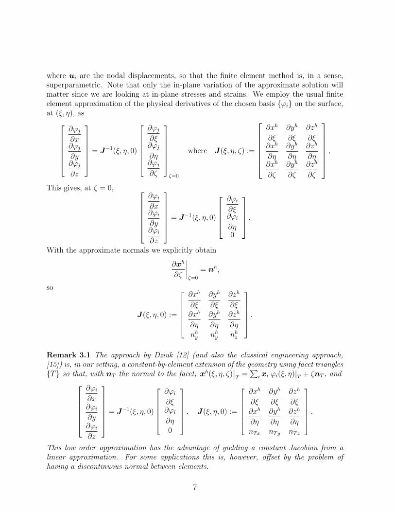
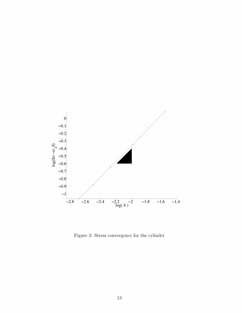
We take as an example a cylinder of radius r = 1 and length L = 4, with materialdata E = 100 and ν = 1/2, with thickness t = 10−2, and with F = 1. In Fig. 1 weshow the solution (exaggerated 10 times) on a particular mesh (shown in Fig. 2). Notethat the lateral contraction creates radial displacements depending on the size of stress.Finally, in Fig. 3 we show the L2 error in stresses, ‖σ − σh‖L2(Ω), where σ := σPΣ(u) andσh := σPΣ(uh), which shows the expected first order convergence for our P 1 approximation.The black triangle shows the 1:1 slope.

4.2 A torus with internal pressure

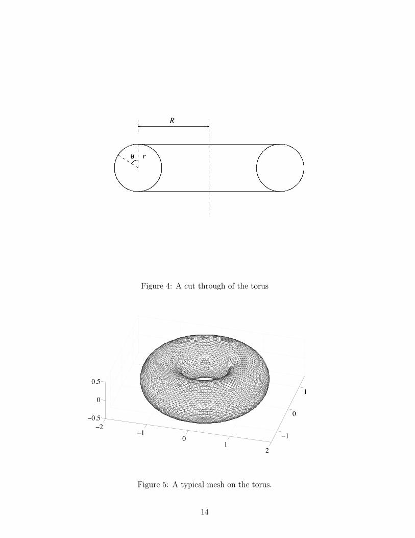
We consider a torus with internal gauge pressure p for which the stresses are staticallydeterminate. Using the angle and radii defined in Fig. 4, the principal stresses are givenby

σ1 =pr

2t, σ2 =

pr

t

(1− r sin θ

2(R + r sin θ)

),

where σ1 is the longitudinal stress, σ2 the hoop stress, and t is the thickness of the surfaceof the torus. The constitutive parameters and thickness where chosen as in the cylinderexample, and we set R = 1, r = 1/2, and p = 1.

Again we compute the stress error ‖σ − σh‖L2(Ω). We show the observed convergencein Fig. 7 at a rate of about 3/4 (the slope of the black triangle), which is suboptimal, butdoes occur in problems where elliptic regularity is an issue, cf. [3], Lemma 10. We thusattribute this loss of convergence to the load now being in the normal direction of the shell,for which we do not have ellipticity.

References

[1] E. Bansch, P. Morin, and R. H. Nochetto. Surface diffusion of graphs: variationalformulation, error analysis, and simulation. SIAM J. Numer. Anal., 42(2):773–799,2004.

[2] J. W. Barrett, H. Garcke, and T. Nurnberg. On the parametric finite element ap-proximation of evolving hypersurfaces in R3. J Comput. Phys., 227(9):4281 – 4307,2008.

[3] E. Burman and P. Hansbo. Edge stabilization for Galerkin approximations ofconvection-diffusion-reaction problems. Comput. Methods Appl. Mech. Engrg., 193(15-16):1437–1453, 2004.

9

[4] P. G. Ciarlet. Mathematical elasticity. Vol. III: Theory of shells, volume 29 of Studiesin Mathematics and its Applications. North-Holland Publishing Co., Amsterdam,2000.

[5] P. G. Ciarlet and V. Lods. Asymptotic analysis of linearly elastic shells. I. Justificationof membrane shell equations. Arch. Rational Mech. Anal., 136(2):119–161, 1996.

[6] P. G. Ciarlet and E. Sanchez-Palencia. Un theoreme d’existence et d’unicite pour lesequations des coques membranaires. C. R. Acad. Sci. Paris Ser. I Math., 317(8):801–805, 1993.

[7] K. Deckelnick, G. Dziuk, C. M. Elliott, and C.-J. Heine. An h-narrow band finite-element method for elliptic equations on implicit surfaces. IMA J. Numer. Anal.,30(2):351–376, 2010.

[8] M. C. Delfour and J.-P. Zolesio. A boundary differential equation for thin shells. J.Differential Equations, 119(2):426–449, 1995.

[9] M. C. Delfour and J.-P. Zolesio. Tangential differential equations for dynamicalthin/shallow shells. J. Differential Equations, 128(1):125–167, 1996.

[10] M. C. Delfour and J.-P. Zolesio. Differential equations for linear shells: comparisonbetween intrinsic and classical models. In Advances in mathematical sciences: CRM’s25 years (Montreal, PQ, 1994), volume 11 of CRM Proc. Lecture Notes, pages 41–124.Amer. Math. Soc., Providence, RI, 1997.

[11] A. Demlow and G. Dziuk. An adaptive finite element method for the Laplace-Beltramioperator on implicitly defined surfaces. SIAM J. Numer. Anal., 45(1):421–442, 2007.

[12] G. Dziuk. Finite elements for the Beltrami operator on arbitrary surfaces. In Par-tial differential equations and calculus of variations, volume 1357 of Lecture Notes inMath., pages 142–155. Springer, Berlin, 1988.

[13] C. M. Elliott and B. Stinner. Modeling and computation of two phase geometricbiomembranes using surface finite elements. J Comput. Phys., 229(18):6585 – 6612,2010.

[14] M. A. Olshanskii, A. Reusken, and J. Grande. A finite element method for ellipticequations on surfaces. SIAM J. Numer. Anal., 47(5):3339–3358, 2009.

[15] O. C. Zienkiewicz. The finite element method in engineering science. McGraw-Hill,London, 1971.

10

02

46 ï2

0

2ï2

ï1

0

1

2

Figure 1: Displacements (exaggerated by one order of magnitude) on a particular mesh.

11

01

23

4ï1

01

ï1.5

ï1

ï0.5

0

0.5

1

1.5

Figure 2: The cylinder before deformation.

12

ï2.8 ï2.6 ï2.4 ï2.2 ï2 ï1.8 ï1.6 ï1.4

ï1

ï0.9

ï0.8

ï0.7

ï0.6

ï0.5

ï0.4

ï0.3

ï0.2

ï0.1

0

log( h )

log(

||m ïm

h||)

Figure 3: Stress convergence for the cylinder

13

θ r

R

Figure 4: A cut through of the torus

ï2ï1

01

2

ï1

0

1

ï0.5

0

0.5

Figure 5: A typical mesh on the torus.

14

ï1.5 ï1 ï0.5 0 0.5 1 1.5ï1

0

1

ï1.5

ï1

ï0.5

0

0.5

1

1.5

Figure 6: Deformations in the torus case, exaggerated by two orders of magnitude.

15

ï3 ï2.9 ï2.8 ï2.7 ï2.6 ï2.5 ï2.4ï2.4

ï2.3

ï2.2

ï2.1

ï2

ï1.9

ï1.8

log( h )

log(

||m ïm

h||)

Figure 7: Convergence of the stresses in the torus case.

16