Intraseasonal variability in the far-east paciﬁc ...

Intraseasonal variability in the far-east pacific: investigationof the role of air–sea coupling in a regional coupled model

R. Justin Small • Shang-Ping Xie • Eric D. Maloney •

Simon P. de Szoeke • Toru Miyama

Received: 4 July 2009 / Accepted: 4 March 2010 / Published online: 25 March 2010

� Springer-Verlag 2010

Abstract Intraseasonal variability in the eastern Pacific

warm pool in summer is studied, using a regional ocean–

atmosphere model, a linear baroclinic model (LBM), and

satellite observations. The atmospheric component of the

model is forced by lateral boundary conditions from

reanalysis data. The aim is to quantify the importance to

atmospheric deep convection of local air–sea coupling. In

particular, the effect of sea surface temperature (SST)

anomalies on surface heat fluxes is examined. Intraseasonal

(20–90 day) east Pacific warm-pool zonal wind and out-

going longwave radiation (OLR) variability in the regional

coupled model are correlated at 0.8 and 0.6 with observa-

tions, respectively, significant at the 99% confidence level.

The strength of the intraseasonal variability in the coupled

model, as measured by the variance of outgoing longwave

radiation, is close in magnitude to that observed, but with a

maximum located about 10� further west. East Pacific

warm pool intraseasonal convection and winds agree in

phase with those from observations, suggesting that remote

forcing at the boundaries associated with the Madden–

Julian oscillation determines the phase of intraseasonal

convection in the east Pacific warm pool. When the ocean

model component is replaced by weekly reanalysis SST in

an atmosphere-only experiment, there is a slight improve-

ment in the location of the highest OLR variance. Further

sensitivity experiments with the regional atmosphere-only

model in which intraseasonal SST variability is removed

indicate that convective variability has only a weak

dependence on the SST variability, but a stronger depen-

dence on the climatological mean SST distribution. A

scaling analysis confirms that wind speed anomalies give a

much larger contribution to the intraseasonal evaporation

signal than SST anomalies, in both model and observa-

tions. A LBM is used to show that local feedbacks would

serve to amplify intraseasonal convection and the large-

scale circulation. Further, Hovmoller diagrams reveal that

whereas a significant dynamic intraseasonal signal enters

the model domain from the west, the strong deep convec-

tion mostly arises within the domain. Taken together, the

regional and linear model results suggest that in this region

remote forcing and local convection–circulation feedbacks

are both important to the intraseasonal variability, but

ocean–atmosphere coupling has only a small effect. Pos-

sible mechanisms of remote forcing are discussed.

R. J. Small (&)

Jacobs Technology, Naval Research Laboratory, Code 7320,

Building 1009, Stennis Space Center, MS 39529, USA

e-mail: [email protected]

R. J. Small � S.-P. Xie

International Pacific Research Center, University of Hawaii,

POST 401, 1680 East-West Rd, Honolulu, HI 96822, USA

S.-P. Xie

Department of Meteorology, School of Ocean and Earth Science

and Technology, University of Hawaii, HIG350,

2525 Correa Rd, Honolulu, HI 96822, USA

E. D. Maloney

Department of Atmospheric Science, Colorado State

University, Fort Collins, CO, USA

S. P. de Szoeke

College of Oceanic and Atmospheric Sciences,

Oregon State University, 104 COAS Admin. Bldg,

Corvallis, OR 97331-5503, USA

T. Miyama

Frontier Research for Global Change, Yokohama, Japan

e-mail: [email protected]

123

Clim Dyn (2011) 36:867–890

DOI 10.1007/s00382-010-0786-2

Keywords Intraseasonal variability �Madden–Julian oscillation � East Pacific � Climate �Tropical meteorology � Air–sea interaction �Coupled models � Regional models

1 Introduction

Intraseasonal variability in the tropics is dominated by the

Madden Julian oscillation (MJO; Madden and Julian 1994;

Zhang et al. 2006). The MJO not only impacts tropical

precipitation and extreme events (e.g. Barlow and Salstein

2006; Maloney and Shaman 2008; Bessafi and Wheeler

2006), but also affects midlatitude weather (e.g. Higgins

et al. 1999; Bond and Vecchi 2003). It is well known that

many global atmospheric general circulation models

(AGCM) and coupled general circulation models (CGCM)

have difficulty simulating the MJO. When compared to

observations, the models typically exhibit weak intrasea-

sonal precipitation variance, little coherence between

winds and precipitation anomalies, and a spectrum that is

too broad, with the ratio of eastward to westward power

being too small (Slingo et al. 1996; Lin et al. 2006; Zhang

2005). Problems with the MJO simulation are often

attributed to inadequacies of the cumulus parameterization

(Slingo et al. 1996; Lin et al. 2006).

The role of SST, and more generally, air–sea interaction,

in the MJO cycle has been studied by a number of authors

using coupled model experiments, with varying results, as

reviewed by Hendon (2005). Coupling was only found to

improve the simulations when the atmospheric model had a

good representation of the phase relationship between

insolation and evaporation (discussed by Hendon 2000).

Such improvements were found by Maloney and Kiehl

(2002a), who coupled an AGCM to a slab ocean model,

and studied the impact on east Pacific intraseasonal pre-

cipitation, and Inness and Slingo (2003) who used a cou-

pled general circulation model and found improved

simulations of Indian Ocean variability compared to results

from an atmosphere-only model forced by slowly varying

SST fields. In contrast the study of Garabowski (2006)

showed a weak dependence of the MJO on SST, in a

coupled aquaplanet/slab-ocean model which employed

superparameterization of cumulus convection. He sug-

gested that the dominant process in his model was a

feedback between convection and free-tropospheric mois-

ture amount, with SST-convection feedbacks playing a

much smaller role.

From satellite and buoy observations, Maloney et al.

(2008) found that MJO-related SST variations of 0.8–1.0�C

occur in the Eastern Pacific warm pool, driven by latent

heat and short wave flux variations. In the east Pacific,

warm SST lead precipitation by about 10 days, whilst the

SST cools during MJO convective events. Maloney and

Kiehl (2002b) suggested that SST-induced moisture con-

vergence and oceanic heat content anomalies helped pre-

condition the atmosphere for convection.

Idealized column models show that under certain con-

ditions, an unforced oscillation of precipitation and SST

can be obtained with an intraseasonal period in a cycle that

resembles a recharge–discharge oscillation (e.g. Sobel and

Gildor 2003). The behavior is highly dependent on the

cloud-radiative feedback parameter (which can also be

thought to represent wind-induced surface flux feedbacks),

and convective timescale, and instability on intraseasonal

timescales was found to be greatest for mixed layer depths

in the range of 10–20 m. If mixed layer depth goes to zero

in a version of the model with prescribed intraseasonal

wind speed forcing, effectively shutting off the wind-

evaporation feedback, model intraseasonal variability

decreases dramatically (e.g. Maloney and Sobel 2004).

Recently, coupled regional models have emerged as an

alternative tool to investigate the effect of large scale

variability on specific regions (Xie et al. 2007; Seo et al.

2007). A regional model has the advantage that propagat-

ing signals associated with the large-scale, hemispheric

MJO can pass into the domain through the lateral boundary

conditions in the atmosphere, and also possibly via oceanic

pathways (Kessler et al. 1995). Regional scale processes

may be better represented by the higher resolution avail-

able in a regional, rather than global, model.

An ideal region for such a study is the far-eastern Pacific

warm pool, where strong intraseasonal variability in the

ocean and atmosphere is known to occur, particularly in

summer, and to be related to the global MJO (e.g. Kayano

and Kousky 1999; Maloney and Hartmann 2000). The east

Pacific is also a region of complex topography and

oceanographic structure, making use of a regional model

particularly useful. Some of the prominent features include

strong winds emanating from the gaps in the Central

American cordillera (Chelton et al. 2000), and high ocean

eddy kinetic energy and SST variability offshore of the

Central American coast and along 10�N (Farrar and Weller

2006; Chang 2009).

Statistically significant 50-day peaks in precipitation,

wind, and SST can be found in the east Pacific warm pool

during boreal summer (Maloney and Esbensen 2003, 2007;

Maloney et al. 2008). An important question is to what

extent such variability in this region is influenced or

enhanced by local processes rather than just being driven

by the global MJO. A related question is whether the east

Pacific can support strong intraseasonal variability in iso-

lation from the west Pacific.

The main aim of this paper is to investigate the role of

air–sea interaction in intraseasonal variability in the eastern

Pacific warm pool, using models and observations. We also

868 R. J. Small et al.: Intraseasonal variability in the far-east pacific

123

discuss the role of local circulation–convection feedbacks,

and remote forcing from the eastern hemisphere. This study

sheds light not only on what regulates intraseasonal vari-

ability in the east Pacific, but may also help illuminate what

controls intraseasonal variability in the tropics, in general.

The structure of the paper is as follows. In Sect. 2 the

datasets, models and methods are described. The fidelity of

the coupled model to simulate MJO events is discussed in

Sect. 3. Section 4 examines the influence of air–sea inter-

action using regional atmospheric model sensitivity

experiments. This is followed by a discussion of the impact

of remote forcing and comparison of the results of this

paper to previous studies, and, finally, conclusions.

2 Data, models and methods

2.1 Observations and reanalysis

The characteristics of convection in the region are deduced

from outgoing longwave radiation (OLR) data and a merged

precipitation analysis. OLR is obtained from National Oce-

anic and Atmospheric Administration (NOAA) polar-orbit-

ing satellites, interpolated daily onto a 2.5� 9 2.5� grid

(Liebmann and Smith 1996). Precipitation is based on the

daily TRMM 3B42 rainrate (v5) gridded onto a 1� grid. This

dataset combines and calibrates the abundant satellite IR

measurements with more accurate passive microwave mea-

surements of precipitation from TRMM. For access to

TRMM3B42 see http://daac.gsfc.nasa.gov/precipitation/

TRMM_README for details.

Neutral wind vectors at 10 m (Wentz and Smith 1999)

are derived from the SeaWinds QuikSCAT scatterometer.

SST and column-integrated water vapor from December

1997 is obtained from the TRMM satellite microwave

imager (TMI). TMI data is not affected by clouds except

under heavy precipitation (Wentz et al. 2000) and hence

has a significant advantage over infrared radiometers in

regions of large cloud cover. The above-mentioned data is

obtained from Remote Sensing Systems (http://www.

ssmi.com), processed on a 0.25� grid. For other fields we

use National Centers for Environmental Prediction

(NCEP)/National Center for Atmospheric Research

(NCAR) daily-mean reanalysis (Kalnay et al. 1996).

2.2 Models

2.2.1 Regional coupled model

The International Pacific Research Center (IPRC) Regional

Ocean Atmosphere Model (IROAM, Xie et al. 2007) is

used for a detailed, high resolution analysis of intraseasonal

variability, and for studies of the sensitivity to SST. The

atmospheric component is a terrain-following normalized

pressure (sigma) coordinate hydrostatic model (Wang et al.

2003). It employs a moisture convergence scheme for

shallow convection and a modified CAPE closure for deep

convection, as well as explicit microphysics. There are 28

vertical levels. Further details and references for the

physical schemes can be found in Wang et al. 2003 and Xie

et al. 2007. At the lateral boundaries the atmospheric model

is nudged towards four-times daily values of temperature

humidity, and wind components from the NCEP/NCAR

reanalysis, in a buffer zone 6� wide. This allows observed

propagating MJO signals to force the atmospheric model at

the boundaries. Including this buffer zone, the model

extends from 150� to 30�W, and from 35�S to 35�N.

The ocean component is the z-coordinate hydrostatic

Modular Ocean Model (MOM2) (Pacanowski and Griffies

2000), employing 30 levels, 20 of which are in the upper

400 m. The vertical mixing scheme is based on Paca-

nowski and Philander (1981). We use a constant Laplacian

lateral eddy viscosity coefficient of 2 9 106 cm2 s-1.

Surface salinity is restored to Levitus values on a timescale

of 30 days. The model covers the Pacific ocean domain

from 35�S to 35�N, with sponge layers at the meridional

boundaries and walls at the eastern and western coastlines.

A 1/2�, co-located grid is employed for the ocean and

atmosphere, with the ocean salinity and tracer points col-

located with atmospheric temperature points. The atmo-

spheric grid is horizontally unstaggered. Xie et al. 2007

(their Fig. 1) describe and illustrate the domain of the

complete model system. The fully coupled ocean–atmo-

sphere part of the model covers the Pacific Ocean from

150�W eastwards to the American coastline, and from 35�S

to 35�N. In the coupled domain, coupling occurs once per

day. The ocean model is spun up with a hindcast from 1991

to the end of 1995 using basin-wide forcing from NCEP/

NCAR reanalysis, then the interactive coupling is switched

on from 1996 to 2003. Further details and an overview of

the model performance can be found in Xie et al. (2007).

2.2.2 Linear baroclinic model

The linear response to diabatic heating anomalies is studied

using the linear baroclinic model (LBM) of Watanabe and

Kimoto (2000). The primitive equations used by the Center

for Climate System Research (CCSR) University of Tokyo/

National Institute for Environmental Studies (NIES)

AGCM, are linearised about a climatological summer (June–

September) mean basic state. The sigma-coordinate LBM

has 20 vertical levels, contains topography, and is run at T42

resolution. The model is time integrated, and has Newtonian

and Rayleigh damping timescales for heat and momentum

ranging from 30 days in the free troposphere to 1 day at the

top and bottom levels. Chiang et al. 2001 find that results

R. J. Small et al.: Intraseasonal variability in the far-east pacific 869

123

http://daac.gsfc.nasa.gov/precipitation/TRMM_README

http://daac.gsfc.nasa.gov/precipitation/TRMM_README

http://www.ssmi.com

http://www.ssmi.com

from a similar model do not sensitively depend on the exact

thermal damping. Some sensitivity to the Rayleigh damping

should however be expected: Wu et al. (2000a) find that even

a relatively weak boundary layer Rayleigh damping

(10 day-1) acts to significantly reduce the boundary layer

wind response to heating. Our choice of relatively strong

damping rate of 1 day-1 will cause weaker boundary layer

winds (see Fig. 11 below) but the free tropospheric winds are

not likely to be strongly reduced. The model is forced by a

specified diabatic heating anomaly which is constant in time

(a) (b)

(c) (d)

(e) (f)

Fig. 1 Summer climatology (June to September mean from 1998 to

2003) of the Eastern Tropical Pacific. a Observed precipitation from

TRMM 3B42 (color, mm day-1) and SST from TMI (contours, �C).

b Observed NOAA OLR (color, W m-2) and mean 10 m wind

vectors from QuikSCAT (m s-1). c As a but for the IROAM coupled

model, SST and precipitation: note different color bar from a. d As bbut for the coupled model OLR and mean wind vectors. In b and d the

zero contour of 10 m zonal wind is overlaid. e Mixed layer depth

(color, m) and sea minus air temperature difference (�C, contour)

from the coupled model. f depth of the 20�C isotherm (color, m), and

near-surface relative humidity (%) from the coupled model. Mixed

layer depth is defined as the depth where the temperature is less than

SST-0.2�C


123

with a specified horizontal and vertical distribution. By

20 days the solution has reached a steady state and these

results are shown here. The damping is sufficient to exclude

baroclinic instabilities from the simulation.

2.3 Methods

We analyse the years 1998–2003, unless specified otherwise.

The first two years of interactive coupling (1996–1997) are

discarded as being part of the model spin-up process, except

where specified. All data is first compiled into pentads before

analysis. Frequency spectra are calculated for boreal summer

precipitation and SST in the warm pool as in Maloney et al.

2008. Before calculation of the spectra, the climatological

seasonal cycle was removed from the data. Spectra were

calculated on each individual May–October period during

1998–2003, and then averaged across all 6 years of data to

compute an average spectrum. An expanded May–October

period is used to compute spectra to minimize bandwidth,

which in our calculations is (180 day-1). The length of

record and 2 degrees of freedom per spectral estimate pro-

duce 12 degrees of freedom for the average spectra. Using

the 1-day lag autocorrelation and square root of the 2-day lag

autocorrelation, an estimate of the red noise background

spectrum is generated using the formula of Gilman et al.

(1963), and then 95% confidence limits on this background

spectrum are calculated using the F statistic.

Hilbert transform complex empirical orthogonal function

analysis (CEOF analysis, e.g. Barnett 1983; Horel 1984) is

conducted during 1998–2003 on modeled June–October

intraseasonal precipitation and SST anomalies. Maloney

et al. (2008) conducted a CEOF analysis using TRMM pre-

cipitation and TMI SST during 1998–2005, to which we will

contrast the leading modes of model intraseasonal precipi-

tation and SST variability. For linear regression analysis and

variance plots, a temporal 12th order Butterworth filter is

applied, to isolate the 20–90 day activity. No spatial filtering

is applied, due to the relatively small size of the interactive

domain compared to the planetary-scale MJO.

Regional coupled model experiments are performed to

analyse the sensitivity of the MJO convection to the surface

boundary conditions. Firstly, a control run was performed

with a fully interactive coupling (as described in Xie et al.

2007), referred to here as Experiment 1 (Exp. 1). Next, an

atmosphere only run was performed (Exp. 2). Here the SST

was set to the Reynolds et al. (2002) weekly product

(interpolated in time to the timestep of the model).1 Third,

a further atmosphere-only run was performed with the SST

smoothed in time such that the intraseasonal variability of

SST is removed in the eastern Pacific warm pool. The

smoothing is done with a box-car filter. The averaging time

period is spatially weighted, taking a maximum value of

21 pentads in the center of interest (chosen as 90�W,

12�N), decaying in a Gaussian fashion with e-folding

widths of 30� longitude and 20� latitude. [With this form,

the averaging interval reduces to about 1 pentad (i.e. no

averaging) close to the domain boundaries, such that an

artificial sharp SST gradient near the boundary is avoided.

The effect of the smoothing is shown later in Fig. 13c.]

This experiment is referred to as Exp. 3.

3 MJO in the eastern Pacific: model and observations

3.1 Summer climatology

In summer a broad warm pool exists in the north-eastern

tropical Pacific with SST above 27�C. The precipitation

over the ocean is mostly confined to this warm pool

region, where convergence occurs in the ITCZ (Fig. 1a,

b). South of the ITCZ, the pronounced equatorial cold

tongue suppresses convection, whilst in the southern

hemisphere tropics and sub-tropics, SST is cooler than at

similar latitudes in the north so that atmospheric con-

vection is largely absent during this season. The distri-

bution of mean OLR from NOAA observations (Fig. 1b)

closely matches that of the precipitation (Fig. 1a), and

shows the presence of deep convection over the warm

pool. The wind field at 10 m from QuikSCAT (Fig. 1b,

vectors) shows the typical trade wind easterly component

dominates everywhere except over the warm pool, which

exhibits mean westerly winds, and at 10�N the mean

10 m zonal winds change sign from easterlies to wester-

lies at around 125�W (see the mean zonal wind zero

contour on Fig. 1b).

The coupled model (IROAM) SST (Fig. 1c) shows a

cold tongue and east Pacific warm pool with similar

absolute temperatures to those observed from TMI

(Fig. 1a). The IROAM rainfall distribution in the Eastern

Pacific (Fig. 1c) is close in horizontal structure to the

TRMM3B42 observations (Fig. 1a), with a single northern

ITCZ, but the magnitude of model precipitation is larger

than observations by about a factor of about 1.5 (note the

different color bars). As discussed by Xie et al. (2007) with

regard to the annual mean climatology, this increase may

be related to higher wind speeds and evaporation in

IROAM. Likewise, the OLR structure is comparable

between model (Fig. 1d) and NOAA satellite OLR data

(Fig. 1b), except for a general bias of higher OLR in the

ITCZ in the model by about 20 W m-2 (linked to a nega-

tive bias in cloud cover/height in IROAM, Xie et al. 2007).

1 The Reynolds et al. 2002 data was used for legacy reasons. It is

acknowledged that a product such as TMI SST or the recent high

resolution NOAA SST analyses (Reynolds et al. 2007) may have been

better choices to capture intraseasonal SST variability (see Sect. 5 on

the strength of SST anomalies).


123

Similar to the observations, the mean zonal winds are

westerly over the warm pool in the model (Fig. 1d).

The climatological mean ocean mixed layer depth in the

model is 20–30 m in the warm pool region (Fig. 1e, color):

this may be compared with an analysis of in-situ obser-

vations by Fiedler and Talley (2006) which showed values

of 20–40 m. The depth of the model 20�C isotherm (a

representative thermocline value) is between 40 and 70 m

in the warm pool (Fig. 1f, color), with a minimum value of

30–40 m centered near 10�N, 90�W (the Costa Rica Dome,

Wyrtki 1964; Kessler 2002; Xie et al. 2005), and again

these values are consistent with those found in observations

(Fiedler and Talley 2006).

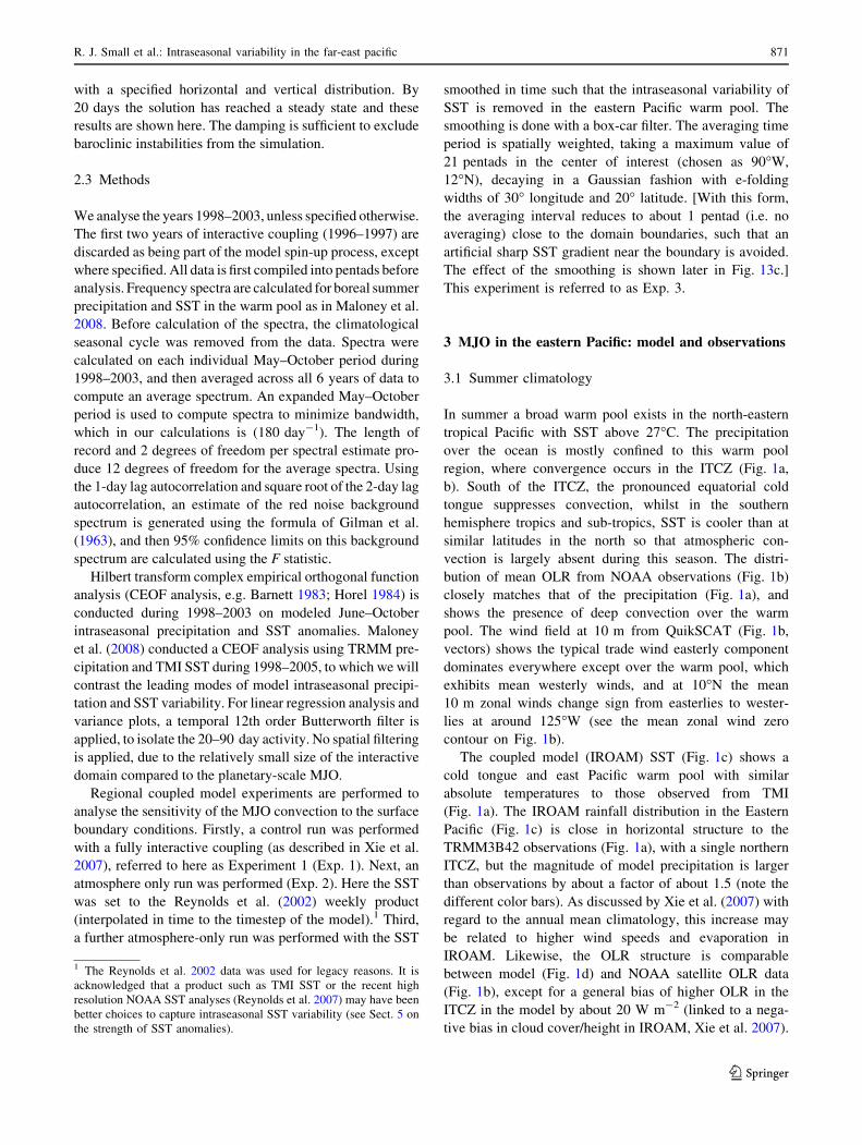
3.2 MJO amplitude and phase relative to observations

Intraseasonal wind variability, as measured by the standard

deviation of filtered zonal wind at 850 hPa, from all

months, is comparable in the IROAM model and the

NCEP/NCAR reanalysis (Fig. 2). In particular, a local

maximum observed in the latitude band 5� to 20�N, and

longitudes 120�W to Central America, is prominent in the

observations and model, with an amplitude of around

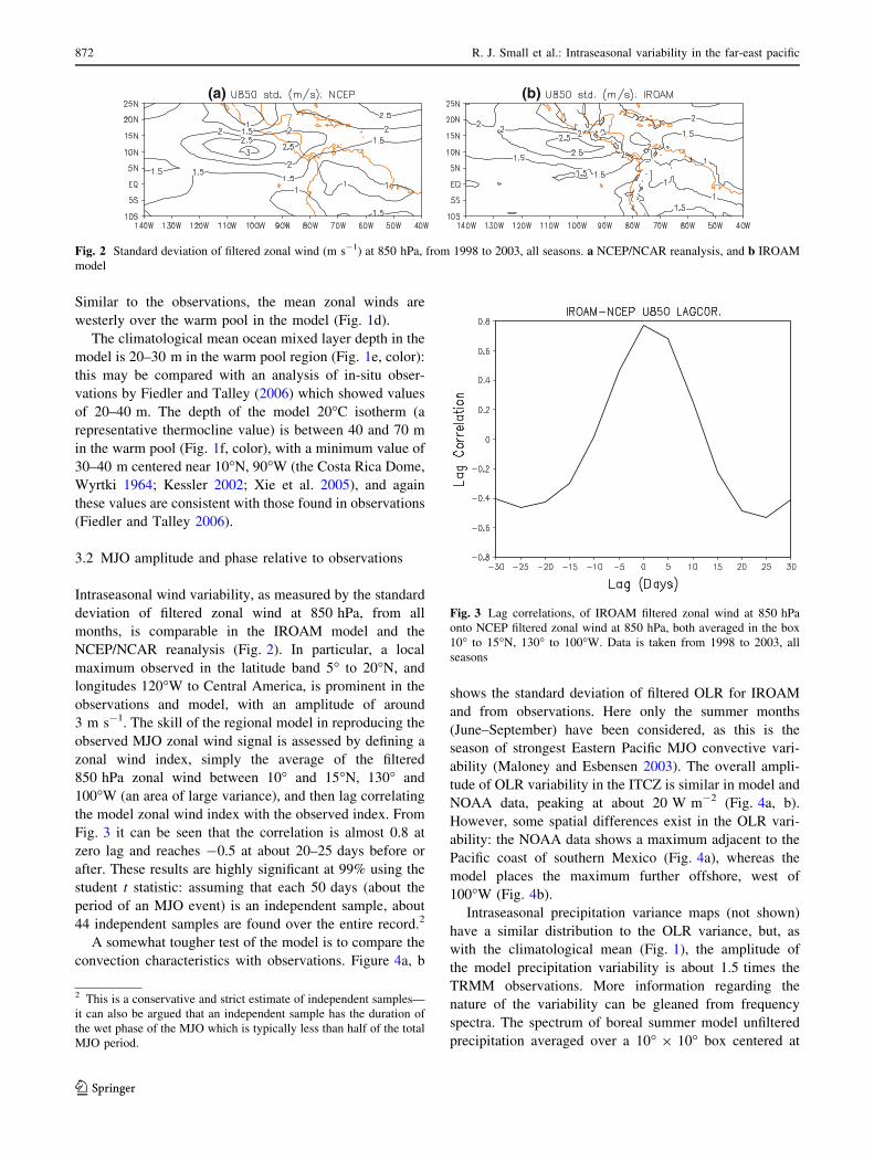
3 m s-1. The skill of the regional model in reproducing the

observed MJO zonal wind signal is assessed by defining a

zonal wind index, simply the average of the filtered

850 hPa zonal wind between 10� and 15�N, 130� and

100�W (an area of large variance), and then lag correlating

the model zonal wind index with the observed index. From

Fig. 3 it can be seen that the correlation is almost 0.8 at

zero lag and reaches -0.5 at about 20–25 days before or

after. These results are highly significant at 99% using the

student t statistic: assuming that each 50 days (about the

period of an MJO event) is an independent sample, about

44 independent samples are found over the entire record.2

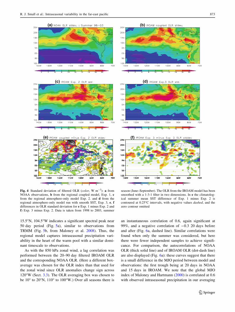
A somewhat tougher test of the model is to compare the

convection characteristics with observations. Figure 4a, b

shows the standard deviation of filtered OLR for IROAM

and from observations. Here only the summer months

(June–September) have been considered, as this is the

season of strongest Eastern Pacific MJO convective vari-

ability (Maloney and Esbensen 2003). The overall ampli-

tude of OLR variability in the ITCZ is similar in model and

NOAA data, peaking at about 20 W m-2 (Fig. 4a, b).

However, some spatial differences exist in the OLR vari-

ability: the NOAA data shows a maximum adjacent to the

Pacific coast of southern Mexico (Fig. 4a), whereas the

model places the maximum further offshore, west of

100�W (Fig. 4b).

Intraseasonal precipitation variance maps (not shown)

have a similar distribution to the OLR variance, but, as

with the climatological mean (Fig. 1), the amplitude of

the model precipitation variability is about 1.5 times the

TRMM observations. More information regarding the

nature of the variability can be gleaned from frequency

spectra. The spectrum of boreal summer model unfiltered

precipitation averaged over a 10� 9 10� box centered at

(a) (b)

Fig. 2 Standard deviation of filtered zonal wind (m s-1) at 850 hPa, from 1998 to 2003, all seasons. a NCEP/NCAR reanalysis, and b IROAM

model

Fig. 3 Lag correlations, of IROAM filtered zonal wind at 850 hPa

onto NCEP filtered zonal wind at 850 hPa, both averaged in the box

10� to 15�N, 130� to 100�W. Data is taken from 1998 to 2003, all

seasons

2 This is a conservative and strict estimate of independent samples—

it can also be argued that an independent sample has the duration of

the wet phase of the MJO which is typically less than half of the total

MJO period.


123

15.5�N, 104.5�W indicates a significant spectral peak near

50 day period (Fig. 5a), similar to observations from

TRMM (Fig. 5b, from Maloney et al. 2008). Thus, the

regional model captures intraseasonal precipitation vari-

ability in the heart of the warm pool with a similar domi-

nant timescale to observations.

As with the 850 hPa zonal wind, a lag correlation was

performed between the 20–90 day filtered IROAM OLR

and the corresponding NOAA OLR. (Here a different box-

average was chosen for the OLR index than that used for

the zonal wind since OLR anomalies change sign across

120�W (Sect. 3.3). The OLR averaging box was chosen to

be 10� to 20�N, 110� to 100�W.) Over all seasons there is

an instantaneous correlation of 0.6, again significant at

99%, and a negative correlation of -0.3 20 days before

and after (Fig. 6a, dashed line). Similar correlations were

found when only the summer was considered, but here

there were fewer independent samples to achieve signifi-

cance. For comparison, the autocorrelations of NOAA

OLR (thick solid line) and of IROAM OLR (dot-dash line)

are also displayed (Fig. 6a): these curves suggest that there

is a small difference in the MJO period between model and

observations: the first trough being at 20 days in NOAA

and 15 days in IROAM. We note that the global MJO

index of Maloney and Hartmann (2000) is correlated at 0.6

with observed intraseasonal precipitation in our averaging

(a) (b)

(c) (d)

(e) (f)

Fig. 4 Standard deviation of filtered OLR (color, W m-2): a from

NOAA observations, b from the regional coupled model, Exp. 1, cfrom the regional atmosphere-only model Exp. 2. and d from the

regional atmosphere-only model run with smooth SST, Exp. 3, e, fdifferences in OLR standard deviation for e Exp. 1 minus Exp. 2 and

f) Exp. 3 minus Exp. 2. Data is taken from 1998 to 2003, summer

season (June–September). The OLR from the IROAM model has been

smoothed with a 1-3-1 filter in two dimensions. In e the climatolog-

ical summer mean SST difference of Exp. 1 minus Exp. 2 is

contoured at 0.25�C intervals, with negative values dashed, and the

zero contour omitted


123

region (Maloney et al. 2008), suggesting that a substantial

portion of the intraseasonal variability there is explained by

the MJO. By comparison, the global MJO index is corre-

lated with regional west Pacific and Indian Ocean OLR by

at most 0.7 during boreal summer and winter. As indicated

in Fig. 6, model intraseasonal convection in the warm pool

is in phase with that from observations, partly due to

forcing of the regional coupled model at the boundaries, in

this case associated with MJO-induced dynamical signals

propagating into the domain, discussed further in Sect. 3.4.

A local complex EOF analysis (CEOF, introduced in

Sect. 2.3) is used to further examine the phase properties of

the leading mode of intraseasonal precipitation variability

in this region. The spatial amplitude, local variance

explained, and spatial phase for the leading CEOF of

modeled intraseasonal precipitation is shown in Fig. 7

(right panels). This leading mode explains 19% of the total

variance of precipitation over the domain shown, and is

separable using the criterion of North et al. (1982) from the

second and third modes (which explain 10 and 8% of the

variance, respectively). For comparison, the observed first

mode explained 26% of the variance (Maloney et al. 2008),

whilst the amplitude structure, spatial phase and propaga-

tion characteristics of the leading mode are very close in

model (Fig. 7d–f) and observations (Fig. 7a–c, taken from

Maloney et al. 2008), with high amplitude across the ITCZ

and east Pacific warm pool. The local variance explained

by this leading model CEOF is slightly smaller than

observations over the warm pool, peaking near 0.5 to the

south of Mexico, whereas observed local variance

explained approaches 0.7. [Note that although there is large

variance explained over the cold tongue in the model

(Fig. 7e) that is not observed (Fig. 7b), the amplitude in

this region is negligible (Fig. 7d).]

In both model and observations the spatial phase of

precipitation varies little in the center of warm pool to the

south of Mexico, albeit with suggestions of slow northward

propagation when combined with increasing temporal

phase (Fig. 7c, f). Precipitation in these central warm pool

regions just south of Mexico lags precipitation along 8�N

to the east of 120�W by about 100� of phase (about

2 weeks for a 50-day cycle). Also similar to observed,

precipitation to the west of 120�W leads that in the warm

pool by 125�–150� of phase.

(a)

95%

(b)

(d)(c)

95%

95%

95%

Fig. 5 Power spectrum of

May–October precipitation

averaged over a 10� 9 10� box

centered at a 15.5�N, 104.5�W,

coupled model and b 15�N,

105�W, from TRMM

precipitation. SST averaged

over a 4� 9 4� box centered c at

20.5�N, 109.5�W for the

coupled model and d at 19�N,

108�W from TMI SST. The

climatological seasonal cycle

was removed before

computation of the spectrum.

Also shown are the red noise

background spectrum and the

95% confidence limits on this

background spectrum


123

3.3 Dynamic and convective structure of MJO

in eastern pacific

The time evolution of typical MJO events in summer in

observations and model is computed by lag regression. As

above, the index used in the regression analysis is defined

as the negative of OLR anomalies averaged in a box 10� to

20�N, 110� to 100�W (shown in Figs. 8c, 9c). It is noted

that local and global indices of intraseasonal activity pro-

duce similar results (e.g. Maloney and Hartmann 2000,

2001). Lag regression plots of OLR and 850 hPa winds

from observations are shown in Fig. 8. Associated with

convection at lag 0 are strong westerlies at 850 hPa

extending from 10�S to 20�N, and positive vorticity to the

north and west (Fig. 8c). During the dry phase in the far

eastern Pacific (e.g. at -20 days and ?20 days, Fig. 8a, e)

there are easterly wind anomalies and anticyclonic vorticity

to the north and west. These features bear some similarities

with the Kelvin wave/Rossby wave couplet of Gill (1980)

for a source in the northern hemisphere, but the easterly

inflow of the Kelvin wave response to heating to the east of

convection appears to be nearly absent in the observed

circulation (Fig. 8c). The correspondence of convective

anomalies in the eastern Pacific warm pool with westerly

wind anomalies and dry anomalies with easterly winds is

similar to the composites of Maloney and Hartmann (2000)

based on a global zonal wind MJO index.

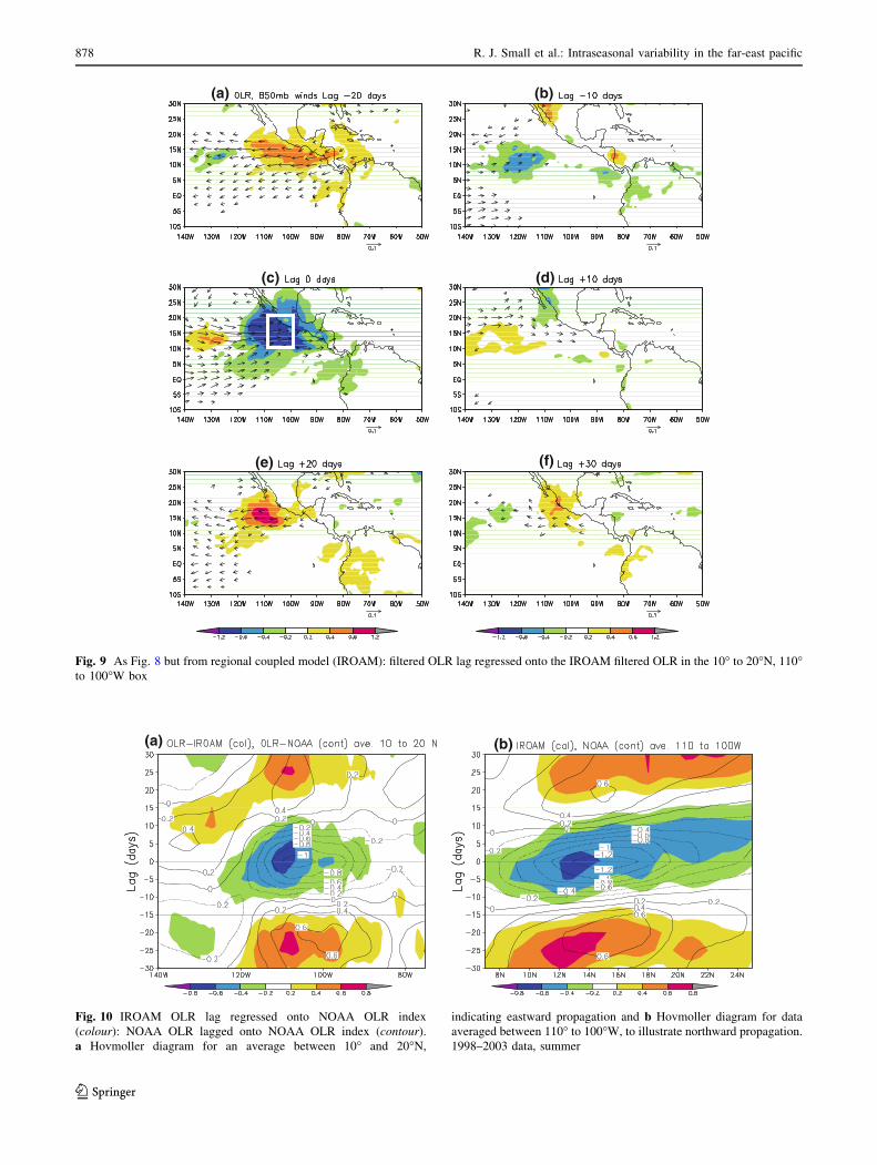
The temporal evolution of OLR in the IROAM model3

(Fig. 9) exhibits very similar, albeit weaker,4 structure to

observations, including the zonal wind/convection rela-

tionship, and a change of sign of the OLR anomaly across

120�W at zero lag. Plots of OLR lag correlation vs longi-

tude (Fig. 10a, averaged over the latitude band 10� to

20�N) reveal that instead of a smooth propagation of

convection from west to east in boreal summer, there is

instead a very rapid change of phase around 120�W.

Northward propagation is also apparent in the lag regres-

sions averaged between 110� and 100�W (Fig. 10b), con-

sistent with the observational analysis of Maloney et al.

(2008) and with the CEOF analysis shown above. This

northward propagation, examined extensively in Jiang and

Waliser (2008), parallels the poleward summertime pro-

pagation manifested in other monsoon systems, especially

the Asian monsoon (e.g. Wang and Xie 1998).

The wind fields associated with the MJO convection in

observations and model may be interpreted with the aid of

a linear baroclinic model (LBM, Sect. 2.2). The diabatic

heating input for the LBM is estimated from the precipi-

tation patterns from TRMM and IROAM, regressed onto

the OLR index, at zero lag. These precipitation patterns are

not shown, but are spatially reasonably similar to the OLR

distributions (Figs. 8c, 9c), with the maximum precipita-

tion anomaly being *0.15 mm day-1 per W m-2 in the

observations. Based on these patterns, a maximum diabatic

heating equivalent to 0.15 mm day-1 is prescribed, i.e. the

heating that is equivalent to 1 W m-2 of OLR variability.

(a)

(b)

Fig. 6 Lag correlations of filtered OLR in the box 10� to 20�N, 110�to 100�W. a NOAA OLR autocorrelation (solid line, symmetric),

IROAM OLR autocorrelation (dash-dot line, symmetric) and the lag

correlation of IROAM OLR onto NOAA OLR (dashed line). b Lag

correlations, of IROAM OLR onto NOAA OLR. Solid line fully

coupled run. Dashed line atmosphere only run with Reynolds SST.

Dot-dashed line atmosphere only run forced with SST with no

intraseasonal variability. Data is taken from 1998 to 2003, all seasons

3 Note that now the model data is regressed onto an OLR index

derived from the model data, so as to display the interrelationship

between model fields more clearly. (For reference Figs 6 and 10 show

the model-observation comparison).4 The slightly weaker amplitudes of the anomalies in the model at

non-zero lags, compared to those in observations, are not due solely to

a weaker variance (as can be seen by noting that the OLR variance in

the model is greater than observed in some locations, (Fig. 4a,b), but

probably also due to a weaker correlation between distant points and

the index box.


123

The horizontal structure is an idealized ellipse based on the

observed convection east of 110�W (Fig. 11a).5

For the vertical structure, we use a sinusoidal profile

(Fig. 11b), which leads to a diabatic heating that peaks at

0.06 K day-1 at r = 0.5 in the center of the ellipse. This

scaling allows direct comparison with Figs. 8, 9 and 10.

[To convert to the heating and response due to a typical

MJO, given the units of the regression coefficient, multiply

the values by about 20, the maximum standard deviation of

OLR (in W m-2; see Fig. 4).] The vertical structure is that

of a highly idealized first baroclinic normal mode for a

system with constant buoyancy frequency (Gill 1980).

Other possible choices of profiles include that simulated by

IROAM, and those from various observational products.

For the former, diabatic heating data was not saved from

the model, but investigation of the vertical velocity data

showed that a low level maximum (800 hPa) was present

in some parts of the Eastern Pacific ITCZ in time mean

fields (not shown). For the latter, observations are rather

limited, but Lin et al. (2004) show slightly elevated heating

anomalies (with a maximum between 400 and 500 hPa)

due to the MJO in the western Pacific warm pool, whilst

Thompson et al. (1979) show a lower maximum at 700 hPa

from observations over the Atlantic ITCZ, and Back and

Bretherton (2006) infer mean heating profiles with low-

level maxima at 800 hPa or below from ERA40 data in the

east Pacific ITCZ. The vertical structure of heating is very

important, as the potential vorticity tendency is related to

vertical gradients of potential temperature tendency

(Mapes, personal communication 2007), and low level

heating maxima may project onto higher modes of the

system with potentially stronger low level winds (Wu et al.

2000b; Chiang et al. 2001). Thus, it is acknowledged that

the following results present an idealized scenario that only

qualitatively illustrate the impact of heating on the low-

level circulation.

The heating results in a band of anomalous westerlies

between 5� and 20�N at 1,000 hPa (Fig. 11c) and 850 hPa

(Fig. 11d). The zero contour of the climatological summer

zonal wind is overlaid on Fig. 11c for reference: within this

contour the anomalous westerlies would enhance the zonal

wind component, and as both the anomalous and mean

meridional wind components are mostly southerly in this

region (Figs. 1b, 11c), the wind speed, and thus the

evaporation (see Sect. 4), would be increased under the

anomalous winds. Further, the background low level con-

vergence would be enhanced by the convergence of the

(a)

(b)

(c) (f)

(e)

(d)Fig. 7 a Spatial amplitude,

b fraction of local variance

explained, and c spatial phase

corresponding to the first CEOF

of June–October 30–90 day

TRMM precipitation. d–f As

a–c but for the coupled model,

Exp. 1. The spatial amplitude

was normalized in the

calculation of the CEOFs.

Increasing spatial phase

indicated the direction of

propagation for increasing

temporal phase. (Spatial phase

is shown where local variance

explained exceeds 0.1.)

5 Note that if we added a second ellipse of opposite sign to represent

the weak and less-broad negative anomaly west of 110�W, the results

are not significantly different, due to the smaller magnitude and

spatial area of this anomaly.


123

1,000 mb anomalous flow (Fig. 11c). The wind response

fields are similar in structure to those observed and seen in

IROAM (Figs. 8c, 9c) but are weaker in magnitude in the

LBM (by approximately a factor of two), whereas the

convergence in the LBM is weaker by a factor of three. The

relatively small anomalies near the surface produced by

the LBM may be a result of the reasonably strong boundary

layer friction employed here (see Sect. 2.2). Another

notable difference is that the reanalysis and IROAM winds

anomalies extend further south than in the LBM, crossing

the equator and suggesting a possible Kelvin wave com-

ponent as discussed in the next section.

To summarise this section, the observations and IROAM

model lower tropospheric fields are mostly consistent with

those expected from the linear response to prescribed

heating, but with a larger amplitude. The difference in

amplitudes may arise from feedbacks between the

circulation and convection (e.g. Zebiak 1986) and other

non-linearities not included in the LBM, or the influence of

remote forcing (see below). The LBM analysis shows that

wind speeds will be increased in the zone of mean

westerlies and decreased in the mean easterly region (e.g.

refer to Fig. 1), thus allowing for the potential of surface

evaporation flux feedback effects whilst frictional conver-

gence induced by the heating could also provide a positive

feedback.

3.4 Remote forcing of intraseasonal convection

The high correlation between intraseasonal precipitation

variability in the east Pacific warm pool and the global

MJO (Maloney et al. 2008) indicates that remote forcing is

likely important for producing intraseasonal variability in

the east Pacific warm pool. Where does the remote forcing

(a) (b)

(c) (d)

(e) (f)

Fig. 8 NOAA filtered OLR (color) lag regressed onto the filtered

OLR in the 10� to 20�N, 110� to 100�W box area for various lags:

a -20 days, b -10 days, c 0 days, d 10 days, e 20 days and

f 30 days. Vectors show NCEP/NCAR reanalysis winds at 850 hPa

lag regressed onto the OLR index: only vectors at every second point

in longitude and with magnitude greater than 0.025 m s-1 per W m-2

are shown. Panels show lags at intervals of 10 days. Negative OLR is

associated with strong convection. White box in c denotes the area

used for linear regression


123

(a) (b)

(c) (d)

(e) (f)

Fig. 9 As Fig. 8 but from regional coupled model (IROAM): filtered OLR lag regressed onto the IROAM filtered OLR in the 10� to 20�N, 110�to 100�W box

(a) (b)

Fig. 10 IROAM OLR lag regressed onto NOAA OLR index

(colour): NOAA OLR lagged onto NOAA OLR index (contour).

a Hovmoller diagram for an average between 10� and 20�N,

indicating eastward propagation and b Hovmoller diagram for data

averaged between 110� to 100�W, to illustrate northward propagation.

1998–2003 data, summer


123

originate from, how does it propagate, and why is the

largest effect of the MJO outside of the Indo-Pacific region

found in the eastern Pacific warm pool?

Hovmoller diagrams provide some insight into the

influence of intraseasonal oscillations propagating into the

domain. Figure 12 shows the time and longitude variation

of filtered 850 hPa zonal wind (U850), averaged between

108S and 108N, and of filtered OLR, averaged between 108and 208N, for the summer of 2002, a year of reasonably

strong MJO variability. (The latitudes of averaging are

(a)

(b)

(c) (d)

Fig. 11 Linear baroclinic model simulations of the response to a heat

source over the Eastern Pacific in summer. a Horizontal structure

(heating rate in K day-1 at r = 0.55), b vertical structure plotted

against r (K day-1, area-average as labeled), c model-simulated

1,000 hPa wind response (m s-1) and the zero contour of the

background summer-mean zonal wind from NCEP/NCAR reanalysis

(mean westerlies are enclosed within the contour), and d model-

simulated 850 hPa wind response (m s-1)

Fig. 12 Hovmoller plots of OLR (color, W m-2) and 850 hPa zonal

wind (U850, contoured at 0.5 m s-1 intervals, negative dashed and

zero omitted), both filtered. OLR is averaged between 10� and 20�N,

whilst U850 is averaged between 10�S and 10�N. Note these plots

cover the complete longitude domain of IROAM from 150 W to

30 W, allowing inspection of boundary conditions. a OLR from

NOAA and U850 from NCEP/NCAR reanalysis for 2002, as a

function of pentad number (pentads 30–53 span the June–September

period). b Corresponding fields from IROAM


123

chosen based on the relative equatorial symmetry of the

global MJO zonal wind anomaly, and the asymmetric

nature of the local convection.)

There are clear signals of U850 anomalies at the western

boundary of the model (1508W) (Fig. 12b, contours) that

are forced by MJO convection in the west Pacific. The BCs

for zonal wind are from the NCEP/NCAR reanalysis,

shown in full in Fig. 12a (contours). (By design of the BCs,

the zonal wind anomalies at the far west and far east of

Fig. 12a and b are nearly identical.) There is a weaker

matching of observed and model OLR anomalies at the

boundaries (Fig. 12a, b, color). This is partly because OLR

is not a prognosed variable passed into the model at the

boundaries: specific humidity is the only moisture variable

that is passed, so it may take some time for convection to

initiate, given the right conditions. There is a rather good

matching of OLR in the interior of the model domain to the

corresponding observations (Fig. 12a, b), which confirms

the linear regression analysis shown above (Fig. 8, 9). The

OLR anomalies are generally stronger in the domain

interior than at the boundaries (in both model and

observations).

Once convection is initiated in the off-equatorial east

Pacific by the equatorial propagating wind signal, the

strongest wind anomalies to the east of 240oE also move

off the equator, as can be seen in Figs. 8 and 9. These

results show that the boundary forcing from zonal winds is

important to the local intraseasonal variability, and since

the east Pacific warm pool is a large spatial area of warm

SST associated with decreased stability, it supports large-

scale anomalies in convection and the circulation.

Global maps of the OLR anomaly during the period of

enhanced convection in the Eastern Pacific warm pool

show a large region of suppressed convection centered on

the western equatorial Pacific/Maritime Continent region

associated with the MJO (e.g. Maloney and Hartmann

2000 their Fig. 3, top panel).6 Associated with the sup-

pressed eastern Hemisphere convection are westerly

anomalies across much of the equatorial Pacific, typical of

an equatorial Kelvin wave response to a negative heating

anomaly.

It is possible that the Eastern Pacific reinitiation of

convection is related to the suppression of convection in

the eastern hemisphere. This would lead to cool tropo-

spheric temperature anomalies, anomalous equatorial sur-

face westerlies and a high pressure anomaly that

propagates eastward, at the fast propagation speed of a dry

Kelvin wave. We note that it would take just 3 days for

such a Kelvin wave to cross the Pacific, essentially

instantaneous communication with the Eastern Pacific in

pentad data. Figure 12 shows evidence of such fast Kelvin

wave propagation. Consequently the convection in the

Eastern Pacific may be initiated by Ekman convergence on

the north-eastward flank of the dry Kelvin wave as it

propagates into the region. These findings are supported by

the work of Maloney and Esbensen (2007), who showed a

substantial meridional convergence signal in QuikSCAT

data associated with the initiation of east Pacific MJO-

related convection events. (A related mechanism was

proposed by Xie et al. 2009 for the remote influence of the

Indian Ocean on the generation of the subtropical anticy-

clonic anomaly in the north-west Pacific in the summer

after El-Nino peaks. There it was proposed that Ekman

divergence on the northern flank of an eastward propa-

gating low pressure Kelvin wave, together with feedbacks

between the circulation and convection, acted to maintain

the anticyclone.)

Other studies have found that intraseasonal variability in

the Tropics preferentially occurs in regions of mean low-

level westerly winds, where westerly wind anomalies

associated with positive precipitation anomalies can add

constructively to the mean flow and cause anomalously

strong surface latent heat fluxes (Sobel et al. 2010). The

mean flow in the east Pacific warm pool is westerly during

boreal summer, and propagation of westerly anomalies into

the region would enhance surface fluxes and possibly ini-

tiate convection.

4 Surface fluxes and air-sea interaction processes

in the MJO

Previous studies have suggested a role for surface flux

anomalies in supporting MJO convective variability, either

through their impact on SST (e.g. Waliser et al. 1999), or

through their direct impact on the atmospheric moisture

and energy budgets (e.g. Raymond 2001; Sobel et al.

2008). In this section, the importance of these processes are

explored in the regional model through modeling experi-

ments both in a coupled mode, and in an atmosphere only

mode with different SST settings.

4.1 SST variability in model and observations

The Eastern tropical Pacific contains ocean mesoscale

variability on a range of timescales. Tropical Instability

Waves contribute to large SST anomalies contained within

5� of the equator, with periods between about 15 and

30 days (Legeckis 1977). In addition strong ocean meso-

scale eddy activity on intraseasonal timescales has been

observed offshore of the Tehuantepec and Papagayo gaps

(Liang et al. 2009, Chang 2009) and out along 10�N (Farrar

6 Further, Wang et al. (2006) show a ‘‘see-saw’’ oscillation between

convection in the Bay of Bengal and the eastern North Pacific region

investigated here.


123

and Weller 2006). Both gap wind forcing (McCreary et al.

1989) and mean flow instabilities are important for the

eddy generation (Chang 2009), with instability of coastal

Kelvin waves playing a role off Papagayo (Zamudio et al.

2006). Along 108N, baroclinic instability of the North

Equatorial Current (Farrar and Weller 2006) energizes

eddies. The local maxima in standard deviation of SST

seen in Fig. 13b close to the equator and close to the Costa

Rica dome (90�W, 10�N) are signatures of the mesoscale

eddy variability discussed above.

This mesoscale variability can have intraseasonal time-

scales, but does not have the large spatial scale of the MJO

SST signal. For example, tropical instability waves typi-

cally have wavelengths about 1,000 km (Legeckis 1977).

In contrast Maloney et al. (2008) used coherence and

complex EOF analysis to show intraseasonal TRMM SST

anomalies that are coherent across the east Pacific warm

pool, and dominated by spatial scales the same size as the

warm pool itself. These warm pool SSTs are correlated at

greater than 0.7 with an MJO index constructed using data

from across the tropics having maximum variance centers

in the Indian and west Pacific Ocean.

The standard deviation of 20–90 day SST anomalies in

the coupled model (Fig. 13a) is between 0.2 and 0.4�C in

the region of greatest OLR variability (Fig. 4b),

comparable to that found in Reynolds et al. SST (shown in

Fig. 13b), but weaker than that found in TRMM TMI

(Maloney et al. 2008). These values are also comparable

with the typical temperature anomalies of 1/3�C in the

Indian and western Pacific Oceans, as summarized by

Hendon (2005). The coupled run has somewhat larger

20–90 day SST variability than the Reynolds et al. SST in

the Equatorial Front and Tropical Instability Wave lati-

tudes (centered around 2�N), and somewhat less variability

off the coast of Mexico north of 15�N (see the difference

field in Fig. 13d), but otherwise the differences are less

than 0.1�C over much of the warm pool convection region.

In the far-eastern tropical Pacific warm pool, a signifi-

cant 50-day spectral peak in SST is found by Maloney et al.

2008 (reproduced in Fig. 5d). However, such a peak is not

found in the model SST, which instead shows an essen-

tially red power spectrum (Fig. 5c). Further, the leading

CEOF of intraseasonal SST in the model shows some

significant differences from observations, particularly in

spatial distribution, having a local minimum of amplitude

around 8–10�N (Fig. 14d), where the amplitude of the

observed CEOF of SST is large (Fig. 14a). Although

temporal phase and amplitude of the leading CEOF of

model precipitation and SST indicate that the complex

principal components are correlated at 0.8, and thus appear

(a) (b)

(c) (d)

Fig. 13 a Standard deviation of 20–90 day filtered SST (�C, see non-

linear color scale) from the coupled model Exp. 1. b As a but for the

Reynolds et al. (2002) SST product, used as boundary conditions for

the uncoupled run Exp. 2. c As a but from the atmosphere-only run

with smoothed SST, Exp. 3, and d difference of SST standard

deviation between Exps. 1 and 2. Data from 1996 to 2003, summer

season


123

to be coupled, the very different spatial structures of pre-

cipitation and SST make it unlikely that intraseasonal SST

anomalies provide important feedbacks onto model intra-

seasonal precipitation variability.

The fact that the structure of model OLR variability is

comparable to observations, but the model SST variability

is not, suggests that either the intraseasonal SST anomalies

do not play an essential role in modulating east Pacific

precipitation variability, or that the model convective vari-

ability is too much dominated by the lateral boundary

forcing (i.e. the model dynamics exaggerate the response

within the domain to the boundary signal) so that SST

effects are overwhelmed. In the following subsections

some testing of these possibilities is done by examining the

role of SST in the surface fluxes, and by performing sen-

sitivity experiments to SST distributions.

4.2 Sensitivity to SST in atmosphere-only experiments

We now compare the OLR variability in the coupled run

(Exp. 1) to that in the atmosphere-only sensitivity runs

(Exps. 2 and 3) introduced in Sect. 2.3. As discussed above,

the differences in 20–90 day SST variability between the

coupled run and Exp. 2, are by definition the same as the

differences with Reynolds et al. (2002) SST (the difference

field is shown in Fig. 13d). In Exp. 3, the effect of the

smoothing the SST can be clearly seen in Fig. 13c, with

essentially all intraseasonal SST variability removed in the

East Pacific Warm Pool.

It is important to note that differences exist in the mean

state produced by these runs, as well in the intraseasonal

variability. Reproduced in Fig. 4e (contours) is the clima-

tological summer mean SST difference between Exps. 1

and 2. Differences reach up to ±1�C: in particular in the

warm pool north of 15�N the SST is warmer in the coupled

run. It is generally cooler in the coupled run to the south of

15�N, except in the upwelling region offshore of Peru.

These changes in mean SST lead to corresponding changes

in mean precipitation and OLR (not shown), such that there

is more (less) precipitation where the coupled model SST is

warmer (cooler). The differences of OLR intraseasonal

variability show a similar pattern, with greater (reduced)

OLR variability in the coupled model relative to the

atmosphere-only model when the mean SST is warmer

(cooler), see Fig. 4e. Thus, in a comparison between Exps.

1 and 2, it will be difficult to determine whether the

changes in convective variability are due to the change in

the mean SST, or due to the modification of intraseasonal

convection by coupling. (This point was recognised by

Waliser et al. 1999, who employed an anomaly-coupled

run to remove this effect, and by Inness et al. (2003), who

found that the MJO was better simulated in a coupled

model when flux correction was employed to constrain the

background state.) These differences in mean state do not

(a)

(b)

(c) (f)

(e)

(d)Fig. 14 a Spatial amplitude,

b fraction of local variance

explained, and c spatial phase

corresponding to the first CEOF

of June–October 30–90 day

observed (TMI) SST. d–f As

above but for the coupled

model, Exp. 1. The spatial

amplitude was normalized in the

calculation of the CEOFs.

Increasing spatial phase

indicates the direction of

propagation for increasing

temporal phase


123

apply when comparing the atmosphere-only runs Exps. 2

and 3, for which the mean SST is the same by design, and

the mean precipitation fields are also very similar (not

shown). It follows that comparison of these two simula-

tions will show changes that are solely due to the presence

or otherwise of intraseasonal SST variability.

The OLR variability in the atmosphere-only run adja-

cent to the Pacific coast of southern Mexico is closer to

observations in this region than the coupled model (com-

pare Fig. 4a–c), and part of the reason for this seems to be

the bias in mean SST in the coupled model relative to

observations (Fig. 4e contours).

In contrast to the systematic differences in intraseasonal

OLR variability between Exps. 1 and 2, differences

between the atmosphere-only run with smooth SST (Exp.

3, Fig. 4d), and the atmosphere-only case with no

smoothing (Exp. 2, Fig. 4c) are patchy in nature (Fig. 4f).

There is no evidence of a systematic reduction in OLR

variability when the SST variability is removed.

The lag correlations between the OLR in the sensitivity

runs and the NOAA OLR (Fig. 6b) reveal that Exp. 2 has a

slightly lower instantaneous correlation (0.54) than Exp. 1

(0.6), and Exp. 3 has the lowest correlation (0.5). Thus,

although the spatial distribution of the OLR variability is

somewhat better in the atmosphere-only run than in the

coupled run, and there is no systematic difference in OLR

variability between Exps. 2 and 3, there does seem to be a

slight improvement in correlation with observations when

coupling and SST variability is included.

4.3 Surface latent heat flux: the contribution of wind

speed and SST anomalies

In the IROAM coupled model, evaporation anomalies are

almost in antiphase with the OLR (Fig. 15a, c), such that

more evaporation occurs in conjunction with convection.

This is consistent with the observational analysis for this

region of Maloney and Kiehl (2002b), and Maloney and

Esbensen (2007). The corresponding regression maps of

scalar wind speed are spatially similar to that of the surface

latent heat flux, except that there is a notable change of sign

west of 120�W (Fig. 16a, b). This change of sign (due to

the fact that the zonal wind anomalies cross the zero point

of the mean zonal wind) is reminiscent of the dipole in

convection. It may be noted from Fig. 15 that there is no

corresponding dipole in latent heat flux. However, when

the latent heat flux is regressed instead on OLR variability

in an index box located in the warm pool west of 120�W, a

high (negative) correlation was found between evaporation

and OLR in that region (not shown). This suggests that

when there is convection east of 120�W, which is accom-

panied with positive OLR anomalies west of 120�W

(Figs. 8c, 9c), there should be negative evaporation

anomalies west of 120�W, which is not seen in Fig. 15a, b,

e, and the reason for this may be a weakness of the

regression technique, with small correlations between

latent heat flux in one dipole and OLR variability in the

other.

The corresponding temporal variations of SST in the

coupled model (Fig. 17a, b) show that the SST is almost in

quadrature with OLR, such that warm SST tends to precede

convection by 2–3 pentads, and cool SST lags convection

by about two pentads. These results are reasonably con-

sistent with the observational analysis of Hendon and Glick

(1997) for the Indian and western Pacific Oceans, and

Maloney and Kiehl 2002b, Maloney et al. 2008 for the

Eastern Pacific summer warm pool. They are also consis-

tent with the expected response of SST to increased

evaporation (and possibly entrainment) under the strong

winds associated with convection, as well as the reduction

of insolation due to increased clouds.

More information on the sensitivity to SST is given by

regression plots for SST and OLR in Exp. 2 (Fig. 17c, d)

which may be compared with the coupled run discussed

above (Fig. 17a, b). The atmosphere-only run produces an

SST-OLR relationship which is slightly altered relative to

the quadrature of the coupled run, such that the SST

anomalies appear about 1 pentad later (compare Fig. 17b,

d), and are thus shifted to closer in phase to the negative

OLR (compare, e.g. Fig. 17a, c). This is a typical one-way

response of the atmosphere to SST, because in this sensi-

tivity experiment the atmosphere is not allowed to modify

the SST via short wave fluxes or evaporation, as would

occur in the coupled run, which would lead to cooling

under convection.

The regression plots for latent heating, wind speed and

SST (Figs. 15, 16, 17) suggest that SST is not having a

significant effect on the evaporation, as summarized in the

following two points. Firstly, in the fully coupled run the

SST is almost in quadrature with (orthogonal to) evapo-

ration, so that the SST anomalies could just be a passive

response to the surface heat flux. Secondly, the evaporation

for the no-SST variability case Exp. 3 (Fig. 15e, f) is

similar to that of Exps. 1 and 2 (Fig. 15a, b) and appears to

be more governed by the wind speed variability which is

qualitatively similar in all cases (not shown, but wind

vector anomalies are shown in Fig. 15a, b, e).

A simple scaling analysis is helpful to estimate the

relative importance of SST and wind speed fluctuations to

the evaporation anomalies. Writing the bulk flux formula-

tion of evaporation E in the standard form

E ¼ qLCEU qsðSSTÞ � qðTaÞð Þ ð1Þ

where U and Ta are near surface (typically 10 m) wind

speed and surface air temperature respectively, q is

humidity, qs is saturation specific humidity, L the latent


123

heat of vaporization, q the air density and CE the 10 m

turbulent exchange coefficient for latent heating, then the

change in evaporation due to a change in wind speed (DU)

and that due to a change in SST (DSST) is given by

DE ¼ qLCE U þ DUð Þ qsðSST þ DSSTÞ � qðTa þ DTaÞð Þ

where it is seen that the air temperature will also respond

by an amount DTa. One way to approximate the relative

roles of SST and wind speed in this expression is to assume

a constant relative humidity (RH) and constant sea minus

air temperature difference. Then the humidity difference in

(1) is given by

qsðSSTÞ � qðTaÞ ¼ qsðSSTÞ � RHqsðTaÞ

Linearising the Clausius–Clapeyron relationship about

the SST, so that qqs/qT = K, a constant, and qsðTaÞ ¼qsðSSTÞ þ KðTa � SSTÞ, it is easily shown that

DE ¼ DEW þ DESST þ DUð1� RHÞKDT ð2Þ

where

DEW ¼ qLCEDU ð1� RHÞqsðSSTÞ þ RH:KðSST � TaÞf gDESST ¼ qLCEUð1� RHÞ KDSSTð Þ

are the wind and SST contributions respectively and the

second-order last term in (2) is neglected.

We can then estimate the change in evaporation from

the IROAM model results, noting that SST anomalies reach

up to *0.6 9 10-2 K per W m-2 (Fig. 17) whilst wind

speed anomalies are around 0.03 m s-1 per W m-2

(Fig. 16). Consider now a 10 W m-2 anomaly of OLR,

which would lead to a change of SST (DSST) of 0.06�C

and a wind speed change (DU) of 0.3 m s-1. Assume also a

background SST of 27�C, and a mean wind speed U of

6 m s-1. Table 1 lists the resulting values of DEW and

DESST for some selected values of RH and SST - Ta. It

can be seen that for a wide range of possible values, the

wind contribution is an order of magnitude larger than the

SST contribution. Typical values of RH and SST - Ta in

our region of interest are 75% (see Fig. 1f) and 1.5�C (see

Fig. 1e) respectively, giving a wind contribution of

7.0 W m-2 and a SST contribution of 0.26 W m-2 from

Table 1. These values do not add up to the original

10 W m-2 because of the approximations of constant RH

and SST - Ta, as well as the linear regression fit.

The above scaling was based on the typical IROAM SST

and wind speed anomalies, but it should be noted that

similar magnitudes of anomalies were seen in NCEP/NCAR

reanalysis winds and Reynolds et al. SST. However, recent

findings from satellite scatterometer and microwave imager

data suggest that the typical anomalies are somewhat larger,

(a) (b) (e)

(c) (d) (f)

Fig. 15 a IROAM filtered evaporation lag regressed onto the

IROAM OLR index: lag (0 days) (mm day-1 per W m-2, color)

for Exp. 1. The ±0.3 OLR regression contour is overlaid for

reference, and 10 m wind regressions are shown as vectors (scale

arrow at bottom right of each plot, units m s-1 per W m-2).

c Hovmoller plot of the evaporation regression (color) averaged

between 10� and 20�N, with OLR contours overlaid, for Exp. 1. b, dAs above but for uncoupled run Exp. 2. e, f As above but for

uncoupled, smooth SST run Exp. 3. 1998–2003 data, summer


123

around 1 m s-1 for wind speed (Maloney and Esbensen

2007) and 0.5�C for SST (Maloney et al. 2008), derived

using an intraseasonal composite method. Again, this gives

rise to much larger values of wind contribution to evapo-

ration (19.6 W m-2) compared to the SST contribution

(1.8 W m-2). This shows that SST variability does not have

a large impact on east Pacific intraseasonal evaporation, and

the coupled model results further suggest that the coupling

does not affect the intraseasonal convection. In contrast the

mean SST is clearly important, presumably since a larger

time-mean SST would foster more convective instability

and support stronger convective events, even if the SST

variability was unchanged.

4.4 SST and the influence on low level convergence

The above analysis has focused on the role of SST and

coupling in modifying the surface latent heat flux.

Another possible avenue by which the SST can affect

the atmospheric convection is via moisture convergence

(Lindzen and Nigam 1987; Waliser et al. 1999). In this

proposed mechanism, air temperature anomalies in the

boundary layer, which are correlated with SST anoma-

lies, induce hydrostatic pressure gradients which drive

winds and convergence. This possibility is investigated

by examining the wind convergence at 10 m, which is

used here as a proxy for the low level moisture

convergence.

In the coupled run (Exp. 1) at lag zero the low level

convergence hugs the Pacific coast (Fig. 18a) whereas the

850 hPa convergence underlies the main convective cen-

ter (Fig. 18c), the latter being expected for a first baro-

clinic mode in the free troposphere. Hovmoller diagrams

confirm that the 10 m convergence leads the OLR

anomaly and the 850 hPa convergence by about 1–2

pentads, particularly in the longitude band of 110� to

1008W (compare Fig. 18b, d). In the atmosphere-only

case (Exp. 2), a similar spatial pattern of low level con-

vergence was obtained, but some weakening (relative to

the coupled run) was seen (not shown). However for the

uncoupled and smooth SST run (Exp. 3), there was very

little difference in surface convergence relative to Exp. 1

(compare Fig. 18e, f with Fig. 18a, b), indicating that

SST variability is not significantly affecting the low level

convergence.

By comparison, Maloney and Kiehl (2002b) also

found a small direct contribution of SST anomalies to

surface convergence (about 10% of the observed total).

However they speculated that this small convergence

anomaly, (which preceeded the main convection by

about two pentads), could trigger initial convection

which would then enhance the convergence anomaly via

the mechanisms demonstrated by the LBM, i.e. convec-

tion–circulation feedbacks. The comparison in this paper

of simulations with SST anomalies (Exp. 2) versus those

without (Exp. 3) would seem to suggest that the

SST-induced moisture convergence and the associated

feedbacks are not having a large effect: rather, the

intraseasonal anomalies in low level convergence in the

model, which lead free tropospheric convergence by 1–2

pentads, are primarily driven by the atmospheric heating

(Gill 1980) and the boundary layer frictional effects

(Wang and Rui 1990; Wang 2005). However it may be

argued that larger amplitude SST anomalies would lead

to a more significant effect (see the related Sect. 5

below).

(a)

(b)

Fig. 16 Maps of the IROAM filtered 10 m scalar wind speed (color)

and 10 m wind vectors (arrow) lag regressed onto the IROAM OLR

index: a at lag (0). The ±0.3 OLR contour is overlaid for reference.

b Hovmoller plot of the wind speed regression (color) averaged

between 10� and 20�N, with OLR contours overlaid. Units for wind

speed and vectors are m s-1 per W m-2. 1998–2003 data, summer


123

5 Discussion

In this paper it has been shown that the coupled model

variability exhibits a significant correlation with the

observed intraseasonal zonal winds and OLR, such that the

phase of zonal wind and OLR anomalies is very close

(within a pentad) between the model and observations.

Obtaining skill in simulating both amplitude and phase

relies on a balance between the role of boundary forcing

and the local convection–circulation and ocean-atmosphere

feedbacks. If the local processes are too strong, the skill

may be reduced, particularly for phase, as the boundary

conditions lose importance. Conversely, weak local feed-

backs would likely lead to small amplitude variability

within the domain. Considering the results of the regional

coupled model, LBM and observations together, it appears

that the intraseasonal variability in the eastern Pacific warm

pool is governed by the global MJO and the feedback

between convection and circulation, but has a weaker

dependence on ocean–atmosphere coupling.

Intraseasonal OLR variability in the coupled model had

slightly improved correlation with observed values when

compared to the atmosphere-only sensitivity runs

(Fig. 6b). However, the phasing of the peak OLR in the

sensitivity runs is close to that in the coupled run and in

the observations, and the amplitude of OLR variability is

not systematically reduced when the SST variability is

smoothed out (Fig. 4). These results suggest that the in-

traseasonal variability of SST in the east Pacific warm

pool is not making a large impact on the intraseasonal

convection in this model and this region. This leads to the

question of why coupling has such a small effect, whereas

most previous studies such as Flatau et al. (1997), Waliser

et al. (1999), and Maloney and Kiehl (2002b) found that

coupling improves the MJO simulation? One possibility is

the regional nature of the model, which contrasts with the

previous papers that typically consider global models. In a

global model, sensitivity to SST in a given region can

(a)

(b)

(c)

(d)

Fig. 17 IROAM filtered SST

(10-2 K per W m-2 color) lag

regressed onto the IROAM OLR

index for Exp. 1. a lag 0. The

±0.3 OLR contour is overlaid

for reference. b Hovmoller plot

of the SST regression (color)

averaged between 10� and

20�N, with OLR contours

overlaid. c, d As above but for

uncoupled run Exp. 2. 1998–

2003 data, summer

Table 1 Relative contributions to evaporation (W m-2) of (a) wind

speed (DEW) and (b) SST (DESST) for a wind speed anomaly of

0.3 m s-1, and an SST anomaly of 0.06�C

Relative humidity % SST - Ta (�C)

0.5 1 1.5 2

(a) Wind speed contribution

80 5.2 5.5 5.9 6.2

75 6.4 6.7 7 7.4

70 7.5 7.8 8.2 8.5

(b) SST contribution

80 0.21 0.21 0.21 0.21

75 0.26 0.26 0.26 0.26

70 0.32 0.32 0.32 0.32

Here the mean wind speed is 6 m s-1, mean SST is 27�C, latent heat

of vaporization *2.5 9 10-6, turbulent heat exchange coefficient

CE = 1.5 9 10-3, density of air *1 kg m-3, and the rate of change

of saturation specific humidity with temperature (qqs/qT = K) is

given by 8.1 9 10-4 K-1


123

influence the global MJO and subsequently affect the

MJO signal coming into that region: whereas in our

regional model this two-way feedback is not possible.

Another possibility is that the slab mixed layer of con-

stant depth utilised by e.g. Waliser et al. (1999) and

Maloney and Kiehl (2000a) does not provide a realistic

simulation of the ocean, e.g. by not capturing the

observed inhomogeneity of background mixed layer depth

(Fig. 1e) or by not allowing mixed layer depth to respond

to surface stress and flux variability. More recently,

another aspect of air-sea interaction has been implicated

for improving simulations of the MJO: Woolnough et al.

(2007) find that a good representation of the near surface

diurnal variability enhances MJO predictability. Our

model does not capture diurnal variability due to the daily

coupling interval.

The SST anomalies produced by the coupled model are

comparable to those seen in the SST analysis of Reynolds

et al. (2002) but weaker than those inferred from TMI data

(Maloney et al. 2008). Our assumption is that the response

to coupling is linear, but it may be possible that nonlinear

effects become important when SST anomalies become

large (i.e. larger than those seen in the coupled model Exp.

1, and also larger than those used in Exp. 2). The expo-

nential form of the Clausius–Clapeyron equation is one

possible source of nonlinearity (which we approximated to

linear in Sect. 4.3). Further, the mean SST in the coupled

model is lower than that in observations (Fig. 4e), which

would act to further reduce the absolute value of SST in the

warm SST phase of the model compared to observations

and weaken the response of surface fluxes anomalies to

SST variations. It may be possible that at higher values of

absolute SST, feedbacks between ocean and atmosphere

become more significant. Thus, for studies of the MJO it is

important that modeling efforts continue with a goal of

obtaining more realistic SST in coupled models and

atmosphere-only models.

A question which arises from the study is how much of

the intraseasonal variability in this region is due to global

MJO, and how much due to other processes. OLR vari-

ability in the east Pacifc warm pool is highly correlated

with an index of the global MJO, as is the intraseasonal

SST variability, both of which are dominated by spatial

structures of the same size as the east Pacific warm pool

itself (Maloney et al. 2008). Other processes, such as strong

gap winds and the high ocean mesoscale variability men-

tioned in the introduction contribute locally to SST vari-

ability but are not likely to have a direct effect on

intraseasonal convective variability on the scale of the

warm pool (although they can affect precipitation on small

scales, e.g. Wijesekera et al. 2005). The gap winds have

decorrelation timescales of around a week or less (see

Chelton et al. 2000, their Fig. 14, thin lines), much shorter

than the intraseasonal timescales of interest.

(a) (c) (e)

(b) (d) (f)

Fig. 18 a Map of the fully coupled IROAM filtered 10 m wind

divergence (color) and 10 m wind vectors (arrow) lag regressed onto

the IROAM OLR index at lag 0 (days). b Hovmoller plot of the 10 m

wind divergence regression (color) averaged between 10� and 20�N,

with OLR contours overlaid. Units for divergence are 10-7 s-1 per

W m-2 and vectors are m s-1 per W m-2. Divergence has been

smoothed twice with a 1-3-1 two-dimensional filter. c, d As a, babove but for 850 hPa winds from the coupled model. The ±0.3 OLR

contour is overlaid for reference. e, f As a, b above but for 10 m

winds from the atmosphere-only, smooth SST run Exp. 3. 1998–2003

data, summer


123

The above discussion should not exclude the possibility

of the interaction between intraseasonal variability and

other phenomena in the region. Maloney and Esbensen

(2007) show that the low level zonal wind anomalies due to

the global MJO modulate the gap winds in the Gulf of

Tehuantepec and Papagayo, and thus the MJO itself may

influence the nature of ocean eddy variability in this region.

In addition, there appears to be a connection between MJO

variability and the mid-summer drought over Central

America and Mexico (Magana et al. 1999; Small et al.

2007). Recent unpublished work by the authors suggests

that in some years, the timing and magnitude of MJO

events (which vary significantly from event to event) can

be such as to reduce the drought (when the convective

phase of a strong MJO passes over) or even to enhance the

drought (dry phase of the MJO coincides with the drought).

6 Conclusions

The intraseasonal variability in the eastern Pacific warm

pool in summer is well represented by a regional coupled

model that is forced at the boundaries by observed meteo-

rological fields during 1998–2003. Correlations between

the model and observations in the east Pacific warm pool

are 0.8 for 850 hPa zonal wind anomalies and 0.6 for OLR

anomalies. The phasing, amplitude, and propagation of

OLR variability and associated lower tropospheric winds

agree well between model and observations.

In the coupled model, evaporation is in phase with

convection in the eastern warm pool, and appears to be

most sensitive to low level wind speed (rather than SST), in

agreement with limited observations in the region (such as

the Tropical Atmosphere Ocean array, see Maloney and

Esbensen 2007). This may be compared with observations

in the eastern hemisphere that show evaporation in phase

with convection or lagging convection by about one week

(summarized in Hendon 2005). These phase relationships

are at odds with the classic WISHE mechanism which

applies for background mean easterlies (Emanuel 1987;

Neelin et al. 1987), but other models have suggested that an

unstable propagating mode can exist when the convection

and evaporation are in phase, or evaporation slightly lags

precipitation, in regions of background westerly flow or no

basic flow (Xie et al. 1993; Raymond 2001; Sobel and

Gildor 2003; Sobel et al. 2008).

The strength of the intraseasonal variability in the cou-

pled model, as measured by the variance of outgoing

longwave radiation, is close in magnitude to that observed,

but with a maximum located about 10� to the west of the

observed maximum off the Pacific coast of southern

Mexico. When the ocean model component is replaced by

weekly reanalysis SST in an atmosphere-only experiment,

there is a slight improvement in the location of the highest

variance (due to differences in the climatological mean

SST fields in the experiments), but there is a slight wors-

ening of the lag correlations between model and observed

OLR variability. Analysis of sensitivity experiments with

the atmosphere-only model reveal a weak sensitivity of the

intraseasonal OLR variability to 20–90 day SST variabil-

ity. SST variability does not have a large effect either on

the latent heat flux or on the low level convergence

anomaly fields on intraseasonal timescales. It appears that

the SST in the coupled model responds passively to

anomalies of latent heat flux and short wave radiation that

accompany intraseasonal convection events.

The intraseasonal wind anomaly patterns in the coupled

model are consistent with the response to local heating in a

linear barotropic model. Observations and the regional

coupled model indicate a dipole in intraseasonal convec-

tion anomalies in the east Pacific centered about 120�W.

The linear barotropic model results suggest that the wind

speed response to heating will change sign across 120�W,

implying that the latent heat flux anomalies will do the

same if they are primarily forced by wind speed, which

appears to be the case. Indeed, analysis of the regional

model results show that there is a dipole of wind speed

anomalies; however, latent heat flux anomalies do not

exhibit a dipole pattern in the regression fields, possibly

due to weaknesses in the linear regression approach. The

circulation response predicted by the linear model would

lead to positive feedbacks to enhance convection (e.g. by

increasing low level convergence and evaporation). This

suggests that local convection–circulation feedbacks are

important to intraseasonal convection in this region.

East Pacific intraseasonal convection appears to be

influenced by the passage of the MJO signals from the

boundaries, together with feedbacks between the circula-

tion and convection. One possibility for the initiation of

convection in the Eastern Pacific warm pool relates to the

coincident suppression of convection in the eastern

Hemisphere and propagation of a corresponding ‘dry’

intraseasonal Kelvin wave from the west Pacific. On reach-

ing the eastern Pacific warm pool, frictional convergence at

its northern flank, combined with the extensive area of warm

SST, as well as possible wind-evaporation feedbacks, favors

(and set the phase of) deep convection anomalies.

Acknowledgments The constructive comments of two anonymous

reviewers helped improve this paper. The majority of this work was

done whilst R. J. S. and S. P. dS were at the International Pacific

Research Center. S.-P. X. and R. J. S. were supported by NASA (grant

NAG-10045 and JPL contract 1216010). S.-P. X., S. P. dS and R. J. S.

were also supported by the Japan Agency for Marine-Earth Science

and Technology (JAMSTEC) through its sponsorship of the Interna-

tional Pacific Research Center, and Japan Ministry of Education,

Culture, Science and Technology through the Kyosei-7 Project.

S.-P. X. received additional support from the National Oceanic


123

and Atmospheric Administration (NOAA) under grant

NA07OAR4310257. IPRC contribution number XXX and SOEST

contribution number YYY. EDM was supported under Award#

NA05OAR4310006 from NOAA, and by the Climate and Large-

Scale Dynamics Program of the National Science Foundation under

Grants ATM-0832868 and ATM-0828531. The statements, findings,

conclusions, and recommendations do not necessarily reflect the

views of NSF, NOAA, or the Department of Commerce.

References

Back LE, Bretherton CS (2006) Geographic variability in the export

of moist static energy and vertical motion profiles in the tropical

Pacific. Geophys Res Lett 33. doi:10.1029/2006GL026672

Barlow M, Salstein D (2006) Summertime influence of the Madden–

Julian oscillation on daily rainfall over Mexico and Central

America. Geophys Res Lett 33. doi:10.1029/2006GL027738

Barnett TP (1983) Interaction of the monsoon and Pacific trade wind

system at interannual time scales Part I: the equatorial zone. Mon

Weather Rev 111:756–773

Bessafi M, Wheeler MC (2006) Modulation of south Indian Ocean

tropical cyclones by the Madden-Julian Oscillation and convec-

tively-coupled equatorial waves. Mon Weather Rev 134:638–656

Bond NA, Vecchi GA (2003) On the Madden Julian oscillation and

precipitation in Oregon and Washington. Weather Forecast

18:600–613

Chang C-H (2009) Subseasonal variability induced by orographic

wind jets in the East Pacific warm pool and South China Sea.

Ph.D. dissertation, Univ. Hawaii, 154 pp

Chelton DB, Freilich MH, Esbensen SK (2000) Satellite observations

of the wind jets off the Pacific Coast of Central America. Part I:

case studies and statistical characteristics. Mon Weather Rev

128:1993–2018

Chiang JCH, Zebiak SE, Cane MA (2001) Relative roles of elevated

heating and surface temperature gradients in driving anomalous

surface winds over tropical oceans. J Atmos Sci 58:1371–1394

Emanuel KA (1987) An air–sea interaction model of intraseasonal

oscillations in the tropics. J Atmos Sci 44:2324–2340

Farrar JT, Weller RA (2006) Intraseasonal variability near 10�N in the

eastern tropical Pacific Ocean. J Geophys Res 111. doi:

10.1029/2005JC002989

Fiedler PC, Talley LD (2006) Hydrography of the eastern tropical

Pacific: a review. Prog Oceanogr 69:143–180

Flatau M, Flatau PJ, Phoebus P, Niiler PP (1997) The feedback

between equatorial convection and local radiative and evapora-

tive processes: The implications for intraseasonal oscillations.

J Atmos Sci 54:2373–2386

Garabowski WW (2006) Impact of explicit atmosphere–ocean

coupling on MJO-like coherent structures in idealized aquaplanet

simulations. J Atmos Sci 63:2289–2306

Gill AE (1980) Some simple solutions for heat-induced tropical

circulation. Q J R Meteorol Soc 106:447–462

Gilman D, Fuglister P, Mitchell JM (1963) On the power spectrum of

red noise. J Atmos Sci 20:182–184

Hendon HH (2000) Impact of air–sea coupling on the Madden–Julian

oscillation in a general circulation model. J Atmos Sci 57:3939–

3952

Hendon HH (2005) Air–sea interaction. In: Lau WKM, Waliser DE

(eds) Intraseasonal variability in the atmosphere–ocean climate

system. Springer, New York, pp 223–246

Hendon HH, Glick J (1997) Intraseasonal air-sea interaction in the

tropical Indian and Pacific Oceans. J Clim 10:647–661

Higgins RW, Chen Y, Douglas AV (1999) Interannual variability of

the North American warm season precipitation regime. J Clim

12:653–680

Horel JD (1984) Complex principal component analysis: theory and

examples. J Appl Meteorol 23:1660–1673

Inness PM, Slingo JM (2003) Simulation of the Madden–Julian

oscillation in a coupled general circulation model. Part 1:

comparison with observations and an atmosphere-only GCM. J

Clim 16:345–364

Inness PM, Slingo JM, Guilyardi E, Cole J (2003) Simulation of the

Madden–Julian oscillation in a coupled general circulation

model. Part II. The role of the basic state. J Clim 16:365–382

Jiang X, Waliser DE (2008) Northward propagation of the subsea-

sonal variability over the eastern pacific warm pool. Geophys

Res Lett. doi:10.1029/2008GL033723

Kalnay E et al (1996) The NCEP/NCAR 40 year re-analysis project.

Bull Am Meteorol Soc 77:437–471

Kayano MT, Kousky VE (1999) Intraseasonal (30–60 day) variability

in the global tropics: Principal modes and their evolution. Tellus

51A:373–386

Kessler WS (2002) Mean three-dimensional circulation in the

northeast tropical pacific. J Phys Oceanogr 32:2457–2471

Kessler WS, McPhaden MJ, Weickmann KM (1995) Forcing of

intraseasonal Kelvin waves in the equatorial Pacific. J Geophys

Res 100:10613–10631

Legeckis R (1977) Long waves in the eastern equatorial Pacific

Ocean: a view from a geostationary satellite. Science 197:1179–

1181

Liang J-H, McWilliams JC, Gruber N (2009) High-frequency

response of the ocean to mountain gap winds in the northeastern

tropical Pacific. J Geophys Res 114. doi:10.1029/2009JC005370

Liebmann B, Smith CA (1996) Description of a complete (interpo-

lated) outgoing longwave radiation Dataset. Bull Am Meteorol

Soc 77:1275–1277

Lin J, Mapes B, Zhang M, Newman M (2004) Stratiform precipita-

tion, vertical heating profiles, and the Madden–Julian oscillation.

J Atmos Sci 61:296–309

Lin JL, Kiladis GN, Mapes BE, Weickmann KM, Sperber KR, Lin W,

Wheeler MC, Scubert SD, Del Genio A, Donner LJ, Emori S,

Gueremy JF, Hourdin F, Rasch PJ, Roeckner E, Scinocca JF

(2006) Tropical intraseasonal variability in 14 IPCC AR4

climate models. Part I: convective signals. J Clim 19:2665–2690

Lindzen RS, Nigam S (1987) On the role of sea surface temperature

gradients in forcing low level winds and convergence in the

tropics. J Atmos Sci 44:2418–2436

Madden RA, Julian PR (1994) Observations of the 40–50-day tropical

oscillation—a review. Mon Weather Rev 122:814–837

Magana V, Amador JA, Medina S (1999) The Midsummer drought

over Mexico and Central America. J Clim 12:1577–1588

Maloney ED, Esbensen SK (2003) The amplification of east Pacific

Madden–Julian oscillation convection and wind anomalies

during June–November. J Clim 16:3482–3497

Maloney ED, Esbensen SK (2007) Satellite and buoy observations of

intraseasonal variability in the tropical northeast Pacific. Mon

Weather Rev 135:3–19

Maloney ED, Hartmann DL (2000) Modulation of eastern north

Pacific hurricanes by the Madden–Julian oscillation. J Clim

13:1451–1460

Maloney ED, Hartmann DL (2001) The sensitivity of intraseasonal

variability in the NCAR CCM3 to changes in convective

parameterization. J Clim 14:2015–2034

Maloney ED, Kiehl JT (2002a) MJO-related SST variations over the

tropical eastern Pacific during Northern Hemisphere summer.

J Clim 15:675–689

Maloney ED, Kiehl JT (2002b) Intraseasonal eastern Pacific precip-

itation and SST variations in a GCM coupled to a slab ocean

model. J Clim 15:2989–3007

Maloney ED, Shaman J (2008) Intraseasonal variability of the west

African monsoon and Atlantic ITCZ. J Clim 21:2898–2918


123

http://dx.doi.org/10.1029/2006GL026672

http://dx.doi.org/10.1029/2006GL027738

http://dx.doi.org/10.1029/2005JC002989

http://dx.doi.org/10.1029/2008GL033723

http://dx.doi.org/10.1029/2009JC005370

Maloney ED, Sobel AH (2004) Surface fluxes and ocean coupling in

the tropical intraseasonal oscillation. J Clim 17:4368–4386

Maloney ED, Chelton DB, Esbensen SK (2008) Subseasonal SST

variability in the tropical eastern north Pacific during boreal

summer. J Clim 21:4149–4167

Neelin JD, Held IM, Cook KH (1987) Evaporation-wind feedback

and low frequency variability in the tropical atmosphere.

J Atmos Sci 44:2341–2348

North GR, Bell TL, Cahalan RF, Moeng FJ (1982) Sampling errors in

the estimation of empirical orthogonal functions. Mon Weather

Rev 110:699–706

Pacanowski RC, Griffies SM (2000) The MOM3 manual. GFDL

Ocean Group Technical Report 4, Geophysical Fluid Dynamics

Laboratory, Princeton, NJ, 680 pp. http://www.gfdl.noaa.gov/

*smg/MOM/web/guide_parent/guide_parent.html

Pacanowski RC, Philander SGH (1981) Parameterization of vertical

mixing in numerical models of tropical oceans. J Phys Oceanogr

11:1443–1451

Raymond DJ (2001) A new model of the Madden–Julian oscillation.

J Atmos Sci 58:2807–2819

Reynolds RW, Rayner NA, Smith TM, Stokes DC, Wang W (2002)

An improved in situ and satellite SST analysis for climate.

J Clim 15:1609–1625

Reynolds RW, Smith TM, Liu C, Chelton DB, Casey KS, Schlax MG

(2007) Daily high-resolution-blended analyses for sea surface

temperature. J Clim 20:5473–5496

Seo H, Miller AJ, Roads JO (2007) The Scripps coupled ocean-

atmosphere regional (SCOAR) model, with applications in the

Eastern Pacific sector. J Clim 20:381–402

Slingo JM et al (1996) Intraseasonal oscillations in 15 atmospheric

general circulation models: results from an AMIP diagnostic

subproject. Clim Dyn 12:325–357

Small RJ, DeSzoeke SP, Xie S-P (2007) The central American mid-

summer drought: regional aspects and large scale forcing. J Clim

20:4853–4873

Sobel AH, Gildor H (2003) A simple time-dependent model of SST

hot spots. J Clim 16:3978–3992

Sobel AH, Maloney ED, Bellon G, Frierson DM (2008) The role of

surface heat fluxes in tropical intraseasonal oscillations. Nat

Geosci 1:653–657

Sobel AH, Maloney ED, Bellon G, Frierson DM (2010) Surface

fluxes and tropical intraseasonal variability: a reassessment.

J Adv Model Earth Syst (in press)

Thompson RM, Payne SW, Recker EE, Reed RJ (1979) Structure and

properties of synoptic scale wave disturbances in the Intertrop-

ical Convergence Zone of the Eastern Atlantic. J Atmos Sci

36:53–72

Waliser DE, Lau KM, Kim JH (1999) The influence of coupled sea

surface temperatures on the madden-Julian Oscillation: a model

perturbation experiment. J Atmos Sci 56:333–358

Wang B (2005) Theory. In: Lau WKM, Waliser DE (eds) Intrasea-

sonal variability in the atmosphere–ocean climate system.

Springer, New York, pp 307–360

Wang B, Rui H (1990) Dynamics of the coupled moist Kelvin–

Rossby wave on an Equatorial b plane. J Atmos Sci 47:397–413

Wang B, Xie X (1998) Coupled modes of the warm pool climate

system. Part I the role of air-sea interaction in maintaining

Madden Julian oscillation. J Clim 11:2116–2135

Wang Y, Sen OL, Wang B (2003) A highly resolved regional climate

model and its simulation of the 1998 severe precipitation events

over China. Part I: model description and verification of

simulation. J Clim 16:1721–1738

Wang B, Webster P, Kikuchi K, Yasunari T, Qi Y (2006) Boreal

summer quasi-monthly oscillations in the global tropics. Clim

Dyn 27:661–675

Watanabe M, Kimoto M (2000) Atmosphere–ocean coupling in the

North Atlantic: a positive feedback. Q J R Meteorol Soc

126:3343–3369

Wentz FJ, Smith DK (1999) A model function for the ocean-

normalised radar cross-section at 14 GHz derived from NSCAT

observations. J Geophys Res 104:11499–11514

Wentz FJ, Gentemann C, Smith D, Chelton D (2000) Satellite

measurements of sea surface temperature through clouds.

Science 288:847–850

Wijesekera HW, Rudnick DL, Paulson CA, Pierce SD, Pegau WS,

Mickett J, Gregg MC (2005) Upper ocean heat and freshwater

budgets in the eastern Pacific warm pool. J Geophys Res 110.

doi:10.1029/2004JC002511

Woolnough SJ, Vitart F, Balmaseda MA (2007) The role of the ocean

in the Madden–Julian Oscillation: implications for MJO predic-

tion. Q R Meteorol Soc 133:117–128

Wu Z, Battisti DS, Sarachik ES (2000a) Rayleigh friction, Newtonian

cooling, and the linear response to steady tropical heating.

J Atmos Sci 57:1937–1957

Wu Z, Sarachik ES, Battisti DS (2000b) Vertical structure of

convective heating and the three dimensional structure of the

forced circulation in the tropics. J Atmos Sci 57:2169–2187

Wyrtki K (1964) Upwelling in the Costa Rica Dome. Fish Bull

63:355–372

Xie S-P, Kubokawa A, Hanawa K (1993) Evaporation-wind feedback

and the organizing of tropical convection on the planetary scale.

Part I: quasi-linear instability. J Atmos Sci 50:3873–3893

Xie S-P, Xu H, Kessler WS, Nonaka M (2005) Air-sea interaction

over the eastern Pacific warm pool: Gap winds, thermocline

dome, and atmospheric convection. J Clim 18:5–25

Xie S-P, Miyama T, Wang Y, Xu H, DeSzoeke SP, Small RJ,

Richards KJ, Mochizuki T, Awaji T (2007) A regional ocean–

atmosphere model for eastern Pacific climate: towards reducing

tropical biases. J Clim 20:1504–1522

Xie S-P, Hu K, Hafner J, Tokinaga H, Du Y, Huang G, Sampe T

(2009) Indian Ocean capacitor effect on Indo-Western Pacific

climate during the summer following El Nino. J Clim 22:730–

747

Zamudio L, Hurlburt HE, Metzger WJ, Morey SL, O’Brien JJ,

Tilburg C, Zavala-Hidalgo J (2006) Interannual variability of

Tehuantepec eddies. J Geophys Res. 111 doi:10.1029/

2005JC003182

Zebiak SE (1986) Atmospheric convergence feedback in a simple

model for El-Nino. Mon Weather Rev 114:1263–1271

Zhang C (2005) Madden–Julian oscillation. Rev Geophys 43,

2004RG000158

Zhang C, Dong M, Gualdio S, Hendon HH, Maloney ED, Marshall A,

Sperber KR, Wang W (2006) Simulations of the Madden–Julian

oscillation in four pairs of coupled and uncoupled global models.

Clim Dyn 21:573–592


123

http://www.gfdl.noaa.gov/~smg/MOM/web/guide_parent/guide_parent.html

http://www.gfdl.noaa.gov/~smg/MOM/web/guide_parent/guide_parent.html

http://dx.doi.org/10.1029/2004JC002511

http://dx.doi.org/10.1029/2005JC003182

http://dx.doi.org/10.1029/2005JC003182

Intraseasonal variability in the far-east paciﬁc ...

Documents

Transcript of Intraseasonal variability in the far-east paciﬁc ...