Intimate Control for Physical Modeling Synthesis

by

Randall Evan JonesB.Sc. University of Wisconsin–Madison 1993

A Thesis Submitted in Partial Fullfillment of theRequirements for the Degree of

MASTER OF SCIENCE

in the Department of Computer Science

c© Randall Evan Jones, 2008University of Victoria

All rights reserved. This thesis may not be reproduced in whole or in part, by photocopyor other means, without the permission of the author.

ii

Intimate Control for Physical Modeling Synthesis

by

Randall Evan JonesB.Sc. University of Wisconsin–Madison 1993

Supervisory Committee

Dr. George Tzanetakis (Department of Computer Science)Supervisor

Dr. W. Andrew Schloss (School of Music)Co-Supervisor

Dr. Peter Driessen (Department of Electrical and Computer Engineering)Outside Member

Dr. W. Tecumseh Fitch (School of Psychology, University of St. Andrews, Scotland)External Examiner

iii

Supervisory Committee

Dr. George Tzanetakis (Department of Computer Science)Supervisor

Dr. W. Andrew Schloss (School of Music)Co-Supervisor

Dr. Peter Driessen (Department of Electrical and Computer Engineering)Outside Member

Dr. W. Tecumseh Fitch (School of Psychology, University of St. Andrews, Scotland)External Examiner

Abstract

Physical modeling synthesis has proven to be a successful method of synthesizing real-

istic sounds, but providing expressive controls for performance remains a major challenge.

This thesis presents a new approach to playing physical models, based on multidimensional

signals. Its focus is on the long-term research question, “How can we make a computer-

mediated instrument with control intimacy equal to the most expressive acoustic instru-

ments?” In the material world, the control and sounding properties of an instrument or

other object are intimately linked by the object’s construction. Multidimensional signals,

used as connections between a gestural controller and a physical model, can in principle

provide the same intimacy. This work presents a new, low-cost sensor design capable of

generating a 2D force signal, a new implementation of the 2D digital waveguide mesh,

and two experimental computer music instruments that combine these components using

different metaphors. The new instruments are evaluated in terms of intimacy, playability

and plausibility. Multidimensional connections between sensors and a physical model are

found to facilitate a high degree of control intimacy, and to reproduce as emergent behavior

some important phenomena associated with acoustic instruments.

iv

Table of Contents

Supervisory Committee . . . . . . . . . . . . . . . . . . . . . . . . . . . . . . . . . ii

Abstract . . . . . . . . . . . . . . . . . . . . . . . . . . . . . . . . . . . . . . . . . iii

Table of Contents . . . . . . . . . . . . . . . . . . . . . . . . . . . . . . . . . . . . iv

List of Figures . . . . . . . . . . . . . . . . . . . . . . . . . . . . . . . . . . . . . . vii

List of Tables . . . . . . . . . . . . . . . . . . . . . . . . . . . . . . . . . . . . . . ix

Acknowledgements . . . . . . . . . . . . . . . . . . . . . . . . . . . . . . . . . . . x

1. Introduction . . . . . . . . . . . . . . . . . . . . . . . . . . . . . . . . . . . . . 1

1.1 Motivation . . . . . . . . . . . . . . . . . . . . . . . . . . . . . . . . . . . 1

1.2 Outline of the Thesis . . . . . . . . . . . . . . . . . . . . . . . . . . . . . 4

1.3 Summary of Contributions . . . . . . . . . . . . . . . . . . . . . . . . . . 5

2. Background . . . . . . . . . . . . . . . . . . . . . . . . . . . . . . . . . . . . . 6

2.1 Physical Modeling Synthesis . . . . . . . . . . . . . . . . . . . . . . . . . 62.1.1 A Brief History . . . . . . . . . . . . . . . . . . . . . . . . . . . . 72.1.2 A Taxonomy . . . . . . . . . . . . . . . . . . . . . . . . . . . . . 9

2.1.2.1 Time Domain Techniques . . . . . . . . . . . . . . . . . 112.1.2.2 Frequency Domain Techniques . . . . . . . . . . . . . . 162.1.2.3 Source-Filter Models . . . . . . . . . . . . . . . . . . . 17

2.2 Playing Physical Models . . . . . . . . . . . . . . . . . . . . . . . . . . . 182.2.1 Playability . . . . . . . . . . . . . . . . . . . . . . . . . . . . . . 202.2.2 Plausibility . . . . . . . . . . . . . . . . . . . . . . . . . . . . . . 212.2.3 Intimacy . . . . . . . . . . . . . . . . . . . . . . . . . . . . . . . 23

2.3 A Multidimensional Approach . . . . . . . . . . . . . . . . . . . . . . . . 252.3.1 Splitting a Hand Drum . . . . . . . . . . . . . . . . . . . . . . . . 262.3.2 The Korg WaveDrum . . . . . . . . . . . . . . . . . . . . . . . . . 292.3.3 Gestural Plausibility . . . . . . . . . . . . . . . . . . . . . . . . . 302.3.4 Research Questions . . . . . . . . . . . . . . . . . . . . . . . . . . 31

v

3. A Multidimensional Force Sensor . . . . . . . . . . . . . . . . . . . . . . . . . . 33

3.1 Related Sensors . . . . . . . . . . . . . . . . . . . . . . . . . . . . . . . . 34

3.1.1 Tactex MTC Express . . . . . . . . . . . . . . . . . . . . . . . . . 34

3.1.2 Continuum Fingerboard . . . . . . . . . . . . . . . . . . . . . . . 35

3.1.3 CNMAT Multitouch Controller . . . . . . . . . . . . . . . . . . . 37

3.1.4 FTIR sensors . . . . . . . . . . . . . . . . . . . . . . . . . . . . . 38

3.1.5 Audio-Input Radio Drum . . . . . . . . . . . . . . . . . . . . . . . 39

3.2 Implementation . . . . . . . . . . . . . . . . . . . . . . . . . . . . . . . . 41

3.2.1 Materials and Construction . . . . . . . . . . . . . . . . . . . . . . 42

3.2.2 Geometry . . . . . . . . . . . . . . . . . . . . . . . . . . . . . . . 43

3.2.3 Sensing . . . . . . . . . . . . . . . . . . . . . . . . . . . . . . . . 44

3.2.4 Electronics . . . . . . . . . . . . . . . . . . . . . . . . . . . . . . 47

3.2.5 Signal Processing . . . . . . . . . . . . . . . . . . . . . . . . . . . 48

3.2.6 Calibration . . . . . . . . . . . . . . . . . . . . . . . . . . . . . . 52

3.3 Results . . . . . . . . . . . . . . . . . . . . . . . . . . . . . . . . . . . . . 53

3.4 Discussion . . . . . . . . . . . . . . . . . . . . . . . . . . . . . . . . . . . 55

4. Experiments in Intimate Control . . . . . . . . . . . . . . . . . . . . . . . . . . 58

4.1 A New 2DWGM Implementation . . . . . . . . . . . . . . . . . . . . . . . 58

4.1.1 Tuning . . . . . . . . . . . . . . . . . . . . . . . . . . . . . . . . 60

4.1.2 Model Size . . . . . . . . . . . . . . . . . . . . . . . . . . . . . . 64

4.1.3 Efficiency . . . . . . . . . . . . . . . . . . . . . . . . . . . . . . . 67

4.2 The Square Dumbek . . . . . . . . . . . . . . . . . . . . . . . . . . . . . 67

4.3 The 2D Guiro . . . . . . . . . . . . . . . . . . . . . . . . . . . . . . . . . 73

4.4 Evaluation . . . . . . . . . . . . . . . . . . . . . . . . . . . . . . . . . . . 76

5. Conclusion . . . . . . . . . . . . . . . . . . . . . . . . . . . . . . . . . . . . . . 79

5.1 Conclusions . . . . . . . . . . . . . . . . . . . . . . . . . . . . . . . . . . 79

5.2 Future Directions . . . . . . . . . . . . . . . . . . . . . . . . . . . . . . . 81

Bibliography . . . . . . . . . . . . . . . . . . . . . . . . . . . . . . . . . . . . . . 83

vi

A. Centroid Detection for Force Sensors . . . . . . . . . . . . . . . . . . . . . . . . 89

A.1 2up.jit.centroids . . . . . . . . . . . . . . . . . . . . . . . . . . . . . . . . 89

A.2 C Source Code . . . . . . . . . . . . . . . . . . . . . . . . . . . . . . . . 89

vii

List of Figures

2.1 A taxonomy of physical modeling techniques. . . . . . . . . . . . . . . . . . 10

2.2 A digital waveguide. . . . . . . . . . . . . . . . . . . . . . . . . . . . . . . . 13

2.3 The digital waveguide mesh. . . . . . . . . . . . . . . . . . . . . . . . . . . 14

2.4 A systems diagram of performer and computer-mediated instrument. . . . . . 19

2.5 Yamaha VL1 synthesizer. . . . . . . . . . . . . . . . . . . . . . . . . . . . . 24

2.6 Pressure data from a slow pitch-bending ga stroke on the tabla. . . . . . . . . 26

2.7 First 3 msec of the attack transients of various taps on the CNMAT forcesensor. From Wessel, Avizienis and Freed [66]. . . . . . . . . . . . . . . . . . 28

2.8 The Korg WaveDrum. . . . . . . . . . . . . . . . . . . . . . . . . . . . . . . 29

3.1 The Tactex MTC Express. . . . . . . . . . . . . . . . . . . . . . . . . . . . . 35

3.2 The Continuum Fingerboard. . . . . . . . . . . . . . . . . . . . . . . . . . . 36

3.3 The Fingerboard’s mechanical sensing. . . . . . . . . . . . . . . . . . . . . 37

3.4 The CNMAT Multitouch Controller. . . . . . . . . . . . . . . . . . . . . . . 38

3.5 Layout of the Radio Drum backgammon sensor and electronics. . . . . . . . . 40

3.6 The Multidimensional Force Sensor . . . . . . . . . . . . . . . . . . . . . . . 43

3.7 Block diagram of multidimensional sensor hardware. . . . . . . . . . . . . . 46

3.8 Block diagram of multidimensional sensor signal processing. . . . . . . . . . 50

3.9 Frequency response of order-5 B-spline interpolator at 44 kHz. . . . . . . . . 51

3.10 Data used in dynamic calibration of the sensor. . . . . . . . . . . . . . . . . . 53

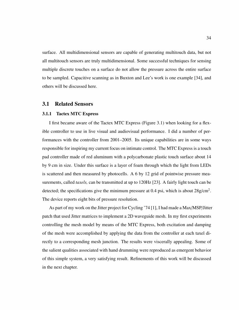
3.11 Image of calibrated force values of three simultaneous touches on the sensor. . 54

3.12 Amplitudes of three hand strikes on the sensor at 44kHz. . . . . . . . . . . . 54

3.13 Amplitudes of rolls on the sensor at 44kHz. . . . . . . . . . . . . . . . . . . . 55

viii

4.1 RMS amplitude measurements of first 12 modes of the waveguide mesh. . . . 62

4.2 Measured versus theoretical frequencies of the first 12 modes of the waveg-uide mesh. . . . . . . . . . . . . . . . . . . . . . . . . . . . . . . . . . . . . 63

4.3 Spectrum of 16x16 mesh at 44kHz. . . . . . . . . . . . . . . . . . . . . . . . 65

4.4 Spectrum of 32x32 mesh at 44kHz. . . . . . . . . . . . . . . . . . . . . . . . 66

4.5 Spectrum of 64x64 mesh at 44kHz. . . . . . . . . . . . . . . . . . . . . . . . 66

4.6 Magnified spectrum of 16x16 mesh at 44kHz. . . . . . . . . . . . . . . . . . 67

4.7 Spectrum of a darbuka, a Turkish hand drum. . . . . . . . . . . . . . . . . . 68

4.8 Controlling the waveguide mesh using a 2D force signal. . . . . . . . . . . . 70

4.9 Max/MSP/Jitter patch implementing the Square Dumbek. . . . . . . . . . . . 71

4.10 Spectrum of p hand strike on the 16x16 mesh at 44kHz. . . . . . . . . . . . . 72

4.11 Spectrum of mf hand strike on the 16x16 mesh at 44kHz. . . . . . . . . . . . 72

4.12 Spectrum of f hand strike on the 16x16 mesh at 44kHz. . . . . . . . . . . . . 73

4.13 Amplitudes of three hand strikes on the sensor at 96kHz. . . . . . . . . . . . 74

4.14 Spectra of three hand strikes on the Multidimensional Force Sensor at 96kHz. 74

ix

List of Tables

3.1 Physical Layers of the Multidimensional Force Sensor . . . . . . . . . . . . . 42

3.2 A Comparison of Multitouch Controllers . . . . . . . . . . . . . . . . . . . . 56

x

Acknowledgements

I would like to express my sincere thanks to the following people for their help with this

thesis—technical, logistical, motivational or otherwise.

Alexandra Albu Thomas Jones

Wendy Beggs Arthur Makosinski

Daniel Peter Biro Kirk McNally

Joshua Clayton Ali Momeni

Cindy Desmarais Eric Moon

Peter Driessen Sven Olsen

Adrian Freed Dale Stammen

Tony Geluch Scott Van Duyne

Amy Gooch Matt Wright

Many thanks to my advisors, Andy Schloss and George Tzanetakis, for their faith in

the value of my mixed bag of interests and their ongoing guidance in how to focus them.

Thanks for the opportunity to study at UVic.

Undying thanks are due to my intended, Chaya, for insight, home cooking, ninja skills

and unflinching support.

Financial support for this work was provided by NSERC and SSHRC Canada.

Chapter 1

Introduction

Musical ideas are prisoners, more than one might believe, of musical devices.

–Pierre Schaeffer

1.1 Motivation

Musical instruments are among the most subtly refined tools ever created by human

beings. They have evolved, over thousands of years in some cases, to facilitate two closely

related goals: the creation of sounds and the control of those sounds. Described as a

tool, an instrument is both sound producer and controller—two functions intertwined by

the physical makeup of the instrument, constrained by its necessary interaction with the

human body. Instruments lend meanings to the sounds they make based on our physical

and historical connections with them, connections that ground each instance of instrumental

practice in a given time and culture.

Computer music research can break from this history in bold new directions, facilitat-

ing radically new and unheard musics. Making new timbral possibilities available to the

composer has been one of the discipline’s greatest successes. But computer music is not

just about new sounds. As with new music in general, computer music can offer new modes

of expression, perception and conceptualization of sound. In particular the prospects for

new kinds of performance expression are exciting, but the inroads made here by computer

music are, to date, less successful.

Music performance, listening and understanding are all physical activities, tied to our

bodies as the medium by which we experience the world. Currently, computer-based instru-

ments minimize this physicality. Julius O. Smith has said, “A musical instrument should be

2

‘alive’ in the hands of the performer.” We can interact with acoustic instruments in varied

and subtle ways, applying a wide range of physical actions from delicate to violent, based

on feedback through multiple senses. It is a failing of the pervading practice in computer

music that we do not tend to achieve, or indeed even expect, this live connection. But it is

one that we have every right to expect. What if we can make new instruments that maintain

the live connections we have with acoustic instruments, yet allow radical new modes of

expression?

Since the 1980’s, a particular class of digital signal processing techniques for sound

synthesis has has rapidly gained popularity. These techniques, in which the equations of

mechanical physics are used to model the dynamics of sound producing objects includ-

ing instruments, are generally referred to as physically-based modeling or simply physical

modeling. Though physical modeling has proven to be a successful method of synthe-

sizing highly realistic sounds, providing deep methods of performance control remains a

major challenge. Research in physical modeling has focused more on emulating the sounds

made by acoustic instruments than the expressive control that their physicality affords. For

example, a physical model of a drum sound may use a complex calculation to simulate

wave travel across a two-dimensional membrane, yet the whole sound is typically triggered

by a single velocity value coming from a keyboard or other controller, after which the sim-

ulation runs its course without further input. The ongoing interactions between sticks or

hands and the membrane itself, by which a drummer controls nuances of the sound, are

missing.

In general, we can categorize interactions between a musician and an instrument in

terms of intimacy. Intimate control over an instrument or sounding object is central to

musical expression. Intimacy is a useful concept partly because it provides a criterion

by which both qualitative and quantitative observations can be judged. This thesis work

is aimed toward realizing the expressive potential of physical modeling by creating more

intimate gestural connections with it.

3

The following quote, from a review of the Yamaha VL7 physical modeling synth, gives

us some feel for the prevailing approach to computer music performance:

“It all looks good, but — and here’s the big ‘but’ —, you really have to learn

how to play it. The VL7 cannot simply be hooked up to a sequencer and

‘fiddled with’ (or rather, it can but it won’t fulfil its potential). To even half

utilise the power of this instrument you need to spend a lot of time practising.

Are you prepared for that?”[13]

Given a passing familiarity with our world’s musical traditions, the assumption that a

player would not have to spend a lot of time practicing an instrument is bizarre. But along

with timbral variety, one of the fruits of computer music research that has been most ar-

dently embraced by the marketplace is ease of learning. This spread of new technology has

been a successful response to a popular and deeply felt need: in this age when listening

to recordings is our primary experience of music, people want to make more music them-

selves. With sampling keyboards, they can. But samplers lack expressive potential; in a

short time, all of the expressive possibilities can be wrung out of a sampler. Contrast this

with the lifetime that can be spent coaxing new qualities of sound from the violin.

Ease of learning will continue to be a major driving force behind new musical tech-

nologies, and who can say that this is a bad thing? Musical practice is not exclusive: every

person who picks up an instrument for the first time is thereby making the world a little

more interesting, no matter how limited their expressive abilities compared to the experts.

But, ease of learning does not preclude expressive potential. Computers create the possi-

bility of making instruments that sound satisfying on the first day, yet offer material for

a lifetime of study. Like acoustic instruments, they will bestow extraordinary expressive

powers through long-term engagement. Few things would please me more than to help

build a new instrument worth learning.

4

1.2 Outline of the Thesis

The rest of this thesis contains four chapters. In Chapter 2, Background, I start by

presenting an overview of physical modeling synthesis in the form of a brief history and a

taxonomy of the major avenues of research. In the next section, Playing Physical Models,

I focus on a few systems for live control of physical modeling that have realized goals

germane to this thesis work. There is a rich discussion around musical expressivity in the

literature, but only a small amount it of concerns physical modeling directly; I connect this

work to the both areas of discussion by introducing several concepts that can be related to

both ideas: playability, plausibility and intimacy. Finally, in the section A Multidimensional

Approach, I use these concepts to make a context for the presentation of hardware and

software to come, generating several questions that can drive long-term research.

Chapter 3 describes my work on a novel multidimensional force sensor. This sensor

is intended for playing live computer music, or as a tool for studying intimate control. A

review of similar sensors from both research labs and the marketplace is given, leading to

a discussion of the design decisions involved in making the new sensor and the details of

its implementation.

Chapter 4, Experiments in Intimate Control, presents the new work in hybrid hardware-

software systems that supports this thesis. First, a new implementation of the 2-D waveg-

uide mesh is discussed. I will explain the design decisions that shaped this implementation,

aimed specifically at investigating intimate control, and present a novel technique for real

time tuning. In addition, I present a new algorithm for processing data from the multidi-

mensional sensor, in the context of a short discussion about signals and events. Then, I

devote a section to each of two experiments in control metaphors, the Square Dumbek and

the 2-D Guiro, in which I present the specific ideas behind the experiment, its implementa-

tion, performance history, and its particular strengths and weaknesses in light of aspects of

expressive control discussed previously. My intent is to tell the story of each experiment,

5

to give technical details enough to repeat it, and to tease apart aspects of its design in order

to build an understanding of how to foster expressive control.

Chapter 5 presents a short recapitulation of the research questions introduced and the

conclusions drawn from the experiments. It concludes with a discussion of future directions

in which the threads of research that make up this thesis work may lead.

1.3 Summary of Contributions

The goal of this thesis is to advance the making of new computer-based instruments for

playing physically modeled sounds expressively. My contributions with respect to this goal

include:

• A new implementation of the 2-D waveguide mesh algorithm for physical modeling

synthesis, allowing excitation by a multidimensional force signal.

• Hardware and software design for a sensor that detects forces applied perpendicular

to a 2-D surface, using a multichannel audio interface for communication with the

host computer.

• A new algorithm for detecting spatial centroids in a two dimensional signal repre-

senting pressure over time.

• Two new software instruments, experiments in intimate control for physical modeling

synthesis.

6

Chapter 2

Background

In this chapter, I present the relevant background in three sections. The first contains an in-

troduction to the major tracks of research within the very broad and active topic of physical

modeling synthesis, including a brief history and a taxonomy. The second section, Playing

Physical Models, describes the concept of a performance metaphor, and describes some

of the most salient metaphors through which performance interfaces have been applied to

control physical modeling synthesis in particular. In the third section, A Multidimensional

Approach, I introduce a new approach for the construction of intimate performance sys-

tems based on multidimensional signals, and describe it by comparison to related work

from both commodity systems and the academic literature.

2.1 Physical Modeling Synthesis

Physically-based modeling, or physical modeling, is a way to make sounds based on

the physics of mechanical systems. Compared to other kinds of synthesis such as FM or

sampling, it tends to be computationally expensive. Interesting vibrating systems, such as

musical instruments, are fairly complex; modeling the physics of these systems is much

more involved than modeling the sound spectra or waveforms they produce. Creating son-

ically interesting physical models that will run in real time has been a major challenge.

Despite this computational cost, however, physical modeling has been the most popular

synthesis approach in academic research since the early 1990s [62]. This popularity is

due largely to its promise to extend our acoustic world in perceptually novel yet intuitively

correct ways. Many researchers consider physical models to offer better prospects than

signal-oriented methods for the design of expressive digital instruments [11].

7

2.1.1 A Brief History

The first published use of physically-based models to synthesize sounds was by John

Kelly and Carol Lochbaum [31]. They described a simplified model of the human vocal

tract as a one-dimensional acoustic tube of varying cross-section. Excitation at one end by

a judicious combination of noise and simulated glottal vibrations, and changing the tube

geometry appropriately in the middle, produced recognizable vocal sounds at the other end.

This first example of physical modeling was also the most widely heard for many years,

due to its use in Stanley Kubrick’s 2001: A Space Odyssey. Max Mathews, collaborating

on musical applications with Kelly and Lochbaum, suggested that they make a song out of

their new vocal sounds, and so in 1961 they programmed their IBM 704 to sing “A Bicycle

Built for Two.” Arthur C. Clarke, working on 2001, heard the result while visiting John

Pierce at Bell Labs and the song was subsequently used in the film as the tragic childhood

reminiscence of the HAL 9000 computer during its disassembly [68].

Research activity on vocal tract models declined after this early work, due in part to

the rise of spectral models. When the overriding goal is computational efficiency, as it

was in speech coding for telecommunications, creating a desired sound spectrum directly

through nonparametric models is a better technique than modeling physical systems [58].

Linear Predictive Coding (LPC) is a form of spectral analysis/synthesis used in current

voice compression algorithms for telephones such as GSM [48].

Most of the early work on physical modeling of musical instruments was focused on

strings. This is due to a combination of happy accidents: the equations describing the

vibration of an ideal string are straightforward to understand, computationally efficient to

simulate, and when used to make even the simplest models, produce sound qualities we

associate with stringed instruments. The Masters thesis of Pierre Ruiz in 1970 was the

first work documenting synthesis of instrument sounds with physical models [49]. In a

two-part paper, Ruiz and Lejaren Hiller described the novel technique step by step, from

8

a physical description of a vibrating string, to differential equations, to excitation, to finite

difference equations, to an iterative solver, to computed vibrations on magnetic tape, and

finally through a D/A converter into sound. They noted the crucial fact that the quality

of a vibrating string sound is mainly defined by the way the string loses energy. In 1979,

McIntyre and Woodhouse [37] described theoretical results that also lead to a realistically

lossy vibrating string equation, but gave no indication that they listened to the resulting

waveforms as sounds.

The 1983 paper of Karplus and Strong [30] introduces what came to be known as the

Karplus-Strong technique for synthesizing plucked strings, and its surprising discovery

which arose out of their work in wavetable synthesis. Noting that strictly repetitive sounds

lack musicality, they experimented with algorithms to modify a cyclic wavetable while

playing it. By simply averaging the two neighboring samples of a wavetable on each cycle,

a frequency-dependent decay was created that sounded string-like. What was so surprising

about this new technique was the ease and computational efficiency with which realistic

string timbres could be produced. In fact, Karplus-Strong synthesis was later seen to be

a special, simplified case of the earlier equations of McIntyre and Woodhouse. Working

simultaneously with Karplus and Strong, Jaffe and Smith [21] published their own exten-

sions to the new algorithm and grounded it more firmly in digital filter theory. In his 1982

composition “Silicon Valley Breakdown,” for computer-generated sound, Jaffe wrung a

remarkable expressive range out of this simple technique.

In 1985, Julius Smith introduced a related but more general theory of digital waveg-

uides in the context of reverberation [56] . The one dimensional waveguide, a bidirectional

delay with reflection at its ends, proved to be an efficient model of many linear physical sys-

tems including strings and acoustic tubes. When used as an element in a network, the digital

waveguide can become a component of higher-dimensional systems. Nonlinearities can of-

ten be introduced into waveguide models in straightforward and robust ways, allowing the

creation of sounds far beyond the reach of analytical methods [57]. These advantages have

9

enabled many researchers since the late 1980’s to produce a variety of realistic instrumental

sounds including brass, flutes and reeds, as well as human vocal sounds. Though today a

listener can still easily tell state-of-the-art waveguide models from the actual instruments,

the current level of expertise allows each instrument to be unmistakably identified, expres-

sively played, and in some cases very accurately reproduced. Digital waveguides continue

to be an active research topic and, in maturing, have become a component of commodity

synthesis systems, both software and hardware-based.

A special case of a waveguide network based on a regular spatial grid, the 2D wave-

guide mesh was introduced by Van Duyne and Smith in their 1993 paper [64]. The natural

and complex collections of modes that can be generated by the algorithm make the 2D

waveguide mesh a powerful tool for modeling complex resonators including natural instru-

ments. 2D meshes are just beginning to be applied in real time, however. As recently as

2001 it was accurately stated that realtime implementation of the 2D waveguide mesh was

impractical [53]. Due to the familiar march of processing power, seven years later this is

no longer the case. Realtime implementations are appearing, both in custom hardware as

by Motuk, Woods and Bilbao [40] and in software as in this thesis work.

Work on the theoretical frontiers of physical modeling is ongoing—prepared pianos,

plate reverberators, transistor-based distortion effects and clapping audiences are just a few

of the wide range of topics from academic articles in the past couple of years [7], [8],

[70], [45]. Physical modeling is a large and vital field; I have attempted here to cover only

the developments most germane to this thesis research. For a regularly updated and more

complete overview, I direct interested readers to Julius Smith’s comprehensive online book

“Physical Audio Signal Processing” [55].

2.1.2 A Taxonomy

Numerically speaking, how do we use the computer to produce the many samples that

represent a physically modeled sound? I start with this basic question in the interests of

10

Frequency domain(spectral)

Physical Modeling

Analytic solutions Discrete-time methods

Time domain

K-models

FDTD schemesLPC Mixed K-W DWG WDF

W-models

Inter-object Intra-object

implicit explicit

Modal synthesis FTM

Source-filter(pseudo-physical)

Figure 2.1: A taxonomy of physical modeling techniques.

putting the thesis work in a larger context and fully explaining my choice of methods, a

wide variety of which are available to the researcher. Calculating sound based on some

aspects of physics is a loosely defined problem that offers many approaches. Figure 2.1

shows a taxonomy. To serve its purpose as an introduction to the thesis work, we will

discuss the various methods in terms that tend toward the qualitative. A more mathematical

treatment of much this material is given by Karjalainen [28].

Consider the basic problem of producing a sound sample, starting from equations de-

scribing a physical system. The most fundamental distinction between possible methods

is whether sounds are computed analytically, through symbolic solutions to the equations,

or by a simulation involving numerical approximations. Given the equations that describe

11

how an object vibrates, using symbolic analysis it is possible to generate sound spectra

for some ideal shapes in two and three dimensions such as rectangles and cylinders. For

systems of interesting complexity, though, this kind of solution is impossible. The most

common use of analytic solutions is in providing a reference spectrum against which to

check other kinds of modeling. If a new algorithm calculates resonant modes for a square

object that check against the analytic theory, for example, then it can presumably be trusted

for more complex shapes.

In practice, physical modeling is almost always done by simulation in the time domain.

A system is described using partial differential equations, with its components in some ini-

tial condition, and successive solutions to the motions of the system are calculated as time

moves forward. Partial differential equations (PDEs) arise not only in the vibrating me-

chanical and acoustic systems we consider here, but also in many other systems described

by classical physics. Other examples are classical electrodynamics, heat transfer in solids,

and the motion of fluids. Partial differential equations with similar forms arise from very

different problems. This is essentially because the language, and in some sense, the philos-

ophy of science, is written in terms of conserving various quantities like momentum, charge

and mass. The essential properties of the description of physical systems on the computer

are that they must be discrete and finite [46]. Therefore, we have to discretize any and all

continuous functions, such as the partial differential equations we want to model.

By dividing time into sufficiently small steps, we can march forward from a set of initial

conditions, calculating new values for the equations at each step. All of the remaining

modeling methods we will discuss here take this approach, and as such are called discrete

time methods.

2.1.2.1 Time Domain Techniques

Time domain techniques are written in terms of variables that can, at any instant, be

used to determine the pressure of the sound waveform. These include finite difference time

12

domain (FDTD) schemes, digital waveguides (DWGs) and wave digital filters (WDFs).

Finite Difference Time Domain Schemes Finite difference time domain schemes are in

some ways the simplest time domain techniques. The variables they manipulate represent

actual physical quantities such as velocity or pressure at discrete points on a spatial mesh.

These quantities are called Kirchhoff variables or K-variables. FDTD schemes offer the ad-

vantage of a relatively simple implementation and, in dimensions higher than one, the best

efficiency of the methods listed here. While efficient and simple to conceptualize, FDTD

schemes must be used with some care because they are prone to numerical instabilities not

suffered by the other methods.

In general, an FDTD method presents a system of equations that must be solved for a

given time step, relating the solution at previous times to the solution at the new time. If

the values of the K-variables at the new time depend only on previous times, the scheme is

said to be explicit, because the solution is defined explicitly by the equations. Otherwise,

the scheme is said to be implicit.

Implicit schemes require a system of equations to be solved at each time step. For

well-behaved problems in the one-dimensional case, these can often be solved in a nearly

constant amount of time for each step. In systems with dimensions higher than one or with

strongly nonlinear terms, however, implicit methods are not generally suitable for real time

use. Nonlinear terms can cause numerical solvers to iterate many more times for some time

steps than others. This varying and unpredictable processing time is a serious problem for

real time systems. In nonlinear cases, solving the implicit equation is hard, and there are

no guarantees of stability. In order to generate digital audio, the system of equations must

be solved at every discrete spatial location of the physical model for every sample—a lot

of computation.

On the other hand, implicit solvers for physical models are in common use in the com-

puter graphics world for computational physics, as well as in video games. Since timesteps

13

N sample delay

K-variable output

N sample delay

+

W-variables

(losses) (losses)

Figure 2.2: A digital waveguide.

of these graphical simulations are typically on the order of 10 milliseconds—two orders of

magnitude slower than audio rates—real time solutions are possible in this context.

FDTD simulations can be created for a wide variety of physical problems of which

the wave equations we focus on here make up only a small part. A good text on FDTD

solutions for PDEs is by Strikwerda [60].

Digital Waveguides Digital waveguide (DWG) methods are based on the d’Alembert

solution of the wave equation, which decomposes it into right-going and left-going compo-

nents as shown in Figure 2.2. These components are called wave variables or W-variables.

DWG methods, as well as WDFs which also use these variables, are called W-models.

Though they do not represent physical qualities exactly, the physical variable at any point

can be calculated by summing the wave variables. In one dimension, waveguides are the

most efficient type of model. The traveling wave formulation can be calculated by simply

shifting the quantities in two delay lines, one for each wave component. The connections

between the delay lines at their ends can incorporate low-pass filters to model losses, or

allpass filters to model frequency-dependent dispersion.

Digital waveguides can be connected to one another through scattering junctions that

satisfy the Kirchhoff constraints for the physical variables. In the case of a junction of

14

J J J

J J J

J J J

Figure 2.3: The digital waveguide mesh.

15

acoustic tubes, we can state that the total pressure leaving the junction must equal the

instantaneous pressure at the junction itself minus the total pressure entering the junction.

Scattering junctions that satisfy this property are also called W-nodes, and are connected to

waveguides through their W-ports. By connecting multiple waveguides to W-nodes, a 2D

structure can be made that models a grid of pipes. Shrinking the size of the waveguides

until each is one sample in length gives an approximation of wave travel on an ideal 2D

membrane. This is the canonical form of the 2D waveguide mesh (2DWGM), as introduced

by Van Duyne and Smith [64], and shown in Figure 2.3. The wave variables are propagated

in two dimensions by the one-sample waveguides, and scattered at each junction J.

The use of the term “waveguide mesh” in the literature can be a bit confusing, because it

refers to an underlying algorithm that may or may not be implemented with digital waveg-

uides. The mathematical equivalence of the digital waveguide and finite difference time

domain schemes is well known—the two techniques are often complementary [59]. The

initial presentation of the 2DWGM by Van Duyne and Smith described its implementation

by an FDTD scheme for efficiency, and since then much but not all of the work on the

2DWGM has followed suit.

Wave Digital Filters Wave digital filters (WDFs) were originally developed for the sim-

ulation of analog electrical circuit elements [28]. As a result of recent research, their close

relationship to digital waveguides is now well known [6]. The main difference between

the two is that DWGs are based on wave propagation and WDFs are based on modeling

lumped elements. In their WDF representations, analog circuit components are realized

very simply. For instance, a wave digital model of a capacitor is simply a unit delay, and

an inductor is a sign-inverted unit delay.

Another particular advantage of WDFs is their low sensitivity to numerical error. The

only approximate aspect of the WDF simulation is the frequency warping caused by the

bilinear transform. With correctly frequency-warped inputs and outputs, WDFs can imple-

16

ment a continuous-time linear time invariant system exactly. [59]

Mixed Modeling Each of these discrete-time models has its advantages; as such, combi-

nations are often used in more complex physical models. Karjalainen and Erkut have intro-

duced a high-level software environment called BlockCompiler for creating these models

[29]. They describe how junctions of FDTD and DWG models can be connected using K/W

converters, digital filters that map the K-variables in a FDTD junction to the W-variables

in a DWG junction and vice versa. They allow the creation of hybrid models that combine

the advantages of the different techniques: large areas of a 2D FDTD mesh for efficiency

with DWG elements for modeling varying impedances, for example.

Inter- and Intra-Object Mechanics All of the above discrete-time, time domain meth-

ods have been used to simulate intra-object mechanics: vibrations within a single object

or a compound object of multiple materials. These situations describe a great deal of the

interesting aspects of our acoustic world, and most aspects of musical instruments. But

the above methods are completely helpless in the face of modeling inter-object mechanics:

say, a handful of gravel thrown on the floor.

Some instruments like maracas create sounds through inter-object collisions, and there

is a great deal of interest in modeling non-instrumental physical systems of motion, such

as footsteps crunching in the snow. Perry Cook and collaborators have developed a toolkit

called PhISM, for Physically Informed Sonic Modeling, that includes software for model-

ing random collisions of many objects [12].

2.1.2.2 Frequency Domain Techniques

While the methods above work in the time domain, there also exist discrete-time meth-

ods in the audio frequency domain, or spectral methods. Two of these are modal synthesis

and the functional transformation method (FTM).

17

Modal synthesis takes a computed or measured response of an instrument or other vi-

brating object as its starting point [2]. One advantage of modal synthesis is the realism

of the sounds produced. In general, these sounds can be more realistic than time domain

models. But the realism comes at the cost of dynamic expressivity: there is no possibility

of arbitrarily adjusting physical parameters of the object as with time-domain techniques.

A violin modeled with model synthesis cannot be morphed into a ’cello, for example, or

changed into steel.

Functional transformation methods can make these kinds of transformations in the fre-

quency domain [47]. However, it is restricted to simple shapes such as strings, tubes and

rectangular plates. It is also computationally expensive, usable in real time only for one

dimensional systems.

2.1.2.3 Source-Filter Models

A third class of simulation, sometimes called pseudo-physical, also bears mention. In

the physical world all connections are two-way, which is to say that Nature does not dis-

tinguish between sources and filters—a system is always affected by others to which it is

connected, even if these others are considered “downstream.” But in many situations the

reciprocal effect has such a small audible presence that treating it as a one-way interaction

is a good approximation. In these cases, the relationship can be expressed as a source pass-

ing through a filter, rather than as a differential equation between the two parts. So the term

source-filter modeling has been applied.

Perhaps the most popular type of source-filter synthesis uses Linear Predictive Coding

(LPC). It models the human voice by decomposing the spectra of vocal sounds into a flat

excitation spectrum and a spectral envelope that imposes vocal formants [58]. It has been

used by composers including Paul Lansky, Andy Moorer and Ken Steiglitz to generate a

wide range of vocal sounds, as well as ones that bridge the gap between vocal and non-vocal

qualities.

18

2.2 Playing Physical Models

There exist a variety of approaches to computer music performance practice today.

What they all have in common is that they link the gestures of performers with some

acoustic results. Aside from that they differ widely, running the gamut from low-level

“one gesture to one acoustic event” paradigms [67] to high-level metaphors more akin to

real time composition than playing. From among these, this thesis work is focused on the

low-level paradigms that parallel the performer’s interaction with a physical instrument, in

order to investigate how physical models can be played more expressively.

Given a score for solo violin, we can imagine two versions: one performed by a sensi-

tive human interpreter of the music and another by a MIDI sequencer in a direct mechanical

translation. These lie at opposite extremes of expressivity. Comparing the two note by note,

we might find many differences: the human-played version has changes in pitch, rhythm,

dynamics and articulation that reinforce particular aspects of the score, or bring new mean-

ings to it. Different human performers, of course, can choose to interpret a piece differently,

bringing different intentions to it. It seems clear that the success of a low-level performance

metaphor can be qualitatively measured by the expressivity it affords.

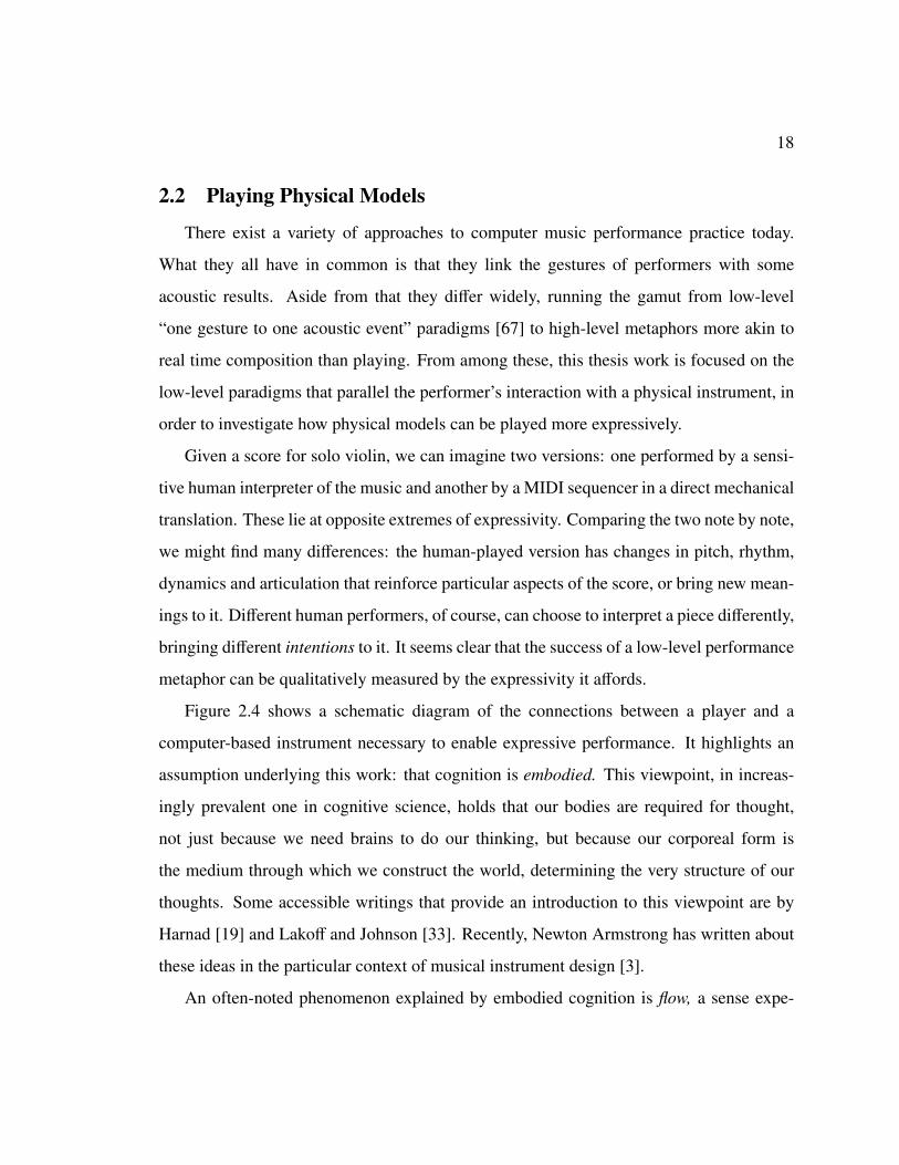
Figure 2.4 shows a schematic diagram of the connections between a player and a

computer-based instrument necessary to enable expressive performance. It highlights an

assumption underlying this work: that cognition is embodied. This viewpoint, in increas-

ingly prevalent one in cognitive science, holds that our bodies are required for thought,

not just because we need brains to do our thinking, but because our corporeal form is

the medium through which we construct the world, determining the very structure of our

thoughts. Some accessible writings that provide an introduction to this viewpoint are by

Harnad [19] and Lakoff and Johnson [33]. Recently, Newton Armstrong has written about

these ideas in the particular context of musical instrument design [3].

An often-noted phenomenon explained by embodied cognition is flow, a sense expe-

19

Bodycognition

Gestural interfaceintimate control

Performer Instrument

Brainintention

Earhearing

Computersound synthesis

Speakersound output

Figure 2.4: A systems diagram of performer and computer-mediated instrument.

20

rienced during intensely concentrated action in different domains of human activity, but

discussed particularly in sports and music [14]. When one’s concentration on an activity

being performed is so complete that that no boundary is perceived between self and en-

vironment, that’s flow. For a performer, musical instruments are part of the environment

merged with in a state of flow. The self extends to embrace the immediate parts of the en-

vironment, which is why the gestural interface is inside the area representing the performer

in Figure 2.4.

The connections pictured here form a complex web of relationships, all of which have

an effect on the potential for expression. Moreover, the expressivity present in a given

performance is somewhat subjective and thereby difficult to judge, even qualitatively. So

instead of focusing on expressivity itself to guide the creation of new instruments, I develop

here several related concepts from the literature that pertain to parts of the diagram, and by

which progress toward expressive control can be judged.

2.2.1 Playability

The concept of playability is a useful one, though it is used in different ways in the

literature. Considering control hardware, one definition of playability is the ergonomic

usability of the instrument [71]. That ergonomic design is part of playability, but can be

successfully sacrificed for other attributes, can be seen in the case of the violin: a highly

expressive instrument that tends to give one a stiff neck. Another aspect of playability is

dynamic range: the physical controller must be capable of supporting an expressive range

of performance gestures along its various control axes. A force-sensitive controller, for

example, should function over a wide range of touch pressures from light to heavy. In

“one gesture to one acoustic event” paradigms, repeated gestures should produce repeated

sounds. This is an important aspect of playability that requires precision and accuracy from

both the controller and the physical model. An ideally playable controller is also precise

over its entire usable range of control.

21

We can also look at synthesis software as well as hardware / software combinations

in terms of playability. Aspects of a bowed string physical model that support playability

have been studied by Woodhouse [69]. In his definition, playability is defined as the size of

the multidimensional parameter space of the simulation in which good tone is produced. In

the bowed string model, these parameters include bowing speed and pressure, which must

be carefully coordinated by the player to achieve ideal motion of the string. Woodhouse’s

experiments show that simulated bowed strings have the same playability as calculated for

real strings. Serafin has also done extensive work on playability of bowed-string models;

her related publications are listed in her PhD thesis [52].

Variety of sounds is another element of playability. A large parameter space resulting

in good tone is useless if that good tone does not vary significantly within the space. The

challenge of making models for computer music performance is addressed by Settel and

Lippe [54]. They note that while you can bang on an empty oil drum in a large number of

different ways, and get just as large a variety of sounds, playing a synthesizer will always

generate sounds bounded by its programming. Though it’s true that any musical system

will be bounded by its programming, an issue that Settel and Lippe address by getting “out

of the box” with electroacoustic instruments, approaching physical modeling control from

the perspective of playability will let us make synthesizers that are more like the oil barrel.

2.2.2 Plausibility

Hearing tells us what kind of things are in our local environment, and where. Our

ability to construct models of the dynamic world around us based on a small amount of

acoustic information—telling a falling rock from a falling branch far in the distance, for

example—is impressive. Just as our ability for language allows us to understand sentences

that we have never heard before, our hearing-based modeling of the world extends to novel

combinations of objects and dynamics. From our interactions with the world, we learn a

kind of grammar of acoustic physics. A lower sound comes from a bigger object, wooden

22

objects resonate in a particular way, and so on. This may have been an important capacity

from an evolutionary perspective—if you hear a tree starting to fall nearby that’s twice as

big as any you have heard before, you may want to be somewhere else.

Many synthesized sounds do not evoke any physical mental models of how they are pro-

duced because they are too far removed from any physical genesis. In general, some sounds

are more likely than others to bring to mind a physical model of production. Castagne and

Cadoz have termed this aspect of sound plausibility[11]. Plausibility is an important fea-

ture of physical modeling synthesis. Synthesis methods such as FM can make physically

plausible sounds, but only if used with great care. Where the space of possible sounds in

FM synthesis contains a very small percentage of physically plausible ones, most physi-

cally modeled sounds are plausible. Simulating physical processes, even in quite imprecise

ways, gives rise to acoustic phenomena which we recognize from our experience with the

physical world. All of the physical modeling techniques discussed above can make plau-

sible sounds, but in a some have particular advantages in control, allowing a performer to

affect the sound in more ways in real time.

Sampling synthesis, the playback of recorded sound events, is highly plausible at first

blush. But this advantage diminishes with long-term listening. Due to our perforce in-

complete modeling of nature’s complexity, a single physically modeled sound event may

be perceptibly less complex and nuanced than a sample of that same event. The longer

term dynamic behavior of this same model, though, will be more satisfying than that of

the sample. If we hit a cymbal and sample it, this single sample may be just as physically

plausible as the original. But hitting the cymbal multiple times is bound to sound more

physically real than replaying the sample. Even if we try to hit the cymbal in the same way

every time, variations in the positions of molecules within the cymbal, which cannot be

controlled even in principle, will lead to audible differences in the sound each time. These

individual sounds may be phenomenologically identical, meaning that we have no way to

refer to the difference between them, and no basis for preferring one over another. But we

23

can still hear that they are different from one another, and this makes the series of physically

modeled sounds more physically plausible, because in nature we hear no exact repetitions.

Plausibility is not a prerequisite for expressive playing—many synthesis methods be-

sides physical modeling are capable of expressive real time control. But there is undoubt-

edly a relationship between plausibility and expressivity, and its extent raises interesting

questions that we will return to later.

2.2.3 Intimacy

We recall from Figure 2.4 that the gestural interface in musical performance can be

considered part of both the performer and instrument. Seen in this light, intimacy is a good

word for our relationships with instruments. Intimate control over sounding objects is cen-

tral to musical expression. F. R. Moore has proposed that “Control intimacy determines the

match between the variety of musically desirable sounds produced and the psychophysio-

logical capabilities of a practiced performer” [38]. He gives the human voice as an example

of a highly intimate instrument, along with the flute and violin. These instruments translate

extremely small gestural movements of the performer’s body to wide variations in sound,

making them both very expressive and very hard to play well. The intimacy that facilitates

expressivity, in other words, makes them less playable at first.

Intimacy is a quality that has several quantitatively measurable requirements. Latency,

the delay between a performance gesture and its acoustic result, is one of these. Low

variation of this latency, or jitter, is also critical. For intimate control, latency should be 10

msec or less, and jitter should be 1 msec or less [67]. These requirements are necessary for

intimacy but not sufficient. This can be seen by examining the use of MIDI keyboards to

control physical models.

The first commercial physical modeling instruments were the Yamaha VL series, the

fruit of Julius Smith’s research at Stanford’s CCRMA on waveguide synthesis in the early

’90s. Since the introduction of these synthesizers, the musical keyboard has been the most

24

Figure 2.5: Yamaha VL1 synthesizer.

popular method of playing physical models. MIDI keyboards typically have acceptable

latency and jitter for intimate control, but the musical keyboard interface is not a good

match for the intimate connection invited by physical modeling synthesis. It’s evident that

Yamaha realized this. They included a breath controller—a little-used option for keyboard

players at the time—with the synthesizers as a strong suggestion that more intimate control

was desirable.

Keyboard instruments are certainly capable of expressive performance, but they do not

offer particularly intimate control. Tools afford certain kinds of use at the expense of others;

seen as musical tools, keyboard instruments trade intimacy for the control of harmonic

complexity. In order to offer this control, the piano mediates its soundmaking apparatus

through events. Each event, a keypress, triggers an excitation of a physical system, the

string, with an impact of a certain velocity. Compared to a guitar, say, the piano affords very

little control over a note once is it started and in general, we can say that signals provide

greater control intimacy than events. Given the ubiquity of the keyboard as synthesizer

controller, its use to control physical models is understandable. But in our search for greater

expressivity, it makes sense to look for more intimate kinds of control.

A haptic connection is another vital aspect of musical intimacy with acoustic instru-

ments. Vibrations of the instrument sensed by touch are often an important part of the per-

former’s sensory experience. Hand drums and the violin are examples in which touch feed-

back figures prominently. Haptic feedback in these contexts has been studied by Nichols,

25

Chafe, O’Modhrain and others [43]. In particular, it has been found that tactile feedback

greatly increases playability in a virtual bowed string instrument [44].

2.3 A Multidimensional Approach

Consider an instrument with extreme control intimacy: the hand drum. In hand drum-

ming, a great variety of expressive techniques arise from a trained performer’s control over

the timing, force and areas of contact with the drum. The tabla is an instrument, consisting

of pair of hand drums, that traditionally provides accompaniment for North Indian vocal

and instrumental music. A characteristic feature of tabla is a circular area on each drum-

head, made denser than the rest of the head by the application of a thick paste of iron oxide,

charcoal, starch and gum [16]. tabla are played using a repertoire of stroke types, some of

which involve quite complex motions of the hand [26]. One example of is the pitch bend-

ing Ga stroke, as played on the Bayan, the larger of the two tabla drums. In the Ga stroke,

the tabla player first excites the drum head with a tap of the middle and index fingers, then

raises the pitch of the stroke by moving the heel of the hand across the drum head. Pressure

data from two seconds of such a stroke are shown in figure 2.6.

The Ga stroke makes its own characteristic sound, as does the simpler slap or Ka stroke.

One way to control a synthesized tabla sound would be to classify these different stroke

types using an appropriate sensor, then trigger the physical model with an excitation that

will produce the appropriate sound. This is the approach taken by Kapur et al. in their

work with banded waveguide synthesis [27]. The ability to recognize particular gesture

types from a tradition of performance has the advantage of decoupling the sensor from the

sound production model, allowing the technique of an expert tabla player to be applied to

domains besides drum synthesis.

For our investigations into expressivity, however, this is not the right model. Any kind

of automatic stroke classification is a layer of abstraction that reduces control intimacy.

26

Figure 2.6: Pressure data from a slow pitch-bending ga stroke on the tabla.

An ideal drum sensor for research into intimate control would allow for meaningful sonic

results from not only certain recognized types of strokes, but the vast expressive space

that surrounds them, including novel strokes, unmusical strokes, and in general as many

of the acoustic phenomena produced by the physical instrument as possible. As a research

tool, it would facilitate meaningful experiments into expressivity by allowing the complete

expression of a player’s musical abilities in a completely malleable environment.

2.3.1 Splitting a Hand Drum

As a thought experiment, we can ask: what would it take to make a physically modeled

hand drum with control intimacy equal to the real thing? Even very simple objects are ca-

pable of making different kinds of sounds. We can use many techniques, different methods

of applying force to the object including tapping, bowing, blowing, scraping and damping,

to control the vibration of the object and of the surrounding air. Given unlimited comput-

ing power, we can imagine a real time simulation of the object’s vibrations to an arbitrary

degree of precision, linked to a sensor that detects applied forces. The link between sensor

and simulation will consist of multidimensional signals.

Since the introduction in 1968 of the first real time computer music system, Mathews

and Moore’s GROOVE, a number of researchers have noted the advantages of continuous

representations over events for gestural control [39]. Expressive live playing cannot be

summed up entirely as events; it consists of a continuum of phenomena ranging from non-

note to note. We would like our hypothetical control system to work with complex gestures

as signals.

27

The forces applied to the surface of an object at a given instant in time can be repre-

sented as a vector field, a continuous 3-dimensional function defined at every point in some

volume of space. When the forces change, this field can be represented as a multidimen-

sional signal. In this case we have a continuous domain 3-dimensional signal representing

force defined in three dimensions, or f [x, y, z] ∈ R3. The volume of space we are interested

in is the signal’s domain in R3. In the case of forces applied a drum head, we can make

some simplifications that will reduce the amount of data required. The head is more or less

flat, and so we can reduce the domain to a two-dimensional one. Better still, because the

head is tensioned, we can disregard the forces not perpendicular to the head and still have a

very good approximation. So we can represent our control gestures as a scalar signal over

R2.

Multidimensional signal processing has a lot in common with the more usual one-

dimensional case; in particular, the Shannon sampling theorem still holds and the Discrete

Fourier Transform can be applied in two and higher dimensions to convert between the

time and frequency domains. This has important consequences for our connection between

sensor and physical model: we can make statements about the continuous connections be-

tween real-world forces and the differential equations of a simulation that are provably

correct within the temporal and spatial limits of our sampling.

What sampling frequency do we need to characterize gestural signals completely?

Though as we have seen, a 1 ms timing resolution is enough to represent distinct events

well, a gesture may well contain more subtle information. The sampling rate of our simu-

lation provides an upper bound for the information we can use. But by experiment, we may

find that we can get equally good results with less data. Thinking in signal terms rather than

events, we can imagine the performance gesture translated directly into audio by a trans-

ducer on the drum head. Recording the forces that the hand can apply in contact with a

hopefully immobile and non-resonant surface, we can find by experiment the bandwidth of

gesture signals, and thereby the sampling frequency needed for a complete representation.

28

Figure 2.7: First 3 msec of the attack transients of various taps on the CNMAT force sensor.

From Wessel, Avizienis and Freed [66].

Wessel et al. have published this kind of data in a description of their new force sensitive

controller [66]. Data from finger taps sampled at 6 kHz show significant differences in

the shapes of attacks. The discussion of gesture bandwidth presented is qualitative, but

from looking at the shapes of the data it is clear that a 6 kHz sampling rate is enough to

characterize subtle aspects of gestures.

A high bound for our spatial sampling frequency can be found by looking at the phys-

ical size of the smallest possible wavelength in our model. We can make a back-of-the-

envelope calculation of the maximum spatial frequency on an idealized hand drum by us-

ing round numbers for the physical attributes of a drum head based on measured data from

Fletcher and Rossing [16]. A Mylar drum head might have a thickness of 2×10−4 m. Mylar

has a density of about 2× 103 kg/m3, giving a density for the head of 0.4 kg/m2. The trans-

verse wave velocity on a membrane is c =√

T/σ, where T is the tension on the membrane

in Newtons per meter, and σ is the membrane density in kg/m2. At a tension of 3 × 102

N/m, the wave speed c is 86 m/s, approximately 100 m/s. At this speed, a transverse wave

with a frequency of 10000 Hz is 1 cm long. So, a spatial resolution of 1 cm is sufficient to

characterize all of the continuous connections between applied forces to a drum head and

29

Figure 2.8: The Korg WaveDrum.

its vibrational modes up to 10 kHz.

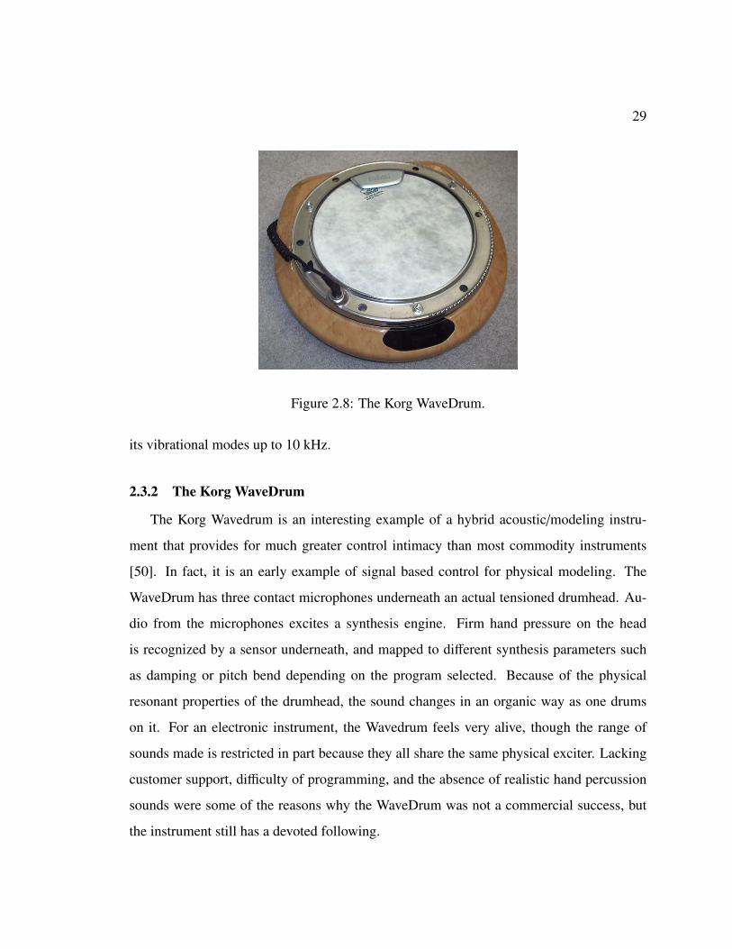
2.3.2 The Korg WaveDrum

The Korg Wavedrum is an interesting example of a hybrid acoustic/modeling instru-

ment that provides for much greater control intimacy than most commodity instruments

[50]. In fact, it is an early example of signal based control for physical modeling. The

WaveDrum has three contact microphones underneath an actual tensioned drumhead. Au-

dio from the microphones excites a synthesis engine. Firm hand pressure on the head

is recognized by a sensor underneath, and mapped to different synthesis parameters such

as damping or pitch bend depending on the program selected. Because of the physical

resonant properties of the drumhead, the sound changes in an organic way as one drums

on it. For an electronic instrument, the Wavedrum feels very alive, though the range of

sounds made is restricted in part because they all share the same physical exciter. Lacking

customer support, difficulty of programming, and the absence of realistic hand percussion

sounds were some of the reasons why the WaveDrum was not a commercial success, but

the instrument still has a devoted following.

30

2.3.3 Gestural Plausibility

Physical models have particular attributes that prompt the consideration of certain con-

trol paradigms. Many physical models, including all of the time domain techniques de-

scribed in Section 2.1.2, have an explicit model of space as part of their construction. Since

performance gestures take place in real space, reconciling real space with the model’s space

would seem to be a main concern in developing metaphors for performance. Physical mod-

eling is more than just a method of sound synthesis, it is a tool for sonifying hypothetical

spaces, and as such, invites new approaches to performance and music creation.

When an instrument produces physically plausible sounds and its control gestures re-

inforce the audible physical system behind them, we can call the resulting system ges-

turally plausible. A few examples are guitar synthesizers, the WaveDrum (with some of

its patches), and experimental instruments such as the vBow of Charles Nichols and the

Vodhran of Marshall et al. [43] [36].

Andrew Schloss has written about the need for an apparent cause-and-effect relation-

ship between performance gestures and sound output, in the wider context of computer

music performance generally [51]. He lists the modes of interaction we use with acoustic

instruments such as blowing, striking/plucking and bowing, and asks: “Can we go beyond

these gestures with electronics? Certainly, but it takes a great deal of experimentation to

discover what works when there is no underlying physicality.”

The piano is certainly an instrument capable of expressive performance. But it is also

a highly refined technological artifact that has abstracted its sound making physics from

its control apparatus. Were one not acquainted with keyboard instruments, one would not

expect pressing down a hinged piece of wood to give rise to the sound of hitting a string

with a soft hammer. In other words, the piano is not gesturally plausible. So in the case of

the piano we see that gestural plausibility is not a prerequisite for expressivity.

Mixed metaphors, in which a gesturally plausible, low level approach is combined with

31

higher level control, are an interesting possibility. The history of tablet-based performance

at U.C. Berkeley’s CNMAT is a rich source of ideas to apply [72]. Seeing the low level

control layer as a synthetic version of a physical instrument, a parallel with sensor-extended

hyperinstruments also becomes clear [35].

2.3.4 Research Questions

Considering the concepts presented in the previous section in light of the overall goal

of expressivity, a number of questions have presented themselves:

Can the expressive potential of new physical models be qualitatively understood in the

absence of intimate control? It is unlikely that excitation with ideal impulses, as is the

current state of the art, is sufficient for an understanding of the behavior of new physical

models. Real world excitations add as well as subtract energy at different locations in

complex ways. In addition, many interesting physical models are strongly nonlinear, which

precludes the use of impulses for a complete understanding.

Can instruments be made that are expressive as any we currently have, but easier to

learn? This question recapitulates the tradeoff between intimacy and playability dis-

cussed above. Computer music research presents a lot of compelling ideas, and one is of a

new instrument, deeply expressive but easy to learn. However, the only examples we have

of highly expressive instruments are, like the violin or sitar, intimately controlled and diffi-

cult to learn. From an embodied cognition viewpoint, it is plausible that learning to express

deeply is inseparable from learning the fine motor skills that these instruments require.

When does increasing the bandwidth and dimensionality of control signals increase

control intimacy? At the low end of the control speed spectrum, defined by MIDI, it’s

easy to see that adding more dimensions of control increases intimacy. At the high end,

32

the increase will only apply up to some threshold at which we can no longer process the

control information. But how much is enough? And how does the relationship depend on

the kind of control and feedback channels involved? The answers will no doubt depend on

the particular models studied.

These are all questions for long-term research, but they raise a common short-term need

for new software and hardware systems. In order to investigate them, we need to develop

controllers and models that can facilitate a degree of intimacy comparable to an acoustic

instrument. In the two following chapters, I present work toward these goals in the form of

a novel multidimensional signal-based interface, physical modeling software, and design

experiments in low-level metaphors for intimate control.

33

Chapter 3

A Multidimensional Force Sensor

Multi-touch sensors are currently an area of active research, and have been since the 1980’s

[34]. Davidson and Han give both a concise history and an overview of current techniques

[15]. Different sensing techniques have been used for multi-touch control, some of which

are capable in principle of making the hypothetical drum system described in the previous

chapter. I will introduce some related sensors here, and present my own work on a new

force sensor design.

Continuing the multidimensional signal-based approach discussed in the previous chap-

ter, we can imagine implementing our ideal drum head sensor as a grid of pressure trans-

ducers arranged on a surface. As concluded in the previous chapter, ideally the sensor

would have a resolution of 1 cm by 1 cm or better, and a bandwidth of approximately DC–

10kHz. To round out the list of blue-sky goals, let’s add an overall size of 50 by 20 cm:

enough to support the full range of hand drumming techniques as well as a wide variety of

expressive two-handed spatial gestures.

On entering the Masters program at UVic, making my own performance hardware was

not on my list of goals. But after almost two years of work on physical modeling control

and audio-visual performance, looking to both commodity hardware and research projects

for a replacement for my aging and irreplaceable small multi-touch interface, I decided to

bite the bullet and make my own. The result is a working surface pressure sensor, rough

around the edges but offering a unique set of capabilities for studying intimate control,

making expressive music, or both.

I describe the novel sensor in this thesis as a multidimensional or surface pressure sensor

rather than multitouch, to emphasize the goal of making a dynamic pressure image over a

34

surface. All multidimensional sensors are capable of generating multitouch data, but not

all multitouch sensors are truly multidimensional. Some successful techniques for sensing

multiple discrete touches on a surface do not allow the pressure across the entire surface

to be sampled. Capacitive scanning as in Buxton and Lee’s work is one example [34], and

others will be discussed here.

3.1 Related Sensors

3.1.1 Tactex MTC Express

I first became aware of the Tactex MTC Express (Figure 3.1) when looking for a flex-

ible controller to use in live visual and audiovisual performance. I did a number of per-

formances with the controller from 2001–2005. Its unique capabilities are in some ways

responsible for inspiring my current focus on intimate control. The MTC Express is a touch

pad controller made of red aluminum with a polycarbonate plastic touch surface about 14

by 9 cm in size. Under this surface is a layer of foam through which the light from LEDs

is scattered and then measured by photocells. A 6 by 12 grid of pointwise pressure mea-

surements, called taxels, can be transmitted at up to 120Hz [23]. A fairly light touch can be

detected; the specifications give the minimum pressure at 0.4 psi, which is about 28g/cm2.

The device reports eight bits of pressure resolution.

As part of my work on the Jitter project for Cycling ’74 [1], I had made a Max/MSP/Jitter

patch that used Jitter matrices to implement a 2D waveguide mesh. In my first experiments

controlling the mesh model by means of the MTC Express, both excitation and damping

of the mesh were accomplished by applying the data from the controller at each taxel di-

rectly to a corresponding mesh junction. The results were viscerally appealing. Some of

the salient qualities associated with hand drumming were reproduced as emergent behavior

of this simple system, a very satisfying result. Refinements of this work will be discussed

in the next chapter.

35

Figure 3.1: The Tactex MTC Express.

Despite its appealing liveness, the limited sampling rate of the MTC Express made this

setup less than ideal for actually playing music. 120 Hz is too slow for the perception

of intimate control. Another closely related problem is that the pressure readings from

the MTC Express are instantaneous, with no lowpass filtering before the analog to digital

conversion. Quick taps on the pad, an essential part of percussive gesture, can be missed

entirely if they fall between the sample points.

Unfortunately its sampling rate limitations make the MTC Express more suited to para-

metric control of synthesis than to playing sounds directly with low-level metaphors. De-

spite its shortcomings, the Tactex is a unique multidimensional controller that provides a

tantalizing glimpse at what future hardware for expressive computer music may be like,

and has been a real inspiration in my work.

3.1.2 Continuum Fingerboard

The Continuum Fingerboard is a performance controller designed by Lippold Haken

and manufactured by Haken Audio. It resembles a full musical keyboard in its size, but

offers continuous control in three dimensions over each touch, of which 16 are possible

simultaneously. It comes in a full size version, shown in Figure 3.2, and a half size version.

36

Figure 3.2: The Continuum Fingerboard.

It was first described by Haken et al. in 1998 [18], and has in the past few years entered

commercial production.

The Continuum uses a unique mechanical sensing technique. Under its neoprene play-

ing surface is an array of 256 vertical rods, mounted on springs at the top and bottom. Hall

effect sensors detect the displacement of the ends, and thereby the location of any force

applied to each rod. By interpolating values from neighboring rods, software in the device

can determine the x and y locations and pressure of a touch. Only one touch is possible at

any given horizontal location, which means that the Continuum is not a true multidimen-

sional sensor. In practice this is not too much of a drawback, since the layout encourages

keyboard-like gestures. The Continuum tends toward being a more capable descendant of

the music keyboard moreso than a generic multi-touch controller.

The scanning interval of the Continuum is reported as 1.33ms, better than many MIDI

keyboards. One difficulty with the device that might impede expression: users report that

multiple touches close to each other are likely to fuse into one, a problem for playing small

intervals. Also, due to its complex mechanical design, the Continuum is quite expensive.

Overall, the Continuum is a new and successful instrument that invites a deep engagement,

and from my perspective a very welcome presence in the commercial hardware market.

37

Figure 3.3: The Fingerboard’s mechanical sensing.

3.1.3 CNMAT Multitouch Controller

Wessel, Avizienis, Freed and Wright at CNMAT have published details of a novel multi-

touch array they made using commodity sensors, the same devices used for laptop trackpads

[66]. Each sensor is about 10 by 6 cm in size. The array has 24 of them, positioned in a

“brick wall” arrangement as can be seen in Figure 3.4. The sensors have a very high spatial

resolution and are scanned at up to 6 kHz. Because each sensor is capable of sensing one

touch, and has a small non-sensing area or “dead band” around its perimeter, the array is

not quite homogeneous, and therefore not capable of general multidimensional control.

Of the related multi-touch sensors discussed here, the CNMAT array is the only one

that definitively has enough temporal resolution for intimate control. Its power comes at

some expense, though—the hardware required to support the sensors includes four circuit

boards of A/D converters and another board with a central FPGA-based controller, a Virtex

FX12 running at 300 MHz. FPGA solutions are very cost effectve for the processing power

they provide, but the difficulty of getting started with them as a developer has been noted

by many.

The thoroughness of execution and commitment to intimate control makes this array

solution a very appealing one. The drawbacks to its use in the context of this thesis work

are moderately high cost, difficulty of the development environment, and a lack of homo-

38

Figure 3.4: The CNMAT Multitouch Controller.

.

geneous multidimensional control.

3.1.4 FTIR sensors

Davidson and Han have described synthesis and control work using a large scale multi-

touch sensing display based on the sensing technique of frustrated total internal reflection

(FTIR) [15]. A big advantage of their system is its low cost. The sensor hardware is just an

image sensor housed in an appropriately lit box. The system works by aiming the sensor at

the surface of a substance such as plexiglass that reflects internally light fed into its edges.

Applied blockers of light such as fingers vary the internal reflection from the surface and

create dark spots that can be detected by the camera. This can be implemented with infrared

LED and a frosted sheet of plexiglass. Resolution and precision of the system will depend

on the quality of the camera and the housing. Many homebrew versions of the system have

sprung up thanks to Davidson and Han’s documentation, often with accompanying demo

videos on YouTube.

39

The possible sampling rate of an FTIR system depends on the speed of the camera used.

Typically these are 30 or 60 Hz, an order of magnitude too slow for percussive control. High

speed cameras exist but are prohibitively expensive. Another drawback of these systems

is their general lack of portability. The camera’s field of view needs to be covered by the

reflection surface; without exotic optics, this means a big enclosure is needed in order to

block external light and get the camera far enough away. On the other hand, having a large

controller provides interesting and dramatic possibilities for performance.

3.1.5 Audio-Input Radio Drum

The idea of the Radio Drum, a three dimensional gesture sensor using capacitive mo-

ments, was developed at Bell Labs by Robert Boie in 1989 [10]. The prototype hardware

was described as a “backgammon” sensor due to the layout of the sensing antennas, as can

be seen in Figure 3.5. Examples of this hardware are still in use at the University of Victoria

and elsewhere. The electrode array, along with the four corner amplifiers and electronics,

is housed in a tablet with an active area of 11 by 15 inches. A cable connects the tablet to a

rack-mount box holding control electronics. Two drum sticks are connected by wires to the

control box. The tips of the sticks contain coils that transmit a different carrier frequency

for each stick. Considered as radio transmissions, these frequencies are in the VLF (very

low frequency) range: between 40 and 50 kHz.

The position sensing works as follows: given the magnitudes of the corner amplifier

voltages VA, VB, VC and VD, the positions x, y and z can be uniquely calculated by the

equations

VT = VA + VB + VC + VD (3.1)

x =VB + VC

VT(3.2)

40

Figure 3.5: Layout of the Radio Drum backgammon sensor and electronics.

41

y =VD + VC

VT(3.3)

z =κ

VT(3.4)

where κ is a scale factor, and the x and y scales are from 0 to 1 [10]. Note that, since

z is inversely related to the total voltage received from the antennas, the uncertainty due to

noise in z readings gets rapidly worse after a certain distance from the tablet.

The earliest use of the Radio Drum was in pioneering work by two groups: one led

by Andrew Schloss at Brown University and IRCAM, and the other by Max Mathews

and his group at CCRMA. Schloss’ work with Boie and Mathews on the Radio Drum

as a synthesizer controller [9] has been much cited in discussions of musical mappings.

Recently, Ben Nevile and others at the University of Victoria have worked to improve

the reliability, latency and precision of the Radio Drum [42], [41]. Where the original

drum required a custom box of control electronics, their new approach relies on an off-the-

shelf audio interface to sample the gestural signals from the Drum. Such a solution would

have been impossible twenty years ago when the Radio Drum was invented. Today, the

continued dropping in price of audio interface hardware, driven in large part by the home

recording market, makes it an increasingly workable and affordable one.

Though not a surface force sensor, the Audio-Input Radio Drum has many attributes

that make its technology interesting to consider. In particular, its control intimacy is very

high, the sampling rate being limited only by the audio interface.

3.2 Implementation

I have implemented a surface force sensor that, like the Audio-Input Radio Drum, uses

a commercial audio interface for communicating with a computer. This new sensor is a

completely passive device: it contains no active electronics and needs no power source.

42

Line level AC signals from the audio interface are applied to carrier electrodes, which are

capacitively coupled to pickup electrodes. Applied force compresses a rubber dielectric

between the carriers and pickups, reducing the distance between them and increasing the

capacitive coupling. The signals are then decoded in software into a representation of the

surface’s displacement from a rest state.

3.2.1 Materials and Construction

The multidimensional sensor consists of ten layers, from top to bottom:

Table 3.1: Physical Layers of the Multidimensional Force Sensor

Layer Thickness Material Function

top 12 mm birch plywood stiffness, appearance

ground .01mm aluminum foil electromagnetic shielding

surface 1mm polypropylene force spreading and tactile feel

carriers .1mm copper tape on polyester send current

bump 3mm plywood add tension to surface

dielectric 3mm silicone rubber dielectric and resilience

pickups .1mm copper tape on polyester receive current

spacer 3mm plywood hold pickups away from ground

ground .01mm aluminum foil electromagnetic shielding

bottom 12 mm birch plywood stiffness

The sensor can be seen in Figure 3.6. A rounded rectangular hole is cut in the top two

layers for access to the polypropylene touch surface. The entire stack of materials has been

drilled through and is held together with nuts and locking bolts. The carrier and pickup

layers are made using adhesive-backed copper tape, made by 3M, on a thin 3 mil polyester

film. The adhesive on the tape has held up through through at least ten cycles of removing

43

Figure 3.6: The Multidimensional Force Sensor

.

and replacing on the polyester film I used as backing. This combination of materials proved

extremely handy for experimenting quickly with different antenna geometries, an activity

that has consumed by far the largest part of the design time to this point.

3.2.2 Geometry

The active area of the touch surface is 20 by 20 cm. This is only about twice as tall

and wide as the MTC Express, but the difference in ability to perform expressive gestures

increases greatly when the surface gets significantly bigger than a single hand. The entire

44

sensor including the audio interface is small enough to be easily portable, a very impor-

tant consideration in a performance instrument. The playable surface offers smooth and

homogeneous response, making this a true multidimensional sensor.

3.2.3 Sensing

Why capacitive sensing? The technique has a definite drawback in its susceptibility to

electrical noise. In addition, I had been warned about its difficulties by Adrian Freed, who

has a great deal of experience making sensors. In my particular application, though, the

disadvantages of the other possible techniques and advantages of capacitance both helped

tilt the balance.

Most kinds of commercially available sensors are cost-prohibitive for this research be-

cause so many are needed to implement a surface with adequate resolution. One design

goal for the sensor is low cost. The less expensive the sensor is to make, the more people

who can potentially benefit from making and experimenting with them. Looking at the

costs and availability of comparable commercial hardware, my feeling is that the entire

bill of materials should be under five hundred dollars if possible for a controller to gain

widespread acceptance. If we want a 1 cm by 1 cm resolution, a medium-sized surface will

have around 500 force sensing elements or taxels. This gives us a budget of around one

dollar per taxel, ruling out pressure sensors, FSRs (force sensing resistors), and any com-

modity technologies for single-point sensors I have come across, which are all an order of

magnitude higher in price.

One very interesting sensing possibility lies in the work of Koehly et al. [32]. They

have made FSRs themselves using conductive ink and a variety of substrates including

paper. This technology could be used to print rather than build a sensor at very low cost,

and with technology in reach of the individual experimenter. The major stumbling block

with this route, for the moment, is the response time of the sensor. Data from the paper cited

shows that after a 3 kg load was applied, the experimental FSR took 75 ms to recover to its

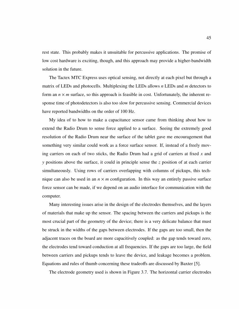
45

rest state. This probably makes it unsuitable for percussive applications. The promise of

low cost hardware is exciting, though, and this approach may provide a higher-bandwidth

solution in the future.

The Tactex MTC Express uses optical sensing, not directly at each pixel but through a

matrix of LEDs and photocells. Multiplexing the LEDs allows n LEDs and m detectors to

form an n × m surface, so this approach is feasible in cost. Unfortunately, the inherent re-

sponse time of photodetectors is also too slow for percussive sensing. Commercial devices

have reported bandwidths on the order of 100 Hz.

My idea of to how to make a capacitance sensor came from thinking about how to

extend the Radio Drum to sense force applied to a surface. Seeing the extremely good

resolution of the Radio Drum near the surface of the tablet gave me encouragement that

something very similar could work as a force surface sensor. If, instead of a freely mov-

ing carriers on each of two sticks, the Radio Drum had a grid of carriers at fixed x and

y positions above the surface, it could in principle sense the z position of at each carrier

simultaneously. Using rows of carriers overlapping with columns of pickups, this tech-

nique can also be used in an n × m configuration. In this way an entirely passive surface

force sensor can be made, if we depend on an audio interface for communication with the

computer.

Many interesting issues arise in the design of the electrodes themselves, and the layers

of materials that make up the sensor. The spacing between the carriers and pickups is the

most crucial part of the geometry of the device; there is a very delicate balance that must

be struck in the widths of the gaps between electrodes. If the gaps are too small, then the

adjacent traces on the board are more capacitively coupled: as the gap tends toward zero,

the electrodes tend toward conduction at all frequencies. If the gaps are too large, the field

between carriers and pickups tends to leave the device, and leakage becomes a problem.

Equations and rules of thumb concerning these tradeoffs are discussed by Baxter [5].

The electrode geometry used is shown in Figure 3.7. The horizontal carrier electrodes

46

ComputerMacBook Pro

1.83 GHz Intel Core Duo

Audio interfaceRME Fireface 800

CARRIERS

f1 = 6891

f2 = 8269

f3 = 9647

f4 = 11025

f5 = 12403

f6 = 13781

f7 = 15159

f8 = 16538

PICKUPS

8

8x

1/4

” pho

no

IEEE 1394(Firewire 400)

8x

1/4

” pho

no

DB

25

DB

25

Passive sensor copper strips, rubber dielectric

8

Figure 3.7: Block diagram of multidimensional sensor hardware.

47

each transmit a different frequency of sine wave from the audio interface. Surrounding

them (omitted in the diagram for clarity) is a grounded guard area. On the other side of the

rubber dielectric are the vertical pickups, each of which is connected directly to a line input

channel of the audio interface. The pickups are also surrounded by grounded conductive

material. Without this surrounding material, charge leaks from the carriers to a hand that

is nearby but not touching the device. Eliminating this leakage is necessary for accurate

readings of force.

3.2.4 Electronics

Because the Multidimensional Force Sensor is completely passive in construction, the

audio interface used is crucial. For this work I have used an RME Fireface 800 interface,

which has special high power outputs not common on commodity audio hardware. Another

device from RME is available, the Fireface 400, that reportedly has nearly identical analog

electronics. It remains to be seen whether less capable audio interfaces can enable the

sensor to work well enough to be useful.

Using the audio interface directly, as in the Audio-Input Radio Drum, has allowed the

sensor to be very durable, inexpensive and easily constructed. Two disadvantages of this

setup are the impedance mismatch between the pickups and the external amplifiers, and the

susceptibility to interference of the connections to the interface. Ideally, to get low-noise

measurements of capacitance, specially designed amplifiers and A/D converters should be

inside the enclosure with the sensor itself. The 16 cables that are now required to get

the force measurements add significant radio frequency noise and low-frequency drift from

motion of the cables and sensor themselves. These errors are largely mitigated in the current

setup by dynamic calibration, discussed below.

A number of circuits have been suggested for future amplifiers in the device itself,

including current-to-voltage converters, hi-Z op-amps and common base transistor pairs. A

circuit that converts impedance to voltage should produce a linear response with electrode

48

separation, according to Baxter [5]. These various approaches warrant more consideration

and collaboration.

Even with the current setup, the signal to noise ratio is surprisingly quite good. The

RMS amplitude am,n from a single taxel at rest (no applied force) was -44.47 dB. With

a 2kg weight applied to the sensor, giving the amplitude of a medium hand slap but at a

steady state, the same electrode produced an amplitude of -40.50 dB. The RMS variance of

each of these measurements was 0.002 dB, giving an SNR of about 2000, or 33dB.

Currently, the whole system is run at a sampling rate of 44.1 kHz, though with faster

computers higher sampling rates could be used with trivial changes. In order to facilitate the

signal processing, described below, carriers with frequencies that are multiples of k(sr/32)

are used. For a sampling rate of 44100, these frequencies are multiples of 1378.125 Hz.

Below 6kHz, the transmission from carriers to pickups is not strong enough for useful

sensing, so higher frequencies, 7000–16000 Hz, are used. Another potential problem to

note is that certain frequencies of carriers are prone to interference from VLF noise present

in the environment. In particular, there is strong VLF energy at 8 and 16 kHz in all of

the places where I have used the sensor. By choosing different carrier frequencies from

among the 16 possible, collisions with these sources of noise can be minimized. Looking

at directories of natural and artificial VLF signals, I found no hint to the source of this

energy. Though it does not stop the sensor from functioning well, more measurements in

different environments will be taken for the sake of curiosity, and to identify other sources

of noise that may pose problems in the future.

3.2.5 Signal Processing

A patch was implemented in the Max/MSP/Jitter environment, along with custom ex-

ternals written in C, to process the real-time data from the sensor. A block diagram of this

DSP network is shown in figure 3.8. The inputs to the network are the 8 pickups from the

sensor, each of which covers one entire column of the 8x8 grid. At every point of the grid,

49

we would like to know the applied force. Assuming some reasonable relationship between

force and carrier amplitude, we calculate the amplitude am,n of the signal transmitted from

a carrier row m to a pickup column n.

At each column n we have a sum S n(k) of amplitudes am,n multiplied by the row carrier

frequencies:

S n(k) =

8∑m=1

am,ncos(2π

kN

(m + c))

=

8∑m=1

am,n12

(e2π j k

N (m+c) + e−2π j kN (m+c)

)(3.5)

where c is the integer offset of the first carrier. Taking a N-point real FFT of this column

signal, we have

S n(r) =12

N/2∑k=−N/2

8∑m=1

am,n

(e2π j k

N (m+c) + e−2π j kN (m+c)

)e−2π j k

N r. (3.6)

Recall that

N−1∑k=0

e2π j kN ae2π j k

N b = δ[a − b]

where

δ[n] =

1 for n = 0,

0 otherwise.

After some manipulation, the DFT can then be written

S n(r) =12

8∑m=1

am,n (δ[m + c − r] + δ[−m − c − r])

= ar−c,n. (3.7)

50

mag(FFT)32 point

PICKUPS

TO MESH

8 columns, f = sr (44kHz), time domain

8x8 taxel amplitudes, f = sr

t

...

t

...

interpolateorder 5 B-spline

8x8 taxel amplitudes, f = sr/32

64

64

Figure 3.8: Block diagram of multidimensional sensor signal processing.

This calculation bears out the more intuitive argument that since each of the carriers

“matches up” with itself at the ends of the window, no distortion is caused by truncating

it at the window ends and considering it as a periodic signal—rectangular windowing is

optimal. After the DFT is calculated for each row, the magnitudes of the complex results

are taken, resulting in eight frequency domain signals, each containing the magnitude of

every carrier in one column plus surrounding bins where no carriers are present. Taking

the 8 carriers am,n from each row n results in 64 real signals at 1/32 the sampling rate. Each

signal is the magnitude of one carrier/pickup pair, which depends on the force over a small

area of the sensor. Since the 64 signals have coherence in time and space, we are justified

in calling the whole bundle one 2D signal.

To apply the 2D signal to the physical model, it must be properly upsampled back to the

overall system sampling rate, otherwise a very objectionable aliasing will be present in the

signal. A usual procedure for upsampling is zero-padding, followed by the application of an

51

Frequency(Hz)

Am

plitu

de(d

B)

Figure 3.9: Frequency response of order-5 B-spline interpolator at 44 kHz.

FIR filter. Unfortunately, this high-quality method of upsampling is quite computationally

expensive. In filtering excitations to the mesh, the reduction of aliased frequencies is the

most important goal. For an acceptably attenuated stopband in this application, a number

of filter taps on the order of 200 would be required. For 32x upsampling, factoring the

problem out into a series of six 2x upsamplers helps somewhat, but even this approach

proved impossible to calculate in real time.

Luckily, by looking at the specific situation we are facing it turns out that a much

more efficient solution can work. Interpolation filters are generally used for digital audio

as components in sample rate converters, but not on their own for filtering signals. This

is because they have significant rolloff all through the passband, a characteristic rarely

acceptable in audio filters. But in our application, where aliasing must be reduced at low

computational cost, they are ideal.

The frequency response of the 6 point, order-5 B-spline used in the sensor is shown

from 0 to sr/2 in Figure 3.9. Because the B-splines are generated by convolving a rectan-

gular function with itself, then convolving the output with itself, and so on, their frequency

responses are powers of the sinc function, sin(x)/x. The 5th order B-spline requires 20 mul-

tiplies and 22 adds per sample, an order of magnitude less work than the FIR filter. Note

52

that, while the frequency response in the passband is bad, as promised, the first sidelobe is

attenuated to -80dB.

By measuring the range of the amplitude signal at the usable extremes of pressure, as

well as its variance of the signal due to RF noise, the usable dynamic range of the sensor can

be measured. With the sensor at rest, the input amplitude of a central taxel was measured

at -44.5 dBFS. With a 2kg weight applied to the surface, this increased to -40.5 dBFS. In

each of these steady states, the RMS magnitude of electrical noise was 0.002 dBFS. This

gives a signal to noise ratio for this measurement of about 2000, or 33dB.

3.2.6 Calibration

After all the DSP above is done to generate a 2D signal, extensive calibration is still

needed. The main reason for this is that the sensor has a strong hysteresis: forces applied to

the surface create an increased measurement even after they are removed. Moreover, this

hysteresis does not have a consistent response—it varies across the surface, and depending

on the presence of other forces that mechanically deform the surface.

A combination of static measurements and dynamic calibration was used to mitigate

these effects. The data used in the calibration of a single taxel are shown in Figure 3.10.

For readability, this figure is not to scale. First, measurements are gathered with no applied

force to generate a mean force offset, Fcal. A histogram of this data is created, and a

threshold, t, is picked so that false triggers are very rare. Another calibration force, Fmax,

is measured by running a hand across the entire surface with medium-hard pressure and

storing the maximum values. During operation, a one-zero lowpass filter is applied to each

calibrated value to generate a dynamic offset, Fdyn. The frequency of the filter is adjusted

based on the incoming force. It ranges from zero to a maximum value, typically 10Hz.

When the force input Fin is near Fcal, Fdyn is allowed to change more rapidly. With a

stronger applied force, it changes less rapidly until Fin > Fmax, at which point the filter

frequency is always zero. Finally, a calibrated force output is generated by normalizing the

53

0.1.

0. FmaxFcal t Fdyn Fmin

F out

= (F

in –

Fm

in) /(

F max

– F

min

)

t – Fcal

Fin (volts)

}

Figure 3.10: Data used in dynamic calibration of the sensor.

range Fmin = Fdyn + t − Fcal to Fmax. An output of 1.0 always results from an input force

Fmax. Overall, this calibration effectively zeroes out the rest values of the sensor, while

keeping more firm forces precise, and preserving the effective shape of the gestural signal.

3.3 Results

Figure 3.11 shows a typical force image produced by the 8x8 taxels of the sensor.

The three touches shown are totally independent: moving one does not affect the others

significantly. The effect of the dynamic calibration can be seen to reduce low-amplitude

taxels to zero, making the boundaries of the touches more distinct than the raw sensor data.

The amplitudes over time of three hand strikes on the sensor at 44.1kHz are shown in

Figure 3.12. In recording the strikes I tried to think of the sensor as a drum, and play three

54

Figure 3.11: Image of calibrated force values of three simultaneous touches on the sensor.

Time(s)

Am

plitu

de

p

mf

f

Figure 3.12: Amplitudes of three hand strikes on the sensor at 44kHz.

55

Time(s)

Am

plitu

de

Figure 3.13: Amplitudes of rolls on the sensor at 44kHz.

hits that would correspond to piano, mezzo-forte, and forte dynamic markings. The shapes

of the amplitudes correspond fairly well with the touch data from the CNMAT sensor shown

previously in Figure 3.4. Rise times to maximum are on the order of 2ms. The onset times

of the CNMAT data are a bit faster. This can be explained by the much harder surface of

the CNMAT sensor compared to the resilient rubber and plastic used here.

The smoothing produced by the interpolation is seen here qualitatively not to filter the

attacks too much. On a larger time scale, three rolls, quick sequences of taps at varying

dynamic levels, give an interesting view of the sensor’s dynamic behavior, as seen in Figure

3.13. Each group appears much more uneven than it would sound, because the strokes move

slightly on the surface. Data from a single taxel is plotted here—the sum of all the taxels

would be approximately equal for each stroke of a roll.

3.4 Discussion

Table 3.2 shows a comparison of the multitouch / multidimensional controllers dis-

cussed in terms of sensing area, simultaneous touches possible, sampling rate, homogene-

ity, force sensing ability and cost. The Continuum Fingerboard comes in both half- and

56

Table 3.2: A Comparison of Multitouch Controllers

Tactex Continuum CNMAT FTIR Multidimensional

MTC Fingerboard Multi-touch sensors Force Sensor

sensing area (cm) 14x9 70x20 40x20 variable 20x20

touches ∼4 16 24 variable ∼4

sampling rate (Hz) 120 750 6000 ∼30 1378

homogeneous yes no no yes yes

force sensing yes yes limited limited almost

cost (USD) 400 3400 ∼ 103 ∼ 102 ∼ 103

full-size versions; the half-width version is compared here. The full-width version is twice

as long, twice as expensive and similar in other respects.

Some of the sensors offer homogeneous response, which is to say that every location

they can sense acts the same. The Fingerboard and the CNMAT sensor have mechanical

restrictions, discussed previously, that prevent them from being truly homogeneous sensors.

The Multidimensional Force Sensor has the same kind of sensor at each point, but the

response and shape varies significantly near the edge because of the slight curvature of the

surface.

In cost, the Multidimensional Force Sensor is hard to quantify exactly because of the

importance of the audio interface. Exclusive of the interface, the material costs for the

sensor about about $50. But in a passive sensor design, the interface should be considered

part of the device itself, bringing the cost up to $1000 or so.

The Multidimensional Force Sensor is basically an array of micrometers, so it’s not

surprising that endlessly fascinating troubles arise in attempting to build such a thing at

low cost. Yet, in order to make a device that others can replicate, in various situations both

inside and outside of academia, this has been my goal. One of the most thorny issues during

57

the design process has been isolating mechanical effects from electrical ones. Without a

completely stable reference it is difficult to tell whether changes in voltage are coming from

capacitive effects or from motion. The spreading of one taxel’s pressure quantity onto its

neighbors, for example, could result from either a capacitive connection that distributes

current or a mechanical connection that distributes force. This problem applies to multiple

kinds of dynamic behaviors that we need to understand including the spreading of forces

and/or fields as well as hysteresis.

In general, this new work can be seen as part of a trend toward smart computers and

dumb sensors, of which the Audio-Input Radio Drum is another example. Just ten years

ago, the kind of DSP power used to read and calibrate the Multidimensional Force Sensor

would have required a much more serious computer. Ten years before that, it would have

been impossible to do in real time on commodity hardware. So it makes sense that a

great deal of effort has historically into the physical design of sensors in order to linearize

their responses. Now that significant DSP ability comes at less and less cost, it is becoming

possible to take less perfectly crafted physical interfaces and generate good data from them.

Since this work takes a signal-based approach to gestural sensing, a comparison of these

sensors in terms of signal to noise and dynamic range would be valuable. In general, such

data are not currently available but can be calculated. A MIDI keyboard, for example, pro-

duces a velocity amplitude from 1–127 and therefore can be said to have a dynamic range

of 42dB. Improving the analog electronics of the Multidimensional Force Sensor seems

like an important goal at present, but in the absence of comparison data from other sensors,

this conclusion comes from a qualitative assessment rather than the signal measurements.

The most satisfying and useful aspect of this new sensor is its temporal resolution.

Physical models are one way to apply all of this data, but there is a huge variety of other

possibilities. Usable in its current form but inviting refinements in both its software and

hardware, the Multidimensional Force Sensor is a very hackable new tool. I hope that my

sharing its details here will spur collaboration, construction, and of course, playing music.

58

Chapter 4

Experiments in Intimate Control

In support of this thesis research, I have developed two real time synthesis programs

that implement different methods for mapping gestural control signals to physical mod-

els. These programs are experiments with low-level metaphors for intimate control. This

chapter details these projects as well as the real time implementations of physical modeling

algorithms that I wrote to support them. After a discussion of the underlying technology, I

devote one section to each experiment, treating its implementation, performance history if

any, and its particular strengths and weaknesses in light of the aspects of expressive control

discussed previously.

4.1 A New 2DWGM Implementation

From the various approaches of physical modeling described in Section 2.1.2, the

FDTD implementation of the 2D Waveguide Mesh (2DWGM) lends itself best to experi-

ments in intimate control for two reasons: efficiency and controllability. The 2DWGM is an

approximation to the 2D wave equation governing displacement of a stretched membrane.

In its original form presented by Van Duyne and Smith [64], this mesh allows the com-

putation of each sample on a spatial grid at a given time step from just its four rectilinear

neighbors at the previous time step and the same sample two times steps previously. This

equation requires just one multiply and five adds at each junction for each sample. Com-

pared to other synthesis methods such as FM, or even 1-D waveguide physical models, this

is still an expensive technique. But is it fast becoming well within the reach of real time

use for interesting models.

In addition to the original 4-connected square mesh, there are many other possible

59

finite difference formulations, or schemes for the solution. Many of these are discussed

in detail by Bilbao [6]. In the thesis work an 8-connected interpolated rectangular mesh,

discussed by both Bilbao and Valimaki[63], is used. While Fontana and Rocchesso [17]

have shown that a triangular mesh geometry has desirable properties including better wave

dispersion characteristics, a rectangular mesh geometry can be calculated as a standard 3

by 3 convolution. This made implementation easier, and may open the door in the future to

interesting methods of acceleration such as the use of graphics coprocessors.

Both the 4-connected mesh and the 8-connected interpolated mesh can be implemented

using the same algorithm with different convolution kernels. As described, the original

algorithm is lossless: any energy that excites the mesh will ring out endlessly. An ex-

ponential decay can be added by simply multiplying the junction values by a constant at

each step. When excited with an ideal impulse, this simple lossy mesh implemented on a

square geometry makes a metallic ping. This sound has a fairly artificial quality because

its strict physical interpretation is of a highly implausible situation. Real world materials

have frequency-dependent losses—the loss of this simple model is constant at all frequen-

cies. Dispersion of frequencies on the simple mesh is also far from ideally equidirectional,

which gives the decay an quality that tends to make it less plausible. Listening to the late

part of the decay or “reverb tail” of this sound, the 8-connected mesh was heard to be much

smoother in quality, and in this sense more plausible, than the 4-connected version.

The waveguide mesh algorithm was implemented as a Max/MSP/Jitter object. An orig-

inal version, 2up.jit.mesh∼, was used in experiments with the Radio Drum and the

Tactex MTC Express as sensors. A new object, birch1 mesh∼, takes eight column sig-

nals from the Multidimensional Force Sensor as input. This means that some of the sensor

DSP discussed in the previous chapter is actually done in the waveguide mesh object. This

division is made for the sake of convenience. It would be conceptually more appropri-

ate, but very unwieldy, to use 64 MSP signals in MSP to connect incoming excitations to

the mesh. Marsyas, a signal processing environment designed for MIR (Musical Infor-

60

mation Retrieval) research created by George Tzanetakis, might have been a better tool

here [61]. Because it supports multidimensional signals and networks of different signal

rates natively, it could have specified the connections much more cleanly and flexibly. In

the present work, however, the author’s existing toolset in Max/MSP/Jitter and the quick

graphical editing possible in the environment made it more immediately useful. I look for-

ward to using someday a tool for signal processing with both the structural flexibility of

Marsyas and the ease of use of Max/MSP/Jitter.

4.1.1 Tuning

The wave speed of the mesh simulation can be tuned continuously by varying the

impedances of the junctions. This has the effect of changing the overall pitch in a way

that is efficient and continuous. This method of pitch changing is physically consistent:

its physical interpretation is of the medium changing density. Since we don’t ever hear

this kind of transformation in nature, the resulting sound has an artificial quality that is

intriguing and potentially compositionally useful.

By looking at the vibrational modes of the mesh, we can verify experimentally that

our mesh model is doing the right thing in the spatial domain. Chladni patterns were first

described by Ernst Chladni in the mid-1700’s. Since then, they have been used widely in

acoustics research and instrument design. They can be made by putting sand onto a flat

plate, then exciting the plate by bowing or some other method of vibrating it. If the plate

is vibrating in a regular pattern, the antinodes of the vibration, where the plate is relatively

still, will collect the sand and a picture of the nodes will result. We can make a synthetic

version of the same pattern by exciting the waveguide mesh model with an input signal, and

measuring the average displacement over some interval. A collection of images captured

from the mesh model in this way are shown in Figure 4.1.

For each vibrational mode, a collection of images shows the different ways in which

the mode can appear. Exciting a given mode at different spatial locations on the mesh can

61

cause it to present these radically different geometries, but these do not affect its theoretical

or measured frequency. The frequencies are shown normalized to the [1, 1] mode.

Like the 1D string, a 2D membrane in a discrete implementation has a fixed number of

modes. Unlike the string, these modes are not harmonically related to one another. The 2D

modes can be labeled [n,m] according to the integer horizontal and vertical mode numbers;

on an ideal membrane the theoretical frequencies of these modes are given by

fmn =12

√Tσ

√m2

L2x

+n2

L2y

(4.1)

where Lx and Ly are the vertical and horizontal lengths of the membrane, T is the

tension, and σ is the density of the membrane. On a square mesh, we can simply say that

the modes are proportional to

√m2 + n2 (4.2)

for [m, n] ∈ I.

By adjusting the excitation frequency to find peaks in the amplitude response of the

mesh, the nodes were measured for the waveguide mesh model at sizes of 16x16, 32x32,

and 64x64. The tuning of each mesh was adjusted so that the [1,1] mode was centered

on 330Hz. The first 12 measured values for each mode are plotted against the theoretical

values in Figure 4.2. We can see that the simulation corresponds fairly well with theory,

and that the errors are predictably linear.

Two different values of d, the mesh damping constant, are plotted for the 16x16 mesh.

The value of d can be seen to have a greater effect on mode shifting than the mesh size does.

In fact, all real membranes will have some damping due to losses of vibrational energy to

heat, both in the surrounding air and within the membrane itself. Damping is necessary for

turning a theoretical membrane into a real instrument.

62

[3, 3]3.00

[4, 2]3.16

[4, 3]3.54

[5, 1]3.61

[5, 2]3.81

[4, 4]4.00

[1, 1]1.00

[m, n] =f0 =

[1, 2]1.58

[2, 2]2.00

[3, 1]2.24

[3, 2]2.55

[1, 4]2.92

Figure 4.1: RMS amplitude measurements of first 12 modes of the waveguide mesh.

63

Figure 4.2: Measured versus theoretical frequencies of the first 12 modes of the waveguide

mesh.

64

4.1.2 Model Size

What size of mesh is required for experiments in intimate control, and for playing

satisfying music in general? This is an important question, because if a mesh bigger than

we can calculate in real time now is required, we should look for faster computers or

optimizations.

One way of finding the needed mesh size is by considering a given simulation. Based

on the measured wave speed in a physical drum head, we can determine the number of

mesh nodes that would be needed to represent all possible traveling waves in the head at a

given sampling frequency. We can recall that the measurements for a generic hand drum

given in Section 2.3.1 lead to a calculation of a 1 cm wavelength for a frequency of 10000

Hz on a small hand drum with a Mylar head. Given the range of frequencies that can be

supported on a discrete mesh of a given size, a translation of the sampling theorem into the

spatial domain, we can calculate the spatial Nyquist frequency, of a 1 cm grid on this drum

as 5000 Hz. This is not very high fidelity, but it is enough to capture most of the salient

information present in the spectrum of a hand drum. If this drum is 20 cm in diameter, we

can implement it with 202 mesh junctions. This is quite a small hand drum but in the range

of some small metal dumbeks. An added advantage of this choice of size is that the size

of the simulated drum and the physical controller can be equal if we choose, allowing for

potential experiments in simulated versus physical control.

Measurements of the actual waveguide meshes provide a complementary view. Figures

4.3, 4.4 and 4.5 show the response to a single-sample impulse excitation from the 16x16,

32x32 and 64x64 meshes, respectively. Only the 16x16 mesh can run in real time now. The

others were calculated offline, using the same software but in Max/MSP/Jitter’s nonrealtime

mode. The 16x16 mesh has significant spectral energy up to 2200 Hz, the 32x32 mesh up

to 5000 Hz, and the 64x64 up to 11500 Hz. An approximate linear scaling is shown with

mesh size, which we would expect from the theory.

65

Frequency(Hz)

Am

plitu

de(d

B)

Figure 4.3: Spectrum of 16x16 mesh at 44kHz.

In Figure 4.6, the frequency response of the 16x16 mesh is shown magnified, from

0-2500 Hz. Here we can see enough to detail to determine that this spectrum coincides

well with the theoretical response of the waveguide mesh given by Van Duyne and Smith,

among others [64]. In the theory, this spectrum is an exact mirror image of itself around the

spatial Nyquist frequency, about 1300 Hz here. As with digital sampling, the upper half of

the frequency response is nonphysical, resulting from aliasing. The usable frequency range

of the 16x16mesh, therefore, is around 1300 Hz.

The spectrum of a recording from a small Turkish hand drum, the darbuka, is shown

in Figure 4.6. Most of its significant energy is under 1000 Hz (note the figure’s amplitude

scale). Therefore, an approximation using the 16x16 mesh can in principle come close to

reproducing its sound. Though the mesh can be tuned higher, doing so cannot create any

more resonant modes—it merely spreads them out, making the overall sound thinner. In

general, we have seen that the design of a physical modeling instrument involves many po-

tential tradeoffs in quality versus speed, and their creation is at least as much art as science.

The data gathered on the new mesh implementation lead to some broad but useful con-

clusions, however. A 16x16 mesh provides acceptable quality for certain situations where

an instrument with limited bandwidth is being simulated. A 64x64 mesh has sufficient

66

Frequency(Hz)

Am

plitu

de(d

B)

Figure 4.4: Spectrum of 32x32 mesh at 44kHz.

Frequency(Hz)

Am

plitu

de(d

B)

Figure 4.5: Spectrum of 64x64 mesh at 44kHz.

67

Frequency(Hz)

Am

plitu

de(d

B)

Figure 4.6: Magnified spectrum of 16x16 mesh at 44kHz.

bandwidth for much more demanding musical applications.

4.1.3 Efficiency

The initial scalar implementation of a 16 by 16 mesh at single-precision floating point

required approximately 40% of the CPU time of a 1.67 GHz G4 Motorola PowerPC pro-

cessor. Optimizing the mesh with the AltiVec vector processing instruction set, I was able

to acheive a 400% speed increase. The scalar code compiled on a 1.83GHz Intel Core Duo

takes about 40% of one processor core; SSE optimization has not been done.

4.2 The Square Dumbek

The Square Dumbek experiment connects the sensor surface to the surface of the model,

both in damping and in excitation. This system grew out of earlier work using the Tactex

MTC Express, in which that controller was connected to a quasi-real-time model in the

Max/MSP/Jitter environment. Despite being primitive, the liveness of the sounds produced

using this arrangement was exciting enough that it spurred work into the multidimensional

sensor introduced in the previous chapter. The 2D force matrix is a layer of abstraction be-

tween our sensors and our model, as shown in Figure 4.8. As discussed previously, both the

68

Frequency(Hz)

Am

plitu

de(d

B)

Figure 4.7: Spectrum of a darbuka, a Turkish hand drum.

input to the model and the output from the sensor are conceptually continuous 2D signals,

discretized in both time and space. Velocity is added to the mesh by taking the difference

of the force signal. In addition, the mesh is damped at each point by multiplication with

a scalar value 1 − f d, where f is force and d is a variable damping scale. The system is

implemented with a Max/MSP/Jitter patch, shown in Figure 4.9.

The Audio Input Radio Drum has also been applied as a sensor in the Square Dumbek

instrument, by treating it as a multi-touch interface. Though the Radio Drum can sense 3D

spatial data in addition to points of contact between the sticks and the surface, as a surface

sensor it is strictly multitouch rather than multidimensional, because it gives no information

on surface forces other than those applied by the two sticks. When present, its two touches

are rasterized to the force matrix as circles that grow in size according to pressure exerted

on the drum’s foam surface. The force matrix affects two parameters of the mesh at each

junction: damping and membrane velocity. When used with the force surface sensor, the

2D force matrix is truly a sampled representation of the continuous multidimensional force

signal over the surface. When used with the Radio Drum, the force matrix is a synthetic

connection rather than one sampled from the physical world. It is a kind of cartoon of a 2D

69

force signal, made using the pressure applied to the drum surface by the sticks.

The interaction between excitation and damping in a physical drum is a complex one.

An example of a control signal generated from the new sensor is shown in Figure 2.6.

Because excitation of the model is done with signals, not events, the background noise from

the sensor generates a steady rumbling from the model if left unattenuated. The exciter

implementation accounts for the noise by simply clipping values below a certain threshold

to zero. A full-hand slap in the middle of the pressure sensor sounds very different from

a sharp tap on the edge. While a slap in the center creates lower frequencies and heavily

damps all of the membrane’s modes except the fundamental, the edge tap excites the mesh

with high frequencies that go relatively undamped. As one moves between these positions

and playing styles, the sound changes smoothly.

The pitch of the ringing drum can be altered with a stroke that moves across the drum

head, as is possible on the Tabla. When a hand moves on the pressure sensor surface toward

the center, it creates a smaller effective area over which resonance occurs, and the pitch is

raised as a result. Another acoustic phenomenon of real drums reproduced in the Square

Dumbek is ringing from pulling quickly off the sensor. Since the mesh is excited with the

derivative of force from the sensor at each node, energy is added to the mesh (but in the up

direction) when a hand is quickly pulled away. This adds a subtle ringing that increases the

physical plausbility of the overall sound.

Figures 4.10, 4.11 and 4.12 show spectra of sounds recorded from the Square Dumbek,

excited by hand slaps at p, mf and f dynamics, respectively. The gradual spectral brighten-

ing is an indication the the system as a whole is doing the right thing. Looking at the spec-

trum of the f slap, the presence of the aliasing vibrational modes of the mesh is evident. In

terms of physically modeling a real instrument, this is a problem because the resulting spec-

trum is nonphysical. In terms of making a satisfying instrument, though, these nonphysical

sounds are surprisingly acceptable, presenting a compelling liveness. The tradeoff between

physical correctness and playable bandwidth can be negotiated by the instrument designer.

70

surface data

force signal

waveguide mesh

interpolate rasterize

multi-touch data

f dampingdf/dt velocity

Figure 4.8: Controlling the waveguide mesh using a 2D force signal.

71

Figure 4.9: Max/MSP/Jitter patch implementing the Square Dumbek.

Sound examples are available on the Web at http://2uptech.com/intimate control.

The waveguide mesh as implemented here is, in theory, an entirely linear system. This

means that no frequencies will be present in its output that were not in the excitation.

Spatial aliasing can therefore be prevented simply by insuring that the input is bandlimited

to the spatial Nyquist frequency. Looking at the interpolation filter response (Figure 3.9), it

seems that nearly no such frequencies would be present in the excitation—the first sidelobe

is attenuated to -80dB. However, these may have been enough to excite the nonphysical

resonances evident in the sound output from the mesh.

72

Frequency(Hz)

Am

plitu

de(d

B)

Figure 4.10: Spectrum of p hand strike on the 16x16 mesh at 44kHz.

Frequency(Hz)

Am

plitu

de(d

B)

Figure 4.11: Spectrum of mf hand strike on the 16x16 mesh at 44kHz.

73

Frequency(Hz)

Am

plitu

de(d

B)

Figure 4.12: Spectrum of f hand strike on the 16x16 mesh at 44kHz.

In order to find out the complete bandwidth of the excitation from a hand, measurements

similar to those in Figure 3.12 were made at a sampling rate of 96kHz. These are shown

in the time domain and the frequency domain in Figures 4.13 and 4.14, respectively. By

1000 Hz, all of the responses are practically the same, lost in noise at around 50dB under

their peak levels. This comparison suggests the surprising idea that a 2kHz sampling rate

is sufficient to capture the full range of hand drumming gestures. However, as already

noted, the surface of the Multidimensional Force Sensor is fairly “squishy.” The surface is

supported by the rubber dielectric/spring under a fairly small amount of tension. The head

of a typical hand drum is much stiffer, which accounts for the higher frequencies of slaps

that can be produced on real hand drums.

4.3 The 2D Guiro

The 2D Guiro combines the multidimensional signal damping of the Square Dumbek

with an entirely different kind of excitation based on the guiro, a Latin american percussion

instrument. The characteristic ratcheting sound of a guiro is made by the scraping of a stick

across a series of grooves. This sound is also filtered through the body of the instrument,

74

Time(s)

Am

plitu

de

p

mf

f

Figure 4.13: Amplitudes of three hand strikes on the sensor at 96kHz.

Frequency(Hz)

Am

plitu

de(d

B)

p

mf

f

Figure 4.14: Spectra of three hand strikes on the Multidimensional Force Sensor at 96kHz.

75

which produces many different sound qualities depending on the stick’s speed of motion

and position of contact with the surface.

Where the excitation in the Square Dumbek was a sampled multidimensional signal, in

the 2D Guiro excitation depends on generating spatial coordinates (x, y, z) for the excitation.

To calculate this single point of excitation, a new Max/MSP/Jitter object was written to get

the centroids of clusters of taxels, discrete gridwise pressure measurements on the surface

of the sensor. The centroid of position of the taxels resulting from an individual touch,

each pixel weighted by its value, can be shown to be the right calculation for the center

of the force. A previous approach to getting centroids from the MTC Express [65] used

a k-means clustering algorithm. While robust, this solution required significant CPU. My

new object, 2up.jit.centroids, works more efficiently by exploiting spatial coherence of the

taxels using a greedy algorithm seeded by maximum values. The object has also been used

in performance by others including Bob Huott [20]. It is available with source code on the

Web [25], and reprinted here in Appendix A.

Like the Square Dumbek, the 2D Guiro can be played with both the Multidimensional

Force Sensor and the Radio Drum. With the Radio Drum, rubbing the stick across the foam

over the pad is not a usable means of excitation, because of friction and the fragility of the

foam. In this kind of playing the foam is quickly damaged. So, a threshold was defined,

about 5cm from the foam, below which the stick is said to be touching a virtual surface.

With this mapping in place, playing the model evokes the same scooping motions from the

performer that characterize physical guiro technique.

Using the guiro as a low-level metaphor presents an interesting opportunity. The grooves

are a necessary yet arbitrary element in the system, one which allows a great deal of compo-

sitional control. The mesh model itself is somewhat rigid in the sense that changes to it are

largely restricted by real time efficiency and mathematical stability concerns. By adding the

somewhat arbitrary element of the modeled grooves for excitation, the 2D Guiro is more

open-ended than the Square Dumbek system. The characteristics of the grooves can be

76

decided on without any particular basis except the maker’s choice, from an infinite number

of options: in short, they can be composed. Any frequency can be decided on, or any wave-

form, including variable waveforms or even short sound samples. Making instruments as

part of a compositional process is an approach with a long history, going back at least to

Harry Partch. David Jaffe’s works for ensemble and Radio Drum are also germane here,

because the Radio Drum is so defined by its mappings, mappings which are specified for

the particular piece and vary over its course [22].

The 2D Guiro presents the interesting combination of real friction sounds with virtual

friction sounds. Because the bandwidth of the sensor allows a significant amount of audio

frequencies to be digitized, actual friction and vibrations on it are transmitted to the model.

Using the virtual excitations, though, allows higher-bandwidth excitations and more com-

positional possibilities. The tension between these two modes of operation may be a useful

idea in composition.

The development of this system was an engaging, fine-grained collaboration with Dr.

Andrew Schloss, an iterative process in which mappings were both created interactively

and fine-tuned for musicality.

4.4 Evaluation

The waveguide mesh model has been used by both Andrew Schloss and myself in

concert performances. Dr. Schloss has worked with the 2D Guiro as part of a performance

system, both solo and in a trio combining computer music with Latin Jazz. The trio, with

pianist Hilario Duran and violinist Irene Mitri, has performed at Real Art Ways in Hartford,

Connecticut and an Electronic Music Foundation concert in New York in February 2007,

and at the Primavera en La Habana in Havana, Cuba, 2008. In April 2006, Jovino Santos

Neto was the pianist for the first performance with the system at Stanford’s CCRMA.

The first performance incorporating the system that later evolved into Square Dumbek

77

was my short solo presentation of “Untitled Audio+Visual Sketches” at NIME 2005 in

Vancouver. The combination of the waveguide mesh with the MTC Express provided a

hint of the liveness of control that would be present in the recent work described above.

In many ways, though, this performance was somewhat unsatisfying. The small size of

the MTC Express limited the possibilities for performance expression. Particularly on

watching the video of the performance, I felt it looked rather “laptoppish”—a futzing with

devices rather than a playing of instruments. And, more importantly, the low sampling rate

of the controller gave me personally a disconnected feeling from the sound production. In

short, I did not get into any kind of flow.

Experiments with the new sensor, including the Square Dumbek and Square 2D Guiro,

have already demonstrated a much greater control intimacy. Using the same physical

model, but through excitation signals rather than events, is like playing a completely dif-

ferent instrument. The excitation and damping by signals creates emergent behaviors that

mimic that of a real drum. The Square Dumbek does not sound like any particular real

drum, but it does sound and behave plausibly drumlike, to a compelling degree.

This use of the sensor and physical model with a visualization system highlights a

kind of danger with using physically plausible mappings. The more specific a plausible

mapping is, the lass flexible it becomes; the more limited are the kinds of transformations

we can make to the connection while preserving its mathematical correctness. The resulting

mappings can have a “science fair” quality, serving more as expressions of technology than

as a means for expressing music. I think that in making compelling new tools, we run the

risk of getting infatuated with the correctness and the cleverness of the systems that we

have made. The ability to reproduce the Chladni patterns on a membrane is a technical

achievement to be enjoyed, but it is not, in itself, one that contributes to expression. In

general, as physical metaphors get more literal, they get more creatively limiting.

By creating fine-grained, multidimensional connections between sensors and a physical

model, two experimental performance systems have been made that exhibit a high degree

78

of responsiveness, and in which phenomena associated with physical instruments emerge

naturally. This emergent behavior is particularly satisfying, as a kind of aesthetic confir-

mation of a theoretical proposition.

Overall, the success of these experiments should be judged primarily by the main goal

set forth in this thesis: enabling creative expression with physical modeling synthesis.

While this research represents a positive contribution, its success in making new instru-

ments, as opposed to experiments, can only be judged in the wider context of musical

practice. Can expressive, virtuoso performance be learned on the new instruments? Can a

pedagogy and a repertoire be developed? These questions will take many hours of com-

posing, practice and performance to answer, activities that I hope will take place alongside

the continuing development of the instruments themselves.

79

Chapter 5

Conclusion

This thesis describes an investigation into new software and hardware systems for intimate

control of physical modeling synthesis. In this chapter I briefly summarize the conclusions

I have drawn from this research, and present some of the most promising directions for

future work.

5.1 Conclusions

The need for more intimate control of physical modeling synthesis is a recent one. But

it is an expression of an old idea: the application of science and technology to making

instruments that offer new expressive capabilities. We can trace the genesis of this idea

back from the present day in several historical bounds, to Max Mathews’ work in the late

Sixties, to instruments such as the Theremin and Ondioline in the early 20th century, to

Francis Bacon’s prophetic visions from three hundred years earlier:

We represent and imitate all articulate sounds and letters and the voices of the

beasts and birds. We have certain helps, which set to the ear do further the

hearing greatly. We have also strange and artificial echoes, reflecting the voice

many times, and as it were tossing it; and some that give back the voice louder

than it came, some shriller and some deeper... We have also means to convey

sounds in trunks and pipes, in strange lines and distances.

– Francis Bacon, ”New Atlantis”, 1627

The computer, capable of manipulating symbols and quantities in ways unbounded by

physical laws, gives us incredible—one could defensibly say all—power to make new

80

sounds. But new music is not just about new sounds. New music composition offers

new modes of expression and perception and conceptualization of sound—all of these, ac-

tivities that are inseparable from our corporeality. My goal in this thesis work has been to

investigate systems that, informed by the embodied logic of both our perceptions and our

playing abilities, enable novel as well as lively sound making.

This thesis has presented two systems for playing music—the Square Dumbek and 2D

Guiro—that combine new hardware and software to implement different approaches to inti-

mate control of physical modeling synthesis. Both systems are instances of a new approach

to intimate control based on multidimensional signals, successful enough to criticize. As

initial steps towards answering long-term research questions about expressive control, I

have analyzed their particular strengths and weaknesses in light of the concepts of playa-

bility, plausibility and intimacy.

An important conclusion of this thesis is that we can, by using multidimensional signals

to link sensors and physical models with a control intimacy that, in principle, can equal

that of an acoustic instrument. We have seen that reproducing the liveness of a simple

instrument such as a hand drum in a computer-mediated artifact is a demanding task at the

bleeding edge of our technological abilities. But, through such an artifact we would have

not only a uniquely capable tool for studying music making, but an instrument for creative

expression. It would give us an existence proof for a constructed intimate control, a ground

from which we could test new musical ides and strike out into less physically plausible and

more idiosyncratic modes of expression.

Consequently, though the Square Dumbek system is a satisfying instrument in many

ways, higher-bandwidth systems will be needed, both in the model and excitation, to repro-

duce the full range of sounds and intimate control found in hand drums. Luckily, the steps

to making these systems can be seen clearly based on the current work.

A high output bandwidth is not strictly necessary to make satisfying instruments. The

correspondence between the gestural signal bandwidth and the model bandwidth is more

81

important to the playability of the instrument than the extent of the bandwidth alone. In

general, we can say that significant overlap of the model and gesture bandwidths is required

for intimate control of physical modeling.

Drumming takes effort. The makes it a particularly revealing kind of music-making to

study from an embodied cognition point of view. But most sensors discourage “playing

rough,” either through their fragility or lack of response to large forces. The Multidimen-

sional Force Sensor introduced here provides a force output that increases smoothly over

the gamut of possible touches, from a light scrape to a very hard pound, inviting the explo-

ration and musical use of these extremes. Effortful play against a surface engages the body

in a very different way than standard computer interface or “office gestures”.

5.2 Future Directions

One of the drawbacks of the Square Dumbek pointed out was the restriction posed by

the literal quality of the multidimensional connection. Extensions to the metaphor that pre-

serve its physicality and intimacy, but add new modes for aesthetic expression, are highly

desirable. One approach with great potential is in compound modeling: adding interactions

between the membrane and other objects that affect its vibration, keeping the low-level

metaphor while expanding the sound palette enormously. We can imagine various kind of

buzzers, rattlers, and so on made of different materials attached to the head. Of course this

has precedent in the Western snare drum and in many traditional African instruments, and is

similar to the approach of preparing the piano. Though these preparations have to be simu-

lated in a physically correct way to insure stability, they can be moved and changed in ways

that would be physically impossible: changing in material, or appearing and disappearing

completely, for example.

There are a number of areas in which the sound of the physical model presented herein

could be improved. Adding a shell to the drum is probably the most effective first step

82

forward. The addition of nonlinear excitation and filtering is also a very promising area,

though proving the stability of nonlinear filters in discrete-time systems is still a difficult

problem [7]. The model of contact with the hand can also be improved. Research on

nonlinear hammer excitations of strings will apply directly here [4].

Audiovisual performance, or live cinema, was the original motivator behind my work

with the Tactex MTC Express. Now that the new controller is in a usable form, I hope to

continue this work as well, extending these ideas about intimate control to a live cinema

performance system. A recent live cinema work of mine, Six Axioms, was presented as

an aestheticization of a real-time simulation [24]. The piece was written for the Radio

Drum as a controller, and used the 3D spatial ability of the Radio Drum to steer particles

through vector fields. The Multidimensional Force Sensor offers many other possibilities

for implementing spatial control metaphors in both the audio and visual domains.

One of the drawbacks with the existing waveguide mesh model is its computational ex-

pense. At this writing, the system is just capable of making plausible and engaging sounds

using commodity hardware. Fortunately, the FDTD solutions are in the class of so-called

embarassingly parallelizable problems, meaning that spreading their calculation equally

onto multiple processing cores is a trivial engineering task. This makes use of the graphics

processing unit, or GPU, a very promising research project, although the constraints on real

time processing posed by the GPU architecture offer potential difficulties for low latency

sound generation.

I believe that, though the motivation behind its creation was control of physical mod-

eling synthesis, the Multidimensional Force Sensor has many potential uses beyond those

described here. Audio interfaces are still dropping in cost and increasing in capabilities.

All of the thesis work was done using a relatively high-end interface (about 1000 USD at

the time of this writing), but similar ones are now available for less than half of that. I hope

that this research will find applications not only in intimate control of physical models, but

in other areas where fast, sensitive and affordable controllers are needed.

83

Bibliography

[1] Cycling ’74. Max/msp/jitter. Online: http://www.cycling74.com, Retrieved July2008.

[2] J.M. Adrien. The missing link: modal synthesis. In Piccialla de Poli and Roads,editors, Representations of Musical Signals. MIT Press, Cambridge, MA, 1991.

[3] N. Armstrong. An Enactive Approach to Digital Musical Instrument Design. PhDthesis, Ph. D. dissertation, Music Department, Princeton University, 2006.

[4] F. Avanzini and D. Rocchesso. Controlling material properties in physical models ofsounding objects. Proc. Int. Computer Music Conf.(ICMC’01), 2001.

[5] L.K. Baxter. Capacitive Sensors: Design and Applications. Institute of Electrical &Electronics Engineers (IEEE), 1997.

[6] S. Bilbao. Wave and Scattering Methods for the Numerical Integration of PartialDifferential Equations. PhD thesis, Stanford University, 2001.

[7] S. Bilbao. Prepared Piano Sound Synthesis. In Proc. of the 9th Int. Conference onDigital Audio Effects, pages 77–82, 2006.

[8] S. Bilbao, K. Arcas, and A. Chaigne. A Physical Model for Plate Reverberation.Acoustics, Speech and Signal Processing, 2006. ICASSP 2006 Proceedings. 2006IEEE International Conference on, 5, 2006.

[9] R. Boie, M. Mathews, and A. Schloss. The radio drum as a synthesizer controller.Proceedings, International Computer Music Conference, pages 42–45, 1989.

[10] R. Boie, L. W. Ruedisueli, and E. R. Wagner. Gesture sensing via capacitivemoments. Technical Report 311401-2099, 311401-2399, AT&T Bell Laboratories,1989.

[11] N. Castagne and C. Cadoz. 10 Criteria for Evaluating Physical Modelling Schemesfor Music Creation. Proc. of the 6th Int. Conference on Digital Audio Effects, 2003.

[12] P.R. Cook. Physically Informed Sonic Modeling (PhISM): Synthesis of PercussiveSounds. Computer Music Journal, 21(3):38–49, 1997.

[13] D. Crombie. Yamaha vl7 review. Sound on Sound, March 1995.

84

[14] M. Csikszentmihalyi. Flow: The Psychology of Optimal Experience. Harper & Row,1990.

[15] P.L. Davidson and J.Y. Han. Synthesis and control on large scale multi-touch sensingdisplays. In New Interfaces for Musical Expression, pages 216–219, 2006.

[16] N.H. Fletcher and T.D. Rossing. The Physics of Musical Instruments. Springer,1998.

[17] F. Fontana and D. Rocchesso. A new formulation of the 2D-waveguide mesh forpercussion instruments. In Proceedings of the XI Colloquium on MusicalInformatics,(Bologna, Italy), pages 27–30, 1995.

[18] L. Haken, E. Tellman, and P. Wolfe. An Indiscrete Music Keyboard. ComputerMusic Journal, 22(1):30–48, 1998.

[19] S. Harnad. The symbol grounding problem. Physica D, 42(1-3):335–346, 1990.

[20] R. Huott. Precise control on compound curves. In New Interfaces for MusicalExpression, pages 244–245. National University of Singapore, Singapore, 2005.

[21] D. Jaffe. Extensions of the Karplus-Strong plucked-string algorithm. ComputerMusic Journal, 7(2):56–69, 1983.

[22] D.A. Jaffe and A. Schloss. A Virtual Piano Concerto-Coupling of the Mathews/BoieRadio Drum and the Yamaha Disklavier Grand Piano in “The Seven Wonders of theAncient World”. Proc. Int. Computer Music Conf., pages 192–192, 1994.

[23] R. Jones. MTC Express Multi-touch Controller(review). Computer Music Journal,25(1):97–99, 2001.

[24] R. Jones. A Poetics of Simulation for Audiovisual Performance. InDW Cunningham, G. Meyer, and L. Neumann, editors, Proc. Int. Conf onComputational Aesthetics (CAe), 2007.

[25] R. Jones. 2up technologies. Online: http://www.2uptech.com, Retrieved July 2008.

[26] A. Kapur, P. Davidson, P.R. Cook, P. Driessen, and W.A. Schloss. Digitizing NorthIndian Performance. In Proc. Int. Computer Music Conf, 2004.

[27] A. Kapur, G. Essl, P. Davidson, and P.R. Cook. The Electronic Tabla Controller.Journal of New Music Research, 32(4):351–359, 2003.

85

[28] M. Karjalainen. Discrete-Time Modeling and Synthesis of Musical Instruments. InProc. Workshop on Applications of Signal Processing to Acoustics and Audio(WASPAA), 2004.

[29] M. Karjalainen and C. Erkut. Digital Waveguides versus Finite DifferenceStructures: Equivalence and Mixed Modeling. EURASIP Journal on Applied SignalProcessing, 2004(7):978–989, 2004.

[30] K. Karplus and A. Strong. Digital synthesis of plucked-string and drum timbres.Computer Music Journal, 7(2):43–55, 1983.

[31] J.L. Kelly and C.C. Lochbaum. Speech synthesis. Proc. Fourth ICA, 1962.

[32] R. Koehly, D. Curtil, and M.M. Wanderley. Paper FSRs and latex/fabric tractionsensors: methods for the development of home-made touch sensors. In NewInterfaces for Musical Expression, pages 230–233, 2006.

[33] G. Lakoff and M. Johnson. Philosophy in the Flesh: The Embodied Mind and ItsChallenge to Western Thought. Basic Books, 1999.

[34] SK Lee, W. Buxton, and KC Smith. A multi-touch three dimensional touch-sensitivetablet. ACM SIGCHI Bulletin, 16(4):21–25, 1985.

[35] T. Machover and J. Chung. Hyperinstruments: Musically intelligent and interactiveperformance and creativity systems. Proceedings of the 1989 InternationalComputer Music Conference, pages 186–190, 1989.

[36] M. Marshall, M. Rath, and B. Moynihan. The virtual Bodhran: the Vodhran. In NewInterfaces for Musical Expression, pages 169–170. National University ofSingapore, Singapore, 2002.

[37] ME McIntyre and J. Woodhouse. On the fundamentals of bowed string dynamics.Acustica, 43(2):93–108, 1979.

[38] F.R. Moore. The dysfunctions of MIDI. Computer Music Journal, 12(1):19–28,1988.

[39] F.R. Moore. Dreams of computer music—then and now. Computer Music Journal,20(1):25–41, 1996.

[40] E. Motuk, R. Woods, and S. Bilbao. Implementation of finite difference schemes forthe wave equation on FPGA. Acoustics, Speech, and Signal Processing, 2005.Proceedings.(ICASSP’05). IEEE International Conference on, 3, 2005.

86

[41] B. Nevile. Gesture analysis through a computer’s audio interface: The Audio-InputDrum. Master’s thesis, University of Victoria, 2007.

[42] B. Nevile, P. Driessen, and WA Schloss. A new control paradigm: software-basedgesture analysis for music. Communications, Computers and signal Processing,2003. PACRIM. 2003 IEEE Pacific Rim Conference on, 1, 2003.

[43] C. Nichols. The vBow: a virtual violin bow controller for mapping gesture tosynthesis with haptic feedback. Organised Sound, 7(02):215–220, 2003.

[44] S. O’Modhrain, S. Serafin, C. Chafe, and J. Smith. Qualitative and QuantitativeAssessment on the Playability of a Virtual Bowed String Instrument. Proceedings ofthe International Computer Music Conference, 2000.

[45] L. Peltola, C. Erkut, P.R. Cook, and V. Valimaki. Synthesis of Hand ClappingSounds. IEEE Transactions on Audio, Speech and Language Processing,15(3):1021–1029, 2007.

[46] D. E. Potter. Occurrence of partial differential equations in physics and themathematical nature of the equations. In Computing as a Language of Physics.International Atomic Energy Agency, Vienna, 1972.

[47] R. Rabenstein and L. Trautmann. Digital sound synthesis of string instruments withthe functional transformation method. Signal Processing, 83(8):1673–1688, 2003.

[48] S. Redl, M.W. Oliphant, M.K. Weber, and M.K. Weber. An Introduction to GSM.Artech House, Inc. Norwood, MA, USA, 1995.

[49] P.M. Ruiz. A technique for simulating the vibration of strings with a digitalcomputer. Master’s thesis, University of Illinois, 1970.

[50] G. Rule. Keyboard Reports: Korg Wavedrum. Keyboard, 21(3):72–78, 1995.

[51] W.A. Schloss. Using Contemporary Technology in Live Performance: The Dilemmaof the Performer. Journal of New Music Research, 32(3):239–242, 2003.

[52] S. Serafin. The Sound of Friction: Real-Time Models, Playability and MusicalApplications. PhD thesis, stanford university, 2004.

[53] S. Serafin, P. Huang, and JO Smith. The Banded Digital Waveguide Mesh. Proc.Workshop on Future Directions of Computer Music (Mosart-01), Barcelona, Spain,November, 2001.

87

[54] Z. Settel and C. Lippe. Convolution brother’s instrument design. In New Interfacesfor Musical Expression, pages 197–200. National University of Singapore,Singapore, 2003.

[55] J. O. Smith. Physical Audio Signal Processing: For Virtual Musical Instruments andEffects. Available: http://ccrma.stanford.edu/˜jos/pasp, retrieved May 2008.

[56] JO Smith. A new approach to digital reverberation using closed waveguidenetworks. Proceedings of the 1985 International Computer Music Conference,Vancouver, pages 47–53, 1985.

[57] JO Smith. Waveguide filter tutorial. Proceedings of the 1987 InternationalComputer Music Conference, Champaign-Urbana, pages 9–16, 1987.

[58] JO Smith. A history of ideas leading to virtual acoustic musical instruments.Applications of Signal Processing to Audio and Acoustics, 2005. IEEE Workshop on,pages 299–306, 2005.

[59] J.O. Smith III. Equivalence of the digital waveguide and finite difference timedomain schemes. The Journal of the Acoustical Society of America, 116:2563, 2004.

[60] J.C. Strikwerda. Finite Difference Schemes and Partial Differential Equations.Wadsworth and Brooks/Cole, 2004.

[61] G. Tzanetakis. Marsyas. Online: http://marsyas.sness.net/., Retrieved July 2008.

[62] V. Valimaki, R. Rabenstein, D. Rocchesso, X. Serra, and J.O. Smith. SignalProcessing for Sound Synthesis: Computer-Generated Sounds and Music for All[from the Guest Editors]. Signal Processing Magazine, IEEE, 24(2):8–10, 2007.

[63] V. Valimaki and L. Savioja. Interpolated and warped 2-D digital waveguide meshalgorithms. In COST G-6 Conference on Digital Audio Effects, pages 7–9, 2000.

[64] S.A. Van Duyne and J.O. Smith. Physical modeling with the 2-D digital waveguidemesh. In Proc. Int. Computer Music Conf, pages 40–47, 1993.

[65] C. van Wrede, P. Laskov, and G. Ratsch. Using classification to determine thenumber of finger strokes on a multi-touch tactile device. In European Symposium onArtificial Neural Networks, pages 549–554, 2004.

[66] D. Wessel, R. Avizienis, A. Freed, and M. Wright. A Force Sensitive Multi-touchArray Supporting Multiple 2-D Musical Control Structures. In New Interfaces forMusical Expression (NIME), pages 41–45, 2007.

88

[67] D. Wessel and M. Wright. Problems and Prospects for Intimate Musical Control ofComputers. Computer Music Journal, 26(3):11–22, 2002.

[68] P. Wood. Recollections with John Robinson Pierce. Computer Music Journal,15(4):17–28, 1991.

[69] J. Woodhouse. On the playability of violins. Acustica, 78:125–153, 1993.

[70] D.T. Yeh, J.S. Abel, A. Vladimirescu, and J.O. Smith. Numerical Methods forSimulation of Guitar Distortion Circuits. Computer Music Journal, 32(2):23–42,2008.

[71] D. Young and S. Serafin. Playability evaluation of a virtual bowed string instrument.Proceedings of the 2003 conference on New interfaces for musical expression, pages104–108, 2003.

[72] M. Zbyszynski, M. Wright, A. Momeni, and D. Cullen. Ten years of tablet musicalinterfaces at CNMAT. Proceedings of the 7th international conference on NewInterfaces for Musical Expression, pages 100–105, 2007.

89

Appendix A

Centroid Detection for Force Sensors

A.1 2up.jit.centroids

To support the thesis work, specifically the 2-D Guiro instrument, I wrote a centroid

detection algorithm designed for use with pressure sensors. The algorithm takes as input a

matrix of pressure values and outputs a list of spatial centroids as positions and pressures.

Exploiting spatial and temporal coherence of taxels, it is conceptually simple and quicker

than the previous solution using the kmeans algorithm described in the literature. A greedy

algorithm seeded by maximum values is followed by a sorting step that attempts to match

detected centroids with ones from the previous matrix. The algorithm runs in O(n): the

maximum number of pixels visited in the inner loop is 2n. The algorithm is wrapped in

code that allows it to run in the Max/MSP/Jitter environment. Though a closed source

project, an extensive API exists for Max/MSP/Jitter [1].

A.2 C Source Code

//-------------------------------------------------------------------------------

// 2up.jit.centroids-- generate centroids of clumps of intensity from a 1D float matrix.

// suitable for use with 2up.jit.tactex.

//

// author: randy jones rej@2uptech.com

// created 23 Mar 2004

// UB version Feb 2007

#include "jit.common.h"

#include <math.h>

// --------------------------------------------------------------------------------

//

#define MAX_CENTROIDS 128 // max number of centroids reported

#define MAX_POSSIBLE_CENTROIDS 1024 // number of potential centroids gathered before sorting.

// e_pixdata-- stores which adjacent pixels are less in intensity.

90

//

typedef unsigned char e_pixdata;

#define PIX_RIGHT 0x01

#define PIX_UP 0x02

#define PIX_LEFT 0x04

#define PIX_DOWN 0x08

#define PIX_ALL 0x0F

#define PIX_DONE 0x80

typedef struct _centroid_info

{

float fp_sum;

float fx;

float fy;

long x_sum;

long y_sum;

} t_centroid_info;

t_centroid_info g_zero_centroid = {0., 0., 0., 0, 0};

typedef struct _jit_centroids

{

t_object ob;

void *obex;

void *matrixout;

void *listout;

float threshold; // only include pixels above this value

long match; // match old centroids with new at each frame

int width;

int height;

e_pixdata * mpc_map;

t_centroid_info ** p_c_info;

t_centroid_info ** p_new_centroids;

short * matchfwd;

short * matchback;

short * was_centroid;

long max_centroids;

long curr_centroids;

char * p_in_data; // ptr to input matrix base addr

long in_rowbytes;

} t_jit_centroids;

void *jit_centroids_new(t_symbol *s, long argc, t_atom *argv);

void jit_centroids_free(t_jit_centroids *x);

void jit_centroids_assist(t_jit_centroids *x, void *b, long msg, long arg, char *dst);

void free_map(t_jit_centroids *x);

void jit_centroids_jit_matrix(t_jit_centroids *x, t_symbol *s, int argc, t_atom *argv);

void gather_and_report_centroids(t_jit_centroids *x);

void gather_centroid(t_jit_centroids *x, int i, int j, t_centroid_info * c);

#pragma mark -

t_class *jit_centroids_class;

void main(void)

{

long attrflags;

void *classex, *attr;

91

setup((t_messlist **)&jit_centroids_class, (method)jit_centroids_new, (method)jit_centroids_free,

(short)sizeof(t_jit_centroids), 0L, A_GIMME, 0);

classex = max_jit_classex_setup(calcoffset(t_jit_centroids, obex));

attrflags = JIT_ATTR_GET_DEFER_LOW | JIT_ATTR_SET_USURP_LOW ;

// attributes

attr = jit_object_new(_jit_sym_jit_attr_offset, "threshold", _jit_sym_float32, attrflags,

(method)0L, (method)0L, calcoffset(t_jit_centroids, threshold));

max_jit_classex_addattr(classex, attr);

attr = jit_object_new(_jit_sym_jit_attr_offset, "max", _jit_sym_long, attrflags,

(method)0L, (method)0L, calcoffset(t_jit_centroids, max_centroids));

max_jit_classex_addattr(classex, attr);

attr = jit_object_new(_jit_sym_jit_attr_offset, "match", _jit_sym_long, attrflags,

(method)0L, (method)0L, calcoffset(t_jit_centroids, match));

max_jit_classex_addattr(classex, attr);

max_addmethod_usurp_low((method)jit_centroids_jit_matrix, "jit_matrix");

addmess((method)jit_centroids_assist, "assist", A_GIMME, 0L);

max_jit_classex_standard_wrap(classex,NULL,0);

max_jit_class_addmethods(jit_class_findbyname(gensym("2up_jit_centroids")));

}

void *jit_centroids_new(t_symbol *s, long argc, t_atom *argv)

{

t_jit_centroids *x;

long i;

x = (t_jit_centroids *)max_jit_obex_new(jit_centroids_class,gensym("2up_jit_centroids"));

max_jit_obex_dumpout_set(x, outlet_new(x,0L)); // general purpose outlet(rightmost)

x->listout = outlet_new(x,0L); // list output

// init vars

x->threshold = 1.;

x->match = 1;

x->mpc_map = 0;

x->p_in_data = 0;

x->in_rowbytes = 0;

x->width = 0;

x->height = 0;

x->curr_centroids = 0;

x->max_centroids = 8; // default

// allocate data for gather_and_report_centroids

x->p_c_info = jit_getbytes(sizeof(void *) * MAX_CENTROIDS);

x->p_new_centroids = jit_getbytes(sizeof(void *) * MAX_POSSIBLE_CENTROIDS);

x->matchfwd = jit_getbytes(sizeof(short) * MAX_CENTROIDS);

x->matchback = jit_getbytes(sizeof(short) * MAX_CENTROIDS);

x->was_centroid = jit_getbytes(sizeof(short) * MAX_CENTROIDS);

if ((!x->p_c_info) || (!x->matchfwd) || (!x->matchback) || (!x->was_centroid) || (!x->p_new_centroids))

{

error("2up.jit.centroids: out of memory!");

92

x = 0;

goto out;

}

for (i=0;i<MAX_CENTROIDS;i++)

{

x->p_c_info[i] = 0;

x->matchfwd[i] = 0;

x->matchback[i] = 0;

x->was_centroid[i] = 0;

}

for (i=0;i<MAX_POSSIBLE_CENTROIDS;i++)

{

x->p_new_centroids[i] = 0;

}

max_jit_attr_args(x,argc,argv); // handle attribute args

out:

return (x);

}

void jit_centroids_free(t_jit_centroids *x)

{

int i;

// free centroids

for (i=0; i<MAX_POSSIBLE_CENTROIDS; i++)

{

if (x->p_new_centroids[i])

{

jit_freebytes(x->p_new_centroids[i], sizeof(t_centroid_info));

}

}

for (i=0; i<MAX_CENTROIDS; i++)

{

if (x->p_c_info[i])

{

jit_freebytes(x->p_c_info[i], sizeof(t_centroid_info));

}

}

jit_freebytes(x->matchfwd, (sizeof(short) * MAX_CENTROIDS));

jit_freebytes(x->matchback, (sizeof(short) * MAX_CENTROIDS));

jit_freebytes(x->was_centroid, (sizeof(short) * MAX_CENTROIDS));

free_map(x);

max_jit_obex_free(x);

}

void jit_centroids_assist(t_jit_centroids *x, void *b, long msg, long arg, char *dst)

{

if (msg==1)

{

if (arg == 0)

{

sprintf(dst, "matrix in (float32, 1 plane)");

}

}

else if (msg==2)

93

{

if (arg == 0)

{

sprintf(dst, "centroids: list (index, x, y, intensity)");

}

else if (arg == 1)

{

sprintf(dst, "dumpout");

}

}

}

void free_map(t_jit_centroids *x)

{

if (x->mpc_map)

{

jit_freebytes(x->mpc_map, x->width * x->height);

x->mpc_map = 0;

}

}

void jit_centroids_jit_matrix(t_jit_centroids *x, t_symbol *s, int argc, t_atom *argv)

{

t_jit_matrix_info info;

t_symbol * matrix_name = 0;

void * matrix = 0;

int i, j;

float * pf_data = 0;

float * pf_data_prev = 0;

float * pf_data_next = 0;

int width, height;

e_pixdata * p_map, * p_map_prev = 0, * p_map_next = 0;

int firstrow, lastrow, firstcol, lastcol;

float pixel;

// get matrix

matrix_name = jit_atom_getsym(&argv[0]);

if (matrix_name != _jit_sym_nothing)

{

matrix = jit_object_findregistered(matrix_name);

}

if (!matrix)

{

error ("2up.jit.centroids: couldn’t get matrix object %s!", matrix_name->s_name);

return;

}

jit_object_method(matrix,_jit_sym_getinfo,&info);

jit_object_method(matrix,_jit_sym_getdata,&(x->p_in_data));

if (x->p_in_data == 0)

{

error("2up.jit.centroids: null data ptr for matrix!");

return;

}

if (info.dimcount != 2)

94

{

error("2up.jit.centroids: input matrix must be 2D.");

return;

}

if (info.planecount != 1)

{

error("2up.jit.centroids: input matrix must be 1 plane.");

return;

}

if (info.type != _jit_sym_float32)

{

error("2up.jit.centroids: sorry, float32 matrix needed.");

return;

}

height = info.dim[1];

width = info.dim[0];

x->in_rowbytes = info.dimstride[1];

// allocate image map

if ((width != x->width) || (height != x->height))

{

free_map(x);

if (!(x->mpc_map = (e_pixdata *)jit_getbytes(width*height)))

{

error("2up.jit.centroids: couldn’t make image map!");

return;

}

else

{

x->width = width; x->height = height;

}

}

// clear map

for (i=0; i<width*height; i++)

{

x->mpc_map[i] = 0;

}

// set direction ptrs to less intensity for neighboring pixels.

// PIX_DOWN means that pixel in down direction has less intensity, etc.

for (i=0; i < height; i++)

{

firstrow = (i==0);

lastrow = (i==height-1);

pf_data = ((float *)(x->p_in_data + i*x->in_rowbytes));

p_map = x->mpc_map + i*width;

if (!firstrow)

{

pf_data_prev = pf_data - x->width;

p_map_prev = x->mpc_map + (i-1)*width;

}

if (!lastrow)

{

pf_data_next = pf_data + x->width;

p_map_next = x->mpc_map + (i+1)*width;

}

95

for (j=0; j < width; j++)

{

firstcol = (j==0);

lastcol = (j==width-1);

pixel = pf_data[j];

// right

if (!lastcol)

{

if (pf_data[j+1] >= pixel)

p_map[j+1] |= PIX_LEFT;

}

else

{

p_map[j] |= PIX_RIGHT;

}

// up

if (!firstrow)

{

if (pf_data_prev[j] >= pixel)

p_map_prev[j] |= PIX_DOWN;

}

else

{

p_map[j] |= PIX_UP;

}

// left

if (!firstcol)

{

if (pf_data[j-1] >= pixel)

p_map[j-1] |= PIX_RIGHT;

}

else

{

p_map[j] |= PIX_LEFT;

}

// down

if (!lastrow)

{

if (pf_data_next[j] >= pixel)

p_map_next[j] |= PIX_UP;

}

else

{

p_map[j] |= PIX_DOWN;

}

}

}

gather_and_report_centroids(x);

}

void gather_and_report_centroids(t_jit_centroids *x)

{

Atom av[6];

int i, j, a;

unsigned char * p_map;

t_centroid_info temp_centroid;

int new_centroids = 0;

96

int new_centroids_unculled = 0;

float fx, fy, fp, rm, dist, min_dist;

for (i=0;i<MAX_CENTROIDS;i++)

{

x->was_centroid[i] = 0;

}

// gathering from peaks collects pixels into new centroids

for (i=0; i< x->height; i++)

{

p_map = x->mpc_map + i*x->width;

for (j=0; j< x->width; j++)

{

// if peak

if (p_map[j] == PIX_ALL)

{

// zero temp

temp_centroid = g_zero_centroid;

// gather

gather_centroid(x, i, j, &temp_centroid);

// if big enough, calc x and y and add to list

if (temp_centroid.fp_sum > x->threshold)

{

x->p_new_centroids[new_centroids_unculled] = jit_getbytes(sizeof(t_centroid_info));

*(x->p_new_centroids[new_centroids_unculled]) = temp_centroid;

rm = 1.0 / (x->p_new_centroids[new_centroids_unculled]->fp_sum);

fx = (float)x->p_new_centroids[new_centroids_unculled]->x_sum * rm;

fy = (float)x->p_new_centroids[new_centroids_unculled]->y_sum * rm;

x->p_new_centroids[new_centroids_unculled]->fx = fx;

x->p_new_centroids[new_centroids_unculled]->fy = fy;

new_centroids_unculled++;

if (new_centroids_unculled >= MAX_POSSIBLE_CENTROIDS) goto done;

}

}

}

}

done:

new_centroids = MIN(x->max_centroids, new_centroids_unculled);

// sort by intensity, cull to x->max_centroids

for (i=0; i<new_centroids; i++)

{

for (j=i; j<new_centroids_unculled; j++)

{

if (x->p_new_centroids[j]->fp_sum > x->p_new_centroids[i]->fp_sum)

{

temp_centroid = *(x->p_new_centroids[j]);

*(x->p_new_centroids[j]) = *(x->p_new_centroids[i]);

*(x->p_new_centroids[i]) = temp_centroid;

}

}

}

// match current centroids up with new ones

if (x->match)

{

97

// clear matches

for (i=0; i<MAX_CENTROIDS; i++)

{

x->matchfwd[i] = -1;

x->matchback[i] = -1;

}

// for all slots

for (i=0; i<MAX_CENTROIDS; i++)

{

float h, v;

// if there is an existing centroid in slot i

if (x->p_c_info[i])

{

min_dist = 16384.;

// for all new centroids

for(a=0; a<new_centroids; a++)

{

// get distance

h = fabs(x->p_c_info[i]->fx - x->p_new_centroids[a]->fx);

v = fabs(x->p_c_info[i]->fy - x->p_new_centroids[a]->fy);

dist = sqrt(h*h + v*v);

if (dist < min_dist)

{

// mark current centroid a as closest

min_dist = dist;

x->matchfwd[i] = a;

}

}

}

}

// for all new centroids i, find min dist to an existing centroid.

// if no existing centroids, matchback[i] will remain -1.

for (i=0; i<new_centroids; i++)

{

min_dist = 16384.;

// for all slots

for(a=0; a<MAX_CENTROIDS; a++)

{

// if there is an existing centroid in slot a

if (x->p_c_info[a])

{

// get city-block distance

dist = fabs(x->p_c_info[a]->fx - x->p_new_centroids[i]->fx) +

fabs(x->p_c_info[a]->fy - x->p_new_centroids[i]->fy);

if (dist < min_dist)

{

// mark current centroid a as closest

min_dist = dist;

x->matchback[i] = a;

}

}

}

}

// find new centroids which are not buddies with current.

98

// if close to the real buddy, delete the new one.

if ((new_centroids > x->curr_centroids) && (new_centroids > 1))

{

for (i=0; i<new_centroids; i++)

{

if (x->matchback[i] >= 0)

{

if (x->matchfwd[x->matchback[i]] != i)

{

float dx, dy;

dx = fabs(x->p_new_centroids[x->matchfwd[x->matchback[i]]]->fx - x->p_new_centroids[i]->fx);

dy = fabs(x->p_new_centroids[x->matchfwd[x->matchback[i]]]->fy - x->p_new_centroids[i]->fy);

dist = sqrt(dx*dx + dy*dy);

if (dist < 3.)

{

// replace with last

if (i < new_centroids-1)

{

*(x->p_new_centroids[i]) = *(x->p_new_centroids[new_centroids-1]);

}

// fix match tables

x->matchback[new_centroids-1] = -1;

for (a=0; a<MAX_CENTROIDS; a++)

{

if (x->matchfwd[a] == i) x->matchfwd[a] = -1;

if (x->matchfwd[a] == new_centroids-1) x->matchfwd[a] = i;

}

new_centroids--;

break;

}

}

}

}

}

// free current centroids

for (i=0; i<MAX_CENTROIDS; i++)

{

if (x->p_c_info[i])

{

x->was_centroid[i] = TRUE;

jit_freebytes(x->p_c_info[i], sizeof(t_centroid_info));

x->p_c_info[i] = 0;

}

}

// write new buddies

for (i=0; i<new_centroids; i++)

{

if (x->matchback[i] >= 0)

{

// buddy?

if (x->matchfwd[x->matchback[i]] == i)

{

if (x->p_c_info[x->matchback[i]] = jit_getbytes(sizeof(t_centroid_info)))

*x->p_c_info[x->matchback[i]] = *(x->p_new_centroids[i]);

else

{

error("2up.jit.centroids: out of memory");

99

return;

}

}

else

{

x->matchback[i] = -1;

}

}

}

// find places for surviving non-matching

for (i=0; i<new_centroids; i++)

{

if (x->matchback[i] == -1)

{

for (a=0; a<MAX_CENTROIDS; a++)

{

if (x->p_c_info[a] == 0)

{

if (x->p_c_info[a] = jit_getbytes(sizeof(t_centroid_info)))

{

*x->p_c_info[a] = *(x->p_new_centroids[i]);

// x->matchback[i] = a; // store matchback for coloring

break;

}

else

{

error("2up.jit.centroids: out of memory");

return;

}

}

}

}

}

}

else // no matching, just write in order.

{

// free current centroids

for (i=0; i<MAX_CENTROIDS; i++)

{

if (x->p_c_info[i])

{

x->was_centroid[i] = TRUE;

jit_freebytes(x->p_c_info[i], sizeof(t_centroid_info));

x->p_c_info[i] = 0;

}

}

for (i=0; i<new_centroids; i++)

{

if (x->p_c_info[i] = jit_getbytes(sizeof(t_centroid_info)))

{

*x->p_c_info[i] = *x->p_new_centroids[i];

}

else

{

error("2up.jit.centroids: out of memory");

return;

}

100

}

}

// write "note-offs" for expired

if (new_centroids < x->curr_centroids)

{

for (i=0; i<MAX_CENTROIDS; i++)

{

// did it turn off?

if ((x->was_centroid[i]) && (!x->p_c_info[i]))

{

jit_atom_setlong(&av[0], i);

jit_atom_setfloat(&av[1], 0.);

jit_atom_setfloat(&av[2], 0.);

jit_atom_setfloat(&av[3], 0.);

outlet_list(x->listout, 0L, 4, av);

}

}

}

x->curr_centroids = new_centroids;

// report each as list of index, x, y, pressure.

for (i=0; i<MAX_CENTROIDS; i++)

{

if (x->p_c_info[i])

{

fp = (x->p_c_info[i])->fp_sum;

fx = (x->p_c_info[i])->fx;

fy = (x->p_c_info[i])->fy;

jit_atom_setlong(&av[0], i);

jit_atom_setfloat(&av[1], fx / x->width);

jit_atom_setfloat(&av[2], fy / x->height);

jit_atom_setfloat(&av[3], fp);

outlet_list(x->listout, 0L, 4, av);

}

}

// free temp centroids

for (i=0; i<new_centroids_unculled; i++)

{

if (x->p_new_centroids[i])

{

jit_freebytes(x->p_new_centroids[i], sizeof(t_centroid_info));

x->p_new_centroids[i] = 0;

}

}

}

void gather_centroid(t_jit_centroids *x, int i, int j, t_centroid_info * c)

{

register float h; // pressure

register float * pf_data; // ptr to float data row

unsigned char * p_map;

int firstrow, lastrow, firstcol, lastcol;

p_map = x->mpc_map + i*x->width;

pf_data = ((float *)(x->p_in_data + i*x->in_rowbytes));

101

h = pf_data[j];

if (p_map[j] & PIX_DONE)

{

return;

}

// add pixel to centroid and mark as read

c->fp_sum += h;

c->x_sum += h*j * ((float)x->width+ 1.) / (float)x->width;

c->y_sum += h*i * ((float)x->height+ 1.) / (float)x->height;

if (h < x->threshold)

{

return;

}

// mark pixel as read

p_map[j] |= PIX_DONE;

// recurse to any unmarked adjacent pixels of lesser intensity

firstrow = (i==0);

lastrow = (i==x->height-1);

firstcol = (j==0);

lastcol = (j==x->width-1);

// right

if (!lastcol)

if (p_map[j] & PIX_RIGHT)

gather_centroid(x, i, j+1, c);

// up

if (!firstrow)

if (p_map[j] & PIX_UP)

gather_centroid(x, i-1, j, c);

// left

if (!firstcol)

if (p_map[j] & PIX_LEFT)

gather_centroid(x, i, j-1, c);

// down

if (!lastrow)

if (p_map[j] & PIX_DOWN)

gather_centroid(x, i+1, j, c);

}

PARTIAL COPYRIGHT LICENSE

FOR THESIS/DISSERTATION/PROJECT

I, ________________________________________, as part of the requirements for the degree of

(name) ______________________________________ in the Faculty of _______________________________,

(degree sought) (Faculty) Department of _____________________________________________________, have submitted a (School or Department, if any) thesis/dissertation/project (Work) under the title of: ___________________________________________________________________________________. ___________________________________________________________________________________. (title of thesis/dissertation/project) This Work is submitted in: � Paper format � PDF format � Other ___________________________________ (please specify) 1. In consideration of the University of Victoria Libraries agreeing to store my thesis/dissertation/project

(“Work”) as required for the granting of the above degree and facilitating access to this Work by others, I hereby grant to the University of Victoria, a non-exclusive, royalty-free license for the full term of copyright protection to reproduce, copy, store, archive, publish, loan and distribute to the public the Work. Distribution may be in any form, including, without limiting the generality of the foregoing, through the Internet or any other telecommunications devices.

2. This license includes the right to deal with this Work as described in paragraph 3 of this agreement in

any format, including print, microform, film, sound or video recording and any and all digital formats. The University may convert this Work from its original format to any other format that it may find convenient to facilitate the exercise of its rights under this license.

3. The University will not use this Work for any commercial purpose and will ensure that any version of

this Work in its possession or distributed by it will properly name me as author of the Work. It will further acknowledge my copyright in the Work and will state that any third party recipient of this Work is not authorized to use it for any commercial purpose or to further distribute or to alter the Work in any way without my express permission.

4. I retain copyright ownership and moral rights in this Work and I may deal with the copyright in this

Work in any way consistent with the terms of this license. 5. I promise that this Work is my original work, does not infringe the rights of others and that I have the

right to make the grant conferred by this non-exclusive license. I have obtained written copyright permission from the copyright owners of any third-party copyrighted material contained in the Work sufficient to enable me to make this grant.

6. I also promise to inform any person to whom I may hereafter assign or license my copyright in the

Work of the rights granted by me to the University in this license. ____________________________________ ______________________________ Signature Date