Interventions for an Artemisinin-based Malaria … for an Artemisinin-based Malaria Medicine Supply...

Interventions for an Artemisinin-based MalariaMedicine Supply Chain

Burak KazazWhitman School of Management, Syracuse University, Syracuse, New York 13244, USA, [email protected]

Scott WebsterW.P. Carey School of Business, Arizona State University, Tempe, Arizona 85287, USA, [email protected]

Prashant YadavWilliam Davidson Institute, Ross School of Business & School of Public Health, University of Michigan, Ann Arbor, Michigan 48109,

USA, [email protected]

A rtemisinin combination therapy, the most effective malaria treatment today, is manufactured from an agriculturallyderived starting material Artemisia annua. Artemisinin, the main ingredient in malaria medicines, is extracted from

Artemisia leaves and used in the production of medicine for treating malaria. The artemisinin market has witnessed highvolatility in the supply and price of artemisinin extract. A large fraction of malaria medicines for endemic countries insub-Saharan Africa is financed by the Global Fund to Fight AIDS, TB, and Malaria and the US President’s Malaria Initia-tive. These agencies together with the World Health Organization, UNITAID, the United Kingdom Department for Inter-national Development and the Bill and Melinda Gates Foundation are exploring ways to increase the level of artemisininproduction, reduce volatility of artemisinin prices, and improve overall access to malaria medicines for the population.We develop a model of the supply chain, calibrate the model using field data, and investigate the impact of various inter-ventions. Our model shows that initiatives aimed at improving average yield, creating a support-price for agriculturalartemisinin, and a larger and carefully managed supply of semi-synthetic artemisinin have the greatest potential forimproving supply and reducing price volatility of artemisinin-based malaria medicine.

Key words: malaria; health care; supply and demand uncertainty.History: Received: November 2014; Accepted: March 2016 by Edward Anderson, after 1 revision.

1. Introduction

The World Health Organization (WHO) reports thatthere were about 219 million cases of malaria in 2012leading to at least 660,000 deaths (WHO 2012). Thevast majority of these deaths, corresponding to 90%,occur in sub-Saharan Africa, and a large fraction ofthem are children under five, pregnant women, andmalnourished people. Malaria continues to be one ofthe most deadly diseases, calling for immediate atten-tion from governments, pharmaceutical companies,and aid organizations.Due to significant levels of resistance against the

widely used drugs such as chloroquine and sulfadox-ine pyrimethamine (SP), WHO has been recommend-ing artemisinin combination therapy (ACT) as thefirst-line treatment for uncomplicated Plasmodium fal-ciparum malaria since April 2002 (WHO 2012). Today,eighty-four countries and territories in Africa utilizeACT as its first-line treatment of the disease. Unlikepreviously used drugs to treat malaria such as

chloroquine and SP, ACTs are manufactured from astarting material derived from a plant, Artemisiaannua; one of the artemisinin derivatives (artemether,artesunate, or dihydroartemisinin) is combined withanother antimalarial compound such as lumefantrine,amodiaquine, or piperaquine in order to obtain ACT.There are eleven companies approved by the WHO tomanufacture ACTs.Who pays for malaria treatment? Given that a large

fraction of people who get malaria cannot afford topay for the cost of treatment using ACT (which isapproximately $2 per adult treatment) and there areno health insurance systems, treatments are often pro-vided free by their governments in government-runclinics. However, most malaria-endemic countries arelow-income countries and have to rely on interna-tional donor support to purchase malaria treatmentsfor their population. The majority of ACTs arefinanced by international agencies, most notably theGlobal Fund to Fight AIDS, TB, and Malaria and theUS President’s Malaria Initiative. Some patients seek

1576

Vol. 25, No. 9, September 2016, pp. 1576–1600 DOI 10.1111/poms.12574ISSN 1059-1478|EISSN 1937-5956|16|2509|1576 © 2016 Production and Operations Management Society

treatment in the private sector and pay for malariamedicines out of pocket.Our work responds to the needs of multilateral

agencies and philanthropic organizations that areconsidering and pursuing interventions that affect theavailability and price of ACTs and its main ingredientartemisinin. These organizations would like to knowwhere to invest their time and effort in order to createthe highest positive impact in treating malaria.We next describe the artemisinin supply chain, and

begin our discussion with supply uncertainty in thecultivation and harvesting process. Artemisia growsprimarily in China, Vietnam, and East Africa due tothe specific climatic conditions required for its culti-vation. China and Vietnam produce over 80% of theglobal supply of Artemisia with the balance producedin East Africa (Shretta and Yadav 2012). Most Artemi-sia is grown by small farmers in plot sizes that aver-age less than 1 hectar. It takes about eight months forthe Artemisia plant to reach full growth. Upon har-vest, dried Artemisia leaves are collected and sent forchemical extraction to obtain artemisinin. The perhectare yield of Artemisia leaves varies considerablyfrom one farm plot to another, and also from year toyear due to rainfall, climate, and other environmentalfactors. In addition, the artemisinin content in theleaves varies considerably with artemisinin content aslow as 0.1% and as high as 1.2% observed in the past.Some of this depends on the variety of seeds used andalso the timing of harvesting and bagging leaves rela-tive to their flowering. Uncertainty in the yield ofArtemisia leaves per hectare of cultivation and thenuncertainty in the kilograms of artemisinin extractedper kilogram of dried leaves together contribute to ahigh level of yield uncertainty for artemisinin; andcollectively, they constitute supply uncertainty in theartemisinin supply chain.Using Coartem�, the ACT from Novartis, Spar and

Delacey (2008) and Spar (2008) demonstrate that thelack of supply creates significant price increases. Kin-dermans et al. (2007) show that the plantation of Arte-misia exhibit significant fluctuations from year toyear. As demonstrated in Kindermans et al. (2007),Schoofs (2008), as well as in our Figure 1, supply fluc-tuations contribute to price fluctuations for the mainingredient, artemisinin, for ACT. Low supply of arte-misinin in 2005 caused the bulk price to go up to$1100/kg, and excess supply decreased the bulk priceto as low as $170/kg in 2007.Farmers grow Artemisia if they have reasonable

expectations that they will be able to sell the driedleaves at a profitable price after the harvest. In makingthis decision, they compare the prices obtained forArtemisia leaves with prices for other cash crops theycan grow such as paddy/rice and corn. Thus, the out-side option plays a crucial role in the farmers’

decisions regarding whether to grow Artemisia or analternative crop. In sum, farmers’ behavior can createfurther supply and price fluctuations for the end-product.In addition to supply uncertainty, another chal-

lenge in the artemisinin supply chain is demanduncertainty. The challenges in predicting the demandfor ACT have been highlighted by Kindermans et al.(2007) and Shretta and Yadav (2012). Shretta andYadav (2012) report that Kenya experienced the worstdrought in 60 years and when the rains returned itresulted in malaria outbreaks and widespreaddemand for malaria medicine. In addition to the natu-ral disasters such as the one in Kenya, Steketee andCampbell (2010) and SPS (2012) report that one of thefactors contributing to an increased level of uncer-tainty is the lack of diagnostic testing and lack ofproper record keeping for diagnosis and treatment.Because the information regarding the needs are nottransmitting back to the upstream in the malaria-medicine supply chain, both studies claim that thedemand for ACT is extremely difficult to predict, andtherefore, demand uncertainty must be incorporatedinto the analysis of the artemisinin supply chain.Demand for ACTs is also influenced by price fluctu-

ations. Despite the provision of free medicines in gov-ernment-run clinics, many patients continue to seektreatment in private sector clinics, drug shops, andpharmacies due to greater convenience and higheravailability. When the price of the drug is more than apatient’s willingness to pay, they purchase malariamedicines that are substandard or inefficacious(Arrow et al. 2004). The overall demand for ACT isthus sensitive to the price at which the manufacturerssell the product. In recognition of this access channel,

Figure 1 Spot Prices of Artemisinin

Source: Prices up to 2012 are as reported at the Artemisinin

Conference in Hanoi in November 2011. Prices for 2012, 2013 and

2014 are 12 month average of monthly median prices as estimated

by William Davidson Institute (WDI) from data on export and

import of artemisinin.

Kazaz, Webster, and Yadav: Malaria Medicine Supply ChainProduction and Operations Management 25(9), pp. 1576–1600, © 2016 Production and Operations Management Society 1577

a pilot project to subsidize the cost of ACT in the pri-vate sector was implemented in 2009 (Adeyi andAtun 2010). However, this project was only carriedout for a limited time and in select countries. Theprice in the private sector remains to be a key barrierfor patients.The uncertainties in supply and demand have cre-

ated a cycle of ups and downs in the price of artemisi-nin and mismatches between the Artemisia cultivatedand its need. A key challenge for matching supplyand demand is the long lead-time (between 14 and18 months) between the planting of Artemisia andthe completion of the final manufacture of the ACTs(Shretta and Yadav 2012). In order to reduce theuncertainty associated with artemisinin prices, largermanufacturers of ACTs engage in forward contractswith extractors for a portion of their volume. Theseforward contracts specify a price and quantity of arte-misinin they will purchase at a future point in time.Smaller manufacturers claim that demand uncertain-ties, lack of capital, and inability to enforce contractslimit them from engaging in forward contracts withartemisinin extractors. Rather, they purchase most oftheir artemisinin supplies from the spot market andcontinue to operate under price uncertainty. Withoutforward contracts, the Artemisia growers and extrac-tors have to plan their supply based on an uncertainmarket demand (in addition to yield uncertainty)which is almost two years into the future.While such ups and downs are observed in many

markets with demand and supply uncertainty, themalaria-medicine market serves a larger social andpublic health goal where increases in consumptioncreate a benefit externality. Because fluctuations in theartemisinin price and the uncertainty in supply anddemand of artemisinin impact both the price andavailability of ACTs for end patients, organizationssuch as the Bill and Melinda Gates Foundation,UNITAID, Clinton Health Access Initiative (CHAI),Global Fund to fight AIDS, TB and Malaria, andthe UK Department for International Developmenthave started focusing on this issue. In particular,these organizations explore if certain investments/interventions can improve outcomes in terms of avail-ability and price.One intervention that has been attempted focused

on stabilizing prices through voluntary price agree-ments. In July 2008, the Clinton Foundation enteredinto an agreement with several Chinese and Indianmanufacturers that would set price ceilings and helpstabilize ACT prices (Schoofs 2008). Another interven-tion focused on increasing the usage of forward con-tracts. In 2009 UNITAID funded an initiative calledAssured Artemisinin Supply Services (A2S2) basedon a tripartite financing model (A2S2 2012). Underthis model, extractors who had existing contracts with

WHO-prequalified ACT manufacturers receivedloan-based pre-financing. The idea was that front-loading the financing would help increase supply andcreate “fair prices” on the market and would incen-tivize those ACT manufacturers who do not currentlyengage in forward contracts to start doing so. How-ever, neither intervention has successfully stabilizedprices (Shretta and Yadav 2012, UNITAID 2011).These somewhat ad hoc interventions have targetedthe commonly observed symptoms and their immedi-ate causes without addressing the underlying rootcauses of artemisinin price and supply volatility. Con-cerns about artemisinin prices soaring and supplybeing insufficient were again raised in 2011 (RBM/UNITAID/WHO 2011).A third intervention, that is ongoing, targeted the

development of a non-plant-based source for artemi-sinin. With financial support from the Bill & MelindaGates Foundation, a research group at the Universityof California-Berkeley and Institute for One WorldHealth has developed a semi-synthetic source of arte-misinin that may help stabilize the price of artemisi-nin (Hale et al. 2007). While commercial-scalemanufacturing of semi-synthetic artemisinin fromthis project is just beginning (Paddon and Keasling2014, Reuters 2014), it is unlikely to resolve all theproblems in the short- to medium-term because theinitial capacity will only be a small fraction of the totalartemisinin supply. Some argue that a larger supplyof semi-synthetic artemisinin could disrupt analready volatile market as agricultural productionmay decrease more than the increase in semi-syn-thetic (Peplow 2013, Van Noordan 2010).In this study, we develop a model of the supply

chain that captures the effects of such factors as avail-able farm space, farmer’s self-interest, volatility incrop yield, volatility in demand, and the introductionof semi-synthetic artemisinin on such measures as thelevel and volatility of medicine price and supply. Wecalibrate the parameters and functions of our model,using data from the field and we investigate theimpact of various interventions. Some of these inter-ventions are under consideration by the global agen-cies and others are new areas of focus that areexposed through our analysis. Our main conclusionsare that initiatives aimed at improving average yield,creating a support-price for agricultural artemisinin,and a larger, but carefully managed supply of semi-synthetic artemisinin have the greatest potential forimproving supply and reducing price volatility ofartemisinin-based malaria medicine.

2. Related Literature

Shretta and Yadav (2012) provide a comprehensivesummary of the challenges in the artemisinin supply

Kazaz, Webster, and Yadav: Malaria Medicine Supply Chain1578 Production and Operations Management 25(9), pp. 1576–1600, © 2016 Production and Operations Management Society

chain, describing the interactions between price fluc-tuations in artemisinin, demand uncertainty in ACTtreatments. Dalrymple (2012) provides a historicalaccount of the development and use of artemisinin-based malaria medicines and also provides an intro-duction to the vast array of literature available onartemisinin. Taylor and Xiao (2014) examine the mer-its of subsidizing retail purchases vs. retail sales inmalaria medicine distribution channels, and reportthat donors should focus on purchase subsidies ratherthan sales subsidies.Both supply and demand uncertainty have found

wide examination in the operations and supplychain literature. Supply uncertainty, in the form ofyield uncertainty, has received extensive considera-tion in the context of production planning prob-lems. Yano and Lee (1995) provide a comprehensivereview of studies that feature yield uncertainty.Rajaram and Karmarkar (2002), Galbreth and Black-burn (2006), and Gupta and Cooper (2005) examineyield uncertainty in the process industries. Tomlinand Wang (2008) and Noparumpa et al. (2016)examine co-production and pricing flexibilitiesunder yield uncertainty.Yield uncertainty is a widely recognized concern in

agricultural supply chains. Jones et al. (2001) examinethe opportunity to diversify production through theuse of alternate growing seasons for a hybrid seedcorn experiencing yield uncertainty in both growingregions. Burer et al. (2009) extend this work by incor-porating supply chain coordination decisions. Black-burn and Scudder (2009) examine the risk ofproducing and distributing fresh produce. Using theolive oil industry, Kazaz (2004) introduces yield-dependent cost and revenue structure with one mainsupplier who experiences yield uncertainty and a con-tingency supplier whose price increases with loweryield. Kazaz and Webster (2011) show the negativeimplications of ignoring the impact of supply risk onleasing, purchasing, and pricing decisions. Li andZheng (2006) and Tang and Yin (2007) study jointpricing and quantity decisions under supply uncer-tainty. Kazaz and Webster (2015) examine joint pric-ing and leasing decisions under supply and demandrisk, and show how characteristically supply riskleads to different results than demand risk in the pres-ence of a single source. The setting with one reliablecontingency supplier is examined in Tomlin (2009),and the setting with multiple suppliers in Tomlin andWang (2005), Dada et al. (2007), and Federgruen andYang (2008). Huh and Lall (2013) study the impact ofrainfall uncertainty on irrigation and crop choice deci-sions. While this literature extensively focuses onmaximizing firm profits, our study differs from thesepublications by investigating the influence of yielduncertainty in public concerns.

Our study makes two main contributions to thesupply chain literature. First, we examine a novelproblem and develop a unique model that (1) extendsthe literature on uncertain yield and uncertaindemand, and (2) deviates from the common perfor-mance measure of firm-level profit or utility. We ana-lyze a public-policy problem for which multiplemeasures are important (e.g., social welfare, supplierwelfare, manufacturer welfare). We develop andrefine our model through an extensive data gatheringprocess, including interactions with those who areactively working in this area at UNITAID, CHAI, andthe Gates Foundation. Our model contains featuresthat other researchers addressing public-policy ques-tions may build upon.Second, our study extends the literature by examin-

ing the impact of interventions to improve supplychain performance where a key raw material has yielduncertainty and the end product demand is uncertain.To the best of our knowledge, interventions in theartemisinin supply chain have not been explicitly ana-lyzed before. Such analyses matter not only to the richcontext considered in this study but more generally toother products such as medicinal plants. Vaccinesand other such products also have uncertain yieldand uncertain demand, and may benefit from a simi-lar analysis to understand what supply chain inter-ventions enhance social welfare the most.

3. Model

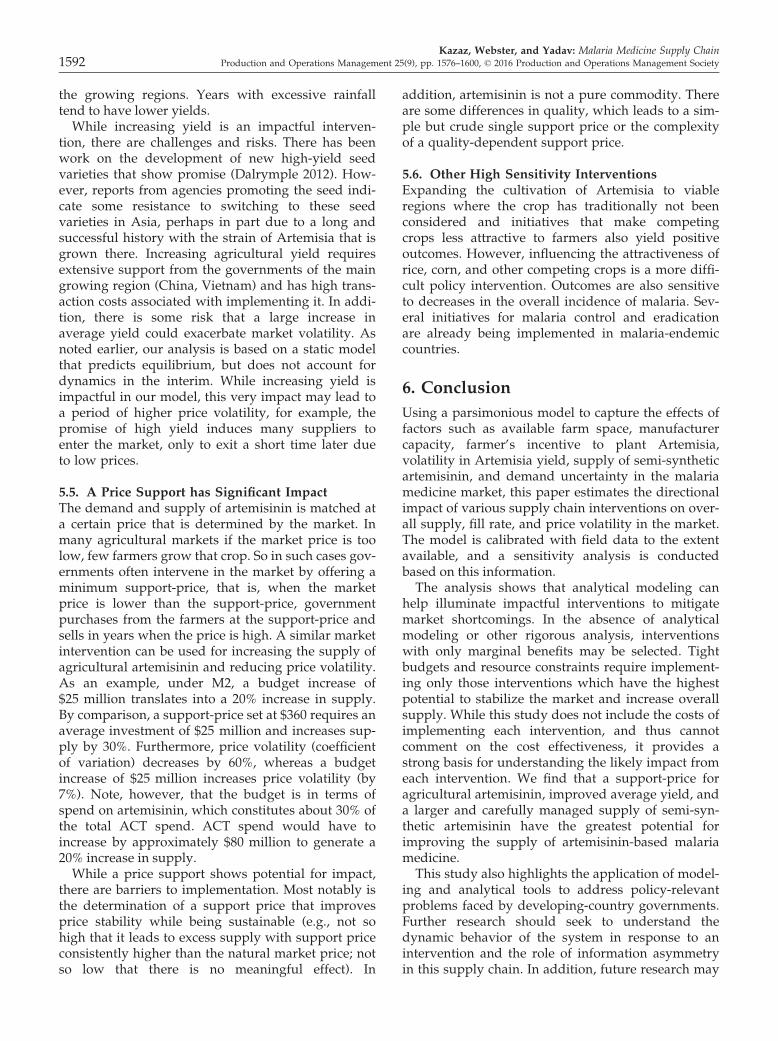
3.1. OverviewWe begin with a high-level description of our artemi-sinin supply chain model. There are two levels in thismodel. Level 2 corresponds to farmers (hereinafterreferred to as suppliers) and level 1 corresponds tothe ACT manufacturers. While farmers and extractorsare separate entities, the relevant decisions are ade-quately captured by treating artemisinin suppliers asa single unit.Suppliers decide whether to produce Artemisia or

the best alternative to Artemisia. The amount of farmspace dedicated to Artemisia is positively influencedby the expected value of the artemisinin spot priceand, due to supplier risk aversion, is negatively influ-enced by its variance. The volatility of the spot priceis influenced by the degree of volatility in the harvestyield and in the size of the market. Price is assured forunits under forward contract. The forward contractprice is aligned with the expected spot price.Artemisinin not under contract is sold in the open

market, and as such, the spot price reflects the marketclearing price. Accordingly, there is a negative rela-tionship between the fraction of growing capacitydedicated to Artemisia and the expected spot price(e.g., the higher the supply, the lower the spot price).


Figure 2 illustrates decisions, processes, and relation-ships in our model of the artemisinin supply chain.

3.2. Equilibrium ConditionLet q denote the amount of farm space dedicated toproducing artemisinin in an upcoming growing sea-son. The random market-clearing price of artemisininafter a season’s harvest of Artemisia (and prior to thenext harvest) is P(q) with moments denoted as

�p qð Þ ¼ E P qð Þ½ �

r2P qð Þ ¼ V P qð Þ½ �:We abstract away the manufacturer’s production

cost and profit margin, so P(q) is also the randomprice of ACT. In the next section, we introduce twomodels that define how the probability distribution ofP(q) is affected by various parameters.Let s denote the quantity of semi-synthetic artemi-

sinin introduced to the market. Semi-synthetic arte-misinin is not subject to yield uncertainty. Describingthe expected yield from each unit of farm spacewith l2, the random organic artemisinin yield is exp-ressed as

Q ¼ ql2Z2; ð1Þwhere Z2 is a positive random variable with cdf Φ2,mean 1, and variance r22: The term ql2 is theexpected amount of artemisinin from farming qunits of farm space. Combining equation (1) withthe amount of semi-synthetic artemisinin productions yields the overall random artemisinin supplyql2Z2 + s. The mean artemisinin supply is ql2 + s.As noted in section 1, some manufacturers offer

forward contracts that specify a price and quantity ofartemisinin they will purchase at a future point intime. And some extractors establish forward pricecontracts with farmers prior to the growing season inorder to obtain sufficient supply. These forward con-tracts specify the price for the farmer’s harvestedcrop. Let a denote the fraction of farm space dedicatedto producing artemisinin that is under forward

contract. The forward contract price is set to matchthe expected spot price �p qð Þ:Let c denote the amount of farm space owned by all

suppliers who could produce artemisinin. The own-ers of c units of farm space have alternatives to pro-ducing artemisinin. Let Ub denote the utility of thebest alternative associated with a randomly selectedunit of farm space. The cdf of Ub is qb(u) and its meanis lb.We model the utility per unit of space dedicated to

producing artemisinin of a representative supplier1 asthe product of two terms: (1) expected yield per unitof farm space, and (2) the utility per unit of artemisi-nin, which is governed by a mean-variance utilityfunction, i.e., ua ¼ l2 � �p qð Þ � cr2P qð Þ� �

:The parameter c ≥ 0 is a measure of risk aversion,

that is, the higher the value of c, the higher the riskaversion; if c = 0, then suppliers are risk neutral. Wesee that utility is increasing in average yield (l2) andaverage price (�p qð Þ), and is decreasing in price vari-ance (r2P qð Þ) with the rate of decrease controlled bythe risk-aversion parameter (c). Note that the utilityof producing artemisinin associated with a unit ofspace under contract is l2�p qð Þ (i.e., by the terms ofthe forward contract, there is no variance in theprice).Let Ub0 denote the random utility of the best alter-

native associated with a unit of farm space under for-ward contract. We define Ub0 as Ub conditioned onthe utility of the best alternative being less than theutility of artemisinin under contract, that is, the utili-ties associated with units of space under contract arerepresentative of the population (conditioned on apreference for artemisinin over the best alternative).Accordingly, the cdf of Ub0 ¼ UbjUb � l2�p qð Þ is

qb0 uð Þ ¼ P Ub0 � u½ � ¼ P Ub � ujUb � l2�p qð Þ½ �¼ qb uð Þ

qb l2�p qð Þð Þfor all u� l2�p qð Þ:

ð2Þ

We are now ready to identify a condition for thevalue of q in equilibrium. For a given q, the amount of

Figure 2 Schematic of Our Model of the Artemisinin Supply Chain


farm space not under contract that is dedicated to pro-ducing artemisinin is

q� aq: ð3ÞAnd, for a given q, the amount of farm space notunder contract with utility of the best alternative nomore than the utility of producing artemisinin is

cqb uað Þ � aqqb0 uað Þ ¼ qb l2 �p qð Þ � cr2P qð Þ� �� c� aq

qb l2�p qð Þð Þ� � ð4Þ

(see equation (2)), that is, the total farm space withUb ≤ ua is reduced by the amount of farm spacewith Ub ≤ ua that is under contract. Equilibrium canbe found by setting equation (3) equal to equa-tion (4) and solving for q.

F q�ð Þ � 1� acq� � a

qb l2�p q�ð Þð Þ� qb l2 �p q�ð Þ � cr2P q�ð Þ� �� ¼ 0:2

ð5ÞWe note that the equilibrium condition given in

equation (5) has a simple interpretation when suppli-ers are risk neutral, that is, if c = 0, then equation (5)reduces to

q� ¼ cqb l2�p q�ð Þð Þ: ð6ÞThe above expression says that the farm space dedi-

cated to producing artemisinin is the fraction ofcapacity with utility of the best alternative no morethan the expected revenue per unit of farm space.Figure 3 illustrates the curves associated with equa-

tions (3) and (4), and the associated equilibriumpoint. Note that equation (3) is increasing in q. Forany realization of supply and demand random

variables, it follows from the market-clearing prop-erty that the spot price is decreasing in q, whichimplies that the expected spot price is decreasing in q,that is,

�p0 qð Þ\0: ð7ÞIf utility ua does not increase as q increases, that is,

d

dql2 �p qð Þ � cr2P qð Þ� �� 0; ð8Þ

then equation (4) is decreasing in q (i.e., the right-hand side of equation (4) is the product of two posi-tive terms that are both decreasing in q), and thusequation (8) is a sufficient condition for a uniqueequilibrium.We emphasize that our model is static in the sense

that it predicts the farm space dedicated to producingartemisinin as the system settles into equilibrium. Wedo not capture the dynamics of behavior in interim.Our model assumes that a supplier’s decision to enterthe market is based on the mean and variance of mar-ket price that suppliers are not biased in their esti-mates of these measures, and that suppliers, inequilibrium, do not move in and out of the market inresponse to random market fluctuations. As a steptowards an understanding of possible interventionsin the complex real-world system, our goal is to strikea balance of modeling the system with enough rich-ness to capture the essence of how elements interactto affect performance while avoiding excess complex-ity that may lead to brittleness in behavior (e.g., smallchanges in model settings generate large changes inresults). In section 5, we consider how the inclusionof dynamics and decision-making biases may affectour conclusions.

Figure 3 Illustration of Equations (3) and (4), and the Corresponding Equilibrium Quantity


3.3. Two Models of Price-Dependent DemandThe random ACT market size (e.g., number of malariacases) is

M ¼ l1Z1;

where l1 is the expected ACT market size and Z1 isa positive random variable with cdf Φ1, mean 1, andvariance r21. We assume that Z1 is independent ofthe yield random variable Z2. This assumption is areasonable approximation of reality in our settingwhere more than 90% of P. falciparum malaria trea-ted by ACTs occurs in sub-Saharan Africa and morethan 80% of Artemisia growing regions are locatedin Asia, for example, a drought in southeast Asia islargely independent of rainfall patterns (and hencemalaria) in sub-Saharan Africa. In addition, weatherpatterns that affect the yield at harvest time occurmuch earlier than when the drug from the harvestbecomes available to serve market needs (influencedby much more recent weather patterns).We consider two price-dependent demand models

in our analyses:

M1: dðpÞ ¼ Mq1ðpÞ

M2: dðpÞ ¼ bp�1:

For example, q1(p) is the fraction of the market will-ing to pay price p or more. The models reflect twoopposing interpretations of the role of market size ondemand:

M1. The fraction of the market willing to pur-chase at price p, q1(p), is independent of themarket size M.

M2. The total volume purchased at price p isindependent of the market size M.

Model M1 is motivated by a setting where the mar-ket is composed of many individual buyers who pur-chase ACT if willing/able to pay the market price.Model M2 is motivated by a setting where the marketis composed of a few buyers (e.g., NGOs and interna-tional agencies) who spend a fixed total budget, b, onwhatever supply is available. The result is an isoelas-tic demand function. M1 is likely a better fit in regionswhere most patients seek treatment in the private sec-tor. M2 is likely a better fit in regions where mostpatients seek treatment in the government or NGO-run health clinics; governments or NGOs have a fixedbudget for purchasing malaria medicines for a givenyear. We examine measures of performance undereach of these models individually. These modelsallow for more detailed characterizations of behaviorthan what could be obtained from a more complexdemand model, and such characterizations are likely

to span the behavior of a system with demand that isa composite of M1 and M2.We now turn our attention to the form of the ran-

dom spot price function P(q) under these two demandmodels, beginning with M1. We consider the impactof a price-support intervention. For this intervention,one or more organizations such as NGOs agree to paya minimum price of p0, effectively assuring that themarket-clearing price will not drop below the sup-port-price p0. We assume that the willingness-to-payfunction q1(p) 2 [0, 1] is strictly decreasing in priceover the range of possible price realizations. Thus, wecan invert q1(p) to obtain expressions for the randommarket-clearing price and its moments (i.e., set supplyql2Z2 + s equal to demand l1Z1q1, solve for q1, theninvert q1(p) while accounting for the restrictions ofq1 2 [0, 1] and p ≥ p0),

M1: PðqÞ ¼ max q1�1 min

ql2Z2 þ s

l1Z1; 1

� �� ; p0

� �; ð9Þ

�p qð Þ ¼ E max q1�1 min

ql2Z2 þ s

l1Z1; 1

� �� ; p0

� �� ;

ð10Þ

r2P qð Þ ¼ V max q1�1 min

ql2Z2 þ s

l1Z1; 1

� �� ; p0

� �� :

For M2, we follow a similar approach,

M2: PðqÞ ¼ maxb

ql2Z2 þ s; p0

� �

�p qð Þ ¼ E maxb

ql2Z2 þ s; p0

� �� ; ð11Þ

r2P qð Þ ¼ V maxb

ql2Z2 þ s; p0

� �� :

3.4. Performance MeasuresIn this section, we introduce measures of performancerelevant to the manufacturer, society, and supplier.The expected artemisinin volume in equilibrium is

p1 ¼ E q�l2Z2½ � þ s ¼ q�l2 þ s;

which is a measure of the manufacturer’s welfare.As an indicator of the availability of the drug fortreatment, p1 is also a measure of public health. Analternative measure of public health is the expectedfraction of total need that is satisfied, or fill rate,

b ¼ E minq�l2Z2 þ s

l1Z1; 1

� �� :


Recall that Ub0 ¼ UbjUb � l2�p qð Þ and that the cdf ofUb0 is qb0 uð Þ ¼ qb uð Þ=qb l2�p qð Þð Þ: Accordingly, the sup-plier surplus associated with aq* units under contractat price �p q�ð Þ is

aq�Zl2�p q�ð Þ

�1l2�p q�ð Þ � tð Þ qb

0 tð Þqb l2�p q�ð Þð Þ dt

¼ aq�Zl2�p q�ð Þ

�1

qb tð Þqb l2�p q�ð Þð Þ dt:

The cdf of the utility of the best alternative afterunits under contract are removed from the populationis as follows:

qbn0 uð Þ ¼cqb uð Þ� aq�qb uð Þ

qb l2�p q�ð Þð Þc�aq� ; u� l2�p q�ð Þ

qb uð Þ; u� l2�p q�ð Þ

8<: ð12Þ

(obtained by dividing equation (4) by the numberof units remaining in the population after remov-ing units under contract). Thus, the suppliersurplus associated with units not under contract isas follows:

c� aq�ð ÞZl2 �p q�ð Þ�cr2 q�ð Þð Þ

�1qbn0 tð Þdt

¼ c� aq�

qb l2�p q�ð Þð Þ� � Zl2 �p q�ð Þ�cr2 q�ð Þð Þ

�1qb tð Þdt

¼ q� 1� að ÞZl2 �p q�ð Þ�cr2 q�ð Þð Þ

�1

qb tð Þqb l2 �p q�ð Þ� cr2p q�ð Þ

� �dt

(the first equality follows from equation (12); thesecond equality follows from equation (5)). Sum-ming the above expressions, the total supplier sur-plus is

p2¼q�"aZl2�p q�ð Þ

�1

qb tð Þqb l2�p q�ð Þð Þdtþ 1�að Þ

Zl2 �p q�ð Þ�cr2 q�ð Þð Þ

�1

qb tð Þqb l2 �p q�ð Þ�cr2p q�ð Þ

� �dt#

¼q�a

qb l2�p q�ð Þð ÞE l2�p q�ð Þ�Ubð Þþ� þ 1�a

qb l2 �p q�ð Þ�cr2p q�ð Þð Þð ÞE l2 �p q�ð Þ�cr2 q�ð Þ� ��Ub

� �þh i24

35:

If Ub is uniform on [uL, uH], for example, then

p2¼ q�

2 uH�uLð Þ

al2�p q�ð Þ�uLð Þ2qb l2�p q�ð Þð Þ þ 1�að Þ

l2 �p q�ð Þ�cr2p q�ð Þ �

�uL �2qb l2 �p q�ð Þ�cr2p q�ð Þ

� �264

375:

4. Analysis

This section presents analysis of the preceding model.The analysis proceeds along the following sequence.We first investigate the impact of changes in parame-ter values on measures of performance analytically(directional impact). We then conduct numerical anal-ysis using a calibrated model. We offer interpretationsof our results and discuss limitations. Section 5 sum-marizes the main implications of our results for policymakers.In order to help reinforce the connection between

our model, its purpose, and the real-world supplychain, we provide a few examples of interventionswith changes in relevant parameters in Table 1.

4.1. Directional Effects of Increasing ParameterValues on q* and p1Table 2 contains comparative-static results for q* andp1 given that suppliers are risk neutral (see section A3in Appendix A for derivations and proofs). The

Table 1 Examples of Interventions to Induce Different Types ofChange

Example intervention Change

Increase availability of high-yield seedvarieties

Increased yield per unit offarm space (l2↑)

Increase supply of competing crops inregions not conducive to growingArtemisia

Reduced attractiveness ofalternative crops (lb↓)

Increase malaria prevention efforts Reduced market size (l1↓)Assure that price will not drop belowa threshold

Introduce a price support(p0↑)

Training/education/resources in regionsthat are underutilized yet conducive togrowing Artemisia

Increased available farmspace (c↑)

Increase investment in semi-syntheticproduction

Increased semi-syntheticsupply (s↑)

Increase spending on ACT Increased purchase budgets(b↑)

Provide low-cost loans to farmers in theevent of low yield

Reduced supplier riskaversion (c↓)

Increase availability of disease-resistantseed varieties

Reduced yield variability(r2↓)

Improve and increase documentation indiagnostic testing and treatment

Reduced market uncertainty(r1↓)

Provide low-cost loans for up-frontpartial payment in forward contracts

Increased usage of forwardcontracts (a↑)


complexity of the model inhibits similar results forthe measures b and p2, and for the case of risk-aversesuppliers.The results in Table 2 generally align with intu-

ition: (1) the increased use of forward contracts (a)has no impact (given suppliers are risk neutral),(2) the spend budget (b) does not play a role underM1, but increases in the budget lead to increases insupply under M2, (3) an increase in farm space withpotential to produce artemisinin (c) leads toincreases in supply, (4) an increase in market size(l1) leads to increases in supply under M1, (5) anincrease in either market size (l1) or market volatil-ity (r1) has no effect on supply under M2, (6) anincrease in the attractiveness of the best alternativeto artemisinin (lb) leads to decreases in supply, and(7) an increase in the support-price (p0) leads to anincrease in supply.Increases in the remaining parameters exhibit less

intuitive effects. Let us begin with the impact of anincrease in the coefficient of variation of organic yield(r2). Suppliers are risk-neutral and thus are not con-cerned about price volatility, so we may expect thatchanges in yield volatility will have no effect on sup-ply. We see this result under M1 when demand is lin-ear. However, changes in yield uncertainty affect

supply when the demand function is nonlinear. Thereason is that the equilibrium condition includes anexpected value of a function of random variables(e.g., see equation (10) and equation (11)). If the func-tion is nonlinear, as is the case of M1 with a nonlineardemand function and M2, then upside deviationsfrom the mean are either amplified or compressed rel-ative to downside deviations. This distortion fromnonlinearity is what drives the directional arrows inTable 2. A convex demand function, for example,means that the increase in price from a unit decreasein supply is greater than the decrease in price from aunit increase in supply. Consequently, an increase inyield uncertainty exerts an upward pressure on theexpected price, which in turn leads to a higher equi-librium quantity. The behavior is reversed if thedemand function is such that a unit increase in supplycauses a larger change in price than a unit decrease insupply (i.e., if the demand function is concave).The changes in supply in response to increases in

the coefficient of variation of market size (r1) underM1 are similar, but not identical, to what we see forr2. There is similarity because the directional arrowsare caused by nonlinearities. However, note that alinear demand function means that the fraction ofthe market willing to pay price p is proportional tosupply but is inversely proportional to market size(see equation (9)), that is, if price is linear in supply,then it is nonlinear in market size. In particular, thedecrease in price from a unit decrease in market size(or need for the drug) is greater than the increase inprice from a unit increase in market size. This putsdownward pressure on the expected price as marketuncertainty increases, and leads to a lower equilib-rium quantity. In the next section, we will see thatthis structural difference between the roles of ran-dom yield and market size contributes to meaningfuldifferences in sensitivities to changes in theseparameters.While an increase in semi-synthetic artemisinin (s)

generally leads to an increase in supply, it is possiblethat supply could decrease if demand is sufficientlyconvex in price. The convexity of the demand curvecan lead to a steep drop in price in response to anincrease in semi-synthetic supply resulting in a largeexit of suppliers from the market and lower total sup-ply (see Figure 8 for an example). The main driver ofthe result is nonlinearity as discussed above, and isparticularly related to the comparative-static resultsfor r2. There is no uncertainty in semi-synthetic yield,and thus as the production of semi-syntheticincreases, the coefficient of variation of total yield—the sum of organic and semi-synthetic—decreases. Ifthe demand function is convex, then a reduction inthe coefficient of variation of total yield puts a down-ward pressure on supply (as shown in Table 2 for r2)

Table 2 Directional Effects of Increases in Different Parameter ValuesWhen Suppliers are Risk Neutral

Increasein

Demandmodel Change in q* Change in p1

a M1 – –M2 – –

b M1 – –M2 ↑ ↑

c M1 ↑ ↑M2 ↑ ↑

l1 M1 ↑ ↑M2 – –

r1 M1 Linear d(p), ↓Max{Z1} ≤ 2:concave d(p), ↓Convex d(p), ↑↓

Linear d(p), ↓Max{Z1} ≤ 2:concave d(p), ↓Convex d(p), ↑↓

M2 – –s M1 ↓ Linear or concave d(p), ↑

Convex d(p), ↑↓M2 ↓ ↑↓

l2 M1 ↑↓ ↑M2 ↑ ↑

r2 M1 Concave d(p), ↓Linear d(p), –Convex d(p), ↑

Concave d(p), ↓Linear d(p), –Convex d(p), ↑

M2 ↑ ↑lb M1 ↓ ↓

M2 ↓ ↓p0 M1 ↑ ↑

M2 ↑ ↑

↑ = increasing, ↓ = decreasing, – = no change, ↑↓ = direction dependson other parameter Values.


that can more than offset the increase in semi-synthetic artemisinin.Lastly, while it is not surprising that supply is

increasing in average yield (l2), it is noteworthy thatthe amount of farm space dedicated to producingartemisinin (q*) can increase as well. This behavior isassured under M2, and depending on the demandfunction, can occur under M1. This is noteworthybecause the system is governed by a negative feed-back loop (stemming from the inverse relationshipbetween supply and price) that, in general, works tomute the impact of interventions. If q* is held fixedand l2 increases, then organic supply will increaseproportionally. The effect of an increase in l2 on sup-ply is amplified when it also leads to an increase in q*.The result hints that l2 is a potentially powerful lever,and we present an illustration of its power in the nextsection.

4.2. Numerical Analysis of Effects of Changes inParameter ValuesThe comparative statics in the previous section arelimited to the case of risk-neutral suppliers. In thissection, we use numerical methods to investigate thesensitivity of system performance to changes inparameters. Using the limited available historical dataas a guide, we develop a set of parameter values andfunctions for our base-case model (see Table 3).Parameters r1, r2, s, a, l1, l2, and b are estimatedusing historical data related to these values.3 We esti-mate the risk aversion parameter as c = 0.008.4 Weassume uniformly distributed willingness-to-pay andutility of the best alternative on the basis of the princi-ple of insufficient reason proposed by Pierre Laplacein the 1700s (Luce and Raiffa 1957); if all that is knownabout a random variable is that it can take on valuesover a finite range, then any distribution other thanuniform implies that something else is known. Weuse the symmetric triangular distribution for Z1 andZ2 in order to capture a central tendency (that is notpresent in the uniform distribution) about the meanof 1. Finally, we use historical data on price, annualsupply, need, and fill rates as a guide, finding valuesof lb, rb, c, and coefficients of linear function q1(p) thatlead to equilibrium results that are generally consis-tent with observed results.We use stochastic optimization with 10,000 trials

per simulation via Analytic Solver Platform fromFrontline Systems to identify the equilibrium quan-tity. Table 4 lists statistics from the base-case model.We compute the sensitivity of performance to

changes in each of the 11 parameters listed in Table 2.With the exception of support-price p0, each parame-ter is varied between �50% and +50% of its base-casevalue (p0 = 0 in the base-case). We find that the rela-tive sensitivity of performance to changes in different

parameter values is reflected in the grouping ofparameters in Table 1. Performance is more sensitiveto changes in parameters listed near the top of Table 1and is less sensitive to changes in parameters listednear the bottom of the table. We categorize theparameters into three groups—high, moderate, andlow sensitivity:

High-sensitivity: average yield (l2), average util-ity of the best alternative (lb),average market size (l1)

Moderate-sensitivity: available farm space (c),semi-synthetic supply (s),spend budget (b)

Low-sensitivity: risk aversion (c), yield variability(r2), demand variability (r1), for-ward contract % (a)

While the boundaries of these categories are subjec-tive (due to multiple performance measures and non-linearities), the parameters in each category exhibitsome commonality that may help explain observeddifferences in sensitivity. In particular, the high cate-gory can be viewed as first-moment parameters, thelow category can be viewed as second-moment

Table 3 Units, Functions, Random Variables, and Parameters in ourBase-Case Model

UnitsSpace unit = 1000hectares (H)

Artemisininunit = 1000 kgs (K)

Currencyunit = $1000 (D)

Functions and random variablesq1(p) = 2 – 0.0032p Z1, Z2 ~ symmetric

triangularr1 = 0.1 K,r2 = 0.3 K/H

Ub ~ uniformlb = 4800 D,rb = 1500 D

ParametersPotential farmspace (c) = 80 H

Semi-syntheticsupply (s) = 60 K

Forward contract %(a) = 25%

Risk aversion(c) = 0.008

Mean demand(l1) = 240 K

Mean yield(l2) = 10 K/H

Purchase budget(b) = 75,000 D

Table 4 Statistics from the Base-Case Model in Equilibrium

Demand model

M1 M2

Hectares producing artemisinin in 000s (q*) 17 15Average total supply in metric tons (p1) 235 212Average semi-synthetic production as fractionof total (%)

26 28

Average fill rate (b) (%) 89 85Average supplier surplus in $000,000s (p2) $10 $8Average total spend in $000,000s $73 $75Average artemisinin price in $ per kg (�p) $345 $373Standard deviation in artemisinin price (rP) 46 90Min and max price per kg (in 10,000 trials) $313, $505 $232, $740


parameters, and the moderate category can be viewedas quantity parameters. In other words, in the high cat-egory, we have parameters that specify the averagesof random variables whereas in the low category wehave parameters that are closely linked to volatility.Parameters r1 and r2 are direct measures of volatility,whereas parameters c and a control the importance ofvolatility in supplier decision making. Parameter cmeasures the degree to which suppliers care aboutvolatility in the market and parameter a controls thefraction of suppliers that are immune to marketvolatility (via a forward contract). The moderate cate-gory contains the remaining parameters that are notclosely linked to moments of the random variables.We do not categorize the support-price parameter (p0)because its base-case value is 0 (i.e., no price supportcurrently in effect).In what follows, we present and discuss results for

one parameter within each category; figures illustrat-ing the sensitivity of performance measures tochanges in other parameters are available in anAppendix S1.Figures 4–6 show the sensitivity of total supply

(p1), fill rate (b), and supplier surplus (p2) to changesin one parameter from each category—forward con-tract percentage (low), semi-synthetic supply (moder-ate), and average yield (high). For all of the sensitivityfigures, we divide p1 and p2 by constants (635 and85,500, respectively) so that all measures take on val-ues between 0 and 1.Recall that a tripartite financing model was intro-

duced in 2009, in part to encourage increased use offorward contracts and thereby increase supply. Ourresults in Figure 4 indicate that increased use of for-ward contracts have minimal impact on supply and

other measures. To assess the robustness of this obser-vation, we increased the risk aversion parameter byan order of magnitude (from c = 0.008 to c = 0.08),and we find little difference in sensitivity. Greatersensitivity can arise in an alternative calibration withhigher variation in utility (rb) and risk aversion (c),but these higher values are not reasonable in the cur-rent market for artemisinin.Figure 7 augments Figure 3 to illustrate how the

base-case equilibrium shifts in response to theextreme of no forward contracts (a = 0). Both Fig-ures 3 and 7 are created using the base-case modelunder M1 (the behavior is similar under M2). We seethat a reduction from a = 0.25 to a = 0 creates anupward shift in equation (3) that puts pressure todecrease equilibrium, and creates an upward shift inequation (4) that puts pressure to increase equilib-rium. The result of these offsetting pressures is a verynarrow band of equilibrium quantities fora 2 [0, 0.25]. In contrast, equation (3) is unaffected bychanges in s or l2, and we find similar or larger shiftsin equation (4) as s or l2 change, leading to largerchanges in equilibrium. As discussed in section 4.1,increases in average yield (l2) positively affect thesupplier’s utility per unit of farm space as well as sup-ply. However, increases in semi-synthetic supply (s)positively affect supply only. This difference helpsexplain the differences in observed sensitivities tochanges in s and l2.Recall from Table 2 that it is possible for total sup-

ply to be decreasing in semi-synthetic productionwhen demand is convex in price, as is the case withdemand model M2. Figure 5 shows that supply isincreasing in semi-synthetic production. However,while we suspect this to be the dominant behavior in

Figure 4 Sensitivity of Total Supply, Fill Rate, and Supplier Surplus to Changes in the Forward Contract Percentage (a)


real-world settings, it does not take much of a changein the base-case model to yield a decreasing supplyfunction. Figure 8 is based on two changes to thebase-case model: suppliers are risk neutral and yielduncertainty is increased by one-third (i.e., c isdecreased from 0.008 to 0 and r2 is increased from 0.3to 0.4).

4.3. Effects of Changes in Parameter Values onPrice VolatilityPrice volatility influences a supplier’s decision onwhether or not to produce artemisinin, and in thissense, the effects of price volatility are captured in thesummary performance measures reported above.

That said, the impact of interventions on price volatil-ity is a measure of interest in its own right among pol-icy makers. As one may expect, the sensitivity of pricevolatility to changes in parameters is consistent withthe sensitivity of other performance measures, that is,parameters that exhibit low (high) sensitivity withrespect to supply, fill rate, and supplier surplus tendto exhibit low (high) sensitivity with respect to pricevolatility.We present selected price volatility sensitivity

results below. In order to highlight how relativeprice volatility changes as parameters change, wereport the price coefficient of variation (CV = SD/mean).

Figure 5 Sensitivity of Total Supply, Fill Rate, and Supplier Surplus to Changes in Semi-Synthetic Production (s). The figure also includessemi-synthetic production as a fraction of the total (s/(s + q*))

Figure 6 Sensitivity of Total Supply, Fill Rate, and Supplier Surplus to Changes in Expected Yield Per Hectare (l2)


Figure 9 illustrates that changes in demand uncer-tainty have little effect on price volatility, whereasreductions in yield uncertainty translate into notice-able reductions in price volatility. The reason forthe difference, in part, is due to the greater degreeof yield uncertainty than demand uncertainty in thebase-case model (e.g., r2 = 3r1 = 0.3, so a 50%increase in r1 is comparable to a 17% increase inr2), though a difference in sensitivity remains whenr2 = r1 = 0.1. As discussed in section 4.1, there is astructural difference in the price function equa-tion (9) that explains this result—the fraction of themarket willing to pay price p is proportional to sup-ply but is inversely proportional to market size.

This nonlinearity acts to soften the effects of chang-ing volatility in market size on the volatility ofprice.While we find the supply, fill rate, and surplus

measures to be relatively insensitive to changes in r1and r2, there is an important lesson for policy makersif interventions to impact r1 and r2 are being consid-ered. Our analysis points to greater impact fromchanges in r2 than r1 for two reasons. The first reasonis the structural difference explained above. A secondreason is that changes in r1 have no effect of on per-formance under M2; the sensitivity of performance tochanges in r1 is further diminished by the extent thatreality reflects M2 over M1.

Figure 8 Sensitivity of Total Supply to Changes in Semi-Synthetic Production (s) with Risk Neutral Suppliers (c = 0) and Higher Yield Uncertainty(r2 = 0.4) Under Demand Model M2

Figure 7 Illustration of Equations (3) and (4), and the Corresponding Equilibrium Quantities for a = 0 and a = 0.25


Figures 10 and 11 illustrate the sensitivity of pricevolatility to changes in semi-synthetic production andto the support-price. These figures also report theaverage price in order to expose the relationshipbetween average price and its relative volatility. Werescale the average price by dividing by $2000. (Aver-age price is virtually unchanged as r1 and r2 are var-ied, so the average price curves are excluded fromFigure 9.)One advantage of increasing semi-synthetic pro-

duction with its deterministic yield is that it trans-lates into lower supply uncertainty, and as aconsequence, lower price volatility. We see this

effect in Figure 10. A 50% increase in semi-syntheticproduction reduces price volatility by 20% for bothM1 and M2. The figure also illustrates the down-ward pressure on price from semi-synthetic produc-tion. A 50% increase in semi-synthetic productionreduces average price by about 5%, slightly less forM1 and slightly more for M2.Similar to an increase in semi-synthetic production,

the introduction of a support-price has a direct effecton price volatility (i.e., by restricting the downwardrange of price). Figure 11 illustrates this effect. Thesupport-price does not affect the system until itreaches about $300 (i.e., the price rarely drops below

Figure 10 Sensitivity of Average Price (Divided by $2000) and Price Coefficient of Variation to Changes in Semi-Synthetic Production (s)

Figure 9 Sensitivity of Price Coefficient of Variation to Changes in Demand Uncertainty (r1) and Yield Uncertainty (r2). The sensitivity to yielduncertainty is illustrated at the base-case value r2 = 0.3, and at r2 = 0.1 = r1. Sensitivity results are not reported for demand model M2because demand uncertainty does not affect the system


$300), and price volatility nearly disappears once thesupport-price reaches $440.

4.4. LimitationsThere are limitations in our model that should betaken into account when interpreting our results. Ourmodel is static, ignoring dynamics that arise from anintervention that causes the system to move towardsa new equilibrium. Thus, interventions that are foundto be especially impactful in our model may have anegative side effect of inducing a greater degree ofdynamic instability in the system, both in terms of themagnitude of supply–demand imbalance in responseto the intervention and the time to settle into a newequilibrium. We come back to this point in the nextsection.As a related point, our model considers a single-

period problem where excess inventory from one yearis not used/sold in the following years. The overthree-year shelf life of artemisinin allows holdinginventory from one year and using it in the followingyears. While suppliers do not necessarily have thecapital to invest in holding inventory, ACT manufac-turers do hold inventory. We have conducted numeri-cal tests of a model that includes random leftoverinventory from the prior period, and we find no dif-ferences in our sensitivity conclusions. This is notunexpected in light of our numerical results in sec-tion 4.2 where we find that the system is insensitiveto changes in volatility measures. This muted behav-ior is influenced by the static nature of our model, thatis, that suppliers do not move in and out of the marketin response to random market fluctuations andinstead decide what to produce based on the meanand variance of market price. The system will be more

erratic than our model predicts if there are many sup-pliers who move in and out of the market based oncurrent conditions. There is a dearth of informationon the extent to which suppliers move in and out ofthe market, and thus represents a potential area forfuture investigation.Our model assumes full and symmetric information

between suppliers, manufacturers, and purchasers/financiers. Suppliers do not under- or over-react tomarket signals. In practice, suppliers may have poorknowledge of market demand compared to the finan-ciers and purchasers (Levine et al. 2008). Forecastinghelps in resolving this information asymmetry morethan reducing the intrinsic demand uncertainty.Finally, the attractiveness of an intervention is based

on both its impact and cost, including ease and speedof implementation. There are likely many possibleapproaches for influencing the value of each parameterin our model, each with its own cost and implementa-tion challenges. The identification and cost assessmentof alternative approaches to affect different types ofdesired change is left to those with specialized exper-tise, and is outside the scope of this study.

5. Summary of Implications for PolicyMakers

Although a number of results developed in the pre-vious section are valuable in developing a betterunderstanding of the market, we discuss the impactof the interventions that have either been imple-mented in this market in the past or are beingactively considered by policy makers. We explain ingreater detail the most significant and the most sur-prising results.

Figure 11 Sensitivity of Average Price (Divided by $2000) and Price Coefficient of Variation to Changes in the Support-Price (p0)


5.1. Increasing Forward Contracting has MarginalImpactAs noted above, the A2S2 initiative was created in 2009to increase artemisinin supply to meet the projectedACT demand. A2S2 was based on a tripartite financingmodel where extractors who had existing contractswith WHO-prequalified ACT manufacturers receivedfinancing at subsidized rates. The underlying premisewas that offering lower interest capital would incen-tivize more forward contracts with farmers andincrease artemisinin supply. An independent reviewestimated the impact to be 35% below expectations,though the team was not able to identify specific rea-sons for the shortfall (UNITAID 2011). The programhas since been terminated. While our results are consis-tent with that outcome, we caution that our analysismay understate the impact of forward contracts. Inparticular, the beneficial impact of increased forwardcontracts, as well as improvements in other second-moment parameters and a support price, are likely tobe greater than predicted by our model if there aremany suppliers who move in and out of the marketbased on current conditions.

5.2. Reducing Demand Uncertainty has MarginalImpactThe model shows that attempts to decrease marketuncertainty through better disease forecasting alsohave limited impact. Understandably, when theoverall budget for purchasing malaria medicines isfixed and known to all actors in the system, reduc-tions in demand uncertainty do not impact the mar-ket outcomes. More interestingly, even when theoverall budget is not fixed and the total quantitypurchased depends upon the price offered, reduc-tions in demand uncertainty through better epidemi-ological forecasting result in only small increases inoverall supply. This result, which is similar to impactof forward contracts noted above, is a reflection ofthe more general phenomenon observed in numeri-cal results of our calibrated model: equilibrium is rel-atively insensitive to changes in measures that relateto volatility.

5.3. Increasing the Production of Semi-SyntheticArtemisinin has a Moderate Impact, and theTransition Period Requires Careful Managementof the Two Sources of SupplyA greater production of semi-synthetic artemisininincreases overall supply, increases fill rate, anddecreases price volatility. This is notable because ofthe debate surrounding the value of this intervention(Peplow 2013, Van Noordan 2010). On the surface,one might view increasing semi-synthetic as a verysignificant and positive tool to improve overall

supply and decrease price volatility. However, we seethat a 50% increase in semi-synthetic productiontranslates into approximately an 8% increase in sup-ply and a 5% increase in fill rate (for both demandmodels). In addition, supplier surplus drops by about15%. We also observe some risk that overall artemisi-nin supply could decrease (see Figure 8). This resultsfrom the semi-synthetic supply not being able to off-set the decrease in agricultural artemisinin produc-tion as suppliers exit the market. However, beyond acertain threshold volume of semi-synthetic produc-tion, overall output increases as semi-syntheticincreases. This highlights that, while semi-syntheticmay increase overall supply unconditionally as itscapacity nears the total demand, in the interim, it isimportant to manage the two sources of supply care-fully in order to avoid decreases in overall supply. Inaddition, increasing semi-synthetic production has itsown challenges. For example, the use of semi-syn-thetic in an ACT production process requires that theproducer go through an FDA-type approval processthat takes time and money. In addition, there is resis-tance to purchasing semi-synthetic by some ACTmanufacturers because the semi-synthetic producer isalso a competitor in the ACT market.

5.4. Increasing Agricultural Yield has SignificantImpactThe overall supply of artemisinin increases withincreases in average yield due to two positive effects –the output per hectare planted increases but addition-ally the farmer’s utility for producing artemisininincreases. Other interventions are one-dimensional inthe sense of exerting a single force on the system. Thesupply chain has a negative feedback loop that damp-ens the sensitivity of performance to interventions.For example, the positive effect of increased outputper hectare is mitigated by the negative relationshipbetween supply and price, i.e., supply up ? pricedown ? reduced supplier interest ? supply down.However, the increased productivity increases bothoutput and farmer utility that, compared to otherinterventions, diminishes the strength of the negativefeedback loop in the system. Figure 6 shows that theimpact of yield improvements is less under M2 thanM1. This is because the fixed total spend under M2leads to larger reductions in price with improvedefficiency.Changes in planting methods, and other agricul-

tural practices can lead to some improvements inyield. Radical improvements can only come from theuse of higher-yielding varieties of Artemisia. Suchhigh-yielding seed varieties may also lead to slightreductions in yield uncertainty, but a large part of theyield uncertainty depends on rainfall and weather in


the growing regions. Years with excessive rainfalltend to have lower yields.While increasing yield is an impactful interven-

tion, there are challenges and risks. There has beenwork on the development of new high-yield seedvarieties that show promise (Dalrymple 2012). How-ever, reports from agencies promoting the seed indi-cate some resistance to switching to these seedvarieties in Asia, perhaps in part due to a long andsuccessful history with the strain of Artemisia that isgrown there. Increasing agricultural yield requiresextensive support from the governments of the maingrowing region (China, Vietnam) and has high trans-action costs associated with implementing it. In addi-tion, there is some risk that a large increase inaverage yield could exacerbate market volatility. Asnoted earlier, our analysis is based on a static modelthat predicts equilibrium, but does not account fordynamics in the interim. While increasing yield isimpactful in our model, this very impact may lead toa period of higher price volatility, for example, thepromise of high yield induces many suppliers toenter the market, only to exit a short time later dueto low prices.

5.5. A Price Support has Significant ImpactThe demand and supply of artemisinin is matched ata certain price that is determined by the market. Inmany agricultural markets if the market price is toolow, few farmers grow that crop. So in such cases gov-ernments often intervene in the market by offering aminimum support-price, that is, when the marketprice is lower than the support-price, governmentpurchases from the farmers at the support-price andsells in years when the price is high. A similar marketintervention can be used for increasing the supply ofagricultural artemisinin and reducing price volatility.As an example, under M2, a budget increase of$25 million translates into a 20% increase in supply.By comparison, a support-price set at $360 requires anaverage investment of $25 million and increases sup-ply by 30%. Furthermore, price volatility (coefficientof variation) decreases by 60%, whereas a budgetincrease of $25 million increases price volatility (by7%). Note, however, that the budget is in terms ofspend on artemisinin, which constitutes about 30% ofthe total ACT spend. ACT spend would have toincrease by approximately $80 million to generate a20% increase in supply.While a price support shows potential for impact,

there are barriers to implementation. Most notably isthe determination of a support price that improvesprice stability while being sustainable (e.g., not sohigh that it leads to excess supply with support priceconsistently higher than the natural market price; notso low that there is no meaningful effect). In

addition, artemisinin is not a pure commodity. Thereare some differences in quality, which leads to a sim-ple but crude single support price or the complexityof a quality-dependent support price.

5.6. Other High Sensitivity InterventionsExpanding the cultivation of Artemisia to viableregions where the crop has traditionally not beenconsidered and initiatives that make competingcrops less attractive to farmers also yield positiveoutcomes. However, influencing the attractiveness ofrice, corn, and other competing crops is a more diffi-cult policy intervention. Outcomes are also sensitiveto decreases in the overall incidence of malaria. Sev-eral initiatives for malaria control and eradicationare already being implemented in malaria-endemiccountries.

6. Conclusion

Using a parsimonious model to capture the effects offactors such as available farm space, manufacturercapacity, farmer’s incentive to plant Artemisia,volatility in Artemisia yield, supply of semi-syntheticartemisinin, and demand uncertainty in the malariamedicine market, this paper estimates the directionalimpact of various supply chain interventions on over-all supply, fill rate, and price volatility in the market.The model is calibrated with field data to the extentavailable, and a sensitivity analysis is conductedbased on this information.The analysis shows that analytical modeling can

help illuminate impactful interventions to mitigatemarket shortcomings. In the absence of analyticalmodeling or other rigorous analysis, interventionswith only marginal benefits may be selected. Tightbudgets and resource constraints require implement-ing only those interventions which have the highestpotential to stabilize the market and increase overallsupply. While this study does not include the costs ofimplementing each intervention, and thus cannotcomment on the cost effectiveness, it provides astrong basis for understanding the likely impact fromeach intervention. We find that a support-price foragricultural artemisinin, improved average yield, anda larger and carefully managed supply of semi-syn-thetic artemisinin have the greatest potential forimproving the supply of artemisinin-based malariamedicine.This study also highlights the application of model-

ing and analytical tools to address policy-relevantproblems faced by developing-country governments.Further research should seek to understand thedynamic behavior of the system in response to anintervention and the role of information asymmetryin this supply chain. In addition, future research may


model extractors as a separate entity in order to assessthe impact of extractor strategic behavior such asprice gouging or constraining supply.

Acknowledgments

The authors thank Alexandra Cameron from UNITAID,Susan Nazzaro from the Bill and Melinda Gates Founda-tion, and Nora Hotte from the William Davidson Insti-tute for their helpful consultations. Prashant Yadavthanks UNITAID for a multi-year grant on market intelli-gence for HIV/AIDS, TB and Malaria medicines and theBill and Melinda Gates Foundation for a grant todevelop the analytical frameworks for market dynamicsinterventions.

Appendix

A.1. Notation

q = units of farm space dedicated to producing artemisinins = units of semi-synthetic artemisinin supply introduced to the marketZ2 = positive supply random variable; E[Z2] = 1, r2

2 = V[Z2]Φ2() = cdf of Z2l2 = expected yield per unit of farm spaceQ = random organic artemisinin supply; Q = ql2Z2Ub = random supplier utility from dedicating farm space to bestalternative to producing artemisinin; lb = E[Ub], rb

2 = V[Ub]qb(u) = cdf of Ub

P(q) = random artemisinin spot price (and ACT price); �p qð Þ ¼ E P qð Þ½ �,r2P qð Þ ¼ V P qð Þ½ �

c = supplier risk aversion parameter; c ≥ 0Z1 = positive and normalized ACT market size random variable;E[Z1] = 1, r1

2 = V[Z1]Φ1() = cdf of Z1l1 = expected value of the ACT market sizeM = random size of the ACT market; M = l1Z1a = fraction of farm space dedicated to producing artemisinin underforward contract

c = units of farm space owned by all suppliers who could produceartemisinin

p0 = artemisinin support-priceq* = equilibrium units of farm space dedicated to producing artemisininq1(p) = fraction of consumers willing to purchase ACT at price p;q10(p) < 0; applicable to demand model M1, d(p) = Mq1(p)b = budget for the purchase of ACT; applicable to demand model M2,d(p) = bp�1

p1 = expected artemisinin volume in equilibrium; p1 = q*l2 + sb = expected availability of ACT as a percent of the total need (marketsize)

p2 = supplier surplus

A.2. Lemma 1A

Let g(x, y) and h(x) be continuous, differentiable func-tions, and let X and Y be independent random vari-ables with pdfs /X, /Y. The following lemma is usedin derivations of comparative-static results.

LEMMA A1. A � E g X;Yð Þh Xð Þ½ � � E g X;Yð Þ½ �E h Xð Þ½ �:

g gx h0 A

1 =0 =02 >0 >0 >0 >03 >0 >0 <0 <04 >0 <0 >0 <05 >0 <0 <0 >06 <0 >0 >0 >07 <0 >0 <0 <08 <0 <0 >0 <09 <0 <0 <0 >0

PROOF. A1-1: If gx = 0, then g(x, y) = a + k(y) forsome function k(y), and E g X;Yð Þh Xð Þ½ � ¼ E aþ k Yð Þð Þ½h Xð Þ� ¼ E aþ k Yð Þ½ �E h Xð Þ½ �:

A1-2:

E g X;Yð Þh Xð Þ½ � ¼ E g X;Yð Þ½ �Z

h xð Þf xð Þdx;where

f xð Þ ¼ E g x;Yð Þ½ �E g X;Yð Þ½ ��

/X xð Þ:

Note that f(x) is a valid pdf (i.e., non-negative andintegrates to 1). From gx > 0, it follows that distribu-tion f(x) has first-order stochastic dominance over dis-tribution /X(x), i.e.,Z1

x

f tð Þdt�Z1x

/X tð Þdt ðA:1Þ

and the inequality is strict for some y (e.g., for any xsuch that /X(z) > 0 for some z ≥ x). From h0 > 0 andequation (A.1) it follows thatZ

h xð Þf xð Þdx[Z

h xð Þ/X xð Þdx ¼ E h Xð Þ½ �: ðA:2Þ

A1-3: The proof parallels the proof of A1-2, exceptthe sign of h0 is reversed, which causes the sign of A tobe reversed.A1-4: The proof parallels the proof of A1-2, except

that gx < 0 causes inequality equation (A.1) to bereversed, which causes the sign of A to be reversed.A1-5: The proof parallels the proof of A1-4, except

the sign of h0 is reversed, which causes the sign of A inA1-4 to be reversed.A1-6 through A1-9: Let g ¼ �g and gx ¼ �gx.

From

A ¼ � E �g X;Yð Þh Xð Þ½ � � E �g X;Yð Þ½ �E h Xð Þ½ �ð Þ¼ � E g X;Yð Þh Xð Þ½ � � E g X;Yð Þ½ �E h Xð Þ½ �ð Þ

it follows that the signs of A in A1-6 and A1-7 areobtained from A1-4 and A1-5 (for whichgx ¼ �gx\0) but with the signs reversed. Similarly,


the signs of A in A1-8 and A1-9 are obtained fromA1-2 and A1-3 but with the signs reversed.

A.3. Derivation of Results in Table 2

For given parameter y 2 {a, b, c, l1, r1, s, l2, r2, lb}

q�0 yð Þ ¼ �Fy q�; yð ÞFq� q�; yð Þ

(obtained by taking the total derivative of both sidesof the equilibrium condition F(q*, y) = 0 with respectto y and solving for q*0(y)). Note that �p0 qð Þ\0

qb0 uð Þ[ 0:

From the preceding inequalities, it follows that

Fq� q�; yð Þ[ 0;

and thus the sign of q�0 yð Þ is determined by the signof �Fy q�; yð Þ:Defining F() in accordance with the risk-neutral

equilibrium condition (6),

M1 : F q�; yð Þ ¼ q� � cqb

l2E max q1�1 min

ql2Z2 þ s

l1Z1; 1

� �� ; p0

� ��

M2 : F q�; yð Þ ¼ q� � cqb l2Eb

q�l2Z2 þ s

� � �:

Note that the truncation functions, max{, } andmin{, }, affect the sensitivity of

qb l2E max q1�1 min

ql2Z2þ s

l1Z1;1

� �� ;p0

� �� ðA:3Þ

to changes in parameter values relative to

qb l2E q1�1 q�l2Z2 þ s

l1Z1

� �� ; ðA:4Þ

but not the direction of change. Thus, to simplifythe presentation of analysis, we predominantly useequation (A.4) in place of equation (A.3). We usethe form given in equation (A.3) only when thetruncation functions play a role in the results.

A.3.1. Demand Model M1A.3.1.1. Increasing a.

Fa ðq�; aÞ ¼ 0 ) q�0 að Þ ¼ 0; p10 að Þ ¼ 0

A.3.1.2. Increasing c.

Fc q�; cð Þ ¼ �qb l2E q1�1 q�l2Z2 þ s

l1Z1

� �� \0

) q�0 cð Þ[ 0; p10 cð Þ[ 0

A.3.1.3. Increasing l1.

@q1�1 q�l2z2þs

l1z1

�@l1

[ 0 for any realization

ðz1; z2Þ )@E q1

�1 q�l2Z2þsl1Z1

�h i@l1

[ 0

) Fl1 q�; l1ð Þ\0

) q�0 l1ð Þ[ 0; p10 l1ð Þ[ 0

A.3.1.3. Increasing r1.

Fr1 q�; r1ð Þ ¼ �cqb0 l2E q1

�1 q�l2Z2 þ s

l1Z1

� ��

� @

@r1l2E q1

�1 q�l2Z2 þ s

l1Z1

� ��

We write Z1 in terms of a standardized randomvariable f with pdf φf as follows: Z1 = 1 + r1f, whereE f½ � ¼ 0;V f½ � ¼ 1; and f[ � 1=r1 (to assure positiveZ1).If q�100

1 ðxÞ ¼ 0 (linear demand), then q1�10 xð Þ ¼ �a

with a > 0 (a is the slope of q1�1), and

@

@r1E q1

�1 q�l2Z2þ s

l1Z1

� �� ¼ a q�l2þ sð Þ

l1E

1

1þr1f

� �2

f

" #:

Letting gðxÞ ¼ 11þr1x

�2and h(x) = x, we have g > 0,

gx < 0, and h0 > 0. Thus, from Lemma A1-4,

E1

1þ r1f

� �2

f

" #\E

1

1þ r1f

� �2" #

E f½ � ¼ 0 ðA:5Þ

and

@

@r1E q1

�1 q�l2Z2 þ s

l1Z1

� ��

¼ a q�l2 þ sð Þl1

E1

1þ r1f

� �2

f

" #\0;

which implies Fr1 q�; r1ð Þ[ 0; q�0 r1ð Þ\0; andp10 r1ð Þ\0:Assume that the right endpoint of the support of

Z1 = 1 + r1f is not more than 2, i.e., the realized mar-ket size is assured to be no more than 100% more thanthe mean:

max 1þ r1ff g� 2: ðA:6Þ


Note that

@

@r1E q1

�1 q�l2Z2þ s

l1Z1

� ��

¼E q1�10 q�l2Z2þ s

l1Z1

� �q�l2Z2þ s

l1

� �� f

1þr1fð Þ2 !" #

Let gðx; yÞ ¼ q1�10 q�l2yþs

l1 1þr1xð Þ �

q�l2yþsl1

�and hðxÞ

¼ �x1þr1xð Þ2 : Note that 1 + r1x > 0 for any realization x

of f (due to positive Z1) and h0ðxÞ ¼ r1x�1

1þr1xð Þ3 � 0 (due to

equation (A.6)) and the inequality is strict for any xinside the support of f. Therefore, if q�100

1 ðxÞ\0

(concave demand), then g\0; gx ¼ q�1001 ð q�l2yþs

l1ð1þr1xÞÞðq�l2yþs

l1Þ2ð �r1

l1ð1þr1xÞ2Þ[ 0; and h0 < 0. Thus, from Lemma

A1-7,

E q1�10 q�l2Z2 þ s

l1Z1

� �q�l2Z2 þ s

l1

� � �f

1þ r1fð Þ2 !" #

\E q1�10 q�l2Z2 þ s

l1Z1

� �q�l2Z2 þ s

l1

� ��

� E�f

1þ r1fð Þ2" #

\0 ðdue to equation ðA:5Þ and

q1�10 xð Þ\0Þ;

which implies Fr1 q�; r1ð Þ[ 0; q�0 r1ð Þ\0; andp10 r1ð Þ\0:If q�100

1 ðxÞ[ 0 (convex demand), then the signof Fr1 q�;r1ð Þ can be positive or negative depend-ing on parameters. To gain some sense into thedeterminants of the sign, we let gðx; yÞ¼ q1

�10 q�l2yþsl1 1þr1xð Þ �

q�l2yþs

l1 1þr1xð Þ2 �

and h(x) = � x, for

which g < 0 and h0 < 0. Note that

gx ¼ q�1001

q�l2yþ s

l1ð1þ r1xÞ� q�l2yþ s

l1

�2 �r1ð1þ r1xÞ4

�

�2q1�10 q�l2yþs

l1 1þr1xð Þ� �

q�l2yþs

l1

� �r1

1þr1xð Þ3 !

¼�2q1�10 q�l2yþs


q�l2yþs


r11þr1xð Þ3

!

1�0:5eq�l2yþ s

l1 1þr1xð Þ� ��

;

Where eðuÞ ¼ �uq�1001 ðuÞ

q�101

ðuÞ is a measure of the degree of

convexity of q1�1 (more formally, e(u) is the elasticity

of function q1�10(u)). For example, if e > 0.5 for all

realizations of f and Z2, then gx < 0, and by Lemma

A1-9,

E q1�10 q�l2Z2 þ s

l1Z1

� �q�l2Z2 þ s

l1 1þ r1fð Þ2 !

�fð Þ" #

[E q1�10 q�l2Z2 þ s

l1Z1

� �q�l2Z2 þ s

l1 1þ r1fð Þ2 !" #

E �f½ � ¼ 0;

and Fr1 q�; r1ð Þ\0; q�0 r1ð Þ[ 0; and p10 r1ð Þ[ 0: Simi-larly, if e < 0.5 for all realizations of f and Z2, thengx < 0, which implies Fr1 q�; r1ð Þ[ 0; q�0 r1ð Þ\0; andp10 r1ð Þ\0:

A.3.1.4. Increasing s. Note thatq1

�1 q�l2z2þsl1z1

�@s \0

for any realization (z1, z2) of (Z1, Z2) ⇒

@E q�11

q�l2Z2þs

l1Z1

�h i@s \0 ) Fs q�; sð Þ[ 0 ) q�0 sð Þ\0:

Now consider the sign of p10 sð Þ ¼ 1þ l2q�0 sð Þ

¼ 1þ l2�Fs q�;sð ÞFq� q�;sð Þ �

:

Fs q�; sð Þ ¼� cqb

0 l2E q1�1 q�l2Z2þ s

l1Z1

� ��

�l2E q1�10 q�l2Z2þ s

l1Z1

� �1

l1Z1

� ��

Fq� q�; sð Þ ¼1� cqb0 l2E q1

�1 q�l2Z2þ s

l1Z1

� ��

�l2E q1�10 q�l2Z2þ s

l1Z1

� �1

l1Z1

� �� l2Z2ð Þ

�

If q�1001 ðxÞ ¼ 0 (linear demand), then by Lemma

1A-1,

Fs q�; sð Þ ¼ cqb

0 l2E q1�1 q�l2Z2 þ s

l1Z1

� ��

� l2E �q1�10 q�l2Z2 þ s

l1Z1

� �� 1

l1Z1

� ��

¼ cqb0 l2E q1

�1 q�l2Z2 þ s

l1Z1

� ��

� l2E �q1�10 q�l2Z2 þ s

l1Z1

� �� E

1

l1Z1

�

Fq� q�; sð Þ ¼ 1þ cqb0 l2E q1

�1 q�l2Z2 þ s

l1Z1

� ��

� l2E �q1�10 q�l2Z2 þ s

l1Z1

� �l2

l1Z1

� �� E Z2½ �

¼ 1þ cqb0 l2E q1

�1 q�l2Z2 þ s

l1Z1

� ��

� l2E �q1�10 q�l2Z2 þ s

l1Z1

� �l2

l1Z1

� �� :


Therefore,

If q�1001 ðxÞ\0 (concave demand), then �q�100

1 ðxÞ\0and by Lemma A1-2

E �q1�10 q�l2Z2 þ s

l1Z1

� �1

l1Z1

� �� l2Z2ð Þ

�

[E �q1�10 q�l2Z2 þ s

l1Z1

� �1

l1Z1

� �� l2;

ðA:7Þ

(i.e., g(x, y) = �q1�10 q�l2xþs

l1y

�1l1y

� �and h(x) = l2x

in the notation of Lemma A1) which implies

If q�1001 ðxÞ[ 0 (convex demand), then inequality

equation (A.7) is reversed, i.e.,

D � E �q1�10 q�l2Z2 þ s

l1Z1

� �1

l1Z1

� ��

� E �q1�10 q�l2Z2 þ s

l1Z1

� �Z2

l1Z1

� �� 1

l2[ 0;

and both p10(s) > 0 and p10(s) < 0 are possible.From the fact that p10(s) > 0 for linear demand, it is

clear that there exist convex demand functions forwhich p10(s) > 0 occurs (e.g., introduce a slight degreeof convexity to a linear demand function). As a simpleexample of p10(s) < 0, suppose q1 = 1/p, r1 = 0, l1 = l2= 1, s = s1 = 1, Z2 is uniform on [0.5, 1.5], and otherparameters and functions are such that the equilib-rium quantity is q1* = 5. Then the expected price inequilibrium is

�p1 ¼ E q1�1 q�1l2Z2 þ s1

l1Z1

� �� ¼ E

1

q�1l2Z2 þ s1

�

¼ E1

5Z2 þ 1

� 0:18

and at this price, fraction qb �p1� �

of farm space is

dedicated to producing artemisinin leading to a total

supply of p1(s1) = cqb �p1� �

l2 þ s1 = q1*l2 + s1 = 5 + 1

= 6. Now suppose that s = s2 = 3. Let q2 = q1* –(s2 – s1)/l2 = 3, which yields the same expected totalsupply, i.e., q2l2 + s2 = q1*l2 + s1 = 6. However, theexpected price at this quantity is

p2 = E q1�1 q2l2Z2þs2

l1Z1

�h i¼ E 1

3Z2þ3

h i 0:17\�p1:

If cqb(p2) < q2 = 3, then more suppliers will exit themarket leading to equilibrium quantity q2* < q2 = 3,and a reduction in total supply, i.e.,

q2*l2 + s2 < q1*l2 + s1 if and only if qb(p2) < 0.6qb �p1� �

:In other words, if the slope of qb() in the neighbor-

hood of �p1 is sufficiently steep, then total supply ats2 = 3 is less than total supply at s1 = 1; otherwisetotal supply increases.

A.3.1.5. Increasing l2.Note that Fl2 q�; l2ð Þ\0 and q�0 l2ð Þ[ 0 ,@@l2

l2E q1�1 q�l2Z2þs

l1Z1

�h i¼ @

@l2l2�p q�; l2ð Þ[ 0

@

@l2l2�p q�; l2ð Þ ¼ �p q�; l2ð Þ 1��l2�pl2 q�; l2ð Þ

�p q�; l2ð Þ

!;

where�l2�pl2 q�;l2ð Þ

�p q�;l2ð Þ is the yield-elasticity of expected

price, which is positive, i.e., @@l2

q1�1 q�l2z2þs

l1z1

�\0 for

any realization (z1, z2) of (Z1, Z2).Thus, the sign of q�0 l2ð Þ depends on whether the

yield-elasticity of expected price is more or less than

1. We require�l2�pl2

q�;l2ð Þ�p q�;l2ð Þ [ 1 (e.g., average equilib-

rium price is relatively sensitive to increases in aver-age yield) for q* to be decreasing in l2, which wesuspect to be unusual in practice. However, in gen-eral, both q�0 l2ð Þ\0 and q�0 l2ð Þ[ 0 are possible.

p10 sð Þ ¼ 1þ �Fs q�; sð Þ

Fq� q�; sð Þ=l2¼1�

cqb0 l2E q1


�h i �l2E �q1


�1

l1Z1

�h i1l2þ cqb0 l2E q1�1 q�l2Z2þs

l1Z1

�h i �l2E �q1�10 q�l2Z2þs

l1Z1

�Z2

l1Z1

�h i

[ 1�cqb

0 l2E q1�1 q�l2Z2þs

l1Z1

�h i �l2E �q1


�1

l1Z1


l1Z1


l1Z1

�1

l1Z1

�h i [ 0:

p10 sð Þ ¼ 1þ �Fs q�; sð Þ

Fq� q�; sð Þ=l2¼ 1�

cqb0 l2E q1


�h i �l2E �q1


�h iE 1

l1Z1

h i1l2þ cqb0 l2E q1�1 q�l2Z2þs

l1Z1


l1Z1

�h iE 1

l1Z1

h i [ 0:


Note that p10 l2ð Þ ¼ q� 1� �l2q�0 l2ð Þq�

�; and thus

p10 l2ð Þ[ 0 , �l2q

�0 l2ð Þq�

\1;

where �l2q�0 l2ð Þq� is the yield-elasticity of the equilib-

rium quantity. Note that

A.3.1.6. Increasing r2. We write Z2 in terms of itsstandardized random variable, i.e.,

Z2 = 1 + r2f,

where E[f] = 0, V[f] = 1, and f > �1/r2 (to assurepositive Z2). Accordingly,

Fr2 q�; r2ð Þ ¼ cqb0 l2E q1

�1 q�l2 1þ r2fð Þ þ s

l1Z1

� ��

� l2E �q1�10 q�l2 1þ r2fð Þ þ s

l1Z1

� �q�l2fl1Z1

� ��

If q�1001 ðxÞ ¼ 0 (linear demand), then

�q1�10 xð Þ ¼ a[ 0 and

E �q1�10 q�l2 1þ r2fð Þ þ s

l1Z1

� �q�l2fl1Z1

� ��

¼ q�l2al1

E1

Z1

� E f½ � ¼ 0;

which implies q�0 r2ð Þ ¼ p10 r2ð Þ ¼ 0:If q�100

1 ðxÞ[ 0 (convex demand), then �q�1001 ðxÞ\0

and by Lemma 1A-4,

E �q1�10 q�l2 1þ r2fð Þ þ s

l1Z1

� �q�l2l1Z1

� �� fð Þ

�

\E �q1�10 q�l2 1þ r2fð Þ þ s

l1Z1

� �q�l2l1Z1

� �� E f½ � ¼ 0;

(i.e., g(x, y) = �q1�10 q�l2 1þr2xð Þþs

l1y

�q�l2l1y

�and h(x) = x

in the notation of Lemma A1) which impliesFr2 q�; r2ð Þ\0; q�0 r2ð Þ[ 0; and p10 r2ð Þ[ 0:

The same approach may be used to conclude that aconcave demand function implies q�0 r2ð Þ\0 andp10 r2ð Þ\0:

A.3.1.7. Increasing lb. Assume that Ub is a non-negative random variable that is based on either ofthe following two models:

Ub = lb + Zb, where E[Zb] = 0, V[Zb] = rb2

Ub = lbZb, where E[Zb] = 1, V[Zb] = rb2.

We make this assumption so that we can isolate theeffect of changing mean while keeping a measure ofvariation fixed. For example, if Ub = lb + Zb, thenV[Ub] = V[Zb] = rb

2 remains fixed as lb increases. IfUb = lbZb, then the coefficient of variation of Ub is[lbrb]/lb = rb, which remains fixed as lb increases.For the above two models of Ub,

@qb uð Þ@lb

¼ @

@lbP lb þ rbZb � u½ � ¼ @

@lbP Zb � u� lb

rb

� \0

@qb uð Þ@lb

¼ @

@lbP lbZb � u½ � ¼ @

@lbP Zb � u

lb

� \0:

Therefore,

Flb q�; lbð Þ ¼ �c@

@lbqb l2E q1

�1 q�l2Z2 þ s

l1Z1

� �� [ 0;

which implies q�0 lbð Þ\0 and p10 lbð Þ\0:

A.3.1.8. Increasing p0.From

�p qð Þ ¼ E max q1�1 min

ql2Z2 þ s

l1Z1; 1

� �� ; p0

� �� ;

it is clear that �p qð Þ is non-decreasing in p0, and thusF q�; p0ð Þ ¼ q� � cqb l2�p qð Þð Þ is non-increasing in p0,which implies q�0 p0ð Þð0 and p10 p0ð Þ� 0:

�l2q�0 l2ð Þq�

¼;l2Fl2 q�; l2ð Þq�Fq� q�; l2ð Þ ¼

cqb0 l2E q1


�h i �l2E �q1


�Z2

l1Z1


l1Z1


l1Z1

�Z2

l1Z1

�h i

�cqb


l1Z1

�h i �E q1


�1q�


l1Z1


l1Z1

�Z2

l1Z1

�h i

\cqb


l1Z1

�h i �l2E �q1


�Z2

l1Z1


l1Z1


l1Z1

�Z2

l1Z1

�h i\1

) p10 l2ð Þ[ 0:


A.3.2. Demand Model M2A.3.2.1. Increasing a.

Fa q�; að Þ ¼ 0 ) q�0 að Þ ¼ 0; p10 að Þ ¼ 0

A.3.2.2. Increasing b.

Fb q�; bð Þ ¼ �cqb0 l2E

b

q�l2Z2 þ s

� � �

� l2E1

q�l2Z2 þ s

� \0

) q�0 bð Þ[ 0; p10 bð Þ[ 0

A.3.2.3. Increasing c.

Fc q�; cð Þ ¼ �qb l2Eb

q�l2Z2 þ s

� � �\0

) q�0 cð Þ[ 0; p10 cð Þ[ 0

A.3.2.4. Increasing l1 and r1. F does not dependon market parameters, and thus q�0 l1ð Þ ¼ 0,p10 l1ð Þ ¼ 0, q�0 r1ð Þ ¼ 0, p10 r1ð Þ ¼ 0:

A.3.2.5. Increasing s. Note that@@s

bq�l2z2þs

�\0 for any realization z2 of Z2. Thus,

@@s E

bq�l2Z2þs

h i\0 and q�0 sð Þ\0:

However, p10(s) > 0 and p10(s) < 0 are possible. Oneexample of positive and negative slopes of p1(s) canbe found in section A.3.1.4, wherein b = 1, andanother example is illustrated in Figure 8.

A.3.2.6. Increasing l2.

@

@l2l2E

b

q�l2Z2 þ s

� ¼ E

b q�l2Z2 þ sð Þ � bl2q�Z2

q�l2Z2 þ sð Þ2" #

¼ Ebs

q�l2Z2 þ sð Þ2" #

[ 0

) Fl2 q�; l2ð Þ\0 and q�0 l2ð Þ[ 0

) p10 l2ð Þ ¼ q� � l2 �q�0 l2ð Þ�

[ 0:

A.3.2.7. Increasing r2. We write Z2 in terms of itsstandardized random variable, i.e.,

Z2 = 1 + r2f,

where E[f] = 0, V[f] = 1, and f > �1/r2 (to assurepositive Z2). Accordingly,

Fr2 q�; r2ð Þ ¼ cqb0 l2E

b

q�l2 1þ r2fð Þ þ s

� � �

� l2Ebq�l2f

q�l2 1þ r2fð Þ þ sð Þ2" #

Ebq�l2f

q�l2 1þ r2fð Þ þ sð Þ2" #

\bq�l2E q�l2 1þ r2fð Þ þ sð Þ�2fh i

E f½ � ¼ 0

(due to Lemma A1-4)⇒ q�0 r2ð Þ > 0 and p10 r2ð Þ[ 0:

A.3.2.7. Increasing lb. As in section A.3.1.7,assume that Ub is a nonnegative random variable thatis based on either of the following two models:

Ub = lb + Zb, where E[Zb] = 0, V[Zb] = rb2

Ub = lbZb, where E[Zb] = 1, V[Zb] = rb2.

Then

@qb uð Þ@lb

¼ @

@lbP lb þ rbZb � u½ � ¼ @

@lbP Zb � u� lb

rb

� \0

@qb uð Þ@lb

¼ @

@lbP lbZb � u½ � ¼ @

@lbP Zb � u

lb

� \0:

Therefore,

Flb q�; lbð Þ ¼ �c@

@lbqb E

b

q�l2Z2 þ s

� � �[ 0;

which implies q�0 lbð Þ\0 and p10 lbð Þ\0:

A.3.2.8. Increasing p0.

From �p qð Þ ¼ E max bql2Z2þs ; p0n oh i

, it is clear that �p qð Þ isnon-decreasing in p0, and thus F q�; p0ð Þ ¼ q�

�cqb l2�p qð Þð Þ is nonincreasing in p0, which implies

q�0 p0ð Þ� 0 and p10 p0ð Þ� 0:

Notes1A representative supplier has utility that is equal to theaverage utility, ua, among the population of suppliers. Tosimplify notation, we use random variable Ub to captureall of the randomness associated with the difference inutilities from the best alternative and artemisinin. Forexample, letting UB = lb + ɛB and Ua = ua + ɛa denote therespective utilities from a randomly selected unit of farmspace where E[ɛB] = E[ɛa] = 0, we define Ub ¼ lb þ eB � ea;and thus the fraction of suppliers who prefer to produceartemisinin is P [UB ≤ Ua] = P[Ub ≤ ua] = qb(ua).2Note if q* < 0, then no artemisinin is grown/produced,or if q* > c, then all capacity is dedicated to producingartemisinin. We assume parameters are such that theseextreme solutions are excluded.3Data sources on historical prices and supply can be foundin A2S2 (2012) and in Figure 1. Other (non-public) data onmarket size, yield, and usage of forward contracts are


collected and provided by UNITAID and WDI as part ofmultiple projects under the A2S2 initiative.4A risk aversion parameter of c = 0.008 is consistentwith a threshold value for participation in 50/50 gambleof winning 0.5/c = $62,500 and losing 0.25/c = $31,125(Howard 1988), for example, a supplier is willing toenter a 50/50 gamble of winning $60K and losing $30K,but not a 50/50 gamble of winning $70K and losing$35K.

ReferencesA2S2. 2012. A2S2: Assured Artemisinin Supply System. Woerden.

Available at http://www.a2s2.org/ (accessed date March 18,2013).

Adeyi, O., R. Atun. 2010. Universal access to malaria medicines:Innovation in financing and delivery. Lancet 376(9755):1869–1871.

Arrow, K. J., C. Panosian, H. Gelband, eds. 2004. Saving Lives,Buying Time: Economics of Malaria Drugs in an Age of Resistance.Institute of Medicine, National Academies Press, Washington,DC.

Blackburn, J., G. Scudder. 2009. Supply chain strategies for perish-able products: The case of fresh produce. Prod. Oper. Manag.18(2): 129–137.

Burer, S., P. C. Jones, T. J. Lowe. 2009. Coordinating the supplychain in the agricultural seed industry. Eur. J. Oper. Res. 185(1):354–377.

Dada, M., N. Petruzzi, L. Schwarz. 2007. A newsvendor’s procure-ment problem when suppliers are unreliable. Manuf. Serv.Oper. Manag. 9(1): 9–32.

Dalrymple, D. G. 2012. Artemisia Annua, Artemisinin, ACTs &Malaria Control in Africa. Politics & Prose Bookstore, Washing-ton, DC.

Federgruen, A., N. Yang. 2008. Selecting a portfolio of suppliersunder demand and supply risks. Oper. Res. 56(4): 916–936.

Galbreth, M., J. Blackburn. 2006. Optimal acquisition and sortingpolicies for remanufacturing. Prod. Oper. Manag. 15(3):384–392.

Gupta, D., W. Cooper. 2005. Stochastic comparisons in productionyield management. Oper. Res. 53(2): 377–384.

Hale, V., J. D. Keasling, N. Renninger, T. T. Diagana. 2007. Micro-bially derived artemisinin: A biotechnology solution to theglobal problem of access to affordable antimalarial drugs. Am.J. Trop. Med. Hyg. 77(Suppl. 6): 198–202.

Howard, R. A. 1988. Decision analysis: Practice and promise.Management Sci. 34(6): 679–695.

Huh, W. T., U. Lall. 2013. Optimizing crop choice and irrigationallocation under contract farming. Prod. Oper. Manag. 22(5):1126–1143.

Jones, P. C., T. Lowe, R. D. Traub, G. Keller. 2001. Matchingsupply and demand: The value of a second chance in pro-ducing hybrid seed corn. Manuf. Serv. Oper. Manag. 3(2):116–130.

Kazaz, B. 2004. Production planning under yield and demanduncertainty with yield-dependent cost and price. Manuf. Serv.Oper. Manag. 6(3): 209–224.

Kazaz, B., S. Webster. 2011. The impact of yield-dependenttrading costs on pricing and production planning undersupply uncertainty. Manuf. Serv. Oper. Manag. 13(3):404–417.

Kazaz, B., S. Webster. 2015. Technical note – price-settingnewsvendor problems with uncertain supply and risk aver-sion. Oper. Res. 63(4): 807–811.

Kindermans, J. M., J. Pilloy, P. Olliaro, M. Gomes. 2007. Ensuringsustained ACT production and reliable artemisinin supply.Malar. J. 6: 125.

Levine, R., J. Pickett, N. Sekhri, P. Yadav. 2008. Demand forecastingfor essential medical technologies. Am. J. Law Med. 34(2–3):225–255.

Li, Q., S. Zheng. 2006. Joint inventory replenishment and pricingcontrol for systems with uncertain yield and demand. Oper.Res. 54(4): 606–705.

Luce, R. F., H. Raiffa. 1957. Games and Decisions. John Wiley andSons, New York.

Noparumpa, T., B. Kazaz, S. Webster. 2016. Production planningunder supply and quality uncertainty with two customer seg-ments and downward substitution. Working paper, SyracuseUniversity.

Paddon, C. J., J. D. Keasling. 2014. Semi-synthetic artemisinin: Amodel for the use of synthetic biology in pharmaceuticaldevelopment. Nat. Rev. Microbiol. 12(5): 355–367.

Peplow, M. 2013. Malaria drug made in yeast causes market fer-ment. Nature 494(7436): 160–161.

Rajaram, K., U. S. Karmarkar. 2002. Product cycling with uncer-tain yields: Analysis and application to the process industry.Oper. Res. 47(2): 183–194.

RBM/UNITAID/WHO. 2011. Artemisinin conference final report.Hanoi, Vietnam. Available at http://www.mmv.org/sites/default/files/uploads/docs/events/2011/2011_Artemisinin_Conference_Report.pdf (accessed date March 18, 2013).

Reuters. 2014. Sanofi rolls out large-scale supply of syntheticmalaria drug. August 12, 2014.

Schoofs, M. 2008. Clinton Foundation sets up malaria-drug priceplan. Wall Street Journal (July 17), New York, NY.

Shretta, R., P. Yadav. 2012. Stabilizing supply of artemisinin andartemisinin-based combination therapy in an era of wide-spread scale-up. Malar. J. 11(1): 399–409.

Spar, D. 2008. The Coartem challenge (B). Harvard Business SchoolCase Study 9- 707-025. Harvard Business School Publishing,Boston, MA.

Spar, D., B. J. Delacey. 2008. The Coartem challenge (A). HarvardBusiness School Case Study 9-706-037. Harvard Business SchoolPublishing, Boston, MA.

SPS (Strengthening Pharmaceutical Systems Program). 2012. Man-ual for Quantification of Malaria Commodities: Rapid DiagnosticTests and Artemisinin-Based Combination Therapy for First-LineTreatment of Plasmodium falciparum Malaria. ManagementSciences for Health, Arlington, VA.

Steketee, R. W., C. C. Campbell. 2010. Impact of national malariacontrol scale-up programmes in Africa: Magnitude and attri-bution of effects. Malar. J. 9(299): 1–15.

Tang, C., R. Yin. 2007. Responsive pricing under supply uncer-tainty. Eur. J. Oper. Res. 182(1): 239–255.

Taylor, T., W. Xiao. 2014. Subsidizing the distribution channel:Donor funding to improve the availability of malaria drugs.Management Sci. 60(10): 2461–2477.

Tomlin, B. 2009. The impact of supply learning when suppliersare unreliable. Manuf. Serv. Oper. Manag. 11(2): 192–209.

Tomlin, B., Y. Wang. 2005. On the value of mix flexibility anddual sourcing in unreliable newsvendor networks. Manuf.Serv. Oper. Manag. 7(1): 37–57.

Tomlin, B., Y. Wang. 2008. Pricing and operational recourse incoproduction systems. Management Sci. 54(3): 522–537.

UNITAID. 2011. Dalberg global development advisors: Indepen-dent mid-term review of the Assured Artemisinin SupplySystem (A2S2) project. Geneva, Switzerland. Available athttp://www.unitaid.eu/images/projects/malaria/110406_A2S2_Final_Report.pdf (accessed date March 18, 2013).


http://www.a2s2.org/

http://www.mmv.org/sites/default/files/uploads/docs/events/2011/2011_Artemisinin_Conference_Report.pdf



http://www.unitaid.eu/images/projects/malaria/110406_A2S2_Final_Report.pdf

http://www.unitaid.eu/images/projects/malaria/110406_A2S2_Final_Report.pdf

Van Noordan, R. 2010. Demand for malaria drug soars Nature 466(7307): 672–673.

WHO. 2012. World Malaria Report 2012. Available at http://www.who.int/malaria/publications/world_malaria_report_2012/wmr2012_no_profiles.pdf (accessed date March 18,2013).

Yano, C. A., H. Lee. 1995. Lot sizing with random yields: Areview. Oper. Res. 43(2): 311–334.

Supporting InformationAdditional Supporting Information may be found in theonline version of this article:

Appendix S1. Derivations and Proofs.


http://www.who.int/malaria/publications/world_malaria_report_2012/wmr2012_no_profiles.pdf



Interventions for an Artemisinin-based Malaria … for an Artemisinin-based Malaria Medicine Supply...

Documents

Transcript of Interventions for an Artemisinin-based Malaria … for an Artemisinin-based Malaria Medicine Supply...