Context-Sensitive, Interprocedural Dataflow Analysis as CFL Reachability
description
Interprocedural AnalysisNoam Rinetzky
Mooly Sagivhttp://www.math.tau.ac.il/~sagiv/courses/pa04.html
Tel Aviv University
640-6706
Textbook Chapter 2.5
Outline The trivial solution Why isn’t it adequate Challenges in interprocedural analysis Simplifying assumptions A naive solution Join over valid paths The functional approach
– A case study linear constant propagation
– Context free reachability The call-string approach Modularity issues Other solutions
A Trivial treatment of procedures
Analyze a single procedure After every call continue with conservative
information– Global variables and local variables which “may be
modified by the call” are mapped to Can be easily implemented Procedures can be written in different languages Procedure inline can help Side-effect analysis can help
Disadvantages of the trivial solution
Modular (object oriented and functional) programming encourages small frequently called procedures
Optimization– Modern machines allows the compiler to schedule
many instructions in parallel
– Need to optimize many instructions
– Inline can be a bad solution
Software engineering– Many bugs result from interface misuse
– Procedures define partial functions
Challenges in Interprocedural Analysis Procedure nesting Respect call-return mechanism Handling recursion Local variables Parameter passing mechanisms: value, value-
result, reference, by name The called procedure is not always known The source code of the called procedure is not
always available – separate compilation
– vendor code
– ...
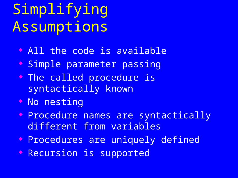
Simplifying Assumptions
All the code is available Simple parameter passing The called procedure is syntactically known No nesting Procedure names are syntactically different from
variables Procedures are uniquely defined Recursion is supported
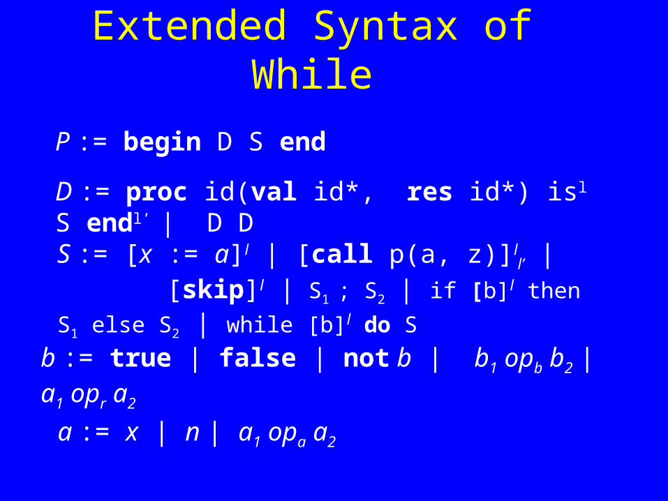
Extended Syntax of While
a := x | n | a1 opa a2
b := true | false | not b | b1 opb b2 | a1 opr a2
S := [x := a]l | [call p(a, z)]ll’ |
[skip]l | S1 ; S2 | if [b]l then S1 else S2 | while [b]l do S
P := begin D S end
D := proc id(val id*, res id*) isl S endl’ | D D
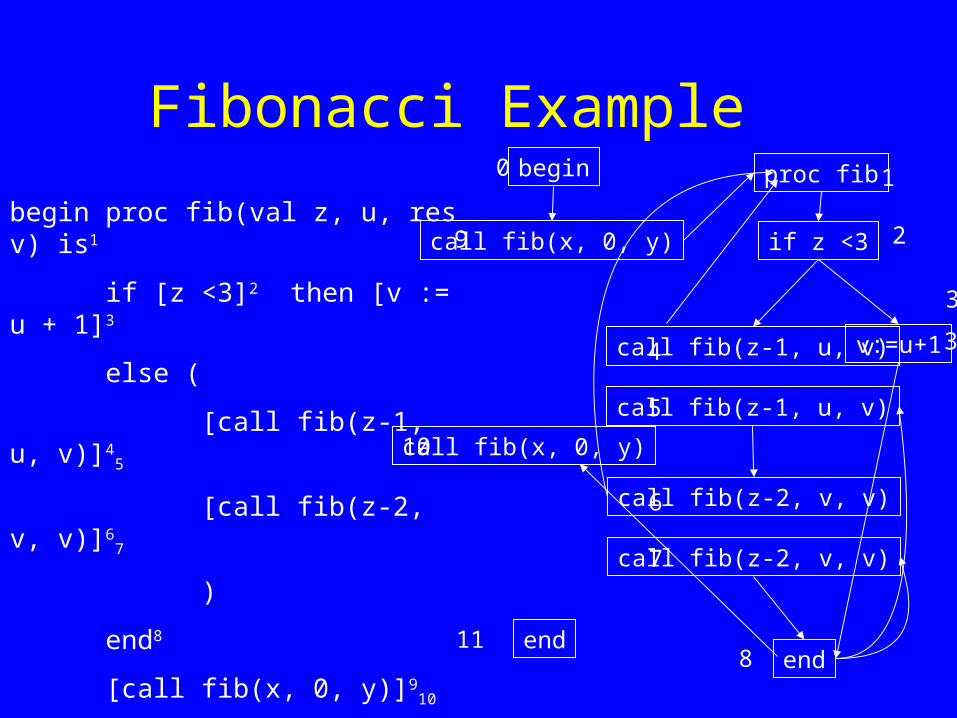
Fibonacci Example
begin proc fib(val z, u, res v) is1
if [z <3]2 then [v := u + 1]3
else (
[call fib(z-1, u, v)]45
[call fib(z-2, v, v)]67
)
end8
[call fib(x, 0, y)]910
end11
begin
call fib(x, 0, y)
call fib(x, 0, y)
end
0
9
10
11
proc fib 1
if z <3 2
3
v:=u+1 3call fib(z-1, u, v)4
call fib(z-1, u, v)5
call fib(z-2, v, v)6
call fib(z-2, v, v)7
end8
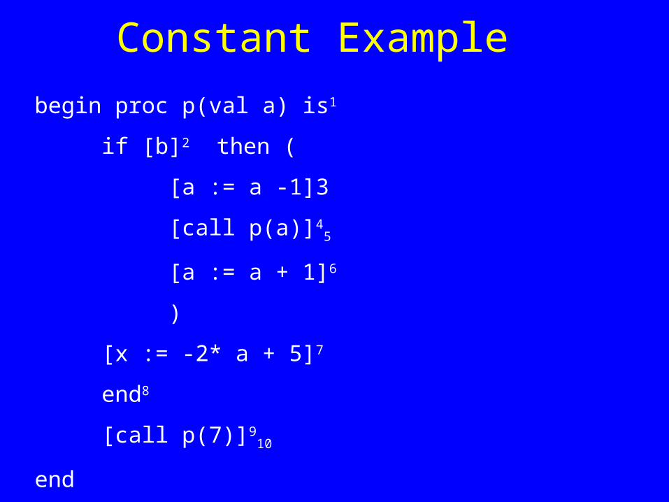
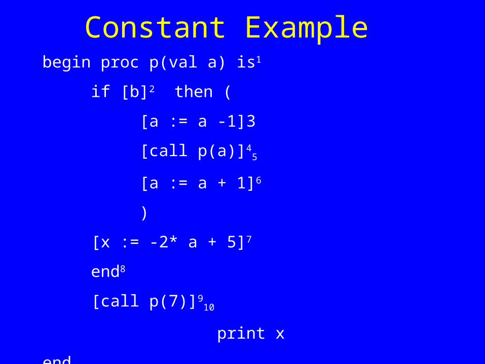
Constant Example
begin proc p(val a) is1
if [b]2 then (
[a := a -1]3
[call p(a)]45
[a := a + 1]6
)
[x := -2* a + 5]7
end8
[call p(7)]910
end
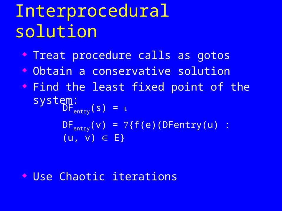
A naive Interprocedural solution Treat procedure calls as gotos Obtain a conservative solution Find the least fixed point of the system:
Use Chaotic iterations
DFentry(s) =
DFentry(v) = {f(e)(DFentry(u) : (u, v) E}

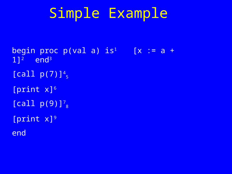
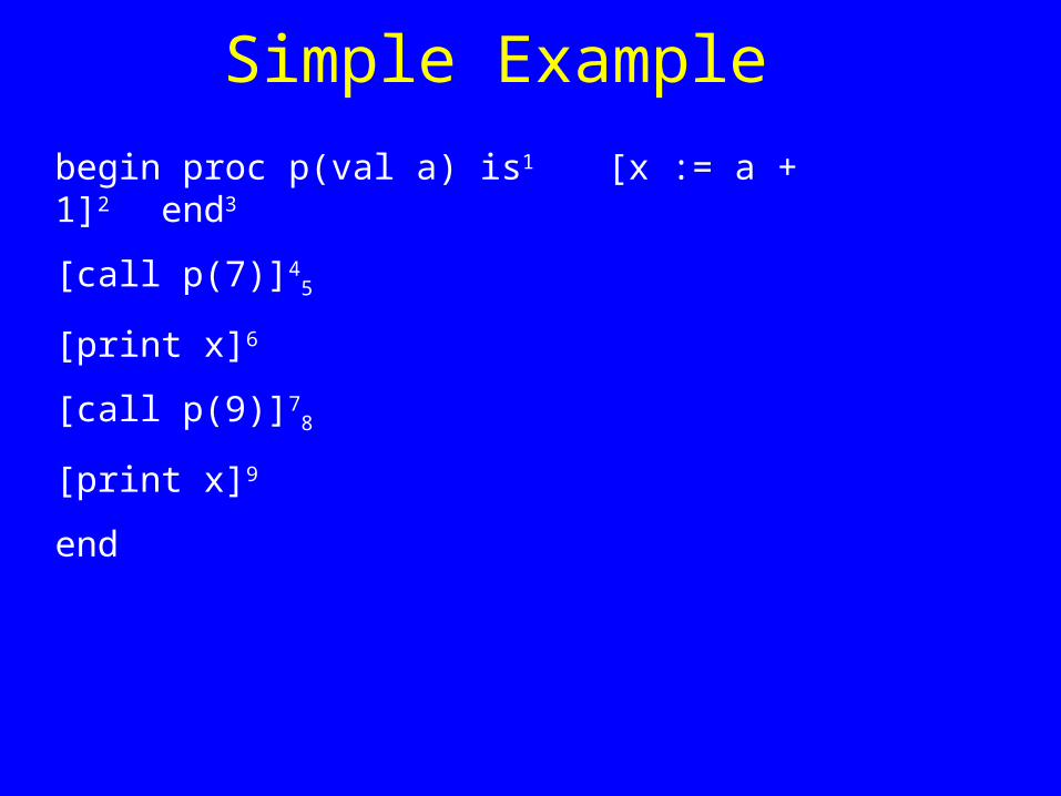
Simple Example
begin proc p(val a) is1 [x := a + 1]2 end3
[call p(7)]45
[print x]6
[call p(9)]78
[print x]9
end

Constant Example
begin proc p(val a) is1
if [b]2 then (
[a := a -1]3
[call p(a)]45
[a := a + 1]6
)
[x := -2* a + 5]7
end8
[call p(7)]910
end
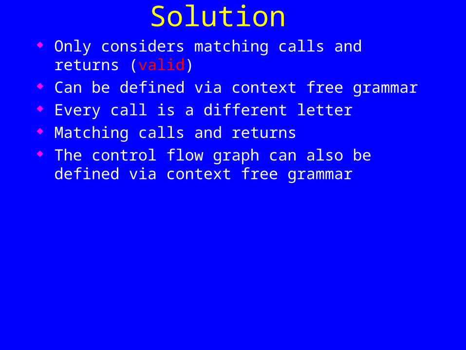
A More Precise Solution Only considers matching calls and returns (valid) Can be defined via context free grammar Every call is a different letter Matching calls and returns The control flow graph can also be defined via context
free grammar
Simple Example
begin proc p(val a) is1 [x := a + 1]2 end3
[call p(7)]45
[print x]6
[call p(9)]78
[print x]9
end

Constant Example
begin proc p(val a) is1
if [b]2 then (
[a := a -1]3
[call p(a)]45
[a := a + 1]6
)
[x := -2* a + 5]7
end8
[call p(7)]910
end
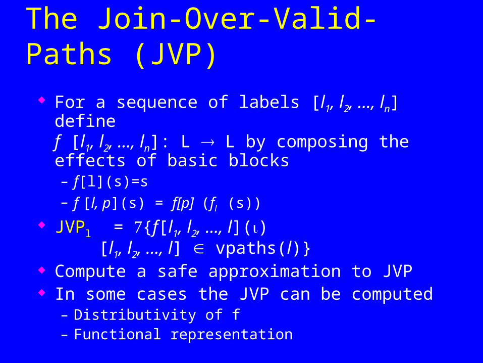
The Join-Over-Valid-Paths (JVP) For a sequence of labels [l1, l2, …, ln] define
f [l1, l2, …, ln]: L L by composing the effects of basic blocks– f[l](s)=s– f [l, p](s) = f[p] (fl (s))
JVPl = {f[l1, l2, …, l]() [l1, l2, …, l] vpaths(l)}
Compute a safe approximation to JVP In some cases the JVP can be computed
– Distributivity of f– Functional representation
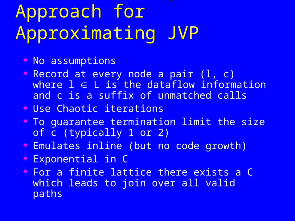
The Call String Approach for Approximating JVP
No assumptions Record at every node a pair (l, c) where l L is
the dataflow information and c is a suffix of unmatched calls
Use Chaotic iterations To guarantee termination limit the size of c
(typically 1 or 2) Emulates inline (but no code growth) Exponential in C For a finite lattice there exists a C which leads to
join over all valid paths
Simple Example
begin proc p(val a) is1 [x := a + 1]2 end3
[call p(7)]45
[print x]6
[call p(9)]78
[print x]9
end
Constant Examplebegin proc p(val a) is1
if [b]2 then (
[a := a -1]3
[call p(a)]45
[a := a + 1]6
)
[x := -2* a + 5]7
end8
[call p(7)]910
print x
end
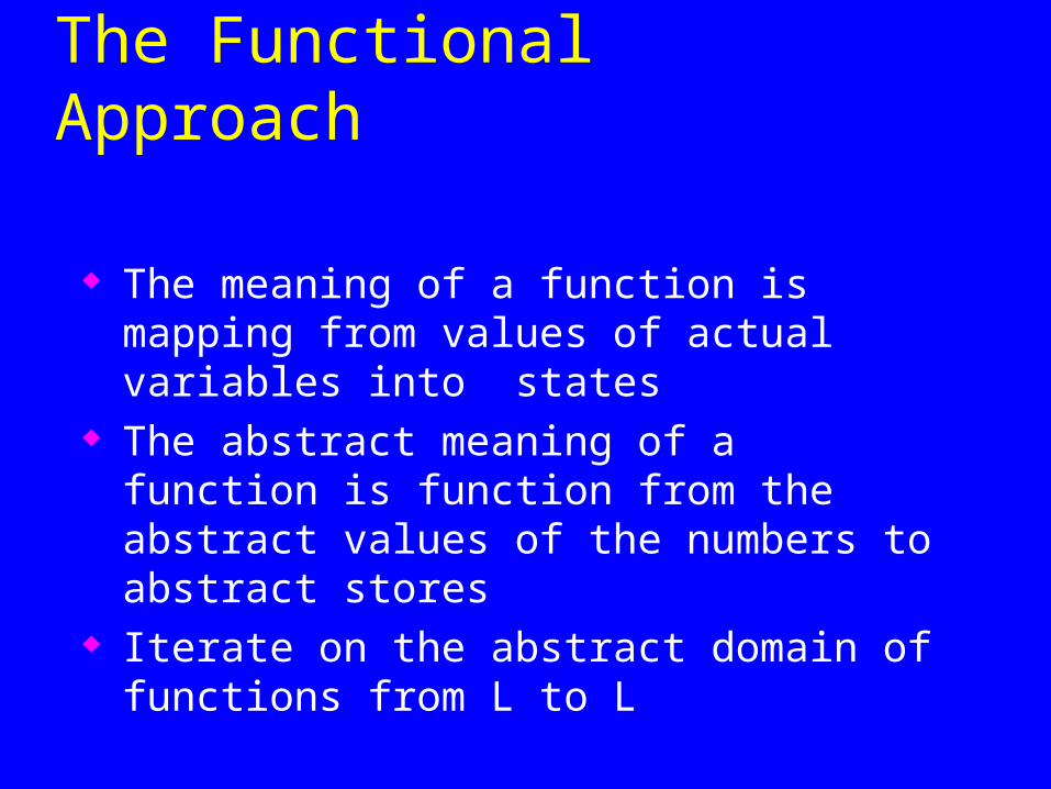
The Functional Approach
The meaning of a function is mapping from values of actual variables into states
The abstract meaning of a function is function from the abstract values of the numbers to abstract stores
Iterate on the abstract domain of functions from L to L
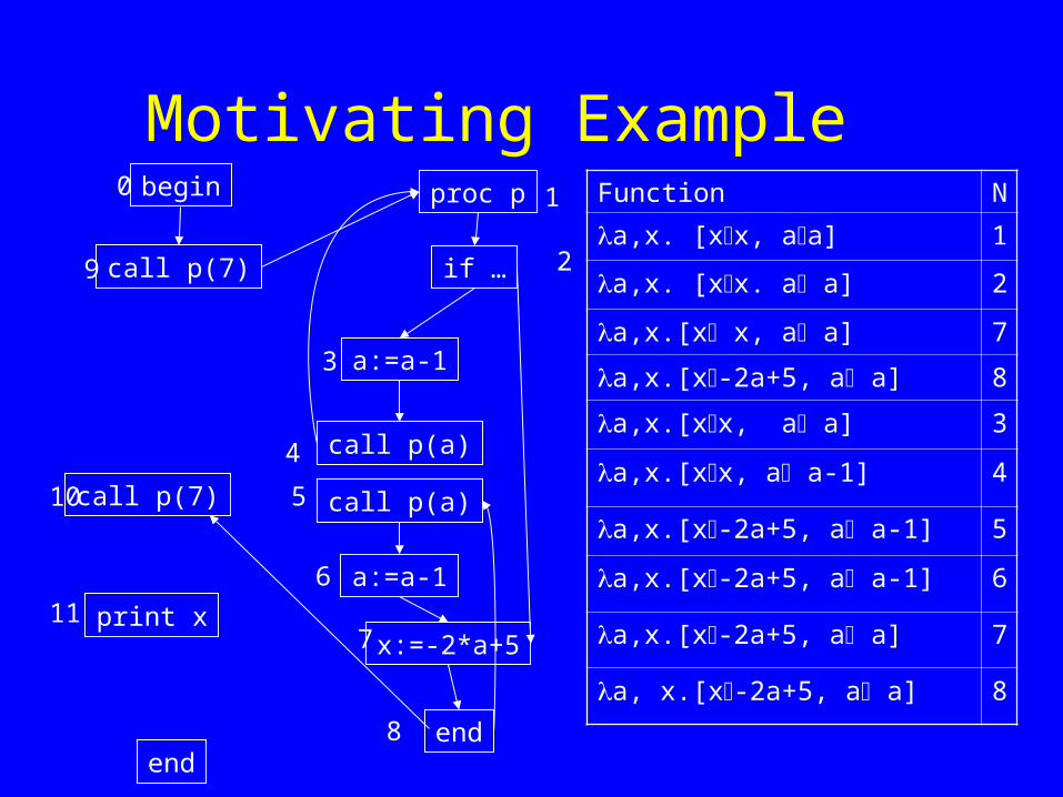
Motivating Examplebegin
call p(7)
call p(7)
print x
0
11
proc p 1
if … 2
a:=a-13
4 call p(a)
6
call p(a)
9
end8
a:=a-1
x:=-2*a+57
end
5
NFunction
1a,x. [xx, aa]
2a,x. [xx. a a]
7a,x.[x x, a a]
8a,x.[x-2a+5, a a]
3a,x.[xx, a a]
4a,x.[xx, a a-1]
5a,x.[x-2a+5, a a-1]
6a,x.[x-2a+5, a a-1]
7a,x.[x-2a+5, a a]
8a, x.[x-2a+5, a a]
10
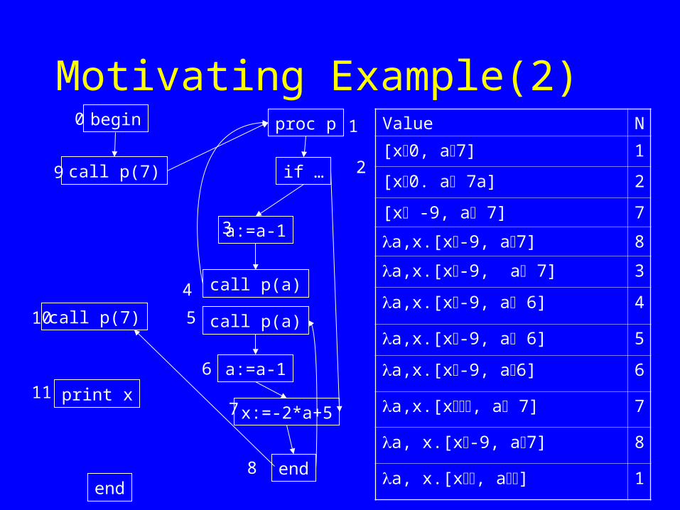
Motivating Example(2)begin
call p(7)
call p(7)
print x
0
11
proc p 1
if … 2
a:=a-13
4 call p(a)
6
call p(a)
9
end8
a:=a-1
x:=-2*a+57
end
5
NValue
1[x0, a7]
2[x0. a 7a]
7[x -9, a 7]
8a,x.[x-9, a7]
3a,x.[x-9, a 7]
4a,x.[x-9, a 6]
5a,x.[x-9, a 6]
6a,x.[x-9, a6]
7a,x.[x, a 7]
8a, x.[x-9, a7]
1a, x.[x, a]
10
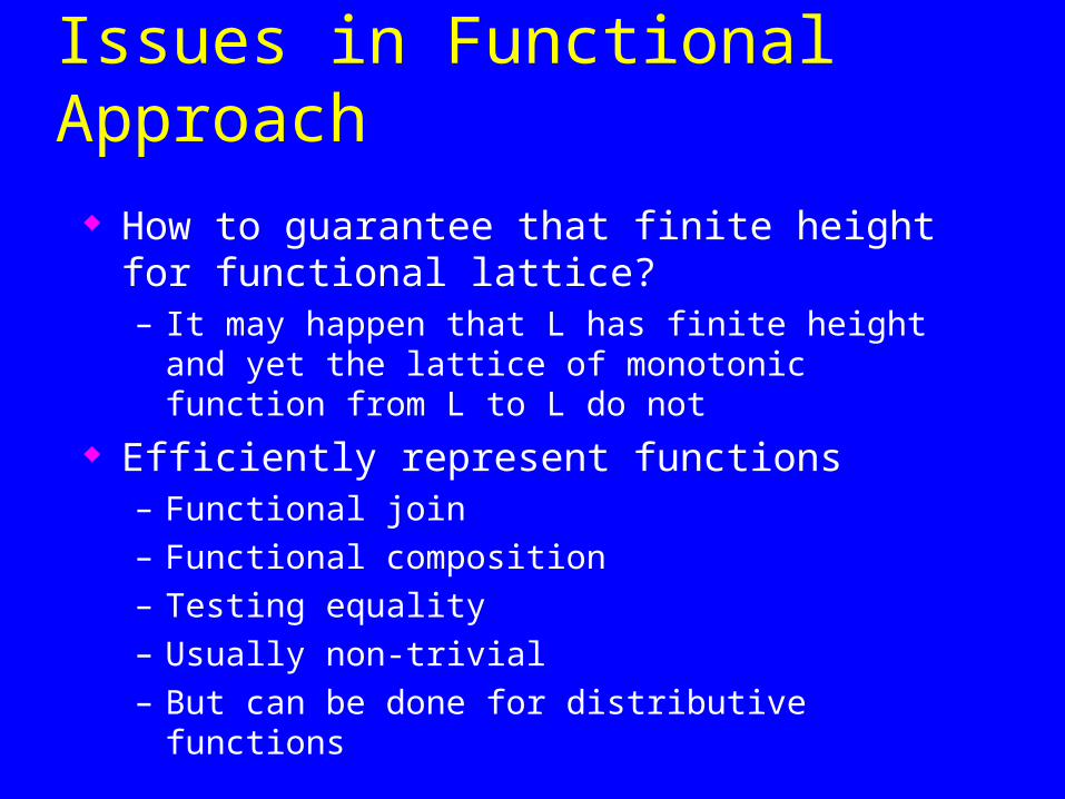
Issues in Functional Approach
How to guarantee that finite height for functional lattice?– It may happen that L has finite height and yet the
lattice of monotonic function from L to L do not
Efficiently represent functions – Functional join
– Functional composition
– Testing equality
– Usually non-trivial
– But can be done for distributive functions
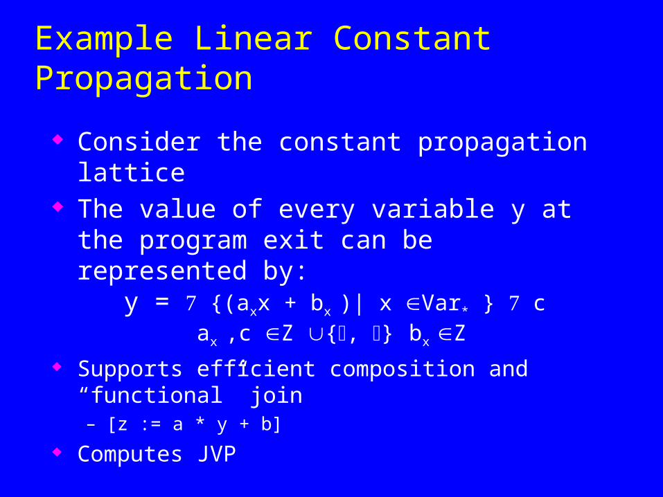
Example Linear Constant Propagation
Consider the constant propagation lattice The value of every variable y at the program exit
can be represented by: y = {(axx + bx )| x Var* } c ax ,c Z {, } bx Z
Supports efficient composition and “functional” join– [z := a * y + b]
Computes JVP
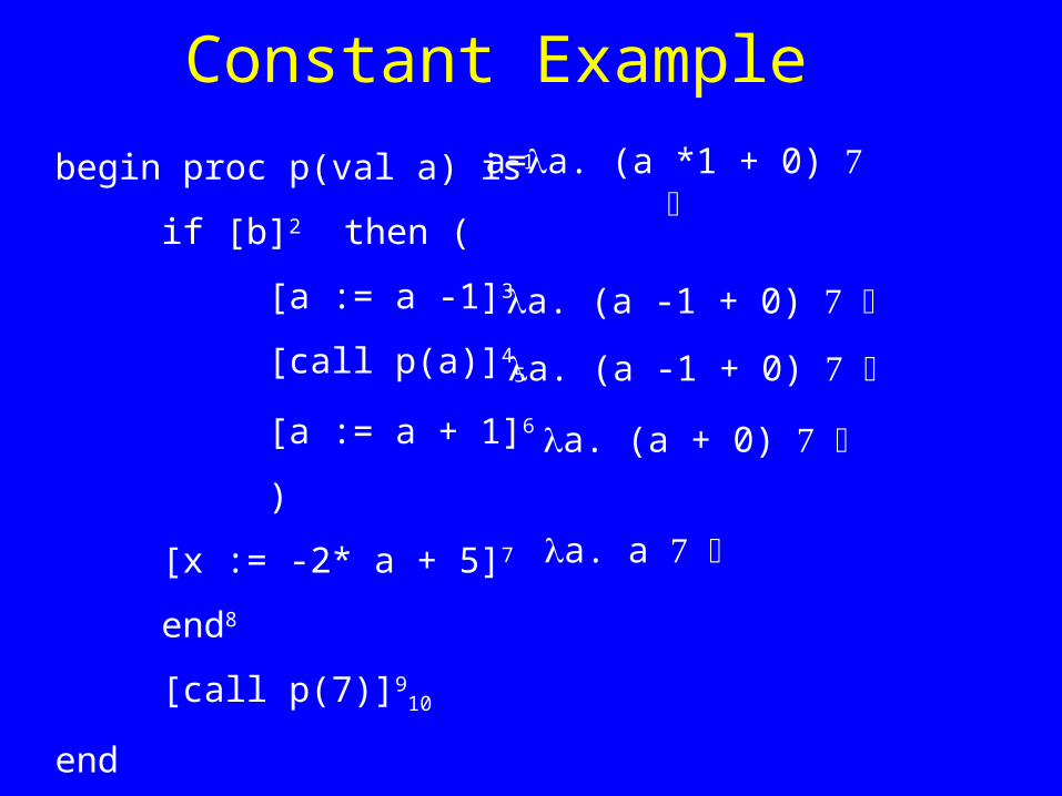
Constant Example
begin proc p(val a) is1
if [b]2 then (
[a := a -1]3
[call p(a)]45
[a := a + 1]6
)
[x := -2* a + 5]7
end8
[call p(7)]910
end
a=a. (a *1 + 0)
a. (a -1 + 0)
a. a
a. (a -1 + 0)
a. (a + 0)
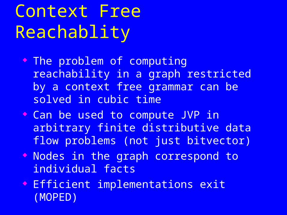
Functional Approach via Context Free Reachablity
The problem of computing reachability in a graph restricted by a context free grammar can be solved in cubic time
Can be used to compute JVP in arbitrary finite distributive data flow problems (not just bitvector)
Nodes in the graph correspond to individual facts Efficient implementations exit (MOPED)
Conclusion
Handling functions is crucial for abstract interpretation
Virtual functions and exceptions complicate thinks
But scalability is an issue Assume-guarantee helps
– But relies on specifications