Interpretable Machine Learning for Materials Design

Interpretable Machine Learning for

Materials Design

James Dean1, Matthias Scheffler2,3, Thomas A. R. Purcell3, Sergey V. Barabash4, RahulBhowmik5, and Timur Bazhirov1,*

1Exabyte Inc, San Francisco, CA, United States2University of California Santa Barbara, Isla Vista, CA, United States

3The NOMAD Laboratory at the Fritz Haber Institute, Berlin, Germany4Intermolecular Inc, San Jose, CA, United States

5Polaron Analytics, Beavercreek, OH, United States*Corresponding Author Email: [email protected]

December 2, 2021

Abstract

Fueled by the widespread adoption of Machine Learning and the high-throughput screening of ma-terials, the data-centric approach to materials design has asserted itself as a robust and powerful toolfor the in-silico prediction of materials properties. When training models to predict material prop-erties, researchers often face a difficult choice between a model’s interpretability or its performance.We study this trade-off by leveraging four different state-of-the-art Machine Learning techniques:XGBoost, SISSO, Roost, and TPOT for the prediction of structural and electronic properties ofperovskites and 2D materials. We then assess the future outlook of the continued integration ofMachine Learning into materials discovery, and identify key problems that will continue to challengeresearchers as the size of the literature’s datasets and complexity of models increases. Finally, weoffer several possible solutions to these challenges with a focus on retaining interpretability, and shareour thoughts on magnifying the impact of Machine Learning on materials design.

Keywords: machine learning, materials science, chemistry, interpretability, rational design.

1 Introduction

Today, big data and artificial intelligence revolutionize many areas of our daily life, and materi-als science is no exception [1–3]. More scientific data is available now than ever before and the sizeof the literature is growing at an exponential rate [4–7]. This has led to multiple efforts in buildingthe digital ecosystem for material discovery, most notably the Materials Genome Initiative (MGI) [8,9].The MGI is a multinational effort focused on improving the tools and techniques surrounding mate-rials research, which recently has included suggestions to adopt the set of Findable, Accessible, In-teroperable, and Reusable (FAIR) principles when reporting data [10]. In the years since the creationof the MGI, a number of large materials and chemical datasets have emerged, including the 2D Ma-terials Encyclopedia (2DMatPedia) [11], Automatic Flow (AFLOW) database [12,13], Computational 2DMaterials Database (C2DB) [14,15], Computational Materials Repository (CMR) [16], Joint AutomatedRepository for Various Integrated Simulations (JARVIS) [17], Materials Project [18], Novel Materials Dis-covery (NOMAD) repository [19], and the Open Quantum Materials Database (OQMD) [20]. We note thatall of these are primarily computational in nature, and that there is still a scarcity of large databasescontaining comprehensively-characterized experimental data. Despite this, at least in computationalmaterials discovery, the current availability of data has been a boon for exploration of the materialsspace, as it allows for highly flexible, data-hungry [21] models to be trained.

One such approach that has seen widespread popularity in recent years is gradient boosting. Gradientboosting [22] is an ensemble technique in which a collection of weak learners (typically decision trees) areincrementally trained with respect to the gradient of the loss function [23]. A well-known implementation

1

arX

iv:2

112.

0023

9v1

[co

nd-m

at.m

trl-

sci]

1 D

ec 2

021

(with over 5,500 citations as of November 2021) is eXtreme Gradient Boosting (XGBoost) [24], which re-formulates the algorithm to provide stronger regularization and improved protection against over-fitting.In chemistry, its applications have been diverse: XGBoost has been used to predict the adsorption en-ergy of noble gases to Metal-Organic Frameworks (MOFs) [25], biological activity of pharmaceuticals [26],atmospheric transport [27], and has even been combined with the representations found in Graph NeuralNetworks (GNNs) to generate accurate models of various molecular properties [28].

Neural networks have also seen a lot of interest, owing to their greater flexibility relative to other modeltypes. This has included the influential Behler-Parinello [29] and Crystal Graph Convolutional NeuralNetwork (CGCNN) [30] architectures based on chemical structure, the Representation Learning fromStoichiometry (Roost) [31] architecture based on chemical formula, and many other approaches [1,2,32–41].

The modern Machine Learning (ML) toolbox is large, although it is still far from complete. As a resultmodel selection techniques are becoming increasingly necessary: this has led to the field of AutomatedMachine Learning (AutoML). This area of work has seen much progress in recent years [42,43], and haseven been extended to Neural Architecture Search (NAS) [44], or the automated optimization of neuralnetwork architectures. In this work, we leverage the Tree-based Pipeline Optimization Tool (TPOT)approach to AutoML [45–47], which uses a Genetic Algorithm (GA) to create effective ML pipelines.Although it generally draws from the models of SciKit-Learn [48], it can also be configured to explore gra-dient boosting models via XGBoost [22], and neural network models via PyTorch [49]. Moreover, TPOTalso performs its own hyperparameter optimization, thus providing a more hands-off solution to identi-fying ML pipelines. The success of GA-based approaches in ML is not isolated to AutoML. Indeed, theyare a fundamental part of genetic programming, where they are used to optimize functions for a partic-ular task [50,51]. Eureqa [52] is a particularly successful example of this [53], leveraging a GA to generateequations fitting arbitrary functions, and has been used in several areas of chemistry, including the gen-eration of adsorption models to nanoparticles [54] and metal atoms to oxide surfaces [55]. This approachof fitting arbitrary functions to a task is also known as “symbolic regression.” Recent work surround-ing compressed sensing has yielded the Sure Independence Screening and Sparsifying Operator (SISSO)approach [56]. SISSO also generates equations mapping descriptors to a target property, proceeding bycombining descriptors using various building blocks, including trigonometric functions, logarithms, ad-dition, multiplication, exponentiation, and many others. This methodology has been highly successfulin a variety of areas including crystal structure classification [57], as well as the prediction of perovskiteproperties [58–60] and 2D topological insulators [61].

The abundance of scientific data in the literature increasingly makes the use of highly flexible (yetdata-hungry) techniques tractable. Although such techniques may deliver models which are highly ac-curate and generalize well to new data, what is oftentimes lost is the physical interpretation of thesemodels. By physical interpretation, we mean an understanding of the relationship between the chosendescriptors and the target property. Although a black-box model which has a high level of accuracy butlittle physical interpretation may lend itself well to the Edisonian screening of a wide range of materials,it may be difficult to understand exactly what feature (or combination of features) actually matters tothe design of the material. Once the screening is done and the target values are calculated, little may bedone to improve performance aside from including new features, adjusting the model’s hyperparameters,or increasing the size of the training set. Alternatively, consider a model which has less accuracy, butwhich has an intuitive explanation, such as an equation describing an approximate relationship betweenfeatures and target. Although such a model may at first glance seem less useful than a highly-accurateblack-box, such a model can help deliver insight into the underlying process that results in the targetproperty. Moreover, by understanding which features are important, the model can give clues into whatmay be done to further improve it — driving the rational discovery of materials. In addition, inter-pretability versus accuracy is not a strict trade-off, and it is possible for interpretable and black-boxmodels to deliver similar accuracy [62]. Therefore, in this work we take steps to compare the performanceof all four models for each problem with respect to i) performance and ii) interpretability.

We leverage a diverse selection of techniques in order to draw comparisons of model accuracy andinterpretability. Taking advantage of the current abundance of chemical data, we can re-use the Density-Functional Theory (DFT) calculations of others stored on several FAIR chemical datasets. A series ofthree problems are investigated: 1) the prediction of perovskite volumes, 2) the prediction of 2D materialbandgaps, and 3) the prediction of 2D material exfoliation energies. For the perovskite volume problem,we leverage the ABX3 perovskite dataset (containing 144 examples) published by Korbel, Marques, andBotti [63]; this dataset is hosted by NOMAD [19], whose repository has strong focus on enabling researchersto report their data such that it satisfies the FAIR data principles [64]. For the 2D material problems,we apply the 2DMatPedia published by Zhou et al [11]; this is a large dataset of 6,351 hypothetical 2D

2

materials identified via a high-throughput screening of systems on the Materials Project [18]. We areaware of other 2D material datasets, such as the C2DB [14] and JARVIS [17], but for the purposes ofsimplifying our study we only choose one.

We find that TPOT delivers high-quality models, generally outperforming the other methods interms of fitness metrics. Despite this, interpretability is not guaranteed, as it can create highly complexpipelines. XGBoost lends itself to interpretation more consistently, as it allows for an importance metric,although it may be harder to understand exactly what the relationship is between the different features(or combinations of different features) and the target variable. We found that Roost performed well onproblems that could be approached via compositional descriptors (i.e. without structural descriptors);as a result, it can help us understand when a target property requires more than just the composition.Finally, we achieve the easiest interpretability from SISSO, as it provides access to descriptors whichdirectly capture the relationship between the features and target variable. Using these results, wediscuss the advantages and disadvantages of each method, and discuss areas where the digital ecosystemsurrounding materials discovery could be improved to improve adherence to FAIR principles. Our workprovides a comparison of several common ML techniques on challenging (but relevant) materials propertyprediction problems.

The manuscript is organized as follows: we begin by training a diverse set of four models, which areXGBoost, TPOT, Roost, and SISSO to investigate each of the three problems, resulting in a total of24 trained models. Performance metrics (and comparative plots) are presented for each trained modelto facilitate comparison, and we discuss the interpretation we can achieve from each of these models.Finally, we provide a discussion of the future outlook of ML in the digital materials science ecosystemand what can be done to further accelerate materials discovery.

2 Methodology

2.1 Data Sources

Crystal structures for the perovskite systems were obtained from the “Stable Inorganic Perovskites”dataset published by Korbel, Marques, and Botti [63], as hosted by NOMAD [19]. This dataset containsa total of 144 DFT-relaxed inorganic perovskites identified via a high-throughput screening strategy.Using this dataset, we develop a model of perovskite volume. As we rely on the use of compositionaldescriptors for these systems, we have scaled the volume of the perovskite unit cell by the number offormula units, such that the volume has units of A3 / formula unit.

Structures for 2D materials were obtained from the 2DMatPedia [11], a large database contain-ing a mixture of 6,351 real and hypothetical 2D systems. This database was generated via a DFT-based high-throughput screening approach, which investigated bulk structures hosted by the MaterialsProject database [18] to find systems which may plausibly form 2D structures. Among other things, the2DMatPedia provides DFT-calculated exfoliation energies and bandgaps, along with a DFT-optimizedstructure for each material. We use this dataset to develop models for the bandgap and exfoliation en-ergy of 2D materials. Although the dataset reports exfoliation energies in units of eV, we have convertedthese into units of J / m2. Bandgaps are reported in units of eV.

2.2 Feature Engineering

To facilitate the development of ML algorithms capable of rapidly predicting material properties, wefocus primarily on features that do not require further (computationally-intensive) DFT calculations.In the case of the 2D material bandgap, we include the DFT-calculated bandgap of the respective bulkmaterial; we note that these values are tabulated on the Materials Project and can be looked up, thuscircumventing the need for further DFT work. A variety of chemical featurization libraries were usedto generate compositional and structural descriptors for the systems we investigated, and are listed insections 2.2.1 and 2.2.2 respectively. Features with values of NaN (which occurred when a feature couldnot be calculated) were assigned a value of 0.

2.2.1 Compositional Descriptors

Compositional (i.e. chemical formula-based) descriptors were calculated via the open-source XenonPypackaged developed by Yamada et al [65]. XenonPy uses tabulated elemental data from Mendeleev [66],Pymatgen [67], the CRC Handbook of Chemistry and Physics [68], and Magpie [69] in order to calculate

3

compositional features. XenonPy does this by combining the elemental descriptors (e.g. atomic weight,ionization potential, etc.) in various ways to form a single composition-weighted value. For example, threecompositional descriptors may be obtained with XenonPy by taking the composition-weighted average,sum, or maximum elemental value of the atomic weight. Leveraging the full list of compositional featuresimplemented in XenonPy results to 290 compositional descriptors, which are explained in greater detailwithin their publication [65].

The compositional descriptors were used for the perovskite volume prediction, 2D material bandgap,and 2D material exfoliation energy prediction problems.

2.2.2 Structural Descriptors

Some structural descriptors were calculated using MatMiner [70], an open-source Python packagegeared towards data-mining material properties. Leveraging MatMiner, the following descriptors werecalculated: Average bond length, average bond angle, Global Instability Index (GII) [71], Ewald Sum-mation Energy [72], a Shannon Information Entropy-based Structural Complexity (both per atom andper cell), and the number of symmetry operations available to the system. In the case of the averagebond length and average bond angle, bonds were determined using Pymatgen’s implementation of theJMol [73] AutoBond algorithm. This list of bonds was also used to calculate an average CoordinationNumber (CN) over all atoms in the unit cell. Finally, we also took the perimeter:area ratio of the 2Dmaterial’s repeating unit.

The structural descriptors were used for the 2D material bandgap and 2D material exfoliation energyproblems.

2.3 Data Filtering

The choice of data filtering methodology was chosen based on the problem at-hand. The perovskitevolume prediction problem did not utilize any data filtering. In the case of the 2D material bandgap andexfoliation energy prediction problems, the data obtained from the 2DMatPedia were required to satisfyall of the following criteria:

1. No elements from the f-block, larger than U, or noble gases were allowed.

2. Decomposition energy must be below 0.5 eV/atom.

3. Exfoliation energy must be strictly positive.

Additionally, in the case of the 2D material bandgap, data were required to have a parent materialdefined on the Materials Project. This was done because we use the Materials Project’s tabulated DFTbandgap of the bulk system as a descriptor for the bandgap of the corresponding 2D system.

2.4 ML Models

When training models, 10% of randomly selected data was held out as a testing set. The sametrain/test split was used for all 4 models considered (XGBoost, TPOT, Roost, and SISSO). To facilitatea transparent comparison between models, in all cases we report the Mean Absolute Error (MAE), RootMean Squared Error (RMSE), Maximum Error, and R2 score of the test set.

2.4.1 Gradient-Boosting with XGBoost

When training XGBoost models, 20% of randomly selected data was held out as an internal validationset. This was used to adopt an early-stopping strategy, where if the model RMSE did not improve after50 consecutive rounds, training was halted early. When training, XGBoost was configured to optimizeits RMSE.

Hyperparameters were optimized via the open-source Optuna [74] framework. The hyperparameterspace was sampled using the Tree-structured Parzen Estimator (TPE) approach [75,76]. To accelerate thehyperparameter search, we leveraged the Hyperband [77] approach for model pruning, using the validationset RMSE to determine whether to prune a model. Hyperband’s budget for the number of trees in theensemble was set to range between 1 and 256 (corresponding with the maximum number of estimatorswe allowed an XGBoost model to have). The search space for hyperparameters is found in Table 1.

4

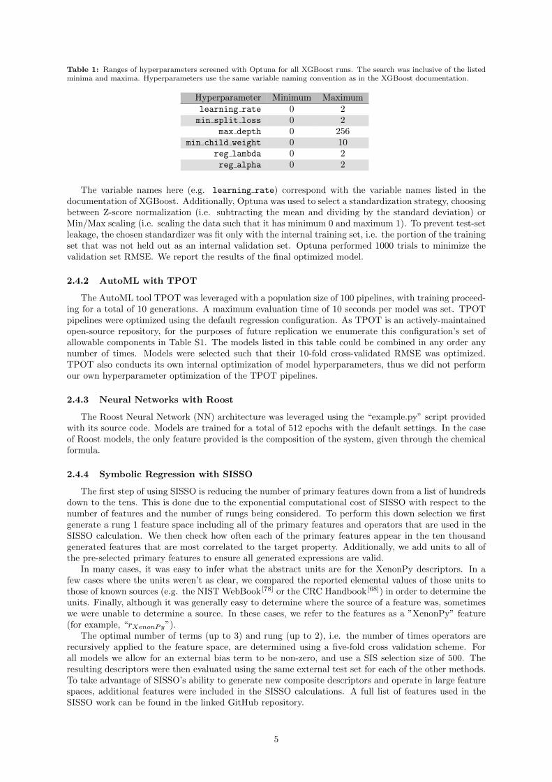
Table 1: Ranges of hyperparameters screened with Optuna for all XGBoost runs. The search was inclusive of the listedminima and maxima. Hyperparameters use the same variable naming convention as in the XGBoost documentation.

Hyperparameter Minimum Maximumlearning rate 0 2min split loss 0 2

max depth 0 256min child weight 0 10

reg lambda 0 2reg alpha 0 2

The variable names here (e.g. learning rate) correspond with the variable names listed in thedocumentation of XGBoost. Additionally, Optuna was used to select a standardization strategy, choosingbetween Z-score normalization (i.e. subtracting the mean and dividing by the standard deviation) orMin/Max scaling (i.e. scaling the data such that it has minimum 0 and maximum 1). To prevent test-setleakage, the chosen standardizer was fit only with the internal training set, i.e. the portion of the trainingset that was not held out as an internal validation set. Optuna performed 1000 trials to minimize thevalidation set RMSE. We report the results of the final optimized model.

2.4.2 AutoML with TPOT

The AutoML tool TPOT was leveraged with a population size of 100 pipelines, with training proceed-ing for a total of 10 generations. A maximum evaluation time of 10 seconds per model was set. TPOTpipelines were optimized using the default regression configuration. As TPOT is an actively-maintainedopen-source repository, for the purposes of future replication we enumerate this configuration’s set ofallowable components in Table S1. The models listed in this table could be combined in any order anynumber of times. Models were selected such that their 10-fold cross-validated RMSE was optimized.TPOT also conducts its own internal optimization of model hyperparameters, thus we did not performour own hyperparameter optimization of the TPOT pipelines.

2.4.3 Neural Networks with Roost

The Roost Neural Network (NN) architecture was leveraged using the “example.py” script providedwith its source code. Models are trained for a total of 512 epochs with the default settings. In the caseof Roost models, the only feature provided is the composition of the system, given through the chemicalformula.

2.4.4 Symbolic Regression with SISSO

The first step of using SISSO is reducing the number of primary features down from a list of hundredsdown to the tens. This is done due to the exponential computational cost of SISSO with respect to thenumber of features and the number of rungs being considered. To perform this down selection we firstgenerate a rung 1 feature space including all of the primary features and operators that are used in theSISSO calculation. We then check how often each of the primary features appear in the ten thousandgenerated features that are most correlated to the target property. Additionally, we add units to all ofthe pre-selected primary features to ensure all generated expressions are valid.

In many cases, it was easy to infer what the abstract units are for the XenonPy descriptors. In afew cases where the units weren’t as clear, we compared the reported elemental values of those units tothose of known sources (e.g. the NIST WebBook [78] or the CRC Handbook [68]) in order to determine theunits. Finally, although it was generally easy to determine where the source of a feature was, sometimeswe were unable to determine a source. In these cases, we refer to the features as a ”XenonPy” feature(for example, “rXenonPy”).

The optimal number of terms (up to 3) and rung (up to 2), i.e. the number of times operators arerecursively applied to the feature space, are determined using a five-fold cross validation scheme. Forall models we allow for an external bias term to be non-zero, and use a SIS selection size of 500. Theresulting descriptors were then evaluated using the same external test set for each of the other methods.To take advantage of SISSO’s ability to generate new composite descriptors and operate in large featurespaces, additional features were included in the SISSO calculations. A full list of features used in theSISSO work can be found in the linked GitHub repository.

5

3 Results

3.1 Perovskite Volume Prediction

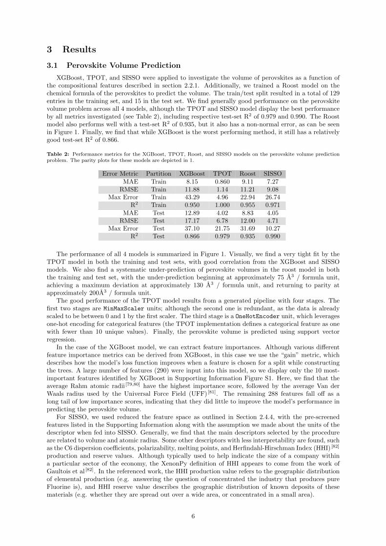
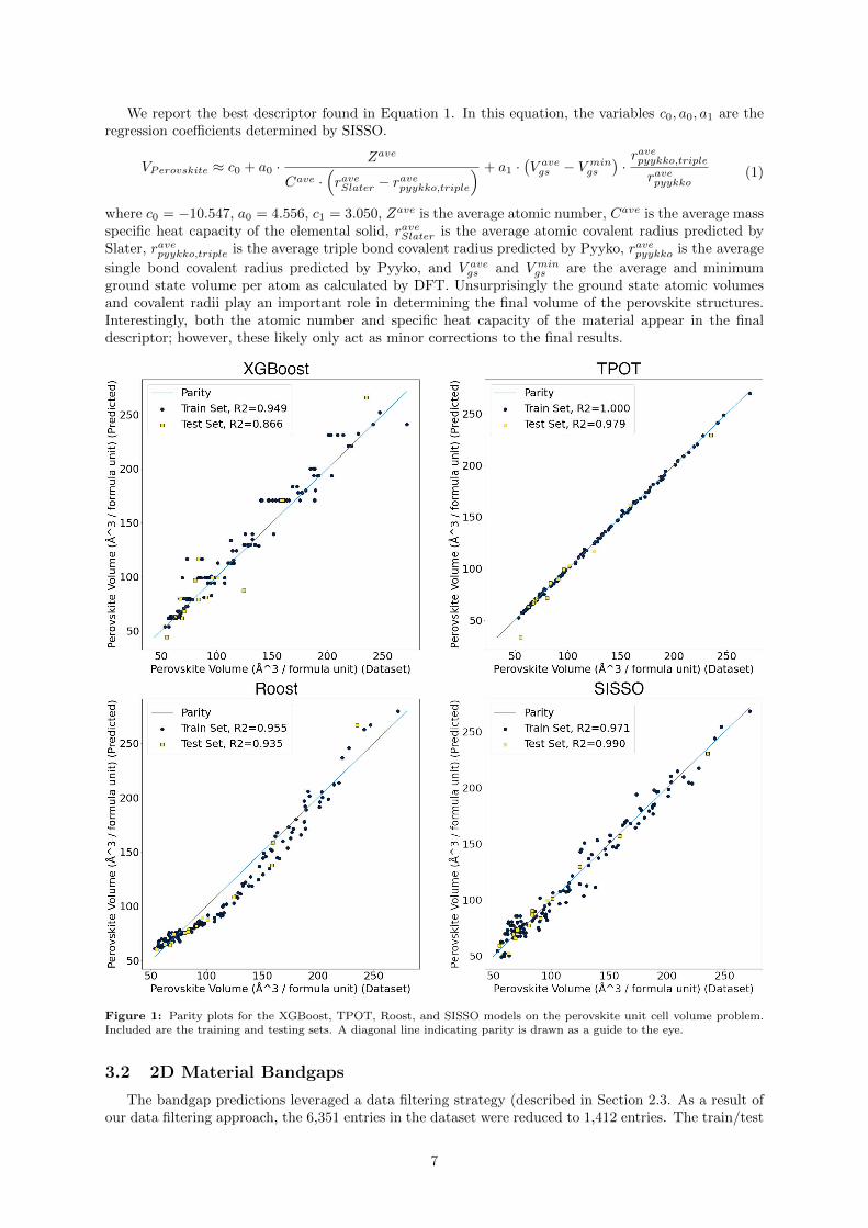
XGBoost, TPOT, and SISSO were applied to investigate the volume of perovskites as a function ofthe compositional features described in section 2.2.1. Additionally, we trained a Roost model on thechemical formula of the perovskites to predict the volume. The train/test split resulted in a total of 129entries in the training set, and 15 in the test set. We find generally good performance on the perovskitevolume problem across all 4 models, although the TPOT and SISSO model display the best performanceby all metrics investigated (see Table 2), including respective test-set R2 of 0.979 and 0.990. The Roostmodel also performs well with a test-set R2 of 0.935, but it also has a non-normal error, as can be seenin Figure 1. Finally, we find that while XGBoost is the worst performing method, it still has a relativelygood test-set R2 of 0.866.

Table 2: Performance metrics for the XGBoost, TPOT, Roost, and SISSO models on the perovskite volume predictionproblem. The parity plots for these models are depicted in 1.

Error Metric Partition XGBoost TPOT Roost SISSOMAE Train 8.15 0.860 9.11 7.27

RMSE Train 11.88 1.14 11.21 9.08Max Error Train 43.29 4.96 22.94 26.74

R2 Train 0.950 1.000 0.955 0.971MAE Test 12.89 4.02 8.83 4.05

RMSE Test 17.17 6.78 12.00 4.71Max Error Test 37.10 21.75 31.69 10.27

R2 Test 0.866 0.979 0.935 0.990

The performance of all 4 models is summarized in Figure 1. Visually, we find a very tight fit by theTPOT model in both the training and test sets, with good correlation from the XGBoost and SISSOmodels. We also find a systematic under-prediction of perovskite volumes in the roost model in boththe training and test set, with the under-prediction beginning at approximately 75 A3 / formula unit,achieving a maximum deviation at approximately 130 A3 / formula unit, and returning to parity atapproximately 200A3 / formula unit.

The good performance of the TPOT model results from a generated pipeline with four stages. Thefirst two stages are MinMaxScaler units; although the second one is redundant, as the data is alreadyscaled to be between 0 and 1 by the first scaler. The third stage is a OneHotEncoder unit, which leveragesone-hot encoding for categorical features (the TPOT implementation defines a categorical feature as onewith fewer than 10 unique values). Finally, the perovskite volume is predicted using support vectorregression.

In the case of the XGBoost model, we can extract feature importances. Although various differentfeature importance metrics can be derived from XGBoost, in this case we use the “gain” metric, whichdescribes how the model’s loss function improves when a feature is chosen for a split while constructingthe trees. A large number of features (290) were input into this model, so we display only the 10 most-important features identified by XGBoost in Supporting Information Figure S1. Here, we find that theaverage Rahm atomic radii [79,80] have the highest importance score, followed by the average Van derWaals radius used by the Universal Force Field (UFF) [81]. The remaining 288 features fall off as along tail of low importance scores, indicating that they did little to improve the model’s performance inpredicting the perovskite volume.

For SISSO, we used reduced the feature space as outlined in Section 2.4.4, with the pre-screenedfeatures listed in the Supporting Information along with the assumption we made about the units of thedescriptor when fed into SISSO. Generally, we find that the main descriptors selected by the procedureare related to volume and atomic radius. Some other descriptors with less interpretability are found, suchas the C6 dispersion coefficients, polarizability, melting points, and Herfindahl-Hirschman Index (HHI) [82]

production and reserve values. Although typically used to help indicate the size of a company withina particular sector of the economy, the XenonPy definition of HHI appears to come from the work ofGaultois et al [82]. In the referenced work, the HHI production value refers to the geographic distributionof elemental production (e.g. answering the question of concentrated the industry that produces pureFluorine is), and HHI reserve value describes the geographic distribution of known deposits of thesematerials (e.g. whether they are spread out over a wide area, or concentrated in a small area).

6

We report the best descriptor found in Equation 1. In this equation, the variables c0, a0, a1 are theregression coefficients determined by SISSO.

VPerovskite ≈ c0 + a0 ·Zave

Cave ·(raveSlater − ravepyykko,triple

) + a1 ·(V avegs − V min

gs

)·ravepyykko,triple

ravepyykko(1)

where c0 = −10.547, a0 = 4.556, c1 = 3.050, Zave is the average atomic number, Cave is the average massspecific heat capacity of the elemental solid, raveSlater is the average atomic covalent radius predicted bySlater, ravepyykko,triple is the average triple bond covalent radius predicted by Pyyko, ravepyykko is the average

single bond covalent radius predicted by Pyyko, and V avegs and V min

gs are the average and minimumground state volume per atom as calculated by DFT. Unsurprisingly the ground state atomic volumesand covalent radii play an important role in determining the final volume of the perovskite structures.Interestingly, both the atomic number and specific heat capacity of the material appear in the finaldescriptor; however, these likely only act as minor corrections to the final results.

Figure 1: Parity plots for the XGBoost, TPOT, Roost, and SISSO models on the perovskite unit cell volume problem.Included are the training and testing sets. A diagonal line indicating parity is drawn as a guide to the eye.

3.2 2D Material Bandgaps

The bandgap predictions leveraged a data filtering strategy (described in Section 2.3. As a result ofour data filtering approach, the 6,351 entries in the dataset were reduced to 1,412 entries. The train/test

7

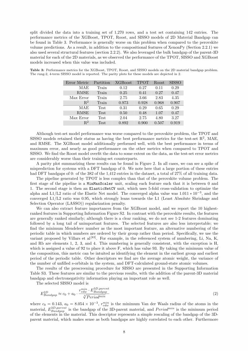
split divided the data into a training set of 1,270 rows, and a test set containing 142 entries. Theperformance metrics of the XGBoost, TPOT, Roost, and SISSO models of 2D Material Bandgap canbe found in Table 3. Performance is generally worse on this problem when compared to the perovskitevolume predictions. As a result, in addition to the compositional features of XenonPy (Section 2.2.1) wealso used several structural features (section 2.2.2). We also leveraged the bulk bandgap of the parent-3Dmaterial for each of the 2D materials, as we observed the performance of the TPOT, SISSO and XGBoostmodels increased when this value was included.

Table 3: Performance metrics for the XGBoost, TPOT, Roost, and SISSO models on the 2D material bandgap problem.The rung-2, 4-term SISSO model is reported. The parity plots for these models are depicted in 2.



R2 Train 0.973 0.928 0.968 0.907MAE Test 0.31 0.29 0.65 0.29


R2 Test 0.892 0.900 0.507 0.919

Although test-set model performance was worse compared to the perovskite problem, the TPOT andSISSO models retained their status as having the best performance metrics for the test-set R2, MAE,and RMSE. The XGBoost model additionally performed well, with the best performance in terms ofmaximum error, and nearly as good performance on the other metrics when compared to TPOT andSISSO. We find the Roost model overfit the data to some extent on the data, as the test-set error metricsare considerably worse than their training-set counterparts.

A parity plot summarizing these results can be found in Figure 2. In all cases, we can see a spike ofmisprediction for systems with a DFT bandgap of 0. We note here that a large portion of these entrieshad DFT bandgaps of 0: of the 382 of the 1,412 entries in the dataset, a total of 27% of all training data.

The pipeline generated by TPOT is less complex than that of the perovskite volume problem. Thefirst stage of the pipeline is a MinMaxScaler unit, scaling each feature such that it is between 0 and1. The second stage is then an ElasticNetCV unit, which uses 5-fold cross-validation to optimize thealpha and L1/L2 ratio of the Elastic Net model. The converged alpha value was 1.011 ∗ 10−3, and theconverged L1/L2 ratio was 0.95, which strongly leans towards the L1 (Least Absolute Shrinkage andSelection Operator (LASSO)) regularization penalty.

We can also extract feature importances from the XGBoost model, and we report the 10 highest-ranked features in Supporting Information Figure S2. In contrast with the perovskite results, the featuresare generally ranked similarly; although there is a clear ranking, we do not see 1-2 features dominatingfollowed by a long tail of unimportant features. The selected features are also less interpretable; wefind the minimum Mendeleev number as the most important feature, an alternative numbering of theperiodic table in which numbers are ordered by their group rather than period. Specifically, we use thevariant proposed by Villars et al [83]. For example, in the referenced system of numbering, Li, Na, K,and Rb are elements 1, 2, 3, and 4. This numbering is generally consistent, with the exception is H,which is assigned a value of 92 to place it above F, which has value 93. By taking the minimum value ofthe composition, this metric can be intuited as identifying the element in the earliest group and earliestperiod of the periodic table. Other descriptors we find are the average atomic weight, the variance ofthe number of unfilled s-orbitals in the system, and DFT-calculated ground-state atomic volumes.

The results of the prescreening procedure for SISSO are presented in the Supporting InformationTable S3. These features are similar to the previous results, with the addition of the parent-3D materialbandgap and electronegativity information playing an important role as well.

The selected SISSO model is

E2DBandgap ≈ c0 + a0 ·

rminvdw · E

3D,parentBandgap

3√Periodmin

(2)

where c0 = 0.143, a0 = 8.054 × 10−3, rminvdw is the minimum Van der Waals radius of the atoms in the

material, E3D,parentBandgap is the bandgap of the 3D-parent material, and Periodmin is the minimum period

of the elements in the material. This descriptor represents a simple rescaling of the bandgap of the 3D-parent material, which makes sense as both bandgaps are highly correlated to each other. Furthermore

8

this results is consistent with the TPOT model which is also primarily controlled by the bandgap of the3D-parent material.

Figure 2: Parity plots for the XGBoost, TPOT, Roost, and SISSO models on the 2D material bandgap problem. Includedare the training and testing sets. A diagonal line indicating parity is drawn as a guide to the eye. Regression statistics forthe models shown on this plot can be found in Table 3.

3.3 2D Material Exfoliation Energy

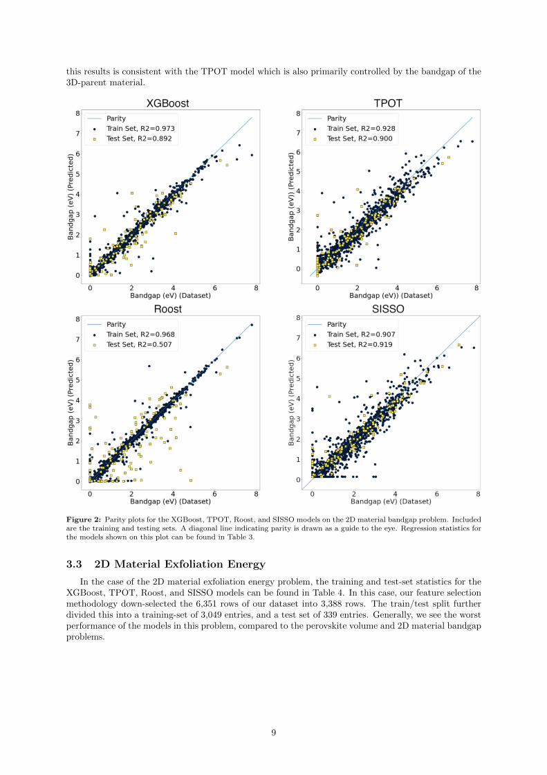
In the case of the 2D material exfoliation energy problem, the training and test-set statistics for theXGBoost, TPOT, Roost, and SISSO models can be found in Table 4. In this case, our feature selectionmethodology down-selected the 6,351 rows of our dataset into 3,388 rows. The train/test split furtherdivided this into a training-set of 3,049 entries, and a test set of 339 entries. Generally, we see the worstperformance of the models in this problem, compared to the perovskite volume and 2D material bandgapproblems.

9

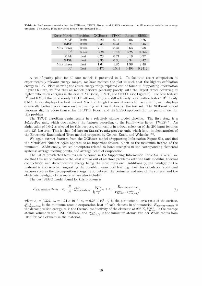
Table 4: Performance metrics for the XGBoost, TPOT, Roost, and SISSO models on the 2D material exfoliation energyproblem. The parity plots for these models are depicted in 3.



R2 Train 0.624 0.702 0.827 0.365MAE Test 0.23 0.21 0.19 0.27


R2 Test 0.476 0.543 0.499 0.2412

A set of parity plots for all four models is presented in 2. To facilitate easier comparison atexperimentally-relevant energy ranges, we have zoomed the plot in such that the highest exfoliationenergy is 2 eV. Plots showing the entire energy range explored can be found in Supporting InformationFigure S6 Here, we find that all models perform generally poorly, with the largest errors occurring athigher exfoliation energies in the case of XGBoost, TPOT, and SISSO. (see Figure 3). The best test-setR2 and RMSE this time is only TPOT, although they are still relatively poor, with a test-set R2 of only0.543. Roost displays the best test-set MAE, although the model seems to have overfit, as it displaysdrastically better performance on the training set than it does on the test set. The XGBoost modelperforms slightly worse than either TPOT or Roost, and the SISSO approach did not perform well forthis problem

The TPOT algorithm again results in a relatively simple model pipeline. The first stage is aSelectFwe unit, which down-selects the features according to the Family-wise Error (FWE) [23]. Analpha value of 0.047 is selected for this purpose, with results in a down-selection of the 299 input featuresinto 125 features. This is then fed into an ExtraTreesRegressor unit, which is an implementation ofthe Extremely Randomized Trees method proposed by Geurts, Ernst, and Wehenkel [84].

We again extract features from the XGBoost model (Supporting Information Figure S3), and findthe Mendeleev Number again appears as an important feature, albeit as the maximum instead of theminimum. Additionally, we see descriptors related to bond strengths in the corresponding elementalsystems: average melting points, and average heats of evaporation.

The list of preselected features can be found in the Supporting Information Table S4. Overall, wesee that this set of features is the least similar out of all three problems with the bulk modulus, thermalconductivity, and decomposition energy being the most prevalent. Additionally, the bandgap of thematerial is also selected, suggesting the possible hierarchical learning. For this calculation additionalfeatures such as the decomposition energy, ratio between the perimeter and area of the surface, and theelectronic bandgap of the material are also included.

The best SISSO model found for this problem is

EExfoliation ≈ c0 + a0 ·P

A· qmin

evaporation ·√∑

i

κi + a1 ·Edecomposition

V aveICSD · rmin

vdw,uff3 (3)

where c0 = 0.327, a0 = 1.24 × 10−4, a1 = 9.26 × 108, PA is the perimeter to area ratio of the surface,

qminevaporation is the minimum atomic evaporation heat of each element in the material, Edecomposition is

the decomposition energy, κi is the thermal conductivity of the elements at 298 K, V aveICSD is the average

atomic volume in the ICSD database, and rminvdw,uff is the minimum atomic Van der Waals radius from

UFF for each element in the material.

10

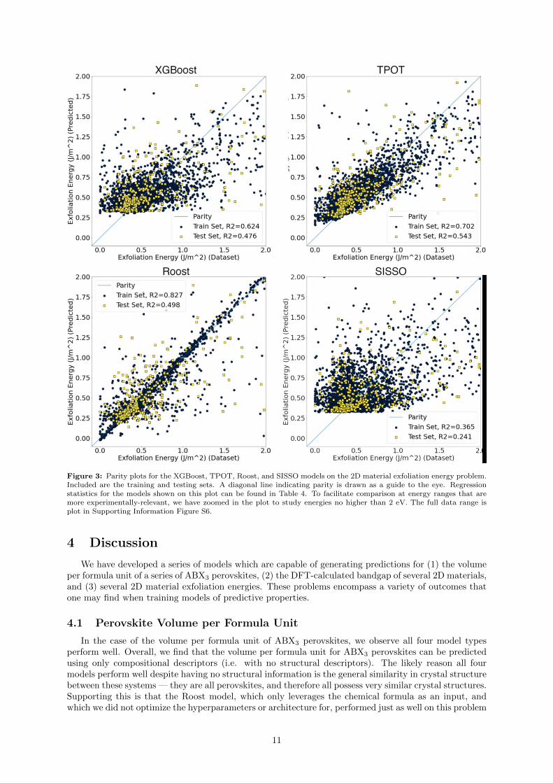
Figure 3: Parity plots for the XGBoost, TPOT, Roost, and SISSO models on the 2D material exfoliation energy problem.Included are the training and testing sets. A diagonal line indicating parity is drawn as a guide to the eye. Regressionstatistics for the models shown on this plot can be found in Table 4. To facilitate comparison at energy ranges that aremore experimentally-relevant, we have zoomed in the plot to study energies no higher than 2 eV. The full data range isplot in Supporting Information Figure S6.

4 Discussion

We have developed a series of models which are capable of generating predictions for (1) the volumeper formula unit of a series of ABX3 perovskites, (2) the DFT-calculated bandgap of several 2D materials,and (3) several 2D material exfoliation energies. These problems encompass a variety of outcomes thatone may find when training models of predictive properties.

4.1 Perovskite Volume per Formula Unit

In the case of the volume per formula unit of ABX3 perovskites, we observe all four model typesperform well. Overall, we find that the volume per formula unit for ABX3 perovskites can be predictedusing only compositional descriptors (i.e. with no structural descriptors). The likely reason all fourmodels perform well despite having no structural information is the general similarity in crystal structurebetween these systems — they are all perovskites, and therefore all possess very similar crystal structures.Supporting this is that the Roost model, which only leverages the chemical formula as an input, andwhich we did not optimize the hyperparameters or architecture for, performed just as well on this problem

11

— albeit with some systematic deviation from parity at intermediate volumes. Although interpretabilityis reduced by virtue of being a neural network, we can still achieve an important insight from this model— just by knowing the chemical formula of the system, we can achieve accurate predictions of perovskitevolumes, which further justifies our use of compositional descriptors (see Section 2.2.1) on this problemas we move to the SISSO, XGBoost, and TPOT models. Additionally, we note this performance wasachieved with a training set containing only 129 entries in the dataset - compared to the original Roostpaper [31] that leveraged approximately 275,000 entries from the OQMD datset [85].

Like the Roost model, we have difficulty in interpreting the pipeline generated by TPOT. TheTPOT model delivers the best performance — which is clearly visible from the parity plot in Figure 1.This performance came at a price, however, and the rather complex pipeline containing scaling, one-hotencoding, and linear support vector regression does not lend itself well to interpretation.

Entering into the realm of interpretability, although the XGBoost model does not produce a directformula for perovskite volumes, we can still gain some insight using it. It is still, however, relativelyaccurate — and allows us access to a feature importance metric (see Supporting Information FigureS2). In this case, we see the five most-important features are the average Rahm [79,80] atomic radius,average UFF [81] atomic radius, sum of elemental velocities of sound in the material, average Ghosh [86]

electronegativity, and the sum of the Pyykko [87] triple-bond covalent radii. Overall, we see a strongreliance on descriptors of atomic radius — which as we noted in the TPOT discussion makes intuitivesense.

Finally, the SISSO model (Equation 1) offers the most direct interpretation, as it is simply an equation.Immediately, we can see that ground state DFT atomic volumes are important. This result is highlyintuitive and is not surprising when we consider that i) we are predicting volume, therefore using anaverage atomic volume makes sense and ii) the TPOT and XGBoost models extensively leveraged atomicradius descriptors that are also related to the volume of the atoms.

The overall good performance of SISSO for this application is promising, as it is one of the mostaccurate models, while being by far the most interpretable. This represents a key advantage to symbolicregression, as if you can find an accurate model, then it will be easy to understand and analyze theresults. Moreover, we note that are not alone in the literature when it comes to leveraging SISSOto generate models of perovskite properties — the last several years have seen success in the creationof models of perovskite properties with this tool. The work of Xie et al. [60] achieved good success inpredicting the octahedral tilt in ABO3 perovskites, the work of Bartel et al. [59] resulted in the creationof a new tolerance factor for ABX3 perovskite formation, and Ihalage and Hao [58] leveraged descriptorsgenerated by SISSO to predict the formation of quaternary perovskites with formula (A1−xA′x)BO3 andA(B1−xB′x)O3.

4.2 2D Material Bandgap

The 2D material bandgap models did not achieve the same performance as for the perovskite systems(see Figure 2). Even in the case of TPOT and SISSO, which still had the best test-set performance bymost metrics, there were a few outliers. Specifically, we find that the test-set MAE for the models rangedbetween 0.29 eV (TPOT and SISSO) and 0.65 eV (Roost) relative to the PBE DFT calculations reportedby the 2DMatPedia. Putting this number in perspective, we note the recent work of Tran et al [88], whichbenchmarked the bandgap predictions of several popular DFT functions for many of the systems in theC2DB; the work identified that the PBE functional exhibited a MAE of 1.50 eV relative to the G0W0

method. Other investigators have studied the prediction of 2D material bandgaps: Rajan et al. [89] alsoachieved a test-set MAE of 0.11 eV on a dataset of 23,870 MXene systems (which, as far as we areaware, has not been made publicly available) using a Gaussian Process regression approach, with DFT-calculated properties including the average M-X bond length, volume per atom, MXene phase, fandheat of formation, and compositional properties including the mean Van der Waals radius, standarddeviation of periodic table group number, standard deviation of the ionization energy, and standarddeviation of the meting temperature. Zhang et al. [90] improved on this error slightly, achieving a test-setMAE of 0.10 eV on the C2DB dataset (around 4000 entries) [14] with both Support-Vector Regressionand Random Forest approaches, albeit using descriptors such as the fermi-energy density of states andtotal energy of the system (requiring further DFT work for additional prediction). In contrast to bothapproaches, which used DFT-calculated values that would need to be obtained for new systems to bepredicted, the only DFT-calculated value we leverage in our feature set is a bulk bandgap tabulatedon the Materials Project [18]. Thus, although our TPOT model had a slightly higher MAE of 0.29 eV,we note that this would not require further DFT work to generate new predictions. As 2D systems

12

are still relatively new, we note that much more work has been performed in the 3D materials space,particularly in the leveraging of neural networks to predict bandgaps. The recent Atomistic LIne GraphNeural Network (ALIGNN) [91] reported a test-set MAE of 0.218 eV for the prediction of bulk materialshosted by Materials Project [18] (which as of October 2021 has over 144,000 inorganic systems). TheMaterials Graph Network (MEGNet) architecture [92] achieved a test-set MAE of 0.32 eV on the bulksystems of the Materials Project. Although these neural network models are on 3D systems, we note thatthey do not leverage DFT properties (which we re-iterate would cause any resulting model to requirea DFT calculation for future prediction) and had access to much larger datasets than the training setwe obtained after filtering the 2DMatPedia entries (see Section 2.3). Overall, although the systems weinvestigate are not 3D bulk systems, we believe this puts the TPOT MAE of 0.29 eV for the bandgap of2D systems in perspective.

In all 4 models we trained, many of the incorrect predictions occur where the DFT bandgap is 0 eV(which represented 27% of the training set values). Because of this, we tried simplifying the bandgapproblem, by training an XGBoost model to predict whether the system was a metal (see SupportingInformation section S.6.3), and showed that we could achieve good results — although we incorporated apurely structural fingerprint, the Sine Matrix Eigenspectrum (see Supporting Information Section S.6.1).As this descriptor resulted in some rather large vectors (of length 40, the maximum number of atomsin any system) with little direct physical intuition, we do not directly include it for the purposes ofthis section. Instead, what we can derive from it is the knowledge that structural features can provideinformation to predict the bandgap.

If we take a closer look at the Roost model, which takes a purely compositional approach to materialsproperty prediction, we can see a poor generalization to the test set (see Table 3). This indicates that wehave likely caused it to over-fit (which could have been improved for example through the use of earlystopping). Overall, we may also use this result to further show the need for structural descriptors whenpredicting bandgaps of these systems.

The TPOT, SISSO, and XGBoost models for 2D material bandgap achieved similar performanceto one-another (see Table 2). Moreover, we again have the opportunity to extract meaning from theTPOT model here, as it leveraged Elastic Net to perform its prediction — a model which is achievedby mixing together Ridge Regression and the LASSO. Additionally, as the L1/L2 ratio is 0.95, thisis nearly entirely L1 regularization (see section 3.2). As a result of this, and that the data were allscaled such that they ranged between 0 and 1, we can view the the feature coefficients approximately(but not entirely) through the lens of LASSO, which does perform feature selection. Doing this, we seethat the corresponding bulk 3D-parent material’s bandgap (as found on Materials Project) is the moststrongly-weighted feature by the elastic net model. This is extremely intuitive as well — it is reasonablefor the bulk bandgap to be correlated with the 2D bandgap.

The XGBoost model, however, suggests an entirely different set of descriptors as being “important.”Instead, we find that the five most-important features are, in order from greatest to least, the mini-mum Mendeleev number, average atomic weight, variance of the number of unfilled s-orbitals, averageground-state DFT volume, and maximum Cordero [93] covalent radius. None of these descriptors have aparticularly intuitive relationship with the bandgap either. This is a similar result to that found by Ra-jan et al. [89], who leveraged several models to predict the GW bandgap of MXene systems; in this work,they found that several of the most-important features exhibited only a statistical (i.e. non-intuitive)relationship with the bandgap.

Finally, the SISSO model (Equation 2) shows an equivalent performance to TPOT and XGBoost,while using only three primary features. Similar to the TPOT model the bandgap of the bulk 3D-parentmaterial is the most important feature, with only minor non-linear contributions from the minimumatomic Van der Waals radius and period. Interestingly, the SISSO model not only misses some of themetallic materials, but also incorrectly predicts some materials to metallic in the training set. Thissuggests the increase simplicity of the SISSO models may slightly reduce their reliability.

Future work on this problem may achieve better performance on the bandgap problem by investigatingthe bond strengths of the different elements in the system. We also note the very good performancethat recent neural network approaches have had on the 3D bandgap problem [91,92], likely due to theirrepresentation of the structure of the 3D systems. Similar to how the Roost model achieves good successwhen compositional descriptors are appropriate, we may find good success in leveraging neural networkapproaches when structural features are required. We note here that Deng et al. [28] achieved good resultson a variety of molecule properties by incorporating various graph representations from different neuralnetwork architectures. Hence, future work in this domain may benefit from the incorporation of theinformation-dense structural fingerprints that may be obtained from neural network-based approaches.

13

4.3 2D Material Exfoliation Energy

We observed some of the worst model performance (across all models) in the case of the 2D materialexfoliation energy. Despite being a larger dataset than either the perovskite (144 total, 129 in thetraining set) or bandgap (1,412 total, 1,270 in the training set), the 3,049 entries in the training set(out of 3,388 total) for the exfoliation energy proved insufficient to achieve good results for any of themodels. Moreover, the compositional and structural features were not sufficient to adequately describethe system.

Some interpretation can at least be derived from the XGBoost and TPOT models. The five most-important features according to XGBoost (see Supporting Information Figure S3) are, in order, themaximum Mendeleev number, average melting point, average evaporation heat, maximum number ofunfilled orbitals, and the sum of the melting points. In the case of the TPOT model, we arrived at anextremely randomized tree approach, which also has a feature importance metric. Here, we find that theaverage Van der Waals radius, maximum dipole polarizability, minimum atomic weight, maximum atomicweight, and maximum elemental (and tabulated) DFT bandgap are weighted as important. Between thetwo models, we see much difference in which features are deemed important. In the XGBoost model,the average melting point, sum of melting points, and average evaporation heat of the elemental systemscan be rationalized if we realize that these are all driven by the strength of the interaction betweenatoms in the material, thus these descriptors may provide information relating to the forces that mustbe overcome when exfoliation is performed. Many of the other features in the two models correlate withsize: the maximum Mendeleev number, average Van der Waals radius, and minimum / maximum atomicweights all provide a description of the size of the atoms in the system.

Finally, the SISSO model (Equation 3) echos these findings. Although it is less performant, it providesintuitive descriptors that tell a similar story. One term takes the ratio of the decomposition energy andapproximations to the atomic volume. This captures a description of atomic size as well as the strengthof atomic bonds. Additionally, the second term in the model incorporates information about the surface,thermal conductivity and the heat or evaporation. Although the second term is less descriptive, it stillcaptures terms relating to the size of the atoms and bond strengths of that atoms involved in the 2Dmaterial. The relatively poor performance of the SISSO models, also highlights the need for betterinput features to describe the exfoliation energy of a material. In cases where only a loose correlationbetween a target property and the inputs exist, the relative simplicity of symbolic regression modelscan be detrimental. While TPOT and XGBoost can utilize information from all features in their finalpredictions, symbolic regression in general and SISSO in particular only acts on the order of tens offeatures. Because of this, it is likely that more structural information is needed to get accurate modelswith SISSO.

In effect, the models can be interpreted as collectively describing the exfoliation energy as a functionof i) the size of the atoms in the 2D material and ii) the strength of the intermolecular forces betweenthose atoms. When we predict exfoliation energies, we’re predicting the interaction between layers in anexfoliable material. Overall, finding better methods of cheaply approximating these weak interactionsmay provide better results in the prediction of exfoliation. Additionally, as the number of datasetswhich contain exfoliation energies increases (such as the 2DMatPedia [11], C2DB [14,15] and JARVIS [17]),further insight into this problem will be possible, and more-complex (albeit less-interpretible) modelswill become feasible.

Additionally, in order to obtain more-accurate predictions of exfoliation energy, data generated via amore thorough computational treatment may be required. We illustrate this by examining an outlier inthe training set at 9.9 J / m2, which all four models heavily under-predicted (see Supporting Informationfigure S6) (7-8 eV in the case of XGBoost and TPOT, and over 9 eV in the case of Roost and SISSO).Upon closer examination of this system, we find that it is actually a pair of layers containing N atoms(Figure 4 A). The 2DMatPedia [11] reports that this system (2dm-id 5985) was not directly sourced bya simulated exfoliation from a bulk structure, but instead was obtained by substituting the atoms in ahypothetical 2D Sb structure (Figure 4 B). The Sb structure (2dm-id 4275) was obtained by a simulatedexfoliation from a structure obtained from materials project (Figure 4 C). The parent bulk material (mp-567409) is reported by the Materials Project [18] to be a monoclinic crystal which undergoes a favorabledecomposition (energy above hull is reported as 0.121 eV / atom) to a triclinic system. That being said,as this is a hypothetical 2D system, comparison with the hypothetical 3D bulk system was necessary forthe calculation of exfoliation energy. As the prediction of crystal structure is a very challenging field withfew easy approximations [94], this may have contributed further to the extreme value of the exfoliationenergy. Indeed, as Zhou et al report [11], the decomposition energy lends itself better to assessing whethera material is truly stable. Indeed, despite the extremely high exfoliation energy of this hypothetical 2D

14

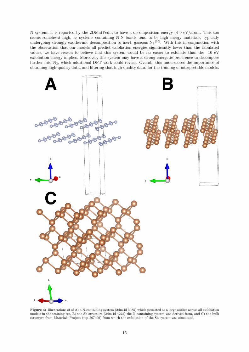
N system, it is reported by the 2DMatPedia to have a decomposition energy of 0 eV/atom. This tooseems somehwat high, as systems containing N-N bonds tend to be high-energy materials, typicallyundergoing strongly exothermic decomposition to inert, gaseous N2

[95]. With this in conjunction withthe observation that our models all predict exfoliation energies significantly lower than the tabulatedvalues, we have reason to believe that this system would be far easier to exfoliate than the 10 eVexfoliation energy implies. Moreover, this system may have a strong energetic preference to decomposefurther into N2, which additional DFT work could reveal. Overall, this underscores the importance ofobtaining high-quality data, and filtering that high-quality data, for the training of interpretable models.

Figure 4: Illustrations of of A) a N-containing system (2dm-id 5985) which persisted as a large outlier across all exfoliationmodels in the training set, B) the Sb structure (2dm-id 4275) the N-containing system was derived from, and C) the bulkstructure from Materials Project (mp-567409) from-which the exfoliation of the Sb system was simulated.

15

4.4 Future Outlook

As ML is further integrated into materials discovery workflows, we anticipate that the numeroussuccesses neural networks have presented [1–3,29–41] will continue to propel them onto the cutting edgeof chemical property prediction. This comes with the challenge of honing our techniques for theirinterpretation, an area which has seen much interest in recent years, and where there is still plentyof opportunity for further development [96,97]. We also expect AutoML techniques such as TPOT willcontinue gaining traction in materials discovery, due to the amount of success and attention they haverecently had [42–47]. This too presents the challenge of interpretability if highly complex pipelines aregenerated (see Sections 3.1 and 4.1). We note here that part of the value that AutoML techniques bringis the ability to make advanced techniques accessible to a wider audience of researchers by lowering thebarrier of entry. Hence, we expect that the problem of interpretation may be compounded for AutoML(and especially NAS) systems: the ability to automatically extract some level of interpretation from thegenerated pipelines is important for automation to make ML truly accessible to non-experts. Overall,we expect that as neural network models and AutoML algorithms continue to grow in capability andcomplexity, work in developing the tools and techniques needed to interpret them will see a greaterattention.

In contrast with challenge of interpreting neural networks or the pipelines found by AutoML systems,symbolic regression tools like Eureqa and SISSO yield an exact equation describing the model, and arethus easier to interpret. This makes it easier to achieve key insights with physical interpretations — suchas the very intuitive way in which SISSO is able to describe the systems. Overall, despite its reducedability to predict the exfoliation energy of a material when compared to the models of TPOT, XGBoost,and Roost, we note the mathematical equations returned by SISSO provide a direct relationship betweenthe target properties and model predictions. Additionally, in the case of the exfoliation energy, we believethat we may see further improvements by including richer structural information. We base this on theobservation that the Roost model performed poorly on both of this problems – recalling that Roost isonly provided the chemical formula of the system, this could indicate that compositional descriptorsalone are insufficient to describe these properties. Indeed, it is well-known that structure and energy areintimately related (the fundamental assumption of geometry optimization techniques is that energy is afunction of atomic position), hence it can be inferred that exfoliation energy and structure are similarlyrelated. In the case of bandgaps, we note that there is also a strong dependence on structure; Chaveset al [98] notes that the number of layers in a 2D material can strongly influence the band gap, reportingdifferences of up to several eV can occur between the bulk and monolayer form of a material.

Interoperability is still a challenge in the materials discovery ecosystem. Although it is possible toeasily convert between different chemical file formats (e.g. by OpenBabel [99]), and packages such asPymatgen [67], Atomic Simulation Environment (ASE) [100], and RDKit [101] can easily convert to eachothers’ format, we note that there is a challenge of calculating features using a variety of differentpackages. Some tools expect Pymatgen objects (e.g. XenonPy), others expect ASE objects, whereasothers require RDKit objects (e.g. all of the descriptors in the RDKit library) to perform a calculationof features, thus creating some standard for the interoperability of these packages would be beneficial.Additionally, further efforts should be made to report the sources of data used by featurization packages.We note that MatMiner [70] is exemplary in this regard: each of the featurization classes it defines has a“citation” method returning the appropriate source to credit. Mendeleev [66] is another good example ofthis; within its documentation, a table lists citations for many (though not all) of the elemental propertiesit can return. Overall, by placing a stronger focus on i) interoperability and ii) data provenance, thePython materials modeling ecosystem can be made stronger — and therefore help accelerate materialsdiscovery.

All of the models we have investigated in this work required sufficient training data to avoid over-fitting. Although techniques such as cross-validation, early-stopping (in the case of neural networks andXGBoost), and train/test splitting can help guard against (and detect) over-fitting, having a sufficiently-large dataset is of the utmost importance to achieve truly generalizable models. As a result, there is acritical need for data management approaches that satsify the set of FAIR principles. This crucial needfor effective data management has led to the incorporation of data storage tooling in popular chemistrypackages including Pymatgen [67], ASE [100], and RDKit [101]. Moreover, advances in both computationalcapacity and techniques has given rise to studies performing the high-throughput screening of chemicalsystems [102–104]. This has resulted in the development of tools focusing on the provenance of data,such as the Automated Interactive Infrastructure and Database for Computational Science (AiiDA)system [105,106].

Overall, we have identified a series of key issues should see more attention as the digital ecosystem

16

surrounding materials modeling continues to develop. First, interpretability of models allows us to derivephysical understanding from the available data. This is a key benefit of symbolic regression tools likeSISSO, which result in the creation of human-readable equations describing the model. Additionally,increasing the accessibility of ML techniques through automation (such as in the field of AutoML) willallow a wider range of researchers the ability to benefit from advances in modeling techniques. Datamanagement and data provenance is another major issue, which allows us to better understand whichdatasets can be combined (e.g. when combining DFT datasets, the methodologies should be consistentbetween them), and to help us understand if something intrinsic to the training data is affecting modelperformance. These data management goals are core focus of platforms such as Exabyte [107], whichprovides an all-in-one solution for i) storing material data and metadata, ii) storing the methodologyrequired to derive a property from a material, and iii) providing the means to automatically performcalculations, and iv) automatically extracting calculation results and storing them for the user. Thisfocus on providing a tool that manages materials, workflows, and calculations has allowed Exabyte to bea highly successful platform, which has led to studies involving automated phonon calculations [108], high-throughput screening of materials for their band-structure [109,110]. Future capabilities of the platformare slated to include a categorization scheme for computational models to provide even more metadatato track the provenance of calculated material properties [111].

5 Conclusion

In this work, we have performed a series of benchmarks on a diverse set of ML algorithms: gradientboosting (XGBoost), AutoML (TPOT), deep learning (Roost), and symbolic regression (SISSO). Thesemodels were used to predict i) the volume of perovskites, ii) the DFT bandgap of 2D materials, and iii)the exfoliation energy of 2D materials. We identify that TPOT, SISSO and XGBoost tend to producemore-accurate models than Roost,but Roost works well in systems where compositional descriptors areenough to predict the target property. Finally, although SISSO was unable to find an accurate modelfor the exfoliation energy, it provides a human-readable equation describing the model, facilitating aneasier interpretation compared to the other algorithms. We believe that interpretability will remain a keychallenge to address as complex techniques (i.e. neural networks and AutoML) become more mainstreamwithin the digital materials modeling ecosystem. Overall, as tools improving the accessibility of machine-learning continue to be developed, data provenance and model interpretability will become even moreimportant, as it is a critical part of ensuring the accessibility of these techniques. By working to ensurethat a wider audience of researchers can achieve insight from the rich digital ecosystem of materialsdesign, materials discovery can be accelerated.

Acknowledgements

This research was supported by the US Department of Energy (DoE) Small Business InnovationResearch (SBIR) program (grant no. DE-SC0021514). Computational resources were provided by Ex-abyte Inc. The authors also wish to acknowledge fruitful discussions with Rhys Goodall (University ofCambridge) regarding the Roost framework.

Data Access

Jupyter (Python) notebooks are available on Exabyte’s GitHub (https://github.com/Exabyte-io/Scientific-Projects/tree/arXiv_interpretableML_nov2021), which contains code to reproduce ourresults and figures.

Disclosures

James Dean and Timur Bazhirov are employed by Exabyte Inc.

17

https://github.com/Exabyte-io/Scientific-Projects/tree/arXiv_interpretableML_nov2021

https://github.com/Exabyte-io/Scientific-Projects/tree/arXiv_interpretableML_nov2021

References

[1] Claudia Draxl and Matthias Scheffler. Big Data-Driven Materials Science and Its FAIR DataInfrastructure. In Wanda Andreoni and Sidney Yip, editors, Handbook of Materials Modeling:Methods: Theory and Modeling, pages 49–73. Springer International Publishing, Cham, 2020. ISBN978-3-319-44677-6. doi: 10.1007/978-3-319-44677-6 104.

[2] Adam C. Mater and Michelle L. Coote. Deep Learning in Chemistry. Journal of Chemical Informa-tion and Modeling, 59(6):2545–2559, June 2019. ISSN 1549-9596. doi: 10.1021/acs.jcim.9b00266.

[3] Keith T. Butler, Daniel W. Davies, Hugh Cartwright, Olexandr Isayev, and Aron Walsh. Machinelearning for molecular and materials science. Nature, 559(7715):547–555, July 2018. ISSN 1476-4687. doi: 10.1038/s41586-018-0337-2.

[4] Lutz Bornmann and Rudiger Mutz. Growth rates of modern science: A bibliometric analysis basedon the number of publications and cited references. Journal of the Association for InformationScience and Technology, 66(11):2215–2222, 2015. ISSN 2330-1643. doi: 10.1002/asi.23329.

[5] Derek J. De Solla Price. Little Science, Big Science. Columbia University Press, March 1963. ISBN978-0-231-88575-1. doi: 10.7312/pric91844.

[6] Derek J. de Solla Price. Science since Babylon. Yale University Press, New Haven, enl. ed edition,1975. ISBN 978-0-300-01797-7.

[7] Derek J. de Solla Price. Networks of Scientific Papers. Science, 149(3683):510–515, July 1965. doi:10.1126/science.149.3683.510.

[8] National Science and Technology Council. Materials Genome Initiative for Global Competitiveness.Government, White House Office of Science and Technology Policy, United States of America, June2011.

[9] Subcommittee on the Materials Genome Initiative Committee on Technology. Materials GenomeInitiative Strategic Plan. Government, National Science and Technology Council, United States ofAmerica, November 2021.

[10] Juan J. de Pablo, Nicholas E. Jackson, Michael A. Webb, Long-Qing Chen, Joel E. Moore, DaneMorgan, Ryan Jacobs, Tresa Pollock, Darrell G. Schlom, Eric S. Toberer, James Analytis, IsmailaDabo, Dean M. DeLongchamp, Gregory A. Fiete, Gregory M. Grason, Geoffroy Hautier, YifeiMo, Krishna Rajan, Evan J. Reed, Efrain Rodriguez, Vladan Stevanovic, Jin Suntivich, KatsuyoThornton, and Ji-Cheng Zhao. New frontiers for the materials genome initiative. npj ComputationalMaterials, 5(1):1–23, April 2019. ISSN 2057-3960. doi: 10.1038/s41524-019-0173-4.

[11] Jun Zhou, Lei Shen, Miguel Dias Costa, Kristin A. Persson, Shyue Ping Ong, Patrick Huck, YunhaoLu, Xiaoyang Ma, Yiming Chen, Hanmei Tang, and Yuan Ping Feng. 2DMatPedia, an opencomputational database of two-dimensional materials from top-down and bottom-up approaches.Scientific Data, 6(1):86, June 2019. ISSN 2052-4463. doi: 10.1038/s41597-019-0097-3.

[12] Stefano Curtarolo, Wahyu Setyawan, Gus L. W. Hart, Michal Jahnatek, Roman V. Chepulskii,Richard H. Taylor, Shidong Wang, Junkai Xue, Kesong Yang, Ohad Levy, Michael J. Mehl,Harold T. Stokes, Denis O. Demchenko, and Dane Morgan. AFLOW: An automatic frameworkfor high-throughput materials discovery. Computational Materials Science, 58:218–226, June 2012.ISSN 0927-0256. doi: 10.1016/j.commatsci.2012.02.005.

[13] Stefano Curtarolo, Wahyu Setyawan, Shidong Wang, Junkai Xue, Kesong Yang, Richard H. Taylor,Lance J. Nelson, Gus L. W. Hart, Stefano Sanvito, Marco Buongiorno-Nardelli, Natalio Mingo, andOhad Levy. AFLOWLIB.ORG: A distributed materials properties repository from high-throughputab initio calculations. Computational Materials Science, 58:227–235, June 2012. ISSN 0927-0256.doi: 10.1016/j.commatsci.2012.02.002.

[14] Morten Niklas Gjerding, Alireza Taghizadeh, Asbjørn Rasmussen, Sajid Ali, Fabian Bertoldo,Thorsten Deilmann, Nikolaj Rørbæk Knøsgaard, Mads Kruse, Ask Hjorth Larsen, SimoneManti, Thomas Garm Pedersen, Urko Petralanda, Thorbjørn Skovhus, Mark Kamper Svendsen,Jens Jørgen Mortensen, Thomas Olsen, and Kristian Sommer Thygesen. Recent progress of the

18

computational 2D materials database (C2DB). 2D Materials, 8(4):044002, July 2021. ISSN 2053-1583. doi: 10.1088/2053-1583/ac1059.

[15] Sten Haastrup, Mikkel Strange, Mohnish Pandey, Thorsten Deilmann, Per S. Schmidt, Nicki F.Hinsche, Morten N. Gjerding, Daniele Torelli, Peter M. Larsen, Anders C. Riis-Jensen, JakobGath, Karsten W. Jacobsen, Jens Jørgen Mortensen, Thomas Olsen, and Kristian S. Thygesen. TheComputational 2D Materials Database: High-throughput modeling and discovery of atomically thincrystals. 2D Materials, 5(4):042002, September 2018. ISSN 2053-1583. doi: 10.1088/2053-1583/aacfc1.

[16] David D. Landis, Jens S. Hummelshøj, Svetlozar Nestorov, Jeff Greeley, Marcin Du lak, ThomasBligaard, Jens K. Nørskov, and Karsten W. Jacobsen. The Computational Materials Repository.Computing in Science Engineering, 14(6):51–57, November 2012. ISSN 1558-366X. doi: 10.1109/MCSE.2012.16.

[17] Kamal Choudhary, Kevin F. Garrity, Andrew C. E. Reid, Brian DeCost, Adam J. Biacchi, An-gela R. Hight Walker, Zachary Trautt, Jason Hattrick-Simpers, A. Gilad Kusne, Andrea Centrone,Albert Davydov, Jie Jiang, Ruth Pachter, Gowoon Cheon, Evan Reed, Ankit Agrawal, XiaofengQian, Vinit Sharma, Houlong Zhuang, Sergei V. Kalinin, Bobby G. Sumpter, Ghanshyam Pila-nia, Pinar Acar, Subhasish Mandal, Kristjan Haule, David Vanderbilt, Karin Rabe, and FrancescaTavazza. The joint automated repository for various integrated simulations (JARVIS) for data-driven materials design. npj Computational Materials, 6(1):1–13, November 2020. ISSN 2057-3960.doi: 10.1038/s41524-020-00440-1.

[18] Anubhav Jain, Shyue Ping Ong, Geoffroy Hautier, Wei Chen, William Davidson Richards, StephenDacek, Shreyas Cholia, Dan Gunter, David Skinner, Gerbrand Ceder, and Kristin A. Persson.Commentary: The Materials Project: A materials genome approach to accelerating materialsinnovation. APL Materials, 1(1):011002, July 2013. doi: 10.1063/1.4812323.

[19] Claudia Draxl and Matthias Scheffler. The NOMAD laboratory: From data sharing to artificialintelligence. Journal of Physics: Materials, 2(3):036001, May 2019. ISSN 2515-7639. doi: 10.1088/2515-7639/ab13bb.

[20] Scott Kirklin, James E. Saal, Bryce Meredig, Alex Thompson, Jeff W. Doak, Muratahan Aykol,Stephan Ruhl, and Chris Wolverton. The Open Quantum Materials Database (OQMD): Assessingthe accuracy of DFT formation energies. npj Computational Materials, 1(1):1–15, December 2015.ISSN 2057-3960. doi: 10.1038/npjcompumats.2015.10.

[21] Tjeerd van der Ploeg, Peter C. Austin, and Ewout W. Steyerberg. Modern modelling techniquesare data hungry: A simulation study for predicting dichotomous endpoints. BMC Medical ResearchMethodology, 14(1):137, December 2014. ISSN 1471-2288. doi: 10.1186/1471-2288-14-137.

[22] Llew Mason, Jonathan Baxter, Peter Bartlett, and Marcus Frean. Boosting Algorithms as GradientDescent. In Advances in Neural Information Processing Systems, volume 12. MIT Press, 2000.

[23] Trevor Hastie, Robert Tibshirani, and J. H. Friedman. The Elements of Statistical Learning: DataMining, Inference, and Prediction. Springer Series in Statistics. Springer, New York, 2nd ed edition,2009. ISBN 978-0-387-84857-0.

[24] Tianqi Chen and Carlos Guestrin. XGBoost: A Scalable Tree Boosting System. Proceedings of the22nd ACM SIGKDD International Conference on Knowledge Discovery and Data Mining, pages785–794, August 2016. doi: 10.1145/2939672.2939785.

[25] Heng Liang, Kun Jiang, Tong-An Yan, and Guang-Hui Chen. XGBoost: An Optimal MachineLearning Model with Just Structural Features to Discover MOF Adsorbents of Xe/Kr. ACSOmega, 6(13):9066–9076, April 2021. doi: 10.1021/acsomega.1c00100.

[26] Nadya Asanul Husna, Alhadi Bustamam, Arry Yanuar, Devvi Sarwinda, and Oky Hermansyah.The comparison of machine learning methods for prediction study of type 2 diabetes mellitus’sdrug design. AIP Conference Proceedings, 2264(1):030010, 2020. doi: 10.1063/5.0024161.

[27] Peter D. Ivatt and Mathew J. Evans. Improving the prediction of an atmospheric chemistrytransport model using gradient-boosted regression trees. Atmospheric Chemistry and Physics, 20(13):8063–8082, July 2020. ISSN 1680-7316. doi: 10.5194/acp-20-8063-2020.

19

[28] Daiguo Deng, Xiaowei Chen, Ruochi Zhang, Zengrong Lei, Xiaojian Wang, and Fengfeng Zhou.XGraphBoost: Extracting Graph Neural Network-Based Features for a Better Prediction of Molec-ular Properties. Journal of Chemical Information and Modeling, 61(6):2697–2705, June 2021. ISSN1549-9596. doi: 10.1021/acs.jcim.0c01489.

[29] Jorg Behler and Michele Parrinello. Generalized Neural-Network Representation of High-Dimensional Potential-Energy Surfaces. Physical Review Letters, 98(14):146401, April 2007. doi:10.1103/PhysRevLett.98.146401.

[30] Tian Xie and Jeffrey C. Grossman. Crystal Graph Convolutional Neural Networks for an Accurateand Interpretable Prediction of Material Properties. Physical Review Letters, 120(14):145301, April2018. ISSN 0031-9007, 1079-7114. doi: 10.1103/PhysRevLett.120.145301.

[31] Rhys E. A. Goodall and Alpha A. Lee. Predicting materials properties without crystal structure:Deep representation learning from stoichiometry. Nature Communications, 11(1):6280, December2020. ISSN 2041-1723. doi: 10.1038/s41467-020-19964-7.

[32] Jorg Behler. Four Generations of High-Dimensional Neural Network Potentials. Chemical Reviews,121(16):10037–10072, August 2021. ISSN 0009-2665. doi: 10.1021/acs.chemrev.0c00868.

[33] Kun Yao, John E. Herr, David W. Toth, Ryker Mckintyre, and John Parkhill. The TensorMol-0.1model chemistry: A neural network augmented with long-range physics. Chemical Science, 9(8):2261–2269, February 2018. ISSN 2041-6539. doi: 10.1039/C7SC04934J.

[34] Julia Westermayr, Michael Gastegger, and Philipp Marquetand. Combining SchNet and SHARC:The SchNarc machine learning approach for excited-state dynamics. The Journal of PhysicalChemistry Letters, 11(10):3828–3834, May 2020. ISSN 1948-7185, 1948-7185. doi: 10.1021/acs.jpclett.0c00527.

[35] Kristof T. Schutt, Pieter-Jan Kindermans, Huziel E. Sauceda, Stefan Chmiela, AlexandreTkatchenko, and Klaus-Robert Muller. SchNet: A continuous-filter convolutional neural networkfor modeling quantum interactions. arXiv:1706.08566 [physics, stat], December 2017.

[36] Alessandra Toniato, Philippe Schwaller, Antonio Cardinale, Joppe Geluykens, and Teodoro Laino.Unassisted noise reduction of chemical reaction datasets. Nature Machine Intelligence, 3(6):485–494, June 2021. ISSN 2522-5839. doi: 10.1038/s42256-021-00319-w.

[37] Philippe Schwaller, Riccardo Petraglia, Valerio Zullo, Vishnu H. Nair, Rico Andreas Haeuselmann,Riccardo Pisoni, Costas Bekas, Anna Iuliano, and Teodoro Laino. Predicting retrosynthetic path-ways using transformer-based models and a hyper-graph exploration strategy. Chemical Science,11(12):3316–3325, March 2020. ISSN 2041-6539. doi: 10.1039/C9SC05704H.

[38] Philippe Schwaller, Teodoro Laino, Theophile Gaudin, Peter Bolgar, Christopher A. Hunter, CostasBekas, and Alpha A. Lee. Molecular Transformer: A Model for Uncertainty-Calibrated ChemicalReaction Prediction. ACS Central Science, 5(9):1572–1583, September 2019. ISSN 2374-7943. doi:10.1021/acscentsci.9b00576.

[39] Philippe Schwaller, Theophile Gaudin, David Lanyi, Costas Bekas, and Teodoro Laino. “Found inTranslation”: Predicting outcomes of complex organic chemistry reactions using neural sequence-to-sequence models. Chemical Science, 9(28):6091–6098, July 2018. ISSN 2041-6539. doi: 10.1039/C8SC02339E.

[40] Alain C. Vaucher, Philippe Schwaller, Joppe Geluykens, Vishnu H. Nair, Anna Iuliano, and TeodoroLaino. Inferring experimental procedures from text-based representations of chemical reactions.Nature Communications, 12(1):2573, May 2021. ISSN 2041-1723. doi: 10.1038/s41467-021-22951-1.

[41] Jane Panteleev, Hua Gao, and Lei Jia. Recent applications of machine learning in medicinalchemistry. Bioorganic & Medicinal Chemistry Letters, 28(17):2807–2815, September 2018. ISSN0960-894X. doi: 10.1016/j.bmcl.2018.06.046.

[42] Pieter Gijsbers, Erin LeDell, Janek Thomas, Sebastien Poirier, Bernd Bischl, and Joaquin Van-schoren. An Open Source AutoML Benchmark. arXiv:1907.00909 [cs, stat], July 2019.

20

[43] Quanming Yao, Mengshuo Wang, Yuqiang Chen, Wenyuan Dai, Yu-Feng Li, Wei-Wei Tu, QiangYang, and Yang Yu. Taking Human out of Learning Applications: A Survey on Automated MachineLearning. arXiv:1810.13306 [cs, stat], December 2019.

[44] Xin He, Kaiyong Zhao, and Xiaowen Chu. AutoML: A survey of the state-of-the-art. Knowledge-Based Systems, 212:106622, January 2021. ISSN 0950-7051. doi: 10.1016/j.knosys.2020.106622.

[45] Trang T Le, Weixuan Fu, and Jason H Moore. Scaling tree-based automated machine learningto biomedical big data with a feature set selector. Bioinformatics, 36(1):250–256, January 2020.ISSN 1367-4803. doi: 10.1093/bioinformatics/btz470.

[46] Randal S. Olson, Ryan J. Urbanowicz, Peter C. Andrews, Nicole A. Lavender, La Creis Kidd, andJason H. Moore. Automating Biomedical Data Science Through Tree-Based Pipeline Optimization.In Giovanni Squillero and Paolo Burelli, editors, Applications of Evolutionary Computation, LectureNotes in Computer Science, pages 123–137, Cham, 2016. Springer International Publishing. ISBN978-3-319-31204-0. doi: 10.1007/978-3-319-31204-0 9.

[47] Randal S. Olson, Nathan Bartley, Ryan J. Urbanowicz, and Jason H. Moore. Evaluation of a Tree-based Pipeline Optimization Tool for Automating Data Science. In Proceedings of the Genetic andEvolutionary Computation Conference 2016, GECCO ’16, pages 485–492, New York, NY, USA,July 2016. Association for Computing Machinery. ISBN 978-1-4503-4206-3. doi: 10.1145/2908812.2908918.

[48] F. Pedregosa, G. Varoquaux, A. Gramfort, V. Michel, B. Thirion, O. Grisel, M. Blondel, P. Pretten-hofer, R. Weiss, V. Dubourg, J. Vanderplas, A. Passos, D. Cournapeau, M. Brucher, M. Perrot, andE. Duchesnay. Scikit-learn: Machine learning in Python. Journal of Machine Learning Research,12:2825–2830, 2011.

[49] Adam Paszke, Sam Gross, Francisco Massa, Adam Lerer, James Bradbury, Gregory Chanan, TrevorKilleen, Zeming Lin, Natalia Gimelshein, Luca Antiga, Alban Desmaison, Andreas Kopf, EdwardYang, Zachary DeVito, Martin Raison, Alykhan Tejani, Sasank Chilamkurthy, Benoit Steiner,Lu Fang, Junjie Bai, and Soumith Chintala. PyTorch: An imperative style, high-performancedeep learning library. In H. Wallach, H. Larochelle, A. Beygelzimer, F. dAlche-Buc, E. Fox, andR. Garnett, editors, Advances in Neural Information Processing Systems 32, pages 8024–8035.Curran Associates, Inc., 2019.

[50] Maryam Amir Haeri, Mohammad Mehdi Ebadzadeh, and Gianluigi Folino. Statistical geneticprogramming for symbolic regression. Applied Soft Computing, 60:447–469, November 2017. ISSN1568-4946. doi: 10.1016/j.asoc.2017.06.050.

[51] Kenneth E. Kinnear, William B. Langdon, Lee Spector, Peter J. Angeline, and Una-May O’Reilly.Advances in Genetic Programming. MIT Press, 1994. ISBN 978-0-262-19423-5.

[52] Michael Schmidt and Hod Lipson. Distilling Free-Form Natural Laws from Experimental Data.Science, 324(5923):81–85, April 2009. doi: 10.1126/science.1165893.

[53] David R. Stoutemyer. Can the Eureqa symbolic regression program, computer algebra and numer-ical analysis help each other? arXiv:1203.1023 [cs], March 2012.

[54] James Dean, Michael G. Taylor, and Giannis Mpourmpakis. Unfolding adsorption on metalnanoparticles: Connecting stability with catalysis. Science Advances, 5(9):eaax5101, 2019. doi:10.1126/sciadv.aax5101.

[55] Kaiyang Tan, Mudit Dixit, James Dean, and Giannis Mpourmpakis. Predicting Metal–SupportInteractions in Oxide-Supported Single-Atom Catalysts. Industrial & Engineering Chemistry Re-search, 58(44):20236–20246, November 2019. ISSN 0888-5885. doi: 10.1021/acs.iecr.9b04068.

[56] Runhai Ouyang, Stefano Curtarolo, Emre Ahmetcik, Matthias Scheffler, and Luca M. Ghiringhelli.SISSO: A compressed-sensing method for identifying the best low-dimensional descriptor in animmensity of offered candidates. Physical Review Materials, 2(8):083802, August 2018. ISSN2475-9953. doi: 10.1103/PhysRevMaterials.2.083802.

21

[57] Runhai Ouyang, Emre Ahmetcik, Christian Carbogno, Matthias Scheffler, and Luca M. Ghir-inghelli. Simultaneous learning of several materials properties from incomplete databases withmulti-task SISSO. Journal of Physics: Materials, 2(2):024002, March 2019. ISSN 2515-7639. doi:10.1088/2515-7639/ab077b.

[58] Achintha Ihalage and Yang Hao. Analogical discovery of disordered perovskite oxides by crystalstructure information hidden in unsupervised material fingerprints. npj Computational Materials,7(1):1–12, May 2021. ISSN 2057-3960. doi: 10.1038/s41524-021-00536-2.

[59] Christopher J. Bartel, Christopher Sutton, Bryan R. Goldsmith, Runhai Ouyang, Charles B. Mus-grave, Luca M. Ghiringhelli, and Matthias Scheffler. New tolerance factor to predict the sta-bility of perovskite oxides and halides. Science Advances, 5(2):eaav0693, February 2019. doi:10.1126/sciadv.aav0693.

[60] Stephen R. Xie, Parker Kotlarz, Richard G. Hennig, and Juan C. Nino. Machine learning of octahe-dral tilting in oxide perovskites by symbolic classification with compressed sensing. ComputationalMaterials Science, 180:109690, July 2020. ISSN 0927-0256. doi: 10.1016/j.commatsci.2020.109690.

[61] Carlos Mera Acosta, Runhai Ouyang, Adalberto Fazzio, Matthias Scheffler, Luca M. Ghiringhelli,and Christian Carbogno. Analysis of Topological Transitions in Two-dimensional Materials byCompressed Sensing. arXiv:1805.10950 [cond-mat], May 2018.

[62] Cynthia Rudin. Stop explaining black box machine learning models for high stakes decisions anduse interpretable models instead. Nature Machine Intelligence, 1(5):206–215, May 2019. ISSN2522-5839. doi: 10.1038/s42256-019-0048-x.

[63] Sabine Korbel, Miguel A. L. Marques, and Silvana Botti. Stability and electronic properties of newinorganic perovskites from high-throughput ab initio calculations. Journal of Materials ChemistryC, 4(15):3157–3167, April 2016. ISSN 2050-7534. doi: 10.1039/C5TC04172D.

[64] Claudia Draxl and Matthias Scheffler. NOMAD: The FAIR Concept for Big-Data-Driven MaterialsScience. arXiv:1805.05039 [cond-mat, physics:physics], May 2018.

[65] Hironao Yamada, Chang Liu, Stephen Wu, Yukinori Koyama, Shenghong Ju, Junichiro Shiomi,Junko Morikawa, and Ryo Yoshida. Predicting Materials Properties with Little Data Using ShotgunTransfer Learning. ACS Central Science, 5(10):1717–1730, October 2019. ISSN 2374-7943. doi:10.1021/acscentsci.9b00804.

[66] Lukasz Mentel. Mendeleev – A Python resource for properties of chemical elements, ions andisotopes, ver. 0.9.0, 2014.

[67] Shyue Ping Ong, William Davidson Richards, Anubhav Jain, Geoffroy Hautier, Michael Kocher,Shreyas Cholia, Dan Gunter, Vincent L. Chevrier, Kristin A. Persson, and Gerbrand Ceder. PythonMaterials Genomics (pymatgen): A robust, open-source python library for materials analysis.Computational Materials Science, 68:314–319, February 2013. ISSN 09270256. doi: 10.1016/j.commatsci.2012.10.028.

[68] John R Rumble, Thomas J Bruno, and Maria J Doa. CRC Handbook of Chemistry and Physics:A Ready-Reference Book of Chemical and Physical Data. CRC Press, Boca Raton, one hundredsecond edition, 2021. ISBN 978-0-367-71260-0.

[69] Logan Ward, Ankit Agrawal, Alok Choudhary, and Christopher Wolverton. A general-purposemachine learning framework for predicting properties of inorganic materials. npj ComputationalMaterials, 2(1):1–7, August 2016. ISSN 2057-3960. doi: 10.1038/npjcompumats.2016.28.

[70] Logan Ward, Alexander Dunn, Alireza Faghaninia, Nils E. R. Zimmermann, Saurabh Bajaj,Qi Wang, Joseph Montoya, Jiming Chen, Kyle Bystrom, Maxwell Dylla, Kyle Chard, Mark Asta,Kristin A. Persson, G. Jeffrey Snyder, Ian Foster, and Anubhav Jain. Matminer: An open sourcetoolkit for materials data mining. Computational Materials Science, 152:60–69, September 2018.ISSN 0927-0256. doi: 10.1016/j.commatsci.2018.05.018.

22

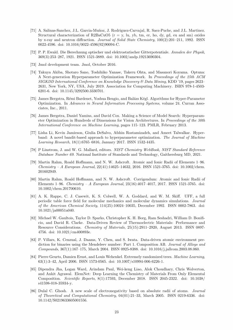
[71] A. Salinas-Sanchez, J.L. Garcia-Munoz, J. Rodriguez-Carvajal, R. Saez-Puche, and J.L. Martinez.Structural characterization of R2BaCuO5 (r = y, lu, yb, tm, er, ho, dy, gd, eu and sm) oxidesby x-ray and neutron diffraction. Journal of Solid State Chemistry, 100(2):201–211, 1992. ISSN0022-4596. doi: 10.1016/0022-4596(92)90094-C.

[72] P. P. Ewald. Die Berechnung optischer und elektrostatischer Gitterpotentiale. Annalen der Physik,369(3):253–287, 1921. ISSN 1521-3889. doi: 10.1002/andp.19213690304.

[73] Jmol development team. Jmol, October 2016.

[74] Takuya Akiba, Shotaro Sano, Toshihiko Yanase, Takeru Ohta, and Masanori Koyama. Optuna:A Next-generation Hyperparameter Optimization Framework. In Proceedings of the 25th ACMSIGKDD International Conference on Knowledge Discovery & Data Mining, KDD ’19, pages 2623–2631, New York, NY, USA, July 2019. Association for Computing Machinery. ISBN 978-1-4503-6201-6. doi: 10.1145/3292500.3330701.

[75] James Bergstra, Remi Bardenet, Yoshua Bengio, and Balazs Kegl. Algorithms for Hyper-ParameterOptimization. In Advances in Neural Information Processing Systems, volume 24. Curran Asso-ciates, Inc., 2011.

[76] James Bergstra, Daniel Yamins, and David Cox. Making a Science of Model Search: Hyperparam-eter Optimization in Hundreds of Dimensions for Vision Architectures. In Proceedings of the 30thInternational Conference on Machine Learning, pages 115–123. PMLR, February 2013.

[77] Lisha Li, Kevin Jamieson, Giulia DeSalvo, Afshin Rostamizadeh, and Ameet Talwalkar. Hyper-band: A novel bandit-based approach to hyperparameter optimization. The Journal of MachineLearning Research, 18(1):6765–6816, January 2017. ISSN 1532-4435.

[78] P Linstrom, J. and W. G. Mallard, editors. NIST Chemistry WebBook, NIST Standard ReferenceDatabase Number 69. National Institute of Standards and Technology, Gaithersburg MD, 2021.

[79] Martin Rahm, Roald Hoffmann, and N. W. Ashcroft. Atomic and Ionic Radii of Elements 1–96.Chemistry – A European Journal, 22(41):14625–14632, 2016. ISSN 1521-3765. doi: 10.1002/chem.201602949.

[80] Martin Rahm, Roald Hoffmann, and N. W. Ashcroft. Corrigendum: Atomic and Ionic Radii ofElements 1–96. Chemistry – A European Journal, 23(16):4017–4017, 2017. ISSN 1521-3765. doi:10.1002/chem.201700610.

[81] A. K. Rappe, C. J. Casewit, K. S. Colwell, W. A. Goddard, and W. M. Skiff. UFF, a fullperiodic table force field for molecular mechanics and molecular dynamics simulations. Journalof the American Chemical Society, 114(25):10024–10035, December 1992. ISSN 0002-7863. doi:10.1021/ja00051a040.

[82] Michael W. Gaultois, Taylor D. Sparks, Christopher K. H. Borg, Ram Seshadri, William D. Bonifi-cio, and David R. Clarke. Data-Driven Review of Thermoelectric Materials: Performance andResource Considerations. Chemistry of Materials, 25(15):2911–2920, August 2013. ISSN 0897-4756. doi: 10.1021/cm400893e.

[83] P. Villars, K. Cenzual, J. Daams, Y. Chen, and S. Iwata. Data-driven atomic environment pre-diction for binaries using the Mendeleev number: Part 1. Composition AB. Journal of Alloys andCompounds, 367(1):167–175, March 2004. ISSN 0925-8388. doi: 10.1016/j.jallcom.2003.08.060.

[84] Pierre Geurts, Damien Ernst, and Louis Wehenkel. Extremely randomized trees. Machine Learning,63(1):3–42, April 2006. ISSN 1573-0565. doi: 10.1007/s10994-006-6226-1.

[85] Dipendra Jha, Logan Ward, Arindam Paul, Wei-keng Liao, Alok Choudhary, Chris Wolverton,and Ankit Agrawal. ElemNet: Deep Learning the Chemistry of Materials From Only ElementalComposition. Scientific Reports, 8(1):17593, December 2018. ISSN 2045-2322. doi: 10.1038/s41598-018-35934-y.

[86] Dulal C. Ghosh. A new scale of electronegativity based on absolute radii of atoms. Journalof Theoretical and Computational Chemistry, 04(01):21–33, March 2005. ISSN 0219-6336. doi:10.1142/S0219633605001556.

23

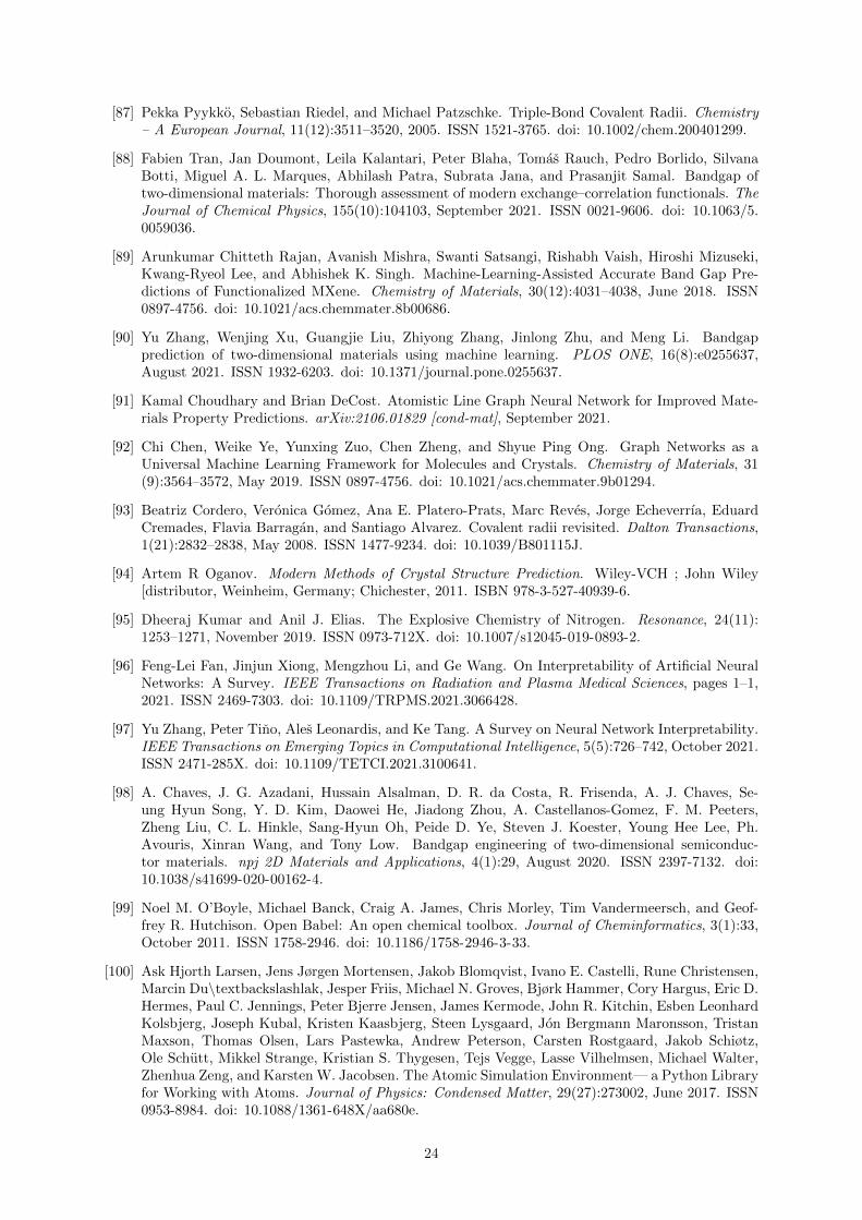
[87] Pekka Pyykko, Sebastian Riedel, and Michael Patzschke. Triple-Bond Covalent Radii. Chemistry– A European Journal, 11(12):3511–3520, 2005. ISSN 1521-3765. doi: 10.1002/chem.200401299.

[88] Fabien Tran, Jan Doumont, Leila Kalantari, Peter Blaha, Tomas Rauch, Pedro Borlido, SilvanaBotti, Miguel A. L. Marques, Abhilash Patra, Subrata Jana, and Prasanjit Samal. Bandgap oftwo-dimensional materials: Thorough assessment of modern exchange–correlation functionals. TheJournal of Chemical Physics, 155(10):104103, September 2021. ISSN 0021-9606. doi: 10.1063/5.0059036.

[89] Arunkumar Chitteth Rajan, Avanish Mishra, Swanti Satsangi, Rishabh Vaish, Hiroshi Mizuseki,Kwang-Ryeol Lee, and Abhishek K. Singh. Machine-Learning-Assisted Accurate Band Gap Pre-dictions of Functionalized MXene. Chemistry of Materials, 30(12):4031–4038, June 2018. ISSN0897-4756. doi: 10.1021/acs.chemmater.8b00686.

[90] Yu Zhang, Wenjing Xu, Guangjie Liu, Zhiyong Zhang, Jinlong Zhu, and Meng Li. Bandgapprediction of two-dimensional materials using machine learning. PLOS ONE, 16(8):e0255637,August 2021. ISSN 1932-6203. doi: 10.1371/journal.pone.0255637.

[91] Kamal Choudhary and Brian DeCost. Atomistic Line Graph Neural Network for Improved Mate-rials Property Predictions. arXiv:2106.01829 [cond-mat], September 2021.

[92] Chi Chen, Weike Ye, Yunxing Zuo, Chen Zheng, and Shyue Ping Ong. Graph Networks as aUniversal Machine Learning Framework for Molecules and Crystals. Chemistry of Materials, 31(9):3564–3572, May 2019. ISSN 0897-4756. doi: 10.1021/acs.chemmater.9b01294.

[93] Beatriz Cordero, Veronica Gomez, Ana E. Platero-Prats, Marc Reves, Jorge Echeverrıa, EduardCremades, Flavia Barragan, and Santiago Alvarez. Covalent radii revisited. Dalton Transactions,1(21):2832–2838, May 2008. ISSN 1477-9234. doi: 10.1039/B801115J.

[94] Artem R Oganov. Modern Methods of Crystal Structure Prediction. Wiley-VCH ; John Wiley[distributor, Weinheim, Germany; Chichester, 2011. ISBN 978-3-527-40939-6.

[95] Dheeraj Kumar and Anil J. Elias. The Explosive Chemistry of Nitrogen. Resonance, 24(11):1253–1271, November 2019. ISSN 0973-712X. doi: 10.1007/s12045-019-0893-2.

[96] Feng-Lei Fan, Jinjun Xiong, Mengzhou Li, and Ge Wang. On Interpretability of Artificial NeuralNetworks: A Survey. IEEE Transactions on Radiation and Plasma Medical Sciences, pages 1–1,2021. ISSN 2469-7303. doi: 10.1109/TRPMS.2021.3066428.

[97] Yu Zhang, Peter Tino, Ales Leonardis, and Ke Tang. A Survey on Neural Network Interpretability.IEEE Transactions on Emerging Topics in Computational Intelligence, 5(5):726–742, October 2021.ISSN 2471-285X. doi: 10.1109/TETCI.2021.3100641.

[98] A. Chaves, J. G. Azadani, Hussain Alsalman, D. R. da Costa, R. Frisenda, A. J. Chaves, Se-ung Hyun Song, Y. D. Kim, Daowei He, Jiadong Zhou, A. Castellanos-Gomez, F. M. Peeters,Zheng Liu, C. L. Hinkle, Sang-Hyun Oh, Peide D. Ye, Steven J. Koester, Young Hee Lee, Ph.Avouris, Xinran Wang, and Tony Low. Bandgap engineering of two-dimensional semiconduc-tor materials. npj 2D Materials and Applications, 4(1):29, August 2020. ISSN 2397-7132. doi:10.1038/s41699-020-00162-4.

[99] Noel M. O’Boyle, Michael Banck, Craig A. James, Chris Morley, Tim Vandermeersch, and Geof-frey R. Hutchison. Open Babel: An open chemical toolbox. Journal of Cheminformatics, 3(1):33,October 2011. ISSN 1758-2946. doi: 10.1186/1758-2946-3-33.

[100] Ask Hjorth Larsen, Jens Jørgen Mortensen, Jakob Blomqvist, Ivano E. Castelli, Rune Christensen,Marcin Du\textbackslashlak, Jesper Friis, Michael N. Groves, Bjørk Hammer, Cory Hargus, Eric D.Hermes, Paul C. Jennings, Peter Bjerre Jensen, James Kermode, John R. Kitchin, Esben LeonhardKolsbjerg, Joseph Kubal, Kristen Kaasbjerg, Steen Lysgaard, Jon Bergmann Maronsson, TristanMaxson, Thomas Olsen, Lars Pastewka, Andrew Peterson, Carsten Rostgaard, Jakob Schiøtz,Ole Schutt, Mikkel Strange, Kristian S. Thygesen, Tejs Vegge, Lasse Vilhelmsen, Michael Walter,Zhenhua Zeng, and Karsten W. Jacobsen. The Atomic Simulation Environment— a Python Libraryfor Working with Atoms. Journal of Physics: Condensed Matter, 29(27):273002, June 2017. ISSN0953-8984. doi: 10.1088/1361-648X/aa680e.

24

[101] Greg Landrum, Paolo Tosco, Brian Kelley, sriniker, gedeck, NadineSchneider, Riccardo Vianello,Ric, Andrew Dalke, Brian Cole, AlexanderSavelyev, Matt Swain, Samo Turk, Dan N, AlainVaucher, Eisuke Kawashima, Maciej Wojcikowski, Daniel Probst, guillaume godin, David Cos-grove, Axel Pahl, JP, Francois Berenger, strets123, JLVarjo, Noel O’Boyle, Patrick Fuller, Jan HolstJensen, Gianluca Sforna, and DoliathGavid. RDKit, 2021.

[102] Bingbing Zhang, Xiaodong Zhang, Jin Yu, Ying Wang, Kui Wu, and Ming-Hsien Lee. First-Principles High-Throughput Screening Pipeline for Nonlinear Optical Materials: Application toBorates. Chemistry of Materials, 32(15):6772–6779, August 2020. ISSN 0897-4756. doi: 10.1021/acs.chemmater.0c02583.

[103] Lorenz M Mayr and Dejan Bojanic. Novel trends in high-throughput screening. Current Opinionin Pharmacology, 9(5):580–588, October 2009. ISSN 1471-4892. doi: 10.1016/j.coph.2009.08.004.

[104] James Dean, Michael J. Cowan, Jonathan Estes, Mahmoud Ramadan, and Giannis Mpourmpakis.Rapid Prediction of Bimetallic Mixing Behavior at the Nanoscale. ACS Nano, 14(7):8171–8180,July 2020. ISSN 1936-0851. doi: 10.1021/acsnano.0c01586.

[105] Martin Uhrin, Sebastiaan P. Huber, Jusong Yu, Nicola Marzari, and Giovanni Pizzi. Workflows inAiiDA: Engineering a high-throughput, event-based engine for robust and modular computationalworkflows. Computational Materials Science, 187:110086, February 2021. ISSN 0927-0256. doi:10.1016/j.commatsci.2020.110086.

[106] Sebastiaan P. Huber, Spyros Zoupanos, Martin Uhrin, Leopold Talirz, Leonid Kahle, RicoHauselmann, Dominik Gresch, Tiziano Muller, Aliaksandr V. Yakutovich, Casper W. Andersen,Francisco F. Ramirez, Carl S. Adorf, Fernando Gargiulo, Snehal Kumbhar, Elsa Passaro, ConradJohnston, Andrius Merkys, Andrea Cepellotti, Nicolas Mounet, Nicola Marzari, Boris Kozinsky,and Giovanni Pizzi. AiiDA 1.0, a scalable computational infrastructure for automated reproducibleworkflows and data provenance. Scientific Data, 7(1):300, September 2020. ISSN 2052-4463. doi:10.1038/s41597-020-00638-4.

[107] Timur Bazhirov. Data-centric online ecosystem for digital materials science. arXiv:1902.10838[cond-mat, physics:physics], February 2019.

[108] Timur Bazhirov and E. X. Abot. Fast and accessible first-principles calculations of vibrationalproperties of materials. arXiv:1808.10011 [cond-mat, physics:physics], August 2018.

[109] Protik Das, Mohammad Mohammadi, and Timur Bazhirov. Accessible computational materialsdesign with high fidelity and high throughput. arXiv:1807.05623 [cond-mat, physics:physics], July2018.

[110] Protik Das and Timur Bazhirov. Electronic properties of binary compounds with high fidelityand high throughput. Journal of Physics: Conference Series, 1290:012011, October 2019. ISSN1742-6588, 1742-6596. doi: 10.1088/1742-6596/1290/1/012011.

[111] Alexander Zech and Timur Bazhirov. CateCom: A practical data-centric approach to categorizationof computational models. arXiv:2109.13452 [cond-mat], September 2021.

[112] Felix Faber, Alexander Lindmaa, O. Anatole von Lilienfeld, and Rickard Armiento. Crystal struc-ture representations for machine learning models of formation energies. International Journal ofQuantum Chemistry, 115(16):1094–1101, 2015. ISSN 1097-461X. doi: 10.1002/qua.24917.

[113] Lauri Himanen, Marc O.J. Jager, Eiaki V. Morooka, Filippo Federici Canova, Yashasvi S. Ranawat,David Z. Gao, Patrick Rinke, and Adam S. Foster. DScribe: Library of descriptors for machinelearning in materials science. Computer Physics Communications, 247:106949, February 2020.ISSN 00104655. doi: 10.1016/j.cpc.2019.106949.

[114] Matthias Rupp, Alexandre Tkatchenko, Klaus-Robert Muller, and O. Anatole von Lilienfeld. Fastand Accurate Modeling of Molecular Atomization Energies with Machine Learning. Physical ReviewLetters, 108(5):058301, January 2012. doi: 10.1103/PhysRevLett.108.058301.

[115] Guillaume Lemaıtre, Fernando Nogueira, and Christos K. Aridas. Imbalanced-learn: A pythontoolbox to tackle the curse of imbalanced datasets in machine learning. Journal of Machine LearningResearch, 18(17):1–5, 2017.

25

S Supporting Information

S.1 XGBoost Feature Importance

The XGBoost approach allows us to assess the feature importance scores of the various model inputs.In this section, we report the importance scores for the 10 most-important features identified by eachmodel. Feature importances are calculated using the default ”Gain” metric available in XGBoost.

Figure S1: Importance metrics for the 10 most-important features identified by the XGBoost perovskite volume modelusing the “gain” feature importance metric.

Figure S2: Importance metrics for the 10 most-important features identified by the XGBoost 2D material bandgap modelusing the “gain” feature importance metric.

26

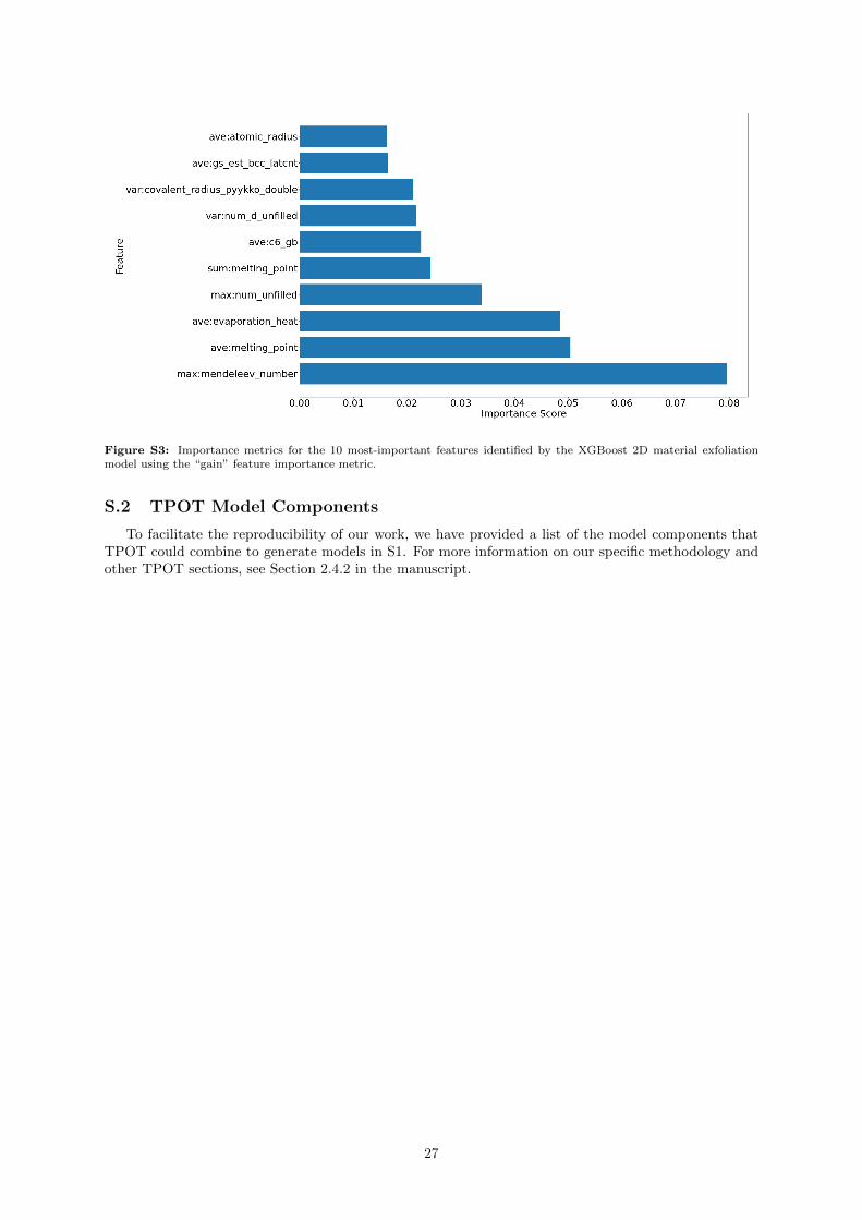
Figure S3: Importance metrics for the 10 most-important features identified by the XGBoost 2D material exfoliationmodel using the “gain” feature importance metric.

S.2 TPOT Model Components

To facilitate the reproducibility of our work, we have provided a list of the model components thatTPOT could combine to generate models in S1. For more information on our specific methodology andother TPOT sections, see Section 2.4.2 in the manuscript.

27

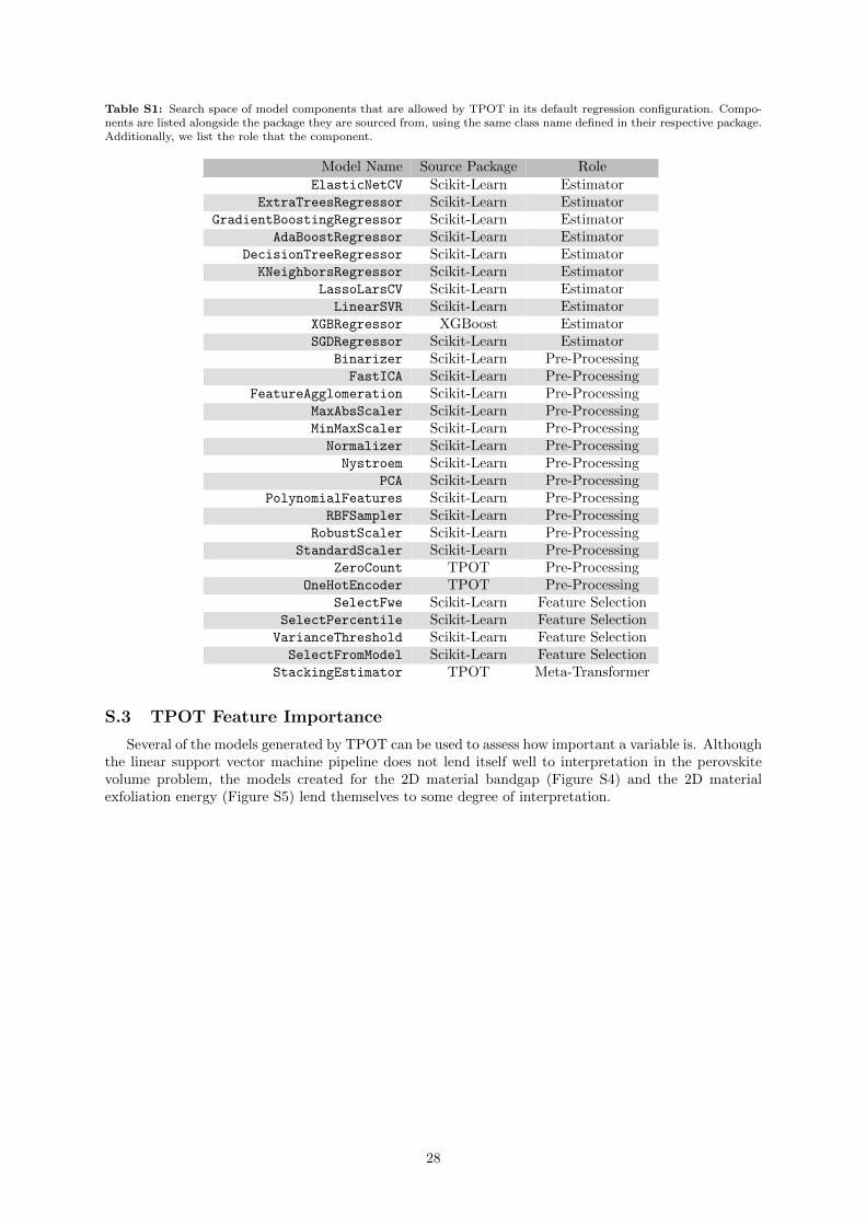
Table S1: Search space of model components that are allowed by TPOT in its default regression configuration. Compo-nents are listed alongside the package they are sourced from, using the same class name defined in their respective package.Additionally, we list the role that the component.

Model Name Source Package RoleElasticNetCV Scikit-Learn Estimator

ExtraTreesRegressor Scikit-Learn EstimatorGradientBoostingRegressor Scikit-Learn Estimator

AdaBoostRegressor Scikit-Learn EstimatorDecisionTreeRegressor Scikit-Learn EstimatorKNeighborsRegressor Scikit-Learn Estimator

LassoLarsCV Scikit-Learn EstimatorLinearSVR Scikit-Learn Estimator

XGBRegressor XGBoost EstimatorSGDRegressor Scikit-Learn Estimator

Binarizer Scikit-Learn Pre-ProcessingFastICA Scikit-Learn Pre-Processing

FeatureAgglomeration Scikit-Learn Pre-ProcessingMaxAbsScaler Scikit-Learn Pre-ProcessingMinMaxScaler Scikit-Learn Pre-ProcessingNormalizer Scikit-Learn Pre-ProcessingNystroem Scikit-Learn Pre-Processing

PCA Scikit-Learn Pre-ProcessingPolynomialFeatures Scikit-Learn Pre-Processing

RBFSampler Scikit-Learn Pre-ProcessingRobustScaler Scikit-Learn Pre-Processing

StandardScaler Scikit-Learn Pre-ProcessingZeroCount TPOT Pre-Processing

OneHotEncoder TPOT Pre-ProcessingSelectFwe Scikit-Learn Feature Selection

SelectPercentile Scikit-Learn Feature SelectionVarianceThreshold Scikit-Learn Feature SelectionSelectFromModel Scikit-Learn Feature Selection

StackingEstimator TPOT Meta-Transformer

S.3 TPOT Feature Importance

Several of the models generated by TPOT can be used to assess how important a variable is. Althoughthe linear support vector machine pipeline does not lend itself well to interpretation in the perovskitevolume problem, the models created for the 2D material bandgap (Figure S4) and the 2D materialexfoliation energy (Figure S5) lend themselves to some degree of interpretation.

28

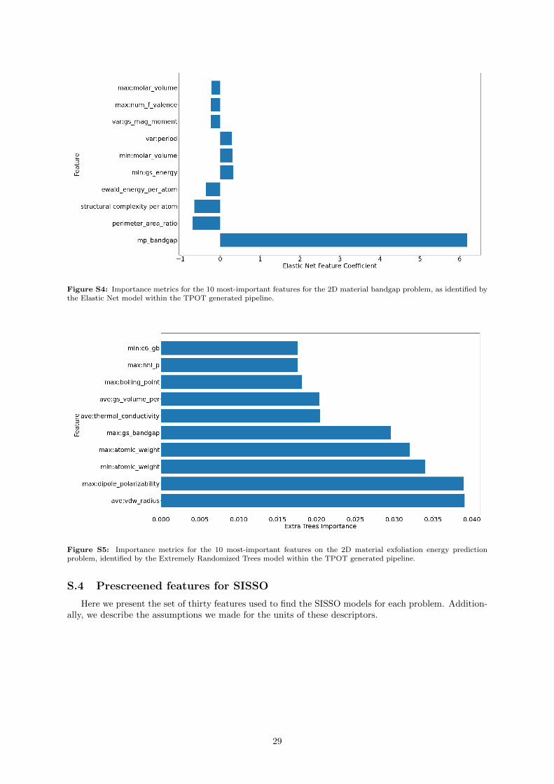
Figure S4: Importance metrics for the 10 most-important features for the 2D material bandgap problem, as identified bythe Elastic Net model within the TPOT generated pipeline.

Figure S5: Importance metrics for the 10 most-important features on the 2D material exfoliation energy predictionproblem, identified by the Extremely Randomized Trees model within the TPOT generated pipeline.

S.4 Prescreened features for SISSO

Here we present the set of thirty features used to find the SISSO models for each problem. Addition-ally, we describe the assumptions we made for the units of these descriptors.

29

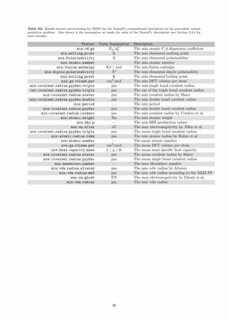
Table S2: Results feature pre-screening for SISSO for the XenonPy compositional descriptors on the perovskite volumeprediction problem. Also shown is the assumption we made for units of the XenonPy descriptors (see Section 2.4.4 formore details).

Feature Units Assumption Descriptionmin:c6 gb Eh/a

60 The min atomic C 6 dispersion coefficient

min:melting point K The min elemental melting pointmin:Polarizability A The min elemental polarizabilitymin:atomic number — The min atomic number

min:fusion enthalpy KJ / mol The min fusion enthalpymin:dipole polarizability A3 The min elemental dipole polarizablity

min:boiling point K The min elemental boiling pointmin:gs volume per cm3/mol The min DFT volume per atom

min:covalent radius pyykko triple pm The min single bond covalent radiusvar:covalent radius pyykko triple pm The var of the triple bond covalent radius

min:covalent radius slater pm The min covalent radius by Slatermin:covalent radius pyykko double pm The min double bond covalent radius

min:period — The min periodmin:covalent radius pyykko pm The min double bond covalent radiusmin:covalent radius cordero pm The min covalent radius by Cordero et al

min:atomic weight Da The min atomic weightmin:hhi p — The min HHI production values

max:en allen eV The max electronegativity by Allen et alave:covalent radius pyykko triple pm The mean triple bond covalent radius

min:atomic radius rahm pm The min atomic radius by Rahm et alave:atomic number — The mean atomic numberave:gs volume per cm3/mol The mean DFT volume per atom

ave:heat capacity mass J / g / K The mean mass specific heat capacityave:covalent radius slater pm The mean covalent radius by Slaterave:covalent radius pyykko pm The mean single bond covalent radius

max:mendeleev number — The max Mendeleev numbermin:vdw radius alvarez pm The min vdw radius by Alvarez

min:vdw radius mm3 pm The min vdw radius according to the MM3 FFmax:en ghosh EN The max electronegativity by Ghosh et al.

min:vdw radius pm The min vdw radius

30

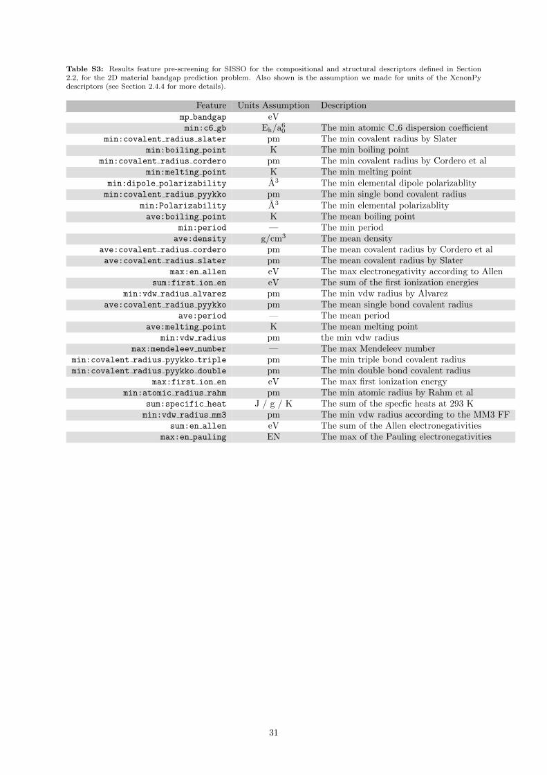
Table S3: Results feature pre-screening for SISSO for the compositional and structural descriptors defined in Section2.2, for the 2D material bandgap prediction problem. Also shown is the assumption we made for units of the XenonPydescriptors (see Section 2.4.4 for more details).

Feature Units Assumption Descriptionmp bandgap eVmin:c6 gb Eh/a

60 The min atomic C 6 dispersion coefficient

min:covalent radius slater pm The min covalent radius by Slatermin:boiling point K The min boiling point

min:covalent radius cordero pm The min covalent radius by Cordero et almin:melting point K The min melting point

min:dipole polarizability A3 The min elemental dipole polarizablitymin:covalent radius pyykko pm The min single bond covalent radius

min:Polarizability A3 The min elemental polarizablityave:boiling point K The mean boiling point

min:period — The min periodave:density g/cm3 The mean density

ave:covalent radius cordero pm The mean covalent radius by Cordero et alave:covalent radius slater pm The mean covalent radius by Slater

max:en allen eV The max electronegativity according to Allensum:first ion en eV The sum of the first ionization energies

min:vdw radius alvarez pm The min vdw radius by Alvarezave:covalent radius pyykko pm The mean single bond covalent radius

ave:period — The mean periodave:melting point K The mean melting point

min:vdw radius pm the min vdw radiusmax:mendeleev number — The max Mendeleev number

min:covalent radius pyykko triple pm The min triple bond covalent radiusmin:covalent radius pyykko double pm The min double bond covalent radius

max:first ion en eV The max first ionization energymin:atomic radius rahm pm The min atomic radius by Rahm et al

sum:specific heat J / g / K The sum of the specfic heats at 293 Kmin:vdw radius mm3 pm The min vdw radius according to the MM3 FF

sum:en allen eV The sum of the Allen electronegativitiesmax:en pauling EN The max of the Pauling electronegativities

31

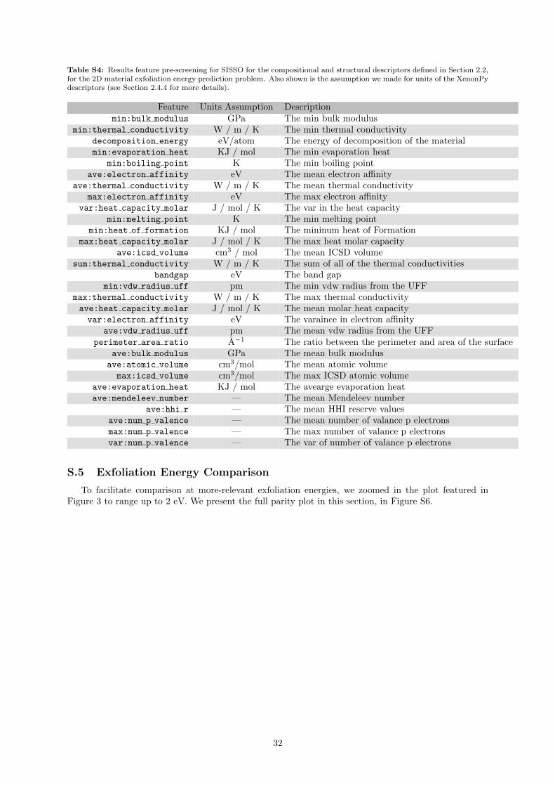
Table S4: Results feature pre-screening for SISSO for the compositional and structural descriptors defined in Section 2.2,for the 2D material exfoliation energy prediction problem. Also shown is the assumption we made for units of the XenonPydescriptors (see Section 2.4.4 for more details).

Feature Units Assumption Descriptionmin:bulk modulus GPa The min bulk modulus

min:thermal conductivity W / m / K The min thermal conductivitydecomposition energy eV/atom The energy of decomposition of the materialmin:evaporation heat KJ / mol The min evaporation heat

min:boiling point K The min boiling pointave:electron affinity eV The mean electron affinity

ave:thermal conductivity W / m / K The mean thermal conductivitymax:electron affinity eV The max electron affinity

var:heat capacity molar J / mol / K The var in the heat capacitymin:melting point K The min melting point

min:heat of formation KJ / mol The mininum heat of Formationmax:heat capacity molar J / mol / K The max heat molar capacity

ave:icsd volume cm3 / mol The mean ICSD volumesum:thermal conductivity W / m / K The sum of all of the thermal conductivities

bandgap eV The band gapmin:vdw radius uff pm The min vdw radius from the UFF

max:thermal conductivity W / m / K The max thermal conductivityave:heat capacity molar J / mol / K The mean molar heat capacityvar:electron affinity eV The varaince in electron affinity

ave:vdw radius uff pm The mean vdw radius from the UFFperimeter area ratio A−1 The ratio between the perimeter and area of the surface

ave:bulk modulus GPa The mean bulk modulusave:atomic volume cm3/mol The mean atomic volume

max:icsd volume cm3/mol The max ICSD atomic volumeave:evaporation heat KJ / mol The avearge evaporation heatave:mendeleev number — The mean Mendeleev number

ave:hhi r — The mean HHI reserve valuesave:num p valence — The mean number of valance p electronsmax:num p valence — The max number of valance p electronsvar:num p valence — The var of number of valance p electrons

S.5 Exfoliation Energy Comparison

To facilitate comparison at more-relevant exfoliation energies, we zoomed in the plot featured inFigure 3 to range up to 2 eV. We present the full parity plot in this section, in Figure S6.

32

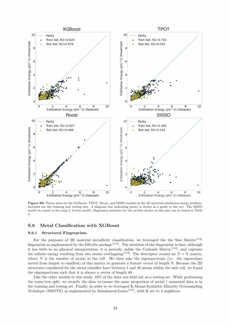
Figure S6: Parity plots for the XGBoost, TPOT, Roost, and SISSO models on the 2D material exfoliation energy problem.Included are the training and testing sets. A diagonal line indicating parity is drawn as a guide to the eye. The SISSOmodel we report is the rung 2, 2-term model. Regression statistics for the models shown on this plot can be found in Table4.

S.6 Metal Classification with XGBoost

S.6.1 Structural Fingerprints

For the purposes of 2D material metallicity classification, we leveraged the the Sine Matrix [112]

fingerprint as implemented by the DScribe package [113]. The intuition of this fingerprint is that, althoughit has little to no physical interpretation, it is periodic unlike the Coulomb Matrix [114], and capturesthe infinite energy resulting from two atoms overlapping [113]. The descriptor creates an N ×N matrix,where N is the number of atoms in the cell. We then take the eigenspectrum (i.e. the eigenvaluessorted from largest to smallest) of this matrix to generate a feature vector of length N. Because the 2Dstructures considered for the metal classifier have between 1 and 40 atoms within the unit cell, we 0-padthe eigenspectrum such that it is always a vector of length 40.

Like the other models in this study, 10% of the data was held out as a testing set. While performingthe train/test split, we stratify the data to ensure the same proportion of metal / nonmetal data is inthe training and testing set. Finally, in order to we leveraged K-Means Synthetic Minority OversamplingTechnique (SMOTE) as implemented by Imbalanced-Learn [115], with K set to 4 neighbors.

33

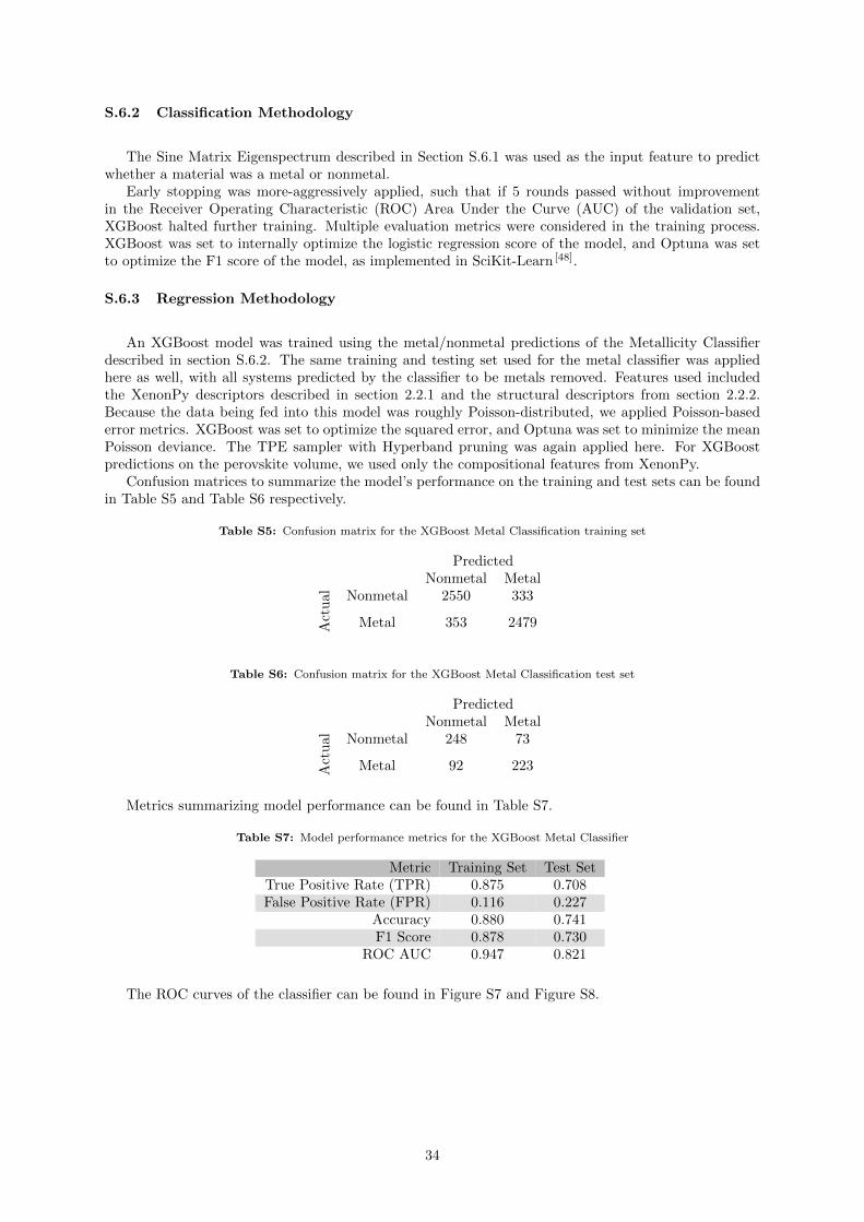
S.6.2 Classification Methodology

The Sine Matrix Eigenspectrum described in Section S.6.1 was used as the input feature to predictwhether a material was a metal or nonmetal.

Early stopping was more-aggressively applied, such that if 5 rounds passed without improvementin the Receiver Operating Characteristic (ROC) Area Under the Curve (AUC) of the validation set,XGBoost halted further training. Multiple evaluation metrics were considered in the training process.XGBoost was set to internally optimize the logistic regression score of the model, and Optuna was setto optimize the F1 score of the model, as implemented in SciKit-Learn [48].

S.6.3 Regression Methodology

An XGBoost model was trained using the metal/nonmetal predictions of the Metallicity Classifierdescribed in section S.6.2. The same training and testing set used for the metal classifier was appliedhere as well, with all systems predicted by the classifier to be metals removed. Features used includedthe XenonPy descriptors described in section 2.2.1 and the structural descriptors from section 2.2.2.Because the data being fed into this model was roughly Poisson-distributed, we applied Poisson-basederror metrics. XGBoost was set to optimize the squared error, and Optuna was set to minimize the meanPoisson deviance. The TPE sampler with Hyperband pruning was again applied here. For XGBoostpredictions on the perovskite volume, we used only the compositional features from XenonPy.

Confusion matrices to summarize the model’s performance on the training and test sets can be foundin Table S5 and Table S6 respectively.

Table S5: Confusion matrix for the XGBoost Metal Classification training set

PredictedNonmetal Metal

Act

ual Nonmetal 2550 333

Metal 353 2479

Table S6: Confusion matrix for the XGBoost Metal Classification test set

PredictedNonmetal Metal

Act

ual Nonmetal 248 73

Metal 92 223

Metrics summarizing model performance can be found in Table S7.

Table S7: Model performance metrics for the XGBoost Metal Classifier

Metric Training Set Test SetTrue Positive Rate (TPR) 0.875 0.708False Positive Rate (FPR) 0.116 0.227

Accuracy 0.880 0.741F1 Score 0.878 0.730

ROC AUC 0.947 0.821

The ROC curves of the classifier can be found in Figure S7 and Figure S8.

34

Figure S7: Training-Set ROC curve for XGBoost model classifying whether a material is metallic or not.

35

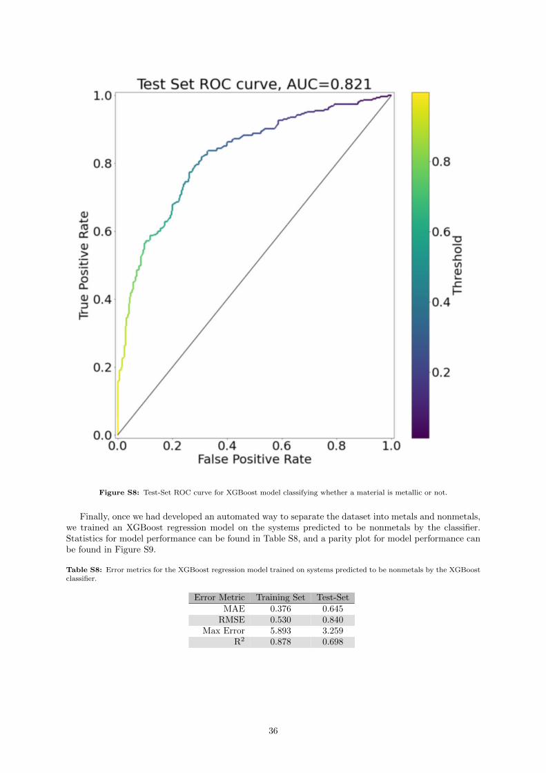
Figure S8: Test-Set ROC curve for XGBoost model classifying whether a material is metallic or not.

Finally, once we had developed an automated way to separate the dataset into metals and nonmetals,we trained an XGBoost regression model on the systems predicted to be nonmetals by the classifier.Statistics for model performance can be found in Table S8, and a parity plot for model performance canbe found in Figure S9.

Table S8: Error metrics for the XGBoost regression model trained on systems predicted to be nonmetals by the XGBoostclassifier.

Error Metric Training Set Test-SetMAE 0.376 0.645

RMSE 0.530 0.840Max Error 5.893 3.259

R2 0.878 0.698

36

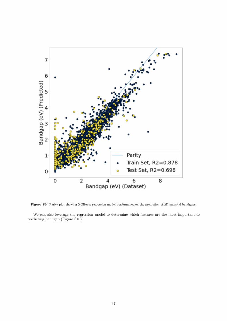
Figure S9: Parity plot showing XGBoost regression model performance on the prediction of 2D material bandgaps.

We can also leverage the regression model to determine which features are the most important topredicting bandgap (Figure S10).

37

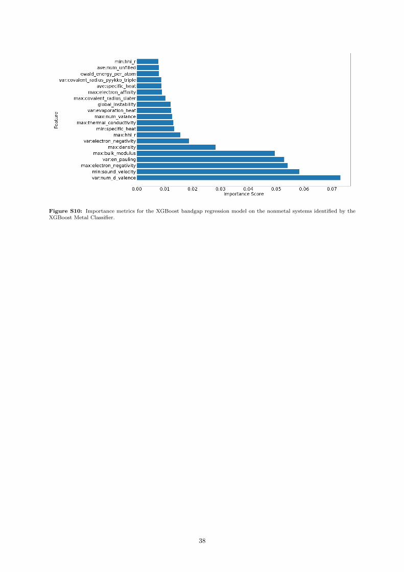
Figure S10: Importance metrics for the XGBoost bandgap regression model on the nonmetal systems identified by theXGBoost Metal Classifier.

38

Interpretable Machine Learning for Materials Design

Documents

Transcript of Interpretable Machine Learning for Materials Design