Interpolating the Missing Values for Multi-DimensionalSpatial-Temporal Sensor Data: A Tensor SVD Approach

Peipei XuSchool of Electronic Engineering

UESTCChengdu, China 611731peipei.xu6@gmail.com

Wenjie RuanDepartment of Computer Science

University of OxfordOxford, UK OX1 3QD

wenjie.ruan@cs.ox.ac.uk

Quan Z. ShengDepartment of Computing

Macquarie UniversitySydney, Australia NSW 2109

michael.sheng@mq.edu.au

Tao GuSchool of CS & ITRMIT University

Melbourne, Australia VIC 3000tao.gu@rmit.edu.au

Lina YaoSchool of Computer Science and

Engineering, UNSWSydney, Australia NSW 2052

lina.yao@unsw.edu.au

ABSTRACTWith the booming of the Internet of Things, enormous number ofsmart devices/sensors have been deployed in the physical worldto monitor our surroundings. Usually those devices generate high-dimensional geo-tagged time-series data. However, these sensorreadings are easily missing due to the hardware malfunction, con-nection errors or data corruption, which severely compromise theback-end data analysis. To solve this problem, in this paper we ex-ploit tensor-based Singular Value Decomposition method to recoverthe missing sensor readings. The main novelty of this paper liesin that, i) our tensor-based recovery method can well capture themulti-dimensional spatial and temporal features by transformingthe irregularly deployed sensors into a sensor-array and folding theperiodic temporal patterns into multiple time dimensions, ii) it onlyrequires to tune one key parameter in an unsupervised manner, andiii) Tensor Singular Value Decomposition structure is more efficienton representation of high-dimension sensor data than other tensorrecovery methods based on tensor’s vectorization or flattening. Theexperimental results in several real-world one-year air quality andmeteorology datasets demonstrate the effectiveness and accuracy ofour approach.

CCS CONCEPTS•Hardware → Signal processing systems; Sensor applicationsand deployments;

KEYWORDSSensor Data Recovery, Tensor Completion, t-SVD, ADMM

ACM Reference format:Peipei Xu, Wenjie Ruan, Quan Z. Sheng, Tao Gu, and Lina Yao. 2017.Interpolating the Missing Values for Multi-Dimensional Spatial-Temporal

Permission to make digital or hard copies of all or part of this work for personal orclassroom use is granted without fee provided that copies are not made or distributedfor profit or commercial advantage and that copies bear this notice and the full citationon the first page. Copyrights for components of this work owned by others than ACMmust be honored. Abstracting with credit is permitted. To copy otherwise, or republish,to post on servers or to redistribute to lists, requires prior specific permission and/or afee. Request permissions from permissions@acm.org.MobiQuitous 2017, Melbourne, VIC, Australia© 2017 ACM. 978-1-4503-5368-7/17/11. . . $15.00DOI: 10.1145/3144457.3144474

Sensor Data: A Tensor SVD Approach. In Proceedings of the 14th EAIInternational Conference on Mobile and Ubiquitous Systems: Computing,Networking and Services, Melbourne, VIC, Australia, November 7–10, 2017(MobiQuitous 2017), 10 pages.DOI: 10.1145/3144457.3144474

1 INTRODUCTIONIn the era of the Internet of Things (IoT), massive number of smartdevices and sensors have been installed in our surrounding environ-ments. According to a report, there are more than 1.9 billion sensorydevices launched into the physical world each week and there will berapidly increased into 9 billion by 2018. Such tremendous numberof smart devices enable us to monitor, analyze and understand ourphysical world, and ultimately support us to better manage variousfacets in the society [9]. For example, with fine-particles (PM 2.5)data across a city, we can understand the trend of environmentalpollution and then make a better plan to manage the factories andtransportation so that we can reduce the air pollution. Given large-scale trajectory data from the GPS in taxicab and smart bicycles, wecan predict the crowd flows in a city so that we can prevent the dan-gerous stampede by traffic control and warning people in advance.One of the important prerequisites for enabling those promising ap-plications is that we can accurately and continuously access sensorydata from the environments.

However, in practice, those sensory data usually suffer fromreading-missing or value-lost due to unexpected hardware failures,communication conflicts or harsh environments etc.. This disturbingphenomenon not only decreases the real-time monitoring capabilityof the sensory devices but also further compromises the accuracy ofback-end data analysis. Therefore, how to accurately yet efficientlyrecover the missing sensor data deserves our careful exploration.However, recovering missing values for a high-dimensional geo-tagged time-series data is a challenging task. Firstly, the sensorreadings are normally absent randomly which may be missing atconsecutive timestamps, or lost at a certain time-stamp for the wholegeographic area. This disturbing situation makes the traditionalregression-based methods or non-negative matrix decompositionmethod useless due to, for example, one or many columns androws are missing at the same time. Secondly, in practice, those

Time

Dimension

Sensor

Readings

Sensor 3

Sensor 1

Sensor 4

Sensor 2

Sensor 6

Sensor 7

Sensor 5

Sensor 8

Sensor 10

Sensor 9

Sensor 11

Sensor 12

Sensor 13

Sensor 15

Sensor 14

Sensor 17

Sensor 16

Sensor 18

Sensor 19

Sensor 20

Sensor 21

Sensor 22

Sensor 23

Sensor 24

S1

S2

S24

S23

S3

S4 ……

S22

S21

……S12

𝑡1 𝑡2 𝑡3 𝑡4 𝑡𝑛−1 𝑡𝑛𝑡i

……

……

……

…

…

…

…

…

…

Spatial Dimension

3-D Tensor

Formulation

4-D Tensor

Formulation

Spatial Dim. 2

Time Dimension

Spatial

Dim. 2

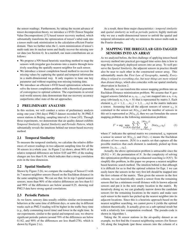
Figure 1: The idea of tensor formulation: Many tensors are irregularly deployed throughout the city (shown by the first figure), and theygenerate huge amount of time series data that normally have two dimensions - time and spatial dimensions (shown by the second figure).Those sensor readings are easily missing or lost (represented by the red dots), so this paper aims to recover those missing sensor readings.The idea is to formulate the data as a 3-order tensor such as two spatial dimensions (i.e., longitude and latitude) plus one time dimension,or 4-order tensor such as two spatial dimensions and two time dimensions (e.g., hours × days).

sensor data are generated by sensors deployed in different locations(e.g.,with different latitudes and longitudes, even altitudes) so thatthey normally exhibit significant non-nonlinearities which not onlystrongly relate to the time dimension but also highly depend on theirspatial attributes (i.e., latitudes, longitudes or altitudes).

To deal with aforementioned challenges, many methods for re-covering missing sensor readings are proposed. The most widelyadopted solutions are based on filtering algorithms such as MedianFiltering, Kriging, Kalman Filtering [12], or built upon regressionmethods with various complexities including ARIMA (AutoRegres-sive Integrated Moving Average), SVR (Support Vector Regres-sion) [30], kNN (k-Nearest Neighbors) [38] etc.. Those methods,however, can only learn spatial or temporal attribute, and are insuffi-cient to capture data’s global dependencies due to the limitation oftheir model structures (only quantifying the local or regional datapoints in terms of time or spatial attributes). Another popular tech-nique is to borrow the idea from recommendation that formulates themulti-dimensional sensor readings as a matrix (e.g., column repre-sents sampling times and row indicates different locations) and thenutilizes some matrix completion methods to interpolate the missingvalues by minimizing the rank of matrix. This solution can quantifyboth global temporal and spatial correlations among sensor readingsbut is still limited to capture the one-dimensional spatial similaritydue to a fact that, in the matrix formulation, the sensors with two-dimensional spatial coordinates are mapped into a one-dimensionalvector, unavoidably resulting in the spatial information loss [7].

Recently, a multi-view learning based method is introduced tocapture both local and global information in terms of spatial and tem-poral perspective, achieving state-of-the-art performance [43]. It alsodemonstrates that both local and global spatial/temporal correlationsplay an important role in the data reconstruction. However, it intro-duces four different models to capture the local and global spatialand temporal information respectively and then a linear regressionmodel is adopted to estimate the final missing values, resulting in

a labor-intensive parameter tuning process. Moreover, it requires asupervised model training using a large non-missing dataset, whichis impractical due to that the collected sensory data may alreadysuffer certain reading loss.

As a result, in this paper, we aim to explore - whether we canaccurately recover the missing sensor values by capturing the globalmulti-dimensional spatial-temporal correlations using a model thatonly needs to tune very few parameters and does not require anysupervised training. To solve this problem, different from previ-ous works, we formate the spatial-temporal sensor data as tensor- a multi-dimensional extension of a matrix and introduce a tensorbased recovery method. Nevertheless, applying this high-level ideainto practice requires addressing several challenges. First, how toaccurately map the sensors’ 2-D coordinates into a matrix is a non-trivial problem, especially considering that the sensors deployedin physical world is not naturally as a square or rectangle array(e.g., some places have no sensor deployed, but other locations havemany sensors). Moreover, tensor completion can be formulated tosolve the problem of minimization on the tensor rank. This generaloptimization problem is NP-hard and thus untraceable [23]. So howto approximate the tensor rank and efficiently solve the optimizationproblem while guaranteeing its convergence is also a challengingissue [15], especially for a large-scale real-world sensor dataset.

To address above challenges, we first map the sensors’ geo-locations into a matrix by finding each sensor’s k nearest neighborsin terms of longitudes and latitudes by proposing a Nearest Neigh-bor (NN) based heuristic searching method. Moreover, instead ofusing one time-dimension to capture the temporal information, wepropose to model the temporal feature in a multi-dimensional viewby measuring the the periodic patterns in sensor data1. Figure 1details the our general idea of using high-order tensor to formulate

1For example, the sensor values in same hours of a day or same day in a week aresimilar, so we can also model the temporal feature as a matrix, being similar to thespatial one.

2

the sensor readings. Furthermore, by taking the recent advance oftensor decomposition theory, we introduce a t-SVD (Tensor SingularValue Decomposition) [17] based tensor recovery method, whichsubstantially transforms the optimization of tensor’s tubal-rank intoa tensor multi-rank minimization in the calculation-efficient Fourierdomain. Then we further relax the `1 norm minimization of tensor’smulti-rank into its nuclear norm and finally recover the missing sen-sor data (see Section 4). In a nutshell, our main contributions are asfollows:• We propose a NN-based heuristic searching method to map the

sensors with irregular geo-locations into a matrix through itera-tively searching the spatially nearest neighbor for each sensor.

• We introduce a tensor completion based method to recover themissing values by capturing the spatial and temporal informationin a multi-dimensional way. It only requires to tune one keyparameter and without requiring non-missing training data.

• We introduce an efficient t-SVD based optimization scheme tosolve the tensor completion problem with a theoretical guaranteeof convergence to optimal solution. The experiments in severalreal-world sensory data demonstrate that our recovery accuracyoutperforms other state-of-the-art approaches.

2 PRELIMINARY ANALYSISIn this section, we will conduct a series of preliminary analysisusing one-year (364 days) PM2.5 dataset recorded by 36 PM2.5sensor stations in Beijing, sampling interval is 1-hour [43]. Throughthose experiments, we demonstrate that air quality dataset exhibitsTemporal Similarity, Spatial Similarity and Periodic Pattern, whichsubstantially reveals the intuitions behind our tensor-based recoverymethod.

2.1 Temporal SimilarityTo measure the temporal similarity, we calculate the relative differ-ences of sensor readings in two adjacent sampling time for all the36 sensors in a whole year. As Figure 2 (a) shows, about 90% of therelative temporal differences are below 0.05 and 99% of the readingchanges are less than 0.16, which indicates that a strong correlationexits in the time dimension.

2.2 Spatial SimilarityShown by Figure 2 (b), we compare the readings of Sensor13 withits 7 nearest neighbor sensors (based on the Euclidean distance) inthe same sampling time. We can see that, for its top-3 spatial nearestsensors, more than 90% of the relative differences are less than 0.1and 99% of the differences are below around 0.25, showing realPM2.5 data have strong spatial correlations.

2.3 Periodic PatternAs we know, sensory data usually exhibits similar environmentalbehaviors at the same time of different days, or same day in differentweeks such as PM2.5 reading will be higher in the traffic busy time(e.g., daily commuting travel time) and lower in the night time. Inour experiments, similar to the spatial and temporal case, we observesignificant periodic pattern (around 70% of the differences are below0.142, and 90% of the differences are less than0.278), which isshown by Figure 2 (c).

As a result, these three major characteristics - temporal similarityand spatial similarity as well as periodic pattern, highly motivatewhy we use a multi-dimensional tensor to unfold the spatial andtemporal information and why we minimize the tensor multi-rank inthe Fourier domain.

3 MAPPING THE IRREGULAR GEO-TAGGEDSENSORS INTO AN ARRAY

As we analyzed before, the first challenge of applying tensor-basedrecovery method into practical geo-tagged time-series data is how tomap those irregularly deployed sensors into an array. To well pre-serve the Spatial Similarity, the adjacent sensors in practice shouldalso be near to each other in the constructed sensor array. Thissubstantially meets the First Law of Geography, namely, Every-thing is related to everything else, but near things are more relatedthan distant things, which also coincides with our spatial similarityobservation in Section 2.

Basically, we can transform this sensor mapping problem into anEuclidean Distance minimization problem. We assume that N geo-tagged sensors (labeled as s1, s2, ..., sN ) are mapped into a n1 × n2array (obviously n1 × n2 = N ) that is represented by matrix S . Eachelement si, j (i = 1, 2, ...,n1; j = 1, 2, ...,n2) in the matrix indicatesa sensor. Assuming that all the adjcent sensors of sensor si, j iscontained in the sensor-set N(si, j ) and the number of sensors inthis set is represented as |N(si, j )|, then we can formulate the sensormapping problem as the following minimization problem:

S∗ = arg minS ∈S(N )

n1∑i=1

n2∑j=1

|N(si, j ) |∑sk ∈N(si, j )

Dis(si, j , sk ) (1)

where S∗ indicates the optimal matrix we constructed, sk representa sensor in sensor set N(si, j ), and Dis(∗, ∗) means the Euclideandistance of two sensors. S(N ) is a matrix set that captures all thepossible matrices that each element is randomly picked up fromsensors s1, s2, ..., sN .

Actually, the above optimization problem is untraceable since the|S(N )| = N !, the permutation of N . So the complexity of solvingthis optimization problem using an exhausted searching isO(N !). Tosimplify this problem, in this paper we propose a nearest neighborbased heuristic search method. The intuition behind is that althoughit is difficult for us to find the optimal solution for Eqn. 1 we caneasily know the sensors in the very first left should be mapped intothe first column of the matrix. Then given the sensors in the firstcolumn, we can heuristically search a sensor from the remainingsensors that has a minimum overall distance with its known adjacentsensors and put it in the next empty location in the matrix. Byiteratively doing so, we can gradually narrow down the candidatesensors for the remaining locations in the matrix and make sureeach sensor in the matrix has picked up the nearest neighbor into itsadjacent locations. Since this is a heuristic approach based on thenearest neighbor searching, we cannot prove it yields the optimalsolution theoretically. It actually gives us a sub-optimal result butwith a relatively low computation overhead. The pseudo-code isshown in Algorithm 1.

Taking the 36 sensor stations in the air-quality dataset as anexample, we first find the 4 nearest neighboring sensors (for Sensor-34) along the longitude (put those sensors into the column of a

3

∆Vtemp

CD

F

(a)∆Vsp

atial

k-th Nearest Neighbor

(b)(c)

Figure 2: (a) CDF of relative temporal differences of adjacent hours; (b) CDF of relative spatial differences of Sensor13 and itsnearest neighbors; (c) CDF of relative differences in periodic pattern for same hours on different days

(a) (b)(c)

Figure 3: (a) The spatial locations of PM2.5 sensor stations throughout the city; (b) The searching result by using NN-based heuristicsearching method; (c) The mapped matrix of sensor array

matrix) and then we consider the next nearest sensor along thelatitude and formulate it as the second column of a matrix. Byiteratively doing so, we finally can fill in a 4 × 9 matrix using allthose sensors, which eventually model the spatial similarity via a2-dimensional matrix. Figure 3 (a)∼(c) show an example of how ourNN-based Heuristic Searching method maps irregularly deployed36 PM2.5 sensors into a sensor array.

Apart form the spatial similarity, we also need to model thetemporal similarity and periodic patterns (as analyzed in Section 2).The most straightforward way is to formulate as one-dimensionalarray (plus the spatial dimensions, forming a 4×9×8759 data tensor),or we can formulate as two dimensions to capture the similarity ofsame hours in a day (overall we can form a 4 × 9 × 24 × 364 4-ordertensor), or as three dimensions to model the similarities of samehours during different days and same days during different weeks(overall forming a 4×9×24×7×52). The general idea is also shownvia Figure 1.

In the next, given the formulated data tensor, we will elaboratehow to use a tensor-SVD based recovery method to estimate thosemissing values.

4 TENSOR SVD BASED SENSOR DATARECOVERY

In this section, we will briefly introduce the notations and definitionsthat are used in our method. For simplicity, all the formulation,mathematical theorems and definitions are based on a 3-order tensor,which can be naturally extended into high-order tensor cases.

We represent matrices by upper letters (A) and a d-order tensor iswritten by calligraphic letters (A). A(i, j,k) denotes the (i, j,k)-thelement of third-order tensor A ∈ Rn1×n2×n3 and A(i, j, :) denotesthe (i, j)-th tubal scalar. A(i, :, :), A(:, j, :), A(:, :,k) (or equivalentlyA(k )) denote the i-th horizontal slice, j-th lateral slice and k-thfrontal slice. The X = fft(X, [ ], i) denotes the FFT on the i-thdimension of a multi-way array [47].

We then introduce following related definitions.

DEFINITION 1. t-product: given two third-order tensor A ∈Rn1×n2×n3 and B ∈ Rn2×n4×n3 , the t-product C = A ∗ B is atensor of size n1 × n4 × n3 given by C = A ∗ B = Fold(bcirc(A) ·Unfold(B)). The bcirc(A) is block circulant matrix and its firstcolumn is [A(1)

T,A(2)

T, · · · ,A(n3)T ]. The Unfold(·) and Fold(·)

4

Algorithm 1: NN-based Heuristic Searching for Sensor-ArrayMapping

Input: Sensor Set: SN = s1, s2, ..., sN Mapping Marix: S ∈ Rn1×n2

1 Manually pick up n1 sensors filling in S∗,12 SN ← SN − S∗,1

3 for i = 1 : n1 do4 for j = 2 : n2 do5 if i == 1 then6 Si, j = sk |minsk

∑Dis(sk , Si, j−1, Si+1, j−1)

7 end8 else if i > 1 && i < n1 then9 Si, j =

sk |minsk∑Dis(sk , Si−1, j , Si−1, j−1, Si, j−1, Si+1, j−1)

10 end11 else12 Si, j =

sk |minsk∑Dis(sk , Si−1, j , Si−1, j−1, Si, j−1)

13 end14 SN ← SN − Si, j15 end16 end

Output: Mapping Matrix S , indicating the sensor locations

operators mean that Unfold(B) = [B(1)T,B(2)

T, · · · ,B(n3)T ] and

Fold(Unfold(B)) = B.

It is consistent with the multiplication of matrices if n3 = 1.

DEFINITION 2. Identity tensor: the identity tensorI ∈ Rn1×n1×n3

is a tensor whose first frontal slice is the n1 × n1 identity matrix andall other frontal slices are zero.

DEFINITION 3. Orthogonal tensor: a tensor Q ∈ Rn1×n1×n3 isorthogonal if Q ∗ Q∗ = Q∗ ∗ Q = I.

DEFINITION 4. f-diagonal tensor: a tensor is called f-diagonalif each frontal slice of the tensor is a diagonal matrix.

4.1 Tensor Singular Value DecompositionGiven the definition of t-product, we introduce the tensor SingularValue Decomposition (t-SVD) [16].

THEOREM 1. For a tensor X ∈ Rn1×n2×n3 , it can be factoredas X = U ∗ S ∗ VT , where U and V are orthogonal tensors ofsize n1 × n1 × n3 and n2 × n2 × n3 respectively. S is a rectangularf-diagonal tensor of size n1 × n2 × n3.

DEFINITION 5. The diagonal of Fncirc(v)F ∗n = fft(v), wherefft(v) is the result of applying the Fast Fourier Transform to v, i.e.diag(Fncirc(v)F ∗n ) = fft(v).

In Definition 1, the t-product is defined by circulant convolution,the computation of t-SVD can be efficiently calculated using the fastFourier transform (FFT) [17]. For a 3-order tensor, we first applythe FFT along the third dimension to attain the Fourier transformedtensor X, and then compute the standard matrix SVD of each frontalslice of X. Finally, we apply an inverse FFT to the third dimension

of the component tensors to compute the final t-SVD decomposition.For the higher order tensors, this concept of the t-SVD can be recur-sively extended by the t-product [28]. For details about this process,see the t-SVD in Algorithm 2.

Algorithm 2: t-SVD

Input: X ∈ Rn1×n2×···×nN , γ = n3n4 · · ·nN1 for i = 3 : N do2 X ← fft(X, [ ], i);3 end4 for i = 1 : γ do5 [U , S, V ] = SVD(X(:, :, i));6 U(:, :, i) = U ; S(:, :, i) = S; V(:, :, i) = V ;7 end8 for i = 3 : N do9 U ← ifft(U, [ ], i); S ← ifft(S, [ ], i);V ← ifft(V, [ ], i);

10 endOutput: (U,S, andV )

The t-SVD of the 3-order tensor are shown in Figure 4. Theconstruction of the t-SVD is similar to the matrix SVD X = USVT

except that the t-product and tensor transpose substitute by theequivalent matrix operations [10]. Similar to the matrix SVD, thet-SVD can also be written as the sum of outer t-products.

Based on the t-SVD, we can define the notion of the tensor rankas follows:

DEFINITION 6. Tensor multi-rank: the multi-rank ofA ∈ Rn1×n2×n3

is a vector r ∈ Rn3 with the i-th element equal to the rank of the i-thfrontal slice of A obtained by taking the Fourier transform alongthe third dimension of the tensor, i.e. ri = rankA(:, :, i).

DEFINITION 7. Tensor tubal-rank: the tensor tubal rank of a3-D tensor is defined to be the number of non-zero tubes of S in thet-SVD factorization.

THEOREM 2. For a tensor A ∈ Rn1×n2×n3 , the tensor nuclearnorm (TNN) is defined as the sum of the singular values of all thefrontal slices of A, denoted by ‖A‖T NN , which is the tightest con-vex relaxation to `1 norm of the tensor multi-rank, i.e. ‖A‖T NN =

rank(blkdiag(A)).

Here, the blkdiag(A) is a block diagonal matrix defined as fol-lows:

blkdiag(A) =

A(1)

A(2)

. . .

A(n3)

(2)

Where A(i) is the i-th frontal slice of A, i = 1, 2, ...,n3.

4.2 Problem FormulationFirst, we mathematically define our target problem. Assuming thatwe have n1×n2 sensors deployed in different spatial areas and collectsensor readings for T timestamps (see the example in Figure 1), wethen can formulate it as a 3-order tensorM ∈ Rn1×n2×T . We define a

5

projection operator PΩ(M) : Rn1×n2×T → RK ,Ω ∈ 0, 1n1×n2×T

that indicates the K observed sensor readings. Hence our goal isto accurately recover the true sensor readings X from a partiallyobserved data tensorMΩ .

Being similar to matrix completion, this problem can be formu-lated as solving a low-rank minimization problem:

min rankt (X) s.t. PΩ(X) = PΩ(M) (3)

where rankt (X) is the tubal rank. However, tensor tubal-rank isNP-hard [46]. Thus, to make it tractable, we replace tubal-rank by arelaxation convex surrogate tensor nuclear norm (TNN) as follows

min ‖X‖T NN s.t. PΩ(X) = PΩ(M) (4)

From Theorem 2, by leveraging the definition of ‖X‖T NN =

‖blkdiag(X)‖∗ (where ‖ · ‖∗ denotes the nuclear norm of matrix,i.e., the sum of its singular values), Eqn. (4) is equivalent with thefollowing equivalent form:

min ‖blkdiag(X)‖∗ s.t. PΩ(X) = PΩ(M) (5)

To resolve the dependence between the frontal slices of the X, weintroduce ADMM [2] to split these interdependent terms. Specif-ically, by introducing an additional tensor Z, we reformulate (5)equivalently as follows:

min ‖blkdiag(Z)‖∗ s.t. X − Z = 0, PΩ(X) = PΩ(M) (6)

4.3 ADMM for Solving Tensor CompletionTo solve the optimization problem Eqn. (6), we first introduce thepartial augmented Lagrangian function of Eqn. (6) as below.

Lµ (Z, X,W) = ‖blkdiag(Z)‖∗+〈W, X−Z〉+µ/2‖X−Z‖2F (7)

whereW is the Lagrange multipliers and µ is a penalty parameter.We present an alternating direction method of multipliers (ADMM)iterative optimization scheme to successively minimize Lµ over(Z,X) and then updateW as follows.

UpdateZk+1: Firstly, we fix X to optimizeZ by solving:

Zk+1 = arg minZ

‖blkdiag(Z)‖∗+ µ/2‖Z − (Xk +1/µWk )‖2F (8)

According to the definition of TNN, we can solve each frontal sliceZk+1,(i), i = 1, ...,n3 by splitting problem (8) into n3 independentminimization problems. Then the resulting each subproblem withrespect to Y = Zk+1,(i) ∈ Rn1×n2 is formulated as follows:

Zk+1,(i) = arg minY‖Y ‖∗ +

µ

2‖Y − (Xk,(i) + 1/µWk,(i))‖2F (9)

Leveraging the singular value thresholding (SVT) operator for amatrix [3], we can calculate each Zk+1,(i) by

Zk+1,(i) = U D1/µ (S)VT = U diag(S(i, i, :) − 1/µ)VT (10)

where SVD(Xk,(i)+1/µWk,(i)) = U SVT , (Xk +1/µWk ) = U∗

S ∗VT and D1/µ (S) = diag(S(i, i, :) − 1/µ)+, where t+ =max(0, t),i.e. the positive part of t .

If we define t-SVD of Zk+1 as Zk+1 =U ∗ D ∗VT , then thesolution for Eqn.(8) is given by D(:, :, i) = diag(S(i, i, :) − 1/µ+) in

Fourier domain, and we can use the inverse FFT to recover Z inoriginal domain [22].

Update Xk+1: To update Xk+1, we have the following subprob-lem:

Xk+1 = arg minX

µ

2‖X − Zk+1 + 1/µWk ‖2F

s.t. PΩ(X) = PΩ(M)(11)

According Karush-Kuhn-Tucker (KKT) conditions, the solution ofthis function (11) is Xk+1 := PΩ(M)+PΩ(Z

k+1 − 1/µWk ), whereΩ represents the supplementary set of Ω.

Update Wk+1: Last, the Lagrange multipliers is updated byWk+1 =Wk + µ(Xk+1 −Zk+1). Based on the above analysis, wedevelop an ADMM algorithm for the tensor-SVD and completionproblem (4), as outlined in Algorithm 3.

Algorithm 3: ADMM for sensor data completion based ont-SVD

Input:M, ΩInitialization:X0 = Z0 =W0 = 0, µ = 0.001, ϵ1 = 10−6, ϵ2 = 10−4

1 while not converged do2 Update the each slice of Zk+1 by Eqn. (10):3 Update Xk+1 by Eqn. (11);

4 UpdateWk+1 byWk+1 =Wk + µ(Xk+1 −Zk+1);5 Check the convergence condition,6 ‖Zk+1 −Zk ‖F < ϵ1, ‖Zk+1 − Xk ‖F < ϵ27 end

Output: ( X )

This algorithm can also be accelerated by adaptively changingfor the Lagrangian parameter µ, increasing µk iteratively by µk+1 =ρµk , where ρ ∈ (1.0, 1.1] in general and µ0 is a very small constant.

5 EXPERIMENTAL RESULTSIn this section, we will show the experimental results by comparingwith other state-of-the-art missing data recovery methods, includ-ing filter and regression based approaches and tensor/matrix basedrecovery methods.

5.1 Datasets and Evaluation MetricsDatasets and Evaluation Metrics: In the paper, we test ourmethod using several real-world datasets: air quality and meteo-rological data in Beijing. The air quality dataset has 8,759 PM2.5readings collected from 2014-05-01 to 2015-04-30 by 36 monitoringstations, the sampling interval is 1 hour. The overall missing ratioof PM2.5 readings is 13.25% in the air quality dataset, which con-tains 8.15% general missing and 2.15% spatial block missing2. Themeteorological dataset contain six different types of data recordedby 16 sensors throughout the Beijing City including in CO, NO2,Humidity and Wind-Speed as well Wind-Direction. To form theground truth dataset, we choose the missing sensor readings using asame scheme as described in [43].2Spatial block missing means at certain sampling times, the readings from all sensorsare missing.

6

(a) (b) (c)

Figure 4: (a) Recovery accuracies for different tensor formulations; (b) Comparison of recovery accuracies for different tensor-basedmethods; (c) Comparison of state-of-the-art sensor reading recovery methods

We adopt the standard Mean Absolute Error (MAE) and MeanRelative Error (MRE) as the evaluation metrics [43].

MAE =∑mi |vi − vi |

m; MRE =

∑mi |vi − vi |∑m

i vi(12)

where vi is the predicted value and vi is the ground truth and m isthe overall number of the missing readings.

5.2 Baseline MethodsWe compare our method with other typical sensor data recoverymethods:

i) ARMA (AutoRegressive Moving-Average): it is one of themost popular models for predicting time series data. ARMA has twopolynomial terms, one is for modeling auto-regression process andanother one is performing moving average.

ii) stKNN (spatial and temporal K-Nearest Neighbors): it adoptsthe k nearest spatial and temporal neighbors as a prediction.

iii) ST-MVL [43]: it is the newest work that achieves the state-of-the-art performance on missing sensor reading recovery. It is builtupon a multi-view learning framework.

iv) CP-WOPT [1]: it solves a weighted least squares problembased on the CANDECOMP/PARAFAC (CP) decomposition.

v) SiLRTC [24]: it uses a low-n-rank tensor nuclear norm toapproximate the tensor rank.

The first three approaches are typical works concentrating onmissing sensor data recovery, and the latter two methods are ten-sor completion methods. However, since those tensor-based tech-niques are primarily designed for recovering noisy images or videos(naturally can be seen as a tensor) and cannot directly applied toour PM2.5 and meteorological datasets, we first use our NN-basedheuristic searching method to transform the irregularly deployed sen-sors into an array and then feed into those methods. The parameterin above baseline methods are tuned based on the tuning descriptionor parameter settings in corresponding papers.

5.3 Experimental SettingsAs analyzed before, to capture the spatial and temporal correlations,we formulate the sensor data as four tensors with different sizes: t-SVD 1: 36×24×364, t-SVD 2: 4×9×8736, t-SVD 3: 4×9×24×364and t-SVD 4: 4×9×168×52. The t-SVD 1 only formulates the spatiallocations of sensors as a vector, and the other three formulationsotherwise model the spatial feature as a matrix as per Section 3.

For the time dimension, we formulate it as Hour × Day (24× 364)or Hour × Week (168 × 52) or a 1-D vector. We set the relatedparameters as: µ = 0.001, ϵ1 = 10−6, ϵ2 = 10−4 and maximumiteration number as 500. In our model, the only parameter we needto tune is the penalty parameter µ (ϵ1, ϵ2 are stop conditions andbeing manually set without tuning in this paper).

5.4 Results in Air Quality DatasetIn the section, we report the experimental results via Figure 4 (a)∼(c).In Figure 4 (a), we compare the recovery performance in terms ofdifferent tensor formulation sizes. We can see that formulating thedata as a 4 × 9 × 8736 tensor or 4 × 9 × 168 × 52 tensor achieves abetter result. Then we compare our results with other tensor basedtechniques in terms of two tensor formulations (i.e., 36 × 24 × 364and 4 × 9 × 8736). We find that, comparing to other popular tensorcompletion methods (normally adopted in recovering the visual data),t-SVD also exhibits a better result. This is due to that CP-WOPThighly relies on the CP rank which is difficult to accurately estimateespecially for a real-world sensor dataset. For SiLRTC, it is basedupon an assumption that the strong low tensor-rank characteristicexits in every mode of the recovered tensor which is also hard tosatisfy for a practical sensor dataset.

In Figure 4 (c) we compare our solution with all the baselinemethods (by picking corresponding best tensor formulation for thetensor based recovery solutions) overall our performance is the bestin terms of MAE and MRE, especially much better than the ARMAand stKNN. The experimental results reveal that by formating thespatial information as a matrix our method can substantially pre-serves a 2-D relative geometry relations among different sensorsand is more advance on capturing the latent global spatial correla-tion. It’s worth mentioning that ST-MVL also achieve a comparable

7

(a) (b) (c)

Figure 5: (a) Impact of parameter µ to the recovery accuracy; (b) Convergence of our model in terms of sNorm ; (c) Convergence ofour model in terms of rNorm ;

performance as our method since it also intensively considers thelocal/global temporal and spatial dependency of the sensors. Butthe superiority of t-SVD lies on that it only needs to tune very fewparameters and does not require the non-missing training data.

5.5 Impact of Parameters and ConvergenceThis section explores the impact of parameters to the performanceof the proposed recovery method. Figure 5(a) depicts the influenceof parameter µ to the recovery accuracy in terms of MAE. Actually,parameter µ is the only key parameter that needs to be fine-tunedin the t-SVD methods. Through the experiments, we observe thatthe performance on missing data recovery is relatively robust to thechanges of µ, which are different from the baseline methods that arenormally sensitive to the parameters (especially the regression basedmethods). Figure 5 (b)∼(c) show the convergence of our model interms of sNorm = ‖Z

k+1 − Xk ‖F and rNorm = ‖Zk+1 −Zk ‖F ,

illustrating that t-SVD can fast converge to an optimal solution byabout 40 ∼ 70 iterations.

MR

E

CO NO2 Humidity WindSpeed WindDirection

Figure 6: Comparing our method with ST-MVL on five meteo-rological datasets in terms of MRE

5.6 Results on Meteorological DatasetsThis section reports the experimental evaluations on five meteoro-logical datasets including CO, NO2, Humidity, Wind-Speed andWind-Direction. As Figure 6 shows, we compare the results oft-SVD 2 and t-SVD 4 with ST-MVL in terms of MRE errors. Byformulating the data as a 3-D tensor, our t-SVD method outperformsST-MVL, the newest and most competitive work in sensor datarecovery, in all five datasets. Although the improvement is not sig-nificant (from 1% to 6.3% improvement), our tensor based recoverymethod involves less parameter tuning process, in which the only re-quired fine-tuning parameter is µ and it is robust to different types ofsensor data, as shown in Figure 5 (a). Most importantly, t-SVD alsodoes not require a large-scale non-missing training data to perform asupervised learning. Because in our optimization objective function,our primary goal is to minimize the overall tensor rank in instead ofminimizing the loss function with true sensor readings. In practical,the true sensor readings are hard to collect (i.e., they are missing inthe first place before you train a model).

Overall, we believe the proposed tensor-based method providesan alternative data-driven and less-laborious approach for accuratelyrecovering the missing spatial-temporal sensor data.

6 RELATED WORKRecovering miss sensor readings given the data observed is a non-trivial research problem. Many promising methods are proposedby researchers from different communities such as meteorology [8],data mining [37], sensor network as well as computer vision [14].In this paper, we review the related works from two aspects. Wewill first discuss recent research advances on sensor data recoveryfrom different communities. Then we will intensively discuss latestmatrix and tensor completion methods which are more close to theapproaches used in this paper.

6.1 Missing Sensor Data RecoveryThe intuitive solutions to solve the sensor reading missing is tomodel the quantitative relations between the observed elements andthe missing values based on some regression or filtering methodssuch as linear regression, Kriging, ARMA and Inverse Distance

8

Weighting (IDW) etc.. Those methods usually are computationallyefficient and interpretable so they are widely adopted in differentapplication domains. For example, in [29], the authors integrateIDW with Geographical Information System (GIS) to estimate theincomplete rainfall records. Wu et al. [41] feed different spatialattributes such as latitudes, longitudes and latitudes into a residualKriging method to interpolate the missing monthly temperature data.Literature [45] intensively compares different missing value recoverymethods in a Turkish meteorological dataset.

Apart from those methods that focus on modeling the spatial ortemporal dependencies, some more sophistical approaches intendto capture both temporal and spatial correlations of sensor readings.For instance, DEMS, proposed by Gruenwald et al. [13], aims to han-dle missing values in the domain of Mobile Sensor Network (MSN),in which the authors first convert mobile sensor readings into virtualstatic sensor readings and then mine the spatial-temporal relation-ships among sensors to estimate the missing readings. In [31], Panet al. propose a k-Nearest Neighbors based missing data estimationmethod, which first adopts linear regression model to capture thespatial correlation among different sensor nodes and then utilizesthe data information of multiple neighbor nodes to estimate themissing data jointly, considering both temporal and spatial corre-lations of sensors. Moreover, in the domain of recommendation,many collaborative filtering based methods are proposed to fill in themissing values in the user or item matrix [26, 27, 40]. Some surveysintensively discuss the related literatures [25, 42].

Recently, Yi and Zheng et al. introduce ST-MVL, a spatial-temporal multi-view learning based learning method that first modelthe global spatial and temporal correlations via regression basedmethods and further incorporates IDW and collaborative filtering tocapture the local spatial-temporal dependencies. ST-MVL achieve astate-of-the-art performance in terms of filling missing geo-taggedsensor readings. However, it ensembles five different models andeach model requires to fine-tune several parameters, which is la-bor intensive. Moreover, ST-MVL is still limited to capture one-dimensional spatio and temporal information and fail to model high-dimension spatial features (e.g.,sensors with longitude, latitude andaltitude) and periodic pattern in the time dimension. In this pa-per, we propose a Tensor-SVD based method that can overcome theabove shortcomings and still achieve a comparable or better recoveryaccuracy.

6.2 Matrix and Tensor Completion ApproachesTo capture the global information of targeted dataset, the “rank” ofthe matrix is a powerful tool and many matrix completion basedmethod are proposed [39]. In [4] authors show that under somemild condition, most low-rank matrices can be perfectly recoveredfrom an incomplete dataset by solving a simple convex optimiza-tion program. Chen et al. [6] investigate the problem of low-rankmatrix completion where a large number of columns are arbitrarilycorrupted. They showed that only a small fraction of the entries areneeded in order to recover the low-rank matrix with high probability.Klopp et al. [18] study the optimal reconstruction error in the casethat the observations are noisy and column-wise or element-wisecorrupted. Although low-rank matrix completion methods haveshown some promising characteristics and played an important role

in missing data recovery, however, such methods cannot work wellon recovering spatial-temporal sensor data with multi-dimensionalspatial correlations [5].

As a result, many tensor-based recovery methods are recently pro-posed. Actually, in many practical applications, the recovered datasetcan be naturally treated as tensor, a multi-dimensional extension ofmatrix [23, 32]. Generally, there are two state-of-the-art techniquesused for tensor completion. One is the nuclear norm minimization,many pioneering similar works are emerged [11, 20, 33, 35] sinceLiu et al. [23, 24] first extended the nuclear norm of matrix (i.e., thesum of all the singular values) to tensor. Later on, Gandy et al. [11]and Signoretto et al. [34] consider a tractable and unconstrainedoptimization problem of low-n-rank tensor recovery and adopt theDouglas-Rachford splitting method and ADMM method. Anotherpopular technique is to utilize the tensor decomposition [21, 36, 44],i.e., decomposing the N th-order tensor into another smaller N th-order tensor (i.e., core tensor) and N factor matrices. Generally,Tucker and CANDECOMP/PARAFAC Decomposition are the twomost popular tensor decomposition frameworks [19], which thusresults in two different definitions of tensor rank, i.e., multi-linearrank that is defined straightforwardly as a weighted sum of nuclearnorm of mode-n matricizations, and CP rank which is defined bythe minimum number of the rank-one term in CP decomposition.In [1], Acar et al. develop an algorithm called CP-WOPT (CPWeighted OPTimization) used a first-order optimization approachfor dealing with missing value and has been testified to provide agood imputation performance. However, those tensor completionmethods are normally applied in visual data and cannot directly dealwith a case that the sensors are deployed irregularly in a 2-D or3-D spaces. In this paper, we first propose a NN-based heuristicsearching method for transforming the sensors into an matrix byfinding each sensor’s k nearest neighbors in terms of longitudes andlatitudes. Then we introduce a Tensor Singular Value Decompositionbased tensor recovery method, which substantially transforms theoptimization of tensor’s tubal-rank into a Fourier domain. By doingso, we can achieve a state-of-the-art recovering accuracy but withless parameter-tuning and computation overhead.

7 DISCUSSION & CONCLUSIONIn this section, we briefly discuss the pros and cons of our approachand point out some unsolved issues that are left for our future work.

First of all, our approach is built upon the assumption that everymode of the tensor is low tubal-rank. This assumption might be toostrong in practice. To deal with this issue, a straight-forward solutionis to add a priori factor/weight to penalize different modes with somepriori knowledge. A method that can adaptively find the low tubal-rank modes and only minimize the modes where low tubal-rank exitsalso worths an investigation in the future. Moreover, in our model,we assume the observed data are free of noise, but in practice thosedata (that we can observe) may also be polluted by some unknownnoise. Therefore, in the future, it is necessary to consider a robustmodel to tackle those cases with noisy observations.

In summary, this paper proposes a missing data recovery methodby formulating the spatial-temporal sensor data as a multi-dimensionaltensor. The main novelty of this paper stands on two sides. On theone side, we propose a nearest neighbor based heuristic searchmethod that can formulate the high-dimensional spatial information

9

as a matrix/tensor. On the other side, the introduced t-SVD methodonly requires to tune one key parameters in a unsupervised man-ner and is computationally efficient. The intensive experiments onseveral real-world sensor datasets demonstrate that the proposedmethod can accurately model spatial and temporal dependenciesamong sensors to enable a high performance on missing sensor datarecovery.

REFERENCES[1] Evrim Acar, Daniel M Dunlavy, Tamara G Kolda, and Morten Mørup. 2011.

Scalable tensor factorizations for incomplete data. Chemometrics and IntelligentLaboratory Systems 106, 1 (2011), 41–56.

[2] Stephen Boyd, Neal Parikh, Eric Chu, Borja Peleato, and Jonathan Eckstein.2011. Distributed optimization and statistical learning via the alternating directionmethod of multipliers. Foundations and Trends® in Machine Learning 3, 1 (2011),1–122.

[3] Jian-Feng Cai, Emmanuel J Candes, and Zuowei Shen. 2010. A singular valuethresholding algorithm for matrix completion. SIAM Journal on Optimization 20,4 (2010), 1956–1982.

[4] Emmanuel J Candes and Benjamin Recht. 2009. Exact matrix completion viaconvex optimization. Foundations of Computational mathematics 9, 6 (2009),717–772.

[5] Yudong Chen, Ali Jalali, Sujay Sanghavi, and Constantine Caramanis. 2013.Low-rank matrix recovery from errors and erasures. Information Theory, IEEETransactions on 59, 7 (2013), 4324–4337.

[6] Yudong Chen, Huan Xu, Constantine Caramanis, and Sujay Sanghavi. 2011. Ro-bust matrix completion with corrupted columns. arXiv preprint arXiv:1102.2254(2011).

[7] Zhe Chen and Andrzej Cichocki. 2005. Nonnegative matrix factorization withtemporal smoothness and/or spatial decorrelation constraints. Laboratory forAdvanced Brain Signal Processing, RIKEN, Tech. Rep 68 (2005).

[8] Andrzej Cichocki, Rafal Zdunek, Anh Huy Phan, and Shun-ichi Amari. 2009.Nonnegative matrix and tensor factorizations: applications to exploratory multi-way data analysis and blind source separation. John Wiley & Sons.

[9] Li Da Xu, Wu He, and Shancang Li. 2014. Internet of things in industries: asurvey. Industrial Informatics, IEEE Transactions on 10, 4 (2014), 2233–2243.

[10] Gregory Ely, Shuchin Aeron, Ning Hao, and Misha E Kilmer. 2015. 5D seismicdata completion and denoising using a novel class of tensor decompositions.Geophysics 80, 4 (2015), V83–V95.

[11] Silvia Gandy, Benjamin Recht, and Isao Yamada. 2011. Tensor completion andlow-n-rank tensor recovery via convex optimization. Inverse Problems 27, 2(2011), 025010.

[12] Mohinder S Grewal. 2011. Kalman filtering. Springer.[13] Le Gruenwald, Md Shiblee Sadik, Rahul Shukla, and Hanqing Yang. 2010. DEMS:

a data mining based technique to handle missing data in mobile sensor networkapplications. In Proceedings of the Seventh International Workshop on DataManagement for Sensor Networks. ACM, 26–32.

[14] Tamir Hazan, Simon Polak, and Amnon Shashua. 2005. Sparse image codingusing a 3D non-negative tensor factorization. In Computer Vision, 2005. ICCV2005. Tenth IEEE International Conference on, Vol. 1. IEEE, 50–57.

[15] Christopher J Hillar and Lek-Heng Lim. 2013. Most tensor problems are NP-hard.Journal of the ACM (JACM) 60, 6 (2013), 45.

[16] Misha E Kilmer, Karen Braman, Ning Hao, and Randy C Hoover. 2013. Third-order tensors as operators on matrices: A theoretical and computational frameworkwith applications in imaging. SIAM J. Matrix Anal. Appl. 34, 1 (2013), 148–172.

[17] Misha E Kilmer and Carla D Martin. 2011. Factorization strategies for third-ordertensors. Linear Algebra Appl. 435, 3 (2011), 641–658.

[18] Olga Klopp, Karim Lounici, and Alexandre B Tsybakov. 2014. Robust matrixcompletion. arXiv preprint arXiv:1412.8132 (2014).

[19] Tamara G Kolda and Brett W Bader. 2009. Tensor decompositions and applica-tions. SIAM review 51, 3 (2009), 455–500.

[20] Nadia Kreimer, Aaron Stanton, and Mauricio D Sacchi. 2013. Tensor comple-tion based on nuclear norm minimization for 5D seismic data reconstruction.Geophysics 78, 6 (2013), V273–V284.

[21] Daniel Kressner, Michael Steinlechner, and Bart Vandereycken. 2014. Low-ranktensor completion by Riemannian optimization. BIT Numerical Mathematics 54,2 (2014), 447–468.

[22] Adrian S Lewis. 1995. The convex analysis of unitarily invariant matrix functions.Journal of Convex Analysis 2, 1 (1995), 173–183.

[23] Ji Liu, Przemyslaw Musialski, Peter Wonka, and Jieping Ye. 2009. Tensorcompletion for estimating missing values in visual data. In Computer Vision, 2009IEEE 12th Intl. Conference on. 2114–2121.

[24] Ji Liu, Przemyslaw Musialski, Peter Wonka, and Jieping Ye. 2013. Tensorcompletion for estimating missing values in visual data. Pattern Analysis and

Machine Intelligence, IEEE Transactions on 35, 1 (2013), 208–220.[25] Jie Lu, Dianshuang Wu, Mingsong Mao, Wei Wang, and Guangquan Zhang. 2015.

Recommender system application developments: a survey. Decision SupportSystems 74 (2015), 12–32.

[26] Hao Ma, Irwin King, and Michael R Lyu. 2007. Effective missing data predictionfor collaborative filtering. In Proceedings of the 30th annual international ACMSIGIR conference on Research and development in information retrieval. ACM,39–46.

[27] Benjamin M Marlin, Richard S Zemel, Sam T Roweis, and Malcolm Slaney.2011. Recommender Systems, Missing Data and Statistical Model Estimation.. InIJCAI proceedings-international joint conference on artificial intelligence, Vol. 22.2686.

[28] Carla D Martin, Richard Shafer, and Betsy LaRue. 2013. An order-p tensorfactorization with applications in imaging. SIAM Journal on Scientific Computing35, 1 (2013), A474–A490.

[29] Mohamad J Noori, Hussein H Hassan, and Yaseen T Mustafa. 2014. SpatialEstimation of Rainfall Distribution and Its Classification in Duhok GovernorateUsing GIS. Journal of Water Resource and Protection 6, 02 (2014), 75.

[30] Anthony M Norcia, Maureen Clarke, and Christopher W Tyler. 1985. Digitalfiltering and robust regression techniques for estimating sensory thresholds fromthe evoked potential. IEEE Engineering in Medicine and Biology Magazine 4, 4(1985), 26–32.

[31] Liqiang Pan and Jianzhong Li. 2010. K-nearest neighbor based missing dataestimation algorithm in wireless sensor networks. Wireless Sensor Network 2, 02(2010), 115.

[32] Wenjie Ruan, Peipei Xu, Quan Z Sheng, Nickolas JG Falkner, Xue Li, andWei Emma Zhang. 2017. Recovering Missing Values from Corrupted Spatio-Temporal Sensory Data via Robust Low-Rank Tensor Completion. In InternationalConference on Database Systems for Advanced Applications. Springer, 607–622.

[33] Wenjie Ruan, Peipei Xu, Quan Z Sheng, Nguyen Khoi Tran, Nickolas JG Falkner,Xue Li, and Wei Emma Zhang. 2016. When sensor meets tensor: filling miss-ing sensor values through a tensor approach. In Proceedings of the 25th ACMInternational on Conference on Information and Knowledge Management. ACM,2025–2028.

[34] Marco Signoretto, Lieven De Lathauwer, and Johan AK Suykens. 2010. Nuclearnorms for tensors and their use for convex multilinear estimation. Linear Algebraand Its Applications 43 (2010).

[35] Marco Signoretto, Raf Van de Plas, Bart De Moor, and Johan AK Suykens. 2011.Tensor versus matrix completion: a comparison with application to spectral data.Signal Processing Letters, IEEE 18, 7 (2011), 403–406.

[36] Laurent Sorber, Marc Van Barel, and Lieven De Lathauwer. 2013. Optimization-based algorithms for tensor decompositions: Canonical polyadic decomposition,decomposition in rank-(L r,L r,1) terms, and a new generalization. SIAM Journalon Optimization 23, 2 (2013), 695–720.

[37] Jimeng Sun, Dacheng Tao, and Christos Faloutsos. 2006. Beyond streams andgraphs: dynamic tensor analysis. In Proceedings of the 12th ACM SIGKDDinternational conference on Knowledge discovery and data mining. ACM, 374–383.

[38] Yufei Tao, Jimeng Sun, and Dimitris Papadias. 2003. Analysis of predictivespatio-temporal queries. ACM Transactions on Database Systems (TODS) 28, 4(2003), 295–336.

[39] Kim-Chuan Toh and Sangwoon Yun. 2010. An accelerated proximal gradientalgorithm for nuclear norm regularized linear least squares problems. PacificJournal of Optimization 6, 615-640 (2010), 15.

[40] Jun Wang, Arjen P De Vries, and Marcel JT Reinders. 2006. Unifying user-based and item-based collaborative filtering approaches by similarity fusion. InProceedings of the 29th annual international ACM SIGIR conference on Researchand development in information retrieval. ACM, 501–508.

[41] Tingting Wu and Yingru Li. 2013. Spatial interpolation of temperature in theUnited States using residual kriging. Applied Geography 44 (2013), 112–120.

[42] Zhe Yang, Bing Wu, Kan Zheng, Xianbin Wang, and Lei Lei. 2016. A Surveyof Collaborative Filtering-Based Recommender Systems for Mobile InternetApplications. IEEE Access 4 (2016), 3273–3287.

[43] Xiuwen Yi, Yu Zheng, Junbo Zhang, and Tianrui Li. 2016. ST-MVL: FillingMissing Values in Geo-sensory Time Series Data. In IJCAI 2016.

[44] Tatsuya Yokota, Qibin Zhao, Chao Li, and Andrzej Cichocki. 2015.Smooth PARAFAC Decomposition for Tensor Completion. arXiv preprintarXiv:1505.06611 (2015).

[45] Ceylan Yozgatligil, Sipan Aslan, Cem Iyigun, and Inci Batmaz. 2013. Comparisonof missing value imputation methods in time series: the case of Turkish meteoro-logical data. Theoretical and applied climatology 112, 1-2 (2013), 143–167.

[46] Zemin Zhang and Shuchin Aeron. 2015. Exact tensor completion using t-SVD.arXiv preprint arXiv:1502.04689 (2015).

[47] Zemin Zhang, Gregory Ely, Shuchin Aeron, Ning Hao, and Misha Kilmer. 2014.Novel methods for multilinear data completion and de-noising based on tensor-SVD. In Proceedings of the IEEE Conference on Computer Vision and PatternRecognition. 3842–3849.

10