Interpolated Delay Lines, Ideal Bandlimited Interpolation, and Fractional Delay Filter ... ·...
42
Interpolated Delay Lines, Ideal Bandlimited Interpolation, and Fractional Delay Filter Design Julius Smith and Nelson Lee RealSimple Project * Center for Computer Research in Music and Acoustics (CCRMA) Department of Music, Stanford University Stanford, California 94305 June 5, 2008 * Work supported by the Wallenberg Global Learning Network 1
Transcript of Interpolated Delay Lines, Ideal Bandlimited Interpolation, and Fractional Delay Filter ... ·...

Interpolated Delay Lines, Ideal Bandlimited Interpolation, and
Fractional Delay Filter Design
Julius Smith and Nelson Lee
RealSimple Project∗
Center for Computer Research in Music and Acoustics (CCRMA)Department of Music, Stanford University
Stanford, California 94305
June 5, 2008
∗Work supported by the Wallenberg Global Learning Network
1

Outline
• Low-Order (Fast) Interpolators
– Linear
– Allpass
• High-Order Interpolation
– Ideal Bandlimited Interpolation
– Windowed-Sinc Interpolation
• High-Order Fractional Delay Filtering
– Lagrange
– Farrow Structure
– Thiran Allpass
• Optimal FIR Filter Design for Interpolation
– Least Squares
– Comparison to Lagrange
2

Simple Interpolators suitable for RealTime Fractional Delay Filtering
Linearly Interpolated Delay Line (1st-Order FIR)
M samples delay z−1
η
1 η−
y(n) ( )Mny η−−
Allpass Interpolated Delay Line (1st-Order)
M samples delay z−1y(n)
η
η−
( )Mny ∆−−
∆ ≈1− η
1 + η
3
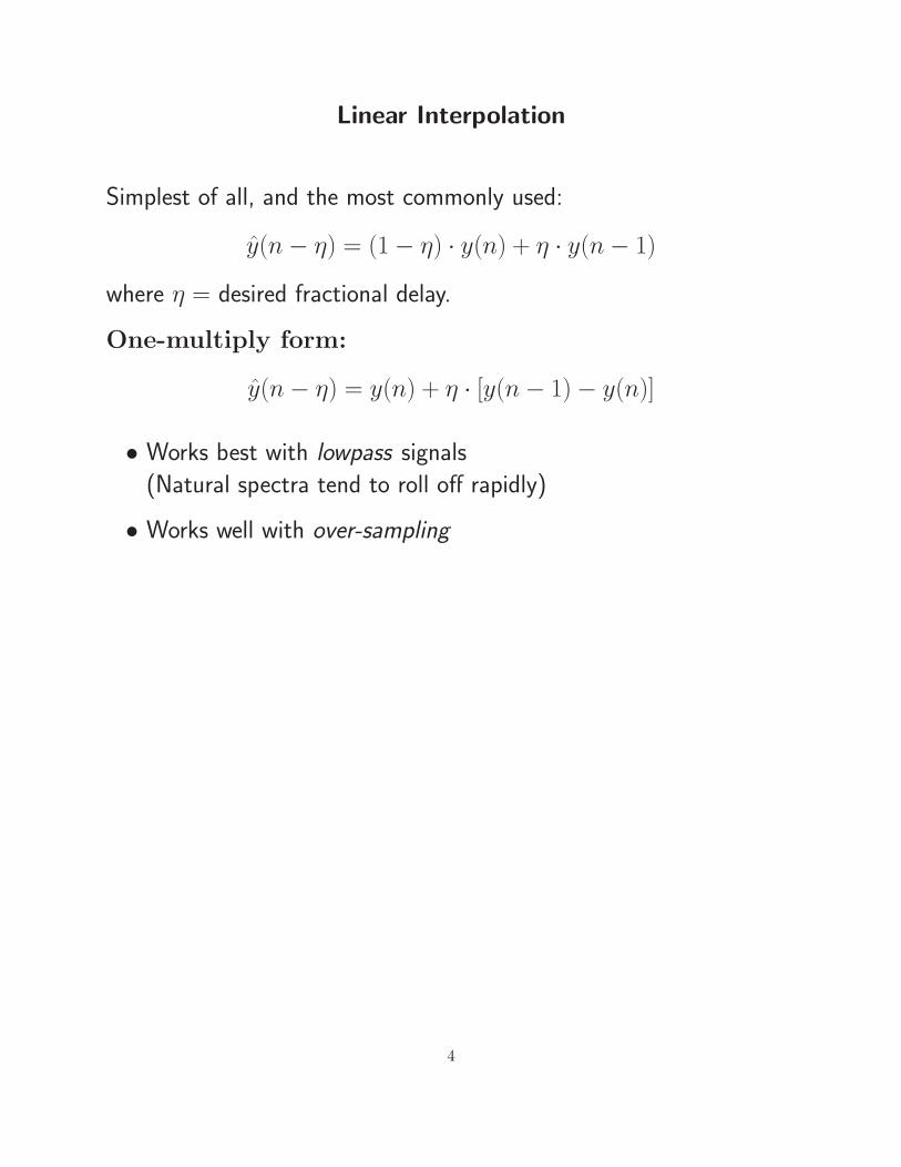
Linear Interpolation
Simplest of all, and the most commonly used:
y(n− η) = (1− η) · y(n) + η · y(n− 1)
where η = desired fractional delay.
One-multiply form:
y(n− η) = y(n) + η · [y(n− 1)− y(n)]
• Works best with lowpass signals
(Natural spectra tend to roll off rapidly)
• Works well with over-sampling
4
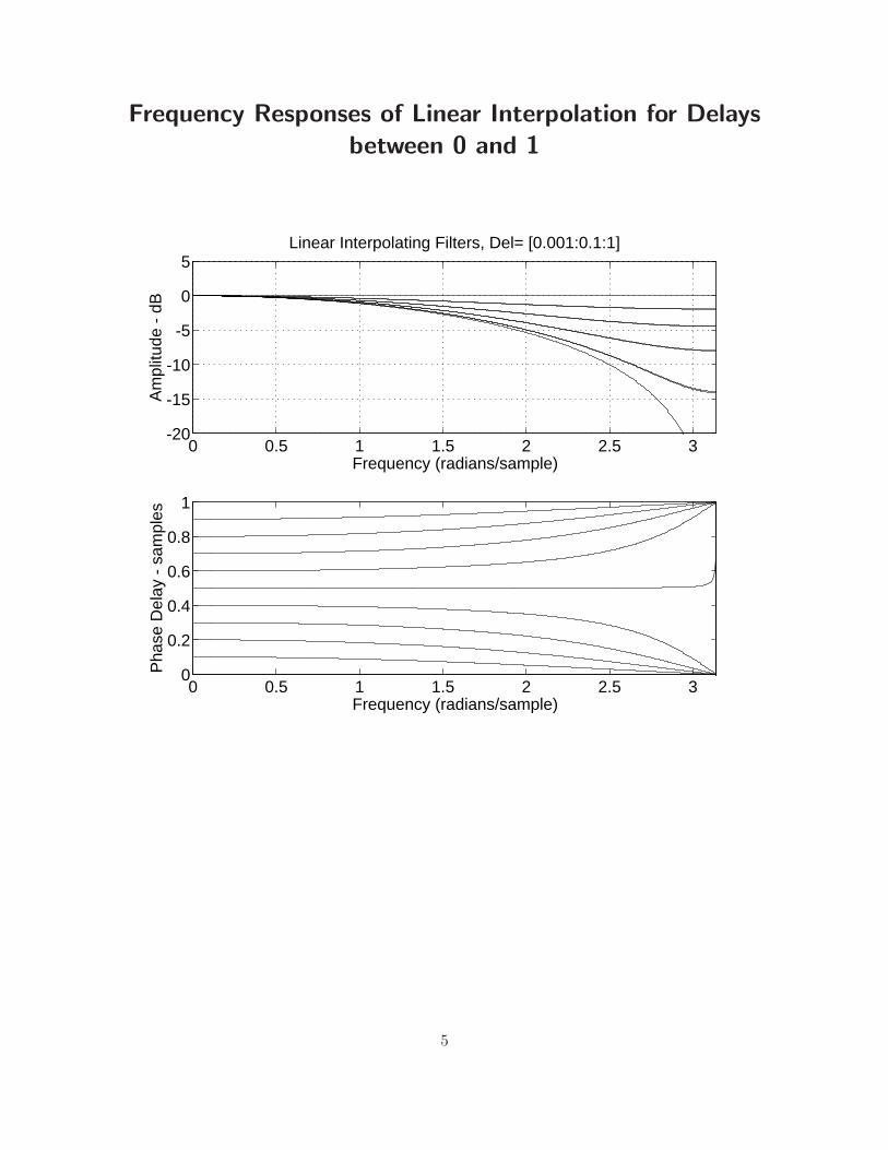
Frequency Responses of Linear Interpolation for Delays
between 0 and 1
0 0.5 1 1.5 2 2.5 3-20
-15
-10
-5
0
5Linear Interpolating Filters, Del= [0.001:0.1:1]
Frequency (radians/sample)
Am
plitu
de -
dB
0 0.5 1 1.5 2 2.5 30
0.2
0.4
0.6
0.8
1
Frequency (radians/sample)
Pha
se D
elay
- s
ampl
es
5

Linear Interpolation as a Convolution
Equivalent to filtering the continuous-time impulse train
N−1∑
n=0
y(nT )δ(t− nT )
with the continuous-time “triangular pulse” FIR filter
hl(t) =
1− |t/T | , |t| ≤ T
0, otherwise
followed by sampling at the desired phase
Replacing hl(t) by hs(t)∆= sinc
(
tT
)
converts linear interpolation to
ideal bandlimited interpolation (to be discussed later)
Upsample, Shift, Downsample View
z−LM M ( )ML
nx −( )nx
6
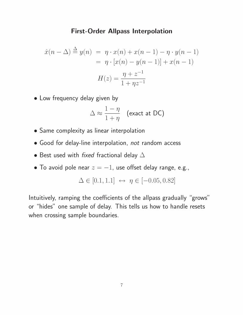
First-Order Allpass Interpolation
x(n−∆)∆= y(n) = η · x(n) + x(n− 1)− η · y(n− 1)
= η · [x(n)− y(n− 1)] + x(n− 1)
H(z) =η + z−1
1 + ηz−1
• Low frequency delay given by
∆ ≈1− η
1 + η(exact at DC)
• Same complexity as linear interpolation
• Good for delay-line interpolation, not random access
• Best used with fixed fractional delay ∆
• To avoid pole near z = −1, use offset delay range, e.g.,
∆ ∈ [0.1, 1.1] ↔ η ∈ [−0.05, 0.82]
Intuitively, ramping the coefficients of the allpass gradually “grows”
or “hides” one sample of delay. This tells us how to handle resets
when crossing sample boundaries.
7
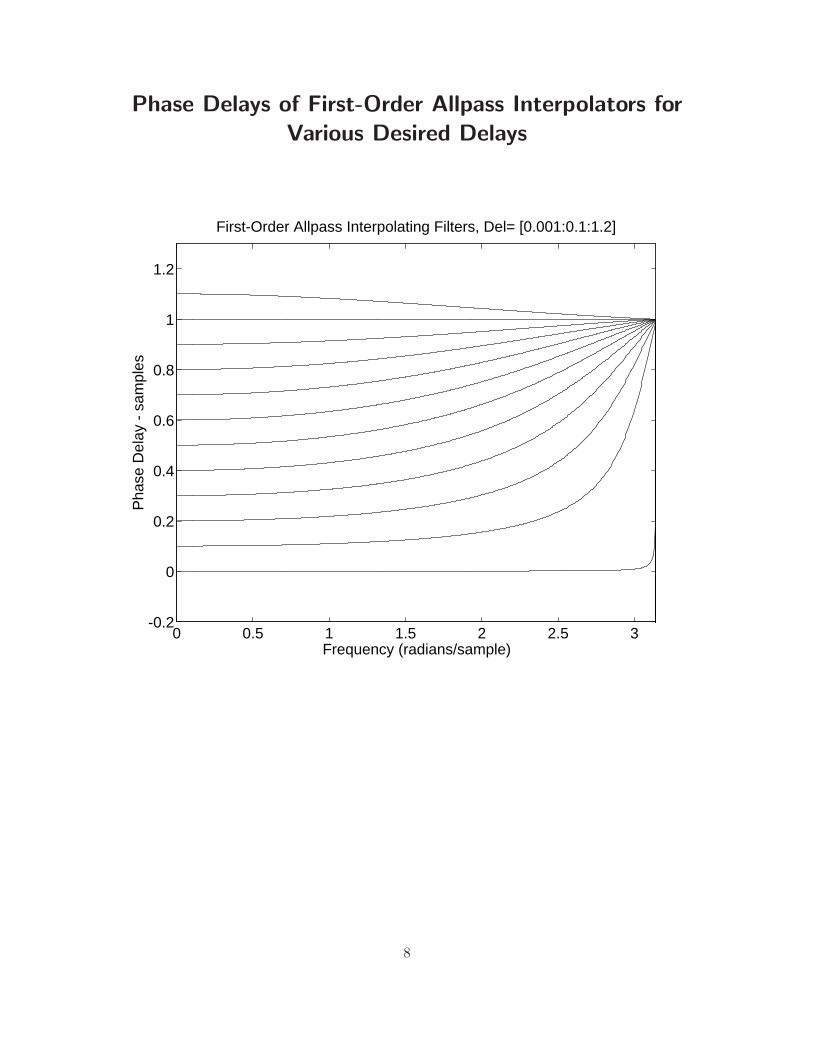
Phase Delays of First-Order Allpass Interpolators for
Various Desired Delays
0 0.5 1 1.5 2 2.5 3-0.2
0
0.2
0.4
0.6
0.8
1
1.2
First-Order Allpass Interpolating Filters, Del= [0.001:0.1:1.2]
Frequency (radians/sample)
Pha
se D
elay
- s
ampl
es
8
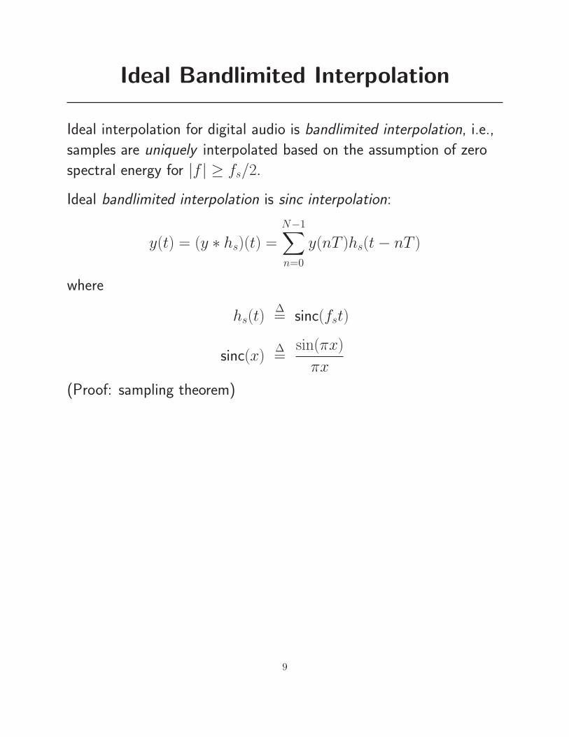
Ideal Bandlimited Interpolation
Ideal interpolation for digital audio is bandlimited interpolation, i.e.,
samples are uniquely interpolated based on the assumption of zero
spectral energy for |f | ≥ fs/2.
Ideal bandlimited interpolation is sinc interpolation:
y(t) = (y ∗ hs)(t) =
N−1∑
n=0
y(nT )hs(t− nT )
where
hs(t)∆= sinc(fst)
sinc(x)∆=
sin(πx)
πx
(Proof: sampling theorem)
9

Applications of Bandlimited Interpolation
Bandlimited Interpolation is used in (e.g.)
• Sampling-rate conversion
• Wavetable/sampling synthesis
• Virtual analog synthesis
• Oversampling D/A converters
• Fractional delay filtering
Fractional delay filtering is a special case of bandlimited
interpolation:
• Fractional delay filters only need sequential access ⇒ IIR filters
can be used
• General bandlimited interpolation requires random access ⇒ FIR
filters normally used
Fractional Delay Filters are used for (among other things)
• Time-varying delay lines (flanging, chorus, leslie)
• Resonator tuning in digital waveguide models
• Exact tonehole placement in woodwind models
• Beam steering of microphone / speaker arrays
10

Example Application of Fractional Delay Filtering and
Bandlimited Interpolation
(x = 0)
. . .
. . .. . .
. . .y (n)-
y (n)+
y (nT,0) y (nT,ξ)
y (n-M)+
y (n+M)
(x = ξ) (x = McT)
M samples delay
M samples delay
-
Digital Waveguide String Model
• “Pick-up” needs Bandlimited Interpolation
• “Tuning” needs Fractional Delay Filtering
11

The Sinc Function (“Cardinal Sine”)
sinc(t)∆=
sin(πt)
πt
-7 -6 -5 -4 -3 -2 -1 1 2 3 4 5 6 7
1
. . .. . .
. . .. . .
Sinc Function
The sinc function is the impulse response of the ideal lowpass filter
which cuts off at half the sampling rate
Ideal Lowpass Filter Frequency Response
-0.4 -0.2 0 0.2 0.4
0.2
0.4
0.6
0.8
1
π−π
12
Ideal D/A Conversion
Each sample in the time domain scales and locates one sinc function
in the unique, continuous, bandlimited interpolation of the sampled
signal.
Convolving a sampled signal y(n) with sinc(n− η) “evaluates” the
signal at an arbitrary continuous time η ∈ R:
y(η) =
N−1∑
n=0
y(n)sinc(η − n)
= Sampley ∗ Shiftn(δ)
13
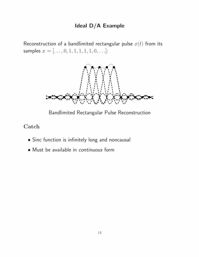
Ideal D/A Example
Reconstruction of a bandlimited rectangular pulse x(t) from its
samples x = [. . . , 0, 1, 1, 1, 1, 1, 0, . . .]:
Bandlimited Rectangular Pulse Reconstruction
Catch
• Sinc function is infinitely long and noncausal
• Must be available in continuous form
14
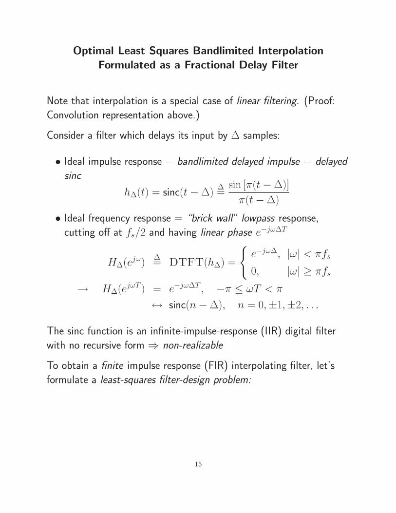
Optimal Least Squares Bandlimited Interpolation
Formulated as a Fractional Delay Filter
Note that interpolation is a special case of linear filtering. (Proof:
Convolution representation above.)
Consider a filter which delays its input by ∆ samples:
• Ideal impulse response = bandlimited delayed impulse = delayed
sinc
h∆(t) = sinc(t−∆)∆=
sin [π(t−∆)]
π(t−∆)
• Ideal frequency response = “brick wall” lowpass response,
cutting off at fs/2 and having linear phase e−jω∆T
H∆(ejω)∆= DTFT(h∆) =
e−jω∆, |ω| < πfs
0, |ω| ≥ πfs
→ H∆(ejωT ) = e−jω∆T , −π ≤ ωT < π
↔ sinc(n−∆), n = 0,±1,±2, . . .
The sinc function is an infinite-impulse-response (IIR) digital filter
with no recursive form ⇒ non-realizable
To obtain a finite impulse response (FIR) interpolating filter, let’s
formulate a least-squares filter-design problem:
15

Desired Interpolator Frequency Response
H∆
(
ejωT)
= e−jω∆T , ∆ = Desired delay in samples
FIR Filter Frequency Response
H∆
(
ejωT)
=
L−1∑
n=0
h∆(n)e−jωnT
Error to Minimize
E(
ejωT)
= H∆
(
ejωT)
− H∆
(
ejωT)
L2 Error Norm
J(h)∆= ‖E ‖22 =
T
2π
∫ π/T
−π/T
∣
∣E(
ejωT)∣
∣
2dω
=T
2π
∫ π/T
−π/T
∣
∣
∣H∆
(
ejωT)
− H∆
(
ejωT)
∣
∣
∣
2
dω
By Parseval’s Theorem
J(h) =
∞∑
n=0
∣
∣
∣h∆(n)− h∆(n)
∣
∣
∣
2
Optimal Least-Squares FIR Interpolator
h∆(n) =
sinc(n−∆), 0 ≤ n ≤ L− 1
0, otherwise
16

Truncated-Sinc Interpolation
Truncate sinc(t) at 5th zero-crossing to left and right of time 0 to get
Frequency Response : Rectangular Window
-400 -200 200 400
-80
-60
-40
-20
Truncated-Sinc Transform
• Vertical axis in dB, horizontal axis in spectral samples
• Optimal in least-squares sense
• Poor stop-band rejection (≈ 20 dB)
• “Gibbs Phenomenon” gives too much “ripple”
• Ripple can be reduced by tapering the sinc function to zero
instead of simply truncating it.
17
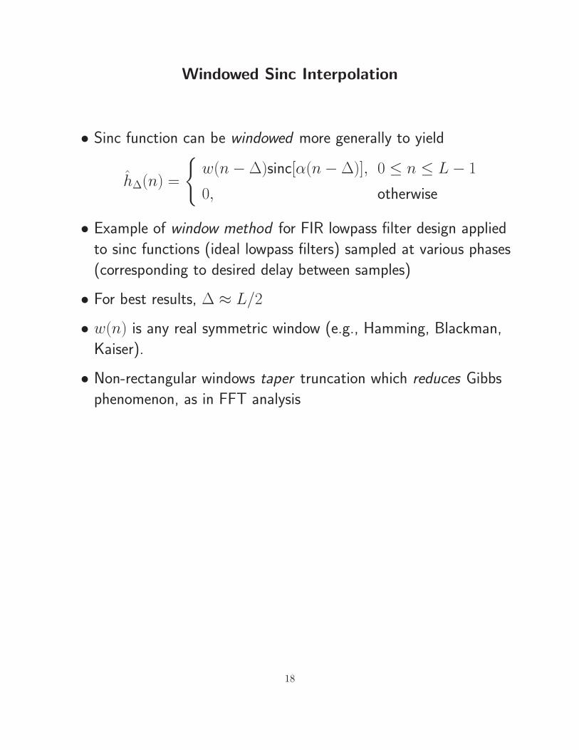
Windowed Sinc Interpolation
• Sinc function can be windowed more generally to yield
h∆(n) =
w(n−∆)sinc[α(n−∆)], 0 ≤ n ≤ L− 1
0, otherwise
• Example of window method for FIR lowpass filter design applied
to sinc functions (ideal lowpass filters) sampled at various phases
(corresponding to desired delay between samples)
• For best results, ∆ ≈ L/2
• w(n) is any real symmetric window (e.g., Hamming, Blackman,
Kaiser).
• Non-rectangular windows taper truncation which reduces Gibbs
phenomenon, as in FFT analysis
18
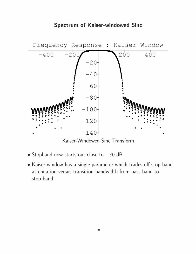
Spectrum of Kaiser-windowed Sinc
Frequency Response : Kaiser Window
-400 -200 200 400
-140
-120
-100
-80
-60
-40
-20
Kaiser-Windowed Sinc Transform
• Stopband now starts out close to −80 dB
• Kaiser window has a single parameter which trades off stop-band
attenuation versus transition-bandwidth from pass-band to
stop-band
19
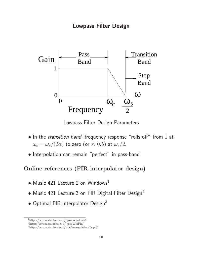
Lowpass Filter Design
ω
Gain
ωc00
1
ωs2
TransitionBand
PassBand
StopBand
Frequency
Lowpass Filter Design Parameters
• In the transition band, frequency response “rolls off” from 1 at
ωc = ωs/(2α) to zero (or ≈ 0.5) at ωs/2.
• Interpolation can remain “perfect” in pass-band
Online references (FIR interpolator design)
• Music 421 Lecture 2 on Windows1
• Music 421 Lecture 3 on FIR Digital Filter Design2
• Optimal FIR Interpolator Design3
1http://ccrma.stanford.edu/˜jos/Windows/2http://ccrma.stanford.edu/˜jos/WinFlt/3http://ccrma.stanford.edu/ jos/resample/optfir.pdf
20
Oversampling Reduces Filter Length
• Example 1:
– fs = 44.1 kHz (CD quality)
– Audio upper limit = 20 kHz
– Transition band = 2.05 kHz
– FIR filter length∆= L1
• Example 2:
– fs = 48 kHz (e.g., DAT)
– Audio upper limit = 20 kHz
– Transition band = 4 kHz
– FIR filter length ≈ L1/2
• Required FIR filter length varies inversely with transition
bandwidth
⇒ Required filter length in example 1 is almost double
(≈ 4/2.1) the required filter length for example 2
• Increasing the sampling rate by less than ten percent reduces the
filter expense by almost fifty percent
21

The Digital Audio Resampling Home Page
• C++ software for windowed-sinc interpolation
• C++ software for FIR filter design by window method
• Fixed-point data and filter coefficients
• Can be adapted to time-varying resampling
• Open source, free
• First written in 1983 in SAIL
• URL: http://ccrma.stanford.edu/˜jos/resample/
• Most needed upgrade:
– Design and install a set of optimal FIR interpolating filters.4
4http://ccrma.stanford.edu/ jos/resample/optfir.pdf
22

Lagrange Interpolation
• Lagrange interpolation is just polynomial interpolation
• N th-order polynomial interpolates N + 1 points
• First-order case = linear interpolation
Problem Formulation
Given a set of N + 1 known samples f(xk), k = 0, 1, 2, . . . , N , find
the unique order N polynomial y(x) which interpolates the samples
Solution (Waring, Lagrange):
y(x) =
N∑
k=0
lk(x)f(xk)
where
lk(x)∆=
(x− x0) · · · (x− xk−1)(x− xk+1) · · · (x− xN)
(xk − x0) · · · (xk − xk−1)(xk − xk+1) · · · (xk − xN)
• Numerator gives a zero at all samples but the kth
• Denominator simply normalizes lk(x) to 1 at x = xk
• As a result,
lk(xj) = δkj∆=
1, j = k
0, j 6= k
• Generalized bandlimited impulse = generalized sinc function:
Each lk(x) goes through 1 at x = xk and zero at all other
sample points
I.e., lk(x) is analogous to sinc(x− xk)
23
• Lagrange interpolaton is equivalent to windowed sinc
interpolation using a binomial window
• Can be viewed as a linear, spatially varying filter (in analogy with
linear, time-varying filters)
24

Example Lagrange Basis Functions
0 200 400 600 800 1000 1200−10
0
10
Lagrange Basis Polynomials, Order = 8,Random xk (marked by dotted lines)
l 1(x)
0 200 400 600 800 1000 1200−10
0
10
l 2(x)
0 200 400 600 800 1000 1200−2
0
2
l 3(x)
0 200 400 600 800 1000 1200−2
0
2
l 4(x)
0 200 400 600 800 1000 1200−5
0
5
l 5(x)
0 200 400 600 800 1000 1200−20
0
20
l 6(x)
0 200 400 600 800 1000 1200−20
0
20
l 7(x)
0 200 400 600 800 1000 1200−5
0
5
l 8(x)
x
25

Lagrange Interpolation Optimality
In the uniformly sampled case, Lagrange interpolation can be
viewed as ordinary FIR filtering:
– Lagrange interpolation filters maximally flat in the frequency
domain about dc:
dmE(ejω)
dωm
∣
∣
∣
∣
ω=0
= 0, m = 0, 1, 2, . . . , N,
where
E(ejω)∆= e−jω∆ −
N∑
n=0
h(n)e−jωn
and ∆ is the desired delay in samples.
– Same optimality criterion as Butterworth filters in classical
analog filter design
– Can also be viewed as “Pade approximation” to a constant
frequency response in the frequency domain
26

Proof of Maximum Flatness at DC
The maximumally flat fractional-delay FIR filter is obtained by
equating to zero all N + 1 leading terms in the Taylor
(Maclaurin) expansion of the frequency-response error at dc:
0 =dk
dωkE(ejω)
∣
∣
∣
∣
ω=0
=dk
dωk
[
e−jω∆ −
N∑
n=0
h(n)e−jωn
]∣
∣
∣
∣
∣
ω=0
= (−j∆)k −
N∑
n=0
(−jn)kh(n)
=⇒N
∑
n=0
nkh(n) = ∆k, k = 0, 1, . . . , N
This is a linear system of equations of the form V h = ∆, where
V is a Vandermonde matrix. The solution can be written as a
ratio of Vandermonde determinants using Cramer’s rule. As
shown by Cauchy (1812), the determinant of a Vandermonde
matrix [pj−1i ], i, j = 1, . . . , N can be expressed in closed form as
∣
∣
∣
[
pj−1i
]∣
∣
∣=
∏
j>i
(pj − pi)
= (p2 − p1)(p3 − p1) · · · (pN − p1) · · ·
(p3 − p2)(p4 − p2) · · · (pN − p2) · · ·
(pN−1 − pN−2)(pN − pN−2) ·
(pN − pN−1)
27
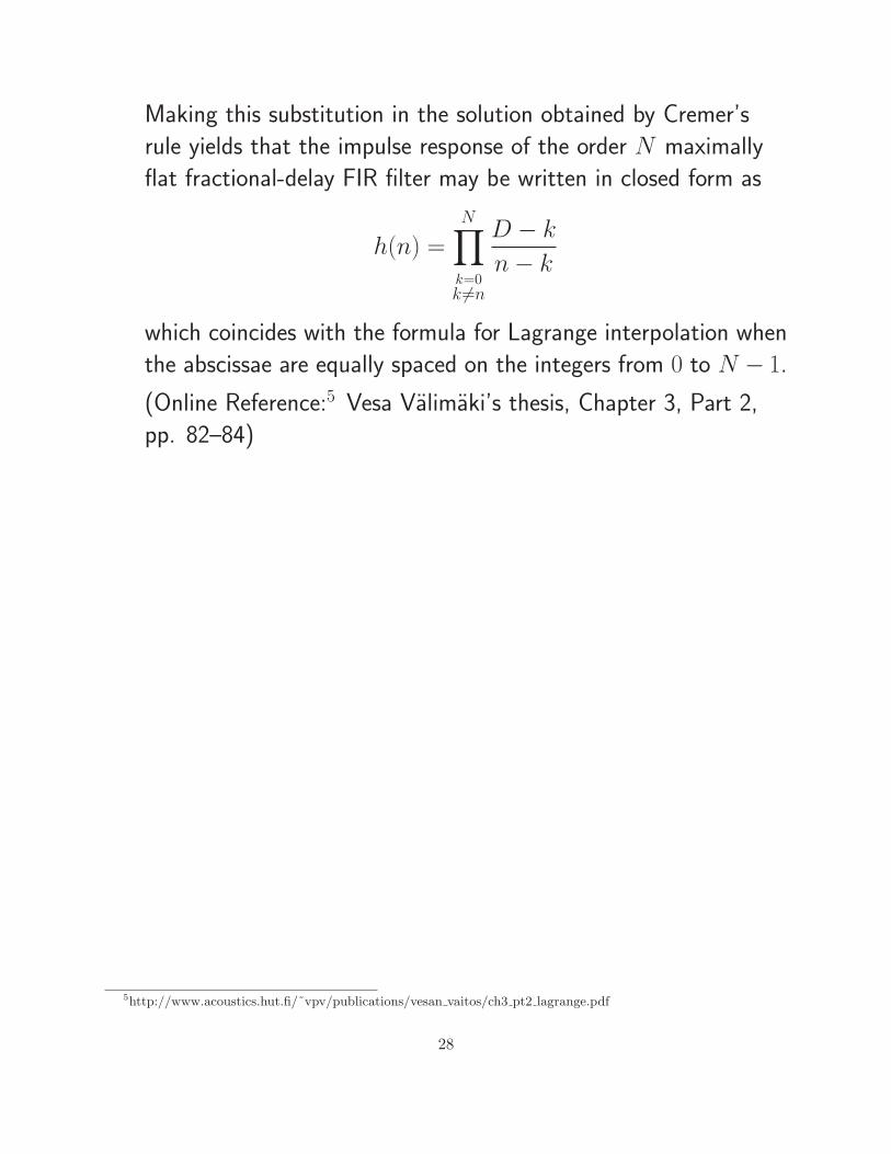
Making this substitution in the solution obtained by Cremer’s
rule yields that the impulse response of the order N maximally
flat fractional-delay FIR filter may be written in closed form as
h(n) =
N∏
k=0
k 6=n
D − k
n− k
which coincides with the formula for Lagrange interpolation when
the abscissae are equally spaced on the integers from 0 to N − 1.
(Online Reference:5 Vesa Valimaki’s thesis, Chapter 3, Part 2,
pp. 82–84)
5http://www.acoustics.hut.fi/˜vpv/publications/vesan vaitos/ch3 pt2 lagrange.pdf
28
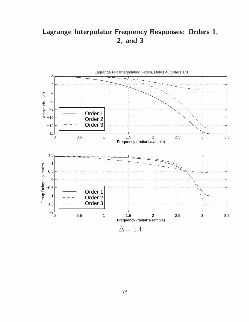
Lagrange Interpolator Frequency Responses: Orders 1,
2, and 3
0 0.5 1 1.5 2 2.5 3 3.5−14
−12
−10
−8
−6
−4
−2
0Lagrange FIR Interpolating Filters, Del=1.4, Orders 1:3
Frequency (radians/sample)
Am
plitu
de −
dB
Order 1Order 2Order 3
0 0.5 1 1.5 2 2.5 3 3.5−2
−1.5
−1
−0.5
0
0.5
1
1.5
Frequency (radians/sample)
Gro
up D
elay
− s
ampl
es
Order 1Order 2Order 3
∆ = 1.4
29
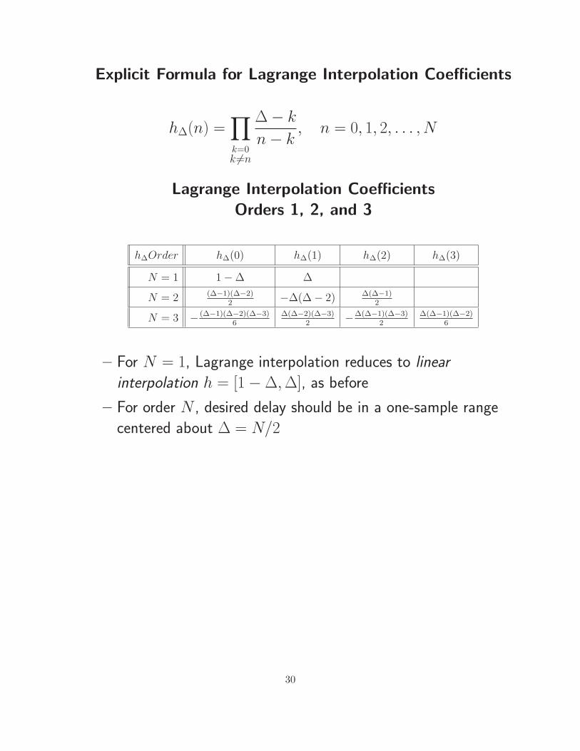
Explicit Formula for Lagrange Interpolation Coefficients
h∆(n) =∏
k=0
k 6=n
∆− k
n− k, n = 0, 1, 2, . . . , N
Lagrange Interpolation Coefficients
Orders 1, 2, and 3
h∆Order h∆(0) h∆(1) h∆(2) h∆(3)
N = 1 1−∆ ∆
N = 2 (∆−1)(∆−2)2
−∆(∆− 2) ∆(∆−1)2
N = 3 − (∆−1)(∆−2)(∆−3)6
∆(∆−2)(∆−3)2
−∆(∆−1)(∆−3)2
∆(∆−1)(∆−2)6
– For N = 1, Lagrange interpolation reduces to linear
interpolation h = [1−∆, ∆], as before
– For order N , desired delay should be in a one-sample range
centered about ∆ = N/2
30

Matlab Code For Lagrange Fractional Delay
function h = lagrange(N, delay)
%LAGRANGE h=lagrange(N,delay) returns order N FIR
% filter h which implements given delay
% (in samples). For best results,
% delay should be near N/2 +/- 1.
n = 0:N;
h = ones(1,N+1);
for k = 0:N
index = find(n ~= k);
h(index) = h(index) * (delay-k)./ (n(index)-k);
end
31
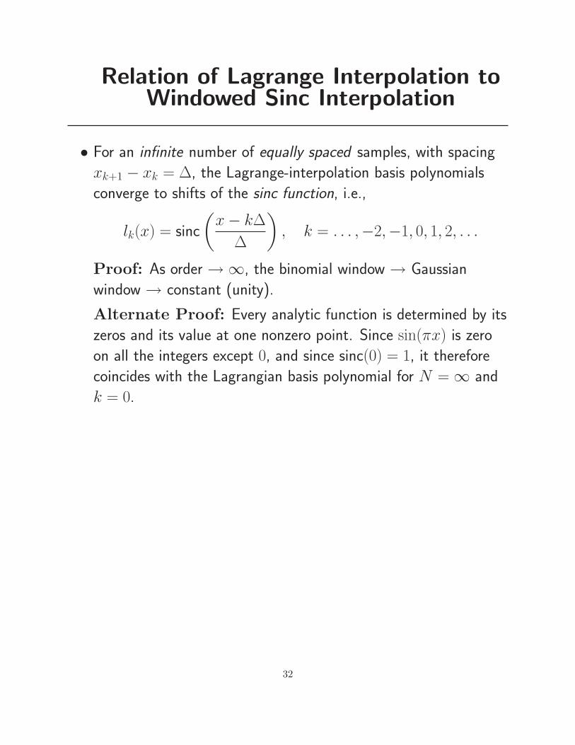
Relation of Lagrange Interpolation toWindowed Sinc Interpolation
• For an infinite number of equally spaced samples, with spacing
xk+1 − xk = ∆, the Lagrange-interpolation basis polynomials
converge to shifts of the sinc function, i.e.,
lk(x) = sinc
(
x− k∆
∆
)
, k = . . . ,−2,−1, 0, 1, 2, . . .
Proof: As order →∞, the binomial window → Gaussian
window → constant (unity).
Alternate Proof: Every analytic function is determined by its
zeros and its value at one nonzero point. Since sin(πx) is zero
on all the integers except 0, and since sinc(0) = 1, it therefore
coincides with the Lagrangian basis polynomial for N =∞ and
k = 0.
32

Variable FIR Interpolating Filter
Basic idea: Each FIR filter coefficient hn becomes a polynomial in
the delay parameter ∆:
h∆(n)∆=
P∑
m=0
cn(m)∆m, n = 0, 1, 2, . . . , N
⇔ H∆(z)∆=
N∑
n=0
h∆(n)z−n
=
N∑
n=0
[
P∑
m=0
cn(m)∆m
]
z−n
=
P∑
m=0
[
N∑
n=0
cn(m)z−n
]
∆m
∆=
P∑
m=0
Cm(z)∆m
• More generally: H∆(x) =∑
m α(∆)Cm(z)
where α(∆) is provided by a table lookup
• Basic idea applies to any one-parameter filter variation
• Also applies to time-varying filters (∆← t)
33

Farrow Structure for Variable Delay FIR Filters
When the polynomial in ∆ is evaluated using Horner’s rule,
Xn−∆(z) = X + ∆ [C1X + ∆ [C2X + +∆ [C3X + · · · ]]] ,
the filter structure becomes
( )nx
( )zCN ( )zC −N 1 ( )zC2 ( )zC1
( )nx ∆−∆ ∆ ∆ ∆
. . .
. . .
As delay ∆ varies, “basis filters” Ck(z) remain fixed
⇒ very convenient for changing ∆ over time
Farrow Structure Design Procedure
Solve the N∆ equations
z−∆i =
N∑
k=0
Ck(z)∆ki , i = 1, 2, . . . , N∆
for the N + 1 FIR transfer functions Ck(z), each order NC in general
References: Laakso et al., Farrow
34

Thiran Allpass Interpolators
Given a desired delay ∆ = N + δ samples, an order N allpass filter
H(z) =z−NA
(
z−1)
A(z)=
aN + aN−1z−1 + · · · + a1z
−(N−1) + z−N
1 + a1z−1 + · · · + aN−1z−(N−1) + aNz−N
can be designed having maximally flat group delay equal to ∆ at DC
using the formula
ak = (−1)k(
N
k
) N∏
n=0
∆−N + n
∆−N + k + n, k = 0, 1, 2, . . . , N
where(
N
k
)
=N !
k!(N − k)!
denotes the kth binomial coefficient
• a0 = 1 without further scaling
• For sufficiently large ∆, stability is guaranteed
rule of thumb: ∆ ≈ order
• Mean group delay is always N samples
(for any stable N th-order allpass filter):
1
2π
∫ 2π
0
D(ω)dω∆= −
1
2π
∫ 2π
0
Θ′(ω)dω = −1
2π[Θ(2π)− Θ(0)] = N
• Only known closed-form case for allpass interpolators of arbitrary
order
• Effective for delay-line interpolation needed for tuning since pitch
perception is most acute at low frequencies.
35

Frequency Responses of Thiran Allpass Interpolators for
Fractional Delay
0 0.5 1 1.5 2 2.5 3 3.5−2
−1.5
−1
−0.5
0
0.5Thiran Interpolating Filters, Del=Order+0.3, Order=[1,2,3,5,10,20]
Gro
up D
elay
− s
ampl
es
Frequency (radians/sample)
1 2 3 5 1020
36

Large Delay Changes
When implementing large delay-length changes (by many samples), a
useful implementation is to cross-fade from the initial delay line
configuration to the new configuration.
• Computation doubled during cross-fade
• Cross-fade should be long enough to sound smooth
• Not a true “morph” from one delay length to another, since we
do not pass through the intermediate delay lengths.
• A single delay line can be shared such that the cross-fade occurs
from one read-pointer (plus associated filtering) to another.
37

L-Infinity (Chebyshev) Fractional Delay Filters
• Use Linear Programming (LP) for real-valued L∞-norm
minimization
• Remez exchange algorithm (remez, cremez)
• In the complex case, we have a problem known as a
Quadratically Constrained Quadratic Program
• Approximated by sets of linear consraints
(e.g., a polygon can be used to approximate a circle)
• Can solve with code developed by Prof. Boyd’s group
• See Mohonk-97 paper6 for details.
6http://ccrma.stanford.edu/ jos/resample/optfir.pdf
38

Chebyshev FD-FIR Design Example
0 0.1 0.2 0.3 0.4 0.5 0.6 0.7 0.8 0.9 17
7.2
7.4
7.6
Normalized Frequency
grou
p de
lay
− sa
mpl
es
0 0.1 0.2 0.3 0.4 0.5 0.6 0.7 0.8 0.9 10
0.5
1
1.5
Ampl
itude
Fractional delay min−max filters
39

0 5 10 15 20 25 300
0.002
0.004
0.006
0.008
0.01
0.012
0.014Modulus of the Error − (infinity norm)
40

Comparison of Lagrange and OptimalChebyshev Fractional-Delay Filter
Frequency Responses
0 0.1 0.2 0.3 0.4 0.5 0.6 0.7 0.8 0.9 17
7.2
7.4
7.6
Normalized Frequency
grou
p de
lay
− s
ampl
es
0 0.1 0.2 0.3 0.4 0.5 0.6 0.7 0.8 0.9 10
0.5
1
Am
plitu
de
Comparison between min−maxs and Lagrange − L=16
41
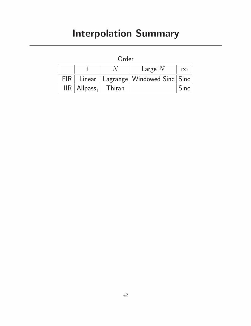
Interpolation Summary
Order
1 N Large N ∞
FIR Linear Lagrange Windowed Sinc Sinc
IIR Allpass1 Thiran Sinc
42