TABLE OF CONTENTS

Introduction 1

Company background 2

My projects outline 3

My project details 4-28

Working culture & management-labour relationship 29

Conclusion 30

Reference 31

Appendix 32

Introduction

This report is a compilation of the experience and work I have done during my 3 months internship from 19th Nov 2012 to 28th Feb 2013. The internship is performed in order to fulfill the requirements of the degree regulation, and the expectations of EAC, Engineers Australia, and the Institution of Engineers Malaysia, and it’s usually done after completing three years (6 semesters) of studies during the year end vacation break. The objective of the internship is to allow us to gain firsthand knowledge of the practice of engineering and to acquire skills and experiences, which will be of value during subsequent studies and later employment.

Here, I would like to thanks my supervisor during my internship, Dr Chong Fei Seong for passing his knowledge and experience to me during these 3 months in order for me to complete the industrial training. Also, I would like to thanks Monash University for giving me the opportunity to gain working experience before I graduate from the university. Besides, special thanks to my colleagues who works with me and making my internship period a fun and enjoyable one.

The roles I play in this company as an intern are mostly dealing with programming tasks. Most of the time, I use MATLAB as my programming tools to design applications for the company. Once in a while, I also have to follow my supervisor to do plant visit and vibration testing. During the visit, I gained a lot of firsthand practical experience as well as encounter many practical issues that we solve together.

Overall, this internship was a success and I am glad that I am able to get the most out of it.

Company background

Sri Wawasan Sdn Bhd was established in 1991, to provide a comprehensive range of specialist services and products in the fields of Vibration, Noise and Maintenance Engineering. Its customers include offshore oil and gas, onshore petrochemical, power generation, marine, manufacturing, food processing and others.

Sri Wawasan Sdn Bhd offers Maintenance Engineering Solutions that reduces maintenance costs, increase equipment availability and reliability, improves safety, and enhances product quality. They offer a wide spectrum of consultancy and engineering services in the fields of vibration, noise and maintenance engineering.

Sri Wawasan Sdn Bhd has working relationships with major industries throughout the country such as Petronas, Shell, Malaysia LNG, utilities, air-conditioner manufacturers and contractor. It also has close coorperation with many specialist partners.

Sri Wawasan Sdn Bhd supplies a complete range of products for application in vibration, noise analysis and machine condition and performance monitoring.

Vibration sensors and signal conditioning hardware Portable dynamic signal analyzers and balancers Online condition and performance monitoring system Performance monitoring software (turbines, compressors, etc) Offline condition monitoring systems Condition monitoring & diagnostic software

Sri Wawasan Sdn Bhd also actively involved in machine monitoring and diagnosis, including a wide spectrum of vibration and noise related problems such as:

On-line & off-line condition monitoring (predictive maintenance) Transient analysis of machine startup/coast down System integration, installation, and commissioning of integrated machinery

management information system Gas turbine and turbo machinery consultancy in collaboration with Fern engineering,

United States of America Vibration troubleshooting and faults diagnostics of machineries, structures, piping,

building & ground In-situ dynamic balancing & alignment Analytical modeling of machinery and machine design audit Noise monitoring/analysis & noise control Calibration of vibration transducers/instrumentation systems

My projects outline

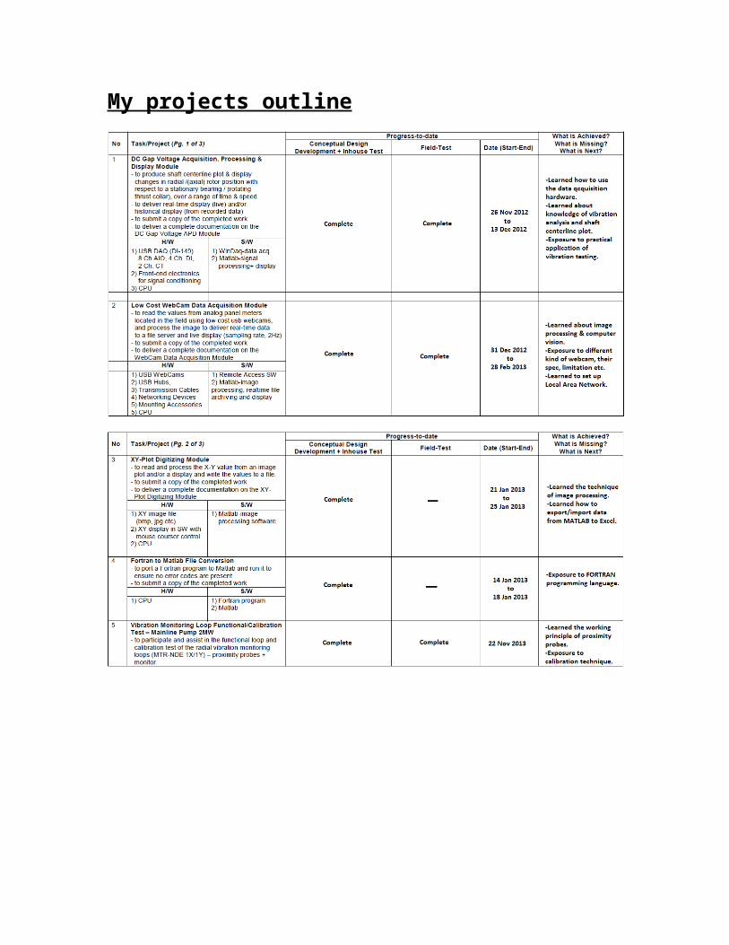
My project details

1) DC gap voltage acquisition, processing & display module

Project background:

In machine condition monitoring, we often need to monitor turbo machinery with fluid film bearing of pump, chiller, compressor etc. Some turbo machinery mechanical faults have characteristic plot shapes. By comparing the acquired plots with any known characteristics we can detect faults and diagnose machine problems.

To acquire the characteristic plot, namely orbit plot, time base plot, and shaft centerline plot, we have to mount 2 proximity probes orthogonally on the fluid film bearing. Proximity probes are devices that show different voltage reading as the distance between its tips and the object varies. It has a linear voltage-distance characteristic over a specified range. The time base plot displays the signals as a function of time in one or more revolutions with two separate plots, one for x-axis and one for y-axis. A shaft centerline plot displays the shaft center DC position changes within a bearing clearance range. An orbit plot represents the shaft center AC dynamic motion. Both the orbit plot and shaft centerline plot is generated by plotting y-axis against x-axis signal data. [1]

Figure 1: Two orthogonally-mounted proximity probes measure the shaft motion. The outer circle depicts the bearing clearance. As the shaft speeds up in the counterclockwise (CCW) rotation direction, the shaft center moves from the bottom of the bearing clearance to the normal operational center, as the Shaft Centerline shows. As the shaft continues in normal operation, the shaft center moves around the normal operating center, as the Shaft Orbit shows.

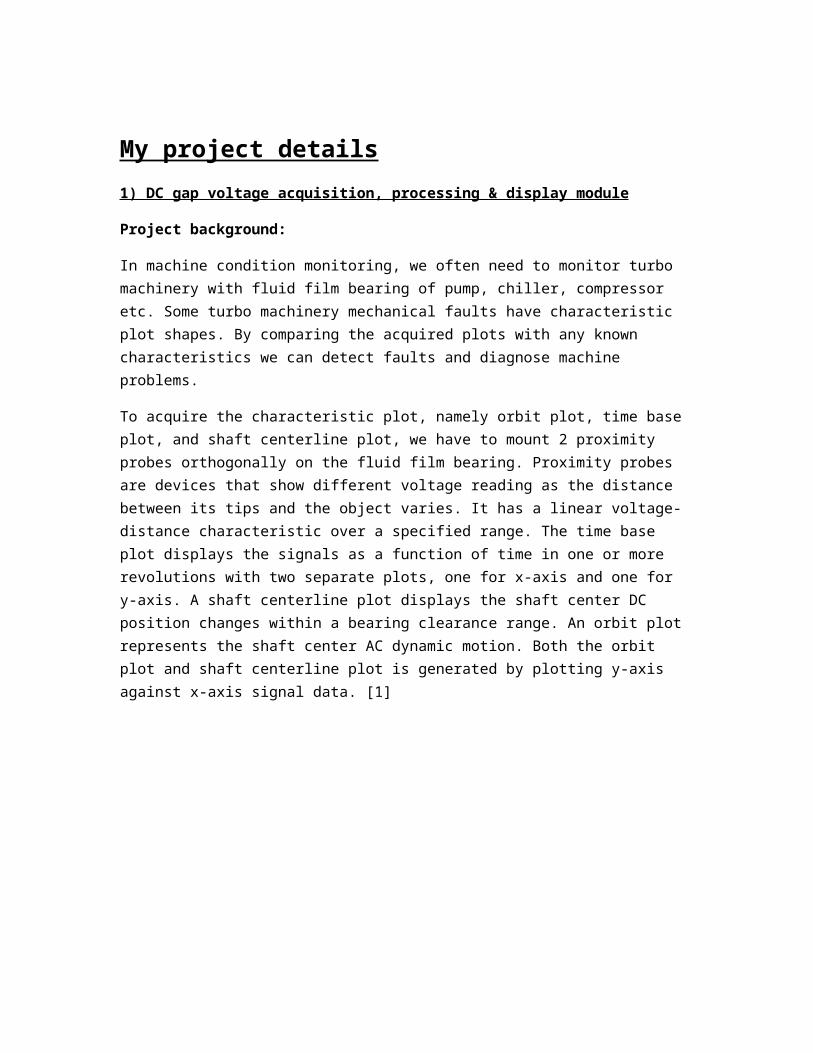
In many cases, we cannot mount probes easily in the desired 90 degrees out of phase horizontal and vertical orientation. Probes often have a 45-degree deviation instead. The following illustration shows the common mounting positions for X and Y probes.

Figure2: Common mounting positions for X and Y probes.

However, an orbit plot assumes that the signals are from probes in true horizontal and vertical positions. To display data with respect to a true vertical and horizontal coordinate system, you must rotate the data by the probe angular offset from the desired coordinates.

Figure 3: Time base plot of the X and Y axis.

Figure 4: Typical shaft centerline plot of a machine startup. The numerical values show the rotational speed.

In this particular project, we only make a program for shaft centerline plot and time base plot, which means it is only designed for DC vibration analysis.

Hardware used:

i) DATAQ (DI-149) data acquisition hardware [2]

ii) Laptop

Software used:

i) MATLAB

ii) DATAQ instrument data acquisition software

Description:

The purpose of this project is to make a standalone application that can display the real time shaft centerline movement of the machine under test and time base plot on the laptop that runs the application. The signal data in the form of electrical voltage is acquired using the DATAQ DI-149 data acquisition hardware. After that, the acquired data is sent to the computer via USB cable and the DATAQ instrument software as interface. A MATLAB standalone application program was designed to receive the signal data, de-noise the data, and then finally the shaft centerline plot is generated by plotting y-axis data against x-axis data. All the process described is performed in real time and it can be depicted as follow:

Figure 5: Process flow of data acquisition module.

Coding detail:

Due to the massive length of the code, only important part of the code is presented here.

Firstly, the time base data is imported to MATLAB and the time base plot is generated.

Secondly, the time base signal is divided into 60 segments with each segment having the same length. The average value of each segment is computed and the result stored in an array.

Thirdly, every individual data is compared with the average value of their respective segment. If the data value differs from the average value of that segment by 2.5%, that particular data point is modified to be equal to the average value. By doing so, all the spike (noise) that ‘’pollute’’ the data will be eliminated and we end up with a ‘’clean’’ signal with useful data.

After that, we compressed the signal data so that the compressed signal has only 250 data points. To do this, we divide the ‘’clean’’ data into 250 segments, and each segments is combined into 1 point representing the average value of that segment. The reason we do this is because the original data length is too big for real time processing. Besides, by compressing the signal, we can see a more general movement of the motor shaft in real time when plotting the shaft centerline movement.

After the data compression, we performed calibration to convert the data signal into distance. This required user to key in sensitivity (mV/um) information of the proximity probes. Also, after the conversion to distance, we shift the data with reference to the DC gap voltage by minus off every data with the DC gap voltage of their respective axis. The formula to do the overall conversion is as follow:

Distance=Data−DCgap voltagesensiti vity

Finally, we perform axis transformation to the distance data if necessary and plot the shaft centerline movement of each axes respectively on the MATLAB GUI in real time.

Figure 6: MATLAB GUI of the module.

2) Low cost webcam data acquisition module

Project background:

In the process of condition monitoring, we have to run a series of vibration test and also performance test for the machines. There are a lot of analogue meter mounted on the machine, which their reading need to be taken and monitored when performing the test. However, the machine is located in a remote location, where human are not allowed or easily allowed to enter and take reading. Furthermore, the location of the machine is far away from the control room where we gather and do the monitoring, thus provide difficulties when taking the reading from the analogue meter. As a solution, I was asked by my supervisor to design a webcam module so that we will place the webcam in front of the meter, and the image taken from the webcam can be accessed in the control room and the webcam module will do the reading automatically.

Hardware used:

i) USB webcam [3]

ii) USB hub

iii) Ethernet cable

iv) Network switch

v) Mounting devices

vi) Laptop

Software used:

i) MATLAB

ii) Team Viewer remote access software

Project description:

The purpose of this project is to design a standalone application using MATLAB so that we can use a low cost USB webcam to read the needle reading of analogue meter, up to 4 webcams at the same time, and at the end export all the reading acquired into Microsoft Excel for further analysis. Basically, the project is divided into 2 parts. The first part of the project deal with image processing, which comprises the computer vision technique to identifies the needle from the image taken, calculate the needle reading after the needles position has been identified, auto sampling module or manual sampling module, and exporting the data into Microsoft Excel up to 4 analogue meters at the same time. The second part of the project basically solve the problem regarding image acquisition, which include setting up the entire network (the distance between analogue meter and control room is about 100m) using network switch and Ethernet cables, solving power issue (as distance increases, the image acquired is getting worse) by using a powered USB hub, and other practical issues at the site.

For the first part of the project, I will describe the image processing technique I used in MATLAB. Firstly, the webcam must be mounted in front of the analogue meter and remain static all the time, otherwise the reading wouldn’t be accurate or sometimes not possible. After that, an image of the analogue meter is captured, and the needle is removed from the image using Paint. This image became the background image of the analogue meter.

Figure 7: Picture on the left shows the image captured of the analogue meter. Picture on right is the image after needle being removed. It is used as a background image for webcam module.

After we have the background image of the analogue meter, we can start the calibration process. The calibration process involves 2 parts, namely needles detection and needle value calculation.

Needle detection process starts with capturing the image of the analogue meter, subtract it from the background image, and convert the subtracted image from RGB to grayscale. By doing so, the subtracted image should be black with only the needles position showing a much higher pixel value. This is because the only difference between the image captured and the background image is the needles (provided the position of the analogue meter and webcam is static), thus most of the subtracted pixel value should be 0 or close to 0 (due to some noise in the images as well as environment noise) except the pixel position where the needles lie on. To increase the contrast between the needles and the rest of the image, we manually calibrate a threshold value such that if the pixel value is higher than the threshold, it will be modified to 255 (white), otherwise it will be set to 0 (black). After this process, we will have a clear image of needles position in white while the rest of the image in black. The diagram below illustrates this process.

Figure 8: Flow diagram of how the needle is detected from the image captured.

The 2nd part of the calibration is to calculate the needles pointing value. To do this, it requires user to pick the meter starting point, needle centre point, ending point and the range of the analogue meter.

Figure 9: Example taken from MATLAB GUI showing the start point, ending point, center point picked as well as all the range defined.

After all the required points are defined, we can find the point that represents the position of the needle. The method I use is to firstly calculate the pixel length of the needle by calculate the distance between start point and center point. After that, a for loop is made to inspect the entire black and white image such that if the pixel position is at the needles length away from the center point defined, and if its pixel value is 255 (white) which indicate it as a needle, that pixel position will be picked as the point representing needle position. The pixel length to inspect can be manually calibrated by user until a satisfactory position is found.

Figure 10: Example taken from MATLAB GUI showing the position of needle detected. The threshold and radius to detect can be changed until a satisfactory point is detected.

The next and final step is to calculate the needle pointing value.

Figure 11: Figure showing how to divide the analogue meter to different region to calculate the needle pointing value.

Needle vector=needle point−center point

Starting vector=starting point−center point

Needle angle=angle between needle vector∧starting vector

Needle pointing value={needle angleangle I

×range I at Region1

range I+ needle angle−angle Iangle II−angle I

×range II at Region2

range I+range II+ needle angle−angle IIangle III−angle II

× range III at Region3

The second part of the project is to set up the image acquisition network. In this particular project, we have all together 6 analogue meters to monitor, with 4 located in the pump house (100m away from the control room) and 2 in the electrical room (1 floor below the control room). All image acquired must be send to control room in real time.

Figure 12: The entire network diagram of the webcam module to be setup.

Figure 13: Main menu of the Webcam module.

Figure 14: GUI of the background capture module.

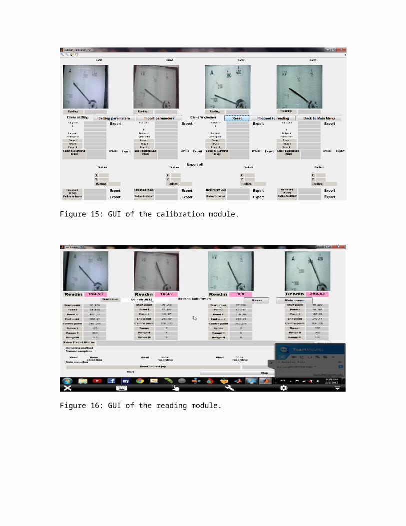
Figure 15: GUI of the calibration module.

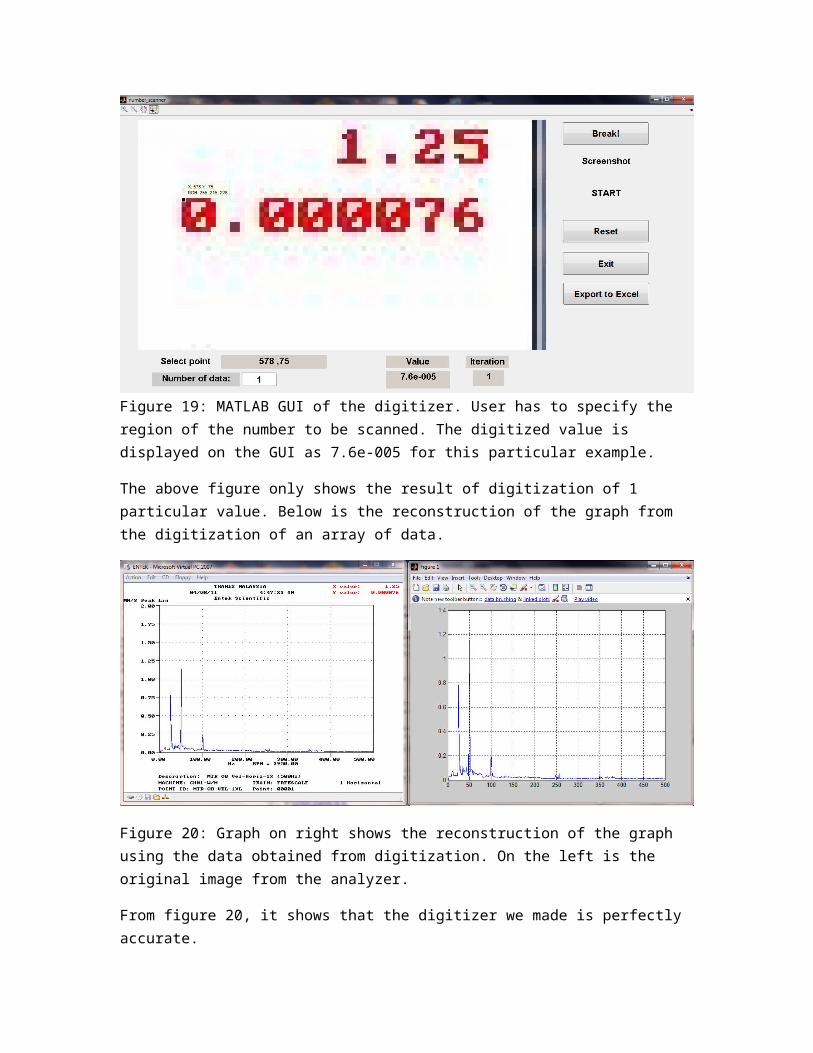
Figure 16: GUI of the reading module.

3) XY-plot digitizing module

Project background:

We use a number of spectrum analyzer to capture the time domain data from the probe, perform fast Fourier transform, and store the resulting spectrum in the analyzer. However, when we want to extract the spectrum graph out from the analyzer to computer for further analysis, some of the spectrum can only be extracted in the form of image file (image of the spectrum), but not the X and Y data value. This causes some problem as we wanted to inspect the spectrum data to calculate certain parameter such as the overall power of the spectrum. Thus, I was asked by my supervisor to design a routine to digitize the spectrum graph from the image file and export the X and Y data value into Microsoft Excel for further analysis.

Hardware used:

i) Spectrum image file

ii) Laptop

Software used:

i) MATLAB

Project description:

The purpose of this project is to digitize the image file of the graph to obtain the X and Y values. 2 types of digitizer were designed. The first type is to digitize the graph from image file to get the X and Y value. The second type is to read the numerical Y value displayed in the image file and digitize it.

For the first type of digitizer, we first import the image file into MATLAB. Then, the user have to define the maximum X point and maximum Y point on the image graph as well as the graph color to be detected. Also, the user has to specify the X data range and Y data range and the number of data pair to be digitized to.

Figure 17: MATLAB GUI of the digitizer. The maximum X point, maximum Y point, color to the detected, X range, Y range, and the number of data pair to be digitized to have to be specified by user.

After all the required information is specified, the program will crop the image according to the maximum X and maximum Y point selected. The cropped image is as show in the right hand side image. Next, the program will digitize the image.

Figure 18: The result of graph digitization as shown by the right hand side plot.

The digitized data can be export to Microsoft Excel for further analysis.

The second type of digitizer is built to read the Y data value displayed in an image. The user have to specify the region where the number to be read is located in the image. After that, the program will do the reading automatically.

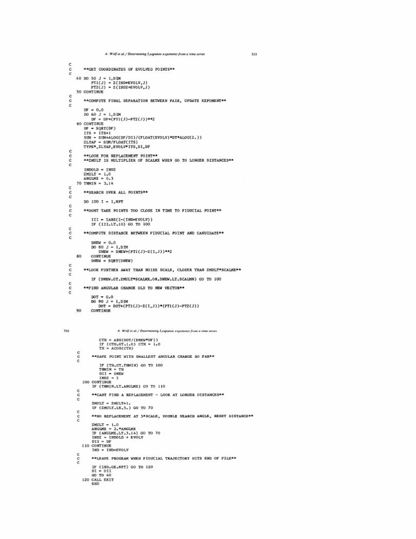
Figure 19: MATLAB GUI of the digitizer. User has to specify the region of the number to be scanned. The digitized value is displayed on the GUI as 7.6e-005 for this particular example.

The above figure only shows the result of digitization of 1 particular value. Below is the reconstruction of the graph from the digitization of an array of data.

Figure 20: Graph on right shows the reconstruction of the graph using the data obtained from digitization. On the left is the original image from the analyzer.

From figure 20, it shows that the digitizer we made is perfectly accurate.

4) FORTRAN to MATLAB code conversion

Project description:

This simple project is given by my supervisor for me to convert a script written in FORTRON language into MATLAB so that its able to run in MATLAB. Before this, I have no experience in working with FORTRAN programming. Throughout this project, I learn some programming language about FORTRAN. Below is the original script given to me in FORTRAN.

The resulting code after conversion into MATLAB is shown below:

function start clear all clc set(0,'RecursionLimit',1000) X=zeros(16384,1); PT1=zeros(12); PT2=zeros(12); NPT=input('NPT='); DIM=input('DIM='); TAU=input('TAU='); DT=input('DT='); SCALMX=input('SCALMX='); SCALMN=input('SCALMN='); EVOLV=input('EVOLV='); IND=1; SUM=0; ITS=0; A=xlsread('data.xlsx'); for I=1:NPT X(I)=A(I); %%%%% end for I=1:NPT for J=1:DIM if I+(J-1)*TAU<=NPT Z(I,J)=X(I+(J-1)*TAU); else Z(I,J)=0; end end end NPT=NPT-DIM*TAU-EVOLV; DI=1e38; for I=11:NPT D=0; for J=1:DIM D=D+(Z(IND,J)-X(I+(J-1)*TAU))^2; end D=sqrt(D); if D<=DI || D>=SCALMN DI=D; IND2=I; end end f_40(NPT,SCALMX,SCALMN,DIM,Z,IND,IND2,EVOLV,ITS,SUM,DI,DT,PT1,PT2);end function f_40(NPT,SCALMX,SCALMN,DIM,Z,IND,IND2,EVOLV,ITS,SUM,DI,DT,PT1,PT2) for J=1:DIM

PT1(J)=Z(IND+EVOLV,J); PT2(J)=Z(IND2+EVOLV,J); end DF=0; for J=1:DIM DF=DF+(PT1(J)-PT2(J))^2; end DF=sqrt(DF); ITS=ITS+1; SUM=SUM+log(DF/DI)/(EVOLV*DT*log(2.)); ZLYAP=SUM/ITS; fprintf('ZLYAP=%.4f\n',ZLYAP); fprintf('EVOLV*ITS=%.4f\n',EVOLV*ITS); fprintf('DI=%.4f\n',DI); fprintf('DF=%.4f\n',DF); INDOLD=IND2; ZMULT=1; ANGLMX=0.3; f_70(NPT,IND,EVOLV,DIM,PT1,Z,ZMULT,SCALMX,SCALMN,PT2,DF,ANGLMX,INDOLD,ITS,SUM,DT);end function f_70(NPT,IND,EVOLV,DIM,PT1,Z,ZMULT,SCALMX,SCALMN,PT2,DF,ANGLMX,INDOLD,ITS,SUM,DT) THMIN=3.14; for I=1:NPT III=abs(I-(IND+EVOLV)); if III>=10 DNEW=0; for J=1:DIM DNEW=DNEW+(PT1(J)-Z(I,J))^2; end DNEW=sqrt(DNEW); if DNEW<=ZMULT*SCALMX || DNEW>=SCALMN DOT=0; for J=1:DIM DOT=DOT+(PT1(J)-Z(I,J))*(PT1(J)-PT2(J)); end CTH=abs(DOT/(DNEW*DF)); if CTH>1 CTH=1; end TH=acos(CTH); if TH<=THMIN THMIN=TH; DII=DNEW; IND2=I; end

end end end if THMIN>=ANGLMX ZMULT=ZMULT+1; if ZMULT<=5 f_70(NPT,IND,EVOLV,DIM,PT1,Z,ZMULT,SCALMX,SCALMN,PT2,DF,ANGLMX,INDOLD,ITS,SUM,DT); else ZMULT=1; ANGLMX=2*ANGLMX; if ANGLMX<3.14 f_70(NPT,IND,EVOLV,DIM,PT1,Z,ZMULT,SCALMX,SCALMN,PT2,DF,ANGLMX,INDOLD,ITS,SUM,DT); else IND2=INDOLD+EVOLV; DII=DF; end end end IND=IND+EVOLV; if IND<NPT DI=DII; f_40(NPT,SCALMX,SCALMN,DIM,Z,IND,IND2,EVOLV,ITS,SUM,DI,DT,PT1,PT2); endend

5) Proximity sensor calibration

Project background:

In condition monitoring, sensor plays an important role. Sensor must be ensure to function correctly and accurately to ensure the accuracy of the analysis result. The type of sensors we used in condition monitoring is proximity probe and accelerometer. Proximity probe changes the voltage value as the gap between the sensor tips and the object varies. Accelerometer changes the voltage value as the acceleration of the object with respect to the sensor tips varies. One important parameter that defines the sensor properties is its sensitivity, which defines how much the voltage value changes per unit measurement. For the proximity probe we use, its sensitivity unit is V/mm, while for accelerometer, the unit is mV/G. Sensor calibration is a common routine to make sure the sensitivity of the sensor still tally with the one specified in the datasheet as well as to establish the range of operation for the sensor. The sensor need to be

calibrated often as the sensitivity may change a little bit over time due to ageing. The project deal with the technique we used to calibrate the proximity sensor.

Hardware used:

i) Proximity probe

ii) Micrometer screw gauge

iii) Multimeter

Software used:

i) Microsoft Excel

Project description:

The purpose of this project is to calibrate a proximity probe using a micrometer screw gauge. This is done to find out the sensitivity of the sensor and also to establish the operating range of the probe. The method to calibrate is straight forward. The sensor is set up to be at a certain gap distance away from an object, adjust using micrometer screw gauge. Then, the voltage value is measured using a multimeter. The process is repeated for gap distance ranging from 0mm to 4mm, with each time increase the gap by 0.2mm. All the voltage value is tabulated in Microsoft Excel and finally a voltage vs gap distance graph is plotted in Excel.

Figure 21: Result of the calibration is tabulated.

0.0 0.2 0.4 0.6 0.8 1.0 1.2 1.4 1.6 1.8 2.0 2.2 2.4 2.6 2.8 3.0 3.2 3.4 3.6 3.8 4.00

5

10

15

20

25

V vs mm

mm

V

Figure 22: Graph showing voltage vs gap distance in mm.

From figure 22, we can see that the operating range of the proximity probe is 2.6mm. After 2.6mm, the voltage does not have linear characteristic.

The sensitivity of the proximity probe can be obtained by calculating the gradient of the linear region. From Microsoft Excel built-in function, the sensitivity is calculated to be 7.628297V/mm.

Working culture & management-labour relationship

During my internship period, I observed a good working culture in the company. Everyone in the company is committed to their work. Besides, all the workers are willing to help each other when help is needed. They are hardworking and punctual, and willing to get their work done even though it is outside the working hour. The management-labour relationship is good in the company. We always have good communication with the management side, so that our job can be done more efficiently.

The company is made up of a multi racial community. There are 3 races in the company, namely Malay, Chinese and Indian. We are all working well together with tolerance. Besides, all the races are willing to help each other when in need. For example, during Chinese New Year, most of the Chinese in the company needed to take extra leave, causing a lack of human resources in the company. However, the Malays and Indian in the company are willing to work during Chinese New Year to help relieve the shortage of human power. We are like a big family, respecting each other’s religious believe and culture, and never have any problem with racial discrimination. I am glad that I have the chance to work in such an environment so that I learned to work with peoples with different races and background. This company definitely demonstrates the spirit of 1 Malaysia.

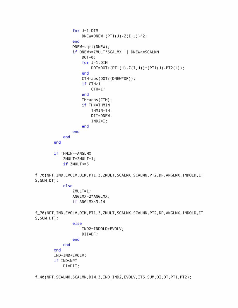
Figure 23: Picture taken during a lunch break with colleagues in a nearby restaurant.

Conclusion

In these three months industrial training in Sri Wawasan Sdn Bhd, I have learnt a lot of things which cannot be learnt in University life. In terms of theory, I realized that not all the theories can be directly applied in a real working environment. Indeed, theory part is the basic for us to know more knowledge but hands-on experience is important as well. In real world there have plenty of unforeseen factors can be occurred. As what I studied in university, most of the theories are for ideal case, but when come to a real world, we need to modify and compensate with certain factors so that the results we get are closest to the ideal.

Other than that, teamwork is one of the important key as well. I got a chance to work as a team with other people. As what I mentioned before, teamwork is very important, it can determine the successful of the given tasks. In real world, it is impossible for us to work alone. We might need others’ helps in order we can complete the tasks.

Lastly, I realized the importance of the learning behaviors. It is an important attitude if you want to be self-upgrade and it’s a key of success. Last time I do not have the initiative to learn a new thing. However during these three months, I understand that if we do not have the initiative to learn, then we will never learn a new thing and we will never ever able to equip ourselves with the latest information. Egoism is the factor to block us to walking forward. Therefore we must empty the cup in order to be filled.

Reference

[1] http://zone.ni.com/reference/en-XX/help/372416A-01/svtconcepts/obt_tbs_shctln/

[2]www.dataq.com

[3] www.made-in-chine.com