International Workshop on Software Engineering FBI-HH-B-294/10

Universität Hamburg Department Informatik Vogt-Kölln-Str. 30 D-22527 Hamburg

Bericht 294 Proceedings of the International Workshop on Petri Nets and Software Engineering PNSE'10 FBI-HH-B-294/10

Herausgeber: Michael Duvigneau Daniel Moldt Universität Hamburg Department Informatik In die Reihe der Berichte des Fachbereichs Informatik aufgenommen durch Prof. Dr. M. Jantzen Prof. Dr. W. Lamersdorf Juni 2010

This document is retrievable

• on CD under the ISBN 978-972-8692-55-1• as printed report (see address on front page)• as electronical copy of the printed report under the URL

http://epub.sub.uni-hamburg.de/informatik/volltexte/2010/148/

http://epub.sub.uni-hamburg.de/informatik/volltexte/2010/148/

AbstractThis report contains the proceedings of the International Workshop on Petri Netsand Software Engineering (PNSE’10) that took place in Braga, Portugal on June22, 2010. For the successful realisation of complex systems of interacting and reac-tive software and hardware components the use of a precise language at differentstages of the development process is of crucial importance. Petri nets provide auniform language supporting the tasks of modelling, validation, and verificationwhich captures fundamental aspects of causality, concurrency and choice in anatural and mathematically precise way without compromising readability.

The use of Petri nets (P/T-nets, coloured Petri nets and extensions) in theformal process of software engineering is presented as well as their applicationand tools supporting the disciplines mentioned above.

ZusammenfassungDieser Bericht enthält die Proceedings des internationalen Workshops über Petri-netze und Softwaretechnik (PNSE’10), der am 22. Juni 2010 in Braga, Portugalstattfand. Zur erfolgreichen Erstellung komplexer Systeme interagierender undreaktiver Software- und Hardwarekomponenten ist die Verwendung einer präzisenSprache während der verschiedenen Entwicklungsstufen von größter Wichtigkeit.Petrinetze stellen eine einheitlich für die Zwecke der Modellierung, Validierungund Verifikation verwendbare Sprache dar, welche fundamentale Aspekte vonKausalität, Nebenläufigkeit und Alternativen auf eine natürliche und mathema-tisch präzise Weise einfängt, ohne die Lesbarkeit der Modelle zu beeinträchtigen.

Der Workshop präsentiert sowohl die Verwendung von Petrinetzen (S/T-Netzen, gefärbten Netzen und Erweiterungen) in den formalen Prozessen der Soft-waretechnik als auch deren Anwendung oder Werkzeuge, welche die genanntenDisziplinen unterstützen.

Editors: Michael Duvigneau andDaniel Moldt

Proceedings of theInternational Workshop on

P etriN ets andS oftwareE ngineeringPNSE’10

University of HamburgDepartment of Informatics

Preface

This booklet contains the proceedings of the International Workshop on PetruNets and Software Engineering (PNSE’10) in Braga, Portugal, June 22, 2010.It is a co-located event of Petri Nets 2010, the 31st international conference onApplications and Theory of Petri Nets and other Models of Concurrency, andACSD 2010, the 10th International Conference on Application of Concurrencyto System Design.

More information about the workshop, like online-proceedings, can befound at

http://www.informatik.uni-hamburg.de/TGI/events/pnse10/

For the successful realisation of complex systems of interacting and reactivesoftware and hardware components the use of a precise language at differentstages of the development process is of crucial importance. Petri nets are be-coming increasingly popular in this area, as they provide a uniform languagesupporting the tasks of modelling, validation, and verification. Their popular-ity is due to the fact that Petri nets capture fundamental aspects of causality,concurrency and choice in a natural and mathematically precise way withoutcompromising readability.

The use of Petri nets (P/T-nets, coloured Petri nets and extensions) inthe formal process of software engineering, covering modelling, validation,and verification, is presented as well as their application and tools supportingthe disciplines mentioned above.

The program committee consists of:

Wil van der Aalst (Eindhoven University, The Netherlands)João Paulo Barros (Instituto Politécnico de Beja, Portugal)Didier Buchs (University of Geneva, Switzerland)Piotr Chrzastowski-Wachtel (University of Warsaw, Poland)Gianfranco Ciardo (University of California at Riverside, USA)Jose-Manuel Colom (University of Zaragoza, Spain)Jörg Desel (Catholic University Eichstätt-Ingolstadt, Germany)Raymond Devillers (Université Libre de Bruxelles, Belgium)Marlon Dumas (University of Tartu, Estonia)Michael Duvigneau (University of Hamburg, Germany) (Chair)Berndt Farwer (University of Durham, UK)João Fernandes (Universidado de Minho, Portugal)Jorge C. A. de Figueiredo (Federal University de Campina Grande,Brasil)Giuliana Franceschinis (University of Piemonte Orientale / Universityof Torino, Italy)Guy Gallasch (University of South Australia, Australia)

viii PNSE’10 – Petri Nets and Software Engineering

Luís Gomes (Universidade Nova de Lisboa, Portugal)Nicolas Guelfi (University of Luxembourg, Luxembourg)Stefan Haar (ENS Cachan, France)Xudong He (Florida International University, USA)Thomas Hildebrandt (University of Copenhagen, Denmark)Vladimir Janousek (University of Brno, Czech Republic)Gabriel Juhas (Slovak University of Technology Bratislava, Slovakia)Peter Kemper (College of William and Mary, USA)Astrid Kiehn (Indraprastha Institute of Information Technology Delhi,India)Ekkart Kindler (Technical University of Denmark, Denmark)Hanna Klaudel (Université d’Evry-Val d’Essonne, France)Michael Köhler-Bußmeier (University of Hamburg, Germany)Fabrice Kordon (University P. & M. Curie, LIP 6, France)Maciej Koutny (Newcastle University, UK)Lars Kristensen (Bergen University College, Norway)Robert Lorenz (University Augsburg, Germany)Daniel Moldt (University of Hamburg, Germany) (Chair)Chun Ouyang (Queensland University of Technology, Australia)Wojciech Penczek (University of Podlasie, Poland)Laure Petrucci (University Paris Nord, France)Lucia Pomello (Università degli Studi di Milano-Bicocca, Italy)Oana Prisecaru (University of Iasi, Romania)Heiko Rölke (DIPF, Germany)Christophe Sibertin-Blanc (University Toulouse 1, France)Harald Störrle (Technical University of Denmark, Denmark)Catherine Tessier (ONERA Toulouse, France)Ulrich Ultes-Nitsche (University of Fribourg, Switzerland)Manuel Wimmer (Vienna University of Technology, Austria)Karsten Wolf (Universität Rostock, Germany)Mengchu Zhou (New Jersey Institute of Technology, USA)Christian Zirpins (University of Karlsruhe, Germany)Wlodek M. Zuberek (Memorial University of Newfoundland, Canada)

We received 16 high-quality contributions. The program committee has ac-cepted four of them for full presentation. Furthermore the committee accepted

Preface ix

five papers as short presentations. Three contributions were submitted and ac-cepted as posters.

The international program committee was supported by the valued work ofMichal Knapik, Levi Lucio, Elisabetta Mangioni and Tarek Melliti as addi-tional reviewers. Their work is highly appreciated.

Furthermore, we would like to thank the organizational teams of the Univer-sidade do Minho and the Instituto Politécnico de Beja, Portugal, for theirgeneral organizational support.

Without the enormous efforts of authors, reviewers, PC members and the orga-nizational teams this workshop wouldn’t provide such an interesting booklet.

Thanks!

Michael Duvigneau and Daniel MoldtHamburg, June 2010

Contents

Part I Invited Talk

Combining Petri Nets and UML for Model-based SoftwareEngineeringJoão Miguel Fernandes . . . . . . . . . . . . . . . . . . . . . . . . . . . . . . . . . . . . . . . . . . . 3

Part II Long Presentations

The Resource Allocation Problem in Software Applications:A Petri Net PerspectiveJuan-Pablo López-Grao and José-Manuel Colom . . . . . . . . . . . . . . . . . . . . . 7

Nets Within Nets Paradigm and Grid ComputingFabio Farina and Marco Mascheroni . . . . . . . . . . . . . . . . . . . . . . . . . . . . . . . . 23

Verifying Reference Nets By Means of Hypernets: a Pluginfor RENEWMarco Mascheroni, Thomas Wagner and Lars Wustenberg . . . . . . . . . . . . . 39

Improving a Workflow Management System with an AgentFlavourDaniel Moldt, José Quenum, Christine Reese and Thomas Wagner . . . . . 55

xii Contents

Part III Short Presentations

IRS-MT: Tool for Modeling Resource Allocation in WorkflowPetri NetsPiotr Chrzastowski-Wachtel and Jakub Rauch . . . . . . . . . . . . . . . . . . . . . . . . 73

Detecting and Repairing Unintentional Change on In-useData in Concurrent Workflow Management SystemThi Thanh Huyen Phan and Koichiro Ochimizu . . . . . . . . . . . . . . . . . . . . . . 89

Automata and Petri Net Models for Visualizing andAnalyzing Complex Questionnaires - A Case StudyHeiko Rölke . . . . . . . . . . . . . . . . . . . . . . . . . . . . . . . . . . . . . . . . . . . . . . . . . . . . . 111

Deadlock Control Software for Tow Automated GuidedVehicles using Petri NetsCarlos Rovetto, Elia Esther Cano Acosta and José Manuel ColomPiazuelo . . . . . . . . . . . . . . . . . . . . . . . . . . . . . . . . . . . . . . . . . . . . . . . . . . . . . . . . 125

Taming the Shrew - Resolving Structural Heterogeneitieswith Hierarchical CPNManuel Wimmer, Gerti Kappel, Angelika Kusel, Werner Retschitzegger,Johannes Schoenboeck and Wieland Schwinger . . . . . . . . . . . . . . . . . . . . . . . 141

Part IV Poster Abstracts

MATLAB / Simulink and Program Sketcher for Verificationof Hybrid Petri Nets Implementation into ProgrammableLogic ControllerLuděk Chomát . . . . . . . . . . . . . . . . . . . . . . . . . . . . . . . . . . . . . . . . . . . . . . . . . . . 161

Instruction Pipeline Modeling using Petri NetsAdam Husar, Tomas Hruska, Karel Masarik and Zdenek Prikryl . . . . . . . 163

BDD-based Bounded Model Checking for Elementary NetSystemsArtur Meski, Wojciech Penczek and Agata Polrola . . . . . . . . . . . . . . . . . . . . 165

Part I

Invited Talk

Combining Petri Nets and UML forModel-based Software Engineering

João M. Fernandes

Dep. Informática / CCTCUniversidade do Minho

4710-057 BragaPortugal

EXTENDED ABSTRACT

UML is by far the most widely used modelling language used nowadays insoftware engineering, due to its large scope and its wide tool support. This soft-ware standard offers many diagrams that cover all typical perspectives for de-scribing and modelling the software systems under consideration. Among thosediagrams, UML includes diagrams (activity diagram, state machine diagram, usecase diagrams, and the interaction diagrams) for describing the behaviour (orfunctionality) of a software system. Petri nets constitute a well-proven formalmodelling language, suitable for describing the behaviour of systems with char-acteristics like concurrency, distribution, resource sharing, and synchronisation.Thus, one may question why not combining some UML diagrams with Petrinets for effectively supporting the activities of the software engineer. The usageof Petri nets for/in Software Engineering was addressed by several well-knownresearchers, like, for example, Reisig [6], Pezzè [1], Machado [5], and Kindler [4].

In this invited talk, we discuss some alternatives to introduce Petri netsinto a UML-based software development process. In particular, we describe howColoured Petri Net (CPN) models can be used to describe the set of scenariosassociated with a given use case. We describe three different alternatives thatcan be adopted to achieve that purpose.

The first approach, initially presented in [7], suggests a set of rules that allowsoftware engineers to transform the behaviour described by a UML 2.0 sequencediagram into a CPN model. Sequence diagrams in UML 2.0 are much richer thanthose in UML 1.x, namely by allowing several traces to be combined in a uniquediagram, using high-level operators over interactions. The main purpose of thetransformation is to allow the development team to construct animations basedon the CPN model that can be shown to the users or the clients in order toreproduce the expected scenarios and thus validate them. Thus, non-technicalstakeholders are able to discuss and validate the captured requirements. Theusage of animation is an important topic in this context, since it permits theuser to discuss the system behaviour using the problem domain language.

In the second approach, discussed in [3], we assume that developers specifythe functionality of the system under consideration with use cases, each of whichis described by a set of UML 2.0 sequence diagrams. For each use case, there

should exist at least one sequence diagram that represents and describes its mainscenario. Other sequence diagrams for the same use case are considered to bevariations of the main scenario. The transformation approach allows the devel-opment team to interactively play or reproduce any possible run of the givenscenarios. In particular, the natural characteristics of the CPN modelling lan-guage facilitate the representation of the hierarchy and concurrency constructsof sequence diagrams.

The third alternative, considered in [2], is an improvement with respect to theprevious approach and is targeted to reactive systems. We identify and justifytwo key properties that the CPN model must have, namely: (1) controller-and-environment-partitioned, which means constituting a description of both thecontroller and the environment, and distinguishing between these two domainsand between desired and assumed behaviour; (2) use case-based, which meansconstructed on the basis of a given use case diagram and reproducing the be-haviour described in accompanying scenario descriptions. We have demonstratedhow this CPN model is useful for requirements engineering, since it provides asolid basis for addressing behavioural issues early in the development process,for example regarding concurrent execution of use cases and handling of failures.

References

1. G. Denaro and M. Pezzè. Petri Nets and Software Engineering. In Lectures onConcurrency and Petri Nets: Advances in Petri Nets, volume 3098 of Lecture Notesin Computer Science, pages 439–466. Springer, 2004. DOI 10.1007/b98282.

2. J.M. Fernandes, J.B. Jørgensen, and S. Tjell. Requirements engineering for reactivesystems: Coloured petri nets for an elevator controller. In 14th Asia-Pacific SoftwareEngineering Conference (APSEC 2007), pages 294–301. IEEE CS Press, December2007. DOI 10.1109/APSEC.2007.81.

3. J.M. Fernandes, S. Tjell, J.B. Jørgensen, and O. Ribeiro. Designing Tool Supportfor Translating Use Cases and UML 2.0 Sequence Diagrams into a Coloured PetriNet. In 6th Int. Workshop on Scenarios and State Machines (SCESM 2007), withinICSE 2007. IEEE CS Press, May 2007. DOI 10.1109/SCESM.2007.1.

4. Ekkart Kindler. Model-Based Software Engineering and Process-Aware InformationSystems. Transactions on Petri Nets and Other Models of Concurrency, 5460:27–45,2009. 10.1007/978-3-642-00899-3_2.

5. R. J. Machado, K. B. Lassen, S. Oliveira, M. Couto, and P. Pinto. RequirementsValidation: Execution of UML Models with CPN Tools. International Journal onSoftware Tools for Technology Transfer, 9(3–4):353–369, 2007. DOI 10.1007/s10009-007-0035-0.

6. W. Reisig. Petri Nets in Software Engineering. In W. Brauer, W. Reisig, andG. Rozenberg, editors, Advances in Petri Nets, volume 255 of Lecture Notes inComputer Science, pages 63–96. Springer, 1987. DOI 10.1007/3-540-17906-2_22.

7. O. Ribeiro and João M. Fernandes. Some Rules to Transform Sequence Diagramsinto Coloured Petri Nets. In K. Jensen, editor, 7th Workshop and Tutorial onPractical Use of Coloured Petri Nets and the CPN Tools (CPN 2006), pages 237–256, October 2006.

4 PNSE’10 – Petri Nets and Software Engineering

Part II

Long Presentations

The Resource Allocation Problem in SoftwareApplications: A Petri Net Perspective⋆

Juan-Pablo López-Grao1 and José-Manuel Colom2

1 Dpt. of Computer Science and Systems Engineering (DIIS)2 Aragonese Engineering Research Institute (I3A)

University of Zaragoza, SpainEmail: jpablo,[email protected]

Abstract. Resource Allocation Systems (RAS) have been intensivelystudied in the last years in the domain of Flexible Manufacturing Sys-tems (FMS). The success of this research line has been based on theidentification of particular subclasses of Petri Nets that correspond to aRAS abstraction of this kind of systems. In this paper we take a parallelroad to that travelled through for FMS, but for the case of software appli-cations. The considered applications present concurrency and deadlockscan happen due to the allocation of shared resources. We will evince thatthe existing subclasses of Petri Nets used to study this kind of deadlockproblems are insufficient, even for very simple software systems. Fromthis starting point we propose a new subclass of Petri Nets that gener-alizes the previously known RAS subclasses and we present a taxonomyof anomalies that can be found in the context of software systems.

1 Introduction

Among the most recurrent patterns in a wide disparity of engineering disciplines,the competition for shared resources between concurrent processes takes a promi-nent position. The reader might think of examples in the context of distributedsystems, operations research, manufacturing plants, etc. The perspective of dis-crete event systems theory proves appropriate and powerful as a framework inwhich provide solutions to the so-called resource allocation problem [1]. Systemsof this kind are often called Resource Allocation Systems (RAS) [2, 3].

RAS are usually conceptualized around two distinct entities, processes and re-sources, thanks to a prior abstraction process which is inherent in the discipline.The resource allocation problem refers to satisfying successfully the requests forresources made by the processes, ensuring that no process ever falls in a dead-lock. A set of processes is deadlocked when they indefinitely wait for resourcesthat are already held by other processes of the same set [4].

RAS can be categorized both on the type of processes (sequential, non-sequential) and resources (serially reusable, consumable) [5]. Hereafter, we will⋆ This work has been partially supported by the European Community’s Seventh

Framework Programme under Project DISC (Grant Agreement n. INFSO-ICT-224498) and the project CICYT-FEDER DPI2006-15390.

focus on Sequential RAS with serially reusable resources. This means that aprocess can increase or decrease the quantity of free resources during its execu-tion. However, the process will contervail that operation before terminating, i.e.resources are used in a conservative way.

Although other models of concurrency have also been considered [6], Petrinets [7] have arguably taken a leading role among the family of formal modelsused for dealing with the resource allocation problem [8, 9]. One of the strengthsof this approach is the smooth mapping between the main entities of RAS and thebasic elements of Petri net models. A resource type can be modelled using a place:the number of instances of it being modelled with tokens. Meanwhile, sequentialprocesses are modelled with tokens progressing through state machines. Arcsfrom resource places to transitions (from transitions to resource places) representthe acquisition (return) of some resources by a process. Petri nets thus providea natural formal framework for the analysis of RAS, besides benefiting from thegoods of compositionality.

This fact is well notorious in the domain of Flexible Manufacturing Systems(FMS), where Petri net models for RAS have widely succeeded since the semi-nal work of Ezpeleta et al. was introduced [8]. This is mostly due to a carefulselection of the subclass of Petri nets used to model these FMS, based upon twosolid pillars. First, the definition of a rich syntax from a physical point of view,which enables the natural expression of a wide disparity of plant configurations.And second, the contribution of sound scientific results which let us characterizedeadlocks from the model structure, as well as provide a well-defined methodol-ogy to automatically correct them in the real system.

Nowadays, there exists a plethora of Petri net models for modelling RAS inthe context of FMS, which often overcome some of the syntactical limitations ofthe S3PR class [8]. S4PR net models [10, 11] generalize the earlier, while allowingmultiple simultaneous allocations of resources per process. S∗PR nets [12] extendthe expressive power of the processes to that of state machines: hence internalcycles in their control flow is allowed. However, deadlocks in S∗PR net modelsare not fully comprehended from a structural perspective. Other classes such asNS-RAP [9], ERCN-merged nets [13] or PNR nets [14] extend the capabilities ofS3PR/S4PR models beyond Sequential RAS by way of lot splitting or mergingoperations.

Most analysis and control techniques in the literature are based on the com-putation of a structural element which univocally characterizes deadlocks inmany RAS models: the so-called bad siphon. A bad siphon is a siphon which isnot the support of a p-semiflow. If bad siphons become (sufficiently) emptied,their output transitions die since the resource places of the siphon cannot regaintokens anymore, thus revealing the deadly embrace. Control techniques thus relyon the insertion of monitor places [15], i.e. controllers in the real system, whichlimit the leakage of tokens from the bad siphons.

Although there exist obvious resemblances between the resource allocationproblem in FMS and that of parallel or concurrent software, previous attemptsto bring these well-known RAS techniques into the field of software engineering


have been, to the best of our knowledge, either too limiting or unsuccessful.Gadara nets [16] constitute the most recent attempt, yet they fall in the over-restrictive side in the way the resources can be used, as a result of inheriting thedesign philosophy applied for FMS. In this work, we will analyze why the netclasses and results introduced in the context of FMS fail when brought to thefield of concurrent programming.

Section 2 presents a motivating example and discusses the elements thata RAS net model should desirably feature in order to successfully explore theresource allocation problem within the software enginering discipline. Taking intoaccount those considerations, section 3 introduces a new Petri net class, calledPC2R. Section 4 relates the new class to those defined in previous works andestablishes useful net transformations which forewarn us about new behaviouralphenomena. Section 5 introduces some of these anomalies which highlight thefact that previous theoretical results in the context of FMS are insufficient inthe new framework. Finally, section 6 summarizes the results of the paper.

2 The RAS view of a software application

Example 1 presents a humorous variation of Dijkstra’s classic problem of thedining philosophers. We will adopt and adapt the beautiful writing by Hoare at[17] for its enunciation.

Example 1. The pragmatic dining philosophers. “Five philosophers spend theirlives thinking and eating. The philosophers share a common dining room wherethere is a circular table surrounded by five chairs, each belonging to one philoso-pher. A microwave oven is also available. In the center of the table there is alarge bowl of spaghetti which is frequently refilled (so it cannot be emptied),and the table is laid with five forks. On feeling hungry, a philosopher enters thedining room, sits in his own chair, and picks up the fork on the left of his place.Then he touches the bowl to feel its temperature. If he feels the spaghetti got toocold, he will leave his fork and take the bowl to the microwave. Once it is warmenough, he will come back to the table, sit on his chair and leave the bowl on thetable after recovering his left fork (please bear in mind that the philosopher isreally hungry by now). Unfortunately, the spaghetti is so tangled that he needsto pick up and use the fork on his right as well. If he can do it before the bowlgets cold again, he will serve himself and start eating. When he has finished, heputs down both forks and leaves the room.”

According to the classic RAS nomenclature, each philosopher is a sequentialprocess, and the five forks plus the bowl are serially reusable resources which areshared among the five processes. From a software perspective, each philosophercan be a process or a thread which will be executed concurrently.

Algorithm 1 introduces the code for each philosopher. Notationally, we mod-elled the acquisition / release of resources by way of the wait() / signal()operations, respectively. Both of them have been generalized for the acquisitionof multiple resources (separated by commas when invoking the function). Finally,

J.-P. López-Grao and J.-M. Colom: The Resource Allocation Problem 9

the trywait() operation is a non-blocking wait operation. If every resource isavailable at the time trywait() is invoked, then it will acquire them and returnTRUE. Otherwise, trywait() will return FALSE without acquiring any resource.For the sake of simplicity, it is assumed that the conditions with two or moreliterals are evaluated atomically.

A4

T3

A2

T4

T1

T8

T5A1

R_F2

A0

R_S

A3

T6

T7

A5

A6

R_F1

T2

Fig. 1. Philosopher 1.

Algorithm 1 - Code for Philosopher i (where i ∈ 1, 2, 3, 4, 5)

varfork: array [1..5] of semaphores; // shared resourcesbowl: semaphore; // shared resource

begindo while (1)

THINK;Enter the room;

(T1) wait(fork[i]);do while (not(trywait(bowl, fork[i+1 mod 5]))

or the spaghetti is cold)(T2) if (trywait(bowl)

and the spaghetti is cold) then(T3) signal(fork[i]);

Go to the microwave;Heat up spaghetti;Go back to table;

(T4) wait(fork[i]);(T5) signal(bowl);

end if;(T6) loop;

Serve spaghetti;(T7) signal(bowl);

EAT;(T8) signal(fork[i], fork[i+1 mod 5]);

Leave the room;loop;

Figure 1 depicts the net for algorithm 1, with i = 1, after abstracting therelevant information from a RAS perspective. Figure 2 renders the compositionof the five philosopher nets via fusion of the common shared resources. Note thatif we remove the dashed arcs from figure 2, then we can see five disjoint stronglyconnected state machines plus six isolated places.

The five state machines represent the control flow for each philosopher. Everystate machine is composed of seven states (each state being represented by aplace). Tokens in a state machine represent concurrent processes/threads whichshare the same control flow. In this case, the unique token in each machine islocated at the so-called idle place. This means that, at the initial state, everyphilosopher is thinking (outside the room). In general, the idle place can be seen


as a mechanism which enforces a structural bound: the number of concurrentactive threads (i.e. non-idle) is limited. Here, at most one philosopher of type ican be inside the room, for each i ∈ 1, 2, 3, 4, 5.

The six isolated places are called resource places. A resource place representsa certain resource type, and the number of tokens in it represents the quan-tity of free instances of that resource type. In this case, every resource placeis monomarked. Thus, at the initial state there is one fork of type i, for everyi ∈ 1, 2, 3, 4, 5, plus one bowl of spaghetti (modelled by way of the resourceplace at the centre of the figure).

Finally, the dashed arcs represent the acquisition or release of resources by theactive threads when they change their execution state. Every time a transitionis fired, the total amount of resources available is altered. Please note, however,that moving one isolated token of a state machine (by firing its transitions)until the token reaches back the idle state, leaves the resource places markingunaltered. Thus, the resource usage is conservative.

Fork 2

Fork 1

Fork 3

Fork 4

Fork 5

Fig. 2. The dining philosophers are thinking. Arcs from/to PR are dashed for clarity.


At this point, we will discuss some capabilities that (in our humble opinion) aRAS model should have so as to support the modelling of concurrent programs.

Although acyclic sequential state machines are rather versatile as modelsfor sequential processes in the context of FMS (as the success of the S3PR andS4PR classes prove), this is clearly too constraining even for very simple softwaresystems. Considering Böhm and Jacopini’s theorem [18], however, we can assumethat every non-structured sequential program can be refactored into a structuredone using while-do loops. Meanwhile, calls to procedures and functions can besubstituted by way of inlining techniques. Let us also remind that fork/joinoperations can also be unfolded into isolated concurrent sequential processes, asevidenced in [9]. As a result, we can restrict process models to state machines inwhich decisions and iterations (in the form of while-do loops) are supported,but not necessarily every kind of internal cycle.

Another significant difference between FMS and software systems from aRAS perspective is that resources in the latter are not necessarily physical (e.g.,a file) but can also be logical (e.g., a semaphore). This has strong implicationsin the degree of freedom allowed for allocating those resources: we will return tothis issue a little later.

In this domain, a resource is an object that is shared among concurrentprocesses/threads and must be used in mutual exclusion. Since the number ofresources is limited, the processes will compete for the resource and will useit in a non-preemptive way. This particular allocation scheme can be imposedby the resources’ own access primitives, which may be blocking. Otherwise, theresource can be protected by a binary semaphore/mutex/lock (if there is only oneinstance of that resource type) or by a counting semaphore (multiple instances).Note that this kind of resources can be of assorted nature (e.g., shared memorylocations, storage space, database table rows) but the required synchronizationscheme is inherently similar.

On the other side, it is well-known that semaphores used in that aim canbe also seen as non-preemptive resources which are used in a conservative way.For instance, a counting semaphore that limits the number of connections to adatabase can be interpreted in that way from a RAS point of view. Here processeswill wait for the semaphore when attempting to establish a database connection,and will release it when they decide to close the aforementioned connection.

However, semaphores also perform a relevant role as an interprocess signalingfacility, which can also be a source of deadlocks. In this work, our goal is thestudy of the resource allocation problem, so this functionality is out of scope.We propose fixing deadlock problems due to resource allocation issues firstly,and later apply other techniques for amending those due to message passing.

Due to their versatility, semaphore primitives are interesting for studying howresources can be allocated by a process/thread. For instance, XSI semaphores(also known as System V semaphores) have a multiple wait primitive (semop withsem_op<0). An example of multiple resource allocation appears in algorithm 1.Besides, an XSI semaphore can be decremented atomically in more than one.Both POSIX semaphores (through sem_trywait) and XSI semaphores (through


semop with sem_op<0 and sem_flag=IPC_NOWAIT) have a non-blocking waitprimitive. Again, algorithm 1 could serve as an example. Finally, XSI semaphoresalso feature inhibition mechanisms (through semopwith sem_op=0), i.e. processescan wait for a zero value of the semaphore.

As we suggested earlier, the fact that resources in software engineering donot always have a physical counterpart is a very peculiar characteristic withconsequences. In this context, processes do not only consume resources but alsocan create them. A process will destroy the newly created resources before itstermination. For instance, a process can create a shared memory variable (or aservice!) which can be allocated to other processes/threads. Hence the resourceallocation scheme is no longer first-acquire-later-release, but it can be the otherway round too. Nevertheless, all the resources will be used in a conservativeway by the processes (either by a create-destroy sequence or by a wait-releasesequence). As a side effect, and perhaps counterintuitively, there may not be freeresources during the system startup (as they still must be created), yet beingthe system live.

Summing up, for successfully modelling RAS in the context of software engi-neering, a Petri net model should have at least the following abstract properties:

1. The control flow of the processes should be represented by state machineswith support for decisions (if-then-else blocks) and nested internal cycles(while-do blocks).

2. There can be several resource types and multiple instances of each one.3. State machines can have multiple tokens (representing concurrent threads).4. Processes/threads use resources in a conservative way5. Acquisition/release arcs can have non-ordinary weights (e.g., a semaphore

value can be atomically incremented/decremented in more than one unit)6. Atomic multiple acquisition/release operations must be allowed7. Processes can have decisions dependent of the allocation state of resources

(due to the non-blocking wait primitives, as in figure 2)8. Processes can lend resources. As a side effect, there could exist processes that

depend on resources which must be created/lent by other processes (hencethey cannot finish if executed in isolation)

3 PC2R nets

In this section, we will present a new Petri net class, which fulfills the require-ments advanced in section 2: the class of Processes Competing for ConservativeResources (PC2R). This class generalizes other subclasses of the SnPR familywhile respecting the design philosophy on these. Hence, previous results are stillvalid in the new framework. However, PC2R nets can deal with more complexscenarios which were not yet addressed from the domain of SnPR nets.

Definition 1 presents a subclass of state machines which is used for modellingthe control flow of the processes in isolation. Iterations are allowed, as well asdecisions within internal cycles, in such a way that the control flow of structured


programs can be fully supported. Non-structured processes can still be refactoredinto them as discussed in Section 2.

Definition 1. An iterative state machine N = 〈p0 ∪ P, T, C〉 is a stronglyconnected state machine such that either every cycle contains p0 or P can bepartitioned into two subsets P1, P2, with a place p ∈ P2 such that:

1. The subnet generated by 〈p ∪ P1,•P1 ∪ P1

•〉 is a strongly connected statemachine in which every cycle contains p, and

2. The subnet generated by 〈p0∪P2,•P2 ∪P2

•〉 is an iterative state machine.

In figure 1, if we remove the resource places R_F1, R_F2 and R_S then weobtain an iterative state machine, with P1 = A2, A3, A4, P2 = A1, A5, A6,p0 = A0 and p = A1. The definition of iterative state machines is instrumentalfor introducing the class of PC2R nets.

PC2R nets are modular models. Two PC2R nets can be composed into anew PC2R model via fusion of the common shared resources. Please note thata PC2R net can simply be one process modelled by an iterative state machinealong with the set of resources it uses. Hence the whole net model can be seenas a composition of the modules for each process. We will formally define theclass in the following:

Definition 2. Let IN be a finite set of indices. A PC2R is a connected gener-alized pure P/T net N = 〈P, T, C〉 where:

1. P = P0 ∪ PS ∪ PR is a partition such that: (a) [idle places] P0 = p01 , ...,p0|IN |; (b) [process places] PS = P1 ∪ ...∪P|IN |, where ∀i ∈ IN : Pi 6= ∅ and∀i, j ∈ IN : i 6= j, Pi ∩ Pj = ∅; (c) [resource places] PR = r1, ..., rn, n > 0.

2. T = T1 ∪ ...∪ T|IN |, where ∀i ∈ IN , Ti 6= ∅, and ∀i, j ∈ IN , i 6= j, Ti ∩ Tj = ∅.3. For all i ∈ IN the subnet generated by restricting N to 〈p0i ∪Pi, Ti〉 is an

iterative state machine.4. For each r ∈ PR, there exists a unique minimal p-semiflow associated to r,

Yr ∈ IN|P |, fulfilling: r = ‖Yr‖ ∩ PR, (P0 ∪ PS) ∩ ‖Yr‖ 6= ∅, and Yr[r] = 1.5. PS =

⋃r∈PR

(‖Yr‖ \ r).

Please note that the support of the Yr p-semiflows (point 4 of definition 2)may include P0: this is new with respect to S4PR nets. Such a resource place r iscalled a lender resource place. If r is a lender, then there exists a process whichcreates (lends) instances of r. In our model, processes can start their executioncreating resource instances, but before acquiring any other resource. Otherwise,it could happen that the support of a minimal p-semiflow would contain morethan one resource place (thus infriging condition 4 of definition 2).

The class supports iterative processes, multiple resource acquisitions, non-blocking wait operations and resource lending. Inhibition mechanisms are notnatively supported (although some cases can still be modelled with PC2R nets).

The next definition generalizes the notion of acceptable initial marking intro-duced for the S4PR class. In software systems all processes/threads are initially


inactive and start from the same point (the begin operation). Hence, all of thecorresponding tokens are in the idle place in the initial marking (the processplaces being therefore empty). Note that lender resource places may be emptyfor an acceptable initial marking. Figure 2 shows a P2CR net with an acceptableinitial marking which does not belong to the S4PR class.

Definition 3. Let N = 〈P0∪PS ∪PR, T, C〉 be a PC2R. An initial marking m0

is acceptable for N iff ||m0|| = P0 ∪PR and ∀p ∈ PS , r ∈ PR : Y Tr ·m0 ≥ Yr[p].

4 Some transformations and related classes

In [19], we introduced a new class of Petri net models for RAS, called SPQR(Systems of Processes Quarreling over Resources). SPQR nets feature an appeal-ing syntactical simplicity and expressive power though they are very challengingfrom an analytical point of view. They can be roughly described as RAS netsin which the process subnets are acyclic and the processes can lend resourcesin any possible (conservative) manner. Every PC2R can be transformed into aStructurally Bounded SPQR net (SB SPQR net).

The transformation rule is based on the idea of converting every while-doblock in an acyclic process which is activated by a lender resource place. Thislender place gets marked once the thread reaches the while-do block. The tokenis removed at the exit of the iteration. This transformation must be appliedstarting by the most intern loops, proceeding in decreasing nesting order. Figure3 depicts the transformation rule. The rule preserves the language accepted bythe net (and thus liveness) since it basically consists in the addition of a implicitplace (place P1 in the right hand net of figure 3, since R_P1 can be seen as arenaming of P1 in the left hand net).

Figure 4 illustrates the transformation of the net of example 1 but restrictedto two philosophers into the corresponding SB SPQR.

Thanks to such transformations, the SB SPQR class can express the widestrange of systems in the Sequential RAS Petri net family. Figure 5 introduces theinclusion relations between a variety of Petri net classes for Sequential RAS.

R_P1P1

T1 T2

T5 T6

PR

P1

T1 T2

T5 T6

P3

P2

T3

T4 P3

P2

T3

T4

Fig. 3. Transforming PC2Rs into SB SPQRs: From iterative to acyclic processes


A3

A0 A5

A4

TA7

TA6

TA8

TA1

TA5

TA2

TA3

A1

A6

R_S

A2

R_F2

R_F1

TB8

B5

TB2

TB5

B3

TB6

TB7

A0 B0

TA1

TA8

TA7

TA6

A1

A6

A5

A2 A3 A4TA2 TA3 TA5TA4

R_S

R_A1

R_F2

R_F1

R_B1

B1

TB7

TB6

B6

B5

TB8

TB1

TB2TB3TB4TB5 B2B3B4

B6

B1

TB1

B0

TB3

TB4

TA4

B4

B2

Fig. 4. From PC2R to SB SPQR: Two pragmatic dining philosophers

Gadara

3

S PR*

PC R2

S PR4

L−S PR3

−+ −process structure

"contains"

"containsafter

transformation"

Legend:

+(SB) SPQR

resource usage

S PR

Fig. 5. Inclusion relations between Petri net classes for RAS


5 Some bad properties through examples

The bad news about the discussion in sections 2 and 3 is that siphon-basedcontrol techniques for RAS do not work in general for concurrent software, evenignoring (i.e., not using) the resource lending feature introduced by PC2R nets.

Let us have a look back at example 1 and its related algorithm 1. It is notdifficult to see that, if every philosopher enters the room, sits down and picksup the fork on the left of himself, the philosophers will be trapped in a livelock.Every philosopher can eventually take the bowl of spaghetti and heat it up in themicrowave. This pattern can be repeated infinitely, but it is completely useless,since no philosopher will ever be able to have dinner.

This behaviour is obviously reflected in the corresponding net representationat figure 2. Let us construct a firing sequence σ containing only the first transitionof each state machine (i.e., the output transition of its idle place). The firing orderof these transitions is irrelevant. Now let us fire such a sequence, and the net fallsin a livelock. The internal cycles are still firable in isolation, but no idle place canever be marked again. Unfortunately, the net has several bad siphons, but noneof them is empty or insufficiently marked in the livelock. In other words, for everyreachable marking in the livelock, there exist output transitions of the siphonswhich are firable. As a result, the siphon-based non-liveness characterization forearlier net classes (such as S4PR [10]) is not sufficient in the new framework.

A similar pattern can be observed in the upper net of figure 4. There existthree bad siphons, which are D1 = A2, A3, A4, A5, A6, B2, B4, B5, B6, R_F2,R_S, D2 = A2, A4, A5, A6, B2, B3, B4, B5, B6, R_F1, R_S and D3 = A2,A4, A5, A6, B2, B4, B5, B6, R_F1, R_F2, R_S. Besides, every transition inthe set Ω = TA2, TA3, TA4, TA5, TB2, TB3, TB4, TB5 is an output tran-sition of D1, D2 and D3. After firing TA1 and TB1 from the initial marking,the state A1 + B1 + R_S is reached. This marking belongs to a livelock withother six markings. The reader can check that, unfortunately, there exists afirable transition in Ω for every marking in the livelock. A similar phenomenoncan be observed for the SB SPQR net at the bottom of figure 4.

In general, livelocks are not a new phenomenon in the context of Petri netmodels for RAS. Even for L − S3PR nets, which are the simplest models inthe family, deadlock freeness does not imply liveness [20]. However, deadlocksand livelocks always could be related to the existence of a siphon which was‘dry’. Unfortunately, this no longer holds. Another well-known result for simplersubclasses was that liveness equalled reversibility for nets with acceptable initialmarkings. For PC2R, this is also also untrue, as figure 6 proves.

We believe that the transformation of PC2R nets into SB SPQR can be use-ful to understand the phenomena from a structural point of view. Intuitivelyspeaking, the concept of lender resource seems a simple yet powerful instrumentwhich still remains to be fully explored. Still, SB SPQRs can present very com-plex behaviour. For instance, acceptably marked SB SPQR nets do not evenhold the directness property [21] (which e.g. was true for S4PR nets). Figure 7shows a marked net which has no home states in spite of being live. This and


R1

R2

R3

TB3

TB1

TB2A0 TA2

TA1

TA3

A2

A1 B2

B1

B0

A2,B1,R1,R2 A1,B2,R2,R3

A1, B1, R2

A2, B3, R3 A3, B2, R1

A2,B2,R1,R2,R3

Fig. 6. An acceptably marked PC2R which is live but not reversible

other properties are profoundly discussed (along with their implications) in aprevious work [19].

T1 T2 T3 T4 T5 T6 T7A1 A2 A3 A4 A5 A6

A0

T8 T9 T10 T11 T12 T13 T14B1 B2 B3 B4 B5 B6

B0

R3R2 R4R1 R5

Fig. 7. A marked SB SPQR which is live but has no home states

6 Conclusion and future work

Although there exist a variety of Petri net classes for RAS, many of these def-inition efforts have been directed to obtain powerful theoretical results for theanalysis and synthesis of this kind of systems. Nevertheless, we believe that theprocess of abstraction is a central issue in order to have useful models from areal-world point of view, and therefore requires careful attention. In this work,


we have followed that path and constructed a requirements list for obtainingan interesting Petri net subclass of RAS models applied to the software engi-neering domain. Considering that list, we defined the class of PC2R nets, whichfulfills those requirements while respecting the design philosophy on the RASview of systems. We also introduced some useful transformation and class rela-tions so as to locate the new class among the myriad of previous models. Finallywe observed that the problem of liveness in the new context is non-trivial andpresented some cases of bad behaviour which will be subject of subsequent work.

A Petri Nets: Basic definitions

A place/transition net (P/T net) is a 3-tuple N = 〈P, T,W 〉, where W is atotal function W : (P × T ) ∪ (T × P ) → IN, being P , T non empty, finite anddisjoint sets. Elements belonging to the sets P and T are called respectivelyplaces and transitions, or generally nodes. P/T nets can be represented as adirected bipartite graph, where places (transitions) are graphically denoted bycircles (rectangles): let p ∈ P , t ∈ T , u = W (p, t), v = W (t, p), there is a directedarc, labelled u (v), beginning in p (t) and ending in t (p ) iff u 6= 0 (v 6= 0).

The preset (poset) or set of input (output) nodes of a node x ∈ P ∪ Tis denoted by •x (x•), where •x = y ∈ P ∪ T | W (y, x) 6= 0 (x• = y ∈P ∪T | W (x, y) 6= 0). The preset (poset) of a set of nodes X ⊆ P ∪T is denotedby •X (X•), where •X = y | y ∈ •x, x ∈ X (X• = y | y ∈ x•, x ∈ X

An ordinary P/T net is a net with unitary arc weights (i.e., W can be definedas a total function (P × T ) ∪ (T × P ) → 0, 1). If the arc weights can be non-unitary, the P/T net is also called generalized. A state machine is an ordinarynet such that for every transition t ∈ T , |•t| = |t•| = 1. An acyclic state machineis an ordinary net such that for every transition t ∈ T , |•t|, |t•| ≤ 1, and there isno circuit in it.

A self-loop place p ∈ P is a place such that p ∈ p••. A pure P/T net (also self-loop free P/T net) is a net with no self-loop places. In pure P/T nets, the net canbe also defined by the 3-tuple N = 〈P, T, C〉, where C is called the incidencematrix, C[p, t] = W (p, t) − W (t, p). Nets with self-loop places can be easilytransformed into pure P/T nets without altering most significant behaviouralproperties, such as liveness, as shown in figure 8.

T

n

P

T’’T’

P

mn

m

Fig. 8. Removing self-loop places


A p-flow is a vector Y ∈ ZZ|P |, Y 6= 0, which is a left annuler of the incidencematrix, Y · C = 0. The support of a p-flow is denoted ‖Y ‖, and its places aresaid to be covered by Y . A p-semiflow is a non-negative p-flow, i.e. a p-flowsuch that Y ∈ IN|P |. The P/T net N is conservative iff every place is coveredby a p-semiflow. A minimal p-semiflow is a p-semiflow such that the g.c.d of itsnon-null components is one and its support ‖Y ‖ is not an strict superset of thesupport of another p-semiflow.

A set of places D ⊆ P is a siphon iff every place p ∈ •D holds p ∈ D•. Thesupport of a p-semiflow is a siphon but the opposite does not hold in general.

Let N = 〈P, T,W 〉 be a P/T net, and let P ′ ⊆ P and T ′ ⊆ T , whereP ′, T ′ 6= ∅. The P/T net N ′ = 〈P ′, T ′,W ′〉 is the subnet generated by P ′, T ′ iffW ′(x, y) ⇔ W (x, y), for every pair of nodes x, y ∈ P ′ ∪ T ′.

A marking m of a P/T net N is a vector IN|P |, assigning a finite numberof marks m[p] (called tokens) to every place p ∈ P . Tokens are represented byblack dots within the places. The support of a marking, ‖m‖, is the set of placeswhich are marked in m, i.e. ‖m‖ = p ∈ P | m[p] 6= 0. We define a marked P/Tnet (also P/T net system) as the pair 〈N ,m0〉, where N is a P/T net, and m0

is a marking for N , also called initial marking. N is said to be the structure ofthe system, while m0 represents the system state.

Let 〈N ,m0〉 be a marked P/T net. A transition t ∈ T is enabled (also firable)iff ∀p ∈ •t : m0[p] ≥ W (p, t), which is denoted by m0[t〉. The firing of anenabled transition t ∈ T changes the system state to 〈N ,m1〉, where ∀p ∈P : m1[p] = m0[p] + C[p, t], and is denoted by m0[t〉m1. A firing sequence σfrom 〈N ,m0〉 is a non-empty sequence of transitions σ = t1 t2 ... tk such thatm0[t1〉m1[t2〉 ...mk−1[tk〉. The firing of σ is denoted by m0[σ〉tk. A marking m isreachable from 〈N ,m0〉 iff there exists a firing sequence σ such that m0[σ〉m. Thereachability set RS(N ,m0) is the set of reachable markings, i.e. RS(N ,m0) =m | ∃ σ : m0[σ〉m.

A transition t ∈ T is live iff for every reachable marking m ∈ RS(N ,m0),∃m′ ∈ RS(N ,m) such that m′[t〉. The system 〈N ,m0〉 is live iff every transitionis live. Otherwise, 〈N ,m0〉 is non-live. A transition t ∈ T is dead iff there isno reachable marking m ∈ RS(N ,m0) such that m[t〉. The system 〈N ,m0〉 isa total deadlock iff every transition is dead, i.e. no transition is firable. A homestate mk is a marking such that it is reachable from every reachable marking,i.e. ∀m ∈ RS(N ,m0) : mk ∈ RS(N ,m). The net system 〈N ,m0〉 is reversibleiff m0 is a home state.

References

1. Lautenbach, K., Thiagarajan, P.S.: Analysis of a resource allocation problem usingPetri nets. In Syre, J.C., ed.: Proc. of the 1st European Conf. on Parallel andDistributed Processing, Toulouse, Cepadues Editions (1979) 260–266

2. Colom, J.M.: The resource allocation problem in flexible manufacturing systems.In van der Aalst, W-M-P. and Best, E., ed.: Proc. of the 24th Int. Conf. on Appli-cations and Theory of Petri Nets. Volume 2679 of LNCS., Eindhoven, Netherlands,Springer–Verlag (June 2003) 23–35


3. Li, Z.W., Zhou, M.C.: Deadlock Resolution in Automated Manufacturing Systems:A Novel Petri Net Approach. Springer, New York, USA (2009)

4. Coffman, E.G., Elphick, M., Shoshani, A.: System deadlocks. ACM ComputingSurveys 3(2) (1971) 67–78

5. Reveliotis, S.A., Lawley, M.A., Ferreira, P.M.: Polynomial complexity deadlockavoidance policies for sequential resource allocation systems. IEEE Transactionson Automatic Control 42(10) (1997) 1344–1357

6. Fanti, M.P., Maione, B., Mascolo, S., Turchiano, B.: Event-based feedback con-trol for deadlock avoidance in flexible production systems. IEEE Transactions onRobotics and Automation 13(3) (1997) 347–363

7. Murata, T.: Petri nets: Properties, analysis and applications. Proceedings of theIEEE 77(4) (1989) 541–580

8. Ezpeleta, J., Colom, J.M., Martínez, J.: A Petri net based deadlock preventionpolicy for flexible manufacturing systems. IEEE Transactions on Robotics andAutomation 11(2) (April 1995) 173–184

9. Ezpeleta, J., Recalde, L.: A deadlock avoidance approach for non–sequential re-source allocation systems. IEEE Transactions on Systems, Man and Cybernetics.Part–A: Systems and Humans 34(1) (January 2004)

10. Tricas, F., García-Valles, F., Colom, J.M., Ezpeleta, J.: A Petri net structure-baseddeadlock prevention solution for sequential resource allocation systems. In: Proc.of the 2005 Int. Conf. on Robotics and Automation (ICRA), Barcelona, Spain,IEEE (April 2005) 272–278

11. Park, J., Reveliotis, S.A.: Deadlock avoidance in sequential resource allocation sys-tems with multiple resource acquisitions and flexible routings. IEEE Transactionson Automatic Control 46(10) (2001) 1572–1583

12. Ezpeleta, J., Tricas, F., García-Vallés, F., Colom, J.M.: A banker’s solution fordeadlock avoidance in FMS with flexible routing and multiresource states. IEEETransactions on Robotics and Automation 18(4) (August 2002) 621–625

13. Xie, X., Jeng, M.D.: ERCN-merged nets and their analysis using siphons. IEEETransactions on Robotics and Automation 29(4) (1999) 692–703

14. Jeng, M.D., Xie, X.L., Peng, M.Y.: Process nets with resources for manufacturingmodeling and their analysis. IEEE Transactions on Robotics 18(6) (2002) 875–889

15. Hu, H.S., Zhou, M.C., Li, Z.W.: Liveness enforcing supervision of video streamingsystems using non-sequential Petri nets. IEEE Transactions on Multimedia 11(8)(December 2009) 1446–1456

16. Wang, Y., Liao, H., Reveliotis, S., Kelly, T., Mahlke, S., Lafortune, S.: Gadara nets:Modeling and analyzing lock allocation for deadlock avoidance in multithreadedsoftware. In: Proc. of the 49th IEEE Conf. on Decision and Control, Atlanta,Georgia, USA, IEEE (December 2009) 4971–4976

17. Hoare, C.A.R.: Communicating sequential processes. Communications of the ACM21(8) (1978) 666–677

18. Harel, D.: On folk theorems. Communications of the ACM 23(7) (1980) 379–38919. López-Grao, J.P., Colom, J.M.: Lender processes competing for shared resources:

Beyond the S4PR paradigm. In: Proc. of the 2006 Int. Conf. on Systems, Man andCybernetics, IEEE (October 2006) 3052–3059

20. García-Vallés, F.: Contributions to the structural and symbolic analysis ofplace/transition nets with applications to flexible manufacturing systems and asyn-chronous circuits. PhD thesis, University of Zaragoza, Zaragoza (April 1999)

21. Best, E., Voss, K.: Free choice systems have home states. Acta Informatica 21(1984) 89–100


Nets-Within-Nets Paradigm and Grid Computing

Marco Mascheroni, Fabio Farina

Dipartimento di Informatica, Sistemistica e ComunicazioneUniversità degli Studi di Milano BicoccaViale Sarca, 336, I-20126 Milano (Italy)⋆⋆

Abstract. Grid is one of the most effective new paradigms in largescale distributed computing. Only recently Petri nets have been adoptedas a formal modeling framework for describing the specific aspects of theGrid. In this paper we describe a Grid tool for High Energy Physics dataanalysis, and we show how modeling its architecture with nets-within-nets has led us to identify and solve a number of defects affecting thecurrent implementation.

1 Introduction

In the last decade the Grid computing [10, 9] approach to parallel and distributedcomputing has defined a new path to enable high performance and throughputapplications. Grid infrastructures expose computational and storage resourcesprovided by different computing centers as uniform families of services that canbe coordinated to create large scale e-Science workflows.

Grand-challenge experiments, like those related to High Energy Physics, life-science, and environmental science adopted the Grid as the tool for implementingtheir software. In this paper we will consider a Grid distributed data analysis tooldeveloped to serve the community of the Compact Muon Solenoid (CMS) [19]experiment at the CERN Large Hadron Collider (LHC) [20]. A specific softwaretool has been developed to analyze physics data over the Grid, so that the usersare protected from the architectural complexities of the distributed infrastruc-ture itself. This application, called CMS Remote Analysis Builder (CRAB) [7] isreleased as open source software and has been adopted by the physics communitysince 2005. Even though the code quality is being continuously improved thanksto code analyzers (e.g., lint), the overall architecture has never been validatedwith formal tools like Petri nets.

The aim of this work is to validate some relevant parts of the CRAB toolusing nets-within-nets [23]. In this paradigm the tokens of a Petri net can bePetri nets themselves. As we will see, the hierarchical structure of the systemcomponents is particularly suited for investigation with this formal framework.The Renew tool [17] has been chosen as modeling platform, as it is the onlynets-within-nets tool that is mature enough to describe a real system like CRAB.⋆⋆ Partially supported by MIUR (Italian Ministry of Education, University and Scien-

tific Research)

In particular, the features of Renew used to model the system are such that theobtained model is very similar to a hypernet [2].This is a class of high level Petrinets which implements the nets-within-nets paradigm using a dynamic hierarchy,and a bounded state space [3]. As detailed in Section 4, this approach allowedus to isolate some problems in the CRAB implementation. Our approach do notcover analysis yet: modeling and simulation are the two means used to unveilthese problems.

In the literature high level Petri nets have been applied to different contextsrelated to Grid computing technologies. Most of the works in this field focuson the usage of Petri nets as a tool for workflows specification and execution[1, 13, 11]. A different application of Petri nets to Grid is reported in [5]. Herethe resources exposed by the distributed computing infrastructure are modeleddirectly with the aim of validating both properties like the soundness and thefairness of their sharing for a process mining workflow. As far as we know, highlevel Petri nets, and in particular hierarchical nets, have been applied neither tothe Grid infrastructure, nor to the study of a classical Grid application patternlike the distributed data analysis.

The remainder of the paper is organized as follows: Section 2 introducesthe basic notion of nets-within-nets we refer to, and the Renew tool. Section3 describes the Grid architecture we are considering, while in Section 4 themodeling of the system and the bugs found thanks to the formal approach arepresented. A discussion about the modeling choices used in our approach is madein Section 5. Finally, some conclusions are reported in Section 6.

2 The Nets-Within-Nets Paradigm and Renew

According to the nets-within-nets paradigm, the tokens of a Petri net can bestructured as Petri nets themselves. This idea is due to Valk (see [21]), whodefined and studied the class of Elementary Object Nets (EOS) in [22]. Later on,properties of EOS were studied in [15], and other classes of high level Petri netswhich uses the nets-within-nets paradigm were defined, like for example [12, 2,14, 24, 18].

In all these models a system is usually modeled as a collection of nets. Onenet is designated as the system net, the top level of the net hierarchy. All othernets are assigned to an initial place, a place in which they reside initially. Thisdistribution of nets induces a hierarchy. The system evolves by moving tokensfrom place to place through the firing of autonomous transitions, or by synchro-nizing transitions between nets at different levels. The hierarchical structure ofthe model is usually static, but in some models there can be interactions be-tween nets at different levels in the hierarchy which can dynamically change thehierarchy itself. For example, in hypernets a net N can be moved from a placebelonging to a net A, to a place belonging to a distinct net B. The interactionbetween nets A and B is only possible if they are close in the hierarchy.

The development of the Renew software tool [17], a Java-based high-levelPetri net simulator that provides a flexible modelling approach based on Refer-


ence nets [16], allows the use of this paradigm to model real systems. Renew isnot only a nets-within-nets editor and simulator: it allows the use high level netconcepts like arc inscriptions, transition guards, and coloured tokens. However,we only use a subset of the features of Renew. In particular, we choose to modelthe system with a hypernet-like model [2] (we will discuss in section 5 why thesystem is not a proper hypernet). The system is modeled as a collection of netinstances. Tokens are references to net instances. Therefore it is possible thata net has more than one reference (token) in the system which refer to it. Arcinscriptions contain single variables. When a transition is fired tokens are boundto these variablesTransition inscriptions may contain channel names, used bytwo or more nets when they need to synchronize. An uplink is used when a netwants to synchronize with the net above it in the hierarchy, a downlink is usedwhen a net wants to synchronize with one of the reference tokens it contains.

From a syntactical point of view the Renew constructs we used in our modelare the following:

– A net instance is created by a transition inscription of the form var : newnetname, which means that the variable var will be assigned a new netinstance of type netname.

– An uplink is specified as a transition inscription :channelname (expr,...).It provides a name for the channel and an arbitrary number of parameterexpressions

– A downlink has the form netexpr :channelname (expr,...) where netexpr isan expression that must evaluate to a net reference.

To fire a transition that has a downlink, there must be an input arc labelledwith a proper variable name (netexpr for the previous downlink example), andthis variable must evaluate to a net instance. The referenced net instance mustprovide an uplink with the same name and parameter count and it must bepossible to bind the variables suitably so that the channel expressions evaluateto the same values on both sides. Parameters are bound to variables present inthe input arcs, and then bound to the parameter in the corresponding down(up)-link. Then the transitions can fire simultaneously.

The exchange of (structured) tokens between nets, typical of hypernets, ispossible by means of parameters. Figure 1 shows an example. The only transitionenabled at the beginning is create (Figure 1(a)), which creates an empty child1net, and a child2 net (Figure 1(b), and Figure 1(c) respectively). The differencebetween using the parenthesis or not using the parenthesis in creating a new net isthat, if you use them, then the transition that is being fired must synchronize onthe channel new() in the child net. Therefore, transition create in the system netsynchronizes with transition create in the child1 net, which creates the ANet net.Afterwards, transitions exchangeNet, moveANet, receiveANet can fire, movingANet to child2.

Let us notice that in our model the exchange of tokens between the twochildren nets, child1 and child2, is made under the supervision of the systemnet. This means that the system net in some way observes the token exchangebetween its children.

F. Farina, M. Mascheroni: Nets Within Nets Paradigm and Grid Computing 25

c2

c1

createc1 :new child1()c2 :new child2

[]exchangeANetc1:ch(net)c2:ch(net)

c1

c2

(a) The system net

net :new ANetcreate

net net

:ch(net)moveANet

ANet(before)

:new()

[]

(b) The child1 net which creates a netof type ANet and sends it upward

netreceiveANet

:ch(net)

ANet(after)

[]

(c) The child2 net whichreceives a net from above

Fig. 1. A simple example

3 The Application Context: Grid distributed analysis

The CMS experiment at CERN produces about 2 Petabytes of data to be storedevery year, and a comparable amount of simulated data is generated. Data needsto be accessed for the whole lifetime of the experiment, for reprocessing and anal-ysis, from a worldwide community: about 3000 collaborators from 183 institutesspread over 38 countries all around the world.

The CMS computing model uses the infrastructure provided by the World-wide LHC Computing Grid (WLCG) Project [6] through the supporting projectsEGEE, OSG and Nordugrid. Grid analysis in CMS is data driven. A prerequi-site is that data is already distributed to some remote computing centers, andcorrespondingly published in the CMS data catalogue, so that users can discoveravailable datasets. Parallelization is provided by splitting the analysis of largedata samples into several jobs. The output data produced by the analyses aretypically copied to the storage of a site and registered in the experiment spe-cific catalogue. Small output data files are returned to the user. In the CMSexperiment the CRAB tool set has been developed in order to enable physiciststo perform distributed analysis over the Grid. The role of CRAB is to allowthe user to run over distributed datasets the very same analysis she/he ran lo-cally, and collect the results at the end. CRAB interacts with the distributedenvironment and the CMS services, hiding as much of the complexity of thesystem as possible. CMS community members use CRAB as a front-end whichprovides a thin client, and an Analysis Server which does most of the work interms of automation, recovery, etc. with respect to the direct interactions withthe Grid. The Analysis Server enables full workflow automation among differ-


ent Grid middlewares and the CMS data and workload management systems.Indeed, the main reasons behind the development for the Analysis Server are:

– automating as much as possible the whole analysis workflow;– reducing the unnecessary human load, moving all possible actions to server

side, keeping a thin and light client as the user interface;– automating as much as possible the interactions with the Grid, perform-

ing submission, resubmission, error handling, output retrieval, post-mortemoperations;

– allowing better job distribution and management;– implementing advanced use cases for important analysis workflows

The server architecture adopts a completely modular software approach.In particular, the Analysis Server is comprised of a set of independent com-ponents (purely reactive agents) implemented as daemons and communicatingasynchronously through a shared messaging service supporting the “publish &subscribe” paradigm. Most of the components are themselves implemented asmulti-threaded systems, to allow a multi-user scalable system, and to avoid bot-tlenecks. The task analyses are completely handled during their lifetime by theserver through different families of components: there are components devotedto monitoring the Grid status of the single jobs in a task, other groups of agentscoordinate to manage the output retrieval and the recovery of the failed jobs byscheduling their resubmission automatically. A relevant part of the agents is de-signed in order to handle the submission chain of user tasks to the Grid. As theAnalysis Server internal architecture is a natural candidate for being analyzedwith the nets-within-nets paradigm, as aforementioned, we decided to modeland study the Grid submission chain. The aim of this study is to check thatthe involved agents behave correctly and efficiently with respect to the foreseensubmission workflow. We decided to consider the system at the component-task-job level, as it represents a good compromise between the effects perceived bythe tool final users and the large number of technical details that a completerepresentation of the Grid would require.

4 Modeling the submission use-case

In this Section we describe in detail the process of submitting jobs to the Gridthrough the CRAB Analysis Server. For each relevant component of the sys-tem its net representation is discussed. In addition, the bugs that have beendiscovered thanks to the net models are presented with the solutions that theactual code has adopted in order to solve the issues. The CRAB analysis suitewas modeled using nets in a hierarchical fashion, as shown in Figure 2. A ver-tical line with multiplicity n, indicates presence of a n nets in the higher one(e.g.: the CRABClient net contains from 1 to N Task nets); a horizontal dashedline indicates that the linked nets are references to the same net. In our mod-eling we consider one client just for the purpose of simplicity. Of course, thediscussed functionalities and use cases still hold when a larger number of clients


Overall System

CRABClientCRABServerWorker TaskRegister

11 1

Job, Job

1..N

SubmissionWorker

1..N

Job

1

Task

1..N

Task

1..N

Job

1..N

reference

Fig. 2. The Nets hierarchy for the CRAB suite.

is considered, as the client server model assumes no direct interactions amongthe clients. In addition, for the use case that will be discussed, the server codeseparates properly the session of work for every task.

The OverallSystem net, which is the system net, contains three nets whichrespectively model the behavior of the client who is using the CRAB server(CRABClient net), the TaskRegister component which is a thread running onthe CRAB server (TaskRegister net), and the CRABServerWorker which is alsoa thread running on the server (CRABServerWorker net). Tasks are the objectsa client creates, and deals with. They are composed of jobs, the single units ofwork that need to be performed. The TaskRegister component is responsiblefor registering tasks, i.e. creating some data structures on server disks, check-ing if each task has all the inputs it needs to be executed, and checking if theGrid can access the proper security credentials to execute it. The CRABServer-Worker component continuously receives jobs, schedules them for execution onthe Grid infrastructure, and creates a SubmissionWorker thread which monitorsthe lifecycle of each job on the Grid. The clients interact with the server, andcan initiate some operations like: submitting jobs, killing them if needed, andasking for the results.

4.1 CRABClient, Tasks, and Jobs

The first component we are going to discuss is the CRAB client, which is modeledwith the net in Figure 3. This component is what enables all the action sequencesthat the users can do on their Grid analyses.

The first thing a client does is to create a new task on the client machine.The typical usage pairs a unique task with a CRAB analysis session. For thisreason we assume that the tasksPool can contain a finite number of tokens. Afterthe task has been locally created on the client machine, the client can performa submit operation, which is of course the most important one as it starts the


tasktask

task

task

task

task

crab -resubmit

crab -kill

crab -getoutputtask:getjob(j)

task:getjob(j)

task:getjob(j)

j:cg()

j:crs()

j:ck()

task

crab -clean

crab -submit

task

task:cs(jobs):cs(jobs)

task task:ck()crab -overkill

crab -submit (first)crab -createtask :new Task()

:csf(task)tasksPool

submittedTaskPool

Fig. 3. The CRABClient net.

submission chain. The first time a task is submitted to the server, it is also regis-tered by the TaskRegister component. Subsequent submits are handled directlyby the CRABServerWorker component. In our model the difference between thetwo types of submits is modeled as two different transitions. In particular crab-submit(first) transition has an uplink (:csf(task)), which means that it must besynchronized with the upper level. As a result the task reference is copied to theTaskRegister component by the Overall System net. After creation, the mainoperations a user can do are submit, resubmit, kill, getoutput, and clean. Allthese operations require an interaction with the server, but since we have focusedon the submission use case, these interactions have not been explicitly modeled.For example the getOutput command is modeled as an interaction between theclient and the job by means of two inscriptions. Handling all the possible inter-actions between the actors involved in the system would have resulted in a verybig model, making it impossible to describe in this paper.

A task, see Figure 4, is a bag of jobs (the system allows to collect up to 4000jobs into a singe task) and it is a representation that CRAB uses to performcollective actions on the Grid processes. Places notRegistered, registering, regis-tered of the Task net contain information about the state of a task itself. Theseplaces control the enabledness of transitions crab -submitFirst, and taskRegis-tered, which are respectively called by the CRABClient when a job is submitted,and by the TaskRegister component when the task has been successfully reg-


istered after a submit first operation. The submit transition is called when aCRABClient performs a submit subsequent action. In our model both taskReg-istered, and submit transitions send upward two jobs through a synchronouschannel, and make the job move to the submission request state.

The net representing the state of Grid jobs and their allowed actions is re-ported in Figure 5. This net has been modeled combining the finite state machinereported in the CRAB official documentation with the information extracted di-rectly from the portion of code devoted to the Grid job state handling. Severaltransitions of this net contain uplinks, and therefore have to be synchronizedwith some other net. Transitions with a :crs() uplink (CRAB Resubmit) aretransition enabled only if the job is in a state where a resubmit is possible, andare synchronized with the crab -resubmit transition of the CRABClient net, orthe resubmit transition of the SubmissionWorker net. In the same way killings(channel :ck()), failures (channel :f()), submission (channel :s()), and output re-trieving (channel :cg()), have to be synchronized with a correspondent transitionin another net.

The integration of the documentation and the code with the formalism ofthe nets has allowed us to identify a bug in the way job states are modified.In particular, the net allows some transitions that are not actually activated byany event observed by the system (bug 1, b1). For example let us consider theunlabeled transition between the sub.success and the cleaned places in Figure5: the latter denotes that a job has been abandoned because the user securitycredentials are expired and the Grid will not manage processes whose ownercannot be recognized. A malicious code interacting with the clients in place ofthe proper server could move jobs arbitrarily to this terminal state. The fix forthis bug consisted in a review of the code managing the job state automata inaccordance with what is stated by the presented Job net. Also the pre-conditionsthat allow a client to perform a kill request over the jobs are not granted properly(b2). This means, for example that a user could run into a condition where afailed job cannot be resubmitted as the system requires to kill it. That meansthe job is in a deadlock, as a failed job cannot be killed on the Grid.

4.2 TaskRegister

The TaskRegister component, shown on the left of Figure 7, duplicates the taskand jobs structures that have been created at the client side and alters all the ob-ject attributes in order to localize them with respect to the running environmentof the server, taking care also of security issues (like user credentials delegation)and files movement (check the existence of input). We modeled this cloning bymeans of the reference semantics: the TaskRegister component receives from theclient a copy of the reference which points to the Task. The component is ableto handle more tasks simultaneously thanks to a pool of threads implementingthe net of Figure 7. The first transition that is fired is submission, which issynchronized with the transition in the system net that receives the task refer-ence from the CRABClient. Then four operations which can fail are executedon the task. These include local modification of the task with respect to the


:getjob(j)

x y z

x:new joby:new jobz:new job

crab -createv:new job

v

j

j1 j2

j1 j2

crab -submitFirstj1:cs()

submit

j2:cs():cs(j1,j2)

:csf()

killSubmitted

createdJobs

killCreated

firstSubmittedJobs

registered

notRegistered

registering

taskRegistered

submitted

j2

:registered(j1,j2)j1:cs()j2:cs()

prematureKill:ck()

killFirstSubmitted

j

j

j

overkilling

:new()

j2j1

j2j1

j1

j1 j2

Fig. 4. The Task net. Only four jobs are considered in order to exemplify therelation with the job net.

server environment, the user’s credential retrieval (also known as delegation),the setting of the server behavior according to what the credentials allow todo and, finally, the checking that the needed input files are accessible from theGrid. If the registration fails the only possible operation available is archive-Task which deletes the reference to the task from the task register component.If the user has the privileges to execute the jobs in the task, and if the inputsneeded by the task are available, then a range of jobs is selected from the taskand passed to the CRABServerWorker by firing the toCSW transition (againunder the supervision of the system net). The modeling and the simulation of


sub.success

cleared

output retrieval

resubmission

submission fail

cleaned

sub.failedkillsuccess

killrequest

killdone

:crs()

:crs()

:ck()

killrequest

:cs()

created[]

aborted

:cg()

:s()

:f()

killfailed

sub.request

submission

tsk/pr expire

job finished

terminated resubmit resubmit

:crs()

submission successful

fastKill

:ck()

resubmit:crs()

gridabort

Fig. 5. The Job net.

the TaskRegister net has highlighted some relevant defects and bugs. In case offailure the TaskRegister component was not able to set properly the status ofthe jobs in a task to fail. This macroscopic lack in the system design implieddifferent side effects. The server was not able to discriminate whether to retryautomatically the registration process or to give up and notify the user aboutthe impossibility to proceed (b3). In addition, the system could not tell if theregistration has been attempted previously. This implies that the client trans-fers the input data every time a registration failure appears, with a waste ofnetwork resources (b4). This defect has been solved by introducing the propersynchronization between the fail transition in the component with submissionfailed in the job net. A second bug has been identified thanks to the study of thesynchronization among the transitions for the client, the jobs and the TaskReg-


ister nets. In detail, the handling of the kill commands presents some issues. Ifa user requires to kill some jobs while the task is being registered, the systemcannot distinguish properly which jobs have to be killed and therefore it appliesan over-killing strategy by halting the whole task (b5). This happens becausethe code performs some sort of synchronization with the Task net instead ofhaving rendezvous with the related transitions into the lists of killing jobs.

4.3 CRABServerWorker, and SubmissionWorkers

In our model the result of a submit operation is that the CRABServerWorkercomponent, showed in Figure 6, receives a structured token in the place ac-cepted. If the submit was the first, transition newTaskRegistered is fired after thetask has been registered by the TaskRegister component by means of transitiontoCSW, which is synchronized with transition newTaskRegistered through theoverall system. If the submit is not the first, the task has been already registered,therefore transition subsequentSubmission is fired. After receiving the range ofjobs, the CRABServerWorker component schedules these jobs for the executionon the Grid infrastructure. The practical effect of this component is to breakthe task into lists of jobs in order to improve the performance thanks to bulkinteractions with the Grid middleware. The Submission Worker thread spawnedby the component monitors the actual submission process of the jobs. We havemodeled this fact by creating a Submission Worker net for each one of the jobs inthe list. Indeed, transition triggerSubmissionWorker creates a new SubmissionWorker assigned to the variable sw and synchronizes it with a transition labeledinit. The thread is responsible both for tracking the submission to the Grid in-

schedulej j

sw

:acceptTR(j1,j2)newTaskRegistered

acceppted

triggerSubmissionWorker

:clean()clean

subsequentSubmission:subsequentSubmission(j1,j2)

j

sw: init(j)sw: new SubmissionWorker

j1 j2

j2j1

Fig. 6. The CRABServerWorker Net

frastructure, and for resubmitting jobs when a failure occurs. Failures can occurfor different reasons: network communication glitches, unavailable compatibleresources, etc. Some types of failures are recoverable and in those cases the Sub-mission Worker automatically tries to resubmit the job a three times. This valuecan be configured but in the model we report the default case set in the code.


fail

x

fail

task

task

fail

fail

task

task

task

task

task

task

task

task

task:csf():csf(task)

archive task

local action

delegate

local action

check input

submission

task

task:registered(j1,j2):mcsw(j1,j2)

toCSW

task

task

task

task

task

task

task

task

j

j:f()

j

j

j

j

j

j

j

j

j:f()fail

j

21 3

[] [] []

:init(j)

j

j

j

j

j

j

j

submit

j

j

j:crs()resubmit

j

j:f()

j:f()fail

fail

fail

fail

j:s()

failj:f()

clean:clean()

evaluateOutcome

listMatch

loadGridData

preSubmCheck

Fig. 7. TaskRegister and SubmissionWorker nets respectively

If the failure persists the job is permanently marked as failed. The net shownon the right in Figure 7 is our model of the submission worker component. Thestudy of the synchronization between the job and the Submission Worker netsallowed us to identify another bug in the code. The submission success transitionin the job net synchronizes with the submit Submission Worker’s transition. Thismeans that the CRAB Server marks the submission as successful just after theinteraction with the Grid. Actually the network latencies could delay the prop-agation of the job failure message (b6) and, therefore, the correct rendezvousshould be enacted between submission success and evaluateOutcome.

It is relevant to observe that the approach followed for the modeling of theCRAB Server submission chain is a particular case for a quite general classof Grid systems. All the Grid middlewares rely on jobs that are represented byfinite state automata and that are concurrently managed by the different servicesinvolved in the Grid. In addition, the intermediate action of a broker like theCRAB Server is becoming a common pattern with the diffusion of scientific


gateways: programmatic portals that abstract the user applications from thecomplexities of the distributed infrastructures acting as back end.

The adoption of the nets-within-nets paradigm has provided a natural andeffective way to model subtle interactions among the different net levels. It wouldhave required a significantly greater effort to discover the same problems witha flat net approach. In the following subsection details about the process ofderiving the models from the documentation and the code are given.

4.4 Details on the model derivation process

The model was derived from the code by analyzing both the official documenta-tion and the source code of the system. The Job net is directly built from the doc-umentation. A finite state automata which describes the Job is reported explic-itly. After that, simply by using pattern matching we analyzed the source coderelevant for the submission use case by searching for interaction with jobs. Eachsource module is modeled as a net (e.g.: CRABClient, TaskRegister, CRAB-ServerWorker etc), and the interactions with the Job nets are modeled using theRenew uplink/downlink mechanism. A modification of the status of a job inthe code is modeled as a pair of synchronized transitions in the model itself: onein the job net and one in the net that models the component changing the jobstatus.

To ensure that the model is an accurate representation of the software, wemade several task submissions with the CRAB tool and monitored the statusof the jobs during the evolution. The request parameters were set up so thatdifferent behaviours of the system are tested. For example, jobs lacking of inputfiles, job submitted by users with expired credentials, and jobs killed before thecompletion of task registration process are test cases that have been considered.After that, we simulated each submission on the model, taking care that thesimulation of the status of the job net was consistent with the actual job statusin the system. These simulations were also useful for highlighting some bugs inthe code, as discussed in the previous Section.

5 Discussion

In the study we have just presented, a formal approach was used to validatea system that has already been implemented. Simulating the behavior of thesystem by means of a computer aided tool was what allowed us to find problemsin the implementation of the CRAB server. However, another great advantageof modeling a system with formal methods is the possibility to apply automaticanalysis techniques to extract information about the system, like invariant anal-ysis, and model checking.

In order to apply some of these techniques, the formal model must respectspecific prerequisites. For example, most algorithms for model checking a con-current system require a bounded state space. Nets-within-nets models whichsatisfy this last requirement are hypernets [2] and their generalization [4], which


can both be expanded to 1-safe Petri nets [3, 18]. This expansion guarantees thepossibility of applying all the analysis techniques of this well known class of Petrinets to hypernets.

The first idea was to use such a class of nets to model the CRAB server,but because of the absence of modeling limitations and verification features inRenew, and because of the high complexity of the system, we preferred touse a slighty more powerful version of hypernets. To come back to the classof hypernets, having therefore the certainty that the state space is limited, thefollowing fixes are necessary:

– Transitions which create or delete tokens must be deleted in some way. Forexample, transition crab -create of the CrabClient net cannot create an un-bounded number of tasks anymore, but an input place which contains asmany tokens as the maximum number of allowed tasks must be added.This is not a big problem. As a matter of fact the computers disks space islimited, and consequently so are the number of tasks which can be createdby a user.

– Hypernets use a value semantics, which means that a net cannot have tworeferences to it. Nevertheless, in our model some transitions duplicate thereferences to a net. Duplication of references is somehow dangerous if theintention is to keep the state space bounded. Loosely speaking, the risk isof an uncontrolled grow of the references of a net without a correspondingdeletion of these references. In our model the use of the value semantics canbe achieved by deleting these duplications of references, and using simpletokens to communicate the intention to modify the referenced net.

Even though analysis of properties is not available with the current versionof the model because of the issues just discussed, the more practicality of thereference semantics from a modeling point of view helped us finding severaldesign defects in the implementation of the CRAB server. In the future we planto restrict the model to a hypernet in order to be able to verify properties likeinvariants, or to do model checking 1. In our opinion, as a first step it wasimportant to use a powerful formalism to avoid getting lost in the details of themodel, even though that meant sacrificing the analysis capabilities.

6 Conclusions

In this paper, we discuss a large scale Grid application used to perform dis-tributed data analysis in High Energy Physics experiments. Because of thecomplexity of the architecture, the software tool has been modeled using thenets-within-nets paradigm in order to validate the correctness of its behavior.In particular we considered the fundamental use case of the submission of userdata analysis to the Grid. Every component of the CRABServer involved in this1 Restricting the model to hypernet is not the only way to have a limited state space,

but using hypernet you have a formal proof thank’s to the 1-safe expansion


use case has been modeled in the hierarchy of the nets and compared to thebehavior expected by its users.

From the analysis and simulation of the model a number of bugs and designdefects emerged. This has led the developers to improve the overall quality ofsystem implementation in the subsequent releases that the users now adopt. Twogroups of bugs have been identified: bugs related to wrong coding of the expectedbehaviors and bugs where the specific adoption of nets-within-nets formalism hashighlighted synchronization problems among the entities .

In addition, the approach followed to model the CRAB tool set has shownits generality in order to model most of the Grid applications in which an or-chestration entity drives the nets representing both the finite state machines ofthe jobs running on the distributed infrastructure and the services exposing theresources themselves.

The class of nets used to model this system is a more powerful version ofhypernets, using the reference semantics instead of the value semantics, andallowing creation/deletion of tokens. As discussed in Section 5, it is possibleto restrict the model to a proper hypernet by sacrificing its readability (someplaces and transitions must be added). Then, by means of hypernets and theirexpansion to 1-safe nets, it will be possible to use all the techniques defined forthe class of 1-safe nets for analyzing the system.

A plugin of Renew that allows to draw and to analyze a hypernet is beingdeveloped. We plan to use this plugin to make automatic verification of propertiesof the system.

References

1. Martin Alt, Andreas Hoheisel, Hans Werner Pohl, and Sergei Gorlatch. A GridWorkflow Language Using High-Level Petri Nets. In Procs of the 6th Int. Conf.on Parallel Processing and Applied Mathematics: PPAM05, pages 715–722, 2005.

2. Marek A. Bednarczyk, Luca Bernardinello, Wiesław Pawłowski, and LuciaPomello. Modelling mobility with Petri Hypernets. In Recent Trends in Alge-braic Development Techniques, volume 3423/2005 of Lecture Notes in ComputerScience, pages 28–44. Springer Berlin / Heidelberg, 2005.

3. Marek A. Bednarczyk, Luca Bernardinello, Wiesław Pawłowski, and LuciaPomello. From Petri hypernets to 1-safe nets. In Proceedings of the Fourth Inter-national Workshop on Modelling of Objects, Components and Agents, MOCA’06,Bericht 272, FBI-HH-B-272/06, 2006, pages 23–43, June 2006.

4. Luca Bernardinello, Nicola Bonzanni, Marco Mascheroni, and Lucia Pomello. Mod-eling symport/antiport p systems with a class of hierarchical Petri nets. In Mem-brane Computing, volume Volume 4860/2007 of Lecture Notes in Computer Sci-ence, pages 124–137. Springer Berlin / Heidelberg, 2007.

5. Carmen Bratosin, Wil van der Aalst, and Natalia Sidorova. Modeling Grid work-flows with Coloured Petri nets. In Procs. of the 8th Workshop on Practical Use ofColoured Petri Nets and CPN Tools: CPN 2007, pages 67–86, 2007.

6. CERN. Worldwide LHC Computing Grid. http://lcg.web.cern.ch/lcg/public/.Accessed May, 2010.


7. Giuseppe Codispoti, Mattia Cinquilli, Alessandra Fanfani, Federica Fanzago, FabioFarina, Carlos Kavka, Stefano Lacaprara, Vincenzo Miccio, Daniele Spiga, andEric Vaandering. CRAB: a CMS Application for Distributed Analysis. IEEETransactions on Nuclear Science, 56(5):2850–2858, 2009.

8. Jordi Cortadella and Wolfgang Reisig, editors. Applications and Theory of PetriNets 2004, 25th International Conference, ICATPN 2004, Bologna, Italy, June 21-25, 2004, Proceedings, volume 3099 of Lecture Notes in Computer Science. Springer,2004.

9. Ian Foster and Carl Kesselman. The Grid 2: Blueprint for a New ComputingInfrastructure. Morgan Kaufmann Publishers Inc., San Francisco, CA, USA, 2003.

10. Ian Foster, Carl Kesselman, Jeffrey M. Nick, and Steven Tuecke. Grid services fordistributed system integration. Computer, 35:37–46, 2002.

11. Zhijie Guan, Francisco Hernandez, Purushotham Bangalore, Jeff Gray, AnthonySkjellum, Vijay Velusamy, and Yin Liu. Grid-Flow: a Grid-enabled scientific work-flow system with a Petri-net-based interface: Research Articles. Concurr. Comput.: Pract. Exper., 18:1115–1140.

12. Kathrin Hoffmann, Hartmut Ehrig, and Till Mossakowski. High-level nets withnets and rules as tokens. In Gianfranco Ciardo and Philippe Darondeau, edi-tors, ICATPN, volume 3536 of Lecture Notes in Computer Science, pages 268–288.Springer, 2005.

13. Andreas Hoheisel and Uwe Der. Dynamic Workflows for Grid Applications. InProcs. of the Cracow Grid Workshop 03, page 8, 2003.

14. Michael Köhler and Berndt Farwer. Object nets for mobility. In Jetty Kleijn andAlexandre Yakovlev, editors, ICATPN, volume 4546 of Lecture Notes in ComputerScience, pages 244–262. Springer, 2007.

15. Michael Köhler and Heiko Rölke. Properties of object Petri nets. In Cortadellaand Reisig [8], pages 278–297.

16. Olaf Kummer. Referenznetze. Logos-Verlag, 2002.17. Olaf Kummer, Frank Wienberg, Michael Duvigneau, Jörn Schumacher, Michael

Köhler, Daniel Moldt, Heiko Rölke, and Rüdiger Valk. An extensible editor andsimulation engine for Petri nets: Renew. In Cortadella and Reisig [8], pages 484–493.

18. Marco Mascheroni. Generalized hypernets and their semantics. In Proceedings ofthe Fith International Workshop on Modelling of Objects, Components and Agents,MOCA’09, Bericht 290, 2009, pages 87–106, September 2009.

19. The CMS Collaboration. The CMS Experiment at CERN LHC. J. Inst., 3:S08004,2008.

20. The TLS Group. The Large Hadron Collider Conceptual Design. Technical report,CERN, 1995. Preprint hep-ph/0601012.

21. Rüdiger Valk. Nets in computer organization. In Petri Nets: Applications andRelationships to Other Models of Concurrency, volume Volume 255/1987 of LectureNotes in Computer Science, pages 218–233. Springer Berlin / Heidelberg, 1987.

22. Rüdiger Valk. Petri nets as token objects: An introduction to elementary objectnets. In Jörg Desel and Manuel Silva, editors, ICATPN, volume 1420 of LectureNotes in Computer Science, pages 1–25. Springer, 1998.

23. Rüdiger Valk. Object Petri nets: Using the nets-within-nets paradigm. In Lectureson Concurrency and Petri Nets, volume 3098/2004 of Lecture Notes in ComputerScience, pages 819–848. Springer Berlin / Heidelberg, 2004.

24. Kees M. van Hee, Irina A. Lomazova, Olivia Oanea, Alexander Serebrenik, NataliaSidorova, and Marc Voorhoeve. Nested nets for adaptive systems. In ICATPN,pages 241–260, 2006.


Verifying Reference Nets By Means of Hypernets:a Plugin for Renew

Marco Mascheroni1, Thomas Wagner2, and Lars Wüstenberg2

1 Dipartimento di Informatica, Sistemistica e ComunicazioneUniversità degli Studi di Milano BicoccaViale Sarca, 336, I-20126 Milano (Italy)⋆⋆

[email protected] University of Hamburg,

Faculty of Mathematics, Informatics and Natural Sciences,Department of Informatics

http://www.informatik.uni-hamburg.de/TGI/

Abstract. In this paper we examine ways to verify reference nets, aclass of high level Petri nets supported by the Renew tool. We chooseto restrict reference nets to hypernets, another nets-within-nets modelmore suitable for verification purposes thanks to an expansion toward1-safe Petri nets. The contribution of the paper is the implementationof such analysis techniques by means of a Renew plugin. With thisplugin it is now possible to draw, and to analyze a hypernet. The workis demonstrated by means of a simple example.

Keywords: Verification, High-level Petri nets, Reference nets, Hyper-nets

1 Introduction

The verification of properties of a software system has become an importantpart of software engineering. Especially specifications critical to the correct ex-ecution of a software system need to be verified in order to guarantee themafter deployment. The problem of verification is its complexity and the effortrequired for it. Without proper methods the verification itself is difficult, costlyand time-consuming.

In this paper we approach the general problem of verification with the helpof Petri nets. The formalism is deeply rooted within established theoretical andformal methodologies, as well as being supported by a multitude of tools andanalysers. Petri nets have been studied in detail and contain properties, for whichestablished verification techniques exist. Using Petri nets the general approachis to map and translate specific software issues and properties to these Petri⋆⋆ Partially supported by MIUR, and DAAD

net properties. These properties can then be verified using the known Petrinet techniques. Assertions made for these can then be translated back for thesoftware behind it.

High level nets, Petri net models enriched with additional abstraction con-structs, are well suited to represent complex systems due to their high abstrac-tion constructs. One of their problems is that verification of their propertiesis difficult. Properties which are computable with low-level formalisms becomeundecidable, and thus cannot be verified anymore in some high-level models.However, high-level formalisms can be restricted in some way so that they canbe translated into low-level formalisms, which in turn can be verified again. Inparticular, the interest of this paper is on high level nets which use the nets-within-nets paradigm, formalisms in which the tokens of a Petri nets can bestructured themselves as Petri net. The two formalisms analyzed are referencenets, the formalism used as a basis for the Renew tool, and hypernets, anothernets-within-nets formalism with particular restrictions that allow the expansiontoward an equivalent 1-safe Petri nets. In this paper we will show how to trans-late a subset of the high-level reference net formalism into hypernets, which inturn can be easily translated into 1-safe nets. These can then be analysed byexisting toolsets. The main result of our work is the implementation of a Re-new hypernet plugin which incorporates features for computing S-invariants,and features for model checking a hypernet. As far as we know, this is the firsttime that analysis techniques typical of Petri nets has been implemented in atool which support the nets-within-nets paradigm, and it is mature enough tobe used in a real application context. In the rest of the paper when we will talkabout invariants we are always referring to S-invariants.

The paper is structured into the following sections. Following this introduc-tion the theoretical and technical background is shortly discussed in section 2.This section will focus on the reference net and hypernet formalisms. In section 3we will show how to translate reference nets into hypernets and determine theprerequisites for analysis. Section 4 describes the Hypernet plugin created forRenew. Section 5 gives a short example how these different tools are incorpo-rated and used to analyse a given net. The conclusion of the paper is found insection 6.

2 Background and related work

In this section we will introduce by means of examples the basic theoreticalformalisms used in this paper, as well as motivate why we have chosen them asour means of verification and modelling. The interested reader can find themin the cited references. In general Petri nets offer a simple way of modellingconcurrent behaviour of a system. Higher level nets often introduce abstractionsfrom the simple net models, which offer structures and methods not available toor difficult to model in low-level Petri nets. One major such abstraction is the ideaof nets within nets, introduced in [11] for Object Petri nets. This paradigm allowsfor arbitrary nets to be the tokens of other nets. In this way it is possible to model


the behaviour and interaction of different entities within a complex system, allmodelled with Petri nets. Using these formalisms to model and even implementsoftware systems is quite natural. Of course high-level Petri nets and especiallyformalisms following the nets-within-nets idea are far more complex then therelatively simple low-level Petri nets. This increases the effort and complexityof verifying properties within these nets, which is the main motivation of thispaper.

In the following subsections we will describe the reference and hypernet for-malisms.

2.1 Reference Nets and Renew

The reference net formalism serves as the starting point of our examinations. Itwas described in [7]. It is a high level Petri net formalism based on the nets-within-nets paradigm. In this formalism it is possible for tokens within a net tobe almost arbitrary objects and especially other Petri nets. Nets can then be usedlike tokens within their respective so-called system net, but it is also possibleto let nets of different layers communicate with one another. The reference netformalism uses reference semantics. This means that tokens within a net do notexclusively correspond to their object/net (value semantics), but only referencetheir object/net. As a result of this multiple tokens can refer to the same object.This makes it possible to express complex systems in a natural way.

Communication between different net instances within the reference net for-malism is handled via synchronous channels, based on the concepts proposedin [5]. Synchronous channels connect two transitions during firing. Transitionsinscribed with a synchronous channel can only fire synchronously, meaning thatboth transitions involved have to be activated before firing can happen. Dur-ing firing arbitrary objects can be transmitted bidirectionally over the channel.While the exchange of data is bidirectional there is a difference in the handlingof the two transitions. The transition, or more accurately the inscription of thetransition, initiating the firing is called the downlink. The downlink must knowthe name of the net in which the other transition, the so-called uplink, is located.The inscription of the downlink has the form netname:channelname(parameters),in which the parameters are the objects being send and received during firing.If the downlink calls an uplink located in the same net the net name is simplyreplaced by the keyword this. The uplink’s inscription is similar, but looses thenet name, so that it has the form :channelname(parameters). Uplinks are notexclusive to one downlink and can be called from multiple downlinks, so thatthis construct can be used in a flexible way. It is also possible to synchronisetransitions over different abstraction levels. While during firing one downlink isalways linked to just one uplink, it is possible to inscribe one transition withmultiple downlinks, so that more than two transitions can fire simultaneously.

Figure 1 shows a simple example of a reference net system. The examplewas modelled using the Renew tool, which will be described later. It modelsa producer/consumer system, which holds an arbitrary number of producersand consumers. The system consists of three kinds of nets: the system net, the

M. Mascheroni et al.: Verifying Reference Nets By Means of Hypernets 41

Fig. 1. Reference net example

producer nets and the consumer nets. The producer and consumer nets bothpossess the same basic structure, but use different channels. The system netserves as a kind of container for the other nets. The transitions labeled manualinitiate the creation of new producers and consumers by creating new tokenswhen a user manually fires them during simulation3. The transitions labeledC and P actually create new producer or consumer nets when firing. Thesenew nets are put onto the places below the transitions. The transition labeledI synchronises the firing of a transition in one consumer and one producer each(labeled I1 and I2 in the other nets). In this way it is possible to simulatethe behaviour in such a way, that whenever a producer produces a product anarbitrary consumer consumes it. It is of course possible to enhance this modelby, for example, adding an intermediary storage, which can store items fromarbitrary producers until consumers need them. Another way of making themodel more realistic is to explicitly model the products as nets as well. Thatway they would not just be simple tokens but actual objects being exchangedvia the synchronous channels between the producers and consumers. In this casethe parameters of the channels would be the nets, which would be transmittedfrom within the producer nets into the consumer nets.

The Petri net editor and simulator Renew (The REference NEt Workshop)was developed alongside the reference net formalism, and is also described in [7]as well as in [8]. It features all the necessary tools needed to create, modify, simu-

3 This is a special function of the Renew tool, which was used for this example.


late and examine Petri nets of different formalisms. It is predominantly used forreference nets, but can be enhanced and extended to support other formalisms.It is fully plugin based, meaning that all functionality is provided by a num-ber plugins that can be chosen, depending on the specific needs. Plugins canencapsulate tools, like a file navigator or certain predefined net components, orextensions to the standard reference net formalism, like hypernets or workflownets. Renew is freely available online and is being further developed and main-tained by the Theoretical Foundations Group of the Department for Informaticsof the University of Hamburg. Since the tool supports the idea of nets withinnets and is flexible enough to support multiple formalisms, it was chosen as thebasic environment for the examinations of this paper.

2.2 Hypernets

As we will discuss later in section 3, we introduce hypernets in this paper be-cause they have been used as a restriction of the reference nets formalism toallow property verification in Renew. Hypernets are a nets-within-nets formal-ism introduced to model systems of mobile agents [2]. After their introductionseveral studies has been conducted on hypernets. In [3] it has been shown thatit is possible to expand a hypernet in a 1-safe Petri net in such a way that the(hyper) reachability graph of the hypernet is equivalent to the reachability graphof the 1-safe net. In [1] a class of transition system, called agent aware transitionsystems, has been introduced to describe the behaviour of hypernets. In order tomodel a class of membrane systems, a generalisation of the hypernet formalismwhich relaxes some constraints of the basic formalism was introduced under thename of generalised hypernet in [4], and a theorem proving the existence of anexpansion towards 1-safe nets for generalised hypernets was proved in [9].

Due to technical limitations in the Renew tool only the basic version ofthe formalismi [3] has been implemented. Now we will informally discuss howhypernets work by means of an example. From a structural point of view a hy-pernet is a collection of (possibly empty) agents N = A1, A2, ..., An, which aremodelled as particular Petri nets. A state of a hypernet is obtained associatingto each one of the Ai agents (nets), but one, a place p belonging to one of theother agents. That place will be the place which contains the agent Ai. Thiscontainment relation induces a hierarchical structure which by definition mustbe a tree. The root of the tree is the only agent which is not associated to anyplace (this agent is the system net).

The system evolves moving agents from place to place. A peculiar character-istic of hypernets is that the hierarchical structure is not static, but an agentcan be moved from a place p belonging to an agent Ai, to a place q belongingto a distinct agent Aj . Another characteristic of hypernets is that agents cannotbe created or destroyed. To ensure this ”law of conservation of tokens” each netrepresenting an agent is structured as a set of modules which have the structureof synchronised state machines, enriched with some communication places thatallow the exchange of tokens between two agents close in the hierarchy. Agents


and modules have a sort, and an agent can only travel along modules of thesame sort.

In Figure 2, and Figure 3 the hypernet modelling a slightly modified versionof the one seater plane case of study is drawn. This case of study has beenintroduced in [3], and models an airport in which planes can do basic things likelanding, deplaning/boarding passenger, refuelling, and taking off. The changeswe made in regards to the number of travellers in the example, the simplificationof the safety refuel check and the part of the hypernet which makes sure a plainis empty when it is being refuelled.

To keep the example simple we considered a version with a plane which hasonly one seat. We choose to illustrate this example to show in an informal wayhow hypernets works. Moreover, in Section 5 we will show how it is possibleto prove some properties of this simple example using the Renew plugin wedeveloped.

Fig. 2. Airport agent

The agent in Figure 2 models the behaviour of the airport. It has three mod-ules, one for handling passengers, one for handling planes and one for synchroni-


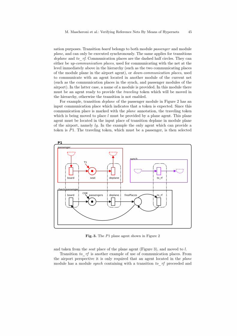
sation purposes. Transition board belongs to both module passenger and moduleplane, and can only be executed synchronously. The same applies for transitionsdeplane and to_rf. Communication places are the dashed half circles. They caneither be up-communication places, used for communicating with the net at thelevel immediately above in the hierarchy (such as the two communicating placesof the module plane in the airport agent), or down-communication places, usedto communicate with an agent located in another module of the current net(such as the communication places in the synch, and passenger modules of theairport). In the latter case, a name of a module is provided. In this module theremust be an agent ready to provide the traveling token which will be moved inthe hierarchy, otherwise the transition is not enabled.

For example, transition deplane of the passenger module in Figure 2 has aninput communication place which indicates that a token is expected. Since thiscommunication place is marked with the plane annotation, the traveling tokenwhich is being moved to place l must be provided by a plane agent. This planeagent must be located in the input place of transition deplane in module planeof the airport, namely lg. In the example the only agent which can provide atoken is P1. The traveling token, which must be a passenger, is then selected

Fig. 3. The P1 plane agent shown in Figure 2

and taken from the seat place of the plane agent (Figure 3), and moved to l.Transition to_rf is another example of use of communication places. From

the airport perspective it is only required that an agent located in the planemodule has a module synch containing with a transition to_rf preceeded and


followed by two up-communication places. This requirement is fulfilled by agentP1, but from the P1 perspective it is also required the enabledness of the syn-chronized to_rf transition in the module check-passenger. Therefore this con-figuration to_rf is not enabled because freePlaces is not marked.

Hypernet being a high level net model means that the execution of a transi-tion, like deplane, has several firing-modes [10]. Each firing-mode in a hypernetis a called consortium, and is obtained by selecting a transition, a set of agentsthat contain the transition, and a set of passive agents that will be moved asshown in the previous example when the consortium fires. For example, one en-abled consortium is the one we just discussed which moves the agent T 1 fromplace seat of the plane, to place rf of the airport agent that we just discussed.Another consortium is corresponding to agent T 2, which in the configurationshown in the example is not enabled since T 2 is not located in place seat.

One of the most important features of hypernets is that they have a straight-forward expansion towards a behaviourally equivalent 1-safe nets. This expansionnot only gives hypernets a precise semantics in terms of a well known Petri netsbasic model, but also guarantees the possibility to reinterpret on hypernet allthe analysis techniques developed for the basic model. The 1-safe net is built inthe following way:

– For each agent A, and for each place p in the hypernet a place named 〈A, p〉is added in the corresponding 1-safe net. A token in this place means thatA is located in p,

– For each consortium Γ in the hypernet a transition named tΓ is added inthe 1-safe net,

– An arc is added from a place 〈A, p〉, to a transition tΓ if A is a passive agentin Γ , and p is the input place from which the agent A comes.

– An arc is added from a transition tΓ , to a place 〈A, p〉 if A is a passive agentin Γ , and p is the output place where the agent A is going to.

Finally, a place 〈A, p〉 of the 1-safe net is marked if in the initial configurationof the hypernet agent A is located in place p.

For example, the one seater plane case of study we just discussed is translatedin the 1-safe net shown in Figure 4. Plane P1 can be in places lg, rf, bg in thehypernet, thus the 1-safe net contains places 〈P1, lg〉, 〈P1, lg〉,〈P1, lg〉. The samemust be done for traveler agents, and for the CHK check agent. Since transitiondeplane in the hypernet has two firing-modes, in the 1-safe net two transitionswhich models each of the firing modes of deplane are added (for simplicity bothcalled deplane). The same has been done for transition board. The firing of atransition in the 1-safe net exactly models what happens when a consortiumfires in the hypernet.

As already mentioned, it can be demonstrated that this net is 1-safe, andhas a reachability graph isomorphic to the one of the corresponding hypernet.Details, formal definitions, and proofs discussed can be found here for hypernetsin [3], and in [9] for the generalization version.


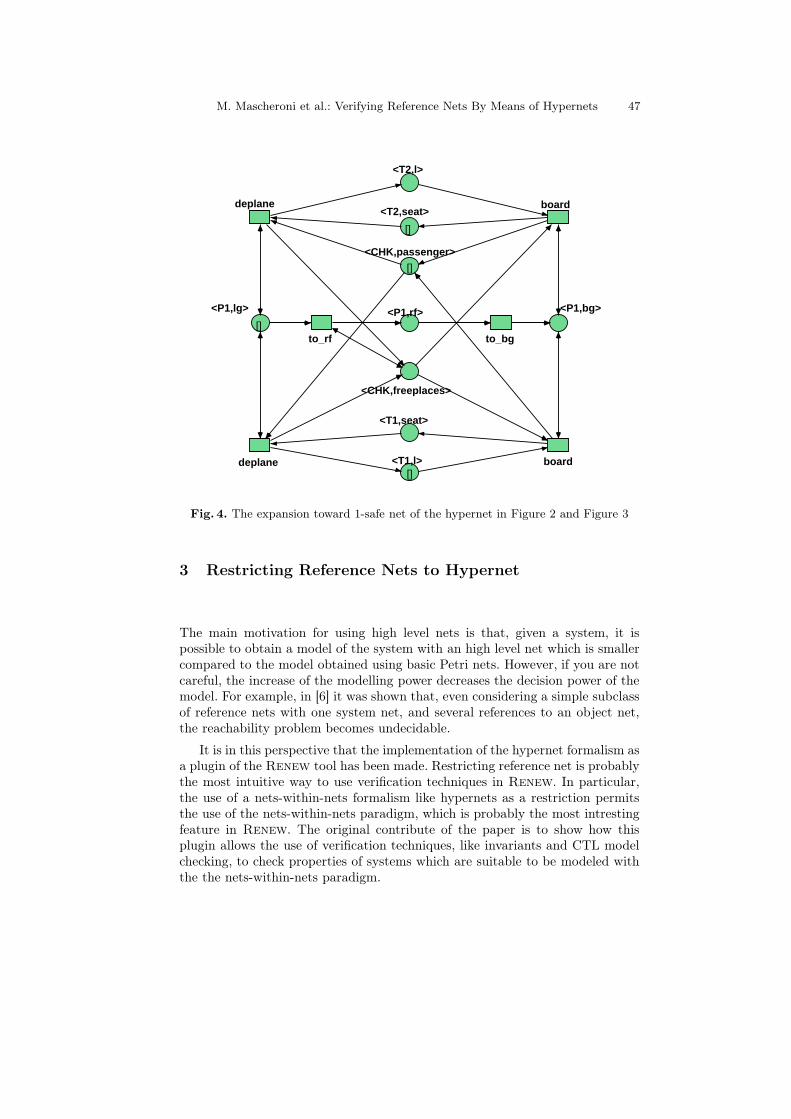
<T1,seat>

<P1,rf>

<T2,l>

[]to_rf to_bg

deplane board

[]

<T2,seat>

<P1,bg><P1,lg>

boarddeplane

<CHK,passenger>

<T1,l>[]

<CHK,freeplaces>

[]

Fig. 4. The expansion toward 1-safe net of the hypernet in Figure 2 and Figure 3

3 Restricting Reference Nets to Hypernet

The main motivation for using high level nets is that, given a system, it ispossible to obtain a model of the system with an high level net which is smallercompared to the model obtained using basic Petri nets. However, if you are notcareful, the increase of the modelling power decreases the decision power of themodel. For example, in [6] it was shown that, even considering a simple subclassof reference nets with one system net, and several references to an object net,the reachability problem becomes undecidable.

It is in this perspective that the implementation of the hypernet formalism asa plugin of the Renew tool has been made. Restricting reference net is probablythe most intuitive way to use verification techniques in Renew. In particular,the use of a nets-within-nets formalism like hypernets as a restriction permitsthe use of the nets-within-nets paradigm, which is probably the most intrestingfeature in Renew. The original contribute of the paper is to show how thisplugin allows the use of verification techniques, like invariants and CTL modelchecking, to check properties of systems which are suitable to be modeled withthe the nets-within-nets paradigm.


4 The Hypernet Plugin

From a technical point of view the implementation of a new formalism in Renewis done using a plugin mechanism. The most important method contained in theclasses implementing the plugin is a compile method which takes as input ashadow net, a set of Java objects containing all the information about the netthe user has drawn in the graphical editor of Renew, and transform it in a setof Java objects used by the simulator engine to simulate the net. This compilemethod is responsible for checking that the net drawn by the user is an actualhypernet in our case. In particular, in order to be able to use Renew as ahypernet simulator, the arc and transition inscriptions used in the modelingprocess must be restricted in such a way that the drawn net is a hypernet.Therefore the restrictions applied in the plugin are the following:

– Inscriptions (tokens) inside places can only be in the following forms: iden-tifier or identifier:netType. In the first case the identifier represent the nameof an empty net, and will be treated by the simulator engine as an blacktoken; in the second case a new instance of the net netType will be createdand placed inside the place.

– Inscriptions on arcs are restricted to single variables only. Each arc mustcontain exactly one variable inscription.

– The inscriptions of input (output) arcs must not be duplicated. In this way itis possible to preserve the identity of nets: duplication of tokens is forbidden.

– Balancing of transition has to be checked, i.e.: the set of variable names usedto inscribe input arcs must coincide with the set of variable names used toinscribe output arcs.

– Communication places are deleted, and are simulated by means of syn-chronous channels. These channels are counted when checking transitionbalance.

For example, the airport agent shown in Figure 2 can be drawn as a hypernetin Renew using the net shown in Figure 5. The traveler empty tokens are placeinscriptions T 1 and T 2, and the plane net instance is created by the P1 : placeinscription. Each transition is balanced. For example transition deplane in theairport has a bidirectional arc labelled pl, and an output arc labelled pa for whichthere is a correspondant downling, namely pl : deplane(pa). Each communicationplace is deleted, and it is replaced with a synchronous channel. Land and takeofftransitions are equipped with two uplink because they were connected to twoup-communication places. Deplane and board transitions contain two downlinksbecause they were connected to down-communicating places. The module nameused to label communicating places is used to retrieve the variable name usedin the downlink.

The P1 agent of Figure 3 is drawn in the hypernet plugin of Renew withthe net in Figure 6. Again, up-communication places are replaced by channels,and transition to_rf must synchronise with the corresponding transition in theairport agent.


pl:land(pl) :takeoff(pl)

plplplplpl

pa pa

pl

lg bg

l

rf

T2

pl:to_rf()

to_bg takeoffland to_rf

deplane board

pl

pl:board(pa)pl:deplane(pa)

P1:plane

Fig. 5. The airport agent drawn with the hypernet plugin of Renew

chk

pa:board(pa) :deplane(pa) :to_rf()

to_rfdeplaneboard

chk

pa

chk

chk

seatT1

chk

CK

freeplaces

numPass

Fig. 6. The plane agent drawn with the hypernet plugin of Renew

As we already mentioned, thanks to the expansion to 1-safe nets it is possibleto use verification techniques defined for this class of net to analyse systemmodelled with a hypernet. Two of the most useful techniques are invariantsanalysis, and model checking. We explored two possibilities of using them inthe plugin we implemented: internal implementation in Renew, or exportingthe 1-safe net in a format understandable by other tools. Since implementingthese analysis techniques in an efficient way is a difficult task (some tools arevery elaborated, and have been implemented over several years), and since veryefficient open source tools are available for free, we decided to use external toolsto implement invariant analysis, and model checking of a hypernet.

In the following sections we will show how the extensions and incorporationcan be used in a practical example.

5 Example

The invariant analysis, and the model checking extensions we implementedin Renew can be used to prove properties of a system. We have chosen theexternal tools LoLA (see http://www2.informatik.hu-berlin.de/top/lola/lola.html) and INA (see http://www2.informatik.hu-berlin.de/~starke/


ina.html) for analysing purposes. Starting from the hypernet example of Sec-tion 2.2, we will prove using invariants that there is never more than one passen-ger on the plane, and we will prove using the model checker that a plane neverrefuels if there are a passenger on board.

By running the invariant analysis we get the following invariants:

T2@l T2@seat CHK@pass P1@lg P1@rf P1@bg CHK@freepl T1@seat T1@l0 0 0 1 1 1 0 0 01 1 0 0 0 0 0 0 00 0 1 0 0 0 1 0 00 0 0 0 0 0 0 1 11 0 1 0 0 0 0 0 10 1 0 0 0 0 1 1 0

The first four invariants are those which guarantee the truth of “law of con-servation of agents”, achieved thanks to the state machine decomposition in theformalism. For each agent there is a corresponding invariant indicating the placesin which that agent can be located. Since the places of each invariant containsonly one token in the initial marking, it is mathematically proved that each agentcan be only in certain places: the places which are of the same sort of the agentitself. Moreover, these four invariants can also be used to prove that the net is1-safe: they cover all places of the net, and contain only one token in the initialmarking.

The fifth invariant is 〈T 2, l〉, 〈CHK,numPass〉, 〈T 1, l〉 and contains twotokens in the initial marking. Together with the second and the fourth invariantsit can be used to prove that if the place 〈CHK,numPass〉 is marked then oneof the two passenger is seated on the plane. The place is not marked only if bothpassenger are in the airport.

The sixth invariant is the counterpart of the fifth, and states that only one ofthe following places can be marked: 〈T 2, seat〉, 〈CHK, freeplaces〉, 〈T 1, seat〉.The information is clear: only one passenger can be in the seat place of the plane.If none of them is in the plane 〈CHK, freeplaces〉 is marked.

In Figure 7 a screenshot of Renew after the computation of invariants isshown.

While invariants analysis can be launched, and the computed invariants canbe analysed to extract information about the system, in order to analyze thesystem using model checking a formula specified in a temporal logic is needed.Since we choose LoLA, which is a CTL model checker, we need to specify theproperty we want to verify using this logic. For example, checking the property“if the plane is located in the place representing the refueling station then nopassenger is on board” can be done by entering as input of the Renew pluginwe implemented the following CTL formula:

ALLPATH ALWAY S

NOT ((T 1.seat = 1 AND P1.rf = 1) OR (T 2.seat = 1 AND P1.rf = 1))


Fig. 7. A screenshot of the invariants computed inside Renew

The formula checks that in every reachable state (ALLPATH ALWAY S) thesituation in which both placed 〈T 1, seat〉 and 〈P1, rf〉 are marked never occurs(and the same for places 〈T 2, seat〉 and 〈P1, rf〉). The analysis performed con-firms that the truth value of the formula is true, which is enough to guaranteethat the property is true for the system.

As it can be seen in this simple example, the advantage of using model check-ing is that it is possible to express, and consequently to verify, more propertiescompared to invariant analysis. In our example, the information that a planenever refuels if a passenger is on board is not present in the computed invari-ants, but can be verified using the model checking. However, the drawback isthat it is necessary to explore the whole state space of the system in order to ver-ify a property. Invariants are computed on the static structure of the net, whichis usually exponentially smaller compared to the state space of the system. Ingeneral, in real huge application both the techniques are useful: invariants give aquick overview of some properties of the system, model checking take more timeand it can be used to verify specific properties of the system.

6 Conclusion

In this paper we discussed the verification of high-level Petri nets which use thenets within nets paradigm, with particular attention to the reference nets andthe hypernets formalisms. We examined them, and we showed how to transforma subset of reference nets into hypernets, which in turn can be transformedinto 1-safe nets. We then proceeded to describe the hypernet plugin created forRenew in the course of our work. With the help of this plugin and external toolswe can analyse the transformed low-level nets, and in this way verify propertiesof the high-level net.

The contributions, and the results of this paper are the implementation of aplugin for Renew with which it is possible to draw of a hypernet, to compute


its invariants, and to model check it. With this approach it is now possible toverify properties of systems modelled with net within nets oriented formalisms,such as reference nets and hypernets.

The results of this paper will make it possible to automatically analyse a hy-pernet, instead of first transforming it by hand, and then analysing the equiva-lent low-level nets. This will make the verification simpler and more user-friendly,which in turn will make it easier for software engineers to use these techniquesin practical use cases. We plan to use these approaches to verify the model ofan actually adopted Grid tool for High Energy Physics data analysis, and in thecontext of the HEROLD project. Future work will also focus on extending thepossibilities of the verification, automating the process as far as possible andextending the toolset to other high-level Petri nets formalisms. The flexibilityand adaptability of the Renew tool will be a large asset in this endeavour.Finally, the definitions of analysis techniques directly on the high level model,without the need of converting it to a low-level one, is a subject for future in-vestigations, because it will avoid the conversion to low-level nets, which is anexpensive operations in term of computational resources.

References

1. M Bednarczyk, L Bernardinello, W Pawłowski, and L Pomello. Modelling andanalysing systems of agents by agent-aware transition systems. In F. Fogelman-Soulie, editor, Mining Massive Data Sets for Security: Advances in Data Mining,Search, Social Networks and Text Mining, and their Applications to Security, vol-ume 19, pages 103–112. IOS Press, 2008.

2. Marek A. Bednarczyk, Luca Bernardinello, Wiesław Pawłowski, and LuciaPomello. Modelling mobility with Petri Hypernets. In Recent Trends in Alge-braic Development Techniques, volume 3423/2005 of Lecture Notes in ComputerScience, pages 28–44. Springer Berlin / Heidelberg, 2005.

3. Marek A. Bednarczyk, Luca Bernardinello, Wiesław Pawłowski, and LuciaPomello. From Petri hypernets to 1-safe nets. In Proceedings of the Fourth Inter-national Workshop on Modelling of Objects, Components and Agents, MOCA’06,Bericht 272, FBI-HH-B-272/06, 2006, pages 23–43, June 2006.

4. Luca Bernardinello, Nicola Bonzanni, Marco Mascheroni, and Lucia Pomello. Mod-eling symport/antiport p systems with a class of hierarchical Petri nets. In Mem-brane Computing, volume Volume 4860/2007 of Lecture Notes in Computer Sci-ence, pages 124–137. Springer Berlin / Heidelberg, 2007.

5. Soren Christensen and Niels Damgaard Hansen. Coloured petri nets extended withchannels for synchronous communication. Lecture Notes in Computer Science,815/1994:159–178, 1994. Application and Theory of Petri Nets 1994.

6. Michael Köhler and Heiko Rölke. Properties of object Petri nets. In Jordi Cor-tadella and Wolfgang Reisig, editors, ICATPN, volume 3099 of Lecture Notes inComputer Science, pages 278–297. Springer, 2004.

7. Olaf Kummer. Referenznetze. Logos Verlag, Berlin, 2002.8. Olaf Kummer, Frank Wienberg, Michael Duvigneau, Jörn Schumacher, Michael

Köhler, Daniel Moldt, Heiko Rölke, and Rüdiger Valk. An extensible editor andsimulation engine for Petri nets: Renew. In J. Cortadella and W. Reisig, editors,


International Conference on Application and Theory of Petri Nets 2004, volume3099 of Lecture Notes in Computer Science, pages 484 – 493. Springer-Verlag, 2004.

9. Marco Mascheroni. Generalized hypernets and their semantics. In Proceedings ofthe Fith International Workshop on Modelling of Objects, Components and Agents,MOCA’09, Bericht 290, 2009, pages 87–106, September 2009.

10. Einar Smith. Principles of high-level net theory. In Lectures on Petri Nets I: BasicModels, volume Volume 1491/1998 of Lecture Notes in Computer Science, pages174–210. Springer Berlin / Heidelberg, 1998.

11. Rüdiger Valk. Object Petri nets: Using the nets-within-nets paradigm. In JörgDesel, Wolfgang Reisig, and Grzegorz Rozenberg, editors, Advanced Course onPetri Nets 2003, volume 3098 of Lecture Notes in Computer Science, pages 819–848. Springer-Verlag, 2003.


Improving a Workflow Management System withan Agent Flavour

Daniel Moldt, José Quenum, Christine Reese, and Thomas Wagner

University of Hamburg, Faculty of Mathematics, Informatics and Natural Sciences,Department of Informatics

http://www.informatik.uni-hamburg.de/TGI/

Abstract. This paper discusses an application of software agents toimprove workflow management systems, with a practical emphasis onPetri net-based systems. The properties of agent technology will be usedto gain advantages within the workflow management systems on botha conceptual and practical level. In this paper we discuss the theoreti-cal background of our work, the conceptual idea and approach and onepossible practical implementation. As a central practical means we usereference nets, a high-level Petri net formalism. These nets are used tomodel both agents and workflows, which results in a clean and naturalintegration of both technologies.

Keywords: High-level Petri nets, workflow management systems,multi-agent systems, software architecture.

1 Introduction

Workflows and Workflow management systems (WFMS) have been very attrac-tive research topics in the last decades [13, 18, 16]. They provide means to furtherunderstand, unambiguously specify and analyse business processes within organ-isations. According to the state of the art, several heterogeneous WFMS can becombined to perform a specific complex task that cuts across various organisa-tions. While such a combination is currently possible in an ad hoc manner, amore systematic approach demands greater care both from the modelling andimplementation perspectives. In this research, we set out to address this limita-tion. This paper discusses the conceptual approach to achieve the overall goal.

Among the rising software paradigms, the concept of agent is a preeminentone. In the last decade, agents have been touted as a most appropriate paradigmto support the design and implementation of decentralised and distributed appli-cations/systems, which yield intelligent behaviour and require a great deal of in-teroperability. A decentralised application implies an application which consistsof autonomous entities. Clearly, these are among the properties one seeks whiledeveloping an approach for interorganizational workflows. Therefore, agents can

contribute a great deal in our quest for a systematic approach for interorganiza-tional workflows.

Using agents to design and implement distributed applications across a net-work is not new in itself. However, the autonomy of the various subparts isnot well captured in the overall collaboration. As such, approaches of this kindcannot be generalised for the design and implementation of collaborative appli-cations across various organisations. Concepts such as workflows, which rendera clear view of business processes within organisations need to come into play.

Introducing agents in WFMS is not counterintuitive. By virtue of being au-tonomous, sociable and intelligent, human agents and artificial ones share manysimilarities. Moreover, human agents’ operational mode can be viewed as a setof independent yet interoperable entities. From that angle, a human agent canbe viewed as an agent system. Finally, since human agents have to coordinatethe various tasks they are involved in at a certain point in time, they can beregarded as a WFMS. We take this human analogy, especially its duality, toshow that both, agents and workflows, can be joined in a complex system.

As discussed in the foregoing, WFMS can benefit from agents in variousregards. In this paper, we discuss seven points where agents help enhance thelevel of management in interorganizational workflows. These include distribu-tion, autonomy, interoperability and intelligence. In order to make the resultingapproach appealing to new technologies, we structure our assumptions and ideasinto a reference architecture, which we believe lays the foundation for more spe-cific and advanced architectures to support collaboration within and betweenorganisations. We do not claim that our current implementation is as powerfulas the existing commercial tools. However, thanks to the Petri nets formalism,our implementation holds the potential to properly handle concurrency, robust-ness and resilience in the future.

The contributions discussed in this paper are a clearer articulation of ideasand intuitions presented in [20–22]. More than all these papers, we elaborate onthe underpinnings of the conceptual role agents can play in the new approach.Finally, we discuss the implementations.

The remainder of the paper comes as follows. Section 2 describes the technicaland theoretical background of our work. Section 3 gives an overview of ouroverall architecture. Section 4 examines the conceptual view of our approach,while Section 5 discusses one implementation of our approach. Finally, Section 6draws conclusions and directions for the future.

2 Frameworks & Formalisms

In this research, MASs are designed following Mulan’s (MULti-Agent Nets)structure [11, 23]. Mulan has been extended with Capa (Concurrent AgentPlatform Architecture) in order to comply with Fipa’s (Foundation forIntelligent and Physical Agent (see http://fipa.org)) (communication) standardsto support concurrent execution [4]. Mulan and Capa describe the various com-ponents of a MAS using reference nets, which can be executed using the Re-


new (REference NEts Workshop (see http://www.renew.de)) tool. The readershould thus note that not only do we offer a formal ground to reason about thebehaviours of agents, but we also provide an execution environment for MAS.

Inspired from the nets within nets concept introduced by Valk [25], Mulan’sstructure is a four-layer architecture used to describe a MAS. These layers re-spectively describe the overall MAS, the agent platforms, the agents and theirbehaviour, the protocols. Every layer within Mulan’s reference architecture ismodelled using reference nets, a high level Petri net formalism which will bediscussed later.

In order to adhere to Fipa’s standards, and especially the communicationmechanisms, Mulan has been extended with Capa. In so doing, Capa agentscan easily interact with any type of Fipa compliant agents.

Each of the key concepts in this paper, agent and MAS on the one hand andworkflows on the other hand, is represented using a Petri net formalism. Agentsand MAS are represented using reference nets, while workflows and WFMSsare represented using workflow nets implemented as a special kind of referencenets. Reference nets have been introduced in [15]. They follow the philosophy ofnets within nets. Reference nets use Java as an inscription language, manipulatevarious types of data structures, and like many other types of high-level Petri netformalisms, offer several types of arcs. Finally they use synchronous channels tosynchronise with other nets or Java objects. The treatment of Java objects andnet instances is transparent, so that both kinds of artefacts can be exchangedarbitrarily. The workflow nets used in our systems are based on principles ofworkflow nets introduced in [26]. They are implemented as reference nets andmake use of a special task transition introduced in [9]. Moreover, in the Petri netcommunity, tool support is a general trend. Therefore, the Renew tool has beendeveloped to support quick prototyping of systems or parts of systems using thereference net formalism. Renew provides an editor to specify and draw the netsas well as a simulation engine to test and validate them.

3 Overall architecture

The results we present in this paper are part of a larger ongoing effort. Thesystems described in the next sections can be classified within the overall archi-tecture described in [19]. The goal of this architecture is to integrate agent andworkflow technologies. The architecture consists of five tiers, built on top of eachother. Each tier itself is a layered architecture, which combines various aspectsof both technologies. Starting from either a pure workflow or agent system, thearchitecture gradually evolves into a novel integrated unit system, which equallybenefits from both original concepts. The main motivation in building this ar-chitecture lies in the shortcomings of each individual concept as is discussed indetail in [19] and [28]. In short, agent technology struggles with offering a clearbehavioural view of large distributed systems, but can describe the structureof such a system in a natural way. Workflow technology can easily describe thebehavioural view of a complex system, but struggles with the structural view.

Moldt et al.: Improving a WfMS with an Agent Flavour 57

Fig. 1. Architecture of the first tier of the overall architecture, modified from [19]

In combining both technologies we can integrate the views offered by both intoone new system which supports both a clean structural and behavioural view. Itshould be explained that the notion of tiers in this architecture denotes a kindof step-by-step refinement/enhancement on the way to the overall goal of inte-gration. The tiers can be viewed as the layers of the overall abstract architecturebut they do not correspond to layers within a concrete architecture. Each tiermodifies the structure of its own layered architecture compared to the previoustier and in doing so enables new or improved aspects to be used. We will nowshortly discuss the five tiers of the architecture.

First Tier The first tier is our starting solution to address the limitations of bothtechnologies. It involves either a pure agent management system (AgMS) or aWFMS. Such systems exclusively use workflow or agent technology to providetheir functionality. This means that there is almost no integration between thetwo. Because of this, the architectural view of this tier (see Figure 1) offers onlytwo layers. The bottom depicts the adopted management system (either agent orworkflow), on top of which an application lies. Examples of systems, which canbe classified into this tier, are Mulan and Capa on the agent side and WFMSlike ADEPT (see [3]) or WIFAi (see [24]) on the workflow side.

Second Tier In the second tier, one of the paradigms is used to realise the other.In other words, we use agents to design a WFMS, and vice versa. Because of this,there are two variants of the second tier (agents in the background or workflowsin the background). The architectural view of this tier (see Figure 2) offers threelayers. The topmost layer still represents an application but between the bottommanagement system and the application an intermediate layer has been added.This layer implements a management system for the alternative concept usingthe functionality of the bottom layer. For example, if the bottom layer is anAgMS, then the intermediate layer is a WFMS based on agents. The applicationlayer of this tier uses only the concept provided by the intermediate layer.

Building on the first tier the second tier can be achieved by designing theapplication within the first tier to be the required management system. On topof that management system another application can then be built, turning theapplication layer of the first tier into the intermediate layer of the second tier.


Fig. 2. Architecture of the second tier of the overall architecture, modified from [19]

Compared to the first tier, the advantage is that one can perceive an inte-gration of the concepts. However, the available constructs only affect the back-ground instead of being directly available in the application layer. For example,distribution, interoperability, etc. are facilitated in WFMS using agents.

In the remainder of this paper, the higher level tiers will only be based onthe variation using agents in the background, i.e. the one including an AgMS,an agent-based WMFS (AgWFMS) and an application. Examples for these kindof systems are detailed in [6], [7] and [10].

Third Tier The third tier greatly enhances the application development by em-ploying both agents and workflows. This results in an arbitrary degree of inte-gration between agents and workflows. In addition to the interface between theapplication and intermediate layer, this tier allows direct access from the ap-plication layer to the bottom management system. In practice, the applicationcan thus use both the interfaces offered by the core AgMS and the AgWFMS.Consequently, the key functionality of the AgMS is then combined with thatof the AgWFMS. The architectural view of this tier (see Figure 3) only adds adirect connection between the application and the bottom layer, compared tothe second tier. While this additional connection is a clear advantage over theprevious tier by expanding potential and flexibility, it suffers from a major lim-itation. The resulting system is completely unstructured, i.e., the relation andintegration between agent and workflow needs to be potentially re-invented foreach application. Consequently it becomes very difficult to harness the power ofthis tier, especially the efficient design of complex systems. In order to reach astructured integration of both concepts within the architecture, we need to takeone step back and limit the immense possibilities offered by this tier.

Fourth Tier The fourth tier adds an integration layer to the architecture, which isresponsible for restricting the possibilities of the third tier in order to provide anexplicit structure for the application developed on it (see Figure 4). Through thisintegration both technologies are used in the background and the relationshipbetween agents and workflows is pre-defined. However, only one perspective is


Fig. 3. Architecture of the third tier of the overall architecture, modified from [19]

supported when modelling on the application layer. In this way it provides anabstraction and thus a higher level of modelling.

In order to achieve the desired explicit structure, this tier basically reducesthe functionality offered to the application layer compared to the third tier. Itrefocuses on either agents or workflows as the exclusive main abstraction forapplication development. There are once again two distinct variations of thistier, one offering agents to the application (called workflowagents ; left hand sideof Figure 4), the other one offering workflows (called agentworkflows ; right handside of Figure 4). The integration layer provides exclusively WFMS or AgMSfunctionality, but uses both technologies in the background. This means that anagent application possesses parts and aspects of workflows and vice versa (in theother variation). In this way the possibilities of this tier are, opposed to the thirdtier, restricted, because we refocus on just one technology. But by doing this,we gain a much more powerful means of supporting one of the two technologies.The integration of both variations will take place in the fifth tier. For now weneed both variations in order to create the desired structure within the relationbetween agents and workflows in both directions separately.

It is worth noting that, even though we are looking at either workflows oragents at the top layer again, the main difference between this tier and thesecond tier is that we no longer have one concept realising the other. Rather,we obtain a successful combination of both, i.e., agents and workflows workingside by side and benefiting from each other. The agentworkflow variation of thistier is the main focus of this paper and will be discussed in detail in the mainsections.

Fifth Tier This tier introduces the concept of unit, an abstraction to any entityinvolved in the design of the system. Units offer both the facets of agents andworkflows. In order to achieve this, the AgMS and WFMS have to be integratedand combined. This results in a novel type of management system, a unit man-agement system (UMS). The architecture of this tier can be seen in Figure 5. Theintegration layer of the fourth tier has been split into two parts, of which UMSrepresents the upper part. Since one can no longer clearly differentiate between


Fig. 4. Architecture of the fourth tier of the overall architecture, modified from [19]

Fig. 5. Architecture of the fifth tier of the overall architecture, modified from [19]

agents and workflows, the application layer is simply called unit application, alsoreferred to as agent/workflow applications in [19]. In merging both agent andworkflow concepts into a single unit concept, both the structural view (from theMAS) and the behavioural one (from the workflows) are available. Note thatboth these views are available during runtime and design time.

4 Conceptual View

In this section we will discuss our conceptual approach to improving workflowmanagement with agent technology. As stated before our goal is to use aspects ofsoftware agents to benefit the execution and management of workflow instances.Because we use agents to improve workflows we generally refer to this approachas agentworkflows. We reason that common properties of agents, like mobility,


autonomy and proactivity, and especially the encapsulation of workflow instancesthrough agents can greatly benefit workflow execution. Having agents in generalhandle aspects of workflow management can also help distribute the executionin order to spare less powerful resources.

As mentioned before this particular work is just part of a larger effort tointegrate workflow and agent technologies in order to achieve a novel approachthat combines the advantages of both technologies. The work presented in thispaper focuses on the fourth tier of the overall architecture (see Section 3). Wediscuss the variation of the fourth tier, in which the integration layer offers aWFMS to the application layer. This WFMS strongly relies on the functionalityof the AgMS in the background in order to provide its own functionality. Thismeans that the workflows offered to the application possess some propertiesgained from the agents. How this can be achieved will be discussed in this section,as well as the advantages and disadvantages of this approach,.

One of the core ideas behind our approach is to encapsulate workflow in-stances through autonomous software agents. With this it is possible to transferproperties of that software agent directly to the workflow instance. In otherwords the clear separation between agent and workflow begins to diminish. Thisis a key concept of the overall architecture and is important for the fifth tier.Another important aspect of our approach is to also consider other entities of theworkflow management system as agents. Having the general functionality of theWFMS be provided by agents is already part of an AgWFMS of the second tier.In our approach agents can be used to realise any of the elements (e.g., tasks,users, resources, etc.) of the workflow as well. In [17] for example, we used agentsto realise activities. Thanks to the agent technology, the resulting WFMS doesnot only focus on the behaviour of the system, as was the case in the previoustiers of the overall architecture, it also emphasises the structure of the system.This paper focusses on the aspect of encapsulating workflow instances throughagents. Other aspects are considered but will not be discussed in great detail.

We will now examine some of the principal and conceptual areas and aspectsin which workflows can benefit from agents. The following points will directlycover some agent properties and their particular benefits but will also includesome general observations.

Encapsulation In general the encapsulation of one or more workflow instancesthrough agents can be seen as a prerequisite to opening up many of thepossibilities offered by the agent-oriented paradigm. Without this conceptit would be hard or impossible to transfer other agent properties over tothe workflows. Nonetheless the encapsulation also benefits the workflows inmore ways than that. For example the encapsulation provides the workflowswith an even clearer identity within the overall system since they can nowbe identified in the same way as the other elements (agents) of the system.This makes it easier to monitor, observe and analyse the system, which inturn makes maintenance and improvement more efficient. A disadvantage ofthe encapsulation is that the number of agents active is possibly, drasticallyincreased, depending on how the encapsulation is handled. This may pose


problems on less powerful systems, which simply cannot handle this numberof agents or the communication between them. However, since agent archi-tectures are generally built to efficiently handle communication, this shouldnot pose a real problem in practical use.

Mobility By allowing workflows to gain agent mobility they benefit in a vari-ety of possibilities. In the context of software agents mobility describes thecapability of a software agent to discontinue its execution within one exe-cution environment (agent platform), migrate to another environment andcontinue the execution there starting off from its previous state. For agent-workflows this means that the execution of a workflow can be discontinuedon one instance of an executing WFMS and continued on another WFMS.Practically this can be used if certain resources needed for the execution ofa workflow are not available on every platform. This can include particular(groups of) users or certain, possibly critical data. Another use case for thisproperty is to have a workflow instance migrate not because certain resourcesare needed, but because its home platform is beginning shutdown or becauseanother platform carries less of a load then the home platform. This use ofmobility can lead to improved flexibility, efficiency and fault tolerance.

Autonomy One of the key concepts of the agent paradigm is that agents areautonomous entities. This means that, to a certain degree, they are indepen-dent of their environment and can choose for themselves whether to executean action or not. In the context of agentworkflows this property can be usedin a number of ways. It can for example be used as a kind of access controlto critical data for which an agent is responsible. This can be a workflow in-stance but also other entities like activities or the handling of users. Anotheruse of this becomes relevant if combined with mobility. An agent migratingto another platform to access certain data or perform certain actions can dothis relatively independent from the other agents and software constructs ofthat platform, if, of course, it has all the necessary permissions.

Intelligence Intelligence in software agents can be used to describe a multitudeof aspects. One major aspect is the ability of certain agents to proactivelydecide by themselves which actions to take. In the context of workflow man-agement this can be used to predetermine which users should be offered cer-tain tasks, taking variables like workload into consideration. At this pointreactivity of agents also comes into play. Software agents can react to eventsin their environment and adapt according to the situation. For example ifthere is an error during the execution of a task the agent could observe thisand retry the action with changed parameters. Another very interesting as-pect where intelligence, proactivity, reactivity and adaptiveness can be usedis the adaptivity of workflow instances. Changing workflow instances andeven entire workflow definitions according to changed circumstances (cur-rent or permanent) improves the flexibility and versatility of a WFMS andcan be handled in a natural way using agent intelligence.

Distribution The agent oriented paradigm naturally supports the design of dis-tributed software systems. The main reasons for this are the asynchronousmessage communication and the autonomy of the individual agents. By re-


lying on agents as the main building blocks of a WFMS it is easy to usethese predispositions for the distribution of the system. The communica-tion of different parts of the system can be handled through asynchronousmessages, which are flexible and versatile. Extending on this idea opens upeven more possibilities of using distribution to the advantage of workflows.Interorganizational workflows can benefit from a distributed WFMS, so thattheir critical information is not stored in some centralised location.

Interoperability The Fipa communication standards are accepted by manywidely-used agent frameworks. Adhering to these standards guarantees in-teroperability between the different involved software systems, independentof agent architecture or framework. This can be translated into workflowmanagement based on agents as well. In this case different WFMS of dif-ferent providers can work together, as long as they can process the datastructures that are exchanged. This aspect is especially important in thecontext of interorganizational workflows since it allows some freedom for thechoice of the different WFMS in the different companies. But also in generaluse cases interoperability can be used to an advantage. A Fipa-compliantWFMS can request data from any other Fipa-compliant system, which im-proves the possibilities of the WFMS. Another aspect which is related tothis and distribution, is the openness of the system. Through interoperabilityand distribution it is possible to create flexible and dynamic open systemsto which different WFMS can connect to, complete some tasks, and thendisconnect again. Open systems can provide users with functionality that isotherwise difficult to obtain without specialised software solutions.

Structure This point is related to the motivation behind our overall architec-ture. As described, we reason that workflow systems have trouble adequatelydescribing the structure of the system they are modelling, while focussingon the behaviour. Agent systems on the other hand possess a strong focuson this structure. By joining the two in the ways described in this paperwe begin to combine this structural view given by the agents with the be-havioural view of the workflows. This is mostly related to the encapsulationaspect discussed above, but contains a more abstract view. By relying onagents one can easily describe the current state of an entity including itscurrent location (in regards to distribution), knowledge and behaviour. Byadapting this for workflow instances it can already help provide the struc-tural view needed within a distributed system. If the agentworkflow idea istaken even further and every aspect of the system modelled through agentsthe structural view becomes even more useful. The location (in regards todistribution) of every resource, user and workflow can be determined anddisplayed in a way that helps monitoring and maintaining the system.

It should be noted that all these properties only unfold their full poten-tial if used in combination. Every one of these properties and aspects possessessome benefits but together with the others new and improved possibilities can beachieved. For example using mobile agents in a distributed environment of manyinteroperable agent platforms is more advantageous then forcing the same agent


system onto all involved partners. Equally an autonomous, intelligent agent candecide for itself if a migration is reasonable or not and initiate the action accord-ingly. Using these properties together also strongly improves interorganizationalworkflow management and execution. While interoperability and distributionalready favour this field, the other properties are also useful, especially in col-laboration. For example mobility allows for the transmission of data in a naturalway, while encapsulation allows for the clear separation of critical data.

The main disadvantage of our approach is that the realisation and handlingof these improved workflows are more complex than handling regular workflows.The reason for this is mainly that the new and improved possibilities will bedifficult to harness. It can, if used in the wrong way, affect execution in a negativeway or even, in the worst case, prohibit correct execution at all. However, ifused correctly and efficiently, they offer clear, distinct advantages to workflowexecution in general. They offer novel ways of modelling many parts of workflowsand can increase efficiency in use.

After discussing the conceptual view in this section we have shown that ourapproach offers many advantages, but is difficult to realise and handle. For therealisation part we have chosen technologies based on Petri nets. One problem ofthe conceptual approach is that different kinds of entities (agents and workflows)have to be combined. By choosing Petri nets as a common basis we can partiallycircumvent this problem, since it is easier to combine the two kinds of entitieswhen they possess the same basis at the lowest level. On the other hand thischoice has the problem of not being widely spread and available. However, certainaspects, like concurrency and displaying behaviour, are very easy to model usingPetri nets. In the next section we will discuss one prototypical implementationof our conceptual approach using Petri nets, which already covers some of theproperties described in this section.

5 Implementation

In this section we will discuss a prototypical implementation of our agentwork-flow approach. As mentioned before we use Petri net based technologies toachieve a common basis for the integration and combination of workflow andagent technologies. In particular we use Mulan and Capa for our agents andworkflow nets for our workflow functionality (see Section 2). The starting pointof the practical work is an AgWFMS of the second tier of the overall architec-ture. This AgWFMS has been described in detail in [27]. It relies solely on agentsto provide the functionality but does not mix the agent and workflow conceptsenough to be considered an agentworkflow system.

Before going into the details of the implementation we will shortly discusshow the different properties observed in the conceptual section can be mappedonto Petri nets. Since discussing these aspects in a reasonable extent would gobeyond the scope of this paper and since extensive work on this has already beenperformed and published we will limit this to referring to other contributions.The mobility aspect has been extensively studied, especially in the context of


Fig. 6. Principle approach of the S-AgWf

nets within nets, for example in [2] and [12]. The autonomy and intelligenceof Petri net agents have been discussed in the context of Mulan in [23]. Theencapsulation aspect has been examined for object-oriented nets in [1]. Interop-erability and openness have been explored in [14]. The final aspect, the structuralview of combining agents and workflows, was discussed in [19].

The practical approach, called structure-agentworkflow (S-AgWf), extendsthe regular AgWFMS (now called AgWFMS*) to allow for the definition andexecution of distributed workflow instances. More precisely, the workflow in-stances are now hierarchical workflows with nested subprocesses as defined bythe WfMC (see [8]).As a consequence the entire system consists of a number ofCapa platforms, which all execute instances of the extended AgWFMS* and areworking together. The different AgWFMS* instances are known to one anotherand messages can be exchanged between them. A more detailed description ofthe S-AgWf approach can be found in [28].

The basic principle of the S-AgWf can be seen in Figure 6. One agent encap-sulates one workflow instance. This agent, called structure-agent, possesses aninternal workflow, the structure-workflow. When the structure-agent for a newworkflow instance is started, it receives the definition of the structure-workflowfrom the database agents of the AgWFMS* and instantiates the workflow net.When this initialisation is finished, the execution of the structure-workflowautomatically begins. The tasks of the structure-workflow correspond to sub-workflows. Sub-workflows can only be executed on certain AgWFMS* instances


within the overall system. The information about which AgWFMS* instanceis suitable is stored within the data of the task and can be extracted by thestructure-agent. Whenever a task becomes active, the structure-agent assigns it-self as the executor of that task. Once this is done the structure-agent queries aspecial agent of his own platform for a list of all the known AgWFMS* instancescurrently active. It then compares this list to the information extracted fromthe task and chooses a suitable AgWFMS* instance. The interface-agent of thechosen instance is then contacted by the structure-agent. The structure-agentasks the interface-agent to instantiate the subworkflow locally and transmits allrelevant parameters, like input data etc. The subworkflow is then executed likeany other workflow in the regular AgWFMS. Once it has reached the end of itsexecution the responsible structure-agent is informed and any (optional) resultsare sent back. The results are transmitted into the structure-workflow net andthe structure-agent completes the task, so that the execution can continue. Theexecution of tasks and subsequent instantiation and execution of sub-workflowsis continued, until the end of the structure-workflow is reached. The initiator ofthe overall workflow is then informed and the structure-agent can terminate.

In the example in Figure 6 two sub-workflows are currently executed onthe two different AgWFMS* platforms. The structure-agent responsible for thestructure-workflow is communicating with the agents of the two AgWFMS*platforms in order to initiate the execution and receive results. When bothsub-workflows are finished the structure-agent will start a final sub-workflow(SubWF C ), before it can conclude the execution of the structure-workflow.

This realisation of the agentworkflow concept offers distinct and practical ad-vantages, but also still suffers from some limitations. The possibility to distributethe execution of workflows is a huge advantage for the otherwise centralised Ag-WFMS. The support of nested subprocesses allows for interorganizational work-flows to be defined and executed. Since the details of the local workflows arenot needed globally, the sub-workflows and any critical data they may containare only known to the local parties. This satisfies the need of interorganizationalworkflows to secure and conceal confidential and valuable information.

The main limitation of this particular, specialised implementation of theagentworkflow concept is its still centralised nature. If the platform of thestructure-agent is disconnected or fails, the entire workflow fails. This couldpartially be rectified by adding mobility to the structure-agent. It can then eas-ily migrate to another platform, if it discovers any changes in its home platformthat might hinder its execution.

The pre-defined relationship between agents and workflows within this sys-tem combines the structural aspect of agents with the behavioural aspect ofworkflows as is the goal in the fourth tier of the overall architecture. Thetwo concepts agent and workflow begin to merge together, since in this sys-tem a workflow is an agent and partly vice versa. The practical advantagesthis particular system gains from this merge mostly consist in a groundwork forfurther enhancements. Agent autonomy may for example be used to give thestructure-agent more control over the workflow instance (e.g. choice over where


sub-workflows are executed), which could result in added flexibility. However theinstances within the S-AgWF system already possess certain degrees of distri-bution (structure-agents communicate with other AgWFMS* platforms in orderto execute their structure-workflow), interoperability (the structure-agents ex-change FIPA-compliant messages so it is possible to exchange the AgWFMS*platforms with other WFMS if they adhere to the interface) and encapsulation(the structure-workflow is clearly encapsulated by the structure-agent).

6 Conclusion

In this paper, we made a strong case for a systematic introduction of the agentconcept to enhance the management of workflows. We pointed out key aspectsin which agents improve workflows and their management.

In our quest to develop a systematic approach to support workflow manage-ment, we proposed a reference architecture, which builds on an integration ofagents and WFMS. The architecture consists of five distinct tiers. These dif-ferent tiers gradually show how the agent concept first integrates into WFMSand then enhances them on the various aspects we discussed above. This effortculminates in the fifth tier, where both concepts exist alongside each other. Asstated in the foregoing, our overall goal in this research is to achieve a seamlessintegration of agents and WFMS. In this paper, we presented an approach whichbuilds on the agent technology to address WFMS. However, the other variantof the fourth tier, the workflowagents, needs to be considered as well. In it, themain abstraction of the application layer are agents, which strongly rely on thefunctionality of the WFMS in the background to address the inherent limita-tions to an agent-based system. Clearly, following that perspective, a WMFScould for example bring its systematic and proof-driven approach to complextask execution. In the future, we wish to explore that perspective as well.

From the lessons learned from both approaches, we expect to collect theamount of information that enables us to design a full-fledged conceptual ap-proach which offers the best of both agent and workflow technologies in onesingle system, i.e. the fifth tier. Such an approach will balance out the weak-nesses of each technology. With the support of high-level Petri nets as a foun-dational formalism, we are guaranteed of combining structure and behaviour inone representation.

References

1. Ulrich Becker and Daniel Moldt. Objekt-orientierte Konzepte für gefärbtePetrinetze. In Gert Scheschonk and Wolfgang Reisig, editors, Petri-Netze im Ein-satz für Entwurf und Entwicklung von Informationssystemen, Informatik Aktuell,pages 140–151, Berlin Heidelberg New York, 1993. Gesellschaft für Informatik,Springer-Verlag.

2. Lawrence Cabac, Daniel Moldt, Matthias Wester-Ebbinghaus, and Eva Müller.Visual Representation of Mobile Agents – Modeling Mobility within the PrototypeMAPA. In Duvigneau and Moldt [5], pages 7–28.


3. Peter Dadam, Manfred Reichert, Stefanie Rinderle-Ma, Kevin Göser, Ulrich Kre-her, and Martin Jurisch. Von ADEPT zur AristaFlow BPM Suite - Eine Visionwird Realität: "Correctness by Construction" und flexible, robuste Ausführung vonUnternehmensprozessen. EMISA Forum, 29(1):9–28, 2009.

4. Michael Duvigneau. Bereitstellung einer Agentenplattform für petrinetzbasierteAgenten. Diploma thesis, University of Hamburg, Department of Computer Sci-ence, Vogt-Kölln Str. 30, D-22527 Hamburg, December 2002.

5. Michael Duvigneau and Daniel Moldt, editors. Proceedings of the Fifth Inter-national Workshop on Modeling of Objects, Components and Agents, MOCA’09,Hamburg, number FBI-HH-B-290/09 in Bericht. University of Hamburg, Septem-ber 2009.

6. Lars Ehrler, Martin Fleurke, Maryam Purvis, and Bastin Tony Roy Savarimuthu.Agent-based workflow management systems (WfMSs) - JBees: a distributed andadaptive WfMS with monitoring and controlling capabilities. Information Systemsand E-Business Management, 4, Number 1 / January, 2006:5–23, 2005.

7. Andrea Freßmann, Rainer Maximini, and Thomas Sauer. Towards Collabora-tive Agent-Based Knowledge Support for Time-Critical and Business-Critical Pro-cesses. In Professional Knowledge Management, volume 3782, pages 420–430,Berlin Heidelberg New York, 2005. Springer-Verlag.

8. David Hollingsworth. The Workflow Reference Model. Workflow ManagementCoalition. Verfügbar auf http://www.wfmc.org/reference-model.html.

9. Thomas Jacob. Implementierung einer sicheren und rollenbasiertenWorkflowmanagement-Komponente für ein Petrinetzwerkzeug. Diploma the-sis, University of Hamburg, Department of Computer Science, Vogt-Kölln Str. 30,D-22527 Hamburg, 2002.

10. N. R. Jennings, T.J. Norman, and P. Faratin. ADEPT: An Agent-Based Approachto Business Process Management. ACM SIGMOD Record, 27:32–39, 1998.

11. Michael Köhler, Daniel Moldt, and Heiko Rölke. Modelling the Structure andBehaviour of Petri Net Agents. In J.M. Colom and M. Koutny, editors, Proceedingsof the 22nd Conference on Application and Theory of Petri Nets 2001, volume 2075of Lecture Notes in Computer Science, pages 224–241. Springer-Verlag, 2001.

12. Michael Köhler, Daniel Moldt, and Heiko Rölke. Modelling mobility and mobileagents using nets within nets. In Wil van der Aalst and Eike Best, editors, Pro-ceedings of the 24th International Conference on Application and Theory of PetriNets 2003 (ICATPN 2003), volume 2679 of Lecture Notes in Computer Science,pages 121–139. Springer-Verlag, 2003.

13. Michael Köhler-Bußmeier. Hornets: Nets within Nets combined with Net Algebra.In Karsten Wolf and Giuliana Franceschinis, editors, International Conference onApplication and Theory of Petri Nets (ICATPN’2009), volume 5606 of LectureNotes in Computer Science, pages 243–262. Springer-Verlag, 2009.

14. Michael Köhler-Bußmeier. SONAR: Eine sozialtheoretisch fundierte Multiagen-tensystemarchitektur. In Rolf v. Lüde, Daniel Moldt, and Rüdiger Valk, editors,Selbstorganisation und Governance in künstlichen und sozialen Systemen, volume 5of Reihe: Wirtschaft – Arbeit – Technik, chapter 8–12. Lit-Verlag, Münster - Ham-burg - London, 2009.

15. Olaf Kummer. Referenznetze. Logos Verlag, Berlin, 2002.16. Kolja Markwardt, Daniel Moldt, and Christine Reese. Support of Distributed

Software Development by an Agent-based Process Infrastructure. In MSVVEIS2008, 2008.


17. Kolja Markwardt, Daniel Moldt, and Thomas Wagner. Net Agents for ActivityHandling in a WFMS. In Thomas Freytag and Andreas Eckleder, editors, 16thGerman Workshop on Algorithms and Tools for Petri Nets, AWPN 2009, Karl-sruhe, Germany, Proceedings, CEUR Workshop Proceedings, 2009.

18. Daniel Moldt. Höhere Petrinetze als Grundlage für Systemspezifikationen. Disser-tation, University of Hamburg, Department of Computer Science, Vogt-Kölln Str.30, D-22527 Hamburg, August 1996.

19. Christine Reese. Prozess-Infrastruktur für Agentenanwendungen. Dis-sertation, University of Hamburg, Department of Informatics, Vogt-Kölln Str. 30, D-22527 Hamburg, 2009. Pdf: http://www.sub.uni-hamburg.de/opus/volltexte/2010/4497/.

20. Christine Reese, Jan Ortmann, Daniel Moldt, Sven Offermann, Kolja Lehmann,and Timo Carl. Architecture for Distributed Agent-Based Workflows. In BrianHenderson-Sellers and Michael Winikoff, editors, Proceedings of the Seventh Inter-national Bi-Conference Workshop on Agent-Oriented Information Systems (AOIS-2005), Utrecht, Niederlande, as part of AAMAS 2005 (Autonomous Agents andMulti Agent Systems), July 2005, pages 42–49, 2005.

21. Christine Reese, Matthias Wester-Ebbinghaus, Till Dörges, Lawrence Cabac, andDaniel Moldt. A Process Infrastructure for Agent Systems. In Mehdi Dastani,Amal El Fallah, Joao Leite, and Paolo Torroni, editors, MALLOW’007 Proceedings.Workshop LADS’007 Languages, Methodologies and Development Tools for Multi-Agent Systems (LADS), pages 97–111, 2007.

22. Christine Reese, Matthias Wester-Ebbinghaus, Till Dörges, Lawrence Cabac, andDaniel Moldt. Introducing a Process Infrastructure for Agent Systems. In MehdiDastani, Amal El Fallah, João Leite, and Paolo Torroni, editors, LADS’007 Lan-guages, Methodologies and Development Tools for Multi-Agent Systems, volume5118 of Lecture Notes in Artificial Intelligence, pages 225–242, 2008. Revised Se-lected and Invited Papers.

23. Heiko Rölke. Modellierung von Agenten und Multiagentensystemen – Grundlagenund Anwendungen, volume 2 of Agent Technology – Theory and Applications. LogosVerlag, Berlin, 2004.

24. Michael Tarullo, Daniela Rosca, Jiacun Wang, and William Tepfenhart. WIFAi -A Tool Suite for the Modeling and Enactment of Inter-organizational Workflows.In SOLI ’09. IEEE/INFORMS International Conference on Service Operations,Logistics and Informatics 2009, pages 764–769. IEEE, 2009.

25. Rüdiger Valk. Concurrency in Communicating Object Petri Nets. In Advancesin Petri Nets: Concurrent Object-Oriented Programming and Petri Nets, volume2001 of Lecture Notes in Computer Science, pages 164–195. Springer-Verlag, BerlinHeidelberg New York, 2001.

26. Wil M.P. van der Aalst. Verification of Workflow Nets. In ICATPN ’97: Proceed-ings of the 18th International Conference on Application and Theory of Petri Nets,volume 1248, pages 407–426, Berlin Heidelberg New York, 1997. Springer-Verlag.

27. Thomas Wagner. A Centralized Petri Net- and Agent-based Workflow ManagementSystem. In Duvigneau and Moldt [5], pages 29–44.

28. Thomas Wagner. Prototypische Realisierung einer Integration von Agenten undWorkflows. Diploma thesis, University of Hamburg, Department of Informatics,Vogt-Kölln Str. 30, D-22527 Hamburg, 2009.


Part III

Short Presentations

IRS-MT: Tool for Intelligent ResourceAllocation.

Piotr Chrzastowski-Wachtel1,2 and Jakub Rauch1

1 Institute of Informatics, Warsaw University,Banacha 2, PL 02-097 Warszawa, Poland

2 Warsaw School of Social Sciences and Humanities,Chodakowska 18/31, PL 03-815 Warszawa, Poland

[email protected], [email protected]

Abstract. A tool for optimizing cost and time of a workflow executionwith respect to allocation of multi-purpose resources is presented. Theoptimization is done as a result of simulations, which take into accountthe cost and time associated with each of the resources, when allocatedto transitions in Petri nets representing a workflow. These attributes canbe collected and updated based on the logs of the finished instances. Theprogram suggests the best allocation procedures, giving the estimates ofthe performance of the whole run for all possible decisions.

1 Introduction

Modeling processes as workflows has become quite popular and proved its use-fulness in practice. One of the problems associated with running a workflow isthe resource management. By resources we mean all components required to runan activity. In our case, their necessity is described by certain requirements (e.g.skills or functions) associated with activities (transitions). With each resourcewe associate a bunch of skills, so we can choose, which of the resources are tobe attached to certain activity at the workflow simulation run-time. The Petrinet approach requires collecting all the resources necessary for a given transitionbefore triggering an acitivity to run. One cannot reserve a resource, and keep itbusy, while waiting for other resources necessary to run an activity. Only whenall resources are available we can make a decision to run (fire) an activity.

It often happens that a resource is requested by different activities. A resourceconflict occurs, when a single resource is shared by two enabled transitions. Wemust make a decision, which activity will use the resource first. We assume herethat the resources are re-usable, and that after finshing a transition the resourcecan be used by another activity.

When we make a decision about the resource allocation, we should takeinto account several aspects. Usually we try to optimize some quality function,like time or cost of the workflow run. We assume here that during a workflowrun we can perform several actions concurrently. Since some of them will becompeting for resources, a proper allocation can improve the quality of workflow

run. Engaging proper resources can diminish for instance the delays caused bylack of the only resource requested by a concurrent action and hence waiting forthis resource to be released.

As described in [BPS09], there are many essential aspects of resources, whichshould be taken under consideration during workflow simulation. One of them isalready mentioned: the multifunctionality of resources. Resources have attributesdescribing their skills. In other words these are the abilities to perform certainactions. Each resource is associated with the set of activities, in which it canbe used. Other attributes taken under consideration are performance and costassociated with engaging the resource. So we know how fast a resource can doan activity and how much it costs to use it. By expense of a resource we meanhere a value per time unit associated with involvement of the resource. A chiefaccountant probably has a driving license, but using him to drive the documentssomewhere can be a waste of his time and precious skills. His cost per hour ismuch higher than that of a professional driver.

Since workflows can be quite complex, the authors do not see any analitycalapproach, which would be effective in the optimization of runs. It is hard topredict all the possible outcomes of the allocations decisions, when resourcesare in many conflicts. Instead, we propose an experimental approach, whichinvolves the simulation of many runs, taking into account different allocationsand estimating the desired measures as a result of allocation decisions. In ourprototype IRS-MT (Intelligent Resource Sharing-Modelling Tool) the managercan edit a structured workflow net and set the number of experiments. Theprogram makes random allocations reporting times and costs of the runs. Basedon this knowledge the manager can use the suggestions of the program and geta picture of possible outcomes of the decisions taken. The decisions can be madeincrementally. After each decision the workflow run advances its state, and whenwe come to the next decision, a separate simulation will be made, basing on theactual state of the system.

2 Basic definitions

In our tool we consider resources (S), roles (R), requirements (Q) and activities(A). Resources and roles are finite and defined a priori (by designer). For eachresource we define a set of skills (roles), which it can use. This is denoted byFSR : S → P (R) function. Additionally, for each role in a resource, its efficiencymay differ. For every resource s ∈ S, we define the efficiency function Es :FSR(s) → R+. This function describes how fast a resource performs each ofits roles. The lower this value is, the higher is the efficiency (one is the basevalue). Additionaly, for every resource we define its use cost per time unit as afunction C : S → N. On the other hand, for each activity in a workflow, a set ofrequirements needed to fire it, should be determined. Every requirement Q ∈ Qis a subset of roles. We define a function FAQ(a) which is a bag of requirementsassociated with the activity. It is important, that every activity has an expectedduration time defined and its standard deviation value. Later, in the generation


and simulation phase, only the available resources fulfilling these requirementswill be considered for taking part in such activity. And so, s ∈ S is fulfillingq = 〈Rq〉, iff Rq ⊆ FSR(s). It is important, that if a resource is involved in someactivity, it cannot be used by any other activity (there is one exception, whichwill be covered later in this section).

Initially all the resources are free, available in a pool of idle resources. Weassume, that all the resources are reusable, so at the beginning of activity exe-cution the needed resources are collected and at the end all the freed resourceswill be returned to the pool of idle resources and will be available for furtheruse. The graphical representation of relations between the introduced notions isdepicted on Fig 1.

Fig. 1. Model

Our workflows are Petri nets created using five basic refinement patterns,proposed in [PCh03]: sequential-split of a place or transition, parallel-split ofa place, choice-split of a transition and loop-split which attaches the spawnedtransition with a self-loop to a place. The additional rule for attaching a resourceplace is dual to the loop-split. It just glues a freshly created (resource) place to atransition by a self-loop. From the Petri net perspective we assume here that suchplace will contain initially a token for each physical resource available. We callthe places created by such splits resource places or activity places. One cannotrefine resource places. Even if the transition is refined, the resource will be allo-cated at the beginning of its execution and released, when it is done. Moreover,every resource place will carry the set of requirements defined for corresponding

P. Chrzastowski-Wachtel, J. Rauch: IRS-MT: Modeling Resource Allocation 75

activity. If we match the resource places with activities accordingly, we will see,that the requirement assignments are defining the FAQ function.

When we use activity refinement on a transition, which is inside some otheractivity, we will create a nested activity. By its ancestor activity we call everyother activity, in which this one is nested. Such nested activities do not differfrom any other activities, except for the fact, that these can use resources fromits ancestors, as long, as the resource will not have one of its roles assigned torequirements in two different activities.

3 Tool overview

The main goal of this work is to provide a a tool, which can be helpful inimproving the resource management. We concentrate on optimization of theworkflow execution by providing the user with relevant statistical informationand letting him make decisions on resource-to-activity assignments. To achievethis, a Petri net defining a workflow with activities and resources, will be created.For this purpose we introduce a Workflow Designer. It is the editor for buildingworkflows using refinement patterns. In the editor we create activities, declarethe set of requirements and approximate execution duration. On the other hand,we have Resources Editor. We use it for defining a pool of resources, assigningroles to them, and determining their effectiveness in each role. The set of definedroles can be modified by an always-visible editor Roles Viewer. All these threeeditors form the static part of the tool. Its more detailed description is presentedin section 3.1.

After defining the model in the static part, we can proceed to the dynamicpart of the tool. We will use Generator, to create sufficent number of randomruns. When this is done, the Simulator, the Report Viewer and the Bucket Editorshows up. The first one displays a copy of our workflow, where resource placescontain both the requirements and lists of currently available resources, fulfillinggiven requirements. Here, the tool provides us with information about expectedtime and cost of workflow completion for each of resource-to-requirement assign-ment we see. Basing on this knowledge we can decide, which resource should beassigned for current requirement. Every choice causes the expected values to berecalculated, so that we can run the workflow deciding, how resources shouldbe used in the activities. The Report View presents detailed information aboutexpected time and cost of workflow completion. It is synchronized with cur-rent simulator state, so all the values are always up-to-date. The Bucket Editoris a tool for storing, and presenting details of the runs, which were manuallyperformed by user in the Simulator.

For example, let us consider the following, simple case. There is a package,which must be delivered to the destination within an hour. We know, that stan-dard travel time by a scooter in current traffic would take around fifty minutes.We have two available scooter drivers: Evan and Gregory. Both of them can dothe delivery, but Gregory has got his license for much longer time than Evan,and he shortens the expected delivery time by around 20 percent. Evan, on the


other hand, is still afraid of driving fast and using tricky shortcuts, so his deliv-eries often take 20 percent longer than normal. However, Gregory’s earnings aretwice the earnings of Evan. This is the classic case, where no optimal resolutionto the problem exists. It must be up to user’s decision, whether time or cost ismore important, and it is up to our tool to provide the user with informationabout expected cost and time consequences of each decision. We achieve it bysimulating many thousands of runs and preparing the estimates with all aspectsof the workflow taken into consideration, i.e.: activities order and dependencies,resources usage conflicts, possible time/cost variations.

3.1 Static Part

To present the tool in more details, we introduce other, more complex example.Let us suppose, that we have two rooms: A and B. We need to plaster and paintboth of them. Additionaly, room A needs to be decorated. Here we assume, thata room cannot be painted, unless it is plastered and it cannot be decorated,unless it is painted. Expected time units, required to complete these tasks foreach room are following:

– Room A — plastering: 20, painting: 10, decorating: 20;– Room B — plastering: 10, painting: 20.

This process is presented on Fig. 2. We also need two resources, applicable forthe work: Steven and Tom. Steven is an experienced painter, with a skill ofplastering. Tom, on the other hand, is a decorator, who also can paint, but ittakes him some more time that it does for Steven.

The purpose of the static part of the tool is to model this situation, so thatit can be then simulated and later analysed in the dynamic part. We will nowexplain, how it can be achieved using available functionalities.

Resources Editor Defining resources consists of identifying the available setof people, machines and tools. For each of them, we can define a set of attributeslike: use cost per time unit, collection of applicable roles (skills) and the effec-tiveness in each role. Every resource may have many skills, and many resourcescan have the same role. As it turns out, we often miss such knowledge duringresources allocation planning and we do not take all the benefits from what aresource is capable of doing. Because of that, we can also miss the optimal reso-lution for given situation. Therefore we need to integrate all these aspects in theanalysed context, so that we can consider consequences of particular situationswith respect to most important factors. It is worth noticing, that in most popu-lar Human Workflow management tools like Tibco [BS07] or Corel iGraphix, aswell as in some academical tools like Yasper [YA06], during the workflow designand simulation phase, the roles are treated as resources. No resource, can havetwo skills. This, for modelling purposes, is a major limitation. It means, thatone resource will never be requested for two activities with different requiredroles, which tightly limits analysed possibilities. In our tool there are no suchboundaries.


Fig. 2. Sample net


Fig. 3. Resources edition

Fig. 3 presents the pair of our resources: Steven and Tom. The interface isstraightforward and it uses drag and drop features across almost every view. Atthe depicted state of modeling Steven lacks the plastering skill yet. In order toadd it, we type plasterer in Roles View, press Add role button, drag the newlycreated role from this view and drop it over the Steven entry. New skill would getall of the necessary attributes initialized to default values. At the bottom of thewindow, we can see the Properties tab, which, as a context panel, allows us tomodify attributes of currently selected object. The information about Steven’sefficiency as a painter (Time Cost row) is displayed here. To be consistent withthe descritpion, we should change this value from 1.0 to 0.8. This indicates thatactivity performed by Steven in a role of painter could take 20 percent shorterthan normal. We repeat similar scenario for Tom, associating with him the roleof painter and decorator and setting the efficiency coefficients for each of theseroles. Expenses for each person should be defined also here.

Workflow Designer In the presented tool we can model sound workflows usingrefinement patterns presented in [PCh03]. To make this process easier it is pos-sible to apply these patterns to any node the refinement tree, including the innerones. Each node can also have its subtree truncated. The structural approachhas been chosen to simplify both the design process and the inner applicationprocessing engine. In this tool we introduced the basic set of six refinements.


These might be extended in future by other patterns like communication orsynchronization patterns described in [PCh03].

Editor offers additional operations for collapsing and expanding nodes, ac-cording to the information held in the refinement tree, so we can view our net atdesired level of detail. The application displays all the nodes automatically in theviewer, but we can also move them around manually. The process from the exam-ple, has been created using refinement patterns, as shown on Fig. 4. Currently theB:[[plasterer]] resource place is selected, so that we can see, which requirementsare defined for this requirement place in the bottom right tab Requirements (inour case all resource places will be labelled 〈room name〉:[[〈required role〉]]). Asit was mentioned earlier, resource places are created by the ACTIVITY pattern,and cannot be further refined. Each resource place is associated with exactly oneactivity, so it is the right place to hold all the needed requirements for activity.

The whole net has been built using only the SEQUENCE, CONCURRENCYand ACTIVITY patterns. On the Fig. 5, all possible refinement operations arepresented both for each standard place (not resource place) and each transition.

Every transition has got a special property, a measure, which describes itsdesire to be executed. We can modify this value to indicate transitions, whichshould have higher/lower probability of being executed, when in conflict withsome other ones. This value is used only when at least two transitions are inconflict. By default this value is set to 1, but if we wish to make some transitionto be executed more often, this value should be set accordingly. For instanceif we have two active transitions, one with this value set to 3, and the secondone to 1, then the first of them will be fired with 75% chance. This way we candeclare, which actions are more probable or what kind of situations occur moreoften.

3.2 Dynamic Part

Statistics Generation Generator is a tool for preparing a list of completeruns with respect to guidelines defined in a workflow project and resources set.For this purpose, a special, extended copy of the designed workflow is created.Apart from copies of all the elements created by the designer, there are additionalresource places for automatic resource availability management. It is guaranteed,that before each run, the whole net will be reset. Allocation decisions takenbetween two different runs are then mutually independent. It can happen thattwo identical runs could be generated by chance. Each run is executed andrecorded using the following algorithm.

Initially, the in place of a workflow, is marked by a token, as well as thereare tokens in the resource places. In a loop, a complete set of active transitions(activities) is constructed. If the set is empty, and the workflow is finished (atoken is present on out place of the workflow), then the run is stored, the tokenfrom out place is moved to back in place. If there are at least two enabled tran-sitions, one of them is randomly chosen (according to its desire to be executed).The selected enabled transition is fired and the loop is repeated. Note, that some


Fig. 4. Designer

of these transitions will indicate the begin or end of some activity. In such casean additional resource acquistion or return will be performed.

When the generator attempts to start an activity, all the requirements arebeing covered by skills owned by resources assigned to it. When we start one ac-tivity, some other can also start or end, so the tool can model various concurrentsituations. When an activity ends, assigned resources are freed, the generatorupdates the workflow timer, the amount of time and cost counters for later anal-ysis. A series of runs allows us to consider usefulness of certain choices in thecontext of further possible events.

The working time of the generator is dependent mostly on the number ofallocations and releases of resources, which corresponds to one run. The com-putation power is also very important. In our case the generation of 10000 (tenthousand) runs on a standard computer takes no more than a few seconds.


Fig. 5. Refinement patterns

Simulator Taking into account possible allocation decisions, we analyse timeand cost of a workflow run. A few similar simulation tools have been reviewedin [BPM05]. On that basis some of the functionalities have been adapted to thistool, and a few flaws have been evaded. As a result, the application provides thesimulator of the given net, and gives us a browser of performed runs.

In the report viewer (described later), we can browse all the runs createdduring generation. All these runs have been performed automatically, so usingsorting capabilities of the report viever, we can easily find the optimal runs.Sometimes the differences in evaluation are very small, and the user may wishto examine the non-optimal allocation. For such purposes the simulator allowsus to perform a step by step manual run of the designed net. An estimated timeand cost of the run completion for every resource-to-requirement assignment atcurrently chosen state is presented. Thanks to this we know, which consequencesare a result of our decision. The simulator remembers all the choices (resourceassignments, order of activities start and end times) that a user makes duringa simulation. It uses this knowledge to find all the statistical runs that areapplicable to this situation, and then provides us with the estimates. Note, thatin neither of Tibco, iGraphix nor Yasper, such manual interference in resourceassignments is possible, because all resources in these simulators can have onlyone role. Moreover, up to the authors knowledge, there is no other tool, whichsupports simulation of resources with multiple roles, giving the user a chance totake part in a simulation at such informative level.

Let us suppose that a simulation has come up to a situation shown on theFig. 6. The tokens presence on places Room A and Room B means that theInitialization phase has already ended. As we can see, enabled transitions havedouble-lined border. At the moment both A:Plaster and B:Plaster transitionsrequire the same skills (in our case: plasterer), which have been defined in thecorresponding places: A:[[plasterer]] and B:[[plasterer]]. Both places contain notokens, which means, that no resources have been assigned to these activitiesyet. Currently selected place A:[[plasterer]] shows in the Properties View all thepossible resource assignments for the plasterer skill. As it turns out, only Stevenis suitable. Next to his name there is some information indicating the estimatedcost and time of the run completion, with him taking part in this activity. Inour example, Steven’s Cost : [1038 − 42.14] 970|1034|1050|1050|1084 Time :[63− 9.44] 50|56|70|70|72 means:


Fig. 6. Simulator

– average cost of completion is 1038 units with standard deviation of 42,14;

– average costs of completion in five successive quantiles are: 970, 1034, 1050,1050, 1084;

– average time of completion is 63 units with standard deviation of 9.44;

– average times of completion in five successive quantiles are: 50, 56, 70, 70,72.

When we select the B:[[plasterer]] place, the estimates for Steven’s change toCost : [1004− 44.44] 950|988|1000|1011|1075 Time : [65− 8.73] 60|60|60|69|80.So, starting work in room A will cost us more, but it will shorten the totalexecution time. Knowing this at such an early stage lets us undertake properdecisions from the very beginning. On that basis we may tend to choose room Afirst, if we want to save time. On the other hand, when cost is being consideredcrucial, we should choose beginning work from room B.


When all requirements are met, the corresponding activity becomes active.We can fire such enabled transition, and move to the next activity, where wewill have more decisions to make. Note, that at every time, we make a decisionor fire a transition, the estimates are being recalculated, to show the currentsituation in the net. This rule also applies to the Report Viewer.

Report Viewer Much more information about current situation in the simu-lated net can be seen on additional report view. The sample screenshot on Fig. 7presents the state of report viewer, when Steven has been assigned to A:Plasteractivity in the simulator. Thanks to synchronization between these two tabs, wecan always take a look at all the computed details and expected values. Diagramson the 7 present:

– Total cost distribution — average, cumulative cost of run performance incurrent simulator situation in 10 successive quantiles;

– Resources cost distribution — as above, but for each of the resource;– Total time distribution — average time of run performance in current

simulator situation in 10 successive quantiles;– Resources time distribution — as above, but for each of the resource.

Diagrams of total cost and time provide us with information about differ-ences between optimistic and pessimistic run executions. When viewing costsof resources, we can see, which of them have major influence on the growth inpessimistic cases. In the example shown above it is a fact that, when consideringcost, in the optimistic case (on the left side of the diagram), Steven involvementis minimal, and the cost of Steven’s work even goes below the cost of Tom’swork. On that basis we can conclude that the main way to cut the cost willbe to maximize Tom’s involvement and minimize Steven’s. It can be seen thatbigger involvement of Steven means smaller involvement of Tom and vice versa.So if time does not matter we will prefer the cheaper resource.

The distribution of resource involvement time gives us somewhat differentconclusions. It cannot be explicitly determined whether one of the resourcesshould be favoured to improve the process duration. It may seem at a first glance,that in order to optimize the run we should always choose the fastest resource.But it is not the case, since it can slow down other parts of the workflow. Thefaster one can be the only one who can perform another action which should notbe delayed.

Two additional tables at the bottom of this view present:

– list of runs, which are up to date with current situation in the simulator(including time and cost of them as well as pointing out the three most busyresources);

– list of successive concurrent events for the run selected in the first table.


Fig. 7. Report viewer


Bucket Editor To ease the efforts, and allow the user to store the most inter-esting runs for further analysis, a simple Bucket Editor has been created. Afterthe simulation comes to an end, the user can store the run he has just performedmanually. This run will be available for later view. The bucket presents informa-tion similar to the report viewer, but because it contains information for several,manually chosen runs (not thousands like report viewer), those can be presentedin a slightly different form.

Fig. 8. Bucket viewer

Fig. 8 shows a screenshot of the bucket with two stored runs. As we can seeit is organized similarly to the report viever, and the visible diagrams presentthe same information as those from report viewer:

– Total cost — total cost of execution each of the stored runs separately;– Resources cost distribution — as above, but for each of resources;


– Total time distribution — total time required to complete each of thestored runs separately;

– Resources time distribution — as above, but for each of resources.

The bottom tables represent information about stored runs, showing exactlythe same attributes and properties, as the report viewer does.

First of them (displayed on the left hand side of every diagram) has beenperformed with the goal to minimize the time. Second, though, was made to runthe process as cheap as possible, ignoring the time at all. As we can see, thecost reduction requires extra time in workflow execution. Of course, increasingthe execution speed increases the cost. Major differences can also be seen in theresource usage distribution in both of these cases. Cost reduction has led to asignificant decrease of Steven’s involvement. In this case, Tom takes some of hisresponsibilities. When the time was the goal, the proportions has significantlychanged. Steven became more desired, because Tom seemed cause the mostdelays.

4 Conclusions and future work

The provided example shows, how largely the work organization can differ, de-pending on goals that we want to achieve. In many cases minor changes in theresource allocation can have large influence on the overall result and, conversely,sometimes major allocation changes result in very similar outcomes. Very oftenhumans do not take under consideration all the aspects, which the presentedtool does. Its role is to simplify this whole process and make it easier, to find asuitable organization plan that will fit our needs and fulfill the criteria. Whilethe simplification of resource allocation planning is one point, the other one isthe possibility to point out uncommon executions, which can lead to increasedeffectiveness and so increase our profits. Combining user’s knowledge and com-puter’s computation power could therefore lead to major design corrections,which would be a basis for further business improvements.

The presented tool is still a prototype, and there are some practical andtheoretical issues that need to be addressed. On the theoretical side additionalextensions to resource and workflow definition language should be introduced.This includes further conformance to the form of resources described in [BPS09],because only a few resource attributes have already been implemented in thistool. There is also a big potential of the currently used workflow language, whichcan be further extended. In the context of statistical data tooling, some addi-tional information could be presented (e.g. the Student’s t-distribution, 3− σ).Finally, no measure of reliability have yet been introduced and, in the sense ofrealism of modelled cases, this is one of the major flaws of the presented tool.

On the more practical side, the integration with existing systems and methodsshould be made. First of all the statistical runs of the net could generate logsfrom the run to make them readable by other applications in the same way as theYAWL does [WS09]. The conformance with CPN seems attractive, because of itsformal basis and constant development. Secondly, the integration with currently


used common tools is to be made as well. The LDAP for instance is a main sourcefor human resource information. The reporting tools like Microsoft Dynamics AX(Microsoft Business Solutions – Axapta) can be a source of information aboutresource experience and effectivness of each of such resource. Any other formof gathering of knowledge about past and predictable future resource usefulnesscan become important in such case. Therefore more integration of this tool willbe examinated and developed in the future.

Acknowledgment

The authors would like to thank the reviewers of this work for the effort theyput into improving the paper by the constructive reviews, which resulted in athorough revision of the paper.

Tool description

The tool is written in Java and can be run on any machinewith Java (JRE 6.0) installed. It can be downloaded from thehttp://duch.mimuw.edu.pl/˜pch/IRSMT/irsmt.zip. The zip file contains afull version of the tool and a README file, which explains how to install anduse the application.

References

[PCh03] Piotr Chrzastowski-Wachtel, Boualem Benatallah, Rachid Hamadi, MiltonO’Dell, Adi Susanto, Top-down Petri Net Based Approach to Dynamic WorkflowModelling, Lecture Note in Computer Science. v2678. 336-353., 2003.

[BPM05] M. Laugna, J. Marklund. Business Process Modeling, Simulation, and De-sign. Prentice Hall, Upper Saddle River, New Jersey, 2005.

[YA06] Kees van Hee, Olivia Oanea, Reinier Post, Lou Somers, Jan Martijn van derWerf, Yasper: a tool for workflow modeling and analysis, Application of Concurrencyto System Design, International Conference on, pp. 279-282, Sixth InternationalConference on Application of Concurrency to System Design (ACSD’06), 2006.

[BS07] Bruce Silver, Bruce Silver Associates, The BPMS Report: TIBCO iProcess Suite10.6, BPMS Watch www.brsilver.com/wordpress, 2007.

[BPS09] W.M.P. van der Aalst, J. Nakatumba, A. Rozinat, and N. Russell. BusinessProcess Simulation: How to get it right? In J. vom Brocke and M. Rosemann, editors,International Handbook on Business Process Management, Springer-Verlag, Berlin,2009.

[WS09] A. Rozinat, M. Wynn, W.M.P. van der Aalst, A.H.M. ter Hofstede, and C.Fidge., Workflow Simulation for Operational Decision Support., Data and Knowl-edge Engineering, 68(9):834-850, 2009.


Detecting and Repairing Unintentional Change in In-use Data in Concurrent Workflow Management System

Phan Thi Thanh Huyen and Koichiro Ochimizu

School of Information Science, Japan Advanced Institute of Science and Technology 1-1 Asahidai, Nomi, Ishikawa, 923-1292, Japan huyenttp, [email protected]

Abstract. Workflow verification has attracted a lot of attention, especially control flow aspect. However, little research has been carried out on data verification in workflow literature although data is one of the most important aspects of workflow. This paper proposes an approach for detecting and repairing Unintentional Change in In-use Data (UCID) in a Concurrent Workflow Management System at build time. We define UCID as a situation in which some data values are lost or some data elements are assigned values different from the intentions of workflow designers due to non-deterministic access to shared data by different activities. Differently from previous studies, we consider UCID in two different ways: between concurrent activities in a single workflow (intra-UCID) and between activities in different concurrent workflows (inter-UCID). In this paper, we first investigate UCID situations in a workflow management system, and then we define a Time Data Workflow, an extension of the WF-Nets with time and data factors, with many attributes supporting UCID detection and correction. Based on these definitions, we develop an algorithm which helps to detect potential intra/inter-UCID at build time, along with algorithm evaluation and UCID resolution methods. Finally, we introduce a concrete project on building a change support environment for cooperative software development using UCID theory.

Keywords: Unintentional Change in In-use Data, Time Data Workflow, concurrent workflows, algorithm, Workflow Nets

1 Introduction

Correctness of a workflow model is very important, because any errors in workflow can lead to execution failure of the corresponding process. Therefore, workflow should be verified carefully before execution to reduce risks to the target process. Workflow verification has received a lot of attention since the birth of the workflow concept. However, researchers have only focused on structure verification, temporal verification and resource verification [2] [4] [7] [9]. Most verification techniques ignore data aspect and there is little support for data flow verification. Previous works on the data flow aspect have concentrated on detecting common data flow errors such as missing data, redundant data, inconsistent data, garbage data, etc. Among them, Unintentional Change in In-use Data (UCID) is perhaps one of the most dangerous

and common problems. We define UCID as a situation in which some data values are lost or some data elements are assigned values different from the intentions of workflow designers due to non-deterministic access to shared data by different activities. Assuming that workflow is free of control errors, and activities in workflow can be scheduled within temporal constraint, we aim to support data verification in the workflow model by concentrating on UCID detection and correction.

Existing approaches have addressed this problem by detecting potential UCID patterns, limited to concurrent activities of a single workflow. Unfortunately, this error can cross a single workflow boundary. In a Workflow Management System (WFMS), in fact, there exist many workflows executing at the same time, which we call Concurrent Workflows, and they may be correlated if two activities from different workflows use shared data. Even if the data flow of each workflow is correct, we cannot ensure correctness of the whole system because of the mutual interactions among workflows. The problem is how to detect non-deterministic access to shared data of activities belonging to not only the same workflow but also different workflows and how to repair this kind of data abnormality.

Reference [19] is our first efforts in handling the UCID problem. Potential UCID situations, Time Data Workflow (TDW) concepts, along with two algorithms for detecting intra-UCID and inter-UCID have been introduced in [19]. This paper is a refined and extended version of the [19]. In this paper, we redefine TDW as an extension of Workflow Nets (WF-Nets) [8] instead of Petri Nets as before. Based on these definitions and two algorithms for detecting intra/inter-UCID in [19], a revised version of UCID detection algorithm is built. Compared with the previous ones, this revised algorithm is more accurate and useful. Furthermore, some heuristics for making the algorithm more flexible and effective are discussed. UCID resolution methods are also proposed in this paper. Then, we illustrate this theory in practice by using it in designing workflows which represent change activities in a software change process.

Our approach in UCID detection is to observe behaviors of concurrent activities having data relation. In the case of activities in the same workflow, their total orders can be decided based on control flow. However, control flow does not help in the case of activities in different workflows. Therefore, we must use activities’ execution time attribute to identify their total orders. Regarding UCID resolution, we take advantage of composition features of the Petri Nets to create new workflows with UCIDs removed.

The rest of this paper is organized as follows. Section 2 discusses the motivation of our research. Section 3 defines the Time Data Workflow (TDW), an extension of the Workflow Net with time and data factors. Section 4 introduces UCID situations caused by concurrent activities in the same workflow (intra-UCID) or activities in different concurrent workflows (inter-UCID) [19]. An algorithm for detecting potential UCID in both cases of intra/inter-UCID at build time, along with algorithm evaluation, is given in Section 5. Section 6 presents UCID resolution methods. Section 7 introduces our project on building a change support environment for cooperative software development. Theory about UCID problem is employed in this project to detect and repair data abnormalities among concurrent Change Support


Workflows. Section 8 reports on related work and finally, Section 9 concludes the paper and discusses points to future work.

2 Motivation

Let’s take an example. We have two workflows W1 and W2, which are being executed independently. Workflow activities are modeled by rectangles, and data modified by an activity are written inside the corresponding rectangle. A small arrow is attached to a rectangle to denote an activity which is being executed. Data of the system are stored in a central repository. W1 has five activities which modify A, X, B, C and D respectively. B and D are modified based on the value of X created by A12. W2 also has five activities which modify E, X, F, G and H respectively. Both A12 and A22 will modify X, but designers of W1 and W2, who don’t have a comprehensive view of the whole system, may not recognize this problem. This is a common problem, especially in a big system with many workflows.

W1

W2

XB = f(X) C A

GFXE

D = g(X)

H

X B = f(X1)

C A

GFXE

D = g(X)

H

XB = f(X1)

C A

GFXE

D = g(X2)

H

X = X1

X = X1

X = X2

XB = f(X1)

C A

GFXE

D = g(X)

H

X = X2

W1

W2

W1

W2

W1

W2

Time

Snapshot 1

Snapshot 2

Snapshot 3

Snapshot 4

A11 A12 A13 A14 A15

A11 A12 A13 A14 A15

A11 A12 A13 A14 A15

A11 A12 A13 A14 A15

A21 A22 A23 A24 A25

A21 A22 A23 A24A25

A21 A22 A23 A24 A25

A21 A22 A23 A24 A25

Fig. 1. Motivating example

Figure 1 describes some snapshots of the system at different time. For simplicity, we concentrate on describing the change in value of data elements relating to shared

T. Huyen Phan and K. Ochimizu: 91

data X. In snapshot 1, A12 changes value of X to X1. In snapshot 2, A13 changes value of B based on the value of X, X1. In the next snapshot, A22 changes value of X from X1 to X2. In the last snapshot, A15 changes value of D based on the current value of X which is X2. If X1 is different from X2, there are two problems in this scenario: X1 is lost and D is assigned an unexpected value because D is modified based on the value X2 instead of the value created by activity A12, X1. This is different from the intentions of the designers of the workflow W1 and may cause an inconsistency between B and D. Regarding our definition of UCID, these errors are categorized into inter-UCID errors.

The first problem is similar to the lost update problem in database theory. Lost update problem occurs when two transactions that access the same database items have their operations interleaved in a way that makes the value of some database item incorrect [20]. In this case, version control systems (VCSs) can be used if data of the system are individual artifacts like documents, source codes, etc. Version control is the management of changes to documents, programs, and other information stored as computer files. Changes are usually identified by a number or letter code, termed the "revision number". Each revision is associated with a timestamp and the person making the change. Revisions can be compared, restored, and with some types of files, merged.

Unfortunately, VCS cannot help to avoid the second problem. In this situation, if data of the system are stored in a central database, the database management system (DBMS) can provide some concurrency control techniques, which are used to ensure the noninterference or isolation property of concurrently executing transactions such as locking techniques, timestamp ordering based techniques, etc. A database transaction is a transaction which satisfies the ACID (atomicity, consistency, isolation and durability) properties. These properties should be enforced by the concurrency control and recovery methods of the DBMS [20]. However, in this method, we must specify the boundary of each transaction. This requirement is difficult to implement because there are many people involved in a workflow and people in a workflow may know nothing about other workflows. If the whole workflow is considered as a unique database transaction, it is impractical because a workflow may use many data elements and may happen for a long time.

If this type of errors is discovered at runtime, a recovery mechanism must be performed to ensure the correctness of the whole system. However, recovery is a rather expensive work, especially in a cooperative environment with many concurrently executing workflows. Therefore, detecting these errors as soon as possible is necessary to reduce risk to the target process.

This paper examines UCID situations in a general basic system without concerning which type of workflow data is stored in the central repository of the system and the implementation of the central repository as well.

Regarding inter-UCID, our problem domain is workflows whose data and estimated execution time can be decided at the design phase, for example workflows in the software evolution process. In these cases, an early UCID detection will help workflow designers to have a more comprehensive view of the system, and make timely adjustments to the original workflows to avoid error at runtime. We assume


that the following steps are conducted before workflow execution: identifying workflow activities and their orders, assigning activity properties (data, time…), and checking error using UCID detection and correction theory. If some potential UCID errors are detected, the first and second steps should be re-executed, based on suggested solutions given by UCID detection system.

With reference to workflows in which estimated execution time is not available at design time, UCID patterns and detection method will be used to detect UCID errors from workflow execution histories. However, this is out of the scope of this paper.

3 Time Data Workflow (TDW)

There are many ways to model a workflow, such as directed graphs, UML activity diagram, PERT, etc. In this paper, we chose the WF-Nets based approach to model workflow process, because it has many useful features needed in the area of business process modeling besides the mathematical nature of the underlying Petri Nets formalism [17].

WF-Nets is a subclass of Petri Nets dedicated for process/workflow modeling and analysis. Petri Nets is a popular graphical and mathematical modeling language in describing and analyzing systems which are characterized as concurrent, asynchronous, distributed, parallel, nondeterministic and/or stochastic [17]. Formally, Petri Nets is a tuple PN = (P, T, F) where P is a finite set of places, T is a finite set of transitions (P ∩ T = ∅) and F ⊆ (P x T) ∪ (T x P) is a set of arcs (flow relation) [8]. A Petri Nets PN = <P, T, F> is a WF-Nets if and only if there is one source place i ∈ P, one sink place o P∈ such that •i = ∅, o• = ∅, and every node x ∈ P ∪ T is on a path from i to o [8]. 　

Our Time Data Workflow (TDW) is an extension of WF-Nets with time and data factors. Time and data are represented as attributes of transitions in a TDW. In this paper, we consider two types of relationships between an activity and a data element. First, an activity may read a particular data element as its input data. Second, an activity may write a particular data element as its output data. This means that this data element is assigned a new value. Inside an activity, read always happens before write. Assuming that durations of activities can be estimated at build time, we augment each activity A with two time values min(A), max(A) which describe the minimum and maximum execution durations of A respectively. The time unit is selected depending on specific workflow applications. Based on reference point P, which is the start time of its corresponding workflow, we can infer the Earliest Start Time, EST(A), and the Latest Finish Time, LFT(A), of A at run time. If S(A), F(A) are the Start Time and Finish Time of this activity at run time respectively, we can conclude that the Active Interval of A, [S(A), F(A)], is within its Estimated Active Interval, [EST(A), LFT(A)], that is, [S(A), F(A)] ⊆[EST(A), LFT(A)] [19].

In a TDW, activities are modeled by transitions, and causal dependencies are modeled by places and arcs, as shown in Figure 2 [19]. Building blocks such as the AND-split, AND-join, OR-split, OR-join are used to model sequential, conditional, parallel and iterative control structures of workflows. AND-split and OR-split transition correspond to transitions with two or more output places, while AND-join


and OR-join transition correspond to transitions with multiple incoming arcs. Different symbols are attached to original rectangles to distinguish normal transitions from transitions containing branching conditions. Figure 2a illustrates a typical transition in a TDW, with execution duration ranging from d1 to d2; data elements a, b are inputs and c, d, e are outputs. The other parts of Figure 2 show how basic constructions of a workflow are represented by TDW’s notations [19]. For the sake of simplicity, each activity is represented by a transition. Therefore, the terms ‘activity’ and ‘transition’ are interchangeably used in this paper.

Activity i

Activity j

Activity k

(b)

(c)

Activity i

Pj Pk

Activity i Activity j Activity k

tj

Pj

1 Pk

Activity i

Activity j

Activity k

Sequential Structure

AND-split Transition

ti

Pk1

1

Pk2 Activity k

AND-join Transition

Activity i

Pk1

1

Pk2

Activity k Activity j

OR-join Transition

ti

Pj

1

Pk

Activity i Activity j Activity k

Iterative Structure

ti

tk

tk

tj

tj

tj

tk tj ti

(d)

(f)

(g) tk

Pj

1

Pk

Activity j OR-split Transition ti

tj

tk

(e)

ti

tk

d1, d2

(a) Pi

1

Pj

Transition

t

r: a, b

w: c, d, e

Pi

1

Pl

1

Pi

1 Pl

1

Pm

1

Pl

1

Pi

1

Pi

1

Pi

1

Pi

1

Pj

1 Pi

1

Pm

1

Pl

1

Pl

1

Pl

1

A typical transition

Fig. 2. Workflow primitives specified by TDW

As an extension of WF-Nets, TDW specifies the time and data properties of a single case in isolation, assuming that different cases are completely independent from each other. Therefore, UCIDs are caused by activities in a single TDW instance or activities belonging to workflow instances of different TDWs. Without the loss of generality, we assume that each TDW has one instance only.


Definition 1 (Time Data Workflow – TDW) A TDW, w, is a tuple <P, T, F, id, D, R, DE, TI > where:

<P, T, F> is a WF-Nets with places P, transitions T and arcs F

id is the workflow identifier.

D is a set of data elements.

R = r, w, u is a set of possible access rights to data elements (r: read, w: write, u: use (either read or write)).

DE: T x R→ 2D is a function that returns a set of data elements associated with a transition and an access right.

TI: T → R+ x (R+ x ∞) is a time interval function that returns minimum and maximum execution durations of a transition.

Definition 2 (Concurrent Time Data Workflow Model) A Concurrent TDW Model cwm = (W, Twm) is a collection of TDWs which have overlapping execution times (concurrent TDWs):

W = w1, w2… wn is a set of concurrent TDWs, where wi = < P, T, F, id, D, R, DE, TI >.

Tcwm = T(w1) T(w∪ 2) … T(w∪ ∪ n) is the set of all transitions (activities) in cwm.

Given a TDW w as in Definition 1, we have the following definitions [19]:

Definition 3 (Path) A Path is a sequence of consecutive arcs.A sequence p = (xo, x1, …, xk) is a Path iff i, 0 < i < k∀ – 1: (xi, xi+1) ∈F

Definition 4 (Transition Path) A sequence p = (t0, p1, t1,… , tk) is a Transition Path iff it is a path and t0, tk ∈ T.

Definition 5 (Transition Reachability) Transition ti is reachable from tj if there exists a transition path (ti,... , tj) on wm.Reachable (ti, tj) = true iff transition path p = (t∃ i,... , tj)

Definition 6 (Transition Distance) Given two transitions ti, tj where Reachable (ti, tj) = true or where Reachable (tj, ti) = true, the Transition Distance between ti, tj is the length of the shortest path between them.

Definition 7 (Nearest Common Transition) Given two transitions ti, tj where Reachable (ti, tj) = false and where Reachable (tj, ti) = false, their Nearest Common Transition is the common transition which has the shortest distances to both of them, denoted as tnct.

Definition 8 (Closest Data Relation Transition) Given two transitions ti, tj, where their nearest common transition is not an OR-split transition, tj is called the Closest Data Relation Transition of ti on data element d if tj just precedes ti in terms of time, and both tj and ti use (read/write) d, denoted as tcdrt.

4 UCIDs in a Concurrent TDW Management System

A Concurrent TDW Management System is a workflow management system which is responsible for TDW construction and management. A module of UCID detection


and correction is also integrated into this system.Data flow can be implemented explicitly as a part of the workflow model by using a separate channel to pass data from one activity to another. Otherwise, it can also be implemented implicitly through a control flow or process data store [3]. The process data store is basically a central repository where all workflows’ activities can access or update their data. We choose implicit data flow through the process data store as a basis for our approach. In this implementation model, UCID may occur, particularly in cases involving concurrent execution paths.

Given a Concurrent TDW Model cwm as in Definition 2, we have the following definitions:

Definition 9 (Data Relation) Two activities ai, aj (i ≠ j) have data relation if DE(ai, u) ∩ DE(aj, u) ≠ ∅ [19].

Definition 10 (Concurrent activities) Two activities are called concurrent activities iff they belong to two parallel branches of a TDW or they are in different TDWs and have overlapping Active Intervals.

Definition 11 (Unintentional Change in In-use Data) A situation in which some data values are lost or some data elements are assigned values different from the intentions of workflow designers due to non-deterministic access to shared data by different activities [19].

Here we distinguish two kinds of UCID: intra-UCID and inter-UCID. The former considers UCID situations concerning concurrent activities in the same workflow, while the latter is related to concurrent activities in different workflows. Definition 12, 13 are based on definitions of read-write conflict and write-write conflict in [1].

Definition 12 (RW Intra-UCID) A situation in which an activity A tries to read data from a shared variable x and an activity B tries to write data to the same shared variable x and vice versa, where A, B are concurrent activities in the same workflow.

Definition 13 (WW Intra-UCID) A situation in which two concurrent activities in the same workflow, A and B, try to write data to the same shared variable.

TDW

wn

F(ank) F(D) S(C) S(D) S(B) S(amj) S(ank) S(ami) S(A

)

Activity ank

Time

TDW wm

Activity ami Activity amj

u: t u:t

w: t

Activity A

r: x

Activity B

w: x

Activity D

w: y

Activity C

w: y

F(C) F(amj) F(B) F(A) F(ami)

Fig. 3. Inter-UCIDs

Definition 14 (RW Inter-UCID) A situation in which an activity A tries to read data from a shared variable x and an activity B tries to write data to the same shared variable x and vice versa, where A, B are in different concurrent workflows and have overlapping Active Interval ([S(A), F(A)] ∩ [S(B), F(B)] ≠ ∅).

Definition 15 (WW Inter-UCID) A situation in which two activities A and B try to write data to the same shared variable, where A, B are in different concurrent


workflows and have overlapping Active Interval ([S(A), F(A)] ∩ [S(B), F(B)] ≠ ∅).Definition 16 (UWU Inter-UCID) A situation in which there are inconsistent

views of shared data by two activities in the same workflow, because their shared data are written externally by an activity in a different concurrent workflow.

As depicted in Figure 3, two activities ami, amj of TDW wm use (read or write) data element t, where amj is the closest to ami in terms of time and F(amj) < S(ami), which means tcdrt(ami, t) = amj. A UWU Inter-UCID happens because activity ank of a different workflow wn writes to t within the time interval [F(amj), S(ami)]. RW Inter-UCID and WW Inter-UCID also happen between activity A and activity B, activity C and activity D respectively.

5 Detection of Potential UCID in a Concurrent TDW Management System

Regarding UCID definitions, inter-UCIDs are identified based on the Active Interval of activities having data relation. However, Active Interval of an activity can only be determined at runtime when it has finished its execution, and hence Estimated Active Interval is used instead of Active Interval to find potential UCID at build time, before a new TDW is put into the Concurrent TDW Management System to start.

5.1 Calculation of Estimated Active Interval [19]

Designating the start time of a TDW w as a reference point, Pw, we can infer the Estimated Active Interval of an activity A [EST(A), LFT(A)] with respect to its minimum and maximum executing durations min(A), max(A) and basic control structures.

Let us say that As is the Start activity of a TDW w, then we have EST(As) = Pw and LFT(As) = Pw + max(As). For executing activity A, EST(A) = S(A) and LFT(A) = F(A) if A has been completed.Sequential Connection (Figure 2b)EST(Aj) = EST(Ai) + min(Ai); LFT(Aj) = LFT(Ai) + max(Aj)AND-Split Connection (Figure 2c)EST(Aj) = EST(Ai) + min(Ai); LFT(Aj) = LFT(Ai) + max(Aj)EST(Ak) = EST(Ai) + min(Ai); LFT(Ak) = LFT(Ai) + max(Ak)AND-joint Connection (Figure 2d)EST(Ak) = MAXEST(Ai) + min(Ai); EST(Aj) + min(Aj)LFT(Ak) = MAX LFT(Ai), LFT(Aj) + max(Ak)OR-Split Connection (Figure 2e)EST(Aj) = EST(Ai) + min(Ai); LFT(Aj) = LFT(Ai) + max(Aj)EST(Ak) = EST(Ai) + min(Ai); LFT(Ak) = LFT(Ai) + max(Ak)OR-joint Connection (Figure 2f)EST(Ak) = MINEST(Ai) + min(Ai); EST(Aj) + min(Aj)LFT(Ak) = MAX LFT(Ai), LFT(Aj) + max(Ak)


5.2 Potential UCID Detection Algorithm

Given a Concurrent TDW Model cwm = (W, Tcwm), where W = w1, w2, …, wk and Tcwm = T(w1) T(w∪ 2) … T(w∪ ∪ k), w = <P, T, F, id, D, R, DE, TI>. The main idea of this algorithm is to select one activity and compare it with the other activities. If two activities have data relation, we will check if there is a potential UCID. In the case of concurrent activities in the same workflow, potential intra-UCIDs can be detected with respect to Definitions 12, 13. If two compared activities are in different workflows and have overlapping Estimated Time Intervals, there is a possibility of an RW/WW inter-UCID occurrence (Definitions 14, 15). If only the data relation exists and one activity occurs before the other, we will compare this situation with the definition 16 and the pattern in Figure 3 to find out a potential UWU inter-UCID.Step 1: Initialization:1.1 Let S be a set of unchecked activities. S is initialized with all unfinished activities of Tcwm;1.2 Calculate Estimated Active Interval for all activities in S;1.3 flag = TRUE is a Boolean variable;Step 2: For every pairwise of activities (ami, ank) in S, execute the following steps:2.1 Check their Data RelationLet Umnik be the set of shared data between ami and ank: Umnik = DE(ami, u) ∩ DE(ank,u);

2.1.1 If Umnik = ∅, ami and ank do not have data relation. Therefore UCID cannot happen between ami and ank; 2.1.2 If Umnik≠ ∅, ami and ank have data relation. Take the next step.

2.2 If ami and ank in the same workflow, check intra-UCID possibility. Otherwise, check inter-UCID possibility;2.2 Check intra-UCID possibility

2.2.1 If ami and ank belong to two parallel branches of a workflow, this means that their Nearest Common Transition, denoted as tnct (ami, ank), is an AND-split transition, they are concurrent activities. Take the next step;2.2.2 For every data element, denoted as dmnikl, in Umnik, check the access right to dmnikl of ami and ank:

2.2.2.1 If both of them have write access right to dmnikl, this means that dmnikl∈DE(ami, w) and dmnikl∈DE(ank, w), then flag = FALSE. There is a potential WW Intra-UCID between ami, ank on dmnikl;2.2.2.2 If one activity has write access right to dmnikl and the other has read access right to dmnikl, this means that (dmnikl∈DE(ami, w) and dmnikl∈DE(ank, r)) or (dmnikl∈DE(ami, r) and dmnikl∈DE(ank, w)), then flag = FALSE. There is a potential RW Intra-UCID between ami, ank on dmnikl;

2.3 Check inter-UCID possibility /* Figure 3*/2.3.1 If ami and ank have overlapping Estimated Active Interval, this means that [EST(ami), LFT(ami)] ∩ [EST(ank), LFT(ank)] ≠ ∅, they are potential concurrent activities: check RW/WW inter-UCID possibility. Otherwise, check UWU inter-UCID possibility;2.3.2 Check potential RW/WW inter-UCID For every data element, denoted as dmnikl, in Umnik, check the access right to dmnikl of


ami and ank:2.3.2.1 If both of them have write access right to dmnikl, this means that dmnikl∈DE(ami, w) and dmnikl∈DE(ank, w), then flag = FALSE. There is a potential WW Inter-UCID between ami, ank on dmnikl;2.3.2.2 If one activity has write access right to dmnikl and the other has read access right to dmnikl, this means that (dmnikl∈DE(ami, w) and dmnikl∈DE(ank, r)) or (dmnikl∈DE(ami, r) and dmnikl∈DE(ank, w)), then flag = FALSE. There is a potential RW Inter-UCID between ami, ank on dmnikl;

2.3.3 Check potential UWU inter-UCID Assume that LFT(ank) < EST(ami). For each data element, denoted as dmnikl, in Umnik

where ank has write access right to dmnikl: dmnikl DE∈ (ank, w), perform the following steps:

2.3.3.1 Find out the Closest Data Relation Transition of ami on dmnikl, denoted as amj: amj = tcdrt(ami, dmnikl). If amj = ∅, UWU inter-UCID may not happen;2.3.3.2 If [EST(ank), LFT(ank)] [LFT(a⊂ mj), EST(ami)], then flag = FALSE. There is a potential UWU Inter-UCID among ami, amj, ank on dmnikl;

Step 3: Return flag.

5.3 Algorithm Evaluation

Let’s say n is the number of unfinished activities in a Concurrent TDW Model cwm. In general, we must inspect n2 combinations of any two unfinished activities to find out some potential UCIDs. This approach allows us to detect not only potential UCID at build time of pre-executed TDWs, but also potential UCID at run time of running TDWs by recalculating the Estimated Active Intervals of their unfinished activities more accurately based on the Active Interval of finished activities. However, depending on applications, we can reduce the number of checking steps by considering some of the following heuristics:

A two dimensional table can be used to record the access right on data elements of activities in a Concurrent TDW Model cwm. Figure 4 describes an example of data flow matrix of a Concurrent TDW Model with three TDWs W1, W2 and W3. D1,…, D10 is the data set of the Concurrent TDW Model. Parallelization can be applied here to reduce execution time. For each element in the data set of cwm, there is a thread being responsible for checking potential UCID caused by activities using this data element.

After designing a new TDW, UCID check is conducted to find potential UCIDs before this TDW is put into the Concurrent TDW Management System for execution. Let’s say m, k, l are the number of unfinished activities in the being considered pre-executed TDW, other pre-executed TDWs, running TDWs respectively, we have n = m + k + l. Because the other pre-executed TDWs have been checked in previous examinations, we can skip combinations of two activities in these TDWs to reduce the number of inspected combination to n2 – k2. If we just want to detect UCIDs caused by activities in the being considered TDW, we will verify m x n activity combinations only. A parallel solution in this case is to create m threads. Each thread will be


responsible for one activity in this TDW and will verify potential UCIDs on combinations created by this activity with the others in different TDWs.

Because potential UCIDs just occur in activities that have shared data, we will verify activities having shared data only. Each data element will store identifications of unfinished activities using it. Therefore, the set of checked activities can be limited to unfinished activities having data relation in the Concurrent TDW Model. If the number of data elements is small, we can start from data elements of the being considered pre-executed TDW to pick out unfinished activities in the Concurrent TDW Model having data relations and use UCID patterns to find out potential errors.

33

A11 A21 A12 A13 A31 A22 A32 A14 A23 A33D1 W R RD2 RD3 W RD4 W R R RD5 W RD6 W RD7 W R W R RD8 W RD9 W RD10 W

W1 W2 W3

Fig. 4. Data flow matrix example

6 Potential UCID Resolution

In general, if potential UCIDs happen, there may be some abnormalities in data flows or control flows of the concerned workflows. A review on the workflow design should be conducted to make sure that this situation is not made on purpose.

Our given solutions in which some of them will change the workflow structure are simply reference models. The final decision will depend on workflow designers to perform modifications that actually lead to a resolved model.

6.1 Potential Intra-UCID Resolution

Potential Intra-UCID may be caused by a mistake of workflow designers in designing parallel branches of a workflow. Therefore, our solution for Intra-UCID is to change the workflow structure by sequentializing or combining error-related activities. Two activities causing potential WW Intra-UCID are merged into one by place/transition fusion (Figure 5a). For RW Intra-UCID, sequentialization is applied to the related


activities. One option is that read activity happens before write activity and the other is that write activity happens before read activity (Figure 5b). Resolution order will begin from WW Intra-UCID cases to RW Intra-UCID cases. With regard to potential UCIDs belonging to the same group, the priority is the happening order.

r: x ...

w: x ...

Activity A Activity B

Activity C Activity D

...

r: x ...

...



... ...

...

...



... ...

w: x

r: x

w: x

w: y ...

w: y ...

Activity E Activity F

Activity G Activity H

... ...

...

...

Activity F

Activity H

... ...w: y

Activity EG

...

(b) RW Intra-UCID Resolution by sequentialization

(a) WW Intra-UCID Resolution by place / transition fusion

Fig. 5. Potential Intra-UCID resolution

6.2 Potential Inter-UCID Resolution

Resolving potential inter-UCID is more complex because workflows are designed for different purposes by different designers and a designer may know nothing about the work of the others. To resolve inter-UCID, the cooperation of different designers is necessary and the result will highly depend on the willingness of designers to communicate with each other.

A method which does not affect the workflow structures is to adjust the workflow schedule by modifying the workflow start time, maximum and minimum execution durations of activities in workflows so that inter-UCID patterns do not occur. Another solution is to change the workflow structure.

First, we will combine related TDWs into one workflow. In order to preserve the structure of the original TDWs, in the new TDW, the Start place connects to an AND-Split transition and the End place is connected to an AND-join transition. Each merged TDW corresponds to a subnet starting from the AND-split transition and ending at the AND-join transition. Because the merged TDWs are started at different times, we insert a Time Start transition between the Start place of each merged TDW and the AND-split transition, a Time End transition between the End place of each merged TDW and the END-join transition. Time activities are just null activities with some duration and they help to merge TDWs without modifying the workflow’s schedule seriously. The AND-split transitions, AND-join transitions, Time Start transitions, Time End transition, places and arcs connecting the related workflows together represent the dependency relationships between different workflows which play an important role in the recovery process in the case of workflow failure. They


will not be used to identify the total order of activities in detecting potential intra-UCID in the synthesis TDW. In the case of a running TDW, we can create a new TDW from the original workflow by removing its finished activities, and this new TDW will be combined with other TDWs in a normal way. Another simpler way is to combine the pre-executed TDWs only. After that, workflow designers can adjust the Estimated Active Interval of activities in the new TDW by modifying workflow start time, maximum and minimum execution duration of its activities so that UCID related activities happen after related activities of the running TDW.

Next, we will deal with activities causing potential Inter-UCID. The mechanism to handle potential WW/RW Intra-UCID is applied to WW/RW Inter-UCID cases (Figure 6a, 6b). Regarding UWU potential UCID, three activities related to this error are connected as shown in Figure 6c. If there are many potential Inter-UCIDs between the same two TDWs, the priority is Inter-UCID types (WW > RW > UWU) and occurring time of activities respectively.

As mentioned earlier, inter-UCID resolution is very complex, especially UWU inter-UCID. Currently, our proposed solution is just a reference model which helps workflow managers to have a more comprehensive view of data related workflows. We will try to improve them in the future work.

7 Application

In this section, we present a project on building a change support environment for cooperative software development. UCID theory is used in this project to detect potential UCID between concurrent workflows.

Software systems must be changed under various circumstances during development and after delivery, such as for new requirement, error correction, performance improvement, etc. However, software change is not an easy task, especially in a cooperative environment where software artifacts with very complex dependency relationships are created based on the cooperation of many people. Besides, other problems such as concurrency of works, synchronization of changes on shared artifacts, etc. also make this task more difficult. Therefore, a change support environment is strongly demanded.


wm Start wm End

wn Start wn End

EndStart

TDW wm

TDW wn

And-Split Start And-Join End

wm Time Start

wm Start

wn Start

wm End

wm Time End

wn Endwn Time Start wn Time End

r: y ...

w: y ...

Activity E Activity F

Activity G Activity HPg Ph

Pe Pf

r: y ...

...

Activity E

Activity F


w: y

Pf

Pg Ph

EndStart


wm Time Start

wm Start

wn Start

wm End

wm Time End


...

...

Activity E

Activity F


Pf

Pg Ph

w: y

r: y

Pe

Pe

wm Start wm End

wn Start wn End

TDW wm

TDW wn

u: d u: d

w: d

Activity I Activity J

Activity KPk Ph

Pi PjPt

EndStart


wm Time Start

wm Start

wn Start

wm End

wm Time End


Activity I

Activity JPi PjPt

Pk Ph

u: d

w: d

u: d

(b) RW Inter-UCID Resolution by sequentialization

(c) UWU Inter-UCID Resolution by sequentialization

w: x ...

w: x ...



wm Start wm End

wn Start wn End

...

...

Activity B

Activity D

w: x

Activity AC

EndStart

TDW wm

TDW wn


Pa Pb

Pc Pd

wm Time Start

wm Start

wn Start

wm End

wm Time End

wn End

Pb

Pdwn Time Start wn Time End

(a) WW Inter-UCID Resolution by place / transition fusion

Pa

Pc

Fig. 6. Potential Inter-UCID resolution

In order to help change workers to perform change activities safety and efficiently in a cooperative environment, we use workflow to represent activities needed to implement a change request. We define Change Support Workflow (CSW) as a sequence of activities required to implement a change. Activities in CSW are


responsible for creating new software artifacts or modifying exiting ones. This means that data elements of CSW are software artifacts which need to be read, modified or created in the change implementation process.

In the first phase of the project, a method for automatically generating dependency relationships among UML elements was given [22]. Change impact analysis which identifies potential consequences of a change can be realized by tracing the generated dependency relationships. Result of this process will be used to generate CSW.

In large and cooperative system, there may be hundreds of CSWs executed at the same time to react to change requirements quickly. However, when there are many CSWs running on the same system, that UML artifacts are shared by different CSWs is unavoidable. If CSWs having shared artifacts are executed at the same time, inconsistencies among their data (UML artifacts) can happen. A version control system is used in our change support environment to deal with data loss; however this system does not help in this situation. Therefore, UCID theory is employed in this project to deal with this problem. Potential UCID can be detected automatically at build time to help workflow designers make timely adjustments to original workflows.

Fig. 7. Example of Relationships between UML Artifacts created during a software development process

Our project supports constructing CSW based on the relationships between impacted UML model elements which are extracted from the result of impact analysis. CSW is modeled by TDW as follows. Each transition corresponds to an activity which creates or modifies at least one UML artifact. Total order of two transitions is identified by examining the dependency relationships between the artifacts modified by these transactions. Access role write is assigned to the artifacts which need to be modified or created; the artifacts for reference only are labeled with read access role. This draft of CSW will help workflow designers in developing the schedule of the change process. The other steps in developing change schedule such


as estimating activity resources and activity durations will be performed by workflow designers. From Activity Duration Estimates in the schedule, minimum and maximum execution durations of transitions in this CSW can be inferred. To reduce risks at runtime, UCID check on this CSW will be conducted. If some potential UCIDs are reported, data and control structure of this CSW should be adjusted in responding to suggested solutions of the change support system.

Because CSW is constructed based on relationships between software artifacts, potential Intra-UCIDs seldom happen. Besides, if potential UCIDs are reported, the possibility of control flow errors is low too. In this case, workflow designers should review data flow and pay attention to shared data elements among concurrent CSWs. With reference to potential inter-UCID, Estimated Active Intervals of activities play a very important role; therefore a change on project schedule may help overcome this error. Let’s have an example. Figure 7 describes an example of relationships between UML artifacts created in different phases of a software development process. If we change UML Artifact 1, we need to change UML Artifacts 4, 5, 8, 9 because of the relationships between them. Similarly, if we change UML Artifact 2, we need to change UML Artifacts 5, 6, 9, 10, 11. By tracing the relationships starting from UML Artifact 1 and UML Artifact 2, we can create two CSWs to respond to change requirements on UML Artifact 1 and UML Artifact 2 respectively (Figure 8). Based on the generated workflows, project manager can conduct other steps in project time management such as estimating activity resources, estimating activity durations, etc. Information about activity duration is used to detect potential UCIDs.

r: d1w: d1

r: d1,d4w: d4

Activity 1 Activity 2

r: d4,d8w: d8

r: d5,d9w: d9

Activity 4

Activity 5

Endr: d2,d4,d5w: d5

AND-joint activityStart Activity 3

Start

r: d2,d4,d5w: d5

r: d2,d6w: d6

Activity B

Activity C

r: d2w: d2

Activity A

r: d5,d9w: d9

r: d6,d10w: d10

Activity D

Activity E

r: d6,d10,d11w: d11

Activity F

End

AND-joint activity

Fig. 8. Example of CSWs created based on the relationships between UML Artifacts

In Table 1, the minimum and maximum execution durations of each activity in CSWs described in Figure 8 are calculated from the Activity Duration Estimate, quantitative assessment of the likely number of work periods that will be required to complete an activity [18], of the corresponding activity in the project time management. Based on these values and the start time of the corresponding workflow, we can calculate the Estimated Active Intervals according to the formulas given in Section 5.1. After using the Inter-UCID detection algorithms, the following potential Inter-UCIDs are


reported: WW Inter-UCID between activity 3 and activity B on artifact 5, WW Inter-UCID between activity 5 and activity D on artifact 9, RW Inter-UCID between activity 3 and activity A on artifact 2, RW Inter-UCID between activity 5 and activity B on artifact 5. By applying the second Inter-UCID resolution method, modifying workflow structure, we get the synthesis CSW as described in Figure 9.

Because detecting potential UCIDs at build time is limited to workflows in which Estimated Active Intervals can be given before execution, solving this problem at runtime will be our next step. The model versioning system AMOR [21] offers some methods to resolve collaborative conflict in model versioning. Regarding this approach, all people who performed the changes are involved in eliminating the conflicts to obtain one consistent model version. We will consider applying this approach in our environment to increase the flexibility of the system.

Table 1. Time aspect of activities in CSWs described in Figure 7

CSW ID

Start time Pw

Activity Name Activity Duration Estimates (days)

Minimum and Maximum execution duration

Estimated Active Interval

W1 5 Activity 1 7.5 ± 0.5 7,8 [5,13]Activity 2 5.5 ± 0.5 5,6 [12,19]Activity 3 11 ± 1 10,12 [17,31]Activity 4 6 ± 1 5,7 [27,38]Activity 5 7 ± 1 6,8 [27,39]AND-joint 0 0,0 [33,39]

W2 15 Activity A 6 ± 1 5,7 [15,22]Activity B 5 ± 1 4,6 [20,28]Activity C 5 ± 1 4,6 [20,28]Activity D 10 ± 1 9,11 [24,39]Activity E 5.5 ± 0.5 5,6 [24,34]Activity F 6 ± 1 5,7 [29,41]AND-joint 0 0,0 [34,41]


r: d1w: d1

r: d1,d4w: d4

Activity 1

Activity 2

r: d4,d8w: d8

Activity 4

Activity 5-D

AND-joint activity

Activity 3-B

r: d2,d6w: d6

r: d2w: d2

Activity A

r: d6,d10w: d10

r: d6,d10,d11w: d11

AND-joint activity

r: d5,d9w: d9

r: d2,d4,d5w: d5

StartAnd-Split Start

Time Start 2

Time Start 1

EndAnd-Joint End

Time End 1

Time End 2

Activity C

Activity E

Activity F

Fig. 9. Modified CSW with potential UCID corrected

8 Related Work

Workflow verification has attracted a lot of attention, especially control flow aspect. However, little research has been carried out on data verification in the workflow literature.

Reference [3] was one of the first studies to mention the importance of data-flow verification, and identified possible errors in the data-flow, like missing data, redundant data, conflict data, etc. Some general discussions on data flow modeling, specifications and verifications have been given, but without any detailed solution. The authors in [12] used data flow matrix and UML activity diagram to specify data flow. Based on this specification, an algorithm for detection of some data anomalies, such as missing data, redundant data, and potential data conflicts, was given [3]. In [11], a new workflow model, named Dual Workflow Nets, was defined to explicitly describe both control flow and data flow. A graph traversal approach was used in [10] to build an algorithm for detecting lost data, missing data and redundant data. More data flow errors were recognized and conceptualized as data flow anti-patterns and expressed in terms of temporal logic CTL* [5, 6]. By using temporal logic, available model checking techniques can be applied to discover these anti-patterns.

Nevertheless, all of these studies consider data flow errors in a single workflow only and no error removal method is given at all. In contrast to previous work, we address not only the interactions of concurrent activities inside a single workflow, but also the mutual influences between concurrent workflows, which are the sources of


data flow errors. In [19], we focused on identifying UCID situations and defining a new workflow model as an extension of Petri Nets. Two algorithms for detecting intra-UCID and inter-UCID were also given in this work. However, there are still many unsolved problems in [19] and this paper is its refined and extended version. In this paper, TDW is defined as an extension of Workflow Nets (WF-Nets) instead of Petri Nets. Because the two algorithms in [19] had many common steps, if we use them separately, execution cost would be high. Therefore, these two algorithms are combined to reduce the cost and to form a more accurate and useful algorithm. Algorithm evaluation is also included in this version. Besides, some heuristics are provided to make the algorithm more flexible and effective. After that, some UCID resolution methods are proposed to help remove UCID errors. Finally, building a change support environment for cooperative software development is introduced as an application domain for our work.

Concerning the mutual influences of the concurrent workflows approach, the research closest to us is [7]. However [7] addressed the verification of workflow resource constraints, and in this work, by nature, handling the resource problem is simpler than the data problem. A Time Constraint Workflow Net was defined to model workflow. Then, they identified the problem of resource constraints in WFMS and proposed a pseudocode algorithm which checked the resource dependency between every two activities. Reference [4] used hybrid automata to model the influences between concurrent workflows, and adopted a model checking technique to detect resource conflict problems.

9 Conclusion and Future Work

In this paper, we have presented Unintentional Change in In-use Data (UCID) concept and classified types of UCID which can occur, between activities in a single workflow or in different concurrent workflows. We have also proposed a Time Data Workflow based on the WF-Nets with many attributes supporting UCID estimation. An algorithm which helps detect intra/inter-UCIDs in a Concurrent TDW Management System has been developed too. After that, algorithms evaluation and some solutions to resolve UCID problem are given. Finally, we have introduced a concrete project supporting software change development process in a cooperative software environment as an application using UCID theory to verify change processes at build time.

As future work, we will implement a prototype of Concurrent TDW Management System and evaluate the effectiveness of UCID detection algorithm by runtime analysis. Then, we will improve inter-UCID resolutions and refine the generated TDW after applying UCID resolution methods in the Concurrent TDW Management System. Detecting and correcting UCID at runtime are our next targets. We also plan to investigate formal verification methods to verify the correctness of our model and method. Finally, we will integrate our system into the open source WoPeD [17]. Another direction of our research is to extend the TDW and improve UCID detection algorithms to address errors in resource and access control constraints.


References

1. Lee, M., Han, D., Shim, J.: Set-based access conflicts analysis of concurrent workflow definition. In: Proceedings of Third International Symposium on Cooperative Database Systems and Applications, pp. 189--196. Beijing, China (2001)

2. Li, H., Yang, Y., and Chen, T. Y.: Resource constraints analysis of workflow specifications. J. Syst. Softw. 73, 2, pp. 271--285 (2004)

3. Sadiq, S., M. Orlowska, W. Sadiq and C. Foulger.: Data flow and validation in workflow modeling. In: Proceedings of 15th Australasian Database Conference. LI, H. pp. 207--214 (2004)

4. Kikuchi S., Tsuchiya S., Adachi M., and Katsuyama T.: Constraint Verification for Concurrent System Management Workflows Sharing Resources. In: Third International Conference on Autonomic and Autonomous Systems (2007)

5. Trčka N., van der Aalst W.M.P., and Sidorova N.: Analyzing Control-Flow and Data-Flow in Workfow Processes in a Unified Way. Technical Report CS 08/31, Eindhoven University of Technology (2008)

6. Trčka N., van der Aalst W.M.P., and Sidorova N.: Data-Flow Anti- Patterns: Discovering Data-Flow Errors in Workflows. In: 21st International Conference on Advanced Information Systems (CAiSE’09). LNCS, vol. 5565, pp. 425--439. Springer-Verlag Berlin Heidelberg (2009)

7. Zhong, J. and Song, B.: Verification of resource constraints for concurrent workflows. In: Proceedings of the Seventh International Symposium on Symbolic and Numeric Algorithms for Scientific Computing, pp. 253--261 (2005)

8. Wil van der Aalst, Kees Max van Hee: Workflow Management: Models, Methods, and Systems. MIT press, Cambridge, MA (2004)

9. Zeng, Q., Wang, H. and Xu, D: Conflict detection and resolution for workflows constrained by resources and non-determined duration. Journal of Systems and Software 81(9), pp 1491--1504 (2008)

10. Sundari M.H., Sen A.K., and Bagchi A.: Detecting Data Flow Errors in Work-flows: A Systematic Graph Traversal Approach. In: 17th Workshop on Information Technology & Systems (WITS-2007). Montreal (2007)

11. Fan S., Dou W.C., and Chen J.: Dual Workflow Nets: Mixed Control/Data-Flow Representation for Workflow Modeling and Verification. In: Advances in Web and Network Technologies, and Information Management (APWeb/WAIM 2007Workshops), LNCS, vol. 4537, pp 433--444. Springer-Verlag, Berlin (2007)

12. Sun S.X., Zhao J.L., Nunamaker J.F., and Liu Sheng O.R.: Formulating the Data Flow Perspective for Business Process Management. Information Systems Research, 17(4), pp 374--391 (2006)

13. Heinlein, C.: Workflow and process synchronization with interaction expressions and graphs. In: Proceedings of the 17th International Conference on Data Engineering (ICDE ’01), pp. 243–252 (2001)

14. Workflow Patterns, http://www.workflowpatterns.com15. Russell N., van der Aalst W.M.P., and ter Hofstede A.H.M.: Designing a Workflow

System Using Coloured Petri Nets. Transactions on Petri Nets and Other Models of Concurrency (ToPNoC) III, 5800, pp 1--24 (2009)

16. Awad, A., Decker, G. and Lohmann, N.: Diagnosing and Repairing Data Anomalies in Process Models. In: 5th International Workshop on Business Process Design. LNBIP, pp


1--24. Springer, Heidelberg (2009)17. Workflow Petri Net Designer, http://193.196.7.195:8080/woped18. PMBOK Guide Fourth Edition. Project Management Institute (2008)19. Phan Thi Thanh Huyen and Koichiro Ochimizu: Detection of Unintentional Change on

In-use Data for Concurrent Workflows. In: Proceedings of the 2010 International Conference on Software Engineering Research and Practice (SERP 10). Las Vegas, Nevada, USA (2010)

20. Elmasri, R. and Navathe, S. B.: Fundamentals of database systems, Benjamin-Cummings Publishing Co., Inc., Redwood City, CA (1989)

21. Adaptable Model Versioning, http://modelversioning.org/22. Masayuki Kotani and Koichiro Ochimizu: Automatic Generation of Dependency

Relationships between UML Elements for Change Impact Analysis. Journal of Information Processing Society of Japan, vol. 49, no.7, pp 2265—2291 (2008)


Automata and Petri Net Modelsfor Visualizing and Analyzing Complex

Questionnaires– A Case Study –

Heiko Rolke

Deutsches Institut fur Internationale Padagogische Forschung(German Institute for International Educational Research)

Solmsstraße 75, 60486 Frankfurt, [email protected]

Abstract. Questionnaires for complex studies can grow to considerablesizes. Several hundred questions are not uncommon. In addition, routingsare used to distinguish between question paths for different respondents.This leads to the question of how to ensure validity and other importantproperties.

We examine this question for a case with even more demanding sideconditions: An important part of the OECD study ”PIAAC”(Programmefor the International Assessment of Adult Competencies) is a backgroundquestionnaire (BQ) containing more than 400 questions. This BQ has tobe adapted by all participating countries. Nevertheless, integrity of theoverall system has to be ensured.

Keywords: automata, Petri nets, questionnaires, analysis

1 Motivation and Overview

Large scale studies in psychology, sociology, and for many other purposes try tofind out characteristics of complete populations or at least of big parts of a pop-ulation. International studies often aim at comparing the complete populationof one country to that of another country. The well-known PISA study of theOECD, as an example, aims at comparing all students of age 15 worldwide. Thisis done by examining representative samples in each country that participatesin PISA.

To be able to compare one first has to find out some background informationabout the people that are compared. This is mainly done by asking those peoplequestions. Larger chunks of questions grouped together in order to find aboutthe background of the surveyed people are called background questionnaires, orBQ in short.

The author of this paper was involved in the definition, implementation,national adaptation, and deployment of the BQ for the OECD PIAAC study.1

The OECD is the ”Organization for Economic Co-Operation and Development”,see [5] for details. Among many other activities, the OECD is well-known fororganizing world-wide comparability studies, like the PISA study. PISA [6] is theabbreviation of ”Programme for International Student Assessment”. The PIAACstudy, ”Programme for the International Assessment of Adult Competencies”canbe seen as an extension of the PISA study for adults. It aims at finding out aboutskills needed by adults in order to be successful in everyday work life. See [7]for details about the PIAAC study. PIAAC is carried out by 24 countries allover the world (participating countries are located in North and South America,Europe, Asia and Oceania).

1.1 Background Questionnaire Properties

There is no exact definition of what a BQ is. It is therefore not possible to exactlydetermine properties that have to be valid for each and every BQ. Naively, it isjust a bunch of questions that an interviewer has to present to an interviewee. Inpractice, in discussions with psychologists, sociologists, or other questionnairepractitioners, certain universally agreed principles and best practices becomeclear. From this starting point, desirable properties can be derived. Neverthe-less, it is not possible in the moment to definitely define and answer all relatedquestions. We strive for more general validity, though.

A BQ usually has one single entry or starting point, the first item or ques-tion. In practice, this is often a hidden item, where predefined data is imported.An example: One often knows the name of the interviewee in advance. Withinthe BQ, there may be many different paths through the question pool, oftendepending on previously entered data or chosen randomly. An item that is in-tended to be the last question of a BQ is called an end item. Again, this may bea visible item (a question) or a hidden item not visible to the interviewer. Whilethere often only is one end item, for example thanking the interviewee for timeand patience or, more technically, exporting the assembled data, this is not astandard requirement of a BQ.

Due to practical considerations, there often is the possibility to pause aninterview or to break it off. While pausing has no implications for the structure,a break-off means that any item can be an end item or has a connection to anend item.

The normal flow through a BQ should not result in a dead end. A dead endis an item that was not considered to be an end item. Other requirements aremore on the semantic side. Each possible question sequence has to make sensesemantically. On the other hand, each desired or planned sequence has to bepossible, e.g. by entering appropriate answers.

1 The work was done in the international consortium responsible for implementing,deploying, and analyzing the study, led by ETS [3] in Princeton, USA. Most ofthe implementation work on the BQ was done by the CRP Henry Tudor [2] inLuxembourg.


1.2 Overview

The rest of the paper is structured as follows: In Section 2 we give an overviewon the BQ of the PIAAC study. We also give examples of the format in thatthe BQ is defined. Following up on that we develop first simple models for thePIAAC BQ in Section 3. The models are put into practice in Section 4. Theyare used to gain quite some insight and find errors, but are not sufficientlypowerful to represent all important aspects of our application. So we carry on inSection 5 with more powerful Petri net models that allow for more sophisticatedanalysis. We conclude in Section 6 with an outlook on further work and possiblegeneralizations.

2 The PIAAC Background Questionnaire

The PIAAC study mainly consists of two important parts: a background ques-tionnaire (BQ) and cognitive tests (cognitive items, CI). Both parts are embed-ded into an overall workflow that controls all parts of the survey. This workflowis implemented in the same way as the BQ.

The PIAAC BQ starts with general questions about the interviewee to findout whether he is suited to take part in the survey or not. Afterwards questionsin different categories are asked, grouped together in blocks. Examples for suchblocks are questions about the educational background, skills needed in everydaywork, and questions about private life related to work skills. In order to shortenthe overall interview time, parts of the blocks are arranged in a rotated designso that not all interviewees are asked the same questions. Another example ofinter-block routing is that certain blocks are not administered if the requirementsfor asking these questions are not fulfilled, e.g. questions about current work incase of an unemployed interviewee.

In addition to the inter-block routing, complex routing is used within blocksto administer the right questions. A good example for such a routing are ques-tions about the education of an interviewee: If an interviewee has never been toan university it is useless to ask questions about academic degrees. Respectivequestions should be skipped. Another typical situation includes loops: One mightbe interested in the degree of skills related to foreign languages. To accommodatespeakers fluent in multiple languages, some kind of cycle or loop is needed.

The code example in Figure 1 shows an example of a questionnaire item witha free text entry. The XML syntax is not important here.2 The item group that isdefined in the code snipped defines a single item, i.e. one question is administered.The item has a unique identifier (ID), instruction text and answering possibilities.In this case a free text entry of length 12.

The second code example in Figure 2 shows a routing with two possible tar-gets. This is a hidden item, i.e. an item that is not displayed but used internally.

2 The XML syntax of the PIAAC BQ has been specially designed for this purpose.At the time of writing of this paper only limited support like editors or visualizersis available.

H. Rölke: Visualizing and Analyzing Complex Questionnaires 113

<itemGroup id="CI_PERSID" responseCondition="ALL" layout="list">

<item id="CI_PERSID">

<instruction>Please enter the sampled person ID</instruction>

<responses layout="radioButton">

<response code="00" freeTextEntry="true"

freeTextEntrySize="12" > Sampled Person ID:[FTE]</response>

</responses>

</item>

</itemGroup>

Fig. 1. BQ code example: free text entry

<itemGroup id="CI_skip-C-200Rule" layout="list"

responseCondition="ALL" hidden="true">

<item id="CI_skip-C-200Rule"/>

<routing>

<condition>

<operator type="equal">

<variable name="CI200Rule"/>

<constant>NI</constant>

</operator>

</condition>

<then>

<goto itemGroup="CI200Rule"/>

</then>

<else>

<goto itemGroup="CI_start"/>

</else>

</routing>

</itemGroup>

Fig. 2. BQ code example - conditional routing


The routing is conditional. It is based on the value of the variable CI200Rule.Based on this variable, the BQ jumps to item CI200Rule or CI_start.

Each variable can only be written once. There is a one-to-one relationshipbetween an item and a variable. The variable has the same name as the itemwhere it is initialized and written. Afterwards the variable can only be read, notchanged or deleted. There is a notable exception to this rule: It is possible to goback in the questionnaire, for example in case of an error noticed later on. If thisis done, the variables connected to the items eventually asked again can also bewritten again.

The PIAAC BQ together with the overall survey workflow contains more than600 items. It has one single start item and one single end item. It is possible tobreak-off the interview at many items, but not all. Break-off leads to a specialitem that asks for the reason for the break-off.

3 BQ Modeling

A basic modeling strategy for background questionnaires is relatively straight-forward. Items (and/or item groups) can be modeled for example as states ofa finite automata. Going from one question to the other is a matter of transi-tion from one state the the next. Routing can be modeled as conflicting statetransitions. We will now have a closer look at this idea and discuss whether it issufficient below.

3.1 Automata models

CI200Rule

CI_start

CI_skip-C-200Rule

VAR CI200Rule not set

VAR CI200Rule set

Fig. 3. Finite automata for code in Fig. 2

Figure 3 illustrates the idea of an automata model for the BQ. The automataimplements the BQ code example of Figure 2. State CI_skip-C-200Rule is con-nected to the states CI200Rule and CI_start. The actual transition dependson the variable CI200Rule as described above. This data dependency causesproblems with this basic model. We will come back to this problem later on.

The benefit even of such a simple formal model is twofold: Once a ques-tionnaire is transformed to a finite automaton, automatic as well as manual


inspection is possible. Automatic inspection can check important properties likeconnectedness and reachability of the final state(s). Manual inspection is enabledby using a graphical tool that displays the complete BQ. This allows for a muchmore convenient way of getting an overview of the BQ. It is nearly impossible tofollow all routings in the sequential XML format, even if this is supported by anappropriate style sheet (XSLT, see [19]) using links and an overview frame. SeeFigure 8 to get an idea of the complexity of the BQ. Note that this figure onlyshows a small part of the overall questionnaire. The model shown in the figureis implemented as a Petri net, not an automaton.

s1 s2 s3

s4

s5

store v1

v1 = 1

v1 = 2

Fig. 4. Data dependent routing

Figure 4 illustrates a general problem with the simple modeling approach.In state s1 the variable v1 is written. Afterwards another state (s2) is reachedand then s3. Only in this state the value of v1 is read again to determine whichstate (s4 or s5) should be reached next. This means that the variable is usednon-locally. While such a situation is common in questionnaires, it is not possibleto model a non-local usage of a variable in an ordinary finite automata.3

3.2 Petri net models

To overcome the problem of non-local variable usage illustrated above, we re-model the very same BQ part as a Petri net.4 This can be seen in Figure 5.

As we can see in the figure, the problem can easily be overcome. Items,previously modeled as states in the automaton, are now modeled as places ofthe Petri net. Transitions have been introduced between the states/places. Theplaces can be seen as the static part, e.g. question or instruction. The transitionsare the dynamic part, e.g. the answer given to the respective question and/or thestored variable. Depending on the values stored and retrieved in the variables,the resulting net can be a Place-/Transition net or a colored Petri net.

Place-/Transition nets are possible for variables with restricted (=finite) do-mains. Luckily, this type is most commonly used in BQs. The vast majority of

3 This is not completely true, because for variables with finite domains it would bepossible to enumerate all reachable states for all values of all variables. Nevertheless,such a model would be hard to read and not very useful.

4 Petri nets are not an arbitrary choice. They offer various advantages: graphical rep-resentation, formal analysis, tool support.


s1 s2 s3

s4

s5

v1 2

1

v1

s1s2 s2s3

s3s5

s3s4

Fig. 5. Data dependent routing of Fig. 4 as PN model

s3

s4

s5

s2s3

s3s5

s3s4

v1

s1 s2

s1s201

02

Fig. 6. Refinement of Fig. 4 as PT net


questions is of a single or multiple-choice type. Such a question is illustrated inFigure 6. The first question in this example is about the gender of the inter-viewee. Only two answers are possible. This can be modeled by a refinement ofthe net of Figure 5, as shown above. The resulting net is a P/T-net and can beanalyzed using the respective tools.

For free text variables or numbers such a modeling would not be possible.Instead, we can use colored nets that support high-level data structures for placesand variables directly. While such models are more difficult to analyze they offerother advantages. We will stick to P/T-nets for the moment and come back tothe advanced net models later on in Section 5.

4 Modeling and Analysis for PIAAC

The definition, implementation, national adaptation, and deployment of thePIAAC BQ was driven by a high time pressure. Pre-existing questionnaire partshad to be combined and extended. A compromise had to be found that was (a)not too long, (b) implementable world-wide - both a cultural and a politicalchallenge, and (c) able to gather enough data to give answers to the ground-ing questions of PIAAC. Therefore the work on the BQ started using a semi-structured approach (printable and human-readable Excel sheets), to be able toquickly disseminate all intermediate versions and get feedback. Only late in theprocess, this was transformed to a well-defined XML format. Therefore also thework on the formal analysis of the BQ started late and is not completely doneyet.

The first attempt to get some insight into the BQ structure handled the BQ asa graph. Only an internal model was built, without any graphical representation.Variables were neglected, only the control flow was mapped. From this simplemodel some important insights were possible: We found dangling routings (jumpsto undefined items, e.g. due to spelling mistakes), duplicate item names andisolated nodes - items that could never be reached. On the other hand, it turnedout to be quite tedious to verify and analyze the error reports of the first analyzerbecause of the lack of a graphical representation.

Therefore we implemented another approach targeting on Petri nets. Thisformalism was chosen to be able to benefit from the advanced set of tools avail-able, allowing to visually inspect a net and formally analyse it at the same time.Our work greatly benefited from the existence and widespread support of thePNML standard - see [8] for an overview or the web site [16] for more informa-tion. The usage of PNML allowed to implement the modeling process – modelinga Petri net that represents a specific BQ – as an XSLT transformation.

The first attempt to do so replicated the graph analyzer mentioned above.Variables were neglected, all routing possibilities were handled equally withoutinterpreting the routing conditions. This resulted in a PNML net definition fileonly containing places, transitions, and arcs. An example can be found in Fig-ure 7. Note that [...] means the omitting of plenty of PNML code.


<?xml version="1.0" encoding="UTF-8"?>

<pnml>

<net id="piaac-BQ-DE-001" type="piaac-analyse">

[...]

<place id="B_C02b1DE2b">

<name>

<text>B_C02b1DE2b</text>

</name>

</place>

[...]

<transition id="t_B_C02b1DE2b_B_Q02b2DE2_32">

<name>

<text>t_B_C02b1DE2b_B_Q02b2DE2_32</text>

</name>

</transition>

[...]

<arc id="B_C02b1DE2b_t_B_C02b1DE2b" source="B_C02b1DE2b"

target="t_B_C02b1DE2b">

<inscription>

<text>1</text>

</inscription>

</arc>

[...]

</net>

</pnml>

Fig. 7. Example PNML Code


Our modeling approach does not generate any graphical information. There-fore a tool had to be found that is able to import PNML files, construct agraphical representation automatically, and analyse the P/T-net. We chose theProM tool for this purpose. For more information on ProM, see [18] and [17].ProM especially well supports the handling of large nets and arranges the netelements in a way that is very well readable for the human eye.

Fig. 8. BQ part as a P/T-net

In Figure 8 a small part of the complete BQ net is shown. As said before thisis a simple model in the sense that the variables have been omitted. The figureis presented here just for illustration purposes. It serves to get an impression ofthe complexity of the overall BQ model. The complete model is way too big tobe presented here. The layout of the example net has been done automaticallyby ProM.

Once available as a P/T-net in ProM, the build-in analysis means can beused. The PIAAC BQ has a single start item and a single end item. All itemsshould be reachable and there may not be a dead end. The resulting BQ nettherefore has to be a net with workflow properties. This is easily analyzable inProM and gives good insight into the BQ definition. Doing so, we were able tofind all the error types mentioned above with the big advantage of directly seeingthe problems in the net graph. It now is way simpler to find fixes for the errors.

5 Advanced Net Models

In this section, we discuss experimental models that have not been used so farfor the complete BQ. Nevertheless, as this is ongoing work, this will change soon.

To get deeper insight into the formal properties of a BQ, factoring in thevariables and (routing) conditions is necessary. However, this may lead to waymore complicated models, as we can see from a simple example. For this, weextend the example of Figure 6 to four possible answer categories on item s1,two answer categories on item s2 and three conditional routings after s3 relyingon the variables v1 and v2:


– s4, if v1 = 1 and v2 = 1

– s5, if v1 = 2

– s6, if v1 > 2 or v2 = 2

s4

s5s3s5

s3s4

s2

s1s2

1

2s1

3

4

s3

s6

v1

1

2

3

4

v21

2s2s3

1

2s3s6-1

s3s6-2

s3s6-3

Fig. 9. Additional net elements for variables and conditions

Even this mild extension leads to a more complicated net model. Especiallythe last routing condition (leading to s6) is interesting, as it has to be unfoldedto three transitions: two for the ”greater-than”and and extra for the ”or”-part. Inreal settings, this can easily grow to huge amounts of transition. As an example,in the German BQ there are routing conditions combining 5 variables, eachenclosing up to 16 possible values, to route to more than 10 targets.

Another possibility is to model colored Petri nets instead of P/T-nets. Col-ored Petri nets directly support high-level data structures and variables. Never-theless, they still allow for analysis, the necessary unfolding process is done insidethe tool, for example the CPN Tools [4,10]. This option is under investigation.

In the moment, the PIAAC BQ is defined by means of writing XML code.This is tedious and error-prone work. The direct syntax can be checked relativelyeasily, but syntactical errors like missing routing targets are harder to detect.Semantic errors like dead ends even harder. Parts of these problems could beovercome by using a high-level Petri net formalism like Workflow Nets [9,15]as a means for rapid prototyping and/or adding small changes and corrections.Workflow Nets are directly executable, so that changes can be tried out eas-ily. The graphical modeling permits typical errors mentioned above and gives agood overview on what one is doing. To support large BQ models, means forabstraction and rapid modeling are necessary. Workflow Nets offer such means.


Abstraction is possible in form of object tokens of the underlying reference netformalism [12,13,14] and by dynamic transition refinement [11]. Rapid modelingis facilitated by workflow patterns, a special form of net components - see [1] foran overview.

6 Conclusions and Outlook

We found a way of making use of well-known and well-understood formalismsand tools for a new domain. While some good results have already been achieved,several ways of extending the work are possible:

– The BQ analysis should be integrated into the normal BQ definition andrelease process. In the moment, it still requires manual work. It has beendone completely only for the German version of the BQ.

– While the single steps of the analysis approach are rather straightforward,the combination still requires some manual work. This should be simplifiedto allow non-expert users to do the analysis on their own.

– The advanced models of Section 5 can be used directly for analysis of theBQ. This is still in an experimental state. We try to partition the BQ netinto independent sub-nets to circumvent the net size explosion.

– In the moment, the BQ definition and especially the national adaptationprocess has long turn-around times. Countries request changes without thepossibility to try them out beforehand. Using the rapid prototyping idea ofSection 5 they could first try out the changes themselves and only requestapproval afterwards, once the changes are stable and working on the nationallevel.

The examples and the analysis shown in this paper could partly be modeledusing a sequential modeling formalism. However, Petri nets offer big advantageswhen it comes to non-local dependencies. For example, in the PIAAC BQ, someof the questions should only be asked a limited number of times in a country. Thisis straightforward to model in PN but maybe more difficult in other modelingformalisms.

The analysis of background questionnaires could benefit a lot from a soundformalization of what a BQ is. As mentioned early in the paper, no such definitionexists so far. This question needs further research. Especially the similarity ofBQs and workflows should be analyzed more deeply.

References

1. Lawrence Cabac. Net components: Concepts, tool, praxis. In Daniel Moldt, editor,Petri Nets and Software Engineering, International Workshop, PNSE’09. Proceed-ings, Technical Reports Universite Paris 13, pages 17–33, 99, avenue Jean-BaptisteClement, 93 430 Villetaneuse, June 2009. Universite Paris 13.

2. Centre Research Public Henri Tudor (CRP-HT). http://www.tudor.lu. WWW.3. Educational Testing Service (ETS). http://www.ets.org. WWW.


4. Computer Tool for Coloured Petri Nets (CPN Tools).http://wiki.daimi.au.dk/cpntools/cpntools.wiki. WWW.

5. Organization for Economic Co-Operation and Development (OECD).http://www.oecd.org. WWW.

6. Programme for International Student Assessment (PISA).http://www.pisa.oecd.org. WWW.

7. Programme for the International Assessment of Adult Competencies (PIAAC).www.oecd.org/els/employment/piaac. WWW.

8. L.M. Hillah, E. Kindler, F. Kordon, L. Petrucci, and N. Treves. A primer on thepetri net markup language and iso/iec 15909-2. Petri Net Newsletter, 2010.

9. Thomas Jacob, Olaf Kummer, Daniel Moldt, and Ulrich Ultes-Nitsche. Implemen-tation of workflow systems using reference nets – security and operability aspects.In Kurt Jensen, editor, Fourth Workshop and Tutorial on Practical Use of ColouredPetri Nets and the CPN Tools, Ny Munkegade, Bldg. 540, DK-8000 Aarhus C,Denmark, August 2002. University of Aarhus, Department of Computer Science.DAIMI PB: Aarhus, Denmark, August 28–30, number 560.

10. Kurt Jensen, Lars Michael Kristensen, and Lisa Wells. Coloured petri nets and cpntools for modelling and validation of concurrent systems. International Journal onSoftware Tools for Technology Transfer (STTT), Volume 9(3):213–254, 2007.

11. Michael Kohler and Heiko Rolke. Dynamic transition refinement. Electronic Notesin Theoretical Computer Science, 175:119–134, June 2007.

12. Olaf Kummer. Referenznetze. Logos Verlag, Berlin, 2002.13. Olaf Kummer, Frank Wienberg, Michael Duvigneau, and Lawrence Cabac. Renew

– the Reference Net Workshop. Available at: http://www.renew.de/, August 2009.Release 2.2.

14. Olaf Kummer, Frank Wienberg, Michael Duvigneau, and Lawrence Cabac. Re-new – User Guide. University of Hamburg, Faculty of Informatics, TheoreticalFoundations Group, Hamburg, release 2.2 edition, August 2009. Available at:http://www.renew.de/.

15. Daniel Moldt and Heiko Rolke. Pattern based workflow design using reference nets.In Wil van der Aalst, Arthur ter Hofstede, and Mathias Weske, editors, Proceedingsof International Conference on Business Process Management, Eindhoven, NL,volume 2678, pages 246–260, 2003.

16. Petri Net Markup Language (PNML). http://www.pnml.org/. WWW.17. Process Mining Toolkit (ProM). http://prom.win.tue.nl/tools/prom/. WWW.18. W.M.P. van der Aalst, B.F. van Dongen, C. Gunther, A. Rozinat, H. M. W. Ver-

beek, and A. J. M. M. Weijters. Prom: The process mining toolkit. In Proceedingsof the BPM 2009 Demonstration Track, Volume 489 of CEUR-WS.org, Ulm, Ger-many, 2009.

19. XSL Transformations (XSLT). http://www.w3.org/tr/xslt. WWW.


Deadlock Control Software for Tow AutomatedGuided Vehicles using Petri Nets

Carlos Rovetto1, Elia Cano1 and José-Manuel Colom2

1 Dpt. of Computer Science and Systems Engineering (DIIS)2 Aragón Institute of Engineering Research (I3A)

University of Zaragoza, Spaincarlos.rovetto,[email protected], [email protected]

Abstract. Factoring and warehouse distribution centers face numerousand interrelated challenges in their efforts to move products and materi-als through their facilities. New technologies in navigation and guidanceallow true autonomy with more flexibility and resource efficiency. In thispaper we investigate a complete design approach to obtain deadlock-freeminimal adaptive routing algorithms for these systems. The approach isbased in an abstract view of the system as a Resource Allocation System.The interconnection network and the routing algorithm elaborated by thedesigner, are the initial information used to obtain in an automatic waya Petri Net model. For this kind of routing algorithms, we prove that theobtained Petri Net belongs to the well-known class of S4PR net systems,and therefore the rich set of analysis and synthesis results can be appliedto enforce the liveness property of the routing algorithm.

Key words: AGVs, Control Software, Resource Allocation Systems (RAS),Modular Models, Structural Analysis.

1 Introduction

Nowadays, many factories and warehouse and distribution centers use Auto-matic Guided Vehicles (AGV s) for item transportation among workstations.The wheeled trailers are the most productive form of AGV for tugging and tow-ing because they haul more conveyor-loads per trip than other AGV types. Inthis paper we consider a warehouse distribution center as a programmable sys-tem for conveyor-loads movement among workstations using tugger AGV . Theproblem to be investigated concerns the design of Deadlock-Free minimal adap-tive routing algorithms for the guidance system of tuggers AGV s, travelling intoan warehouse distribution center. We say that the routing algorithm is minimalbecause only routes of minimal length between two workstations are taken intoaccount. Moreover, the routing algorithms we are considering are adaptive inthe sense that the route of a conveyor-load is constructed segment by segment.The assignment of a segment to the route of a conveyor-load is done in a work-station when the first trailer try to leave the workstation towards its destinationworkstation.

From the methodological point of view, the design of deadlock-free minimaladaptive routing algorithms is a complex task, where the designer experienceis required because deadlock states can appear. There exist several approachesto cope with this problem [1–5]. They consider more general routing algorithmsthan those considered in this paper (including, for example, non-minimal routes).Because this generality, very few powerful analysis and synthesis results areavailable.

Our approach gives a full design cycle for minimal adaptive routing algorithmsusing Petri Nets as formal model that allows structural analysis of the livenessproperty of the model. Afterwards, if it is necessary, the initial routing algorithmis changed. From the point of view of software engineering, in the context of thecontrol software for AGV s systems, this paper intends to make contributions inthe following directions: (a) The formalization of an abstraction process of thesystem to retain only the relevant characteristics in the study of deadlock prob-lems in the routing software of AGV s. This abstraction is constructed around aminimal set of concepts – processes and resources. (b) The demonstration thatfor AGVs with minimal adaptive routing algorithms, the proposed abstractionprocess gives rise to models belonging to a well known class of Petri Nets namedS4PR, and so, we have many available results to cope with these systems. (c)A modular methodology to construct the models based on the specification ofprocesses with resources that form the modules. The modules are composed bythe fusion of common shared resources (segments) by different modules. Thispaper is organized as follows. In Section 2 an illustrative example is presented.In section 3 the proposed methodology is presented in detail. Section 4 presentsthe first step of the methodology consisting of the abstraction of the warehousedistribution center and the routing algorithm to retain only those aspects relatedto the appearing of deadlocks. Section 5 is devoted to the Petri Net model rep-resenting the Resource Allocation view of the system. This section also provesthat the Petri Nets obtained for these routing algorithms belong to the classof the S4PR nets. Section 6 presents the analysis and synthesis phases of themethodology that profit the theoretical results known for the class of S4PR.Finally, section 7 presents some conclusions.

2 An Example

In this section, a simple example of a warehouse distribution center, will be pre-sented. The specification of this example illustrates the typical situation in thetransportation system of items. We start with a layout of the shipping areasdefined by a set of workstations WS and a set of segments SG interconnectingthe workstations. The connection pattern among workstations will be called theframework of the warehouse distribution center. The example that we are con-sidering is an unidirectional ring in clockwise fashion as underlying framework.There are four workstations WS=w0, w1, w2, w3 and they are interconnectedby a set of segments SG=sa0, sa1, sa2, sl1, sl2, sl3. This warehouse distributioncenter is depicted in schematic way in Fig. 1.a. Observe that if a workstation


Fig. 1. a) Framework skeleton and its, b) Warehouse Graph.

has two output segments, a train can follow any of them. This decision is takenby the local minimal adaptive routing algorithm of the workstation. The otherdefining element of the warehouse distribution center is the behavior of theconveyors because a train can tow single or multiple trailers hence the lengthof the conveyors is variable. As the conveyors flow in pipeline fashion throughthe framework, these can have simultaneously allocated several segments of theframework. The first trailer of the AV G train is the head of the conveyors andreserve the segments to transit; the last trailer is the tail and release them. Tra-ditionally, each segment supports only one conveyor at time to avoid collisions.In our example, each workstation executes, an instance of the following minimaladaptive routing algorithm parameterized by the identity of the workstation.

ALGORITHM 1 Minimal Adaptive Routing Algorithm for workstation i.Input: The head trailer cl from the conveyor-load queue.Local: Si ⊆ SG, output segments for workstation i

F ⊆ Si, set of non-assigned output segmentsOutput: The next segment to be used for clbeginif (destination(cl) = i) then store the conveyor-load cl in workstation ielse

if ( sai ∈ F ) then use sai ; F :=F\saielse

if ((destination(cl) < i) ∧ (sli ∈ F )) thenuse sli ; F :=F\sli

else enqueue clend if

end ifend if

end

That means the workstation knows its non-assigned output segments and thealgorithm assigns, if it is possible, the output segment that the first trailer mustfollows in order to reach its destination. In other words, to reach a destinationworkstation, wd, different to the current workstation wi, the algorithm tries toassign the output segment sai if it is an output free segment of wi. Otherwise,sli is assigned if this segment is an output free segment of wi and the index dof the workstation wd is less than the index i of wi. This reservation is done by

C. Rovetto et al.: Deadlock Control Software for TAGV using Petri Nets 127

the head trailers. The intermediate trailers follow through the reserved segmentsand the tail trailer release the segments that they will be added to the set of freesegments F . The design of minimal adaptive routing algorithms can lead to so-lutions where deadlock states can be reached. A deadlock state, in a warehousedistribution center, arise when a set of conveyor-loads are in transit to theirrespective destination workstations but all of them are stopped forever in inter-mediate workstations. They are waiting for the availability of output segments ofthese intermediate workstations that have been previously assigned to conveyor-loads belonging to this set. Therefore, none of the implied conveyor-loads willreach their destination workstations. The minimal adaptive routing algorithmof our example presents this anomaly that we illustrate by means of the fol-lowing deadlock state. We have four conveyor-loads, cl1, cl2, cl3, cl4, each onecomposed by more than one trailer. It is easy to verify that the state describedin table 1, for the four conveyor-loads in transit, is reachable, where H and Trepresent the current workstations of the head and tail trailers, respectively. Therest of the columns in the table 1 represent: Allocated segments− segments as-signed to the conveyor-load; Destination workstation− represents the destinationworkstation of the conveyor-load; Next segment− segment to be assigned to thehead trailer according to the minimal adaptive routing algorithm. Observe that

Conveyor Trailers Allocated Destination Next-loads H T Segments Workstation segmentcl1 w0 w3 sl3 w1 sa0

cl2 w1 w0 sa0 w2 sa1

cl3 w2 w1 sa1 w3 sa2

cl4 w3 w2 sa2 w1 sl3

Table 1. Deadlock state reached in the example concerning four conveyor-loads.

all conveyor-loads are in intermediate workstations and in order to advance inthe warehouse distribution center, all conveyor-loads need segments (those givenby the minimal adaptive routing algorithm) that they are allocated by otherconveyor-loads in the same set (compare the two columns "Allocated Segments"and "Next segment" in the table 1). On the other hand, none of the tail trailerscan release segments because if some tail trailer moves ahead, it will be in thesame workstation that the head trailer and this is not possible. Therefore, wehave reached a deadlock state where the four classical necessary conditions forthe existence of a deadlock are fulfilled. Finally, you can observe that althoughwe are in a deadlock state, there exist two segments, sl1 and sl2, that they arefree, and the minimal adaptive routing algorithm cannot assign these segmentsto the four conveyor-loads of our scenario.


3 The proposed methodology

In this paper we advocate for a methodology where, after an analysis phaseof the model obtained from the framework (the interconnection network) andthe minimal adaptive routing algorithm, a synthesis procedure transform theoriginal routing algorithm to make it deadlock-free. In order to implement thismethodology we will make use of Petri Net models. Therefore, the first task willbe the construction of the Petri Net model that retains only those aspects relatedto the appearing of the deadlock states. Deadlocks appear as a consequence ofthe allocation of the segments by the conveyor-loads in transit in the warehousedistribution center. Therefore, we will adopt a Resource Allocation perspectiveto abstract the system (RAS view of the warehouse distribution center) wheresegments will be considered as resources, that they are used in a conservativeway (they are not created nor destroyed) by the user processes that they arethe conveyor-load moving from a source workstation to a destination worksta-tion. In next section, from the framework and the routing algorithm we willobtain a Routing Graph for each destination workstation. One of these RoutingGraphs represents a transition graph where we present the reachable states of aconveyor-load, composed by more than one trailer, from a source workstation ofthe warehouse distribution center to the destination workstation correspondingto the Routing Graph. From these Routing Graph and the segments consid-ered as resources, in section 5 we obtain a Petri Net that, in the case of minimaladaptive routing algorithms, belongs to the well known class of S4PR nets. Now,using the known analysis results for this class of nets we can characterize theexistence of deadlocks using a structural reasoning. The synthesis procedure isbased on the methods for liveness enforcing developed by different authors [6][7] [8]. The Fig. 2 presents in graphical form the methodology we propose for thedesign of deadlock-free minimal adaptive routing algorithms. In this methodol-ogy, the Petri Nets play a central role, because they are used to model the RASview of the warehouse distribution center, and this is the reason of this paper:to present how to obtain these Petri Nets and to prove that they belong to apreviously known class of Petri Nets (S4PR), and so well studied.

4 Construction of the Routing Graph

The goal of this section is to represent, step by step, the construction of the socalled Routing Graph from the information about the framework of the ware-house distribution center and the minimal adaptive routing algorithm. ThisRouting Graph will represent the sequence of states that a conveyor-load mustfollow to reach a given destination workstation, wi. The definition of the stateconcerns the set of segments that the conveyor-load is using each time. Therefore,RG give us the so called Resource Allocation (RAS) view of the warehouse distri-bution center. First, the framework is formalized through the Warehouse Graph(WG). The WG is a labeled graph WG=(W,S), where W is a set of verticesand S is a set of edges. The set W is equal to WS and S⊆W×2SG×W , where


Framework Minimal Adaptive

Routing Algorithm

Minimal Path Graph

Petri Net of the class S4PR

Liveness Analysis in S4PR

Live

Synthesis procedurefor liveness

enforcing in thewarehouse net model

Backward propagationof the constrains on

the model to theminimal adaptiverouting algorithm

Sp

ecifica

tion

YesNo

Routing Graph

Start

Warehouse Graph

Designer

SpecificationA

bstra

ction

Segments

State space

of a given

conveyor-load

with destination

workstation wsi

Resources Processes

Formal ModelRAS view

Fo

rma

lM

od

el

An

aly

sis

The designer

specification

is accepted

The modified

specification

is accepted

Sy

nth

esis

Ph

ase

Conveyor Behaviour Graph

Fig. 2. Design Flow Methodology.

WS is the set of vertices and SG the set of segments. An edge (w1, s, w2)∈Smeans that there exists a set of segments s⊆SG from the workstation w1 to theworkstation w2, as it is shown in the Fig. 1.b. We are considering the class ofminimal adaptive routing algorithms. Therefore we will represent for each desti-nation workstation wi all the paths of minimal length from a workstation wj tothe destination workstation wi. This information is captured into the MinimalPath Graph (MPGi) with destination workstation wi. Each one of these graphsis a subgraph of the WG = (W,S) and it will be an acyclic directed labeledgraph, MPGi=(V,E), where V =W , and E⊆S, verifying that:

1. All output arcs of wi in WG do not belong to E.2. The function Li:V→IN is well defined: Li(wi)=0 and ∀wj 6=wi, Li(wj)=k,

where k is the length of the minimal path from wj to wi in the WG.3. All arcs (w1, s, w2) ∈ S in WG, such that Li(wi)+1 6=Li(w2), do not belong

to E.

The graphs MGPi for the example of Fig. 1 are depicted in the Fig. 3. Observethat we will have four of these graphs, one for each possible destination worksta-tion. Each MPGi can be seen as the set of paths that can follow a conveyor-loadoriginated in the workstation wj with destination workstation wi, an this pathsatisfy the minimality condition of the considered routing algorithm. Neverthe-less, we are considering conveyor-loads with more than one trailer of length,


Fig. 3. Minimal Path Graph for all destination of our example.

because a conveyor-load with only one trailer cannot participate into a dead-lock, since a deadlock must fulfill the Hold and Wait condition. Therefore in ourmodel we must distinguish states according to the workstations where the headand tail trailers can be found. On the other hand, it is important to say that theadvancement of the head trailer from a workstation to another can be done if andonly if there exists at least a segment that can be allocated for this movement.Segments, therefore are resources in our RAS view of the warehouse distributioncenter. If the head trailer allocates the needed resources for the movement of thefull conveyor-load, the tail trailer take charge of the release operation after theuse of a segment. In order to represent the states of a conveyor-load with desti-nation workstation wi we will construct, from the MPGi, the so called ConveyorBehaviour Graph (CBG) for the destination workstation wi, CBGi=(Q,F ), ver-ifying that.

1. Q⊆V×V , where ∀wh, wt∈Q, wh=wt or L(wh)<L(wt). That is, the first com-ponent of the defined states corresponds to the workstation where the headtrailer is, and the second to the workstation where the tail trailer can befound.

2. F⊆Q×A,R×2SG×Q, where F will contain the following edges:(a) Allocation edges ((wh1, wt), A, S, (wh2, wt)), ∀ wt∈V ,∀((wh1, s, wh2) ∈

E.(b) Release edges ((wh, wt1), R, S, (wh, wt2)), ∀ wh∈V ,∀((wt1, s, wt2) ∈ E.

Obviously, CBGi is a directed acyclic graph because MPGi is also a directedacyclic graph. The Fig. 4 shows the Conveyor Behaviour Graph for destina-tion workstation 0, CBG0, corresponding to the MGP0 of Fig. 3. Finally, toconstruct the announced Routing Graph of our warehouse distribution centerwe need to incorporate the information corresponding to the routing algorithm.The routing algorithm is a function R:WS×WS→2SG, such that if wc is thecurrent workstation of the head trailer and wd the destination workstation ofthe conveyor-load R((wc,wd)) determines the output segments of wc to be al-located in order to reach the destination workstation. The model that we willconstruct is a possibilistic model, in the sense that from a current workstationwe can have several alternative transitions, each one corresponding to a differentallocated segment. Therefore in order to represent this information of the rout-ing algorithm, from each CBGi we will construct the so called Routing Graph


Fig. 4. Conveyor Behaviour Graph for destination workstation 0.

(RG) to the destination workstation wi, RGi=(Q′, F ′), where Q ⊆ V ×V ×SG∗

represents the set of states in which a conveyor-load can be found.

ALGORITHM 2 Construction of the RGi = (Q′, F ′)Input: CBGi = (Q,F )Output: RGi = (Q′, F ′)begin

next-level := (w,w, ε)|(w,w) ∈ QQ′ := next-level; F ′ := ∅;while next-level 6= ∅ docurrent-level := next-level; next-level := ∅;for each (w1, w2, r) ∈ current-level dofor each ((w1, w2), X, S, (w3, w4)) ∈ F dofor each c ∈ S doif (c ∈ R(w1, wi)) and (X = A)then next-level := next-level ∪(w3, w4, r&c);

Q′ := Q′ ∪ (w3, w4, r&c);F ′ := F ′ ∪ ((w1, w2, r), X, c, (w3, w4, r&c));

endifif (r = c&t) and (X = R)then next-level := next-level ∪(w3, w4, t);

Q′ := Q′ ∪ (w3, w4, t);F ′ := F ′ ∪ ((w1, w2, c&t), X, c, (w3, w4, t));

endifendfor

endforendfor

endwhileend

The state is characterized by the workstations of the head trailer and thetail trailer, respectively, and the sequence of segments that, in this state, theconveyor-load maintains allocated; F ′ ⊆ Q′ × A,R × SG × Q′ is the set ofarcs that represents the transition from a state to another by the movement of


the head trailer or tail trailer. The movement of the head trailer allocates (A)the segment specified in the arc. Observe, that now in the RGi a path from astate (w,w, ǫ), w 6=wi, that corresponds to the birth of a conveyor-load in theworkstation w, to the state (wi, wi, ǫ), represents the routing of a conveyor-loadin the warehouse distribution center from the source workstation w to the des-tination workstation wi. So, in order to obtain this RGi = (Q′, F ′) from thecorresponding CBGi(Q,F ), we apply the algorithm 2 (Note: with the symbol &,in the algorithm, we denote the concatenation operation of two strings) In the

Fig. 5. Routing Graph for destination workstation 0.

Fig. 5 the RG0, obtained from the CBG0 of the Fig. 4. Applying the previousalgorithm, we use the solid arcs to represent the segment allocation, and thedashed arcs to represent the segment release.

5 The Petri Net Model

In the previous section we have obtained the RAS abstraction of the warehousedistribution center plus the considered path selection algorithm. This abstractionis composed by the resources: The set SG of segments; and the set of processes :the set of routing processes to a destination workstation, each one represented bymeans of the corresponding Routing Graph. From these elements, in this sectionwe proceed to the construction of a Petri Net integrating all processes and allresources.First, from the RGi(Q

′, F ′), we construct the Petri Net Ni = 〈P0i ∪ Psi, Ti, Fi〉representing the state space of a conveyor-load born in the warehouse distribu-tion center with destination workstation wi. This construction proceeds accord-ing to the following rules.


Fig. 6. Petri Net model for the example of the Fig. 1.

1. Add a place to the set Psi for each vertex of the RGi, (w1, w2, s) ∈ Q′ suchthat w1 6= w2. The name of the place will be formed by the concatenationof identifiers of the workstations of the head and tail trailer, w1 and w2,respectively, and the sequence of segments that remain allocated for thisconveyor-load and represented by s. All these places are unmarked at theinitial marking M0, because in the initial state there are not conveyor-loadsin transit. We call these places process places.


2. Add a unique place poi, Poi = poi, corresponding to the fusion of statesof the form (w,w, ǫ) ∈ Q′. The initial marking of this place will be equalto the maximum number of conveyor-loads that can be simultaneously intransit to the destination workstation wi. If this number is not limited, orit its unknown, then we don’t need to add a place poi, i.e. the numberof conveyor-loads with destination workstation wi, in this network, is onlylimited by the available segments. These places will be called idle places.

3. Add a transition to the set Ti for each arc of the graph RGi. For anarc ((w1, w2, s), X, c, (w3, w4, r)) ∈ F ′, the name of the transition will bew1&w2&s&w3&w4&r. (The concatenation of this strings identifying the el-ements of the arcs).

4. For each arc ((w1, w2, s), X, c, (w3, w4, r)) ∈ F ′, w1 6= w2, add an arc fromthe place w1&w2&s to the transition w1&w2&s w3&w4&r, and an arc fromthis transition to the place w3&w4&r.

5. For each arc ((w,w, s), X, c, (w3, w4, r)) ∈ F ′ add an arc from the idle placep0i (if there exists) to the transition w&w&s&w3&w4&r, and an arc fromthis transition to the place w3, w4, r.

Observe that the net Ni, obtained following the rules of the preceding para-graphs, is a strongly connected state machine. In effect, by construction, eachtransition has only one input place and only one output place because a transi-tion has been added for each arc in the graph RGi, and the places correspondto the both ends of the directed arc. Moreover, it is a strongly connected statemachine because all vertex in RGi, (w1, w2, s), is reachable by a path from asource vertex (w,w, ǫ), since the construction of RGi requires that we can con-struct the sequence of allocated segments s from a source vertex; and from avertex (w1, w2, s) always exists a path to the destination vertex (w,w, ǫ). Takinginto account that place P0i represent the fusion of all vertices (w,w, ǫ) of thegraph RGi, we can conclude that the net Ni is strongly connected. Additionally,we can see that all circuits of Ni contain the place p0, because the original RGi

is acyclic. After all these transformations we obtain a set of strongly connectedstate machines Ni, each one corresponding to a different destination workstationin the warehouse distribution center. The last step to obtain the RAS view ofthe warehouse distribution center is the addition of the resources, that, in thiscase, they are the segments connecting the workstations, and their integrationwith to the state machines. This can be done state machine by state machineand constructing the full model by fusion of the resource places with the samename. That is, we are constructing the model in modular way. The two steps tobe applied are:

1. Add a place pc to the set PR for each segment c ∈ SG of in the warehousedistribution center. The initial marking of this place will be equal to themaximum number of trailers that can be in transit simultaneously in thesegment. (Normally. it will be equal to one representing tha availability ofthe segment).

2. For each arc of the graph RGi of the form ((w1, w2, s), A, c, (w3, w4, r)) ∈F ′, add an arc from the place pc, (resource place representing the segment


c) to the transition w1&w2&s&w3&w4&r. This arc, in the Petri Net, willrepresent the allocation of the segment c. For each arc of the graph RGi ofthe form ((w1, w2, s), R, c, (w3, w4, r)) ∈ F ′ add an arc from the transitionw1&w2&s&w3&w4&r to the place c. This arc in the Petri Net represents therelease of the segment c.

We denote this net by NRi , representing the routing of the conveyor-loads to

the destination workstation wi, and the competition for the resource/segments.The full model is obtained from the different NR

i by the fusion of the resourceplaces (segments places) with the same name that appear in different NR

i . TheFig. 6 represents, in an schematic way, the full Petri Net corresponding to theexample in Fig. 2. In this Fig. 2 the names of places and transitions have beensimplified in order to maintain readable. In order to identify the states of theconveyor-loads with the places that represent them, we have used the simplifiednotation hi+tj ; that it means that the head trailer is in workstation i and thetail trailer is in workstation j.

The final part of this section is devoted to prove that the obtained PetriNets for warehouse distribution centers with minimal path selection algorithmsbelong to the subclass of Petri Nets named S4PR [6][9]. In order to do that werecall the basic definitions of this class of nets.

Definition 1 (The class of S4PR nets) Let IN=1, 2, ...,m be a finite setof indices. An S4PR net is a connected generalised self–loop free Petri netN=〈P, T,C〉 where:

1. P = P0 ∪ PS ∪ PR is a partition such that:(a) PS =

⋃i∈IN

PSi , PSi 6= ∅ and PSi ∩ PSj = ∅, for all i 6= j.(b) P0 =

⋃i∈IN

p0i.(c) PR = r1, r2, . . . , rn, n > 0.

2. T =⋃

i∈IN Ti, Ti 6= ∅, Ti ∩ Tj = ∅, for all i 6= j

3. For all i ∈ IN , the subnet Ni generated by PSi ∪ p0i ∪ Ti is a stronglyconnected state machine, such that every cycle contains p0i .

4. For each r ∈ PR there exists a minimal P–Semiflow, yr ∈ IN|P |, such thatr = ||yr|| ∩ PR, yr[r] = 1, P0 ∩ ||yr || = ∅, and PS ∩ ||yr|| 6= ∅.

5. PS =⋃

r∈PR(||yr || \ r).

Each place p0i is called idle place. Places of PR are called resource places beingunique for the whole model. The Places of PS are called process places. This def-inition must be completed with the definition of the acceptable initial markings.Initial markings represent no activity in the system, allowing the routing of eachconveyor-load in isolation.

Definition 2 Let N = 〈P0 ∪ PS ∪ PR, T,C〉 be a S4PR net. An initial markingm0 is acceptable for N if and only if: (1) ∀i ∈ IN , m0[p0i ] > 0. (2) ∀p ∈ PS,m0[p] = 0. (3) ∀r ∈ PR, m0[r] ≥ maxp∈||yr||\r yr[p].


From the previous definitions and the procedures described in the sections 4 and5 to obtain the Petri Net model of an warehouse distribution center the followingresult can be easily verified.

Proposition 1 Given an warehouse distribution center specified by means ofa framework and a minimal adaptive routing algorithm, the Petri Net modelobtained through the procedure described in sections 4 and 5, belongs to the classof S4PR net systems.

Proof (Sketch of the proof). In the section 5, after the rules to obtain the PetriNets Ni from the corresponding Routing Graph RGi, we have proven that eachNi is a strongly connected state machine, and for all Ni,Nj , i 6= j, they aredisjoint net systems. We have also proven that every cycle of each stronglyconnected state machine Ni contains P0i . Therefore, to complete the proof weonly need to prove the existence of a unique p-semiflow yr ∈ IN|P | for eachresource r. But this is very easy to proof because from each transition where theresource place r inputs (the resource is allocated), there exists a unique path, inthe strongly connected state machine, to reach each transition where r outputs(the resource is released). Moreover, all transitions where r is an output placein the state machine Ni are connected by means of a minimal path from sometransition where r is an input place. Therefore, the resource r plus all the processplaces defining the minimal paths connecting the output transitions of r and theinput transitions of r form the p-semiflow that it is unique because we are dealingwith the nets Ni that they are state machines.

Observe that the previous result is also true for non-regular frameworks becausewe are considering in an explicit way the paths to a destination workstation.Therefore, non regularity does not affect the final Petri Net. Nevertheless, non-minimality of the path selection algorithms can lead to more general class ofnets than the S4PR in the case of existence of cycles in the followed route bysome conveyor-load. Once we have characterized the type of nets we can obtain,we can use the developed theory for S4PR, trying to interpret these results fromthe point of view of the warehouse distribution centers, in the next section. Insome cases we will see that we arrive to some negative results.

6 The Analysis and synthesis phase

The Petri Net model obtained in the previous section belong to the S4PR class.Therefore, we can take advantage of this property and use the theoretical resultsabout the liveness characterization in S4PR. One of this results is presented inthe following theorem.

Theorem 2 ([6]) An S4PR, 〈N ,m0〉, is non–live if and only if there exists amarking m ∈ RS(N ,m0) such that the set of m–process–enabled transitions isnon–empty and each one of these transitions is m–resource–disabled.


This characterization is a state based characterization. The interpretation interms of the warehouse distribution center is very easy. A token in a process placeof the state machine Ni represent a conveyor-load in an intermediate workstationwith destination workstation wi. That is, is a conveyor-load in transit. Thetheorem 2 says that if all conveyor-loads in transit cannot advance because thereis no an available segment to advance (each one of these transitions is not enabledbecause an input resource place is empty), this situation characterizes a deadlockstate: none of these conveyor-loads will arrive to its destination workstationbecause they are stopped forever in the current process places. In [6], verificationprocedures of the characterization stated in this theorem are presented. Theyare based in Integer Linear Programming Techniques.An equivalent characterization to the previous one is based in the Petri Netconcept of siphon. A siphon is a set of places that if they become a set of emptyplaces, they remain empty forever (these is a structural definition of siphon butwe prefer to present the deep reason for the appearing of deadlocks in this class ofnets). Therefore, all output transitions of the places of the empty siphon will bedead forever because at least an input place (that belong to the siphon) is emptyforever. The presence of one of this siphons in the net is potentially bad becausethis siphon can become an empty siphon. The verification procedures searchfor a siphon and a reachable marking under which the siphon is empty. Emptysiphons represent a generalization of the circular waits, because in a siphon wecan find an intricate structure of superposed cycles of empty resources. For thePetri Net in Fig. 6, you can find the two following bad siphons Di=p1, p2, p3,p4, p13, p15−to−20, p22, p24, p25, p28, p30, p31, p33, p34, p36, p37, p39, p40, p42, p43,p45, p46 and Dj=p1, p2, p3, p4, p6, p13, p15, p16, p17, p18, p19, p20, p22, p24, p25,p27, p28, p30, p31, p33, p34, p36, p37, p39, p40, p42, p43, p45, p46. The deadlockstate described in section 2 corresponds to the reachable marking written as asymbolic sum mr = p5+p6+5 ·p7+2 ·p8+ ·p9+2 ·p10+p29+p32+p38+p44. Thereader can easily verify that the siphon Di is insufficiently marked or he/she canverify the mr satisfy the conditions of the theorem 2. Therefore, we conclude thatthe proposed path selection algorithm is not deadlock-free. After the previousanalysis phase, the theory of S4PR nets gives results and methods to enforcethe liveness in the case of nets presenting deadlock states. These techniquestransform the initial Petri Net model in such a way that deadlock states becomenot reachable. In some sense, they correspond to deadlock prevention techniques.We can incorporate this phase because we are using Petri Nets as formal modeland they belong to the subclass of S4PR. The known synthesis approachesenforcing liveness work on the bad siphons that can be found in the Petri Netmodel. These techniques can be classified into two groups.

1. Centralized Approach: [6][9] These techniques compute a place for eachbad siphon preventing that the siphon becomes empty. This new place is ofthe same category that the resource places, and so it is said that the synthesisproblem is solved by using virtual resources that they are implemented asa centralized monitors in the central software. In the case of the Petri Netof the Fig. 6 we need three places to make live the net. In fact, in some


cases, to take the decision to allocate the virtual resource/segment in a localworkstation we can need coordinate the local path selection algorithm withother local routing algorithms.

2. Distributed Approach:[10]. Previous limitations are solved developing adistributed control policy using the so called swap virtual segments.

All these methods are iterative, but the performed transformations maintain thetransformed Petri Net inside the class of S4PR nets.

7 Conclusions

The design of deadlock-free minimal adaptive routing algorithms for warehousedistribution centers is a complex and tedious task, for which the current method-ologies, in many cases, only supply trial and error procedures. The assistance tothe designer is very small in order to fix the problem in the proposed algorithm.In this paper we propose a methodology oriented to the design of deadlock-freeminimal adaptive routing algorithms trying to cope with all phases of the design.The first step in this methodology consists of the abstraction of the system in or-der to retain only the elements of the system allowing the study of the appearingof deadlocks. These elements are the segments of the warehouse distribution cen-ter, that they are seen as the resources for which the routing processes competeto send conveyor-loads to destination workstations. The other elements are therouting processes itself that represent the routing sequence through the frame-work according to the routing algorithm. The result of this abstraction process isformalized by means of a Routing Graph for each possible destination worksta-tion. From the Routing Graphs and the segments we have obtained Petri Netsthat, for the class of routing algorithms that we are considering, belong to theclass of S4PR. Therefore, we profit that the class of S4PR is a well studied sub-class of Petri Nets and using the known results we can proceed with the analysisand synthesis phases of our methodology. So, the deadlock-free property in thewarehouse distribution center correspond to the liveness-property in our PetriNet model. The analysis of this liveness property can be done by two alternativecharacterizations that have a good interpretation at the level of warehouse dis-tribution center. Algorithms and methods to verify the property can be found in[6]. In the case of non-liveness, there exist methods to enforce the liveness prop-erty based in the addition of places that can be interpreted in terms of Petri Netmodel as centralized software monitors.

References

1. Fanti, M.: A deadlock avoidance strategy for AGV systems modelled by colouredPetri nets. In: Discrete Event Systems, 2002. Proc. Sixth Int. Workshop on. (2002)61 – 66

2. Wu, N., Zhou, M.: Resource-oriented Petri nets in deadlock avoidance of AGVsystems. In: Robotics and Autom., 2001. Proc. 2001 ICRA. IEEE Int. Conf. on.Volume 1. (2001) 64 – 69 vol.1


3. Wu, N., Zhou, M.: Modeling and deadlock control of automated guided vehiclesystems. Mechatronics, IEEE/ASME Transactions on 9(1) (2004) 50 –57

4. Wu, N., Zhou, M.: Modeling and deadlock avoidance of automated manufacturingsystems with multiple automated guided vehicles. Systems, Man, and Cybernetics,Part B: Cybernetics, IEEE Transactions on 35(6) (2005) 1193 –1202

5. Wu, N., Zhou, M.: Shortest routing of bidirectional automated guided vehiclesavoiding deadlock and blocking. Mechatronics, IEEE/ASME Transactions on 12(1)(2007) 63 –72

6. Tricas, F.: Analysis, Prevention and Avoidance of Deadlocks in Sequential ResourceAllocation Systems. PhD thesis, Zaragoza. España, Departamento de IngenieríaEléctrica e Informática, Universidad de Zaragoza (2003)

7. Tricas, F., Colóm, J., Ezpeleta, J.: A Solution to the Problem of Deadlocks inConcurrent Systems Using Petri Nets and Integer Linear Programming. In Horton,G., Moller, D., Rude, U., eds.: Proc. of the 11th European Simulation Symp.,Erlangen, Germany, The society for Computer Simulation Int. (1999) 542–546

8. Park, J., Reveliotis, S.A.: Enhancing the Flexibility of Algebraic Deadlock Avoid-ance Policies Through Petri Net Structural Analysis. In: Proc. of the 2000 IEEEInt. Conf. on Robotics and Autom., San, Francisco, USA (2000) 3371–3376

9. Tricas, F., García-Vallés, F., Colóm, J.M., Ezpeleta, J.: A Petri Net Structure-Based Deadlock Prevention Solution for Sequential Resource Allocation Systems.In: Proc. of the 2005 IEEE Int. Conf. on Robotics and Autom., Barcelona, Spain(2005) 272–278

10. Rovetto, C., Cano, E., Colóm, J.: Liveness Enforcing Methods for Resource Allo-cation Distributed Systems using Petri Nets, Research Report RR-056-09. Deptode Informática e Ingeniería de Sistemas., University of Zaragoza (2009)

Acknowledgement

This work has been partially supported by the European Community’s SeventhFramework Programme under project DISC (Grant Agreement n. INFSO-ICT-224498). This work has been also partially supported by the project CICYT-FEDER DPI2006-15390.


Taming the Shrew – Resolving StructuralHeterogeneities with Hierarchical CPNs∗

M. Wimmer1, G. Kappel1, A. Kusel2,W. Retschitzegger2, J. Schoenboeck1, and W. Schwinger2

1 Vienna University of Technology, [email protected]

2 Johannes Kepler University Linz, [email protected]

Abstract. Model transformations play a key role in the vision of Model-Driven Engineering (MDE) whereby the overcoming of structural hetero-geneities, being a result of applying different meta-modeling constructsfor the same semantic concept, is a challenging, recurring problem, ur-gently demanding for reuse of transformations. In this respect, an ap-proach is required which (i) abstracts from the concrete execution lan-guage allowing to focus on the resolution of structural heterogeneities, (ii)keeps the impedance mismatch between specification and execution lowenabling seamless debuggability, and (iii) provides formal underpinningsenabling model checking. Therefore, we propose to specify model trans-formations by applying a set of abstract mapping operators (MOPs),each resolving a certain kind of structural heterogeneity. For specifyingthe operational semantics of the MOPs, we propose to use Transforma-tion Nets (TNs), a DSL on top of Colored Petri Nets (CPNs), since itallows (i) to keep the impedance mismatch between specification andexecution low and (ii) to analyze model transformations by evaluatingbehavioral properties of CPNs.

Key words: Model Transformation Reuse, Hierarchical CPNs, Struc-tural Heterogeneities, Mapping

1 Introduction

MDE is a current trend in software engineering where models are used as first-class artifacts throughout the software lifecycle [2], which are then systemati-cally transformed to concrete implementations. In this respect, model transfor-mations play a vital role, representing the key mechanism for vertical transfor-mations like the generation of code and horizontal transformations like modelexchange between different modeling tools, to mention just a few. In the con-text of transformations between different metamodels and their correspondingmodels, the overcoming of structural heterogeneities, being a result of applying∗ This work has been funded by the Austrian Science Fund (FWF) under grantP21374-N13.

different meta-modeling constructs for the same semantic concept [11, 13] is achallenging, recurring problem, urgently demanding for reuse of transformations.

In this respect, reusable transformations should abstract from a concretetransformation language, allowing to (preferably graphically) specify transfor-mations in an explicit specification view without having to struggle with theintricacies of a certain transformation language. Secondly, for being able to de-bug and comprehend resulting specifications, the impedance mismatch betweenthe specification view and the executable formalism needs to be minimized, de-manding for a debugging view which retains the structure of the specificationview, i.e., components used in the specification view should not get scattered inthe debugging view. Finally, since debugging can only provide limited evidenceof correctness by means of a set of test runs, the underlying executable formalismfor the execution view should provide means to enable model checking [3].

We therefore propose to specify horizontal model transformations by meansof abstract mappings representing a set of reusable transformation components,called mapping operators (MOPs), to resolve recurring structural heterogeneities.These MOPs operate on different levels of granularity, i.e., we provide a set ofkernel MOPs representing the basic functionality needed for resolving structuralheterogeneities and a set of composite MOPs encapsulating several kernel MOPs,thus enhancing scalability of our approach. In order to specify the operationalsemantics of the MOPs, we propose to use TNs [23], a DSL on top of CPNs [9],since TNs allow to keep the impedance mismatch between specification view anddebugging view low by encapsulating the transformation logic of a single MOPtogether with the metamodels and the models. Thereby debuggability and com-prehensibility are fostered, i.e., the ability of finding and reducing the numberof bugs. Moreover, the underlying CPNs allow to specify reusable componentsin the form of modules, which can be nested in a hierarchical way, allowing toaccordingly represent composite MOPs. Therefore the main contribution of thispaper is to enable reuse also on the execution level, i.e., the Petri Net layer.Finally, the formal underpinnings of CPNs allow the application of generallyaccepted behavioral properties to analyze the transformation specification. Thewhole framework is called TROPIC – TRansformations On Petri nets In Color.

The remainder of this paper is structured as follows. Section 2 introduces amotivating example, Section 3 concentrates on the specification of a transfor-mation and Section 4 deals with the debugging thereof. The subsequent Section5 shows how TNs are represented in standard CPNs and how behavioral prop-erties are exploited to analyze the transformation specification. Lessons learnedare discussed in Section 6 and related work is surveyed in Section 7. Finally,Section 8 concludes the paper with an outlook on future work.

2 Motivating Example

Structural heterogeneities between different metamodels occur due to the factthat semantically equivalent concepts can be expressed by different metamod-eling concepts, e.g., explicitly by classes or only by attributes. Fig. 1 shows an


ClassDiagram

0..*

Source

Classname : String

classes

target 1

ERDiagram

Target

Entityname : String

0..*entities

1:1

1:1ta

mo

del

s (M

2) Propertyname : Stringtype : String

0..*properties

Attributename : String

Type

0..*attributes

1type

types

1refersTo

Relationshipname : String

0..*relationships

n:1

1:n

Met

Referencename : StringupperBound : IntlowerBound : Int

0..*references

ypname : String 0..*

name : String

Rolename : String

Cardinality

roles2

cardinality1

1:n

S1:ClassDiagram

C1:Class

classes

f

references

i

properties

S1:ERDiagram

C1:Entity

entities

X1:Relationship

relationships

lowerBound : Int

1opposite

upper : Intlower : Int

Mo

del

s (M

1)

name = ‘Person‘

R1:Referencename = ‘husband‘upperBound = 1lowerBound = 0

opposite

references

target target

P1:Propertyname = ‘fname‘type = ‘String‘

properties name = ‘Person‘name = ‘husband_wife‘

Y1:Rolename = ‘wife‘

roles

Z1:Cardinalityupper = 1lower = 0

cardinality

refersTo

refersTo

P1:Attributename = ‘fname‘

P2:Attributename = ‘lname‘

attributesattributes

type type

R2:Referencename = ‘wife‘upperBound = 1lowerBound = 0

opposite

P2:Propertyname = ‘lname‘type = ‘String‘

Y2:Rolename = ‘husband‘

roles

Z2:Cardinalityupper = 1lower = 0

cardinality

T1:Typename = ‘String‘

types

Fig. 1. Metamodels and Models of the Running Example

example used throughout the rest of the paper which exhibits common structuralheterogeneities between metamodels, applying different modeling constructs torepresent relationships as can be found e.g., in Ecore3 or in Entity-RelationshipModels. The ClassDiagram shown on the left side of Fig. 1, only provides uni-directional references, thus bidirectionality needs to be modeled by a pair ofopposite references. In contrast to that, the ERDiagram explicitly represents bidi-rectionality, allowing to express relationships in more detail, e.g., using roles.

3 http://www.eclipse.org/modeling/emf/

M. Wimmeret al.: Resolving Structural Heterogeneities 143

In the following, the main correspondences between the ClassDiagram andthe ERDiagram are shortly described. On the level of classes, three main corre-spondences can be recognized, namely 1:1 correspondences, 1:n correspondencesand n:1 correspondences, which are also indicated by dotted lines in Fig. 1. 1:1correspondences can be found (i) between the root classes ClassDiagram andERDiagram as well as (ii) between Class and Entity. Regarding 1:n correspon-dences, again two cases can be detected, namely (i) between the class Propertyand the classes Attribute and Type and (ii) between the class Reference andthe classes Role and Cardinality. Although these are two occurrences of a 1:ncorrespondence, there is a slight difference between them, since in the first caseonly for distinct values of the attribute Property.type, an instance of the classType should be generated. Finally, there is one occurrence of a n:1 correspon-dence, namely between the class Reference and the class Relationship. It isclassified as n:1 correspondence, since for every pair of References, that are op-posite to each other, a corresponding Relationship has to be established. Con-sidering attributes, only 1:1 correspondences occur, e.g., between Class.nameand Entity.name, whereas regarding references, 1:1 correspondences and 0:1correspondences can be detected. Concerning the first category, one examplethereof arises between ClassDiagram.classes and ERDiagram.entities. Re-garding the latter category, e.g., the relationship ERDiagram.types exists in thetarget without any corresponding counterpart in the source.

3 Specification View

As mentioned before, the actual specification of a transformation problem shouldabstract from a concrete transformation language allowing the transformationdesigner to focus on the resolution of structural heterogeneities without having tostruggle with the intricacies of a certain transformation language. Therefore wepropose to specify model transformations by means of abstract mappings beinga declarative description of the transformation, as known from the area of dataengineering [1]. For this we provide a library of composite MOPs [21]. Therebywe identified typical mapping situations being 1:1 copying, 1:n partitioning, n:1merging, and 0:1 generating of objects, for which different MOPs are provided.In this respect, reuse is leveraged as the proposed MOPs are generic in the sensethat they abstract from concrete metamodel types since they are typed by thecore concepts of current meta-modeling languages like Ecore or MOF (i.e., class,attributes, references). To further structure the mapping process we propose tospecify mappings in two steps.

In a first step, composite MOPs, describing mappings between classes areapplied, providing an abstract blackbox-view (cf. Fig. 2). Every composite MOPconsists of so-called kernel MOPs, thus the composite behavior is realized bya set of basic building blocks. These kernel MOPs are responsible for resolvingstructural heterogeneities and therefore they have to be able to map classes, at-tributes, and references in all possible combinations and mapping cardinalities.In this respect, MOPs are provided for copying exactly one object, value, or link


ClassDiagram ERDiagram

Source TargetMapping

a

0..*

Classname : String

classes

1 Entityname : String

0..*entities

0..*

attributes types1

properties

relationships

CC

b

cl clC

attr1 attr1

CCC CCT

22C CC C22C CC C22C CC C

CC

referencestarget

Attributename : String

Typename : String

1

type

0..*

refersTo

Propertyname : Stringtype : String

0..*

p p

Relationship0..*

CC

c

e

ref1R

attr1A

attr1CC

CC

T

R

CC

AA AAA22A AA A22A AA A22A AA A

ref1RR RR 22R RR R22R RR R22R RR R

Referencename : StringupperBound : IntlowerBound : Int

0..*

1 opposite

Relationshipname : String

Rolename : String

roles2

cardinality1

CC

d

e

CC

Cardinalityupper : Intlower : Int

cl cl

ref1

C

R

attr1A

attr1

CC CT

22C CC C

C

CR

A A

C

A22A AA A

ref1R R 22R RR R

T C

Fig. 2. Solution of the Running Example

from source to target, respectively (denoted as C(lass)2C(lass), A(ttribute)2A(ttri-bute), and R(eference)2R(eference)). Moreover, MOPs are needed for mergingobjects, values, and links (denoted as Cn

2C, An2A, and Rn

2R) resolving the struc-tural heterogeneity that concepts in the source metamodel are more fine-grainedthan in the target metamodel. Finally, MOPs are needed for generating a targetelement without an obvious source element (denoted as 02C, 02A, and 02R) toresolve heterogeneities resulting from expressing the same modeling concept withdifferent meta-modeling concepts – a situation which often occurs in metamod-eling practice.4 In a second step, the composite MOPs, which solely describe amapping between classes at first, have to be refined to also map attributes andreferences in the so-called whitebox-view by the usage of kernel MOPs (cf. ex-panded Copier (b) in Fig. 2). Furthermore, kernel MOPs can be used to assemblenew, user-defined composite MOPs.

As a concrete syntax for MOPs we are using a subset of the UML 2 com-ponent diagram concepts enabling the specification of model transformations ina plug & play manner. With this formalism, every MOP is defined as a dedi-cated component, representing a modular part of the transformation specifica-tion which encapsulates an arbitrary complex structure and behavior, providingwell-defined interfaces. Every MOP has input ports with required interfaces (leftside of the component) as well as output ports with provided interfaces (right

4 Please note, that although composite MOPs for 1:n partitioning are provided, noadditional kernel MOps are needed, since such situations can be simulated by n x 1:1MOps.


Table 1. Overview of Composite MOPs used in the Example

1:1 - copying Copier creates exactly one target object per source object Copier: C2C A2A | An

2A | 02A | R2R | Rn2R | 02R

1:n - partitioning VerticalPartitioner splits one source object into several target objects VerticalPartitioner: Copier ObjectGenerator | Copier

n:1 - merging VerticalMerger merges several source objects to one target object VerticalMerger: Cn

2C A2A | An2A | 02A |R2R | Rn

2R | 02R

0:1 - generating ObjectGenerator generates a new target object without corresponding source object ObjectGenerator: 02C A2A | An

2A | 02A | R2R | Rn2R | 02R

Composition of Kernel MOPs (EBNF)Correspondence MOP Description

side of the component), typed to classes (C), attributes (A), and relationships(R) (cf. Copier (b) in Fig. 2). Since there are dependencies between MOPs,e.g., a value can only be set after the owning object has been created, MOPsdealing with the transformations of classes additionally offer a trace port (T)at the bottom providing context information, indicating which target object hasbeen produced from which source object(s). This port can be used by depen-dent MOPs to access context information via required context ports (T). In caseof MOPs dealing with the mapping of attributes the corresponding interface isshown via one port on top, or in case of MOPs dealing with the mapping of ref-erences via two ports, whereby the top port depicts the required source contextand the bottom port the required target context (cf. Copier (b) in Fig. 2).

For solving the running example, several composite MOPs have been appliedas can be seen in Fig. 2. Table 1 presents an overview of the used compositeMOPs to solve the example as well as their composition of kernel MOPs. For adetailed classification and description of all available kernel as well as compositeMOPs we refer to [21]. To resolve the 1:1 correspondences between ClassDiagramand ERDiagram as well as between Class and Entity in our example we ap-plied two Copiers since for every source object a corresponding target objectshould be generated (cf. MOPs (a) and (b) in Fig. 2)). The whitebox-view ofthe Copier (b) thereby shows the mapping of class Class to class Entity usinga C2C MOP. Moreover, the attribute Class.name is mapped to the attributeEntity.name by using an A2A MOP. Finally, the reference Class.propertiesis mapped to the reference Entity.attribute using a R2R MOP. To split theattributes of the class Reference to the target classes Role and Cardinality aVerticalPartitioner is applied (cf. MOP (d) in Fig. 2). Besides this defaultbehavior, aggregation functionality is sometimes needed as is the case when split-ting the Property concept into the Attribute and Type concepts, since a Typeshould only be instantiated for distinct Property.type values (cf. MOP (c) inFig. 2). To merge two Reference objects to a single Relationship object aVerticalMerger is applied (cf. MOP (e) in Fig. 2).

4 Debugging View

In the previous section we showed how structural heterogeneities can be resolvedby applying MOPs resulting in a declarative mapping specification. In order


to execute this specification it has to be translated into an executable formal-ism, i.e., every MOP has to be assigned an operational semantics. Thereby, theimpedance mismatch between the declarative specification and the actual oper-ational semantics should be minimized in order to foster comprehensibility anddebuggability. Since current transformation languages (cf. [4] for an overview)provide only a limited view on a model transformation problem, i.e., they do notvisualize the actual metamodel and model being transformed, we proposed theTN formalism [23], being a DSL on top of CPNs [9]. The basic idea of TNs is torepresent the transformation logic together with the metamodels and the models,whereby metamodel elements are represented by places, model elements by theaccording markings and the actual transformation logic by a system of transi-tions. Thus, an explicit runtime model is provided which can be used to observethe runtime behavior of a certain transformation. In the following we describethe core concepts of TNs as well as the adaptations introduced in comparison tostandard CPNs to better suit the domain of model transformations.

Representation of Metamodels and Models. Since we rely on the coreconcepts of an object-oriented meta-metamodel the graph which represents themetamodel consists of classes, attributes, and references which are representedby according places in TNs. Therefore Fig. 3 depicts a place for the class Classas well as one place for the attribute Class.name and one place for the referenceClass.properties. The graph which represents a conforming model consists ofobjects, data values and links which are represented by tokens in the accordingplaces. For every object that occurs in a model a one-colored ObjectToken isproduced, which is put into a place that corresponds to the respective class inthe source metamodel, e.g., the token C1 in the Class place and the tokens P1 andP2 in the place Property, representing the objects of the source model depictedat the bottom of Fig. 1. The color is realized through a unique value that isderived from the object id (OID). For every value, two-colored AttributeTokensare produced whereby the upper color represents the object and the lower colorthe actual value, e.g., the C1|Person token represents the value “Person” of theattribute Class.name for the object C1 in Fig. 3. Finally, for every link a two-colored ReferenceToken is produced. The outer color refers to the color of thetoken that corresponds to the owning object. The inner color is given by the colorof the token that corresponds to the referenced target object, which is depictedby the corresponding tokens in the Class.properties place in Fig. 3.

Specification of Transformation Logic. The actual transformation logicis specified by means of a system of transitions and additional places, so-calledtrace places storing context information which reside in-between those placesrepresenting the original input and output metamodels. Transitions consist ofso-called query tokens (LHS of the transition) representing the pre-condition ofa certain transition, whereas production tokens (RHS of the transition) depict itspostcondition. Thereby different query and production tokens for objects, values,links and context information are provided whose colors represent variables thatare bound during execution, i.e, colors of query tokens are not the required colorsfor input tokens, instead they describe configurations that have to be fulfilled by


input tokens. In the copying sceanrio the color of the production tokens dependon the color of the query tokens, e.g., the production token and the query tokenof the C2C transition exhibit the same color and therefore the source and thetarget object tokens exhibit the same color (cf. Fig. 3). However, it is also possibleto produce a token of a not yet existing color if a target object is needed whichdoes not directly correspond to a source object, e.g., in case a Cn

2C MOP whichmerges several source objects to a single new target object. Furthermore, torepresent trace ports of MOPs, trace places containing context tokens indicatewhich target object has been created from which source object(s). Thereby thecolor(s) of the slot (left side) indicate(s) the used source object(s) whereas thegenerated target object is represented by the color of the remaining slice (rightside of token). Since object tokens are simply copied in case of the depicted C2Ctransition source and target context tokens exhibit equal colors (cf. Fig. 3(a)).Only if context information is available in a trace place, dependent transitions,e.g., the A2A and R2R transitions, are able to fire. For this, they query thecontext tokens in order to add a value or a link to the target object acquiredfrom the context token (cf. Fig. 3(b)). Please note that in case of creating anew target object, source and target color of the context tokens differ from eachother. Thus, dependent transitions must be able to cope with differently coloredcontext tokens and therefore the context query tokens of the dependent A2Aand R2R transitions in Fig. 3 show different colors (which are only variables andare therefore also able to match for same colored tokens).

Adaptations of Standard CPNs. In contrast to standard CPNs, TNs ex-hibit a different default firing behavior, i.e., tokens are not consumed per default(therefore source tokens are preserved in their corresponding source places). Thisis since all possible token combinations must be taken into account. For example,if the R2R transition would consume Class tokens and Property tokens fromthe trace places (cf. Fig. 3), the transition could fire only once although multipleProperties would be available, since there is a 1:n relationship between Classand Property. Moreover, if more than one transition accesses a certain place,consuming firing behavior would lead to erroneous race conditions.

22C CC C 22C CC CClass

name

properties

Entity

name

attributes

22

22A AA A

22R RR R

trace

c1

‘Person‘c1

c1

c1 c1p1 p2

Class

name

properties

Entity

name

attributes

22C CC C

22A AA A

22R RR R

trace

c1

‘Person‘c1

c1

‘Person‘c1

c1 c1p1 p2

c1 c1p1 p2

Propertynametype

0..*

name

0..*22R RR R

T

Attributep1 p2 p1 p2

trace

Propertynametype

0..*

name

0..*22R RR R

T

Attributep1 p2 p1 p2

trace

T

C C …T

C C …

(a) Running State of Transformation Net (b) Finished State of Transformation Net

Fig. 3. Debugging View of Copier MOP


Summarizing, TNs provide a formalism to specify the operational seman-tics of the provided MOPs. Thereby TNs reduce the impedance mismatch be-tween the abstract declarative mapping specification and the actual operationalsemantics since there is a 1:1 correspondence between kernel MOPs and tran-sitions. Additionally, all artifacts in a model transformation, i.e., metamodel,transformation logic and the involved models are represented in a homogenousview. Furthermore, as query and production tokens are only typed to the coreconcepts of object-oriented metamodels (class, attributes and references) thespecified transformation logic can be reused between arbitrary metamodels (asintended by the MOPs). Due to the fact that every MOP is realized by anindependent set of transitions every MOP can be debugged individually, thusenabling a component-oriented debugging approach.

5 Execution View

Since TNs represent a DSL on top of CPNs they can be fully translated into exist-ing CPN concepts to make use of efficient execution engines and their propertiesto analyze model transformations [20]. The actual translation is transparent tothe user since a TN is automatically converted to an according CPN using theASAP platform [19]. The ASAP platform provides an EMF-based implementa-tion of the PNML standard5 for CPNs. The CPN model can then be used tocheck the syntax of the corresponding TN, to simulate the TN and to calcu-late behavioral properties for the specified model transformations. Since everyMOP is realized by an independent set of TN transitions we provide pre-definedhierarchical CPNs for kernel and composite MOPs, detailed in the following.Furthermore, the application of behavioral properties for analyzing model trans-formations is shown.

5.1 Representation of Kernel MOPs

Kernel MOPs and their respective operational semantics in TNs can be repre-sented by means of modules or so-called substitution transitions in hierarchicalCPNs whereby the ports of the substitution transitions are only typed by classes,attributes, and references. The ports are then bound to the corresponding socketplaces being the places derived from the source and target metamodel. In thefollowing we show how to realize the non-consuming behavior in CPNs as wellas the translation of kernel MOPs to hierarchical CPNs.

Adaptations of Standard CPNs. To realize the non-consuming firing be-havior, a so-called history place is introduced for every transition. It stores alltoken combinations that have already been fired by this transition in a sortedlist in order not to blow up the state space, i.e., there is no difference if token P1or token P2 has been transformed first in our scenario. The history place is con-nected to the corresponding transition whereby a guard condition prevents the

5 http://www.pnml.org/


Context

1òbject=2,name="C1",valueId=3,value="Person"

1`source=2,sname="C1",target=12,tname="P1"++1`source=2,sname="C1",target=13,tname="P2"

1òbject=2,name="C1"

Contextctx_EntityOutOut

Reference

Attribute

ClassClass

Attribute

Reference

ClassI/OI/O

EntityOutOut

C2C

C2CC2C

R2R

R2RR2R

Entity_attributesOutOut

A2A

A2AA2A

Entity_nameOutOut

ctx_AttributeI/OI/O

Class_propertiesI/OI/O

Class_nameI/OI/O

h

A2A

nil

History

Attribute

Attribute

history

InsertSorted [id,valId] h

targetOutOut

object=tid,name=tlit,valueId=valId,value=v

object=id,name=lit,valueId=valId,value=v

sourceI/OI/O

Context

source=ctx,target=object=tid,name=tlit

[not (List.exists(fn x=>Contains(x,[id,valId],2))h)andalsoList.exists(fn y=>y=object=id,name=lit) ctx]

contextI/OI/O

object=id,name=litC2C Class

Class

Context

nil

History

1òbject=2,name="C1"

sourceI/OI/O

object=id,name=littarget

OutOut

h InsertSorted[id] h

source=[object=id,name=lit],target=object=id,name=lit

contextOutOut

history

[not (List.exists(fn x=>Contains(x,[id],1))h)]

R2R

Context

Context

Reference

History

Reference

history

InsertSorted [id1,id2] hh

target

OutOut

source=tid1,sname=tlit1,target=tid2,tname=tlit2

[not (List.exists(fn x=>Contains(x,[id1,id2],2))h)andalsoList.exists(fn y=>y=object=id1,name=lit1) sctx andalsoList.exists(fn z=>z=object=id2,name=lit2) tctx]

nil

source=sctx,target=object=tid1,name=tlit1

source=id1,sname=lit1,target=id2,tname=lit2

source=tctx,target=object=tid2,name=tlit2

sourceCtxI/OI/O

sourceI/OI/O

targetCtxI/OI/O

(a) C2C

(b) A2A

(c) R2R (d) Copier

Fig. 4. Realization of MOPs by Hierarchical CPNs

transition from firing a certain token combination twice. Moreover, the standardarcs are replaced by so-called test arcs, which do not consume tokens from theconnected input places. For further details on the translation of TNs to CPNswe refer the interested reader to [23].

MOPs mapping Classes. In case of kernel MOPs dealing with the map-ping of classes, e.g., a C2C MOP as depicted in Fig. 4(a), the in- and outportshave to be typed to the colorset Class (colset Class = record object :INT * name : STRING). As a C2C MOP simply copy tokens, the same arc in-scription can be found on the in- and outgoing arcs (represented by the samecolors of query and production token in TNs). Furthermore, kernel MOPs map-ping classes provide context information stored in the context port6. The col-orset Context thereby defines a record consisting of a list of classes (since morethan one class can be used to enable the transition in case of a Cn

2C) and atarget class (colset Context = record source:SourceContext * target :Class; colset SourceContext = list Class;).

6 Note that ports providing context information in MOPs and CPNs are used toenable dependent MOPs or transitions, i.e, they provide required tokens to enable atransition, whereas the history concepts solely hinders multiple firings of transitionin CPNs


MOPs mapping Attributes or References. In case of kernel MOPsdealing with the mapping of attributes or references, e.g., an A2A MOP orR2R MOP as depicted in Fig. 4(b) and (c), the ports have to be typed to thecolorset Attribute and Reference respectively (colset Attribute = recordobject:INT * name:STRING * valueId : INT * value : STRING; colsetReference = record source:INT * sname: STRING * target:INT * tname:STRING;). Since attributes and references should only be transformed if the own-ing object of an attribute or the source and target objects of a reference havealready been transformed, the guard condition of the transition not only preventsthe multiple firing but additionally checks if the context place already containsthe necessary context information. If the condition is fulfilled, an attribute orreference token is produced whereby the new owning object tid is acquired fromthe context tokens (cf. arc inscription at the in- and outgoing arcs from contextplaces Fig. 4(b) and (c)). These hierarchical CPNs can then be assembled tomore coarse-grained hierarchical CPNs to represent, e.g., a Copier as shown inFig. 4(d). In the following, composite MOPs are elaborated in more detail.

5.2 Representation of Composite MOPs

Specification View. In Section 3 we introduced coarse-grained composite MOPswhich encapsulate several kernel MOPs, e.g., a Copier consists of exactly oneC2C, and several MOPS for mapping attributes or references. As can be seen inTable 1, composite MOPs can not only consist of kernel MOPs but might encom-pass composite ones themselves, e.g., VerticalPartitioner which consists ofa Copier and an ObjectGenerator (cf. Fig. 5(a)). In our running example thisMOP was used to split the source concept Property into the concepts Attribute(achieved by the contained Copier) and Type, whereby a Type should only be in-stantiated for distinct Property.type values overcoming the heterogeneity thata concept is expressed as an attribute in the source metamodel and as a class inthe target metamodel (achieved by the contained ObjectGenerator).

Debugging View. The relation between composite and the kernel MOPscan be seen in the debugging view (cf. Fig. 5(b)). First, the C2C transition of thecopier streams the corresponding object tokens, thus creating an Attribute forevery Property. The thereby generated context information enables the A2Atransition in order to set the Attribute.name values. Second, the A2C tran-sition generates a Type object token for distinct Property.type values, whichis indicated by the distinctInputValue annotation on the transition meaningthat only context information in the according trace place is generated but nonew target token in case that a value occurs several times. Therefore, the traceplace of the ObjectGenerator composite MOP contains two Property.type to-kens which both have been mapped to the same Type object (depicted by theequal target color of the context tokens) since both source tokens have the samevalue “String”. In order not to produce too many attribute tokens the depen-dent A2A MOP has to match only for distinct target colors of context tokensresulting in distinct output values (indicated by the according annotation in (cf.


Fig. 5(b)). Finally, the generated Attribute and Type objects have to be accord-ingly linked by the reference Attribute.type. Since there is no according sourcereference available we have to generate this reference by applying a 02R MOP.Nevertheless, the transformation designer has to define during specification howthe generated target objects are related to each other in the source model. Inour example the intention is to generate a reference for every Attribute objecthaving set an according Attribute.type value. In order to get this input theInputGen transition collects the tokens and thereby generates (self) references.These references can then be processed by the Linker component which finallyproduces the according Attribute.type references.

Execution View. In order to represent the different levels of granularity, thecorresponding hierarchical CPN again consists of several nested ones, thus lead-ing to multi-level hierarchical CPNs. As shown in Fig. 5(c) the VerticalParti-tioner consists of two substitution transitions, being a Copier and an ObjectGen-erator. As already shown in the debugging view (cf. Fig. 5(b)), the main part ofan ObjectGenerator is an A2C kernel MOP. Since only for distinct values a newtarget object should be generated, an additional values place containing a listof records (colset A2CList = list A2C; colset A2C = record value:INT

22C CC C22C CC C

cl parentCCC CCCC CC 22C CC C22C CC C22C CC CProperty 11 Attribute Attribute22A AA A p pCC

namenameCC CC

T222222p y

name1111 Attribute22

tracep1 p2

p1p1 p2p2typetype *

CC

11

Property namep1 p2‘fname‘p1

‘fname‘p1

‘lname‘p2

‘lname‘p2

attr1 AparAttr1CC

A22A AA A22A AA A22A AA A A name type‘f ‘p1

‘f ‘p1

‘lname‘p2

‘lname‘p2 0 R0 R22

fAA

A

CCAA AA

A22A AA A22A AA A22A AA A A name

type

y

Li kLi k

‘fname‘‘fname‘ ‘lname‘‘lname‘

p1 p2distinctOutputInputGenInputGenref R type

CCR220 R0 R R

type1..1

LinkerLinker‘String‘p1

‘String‘p2 InputGenInputGen

CCTypet1

child T t1CCname

ypt1child

T t2

name‘String‘

1

1C child C TypeType

1C22AA CC22AA CC22AA CC distinctInputValueC Type

nameTypename

C

T222222

22A CA Cp

childAttr1attr2 CC distinctOutputchildAttr1 Aattr2AA AA AAA A22AA AA22AA AA22AA AA 22A AA A

tracetrace

T t1 U t2

(a) Specification View - VPartitioner (b) Debugging View - VPartitionernil

histoAttribute

History1000

historyAttributeOutOut History

1òbject=12,name="P1",valueId=16,value="String"++1òbject=13,name="P2",valueId=16,value="String"

NewColPlaceFusion 1Fusion 1 i+1Copier

Class

Property

h

j , , , g Fusion 1Fusion 1 i+1InsertSorted[id] hINT

Copier

CopierCopier

Property

I/OI/O Attribute namei if List.exists(fn y=>(#value y)=valId) vals

then

CopierCopierClass

Attribute_name

OutOut

object=id,name=lit,valueId=valId,value=v

empty else1òbject=i,name="default"

Attribute

ctx Attribute A2C,

Property_typeI/OI/O

j , Type

OutOutProperty_namectx_Attribute

I/OI/O I/OI/OAttribute Class[not (List.exists(fn x=>Contains(x,[id],1))h)]

AttributeI/OI/O Attribute_type

OutOut

Context

if List.exists(fn y=>(#value y)=valId) vals thenvals

if List.exists(fn y=>(#value y)=valId) vals then source=[object=id,name=lit],

Attribute

Reference

OutOutctx_Type

I/OI/Oelsevalue=valId,

[ j , ],target=(#target (valOf(List.find(fn y=>(#value y)=valId) vals)))Context

I/OI/O

vals

,target=object=i,name="default"::vals

( g ( ( ( y ( y) ) )))else source=[object=id,name=lit],Type

nil [ j , ],

target=object=i,name="default"ObjectGenerator ClassProperty type

OutOut

Context_6values

ObjectGenerator

ObjectGeneratorObjectGenerator

ClassProperty_type

I/OI/O _

OutOutContext

A2CListjj

AttributeType name Context

Attribute

ype_ a e

OutOut

( ) E ti Vi VP titi (d) E ti Vi A2CAttribute

(c) Execution View - VPartitioner (d) Execution View - A2C

Fig. 5. Different Views of VerticalPartitioner


* target:Class), expressing which values have already been converted to acertain class token, is introduced (cf. Fig. 5(d)). The conditions on the outgoingarcs to the target place and to the values places ensure that a token is onlycreated if the value has not been contained in the values list before. In contrastto that, context information is produced for any firing of the transition wherebythe source object is connected to an already existing class target token if thevalues list contains an according entry, i.e., if a Type has already been createdfor a certain Property.type value. To represent the fact that a Type object hasno according counterpart in the source model, we generate a new object id whichis the task of the (fusion) place NewColPlace and the according arc inscriptionsrepresented by a newly colored object production token in TNs.

5.3 Behavioral Properties to Analyze Mappings

Although the operational semantics of MOPs is predefined, configuration errorsmight occur when applying the MOPs in the specification phase leading to anerroneous interplay between MOPs. In the following we show how typical errorscan be detected by means of behavioral properties of the underlying CPNs [20].

Model Comparison using Boundedness Properties. Typically, the firststep in analyzing the correctness of a transformation is to compare the generatedtarget model to an expected target model. To identify wrong or missing targetelements in terms of tokens automatically, Boundedness properties can be ap-plied. An example thereof could be the A2C MOP in the above example whichcreates target tokens for distinct values only. Therefore dependent transitionsneed to generate a distinct output as well, e.g., to set the Type.name value onlyonce. If this is not specified by the user accordingly, too many Type.name tokensare generated which can be detected by comparing the Boundedness propertiesof the according place of the generated model to the expected target model.

Checking Interplay of MOPs using Liveness Properties. Anothersource of error during the refinement of composite MOPs by kernel MOPs isthe mapping of dependent attributes and references. In case that MOPs dealingwith attributes and references are connected to wrong source or target contextports the corresponding transition is not able to fire which can be detected byLiveness Properties such as Dead Transition Instances or L0-Liveness.

Termination and Confluence Analysis using Dead and Home Mark-ings. A transformation specification must always terminate, thus the state spacehas to contain at least one Dead Marking, which is typically ensured by the his-tory concept. Moreover, it has to be ensured that a dead marking is alwaysreachable, meaning that a transformation specification is confluent, which canbe checked by the Home Marking. Furthermore, it is possible to check if a cer-tain marking, i.e., the target marking derived from the expected target model, isreachable. If this marking is equal to the Dead and Home Marking it is ensuredthat the specified mapping always generates the expected target model.


6 Lessons Learned

This section presents lessons learned and discusses key features of our approach.Kernel MOPs Enable Extensibility. Kernel MOPs form the basis for

overcoming structural heterogeneities and thereby have to exhibit a well-definedoperational semantics. Since composite MOPs are solely based on kernel MOPs,the composite operational semantics results from the operational semantics of thekernel MOPs. Therefore, the library of composite MOPs can be easily extendedon basis of the kernel MOPs without the need of adapting the compilation toTNs and CPNs, respectively.

CPNs Allow for Parallel Execution. As CPNs exhibit an inherent con-currency, parallel execution of transformation logic is possible thereby increasingthe efficiency of a transformation execution. In particular, mappings betweenclasses are independent from each other and therefore the transformation of ob-jects can be fully parallelized. The same is true for depending attributes andreferences which can also be transformed in parallel after the owning objectshave been created and thus the needed context tokens are available.

Visual Formalism Eases Debugging and Understandability. TNs pro-vide a visual formalism for defining model transformations which is especiallyuseful for debugging purposes, since the actual execution of a certain modeltransformation can be simulated. In this respect, the transformation of modelelements can be directly followed by observing the flow of tokens and thereforeundesired results can be detected easily.

History Ensures Termination. As mentioned above, TNs introduce aspecific firing behavior in that transitions do not consume the source tokenssatisfying the precondition but hold them in a history. Thus, a transition canonly fire once for a specific combination of input tokens prohibiting infinite loops,even for test arcs or cycles in the net. Only if a transition occurs in a cycleand if it produces new objects every time it fires, the history concept can notensure termination. Such cycles, however, can be detected at design time and areautomatically prevented for TNs. In contrast to model transformation languagesbased on graph grammars, where termination is undecidable in general [14], TNsensure termination already at design time.

State Space Explosion Limits Model Size. A known problem of modelchecking and thus also of behavioral properties of Petri Nets is that the statespace might become very large. Currently, the full occurrence graph is con-structed to calculate properties leading to memory and performance problemsfor large source models and transformation specifications. Often a marking Mhas n concurrently enabled, different binding elements leading all to the samemarking. Nevertheless, the enabled markings can be sorted in n! ways, resultingin an explosion of the state space. As model transformations typically do notcare about the order how certain elements are bound, the number of bindingscan be reduced to 2n bindings, thus enhancing scalability of our approach.


7 Related Work

In the following, related work is summarized according to the proposed views.Specification View. In the area of model engineering only the ATLAS

Model Weaver (AMW) [7] provides a dedicated mapping tool allowing the def-inition of model transformations independent of a concrete transformation lan-guage. By extending the weaving metamodel, one can define the abstract syntaxof new weaving operators which roughly correspond to our MOPs. The semanticsof weaving operators is determined by a higher-order transformation [16], takinga model transformation as input and generating another model transformationas output. Compared to our approach, the weaving models are compiled intolow-level ATL [10] transformation code which is in fact a mixture of declarativeand imperative language constructs. Thus, this solution exhibits an impedancemismatch, hindering the understanding and debugging of the resulting code.

Debugging View. Concerning model transformations in general, there islittle debugging support available. Most often only low-level information avail-able through the execution engine is provided, but traceability according to thehigher-level correspondence specifications is missing. For example, in the Fujabaenvironment, a plugin called MoTE [18] compiles TGG rules [12] into Fujabastory diagrams that are implemented in Java, which obstructs a direct debug-ging on the level of TGG rules. In [8], the generated source code is annotatedaccordingly to allow the visualization of debugging information in the generatedstory diagrams, but not on the TGG level. Concerning the understandability ofmodel transformations in terms of a visual representation and a possibility fora graphical simulation, only graph transformation approaches like Fujaba allowfor a similar functionality. However, these approaches neither provide an inte-grated view on all transformation artifacts nor do they provide an integratedview on the whole transformation process in terms of the past state, i.e., whichrules fired already, the current state, and the prospective future state, i.e., whichrules are now enabled to fire. Therefore, these approaches provide snapshots ofthe current transformation state, only.

Execution View. Current transformation languages provide only limitedsupport to analyze transformation specifications as summarized in the follow-ing. In the area of graph transformations some work has been conducted thatuses Petri Nets to check properties of graph production rules. Thereby, the ap-proach proposed in [17] translates individual graph rules into a Place/TransitionNet and checks for its termination. Another approach is described in [6], wherethe operational semantics of a visual language in the domain of production sys-tems is described with graph transformations. The production system models aswell as the graph transformations are transformed into Petri Nets in order tomake use of analysis techniques for checking properties of the production systemmodels. Finally, a recent work by de Lara and Guerra [5] proposes to translateQVT-Relations into CPNs - on the one hand to provide a formal semantics forQVT Relations and on the other hand to analyze QVT Relations specifications -pursuing similar ideas as followed in our previous work [22]. Nevertheless, theseapproaches are using Petri Nets only as a back-end for analyzing properties of


transformations, whereas we are using a DSL on top of CPNs as a front-end formodel transformations, thereby fostering debuggability.

8 Future Work

Currently, only the most important concepts of modeling languages, i.e., classes,attributes and relationships have been considered by our MOPs. It would bedesirable, however, to extend our MOP library to be able to deal also withconcepts such as inheritance or complex mathematical operations. Furthermore,only a basic prototype of the proposed debugging view is available. We thereforefocus on improving our prototype, e.g., by accordingly visualizing the findingsof the formal properties. Concerning verification support, we focused on smallmapping scenarios up to now only, not least due to the state space explosionproblem. Nevertheless the ASAP platforms provides the possibility to specifyown algorithms to explore the state space which could additionally be adoptedto the domain of model transformation to enable verification support for largerscenarios. To further support the transformation designer in complementing themapping in the whitebox-view, auto-completion strategies should be incorpo-rated. In this respect, we will investigate on matching strategies [15] which maybe applied to automatically derive attribute and relationship mappings.

References

1. P. A. Bernstein and S. Melnik. Model management 2.0: manipulating richer map-pings. In Proc. of SIGMOD’07, pages 1–12. ACM, 2007.

2. J. Bézivin. On the Unification Power of Models. Journal on Software and SystemsModeling, 4(2):31, 2005.

3. E. M. Clarke, O. Grumberg, and D. A. Peled. Model Checking. The MIT Press,1999.

4. K. Czarnecki and S. Helsen. Feature-based Survey of Model Transformation Ap-proaches. IBM Systems Journal, 45(3):621–645, 2006.

5. J. de Lara and E. Guerra. Formal Support for QVT-Relations with Coloured PetriNets. In Proc. of MoDELS’09, 2009.

6. J. de Lara and H. Vangheluwe. Automating the Transformation-Based Analysis ofVisual Languages. Formal Aspects of Computing, 21, Mai 2009.

7. M. Del Fabro and P. Valduriez. Towards the efficient development of model trans-formations using model weaving and matching transformations. SoSyM, 8(3):305–324, 2009.

8. L. Geiger. Model Level Debugging with Fujaba. In Proceedings of 6th InternationalFujaba Days, pages 23–28, Dresden, Germany, 2008.

9. K. Jensen and L. M. Kristensen. Coloured Petri Nets - Modeling and Validationof Concurrent Systems. Springer, 2009.

10. F. Jouault, F. Allilaire, J. Bézivin, and I. Kurtev. ATL: A Model TransformationTool. Science of Computer Programming, 72(1-2):31–39, June 2008.

11. V. Kashyap and A. Sheth. Semantic and schematic similarities between databaseobjects: A context-based approach. The VLDB Journal, 5(4):276–304, 1996.

12. A. Koenigs. Model Transformation with TGGs. In Proc. of Model Transformationsin Practice Workshop of MoDELS’05, Montego Bay, Jamaica, 2005.


13. F. Legler and F. Naumann. A Classification of Schema Mappings and Analysis ofMapping Tools. In Proc. of BTW’07, 2007.

14. D. Plump. Termination of graph rewriting is undecidable. Fundamental Informat-ics, 33(2), 1998.

15. E. Rahm and P. A. Bernstein. A survey of approaches to automatic schema match-ing. The VLDB Journal, 10(4):334–350, 2001.

16. M. Tisi, F. Jouault, P. Fraternali, S. Ceri, and J. Bézivin. On the Use of Higher-Order Model Transformations. In Proc. of ECMDA-FA’09, pages 18–33, 2009.

17. D. Varró, S. Varró-Gyapay, H. Ehrig, U. Prange, and G. Taentzer. TerminationAnalysis of Model Transformation by Petri Nets. In Proc. of ICGT’06, pages260–274, 2006.

18. R. Wagner. Developing Model Transformations with Fujaba. In Proc. of the 4thInt. Fujaba Days 2006, pages 79–82, 2006.

19. M. Westergaard and L. M. Kristensen. The Access/CPN Framework: A Tool forInteracting with the CPN Tools Simulator. In Proc. of the 30th Int. Conf. onApplications and Theory of Petri Nets, pages 313–322, 2009.

20. M. Wimmer, G. Kappel, A. Kusel, W. Retschitzegger, J. Schoenboeck, andW. Schwinger. Right or Wrong? - Verification of Model Transformations usingColored Petri Nets. In Proc. of 9th DSM Workshop, 2009.

21. M. Wimmer, G. Kappel, A. Kusel, W. Retschitzegger, J. Schönböck, andW. Schwinger. Surviving the Heterogeneity Jungle with Composite Mapping Op-erators. In Proc. of ICMT’10, 2010.

22. M. Wimmer, A. Kusel, J. Schoenboeck, G. Kappel, W. Retschitzegger, andW. Schwinger. Reviving QVT Relations: Model-based Debugging using ColoredPetri Nets. In Proc. of MoDELS’09, pages 727–732, 2009.

23. M. Wimmer, A. Kusel, J. Schönböck, T. Reiter, W. Retschitzegger, andW. Schwinger. Lets’s Play the Token Game – Model Transformations PoweredBy Transformation Nets. In Proc. of PNSE’09, pages 35–50, 2009.


Part IV

Poster Abstracts

MATLAB / Simulink and Program Sketcher for Verification of Hybrid Petri Nets Implementation into

Programmable Logic Controller

Luděk Chomát, Petr Malounek, Petr Pivoňka

Brno University of Technology, Faculty of Elektrotechnical Engineering and

Communication, Department of Control and Instrumentation, 2906/4 Kolejní, 612 00 Brno, Czech Republic

[email protected]

Abstract: The main goal of this work-in-progress is to find a suitable tool for modeling and verification of Hybrid Petri Nets. A suitable mathematical tool is MATLAB/Simulink for which is created PN_CLGtoolbox in CLG laboratory. The created tool together with already existing program Sketcher will be used to explore and consider different approaches for engine control modeling.

Keywords: MATLAB / Simulink, PLC, Sketcher, Petri Net, Motor, Implementation and Verification.

1 Introduction

Currently, we have high demands on engine control and synchronization between them. Petri nets are a suitable tool for parallel system modeling which can be used for engine control. Essentially, it is possible to control any power (DC, synchronous, asynchronous, stepper, etc.) with approximately the same control algorithm. However, it is necessary to find a similar basic structure of control that can be implemented by hybrid Petri nets. Programmable logic controllers in conjunction with Petri nets are appropriate tools for managing dynamic systems. At the beginning, it is important to identify and verify hybrid Petri net [1], which will help us in finding the basic structure for engines.

2 Identification and Verification of Petri Nets

Figure 1. shows the Petri nets process scheme and deployment to a real technological process. Here we see that at first, it is necessary to propose a hybrid Petri net, which we simulate to determine the proper functioning of the net, prior to implementation of the real process. Using simulations, we identify characteristics of hybrid Petri nets, which we compare with the identification of hybrid Petri nets from the programmable controller or other platforms. For identification we use MATLAB /

Simulink. Verification of hybrid Petri nets is very important for safe working of the real process. This prevents possible engine accident condition, which could have disastrous financial or environmental threats, or may endanger human life. If we implemented a hybrid Petri net into programmable logic controller [2] (PLC or on other platforms), we can use visualization to monitor active hybrid Petri nets, which is connected to a real process with input and output modules. Controlled process can be further identified and compared with the desired or expected results. Ideally should be the real verification process 100% identical, but in practice often only comes close to this value.

Fig. 1. Verification hybrid Petri nets

3 Conclusion

The already created tool Sketcher [3] is suitable for design, simulation, visualization and implementation of Petri Nets into a Programmable Logic Controller. In CLG laboratory is being developed PN_CLGtoolbox for MATLAB/Simulink for Hybrid Petri Nets design. The toolbox currently supports reading, writing and displaying parameters from PLC in real-time.

Acknowledgments This work has been supported in part by Ministry of Education, Youth and Sports of the Czech Republic (Research Intent MSM0021630529 Intelligent systems in automation), Grant Agency of the Czech Republic (102/09/H081 SYNERGY - Mobile Sensoric Systems and Network) and by Brno University of Technology.

References

1. David, R., Alla, H.,: Discrete, Continuous and Hybrid Petri Nets, Springer-Verlag (2005) 2. Chomát, L.: Petri net in environment of program logic controller B&R, Diploma thesis,

VUT Brno (2006) 3. Chomát, L.: Paper about Petri Nets, GRAFCET, Ladder Diagram and Manual for software

Sketcher, Rovira I Virgili Tarragona (2008)


Instruction Pipeline Modeling using Petri Nets

Adam Husár, Tomáš Hruška, Karel Masařík, Zdeněk Přikryl

Brno University of Technology, Faculty of Information Technologyihusar, hruska, masarik, [email protected]

Abstract. This paper deals with instruction pipeline modeling usingPetri Nets. Such model would be useful for processor pipeline design,verification and also for instruction scheduling in C compiler backend.This paper presents ongoing work and mainly states what requirementswe have on such model.

1 Introduction

Embedded systems are more and more performance demanding, especially inthe areas of multimedia processing, software radio and diverse pattern recog-nition. One possible solution is to improve application performance by usingapplication-specific instruction set processors (ASIPs), where instruction set ex-tensions (ISEs) can speed the critical parts of application up. This gets us toproject Lissom, where we develop an ASIP development environment. Usingit, the user can describe processor architecture and microarchitecture with anarchitecture description language called ISAC.

Architecture description languages (ADLs) are languages targeted at pro-cessor design. Three of the most popular languages that are used in industryto develop processors are LISA from CoWare, nMl from Target and TIE fromTensilica. Our language ISAC is partially based on LISA. ADL models try tocapture all the information needed for generation of toolchain (mainly compilerand assembler), simulator and hardware description.

2 Pipeline Modeling in ISAC

Two types of processor models can be designed using ISAC: 1) architectural thatdescribe only the HW/SW interface and 2) microarchitectural, where architec-ture implementation using instruction pipeline is also captured.

Instruction set syntax and binary coding is in ISAC modeled using context-free grammars [4]. Instruction behavior is described in C language. Togetherwith constructs for delayed execution, we can define the instruction pipeline.There are two ways how to describe pipelines in ISAC.

First approach is hardware-oriented. Here is each pipeline stage describedusing a C function that reads input latch registers and stores stage result inoutput latch registers.

Second approach is instruction-set-oriented. In a description of an instructionbehavior, user may specify what action should be executed in specific clock cyclesafter the instruction was decoded.

Microarchitectural models defined in ISAC using instruction-set-oriented ap-proach tend to be rather large (5000 lines for a model of microcontroller 8051),compared to hardware-oriented approach (2500 lines for VLIW DSP Chili 2from OnDemand Microelectronics and 2000 lines for partial model of VLIWDSP C6400 from Texas Instruments), so even if the instruction-set-oriented ap-proach was planned to be more abstract, the advantage is disputable. On theother hand, when using the hardware-oriented approach, every little detail ofthe pipeline must be described. None of these two approaches is very much suit-able and we need to find a model that is as abstract as possible and reflects thepipeline behavior.

3 Approaches to Modeling Pipelines Using Petri Nets

The main reason to model pipelines using Petri Nets is that they allow to de-scribe instruction flows, hazards, pipeline stalls and memory subsystems in astraightforward way. Also, one of the most important requirements on the modelis verification. Here can be already existing Petri Nets analysis tools used.

For example in paper [1], the authors use for pipeline description so-calledReduced Colored Petri Nets, where two types of tokens are used. First typerepresents instructions and may carry additional information. Second type is asimple synchronization token. Another approach is described in [3]. Even thoughthe pipeline modeling did not receive much attention yet, the problematics ofhardware modeling using Petri Nets is already quite explored [2].

As stated in the abstract, this paper presents ongoing work and the exactmodeling style that will be used is still under consideration. This paper accom-panies a poster, where some examples of considered approaches will be presented.

This research was supported by the grants of MPO Czech Republic FT-TA3/128and FR-TI1/038, by the Research Plan MSM No. 0021630528, by the doctoralgrant GA CR 102/09/H042 and by the BUT FIT grant FIT-SS-10-1.

References

1. Reshadi, M., Dutt, N.: Generic Pipelined Processor Modelling and High Perfor-mance Cycle-Accurate Simulator Generation. In: Proceedings of the conference onDesign, Automation and Test in Europe - Volume 2, (2005) 786–791

2. Yakovlev, A. V., Koelmans, A. M.: Petri Nets and Digital Hardware Design. In:Lectures on Petri Nets II: Applications, (1998) 154-236, ISBN 978-3-540-65307-3

3. Razouk, R. R.: The Use of Petri Nets for Modeling Pipelined Processors. In: Pro-ceedings of the 25th ACM/IEEE Design Automation Conference, (1988) 548–553

4. Lukáš, R., Hruška, T., Kolář, D., Masařík, K.: Two-Way Deterministic Translationand Its Usage in Practice. In: ISIM’05, Ostrava, CZ, 2005, p. 101–107.


BDD-based Bounded Model Checking forElementary Net Systems?

extended abstract

Artur Meski1, Wojciech Penczek2,3, and Agata Półrola1

1 University of Łódź, FMCS, ul. Banacha 22, 90-238 Łódź, Polandmeski,[email protected]

2 Polish Academy of Sciences, ICS, ul. Ordona 21, 01-237 Warsaw, Poland3 University of Podlasie, ICS, Sienkiewicza 51, 08-110 Siedlce, Poland

[email protected]

The process of design and production of both systems and software – amongthem the concurrent ones – involves testing whether the product conforms to itsspecification. To this aim, various kinds of formal methods can be applied. Oneof the possible approaches, widely used and intensively developed, are modelchecking techniques.

The main idea of model checking consists in representing a system to beverified in a form of a transition system (model), representing a specificationas a temporal logic formula, and checking automatically whether the formulaholds in the model. Unfortunately, the practical applicability of the approach isusually limited due to the state explosion problem: the state space of the systemtested, which is to be searched when testing whether the formula holds, growssignificantly for large concurrent systems, which follows, among others, fromrepresenting concurrency of operations by their interleavings.

One of the methods used to overcome the above problem is to apply a sym-bolic model checking technique. A wide class of these techniques exploits variouskinds of decision diagrams to represent the model [3, 6, 7], among them reducedordered binary decision diagrams – ROBDDs. Another branch involves SAT-based verification methods.

Bounded model checking (BMC) is an efficient verification method whosemain idea consists in considering a model truncated up to a specific depth. Thereexist numerous papers which deal with that approach in the context of SAT-based verification for existential temporal properties: a model checking problemon a fraction of the model is translated into a test of propositional satisfiabil-ity, which is then performed using a SAT-solver [1, 9, 10]. SAT-based BMC forelementary net systems and the existential fragment of the Computation TreeLogic (CTL) was considered in [8].

Performing bounded model checking using BDDs instead of SAT was in-vestigated in [4, 2]. However, both these papers focused on a limited class ofproperties. On the other hand, Jones and Lomuscio [5] presented a BDD-based

? Partly supported by the Polish Ministry of Science and Higher Education under thegrant No. N N206 258035.

bounded model checking for the existential fragment of the epistemic logic CTLKand interpreted systems.

The aim of our work is to present a BDD-based BMC verification for elemen-tary net systems and the existential fragment of the logic CTL. Although thenovelty of the approach is not significant, we expect to obtain a technique of abetter efficiency than the previous SAT-based one shown in [8]. Such an expec-tation follows from the encouraging results of Jones and Lomuscio presented in[5]. We are going to provide a comparison of the experimental results.

In order to obtain a possibly complete verification tool for elementary netsystems, we are also going to describe and implement a BDD-based BMC veri-fication of LTL properties.

References1. P. A. Abdulla, P. Bjesse, and N. Eén. Symbolic reachability analysis based on SAT-

solvers. In Proc. of the 6th Int. Conf. on Tools and Algorithms for the Construc-tion and Analysis of Systems (TACAS’00), volume 1785 of LNCS, pages 411–425.Springer-Verlag, 2000.

2. G. Cabodi, P. Camurati, and S. Quer. Can BDD compete with SAT solvers onbounded model checking? In Proc. of the 39th Design Automation Conference(DAC’02), pages 117–122, 2002.

3. G. Cabodi, S. Nocco, and S. Quer. Mixing forward and backward traversals inguided-prioritized BDD-based verification. In Proc. of the 14th Int. Conf. onComputer Aided Verification (CAV’02), volume 2404 of LNCS, pages 471–484.Springer-Verlag, 2003.

4. F. Copty, L. Fix, R. Fraer, E. Giunchiglia, G. Kamhi, A. Tacchella, and M. Vardi.Benefits of bounded model checking at an industrial setting. In Proc. of the 13thInt. Conf. on Computer Aided Verification (CAV’01), volume 2102 of LNCS, pages436–453. Springer-Verlag, 2001.

5. A. Jones and A. Lomuscio. A BDD-based BMC approach for the verification ofmulti-agent systems. In L. Czaja, editor, Proc. of the Int. Workshop on Con-currency, Specification and Programming (CS&P’09), volume 1, pages 253–264.Warsaw University, 2009.

6. A. Miner and G. Ciardo. Efficient reachability set generation and storage usingdecision diagrams. In Proc. of the 20th Int. Conf. on Applications and Theoryof Petri Nets (ICATPN’99), volume 1639 of LNCS, pages 6–25. Springer-Verlag,1999.

7. J. Møller, J. Lichtenberg, H. Andersen, and H. Hulgaard. Difference DecisionDiagrams. In Proc. of the 13th Int. Workshop Computer Science Logic (CSL’99),volume 1683 of LNCS, pages 111–125. Springer-Verlag, 1999.

8. W. Penczek, B. Woźna, and A. Zbrzezny. Bounded model checking for the universalfragment of CTL. Fundamenta Informaticae, 51(1-2):135–156, 2002.

9. W. Penczek, B. Woźna, and A. Zbrzezny. Towards bounded model checking for theuniversal fragment of TCTL. In Proc. of the 7th Int. Symp. on Formal Techniquesin Real-Time and Fault Tolerant Systems (FTRTFT’02), volume 2469 of LNCS,pages 265–288. Springer-Verlag, 2002.

10. O. Strichman. Tuning SAT checkers for bounded model checking. In Proc. of the12th Int. Conf. on Computer Aided Verification (CAV’00), volume 1855 of LNCS,pages 480–494. Springer-Verlag, 2000.


International Workshop on Software Engineering FBI-HH-B-294/10

Documents

Transcript of International Workshop on Software Engineering FBI-HH-B-294/10