International Poverty Comparisons - World...

181

10

Summary

The central target of the Millennium Development Goals (MDGs) is to halve, between

1990 and 2015, the proportion of people in developing countries whose income is less

than $1/day. To measure progress toward this goal it is necessary to compare poverty

rates across countries.

The World Bank measures world poverty by (a) establishing a dollar-valued

poverty line (now $1.25 per person per day in 2005 dollars), (b) converting it to local

currencies using purchasing power parity (PPP) exchange rates, (c) using local con-

sumer price indexes to determine the local-currency poverty line for any given year,

(d) estimating Lorenz curves from household survey data, (e) thereby inferring local

poverty rates and levels, and (f) aggregating the results by region and worldwide. The

World Bank reports that the $1.25/day poverty rate fell from 52 percent of the popu-

lation of developing countries in 1981 to 25 percent by 2005, with the biggest decline

occurring in East Asia (from 78 percent to 17 percent) and almost no reduction in

Sub-Saharan Africa.

This approach has been criticized for using a poverty rate that is not rooted in

theory; for being overly sensitive to measurements of PPP exchange rates; for not

using poor-person price indexes to inflate poverty lines locally; and for not ade-

quately recognizing the uncertainties in poverty measurement in India and China,

where half of the population of the developing world lives. An alternative approach

would be to compute poverty levels and rates based on basic needs, for each country

(as set out in chapter 3), but this approach has its own methodological problems,

and is time and labor intensive.

Chapter

International Poverty Comparisons

Haughton and Khandker10

182

Household survey data understate income (and expenditure). When reconciling

the results with national accounts it is tempting, but often misleading, to gross up the

income of every household by the same proportion to achieve consistency with the

measure of national income. Over the long run, economic growth powers poverty

reduction, but in the short run the link is weaker.

Learning Objectives

After completing the chapter on International Poverty Comparisons, you should be

able to

1. Describe the main target of the Millennium Development Goals.

2. Justify the need to make international comparisons of poverty.

3. Identify those parts of the world where poverty has fallen most quickly, and least

quickly, since 1981, according to the World Bank.

4. Summarize the methodology used by the World Bank to compute world poverty

rates, and explain

• the role played by the initial choice of poverty line,

• the need to use purchasing power parity (PPP) exchange rates,

• the use of domestic consumer price indexes to adjust local currency poverty

lines to the survey year, and

• how the poverty rate and level is measured using a Lorenz curve and poverty

line.

5. Explain and evaluate the main elements of the criticisms of the World Bank

approach to measuring world poverty.

6. Explain how world poverty could be measured using a cost of basic needs

approach.

7. Summarize the challenges involved in reconciling household survey data (where

income and expenditure are typically undervalued) with national accounts data.

8. Recognize that while economic growth drives poverty reduction in the long run,

this need not be the case in the short run.

Introduction

The first target of the MDGs is to halve, between 1990 and 2015, the proportion of

people in the developing world living on less than $1/ day.1 This naturally leads to a

simple question: Are we on track to meet this goal? But to answer this question we

need to be able to compare poverty rates across countries.

CHAPTER 10: International Poverty Comparisons10

183

The World Bank and other donor and lender agencies have limited resources.

Many are interested in channeling these scarce resources to countries where poverty

is especially high. But to do this one again needs to be able to compare poverty rates

across countries.

The approach taken by the World Bank (see, for example, Chen and Ravallion

2004, 2008) measures world poverty based on a modest amount of information from

over 600 household surveys, coupled with data on purchasing power parity (PPP)

exchange rates and domestic consumer price indexes. We first set out this approach,

and then address two main issues: First, how should survey data be reconciled with

national accounts? The difficulty here is that when one adds up consumption based

on household budget survey (HBS) data, the result is typically smaller than one

would expect based on national income data. Second, would it be preferable instead

to use a cost of basic needs approach to measure poverty rates in each country—an

approach that would avoid the use of PPP exchange rates but require more detailed

examination of survey data?

Overview of Poverty Analysis

To recapitulate briefly, the key steps in the measurement of poverty are to specify a

minimal socially acceptable level of income or consumption (the poverty line), imple-

ment a representative survey in which the corresponding income or consumption

concept is measured, and choose and calculate a specific poverty measure. The most

common implementation of these steps is to have a fixed, monetary, consumption-

based threshold for poverty, with data coming from a household survey, and

poverty measured as the percentage of individuals with per capita consumption

below the poverty line (the headcount measure).

Even at this broad level, notice the subtle restrictions that have already emerged;

we are defining poverty in absolute and not relative terms; we tend not to focus on

nonmonetary measures of well-being, such as health; poverty is a concept that

applies to individuals but is measured from household data; and in practice, we

nearly always use the headcount measure, even though this is just one of many pos-

sible measures.

Chapter 2 discussed the need to identify the preferred indicator of welfare

according to which the poverty line will be specified. For economists, the choice of

indicator typically boils down to income versus consumption. There tends to be a

preference for measuring poverty using consumption, especially for developing

countries in which participation in the formal labor market (and the associated

income paper trail) is generally limited. First, it is consumption that appears in

utility functions. Second, consumption corresponds more closely to “permanent

income.” Third, the conceptual advantage of consumption over income is

strengthened by data considerations. The measurement of income suffers from

Haughton and Khandker

International Poverty Comparisons

World Bank researchers Shaohua Chen and Martin Ravallion (2008) have recently

undertaken a massive revision of their earlier estimates of developing world poverty.

These new results are summarized in table 10.1; after commenting on the results, we

discuss in more detail the underlying methodology used.

10

184

deliberate understatement, measurement error, and omission of key components

(for example, capital gains on infrequently marketed assets).

However, consumption also poses difficult measurement issues, especially bear-

ing in mind that it requires data on both quantities and prices. There is relatively

good experience worldwide with measurement of nondurable consumption. But we

should also be including the service flow from all durable goods, and only some

household surveys attempt to do this. With a perfect rental market in durable goods,

this would be easy: consumption service flow would correspond to the market or

shadow rent on the durable good, which in turn would equal depreciation plus

opportunity cost. But durable goods markets exist for few goods and can be thin

even when they do exist. We are therefore forced to make essentially arbitrary

assumptions about depreciation, and the opportunity cost, of durable goods used by

the poor; in particular, the standard procedure of using market interest rates as a

measure of opportunity cost may make little sense for the poor, who have con-

strained access to capital markets.

1. International comparisons of poverty are needed for all of the followingreasons except

° A. To judge whether the World Bank is effective in its goal of achieving a worldfree of poverty.

° B. To identify where in the world the poorest people live.

° C. To determine each country’s contribution to the International Monetary Fund.

° D. To measure progress toward the attainment of the Millennium DevelopmentGoals.

2. Which of the following is not part of the normal process of determiningthe poverty rate in a country?

° A. It is necessary to impute the rental value of a household’s durable goodswhen measuring expenditure.

° B. A poverty line needs to be determined.

° C. Census data are required to determine the proportion of people who are poor.

° D. It is assumed that members of a household have the same level of welfare.

Review Questions


185

The most important finding is that the proportion of people in less-developed

countries living on less than US$1.25 a day (in 2005 prices) more than halved

between 1981 and 2005, falling from 52 percent to 25 percent. The absolute number

of poor people also fell during this time, from 1.9 billion in 1981 to 1.4 billion by

2005, with three-fifths of this reduction occurring since 1999.

Of particular note are the rapid reduction in the poverty rate in East Asia between

1981 and 2005, largely a result of the drop in poverty in China (from 84 percent to

16 percent); the rise in poverty in Europe and Central Asia (mainly in the states of

the former Soviet Union) in the 1990s; and the high and relatively steady poverty

rates in Sub-Saharan Africa.

The reduction in the headcount poverty rate is robust to the choice of poverty

line; if a $1/day line is used, the headcount poverty rate fell from 41 percent in 1981

to 16 percent in 2005; if the line is set at $2.50 per person per day, poverty fell from

75 percent in 1981 to 57 percent in 2005. However, the choice of poverty line mat-

ters when examining the absolute number of those in poverty: using the low poverty

line of $1/day, there were 1.5 billion (extremely) poor people in 1981 and 0.9 billion

in 2005, but if the bar is set at $2.50/day, there were 2.7 billion poor in 1981 and 3.1

billion in 2005, representing 48 percent of total world population, and 57 percent of

the population of less-developed countries, at this latter date.

Estimating Poverty in the Developing World

To compare (absolute) poverty across countries, it is first necessary to establish a

poverty line. Chen and Ravallion (2008) argue that an appropriate standard is

US$1.25 per person per day, in 2005 prices. They base this on the mean of the

Table 10.1 Headcount Indexes: Percentage of Population in Developing Countries Living below $1.25/Day

Region 1981 1984 1987 1990 1993 1996 1999 2002 2005

East Asia and Pacific 77.7 65.5 54.2 54.7 50.8 36.0 35.5 27.6 16.8China 84.0 69.4 54.0 60.2 53.7 36.4 35.6 28.4 15.9Europe and Central Asia 1.7 1.3 1.1 2.0 4.6 4.6 5.1 4.6 3.7Latin America and the Caribbean 11.5 13.4 12.6 9.8 9.1 10.8 10.8 11.0 8.4Middle East and North Africa 7.9 6.1 5.7 4.3 4.1 4.1 4.2 3.6 3.6South Asia 59.4 55.6 54.2 51.7 46.9 47.1 44.1 43.8 40.3India 59.8 55.5 53.6 51.3 49.4 46.6 44.8 43.9 41.6Sub-Saharan Africa 53.7 56.2 54.8 57.9 57.1 58.7 58.2 55.1 51.2All developing countries 51.8 46.6 41.8 41.6 39.1 34.4 33.7 30.6 25.2

Memo itemsLDC poverty rate at $1.00 a day 41.4 34.4 29.8 29.5 27.0 23.1 22.8 20.3 16.1LDC poverty rate at $2.00 a day 69.2 67.4 64.2 63.2 61.5 58.2 57.1 53.3 47.0LDC poverty rate at $2.50 a day 74.6 73.7 71.6 70.4 69.2 67.2 65.9 62.4 56.6

Source: Chen and Ravallion 2008, table 7. Also available on the World Bank’s PovcalNet.

Note: LDC � Less-developed country. $1.25 refers to prices in 2005, converted to local currency equivalents using purchasingpower parity exchange rates.


186

poverty lines in the poorest 15 countries in their sample.2 The mean level of con-

sumption per person in these countries was US$1.40 per day in 2005; once con-

sumption per person rises above about US$2.00 per day, the poverty line itself begins

to rise, as we saw in chapter 3. It appears that the poverty line is robust to the choice

of the set of poor countries used to compute it.

Before these recent revisions, the World Bank used a “dollar a day” poverty line.

It was actually based on the purchasing power of US$1.08 per person per day in

1993, and in their earlier work Chen and Ravallion (2001, 2004) argued that this line

was representative of the poverty lines used in very poor countries at that time.

A major practical problem arises in the conversion of local poverty lines, which

are denominated in local currencies, into US dollars, and vice versa. The problem

arises because the official (or market) exchange rate is a poor guide to measuring the

relative costs of living in different countries: a dollar in Boston (USA) buys less than

43 rupees in India, even when the exchange rate is 43 rupees per U.S. dollar (as was

the case in mid-2008). Someone living on $500 per month in the United States

would be poor; in India they would be comfortably off.

So why do exchange rates not reflect the relative purchasing powers of different

currencies? The answer is that tradable goods (for example, TVs, basmati rice) have

similar prices everywhere—allowing for transport costs, of course. This is not true of

nontradable goods. For instance, a simple haircut in Hanoi (Vietnam) costs $0.33,

while in Boston (USA) it costs $12. Despite this price differential, it does not make

sense for people to fly from Boston to Hanoi to get a haircut. The standard solution

to the exchange rate problem is to recompute incomes, for different countries, in a

common set of international prices. First done on a large scale by the UN-sponsored

International Comparison Project, this is the basis for PPP cross-country compar-

isons of per capita GDP.

To see how this works, suppose that we want to compare two countries, the “USA”

(which uses dollars and has a million people) and “India” (which uses rupees and has

2 million people). For simplicity, suppose that these economies only produce wheat

and education, with the latter only involving the cost of teachers. Assume that the

USA has 1,000 teachers, each paid $30,000 annually; and produces 40,000 tons of

wheat annually at $250/ton. As table 10.2 shows, total GDP will then be $40 million,

for a GDP per capita of $40 per year.

Assume further that the exchange rate is 46 rupees per dollar. Wheat is a

tradable good, so roughly should cost the same everywhere. Thus, in India a ton of

wheat will cost 11,500 rupees. And let us suppose that teachers in India are paid

36,800 rupees annually (equivalent to $800 annually when converted at the

exchange rate). No doubt, many Indian teachers would like to move to the USA to

earn a higher salary, but visa restrictions do not permit this; thus, the salary dif-

ferential persists. As may be seen from table 10.2, total GDP will be 174.8 million

rupees, or 87.4 rupees per capita.


187

Using the exchange rate, Indian GDP is just $1.90 per capita, or 4.8 percent of the

U.S. level. Yet, it is clear that this does not do justice to the volume of goods and serv-

ices produced in India, and thus understates India’s real GDP relative to that of the USA.

One solution would be to value GDP in both countries using U.S. prices. This

gives a GDP per capita of $16.50 for India, or 41.3 percent of the U.S. level of $40.

Alternatively, one might value GDP in both countries using Indian prices. This gives

a GDP per capita of 496.8 rupees for the USA; now the Indian level is 17.6 percent

of the U.S. level. In short,

Table 10.2 Computing GDP per Capita in Purchasing Power Parity (PPP) Terms

USA India

Price ($) Quantity Price (Rs) QuantityTeachers 30,000 1,000 36,800 1,000Wheat 250 40,000 11,500 12,000GDP $40 million Rs 174.8 million

= $3.8 million at 46 Rs/$Population 1,000,000 2,000,000GDP/capita $40 Rs 87.4

= $1.90 at 46 Re/$GDP/capita, U.S. prices $40 $16.50GDP/capita, Indian prices Rs 496.8 Rs 87.4

Source: Author’s compilation.

GDP per capita

In USA In India India/USA (%)

Using exchange rate, in $ 40.00 1.90 4.8Using U.S. prices ($) 40.00 16.50 41.3Using Indian prices (rupees) 496.8 87.4 17.6

So, although it is clear that using exchange rates to compare GDP per capita is not

generally appropriate, we are left with the difficult issue of what common set of

prices to use instead. There is no entirely satisfactory answer to this question.

Note the numbers in our example also allow us to compute the PPP exchange rate.

If U.S. prices are used, India’s GDP of Rs 87.4/capita is worth $16.50, which implies a

PPP exchange rate of Rs 5.3/$. Alternatively, if Indian prices are used, the US GDP of

$40.00 is worth Rs 496.80, which implies a PPP exchange rate of Rs 12.4/$. Both of

these are very different from the official (or market) exchange rate of Rs 43/$.

3. According to the World Bank, the “$1/day” poverty rate approximatelyhalved between 1980 and 2001, and most of the reduction was due torapid reductions in poverty in China and India.

° True

° False

° Uncertain

Review Questions


188

Until about 2000, World Bank estimates of poverty used estimates of the PPP

exchange rates for 1993, based on work done by the International Comparison

Project (ICP) run by the United Nations and the University of Pennsylvania (the

Penn World Tables). Subsequent estimates augmented these exchange rates with

PPP estimates undertaken by the World Bank’s Development Data Group. These

estimates all showed a strong “Penn effect”—the observed finding that market

exchange rates systematically understate the incomes of less-developed countries.

A more ambitious round of PPP computations was undertaken in the 2005

round of the ICP: more countries were covered, including, for the first time,

China, and the price comparisons were more extensive and accurate. The most

striking result of these recent revisions is that the Penn effect is less pronounced

than originally thought. In other words, official exchange rates do not understate

less-developed country incomes by as much as had been believed. Some of the

effects of the revision are dramatic: using the 2005 ICP data, China’s GDP per

capita was $4,091, while previous PPP estimates had put it at $6,750.

Given a dollar-denominated poverty line, such as $1.25 a day, and a PPP exchange

rate, it is straightforward to compute the poverty line in local currency. Chen and

Ravallion (2008) use local consumer price indexes to compute the poverty line in

other years.

Example: Suppose that the poverty line is $1.25 in 2005, and the PPP exchange

rate in that year is 10 pesos/US$. This gives a poverty line of 12.50 pesos in

2005. We can now back into the peso value of the poverty line in 2003 and 2004

using the local consumer price index, as shown in the table at the top of p. 187.

The next step is to use household survey data, along with the poverty line, to

determine the poverty rate. If, in a given year, there was no such survey, one could

4. A U.S. dollar buys fewer goods and services in the United States than adollar’s worth of dong buys in Vietnam because

° A. Inflation is higher in the United States.

° B. Nontradable services are cheaper in Vietnam, but the dong-dollar exchangerate is mainly based on the prices of tradable goods.

° C. Living standards are rising more slowly in Vietnam.

° D. Vietnam deliberately keeps the dong cheap.

5. In the example set out in table 10.2, suppose that the exchange rate wereRs 50/$ instead of Rs 46/$. Then the value of Indian GDP/capita, usingU.S. prices, would be

° A. $1.90.

° B. $1.75.

° C. $16.50.

° D. $2.07.


189

interpolate a poverty rate for the intervening years.3 Note that here, as always,

such comparisons require that the surveys be designed so that they are compara-

ble over time.

Given estimates of poverty rates for (almost) all countries for (almost) all years

since 1981, one can trace the evolution of worldwide poverty over time, as well as its

geographical distribution.

Further Methodological Considerations

Although the procedure outlined above is clean and relatively straightforward, there

are a number of methodological problems of which one needs to be aware.

The first problem is that the computation of PPP exchange rates is based on com-

paring the costs, in different countries, of a basket of goods and services—teachers

and grain in our simplified example—that reflects the average consumption patterns

in a country. This is not generally appropriate when our concern is with comparing

living standards for the poor.

Conceptually, the answer is not too difficult, as Deaton (2003b) emphasizes: to

construct a PPP exchange rate that is appropriate for determining a poverty line, take

a benchmark consumption basket of the poor in one country and price it directly in

the other countries.

Example: To illustrate, using our example, suppose that the poorest quarter of

the population in “India” collectively uses the services of 100 teachers and

2,400 tons of grain. This is worth $3.6 million when valued directly in dollar

prices and Rs 31.28 when valued directly in rupees, which gives a PPP

exchange rate for the poor of Rs 8.7/$. In this case the “poor-PPP” exchange

rate, at Rs 8.7/$, is closer to the market exchange rate (Rs 43/$) than is the

“average” PPP exchange rate (Rs 5.3/$), and the use of the average PPP

exchange rate—which is standard practice—would lead to the construction

of a poverty line for India that is unduly low. To the extent that poor house-

holds consume relatively high amounts of tradable (relative to nontradable)

goods, there would be a tendency for this procedure systematically to under-

state poverty lines in poor countries.

In practice, such computations are almost never done. They may not even be

practical; it may be impossible to value the consumption basket of a poor Indone-

sian (cassava, rice, chili sauce, dried fish) in the United States (or other compara-

tor country, such as India), where the diets of the poor are entirely different. There

2003 2004 2005Consumer price index 93.5 100.0 106.2Poverty line in localprices (pesos)

11.01 (= 12.5 x 93.5/106.2)

11.77 (= 12.5 x 100.0/106.2)

12.5


190

is also an urban bias in many of the PPP price baskets. A fuller discussion, including

attention to related index number problems, is given in Alatas, Friedman, and

Deaton (2004).

A second problem is that for a number of countries, PPP exchange rates are

imputed, rather than estimated directly using micro-level price data. This is usually

done by estimating a regression along the lines of

erPPP/er = a + b x literacy rate + c x food consumption/capita + …

where erPPP is the PPP exchange rate, and er is the market exchange rate, for

countries for which PPP computations have been made.4 The estimated equation

is then used to predict the PPP exchange rate for the remaining countries.

Although some imputation may be unavoidable, we must recognize that it is a

noisy and imperfect procedure.

The third problem is that measures of PPP exchange rates change over time.

Indeed, an implication of the Penn effect is that as a country becomes richer, the gap

between the PPP exchange rate and the market exchange rate narrows and eventu-

ally vanishes. Furthermore, PPP exchange rates can be affected by changes in a coun-

try’s economic structure—for instance, if a country finds oil. Chen and Ravallion

(2008) use just the 2005 version of PPP exchange rates to link currencies, even

though they report poverty rates over a period of almost 25 years. An implication is

that the degree of poverty reduction is likely to be overstated in (fast-) growing

economies such as China.

One might be tempted to use the 1985 and 1993 versions of PPP exchange

rates, rather than the 2005 version, for computations of the poverty rate in the

earlier years. Unfortunately, the revisions to the earlier PPP exchange rates have been

substantial, raising doubts about the viability of the earlier measures, at least for

some countries.

In determining the poverty line within a country over time, the 2005 poverty line

is adjusted using the local consumer price index (CPI). The problem here is that the

CPI tracks a basket of goods consumed by the average consumer, and may not be a

good guide to how the cost of living for the poor has evolved. In principle, it would

be desirable to construct and use a “poor person’s price index,” but this is rarely done

in practice.

The final problem is that the raw survey data may not be publicly available, so

one is obliged to estimate the poverty rate based on tabulated data—for instance,

data on expenditure per capita by quintile. The procedure that is typically used,

and which also underpins the World Bank’s interactive PovcalNet program,5 is to

fit a Lorenz curve to the data, apply the chosen poverty line, and read off the

poverty rate. The procedure works relatively well, except at the tails of the distri-

bution; but it is an approximation, so there is necessarily some loss of information

in the process.


Survey Data and National Accounts

Standard measures of poverty are constructed from household budget surveys

(HBS). Thus, standard measures incorporate the HBS sampling frame and the HBS

measure of consumption. The potential problems with this source have been long

known but acquired new relevance with research on “pro-poor growth,” which looks

at the extent of poverty reduction arising from economic growth. There were some

findings for the 1990s that poverty was not falling at the rate we would expect given

economic growth, especially in India, yet there was no evidence of rising measured

inequality; so where did the growth “go?”

A typical HBS is designed to be a representative sample (for example, via the most

recent census). But even using a representative sample as a basis, the sample drawn

from it can be systematically biased. There are actually two problems:

• Nonresponse bias. There is strong evidence that rich households are less likely to

comply with HBS reporting.

• Underreporting bias. It is a general rule that richer households, when they do

respond to a survey, are more likely to understate their true income (or

expenditure).

These effects probably reflect a desire to conceal income or consumption, as well

as the opportunity cost of time spent responding to a survey.

The first result is that upper-income households are underrepresented in the

HBS, so the headcount measure of poverty is potentially overstated.

But this is not the end of the story. The macroeconomic national accounts will

“see” the transactions of upper-income households in their expenditures, so they 191

6. The use of PPP exchange rates to translate the $1/day standard into localcurrencies is noisy and imperfect because

° A. Some PPP exchange rates are imputed econometrically rather than computed directly.

° B. PPP exchange rates are not based on the consumption baskets of poor households.

° C. PPP exchange rates vary over time.

° D. All of the above.

Review Questions

7. Exercise

Use the World Bank’s PovcalNet site to compute the poverty rates (P0, P1, and P2) forKenya for 2005 assuming (a) a poverty line of $1.25 per person per day; (b) a povertyline of $2.50 per person per day. (Note: You are on the right track if you find that theheadcount poverty rate for the first of these poverty lines is 20 percent.)


192

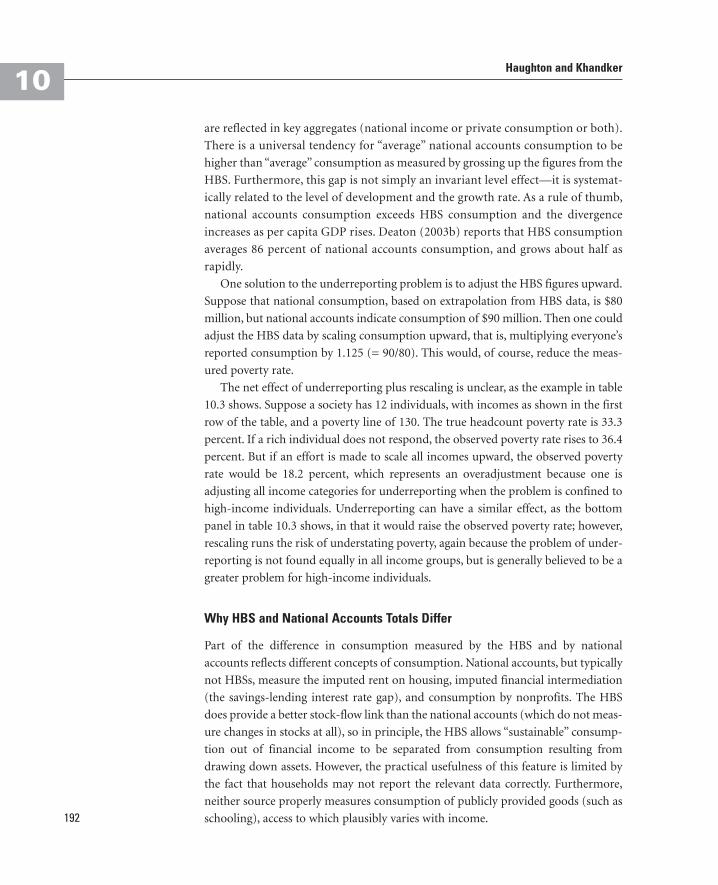
are reflected in key aggregates (national income or private consumption or both).

There is a universal tendency for “average” national accounts consumption to be

higher than “average” consumption as measured by grossing up the figures from the

HBS. Furthermore, this gap is not simply an invariant level effect—it is systemat-

ically related to the level of development and the growth rate. As a rule of thumb,

national accounts consumption exceeds HBS consumption and the divergence

increases as per capita GDP rises. Deaton (2003b) reports that HBS consumption

averages 86 percent of national accounts consumption, and grows about half as

rapidly.

One solution to the underreporting problem is to adjust the HBS figures upward.

Suppose that national consumption, based on extrapolation from HBS data, is $80

million, but national accounts indicate consumption of $90 million. Then one could

adjust the HBS data by scaling consumption upward, that is, multiplying everyone’s

reported consumption by 1.125 (= 90/80). This would, of course, reduce the meas-

ured poverty rate.

The net effect of underreporting plus rescaling is unclear, as the example in table

10.3 shows. Suppose a society has 12 individuals, with incomes as shown in the first

row of the table, and a poverty line of 130. The true headcount poverty rate is 33.3

percent. If a rich individual does not respond, the observed poverty rate rises to 36.4

percent. But if an effort is made to scale all incomes upward, the observed poverty

rate would be 18.2 percent, which represents an overadjustment because one is

adjusting all income categories for underreporting when the problem is confined to

high-income individuals. Underreporting can have a similar effect, as the bottom

panel in table 10.3 shows, in that it would raise the observed poverty rate; however,

rescaling runs the risk of understating poverty, again because the problem of under-

reporting is not found equally in all income groups, but is generally believed to be a

greater problem for high-income individuals.

Why HBS and National Accounts Totals Differ

Part of the difference in consumption measured by the HBS and by national

accounts reflects different concepts of consumption. National accounts, but typically

not HBSs, measure the imputed rent on housing, imputed financial intermediation

(the savings-lending interest rate gap), and consumption by nonprofits. The HBS

does provide a better stock-flow link than the national accounts (which do not meas-

ure changes in stocks at all), so in principle, the HBS allows “sustainable” consump-

tion out of financial income to be separated from consumption resulting from

drawing down assets. However, the practical usefulness of this feature is limited by

the fact that households may not report the relevant data correctly. Furthermore,

neither source properly measures consumption of publicly provided goods (such as

schooling), access to which plausibly varies with income.


193

Table 10.3 Illustrating the Effects of Response Bias and Underreporting

1 2 3 4 5 6 7 8 9 10 11 12

Headcountindex

P0(percent)

Response bias

True income/capita

80 100 110 121 140 220 270 310 400 490 620 750 33.3

Observedincome/capitawith responsebias

80 100 110 121 140 220 270 310 400 490 620 Notreported

36.4

Scaled income/capita to adjust forresponse bias

101 126 139 153 177 278 341 391 505 618 783 — 18.2

Underreporting

True income/capita

80 100 110 121 140 220 270 310 400 490 620 750 33.3

Observedincome/capita withunderreporting

80 100 108 121 125 220 250 300 400 450 560 600 36.4

Scaled income/capita to adjust for under-reporting

87 109 118 132 136 240 272 327 436 490 610 654 25.0

Source: Author’s illustration.

Note: To rescale for response bias, divide the sum across individuals of true income per capita by the sum across individuals ofobserved income per capita, then multiply by the observed income per capita for each individual. A similar adjustment is made torescale for underreported income. The poverty line is 130.

8. Survey data suffer from nonresponse bias and underreporting bias, typically leading to

° A. An overstatement of the headcount poverty rate and an understatement of the degree of inequality.

° B. An overstatement of the headcount poverty rate and an overstatement of the degree of inequality.

° C. An understatement of the headcount poverty rate and an understatement of the degree of inequality.

° D. An understatement of the headcount poverty rate and an overstatement of the degree of inequality.

Review Questions

Individual number


194

Overall, though, the consumption of items missed by the HBS is correlated with

wealth, both in cross-section and over time. The growth process reinforces the gap

because the national accounts register the increase in market-based consumption as

an economy grows—not all of which represents true economic growth. Similarly,

growth shifts activities from the informal to the formal sector. However, and we will

return to this point later, it is precisely because the national accounts tend to better

reflect the process of wealth accumulation that the HBS measure could still be a

“truer” measure of consumption for the poor.

Debate 1: Is World Poverty Falling?

The current debate about poverty trends is centered on the appropriate measure of

consumption. Bhalla (2002) argues that the national accounts measure is more accu-

rate. Thus, he measures the distribution of consumption from the HBS, but adjusts

the level upward to correspond to the national accounts. This method results in a

much lower level of measured poverty in India, because the divergence between the

two sources is severe in India; and the method predicts much more optimistic trends

in poverty reduction than standard projections. In fact, it implies that the world has

already met, or will soon meet, the MDGs for poverty.

This debate has been conducted in most detail for India, which, because of its

size, matters significantly for global poverty monitoring. However, the issues are ger-

mane for other countries as well.

Critics have focused on the fact that Bhalla uses the HBS to get the distribution

of consumption but the national accounts to get the mean. He is thus assuming a

very specific type of measurement error in the HBS—that all of it is in the mean, and

none is in the variance. Conversely, there is an assumption that the national accounts

have less measurement error in the mean than does the HBS. It is highly unlikely that

the measurement errors take exactly this form. In reality, both sources have errors in

both mean and variance.

Consider in particular the national accounts estimate of consumption. The fun-

damental macroeconomic identity gives

9. Rescaling household survey data on expenditure to ensure that it is consistent with national accounts data is only appropriate when trying to measure poverty if the proportion by which expenditure is underreported is the same across all expenditure groups.

° True

° False

° Uncertain


195

GDP � C + I + G + X – IM, (10.1)

where C is consumption spending, I is investment, G is government spending on

goods and services, X is exports, and IM is imports.

In most cases, consumption spending is estimated as a residual, obtained from

estimated final production (that is, GDP) less net exports, investment, and govern-

ment consumption (for which relatively good data exist). For a poor country, the

production estimate begins as physical volume (for example, projected crop yields

multiplied by estimated crop area), and is then converted to values. This is coupled

with a fixed coefficient assumption for the rest of the production sector (for exam-

ple, the allocation of goods to intermediate versus final usage). Notice the multiple

entry points for error.

The information on distribution may also be suspect. Practitioners of the national

accounts method often use the published income or consumption quintiles (as

opposed to the unit-level survey data), which may disguise severe problems in the

underlying data. Of course, in this respect it is unfair to blame researchers for their

use of quintile data, because the unit-level data are often not publicly available.

In any event, the direction of errors induced by the acknowledged flaws in the

HBS is not clear. Even if the underrepresentation of upper incomes causes the

HBS to underestimate mean and variance, the “true” distribution may not have a

greater mass below the poverty line than the estimated one. However, the national

accounts consumption adjustment, being a pure scale adjustment, clearly reduces

the headcount measure.

This seemingly technical debate about data sources has been conducted against the

background of an increased orientation in international development policy toward

achieving results, and specifically an expectation that the cumulative official resource

flows to developing countries and the associated initiatives (such as Poverty Reduc-

tion Strategy Papers and the Highly Indebted Poor Countries initiative) should by

now have led to an appreciable reduction in poverty. However, countries that have

been considered success stories in their pursuit of these new development frameworks

(Uganda, for instance) have displayed disappointing rates of poverty reduction rela-

tive to per capita GDP growth.

Increased research attention has therefore been directed to the issue of “pro-poor

growth,” namely, the extent to which those at the lower end of the income distribution

benefit from the growth process. It is the antithesis of this approach to simply ascribe

the mean rate of consumption growth to the entire distribution, which assumes that

the benefits of growth across the income distribution are neutral. A fuller discussion

of the decomposition of poverty changes into growth and distribution components is

given in chapter 11, along with some recent examples that show that, in the short run

at least, changes in distribution have an appreciable effect on the extent to which

economic growth translates into lower poverty rates.


196

The assumption that national accounts data represent a simple grossing up of

household budget survey data is a problem for the consumption categories where the

two measures do not overlap and where consumption patterns differ systematically

across the income distribution. Nevertheless, these arguments cut both ways; if we

acknowledge that the HBS data do seem to miss some aspects of growth, whether it

is safe to use them to study pro-poor growth can be questioned. All our information

about income distribution comes from the HBS, meaning that we know very little

about the distribution of national accounts consumption, yet it is this distribution

that may drive public perceptions of the equality of the growth process.

Finally, as with many seemingly tempestuous disputes in economics, some of the

apparent differences between different schools of thought weaken in the face of

pragmatism. For instance, Karshenas (2004) advocates a hybrid approach to meas-

uring poverty in which HBS and national accounts are combined, in recognition of

potential errors in both. Similarly, while World Bank researchers have doggedly

defended their reliance on survey data, they use national accounts consumption

growth data to extrapolate their poverty counts between survey years and to gener-

ate forecasts of poverty reduction.

Debate 2: Is World Poverty Really Falling?

The World Bank’s estimates of the fall in poverty since the early 1980s have been crit-

icized by Sanjay Reddy and his coauthors (Pogge and Reddy 2003; Reddy and

Minoiu 2006; Reddy, Visaria, and Asali 2006), and while few of the points they raise

are new, they have argued them with considerable vigor. To recap, the methodology

used by the World Bank (Chen and Ravallion 2004, 2008)

• Picks a poverty line (now $1.25 per person per day in 2005 prices)

• Uses PPP exchange rates to translate this into poverty lines in domestic curren-

cies in 2005

• Uses domestic consumer price indexes to find the poverty line, in domestic cur-

rencies, for years other than 2005

• Applies the poverty line to expenditure distribution data that have been collected

by 675 household surveys in 116 developing countries; where possible, original

survey data are used, but often the computations are based on fitting Lorenz

curves to published tabulated data from the surveys, to establish the number and

proportion of people who are poor

• Establishes poverty rates and levels for three-year intervals, using interpolation

for those cases where household surveys were undertaken on “off” years

• Aggregates the numbers for individual countries to provide poverty rates and lev-

els by broad region and worldwide.


Choice of Poverty Line

Pogge and Reddy (2003) argue that the original “$1/day” poverty line—in effect,

$1.08 per person per day in 1993 prices—is too low. They claim that this level is

arbitrary and is not properly rooted in a “capabilities” (or basic needs) approach to

measuring poverty, and they suggest that one could hardly survive on such a small

amount in the United States; by implication, if this poverty line is appropriately

translated into other currencies, it would be difficult to survive at such a low

poverty line in those currencies, too. The revision of the poverty line to US$1.25 in

2005 prices would not alter this criticism.

A more recent article by Reddy, Visaria, and Asali (2006) no longer makes the case

that the $1/day poverty line is too low. They compare poverty lines for Nicaragua,

Tanzania, and Vietnam generated using a cost of basic needs approach (as outlined in

chapter 3), with poverty lines based on the $1/day and $2/day standards. The results

are displayed in table 10.4, and show that for Nicaragua and Tanzania the cost of basic

needs approach actually gives a lower poverty line than the $1/day approach; however,

197

Each of these steps may be criticized, and the debate is summarized below. Ravallion

offers a spirited defense of the World Bank’s approach, arguing that Reddy and his

coauthors overstate the possible weaknesses of the Bank’s methodology, and have

“sidestepped the problem” of setting up an international poverty line that reflects

constant purchasing power over commodities (Ravallion 2008).

11. Which of the following steps is not part of the World Bank’s methodologyfor computing the $1/day world poverty rate?

° A. Pick a poverty line that allows households to buy enough food and other basic needs.

° B. Use an average PPP exchange rate to translate the poverty line into domesticcurrency terms.

° C. Use a domestic consumer price index to find the appropriate poverty line, in domestic currency, for the years in which household surveys were undertaken.

° D. Measure the number of poor in a country by determining, based on fittingLorenz curves, how many fall below the poverty line.

10. Bhalla adjusts household survey data on expenditures upward to ensureconsistency with national accounts figures, and argues that the result isthat the world is already close to meeting, or may even have met, theMillennium Development Goals for poverty reduction.

° True

° False

° Uncertain

Review Questions


198

for Vietnam the cost of basic needs poverty line is close to the $2/day poverty line. The

conclusion is clear: the $1/day or $2/day standard provides a poor approximation to

the (relatively theoretically satisfactory) cost of basic needs approach, but does not

necessarily systematically underestimate it.

Use of PPP Exchange Rates

There are two further distinct issues. The first involves the stability of PPP exchange

rates over time, and the appropriateness of using an “average” PPP exchange rate.

Pogge and Reddy (2003) note that when a new set of PPP exchange rates was

published for 1993, superseding those of 1985, they led to considerable changes in

measured poverty rates (using the $1/day poverty line); a similarly large set of revisions

occurred when the 2005 PPP exchange rates were introduced. Thus, international

comparisons of poverty are not robust to the measures of PPP exchange rates, many of

which are, in any case, imputed using regression techniques rather than being based on

direct price observations. Deaton (2003b) suggests that a pragmatic response is to

avoid revising the PPP exchange rates too often; but eventually revisions become

inevitable, and the problem re-emerges, and we know (theoretically from the Balassa-

Samuelson effect, empirically from the Penn effect)6 that PPP exchange rates vary sys-

tematically over time, showing a faster appreciation in countries with more rapid

economic growth.

The second problem is that the World Bank uses a PPP exchange rate that is

applied to a broad basket of goods and services, and not necessarily the basket of

goods and services that is relevant for poor households. Pogge and Reddy (2003)

suggest that poverty (measured using the $1/day standard) is understated as a result,

on the grounds that the poor mainly consume tradable goods, so the use of a PPP

exchange rate overadjusts for price differentials. However, this is by no means self-

evident, and merits further study.

Use of Consumer Price Indexes to Adjust the Poverty Lines over Time

Ideally, one would use a price index that reflects the costs faced by poor consumers,

not by the average consumer, to adjust poverty lines over time, but this is rarely done.

Table 10.4 Poverty Lines Using $1/Day and $2/Day and Basic Needs Measures

Poverty lineNicaragua, 1998

(cordobas)Tanzania, 2000/01

(shillings)Vietnam, 1993

(dong)Vietnam, 1998

(dong)

$1/day 4,017 147,614 629,341 953,794$2/day 8,034 295,227 1,258,682 1,907,588Cost of basic needs 3,018 80,365 1,160,363 1,758,581

Source: Reddy, Visalia, and Asali 2006.


199

Sometimes it is possible to adjust the poverty line using an index of food prices, but

this, of course, ignores the evolution of the prices of nonfood items, which consti-

tute about a third of total expenditures for someone at the poverty line. The prob-

lems involved in finding appropriate price indexes are serious, as our discussion of

the studies of poverty in Indonesia following the financial crisis of 1997 makes clear

(see chapter 11).

Applying the Poverty Line to Household Survey Data

About half of all the people in the developing world live in China and India alone.

It follows that the evolution of world poverty will depend heavily on the course of

poverty in these two countries. Unfortunately, the data on poverty for these two

countries have some serious problems. The surveys done in China in the 1980s were

of questionable quality; and until recently there was no direct measure of China’s

PPP exchange rate. A change in the survey methodology used in the “thick” round of

the Indian National Sample Survey in 1999–2000 appeared to imply that poverty in

India had fallen but little in the 1990s, which was hardly plausible given the rapid

economic growth experienced during that decade. A number of efforts have been

made to adjust the 1999–2000 numbers to make them more comparable with previ-

ous survey data (there is an extended discussion of this in chapter 16) but there

remains considerable uncertainty about the true extent of poverty reduction in India

during the period in question. Reddy and Minoiu (2006) present the results of a sen-

sitivity analysis showing that it is just possible that the world poverty rate (using the

$1/day level) did not fall in the 1990s, and it is more possible that the number of peo-

ple in poverty did not fall during that decade. The real message here is that measures

of world poverty are not yet robust enough to be used to make strong statements

about progress in reducing poverty.

Pogge and Reddy (2003) argue that the World Bank approach to measuring

world poverty is too flawed to be useful. Instead, they would ask every country

to measure poverty using a cost of basic needs approach—they refer to it as

measuring a “set of elementary capabilities,” but it comes to the same thing—

based on the expenditure required to provide enough calories to live on, plus a

reasonable nonfood component. This is an attractive, if not particularly new,

idea. Why, then, has this approach not been used? The answer is that it is costly

and has its own methodological problems.

The World Bank’s $1/day approach—now US$1.25 a day—makes parsimonious

use of survey data; all that is really needed are the average expenditure level and a

breakdown by, for instance, expenditure per capita quintiles, along with PPP exchange

rates and consumer price indexes. A good researcher could input the data for hundreds

of surveys into PovcalNet and come up with estimates of world poverty and its evolu-

tion in a matter of a few weeks. However, to implement a cost of basic needs approach,


Conclusion

We conclude by mentioning some current directions of research on the link between

macroeconomic and poverty outcomes. It is now well documented that the elastic-

ity of poverty with respect to growth varies over time and space, prompting investi-

gation of what set of initial conditions makes this elasticity bigger. Furthermore, it is

increasingly recognized that while growth remains central to poverty reduction—as

the discussion of the Dollar and Kraay results in chapter 9 made clear—it is not the

10

200

researchers have to work with the underlying survey data, which is relatively tedious

(and requires that the data be available, which is by no means always the case).

Over time, it is likely that most countries will have in-house analysts who can

measure poverty using the cost of basic needs approach, following a consistent set of

guidelines. But perfect comparability will never be achieved: surveys will ask differ-

ent questions and in different ways; they will differ in sample size and design; they

will use different techniques to measure food and other prices; they will use differ-

ent methods to inflate prices over time. And one still has to address the issues of

whether survey data need to be adjusted to be compatible with national accounts;

whether one should use adult-equivalence methods; and how precisely to determine

an appropriate level of nonfood (or even food) spending.

Perhaps these problems are no different from those faced by statisticians who

compile national accounts data, even though they all follow the same UN guidelines.

A similar effort might be worthwhile for poverty measurement—the compilation of

a set of formal guidelines for measuring poverty using the cost of basic needs method.

12. Which of the following is not a criticism that Reddy and his co-authorshave levied at the World Bank’s approach to measuring world poverty?

° A. Measured PPP exchange rates vary over time.

° B. The $2/day standard is too low.

° C. The data on poverty reduction on India are subject to considerable uncertainty.

° D. The use of a consumer price index does not necessarily reflect the evolutionof prices of the goods and services consumed by the poor.

Review Questions

13. The World Bank’s approach to measuring world poverty requires lessinformation from individual household surveys than would be required if one were to apply a cost of basic needs approach.

° True

° False

° Uncertain


201

only way to reduce poverty; particularly in the short and medium term, inequality

also matters.

There are certain policies with modest immediate growth effects but strong

poverty impacts, or in the terminology above, policies that lead to a high elasticity of

poverty reduction with respect to growth. Prime examples are reforms to security of

land tenure, microcredit, and the expansion of basic education. A strict focus on a

growth-poverty link might overlook such policies.

Poverty analysts are also looking at methods to improve the measurement of con-

sumption, with the objective of balancing the gain from better source data with the

loss of comparability to previous data.

Notes

1. Information on the overall MDGs and progress toward them can be found at http://www.

developmentgoals.org/.

2. The countries are Malawi, Mali, Ethiopia, Sierra Leone, Niger, Uganda, The Gambia,

Rwanda, Guinea-Bissau, Tanzania, Tajikistan, Mozambique, Chad, Nepal, and Ghana (Chen

and Ravallion 2008, 11).

3. For years in which there are no household surveys, Chen and Ravallion adjust the house-

hold survey data on consumption from other years by linking this information to the

evolution of consumption in the national accounts; they then recompute the poverty rate

using the consumption data thus interpolated.

4. Chen and Ravallion (2008) used PPP exchange rates for 98 of the 116 countries in their

sample, and used PPPs based on regression models for Algeria, Costa Rica, the Dominican

Republic, El Salvador, Guatemala, Guyana, Haiti, Honduras, Jamaica, Nicaragua, Panama,

Papua New Guinea, St. Lucia, Suriname, Timor-Leste, Trinidad and Tobago, Turkmenistan,

and Uzbekistan.

5. Available on the Web at http://go.worldbank.org/NT2A1XUWP0.

6. See http://en.wikipedia.org/wiki/Balassa-Samuelson_effect.

References

Alatas, Vivi, Jed Friedman, and Angus Deaton. 2004. “Purchasing Power Parity Exchange Rates

from Household Survey Data: India and Indonesia.” Working paper, Research Program in

Development Studies, Princeton University.

Bhalla, Surjit. 2002. “Imagine There Is No Country: Poverty, Inequality, and Growth in the Era

of Globalization.” Institute for International Economics, Washington, DC.

Carey, Kevin. 2004. “Poverty Analysis for Macroeconomists.” World Bank Institute,

Washington, DC.

Chen, Shaohua, and Martin Ravallion. 2001. “How Did the World’s Poorest Fare in the 1990s?”

Review of Income and Wealth 47 (3): 283–300.


———. 2004. “How Have the World’s Poorest Fared Since the Early 1980s?” Development

Economics Working Paper No. 3341, World Bank, Washington, DC.

———. 2008. “The Developing World Is Poorer Than We Thought, But No Less Successful

in the Fight against Poverty.” Policy Research Working Paper No. 4703, World Bank,

Washington, DC.

Deaton, Angus. 2003a. “How to Monitor Poverty for the Millennium Development Goals.”

Journal of Human Development 4 (3): 353–78.

———. 2003b. “Measuring Poverty in a Growing World (or Measuring Growth in a Poor World).”

NBER Working Paper No. 9822, National Bureau of Economic Research, Cambridge, MA.

Karshenas, Massoud. 2004. “Global Poverty Estimates and the Millennium Goals: Towards a

Unified Framework.” International Labour Organisation Employment Strategy Papers,

2004/5, ILO, Geneva.

Pogge, Thomas, and Sanjay Reddy. 2003. “Unknown: The Extent, Distribution, and Trend of

Global Income Poverty.” Columbia University, NY.

Ravallion, Martin. Forthcoming. “How Not to Count the Poor? A Reply to Reddy and Pogge.”

In Debates on the Measurement of Poverty, ed. Sudhir Anand, Paul Segal, and Joseph Stiglitz.

Oxford, UK: Oxford University Press.

Reddy, Sanjay, and Carnelia Minoiu. 2006. “Has World Poverty Really Fallen?” Columbia

University, NY.

Reddy, Sanjay, Sujata Visaria, and Muhammad Asali. 2006. “Inter-Country Comparisons of

Poverty Based on a Capability Approach: An Empirical Exercise.” Working Paper No. 27,

International Poverty Centre, UNDP, Brasilia.

10

202

International Poverty Comparisons - World...

Documents

Transcript of International Poverty Comparisons - World...