International Liquidity and Exchange Rate Dynamics

Xavier Gabaix∗ Matteo Maggiori†

November 2014

Abstract

We provide a theory of the determination of exchange rates based on capital flows in im-perfect financial markets. Capital flows drive exchange rates by altering the balance sheets offinanciers that bear the risks resulting from international imbalances in the demand for financialassets. Such alterations to their balance sheets cause financiers to change their required com-pensation for holding currency risk, thus impacting both the level and volatility of exchangerates. Our theory of exchange rate determination in imperfect financial markets not only helpsto rationalize the empirical disconnect between exchange rates and traditional macroeconomicfundamentals, but also has real consequences for output and risk sharing. Exchange rates aresensitive to imbalances in financial markets and seldom perform the shock absorption role thatis central to traditional theoretical macroeconomic analysis. We derive conditions under whichheterodox government financial policies, such as currency interventions and taxation of capitalflows, can be welfare improving. Our framework is flexible; it accommodates a number of im-portant modeling features within an imperfect financial market model, such as non-tradables,production, money, sticky prices or wages, various forms of international pricing-to-market,and unemployment.

JEL Codes: E42, E44, F31, F32, F41, F42, G11, G15, G20.Keywords: Capital Flows, Exchange Rate Disconnect, Foreign Exchange Intervention, Limits ofArbitrage.∗New York University, Stern School of Business, NBER and CEPR. Email: xgabaix@stern.nyu.edu.†Harvard University, Department of Economics, NBER and CEPR. Email: maggiori@fas.harvard.edu.

We thank Ariel Burstein, John Campbell, Nicolas Coeurdacier, Alessandro Dovis, Bernard Dumas, Emmanuel Farhi,Luca Fornaro, Kenneth Froot, Nicolae Garleanu, Gita Gopinath, Pierre-Olivier Gourinchas, Elhanan Helpman, Oleg It-skhoki, Andrew Karolyi, Nobuhiro Kiyotaki, Anton Korinek, Arvind Krishnamurthy, Guido Lorenzoni, Brent Neiman,Maurice Obstfeld, Anna Pavlova, Fabrizio Perri, Hélène Rey, Kenneth Rogoff, Lucio Sarno, Hyun Song Shin, AndreiShleifer, Jeremy Stein, and seminar participants at NBER (EFG, IFM, ME, IPM, IAP, MWAB, MATS), Princeton Uni-versity, Harvard University, MIT, Stanford SITE, UC Berkeley, University of Chicago Booth, Northwestern University,Yale University, Wharton, LBS, LSE, Yale Cowles Conference on General Equilibrium, University of Minnesota, Min-neapolis Fed, University of Maryland, Johns Hopkins University, University of Michigan, UT Austin, UNC, MacroFinancial Modeling Meeting, Barcelona GSE Summer Forum, EEIF, Chicago/NYU Junior Conference in InternationalMacroeconomics and Finance, PSE, INSEAD, IMF, Federal Reserve Board, ECB, Bank of Japan, Cornell University,AEA annual meeting, SED, and NYU. We thank Miguel de Faria e Castro and Jerome Williams for excellent researchassistance. We gratefully acknowledge the financial support of the NSF (0820517,1424690), the Dauphine-AmundiFoundation, and the NYU CGEB. Maggiori thanks the International Economics Section, Department of Economics,Princeton University for hospitality during part of the research process for this paper.

We provide a theory of exchange rate determination based on capital flows in imperfect fi-nancial markets. In our model, exchange rates are governed by financial forces because globalshifts in the demand and supply of assets result in large scale capital flows that are intermediatedby the global financial system. The demand and supply of assets in different currencies and thewillingness of the financial system to absorb the resulting imbalances are first order determinantsof exchange rates. A framework to characterize such forces and their implications for welfareand policy, while desirable, has proven elusive.

In our model, financiers absorb part of the currency risk originated by imbalanced globalcapital flows. Alterations to the size and composition of financiers’ balance sheets induce themto differentially price currency risk, thus affecting both the level and the volatility of exchangerates. Our theory of exchange rate determination in imperfect financial markets differs from thetraditional open macroeconomic model by introducing financial forces, such as portfolio flows,financiers’ balance sheets, and financiers’ risk bearing capacity as first order determinants ofexchange rates.

We first present a basic theory of exchange rate financial determination in a two-period two-country model where capital flows are intermediated by global financiers. Each country borrowsor lends in its own currency and financiers absorb all currency risk that is generated by the mis-match of global capital flows. Since financiers require compensation for holding currency riskin the form of expected currency appreciation, exchange rates are jointly determined by capitalflows and by the financiers’ risk bearing capacity. Our theory, therefore, is an elementary onewhereby supply and demand determine a price, the exchange rate, that clears markets.

The exchange rate is disconnected from traditional macroeconomic fundamentals such as im-ports, exports, output, or inflation in as much as these same fundamentals correspond to differentequilibrium exchange rates depending on financiers’ balance sheets and risk bearing capacity.An extension to a multi-period model strengthens this intuition by solving the exchange rate asa present value relationship. The exchange rate discounts future current account balances, butthe rate of discounting is determined in financial markets and therefore hinges on financiers’ riskbearing capacity and balance sheets. Changes in such capacity affect both the level and volatilityof the exchange rate. Financiers both act as shock absorbers, by using their risk bearing capacityto accommodate flows that result from fundamental shocks, and are themselves the source offinancial shocks that distort exchange rates.

The financial determination of exchange rates in imperfect financial markets has real conse-quences for output and risk sharing. To more fully analyze these consequences, we extend thebasic model by introducing nominal exchange rates, monetary policy, and both flexible and stickyprices. In the presence of goods’ prices that are sticky in the producers’ currencies, a capital in-flow or financial shock that produces an overly appreciated exchange rate causes a fall in demand

1

for the inflow-receiving country’s exports and a corresponding fall in output.Our theory yields novel predictions for policy analysis in the presence of flexible exchange

rates. In a financial world, exchange rate movements are dominated by financial factors and sel-dom perform the benign expenditure switching role that is central to traditional macroeconomicanalysis. In fact, the traditional macroeconomic rationale for prescribing pure floating exchangerates is that, in the presence of asymmetric real shocks, the exchange rate acts as a shock absorberby shifting global demand toward the country that has been most negatively affected by the shockvia a depreciation of its currency.

By contrast, we show that in our framework the floating exchange rate is itself distorted byimbalances in financial markets and shocks to the financial system’s risk bearing capacity; theexchange rate can often be the vehicle of transmission of financial shocks to the real economy.Our policy analysis suggests that novel trade-offs emerge when financial markets are disruptedor are less developed overall, and when output is far below its potential so that an exchange ratedepreciation increases output via an increase in net exports. Heterodox policies, such as largescale currency interventions and capital controls, are shown to be beneficial in these specificcircumstances.

We focus on providing a framework that is not only sufficiently rich to analyze the finan-cial forces at the core of our theory in a full general equilibrium model, but also sufficientlytractable as to provide simple pencil-and-paper solutions that make the analysis as transparent aspossible. While tractability requires some assumptions, we also verify that the core forces of ourframework remain the leading forces of exchange rate determination even in more general setups,where a number of assumptions are relaxed and solutions (in some cases) have to be computednumerically.

Our model helps to make sense of a number of fundamental issues in open macroeconomics;these include the failure of the uncovered interest rate parity condition, external financial adjust-ment of creditors and debtor countries, the effectiveness of currency intervention, exchange ratedisconnect from macroeconomic fundamentals, the failure of purchasing power parity, the failureof the Backus and Smith risk sharing condition, and the carry trade. While these issue have cer-tainly been analyzed in other models, our work, while qualitative, provides a different, unified,and tractable treatment of these phenomena with a single main friction.

Our framework is flexible in accommodating a number of modeling features that are impor-tant in open economy analysis within an imperfect capital market model, such as non-tradables,production, money, sticky prices or wages, and various forms of international pricing-to-market.In each extension, we focused on simple and tractable modeling to map out in closed form bothits basic channels and the interaction with the core forces of the paper. While the results are qual-itative, we stress that the framework is versatile and can be easily employed in future research to

2

address a number of open questions in international macroeconomics.We summarize our contribution as providing a tractable modern general-equilibrium frame-

work for the determination of exchange rates in imperfect financial markets via capital flows andthe risk-bearing capacity of financiers. Our general equilibrium framework combines financialforces such as risk taking and financial intermediation in imperfect capital markets with the tra-ditional real economy analysis of production, import and export activities. A distinctive positivefeature of our model is the direct relevance of flows, not just stocks, of assets for exchange ratedetermination. Our foundations allow us to study welfare and characterize optimal policy, suchas foreign exchange rate intervention, in the presence of both financial and nominal frictions. Wefurther show how the core force of the model, limited risk taking by the financiers, can help torationalize a number of classic issues of international macroeconomics.

Related Literature Two important papers were published in 1976, the now classic exchangerate overshooting model (Dornbusch (1976)) and the portfolio balance model (Kouri (1976)).While we incorporate important aspects of the Keynesian tradition upon which Dornbusch builds,our model provides modern foundations to the spirit of Kouri’s portfolio balance theory of ex-change rates. Obstfeld and Rogoff (1995) brought the Keynesian approach into modern inter-national economics by providing micro-foundations to the dynamic version of the Mundell-Fleming-Dornbusch model. Their foundations have been essential not only for the analysis ofexchange rate determination, but also for that of optimal policy and welfare. However, finan-cial forces play little role in this class of models. In the real version of these models, exchangerates are mostly determined by the demand and supply of domestic and foreign goods. Even inthe nominal versions of the models, where the nominal exchange rate is often expressed as thepresent discounted sum of future monetary policy and other macroeconomic fundamentals, theimpact of finance is limited because in most cases the uncovered interest parity holds, the demandfor money is tightly linked to consumption expenditures, and/or the model is linearized.

This paper is related to three broad streams of literature: literature on portfolio balance inreduced form, micro-founded literature on portfolio demand in complete or incomplete markets,and micro-founded literature on frictions and asset demand.

As mentioned above, our paper is inspired by the early literature on portfolio balance modeledin reduced form. With respect to this literature our contribution consists of three main aspects: weprovide a fully specified framework in general equilibrium with optimizing agents in the presenceof frictions, we provide welfare and normative analysis, and we provide, via the foundations ofthe model, a theoretically distinct role for the balance sheet of financiers that is absent in theearlier literature. The closest paper in this early literature is Driskill and McCafferty (1980a)

3

who builds on earlier contributions by Kouri (1976).1 Our main contribution of providing a fullmodern treatment of the forces sketched in these earlier papers is one that, in our view, wasmissing from the literature. For example, prominent economists have lamented that this earlierresearch effort “had its high watermark and to a large extent a terminus in Branson and Henderson(1985) handbook chapter” (see Obstfeld (2004)) and is “now largely and unjustly forgotten” (seeBlanchard, Giavazzi and Sa (2005)). In our view, a major factor in the neglect of this sensibleview of exchange rates is the lack of a modern micro-founded model that the field can build on infuture work (on the contrary, the still popular Dornbusch model has received such fundamentaluplifting in the celebrated article of Obstfeld and Rogoff (1995)).

The foundations provided in our model allow for the explicit analysis of policy and welfare.We provide a novel analysis of optimal foreign exchange intervention and show under which con-ditions it can be welfare improving. This could not be done without the foundations: for example,Backus and Kehoe (1989) provided a serious challenge to the portfolio balance literature claimson the effectiveness of intervention by showing that intervention is ineffective in a large set ofmodern micro-founded currency models with frictionless portfolios choice despite the currenciesbeing imperfect substitutes due to risk premia.

A final distinction between our work and this earlier literature is that our foundations empha-size and provide a special role for the balance sheet of financiers and their risk bearing capacitywhile the previous work focused on the stock of external assets at the country level. Of course, thetwo need not be the same as showed in our work once the basic model is progressively extended.Understanding which flows and stocks are “stuck” on the financiers balance sheet provides botha new theoretical view and a novel avenue for future empirical work.

The literature that followed the earlier reduced-form modeling efforts has provided fully spec-ified asset demand functions as well as general equilibrium effects. Most of the literature has fo-cused on complete markets (Lucas, 1982, Backus, Kehoe and Kydland, 1992, Backus and Smith,1993, Dumas, 1992, Verdelhan, 2010, Colacito and Croce, 2011, Hassan, 2013).2 Pavlova andRigobon (2007) analyze a real model with complete markets where countries’ representativeagents have logarithmic preferences affected by taste shocks similar to those considered in thispaper.3 A smaller literature has analyzed the importance of incomplete markets (for recent ex-amples: Chari, Kehoe and McGrattan (2002), Corsetti, Dedola and Leduc (2008), Pavlova andRigobon (2012)). With respect to both literatures we provide a different, and complementary,

1An active early literature also includes: Allen and Kenen (1983), Henderson and Rogoff (1982), Dornbusch andFischer (1980), Calvo and Rodriguez (1977), Branson, Halttunen and Masson (1979), Tobin and de Macedo (1979),Diebold and Pauly (1988), Driskill and McCafferty (1980b), de Macedo and Lempinen (2013). De Grauwe (1982)considers the role of the banking sector in generating portfolio demands.

2Among others see also: Farhi and Gabaix (2014), Martin (2011), and Stathopoulos (2012).3Similar preferences are also used in Pavlova and Rigobon (2008, 2010).

4

approach by studying financial frictions. Our model has a set of distinct theoretical, and em-pirical, predictions, most prominently the importance of the balance sheet of financiers and ofgross flows, not just stocks of assets in determining the exchange rate. Such gross flows matter inthe presence of financial frictions, but would not matter in their absence both when markets arecomplete or incomplete.4 This central prediction of our model has received confirmation in thedata (Hau, Massa and Peress, 2010) as well as having been the focus of an important literature inother assets (De Long et al., 1990a,b), but had yet to be incorporated in a fully specified generalequilibrium model of exchange rates.

The most closely related stream of the literature is the small set of papers that focused onexchange rate modeling in the presence of frictions. One set of papers are models of partialequilibrium. This set includes important contributions by Jeanne and Rose (2002), Evans andLyons (2002), Hau and Rey (2006), Bruno and Shin (2014). Our contribution with respect tothese papers is to provide a model of general equilibrium that merges the financial determinationof exchange rates with the more traditional effects arising from the goods market via the tradebalance. The general equilibrium set-up not only allows us to discuss positive predictions of themodel about debtor/creditor countries and the exchange rate disconnect, but is also a requisite forthe welfare analysis. One other important set of papers has a very different focus: informationalfrictions, infrequent portfolio rebalancing, or frictions in access to domestic money/funding mar-ket. Evans and Lyons (2012) focuses on how disaggregate order flows from customers mightconvey information about the economy fundamentals to exchange rate market makers who ob-serve the consolidated flow. Bacchetta and Van Wincoop (2010) studies the implications of agentsthat infrequently rebalance their portfolio in an OLG setting. Alvarez, Atkeson and Kehoe (2002,2009) and Maggiori (2014) are models of exchange rates where the frictions, a form of marketsegmentation, are only present in the domestic money market or funding market. Our modelis both conceptually and empirically distinct from these papers because our frictions are onlypresent on the international side and hence directly involve the exchange rate.

Recent economic events, such as the global financial and European crises, have rekindled aninterest in the analysis of optimal policy and welfare in open economies. Aguiar, Amador andGopinath (2009), Farhi, Gopinath and Itskhoki (2014), Farhi and Werning (2012a,b), Schmitt-Grohé and Uribe (2012), and Costinot, Lorenzoni and Werning (2014) provide innovative analy-ses of policies such as capital controls, fiscal transfers and fiscal devaluations in the context of thesmall-open-economy (new-Keynesian) model. We contribute to this literature by analyzing poli-cies, and in particular foreign exchange rate intervention, in a two-country world where financial

4This difference can easily be verified by considering the Basic Gamma model. The number of shocks ensures thatthe two bond economy when Γ = 0 is an incomplete market model with risk averse agents, yet f flows have no effecton the exchange rate as in Proposition 4.

5

flows are direct determinants of exchange rates and where the condition of financial markets is animportant policy consideration. We find that public financial policies, which cannot be analyzedunder the UIP-assumption, complete markets, or simple forms of market incompleteness, can bebeneficial in specific circumstances. We characterize the policy instruments (FX interventions,currency-swaps, and capital controls) that can be used to implement these polices.

1 Basic Gamma Model

Let us start with a minimalistic model of financial determination of exchange rates in imper-fect financial markets. This simple real model carries most of the economic intuition and coremodeling that we will then extend to more general set-ups.

Time is discrete and there are two periods: t = 0,1. There are two countries, the USA andJapan, each populated by a continuum of households. Households produce, trade (internationally)in a market for goods, and invest with financiers in risk-free bonds in their domestic currency.5

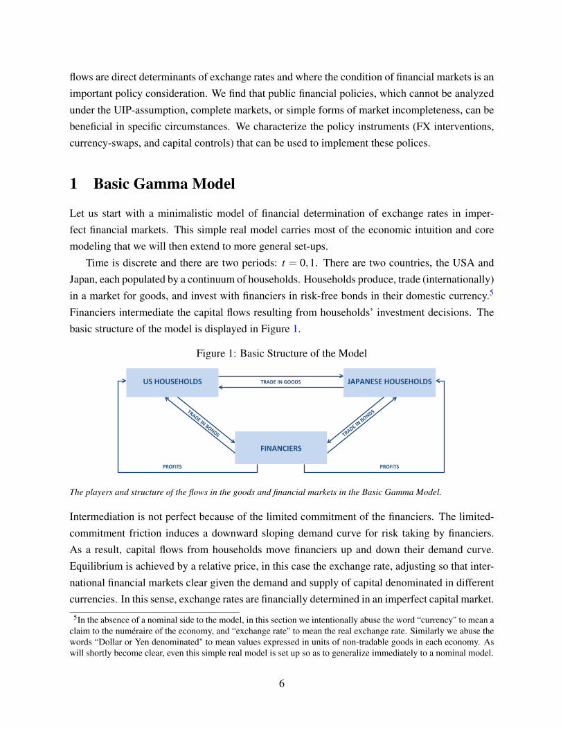
Financiers intermediate the capital flows resulting from households’ investment decisions. Thebasic structure of the model is displayed in Figure 1.

Figure 1: Basic Structure of the Model

FINANCIERS

US HOUSEHOLDS JAPANESE HOUSEHOLDS

PROFITS PROFITS

TRADE IN GOODS

The players and structure of the flows in the goods and financial markets in the Basic Gamma Model.

Intermediation is not perfect because of the limited commitment of the financiers. The limited-commitment friction induces a downward sloping demand curve for risk taking by financiers.As a result, capital flows from households move financiers up and down their demand curve.Equilibrium is achieved by a relative price, in this case the exchange rate, adjusting so that inter-national financial markets clear given the demand and supply of capital denominated in differentcurrencies. In this sense, exchange rates are financially determined in an imperfect capital market.

5In the absence of a nominal side to the model, in this section we intentionally abuse the word “currency" to mean aclaim to the numéraire of the economy, and “exchange rate" to mean the real exchange rate. Similarly we abuse thewords “Dollar or Yen denominated" to mean values expressed in units of non-tradable goods in each economy. Aswill shortly become clear, even this simple real model is set up so as to generalize immediately to a nominal model.

6

We now describe each of the model’s actors, their optimization problems, and analyze theresulting equilibrium.

1.1 Households

Households in the US derive utility from the consumption of goods according to:

θ0 lnC0 +βE [θ1 lnC1] , (1)

where C is a consumption basket defined as:

Ct ≡ [(CNT,t)χt (CH,t)

at (CF,t)ιt ]

1θt , (2)

where CNT,t is the US consumption of its non-tradable goods, CH,t is the US consumption of itsdomestic tradable goods, and CF,t is the US consumption of Japanese tradable goods. We use thenotation χt ,at , ιt for non-negative, potentially stochastic, preference parameters and we defineθt ≡ χt +at + ιt .

The non-tradable good is the numéraire in each economy and, consequently, its price equals1 in domestic currency (pNT = 1). Non-tradable goods are produced by an endowment processthat we assume for simplicity to follow YNT,t = χt , unless otherwise stated.6

Households can trade both tradable goods in a frictionless goods market across countries,but can only trade non-tradable goods within their domestic country. Financial markets are in-complete and each country trades a risk-free domestic currency bond. The assumption that eachcountry only trades in its own currency bonds is made here for simplicity and to emphasize thecurrency mismatch that the financiers have to absorb; we relax the assumption in later sections.Risk-free here refers to paying one unit of non-tradable goods in all states of the world and istherefore akin to “nominally risk free".

US households’ optimization problem is:

max(CNT,t ,CH,t ,CF,t)t=0,1

θ0 lnC0 +βE [θ1 lnC1] , (3)

subject to (2),

and1

∑t=0

R−t (YNT,t + pH,tYH,t) =1

∑t=0

R−t (CNT,t + pH,tCH,t + pF,tCF,t) . (4)

6The assumption, while stark, makes the analysis of the basic model most tractable. We stress that the assumptionis one of convenience, and not necessary for the economics of the paper. The reader might find it useful to think of χ

and YNT as constants and the equality between the two as a normalization that makes the closed form solutions of thepaper most readable. Section 2 and the appendix provide more general results that do not impose this assumption.

7

US households maximize the utility by choosing their consumption and savings in dollarbonds subject to the state-by-state dynamic budget constraint. The households’ optimizationproblem can be divided into two separate problems. The first is a static problem, whereby house-holds decide, given their total consumption expenditure for the period, how to allocate resourcesto the consumption of various goods. The second is a dynamic problem, whereby householdsdecide intertemporally how much to save and consume.

The static utility maximization problem takes the form:

maxCNT,t ,CH,t ,CF,t

χt lnCNT,t +at lnCH,t + ιt lnCF,t +λt (CEt−CNT,t− pH,tCH,t− pF,tCF,t) , (5)

where CEt is aggregate consumption expenditure, which is taken as exogenous in this static op-timization problem and later endogenized in the dynamic optimization problem, λt is the associ-ated Lagrange multiplier, pH,t is the Dollar price in the US of US tradables, and pF,t is the Dollarprice in the US of Japanese tradables. First-order conditions imply: χt

CNT,t= λt , and ιt

CF,t= λt pF,t .

Our assumption that YNT,t = χt , combined with the market clearing condition for non-tradablesYNT,t =CNT,t , implies that in equilibrium λt = 1. This yields:

pF,tCF,t = ιt ,

i.e., the Dollar value of US imports is simply ιt .Japanese households derive utility from consumption according to: θ ∗0 lnC∗0 +β ∗E [θ ∗1 lnC∗1 ],

where starred variables denote Japanese quantities and prices. By analogy with the US case, the

Japanese consumption basket is: C∗t ≡[(C∗NT,t)

χ∗t (C∗H,t)ξt (C∗F,t)

a∗t] 1

θ∗t , where θ ∗t ≡ χ∗t + a∗t + ξt .The Japanese static utility maximization problem, reported for brevity in the appendix, togetherwith the assumption Y ∗NT,t = χ∗t , leads to a Yen value of US exports to Japan, p∗H,tC

∗H,t = ξt , that

is entirely analogous to the import expression derived above.The exchange rate et is defined as the quantity of dollars bought by 1 yen, i.e. the strength of

the Yen. Consequently, an increase in e represents a Dollar depreciation.7 The Dollar value of USexports is: etξt . US net exports, expressed in dollars, are given by: NXt = et p∗H,tC

∗H,t− pF,tCF,t =

ξtet− ιt .8 We collect these results in the Lemma below.

Lemma 1 (Net Exports) Expressed in dollars, US exports to Japan are ξtet; US imports from

Japan are ιt; so that US net exports are NXt = ξtet− ιt .

7In this real model, the exchange rate is related to the relative price of non-tradable goods. Section 5.2 provides afull discussion of this exchange rate and its relationship to both the nominal exchange rate, formally introduced inSection 2.1 , and the CPI-based real exchange rate.

8Note that we chose the notation so that imports are denoted by ιt and exports by ξt .

8

Note that this result is independent of the pricing procedure (e.g. price stickiness under eitherproducer or local currency pricing). Under producer currency pricing (PCP) and in the absenceof trade costs, the US Dollar price of Japanese tradables is pH/e, while under local currencypricing (LCP) the price is simply p∗H .

It follows that under financial autarky, i.e. if trade has to be balanced period by period, theequilibrium exchange rate is: et =

ιtξt

. In financial autarky, the Dollar depreciates (↑ e) when-ever US demand for Japanese goods increases (↑ ι) or whenever Japanese demand for US goodsfalls (↓ ξ ). This has to occur because there is no mechanism, in this case, to absorb the excessdemand/supply of dollars versus yen that a non-zero trade balance would generate.The optimization problem (3) for the intertemporal consumption-saving decision leads to a stan-dard optimality condition (Euler equation):

1 = E

[βR

U ′1,CNT

U ′0,CNT

]= E

[βR

χ1/CNT,1

χ0/CNT,0

]= βR, (6)

where U ′t,CNTis the marginal utility at time t over the consumption of non-tradables. Given our

simplifying assumption that CNT,t = χt , the above Euler equation implies that R = 1/β . Anentirely similar derivation yields: R∗ = 1/β ∗.9

We stress that the aim of our simplifying assumptions is to create a real structure of the basiceconomy that captures the main forces (demand and supply of goods), while making the real sideof the economy as simple as possible. This will allow us to analytically flesh out the crucial forcesof the paper in the financial markets in the next sections without carrying around a burdensomereal structure. Should the reader be curious as to the robustness of our model to relaxing someof the assumptions made so far, the quick answer is that it is quite robust. We will make suchrobustness explicit in Section 2, and in the appendix.

1.2 Financiers

Suppose that global financial markets are imbalanced, such that there is an excess supply ofdollars versus yen resulting from, for example, trade or portfolio flows. Who will be willing toabsorb such an imbalance by providing Japan those yen, and holding those dollars? We posit thatthe resulting imbalances are absorbed, at some premium, by global financiers.

We assume that there is a unit mass of global financial firms, each managed by a financier.

9It might appear surprising that in a model with risk averse agents the equilibrium interest rate equals the rate oftime preference. Of course, this occurs here because the marginal utility of non-tradable consumption, in which thebonds are denominated, is constant in equilibrium given the assumption YNT,t = χt . This assumption is relaxed inlater sections and the model still offers closed-form solutions.

9

Agents from the two countries are selected at random to run the financial firms for a singleperiod.10 Financiers start their jobs with no capital of their own and can trade bonds denominatedin both currencies. Therefore, their balance sheet consists of q0 dollars and −q0

e0yen, where q0 is

the Dollar value of Dollar-denominated bonds the financier is long of and −q0e0

the correspondingvalue in Yen of Yen-denominated bonds. At the end of (each) period, financiers pay their profitsand losses out to the households.

Our financiers are intended to capture a broad array of financial institutions that intermediateglobal financial markets. These institutions range from the proprietary desks of global investmentbanks such as Goldman Sachs and JP Morgan, to macro and currency hedge funds such as SorosFund Management, to active investment managers and pension funds such as PIMCO and Black-Rock. While there are certainly significant differences across these intermediaries, we stress theircommon characteristic of being active investors that profit from medium-term imbalances in in-ternational financial markets, often by bearing the risks (taking the other side) resulting fromimbalances in currency demand due both to trade and financial flows. They also share the char-acteristic of being subject to financial constraints that limit their ability to take positions, basedon their risk bearing capacities and existing balance sheet risks.11

We assume that each financier maximizes the expected value of her firm:12

V0 = E[

β

(R−R∗

e1

e0

)]q0 = Ω0q0. (7)

In each period, after taking positions but before shocks are realized, the financier can divert aportion of the funds she intermediates. If the financier diverts the funds, her firm is unwound andthe households that had lent to her recover a portion 1−Γ

∣∣∣q0e0

∣∣∣ of their credit position∣∣∣q0

e0

∣∣∣, where

Γ = γ var (e1)α , with γ ≥ 0,α ≥ 0.13 As will become clear below, our functional assumption

regarding the diversion of funds is not only a convenient specification for tractability, but also

10In this set-up, being a financier is an occupation for agents in the two countries rather than an entirely separateclass of agents. The selection process is governed by a memoryless Poisson distribution. Of course, there are noselection issues in the one period basic economy considered here, but we proceed to describe a more general set-upthat will also be used in the model extensions.11An interesting literature also stresses the importance of global financial frictions for the international transmissionof shocks, but does not study exchange rates: Kollmann, Enders and Müller (2011), Kollmann (2013), Dedola,Karadi and Lombardo (2013), Perri and Quadrini (2014).12We derive this value function explicitly in the appendix. Here we only stress that this function does not requirefinanciers to be risk neutral; in fact, it actually corresponds to the way in which US households would value currencytrading, i.e their shadow Euler equation.13Given that the balance sheet consists of q0 dollars and− q0

e0yen, the Yen value of the financier’s liabilities is always

equal to∣∣∣ q0

e0

∣∣∣, irrespective of whether q0 is positive or negative; hence the use of absolute value in the text above.

More formally, the financier’s creditors can recover a Yen value equal to: max(

1−Γ

∣∣∣ q0e0

∣∣∣ ,0)∣∣∣ q0e0

∣∣∣. See the appendixfor further details.

10

stresses the idea that financiers’ outside options increase in the size and volatility, or complex-ity, of their balance sheet.14 This constraint captures the relevant market practice in financialinstitutions whereby risk taking is limited not only by the overall size of the positions, positionlimits, but also by their expected riskiness, often measured by their variance. Since creditors,when lending to the financier, correctly anticipate the incentives of the financier to divert funds,the financier is subject to a credit constraint of the form:

V0

e0︸︷︷︸Intermediary Value

in yen

≥∣∣∣∣q0

e0

∣∣∣∣︸︷︷︸Total

Claims

Γ

∣∣∣∣q0

e0

∣∣∣∣︸ ︷︷ ︸DivertedPortion

= Γ

(q0

e0

)2

.︸ ︷︷ ︸Total divertable

Funds

(8)

Limited commitment constraints in a similar spirit have been popular in the literature; for earlieruse as well as foundations see among others: Caballero and Krishnamurthy (2001), Kiyotakiand Moore (1997), Hart and Moore (1994), and Hart (1995). Here we follow most closely theformulation in Gertler and Kiyotaki (2010) and Maggiori (2014).15

For simplicity, we assume (for now and for much of this paper) that financiers rebate theirprofits and losses to the Japanese households, not the US ones. This asymmetry gives muchtractability to the model, at fairly little cost to the economics.16

The constrained optimization problem of the financier is:

maxq0

V0 = E[

β

(R−R∗

e1

e0

)]q0, subject to V0 ≥ Γ

q20

e0. (9)

Since the value of the financier’s firm is linear in the position q0, while the right hand side ofthe constraint is convex in q0, the constraint always binds.17 Substituting the firm’s value into

14It is outside the scope of this paper to provide deeper foundations for this constraint. The reader can think of it as aconvenient specification of a more complicated contracting problem. However, such foundations could potentially beachieved in models of financial complexity where bigger and riskier balance sheets lead to more complex positions.In turn, these more complex positions are more difficult and costly for creditors to unwind when recovering theirfunds in case of a financier’s default.15We generalize these constraints by studying cases where the outside option is directly increasing in the size of thebalance sheet and its variance. Adrian and Shin (2013) provide foundations and empirical evidence for a value-at-riskconstraint that shares some of the properties of our constraint above.16For completeness, note that this assumption had already been implicitly made in deriving the US households’inter-temporal budget constraint in equation (4). This assumption is relaxed in the appendix, where we solve forgeneral and symmetric payoff functions numerically.17Intuitively, given any non-zero expected excess return in the currency market, the financier will want to eitherborrow or lend as much as possible in Dollar and Yen bonds. The constraint limits the maximum position andtherefore binds. We make the very mild assumption that the model parameters always imply: Ω0 ≥ −1. That is,we assume that the expected excess returns from currency speculation never exceed 100% in absolute value. Thisbound is several order of magnitudes greater than the expected returns in the data (of the order of 0-6%) and has noeconomic bearing on our model. See appendix for further details.

11

the constraint and re-arranging (using R = 1/β ), we find: q0 =1ΓE[e0− e1

R∗R

]. Integrating the

above demand function over the unit mass of financiers yields the aggregate financiers’ demandfor assets: Q0 =

1ΓE[e0− e1

R∗R

]. We collect this result in the Lemma below.

Lemma 2 (Financiers’ downward sloping demand for dollars) The financiers’ constrained opti-

mization problem implies that the aggregate financial sector’s optimal demand for Dollar bonds

versus Yen bonds follows:

Q0 =1ΓE[

e0− e1R∗

R

]. (10)

where

Γ = γ (var (e1))α . (11)

The demand for dollars decreases in the strength of the dollar (i.e. increases in e0), controllingfor the future value of the Dollar (i.e. controlling for e1). Notice that Γ governs the ability offinanciers to bear risks; hence in the rest of the paper we refer to Γ as the financiers’ risk bearingcapacity. The higher Γ, the lower the financiers’ risk bearing capacity, the steeper their demandcurve, and the more segmented the asset market. To understand the behavior of this demand, letus consider two polar opposite cases. When Γ = 0, financiers are able to absorb any imbalances,i.e. they want to take infinite positions whenever there is a non-zero expected excess return incurrency markets. So uncovered interest rate parity (UIP) holds: E

[e0− e1

R∗R

]= 0. When Γ ↑∞,

then Q0 = 0; financiers are unwilling to absorb any imbalances, i.e. they do not want to takeany positions, no matter what the expected returns from risk-taking. In the intermediate cases(0 < Γ < ∞) the model endogenously generates a deviation from UIP and relates it to financiers’risk taking. On the contrary, since the covered interest rate parity (CIP) condition is an arbitrageinvolving no risk it is always satisfied. Similarly the model smoothly converges to the frictionlessbenchmark (Γ ↓ 0) as the economy becomes deterministic (var(e1) ↓ 0). Section 5.1 studies thecarry trade and provides further analysis on UIP and CIP.

Since Γ, the financiers’ risk bearing capacity, plays a crucial role in our theory, we referhereafter to the setup described so far as the basic Gamma model. In many instances, like the oneabove, it is most intuitive to consider comparative statics on Γ rather than its subcomponents, andwe do so for the remainder of the paper; in some instances it is interesting to consider the effectof each subcomponent γ and var(e1) separately.18

We stress that the above demand function captures the spirit of international financial inter-mediation by providing a simple and tractable specification for the constrained portfolio problemthat generates the demand function that has been central to the limits of arbitrage theory pio-

18The reader is encouraged either to intuitively consider the case α = 0, or to follow the formal proofs that show thesign of the comparative statics to be invariant in Γ and γ .

12

neered by De Long et al. (1990a,b), Shleifer and Vishny (1997), and Gromb and Vayanos (2002).It yields a full characterization of the exchange rate and allows to characterize optimal policy andwelfare. As we show in Section 4, welfare only has to consider the utility of households, whoconsume goods, with no direct weight attached to the well being of financiers.

While we emphasize the importance of a fully specified, general equilibrium analysis of ex-change rates, we find that it is beyond the scope of this paper to provide the contract-theoryfoundations that determine which assets and contracts the financiers trade in equilibrium, and adetailed analysis of the origins of frictions. We follow the pragmatic tradition of macroeconomicsand frictional finance, and we take as given the prevalence of frictions and short-term debt in dif-ferent currencies, and proceed to analyze their equilibrium implications. This direct approachto modeling financial imperfections has a long standing tradition and has proved very fruitfulwith recent contributions by Kiyotaki and Moore (1997), Gromb and Vayanos (2002), Mendoza,Quadrini and Rıos-Rull (2009), Mendoza (2010), Gertler and Kiyotaki (2010), Garleanu andPedersen (2011), Perri and Quadrini (2014).19 Similarly the recent literature on externalities andmacro prudential policies has employed a similar modeling approach often taking the constraintsand frictions as given (Bianchi (2010), Farhi and Werning (2014)).

Before moving to the equilibrium, note that we are modeling the ability of financiers to bearsubstantial risks over a horizon that ranges from a quarter to a few years. Our model is silent onthe high frequency market-making activities of currency desks in investment banks. To make thisdistinction intuitive, let us consider that the typical daily volume of foreign exchange transactionsis estimated to be $5.3 trillion.20 This trading is highly concentrated among the market makingdesks of banks and is the subject of attention in the market microstructure literature pioneeredby Evans and Lyons (2002). While these microstructure effects are interesting, we completelyabstract away from these activities by assuming that there is instantaneous and perfect risk shar-ing across financiers, so that any trade that matches is executed frictionlessly and nets out. Weare only concerned with the ultimate risk, most certainly a small fraction of the total tradingvolume, which financiers have to bear over quarters and years because households’ demand isunbalanced.21

19Even in the most recent macro-finance literature in closed economy, intense foundations of the contracting envi-ronment have either been excluded or relegated to separate companion pieces (Brunnermeier and Sannikov (2014),He and Krishnamurthy (2013)).20Source: Bank of International Settlements (2013).21This is consistent with evidence that market-making desks in large investment banks, for example Goldman Sachs,might intermediate very large volumes on a daily basis but are almost always carrying no residual risk at the end of thebusiness day. In contrast, proprietary trading desks (before recent changes in legislation) or investment managementdivisions of the same investment banks carry substantial amounts of risk over horizons ranging from a quarter to afew years. These investment activities are the focus of this paper. Similarly, our financiers capture the risk-takingactivities of hedge funds and investment managers that have no market making interests and are therefore not thecenter of attention in the microstructure literature.

13

1.3 Equilibrium Exchange Rate

Recall that for simplicity we are for now only considering imbalances resulting from trade flows(imbalances from portfolio flows will soon follow). The key equations of the model are thefinanciers’ demand:

Q0 =1ΓE[

e0− e1R∗

R

], (12)

and the equilibrium “flow” demand for dollars in the Dollar-Yen market at times t = 0,1:

ξ0e0− ι0 +Q0 = 0, (13)

ξ1e1− ι1−RQ0 = 0. (14)

Equation (13) is the market clearing equation for the Dollar against Yen market at time zero. Itstates that the net demand for Dollar against Yen has to be zero for the market to clear. The netdemand has two components: ξ0e0−ι0, from US net exports, and Q0, from financiers. Recall thatwe assume that US households do not hold any currency exposure: they convert their Japanesesales of ξ0 yen into dollars, for a demand ξ0e0 of dollars. Likewise, Japanese households have ι0

dollars worth of exports to the US and sell them, as they only keep Yen balances.22 At time one,equation (14) shows that the same net-export channel generates a demand for dollars of ξ1e1− ι1;while the financiers need to sell their dollar position RQ0 that has accrued interest at rate R.23 Wenow explore the equilibrium exchange rate in this simple setup.

Equilibrium exchange rate: a first pass To streamline the algebra and concentrate on thekey economic content, we assume for now that β = β ∗ = 1, which implies R = R∗ = 1, and thatξt = 1 for t = 0,1. Adding equations (13) and (14) yields the US external intertemporal budgetconstraint:

e1 + e0 = ι0 + ι1. (15)

Taking expectations on both sides: E [e1] = ι0+E[ι1]−e0. From the financiers’ demand equationwe have:

E [e1] = e0−ΓQ0 = e0−Γ(ι0− e0) = (1+Γ)e0−Γι0,

22These assumptions are later relaxed in Sections 2.2 and in the appendix where households are allowed to have(limited) foreign currency positions.23At the end of period 0, the financiers own Q0 dollars and −Q0/e0 yen. Therefore, at the beginning of periodone, they hold RQ0 dollars and −R∗Q0/e0 yen. At time one, they unwind their positions and give the net profits totheir principals, which we assume for simplicity to be the Japanese households. Hence they sell RQ0 dollars in theDollar-Yen market at time one.

14

where the second equality follows from equation (13). Equating the two expressions for thetime-one expected exchange rate, we have:

E [e1] = ι0 +E[ι1]− e0 = (1+Γ)e0−Γι0.

Solving this linear equation for the exchange rate at time zero, we conclude:

e0 =(1+Γ) ι0 +E[ι1]

2+Γ.

We define X ≡ X−E[X ] to be the innovation to a random variable X . Then, the exchange rateat time t = 1 is:

e1 = ι0 + ι1− e0 = ι0 +E[ι1]+ι1− e0

= ι1+ ι0 +E[ι1]−(1+Γ) ι0 +E[ι1]

2+Γ= ι1+

ι0 +(1+Γ)E[ι1]

2+Γ.

This implies that var (e1) = var (ι1), so that, by (11), Γ = γ var (ι1)α .

We collect these results in the Proposition below.

Proposition 1 (Basic Gamma equilibrium exchange rate) Assume that ξt = 1 for t = 0,1, and

that interest rates are zero in both countries. The exchange rate follows:

e0 =(1+Γ) ι0 +E[ι1]

2+Γ, (16)

e1 = ι1+ι0 +(1+Γ)E[ι1]

2+Γ,

where ι1 is the time-one import shock. The expected Dollar appreciation is: E[

e0−e1e0

]=

Γ(ι0−E[ι1])(1+Γ)ι0+E[ι1]

. Furthermore, Γ = γ var (ι1)α .

Depending on Γ, the time-zero exchange rate varies between two polar opposites: the UIP-basedand the financial-autarky exchange rates, respectively. Both extremes are important benchmarksof open economy analysis, and the choice of Γ allows us to modulate our model between thesetwo useful benchmarks. Γ ↑ ∞ results in e0 =

ι0ξ0

, which we have shown in Section 1.1 to be thefinancial autarky value of the exchange rate. Intuitively, financiers have so little risk-bearing ca-pacity that no financial flows can occur between countries and, therefore, trade has to be balancedperiod by period. When Γ = 0, UIP holds and we obtain e0 =

ι0+E[ι1]2 . Intuitively, financiers are

so relaxed about risk taking that they are willing to take infinite positions in currencies wheneverthere is a positive expected excess return from doing so. UIP only imposes a constant exchange

15

rate in expectation E[e1] = e0; the level of the exchange rate is then obtained by additionallyusing the inter-temporal budget constraint in equation (15).

To further understand the effect of Γ, notice that at the end of period 0 (say, time 0+), theUS net foreign asset (NFA) position is N0+ = ξ0e0− ι0 =

E[ι1]−ι02+Γ

. Therefore, the US has positiveNFA at t = 0+ iff ι0 < E [ι1]. If the US has a positive NFA position, then financiers are long theYen and short the Dollar. For financiers to bear this risk, they require a compensation: the Yenneeds to appreciate in expectation. The required appreciation is generated by making the Yenweaker at time zero. The magnitude of the effect depends on the extent of the financiers’ riskbearing capacity (Γ), as formally shown here by taking partial derivatives: ∂e0

∂Γ= ι0−E[ι1]

(2+Γ)2 =−N0+2+Γ

.We collect the result in the Proposition below.

Proposition 2 (Effect of financial disruptions on the exchange rate) In the basic Gamma model,

we have: γ

Γ

de0dγ

= ∂e0∂Γ

=−N0+2+Γ

, where N0+ = E[ι1]−ι02+Γ

is the US net foreign asset (NFA) position.

When there is a financial disruption (↑ γ,↑ Γ), countries that are net external debtors (N0+ < 0)experience a currency depreciation (↑ e), while the opposite is true for net-creditor countries.

Intuitively, net external-debtor countries have borrowed from the world financial system, thusgenerating a long exposure for financiers to their currencies. Should the financial system’s riskbearing capacity be disrupted, these currencies would depreciate to compensate financiers for theincreased (perceived) risk. This modeling formalizes a number of external crises where broadlydefined global risk aversion shocks, embodied here in Γ, caused large depreciations of the curren-cies of countries that had recently experienced large capital inflows. Della Corte, Riddiough andSarno (2014) confirm our theoretical prediction in the data. They show that net-debtor countries’currencies have higher returns than net-creditors’ currencies, tend to be on the receiving end ofcarry trade related speculative flows, and depreciate when financial disruptions occur.

To illustrate how the results derived so far readily extend to more general cases, we reportbelow expressions allowing for stochastic US export shocks ξt , as well as non-zero interest rates.Several more extensions can be found in Section 2.

Proposition 3 With general trade shocks and interest rates (ιt ,ξt ,R,R∗), the values of exchange

rate at times t = 0,1 are:

e0 =

E[

ι0+ι1R

ξ1

]+ Γι0

R∗

E[

ξ0+ξ1R∗

ξ1

]+ Γξ0

R∗

; e1 = E [e1]+e1 , (17)

16

where we again denote by X ≡ X−E [X ] the innovation to a random variable X, and

E [e1] =RR∗

E[

R∗ξ1

(ι0 +

ι1R

)]+Γξ0E

[R∗ξ1

ι1R

]E[

R∗ξ1

(ξ0 +

ξ1R∗

)]+Γξ0

, (18)

e1=

ι1

ξ1

+R

ι0−E[ξ0

R∗ξ1

ι1R

]E[

R∗ξ1

(ξ0 +

ξ1R∗

)]+Γξ0

1ξ1

. (19)

When ξ1 is deterministic, Γ = γvar( ι1ξ1)α . The proof of this Proposition reports the corresponding

solution for Γ when ξ1 is stochastic.

1.4 The Impact of Portfolio Flows

We now further illustrate how the supply and demand of assets do matter for the financial de-

termination of the exchange rate. We stress the importance of portfolio flows in addition, andperhaps more importantly than, trade flows for our framework. The basic model so far has fo-cused on current account, or net foreign asset, based flows; we introduce here pure portfolio flowsthat alter the countries’ gross external positions. We focus here on the simplest form of portfolioflows from households, not so much for their complete realism, but because they allow for thesharpest analysis of the main forces of the model. The rest of the paper, as well as the appendix,extends this minimalistic section to more general flows.

1.4.1 Asset Flows Matter in the Gamma Model

Consider the case where Japanese households have, at time zero, an inelastic demand (e.g. somenoise trading) f ∗ of Dollar bonds funded by an offsetting position − f ∗/e0 in Yen bonds. Bothtransactions face the financiers as counter parties.

While we take these flows as exogenous, they can be motivated as a liquidity shock, or per-haps as a decision resulting from bounded rationality or portfolio delegation. Technically, themaximization problem for the Japanese household is the one written before, where the portfolioflow is not a decision variable coming from a maximization, but is simply an exogenous action.24

The flow equations are now given by:

ξ0e0− ι0 +Q0 + f ∗ = 0, ξ1e1− ι1−RQ0−R f ∗ = 0. (20)

24 The Japanese households’ state-by-state budget constraint is ∑1t=0

Y ∗NT,t+p∗F,tYF,t+π∗tR∗t = ∑

1t=0

C∗NT,t+p∗H,tC∗H,t+p∗F,tC

∗F,t

R∗t ,where π∗t are FX trading profit to the Japanese, so π∗0 = 0, π∗1 = ( f ∗+Q0)(R−R∗ e1

e0)/e1 (recall that the financiers

rebate their profits to the Japanese).

17

The financiers’ demand is still Q0 =1ΓE[e0− R∗

R e1

]. The equilibrium exchange rate is derived in

the Proposition below.

Proposition 4 (Gross capital flows and exchange rates) Assume ξt = R = R∗ = 1 for t = 0,1.

With an inelastic time-zero additional demand f ∗ for Dollar bonds by Japanese households who

correspondingly sell − f ∗/e0 of Yen bonds, the exchange rates at times t = 0,1 are:

e0 =(1+Γ) ι0 +E[ι1]−Γ f ∗

2+Γ; e1 = ι1+

ι0 +(1+Γ)E[ι1]+Γ f ∗

2+Γ.

Hence, additional demand f ∗ for dollars at time zero induces a Dollar appreciation at time

zero, and subsequent depreciation at time one. However, the time-average value of the Dollar is

unchanged: e0 + e1 = ι0 + ι1, independently of f ∗. Furthermore, Γ = γ var(ι1)α .

Proof. Define: ι0 ≡ ι0− f ∗, and ι1 ≡ ι1 + f ∗. Given equations (20), our “tilde” economyis isomorphic to the basic economy considered in equations (13) and (14). For instance, importdemands are now ιt rather than ιt . Hence, Proposition 1 applies to this “tilde” economy, thusimplying that:

e0 =(1+Γ) ι0 +E[ι1]

2+Γ=

(1+Γ) ι0 +E[ι1]−Γ f ∗

2+Γ,

e1 = ι1+ι0 +(1+Γ)E[ι1]

2+Γ= ι1+

ι0 +(1+Γ)E[ι1]+Γ f ∗

2+Γ.

An increase in Japanese demand for Dollar bonds needs to be absorbed by financiers, who cor-respondingly need to sell Dollar bonds and buy Yen bonds. To induce financiers to provide thedesired bonds, the Dollar needs to appreciate on impact as a result of the capital flow, in order tothen be expected to depreciate, thus generating an expected gain for the financiers’ short Dollarpositions. This example emphasizes that our model is an elementary one where a relative price,the exchange rate, has to move in order to equate the supply and demand of two assets, Yen andDollar bonds. The capital flows considered in this section are gross flows that do not alter thenet foreign asset position, thus introducing a first example of the distinct role for the financiers’balance sheet from the country net foreign asset position. In the data gross flows are much largerthan net flows and we provide a reason why they play an important role in determining the ex-change rate.25

This framework can analyze concrete situations, such as the recent large scale capital flowsfrom developed countries into emerging market local-currency bond markets, say by US investors

25One could extend the distinction between country level positions and financiers’ balance sheet further by mod-eling situations where not all gross flows are stuck, either temporarily or permanently, on the balance sheet of thefinanciers.

18

into Brazilian Real bonds, that put upward pressure on the receiving countries’ currencies. Whilesuch flows and their impact on currencies have been paramount in the logic of market participantsand policy makers, they had thus far proven elusive in a formal theoretical analysis.

Hau, Massa and Peress (2010) provide direct evidence that plausibly exogenous capital flowsimpact the exchange rate in a manner consistent with the Gamma model. They show that, fol-lowing a restating of the weights of the MSCI World Equity Index, countries that as a resultexperienced capital inflows (because their weight in the index increased) saw their currenciesappreciate.

To stress the difference between our basic Gamma model of the financial determination ofexchange rates in imperfect financial markets and the traditional macroeconomic framework, wenext illustrate two polar cases that have been popular in the previous literature: the UIP-basedexchange rate, and the complete market exchange rate.

Financial Flows in a UIP Model. Much of the now classic international macroeconomic anal-ysis spurred by Dornbusch (1976) and Obstfeld and Rogoff (1995) either directly assumes thatUIP holds or effectively imposes it by solving a first order linearization of the model.26 Theclosest analog to this literature in the basic Gamma model is the case where Γ = 0, such that UIPholds by assumption. In this world, financiers are so relaxed, i.e. their risk bearing capacity is soample, about supplying liquidity to satisfy shifts in the world demand for assets that such shiftshave no impact on expected returns. Consider the example of US investors suddenly wanting tobuy Brazilian Real bonds; in this case financiers would simply take the other side of the investors’portfolio demand with no effect on the exchange rate between the Dollar and the Real. In fact,equation (21) confirms that if Γ = 0, then portfolio flow f ∗ has no impact on the equilibriumexchange rate.27

Financial Flows in a Complete Market Model. Another strand of the literature has analyzedrisk premia predominantly under complete markets. We now show that the exchange rate in asetup with complete markets (and no frictions) but otherwise identical to ours is constant, andtherefore trivially not affected by the flows.

Lemma 3 (Complete Markets) In an economy identical to the set-up of the basic Gamma model,

other than the fact that financial markets are complete and frictionless, the equilibrium exchange

rate is constant: et = ν , where ν is the relative Negishi weight of Japan.

26Intuitively, a first order linearization imposes certainty equivalence on the model and therefore kills any risk premiasuch as those that could generate a deviation from UIP.27These gross flows do not play a role in determining the exchange rate even in models, for example Schmitt-Grohéand Uribe (2003), that assume reduced-form deviations from UIP to be convex functions of the net foreign assetposition.

19

Here, we only sketch the logic and the main equations; a full treatment is relegated to the ap-pendix. Under complete markets, the marginal utility of US and Japanese agents must be equalwhen expressed in a common currency. Intuitively, the full risk sharing that occurs under com-plete markets calls for Japan and the US to have the same marginal benefit from consumingan extra unit of non-tradables. In our set-up, this risk sharing condition takes a simple form:χt/CNT,tχ∗t /C∗NT,t

et = ν , where ν is a constant.28 Simple substitution of the conditions CNT,t = χt and

C∗NT,t = χ∗t shows that et = ν , i.e. the exchange rate is constant.29

1.4.2 Flows, not just Stocks, Matter in the Gamma model

In frictionless models only stocks matter, not flows per se. In the Gamma model, instead, flowsper se matter. This is a distinctive feature of our model. To illustrate this, consider the case wherethe US has an exogenous Dollar-denominated debt toward Japan, equal to D0 due at time zero,and D1 due at time one.30 For simplicity, assume β = β ∗ = R = R∗ = ξt = 1 for t = 0,1. Hence,total debt is D0 +D1. The flow equations now are:

e0− ι0−D0 +Q0 = 0; e1− ι1−D1 +Q1 = 0.

The exchange rate at time zero is:31

e0 =(1+Γ) ι0 +E [ι1]

2+Γ+

(1+Γ)D0 +D1

2+Γ.

Hence, when finance is imperfect (Γ > 0), both the timing of debt flows, as indicated by the term(1+Γ)D0 +D1, and the total stock of debt (D0 +D1) matter in determining exchange rates. Theearly flow, D0, receives a higher weight

(1+Γ

2+Γ

)than the late flow, D1,

( 12+Γ

). In sum, flows, not

just stocks, matter for exchange rate determination.To highlight the contrast, let us parametrize the debt repayments as: D0 =F and D1 =−F+S.

The parameter F alters the flow of debt repayment at time zero, but leaves the total stock of debt(D0 +D1 = S) unchanged. The parameter S, instead, alters the total stock of debt, but does notaffect the flow of repayment at time zero. We note that: de0

dF = Γ

2+Γ, and de0

dS = 12+Γ

. When Γ ↑ ∞,

28Formally, the constant is the relative Pareto weight assigned to Japan in the planner’s problem that solves forcomplete-market allocations.29The irrelevance of the f gross flows generalizes also to complete, and incomplete, market models where theexchange rate is not constant and the presence of a risk premium makes the two currencies imperfect substitutes.Intuitively in these models the state variables are ratios of stocks of assets, such as wealth, and since these grossflows do not alter the value of such stocks, they have no equilibrium effects because the agents can frictionlesslyunwind them. In our model they have effects because these flows alter the balance sheet of constrained financiers.30Hence, the new budget constraint is ∑

1t=0 R−t (YNT,t + pH,tYH,t −Dt) = ∑

1t=0 R−t (CNT,t + pH,tCH,t + pF,tCF,t) .

31The derivation follows from Proposition 6 by defining the pseudo imports as ιt ≡ ιt +Dt .

20

only flows affect the exchange rate at time zero; this is so even when flows leave the total stocksunchanged

(de0dF > 0 = de0

dS

). In contrast, when finance is frictionless (Γ = 0), flows have no

impact on the exchange rate, and only stocks matter(

de0dF = 0 < de0

dS

). We collect the result in the

Proposition below.Proposition 5 (Stock Vs flow matters in the Gamma model) Flows matter for the exchange rate

when Γ > 0. In the limit when financiers have no risk bearing capacity (Γ ↑∞), only flows matter.

When risk bearing capacity is very ample (Γ = 0), only stocks matter.

1.4.3 The Exchange Rate Disconnect

The Meese and Rogoff (1983) result on the inability of economic fundamentals such as output,inflation, exports and imports to predict, or even contemporaneously co-move with, exchangerates has had a chilling and long-lasting effect on theoretical research in the field (see Obstfeld andRogoff (2001)).32 The Gamma model helps to reconcile the disconnect by introducing financialforces, both the risk bearing capacity Γ and the balance sheet Q, as determinants of exchangerates. Intuitively a disconnect occurs because economies with identical fundamentals featuredifferent equilibrium exchange rates depending on the incentives of the financiers to hold theresulting (gross) global imbalances.

Recently new evidence has been building in favor of these new financial channels. In ad-dition to the instrumental variable approach in Hau, Massa and Peress (2010) discussed earlier,Froot and Ramadorai (2005), Adrian, Etula and Groen (2011), Hong and Yogo (2012), Kim, Liaoand Tornell (2014), and Adrian, Etula and Shin (2014) find that flows, financial conditions, andfinanciers’ positions provide information about expected currency returns. Froot and Ramado-rai (2005) show that medium-term variation in expected currency returns is mostly associatedwith capital flows, while long-term variation is more strongly associated with macroeconomicfundamentals. Hong and Yogo (2012) show that speculators’ positions in the futures currencymarket contain information that is useful, beyond the interest rate differential, to forecast futurecurrency returns. Adrian, Etula and Groen (2011), Adrian, Etula and Shin (2014) show that em-pirical proxies for financial conditions and the tightness of financiers’ constraints help forecastboth currency returns and exchange rates. Kim, Liao and Tornell (2014) show that informationextracted from the speculators’ positions in the futures currency market helps to predict exchangerate changes at horizons between 6 and 12 months.

The model can also help to rationalize the co-movement across bilateral exchange rates andbetween exchange rates and other asset classes. Intuitively, this occurs because all these assets32Some forecastability of exchange rates using traditional fundamentals appears to occur at very-long horizons (e.g.10 years) in Mark (1995) or for specific currencies, such as the US Dollar, using transformations of the balance ofpayments data (Gourinchas and Rey (2007b), Gourinchas, Govillot and Rey (2010)).

21

are traded by financiers and are therefore affected to some degree by the same financial forces.We formalize this intuition in an extension of the base model to multiple countries and assets inAppendix A.3.2. Verdelhan (2013) shows that there is substantial co-movement between bilateralexchange rates both in developed and emerging economies, while Dumas and Solnik (1995), Hauand Rey (2006), Farhi and Gabaix (2014), Verdelhan (2013), Lettau, Maggiori and Weber (2014)link movements in exchange rates to movements in equity markets.

1.5 Endowment Economy

Very little has been said so far about output; we now close the general equilibrium by describingthe output market. To build up the intuition for our framework, we consider here a full endowmenteconomy, and consider production economies under both flexible and sticky prices in Section 3.

Let all output stochastic processes YNT,t ,YH,t ,Y ∗NT,t ,YF,t1t=0 be exogenous strictly-positive

endowments. Assuming that all prices are flexible and that the law of one price (LOP) holds, onehas: pH,t = p∗H,tet , and pF,t = p∗F,tet .

Summing US and Japanese demand for US tradable goods (CH,t =at

pH,tand C∗H,t =

ξtetpH,t

, re-spectively, which are derived as in Section 1.1), we obtain the world demand for US tradables:DH,t ≡CH,t +C∗H,t =

at+ξtetpH,t

. Clearing the goods market, YH,t = DH,t , yields the equilibrium price

in dollars of US tradables: pH,t =at+ξtet

YH,t. An entirely similar argument yields: p∗F,t =

a∗t +ιtet

YF,t.

2 Nominal Exchange Rate, Interest Rates, and Capital Flows

We now extend the basic Gamma model from the previous section to account for the nominalside of the economy, direct (but limited) trading of foreign currency bonds by the households,and for a preexisting stock of external debt. Each of the extensions is not only of interest on itsown, but also explores the flexibility of our framework by incorporating a number of features thatare important in open-economy analysis within an imperfect-market general-equilibrium model.

We introduce each extension separately starting from the basic Gamma model and derivethe extended version of the flow equations in the bond market (extensions of equations (13-14)). In all cases, except in the nominal extension of the model, the financiers’ demand equation(equation (10)) is unchanged from the basic Gamma model. Finally, we solve in closed form forthe equilibrium exchange rate resulting jointly from all extensions.

22

2.1 Nominal Exchange Rate

We have thus far considered a real model; we now investigate a nominal version of the Gammamodel where the nominal exchange rate is determined, similarly to our baseline model, in animperfect financial market.33

We assume that money is only used domestically by the households and that its demand iscaptured, in reduced form, in the utility function of households in each country.34 Financiersdo not use money, but they trade in nominal bonds denominated in the two currencies. The USconsumption basket is now extended to include a real money balances component such that the

consumption aggregator is: Ct ≡[(

MtPt

)ωt(CNT,t)

χt (CH,t)at (CF,t)

ιt] 1

θt , where M is the amount of

money held by the households and P is the nominal price level so that MP is real money balances.35

We maintain the normalization of preference shocks by setting θt ≡ωt +χt +at + ιt . Correspond-

ingly, the Japanese consumption basket is now: C∗t ≡[(

M∗tP∗t

)ω∗t(C∗NT,t)

χ∗t (C∗H,t)ξt (C∗F,t)

a∗t

] 1θ∗t

.

Money is the numéraire in each economy, with local currency price equal to 1. The staticutility maximization problem is entirely similar to the one in the basic Gamma model in Sec-tion 1.1, and standard optimization arguments lead to demand functions: Mt =

ωtλt

; pNT,tCNT,t =χtλt

; pF,tCF,t =ιtλt

, where, we recall from earlier sections, λt is the Lagrange multiplier on thehouseholds’ static budget constraint.36 Substituting for the value of the Lagrange multiplier,money demand is given by Mt = ωtPtCt and is proportional to total nominal consumption expen-ditures; the coefficient of proportionality, ωt , is potentially stochastic.37

Let us define mt ≡ Mst

ωtand m∗t ≡

Ms∗t

ω∗t, where Ms

t and Ms∗t are the money supplies.38 Notice

33Notice that we have indeed set up the “real” model in the previous sections in such a way that non-tradables ineach country play a role very similar to money and where, therefore, the exchange rate is rather similar to a nominalexchange rate (see Obstfeld and Rogoff (1996)[Ch. 8.3]). In this section we make such analogy more explicit.Section 5.2 provides a full discussion of the CPI-based real exchange rate in our model. Alvarez, Atkeson andKehoe (2009) provide a model of nominal exchange rates with frictions in the domestic money markets, while ourmodel has frictions in the international capacity to bear exchange-rate risk.34A vast literature has focused on foundations of the demand for money; such foundations are beyond the scope ofthis paper and consequently we focus on the simplest approach that delivers a plausible demand for money and muchtractability.35See section 5.2 for details on the price index.36The budget constraint of the households is now:

1

∑t=0

R−t (pNT,tYNT,t + pH,tYH,t +Mst ) =

1

∑t=0

R−t (pNT,tCNT,t + pH,tCH,t + pF,tCF,t +Mt) .

where Mst is the seignorage rebated lump-sum by the government, which is equal to Mt in equilibrium.

37The money demand equation is similar to that of a cash in advance constraint where money is only held by theconsumers within the period, i.e. they need to have enough cash at the beginning of the period to carry out theplanned period consumption. For constraints of this type see Helpman (1981), Helpman and Razin (1982).38In the normative part, it will be convenient to consider the cashless limit of our economies by taking the limit case

23

that since money (as in actual physical bank notes) is non-tradable across countries or with thefinanciers (but bonds that pay in units of money are tradable with the financiers as in the previoussections), the money market clearing implies that the central bank can pin down the level ofnominal consumption expenditure (mt = λ

−1t ,m∗t = λ

∗−1t ).39 The nominal exchange rate et is the

relative price of the two currencies. It is defined as the strength of the Yen, so that an increase inet is a Dollar depreciation.40

US nominal imports in dollars are: pF,tCF,t =ιtλt= ιtmt . Similarly, Japanese demand for US

tradables is: p∗H,tC∗H,t = ξtm∗t . Hence, US nominal exports in dollars are: p∗H,tC

∗H,t et = ξtetm∗t .

We conclude that US nominal net exports in dollars are: NXt = ξtetm∗t − ιtmt .The key equations to solve for the equilibrium nominal exchange rate are the flow equations

in the international bond market:

ξ0e0m∗0− ι0m0 +Q0 = 0; ξ1e1m∗1− ι1m1−RQ0 = 0, (21)

and the extended financiers’ demand curve:41

Q0 =m∗0ΓE[

e0− e1R∗

R

]. (22)

Finally, the nominal interest rates are given by the households’ intertemporal optimality condi-tions (Euler Equations):

1 = E

[βR

U ′1,CNT/

U ′0,CNT

pNT,0

pNT,1

]= E

[βR

χ1/CNT,1

χ0/CNT,0

pNT,0

pNT,1

]= βRE

[m0

m1

],

so that R−1 = βE[

m0m1

]. Similarly, R∗−1 = β ∗E

[m∗0m∗1

]. These interest rate determination formulas

extend those in equation (6) to the nominal setup.

when Mst ,M

s∗t ,ωt ,ω

∗t ↓ 0 such that mt ,m∗t are finite; however, this is not needed for the positive analysis.

39The central bank in each period choses money supply after the preference shocks are realized so that m and m∗ arepolicy variables. We abstract here from issues connected with the zero lower bound (ZLB) on nominal interest rates.Notice the duality between money in the current setup and non-tradable goods in the basic Gamma model of Section1. If Mt = ωt and CNT,t = χt , one recovers the equations in Section 1, because the demand for money implies λt = 1,in which case the demand for non-tradables implies that pNT,t = 1.40We intentionally abuse the notation by denoting the nominal exchange rate by et the same symbol used for theexchange rate in the basic Gamma model. This allows the notation to be simpler and for the basic concepts of thepaper to be more easily compared across a number of different extensions.41Intuitively, scaling by m∗0 makes sure that the real demand is invariant to the level of the money supply. Seeappendix for further details.

24

2.2 Capital Flows

Section 1 focused, for simplicity, on capital flows originated by trade in the goods market. Section1.4.1 provided a first extension to pure portfolio flows by allowing for a time-zero inelastic, ornoise, demand by Japanese households for Dollar bonds in the amount of f ∗.

In this section we allow households to directly trade foreign bonds, albeit in limited amounts.42

These flows alter the composition of the countries’ foreign assets and liabilities, thus extendingresults in Section 1 that focused on current account or net capital flows. We consider here demandfunctions for foreign bonds that depend on all fundamentals, but that do not directly depend onthe exchange rate. These demand functions still allow the model to be solved in closed form.Rather than providing precise foundations for the many possible forms that these demands couldtake, we focus on a general theory of how they impact the equilibrium exchange rate.43

We allow the demand functions for foreign bonds from US and Japanese households, de-noted by f and f ∗ respectively, to depend on all present and expected future fundamentals.We use the shorthand notation f and f ∗ to denote the generic functions: f (R,R∗, ι ,ξ , ...) andf ∗(R,R∗, ι ,ξ , ...). For example, demand functions that load on a popular trading strategy, thecarry trade, that invests in high interest rate currencies while funding the trade in low interest ratecurrencies can be expressed as f = b+ c(R−R∗) and f ∗ = d + g(R−R∗), for some constantsb,c,d,g.44 The flow equations in the bond market are now given by:

e0ξ0− ι0 +Q0 + f ∗− f e0 = 0; e1ξ1− ι1−RQ0−R f ∗+R∗ f e1 = 0.

The above flow equations highlight that the demand for Dollar bonds at time zero is increasingin the Japanese households’ demand for these bonds ( f ∗) and decreasing in the US households’demand for Yen bonds ( f ) that is funded by a corresponding short position in US bonds (− f e0).The flows are reversed at time 1 after interest has accrued and at the new equilibrium exchangerate e1.42While it is important that the households are not allowed to optimally trade unlimited amounts in foreign currencyin order to avoid sidestepping the financiers that are at the core of this paper, limited direct trading or buy-and-holdpositions can easily be accommodated in the model.43The appendix extends the present results to demand functions that depend on the exchange rate directly by solvingthe model numerically.44Possible microfoundations for these strategies range from the “boundedly rational” households who focus on theinterest rate when investing without considering future exchange rate changes or covariance with marginal utility(as in Gabaix (2014)), to models of “reaching for yield" (Hanson and Stein, 2014) or rational models of portfoliodelegation where the interest rate is an observable variable that is known, in equilibrium, to load on the sources of riskof the model (see Section 5.1). Interestingly, both gross capital flows and trade flows could be ultimately generatedby financial frictions (see Antràs and Caballero (2009)). Dekle, Hyeok and Kiyotaki (2014) employ the reducedform approach and put holdings of foreign bonds directly in the utility function of domestic agents to generate flows.

25

2.3 External Debt, Currency Denomination, and Financial Adjustment

We consider here the impact of external debt and of its currency denomination on equilibriumexchange rates. We allow each country to start with a stock of foreign assets and liabilities. TheUS net foreign liabilities in dollars are DUS and Japan net foreign liabilities in yen are DJ . Theflow equations, therefore, are now extended to be:

e0ξ0− ι0 +Q0−DUS +DJe0 = 0; e1ξ1− ι1−RQ0 = 0.

Notice that DUS and DJ enter the equations at time t = 0 because the stock of debt has to be in-termediated and the different signs with which they enter correspond to their respective currencydenomination.45

2.4 Equilibrium Exchange Rate in the Extended Setup

When we include all the extensions to the basic Gamma model considered in the previous Sec-tions 2.1-2.3, the flow equations for the Dollar-Yen market become:

m∗0ξ0e0−m0ι0 +Q0 + f ∗− f e0−DUS +DJe0 = 0, (23)

m∗1ξ1e1−m1ι1−RQ0−R f ∗+R∗ f e1 = 0. (24)

The above equations in conjunction with the financiers’ extended demand curve, equation (22),can be used to solve for the equilibrium exchange rate. We show in the Proposition below thatthe solution method, even in this more general case, follows the simple derivation of the basicmodel by representing the current economy as a “pseudo” basic economy. We also note that theseresults do not impose that YNT,t = χt and Y ∗NT,t = χ∗t , thus generalizing the analysis in Section 1.

Proposition 6 In the richer model above (with money, portfolio flows, external debt, and shocks

to imports and exports) the values for the exchange rates e0 and e1 are those in Proposition 3,

replacing imports (ιt), exports (ξt), and the risk bearing capacity (Γ) by their “pseudo” coun-

terparts ιt , ξt , Γ, defined as: ι0 ≡ m0ι0 +DUS− f ∗; ξ0 ≡ m∗0ξ0 +DJ − f ; ι1 ≡ m1ι1 +R f ∗;

ξ1 ≡ m∗1ξ1 +R∗ f ; γ ≡ γ/m∗0, Γ≡ Γ/m∗0.

Proof: Equations (23)-(24) reduce to the basic flow equations, equations (13)-(14), provided wereplace ιt and ξt by ιt and ξt . Similarly, equation (22) reduces to equation (10), provided wereplace Γ by Γ. Then the result follows from the proof of Proposition 3.

45We could have alternatively assumed that only a fraction α of the debt had to be intermediated in which case wewould get a flow of αD at time zero and a flow (1−α)RD at time 1.

26

Intuitively, the pseudo imports (ι) are composed of factors that lead consumers and firms to selldollars and hence “force” financiers to be long the Dollar. An entirely symmetric intuition appliesto the pseudo exports

(ξ

).

We collect here a number of qualitative results for the generalized economy. While someproperties do not strictly depend on Γ > 0 and therefore can be derived even in UIP models, itis nonetheless convenient to provide a unified treatment in the present model. We assume thatιt and ξt are positive at dates 0 and 1. Otherwise, various pathologies can happen, including thenon-existence of an equilibrium (e.g. formally, a negative exchange rate).

Proposition 7 The Dollar is weaker: 1) (Imports-Exports) when US import demand for Japanese

goods (ιt) is higher; when Japanese import demand for US goods (ξt) is lower; 2) (“Myopia”from an imperfect financial system) higher Γ increases the effects in point 1) by making current

imports matter more than future imports;46 3) (Debts and their currency denomination) when US

net external liabilities in dollars (DUS) are higher; when Japanese net external liabilities in Yen

(DJ) are lower; 4) (Financiers’ risk-bearing capacity) when financial conditions are worse (Γ is

higher), conditional on Japan being a net creditor at time 0+ (N0+ < 0); 5) (Demand pressure)when the noise demand for the Dollar ( f ∗) is lower, as long as Γ > 0; 6) (Interest rates) when the

US real interest rate is lower; when the Japanese real interest rate is higher; 7) (Money supply)when the US current money supply (m0) is higher; when the Japanese current money supply (m∗0)

is lower.

Point 3 above highlights a valuation channel to the external adjustments of countries.47 Theexchange rate moves in a way that facilitates the re-equilibration of external imbalances. Inter-estingly, it is not just the net-external position of a country, its net foreign assets, that mattersfor external adjustment, but actually the (currency) composition of its gross external assets andliabilities (DUS and DJ). This basic result is consistent with the valuation channel to externaladjustment highlighted in Gourinchas and Rey (2007a,b), Lane and Shambaugh (2010).

46That is, ∂e0/∂ ι0 and ∂e0/∂ ι1 are positive and respectively increasing and decreasing in Γ.47Various propositions take comparative statics with respect to (w.r.t) Γ. For instance, Proposition 2 studies ∂e0

∂Γ. As

a matter of mathematics, ∂e0∂Γ

is well-defined: it is simply the partial derivative w.r.t. Γ in the expression for e0 in(13). The reader might wonder if taking the partial derivative w.r.t. to endogenous parameter is allowed. The answeris yes. For instance, economists routinely take the partial derivative of demand w.r.t. a price, even though it mightbe endogenous: this is well-defined mathematically. What happens if we take the derivative w.r.t the more primitiveγ (recall that Γ = γvar (e1)

α ). In almost all the expressions of quantities F in this paper, dFdγ

= Γ

γ

∂F∂Γ

, so that the signsof comparative statics are preserved. This is because (in most of the paper, where ξ1 is deterministic) var (e1) =

var (ι1/ξ1), so that that Γ = γvar (ι1/ξ1)α . So, for instance, in Proposition 2 de0

dγ= Γ

γ

∂e0Γ

. The same logic is at

work throughout the paper. In particular, in Propositions 2, 7 (provided ξ1 is deterministic), 12, 13, the signs of thecomparative statics remain the same when they are taken w.r.t. γ rather than w.r.t. Γ.

27

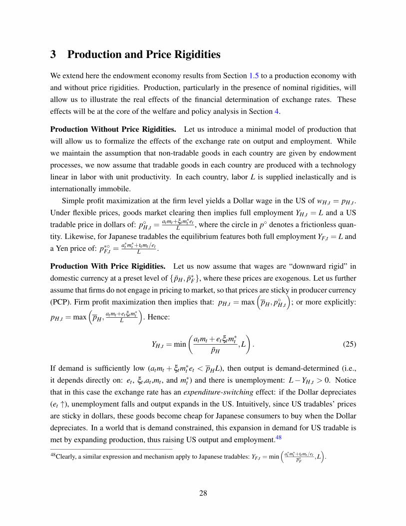
3 Production and Price Rigidities

We extend here the endowment economy results from Section 1.5 to a production economy withand without price rigidities. Production, particularly in the presence of nominal rigidities, willallow us to illustrate the real effects of the financial determination of exchange rates. Theseeffects will be at the core of the welfare and policy analysis in Section 4.

Production Without Price Rigidities. Let us introduce a minimal model of production thatwill allow us to formalize the effects of the exchange rate on output and employment. Whilewe maintain the assumption that non-tradable goods in each country are given by endowmentprocesses, we now assume that tradable goods in each country are produced with a technologylinear in labor with unit productivity. In each country, labor L is supplied inelastically and isinternationally immobile.

Simple profit maximization at the firm level yields a Dollar wage in the US of wH,t = pH,t .Under flexible prices, goods market clearing then implies full employment YH,t = L and a UStradable price in dollars of: pH,t =

atmt+ξtm∗t etL , where the circle in p denotes a frictionless quan-

tity. Likewise, for Japanese tradables the equilibrium features both full employment YF,t = L anda Yen price of: p∗F,t =

a∗t m∗t +ιtmt/etL .

Production With Price Rigidities. Let us now assume that wages are “downward rigid” indomestic currency at a preset level of pH , p∗F, where these prices are exogenous. Let us furtherassume that firms do not engage in pricing to market, so that prices are sticky in producer currency(PCP). Firm profit maximization then implies that: pH,t = max

(pH , pH,t

); or more explicitly:

pH,t = max(

pH ,atmt+etξtm∗t

L

). Hence:

YH,t = min(

atmt + etξtm∗tpH

,L). (25)

If demand is sufficiently low (atmt + ξtm∗t et < pHL), then output is demand-determined (i.e.,it depends directly on: et , ξt ,at ,mt , and m∗t ) and there is unemployment: L−YH,t > 0. Noticethat in this case the exchange rate has an expenditure-switching effect: if the Dollar depreciates(et ↑), unemployment falls and output expands in the US. Intuitively, since US tradables’ pricesare sticky in dollars, these goods become cheap for Japanese consumers to buy when the Dollardepreciates. In a world that is demand constrained, this expansion in demand for US tradable ismet by expanding production, thus raising US output and employment.48

48Clearly, a similar expression and mechanism apply to Japanese tradables: YF,t = min(

a∗t m∗t +ιt mt/etp∗F

,L)

.

28

The expenditure switching role of exchange rates has been central to the Keynesian analysis ofopen macroeconomics of Dornbusch (1976), Obstfeld and Rogoff (1995). In the Gamma model,it is enriched by being the central channel for the transmission of financial forces affecting theexchange rate, such as the risk-bearing capacity and balance sheet of the financiers, into outputand employment.

The financial determination of exchange rates has real consequences. Let us reconsider ourearlier example of a sudden inflow of capital from US investors into Brazilian Real bonds. Theexchange rate in this economy with production and sticky prices is still characterized by equa-tion (21). As previously discussed, the capital inflow in Brazil causes the Real to appreciate(

∂e0∂ f =− Γ

2+Γ< 0)

, and, if the flow is sufficiently strong ( f sufficiently high) or the financiers’risk bearing capacity sufficiently low (Γ sufficiently high), the appreciation (the increase in e0)can be so strong as to make Brazilian goods uncompetitive on international markets; the corre-sponding fall in world demand for Brazilian output (↓C∗H = ι0

e0 p∗F) causes an economic slump in

Brazil with both falling output and increasing unemployment.49

Despite extensive debates on the possibility of this type of adverse effect on the real economyof fluctuations in exchange rates due to capital flows and imbalances in financial markets, littleformal modeling has been carried out in the academic literature to provide the necessary theoret-ical foundations. We focused here on providing such foundations in a positive model; Section 4provides the corresponding normative analysis.

The main focus of our model is to disconnect the exchange rate from fundamentals by alteringthe structure of financial markets. Of course, part of the disconnect in practice also comes fromfrictions in the goods makers. These frictions can be analyzed in our model; we illustrate thisby considering prices that are sticky in the export destination currency (LCP). To make the pointsharp, assume that prices for US tradable goods are exogenously set at pH , p∗H in dollars in theUS and in yen in Japan, respectively.

Lemma 4 (LCP vs PCP) Under Local Currency Pricing the value of the exchange rate is the

same as under Producer Currency Pricing, but US tradable output does not depend on the ex-

change rate: YH,t = min(

atmtpH

+ξtm∗tp∗H

,L).

Proof Because of the log specification, the dollar value of US imports and exports is un-changed: they are still ιtmt and etξtm∗t . Consequently, net exports are unchanged, and the ex-change rate is unchanged from the previous formulae. Total demand is derived as in Section 1.5..49The Brazilian Finance Minister Guido Mantega complained, as reported in Forbes Magazine (2011), that: “Wehave to face the currency war without allowing our productive sector to suffer. If we allow [foreign] liquidity to[freely] enter [the economy], it will bring the Dutch Disease to the economy.”

29

LCP helps to further the disconnect between the exchange rate and fundamentals by preventingoutput in the tradable sector from responding to the exchange rate.50

4 Welfare and Heterodox Policies

The Gamma model of exchange rates considered so far in the positive analysis has made clear thatexchange rates are affected by financial forces and that their behavior can be quite different fromthat implied by the traditional macroeconomic analysis. We have also shown how the financialdetermination of exchange rates in imperfect financial markets has real consequences for outputand risk sharing.

The Mundellian prescription of pure floating exchange rates rests on the idea that a countryhit by a negative (asymmetric) real shock would be helped by a depreciating currency that in turn,under some form of sticky prices, would boost its exports and therefore alleviate the adverse im-pact of the shock on output and employment. In our model we focused on an alternative scenariowhereby financial shocks and imbalances in financial markets might cause an appreciation of acountry’s exchange rate and depress its exports and therefore output.

The possibility of such perverse effects of floating exchange rates has been the subject ofextensive debates (Rey (2013), Farhi and Werning (2013)), culminating in the threat of currency

wars, but its theoretical analysis and the development of policies to improve welfare is still in itsinfancy. The renewed research effort on analyzing the welfare consequences of capital controlshas mostly focused on fixed exchange rate regimes in the context of the small-open-economynew-Keynesian model. Farhi, Gopinath and Itskhoki (2014), Farhi and Werning (2012a,b),Magud, Reinhart and Rogoff (2011), and Schmitt-Grohé and Uribe (2012) provide innovativeanalyses of policies such as capital controls, fiscal transfers and fiscal devaluations in this con-text.51

We analyze welfare and policy in the Gamma model described in the previous sections. Inparticular, we focus on economic situations where the financial market imperfections that are atthe core of our model, namely having Γ > 0 in the presence of capital flows, play an importantrole both in the welfare distortions and in the suggested policy reaction.

50Devereux and Engel (2003) stressed the absence of exchange rate effects on output under LCP. The empiricalevidence shows that, in practice, a combination of PCP, LCP and limited pass-through are present in the data (seeGopinath and Itskhoki (2010), Gopinath, Itskhoki and Rigobon (2010), Amiti, Itskhoki and Konings (2014), Bursteinand Gopinath (2015)). For much of this paper, we focus on flexible prices or PCP as the basic cases. As shown inProposition 4 above, our qualitative analysis can easily accommodate a somewhat more limited pass-through ofexchange rate changes to local prices of internationally traded goods.51See also the literature on macro-prudential regulation, amongst others: Mendoza (2010), Bianchi (2010), Korinek(2011).

30

4.1 Exchange Rate Manipulation

We first show under which conditions direct government interventions in the currency market canaffect the equilibrium exchange rate. Then, we derive optimal currency management policy.

For notational simplicity, we set most parameters at 1: e.g. ι0 = ξt = at = a∗0 = β = β ∗ = 1.We allow ι1 to be stochastic (keeping E [ι1] = 1, and setting a∗1 = ι1 for symmetry) purely sothat currency trading is risky. The reader is encouraged to proceed keeping in mind the intuitioncoming from the simpler case in which ι1 is not stochastic and set equal to 1.52

Positive analysis At time 0, the US government intervenes in the currency market vis-à-vis thefinanciers: it buys q yen and sells qe0 dollars. By Proposition 6 we immediately obtain the resultbelow (as the government creates a flow f = q in the currency market):

Lemma 5 If the US government buys q yen and sells qe0 dollars at time 0, the exchange rates

satisfy (for small q): e0 = 1+ Γ

2+Γq+O

(q2), and E [e1] = 1− Γ

2+Γq+O

(q2).

The intervention’s impact on the average exchange rate is only second order: it induces a de-preciation at time 0, and an appreciation at time 1. We call this effect the “boomerang effect”.A currency intervention can change the level of the exchange rate in a given period, but not theaverage level of the exchange rate over multiple periods.

The imperfections in financial markets are at the core of the effects of FX intervention onexchange rates. Indeed, Backus and Kehoe (1989) show that in a general class of models inwhich currencies are imperfect substitutes due to risk premia, but in which there are no financialfrictions, FX interventions have no effect on the exchange rate.53 Lemma 5 correspondinglyhighlights the importance of the frictions: if Γ = 0, a frictionless set-up analogous to that inBackus and Kehoe (1989), there is no first order effect of the intervention on the exchange rate.

Normative analysis We assume that in the short run, i.e. period t = 0, US tradables’ prices aresticky in domestic currency (PCP) as in Section 3; prices are flexible in the long run, i.e. periodt = 1. We postulate that at time zero the price is downward rigid at a level pH that is sufficientlyhigh as to cause unemployment in the US tradable sector. Japanese tradable prices are assumedto be flexible. Currency intervention can be welfare improving in this economy. 54

52We make one more, largely technical, assumption. In this Section 4, we take the case α = 0, so as to abstractfrom (potentially very small) feedback effect from exchange rate interventions to exchange rate volatility and thenthe exchange rate itself. We conjecture that the whole analysis remains the same, provided α is small enough.53More specifically, sterilized foreign exchange rate interventions have no direct effect; if an effect is present, it isonly due to possible distortionary fiscal measures adopted by the governments to redistribute profits and losses ofthe intervention. Similarly unsterilized intervention has no direct effect, and the only possible effects occur via theindirect change in the money supply.54 We make an ancillary assumption, that the proof of Proposition 8 makes precise. We also assume that pH is abovethe market clearing price, but not too far above it.

31

Proposition 8 (FX intervention) Assume that Γ > 0 and that at time zero US tradable goods are

downward rigid at a price pH that is sufficiently high to cause unemployment in the US tradable

sector. A US government currency intervention, whereby the government buys q ∈ [0,qopt ] worth

of Yen bonds and sells qe0 Dollar bonds at time zero, improves welfare both in the US and in

Japan. The welfare improvement is monotonically increasing in the size of the intervention up to

size qopt , which is the smallest intervention that restores full employment in the US.

Note that there are two preconditions for this intervention to be welfare improving. The first oneis that prices are sticky (fixed) in the short run at a level that generates a fall in aggregate demandand induces an equilibrium output below the economy’s potential. This condition, i.e. being in ademand driven state of the world, is central to the Keynesian analysis where a depreciation of theexchange rate leads to an increase in output via an increase in export demand. If this condition issatisfied a first order welfare loss would occur even in a world of perfect finance.55

The second precondition is that financial markets are imperfect, i.e. Γ > 0. Intuitively, Γ

regulates the efficacy of an intervention. In fact, recall from Lemma 5 that the ability of thegovernment to affect the time-zero exchange rate is inversely proportional to Γ. When markets arefrictionless (Γ = 0) the government FX policy has no effect on the time-zero exchange rate, evenif prices are sticky, because financiers would simply absorb the intervention without requiring acompensation for the resulting risk.56

Interestingly, the suggested policy is not of the beggar thy neighbor type: the US currencyintervention, even with its aim to weaken the Dollar, actually increases welfare for both US andJapan. This occurs because the intervention induces first order welfare gains for both US andJapanese consumers by increasing US output, but only induces second order losses due to theensuing inter-temporal distortions in consumption. We highlight that currency wars can onlyoccur when both countries are in a slump and the post-intervention weaker dollar causes a firstorder output loss in Japan.

More generally, our results highlight that heterodox policies could be welfare improving whenthe currency appreciation is so strong as to actually cause a slump in domestic employment andwhen private markets are sufficiently disrupted for the government currency intervention to havea meaningful impact on the exchange rate.

55Indeed, in this economy (before the government intervention) financiers optimally choose to not trade at all. Theexchange rate is at 1, and is expected to remain at 1 on average, so that there are no gains from trading financialassets. Even if US households were to be allowed to directly trade Yen bonds, they would not change the value ofthe exchange rate.56We note that after the government intervention the financiers are at their optimum and do not want to change theirposition. However, US households, that had no incentives to trade Yen bonds in the original equilibrium, would wantto trade the Yen bonds after the government intervention. Of course, these unlimited trades are not possible due tothe frictions in the intermediation process. Therefore the policy success relies on the presence of financial frictionsrather than a direct failure of Ricardian equivalence.

32

Large-scale currency interventions, outspokenly justified by rationales very similar to thetheory provided in this paper, were undertaken by the governments of Switzerland and Israelduring the recent financial crisis.57 Both governments aimed to relieve their currency appreciationin the face of turmoil in financial markets. By most accounts, the interventions successfullyweakened the exchange rate and boosted the real economy.58 Blanchard, de Carvalho Filho andAdler (2014) find empirical support for the efficacy of this policy.59

A classic criticism of portfolio balance models is that only extremely big interventions areeffective because for an intervention to be effective it needs to alter very large stocks of assets:either the entire stock of assets outstanding or the country level gross external assets and lia-bilities. In our framework interventions are more effective because they need only alter Q, thebalance sheet of financiers, which is potentially substantially smaller than the entire stock ofassets.

4.2 Taxing International Finance

We now study a second policy instrument, taxation of the financiers, which is a form of capitalcontrols. We consider a proportional (US) government tax on each financier’s profits; the taxproceeds are rebated lump sum to financiers as a whole. Recall the imperfect intermediationproblem in Section 1.2, we now assume that the after-tax value of the intermediary is Vt(1−τ), where τ is the tax rate. The financiers’ optimality condition, derived in a manner entirely

analogous to the optimization problem in equation (9), is now: Q0 =E[e0−e1

R∗R

](1−τ)

Γ. Notice that

this is equivalent to changing Γ to an effective Γeff ≡ Γ

1−τ, so that the financiers’ demand can be

rewritten as Q0 =E[e0−e1

R∗R

]Γeff . We collect the result in the Lemma below.60

Lemma 6 A tax τ on finance is equivalent to lowering the financiers’ risk bearing capacity by

increasing Γ to Γeff ≡ Γ

1−τ. A higher tax increases the effective Γeff, thus reducing the financiers’

risk bearing capacity.57The Czech Republic also intervened in the currency market in November 2013 with the aim of depreciating theKoruna to boost the domestic economy58Israel central bank governor Stanley Fisher remarked: “I have no doubt that the massive purchases [of foreignexchange] we made between July 2008 and into 2010 [...] had a serious effect on the exchange rate which I think ispart of the reason that we succeeded in having a relatively short recession.” Levinson (2010)59Empirical studies have to confront the thorny issue of endogeneity of the policy and future empirical work isnecessary to provide a full empirical assessment. An earlier skeptical empirical literature, that mostly focused oninterventions of considerable smaller size, is summarized by Sarno and Taylor (2001). Dominguez and Frankel(1993a,b) find empirical support for the effect of foreign exchange rate intervention via a portfolio balance channel.60A tax might also plausibly impact the flows from carry traders. For instance, in the specification of Section 2.2,we could have f ∗ = d +g(R−R∗− τ). We do not explore here this possibility.

33

Positive analysis First we note that if the equilibrium before the government intervention fea-tures zero risk taking by the financiers (Q0 = 0), as was the case in the economy studied in theprevious subsection, then the tax τ is entirely ineffective. Intuitively, this occurs because thereare zero expected profits to tax, and therefore the tax has no effect on ex-ante incentives.

More generally we recall from Proposition 2 that an increase in Γ, in this case an increase inΓeff due to an increase in τ , has the opposite effect on the exchange rate depending on whetherthe financiers are long or short the Dollar to start with, i.e. depending on the sign of Q0 before thetax is imposed. For example, the tax would make the Dollar depreciate on impact if the financierswere long dollars to start with (Q0 > 0), but the same tax would make the Dollar depreciate ifthe financiers had the opposite position to start with. In practice this means that policy makerswho are considering imposing capital controls, or otherwise taxing international finance, shouldpay close attention to the balance sheets of financial institutions that have exposures to theircurrency. Basing the policy on reduced form approaches or purely on traditional macroeconomicsfundamentals can not only be misguiding, but might actually generate the opposite outcome forthe exchange rate from the desired one.

In order to study the impact of our tax policy, we start from an economy that features activerisk taking by the financiers. In the interest of tractability, we focus on a special case of the basicGamma model of Section 1. Namely, we assume that E [ι1] < ι0 and set all other parametersof the model to 1. We maintain from the previous subsection the assumption that US tradableprices are downward rigid at time 0 and flexible at time 1. In this set-up, the Dollar is so strongcompared to the Yen at time zero that US output is below potential and there is unemployment inthe US. We study in the Lemma below the impact of the tax policy on the exchange rate.

Lemma 7 If financiers are taxed at rate τ , the equilibrium exchange rate is:

e0 (τ) =

(1+ Γ

1−τ

)ι0 +E [ι1]

2+ Γ

1−τ

, e1 (τ) =ι0 +

(1+ Γ

1−τ

)E [ι1]

2+ Γ

1−τ

+ι1 . (26)

Notice that while the tax affects the equilibrium exchange rate in each period, it has no effecton the average rate across the two periods e0 + e1 = ι0 + ι1. We, therefore, recover here thesame “boomerang effect” that was noted in the previous section for FX interventions. As Γeff

goes from Γ to infinity, i.e. as τ goes from zero to 1, the time zero exchange rate approaches ι0

monotonically from below. Hence, given our assumption that E [ι1] < ι0, a tax on capital flowsdevalues the time zero exchange rate.

Normative analysis To keep the analytics to a minimum, we make the countries symmetric byimposing that both have equal taste for foreign tradable goods, at = ξt = 1, a∗t = ιt . We define

34

e0 ≡ pHL−1 as the least-weak value of the Dollar versus the Yen that, in equilibrium, generatesfull employment in the US. 61

Proposition 9 (Taxing international finance) Assume that at time zero: the US Dollar is so strong

as to induce a fall in US output below potential (YH,0 < L), financial markets are imperfect (Γ >

0), and the US runs a trade deficit (ι0 > E [ι1]). A US government tax on the financiers’ profits

at rate τ ∈ [0,τopt ], improves welfare in both the US and in Japan. The welfare improvement is

monotonically increasing in the tax rate up to the tax rate τopt . This rate is the lowest tax rate

that ensures full employment: e0 (τopt) = e0.

Note that there are three preconditions for this policy to be welfare improving. As for the caseof an FX intervention described in the previous subsection, two preconditions are that outputhas to be demand driven and that financial markets have to be imperfect. The latter condition isnecessary, but in this case no longer sufficient, for the policy to affect the exchange rate. As thereader will recall from our discussion of Lemma 6, a new condition is necessary, and sufficientjointly with Γ > 0, for the policy to have an effect: financiers need to have a non-zero exposureto currency before the policy is implemented.

4.3 Joint Optimal Monetary and Financial Policy

We have analyzed above optimal financial policy in the form of FX intervention and taxation ofinternational finance in a Gamma world. We analyze here the optimal mix of monetary policyand financial policy.

In order to perform the analysis with minimal algebra, we study a particularly clean casewhere most model parameters, (β ,β ∗, ιt ,ξt , ...), are set to 1. We also initialize mt = m∗t = 1 fort = 0,1. Before the disruption, the equilibrium exchange rates are e0 = e1 = 1. The US economystarts with rigid (in dollars) tradable prices pH at a level that just clears the goods market at fullemployment (i.e., a slightly higher price would lead to unemployment). We assume that the USgovernment’s objective function is: E [U0 +U1]− g(m0), where Ut is the household utility attime t as in equation (1), and g(m0) is a convex cost of monetary policy surprises, minimal whenm0 = 1.62

We consider two types of “shocks”: an unexpected increase in the Japanese money supply attime zero, from m∗0 = 1 to m∗

′0 > 1, while keeping m∗1 constant so that the interest rate R∗ falls,

and an increase in the pre-set price for US tradables ( pH).63 We first analyze the monetary shock.

61We make the same assumption as in footnote 54. In addition, we assume that ι0−E [ι1]> 0 is not too large.62These costs could be micro-founded in several ways (price dispersion inefficiencies, inflation cost in terms ofwealth redistribution, etc...), but here we take the simpler reduced form approach.63For transparency, we abstract here from uncertainty, but it is easy to add fundamental uncertainty, e.g. along the

35

Proposition 10 (“Benign neglect” of foreign monetary shocks) If the Dollar appreciation is sim-

ply due to a monetary shock (increase in m∗0), then no US policy response is needed (m0 = 1,

q = 0) to restore full employment. The shock has no real impact, and the economies maintain full

employment.

We next consider the optimal policy reaction to an increase in the pre-set price for US tradables.

Proposition 11 (Trade-off between FX intervention and monetary accommodation) Suppose

that at time zero pH is downwards rigid at a level above the full-employment flexible price, and

that at time 1 it is either: 1) flexible (“short-lasting rigidity”) or 2) rigid (“long-lasting rigidity”).

If the rigidity is short-lasting, then the optimal policy reaction combines both FX intervention and

monetary policy, where at the optimum q > 0 and m0 > 1. The policy relies more heavily on the

FX intervention compared to monetary intervention (i.e. |m0−1| is lower) the higher Γ is. If the

rigidity is long-lasting, then the optimal policy reaction employs only monetary policy. In this

case, a currency intervention is welfare reducing.

Intuitively, FX interventions are more desirable when financial markets are more constrained, be-cause an higher Γ makes it is easier for the policy to affect the exchange rate, and when distortionsare of shorter duration, because an FX intervention cannot move the exchange rate forever. Thereader will recall the “boomerang effect” of a currency intervention: it depreciates the exchangerate at time 0, but then appreciates it at time 1. If the price rigidities are long lasting, in this caselast for both periods, then the intervention only generates negative net welfare benefits becauseof the inter-temporal distortions that it causes.

Note that the government actions would not be taken by the households in the competitiveequilibrium. After the shock (in m∗0 or pH), there is no incentive for US consumers to interveneand trade the Yen because the (expected) currency returns are zero (e0 = R∗E [e1]). The USgovernment chooses to intervene because it internalizes the wage externality (i.e. internalizes theimpact on unemployment).

Hence, there are at least three policy tools, (i) monetary policy (ii) FX interventions, (iii)taxation of finance. In general, all might be used, and FX interventions are particularly potentwhen Γ is high – when financial market are disrupted. While (i) was already well-understood,our analysis allows us to analyze (ii) and (iii) in a way that was difficult in previous treatmentsthat did not have a model of imperfect financial markets.

lines of Propositions 8 and 9. Then the Propositions in this subsection hold, up to second order terms in the standarddeviation of that fundamental uncertainty.

36

5 Revisiting Canonical Issues with the Gamma Model

We consider in this section a number of canonical issues of international macroeconomics viathe lenses of the Gamma model. While these classic issues have also been the subject of previ-ous literature, our analysis not only provides new insights, but also allows us to illustrate howthe framework built in the previous sections provides a unified and tractable rationalization ofempirical regularities that are at the center of open-economy analysis.

5.1 The Carry Trade in the Presence of Financial Shocks

In the Gamma model there is a profitable carry trade. Let us give the intuition in terms of themost basic model first and then extend it to a set-up with shocks to the financiers’ risk bearingcapacity (Γ shocks).

First, imagine a world in which countries are in financial autarky because the financiers havezero risk bearing capacity (Γ = ∞), suppose that Japan has a 1% interest rate while the US hasa 5% interest rate, and that all periods (t = 0, ...,T ) are ex-ante identical with ξt = 1 and ιt amartingale. Thus, we have et = ιt , and the exchange rate is a random walk e0 = E [e1] = ... =

E [eT ]. A small financier with some available risk bearing capacity, e.g. a small hedge fund,could take advantage of this trading opportunity and pocket the 4% interest rate differential. Inthis case, there is a very profitable carry trade. As the financial sector risk bearing capacityexpands (Γ becomes smaller, but still positive), this carry trade becomes less profitable, but doesnot disappear entirely unless Γ = 0, in which case the UIP condition holds. Intuitively, the carrytrade in the basic Gamma model reflects the risk compensation necessary to induce the financiersto intermediate global financial flows.

In the most basic model, the different interest rates arise from different rates of time prefer-ences, such that R = β−1 and R∗ = β ∗−1. Without loss of generality, assume R < R∗ so that theDollar is the “funding” currency, and the Yen the “investment” currency. The return of the carrytrade is: Rc ≡ R∗

Re1e0− 1. For notational convenience we define the carry trade expected return

as Rc ≡ E[Rc]. The calculations in Proposition 3 allow us to immediately derive the equilibriumcarry trade.

Proposition 12 Assume ξt = 1. The expected return to the carry trade in the basic Gamma model

is:

Rc= Γ

R∗R E [ι1]− ι0

(R∗+Γ) ι0 +R∗R E [ι1]

, where Γ = γ var(ι1)α . (27)

Hence the carry trade return is bigger (i) when the return differential R∗/R is larger (ii) when the

funding country is a net foreign creditor (iii) when finance is more imperfect (higher Γ).

37

To gain further intuition on the above result, consider first the case where ι0 = E [ι1]. Thefirst order approximation to Rc in the case of a small interest rate differential R∗−R is: Rc

=Γ

2+Γ(R∗−R). Notice that we have both ∂Rc

∂Γ> 0 and ∂Rc

∂ (R∗−R) > 0, so that the profitability of thecarry trade increases the more limited the risk bearing capacity of the financiers and the largerthe interest rate differential.64

The effects of broadly defined “global risk aversion”, here proxied by Γ, on the profitabilityof the carry trade have been central to the empirical analysis of for example Brunnermeier, Nageland Pedersen (2009), Lustig, Roussanov and Verdelhan (2011), and Lettau, Maggiori and Weber(2014). Here we have shown that the carry trade is more profitable the lower the risk bearingcapacity of the financiers; we next formally account for shocks to such capacity in the form of astochastic Γ.

In addition to a pure carry force due to the interest rate differential, our model features globalimbalances as a separate risk factor in currency risk premia. The reader should recall Proposi-tion 2 that showed how net-external-debtor countries’ currencies have a positive excess returnand depreciate whenever risk bearing capacity decreases (↑ Γ). This effect occurs even if bothcountries have the same interest rate, thus being theoretically separate from the pure carry trade.Della Corte, Riddiough and Sarno (2014) test these theoretical predictions and find evidence of aglobal imbalance risk factor in currency excess returns. Notice that we built the model so that fi-nancial forces have no effect on the interest rates and the exchange rate makes all the adjustment;while this sharpens the model, we could extend the framework to allow for effects of imbalanceson both the exchange rate and interest rates.

The exposure of the carry trade to financial disruptions We now expand on the risks of thecarry trade by studying a three period (t = 0,1,2) model with stochastic shocks to the financiers’risk bearing capacity in the middle period. To keep the analysis streamlined, we take period2 to be the “long run”. Intuitively, period 2 will be a long-run steady state where countrieshave zero net foreign assets and run a zero trade balance. This allows us to quickly focus onthe short-to-medium-run exchange rate dominated by financial forces and the long-run exchangerate completely anchored by fundamentals. We jump into the analysis, and provide many of thebackground details of this model in the appendix.65

We assume that time-1 financial conditions, Γ1, are stochastic. In the 3-period economy with

64The first effect occurs because, given an interest rate differential, expected returns to the carry trade have to increasewhenever the risk bearing capacity of the financiers goes down to induce them to intermediate financial flows. Thesecond effect occurs because, given a level of risk bearing capacity for the financiers, an increase in the interest ratedifferential will not be offset one to one by the expected exchange rate change due to the risk premium.65The flow demand equations in the Yen / Dollar market are: et − ιt +Qt = 0 for t = 0,1, and in the long-run period

e2− ι2 = 0, with the financiers’ demand for dollars: Qt =et−E[et+1]

R∗R

Γt.

38

a long-run last period, the equilibrium exchange rates are:

e0 =Γ0ι0 +

R∗R E0

[Γ1ι1+ι2R∗/R

Γ1+1

]Γ0 +1

; e1 =Γ1ι1 +

R∗R E1 [ι2]

Γ1 +1; e2 = ι2. (28)

Recall that the carry-trade return between period 0 and 1 is: Rc ≡ R∗R

e1e0− 1. Interestingly, in

this case the carry trade also has “exposure to financial conditions”. Notice that ∂e1∂Γ1

< 0 in theequations above, so that the Dollar (the funding currency) appreciates whenever there is a negativeshock to the financiers’ risk bearing capacity (↑ Γ1, ↓ e1). Since in our chosen parametrizationthe carry trade is short Dollar and long Yen, we correspondingly have: ∂Rc

∂Γ1< 0, the carry trade

does badly whenever there is a negative shock to the financiers’ risk bearing capacity (↑ Γ1). Thisis consistent with the intuition and the empirical findings in Brunnermeier, Nagel and Pedersen(2009); we obtain this effect here in the context of an equilibrium model. We formalize and provethe results obtained so far in the proposition below.

Proposition 13 (Determinants of expected carry trade returns) Assume that R∗ > R, 1 = ι0 =

E0 [ι1] and ι1 = E1 [ι2]. Define the “certainty equivalent” Γ1 by Γ1+R∗/RΓ1+1

≡ E0

[Γ1+R∗/R

Γ1+1

]. Con-

sider the returns to the carry trade, Rc. The corresponding expected return Rc ≡ E0 [Rc] is

Rc= (R∗−1)Γ0

Γ1 +1+R∗

Γ1(Γ0 +R∗)+Γ0 +(R∗)2 .

with R∗ ≡ R∗R . We have:

1. An adverse shock to financiers affects the returns to carry trade negatively : ∂Rc

∂Γ1< 0.

2. The carry trade has positive expected returns: Rc> 0.

3. The expected return to the carry trade is higher the worse the financial conditions are

at time 0(

∂Rc

∂Γ0> 0)

, the better the financial conditions are expected to be at time 1(∂Rc

∂Γ1< 0)

, and the higher the interest rate differential ( ∂Rc

∂R∗ > 0, ∂Rc

∂R < 0).

The Fama Regression The classic UIP regression of Fama (1984) is in levels:66

e1− e0

e0= α +βUIP (R−R∗)+ ε1.

Under UIP, we would find βUIP = 1. However, a long empirical literature finds βUIP < 1, andsometimes even βUIP < 0. The proposition below rationalizes these findings in the context of an66The regression is most commonly performed in its logarithmic approximation version, but the levels prove moreconvenient for our theoretical treatment without loss of economic content.

39

equilibrium model.

Proposition 14 (Fama regression and market conditions) The coefficient of the Fama regression

is βUIP = 1+Γ1−Γ0(1+Γ0)(1+Γ1)

. Therefore one has βUIP < 1 whenever Γ0 > 0. In addition, one has

βUIP < 0 if and only if Γ1+1 < Γ0, i.e. if risk bearing capacity is very low in period 0 compared

to period 1.

Intuitively financial market imperfections always lead to βUIP < 1 and very bad current marketimperfections compared to future ones lead to βUIP < 0. This occurs because any positive Γ leadsto a positive risk premium on currencies that the financiers are long of and hence to a deviationfrom UIP (βUIP < 1). If, in addition, financial conditions are particularly worse today comparedto tomorrow the risk premium is so big as to induce currencies that have temporarily high interestrates to appreciate on average (βUIP < 0).

The intuition for βUIP < 1 is as follows. In the language of Fama (1984), when Japan hashigh interest rates, the risk premium on the Yen is high. The reason is that the risk premium isnot entirely eliminated by financiers, who have limited risk-bearing capacity. In the limit wherefinance is eliminated (Γ = ∞), an interest rate of 1% translate one-for-one into a risk premium of1% (βUIP = 0).

If riskiness (assuming α > 0) or financial frictions go to 0, then βUIP goes to 1.67 In allcases, however, Covered Interest Rate Parity (CIP) holds in the model. This is because we allowfinanciers to eliminate all riskless arbitrages. The machinery to justify this is spelled out in theonline appendix (section A.3.3). There, we formulate a version of our basic demand (equation(10)), that applies to an arbitrary number of assets, and is arbitrage-free. One upshot is that CIPis respected.

Exchange Rate Excess Volatility In the data exchange rates are more volatile than funda-mentals, a fact often referred to as exchange rate excess volatility. The Gamma model helps torationalize this volatility not only by directly introducing new sources of variation, for exampleshocks to the risk bearing capacity of the financiers (γt) and gross flows ( ft), but also indirectlyby endogenously amplifying fundamental volatility via the financial constraints. The intuition isthat higher fundamental volatility tightens financial constraints, tighter constraints lead to highervolatility, thus generating a self-reinforcing feedback loop. We formalize this more subtle effectin the Lemma below and sharpen it by not only maintaining the assumption that ξt = 1 at all dates,but also by considering the case of deterministic (γt), so that the only source of volatility is funda-mental, and no information revelation about future shocks E1[ι2] = E0[ι2] and Var1[ι2] =Var0[ι2].

67As riskiness (var (e1) ,var (e2)) goes to 0, Γ0 and Γ1 go to 0, so βUIP goes to 1.

40

Lemma 8 (Endogenous Amplification of Volatility) The volatility of the exchange rate at time

one is: var(e1) =(

Γ11+Γ1

)2var(ι1), where Γ1 = γ1var(ι2)

α . If α > 0 and γ1 > 0, then fundamental

volatility is endogenously amplified by the financial constraint: ∂var(e1)∂var(ι2)

> 0. Notice that if γ1 = 0,

then ∂var(e1)∂var(ι2)

= 0.

5.2 Nominal and Real Exchange Rates

We explore here the relationship between the nominal and the real CPI-based exchange rate inour framework. The real exchange rate can be defined as the ratio of two broad price levels,one in each country, expressed in the same numéraire. It is most common to use consumer priceindices (CPI) adjusted by the nominal exchange rate, in which case one has: E ≡ P∗e

P . Notice thata fall in E is a US Dollar real appreciation.

Consider the nominal version of the basic Gamma model in Section 2.1. Standard calculationsreported in the appendix imply that the real CPI-based exchange rate is:

E = θ(p∗H)

ξ ′(p∗F)a∗′(p∗NT )

χ∗′

(pH)a′(pF)ι′(pNT )χ

′ et , (29)

where θ is a function of exogenous shocks also reported in the appendix, and primed variablesare normalized by θ . The above equation is the most general formulation of the relationshipbetween the CPI-RER and the nominal exchange rate in the Gamma model. If we impose furtherassumptions, we can drive a useful special case.

The Basic Gamma Model Assume that ω = ω∗ = 0 and pNT = p∗NT = 1 so that there is nomoney and the numéraire in each economy is the non-tradable good. Recall that in the basicGamma model of Section 1 the law of one price holds for tradables, so we have pH = p∗He andpF = p∗Fe. Equation (29) then reduces to: E = θ (pH)

ξ′−a′(pF)

a∗′−ι′eχ∗

′. This equation describes

the relationship between the RER as defined in the basic Gamma model and the CPI-based RER.Notice that the two are close proxies of each other whenever the baskets’ shares of tradables aresymmetric across countries (i.e. ξ

′ ≈ a′

and a∗′ ≈ ι

′) and the non-tradable goods are a large

fraction of the Japanese overall basket (i.e. χ∗′ ≈ 1).

6 Conclusion

We presented a theory of exchange rate determination in imperfect capital markets where fi-nanciers bear the risks resulting from global imbalances in the demand and supply of internationalassets. Exchange rates are determined by the balance sheet risks and risk bearing capacity of

41

these financiers. Exchange rates in our model are disconnected from traditional macroeconomicfundamentals, such as output, inflation and the trade balance and are instead more connectedto financial forces such as the demand for assets denominated in different currencies. We haveshown how seemingly heterodox policies, such as government interventions in currency markets,can be welfare improving in this context. Our model is tractable, with simple to derive closedform solutions, and can be generalized to address a number of both classic and new issues ininternational macroeconomic analysis.

ReferencesAdrian, Tobias, and Hyun Song Shin. 2013. “Procyclical leverage and value-at-risk.” Review of Financial Studies.Adrian, Tobias, Erkko Etula, and Hyun Song Shin. 2014. “Risk appetite and exchange rates.” Federal Reserve

Bank of New York Staff Report.Adrian, Tobias, Erkko Etula, and Jan JJ Groen. 2011. “Financial amplification of foreign exchange risk premia.”

European Economic Review, 55(3): 354–370.Aguiar, Mark, Manuel Amador, and Gita Gopinath. 2009. “Investment cycles and sovereign debt overhang.”

Review of Economic Studies, 76(1): 1–31.Allen, Polly R., and Peter B. Kenen. 1983. Asset Markets and Exchange Rates: Modeling an Open Economy.

Cambridge University Press, Cambridge, UK.Alvarez, Fernando, Andrew Atkeson, and Patrick J Kehoe. 2002. “Money, interest rates, and exchange rates with

endogenously segmented markets.” Journal of political economy, 110(1): 73–112.Alvarez, Fernando, Andrew Atkeson, and Patrick J Kehoe. 2009. “Time-varying risk, interest rates, and exchange

rates in general equilibrium.” Review of Economic Studies, 76(3): 851–878.Amiti, Mary, Oleg Itskhoki, and Jozef Konings. 2014. “Importers, Exporters, and Exchange Rate Disconnect.”

American Economic Review, 104(7): 1942–78.Antràs, Pol, and Ricardo J Caballero. 2009. “Trade and Capital Flows: A Financial Frictions Perspective.” Journal

of Political Economy, 117(4): 701–744.Bacchetta, Philippe, and Eric Van Wincoop. 2010. “Infrequent portfolio decisions: A solution to the forward

discount puzzle.” American Economic Review, 100(3): 870–904.Backus, David K., and Gregor W. Smith. 1993. “Consumption and real exchange rates in dynamic economies with

non-traded goods.” Journal of International Economics, 35(3-4): 297–316.Backus, David K., and Patrick J. Kehoe. 1989. “On the denomination of government debt : A critique of the

portfolio balance approach.” Journal of Monetary Economics, 23(3): 359–376.Backus, David K., Patrick J. Kehoe, and Finn E. Kydland. 1992. “International Real Business Cycles.” Journal

of Political Economy, 100(4): 745–75.Bank of International Settlements. 2013. “Triennial Central Bank Survey.” Preliminary Report.Bianchi, Javier. 2010. “Credit externalities: Macroeconomic effects and policy implications.” American Economic

Review, 100(2): 398–402.Blanchard, Olivier, Francesco Giavazzi, and Filipa Sa. 2005. “International Investors, the U.S. Current Account,

and the Dollar.” Brookings Papers on Economic Activity, 36(1): 1–66.Blanchard, Olivier, Irineu de Carvalho Filho, and Gustavo Adler. 2014. “Can Sterilized Foreign Exchange In-

tervention Stem Exchange Rate Pressures from the Global Financial Cycle?” Unpublished Manuscript.Branson, William H., and Dale W. Henderson. 1985. “The specification and influence of asset markets.” In Hand-

book of International Economics. Vol. 2 of Handbook of International Economics, , ed. R. W. Jones and P. B.Kenen, Chapter 15, 749–805. Elsevier.

Branson, William H., Hannu Halttunen, and Paul Masson. 1979. “Exchange rates in the short run : Some furtherresults.” European Economic Review, 12(4): 395–402.

42

Brunnermeier, Markus, and Yuliy Sannikov. 2014. “A macroeconomic model with a financial sector.” AmericanEconomic Review, 104(2): 379–421.

Brunnermeier, Markus K., Stefan Nagel, and Lasse H. Pedersen. 2009. “Carry Trades and Currency Crashes.”In NBER Macroeconomics Annual 2008, Volume 23. NBER Chapters, 313–347. NBER, Inc.

Bruno, Valentina, and Hyun Song Shin. 2014. “Cross-Border Banking and Global Liquidity.” Forthcoming Reviewof Economic Studies.

Burstein, Ariel, and Gita Gopinath. 2015. “Chapter 7 - International Prices and Exchange Rates.” In Handbook ofInternational Economics. Vol. 4 of Handbook of International Economics, , ed. Kenneth Rogoff Elhanan Helpmanand Gita Gopinath, 391 – 451. Elsevier.

Caballero, Ricardo J., and Arvind Krishnamurthy. 2001. “International and domestic collateral constraints in amodel of emerging market crises.” Journal of Monetary Economics, 48(3): 513–548.

Calvo, Guillermo A, and Carlos Alfredo Rodriguez. 1977. “A model of exchange rate determination under cur-rency substitution and rational expectations.” The Journal of Political Economy, 617–625.

Carvalho, Carlos, and Fernanda Nechio. 2011. “Aggregation and the PPP Puzzle in a Sticky-Price Model.” Amer-ican Economic Review, 101(6): 2391–2424.

Chari, Varadarajan V, Patrick J Kehoe, and Ellen R McGrattan. 2002. “Can sticky price models generatevolatile and persistent real exchange rates?” The Review of Economic Studies, 69(3): 533–563.

Colacito, Riccardo, and Mariano M. Croce. 2011. “Risks for the Long Run and the Real Exchange Rate.” Journalof Political Economy, 119(1): 153–181.

Corsetti, Giancarlo, Luca Dedola, and Sylvain Leduc. 2008. “International risk sharing and the transmission ofproductivity shocks.” The Review of Economic Studies, 75(2): 443–473.

Costinot, Arnaud, Guido Lorenzoni, and Ivan Werning. 2014. “A theory of capital controls as dynamic terms-of-trade manipulation.” Journal of Political Economy, 122(1): 77–128.

Dedola, Luca, Peter Karadi, and Giovanni Lombardo. 2013. “Global implications of national unconventionalpolicies.” Journal of Monetary Economics, 60(1): 66 – 85. Carnegie-NYU-Rochester Conference.

De Grauwe, Paul. 1982. “The exchange rate in a portfolio balance model with a banking sector.” Journal of Inter-national Money and Finance, 1(1): 225–239.

Dekle, Robert, Jeong Hyeok, and Nobuhiro Kiyotaki. 2014. “Dynamics of Firms and Trade in General Equilib-rium.” Unpublished Manuscript Princeton University.

Della Corte, Pasquale, S. Riddiough, and Lucio Sarno. 2014. “Currency Premia and Global Imbalances.” Unpub-lished manuscript, Imperial College and City University.

De Long, J. Bradford, Andrei Shleifer, Lawrence H. Summers, and Robert J. Waldmann. 1990a. “Noise TraderRisk in Financial Markets.” Journal of Political Economy, 703–738.

De Long, J. Bradford, Andrei Shleifer, Lawrence H. Summers, and Robert J. Waldmann. 1990b. “Positivefeedback investment strategies and destabilizing rational speculation.” Journal of Finance, 45(2): 379–395.

de Macedo, Jorge Braga, and Urho Lempinen. 2013. “Exchange rate dynamics revisited.” National Bureau ofEconomic Research, Inc NBER Working Papers 19718.

Devereux, Michael B., and Charles Engel. 2003. “Monetary policy in the open economy revisited: Price settingand exchange-rate flexibility.” Review of Economic Studies, 70(4): 765–783.

Diebold, Francis X., and Peter Pauly. 1988. “Endogenous risk in a portfolio-balance rational-expectations modelof the Deutschemark-Dollar rate.” European Economic Review, 32(1): 27–53.

Dominguez, Kathryn M, and Jeffrey A Frankel. 1993a. “Does Foreign-Exchange Intervention Matter? The Port-folio Effect.” American Economic Review, 83(5): 1356–69.

Dominguez, K.M., and J.A. Frankel. 1993b. Does Foreign Exchange Intervention Work? Institute for InternationalEconomics.

Dornbusch, Rudiger. 1976. “Expectations and Exchange Rate Dynamics.” Journal of Political Economy,84(6): 1161.

Dornbusch, Rudiger, and Stanley Fischer. 1980. “Exchange Rates and the Current Account.” American EconomicReview, 70(5): 960–71.

Driskill, Robert, and Stephen McCafferty. 1980a. “Exchange-rate variability, real and monetary shocks, and thedegree of capital mobility under rational expectations.” Quarterly Journal of Economics, 95(3): 577–586.

43

Driskill, Robert, and Stephen McCafferty. 1980b. “Speculation, rational expectations, and stability of the foreignexchange market.” Journal of International Economics, 10(1): 91–102.

Dumas, Bernard. 1992. “Dynamic Equilibrium and the Real Exchange Rate in a Spatially Separated World.” Reviewof Financial Studies, 5(2): 153–80.

Dumas, Bernard, and Bruno Solnik. 1995. “The World Price of Foreign Exchange Risk.” Journal of Finance,50(2): 445–79.

Evans, Martin, and Richard K. Lyons. 2002. “Order Flow and Exchange Rate Dynamics.” Journal of PoliticalEconomy, 110(1): 170–180.

Evans, Martin D. D., and Richard K. Lyons. 2012. “Exchange Rate Fundamentals and Order Flow.” QuarterlyJournal of Finance, 2(4): 1–63.

Fama, Eugene F. 1984. “Forward and spot exchange rates.” Journal of Monetary Economics, 14(3): 319–338.Farhi, Emmanuel, and Ivan Werning. 2012a. “Dealing with the Trilemma: Optimal Capital Controls with Fixed

Exchange Rates.” Unpublished manuscript, Harvard University and MIT.Farhi, Emmanuel, and Ivan Werning. 2012b. “Fiscal Unions.” Unpublished manuscript, Harvard University and

MIT.Farhi, Emmanuel, and Ivan Werning. 2013. “Dilemma not trilemma? Capital controls and exchange rates with

volatile capital flows.” IMF working paper. Harvard University and MIT.Farhi, Emmanuel, and Ivan Werning. 2014. “A Theory of Macroprudential Policies in the Presence of Nominal

Rigidities.” Unpublished manuscript, Harvard University and MIT.Farhi, Emmanuel, and Xavier Gabaix. 2014. “Rare Disasters and Exchange Rates.” Unpublished manuscript,

Harvard University and NYU.Farhi, Emmanuel, Gita Gopinath, and Oleg Itskhoki. 2014. “Fiscal Devaluations.” Forthcoming Review of Eco-

nomic Studies.Feenstra, Robert C. 1986. “Functional equivalence between liquidity costs and the utility of money.” Journal of

Monetary Economics, 17(2): 271–291.Forbes Magazine. 2011. http: // www. forbes. com/ sites/ afontevecchia/ 2011/ 04/ 18/

mantega-inflation-under-control-in-brazil-as-qe2-pressures-real/ .Froot, Kenneth A, and Jeremy C. Stein. 1991. “Exchange rates and foreign direct investment: an imperfect capital

markets approach.” Quarterly Journal of Economics, 106(4): 1191–1217.Froot, Kenneth A., and Tarun Ramadorai. 2005. “Currency Returns, Intrinsic Value, and Institutional-Investor

Flows.” Journal of Finance, 60(3): 1535–1566.Froot, Kenneth A., Paul G. J. O’Connell, and Mark S. Seasholes. 2001. “The portfolio flows of international

investors.” Journal of Financial Economics, 59(2): 151–193.Gabaix, Xavier. 2014. “A Sparsity-Based Model of Bounded Rationality.” Quarterly Journal of Economics.Garleanu, Nicolae, and Lasse Heje Pedersen. 2011. “Margin-based asset pricing and deviations from the law of

one price.” Review of Financial Studies, 24(6): 1980–2022.Gertler, Mark, and Nobuhiro Kiyotaki. 2010. “Financial Intermediation and Credit Policy in Business Cycle

Analysis.” In Handbook of Monetary Economics. Vol. 3 of Handbook of Monetary Economics, Chapter 11, 547–599. Elsevier.

Gertler, Mark, and Peter Karadi. 2011. “A model of unconventional monetary policy.” Journal of monetary Eco-nomics, 58(1): 17–34.

Gopinath, Gita, and Oleg Itskhoki. 2010. “Frequency of Price Adjustment and Pass-Through.” The QuarterlyJournal of Economics, 125(2): 675–727.

Gopinath, Gita, Oleg Itskhoki, and Roberto Rigobon. 2010. “Currency Choice and Exchange Rate Pass-Through.” American Economic Review, 100(1): 304–36.

Gourinchas, Pierre-Olivier, and Helene Rey. 2007a. “From world banker to world venture capitalist: US externaladjustment and the exorbitant privilege.” In G7 Current Account Imbalances: Sustainability and Adjustment.

Gourinchas, Pierre-Olivier, and Hélène Rey. 2007b. “International financial adjustment.” Journal of PoliticalEconomy, 115(4): 665–703.

Gourinchas, Pierre-Olivier, and Helene Rey. 2013. “External Adjustment, Global Imbalances and Valuation Ef-fects.” Forthcoming Handbook of International Economics.

44

Gourinchas, Pierre-Olivier, Nicolas Govillot, and Hélène Rey. 2010. “Exorbitant Privilege and Exorbitant Duty.”Unpublished manuscript, UC Berkeley and LBS.

Gromb, Denis, and Dimitri Vayanos. 2002. “Equilibrium and welfare in markets with financially constrainedarbitrageurs.” Journal of Financial Economics, 66(2): 361–407.

Hanson, Samuel G., and Jeremy C. Stein. 2014. “Monetary policy and long-term real rates.” Journal of FinancialEconomics.

Hart, Oliver. 1995. Firms, contracts, and financial structure. Oxford University Press.Hart, Oliver, and John Moore. 1994. “A theory of debt based on the inalienability of human capital.” Quarterly

Journal of Economics, 109(4): 841–879.Hassan, Tarek A. 2013. “Country Size, Currency Unions, and International Asset Returns.” Journal of Finance,

68(6): 2269–2308.Hau, Harald, and Hélène Rey. 2006. “Exchange Rates, Equity Prices, and Capital Flows.” Review of Financial

Studies, 19(1): 273–317.Hau, Harald, Massimo Massa, and Joel Peress. 2010. “Do Demand Curves for Currencies Slope Down? Evidence

from the MSCI Global Index Change.” Review of Financial Studies, 23(4): 1681–1717.Helpman, Elhanan. 1981. “An exploration in the theory of exchange-rate regimes.” The Journal of Political Econ-

omy, 865–890.Helpman, Elhanan, and Assaf Razin. 1982. “Dynamics of a Floating Exchange Rate Regime.” Journal of Political

Economy, 90(4): pp. 728–754.Henderson, Dale W., and Kenneth Rogoff. 1982. “Negative net foreign asset positions and stability in a world

portfolio balance model.” Journal of International Economics, 13(1-2): 85–104.He, Zhiguo, and Arvind Krishnamurthy. 2013. “Intermediary Asset Pricing.” American Economic Review,

103(2): 732–70.Hong, Harrison, and Motohiro Yogo. 2012. “What does futures market interest tell us about the macroeconomy

and asset prices?” Journal of Financial Economics, 105(3): 473–490.Ivashina, Victoria, David S. Scharfstein, and Jeremy C. Stein. 2012. “Dollar Funding and the Lending Behavior

of Global Banks.” NBER Working Paper 18528.Jeanne, Olivier, and Andrew K. Rose. 2002. “Noise trading and exchange rate regimes.” Quarterly Journal of

Economics, 117(2): 537–569.Kim, Young Ju, Zhipeng Liao, and Aaron Tornell. 2014. “Speculators Positions and Exchange Rate Forecasts:

Beating Random Walk Models.” Unpublished Manuscript UCLA.Kiyotaki, Nobuhiro, and John Moore. 1997. “Credit Cycles.” Journal of Political Economy, 105(2): 211–248.Kollmann, Robert. 2013. “Global Banks, Financial Shocks, and International Business Cycles: Evidence from an

Estimated Model.” Journal of Money, Credit and Banking, 45(s2): 159–195.Kollmann, Robert, Zeno Enders, and Gernot J Müller. 2011. “Global banking and international business cycles.”

European Economic Review, 55(3): 407–426.Korinek, Anton. 2011. “The new economics of prudential capital controls: A research agenda.” IMF Economic

Review, 59(3): 523–561.Kouri, Pentti J. K. 1976. “The Exchange Rate and the Balance of Payments in the Short Run and in the Long Run:

A Monetary Approach.” Scandinavian Journal of Economics, 78(2): 280–304.Lane, Philip R, and Jay C Shambaugh. 2010. “Financial exchange rates and international currency exposures.”

American Economic Review, 100(1): 518–540.Lettau, Martin, Matteo Maggiori, and Michael Weber. 2014. “Conditional risk premia in currency markets and

other asset classes.” Journal of Financial Economics, 114(2): 197 – 225.Levinson, Charles. 2010. “Interview Transcript: Stanley Fischer.” Wall Street Journal. http: // online. wsj.

com/ news/ articles/ SB10001424052702304510704575562410676436730 (accessed January 15, 2014).Lucas, Robert E. 1982. “Interest rates and currency prices in a two-country world.” Journal of Monetary Economics,

10(3): 335–359.Lustig, Hanno, Nikolai Roussanov, and Adrien Verdelhan. 2011. “Common risk factors in currency markets.”

Review of Financial Studies, 24(11): 3731–3777.Maggiori, Matteo. 2014. “Financial Intermediation, International Risk Sharing, and Reserve Currencies.” Unpub-

45

lished manuscript, Harvard University.Magud, Nicolas E., Carmen M. Reinhart, and Kenneth S. Rogoff. 2011. “Capital Controls: Myth and Reality -

A Portfolio Balance Approach.” National Bureau of Economic Research, Inc NBER Working Papers 16805.Mark, Nelson C. 1995. “Exchange Rates and Fundamentals: Evidence on Long-Horizon Predictability.” American

Economic Review, 85(1): 201–18.Martin, Ian. 2011. “The Forward Premium Puzzle in a Two-Country World.” NBER Working Paper 17564.Meese, Richard A., and Kenneth Rogoff. 1983. “Empirical exchange rate models of the seventies : Do they fit out

of sample?” Journal of International Economics, 14(1-2): 3–24.Mendoza, Enrique G. 2010. “Sudden Stops, Financial Crises, and Leverage.” American Economic Review,

100(5): 1941–1966.Mendoza, Enrique G, Vincenzo Quadrini, and Jose-Vıctor Rıos-Rull. 2009. “Financial Integration, Financial

Development, and Global Imbalances.” Journal of Political Economy, 117(3).Obstfeld, Maurice. 2004. “External adjustment.” Review of World Economics, 140(4): 541–568.Obstfeld, Maurice, and Kenneth Rogoff. 1995. “Exchange Rate Dynamics Redux.” Journal of Political Economy,

103(3): 624–660.Obstfeld, Maurice, and Kenneth Rogoff. 2001. “The six major puzzles in international macroeconomics: is there

a common cause?” In NBER Macroeconomics Annual 2000, Volume 15. , ed. Ben S. Bernanke and KennethRogoff, 339–412. The MIT Press.

Obstfeld, Maurice, and Kenneth S. Rogoff. 1996. Foundations of International Macroeconomics. MIT Press.Pavlova, Anna, and Roberto Rigobon. 2007. “Asset Prices and Exchange Rates.” Review of Financial Studies,

20: 1139–1180.Pavlova, Anna, and Roberto Rigobon. 2008. “The Role of Portfolio Constraints in the International Propagation

of Shocks.” Review of Economic Studies, 75(4): 1215–1256.Pavlova, Anna, and Roberto Rigobon. 2010. “An asset-pricing view of external adjustment.” Journal of Interna-

tional Economics, 80(1): 144–156.Pavlova, Anna, and Roberto Rigobon. 2012. “Equilibrium Portfolios and External Adjustment Under Incomplete

Markets.” Unpublished Manuscript LBS.Perri, Fabrizio, and Vincenzo Quadrini. 2014. “International recessions.”Rey, Hélène. 2013. “Dilemma not Trilemma: The global financial cycle and monetary policy independence.” Jack-

son Hole Economic Symposium.Sarno, Lucio, and Mark P. Taylor. 2001. “Official Intervention in the Foreign Exchange Market: Is It Effective

and, If so, How Does It Work?” Journal of Economic Literature, 39(3): pp. 839–868.Schmitt-Grohé, Stephanie, and Martın Uribe. 2003. “Closing small open economy models.” Journal of interna-

tional Economics, 61(1): 163–185.Schmitt-Grohé, Stephanie, and Martín Uribe. 2012. “Pegs and Pain.” Working paper Columbia University.Shleifer, Andrei, and Robert W. Vishny. 1997. “The limits of arbitrage.” Journal of Finance, 52(1): 35–55.Stathopoulos, Andreas. 2012. “Asset prices and risk sharing in open economies.” Unpublished manuscript, Univer-

sity of Southern California.Tobin, James, and Jorge B. de Macedo. 1979. “The Short-Run Macroeconomics of Floating Exchange Rates:

An Exposition.” Cowles Foundation for Research in Economics, Yale University Cowles Foundation DiscussionPapers 522.

Verdelhan, Adrien. 2010. “A Habit-Based Explanation of the Exchange Rate Risk Premium.” Journal of Finance,65(1): 123–146.

Verdelhan, Adrien. 2013. “The share of systematic variation in bilateral exchange rates.” Unpublished ManuscriptMIT.

46

Appendix to “International Liquidity and Exchange RateDynamics”

Xavier Gabaix Matteo Maggiori

Not for Publication. November 2014

A.1 Analytical Generalization of the Model

A.1.1 The Exchange Rate with Infinite HorizonWe provide here the infinite-horizon extension of the model. In this model the flow equation is: ξtet − ιt −RQt−1 +Qt = 0.

Proposition A.1 (Exchange rate with infinite horizon) Assume a non-negative stochastic process for im-ports ιt and that ξt = 1 for all t. Denote by RQt−1 the accrued net foreign liabilities of the US (denominatedin dollars) to be absorbed by the financiers at t. The equilibrium exchange rate is:

et = Et

[∞

∑s=t

Λs−t (1−Λ) ιs

]+(1−Λ)RQt−1, (A.1)

where Λ≡ (1+R+Γ)−√

(1+R+Γ)2−4R2R ∈ (0, 1

R ]. If Γ = 0, then Λ = 1R ; otherwise, Λ is decreasing in Γ.

This Proposition shows that Γ is akin to inducing myopia about future flows. If Γ = 0 so that UIP holds andΛ = 1/R, then future flows are discounted at the US interest rate. When Γ > 0, future flows are discountedat a rate higher than this interest rate.

It is interesting to analyze the model in the presence of portfolio flows, f ∗t , along the lines of Sections1.4.1 and 2.2, so that the flow equation is, for all t, ξtet− ιt + f ∗t +Qt−RQt−1 = 0. Recall that for analyticaltractability we assume that these flows can depend on most fundamental variables, e.g. the interest rate,but cannot depend directly on the exchange rate.68 We perform a Taylor expansion in the interest ratedifferential, linearizing around R∗t = Rt ≈ R, assuming that ιt is close to its steady state value ι , and assumingthat RQt−1 is close to 0, so that we can expand the exchange rate around e≡ ι . Then

et = Et

∞

∑s=t

Λs−t[(1−Λ)(ιs− f ∗s )+Λe

R∗s −Rs

R

]+(1−Λ)RtQt−1. (A.2)

The above expression is exact in its treatment of the term in (ιs− f ∗s ), but contains a Taylor expansion in theR∗s −Rs term.

This generalizes to an infinite horizon the effects of portfolio flows on the exchange rate, which werethe focus of Proposition 7 in the two period model. The Yen is stronger: if Japan is a creditor (Qt−1 > 0);if there is high import demand for Japanese goods (ιs > 0); if interest rates are higher in Japan than in theUS (R∗s −Rs > 0); and if there is selling pressure on the Dollar ( f ∗s < 0). Compared to the UIP case, thefirst effect is amplified, the import-demand and interest-rate effects are simply discounted at a higher rate(we have Λ < 1

R in this Gamma model, rather than Λ = 1R in the UIP case). The last effect (the f ∗s term) is

entirely specific to the Gamma model.69

68Section A.4 provides numerical solutions for the case of portfolio flows that depend directly on the exchange rate.69The derivation of equation (A.2) in the Proof section of this appendix provides details for this latter effect.

A.1

A.1.1.1 Slow Digestion of Imbalances

To further understand the dynamics of exchange rates, consider a very simple example: there is an initialdebt Q−0 at time 0, ιt is i.i.d. with mean 1 with Rt = R∗t = R for all t.

Proposition A.2 (Slow digestion of imbalances when Γ > 0) Given an initial debt Q−0 , the dynamics of theexchange rate are: E0et = 1+(1−Λ)Q−0 λ t . US net foreign liabilities evolve according to: RE0Qt = Q−0 λ t ,where λ ≡ RΛ. If Γ = 0, then λ = 1, and otherwise 0 < λ < 1.

In the UIP case (Γ= 0) the debt and the exchange rate are constant in expectation. The Dollar is permanentlyweak. For the general case, we reason in expectation. When Γ > 0, and therefore λ < 1, the debt slowlyshrinks to 0, and the Dollar slowly mean-reverts to its fundamental value with no debt (e∞ = 1). Intuitively,this “slow digestion”occurs because the US has a debt at time zero and the financiers need to be convinced tohold it. Given that interest rates are the same in both countries, the Dollar needs to be expected to appreciateto give a capital gain to the financiers. Hence, the Dollar is weak initially, and it will appreciate as long asthere is debt remaining. Indeed, it appreciates until Qt = 0, which happens in the limit as t→ ∞. Viewed ina different way, the Dollar is depreciated, so US exports are higher, which allows the US to repay its debtslowly.

Hence, the financial imperfections modeled in this Gamma framework lead to qualitatively differentdynamics compared to the traditional UIP case.

A.1.2 Japanese Households and the Carry TradeIn most of the main body of the paper, consumers do not do the carry trade themselves. In this subsection,we analyze the case where Japanese consumers buy a quantity f ∗ of dollar bonds, financing the purchase byshorting an equivalent amount of Yen bonds. We let this demand take the form:

f ∗ = b(R−R∗) .

If b≥ 0 the Japanese household demand is a form of carry trade. The flow equations now are:

NX0 +Q+ f ∗ = 0; NX1−R(Q+ f ∗) = 0.

We summarize the implications for the equilibrium carry trade in the Proposition below.

Proposition A.3 When Japanese consumers do the carry trade, the expected return to the carry trade in thebasic Gamma model is:

Rc= Γ

R∗R E [ι1]− ι0 + f ∗(1+R∗)

(R∗+Γ) ι0 +R∗R E [ι1]−Γ f ∗

.

Hence the carry trade return is bigger: (i) when R∗/R is higher, (ii) when the funding country is a net foreigncreditor, or (iii) when consumers do the carry trade less ( f ∗ increases).

If consumers do the carry trade on too large a scale ( f ∗ too negative), then the carry trade becomes unprof-itable, Rc

< 0.

A.2 Further Details for the Main Body of the Paper

A.2.1 A more abstract version of the market structureIt may be useful to have a more abstract presentation of the basic model. We focus on the US side, as theJapanese side is entirely symmetric.

A.2

For generality, we present the monetary model, and then show how the real model can be viewed as aspecial case of it. We call

c = (CH ,CF ,CNT ,M,0,0) ,

the vector of consumptions of CH US tradables, CF Japanese tradables, CNT US non-tradables, and a quantityM of US money, respectively. The last 2 slots in vector c (set at 0) are the consumption of Japanese non-tradables, and Japanese money: they are zero for the US consumer. Likewise, the Japanese consumer hasconsumption:

c∗ = (C∗H ,C∗F ,0,0,C

∗NT ,M

∗) .

The Japanese household consumes C∗H US tradables, C∗F Japanese tradables, 0 US non-tradables, 0 USmoney, C∗NT Japanese non-tradables, and M∗ Japanese money.

The US production vector isy = (yH ,0,yNT ,Ms,0,0) .

This shows that the US produces yH US tradables, 0 Japanese tradables, yNT US non-tradables, and 0Japanese non-tradables and money . Here Ms is the money supply given by the government to the household.Japanese production is similarly

y∗ = (0,y∗F ,0,0,y∗NT ,M

s∗) .

The vector of prices in the US isp = (pH , pF , pNT ,1,0,0) .

Utility is u(ct ,φt), where φt is a taste shock. In the paper, φt = (at , ιt ,χt ,ωt ,0,0), so that in the utilityfunction is

u(ct ,φt) =6

∑i=1

φit lncit , for t = 0, . . . ,T.

Consumptions are non-negative, cit ≥ 0 for all i, t.The fourth and sixth components of the above vectors correspond to money. In the real model they are

set to 0. Then, in this real money, the numéraire is the non-tradable good, so that pNT = 1.We call Θt =

(ΘUS

t ,ΘJt)

the holding by the US of US bonds and Japanese bonds, Pt = (1,et) the priceof bonds in dollars.

The US consumers’ problem is:

max(ct ,Θ

USt )t≤T

ET

∑t=0

βtu(ct ,φt) , (A.3)

s.t.

pt · (yt − ct)+Pt ·DtΘt−1 +πFt = Pt ·Θt , for t = 0, ...,T, (A.4)

andΘT = 0. (A.5)

Here Dt = diag(R,R∗) is the diagonal matrix expressing the gross rate of return of bonds in each cur-rency and πF

t is a profit rebated by financiers. The left-hand side of (A.4) is the households’ financial wealth(in dollars) after period t. US firms are fully owned by US households. Because the economy is fullycompetitive, they make no profit. The entire production comes as labor income, whose value is pt · yt . Thebudget constraint is the terminal asset holdings should be 0, which is expressed by (A.5). Finally, as is usual,ct and ΘUS

t are adapted process, i.e. they depend only on information available at date t.In the above maximization problems, US consumers choose optimally their consumption vector ct and

A.3

their dollar bond holdings ΘUSt . However, they do not choose their holding of Japanese bonds ΘJ

t optimally.In the basic model we preclude such holdings and set ΘJ

t = 0. In the extended model, we allow for suchholdings and study simple and intuitive cases: for instance, at time 0 the holdings of Japanese bonds can bean endowment ΘJ

−1 = DJ (or Japanese debt denoted in Yen). Alternatively, they could be a liquidity (noisetrader) shock ΘJ

0 =− f , or we could have f be a function of observables, but not the exchange rate directly,e.g. f = b+c(R−R∗) for a carry-trader (see Section 2.2). We do not focus on the foundations for each typeof demand, but actually take the demands as exogenously specified. Possible microfoundations for thesedemands range from rational models of portfolio delegation where the interest rate is an observable variablethat is known, in equilibrium, to load on the sources of risk of the model (see Section 5.1), to models of“reaching for yield" (Hanson and Stein, 2014), or to the “boundedly rational” households who focus on theinterest rate when investing without considering future exchange rate changes or covariance with marginalutility (as in Gabaix (2014)).

To summarize, while all goods are frictionlessly traded within a period (with the non-tradable goodsbeing traded only within a country), asset markets are restricted: only US and Japanese bonds are traded(rather than a full set of Arrow-Debreu securities).

The goods market clearing condition is:

yt + y∗t = ct + c∗t at all dates t ≤ T. (A.6)

Firms produce and repatriate their sales at every period. They have net asset flows,

Θf irmst = p∗Htc

∗Ht (et ,−1) ,

Θf irms,∗t = pFtcFt

(−1,

1et

).

The first equation expresses the asset flows of US exporters : in Japan, they have sales of p∗Htc∗Ht Yen in

Japan market; they repatriate those yens (hence a flow of −p∗Htc∗Ht in Yen), to buy dollars (hence a flow of

p∗Htc∗Htet dollars).

For instance, in the model with the log specification,

Θf irmst = p∗Htc

∗Ht (et ,−1) = m∗t ξt (et ,−1) ,

Θf irms,∗t = pFtcFt

(−1,

1et

)= mtιt

(−1,

1et

),

so that Θf irmst +Θ

f irms,∗t = (m∗t ξtet −mtιt)

(1,− 1

et

). The real model is similar, replacing mt and m∗t by 1.

The gross demand by financiers is Qt (1,−1/et). Each period the financiers sell the previous periodposition, so that their net demand is:

Qt (1,−1/et)−DtQt−1 (1,−1/et−1) = (1−DtL )Qt (1,−1/et) , (A.7)

where L is the lag operator, L Xt = Xt−1.Financiers choose Qt optimally, given the frictions, as in the main body of the paper and we do not

restate their problem here for brevity. In the last period, holdings are 0, i.e. QT = 0.The asset market clearing condition is that the net demand for bonds is 0

Θf irmst +Θ

f irms,∗t +(1−DtL )(Θt +Θ

∗t +Qt (1,−1/et)) = 0. (A.8)

For instance, for consumers, (1−DtL )Θt is the increased asset demand by the agent. To gain some intu-

A.4

ition, the first coordinate of equation (A.8), evaluated at time t = 0, in the case where Θt = Θ∗t = 0, givesequation (21) of the paper:

ξ0e0m∗0− ι0m0 +Q0 = 0;

and in the real case (corresponding to m0 = m∗0 = 1), we obtain the basic equation (13) of the paper:

ξ0e0− ι0 +Q0 = 0.

We now state formally the definition of equilibrium in the case of flexible prices. Recall that we assume thelaw of one price in goods market to hold such that:

p∗Ht = pHt/et , p∗Ft = pFt/et . (A.9)

Definition 1 A competitive equilibrium consists of allocations(

ct ,c∗t ,Θt ,Θ∗t ,Θ

f irmst ,Θ f irms,∗

t ,Qt

), prices

pt , p∗t , exchange rate et , for t = 0, . . . ,T such that the US consumers optimize their utility function (A.3)under the above constraints (A.4-A.5), Japanese consumers optimize similarly, goods markets clear (A.6),and asset markets clear (A.8), and the low of one price (A.9) holds.

As explained in the paper (Lemma 4), if we use local currency pricing (i.e. change (A.9), and replacethe value of p∗Ht and pFt by other, potentially arbitrary, values), the equilibrium value of the exchange ratedoes not change (though consumptions do change).

The timing was already stated in the paper, but for completeness we restate it here. At time 0, producersproduce, consumers demand and consume, exporters repatriate their sales, financiers take their FX positions,and asset and goods market clear (simultaneously, like in Arrow-Debreu). The potential diversion by thefinanciers happens at time 0+, right after time 0 (of course, no diversion happens on the equilibrium path).Then, at time 1 and potentially future periods, the same structure is repeated (with no financiers’ position inthe last period).

A.2.2 Maximization Problem of the Japanese HouseholdWe include there many details excluded from Section 1 for brevity. The dynamic budget constraint ofJapanese households (which holds state by state) is:

1

∑t=0

Y ∗NT,t + p∗F,tYF,t +π∗tR∗t

=1

∑t=0

C∗NT,t + p∗H,tC∗H,t + p∗F,tC

∗F,t

R∗t,

where π∗t are the financiers’ profits remittances to the Japanese, π∗0 = 0, π∗1 = Q0(R−R∗e1/e0)/e1.The static utility maximization problem of the Japanese household:

maxC∗NT,t ,C

∗H,t ,C

∗F,t

χ∗t lnC∗NT,t +ξt lnC∗H,t +a∗t lnC∗F,t +λ

∗t(CE∗t −C∗NT,t − p∗H,tC

∗H,t − p∗F,tC

∗F,t),

where CE∗t is aggregate consumption expenditure of the Japanese household, λ ∗t is the associated Lagrangemultiplier, p∗H is the Yen price in Japan of US tradables, and p∗F is the Yen price in Japan of Japanesetradables. Standard optimality conditions imply:

C∗NT,t =χ∗tλ ∗t

; p∗H,tC∗H,t =

ξt

λ ∗t; p∗F,tC

∗F,t =

a∗tλ ∗t

.

A.5

Our assumption that Y ∗NT,t = χ∗t , combined with the market clearing condition for Japanese non-tradablesY ∗NT,t =C∗NT,t , implies that in equilibrium λ ∗t = 1. We obtain:

p∗H,tC∗H,t = ξt ; p∗F,tC

∗F,t = a∗t .

A.2.3 The Euler Equation when there are Several GoodsWe state the general Euler equation when there are several goods.

With utility ut (Ct) + βut+1 (Ct+1), where Ct is the vector of goods consumed (for instance, Ct =(CNT,t ,CH,t ,CF,t) in our setup), if the consumer is at his optimum, we have:

Lemma A.1 When there are several goods, the Euler equation is:

1 = Et

[βR

ut+1c j,t+1

/p j,t+1

utci,t/pi,t

]for all i, j. (A.10)

This should be understood in “nominal” terms, i.e. the return R is in units of the (potentially arbitrary)numéraire.

Proof. It is a variant on the usual one: the consumer can consume dε fewer dollars’ worth (assuming thatthe “dollar” is the local unit of account) of good i at time t (hence, consume dci,t =− dε

pi,t), invest them at rate

R, and consume the proceeds, i.e. Rdε more dollars of good j at time t+1 (hence, consume dc j,t+1 =Rdε

p j,t+1).

The total utility change is:

dU = utci,t

dci,t +βEtut+1c j,t+1

dc j,t+1 = Et

(−ut

ci,t/pi,t +βRut+1

c j,t+1/p j,t+1

)dε.

At the margin, the consumer should be indifferent, so dU = 0, hence (A.10). Applying this to our setup, with i = j = NT , with pNT,t = 1 and ut

cNT,t= χt

CNT,t= 1 for t = 0,1, we obtain:

1 = E[βR 1/1

1/1

], hence R = 1/β .

A.2.4 The Financiers’ Demand FunctionThe financiers’ optimization problem. We clarify here the role of the mild assumption, made infootnote 17, that 1≥Ω0 ≥−1. Formally, the financiers’ optimization problem is:

maxq0

V0 = Ω0q0, subject to V0 ≥min(

1,Γ|q0|e0

)|q0| , where Ω0 ≡ E

[1− R∗

Re1

e0

].

Notice that Ω0 is unaffected by the individual financier’s decisions and can be thought of as exogenous here.Consider the case in which Ω0 > 0, then the optimal choice of investment has q0 ∈ (0,∞). Notice that

Ω0 ≤ 1 trivially. Then one has V0 ≤ q0. In this case, the constraint can be rewritten as: V0 ≥ Γq2

0e0

, because

the constraint will always bind before the portion of assets that the financiers can divert Γ|q0|e0

reaches 1. Thisyields the simpler formulation of the constraint adopted in the main text.

Now consider the case in which Ω0 < 0, then the optimal choice of investment has q0 ∈ (−∞,0). Itis a property of currency excess returns that Ω0 has no lower bound. In this paper, we assume that theparameters of the model are as such that Ω0 > −1, i.e. we assume that the worst possible (discounted)expected returns from being long a Dollar bond and being short a Yen bond is -100%. Economically this isan entirely innocuous assumption given that the range of expected excess returns in the data is approximately[-6%,+6%]. With this assumption in hand we have V0 ≤ |q0|, and hence we can once again adopt the simpler

A.6

formulation of the constraint because the constraint will always bind before the portion of assets that thefinanciers can divert Γ

|q0|e0

reaches 1.

The financiers’ value function and households’ valuation of currency trades. We now analyze,in the context of the basic Gamma model of Section 1, the connection between the financiers’ value function,equation (7), and the households’ optimal demand for foreign currency in the absence of frictions. If UShouseholds were allowed to trade Yen bonds as well as Dollar bonds we would recover the standard Eulerequation:

0 = E

[β

U ′1,CNT

U ′0,CNT

(R−R∗

e1

e0

)]= E

[β

χ1/CNT,1

χ0/CNT,0

(R−R∗

e1

e0

)]= E

[1− R∗

Re1

e0

],

where the last equality follows from the assumption that CNT,t = χt and the result that βR = 1 derived in themain text (see equation (6)). US households optimally value the currency trade according to its expected(discounted at R) excess returns. Notice that this mean-return criterion holds despite the households beingrisk averse. The simplification occurs because variations in marginal utility are exactly offset by variationsin the relative price of non-tradable goods, so that marginal utility in terms of the numéraire (the NT good)is constant across states of the world.

The reader can verify from our discussion above that, in the absence of frictions, the first order conditionfor the investment qt in the basic Gamma model would be: 0 =E

[1− R∗

Re1e0

], where we have again made use

of βR = 1. We conclude, therefore, that our assumption about the financiers’ value function reflects the riskadjusted value of the currency trade to the US households. In the absence of frictions the financiers are a“veil” and choose exactly the same currency trade as the US household would choose. It is the friction Γ > 0that makes the financiers’ problem interesting in our set-up. As pointed out in the numerical generalizationsection of this appendix (Section A.4), more general (and non-linear) value functions would apply dependingon who the financiers’ repatriate their profit and losses to. In the main draft, we maintain the assumptionthat the financiers’ use the US household valuation criterion; this makes the model most tractable while verylittle economic content is lost. The numerical generalizations in this appendix provide robustness checks bysolving the non-linear cases.

The financiers’ demand in the extended model. In the main body of the paper, when we con-sider setups that are more general than the basic Gamma model of Section 1, we maintain the simplerformulation of the financiers’ demand function. We do not directly derive the households’ valuation ofcurrency trades in these more general setups. Our demand functions are very tractable and carry most ofthe economic content of more general treatments; we leave it for the extension Section A.4 to characterizenumerically financier value functions more complex than those analyzed, in closed form, in the main partsof the paper. We provide here a few details regarding the monetary model. We assume that the financierssolve:

maxq0

V0 = Ω0q0, subject to V0 ≥min(

1,Γ|q0|

m∗0e0

)|q0| , where Ω0 ≡ E0

[1− R∗

Re1

e0

].

Notice that m∗0 is now scaling the portion of nominal assets that the financiers’ can divert to ensure that suchfraction is scale invariant to the level of the Japanese money supply and hence the nominal value in Yen ofthe assets. 70

70The constraint Γ = γvar(e1)α can become Γ = γvar(e1

m∗1m1

)α , to make the model invariant to predictable changes tomoney supply.

A.7

A.2.5 A “Short-Run” Vs “Long-Run” AnalysisAs in undergraduate textbooks, it is handy to have a notion of the “long run”. We develop here a way tointroduce it in our model. We have periods of unequal length: we say that period 0 is short, but period “1”lasts for a length T . The equilibrium flow equations in the dollar-yen market become:

ξ0e0− ι0 +Q0 = 0,

T (ξ1e1− ι1)−RQ0 = 0. (A.11)

The reason for the “T ” is that the imports and exports will occur over T periods. We assume a zero interestrate “within period 1”. This already gives a good notion of the “long run”.71

Some extra simplicity is obtained by taking the limit T → ∞. The interpretation is that period 1 is “verylong” and period 0 is “very short”. The flow equation (A.11) can be written: ξ1e1− ι1− RQ0

T = 0. So in thelarge T limit we obtain: ξ1e1− ι1 = 0. Economically, it means the trades absorbed by the financiers are verysmall compared to the trades in the goods markets in the long run. We summarize the environment and itssolution in the following proposition.72

Proposition A.4 Consider a model with a “long-run” last period. Then, the flow equations become ξ0e0−ι0 +Q0 = 0 and e1− ι1 = 0, while we still have Q0 =

1ΓE[e0− e1

R∗R

]. The exchange rates become:

e0 =

R∗R E[

ι1ξ1

]+Γι0

1+Γξ0; e1 =

ι1

ξ1.

In this view, the “long run” is determined by fundamentals e1 =ι1ξ1

, while the “short run” is determined bothby fundamentals and financial imperfections (Γ) with short-run considerations (ι0,ξ0). In the simple caseR = R∗ = ξt = 1, we obtain: e0 =

Γι0+E[ι1]Γ+1 and e1 = ι1.

Application to the carry trade with three periods. In the 3-period carry trade model of Section 5.1,we take period 2 to be the “long run”. We assume that in period t = 1 financiers only intermediate the newflows; stocks arising from previous flows are held passively by the households (long term investors) untilt=2. That allows us to analyze more clearly the dynamic environment. Without the “long-run” period 2, theexpressions are less intelligible, but the economics is the same.

A.2.6 Price Indices, Nominal and Real Exchange RatesWe report here a few details omitted for brevity in Section 5.2.

Let us first derive the price indices P,P∗. The US price index P is defined as the minimum cost, inunits of the numéraire (money), of obtaining one unit of the consumption basket:

Ct ≡[(

Mt

Pt

)ωt

(CNT,t)χt (CH,t)

at (CF,t)ιt

] 1θt

.

Let us define a “primed” variable as being normalized by the sum of the preference coefficients θt ; sothat, for example, χ

′t ≡

χtθt

. Substituting the optimal demand for goods (see the first order conditions at the

71The solution is simply obtained by Proposition 3, setting ι1 = T ι1, ξ1 = T ξ1.72One derivation is as follows. Take Proposition 3, set ι1 = T ι1, ξ1 = T ξ1, and take the limit T → ∞.

A.8

beginning of Section 5.2) in the consumption basket formula we have:

1 =(

ω′P)ω

′ (a′ PpH

)a′ (

ι′ PpF

)ι′ (

χ′ PpNT

)χ′

.

Hence:P = (pH)

a′(pF)ι′(pNT )

χ′ [(ω

′t )−ω

′t (ι

′t )−ι′t (a

′t)−a′t (χ

′t )−χ′t

].

The part in square brackets is a residual and not so interesting. Similarly for Japan, we have:

P∗ = (p∗H)ξ ′(p∗F)

a∗′(p∗NT )

χ∗′ [(ω∗

′t )−ω∗

′t (ξ

′t )−ξ′t (a∗

′t )−a∗

′t (χ∗

′t )−χ∗

′t

].

The CPI-RER in equation (29) is then obtained by substituting the price indices above in the definition ofthe real exchange rate E ≡ P∗e

P . For completeness, we report below the full expression for the function θ

that enters in equation (29):

θt =(ω∗

′t )−ω∗

′t (ξ

′t )−ξ′t (a∗

′t )−a∗

′t (χ∗

′t )−χ∗

′t

(ω′t )−ω

′t (ι

′t )−ι′t (a′t)−a′t (χ

′t )−χ′t

.

The Basic Complete Market Model The main text of the paper illustrated the relationship betweenthe CPI-RER and the definition of the real exchange rate in the basic Gamma model. For completenesswe include here a similar analysis for the case of complete and frictionless markets. We maintain all theassumptions from the paragraph on the Basic Gamma model in Section 5.2, except that we now assumemarkets to be complete and frictionless. Recall from Lemma 3 that we then obtain et = ν . Hence, the CPI-RER now follows: E = θ (pH)

ξ′−a′(pF)

a∗′−ι

′νχ∗

′. Notice that while the real exchange rate (e) is constant

in complete markets in the basic Gamma model, the CPI-RER will in general not be constant as long as theCPI baskets are not symmetric and relative prices of goods move.

A.2.7 The Backus and Smith ConditionIn the spirit of re-deriving some classic results of international macroeconomics with the Gamma model,let us analyze the Backus and Smith condition (Backus and Smith (1993)). Let us first consider the basicGamma set-up but with the additional assumption of complete markets as in Lemma 3. Then by equatingmargin utility growth in the two countries and converting, via the exchange rate, in the same units, we have:P0C0/θ0P1C1/θ1

=P∗0 C∗0/θ ∗0P∗1 C∗1/θ ∗1

e0e1

. Re-arranging we conclude:

C0/θ0

C1/θ1=

C∗0/θ ∗0C∗1/θ ∗1

E0

E1, (A.12)

where the reader should recall the definition E = P∗eP . This is the Backus and Smith condition in our set-up

under complete markets: the perfect risk sharing benchmark equation.Of course, this condition fails in the basic Gamma model because agents not only cannot trade all Arrow-

Debreu claims, but also have to trade with financiers in the presence of limited commitment problems. Inour framework (Section 1), however, an extended version of this condition holds:

C0/θ0

C1/θ1=

C∗0/θ ∗0C∗1/θ ∗1

E0

E1

e1

e0. (A.13)

The simple derivation of this result is reported below. The above equation is the extended Backus-Smith

A.9

condition that holds in our Gamma model. Notice that our condition in equation (A.13) differs from thestandard Backus-Smith condition in equation (A.12) by the growth rate of the “nominal” exchange rate e1

e0.

Since exchange rates are much more volatile in the data than consumption, this omitted term creates anample wedge between the complete market and the Gamma version of the Backus-Smith condition.

The condition in equation (A.12) can be verified as follows:

C0/θ0

C1/θ1=

C∗0/θ ∗0C∗1/θ ∗1

E0

E1

e1

e0⇐⇒ P0C0/θ0

P1C1/θ1=

P∗0 C∗0/θ ∗0P∗1 C∗1/θ ∗1

⇐⇒ 11=

11,

where the first equivalence simply makes use of the definition E ≡ P∗eP , and the second equivalence follows

from PtCt = θt and P∗t C∗t = θ ∗t for t = 0,1. These latter equalities (we focus here on the US case) canbe recovered by substituting the households’ demand functions for goods in the static household budgetconstraint: PtCt =CNT,t + pH,tCH,t + pF,tCF,t = χt +at + ιt = θt .

A.3 Model Extensions: Multi-Country, Multi-Asset Model, andAdditional Material on the Variance in the Constraint

We provide below generalizations of the model. In particular, we develop a multi-asset, multi-countrymodel.

A.3.1 Verification of the tractability of the model when the variance is in theconstraint

In the paper, we propose a formulation of Γ = γvar(e1)α . We verify that it leads to a tractable model in the

core parts of the paper. In this subsection of the appendix, we check that we also keep a tractable model inother important cases.

Infinite horizon model We verify that the infinite horizon model in A.1 is also tractable with ourendogenous Γ given in (1). Suppose that ιt follows an AR(1): ιt −1 = ρ (ιt−1−1)+ ειt . An innovation ειt

to import creates an innovation to ιt+s equal to ρsειt , hence an innovation to the exchange rate equal to

et= ∑i≥0

Λi (1−Λ)ρ

iειt =

1−Λ

1−ρΛειt ,

implying that vart (et) =(

1−Λ

1−ρΛ

)2σ2

ι . Hence,

Γ = γ

(1−Λ

1−ρΛ

)2α

σ2αι . (A.14)

Next, we need to solve for the endogenous Λ. Recall that Λ2− (1+R+Γ)Λ+R = 0. This means:

(1−Λ)(R−Λ) = ΛΓ = γΛ

(1−Λ

1−ρΛ

)2α

σ2αι .

A.10

Hence,

R−Λ = γΛ(1−Λ)2α−1

(1−ρΛ)2ασ

2αι . (A.15)

When α = 1, we obtain a cubic polynomial in the equation for Λ.

T period model When ξt is deterministic, the formulation remains tractable. We obtain each Γt inclosed form.73 Let us work out explicitly a 3-period example. We take ξt = R = R∗ = 1 for simplicity. Theequations are:

e0− ι0 +Q0 = 0,

e1− ι1−Q0 +Q1 = 0,

e2− ι2−Q1 = 0,

Qt =Et [et − et+1]

Γtfor t = 0,1,

Γt = γ vart (et+1)α .

Notice that the model at t = 1,2 : is like the basic model with 2 periods, except for the pseudo-import termι1 = ι1−Q1. Hence, we have e2= ι2, and

Γ1 = γσ2αι2

. (A.16)

This also implies that (by Proposition 3 applied to (e1,e2) rather than (e0,e1)): e1 = 1+Γ12+Γ1ι1, which

gives:

Γ0 = γ

(1+Γ1

2+Γ1σι1

)2α

, (A.17)

so we endogenize Γ0. Note that the σι1 is, in general, the variance of pseudo-imports, hence it would includethe volatility due to financial flows. Notice also that fundamental variance is endogenously amplified by theimperfect financial market: var(e1) depends positively on Γ1, that itself depends positively on fundamentalvariance.

The same idea and procedure applies to an arbitrary number of periods, and indeed to the infinite periodmodel. We could also have correlated innovations in ιt .

A.3.2 A tractable multi-country modelA.3.2.1 General formulation

We call eti the exchange rate of country i at date t, with a high et

i being an appreciation of country i’scurrency versus the USD. There is a central country 0, for which we normalize et

0 = 1 at all dates t. As ashort hand, we call this country “the US”. For i 6= j, call ξi j < 0 exports of country i to country j (minus theCobb-Douglas weight), and xi =−ξi0 > 0 exports of country i to country 0. Define the import weight as:

ξii ≡− ∑j=0,...,n, j 6=i

ξ ji > 0,

73However, when ξt is stochastic, the formulation is more complex. We obtain a fixed point problem not just in Γ0(like in the 2-period model), but in (Γ0,...,ΓT−1).

A.11

so that ξii equals total imports of country i. Call θi the holdings of country i’s bonds by financiers, expressedin number of bonds: so, the dollar value of those bond holdings is qi ≡ θie0

i .Hence, the net demand for currency i in the currency i / USD spot market, expressed in dollars, is:

−∑j 6=0

ξ0i je

0j + x0

i +θie0i ,= 0, (A.18)

and has to be 0 in market equilibrium. Indeed, at time 0 the country imports a dollar value ξ 0ii e

0i , creating a

negative demand −ξ 0ii e

0i for the currency. It also exports a dollar value −∑ j 6=0 ξ 0

i je0j + x0

i (recall that ξi j < 0for i 6= j); as those exports are repatriated, they lead to a demand for the currency. Finally, financiers demanda dollar value θie0

i of the country’s bonds. Using qi ≡ θie0i , equation (A.18) can be rewritten in vector form:

−ξ0e0 + x0−q = 0. (A.19)

The flow equation at time t = 1 is (again, net demand for currency i in the dollar-currency i market, expressedin dollars):

−∑j 6=0

ξ1i je

1j + x1

i −θie1i +Πi = 0 (A.20)

where Πi is the time-1 rebate of financiers profits to country i. In the first equation, imports enter as−ξiie0i <

0, creating a net negative demand for currency i, and exports to other countries enter as −∑ j 6=0,i ξi je0j > 0.

Total financiers’ profit is: Π ≡ ∑i Πi = ∑i θi(e1

i − e0i

). We posit the following rule for the rebate Πi to

country i: Πi = θi(e1

i − e0i

). Then, (A.20) becomes: −∑ j 6=0 ξ 1

i je1j + x1

i −θie1i = 0, i.e., in vector form:

−ξ1e1 + x1−q = 0. (A.21)

Finally, we will have the generalized demand for assets:

q = Γ−1E

[e1− e0] , (A.22)

where q, et are vectors, and Γ is a matrix. We provide foundations for this demand in section A.3.3. Thefinanciers buy a dollar value qi of country i’s bonds at time 0, and −∑

ni=1 qi dollar bonds, so that the net

time-0 value of their initial position is 0. The correspondence with the basic Gamma model (with only 2countries) is q =−Q, xit = ιit .

We summarize the set-up below.

Lemma A.2 In the extended n-country model, the basic equations describing the vectors of exchange rateset are:

ξ0e0− x0−q = 0, (A.23)

ξ1e1− x1 +q = 0, (A.24)

E[e1− e0]= Γq. (A.25)

Those are exactly the equations of the 2−country model (with QGamma = −qhere), and ιGamma = xhere, butwith n countries (so et ∈ Rn−1). Hence the solution is the same (using matrices). We assume that ξ 1 isdeterministic.

A.12

Proposition A.5 The exchange rates in the n−country model are given by the following vectors:

e0 =(ξ

0 +ξ1 +ξ

1Γξ

0)−1 ((1+ξ

1Γ)

x0 +E[x1]) , (A.26)

e1 =(ξ

0 +ξ1 +ξ

0Γξ

1)−1 (x0 +

(1+ξ

0Γ)E[x1])+ (ξ 1)−1

x1 . (A.27)

Hence, the above model has networks of trade in goods, and multi-country asset demand.

A.3.2.2 Case of a star network

The model becomes particularly transparent (at little cost for the economics) in the case

ξt = I, where I is the identity matrix.

i.e. country i always imports 1 (in country i’s domestic currency units) from country 0, nothing from theother countries, and exports xt

i to country 0 (in country 0’s currency units). This is usually called a “star”network. Transposition of our earlier results give the following.

Lemma A.3 Assume that Ri = 1 for all i. The exchange rate vectors et are characterized by the followingequations:

e0− x0−q = 0,

e1− x1 +q = 0,

E[e1− e0]= Γq.

Proposition A.6 (Basic exchange rates with n countries) In the n-country model with a start network (withRi = 1 for all i), the (vectors of) exchange rates are:

e0 = (2+Γ)−1 ((1+Γ)x0 +E[x1]) , (A.28)

e1 = (2+Γ)−1 (x0 +(1+Γ)E[x1])+x1 , (A.29)

or, defining the matrix A asA = (2+Γ)−1 , (A.30)

we have:

e0 = (1−A)x0 +AE[x1] , (A.31)

e1 = Ax0 +(1−A)E[x1]+x1 . (A.32)

Note that, here, the exchange rates are vectors. We lighten up the notation by using 1 rather than I, theidentity matrix of the correct size, (n−1)× (n−1). Using the I notation, we can write the basic equationsas

e0 = (2I +Γ)−1 ((I +Γ)x0 +E[x1]) ,

and e0 = (I−A)x0 +AE[x1].

Explicit calculations. Suppose that

Γ =

(γ ρ

ρ γ

).

A.13

where |ρ| ≤ γ . This captures the fact that the exchange rate innovations are correlated. The case ρ = 0corresponds to entirely decoupled countries. That implies, for A = (2+Γ)−1,

A =

(α −β

−β α

), (A.33)

whereα =

2+ γ

(2+ γ)2−ρ2; β =

ρ

(2+ γ)2−ρ2, (A.34)

0≤ α ≤ 12

; |β | ≤ α; α +β ≤ 12

; sign(β ) = sign(ρ) . (A.35)

It is more convenient to do calculations in terms of α,β rather than Γ. When γ = 0, (α,β ) =(1

2 ,0). When

γ → ∞, with ρ = ργ for a constant ρ , (α,β )∼ 1γ(1−ρ)2 (1,ρ). α and |β | are decreasing in γ and increasing

in |ρ|.Hence, using (A.31), we have that

Proposition A.7 The exchange rates of country i are

e0i = (1−α)x0

i +αEx1i +β

(x0−i−Ex1

−i), (A.36)

e1i = αx0

i +(1−α)Ex1i −β

(x0−i−Ex1

−i)+

x1i. (A.37)

where xti are exports of country i at time t, and xt

−i are exports of the other country at time t.

Contagion in the n−country model We obtain the intuition of the basic model, but now with“contagion”.

Proposition A.8 (Contagion via finance) Suppose that ρ > 0, i.e. the financiers’ demands for the twocountries are correlated. Suppose that all xt

i = 1, except x01 < 1: country 1 has a negative export shock

at time 0. That naturally devalues country 1’s currency. Because of imperfect finance, that also devaluescountry 2’s currency: e0

1 < e02 < 1. However, country 1’s currency is also devalued at time 1, while country

2’s currency bounces back: e11 < 1 < e1

2.

Proof: Using (A.36)-(A.37),

e01 = (1−α)x0

1 +α,

Ee11 = αx0

1 +1−α,

e02 = 1+β

(x0

1−1),

Ee12 = 1−β

(x0

1−1),

hence, calling x01 = 1− y for y > 0,

e01 = 1− (1−α)y,

Ee11 = 1−αy,

e02 = 1−βy,

Ee12 = 1+βy,

A.14

E [∆e1] = (1−2α)y,

E [∆e2] = 2βy,

hence we have that (using 0 < β < α < 12 ),

e01 < Ee1

1 < 1,

that is, country 1’s currency is permanently depreciated, more at time 0 and less at time 1. We also have that

e02 < 1 < Ee1

2,

country 2’s currency is depreciated at time 0, and appreciated at time 1. Furthermore,

e01 < e0

2,

the depreciation of country 1’s currency is larger than that of country 2’s currency. Finally,

0 < E [∆e2]< E [∆e1] .

both countries’ currencies appreciate in the second period, with country 1’s currency appreciating more. Here we see how real (or financial) shocks can create contagion.

A.3.3 Foundation of the multi-asset, multi-country demandWe derive the financiers’ demand function in a multi-asset case. We start with a general asset case, and thenspecialize our results to exchange rates.

A.3.3.1 General asset pricing case

Basic case We use notations that are valid in general asset pricing, as this makes the expositionclearer and more general. We suppose that there are assets a = 1, . . . ,A, with initial price p0, and period 1payoffs p1 (all in RA). Suppose that the financiers hold a quantity position θ ∈ RA of those assets, so thatthe terminal value is θ · p1. We want to compute the equilibrium price at time 0.

Letπ = E

[p1]− p0,

denote the expected gain (a vector), andV = var

(p1) ,

denote the variance-covariance matrix of period 1 payoffs.Given a matrix G, our demand will generate the relation

π = Gθ∗, (A.38)

This is a generalization to an arbitrary number of assets of the basic demand of Lemma 2, Q0 =1ΓE[e0− e1

R∗R

].

The traditional mean-variance case is G = γV . The present machinery yields more general terms: for exam-ple, we could have G =V H ′, for a “twist” matrix H. The mean-variance case is H = γIn, for a risk-aversionscalar γ . The H can, however, represent deviations from that benchmark, e.g. source-dependent risk aver-sion (if H = diag(γ1, ...,γA), we have a “risk aversion" scalar γa for source a), or tractability-inducing twists(our main application here). Hence, the machinery we develop here will allow to go beyond the traditionalmean-variance setup.

A.15

The financiers’ profits (in dollars) are: θ ·(

p1− p0), and their expected value is θ ′π , where π :=

E[p1]− p0. We posit that financiers solve:

maxθ∈RA

θ′π s.t. θ

′π ≥ θ

′Sθ ,

where S is a symmetric, positive semi-definite matrix. This a limited commitment constraint: the financiers’outside option is θ ′Sθ . Hence, the incentive-compatibility condition is θ ′π ≥ θ ′Sθ . Again, this is a gener-alization (to an arbitrary number of assets) of the constraint in the paper in Equation (8).

The problem implies:π = Sθ

∗,

where θ ∗ is the equilibrium θ .74

Hence, we would deliver (A.38) if we could posit S = G. However, this is not exactly possible, becauseS must be symmetric, and G is not necessarily symmetric.

We posit that the outside option θ ′Sθ equals:75

θ′Sθ ≡∑

i, jθ

2i

1θ ∗i 6=0

θ ∗iGi jθ

∗j , (A.39)

where θ is chosen by the financier under consideration, and θ ∗ is the equilibrium demand of other financiers(in equilibrium, θ = θ ∗). This functional form captures the fact that as the portfolio or balance sheetexpands (θi high), it is “more complex” and the outside option of the financiers increases. In addition,(if say G = γV ), it captures that high variance assets tighten the constraint more (perhaps again becausethey are more “complex” to monitor). The non-diagonal terms indicate that “similar” assets (as measuredby covariance) matter. Finally, the position of other financiers matter. Mostly, this assumption is made forconvenience. However, it captures the idea (related to Basak and Pavlova (2013)) that the positions of othertraders influence the portfolio choice of a given trader. The influence here is mild: when G is diagonal, thereis no influence at all.

We will make the assumption that

∀i, sign(πi) = sign(θ ∗i ) , where π∗ ≡ Gθ

∗. (A.40)

This implies that S is a positive semi-definite matrix: for instance, when θ ∗i 6= 0, ∑ j1

θ ∗iGi jθ

∗j ≥ 0. Equation

(A.40) means that the sign of the position θ ∗i is equal to the sign of the expected return πi. This is a mildassumption, that rules out situations where hedging terms are very large.

We summarize the previous results. Recall that we assume (A.40).

Proposition A.9 (General asset pricing case: foundation for the financiers’ demand) With the above mi-crofoundation, the financiers’ equilibrium holding θ ∗ satisfies:

E[p1− p0]= Gθ

∗, (A.41)

with G a matrix. When G is invertible, we obtain the demand θ ∗ = G−1E[p1− p0

].

Proof: First, take the case θ ∗i 6= 0. Deriving (A.39) w.r.t. θi: 2(Sθ)i = ∑ j2θiθ ∗i

Gi jθ∗j , so that (Sθ ∗)i =

∑ j Gi jθ∗j = (Gθ ∗)i. When θ ∗i = 0, assumption (A.40) implies again (Sθ ∗)i = ∑ j Si jθ

∗j = 0 = π∗i = (Gθ ∗)i.

74The proof is as follows. Set up the Lagrangian L = θ ′π + λ (θ ′π−θ ′Sθ). The first-order condition reads 0 =Lθ ′ = (1+λ )π−2λSθ . So, π = 2λ

1+λSθ . Left-multiplying by θ ′ yields θ ′π = 2λ

1+λθ ′Sθ . Since θ ′π ≥ θ ′Sθ , we need

λ ≥ 1. Hence, π = Sθ .75This is, Si j = 1i= j

1θ∗i

Gi jθ∗j if θ ∗i 6= 0, Si j = 0 if θ ∗i = 0.

A.16

Thus, Sθ ∗ = Gθ ∗. Hence, the foundation induces π = Sθ ∗ = Gθ ∗.

Proposition A.10 Suppose that we can write G =V H ′, for some matrix H. Then, a riskless portfolio simplyoffers the riskless US return, and in that sense the model is arbitrage-free.

Proof: Suppose that you have a riskless, 0-investment portfolio κ: κ ′V = 0. Given π =V H ′θ , we haveκ ′π = κ ′Gθ = κ ′V H ′θ ∗ = 0, i.e. the portfolio has 0 expected return, hence, as it is riskless, the portfoliohas 0 return.

Proposition A.12 offers a stronger statement that the model is arbitrage-free.

A.3.3.2 Extension with derivatives and other redundant assets

The reader may wish to initially skip the following extension. When there are redundant assets (like deriva-tives), some care needs to be taken when handling indeterminacies (as many portfolios are functionallyequivalent). Call Θ the full portfolio, including redundant assets, and Pt the full price vector. We say thatassets a ≤ B are a basis, and we reduce the portfolio Θ into its “basis-equivalent” portfolio in the basis,θ ∈ RB, with price pt , defined by:

Θ ·P1 = θ · p1, for all states of the world.

For instance, if asset c is redundant and equal to asset a minus asset b (p1c = p1

a− p1b), then (θa,θb) =

(Θa +Θc,Θb−Θc).More generally, partition the full portfolio into basis assets ΘB and derivative assets ΘD, Θ = (ΘB,ΘD),

and similarly partition prices in P = (p, pD). As those assets are redundant, there is a matrix Z such that

p1D = Zp1.

Then the basis-equivalent portfolio θ = ΘB +Z′ΘD.76

Then, we proceed as above, with the “basis-equivalent portfolio”. This gives the equilibrium pricing ofthe basis assets, p0

B. Then, derivatives are priced by arbitrage:

p0D = Zp0,

A.3.3.3 Formulation with a Stochastic Discount Factor

The following section is more advanced, and may be skipped by the reader.It is often useful to represent pricing via a Stochastic Discount Factor (SDF). Let us see how to do that

here. Call w = P′1Θ = p′1θ the time-1 wealth of the financiers. Recall that we have π = Gθ , with G =V H ′.If we had traditional mean-variance preferences, with π = γV θ , we could use a SDF: M = 1− γ w,

for a scalar γ . We want to generalize that idea.As before, we define

X ≡ X−E[X ],

to be the innovation to a random variable X .Recall that we are given B basis assets a = 1, . . . ,B (i.e.,

(p1

a)

a=1,...,B are linearly independent), whileassets a = B+1, ...,A are derivatives (e.g. forward contracts), and so their payoffs are spanned by the vector(

p1a)

a≤B.

76Proof: the payoffs are Θ′P1 = Θ′B p1 +Θ′D p1D = Θ′B p1 +Θ′DZp1

B = θ ′p1B with θ ′ = Θ′B +Θ′DZ.

A.17

Next, we choose a twist operator Ψ for the basis assets, that maps random variables into random vari-ables.77 It is characterized by:

Ψ

p1a= ∑

bHab

p1

b

for a = 1, . . . ,B,

or, more compactly:Ψ

p1= H

p1 .This is possible because the pa

1 are linearly independent. The operator extends to the whole space S oftraded assets (including redundant assets).

Proposition A.11 The pricing is given by the SDF:

M = 1−Ψw , (A.42)

where w = P′1Θ = p′1θ is the time-1 wealth of the financiers.

Proposition A.12 If the shocks

p1

are bounded and the norm of matrix H, ‖H‖, is small enough, thenM > 0 and the model is arbitrage-free.

In addition, it shows that the SDF depends linearly on the agents’ total terminal wealth w, includingtheir proceeds from positions in derivatives.

Proof. We need to check that this SDF generates: p0 = E[Mp1

]. Letting M = 1−m with m = Ψw,

we need to check that p0 = E[p1−mp1

]= E

[p1]−E

[mp1

], i.e. π := E

[p1− p0

]= E

[mp1

]. Recall that

we have π = Gθ =V H ′θ .Hence, we compute:

E[mp1

a]= E

[p1

a (Ψw)]

= E

[p1

a ∑b,c

θcHcb

p1b]

= ∑b,c

E[p1

a

p1b]

Hcbθc

= ∑b,c

Vab(H ′)

bc θc =(V H ′θ

)a

i.e., indeed, E[mp1

]=V H ′θ = π .

A.3.3.4 Application to the FX case in multi-country set-up

We now specialize the previous machinery to the FX case. In equilibrium we will indeed have (with q =(qi)i=1,...,n):

q = Γ−1E

[e1− e0] , (A.43)

and q0 =−∑ni=1 qi ensures ∑

ni=0 qi = 0. We endogenize this demand, with

Γ = γV α , (A.44)

77Mathematically, call S the space of random payoffs spanned by (linear combinations of) the traded assets,(p1

a)

a=1,...,B. S is a subset of L2 (Ω), where Ω is the underlying probability space. Ψ : S→ S is an operator fromS to S, while H is a B×B matrix.

A.18

where V = var(e1), and var (x) =E [x′x]−E [x]E [x′] is the variance-covariance matrix of a random vector x.

Note that because of (A.29), var(e1)= var

(x1)

is independent of e0. Hence, with this endogenous demand,we have a model that depends on variance, is arbitrage free, and (we believe) sensible.

Let us see how the general asset pricing case applies to the FX case. The basis assets are the currencies,with pt = et , θa is the position in currency a, and qa = θae0

a is the initial dollar value of the position. Theposition held in dollars is q0 (and we still have et

0 = 1 as a normalization). We define

D = diag(e0) , (A.45)

so that q = Dθ . We take the G matrix to be

G = γV αD, (A.46)

for scalars γ > 0 and α ≥ 0. Recall that V = var(e1)

is a matrix. The reader is encouraged to considerthe leading case where α = 1. In general, V α is the variance-covariance matrix to the power α: if we writeV =U

′ΛU for U an orthogonal matrix and Λ = diag(λi) a diagonal matrix, V α =U

′diag(λ α

i )U .

Proposition A.13 (FX case: Foundation for the financiers’ demand (A.22)) With the above foundation, thefinanciers’ equilibrium holding q satisfies:

E[e1− e0]= Γq, (A.47)

withΓ = γV α ,

where γ > 0 and α ≥ 0 are real numbers, and V = var(e1)

is the variance-covariance matrix of exchangerates. In other terms, when Γ is invertible, we obtain the Gamma demand (A.22), q = Γ−1E

[e1− e0

].

Proof. This is a simple correlate of Proposition A.9. This Proposition yields

E[p1− p0]= Gθ ,

Using pt = et , Γ≡ γV α , G≡ ΓD, q = Dθ , we obtain

E[e1− e0]= Gθ = ΓDθ = Γq.

It may be useful to check the logic by inspecting what this yields in the Basic Gamma model. There,

the outside option of the financiers is given by (A.39) (using θ = −q/e0, since in the basic Gamma modelthe dollar value of the yen position is −q)

θ′Sθ = γθ

2var (e1)α e0 = γvar (e1)

α q2

e0.

The financiers’ maximization problem is thus:

maxq

V0 where V0 := E[

1− e1

e0

]q,

s.t. V0 ≥ γ var (e1)α q2

e0,

A.19

i.e., the divertable fraction is γvar (e1)α q

e0. It is increasing in q and the variance of the trade (a “complexity”

effect).The constraint binds, and we obtain:

E[

1− e1

e0

]q = γvar (e1)

α q2

e0,

or,E [e0− e1] = γvar (e1)

α q, (A.48)

which confirms the intuitive properties of this foundation.

A.3.3.5 Application to the CIP and UIP trades

Suppose that the assets are: dollar bonds paying at time 1, yen bonds paying at time 1 (so that their payoffis e1), and yen futures that pay e1−F at time 1, where F is the futures’ price. The payoffs (expressed indollars) are:

P1 = (1,e1,e1−F)′ ,

and the equilibrium time-0 price is:P0 = (1,e0,0)

′ ,

as a futures position requires 0 initial investment.Suppose that financiers undertake the CIP trade, i.e. they hold a position:

ΘCIP = (e0,−1,1)′ ,

where they are long the dollar, short the yen, and long the future. To review elementary notions in thislanguage, the initial price is ΘCIP ·P0 = 0. The terminal payoff is ΘCIP ·P1 = e0−F , hence, by no arbitrage,we should have F = e0.

The financiers can also engage in the UIP trade; in the elementary UIP trade they are long 1 dollar, andshort the corresponding yen amount:

ΘUIP =

(1,−1e0

,0)′

.

Assume that financiers’ portfolio is composed of C CIP trades, and q UIP trades:

Θ =CΘCIP +qΘ

UIP.

We expect the risk premia in this economy to come just from the risk currency part (q), not the CIP position(C). Let us verify this.

In terms of the reduced basis, we have

θCIP = (e0−F,0)′ ,

θUIP =

(1,−1e0

)′,

so thatθ =Cθ

CIP +qθUIP.

Hence, the model confirms that the financiers have 0 exposure to the yen coming from the CIP trade. We

A.20

then haveE [e0− e1] = Γq,

with Γ = γvar (e1)α . The CIP trade, causing no risk, causes no risk premia. We summarize the results in the

following lemmas.

Lemma A.4 If the financiers undertake both CIP and UIP trades, only the net positions coming from theUIP trades induce risk premia.

Lemma A.5 Assume that α ≥ 1, or that V = var(x1)

is invertible (and α ≥ 0). Then, in the FX modelrisk-less portfolios earn zero excess returns. In particular, CIP holds in the model, while UIP does not.

Proof: Define W = γV α−1D, which is well-defined under the lemma’s assumptions. Then, we can writeG = γV αD as G =VW , and apply Proposition A.10.

A.4 Numerical Generalization of the ModelWe include here both a generalization of the basic Gamma model of Section 1 that relaxes some of theassumptions imposed in the main body of the paper for tractability, and an example of how to incorporatethe financial market structure of our model in a model with pricing frictions in the goods market (incompletepass trough) .

The generalization of the model in Section 1 has to be solved numerically. Our main aim is to verify, atleast numerically, that all the core forces of the basic model carry through to this more general environment.Similarly the model with incomplete pass-trough has to be solved for numerically. Our main aim is to showthe reader how to incorporate our financial model in larger macroeconomics models that potentially haveextensive features on the productions and goods market side.

For both models we provide a brief numerical simulation. We stress, however, that this is only a numer-ical example without any pretense of being a full quantitative assessment. A full quantitative assessment,with its need for further channels and numerical complications, while interesting, is the domain of futureresearch.

A.4.1 Numerical Generalization of the Gamma ModelModel Equations Since the model is a generalization of the basic one, we do not restate, in the interest ofspace, the entire structure of the economy. We only note here that the model has infinite horizon, symmetricinitial conditions (both countries start with zero bond positions), and report below the system of equationsneeded to compute the solution.

Rt+1 =χt/YNT,t

βtEt [χt+1/YNT,t+1], (A.49)

R∗t+1 =χ∗t /Y ∗NT,t

β ∗t Et [χ∗t+1/Y ∗NT,t+1], (A.50)

Qt =1ΓEt

[(ηβt

YNT,t/χt

YNT,t+1/χt+1+(1−η)β ∗t

et

et+1

Y ∗NT,t/χ∗tY ∗NT,t+1/χ∗t+1

)(etRt+1−R∗t+1et+1

)](A.51)

Qt = ftet − f ∗t −Dt , (A.52)

Dt = Dt−1Rt +(αQt−1− et−1 ft−1)

(Rt −R∗t

et

et−1

)+ et

ξt

χ∗tY ∗NT,t −

ιt

χtYNT,t , (A.53)

A.21

where η is the share of financiers’ profits repatriated to the US, and D are the US net foreign assets. This isa system of five nonlinear stochastic equations in five endogenous unknowns R,R∗,e,Q,D. We solve thesystem numerically by second order approximation. The exogenous variables evolve according to:

ln ιt = (1−φι) ln ιt−1 +σιει ,t ; lnξt = (1−φξ ) lnξt−1 +σξ εξ ,t , (A.54)

ft = (1−φ f ) ft−1 +σ f ε f ,t ; f ∗t = (1−φ f ) f ∗t−1 +σ f ε f ∗,t , (A.55)

βt = β exp(xt); β∗t = β exp(x∗t ), (A.56)

xt = (1−φx)xt−1 +σxεx,t ; x∗t = (1−φx)x∗t−1 +σxεx∗,t , (A.57)

where [ει ,εξ ,ε f ,ε f ∗ ,εx,εx∗] ∼ N(0, I). We assume that all other processes, including the endowments, areconstant.

The deterministic steady state is characterized by: e = 1, R = R∗ = β−1, Q = D = D∗ = 0.78 In orderto provide a numerical example of the solution, we briefly report here the chosen parameter values. Westress that this is not an estimation, but simply a numerical example of the solutions. We set β = 0.985 toimply a steady state annualized interest rate of 6%. We set the share of financiers’ payout to households atη = 0.5, so that it is symmetric across countries. We set all constant parameters at 1 (YH =YL = a = a∗ = 1),except for the value of non-tradables set at 18 (YNT = Y ∗NT = χ = χ∗ = 18), so that they account for 90% ofthe consumption basket. We set Γ = 0.1.79 Finally, we set the shock parameters to: φι = φξ = 0.0018,σι =σξ = 0.0037,φ f = 0.0001,σ f = 0.05,φx = 0.0491,σx = 0.0073.

We report in Table A.1 below a short list of simulated moments.80 For a rough comparison, we alsoprovide data moments focusing on the GBP/USD exchange rate and US net exports.

Finally, we provide a numerical example of classic UIP regressions. The regression specification fol-lows:

∆ ln(et+1) = α +βUIP[ln(Rt)− ln(R∗t )]+ εt .

The above regression is the empirical analog to the theoretical results in Section 5.1.81 We find a regressioncoefficient well below one (β = 0.34), the level implied by UIP. Indeed, on average we strongly rejectUIP with an average standard error of 0.42. The regression adjusted R2 is also low at 0.039. The resultsare broadly in line with the classic empirical literature on UIP. As a reference, if we perform the sameregression on the GBP/USD exchange rate for the period from 1975Q1 to 2012Q2 we find a coefficient of0.42 (standard error equal to 0.24), which is significantly below the UIP value of 1, and R2 = 0.014.

78Note that the deterministic steady state is stationary whenever Γ > 0, which we always assume here (i.e α = 0 fromthe main text), as shown in Proposition A.2. Similarly the portfolio of the intermediary is determinate via the assump-tion that households only save in domestic currency and via the limited commitment problem of the intermediary.79We set this conservative value of Γ based on a thought experiment on the aggregate elasticity of the exchange rate tocapital flows. We suppose that an inelastic short-term flow to buy the Dollar, where the scale of the flow is comparableto 1 year worth of US exports (i.e. f ∗ = 1), would induce the Dollar to appreciate 10%. The numbers are simplyillustrative, but are in broad congruence with the experience of Israel and Switzerland during the recent financialcrisis. Let us revert to the basic Gamma model. Suppose that period 1 is a “long run” during which inflows havealready mean-reverted (so that the model equations are: e0−1+ f ∗+Q = 0, e1 = 1, Q = 1

Γ(e0− e1)). Then, we have

e0 = 1− Γ

1+Γf ∗. Hence, the price impact is e0−1 =− Γ

1+Γ'−0.1. This leads to Γ' 0.1.

80The moments are computed by simulating 500,000 periods. We drop the first 100,000 observations (burn-in period).81To estimate the regression based on model-produced data, we simulate the model for 500,000 periods, dropping thefirst 100,000, and then sample at random 10,000 data intervals of length 150. The length is chosen to reflect the dataspan usually available for the modern period of floating currencies (150 quarters). On each data interval, we estimatethe above regression. Finally, we average across the regression output from the 10,000 samples.

A.22

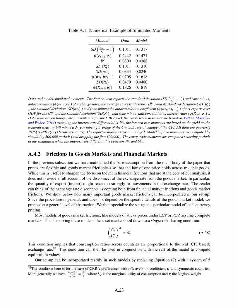
Table A.1: Numerical Example of Simulated Moments

Moment Data Model

SD(

et+1et−1)

0.1011 0.1317

φ(et+1,et) 0.2442 0.1471Rc 0.0300 0.0388

SD(Rct ) 0.1011 0.1310

SD(nxt) 0.0334 0.0240φ(nxt ,nxt−1) 0.0708 0.1618

SD(Rt) 0.0479 0.0480φ(Rt+1,Rt) 0.1826 0.1819

Data and model-simulated moments. The first column reports the standard deviation (SD(et+1

et−1)) and (one minus)

autocorrelation (φ(et+1,et)) of exchange rates, the average carry trade return (Rc ) and its standard deviation (SD(Rct )

), the standard deviation (SD(nxt) ) and (one minus) the autocorrelation coefficient (φ(nxt ,nxt−1) ) of net exports overGDP for the US, and the standard deviation (SD(Rt) ) and (one minus) autocorrelation of interest rates (φ(Rt+1,Rt) ).Data sources: exchange rate moments are for the GBP/USD, the carry trade moments are based on Lettau, Maggioriand Weber (2014) assuming the interest rate differential is 5%, the interest rate moments are based on the yield on the6-month treasury bill minus a 3-year moving average of the 6-month rate of change of the CPI. All data are quarterly1975Q1-2012Q2 (150 observations). The reported moments are annualized. Model implied moments are computed bysimulating 500,000 periods (and dropping the first 100,000). The carry trade moments are computed selecting periodsin the simulation when the interest rate differential is between 4% and 6%.

A.4.2 Frictions in Goods Markets and Financial MarketsIn the previous subsection we have maintained the base assumption from the main body of the paper thatprices are flexible and goods market frictionless so that the law of one price holds across tradable goods.While this is useful to sharpen the focus on the main financial frictions that are at the core of our analysis, itdoes not provide a full account of the disconnect of the exchange rate from the goods market. In particular,the quantity of export (import) might react too strongly to movements in the exchange rate. The readercan think of the exchange rate disconnect as coming both from financial market frictions and goods marketfrictions. We show below how many important goods market frictions can be incorporated in our set-up.Since the procedure is general, and does not depend on the specific details of the goods market model, weproceed at a general level of abstraction. We then specialize the set-up to a particular model of local currencypricing.

Most models of goods market frictions, like models of sticky prices under LCP or PCP, assume completemarkets. Thus in solving these models, the asset markets boil down to a single risk sharing condition:(

Ct

C∗t

)σ

= Et . (A.58)

This condition implies that consumption ratios across countries are proportional to the real (CPI based)exchange rate.82 This condition can then be used in conjunction with the rest of the model to computeequilibrium values.

Our set-up can be incorporated readily in such models by replacing Equation (7) with a system of 5

82The condition here is for the case of CRRA preferences with risk aversion coefficient σ and symmetric countries.More generally we have: Uc(C∗t )

Uc(Ct )= Et

ν, where Uc is the marginal utility of consumption and ν the Negishi weight.

A.23

equations that fully characterize the imperfect financial markets in our model. These equations are:

1 = Et

[βt

C−σ

t+1

C−σt

Pt

Pt+1Rt+1

], (A.59)

1 = Et

[β∗t

C∗−σ

t+1

C∗−σt

P∗tP∗t+1

R∗t+1

], (A.60)

Qt =P∗tΓEt

[(ηβt

C−σ

t+1

C−σt

Pt

Pt+1+(1−η)β ∗t

et

et+1

C∗−σ

t+1

C∗−σt

P∗tP∗t+1

)(etRt+1− et+1R∗t+1

)], (A.61)

Qt = P∗t ftet − ftPt −Dt , (A.62)

Dt = RtDt−1 +(ηQt−1− et−1 ft−1P∗t−1)

(Rt −R∗t

et

et−1

)+ etP∗H,tC

∗H,t −PF,tCF,t . (A.63)

Notice that these equations are the same (slightly more general) block of equations we used to solve theself contained model in the previous subsection. In this sense these equations are quite portable and can beembedded in larger set-ups. Before we do so, we analyze each equation in turn. Equations (A.59-A.60) arestandard Euler equations for a CRRA agent trading nominal risk-free interest rates. Equation (A.61) is thedemand equation of the financiers, which in this case we extended to the nominal set-up (Qt is in nominaldollars). Equation (A.62) is the market clearing condition for the foreign exchange market. Equation (A.63)is the evolution of the US net foreign assets. The last two terms on the right hand side of Equation (A.63)are US net exports in nominal dollars. Note that we are allowing for local currency pricing (i.e. P∗H,t is thenominal price in Yen of US export goods faced by the Japanese in Japan). Finally, the exogenous forcingvariables for flow shocks ( f , f ∗), which are defined in real terms, and discount factor shocks are given byEquations (A.55-A.57).

We report below the first order approximation (log-linearization) to the above system of equations:83

rt+1 = xt +Et [∆pt+1 +σ∆ct+1], (A.64)

r∗t+1 = x∗t +Et [∆p∗t+1 +σ∆c∗t+1], (A.65)

qt =1ΓEt [rt+1− r∗t+1−∆et+1], (A.66)

qt = ft − f ∗t − dt , (A.67)

∆dt = β−1

∆dt−1 +C∗H [∆c∗H,t −∆cF,t +∆et +∆p∗H,t −∆pF,t ], (A.68)

where qt , dt are expressed in deviation from steady state and are in units of real dollars (i.e. Q≡ Q/P), andC∗H is the steady state level of US export quantities.

Contrary to the model in the previous section, the above equations do not describe the entire equilibriumin the present set-up. For example, the dynamics of import and export prices (∆p∗H,t−∆pF,t) will depend onoptimal price setting conditions by producers. In order to analyze one interesting example of equilibrium,we embed the above financial market set-up in the new-Keynesian model with sticky prices in local currency

83Since in many nominal models, including the one that we consider here, the price level is not stationary we log-linearize the real version of the system of equations around the deterministic steady state. All variables are expressedin percentage deviation from steady state. For variables such as Qt that have value zero in steady state, we linearizerather than log-linearize.

A.24

described in the Handbook of International Economics chapter of Burstein and Gopinath (2015).84 In theinterest of not stating from first principles an extensive model that is not the main focus of our paper, werather summarize their set-up and refer the interested reader to the original paper.

The model in Burstein and Gopinath (2015) consists of two symmetric countries with infinitely livedagents who consume a composite final good composed of non-tradable and tradable goods. All goods areproduced with a technology linear in labor with no productivity shocks and no capital. Households have anisoelastic disutility of labor and wages are flexible. The tradable component of the final good is itself anaggregator of intermediate goods produced domestically and in the foreign economy. Intermediate goodsproducers are monopolistically competitive and set their prices according to a Calvo mechanism. Whenselected to re-set prices producers can choose, at the same time, two different prices for the domestic marketin domestic currency and for the foreign market in foreign currency (hence the local currency pricing).Agents are subject to a cash in advance constraint that always binds and sets the level of nominal expenditurein each period equal to the exogenous money supply (PtCt = Mt). The growth rate of the money supplyfollows an AR(1) process.

We close the model in Burstein and Gopinath (2015) by removing the complete market risk sharingequation (the analogous of Equation (7)) and replacing it with our financial structure (Equations A.64-A.68). In Table A.2 we report a simulated numerical example of the resulting model. We stress that this isan example, without the pretense of being a full quantitative assessment.85

The model appears to be able to broadly match major moments of the data. Many moments are similarto those shown in the previous subsection in the case of fully flexible prices. Of particular interest is thecorrelation between export quantities and nominal exchange rates. Columns 3 and 4 of Table A.2 show thatthe correlation decreases, while leaving most other macro moments unchanged, as prices in local currencybecome stickier (κ being the probability of not adjusting the price in a given period). Intuitively, a nominaldepreciation of the USD does not lead to a big export increase if US producers keep their price constant inJapanese yen. This is one of the main roles played by the goods market frictions here. A correspondingmoment in the data is not readily identifiable given that price adjustment frequencies change substantiallyacross goods and countries often use a combination of LCP and PCP. We thus prefer to show the abilityof the model to generate an imperfect correlation, with lower correlation for goods with higher level ofstickiness in local currency.86 The goods market pricing frictions, together with the financial frictions,also help break the complete market risk sharing equation, i.e. the Backus and Smith condition. Backusand Smith (1993) document that consumption growth rates across countries are largely unrelated to realexchange rates. On the contrary, the complete market risk sharing equation (Equation (7)) implies a perfectcorrelation. Our financial imperfections break the Backus and Smith condition, and interestingly interactwith the price setting frictions (which affect the real exchange rate dynamics) to produce a relatively lowcorrelation between consumption and real exchange rates.87

84In particular see Sections 7 and 9 in Burstein and Gopinath (2015). The handbook chapter itself builds on the modelof Carvalho and Nechio (2011).85We parametrize the model following most closely Carvalho and Nechio (2011). We set β = 0.985 to obtain a6% steady state rate of interest, the autocorrelation of money growth at 0.55 and its standard deviation at 0.015, therelative risk aversion of the agents (σ ) at 3, the Frisch elasticity at 1, the share of non-tradables at 0.5, and the importshare in tradables at 0.25, the elasticity of substitution between imported and home intermediate goods at 1.5, and wevary the probability of price adjustment between 0.49 and 0.6. Finally we set φ f = 0.05,σ f = 0.1,φx = 0.0491,σx =0.0073,Γ = 0.1. All shocks are orthogonal.86Aggregation of the micro evidence to a symmetric macro model, like the one considered here, is an arduous task.For example, Gopinath and Rigobon (2008) show that for the US export goods tend to predominantly be under PCPbut import goods tend to be under LCP, furthermore within each type of pricing the frequency of price adjustmentvaries substantially across goods.87Indeed Burstein and Gopinath (2015) note that in the model that they analyze under the assumption of complete

A.25

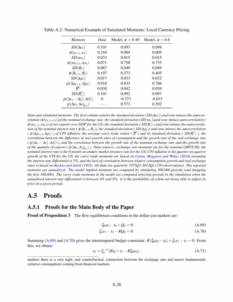
Table A.2: Numerical Example of Simulated Moments: Local Currency Pricing

Moment Data Model, κ = 0.49 Model, κ = 0.6

SD(∆et) 0.101 0.093 0.098φ(et+1,et) 0.244 0.004 0.005SD(nxt) 0.033 0.015 0.015

φ(nxt+1,nxt) 0.071 0.758 0.755SD(Rt) 0.067 0.049 0.049

φ(Rt+1,Rt) 0.197 0.373 0.405SD(∆pt) 0.017 0.033 0.032

ρ(∆pt+1,∆pt) 0.918 0.833 0.786RC 0.030 0.042 0.039

SD(RCt ) 0.101 0.092 0.097

ρ(∆ct −∆c∗t ,∆Et) 0 -0.373 -0.033ρ(∆et ,∆c∗H,t) −− 0.573 0.392

Data and simulated moments. The first column reports the standard deviation (SD(∆et)) and (one minus) the autocor-relation (φ(et+1,et))of the nominal exchange rate, the standard deviation (SD(nxt))and (one minus) autocorrelation (φ(nxt+1,nxt)) of net exports over GDP for the US, the standard deviation ( SD(Rt) ) and (one minus) the autocorrela-tion of the nominal interest rate ( φ(Rt+1,Rt)), the standard deviation ( SD(∆pt)) and (one minus) the autocorrelation( ρ(∆pt+1,∆pt) ) of CPI inflation, the average carry trade return ( RC) and its standard deviation ( SD(RC

t ) ), thecorrelation between the difference in real growth rates of consumption and the growth rate of the real exchange rate( ρ(∆ct −∆c∗t ,∆Et) ), and the correlation between the growth rate of the nominal exchange rate and the growth rateof the quantity of exports ( ρ(∆et ,∆c∗H,t) ). Data sources: exchange rate moments are for the nominal GBP/USD, thenominal interest rate is the 6-month secondary market treasury rate for the US, CPI inflation is the quarter-on-quartergrowth of the CPI for the US, the carry trade moments are based on Lettau, Maggiori and Weber (2014) assumingthe interest rate differential is 5%, and the lack of correlation between relative consumption growth and real exchangerates is based on Backus and Smith (1993). All data are quarterly 1975Q1-2012Q2 (150 observations). The reportedmoments are annualized. The model implied moments are computed by simulating 500,000 periods (and droppingthe first 100,000). The carry trade moments in the model are computed selecting periods in the simulation when theannualized interest rate differential is between 4% and 6%. κ is the probability of a firm not being able to adjust itsprice in a given period.

A.5 Proofs

A.5.1 Proofs for the Main Body of the PaperProof of Proposition 3 The flow equilibrium conditions in the dollar-yen markets are:

ξ0e0− ι0 +Q0 = 0, (A.69)

ξ1e1− ι1−RQ0 = 0. (A.70)

Summing (A.69) and (A.70) gives the intertemporal budget constraint: R(ξ0e0− ι0)+ξ1e1− ι1 = 0. Fromthis, we obtain:

e1 = ξ−11 (Rι0 + ι1−Rξ0e0) . (A.71)

markets there is a very tight, and counterfactual, connection between the exchange rate and macro fundamentals(relative consumption) coming from financial markets.

A.26

The market clearing in the Dollar / Yen market, ξ0e0− ι0 +1ΓE[e0− R∗

R e1]= 0, gives:

R∗

RE [e1] = e0 +Γ(ξ0e0− ι0) = (1+Γξ0)e0−Γι0. (A.72)

Combining (A.71) and (A.72),

E [e1] = E[ξ−11 (Rι0 + ι1)

]−E

[ξ−11

]ξ0Re0 =

RR∗

(1+Γξ0)e0−RR∗

Γι0,

i.e.

e0 =RR∗Γι0 +E

[ξ−11 (Rι0 + ι1)

]RR∗ (1+Γξ0)+E

[ξ−11

]ξ0R

=

(E[R∗ξ−1

1

]+Γ)

ι0 +E[R∗

R ξ−11 ι1

](E[R∗ξ−1

1

]+Γ)

ξ0 +1

=E[

R∗ξ1

(ι0 +

ι1R

)]+Γι0

E[

R∗ξ1

(ξ0 +

ξ1R∗

)]+Γξ0

.

We can now calculate e1. We start from its expected value:

R∗

RE [e1] = (1+Γξ0)e0−Γι0 = (1+Γξ0)

(E[

R∗ξ1

]+Γ

)ι0 +E

[R∗ξ1

ι1R

](E[

R∗ξ1

]+Γ

)ξ0 +1

−Γι0

=

(1+Γξ0)

(E[

R∗ξ1

]+Γ

)−Γ

[(E[

R∗ξ1

]+Γ

)ξ0 +1

]ι0 +(1+Γξ0)E

[R∗ξ1

ι1R

](E[

R∗ξ1

]+Γ

)ξ0 +1

=E[

R∗ξ1

]ι0 +(1+Γξ0)E

[R∗ξ1

ι1R

](E[

R∗ξ1

]+Γ

)ξ0 +1

=E[

R∗ξ1

(ι0 +

ι1R

)]+Γξ0E

[R∗ξ1

ι1R

]E[

R∗ξ1

(ξ0 +

ξ1R∗

)]+Γξ0

.

To obtain the time-1 innovation, we observe that e1 =1ξ1(Rι0 + ι1−Rξ0e0) implies:

e1=

ι1

ξ1

+R(ι0−ξ0e0)

1ξ1

.

As:

ι0−ξ0e0 = ι0−ξ0

(E[

R∗ξ1

]+Γ

)ι0 +E

[R∗ξ1

ι1R

](E[

R∗ξ1

]+Γ

)ξ0 +1

=ι0−E

[ξ0

R∗ξ1

ι1R

](E[

R∗ξ1

]+Γ

)ξ0 +1

,

we obtain:

e1=

ι1

ξ1

+R

ι0−E[ξ0

R∗ξ1

ι1R

](E[

R∗ξ1

]+Γ

)ξ0 +1

1ξ1

.

We next derive the value of Γ. Notice that we can write the above equation as:

e1= ε +1

a+Γη ,

ε ≡

ι1

ξ1

,

A.27

η ≡(

ι0−E[

ξ0R∗

ξ1

ι1

R

])1ξ0

1ξ1

,

a≡ E[

R∗

ξ1

(ξ0 +

ξ1

R∗

)]1ξ0

.

Then,

var (e1) = σ2ε +

2σεη

a+Γ+

σ2η

(a+Γ)2 .

Letting G(Γ) be

G(Γ)≡ Γ− γ

(σ

2ε +

2σεη

a+Γ+

σ2η

(a+Γ)2

)α

, (A.73)

then Γ is defined asG(Γ) = 0. (A.74)

When α = 0, we get the basic Gamma model. When α = 1, we have a polynomial of degree 3 in Γ. Whenthere is no noise and α > 0, Γ = 0. In general, it is still amenable to computation: there is a unique positivesolution of G(Γ) (as G(Γ) is increasing in Γ, and G(0)< 0, limΓ→∞ G(Γ) = ∞).

Proof of Lemma 3 In the decentralized allocation, the consumer’s intra-period consumption, Equation(5), gives the first order conditions:

pNTCNT =χ

λ; p∗NTC∗NT =

χ∗

λ ∗;

pHCH =aλ

;pH

eC∗H =

ξ

λ ∗; (A.75)

ep∗FCF =ι

λ; p∗FC∗F =

a∗

λ ∗.

so that

e =C∗H λ ∗

ξ

CH λ

a

.

Suppose that the Negishi weight is ν . The planner maximizes U +νU∗ subject to the resource constraint;hence, in particular maxCH+C∗H≤YH a lnCH +νξ lnC∗H , which gives the planner’s first order condition a

CH= νξ

C∗H.

Hence, in the first best exchange rate satisfies:

eFBt = ν

λ ∗tλt

= νpNTCNT, t/χt

p∗NTC∗NT, t/χ∗t.

In the basic case of Lemma 3, we have λt = λ ∗t = 1, so eFBt = ν . Note that this is derived under the

assumption of identical discount factor β = β ∗.

Proof of Proposition 7 We first prove a Lemma.

Lemma A.6 In the setup of Proposition 3, e0 is increasing in ιt and R∗ and decreasing in ξt and R; ∂e0∂ ι0

increases in Γ. In addition, e0 increases in Γ if and only the US is a natural net debtor at time 0+, i.e.N0+ ≡ ξ0e0− ι0 < 0.

A.28

Proof: The comparative statics with respect to ιt ,ξ0, and R are simply by inspection. We report here the lessobvious ones:

∂e0

∂ξ1=

E[

e0ξ0−ι0−ι1R

ξ 21

]E[

ξ0+ξ1R∗

ξ1

]+ Γξ0

R∗

=−E[

e1Rξ1

]E[

ξ0+ξ1R∗

ξ1

]+ Γξ0

R∗

< 0,

where we made use of the state-by-state budget constraint e0ξ0− ι0 +e1ξ1−ι1

R = 0. To be very precise, anotation like ∂e0

∂ξ1is the sensitivity of e0 to a small, deterministic increment to random variable ξ1.

∂e0

∂R∗=

1R∗2

e0−ΓQ

E[

ξ0+ξ1R∗

ξ1

]+ Γξ0

R∗

=1

RR∗E [e1]

E[

ξ0+ξ1R∗

ξ1

]+ Γξ0

R∗

> 0,

where we made use of the financiers’ demand equation, ΓQ0 = E[e0− R∗

R e1], and the flow equation, ξ0e0−

ι0 +Q0 = 0.We also have,

∂e0

∂Γ=−N0+

1

1+R∗E[

ξ0ξ1

]+ξ0Γ

< 0,

where we made use of the definition N0+ = e0ξ0− ι0. This implies:

∂ 2e0

∂Γ∂ ι0=

1(R∗E

[ξ0ξ1

]+1+Γξ0

)2 > 0.

This implies all the points of Proposition 7 with two exceptions. The effects with respect to interest ratechanges, both domestic and foreign, hold for f , f ∗ sufficiently small. Finally, we focus on the impact of f ∗.Simple calculations yield:

∂e0

∂ f ∗=− Γ

R∗E[

ξ0ξ1

]+1+Γξ0

< 0.

We notice that the comparative statics with respect to f are less clear-cut, because f affects the value of Γξ1,and hence affects risk-taking. However, we have ∂e0

∂ f > 0 for typical values (e.g. R = R∗ = 1, ξ0 = ξ1).

Proof of Lemma 5 and Proposition 8 The economy is described by:

e0−1−qe0 +Q0 = 0; e1− ι1 +qe1−Q0 = 0.

Using Proposition 6 (with ξ0 = 1−q, ξ1 = 1+q), we have:

e0 (q) = 1+Γ(q+q2

)2+Γ(1−q2)

, (A.76)

e1 (q) = 1+Γ(−q+q2

)2+Γ(1−q2)

+ε

1+q. (A.77)

where we define ε ≡ ι1−1, the innovation to ι1 (recall Eι1 = 1). This implies Lemma 5.The intervention’s impact on the average exchange rate is only second order: it creates a depreciation at

time 0, and an appreciation at time 1.

A.29

Recall that we assume a∗t = ιt to keep the countries symmetric in their demands of tradables, and simplifythe algebra. Given equation (A.75) and λt = λ ∗t = 1, we can define st ≡ CH,t

CH,t+C∗H,t=

CF,tCF,t+C∗F,t

to be the realUS share of consumption in both US or Japanese tradables. This share is equal to:

st =1

1+ et. (A.78)

By definition, US consumption of good g is Cg,t = stYg,t , where Yg,t is the world production of good g.US welfare at time t is (dropping the non-tradables endowment term, and correspondingly setting χ = 0 foralgebraic convenience):

Ut = at lnCH,t + ιt lnCF,t = at ln(stYH,t)+ ιt ln(stYF,t)

= (at + ιt) lnst +at lnYH,t + ιt lnYF,t ,

and intertemporal US welfare is (using at = 1):

U (q) = E [U0 +U1] = E1

∑t=0

((1+ ιt) lnst + lnYH,t + ιt lnYF,t) .

US production of tradables at time 0 is (by equation (25)): YH,0 = min(

1+e0pH

,L)

, so YH,0 increases in e fore ∈ [0,e0], with e0 ≡ pHL−1. Hence:

U (q) = lnmin(

1+e0 (q)pH

,L)+h(q)+K, (A.79)

where h(q)≡ E∑1t=0 (1+ ιt) lnst captures the allocational distortions, and K = 3lnL is a constant indepen-

dent of policy (as prices are flexible at t = 1 in the US). Hence, US welfare goes up when its share st ishigher and when world production is higher (YH,0 higher).

We shall see that the intervention on a scale q, by inducing a time-0 Dollar devaluation (i) improves bya first order effect the production at time 0, and (ii) leads only to a second order loss in the total share ofconsumption h(q). Hence, the intervention is desirable. In addition, it is desirable also for Japan: Japanbenefits from the increase in world production, and experiences only a second order change from the inter-temporal distortion. Let us see this analytically.

We define, by analogy with (A.79):

V (q)≡ ln1+e0 (q)

pH+h(q)+K,

so that V (q) =U (q) when 1+e0(q)pH≤ L, i.e. in the unemployment region. We have: V ′ (0) = e′0(0)

1+e0(0)+h′ (0)

and e0 (0) = 1. Taking the derivative of (A.76) and (A.77) at q = 0 gives:

e′0 (0) =Γ

2+Γ, (A.80)

e′1 (0) =−Γ

2+Γ− ε. (A.81)

Hence:V ′ (0) =

Γ

2(2+Γ)+h′ (0) .

A.30

Recalling ι1 = 1+ ε we then compute:

h′ (0) = E1

∑t=0

(1+ ιt)d lnst

dq

∣∣∣∣q=0

=−2e′0(0)

1+ e0 (0)−E

[(2+ ε)

e′1(0)1+ e1 (0)

]by (A.78)

=−2Γ

2+Γ

2−E

[(2+ ε)

−Γ

2+Γ− ε

2+ ε

]= 0.

This confirms that intertemporal distortions induced are second order.Given V ′ (0)> 0, by continuity, there exists a qmax such that V ′ (q)> 0 for q ∈ [0,qmax). We call q(e0)

the inverse of the function e0 (q). Since e0 (q) is an increasing function (for q≥ 0), so is q(e0). Recall alsothat the least-devalued exchange rate that ensures full employment is e0 = pHL−1. Define pmax

H such thatq(pmax

H L−1) = qmax. Finally, recall that pH,0 = 2L is the flexible equilibrium price of US tradable. The

assumption that there is unemployment initially is equivalent to pH > pH,0.Take an initial price pH ∈ (pH,0, pmax

H ). To eliminate unemployment caused by pH , the governmentcan perform the intervention qopt ≡ q(pHL−1). Now, given that q(·) is increasing and pH < pmax

H , wehave qopt < qmax. Given that V ′ (q) > 0 for q ∈ [0,qmax), and that U ′ (q) = V ′ (q) for q ∈ [0,qopt), we haveU ′ (q)> 0 for q ∈ [0,qopt). This means that welfare is increasing in the size of the intervention, in the rangeq ∈ [0,qopt).

Japanese welfare. It is intuitive that Japanese welfare will also increase when the US government’sFX intervention devalues the Dollar: Japan enjoys a first-order gain from the increase in US productionand experiences only a second-order change from the intertemporal distortion (at least, omitting for nowpotential Jensen’s terms). Of course, this hinges on the assumption that prices are flexible in Japan. Weprovide here the more formal arguments.

Defining s∗t to be the Japanese share of tradables at t,

s∗t = 1− st =et

1+ et,

Japanese utility at time t is (using a∗t = ιt , ξt = 1):

U∗t = a∗t lnC∗H,t +ξt lnC∗F,t = ιt lns∗t YH,t + lns∗t YF,t

= (1+ ιt) lns∗t + ιt lnYH,t + lnYF,t .

Hence, Japanese welfare is

U∗ (q) = E [U∗0 +U∗1 ] = E1

∑t=0

((1+ ιt) lns∗t + ιt lnYH,t + lnYF,t)

= lnmin(

1+e0 (q)pH

,L)+h∗ (q)+K,

defining h∗ (q) ≡ E∑1t=0 (1+ ιt) lns∗t . We define, as for the US case, V ∗ (q) ≡ ln 1+e0(q)

pH+ h∗ (q)+K. That

A.31

implies:

V ∗′(0) =

e′0 (0)1+ e0 (0)

+h∗′(0)

=Γ

2(2+Γ)+h∗

′(0) .

We next calculate h∗′ (0). We start with lns∗t = ln et1+et

= lnet − ln(1+ et), so

d lns∗tdq

∣∣∣∣q=0

= e′t (0)[

1et (0)

− 11+ et (0)

]=

e′t (0)et (0)(1+ et (0))

and:

h∗′(0) = E

1

∑t=0

(1+ ιt)d lns∗t

dq

∣∣∣∣q=0

= E1

∑t=0

(1+ et (0))e′t (0)

et (0)(1+ et (0))using ιt = et (0) ,

= E1

∑t=0

e′t (0)et (0)

= e′0 (0)+E−e′0 (0)− ε

1+ εusing (A.80)-(A.81) and e1 (0) = 1+ ε

=(e′0 (0)−1

)E

ε

1+ ε=

(Γ

2+Γ−1)E

ε

1+ ε

=− 22+Γ

Eε

1+ ε

≥ 0

because the function x1+x is concave in the domain x >−1, and Eε = 0, so that E ε

1+ε≤ 0.

Summing up, we have:

V ∗′(0) =

Γ

2(2+Γ)+h∗

′(0)≥ Γ

2(2+Γ)> 0

Given V ∗′(0)> 0, by continuity, there is a qmax,∗ such that V ∗

′(q)> 0 for q ∈ [0,qmax,∗). Hence (by the

reasoning done above for the US consumer), the Proposition also holds for Japanese welfare (i.e., welfarein both US and Japan increases as q increases, for q ∈ [0,qopt ]), provided that the initial distortion pH is nottoo great. More specifically, we should have pH ∈ (pH , pmax

H ), where we define pmaxH to be the price such

that q(pmaxH L−1) = min(qmax,qmax,∗).

Proof of Proposition 9 The proof is quite similar to that of Proposition 8. Given the countries aresymmetric in their taste for foreign tradable goods (at = ξt = 1, a∗t = ιt), the share of US consumption forboth the US and Japanese tradable good is st =

11+et

.

A.32

Intertemporal US welfare is:88

U = E [U0 +U1] = E1

∑t=0

(ιt +at) lnst +at lnYH,t + ιt lnYF,t ,

i.e.

U (τ) = lnmin(

1+e0 (τ)

pH,L)+h(τ)+K, (A.82)

where K is a constant independent of policy, and h(τ) captures the sum of the allocational distortions:

h(τ)≡ E1

∑t=0

(1+ ιt) lnst = E1

∑t=0

(1+ ιt) ln1

1+ et (τ).

We define:

V (τ) = ln1+e0 (τ)

pH+h(τ)+K,

the counterpart of U (τ), without the “min” sign (V (τ) is welfare, assuming that the economy is below fullemployment).

We recall:

e0 (τ) =

(1+ Γ

1−τ

)ι0 +E [ι1]

2+ Γ

1−τ

,

e1 (τ) =ι0 +

(1+ Γ

1−τ

)E [ι1]

2+ Γ

1−τ

+ι1 ,

which implies

e′0 (0) = Γι0−E[ι1]

(2+Γ)2 =−e′1 (0) ,

so that

h′ (0) =−E1

∑t=0

(1+ ιt)e′t (0)

1+ et (0) ,

h′ (0) =−e′0 (0)D,

D≡ E[

1+ ι0

1+ e0 (0)− 1+ ι1

1+ e1 (0)

]The marginal impact welfare of a small tax is:

V ′ (0) =e′0 (0)

1+ e0(0)+h′ (0) = e′0 (0)

[1

1+ e0(0)−D

].

We observe that when Eι1 = ι0, then e0 (0) = ι0 and e1 (0) = ι1, so that 1+ι01+e0(0)

− 1+ι11+e1(0)

= 0 and D = 0.By continuity, when |Eι1− ι0| is small enough, D is close to 0. Hence, we assume that |Eι1− ι0| is smallenough, so that we have 1

1+e0(0)−D > 0. That implies V ′ (0)> 0.

88The analysis for Japanese welfare is entirely symmetric: the same small tax creates a first-order improvement inJapanese welfare because it increases US tradable output and hence the Japanese equilibrium consumption of UStradable goods, but only creates a smaller distortion in the intertemporal Japanese consumption shares.

A.33

Given V ′ (0)> 0, by continuity, there is a τmax such that V ′ (τ)> 0 for τ ∈ [0,τmax).We call τ (e0) the inverse of the function e0 (τ). Define pmax

H such that τ (pmaxH L−1) = τmax. Then, for

all pH ∈ [pH,0, pmaxH ), we have U ′ (τ)> 0 for τ ∈ [0,τ (pH −1)]. This means that welfare is increasing in the

size of the intervention. The optimal intervention in that range is τopt = τ (pH −1), the smallest (positive)tax that restores full employment.

The part on Japanese welfare is proven by exactly the same arguments as the arguments above, and thoseof the Japanese welfare part at the end of the proof of Proposition 8.

Proof of Proposition 10 Suppose that m∗′

0 deviates from its original value, 1, keeping m∗1 constant.Then, R∗

′= 1/m∗

′0 , hence (by Proposition 6) e′0 = 1/m∗

′0 , while e1 is unchanged at 1. Japanese demand for

US exports is unchanged because e′0m∗′

0 = 1 . Hence, the US export market is still in equilibrium with theUS at full employment (YH,0 = L). There is no need for policy intervention to ensure full employment.

Proof of Proposition 11 The case of short-lasting rigidity. We follow the notations and procedure ofthe proof of Proposition 8. To make the proof readable, we simply consider the case with ι1 ≡ 1. One canrestate the arguments of the proof of Proposition 8 for the more general case.

We first derive the exchange rate. The pseudo-imports and exports are:

ι0 = m0; ι1 = 1;

ξ0 = 1−q; ξ1 = 1+q.

and the gross interest rates are: R = 1m0

and R∗ = 1.The exchange rate is (using Proposition 3 and Proposition 6):

e0 =

E[

ι0+ι1R

ξ1

]+ Γι0

R∗

E[

ξ0+ξ1R∗

ξ1

]+ Γξ0

R∗

= m02+Γ(1+q)2+Γ(1−q2)

;

e1 =RR∗

E[

R∗

ξ1

(ι0 +

ι1R

)]+Γξ0E

[R∗

ξ1

ι1R

]E[

R∗

ξ1

(ξ0 +

ξ1R∗

)]+Γξ0

=1

m0m0

2+Γ(1−q)2+Γ(1+q)(1−q)

=2+Γ(1−q)2+Γ(1−q2)

.

with e1= 0. Hence,

e0 = m0 (1+η0) ; e1 = 1+η1,

where η0 =Γ(q+q2)

2+Γ(1−q2)and η1 =

Γ(−q+q2)2+Γ(1−q2)

are the expressions we found in the proof of Proposition 8.

Output is: YH,t = min(

at mt+ξt et m∗tpH

,L)= min

(m0+e0

pH,L)

, i.e.,

YH,t = min(

m0 (2+η0)

pH,L).

A.34

US welfare is given by (A.79), augmented for the cost of monetary distortions:

U (q) = lnmin(

1+e0 (q)pH

,L)+h(q)−g(m0)+K, (A.83)

where K = 3lnL is a constant, and h(q) ≡ 2E∑1t=0 lnst is the sum of the allocational distortions, with st is

the share of the home good going to the US: st =1

1+ etmt

, i.e.

st =1

2+ηt.

Let us compute a few expressions that will be useful in later derivations. We will use the Taylor expansionsbelow, when q is small, i.e. when η0 and η1 are small:

η0 =Γ

2+Γq+O

(q2) ,

which implies

q =2+Γ

Γη0 +O

(η

20),

η1 +η0 =2Γq2

2+Γ(1−q2)=

2Γ

2+Γq2 +O

(q4)

=2Γ

2+Γ

(2+Γ

Γη0 +O

(η

20))2

+O(q4)= 2(2+Γ)

Γη

20 +O

(η

30)

= 2(

2Γ+1)

η20 +O

(η

30).

We now calculate the distortion term:

−h2=−

1

∑t=0

lnst =−1

∑t=0

ln1

2+ηt= ln [(2+η0)(2+η1)]

= ln [4+2(η0 +η1)+η0η1]

= ln[

4+2(

2(

2Γ+1)

η20 +O

(η

30))

+η0(−η0 +O

(η

20))]

= ln[

4+(

8Γ+3)

η20 +O

(η

30)]

= ln4+(

2Γ+

34

)η

20 +O

(η

30),

hence

h = h(η0,Γ) =−2ln4−(

4Γ+

32

)η

20 +O

(η

30). (A.84)

We can now reconsider welfare (A.83). For the purposes of the impact of Γ on the choice of monetaryversus FX policy, it is enough to consider the subproblem of achieving a given employment level YH , withoutoptimizing for YH . The problem is to minimize distortions subject to achieving the desired YH ≤ L:

minη0,m0

h(η0)−g(m0) s.t. m0 (2+η0) = pHYH .

A.35

This yields η0 = η0 (m0)≡ pHYHm0−2, so that the optimal monetary intervention is:

maxm0

W (m0) = h(η0 (m0))−g(m0) ,

so that Wm0 = 0 and Wm0m0 < 0 at the optimum.We want to ask: “do we have less reliance on monetary policy (rather than FX intervention) when Γ

increases?”. The answer is yes if ∂m0∂Γ

< 0. Accordingly, we calculate:

sign(

∂m0

∂Γ

)= sign

(−Wm0Γ

Wm0m0

)as Wm0 = 0 implies

∂m0

∂Γ=−Wm0Γ

Wm0m0

= sign(Wm0Γ) as Wm0m0 < 0

= sign(hη0Γη

′0 (m0)

)=−sign(hη0Γ) since η

′0 (m0)< 0

< 0,

since equation (A.84) implies hη0Γ > 0 for a small enough, positive intervention.Case of the long-lasting rigidity. Here we simply sketch the argument, given that the detailed analyticalforces have been already made explicit in the above proof and the proof of Proposition 8. An FX interven-tion won’t improve welfare for the following reason: a high intervention to buy Yen today makes the Yenappreciate today (which helps the US) but makes it (by the “boomerang” effect) depreciate tomorrow, by thesame amount. Hence, there has been no net help: the welfare impact of q policies is 0 on the unemploymentfront, and negative on the intertemporal distortion front. Hence, on net, a q policy has negative impact.

Hence, only monetary policy helps, in the usual way: the government wants to partially inflate, i.e.increase m0 and m1 (even though there’s a cost g of doing so).

Proof of Proposition 12

Rc=

E[R∗

R e1− e0]

e0=−ΓQ0

e0

=−Γ

(ι0− e0

e0

)= Γ

(1− ι0

e0

).

Recall that:

e0 =(R∗+Γ) ι0 +

R∗R E [ι1]

R∗+Γ+1,

so that we conclude:

Rc= Γ

(1− ι0

R∗+Γ+1(R∗+Γ) ι0 +

R∗R E [ι1]

).

which, rearranged, gives the announced expression.

Derivation of 3-period economy exchange rates We will use the notation:

R∗ ≡ R∗

R.

Recall that we assume that in period t = 1 financiers only intermediate the new flows; stocks arising fromprevious flows are held passively by the households (long term investors) until t=2. Therefore, from theflow demand equation for t = 1, e1− ι1 +Q1 = 0, and the financiers’ demand, Q1 =

e1−R∗E[e2]Γ1

, we get an

A.36

expression for e1:

e1 =Γ1ι1 +R∗E1 [e2]

Γ1 +1.

The flow demand equation for t = 2 gives e2 = ι2, so we can rewrite e1 as:

e1 =Γ1ι1 +R∗E1 [ι2]

Γ1 +1.

Similarly for e0, we have

e0 =Γ0ι0 +R∗E0 [e1]

Γ0 +1,

and we can use our expression for e1 above to express e0 as:

e0 =Γ0ι0 +R∗E0

[Γ1ι1+R∗ι2

Γ1+1

]Γ0 +1

.

Proof of Proposition 13 We have already derived Claim 1. For Claim 2, we can calculate, from thedefinition of carry trade returns (Rc ≡ R∗

Re1e0−1) and equation (28):

Rc= (R∗−1)Γ0

Γ1 +1+R∗

Γ1(Γ0 +R∗)+Γ0 +(R∗)2 > 0.

Hence, the expected carry trade return is positive.For Claim 3, recall that a function ax+b

cx+d is increasing in x iff ∆x ≡ ad−bc > 0. For Γ0,

∆Γ0 =

(1+Γ1 +R∗

)(Γ1R

∗+(R∗)2)> 0,

which proves ∂Rc

∂Γ0> 0.

For Γ1, the discriminant is

∆Γ1

(R∗−1)Γ0= Γ0 +(R∗)2− (1+R∗)(Γ0 +R∗) =−R∗ (1+Γ0)< 0,

so that ∂Rc

∂Γ1< 0.

Finally, for R∗, we simply compute:

∂Rc

∂R∗=

Γ0 (1+Γ0)(1+Γ1)(2R∗+Γ1

)(Γ0(1+Γ1

)+Γ1R∗+(R∗)2

)2 > 0.

Proof of Proposition 14 The regression corresponds to: βUIP = −∂

∂R∗E[

e1e0−1]. For simplicity we cal-

culate this derivative at R = R∗ = Eιt = 1, and with deterministic Γ1 = Γ1. Equation (28) yields, for thosevalues but keeping R∗ potentially different from 1:

e0 =Γ0 +R∗ Γ1+R∗

Γ1+1

Γ0 +1; Ee1 =

Γ1 +R∗

Γ1 +1.

A.37

Calculating βUIP = −∂

∂R∗E[

e1e0−1]= −∂

∂R∗Ee1e0

gives:

βUIP =1+Γ1−Γ0

(1+Γ0)(1+Γ1

) .Hence, βUIP ≤ 1+Γ1

(1+Γ0)(1+Γ1)= 1

1+Γ0< 1.

A.5.2 Proofs for Appendix A.1Proof of Proposition A.1 Derivation of equation (A.1). Assume ξt = 1. We start from the flowequation, NXt −RQt−1 +Qt = 0, and Qt =

Et [et−et+1]Γ

. Hence:

Γ(et − ιt)−R(et−1− et)+ et −Et [et+1] = 0,

i.e.Et [et+1]− (1+R+Γ)et +Ret−1 +Γιt = 0.

The characteristic equation of the (homogenous version) of this second order difference equation is:

g(X)≡ X2− (1+R+Γ)X +R = 0, (A.85)

and the solutions are:

λ =(1+R+Γ)−

√(1+R+Γ)2−4R

2; λ

′ =Rλ.

We define Λ = 1λ ′ , i.e. Λ = λ

R . The geometry of the solutions of a quadratic equation indicates (via λ < λ ′

and g(1)< 0 < g(0)) that we have 0 < λ < 1 < λ ′, hence Λ < 1R .

It is well-known that the solution is of the type et = AQt−1 +Et[∑

∞s=t(B(λ ′)t−s +Cλ t−s

)ιs], for some

constants A,B,C. Because λ < 1, we need C = 0, otherwise the sum would diverge. Hence, we can write:

et = AQt−1 +BEt

[∞

∑s=t

Λs−t

ιs

].

Also, when Qt−1 = 0 and ιs = ι for all s≥ t, we must have et = ι (indeed, then es is constant, so that Qs = 0and the dollar flow equation gives es− ι = 0). That gives 1 = B∑

∞s=t Λs−t = B

1−Λ, i.e. B = 1−Λ. Finally,

careful examination of the boundary condition at 0 (or use of the analogy ι0 ≡ ι0 +Q−0 ) gives AQ−1 = BQ−0 ,with Q−0 ≡ RQ−1. We conclude:

et = Et

[∞

∑s=t

Λs−t (1−Λ) ιs

]+(1−Λ)RQt−1.

Another proof is possible, relying on the machinery in Blanchard and Kahn (1980). We sketch thatalternative proof here. In terms of the Blanchard-Kahn notation, the system is

Et

(Qt

et+1

)=

(R −1−ΓR 1+Γ

)(Qt−1

et

)+

(1−Γ

)ιt

and the eigenvalues of the matrix are λ1 = λ , λ2 = 1/Λ. Then the value of et comes from the last equation

A.38

p.1309 of their paper, with µ ≡ (λ1−a11)γ1−a12γ2 in their notation.

Derivation of (A.2). It is enough to prove (A.2) for t = 0. First, the term f ∗s comes simply from usingιs = ιs− f ∗s and using (A.1). The more involved term concerns the interest rates. We note ρt ≡

R∗t+1Rt+1−1 the

interest rate differential. We perform a Taylor expansion in it. The financiers’ demand satisfies:

ΓQt = Et

[et − et+1

R∗tRt

]= Et [et − et+1 (1+ρt)] = Et [et − et+1]−ρtEt [et+1]

= Et [et − et+1]−ρte∗+o(ρt)

where we approximate Et [et+1] by the steady state value, e∗. For instance, e∗ = ι∗ξ∗

. Then, the Dollar-Yenbalance equation NXt −RQt−1 +Qt = 0 becomes (dropping for now the o(ρt) terms):

et − ιt −REt−1 [et−1− et ]−ρt−1e∗

Γ+

Et [et − et+1]−ρte∗Γ

= 0,

hence we have the same system as before, replacing ιt by

ιt ≡ ιt +e∗Γ(ρt −Rρt−1) ,

using the convention ρ−1 = 0 when we calculate e0 to simplify the boundary conditions. Indeed, we thenhave:

et − ιt −REt−1 [et−1− et ]

Γ+

Et [et − et+1]

Γ= 0.

Hence, equation (A.1) gives (when RQt−1 = 0)

e0 = (1−Λ)E0

[∞

∑s=0

Λsιs

]= (1−Λ)E0

[∞

∑s=0

Λsιs

]+H

H = (1−Λ)E0

[∞

∑s=0

Λs e∗

Γ(ρs−Rρs−1)

]

= (1−Λ)e∗ΓE0

[∞

∑s=0

Λs (1−RΛ)ρs

]by rearranging (by “Abel transformation”)

=(1−Λ)(1−RΛ)

Γe∗E0

[∞

∑s=0

Λsρs

],

and

(1−Λ)(1−RΛ)

Γ=

(1− λ

R

)(1−λ )

Γusing Λ =

λ

R

=λ 2− (1+R)λ +R

RΓ

=Γλ

RΓas λ satisfies (A.85)

= Λ,

A.39

so

H = Λe∗E0

[∞

∑s=0

Λsρs

],

Hence,

e0 = (1−Λ)E0

[∞

∑s=0

Λsιs

]+ e∗E0

[∞

∑s=0

Λs+1

ρs

]

= (1−Λ)E0

[∞

∑s=0

Λsιs

]+ e∗E0

[∞

∑s=0

Λs+1 R∗s −Rs

Rs

],

up to higher-order terms in R∗s −Rs. Finally, we verify that the f ∗s impact is present only when Γ > 0. The net present value of the noise

traders’ demand is 0: ∑∞s=t

1Rs−t fs =−F∗−t ,where F∗−t is the holding of the f ∗s traders at the beginning of time

t. As the US net foreign assets are Nt = Qt +F∗t , when Γ = 0 (so that Λ = 1R ) the expression reduces (when

ιt = ι∗, r∗t − rt = 0 for simplicity):

et = e∗+Et

∞

∑s=t

(1R

)s−t [(1− 1

R

)(− f ∗s )

]+

(1− 1

R

)Q−t

= e∗+(

1− 1R

)(Q−t +F∗−t

)= e∗+

(1− 1

R

)Nt ,

hence the actions of the noise traders don’t have an effect when Γ = 0.

Proof of Proposition A.2 Using Proposition A.1, we have:

Et−1et = 1+(1−Λ)RQt−1.

On the other hand, the equation of motion NXt −RQt−1 +Qt gives: E0et − 1−RE0Qt−1 +E0Qt = 0, soE0Qt = ΛRE0Qt−1 = λE0Qt−1 and

E0Qt−1 = λtQ−1

The debt due at t is Q−t = RQt−1; so E0Q−t = λ tQ−0 , and

E0et −1 = (1−Λ)RE0Qt−1 = (1−Λ)E0Q−t = (1−Λ)λ tQ−0

Appendix ReferencesBackus, David K., and Gregor W. Smith. 1993. “Consumption and real exchange rates in dynamic

economies with non-traded goods.” Journal of International Economics, 35(3-4): 297–316.Basak, Suleyman, and Anna Pavlova. 2013. “Asset prices and institutional investors.” The American Eco-

nomic Review, 103(5): 1728–1758.Blanchard, Olivier, and Charles Kahn. 1980. “The solution of linear difference models under rational

expectations.” Econometrica, 1305–1311.Burstein, Ariel, and Gita Gopinath. 2015. “Chapter 7 - International Prices and Exchange Rates.” In Hand-

book of International Economics. Vol. 4 of Handbook of International Economics, , ed. Kenneth RogoffElhanan Helpman and Gita Gopinath, 391 – 451. Elsevier.

Carvalho, Carlos, and Fernanda Nechio. 2011. “Aggregation and the PPP Puzzle in a Sticky-PriceModel.” American Economic Review, 101(6): 2391–2424.

A.40

Gopinath, Gita, and Roberto Rigobon. 2008. “Sticky Borders.” The Quarterly Journal of Economics,123(2): 531–575.

Lettau, Martin, Matteo Maggiori, and Michael Weber. 2014. “Conditional risk premia in currency mar-kets and other asset classes.” Journal of Financial Economics, 114(2): 197 – 225.

A.41