International Journal of Swarm - OMICS Publishing … algorithms for combinatorial, ... (EACO)...

Research Article Open Access

Diwekar and Gebreslassie, Int J Swarm Intel Evol Comput 2016, 5:2 DOI: 10.4172/2090-4908.1000131

Research Article Open Access

International Journal of Swarm Intelligence and Evolutionary Computation

Volume 5 • Issue 2 • 1000131Int J Swarm Intel Evol ComputISSN: 2090-4908 SIEC, an open access journal

Keywords: Efficient ant colony optimization (EACO), Hamersleysequence sampling (HSS), Metaheuristics, Oracle penalty method

IntroductionA wide range of optimization problems, which include a large

number of continuous and/or discrete design variables, fall into the category of linear programming (LP), nonlinear programming (NLP), integer programming (IP), mixed integer linear programming (MILP), and mixed integer nonlinear programming (MINLP). Gradient based methods such as Branch and Bound (BB), Generalized Bender's Decomposition (GBD), and Outer Approximation (OA), are generally used for solving IP, MILP, and MINLP problems. However, these methods have limitations whenever, the optimization problems do not satisfy convexity conditions, the problems have large combinatorial explosion, or the search domain is discontinuous [1]. Metaheuristic optimization strategies such as simulated annealing (SA) [2], genetic algorithm (GA) [3] and ant colony optimization (ACO) [4] can provide a viable alternative to the gradient based programming techniques. Review on metaheuristic algorithms can be viewed at Kahraman et al. [5]. One of the metaheuristic optimization techniques that attract researchers in recent years is an ACO algorithm. ACO algorithm was first introduced by Dorigo [4] and it has been receiving increased attention because of a series of successful applications in different disciplines such as routing, scheduling, machine learning, assignment, and design problems, and different branches of engineering [6-10]. Even though, ACO algorithm was practiced with great success for combinatorial optimization problems, in recent years, the research focus has been on extending the combinatorial ACO algorithm to continuous and mixed variable nonlinear programming problems. In this work, a new variant of ACO algorithm to solve deterministic optimization problems is proposed.

An ant colony is a population of simple, independent, asynchronous agents that cooperate to find a good solution to an optimization problem. In the case of real ants, the problem is to find good quality of food in a close vicinity of the nest, while in the case of artificial ants, it is to find a good solution to a given optimization problem [6]. A single ant is able to find a solution to its problem, but only cooperation among many individual ants through stigmergy (indirect communication) enables them to find good or global optimal solutions. Therefore, the ACO algorithm is inspired by the ants' foraging behavior. Natural ants deposit pheromone on the ground in order to mark some favorable path that should be followed by other members of the colony. ACO

algorithm exploits a similar mechanism for solving optimization problems [4]. It was originally introduced to solve combinatorial optimization problems, in which decision variables are characterized by a finite set of components. However, in recent years, its adaptation to solve continuous [11-14] and mixed variable [15-17] programming problems has received an increasing attention.

In this paper, a new strategy that improves the computational performance of ACO algorithm by increasing the initial solution archive diversity and the uniformity of the random operations using a quasi-random sampling technique referred as Hammersley Sequence Sampling (HSS) [20]. This sampling mechanism has been shown to exhibit better uniformity property over the multivariate parameter space than the crude Monte Carlo sampling (MCS) and the variance reduction techniques such as Latin hypercube sampling (LHS) [14-17]. The ACO benefits from the multivariate uniformity property of the HSS. Therefore, the main advantage of the proposed algorithm is the high computational efficiency attained from the EACO algorithm compared to the conventional ACO algorithm.

The rest of this article is organized as follows: The Ant colony optimization algorithms for combinatorial, continuous and mixed variables are presented in the next section. In Section 3, Oracle penalty method to solve constrained optimization problems is introduced. The "Sampling Techniques" are introduced in Section 4. The efficient ant colony optimization algorithm proposed in this work is presented in Section 5. Following the benchmark problems presentation in Section 6, results and discussions of the benchmark problems are presented in Section 7. Finally, the concluding remarks are presented in the Section 8.

*Corresponding author: Urmila M Diwekar, Center for Uncertain Systems: Toolsfor Optimization & Management (CUSTOM), Vishwamitra Research Institute,Crystal Lake, USA, Tel:(630)-886-3047, Email: [email protected]

Received March 03, 2016; Accepted March 06, 2016; Published March 10, 2016

Citation: Diwekar UM, Gebreslassie BH (2016) Efficient Ant Colony Optimization (EACO) Algorithm for Deterministic Optimization. Int J Swarm Intel Evol Comput 5: 131. doi: 10.4172/2090-4908.1000131

Copyright: © 2016 Diwekar UM, et al. This is an open-access article distributedunder the terms of the Creative Commons Attribution License, which permitsunrestricted use, distribution, and reproduction in any medium, provided theoriginal author and source are credited.

AbstractIn this paper, an efficient ant colony optimization (EACO) algorithm is proposed based on efficient sampling method

for solving combinatorial, continuous and mixed-variable optimization problems. In EACO algorithm, Hammersley Sequence Sampling (HSS) is introduced to initialize the solution archive and to generate multidimensional random numbers. The capabilities of the proposed algorithm are illustrated through 9 benchmark problems. The results of the benchmark problems from EACO algorithm and the conventional ACO algorithm are compared. More than 99% of the results from the EACO show efficiency improvement and the computational efficiency improvement range from 3% to 71%. Thus, this new algorithm can be a useful tool for large-scale and wide range of optimization problems. Moreover, the performance of the EACO is also tested using the five variants of ant algorithms for combinatorial problems.

Efficient Ant Colony Optimization (EACO) Algorithm for Deterministic OptimizationUrmila M Diwekar*and Berhane H GebreslassieCenter for Uncertain Systems: Tools for Optimization & Management (CUSTOM), Vishwamitra Research Institute, Crystal Lake, USA

Internationa

l Jou

rnal

of S

warm Intelligence and Evolutionary Computation

ISSN: 2090-4908


of 10


Ant Colony OptimizationThe ACO is a metaheuristic class of optimization algorithm

inspired by the foraging behavior of real ants [6]. Natural ants randomly search food by exploring the area around their nest. If an ant locates a food source, while returning back to the nest, it lay down a chemical pheromone trail that marks its path. This pheromone trail will indirectly communicate with other members of the ant colony to follow the path. Over time, the pheromone will start to evaporate and therefore reduce the attraction of the path. The routes that are used frequently will have higher concentration of the pheromone trial and remain attractive. Thus, the shorter the route between the nest and food source imply short cycle time for the ants and these routes will have higher concentration of pheromone than the longer routes. Consequently, more ants are attracted by the shorter paths in the future. Finally, the shortest path will be discovered by the ant colony [6,8].

In ACO algorithms, artificial ants are stochastic candidate solution construction procedures that exploit a pheromone model and possibly available heuristic information of the mathematical model. The artificial pheromone trails (numeric values) are the sole means of communication among the artificial ants. Pheromone decay, a mechanism analogous to the evaporation of the pheromone trial of the real ant colony allows the artificial ants to forget the past history and focus on new promising search directions. Like the natural ants, by updating the pheromone values according to the information learned in the preceding iteration, the algorithmic procedure leads to very good and hopefully, a global optimal solution.

ACO for Discrete optimization problems

In a discrete optimization problem (shown in Eqn.1), the search domain of the problem is partitioned into a finite set of components, and the discrete optimization algorithm attempts to find the optimal combination or permutation of a finite set of elements from large and finite set of the search domain [17].

Yyygyhts

yfx

∈≤=

0)(0)(..

)(min (1)

The combinatorial search space Y is given as a set of discrete variables yi where i = 1, ..., NDIM, with possible set of options

iNOPi

2i

1i ,...,, vvvNOPv i

ji =∈ . If a solution vector Yy∈ takes a value for

each decision variable that satisfies all the constraints, it is a feasible solution of the discrete optimization problem. A solution Yy ∈∗ is called a global optimal if and only if; Yyyfyf ∈∀≤∗ ),()( . Therefore, solving a discrete optimization problem involves finding at least one

Yy ∈∗ .

To solve a discrete optimization problem, artificial ants construct a solution by moving from one solution state to another in a sequential manner. Real ants walk to locate the shortest path by choosing a direction based on local pheromone concentrations and a stochastic decision policy. Likewise, the artificial ants construct solutions by moving through each decision variable guided by the value of the artificial pheromone trial and by making stochastic decisions at each state.

The important differences between the real and artificial ants are

• Artificial ants move sequentially through a finite set of decision variable set of options. Real ants move in a direction of the food by selecting from different passible paths, which are not finite.

• Real ants deposit and react to the concentration of the pheromone while walking. However, in artificial ants, sometimes the pheromone update is done only by some of the artificial ants, and often the pheromone updated is only after a complete solution is constructed.

• Artificial ants can introduce additional mechanisms to improve the solution such as adding local search strategies that does not exist in real ants.

The decision policy in choosing the solution component considers a trade-off between the pheromone intensity on a particular edge and the desirability of that edge with respect to the edge contribution on the objective function [4]. Taking these two properties of an edge into account, ACO algorithms effectively utilize the pheromone intensity which is based on the information learnt from the prior solution construction and the edge desirability. The decision policy is given by the transition probability function as shown in Eqn. 2.

(it)ij ijprob (it)ij (it)ij ijil

βατ η=

βατ η∑ (2)

where probij(it) is the probability of choosing edge ij as a solution component when an ant is at node i at iteration it, ij (it) τ is the pheromone value associated with edge ij at iteration it, ij (it) η is the desirability of edge ij. α and β are parameters that control the relative importance of pheromone intensity and desirability, respectively. If α >> β, the algorithm will make decisions based on mainly on the learned information, represented by the pheromone, and ifα << β, the algorithm will act as a greedy heuristic selecting mainly the cheapest edges, disregarding the learned information [6].

Evaluation of the pheromone value ij (it) τ at the end of each of the iteration is the core of ACO algorithm. After each ant has constructed a solution (i.e., at each iteration) the pheromone value on each edge is updated. The goal of the pheromone update is to increase the pheromone values associated with good or promising solutions, and to decrease those that are associated with bad ones. The pheromone updating rule consists of two operations:

• The pheromone evaporation operation that reduces the current level of pheromone

• The pheromone additive operation: depends on the quality of the solutions generated at the iteration, pheromone is added to the edge of good solutions. The updating rule is given as follows [6] as shown in Eqn. 3.

ij ij ij(it 1) (it) (it)τ + = ρτ + ∆τ (3)

Where ρ is the pheromone evaporation factor representing the pheromone decay (0 ≤ ρ ≤1) and ij (it)∆τ is the pheromone addition for edge ij. The decay of the pheromone levels enables the colony to 'forget' poor edges and increases the probability of good edges being selected (i.e. the assumption behind this is that as the process continues in time, the algorithm learns to add pheromone only to good edges, implying that more recent information is better than older information). For 1→ρ , only small amounts of pheromone are decayed between iterations and the convergence rate is slower. This is characterized by the high probability of finding the global optimal solution at the expense computational efficiency. Whereas for 0→ρmore pheromone is decayed resulting in a faster convergence. This trend leads to getting stuck at the local optimal solutions.


of 10


The pheromone addition operation is increasing the pheromone values associated with good or promising solutions and it is the main feature that dictates how an ACO algorithm utilizes its learned information. Typically, pheromone is only added to edges that have been selected, and the amount of pheromone added is proportional to the quality of the solution. In this way, solutions of higher quality receive higher amounts of pheromone [17]. The pheromone concentration added at iteration it is determined from Eqn. 4.

nAntsk

ij ijk

(it) (it)∆τ = ∆τ∑ (4)

Where the pheromone concentration associated with ant k as function of the quality of the objective function is determined as shown below.

( )( ) ∈∆ =

ij

if ij edgevisited by ant kf yit

Otherwise (5)

ACO algorithm to solve discrete optimization problems has five most popular variants which are the ant system (AS) [4], elitist ant system (EAS) [4], rank based ant system (RAS), ant colony system (ACS) and the Max-Min ant system (MMAS). For details of the ant algorithm variants, the book by Dorigo and Stutzle [6] can be viewed. These variants are derived from the AS algorithm and they follow similar solution construction procedure and pheromone evaporation procedure. The main differences among these variants are the way the pheromone update and pheromone trial management are performed.

ACO for Continuous domain optimization problem

Continuous variable optimization problems could be tackled with a discrete optimization algorithm only if the continuous ranges of the decision variables are discretized into finite sets [17]. The continuous ACO algorithm stores a set of K solutions in a solution archive which represents as the pheromone model of the combinatorial ACO algorithm. This solution archive is used to generate a probability distribution of the promising solutions over the search space. In this algorithm, the solution archive is first initialized and the algorithm iteratively finds the optimal solution by generating new solutions of size equal to the number of ants (nAnts). The new nAnts size solutions are then added to the K size solutions from the previous iteration. To propagate the updated K size solutions to the next iteration, the K + nAnts solutions are first sorted according to the quality of the objective function of each solution. Then, the solution archive is updated by keeping the best K solutions of the combined solutions and removing the worst nAnts size solutions. The details of the algorithm formulation can be found in Socha [17], but for the completion of this work the main features of the formulation are presented below.

Similar to the combinatorial ACO algorithm the solution construction of ants is accomplished in an incremental manner, i.e variable by variable. First, an ant chooses probabilistically one of the solutions in the solution archive as a solution construction guide. The probability of choosing solution j as guide is given by Eqn. 6:

∑=

=

K

rr

jjprob

1ω

ω (6)

where jω is the weight associated with solution j. The weight is determined using the Gaussian function [17] as follows:

2

2( j 1)

2(qK)j

1 eqK 2

− −

ω =π

(7)

where, j is rank of the solution in the archive, q is an algorithmic parameter and K is the size of the solution archive. The mean of the

Gaussian function is 1, so that the best solution has highest weight [17]. The ant treats each problem variable i = 1, . . . NDIM separately. It takes value i

jx of variable i of the jth solution guide and samples its neighborhood.

The algorithm for continuous domain is designed with the aim of obtaining multimodal one dimensional density function (PDF) from a set of probability density functions. Each PDF is obtained from the search experience and it is used to incrementally build a solution

nx ℜ∈ . Where, x is a vector of the continuous decision variables. To approximate a multimodal PDF [14] proposed a Gaussian kernel which is defined as a weighted sum of several one dimensional Gaussian functions gji(x) as shown in Eqn. 8.

∑∑=

−−

===

K

j

ji

jix

jij

K

jjiji exgxG

1

22

2)(

1 21)()( σ

µ

πσωω (8)

where Ki ,...,2,1∈ and Kj ,...,2,1∈

identify the optimization

problem dimensionality and ranking of the solution in the archive. jωis vector of weights associated with the individual Gaussian function.

ijµ is the vector of means of the individual solution components. ijσ is vector of the standard deviations. All these vectors have cardinality K.

Each row of the solution archive maintains the solution components n

jx ℜ∈ where xj is vector of solution of row j of the solution archive

),...,,( 21 jnjjj xxxx = , the objective function f(xj) and the weight associated with the solution (ωi). The objective function values and the corresponding weight are stored in such a way that f(x1) < f(x2), . . . , < f(xj), . . . , < f(xK) and ω1 > ω2, . . . , > j , . . . , > ωK . The solutions in the achieve T are, therefore, used to dynamically generate the PDFs involved in the Gaussian kernels. More specifically, in order to obtain the Gaussian kernel Gi , the three parameters ( iω , iµ , and iσ ) has to be determined. Thus, for each Gi , the values of the ith variable of the K solutions in the archive will be elements of vector µi, that is,

KijiiiKijiiii xxxx ...,,...,,...,,...,, 2121 == µµµµµ . O n the other hand, each component of the standard deviation vector

Kijiiii σσσσσ ...,,...,, 21= is determined as shown in Eqn. 9.

∑−−

==

K

z

jizi

ji Kxx

1 1ξσ

(9)

where Kj ,...,2,1∈ , ξ > 0 is a parameter that has similar effect to that of the pheromone evaporation parameter in combinatorial ACO algorithm. The higher the value of ξ leads to the lower convergence speed of the algorithm.

The solution archive update is performed following the three steps below.

• The newly generated solutions of size equal to the number of ants (nAnts) are added to the old solution archive.

• The combined solutions are sorted according to the quality of the objective functions.

• The first K best solutions are stored and the worst nAnts size solutions are removed.

ACO for Mixed-integer nonlinear programming problem

For optimization problem that includes continuous and discrete variables, the ACO algorithm uses a continuous-relaxation approach for ordering variables and similar to the combinatorial approach for categorical variables [17].

Ordering discrete variables: the algorithm works with indexes. In


of 10


similar fashion to that of the algorithm for continuous variables, the ACO algorithm generates values of the indexes for a new solution as real numbers. However, before the objective function is evaluated, a heuristic rule is applied for the continuous values that represent the discrete variables by round off the continuous values to the closest index, and the value at the new index is then used to evaluate the objective function.

Categorical discrete variables: in conventional ACO algorithm for combinatorial problems, solutions are constructed by choosing the solution component values from the finite search domain following the transition probability test that depend on the static pheromone value. However, because the solution archive replaces the pheromone model of the ACO algorithm, the transition probabilistic rule is modified to handle the solution archive.

Similar to the case of continuous variables, each ant constructs the discrete part of the solution incrementally. For each i = 1, NT discrete variables, each ant chooses probabilistically one solution component sci from the finite set of solution component options available

iNOPi

2i

1i ,...,, vvvNOPv i

ji =∈ . The probability of choosing the jth

value is given by Eqn. 10.

∑=

=

SC

rr

jj

iprob1ω

ω (10)

where ωj is the weight associated with the jth available option. It is calculated based on the weights (ω) and some additional parameters as shown below:

ηω

ω qu r

i

jr

j += (11)

where the weight ωjr is calculated according to Eqn. 7, jr is the index of the highest quality solution in the solution archive that uses value j

iv for the ith variable. r

iu is the number of solutions in the archive that use value j

iv for the ith variable. Therefore, the more popular value jiv in the

archive, the lower is its final weight. The second component is a fixed value (i.e., it does not depend on the value j

iv selected): η is the number of values of j

iv from the sci available that are unused by the solutions in the archive, and q is the same algorithm parameter that was used in Eqn. 7. Some of the available categorical values j

iv may be unused for a given ith decision variable in all the solutions of the archive. Hence, their initial weight is zero. The second component is added in order to enhance exploration and prevent premature convergence.

Oracle Penalty MethodThe problem given in Eqn. 1 is a constrained optimization problem,

which can be solved using a penalty method. To solve such problem, first the problem is transformed into unconstrained optimization problem by transforming the original objective function into a penalty function. In most cases, the penalty function is given as a weighted sum of the original objective function and the constraint violations [15,22]. In such a way, the penalty function serves as an objective function. The main advantage of the penalty method is its simplicity. However, the simple penalty methods often perform very poorly on challenging constrained optimization problems, while the more advanced methods need additional parameters thus require an additional tuning of these parameters. An oracle penalty method proposed by Kalagnanam [23] is a simple to implement and general method capable of handling simple and challenging constrained optimization problems. In oracle penalty method, the objective function is first transformed into additional

equality constraint h0(x) = f(x) - Ω; where Ω is a parameter called oracle. The objective function becomes redundant in the transformed problem definition. Therefore, it is a constant zero function )(~ xf and the transformed optimization problem is presented as shown below:

( )( )( )

n

x

xxgxh

xfxhts

xf

ℜ∈

≤=

Ω−=

00

)(..

)(~min

0 (12)

By transforming the objective function into an equality constraint, then minimizing the new constraint h0(x) and the residual of the original constraints h(x) and g(x) becomes directly comparable. The penalty function balances its penalty weight between the transformed objective function and the violation of the original constraints. The implementation of the oracle penalty function can be found in Appendix A.

Sampling TechniquesSampling is a statistical procedure that involves selecting a finite

number of observations, states, or individuals from a population of interest. A sample is assumed to be representative of the whole population to which it belongs. Instead of evaluating all the members of the population, which would be time consuming and costly, sampling techniques are used to infer some knowledge about the population. Sampling techniques are used in a wide range of science and engineering applications. The most commonly used sampling technique is a probabilistic sampling technique which is based on a pseudo-random number generator called Monte Carlo Sampling (MCS). This sampling technique has probabilistic error bounds and large sample sizes are needed to achieve the desired accuracy. Variance reduction techniques have been applied to circumvent the disadvantages of Monte Carlo sampling [18,19,24].

Monte Carlo Sampling

One of the simplest and most widely used methods for sampling is the Monte Carlo sampling. Monte Carlo method is a numerical method that provides approximate solution to a variety of physical and mathematical problems by random sampling. In crude Monte Carlo approach, a value is drawn at random from the probability distribution for each input, and the corresponding output value is computed. The entire process is repeated n times producing n corresponding output values. These output values constitute a random sample from the probability distribution over the output induced by the probability distributions over the inputs. One advantage of this approach is that the precision of the output distribution may be estimated using standard statistical techniques. On average, the error ϵ of approximation is of the order O(N1/2). One important feature of this sampling technique is that the error bound is not dependent on the dimension. However, this error bound is probabilistic, which means that there is never any guarantee that the expected accuracy will be achieved. The pseudorandom number generator produces samples that may be clustered in certain regions of the population and does not produce uniform samples. Therefore, in order to reach high accuracy, larger sample sizes are needed, which adversely affects the computational efficiency [18,19].

Hammersley Sequence Sampling

To improve the efficiency of Monte Carlo simulations and overcome the disadvantages, eg, probabilistic error bounds, variance reduction


of 10


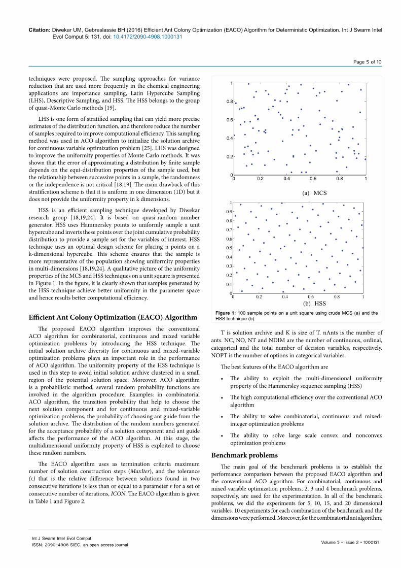
techniques were proposed. The sampling approaches for variance reduction that are used more frequently in the chemical engineering applications are importance sampling, Latin Hypercube Sampling (LHS), Descriptive Sampling, and HSS. The HSS belongs to the group of quasi-Monte Carlo methods [19].

LHS is one form of stratified sampling that can yield more precise estimates of the distribution function, and therefore reduce the number of samples required to improve computational efficiency. This sampling method was used in ACO algorithm to initialize the solution archive for continuous variable optimization problem [25]. LHS was designed to improve the uniformity properties of Monte Carlo methods. It was shown that the error of approximating a distribution by finite sample depends on the equi-distribution properties of the sample used, but the relationship between successive points in a sample, the randomness or the independence is not critical [18,19]. The main drawback of this stratification scheme is that it is uniform in one dimension (1D) but it does not provide the uniformity property in k dimensions.

HSS is an efficient sampling technique developed by Diwekar research group [18,19,24]. It is based on quasi-random number generator. HSS uses Hammersley points to uniformly sample a unit hypercube and inverts these points over the joint cumulative probability distribution to provide a sample set for the variables of interest. HSS technique uses an optimal design scheme for placing n points on a k-dimensional hypercube. This scheme ensures that the sample is more representative of the population showing uniformity properties in multi-dimensions [18,19,24]. A qualitative picture of the uniformity properties of the MCS and HSS techniques on a unit square is presented in Figure 1. In the figure, it is clearly shown that samples generated by the HSS technique achieve better uniformity in the parameter space and hence results better computational efficiency.

Efficient Ant Colony Optimization (EACO) AlgorithmThe proposed EACO algorithm improves the conventional

ACO algorithm for combinatorial, continuous and mixed variable optimization problems by introducing the HSS technique. The initial solution archive diversity for continuous and mixed-variable optimization problems plays an important role in the performance of ACO algorithm. The uniformity property of the HSS technique is used in this step to avoid initial solution archive clustered in a small region of the potential solution space. Moreover, ACO algorithm is a probabilistic method, several random probability functions are involved in the algorithm procedure. Examples: in combinatorial ACO algorithm, the transition probability that help to choose the next solution component and for continuous and mixed-variable optimization problems, the probability of choosing ant guide from the solution archive. The distribution of the random numbers generated for the acceptance probability of a solution component and ant guide affects the performance of the ACO algorithm. At this stage, the multidimensional uniformity property of HSS is exploited to choose these random numbers.

The EACO algorithm uses as termination criteria maximum number of solution construction steps (MaxIter), and the tolerance (ϵ) that is the relative difference between solutions found in two consecutive iterations is less than or equal to a parameter ϵ for a set of consecutive number of iterations, ICON. The EACO algorithm is given in Table 1 and Figure 2.

T is solution archive and K is size of T. nAnts is the number of ants. NC, NO, NT and NDIM are the number of continuous, ordinal, categorical and the total number of decision variables, respectively. NOPT is the number of options in categorical variables.

The best features of the EACO algorithm are

• The ability to exploit the multi-dimensional uniformity property of the Hammersley sequence sampling (HSS)

• The high computational efficiency over the conventional ACO algorithm

• The ability to solve combinatorial, continuous and mixed-integer optimization problems

• The ability to solve large scale convex and nonconvex optimization problems

Benchmark problemsThe main goal of the benchmark problems is to establish the

performance comparison between the proposed EACO algorithm and the conventional ACO algorithm. For combinatorial, continuous and mixed-variable optimization problems, 2, 3 and 4 benchmark problems, respectively, are used for the experimentation. In all of the benchmark problems, we did the experiments for 5, 10, 15, and 20 dimensional variables. 10 experiments for each combination of the benchmark and the dimensions were performed. Moreover, for the combinatorial ant algorithm,

(a) MCS

(b) HSS Figure 1: 100 sample points on a unit square using crude MCS (a) and the HSS technique (b).


of 10


Figure 2: EACO algorithm for continuous, combinatorial and mixed variable problems.

Start program• Set K, nAnts, NC, NO, NT, NOPT, , q, ξ and termination criteria • Initialize solution archive T(K, NC + NO) using HSS • Initialize solution archive T(K, NT) randomly from the possible options • Combine and evaluate the objective function of the K solutions T(K, NDIM)• Rank solutions based on the quality of the objective function (T = rank(S1

…SK))• For categorical optimization problems, introduce multidimensional random

number generated with HSS (IterMax × nAnts × NT, NOPT)While Termination criterion is not satisfied• Generate solutions equivalent to the number of ants (nAnts)

For all # nAnts• Incremental solution construction

For all # NDIM Probabilistically construct continuous decision variables Probabilistically construct ordinal decision variables Probabilistically construct categorical decision variables

End for # NDIM• Store and evaluate the objective function of the newly generated solutions

End for # nAnts• Combine, rank and select the best K solutions, T = Best(rank(S1 ... SK ... SK+

nAnts), K)• Update solution

End whileEnd program

Table 1: EACO Algorithm for continuous, combinatorial and mixed variable problem.

Function Formula RangeCombinatorial Optimization Problems1 Travelling Salesman Problem

2 EX. II

1y2 i 2 i 2

BC 1 2 3i 1

f (y) (y 3) (y 3) (y 3)=

= − + − + −∑ [1,5]NC

Continuous Combinatorial Optimization Problems

3 Parabolic (PRCV)

NC2

PR ii-1

f (x) x =∑ [-3,3] NC

4 Ellipsoid (ELCV)

i-1NC2n-1

EL ii 1

f (x) 5 x =

=∑ [-3,3] NC

5 Cigar (CGCV)

NC2 4 2

CG 1 ii 2

f (x) x 10 x =

= + ∑ [-3,3] NC

Mixed-variable Combinatorial Optimization Problems

6 Parabolic (PRMV)

NC ND2 2

PR i ii 1 i 1

f (x, y) x y = =

= +∑ ∑ [-3,3] NM

7 Ellipsoid (ELMV)

i-1 i-1NC ND2 2n-1 n-1

EL i ii 1 i 1

f (x, y) 5 x 5 y= =

= +∑ ∑ [-3,3] NM

8 Cigar (CGMV)

NC ND2 4 2 2 4 2

CG 1 i 1 ii 2 i 2

f (x, y) x 10 x y 10 y = =

= + + +∑ ∑ [-3,3] NM

9 EX. III( )

i

NDNC ND2 2

i ii 1 i 1 i 1

f (x, y) x i / NC y cos(4 y )= = =

= − + + π∑ ∑ ∏ [-3,3] NM

Table 2: Benchmarks problems.

there are five most popular algorithm variants [6]. The performance of each variant is tested using the EACO algorithm. The performance measure used to evaluate the algorithms was based on the number of iterations that the algorithm needed to reach the global optimal of the test functions for the same algorithmic parameter setting and terminating criterion. The benchmark problems are explained below and are given in Table 2.


of 10


• Traveling Salesman Problem (TSP): Given the number of cities to be visited and the distances between each pair of cities, find the shortest possible route that lead to visiting each city exactly once and returns back to the origin city. The TSP is an NP-hard combinatorial optimization problem.

• A TSP with known global optimal solution is also retrieved from the TSPLIB benchmark library accessible at http://www.iwr.uni-heidelberg.de/groups/comopt/software/TSPLIB95/. For each variant of the combinatorial ACO optimization algorithm, a 16 Odyssey geographical locations (ulysses16.tsp) with global optimal solution of 6859 is used to perform the computational efficiency comparison between the EACO and the conventional ACO algorithm.

• A pure combinatorial problem, example II of Kim and Diwekar [26]. This problem has one global minimum 0 when all y1; y2i; and y3i are equal to 3.

• Three test functions are used for the continuous optimization problems. The parabolic function is from Kim and Diwekar example I [26]. This function is a multidimensional parabolic function that has one global optimum at 0 for all decision variables equal to 0. The second and third test functions, which are the ellipsoid and cigar functions, are from Socha [17].

• The three test functions used for the continuous optimization problem are further modified to represent mixed variable optimization problems as shown in Table 2.

• Example III from Kim and Diwekar [26] which is an MINLP problem that has one global minimum -1 is further used as an MINLP benchmark problem.

• Case studies on real world optimization problems solved by the proposed EACO algorithm can be viewed in references [28,29].

Results and DiscussionsBenchmark Problems

This section presents a comparative study between the EACO and the conventional ACO algorithm that use MCS for initializing the solution archive and generating the multidimensional random number to optimize the 9 benchmark problems presented in Table 2. The proposed EACO algorithm effectively solves discrete, continuous, and mixed-integer optimization problem benchmarks. The algorithm terminates when it reaches maximum number of solution construction steps, MaxIter, or if the tolerance (ϵ) that is the relative difference between solutions found in two consecutive iterations is less than or equal to a parameter ϵ for a set of consecutive number of iterations, ICON.

In order to make unbiased comparison between the EACO and the conventional ACO algorithms, we use the same parameters to conduct the experiments. The results are based on 10 independent runs on each benchmark problem. Each run differs in the seed to generate the random numbers and the solution archive initialization. The parameters used to tackle the problems are selected after performing a number of experimentations using different combination of the parameters. The experiments to get the parameter settings are performed using the conventional ACO algorithm. The summary of the parameters that we use for the algorithms are presented in Table 3. As shown in Table 3, the parameter setting differs from problem to problem. The archive size K and the number of ants nAnts for 5 dimensional variables are 50 and 2,

respectively.

x and y are vector of continuous and discrete variables, respectively. NC, ND, and NM are number of continuous, discrete and mixed variable, respectively.

EX. II and III refers to examples from Diwekar [26].

Combinatorial EACO algorithms: The results of the discrete benchmark problems are presented in Tables 4-5. As shown in the tables, for each of the 40 (3×10 + 10) pair of the experimental runs of the benchmark problems, the EACO algorithm shows a better computational efficiency than the conventional ACO algorithm. The iteration improvement ranges from 24.2% of the multistage turbine problem of example II from Kim and Diwekar [26] to 33% of the travelling salesman problem with 10 and 20 numbers of cities to be visited. For the discrete optimization problems, by keeping the diversity of the multidimensional random numbers, the EACO algorithm produces more uniform operation to guide ants in making decisions of accepting or rejecting the current transition probability that lead to the finding of a new solution component. The results in Table 4 and 5 show that the EACO benefits from the uniformity property and diversified multidimensional random number generations.

Comparison of variants of the combinatorial EACO algorithms: To compare the performance of the EACO algorithm with the variants of the combinatorial ACO algorithms, the following algorithm parameter settings are used. Maximum number of tour construction steps (MaxIter) of 1000 and absolute error between the global optimal and the best so-far solution ϵ = 1E-6 are used as stopping criteria. Moreover, the parameter settings dependent on the algorithm variant are given as follows. AS: α = 1; β = 3; ρ = 0.5, and nAnts = n, that is number of ants equal to the number of the geometrical locations (n). EAS: α = 1; β = 5; ρ = 0.5, e = n, and nAnts = n. RAS: α = 1; β = 4; ρ = 0.6, w = 10, and nAnts = n. ACS: α = 1; β = 3; ρ = 0.9, ξ = 0.1, and nAnts = n. MMAS : α = 1; β = 5; ρ = 0.98, pbst = 0.05; and nAnts = n. The pheromone update for MMAS is performed using only the iteration-best ant.

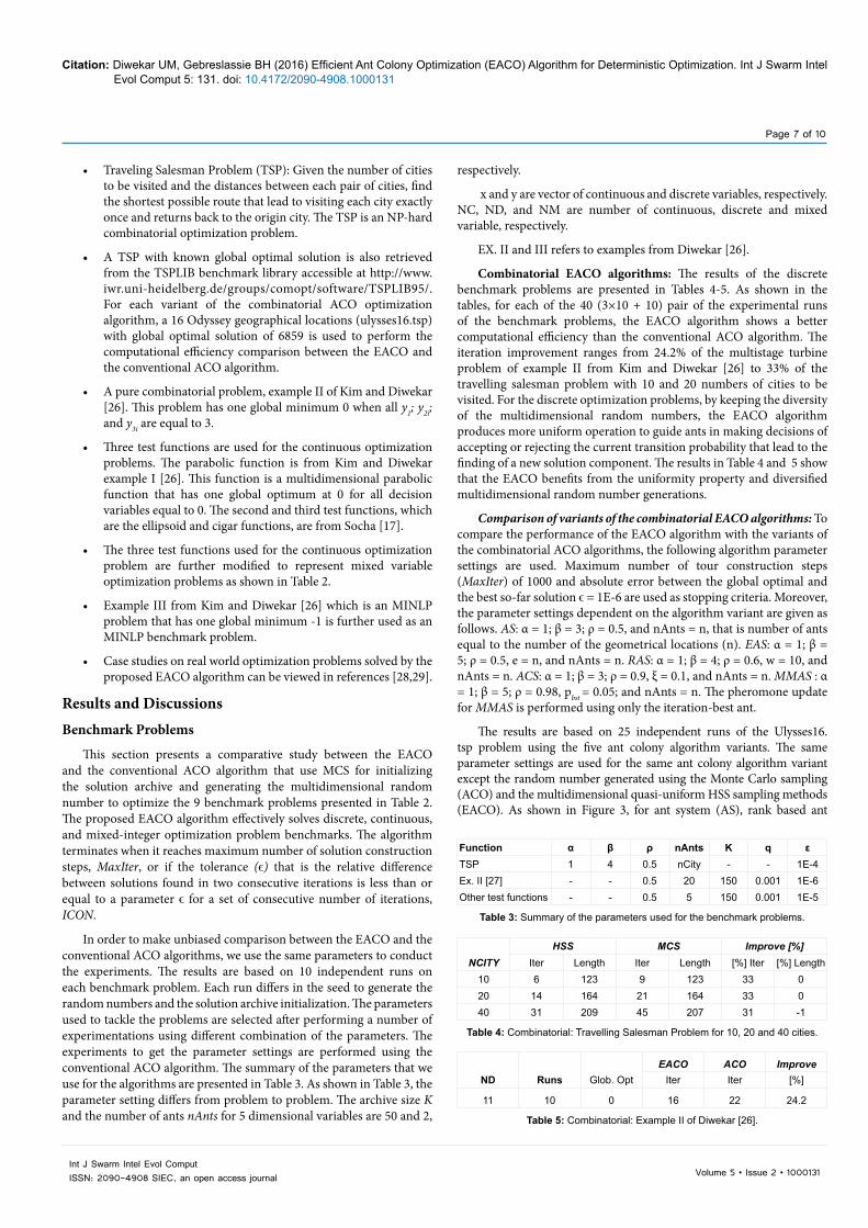
The results are based on 25 independent runs of the Ulysses16.tsp problem using the five ant colony algorithm variants. The same parameter settings are used for the same ant colony algorithm variant except the random number generated using the Monte Carlo sampling (ACO) and the multidimensional quasi-uniform HSS sampling methods (EACO). As shown in Figure 3, for ant system (AS), rank based ant

NCITYHSS MCS Improve [%]

Iter Length Iter Length [%] Iter [%] Length10 6 123 9 123 33 020 14 164 21 164 33 040 31 209 45 207 31 -1

Table 4: Combinatorial: Travelling Salesman Problem for 10, 20 and 40 cities.

ND Runs Glob. OptEACO ACO Improve

Iter Iter [%]

11 10 0 16 22 24.2

Table 5: Combinatorial: Example II of Diwekar [26].

Table 3: Summary of the parameters used for the benchmark problems.

Function α β ρ nAnts K q εTSP 1 4 0.5 nCity - - 1E-4Ex. II [27] - - 0.5 20 150 0.001 1E-6Other test functions - - 0.5 5 150 0.001 1E-5


of 10


system (RAS), and ant colony system (ACS), the EACO form of these algorithms perform better than the conventional ACO algorithm form of these variants. That is, the numbers of runs that find the global optimal solution using the EACO form of AS, RAS and ACCS are higher than that of the conventional ACO algorithm forms of the same variants. In the case of elitist ant system, both methods find the global optimal solutions for the same number of runs (17/25). However, for Max-Min ant system, the conventional ACO algorithm find global optimal solution in more runs (23/25) than the EACO algorithm (22/25). This could be attributed to the fact that the small problem size and already MMAS is an efficient method of all the ant variants.

Continuous EACO algorithm: The results of the continuous benchmark problems are presented in Tables 6-8. Among the 120 (3 ×4×10) pair of the experimental runs of the benchmark problems, only in one instant (Table 6 of parabolic function with 5 decision variables) the two algorithms have same performance. For 99.2% of the experimental runs of the continuous functions the performance of

the EACO algorithm is better than the conventional ACO algorithm. Because of the multidimensional uniformity property of HSS, the EACO algorithm needed less iteration than using the MCS to find the global optimal solutions. The computational efficiency improvement ranges from 7% for the parabolic function with 20 decision variables (Table 6) to 23.5% of the cigar function with 15 decision variables (Table 8).

MINLP EACO algorithm: The results of the mixed-integer benchmark problems are presented in Tables 9-12. Among the 160 (4 ×4×10) pair of the experimental runs of the benchmark problems, all of the 160 pair experimental runs show that the performance of the EACO algorithm is better than the conventional ACO algorithm. The computational efficiency improvement ranges from 3% for the mixed variable cigar function with 20 decision variables (see Table 11) to 71% of the same function with 5 decision variables. Moreover, the tables also show that for the mixed variable optimization problems, the improvement on the computational efficiency of EACO is more pronounced.

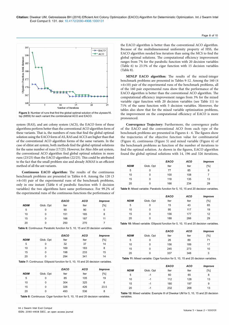
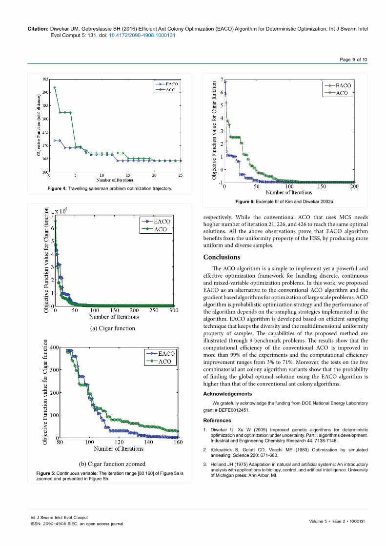
Convergence Trajectory: Furthermore, the convergence paths of the EACO and the conventional ACO from each type of the benchmark problems are presented in Figures 4 - 6. The figures show the trajectories of the objective function value for combinatorial (Figure 4), continuous (Figure 5) and mixed variable (Figure 6) of the benchmark problems as function of the number of iterations to find the optimal solution. As shown in the figures, EACO algorithm found the global optimal solutions with 14, 196 and 326 iterations,

Figure 3: Number of runs that find the global optimal solution of the ulysses16.tsp (6859) for each variant the combinatorial ACO and EACO.

NDIMEACO ACO Improve

Glob. Opt Iter Iter [%]5 0 15 43 65

10 0 95 117 1915 0 156 177 1220 0 188 266 29

Table 10: Mixed variable: Ellipsoid function for 5, 10, 15 and 20 decision variables.

NDIM EACO ACO Improve


10 0 156 189 1715 0 245 273 1020 0 337 348 3

Table 11: Mixed variable: Cigar function for 5, 10, 15 and 20 decision variables.



10 0 100 108 715 0 118 135 1320 0 166 234 29

Table 9: Mixed variable: Parabolic function for 5, 10, 15 and 20 decision variables.


Glob. Opt Iter Iter [%]5 -1 60 65 8

10 -1 112 128 1315 -1 180 197 920 -1 232 268 13

Table 12: Mixed variable: Example III of Diwekar UM for 5, 10, 15 and 20 decision variables.



10 0 151 165 815 0 166 187 1120 0 250 270 7

Table 6: Continuous: Parabolic function for 5, 10, 15 and 20 decision variables.



10 0 169 183 815 0 198 233 1520 0 294 341 14

Table 7: Continuous: Ellipsoid function for 5, 10, 15 and 20 decision variables.



10 0 304 325 615 0 326 426 23.520 0 493 536 8

Table 8: Continuous: Cigar function for 5, 10, 15 and 20 decision variables.


of 10


Figure 4: Travelling salesman problem optimization trajectory.

(a) Cigar function.

(b) Cigar function zoomedFigure 5: Continuous variable: The iteration range [80 160] of Figure 5a is zoomed and presented in Figure 5b.

Figure 6: Example III of Kim and Diwekar 2002a.

respectively. While the conventional ACO that uses MCS needs hogher number of iteration 21, 226, and 426 to reach the same optimal solutions. All the above observations prove that EACO algorithm benefits from the uniformity property of the HSS, by producing more uniform and diverse samples.

ConclusionsThe ACO algorithm is a simple to implement yet a powerful and

effective optimization framework for handling discrete, continuous and mixed-variable optimization problems. In this work, we proposed EACO as an alternative to the conventional ACO algorithm and the gradient based algorithms for optimization of large scale problems. ACO algorithm is probabilistic optimization strategy and the performance of the algorithm depends on the sampling strategies implemented in the algorithm. EACO algorithm is developed based on efficient sampling technique that keeps the diversity and the multidimensional uniformity property of samples. The capabilities of the proposed method are illustrated through 9 benchmark problems. The results show that the computational efficiency of the conventional ACO is improved in more than 99% of the experiments and the computational efficiency improvement ranges from 3% to 71%. Moreover, the tests on the five combinatorial ant colony algorithm variants show that the probability of finding the global optimal solution using the EACO algorithm is higher than that of the conventional ant colony algorithms.

Acknowledgements

We gratefully acknowledge the funding from DOE National Energy Laboratory grant # DEFE0012451.

References

1. Diwekar U, Xu W (2005) Improved genetic algorithms for deterministic optimization and optimization under uncertainty. Part I. algorithms development. Industrial and Engineering Chemistry Research 44: 7138-7146.

2. Kirkpatrick S, Gelatt CD, Vecchi MP (1983) Optimization by simulated annealing. Science 220: 671-680.

3. Holland JH (1975) Adaptation in natural and artificial systems: An introductory analysis with applications to biology, control, and artificial intelligence. University of Michigan press: Ann Arbor, MI.

http://pubs.acs.org/doi/abs/10.1021/ie049127d?journalCode=iecred



http://www2.stat.duke.edu/~scs/Courses/Stat376/Papers/TemperAnneal/KirkpatrickAnnealScience1983.pdf

http://www2.stat.duke.edu/~scs/Courses/Stat376/Papers/TemperAnneal/KirkpatrickAnnealScience1983.pdf

https://mitpress.mit.edu/books/adaptation-natural-and-artificial-systems




of 10


4. Dorigo M (1992) Optimization, learning and natural algorithms. PhD Thesis, Dept. of Electronics, Politecnico di Milano, Italy.

5. Senvar O, Turanoglu E, Selcuk, Kahraman C (2013) Usage of Metaheuristics in Engineering: A Literature Review. Meta-Heuristics Optimization Algorithms in Engineering, Business, Economics, and Finance Pandian M. Vasant pp: 484-528.

6. Dorigo M, Stutzle T (2004) Ant colony optimization theory. A Brandford Book, The MIT Press, Cambridge, Massachusetts.

7. Chebouba A, Yalaouia F, Smati A, Amodeo L, Younsi K, et al. (2009) Optimization of natural gas pipeline transportation using ant colony optimization. Computers & Operations Research 36: 1916-1923.

8. Zecchin A, Simpson A, Maier H, Leonard M, Roberts A, et al. (2006) Application of two ant colony optimization algorithms to water distribution system optimization. Mathematical and Computer Modelling 44: 451-468.

9. Liao C, Juan H (2007) An ant colony optimization for single-machine tardiness scheduling with sequence-dependent setups. Computers & Operations Research 34: 1799-1909.

10. Blum C (2005) Beam-ACO hybridizing ant colony optimization with beam search: an application to open shop scheduling. Computers & Operations Research 32: 1565-1591.

11. Liao T, Montes De Oca MA, Aydin D, Stutzle T, Dorigo M (2011) An incremental ant colony algorithm with local search for continuous optimization pp: 1-17.

12. Liao T, Stutzle T, Montes De Oca MA, Dorigo M (2014) A unified ant colony optimization algorithm for continuous optimization. European Journal of Operational Research 234: 597-609.

13. Socha K, Blum C (2007) An ant colony optimization algorithm for continuous optimization: Application to feed-forward neural network training. Neural Computing and Applications 16: 235-247.

14. Socha K, Dorigo M (2008) Ant colony optimization for continuous domains. European Journal of Operational Research 185: 1155-1173.

15. Schluter M, Egea J, Banga J (2009) Extended ant colony optimization for non-convex mixed integer nonlinear programming. Computers and Operations Research 36: 2217-2229.

16. Schluter M, Gerdts M, Ruckmann JJ (2012) A numerical study of MIDACO on 100 MINLP benchmarks. Optimization 61: 873-900.

17. Socha K (2009) Ant Colony Optimization for Continuous and Mixed-Variable Domains.

18. Diwekar UM, Kalagnanam JR (1997) Efficient sampling technique for optimization under uncertainty. AIChE Journal 43: 440-447.

19. Diwekar UM, Ulas S (2007) Sampling Techniques. Kirk-Othmer Encyclopedia of Chemical Technology 26.

20. Kim K, Diwekar UM (2002) Efficient combinatorial optimization under uncertainty 2 Application to stochastic solvent selection. Industrial and Engineering Chemistry Research 41: 1285-1296.

21. Kim K, Diwekar UM (2002) Hammersley stochastic annealing: Efficiency improvement for combinatorial optimization under uncertainty. IIE Transactions Institute of Industrial Engineers 34: 761-777.

22. Zhu W, Lin G (2011) A dynamic convexized method for nonconvex mixed integer nonlinear programming. Computers & Operations Research 38: 1792-1804.

23. Schluter M, Gerdts M (2010) The Oracle penalty method. Journal of Global Optimization 47: 293-325.

24. Kalagnanam JR, Diwekar UM (1997) An efficient sampling technique for off-line quality control. Technometrics 39: 308-319.

25. Leguizamón G, Coello C (2010) An alternative ACOR algorithm for continuous optimization problems. In: Dorigo M et al. (eds.) Proceedings of the seventh international conference on swarm intelligence, ANTS. LNCS; 6234: 48-59. Berlin, Germany: Springer.

26. Kim K, Diwekar UM (2002) Efficient combinatorial optimization under uncertainty. 1. Algorithmic development. Industrial and Engineering Chemistry Research 41: 1276-1284.

27. Gebreslassie BH, Diwekar UM (2015) Efficient ant colony optimization for computer aided molecular design: Case study solvent selection problem. Computers & Chemical Engineering 78:1-9.

28. Benavides PT, Gebreslassie BH, Diwekar UM. (2015) Optimal design of adsorbents for NORM removal from produced water in natural gas fracking. Part 2: CAMD for adsorption of radium and barium. Chemical Engineering Science 137: 977-985.

29. Diwekar UM (2003) Introduction to Applied Optimization. Kluwer Academic Publishers, Norwell, MA.

30. Bullnheimer B, Hartl RF, Strauss C (1997) A New Rank Based Version of the Ant System - A Computational Study. Central European Journal for Operations Research and Economics.

31. Stutzle T, Hoos H (1997) The MAX–MIN Ant System and local search for the traveling salesman problem. Proceedings of the 1997 IEEE International Conference on Evolutionary Computation pp: 309-314.


http://www.igi-global.com/chapter/usage-metaheuristics-engineering/69895



http://www.sciencedirect.com/science/article/pii/S0304397505003798


http://dl.acm.org/citation.cfm?id=1465905












http://iridia.ulb.ac.be/IridiaTrSeries/rev/IridiaTr2011-005r002.pdf

http://iridia.ulb.ac.be/IridiaTrSeries/rev/IridiaTr2011-005r002.pdf




http://link.springer.com/article/10.1007%2Fs00521-007-0084-z#page-1



http://natcomp.liacs.nl/SWI/papers/ant.colony.optimization/Ant colony optimization for continuous domains.pdf

http://natcomp.liacs.nl/SWI/papers/ant.colony.optimization/Ant colony optimization for continuous domains.pdf




http://www.ingentaconnect.com/content/tandf/gopt/2012/00000061/00000007/art00005

http://www.ingentaconnect.com/content/tandf/gopt/2012/00000061/00000007/art00005

http://iridia.ulb.ac.be/~mdorigo/HomePageDorigo/thesis/phd/SochaPhDThesis.pdf

http://iridia.ulb.ac.be/~mdorigo/HomePageDorigo/thesis/phd/SochaPhDThesis.pdf

http://onlinelibrary.wiley.com/doi/10.1002/aic.690430217/abstract

http://onlinelibrary.wiley.com/doi/10.1002/aic.690430217/abstract

http://onlinelibrary.wiley.com/doi/10.1002/0471238961.sampdiwe.a01/abstract

http://onlinelibrary.wiley.com/doi/10.1002/0471238961.sampdiwe.a01/abstract

http://pubs.acs.org/doi/abs/10.1021/ie0101691?journalCode=iecred











http://link.springer.com/chapter/10.1007/978-3-642-15461-4_5#page-1
















http://epub.wu.ac.at/616/1/document.pdf



http://www.gta.ufrj.br/ensino/cpe717-2011/stutzle97-icec.pdf



International Journal of Swarm - OMICS Publishing … algorithms for combinatorial, ... (EACO)...

Documents

Transcript of International Journal of Swarm - OMICS Publishing … algorithms for combinatorial, ... (EACO)...