International Journal of Materials & Structural Reliability Vol.4, … IJMSR_paper_6.pdf · D....

D. Codetta-Raiteri and A. Bobbio / International Journal of Materials & Structural Reliability Vol.4, No.1, March 2006, 65-77

65

International Journal of Materials

& Structural Reliability

International Journal of Materials & Structural Reliability Vol.4, No.1, March 2006, 65-77

Stochastic Petri Nets Supporting Dynamic Reliability Evaluation

D. Codetta-Raiteri1* and A. Bobbio2

1Dipartimento di Informatica, Università di Torino, Corso Svizzera 185, 10149 Torino, Italy

2Dipartimento di Informatica, Università del Piemonte Orientale, Via Bellini 25/G, 15100 Alessandria, Italy Abstract

A benchmark on dynamic reliability taken from the literature is considered; though the behaviour of this system is dynamic and is described by continuous variables, we show that the system is suitable to an analytical solution, instead of simulation. The system consists of a tank containing some liquid whose level is monitored by a controller acting on two pumps and one valve, in order to avoid the liquid dry out or overflow. The reliability evaluation of the system is obtained by resorting to Generalized Stochastic Petri Nets (GSPN) and Fluid Stochastic Petri Nets (FSPN). FSPNs are hybrid models and differ from GSPNs by the presence of both fluid places (modelling continuous variables) and discrete places (containing a discrete number of tokens). GSPNs are used for the analytical solution of the benchmark, while the simulation on the FSPNs, is run with the aim of validating the analytical results. Keywords: Dynamic Reliability, Generalized Stochastic Petri Nets, Fluid Stochastic Petri Nets 1. Introduction

Several models for the reliability analysis of complex systems have been proposed in the literature, but most of them are not suitable to represent the system when its behaviour needs to be expressed by means of continuous variables (temperature, pressure, etc.), or when the system changes its configuration during its life. In the first case, we talk about hybrid models (or systems), in the second case, of Dynamic Reliability. In both cases, simulation is typically the most utilized technique to evaluate the system behaviour, while the analytical approach is often unpractical. However, in some cases an analytical approach can be afforded by resorting to a peculiar use of ordinary Generalized Stochastic Petri Nets (GSPN) [1], or to a rather new extension called Fluid Stochastic Petri Nets (FSPN) [2, 3, 4, 5].

The advantages of using an analytical solution rather then a simulative approach are well known, and we show how to tackle a hybrid dynamic reliability problem by using the analytical *Corresponding author. E-mail : [email protected]


66

approach on GSPNs. The example is a benchmark taken from the literature [6], and consists of a tank containing some liquid whose level is influenced by a controller acting on three components (two pumps and one valve); the controller orders the components to switch on or off, with the aim of avoiding the dry out or the overflow failure condition. Several configurations of the system have been proposed and simulated in [6]; in this paper, we focus on the usual case of time and state independent failure rates, and we include the case with repairable components.

FSPNs are a recently developed evolution of the Petri Nets that allow to augment a standard Petri Net by accommodating continuous variables, by means of new primitives called fluid places and fluid arcs. Fluid places contain a continuous level of fluid (instead of a discrete number of tokens) that flows in and out through fluid arcs (pipes). This extension increases the modelling power of Stochastic Petri Nets by providing a modelling framework in which discrete variables can be combined with continuous variables and the properties of the former depends on the latter and vice-versa. This new framework has proved to be useful to model systems where physical continuous quantities, such as the liquid level or temperature, need to be represented [6].

In this paper, the reliability evaluation of the benchmark proposed in [6], is first obtained by modelling and analyzing the system as a GSPN. Moreover, it is shown that by means of a suitable discretization procedure to be applied to continuous variables, GSPNs can cope with the problem. Then the analytical results are validated by means of simulation on the FSPN. The obtained results are also quite similar to those returned by applying the Monte Carlo simulation, and reported in [6].

2. The Case Study

The system (Fig. 1) is composed by a tank containing some liquid, two pumps (P1 and P2) to

fill the tank, a valve (V) to remove liquid from the tank, and a controller monitoring the liquid level (H) and acting on P1, P2 and V.

Fig. 1 System scheme


67

Fig. 2 Possible state transitions of a component due to its failure; λ is the failure rate of the

component

Initially H is equal to 0, with P1 and V in state ON, and P2 in state OFF; since both pumps and the valve have the same rate of level variation (0.6 m/h), the liquid level does not change while the initial configuration holds. The cause of a variation of H is the occurrence of the failure of one of the components; a failure consists of turning to the state stuck ON or stuck OFF whatever is the current state of the component (see Fig. 2). The failure probability obeys the negative exponential distribution and the failure rate does not depend on the current state of the component. The failure rate of P1 is 0.004566 1/h; the failure rate of P2 is 0.005714 1/h; the failure rate of V is 0.003125 1/h. Table 1 shows how H changes with respect to the current configuration of the component states; the controller believes that the system is functioning correctly while H is inside the region between the levels denoted by HLA (-1) and HLB (+1). If H reaches HLB there is the risk of the liquid overflow; this event occurs when H exceeds the level denoted as HLP (+3). To avoid this undesired situation, the controller orders to both pumps to switch OFF and to the valve to switch ON, with the aim of decreasing H. If a component is stuck, it does not obey the controller order and maintains its current state.

Table 1 H variation for every system configuration

state of P1 state of P2 state of V effect on H level variation rate ON ON ON ON OFF OFF OFF OFF

OFF ON OFF ON OFF ON OFF ON

OFF OFF ON ON OFF OFF ON ON

↑ ↑↑ = ↑ = ↑ ↓ =

0.6 m/h 1.2 m/h

0.6 m/h

0.6 m/h 0.6 m/h

The other undesired situation is the tank dry out; this happens when H is below HLV (-3); to

avoid the dry out, when H reaches HLA, the controller orders to both pumps to switch ON and to the valve to switch OFF, with the aim of increasing H. Table 2 shows the control laws with respect to H.

The failure of the whole system happens when the dry out or the overflow occurs.


68

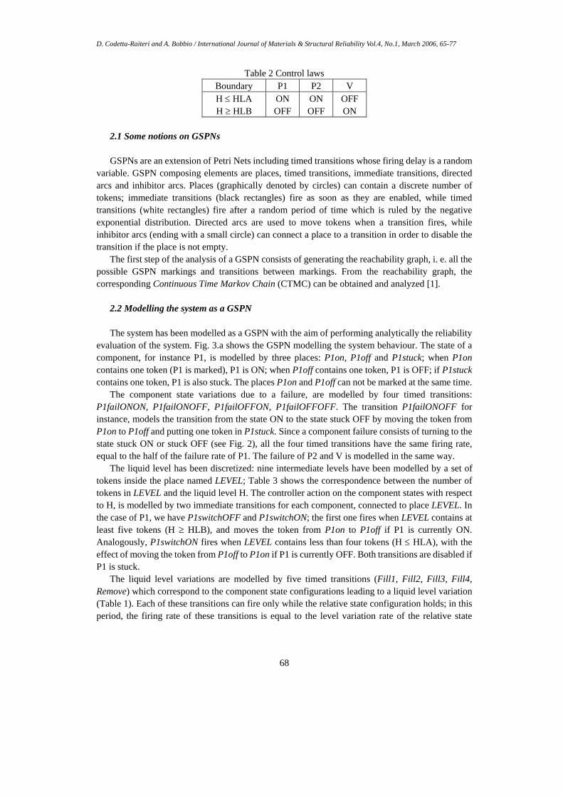
Table 2 Control laws Boundary P1 P2 V H ≤ HLA H ≥ HLB

ON OFF

ON OFF

OFF ON

2.1 Some notions on GSPNs GSPNs are an extension of Petri Nets including timed transitions whose firing delay is a random

variable. GSPN composing elements are places, timed transitions, immediate transitions, directed arcs and inhibitor arcs. Places (graphically denoted by circles) can contain a discrete number of tokens; immediate transitions (black rectangles) fire as soon as they are enabled, while timed transitions (white rectangles) fire after a random period of time which is ruled by the negative exponential distribution. Directed arcs are used to move tokens when a transition fires, while inhibitor arcs (ending with a small circle) can connect a place to a transition in order to disable the transition if the place is not empty.

The first step of the analysis of a GSPN consists of generating the reachability graph, i. e. all the possible GSPN markings and transitions between markings. From the reachability graph, the corresponding Continuous Time Markov Chain (CTMC) can be obtained and analyzed [1].

2.2 Modelling the system as a GSPN

The system has been modelled as a GSPN with the aim of performing analytically the reliability

evaluation of the system. Fig. 3.a shows the GSPN modelling the system behaviour. The state of a component, for instance P1, is modelled by three places: P1on, P1off and P1stuck; when P1on contains one token (P1 is marked), P1 is ON; when P1off contains one token, P1 is OFF; if P1stuck contains one token, P1 is also stuck. The places P1on and P1off can not be marked at the same time.

The component state variations due to a failure, are modelled by four timed transitions: P1failONON, P1failONOFF, P1failOFFON, P1failOFFOFF. The transition P1failONOFF for instance, models the transition from the state ON to the state stuck OFF by moving the token from P1on to P1off and putting one token in P1stuck. Since a component failure consists of turning to the state stuck ON or stuck OFF (see Fig. 2), all the four timed transitions have the same firing rate, equal to the half of the failure rate of P1. The failure of P2 and V is modelled in the same way.

The liquid level has been discretized: nine intermediate levels have been modelled by a set of tokens inside the place named LEVEL; Table 3 shows the correspondence between the number of tokens in LEVEL and the liquid level H. The controller action on the component states with respect to H, is modelled by two immediate transitions for each component, connected to place LEVEL. In the case of P1, we have P1switchOFF and P1switchON; the first one fires when LEVEL contains at least five tokens (H ≥ HLB), and moves the token from P1on to P1off if P1 is currently ON. Analogously, P1switchON fires when LEVEL contains less than four tokens (H ≤ HLA), with the effect of moving the token from P1off to P1on if P1 is currently OFF. Both transitions are disabled if P1 is stuck.

The liquid level variations are modelled by five timed transitions (Fill1, Fill2, Fill3, Fill4, Remove) which correspond to the component state configurations leading to a liquid level variation (Table 1). Each of these transitions can fire only while the relative state configuration holds; in this period, the firing rate of these transitions is equal to the level variation rate of the relative state


69

configuration indicated in Table 1. The effect of the firing is the addition (or the removal) of one token in LEVEL; in this way, we model the increase (or the decrease) of H.

Table 3 Representation of H as the discrete marking of the place LEVEL in the GSPN,

and as the fluid marking of the place L in the FSPN

H

Condition #tokens

in LEVEL (GSPN)

level in L

(FSPN)> +3

+3 +2 +1

0 -1 -2 -3

< -3

overflow HLP

HLB

initial level HLA

HLV

dry out

8 7 6 5 4 3 2 1 0

6 5 4 3 2 1 0

The dry out and overflow conditions are detected by two specific immediate transitions: Empty and Full respectively; the first one fires when LEVEL contains no tokens (H<HLV), and puts one token inside the place DRYOUT meaning that the dry out has occurred; the second one fires when LEVEL contains eight tokens (H>HLV), and puts one token inside OVERFLOW.

To model the initial configuration, P1on, P2off and Von are marked with one token, while LEVEL contains four tokens corresponding to H=0.

2.3 Some notions on FSPNs

FSPNs are a new extension of Petri nets including the same elements of GSPNs with the addition of fluid places and arcs; fluid places contain a continuous fluid level and are suitable to represent continuous variables such as the temperature and the pressure. A fluid place can be connected to a timed transition by means of a fluid arc (pipe); while the timed transition is enabled to fire, some fluid is moved through the fluid arc, from or to the fluid place with respect to the flow rate associated with the fluid arc. Moreover, the firing of a timed transition may depend on the fluid level inside a fluid place: the Dirac delta function is used to make a transition fire when the fluid level reaches a certain value.

The Dirac delta function returns 0 if its argument differs from 0, while it returns +∞ if its argument is equal to 0. So if we want a transition to fire when the fluid level inside the place L is equal to x, we have to set the firing rate of the transition to the function Dirac(L-x).

2.4 Modelling the system as a FSPN

In order to verify the correctness of the results (reported in section 2.5) obtained through the

liquid level discretization in the GSPN model, we built also the FSPN model relative to the same system.


70

Fig. 3.b shows the FSPN model of the system, where some new elements appear: a fluid place named L modelling the liquid level in the tank and three fluid arcs with the shape of a pipe, modelling the action of the two pumps and of the valve on L; if we consider for instance P1, the fluid variation rate of the relative fluid arc is 0.6 ⋅ #P1on, where #P1on is the number of tokens inside P1on; in other words, some fluid is moved to L only while P1 is ON. Table 3 shows the correspondence between the liquid level in the tank (H) and the fluid level in L.

The current state and the failure of a component are modelled in the same way as in the GSPN; the controller action on the components is now modelled by two timed transitions for each component. In the case of P1, they are P1switchOFF and P1switchON; the first one must fire when H reaches HLB, so its firing rate is the function Dirac(L-4) and it switches P1 to OFF if P1 is currently ON. The second transition must fire when H reaches HLA, so its firing rate is Dirac(L-2) and it switches P1 to ON if P1 is currently OFF. Both transitions are disabled if P1 is stuck.

Two timed transitions named Empty and Full, detect the dry out and the overflow condition respectively; Empty must fire when H reaches HLV; this happens when L is equal to 0, so the firing rate of this transition is Dirac(L). Full must fire when H reaches HLP, so its firing rate is Dirac(L-6).

Fig. 3 a) GSPN model of the system b) FSPN model of the system


71

2.5 Comparison of the results obtained on both models In order to evaluate the reliability of the system, we calculated analytically the dry out and

overflow cumulative distribution function (cdf) on the GSPN of Fig. 3.a; this means computing the probability that the system is in the dry out or in the overflow condition respectively, as a function of the time. The cdf of the dry out is calculated as the probability of the presence of one token in the place DRYOUT; the cdf of the overflow is the probability to have one token in OVERFLOW. The GSPN model has been drawn and analyzed by means of the GreatSPN tool [7].

Table 4 Dry out and overflow cdf: the columns labelled as “cdf” report the analytical results

computed on the GSPN; the columns labelled as “min” and “max” report the bounds returned by the simulation on the FSPN

time dry out min (FSPN)

dry out cdf (GSPN)

dry out max (FSPN)

overflow min (FSPN)

overflow cdf (GSPN)

overflow max (FSPN)

100 h 200 h 300 h 400 h 500 h 600 h 700 h 800 h 900 h

1000 h

0.002845 0.020963 0.041510 0.062215 0.076387 0.087603 0.095643 0.101947 0.105926 0.109810

0.004463 0.022077 0.044846 0.065827 0.082568 0.095014 0.103939 0.110227 0.114622 0.117689

0.005355 0.027037 0.049890 0.072385 0.087613 0.099597 0.108157 0.114853 0.119074 0.123190

0.068572 0.191723 0.284943 0.350404 0.397253 0.428575 0.448382 0.462773 0.471251 0.477266

0.074208 0.195182 0.292146 0.359876 0.405374 0.435689 0.455953 0.469595 0.478857 0.485200

0.079228 0.209277 0.306257 0.373996 0.422347 0.454625 0.475018 0.489827 0.498549 0.504734

Fig. 4 Dry out cdf: the solid line shows the GSPN analytical results; the dashed lines show the

FSPN simulation results


72

Fig. 5 Overflow cdf: the solid line shows the GSPN analytical results; the dashed lines show the

FSPN simulation results On the FSPN model of Fig. 3.b instead, we performed 10000 cycles of simulation returning the

lower and the upper bounds for the dry out cdf and the overflow cdf at the same mission times adopted for the analytical approach on the GSPN. The FSPN model has been drawn and simulated by means of the FSPNEdit tool [8].

The results obtained on both the GSPN and the FSPN are reported in Table 4; comparing the analytical results of the GSPN and the simulation results of the FSPN, we can observe that each probability value computed on the GSPN belongs to the range of values between the lower and the upper bound returned by the simulation on the FSPN for the same mission time; this situation is graphically shown in Fig. 4 (dry out) and in Fig. 5 (overflow).

Our analytical results are also quite similar to those reported in [6], obtained via Monte Carlo simulation. This means that the analytical approach based on liquid level discretization and GSPN, returns acceptable results, considering that the simulation of the FSPN can deal with continuous variables, while in the GSPN we can deal only with discrete quantities.

3. Modelling the Components Repair

3.1 Repair policy A variation proposed in [6] to the initial version of the benchmark, deals with the possibility of

repairing the failed (stuck) components. The reliability of the system can be improved in a considerable way by introducing the repair process. In the case of the benchmark, the controller discovers a failure by observing the liquid level H: if H is not inside the region of correct functioning (HLA<H<HLB), the controller suspects the occurrence of a failure, so it enables the repair process for the stuck components. The time to repair of a component is a random variable obeying a negative exponential distribution with the repair rate equal to 0.2 1/h.

The repair is only allowed while the liquid level is outside the region of correct functioning (grace period); the effect of the repair consists of removing the stuck condition of a component. So, after the repair, a component can respond again and immediately to the controller orders changing its state if necessary. In order to have a significant grace period with respect to the repair time, the thresholds for the dry out and the overflow conditions, are now –5 and +5 respectively.


73

Fig. 6 GSPN model of the repairable system

3.2 GSPN model of the repairable system

With the aim of modelling the presence of the repair process in the system, and the new

thresholds, we changed the discretization of the liquid level H, and added some new places and transitions in the GSPN model (Fig. 6); Table 5 shows the new correspondence between H and the number of tokens inside the place called LEVEL.


74

Tab. 5 Representation of H as the discrete marking of the place LEVEL in the GSPN, and as the fluid marking of the place L in the FSPN

H

Condition

#tokens in LEVEL (GSPN)

level in L

(FSPN) > +5

+5 +4 +3 +2 +1

0 -1 -2 -3 -4 -5

< -5

overflow HLP

HLB initial level

HLA

HLV dry out

12 11 10 9 8 7 6 5 4 3 2 1 0

10 9 8 7 6 5 4 3 2 1 0

In the current GSPN, we have some new elements: the transition tooHIGH fires when LEVEL

contains at least seven tokens (H ≥ HLB), and puts one token in the place dangerHIGH (enabling the immediate transitions modelling both pumps stop and the activation of the valve). In a similar way, the transition tooLOW fires when LEVEL contains less than six tokens (H ≤ HLA) and puts one token in the place dangerLOW (enabling the activation of both pumps and the valve stop).

The presence of one token inside the place dangerLOW or dangerHIGH, means that we are in the grace period, so a timed transition modelling the repair, is enabled for each component; the firing rate of such transitions is the repair rate. In the case of P1, the transition P1repair removes the token from the place P1stuck. The repair is allowed only during the grace period, so if H is back to the correct functioning region (six tokens inside LEVEL) as a consequence of a repair, the transition enoughLOW or enoughHIGH fires removing the token from dangerHIGH or dangerLOW respectively, and disabling the repairs.

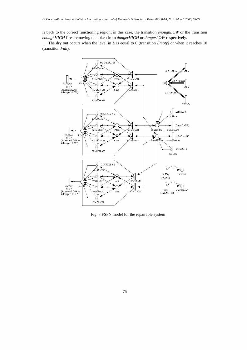
3.3 FSPN model of the repairable system As in the initial case, we verify the correctness of the analytical results on the GSPN by

comparison with the simulation results computed on the FSPN model of the system (such results are reported in section 3.4). Fig. 7 shows the FSPN including the repair process; Table 5 shows the correspondence between the level in L and the new thresholds.

With respect to the initial FSPN, we added some new elements in order to model the repair in the grace period: the firing rate of the timed transition tooHIGH is the function Dirac(L-6), so it fires when H reaches HLB putting one token in the place dangerHIGH which enables the immediate transitions modelling the relative control law on the components. The timed transition tooLOW instead, fires when H reaches HLA putting one token in dangerLOW, enabling the immediate transitions modelling the control law in this condition.

The repair is modelled in the same way as in the GSPN, by three timed transitions enabled by the presence of one token inside the place dangerHIGH or dangerLOW. The grace period ends when H


75

is back to the correct functioning region; in this case, the transition enoughLOW or the transition enoughHIGH fires removing the token from dangerHIGH or dangerLOW respectively.

The dry out occurs when the level in L is equal to 0 (transition Empty) or when it reaches 10 (transition Full).

Fig. 7 FSPN model for the repairable system


76

Table 6 Dry out and overflow cdf: the columns labelled as “cdf” report the analytical results computed on the GSPN; the columns labelled as “min” and “max” report the bounds returned by

the simulation on the FSPN

3.4 Comparison of the results obtained on both models The probabilities of the dry out and of the overflow conditions, computed in the analytical way

on the GSPN and by simulation on FSPN, are reported in Table 6 for a mission time varying from 50 to 500 hours. As in the previous system configurations, the analytical results are coherent with those returned by the simulation.

Conclusions

Though simulation is the typical method to evaluate the reliability of hybrid and dynamic

systems, in this paper we showed the way to adapt a form of discrete modelling and analysis such as GSPNs, to the benchmark proposed in [6]. The success of our approach has been verified by comparing the analytical results we obtained using GSPNs, with those returned by simulation on FSPNs (a formalism specifically studied to deal with continuous quantities) and with the results reported in [6]. So, we can conclude that the use of GSPNs is suitable in several cases of dynamic reliability analysis. In [9] another version of the benchmark have been modelled and evaluated as a FSPN: the case with component failure rates expressed as a function of the liquid temperature assuming the presence of a heat source to warm the liquid in the tank.

Acknowledgements

This work was orginated by the 3ASI [10] workgroup on Dynamic Reliability coordinated by

Enrico Zio (Politecnico di Milano). This work was supported by the Italian Ministry of Education, Universities and Research

(MIUR) in the framework of the FIRB-Perf project.

time dry out min

(FSPN)

dry out cdf (GSPN)

dry out max (FSPN)

overflow min (FSPN)

overflow cdf (GSPN)

overflow max (FSPN)

50 h 100 h 150 h 200 h 250 h 300 h 350 h 400 h 450 h 500 h

0.000000 0.000000 0.000000 0.000008 0.000120 0.000246 0.000246 0.000312 0.000312 0.000521

0.000010 0.000062 0.000156 0.000280 0.000419 0.000561 0.000697 0.000825 0.000941 0.001045

0.000015 0.000070 0.000296 0.000792 0.001080 0.001354 0.001354 0.001488 0.001488 0.001879

0.000380 0.001844 0.003442 0.005891 0.009762 0.014259 0.017787 0.021807 0.025474 0.028588

0.000967 0.003168 0.006015 0.009238 0.012682 0.016254 0.019893 0.023558 0.027221 0.030860

0.001620 0.003956 0.006158 0.009309 0.014038 0.019341 0.023413 0.027993 0.032126 0.035612


77

References

1. Ajmone-Marsan M., Balbo G., Conte G., Donatelli S., Franceschinis G. Modelling with Generalized Stochastic Petri Nets. Wiley Series on Parallel Computing, 1995. 2. Gribaudo M., Sereno M., Bobbio A. Fluid Stochastic Petri Nets: An Extended Formalism to Include non-Markovian Models. 8-th International Conference on Petri Nets and Performance Models. IEEE Computer Society Press, 1999. 74-81. 3. Gribaudo M., Sereno M., Horvath A., Bobbio, A. Fluid stochastic Petri nets augmented with flush-out arcs: Modelling and analysis. Discrete Event Dynamic Systems 11(1/2), 2001. 97-117. 4. Bobbio A., Gribaudo M., Sereno M. Modelling Physical Quantities in Industrial Systems using Fluid Stochastic Petri Nets. Proceedings 5th International Workshop on Performability Modeling of Computers and Communication Systems, 2001. 81-85. 5. Bobbio A., Gribaudo M., Horvath A. Modeling a car safety controller using fluid stochastic Petri nets. Proceedings 6th International Workshop on Performability Modeling of Computer and Communication Systems, 2003. 27-30. 6. Marseguerra M., Zio E. Monte Carlo approach to PSA for dynamic process system. Reliability Engineering and Safety System 52, 1996. 227-241. 7. Chiola G., Franceschinis G., Gaeta R., Ribaudo M. GreatSPN 1.7: Graphical Editor and Analyzer for Timed and Stochastic Petri Nets. Performance Evaluation 24, 1995. 47-68. 8. Gribaudo M. FSPNEdit: a Fluid Stochastic Petri Net Modeling and Analysis Tool. Proceedings of the International Conference on Measuring, Modeling and Evaluation of Computer and Communication Systems, 2001. 24-28. 9. Codetta-Raiteri D., Bobbio A. Evaluation of a benchmark on dynamic reliability via Fluid Stochastic Petri Nets. Proceedings of the 7th International Workshop on Performability Modeling of Computer and Communication Systems, 2005. 52-55. 10. http://www.3asi.it - web page of the 3ASI Association.

International Journal of Materials & Structural Reliability Vol.4, … IJMSR_paper_6.pdf · D....

Documents

Transcript of International Journal of Materials & Structural Reliability Vol.4, … IJMSR_paper_6.pdf · D....