International Journal of Heat and Mass Transfer · neous ﬂow ﬁeld data. Despite geometrical...

International Journal of Heat and Mass Transfer 104 (2017) 178–198

Contents lists available at ScienceDirect

International Journal of Heat and Mass Transfer

journal homepage: www.elsevier .com/locate / i jhmt

Investigation of coherent structures in a turbulent channel with built-inlongitudinal vortex generators

http://dx.doi.org/10.1016/j.ijheatmasstransfer.2016.07.1050017-9310/� 2016 Elsevier Ltd. All rights reserved.

⇑ Corresponding author at: Department of Mechanical Engineering, IndianInstitute of Technology Guwahati, Guwahati 781039, India.

E-mail address: [email protected] (G. Biswas).

P. Saha a, G. Biswas a,b,⇑, A.C. Mandal c, S. Sarkar a

aDepartment of Mechanical Engineering, Indian Institute of Technology Kanpur, Kanpur 208016, IndiabDepartment of Mechanical Engineering, Indian Institute of Technology Guwahati, Guwahati 781039, IndiacDepartment of Aerospace Engineering, Indian Institute of Technology Kanpur, Kanpur 208016, India

a r t i c l e i n f o

Article history:Received 10 January 2016Received in revised form 21 July 2016Accepted 29 July 2016

Keywords:Turbulent channel flowVortex generatorsLarge eddy simulation (LES)Proper orthogonal decomposition (POD)Quadrant analysisVortical motionBursting eventsCoherent structures

a b s t r a c t

The present study discusses the results pertaining to eduction of coherent structures and assesses theircontribution in promoting mixing between low and high momentum fluid streams to enhance thermalconvection. The analysis has been carried out numerically in a periodic parallel-plate-channel containingbuilt-in longitudinal vortex generators on the bottom wall. The Reynolds number of the investigation is6000 based on the channel height and bulk mean velocity. The computational geometry resembles heatexchanger surfaces on which the vortex generators create strong longitudinal vortices that enhance heattransfer on the plane channel wall. At high Reynolds numbers, the enhancement of convective heat trans-fer near the wall largely depends on the large scale turbulent structures (coherent structures) that disap-pear and reappear frequently and exhibit typical correlated scales in time or space. Proper orthogonaldecomposition (POD) is an efficient tool to identify these coherent turbulent structures from instanta-neous flow field data. Despite geometrical simplicity, the complex swirling motion behind the vortexgenerators demands highly accurate computational method, like the large eddy simulation (LES) of tur-bulence for capturing the nuances of flow. The instantaneous velocity data at a cross-flow plane havebeen assembled over a long time-window and analyzed deploying POD technique to extract the large-and small-scale structures based on the turbulent kinetic energy of the structures. Reconstructions ofthe velocity field using different combinations of eigenmodes have yielded different patterns of the flow.Large-scale structures have been visualized using first few energetic modes, while remaining less ener-getic modes have provided small-scale structures. The technique enables us to identify coherent struc-tures hidden in the random flow field by filtering the small scale effects. The analysis yields as large as15 dominant POD modes to cumulatively capture as low as 25% of the total turbulent kinetic energy ofthe flow, indicating broad range of energy spectrum that shares a large number of POD modes andthereby concludes highly complex turbulent fields with numerous spatial and temporal turbulent scales.Reconstructed velocity fields considering the leading dominant modes reveal a cut-off of 43% turbulentkinetic energy to clearly expose the coherent structures, which are consistent with published literatureon similar turbulent channel flows. Additionally, quadrant analysis on the reconstructed velocity fieldshas clearly revealed that sweep and ejection modes are the only dominating Reynolds-stress-producing events for the current flow of interest, where the vortices lift the low-momentum fluid awayfrom wall through the ejection mechanism. The high-momentum fluid impinges on the wall in sweepmode.

� 2016 Elsevier Ltd. All rights reserved.

1. Introduction

It is of significant importance to analyze and interpret the spa-tial and temporal structures contained in the instantaneous veloc-ity data to understand the nature of turbulence, and to decipher

information related to formation and interaction of flow structurestypical of the members of the ensemble in some sense. Despiterandom in nature, turbulent flows provide regular flow patternsascribed as coherent structures. Since its inception [1], the studyon coherent structures has become extremely useful in providingnew insights related to kinematics, dynamics and scales of turbu-lence. In turbulent flow fields, coherent structures are character-ized as distinguishable large-scale turbulent fluid mass thatdisappear and reappear in a repetitive manner. These structures

http://crossmark.crossref.org/dialog/?doi=10.1016/j.ijheatmasstransfer.2016.07.105&domain=pdf

http://dx.doi.org/10.1016/j.ijheatmasstransfer.2016.07.105

mailto:[email protected]

http://dx.doi.org/10.1016/j.ijheatmasstransfer.2016.07.105

http://www.sciencedirect.com/science/journal/00179310

http://www.elsevier.com/locate/ijhmt

Nomenclature

t timeu, v, w velocities in streamwise, wall-normal and spanwise

directionsLp length of channelBp width of channelH half height of channell length of winglet pairh height of winglet pairUm mean streamwise velocityRe Reynolds numberM number of snapshotsN number of spatial pointsRðx;x0Þ two-point correlation tensorx streamwise directiony wall-normal directionz spanwise directionQ second invariantPOD proper orthogonal decompositionTKE turbulent kinetic energyLES large eddy simulationSGS subgrid-scale stress tensorSISM shear improved Smagorinsky modelCs Smagorinsky constant

Greekm kinematic viscositymT Eddy viscosityq densityb angle of attack of winglet paira eigenvectork eigenvalueU eigenfunctionD grid filter width

Symbolshi time averaging(,) inner product|| || norm

Superscripts and SubscriptsðÞþ normalized by us, d and qðÞ0 fluctuation componentð�Þ filtered quantityðÞT transpose vectorp period

P. Saha et al. / International Journal of Heat and Mass Transfer 104 (2017) 178–198 179

also retain their shape for a relatively long time against dissipation,and thus exhibit typical correlated scales in time or space that aresignificantly larger compared to the smallest local scales of flow.

A wide class of coherent motions is documented in the litera-ture [2]. Examples of some typical coherent motions include:streaks of high and low speed fluid motions in boundary layer[1], outward ejections of low speed fluid and sweeps of high speedfluid towards the wall [3] and vortical structures of different shape[4]. High and low velocity streaks, distributed randomly in space,are commonly found in the inner region of boundary layer. Ejectionand sweep mechanisms, often found in the turbulent boundarylayers, maintain turbulence production process. Similarly, rele-vance of the vortical coherent motions, such as, symmetric archvortices, quasi-streamwise vortices and hairpin vortices, has beenelucidated in the literature [1,5–7].

Since the characterization and interpretations of coherentmotions solely depend on the method used to identify these struc-tures, it is necessary to devise accurate methods for educing coher-ent structures. Using physically meaningful flow quantities,numerous identification techniques have been proposed andimplemented to identify coherent structures. Reynolds decomposi-tion and vorticity are traditional approaches. Unfortunately, Rey-nolds decomposition provides little information regarding theturbulent structures as illustrated by Adrian et al. [8]. Alternativeprocedures to Reynolds averaging are Galilean decompositionand low-pass filtering [8]. Some promising modern techniquesinclude two-point correlation [9], critical-point analysis of localvelocity gradient tensor [10], conditional sampling [11] andstochastic estimation [12]. The suitability of the method dependson the structures to be investigated for a particular purpose. Somemethods are better suited for educing small scale vortices andsome methods are appropriate for extracting large scale vortices.

The study of coherent structures thus calls for an accurate,unbiased and statistical method which can exploit the quantitativenature of the data to extract coherent patterns from multidimen-sional data sets. Proper orthogonal decomposition (POD) [13] isone such efficient method that takes advantage of the spatial infor-mation of the multipoint instantaneous velocity fields obtainedeither from experimental PIV measurement or numerical simula-

tions. POD is a powerful mathematical tool that decomposes anensemble of data into spatiotemporal modes or sets of optimalbasis functions [14,15]. More specifically, the decomposition pro-vides a set of time-independent orthogonal spatial componentsor eigenfunctions and time varying coefficients. The decompositionis unbiased because it does not look for prior information of theflow and the basis functions are obtained from the data set itselfin contrast to other expansion techniques, such as, wavelet orFourier transforms. The method is optimal in the sense that expan-sion with any arbitrary number of modes can converge faster andrecover larger fraction of energy from the data compared to anyother available expansion techniques (e.g. Fourier expansion).Therefore, the method is truly efficient for extracting the dominantenergetic structures of a multi-dimensional process while employ-ing only a few modes. Since POD acts as an inhomogeneous low-pass filter, it is highly effective for studying inhomogeneous turbu-lent flow fields [8]. The dominant structures obtained from thisdecomposition are found to represent coherent motions [15].

The POD procedure has been applied in many disciplines.Depending on the application, it was popularly known as Karhu-nen–Loeve (K–L) decomposition, singular value decomposition[15] or principal component analysis. In the context of turbulentflow, for the identification of coherent structures, the classicalPOD technique was first introduced by Lumley [16]. He suggestedthat the POD modes represent coherent structures if and only if itpossess a dominant fraction of energy. Although, the implementa-tion of classical POD has been restricted due to high computationalpower, snapshot POD technique as introduced by Sirovich [17], hasbeen found to be an efficient method. Some notable works by Sir-ovich et al. [18], Berkooz et al. [13], Bakewell et al. [19] and Aubryet al. [20] have established the potential of this technique in fluidmechanics.

The method of interest has been adopted in many flow config-urations, such as, in free shear flows by Kirby et al. [21], in sepa-rated flows by Alfonsi et al. [22], in transitional boundary layer[23], in motored engine flows [24] and so on. Moin et al. [25]and Ball et al. [26] have investigated coherent structures inturbulent channel flows using POD method. Alfonsi et al. [27]applied 3D snapshot POD to extract the coherent structures in

180 P. Saha et al. / International Journal of Heat and Mass Transfer 104 (2017) 178–198

periodic turbulent channel flows; they found the existence of dom-inant flow structures elongated in the streamwise direction. Gurkaet al. [28] used vorticity based POD to identify large-scale coherentstructures resembling elongated, quasi-streamwise vortical struc-tures. Meyer et al. [29] carried out POD analysis of their PIV dataof a jet in cross-flow to study the flow pattern in different planes.They found that the first two modes capture more energy than theremaining modes. Wu et al. [30] performed the snapshot POD anal-ysis of PIV data to investigate the effect of roughness on the spatialstructure of a turbulent boundary layer with irregular surfaceroughness. They compared the statistical contributions of boththe large scale and the small scale structures obtained from recon-structed velocity field. Their results revealed that the large scalecoherent structures more sensitive to roughness compared to thesmall scale spatial structures. Similarly, Shinneeb et al. [31] carriedout snapshot POD analysis of their PIV data of an axisymmetric freejet and shallow water jet to identify large scale vortical structuresand subsequent statistical study of the vortex properties. Theyfound very few modes to recover the large scale structures. Usingsnapshot POD analysis of their PIV data of the wake of a sharp-edged bluff body immersed in a shallow channel flow, Singhaet al. [32] investigated the statistics of coherent structures. Theirstudy revealed considerable numbers of vortices (coherentstructures) with both senses of rotations in the wake. They foundmost of the coherent structures to reside in the central region.

To summarize, coherent motions play an important role inmaintaining the transport mechanism, production and dissipationof turbulence in wall-bounded and shear flows and thereby influ-ence processes such as mixing, heat transfer, drag reduction etc.Also, knowledge of coherent motions is of significant importancein engineering practices as shown by Li et al. [33] in the contextof drag reduction by suppressing these turbulent structures. Thus,an accurate understanding regarding the role of coherent struc-tures in transport phenomena may be used to control turbulence(reduction of skin-friction, separation delay and enhanced mixingin wall bounded flows) and develop new turbulence models (SGSmodel in LES).

In this work, the behavior of coherent structures has beenaddressed for a turbulent flow in a channel with built-in longitudi-nal vortex generators on the bottom wall placed periodically inspace. The computational geometry resembles heat exchanger sur-faces in which the vortex generators promote heat transfer on theplane channel wall. In particular, the vortex generator technologyis frequently used in industry to augment heat transfer in heatexchangers [34]. Most of the earlier experimental and numericalstudies involving vortex generators embedded in channel flowhave focused their attention on determination of heat transfercoefficient (Nusselt number), friction factor and performance indexof heat exchangers by varying the type, orientation and arrange-ments of vortex generators [35,36]. Moreover, majority of the pub-lished work have considered single, pair, or a single row ofwinglets and the flow conditions are restricted mostly to laminarand transitional regimes [35]. However, in practical industrial heatexchanger, arrays of vortex generators are placed on the channelwalls and often they are operated in turbulent regimes, in-whichthe flow field becomes periodically fully developed at a distanceaway from the entrance [37]. Thus, the computational geometrywith periodic flow configurations is expected to be more relevantand consistent with the practical application. Surprisingly, veryfew investigations have diagnosed the effects vortex generatorsin turbulent regimes and that too employing single or pair of vor-tex generators in developing regimes [38,39]. To the best of ourknowledge, only experimental investigation on a similar flowconfiguration (high Reynolds number internal flows in the pres-ence of arrays of winglets) was seen in work of Lau [40] and the

corresponding numerical validation using eddy-viscosity basedRANS turbulence model was done by Tatsumi et.al.[41]. Both theseexperimental and numerical work focused on mean flow and heattransfer characteristics. No emphasis was given on the study ofinstantaneous flow features or turbulent structures. However,vortex generators create very complex swirling motion on thecross-flow planes that generates phase-correlated vortices whichplay key role towards heat transfer augmentation. Moreover, athigh Reynolds numbers, the enhancement of convective heattransfer near the wall largely depends on the large scale turbulentstructures (coherent structures) that disappear and reappear in arepetitive manner and exhibit typical correlated scales in time orspace. The instantaneous flow structures contain random fluctua-tions due to turbulence, thus may not be able to illustrate largescale dominating coherent structures. Therefore, an efficient statis-tical tool is necessary to extract dynamic flow-structures. Properorthogonal decomposition (POD) is an efficient tool to identifythese coherent turbulent structures from instantaneous flow fielddata. Despite geometrical simplicity, the complex swirling motionbehind the vortex generators makes the current study more chal-lenging. It is speculated that the coherent motions in the presentstudy may be more complicated than those in plane channel due tothe inherent complex swirling motion embedded in the mean flow.

The main objective of the present study is to identify the coher-ent vortical structures based on judiciously selected cut-off of tur-bulent kinetic energy that can explain the dynamic nature ofvortices responsible for promoting mixing between low and highmomentum fluid streams. Since secondary flows at the cross-flow plane are mainly dominating, a large ensemble of instanta-neous velocity field data containing all three components ofvelocities have been gathered on a cross- flow plane. The snapshotPOD technique has been applied on the fluctuating velocity field.Based on the relative shared energy, the dominant POD modesare analyzed. These modes can describe the dynamical generationof sequence of various vortices and aims to establish their contri-bution in lifting low-momentum fluid from wall and impinginghigh-momentum fluids onto the wall. Subsequently, reconstruc-tion of the velocity field has been performed using the first fewenergetic modes. This reveals the dominant structures hidden inthe flow by filtering the small-scale, less energetic structures. Atthis stage a careful examination is done to set proper cut-off ofenergy that can capture the coherent structures. Finally, quadrantanalysis on the reconstructed velocity fields is performed to findout the dominating Reynolds stress producing events (ejection,sweep mechanism, outward and wall ward interaction) that areresponsible for lifting the low momentum fluid away from walland impinging high-momentum fluid on the wall. This quadrantanalysis is expected to bring forth new perspective on the mecha-nism of transport phenomenon near the heat exchanger wall. Inbrief, the instantaneous coherent vortical structures reveal thedynamic events of transport mechanism, on contrary, the conven-tional statistical mean flow structures show existence of two coun-teracting vortices and at the best can explain global flow features.The current study explains dynamically important coherent struc-tures responsible for enhancement of convection current near thewall in vortex dominated flows which are rarely appreciated fromthe mean or instantaneous flow field data.

2. POD methodology

2.1. Basic equation

A brief mathematical description of the POD theory is outlinedhere. More detailed descriptions of the general POD technique areavailable in the book authored by Holmes et al. [15].


As shown by Lumley [16], the coherent structure in turbulentflows resembles a representative pattern in the flow that has max-imum projection on to the flow. Since the study concerns the tur-bulence, consider uðx; tÞ as an ensemble of temporal realizations offluctuating velocity field on a finite space and UðxÞ as the deter-ministic basis function.

Hence, the POD technique is to find a set of basis functions,UðxÞsuch that the projection of the fluctuating velocity field, uðx; tÞ onthe set of basis functions can be maximized. Specifically, this cor-responds to optimize the following normalized inner product,

hjðu;UÞj2ikUk2

: ð1Þ

The angle bracket denotes ensemble average; (,) denotes innerproduct and || || denotes norm. According to calculus of variation,the maximization process determines the basis function U by solv-ing the following Fredholm integral equation of the second kind[42]ZXRðx; x0ÞUðx0Þdx0 ¼ kUðxÞ; ð2Þ

where X denotes the spatial domain and Rðx;x0Þ is the two-pointcorrelation tensor; k and U are eigenvalues and eigenfunctions,respectively. Since the correlation tensor is symmetric and thedomain of integration is bounded, it can be shown that Eq. (2) pos-sesses a number of useful properties and can be solved to get mutu-ally orthonormal eigenfunctions. These properties are thefoundation of the proper orthogonal decomposition theoremaccording to the Hilbert Schmidt theory [15].

The solution of Eq. (2) provides a finite set of empirical eigen-functions and coefficients, often called eigenmodes UðmÞðxÞ andeigenvalues kðmÞ respectively, where ðmÞ is the order of decomposi-tion. The orthogonality condition implies that the individual eigen-modes are independent of each other and therefore their scalarproduct is zero. This corresponds to the following mathematicalrelation as:

UðmÞ �UðlÞ ¼ dml; ð3Þwhere dml is the Kronecker delta and dot indicates standard innerproduct. Using these eigenfunctions, every member of the ensemblecan be reconstructed as follows:

uðxÞ ¼XMm¼1

aðmÞðtÞUðmÞðxÞ: ð4Þ

The time dependent coefficients aðmÞðtÞ are determined throughthe projection of the original data set onto the eigenfunction spaceas follows:

aðmÞðtÞ ¼XNn¼1

uðxn; tÞUðmÞðxnÞ; ð5Þ

where M indicates the length of realization vectors or snapshotsand N is the number of spatial points.

The coefficients are independent and their mean values arerelated to the eigenvalues by the following relation as:

haðmÞ aðlÞi ¼ dml kðmÞ: ð6Þ

Since the coefficients, aðmÞðtÞ have the dimension of velocity, Eq.(6) indicates that each eigenvalue corresponds to a measure of thekinetic energy associated with that mode. In fact, mean squarevalue of each coefficient represents the amount of energy of theoriginal data in the direction of the corresponding eigenmode.Therefore, the total energy, E, is expressed as the sum in alldirections

E ¼XMm¼1

aðmÞðtÞ2 ¼XMm¼1

kðmÞ: ð7Þ

We may note that E is equal to twice the average turbulentkinetic energy of the flow. Also, the relative kinetic energy cap-tured by the mth eigenmode is determined as

Em ¼ km

E: ð8Þ

The above expressions imply that the sum of all eigenvaluesrepresents the total turbulent kinetic energy captured in properorthogonal decomposition of the data. Moreover, the magnitudeof eigenvalue determines the amount of turbulent kinetic energycontained in a coherent structure. Thus, the eigenfunction corre-sponding to largest eigenvalue is considered to be the most ener-getic one, and hence the largest structure of the flow. In actualpractice, the eigenvalues are sorted in descending order. Thus,the first eigenvalue (largest) shows largest amount of kineticenergy and the successive eigenvalues contain progressivelydecreasing amount of energy. Hence, the most energetic structurescan be obtained from the first few POD modes.

Therefore, a low-order energy based reconstruction of thevelocity field using first few dominant POD modes is possible,and this is obtained as follows

~uðxÞ ¼XS

m¼1

aðmÞðtÞUðmÞðxÞ; S < M: ð9Þ

In practical application POD may be carried out in two ways,depending on the definition of two-point correlation tensor or ker-nel, Rðx;x0Þ: the direct method or classical POD [16], using spatialcorrelation tensor and the snapshot method [17], using temporalcorrelation tensor. The application depends on the size of the cor-relation matrix. In most of the work (experimental or numerical),the number of samples at discrete times is usually less comparedto the associated spatial grid points. Thus, the size of the temporalcorrelation matrix is smaller than the corresponding size of spatialcorrelation matrix. This greatly reduces the computation time andconsumption of memory for the second method. Hence, snapshotPOD is preferred over direct POD method for large spatial points.In the present work, the snapshot method has been adopted whichis discussed in the next section.

2.2. The method of snapshots

The snapshot POD method was introduced by Sirovich [17]. ForM number of realizations or snapshots with N number of spatialpoints, the snapshot method uses the temporal correlation matrixof size M�M instead of directly computing the spatial correlationmatrix of size N�N, when M < N. Thus, the snapshot method pro-vides an equivalent solution to the direct method but greatly savescomputational resources.

Mathematically, the snapshot method involves the solution ofthe following eigenvalue problem,

Ra ¼ ka; ð10Þwhere R represents the temporal correlation matrix, a refers to theeigenvector and k indicates the eigenvalue. The member of the tem-poral correlation matrix, Rði; jÞ, is determined as [43],

Rði; jÞ ¼ 1M

XNn¼1

uðxn; tiÞ � uðxn; tjÞ; i; j ¼ 1 . . .M; ð11Þ

Thus, the element of correlation matrix represents the innerproduct of each field with all other fields. Since the correlationmatrix (R) is symmetric, all the eigenvalues are real and positive,


and can be arranged in a descending order, such as, kðmÞ > kðmþ1Þ.After calculation of eigenvalue and eigenvector from Eq. (10),

the POD modes, UðmÞðxÞ, are calculated by projecting the eigenvec-tor on the original data as,

UðmÞðxÞ ¼XMk¼1

aðmÞk uðx;tkÞ; ð12Þ

where aðmÞk ¼ ðaðmÞ

1 . . .aðmÞM ÞT is the set of mth eigenvector corre-

sponding to the eigenvalue kðmÞ Once the POD modes are obtained,the POD coefficients are determined from Eq. (5). In the last step,reconstruction is performed using Eq. (9). In the next section, wewill explain how these basic equations of POD are implementedin actual practice for the present numerical data set in a discretesense.

2.3. Outline of the snapshot POD technique implementation

In the present work, the POD analysis is performed on a two-dimensional (2D) discrete dataset extracted numerically. Aninstantaneous velocity realization on a 2D plane is described hereas a snapshot of the flow. The analysis usually involves a largenumber of uncorrelated snapshots collected on the same plane.The POD is often performed on the fluctuating velocity field. In firststep, the mean velocity field is computed and then subtracted fromeach instantaneous velocity field to obtain the fluctuating part ofthe snapshots. Consider M number of snapshots for the same planeconsisting of N spatial data points. Then, the fluctuating velocitycomponents from all the snapshots are arranged in a matrix U,where each snapshot is stored in one column as follows,

1 2 ......⎡ ⎤= =⎣ ⎦MU u u u

1 2 M1 1 1

1 2 MN N N1 2 M1 1 1

1 2 MN N N1 2 M1 1 1

1 2 MN N N

u u .......... u. . . . .. . . . .u u ........ u

v v ......... v. . . . .. . . . .v v ........ v

w w ......... w. . . . .. . . . .w w ....... w

⎡ ⎤⎢ ⎥⎢ ⎥⎢ ⎥⎢ ⎥⎢ ⎥⎢ ⎥⎢ ⎥⎢ ⎥⎢ ⎥⎢ ⎥⎢ ⎥⎢ ⎥⎢ ⎥⎢ ⎥⎢ ⎥⎢ ⎥⎢ ⎥⎢ ⎥⎣ ⎦

ð13Þ

Here, u, v and w indicate the three fluctuating velocity components.The size of the matrix, U, is the product of the number of velocitycomponents times the spatial points and snapshots; that is, forthe present study, it is 3N �M.

Now, the temporal correlation matrix or auto-covariance matrixR is calculated using Eq. (11) as

R ¼ UTU: ð14ÞNext, the eigenvalues and eigenvectors of the correlation matrix

are obtained by solving the following eigenvalue problem,

Ram ¼ kmam; ð15ÞThe eigenvectors so obtained are arranged in descending order

according to the magnitude of eigenvalues as

k1 > k2 > � � � > kM ¼ 0: ð16ÞNow, the POD modes UðmÞ are computed as the weighted sum of

eigenvectors and the original velocity ensemble as

UðmÞn ¼

PMk¼1a

ðmÞk uk

nPMk¼1a

ðmÞk uk

n

�� ; m ¼ 1; . . .M and n ¼ 1; . . .N: ð17Þ

Here,UðmÞn is the nth component (spatial) of themth modal value

corresponding to eigenvalue km and ukn corresponds to the nth com-

ponent (spatial) of the kth snapshot of the velocity data. The term

aðmÞk ¼ ðaðmÞ

1 . . .aðmÞM ÞT denotes the component of mth eigenvector

set corresponding to the eigenvalue kðmÞ and the symbol kk refersto the discrete L-2 norm.

The POD coefficients aðmÞk are determined by projecting the fluc-

tuating velocity field on to each of the POD modes as:

aðmÞk ¼

XNn¼1

uknU

ðmÞn ð18Þ

where, k and m denotes the snapshot and mode number, respec-tively. The coefficients represent the projected amount of energyof the velocity field towards the POD mode. Thus, the relative mag-nitudes of POD coefficients directly measure the contribution of thecorresponding mode towards eduction of coherent structure.

Finally, a snapshot or velocity realization is reconstructed usingthe POD coefficients and the POD modal values. The aim of thedecomposition of any turbulent signal is to identify a coherent orlarge scale structure containing most of the turbulent kineticenergy. Since first few modes account for most of the turbulentkinetic energy, the reconstruction of any snapshot can be per-formed according to the energy to be recovered as:

ukn ¼

XS

m¼1

aðmÞk UðmÞ

n S < M ð19Þ

Here, k and n denote the snapshot and spatial points respec-tively. S, is the number of mode that is selected depending on a‘‘cut-off energy” required to expose large scale structures.

The POD exhibits some well-known and interesting propertiesthat are summarized as follows. It is optimal in the sense that ithas faster convergence of capturing the energy of the flow. It ishighly efficient in extracting the most energetic components of arandom process with only a few modes [15].

3. Numerical methodology

The current section outlines detailed descriptions of the compu-tational domain with associated geometrical parameters, solutiontechnique with associated boundary conditions, numerical accu-racy through proper grid resolutions and validation.

3.1. Problem descriptions

The present study focuses on numerical investigation of turbu-lent flow through a periodic channel containing built-in longitudi-nal vortex generators on the bottom wall. In practical applications,in order to enhance heat transfer, arrays of vortex generators areplaced on the bottom wall in such a way that owing to the period-ically placed vortex generators, the flow repeats with streamwiseperiodic variations between the consecutive rows of vortexgenerators. Therefore, computations are performed in a three-dimensional periodic channel module with a pair of vortex gener-ators as shown in Fig. 1. The obstacles, in the form of a rectangularwinglet pair, are attached on the bottom wall of the channel in acommon-flow-down arrangement. The computational domain isdescribed in the rectangular Cartesian coordinate system (x, y,and z), in which the x-axis is aligned with the streamwise flowdirection, the y-axis is directed towards the wall normal directionand the z-axis is oriented in the spanwise direction. The geometrical

Fig. 1. Computational domain showing (a) geometric parameters of periodic element of channel with built-in winglet pair (b) cross-flow plane at an axial location ofx/H = 6.24.


dimensions of the computational domain and winglet pair havebeen taken from earlier experimental work of Lau [40]. Therelevant geometrical dimensions are as the following. Length ofchannel is Lp ¼ 10H, width of channel is Bp ¼ 8H, height of chan-nel is 2H, angle of attack of the winglet pair is b ¼ 30�, length ofthe winglet is l ¼ 4H and height of winglet is h ¼ H, where H refersto channel half height. However, the leading edge of the wingletpair is placed at a distance of S = 2.268H from the channel inletplane and the gap between the winglet pair at the leading edgeis e = 2H. The flow is from left to the right and considered asincompressible, fully developed turbulent with constant fluidproperties. The Reynolds number of interest is 6000, based onchannel height (2H) and mean axial velocity (Um).

3.2. Solution technique

In large eddy simulation (LES) approach, the filtered forms ofthe continuity and the momentum equations for incompressibleflows, describing large-scale energy-carrying motions, areexpressed as follows [44]:

@�ui

@xi¼ 0 ð20Þ

@�ui

@tþ @ð�ui�ujÞ

@xj¼ � @�p

@xiþ 1Re

r2�ui � @sij@xj

ð21Þ

where, the overbear, ð�Þ indicates the filtered components, theindices i and j = 1, 2, 3 refer to x (streamwise), y (wall-normal)and z (spanwise) coordinates respectively. The repeated indicesimply summation. Additionally, �ui ¼ �u; �v ; �w corresponds to theinstantaneous filtered velocity components in x, y and z directionsrespectively. In the above equations the velocities have been non-dimensionalized by the average streamwise velocity Um and pres-sure by qU2

m. All lengths are made dimensionless with the channelhalf height H. This leads to the following non-dimensional parame-ters: Reynolds number, Re ¼ UmH=m, dimensionless time as tUm=H,with m as the kinematic viscosity. The above equations represent

the large-scale motion. The effect of small- scale appears througha subgrid-scale stress (SGS) tensor are modeled as:

sij ¼ uiuj � �ui�uj ð22ÞThe term sij ¼ uiuj � �ui�uj in Eq. (22) is known as subgrid-scale

(SGS) Reynolds stress, which represents the interactions betweenthe grid-scale and the subgrid- scale. In LES, this unknownadditional stress (SGS) needs to be expressed in terms of thegrid-scale velocity field in order to close the equation. The mostcommonly used subgrid-scale closure is Smagorinsky eddy-viscosity model [45] which relates to the SGS stress tensor as:

si j � 13dijskk ¼ �2mTSij; where Sij ¼ 1

2@�ui

@xjþ @�uj

@xi

� �; ð23Þ

where Sij, represents the resolved rate of strain tensor and mT is the

eddy viscosity. The eddy viscosity is formulated as: mT ¼ ðCsDÞ2jSj,where jSj ¼ ffiffiffiffiffiffiffiffiffiffiffiffiffi

2SijSijp

is the magnitude of the instantaneousresolved-rate of strain tensor, D is the grid filtered width providingthe characteristic smallest length scale retained in the resolvedvelocity field and Cs is the model coefficient known as Smagorinskyconstant. The present study has employed Shear-improvedSmagorinsky model (SISM) introduced by Lévéque et al. [46], whichmodifies the eddy-viscosity as:

mT ¼ ðCsDÞ2:ðjSj � jhSijÞ; ð24ÞHere, jhSij indicates the magnitude of mean resolved rate of

strain tensor or mean shear. The angle bracket hi a priori denotesan ensemble average to get the mean shear. Therefore, for eachtime step, the solver requires to calculate a running time ‘‘meanshear” from the instantaneous velocity time series. This is com-monly implemented through space average over homogeneousdirections, whenever it is available. For non-homogeneous station-ary flow, a simple time average is adequate, while for non-stationary flow an average in time over a ‘‘proper time window”is desired. Here, exponentially weighted moving average techniquecommonly known as exponential smoothing has been used to


extract the mean velocity field and subsequently the mean shear,In-depth theoretical descriptions along with mathematical formu-lations and implementation procedure of SISM-LES technique havebeen discussed in the earlier work by Saha and Biswas [47].

The solution algorithm follows finite-difference formulations ina staggered grid approach employing modified version of the MACmethod of Harlow and Welch [48]. Spatial discretization wasapproximated by a second order central differencing scheme forthe convective and diffusive terms. The temporal advancementwas implemented through the fully explicit, second-order-accurate, Adams–Bashforth scheme. A detailed description of thesolution technique can be found in Saha and Biswas [47]. Sincethe flow is periodically fully developed in streamwise direction,periodic boundary conditions for all variables are enforcedbetween the inlet and the outlet. While, symmetric boundary con-ditions are deployed at the side boundaries to mimic the symmet-ric flow configurations. A natural no-slip boundary condition isimposed on all solid walls including the winglet surfaces by resolv-ing explicitly the linear viscous sub-layer. Thus, no wall-modelingis used. It is obvious that pressures need to be specially treated forsuch periodic flow situations [47].

Fig. 2. Grid resolution in wall coordinates o

3.3. Numerical accuracy and validation

In LES approach, the accuracy of the numerical data heavilydepends on the proper grid resolution and turbulence model. Thusthe size and distributions of the grid properties have been judi-ciously chosen. The computational domain is divided into a set ofrectangular cells. The number of grid points used for this simula-tion is 89� 70� 122 in x, y and z-directions respectively. Uniformgrid distribution is applied in the horizontal x (streamwise) and z(span-wise) directions. In the wall-normal direction (y), a non-uniform grid distribution based on algebraic stretching functionwith stretching parameter of 1.06 is used. The stretching functionenables a concentrated finer grid in the near wall region and aslightly coarser grid near the channel center plane. With the abovenon-uniform grid distribution, the change in the size of neighbor-ing grids is always below 6%, which is found to be well within theradius for second-order convergence. Thus the stretching ensuresexact second-order accuracy of the second-order spatial discretiza-tion operations in non-uniform space. Since no wall-modeling isused, the viscous sub-layer near both the walls needs to beexplicitly resolved. In the present computation, this is achieved

n winglet wall: (a) Dx+ (b) Dy+ (c) Dz+.


by employing finer grid spacing near the wall in the verticaldirection.

In order to check the grid resolutions and numerical accuracy ofthe SISM-LES turbulence model, simulation in a periodic turbulentchannel without winglet pair has been investigated first. The meanvelocity profiles and turbulent statistics for turbulent channel flowagree very well with the published Direct Numerical Simulation(DNS) data. The complete validation data with grid resolution forturbulent channel flow are well documented in Saha and Biswas[47]. After successful validation, winglet pair is deployed on thebottom wall of periodic channel and the simulation is further runto achieve statistically stationary conditions. Since, the winglet-pair induces high velocity gradients in the cross-flow directions,slightly finer grids compared to plane channel set up is used.

To ensure proper grid resolution for channel with built-in wing-let pair, the grid sizes in wall coordinates are calculated at the endof simulation using the current computed fields. The grid resolu-tions along streamwise ðDxþÞ, spanwise ðDzþÞ and wall-normalðDyþÞ directions on the bottom wall are displayed in Fig. 2, respec-tively. The maximum grid spacing in the streamwise and spanwisedirections in wall units is found as Dxþ � 45 and Dzþ � 25. It isworth mentioning that Liu et al. [49] employed a grid resolutionof Dxþ � 125 and Dzþ � 45 for their LES for similar type of flowconfigurations. In the wall-normal direction, the grid resolutionat the first cell from the wall is found to vary as Dyþ ¼ ð0:1 � 1Þ.Additionally, the transverse grid size at the channel centerline isapproximately Dyþ ¼ ð5 � 25Þ, while the first five grids from thewinglet wall are placed within yþ < 7 as shown in Fig. 3. It is tobe noted that the wall shear stress on the winglet wall has a largervalue immediately below and around the common region betweenthe winglet pair; yielding a larger value of local friction velocitythat demands finer grids. Interestingly, the present grid resolutionsare fine enough and meet the standard necessary recommenda-tions for LES employing second-order central differencing schemeapproximation of spatial derivatives as mentioned in Liu et al. [49].

An attempt has been made to compare the turbulent statisticsemerging from the present investigation with the experimentaldata of Lau et al. [40] and the RANS data of Tatsumi et al. [41].The geometric configurations treated in the present study areexactly similar to the experiments carried out by Lau [40]. Since,the mean turbulence quantities show large variations around thevortex, thus the comparisons mainly focus on three spanwise loca-tions such as, at z/H = 5, z/H = 6 and z/H = 7, at a streamwise posi-tion at x/H = 1.08, where the experimental data are available. Fig. 4

Fig. 3. Transverse grid resolution in wall coordinates (Dy+): (a) at a plan

demonstrates the comparison of wall normal distribution of meanstreamwise velocity profiles with the experimental data and RANSdata. The velocity profiles agree quite well at z/H = 5 (Fig. 4(a)) andat z/H = 7 (Fig. 4(c)), with a slight under-prediction near the chan-nel centerline at z/H = 6 (Fig. 4(b)). Overall, streamwise profilesindicate satisfactory agreements, while, close to the wall the calcu-lations predict accurately. A complete validation is documented inSaha and Biswas [50].

4. Results and discussions

POD analysis is mostly applied on the fluctuating velocity fields[15]. Hence, local mean velocity fields are calculated first by timeaveraging the instantaneous velocity field. Then, the local meanvalue is subtracted from each instantaneous velocity field to obtainthe fluctuating velocity fields. Now, the resulting fluctuating veloc-ity fields are processed via the POD technique.

In the present work, 2D POD analysis has been conducted basedon the instantaneous data ensemble from a 2D plane. The crossflow plane considered for the present analysis is shown schemati-cally in Fig. 1(b). As shown by the shaded region, investigation isfocused on a spanwise-wall normal (z-y) plane which is locatedat an axial position of x=H ¼ 6:24 and very near to the winglet trail-ing edge.

A total of 800 statistically independent instantaneous velocityfields (snapshots) consisting of two-dimensional planner data con-taining all three velocity components have been acquired for thePOD analysis. Hence, the temporal correlation matrix yields a sizeof 800� 800. The numbers of spatial-grid points for data collectionare 120� 68 in the spanwise (z) and the wall-normal (y) direc-tions, respectively. The time separation between any two consecu-tive velocity fields is 0:6Um=H. It is to be noted that the PODanalysis requires the individual realizations to be uncorrelated. Atest has been done to ensure that the present sampling frequencyyields reasonably uncorrelated data.

4.1. Correlation between the snapshots

As mentioned earlier, the snapshots or flow realizations need tobe uncorrelated or statistically independent for POD analysis bymethod of snapshot. This needs a large ‘‘time separation” betweenany two consecutive data sets. The ‘‘time separation” should be typ-ically larger than the temporal integral scale of turbulence. The

e first five grids away from winglet wall (b) at vertical mid-plane.

Fig. 4. Comparison of mean streamwise velocity profiles with the experimentaldata of Lau et al. [40] and the RANS data of Tatsumi et al. [41]: wall-normaldistribution at the streamwise station at x/H = 1.08 for three spanwise locations at(a) z/H = 5 (b) z/H = 6 (c) z/H = 7.

Fig. 5. Variations of correlation coefficient (j0(ti, 240)), of the velocity field attj = 240 with the velocity fields at all other times (ti).


time scale provides the lifecycle of any turbulent event and is cal-culated using the two-point correlation tensor as [51]

jðti; tjÞ ¼ 1M

XNn¼1

uðxn; tiÞ � uðxn; tjÞ; i; j ¼ 1 . . .M ð25Þ

where, u represents the fluctuating velocity vector, x refers to thespace vector, t indicates time, M denotes the number of snapshots,N is the total number of spatial locations, subscripts i and j indicatethe time instants or snapshot indices and the dot accounts for innerproduct. The correlation coefficient is defined as

j0ðti; tjÞ ¼ jðti; tjÞffiffiffiffiffiffiffiffiffiffiffiffiffiffiffiffijðti; tiÞ

p ffiffiffiffiffiffiffiffiffiffiffiffiffiffiffiffijðtj; tjÞ

p : ð26Þ

In the present study, the number of snapshots considered isM ¼ 800 with a non-dimensional time delay of 0.6, yielding a totalsample length of 480 in non-dimensional time unit. Here, the cor-relation coefficients are computed for the velocity field at timetj¼M=2 ¼ 240 with the velocity fields at all other times ti of the dataensemble; note that consecutive fields are separated by 0.6 unit ofnon-dimensional time. The variation of the correlation coefficient,as shown in Fig. 5, clearly reveals that all the correlation values arevery small ðjj0ðti;240Þj < 0:2Þ compared to the self-correlationvalue at tj ¼ ti ¼ 240. The coefficient become unity at the self-correlation point as it represents the correlation of the velocityfields with itself. This ensures that the data ensemble is statisti-cally independent or uncorrelated.

4.2. Sample size convergence

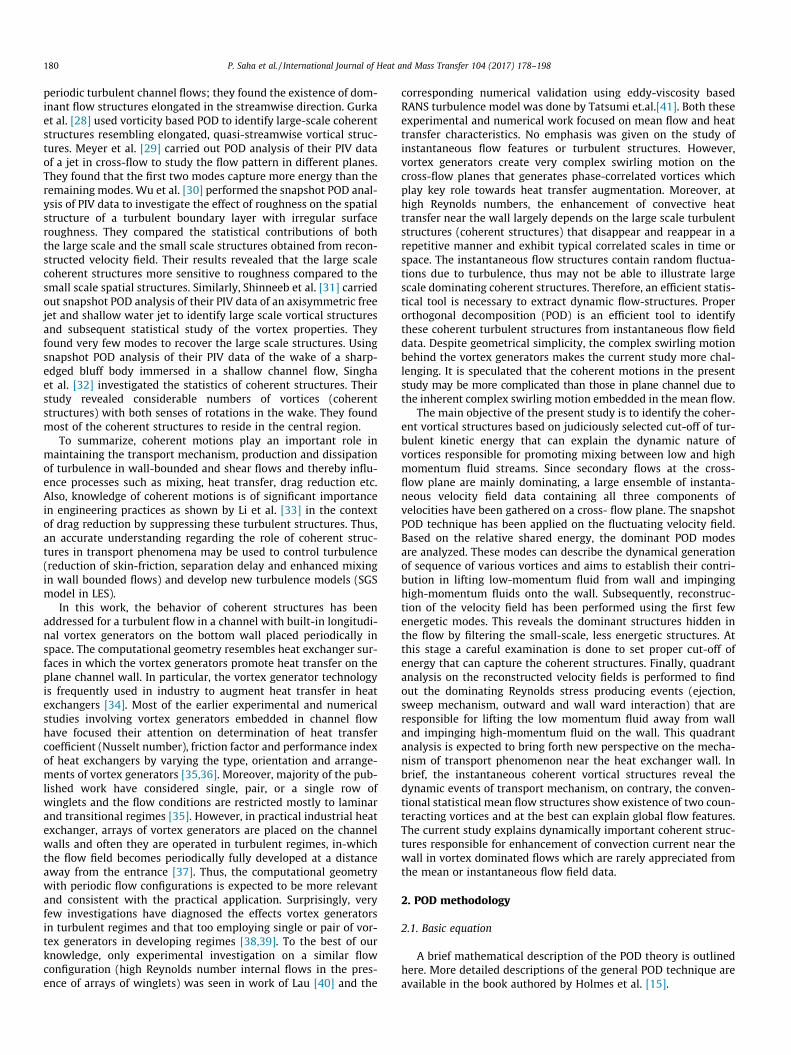
The size of the temporal correlation matrix and computationalmemory requirement is directly linked with the number of snap-shots. Also, the number of snapshots has a direct relation to theaccuracy of the computed eigenvalues. As mentioned by Cazemieret al.[52], the number of snapshots should be increased as much aspossible for an accurate measure of the eigenfunctions. This is ver-ified by observing the convergence of the computed eigenvaluesðkmÞ with the number of snapshots ðMÞ. We consider that a suffi-cient number of snapshots have been obtained when the eigenval-ues no longer change in magnitude with further increase in thenumber of samples. The variations of eigenvalue spectra withrespect to sample size for the first five modes are shown inFig. 6. These eigenvalues have been calculated using a differentnumber of sample sizes from the same data. It is to be noted thatthe eigenvalues represent the amount of turbulent kinetic energyof the flow and their sum indicates the total energy. Therefore, asthe number of snapshots is increased, the number of available


modes among which the energy gets distributed also increases.Hence, the energy content as well as the magnitude of eigenvaluesalso changes with respect to sample size as seen from Fig. 6. Theplot also reflects that as the number of snapshots is increased,the first two modes (mode1 and mode 2), release some of theirenergy as evidenced from their reduced values. It is believed thatthis energy is transferred among the higher modes. Moreover, itis clear from the figure that no significant changes are noticed inthe consecutive magnitude of eigenvalues for all five modes oncethe sample size exceeds 600. Therefore, we have considered that800 snapshots are quite accurate for POD analysis in this study.

4.3. Energy content in different modes

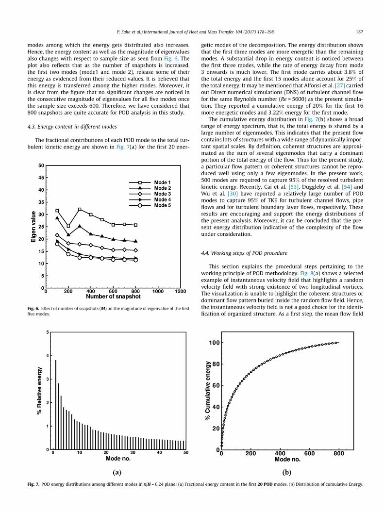
The fractional contributions of each POD mode to the total tur-bulent kinetic energy are shown in Fig. 7(a) for the first 20 ener-

Fig. 6. Effect of number of snapshots (M) on the magnitude of eigenvalue of the firstfive modes.

Fig. 7. POD energy distributions among different modes in x/H = 6.24 plane: (a) Fraction

getic modes of the decomposition. The energy distribution showsthat the first three modes are more energetic than the remainingmodes. A substantial drop in energy content is noticed betweenthe first three modes, while the rate of energy decay from mode3 onwards is much lower. The first mode carries about 3:8% ofthe total energy and the first 15 modes alone account for 25% ofthe total energy. It may be mentioned that Alfonsi et al. [27] carriedout Direct numerical simulations (DNS) of turbulent channel flowfor the same Reynolds number (Re = 5600) as the present simula-tion. They reported a cumulative energy of 20% for the first 16more energetic modes and 3:22% energy for the first mode.

The cumulative energy distribution in Fig. 7(b) shows a broadrange of energy spectrum, that is, the total energy is shared by alarge number of eigenmodes. This indicates that the present flowcontains lots of structures with a wide range of dynamically impor-tant spatial scales. By definition, coherent structures are approxi-mated as the sum of several eigenmodes that carry a dominantportion of the total energy of the flow. Thus for the present study,a particular flow pattern or coherent structures cannot be repro-duced well using only a few eigenmodes. In the present work,500 modes are required to capture 95% of the resolved turbulentkinetic energy. Recently, Cai et al. [53], Duggleby et al. [54] andWu et al. [30] have reported a relatively large number of PODmodes to capture 95% of TKE for turbulent channel flows, pipeflows and for turbulent boundary layer flows, respectively. Theseresults are encouraging and support the energy distributions ofthe present analysis. Moreover, it can be concluded that the pre-sent energy distribution indicative of the complexity of the flowunder consideration.

4.4. Working steps of POD procedure

This section explains the procedural steps pertaining to theworking principle of POD methodology. Fig. 8(a) shows a selectedexample of instantaneous velocity field that highlights a randomvelocity field with strong existence of two longitudinal vortices.The visualization is unable to highlight the coherent structures ordominant flow pattern buried inside the random flow field. Hence,the instantaneous velocity field is not a good choice for the identi-fication of organized structure. As a first step, the mean flow field

al energy content in the first 20 POD modes. (b) Distribution of cumulative Energy.

Fig. 8. POD working steps showing the in-plane velocity vectors for plane x/H = 6.24: (a) Instantaneous velocity field. (b) Mean velocity field. (c) Fluctuatingvelocity field. (d) Reconstructed velocity field (�100% energy). (e) Reconstructedvelocity field (�35% energy).

Table 1Measure of the relative out-of-plane motion for POD modes.

Mode number 1 2 3 4

Urel 0.55818 1.3509 0.60068 0.95444


(Fig. 8(b)) obtained by Reynolds decomposition is subtracted fromthe instantaneous field to provide the fluctuating velocity field asshown in Fig. 8(c). Now, the POD decomposition and correspondingreconstruction is employed on this fluctuating velocity field. Fig. 8(d) illustrates a reconstructed velocity field obtained using all thePOD modes or 100% resolved energy. It is interesting to note thatthe reconstructed velocity field (Fig. 8(d)) exactly retrieves the cor-responding original fluctuating field. This establishes the accuracyof the present POD procedure. It is worth noting that the recon-structed velocity field using the entire POD modes (Fig. 8(d)) isalso, not sufficient to visualize any dominant structures. Lumley[16] pointed out that lower order POD modes capture large-scaleenergy containing structures, while higher order POD modes indi-cate less energetic small-scale events. Thus POD reconstructionneeds to filter out the effects of small scale structures to exposethe large scale structure. This is carried out by reconstructing thevelocity field using only a certain percentage of the total resolvedenergy or leading modes. Fig. 8(e) presents reconstructed velocityfield that recover about 35% resolved energy. This clearly revealsdynamically important large-scale structures such as the largersize vortices that manifest spiraling motion; whereas any such sys-tematic organized pattern is not discernable from the original fluc-tuating velocity field or reconstructed velocity field (obtained fromhigher percentage of energy content), because small scale struc-tures try to mask the large-scale structures.

4.5. POD eigenmodes

The POD eigenmodes are obtained by a linear weighted sum ofthe velocity field with the components of an eigenvector corre-sponding to an eigenvalue. It is well known from the theory thatthese POD modes provide information about the spatial structuresof the flow fields and are stationary over time. The modes areordered according to the energy content of the flow. Lower ordermodes depict large-scale spatial structure and are considered asdominant modes, while higher order modes reflect small-scalestructure. The coherent structures of the flow are reconstructedusing the information of different modes. Therefore, before recon-struction, the POD modes alone are analyzed first to get importantinformation about the flow field without investigating the wholevelocity field.

First, a brief explanation of the plotting method is outlined here.The POD modes are three-component velocity fields. In the follow-ing plots, velocity vectors indicate the in-plane components ofvelocities (spanwise and wall normal components) whereas, theout-of-plane component is represented by the contour map interms of streamwise velocity. The scaling of the vector plots andthe contour map are indicated in the plots. In order to comparethe different modes, the scaling of the velocity vectors and thegap between the contours level are kept the same. Also, the selec-tion of the length scale of vector plots and levels of color contourshas been selected for better visualization of the underlying struc-tures. The relative percentage of the total kinetic energy of velocityfluctuations, shared by different modes is mentioned in the corre-sponding plots. It is important to note that POD modes providequalitative features of the flow and address the issue partially.Thus, the ‘‘length of the vectors” does not convey any physical

5 6 15 30 50

1.0212 1.073 0.93398 0.75114 0.81897

Fig. 9. Plane x/H = 6.24, POD modes 1, 2 and 3: vector represents in-plane velocities and contour represents out-plane velocity.


meaning until the modes are projected onto POD-coefficients toprovide a reconstructed velocity field. In order to assess the rela-tive importance of the in-plane velocity POD mode componentswith respect to the out-of-plane velocity POD mode component,a relative measure parameter is used which takes the form as [29]:

Urel ¼P

kjukjPk

ffiffiffiffiffiffiffiffiffiffiffiffiffiffiffiffiffiv2k þw2

k

q ; k ¼ 1;2 . . .N ð27Þ

The calculated values are tabulated in Table 1 for differentmodes. The first six leading modes are shown in Figs. 9 and 10and a few selective higher modes are shown in Fig. 11. The large-scale spatial structures are depicted by the first leading eigen-modes as shown in Figs. 9 and 10. Higher POD modes, as shownin Fig. 11, appear to be more complex and the spatial scales ofthe structures are found to be decreasing.

Considering structures described by in-plane velocity vectors inFig. 9, first POD mode clearly depicts two co-rotating vortices nearthe bottom wall centered at z=H ¼ 2 and 6, respectively, and alarge vortex near the top wall at the spanwise symmetry line.The contours (streamwise fluctuating velocity) show a couple ofnearly circular structures residing on one another around the vor-tices. The visualization also manifests strong impingement of low-momentum fluid ðu0 < 0Þ towards the wall for the left vortex andlifting of high-momentum fluid ðu0 > 0Þ away from the wall forthe right vortex. In POD mode 2, the out-of-plane component is

very strong as compared to the in-plane velocity vectors, as shownby two large bean-shaped fluid regions. This is further confirmedby considering the relative importance of the in- and out-of- planevelocity components as mentioned in Table 1 for POD mode 2. InPOD mode 3, the in-plane velocities around mid-portions arenearly parallel to the spanwise direction with traces of two vorticesdetected underneath. Mode 4 depicts two counter-rotating vor-tices and lifting of the low-momentum fluid away from wall,thereby, representing ejection mechanism. POD modes 5 and 6contain almost the same percentage of energy and they representnearly same structures, differing only in the locations of the con-tour maps and direction of velocity vector. Furthermore, the in-plane velocity vector has less influence in most parts of thedomain.

Considering the higher modes, such as mode 15, 30, 50 andmode 100 (Fig. 11), it is expected that the small scale structureswould play an important role in these modes due to very lessenergy content. These higher modes are characterized by therandom variations of velocity vectors and small patches ofstreamwise fluctuating velocity contours. As it is seen duringreconstruction, inclusion of all these less energetic structures triesto obscure the identification of large-scale coherent motion.Further, it is not possible to extract coherent structures using onlysingle POD mode. In other words, reconstruction processes oftenemploy too many modes that embody certain meaningful coherentstructures.

Fig. 10. Plane x/H = 6.24, POD modes 4, 5 and 6: vector represents in-plane velocities and contour represents out-plane velocity.


4.6. POD coefficients

Recalling the POD theory, the POD coefficients (Eq. (18)) aredetermined by projecting the velocity field onto the POD modesand they indicate the weight of each eigenmode. Moreover, thespatial structures provided by eigenmodes are time independentand they are unable to convey any physical meaning with refer-ence to the scale or sign of the flow field. Thus it is the sign and sizeof the POD coefficients which directly influence the POD modes todescribe any snapshot. Furthermore, the POD coefficients are ran-dom over time and reflect the embodied energy of a particular spa-tial structure. Therefore, studying the time characteristics of PODcoefficients will bring forth greater insight about the evolution ofthe dynamic behavior of the structures represented by the PODmodes.

The time evolution of first two POD coefficients is shown inFig. 12(a), which indicates strong variations in the amplitude ofcoefficients with time, yielding the complexity of the flow. Addi-tionally, the distributions look qualitatively same with a shiftingof phase suggesting a strong coupling between them. Furthermore,it is clearly shown that they have almost equal magnitudes leadingto nearly same contributions towards corresponding modes. Thephase plots between POD- coefficients a1 –a2 and coefficients a1

–a5 are portrayed in Fig. 12(b) and (c) respectively. Both the phaseplots resemble a circular shape. Larger portions of the points arevisible around a circle of radius 8 and centered at (0, 0). The circu-

lar distributions signify a strong correlation between the modesconsidered and more importantly suggest a cyclic variationbetween them describing different phases of a process. The scatter-ing nature of the phase plots indicates the presence of strong localvariations of velocity fluctuations. This phase plot becomes veryimportant during reconstruction of a velocity field to describe cer-tain flow features. After selecting the number of modes for recon-struction, the time instants of the mode is selected in such a waythat they follow nearly circular paths. This will provide the correctsequence of snapshots that could better describe the significantphase of certain flow dynamics such as the vortex shedding pro-cess for a cylinder.

4.7. Selection of cut-off energy for reconstruction of coherentstructures

The POD decomposition separates the fluctuating velocity fieldinto large- and small-scale POD eigenmodes as explained earlier.Furthermore, the leading dominant modes are found to representlarge-scale coherent structures (see Fig. 9). Thus, each individualfluctuating velocity field (or snapshot) can be reconstructed usinga few leading eigenmodes that expose large scale flow features.Unfortunately, the number of leading modes required to identifylarge-scale energetic coherent structures is difficult to decide. Itdepends primarily on the flow conditions. In the present work,the nature of energy distribution plot (Fig. 7(b)), suggests that

Fig. 11. Plane x/H = 6.24, POD modes 15, 30, 50 and 100: vector represents inplane velocities and contour represents out-plane velocity.


the velocity field is complex and the coherent structures may notbe represented using only few dominant eigenmodes. In order toinvestigate the effect of the number of POD modes, the reconstruc-tion process has been repeated by varying the number of modescorresponding to different amounts of cumulative energy contentas shown in Figs. 13 and 14. In this figure, in-plane velocities con-stitute the velocity vectors and the contour maps represent a scalarquantity known as Q-criterion introduced by Hunt et al. [55]. It isobvious that velocity vector maps are not sufficient to reveal thelocations of all vortices, since the reconstructed velocity field isnot a Galilean invariant. In order to better visualize the vorticalstructures embedded within the flow, the definition of ‘‘positivesecond invariant of the velocity gradient tensor” referred to as Q-criterion has been adopted. This is calculated by subtracting the

magnitude of mean rate-of- strain tensor from the magnitude ofmean vorticity vector. Thus, regions with positive Q indicate thedominance of rotation over shear and identify the locations of vor-tices accurately. The measure of Q is shown as grayscale contourswith higher values indicated by darker colors. The contours corre-sponding to negative Q value are not shown. Thus, the locationsand extent of vortices are visualized as the darker color regions.

Fig. 13(a) and (b) show reconstructed fluctuating velocity fieldscorresponding to only 12% and 25% resolve energy content, respec-tively. Since the reconstruction considered only lower modes thatfilter out small scale structures corresponding to higher modes,the plots (Fig. 13(a) and (c)) reveal relatively larger sized vorticeswith less number of structures. It is to be noted that higher energyaccumulation introduces progressively small scale structures

Fig. 12. Distribution of POD coefficients corresponding to plane x/H = 6.24. (a) Time variations of the first two reconstruction coefficient. (b) Phase plot between PODcoefficients of mode 1 and 2. (c) Phase plot between POD coefficients corresponding to mode 1 and 5.


which provides higher strength of vortices. In Fig. 13(c), 35% of thecumulative energy is recovered and more detailed vortical struc-tures with higher strength are exposed. According to Lumley[16], the coherent structure should recover a dominant percentageof energy. But, as the cumulative energy content is increased, theinclusion of small-scale less important structures tries to obscurethe large scale structures. Therefore, the threshold of cut-off energyshould be such that, more detailed information is ensured withoutlosing any identity of the large-scale structures. In Fig. 14(a) and (b), higher modes have been added during reconstructionthat retrieves 43% and 50% cumulative turbulent kinetic energy,respectively. This shows a coherent pattern representing the headsof hairpin-like vortex structures more clearly. Furthermore, it is

noticed that Figs. 13(c), 14(a) and 14(b) seem to represent flowpatterns that are quite similar to each other, but relatively moredetailed information has been captured. More importantly, inFig. 14(b), the influences of small scale structures become slightlyintense and the large-scale structures get relatively blurred whichinhibit any possible interpretation of the physics pertaining todominant coherent structures. Another reconstructed velocity fieldthat accumulates 95% cumulative energy is displayed in Fig. 14(c).This represents almost similar structures as the original fluctuatingvelocity field. The plots clearly reflect the influence of higher butless important small-scale modes that result in chaotic randomstructures and the large-scale pattern goes out of focus. Thus, asuitable threshold or cut-off percentage of the cumulative energy

Fig. 13. Effect of cut-off energy on reconstructed fluctuating velocity field for plane x/H = 6.24 (a) (�12% energy) (b) (�25% energy) (c) (�35% energy); (Vectors indicate in-plane velocities and contours represents Q criterion.).


content is necessary to educe accurately the large scale coherentstructures that provide detailed information related to flow phe-nomena of dominant structures.

A unique choice is practically unattainable. Roussinova et al.[56] extensively explained the selection procedure and used 50%cut-off energy to expose the energetic structures for smooth openchannel flow. Liu et al. [9] and Wu et al. [30] adopted a 50% thresh-old criterion to estimate the large scale structures in turbulentchannel and boundary layer flows, respectively. While, Shinneebet al. [31] and Singha et al. [32] found 40% cut-off energy criterionto be satisfactory for eduction of coherent structure in axisymmet-ric free jet and swallow channel flow. In the present study, it isobserved that energy content less than 43% is unable to providedetailed information, and that more energy content introducesthe influence of small scale structures. Thus the above investiga-tions reveal that patterns containing 43% cumulative energymeet all the qualities of a large scale structures. Therefore, 43%cut-off energy content corresponding to the 50 leading POD modeshas been considered for POD reconstruction as shown in Fig. 14(a),which describes the turbulent transport mechanism accurately asdiscussed in the next section.

4.8. Interpretations of reconstructed snapshot

This section represents some selected POD-reconstructed veloc-ity fields along with the corresponding original velocity fields todecipher additional information about the flow structures and toexplain the momentum transport mechanism in terms of stressproducing events. As explained earlier, the POD-reconstructedvelocity fields corresponding to a cut-off of 43% turbulent kineticenergy have been considered among the alternatives, because theycarry a significant amount of information regarding large scalestructures. Furthermore, the snapshots have been selected byinspecting an animation of 200 realizations that provide evidenceof meaningful flow events such as ejections, sweeps and swirlingeffects generated by the vortices. Examples of original fluctuatingvelocity field and some typical POD-reconstructed fluctuatingvelocity fields are shown in Fig. 15. The in-plane fluctuatingvelocity components ðw0;v 0Þ are shown as vectors, while the out-of-plane component ðu0Þ is shown as color contours. The originalfluctuating velocity field as depicted by Fig. 15(a) manifests littleevidence of significant spatial structures due to the mixing of allthe scales of motions. However, several small patches of positive

Fig. 14. Effect of cut-off energy on reconstructed fluctuating velocity field for plane x/H = 6.24 (a) (�43% energy) (b) (�50% energy) (c) (�95% energy); Vectors indicate in-plane velocities and contours represents Q criterion.


and negative streamwise velocity fluctuations ðu0Þ, which are quiteevident in the contour maps of Fig. 15(a), indicate spatial imprintsof high-momentum ðu0 > 0Þ and low-momentum ðu0 < 0Þ regions,respectively. While, Fig. 15(b–d), display some typical sets ofPOD-reconstructed fluctuating velocity fields. These plots highlightstructures that are more clearly visible and many important stressproducing events are noted.

In order to investigate the Reynolds-stress-producing events,quadrant analysis [57] based on streamwise-wall normal fluctuat-ing velocity ðu0;v 0Þ components have been carried out. Notableexplanation and application of quadrant analysis on POD recon-structed velocity field can be found in the works of Roussinovaet al. [56] and Cai et al. [53], respectively. According to the flowdirection of fluid motions considering only the sign of ðu0Þ andðv 0Þ, Fig. 16 schematically categorizes the various events that con-tribute to the total turbulence production. The first quadrant,ðu0 > 0Þ and ðv 0 > 0Þ, provides outward interaction of high-momentum fluid referred to as Q1 motion, while the second quad-rant, ðu0 < 0Þ and ðv 0 > 0Þ, constitutes fluid motion that ejects thelow-momentum fluid away from wall (Q2 motion). However, thethird quadrant is represented by ðu0 < 0Þ and ðv 0 < 0Þ, and provideswall-ward motion of low-momentum fluid (Q3 motion); and the

fourth quadrant, ðu0 > 0Þ and ðv 0 < 0Þ, contains sweeps of highmomentum fluid towards the wall designated as Q4 motion.

Numerous vortical motions are captured by the POD-reconstructed fields as depicted by the velocity vectors. Fig. 15(b)mostly captures ejection (labeled Q2) and sweep events (labeledQ4). The field in Fig. 15(b) is actually reconstructed from the fluc-tuating velocity field depicted in Fig. 15(a). A large vortex has beenidentified around z/H = 2 and close to the bottomwinglet wall witha rotation in counter-clockwise direction and slightly inclinedtoward the wall in the span-wise direction, as may be seen inFig. 15(b). This vortical motion induces lifting of low-momentumfluid particles away from the wall providing ejection events(labeled Q2). Further, sweeps of fluid motion with positivestream-wise fluctuations have been noticed near both the wallsand have been labeled as Q4 in the plot. In Fig. 15(c), a counter-clockwise rotating small vortex is seen close to the lower wallaround z/H = 3 which causes elevation of low momentum fluidaway from the wall representing the Q2 event. This vortical motionproduces a strong negative spanwise motion towards right partwith high-momentum fluid being pushed toward the wall provid-ing a sweep event (labeled Q4). Fig. 15(c) also shows another vor-tex close to the near wall at z/H = 6, where negative streamwise

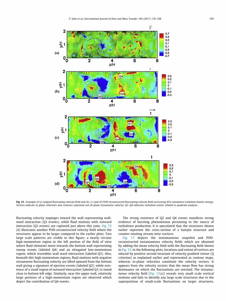
Fig. 15. Example of (a) original fluctuating velocity field and (b), (c) and (d) POD reconstructed fluctuating velocity field recovering 43% cumulative turbulent kinetic energy;Vectors indicate in-plane velocities and contours represent out-of-plane streamwise velocity. Q1–Q4 indicates turbulent events related to quadrant analysis.


fluctuating velocity impinges toward the wall representing wall-ward interaction (Q3 events), while fluid motions with outwardinteraction (Q1 events) are captured just above this zone. Fig. 15(d) illustrates another POD-reconstructed velocity field where thestructures appear to be larger compared to the earlier plots. Twolarge scale patterns are visible in this figure; a nearly circularhigh-momentum region in the left portion of the field of viewwhere fluid elements move towards the bottom wall representingsweep events (labeled Q4) and an elongated low-momentumregion, which resembles wall ward interaction (labeled Q3). Also,beneath this high momentum regions, fluid motions with negativestreamwise fluctuating velocity are lifted upward from the bottomwall giving a signature of ejection events (labeled Q2), while exis-tence of a small region of outward interaction (labeled Q1) is notedclose to bottom left edge. Similarly, near the upper wall, relativelylarge portions of a high-momentum region are observed whichdepict the contribution of Q4 events.

The strong existence of Q2 and Q4 events manifests strongevidence of bursting phenomenon pertaining to the source ofturbulence production. It is speculated that the structures shownearlier represent the cross-section of a hairpin structure andcounter-rotating stream-wise vortices.

Fig. 17 depicts the instantaneous snapshot and POD-reconstructed instantaneous velocity fields which are obtainedby adding the mean velocity field with the fluctuating field shownin Fig. 15. In the following plots, locations and extent of vortices areeduced by positive second invariant of velocity gradient tensor (Qcriterion) as explained earlier and represented as contour maps,whereas in-plane velocities constitute the velocity vectors. Itappears from the velocity vectors that the mean flow has strongdominance on which the fluctuations are overlaid. The instanta-neous velocity field (Fig. 17(a)) reveals very small scale vorticalmotions and fails to identify any large scale structures due to thesuperposition of small-scale fluctuations on larger structures.

Fig. 16. Schematic diagram showing different turbulent fluid motions according to quadrant analysis procedure.


However, the remaining plots (Fig. 17(b–d)) clearly expose a circu-lar pattern of velocity vectors representing counter-rotating quasi-stream-wise vortices.

Since velocity vectors in fixed reference frame are unable toidentify all the vortices, the large scale vortical motions are identi-fied by measuring the Q value as shown by the gray scale contourmaps with darker contours indicating higher values. Hence, thelocations and extent of vortices are clearly visualized by the darkercolored regions. All contour maps in reconstructed fields (Fig. 17(b–d)) employ the same scale for better comparison of the relativestrength of vortices among the reconstructed fields. However, thelevel of contour map in instantaneous velocity field (Fig. 17(a)) ismuch higher compared to reconstructed fields (Fig. 17(b–d)). Thishigher value is an indication of the existence of small scale vorticesthat possess large concentrated vorticity. The Q criterion clearlyindicates the spatial imprints of horse-shoe vortices near the bot-tom wall and beneath the main vortex. This also provides detailedinformation about numerous vortical motions.

5. Conclusions

Our large eddy simulation (LES) results are analyzed in order tounderstand the origin and development of dynamical large scaleflow structures. The characteristics of the flow and thermal fieldsare connected. A turbulent flow is composed of several structures.Since, the conventional mean flow fields can at best explain theglobal features, it is important to identify large turbulence struc-tures based on dominant shared energy that can explain the mix-ing between low and high momentum fluid streams. The mixingenhances convective transport coefficient near the wall of the heatexchanger surfaces.

The proper orthogonal decomposition (POD) method in con-junction with quadrant analysis and vortex identification tool such

as positive second invariant method have been employed to studythe ensemble of instantaneous velocity fields in a vortex domi-nated turbulent channel flow. The computational geometry resem-bles heat exchanger surfaces on which the vortex generators createstreamwise longitudinal vortices that disrupt the growth of ther-mal boundary layers entailing enhancement of heat transfer onthe above mentioned surfaces. The aim of the present investigationis to extract the large scale coherent structures in the form ofsreamwise vortices buried within random velocity fields and togain more insight into the role of these coherent motions in pro-moting turbulent transport near the wall that is responsible forenhancement of convective heat transfer.

The novel findings from the current investigations are asfollows:

� The energy distribution curves yield as many as 15 dominantPOD modes to cumulatively capture as low as 25% of the totalturbulent kinetic energy of the flow, indicating broad range ofenergy spectrum shared amongst a large number of PODmodes.This characterizes the flow fields behind the vortex generatorsas highly complex turbulent fields composed of numerous spa-tial and temporal turbulent scales. Subsequently, the energydistribution curve indicates the requirements of many PODmodes to characterize various meaningful coherent structures.

� A typical POD mode can describe coherent structures, if andonly if it contains a dominant fraction of energy. The energy dis-tribution and subsequent contour plots depict that first fewleading PODmodes (Figs. 9 and 10) clearly reproduce the coher-ent vortical structures, while, the higher modes (Fig. 11) possessrandomly behaved less energetic small scale structures.

� The contour plots of dominant POD modes dynamically depict(Figs. 9 and 10) the systematic generation of co-rotating,counter-rotating and bean-shaped vortices and their movement

Fig. 17. Example of (a) original instantaneous velocity field and (b), (c) and (d) POD reconstructed instantaneous velocity field (mean + fluctuation) corresponding to Fig. 12.Vectors indicate in-plane velocities and contours represents Q criterion.


from channel centers to sideward locations, while, the vectorplots of POD modes explain the contribution of the vortices inlifting lowmomentum fluids away from the wall and in imping-ing high momentum fluids onto the wall to increase convectivetransport.

� The phase plots of the leading POD coefficients establish astrong correlation implying cyclic variations between theevents at different instants. The scattering nature of the phaseplots indicates the presence of strong local variations of velocityfluctuations.

� The choice of cut-off energy during reconstruction of velocityfields to expose meaningful coherent structures poses a hugechallenge. The coherent structures require dominant fractionof energy. Addition of too many higher less energetic modesprohibit the large scale structures from being properly inter-preted. A careful examination revealed a cut-off of 43% turbu-

lent kinetic energy is sufficient to clearly expose the coherentstructures for the flow of interest. This is also consistent withthe published literature on similar flows.

� Finally, quadrant analysis on the reconstructed velocity fieldsreveals that the convective transport near the wall is mainlydriven by two important Reynolds stress producing events(ejection and sweep mechanism), in which, the vortices liftsthe low momentum fluid away from wall through the ejectionmechanism. The high-momentum fluid impinges on the wallin sweep mode and thereby enhances convection near the wall.

� It is to be noted that the conventional statistical mean flowstructures show existence of counteracting vortices and providemerely global flow features. The POD modes in the currentinvestigation exposed numerous dynamical vortices (co-rotating, counter-rotating and bean-shaped vortices) and theircontribution towards local variations of flows.


� Visualization of vortices by deploying another mathematicaltool, positive second invariant, on both the instantaneous andreconstructed velocity fields, has strengthen the evidence ofthe large scale coherent structures revealed in POD modesand manifests various spatial imprints of vortical motion per-taining to large scale momentum transfer.

In brief, the current analyses show that the dynamical vorticalstructures, such as co-rotating, counter-rotating and bean shapedvortices along with the ejection and sweepmode of Reynolds stres-ses producing events are the principal mechanisms which createstrong lifting and impingements of low and high- momentum flu-ids. Such mechanisms promote mixing indicating enhancement ofconvective transport near the heat exchanger surfaces.

References

[1] S.J. Kline, W.C. Reynolds, F.A. Schraub, P.W. Runstadler, The structure ofturbulent shear layers, J. Fluid Mech. 30 (1967) 741–773.

[2] S.K. Robinson, Coherent motions in the turbulent boundary layer, Annu. Rev.Fluid Mech. 23 (1991) 601–639.

[3] E.R. Corino, R.S. Brodkey, A visual investigation of the wall region in turbulentflow, J. Fluid Mech. 37 (1969) 1–30.

[4] M.R. Head, P. Bandyopadhyay, New aspects of turbulent boundary-layerstructure, J. Fluid Mech. 107 (1981) 297–338.

[5] A.E. Perry, M.S. Chong, On the mechanism of wall turbulence, J. Fluid Mech. 119(1982) 173–217.

[6] C.R. Smith, J.D.A. Walker, A.H. Haidari, U. Soburn, On the dynamics of near-wallturbulence, Phil. Trans. R. Soc. A 336 (1991) 131–175.

[7] B.A. Singer, R.D. Joslin, Metamorphosis of a hairpin vortex into a youngturbulent spot, Phys. Fluids 6 (1994) 3724–3736.

[8] R.J. Adrian, K.T. Christensen, Z.C. Liu, Analysis and interpretation ofinstantaneous turbulent velocity fields, Exp. Fluids 29 (2000) 275–290.

[9] Z. Liu, R.J. Adrian, T.J. Hanratty, Large-scale modes of turbulent channel flow:transport and structure, J. Fluid Mech. 448 (2001) 53–80.

[10] J. Zhou, R.J. Adrian, S. Balachandar, T.M. Kendall, Mechanisms for generatingcoherent packets of hairpin vortices in channel flow, J. Fluid Mech. 387 (1999)353–396.

[11] R.A. Antonia, Conditional sampling in turbulence measurement, Annu. Rev.Fluid Mech. 13 (1981) 131–156.

[12] R.J. Adrian, P. Moin, Stochastic estimation of organized turbulent structure:homogeneous shear flow, J. Fluid Mech. 190 (1988) 531–559.

[13] G. Berkooz, P. Holmes, J.L. Lumley, The proper orthogonal decomposition in theanalysis of turbulent flows, Annu. Rev. Fluid Mech. 25 (1993) 539–575.

[14] A. Chatterjee, An introduction to the proper orthogonal decomposition, Curr.Sci. 78 (2000) 808–817.

[15] P. Holmes, J.L. Lumley, G. Berkooz, Turbulence, Coherent Structures, DynamicalSystems and Symmetry, Cambridge University Press, Cambridge, 1996.

[16] J.L. Lumley, The structure of inhomogeneous turbulent flows, in: A.M. Yaglom,V.I. Tararsky (Eds.), Atmospheric Turbulence and Radio Wave Propagation,1967. Nauka, Moscow.

[17] L. Sirovich, Turbulence and the dynamics of coherent structures. Part I:coherent structures. Part II: symmetries and transformations. Part III:dynamics and scaling, Q. Appl. Math. 45 (1987) 561–590.

[18] L. Sirovich, S. Karlsson, Turbulent drag reduction by passive mechanisms,Nature 388 (1997) 753–755.

[19] H.P. Bakewell, J.L. Lumley, Viscous sublayer and adjacent wall region inturbulent pipe flows, Phys. Fluids 10 (1967) 1880–1889.

[20] N. Aubry, P. Holmes, J.L. Lumley, E. Stone, The dynamics of coherent structuresin the wall region of a turbulent boundary layer, J. Fluid Mech. 192 (1988)115–173.

[21] M. Kirby, J. Boris, L. Sirovich, An eigenfunction analysis for axisymmetric jetflow, J. Comput. Phys. 90 (1990) 98–122.

[22] G. Alfonsi, C. Restano, L. Primavera, Coherent structures of the flow around asurface mounted cubic obstacle in turbulent channel flow, J. Wind Eng. Ind.Aerodyn. 91 (2003) 495–511.

[23] H. Gunes, U. Rist, Proper orthogonal decomposition reconstruction of atransitional boundary layer with and without control, Phys. Fluids 16 (2004)2763–2784.

[24] M. Fogleman, J.L. Lumley, D. Rempfer, D. Haworth, Application of the properorthogonal decomposition to datasets of internal combustion engine flows, J.Turbul. 5 (2004) 023–030.

[25] P. Moin, R.D. Moser, Characteristic-eddy decomposition of turbulence in achannel, J. Fluid Mech. 200 (1989) 471–509.

[26] K.S. Ball, L. Sirovich, L.R. Keefe, Dynamical eigenfunction decomposition ofturbulent channel flow, Int. J. Numer. Meth. Fluids 12 (1991) 585–604.

[27] G. Alfonsi, L. Primavera, The structure of turbulent boundary layers in the wallregion of plane channel flow, Proc. R. Soc. A 463 (2007) 593–612.

[28] R. Gurka, A. Liberzon, G. Hetsroni, POD of vorticity fields: a method for spatialcharacterization of coherent structures, Int. J. Heat Fluid Flow 27 (2006) 416–423.

[29] K.E. Meyer, J.M. Pedersen, O. Ozcan, A turbulent jet in crossflow analysed withproper orthogonal decomposition, J. Fluid Mech. 583 (2007) 199–227.

[30] Y. Wu, K.T. Christensen, Spatial structure of a turbulent boundary layer withirregular surface roughness, J. Fluid Mech. 655 (2010) 380–418.

[31] A.M. Shinneeb, R. Balachandar, J.D. Bugg, Analysis of coherent structures in thefar-field region of an axisymmetric free jet identified using particle imagevelocimetry and proper orthogonal decomposition, ASME J. Fluids Eng. 130(2008). 011202-1–011202-9.

[32] A. Singha, R. Balachandar, Coherent structures statistics in the wake of a sharp-edged bluff body placed vertically in a shallow channel, Fluid Dyn. Res. 43(2011) 055504.

[33] F.C. Li, Y. Kawaguchi, K. Hishida, M. Oshima, On turbulent contribution tofrictional drag in wall-bounded turbulent flow, Chin. Phys. Lett. 23 (2006)1226.

[34] M. Fiebig, P. Kallweit, N.K. Mitra, St. Tigglbeck, Heat transfer enhancement anddrag by longitudinal vortex generators in a channel flow, Exp. Thermal FluidSci. 4 (1991) 103–114.

[35] G. Biswas, K. Torii, D. Fujii, K. Nishino, Numerical and experimentaldetermination of flow structure and heat transfer effects of longitudinalvortices in a channel flow, Int. J. Heat Mass Transfer 39 (1996) 3441–3451.

[36] A. Pal, D. Bandyopadhyay, G. Biswas, V. Eswaran, Enhancement of heat transferusing delta-winglet type vortex generators with a common flow uparrangement, Numer. Heat Transfer, Part A 61 (2012) 912–928.

[37] U. Brockmeier, T.H. Guentermann, M. Fiebig, Performance evaluation of avortex generator heat transfer surface and comparison with different highperformance surfaces, Int. J. Heat Mass Transfer 36 (1993) 2575–2587.

[38] Z.X. Yuan, W.Q. Tao, X.T. Yan, Experimental study on heat transfer in ductswith winglet disturbances, Heat Transfer Eng. 24 (2003) 76–84.

[39] P. Deb, G. Biswas, N.K. Mitra, Heat transfer and flow structure in laminar andturbulent flows in a rectangular channel with longitudinal vortices, Int. J. HeatMass Transfer 38 (1995) 2427–2444.

[40] S. Lau, Experimental study of the turbulent flow in a channel with periodicallyarranged longitudinal vortex generators, Exp. Thermal Fluid Sci. 11 (1995)255–262.

[41] K. Tatsumi, H. Iwai, K. Inaoka, K. Suzuki, Numerical analysis for heat transfercharacteristics of an oblique discrete rib mounted in a square duct, Numer.Heat Transfer A 44 (2003) 811–831.

[42] J. Kostas, J. Soria, M.S. Chong, A comparison between snapshot POD analysis ofPIV velocity and vorticity data, Exp. Fluids 38 (2005) 46–160.

[43] P.G. Cizmas, A. Palacios, T. O’Brien, M. Syamlal, Proper orthogonaldecomposition of spatio-temporal patterns in fluidized beds, Chem. Eng. Sci.58 (2003) 4417–4427.

[44] J. Srikanth, E.G. Tulapurkara, G. Biswas, Large eddy simulation of flow pastbuilt-in winglet-pair in rectangular channel, Int. J. Fluid Mech. Res. 32 (2005)310–326.

[45] J. Smagorinsky, General circulation experiments with the primitive equations.I. The basic equations, Mon. Weather Rev. 91 (1963) 99–164.

[46] E. Lévêque, F. Toschi, L. Shao, J.P. Bertoglio, Shear-improved Smagorinskymodel for large-eddy simulation of wall-bounded turbulent flows, J. FluidMech. 570 (2007) 491–502.

[47] P. Saha, G. Biswas, Assessment of a shear-improved subgrid stress closure forturbulent channel flows, Int. J. Heat Mass Transfer 53 (2010) 4789–4795.

[48] F.H. Harlow, J.E. Welch, Numerical calculation of time-dependent viscousincompressible flow of fluid with free surface, Phys. Fluid 8 (1965) 2182–2188.

[49] J. Liu, U. Piomelli, P.R. Spalart, Interaction between a spatially growingturbulent turbulent layer and embedded streamwise vortices, J. Fluid Mech.326 (1996) 151–179.

[50] P. Saha, G. Biswas, Numerical simulation of turbulent flow in a rectangularchannel with periodically mounted longitudinal vortex generators, Front. HeatMass Transfer 2 (2011) 33008.

[51] A.M. Shinneeb, Confinement effects in shallow water jets PhD dissertation,University of Saskatchewan, Canada, 2006.

[52] W. Cazemier, R.W.C.P. Verstappen, A.E.P. Veldman, Proper orthogonaldecomposition and low dimensional models for driven cavity flows, Phys.Fluids. 10 (1998) 1685–1699.

[53] W.-H. Cai, F.-C. Li, H.-N. Zhang, X.-B. Li, B. Yu, J.-J. Wei, Y. Kawaguchi, K.Hishida, Study on the characteristics of turbulent drag-reducing channel flowby particle image velocimetry combining with proper orthogonaldecomposition analysis, Phys. Fluids. 21 (2009). 115103-1–115103-12.

[54] A. Duggleby, K.S. Ball, M.R. Paul, P.F. Fischer, Dynamical eigenfunctiondecomposition of turbulent pipe flow, J. Turbul. 8 (2007) 1–24.

[55] J.C.R. Hunt, A.A. Wray, P. Moin, Eddies, streams and convergence zones inturbulent flows, in: Proc. CTR Summ. Progr., NASA Ames/Stanford University,1998, pp. 193–208.

[56] V. Roussinova, A.M. Shinneeb, R. Balachandar, Investigation of fluid structuresin a smooth open-channel flow using proper orthogonal decomposition, J.Hydraul. Eng. 136 (2010) 143–154.

[57] S.S. Lu, W.W. Willmarth, Measurements of the structure of the Reynolds stressin a turbulent boundary layer, J. Fluid Mech. 60 (1973) 481–571.

http://refhub.elsevier.com/S0017-9310(16)30086-2/h0005




















































































































































International Journal of Heat and Mass Transfer · neous ﬂow ﬁeld data. Despite geometrical...

Documents

Transcript of International Journal of Heat and Mass Transfer · neous ﬂow ﬁeld data. Despite geometrical...