International Journal of Engineering Research and General...
14
International Journal of Engineering Research and General Science Volume 4, Issue 2, March- April, 2016 ISSN 2091-2730 764 www.ijergs.org A SENSORLESS SLIDING MODE CONTROL BASED INDUCTION MOTOR DRIVE FOR INDUSTRIAL APPLICATION 1 LAVANYA.S 2 MOHAMED APPAS.J 3 SURESH KUMAR.P 4 VIJAYALAKSHMI.V 5 JENIFER ROSNEY.J DEPARTMENT OF ELECTRICAL AND ELECTRONICS ENGINEERING MAHARAJA INSTITUTE OF TECHNOLOGY, COIMBATORE EMAIL: [email protected]/ Ph.No. 9566650283 Abstract— Parameter identification plays an important role in speed estimation schemes. This paper presents a speed estimation scheme based on second-order sliding-mode super twisting algorithm (STA) and model reference adaptive system (MRAS) estimation theory, in which both variations of stator resistance and rotor resistance are deliberately treated. A stator current observer is designed based on the STA, which is utilized to take the place of the reference voltage model of the standard MRAS algorithm. The observer is insensitive to the variation of rotor resistance and perturbation when the states arrive at the sliding mode. Derivatives of rotor flux are obtained and designed as the state of MRAS, thus eliminating the integration. Furthermore, in order to improve the near- zero speed operation, a parallel adaptive identification of stator resistance is designed relying on derivatives of rotor flux and stator current. Compared with the first-order sliding-mode speed estimator, the proposed scheme makes full use of the auxiliary sliding- mode surface, thus alleviating the chattering behavior without increasing the complexity. The robustness and effectiveness of the proposed scheme have been validated experimentally. Keywords— DC link, Induction Motor, Inverter, Inverse Park transformation, Model reference adaptive system, PI controller, Park Transformation, PWM, Rectifier, Sliding Mode Technique. 1. INTRODUCTION With the invention of vector control technique the induction motor (IM) became popular for variable-speed drives and motion control. In indirect vector control of IM, flux and torque are decoupled under estimation of the slip speed with appropriate information of the rotor time constant. The accuracy of motor parameters, particularly, the rotor time constant plays an important role for the accuracy of the indirect vector method. To cope with that, recently, variable- structure controls (VSC), and in particular, sliding-mode control (SMC) system, have been applied for electric motor drive. The SMC-based drive system has many attractive features such as: 1) it is robust to parameter variations and model uncertainties and insensitive to external load disturbance; 2) it offers a fast dynamic response, and stable control system; 3) it can handle some nonlinear systems that are not stable by using linear controller; and, 4) it requires an easy hardware/software implementation. However, due to discontinuous nature, it has some limitations in electrical drives and shows high-frequency oscillations as chattering characteristics. The chattering makes various undesirable effects such as current harmonics and torque pulsation. In recent years, the chattering issue has become the research focus of many scholars. Generally, introducing a thin boundary layer around the sliding surface can solve the chattering problem by interpolating a continuous function inside the boundary layer of switching surface. However, the slope of the continuous function is a compromise between control performance and chattering elimination. Also, asymptotic stability is not guaranteed and may cause a steady-state error. 2. OBJECTIVES OF THE THESIS The objectives of the thesis are listed below: To reduce the overshoot of the DC link in existing system. To measure the speed without sensors. To use sliding mode technique to estimate speed. To acknowledge the efficient working of the existing system using this proposed system in the company. To design a model sufficient to prove the result.
Transcript of International Journal of Engineering Research and General...

International Journal of Engineering Research and General Science Volume 4, Issue 2, March- April, 2016 ISSN 2091-2730
764 www.ijergs.org
A SENSORLESS SLIDING MODE CONTROL BASED INDUCTION
MOTOR DRIVE FOR INDUSTRIAL APPLICATION
1 LAVANYA.S
2 MOHAMED APPAS.J
3 SURESH KUMAR.P
4 VIJAYALAKSHMI.V
5JENIFER ROSNEY.J
DEPARTMENT OF ELECTRICAL AND ELECTRONICS ENGINEERING
MAHARAJA INSTITUTE OF TECHNOLOGY, COIMBATORE
EMAIL: [email protected]/ Ph.No. 9566650283
Abstract— Parameter identification plays an important role in speed estimation schemes. This paper presents a speed
estimation scheme based on second-order sliding-mode super twisting algorithm (STA) and model reference adaptive system (MRAS)
estimation theory, in which both variations of stator resistance and rotor resistance are deliberately treated. A stator current observer is
designed based on the STA, which is utilized to take the place of the reference voltage model of the standard MRAS algorithm. The
observer is insensitive to the variation of rotor resistance and perturbation when the states arrive at the sliding mode. Derivatives of
rotor flux are obtained and designed as the state of MRAS, thus eliminating the integration. Furthermore, in order to improve the near-
zero speed operation, a parallel adaptive identification of stator resistance is designed relying on derivatives of rotor flux and stator
current. Compared with the first-order sliding-mode speed estimator, the proposed scheme makes full use of the auxiliary sliding-
mode surface, thus alleviating the chattering behavior without increasing the complexity. The robustness and effectiveness of the
proposed scheme have been validated experimentally.
Keywords— DC link, Induction Motor, Inverter, Inverse Park transformation, Model reference adaptive system, PI controller, Park Transformation, PWM,
Rectifier, Sliding Mode Technique.
1. INTRODUCTION
With the invention of vector control technique the induction motor (IM) became popular for variable-speed drives
and motion control. In indirect vector control of IM, flux and torque are decoupled under estimation of the slip speed with appropriate
information of the rotor time constant. The accuracy of motor parameters, particularly, the rotor time constant plays an important role
for the accuracy of the indirect vector method. To cope with that, recently, variable- structure controls (VSC), and in particular,
sliding-mode control (SMC) system, have been applied for electric motor drive. The SMC-based drive system has many attractive
features such as: 1) it is robust to parameter variations and model uncertainties and insensitive to external load disturbance; 2) it offers
a fast dynamic response, and stable control system; 3) it can handle some nonlinear systems that are not stable by using linear
controller; and, 4) it requires an easy hardware/software implementation. However, due to discontinuous nature, it has some
limitations in electrical drives and shows high-frequency oscillations as chattering characteristics.
The chattering makes various undesirable effects such as current harmonics and torque pulsation. In recent years, the
chattering issue has become the research focus of many scholars. Generally, introducing a thin boundary layer around the sliding
surface can solve the chattering problem by interpolating a continuous function inside the boundary layer of switching surface.
However, the slope of the continuous function is a compromise between control performance and chattering elimination. Also,
asymptotic stability is not guaranteed and may cause a steady-state error.
2. OBJECTIVES OF THE THESIS
The objectives of the thesis are listed below:
To reduce the overshoot of the DC link in existing system.
To measure the speed without sensors.
To use sliding mode technique to estimate speed.
To acknowledge the efficient working of the existing system using this proposed system in the company.
To design a model sufficient to prove the result.

International Journal of Engineering Research and General Science Volume 4, Issue 2, March- April, 2016 ISSN 2091-2730
765 www.ijergs.org
3. BLOCK DIAGRAM OF EXISTING SYSTEM
Fig 3.1: Block diagram of existing system.
The above block diagram shows the existing system, in this AC Supply given to diode bridge rectifier circuit. The input
supply is converted to DC. The DC link circuit act as a mediator reducing the hormones and over shoots. The DC link circuit output is
input to three Phase voltage source inverter. The voltage source inverter drives the induction motor by converting by DC input to AC
output. By using sensor we calculate actual speed, current, voltage. It is given to conventional PI controller and V/F controller and its
compare the actual speed and set speed. The feedback is given to the PWM generator. The PWM generator is triggers the voltage
source and thus the induction motor is controlled using direct input method.
3.1 DRAWBACKS
Using more sensors.
Cost is high.
4. BLOCK DIAGRAM OF PROPOSED SYSTEM
Fig 4.1 Block diagram of proposed system.

International Journal of Engineering Research and General Science Volume 4, Issue 2, March- April, 2016 ISSN 2091-2730
766 www.ijergs.org
The above block diagram shows the proposed system, in this AC Supply given to diode bridge rectifier circuit. The input
supply is converted to DC. The DC link circuit act as a mediator reducing the hormones and over shoots. The DC link circuit output is
input to three Phase voltage source inverter. The output current of voltage source inverter is given to park transformation. The park
transformation converts the three phase current (Ia, Ib, Ic) to two phase current (Id, Iq). From this current is taken as a reference and its
used in sliding mode technique. In sliding mode technique we calculate the actual speed, magnetic flux, torque, rotor position. The
output is given to control unit then it compare the actual speed and set speed. The feedback is given to inverse park transformation.
The inverse park transformation is convert two phase current (Id, Iq) to three phase current (Ia, Ib, Ic). The output current is given to the
PWM generator and it triggers the voltage source and thus the induction motor is controlled using direct input method.
4.1 DRAWBACKS
The conventional H- Bridge inverter produces only two levels of output, it contains higher order of harmonics say third level . Say
50% of THD. The system consists of power electronics filters like inductive and capacitive for filtering purpose. This increases the
cost and weight of the system. To overcome these drawback a new modified system is proposed .
5. UNIVERSAL BRIDGE
The power bridges example illustrates the use of two Universal Bridge blocks in an ac/dc/ac converter consisting of a rectifier
feeding an IGBT inverter through a DC link. The inverter is pulse-width modulated (PWM) to produce a three-phase 50 Hz sinusoidal
voltage to the load. In this example the inverter chopping frequency is 4000 Hz.
Fig 5.1 Example of universal bridge.
The IGBT inverter is controlled with a PI regulator in order to maintain a 1 pu voltage (380 Vrms, 50 Hz) at the load terminals. A
Multimeter block is used to observe commutation of currents between diodes 1 and 3 in the diode bridge and between IGBT/Diodes
switches 1 and 2 in the IGBT Bridge. Start simulation. After a transient period of approximately 40 ms, the system reaches a steady
state. Observe voltage waveforms at DC bus, inverter output, and load on Scope1. The harmonics generated by the inverter around
multiples of 2 kHz are filtered by the LC filter. As expected the peak value of the load voltage is 537 V (380 V RMS).
Fig 5.1 Simulation diagram of universal bridge.
International Journal of Engineering Research and General Science Volume 4, Issue 2, March- April, 2016 ISSN 2091-2730
767 www.ijergs.org
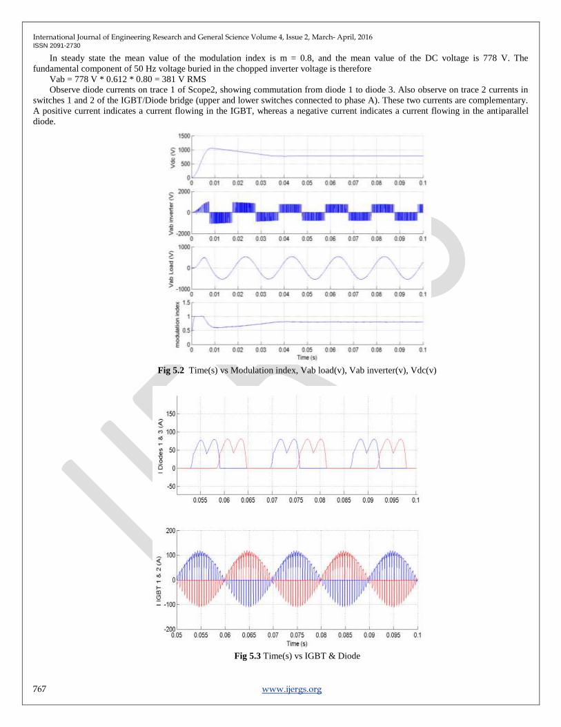
In steady state the mean value of the modulation index is m = 0.8, and the mean value of the DC voltage is 778 V. The
fundamental component of 50 Hz voltage buried in the chopped inverter voltage is therefore
Vab = 778 V * 0.612 * 0.80 = 381 V RMS
Observe diode currents on trace 1 of Scope2, showing commutation from diode 1 to diode 3. Also observe on trace 2 currents in
switches 1 and 2 of the IGBT/Diode bridge (upper and lower switches connected to phase A). These two currents are complementary.
A positive current indicates a current flowing in the IGBT, whereas a negative current indicates a current flowing in the antiparallel
diode.
Fig 5.2 Time(s) vs Modulation index, Vab load(v), Vab inverter(v), Vdc(v)
Fig 5.3 Time(s) vs IGBT & Diode

International Journal of Engineering Research and General Science Volume 4, Issue 2, March- April, 2016 ISSN 2091-2730
768 www.ijergs.org
6. INTRODUCTION TO PARK TRANSFORMATION
Perform Park transformation from three-phase (abc) reference frame to dq0 reference frame. The ransformations section of
the Control and Measurements library contains the abc to dq0 block. This is an improved version of the abc_to_dq0 Transformation
block. The new block features a mechanism that eliminates duplicate continuous and discrete versions of the same block by basing the
block configuration on the simulation mode. If your legacy models contain the abc_to_dq0 Transformation block, they continue to
work. However, for best performance, use the abc to dq0 block in your new models.
6.1 DESCRIPTION
Fig 6.1: Park transformation.
The abc_to_dq0 Transformation block computes the direct axis, quadratic axis, and zero sequence quantities in a two-axis
rotating reference frame for a three-phase sinusoidal signal. The following transformation is used:
VdVqV0=23(Vasin(ωt)+Vbsin(ωt−2π/3)+Vcsin(ωt+2π/3))=23(Vacos(ωt)+Vbcos(ωt−2π/3)+Vccos(ωt+2π/3))=13 (Va+Vb+Vc),
where ω = rotation speed (rad/s) of the rotating frame.
The transformation is the same for the case of a three-phase current; you simply replace the Va, Vb, Vc, Vd, Vq,
and V0 variables with the Ia, Ib, Ic, Id, Iq, and I0variables.
This transformation is commonly used in three-phase electric machine models, where it is known as a Park transformation. It
allows you to eliminate time-varying inductances by referring the stator and rotor quantities to a fixed or rotating reference frame. In
the case of a synchronous machine, the stator quantities are referred to the rotor. Id and Iq represent the two DC currents flowing in the
two equivalent rotor windings (d winding directly on the same axis as the field winding, and q winding on the quadratic axis),
producing the same flux as the stator Ia, Ib, and Ic currents.
You can use this block in a control system to measure the positive-sequence component V1 of a set of three-phase voltages or
currents. The Vd and Vq (or Id and Iq) then represent the rectangular coordinates of the positive-sequence component.
You can use the Math Function block and the Trigonometric Function block to obtain the modulus and angle of V1:
V1∠V1=GV2q+V2d=atan2(Vq/Vd).
This measurement system does not introduce any delay, but, unlike the Fourier analysis done in the Sequence Analyzer
block, it is sensitive to harmonics and imbalances.
6.2 DIALOG BOX AND PARAMETERS
Fig 6.2: Dialog box and parameters.
6.3 INPUTS AND OUTPUTS
abc
Connect to the first input the vectorized sinusoidal phase signal to be converted [phase A phase B phase C].
sin_cos
Connect to the second input a vectorized signal containing the [sin(ωt) cos(ωt)] values, where ω is the rotation speed of the
reference frame.
dq0
The output is a vectorized signal containing the three sequence components [d q o], in the same units as the abc input signal.

International Journal of Engineering Research and General Science Volume 4, Issue 2, March- April, 2016 ISSN 2091-2730
769 www.ijergs.org
7. INTRODUCTION TO INVERSE PARK TRANSFORMATION
The Four Axis instance of this VI requires fixed size four elements arrays (one per axis) for all inputs, and returns fixed size
four element array outputs. Calculates the Inverse Park Transform portion of the field-oriented control (FOC) commutation algorithm.
The Inverse Park Transform modifies the flux,torque (d,q) rotating reference frame into a two phase orthogonal system (alpha,beta).
The output is called the voltage vector. The data type you wire to any input determines the polymorphic instance to use.
7.1 Inverse Park Transformation (Single Axis)
Fig 7.1 Single axis of inverse park transformation.
Comcommand angle—Specifies the calculated flux angle for the Park and Inverse Park transforms, in pi radian
direct voltage—Specifies the direct voltage value calculated by the flux/torque loop for use with the Inverse Park
Transform.
quad voltage—Specifies the quad voltage value calculated by the flux/torque loop for use with the Inverse Park
Transform.
voltage alpha—Specifies the alpha voltage calculated by the Inverse Park Transform for the Space Vector
Modulation function.
voltage beta—Specifies the beta voltage calculated by the Inverse Park Transform for the Space Vector
Modulation function.
7.2 Inverse Park Transformation (Four Axis)
Fig 7.2 Four axis of inverse park transformation.
command angle—Specifies the calculated flux angle for the Park and Inverse Park transforms, in pi radians.
direct voltage—Specifies the direct voltage value calculated by the flux/torque loop for use with the Inverse Park
Transform.
quad voltage—Specifies the quad voltage value calculated by the flux/torque loop for use with the Inverse Park
Transform.
voltage alpha—Specifies the alpha voltage calculated by the Inverse Park Transform for the Space Vector
Modulation function.
voltage beta—Specifies the beta voltage calculated by the Inverse Park Transform for the Space Vector
Modulation function.
http://zone.ni.com/reference/en-XX/help/371093K-01/nimclvfb/controlip.inverseparktransform_00b20056/
http://zone.ni.com/reference/en-XX/help/371093K-01/nimclvfb/controlip.inverseparktransform_00b20056/
http://zone.ni.com/reference/en-XX/help/371093K-01/nimclvfb/controlip.inverseparktransform_00b20056/
http://zone.ni.com/reference/en-XX/help/371093K-01/nimclvfb/controlip.inverseparktransform_00b20056/
http://zone.ni.com/reference/en-XX/help/371093K-01/nimclvfb/controlip.inverseparktransform_00b20056/
http://zone.ni.com/reference/en-XX/help/371093K-01/nimclvfb/controlip.inverseparktransform_00b20056/

International Journal of Engineering Research and General Science Volume 4, Issue 2, March- April, 2016 ISSN 2091-2730
770 www.ijergs.org
7.3 DETAILS
Use the Inverse Park Transform function to calculate the Inverse Park Transform portion of the field-oriented control (FOC)
commutation algorithm, which modifies the flux, torque (d,q) rotating reference frame in a
two phase orthogonal system (alpha, beta).
The Inverse Park Transform uses the following equations:
Where
valpha isthe alpha voltage,
vd is the direct voltage,
vq is the quad voltage,
vbeta is the beta voltage, and
θ is the angle of rotation for the transformed reference frame.
The following figure shows the NI Soft Motion FOC commutation algorithm block diagram, and the location of the Inverse
Park Transform within it.
Fig 7.3 Block diagram NI Soft Motion FOC commutation algorithm.
7.4 FIXED-POINT DETAILS
The Motor Control VIs use fixed-point values when possible. When you wire fixed-point values to Motor Control VIs, the
VIs usually return values that do not lose any bits of word length. However, if the operation creates a value that exceeds the maximum
word length that LabVIEW accepts, overflow or rounding conditions can occur. LabVIEW accepts a maximum word length of 64
bits. Refer to Using the Fixed-Point Data Type in the FPGA Module help for information about how fixed-point numbers might
impact timing.
8. SLIDING MODE TECHNIQUE
8.1 STATOR CURRENT:
3ϕ Isd
Isq
The park transformation converts the three phase current to two phase (Isd, Isq)
Iabc = Stator current
Isd = Stator direct current
Isq = Stator quadrature current
PARK
TRANSFORMATION

International Journal of Engineering Research and General Science Volume 4, Issue 2, March- April, 2016 ISSN 2091-2730
771 www.ijergs.org
8.2 STATOR VOLTAGE:
3ϕ Isd
Isq
The park transformation converts the three phase current to two phase (Vsd, Vsq)
Vabc= Stator voltage
Vsd = Stator direct voltage
Vsq = Stator quadrature voltage
STATOR FLUX :
sd= (1)
sq= (2)
Where,
Isd =
( Ia-
Ib-
Ic) (3)
Isq =--
(-(√ ) Ib+(√ ) Ic) (4)
sd = Direct stator flux
sq = Quadrature stator flux
Vd= Direct voltage
Vq= Quadrature voltage
Rs-Stator Resistance
MAGNITUDE OF STATOR FLUX :
Magnitude of stator flux =√ (5)
ROTOR POSITION:
= (
) (6)
Where,
θ = Rotor position.
TORQUE ESTIMATOR:
Te=(3/2)(p)( (7)
Where,
P – no of poles
Slip = Te*(Rr/2) (8)
Where,
Te = Estimated torque
Rr = Rotor resistance
ELECTRICAL SPEED:
Electrical speed =(speed of field-slip)/square of rotor flux (9)
Speed of rotor field = (10)
ROTOR FLUX :
rd = (LM/LR) sd (11)
rq = (LM/LR) sq (12)
MECHANICAL SPEED:
m = (1/2) * Electrical speed. (13)
Where,
m = Mechanical speed
In sliding mode technique we calculate the actual speed, magnetic flux, torque, rotor position. The output is given to control unit then
it compare the actual speed and set speed
9. SIMULATIONS AND RESULTS
The detailed description about the result of the proposed system with the help of MATLAB and the results of the simulated
system is drawn here.
PARK
TRANSFORMATION

International Journal of Engineering Research and General Science Volume 4, Issue 2, March- April, 2016 ISSN 2091-2730
772 www.ijergs.org
9.1 SIMULATION DIAGRAM
The simulation diagram of proposed system is shown below.
Fig 9.1: Simulation diagram of the proposed system.
9.2 TRIGGER CIRCUIT SPWM GENERATOR
Fig 9.2: Circuit diagram of SPWM generator.
The output from the inverse park transformation is fed into selector bus and the gain is added with it .The output from the
gain is fed into SPWM generator the PWM pulses are produced.
9.3 TRIGGER CIRCUIT PARK TRANSFORMATION
Fig 9.3: Circuit Diagram of Al-Be to ABC.
The stator current is fed into the gain and is summed up in the summing point and three phases converted into two phase
stator current.

International Journal of Engineering Research and General Science Volume 4, Issue 2, March- April, 2016 ISSN 2091-2730
773 www.ijergs.org
9.4 TRIGGER CIRCUIT INVERSEPARK TRANSFORMATION
Fig 9.4: Circuit diagram of inverse park transformation.
In this circuit by adding gains and summing point with references the two phase again converted into three phase.
9.5 TRIGGER CIRCUIT PI CONTRLLER
Fig 9.5 : Circuit diagram of PI controller.
The reference speed, estimated speed ,reference flux, estimated flux, estimated angle ,estimated torque are given to control
unit.It compares the actual speed and set speed and its given to the inverse park transformation.
9.6 TRIGGER CIRCUIT SLIDING MODE
Fig 9.6: circuit diagram of sliding mode control.
International Journal of Engineering Research and General Science Volume 4, Issue 2, March- April, 2016 ISSN 2091-2730
774 www.ijergs.org
The flux and voltage are taken as reference and the feedback current is fed into gain then it is given to derivative alpha and
beta. Then the output is given to the speed of rotor flux and it is converted as electrical to mechanical speed .The final estimated speed
is obtained.
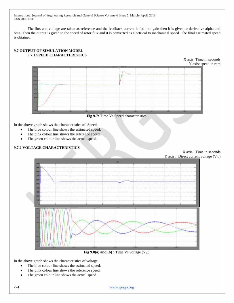
9.7 OUTPUT OF SIMULATION MODEL
9.7.1 SPEED CHARACTERISTICS
X axis: Time in seconds
Y axis: speed in rpm
Fig 9.7: Time Vs Speed characteristics.
In the above graph shows the characteristics of Speed.
The blue colour line shows the estimated speed.
The pink colour line shows the reference speed.
The green colour line shows the actual speed.
9.7.2 VOLTAGE CHARACTERISTICS
X axis : Time in seconds
Y axis : Direct current voltage (Vdc)
Fig 9.8(a) and (b) : Time Vs voltage (Vdc).
In the above graph shows the characteristics of voltage.
The blue colour line shows the estimated speed.
The pink colour line shows the reference speed.
The green colour line shows the actual speed.

International Journal of Engineering Research and General Science Volume 4, Issue 2, March- April, 2016 ISSN 2091-2730
775 www.ijergs.org
9.7.3 TORQUE CHARACTERISTICS
X axis : Time in seconds
Y axis : Direct current voltage (Vdc)
Fig 9.9 (a) and (b) : Time Vs voltage (Vdc).
In the above graph shows the characteristics of torque.
The blue colour line shows the estimated speed.
The pink colour line shows the reference speed.
The green colour line shows the actual speed.
9.7.4 STATOR FLUX CHARACTERISTICS
X axis : Time in seconds
Y axis : Speed in rpm
Fig 9.10 : Time Vs Speed
In the above graph shows the characteristics of stator flux.
The blue colour line shows the estimated speed.
The pink colour line shows the reference speed.
The green colour line shows the actual speed.
9.7.5 STATOR CURRENT CHARACTERISTICS
X axis : Time in seconds
Y axis : Speed in rpm
Fig 9.11 : Time Vs Speed.

International Journal of Engineering Research and General Science Volume 4, Issue 2, March- April, 2016 ISSN 2091-2730
776 www.ijergs.org
In the above graph shows the characteristics of stator current.
The blue colour line shows the estimated speed.
The pink colour line shows the reference speed.
The green colour line shows the actual speed.
10. CONCLUSION
This paper presents a modified speed-sensorless control scheme based on second-order sliding-mode STA and MRAS
estimation theory. The estimation scheme has been obtained by combining a second-order sliding-mode current observer with a
parallel speed and stator resistance estimator based on rotor flux-based MRAS. Both the error in instantaneous phase position and the
error in amplitudes are used respectively for speed estimation and Rs identification, thus overcoming the problems of Rs variation,
particularly for low-speed operation.
The STA-based observer is utilized to take the place of the reference voltage model of the standard MRAS. Derivatives of
rotor flux are obtained and designed as the state of MRAS, thus eliminating the integration. Moreover, by making full use of auxiliary
surfaces, the observations are insensitive to rotor parameter perturbation with the alleviation of chattering behavior at the same time.
The proposed scheme is insignificantly more complex than its counterpart with speed estimation only, so it is easy to implement in the
already existing MRAS-based speed estimator. However, since the scheme is designed based on the mathematical model of IM, its
observability is generally lost at zero magnetic field frequency. Machine state observability can be improved by additional stator
voltage change injection, which is considered to be the further work.
REFERENCES:
1. Akin. B and Bhardwaj. M, ―Sensored field oriented control of 3-phase induction motors‖, Texas Instrument Guide, Dallas,
TX, USA. [Online]. Available: www.ti.com/litv/pdf/sprabp8.
2. Araki. M and Taguchi. H, ―Two-degree-of-freedom PID controllers,‖ Int. J. Control, Autom., Syst., vol. 1, no. 4, pp. 401–
411, Dec. 2003.
3. Barrero. F, Gonzalez. A, Torralba. A, Galvan. E, and Franquelo.L.G, ―Speed control of induction motors using a novel fuzzy
sliding-mode structure,‖ IEEE Trans. Fuzzy Syst., vol. 10, no. 3, pp. 375–383, Jun. 2002.
4. Cupertino. F, Naso. D, Mininno. E, and Turchiano. B, ―Sliding-mode control with double boundary layer for robust
compensation of payload mass and friction in linear motors,‖ IEEE Trans. Ind. Appl., vol. 45, no. 5, pp. 1688–1696,
Sep./Oct. 2009.
5. Chien. C. J, ―A combined adaptive law for fuzzy iterative learning control of nonlinear systems with varying control tasks,‖
IEEE Trans. Fuzzy Syst., vol. 16, no. 1, pp. 40–51, Feb. 2008.
6. Faa-Jeng. L, Po-Huan. C, Chin-Sheng. C, and Yu-Sheng. L , ―DSP-based cross-coupled synchronous control for dual linear
motors via intelligent complementary sliding mode control,‖ IEEE Trans. Ind. Electron., vol. 59, no. 2, pp. 1061–1073, Feb.
2012.
7. Franklin. P and Powell. J. D, Emami-Naeini Feedback Control of Dynamic Systems, vol. 4. Englewood Cliffs, NJ, USA:
Prentice-Hall, 2006, p. 2.
8. Gadoue. S. M, Giaouris. D, and Finch. J. W, ―MRAS sensorless vector control of an induction motor using new sliding-mode
and fuzzy-logic adaptation mechanisms,‖ IEEE Trans. Energy Convers., vol. 25, no. 2, pp. 394–402, Jun. 2010.
9. Garrido. A. J, Garrido. I, Amundarain. M, Alberdi. M, and De la Sen. M, ―Sliding-mode control of wave power generation
plants,‖ IEEE Trans Ind. Appl., vol. 48, no. 6, pp. 2372–2381, Nov./Dec. 2012.
10. Hongyi. L, Jinyong. Y, Hilton. C, and Honghai. L, ―Adaptive sliding-mode control for nonlinear active suspension vehicle
systems using T-S fuzzy approach,‖ IEEE Trans. Ind. Electron., vol. 60, no. 8, pp. 3328–3338, Aug. 2013.
11. Jinhui. Z, Peng. S, and Yuanqing. X, ―Robust adaptive sliding-mode control for fuzzy systems with mismatched
uncertainties,‖ IEEE Trans. Fuzzy Syst., vol. 18, no. 4, pp. 700–711, Aug. 2010.
12. Kim. Y. K and Jeon. G. J , ―Error reduction of sliding mode control using sigmoid-type nonlinear interpolation in the
boundary layer,‖ Int. J.Control Syst., vol. 2, no. 4, pp. 523–529, 2004.
13. Kung. C. C and Su. K. H, ―Adaptive fuzzy position control for electrical servo drive via total-sliding-mode technique,‖ Proc.
Inst. Elect.Eng.—Elect. Power Appl., vol. 152, no. 6, pp. 1489–1502, Nov. 2005.
14. C. Lin, T. Liu, M. Wei, L. Fu, and C. Hsiao, ―Design and implementation of a chattering-free non-linear sliding-mode
controller for interior permanent magnet synchronous drive systems,‖ IET Elect. Power Appl., vol. 6, no. 6, pp. 332–344, Jul.
2012.
15. Lorenz. R, ―A simplified approach to continuous on-line tuning of fieldoriented induction machine drives,‖ IEEE Trans. Ind.
Appl., vol. 26, no. 3, pp. 420–424, May/Jun. 2002.
16. Orowska-Kowalska. T, Kaminski. M, and Szabat. K, ―Implementation of a sliding-mode controller with an integral function
and fuzzy gain value for the electrical drive with an elastic joint,‖ IEEE Trans. Ind. Electron., vol. 57, no. 4, pp. 1309–1317,
Apr. 2010.

International Journal of Engineering Research and General Science Volume 4, Issue 2, March- April, 2016 ISSN 2091-2730
777 www.ijergs.org
17. Pupadubsinet al. P., ―Adaptive integral sliding-mode position control of a coupled-phase linear variable reluctance motor for
high-precision applications,‖ IEEE Trans. Ind. Appl., vol. 48, no. 4, pp. 1353–1363, Jul./Aug. 2012.
18. Rong-Jong. W, ―Fuzzy sliding-mode control using adaptive tuning technique,‖ IEEE Trans. Ind. Electron., vol. 54, no. 1, pp.
586–594, Feb. 2007.
19. Rong-Jong. W and Kuo-Ho. S, ―Adaptive enhanced fuzzy sliding-mode control for electrical servo drive,‖ IEEE Trans. Ind.
Electron., vol. 53, no. 2, pp. 569–580, Apr. 2006.
20. Roopaei. M, Zolghadri. M, and Meshksar. S, ―Enhanced adaptive fuzzy sliding mode control for uncertain nonlinear
systems,‖ Commun. NonlinearSci. Numer. Simul., vol. 14, no. 9/10, pp. 3670–3681, Sep./Oct. 2009.