International Journal of Engineering (IJE), Volume (3): Issue (6)
164
-
Upload
ai-coordinator-csc-journals -
Category
Documents
-
view
229 -
download
0
Transcript of International Journal of Engineering (IJE), Volume (3): Issue (6)

8/8/2019 International Journal of Engineering (IJE), Volume (3): Issue (6)
http://slidepdf.com/reader/full/international-journal-of-engineering-ije-volume-3-issue-6 1/164

8/8/2019 International Journal of Engineering (IJE), Volume (3): Issue (6)
http://slidepdf.com/reader/full/international-journal-of-engineering-ije-volume-3-issue-6 2/164
International Journal of
Engineering (I JE)
Volume 3, Issue 6, 2010
Edited ByComputer Science Journals
www.cscjournals.org

8/8/2019 International Journal of Engineering (IJE), Volume (3): Issue (6)
http://slidepdf.com/reader/full/international-journal-of-engineering-ije-volume-3-issue-6 3/164
Editor in Chief Dr. Kouroush Jenab
International Journal of Engineering (IJE)
Book: 2010 Volume 3, Issue 6Publishing Date: 31-01-2010
Proceedings
ISSN (Online): 1985-2312
This work is subjected to copyright. All rights are reserved whether the whole or
part of the material is concerned, specifically the rights of translation, reprinting,
re-use of illusions, recitation, broadcasting, reproduction on microfilms or in any
other way, and storage in data banks. Duplication of this publication of parts
thereof is permitted only under the provision of the copyright law 1965, in its
current version, and permission of use must always be obtained from CSC
Publishers. Violations are liable to prosecution under the copyright law.
IJE Journal is a part of CSC Publishers
http://www.cscjournals.org
©IJE Journal
Published in Malaysia
Typesetting: Camera-ready by author, data conversation by CSC Publishing
Services – CSC Journals, Malaysia
CSC Publishers

8/8/2019 International Journal of Engineering (IJE), Volume (3): Issue (6)
http://slidepdf.com/reader/full/international-journal-of-engineering-ije-volume-3-issue-6 4/164
Editorial Preface
This is the sixth issue of volume three of International Journal of Engineering(IJE). The Journal is published bi-monthly, with papers being peer reviewedto high international standards. The International Journal of Engineering is
not limited to a specific aspect of engineering but it is devoted to thepublication of high quality papers on all division of engineering in general. IJEintends to disseminate knowledge in the various disciplines of theengineering field from theoretical, practical and analytical research tophysical implications and theoretical or quantitative discussion intended foracademic and industrial progress. In order to position IJE as one of the good
journal on engineering sciences, a group of highly valuable scholars areserving on the editorial board. The International Editorial Board ensures thatsignificant developments in engineering from around the world are reflectedin the Journal. Some important topics covers by journal are nuclearengineering, mechanical engineering, computer engineering, electrical
engineering, civil & structural engineering etc.
The coverage of the journal includes all new theoretical and experimentalfindings in the fields of engineering which enhance the knowledge of scientist, industrials, researchers and all those persons who are coupled withengineering field. IJE objective is to publish articles that are not onlytechnically proficient but also contains information and ideas of fresh interestfor International readership. IJE aims to handle submissions courteously andpromptly. IJE objectives are to promote and extend the use of all methods in
the principal disciplines of Engineering.
IJE editors understand that how much it is important for authors andresearchers to have their work published with a minimum delay aftersubmission of their papers. They also strongly believe that the directcommunication between the editors and authors are important for thewelfare, quality and wellbeing of the Journal and its readers. Therefore, allactivities from paper submission to paper publication are controlled throughelectronic systems that include electronic submission, editorial panel andreview system that ensures rapid decision with least delays in the publicationprocesses.

8/8/2019 International Journal of Engineering (IJE), Volume (3): Issue (6)
http://slidepdf.com/reader/full/international-journal-of-engineering-ije-volume-3-issue-6 5/164
To build its international reputation, we are disseminating the publicationinformation through Google Books, Google Scholar, Directory of Open AccessJournals (DOAJ), Open J Gate, ScientificCommons, Docstoc and many more.Our International Editors are working on establishing ISI listing and a goodimpact factor for IJE. We would like to remind you that the success of our
journal depends directly on the number of quality articles submitted forreview. Accordingly, we would like to request your participation bysubmitting quality manuscripts for review and encouraging your colleagues tosubmit quality manuscripts for review. One of the great benefits we canprovide to our prospective authors is the mentoring nature of our reviewprocess. IJE provides authors with high quality, helpful reviews that areshaped to assist authors in improving their manuscripts.
Editorial Board MembersInternational Journal of Engineering (IJE)

8/8/2019 International Journal of Engineering (IJE), Volume (3): Issue (6)
http://slidepdf.com/reader/full/international-journal-of-engineering-ije-volume-3-issue-6 6/164
Editorial Board
Editor-in-Chief (EiC)
Dr. Kouroush Jenab
Ryerson University, Canada
Associate Editors (AEiCs)
Professor. Ernest BaafiUniversity of Wollongong, (Australia)
Dr. Tarek M. SobhUniversity of Bridgeport, (United States of America)
Professor. Ziad SaghirRyerson University, (Canada)
Professor. Ridha Gharbi Kuwait University, (Kuwait)
Professor. Mojtaba Azhari Isfahan University of Technology, (Iran)
Dr. Cheng-Xian (Charlie) L in
University of Tennessee, (United States of America)
Editorial Board Members (EBMs)
Dr. Dhanapal Durai Dominic P
Universiti Teknologi PETRONAS, (Malaysia)
Professor. Jing Zhang
University of Alaska Fairbanks, (United States of America)
Dr. Tao Chen
Nanyang Technological University, (Singapore)
Dr. Oscar Hui University of Hong Kong, (Hong Kong)
Professor. Sasikumaran Sreedharan King Khalid University, (Saudi Arabia)
Assistant Professor. Javad Nematian University of Tabriz, (Iran)
Dr. Bonny Banerjee (United States of America)
AssociateProfessor. Khalifa Saif Al-Jabri Sultan Qaboos University, (Oman)

8/8/2019 International Journal of Engineering (IJE), Volume (3): Issue (6)
http://slidepdf.com/reader/full/international-journal-of-engineering-ije-volume-3-issue-6 7/164
Table of Contents
Volume 3, Issue 6, January 2010.
Pages
521 - 537
538 - 553
554 - 564
565 - 576
577 - 587
Influence of Helicopter Rotor Wake Modeling on Blade Airload
Predictions
Christos Zioutis, Apostolos Spyropoulos, Anastasios Fragias,Dionissios Margaris, Dimitrios Papanikas
CFD Transonic Store Separation Trajectory Predictions with
Comparison to Wind Tunnel Investigations
Elias E. Panagiotopoulos, Spyridon D. Kyparissis
An efficient Bandwidth Demand Estimation for Delay Reduction in
IEEE 802.16j MMR WiMAX Networks
Fath Elrahman Ismael Khalifa Ahmed, Sharifah K. Syed
Yusof, Norsheila Fisal
Prediction of 28-day Compressive Strength of Concrete on theThird Day Using artificial neural networks Vahid. K. Alilou, Mohammad. Teshnehlab
The Influence of Cement Composition on Superplasticizers’
Efficiency Ghada Bassioni

8/8/2019 International Journal of Engineering (IJE), Volume (3): Issue (6)
http://slidepdf.com/reader/full/international-journal-of-engineering-ije-volume-3-issue-6 8/164
588 - 596
597 - 608
609 - 621
622 - 638
639 - 652
653 – 661
662 - 670
The Effect of a Porous Medium on the Flow of a Liquid Vortex
Fatemeh Hassaipour, Jose L. Lage
New PID Tuning Rule Using ITAE Criteria
Ala Eldin Abdallah Awouda, Rosbi Bin Mamat
Performance Analysis of Continuous Wavelength Optical Burst
Switching Networks
Aditya Goel, A.K. Singh , R. K. Sethi, Vitthal J. Gond
Knowledge – Based Reservoir Simulation – A Novel Approach
M. Enamul Hossain, M. Rafiqul Islam
TGA Analysis of Torrified Biomass from Malaysia for Biofuel
Production
Noorfidza Yub Harun, M.T Afzal, Mohd Tazli Azizan
An Improved Mathematical Model for Assessing the Performance
of the SDHW Systems Imad Khatib, Moh'd Awad, Kazem Osaily
Modeling and simulation of Microstrip patch array for smart
Antennas
K.Meena alias Jeyanthi, A.P.Kabilan
International Journal of Engineering, (IJE) Volume (3) : Issue (6)

8/8/2019 International Journal of Engineering (IJE), Volume (3): Issue (6)
http://slidepdf.com/reader/full/international-journal-of-engineering-ije-volume-3-issue-6 9/164
C. K. Zioutis, A. I. Spyropoulos, A. P. Fragias, D. P. Margaris & D. G. Papanikas
International Journal of Engineering (IJE), Volume (3): Issue (6) 521
Influence of Helicopter Rotor Wake Modelingon Blade Airload Predictions
Christos K. Zioutis [email protected] Engineering and Aeronautics Department University of Patras Rio Patras, 26500, Greece
Apostolos I. Spyropoulos [email protected] Engineering and Aeronautics Department University of Patras Rio Patras, 26500, Greece
Anastasios P. Fragias [email protected]
Mechanical Engineering and Aeronautics Department University of Patras Rio Patras, 26500, Greece
Dionissios P. Margaris [email protected] Engineering and Aeronautics Department University of Patras Rio Patras, 26500, Greece
Dimitrios G. Papanikas [email protected] Engineering and
Aeronautics Department University of Patras Rio Patras, 26500, Greece
Abstract
In the present paper a computational investigation is made about the efficiency ofrecently developed mathematical models for specific aerodynamic phenomena ofthe complicated helicopter rotor flowfield. A developed computational procedureis used, based on a Lagrangian type, Vortex Element Method. The free vorticalwake geometry and rotor airloads are computed. The efficiency of special models
concerning vortex core structure, vorticity diffusion and vortex straining regardingrotor airloads prediction is tested. Investigations have also been performed inorder to assess a realistic value for empirical factors included in vorticity diffusionmodels. The benefit of using multiple vortex line to simulate trailing wake vorticitybehind blade span instead of isolated lines or vortex sheets, despite theircomputational cost, is demonstrated with the developed wake relaxation method.The computational results are compared with experimental data from wind tunneltests, performed during joined European research programs.

8/8/2019 International Journal of Engineering (IJE), Volume (3): Issue (6)
http://slidepdf.com/reader/full/international-journal-of-engineering-ije-volume-3-issue-6 10/164
C. K. Zioutis, A. I. Spyropoulos, A. P. Fragias, D. P. Margaris & D. G. Papanikas
International Journal of Engineering (IJE), Volume (3): Issue (6) 522
Keywords: Helicopter aerodynamics, rotor wake, vortex core.
1. INTRODUCTION
Computational research on helicopter rotors focuses on blade airloads prediction, trying toidentify the effects of important operational, structural and flowfield parameters such as wakeformation, blade planform, flight conditions etc on blade vibrations and noise emissions. Improvedhelicopter performance is a continuous research challenge as aeronautical industry is alwaysseeking for a more efficient, vibration free and "quiet" rotorcraft with increased public acceptance.
The main issue in helicopter aerodynamics examined by many computational and experimentalefforts is the interaction of rotor blades with wake vortices, a phenomenon which characterizeshelicopters and is the source of blade vibration and noise emission. As in other similaraerodynamic flowfields, such as the trailing wake of aircrafts or wind turbines, the velocity field inthe vicinity of a helicopter rotor must be calculated from the vorticity field. A prerequisite for sucha calculation is that the physical structure and the free motion of wake vortices are adequatelysimulated.
Vortex Element Methods (VEM) have been established during recent years computationalresearch as an efficient and reliable tool for calculating the velocity field of concentrated three-dimensional, curved vortices [1,2]. Wake vortices are considered as vortex filaments which arefree to move in Lagrangian coordinates. The filaments are descritized into piecewise segmentsand a vortex element is assigned to each one of them. Since the flow is considered inviscidexcept for the vortices themselves, the Biot-Savart low is applied in closed-form integration overeach vortex element for the velocity field calculation. Marked points are traced on vortex filamentsas they move freely due to the mutual-induced velocity field, either by externally imposinggeometrical periodicity (relaxation methods) or not (time marching methods). Thus, VEM cancomputationally reproduce an accurate geometry of the concentrated wake vortices spinningclose to rotor disk. As a result the non-uniform induced downwash of lifting helicopter rotors canbe computed, which is responsible for rotor blade vibratory airloads.
From the first simplified approaches [3,4], to recent advanced procedures [5-9], the vorticityelements used are vortex lines and vortex sheets [5,10]. The sophistication level of rotor wakeanalysis can vary from preliminary to advanced manufacture calculations. The basic formulationof VEM is closely related to classical vortex methods for boundary layer and vortical flow analysisextensively applied by Chorin [11], Leonard [12] and other researchers [13,33].
The extensive effort made by a number of researchers has resulted to several models proposedfor simulating viscous vortex core structure, vorticity diffusion, trailing vortex rollup process, rotorblade dynamic stall and other phenomena [14]. These different physico-mathematical modelshave a significant influence on computed blade airload distributions, while their reliability for themajority of helicopter rotor flow conditions is always under evaluation.
The contribution of the work presented here is to investigate the influence of specific aerodynamicmodels on computed blade airloads, evaluating their reliability by comparisons of computedresults with experimental data. In addition, the values of empirical factors included in thesemodels are computationally verified. The applied method consists of a free wake analysis, using awake-relaxation type VEM [15,16,29] and a coupled airload computation module which has theflexibility to adopt either lifting line or lifting surface methods. Blade motion calculations includeprovisions for articulated or hingeless blades and the main rigid and elastic flapping modules canbe regarded separately or coupled.

8/8/2019 International Journal of Engineering (IJE), Volume (3): Issue (6)
http://slidepdf.com/reader/full/international-journal-of-engineering-ije-volume-3-issue-6 11/164
C. K. Zioutis, A. I. Spyropoulos, A. P. Fragias, D. P. Margaris & D. G. Papanikas
International Journal of Engineering (IJE), Volume (3): Issue (6) 523
When helicopter rotor wakes are simulated, then the line segment discretization of wake vorticesis prevailed. Methods with straight [8,10] or curved [6,17] line segments have been proposed andtheir accuracy was found to be of second order comparing to vortex ring analytical solution[18,19]. Rarely, the distributed vorticity behind the inner part of blade span is modeled by surfaceelements such as vortex sheets [10]. For the present investigation, a model of multiple trailinglines is adopted and compared with models of simpler discretization.Viscous effects on wake vorticity have also been the subject of computational and experimentalefforts because of their significant impact on induced velocity calculations especially for largewake ages [20-22]. These effects are the vortex core formation in the center of vortex lines andthe diffusion of the concentrated vorticity as time progresses. Both of these phenomena are foundto be of crucial importance for a reliable wake representation. In the present paper severalmodels are compared, assuming both laminar and turbulent vortex core flow, in order todemonstrate their effectiveness and a parametric investigation is performed concerning empiricalfactors employed by these models.
The experimental data used for comparisons include test cases executed during cooperativeEuropean research programs on rotorcraft aerodynamics and aeroacoustics performed in theopen test section of the German-Dutch Wind Tunnel (DNW) The Netherlands [23].
2. AERODYNAMIC FORMULATION
2.1 Rotor Wake ModelThe vorticity generated in rotor wake is distinguished regarding its source in two main parts, thetrailing and the shed vorticity. Conservation of circulation dictates that the circulation gradients ona rotor blade determine the vorticity shed at specific spanwise locations behind the blade. Thusspanwise circulation variations generate trailing vorticity, gn, whose direction is parallel to thelocal flow velocity (Figure 1). On the other hand, azimuthal variations produce shed vorticityradially oriented, gs, due to the transient periodical nature of the rotor blade flowfield. In general,bound circulation has a distribution as shown in Figure 1, where the pick is located outboard ofthe semi-span and a steep gradient appears closely to blade tip. This gradient generates a highstrength trailing vortex sheet just behind the blade which quickly rolls up and forms a strong tipvortex.
FIGURE 1: Rotor wake physicomathematical modeling.
The continuous distribution of wake vorticity shown in Figure 1 is discretized into a series ofvortex elements. Depending on the degree of analysis of wake flowfield and on targetedcomputational consumption, some VEMs use simple disretization as shown in Figure 2. In this

8/8/2019 International Journal of Engineering (IJE), Volume (3): Issue (6)
http://slidepdf.com/reader/full/international-journal-of-engineering-ije-volume-3-issue-6 12/164
C. K. Zioutis, A. I. Spyropoulos, A. P. Fragias, D. P. Margaris & D. G. Papanikas
International Journal of Engineering (IJE), Volume (3): Issue (6) 524
case, bound circulation is assumed as a linearized distribution, as shown in the figure. Accordingto such an assumption, trailing vorticity emanates from the inner part of blade span and ismodeled with vortex sheets extending from A to C. Shed vorticity is modeled either with vortexsheets extending from B to E or with vortex lines parallel to blade span as shown in Figure 2.Vortex line discretization is used for tip vortex, except for the area just behind the blade where arolling up vortex sheet is used. Roll up is simulated with diminishing vortex sheets together withline segments of correspondingly increasing circulation. This type of discretization simulates thebasic features of rotor wake with acceptable accuracy and reduces computational consumptionespecially when VEMs are used in conjunction with CFD simulations of rotor wake in hybridschemes.
FIGURE 2: Rotor wake simulation, where the trailing wake is represented by vortex sheets, the shed wakeeither by vortex sheets or vortex lines and the concentrated tip vortex by vortex lines.
Despite the computational efficiency of the above approach, the simplification made in boundcirculation distribution can lead to unrealistic results for certain blade azimuth angles. Forexample, in the cases of reverse flow regions or low advance ratios, where the air hits the rotorblades at the trailing edge or when the rotor blades cut the concentrated tip vortices respectively,a phenomenon known as Blade Vortex Interaction (BVI) is apparent. In these cases the boundcirculation distribution departs from the form of Figure 2 and a more detailed discretization isneeded in order to catch the specific circulation variations.
In this work, the wake vorticity is discretized in a multitude of trailing and shed vortex lines asshown in Figure 3, in order to simulate the bound circulation distribution in a way that takes intoaccount the fluctuations produced in the majority of blade azimuth angles.

8/8/2019 International Journal of Engineering (IJE), Volume (3): Issue (6)
http://slidepdf.com/reader/full/international-journal-of-engineering-ije-volume-3-issue-6 13/164
C. K. Zioutis, A. I. Spyropoulos, A. P. Fragias, D. P. Margaris & D. G. Papanikas
International Journal of Engineering (IJE), Volume (3): Issue (6) 525
FIGURE 3: Modeling of rotor blade bound circulation distribution and wakevorticity formations with multiple vortex lines.
Trailing vorticity is simulated by n-straight line vortex segments, labeled ℓℓ, which run from ℓ1 at theroot to ℓn at the tip. There are ηℓ=n-1 radial stations where bound circulation is computed, where ηℓ runs from η1 between ℓ1 and ℓ2 to ηn-1 between ℓn-1 and ℓn. The strength of each segment is equalto the gradient of the bound circulation gbv between two successive radial stations. This meansthat for all intermediate segments at azimuthal angle ψ:
)ψ ,η(g)ψ ,η(g)ψ ,(g bvbvn llll −=
−1 (1)
The first term is equal to zero at the root because there is no bound circulation inboard the root.Analogically the second term is zero at the tip. The shed vorticity is simulated by n-1 straight linevortex segments which are extended radially between two adjacent trailing vortices as shown inFigure 3. The strength of each segment is equal to the azimuthal variation of bound circulation for
each radial station:
)ψ ,η(g)ψ ∆ψ ,η(g)ψ ,(g bvbvs 11 −−−+=
llll (2)
where ∆ψ is the azimuthal step. A number of 50 trailing and shed vortex line segments perazimuthal step were found adequate to discretize the wake vorticity. More detailed discretizationwill increase computational cost without any tangible improvement of accuracy.
2.2 Induced Velocity CalculationThe distortion of the initial helical geometry of the rotor wake vortices, makes the calculation ofthe rotor downwash almost impossible with direct numerical integration of the Biot-Savart law,over the actual wake geometry. This procedure is used only for simplified approaches such as the
rigid or semi-rigid wake assumptions [3,4]. The utilization of discrete computational elements(vortex lines and sheets) by VEM, converts direct integration in a closed form integration of theBiot-Savart law over the known spatial locations of these elements. The contribution of a vortexline segment i to the induced velocity ijw
rat an arbitrary point in space j, is given by the relation
( )∫
⋅−
×⋅−−=
34
1
k ijm
k ijmi
ij
ek r
k d ek r g
π w
rr
rrrr
(3)

8/8/2019 International Journal of Engineering (IJE), Volume (3): Issue (6)
http://slidepdf.com/reader/full/international-journal-of-engineering-ije-volume-3-issue-6 14/164
C. K. Zioutis, A. I. Spyropoulos, A. P. Fragias, D. P. Margaris & D. G. Papanikas
International Journal of Engineering (IJE), Volume (3): Issue (6) 526
where ijmrr
is the minimum distance from vortex line i to the point j, k er
the unit vector in the
direction of the vortex segment, gi the circulation strength of the vortex segment and k thecoordinate measured along the vortex segment. With a reasonable step of discretization, thesimplification made to the actual wake geometry can be overcome. After computationalinvestigation the azimuthal step for realistic rotor wake simulations has been proposed by
different researchers to be from 2 to 5 degrees [5,32]. The calculation of velocity induced byvortex sheet can be found in [15].
Free vortical wake computation is an iterative procedure, which initiates from rigid wakegeometry. Each iteration defines a new position of each vortex element, and takes into accountthe contribution of all the wake elements to the local flow velocity. At the end of each iteration anew distorted wake geometry is calculated, which is the starting point for the next cycle. Thisscheme continues until distortion convergence is achieved.
Rotor blade dynamics influence the angle of attack distribution seen by the blade, and thereforealter the bound circulation distribution. Due to out-of-plane motion, rotor blade balances theasymmetry of rotor disk loading. For studying rotor aerodynamics, blade flapwise bending can berepresented by a simple mode shape, without significant loss of accuracy [10]. In general the outof plane deflection z(r,t) can be written as a series of normal modes describing the spanwisedeformation
∑∞
==
1k κ κ )t (q)r (n)t ,r ( z (4)
where nκ is the mode shape and qκ(t) is the corresponding degree of freedom. For the developedprocedure rigid blade motion and the first flapwise bending mode shape, n=4r
2-3r, which is
appropriate for blade's basic bending deformation can be used alternatively [15].By these means a detailed rotor induced downwash distribution is obtained by free wakecalculations. Sequentially, the blade section angle of attack distribution is computed by
( ) ( ) ( )T P uutanr θ ψ ,r α 1−−= (5)
where uP is the air velocity perpendicular to No Feathering Plane (NFP), which includesnonuniform rotor downwash, uT is the tangential velocity to blade airfoil, both normalized by therotor tip speed R, and θ(r) is the collective pitch angle (since NFP is taken as reference). Withknown angle of attack and local velocity, a blade-element type methodology is applied for bladesection lift calculations. The above computational procedure is extensively documented in [15].
2.3 Vortex Core StructureAs mentioned above, rotor induced velocity calculation is based on potential field solution such asBiot-Savart law. Due to the absence of viscosity, the induced velocity calculated at a point lyingvery close to a vortex segment, tends to be infinite which is unrealistic. In order to remove such
singularities and model the effects of viscosity in a convenient way the vortex core concept isintroduced. A great deal of the current knowledge about the role of viscosity in a vortex core hasbeen derived mainly from experimental measurements. As a result empirical relations arecommonly used for the vortex core radius, the velocity distribution at the core region and theviscous core growth.The core radius is defined as the distance from the core center where the maximum tangentialvelocity is observed. A corresponding expression for the radial circulation distribution inside thecore region is introduced in the computations, which alters the velocity induced from a vortexelement. Outside the core region the induced velocity has an approximately potential distributionwhich tends to coincide with the Biot-Savart distribution fairly away from the vortex line.

8/8/2019 International Journal of Engineering (IJE), Volume (3): Issue (6)
http://slidepdf.com/reader/full/international-journal-of-engineering-ije-volume-3-issue-6 15/164

8/8/2019 International Journal of Engineering (IJE), Volume (3): Issue (6)
http://slidepdf.com/reader/full/international-journal-of-engineering-ije-volume-3-issue-6 16/164
C. K. Zioutis, A. I. Spyropoulos, A. P. Fragias, D. P. Margaris & D. G. Papanikas
International Journal of Engineering (IJE), Volume (3): Issue (6) 528
This result came up by differentiating equation 9 with respect to r and setting the derivative tozero. The Lamb-Oseen vortex can be regarded as the “desingularisation” of the rectilinear linevortex, in which the vorticity has a delta-function singularity.Squire [30] showed that the solution for a trailing vortex is identical to the Lamb-Oseen solution.
So the downstream distance z from the origin of the vortex can be related to time as t=z/V 4. Inorder to account for effects on turbulence generation, Squire introduced an eddy viscosity
coefficient δ. In the case of a helicopter rotor, time t is related to the wake age δℓ as δℓ =t, where is the angular velocity of the rotor. Thus, including these parameters equation 10 can be writtenas
+=
δδδν.)δ(r diff
0241812 l
l (11)
In the above equation δ0 is an effective origin offset, which gives a finite value of the vortex coreradius at the instant of its generation (δℓ=0) equals to
=≡=
δδν.r )δ(r diff 00 2418120l (12)
At this work δ0 was selected to have an age between 15o
and 30o. According to Squire, the eddy
viscosity coefficient is proportional to the vortex Reynolds number Rev and equals to
vS Reδ a +=1 (13)
where as is the Squire’s parameter and its value is determined from experimental measurements.A phenomenon often opposing vortex diffusion is the straining of vortex filaments due to theirfreely distorted geometry. In fact the steep gradients of wake induced velocities cause them to
stretch or to squeeze and their core radius to decrease or to increase correspondingly. Forstraining effects, the following fraction is defined
l
l ∆ε = (14)
as the strain imposed on the filament over the time interval ∆t, where ∆ℓ is the deformation fromits initial length ℓ. Now assume that the filament has a core radius r diff(δℓ) at time δℓ. At time δℓ+∆ψ the filament will have a core radius rdiff(δℓ+∆ψ)-∆rdiff(δℓ)=rstrain because of straining. Applying theprinciple of conservation of mass leads to the following result
ε)δ(r )ψ ∆δ(r diff strain
+
=+
1
1ll
(15)
Combining equations (11) and (15) a vortex core radius including both diffusion and strainingeffects can be defined as

8/8/2019 International Journal of Engineering (IJE), Volume (3): Issue (6)
http://slidepdf.com/reader/full/international-journal-of-engineering-ije-volume-3-issue-6 17/164
C. K. Zioutis, A. I. Spyropoulos, A. P. Fragias, D. P. Margaris & D. G. Papanikas
International Journal of Engineering (IJE), Volume (3): Issue (6) 529
ε)ψ ∆δ(r )δ(r )δ(r )δ(r )δ(r diff diff straindiff c
+
−−=−=
1
1lllll
(16)
3. RESULTS AND DISCUSSION
Table 1 summarizes the basic parameters of the test cases used at the present work. For all ofthe test cases the rotor blade radius and the chord length were equal to 2.1 m and 0.14 mrespectively.
TABLE 1: Basic parameters of the experimental flight test cases used at the present work.
TestCase
AdvanceRatioµ
Tip PathPlane Angle
aTPP
ThrustCoefficient
CT
Tip MachNumber
MTIP
Type ofFlight
1 0.168 6.0o
0.0069 0.616 Ascent2 0.264 3.0
o0.0071 0.662 Ascent
3 0.166 -1.8o
0.0069 0.617 Descent
4 0.166 -5.7
o
0.0070 0.617 Descent
Table 2 shows three different wake models which are compared for the present work. Each ofthese wake models has been tested with the developed computational procedure and itsinfluence on the rotor aerodynamic forces has been studied.
TABLE 2: Different wake models used for rotor wake simulation.SLV = Straight Line Vortex, VS = Vortex Sheet
WakeModel
ShedWake
InboardWake
TipVortex
1 50 SLV 50 SLV 1 SLV2 1 SLV VS 1 SLV3 VS VS 1 SLV
0 45 90 135 180 225 270 315 3600.0
0.2
0.4
0.6
0.8
1.0
1.2
C n
Azimuthal angle, [deg]
Wake Model 1Wake Model 2Wake Model 3Experimental
(a)
0 45 90 135 180 225 270 315 3600.0
0.2
0.4
0.6
0.8
1.0
1.2
C n
Azimuthal angle, [deg]
Wake Model 1Wake Model 2Wake Model 3Experimental
(b)
FIGURE 4: Influence of different wake models on the normal force coefficient at radial station 0.82 for twoclimb cases with different advance ratio, (a) Test Case 1, µ=0.168, (b) Test Case 2, µ=0.268.

8/8/2019 International Journal of Engineering (IJE), Volume (3): Issue (6)
http://slidepdf.com/reader/full/international-journal-of-engineering-ije-volume-3-issue-6 18/164
C. K. Zioutis, A. I. Spyropoulos, A. P. Fragias, D. P. Margaris & D. G. Papanikas
International Journal of Engineering (IJE), Volume (3): Issue (6) 530
0.4 0.5 0.6 0.7 0.8 0.9 1.00.0
0.1
0.2
0.3
0.4
0.5
0.6Wake Model 1Wake Model 2Wake Model 3Experimental
C
n
Radial Station, r/R (a)
0.4 0.5 0.6 0.7 0.8 0.9 1.00.0
0.1
0.2
0.3
0.4
0.5
0.6Wake Model 1Wake Model 2Wake Model 3Experimental
C
n
Radial Station, r/R (b)
FIGURE 5: Influence of different wake models on the normal force coefficient at azimuth angle Ψ=45ο
fortwo climb cases with different advance ratio, (a) Test Case 1, µ=0.168, (b) Test Case 2, µ=0.268.
In Figure 4 the resulting azimuthal distribution of normal force coefficient C n is compared withexperimental data for the first two test cases of Table 1. For the same test cases the radial
distribution of normal force coefficient Cn is compared with experimental data as shown in Figure5.
It is evident from these figures that representing the total rotor wake with n-straight line vortices ispreferable than using vortex sheets for trailing or shed wake. Especially at rotor disk areas whereBlade Vortex Interaction phenomena are likely to occur, as for azimuth angles 90
oto 180
oand
270o
to 360o, wake model 1 gives substantially better results because the existing fluctuations of
bound circulation distribution are adequate simulated. For the test cases shown, radial airloadsdistribution also differs at 45
owhere the results of wake model 1 follow closely the experimental
values. For this reason wake model 1 is used hereafter.
Another observation is that wake models 2 and 3 give better results by the increment of theadvance ratio, which demonstrates that helicopter rotor wake representation could be simpler for
high speed flights, saving extra computational time. On the other hand an elaborate rotor wakemodel is crucial for low speed flights.
0 45 90 135 180 225 270 315 360
0.0
0.1
0.2
0.3
0.4
0.5
0.6
0.7
0.8
0.9
1.0
C n
Azimuthal angle, [deg]
Wake Model 1Wake Model 2Wake Model 3Experimental
(a)
0 45 90 135 180 225 270 315 360
0.0
0.1
0.2
0.3
0.4
0.5
0.6
0.7
0.8
0.9
1.0
C n
Azimuthal angle, [deg]
Wake Model 1Wake Model 2Wake Model 3Experimental
(b)
FIGURE 6: Influence of different wake models on the normal force coefficient at radial station 0.82 for twodescent cases with different TPP angle, (a) Test Case 3, aTPP =-1.8
o, (b) Test Case 4, aTPP =-5.7
o.
8/8/2019 International Journal of Engineering (IJE), Volume (3): Issue (6)
http://slidepdf.com/reader/full/international-journal-of-engineering-ije-volume-3-issue-6 19/164
C. K. Zioutis, A. I. Spyropoulos, A. P. Fragias, D. P. Margaris & D. G. Papanikas
International Journal of Engineering (IJE), Volume (3): Issue (6) 531
0.4 0.5 0.6 0.7 0.8 0.9 1.00.0
0.1
0.2
0.3
0.4
0.5
0.6
0.7
0.8Wake Model 1Wake Model 2Wake Model 3Experimental
C
n
Radial Station, r/R (a)
0.4 0.5 0.6 0.7 0.8 0.9 1.00.0
0.1
0.2
0.3
0.4
0.5
0.6
0.7
0.8Wake Model 1Wake Model 2Wake Model 3Experimental
C
n
Radial Station, r/R (b)
FIGURE 7: Influence of different wake models on the normal force coefficient at azimuth angle Ψ=45ο
fortwo descent cases with different TPP angle, (a) Test Case 3, aTPP=-1.8
o, (b) Test Case 4, aTPP =-5.7
o.
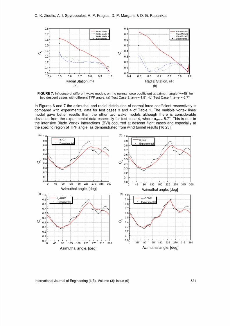
In Figures 6 and 7 the azimuthal and radial distribution of normal force coefficient respectively iscompared with experimental data for test cases 3 and 4 of Table 1. The multiple vortex lines
model gave better results than the other two wake models although there is considerabledeviation from the experimental data especially for test case 4, where aTPP=-5.7
o. This is due to
the intensive Blade Vortex Interactions (BVI) occurred at descent flight cases and especially atthe specific region of TPP angle, as demonstrated from wind tunnel results [16,23].
0 45 90 135 180 225 270 315 3600.0
0.1
0.2
0.3
0.4
0.5
0.6
0.7
0.8
0.9
1.0
C n
Azimuthal angle, [deg]
as=0.1
Experimental
(a)
0 45 90 135 180 225 270 315 3600.0
0.1
0.2
0.3
0.4
0.5
0.6
0.7
0.8
0.9
1.0
C n
Azimuthal angle, [deg]
as=0.01
Experimental
(b)
0 45 90 135 180 225 270 315 3600.0
0.1
0.20.3
0.4
0.5
0.6
0.7
0.8
0.9
1.0
C n
Azimuthal angle, [deg]
as=0.001
Experimental
(c)
0 45 90 135 180 225 270 315 3600.0
0.1
0.2
0.3
0.4
0.5
0.6
0.7
0.8
0.9
1.0
C n
Azimuthal angle, [deg]
as=0.0001
Experimental
(d)

8/8/2019 International Journal of Engineering (IJE), Volume (3): Issue (6)
http://slidepdf.com/reader/full/international-journal-of-engineering-ije-volume-3-issue-6 20/164
C. K. Zioutis, A. I. Spyropoulos, A. P. Fragias, D. P. Margaris & D. G. Papanikas
International Journal of Engineering (IJE), Volume (3): Issue (6) 532
0 45 90 135 180 225 270 315 3600.0
0.1
0.2
0.3
0.4
0.5
0.6
0.7
0.8
0.9
1.0
C n
Azimuthal angle, [deg]
as=0.00001
Experimental
(e)
0 45 90 135 180 225 270 315 3600.0
0.1
0.2
0.3
0.4
0.5
0.6
0.7
0.8
0.9
1.0
C
n
Azimuthal angle, [deg]
as=0.000065
Experimental
(f)
FIGURE 8: Computational investigation for the definition of Squire’s parameter as. The diagrams correspondto the test case 1 flight conditions.
As mentioned before in order to include diffusion effects in the vortex core, Squire’s parameter as must be defined. For this purpose a computational investigation has been done for the derivation
of an acceptable value of as.
Figure 8 shows the azimuthal distribution of the normal force coefficient for several values of a s varying from 10
-1to 10
-5. Comparing the computed results with the corresponding experimental
ones for test case 1, a value of the order 10-4
to 10-5
, as indicated in diagrams (d) and (e) inFigure 8, seems to achieve best results. This value for as has also been suggested by Leishman[31]. At this work a value of 0.000065 was selected for as as shown in the diagram (f) in Figure 8.
0 45 90 135 180 225 270 315 3600.0
0.2
0.4
0.6
0.8
1.0
1.2
C n
Azimuthal angle, [deg]
Rotary WingScully-KauffmanBagai-LeishmanLamb-OseenExperimental
(a)
0 45 90 135 180 225 270 315 3600.0
0.2
0.4
0.6
0.8
1.0
1.2
C n
Azimuthal angle, [deg]
Rotary WingScully-KauffmanBagai-LeishmanLamb-OseenExperimental
(b)
FIGURE 9: Influence of different core models on the normal force coefficient at radial station 0.82 for twoclimb cases with different advance ratio, (a) Test Case 1, µ=0.168, (b) Test Case 2, µ=0.268.
Having found an appropriate value for as, several core models are applied to simulate the tip
vortex core structure. In Figures 9 and 10 the azimuthal and radial distribution of normal forcecoefficient respectively is compared with experimental data for test cases 1 and 2 as presented inTable 1. Four different core models are tested. As expected, Scully-Kauffman, Bagai-Leishmanand Lamb-Oseen core models give about the same results. This is due to the fact that these coremodels were obtained from the same series family proposed by Vatistas. The rotary wing gavebetter results than the other three core models, demonstrating that this model is suitable forhelicopter climb test cases.

8/8/2019 International Journal of Engineering (IJE), Volume (3): Issue (6)
http://slidepdf.com/reader/full/international-journal-of-engineering-ije-volume-3-issue-6 21/164
C. K. Zioutis, A. I. Spyropoulos, A. P. Fragias, D. P. Margaris & D. G. Papanikas
International Journal of Engineering (IJE), Volume (3): Issue (6) 533
0.4 0.5 0.6 0.7 0.8 0.9 1.00.0
0.1
0.2
0.3
0.4
0.5
0.6Rotary WingScully-KauffmanBagai-LeishmanLamb-OseenExperimental
C
n
Radial Station, r/R (a)
0.4 0.5 0.6 0.7 0.8 0.9 1.00.0
0.1
0.2
0.3
0.4
0.5
0.6Rotary WingScully-KauffmanBagai-LeishmanLamb-OseenExperimental
C
n
Radial Station, r/R (b)
FIGURE 10: Influence of different core models on the normal force coefficient at azimuth angle Ψ=45ο
fortwo climb cases with different advance ratio, (a) Test Case 1, µ=0.168, (b) Test Case 2, µ=0.268.
The same core models were applied for the two descent test cases 3 and 4 (Table 1). As shownin Figure 11 all core models give about the same overall results, underestimating the value of Cn
at azimuthal angles between 90o and 135o. The three core models which belong to the sameseries family fit better to the experimental data than the rotary wing, for azimuthal angles between315
oand 360
o. Also from Figure 12 seems that these models correspond better to the
experimental data and especially for the second descent test case, as shown in Figure 12b whereintense BVI phenomena occurred as mentioned previously. Due to its simplicity the Scully-Kauffman core model is an option, but in order to include diffusion and straining effects the Lamb-Oseen model is preferable.
0 45 90 135 180 225 270 315 3600.0
0.1
0.2
0.3
0.40.5
0.6
0.7
0.8
0.9
1.0
C n
Azimuthal angle, [deg]
Rotary WingScully-Kauffman
Bagai-Leishman
Lamb-OseenExperimental
(a)
0 45 90 135 180 225 270 315 3600.0
0.1
0.2
0.3
0.40.5
0.6
0.7
0.8
0.9
1.0
C n
Azimuthal angle, [deg]
Rotary WingScully-KauffmanBagai-Leishman
Lamb-OseenExperimental
(b)
FIGURE 11: Influence of different core models on the normal force coefficient at radial station 0.82 for twodescent cases with different TPP angle, (a) Test Case 3, aTPP =-1.8
o, (b) Test Case 4, aTPP =-5.7
o.
8/8/2019 International Journal of Engineering (IJE), Volume (3): Issue (6)
http://slidepdf.com/reader/full/international-journal-of-engineering-ije-volume-3-issue-6 22/164
C. K. Zioutis, A. I. Spyropoulos, A. P. Fragias, D. P. Margaris & D. G. Papanikas
International Journal of Engineering (IJE), Volume (3): Issue (6) 534
0.4 0.5 0.6 0.7 0.8 0.9 1.00.0
0.1
0.2
0.3
0.4
0.5
0.6
0.7
0.8
Rotary WingScully-KauffmanBagai-LeishmanLamb-OseenExperimental
C n
Radial Station, r/R
(a)
0.4 0.5 0.6 0.7 0.8 0.9 1.00.0
0.1
0.2
0.3
0.4
0.5
0.6
0.7
0.8
Rotary WingScully-KauffmanBagai-LeishmanLamb-OseenExperimental
C
n
Radial Station, r/R (b)
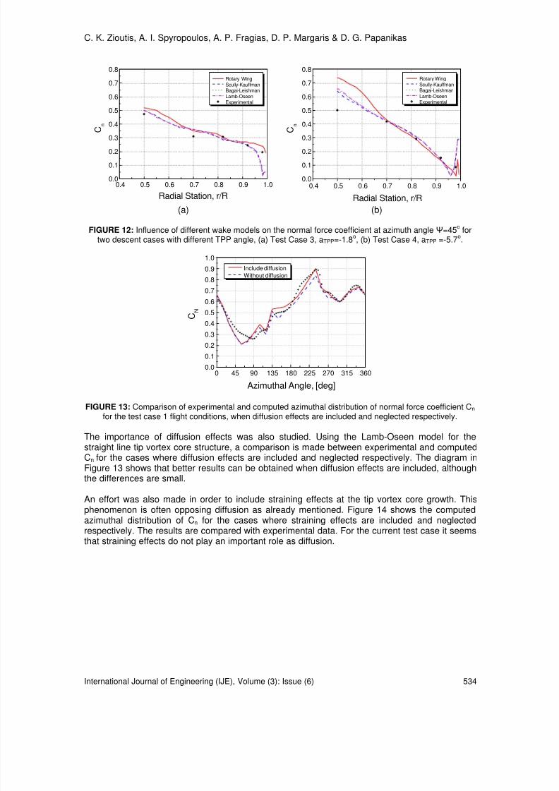
FIGURE 12: Influence of different wake models on the normal force coefficient at azimuth angle Ψ=45ο
fortwo descent cases with different TPP angle, (a) Test Case 3, aTPP=-1.8
o, (b) Test Case 4, aTPP =-5.7
o.
0 45 90 135 180 225 270 315 3600.0
0.1
0.2
0.3
0.4
0.5
0.6
0.7
0.8
0.9
1.0
C N
Azimuthal Angle, [deg]
Include diffusion
Without diffusion
FIGURE 13: Comparison of experimental and computed azimuthal distribution of normal force coefficient Cn
for the test case 1 flight conditions, when diffusion effects are included and neglected respectively.
The importance of diffusion effects was also studied. Using the Lamb-Oseen model for thestraight line tip vortex core structure, a comparison is made between experimental and computedCn for the cases where diffusion effects are included and neglected respectively. The diagram inFigure 13 shows that better results can be obtained when diffusion effects are included, althoughthe differences are small.
An effort was also made in order to include straining effects at the tip vortex core growth. Thisphenomenon is often opposing diffusion as already mentioned. Figure 14 shows the computedazimuthal distribution of Cn for the cases where straining effects are included and neglectedrespectively. The results are compared with experimental data. For the current test case it seemsthat straining effects do not play an important role as diffusion.

8/8/2019 International Journal of Engineering (IJE), Volume (3): Issue (6)
http://slidepdf.com/reader/full/international-journal-of-engineering-ije-volume-3-issue-6 23/164
C. K. Zioutis, A. I. Spyropoulos, A. P. Fragias, D. P. Margaris & D. G. Papanikas
International Journal of Engineering (IJE), Volume (3): Issue (6) 535
0 45 90 135 180 225 270 315 3600.0
0.1
0.2
0.30.4
0.5
0.6
0.7
0.8
0.9
1.0
C N
Azimuthal angle, [deg]
Include diffusion
Include diffusion
and straining
FIGURE 14: Comparison of experimental and computed azimuthal distribution of normal force coefficient Cn for the test case 1 flight conditions, when straining effects are included and neglected respectively.
4. CONSLUSIONS
A computational model for the simulation of helicopter rotor wake has been developed usingmultiple trailing vortex lines. Diffusion and straining effects of the tip vortex have been appropriateincorporated in order to investigate their influences. To include viscous effects several coremodels have been tested.The conclusions from this study are summarized as follows:1. Despite the extra computational cost, simulating the rotor wake by multiple trailing vortex
lines is preferable than using vortex sheets for the inboard or the shed wake. This is crucialespecially for low speed helicopter flight.
2. In order to include diffusion effects, Squire’s parameter as has been found to be of the orderof 10
-4to 10
-5. At this work a value equal to 0.000065 was selected.
3. The rotary wing core model seems to be more suitable for helicopter climb flight cases.4. For descent flight cases, where intense BVI phenomena occurred, the Lamb-Oseen core
model is preferable due to its ability to include diffusion and straining effects. The Scully-Kauffman core model is an option because of its simplicity.
5. Diffusion effects are important on the calculation of helicopter rotor aerodynamic forces, butstraining effects do not influence computational results as much as diffusion.
5. REFERENCES
1. W. Johnson. “Rotorcraft aerodynamics models for a comprehensive analysis” . Proceedings of54th Annual Forum of American Helicopter Society, Washington, DC, May 20-22, 1998.
2. G. J. Leishman, M. J. Bhagwat and A. Bagai. “Free-vortex filament methods for the analysis of helicopter rotor wakes” . Journal of Aircraft, 39(5):759-775, 2002.
3. T. A. Egolf and A. J. Landgrebe. “A prescribed wake rotor inflow and flow field prediction analysis” . NASA CR 165894, June 1982.
4. T. S. Beddoes. “A wake model for high resolution airloads ”. Proceedings of the 2ndInternational Conference on Basic Rotorcraft Research, Univ. of Maryland, College Park, MD,
1985.5. M. J. Bhagwat and G. J. Leishman. “Stability, consistency and convergence of time-marching free-vortex rotor wake algorithms ”. Journal of American Helicopter Society, 46(1):59-71,2001.
6. T. R. Quackenbush, D. A. Wachspress and Boschitsch. “Rotor aerodynamic loads computation using a constant vorticity contour free wake model ”. Journal of Aircraft,32(5):911-920, 1995.
7. K. Chua and T.R. Quackenbush. “Fast three-dimensional vortex method for unsteady wake calculations ”. AIAA Journal, 31(10):1957-1958, 1993.

8/8/2019 International Journal of Engineering (IJE), Volume (3): Issue (6)
http://slidepdf.com/reader/full/international-journal-of-engineering-ije-volume-3-issue-6 24/164
C. K. Zioutis, A. I. Spyropoulos, A. P. Fragias, D. P. Margaris & D. G. Papanikas
International Journal of Engineering (IJE), Volume (3): Issue (6) 536
8. M. J. Bhagwat and G. J. Leishman. “Rotor aerodynamics during manoeuvring flight using a time-accurate free vortex wake ”. Journal of American Helicopter Society, 48(3):143-158,2003.
9. G. H. Xu and S. J. Newman. “Helicopter rotor free wake calculations using a new relaxation technique ”. Proceedings of 26th European Rotorcraft Forum, Paper No. 37, 2000.
10. M. P. Scully. “Computation of helicopter rotor wake geometry and its influence on rotor harmonic airloads ”. ASRL TR 178-1, 1975
11. A. J. Chorin. “Computational fluid mechanics ”. 1st edition, Academic Press, (1989).12. T. Leonard. “Computing three dimensional incompressible flows with vortex elements ”.
Annual Review of Fluid Mechanics, 17: 523-559, 1985.13. T. Sarpkaya. “Computational methods with vortices - The 1988 Freeman scholar lecture ”.
ASME Journal of Fluids Engineering, 111(5):5-52, March 1989.14. N. Hariharan and L. N. Sankar. “A review of computational techniques for rotor wake
modeling ”. Proceedings of AIAA 38th Aerospace Sciences Meeting, AIAA 00-0114, Reno NV,2000.
15. A. I. Spyropoulos, A. P. Fragias, D. G. Papanikas and D. P. Margaris. “Influence of arbitrary vortical wake evolution on flowfield and noise generation of helicopter rotors ”. Proceedings ofthe 22nd ICAS Congress, Harrogate, United Kingdom, 2000.
16. A. I. Spyropoulos, C. K. Zioutis, A. P. Fragias, E. E. Panagiotopoulos and D. P. Margaris.“Computational tracing of BVI phenomena on helicopter rotor disk ”. International Review of
Aerospace Engineering (I.RE.AS.E), 2(1):13-23, February 2009.17. D. B. Bliss, M. E. Teske and T. R. Quackenbush. “A new methodology for free wake analysis
using curved vortex elements ”. NASA CR-3958, 1987.18. S. Gupta and G. J. Leishman. “Accuracy of the induced velocity from helicoidal vortices using
straight-line segmentation ”. AIAA Journal, 43(1):29-40, 2005.19. D. H. Wood and D. Li. “Assessment of the accuracy of representing a helical vortex by
straight segments ”. AIAA Journal, 40(4):647-651, 2005.20. M. Ramasamy, G. J. Leishman. “Interdependence of diffusion and straining of helicopter
blade tip vortices ”. Journal of Aircraft, 41(5):1014-1024, 2004.21. C. Tung and L. Ting. “Motion and decay of a vortex ring ”. Physics of Fluids, 10(5):901-910,
1967.22. J. A. Stott and P. W. Duck. “The effects of viscosity on the stability of a trailing-line vortex in
compressible flow ”. Physics of Fluids, 7(9):2265-2270, 1995.
23. W. R. Splettstoesser, G. Niesl, F. Cenedese, F. Nitti and D. G. Papanikas. “Experimental results of the European HELINOISE aeroacoustic rotor test ”. Journal of American HelicopterSociety, 40(2):3-14, 1995.
24. S. E. Windnall and T. L. Wolf. “Effect of tip vortex structure on helicopter noise due to blade vortex interactions ”. AIAA Journal of Aircraft, 17(10):705-711, 1980.
25. J. M. Bhagwat and G. J. Leishman. “Correlation of helicopter rotor tip vortex measurements ”.AIAA Journal, 38(2):301-308, 2000.
26. G. H. Vatistas, V. Kozel and W. C. Mih. “A simpler model for concentrated vortices ”.Experiments in Fluids, 11(1):73-76, 1991.
27. M. P. Scully and J. P. Sullivan. “Helicopter rotor wake geometry and airloads and development of laser Doppler velocimeter for use in helicopter rotor wakes ”. MassachusettsInstitute of Technology Aerophysics Laboratory Technical Report 183, MIT DSR No. 73032,1972.
28. G. K. Batchelor, “Introduction to fluid dynamics ”. Cambridge University Press, (1967).29. C. K Zioutis, A. I. Spyropoulos, D. P. Margaris and D. G. Papanikas. “ Numerical investigation of BVI modeling effects on helicopter rotor free wake simulations ”. Proceedings of the 24thICAS Congress, 2004, Yokohama, Japan.
30. H. B. Squire. “The growth of a vortex in turbulent flow ”. Aeronautical Quarterly, 16(3):302-306, 1965.
31. J. M. Bhagwat and G. J. Leishman. “Generalized viscous vortex model for application to free- vortex wake and aeroacoustic calculations ”. Proceedings of American Helicopter Society 58thAnnual Forum and Technology Display, Montreal, Canada, 2002.

8/8/2019 International Journal of Engineering (IJE), Volume (3): Issue (6)
http://slidepdf.com/reader/full/international-journal-of-engineering-ije-volume-3-issue-6 25/164
C. K. Zioutis, A. I. Spyropoulos, A. P. Fragias, D. P. Margaris & D. G. Papanikas
International Journal of Engineering (IJE), Volume (3): Issue (6) 537
32. G. J. Leishman, A. Baker and A. Coyne "Measurements of rotor tip vortices using three- component laser doppler velocimetry" . Journal of American Helicopter Society, 41(4):342-353, 1996.
33. C. Golia, B. Buonomo and A. Viviani. “Grid Free Lagrangian Blobs Vortex Method with Brinkman Layer Domain Embedding Approach for Heterogeneous Unsteady Thermo Fluid Dynamics Problems”. International Journal of Engineering, 3(3):313-329, 2009.

8/8/2019 International Journal of Engineering (IJE), Volume (3): Issue (6)
http://slidepdf.com/reader/full/international-journal-of-engineering-ije-volume-3-issue-6 26/164
Elias E. Panagiotopoulos & Spyridon D. Kyparissis
International Journal of Engineering (IJE), Volume (3): Issue (6) 538
CFD Transonic Store Separation Trajectory Predictions withComparison to Wind Tunnel Investigations
Elias E. Panagiotopoulos [email protected] Military Academy Vari, Attiki, 16673, Greece
Spyridon D. Kyparissis [email protected] Engineering and Aeronautics Department University of Patras Patras, Rio, 26500, Greece
Abstract
The prediction of the separation movements of the external store weapons
carried out on military aircraft wings under transonic Mach number and variousangles of attack is an important task in the aerodynamic design area in order todefine the safe operational-release envelopes. The development ofcomputational fluid dynamics techniques has successfully contributed to theprediction of the flowfield through the aircraft/weapon separation problems. Thenumerical solution of the discretized three-dimensional, inviscid andcompressible Navier-Stokes equations over a dynamic unstructured tetrahedralmesh approach is accomplished with a commercial CFD finite-volume code. Acombination of spring-based smoothing and local remeshing are employed withan implicit, second-order upwind accurate Euler solver. A six degree-of-freedomroutine using a fourth-order multi-point time integration scheme is coupled with
the flow solver to update the store trajectory information. This analysis is appliedfor surface pressure distributions and various trajectory parameters during theentire store-separation event at various angles of attack. The efficiency of theapplied computational analysis gives satisfactory results compared, whenpossible, against the published data of verified experiments.
Keywords: CFD Modelling, Ejector Forces and Moments, Moving-body Trajectories, Rigid-body
Dynamics, Transonic Store Separation Events.
1. INTRODUCTION
With the advent and rapid development of high performance computing and numerical algorithms,computational fluid dynamics (CFD) has emerged as an essential tool for engineering andscientific analyses and design. Along with the growth of computational resources, the complexityof problems that need to be modeled has also increased. The simulation of aerodynamicallydriven, moving-body problems, such as store separation, maneuvering aircraft, and flapping-wingflight are important goals for CFD practitioners [1].
The aerodynamic behavior of munitions or other objects as they are released from aircraft iscritical both to the accurate arrival of the munitions and the safety of the releasing aircraft [2]. In

8/8/2019 International Journal of Engineering (IJE), Volume (3): Issue (6)
http://slidepdf.com/reader/full/international-journal-of-engineering-ije-volume-3-issue-6 27/164
Elias E. Panagiotopoulos & Spyridon D. Kyparissis
International Journal of Engineering (IJE), Volume (3): Issue (6) 539
the distant past separation testing was accomplished solely using flying tests. This approach wasvery time-consuming, often requiring years to certify a projectile. It was also expensive andoccasionally led to the loss of an aircraft due to unexpected behavior of the store being tested.
In the past, separation testing was accomplished solely via flight tests. In addition to being verytime consuming, often taking years to certify a weapon, this approach was very expensive andoften led to loss of aircraft. In the 1960s, experimental methods of predicting store separation inwind tunnel tests were developed. These tests have proven so valuable that they are now theprimary design tool used. However, wind tunnel tests are still expensive, have long lead times,and suffer from limited accuracy in certain situations, such as when investigating stores releasedwithin weapons bays or the ripple release of multiple moving objects. In addition, because verysmall-scale models must often be used, scaling problems can reduce accuracy.
In recent years, modelling and simulation have been used to reduce certification cost andincrease the margin of safety of flight tests for developmental weapons programs. Computationalfluid dynamics (CFD) approaches to simulating separation events began with steady-statesolutions combined with semi-empirical approaches [3] - [7]. CFD truly became an invaluableasset with the introduction of Chimera overset grid approaches [8]. Using these methods,unsteady full field simulations can be performed with or without viscous effects.
The challenge with using CFD is to provide accurate data in a timely manner. Computational costis often high because fine grids and small time steps may be required for accuracy and stability ofsome codes. Often, the most costly aspect of CFD, both in terms of time and money, is gridgeneration and assembly. This is especially true for complex store geometries and in the case ofstores released from weapons bays. These bays often contain intricate geometric features thataffect the flow field.
Aerodynamic and physical parameters affect store separation problems. Aerodynamicparameters are the store shape and stability, the velocity, attitude, load factor, configuration of theaircraft and flow field surrounding the store. Physical parameters include store geometriccharacteristics, center of gravity position, ejector locations and impulses and bomb rack. Theabove parameters are highly coupled and react with each other in a most complicated manner[9] - 11]. An accurate prediction of the trajectory of store objects involves an accurate prediction
of the flow field around them, the resulting forces and moments, and an accurate integration ofthe equations of motion. This necessitates a coupling of the CFD solver with a six degree offreedom (6-DOF) rigid body dynamics simulator [12]. The simulation errors in the CFD solver andin the 6-DOF simulator have an accumulative effect since any error in the calculated aerodynamicforces can predict a wrong orientation and trajectory of the body and vice-versa. The forces andmoments on a store at carriage and various points in the flow field of the aircraft can be computedusing CFD applied to the aircraft and store geometry [13].
The purpose of this paper is to demonstrate the accuracy and technique of using an unstructureddynamic mesh approach to store separation. The most significant advantage of utilizingunstructured meshes [14] is the flexibility to handle complex geometries. Grid generation time isgreatly reduced because the user’s input is limited to mainly generation of a surface mesh.Though not utilized in this study, unstructured meshes additionally lend themselves very well to
solution-adaptive mesh refinement/coarsening techniques, especially useful in capturing shocks.Finally, because there are no overlapping grid regions, fewer grid points are required.
The computational validation of the coupled 6-DOF and overset grid system is carried out using asimulation of a safe store separation event from underneath a delta wing under transonicconditions (Mach number 1.2) at an altitude of 11,600 m [15] and various angles of attack (0°, 3°and 5°) for a particular weapon configuration with appropriate ejection forces. An inviscid flow isassumed to simplify the above simulations. The predicted computed trajectories are comparedwith a 1/20 scale wind-tunnel experimental data conducted at he Arnold EngineeringDevelopment Center (AEDC) [16] - [17].

8/8/2019 International Journal of Engineering (IJE), Volume (3): Issue (6)
http://slidepdf.com/reader/full/international-journal-of-engineering-ije-volume-3-issue-6 28/164
Elias E. Panagiotopoulos & Spyridon D. Kyparissis
International Journal of Engineering (IJE), Volume (3): Issue (6) 540
2. WEAPON / EJECTOR MODELLING
In the present work store-separation numerically simulation events were demonstrated on ageneric pylon/store geometric configuration attached to a clipped delta wing, as shown inFIGURE 1. Benchmark wind-tunnel experiments for these cases were conducted at the ArnoldEngineering Development Center (AEDC) [16], and the details of the data can be found inLijewski and Suhs [18]. Results available from these studies include trajectory informations and
surface pressure distributions at multiple instants in time. The computational geometry matchesthe experimental model with the exception of the physical model being 1/20 scale.
FIGURE 1: Global coordinate system OXYZ for store separation trajectory analysis.
It can be seen from FIGURE 1 the global coordinate system orientation OXYZ for the storeseparation simulation analysis. The origin O is located at the store center of gravity while instorage. X-axis runs from the tail to nose of the store, Y-axis points away from the aircraft and Z-axis points downward along the direction of the gravity.
The aircraft’s wing is a 45-degree clipped delta with 7.62 m (full scale) root chord length, 6.6 msemi-span, and NACA 64A010 airfoil section. The ogive-flat plate-ogive pylon is located spanwise3.3 m from the root, and extends 61 cm below the wing leading edge. The store consists of atangent-ogive forebody, clipped tangent-ogive afterbody, and cylindrical centerbody almost 50 cmin diameter. Overall, the store length is approximately 3.0 m. Four fins are attached, eachconsisting of a 45-degree sweep clipped delta wing with NACA 008 airfoil section. To accuratelymodel the experimental setup, a small gap of 3.66 cm exists between the missile body and thepylon while in carriage.
In the present analysis the projectile is forced away from its wing pylon by means of identicalpiston ejectors located in the lateral plane of the store, -18 cm forward of the center of gravity(C.G.), and 33 cm aft. While the focus of the current work is not to develop an ejector model forthe examined projectile configuration, simulating the store separation problem with an ejector
model which has known inaccuracies serves little purpose [9].
The ejector forces were present and operate for the duration of 0.054 s after releasing the store.The ejectors extend during operation for 10 cm, and the force of each ejector is a constantfunction of this stroke extension with values 10.7 kN and 42.7 kN, respectively. The basicgeometric properties of the store and ejector forces for this benchmark simulation problem aretabulated in TABLE 1 and are depicted in a more detail drawing in FIGURE 2.

8/8/2019 International Journal of Engineering (IJE), Volume (3): Issue (6)
http://slidepdf.com/reader/full/international-journal-of-engineering-ije-volume-3-issue-6 29/164
Elias E. Panagiotopoulos & Spyridon D. Kyparissis
International Journal of Engineering (IJE), Volume (3): Issue (6) 541
As the store moves away from the pylon, it begins to pitch and yaw as a result of aerodynamicforces and the stroke length of the individual ejectors responds asymmetrically.
FIGURE 2: Ejector force model for the store separation problem.
Characteristic Magnitudes Values
Mass m, kg 907
Reference Length L, mm 3017.5
Reference Diameter D, mm 500
No. of fins 4
Center of gravity xC.G., mm 1417 (aft of store nose)
Axial moment of inertia IXX, kg·m2
27
Transverse moments of inertiaIyy and Izz, kg·m
2
488
Forward ejector location LFE., mm 1237.5 (aft of store nose)
Forward ejector force FFE, kN 10.7
Aft ejector location LAE, mm 1746.5 (aft of store nose)
Aft ejector force FAE, kN 42.7
Ejector stroke length LES, mm 100
TABLE 1: Main geometrical data for the examined store separation projectile.
3. FLOWFIELD NUMERICAL SIMULATION
The computational approach applied in this study consists of three distinct components: a flowsolver, a six degree of freedom (6DOF) trajectory calculator and a dynamic mesh algorithm [12].The flow solver is used to solve the governing fluid-dynamic equations at each time step. Fromthis solution, the aerodynamic forces and moments acting on the store are computed byintegrating the pressure over the surface. Knowing the aerodynamic and body forces, the

8/8/2019 International Journal of Engineering (IJE), Volume (3): Issue (6)
http://slidepdf.com/reader/full/international-journal-of-engineering-ije-volume-3-issue-6 30/164
Elias E. Panagiotopoulos & Spyridon D. Kyparissis
International Journal of Engineering (IJE), Volume (3): Issue (6) 542
movement of the store is computed by the 6DOF trajectory code. Finally, the unstructured meshis modified to account for the store movement via the dynamic mesh algorithm.
3.1 Flow SolverThe flow is compressible and is described by the standard continuity and momentum equations.The energy equation incorporates the coupling between the flow velocity and the static pressure.The flow solver is used to solve the governing fluid dynamic equations that include an implicitalgorithm for the solution of the Euler Equations [11] - [14]. The Euler equations are well knownand hence, for purposes of brevity, are not shown. The present analysis employs a cell-centeredfinite volume method based on the linear reconstruction scheme, which allows the use ofcomputational elements with arbitrary polyhedral topology. A point implicit (block Gauss-Seidel)linear equation solver is used in conjunction with an algebraic multigrid (AMG) method to solvethe resultant block system of equations for all dependent variables in each cell. Temporally, a firstorder implicit Euler scheme is employed [14] - [23].
The conservation equation for a general scalar f on an arbitrary control volume whose boundaryis moving can be written in integral form as:
( )g f
V V V V
fdV f u u dA fdA S dV
t
ρ ρ Γ
∂ ∂
∂+ − = ∇ +
∂∫ ∫ ∫ ∫
r r r r (1)
The time derivative in Eq.(1) is evaluated using a first-order backward difference formula:
( ) ( )k 1 k
V
fV fV d fdV
dt t
ρ ρ ρ
∆
+
−=∫ (2)
where the superscript denotes the time level and also
k 1 k dV V V t
dt ∆+
= + (3)
The space conservation law [24] is used in formulating the volume time derivative in the aboveexpression Eq.(3) in order to ensure no volume surplus or deficit exists.
3.2 Trajectory CalculationThe 6DOF rigid-body motion of the store is calculated by numerically integrating the Newton-Euler equations of motion within Fluent as a user-defined function (UDF). The aerodynamicforces and moments on the body store are calculated based on the integration of pressure overthe surface. This information is provided to the 6DOF from the flow solver in inertial coordinates.The governing equation for the translational motion of the center of gravity is solved for in theinertial coordinate system, as shown below:
G Gv m f = ∑rr& (4)
where Gvr& is the translational motion of the center of gravity, m is the mass of the store and G f
ris
the force vector due to gravity.
The angular motion of the moving object ω Βr
, on the other hand, is more readily computed in body
coordinates to avoid time-variant inertia properties:
( )1
B L M Lω ω ω −
Β Β Β= − ×∑rr r r& (5)

8/8/2019 International Journal of Engineering (IJE), Volume (3): Issue (6)
http://slidepdf.com/reader/full/international-journal-of-engineering-ije-volume-3-issue-6 31/164
Elias E. Panagiotopoulos & Spyridon D. Kyparissis
International Journal of Engineering (IJE), Volume (3): Issue (6) 543
where L is the inertia tensor and B M r
is the moment vector of the store.
The orientation of the store is tracked using a standard 3-2-1 Euler rotation sequence. Themoments are therefore transformed from inertial to body coordinates via
B G M RM =r r
(6)
where R is the transformation matrix
c c c s s
R s s c c s s s s c c c s
c s c s s c s s s c c c
θ ψ θ ψ θ
φ θ ψ φ ψ φ θ ψ φ ψ θ φ
φ θ ψ φ ψ φ θ ψ φ ψ θ φ
−
≡ − + + −
(7)
with the shorthand notation cξ = cos(ξ) and sξ = sin(ξ) has been used.Once the translational and angular accelerations are computed from Eqs (4) and (5), the angularrates are determined by numerically integrating using a fourth-order multi-point Adams-Moultonformulation:
( )k 1 k k 1 k k 1 k 2t 9 19 5
24
∆ξ ξ ξ ξ ξ ξ + + − −
= + + − +& & & & (8)
where ξ represents either Gvr
or ω Βr
.
The dynamic mesh algorithm takes as input Gvr
and Gω r
. The angular velocity, then, is
transformed back to inertial coordinates via
G B M R M Τ
=r r
(9)
where R is given in Eq.(7).
FIGURE 3: Refined mesh in the region near the store.
3.3 Dynamic MeshThe geometry and the grid were generated with Fluent’s pre-processor, Gambit® usingtetrahedral volume mesh [25]. As shown in FIGURE 3, the mesh of the fluid domain is refined inthe region near the store to better resolves the flow details. In order to simulate the storeseparation an unstructured dynamic mesh approach is developed. A local remeshing algorithm is

8/8/2019 International Journal of Engineering (IJE), Volume (3): Issue (6)
http://slidepdf.com/reader/full/international-journal-of-engineering-ije-volume-3-issue-6 32/164
Elias E. Panagiotopoulos & Spyridon D. Kyparissis
International Journal of Engineering (IJE), Volume (3): Issue (6) 544
used to accommodate the moving body in the discretized computational domain. Theunstructured mesh is modified to account for store movement via the dynamic mesh algorithm.
FIGURE 4: Surface mesh of the examined store.
When the motion of the moving body is large, poor quality cells, based on volume or skewnesscriteria, are agglomerated and locally remeshed when necessary. On the other hand, when themotion of the body is small, a localized smoothing method is used. That is, nodes are moved toimprove cell quality, but the connectivity remains unchanged. A so-called spring-based smoothingmethod is employed to determine the new nodal locations. In this method, the cell edges aremodeled as a set of interconnected springs between nodes.
The movement of a boundary node is propagated into the volume mesh due to the spring forcegenerated by the elongation or contraction of the edges connected to the node. At equilibrium,the sum of the spring forces at each node must be zero; resulting in an iterative equation:
11
1
i
i
nm
ij i
jmi n
ij
j
k x
x
k
=+
=
∆
∆ =
∑
∑
r
r (10)
where the superscript denotes iteration number. After movement of the boundary nodes, as
defined by the 6DOF, Eq.(10) is solved using a Jacobi sweep on the interior nodes, and the nodallocations updated as
k 1 k
i i i x x x∆+= +
r r r (11)
where here the superscript indicates the time step.
In FIGURE 4 the surface mesh of the store is illustrated. A pressure far field condition was usedat the upstream and downstream domain extents. The initial condition used for the store-separation simulations was a fully converged steady-state solution [26] - [28]. This approach wasdemonstrated on a generic wing-pylon-store geometry with the basic characteristics shown on theprevious section. The domain extends approximately 100 store diameters in all directions aroundthe wing and store.
The working fluid for this analysis is the air with density ρ = 0.33217 kg/m3. The studied angles of
attack are 0°, 3° and 5°, respectively. The store separation is realized to an altitude of 11,600 m,where the corresponding pressure is 20,657 Pa and the gravitational acceleration is g = 9.771m/s
2. The Mach number is M = 1.2 and the ambient temperature is T = 216.65 K [15], [29], [30].
4. NUMERICAL ANALYSIS RESULTS
The full-scale separation events are simulated under transonic conditions (Mach number 1.2) atan altitude of 11,600 m and various angles of attack (0°, 3° and 5°) using CFD-FLUENT package
8/8/2019 International Journal of Engineering (IJE), Volume (3): Issue (6)
http://slidepdf.com/reader/full/international-journal-of-engineering-ije-volume-3-issue-6 33/164
Elias E. Panagiotopoulos & Spyridon D. Kyparissis
International Journal of Engineering (IJE), Volume (3): Issue (6) 545
[31] - [32]. The initial condition used for the separation analysis was a fully converged steady-state solution. Because an implicit time stepping algorithm is used, the time step ∆t is not limitedby stability of the flow solver. Rather, ∆t is chosen based on accuracy and stability of the dynamicmeshing algorithm. Time step ∆t = 0.002 sec is chosen for the convergence of store-separationtrajectory simulations.
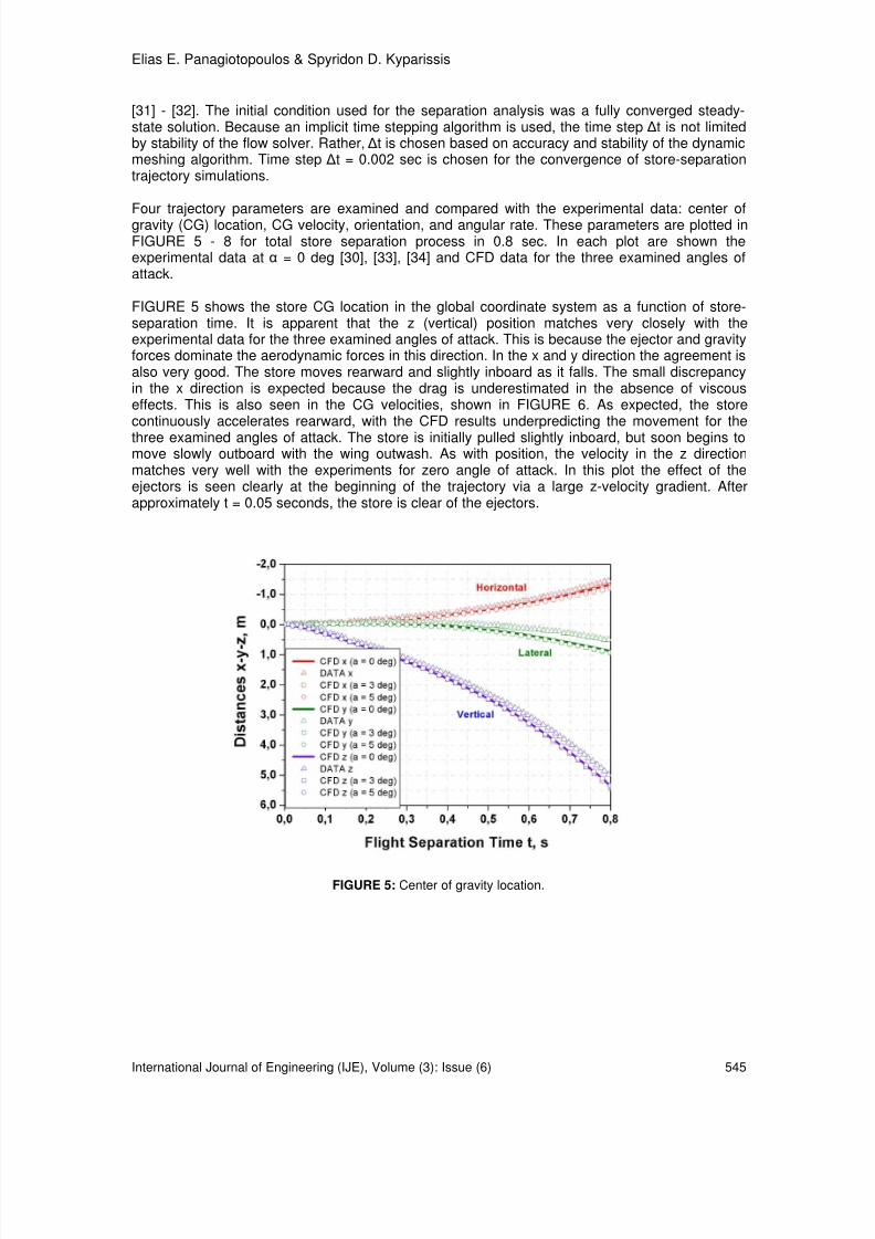
Four trajectory parameters are examined and compared with the experimental data: center ofgravity (CG) location, CG velocity, orientation, and angular rate. These parameters are plotted inFIGURE 5 - 8 for total store separation process in 0.8 sec. In each plot are shown theexperimental data at α = 0 deg [30], [33], [34] and CFD data for the three examined angles ofattack.
FIGURE 5 shows the store CG location in the global coordinate system as a function of store-separation time. It is apparent that the z (vertical) position matches very closely with theexperimental data for the three examined angles of attack. This is because the ejector and gravityforces dominate the aerodynamic forces in this direction. In the x and y direction the agreement isalso very good. The store moves rearward and slightly inboard as it falls. The small discrepancyin the x direction is expected because the drag is underestimated in the absence of viscouseffects. This is also seen in the CG velocities, shown in FIGURE 6. As expected, the storecontinuously accelerates rearward, with the CFD results underpredicting the movement for the
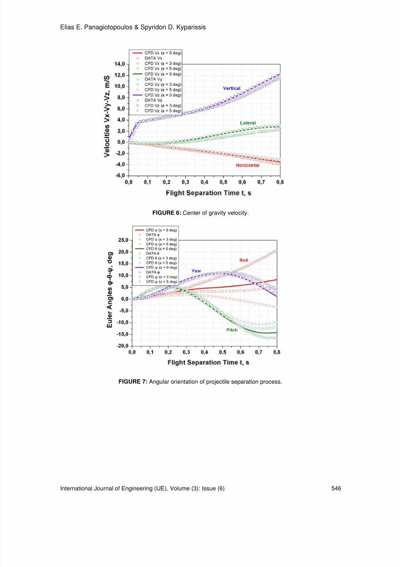
three examined angles of attack. The store is initially pulled slightly inboard, but soon begins tomove slowly outboard with the wing outwash. As with position, the velocity in the z directionmatches very well with the experiments for zero angle of attack. In this plot the effect of theejectors is seen clearly at the beginning of the trajectory via a large z-velocity gradient. Afterapproximately t = 0.05 seconds, the store is clear of the ejectors.
FIGURE 5: Center of gravity location.
8/8/2019 International Journal of Engineering (IJE), Volume (3): Issue (6)
http://slidepdf.com/reader/full/international-journal-of-engineering-ije-volume-3-issue-6 34/164
Elias E. Panagiotopoulos & Spyridon D. Kyparissis
International Journal of Engineering (IJE), Volume (3): Issue (6) 546
FIGURE 6: Center of gravity velocity.
FIGURE 7: Angular orientation of projectile separation process.

8/8/2019 International Journal of Engineering (IJE), Volume (3): Issue (6)
http://slidepdf.com/reader/full/international-journal-of-engineering-ije-volume-3-issue-6 35/164
Elias E. Panagiotopoulos & Spyridon D. Kyparissis
International Journal of Engineering (IJE), Volume (3): Issue (6) 547
FIGURE 8: Angular rate of the examined store movement.
The orientation of the store is more difficult to model than the CG position. This is evident inFIGURE 7, which shows the Euler angles as a function of time. The pitch and yaw angles agreewell with the experiment for α = 0, 3 and 5 degrees, respectively. The store initially pitches nose-up in response to the moment produced by the ejectors, as shown in FIGURE 2. Once free of theejectors after 0.05 seconds, though, the nose-down aerodynamic pitching moment reverses thetrend. The store yaws initially outboard until approximately 0.55 seconds, after which it beginsturning inboard. The store rolls continuously outboard throughout the first 0.8 seconds of theseparation. This trend is under-predicted by the CFD simulation analysis, and the curve tends todiverge from the experiments after approximately 0.3 seconds for all the examined angles ofattack. The roll angle is especially difficult to model because the moment of inertia about the roll
axis is much smaller than that of the pitch and yaw axes, see TABLE 1. Consequently, roll is verysensitive to errors in the aerodynamic force prediction. The body angular rates are plotted inFIGURE 8. Here again it is shown that the pitch and yaw rates compare well with the experimentsat α = 0 deg, while the roll rate is more difficult to capture.
It is obvious, that the CFD performs very well in modelling the whole store separation events. Thisis reiterated in FIGURE 9, in which views of the simulated store movements at α = 0 and α = 5deg, respectively, are compared at discrete instants in time throughout the separation for the first0.8 seconds. In the examined two cases the stores pitch down even though the applied ejectorforces causes a positive (nose up) ejector moment and roll inboard and yaw outboard. Thisdownward pitch of the store is a desirable trait for safe separation of a store from a fighter aircraft[2].
The fluid dynamics prediction analysis also gives pressure coefficient distributions for the totalseparation history along axial lines on the store body at four circumferential locations and threeinstants in time. The simulation data are compared with experimental surface pressure data fromthe wind tunnel tests [31], [33], 34], as depicted in FIGURES 10 up to 13.

8/8/2019 International Journal of Engineering (IJE), Volume (3): Issue (6)
http://slidepdf.com/reader/full/international-journal-of-engineering-ije-volume-3-issue-6 36/164
Elias E. Panagiotopoulos & Spyridon D. Kyparissis
International Journal of Engineering (IJE), Volume (3): Issue (6) 548
(a) Front view with side angles
(b) Front view
(c) Side view
FIGURE 9: Store separation events with ejectors at Mach 1.2 for 0 and 5 deg angle of attacks, respectively.

8/8/2019 International Journal of Engineering (IJE), Volume (3): Issue (6)
http://slidepdf.com/reader/full/international-journal-of-engineering-ije-volume-3-issue-6 37/164
Elias E. Panagiotopoulos & Spyridon D. Kyparissis
International Journal of Engineering (IJE), Volume (3): Issue (6) 549
FIGURE 10: Surface pressure profile for phi = 5 deg.
FIGURE 11: Surface pressure profile for phi = 95 deg.

8/8/2019 International Journal of Engineering (IJE), Volume (3): Issue (6)
http://slidepdf.com/reader/full/international-journal-of-engineering-ije-volume-3-issue-6 38/164
Elias E. Panagiotopoulos & Spyridon D. Kyparissis
International Journal of Engineering (IJE), Volume (3): Issue (6) 550
FIGURE 12: Surface pressure profile for phi = 185 deg.
FIGURE 13: Surface pressure profile for phi = 275 deg.
The circumferential locations are denoted by the angle phi. The value phi = 0 is located at the top(y = 0, nearest the pylon) of the store while in carriage and is measured counter clockwise when
viewed from upstream. FIGURES 10 - 13 show the pressure profiles along the non-dimensionalaxis of symmetry length x/L at phi = 5, 95, 185, and 275 deg for three time instants t = 0.0, 0.16,and 0.37 seconds with 0°, 3° and 5° degrees angle of attack (blue, green and red solid lines),respectively. It is obvious the agreement between computational and experimental data,especially in the region near the nose of projectile where the pressure coefficient Cp takespositive values.
The CFD numerical results correspond to the nominal grid with time step ∆t = 0.002 sec run.Agreement is exceptional. Of particular interest is the phi = 5 deg line at t = 0.0 because it is
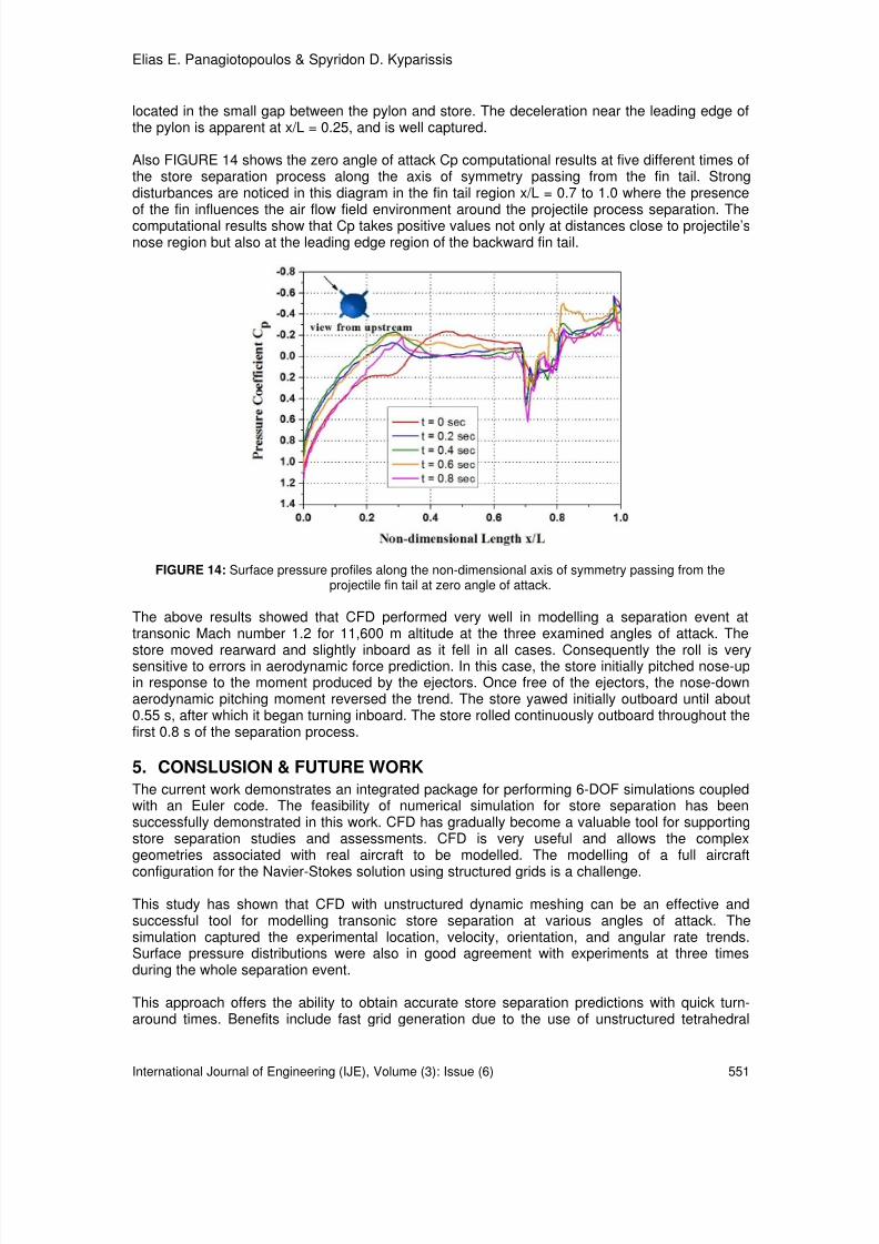
8/8/2019 International Journal of Engineering (IJE), Volume (3): Issue (6)
http://slidepdf.com/reader/full/international-journal-of-engineering-ije-volume-3-issue-6 39/164
Elias E. Panagiotopoulos & Spyridon D. Kyparissis
International Journal of Engineering (IJE), Volume (3): Issue (6) 551
located in the small gap between the pylon and store. The deceleration near the leading edge ofthe pylon is apparent at x/L = 0.25, and is well captured.
Also FIGURE 14 shows the zero angle of attack Cp computational results at five different times ofthe store separation process along the axis of symmetry passing from the fin tail. Strongdisturbances are noticed in this diagram in the fin tail region x/L = 0.7 to 1.0 where the presenceof the fin influences the air flow field environment around the projectile process separation. Thecomputational results show that Cp takes positive values not only at distances close to projectile’snose region but also at the leading edge region of the backward fin tail.
FIGURE 14: Surface pressure profiles along the non-dimensional axis of symmetry passing from theprojectile fin tail at zero angle of attack.
The above results showed that CFD performed very well in modelling a separation event attransonic Mach number 1.2 for 11,600 m altitude at the three examined angles of attack. The
store moved rearward and slightly inboard as it fell in all cases. Consequently the roll is verysensitive to errors in aerodynamic force prediction. In this case, the store initially pitched nose-upin response to the moment produced by the ejectors. Once free of the ejectors, the nose-downaerodynamic pitching moment reversed the trend. The store yawed initially outboard until about0.55 s, after which it began turning inboard. The store rolled continuously outboard throughout thefirst 0.8 s of the separation process.
5. CONSLUSION & FUTURE WORK
The current work demonstrates an integrated package for performing 6-DOF simulations coupledwith an Euler code. The feasibility of numerical simulation for store separation has beensuccessfully demonstrated in this work. CFD has gradually become a valuable tool for supportingstore separation studies and assessments. CFD is very useful and allows the complexgeometries associated with real aircraft to be modelled. The modelling of a full aircraft
configuration for the Navier-Stokes solution using structured grids is a challenge.
This study has shown that CFD with unstructured dynamic meshing can be an effective andsuccessful tool for modelling transonic store separation at various angles of attack. Thesimulation captured the experimental location, velocity, orientation, and angular rate trends.Surface pressure distributions were also in good agreement with experiments at three timesduring the whole separation event.
This approach offers the ability to obtain accurate store separation predictions with quick turn-around times. Benefits include fast grid generation due to the use of unstructured tetrahedral

8/8/2019 International Journal of Engineering (IJE), Volume (3): Issue (6)
http://slidepdf.com/reader/full/international-journal-of-engineering-ije-volume-3-issue-6 40/164
Elias E. Panagiotopoulos & Spyridon D. Kyparissis
International Journal of Engineering (IJE), Volume (3): Issue (6) 552
meshes, and a fully parallelized, accurate, and stable solver that allows small grids and relativelylarge time steps. Grid generation can be accomplished in a matter of hours, and runs such as thenominal grid case with time step ∆t = 0.002 seconds examined in this study can be completedovernight on a desktop workstation.
Some error did exist between the simulation and experiment, most prominently in the roll angle.Sources of error include the inviscid assumption (resulting in an under-prediction of drag forces)and the quasi-steady nature of the experiment.
Future work is planned to address the viscous effects. Modeling of the boundary layer requiresconstruction of a rigid viscous mesh attached to the store. Additionally, an adaptive gridrefinement algorithm is to be added to the solution procedure, providing more accurate predictionof shock strengths and locations to improve the aerodynamic model.
6. REFERENCES
1. A. Arabshahi, D. L. Whitfield. “A Multi-Block Approach to Solving the Three-Dimensional Unsteady Euler Equations about a Wing-Pylon-Store Configuration”. AIAA Paper 89-3401,August 1989
2. E. E. Covert. “Conditions for Safe Separation of External Stores”. Journal of Aircraft, 18(8),
19813. W. L. Sickles, C. H. Morgret, A. G. Denny and R. H. Nichols. “Comparison of Time-Accurate CFD and Engineering Methods for the JDAM Separation from an F-18C Aircraft” . Inproceedings of the Aircraft-Store Compatibility Symposium sponsored by International Testand Evaluation Association, Joint Ordinance Commanders Group, Aircraft Store CompatibilitySubgroup, Destin, FL, March 5–8, 2001
4. W. L. Sickles, A. G. Denny and R. H. Nichols. “Time-Accurate CFD Store Separation Predictions with Comparison to Flight Data” . AIAA Paper No. 2000-0796, In proceedings ofthe 37th Aerospace Sciences Meeting and Exhibit, Reno, NV, January 10–13, 2000
5. A. Cenko, E. N. Tinoco, R. D. Dyer and J. DeJongh. “PANAIR Applications to Weapons Carriage and Separation” . Journal of Aircraft, 18:128–134, 1981
6. E. Ray. “CFD Applied to Separation of SLAM-ER from the S-3B”. AIAA Paper No. 2003-4226,In proceedings of the AIAA 21st Applied Aerodynamics Conference, Orlando, Florida, June23–26, 2003
7. S. M. Murman, M. J. Aftosmis and M. J. Berger. “Simulations of Store from an F/A-18 with a Cartesian Method”. Journal of Aircraft, 41(4):870–878, 2004
8. N. C. Prewitt, D. M. Belk, Soni and W. Shyy. “Parallel Computing of Overset Grids for Aerodynamic Problems with Moving Objects”. Progress in Aerospace Sciences, 36(2):117-172, 2000
9. K. S. Keen. “New Approaches to Computational Aircraft/Store Weapons Integration” . AIAAPaper No. 90-0274, In proceedings of the AIAA 28th Aerospace Sciences Meeting, Reno,NV, January 8–11, 1990
10. T. L. Donegan, J. H. Fox. “Analysis of Store Trajectories from Tactical Fighter Aircraft”. AIAAPaper No. 91-0183, In proceedings of the AIAA 29th Aerospace Sciences Meeting, Reno,NV, January 7–10, 1991
11. W. L. Sickles, M. J. Rist, C. H. Morgret, S. L. Keeling, K. N. Parthasarathy. “Separation of the Pegasus XL from an L-1011 Aircraft”. AIAA Paper No. 94-3454, In proceedings of the AIAA
Atmospheric Flight Mechanics Conference, August 1–3, 199412. R. Koomullil, G. Cheng, B. Soni, R. Noack and N. Prewitt. “Moving-body Simulations Using
Overset Framework with Rigid Body Dynamics”. Mathematics and Computers in Simulation,78(5-6):618-626, 2008
13. R. Meyer, A. Cenko and S. Yaros. “An Influence Function Method for Predicting Aerodyanmic Characteristics During Weapon Separation”. In proceedings of the 12th Navy Symposium onAeroballistics, May 1981

8/8/2019 International Journal of Engineering (IJE), Volume (3): Issue (6)
http://slidepdf.com/reader/full/international-journal-of-engineering-ije-volume-3-issue-6 41/164
Elias E. Panagiotopoulos & Spyridon D. Kyparissis
International Journal of Engineering (IJE), Volume (3): Issue (6) 553
14. S. E. Kim, S. R. Mathur, J. Y. Murthy and D. Choudhury. “A Reynolds –Averaged Navier- Stokes Solver Using Unstructured Mesh-Based Finite-Volume Scheme” . AIAA Paper 98-0231, 1998
15. E. E. Panagiotopoulos and S. D. Kyparissis. “Computational Flowfield Investigation of Store Separation Trajectories from Transonic Aircraft Wing”. International Review of AerospaceEngineering, 2(3):139-144, 2009
16. R. R. Heim. “CFD Wing/Pylon/Finnned Store Mutual Interference Wind Tunnel Experiment”.
AEDC-TSR-91-P4, 1991
17. L. E. Lijewski. “Comparison of Transonic Store Separation Trajectory Predictions Using the Pegasus/DXEagle and Beggar Codes”. AIAA Paper 97-2202, 1997
18. L. E. Lijewski, N. E. Suhs. “Time-Accurate Computational Fluid Dynamics Approach to Transonic Store Separation Trajectory Prediction”. Journal of Aircraft, 31(4):886-891, July1994
19. L. H. Hall, C. R. Mitchell and V. Parthasarathy. “An Unsteady Simulation Technique for Missile Guidance and Control Applications”. AIAA Paper AIAA97-0636, 1997
20. S. Westmoreland. “A Comparison of Inviscid and Viscous Approaches for Store Separations”. AIAA Paper AIAA2002-1413, 2002
21. A. Benmeddour, F. Fortin, T. Amirlatifi and N. Stathopoulos. “Prediction of the CF-18/MK-83 LD Store Separation Characteristics Using a Quasi-Steady CFD Approach”. AIAA Paper No.
2003-4222, In proceedings of the AIAA 21st Applied Aerodynamics Conference, Orlando,Florida, June 23–26, 200322. L. Formaggia, J. Peraire and K. Morgan. “Simulation of a Store Separation Using the Finite
Element Method“ . Journal of Applied Mathematical Modelling, 12(2):175–181, 198823. E. Lath, K. Kailasanath and R. Lockner. “Supersonic Flow over an Axisymmetric Backward-
Facing Step” . Journal of Spacecraft and Rockets, 29(3): 352-359, 199224. I. Demirdzic, M. Peric. “Space Conservation Law in Finite Volume Calculations of Fluid Flow” .
International Journal for Numerical Methods in Fluids, 8: 1037-1050, 198825. R. W. Tramel, R.H. Nichols. “A Highly Efficient Numerical Method for Overset-Mesh Moving-
Body Problems”. AIAA Paper 97-2040, In proceedings of the AIAA 13th Computational FluidDynamics Conference, Snowmass Village, CO, June 29–July 2, 1997
26. R. D. Thomas, J. K. Jordan. “Investigation of Multiple Body Trajectory Prediction Using Time Accurate Computational Fluid Dynamics” . AIAA Paper AIAA95-1870, 1995
27. R. M. Lee. “Beggar Code Implementation of the 6DOF Capability for Stores with Moving
Components”. AIAA Paper AIAA2004-1251, 200428. J. K. Jordan, N. E. Suhs, R. D. Thoms, R. W. Tramel, J. H. Fox and J. C. Erickson.
“Computational Time-Accurate Body Movement Methodology, Validation, and Application”. AEDC-TR-94-15, October 1995
29. J. H. Fox, T. L. Donegan, J. L. Jacocks and R. H. Nichols. “Computed Euler Flowfield for a Transonic Aircraft with Stores” . Journal of Aircraft, 28( 6):389–396, 1991
30. L. E. Lijewski. “Transonic Euler Solutions on Mutually Interfering Finned Bodies”. AIAA
Journal, 28(6):982-988, June 1990
31. Gambit Modeling Guide, Fluent Incorporated, Lebanon, NH, 1998
32. TGrid 3.4 User’s Guide, Fluent Incorporated, Lebanon, NH, 200133. J. B. Carman, D. W. Hill and J. P. Christopher. “Store Separation Testing Techniques at the
Arnold Engineering Development Center, Volume II: Description of Captive Trajectory Store
Separation Testing in the Aerodynamic Wind Tunnel (4T)”. AEDC-TR-79-1, Vol. II (AD-A087561), 198034. C. H. Morgret, R. E. Dix and L. E. Lijewski. “Development of Analytical and Experimental
Techniques for Determining Store Airload Distribution”. Journal of Spacecraft and Rockets,19(6):489–495, 1982

8/8/2019 International Journal of Engineering (IJE), Volume (3): Issue (6)
http://slidepdf.com/reader/full/international-journal-of-engineering-ije-volume-3-issue-6 42/164
Fath Elrahman Ismael, Sharifah K. Syed Yusof & Norsheila Fisal
International Journal of Engineering (IJE), Volume (3): Issue (6) 554
An efficient Bandwidth Demand Estimation for Delay Reductionin IEEE 802.16j MMR WiMAX Networks
Fath Elrahman Ismael [email protected]
UTM MIMOS CoE Telecommunication Technology,Faculty of Electrical Engineering (FKE)Universiti Teknologi Malaysia (UTM)Johor, 81300, Malaysia
Sharifah K. Syed Yusof [email protected] UTM MIMOS CoE Telecommunication Technology,Faculty of Electrical Engineering (FKE)Universiti Teknologi Malaysia (UTM)Johor, 81300, Malaysia
Norsheila Fisal [email protected] UTM MIMOS CoE Telecommunication Technology,Faculty of Electrical Engineering (FKE)Universiti Teknologi Malaysia (UTM)Johor, 81300, Malaysia
Abstract
IEEE 802.16j MMR WiMAX networks allow the number of hops between the user and
the MMR-BS to be more than two hops. The standard bandwidth request procedure in
WiMAX network introduces much delay to the user data and acknowledgement of the
TCP packet that affects the performance and throughput of the network. In this paper,we propose a new scheduling scheme to reduce the bandwidth request delay in MMR
networks. In this scheme, the MMR-BS allocates bandwidth to its direct subordinate RSs
without bandwidth request using Grey prediction algorithm to estimate the required
bandwidth of each of its subordinate RS. Using this architecture, the access RS can
allocate its subordinate MSs the required bandwidth without notification to the MMR-BS.
Our scheduling architecture with efficient bandwidth demand estimation able to reduce
delay significantly.
Keywords – IEEE 802.16j, Grey prediction, Delay, throughput, wireless networks.
1. INTRODUCTIONThe IEEE 802.16 WiMAX is a standard for the wireless broadband access networks and is
recognized as one of the strongest contenders of the wired networks to provide internet
connection to the end users. However, the existing WiMAX products have limited coverage and
provide poor signal strength for indoor users as well as users at cell boundaries [1].
Mobile Multi-hop Relay (MMR) WiMAX systems have the potential to offer improved coverage
and capacity over single-hop radio access systems. Standards development organizations are
considering how to incorporate such techniques into new standards. One such initiative is the

8/8/2019 International Journal of Engineering (IJE), Volume (3): Issue (6)
http://slidepdf.com/reader/full/international-journal-of-engineering-ije-volume-3-issue-6 43/164
Fath Elrahman Ismael, Sharifah K. Syed Yusof & Norsheila Fisal
International Journal of Engineering (IJE), Volume (3): Issue (6) 555
IEEE 802.16j standardization activity, adding relay capabilities to IEEE 802.16e systems [2]. The
Relay Station (RS) significantly reduces the installation and operation cost [3]. Moreover, the RS
increases the overall network capacity as a result of enhancing CINR in a poor coverage area.
Transmission Control Protocol (TCP) is the most commonly used transport protocol on theInternet [16]. But conventional TCP requires acknowledgement from the receiver side to knowthat the sent packet is received correctly or not.
The bandwidth request- grant mechanism in the standard WiMAX when applied to multi- hopsystems affects the performance of the TCP traffic. It introduces much delay to the transmitteddata in the uplink and also to the TCP acknowledgement, which increases the Round Trip Time(RTT) and leads to unnecessary retransmission and reduces the throughput.The paper is organized as follows. Section 2 introduces general overview on MMR networkarchitecture. In 3 scheduling algorithm of WiMAX networks are discussed. The Problem definitionis stated in 4. The literature and related work is given in 5. The proposed scheduling architectureis explained in 6, the grey prediction algorithm is discussed in 7, the performance of the proposedscheme is evaluated in 8, and the conclusion in 9.
2. Mmr networks architecture
The MMR networks consist of three types of station: the MMR-BS, a fixed (RS), and the (MS) as
shown in FIGURE 1. The MS can communicate with a MMR-BS either directly or over a two-hop
via the RS, and also more than two hops can be exploited via multiple RSs. The direct link
between the MS and the MMR-BS or RS is referred to as an access link, while the backhaul link
between the RS and the MMR-BS referred to as a relay link.
FIGURE 1: MMR network architecture
In WiMAX OFDMA the most common duplexing mode is frame structure TDD, in which the frame
is divided into downlink and uplink sub frame that are separated by a guard interval. At the
beginning of each Downlink (DL) frame there are several symbols that used for frame control asshown in FIGURE 2. The Preamble enables MS to synchronize to the MMR-BS. DL MAP maps
each MS the location of its pertinent burst in the DL sub frame. UL MAP that define for the MS the
burst location and size in the coming UL sub frame. Frame Check Header (FCH) which is a
special management burst that is used for the MMR-BS to advertize the system configuration The
relay operation is classified in two different modes: transparent and non-transparent relay (NTR):
The transparent relay is an element that is located in the network between the MMR-BS and the
MS, without the MS being aware of its existence. It does not transmit any control data. The MS
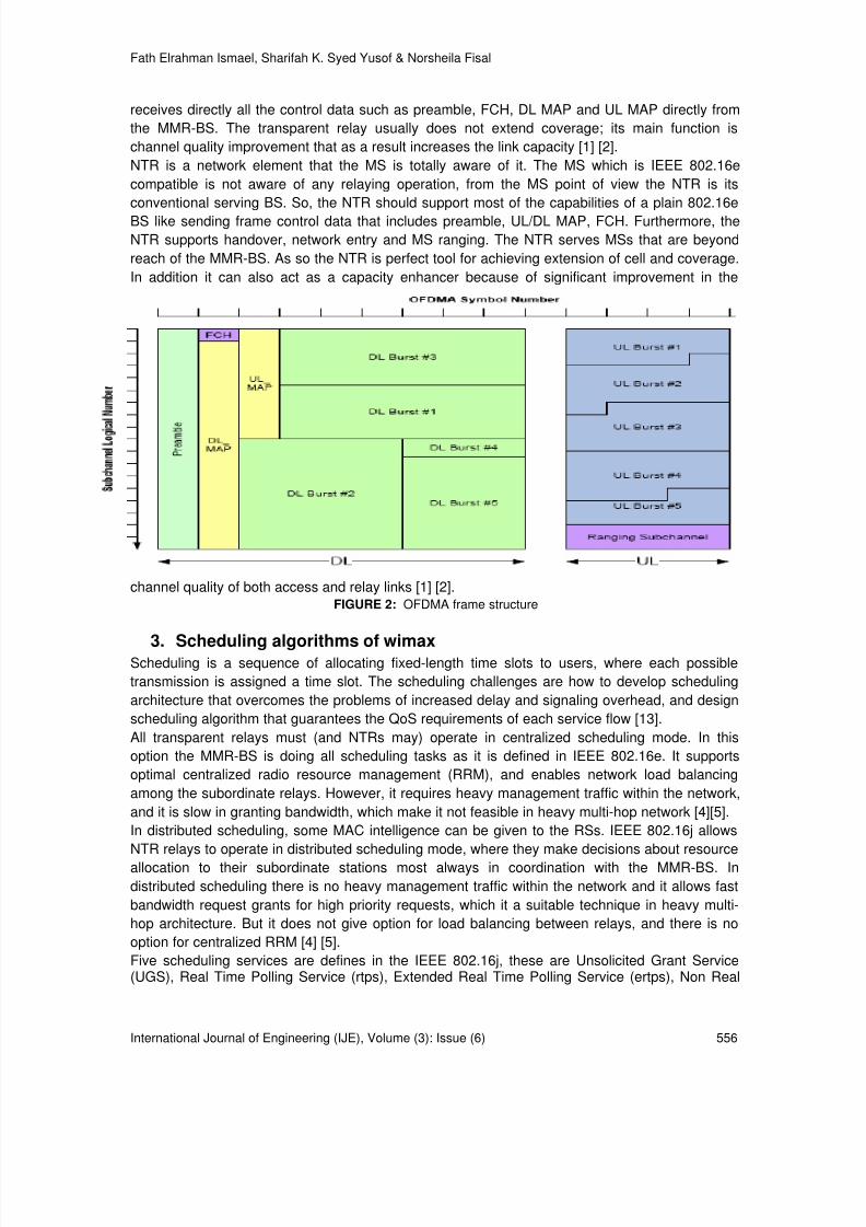
8/8/2019 International Journal of Engineering (IJE), Volume (3): Issue (6)
http://slidepdf.com/reader/full/international-journal-of-engineering-ije-volume-3-issue-6 44/164
Fath Elrahman Ismael, Sharifah K. Syed Yusof & Norsheila Fisal
International Journal of Engineering (IJE), Volume (3): Issue (6) 556
receives directly all the control data such as preamble, FCH, DL MAP and UL MAP directly from
the MMR-BS. The transparent relay usually does not extend coverage; its main function is
channel quality improvement that as a result increases the link capacity [1] [2].
NTR is a network element that the MS is totally aware of it. The MS which is IEEE 802.16e
compatible is not aware of any relaying operation, from the MS point of view the NTR is its
conventional serving BS. So, the NTR should support most of the capabilities of a plain 802.16e
BS like sending frame control data that includes preamble, UL/DL MAP, FCH. Furthermore, the
NTR supports handover, network entry and MS ranging. The NTR serves MSs that are beyond
reach of the MMR-BS. As so the NTR is perfect tool for achieving extension of cell and coverage.
In addition it can also act as a capacity enhancer because of significant improvement in the
channel quality of both access and relay links [1] [2].FIGURE 2: OFDMA frame structure
3. Scheduling algorithms of wimaxScheduling is a sequence of allocating fixed-length time slots to users, where each possible
transmission is assigned a time slot. The scheduling challenges are how to develop scheduling
architecture that overcomes the problems of increased delay and signaling overhead, and design
scheduling algorithm that guarantees the QoS requirements of each service flow [13].
All transparent relays must (and NTRs may) operate in centralized scheduling mode. In this
option the MMR-BS is doing all scheduling tasks as it is defined in IEEE 802.16e. It supports
optimal centralized radio resource management (RRM), and enables network load balancing
among the subordinate relays. However, it requires heavy management traffic within the network,
and it is slow in granting bandwidth, which make it not feasible in heavy multi-hop network [4][5].
In distributed scheduling, some MAC intelligence can be given to the RSs. IEEE 802.16j allows
NTR relays to operate in distributed scheduling mode, where they make decisions about resource
allocation to their subordinate stations most always in coordination with the MMR-BS. In
distributed scheduling there is no heavy management traffic within the network and it allows fast
bandwidth request grants for high priority requests, which it a suitable technique in heavy multi-
hop architecture. But it does not give option for load balancing between relays, and there is no
option for centralized RRM [4] [5].
Five scheduling services are defines in the IEEE 802.16j, these are Unsolicited Grant Service(UGS), Real Time Polling Service (rtps), Extended Real Time Polling Service (ertps), Non Real

8/8/2019 International Journal of Engineering (IJE), Volume (3): Issue (6)
http://slidepdf.com/reader/full/international-journal-of-engineering-ije-volume-3-issue-6 45/164
Fath Elrahman Ismael, Sharifah K. Syed Yusof & Norsheila Fisal
International Journal of Engineering (IJE), Volume (3): Issue (6) 557
Time polling Service (nrtps), and Best Effort (BE). The selected network service should allocatesufficient amount of bandwidth in order to actually guarantee network QoS provisioning [17].
4. Problem definition
In WiMAX network when the MS wants to send data, it first sends a bandwidth request message
to the corresponding base station (BS), and then the BS grants the appropriate amount of
bandwidth to the MS based on the uplink scheduling algorithm. In MMR networks, the control
messages used for network entry or bandwidth request are doubled for every RS introduced
between MS and MMR-BS, as shown in FIGURE 3. The main reason of the increasing overhead
and latency is because all service flow management decisions should be made by MMR-BS in
spite of centralized or distributed scheduling. In the centralized scheduling all the functions of
network entry and bandwidth request are performed by the MMR-BS. The signaling messages
received by the RS from the MSs are forwarded to the MMR-BS, which decides and sends a
response messages to the MSs through the intermediate RSs, this process increases the
signaling messages exchanged and the delay. Although in the distributed scheduling the RS have
an ability to respond to the bandwidth request from their subordinate stations, the relay station
requires also a bandwidth request to relay received data to the MMR-BS, which also increase the
signaling overhead and delay. Considering that, a signaling message from one hop to anothercannot be transmitted in one frame’s duration, the delay of control messages transfer from
MMR-BS to the MS will increase significantly due to the multi-hop added.
The increased delay affects the performance of the services offered by the MMR WiMAX,
because in UGS, rtps, and ertps services the lower latency is required as a QoS metric.
Furthermore, even for the BE using TCP as transport protocol, the increased delay increases
Round Trip Time (RTT) which degrades the throughput.
FIGURE 3: Bandwidth request procedure

8/8/2019 International Journal of Engineering (IJE), Volume (3): Issue (6)
http://slidepdf.com/reader/full/international-journal-of-engineering-ije-volume-3-issue-6 46/164
Fath Elrahman Ismael, Sharifah K. Syed Yusof & Norsheila Fisal
International Journal of Engineering (IJE), Volume (3): Issue (6) 558
5. Related works
In the literature there is some works done to reduce the signaling overhead and delay in one hop
WiMAX networks such as IEEE 802.16e.
The authors of [8, 9] suggest bandwidth grant mechanism without bandwidth request to fully
utilize the available bandwidth for the BE traffic. The BE traffic has a lower priority among
services supported by WiMAX; this will result in small amount of bandwidth for this type ofservice. In addition the BE uses contention based bandwidth request, in which BE connections
contend limited number of shared slots for sending their request, and if there is more than one SS
attempts to send their requests via a slot, the requested are corrupted.
In this scheme, the BS allocate bandwidth to the SSs without bandwidth request, the amount of
granted bandwidth is determined from the current sending rate, this scheme is suitable for large
scale network. On the other hand, it may waste the bandwidth when the sending rate is highly
fluctuated, and it’s hard to estimate the required bandwidth accurately.
In the downlink TCP flow, the standard bandwidth request- grant mechanism in single hop
networks introduces much delay to transmit uplink TCP acknowledgement, which increase the
Round Trip Time (RTT) and causes unnecessary retransmission that reduce the TCP trafficperformance. The authors of [11] introduce new bandwidth scheme that simultaneously allocate
bandwidth for both downlink TCP data and uplink TCP acknowledgement.
In the uplink TCP traffic, since the BS controls the uplink transmission and the MS needs to get
permission before transmission, these steps severely limit the performance of the TCP by
introducing much delay and degrade the throughput. The authors of [12] propose scheme
allocating uplink bandwidth in advance. When the BS receive acknowledgement to be sent to the
MS, it relays the TCP ACK and at the same time allocate bandwidth for the uplink TCP data
packet without bandwidth request from the SS. These schemes for bidirectional bandwidth
allocation require more information about the actual SS needs to not waste the bandwidth.
For MMR networks there are a little work done to reduce the signaling overhead and delay. In [6]
MSs send their bandwidth request to their super ordinate RS at their respective polling intervals.
The RS collects all bandwidth requests from MSs and generates an aggregated bandwidth
request to the MMR-BS. The MMR-BS, instead of allocating the bandwidth to the MSs directly, it
grants bandwidth to the intermediate RS, which then allocates bandwidth to individual MSs. This
scheme decreases the signaling overhead, but not decreases the delay.
The authors of [7], has defined an operation called concatenation, whereby multiple packet data
units (MPDUs) can be concatenated into a single transmission burst in either uplink or downlink
directions, regardless whether these MPDUs belong to the same connection or not. Also multiple
service data units (MSDUs) belong to the same connection can be aggregated to form one
MPDU. These schemes reduce the signaling overhead but there is still much delay.
In [10], the authors propose Extra Resource Reservation (ERR) scheme in which the MMR-BS
pre-allocate some resources to the RSs for purpose of transporting control messages or data
traffic. So the RS can admit its MSs without MMR-BS notification. This scheme can reduce thedelay but it wastes the channel resources if the ERR is used ineffectively in the RS.
Grey theory has been widely applied to many disciplines such as economics, sociology,
engineering, and so forth. The authors of [14] use the grey prediction to estimate the demand
value of the electricity on line. In [15] it is used for internet access forecasting.

8/8/2019 International Journal of Engineering (IJE), Volume (3): Issue (6)
http://slidepdf.com/reader/full/international-journal-of-engineering-ije-volume-3-issue-6 47/164
Fath Elrahman Ismael, Sharifah K. Syed Yusof & Norsheila Fisal
International Journal of Engineering (IJE), Volume (3): Issue (6) 559
6. The proposed scheduling algorithm
The IEEE 802.16j support tree architecture in which all the traffic go through the MMR-BS, so it
should be managed in a centralized manner. But to reduce the signaling overhead and delay its
better to distribute the management of the bandwidth request in the access RS. So, our scheme
manages the relay links centrally in the MMR-BS, and the bandwidth request for the end users
distributed in the RS to take the advantages of both scheduling architectures.The aims of the proposed scheduling scheme are to fully utilize the available bandwidth, and
effectively respond to the demand changes of the subordinate Relay Stations.
In the proposed scheduling architecture in FIGURE 4, the MMR-BS manages its subordinate RSs
as one hop stations. The same procedure is applied in the intermediate RS in the case of more
than two hops, and in the access RS the conventional bandwidth request can be deployed.
FIGURE 4: Proposed Scheduling Architecture
In this scheme the bandwidth request is not needed, instead MMR-BS measures the existing
sending rate of its subordinate RSs, estimates the future demand of each RS using Greyprediction algorithm and grants them a suitable bandwidth without request.
Grey prediction theory [14] aims to find the optimized system parameters of a Grey differential
equation such that the dynamic behavior of the traffic demand could be best fitted with the
differential equation.
One of the major advantages of Grey prediction theory is that only small amounts of data are
needed to describe the demand behavior and reveal the continuous changing in the required
bandwidth.
7. The grey prediction algorithm
The grey prediction algorithm is used in the proposed scheme to estimate the required bandwidth
of each RS from the previous values. In this paper, the GM (1, 1) model is adopted to perform the
prediction of the required bandwidth for each RS. The standard procedure is as follows:
Step 1: Collecting the original data sequence, those are at least four consequence values of the
measured traffic for the RS that is used in the estimation process.
{ } )1(4)(.),........2(),1()0()0()0()0(
≥= mm x x x x Step 2: Calculating an accumulated generation operation, AGO, on the original data sequence in
order to diminish the effect of data uncertainty.

8/8/2019 International Journal of Engineering (IJE), Volume (3): Issue (6)
http://slidepdf.com/reader/full/international-journal-of-engineering-ije-volume-3-issue-6 48/164
Fath Elrahman Ismael, Sharifah K. Syed Yusof & Norsheila Fisal
International Journal of Engineering (IJE), Volume (3): Issue (6) 560
)2(,......,2,1)()()0(
1
)1( mk i xk xk
i
== ∑=
Step 3: Establishing Grey differential equation and then calculating its background values: First
we define z (1) as the sequence obtained by the MEAN operation to x (1) as:
mk for
k xk xk z
,...3,2
)3()1()1()(*)()1()1()1(
=
−−+= α α
Secondly Grey differential equation can be obtained the as follow:
)4()()()1()0(
bk azk x =+
Where the parameters a, b are called the development coefficient and the grey input,
respectively. The equation (5) is called the whitening equation corresponding to the grey
differential equation.
)5()1(
)1(
baxdt
dx=+
Step 4: calculate the value of a, b by means of the least square method.
)6()(
1 N T T
x B B Bb
a−
=
Where
)7(
1)(
.
.
.
1)3(
1)2(
)1(
)1(
)1(
−
−
−
=
m z
z
z
B
And [ ] )8()()...3()2()0()0()0( T N m x x x x =
Step 5: Deriving the solution to the Grey difference equation:
)9()1()1(ˆ )()0()1(
a
be
a
b xk x
k a+
−=+
−
Where the parameter (k) is the forecasting step size and the up script “^” means the value x̂ is a
forecasting value of traffic demand.
Step 6: conducting the inverse accumulated generation operation (IAGO) on)1(ˆ x to obtain a
prediction value as follow:
nK
k xk xk x
,......,3,2
)10()1(ˆ)(ˆ)(ˆ )1()1()0(
=
−−=
Combining the equations (9) and (10) gives the predicted value of the traffic demand as stated in
(11)
)11()1()1()(ˆ )1()0()0( −−
−−=
k aae
a
b xek x
Step 7: The parameters are changed and the accuracy of the estimated value is calculated using
the formula:

8/8/2019 International Journal of Engineering (IJE), Volume (3): Issue (6)
http://slidepdf.com/reader/full/international-journal-of-engineering-ije-volume-3-issue-6 49/164
Fath Elrahman Ismael, Sharifah K. Syed Yusof & Norsheila Fisal
International Journal of Engineering (IJE), Volume (3): Issue (6) 561
nK
k x
k xk xk e
i
ii
<=
−= )12(%100*
)(ˆ
)()(ˆ)(
)0(
)0()0(
The average error percentage can be calculated as below:
65,4
)13(%100*)1(*)(
1 1
4
or m
k emn
en
k
=
+−
= ∑−
=
The accuracy of the traffic demand prediction can be given by:
)14(%100*)1( e−=ε
8. Performance evaluation
In the Grey prediction, the parameter settings are highly relevant to accuracy of prediction. To
get more accurate predicted value, there are three parameters should be optimized, these are:
the number of modeling points , those are the previous values used in the estimation (m), the
parameterα
used to construct the matrix z in equation (3), and the time difference betweensuccessive estimations or the number of estimated values in a given time (n).
To evaluate the Grey prediction algorithm, we write a MATLAB program, in which the traffic
sequence is generated using random function that generates traffic between 10 Kbps and 40
Kbps. Initially we begin with minimum values, in this case it’s taken as 10 Kbps for all modeling
points, then after each cycle we shift the old values left and insert the actual measured traffic
value, and so after m cycles all the modeling points should be replaced by the actual traffic
values.
In the simulation program we use the equations from (1) to (11) to estimate the next traffic value
and then we used the equations from (12) to (14) to calculate the accuracy and the error
percentage
We changed the time difference between the successive samples, the modeling points, and the
parameter α to select the suitable values of these parameters that give best estimation accuracy.Our experimental results shows that the optimal parameters settings of the Grey prediction are
that it is better to take the sampling time as short as possible or n maximum, the Modeling points
maximum (m=6), and the Parameter α=0.5. The selection of this parameters give an accuracy of
(ε=97.8992 %) and error of (e=2.1008 %).
The optimum parameters of Grey prediction are chosen to give the highest accuracy and then we
plot the FIGURE 5 for the increasing traffic and the decreasing one.

8/8/2019 International Journal of Engineering (IJE), Volume (3): Issue (6)
http://slidepdf.com/reader/full/international-journal-of-engineering-ije-volume-3-issue-6 50/164
Fath Elrahman Ismael, Sharifah K. Syed Yusof & Norsheila Fisal
International Journal of Engineering (IJE), Volume (3): Issue (6) 562
0 5 10 15 20 25 30 35 40 45 505
10
15
20
25
30
35
Sampling Instance
T r a f f i c i n
K b p s
Original Traffic
Predicted Traffic
FIGURE 5: Predicted RS traffic using Grey prediction algorithm
The gained prediction accuracy makes the deployment of our scheduling algorithm to overcome
the effects of the delay in MMR networks applicable. To evaluate the performance of theproposed scheduling algorithm, we assume that the RS uses the next frame to relay the data
received in the current frame and there are no errors in the transmission, and the frame duration
is τ =10 ms, and the number of hops is n<=10. The delay associated a data packet a cross n
hops with a conventional bandwidth request scheme given by:
)15(**4 n D τ =
The delay for n hops using our proposed scheduling architecture can be given by:
)16(*)1(*4 τ τ −+= n D FIGURE 6 indicates that, as the number of hops increased the delay rapidly increased in the
conventional bandwidth allocation (CBR) scheme, but in our enhanced bandwidth allocation
(EBA) scheme it increased slightly. This figure shows that our algorithm can be more useful to
reduce the signaling overhead and the delay when the number of hops is high.
FIGURE 6: Delay in MMR network
9. Conclusion
In this paper we have presented an efficient bandwidth demand estimation to estimate the
required bandwidth of the RS in IEEE 802.16j using the Grey prediction algorithm. The high
accuracy offered by Grey prediction algorithm make the use of hybrid centralized and distributed
0 10 20 30 40 50 6010
15
20
25
30
35
40
Sampling Instance
T r a f f i c
i n K b p s
Original Traffic
Predicted Traffic

8/8/2019 International Journal of Engineering (IJE), Volume (3): Issue (6)
http://slidepdf.com/reader/full/international-journal-of-engineering-ije-volume-3-issue-6 51/164
Fath Elrahman Ismael, Sharifah K. Syed Yusof & Norsheila Fisal
International Journal of Engineering (IJE), Volume (3): Issue (6) 563
scheduling architecture applicable solution of the increased signaling overhead and delay in
IEEE 802.16j MMR WiMAX networks.
In this scheme, the MMR-BS allocates bandwidth to its direct subordinate station without
bandwidth request. Using this scheduling architecture, each RS can admit its subordinate SSs
the required bandwidth without notification to the MMR-BS. Our scheme can reduce the delay in
MMR WiMAX networks significantly.
10. References
1. Steven W. Peters and Robert W. Heath, “The future of WiMAX: Multihop relaying with IEEE802.16j”, IEEE communication magazine, January 2009.
2. Vasken Genc, Sean Murphy, Yang Yu, and John Murphy, “IEEE 802.16j Relay BasedWireless Access Networks: An overview”, IEEE wireless communications, October 2008.
3. Bharathi Upase, and Mythri Hunukumbure, “Dimensioning and cost analysis of Multihop relayenabled WiMAX networks”, FUJITSU Sci. Tech. J., 44, 3, p.303-317(July 2008).
4. Masato Okuda, Chenxi Zhu, and Dorin Viorel, “Multihop relay extension for WiMAX Networksoverview and benefits of IEEE 802.16j standard”, Fujtsu Sci. Tech. J., 44, 3, p.292-302(July2008).
5. REWIND project, " D4.1: Summary of Network Architecture Analysis and Selected Network
Architecture”, December 2008.6. Chun Nie, Thanasis Korakis, and Shivendra Panwar, “ A Multihop polling service withbandwidth request aggregation in IEEE 802.16j networks”, 978-1- 4244-1645-5/08/2008IEEE.
7. Zhifeng Tao, Koon Hoo Teo, and Jinyun Zhang,” Aggregation and Concatenation in IEEE802.16j Mobile Multihop Relay (MMR) networks”, 1-4244-0957-8/07, 2007 IEEE.
8. Seungwoon Kim, Minwook Lee, and Ikjun Yeom, “ Impact of bandwidth request schemes forBest Effort traffic in IEEE 802.16 networks”, Science Direct, Computer Communications 32(2009) 235-245.
9. Seungwoon Kim, and Ikjun Yeom, “TCP aware uplink scheduling for IEEE 802.16”, IEEEcommunication letters (February) (2) (2007) 146-148.
10. Junkai Zhang, Suili Feng, We Ye, and Hongcheng Zhung,” Reducing signaling overhead andlatency of 802.16j service flow management”, 978-1-4244-2108-4/08, 2008 IEEE
11. Eun Chan Park, Jae Young Kim, Hwangnam Kim, and Han Seok Kim, “Bidirectional
bandwidth allocation for TCP performance enhancement in IEEE 802.16 broadband wirelessaccess networks”, WiBro system Lab, Telecommunication and networking devision,Samsung Electronics Co., LTD, Korea.
12. Noureddine Lasfar, Jeonghoon Mo, and Byongkwon Moon, “ TCP ACK Triggered bandwidthrequest scheme in IEEE 802.16e systems”, School of Engineering, Information andCommunications University, Korea.
13. Carlos G. Bilich, “TCP over WiMAX Networks”, Wireless Access networks project number II,University of Trento, Trento, TN 38100 italy.
14. Albert W.L. Yao, S.C. Chi, “Analysis and design of a Taguchi–Grey based electricity demandpredictor for energy management systems”, Elsevier, Energy Conversion and Management45 (2004) 1205–1217.
15. Wann-Yih Wu, Shuo-Pei Chen, “A prediction method using the grey model GMC(1,n)combined with the grey relational analysis: a case study on Internet access population
forecast”, Elsevier, Applied Mathematics and Computation 169 (2005) 198–217.16. Sachin Shetty, Ying Tang & William Collani, “A Cross-Layer Packet Loss Identification
Scheme to Improve TCP Veno Performance”, International Journal of Computer Networks(IJCN), Volume (1): Issue (1), November 2009.
17. Qiang Duan, Enyue Lu, “Network Service Description and Discovery for the Next GenerationInternet”, International Journal of Computer Networks (IJCN), Volume (1): Issue (1),November 2009.

8/8/2019 International Journal of Engineering (IJE), Volume (3): Issue (6)
http://slidepdf.com/reader/full/international-journal-of-engineering-ije-volume-3-issue-6 52/164
Fath Elrahman Ismael, Sharifah K. Syed Yusof & Norsheila Fisal
International Journal of Engineering (IJE), Volume (3): Issue (6) 564
18. Syed S. Rizvi, Aasia Riasat, & Khaled M. Elleithy, “Deterministic Formulization of End-to-EndDelay and Bandwidth Efficiency for Multicast Systems”, International Journal of ComputerNetworks (IJCN), Volume (1): Issue (1), November 2009.

8/8/2019 International Journal of Engineering (IJE), Volume (3): Issue (6)
http://slidepdf.com/reader/full/international-journal-of-engineering-ije-volume-3-issue-6 53/164
Vahid. K. Alilou & Mohammad. Teshnehlab.
International Journal of Engineering (IJE), Volume (3) : Issue (6) 565
Prediction of 28-day compressive strength of concrete on thethird day using artificial neural networks
Vahid. K. Alilou [email protected] of Computer Engineering Science and Research Branch, Islamic Azad University, Tehran, Iran Khvoy, 58197-38131, IRAN
Mohammad. Teshnehlab [email protected] of Electronic Engineering K.N. Toosi University of Technology, Tehran, Iran Tehran, IRAN
Abstract
In recent decades, artificial neural networks are known as intelligent methods formodeling of behavior of physical phenomena. In this paper, implementation of anartificial neural network has been developed for prediction of compressivestrength of concrete. A MISO (Multi Input Single Output) adaptive system hasbeen introduced which can model the proposed phenomenon. The data hasbeen collected by experimenting on concrete samples and then the neuralnetwork has been trained using these data. From among 432 specimens, 300data sample has been used for train, 66 data sample for validation and 66 datasample for the final test of the network. The 3-day strength parameter of concretein the introduced structure also has been used as an important index forpredicting the 28-day strength of the concrete. The simulations in this paper are
based on real data obtained from concrete samples which indicate the validity ofthe proposed tool.
Keywords: Concrete, Strength, Prediction, Artificial, Neural Networks.
1. INTRODUCTION
Different sciences are developing fast in today's world. In recent decades, man has seenincreased relationship of sciences in different fields and the more relationship has led to theappearance of the more new knowledge and technology. Nowadays, one of the most importantproblems of man are technical and engineering problems. The complexity of the most of the
problems in this field has made the experts of this field use the new mathematical and modelingmethods for solving this type of problems. Intelligent systems can be used as suitable tools foridentifying complex systems, due to their ability of learning and adaptation.One of the complex problems in our world is the problem of the concrete. The main criterion forevaluating the compressive strength of concrete is the strength of the concrete on 28
thday. The
concrete sample is tested after 28 days and the result of this test is considered as a criterion forquality and rigidity of that concrete.

8/8/2019 International Journal of Engineering (IJE), Volume (3): Issue (6)
http://slidepdf.com/reader/full/international-journal-of-engineering-ije-volume-3-issue-6 54/164
Vahid. K. Alilou & Mohammad. Teshnehlab.
International Journal of Engineering (IJE), Volume (3) : Issue (6) 566
Concrete is the most widely used structural material in constructions in the world. Massiveconcreting in huge civil projects like dams, power plants, bridges and etc… usually is notpracticable and it is necessary to be performed in several layers and the compressive strength ofeach layer should not be less than the specified compressive strength. Therefore one should wait28 days to achieve 28-day strength of each layer of concrete. Thereupon if we have n layers ofconcrete we need 28 ×n days to complete the total project. [1]
2. CONCRETE
Concrete is the only major building material that can be delivered to the job site in a plastic state.This unique quality makes concrete desirable as a building material because it can be molded tovirtually any form or shape. Concrete provides a wide latitude in surface textures and colors andcan be used to construct a wide variety of structures, such as highways and streets, bridges,dams, large buildings, airport runways, irrigation structures, breakwaters, piers and docks,sidewalks, silos and farm buildings, homes, and even barges and ships.The two major components of concrete are a cement paste and inert materials. The cement pasteconsists of Portland cement, water, and some air either in the form of naturally entrapped airvoids or minute, intentionally entrained air bubbles. The inert materials are usually composed offine aggregate, which is a material such as sand, and coarse aggregate, which is a material such
as gravel, crushed stone, or slag.When Portland cement is mixed with water, the compounds of the cement react to form acementing medium. In properly mixed concrete, each particle of sand and coarse aggregate iscompletely surrounded and coated by this paste, and all spaces between the particles are filledwith it. As the cement paste sets and hardens, it binds the aggregates into a solid mass.Under normal conditions, concrete grows stronger as it grows older. The chemical reactionsbetween cement and water that cause the paste to harden and bind the aggregates togetherrequire time. The reactions take place very rapidly at first and then more slowly over a long periodof time. [2]
3. CEMENT
Cement is a material that has adhesive and cohesive properties enabling it to bond mineral
fragments into a solid mass. Cement consists of silicates and aluminates of lime made fromlimestone and clay (or shale) which is ground, blended, fused in a kiln and crushed to a powder.Cement chemically combines with water (hydration) to form a hardened mass. The usualhydraulic cement is known as Portland cement because of its resemblance when hardened toPortland stone found near Dorset, England. The name was originated in a patent obtained byJoseph Aspdin of Leeds, England in 1824.Typical Portland cements are mixtures of tricalcium silicate (3CaO • SiO2), tricalcium aluminate(3CaO • Al2O3), and dicalcium silicate (2CaO • SiO2), in varying proportions, together with smallamounts of magnesium and iron compounds. Gypsum is often added to slow the hardeningprocess. [2,3]
4. WATER
The water has two roles in concrete mixture: First is the chemical composition with cement and
perform cement hydration and second is to make the concrete composition fluent and workable.The water which is used to make the concrete is drink water. The impurity of water can haveundesirable effect on concrete strength. [4]
5. AGGREGATES
Since aggregate usually occupies about 75% of the total volume of concrete, its properties have adefinite influence on behavior of hardened concrete. Not only does the strength of the aggregateaffect the strength of the concrete, its properties also greatly affect durability (resistance todeterioration under freeze-thaw cycles). Since aggregate is less expensive than cement it is

8/8/2019 International Journal of Engineering (IJE), Volume (3): Issue (6)
http://slidepdf.com/reader/full/international-journal-of-engineering-ije-volume-3-issue-6 55/164
Vahid. K. Alilou & Mohammad. Teshnehlab.
International Journal of Engineering (IJE), Volume (3) : Issue (6) 567
logical to try to use the largest percentage feasible. Hence aggregates are usually graded by sizeand a proper mix has specified percentages of both fine and coarse aggregates. Fine aggregate(sand) is any material passing through a No. 4 sieve. Coarse aggregate (gravel) is any material oflarger size.Fine aggregate provides the fineness and cohesion of concrete. It is important that fine aggregateshould not contain clay or any chemical pollution. Also, fine aggregate has the role of space fillingbetween coarse aggregates. Coarse aggregate includes: fine gravel, gravel and coarse gravelIn fact coarse aggregate comprises the strongest part of the concrete. It also has reverse effecton the concrete fineness. The more coarse aggregate, the higher is the density and the lower isthe fineness. [3,5]
6. COMPRESSIVE STRENGTH OF CONCRETE
The strength of concrete is controlled by the proportioning of cement, coarse and fine aggregates,water, and various admixtures. The ratio of the water to cement is the chief factor for determiningconcrete strength as shown in figure1. The lower the water-cement ratio, the higher is thecompressive strength. A certain minimum amount of water is necessary for the proper chemicalaction in the hardening of concrete; extra water increases the workability (how easily the concretewill flow) but reduces strength. A measure of the workability is obtained by a slump test.Actual strength of concrete in place in the structure is also greatly affected by quality control
procedures for placement and inspection. The strength of concrete is denoted in the UnitedStates by f ' c which is the compressive strength of test cylinder 6 in. in diameter by 12 in. high
measured on the 28th day after they are made. [3]
42
49
0.4 0.5 0.6 0.70.3
7
14
21
28
35
56
Tensile Strength
C o m p r e s s i v e S t r e n g t h
S t r e n g t h ( N / m m 2
)
Water/Cement Ratio
FIGURE 1: illustration of the effect of water/cement ratio in concrete strength [1]

8/8/2019 International Journal of Engineering (IJE), Volume (3): Issue (6)
http://slidepdf.com/reader/full/international-journal-of-engineering-ije-volume-3-issue-6 56/164
Vahid. K. Alilou & Mohammad. Teshnehlab.
International Journal of Engineering (IJE), Volume (3) : Issue (6) 568
7. CONCRETE SAMPLING
Acceptance of the concrete in the site is performed based on the results of the compressive testsof concrete samples. The concrete samples must be taken from the final consumption place.The purpose of the concrete sampling is to prepare two specimens of concrete which theircompressive tests will be performed after 28 days or in any predetermined day. To predict the 28-day compressive strength of concrete we can also have another sample to be tested earlier than
28 days. [1]
8. CONCRETE MIX DESIGN
The concrete mix design is a process of selecting the suitable ingredients of concrete anddetermining their most optimum proportion which would produce, as economically as possible,concrete that satisfies a certain compressive strength and desired workability. [6]The concrete mix design is based on the principles of
• Workability
• Desired strength and durability of hardened concrete
• Conditions in site, which helps in deciding workability, strength and durabilityrequirements
9. ADAPTIVE SYSTEMS
Adaptability, in essence, is the ability to react in sympathy with disturbances to the environment.A system that exhibits adaptability is said to be adaptive. Biological systems are adaptivesystems; animals, for example, can adapt to changes in their environment through a learningprocess [7]. A generic adaptive system employed in engineering is shown in Figure 2. It consistsof
• set of adjustable parameters (weights) within some filter structure;
• An error calculation block (the difference between the desired response and the output ofthe filter structure);
• A control (learning) algorithm for the adaptation of the weights.The type of learning represented in Figure 2 is so-called supervised learning, since the learning isdirected by the desired response of the system. Here, the goal is to adjust iteratively the free
parameters (weights) of the adaptive system so as to minimize a prescribed cost function in somepredetermined sense. [8]
Σ- +
INPUTSIGNAL
CONTROLALGORITHM
OUTPUT DESIREDSIGNAL
ERROR
ADAPTIVE SYSTEM
STRUCTURE
FIGURE 2: Block diagram of an adaptive system

8/8/2019 International Journal of Engineering (IJE), Volume (3): Issue (6)
http://slidepdf.com/reader/full/international-journal-of-engineering-ije-volume-3-issue-6 57/164
Vahid. K. Alilou & Mohammad. Teshnehlab.
International Journal of Engineering (IJE), Volume (3) : Issue (6) 569
10. ARTIFICIAL NEURAL NETWORKS
Artificial Neural Network (ANN) models have been extensively studied with the aim of achievinghuman-like performance, especially in the field of pattern recognition and system identification.These networks are composed of a number of nonlinear computational elements which operate inparallel and are arranged in a manner reminiscent of biological neural inter-connections.The property that is of primary significance for a neural network is the ability of the network to
learn from its environment, and to improve its performance through learning. The improvement inperformance takes place over time in accordance with some prescribed measure. A neuralnetwork learns about its environment through an interactive process of adjustments applied itssynaptic weights and bias levels. Ideally, the network becomes more knowledgeable about itsenvironment after each iteration of the learning process. [7]
11. CONCRETE STRENGTH PREDICTION
To predict 28-day strength of concrete, It should identify the effective parameters of the concretestrength. The more accurately identified the parameters, the better is the result.The studies in this paper were performed in two phases:
1. Phase one, includes the studies about the concrete and effective factors of the concretecompressive strength and also performing the experiments in the real environment andcollecting data.
2. Phase two, include studies about how to use artificial neural networks to identify thepresented system and to achieve accurate prediction of concrete 28-day compressivestrength. [1]
12. PERFORMING EXPERIMENTS
In this study the ACI method is used to perform experiments. Experiments were performed inAghchay dam in west Azerbaijan in IRAN. The cement used in the experiments was providedfrom Sofiyan cement plant and the aggregates were provided from the natural materials of theAghchay dam site. [1]
13. COLLECTING DATA
There are lots of Parameters affect on compressive strength of concrete. But the most important
parameters were collected in table 1. It is important that the range of each parameter is limiteddue to regarding ACI standard.
TABLE 1: Effective parameters of the compressive strength of the concrete
Row Parameter Unit Range
1 Mix Design - A-L
2 Water/Cement Ratio % 35.0 - 75.0
3 Density ton/m3 2.30 - 2.60
4 Slump mm 70 - 150
5 Air % 1.0 - 7.0
6 Silica fumes gr 0 - 4007 Super-Plasticizer kg 0.0 - 3.5
8 Age day 3, 7, 14, 28, 42
9 Compressive Strength kg/cm2 70.00 - 420.00
The concrete mix design is affected by these factors:Cement, Fine aggregate, Fine gravel, gravel, coarse gravel, air

8/8/2019 International Journal of Engineering (IJE), Volume (3): Issue (6)
http://slidepdf.com/reader/full/international-journal-of-engineering-ije-volume-3-issue-6 58/164
Vahid. K. Alilou & Mohammad. Teshnehlab.
International Journal of Engineering (IJE), Volume (3) : Issue (6) 570
The 1st
to 7th
parameters are determined in the first day. There is a salient point about 8th
parameter (age). As previously mentioned, the concrete age has a direct arithmetic relation withthe concrete strength. The more aged the concrete the higher is the compressive strength. [1]Here is an interesting point so that the 3-day compressive strength of concrete has amathematical relation with the compressive strength of the same concrete in 7
th, 14
th, 28
thand
42th
day. Therefore it can be used as an important parameter for prediction of this system. Inother words, the 3-day compressive strength of concrete is a very good criterion to achieve the28-day compressive strength.It is conceived from figure.3 that the higher the 3-day compressive strength the higher is the 28-day compressive strength of the concrete. Figure.4 shows the relationship between 3-daycompressive strength and 28-day compressive strength for 4 types of concrete with variable w/cratios, this relation is linear relatively.
281 3 7 14
7.50
15.00
22.50
30.00
37.50
45.00
52.50
60.00
0.40
0.50
0.600.70
7.50
15.00
22.50
30.00
37.50
45.00
52.50
60.00
w/c
C o m p r e s s i v e S t r e n g t h ( N / m m 2 )
Concrete Age ( day ) FIGURE 3: illustration of relationship between age and compressive strength of concrete [1]
0
10
20
30
40
50
60
10 20 30 40
2 8 - D a y C o m p r e s s i v e S t r e n g t h
3-Day Compressive Strength
FIGURE 4: illustration of relationship between 3-day and 28-day strength of concrete [1]
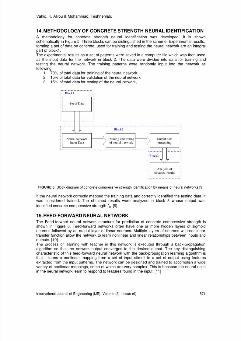
8/8/2019 International Journal of Engineering (IJE), Volume (3): Issue (6)
http://slidepdf.com/reader/full/international-journal-of-engineering-ije-volume-3-issue-6 59/164
Vahid. K. Alilou & Mohammad. Teshnehlab.
International Journal of Engineering (IJE), Volume (3) : Issue (6) 571
14. METHODOLOGY OF CONCRETE STRENGTH NEURAL IDENTIFICATION
A methodology for concrete strength neural identification was developed. It is shownschematically in Figure 5. Three blocks can be distinguished in the scheme. Experimental results,forming a set of data on concrete, used for training and testing the neural network are an integralpart of block1.The experimental results as a set of patterns were saved in a computer file which was then used
as the input data for the network in block 2. The data were divided into data for training andtesting the neural network. The training patterns were randomly input into the network asfollowing:
1. 70% of total data for training of the neural network2. 15% of total data for validation of the neural network3. 15% of total data for testing of the neural network,
Set of Data
Neural Network Input Data
Training and testingof neural network
Output data
processing
Analysis of
obtained results
Block1
Block2
Block3
FIGURE 5: Block diagram of concrete compressive strength identification by means of neural networks [9]
If the neural network correctly mapped the training data and correctly identified the testing data, itwas considered trained. The obtained results were analyzed in block 3 whose output was
identified concrete compressive strength f ' c . [9]
15. FEED-FORWARD NEURAL NETWORK
The Feed-forward neural network structure for prediction of concrete compressive strength isshown in Figure 6. Feed-forward networks often have one or more hidden layers of sigmoidneurons followed by an output layer of linear neurons. Multiple layers of neurons with nonlineartransfer function allow the network to learn nonlinear and linear relationships between inputs and
outputs. [10]The process of learning with teacher in this network is executed through a back-propagationalgorithm so that the network output converges to the desired output. The key distinguishingcharacteristic of this feed-forward neural network with the back-propagation learning algorithm isthat it forms a nonlinear mapping from a set of input stimuli to a set of output using featuresextracted from the input patterns. The network can be designed and trained to accomplish a widevariety of nonlinear mappings, some of which are very complex. This is because the neural unitsin the neural network learn to respond to features found in the input. [11]

8/8/2019 International Journal of Engineering (IJE), Volume (3): Issue (6)
http://slidepdf.com/reader/full/international-journal-of-engineering-ije-volume-3-issue-6 60/164
Vahid. K. Alilou & Mohammad. Teshnehlab.
International Journal of Engineering (IJE), Volume (3) : Issue (6) 572
The number of input and output units is determined by dimensions of the data set whereas thenumber of hidden layer (M) is a free parameter which is adjusted to achieve the maximumperformance. Note that, M determines the degree of freedom of the system. Therefore we expectthat there was an optimum value for M. The criterion to achieve the optimum M is defined as:"The smallest M which causes minimum mse while the maximum error is small"
Fnet
1
1
Neuron 1
1
o 1
1
w1
1
Fnet
1
2
Neuron 1
2
o 2
1
w2
1
Fnet1
Neuron1
n
on
1
w1
1
. .
.
x o1
1
. . .
x2
x3
x
x0 1=
n1
n1
o0
1
1=
Fnet 2
1
Neuron 21
o12
w1
2
Mix Design
Fineness
Air
Admixture
3-Day Strength
4
x1
x5
28-Day Strength
FIGURE 6: Diagram of the feed-forward neural network used for concrete compressive strength prediction
Figure.7 shows the mean squared error of the network output for validation and test data with 10iterations for each number of hidden neurons. Figure.8 shows the maximum error betweendesired outputs and the network outputs with 10 iterations for each number of hidden neurons.The optimum value in this structure is to choose M=11 for the number of hidden neurons.In order to backpropagage the error and update the network weights, Gradient-Descent, Quasi-Newton, Conjugate-Gradient and Levenberg-Marquardt Algorithms were used.
• Gradient Descent k gk W k W κ α −=+ )()1(
• Quasi Newton K K g H k W k W 1
)()1(−
−=+
• Conjugate Gradientκ κ
α W gk W k W k ∆+−=++1)()1(
Where W is the weight matrix, α is the learning rate, g is the gradient of error and H is the hessianmatrix of the cost function. [12]The levenberg-marquardt algorithm is like quasi-newton but it doesn't need to calculate hessianmatrix where it can be estimated as follows:
J J H T
= , e J E T
=∇
E I H k W k W ∇+−=+− .][)()1( 1
µ

8/8/2019 International Journal of Engineering (IJE), Volume (3): Issue (6)
http://slidepdf.com/reader/full/international-journal-of-engineering-ije-volume-3-issue-6 61/164
Vahid. K. Alilou & Mohammad. Teshnehlab.
International Journal of Engineering (IJE), Volume (3) : Issue (6) 573
0 1 2 3 4 5 6 7 8 9 10 11 12 13 14 15 16 17 18 19 200
0.5
1
1.5
2
2.5
3
3.5
4
4.5
FIGURE 7: Diagram of mean squared error of the network output with 10 iterations for certain number of
neurons
0 1 2 3 4 5 6 7 8 9 10 11 12 13 14 15 16 17 18 19 200
1
2
3
4
5
6
7
8
9
10
FIGURE 8: Diagram of maximum error of the network output with 10 iterations for certain number of neurons
The results of above algorithms have been collected in Table 2. Each row of the table is the resultof average 40 iterations of each method. Evaluation criterion of adaptive systems was defined asfollowing formula:
%T
e
N APE or centageErr AveragePer
N
i i
i 100*1
:1
∑=
=
Where T i is the desired output and e i is the output error. [13]
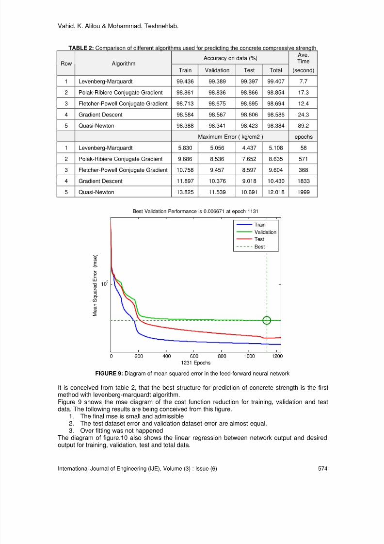
8/8/2019 International Journal of Engineering (IJE), Volume (3): Issue (6)
http://slidepdf.com/reader/full/international-journal-of-engineering-ije-volume-3-issue-6 62/164
Vahid. K. Alilou & Mohammad. Teshnehlab.
International Journal of Engineering (IJE), Volume (3) : Issue (6) 574
TABLE 2: Comparison of different algorithms used for predicting the concrete compressive strength
Accuracy on data (%)Ave.TimeRow Algorithm
Train Validation Test Total (second)
1 Levenberg-Marquardt 99.436 99.389 99.397 99.407 7.7
2 Polak-Ribiere Conjugate Gradient 98.861 98.836 98.866 98.854 17.33 Fletcher-Powell Conjugate Gradient 98.713 98.675 98.695 98.694 12.4
4 Gradient Descent 98.584 98.567 98.606 98.586 24.3
5 Quasi-Newton 98.388 98.341 98.423 98.384 89.2
Maximum Error ( kg/cm2 ) epochs
1 Levenberg-Marquardt 5.830 5.056 4.437 5.108 58
2 Polak-Ribiere Conjugate Gradient 9.686 8.536 7.652 8.635 571
3 Fletcher-Powell Conjugate Gradient 10.758 9.457 8.597 9.604 368
4 Gradient Descent 11.897 10.376 9.018 10.430 1833
5 Quasi-Newton 13.825 11.539 10.691 12.018 1999
0 200 400 600 800 1000 1200
10
0
Best Validation Performance is 0.006671 at epoch 1131
M e a n S q u a r e d E r r o r ( m s e )
1231 Epochs
Train
Validation
Test
Best
FIGURE 9: Diagram of mean squared error in the feed-forward neural network
It is conceived from table 2, that the best structure for prediction of concrete strength is the firstmethod with levenberg-marquardt algorithm.Figure 9 shows the mse diagram of the cost function reduction for training, validation and testdata. The following results are being conceived from this figure.
1. The final mse is small and admissible2. The test dataset error and validation dataset error are almost equal.3. Over fitting was not happened
The diagram of figure.10 also shows the linear regression between network output and desiredoutput for training, validation, test and total data.
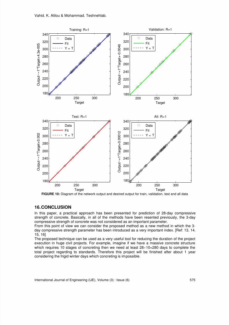
8/8/2019 International Journal of Engineering (IJE), Volume (3): Issue (6)
http://slidepdf.com/reader/full/international-journal-of-engineering-ije-volume-3-issue-6 63/164
Vahid. K. Alilou & Mohammad. Teshnehlab.
International Journal of Engineering (IJE), Volume (3) : Issue (6) 575
200 250 300
180
200
220
240
260
280
300
320
340
Target
O u t p u t ~ = 1 * T a r g e t + 4 . 3 e - 0 0 5
Training: R=1
Data
Fit
Y = T
200 250 300180
200
220
240
260
280
300
320
340
Target
O u t p u t ~ = 1 * T a r g e t +
- 0 . 0
0 4 6
Validation: R=1
Data
Fit
Y = T
200 250 300
180
200
220
240
260
280
300
320
340
Target
O u t p u t ~ = 1 * T a r g e t + 0 . 0
0 2
Test: R=1
Data
Fit
Y = T
200 250 300
180
200
220
240
260
280
300
320
340
Target
O
u t p u t ~ = 1 * T a r g e t + 0 . 0
0 0 1 2
All: R=1
Data
Fit
Y = T
FIGURE 10: Diagram of the network output and desired output for train, validation, test and all data
16. CONCLUSION
In this paper, a practical approach has been presented for prediction of 28-day compressivestrength of concrete. Basically, in all of the methods have been resented previously, the 3-daycompressive strength of concrete was not considered as an important parameter.
From this point of view we can consider the proposed method as a new method in which the 3-day compressive strength parameter has been introduced as a very important index. [Ref: 13, 14,15, 16]The proposed technique can be used as a very useful tool for reducing the duration of the projectexecution in huge civil projects. For example, imagine if we have a massive concrete structurewhich requires 10 stages of concreting then we need at least 28×10=280 days to complete thetotal project regarding to standards. Therefore this project will be finished after about 1 yearconsidering the frigid winter days which concreting is impossible.

8/8/2019 International Journal of Engineering (IJE), Volume (3): Issue (6)
http://slidepdf.com/reader/full/international-journal-of-engineering-ije-volume-3-issue-6 64/164
Vahid. K. Alilou & Mohammad. Teshnehlab.
International Journal of Engineering (IJE), Volume (3) : Issue (6) 576
Using the proposed tool we can have a precise prediction of the 28-day compressive strength ofthe concrete on the third day. Thereupon we need 3×10=30 days to complete this project and this
is an important progress in order to reducing the duration of the civil projects execution.
17. REFERENCES
1. V. K. Alilou. “Designing a learning machine for prediction of the compressive strength of the concrete by using Artificial neural networks” . M.sc Thesis, Science and Research Branch,Islamic Azad University,Tehran,Iran, August 2009
2. “Microsoft Encarta Encyclopedia”, Microsoft Corporation, (2009)3. Chu Kia Wang, Charles G. Salmon. “Reinforced Concrete Design” , Harper & Row Publishers,
USA, (1979)4. M. Teshnehlab, V. K. Alilou, “Concrete strength prediction using learning machine and neural
networks”. In 2nd
Joint Congress on Fuzzy and Intelligent Systems. Tehran, IRAN, 20085. J.D.Dewar. “Computer Modeling of concrete mixture” , E&FN Spon, LONDON, (1999)6. Rishi. Garge. “Concrete Mix Design using Artificial Neural Network” . M.sc Thesis, Thapar
Institute of Engineering and Technology, June 2003
7. Simon Haykin. “Neural Networks – A Comprehensive Foundation” , Prentice-Hall, (1999)8. Danilo P. Mandic, Jonathon A. Chambers. “Recurrent Neural Networks for Prediction” , John
Willey & Sons Inc., (2001)9. Jerzy Hola, Krzysztof Schabowicz. “Application of Artificial Neural Networks to determine concrete compressive strength based on non-destructive tests” . Journal of civil Engineeringand Management, 11(1):23-32, 2005
10. Howard Demuth, Mark Beale. “Neural Network Toolbox” , Mathworks, (1998)11. Madan M.Gupta, Liang Jin, Noriyasu Homma. “Static and Dynamic Neural Networks” , Wiley-
Interscience, (2003)12. Martin T. Hagan, Howard B. Demuth, Mark Beale. “Neural Network Design” , University of
Colorado Bookstore, (1996)13. Ilker Bekir Topcu, Mustafa Saridemir. “Prediction of compressive strength of concrete
containing fly ash using Artificial Neural Networks and Fuzzy Logic” . ScienceDirect,Computational Materials Science, 41(3):305-311, 2008
14. E. Rasa, H. Ketabchi, M. H. Afshar. “Predicting Density and Compressive Strength of Concrete Cement Paste Containing Silica Fume Using Artificial Neural Networks” . ScientiaIranica, 16(1):32-42, 2009
15. Jong In Kim, Doo Kie Kim. “Application of Neural Networks for Estimation of Concrete Strength” . KSCE Journal of Civil Engineering, 6(4):429-438, 2002
16. Ji Zong Wang, Xi-Juan Wang, Hong-Guang NI. “An Algorithm of Neural Network and Application to Data Processing in Concrete Engineering” . Informatica Institute of Mathematicsand Informatics, 14(1):95-110, 2003

8/8/2019 International Journal of Engineering (IJE), Volume (3): Issue (6)
http://slidepdf.com/reader/full/international-journal-of-engineering-ije-volume-3-issue-6 65/164
G. Bassioni
International Journal of Engineering (IJE), Volume (3) : Issue (6) 577
The influence of cement composition on superplasticizers’
efficiency
Ghada Bassioni [email protected] Engineering Program The Petroleum Institute Abu Dhabi, P. O. Box 2533, United Arab Emirates On leave from Chemistry Department, Faculty of Engineering Ain Shams University Cairo, Egypt
Abstract
Fundamental interactions between polymeric superplasticizers and cement arestudied. Cements with different alite-, belite-, C3A- and C4AF-contents are used.
The use of commercially available superplasticizers like melamine formaldehydesulfite- (MFS) and β-naphthalene sulfonic acid formaldehyde-(NSF) resins isinvestigated. These superplasticizers (industrial products) are characterized bymeans of their molecular weights and polymeric radii, as well as by estimatingthe anionic charge density in water and in the cement filtrate of four CEM Icements. Application data of the eight cement-superplasticizer-combinations(heat flow calorimetry and mini-slump tests) are obtained and the surfacechemistry of the superplasticizers with cement (zeta potentials andsuperplasticizer adsorption on cement) is studied.
Keywords: cement, superplasticizers, adsorption, zeta potential, charge density.
1. INTRODUCTION
The arising request for modern building materials that show better workability and durability canonly be fulfilled by the application of different construction-chemical admixtures. Although somevery good recipes have been developed e.g. for dry mix mortars, problems of compatibilitybetween cement and organic admixtures have arisen. For this reason, the interaction of somesuperplasticizers on cement is studied. The results give some fundamental understanding in howfar the cement industry can reduce the cement production and consequently the CO2-emissionwhich is of high environmental interest.
The relation between the C3A content and naphthalene based-superplasticizers adsorption hasbeen investigated by many researchers. It is clear that a large amount is adsorbed on C 3A ofordinary Portland cement [1]. The adsorption is also determined by the cement fineness [2]. It hasbeen reported that hydration reactivity corresponds to high calcium aluminate contents [3, 4].Generally, a certain amount of anionic superplasticizers are adsorbed on the surface of thecement grain or its hydrated phases to obtain a dispersing effect. The impact of thesesuperplasticizers can be understood considering that polycondensates possess many –SO 3
2--
groups and therefore a high negative charge. The grain surface will be also negatively charged,once these superplasticizers adsorb. Due to the repulsion forces between equal charges, a gooddispersing effect is obtained and reagglomeration is avoided.

8/8/2019 International Journal of Engineering (IJE), Volume (3): Issue (6)
http://slidepdf.com/reader/full/international-journal-of-engineering-ije-volume-3-issue-6 66/164
G. Bassioni
International Journal of Engineering (IJE), Volume (3) : Issue (6) 578
The information about variation in adsorption behavior of polycondensates with the different typesof cements is very important for application to give an indication about the dosages necessaryrelated to the type of cement. In extreme cases, adsorption can be as low as 10 % and noliquefaction of the cement paste is observed. This would confirm the cement “incompatibility” withpolycondensate-superplasticizers and emphasize the need for intensive research in this area.Another important factor for this “incompatibility” can rely on the type and availability (solubility) ofthe sulfate carrier in the cement.
The aim of this research work is to establish fundamental interactions between polymericsuperplasticizers and cement. For this purpose, cements with different alite-, belite-, C3A- andC4AF-contents are used. The use of commercially available superplasticizers like melamineformaldehyde sulfite- (MFS) and a β-naphthalene sulfonic acid formaldehyde-(NSF) resin andfour CEM I (A-D) cements of different chemical composition is investigated. The adsorptionbehavior of the superplasticizer on cement is studied.
2. EXPERIMENTAL
The experiments are performed with aqueous suspensions of the different cements CEM I (A-D).Their medium particle size D 50 is determined by using laser granulometry (Cilas 1064; Co. Cilas).
The densities of these cements are established by a helium pycnometer.
The MFS- and NSF- resins are industrial products and are used without further purification. Thesolid content of the polymeric solutions are established by using an IR-balance. Thecharacterization of the polymers is made by GPC, coupled with a refractive index and lightscattering detector. This equipment permits calculation of molecular weights and radii of thepolymers. Moreover polymer solutions with a concentration of 10 mg / mL (with respect to thepolymeric solid content) are prepared. The solvent used is a 0.1 mol/L NaNO3 solution; pH =12.0; adjusted with NaOH). The column material (Co. Waters) used contained three columnsconsecutively connected (Ultrahydrogel 120, Ultrahydrogel 250, Ultrahydrogel 500). They cover aseparation area of 5,000 – 400,000 Dalton. Each sample is injected with a syringe containing aforwarded spaced filter (0,2 µm) in a 2-mL-GPC-sample holder, out of which the GPC-apparatusinjects 100 µL into the system. Therefore the polymeric solution needed for one run is 1.0 mg.The evaluation is carried out with the GPC-Software Astra 4,908 (Co. Wyatt Technologies). Tocalculate the averaged molecular weights, a 3rd order fit is used.
The anionic charges of the superplasticizers under investigation are measured by means of theparticle charge detector PCD 03 pH (Co. Mütek). 100 mL standard solutions of polymericconcentration of 200 mg/L are used. The filtrates of cement pastes with a w/c-value necessary toproduce a flow value of 18 ± 0.5 cm (mini-slump test) are used as a solvent for the polymers tomeasure the anionic charge in the pore solution. The charge density is determined by means ofa titration experiment with the polymer poly-dadmac (0.001 N), a cationic polyelectrolyte.
Adsorption measurements are carried out at RT by determining the organic carbon content viaHigh TOC II analyser (Elementar) of the centrifugate (20 min at 8500 rpm) previously producedfrom the cement pastes with polymeric admixtures.
The zeta potentials of the cement pastes with different amounts of polymers are measured usingModel DT-1200 electroacustic spectrometer (Dispersion Technology, Inc.). The following mixingprocedure is used to prepare the cement pastes: cement is added to water (according to thenecessary w/c-value) within 1 min. This paste is let sit for one more minute. Then, the mixture isvigorously stirred for 2 min in a casserole by using a spoon. The filtrate is taken for themeasurement of the ionic background of the cement paste that is subtracted from the zetapotential values of the cement pastes containing the polymers.To estimate the flow value, the superplasticizer dosages given in table 6 are poured into themixing water in a porcelain casserole. After cement is added, the resulting paste is poured into a

8/8/2019 International Journal of Engineering (IJE), Volume (3): Issue (6)
http://slidepdf.com/reader/full/international-journal-of-engineering-ije-volume-3-issue-6 67/164
G. Bassioni
International Journal of Engineering (IJE), Volume (3) : Issue (6) 579
VICAT-ring (h = 40 mm, dinner,above = 70 mm, dinner,below = 80 mm). After lifting up the VICAT-ringthe diameter of the paste is determined.
3. RESULTS AND DISCUSSION
3.1 Characterization of the four types of cementThe analysis of the four types of cement is performed by using the Rietveld analysis- method.The results are listed in (table 1).
TABLE 1: Rietveld analysis of the cements CEM I (A-D).
Cement typeMineral Phase
CEM I(A)
CEM I(B)
CEM I(C)
CEM I(D)
Alite 67.3 60.1 69.8 61.0
Belite 10.9 22.4 6.9 22.0
C3A (cub.) 5.7 2.3 1.3 0.4
C3A (orth) 5.6 0.0 4.6 1.1
Na2O 0.27 0.21 0.18 0.27
K2O 0.67 0.63 0.72 1.27
C4AF 1.7 12.2 6.8 14.0
Al2O3 4.47 3.55 3.63 4.15
Fe2O3 1.2 4.56 2.38 2.46
CaSO4*2H2O 0.1 2.5 0.1 1.1
CaSO4 2.5 0.0 2.4 0.0
CaO free 0.3 0.2 1.1 0.3
w/c 0.6 0.46 0.47 0.6
It can be seen that CEM I (C) has the highest alite content, while CEM I (B) & (D) comparablyhave the highest belite content. The highest C3A content, whether cubic or orthorhombic, is foundfor CEM I (A).
3.2 Characterization of the superplasticizersThe solid content determined by an IR-balance is found to be 38.71 % and 8.47 % for MFS- andNSF- resins, respectively. The pH-values of the polymeric solutions differed slightly from oneanother and found to be 8.47 in case of MFS-resin and 7.47 for the NSF-resin.
The GPC- analysis of the MFS-resin is listed in (table 2). Because the NSF-superplasticizer NSF-resin could not be analyzed chromatographically in aqueous medium because of adsorptiveeffects with the column material, a "batch"-measurement is carried out. The polymer samples of
different concentrations are injected directly into the cell of the light scattering detector.Adsorptive Interactions of the polymers with the column are excluded. The "batch"-measurementgave the weight-average molecular weight Mw, the z-average radius of gyration Rgz as well as theQELS (quasi elastic light scattering) – correlation function of the average hydrodynamic radiusRh(avg). Because of the absence of concentration information out of the refractive index detector,no values for Mn, Mz, Rgn, Rgw, Rhn, Rhz and polydispersity are obtained.
The "batch"-analysis via ZIMM-Plot is successful using double extrapolation. The firstextrapolation occurs on the concentration zero. This is necessary to eliminate the intermolecular

8/8/2019 International Journal of Engineering (IJE), Volume (3): Issue (6)
http://slidepdf.com/reader/full/international-journal-of-engineering-ije-volume-3-issue-6 68/164
G. Bassioni
International Journal of Engineering (IJE), Volume (3) : Issue (6) 580
interactions, because the scattered light intensity of a single molecule should be measured. Thesecond extrapolation occurs on the scattering angle zero to eliminate the intramolecularinfluence. In the ZIMM-Plot all measured points are applied and connected to straight lines. Fromthe slope of these straight lines the values of the 2
ndvirial coefficient A2 and the z average radius
of gyration Rgz are obtained. With this information the weight-average molecular weight Mw of theNSF-resin could be deduced (table 3). It is clear that the molecular weights of thepolycondensates are very high. The molecular weights and the polymeric radii lie withinexpectations [5].
TABLE 2: GPC-Analysis of MFS-resin and “batch” - analysis of the NSF-resin. Property MFS – resin NSF – resin
(“Batch”-analysis)
Molecular weight [g/mol] Mn 77670
Molecular weight [g/mol] Mw 109800 193500 (4 %)
Poly-dispersity [Mw/Mn] 1.41
R.M.S. Radius (Rg) [nm] Rgn 12.0
R.M.S. Radius (Rg) [nm] Rgw 13.5
R.M.S. Radius (Rg) [nm] Rgz 16.9 38.7 (8 %)
QELS Hydro dynamic Radius moment [nm] Rhn 7.5
QELS Hydro dynamic Radius moment [nm] Rhw 8.4
QELS Hydro dynamic Radius moment [nm] Rhz 10.7
QELS Hydro dynamic Radius moment [nm]Rh(avg)
5.8
According to the calculated Burchard-Parameter ([Rgz / Rh(avg)] = 2.56) it is found that the MFS-resin in solution lies in form of steady chains.
3.3 Estimation of the specific anionic charge density
The results of the specific anionic charge density measurements are found in figure 1.

8/8/2019 International Journal of Engineering (IJE), Volume (3): Issue (6)
http://slidepdf.com/reader/full/international-journal-of-engineering-ije-volume-3-issue-6 69/164
G. Bassioni
International Journal of Engineering (IJE), Volume (3) : Issue (6) 581
0
500
1000
1500
2000
2500
3000
3500
4000
4500
NSF-resinMFS-resin
C h a r g e d e n s i t y [ 1 0 - 6 e q / g ]
in water
in PW of CEM I (A)
in PW of CEM I (B)
in PW of CEM I (C)
in PW of CEM I (D)
FIGURE 1: Anionic charge densities of the superplasticizers.
As expected, the polycondensates (MFS and NSF) show in salt free water as well as in the porewater of the four cements very high anionic charge densities.
While in water, the anionic charge density of the superplasticizers appear higher than in the
different pore waters of the cements under investigation, due to the fact that pore water containsCa
2+ions which form complexes with the superplasticizers. The two superplasticizers behave
differently depending on the amount of free Ca2+
ions present in the pore solution and the affinityto form complexes with them.
3.4 Liquefying effect of the superplasticizersThe dosage (w.r.t cement) for each superplasticizer is estimated according to that necessary toproduce a flow value of 26 ± 0.5 cm (mini-slump test). The blank value is a cement paste with aw/c-value for which the flow value is 18 ± 0.5 cm. By adding each superplasticizer, the dosage isadjusted so that a flow value of 26 ± 0.5 cm is obtained. The water content in the polymericsolutions is considered.
The dosages necessary to obtain a flow value of 26 ± 0.5 cm are similar for both
polycondensates (table 6). Among all cements CEM I (B) is liquefied the best i.e. with the leastdosage of superplasticizer, the best result is obtained. This is attributed to its low C 3A-content.Comparable behaviour is given by CEM I (A).
The cements CEM I (C) and CEM I (D) need much higher dosages.
TABLE 3: Dosages of the superplasticizers necessary to obtain a flow value of 26 ± 0.5 cm.

8/8/2019 International Journal of Engineering (IJE), Volume (3): Issue (6)
http://slidepdf.com/reader/full/international-journal-of-engineering-ije-volume-3-issue-6 70/164
G. Bassioni
International Journal of Engineering (IJE), Volume (3) : Issue (6) 582
Cement; w/c MFS-resin NSF-resin
CEM I (A); w/c = 0.6 0.15 % 0.15 %
CEM I (B); w/c = 0.46 0.12 % 0.1 %
CEM I (C); w/c = 0.47 0.25 % 0.25 %
CEM I (D); w/c = 0.6 0.25 % 0.25 %
This can be explained by the high sulfate content - especially the rapidly soluble sulfates likearcanite. The free sulfate adsorbs on the surface of cement hydration phases and prevents thesuperplasticizers to adsorb and function as liquefiers [6]. Another reason for the bad compatibilityof the superplasticizer with cement is the free CaO content.
3.5 Estimation of the superplasticizers adsorption on cementFirst, the TOC-content in the pore solution without superplasticizer is estimated as background.Then the superplasticizer dosages listed in table 3 are examined by adsorption measurementsdetermining the TOC-content in the filtrate of non-adsorbed superplasticizer. Subtraction fromstarting dosages leads to the amount adsorbed. The results are shown in figure 2.
0,0
0,2
0,4
0,6
0,81,0
1,2
1,4
1,6
1,8
2,0
2,2
2,4
2,6
2,8
3,0
NSF-resinMFS-resin A d s o r b e d a m o u n
t o f p l a s t i c i z e r [ m g / g c e m e n t ]
CEM I (A)
CEM I (B)
CEM I (C)
CEM I (D)

8/8/2019 International Journal of Engineering (IJE), Volume (3): Issue (6)
http://slidepdf.com/reader/full/international-journal-of-engineering-ije-volume-3-issue-6 71/164
G. Bassioni
International Journal of Engineering (IJE), Volume (3) : Issue (6) 583
0
10
20
30
40
50
60
70
80
90
100
NSF-resin
A d s o r p t i o n [ % ]
CEM I (A)
CEM I (B)
CEM I (C)
CEM I (D)
MFS-resin
FIGURE 2: Adsorbed amount of superplasticizers in mg/g cement (above) and percentadsorption of the superplasticizers (below).
As expected, the C3A-poor cement CEM I (B) adsorbed the least amount of superplasticizers,while CEM I (C) and CEM I (D) adsorbed the most. These results are consistent with the findingabout dependence of adsorbed amount on the formation of ettringite [7]. In accordance with this,the high contents of sulfate and free CaO of CEM I (C) resulted in a high consumption ofsuperplasticizers although it has a moderate C3A-content.
Regarding the adsorbed amount of superplasticizers, the adsorption behaviors of MFS-resin undNSF-resin are very similar. The values of percental adsorption of these products indicated theirlimited function as superplasticizers (bad slump loss – behavior). These superplasticizers aregood for precast concrete, because they show a high starting liquefaction of cement pastes withlow dosages.
3.6 Zeta potential measurements
The zeta potentials are determined first without then with superplasticizer (figure 3) according tothe dosages listed in table 3. The physical data needed to execute such experiments are given inas follows:CEM I (B) - (D) have a density of 3.14 g/ cm
3, while CEM I (A)’s density is 3.12 g/ cm
3. The
particle sizes D50 [µm] of the CEM I (A) – (D) are 7.5, 11.28, 17.49 and 8.81, respectively.
The zeta potential of the cement pastes are -2.6 mV for CEM I (A), -8.3 mV for CEM I (B), -1.9mV for CEM I (C) and -2.8 mV for CEM I (D) without superplasticizers addition (figure 3). Thezeta potentials of the pure cements depend on their C3A-content. Cements with higher C3A- andsulfate contents can form higher amounts of ettringite during the hydratation process which
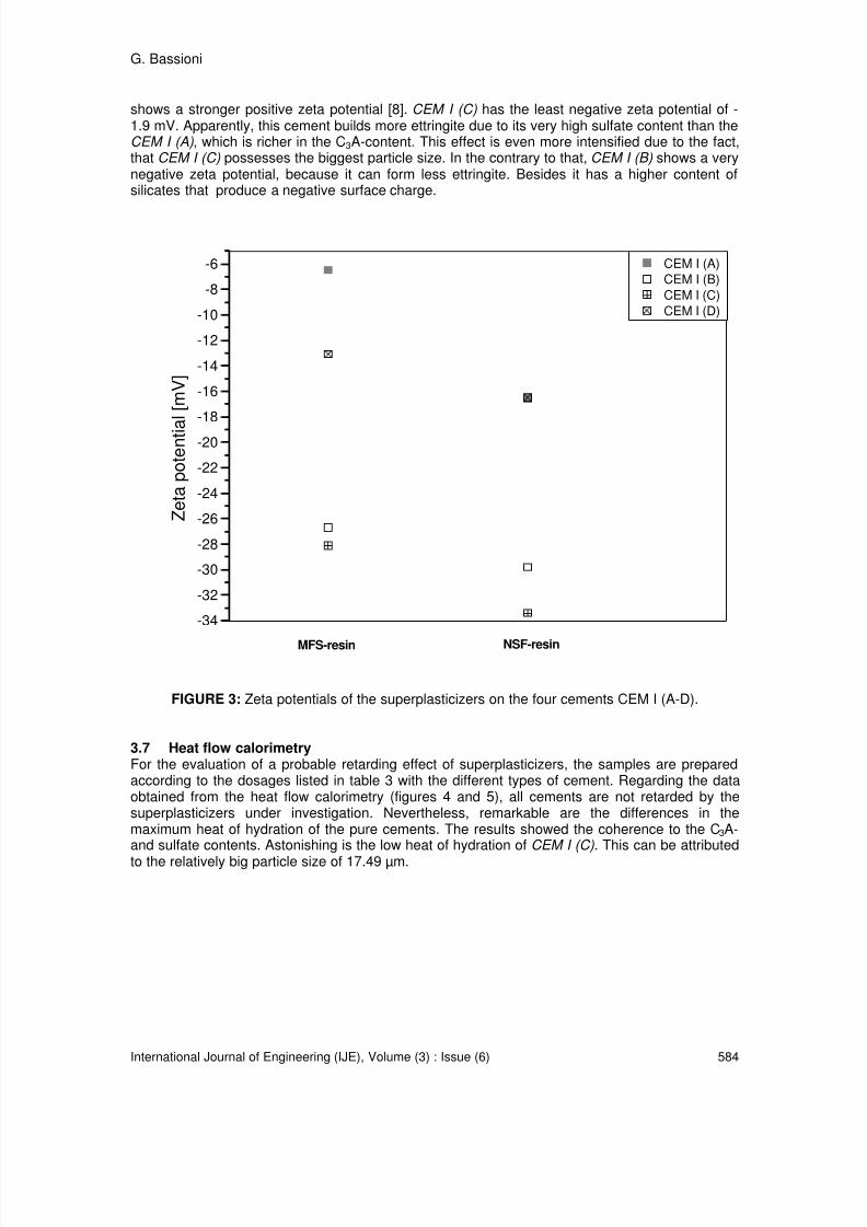
8/8/2019 International Journal of Engineering (IJE), Volume (3): Issue (6)
http://slidepdf.com/reader/full/international-journal-of-engineering-ije-volume-3-issue-6 72/164
G. Bassioni
International Journal of Engineering (IJE), Volume (3) : Issue (6) 584
shows a stronger positive zeta potential [8]. CEM I (C) has the least negative zeta potential of -1.9 mV. Apparently, this cement builds more ettringite due to its very high sulfate content than theCEM I (A), which is richer in the C3A-content. This effect is even more intensified due to the fact,that CEM I (C) possesses the biggest particle size. In the contrary to that, CEM I (B) shows a verynegative zeta potential, because it can form less ettringite. Besides it has a higher content ofsilicates that produce a negative surface charge.
-34
-32
-30
-28
-26
-24
-22
-20
-18
-16
-14
-12
-10
-8
-6
NSF-resinMFS-resin
CEM I (A)
CEM I (B)
CEM I (C)
CEM I (D)
Z e t a p o t e n t i a l [ m V ]
FIGURE 3: Zeta potentials of the superplasticizers on the four cements CEM I (A-D).
3.7 Heat flow calorimetryFor the evaluation of a probable retarding effect of superplasticizers, the samples are preparedaccording to the dosages listed in table 3 with the different types of cement. Regarding the dataobtained from the heat flow calorimetry (figures 4 and 5), all cements are not retarded by thesuperplasticizers under investigation. Nevertheless, remarkable are the differences in themaximum heat of hydration of the pure cements. The results showed the coherence to the C3A-and sulfate contents. Astonishing is the low heat of hydration of CEM I (C). This can be attributed
to the relatively big particle size of 17.49 µm.

8/8/2019 International Journal of Engineering (IJE), Volume (3): Issue (6)
http://slidepdf.com/reader/full/international-journal-of-engineering-ije-volume-3-issue-6 73/164
G. Bassioni
International Journal of Engineering (IJE), Volume (3) : Issue (6) 585
0,0
0,5
1,0
1,5
2,0
2,5
3,0
3,5
4,0
4,5
5,0
0 12 24
Hydratation time [h]
P [ m W / g ]
CEM I (A) CEM I (A) with MFS-resin
CEM I (A) with NSF-resin
0,0
0,5
1,0
1,5
2,0
2,5
3,0
0 12 24
Hydratation time [h]
P [ m W / g ]
CEM I (B) CEM I (B) with MFS-resin
CEM I (B) with NSF-resin
FIGURE 4: Heat flow calorimetry of the superplasticizers with CEM I (A) (above) and CEM I (B)(below).

8/8/2019 International Journal of Engineering (IJE), Volume (3): Issue (6)
http://slidepdf.com/reader/full/international-journal-of-engineering-ije-volume-3-issue-6 74/164
G. Bassioni
International Journal of Engineering (IJE), Volume (3) : Issue (6) 586
0,0
0,5
1,0
1,5
2,0
2,5
0 12 24
Hydratation time [h]
P [ m W / g ]
CEM I (C) CEM I (C) with MFS-resin
CEM I (C) with NSF-resin
0,0
0,5
1,0
1,5
2,0
2,5
3,0
3,5
4,0
0 12 24
Hydratation time [h]
P [ m W / g ]
CEM I (D) CEM I (D) with MFS-resin
CEM I (D) with NSF-resin
FIGURE 5: Heat flow calorimetry of the superplasticizers with CEM I (C) (above) and CEM I (D)(below).

8/8/2019 International Journal of Engineering (IJE), Volume (3): Issue (6)
http://slidepdf.com/reader/full/international-journal-of-engineering-ije-volume-3-issue-6 75/164
G. Bassioni
International Journal of Engineering (IJE), Volume (3) : Issue (6) 587
4. CONSLUSION & FUTURE WORKThe interaction of two superplasticizers with four different types of cement is studied.Characterization of the polycondensates, MFS- and NSF-resins, showed that they have very highmolecular weights. In solution, the MFS-resin lies as a steady chain according to the Burchard-Parameter. The adsorption behavior is affected by the anionic charge of the polymers in waterand in the pore solutions of the four cements: The higher the anionic charge, the better the
adsorption [9]. On the basis of low C3A-content it is observed that CEM I (B) shows the bestliquefying effect. The two cements CEM I (C) and CEM I (D) need higher dosages ofsuperplasticizers to obtain the same result due to their high content of sulfate and free CaO. Theadsorbed amounts of the superplasticizers in mg / g cement correlated with the dosages to obtaina flow value of 26 ± 0.5 cm. The C3A-poor cement CEM I (B) adsorbed in all cases the leastamount of superplasticizer. Regarding the heat flow values, no significant differences areobserved for the cement combinations with superplasticizers. The results give an insight in howfar the cement production (and consequently the CO2 -emission) can be minimized by usingadmixtures which give good workability and compatibility which is of high environmental value.
5. REFERENCES
[1] a) S. Suzu, E. Okada and K. Hattori, “Adsorption of superplasticizers on cement” CAJ Review,
108-110, 1981. b) S. Goyal, M. Kumar, B. Bhattacharjee, “Effect of relative proportion of pozzolana on compressive strength of concrete under different curing conditions ”, Int. J. Eng.,2(1): 20-34, 2008.[2] E. Asakura, H. Yoshida and H. Nakae, “Influence of superplasticizers on fluidity of fresh cement paste with different clinker phase composition” , In Proceedings of 9th Int. Cong.Chemistry of Cement, New Delhi, India, 5: 570-576, 1992.[3] K. Yamada, S. Ogawa and S. Hanehara, “Working Mechanism of Poly-Beta-Naphthalene Sulfonate and Polycarboxylate Superplasticizer Types from Point of Cement Paste Characteristics” , In Proceedings of. 6th CANMET/ACI Int. Conf. on Superplasticizers, Nice,France, 195: 367-382, 2000.[4] a) E. Sakai, J. K. Yamada and A. Ohta, “Molcular Structure and Dispersion-Adsorption Mechansims of Coomb-Type Superplasticizers used in Japan” , J. Adv. Concr. Tech. 1(1): 16-25,2003. b) P. P. Bansal, M. Kumar, S. K. Kaushik “Effect Of Wire Mesh Orientation On Strength Of
Beams Retrofitted Using Ferrocement Jackets ”, Int. J. Eng. 2(1): 8-19, 2008.[5] G. Bassioni, “Global warming and Construction Aspects” , In Proceeding of the 7thInternational Scientific and Practical Conference on Environmental Technology Resources,Rezekne, Latvia, 2: 78-86, 2009.[6] G. Bassioni, J. Plank, “Untersuchungen zur kompetitiven Adsorption anorganischer Anionen am Modellsystem Kalksteinmehl” , GDCh Monographie, 36: 225-232, 2006.[7] J. Plank, G. Bassioni, Z. Dai, H. Keller, B. Sachsenhauser, N. Zouaoui, “Neues zur Wechselwirkung zwischen Zementen und Polycarboxylat-Fließmitteln” , ibausil-Tagungsband, 16:579-598, 2006.[8] a) J. Plank, Ch. Hirsch, "Superplasticizer Adsorption on Synthetic Ettringite" , In Proceedings of7th CANMET/ACI Conference on Superplasticizers in Concrete, Berlin, Germany, 217: 283-298,2003. b) A. Elazhary, Hassan Soliman, “Analytical Investigation of the Flow Hydrodynamics in Micro-Channels at High Zeta Potentials ”, Int. J. Eng., 3(3): 267-279, 2008.[9] J. Plank, G. Bassioni, “Adsorption of Carboxylate on CaCO 3 surface” , Z. Naturforsch. B, 62b:1277-1284, 2007.

8/8/2019 International Journal of Engineering (IJE), Volume (3): Issue (6)
http://slidepdf.com/reader/full/international-journal-of-engineering-ije-volume-3-issue-6 76/164
Fatemeh Hassanipour & Jose L. Lage
International Journal of Engineering (IJE), Volume (3) : Issue(6) 587
The Effect of a Porous Medium on the Flow of a Liquid Vortex
Fatemeh Hassanipour [email protected] of Mechanical Engineering University of Texas at Dallas Richardson, TX 75080, USA
Jose L. LageDepartment of Mechanical Engineering [email protected] Southern Methodist University Dallas, TX 75205, USA
Abstract
This study investigates the predominant criteria in the persistence or decay ofvortex flows in porous media. A simple approach is used to build a pair ofvortices in a fluid. The vortices impinge on a permeable wall, thus allowing astudy of the interaction of vortices with the porous medium. New insights areobtained, among them that permeability has a more important effect on thisinteraction compared with either porosity or the vortex transport velocity.
Keywords: vortex flow, porosity, permeability
1. INTRODUCTION
Modeling and simulation of vortical flow through permeable (porous) media are essential for thedesign of new devices and the prediction of a myriad of natural and man-made processes, suchas metal (alloy) processing, beach erosion, forest fires, snow avalanche, grain storage,underground flow, and alveolar respiration. In forestry, accurate simulation of turbulent air flowthrough the vegetative porous medium can predict the spread of forest fires as well as thespreading of seeds that result in biodiversity. Dispersion of smog in heavily built cities can beaccurately modeled by turbulent flow in porous media. The aerial spreading of hazardoussubstances in a city is similarly modeled, with applications in homeland security. Detection ofbiological and biochemical compounds in permeable fabrics via turbulent air “puffs” is yet anotherapplication. In energy exploration, the flow of oil and gas along a radial-inward path in an oil well
is accelerated by turbulence arising as the flow reaches a more permeable region (the well).
Our study involves vortex flows and porous media, two subject matters that can individually becomplex and interesting on their own. The issue of vortex flow in porous media begins withtransition from laminar flow behavior to turbulence flow. Transition to turbulence in porous mediais among the interesting topics reviewed by Getachew et al [1] who discussed severalexperimental studies related to transition to turbulence in porous media, and by Inoue et al [2].Vortex rings are also used by other investigators to unveil the basic structure of a turbulent round jet by Lau and Fisher [3] and the dynamics of coherent structures in turbulent boundary layers by

8/8/2019 International Journal of Engineering (IJE), Volume (3): Issue (6)
http://slidepdf.com/reader/full/international-journal-of-engineering-ije-volume-3-issue-6 77/164
Fatemeh Hassanipour & Jose L. Lage
International Journal of Engineering (IJE), Volume (3) : Issue(6) 588
Lim [4]. Moreover, Chu and Falco [5] used laminar vortex rings interacting with an inclined,moving wall to reproduce some of the features observed in turbulent boundary layers. In additionto laminar vortex rings, other investigations have studied the entrainment, growth, and turbulenceproduction in turbulent vortex rings to better understand the role of coherent structures inturbulence by Maxworthy [6], Glezer et al. [7] and Olcay et al.[8]. However, the behavior of vortexflow in porous media has not been directly studied.
The interaction of vortex flows and porous media is on the cutting edge of knowledge in fluidmechanics. Vortex flows are inherently nonlinear and are known to display intriguing behaviorwhile interacting with boundary conditions and various flow conditions. Porous media also withtheir various morphologies are a challenging area of ongoing study. When these two subjectareas come together, an even richer set of conditions emerge and, as shown by the analysis inthe sequel, display interesting behaviors.
The current study investigates the transport of large vortical structures through permeableobstructions. The focus on large-scale vortical structures is motivated by their intricate localtransport behavior depending on the characteristics of the permeable obstruction. This study aimsat building a protocol for predicting the behavior of vortical flow based on permeable media andflow characteristics. Numerical simulations demonstrate the effect of permeable media propertiesand vortex strength on the transport of vortex flow in porous medium.
2. MODEL CONFIGURATION
A simplified two-dimensional model is used, shown in Figure 1. The vortex ring generator is apiston–cylinder mechanism located in a 160 x 60 x 60 cm water tank. The cylinder is 50 cm longwith a diameter of 5cm, which is used to produce a finite-duration jet pulse. The jet velocityprogram is trapezoidal to create a vortex flow, Fig 2.
The vortex ring impinges to a 40 x 20 x 20 cm porous medium located within 40 cm in front of it.
Porous media with various morphologies are characterized by the porosity and
permeability .
FIGURE 1: Schematic model configuration
Porous MediaVortex Ring
D=5cm
w=20cm
h=40cm
40cm
L=160cm
P=50cm
Water Tank
H=60cm

8/8/2019 International Journal of Engineering (IJE), Volume (3): Issue (6)
http://slidepdf.com/reader/full/international-journal-of-engineering-ije-volume-3-issue-6 78/164
Fatemeh Hassanipour & Jose L. Lage
International Journal of Engineering (IJE), Volume (3) : Issue(6) 589
The test is repeated with two different velocities of 0.179 and 0.058 . Jet Reynolds number
is calculated based on the piston’s maximum velocity , piston diameter and the fluid
viscosity ( ), namely,
Two velocity profiles by the vortex ring generator are:
Case 1: Re (jet)=9000
ififif
Case 1: Re (jet)=3000
ififif
These profiles are obtained based on the extracted data from experimental set up made.

8/8/2019 International Journal of Engineering (IJE), Volume (3): Issue (6)
http://slidepdf.com/reader/full/international-journal-of-engineering-ije-volume-3-issue-6 79/164
Fatemeh Hassanipour & Jose L. Lage
International Journal of Engineering (IJE), Volume (3) : Issue(6) 590
FIGURE 2: Typical Trapezoidal piston velocity for Re=3000 and Re=9000
3. THEORETICAL FORMULATION
The general equation for fluid flow through an isotropic, rigid, homogenous porous medium isBrinkman-Hazen-Dupuit-Darcy equation: [1]
Observe that Equation 4 has six physical properties: fluid density ρ, fluid dynamic viscosity µ,
effective viscosity , permeability , form coefficient , and porosity The latter is definedas:
is the area occupied by the fluid and is the total volume of the mateiral. Parameter ρ, µ,
can be measure independently but the other three namely , and depends on thegeometry of the permeable medium. They cannot be measured directly, nor calculatedanalytically, because there is no model relating them to more basic (measurable) quantities validfor all porous media. In principle, these quantities should be obtained simultaneously by matchingthe solution of Equation 4 to experimental data.
The Brinkman-Hazen-Dupuit-Darcy equation also has an alternative form where is replaced by
. The constant is often takes the value 0.55.

8/8/2019 International Journal of Engineering (IJE), Volume (3): Issue (6)
http://slidepdf.com/reader/full/international-journal-of-engineering-ije-volume-3-issue-6 80/164
Fatemeh Hassanipour & Jose L. Lage
International Journal of Engineering (IJE), Volume (3) : Issue(6) 591
In our study varies from 10-8
to 10-2
. Porosity changes from 0.2 to 0.8, and the value for
varies accordingly, as listed in Table 1.
TABLE 1: Tables Representative of porous media properties
4. SIMULATION
A structured grid technique is adopted for accelerating the convergence to the steady-state. As areference criterion, average vorticity of the flow is calculated by numerical methods to achieve an
optimum grid (G) and time interval (i) size. Vorticity ( is found mathematically at a point foreach element of fluid that is a vector and is defined as the curl of the velocity
The average vorticity, in a small region of fluid flow is defined as the circulation around the
boundary of the small region, divided by the area of that region.
Where and are the porous medium dimensions.
In Table 2, representative results for show that the optimum grid size of 0.5 cm and intervaltime of 0.125 seconds are good values for running the simulation.
G (cm) i (s) 1/s)
1.00 0.500 0.00860.50 0.500 0.01180.25 0.500 0.01041.00 0.250 0.0080
0.50 0.250 0.00960.25 0.250 0.0093
1.00 0.125 0.00780.50 0.125 0.00930.25 0.125 0.0092

8/8/2019 International Journal of Engineering (IJE), Volume (3): Issue (6)
http://slidepdf.com/reader/full/international-journal-of-engineering-ije-volume-3-issue-6 81/164
Fatemeh Hassanipour & Jose L. Lage
International Journal of Engineering (IJE), Volume (3) : Issue(6) 592
TABLE 2: Representative grid and time interval accuracy for Re=9000
The mathematical formulation for the vortex flow behavior in porous media is solved by the finitevolume method with successive over-relaxation. The Solver method is segregated and second-
order accurate in space. The porous media object is modeled by the addition of a momentumsource term to the standard fluid flow equations. The source term is composed of two parts: aviscous loss term (Darcy) and an inertial loss term:
where
is the permeability, is the viscous resistance coefficient (1/m2), and is the inertial
resistance factor (1/m). If we compare Equations 4,8 and 9, then:
and
Table 3 shows the modified values based on the new parameters in Equation 8 for running thesimulation to investigate the transport phenomena of vortex flow in porous media.
5.5 0.44
5500 440
5.5 7.04
5500 7040
5.5 0.44
5500 4405.5 7.04
5500 7040
TABLE 3: Properties of various porous media and vortex strength used in simulation

8/8/2019 International Journal of Engineering (IJE), Volume (3): Issue (6)
http://slidepdf.com/reader/full/international-journal-of-engineering-ije-volume-3-issue-6 82/164
Fatemeh Hassanipour & Jose L. Lage
International Journal of Engineering (IJE), Volume (3) : Issue(6) 593
5. RESULTS
Numerical analysis and simulations are performed to illustrate the transport of vortical flow withvarious velocities through porous media with various morphologies. The significance, expansion,contraction and separation of vortex flow is distinguishable in color-coded figures. Table 4 liststhese figures and their relevant parameters.
Figure
3-a
3-b
3-c
3-d
3-e
3-f
3-g
3-h
TABLE 4: Vortex flow experiments and their parameters
In our numerical experiments, Reynolds number changes from 3000 to 9000 and porous mediaare used with different permeability and form-coefficient.
In Figure 3(a,c), vortex flow passes through the porous media for the minimum Reynolds numberand maximum permeability. While propagating into the porous object, the lower vortex ringexpands and partly blocks the upper vortex from traveling. Observation shows that the amount ofporosity affects proportionally the size of vortex expansion.
For the same low Reynolds number but minimum permeability, the vortex pair does not pass
through the porous object. The vortices mostly survive and return to the fluid with identicalvelocities. As observed in Fig. 3(b,d) separation of vortex rings does not occur. Investigationshows that in low permeability porous media and small Reynolds number flows, porosity has noeffect on the behavior of vortex flow.
In another test, the Reynolds number was increased to 9000 and simulations repeated with thesame porous permeability and porosities. When permeability is at maximum, the lower vortex ringexpands, covers the whole porous medium and propagates through. Due to this quick expansion,it prevents the upper vortex from passing through the porous medium and makes it bounce backbefore making contact with the porous media. Returning to the flow, the upper vortex breaks intosmaller vortexes in front of the porous object. Results show that the size and quantity of the splitvortices are proportional to the porosity of the domain. See Fig. 3(e,g).
For the same Reynolds number of 9000 but minimum permeability, both vortex rings bounceback. In both porosities, a part of the lower vortex passes the porous medium and creates a newsmall vortex behind the porous medium (see Fig.3(f,h)). So, porosity does not affect the flow termwhen the Reynolds number is large and permeability of the porous medium is very low.
If compare the four figures, we observe that regardless of Reynolds number, vortex flows bounceback and cannot pass through a low-permeability porous medium. However, Reynolds numbersaffect the expansion, breaking and return velocity of vortex rings. Permeability also plays animportant role in the transport of vertical flow in the porous domain.

8/8/2019 International Journal of Engineering (IJE), Volume (3): Issue (6)
http://slidepdf.com/reader/full/international-journal-of-engineering-ije-volume-3-issue-6 83/164
Fatemeh Hassanipour & Jose L. Lage
International Journal of Engineering (IJE), Volume (3) : Issue(6) 594
Figure 5 also shows the process of vortex flow movement in the porous media for case 1 and 8for a duration of 312 seconds. Shots are taken in equal time intervals. Simulation reveals theareas in the domain that are more susceptible to the vortex streamlines.
(a) (e)
(b) (f)
(c) (g)
(d) (h)
FIGURE 3: Local transport behavior of vertical flow in porous domain

8/8/2019 International Journal of Engineering (IJE), Volume (3): Issue (6)
http://slidepdf.com/reader/full/international-journal-of-engineering-ije-volume-3-issue-6 84/164
Fatemeh Hassanipour & Jose L. Lage
International Journal of Engineering (IJE), Volume (3) : Issue(6) 595
t(s)
6.25
25.1
37.5
50
81
148
312

8/8/2019 International Journal of Engineering (IJE), Volume (3): Issue (6)
http://slidepdf.com/reader/full/international-journal-of-engineering-ije-volume-3-issue-6 85/164
Fatemeh Hassanipour & Jose L. Lage
International Journal of Engineering (IJE), Volume (3) : Issue(6) 596
FIGURE 4: Process of vortex movement: Re=3000, (left),
Re=9000, (right)
6. REFERENCES
1. D. Getachew, W.J. Minkowycz, J.L. Lage, “A modified form of the κ – ε model for turbulentflows of an incompressible fluid in porous media”. International Journal of Heat and MassTransfer, 43(16):2909-2915, 2000.
2. T Inoue, T Masuoka, Y Takatu, Flow Transition to Turbulence in Porous Media, NationalHeat Transfer Symposium of JAPAN 2000 - Japan Heat Transfer Society; 1999.
3. J.C. Lau, M.J. Fisher, “The vortex-street structure of turbulent jets”, Part 1, Journal ofFluid Mechanics Digital Archive: 299-337, 2006.
4. T.T. Lim, “On the breakdown of vortex rings from inclined nozzles”, Physics of Fluids,1998.
5. C.C. Chu, R.E. Falco, “Vortex ring/viscous wall layer interaction model of the turbulenceproduction process near walls”. Journal of Experiments in Fluids, 305-315, 1987.
6. T. Maxworthy, Journal of Fluid Mechanics Digital Archive, 465-495, 1977.
7. A. Glezer, D. Coles, “Journal of Fluid Mechanics Digital Archive, An experimental study ofa turbulent vortex ring”: 243-283, 1990
8. A.B. Olcay, P. Krueger, “Measurement of ambient fluid entrainment during laminar vortexring formation”. Journal of Experiments in Fluids: 235-247, 2007

8/8/2019 International Journal of Engineering (IJE), Volume (3): Issue (6)
http://slidepdf.com/reader/full/international-journal-of-engineering-ije-volume-3-issue-6 86/164
Ala Eldin Awouda & Rosbi Bin Mamat
International Journal of Engineering (IJE), Volume (3 ), Issue (6 ) 597
New PID Tuning Rule Using ITAE Criteria
Ala Eldin Abdallah Awouda [email protected] of Mechatronics and Robotics,Faculty of Electrical Engineering,Universiti Teknologi Malaysia,Johor, 83100, Malaysia [email protected]
Rosbi Bin MamatDepartment of Mechatronics and Robotics, [email protected] Faculty of Electrical Engineering,Universiti Teknologi Malaysia,Johor, 83100, Malaysia
Abstract
This paper demonstrates an efficient method of tuning the PID controller parametersusing the optimization rule for ITAE performance criteria. The method implies ananalytical calculating the gain of the controller (Kc), integral time (Ti) and the
derivative time (Td) for PID controlled systems whose process is modeled in firstorder lag plus time delay (FOLPD) form. Firstly A mat lab program with objectivefunction is written to find the optimum value for the PID controller parameters whichcan achieve most of the systems requirements such as reducing the overshoot,maintaining a high system response, achieving a good load disturbances rejectionand maintaining robustness. The objective function is selected so as to minimize theintegral of Time Absolute Error (ITAE) performance index. Using crave fittingtechnique, equations that define the controller parameters is driven. A comparisonbetween the proposed tuning rules and the traditional tuning rules is done throughthe Matlab software to show the efficiency of the new tuning rule.
Keywords: ITAE criteria; AMIGO; Z-N tuning rule; PID;
1. INTRODUCTION
Controlling the process is the main issue that rises in the process industry. It is very important to keepthe process working probably and safely in the industry, for environmental issues and for the quality ofthe product being processed. In order for the controllers to work satisfactorily, they must be tunedprobably. Tuning of controllers can be done in several ways, depending on the dynamics desiredstrengths of the system, and many methods have been developed and refined in recent years. Theproportional-integral-derivative (PID) controller is widely used in the process industries. The mainreason is their simple structure, which can be easily understood and implemented in practice. Finding
design methods that lead to the optimal operation of PID controllers is therefore of significant interest. It has been stated, for example, that 98% of control loops in the pulp and paper industries arecontrolled by PI controllers (Bialkowski, 1996) and that, in more general process control applications,more than 95% of the controllers are of PID type (Åström and Hägglund, 1995). In order for the PIDcontroller to work probably it has to be tuned which mean a selection of the PID controller parametershas to be made [8]. The requirement to choose either two or three controller parameters has meantthat the use of tuning rules to determine these parameters is popular. There are many tuning rules forthe PID controller as it has been noted that 219 such tuning rules in the literature to specify the PIcontroller terms, with 381 tuning rules defined to specify the PID controller parameters (O’Dwyer,

8/8/2019 International Journal of Engineering (IJE), Volume (3): Issue (6)
http://slidepdf.com/reader/full/international-journal-of-engineering-ije-volume-3-issue-6 87/164

8/8/2019 International Journal of Engineering (IJE), Volume (3): Issue (6)
http://slidepdf.com/reader/full/international-journal-of-engineering-ije-volume-3-issue-6 88/164
Ala Eldin Awouda & Rosbi Bin Mamat
International Journal of Engineering (IJE), Volume (3 ), Issue (6 ) 599
2.2. AMIGO tuning rules
AMIGO tuning rule consider a controller described by:-
)
d
Where u is the control variable, ysp the set point, y the process output, and yf is the filtered processvariable, i.e. Yf(s) = Gf(s)Y(s) The transfer function Gf(s) is a first order filter with time constant Tf , ora second order filter if high frequency roll-off is desired [7].
Parameters b and c are called set-point weights. They have no influence on the response todisturbances but they have a significant influence on the response to set point changes. Neglectingthe filter of the process output the feedback part of the controller has the transfer function
The advantage by feeding the filtered process variable into the controller is that the filter dynamics
can be combined with in the process dynamics and the controller can be designed designing an idealcontroller for the process P(s) Gf(s). The objective of AMIGO was to develop tuning rules for the PIDcontroller in varying time-delay systems by analyzing different properties (performance, robustnessetc.) of a process test batch. The AMIGO tuning rules are based on the KLT-process model obtainedwith a step response experiment. The AMIGO tuning rules are
In order to use the PID controller with filtering, the rules are extended as follows:
Where: - is the gain crossover frequency and is the relative dead-time of theprocess, which has turned out to be an important process parameter for controller tuning [4, 7].
3. THE PROPOSED TUNING RULE
The proposed tuning rule is driven using several steps Step 1:- Find relations between the controller tuning parameters and process parameters as
stated below:-
Kc = ƒ1 (KP; L; T) ; Ti = ƒ2 (KP; L; T) ; Td = ƒ3 (KP; L; T)

8/8/2019 International Journal of Engineering (IJE), Volume (3): Issue (6)
http://slidepdf.com/reader/full/international-journal-of-engineering-ije-volume-3-issue-6 89/164
Ala Eldin Awouda & Rosbi Bin Mamat
International Journal of Engineering (IJE), Volume (3 ), Issue (6 ) 600
Function ƒ1, ƒ2 and ƒ3 should be determined such that the load disturbances response is minimizedand the robustness constraint is satisfied.
Step 2:-, Create dimension less expressions through diving and multiplying the factors of theprocess parameters with appropriate scale factors of each other such as L/T or ; Ti /L orTi /T ; Td /L or Td /T ; Kc*KP
Step 3:- Select one factor of the above to find the relations between the tuning parametersand the process parameters. In this paper the factor (L/T) is being selected.
Kc* KP = Қ1 (L/T) ; Ti /L = Қ2 (L/T) ; Td /L = Қ3 (L/T)
Step 4:- For a defined values of the factor L/T determine the optimal value of the tuningparameters Kc; Ti; Td which minimize a specific performance criteria ( ITAE). In order to takeFOPDT processes with a very small, medium and fairly long value of dead time into account,the values of the dimensionless factor L/T are considered from 0.1 to 2.
Step 5:- Find the values of Kc* KP; Ti /L; Td /L corresponding to the values of L/T.
Step 6:- Drive the equations of Қ1; Қ2; Қ3 using carve fitting techniques.
In step 4 a Matlab m-file is defined to calculate the ITAE index (the objective function) which is
mathematically given by:-
Where t is the time and e (t) is the error which is calculated as the difference between the set pointand the output. A function of Matlab optimization toolbox (fminsearch ) is called to calculate theminimum of the objective function. Like most optimization problems, the control performanceoptimization function is needed to be initializing and a local minimum is required. To do so, the initialcontroller parameters are set to be determined by one of existing tuning rules. In this way, thecontroller derived is at least better than that determined by the tuning method. The stability marginbased Ziegler-Nichols is used for initial controller parameters and for performance comparison.
On each evaluation of the objective function, the process model develop in the simulink isexecuted and the IATE performance index is calculated using multiple application Simpson’s 1/3 rule.The simulation s repeated with different values of the process parameters (T; L; KP)
4. RSEULTS
Using Matlab simulation tools several processes with different parameters were taken under test. Arecord of the controller parameters (Kc, Ti and Td) that minimize ITAE performance criteria wasobserved as shown in table (2). The processes under test were first order plus dead time (FOPDT)process.
Table 2:- Controller parameters for different Process parameters
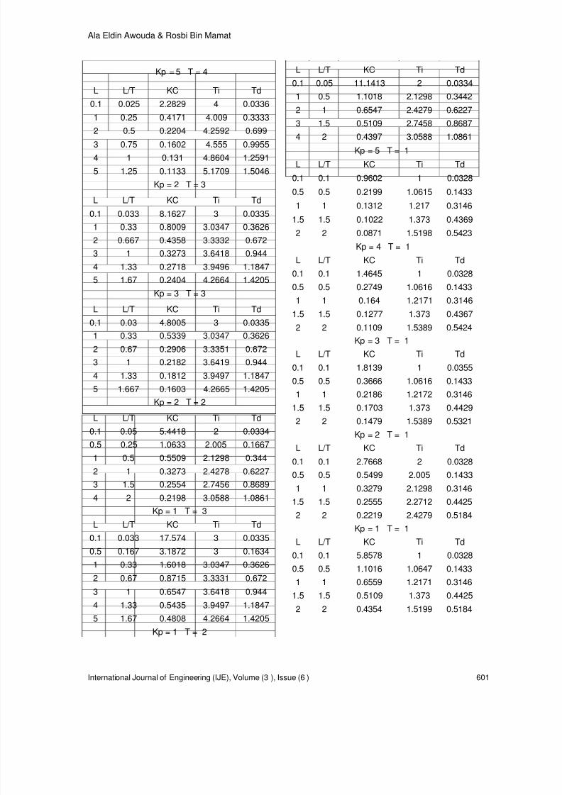
8/8/2019 International Journal of Engineering (IJE), Volume (3): Issue (6)
http://slidepdf.com/reader/full/international-journal-of-engineering-ije-volume-3-issue-6 90/164
Ala Eldin Awouda & Rosbi Bin Mamat
International Journal of Engineering (IJE), Volume (3 ), Issue (6 ) 601
Kp = 5 T = 4
L L/T KC Ti Td
0.1 0.025 2.2829 4 0.0336
1 0.25 0.4171 4.009 0.3333
2 0.5 0.2204 4.2592 0.699
3 0.75 0.1602 4.555 0.9955
4 1 0.131 4.8604 1.2591
5 1.25 0.1133 5.1709 1.5046
Kp = 2 T = 3
L L/T KC Ti Td
0.1 0.033 8.1627 3 0.0335
1 0.33 0.8009 3.0347 0.3626
2 0.667 0.4358 3.3332 0.672
3 1 0.3273 3.6418 0.944
4 1.33 0.2718 3.9496 1.1847
5 1.67 0.2404 4.2664 1.4205Kp = 3 T = 3
L L/T KC Ti Td
0.1 0.03 4.8005 3 0.0335
1 0.33 0.5339 3.0347 0.3626
2 0.67 0.2906 3.3351 0.672
3 1 0.2182 3.6419 0.944
4 1.33 0.1812 3.9497 1.1847
5 1.667 0.1603 4.2665 1.4205
Kp = 2 T = 2
L L/T KC Ti Td0.1 0.05 5.4418 2 0.0334
0.5 0.25 1.0633 2.005 0.1667
1 0.5 0.5509 2.1298 0.344
2 1 0.3273 2.4278 0.6227
3 1.5 0.2554 2.7456 0.8689
4 2 0.2198 3.0588 1.0861
Kp = 1 T = 3
L L/T KC Ti Td
0.1 0.033 17.574 3 0.0335
0.5 0.167 3.1872 3 0.1634
1 0.33 1.6018 3.0347 0.3626
2 0.67 0.8715 3.3331 0.672
3 1 0.6547 3.6418 0.944
4 1.33 0.5435 3.9497 1.1847
5 1.67 0.4808 4.2664 1.4205
Kp = 1 T = 2
L L/T KC Ti Td
0.1 0.05 11.1413 2 0.0334
1 0.5 1.1018 2.1298 0.3442
2 1 0.6547 2.4279 0.6227
3 1.5 0.5109 2.7458 0.8687
4 2 0.4397 3.0588 1.0861Kp = 5 T = 1
L L/T KC Ti Td
0.1 0.1 0.9602 1 0.0328
0.5 0.5 0.2199 1.0615 0.1433
1 1 0.1312 1.217 0.3146
1.5 1.5 0.1022 1.373 0.4369
2 2 0.0871 1.5198 0.5423
Kp = 4 T = 1
L L/T KC Ti Td
0.1 0.1 1.4645 1 0.0328
0.5 0.5 0.2749 1.0616 0.1433
1 1 0.164 1.2171 0.3146
1.5 1.5 0.1277 1.373 0.4367
2 2 0.1109 1.5389 0.5424
Kp = 3 T = 1
L L/T KC Ti Td
0.1 0.1 1.8139 1 0.0355
0.5 0.5 0.3666 1.0616 0.1433
1 1 0.2186 1.2172 0.3146
1.5 1.5 0.1703 1.373 0.4429
2 2 0.1479 1.5389 0.5321Kp = 2 T = 1
L L/T KC Ti Td
0.1 0.1 2.7668 2 0.0328
0.5 0.5 0.5499 2.005 0.1433
1 1 0.3279 2.1298 0.3146
1.5 1.5 0.2555 2.2712 0.4425
2 2 0.2219 2.4279 0.5184
Kp = 1 T = 1
L L/T KC Ti Td
0.1 0.1 5.8578 1 0.03280.5 0.5 1.1016 1.0647 0.1433
1 1 0.6559 1.2171 0.3146
1.5 1.5 0.5109 1.373 0.4425
2 2 0.4354 1.5199 0.5184

8/8/2019 International Journal of Engineering (IJE), Volume (3): Issue (6)
http://slidepdf.com/reader/full/international-journal-of-engineering-ije-volume-3-issue-6 91/164
Ala Eldin Awouda & Rosbi Bin Mamat
International Journal of Engineering (IJE), Volume (3 ), Issue (6 ) 602
Using carve fitting techniques the tuning rule are found as shown below.
5. MATLAB SIMULATION RESULTS
Several process models were examined in this analysis representing different types of processes.After finding the controller settings for the different processes, the responses of the systems wereplotted. All processes were Fist order Plus Dead Time. A reduction procedure is used to modulate thehigher order models in the FOPDT model.
Table 3: Controller settings of AMIGO and proposed tuning rule for process G1(s)
Algorithm KC Ti Td
Z-N 0.9238 7.7556 1.9389
AMIGO 0.432 4.3178 1.7695
Proposed tuning rule 0.499 4.4020 1.6868
Table 4: The response parameters values of Z-N, AMIGO and Proposed tuning rule for the process G 1(s).
Algorithm Rise time (s) Settling Time (s) Set point overshoot % IAE
Z-N 10.2 22.8 11.42 83.28
AMIGO 15.5 17.2 4.19 100.36
Proposed tuning rule 13.5 14.6 7 88.54

8/8/2019 International Journal of Engineering (IJE), Volume (3): Issue (6)
http://slidepdf.com/reader/full/international-journal-of-engineering-ije-volume-3-issue-6 92/164
Ala Eldin Awouda & Rosbi Bin Mamat
International Journal of Engineering (IJE), Volume (3 ), Issue (6 ) 603
Figure 1:- Step response for the second order process with delay
Table 5: Controller settings of Z-N, AMIGO and proposed tuning rule for process G 2(s)
Algorithm KC Ti Td
Z-N 2.7819 2.7641 0.6910
AMIGO 1.065 1.707236 0.694965
Proposed tuning rule 1.219 1.71901 0.662852
Table 6: The response parameters values of Z-N, AMIGO and Proposed tuning rule for the process G 2(s).
Algorithm Rise time (s) Settling Time (s) Set point overshoot % IAE Yd
Z-N 3.2 6 18.13 9.94
AMIGO 6.2 7.3 0.9 16.03
Proposed tuning rule 5.3 9 2.36 14.10

8/8/2019 International Journal of Engineering (IJE), Volume (3): Issue (6)
http://slidepdf.com/reader/full/international-journal-of-engineering-ije-volume-3-issue-6 93/164
Ala Eldin Awouda & Rosbi Bin Mamat
International Journal of Engineering (IJE), Volume (3 ), Issue (6 ) 604
Figure 2:- Step response for the high order process with delay
Table 7: Controller settings of AMIGO and proposed tuning rule for process G3(s)
Algorithm KC Ti Td
Z-N 1.0345 6.4481 1.6120
AMIGO 0.451 3.755031 1.523637
Proposed tuning rule 0.514 3.762972 1.354542
Table 8: The response parameters values of AMIGO and Proposed tuning rule for the process G 3(s).
Algorithm Rise time (s) Settling Time (s) Set point overshoot % IAE Yd
Z-N 7.6 17.7 14.45 65.5
AMIGO 12.8 15 1.48 83.33
Proposed tuning rule 10.9 11.9 3.66 72.99

8/8/2019 International Journal of Engineering (IJE), Volume (3): Issue (6)
http://slidepdf.com/reader/full/international-journal-of-engineering-ije-volume-3-issue-6 94/164
Ala Eldin Awouda & Rosbi Bin Mamat
International Journal of Engineering (IJE), Volume (3 ), Issue (6 ) 605
Figure 3:- Step response for the third order process with delay
Table 9: Controller settings of AMIGO and proposed tuning rule for process G4(s)
Algorithm KC Ti Td
Z-N 0.9101 5.4901 1.3725
AMIGO 0.425 3.047619 1.25
Proposed tuning rule 0.492 3.113137 1.191489
Table 10: The response parameters values of AMIGO and Proposed tuning rule for the process G 4(s).
Algorithm Rise time (s) Settling Time (s) Set point overshoot % IAE
Z-N 6.8 23 16.39 60.24
AMIGO 11.1 12.9 1.78 71.94
Proposed tuning rule 9.3 10.3 3.65 63.29

8/8/2019 International Journal of Engineering (IJE), Volume (3): Issue (6)
http://slidepdf.com/reader/full/international-journal-of-engineering-ije-volume-3-issue-6 95/164
Ala Eldin Awouda & Rosbi Bin Mamat
International Journal of Engineering (IJE), Volume (3 ), Issue (6 ) 606
Figure 4:- Step response for FOPDT process
Table 11: Controller settings of AMIGO and proposed tuning rule for process G 5(s)
Algorithm KC Ti Td
Z-N 7.5449 1.4050 0.3512
AMIGO 1.591 1.262184 0.441037
Proposed tuning rule 1.676 1.16577 0.422533
Table 12: The response parameters values of AMIGO and Proposed tuning rule for the process G 5(s).
Algorithm Rise time (s) Settling Time (s) Set point overshoot % IAE
Z-N 1.3 44.18 4.1 1.86
AMIGO 3.4 4.91 3.8 7.93
Proposed tuning rule 3.1 8.64 6.7 6.95

8/8/2019 International Journal of Engineering (IJE), Volume (3): Issue (6)
http://slidepdf.com/reader/full/international-journal-of-engineering-ije-volume-3-issue-6 96/164
Ala Eldin Awouda & Rosbi Bin Mamat
International Journal of Engineering (IJE), Volume (3 ), Issue (6 ) 607
Figure 5:- Step response for high order process without delay
6. CONCLUSION
The analysis shows that the proposed tuning and AMIGO settings give the least oscillatoryresponse than Z-N setting. It is also seen that the IAE (integral of absolute error) for the disturbancefor the proposed tuning settings is less than the AMIGO setting but slightly higher than Z-N setting.The proposed tuning setting give a small rise time comparing to that of the AMIGO tuning, but slightlyhigher than ZN setting. In the other hand the proposed tuning gives a settling time faster than Z-N’s.Test batch of different process had been used to simulate the proposed tuning. The most importantadvantage of this design is in the use of the IATE performance criteria index to find the new tuning
rule since it can provide the controller with a good performance. As it appears from the simulation, theproposed tuning rule is able to deal with the possible variation of system parameters. It is so obviousthat the proposed tuning rule has the same or better performance than AMIGO tuning rule and amuch better performance than Z-N tuning rule. The observation from those results shows that a highovershoot appears in the output of the system for some cases of processes. This overshoot appearsas expense of achieving a high response and a better load disturbance rejection. In the other handthe proposed tuning rule maintain robustness. The concluded important contributions in this paperregarding the use of the proposed tuning rule are that it proves the ability of the proposed tuning rulein tuning the PID controller probably. Also it validates the flexibility of the proposed tuning rule to dealwith different modeling systems with different parameters. As a future work, the proposed tuning rulecan be used in a practical experiment so as to prepare this proposed tuning rule to be used in thepractical industrial applications.
7. REFRENCES
1. C.-Y. Kao and B. Lincoln, “Simple stability criteria for systems with time-varying delays,”Automatica, vol. 40, pp. 1429-1434, Aug. 2004.
2. Dingyu Xue, YangQuan Chen. Derek P. Atherton. "Linear Feedback Control" Society forIndustrial and Applied Mathematics. 2007.
3. Guillermo J. Silva, Aniruddha Datta. S. P. Bhattacharyya. “PID Controllers for Time-DelaySystems”. Boston. ISBN 0-8176-4266-8.2005.

8/8/2019 International Journal of Engineering (IJE), Volume (3): Issue (6)
http://slidepdf.com/reader/full/international-journal-of-engineering-ije-volume-3-issue-6 97/164
Ala Eldin Awouda & Rosbi Bin Mamat
International Journal of Engineering (IJE), Volume (3 ), Issue (6 ) 608
4. Hang, C.C, K.J.Astrom and W.K. Ho, “refinement of Ziegler-Nichols Tuning Formula”, IEE Proc.Pt. D, Vol. 138, pp. 111-118 .1991.
5. J. G. Ziegler and N. B. Nichols, “Optimum Settings for Automatic Controllers,” Trans. ASME, Vol.64, pp. 759-768, 1942.
6. K. J. Astrom and T. Hagglund, “The Future of PID Control,” IFAC J. Control EngineeringPractice, Vol. 9, pp. 1163-1175, 2001.
7. K.J.Astrom, T.Hagglund, “Revisiting the Ziegler–Nichols step response method for PID control”,
Journal of Process Control 14,635–650, Department of Automatic Control, Lund Institute ofTechnology. 2004.8. Lasse M. Eriksson and Mikael Johansson, “PID Controller Tuning Rules for Varying Time-Delay
Systems”, Proceedings of the 2007 American Control Conference ,New York City, USA, July 11-13, 2007.
9. L. Eriksson and T. Oksanen, ”PID Controller Tuning for Integrating Processes: Analysis and NewDesign Approach,” In Proc. Fourth International Symposium on Mechatronics and itsApplications, harjah, UAE, Mar. 2007
10. Panagopoulos H., Astrom K. J., Hagglund T., “Design of PID Controllers Based on ConstrainedOptimisation”, IEE Proc., Control Theory Appl., Vol. 149, No. 1. – P. 32–40. 2002.
11. P. Cominos and N. Munro, “PID Controllers: Recent Tuning Methods and Design toSpecification,” IEE Proc. D, Control Theory and Applications, Vol. 149, No. 1, pp. 46-53, 2002.

8/8/2019 International Journal of Engineering (IJE), Volume (3): Issue (6)
http://slidepdf.com/reader/full/international-journal-of-engineering-ije-volume-3-issue-6 98/164
ADITYA GOEL, VITTHAL J GOND, R K SETHI and A K SINGH
International Journal of Engineering, Volume (3): Issue (6) 609
Performance Analysis of Continuous Wavelength Optical BurstSwitching Networks
Aditya Goel [email protected] of Electronics & Communication MANIT (Deemed University)Bhopal-462051, India
Vitthal J. Gond [email protected] of Electronics & Communication MANIT (Deemed University)Bhopal-462051, India
R K Sethi [email protected] of Electronics & Communication MANIT (Deemed University)
Bhopal-462051, India
And A K SINGH [email protected] of Electronics & Communication MANIT (Deemed University)Bhopal-462051, India
Abstract
Considering the economic and technical aspects of wavelength converters, fullwavelength conversion capability will not be available throughout opticalnetworks in the foreseeable future. In this paper we have used balanced static
wavelength assignment (BSWA) algorithm. It is a technique to improve theperformance of an all-optical network in respect of blocking probability & otherparameters to provide cost effective optical communication system. We carriedout the performance analysis of wavelength-continuous optical burst switchingnetwork-using BSWA for the network topologies namely NSFNET andINTERNET2NET with the initial assumption that there is no wavelength converteror optical buffer in the networks. For simulation we have used a powerful toolMatplanWDM. The performance analysis of burst loss probability v/s traffic loadusing BSWA algorithm shows that its performance is better than other staticwavelength assignment algorithm. We have also explored the performances ofNSFNET and INTERNET2NET networks on the basis of channel utilization,
message delay, and the ratio of traffic transferred in single hop to total trafficoffered against percentage of reused wavelength in the network. It has beenobserved that channel utilization becomes the maximum for 40% of reusedwavelengths per fiber and beyond that cost of network unnecessary increases.By the performance analysis of message propagation delay for both networkTopology, it is observed that message propagation delay, is minimum at 40% ofreused wavelength per fiber and it becomes constant beyond that. It is thereforerecommended that reused wavelengths per fiber should not exceed 40 % of thetotal available wavelength so as to yield cost effective solution with optimumperformance.

8/8/2019 International Journal of Engineering (IJE), Volume (3): Issue (6)
http://slidepdf.com/reader/full/international-journal-of-engineering-ije-volume-3-issue-6 99/164
ADITYA GOEL, VITTHAL J GOND, R K SETHI and A K SINGH
International Journal of Engineering, Volume (3): Issue (6) 610
Keywords: BSWA: Balanced Static Wavelength Assignment, OBS: Optical Burst Switching, OADM:Optical Add/Drop Multiplexers, OXC: Optical Cross-Connect, TBS: Terabit Burst Switching, PWA: PriorityWavelength Assignment.
1. INTRODUCTION
Due to the introduction of various wide band applications, such as video conferencing, broadbandwireless communication [1] etc the demand of transmission capacity is growing exponentially.This has motivated the researcher to device & employ different techniques [2,3] to enhance theexisting transmission capacity of optical terrestrial and wireless networks. In order toaccommodate this wide capacity requirement, efficient and cost-effective wavelength divisionmultiplexing (WDM) can be used between network nodes [4]. Today up to several Tbit/s trafficcan be carried by the optical link over long distances. e.g. in an ultra-dense WDM transmissiontotal capacity of 50 Tbit/s have already been experimentally demonstrated [5]. However, with theintroduction of very high capacity WDM optical transmission techniques, the discrepancy betweenoptical transmission capacity and electronic switching capability increases. Moreover, due to costand complexity aspects, it is advantageous to keep data in the optical domain and to avoid bit-level signal processing. Burst switched WDM optical networks are coming up as suitable network
architectures for future Optical Internet backbones [6]. Optical Burst Switching (OBS) hasemerged as a new paradigm for an optical Internet [7]. During the past years, there are largeefforts to realize OBS. Although the concept of burst switching had already been known since the1980s, it has never been a big success in electrical networks. The main reason is that itscomplexity and realization requirements are comparable to that of more flexible electronic packetswitching techniques. Optical circuit switching (OCS) does not support fine switching granularityon the packet-level. Only poor bandwidth utilization is obtained due to the absence of statisticalmultiplexing. On the other hand, Optical Packet Switching (OPS) are still too complex to berealized in the near future. Therefore, a hybrid approach like burst switching seems promising forthe WDM-based optical networks. Optical burst switching (OBS) was proposed in the late 1990[7,8] and it tries to exploit the advantages of both OCS and OPS approaches and avoid a part oftheir limitations. OBS is considered as one of the most promising approaches to implement IPover WDM [9]. At the moment, due to the fast development of this new approach and the large
number of new proposals, OBS is still at its definition phase and no common definition of OBScan be found. However, among several different definitions two main definitions can be found.One is more oriented towards fast wavelength switching. Synonyms like optical flow switching(OFS) [10] and wavelength routed OBS (WR-OBS) [11,12,13] can be found in the literature. Here,an acknowledged two-way reservation is generally used. A burst will be only transmitted afterhaving received a positive acknowledgement of its reservation request. Another most widely useddefinition for OBS is more packets oriented and was proposed by Qiao and Turner [14,7,8].
To realize an OBS network, a new optical layer is mandatory. Furthermore, an OBS network willbe only possible if fast and efficient switching nodes can be built. To constitute the OBS networknodes several key components are needed e.g. optical space switches, tunable filters/lasers,wavelength converters etc. Most of the studies on OBS networks assume that full wavelengthconversion is available throughout the network. However, such capability is not at present arealistic assumption. Although use of wavelength converters give better performance with respectto blocking probability but it is quite expensive. So, the absence of (full) wavelength conversioncapabilities calls for good and efficient wavelength assignment policies. The WavelengthAssignment Algorithm is a method to improve the performance in respect of blocking probabilityand to provide cost effective communication system. To solve the above problems there havebeen developed number of wavelength assignment techniques e.g. Random, FF-TE, BSWA etc.Traditional first-fit or random wavelength assignment algorithm in OCS network is not appropriatefor wavelength-continuous OBS networks, since the burst is transmitted without knowledge of thewavelength occupation status of the following links.Out of the number of wavelength assignment techniques we have selected Balanced Staticwavelength assignment (BSWA) algorithm. The BSWA algorithm is new and improvedwavelength assignment policy [15] In BSWA wavelength order lists are carefully designed during

8/8/2019 International Journal of Engineering (IJE), Volume (3): Issue (6)
http://slidepdf.com/reader/full/international-journal-of-engineering-ije-volume-3-issue-6 100/164
ADITYA GOEL, VITTHAL J GOND, R K SETHI and A K SINGH
International Journal of Engineering, Volume (3): Issue (6) 611
the network-planning phase, and no extra information exchange or signaling is needed. TheBSWA improves the performance of blocking probability vs. traffic load than other existing staticwavelength assignment policies. The BSWA also reduces the cost of communication systembecause it reduces the number of wavelength converters, which is too costly. The BSWA hasimproved the performance in respect of blocking probability as compared to other staticapproaches. Numerical results show that BSWA reduces the burst loss probability in comparison
with existing static approaches, and almost achieves the same performance as PWA (PriorityWavelength Assignment) with the advantage that no extra dynamic information is needed. In thiswork performance analysis for NSFNET and INTERNET2NET networks have been carried out forvarious crucial parameters like burst loss probability, message propagation delay and channelutilization.
1.1 Optical Burst Switching (OBS)The main characteristics of OBS can be summarized as follows:
• Client layer data (IP-Packet) is aggregated and assembled into variable length opticalbursts in edge nodes. OBS assumes more extensive burst aggregation, to realize burstswith payloads typically carrying tens of Kbytes.
• There is a separation between control information (header) and user information (data) inspace and in time. Control header packets are sent on a separate wavelength (out-of-band) and processed electronically in all OBS core nodes to set up the switch matrixbefore the data bursts arrive.
• Data bursts are asynchronously switched in core nodes and stay in the optical domainuntil they reach their destination edge node. Only wavelength conversion and/or somedegree of regeneration are applied to the signal.
• Resources are allocated by using one-pass reservation, i.e., burst transmission is notdelayed until an acknowledgment of successful end- to-end path setup is received but isinitiated after the burst was assembled and the control packet was sent out.
• Burst switching does not require buffering inside the core network.
2. BSWA ALGORITHM & IMPLEMENTATION
To reduce the blocking probability, wavelength assignment techniques play an important role inOBS Network, which are not having full wavelength conversion capability. To address the burning
problem of network congestion along with low cost, various wavelength assignment algorithmshave been developed like First-Fit, Random, First-Fit-TE, etc. In this paper we have carried outthe performance analysis of newly developed wavelength assignment algorithm, Balanced StaticWavelength Assignment algorithm. BSWA is capable of reducing the burning problem of networkcongestion to a substantial amount in comparison to other traditional wavelength assignmentalgorithm.
2.1 BSWA Algorithm
BSWA algorithm is static approach, which does not require the exchange of any informationamong network routers. Thus, the assignment rules are determined during the network-planningphase, depending on certain properties of the network like topology, routing paths, and traffic. Inthis work we used traffic information for wavelength assignment. In this BSWA tries to fullybalance the traffic that shares common links between different source-destination pairs among
wavelength on those links.
An OBS network is represented by a graph G (V, E), where V = {V 1, V2,...,VN} is the set of nodes,and E={E1, E2,…,EM} is the set of unidirectional fiber links. The link E(Vs, Vd) connects Vs to Vd
and contains W different wavelengths labeled arbitrarily, say, , λ 1, λ 2 ,……, λ w . By P{Vs ,Vd}, we
denote the routing path from Vs to Vd, and ρ(Vs ,Vd) is the given traffic load from V s to Vd. We define
virtual_wl_cost(Vi, V j, λ k ) to be the virtual cost of wavelength λ k on link E(Vi, V j), and path_cost(Vs, Vd,
λ k ) to be the cost of the the path on λ k along which the source Vs sends bursts to the destination Vd. Thus ,
path_cost(Vs, Vd, λ k ) is calculated as

8/8/2019 International Journal of Engineering (IJE), Volume (3): Issue (6)
http://slidepdf.com/reader/full/international-journal-of-engineering-ije-volume-3-issue-6 101/164
ADITYA GOEL, VITTHAL J GOND, R K SETHI and A K SINGH
International Journal of Engineering, Volume (3): Issue (6) 612
path_cost(Vs, Vd, λ k ) = ( )( ) ( )i j s d
i j k
E V , V P V ,V
virtual _ wl _ cost V , V , λ
∈
∑ (1)
Balanced static wavelength assignment (BSWA) algorithm:
Input: G(V,E), P(Vs ,Vd), ρ(Vs ,Vd) for all s,d є {1,2,……..,n}
Output: WA(Vs, Vd, t) for all s,d є {1,2,……..,n}, t є {1,2,……..,w}
Initialization: virtual_wl_cost (Vi, V j, λ k ) = 0 for all i, j є {1,2, ... ,N},t є {1,2, ... ,W}
FOR t← from 1 to W
FOR s← from 1 to N
FOR d← from 1 to N
Step 1: Compute the path_cost for each wavelength that has not been assigned before for this
s-d pair.Step 2: Choose the λ k that has the least path_cost, and make it the wavelength assigned in this
loop.That is, WA(Vs, Vd, t)= λ k .
Step 3: Update virtual_wl_cost(Vi, V j, λ k ) for all E(Vi, V j) є P{Vs, Vd} by virtual_wl_cost(Vi, V j, λ k ) =
virtual_wl_cost(Vi, V j, λ k ) + ρ(Vs, Vd) (2)
The process of BSWA is stated as follows. First the cost of each wavelength on all links,
virtual_wl_cost(Vi, V j, λ k ) is initialized to 0. Then we begin to assign wavelengths for s-d pairs one by one.
The value of path_cost(Vs, Vd, λ k ), k є {1, 2, ….,w}, is calculated for each (V s, Vd) pair, and λ k that has theleast path_cost is chosen as the wavelength assigned for the (V s, Vd) pair.Every time we assign a
wavelength (e.g. λ k ) for an s-d pair, we increase virtual_wl_cost(Vi, V j, λ k ) on all the passing links of P{Vs
,Vd} by ρ(Vs ,Vd) so that the wavelength is less likely to be chosen by other s-d pairs if it is already heavily
loaded. We continue to do this for all s-d pairs, so that each pair is assigned a wavelength. Theprocess described is called searching loop W times, we can get a list of the wavelengthassignment order for each s-d pair.
2.2 Implementation of BSWA AlgorithmTo reduce the data congestion with low cost, we have used balanced static wavelengthassignment algorithm to assign the wavelength for each source-destination pair (s-d pair). Theprogramming of the BSWA algorithm has been coded in Matlab. We have used a very powerfultool named as Matplan-wdm to implement the coded algorithm. This works on the platform of
Matlab7.0 or above version. The optimization in this tool will be done with the help of Tomlab,which is also a powerful tool for optimization. The algorithm has been implemented in twonetwork topology namely NSFNET & INTERNET2NET as shown in Figure 1 & Figure 2 respectively. The NSFNET consist of 14 nodes and 21 bi-directional fiber links, where asINTERNET2NET consist of 9 nodes and 13 bi-directional fiber links. The traffic loads have beentaken in erlangs per wavelength. The NSFNET have 40 maximum wavelengths per fiber whereas INTERNET2NET have 32 maximum wavelengths per fiber. It is assumed that there are notavailable wavelengths converters and optical buffers in both networks. We have used theDijkastra’s shortest-path algorithm to calculate the route for each s-d pair [15]. In this algorithmeach s-d pair will select shortest path in network to transfer the data. This algorithm has beenalso coded in Matlab. We have analyzed the burst loss probability by varying the traffic load inerlangs per wavelength. Similarly we have done performance analysis of channel utilization,traffic transferred in single hop, message propagation delay by varying the number ofwavelengths per fiber. The channel utilization has been calculated as how many wavelengthschannels are being used to transfer the data out of total wavelengths channels available in thenetwork. The traffic transferred in single hop has been calculated as ratio of traffic transferred insingle hop to total traffic offered in percentage. The message propagation delay has beencalculated as the difference between the time that message being transmitted at transmitter andthat is being received at receiver. It is assumed that burst dropped at transmitter have negligiblepropagation delay. The number of wavelengths per fiber varied as percentage of maximumwavelengths used per fiber in the particular network. For example in NSFNET maximumwavelengths per fiber is 40 and in INTERNET2NET that is 32.

8/8/2019 International Journal of Engineering (IJE), Volume (3): Issue (6)
http://slidepdf.com/reader/full/international-journal-of-engineering-ije-volume-3-issue-6 102/164
ADITYA GOEL, VITTHAL J GOND, R K SETHI and A K SINGH
International Journal of Engineering, Volume (3): Issue (6) 613
1
2
3
45
6
7
8 9
10
11 12
13
14
FIGURE 1: NSFNET (14 Nodes, 21 Bi-directional Link)
FIGURE 2:INTERNET2NET (9 Nodes, 13 Bi-directional Link)
2.3 Validation of BSWAWe have validated our simulated results generated through our code with the previouslypublished results [15] as reported by Chunlei Zhu, Wenda Ni at all in their paper titled “New andImproved Approaches for Wavelength Assignment in Wavelength-Continuous Optical BurstSwitching Network,” By The tabular comparison of the two shows that the simulated result is inreasonably good agreement with the reported result [15]. The comparison of result is for NSFNETwith 14 nodes and 21 bidirectional fiber links. The load is taken in erlangs per wavelength.
Table: 2.1 Result ValidationsLOAD (Erlang)
PublishedResult (1)
Simulated
0.1 0.0015 0.002
0.2 0.009 0.009
0.3 0.026 0.03
0.4 0.05 0.06
0.5 0.08 0.08
0.6 0.12 0.12
0.7 0.15 0.15
0.8 0.2 0.19
0.9 0.25 0.26
1.0 0.30 0.30
3

8/8/2019 International Journal of Engineering (IJE), Volume (3): Issue (6)
http://slidepdf.com/reader/full/international-journal-of-engineering-ije-volume-3-issue-6 103/164
ADITYA GOEL, VITTHAL J GOND, R K SETHI and A K SINGH
International Journal of Engineering, Volume (3): Issue (6) 614
FIGURE 3: Result validation
The Figure 3 shows that there is small variation of simulated result from that with published result[15] up to 0.5 erlangs of traffic load and after 0.5 erlangs of traffic load the simulated result and
published result [15] are almost coincident. Hence this shows that simulated results are in goodagreement reasonably with that of published reported results [15]. Once the validation has beendone, it is ensured that the simulated code is free from logical & other errors. Hence we can applyour code to other networks and applications.
2.4 Comparison of Various Wavelength AssignmentsThe comparision of various wavelength assignment policies with respect to burst loss probabilityhave been shown in the Figure. 4. In this we can see at low load, burst loss probability isminimum for BSWA.This comparision is demonstrated for NSFNET network with 14 nodes, 21bidirectional link.The load is in erlangs per wavelength . At high load burst loss probability isalmost same as PWA which is dynamic wavelength assignment algorithm. Thus BSWA is givingoptimum performance because it is giving almost the same result as PWA with the advantagethat no extra dynamic information is needed.The Figure 4 shows that up to 0.2 erlangs, the BSWA is giving optimum performance. After 0.2
erlangs load BSWA shows the same performance as PWA with small variation in burst lossprobability and after 0.9 erlang it shows almost same performance as PWA. The advantage ofBSWA is that it shows almost same performance as PWA without incorporating any extradynamic information exchange.
FIGURE 4: Traffic Load vs. Burst Loss Probability for Various WavelengthsAssignments Policies (NSFNET, 14 Nodes, 21 Bi-directional Link)

8/8/2019 International Journal of Engineering (IJE), Volume (3): Issue (6)
http://slidepdf.com/reader/full/international-journal-of-engineering-ije-volume-3-issue-6 104/164
ADITYA GOEL, VITTHAL J GOND, R K SETHI and A K SINGH
International Journal of Engineering, Volume (3): Issue (6) 615
2.5 Performance AnalysisThe performance analysis of wavelength-continuous optical burst switching network [17 has beencarried out, by evaluating the performance of following parameters: -
2.5.1 Burst loss probabilityBurst loss probability [17 is given by,
Pb = ( )( )Numer of burst droppedTotal number of arrivals
(3)
Here we have assumed that if any route is blocked then coming burst through this rote will be dropped.Hence the burst loss probability has been calculated as the average blocking probability Pb for the networkand is defined as average of the blocking probabilities on all the routes and is given by,
Pb = 1
R
r
Br
R
=
∑(4)
Where R is the total number of routes in the network.
Br is the blocking probability of a route r, which involves multiple links (say n links), is given by,
Br = 1-1
(1 )
n
iPi
=−∏ (5)
Where Pi is the blocking probability of a link i with capacity C (number of wavelengths on link) and is givenby
Pi = R (L (i), C) =( ) ( )
1C n
0
L i L i
!
C
nC n
−
=
∑ (6)
Where L (i) is carried traffic on link i which has frequency of usage, F i and is given by,
L (i) =
1
iF
r
j
L=
∑ =i
L F
R
×(7)
Where Lr is the load on any route r and is given by,
Lr = L R
(8)
Where L is the total load (erlangs) on the network and is given by,L = l × N (9)
and R is the total number of bi-directional routes and is given by,
R =( 1)
2
N N × −(10)
2.5.2 Channel UtilizationChannel Utilization [17] s given by,
U=Average value of occupied channels in the network
Total available channels in the network (11)
=1
1 0( ) ( ) J C
ii mC m P C m
C J
−= = − −
∗∑ ∑ (12)
Total Available Channels = C × J(13)
Here Occupied channels =
1
1 0
( ) ( ) J C
i
i m
C m P C m−
= =
− −∑∑ ; where0
( ) 1C
i
m
P m=
=∑ (14)
Where Pi(C-m) = qi(m) (15)
≅ Probability of finding C-m wavelengths occupied in link i
≅ Probability of finding m wavelengths free on link i

8/8/2019 International Journal of Engineering (IJE), Volume (3): Issue (6)
http://slidepdf.com/reader/full/international-journal-of-engineering-ije-volume-3-issue-6 105/164
ADITYA GOEL, VITTHAL J GOND, R K SETHI and A K SINGH
International Journal of Engineering, Volume (3): Issue (6) 616
Where qi(m) is the probability of finding m idle or free wavelengths on link i and from theBirth-death model, qi(m) is given as,
qi(m) =( 1)......( 1)
( )m
eff
C C C m
L i
− − +qi(0); m = 1,2,…..C (16)
Where
qi(0) =1
( 1)......( 1)1( )
C
mm eff
C C C m
L i=
− − ++
∑ (17)
and Leff(i) is the effective carried traffic on link I and is given by,
Leff(i) =1
(1 )iF
r i r
r
L P B=
+ −∑ =1
iF
r i i i r
r
L F F P B=
+ × −
∑ (18)
Since in the formula of channel utilization given, channel utilization mainly depends on value ofoccupied channels so we have simulated the result for average Occupied Channel used againsttotal channel available.
2.5.3 Message propagation delayThis is the difference between the times of Message being transmitted from source and message
being received at receiver. The assumption has been taken that dropped burst have notransmission delay.
2.5.4 Ratio of single hop traffic to total traffic offeredIt is the ratio of traffic being transmitted in single hop to total traffic offered to network. In oursimulation traffic is being transmitted through Dijkastra’s shortest path [15].
2.6 Burst loss calculation for OBS Network using full wavelength converter capabilityThe objective of calculation of burst loss probability for full wavelength conversion capability
network is to show that wavelength converters have very important roll to reduce the burst lossprobability. The disadvantage of wavelength converter is, it is too costly. So to reduce the costwavelength assignment policies is being used. Let in the OBS Network, there are (M+1)wavelengths per fiber link. In (M+1) wavelengths one wavelength is used as reservation channel
for signaling and other M wavelengths channel carry data bursts. The bursts loss probability B oneach fiber link is the same and is given by using the well known Erlang loss formula [16,17] with
MB(A,M) = (A
M/ M!) / ( Σ A
i/ i!) , (19)
i=0Where A is the offered traffic load and M the number of wavelengths (which will carry data
bursts) per out put fiber. Therefore A/M is the normalized offered traffic, which corresponds toutilization of output fiber of the node.
3. Results and Discussion
The typical network topologies we have used in this simulation are NSFNET (14 nodes, 21 bi-
directional fiber links) and INTERNET2NET (9 nodes, 13 bi-directional fiber links) as shown inFigure 1 and Figure 2 respectively. We initially assume wavelength converters are not available.Dijkstra’s shortest-path algorithm is used to calculate the route for each s-d pair. Theperformance of BSWA has been investigated by evaluating the performance of followingparameters:1. Burst loss probability vs. traffic load in Erlangs with BSWA.2. Number of used wavelength channels v/s. % of wavelengths used per fiber.3. Message propagation Delay v/s % of wavelengths used per fiber.
Further we have also calculated the blocking probability of OBS Network with full wavelengthconversion capability using Erlangs Loss formula for NSFNET. 3.1 Burst Loss Probability with BSWA Algorithm3.1.1 NSFNET Topology

8/8/2019 International Journal of Engineering (IJE), Volume (3): Issue (6)
http://slidepdf.com/reader/full/international-journal-of-engineering-ije-volume-3-issue-6 106/164
ADITYA GOEL, VITTHAL J GOND, R K SETHI and A K SINGH
International Journal of Engineering, Volume (3): Issue (6) 617
0.1 0.2 0.3 0.4 0.5 0.6 0.7 0.8 0.9 110
-3
10-2
10-1
100
traffic load(erlangs)
b u r s t l o s s
p r o b a b
i l i t y
FIGURE 5: for NSFNET Topology FIGURE 6:for INTERNET2NET Topology
The results of burst loss probability vs traffic load with BSWA algorithm have been shown inFigure 5 for NSFNET. We observe that as the load increases burst loss probability also
increases. From Figure 5 it is evident that up to 0.3 erlangs traffic load, burst loss probabilityincreases rapidly and at 0.3 erlangs it is approximately 3×10⁻²
.beyond 0.3 erlangs of traffic load,burst loss probability increases at aslower pace and after 0.8 erlangs it becomes nearly uniform(burst loss probability is approximately 0.2 to 0.3 as traffic load ranges between 0.8 erlangs to 1.0erlangs) .
3.1.2 INTERNET2NET Topology The results of burst loss probability vs traffic load with BSWA algorithm have been shown inFigure 6 for INTERNET2NET. We observe from Figure 6 as load increases burst loss probabilityalso increases. From Figure 6 it is clear that up to 0.2 erlangs of traffic load, burst loss probabilityincreases rapidly and between 0.2 erlangs to 0.5 erlangs of traffic load, burst loss probabilityincreases but at a slower rate. At 0.1 erlangs burst loss probability is approximately 3×10
-3and at
0.2 erlangs of traffic load it is approximately 2×10⁻²
. Beyond 0.5 erlangs of load, burst lossprobability increases at a much slower rate while after 0.8 erlangs it becomes almost uniform, so
no need was felt to simulate for more than 1.0 erlags of traffic load.
3.2 Number of Used Wavelength Channels vs. % of Wavelengths Used per Fiber3.2.1 NSFNET Topology
FIGURE 7: for NSFNET Topology. FIGURE 8:for INTERNET2NET Topology

8/8/2019 International Journal of Engineering (IJE), Volume (3): Issue (6)
http://slidepdf.com/reader/full/international-journal-of-engineering-ije-volume-3-issue-6 107/164
ADITYA GOEL, VITTHAL J GOND, R K SETHI and A K SINGH
International Journal of Engineering, Volume (3): Issue (6) 618
For simulation we have taken number of wavelengths per fiber equal to 40 for NSFNET network.The simulation results are shown in Fig. 7 for traffic load of 0.2 erlangs. In Figure 7 at 10% ofwavelengths used per fiber, number of used wavelengths channels are 140 and it increases withthe % of wavelengths used per fiber. Again at 40% of wavelengths used per fiber (i.e. numberof wavelengths per fiber w =16), the number of used wavelengths channels is 360 and that isalmost constant after 40% of wavelengths used per fiber. Hence beyond 40 % , wavelengths
reused per fiber more than 40% are unnecessary going to augment overall cost of the network.
3.2.2 INTERNET2NET TopologyHere for simulation we have taken maximum number of wavelengths per fiber = 32 . Thesimulation results are shown in Figure 8 for traffic load of 0.2 erlangs. As shown in Figure 8, for10% of wavelengths used per fiber, number of used wavelengths channels are 60 and itincreases with the % of wavelengths used per fiber. Again at 40% of wavelengths used perfiber ( i.e. number of wavelengths per fiber w = 12), the number of used wavelengths channels is145 and thereafter it is almost constant. Hence here also the % of wavelength reused per fibershould not be allowed to exceed 40 %.
3.3 Message Propagation Delay vs. % of Wavelengths Used Per Fiber3.3.1 NSFNET Topology
FIGURE 9: for NSFNET Topology. FIGURE10: for INTERNET2NET.Topology
we have assumed maximum number of wavelength per fiber W = 40 . The simulation results areshown in Figure 9 for traffic load of 0.2 erlangs. From Figure 9 we noticed that messagepropogation delay increases upto 25 % of wavelengths used per fiber and then it suddenlydecreases. It become nearlyuniform 40 % of wavelength used per fibr. As % of wavelengths usedper fiber increases up to 25%, message reaches from source to destination with significant delayand therefore initially the message propagation delay also increases.However after 25% of wavelengths used per fiber, number of available wavelength channels alsoincreases and more message are being propagated through single hop which led to decrease indelay up to 40% of wavelengths used per fiber. Thereafter it becomes saturated because alltraffic is being propagated through the single hop. This investigation also reveals that wavelengthused per fiber should be confined within 40 %.
3.3.2 INTERNET2NET TopologyFor simulation we have taken maximum number of wavelength per fiber = 32 .The simulationresult are demonstrated in Figure 10 for traffic load of 0.2 erlangs. Here also up to 25% ofwavelengths per fiber, message propagation delay increases with a further decreases till 40 %and thereafter becomes nearly uniform . As % of wavelengths used per fiber increases up to25%, message reaches from source to destination with a significant delay,thereby resulting inincrease of message propogation delay.Since after 25% of wavelengths used per fiber, number of available wavelength channelsincreases and more message are being propagated through the single hop which ultimatelyresults in decrease of delay up to 40% of wavelengths used per fiber. Thereafter delay becomes
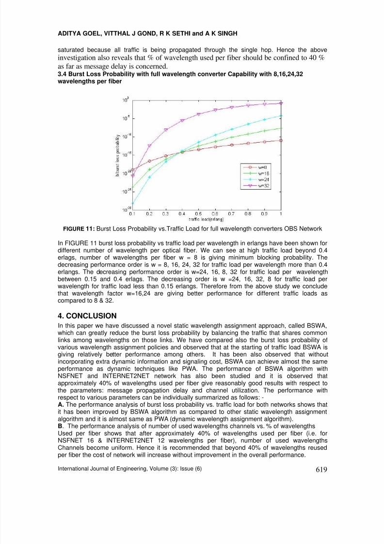
8/8/2019 International Journal of Engineering (IJE), Volume (3): Issue (6)
http://slidepdf.com/reader/full/international-journal-of-engineering-ije-volume-3-issue-6 108/164
ADITYA GOEL, VITTHAL J GOND, R K SETHI and A K SINGH
International Journal of Engineering, Volume (3): Issue (6) 619
saturated because all traffic is being propagated through the single hop. Hence the above investigation also reveals that % of wavelength used per fiber should be confined to 40 %
as far as message delay is concerned.3.4 Burst Loss Probability with full wavelength converter Capability with 8,16,24,32wavelengths per fiber
FIGURE 11: Burst Loss Probability vs.Traffic Load for full wavelength converters OBS Network
In FIGURE 11 burst loss probability vs traffic load per wavelength in erlangs have been shown fordifferent number of wavelength per optical fiber. We can see at high traffic load beyond 0.4erlags, number of wavelengths per fiber w = 8 is giving minimum blocking probability. Thedecreasing performance order is w = 8, 16, 24, 32 for traffic load per wavelength more than 0.4erlangs. The decreasing performance order is w=24, 16, 8, 32 for traffic load per wavelengthbetween 0.15 and 0.4 erlags. The decreasing order is w =24, 16, 32, 8 for traffic load per
wavelength for traffic load less than 0.15 erlangs. Therefore from the above study we concludethat wavelength factor w=16,24 are giving better performance for different traffic loads ascompared to 8 & 32.
4. CONCLUSION
In this paper we have discussed a novel static wavelength assignment approach, called BSWA,which can greatly reduce the burst loss probability by balancing the traffic that shares commonlinks among wavelengths on those links. We have compared also the burst loss probability ofvarious wavelength assignment policies and observed that at the starting of traffic load BSWA isgiving relatively better performance among others. It has been also observed that withoutincorporating extra dynamic information and signaling cost, BSWA can achieve almost the sameperformance as dynamic techniques like PWA. The performance of BSWA algorithm withNSFNET and INTERNET2NET network has also been studied and it is observed that
approximately 40% of wavelengths used per fiber give reasonably good results with respect tothe parameters: message propagation delay and channel utilization. The performance withrespect to various parameters can be individually summarized as follows: -A. The performance analysis of burst loss probability vs. traffic load for both networks shows thatit has been improved by BSWA algorithm as compared to other static wavelength assignmentalgorithm and it is almost same as PWA (dynamic wavelength assignment algorithm).B. The performance analysis of number of used wavelengths channels vs. % of wavelengthsUsed per fiber shows that after approximately 40% of wavelengths used per fiber (i.e. forNSFNET 16 & INTERNET2NET 12 wavelengths per fiber), number of used wavelengthsChannels become uniform. Hence it is recommended that beyond 40% of wavelengths reusedper fiber the cost of network will increase without improvement in the overall performance.

8/8/2019 International Journal of Engineering (IJE), Volume (3): Issue (6)
http://slidepdf.com/reader/full/international-journal-of-engineering-ije-volume-3-issue-6 109/164
ADITYA GOEL, VITTHAL J GOND, R K SETHI and A K SINGH
International Journal of Engineering, Volume (3): Issue (6) 620
C. The performance analysis of message propagation delay vs. % of wavelengths used per fibershows that after approximately 40% of wavelengths used per fiber (i.e. for NSFNET 16 andINTERNET2NET 12 wavelengths per fiber), message propagation delay is minimum and nearlyuniform. Here again it is observed that % of wavelengths used per fiber must be confined to 40%, as there is no significant improvement in the performance beyond that.Further we have also analyzed the performance with wavelength converters for different number
of wavelengths per fiber and it is observed that wavelengths factor w = 16 and 24 reduces theblocking probability more efficiently in comparison with w= 8 & 32.The above investigations ultimately conclude that % of wavelengths reused per fiber
should not be allowed to exceed 40% as otherwise it augments the overall network cost withoutany further significant improvement in the performance of the network. The Performance analysisof Optical Burst Switching Networks for INTERNET2NET and NSFNET can also be carried out infuture by using dynamic wavelength techniques. The possibility of optimizing an arbitrary networktopologies to yield better network performance can also be explored in future.
REFERENCES
1. Aditya Goel, Ajaii Sharma “Performance Analysis of Mobile ADOC Network using AODVProtocol” International Journal of Computer Science and Security Volume 3 Issue 5 pages 334-
343, 2009.2. Aditya Goel, R K Sethi “Integrated Optical wireless network for next generation wireless
Systems”, Signal Processing – An International Journal, vol. 3 Issue 1, Pages 1-13, 2009.3. Aditya Goel, Ravi Shankar Mishra Remote Date Acquisition Using Wireless SCADA System
International Journal of Engineering Volume 3 Issue 1 pages 58 – 64, 2009.4. Shikha Nema, Aditya Goel, R P Singh, “Integrated DWDM and MIMO-OFDM system for 4G
High capacity mobile communication System” Signal Processing – An International JournalVolume 3 Issue 5 pages 132-143, Nov/Dec 2009.
5. F. Kukuchi et al.,”10.92-Tbits/s triple-band / ultra dense optical repeated transmissionExperiment,” in Proceedings of Optical Fiber Communication Conference (OFC), Anaheim,California, USA, March 2001 number PD24.
6. X. Wang, H. Morikawa, and T. Aoyama, “Priority-based wavelength assignment algorithm for burst switched WDM optical networks,”
IEICE Trans. Commun E86-B (5), 1508–1514 (May 2003)7. C. Qiao and M. Yoo, “Optical burst switching (OBS)—a new paradigm for an optical Internet,”
J. High Speed Networks. 8(1), 69–84(1999)8. J S Turner, “Terabit burst switching,” J. High-Speed Networks, vol.8, no.1, pp.3-16, Jan.1999.9. Jiangtao Luo , Jun Huang, Hao Chang et.al. ,” ROBS: A novel architecture of Reliable
Optical Burst Switching with congestion control,” J. High-Speed Networks, vol.16,No.2, pp.123-131, 2007
10. C.H. Xin and C.Qiao, “A comparative study of OBS and OFS,” in Proceedings of OpticalFiber Communication Conference (OFC), Anaheim, California, USA, no. ThG7-1, Mar 2001
11. M. Düser and P. Bayvel, “Analysis of a dynamically wavelength-routed optical burst switchedNetwork architecture,” IEEE J. of Light wave Technology, vol. 20, no. 4, pp. 574-585, April 2002.
12. De Miguel, M. Düser, and P. Bayvel, “Traffic load bounds for optical burst switched networks withDynamic wavelength allocation,” in Proc. of the IFIP TC6 5th International Working Conference onOptical Network Design and Modeling (ONDM 2001), Vienna, February 2001.
13. M. Düser and P. Bayvel, “Bandwidth utilization and wavelength re-use in WDM optical burst-Switched packet networks,” in Proc. of the IFIP TC6 5th International Working Conference onOptical Network Design and Modeling (ONDM 2001), Vienna, February 2001.
14. C. Qiao and M. Yoo, “Choices, features and issues in Optical Burst Switching,” OpticalNetworks Magazine, vol. 1, no. 2, pp. 37-44, April 2000.
15. Chunlei Zhu, Wenda Ni, Yu Du, Yanhe Li, Xiaoping Zheng, Yili Guo and Hanyi Zhang, “Newand Improved Approaches for Wavelength Assignment in Wavelength-Continuous OpticalBurst Switching Network,” Optical Engineering September 2007/vol.46 (9).
16. L. Kleinrock, Queueing Systems - Volume I: Theory, John Wiley & sons, New York, 1975.
17 Rajalakshmi P and Ashok Jhunjhunwala, “Analytical performance computation for all optical networks

8/8/2019 International Journal of Engineering (IJE), Volume (3): Issue (6)
http://slidepdf.com/reader/full/international-journal-of-engineering-ije-volume-3-issue-6 110/164
ADITYA GOEL, VITTHAL J GOND, R K SETHI and A K SINGH
International Journal of Engineering, Volume (3): Issue (6) 621
With wavelength conversion, ”IETE Journal of Research , Vol. 54, No.1, Jan-Feb 2008, pp 31-38.18 P.J. Kühn, Teletraffic Theory and Engineering, Lecture at University Stuttgart, 2002/2003.

8/8/2019 International Journal of Engineering (IJE), Volume (3): Issue (6)
http://slidepdf.com/reader/full/international-journal-of-engineering-ije-volume-3-issue-6 111/164
M. Enamul Hossain and M. Rafiqul Islam
International Journal of Engineering (IJE), Volume (3): Issue (6) 622
Knowledge – Based Reservoir Simulation – A Novel Approach
M. Enamul Hossain [email protected] Department of Petroleum Engineering King Fahd University of Petroleum & Minerals Dhahran 31261, Saudi Arabia
M. Rafiqul Islam [email protected] Department of Civil and Resource Engineering Dalhousie University Sexton Campus, 1360 Barrington Street, Halifax, NS B3J 2X4, Canada
Abstract
It is well known that reservoir simulation studies are very subjective and vary fromsimulator to simulator. While SPE benchmarking has helped accept differences inpredicting petroleum reservoir performance, there has been no scientific explanationbehind the variability that has frustrated many policy makers and operations managers andpuzzled scientists and engineers. In a recent book by the research group of R. Islam, anew approach is taken to add the Knowledge dimension to the problem. For the first time,reservoir simulation equations are shown to have embedded variability and multiplesolutions that are in line with physics rather than spurious mathematical solutions. Withthis clear description, a fresh perspective in reservoir simulation is presented. Unlike themajority of reservoir simulation approaches available today, the 'knowledge-based'approach does not stop at questioning the fundamentals of reservoir simulation but offerssolutions and demonstrates that proper reservoir simulation should be transparent andempower decision makers rather than creating a black box. Mathematical developments ofnew governing equations based on in-depth understanding of the factors that influencefluid flow in porous media under different flow conditions are introduced. Behavior of flowthrough matrix and fractured systems in the same reservoir, heterogeneity and fluid/rock
properties interactions, Darcy and non-Darcy flow are among the issues that are thoroughlyaddressed. For the first time, the fluid memory factor is introduced with a functionalform. The resulting governing equations are solved without linearization at any stage. Aseries of clearly superior mathematical and numerical techniques are also presented thatallow one to achieve this objective. Mathematical solutions that provide a basis forsystematic tracking of multiple solutions that are inherent to non-linear governingequations. This was possible because the new technique is capable of solving non-linearequations without linearization. To promote the new models, a presentation of the commoncriterion and procedure of reservoir simulators currently in use is provided. The models areapplied to difficult scenarios, such as in the presence of viscous fingering, fractures, andothers. It is demonstrated that the currently available simulators only address very limitedrange of solutions for a particular reservoir engineering problem. Examples are provided to
show how the Knowledge-based approach extends the currently known solutions andprovide one with an extremely useful predictive tool for risk assessment.
Keywords: Emulation, Newtonian Mechanics, New Energy Balance Formulation, Energy Pricing, Non-LinearMathematics
1. INTRODUCTION
In reservoir simulation, the principle of GIGO (Garbage in and garbage out) is well known [1]. This principleimplies that the input data have to be accurate for the simulation results to be acceptable. Petroleum industry

8/8/2019 International Journal of Engineering (IJE), Volume (3): Issue (6)
http://slidepdf.com/reader/full/international-journal-of-engineering-ije-volume-3-issue-6 112/164
M. Enamul Hossain and M. Rafiqul Islam
International Journal of Engineering (IJE), Volume (3): Issue (6) 623
has established itself as the pioneer of subsurface data collection [2]. Historically, no other discipline hastaken so much care in making sure input data are as accurate as the latest technology would allow. Therecent superflux of technologies dealing with subsurface mapping, real time monitoring, and high speed datatransfer is an evidence of the fact that input data in reservoir simulation are not the weak link of reservoirmodelling.
However, for a modelling process to be knowledge-based, it must fulfi ll two criteria, namely, the source has tobe true (or real) and the subsequent processing has to be true [3]. As indicated earlier, the source is not a
problem in the petroleum industry. The potential problem lies within the processing of data. For the process tobe knowledge-based, the following logical steps have to be taken:
• Collection of data with constant improvement of the data acquisition technique. The data set to becollected is dictated by the objective function, which is an integral part of the decision making process.Decision making, however, should not take place without the abstraction process. The connectionbetween objective function and data needs constant refinement. This area of research is one of thebiggest strength of the petroleum industry, particularly in the information age.
• The gathered data should be transformed into Information so that they become useful. With today’stechnology, the amount of raw data is so huge, the need for a filter is more important than ever before.However, it is important to select a filter that doesn’t skew data set toward a certain decision.Mathematically, these filters have to be non-linearized [4]. While the concept of non-linear filtering is notnew, the existence of non-linearized models is only beginning to be recognized [2].
• Information should be further processed into ‘knowledge’ that is free from preconceived ideas or a
‘preferred decision’. Scientifically, this process must be free from information lobbying, environmentalactivism, and other forms of bias. Most current models include these factors as an integral part of thedecision making process [5], whereas a scientific knowledge model must be free from those interferencesas they distort the abstraction process and inherently prejudice the decision making. Knowledge gatheringessentially puts information into the big picture. For this picture to be distortion-free, it must be free fromnon-scientific maneuvering.
• Final decision making is knowledge-based, only if the abstraction from 1) through 4) has been followedwithout interference. Final decision is a matter of Yes or No (or True or False or 1 or 0) and this decisionwill be either knowledge-based or prejudice-based. Figure 1 shows the essence of the knowledge baseddecision making.
The process of aphenomenal or prejudice-based decision-making is illustrated by the inverted triangle,proceeding from the top down (Figure 2). The inverted representation stresses the inherent instability andunsustainability of the model. The source data from which a decision eventually emerges already
incorporates their own justifications, which are then massaged by layers of opacity and disinformation.
The disinformation referred to here is what results when information is presented or recapitulated in theservice of unstated or unacknowledged ulterior intentions [6]. The methods of this disinformation achieve theireffect by presenting evidence or raw data selectively, without disclosing either the fact of such selection or thecriteria guiding the selection. This process of selection obscures any distinctions between the data comingfrom nature or from any all-natural pathway, on the one hand, and data from unverified or untestedobservations on the other. In social science, such manoeuvering has been well known, but the recognition ofthis aphenomenal model is new in science and engineering [7].
FIGURE1: The knowledge model and the direction of abstraction FIGURE 2: Aphenomenal decision-making

8/8/2019 International Journal of Engineering (IJE), Volume (3): Issue (6)
http://slidepdf.com/reader/full/international-journal-of-engineering-ije-volume-3-issue-6 113/164
M. Enamul Hossain and M. Rafiqul Islam
International Journal of Engineering (IJE), Volume (3): Issue (6) 624
2. SHORTCOMINGS OF THE CONVENTIONAL APPROACH
Recently, Mustafiz and Islam [8] published a comprehensive review of currently available reservoir simulationapproaches. In this paper, the discussion is limited to finite difference approach because that is the mostcommonly used technique in the petroleum reservoir modelling community.
The history of differential calculus dates back to the time of Leibnitz and Newton. In this concept, thederivative of a continuous function to the function itself is related. In the core of differential calculus is theNewton’s formula that has the following approximation attached to it: the magnitude and direction change
independently of one another. There is no problem in having separate derivatives for each component of thevector or in superimposing their effects separately and regardless of order. That is what mathematiciansmean when they describe or discuss Newton’s derivative being used as a “linear operator”. Following this,comes Newton’s difference-quotient formula. When the value of a function is inadequate to solve a problem,the rate at which the function changes, sometimes, becomes useful. Therefore, the derivatives are alsoimportant in reservoir simulation. In Newton’s difference-quotient formula, the derivative of a continuousfunction is obtained. This method relies implicitly on the notion of approximating instantaneous moments ofcurvature, or infinitely small segments, by means of straight lines. This alone should have tipped everyone offthat his derivative is a linear operator precisely because, and to the extent that, it examines change over time(or distance) within an already established function. This function is applicable to an infinitely small domain,making it non-existent. When, integration is performed, however, this non-existent domain is assumed to beextended to finite and realistic domain, making the entire process questionable.
Zatzman and Islam [9] identified the most significant contribution of Newton in mathematics as the famous
definition of the derivative as the limit of a difference quotient involving changes in space or in time as smallas anyone might like, but not zero, viz.
(1)
Without regards to further conditions being defined as to when and where differentiation would produce ameaningful result, it was entirely possible to arrive at “derivatives” that would generate values in the range ofa function at points of the domain where the function was not defined or did not exist. Indeed: it took anothercentury following Newton’s death before mathematicians would work out the conditions – especially therequirements for continuity of the function to be differentiated within the domain of values – in which itsderivative (the name given to the ratio-quotient generated by the limit formula) could be applied and yieldreliable results. Kline [10] detailed the problems involving this breakthrough formulation of Newton. However,
no one in the past did propose an alternative to this differential formulation, at least not explicitly. Thefollowing figure (Figure 3) illustrates this difficulty.
FIGURE 3: Economic wellbeing is known to fluctuate with time
In this figure, economic index (it may be one of many indicators) is plotted as a function of time. In nature, allfunctions are very similar. They do have local trends as well as global trend (in time). One can imagine howthe slope of this graph on a very small time frame would quite arbitrary and how devastating it would be to

8/8/2019 International Journal of Engineering (IJE), Volume (3): Issue (6)
http://slidepdf.com/reader/full/international-journal-of-engineering-ije-volume-3-issue-6 114/164
M. Enamul Hossain and M. Rafiqul Islam
International Journal of Engineering (IJE), Volume (3): Issue (6) 625
take that slope to a long-term. One can easily show the trend, emerging from Newton’s differential quotientwould be diametrically opposite to the real trend. Zatzman and Islam [9] provided a basis for determining realgradient, rather than local gradient that emerges from Newtonian’s differential quotient. In that formulation, itis shown that the actual value of t, over which a reliable gradient has to be observed, needs to be severaltime greater than the characteristic time of a system. The notion of Representative Elemental Volume (REV),as first promoted by Bear [11] is useful in determining a reasonable value for this characteristic time. Thesecond principle is that at no time t be allowed to approach 0 (Newton’s approximation), even when thecharacteristic value is very small (e.g. phenomena at nano scale). With the engineering approach, it turns out
such approximation is not necessary [12] because this approach bypasses the recasting of governingequations into Taylor series expansion, instead relying on directly transforming governing equations into a setof algebraic equations. In fact, by setting up the algebraic equations directly, one can make the processsimple and yet maintain accuracy [4]. Finally, initial analysis should involve the extension t to ∞ in order todetermine the direction, which is related to sustainability of a process [13].
Figure 4 shows how formulation with the engineering approach ends up with the same linear algebraicequations if the inside steps are avoided. Even though the engineering approach was known for decades(known as the control volume approach), no one identified in the past the advantage of removing in-betweensteps. In analyzing further the role of mathematical manipulation in solving a natural problem, the followingextremely simple example can be cited. Consider the function, y = 5. Following steps show how this functionsimple function can take route of knowledge or prejudice, based on the information that is exposed or hidden,respectively.
FIGURE 4: Major steps used to develop reservoir simulators (redrawn from Abou-Kassem et al., 2006, Hossain et al.,2009)
Step 1: y = 5. This is an algebraic equation that means, y is a constant with a value of 5. This statement is
an expression of tangibles, which becomes clear if the assumptions are pointed out. The assumptions are: a) y has the same dimension as 5 (meaning dimensionless); b) nothing else matters (this one actually is aclarification of the condition a). Therefore, the above function implies that y cannot be a function of anything(including space and time). The mere fact that there is nothing in nature that is constant makes the functionaphenomenal. However, subsequent manipulations (as in Step 2) make the process even more convoluted.
Step 2: = 0. This simple derivation is legitimate in calculus that originates from Newton’s ratio ofquotient theory. In this, even partial derivative would be allowed with equal legitimacy as nothing states inconventional calculus that such operation is illegitimate. By adding this derivative in x (as in x direction inCartesian coordinate), a spurious operation is performed. In fact, if Step 1 is true, one can add any dimensionto this the differential would still be 0 – statement that is ‘technically’ true but hides background informationthat becomes evident in Step 3.
Step 3: If one integrates , one obtains, y = C, where C is a constant that can have infinite number ofvalues, depending on which special case it is being solved for. All of a sudden, it is clear that the originalfunction. All of a sudden, it is clear that the original function (y = 5) has disappeared.
Step 4: One special case of y = C is, y = 5. To get back the original and unique function (as in Step 1), onenow is required to have boundary conditions that are no longer attached to the mathematical formulation. If aspecial case of C = 5 is created, similarly one can have y =1, 2, 3, 4, 5, 6,... How does one know whichsolution will give the ‘true’ solution. In this particular case, all but one solution are called ‘spurious' solutions,because they failed to match the solution of interest, i.e., y = 5.
This simple example shows how imposing Newton's differential and integrating procedure convolutes theentire process, while losing information that would allow anyone to trace back the original algebraic function.

8/8/2019 International Journal of Engineering (IJE), Volume (3): Issue (6)
http://slidepdf.com/reader/full/international-journal-of-engineering-ije-volume-3-issue-6 115/164
M. Enamul Hossain and M. Rafiqul Islam
International Journal of Engineering (IJE), Volume (3): Issue (6) 626
On the other hand, if one is looking at an actual phenomenon, then = 0 could mean that we are at the
very start of something, or at the very end of something. If we look at ∂y/ ∂x, on the other hand, then we haveto look also at ∆y/ ∆t, and then we also have to consider the situation where ∆y/ ∆x=0 but ∆y/ ∆t is non-0. Thismight very well be a branch-point, a point of bifurcation or, generally speaking, something marking a changefrom an old state to a new state. Branch-points in physical natural reality clearly imply infinite solutions, sincethe process could go, literally, anywhere from that branch-point. This approach of locating bifurcationphenomena has eluded previous researchers engaged in modelling chaos [14]. With the engineeringapproach, the following steps can be taken. Note the similarity of these steps with the one shown above
regarding a simpler function.
Step 1) Mass balance + Darcy's law It is an algebraic equation.Step 2a) Time variable is added to it through Newton's differential quotient time increment is allowed to
approach to 0.Step 2b) Space variable is added through Newton's differential quotient space increment is allowed to
approach 0.Step 2c) Differential equations emerge, burying assumptions added in 2a and 2b.Step 3) Differential equation integrated analytically, original solutions will not be recovered. The integrated
values will have the possibility of having infinite solutions, depending on the boundary conditions,initial conditions, etc.
Step 4) Three special cases (out of infinite number of solutions possible) are identified as part of theintegrated solution of the Differential equation in Step 3. They are:
Step 4a) Steady state, compressible. This is Mass balance and Darcy's law as in Step 1.
Step 4b) Unsteady state, slightly compressible fluid. This is the typical equation that gives rise to theDiffusivity equation. This one would have liquid density as the only equation of state (density as afunction of pressure).
Step 4c) Unsteady state, compressible fluid case. This is the typical gas flow equation. This would have gascompressibility (z factor that is a function of pressure and temperature). Here the term 'unsteady'means there is a time derivative. As time extends to infinity, this term drops off, making the modelsteady state. This alone shows that these 'unsteady state' models are not dynamic models and donot emulate nature that is dynamic at all time.
Step 5) Because analytical methods are very limited in solving a PDE and require their additionalassumptions regarding boundary conditions, numerical techniques were introduced. This oneessentially involves discretisation through Taylor series approximation and subsequent eliminationof higher order terms, arguing that at higher order they are too small (e.g. if ∆x is less than 1, ∆x
2is
<< 1; ∆x3
<<< 1).Step 6) The removal of higher order terms, as in Step 5, is equivalent to eliminating the additions of space
and time variables as in Steps 2a and 2b. We, therefore, recover original mass balance andDarcy's law (Momentum balance equation) as in Step 1. The Engineering approach works withthese algebraic equations (Step 1) rather than working with PDE and subsequent discretizedforms. This explains why Engineering approach coefficients are the same as the 'mathematicalapproach' coefficients.
When we go from y = 5 to = 0, we add the possibility of adding an infinite series. When we then gofrom to y = constant, we are left with infinite solutions, all because of the previous addition. On theother hand, if we do this integration numerically (by invoking Taylor series approximation), we end up havingthe original solution only if we ignore the left over terms of the infinite series that may or may not beconvergent. It is important to see the actual derivation of Taylor series expansion.
3. NUMERICAL CHALLENGES
3.1. Theory of Onset and Propagation of Fractures due to Thermal StressFundamental work needs to be performed in order to develop relevant equations for thermal stresses.Similar work has been initiated by Wilkinson et al. [15], who used finite element modelling to solve theproblem. There has been some progress in the design of material manufacturing for which in situ fracturesand cracks are considered to be fatal flaws. Therefore, formulation complete equations are required in orderto model thermal stress and its effect in petroleum reservoirs. It is to be noted that this theory deals with onlytransient state of the reservoir rock.

8/8/2019 International Journal of Engineering (IJE), Volume (3): Issue (6)
http://slidepdf.com/reader/full/international-journal-of-engineering-ije-volume-3-issue-6 116/164
M. Enamul Hossain and M. Rafiqul Islam
International Journal of Engineering (IJE), Volume (3): Issue (6) 627
3.2. 2-D and 3-D solutions of the governing equationsIn order to determine fracture width, orientation, and length under thermal stresses as a function of time, it isimperative to solve the governing equations first in 2-D. The finite difference is the most accepted techniqueto develop the simulator. An extension of the developed simulator to the cylindrical system is useful indesigning hydraulic fractures in thermally active reservoirs. The 3-D solutions are required to determine 3-Dstresses and the effects of permeability tensor. Such simulation will provide one with the flexibility ofdetermining fracture orientation in the 3-D mode and guide as a design tool for hydraulic fracturing. Althoughthe 3-D version of the hydraulic fracturing model can be in the framework put forward earlier [15], differences
of opinion exist as to how thermal stress can be added to the in situ stress equations.
3.3 Viscous fingering during miscible displacementViscous fingering is believed to be dominant in both miscible and immiscible flooding and of much importancein a number of practical areas including secondary and tertiary oil recovery. However, modelling viscousfingering remains a formidable task. Only recently, researchers from Shell have attempted to model viscousfingering with the chaos theory. Islam (1993) has reported in a series of publications that periodic and evenchaotic flow can be captured properly by solving the governing partial differential equations with improvedaccuracy ( x
4, t
2). This needs to be demonstrated for viscous fingering. The tracking of chaos (and hence
viscous fingering) in a miscible displacement system can be further enhanced by studying phenomena thatonset fingering in a reservoir. It eventually will lead to developing operating conditions that would avoid orminimize viscous fingering. Naami et al. [[16] conducted both experimental and numerical modelling ofviscous fingering in a 2-D system. They modelled both the onset and propagation of fingers by solvinggoverning partial differential equations. Recent advances in numerical schemes [17 – 18] can be suitably
applied in modelling of viscous fingering. The scheme proposed by Bokhari and Islam [18] is accurate in theorder of x4
in space and t2
in time. This approach has been used to model viscous fingering withreasonable agreement with experimental results [19]. Similar approach can be extended for tests in a 3-Dsystem in future. Modelling viscous fingering using finite element approach has been attempted as well [20].
4. CHALLENGES OF MODELLING SUSTAINABLE PETROLEUM OPERATIONS
Recently, Khan and Islam [21 – 22] outlined the requirements for rending fossil fuel production sustainable.This scientific study shows step by step how various operations ranging from exploration to fuel processingcan be performed in such a manner that resulting products will not be toxic to the environment. However,modelling such a process is a challenge as the conventional characterization of matter does not make anyprovision for separating sustainable operations from unsustainable ones. In order to avoid some of thedifficulties associated with conventional approach, Khan et al. [23] recently introduced simultaneouscharacterization of matter and energy. This renders time a characteristic of matter itself within the overallcontext of mass-energy-momentum conservation. In other words, time ceases to be mainly or only a
derivative of some spatial displacement of matter. In this way, it becomes possible at last to treat time,consistently, as a true fourth dimension — and no longer as merely the independent variable. This descriptionis consistent with Einstein’s revolutionary relativity theory, but does not rely on Maxwell’s equations as thestarting point. The resulting equation is shown to be continuous in time, thereby allowing transition from massto energy. As a result a single governing equation emerges. This equation is solved for a number of casesand is shown to be successful in discerning between various natural and artificial sources of mass andenergy. With this equation, the difference between chemical and organic fertilizers, microwave and woodstove heating, and sunlight and fluorescent light can be made with unprecedented clarity. This analysis wouldnot be possible with conventional techniques. Finally, analysis results are shown for a number of energy- andmaterial-related prospects. The key to the sustainability of a system lies within its energy balance. Khan et al.recast the combined energy-mass balance equation in the following form:
(2)
Dynamic balances of mass, energy and momentum imply conditions that will give rise to multiple solutions, atleast with the currently available mathematical tools. When it comes to the Nature, a portion of the space-timecontinuum in which real physical boundary conditions are largely absent, a mathematics that requires ∆t 0is clearly inappropriate. What is needed are non-linear algebraic equations that incorporate all relevantcomponents (unknowns and other variables) involved in any of these critical balances that must be preservedby any natural system. In this context, Eq. 2 is of utmost importance. This equation can be used to define anyprocess, for which the following equation applies:
Q in = Q acc. + Q out (3)

8/8/2019 International Journal of Engineering (IJE), Volume (3): Issue (6)
http://slidepdf.com/reader/full/international-journal-of-engineering-ije-volume-3-issue-6 117/164
M. Enamul Hossain and M. Rafiqul Islam
International Journal of Engineering (IJE), Volume (3): Issue (6) 628
In the above equation classical mass balance equation, Q in in expresses Eq. 2 for inflow matter, Q acc represents the same for accumulating matter, and Q out represents the same for outflowing matter. Q acc willhave all terms related to dispersion/diffusion, adsorption/desorption, and chemical reactions. This equationmust include all available information regarding inflow matters, e.g., their sources and pathways, the vesselmaterials, catalysts, and others. In this equation, there must be a distinction made among various matter,based on their source and pathway. Three categories are proposed: 1) biomass (BM); 2) convertible non-biomass (CNB); and 3) non-convertible non-biomass (NCNB). Biomass is any living object. Even though,conventionally dead matters are also called biomass, we avoid that denomination as it is difficult to
scientifically discern when a matter becomes non-biomass after death. The convertible non-biomass (CNB) isthe one that due to natural processes will be converted to biomass. For example, a dead tree is convertedinto methane after microbial actions, the methane is naturally broken down into carbon dioxide, and plantsutilize this carbon dioxide in presence of sunlight to produce biomass. Finally, non-convertible non-biomass(NCNB) is a matter that emerges from human intervention. These matters do not exist in nature and theirexistence can be only considered artificial. For instance, synthetic plastic matters (e.g. polyurethane) mayhave similar composition as natural polymers (e.g. human hair, leather), but they are brought into existencethrough a very different process than that of natural matters. Similar examples can be cited for all syntheticchemicals, ranging from pharmaceutical products to household cookwares. This denomination makes itpossible to keep track of the source and pathway of a matter. The principal hypothesis of this denominationis: all matters naturally present on Earth are either BM or CNB, with the following balance:
Matter from natural source + CNB1 = BM + CNB2 (4)
The quality of CNB2 is different from or superior to that of CNB1 in the sense that CNB2 has undergone oneextra step of natural processing. If nature is continuously moving to better environment (as represented bythe transition from a barren Earth to a green Earth), CNB 2 quality has to be superior to CNB1 quality.Similarly, when matter from natural energy sources come in contact with BMs, the following equation can bewritten.
Matter from natural source + B1M = B2M + CNB (5)
Applications of this equation can be cited from biological sciences. When sunlight comes in contact withretinal cells, vital chemical reactions take place that results in the nourishment of the nervous system, amongothers [24]. In these mass transfers, chemical reactions take place entirely differently depending on the lightsource, the evidence of which has been reported in numerous publications [25]. Similarly, sunlight is alsoessential for the formation of vitamin D, which is in itself essential for numerous physiological activities. In theabove equation, vitamin D would fall under B2M. This vitamin D is not to be confused with the syntheticvitamin D, the latter one being the product of artificial process. It is important to note that all products on theright hand side are of greater value than the ones on the left hand side. This is the inherent nature of naturalprocessing – a scheme that continuously improves the quality of the environment and is the essence ofsustainable technology development.
Following equation shows how energy from NCNB will react with various types of matter.
Matter from unnatural source + B1M = NCNB2 (6)
An example of the above equation can be cited from biochemical applications. For instance, if artificiallygenerated UV is in contact with bacteria, the resulting bacteria mass would fall under the category of NCNB,stopping further value addition by nature. Similarly, if bacteria are destroyed with synthetic antibiotic(pharmaceutical product, pesticide, etc.), the resulting product will not be conducive to value addition throughnatural processes, instead becoming trigger for further deterioration and insult to the environment.
Matter from unnatural source + CNB1 = NCNB3 (7)
An example of the above equation can be cited from biochemical applications. The NCNB1 which is createdartificially reacts with CNB1 (such as N2, O2) and forms NCNB3. The transformation will be in negativedirection, meaning the product is more harmful than it was earlier. Similarly, the following equation can bewritten:
Matter from unnatural source + NCNB21 = NCNB2 (8)

8/8/2019 International Journal of Engineering (IJE), Volume (3): Issue (6)
http://slidepdf.com/reader/full/international-journal-of-engineering-ije-volume-3-issue-6 118/164
M. Enamul Hossain and M. Rafiqul Islam
International Journal of Engineering (IJE), Volume (3): Issue (6) 629
An example of this equation is that the sunlight leads to photosynthesis in plants, converting NCBM to MB,whereas fluorescent lighting would freeze that process can never convert natural non-biomass into biomass.
4.1 Implications of the Simultaneous CharacterizationThe principles of the knowledge-based model proposed here are restricted to those of mass (or material)balance, energy balance and momentum balance. For instance, in a non-isothermal model, the first step is toresolve the energy balance based on temperature as the driver for some given time-period, the duration ofwhich has to do with characteristic time of a process or phenomenon. Following the example of the
engineering approach employed by Abou-Kassem, [12] and Abou-Kassem et al. [2], the availabletemperature data are distributed block-wise over the designated time-period of interest. Temperature beingthe driver, as the bulk process of interest, i.e., changes with time, a momentum balance may be derived.Velocity would be supplied by local speeds, for all known particles. This is a system that manifestsphenomena of thermal diffusion, thermal convection and thermal conduction, without spatial boundaries butgiving rise nonetheless to the “mass” component.
The key to the system’s sustainability lies with its energy balance. Here is where natural sources of biomassand non-biomass must be distinguished from non-natural, non-characteristic industrially synthesised sourcesof non-biomass.
Figure 5 envisions the environment of a natural process as a bioreactor that does not and will not enableconversion of synthetic non-biomass into biomass. The key problem of mass balance in this process, as inthe entire natural environment of the earth as a whole, is set out in Figure 6: the accumulation rate of
synthetic non-biomass continually threatens to overwhelm the natural capacities of the environment to use orabsorb such material.
In evaluating Eq. 3, it is desirable to know all the contents of the inflow matter. However, it is highly unlikely toknow the all the contents, even at macroscopic level. In absence of a technology that would find the detailedcontent, it is important to know the pathway of the process to have an idea of the source of impurities. Forinstance, if de-ionised water is used in a system, one would know that its composition would be affected bythe process of de-ionisation. Similar rules apply to products of organic sources, etc. If we considercombustion reaction (coal, for instance) in a burner, the bulk output will likely to be CO2. However, this CO2 will be associated with a number of trace chemicals (impurities) depending upon the process it passesthrough. Because, Eq. 3 includes all known chemicals (e.g. from source, adsorption/desorption products,catalytic reaction products), it would be able to track matters in terms of CNB and NCNB products.Automatically, this analysis will lead to differentiation of CO2 in terms of pathway and the composition of theenvironment, the basic requirement of Eq. 2. According to Eq. 4, charcoal combustion in a burner made up ofclay will release CO
2and natural impurities of charcoal and the materials from burner itself. Similar
phenomenon can be expected from a burner made up of nickel plated with an exhaust pipe made up ofcopper.
FIGURE 5: Sustainable pathway for material substance in the environment

8/8/2019 International Journal of Engineering (IJE), Volume (3): Issue (6)
http://slidepdf.com/reader/full/international-journal-of-engineering-ije-volume-3-issue-6 119/164
M. Enamul Hossain and M. Rafiqul Islam
International Journal of Engineering (IJE), Volume (3): Issue (6) 630
FIGURE 6: Transitions of natural and synthetic materials
Anytime, CO2 is accompanied with CNB matter, it will be characterised as beneficial to the environment. This
is shown in the positive slope of Figure 7. On the other hand, when CO2 is accompanied with NCNB matter, itwill be considered to be harmful to the environment, as this is not readily acceptable by the eco-system. Forinstance, the exhaust of the Cu or Ni-plated burner (with catalysts) will include chemicals, e.g. nickel, copperfrom pipe, trace chemicals from catalysts, beside bulk CO2 because of adsorption/desorption, catalystchemistry, etc. These trace chemicals fall under the category of NCNB and cannot be utilised by plants(negative slope from Figure 7). This figure clearly shows that on the upward slope case is sustainable as itmakes an integral component of the eco-system. With conventional mass balance approach, the bifurcationgraph of Figure 7 would be incorrectly represented by a single graph that is incapable of discerning betweendifferent qualities of CO2 because the information regarding the quality (trace chemicals) are lost in thebalance equation. Only recently, the work of Sorokhtin et al. [26] has demonstrated that without suchdistinction, there cannot be any scientific link between global warming and fossil fuel production andutilisation. In solving Eq. 3, one is likely encounter a set of non-linear equations. These equations cannot belinearised. Recently, Moussavizadegan et al. [27] proposed a method of solving non-linear equations. Theprinciple is to cast Eq. 3 in engineering formulation, as outlined by Abou-Kassem et al. [2], whose principles
were further elaborated in Abou-Kassem [12].
FIGURE 7: Divergent results from natural and artificial

8/8/2019 International Journal of Engineering (IJE), Volume (3): Issue (6)
http://slidepdf.com/reader/full/international-journal-of-engineering-ije-volume-3-issue-6 120/164
M. Enamul Hossain and M. Rafiqul Islam
International Journal of Engineering (IJE), Volume (3): Issue (6) 631
The non-linear algebraic equations then can be solved in multiple solution mode. Mousavizadegan [27]recently solved such an equation to contemporary professionally acceptable standards of computationalefficiency. The result looked like what is pictured in Figure 8.
FIGURE 8: The solution behaviour manifested by just two non-linear bivariate equations, x4
+ x3y + 0.5y
4- 15x - 3 = 0 and
2x4
- y4- 10y + 3 = 0, suggests that a “cloud” of solutions would emerge.
5. EXAMPLES OF KNOWLEDGE-BASED SIMULATION
A series of computer simulation runs were performed, using the knowledge-based approach. The first seriesinvolved the solution of the 1-D multiphase flow problem. The Buckley-Leverett approach involves neglectingthe capillary pressure term, leading to spurious multiple solutions. In order to remedy this problem, the wellknown ‘shock’ is introduced. While this approach is a practical solution to the problem, it is scientificallyinaccurate. The knowledge-based approach requires that à priori simplification and/or linearisation beavoided. The governing 1-D multiphase equation, including the capillary pressure term, was solved usingAdomian domain decomposition technique. This technique is capable of solving non-linear equations. Thedetails of the approach are available elsewhere [28]. Figure 9 shows the results obtained for this case. Thisfigure shows how the spurious multiple solutions disappear in favour of a set of monotonous functions.However, one would easily recall that such solutions also appear with conventional finite difference approach,even though this method does use linearisation, albeit at a later stage (during matrix inversion).
In order to determine the role of this linearisation, a series of numerical runs was performed using a non-linear solver. No linearisation was performed during the solution of these multiphase flow problems.

8/8/2019 International Journal of Engineering (IJE), Volume (3): Issue (6)
http://slidepdf.com/reader/full/international-journal-of-engineering-ije-volume-3-issue-6 121/164
M. Enamul Hossain and M. Rafiqul Islam
International Journal of Engineering (IJE), Volume (3): Issue (6) 632
FIGURE 9: 1D multiphase problem solved without linearisation (classical Buckley Leverett equation)
The flow depends on two types of parameters. The first types are those that is changed with the variation ofpressure, such as the fluid formation volume factor, the viscosity of the oil and the porosity of the formation.The second type depends on the variation of water saturation. These are the relative permeability of oil andwater and the capillary pressure. The parameters are categorised based on their dependency on thepressure or water saturation and the effect of each group are studied separately. A complete description ofthese runs is available elsewhere [29]. In the first series of runs, the value of the fluid formation volume factorin the process of oil production was varied between 1.2063 to 1.22 from the reservoir pressure to the bubblepoint pressure. We neglect the compressibility of the fluid and take that B o = 1.22 during the productionprocess. The pressure and water saturation distribution are computed for a year with t = 1(day) and n = 256.The result for t = 3, 6, 9 and 12 (months) are given in Figure 10. The obtained results are then compared withthe solutions when the fluid formation volume factor is changed with change in pressure. There are nosignificant differences at early months of production. But, the differences are increased with time and with theincrease in production time. However, it shows that the variation of Bo has a minor effect on the distribution ofpo and Sw.
The variation of the viscosity with the pressure is neglected and it is assumed that o = 1.1340 cp during theproduction process. This corresponds to the viscosity at the initial reservoir pressure, PR = 4000 psia. Thecomputations are carried out for a year with t = 1(day) and m = 256. The pressure and water saturationdistributions are shown in Figure 11 for t = 3, 6, 9 and 12 (months). The results are compared with the thecase when µo = f(po) as given in (4). There are not significant differences between the results whenµo = Const. and µo = f(po) for various depicted times. It indicates that the variation of viscosity has not a majoreffect on the pressure and water saturation distributions.

8/8/2019 International Journal of Engineering (IJE), Volume (3): Issue (6)
http://slidepdf.com/reader/full/international-journal-of-engineering-ije-volume-3-issue-6 122/164
M. Enamul Hossain and M. Rafiqul Islam
International Journal of Engineering (IJE), Volume (3): Issue (6) 633
FIGURE 10: Distribution of oil phase pressure and water saturation for constant and variable fluid formation volumefactors
The porosity variation due to pressure change is neglected in this part. It is assumed that φ = φ0 = 0.27 duringthe production process. The computations are carried out for a year with t = 1(day) and m = 256. Thepressure and water saturation distributions do not demonstrate any difference between two cases ofφ = Const. and φ = f(po). The pressure and water distributions are shown in Figure 12. There is not anydifference between the graphs at a certain time with constant and variable φ, respectively, and the diagramscoincide completely.
FIGURE 11: The distribution of oil phase pressure and water saturation for constant and variable oil viscosity

8/8/2019 International Journal of Engineering (IJE), Volume (3): Issue (6)
http://slidepdf.com/reader/full/international-journal-of-engineering-ije-volume-3-issue-6 123/164
M. Enamul Hossain and M. Rafiqul Islam
International Journal of Engineering (IJE), Volume (3): Issue (6) 634
In order to study the combined effects, a series of runs was conducted. It was assumed that Bo = 1.22,
o = 1.1340 cp and φ = φo = 0.27 during the production process. The computations are carried out for a yearwith t = 1(day) and n = 256. The pressure and water saturation distributions are given in Figure 12 for t =1(year). The results are compared for various cases. Note that, all the results were obtained withoutlinearization at any stage. From these results, it appears that the oil formation volume factor, Bo has majoreffects while the porosity variation has the minor effect on the oil pressure and water saturation distributions.The water permeability of water and oil and the capillary pressure are dependent on the variation of watersaturation. The pressure distribution of the single and double phase flows are given for t = 1(year) in
Figure 13. The pressure distribution with neglecting the variation of the pressure dependent parameters isalso depicted to provide a comparison and to find out the effect of different parameters on the final results.The effect of the pressure dependent parameters is very small compared with the influence of the watersaturation variation.
FIGURE 12: Distribution of oil phase pressure and water saturation for constant and variable porosity
FIGURE 13: Distribution of oil phase pressure and water saturation for constant and variable pressure dependentparameters

8/8/2019 International Journal of Engineering (IJE), Volume (3): Issue (6)
http://slidepdf.com/reader/full/international-journal-of-engineering-ije-volume-3-issue-6 124/164
M. Enamul Hossain and M. Rafiqul Islam
International Journal of Engineering (IJE), Volume (3): Issue (6) 635
The effective permeabilities to water and oil and the capillary pressure are dependent on the variation ofwater saturation. The pressure distribution of the single and double phase flows are given for t = 1(year) inFigure 14. The pressure distribution with neglecting the variation of the pressure dependent parameters isalso depicted to provide a comparison and to find out the effect of different parameters on the final results.The effect of the pressure dependent parameters is very small compared with the influence of the watersaturation variation.
FIGURE 14: Distribution of pressure and water saturation for constant and variable cases
FIGURE 15: The role of memory function in determining apparent viscosity

8/8/2019 International Journal of Engineering (IJE), Volume (3): Issue (6)
http://slidepdf.com/reader/full/international-journal-of-engineering-ije-volume-3-issue-6 125/164
M. Enamul Hossain and M. Rafiqul Islam
International Journal of Engineering (IJE), Volume (3): Issue (6) 636
Finally, results using a recently developed fluid rheology model that includes fluid memory are presented inFigure 15. Once again, fluid memory is considered to be the continuous time function. With the inclusion ofthe memory, results deviate significantly from the conventional approaches. When, this rheology is coupledwith the momentum balance equation, classical cases of multiple solutions arise. Because the exact form ofthe memory is never known, this depiction would give one an opportunity to refine the prediction envelop,rather than putting too much emphasis on a single solution. Further details of this technique are available inrecent work of Hossain and Islam [30].
6. FUTURE RESEACH
Recent research has shown, the source of this uncertainty is the linearization of all governing equations – astandard practice in reservoir simulation. If this linearization is eliminated, the accuracy of the results canimprove as much as 30%. A more accurate scenario of the reservoir would add science to the risk analysis,which is often left to arbitrary assignment of the risk factor. A more accurate range of predicted values willreduce the uncertainty to a great extent. The most important aspect of the knowledge-based approach is thatit leaves the open the option of multiple solutions, generating a set of cloud points rather than single pointsolution. The same model is applicable to other fields of engineering, including aviation engineering andbiomedical engineering.
Concrete justifications on their results in order to prove that with their knowledge-based approach, results are significantly different for most of the solution regime.
The results and successes reported by recent works of Mousavizadegan et al. (2007), Mustafiz et al. (2008a,2008b), and Mousavizadegan et al. (2008) in solving equations without linearization promise the success ofthe knowledge-based approach The benefits of the knowledge-based approach are two-fold. For a specificstudy, if the results show significant differences between the solutions of the linearized and non-linearizedmodels, the stage will be set to seriously consider the new approach in reservoir simulation. If however theresults show insignificant differences for a given range of parametric values, then the proposed researchreaffirms that current method of linearization of model equations is appropriate for the given range and,therefore, delineates the range for which fine tuning of the current techniques is necessary.
7. CONCLUSION
In the paper, the concept of knowledge-based modelling is presented. Proposals are made to overcome anumber of challenges encountered during modelling of petroleum reservoirs. It is shown that with theknowledge-based approach, results are significantly different for most of the solution regime. This findingwould help determine more accurate range of risk factors in petroleum reservoir management. With theproposed technique, sustainable petroleum operations can be modelled to yield different results fromunsustainable practices. This also allows one to distinguish between materials that cause global warming andthe ones that don’t. Such distinction was not possible with conventional modelling techniques.
8. ACKNOWLEDGMENTS
This paper summarizes recent work of a number of current and former PhD students, such as, Dr ShabbirMustafiz, Dr Enamul Hossain, Dr Hadi Belhaj, and Mr M. Moniruzzaman Khan. They were funded by variousfunding agencies and industries. That funding is gratefully acknowledged. The first author gratefullyacknowledges the support of King Fahd University of Petroleum & Minerals during the preparation of themanuscript.
9. NOMENCLATURE
All symbols and notations are explained in the text.

8/8/2019 International Journal of Engineering (IJE), Volume (3): Issue (6)
http://slidepdf.com/reader/full/international-journal-of-engineering-ije-volume-3-issue-6 126/164
M. Enamul Hossain and M. Rafiqul Islam
International Journal of Engineering (IJE), Volume (3): Issue (6) 637
10. REFERENCES
1. Rose W. Myths about later-day extensions of Darcy’s law. J. Pet. Sci. Eng. 2000: 26(1-4), May; 187-198.
2. Abou-Kassem JH, Farouq Ali, SM. and Islam, MR. A Basic Approach to Reservoir Simulation. GulfPublishing Co., Houston, Texas, 2006; 455.
3. Zatzman GM and Islam MR. Truth, consequences and intentions: The study of natural and anti-
natural starting points and their implications. J. Nature Science and Sustainable Technology 2007;1(3): 169-174.
4. Mustafiz S. Mousavizadegan H. and Islam, MR. The effects of linearization on solutions of reservoirengineering problems. Pet. Sci. Tech. 2008: 26(11-12): 1224-1246.
5. Eisenack K. Matthias KB. Lüdeke MKB. Petschel-Heldl G. Scheffran J. and Kropp JP. Qualitativemodelling techniques to assess patterns of global change, in advanced methods for decision makingand risk management in sustainability science, Kropp, J. and Scheffran, J. (eds.), Nova SciencePublishers 2007; 83-127.
6. Zatzman GM. and Islam MR. Truth, consequences and intentions: The study of natural and anti-natural starting points and their implications. J. Nature Science and Sustainable Technology 2007a;1(2): 169-174.
7. Shapiro R. Zatzman GM. and Mohiuddin Y. Towards understanding disinformation. J. Nature Scienceand Sustainable Technology 2007; 1(3): 471-504.
8. Mustafiz S. and Islam MR. State of the art of reservoir simulation. Pet. Sci. Tech. 2008; 26(11-12):
1303-1329.9. Zatzman, GM. and Islam MR. Economics of intangibles. Nova Science Publishers: 431; 2007b.10. Kline M. Mathematical thought from ancient to modern times. Oxford University Press, New York,
USA, 1238: 1972.11. Bear J. Dynamics of fluids in porous media. American Elsevier Publishing Co., New York, 761; 1972.12. Abou-Kassem JH. Engineering approach vs the mathematical approach in developing reservoir
simulators, J. Nature Science and Sustainable Technology. 2007; 1(1): 35-68.13. Zatzman GM. Khan MM. and Islam MR. The use of newly formulated comprehensive mass and
energy balance equation to develop an atmospheric model. paper ID: 588-301, WSEAS Transaction;2008.
14. Gleick J. Chaos – making a new science. Penguin Books, NY; 352; 1987.15. Wilkinson DS. Maire E. and Embury JD. The role of heterogeneity on the flow and fracture of two-
phase materials. Materials Science and Engineering. A. Structural 997; 233: 145-154.16. Naami AM. Catania P. and Islam MR. Numerical and experimental modelling of viscous fingering in
two-dimensional consolidated porous medium. CIM paper no. 118, CIM conference, Regina, Oct.1999.
17. Aboudheir A. Kocabas I. and Islam MR. Improvement of numerical methods in petroleum engineeringproblems. Proceedings IASTED International Conference, Applied Modelling and Simulation, Cairns,Australia, Sept. 1-3. 1999.
18. Bokhari K. and Islam MR. Improvement in the time accuracy of numerical methods in petroleumengineering problems – A new combination. Energy Sources 2005; 27(1-2): 45-60.
19. Bokhari K. Mustafiz S. and Islam MR. Numerical modelling of viscous fingering under combinedeffects of thermal, solutal and mixed convection in liquid-liquid miscible displacements. Journal ofPetroleum Science and Technology. accepted for publication, May, 2006.
20. Saghir, Z., Chaalal, O. and Islam, M.R., 2000, “Experimental and Numerical Modeling of ViscousFingering”, J. Pet. Sci. Eng., vol. 26(1-4), 253-262.
21. Khan MI. and Islam MR. The petroleum engineering handbook: sustainable operations. GulfPublishing Co., Houston, USA, 461: 2007.
22. Khan MI. and Islam MR. True Sustainability in technological development and natural resourcesmanagement. Nova Science Publishers, New York, USA, 381: 2007b.
23. Khan MM. Zatzman GM. and Islam MR. The formulation of a comprehensive mass and energybalance equation, ASME International Mechanical Engineering Congress and Exposition, Nov. 2-6,Boston, MA.: 2008.
24. Chhetri AB. and Islam MR. Inherently sustainable technology developments, Nova SciencePublishers, New York, 452; 2008.
25. Lim, M.L., Land, M.F., 2007, “Sex-specific UV and Fluorescence Signals in Jumping Spiders”, Jan.26:315 (5811), pp. 481.
26. Sorokhtin OG. Chilingar GV. and Khilyuk LF. Global warming and cooling. Elsevier, 313; 2007.

8/8/2019 International Journal of Engineering (IJE), Volume (3): Issue (6)
http://slidepdf.com/reader/full/international-journal-of-engineering-ije-volume-3-issue-6 127/164
M. Enamul Hossain and M. Rafiqul Islam
International Journal of Engineering (IJE), Volume (3): Issue (6) 638
27. Mousavizadegan SH. Mustafiz S. and Rahman M. The adomian decomposition method on solution ofnon-linear partial differential equations, J. Nature Science and Sustainable Technology 2007; 1(1):115-131.
28. Mustafiz S. Mousavizadegan H. and Islam MR. Adomian decomposition of Buckley Leverett equationwith capillary terms, Pet. Sci. Tech.: in press.
29. Islam MR. Mousavizadeghan and Mustafiz S. Handbook of knowledge-based reservoir simulation.Gulf Publishing Company, Houston, TX, to be published in March 2009.
30. Hossain, ME and Islam, MR. An Advanced Analysis Technique for Sustainable Petroleum
Operations. VDM Verlag Dr. Muller Aktiengesellschaft & Co. KG, Germany, 2009.31. Hossain, M.E., Mousavizadegan, S.H. and Islam, M.R. (2009). The Mystery and Uncertainty Cloud
during Reservoir Simulation in Petroleum Industry. Advances in Sustainable Petroleum Engineering Science , in press.

8/8/2019 International Journal of Engineering (IJE), Volume (3): Issue (6)
http://slidepdf.com/reader/full/international-journal-of-engineering-ije-volume-3-issue-6 128/164
N.Yub Harun, M.T. Afzal and M.T. Azizan
International Journal of Engineering Volume (3): Issue (6) 639
TGA Analysis of Rubber Seed Kernel
Noorfidza Yub Harun [email protected] Graduate Student Faculty of Forestry and Environmental Management
University of New Brunswick Fredericton, E3B 5A3, Canada
M.T. Afzal [email protected] Professor Faculty of Forestry and Environmental Management University of New Brunswick Fredericton, E3B 5A3, Canada
Mohd Tazli Azizan [email protected] Graduate Student Chemical Engineering Department
University College of London Gower Street,London, WC1E 6BT,United Kingdom
Abstract
This project investigated the possibility of converting biomass wastes into solidfuels by undergoing torrefaction process. Rubber seed kernel was used toproduce torrefied material and the factors affecting torrefaction were investigated.Samples of rubber seed kernel were dried, ground, sieved, heated and cooled toobtain the torrefied material. It was found that minimum 30% of the moisture
content was removed from its original value during torrefaction process. Almost100% of the calorific value in all the samples can be retained or increased by upto 10% from the original waste calorific value. The proximate analysis wascarried out using Thermo Gravimetric Analyzer (TGA) where rubber seed kernelsexhibited high fixed carbon region at the respective temperature. At the optimumcondition of temperature 280°C and particle size of 0.025 mm, the torrefiedmaterial produced is viable to be promoted at a larger scale.
Keywords: Torrefaction, Biomass, Temperature, Particle Size.
1. INTRODUCTION
Nowadays, the increasing demands on fossil fuel have awakened the oil and gas industry due tothe limiting resources of its reserved. Apart from that, concerning the environmental effect,continuous and increasing use of petroleum will intensify local air pollution and magnify the globalwarming problems caused by CO2. In order to meet rapidly increasing energy demand as well asto conserve the world, alternative energy sources should be utilized effectively.

8/8/2019 International Journal of Engineering (IJE), Volume (3): Issue (6)
http://slidepdf.com/reader/full/international-journal-of-engineering-ije-volume-3-issue-6 129/164
N.Yub Harun, M.T. Afzal and M.T. Azizan
International Journal of Engineering Volume (3): Issue (6) 640
Of all alternative energy resources, biomass has a great potential today and in the future, since itis renewable, in contrast to the nature of the fossil fuels [3]. Biomass is seen as one of the bestoptions that can provide a renewable fuel which can be utilized in a range of energy conversiontechnologies and also has the added advantage of being CO2 neutral [7]. It is biodegradable andnon-toxic. It has low emission profiles and thus is environmentally beneficial. There are manybiomass resources available in the world and one of those is rubber seed kernel which is notedible. Rubber seed kernel can be converted into source of energy via biomass processes whichare torrefaction and fast pyrolysis.
Peninsular Malaysia, comprising 12 of the 14 states in the Malaysian federation is among theworld’s most important rubber growing area. Rubber is also grown in Sabah (formerly NorthBorneo) and Sarawak, which, known together as East Malaysia.Altogether Malaysia produces almost 20% of the world’s natural rubber. More than halfMalaysia’s rubber comes from thousands of privately owned small landholdings, which areusually about 2 hectares. The rest is grown on big estates owned by various companies; eachcan cover over a thousand hectares. Altogether, Malaysia has 1.7 million hectares of rubberplantation [19]
Torrefaction produces solid product of carbon sources material like biomass, retainingapproximately 70% of the initial weight and 80%-90% of the original energy content [4]. As the
temperature increases, biomass begins to be brown and gives off moisture, carbon dioxide, andlarge amount of acetic acid with some phenols [5].
This project studies the possibility of using rubber seed kernel to produce biofuel via torrefaction.As the annual rubber seed production in Malaysia is high, this makes the source unlimited andrenewable throughout the years.
2. METHODOLOGY
The biomass waste of rubber seed kernel was obtained from a local supplier. It was dried at110 °C for 2 hours, then grinded into smaller particles and finally sieved into two mesh sizes i.e.250 and 500 µm, respectively. Each sample weighing 10 grams underwent torrefaction processwhere it was heated for 1.5 and 3 hours respectively in a special furnace called Fixed BedActivation Unit at two different temperatures i.e. 240 °C and 280 °C, in the presence of inertnitrogen. The torrefied material was then cooled to room temperature and reweighed to determinethe weight loss from the material due to the torrefaction process.
2.1 Sample Analysis
2.1(a) Moisture Content AnalysisThe moisture content of material was analyzed by using Halogen Moisture Analyzer (HMA). It isan important indication and method to determine the moisture content loss of the biomass sampleafter undergoing torrefaction or pyrolysis process. The measurement was conducted two times,which are before and after the torrefaction or pyrolysis process.
2.1(b) Ultimate Analysis
The ultimate analysis was conducted by using Carbon Hydrogen Nitrogen Sulphur (CHNS)Analyzer. The samples were weighed around 1.5 milligrams to 2.0 milligrams in aluminiumcontainer prior entering the analyzer. The analyzer will then display the composition of thatcarbon, hydrogen, nitrogen, and sulphur contained within the material in percentage value. Theoxygen composition is calculated by difference method.
2.1(c) Calorific Value Analyses

8/8/2019 International Journal of Engineering (IJE), Volume (3): Issue (6)
http://slidepdf.com/reader/full/international-journal-of-engineering-ije-volume-3-issue-6 130/164
N.Yub Harun, M.T. Afzal and M.T. Azizan
International Journal of Engineering Volume (3): Issue (6) 641
The calorific value of biomass sample before and after undergoing torrefaction or pyrolysis wasdetermined using Bomb Calorimeter by IKA which technology approved by DIN 51900, ASTM240D, ISO 1928 and BSI.
2.1(d) Weight Loss AnalysesThe weight loss of the heated material is determined by weighing the initial and final mass of thesample before and after heating.
Percentage of weight loss = A – B x 100A
Where;A: weight of the sample before heating, gB: weight of the sample after heating, g
The moisture content is determined by establishing the loss in the weight of the sample whenheated under rigidly controlled conditions of temperature, time and atmosphere, sample weight,and equipment specification. The percentage of moisture in the analysis sample is calculated asfollows:
Percentage of moisture = A – B x 100B – C
Where;A: mass of container and wet sample, gB: mass of container and dry sample, gC: mass of container, g
2.1(e) TGA AnalysesThe proximate analysis conducted by using Thermal Gravitational Analyzer (TGA). The samplesare weighed approximately 5mg to 10mg to fit the small pan of TGA. A set methodology wasprogrammed to the TGA controller to ensure the result obtained aligned with the objectives. Themethod was set as followed:
i. Hold for 1 minute at 50°Cii. Heat from 50°C to 800°C at 40.00°C/min with nitrogen flow rate of 20ml/min
Next, the TGA procedure was followed to complete the analysis. The outcome of the analysis willbe displayed in term of decomposition regime graph, and then further analysis will be carried on.TGA is used to determine elements of:
i. Moisture contentii. Volatile matteriii. Fixed carboniv. Ash
3. RESULT AND DISCUSSION
3.1 Sample Pretreatment
The drying process took place in an oven having muffle temperature of 110°C for more than twohours. The weight of the biomass sample is taken periodically every 15 minutes until the weight isconstant. Figure 1 shows a gradual decrease in the weight of the sample is observed for the firsttwo hours. After two hours, the rate of weight loss is lower and remains constant until 24 hours.

8/8/2019 International Journal of Engineering (IJE), Volume (3): Issue (6)
http://slidepdf.com/reader/full/international-journal-of-engineering-ije-volume-3-issue-6 131/164
N.Yub Harun, M.T. Afzal and M.T. Azizan
International Journal of Engineering Volume (3): Issue (6) 642
Weight of sample vs heating time
15 30 45 60 75 90 105 120 135 150 165
570
590
610
630
650
Time (min)
Weight of sample (g)
Figure 1: Weight of rubber seed kernel versus heating time
Referring to Alves and Figueiredo [19], when heat is applied into wood particles, it will begin todry more intensely at the outer boundary with the increasing temperature. The bound and free
water tend to move outwards by convection and diffusion, while some may migrate towards theinner, which is the colder part of the solid where condensation occurs. However, as the dryingprocess proceeds, the penetration of heat into the deeper part of the wood particle and moisturemovement to the surface becomes harder due to material resistance. This results in the ratedecrease of drying.
This concept can also be applied to the pre-treatment process of rubber seed kernel via drying inthe oven. This is because, the concept applied is similar in both cases where heat is applied tothe wet raw material in order to remove the bound and free water; in this case; rubber seedkernel. The drying is considered finished when the weight of sample remains constant. Duringthis time, it is assumed that all bound and free water have been released. The rate of weight lossgradually decreases because as time goes by, the moisture content in the raw material becomeslower and lower. Therefore, less water is removed from the sample from time to time throughoutthe drying period until the weight remains constant.
3.2 Sample Analysis
Sample analysis before heating is carried out using CHNS Analyzer. The equipment onlyevaluates the carbon, hydrogen, nitrogen, and sulphur composition of the material. The remainingcomposition of the material is oxygen which is determined by difference method. In this case,oxygen value is 50.25%. This is done to compare the composition of the sample before and afterheating. From this analysis, the major components of rubber seed kernel initially are carbon andoxygen. This result will be compared with the composition obtained from the samples undergoingthe heating process.
From CHNS analysis also, it is found out that hydrogen, nitrogen, and sulphur are minorcomponents of rubber seed kernel. The percentages of those components are acceptable after
comparison made with other torrefied biomass wastes used as solid biofuel production such asbeech, willow, larch, and straw [9] as shown in the Table 1.
Apart from the CHNS analysis, the initial calorific value of the raw sample is also determinedusing bomb calorimeter before the heating process takes place which is 17218 J/g. From the firstlook also, rubber seed kernel is seen as a good viable source of alternative solid fuel as bynature.

8/8/2019 International Journal of Engineering (IJE), Volume (3): Issue (6)
http://slidepdf.com/reader/full/international-journal-of-engineering-ije-volume-3-issue-6 132/164
N.Yub Harun, M.T. Afzal and M.T. Azizan
International Journal of Engineering Volume (3): Issue (6) 643
Composition of Raw Sample
0 10 20 30 40 50 60
Raw Sample
Composition (%)
carbon hydrogen nitrogen sulphur
sulphur 0,019
nitrogen 0,547
hydrogen 5,973
carbon 43,21
Raw Sample
Figure 2: Composition of fresh rubber seed kernel
Biomass Type % Carbon % Hydrogen % Nitrogen
Beech 47.2 6.0 0.40
Willow 47.2 6.1 0.34Larch 48.8 6.1 0.10
Straw 44.3 5.8 0.40
Rubber Seed Kernel 43.2 6.0 0.55
Table 1: Compositions of hydrogen and nitrogen of torrefied biomass wastes
3.3 Experimental Results
3.3(a) Color Changes
A B CFigure 3: Colour change of samples
A is the sample taken before heating process takes place. B and C are samples observed whenheated in the fix bed activation unit at temperature 240°C and 280°C respectively. From Figure 3,the colour of samples becomes darker as the temperature of heating increases. According to J.Bourgeois [5], he has proven from his research that as temperature increases, biomass begins tobe browned off and gives off moisture, carbon dioxide and large amounts of acetic acid with some
phenols. The colour turns into darker due to the increasing carbon content of the heating sample.
3.3(b) Effect of Duration, Temperature and Particle Size to Weight Loss
During torrefaction process where sample is heated at temperature range between 225°C to300°C, two main reactions occur which are dehydration and carbonization. In general, higherprocess temperature and longer time period result in lower production of solid product as morebiomass is converted to gas and liquid. This is proven by research done by Farah Dila [7] wherelonger reaction time from 1.5 hours to 4 hours produce higher liquid yield for pyrolysis processand lower product yield. This can also be applied to torrefaction. However, the portion of liquid

8/8/2019 International Journal of Engineering (IJE), Volume (3): Issue (6)
http://slidepdf.com/reader/full/international-journal-of-engineering-ije-volume-3-issue-6 133/164
N.Yub Harun, M.T. Afzal and M.T. Azizan
International Journal of Engineering Volume (3): Issue (6) 644
and gas produced during torrefaction is lower compared to pyrolysis due to the difference intemperature ranges.
Weight Loss (%) vs Duration
T = 240
T = 280
1.5 3
2
4
6
8
10
12
14
16
Duration (hour)
Weight Loss (%)
Weight Loss (%) vs Temperature
size = 500
size = 250
240 280
2
4
6
8
10
12
14
16
Temperature (C
Weight loss (%)
Figure 4: Effect of duration Figure 5: Effect of Temperature
Weight Loss (%) vs Sample Size
T= 280
T= 240
250 500
2
2.5
3
3.5
4
4.5
size (micrometer)
Weight loss (%)
Figure 6: Effect of Size
By referring to Figure 4, heating time gives a massive impact to the weight loss. As the reaction
time is increased, more weight loss is observed. This is expected because, as time goes by, morewater in the sample, which constitutes as the major contribution to the mass, is evaporatedleaving behind the solid. This is true since the greater the size is, the longer time is needed toconvert to the torrefied material.
From Figure 5, it is observed that, as the heating temperature is increased, the weight loss is alsoincreased. When the biomass is heated, drying process takes place first. Further heatingremoves new amount of water from chemical reactions through thermo-condensation process,which occurs at temperature above 160°C, as well as the formation of carbon dioxide gas begins.This results to the weight loss of the sample as the heating process takes place. As the heatingtemperature is increased, the rate of evaporation of water in the material becomes higher, thusthe weight loss increases. That is why it is observed that, at temperature 240°C the weight loss is8.0% while at temperature 280°C, 14.9% weight loss is exhibited which is nearly two times of the
previous value.
Referring to Herlina [6] and Farah Dila [7], both concluded that higher temperature promoteshigher evaporation and changes the solid to gaseous form. This is because, more crackingoccurs at higher temperature resulting in higher gas yield and lower solid yield. From this study,the highest weight loss occured at temperature 280°C and reaction time of 3 hours with thesmaller particle size of rubber seed kernel.
As the size increases, weight loss is decreased. This is because, as the size of particles increase,the surface area exposed to the heating process decreases. Therefore, less water can be

8/8/2019 International Journal of Engineering (IJE), Volume (3): Issue (6)
http://slidepdf.com/reader/full/international-journal-of-engineering-ije-volume-3-issue-6 134/164
N.Yub Harun, M.T. Afzal and M.T. Azizan
International Journal of Engineering Volume (3): Issue (6) 645
evaporated as the process takes place. This is within expectation because as time goes by within1.5 hours, there are still more water evaporated, leaving behind the solid. The greater the size is,the longer time is needed to convert to torrefied material. This is also proven by the moisture lossanalysis which exhibits higher value in smaller sample size compared to the bigger one which willbe discussed further in the next part.
Apart from that, with less surface area exposed, less contact area is established for the reactionto take place, either for dehydration or degradation of biomass sample. As a result, lessdegradation of solid to convert to gas exhibits lesser weight loss for bigger sample size and viceversa.
3.3 (c) Effect of Duration, Temperature and Particle Size Composition
Figure 7 shows the comparison of the rubber seed kernel composition before and after heating atdifferent duration of time. The torrefied materials still exhibit carbon and oxygen content as themajor composition while others remain as minor ones. However, as the raw material undergoesheating process and the heating duration increases, the carbon content also increases. Thus, thetorrefied material contains higher percentage of carbon compared to the raw material. In addition,the increase is more significant at longer time period and higher temperature. In contrast, theoxygen content become lesser as the duration is longer and carbon content is higher.
Duration vs Compos ition
0 10 20 30 40 50 60
Raw
1,5 hr
3 hr
S a m p l e
Composition (%)
carbon
hydrogen
nitrogen
sulphur
sulphur 0,019 0,037 0,043
nitrogen 0,547 0,709 0,416
hydrogen 5,973 6,071 5,852
carbon 43,21 44,97 48,19
R aw 1,5 hr 3 hr
Temperature vs C ompos ition
0 10 20 30 40 50 60
Ra w
240
280
S a m p l e
Composition (%)
carbon
hydrogen
nitrogen
sulphur
sulphur 0,019 0,043 0,043
nitrogen 0,547 0,454 0,416
hydrogen 5,973 6,523 5,852
carbon 43,21 44,93 48,19
R aw 240 280
Figure 7: Effect of Duration Figure 8: Effect of Temperature
Size vs C omposition
0 10 20 30 40 50 60
Ra w
500
250
S a m
p l e
Composition (%)
carbon
hydrogen
nitrogen
sulphur
sulphur 0,019 0,063 0,043
nitrogen 0,547 0,249 0,416
hydrogen 5,973 6,475 5,852
carbon 43,21 44,7 48,19
R aw 500 250
Figure 9: Effect of Size
According to Patrick et. al [20], in torrefaction process biomass loses relatively more oxygen andhydrogen compared to carbon. Water from dehydration is the best example, but also all organicreaction products (acetic acid, furans, methanol) and gases (mostly CO2 and CO) contain aconsiderable amount of oxygen. Therefore, torrefied material has higher carbon content and

8/8/2019 International Journal of Engineering (IJE), Volume (3): Issue (6)
http://slidepdf.com/reader/full/international-journal-of-engineering-ije-volume-3-issue-6 135/164
N.Yub Harun, M.T. Afzal and M.T. Azizan
International Journal of Engineering Volume (3): Issue (6) 646
lower oxygen content compared to the raw sample. Due to removal of water and CO 2, thecomposition of torrefied material has a lower Oxygen/Carbon and Hydrogen/Carbon ratio.
As longer duration takes place, more water and gases are removed from the biomass sample,therefore lower oxygen content exhibits lower Oxygen/Carbon ratio which is 0.9 and thus thetorrefied product becomes a better biofuel. However, the common Oxygen/Carbon ratio accordingto Prins [8] is 0.69 to 0.72 which is quite low compared to the result obtained. It can be concludedthat, the oxygen content in the torrefied product is still high to be accepted as a good biofuel.
Figure 8 shows nitrogen and hydrogen decrease while the carbon content exhibits highercomposition at higher temperature. In conjunction with that, the oxygen content decreases as thetemperature increases. In this study, the highest percentage of carbon content is at 280°C, whichis the maximum temperature of the experiment.
Rapid breakdown of the biomass structure increases tremendously at higher temperature, leavingthe decreased amount of torrefied product as discussed in the weight loss section previously. Thereason is, at high temperature, the reaction achieves complete conversion to form more stableform of solid. Besides, at higher temperature, greater amount of raw material is oxidised withother component exist in it. With high burn-off rate, most of the original sample has undergonecomplete reaction with oxygen. Therefore, more water and gas are released from the biomass
sample as the temperature increases. That is why hydrogen and nitrogen components decreasewhile the carbon content increases.
The decrease in Oxygen/Carbon ratio from 1.2 to 0.9 as the heating temperature increasesexhibit better biofuel. However, as discussed earlier, the ratio does not meet the torrefied woodratio which is from 0.69 to 0.72. In addition, the changes in composition is significant only athigher temperature and longer time period as the increase of carbon content is higher comparedto at lower temperature and shorter time period.
Figure 9 shows the relationship between the particle size and composition of torrefied material.Theoretically, the lower the particle size, the higher the surface and contact area exposed to theheating process as well as the reaction to take place. High surface area can induce moreevaporation of water and other volatile products such as CO and CO2 to leave the sample quickly
and thus, resulting in lower volatile matter in the product and higher fixed carbon content. Theremoval of those water and volatile matter reduces the hydrogen and nitrogen content as well asOxygen/Carbon ratio which results to better biofuel product. Furthermore, the result is moresignificant at longer heating time as the change in composition is more compared to at shorterheating time.
From the analysis done to the torrefied products composition with the effect of reaction time,temperature, and sample size, the best biofuel product exhibited is at 280°C for 3 hours reactiontime of 250 µm sample which has 48.19% carbon with 0.9 Oxygen/Carbon ratios.
3.3 (d) Effect of Duration, Temperature and Particle Size to Moisture Loss
Basically, all the effects studied for moisture content loss are similar to weight loss behaviour.
Figure 10 shows the effect of reaction time to the moisture loss of the torrefied material. It isobserved that as the reaction time increases, the moisture loss also increases. This is because,as the heating process takes place, water is removed from the biomass sample. Thus, as moretime left for the biomass to be heated, more and more water can be removed as time goes by.
Apart from that, the moisture content loss is also affected by temperature where the higher thetemperature, the higher the moisture loss is. This is proven by Figure 11. Referring to Zanzi et. al [9], at temperatures between 180°C and 270°C an exothermically reaction takes place, as well asthe degradation of hemicelluloses goes on. Biomass begins to be brown and gives off moisture,carbon dioxide and large amounts of acetic acid with some phenols. As the temperature
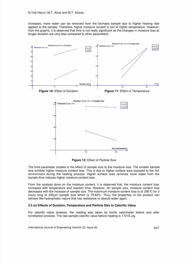
8/8/2019 International Journal of Engineering (IJE), Volume (3): Issue (6)
http://slidepdf.com/reader/full/international-journal-of-engineering-ije-volume-3-issue-6 136/164
N.Yub Harun, M.T. Afzal and M.T. Azizan
International Journal of Engineering Volume (3): Issue (6) 647
increases, more water can be removed from the biomass sample due to higher heating rateapplied to the sample. Therefore, higher moisture content is lost at higher temperature. However,from the graphs, it is observed that time is not really significant as the changes in moisture loss atlonger duration are very less compared to other parameters.
Moisture Loss (%) vs D urationT = 240
T = 280
1.5 3
10
20
30
40
50
60
70
80
Duration (hour)
Moisture Loss (%)
Moisture Loss (%) vs Te mperature
size = 500
size = 250
240 280
20
40
60
80
T (C)
Moisture Loss (%)
Figure 10: Effect of Duration Figure 11: Effect of Temperature
Moisture Loss (%) vs Sample Size
T = 240
T = 280
250 500
20
40
60
80
size (micrometer)
Moisture Loss (%)
Figure 12: Effect of Particle Size
The third parameter studied is the effect of sample size to the moisture loss. The smaller samplesize exhibits higher moisture content loss. This is due to higher surface area exposed to the hotenvironment during the heating process. Higher surface area removes more water from thesample thus induces higher moisture content loss.
From the analysis done on the moisture content, it is observed that, the moisture content lossincreases with temperature and reaction time. However, for sample size, moisture content lossdecreases with the increase of sample size. The maximum moisture content loss is at 280°C for 3hours long of 250µm sample size which is 75.62%. Thus, the properties of the product canbehave like hydrophobic nature that has resistance to absorb water again.
3.3 (e) Effects of Duration, Temperature and Particle Size to Calorific Value
For calorific value analysis, the reading was taken by bomb calorimeter before and aftertorrefaction process. The raw sample calorific value before heating is 17218 J/g.

8/8/2019 International Journal of Engineering (IJE), Volume (3): Issue (6)
http://slidepdf.com/reader/full/international-journal-of-engineering-ije-volume-3-issue-6 137/164
N.Yub Harun, M.T. Afzal and M.T. Azizan
International Journal of Engineering Volume (3): Issue (6) 648
Figure 13: Effect of Duration Figure 14: Effect of Temperature
Figure 15: Effect of Particle Size
Referring to Figure 13, 14 and 15, it is clearly seen that, the torrefied materials can retain thecalorific value almost 100% of the initial value. The research done by Itebe et. al [23] thattorrefaction process can retain up to 90% of the original energy is proven. In fact, the valuesincrease with the increasing heating temperature and reaction time. However, the calorific valuedecreases with the increasing sample size. The higher the calorific value, the better the torrefiedmaterial will be as it provides enough energy to be an alternative fossil fuel.
According to Patrick et. al [20], an increase of the calorific is the main result from the increasingcarbon content and decreasing O/C ratio with the removal of water and gas during torrefaction.Depending on the torrefaction conditions, the low heating value dry of biomass, specifically woodcan be increased from 17-19 MJ/kg to 19 to 23 MJ/kg. Also referring to R. Zanzi et. Al [9], athigher temperature, the carbon content in the product increases while the contents of H and Odecrease. H/C and O/C atomic ratios decrease with the temperature. As a result, the calorificvalue (CV) of the solid product increases with the temperature and at longer residence time.
17000
17100
17200
17300
17400
17500
17600
17700
Calorific
Value (J/g)
Sample
Calorific Value for different duration
Raw
1.5 hours
3 hours
16000
16500
17000
17500
18000
18500
19000
Calorific
Value (J/g)
Sample
Calorific Value for different temperature
Raw
T = 240 C
T = 280 C
16600168001700017200174001760017800180001820018400
Calorific
Value (J/g)
Sample
Calorific Value for different sample size
Raw
500 micrometer
250 micrometer

8/8/2019 International Journal of Engineering (IJE), Volume (3): Issue (6)
http://slidepdf.com/reader/full/international-journal-of-engineering-ije-volume-3-issue-6 138/164
N.Yub Harun, M.T. Afzal and M.T. Azizan
International Journal of Engineering Volume (3): Issue (6) 649
3.3(f) TGA Analysis
Based on the TGA graph obtained, there are three main regions which are the moisture contentrepresented by the first slope, the volatile matter represented by the second slope, and the fixedcarbon represented by the third slope.
0
20
40
60
80
100
120
0 100 200 300 400 500 600 700 800 900
Temperature (oC)
w e i g h t ( % )
RSK 280,3,250
RSK 240,3,250
RSK 280,3,500
Figure 16: TGA graph of Rubber Seed Kernel for each torrefaction condition
From Figure 16, rubber seed kernel of 250 µm that torrefied at 280oC has shown lesser weight
reduction than torrefied at 240oC in the first slope, which region referred as moisture content.Water content has been removed approximately 7% difference between the two conditions.
However, for rubber seed kernel of 500 µm has shown to remove about 6% more than 250 µmsample condition. At same temperature condition bigger particle size gives off lower moisturecontent and lower burn off rate due to smaller surface area in contact to reaction.
Composition vs Temperature
0
10
2030
40
50
60
70
Raw 240 C 280 C
Temperature (C)
C o m p o s i t i o n ( % )
Moisture
Volatile Matter
Fixed Carbon
Composition vs Size
0
10
20
30
40
50
60
70
Raw 500
micron
250
micron
Size (micrometer)
C o m
p o s i t i o n ( %
Moisture
Volatile Matter
Fixed Carbon
Figure 17: Effect of Temperature Figure 18: Effect of Size

8/8/2019 International Journal of Engineering (IJE), Volume (3): Issue (6)
http://slidepdf.com/reader/full/international-journal-of-engineering-ije-volume-3-issue-6 139/164
N.Yub Harun, M.T. Afzal and M.T. Azizan
International Journal of Engineering Volume (3): Issue (6) 650
From Figure 17, it is observed that, the moisture content and volatile matter compositions arereduced slightly as temperature increases. As discussed previously, the reduction is due to theincrease in drying rate of the sample at higher temperature. Therefore, more water and volatilematter is removed at 280°C compared to at 240°C. The moisture content is the first elementwhich is decomposed normally at temperature 100 °C to 150 °C where at this temperature therecondensation and depolymerisation occur to remove the moisture. It is important to analyze thebehaviour of torrefied material as hydrophobic nature which has the resistance to absorb water.Thus, it is expected that the moisture content within the material has lower value for this purpose.As the temperature increases, more moisture can be removed from the torrefied material.
According to Herlina [6], the volatile matter indicates the by-product of torrefaction which includesnon-condensable and condensable gases. High values of volatile matter are a result of highnumber of functional groups and low number of aromatic structures in organic materials. Highvolatile charcoal may be easy to ignite but it burns with heavy smoke. In addition, with highvolatility, the material commonly will be less friable than ordinary material with low volatile matter.Devolutilisation occurs at temperature of 150 °C to 220 °C. The volatile matter should exhibit lowvalue for it to be more friable. In addition, rate of volatile matter removal increases as temperatureincreases.
Apart from that, the fixed carbon content increases as heating process takes place and the value
also increases at higher temperature. High fixed carbon content illustrates high heating capacityas discussed before. As the temperature increases, more volatile matter is being discharged tothe environment which leads to a higher amount of carbon left in the torrefied product. However,the increase is very slight. As referred to Herlina [6], the fixed carbon should illustrate highcontent for torrefied materials. The fixed carbon content induces high calorific value and hencecontributes to become potential fossil fuels for its high energy content. Normally, thecarbonization for torrefaction occurs at temperature between 250 °C to 300 °C.
From the composition analysis done using CHNS Analyzer, the percentage of carbon contentdetermined for torrefied material at 280 °C is 48.19%, while the fixed carbon analyzed by TGAAnalyzer is 36%. Therefore, we can conclude that about 25% of carbon is burnt as volatilehydrocarbon and 75% of total carbon content remains. On the other hand, the percentage ofcarbon content of torrefied material at 240 °C, analyzed by CHNS Analyzer is 44.88% while the
fixed carbon analyzed by TGA Analyzer is 30%. In total, the remaining carbon content left in thetorrefied material is about 67% which is much lower compared to at 280 °C.
Figure 18 shows the relationship between size and the composition of the torrefied products. Theresults obtained shows that the moisture and volatile matter content decrease as the sample sizedecreases while the fixed carbon increases. High surface area of smaller sample size causes theevaporation of water and volatile matter to leave the charcoal quickly and thus, resulting in lowervolatile matter in the product and higher fixed carbon content. This is due to the decrease inOxygen/Carbon and Hydrogen/Carbon ratio. However, the changes are not so much that theamounts of those three components are almost equal for different sizes of material.
For the torrefied material with size of 500 µm, the CHNS Analyzer gives carbon content of 44.2%while the TGA Analyzer gives fixed carbon value of 33%. This shows that the remaining carbon
left is about 75% while the rest is burnt as volatile hydrocarbon. In comparison, the torrefiedmaterial with size of 250 µm also has carbon content left of 75%. This proves that the particlesize of the sample does not give much effect to the torrefied material.
4. CONCLUSION
It is observed that temperature, particle size, and residence time do affect the physical andchemical characteristics of the torrefied products. Almost 100% of the calorific value in all thesamples can be retained or increased by up to 10% from the original waste calorific value. Fromthe Thermo Gravimetric Analysis (TGA), rubber seed kernels exhibited high fixed carbon region

8/8/2019 International Journal of Engineering (IJE), Volume (3): Issue (6)
http://slidepdf.com/reader/full/international-journal-of-engineering-ije-volume-3-issue-6 140/164
N.Yub Harun, M.T. Afzal and M.T. Azizan
International Journal of Engineering Volume (3): Issue (6) 651
at the respective temperature. At the optimum condition of temperature 280°C and particle size of0.025 mm, the torrefied material produced is viable to be promoted at a larger scale.
5. REFERENCES
1. Dewi Soraya. “Torrefied Biomass Waste as Alternative Replacement to Fossil Fuel”. FinalYear Project Dissertation, University Technology PETRONAS, Malaysia. 2008
2. A.V. Bridgwater, G.V.C. Peacocke. “Fast pyrolysis processes for biomass” . Renew. Sust.Energy Rev. 4(1): 1-73, 2000
3. E. Natarajan, A. Nordin, A.N. Rao. “Overview of Combustion and Gasification of Rice Husk in Fluidized Bed Reactors ”. Biomass and Bioenergy, 14(5): 533-546, 1998
4. J. Arcate. “New process for torrefied wood manufacturing”. Bioenergy Update. 2(4), 2000
5. J. Bourgeois and J. Doat. “Proceedings Conference on bioenergy”. Göteborg. Vol.3, 1985
6. M. Herlina. “Production of Torrefied Materials from Waste Biomass”. Final Year ProjectDissertation, University Technology PETRONAS, Malaysia. 2002
7. M. L. Farah Dila. “Pyrolysis of Biomass for Production of Liquid Fuel”. Final Year ProjectDissertation, University Technology PETRONAS, Malaysia. 2008
8. Mark J. Prins, Krzysztof J. Ptasinski, Frans J.J.G. Janssen. “More efficient biomass gasification via torrefaction”. Energy, 31: 3458-3470. 2006
9. R. Zanzi, D. Tito Ferro2, A. Torres3, P. Beaton Soler2, E. Björnbom. “Biomass torrefaction” .http://hem.fyristorg.com/zanzi/paper/zanziV2A-17.pdf , Royal Institute of Technology (KTH),Stockholm, Sweden. 1989
10. Alberto J. Tsamba, Weihong Yang, Wlodzimierz Blasiak. “Pyrolysis characteristics and global kinetics of coconut and cashew nut shells” . Fuel Process Technology, 87(6): 523-530. 2006
11. A.S. Ramadhas, S. Jayaraj, C. Muraleedharan. “Characterization and effect of using rubber seed oil as fuel in the compression ignition engines” . Renewable Energy, 30(5): 795-803,2005
12. A.S. Ramadhas, S. Jayaraj, C. Muraleedharan. “Dual fuel mode operation in diesel engines using renewable fuels: Rubber seed oil and coir-pith producer gas” . Renewable Energy,33(9): 2077-2083, 2008
13. B.V. Babu, A.S. Chaurasia. “Modeling, simulation and estimation of optimum parameters in pyrolysis of biomass” . Energy Conversion Management, 44(13): 2135-2158, 2003
14. A.V. Bridgwater, G.V.C. Peacocke. “Fast pyrolysis processes for biomass” . RenewableSustainability Energy Revision. 4(1): 1-73, 2000
15. Ersan Pu¨tu¨n , Funda Ates, Ays_e Eren Pu¨tu. « Catalytic pyrolysis of biomass in inert and steam atmospheres” . Fuel 87(6): 815-824, 2008

8/8/2019 International Journal of Engineering (IJE), Volume (3): Issue (6)
http://slidepdf.com/reader/full/international-journal-of-engineering-ije-volume-3-issue-6 141/164
N.Yub Harun, M.T. Afzal and M.T. Azizan
International Journal of Engineering Volume (3): Issue (6) 652
16. F. Fonseca Felfli, C. Luengo, G. Bezzon and P. Beaton. “ Bench unit for biomass residues torrefaction”. In Proceedings of Conference on Biomass for Energy and Industry. Würzburg,Germany. 1998
17. Joe¨l Blin, Ghislaine Volle, Philippe Girard, Tony Bridgwater, Dietrich Meier, Biodegradability of biomass pyrolysis oils: Comparison to conventional petroleum fuels and alternatives fuels in current use . Fuel. 86(17-18): 2679-2686. 2007
18. Mohamad K.M. Sabil. “Study on the Production of Charcoal by Carbonization Using Mangrove Wood in Malaysia ”. In Proceedings of Second Engineering CongressionEngineering Innovation and Sustainability: Global Challenges and Issues. Sarawak,Malaysia. 2002
19. S.S. Alves, Figuereido. “A model for pyrolysis for wet wood ”. Chemical Engineering Science,44(12): 2861-2869, 1989
20. Patrick C.A. Bergman, Jacob H.A. Kiel. “Torrefaction for Biomass Upgrading“. InProceedings of 14
th.European Biomass Conference & Exhibition. Paris, France. 2005
21. Malaysian Rubber Review Third Quarterly Industrial Report 2006
22. International Energy Outlook 2007
23. http://library.thinkquest.org/11226/why.htm [retrieved on 11th
March 2008]
24. http://en.wikipedia.org/wiki/Carbon_cycle [retrieved on 12th
March 2008]
25. http://en.wikipedia.org/wiki/Kyoto_Protocol [retrieved on 12th
March 2008]
26. http://unfccc.int/kyoto_protocol/items/2830.php [retrieved on 12th
March 2008]
27. http://en.wikipedia.org/wiki/Biofuel [retrieved on 9th
March 2008]
28. http://en.wikipedia.org/wiki/Second_generation_biofuels [retrieved on 9th
March 2008]
29. http://www.cpeo.org/techtree/ttdescript/pyrols.htm [retrieved on 9th
March 2008]
30. http://www.bioenergywiki.net/index.php/Pyrolysis [retrieved on 11th
March 2008]
31. http://www.btgworld.com/technologies/pyrolysis.html [retrieved on 9th
March 2008]

8/8/2019 International Journal of Engineering (IJE), Volume (3): Issue (6)
http://slidepdf.com/reader/full/international-journal-of-engineering-ije-volume-3-issue-6 142/164

8/8/2019 International Journal of Engineering (IJE), Volume (3): Issue (6)
http://slidepdf.com/reader/full/international-journal-of-engineering-ije-volume-3-issue-6 143/164
Imad Khatib, Moh’d Awad, Kathem Osaily
International Journal of Engineering (IJE), Volume(3):Issue(6) 654
The establishment of the Renewable Energy and Environment Research Unit (REERU) at thePalestine Polytechnic University and its involvement in a multilateral project funded by the US-Citizen Exchange Program of the Department of State entails its cooperation with the FloridaSolar Energy Center (FSEC) of the University of Central Florida and a consortium of universitiesin the Middle East. The outcome of the cooperation is the establishment of the solar energytesting facility at REERU and strengthening the required human capacity. Through cooperationamong REERU, the Palestinian Standards Institute and the Ministry of Higher Education, REERUwas assigned to evaluate the performance of the locally produced SDHW systems and to validatea standard performance testing procedure that enables understanding, predicting and comparingthe performance of the different SDHW systems.
2. TESTING SDHW SYSTEM’S COMPONENTS
The SDHW system used is a thermo-siphon integrated two flat-plate collectors tested with athermal storage tank in an open cycle. The thermal storage tank capacity is 126-Liters. Eachcollector is having an aperture area of 1.42m
2. The collector housing is made of galvanized steel
with 30mm polyurethane insulation separating the housing from the flow risers and headers tubesthat are made of iron. The absorber plate is made of black steel and above it are transparentglass plates. This configuration is usually used in all locally manufactured flat plate solarcollectors. The storage tank core is non-enameled made of 4mm steel sheets insulated from thehousing with 50mm polyurethane and it withstands a maximum attainable pressure of 12bar. Thecollector housing is made of a 0.4mm galvanized steel sheet.
Both the flat plate collectors and the storage tank were tested under transient conditions inaccordance with ANSI/ASHRAE 93-2003 [2] and ISO 1995 [3] standards testing procedures andmethods.
2.1. TESTING FLAT-PLATE SOLAR COLLECTORS
The method used to test the collectors operating with constant flow rate is the steady-statemethod. The method was first proposed by Hill and Kausuda [4], and later published in ASHRAE
standard [5] and ISO 1995 [3]. The steady state testing method depends on measuring theinstantaneous collector efficiency over a range of operating temperature. The data collectedshould correspond to stationary conditions over a period of 15 to 20 minutes. A straight linepresentation is then plotted using the relationship:
η = ηo – UT* (1)
Where the reduced temperature difference T*is computed using Eq. 2:
T*= (Tm – Ta) / GT (2)
And Tm is the mean plate operating temperature, i.e.
Tm
= (Ti+ T
e) / 2 (3)
The slope in Eq. 1 represents the collector heat loss coefficient; U and the intercept with the Y-axis (ηo) is the collector zero loss efficiency or the optical efficiency. For each testing point, theenergy output of the collectors is calculated as:
Qout = mc cP (Te – Ti) (4)
and the energy input as
Qin = GT AC (5)

8/8/2019 International Journal of Engineering (IJE), Volume (3): Issue (6)
http://slidepdf.com/reader/full/international-journal-of-engineering-ije-volume-3-issue-6 144/164
Imad Khatib, Moh’d Awad, Kathem Osaily
International Journal of Engineering (IJE), Volume(3):Issue(6) 655
The resulting of instantaneous efficiency η represented by the ratio of the output to the input(Qout /Qin) is plotted versus the reduced temperature difference T
* in the straight line presentation
of Fig. 1, which represents the collector performance.
FIGURE 1: Solar collector testing results.
The results showed that the collectors have an optical efficiency (ηo) of 65%, which agrees wellwith optical efficiency values for similar collector types, and have a heat loss coefficient (U) of 7.2W/m
2oC.
2.2. TESTING THERMAL STORAGE TANK
The thermal storage tank performance test is carried out to determine the storage heat losscoefficient UAS. The test method is described in ASHRAE 93-2003. In this test, the storage tankis charged to a temperature 61.7
oC attained using the solar collectors and allowed to cool for 48
hours. During charging, no fluid is added to or extracted from the system. Hourly measurement isperformed for the storage temperature and the ambient air temperature where the test isconducted.
By assuming a fully mixed storage losing heat to ambient temperature of Ta it is possible tointegrate the storage tank energy balance equation (Eq. 6) over the test duration; i.e. t in secondsto compute the storage heat loss coefficient as in Eq. 7, i.e.
Ms cp Ts = UAs (Ta – Ts) (6)
UAs = -1/t Ms cp ln{1-(Tsf – Tsi) / (Ta – Tsi)} (7)
A plot (Fig. 2) showing the store temperature decrease over the testing time constitutes anindicator of the thermal storage performance.

8/8/2019 International Journal of Engineering (IJE), Volume (3): Issue (6)
http://slidepdf.com/reader/full/international-journal-of-engineering-ije-volume-3-issue-6 145/164
Imad Khatib, Moh’d Awad, Kathem Osaily
International Journal of Engineering (IJE), Volume(3):Issue(6) 656
FIGURE 2: Storage tank temperature trend over the 48 hours.
The storage tank heat loss coefficient UAS was computed at 1.42 WoC
-1, a value considered
relatively good for such thermal storage. However, in order to improve the thermal storageperformance better insulation may be used including enameling the core of the storage tank.
2.3. TESTING IN SITU THE SDHW SYSTEM
It is clear that the ISO 9459-2 standard testing method is based on the European CSTG method[6]. The method assumes that for a fixed system and a fixed load, where there is little or no carry-over of energy from one day to the next, the climatic parameters which significantly affect dailysystem performance are:
• the daily solar irradiance on the plane of the collector H,• the average ambient air temperature Ta during day time, and• main cold water temperature supplied to the system TC.
A correlation between these parameter is assumed which represents an approximate linearrelationship between the solar irradiance and the system output which takes the form in Eq. 8:
Qout = a1H + a2(Ta – Tc) + a3 (8)
The correlation expressed in Eq. (8) forms the basis of the test method where, from results ofseveral tests employing different values of H, Ta and Tc, the values a1, a2 and a3 can bedetermined using a multi-regression fit method. It is worth mentioning that a 1 represent theirradiance part of the model equation, a2 is the part of the energy lost or gained from thetemperature difference and a3 is the balance coefficient.
The test procedure carried out consists of one day tests which are independent of each other. Foreach test the system is first preconditioned bringing the store temperature to the cold watertemperature. During that time collectors are covered to ensure no heat gained by solar radiation.The circulation of water through the store is stopped after ensuring that the temperature in thestore is uniformly distributed. The system then charges by taking off the collectors' cover and
exposing them to sun rays. Immediately after the charge phase a single draw-off of three timesthe store volume is performed in order to ensure that there was no carryover of energy to the nextday.
The test is repeated over several days constituting different values of irradiance levels, ambientair temperatures, and mains water temperatures. During the course of each test the irradiance ismeasured over the plans of the collectors. And during the charging phase, hourly measurementsare performed for the ambient air temperature, and the store temperature. The temperaturedifference between the outlet and the inlet to the store is also recorded over a time increment of60 seconds.

8/8/2019 International Journal of Engineering (IJE), Volume (3): Issue (6)
http://slidepdf.com/reader/full/international-journal-of-engineering-ije-volume-3-issue-6 146/164
Imad Khatib, Moh’d Awad, Kathem Osaily
International Journal of Engineering (IJE), Volume(3):Issue(6) 657
The test is performed using an average flow rate of draw-off that is recommended by the testingmethod, which is 600 Liter/hour. The data obtained from the different tests are used in themathematical thermal model equation (Eq. 8) and by using a multi-regression method themathematical model coefficients a1, a2 and a3 are identified for the different levels of irradiances(Table 1).
Irradiance Levela1
(m2)
a2(MJ/K.day)
a3(MJ/day)
Low 0.56 0.26 0.60Medium 0.53 2.11 4.02High 1.01 1.19 3.72
TABLE 1: Mathematical model constants (a-parameters).
The values of the model constants a1 – a3 are used then in predicting the long-term performanceof the SDHW system.
2.4. SYSTEM DRAW-OFF TEST
The performance of the SDHW system depends on the internal operation of its component. Oneof the most influential parts of the SDHW system is the thermal storage tank. During extraction of
energy the type of the store is dependent on the flow rate. The stratification will decrease withincrease in the flow rate through the store due to increase in mixing between mains cold waterentering the store and the hot water inside the store.
The system under test showed that its vertical storage tank type tends to be fully mixed during theenergy charging phase. During extraction of energy the store appears to be stratified. Thestratification increase with the increase in the energy input. In Fig. 3 below are the three curvesshowing different draw-offs under different irradiance levels. It could be seen that the dischargedheat (Qout) is proportional to the area under the curve.
FIGURE 3: Draw-off curves for the different irradiance levels.
The draw-off curves that represent the energy output of the system when drawing 3 times its volume, couldbe used to measure the energy output from the system and the energy left over in the system by assigningthe draw-off energy fraction f(v). By knowing the demand water volume that would be drawn-off (extracted)from the system, the fraction f(v) could be calculated. In this test a demand water volume of 150 Liter/day isconsidered, which constitute 1.19 times the tank volume of 126 Liter. Using the draw-off curves for the

8/8/2019 International Journal of Engineering (IJE), Volume (3): Issue (6)
http://slidepdf.com/reader/full/international-journal-of-engineering-ije-volume-3-issue-6 147/164
Imad Khatib, Moh’d Awad, Kathem Osaily
International Journal of Engineering (IJE), Volume(3):Issue(6) 658
different levels of irradiance, the different values of f(v) could be calculated as shown in Table 2. The sametable shows the fraction of energy when extracting the same tank volume of 126 Liter.
Irradiance Level f(v) for 150 Liter f(v) for 126 LiterLow 0.78 0.66Medium 0.79 0.68High 0.84 0.72
TABLE 1: Values of the fraction f(v) calculated for different levels of Irradiance.
2.4. SYSTEM MIXING TEST
While the draw-off profile represents the effect of temperature stratification in the storage tank,and mixing during discharging the system, there is a need to determine the effect of mixing duringdraw-off independent of the temperature stratification inside the store. This is achieved bydischarging the system after establishing a uniform temperature distribution inside the store, andby using the same flow rate utilized in draw-off profiles.
The resulting mixing profile can be seen in Fig. 4. It is seen that after consuming a volume equalsto store volume (i.e. 126 Liter), the fraction of energy extracted g(v) is approximately 0.86 of thetotal energy withdrawn, and 0.90 of the total energy is for a demand load of 150 Liter.
FIGURE 4: Mixing profile.
3. LONG-TERM SYSTEM PERFORMANCE PREDICTION
Long term performance prediction of the SDHW system is computed using a Day-by-Day methoddescribed in the European CSTG documents and later adopted by the ASHRAE 93-2003. Themethod requires several parameters to be pre-identified, i.e. those identified in the short-temtests, as well as the dominant meteorological settings (or any other setting) for the location wherethe system is going to be installed. In addition daily mains cold water temperature recorded orcalculated is considered essential for consistent calculations. In this respect, the BritishStandards (BS 5918) of 1982 [7] referenced a correlation for computing mains cold watertemperature. This correlation was later modified to suit the Palestine climate and is written in the
form:
Tc =18 - 5.5 x cos((2 x pi/365.5) x (D + 11.25)) (9)
For the long-term calculation, the annual climate data used is taken from the MeteorologicalStation of the Renewable Energy and Environment Research Unit (REERU).The weather stationrecords values on time increment of 15 minutes and store them for each year.

8/8/2019 International Journal of Engineering (IJE), Volume (3): Issue (6)
http://slidepdf.com/reader/full/international-journal-of-engineering-ije-volume-3-issue-6 148/164
Imad Khatib, Moh’d Awad, Kathem Osaily
International Journal of Engineering (IJE), Volume(3):Issue(6) 659
The Day-by-Day method calculate the performance of the SDHW system for each day using theinput meteorological values of that day, and taking into account any energy in the system that iscarried over from the previous day. The method assumes that if the water in the storage tank is ata temperature higher than the cold water temperature at the beginning of the day, due to carry-over of energy from the previous day, this energy is equally spread over the tank volume at startof the next day (i.e. the storage tank is always in a fully mixed state with a uniform temperature atthe start of each day).
The total energy captured by the first operating day is given by the Input\Output diagram. Thedraw-off temperature profile enables the division of this amount of energy into useful energyextracted during draw-off and energy carried over through using the fraction f(v).
The energy remaining in the storage tank will partly be lost overnight due to heat losses , and willforce the system to start the next morning at a temperature higher than the cold supplytemperature. At this stage, and for each of following days, the assumption mentioned before ismade so that the energy is uniformly distributed over the store, leading to a uniform temperatureat the beginning of the next day.
At the end of the second day and all the following days the system output can be calculated usingthe morning store temperature. A division is made in used and remaining energy using the draw-
off profile f(v). This energy output represent only a part of the total energy output, as the systemrefilled with water at temperature Tc and not the morning store temperature. The division of thesecond part of the extracted and remaining energies is made based on the mixing-profile g(v).And so forth, the calculation is performed day-by-day, for each month and for the whole year. Theoutput are the solar fraction for each month of the year (fm), the yearly solar fraction (f), theenergy output from the system and the energy delivered to the system.
3.1. LONG-TERM PREDICTION RESULTS
The system coefficients a1, a2 and a3 computed are used in three consecutive model runs topredict the annual system performance. The annual delivered energy Qout, which is the sum of thedaily delivered energy, was calculated using a fixed demand volume of 150 Liters, and a demandtemperature of 60
oC was chosen for the calculation.
The results of the annual performance prediction using the day-by-day performance predictionmethod is seen in Fig. 5 where both energy delivered to the SDHW system and energy extractedfor each month of the year considered are presented in histograms.
FIGURE 5: Histogram showing monthly variations between energy output and energy delivered.
The annaul solar fraction was computed at 0.18 which means in economic words an annualsaving of more than US$120 and a payback period for the SDHW system of 6-7 years.

8/8/2019 International Journal of Engineering (IJE), Volume (3): Issue (6)
http://slidepdf.com/reader/full/international-journal-of-engineering-ije-volume-3-issue-6 149/164
Imad Khatib, Moh’d Awad, Kathem Osaily
International Journal of Engineering (IJE), Volume(3):Issue(6) 660
It should be mentioned here that the mathematical input/output model (Eq. 8) showed highsensitivity for the day length and the variation in the level of irradiance.
3.2. RECOMMEDNED MODIFIED MATHEMATICAL MODLE
The sub-task E of the International Energy Agency (IEA) has suggested a stationary model for
the short-term testing of the SDHW systems [8]. The model was called the c-model that identifies5 parameters, reduce the testing time and provide more variability of test data. The correlationmodel expressed in the form:
Qout (1+c3c4δt / (ML cp)) = c1 Σ (GT Kατ – c2 {Tc - Ta+c4 Qout / (ML cp)})
+ ∆t – c3 δt (Tc – Ta) –
c5 δt (TD – Ta) (10)
The coefficient c1 – c5 are system parameters that can be identified by a best fit to test data. It isworth mentioning that the last term of Eq. 10 accounts for thermal auxiliary source during testingand hence for real testing the term could be excluded; i.e. c5 accounts to zero. Marshall et al. [9]have added a term to Eq. 10 that accounts for carryover of energy, changing the model fromstationary to non-stationary model as in Eq. 11:
Qout (1+c3c4δt / (ML cp)) = c1 Σ (GT Kατ – c2 {Tc - Ta +c4 Qout / (ML cp)})
+ ∆t – c3 δt (Tc – Ta) –
Ms cp δt (Tsn+1
– Tsn) (11)
Where, Tsn+1
and Tsn
are the store temperature at end of the test day and at the beginning of thetest day respectively.
Eq. 11 could be written in terms of energy output (Qout) as:Qout = c1Σ(GT - c2 {Tc – Ta + c4 Qout / (ML cp)})
+ ∆t –
c3 δt (Tc - Ta) – c3 c4 δt Qout / ML cp) – Ms cp (Ts
n+1– Ts
n) (12)
By assuming that all energy is utilizable (the + sign) then the equation should be reduced to:
Qout (1+(c1c2c4 /ML cp)Σ∆t + c3c4 δt / ML cp) =c1 ΣGT ∆t – c1c2 (Tc – Ta)Σ∆t – c3 δt (Tc - Ta) – Ms cp (Ts
n+1– Tn
n) (13)
OrQout = [c1 / (1+d+e)]H +
[c1c2 Σ∆t + c3δt / (1+d+e)] (Ta – Tc) +[-1 / (1+d+e)] ∆Qstore (14)
Assuming that the values:d = (c1c2c4 / ML cp) Σ ∆te = c3c4 δt / ML cp
∆Qstore = Ms cp (Ts
n+1
– Ts
n
)
Comparing the model Eq. 14 with the model Eq. 8 showed that the coefficients a 1 – a3 are givenby:
a1 = c1 / (1+d+e)a2 = c1c2 Σ δt + c3 t / 1+d+ea3 = -1 / 1+d+e

8/8/2019 International Journal of Engineering (IJE), Volume (3): Issue (6)
http://slidepdf.com/reader/full/international-journal-of-engineering-ije-volume-3-issue-6 150/164
Imad Khatib, Moh’d Awad, Kathem Osaily
International Journal of Engineering (IJE), Volume(3):Issue(6) 661
By knowing either a1 – a3 or c1 – c4 the other parameters could be identified. This mathematicalmodel assumes one day length and the four c - parameters depend primarily on the SDHWsystem operation conditions and its performance parameters. Hence, to reduce the sensitivity ofthe input/output model (Eq. 8) on the day length and the irradiance levels it is possible to performfew short-term tests using constant day length and solve the equation to find c-parameters andthe corresponding a-parameters for the long-term calculations.
The mathematical model needs to be verified and hence future work will concentrate on testingthe model and comparing the results with the previous ones.
4. CONCLUSIONS
Testing the performance of the locally manufactured SDHW system and its components using theASHRAE 93-2003 and ISO 1995 and combining the resulted performance parameters to the day-by-day long-term performance prediction procedure brought relatively good results. However, it isfound that the results of the mathematical input/output model and the testing procedure aresensitive to day length and to irradiance levels. A new mathematical model that is based on theIEA utilizable model and the input/output model used is proposed. It is suggested that the newmodel may minimizes the dependency of the input/output model on the day length and the
irradiance levels.
4. CONSLUSION & FUTURE WORK
5. REFERENCES
1. PCBS “Households energy survey results - April 2008”. Palestinian Central Bureau ofStatistics, Palestinian Authority, 2008
2. ANSI/ASHRAE Standards 93-2003 “Methods of testing to determine the thermal performanceof solar collectors”. ASHRAE publication, Atlanta, GA30329, 2003
3. ISO 1995 “Solar heating-domestic water heating systems – part 2: outdoor test method forsystem performance characterization and yearly performance prediction of solar onlysystems”. Ref. no. ISO 9459-2:1995(E), International Standards Organization, 2995
4. Hill, J.E. and Kausuda, T. “Methods of testing for rating solar collectors based on thermalperformance”. NBS Report, NBSIR, 74-635, 1974
5. ASHRAE Standards 95-1981 “Methods of testing to determine the thermal performance ofsolar domestic water heating systems”. AHRAE publication, Atlanta, GA30329, 1981
6. European Solar and System Testing Group “Test method for solar water heating systems,Second international draft, Proceedings of the 6
thmeeting of the European Solar Collector
and System Testing Group (CSTG), Joint Research Center, Ispra, Italy, 19877. BS 5918 “Code of practice for solar heating systems for domestic hot water”. British
Standards Institution, London, UK, 1982
8. Spirikl, W. “SDHW short-term test simulation using a utilizability based correlation model”.Internal Report to the International Energy Agency (IEA), III-E Document, IEA, 1987
9. Marshall, R. and Barragan, F. A simulation study of the IEA system test procedure”. Dept. ofMechanical Engineering and Energy studies, report no. 1440, University of Wales, Cardiff, U,1988

8/8/2019 International Journal of Engineering (IJE), Volume (3): Issue (6)
http://slidepdf.com/reader/full/international-journal-of-engineering-ije-volume-3-issue-6 151/164
K.Meena alias Jeyanthi & A.P.Kabilan
International Journal of Engineering,IJE volume(3),Issue(6) 662
Modeling and simulation of Microstrip patch array for smartantennas
K.Meena alias Jeyanthi, [email protected]
Assistant Professor,PSNA College of Engineering & Technology,Dindigul, Tamil Nadu, India.
A.P.Kabilan, [email protected] Principal,Chetinad College of Engineering & Technology,Karur, Tamil Nadu, India.
Abstract
The aim of the paper is two fold. One is to design and simulate an antenna array
suitable for wireless applications and the other is the design of beamformingalgorithm. In this paper, the first module presents the design of multiplemicrostrip rectangular patch elements suitable for beamforming technique inwireless applications in the range of 1.8 - 2.4 GHz. By designing 1x8 patch array,it is possible to achieve 15 dB gain and 58% more directivity compared to theconventional patches. The second module suggests a NLVFF-RLS algorithm forbeamforming technique to concentrate the power in the desired direction andnullify the power in the interferer direction with HPBW of 13°.The results areanalyzed for the scanning sector of -60° to 60°. The modeling and simulation ofantenna array is computed using Agilent’s ADS. The beamforming algorithm isdesigned in Matlab.
Key words: Adaptive antennas, antenna arrays, microstrip patch, beamforming.
1. INTRODUCTION
The rising importance of wireless communication and multimedia services increasing the effortsto the design and implementation of novel microstrip patch structures from miniaturized electroniccircuits to the antenna arrays[2]. The main advantages of microstrip patches are light weight, lowcost, planar or conformal and ability of integration with electronic or signal processing circuitry.Microstrip antenna elements radiates efficiently as devices on microstip printed circuit boards.Microstrip antenna array consists of microstrip antenna elements, feed and phasingnetworks.Designing microstrip structure requires understanding of both mathematical relativesand applications[2].The microstrip array is very reliable since the entire array is one continous
piece of copper.
Microstrip patch antenna consists of a radiating patch on one side of a dielectric substrate with acontinuous metal layer bonded to the opposite side of the substrate which forms a ground plane.The patch is generally made of conducting material such as copper or gold and can take anypossible shape. A patch antenna is a narrowband, wide-beam antenna fabricated by photoetching the antenna element pattern in metal trace on the dielectric substrate shown in figure 1.
1.1 Design of microstrip patch array

8/8/2019 International Journal of Engineering (IJE), Volume (3): Issue (6)
http://slidepdf.com/reader/full/international-journal-of-engineering-ije-volume-3-issue-6 152/164
K.Meena alias Jeyanthi & A.P.Kabilan
International Journal of Engineering,IJE volume(3),Issue(6) 663
r
Lε
λ
2=
The following are the design equations of the single patch[2],The actual Length of the Patch is, (1)
Effective relative dielectric permittivity,(2)
the effective Length of the Patch is, (3)
FIGURE 1: Rectanular microstrip antenna element
The Extension Length due to fringing field,
(4)
The coaxial feed is a very common technique used for feeding microstrip patch antennas asshown in figure 2.
FIGURE 2: side view of element with coaxial feed
1.2 Simulation of single and multiple array
A single patch antenna provides a maximum directive gain of around 6-9 dB. It is relatively easyto print an array of patches on a single (large) substrate using lithographic techniques[2]. Patcharrays can provide much higher gain than a single patch at little additional cost; matching andphase adjustment can be performed with printed microstrip feed structures. The ability to createhigh gain arrays in a low-profile antenna is one reason that patch arrays are common in allwireless applications[2]. The antenna model is simulated by Agilent’s ADS which is a powerfultool in the design of multilayer micostrip antennas. In early days, most of the designers usesgraphical tool for the design of antennas[10,11]. Figure 3 shows the return loss of -13 dB forsingle patch and figure 4 shows the return loss of -18dB for 1x8 patch array for the center

8/8/2019 International Journal of Engineering (IJE), Volume (3): Issue (6)
http://slidepdf.com/reader/full/international-journal-of-engineering-ije-volume-3-issue-6 153/164
K.Meena alias Jeyanthi & A.P.Kabilan
International Journal of Engineering,IJE volume(3),Issue(6) 664
1.85 1.90 1.95 2.00 2.05 2.10 2.151.80 2.20
-15
-10
-5
-20
0
freq, GHz
_
,
1.85 1.90 1.95 2.00 2.05 2.10 2.151.80 2.20
-10
-5
-15
0
Frequency
a g .
S11
frequency of 1.85GHz. Even the fractal antennas have the S11 of -27dB which is comparable withthis.[9].Figure 3 & 4 shows the return loss is obtained for the same resonant frequency of1.85GHz accurately.
FIGURE 3: Return loss of single patch
FIGURE 4: return loss of 1x8 elements
2. DESIGN OF ARRAY OF PATCHES
2.1 Substrate selectionIt is important to choose a suitable dielectric substrate of appropriate thickness’ h’ and losstangent ’δ’. A thicker substrate are mechanically strong, will increase the radiated power, reduce
conductor loss and improve the impedance bandwidth[2]. A high loss tangent increases thedielectric loss and therefore reduces antenna efficiency. Here the substrate selected as1/32in(1.58mm)and loss tangent of 0.024 for the operating frequency ranges from 1.8-2.4GHz.2.2 Element width and LengthPatch width has a minor effect on the resonant frequency and radiation pattern of the antenna.With the proper excitation, a patch width ‘W’ greater than the patch length ‘L’ without excitingundesired modes. The patch width affects the cross polarization characteristics.

8/8/2019 International Journal of Engineering (IJE), Volume (3): Issue (6)
http://slidepdf.com/reader/full/international-journal-of-engineering-ije-volume-3-issue-6 154/164
K.Meena alias Jeyanthi & A.P.Kabilan
International Journal of Engineering,IJE volume(3),Issue(6) 665
FIGURE 5: Array of 8 patches
In this paper, a broadband rectangular microstrip patch antenna using the permittivity of εr of4.28, log tan δ of 0.024. The length and breadth of the patch is 51.25mm and 40.01mmrespectively. The uniform linear array of patches with spacing of 0.5λ are arranged as shown infigure 5.2.3 Radiation patternThe radiation pattern of an antenna is prime important in determining most of the characteristics
which include beamdwidth,beam shape, sidelobe level, directivity and radiated power. Radiationpattern is computed using method of moments in ADS.2.4 BeamwidthThe half power beamwidth(HPBW) of an antenna is equal to the angular width between thedirections where radiated fields reduced to 1/ √2 times the maximum value.2.5 Directivity and gainThe directivity is a measure of the directional properties of an antenna compared to the isotropicantenna. Directivity is generally high for array antennas. The gain of the antenna directly dependson the radiation efficiency and the directivity of the antenna[2]. It is observed that directivityincreases with increase of substrate thickness and patch width. Conversely, the beamwidth isexpected to decrease for higher values of ‘h ‘and ‘W’.
Figure 6 shows the E plane beamwidth of the array. The dimensions and the antenna parameters
are tabulated in table 1.
FIGURE 6: Radiation pattern of 1x8 patches

8/8/2019 International Journal of Engineering (IJE), Volume (3): Issue (6)
http://slidepdf.com/reader/full/international-journal-of-engineering-ije-volume-3-issue-6 155/164
K.Meena alias Jeyanthi & A.P.Kabilan
International Journal of Engineering,IJE volume(3),Issue(6) 666
The conventional single patch has the directivity of 7-8dB.But it is observed that the directivity of1x8 array is improved by 6 dB compared to the single patch. The gain of the array is found to be15 dB.
Operating frequency(fo) 1.85 GHz Power radiated(Watts) 0.046
Width of single patch(W) 51.25mm Effective angle(deg) 0.41 steradian
Length of single patch(L) 40.01mm Directivity(dB) 14.832
Height 1.5 mm Gain(dB) 14.8287
No.of elements 8 Intensity(Watts) 0.112
Distance between elements 0.5 λ E(theta) 81.68
Feed line length 9.5 mm E(phi) 82.68
Radius of the field 0.5 mm
Table 1: Antenna parameters
3. SMART ANTENNAS
Smart antennas gain more space in modern wireless communication systems using the importantproperty of spatial filtering[8]. The increasing demand for mobile communication services in alimited RF spectrum motivates the need for better techniques to improve spectrum utilization aswell as the development of new high bit rate applications[1]. A smart antenna is an antenna arraysystem aided by some smart algorithm designed to adapt to different signal environments[2]. Inthis paper our approach is presented by designing an adaptive algorithm using a lineararrangement of rectangular antenna array, with 8 elements, a high degree-of-freedom exists tosynthesize very sophisticated radiation patterns[7].
FIGURE 7: Structure of the adaptive array

8/8/2019 International Journal of Engineering (IJE), Volume (3): Issue (6)
http://slidepdf.com/reader/full/international-journal-of-engineering-ije-volume-3-issue-6 156/164
K.Meena alias Jeyanthi & A.P.Kabilan
International Journal of Engineering,IJE volume(3),Issue(6) 667
A linearly arranged and equally spaced array of antenna forms the structure of a beam former. Inorder to form a beam, each user input signal is multiplied by a set of complex weights and thentransmitted from the array to the distant point, the signal emitted from the antennas in the arraydiffer in phase as well as amplitude. If the weights are computed and updated in real time, theprocess is known as adaptive beam forming [3]. The structure of the adaptive antenna array isshown in figure 7.
Adaptive process permits narrower beam and improving the signal to noise ratio only in thedirection of that particular user. This technique drastically reduces the interference in the system.In digital beamforming, the received RF signals are down converted to intermediate frequency(IF) and then digitized by Analog-to-digital converters (ADC). The availability of digital signalsenables the use of a considerable number of processing algorithms, because the adaptation canbe performed by the controlling software at a lower frequency.
3.1. Non linear variable forgetting factor recursive least squares algorithm (NLVFF-RLS)
The Recursive Least Squares (RLS) algorithm offers an alternative to the LMS algorithm as a toolfor the solution of adaptive filtering problems. This algorithm uses the least squares estimate ofthe tap weight vector of the filter at iteration n-1, to compute the updated estimate of the vector at
iteration ‘n’ upon the arrival of new data. Hence this algorithm is referred as the Recursive LeastSquares (RLS) algorithm.The recursive equation for updating the tap- weight vector is,
−−
+−= )()()1()(*nnk nW nW ξ (5)
)1()()()(
*
−−=
−
nW nund nT ξ , (6)
is the a priori estimation error.k(n) is the gain vector. k(n) is expressed as
)()(
)()(
nnu
nnk
H π λ
π
+
= (7)
The intermediate quantity )(nπ is computed as
)()1()( nunPn −=π (8)
The inverse correlation matrix is computed as
)1()()()1()(11
−−−=−−
nPnunk nPnPH λ λ (9)
3.2 Forgetting factor
In the case of non stationary environment, the algorithm[3] uses the forgetting factor λ €(0,1).
Here the constant forgetting factor used is λ =0.95.The constant forgetting factor will not produce
the optimal performance. Hence the nonlinear variable forgetting factor is preferred. RLSapproach leads to higher complexity, but provides a higher speed of convergence and performsbetter in flat fading channels. The nonlinear forgetting factor can be obtained by error
measurements and updating the constant forgetting factor λ non linearly .The optimal filtering
gain k should be chosen in such a way that the equalization error is an uncorrelated noisesequence.
i
H
i
i
S
iuiPnu ))1()1()(1(1 −−+=
−λ
λ (10)
where ,0)1(1
=−−−
iiiSk unPλ
This algorithm produces feed back control by updating the gain and forgetting factor λ based on
the nonstationary environment.

8/8/2019 International Journal of Engineering (IJE), Volume (3): Issue (6)
http://slidepdf.com/reader/full/international-journal-of-engineering-ije-volume-3-issue-6 157/164
K.Meena alias Jeyanthi & A.P.Kabilan
International Journal of Engineering,IJE volume(3),Issue(6) 668
Linear Polarization
- 8 0
- 6 0
-4 0
-2 0
0 2 0
4 0
6 0
8 0
-1 0 0
1 0 0
-50
-40
-30
-20
-10
-60
0
THETA
a g . [ d
]
E_co E_cross
- 8 0
- 6 0
-4 0
-2 0
0 2 0
4 0
6 0
8 0
-1 0 0
1 0 0
-135
-90
-45
0
45
90
135
-180
180
THETA
P h a s e [ d e g ]
- 8 0
- 6 0
-4 0
-2 0
0 2 0
4 0
6 0
8 0
-1 0 0
1 0 0
10
20
30
40
0
50
THETA
M a g . [ d B ]
Axial Ratio
- 8 0
- 6 0
-4 0
-2 0
0 2 0
4 0
6 0
8 0
-1 0 0
1 0 0
-135
-90
-45
0
45
90
135
-180
180
THETA
P h a s e [ d e g ]
Circular Polarization
- 8 0
- 6 0
-4 0
-2 0
0 2 0
4 0
6 0
8 0
-1 0 0
1 0 0
-50
-40
-30
-20
-10
-60
0
THETA
a g .
[ d
]
E_left E_right
- 8 0
- 6 0
-4 0
-2 0
0 2 0
4 0
6 0
8 0
-1 0 0
1 0 0
-135
-90
-45
0
45
90
135
-180
180
THETA
P h a s e [ d e g ]
- 8 0
- 6 0
-4 0
-2 0
0 2 0
4 0
6 0
8 0
-1 0 0
1 0 0
10
20
30
40
0
50
THETA
M a g .
[ d B ]
Axial Ratio
- 8 0
- 6 0
-4 0
-2 0
0 2 0
4 0
6 0
8 0
-1 0 0
1 0 0
-135
-90
-45
0
45
90
135
-180
180
THETA
P h a s e [ d e g ]
Absolute Fields
- 8 0
- 6 0
-4 0
-2 0
0 2 0
4 0
6 0
8 0
-1 0 0
1 0 0
1
1E-1
9E0
THETA
a g .
[ ]
Etheta Ephi
- 8 0
- 6 0
-4 0
-2 0
0 2 0
4 0
6 0
8 0
-1 0 0
1 0 0
-135
-90
-45
0
45
90
135
-180
180
THETA
P h a s e [ d e g ]
Htheta Hphi
- 8 0
- 6 0
-4 0
-2 0
0 2 0
4 0
6 0
8 0
-1 0 0
1 0 0
-135
-90
-45
0
45
90
135
-180
180
THETA
P h a s e [ d e g ]
Power
- 8 0
- 6 0
-4 0
-2 0
0 2 0
4 0
6 0
8 0
-1 0 0
1 0 0
-30
-20
-10
0
10
-40
20
THETA
a g .
[ d
]
Gain Directivity
- 8 0
- 6 0
-4 0
-2 0
0 2 0
4 0
6 0
8 0
-1 0 0
1 0 0
1020
3040
5060
7080
90
0
100
THETA
e r c e n t a g e
Efficiency
- 8 0
- 6 0
-4 0
-2 0
0 2 0
4 0
6 0
8 0
-1 0 0
1 0 0
1E-5
1E-4
1E-3
1E-2
1E-6
4E-2
THETA
a g .
[ m 2 ]
Effective Area
- 8 0
- 6 0
-4 0
-2 0
0 2 0
4 0
6 0
8 0
-1 0 0
1 0 0
1E-5
1E-4
1E-3
1E-2
1E-6
1E-1
THETA
a g .
[
/ s t e r a d ]
Radiated Power
- 8 0
- 6 0
-4 0
-2 0
0 2 0
4 0
6 0
8 0
-1 0 0
1 0 0
1E-3
1E-2
1E-4
3E-2
THETA
a g .
[ ]
4. RESULTS AND DISCUSSION
The simulated system consists of an eight element uniform linear array spaced at halfwavelength. The operating frequency selected as 1.8GHz. The channel is modeled as additivewhite Gaussian channel. The received signals are modeled in the base band processing andmodulated by MSK (Minimum Shift Keying) signals. The modulated signals are multiplied bysteering vectors to simulate array processing technology. Inverse correlation matrix wascomputed, and the weights are updated.
FIGURE 8: Amplitude response of the array

8/8/2019 International Journal of Engineering (IJE), Volume (3): Issue (6)
http://slidepdf.com/reader/full/international-journal-of-engineering-ije-volume-3-issue-6 158/164
K.Meena alias Jeyanthi & A.P.Kabilan
International Journal of Engineering,IJE volume(3),Issue(6) 669
-60 -40 -20 -12 0 810 15 20 25 30-50
-45
-40
-35
-30
-25
-20
-15-14
-10
-5
0
5Beam pattern of VFF-RLS & RLS
( d B )
angle(degrees)
RLS
NLVFF-RLS
HPBW-13
Figure 8 shows the Amplitude response the 1x8 antenna array. Figure 9 shows the power patterncomparison of NLVFF-RLS and RLS algorithm which is scanning efficiently with half power beamwidth of 13 º for the scanning sector of -60º to 60º . The side lobe level is varying between -14 dBto -18dB which is appreciable value compared to the conventional methods [12].
Figure 9: Beam pattern comparison of NLVFF-RLS and RLS
The various parameters are computed for the scanning sector of -60° to 60° are half power beamwidth(HPBW), null point suppression and compared with the conventional LMS and RLSalgorithms are shown in table 2.
Table 2: Comparision of algorithms
4. CONCLUSION
Due to the high cost and complexity of the design for planar and high resolution array, the designfocused on the development of uniform linear array antenna. The array designed using method ofmoments in ADS to obtain the directivity of 14 dB (58% increase compared to the normalpatch).The proposed structure uses the spacing 0.5 λ, provides the return loss of 18 dBreferenced to the center frequency 1.85 GHz. The second goal is achieved by concentrating thepower in the specified direction with a HPBW of 13° in the scan sector of -60° to 60°. Simulationresults showed that NLVFF-RLS provides remarkable improvement in null point suppression of50dB, convergence rate of 10 iterations and minimum mean square error over that of RLS. The
Algorithm HPBW(deg)
SLL(db)
No.ofIter
Null pointSupp(db)
LMS 14 12 25 30
RLS 18 14 15 40
NLVFF-RLS 13 14 10 50

8/8/2019 International Journal of Engineering (IJE), Volume (3): Issue (6)
http://slidepdf.com/reader/full/international-journal-of-engineering-ije-volume-3-issue-6 159/164
K.Meena alias Jeyanthi & A.P.Kabilan
International Journal of Engineering,IJE volume(3),Issue(6) 670
presented algorithm confirms the adaptive antennas are able to sustain a large number ofsimultaneous communication with respect to directional and switched beam technologies.
5. REFERENCES
1. Simon Haykin, “Adaptive Filter Theory”, Fourth edition n, 2002
2. Ramesh Gharg, Prakash Bhartia, ”Microstrip Antenna design Handbook”, Artech House,2000
3. Jeffrey H. Reed, ”Software Defined radio”, Pearson education, 2006
4. M.Mukhopadhyay, B.K.Sarkar, ”Augmentation of antijam GPS system using smartantenna with a simple DoA estimation algorithm”, PIER, 67, 231-249,2007.
5. L. J. Griffith and C. W. Jim, “An Alternative Approach to Linearly Constrained AdaptiveBeamforming”, IEEE Trans. AP , 30(1): 27–34, 1982.
6. K.Meena alias Jeyanthi, Dr.A.P.Kabilan, “A simple adaptive beamforming allgorithm withinterference suppression”, International journal of Engineering and Technology, vol.1,N0.1, pp 67-70, April 2009.
7. K.Meena alias Jeyanthi, Dr.A.P.Kabilan, “A NLVFF-RLS approach to adaptivebeamforming for wireless communication”, ICCCNET,2008.
8. A.P. Kabilan, P. Elizabeth Caroline, X. Susan Christina, “An optical beamformer for smartantennas in mobile broadband communication”, International journal of mobilecommunications, vol.7, no.6, pp-683-694, 2009.
9. Niruth Prombutr, Prayoot Akkaraaektharm, ”Analysis and design of Hilbert curve fractalantenna feed with coplanar wave guide for multiband wireless communications”,
International Journal of Engineering, volume 2, Issue 3, 2003.
10. Z.Rostamy, “Determination of resonant requency of dominant and higherorder modes in thin and thick circular mcrostrip patch antennas withsuperstrate by MWM”, International journal of Engineering,volume 16,November 2003.
11. M.R. Doushabchizadeh, S. Taromi and A.Radji, ”TV and OR FMtransmitting antennas design using computer graphic system”, volume 7,International Journal of Engineering, August 1994.
12. Ali Varahram, Jalil Rashed Mohassel, K.Mafinezhad, ”Optimization ofarray using modified genetic algorithm”, Vol. 17, No 4, IJE Transactions:
Applications, Dec 2004.

8/8/2019 International Journal of Engineering (IJE), Volume (3): Issue (6)
http://slidepdf.com/reader/full/international-journal-of-engineering-ije-volume-3-issue-6 160/164
CALL FOR PAPERS
International Journal of Engineering (IJE) is devoted in assimilatingpublications that document development and research results within
the broad spectrum of subfields in the engineering sciences. The journal intends to disseminate knowledge in the various disciplines of
the engineering field from theoretical, practical and analytical research
to physical implications and theoretical or quantitative discussion
intended for both academic and industrial progress.
Our intended audiences comprises of scientists, researchers,
mathematicians, practicing engineers, among others working in
Engineering and welcome them to exchange and share their expertisein their particular disciplines. We also encourage articles,
interdisciplinary in nature. The realm of International Journal of
Engineering (I JE) extends, but not limited, to the following:
Aerospace Engineering
Agricultural Engineering
Biomedical EngineeringChemical Engineering
Civil & Structural EngineeringComputer Engineering
Control Systems Engineering
Education Engineering
Electrical EngineeringElectronic Engineering
Engineering Mathematics
Engineering Science
Environmental EngineeringFluid Engineering
Geotechnical Engineering
Industrial Engineering
Manufacturing Engineering
Materials & Technology EngineeringMechanical Engineering
Mineral & Mining EngineeringNuclear Engineering
Optical EngineeringPetroleum Engineering
Robotics & Automation Engineering
Telecommunications Engineering

8/8/2019 International Journal of Engineering (IJE), Volume (3): Issue (6)
http://slidepdf.com/reader/full/international-journal-of-engineering-ije-volume-3-issue-6 161/164
CFP SCHEDULE
Volume: 4Issue: 1
Paper Submission: January 31 2010
Author Notification: February 28 2010Issue Publication: March 2010

8/8/2019 International Journal of Engineering (IJE), Volume (3): Issue (6)
http://slidepdf.com/reader/full/international-journal-of-engineering-ije-volume-3-issue-6 162/164
CALL FOR EDITORS/ REVIEWERS
CSC Journals is in process of appointing Editorial Board Members for
I nternat ional Journal of Engineering ( I JE) . CSC Journals wouldlike to invite interested candidates to join IJE network of
professionals/researchers for the positions of Editor-in-Chief, AssociateEditor-in-Chief, Editorial Board Members and Reviewers.
The invitation encourages interested professionals to contribute into
CSC research network by joining as a part of editorial board members
and reviewers for scientific peer-reviewed journals. All journals use anonline, electronic submission process. The Editor is responsible for the
timely and substantive output of the journal, including the solicitation
of manuscripts, supervision of the peer review process and the final
selection of articles for publication. Responsibilities also includeimplementing the journal’s editorial policies, maintaining high
professional standards for published content, ensuring the integrity of
the journal, guiding manuscripts through the review process,
overseeing revisions, and planning special issues along with theeditorial team.
A complete list of journals can be found at
http://www.cscjournals.org/csc/byjournal.php. Interested candidatesmay apply for the following positions throughhttp://www.cscjournals.org/csc/login.php.
Please remember that it is through the effort of volunteers such as
yourself that CSC Journals continues to grow and flourish. Your helpwith reviewing the issues written by prospective authors would be very
much appreciated.
Feel free to contact us at [email protected] if you have anyqueries.

8/8/2019 International Journal of Engineering (IJE), Volume (3): Issue (6)
http://slidepdf.com/reader/full/international-journal-of-engineering-ije-volume-3-issue-6 163/164
Contact Information
Computer Science Journals Sdn BhDM-3-19, Plaza Damas Sri Hartamas
50480, Kuala Lumpur MALAYSIA
Phone: +603 6207 1607
+603 2782 6991
Fax: +603 6207 1697
BRANCH OFFICE 1
Suite 5.04 Level 5, 365 Little Collins Street,
MELBOURNE 3000, Victoria, AUSTRALIA
Fax: +613 8677 1132
BRANCH OFFICE 2Office no. 8, Saad Arcad, DHA Main Bulevard
Lahore, PAKISTAN
EMAIL SUPPORT
Head CSC Press: [email protected] Press: [email protected]
Info: [email protected]

8/8/2019 International Journal of Engineering (IJE), Volume (3): Issue (6)
http://slidepdf.com/reader/full/international-journal-of-engineering-ije-volume-3-issue-6 164/164