International Journal of Applied Mathematics————————————————————–Volume 27 No. 5 2014, 491-518ISSN: 1311-1728 (printed version); ISSN: 1314-8060 (on-line version)doi: http://dx.doi.org/10.12732/ijam.v27i5.7

FRACTIONAL-ORDER VARIATIONAL DERIVATIVE

Vasily E. Tarasov

Skobeltsyn Institute of Nuclear PhysicsLomonosov Moscow State University

Moscow, 119991, RUSSIA

Abstract: We consider some possible approaches to the fractional-order gen-eralization of definition of variation (functional) derivative. Some problems offormulation of a fractional-order variational derivative are discussed. To givea consistent definition of the fractional-order variations, we use a fractionalgeneralization of the Gateaux differential.

AMS Subject Classification: 26A33, 49S05Key Words: fractional derivative, variational derivative, Gateaux differential

1. Introduction

The derivatives of non-integer order are well-known in mathematics, see forexample, [1]-[5]. The fractional calculus has a long history since 1695, whenthe derivative of order α = 0.5 has been discussed by Leibniz [6, 7, 8, 9, 10].Derivatives and integrals of fractional order have found many applications inrecent studies in mechanics and physics. The interest to fractional equationshas been growing continually during the last few years because of numerousapplications, [11]-[17].

In mathematics and theoretical physics, the variational (functional) deriva-tive is a generalization of the usual derivative that arises in the calculus ofvariations. In a variational (functional) derivative, instead of differentiating afunction with respect to a variable, one differentiates a functional with respectto a function. A fractional generalization of variational (functional) derivativeis suggested in this paper.

Received: September 14, 2014 c© 2014 Academic Publications

492 V.E. Tarasov

In this paper some problems of formulation of a fractional-order variationalderivative are discussed. To give a definition of fractional variation, we suggestto use a fractional generalization of the Gateaux differential.

In Section 2, some properties of the Riemann-Liouville or Caputo frac-tional derivatives are noted. In Section 3, we give definitions of variational(functional) derivatives of integer orders. In Section 4, we discuss problems ofdifferent possible ways to define a fractional generalization of variational (func-tional) derivatives. In Section 5, we suggest a definition of fractional-ordervariational (functional) derivatives by using the proposed fractional generaliza-tion of Gateaux differential. In Section 6, a fractional variation of fields that isdefined by fractional exterior derivatives are considered. A conclusion is givenin Section 7.

2. Fractional Derivative

The theory of derivatives of non-integer order goes back to Leibniz, Liouville,Riemann, Grunwald, and Letnikov, see e.g. [1]-[5]. The authors of many papersuse the fractional derivative Dα

x in the Riemann-Liouville or Caputo forms. Letus give definitions of these derivatives and some properties.

Definition 1. ([1]) The Riemann-Liouville fractional derivative of the func-tion f(x) belonging to the space ACn[a, b] of absolutely continuous functions isdefined on [a, b] by the equation

Dαxf(x) =

1

Γ(m− α)

dm

dxm

∫ x

a

f(y) dy

(x− y)α−m+1, (1)

where Γ(·) is the Gamma function, m is the first integer number greater thanor equal to α.

In equation (1), the initial point of the fractional derivative can be set tozero. Then the derivative of powers k of x is

Dαx (x)

k =Γ(k + 1)

Γ(k + 1− α)xk−α (x > a), (2)

where k ≥ 1, and α ≥ 0. Note that the derivative (1) of a constant C needsnot be zero:

DαxiC =

x−αi

Γ(1− α)C.

FRACTIONAL-ORDER VARIATIONAL DERIVATIVE 493

Therefore we see that constants C in the equation V (x) = C cannot define astationary state for the equation Dα

xV (x) = 0. In order to define stationaryvalues, we should consider solutions of the equations Dα

xiV (x) = 0.

The Riemann-Liouville fractional derivative has some notable disadvantagesin the physical applications such as the hyper-singular improper integral, wherethe order of singularity is higher than the dimension, and nonzero of the frac-tional derivative of constants, which would entail that dissipation does notvanish for a system in equilibrium. The desire to formulate initial value prob-lems for physical systems leads to the use of the so-called Caputo fractionalderivatives, see e.g. [22, 23, 24] (see also [3, 4]) rather than Riemann-Liouvillefractional derivative.

Definition 2. The Caputo fractional derivative of the function f(x) be-longing to the space ACn[a, b] of absolutely continuous functions is defined on[a, b] by the equation

Dαxf(x) =

1

Γ(m− α)

∫ x

a

dy

(x− y)α−m+1

dmf(y)

dym(x > a), (3)

where f (m)(y) = dmf(y)/dym, and m is the first integer number greater thanor equal to α.

This definition is of course more restrictive than (1), in that requires the ab-solute integrability of the derivative of order m. The Caputo fractional deriva-tive first computes an ordinary derivative followed by a fractional integral toachieve the desire order of fractional derivative. The Riemann-Liouville frac-tional derivative is computed in the reverse order. Integration by part of (3)leads us to the relation

Dα∗ xf(x) = Dα

xf(x)−

m−1∑

k=0

xk−α

Γ(k − α+ 1)f (k)(0+). (4)

It is observed that the second term in Eq. (4) regularizes the Caputo fractionalderivative to avoid the potentially divergence from singular integration at x =0+. In addition, the Caputo fractional differentiation of a constant results inzero. If the Caputo fractional derivative is used instead of the Riemann-Liouvillefractional derivative then the stationary values are the same as those for theusual case (V (x)−C = 0). The Caputo formulation of fractional calculus can bemore applicable to definition of fractional variation than the Riemann-Liouvilleformulation.

494 V.E. Tarasov

3. Variational Derivatives of Integer Order

In mathematics and theoretical physics, the variational (functional) derivativeis a generalization of the usual derivative that arises in the calculus of variations.In a variational (functional) derivative, instead of differentiating a function withrespect to a variable, one differentiates a functional with respect to a function.

3.1. Definition by Increment and Taylor Series

The variational derivative can be defined in the following way. Let us considerthe increment of the functional F [u] that is defined by the equation

∆F [u] = F [u+ h]− F [u], (5)

and consider an integer-order variational derivative.

Definition 3. If this increment of the functional F [u] exists, and can berepresented in the form

∆F [u] = δF (u, h) + ω(h, u), (6)

where

lim||h||→0

||ω(h, u)||

||h||= 0,

then δF is called the first variation or Frechet derivative [29, 30, 26] of functionalF . The function h = h(x) is called the variation, and it is denoted by δu.

Example 1. Let us define the functional

F [u] =

∫ x2

x1

f(u)dx (7)

in some Banach space E. The increment of the functional F [u] is defined bythe equation

∆F [u] = F [u+ h]− F [u] =

∫ x2

x1

f(u+ h)dx −

∫ x2

x1

f(u)dx. (8)

Here we suppose that the variation h(x) = δu(x) is equal to zero in boundarypoints x1 and x2. Let us expand the integrand f(x, u+ h) in the power seriesup to first order

f(u+ h) = f(u) +∂f(u)

∂uh+R(h, u),

FRACTIONAL-ORDER VARIATIONAL DERIVATIVE 495

wherelimh→0

h−1R(h, u) = 0. (9)

Then we have

δF [u] =

∫ x2

x1

∂f(u)

∂uhdx. (10)

The variational derivative for functional (7) has the form

δF [u]

δu=

∂f(u)

∂u. (11)

Example 2. Let us consider the functional

F [u] =

∫ x2

x1

f(u, ux)dx. (12)

We can derive the first variation of the functional by the equation

δF [u] = F [u+ δu]− F [u] =

∫ x2

x1

f(u+ h, [u+ h]x)dx−

∫ x2

x1

f(u, ux)dx. (13)

Here we suppose that the variation h(x) = δu(x) is equal to zero in boundarypoints x1 and x2. Let us expand the integrand f(u + δu, (u + δu)x) in powerseries up to first order

f(u+ h, (u+ h)x) = f(u, ux) +∂f

∂uh+

∂f

∂uxhx,

where hx = dh/dx. Then we get the variation of the functional

δF [u] =

∫ x2

x1

[

∂f

∂uh+

∂f

∂uxhx

]

dx. (14)

Integrating the second term by part, and supposing

h(x1) = h(x2) = 0,

we get the result

δF [u] =

∫ x2

x1

[

∂f

∂u−

d

dx

(

∂f

∂ux

)]

h(x) dx. (15)

Using this relation, we get the variational derivative of the functional (12) inthe form

δF [u]

δu=

∂f

∂u−

d

dx

(

∂f

∂ux

)

. (16)

496 V.E. Tarasov

Example 3. If we consider the functional

F [u] =

∫ x2

x1

f(x, u, ux, ...u(n))dx, (17)

then the variation of the functional is defined by the equation

δF [u] =

∫ x2

x1

n∑

m=0

∂f

∂u(m)(δu)(m)dx, (18)

and the variational derivative has the form

δF [u]

δu=

n∑

m=0

(−1)mdm

dxm

(

∂f

∂u(m)

)

, (19)

where u(m) = dmu(x)/dxm.

3.2. Definition by Composite Function of Parameter

There is another approach to definition of variation and variational derivative.Let us consider the functional (12), where u is a function of coordinates x andparameter a, i.e., u = u(x, a), and

F [u] =

∫ x2

x1

f(u(x, a), ux(x, a))dx. (20)

The derivative of F with respect a can be written as

dF

da=

∫ x2

x1

dxdf

da=

∫ x2

x1

[

∂f

∂u

∂u

∂a+

∂f

∂ux

∂ux∂a

]

dx. (21)

Using∂ux∂a

=∂

∂a

∂u

∂x=

∂

∂x

∂u

∂a,

the conditions δu(x1, a) = δu(x2, a) = 0, and integrating by part, we get

dF

da=

∫ x2

x1

∂u

∂a

[

∂f

∂u−

∂

∂x

(

∂f

∂ux

)]

dx. (22)

As a result, we havedF

da=

∫ x2

x1

∂u(x)

∂a

δF [u]

δu(x)dx. (23)

FRACTIONAL-ORDER VARIATIONAL DERIVATIVE 497

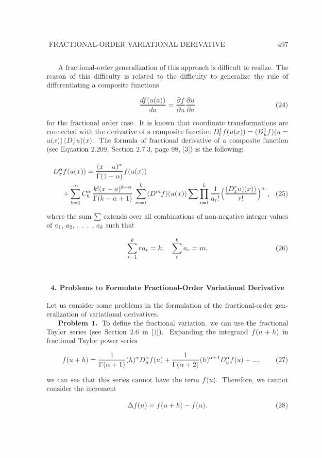
A fractional-order generalization of this approach is difficult to realize. Thereason of this difficulty is related to the difficulty to generalize the rule ofdifferentiating a composite functions

df(u(a))

da=

∂f

∂u

∂u

∂a(24)

for the fractional order case. It is known that coordinate transformations areconnected with the derivative of a composite function D1

t f(u(x)) = (D1uf)(u =

u(x)) (D1xu)(x). The formula of fractional derivative of a composite function

(see Equation 2.209, Section 2.7.3, page 98, [3]) is the following:

Dαxf(u(x)) =

(x− a)α

Γ(1− α)f(u(x))

+

∞∑

k=1

Cαk

k!(x− a)k−α

Γ(k − α+ 1)

k∑

m=1

(Dmf)(u(x))∑

k∏

r=1

1

ar!

((Drxu)(x))

r!

)ar, (25)

where the sum∑

extends over all combinations of non-negative integer valuesof a1, a2, . . . , ak such that

k∑

r=1

rar = k,k

∑

r

ar = m. (26)

4. Problems to Formulate Fractional-Order Variational Derivative

Let us consider some problems in the formulation of the fractional-order gen-eralization of variational derivatives.

Problem 1. To define the fractional variation, we can use the fractionalTaylor series (see Section 2.6 in [1]). Expanding the integrand f(u + h) infractional Taylor power series

f(u+ h) =1

Γ(α+ 1)(h)αDα

uf(u) +1

Γ(α+ 2)(h)α+1Dα

uf(u) + ..., (27)

we can see that this series cannot have the term f(u). Therefore, we cannotconsider the increment

∆f(u) = f(u+ h)− f(u). (28)

498 V.E. Tarasov

In order to use the Taylor series for the definition, we can consider the incrementin the form

∆qf = f(u+ h)− f(u+ qh), (29)

where 0 < q < 1. In this case, we have

∆f(u) =1− qα

Γ(α+ 1)hαDα

uf(u) +1− qα+1

Γ(α+ 2)hα+1Dα

uf(u) + .... (30)

This approach can be connected with the q-analysis [31], and fractional q-derivatives [32, 33]. We will consider the fractional variational q-derivative inthe next paper.

We can consider the increment of the functional F [u] that is defined by theequation

∆qF [u] = F [u+ h]− F [u+ qh]. (31)

If this increment of the functional F [u] exists, and can be represented in theform

∆qF [u] = δαF (u, hα) + ω(hα, u), (32)

where

lim||h||→0

||ω(hα, u)||

||hα||= 0,

then δαF can be considered as a fractional variation of functional F .

Problem 2. To define the fractional generalization of variation and frac-tional exterior variational calculus [21], we can use an analogy with the defini-tion of fractional exterior derivative. If the partial derivatives in the definitionof the exterior derivative

d = dxi∂/∂xi

are allowed to assume fractional order, a fractional exterior derivative can bedefined [20] by the equation

dα = (dxi)αDα

xi, (33)

where Dαx is the fractional derivative with respect to x. Using this analogy,

we can define the fractional variation in the following way. For the point u offunctional space, we can define the fractional variation δF [u] of the functional

F [u] =

∫ x2

x1

f(u, ux)dx,

FRACTIONAL-ORDER VARIATIONAL DERIVATIVE 499

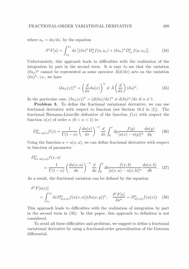
where ux = du/dx, by the equation

δαF [u] =

∫ x2

x2

dx[

(δu)αDαuf(u, ux) + (δux)

αDαuxf(u, ux)

]

. (34)

Unfortunately, this approach leads to difficulties with the realization of theintegration by part in the second term. It is easy to see that the variation(δux)

α cannot be represented as some operator A(d/dx) acts on the variation(δu)α, i.e., we have

(δux(x))α =

(

d

dxδu(x)

)α

6= A

(

d

dx

)

(δu)α. (35)

In the particular case, (δux(x))α = (d(δu)/dx)α 6= d(δu)α/dx if α 6= 1.

Problem 3. To define the fractional variational derivative, we can usefractional derivative with respect to function (see Section 18.2 in [1]). Thefractional Riemann-Liouville defivative of the function f(x) with respect thefunction u(x) of order α (0 < α < 1) is:

Dα0+,u(x)f(x) =

1

Γ(1− α)

(

du(x)

dx

)−1 d

dx

∫ x

0dy

f(y)

[u(x)− u(y)]αdu(y)

dy. (36)

Using the function u = u(x, a), we can define fractional derivative with respectto function of parameter

Dα0+,u(x,a)f(x, a)

=1

Γ(1− α)

(

du(x, a)

da

)−1 d

da

∫ a

0db

f(x, b)

[u(x, a) − u(x, b)]αdu(x, b)

db. (37)

As a result, the fractional variation can be defined by the equation

δαF [u(x)]

=

∫ x2

x1

dxDαu(x,a)f(u(x, a))(δu(x, q))

α ,δαF [u]

δuα= Dα

u(x,a)f(u(x)). (38)

This approach leads to difficulties with the realization of integration by partin the second term in (35). In this paper, this approach to definition is notconsidered.

To avoid all these difficulties and problems, we suggest to define a fractionalvariational derivative by using a fractional-order generalization of the Gateauxdifferential.

500 V.E. Tarasov

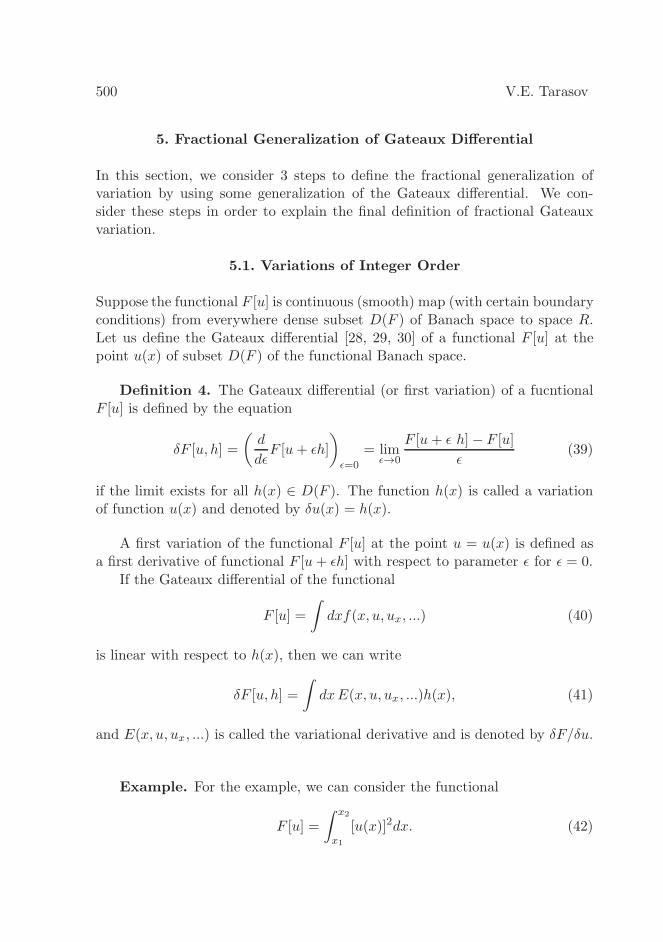
5. Fractional Generalization of Gateaux Differential

In this section, we consider 3 steps to define the fractional generalization ofvariation by using some generalization of the Gateaux differential. We con-sider these steps in order to explain the final definition of fractional Gateauxvariation.

5.1. Variations of Integer Order

Suppose the functional F [u] is continuous (smooth) map (with certain boundaryconditions) from everywhere dense subset D(F ) of Banach space to space R.Let us define the Gateaux differential [28, 29, 30] of a functional F [u] at thepoint u(x) of subset D(F ) of the functional Banach space.

Definition 4. The Gateaux differential (or first variation) of a fucntionalF [u] is defined by the equation

δF [u, h] =

(

d

dǫF [u+ ǫh]

)

ǫ=0

= limǫ→0

F [u+ ǫ h]− F [u]

ǫ(39)

if the limit exists for all h(x) ∈ D(F ). The function h(x) is called a variationof function u(x) and denoted by δu(x) = h(x).

A first variation of the functional F [u] at the point u = u(x) is defined asa first derivative of functional F [u+ ǫh] with respect to parameter ǫ for ǫ = 0.

If the Gateaux differential of the functional

F [u] =

∫

dxf(x, u, ux, ...) (40)

is linear with respect to h(x), then we can write

δF [u, h] =

∫

dxE(x, u, ux, ...)h(x), (41)

and E(x, u, ux, ...) is called the variational derivative and is denoted by δF/δu.

Example. For the example, we can consider the functional

F [u] =

∫ x2

x1

[u(x)]2dx. (42)

FRACTIONAL-ORDER VARIATIONAL DERIVATIVE 501

The functional F [u+ ǫh] has the form

F [u+ ǫh] =

∫ x2

x1

[u(x)]2dx+ 2ǫ

∫ x2

x1

u(x)h(x)dx + ǫ2∫ x2

x1

[h(x)]2dx. (43)

The derivative of first order with respect to parameter ǫ is

d

dǫF [u+ ǫh] = 2

∫ x2

x1

u(x)h(x)dx + 2ǫ

∫ x2

x1

[h(x)]2dx. (44)

As a result, the variational derivative is equal

(

d

dǫF [u+ ǫh]

)

ǫ=0

= 2

∫ x2

x1

u(x)h(x)dx. (45)

5.2. Step 1.

It seems that we can define a fractional variation by the equation

δαF [u, h] =

([

d

dǫ

]α

F [u+ ǫh]

)

ǫ=0

. (46)

Let us consider the fractional Riemann-Liouville derivative of functional(43) with respect to parameter ǫ:

Dαǫ F [u+ ǫh] = (Dα

ǫ 1)

∫ x2

x1

[u(x)]2dx+ 2(Dαǫ ǫ)

∫ x2

x1

u(x)h(x)dx

+ (Dαǫ ǫ

2)

∫ x2

x1

[h(x)]2dx. (47)

Using (2),

Dαǫ ǫ

k =Γ(k + 1)

Γ(k + 1− α)ǫk−α, (48)

we have

Dαǫ F [u+ ǫh] =

ǫ−α

Γ(1− α)

∫ x2

x1

[u(x)]2dx+2ǫ1−α

Γ(2− α)

∫ x2

x1

u(x)h(x)dx+

+2

Γ(3− α)ǫk−α

∫ x2

x1

[h(x)]2dx. (49)

If the derivatives with respect to parameter ǫ in the definition of variational(39) are allowed to assume fractional order, a fractional variational can be

502 V.E. Tarasov

defined. Unfortunately, if we define the fractional variation of the functional bythe equation

δαF [u] = (Dαǫ F [u+ ǫh])ǫ=0 , (50)

then we have some problems about incorrectness of definition (50). Theseproblems are following:

1) The first term of right hand side of equation (49) leads us to infinity. Ifǫ tends to zero, then we get ǫ−α → ∞, and Dα

ǫ F [u + ǫh] → ∞. Therefore thefirst term that is follows from the relation Dα

ǫ C = 0 must be removed. For thisaim we can use the Caputo fractional derivative [3, 22, 23, 24]. Using (4) for0 < α < 1, we have

Dα∗ ǫf(ǫ) = Dα

ǫ f(ǫ)−ǫ−α

Γ(2− α)f(0+). (51)

2) The second term of the right hand side of equation (49) is proportionalto ǫ1−α. This proportionality leads us to zero in the limit ǫ → 0, and wecannot derive some nonzero relation. Therefore we must consider the functionalF [u+ (ǫh)α] in the definition.

As the result, we cannot use the definitions (46) and (50).

5.3. Step 2.

Let us consider the following definition of fractional variational functional F [u]:

δαF [u] = (Dαǫ F [u+ (ǫh)α])ǫ=0 , (52)

where Dαǫ = Dα

∗ is a Caputo fractional derivative of order α with respect to ǫ.

If we consider the functional (42), then

F [u+(ǫh)α] =

∫ x2

x1

[u(x)]2dx+2ǫα∫ x2

x1

u(x)hα(x)dx+ǫ2α∫ x2

x1

[h(x)]2αdx. (53)

The fractional derivative (52) of this functional is equal to

Dαǫ F [u+ (ǫh)α] = 2Γ(α+ 1)

∫ x2

x1

u(x)hα(x)dx

+Γ(2α+ 1)

Γ(α+ 1)ǫα

∫ x2

x1

[h(x)]2αdx. (54)

FRACTIONAL-ORDER VARIATIONAL DERIVATIVE 503

Therefore, we get the following equation

(Dαǫ F [u+ (ǫh)α])ǫ=0 = 2Γ(α + 1)

∫ x2

x1

u(x)hα(x)dx. (55)

Note that for α = 1, we get the usual relation

δα=1F [u] = 2

∫ x2

x1

u(x)h(x)dx. (56)

Unfortunately, if we put α = 0, we get

F [u] = δα=0F [u] = 2

∫ x2

x1

u(x)(h(x))0dx = 2

∫ x2

x1

u(x)dx 6= F [u]. (57)

Therefore we cannot use the definition (52).

5.4. Step 3.

The usual definition (39) can be rewritten in the form

δF [u] =

(

d

dǫF

[

u

(

1 +ǫh

u

)])

ǫ=0

. (58)

The fractional variation can be defined by the equation

δαF [u] =

(

Dαǫ F

[

u

(

1 +

[

ǫh

u

]α)])

ǫ=0

. (59)

This definition is more consistent in order to realize the physical dimensions.In this definition the parameter ǫ is dimensionless.

If we consider the functional (42), then

F

[

u

(

1 +

[

ǫh

u

]α)]

= F [u+ (ǫh)αu1−α] =

∫ x2

x1

[u(x)]2dx+ 2ǫα∫ x2

x1

u2−α(x)hα(x)dx+ ǫ2α∫ x2

x1

u2−2α(x)[h(x)]2αdx. (60)

The fractional derivative of this functional is equal to

Dαǫ F [u+ (ǫh)αu1−α] = 2Γ(α + 1)

∫ x2

x1

u2−α(x)hα(x)dx

+Γ(2α+ 1)

Γ(α+ 1)ǫα

∫ x2

x1

u2−2α(x)[h(x)]2αdx. (61)

504 V.E. Tarasov

As a result, we get

(

Dαǫ F [u+ (ǫh)αu1−α]

)

ǫ=0= 2Γ(α+ 1)

∫ x2

x1

u2−α(x)hα(x)dx. (62)

For α = 1, we get the usual relation. For α = 0, we have

F [u] = δα=0F [u] = 2

∫ x2

x1

u2(x)dx 6= F [u]. (63)

If we consider the functional

F [u] =

∫ x2

x1

un(x)dx, (64)

then definition (59) leads to the relation

(

Dαǫ F [u+ (ǫh)αu1−α]

)

ǫ=0= nΓ(α+ 1)

∫ x2

x1

un−α(x)hα(x)dx (65)

and, for α = 0

F [u] = δα=0F [u] = n

∫ x2

x1

un(x)dx 6= F [u]. (66)

Therefore we have to implement some changes in the definition (59). Thismodification is suggested in the next subsection.

5.5. Definition of Variation of Fractional Order

Taking into account the remarks in the form of Step 1-3 and using Eq. (58) forvariation of integer order, we can define the fractional variation in the followingform.

Definition 5. The fractional-order variation δαF [u] of the functional F [u]is defined by the equation

δαF [u] =

(

Dαǫ F

[

u

(

1 +ǫh

u

)α])

ǫ=0

, (67)

or, in an equivalent form

δαF [u] =(

Dαǫ F

[

u1−α(u+ ǫh)α])

ǫ=0, (68)

FRACTIONAL-ORDER VARIATIONAL DERIVATIVE 505

where ǫ ≥ 0.

Example. If we consider the functional (42), we have

F[

u1−α(u+ ǫh)α]

=

∫ x2

x1

u2−2αh2α(ǫ+ u/h)2αdx. (69)

Using the relation

Dαǫ (ǫ+ u/h)2α =

Γ(2α + 1)

Γ(α+ 1)(ǫ+ u/h)α, (70)

where we consider ǫ+u(x)/h(x) = ǫ− ǫ0 with ǫ0 = ǫ0(x) = −u(x)/h(x), we getthe fractional derivative of functional (69) in the form

Dαǫ F

[

u1−α(u+ ǫh)α]

=Γ(2α + 1)

Γ(α+ 1)

∫ x2

x1

u2−2αh2α(ǫ+ u/h)αdx. (71)

As the result, we get

(

Dαǫ F

[

u1−α(u+ ǫh)α])

ǫ=0=

Γ(2α+ 1)

Γ(α+ 1)

∫ x2

x1

dxu2−α(x)hα(x). (72)

For α = 1, and α = 0, we get the usual relations. Therefore definition (67)satisfies the correspondent requirements for α = 0 and α = 1. As the result, weget the fractional variational derivative of order 0 ≤ α ≤ 1 in the form (68).

Proposition 1. The fractional-order variation derivative (67) of the func-tional

F [u] =

∫ x2

x1

un(u)dx (73)

has the form

δαF [u] = λ(α, n)

∫ x2

x1

dx (Dαuu

n)(x)hα(x), (74)

where

λ(α, n) =Γ(nα+ 1)Γ(n + 1− α)

Γ((n− 1)α + 1)Γ(n+ 1). (75)

Proof. Using (73), we have

F[

u1−α(u+ ǫh)α]

=

∫ x2

x1

un−nαhnα(ǫ+ u/h)nαdx. (76)

506 V.E. Tarasov

From the relation

Dαǫ (ǫ+ u/h)nα =

Γ(nα+ 1)

Γ((n− 1)α + 1)(ǫ+ u/h)(n−1)α, (77)

we get the fractional derivative of functional (73) in the form

δαF [u] =(

Dαǫ F

[

u1−α(u+ ǫh)α])

ǫ=0=

Γ(nα+ 1)

Γ((n− 1)α + 1)

∫ x2

x1

dxun−α(x)hα(x).

(78)This equation can be represented in the form

δαF =

∫ x2

x1

dx(Dαuu

n)hα(x), (79)

up to numerical factor. For equation (79), we have

(Dαuu

n) =Γ(n+ 1)

Γ(n+ 1− α)un−α. (80)

This ends the proof.

The fractional variational derivative of order α ≥ 1 can be defined by theusual relation

δα = δ[α]δ{α} (81)

by analogy with fractional derivative

Dαx =

d[α]

dx[α]D{α}

x , (82)

where [α] is the integer part of α, and {α} is the fractional part of number α,i.e., {α} = α− [α].

5.6. Functional with Derivative of Field

Let us consider the functional F [u] of the form

F [u] =

∫ x2

x1

f(u, ux)dx, (83)

where ux = du(x)dx

. The first variation of this functional is defined by

δF [u] =

(

d

dǫF [u+ ǫh]

)

ǫ=0

= limǫ→0

(

d

dǫ

∫ x2

x1

f(u+ ǫh, [u+ ǫh]x)

)

dx, (84)

FRACTIONAL-ORDER VARIATIONAL DERIVATIVE 507

where we use[u+ ǫh]x = ux + ǫhx. (85)

In order to use the equation

Dαǫ (ǫ− ǫ0)

β =Γ(β + 1)

Γ(β + 1− α)(ǫ− ǫ0)

β−α, (86)

for the relation [ǫ + u(x)/h(x)], we consider ǫ0 = ǫ0(x) = −u(x)/h(x). Thedefinition of the fractional variation of functional (83) can be realized in thefollowing form.

Definition 6. The fractional-order variation derivative of the functional(83) is defined by the equation

δαF [u] = limǫ→0

∫ x2

x1

(

Dαǫ f

(

u1−α(u+ ǫh)α, [u1−α(u+ ǫh)α]x

))

. (87)

Using the definition (68), we have the fractional variation of functional (83)in the form

δαF [u] =

∫ x2

x1

(

Dαǫ f

(

u1−α(u+ ǫh)α, [u1−α(u+ ǫh)α]x

))

ǫ=0. (88)

It is easy to see that the expression [u1−α(u+ ǫh)α]x cannot be represented inthe form of similar Eq. (85). This expression has the form

[u1−α(u+ ǫh)α]x = [(1− α)u−α(u+ ǫh)α + αu1−α(u+ ǫh)α−1]ux

+ αu1−α(u+ ǫh)α−1ǫhx. (89)

For α = 0, we have[u1−α(u+ ǫh)α]x = ux, (90)

and for α = 1, we have

[u1−α(u+ ǫh)α]x = ux + ǫhx. (91)

Let us give the proposition for a special form of the functional.

Proposition 2. The fractional-order variation derivative (87) of the func-tional

F [u] =

∫ x2

x1

u(x)ux(x)dx. (92)

508 V.E. Tarasov

has the form

δαF [u] =

∫ x2

x1

dx(

A1(α)ux(x)h(x) +A2(α)u2−α(x)αhα−1(x)hx(x)

)

, (93)

where

A1(α) =

[

(1− α)Γ(2α + 1)

Γ(α+ 1)+

αΓ(2α)

Γ(α)

]

, A2(α) =α2Γ(2α)

Γ(α+ 1). (94)

Proof. Let us use the functional

F [u1−α(u+ ǫh)α] =

∫ x2

x1

dx = u1−α(u+ ǫh)α[u1−α(u+ ǫh)α]x

=

∫ x2

x1

dx(

(1− α)u1−2αh2α(ǫ+ u/h)2αux + αu2−2αh2α−1(ǫ+ u/h)2α−1ux

+ αu2−2αh2α−1(ǫ+ u/h)2α−1ǫhx

)

. (95)

Consider ǫ0 = ǫ0(x) = −u(x)/h(x). We can use the following relations

Dαǫ (ǫ− ǫ0)

β =Γ(β + 1)

Γ(β + 1− α)(ǫ− ǫ0)

β−α, (96)

and

Dαǫ (ǫ− ǫ0)

β(ǫ− 0)γ =Γ(β + 1)

Γ(β + 1− α)

F2;1

(

−γ, β + 1;β + 1− α;−ǫ− ǫ0ǫ0

)

(ǫ0)γ(ǫ− ǫ0)

β−α. (97)

Note that Eq. (96) is satisfied for β > −1, and Eq. (97) is satisfied for β > −1,ǫ > ǫ0 > 0 . Here F2;1(a, b, c, z) is the Gauss hypergeometric function [1]:

F2;1(a, b, c, z) =∞∑

k=0

(a)k(bk)

(c)k

zk

k!,

and

(z)k = z(z + 1)...(z + n− 1) =Γ(z + n)

Γ(z).

For the function F2;1(a, b, c, z) there exists the Euler integral representation

F2;1(a, b, c, z) =Γ(c)

Γ(b)Γ(c − b)

∫ 1

0tb−1(1− t)c−b−1(1− zt)−adt, (98)

FRACTIONAL-ORDER VARIATIONAL DERIVATIVE 509

where Re(c) > Re(b) > 0, |arg(1 − z)| < π, and the relation

F2;1[a, b; c; 1] =Γ(c)Γ(c− a− b)

Γ(c− a)Γ(c− b), (99)

where Re(c− a− b) > 0 . For the case α > 1, we can use

dk

dzkF2;1[a, b; c; z] =

(a)k(bk)

(c)kF2;1[a+ k, b+ k; c+ k; z], (100)

where k = [α] is the integer part of α. As a result, we get

δαF [u] =

∫ x2

x1

dx

[

(1− α)Γ(2α + 1)

Γ(α+ 1)+

αΓ(2α)

Γ(α)

]

ux(x)h(x)

+

∫ x2

x1

dxαΓ(2α)

Γ(α+ 1)u2−ααhα−1hx. (101)

This ends the proof.

For α → 1, we have the usual relation

δF [u] =

∫ x2

x1

dx[uxh+ uhx].

Note that we can useαhα−1hx = (hα)x,

and then∫ x2

x1

dxΓ(2α)Γ(1 − α)

Γ(−α)Γ(α + 1)u2−ααhα−1hx = −

∫ x2

x1

dxΓ(2α)Γ(1 − α)

Γ(−α)Γ(α+ 1)(u2−α)xh

α.

(102)This allows us to realize integration by part in the second term of Eq. (101).

6. Fractional Variation of Fields

In this section we consider the definition of fractional variational derivativewithout using the increment

∆F [u] = F [u+ h]− F [u]

of the functional F [u], and without using the derivative with respect to param-eter ǫ as in the Gateaux derivative. We suppose that the functional F [u] hassome densities f(u, ux, ...).

510 V.E. Tarasov

If u = (u1, ..., um)(x, t) is a smooth vector-function defined in the regionW ⊂ Rn, then the variation of the functional

F [u] =

∫

W

f(u,ux)dx

can be defined by the relation

δF [u] =

∫

W

δf(u,ux)dx =

∫

W

[

∂f

∂uµδuµ +

∂f

∂uµxδuµx

]

dx. (103)

To define the fractional generalization of variation and fractional exteriorvariational calculus [21], we can use an analogy with the definition of fractionalexterior derivative. If the partial derivatives in the definition of the exteriorderivative

d = dxi∂/∂xi

are allowed to assume fractional order, a fractional exterior derivative can bedefined [20] by the equation

dα = (dxi)αDα

xi, (104)

where Dαx are the fractional derivative with respect to x. Using this analogy,

we can define the fractional variation in the following way. For the point u offunctional space, we can define the fractional variation δF [u] of the functional

F [u] =

∫ x2

x1

f(u, ux)dx, (105)

where ux = du/dx, by the equation

δαF [u] =

∫ x2

x1

δf(u, ux)dx =

∫ x2

x2

dx[

(δu)αDαuf(u, ux) + (δux)

αDαuxf(u, ux)

]

.

(106)

This approach has a difficulty with the realization of integration by part inthe second term of (106). It is easy to see that the variation (δux)

α cannot berepresented as some operator acts on the variation (δu)α, i.e., we have

(δux(x))α =

(

d

dxδu(x)

)α

6=d

dx(δu)α. (107)

In order to resolve this difficulty we can use the following.

FRACTIONAL-ORDER VARIATIONAL DERIVATIVE 511

Let us define the fractional variation of the functional

F [u] =

∫

f(u1, u2, ..., um)dx, (108)

by the equation

δαF [u] =

∫

[

m∑

k=1

(Dαukf)(δuk)

α

]

dx (109)

by analogy with

δF [u] =

∫ m∑

k=1

(D1ukf)δukdx. (110)

In this case, we have

δαul =

∫

[

m∑

k=1

(Dαukul)(δuk)

α

]

. (111)

It is known, that

δul =

∫

[

m∑

k=1

(D1ukul)δuk

]

dx =

∫

[δklδ(y − x)δuk] dx. (112)

Using the Caputo fractional derivative, we have

Dαuk(y)

ul(x) =u1−α

Γ(2− α)δklδ(y − x). (113)

Here the Caputo fractional derivative leads to the δkl, i.e.,

Dαuk(y)

ul(x) = 0 k 6= l.

As the result, we get

δαul =u1−α

Γ(2− α)δkl(δuk)

α. (114)

Therefore, we have(δuk)

α = Γ(2− α)uα−1k δαuk. (115)

For the Riemann-Liouville fractional derivatives, we can derive some analogousrelation:

(δuk)α = Akl

(

Γ(2− α)uα−1k ; Γ(1 − α)u−1

k uαl)

δαuk. (116)

Substituting Eq. (115) in Eq. (109), we have the following definition.

512 V.E. Tarasov

Definition 7. The fractional order variation δαF [u] of the functional (108)is defined by the equation

δαF [u] = Γ(2− α)

∫

[

m∑

k=1

(Dαukf)uα−1

k δαuk

]

dx. (117)

We can define the fractional variation for derivative duk(x)/dx by the equa-tion

δαd

dxuk(x) =

d

dxδαuk(x), (118)

where we suppose that the fields uk do not connected by some constraint.Analogously, we have

δαDβxuk(x) = Dβ

xδαuk(x). (119)

Let us consider u1 = u, and u2 = ux and the functional

F [u] =

∫

f(u1, u2)dx =

∫

f(u, ux)dx. (120)

As the result, we have

δαF [u] = Γ(2− α)

∫[

(Dαukf)uα−1

k δαu−d

dx

(

Dαukx

f)uα−1kx

)

]

δαukdx. (121)

We can use this relation only if ux and u can be considered as independentvalues, i.e., for the case

Dαuxu = 0, Dα

uux = 0. (122)

Note that Eq. (122) cannot be satisfied in the general case. Therefore, wehave to consider the functional

F [u] =

∫[

f(u1, u2) + λ

(

u2 −d

dxu1

)]

dx, (123)

instead of the functional (120).

Proposition 3. The fractional-order variation equation

δαF [u] = 0

of the functional (123) gives

(Dαu1f)u2α−2

1 −d

dx

(

uα−11 uα−1

2 Dαu2f)

= 0. (124)

FRACTIONAL-ORDER VARIATIONAL DERIVATIVE 513

where u2 = du1/dx.

Proof. The fractional-order variation of the functional (123) gives

δαF [u] = Γ(2− α)

∫

dx

[

(Dαu1f)uα−1

1 − λ

(

Dαu1

d

dxu1

)

uα−11

]

δαu1

+Γ(2− α)

∫

dx[

(Dαu2f)uα−1

2 + λ(Dαu2u2)u

α−12

]

δαu2

+Γ(2− α)

∫

dx

[

u2 −d

dxu1

]

(Dαλλ)λ

α−1k δαλ. (125)

Using

λ

(

Dαu1

d

dxu1

)

uα−11 = λuα−1

1

d

dx

(

Dαu1u1

)

=d

dx

(

λuα−11 Dα

u1u1

)

−Dαu1u1

d

dx

(

λuα−11

)

, (126)

we get the following fractional variation of the functional

δαF [u] = Γ(2− α)

∫

dx

[

(Dαu1f)uα−1

1 +Dαu1u1

d

dx

(

λuα−11

)

]

δαu1

+Γ(2− α)

∫

dx[

(Dαu2f)uα−1

2 + λ(Dαu2u2)u

α−12

]

δαu2

+Γ(2− α)

∫

dx

[

u2 −d

dxu1

]

(Dαλλ)λ

α−1k δαλ. (127)

As the result, we get the field equations

(Dαu1f)uα−1

1 +Dαu1u1

d

dx

(

λuα−11

)

= 0, (128)

(Dαu2f) + λ(Dα

u2u2) = 0, (129)

u2 −d

dxu1 = 0. (130)

From the Eq. (129), we derive the Lagrange multiplier

λ = −Dα

u2f

Dαu2u2

. (131)

Substituting this equation in Eq. (128), we have

(Dαu1f)uα−1

1 −Dαu1u1

d

dx

(

uα−11

Dαu2u2

Dαu2f

)

= 0. (132)

Using Dαuu = u1−α/Γ(2− α), we get (124).

Equation (124) is the fractional Euler-Lagrange equation.

514 V.E. Tarasov

7. Conclusion

In the general case, the equation of motion cannot be derived from the station-ary action principle. The class of equations that can be derived from stationaryaction principle by using fractional variation is a wider class than the usualclass equations that can be derived by usual (integer, first order) variation.The usual (integer order) equations of motion can be considered as special caseof equations that can be derived by fractional variation such that α = 1.

It can seems that the fractional variations are abstract and formal construc-tions. For this reason, we would like to pay attention that the suggested frac-tional variations can have wide application in study of fractional gradient typeequations and fractional generalization of Lyapunov direct (second) method inthe theory of stability.

The possible importance of fractional variations are connected with thefollowing ideas. The class of gradient dynamical systems is a restricted class ofall dynamical systems. However these systems have important property. Thegradient system can be described by one function - potential, and the studyof the system can be reduced to research of potential. For example, the wayof chemical reactions is defined from the analysis of potential energy surfaces[35, 36, 37]. The fractional gradient systems has been suggested in Refs. [18, 19].The fractional gradient systems are non-gradient dynamical systems that can bedescribed by one function - some potential. For example, the Lorenz equationsand Rossler equations are fractional gradient systems [18, 19]. Therefore thestudy the some non-gradient system can be reduced to research of potential. Forexample, the way of some chemical reactions with dissipation, dynamical chaosand self-organizing can be considered by the analysis of some potential energysurfaces. The suggested fractional variations allow us to define the fractionalgeneralization of gradient type equations that can have wide applications forthe description of dissipative structures [38, 39]. The suggested approach canalso be generalized for lattice systems by using the lattice fractional calculus[34].

Appendix

The following rules for variational defivatives are known:

• The variation derivative of the field u(x) is defined by the equation

δu(x)

δu(y)= δ(y − x), (133)

FRACTIONAL-ORDER VARIATIONAL DERIVATIVE 515

where we use

δu(x) =

∫

δ(y − x)δu(y). (134)

The variational derivatives of linear functional

F [u] =

∫

g(x)u(x)dx (135)

can be calculated by the simple formula

δF [u]

δu(y)=

∫

g(x)δu(x)

δu(y)dx =

∫

g(x)δ(y − x)dx = h(y).

• If the u function in the functional is affected by differential operators,then, in order to make use of the rule (133), one should at first ”throwthem over” to the left, fulfilling integration by parts. For example,

δ

δu(y)

∫

g(x)[∇u(x)]dx = −δ

δu(y)

∫

[∇g(x)]u(x)dx = −∇g(y).

We assumed here that on the boundary of integration domain the productu(x)h(x) becomes zero.

• The variational derivative of nonlinear functionals is calculated accord-ing to the rule of differentiating a complex function similarly to partialderivatives:

δ

δu(y)

∫

f(u(x))dx =

∫

δf(u)

δu(x)

δu(x)

δu(y)dx

=

∫

δf(u)

δu(x)δ(y − x)dx =

δf(u(y))

δu(y).

For example,δ

δu(y)

∫

[u(x)]ndx = n[u(y)]n−1.

References

[1] S.G. Samko, A.A. Kilbas, O.I. Marichev, Integrals and Derivatives of

Fractional Order and Applications, Nauka i Tehnika, Minsk (1987); andFractional Integrals and Derivatives Theory and Applications, Gordon andBreach, New York (1993).

516 V.E. Tarasov

[2] V. Kiryakova, Generalized Fractional Calculus and Applications, Longman,Harlow and Wiley, New York (1994).

[3] I. Podlubny, Fractional Differential Equations, Academic Press, San Diego(1998).

[4] A.A. Kilbas, H.M. Srivastava, J.J. Trujillo, Theory and Applications of

Fractional Differential Equations, Elsevier, Amsterdam (2006).

[5] D. Valerio, J.J. Trujillo, M. Rivero, J.A. Tenreiro Machado, D. Baleanu,Fractional calculus: A survey of useful formulas, The European Physical

Journal. Special Topics, 222, No 8 (2013), 1827-1846.

[6] B. Ross, A brief history and exposition of the fundamental theory of frac-tional calculus. In: Fractional Calculus and Its Applications, Lecture Notesin Mathematics. 457 (Ed. B. Ross), Springer-Verlag, Berlin (1975), 1-36.

[7] L. Debnath, A brief historical introduction to fractional calculus, Interna-tional Journal of Mathematical Education in Science and Technology, 35,No 4 (2004), 487-501.

[8] J. Tenreiro Machado, V. Kiryakova, F. Mainardi, Recent history of frac-tional calculus, Communications in Nonlinear Science and Numerical Sim-

ulation, 16, No 3 (2011), 1140-1153.

[9] J.A. Tenreiro Machado, A.M. Galhano, J.J. Trujillo, Science metrics onfractional calculus development since 1966, Fractional Calculus and Ap-

plied Analysis, 16, No 2 (2013), 479-500.

[10] J.A. Tenreiro Machado, A.M.S.F. Galhano, J.J. Trujillo, On developmentof fractional calculus during the last fifty years, Scientometrics, 98, No 1(2014), 577-582.

[11] F. Mainardi, Fractional Calculus and Waves in Linear Viscoelasticity: An

Introduction to Mathematical Models, World Scientific, Singapore (2010).

[12] V.E. Tarasov, Fractional Dynamics: Applications of Fractional Calculus

to Dynamics of Particles, Fields and Media, Springer, New York (2011).

[13] J. Klafter, S.C. Lim, R. Metzler (Eds.), Fractional Dynamics. Recent Ad-

vances, World Scientific, Singapore (2011).

[14] M.M. Meerschaert, A. Sikorskii, Stochastic Models for Fractional Calculus,Walter de Gruyter, Berlin/Boston (2012).

FRACTIONAL-ORDER VARIATIONAL DERIVATIVE 517

[15] V.E. Tarasov, Review of some promising fractional physical models, Inter-national Journal of Modern Physics B, 27, No 9 (2013), 1330005.

[16] V. Uchaikin, R. Sibatov, Fractional Kinetics in Solids: Anomalous Charge

Transport in Semiconductors, Dielectrics and Nanosystems, World Scien-tific, Singapore (2013).

[17] T. Atanackovic, S. Pilipovic, B. Stankovic, D. Zorica, Fractional Calcu-lus with Applications in Mechanics: Vibrations and Diffusion Processes,Wiley-ISTE, London, Hoboken (2014).

[18] V.E. Tarasov, Fractional generalization of gradient and Hamiltonian sys-tems, Journal of Physics A, 38, No 26 (2005), 5929-5943.

[19] V.E. Tarasov, Fractional generalization of gradient systems, Letters in

Mathematical Physics, 73, No 1 (2005), 49-58.

[20] K. Cottrill-Shepherd, M. Naber, Fractional differential forms, Journal ofMathematical Physics 42, No 5 (2001), 2203-2212.

[21] R. Aldrovandi, R.A. Kraenkel, On exterior variational calculus, Journal ofPhysics A, 21, No 6 (1988), 1329-1339.

[22] M. Caputo, Linear models of dissipation whose Q is almost frequency in-dependent, Geophysical Journal of the Royal Astronomical Society, 13, No5 (1967), 529-539.

[23] M. Caputo, F. Mainardi, A new dissipation model based on memory mech-anism, Pure and Applied Geophysics, 91, No 1 (1971), 134-147.

[24] R. Gorenflo, F. Mainardi, Fractional calculus, integral and differentialequations of fractional order, In: Fractals and Fractional Calculus in Con-

tinuum Mechanics, A. Carpinteri and F. Mainardi (Eds.), Springer Verlag,Wien and New York (1997), 223-276.

[25] K. Diethelm, The Analysis of Fractional Differential Equations. An

Application-Oriented Exposition Using Differential Operators of Caputo

Type, Springer-Verlag, Berlin, Heidelberg (2010).

[26] M.M. Vainberg, Variational Methods for the Study of Nonlinear Opera-

tors, Moscow, GosTehIzdat (1956) in Russsian; Holden-Day, San Francisco(1964).

518 V.E. Tarasov

[27] O.P. Agrawal, Formulation of Euler-Lagrange equations for fractional vari-ational problems, Journal of Mathematical Analysis and Applications, 272,No 1 (2002), 368-379.

[28] R. Gateaux, Fonctions iVune infiniti des variables indipendantes, Bulletinde la Societe Msathematique de France, 47, (1919), 70-96.

[29] M. Frechet, La notion de differentielle dans l’analyse generale, Annales

Scientifiques de l’Ecole Normale Ssuperieure, 42, (1925), 293-323.

[30] M. Frechet, Sur la notion de differentielle, Journal de Mathematiques, 16,(1937), 233-250.

[31] V. Kac, P. Cheung, Quantum Calculus, Springer, New York (2002).

[32] W.A. Al-Salam, Some Fractional q-Integrals and q-Derivatives, Proceedingsof the Edinburgh Mathematical Society, 15, No 2 (1966), 135-140.

[33] R.P. Agarwal, Certain fractional q-integrals and q-derivatives, Mathemat-

ical Proceedings of the Cambridge Philosophical Society, 66, No 2 (1969),365-370.

[34] V.E. Tarasov, Toward lattice fractional vector calculus, Journal of PhysicsA, 47, No 35 (2014), 355204.

[35] R.D. Levine, J. Bernstein, Molecular Reaction Dynamics, Oxford Univer-sity Press, New York (1974).

[36] K. Fukui, Formulation of the reaction coordinate, The Journal of Physical

Chemistry, 74 (1970), 4161-4163.

[37] K. Fukui, The path of chemical reactions the IRC approach, Accounts of

Chemical Research, 14, No 12 (1981), 363-368.

[38] G. Nicolis, I. Prigogine, Self-Organization in Nonequilibrium Systems:

From Dissipative Structures to Order through Fluctuations, John Wiley,New York (1977).

[39] R.Z. Sagdeev, D.A. Usikov, G.M. Zaslavsky, Nonlinear Physics, HarwoodAcademic, New York (1988).