2012

Columbia University SIPA

[ Two essays on International Finance]

By: Azin Aliabadi Zanyar Golabi

Supervisor: Prof. Guillermo Calvo

Introduction:

In our research, we present two essays on international finance. In the first essay, we explore a dilemma that emerging markets often face. “Fear of floating” premises, including the pass-through of exchange rate volatility into inflation and the balance sheet effect usually justify the fixed exchange rate regimes in emerging markets with open capital accounts. In our research, we argue that under normal condition, while the fear of sudden stop of capital inflow is not threatening the private sector and investment, fixing the exchange rate to the dollar is the optimal policy. In this case, monetary authorities don’t face a dilemma. They should prevent the inflation and reduce troubling consequences of balance sheet effect by reducing the volatility of exchange rates. However, when the threat of sudden stop and liquidity crunch emerges, a new dilemma arises: Which one is more important? The underinsurance of private sector and thereby, as we prove in this research, the contraction of output or the consequences of exchange rate volatility including high inflation and balance sheet deterioration?

In our research we demonstrate that fixing the exchange rate to the dollar is not always the optimal monetary policy. Since the underinsurance of private sector against capital inflow’s sudden stop may lead to over borrowing of the private sector and thereby, a liquidity crunch in upcoming periods, exchange rate volatility can help prevent the consequences of over borrowing. In addition we conclude that the credibility of monetary authorities and the expectations of private sector regarding the expected monetary policy play an important role in mitigating the underinsurance of private sector.

In the second essay, we examine the variables affecting the current account. The first part of this essay investigates whether a number of variables affected the current account in a panel of developing and developed countries. The second part of the essay will provide an analytical framework to analyze the relationship between terms of trade volatility and current account dynamics.

First Essay:

Fear of Floating or Fear of Sudden Stop: On the Optimal Monetary Policy in Emerging Markets

Abstract:

In this essay, we explore a dilemma that emerging markets often face. “Fear of floating” premises, including the pass-through of exchange rate volatility into inflation and the balance sheet effect usually justify the fixed exchange rate regimes in emerging markets with open capital accounts. In our research, we argue that under normal condition, while the fear of sudden stop of capital inflow is not threatening the private sector and investment, fixing the exchange rate to the dollar is the optimal policy. In this case, monetary authorities don’t face a dilemma. They should prevent the inflation and reduce troubling consequences of balance sheet effect by reducing the volatility of exchange rates. However, when the threat of sudden stop and liquidity crunch emerges, a new dilemma arises: Which one is more important? The underinsurance of private sector and thereby, as we prove in this research, the contraction of output or the consequences of exchange rate volatility including high inflation and balance sheet deterioration?

In our research we demonstrate that fixing the exchange rate to dollar is not always the optimal monetary policy. Since the underinsurance of private sector against capital inflow’s sudden stop may lead to over borrowing of the private sector and thereby, a liquidity crunch in upcoming periods, exchange rate volatility can help prevent the consequences of over borrowing. In addition we conclude that the credibility of monetary authorities and the expectations of private sector regarding the expected monetary policy play an important role in mitigating the underinsurance of private sector.

Keywords: Optimal monetary policy, Fear of floating, sudden stop, under

insurance of private sector

Introduction:

“Fear of floating” plays a major role in identifying the exchange rate regimes specifically in emerging markets. Many officially free or managed floats in reality show low exchange rate volatility (Calvo G.A., Reinhart C.M. [CR] (2002)). Calvo G.A., Reinhart C.M. (2002) report evidence on the behavior of bilateral exchange rates, foreign exchange reserves and real interest rates. In their paper, monetary policy is set to target inflation. Furthermore due to the lack of credibility, there is uncertainty in both country-specific risk premia and in money demand. They conjecture that emerging markets have a higher exchange rate pass-through to inflation, lack of policy credibility (time inconsistency) and are in turn more volatile. The sources of volatility are: Variability of risk premia on government debt (which could be the consequence of low credibility or default risk) and money demand shocks (G.A., Reinhart C.M. (2002)).

Because of pass-through, exchange rate movements are domestic price movements (G.A., Reinhart C.M. (2002)). The central bank changes interest rate one-for-one to changes in the risk premium: it minimizes swings in exchange rate depreciation due to exogenous risk premium movements. The central bank changes interest rate proportionally to changes in money demand: it minimizes inflation but taking into account that a positive shock means higher real money demand and therefore higher seigniorage (G.A., Reinhart C.M. (2002)).

In sum, monetary policy in emerging markets may be even more constrained than suggested by the trilemma: an economy open to financial flows and with floating exchange rate may want to manage exchange rate volatility in two cases:

1. When there is high pass-through from exchange rates to inflation 2. When debts are denominated in foreign currency: in this case depreciations

are more harmful On the other hand, a country may want to target a depreciated real interest rate

to keep the economy competitive and to accumulate foreign reserves that create a buffer against swings in the international financial markets. In other words, “fear of floating” is the main driving force for applying monetary responses to prevent (a) pass through of exchange rate volatility into domestic inflation; (b) dollarization of liability; and (c) balance sheet effect. However, low exchange rate volatility may lead

to the so-called “underinsurance” of private sector against sudden stops. Accepting exchange rate volatility during “bad state” (which represent a crisis situation) may influence the private sector to stop over borrowing and thereby, preserve a level of external liquidity that is needed to maintain the necessary operations of the private sector.

In our essay, we develop a simple model that takes into account the economic climate of the economy. We consider two states: a “good state” (non-crisis situation) and a “bad state” (crisis situation). The objective function of monetary authority is extended to take both states into account when they are making decisions regarding the optimal monetary policy. We show that without adequate insurance for private sector in emerging markets, higher exchange rate volatility in the presence of sudden stops would be preferred exchange rate policy. Moreover, we determine that in the presence of high credibility, the optimal exchange rate regime is dependent upon the state of the economy. During a non-crisis situation, a fixed exchange rate regimes is maintained, whereas during a crisis the exchange rate is allowed to float. We show how exchange rate flexibility can reduce the threat of sudden stop by increasing the storage of dollar-dominated assets by the private sector. Thus, our central argument is that in the presence of a sudden stop in capital inflow, flexibility of exchange rate can act as an insurance policy for private sector against sudden crunch of liquidity needed for their activities. We show that the credibility of central government and central bank are critical in providing these insurance benefits through increasing exchange rate flexibility.

Caballero and Krishnamurthy (2004) argue that during a normal state, low volatility of exchange rate is the optimal monetary response to the “fear of floating” in emerging markets, but limited volatility in exchange rates movements can weaken the position of the private sector during “severe crisis”. According to their argument, the expectations of private sector in emerging markets is important, because if private firms predict a that the exchange rate will remain fixed during a crisis, this expectation, in turn, leads to high dollarization. Private sectors expectations are associated with the level credibility of the monetary authorities.

Our paper is an extension of Caballero and Krishnamurthy (2004) idea. We show how the tradeoffs between fear of floating and fear of sudden stop can change the optimal monetary policy.

The Model Our main assumptions are those of Caballero and Krishnamurthy (2004). We

assume that we have a three date economy {0,1,2}. We have one tradable good. At time 0, firms make investment and financing decisions (planning period). At time 1, the state of the economy is determined. If a crisis happens, the state will be “bad”, if not, we assume a non-crisis or a “good” state. The state of the economy is denoted by 𝛼 ∈ [𝑔, 𝑏]. The probability of the crisis is 𝑝. Finally, at date 2, firms pay back debts and start consuming in this period. The level of investment (for instance the size of

the plant) is denoted by 𝑘. The cost of investment is 𝑐(𝑘) where (𝑘) > 0 , 𝑑𝑐(𝑘)𝑑𝑘

> 0 and

𝑑2𝑐(𝑘)𝑑𝑘2

> 0. The maximum output realizes if no shock hits the firms which is 𝑦𝑚𝑎𝑥 =

𝐴𝑘. If a negative shock hits the firm, the output is no longer optimal. In other words, 𝑦𝑠ℎ𝑜𝑐𝑘𝑠 = 𝑎𝑘 ≤ 𝐴𝑘 . At time 0, firms have no resources and need to borrow from international capital markets to finance their investment activities. Firms decide how much to invest and how much to borrow to maximize the expected profit function at time 2. But firms face financial constraints based on their financial net worth. Meanwhile, we assume that all firms are endowed 𝑤 units of international collateral in form of receivables arriving at time 2 (e.x prime exports). (Caballero and Krishnamurthy (2004)). At time 0, firms sign debt contracts with foreigners. The contracted repayments depend on the state of the economy (“bad” or “good). We denote the contracted repayments by 𝑓𝛼 . In other words, 𝑓𝛼 is firms’ financing

decision or level of borrowing at time 0. Firms can borrow both at time 0 and 1. The interest rate at time 0 and 1 are 𝑖0 and 𝑖1 , respectively. Notice that 𝑓𝛼 ≤ 𝑤. We

assume that firms can borrow from other domestic agents. We also assume that the output at time 2, 𝑦 = 𝑎𝑘, can be used as a collateral for domestic borrowing. Also we assume that firms are endowed 𝑀� units of domestic money that they can sell to other domestic agents. We assume that domestic assets are denominated in peso and international collaterals are denominated in dollar. Therefore, exchange rate

volatility affects domestic assets and doesn’t affect the value of international collateral.

Now we explore shocks and credit constraints. If the state of economy is “good”, then we don’t face an external shock. Let’s assume that the state of economy is “bad” (with probability of p). We assume that ½ of domestic firms receive the shock at time 1, when a crisis happens. These firms are called “distressed”. The rest of the domestic firms are called “intact”. The shock will reduce the output of distressed firms from 𝐴𝑘 to 𝑎𝑘 . The distressed firms can reinvest 𝜃𝑘 goods, to offset the productivity decline. Therefore, their output at time 2 is:

𝑦 = �𝑎 + 𝜃(𝐴 − 𝑎)�𝑘

If a crisis happens, 𝜃 < 1 and therefore 𝑦 < 𝑦𝑚𝑎𝑥. Note that ∆= 𝐴 − 𝑎 is return on reinvestment of distressed firms at time 1. We assume return on reinvestment is higher than international interest rate, therefore distressed firms can borrow as much as they need.

In other words: ∆> 1 + 𝑖1

Distressed firms first start borrowing from foreigners to reinvest (against their international collateral of 𝑤). If the international liquidity exhausts, they will turn to domestic firms that are intact. As previously noted, both output of distressed firms at time 2 and also the money that they hold at time 2 can be used as collateral against domestic borrowings. Therefore, the domestic collateral (called domestic liquidity) is:

𝑎𝑘 + 𝑀�/𝑒2 We also assume that national price level at time 2 is equal to nominal exchange

rate at time 2, denoted by 𝑒2. Meanwhile, with interest rate of 𝑖1, firms can borrow from foreigners at time 1 to a certain level. The maximum level they can borrow is:

𝑤 − 𝑓1 + 𝑖1

= 𝑤𝑛

If firms borrow 𝑤𝑛 at time 1, they should payback 𝑤𝑛(1 + 𝑖1) at time 2. Their net international collateral (𝑤 − 𝑓) should be equal to 𝑤𝑛(1 + 𝑖1) to be able to borrow at

time 1 and repay in the next period. 𝑤𝑛 is called international liquidity. The overall liquidity is:

𝑙 = 𝑎𝑘 + 𝑀�/𝑒2+𝑤𝑛

Meanwhile, at time 1, central bank can inject 𝑀 −𝑀� to increase money

outstanding to 𝑀. This money is distributed at time 1 and is redeemed at time 2 through tax collection. We also assume that domestic peso interest rate is zero and it is unaffected by monetary decisions. We explore two cases:

1. Inflation credibility: we assume central bank is credible in maintaining the price level at time 2 equal to 1. In other words, 𝑒2 = 1.

2. Limited inflation credibility: 𝑒2 ≠ 1 Inflation credibility

We explore time 1 dynamics. Therefore, we assume investment and financing decisions or 𝑘 𝑎𝑛𝑑 𝑓 are given. Also we assume that crisis has happened and central

bank has injected 𝑀−𝑀� of money. We then segregate a crisis situation into two counterparts. We assume two types of crisis: mild and severe.

The distressed firms’ domestic net worth at time 1 is: (𝑎𝑘 + 𝑀)/𝑒1

And their total net worth is (at time 1): 𝑎𝑘 + 𝑀𝑒1

+ 𝑤𝑛

Recall that first distressed firms borrow money from foreigners up to 𝑤𝑛 . If international liquidity 𝑤𝑛 is limited for their financing (due to lack of collateral), they turn to intact domestic firms to borrow. Domestic firms have to borrow from international capital market to finance distressed firms. As aforementioned above, the firms accept money and output at time 2 as collateral for distressed firms. Two situations can arise:

1. �12�𝑤𝑛 > (1

2) 𝑎𝑘+𝑀

𝑒1. Intact firms have enough access to international capital

markets to finance domestic firms (mild crisis or horizontal situation).

2. �12�𝑤𝑛 < (1

2) 𝑎𝑘+𝑀

𝑒1. Intact firms don’t have enough access to international

capital market to finance distressed firms (severe crisis or vertical situation). Recall that we assumed full inflation credibility. Now, we want to see how the

exchange rate reacts to crisis in both cases. Following figures show the reaction of exchange rate at time 1 to crisis in both cases:

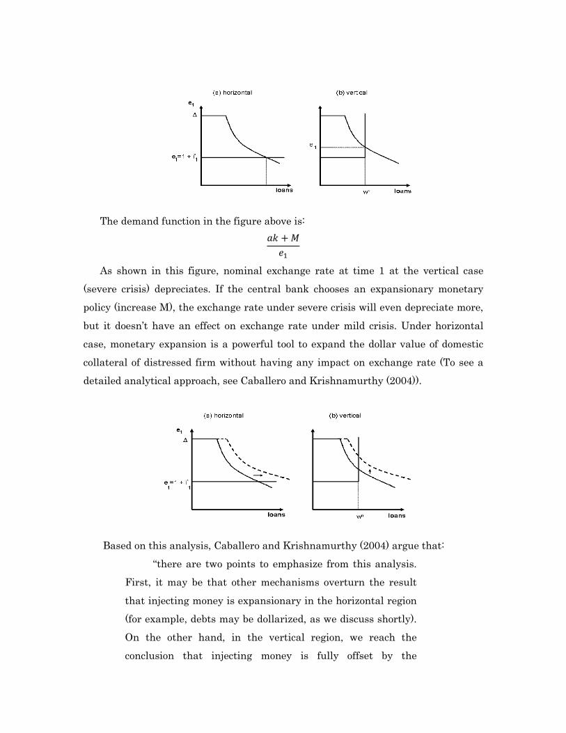
The demand function in the figure above is:

𝑎𝑘 + 𝑀𝑒1

As shown in this figure, nominal exchange rate at time 1 at the vertical case (severe crisis) depreciates. If the central bank chooses an expansionary monetary policy (increase M), the exchange rate under severe crisis will even depreciate more, but it doesn’t have an effect on exchange rate under mild crisis. Under horizontal case, monetary expansion is a powerful tool to expand the dollar value of domestic collateral of distressed firm without having any impact on exchange rate (To see a detailed analytical approach, see Caballero and Krishnamurthy (2004)).

Based on this analysis, Caballero and Krishnamurthy (2004) argue that:

“there are two points to emphasize from this analysis. First, it may be that other mechanisms overturn the result that injecting money is expansionary in the horizontal region (for example, debts may be dollarized, as we discuss shortly). On the other hand, in the vertical region, we reach the conclusion that injecting money is fully offset by the

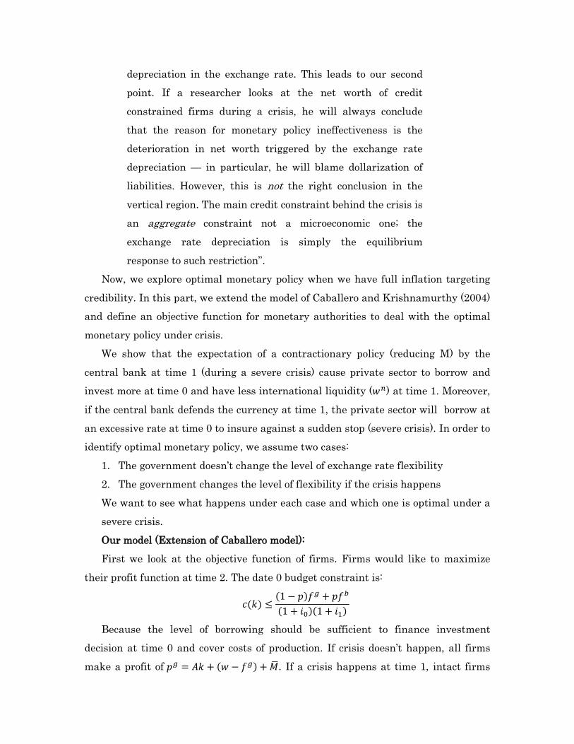
depreciation in the exchange rate. This leads to our second point. If a researcher looks at the net worth of credit constrained firms during a crisis, he will always conclude that the reason for monetary policy ineffectiveness is the deterioration in net worth triggered by the exchange rate depreciation — in particular, he will blame dollarization of liabilities. However, this is not the right conclusion in the vertical region. The main credit constraint behind the crisis is an aggregate constraint not a microeconomic one; the exchange rate depreciation is simply the equilibrium response to such restriction”.

Now, we explore optimal monetary policy when we have full inflation targeting credibility. In this part, we extend the model of Caballero and Krishnamurthy (2004) and define an objective function for monetary authorities to deal with the optimal monetary policy under crisis.

We show that the expectation of a contractionary policy (reducing M) by the central bank at time 1 (during a severe crisis) cause private sector to borrow and invest more at time 0 and have less international liquidity (𝑤𝑛) at time 1. Moreover, if the central bank defends the currency at time 1, the private sector will borrow at an excessive rate at time 0 to insure against a sudden stop (severe crisis). In order to identify optimal monetary policy, we assume two cases:

1. The government doesn’t change the level of exchange rate flexibility 2. The government changes the level of flexibility if the crisis happens We want to see what happens under each case and which one is optimal under a severe crisis. Our model (Extension of Caballero model): First we look at the objective function of firms. Firms would like to maximize

their profit function at time 2. The date 0 budget constraint is:

𝑐(𝑘) ≤(1 − 𝑝)𝑓𝑔 + 𝑝𝑓𝑏

(1 + 𝑖0)(1 + 𝑖1)

Because the level of borrowing should be sufficient to finance investment decision at time 0 and cover costs of production. If crisis doesn’t happen, all firms make a profit of 𝑝𝑔 = 𝐴𝑘 + (𝑤 − 𝑓𝑔) + 𝑀�. If a crisis happens at time 1, intact firms

make a profit of 𝑝𝑖𝑏 = 𝐴𝑘 + �𝑤−𝑓𝑏�𝑒1𝑏

1+𝑖1+ 𝑀 and the distressed firms make a profit of

𝑝𝑑𝑏 = (𝑎𝑘+𝑀𝑒1𝑏 + �𝑤−𝑓𝑏�

1+𝑖1) × (𝐴 − 𝑎) . If the crisis is mild (horizontal region), we have

𝑒1𝑏 = 1 + 𝑖1, therefore, intact firms make a profit of 𝐴𝑘 + �𝑤 − 𝑓𝑏� + 𝑀 and distressed

firms make a profit of (𝑎𝑘+𝑀+�𝑤−𝑓𝑏�

1+𝑖1) × (𝐴 − 𝑎) . Therefore, firms face following

optimization problem:

Max 𝑝𝑔(1 − 𝑝) + (𝑝𝑑𝑏 + 𝑝𝑖𝑏) × 𝑝 × 12

s.t:

𝑐(𝑘) ≤(1 − 𝑝)𝑓𝑔 + 𝑝𝑓𝑏

(1 + 𝑖0)(1 + 𝑖1)

𝑓𝑔 = 𝑤 𝑓𝑏 < 𝑤

Now let’s assume we increase the level of investment at time 0 by one unit. According to profit formula, the profit at time 2 goes up by (just change k to k+1 in profit formula):

𝑀𝐵 = (1 − 𝑝)𝐴 + 1/2𝑝(𝐴 + 𝑎(𝐴 − 𝑎)/𝑒1𝑏) But 𝑓𝑏 must go up to cover the additional cost of the higher level of investment

by: 𝑐′(𝑘)(1 + 𝑖0)(1 + 𝑖1)/𝑝

But if we enhance 𝑓𝑏, we will have less liquidity at time 1 to face shocks. The cost of less liquidity is (just change 𝑓𝑏 𝑡𝑜 (𝑓𝑏 + 𝑐′(𝑘)(1 + 𝑖0)(1 + 𝑖1)/𝑝) in profit

formula):

(𝑐′(𝑘)(1 + 𝑖0)(1 + 𝑖1)/𝑝) × 𝑝/2 × (𝐴 − 𝑎 + 𝑒1𝑏)/(1 + 𝑖1) Or after some algebraic simplifications:

𝑀𝐶 = 𝑐′(𝑘)(1 + 𝑖0)( 𝐴 − 𝑎 + 𝑒1𝑏)/2 To find the optimal level of investment, we have 𝑀𝐵 = 𝑀𝐶 or

𝑐′(𝑘)(1 + 𝑖0)( 𝐴 − 𝑎 + 𝑒1𝑏)/2 = (1 − 𝑝)𝐴 + 1/2𝑝(𝐴 + 𝑎(𝐴 − 𝑎)/𝑒1𝑏) In other words, marginal cost of increasing one unit of k (level of investment)

must be equal to marginal benefit of increasing one unit of investment. Note that

marginal benefit of increasing one unit of investment is a decreasing function of 𝑒1𝑏

and marginal cost is an increasing function of 𝑒1𝑏. If 𝑒1𝑏 depreciates, firm invest less

at time 0 and decrease level of borrowing at time 0. Therefore, more international

liquidity will be available at time 1. The expectation of private sector plays a major role here. If firms anticipate an injection of money by central bank and therefore depreciation of exchange rate, they won’t over borrow and over invest at time 0 and therefore, the liquidity crunch won’t happen as a result (or at least, the severity of crisis will be less than the alternative).

Now we will see how optimal policy gets changed under different scenarios. This part is our main extension of Caballero and Krishnamurthy (2004) research. Monetary authority wants to solve the following problem:

𝑀𝑎𝑥 𝑧 = 𝑓�𝑝𝐴(𝜃)𝑘 + (1 − 𝑝)𝐴𝑘,𝑝𝜋�𝑒1𝑏�+ (1 − 𝑝)𝜋(𝑒1𝑔)�

�𝑦 = 𝐴(𝜃)𝑘 = (𝑎 + 𝜃(𝐴 − 𝑎)�𝑘

𝐴(𝜃)𝑘 is output at time 2 which depends on the state of the economy at time 1. If crisis happens (bad state), 𝜃 < 1. The monetary authority is in favor of growth,

therefore 𝑑𝑓/𝑑𝑦 is positive. Meanwhile, inflation is not favorable and therefore 𝑑𝑓𝑑𝜋

<

0. If the exchange rate is flexible, during bad state, exchange rate depreciates and inflation increases (Calvo G.A., Reinhart C.M. [CR] (2002)) if the government doesn’t

defend exchange rate. Therefore, inflation is a function of exchange rate and 𝑑𝜋𝑑𝑒

> 0.

As we proved before, investment decision is a function of rationally expected exchange rate at time 1. As we discussed before, the marginal cost of increasing one unit of k (level of investment) must be equal to marginal benefit of increasing one unit of investment. Note that marginal benefit of increasing one unit of investment

is a decreasing function of 𝑒1𝑏 and marginal cost is an increasing function of 𝑒1𝑏. If 𝑒1𝑏

depreciates, firm invest less at time 0 and decrease level of borrowing at time 0. In

other words, 𝑑𝑘/𝑑𝑒1𝑏 < 0 . We verified that there is a relationship between output at

time 2 and exchange rate at time 1. If no crisis happens and we depreciate exchange rate, then:

𝑑𝑦𝑔

𝑑𝑒1𝑔 < 0

But if crisis happens, we have: 𝑑𝑦𝑏

𝑑𝑒1𝑏> 0

Therefore, monetary authority faces a dilemma. If they depreciate the exchange rate during a crisis (Rationally expected depreciation), output will increase with the cost of inflation. If, however, during a crisis they defend exchange rate, the aggregate output will decrease but inflation will remain constant.

Now we argue two cases: 1. The government doesn’t react to crisis and doesn’t change exchange rate

flexibility 2. The government reacts to the crisis by setting a flexible exchange rate

Case1.

The optimal decision is when marginal benefit and costs of decision are equal. Since the government doesn’t react to the crisis, we have:

𝑀𝐵𝑐𝑎𝑠𝑒1 =𝑑𝑓𝑑𝑦

× 𝑦 =𝑑𝑓𝑑𝜋

× 𝜋 = 𝑀𝐶𝑐𝑎𝑠𝑒1

As shown in the formula above, the state of the economy is irrelevant. Case 2. For this case, we have to separate each state of economy and explore each one individually. In a bad state, the government responds to the crisis by depreciating the exchange rate. We have:

𝑀𝐵𝑏𝑐𝑎𝑠𝑒2 = 𝑝 ×𝑑𝑓𝑑𝑦𝑏

× 𝑦𝑏 = 𝑝 ×𝑑𝑓𝑑𝜋𝑏

× 𝜋𝑏 = 𝑀𝐶𝑏𝑐𝑎𝑠𝑒2

In a good state, if the government depreciates the exchange rate we have:

𝑀𝐵𝑔𝑐𝑎𝑠𝑒2 = 0 = (1 − 𝑝) ×𝑑𝑓𝑑𝜋𝑏

× 𝜋𝑏 = 𝑀𝐶𝑔𝑐𝑎𝑠𝑒2

In other words, in the event that a crisis does not occur, the only variable that is of importance is inflation. But when a crisis is expected, both benefits from insurance of private sector and costs of inflation have to be taken into account. Optimal policy: We want to see which of the previously noted policies is optimal: To (a) respond to a potential crisis at time 1 by depreciating the currency; or (b) defend the exchange rate (for fear of inflation) during a severe crisis. In taking into account the inflation and underinsurance of private sector under “severe crisis”, the government gets a greater marginal benefit if they depreciate the exchange rate (marginal benefit increase, marginal cost decrease).

Note that we did not consider the effect of liability dollarization in our model and government objective has two variables: output and inflation. The reason is fully explained analytically in caballero paper. We just provide an intuition as to why under severe crisis, liability dollarization is not effective. They explain that “while dollarization may have the balance-sheet effect highlighted in that literature during mild crises (horizontal region), it does not during severe crises (vertical region) […] at the firm level, it will seem that the problem is one of dollarized liabilities: Firms are credit constrained, and the depreciated exchange rate will worsen balance sheets. But the relevant constraint is a shortage of aggregate international liquidity, not a firm-level balance sheet problem. That is, in a vertical crisis, the country faces a macroeconomic constraint not a microeconomic one” (Caballero and Krishnamurthy (2004))

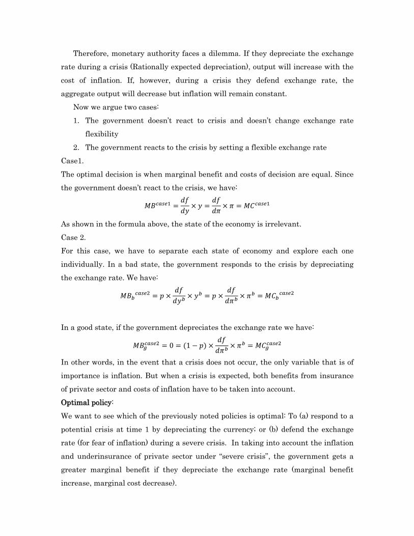
Chile and Response to Asian/Russian crisis: Fear of floating or fear of sudden stop? (Data from Kevin Cowan, Jonathan Kearns (2004))

In 1998, Chile faced a significant deterioration in terms of trade (Figure 1) after Asian/Russian crisis.

Figure 1. Terms of trade volatility following Asian/Russian crisis (Kevin Cowan, Jonathan Kearns (2004))

Despite Chile’s record high annual growth rate (8%), from 1997 to 1999 the

growth rate fell sharply.

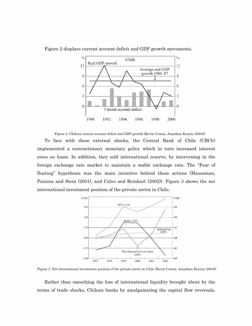
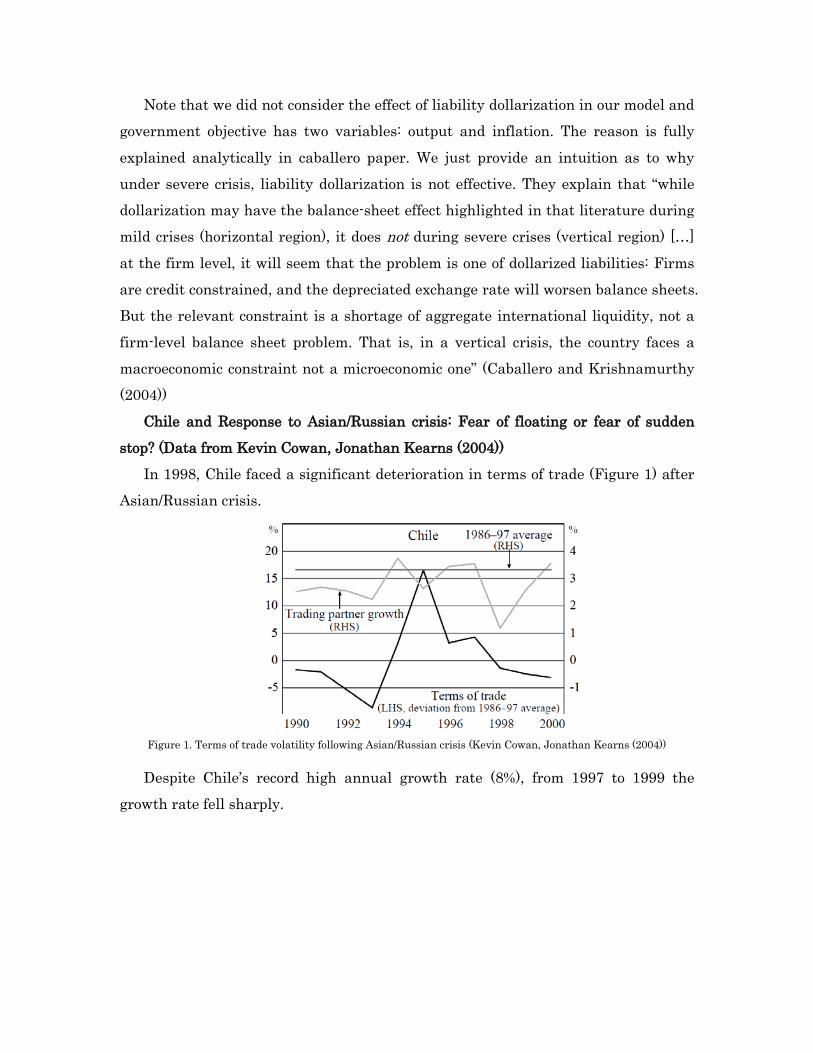
Figure 2 displays current account deficit and GDP growth movements.

Figure 2. Chilean current account deficit and GDP growth (Kevin Cowan, Jonathan Kearns (2004))

To face with these external shocks, the Central Bank of Chile (CBCh) implemented a contractionary monetary policy which in turn increased interest rates on loans. In addition, they sold international reserve, by intervening in the foreign exchange rate market to maintain a stable exchange rate. The “Fear of floating” hypothesis was the main incentive behind these actions (Haussman, Panizza and Stein (2001), and Calvo and Reinhart (2002)). Figure 3 shows the net international investment position of the private sector in Chile.

Figure 3. Net international investment position of the private sector in Chile (Kevin Cowan, Jonathan Kearns (2004))

Rather than smoothing the loss of international liquidity brought about by the

terms of trade shocks, Chilean banks by amalgamating the capital flow reversals,

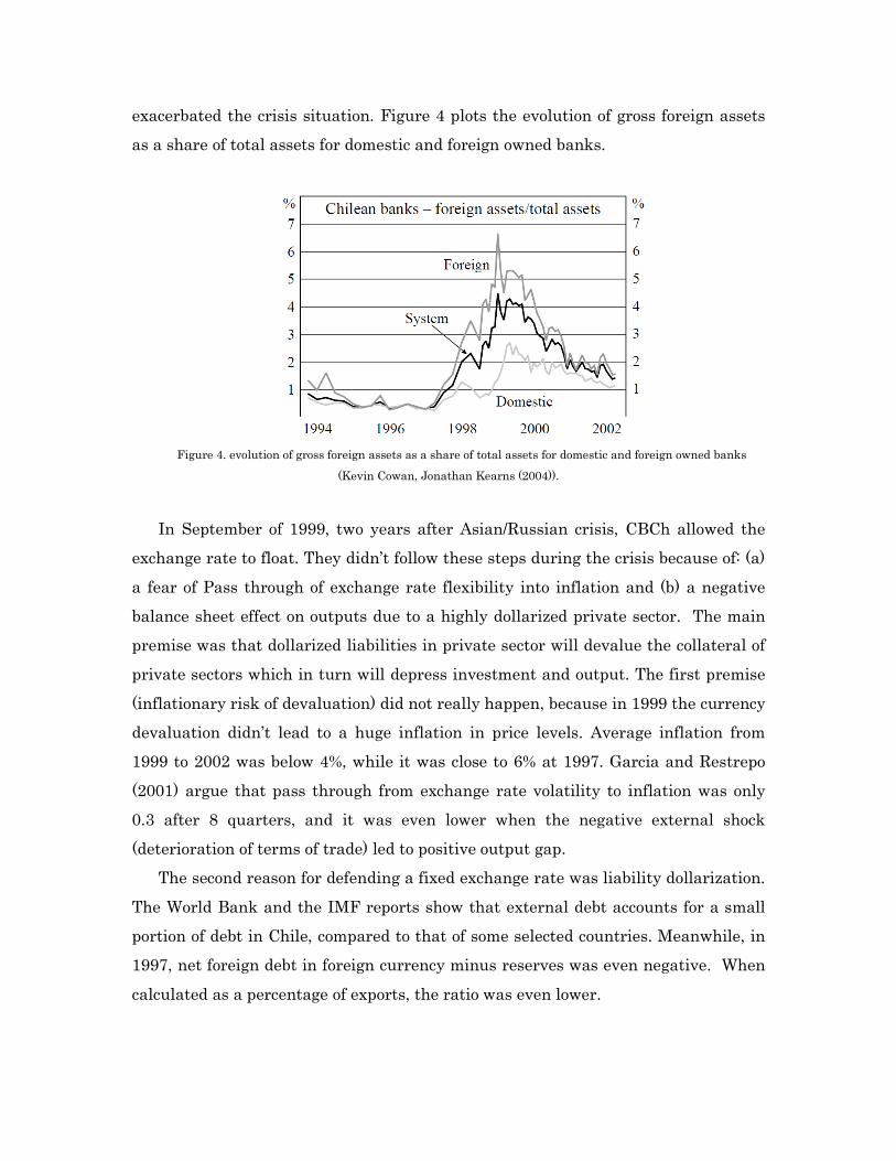
exacerbated the crisis situation. Figure 4 plots the evolution of gross foreign assets as a share of total assets for domestic and foreign owned banks.

Figure 4. evolution of gross foreign assets as a share of total assets for domestic and foreign owned banks

(Kevin Cowan, Jonathan Kearns (2004)).

In September of 1999, two years after Asian/Russian crisis, CBCh allowed the

exchange rate to float. They didn’t follow these steps during the crisis because of: (a) a fear of Pass through of exchange rate flexibility into inflation and (b) a negative balance sheet effect on outputs due to a highly dollarized private sector. The main premise was that dollarized liabilities in private sector will devalue the collateral of private sectors which in turn will depress investment and output. The first premise (inflationary risk of devaluation) did not really happen, because in 1999 the currency devaluation didn’t lead to a huge inflation in price levels. Average inflation from 1999 to 2002 was below 4%, while it was close to 6% at 1997. Garcia and Restrepo (2001) argue that pass through from exchange rate volatility to inflation was only 0.3 after 8 quarters, and it was even lower when the negative external shock (deterioration of terms of trade) led to positive output gap.

The second reason for defending a fixed exchange rate was liability dollarization. The World Bank and the IMF reports show that external debt accounts for a small portion of debt in Chile, compared to that of some selected countries. Meanwhile, in 1997, net foreign debt in foreign currency minus reserves was even negative. When calculated as a percentage of exports, the ratio was even lower.

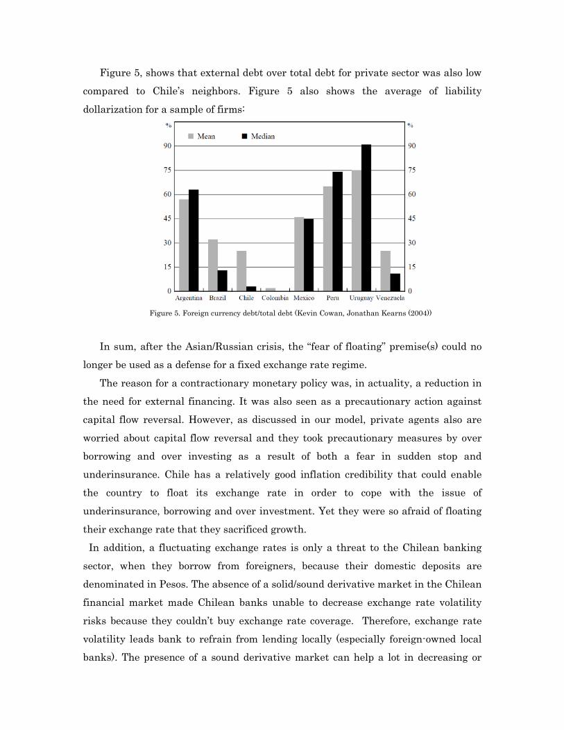
Figure 5, shows that external debt over total debt for private sector was also low compared to Chile’s neighbors. Figure 5 also shows the average of liability dollarization for a sample of firms:

Figure 5. Foreign currency debt/total debt (Kevin Cowan, Jonathan Kearns (2004))

In sum, after the Asian/Russian crisis, the “fear of floating” premise(s) could no

longer be used as a defense for a fixed exchange rate regime. The reason for a contractionary monetary policy was, in actuality, a reduction in

the need for external financing. It was also seen as a precautionary action against capital flow reversal. However, as discussed in our model, private agents also are worried about capital flow reversal and they took precautionary measures by over borrowing and over investing as a result of both a fear in sudden stop and underinsurance. Chile has a relatively good inflation credibility that could enable the country to float its exchange rate in order to cope with the issue of underinsurance, borrowing and over investment. Yet they were so afraid of floating their exchange rate that they sacrificed growth. In addition, a fluctuating exchange rates is only a threat to the Chilean banking sector, when they borrow from foreigners, because their domestic deposits are denominated in Pesos. The absence of a solid/sound derivative market in the Chilean financial market made Chilean banks unable to decrease exchange rate volatility risks because they couldn’t buy exchange rate coverage. Therefore, exchange rate volatility leads bank to refrain from lending locally (especially foreign-owned local banks). The presence of a sound derivative market can help a lot in decreasing or

offsetting the exchange rate volatility in those economies. In fact, domestic liabilities are usually dollarized since there is no market to offset the risks of exchange rate volatility. References:

1. Caballero, R. & Krishnamurthy, “A. (2004), Exchange Rate Volatility and the Credit Channel in Emerging Markets: A Vertical Perspective”, NBER Working Paper 10517

2. Caballero, R. (2002), Coping with Chile’s External Vulnerability: A Financial Problem, in N. Loayza & R. Soto, eds, ‘Economic Growth: Sources, Trends and Cycles’, Banco Central de Chile, Santiago, Chile, pp. 377—416.

3. Caballero, R. & Krishnamurthy, A. (2003), ‘Excessive Dollar Debt: Financial Development and Underinsurance’, Journal of Finance 58(2), 867—894.

4. Caballero, R. & Krishnamurthy, A. (2004), “Inflation Targeting and Sudden Stops”. B. Bernanke & M. Woodford, eds, ‘Inflation Targeting’.

5. Caballero, R. & Panageas, S. (2003), “Hedging sudden stops and precautionary recessions: A quantitative framework”. Mimeo MIT.

6. Calvo, G. & Reinhart, C. (2002), “Fear of Floating”, The Quarterly Journal of Economics 67, 379—408.

7. Bordo, M. D., Meissner, C. & Redish, A. (2003), “How “original sin” was overcome: the evolution of external debt denominated in domestic currencies in the United States and the British dominions 1800-2000”, Working Paper 9841, NBER

8. Kevin Cowan, Jonathan Kearns (2004), “Fear of Sudden Stops: Lessons from Australia and Chile”, Inter-American Development Bank

9. Garcia, C. J. & Restrepo, J. E. (2001), Price Inflation and Exchange Rate Pass-Through in Chile, Working Paper 128, Central Bank of Chile

Second essay: Global imbalances and Current Account Determinants

Abstract:

The current account imbalances have always been the central focus of policymakers, in part due to the central role the current account plays in countries’ wealth formation, the development of countries balance of payments, and in foreseeing economic and exchange rate crises. As a result, policymakers have been interested in answering the following three questions: “Why are global imbalances rising?” “What are the factors contributing to this rise?” and “What are the possible scenarios in the future?” In an attempt to answer the aforementioned questions, we must examine the variables affecting the current account. The determinants found can be used later in country-by-country case to calculate sustainable “current account norm” and to assess current account misalignments, which will demand policy correction. The first part of this essay investigates whether a number of variables affected the current account in a panel of developing and developed countries. The second part of the essay will provide an analytical framework to analyze the relationship between terms of trade volatility and current account dynamics.1

Introduction: The current account imbalances have always been the central focus of

policymakers, in part due to the central role the current account plays in countries wealth formation, the development of countries balance of payments, and in foreseeing economic and exchange rate crises. In recent years, policymakers around the world have been especially concerned with global imbalances, which reflect the growing discrepancies in the current account balances between a number of developed countries, notably the US, and a group of developing countries, mainly China, South-East Asia and oil-exporting economies. The global financial and economic crisis of 2007-2009 did not nullify but rather mitigated the global

1 This research is a revised and extended version of our research on current account determinants

imbalances, which continued to grow again in 2010. Therefore, in light of the current financial crisis dating back to 2007, policymakers have been primarily focused on the connection between the global economy and growing global imbalances. As a result, policymakers have been interested in answering the following three questions: “Why are global imbalances rising?” “What are the factors contributing to this rise?” and “What are the possible scenarios in the future?” In an attempt to answer the aforementioned questions, we must examine the variables affecting the current account. The determinants found can be used later in country-by-country case to calculate sustainable “current account norm” and to assess current account misalignments, which will demand policy correction.

The first part of this essay investigates whether a number of variables affected the current account in a panel of developing and developed countries. The structural model considers the current account as a savings-investments balance and it examines the factors affecting the level of savings and investments in a country. In economic literature, the main factors considered are: economic growth, demographic factors, financial liberalization, trade openness, foreign direct investments, remittances, terms of trade, relative income per capita, fiscal deficit and net indebtedness. The second part of the essay will provide an analytical framework to analyze the relationship between terms of trade volatility and current account dynamics.

Literature Review Many researchers conduct studies to understand the mechanisms by which

variables affect the current account. Numerous economic research papers have also been written on this subject. The fundamental model of the current account suggests that the variables affecting the current account are mainly a result of “inter-temporal consumption smoothing” by economic agents (Rogoff, Obstfeld (1996)). The International Monetary Fund (IMF), in an attempt to calculate equilibrium real exchange rate, assessed the sustainable level of current account based on two different perspectives – savings-investments and net foreign assets (Isard, Faruque (1998), Isard and others (2001), IMF (2006), Milesi-Ferretti and others (2008)). Our paper presents the applications of current account assessment by determining the

variables affecting savings and investments of countries, referred to as the “IMF Macroeconomic Balance Approach”. The methodology has been widely used by numerous researchers in the past decade, notably Chinn and Prasad (2000), Chinn and Ito (2008), Calderon, Chong and Loayza (2011), Medina, Prat, Thomas (2010). Chinn and Prasad (2000) found that the current account balances are positively correlated with initial stock of net foreign assets and government budget balances. Other factors include: relative income, financial deepening, relative dependency, GDP growth, openness, capital control and terms of trade volatility. In addition to the aforementioned factors, Chinn and Ito (2008) also considered legal and institutional development and its interactions with openness and financial development. Medina, Prat, Thomas (2010) added population growth and oil balance as interest variables and Asian crisis dummy as controlled variable. Calderon, Chong, Loayza (1999) used private and public savings, as well as output gap and real exchange rate2

The above noted papers considered different variables that can affect the current account. In this report, we incorporate variables that are relevant to our research scope. In addition, the aforementioned papers failed to use the GLS method in order to address individual heterogeneity of countries. Therefore, this essay differs from previous academic and theoretical findings in both the number of variables considered and the estimation method. By using the Wald test and the GLS method, we have added more measures to test our hypothesis.

.

Why Global Imbalances Matter? In our opinion, there is a link between financial crisis and global imbalances, but

the connection is complicated and very dynamic. In the U.S., the interaction among the Fed’s monetary policies, international real interest rates, financial distortions, and financial innovation promoted an environment that largely contributed to global financial crisis. I believe that the imbalances created a dynamic that contributed to the creation of that environment. The expansion of gross international position has been a primary result of financial globalization which in turn eased the financing of U.S external net borrowing and as a result caused lower dollar interest rate, higher

2 The output gap and real exchange rate in IMF methodology are variables, which should explain the gap between predicted “current account norm” and “underlying current account” (explained by output gap), and later between “underlying current account” and actual current account (explained by real exchange rate misalignment).

U.S spending and stronger dollar. Low interest rates, high liquidity, and optimistic expectations about the home prices’ trend, coupled with unrealistic financial incentives created a huge bubble which led to subprime mortgage crisis. Those driving forces also resulted in the unprecedented U.S deficit. U.S could easily finance its unsustainable real estate bubble by borrowing cheaply from emerging markets, notably China, mainly a result of exchange rate policies in China. Those policies in China enabled U.S to borrow cheaply from abroad and prevent U.S from making robust policy choices. Foreign banks, mainly from Europe started investing in toxic assets that were rated AAA, but were systematically risky. Basel II low assessment of required capital on those assets contributed to those investment decisions. At the same time, countries with current account surpluses didn’t feel

enough pressure to adjust. As Maurice Obstfeld and Kenneth Rogoff argue, “ China’s

ability to sterilize the immense reserve purchases placed in U.S. markets allowed it to maintain an undervalued currency and defer rebalancing its own economy. Complementary policy distortions therefore kept China artificially far from its lower autarky interest rate and the U.S. artificially far from its higher autarky interest rate. Had seemingly low-cost postponement options not been available, the subsequent crisis might well have been mitigated, if not contained.”3

In 2000, the dotcom bubble burst. As a policy response, the interest rate declined, so did savings. The recession caused by bubble burst and the 9/11 attacks made FED respond to shocks through monetary policy choices which later accentuated interest rate trends. The low rates, however, contributed to commodity prices (mainly oil prices) soaring in 2004. Sterilization in China, coupled with undervalued currency and pegged currency to the dollar, largely contributed to capital inflows to U.S. Chinese savings increased as a result of the growth, so did commodity prices. The world’s saving increased as a result of high commodity prices which in turn shifted income from countries that were unable to increase consumption quickly. In 2003-04, as a result of concerns regarding deflation, FED held policy rates low. The low interest rate contributed to housing price increase and excessive mortgage loan availability which in turn led to the excessive borrowing on home equities. All these

3 Maurice Obstfeld and Kenneth Rogoff, “Global Imbalances and the Financial Crisis: Products of Common Causes”, 2009

factors together led to a compression of risk premia, excessive leverage by financial institutions and commodity price inflation 4 . In order to resolve the emerging inflation, FED responded to these dynamics in mid-2004 by choosing monetary tightening policy. As a result, real long-term rates appreciated, adjustable mortgage rates reset and the housing bubble appeared.5

The primary Causes of Global imbalances

The savings glut contributed to the creation of global imbalances as savings exceeded investment in many emerging market countries, notably China. Saving glut story can be explained by highlighting following driving forces:

1. Policy interventions to boost exports in east Asia 2. High commodity price in Middle-east 3. Aging population in advanced economies coupled with a dearth of

investment opportunities 4. High savings in emerging markets and low level of financial

development which creates higher precautionary saving

5. Low investment rate in EMs, following Asian crisis

4 Frankel, Jeffrey A. 2008. “The Effect of Monetary Policy on Real Commodity Prices.” In Asset Prices and Monetary Policy, ed. John Y. Campbell. Chicago: University of Chicago Press. 5To see an alternative view, refer to: “Global imbalances and the financial crisis: Link or no link? by

Claudio Borio and Piti Disyatat, BIS working papers, No. 347, Monetary and Economic Department”.

They argue that “…Many observers have recently singled those [global imbalances] out as a key factor contributing to the global financial crisis. Current account surpluses in several emerging market economies are said to have helped fuel the credit booms and risk-taking in the major advanced deficit countries at the core of the crisis, by putting significant downward pressure on world interest rates

and/or by simply financing the booms in those countries (the “excess saving” view). We argue that this perspective on global imbalances bears reconsideration. We highlight two conceptual problems: (i) drawing inferences about a country’s cross-border financing activity based on observations of net capital flows; and (ii) explaining market interest rates through the saving-investment framework. […]

We conjecture that the main contributing factor to the financial crisis was not “excess saving” but the “excess elasticity” of the international monetary and financial system. […]Credit creation, a defining feature of a monetary economy, plays a key role in this story. “

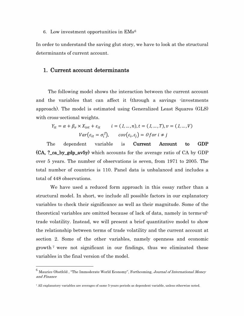
6. Low investment opportunities in EMs6

In order to understand the saving glut story, we have to look at the structural determinants of current account.

1. Current account determinants

The following model shows the interaction between the current account and the variables that can affect it (through a savings -investments approach). The model is estimated using Generalized Least Squares (GLS)

with cross-sectional weights. 𝑌𝑖𝑡 = 𝛼 + 𝛽𝑣 × 𝑋𝑖𝑣𝑡 + 𝜀𝑖𝑡 𝑖 = (1, … ,𝑛), 𝑡 = (1, … ,𝑇),𝑣 = (1, … ,𝑉)

𝑉𝑎𝑟�𝜀𝑖𝑡 = 𝜎𝑖2�, 𝑐𝑜𝑣�𝜀𝑖, 𝜀𝑗� = 0 𝑓𝑜𝑟 𝑖 ≠ 𝑗

The dependent variable is Current Account to GDP

(CA, ?_ca_by_gdp_av5y) which accounts for the average ratio of CA by GDP over 5 years. The number of observations is seven, from 1971 to 2005. The total number of countries is 110. Panel data is unbalanced and includes a total of 448 observations.

We have used a reduced form approach in this essay rather than a structural model. In short, we include all possible factors in our explanatory variables to check their significance as well as their magnitude. Some of the

theoretical variables are omitted because of lack of data, namely in terms-of-trade volatility. Instead, we will present a brief quantitative model to show the relationship between terms of trade volatility and the current account at

section 2. Some of the other variables, namely openness and economic growth 7

6 Maurice Obstfeld , “The Immoderate World Economy”, Forthcoming, Journal of International Money and Finance

were not significant in our findings, thus we eliminated these variables in the final version of the model.

7 All explanatory variables are averages of same 5-years periods as dependent variable, unless otherwise noted.

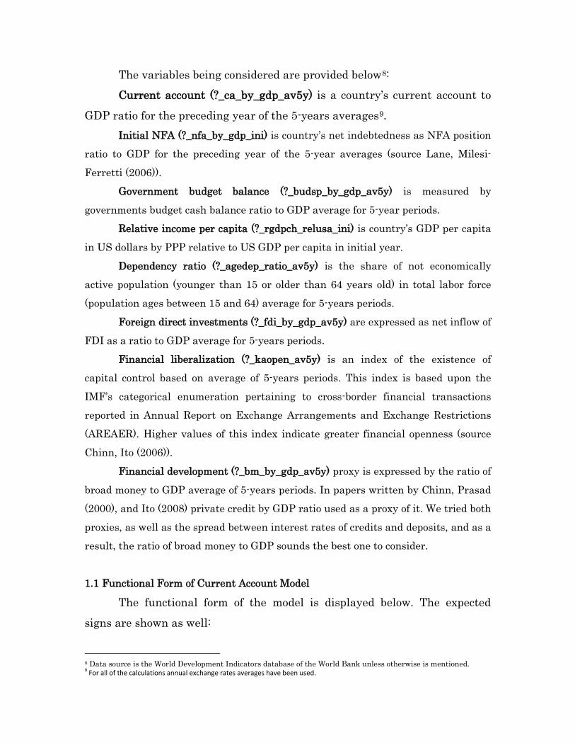
The variables being considered are provided below8

Current account (?_ca_by_gdp_av5y) is a country’s current account to

GDP ratio for the preceding year of the 5-years averages

:

9

Initial NFA (?_nfa_by_gdp_ini) is country’s net indebtedness as NFA position ratio to GDP for the preceding year of the 5-year averages (source Lane, Milesi-Ferretti (2006)).

.

Government budget balance (?_budsp_by_gdp_av5y) is measured by governments budget cash balance ratio to GDP average for 5-year periods.

Relative income per capita (?_rgdpch_relusa_ini) is country’s GDP per capita in US dollars by PPP relative to US GDP per capita in initial year.

Dependency ratio (?_agedep_ratio_av5y) is the share of not economically active population (younger than 15 or older than 64 years old) in total labor force (population ages between 15 and 64) average for 5-years periods.

Foreign direct investments (?_fdi_by_gdp_av5y) are expressed as net inflow of FDI as a ratio to GDP average for 5-years periods.

Financial liberalization (?_kaopen_av5y) is an index of the existence of capital control based on average of 5-years periods. This index is based upon the IMF’s categorical enumeration pertaining to cross-border financial transactions reported in Annual Report on Exchange Arrangements and Exchange Restrictions (AREAER). Higher values of this index indicate greater financial openness (source Chinn, Ito (2006)).

Financial development (?_bm_by_gdp_av5y) proxy is expressed by the ratio of broad money to GDP average of 5-years periods. In papers written by Chinn, Prasad (2000), and Ito (2008) private credit by GDP ratio used as a proxy of it. We tried both proxies, as well as the spread between interest rates of credits and deposits, and as a result, the ratio of broad money to GDP sounds the best one to consider.

1.1 Functional Form of Current Account Model

The functional form of the model is displayed below. The expected

signs are shown as well:

8 Data source is the World Development Indicators database of the World Bank unless otherwise is mentioned. 9 For all of the calculations annual exchange rates averages have been used.

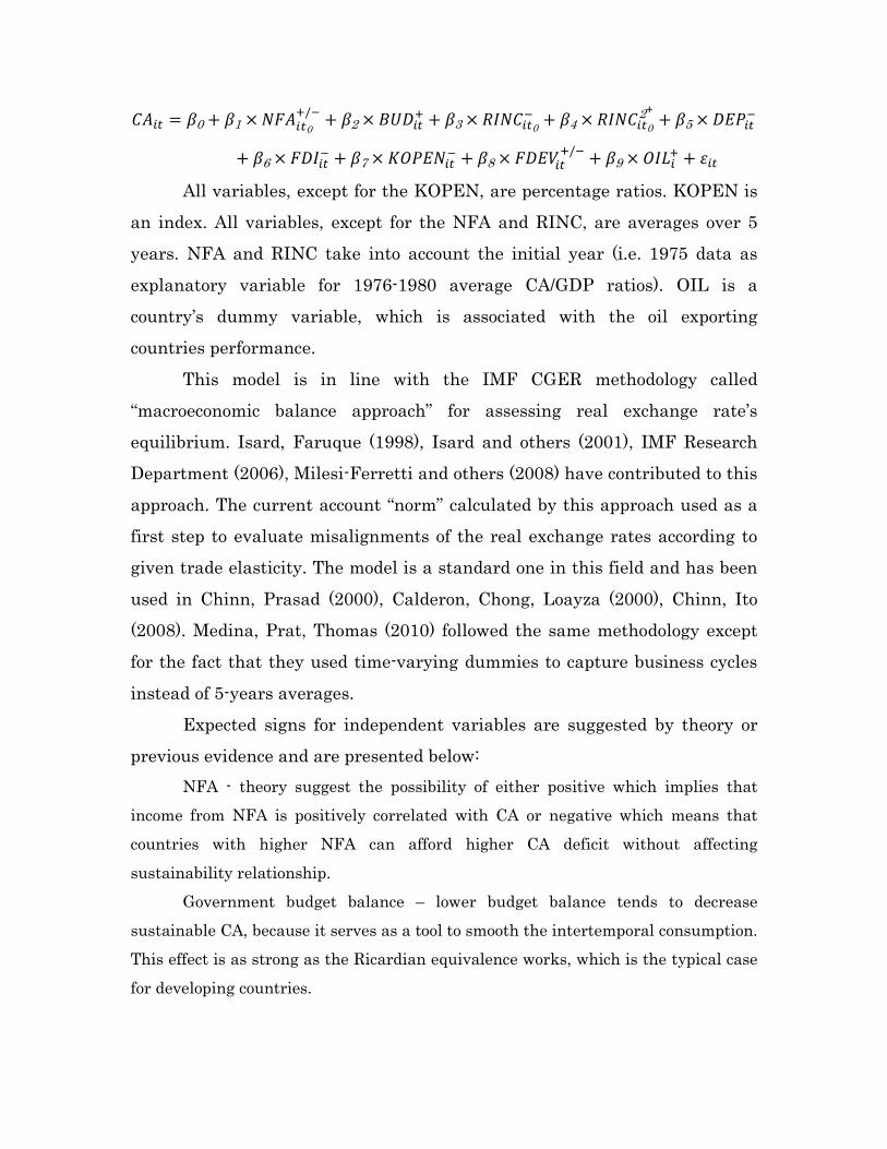
𝐶𝐴𝑖𝑡 = 𝛽0 + 𝛽1 × 𝑁𝐹𝐴𝑖𝑡0+/− + 𝛽2 × 𝐵𝑈𝐷𝑖𝑡+ + 𝛽3 × 𝑅𝐼𝑁𝐶𝑖𝑡0

− + 𝛽4 × 𝑅𝐼𝑁𝐶𝑖𝑡02+ + 𝛽5 × 𝐷𝐸𝑃𝑖𝑡−

+ 𝛽6 × 𝐹𝐷𝐼𝑖𝑡− + 𝛽7 × 𝐾𝑂𝑃𝐸𝑁𝑖𝑡− + 𝛽8 × 𝐹𝐷𝐸𝑉𝑖𝑡+/− + 𝛽9 × 𝑂𝐼𝐿𝑖+ + 𝜀𝑖𝑡

All variables, except for the KOPEN, are percentage ratios. KOPEN is an index. All variables, except for the NFA and RINC, are averages over 5 years. NFA and RINC take into account the initial year (i.e. 1975 data as

explanatory variable for 1976-1980 average CA/GDP ratios). OIL is a country’s dummy variable, which is associated with the oil exporting countries performance.

This model is in line with the IMF CGER methodology called “macroeconomic balance approach” for assessing real exchange rate’s equilibrium. Isard, Faruque (1998), Isard and others (2001), IMF Research Department (2006), Milesi-Ferretti and others (2008) have contributed to this

approach. The current account “norm” calculated by this approach used as a first step to evaluate misalignments of the real exchange rates according to given trade elasticity. The model is a standard one in this field and has been

used in Chinn, Prasad (2000), Calderon, Chong, Loayza (2000), Chinn, Ito (2008). Medina, Prat, Thomas (2010) followed the same methodology except for the fact that they used time-varying dummies to capture business cycles

instead of 5-years averages. Expected signs for independent variables are suggested by theory or

previous evidence and are presented below: NFA - theory suggest the possibility of either positive which implies that

income from NFA is positively correlated with CA or negative which means that countries with higher NFA can afford higher CA deficit without affecting sustainability relationship.

Government budget balance – lower budget balance tends to decrease sustainable CA, because it serves as a tool to smooth the intertemporal consumption. This effect is as strong as the Ricardian equivalence works, which is the typical case for developing countries.

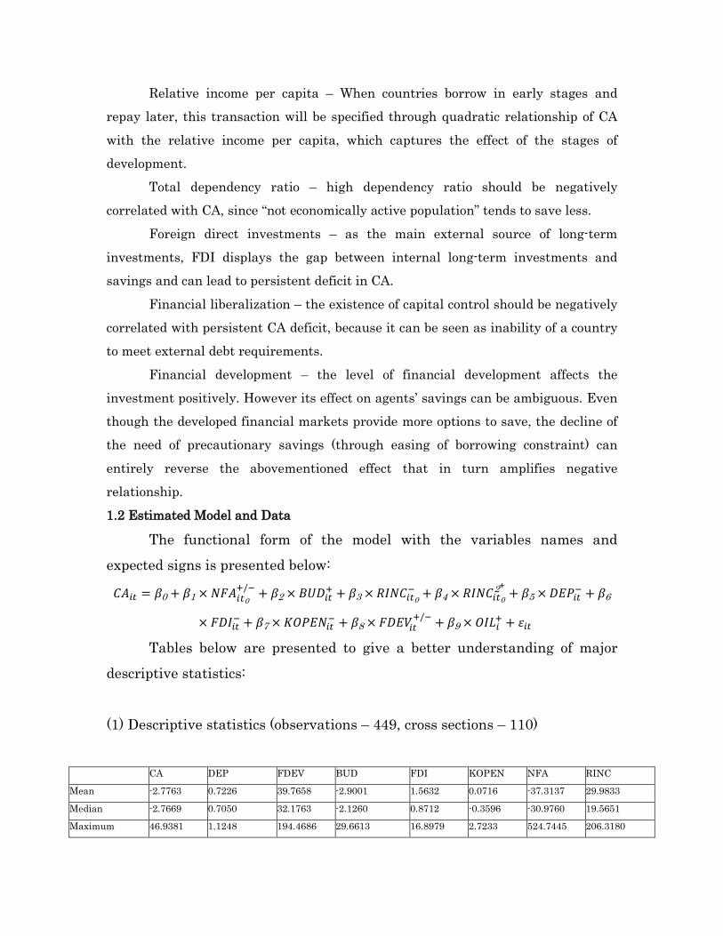
Relative income per capita – When countries borrow in early stages and repay later, this transaction will be specified through quadratic relationship of CA with the relative income per capita, which captures the effect of the stages of development.

Total dependency ratio – high dependency ratio should be negatively correlated with CA, since “not economically active population” tends to save less.

Foreign direct investments – as the main external source of long-term investments, FDI displays the gap between internal long-term investments and savings and can lead to persistent deficit in CA.

Financial liberalization – the existence of capital control should be negatively correlated with persistent CA deficit, because it can be seen as inability of a country to meet external debt requirements.

Financial development – the level of financial development affects the investment positively. However its effect on agents’ savings can be ambiguous. Even though the developed financial markets provide more options to save, the decline of the need of precautionary savings (through easing of borrowing constraint) can entirely reverse the abovementioned effect that in turn amplifies negative relationship. 1.2 Estimated Model and Data

The functional form of the model with the variables names and expected signs is presented below:

𝐶𝐴𝑖𝑡 = 𝛽0 + 𝛽1 × 𝑁𝐹𝐴𝑖𝑡0+/− + 𝛽2 × 𝐵𝑈𝐷𝑖𝑡+ + 𝛽3 × 𝑅𝐼𝑁𝐶𝑖𝑡0

− + 𝛽4 × 𝑅𝐼𝑁𝐶𝑖𝑡02+ + 𝛽5 × 𝐷𝐸𝑃𝑖𝑡− + 𝛽6

× 𝐹𝐷𝐼𝑖𝑡− + 𝛽7 × 𝐾𝑂𝑃𝐸𝑁𝑖𝑡− + 𝛽8 × 𝐹𝐷𝐸𝑉𝑖𝑡+/− + 𝛽9 × 𝑂𝐼𝐿𝑖+ + 𝜀𝑖𝑡

Tables below are presented to give a better understanding of major descriptive statistics:

(1) Descriptive statistics (observations – 449, cross sections – 110)

CA DEP FDEV BUD FDI KOPEN NFA RINC

Mean -2.7763 0.7226 39.7658 -2.9001 1.5632 0.0716 -37.3137 29.9833

Median -2.7669 0.7050 32.1763 -2.1260 0.8712 -0.3596 -30.9760 19.5651

Maximum 46.9381 1.1248 194.4686 29.6613 16.8979 2.7233 524.7445 206.3180

-60

-40

-20

0

20

40

60

-50 -40 -30 -20 -10 0 10 20 30 40

?_BUDSP_BY_GDP_AV5Y

?_C

A_BY

_GD

P_AV

5Y

-20

-15

-10

-5

0

5

10

15

20

-20 -10 0 10 20

?_BUDSP_BY_GDP_AV5Y

?_C

A_BY

_GD

P_AV

5Y

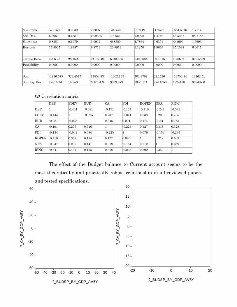
Minimum -40.1532 0.3930 7.3097 -41.7408 -5.7219 -1.7528 -654.6016 1.7114

Std. Dev. 6.3060 0.1887 26.2536 4.5732 2.2928 1.4746 65.5357 28.7185

Skewness 0.8380 0.1979 1.9912 -0.8550 1.7864 0.6351 -0.4999 1.5693

Kurtosis 17.9005 1.8387 8.8716 20.8913 9.1250 1.9669 35.1098 6.0611

Jarque-Bera 4206.231 28.1602 941.6948 6043.186 940.6634 50.1516 19307.71 359.5869

Probability 0.0000 0.0000 0.0000 0.0000 0.0000 0.0000 0.0000 0.0000

Sum -1246.575 324.4577 17854.83 -1302.135 701.8782 32.1526 -16753.84 13462.51

Sum Sq. Dev. 17815.14 15.9535 308784.9 9369.379 2355.171 974.1358 1924128. 369487.6

(2) Correlation matrix DEP FDEV BUD CA FDI KOPEN NFA RINC

DEP 1 -0.444 -0.081 -0.191 -0.134 -0.418 -0.247 -0.541

FDEV -0.444 1 -0.025 0.207 -0.041 0.368 0.236 0.435

BUD -0.081 -0.025 1 0.346 0.094 0.174 0.141 0.155

CA -0.191 0.207 0.346 1 -0.225 0.127 0.318 0.378

FDI -0.134 -0.041 0.094 -0.225 1 0.076 -0.154 -0.235

KOPEN -0.418 0.368 0.174 0.127 0.076 1 0.212 0.509

NFA -0.247 0.236 0.141 0.318 -0.154 0.212 1 0.359

RINC -0.541 0.435 0.155 0.378 -0.235 0.509 0.359 1

The effect of the Budget balance to Current account seems to be the

most theoretically and practically robust relationship in all reviewed papers and tested specifications.

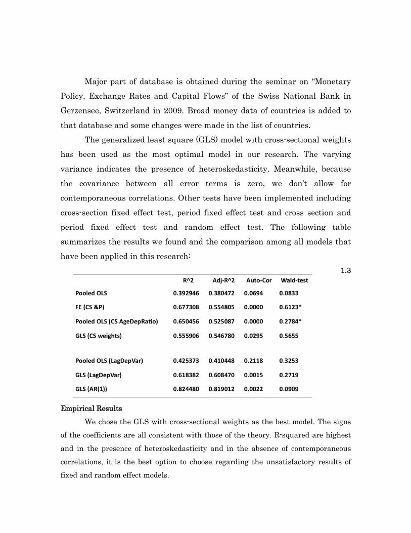
Major part of database is obtained during the seminar on “Monetary Policy, Exchange Rates and Capital Flows” of the Swiss National Bank in Gerzensee, Switzerland in 2009. Broad money data of countries is added to

that database and some changes were made in the list of countries. The generalized least square (GLS) model with cross-sectional weights

has been used as the most optimal model in our research. The varying

variance indicates the presence of heteroskedasticity. Meanwhile, because the covariance between all error terms is zero, we don’t allow for contemporaneous correlations. Other tests have been implemented including

cross-section fixed effect test, period fixed effect test and cross section and period fixed effect test and random effect test. The following table summarizes the results we found and the comparison among all models that have been applied in this research:

1.3

Empirical Results We chose the GLS with cross-sectional weights as the best model. The signs

of the coefficients are all consistent with those of the theory. R-squared are highest and in the presence of heteroskedasticity and in the absence of contemporaneous correlations, it is the best option to choose regarding the unsatisfactory results of fixed and random effect models.

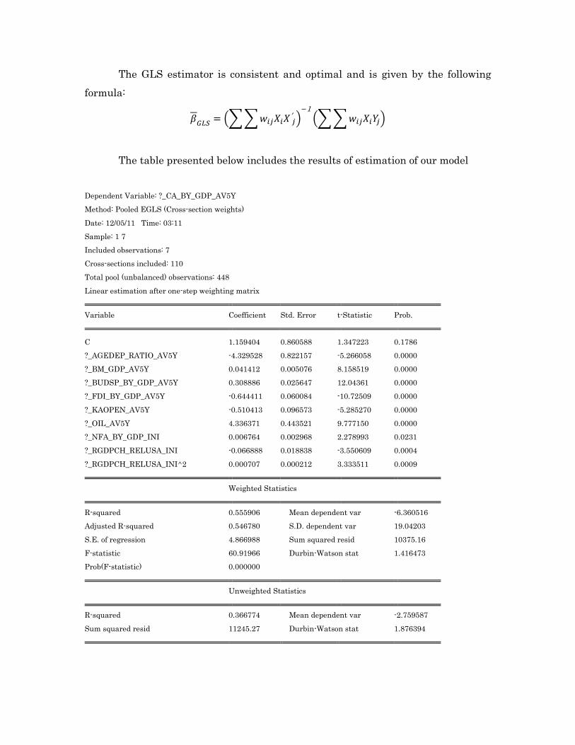
The GLS estimator is consistent and optimal and is given by the following formula:

𝛽𝐺𝐿𝑆 = ���𝑤𝑖𝑗𝑋𝑖𝑋′𝑗�−1���𝑤𝑖𝑗𝑋𝑖𝑌𝑗�

The table presented below includes the results of estimation of our model

Dependent Variable: ?_CA_BY_GDP_AV5Y Method: Pooled EGLS (Cross-section weights)

Date: 12/05/11 Time: 03:11 Sample: 1 7 Included observations: 7 Cross-sections included: 110 Total pool (unbalanced) observations: 448

Linear estimation after one-step weighting matrix Variable Coefficient Std. Error t-Statistic Prob. C 1.159404 0.860588 1.347223 0.1786 ?_AGEDEP_RATIO_AV5Y -4.329528 0.822157 -5.266058 0.0000 ?_BM_GDP_AV5Y 0.041412 0.005076 8.158519 0.0000 ?_BUDSP_BY_GDP_AV5Y 0.308886 0.025647 12.04361 0.0000 ?_FDI_BY_GDP_AV5Y -0.644411 0.060084 -10.72509 0.0000

?_KAOPEN_AV5Y -0.510413 0.096573 -5.285270 0.0000 ?_OIL_AV5Y 4.336371 0.443521 9.777150 0.0000 ?_NFA_BY_GDP_INI 0.006764 0.002968 2.278993 0.0231 ?_RGDPCH_RELUSA_INI -0.066888 0.018838 -3.550609 0.0004

?_RGDPCH_RELUSA_INI^2 0.000707 0.000212 3.333511 0.0009 Weighted Statistics R-squared 0.555906 Mean dependent var -6.360516 Adjusted R-squared 0.546780 S.D. dependent var 19.04203 S.E. of regression 4.866988 Sum squared resid 10375.16 F-statistic 60.91966 Durbin-Watson stat 1.416473 Prob(F-statistic) 0.000000

Unweighted Statistics

R-squared 0.366774 Mean dependent var -2.759587

Sum squared resid 11245.27 Durbin-Watson stat 1.876394

The table displayed above shows that 110 cross-section included while we have 7 observations. The variables and their definitions are all mentioned in the previous section.

As shown in the GLS table above, we can see that all coefficients have the expected signs and they are all statistically significant. Here, we discuss the signs and significance of coefficients;

1. P-values for all of the coefficients estimated in the table is less than 5% indicating that they are all statistically significant and depends on their sign, positively or negatively affect current account.

2. The signs are all expected. As mentioned in section 2, we have following variables included in the model. According to the table, we have following results and justifications as to signs; NFA - In this case, we have positive coefficient for NFA, indicating that

income from NFA is positively correlated with CA. Government budget balance – the coefficient is positive showing that

sustainably lower budget balance tends to decrease sustainable CA, because it serves as a tool to smooth the intertemporal consumption.

Relative income per capita – The relative income per capita, which captures the stage of development, has a quadratic relationship with CA. The signs are consistent with those that the theory of development stages suggest. In other word, when relative income per capita is higher than 1, an increase in relative income has a positive impact on CA as expected, because the sign of INI^2 is positive and the sign of INI is negative.

Total dependency ratio – high dependency ratio should be negatively correlated with CA, as not economically active population tends to save less. The sign is in line with the expectation.

Foreign direct investments – as the main external source of long-term investments, FDI witnesses the gap between internal long-term investments and savings and can lead to sustainable deficit in CA. Therefore, the sign should be negative which is in line with the theory.

Financial liberalization – the existence of capital control should be negatively correlated with sustainable CA deficit, because it is seen as inability of a country to

serve external debt. The sign has to be negative which is consistent with the previous explanation.

Financial development – the level of financial development affects positively on investments, while its effect on agents savings can be ambiguous. Even though the developed financial markets propose more possibilities to save, the decline of the need of precautionary savings (through easing of borrowing constraint) can entirely reverse the abovementioned effect amplifying negative relationship. The positive sign in the table seems to capture perfectly the impact of financial development on CA. This finding can be explained by the fact, that we used broad money to GDP ratio as a proxy for financial development. While broad money tends to reflect more the saving side of money, the investment side can be captured by applying the assets point of view (i.e. by credits to GDP ratio).

Also we tested the assumptions for uncorrelated errors, which were proved not to be auto correlated. Considering all of the mentioned points, the final model is; 𝐶𝐴𝑖𝑡 = 0.006764 × 𝑁𝐹𝐴𝑖𝑡0 + 0.308886 × 𝐵𝑈𝐷𝑖𝑡 − 0.066888 × 𝑅𝐼𝑁𝐶𝑖𝑡0 + 0.000707

× 𝑅𝐼𝑁𝐶𝑖𝑡02 − 4.329528 × 𝐷𝐸𝑃𝑖𝑡 ± 0.644411 × 𝐹𝐷𝐼𝑖𝑡 − 0.510413 × 𝐾𝑂𝑃𝐸𝑁𝑖𝑡

+ 0.041412 × 𝐹𝐷𝐸𝑉𝑖𝑡 + 4.336371 × 𝑂𝐼𝐿𝑖 + 𝜀𝑖𝑡

2. Terms of trade volatility and Current account dynamic

As previously mentioned, some of the theoretical variables are omitted due to the lack of data, notably terms-of-trade volatility. In this research, we will briefly explore the interaction between terms of trade and the current account. This part of research is a simplified and more specific version of Christopher Kent and Paul Cashin (2003).

Some of the key assumptions in our model are as follows: 1. We have a small open economy 2. We have one agent with infinite life time

3. The agent supplies one unit of labor 4. We have two goods: imported and exported goods 5. Depreciation rate of capital stock is zero

6. The interest rate on capital is fixed and equal to the world’s interest

rate,

rt = r

The agent must figure out the optimal consumption and investment decisions. The utility function of the firm is as below:

MaxU = βtu(ct )t =0

∞

∑s.t :∆bt +1 = rbt + pt yt − ct − ∆kt

where′ u > 0′ ′ u < 0

0 < β <1

Where

kt is the capital stock,

bt is the stock of foreign assets. The

budget constraint above represents the current account balance as well. The

price of imported goods and exported goods are

pti and

pte respectively. Thereby,

the term of trade is:

pt = pte / pt

i

The production function for exported good is:

yt = At f (kt )where

′ f (kt ) > 0′ ′ f (kt ) < 0

Where

At is the productivity level. We assume that the investment at a

certain time will add to the capital stock and increase the level of capital stock in the next period. In other words:

∆kt = It

In steady state, we assume that

pt = p and

At = A . Therefore, we have:

At ′ f (kt ) = r / pt

Which means that the marginal value product of capital is equal to

world’s interest rate. Note that elasticity of the capital with respect to the

terms of trade is equal to the elasticity of the capital with respect to the productivity level. In other words:

At /kt × dkt / pt = pt /kt × dkt / pt = − ′ f (kt ) / ′ ′ f (kt ) > 0

After deciding about the investment path, the agent must decide about the consumption path. According to Euler’s equation, we have:

′ u (ct +1) / ′ u (ct ) = (1+ r) /β

Consumption smoothing effect implies that the level of permanent income must be equal to consumption. Now we assume that

(1+ r) =1/β .

Solving the optimization problem, we have:

ytp = r[bt + p j y j /(1+ r) j − t

j = t

∞

∑ ] = ct

We then impose a shock to either productivity or terms of trade. We would like to see how the current account responds to terms of trade shocks.

Let’s assume that

δ equals to the percentage change of the

pt At for

t = 0,1,2,...,τ . We investigate the response of the current account to the positive

shocks under three scenarios: 1)

τ = ∞ : A permanent increase in terms of trade is an incentive for

investment. But according to

∆kt = It , the level of capital will increase later in

the next period. Therefore,

ytp ≠ ct which through the consumption smoothing

effects leads to a current account deficit at the present time. 2)

τ = 0 : In a temporary positive shock, The investment will be zero

given the fact that investors can not immediately respond, therefore change in capital level will be zero. The level of current income raises more than the

permanent income and through

∆bt +1 = rbt + pt yt − ct − ∆kt , we will have a

current account surplus. 3)

0 < τ < ∞ : A temporary but lasting shock is a bit more complicated.

Two forces will change the current account: investment and consumption

smoothing effect. The dominance of each of the forces implies different impacts on the current account. This dominance depends on the magnitude of

the shock and its persistence. For less persistent shocks, consumption smoothing will prevail and for positive shocks, we will experience current

account surplus. For some level of persistence, they cancel each other out. For more persistent shocks, the investment effect will dominate and for positive shock, it leads to current account deficit.

Conclusion As a result, the paper investigates whether a number of variables affected

the current account in a panel of developing and developed countries. Variables found significant are Net indebtedness, Budget balance, Relative income, Dependency ratio, foreign direct investments, financial liberalization and financial development. These variables affect current account through savings or investments, as current account identity presents it as a savings investments difference. The model is estimated used Generalized Least Squares with cross-sectional weights.

𝑌𝑖𝑡 = 𝛼 + 𝛽𝑣 × 𝑋𝑖𝑣𝑡 + 𝜀𝑖𝑡 𝑖 = (1, … ,𝑛), 𝑡 = (1, … ,𝑇),𝑣 = (1, … ,𝑉)

𝑉𝑎𝑟�𝜀𝑖𝑡 = 𝜎𝑖2�, 𝑐𝑜𝑣�𝜀𝑖, 𝜀𝑗� = 0 𝑓𝑜𝑟 𝑖 ≠ 𝑗

The following models have been conducted; Pooled OLS, Cross-sectional FE, Period FE, Cross-sectional RE, GLS (Cross-sectional weights, Period weights). Based on the results we have so far, the generalized least square (GLS) model with cross-sectional weights has been used. The “stages of development” hypothesis was checked by Wald test of the appropriate coefficients of relative income variable. As previously mentioned, we could not get data on volatility of countries terms of trade. Instead we developed an analytical model that can capture the effect of terms of trade volatility on the current account deficit. Another possible improvement can be the estimation of the model with the constraint on the relative income hypothesis, which was tested using the Wald test.

References: 1. “Foundations of International Macoeconomics”, Rogoff, Kenneth and

Obstfeld, Maurice, The MIT Press, 1996. 2. “Exchange rate assessment : extensions of the macroeconomic balance

approach”, Isard, Peter and Faruque, Hamid, Occasional paper 167, International Monetary Fund, 1998.

3. “Medium-Term Determinants Of Current Accounts In Industrial And Developing Countries: An Empirical Exploration”, Menzie Chinn, Eswar S. Prasad, NBER Working Paper 7581, 2000.

4. ”Determinants of Current Account Deficits in Developing Countries”, Cesar Calderon, Alberto Chong, Norman Loayza, The World Bank, Policy Research Working Paper 2398, 2000.

5. “Methodology for current account and exchange rate assessments”, Isard, Peter, Faruque, Hamid, Kincaid, G. Russell, and Fetherston, Martin, Occasional paper 209, International Monetary Fund, 2001.

6. “Methodology for CGER Exchange Rate Assessments”, Research department, International Monetary Fund, 2006.

7. “What Matters for Financial Development? Capital Controls, Institutions and Interactions,” Chinn, Menzie and Ito, Hiro, Journal of

Development Economics 81, 2006. 8. “Exchange rate assessments: CGER methodologies”, Milesi-Ferretti,

Gian Maria, Lee, Jaewoo, Ostry, Jonathan, Prati Alessandro, and Ricci,

Luca Antonio, Occasional Paper 261, International Monetary Fund, 2008.

9. “Global Current Account Imbalances: American Fiscal Policy versus

East Asian Savings”, Menzie D. Chinn and Hiro Ito, Review of International Economics, 16(3), 479–498, 2008.

10. “Current Account Balance Estimates for Emerging Market Economies”,

Leandro Medina, Jordi Prat and Alun Thomas, Working Paper 10/43, International Monetary Fund, 2010.

11. “The response of current account to terms of trade shocks: persistent matters”, Christopher Kent and Paul Cashin (2003), IMF Working

Papers, July 2003