International Asset Allocation under Regime Switching, Skew and

Research Division Federal Reserve Bank of St. Louis Working Paper Series

International Asset Allocation under Regime Switching, Skew and Kurtosis Preferences

Massimo Guidolin and

Allan Timmermann

Working Paper 2005-034C http://research.stlouisfed.org/wp/2005/2005-034.pdf

June 2005 Revised August 2007

FEDERAL RESERVE BANK OF ST. LOUIS Research Division

P.O. Box 442 St. Louis, MO 63166

______________________________________________________________________________________

The views expressed are those of the individual authors and do not necessarily reflect official positions of the Federal Reserve Bank of St. Louis, the Federal Reserve System, or the Board of Governors.

Federal Reserve Bank of St. Louis Working Papers are preliminary materials circulated to stimulate discussion and critical comment. References in publications to Federal Reserve Bank of St. Louis Working Papers (other than an acknowledgment that the writer has had access to unpublished material) should be cleared with the author or authors.

International Asset Allocation under Regime Switching, Skew

and Kurtosis Preferences∗

Massimo Guidolin†

Federal Reserve Bank of St. Louis

Allan Timmermann‡

University of California, San Diego

June 2006

JEL code: G12, F30, C32.

Abstract

This paper proposes a new tractable approach to solving asset allocation problems in situations with

a large number of risky assets which pose problems for standard approaches. Investor preferences are

assumed to be defined over moments of the wealth distribution such as its mean, variance, skew and

kurtosis. Time-variations in investment opportunities are represented by a flexible regime switching

process. In the context of a four-moment international CAPM specification that relates stock returns

in five regions to returns on a global market portfolio, we find evidence of distinct bull and bear states.

Ignoring regimes, an unhedged US investor’s optimal portfolio is strongly diversified internationally. The

presence of regimes in the return distribution leads to a large increase in the investor’s optimal holdings

of US stocks as does the introduction of skew and kurtosis preferences. Our paper therefore offers an

explanation of the strong home bias observed in US investors’ asset allocation based on regime switching

and skew and kurtosis preferences.

Key words: International Asset Allocation, Regime Switching, Skew and Kurtosis Preferences, Home

Bias.

∗We thank the editor, Cam Harvey, and an anonymous referee for making many valuable suggestions. We also thank Karim

Abadir, Lucio Sarno, Fabio Trojani, Giorgio Valente, and Mike Wickens. Seminar participants at the European Financial

Management 2005 Annual Conference in Milan, Real Collegio Carlo Alberto Foundation in Turin, HEC Paris, Imperial College

Tanaka Business School, Krannert School of Management at Purdue, Manchester Business School, University of Washington,

University of York (UK), Catholic University, Milan, Warwick Business School, and the World Congress of the Econometric

Society in London also provided helpful comments. All errors remain our own.†Research Division, P.O. Box 442, St. Louis, MO 63166, United States. E-mail: [email protected]; phone:

314-444-8550.‡Rady School and Dept. of Economics, UCSD, 9500 Gilman Drive, La Jolla CA 92093-0508, United States. E-mail:

[email protected]; phone: 858-534-4860

.

Abstract

This paper proposes a new tractable approach to solving asset allocation problems in situa-

tions with a large number of risky assets which pose problems for standard approaches. Investor

preferences are assumed to be defined over moments of the wealth distribution such as its mean,

variance, skew and kurtosis. Time-variations in investment opportunities are represented by a

flexible regime switching process. In the context of a four-moment international CAPM specifi-

cation that relates stock returns in five regions to returns on a global market portfolio, we find

evidence of distinct bull and bear states. Ignoring regimes, an unhedged US investor’s optimal

portfolio is strongly diversified internationally. The presence of regimes in the return distribution

leads to a large increase in the investor’s optimal holdings of US stocks as does the introduction

of skew and kurtosis preferences. Our paper therefore offers an explanation of the strong home

bias observed in US investors’ asset allocation based on regime switching and skew and kurtosis

preferences.

2

1. Introduction

Despite the increased integration of international capital markets, investors continue to hold equity portfolios

that are largely dominated by domestic assets. According to Thomas, Warnock and Wongswan (2004), by

the end of 2003 US investors held only 14% of their equity portfolios in foreign stocks at a time when

such stocks accounted for 54% of the world market capitalization.1 This evidence is poorly understood:

Calculations reported by Lewis (1999) suggest that a US investor with mean-variance preferences should

hold upwards of 40% in foreign stocks or, equivalently, only 60% in US stocks.

Potential explanations for the home bias include barriers to international investment and transaction

costs (Black (1990), Stulz (1981)); hedging demand for stocks that have lower correlations with domestic

state variables such as inflation risk or non-traded assets (Adler and Dumas (1983), Serrat (2001)); infor-

mation asymmetries and higher estimation uncertainty for foreign than domestic stocks (Gehrig (1993),

Brennan and Cao (1997)) and political/country risk (Erb et al. (1996)).2

As pointed out by Lewis (1999) and Karolyi and Stulz (2002), the first of these explanations is weakened

by the fact that barriers to international investment have come down significantly over the last thirty years

and by the large size of gross investment flows. Yet there is little evidence that US investors’ holdings of

foreign stocks have been increasing over the last decade where this share has fluctuated around 10-15%.

The second explanation is weakened by the magnitude by which foreign stocks should be correlated more

strongly with domestic risk factors as compared with domestic stocks. In fact, correlations with deviations

from purchasing power parity can exacerbate the home bias puzzle (Cooper and Kaplanis (1994)) as can

the strong positive correlation between domestic stock returns and returns on human capital (Baxter and

Jermann (1997)). It is also not clear that estimation uncertainty provides a good explanation.3 Finally,

political risk seems to apply more to emerging and developing financial markets and is a less obvious

explanation of investors’ limited diversification among stable developed economies. Observations such as

these lead Lewis (1999, p. 589) to conclude that “Two decades of research on equity home bias have yet to

provide a definitive answer as to why domestic investors do not invest more heavily in foreign assets.”

This paper proposes a new explanation for the home bias. We modify the standard international CAPM

(ICAPM) specification that assumes mean-variance preferences over a time-invariant distribution of local

stock returns in two ways. First, we allow investor preferences to depend not only on the first two moments

of returns but also on third and fourth moments such as skew and kurtosis. This turns out to be important

because the co-skew and co-kurtosis properties of US stocks with the world market portfolio make these

stocks attractive to domestic investors. Our approach follows recent papers such as Harvey and Siddique

(2000), Dittmar (2002) and Harvey, Liechty, Liechty and Muller (2004) that emphasize the need to consider

moments beyond the mean and variance in portfolio choice and asset pricing applications.

Second, we model local stock returns in the context of a four-moment ICAPM with regimes that track

1Similar home biases are present in other countries, see French and Poterba (1991) and Tesar and Werner (1994).2Behavioral explanations (e.g. ‘patriotism’ or a generic preference for ‘familiarity’) have been proposed by Coval and

Moskowitz (1999) and Morse and Shive (2003). Uppal and Wang (2003) provide theoretical foundations based on ambiguity

aversion. Other papers have explored the effects of heterogeneity in the quality of corporate governance (investor protection)

on international portfolio diversification, e.g. Dahlquist et al. (2004).3When investors have strong beliefs that the world ex-US portfolio has a zero alpha, Pastor (2000) finds that US investors’

home bias can be explained in a CAPM context where the US domestic market is the benchmark portfolio and the world ex-US

portfolio is an additional asset. However, in the more common setting used in international finance where the world portfolio

is the benchmark, the smallest allocation to non-US stocks generated in his model is 30 percent.

1

time-variations in the volatility, skew and kurtosis of the world market portfolio. In addition, we allow the

world price of covariance, co-skew and co-kurtosis risk to vary across regimes. Empirical evidence suggests

that returns on stocks and other financial assets can be captured by this class of models.4 The regime

switching model accurately approximates the return distribution and captures volatility clustering, return

correlations that strengthen in down markets, outliers that occur simultaneously in several markets, fat

tails and skewness. We find evidence of two regimes in the joint distribution of international stock returns:

A bear state with high volatility and low mean returns and a bull state with high mean returns and low

volatility. Variations in the skew and kurtosis of the world market portfolio are also linked to uncertainty

induced by regime switches. The uncertainty surrounding a switch from a bull to a bear state takes the

form of an increased probability of large negative returns (high kurtosis and large negative skew). When

exiting from the bear state to the bull state, the kurtosis again goes up−reflecting the increased uncertaintyassociated with a regime shift−while the volatility and skew decline to their normal levels.

Both modifications of the standard model are needed to explain the home country bias. Regimes in

the distribution of international equity returns generate skew and kurtosis and therefore affect the asset

allocation of a mean-variance investor differently from that of an investor whose objectives depend on

higher moments of returns. This is significant since the single state model is severely misspecified and fails

to capture basic features of international stock market returns.

Our sample estimates suggest that a US mean-variance investor with access to the US, UK, European,

Japanese and Pacific stock markets should hold only 30 percent in domestic stocks. The presence of bull

and bear states raises this investor’s weight on US stocks to 50 percent. Introducing both skew and kurtosis

preferences and bull and bear states further increases the weight on US stocks to 70 percent of the equity

portfolio.

Accounting for a relatively large set of risky assets as we do in our analysis creates problems for standard

techniques. An additional contribution of our paper is therefore to propose a new tractable approach to

optimal asset allocation that is both convenient to use and offers new insights into asset allocation problems

in the presence of regime switching. When coupled with a utility specification that incorporates skew and

kurtosis preferences, the otherwise complicated numerical problem of optimal asset allocation is reduced to

that of solving for the roots of a low-order polynomial. The ability of our approach to solve the portfolio

selection problem in the presence of multiple risky assets is important since gains from international asset

allocation can be quite sensitive to the number of included assets.5

Four papers are closely related to ours. Ang and Bekaert (2002) consider bivariate and trivariate regime

switching models that capture asymmetric correlations in volatile and stable markets and characterize a US

investor’s optimal asset allocation under power utility. Our analysis extends Ang and Bekaert’s to include

a wider set of stock markets and employs a moment-based utility specification that offers advantages both

computationally and in terms of the economic intuition for how results change relative to the case with

mean-variance preferences. Furthermore, we work with a model that has a straightforward interpretation

as a time-varying version of the ICAPM in which the types (co-skewness and co-kurtosis in addition to

4See, e.g., Ang and Bekaert (2002), Ang and Chen (2002), Bekaert and Harvey (1995), Engel and Hamilton (1990), Guidolin

and Timmermann (2006), Gray (1996), Perez-Quiros and Timmermann (2000) and Whitelaw (2001).5For example, using all-equity portfolios and power utility with a coefficient of risk aversion of five, Ang and Bekaert (2002)

find that the null of no international diversification cannot be rejected for a US investor who also considers UK stocks. However,

this hypothesis is strongly rejected when the US investor has access to both UK and German stocks.

2

covariance risk), quantities and prices of risk are allowed to depend on an underlying state variable that has

an intuitive interpretation in terms of bull and bear states in international equity markets.

Harvey, Liechty, Liechty and Muller (2004) propose a Bayesian framework for portfolio choice based on

(second and third-order) Taylor expansions of an underlying expected utility function. They assume that

the distribution of asset returns is a multivariate skewed normal. In their application to an international

diversification problem, they find that under third-moment preferences, roughly 50 percent of the equity

portfolio should be invested in US stocks. A different but related approach is proposed by Das and Uppal

(2004) who use a multivariate jump-diffusion model in which jumps affect several markets simultaneously.

This captures the stylized fact that large declines occur simultaneously across international stock markets.

Correlated jumps provide an alternative to capturing the existence of (unconditional) skew and fat tails in

the empirical distribution of asset returns. In fact, Das and Uppal find that under levels of (relative) risk

aversion similar to the ones employed in our paper, it can be optimal to limit the extent of international

portfolio diversification. While our model shares some intuition with this approach, the bull and bear states

identified by our regime switching model are quite different and do not identify isolated outliers or jumps.6

Dittmar (2002) investigates the asset pricing implications of a single-state four-moment CAPM and

finds that it offers considerable explanatory power for the cross-section of US stock returns. The resulting

pricing kernel is a polynomial function in aggregate wealth. Like Dittmar’s, our approach approximates the

unknown marginal utility function by means of a Taylor series expansion of the utility function. However,

differently from Dittmar, we allow the quantity and price of risk to follow a regime switching process and

explore the international portfolio choice implications of the model.

The plan of the paper is as follows. Section 2 describes the return process in the context of an ICAPM

extended to account for higher order moments, time-varying returns and regime switching and reports

empirical results for this model. Section 3 sets up the optimal asset allocation problem for an investor with

a polynomial utility function over terminal wealth when asset returns follow a regime switching process.

Section 4 describes the solution to the optimal asset allocation problem, while Section 5 reports extensions

and robustness checks. Section 6 concludes. Appendices provide technical details.

2. A Four-Moment ICAPM with Regime Switching in Asset Returns

Our assumptions about the return process build on extensive work in asset pricing based on the no-arbitrage

stochastic discount factor model for (gross) returns on an arbitrary asset (i) Rit+1:

E[Rit+1mt+1|Ft] = 1 i = 1, ..., h. (1)

Here E[.|Ft] is the conditional expectation given information available at time t,Ft, andmt+1 is the investor’s

intertemporal marginal rate of substitution between current and future consumption or−under restrictionsestablished by Brown and Gibbons (1985)−current and future wealth.

The two-moment CAPM follows from this equation when the pricing kernel, mt+1, is linear in the returns

on an aggregate wealth portfolio. Harvey (1991) shows that when countries are viewed as equity portfolios

in a globally integrated market, differences across country portfolios’ expected returns should be driven by

6Other papers have considered international asset pricing models under regime switching (Bekaert and Harvey (1995)) and

the effects of non-normalities and higher order moments on international portfolio choice (Bekaert et al. (1998)).

3

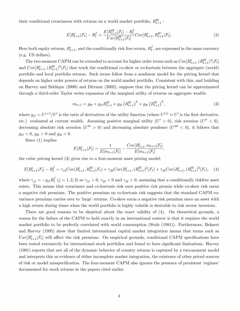
their conditional covariances with returns on a world market portfolio, RWt+1 :

E[Rit+1|Ft]−Rf

t =E[RW

t+1|Ft]−Rft

V ar[RWt+1|Ft]

Cov[Rit+1, R

Wt+1|Ft]. (2)

Here both equity returns, Rit+1, and the conditionally risk free return, R

ft , are expressed in the same currency

(e.g. US dollars).

The two-moment CAPM can be extended to account for higher order terms such as Cov[Rit+1, (R

Wt+1)

2|Ft]and Cov[Ri

t+1, (RWt+1)

3|Ft] that track the conditional co-skew or co-kurtosis between the aggregate (world)portfolio and local portfolio returns. Such terms follow from a nonlinear model for the pricing kernel that

depends on higher order powers of returns on the world market portfolio. Consistent with this, and building

on Harvey and Siddique (2000) and Dittmar (2002), suppose that the pricing kernel can be approximated

through a third-order Taylor series expansion of the marginal utility of returns on aggregate wealth:

mt+1 = g0t + g1tRWt+1 + g2t

¡RWt+1

¢2+ g3t

¡RWt+1

¢3, (3)

where gjt = U j+1/U 0 is the ratio of derivatives of the utility function (where U (1) ≡ U 0 is the first derivative,

etc.) evaluated at current wealth. Assuming positive marginal utility (U 0 > 0), risk aversion (U 00 < 0),

decreasing absolute risk aversion (U 000 > 0) and decreasing absolute prudence (U 0000 < 0), it follows that

g1t < 0, g2t > 0 and g3t < 0.

Since (1) implies

E[Rit+1|Ft] =

1

E[mt+1|Ft]−

Cov[Rit+1,mt+1|Ft]

E[mt+1|Ft],

the cubic pricing kernel (3) gives rise to a four-moment asset pricing model:

E[Rit+1|Ft]−Rf

t = γ1tCov(Rit+1, R

Wt+1|Ft) + γ2tCov(R

it+1, (R

Wt+1)

2|Ft) + γ3tCov(Rit+1, (R

Wt+1)

3|Ft), (4)

where γjt = −gjtRft (j = 1, 2, 3) so γ1t > 0, γ2t < 0 and γ3t > 0, assuming that a conditionally riskfree asset

exists. This means that covariance and co-kurtosis risk earn positive risk premia while co-skew risk earns

a negative risk premium. The positive premium on co-kurtosis risk suggests that the standard CAPM co-

variance premium carries over to ‘large’ returns. Co-skew earns a negative risk premium since an asset with

a high return during times when the world portfolio is highly volatile is desirable to risk averse investors.

There are good reasons to be skeptical about the exact validity of (4). On theoretical grounds, a

reason for the failure of the CAPM to hold exactly in an international context is that it requires the world

market portfolio to be perfectly correlated with world consumption (Stulz (1981)). Furthermore, Bekaert

and Harvey (1995) show that limited international capital market integration means that terms such as

V ar[Rit+1|Ft] will affect the risk premium. On empirical grounds, conditional CAPM specifications have

been tested extensively for international stock portfolios and found to have significant limitations. Harvey

(1991) reports that not all of the dynamic behavior of country returns is captured by a two-moment model

and interprets this as evidence of either incomplete market integration, the existence of other priced sources

of risk or model misspecification. The four-moment CAPM also ignores the presence of persistent ‘regimes’

documented for stock returns in the papers cited earlier.

4

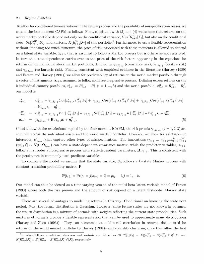
2.1. Regime Switches

To allow for conditional time-variations in the return process and the possibility of misspecification biases, we

extend the four-moment CAPM as follows. First, consistent with (3) and (4) we assume that returns on the

world market portfolio depend not only on the conditional variance, V ar[RWt+1|Ft], but also on the conditional

skew, Sk[RWt+1|Ft], and kurtosis, K[RW

t+1|Ft] of this portfolio.7 Furthermore, to use a flexible representation

without imposing too much structure, the price of risk associated with these moments is allowed to depend

on a latent state variable, St+1, that is assumed to follow a Markov process but is otherwise not restricted.

In turn this state-dependence carries over to the price of the risk factors appearing in the equations for

returns on the individual stock market portfolios, denoted by γ1,St+1 (covariance risk), γ2,St+1 (co-skew risk)

and γ3,St+1 (co-kurtosis risk). Finally, consistent with empirical evidence in the literature (Harvey (1989)

and Ferson and Harvey (1991)) we allow for predictability of returns on the world market portfolio through

a vector of instruments, zt+1, assumed to follow some autoregressive process. Defining excess returns on the

h individual country portfolios, xit+1 = Rit+1 −Rf

t (i = 1, ..., h) and the world portfolio, xWt+1 = RW

t+1 −Rft ,

our model is

xit+1 = αiSt+1 + γ1,St+1Cov[xit+1, x

Wt+1|Ft] + γ2,St+1Cov[x

it+1, (x

Wt+1)

2|Ft] + γ3,St+1Cov[xit+1, (x

Wt+1)

3|Ft]

+biSt+1zt + ηit+1

xWt+1 = αWSt+1 + γ1,St+1V ar[xWt+1|Ft] + γ2,St+1Sk[x

Wt+1|Ft] + γ3,St+1K[x

Wt+1|Ft] + bWSt+1zt + ηWt+1

zt+1 = μz,St+1 +BzSt+1zt + ηZt+1. (5)

Consistent with the restrictions implied by the four-moment ICAPM, the risk premia γj,St+1 (j = 1, 2, 3) are

common across the individual assets and the world market portfolio. However, we allow for asset-specific

intercepts, αiSt+1 , that capture other types of misspecification. The innovations ηt+1 ≡ [η1t+1...ηht+1 ηWt+1

(ηZt+1)0] ∼ N(0,Ωst+1) can have a state-dependent covariance matrix, while the predictor variables, zt+1,

follow a first order autoregressive process with state-dependent parameters, BzSt+1 . This is consistent with

the persistence in commonly used predictor variables.

To complete the model we assume that the state variable, St, follows a k−state Markov process withconstant transition probability matrix, P:

P[i, j] = Pr(st = j|st−1 = i) = pij , i, j = 1, .., k. (6)

Our model can thus be viewed as a time-varying version of the multi-beta latent variable model of Ferson

(1990) where both the risk premia and the amount of risk depend on a latent first-order Markov state

variable.

There are several advantages to modelling returns in this way. Conditional on knowing the state next

period, St+1, the return distribution is Gaussian. However, since future states are not known in advance,

the return distribution is a mixture of normals with weights reflecting the current state probabilities. Such

mixtures of normals provide a flexible representation that can be used to approximate many distributions

(Harvey and Zhou (1993)). They can accommodate mild serial correlation in returns−documented forreturns on the world market portfolio by Harvey (1991)−and volatility clustering since they allow the first

7In what follows, conditional skewness and kurtosis are defined as Sk[RWt+1|Ft] ≡ E[(RW

t+1 − E(RWt+1|Ft))3|Ft] and

K[RWt+1|Ft] ≡ E[(RW

t+1 −E(RWt+1|Ft))4|Ft], respectively.

5

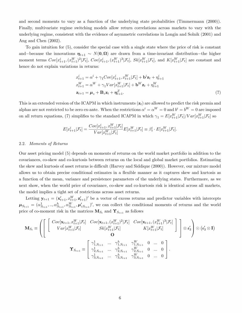
and second moments to vary as a function of the underlying state probabilities (Timmermann (2000)).

Finally, multivariate regime switching models allow return correlations across markets to vary with the

underlying regime, consistent with the evidence of asymmetric correlations in Longin and Solnik (2001) and

Ang and Chen (2002).

To gain intuition for (5), consider the special case with a single state where the price of risk is constant

and−because the innovations ηt+1 ∼ N(0,Ω) are drawn from a time-invariant distribution−the highermoment terms Cov[xit+1, (x

Wt+1)

2|Ft], Cov[xit+1, (x

Wt+1)

3|Ft], Sk[xWt+1|Ft], and K[xWt+1|Ft] are constant and

hence do not explain variations in returns:

xit+1 = αi + γ1Cov[xit+1, x

Wt+1|Ft] + bizt + ηit+1

xWt+1 = αW + γ1V ar[xWt+1|Ft] + b

Wzt + ηWt+1

zt+1 = μz +Bzzt + ηZt+1. (7)

This is an extended version of the ICAPM in which instruments (zt) are allowed to predict the risk premia and

alphas are not restricted to be zero ex-ante. When the restrictions αi = αW = 0 and bi = bW = 0 are imposed

on all return equations, (7) simplifies to the standard ICAPM in which γ1 = E[xWt+1|Ft]/V ar[xWt+1|Ft] so

E[xit+1|Ft] =Cov[xit+1, x

Wt+1|Ft]

V ar[xWt+1|Ft]E[xWt+1|Ft] ≡ βit ·E[xWt+1|Ft].

2.2. Moments of Returns

Our asset pricing model (5) depends on moments of returns on the world market portfolio in addition to the

covariances, co-skew and co-kurtosis between returns on the local and global market portfolios. Estimating

the skew and kurtosis of asset returns is difficult (Harvey and Siddique (2000)). However, our mixture model

allows us to obtain precise conditional estimates in a flexible manner as it captures skew and kurtosis as

a function of the mean, variance and persistence parameters of the underlying states. Furthermore, as we

next show, when the world price of covariance, co-skew and co-kurtosis risk is identical across all markets,

the model implies a tight set of restrictions across asset returns.

Letting yt+1 = (x0t+1, xWt+1, z

0t+1)

0 be a vector of excess returns and predictor variables with intercepts

μSt+1 = (α1St+1 , .., αhSt+1

, αWSt+1 ,μ0zSt+1

)0, we can collect the conditional moments of returns and the world

price of co-moment risk in the matrices MSt and ΥSt+1 as follows

MSt ≡

⎛⎜⎝⎡⎢⎣"Cov[xt+1, x

Wt+1|Ft] Cov[xt+1, (x

Wt+1)

2|Ft] Cov[xt+1, (xWt+1)

3|Ft]V ar[xWt+1|Ft] Sk[xWt+1|Ft] K[xWt+1|Ft]

#O

⎤⎥⎦⊗ ι03⎞⎟⎠¯ ¡ι03 ⊗ I¢

ΥSt+1 ≡

⎡⎢⎣ γ11,St+1 ... γh1,St+1 γW1,St+1 0 ... 0

γ12,St+1 ... γh2,St+1 γW2,St+1 0 ... 0

γ13,St+1 ... γh3,St+1 γW3,St+1 0 ... 0

⎤⎥⎦ .

6

where ι3 is a 3× 1 vector of ones and J is a matrix that selects the co-moments of excess returns:

J ≡

⎡⎢⎢⎢⎢⎢⎢⎢⎢⎢⎢⎢⎢⎢⎢⎢⎣

1 1 1 0 0 0 0 0 0

1 1 1 0 0 0 0 0 0...........................

1 1 1 0 0 0 0 0 0

0 0 0 1 1 1 0 0 0

0 0 0 0 0 0 0 0 0...........................

0 0 0 0 0 0 0 0 0

⎤⎥⎥⎥⎥⎥⎥⎥⎥⎥⎥⎥⎥⎥⎥⎥⎦.

We can then write (5) more compactly as

yt+1 = μSt+1 +MStvec(ΥSt+1) +Bst+1yt + ηt+1. (8)

Here BSt+1 captures autoregressive terms in state St+1 and also collects the coefficients biSt+1

and bWSt+1 that

measure the impact of the lagged instruments zt on the risk premia; ηt+1 ∼ N(0,ΩSt+1) is the vector of

heteroskedastic innovations.

To characterize the moments of returns on the world market portfolio and the co-moments with local

market returns, note that mean returns can be computed from

yt+1 ≡ E[yt+1|Ft] =kXl=1

(π0tPel)μl +kXl=1

(π0tPel)Alyt, (9)

where πt is the vector of state probabilities, el is a vector of zeros with a one in the l-th position so

(π0tPel) is the ex-ante probability of being in state St+1 at time t+ 1 given information at time t, Ft, and

μl ≡ μl +MStvec(Υl).

Because μl involves higher order moments of the world market portfolio such as MStvec(Υl) as well

as higher order co-moments between individual portfolio returns and returns on the global market port-

folio, the (conditional) mean returns E[yt+1|Ft] enter the right-hand side of (8). For instance, computing

Cov[xt+1, xWt+1|Ft] requires knowledge of the first h elements of E[yt+1|Ft]. Appendix B explains our iterative

estimation procedure used to solve the associated nonlinear optimization problem.

The conditional variance, skew and kurtosis of returns on the world market portfolio, xWt+1, can now be

computed as follows:

V ar[xWt+1|Ft] =kXl=1

(π0tPel)h¡μWl − e0h+1yt+1 + (e0h+1Al − αh+1)yt

¢2i+

kXl=1

(π0tPel)V ar[ηWt+1|St+1 = l]

Sk[xWt+1|Ft] =kXl=1


¢3i+3

kXl=1

(π0tPel)£¡μWl − e0h+1yt+1 + (e0h+1Al − αh+1)yt

¢V ar[ηWt+1|St+1 = l]

¤K[xWt+1|Ft] =

kXl=1


¢4i(10)

+6kXl=1


¢2V ar[ηWt+1|St+1 = l]

i.

7

Clearly the skew and kurtosis are functions of the mean and variance parameters μi,l, .., μh,l, Al, Ωlkl=1,state probabilities, πt, and the mean of the VAR coefficients, αj ≡ e0j

Pkl=1(π

0tPel)Al. Hence, no new

parameters are introduced to capture the higher moments of the return distribution. Such model-based

estimates are typically determined with considerably more accuracy than estimates of the third and fourth

moments obtained directly from realized returns which tend to be very sensitive to outliers.

Similarly, the covariance between country returns, xit+1, and the world market return, xWt+1, is

Cov[xit+1, xWt+1|Ft] =

kXl=1

(π0tPel)£¡μi,l − e0iyt+1 + (e0iAl − αi)yt

¢ ¡μWl − e0h+1yt+1 + (e0h+1Al − αh+1)yt

¢¤+

kXl=1

(π0tPel)Cov[ηit+1, η

Wt+1|St+1 = l], (11)

Given estimates of the parameters and state probabilities, Cov[xit+1, xWt+1|Ft, St] can easily be calculated.

Finally, the co-skew and co-kurtosis between local market returns and the world market return is

Cov[xit+1, (xWt+1)

2|Ft] =kXl=1

(π0tPel)h¡μi,l − e0iyt+1 + (e0iAl − αi)yt


¢2i+

kXl=1



¤+2

kXl=1

(π0tPel)£¡μWl − e0h+1yt+1 + (e0h+1Al − αh+1)yt

¢Cov[ηit+1, η

Wt+1|St+1 = l]

¤and

Cov[xit+1, (xWt+1)

3|Ft] =kXl=1

(π0tPel)h¡μi,l − e0iyt+1 + (e0iAl − αi)yt


¢3i+3

kXl=1




¤+3

kXl=1


¢2Cov[ηit+1, η

Wt+1|St+1 = l]

i.

Terms such as¡μi,l − e0iyt+1

¢ ¡μWl − e0h+1yt+1

¢show the deviations of the state-specific mean from the

overall mean and do not arise in single-state models.

2.3. Data

In addition to the world market portfolio, our analysis incorporates the largest international stock markets,

namely the United States, Japan, the United Kingdom, the Pacific region (ex-Japan), and continental

Europe. More markets could be included but parameter estimation errors are likely to become increasingly

important when more markets are included so we do not go beyond five equity portfolios in addition to the

world market portfolio (h = 6).8

8At the end of 2005 these markets represented roughly 97% of the world equity market capitalization.

8

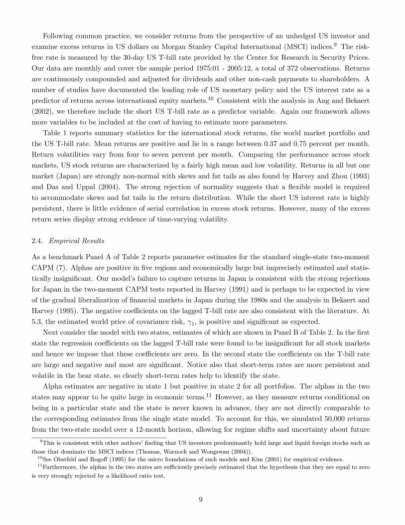
Following common practice, we consider returns from the perspective of an unhedged US investor and

examine excess returns in US dollars on Morgan Stanley Capital International (MSCI) indices.9 The risk-

free rate is measured by the 30-day US T-bill rate provided by the Center for Research in Security Prices.

Our data are monthly and cover the sample period 1975:01 - 2005:12, a total of 372 observations. Returns

are continuously compounded and adjusted for dividends and other non-cash payments to shareholders. A

number of studies have documented the leading role of US monetary policy and the US interest rate as a

predictor of returns across international equity markets.10 Consistent with the analysis in Ang and Bekaert

(2002), we therefore include the short US T-bill rate as a predictor variable. Again our framework allows

more variables to be included at the cost of having to estimate more parameters.

Table 1 reports summary statistics for the international stock returns, the world market portfolio and

the US T-bill rate. Mean returns are positive and lie in a range between 0.37 and 0.75 percent per month.

Return volatilities vary from four to seven percent per month. Comparing the performance across stock

markets, US stock returns are characterized by a fairly high mean and low volatility. Returns in all but one

market (Japan) are strongly non-normal with skews and fat tails as also found by Harvey and Zhou (1993)

and Das and Uppal (2004). The strong rejection of normality suggests that a flexible model is required

to accommodate skews and fat tails in the return distribution. While the short US interest rate is highly

persistent, there is little evidence of serial correlation in excess stock returns. However, many of the excess

return series display strong evidence of time-varying volatility.

2.4. Empirical Results

As a benchmark Panel A of Table 2 reports parameter estimates for the standard single-state two-moment

CAPM (7). Alphas are positive in five regions and economically large but imprecisely estimated and statis-

tically insignificant. Our model’s failure to capture returns in Japan is consistent with the strong rejections

for Japan in the two-moment CAPM tests reported in Harvey (1991) and is perhaps to be expected in view

of the gradual liberalization of financial markets in Japan during the 1980s and the analysis in Bekaert and

Harvey (1995). The negative coefficients on the lagged T-bill rate are also consistent with the literature. At

5.3, the estimated world price of covariance risk, γ1, is positive and significant as expected.

Next consider the model with two states, estimates of which are shown in Panel B of Table 2. In the first

state the regression coefficients on the lagged T-bill rate were found to be insignificant for all stock markets

and hence we impose that these coefficients are zero. In the second state the coefficients on the T-bill rate

are large and negative and most are significant. Notice also that short-term rates are more persistent and

volatile in the bear state, so clearly short-term rates help to identify the state.

Alpha estimates are negative in state 1 but positive in state 2 for all portfolios. The alphas in the two

states may appear to be quite large in economic terms.11 However, as they measure returns conditional on

being in a particular state and the state is never known in advance, they are not directly comparable to

the corresponding estimates from the single state model. To account for this, we simulated 50,000 returns

from the two-state model over a 12-month horizon, allowing for regime shifts and uncertainty about future

9This is consistent with other authors’ finding that US investors predominantly hold large and liquid foreign stocks such as

those that dominate the MSCI indices (Thomas, Warnock and Wongswan (2004)).10See Obstfeld and Rogoff (1995) for the micro foundations of such models and Kim (2001) for empirical evidence.11Furthermore, the alphas in the two states are sufficiently precisely estimated that the hypothesis that they are equal to zero

is very strongly rejected by a likelihood ratio test.

9

states. Measured this way, the 12-month alphas starting from the first and second states are 0.06 and 0.70

for the US, while those for Japan are -0.45 and 0.86. The world portfolio generates alphas of -0.13 and

0.70, starting from the first and second state, respectively. Hence, although the individual state alphas

appear to be quite large conditional on knowing the true state, in many regards they imply weaker evidence

of mispricing than the single-state model which assumes that non-zero alphas are constant and constitute

evidence of permanent model misspecification or mispricing.

Volatility is highest in the first state for five of the equity portfolios, the one exception being the UK.12

Note that to reduce the number of parameters, the model reported in Table 2 assumes that the correlations

between country-specific innovations is the same in the two states.13 However, as we shall see below, this

does not imply that the correlations between country returns (Cor(xit+1, xjt+1)) are the same in the two states

since state-dependence in both the alphas and in the biSt+1 and bWSt+1 coefficients generate time-variations in

return correlations.

The persistence of the first state (0.90) is considerably lower than that of the second state (0.94) and so

the average duration of the first state (ten months) is far shorter than that of the second one (20 months).

In steady state one-third and two-thirds of the time is spent in the states one and two, respectively. These

findings show that neither of the states identifies isolated ‘outliers’ or jumps−a feature distinguishing ourmodel from that proposed by Das and Uppal (2004).

The economic interpretation suggested by these findings is that state one is a bear state with low mean

returns and relatively high volatility, while state two is a bull state with higher mean returns and more

modest volatility. Figure 1 shows that the two states are generally well identified with state probabilities

near zero or one most of the time. Returns were associated with the bear state during a three-year period

between 1979 and 1982 and again during shorter spells in 1984, 1987, 1990/1991 and 2002. These periods

coincide with global recessions (the early 1980s, 1990s and 2002 recessions) and occasions with high return

volatility such as October 1987.

Figure 2 plots the time series of expected returns for the stock portfolios in excess of the US T-bill rate.

Periods where the bear state is most likely are shown as gray areas. Clearly the bear state is associated

with systematically lower mean excess returns across all markets (in addition to higher volatility, see Table

2). Mean excess returns are always positive for the US portfolio and it is very rare that the expected excess

return is negative for any of the other markets.

Figure 3 shows that consistent with previous studies (Ang and Bekaert (2002), Longin and Solnik (1995,

2001) and Karolyi and Stulz (1999)), return correlations are higher in the bear state than in the full sample.

Pairwise correlations between US stock returns and returns in Japan, Pacific ex-Japan, UK and Europe in

the bear (bull) states are 0.39 (0.27), 0.65 (0.47), 0.67 (0.48) and 0.59 (0.45) and are thus systematically

higher in the bear state. This happens despite the fact that correlations between return innovations are

identical in the two states. In part this is due to the higher volatility of the common world market return

in the bear state. Furthermore, since mean returns are different in the two states, return correlations also

depend on the extent of the co-variation between these parameters.

Turning to the risk premia, the premium on covariance with returns on the world market portfolio (γ1)

12The finding for the UK is due to two outliers in January and February of 1975 with monthly excess returns of 44 and 23

percent. If excluded from the data, the volatilility in the first state is highest also for the UK.13This restriction is supported by the data: a likelihood ratio test of the restriction that correlations do not depend on the

state, i.e. Cov(ηit+1, ηjt+1) = Cor(ηit+1, η

jt+1)σ

iSt+1

σjSt+1 , produces a p-value of 0.11 and is not rejected.

10

is positive in both states but, at 15.9, is much higher in the bull state than in the bear state for which an

estimate of 9.5 is obtained. The number reported by Harvey (1991) for the subset of G7 countries is 11.5

and hence lies between these two values. Consistent with the large difference between the covariance risk

premium in the bull and bear state, Harvey rejects that the world price of risk is constant.

A similar conclusion holds for the co-kurtosis premium (γ3) which is positive and insignificant in the

bear state but positive and significant in the bull state. The estimates of γ3 can be compared to the price of

covariance risk, γ2, by scaling them by the ratio of the world market kurtosis to its variance so the units are

the same. This yields a co-kurtosis risk premium of 1.7 and 12.3 in the bear and bull state, respectively, and

a steady state average of 8.7. As expected, the co-skew premium (γ2) is negative in both states although it

is only significant (and by far largest) in the bull state. When converted to the same units as the covariance

risk premium, the estimates are -1.1 and -3.1 in the bear and bull state, respectively, while the steady state

average is -2.4.

We conclude from this analysis that all coefficients have the expected sign and are economically mean-

ingful: Investors dislike risk in the form of higher volatility or fatter tails but like positively skewed return

distributions. Furthermore, both the co-skew and co-kurtosis risk premia appear to be important in economic

terms as they are of the same order of magnitude as the covariance risk premium.

A final way to interpret the two states is through the time-variation in the conditional moments of the

world market portfolio. To this end, Figure 4 shows the volatility, skew and kurtosis implied by our model

estimates, computed using (10). Large changes in the conditional skew and kurtosis turn out to be linked to

regime switches. Preceding a shift to the bear state, the kurtosis of the world market portfolio rises while its

skew becomes large and negative and volatility is low. Uncertainty surrounding shifts from a bull to a bear

state therefore takes the form of an increased probability of large negative returns. Once in the bear state,

the kurtosis gets very low and the skew close to zero, while world market volatility is much higher than

normal. Hence the return distribution within the bear state is more dispersed, although closer to symmetric.

Finally, when exiting from the bear state to the bull state, the kurtosis again rises−reflecting the increaseduncertainty associated with a regime shift−while volatility and skew decline to their normal levels. Theselarge variations in the volatility, skew and kurtosis of world market returns means that our model is able to

capture the correlated extremes across local markets found to be an important feature of stock returns in

Harvey et al. (2004).

2.4.1. Are Two States Needed?

A question that naturally arises in the empirical analysis is whether regimes are really present in the distri-

bution of international stock market returns. To answer this we computed the specification test suggested

by Davies (1977), which very strongly rejected the single-state specification. A more extensive analysis of

the number of regimes confirmed the presence of two states in the joint return distribution.14

Furthermore, to see whether the two-state model does a better job at accounting for the characteristics

of returns on the international stock market portfolios, Table 3 reports a set of specification tests for the

standardized residuals from the single state and two-state models. Such diagnostics are similar to the ones

reported for the international CAPM regression residuals by Harvey and Zhou (1993). Like them, we find

14Regime switching models have parameters that are unidentified under the null hypothesis of a single state. Standard critical

values are therefore invalid in the hypothesis test. Details of the analysis are available on request.

11

that, with the exception of Japan, the single-state model is strongly rejected and fails to capture even the

most basic properties of the international returns data. In contrast, the two-state model performs far better

and is either not rejected for most of the portfolios or reduce the diagnostic test statistics very considerably.

Hence the evidence of misspecification is far weaker for the two-state model.15

3. The Investor’s Asset Allocation Problem

We next turn to the investor’s asset allocation problem. Consistent with the analysis in the previous section,

we assume that investor preferences depend on higher order moments of asset returns and allow regimes to

be present in the return process.

3.1. Preferences over Moments of the Wealth Distribution

Suppose that the investor’s utility function U(Wt+T ;θ) only depends on wealth at time t+ T , Wt+T , and a

set of shape parameters, θ, where t is the current time and T is the investment horizon. Consider an m-th

order Taylor series expansion of U around some wealth level vT :

U(Wt+T ;θ) =mXn=0

1

n!U (n)(vT ;θ) (Wt+T − vT )

n + ςm, (12)

where the remainder ςm is of order o((Wt+T − vT )m) and U (0)(vT ;θ) = U(vT ;θ). U

(n)(.) denotes the n−thderivative of the utility function with respect to terminal wealth. Provided that (i) the Taylor series con-

verges; (ii) the distribution of wealth is uniquely determined by its moments; and (iii) the order of sums

and integrals can be exchanged, the expansion in (12) extends to the expected utility functional:

Et[U(Wt+T ;θ)] =mXn=0

1

n!U (n)(vT ;θ)Et[(Wt+T − vT )

n] +Et[ςm],

where Et[.] is short for E[.|Ft]. We thus have

Et[U(Wt+T ;θ)] ≈ Et[Um(Wt+T ;θ)] =

mXn=0

1

n!U (n)(vT ;θ)Et[(Wt+T − vT )

n]. (13)

While the approximation improves as m gets larger, many classes of Von-Neumann Morgenstern expected

utility functions can be well approximated using a relatively small value of m and a function of the form:

Et[Um(Wt+T ;θ)] =

mXn=0

κnEt[(Wt+T − vT )n], (14)

with κ0 > 0, and κn positive (negative) if n is odd (even).

3.2. Solution to the Asset Allocation Problem

We next characterize the solution to the investor’s asset allocation problem when preferences are defined

over moments of terminal wealth while, consistent with the analysis in Section 2, returns follow a regime

15We also tested our model against a “pure” regime switching four-moment ICAPM which corresponds to (7) with αi =

αW = 0 so only the risk premia and the amount of risk differ across states. A likelihood-ratio test of these restrictions produced

a p-value of essentially zero.

12

switching process. Following most papers on portfolio choice (e.g., Ang and Bekaert (2002) and Das and

Uppal (2004)), we assume a partial equilibrium framework that treats returns as exogenous.

The investor maximizes expected utility by choosing among h risky assets whose continuously com-

pounded excess returns are given by the vector xst ≡ (x1t x2t ... xht )0. Portfolio weights are collected in the

vector ω1t ≡ (ω1t ω2t ... ωht )0 while (1−ω0tιh) is invested in a short-term interest-bearing bond. The portfolio

selection problem solved by a buy-and-hold investor with unit initial wealth then becomes

maxωt

Et [U(Wt+T (ωt);θ)]

s.t. Wt+T (ωt) =n(1− ω0tιh) exp

³Rbt+T

´+ ω0t exp

¡Rs

t+T

¢o, (15)

where Rst+T ≡ (xst+1 + rbt+1) + (x

st+2 + rbt+2) + ...+ (xst+T + rbt+T ) is the vector of continuously compounded

equity returns over the T−period investment horizon while Rbt+T ≡ rbt+1+r

bt+2+ ...+rbt+T is the continuously

compounded return on the bond investment. Accordingly, exp(Rst+T ) is a vector of cumulated returns.

Short-selling can be imposed through the constraint ωit ∈ [0, 1] for i = 1, 2, ..., h.To gain intuition we first study the problem under the simplifying assumption of a single risky asset

(h = 1), a risk-free asset paying a constant return rf and a regime switching process with two states:

xt+1 = μSt+1 + σSt+1εt+1, εt+1 ∼ N(0, 1),

Pr(St+1 = i|St = i) = pii, i = 1, 2 (16)

This specification is consistent with the ICAPM analysis in section 2 since the conditional moment infor-

mation from (5) can be folded into μSt+1 , σSt+1 as described in Section 2.With a single risky asset (stocks) and initial wealth set at unity, the wealth process is

Wt+T = (1− ωt) exp (Trf ) + ωt exp (Rt+T ) (17)

where Rt+T is the continuously compounded stock return over the T periods and ωt is the stock holding.

For a given value of ωt, the only unknown component in (17) is the cumulated return, exp(Rt+T ). Under

the assumption of two states, k = 2, the nth non-central moment of the cumulated returns is given by

M(n)t+T = E [(exp(rt+1 + ...+ rt+T ))

n |Ft]

=2X

St+T=1

E [(exp(rt+1 + ...+ rt+T ))n |St+T ,Ft] Pr(St+T |Ft) (18)

≡ M(n)1t+T +M

(n)2t+T ,

where rt ≡ xt + rf . Using properties of the moment generating function of a log-normal random variable,

each of these conditional moments M(n)it+1 (i = 1, 2) satisfies recursions

M(n)it+T = E [exp(n(rt+1 + ...+ rt+T−1))|St+T ]E [exp(nrt+T )|St+T ,Ft] Pr(St+T |Ft)

=³M(n)it+T−1pii +M

(n)−i,t+T−1(1− p−i−i)

´exp

µnμi +

n2

2σ2i

¶, (i = 1, 2)

where we used the notation −i for the converse of state i, i.e. −i = 2 when i = 1 and vice versa. In more

compact notation we have

M(n)1t+1 = ξ

(n)1 M

(n)1t + β

(n)1 M

(n)2t

M(n)2t+1 = ξ

(n)2 M

(n)1t + β

(n)2 M

(n)2t , (19)

13

whereξ(n)1 = p11 exp

³nμ1 +

n2

2 σ21

´, β

(n)1 = (1− p22) exp

³nμ1 +

n2

2 σ21

´,

ξ(n)2 = (1− p11) exp

³nμ2 +

n2

2 σ22

´, β

(n)2 = p22 exp

³nμ2 +

n2

2 σ22

´.

Equation (19) can be reduced to a set of second order difference equations:

M(n)it+2 = (ξ

(n)1 + β

(n)2 )M

(n)it+1 + (ξ

(n)2 β

(n)1 − β

(n)2 α

(n)1 )M

(n)it , (i = 1, 2). (20)

Collecting the two regime-dependent moments in the vector ϑ(n)it+T ≡ (M

(n)it+T M

(n)it+T−1)

0, equation (20) can

be written in companion form:

ϑ(n)it+T =

"ξ(n)1 + β

(n)2 ξ

(n)2 β

(n)1 − β

(n)21 ξ

(n)

1 0

#ϑ(n)it+T−1 ≡ A

(n)ϑ(n)it+T−1.

The elements of A(n) only depend on the mean and variance parameters of the two states (μ1, σ21, μ2, σ

22)

and the state transitions, (p11, p22). Substituting backwards, we get the ith conditional moment:

ϑ(n)it+T =

³A(n)

´Tϑ(n)it .

Applying similar principles at T = 1, 2 and letting π1t = Pr(St = 1|Ft), the initial conditions used in

determining the nth moment of cumulated returns are as follows:

M(n)1t+1 = (π1tp11 + (1− π1t)(1− p22)) exp

µnμ1 +

n2

2σ21

¶,

M(n)1t+2 = p11 (π1tp11 + (1− π1t)(1− p22)) exp

¡2nμ1 + n2σ21

¢+

+(1− p22) (π1t(1− p11) + (1− π1)p22) exp

µn(μ1 + μ2) +

n2

2(σ21 + σ22)

¶,

M(n)2t+1 = (π1t(1− p11) + (1− π1)p22) exp

µnμ2 +

n2

2σ22

¶,

M(n)2t+2 = p22 (π1t(1− p11) + (1− π1)p22) exp

¡2nμ2 + n2σ22

¢+

+(1− p11) (π1tp11 + (1− π1t)(1− p22)) exp

µn(μ1 + μ2) +

n2

2(σ21 + σ22)

¶. (21)

Finally, using (18) we get an equation for the nth moment of the cumulated return:

M(n)t+T =M

(n)1t+T +M

(n)2t+T = e

01ϑ

(n)1t+T + e

02ϑ

(n)2t+T = e

01

³A(n)

´Tϑ(n)1t + e

02

³A(n)

´Tϑ(n)2t , (22)

where ei is a 2× 1 vector of zeros except for unity in the ith place.Having obtained the moments of the cumulated return process, it is simple to compute the expected

utility for any mth order polynomial representation by using (14) and (17):

Et[Um(Wt+T ;θ)] =

mXn=0

κn

nXj=0

(−1)n−jvn−jT

µn

j

¶Et[W

jt+T ]

=mXn=0

κn

nXj=0

(−1)n−jvn−jT

µn

j

¶ jXi=0

µj

i

¶ωitM

it+T ((1− ωt) exp (Trf ))

j−i . (23)

14

The first order condition is obtained by differentiating this equation with respect to ωt :

mXn=0

κn

nXj=0

(−1)n−jvn−jT

µn

j

¶ jXi=1

µj

i

¶ωi−1t (1− ωt)

j−i−1M it+T exp ((j − i)Trf ) (i− jωt) = 0.

The solution takes the form of the roots of an m− 1 order polynomial in ωt, which are easily obtained. Theoptimal solution for ωt corresponds to the root for which (23) has the highest value.

From this analysis it is clear that the optimal asset allocation depends on the following factors:

1. The current state probabilities (πt, 1− πt) which determine the moments of future returns.

2. State transition probabilities (p11, p22) which affect the speed of mean reversion in the investment

opportunity set towards its steady state.

3. Differences between mean parameters (μ1, μ2) and variance parameters (σ1, σ2) (and more generally

covariance parameters) across states. For example, skew in the return distribution can only be induced

provided that μ1 6= μ2, c.f. Timmermann (2000).

4. The number of moments of the wealth distribution that matters for preferences, m, in addition to the

weights on the various moments.

5. The investment horizon, T .

3.3. General Results

In many applications rt+1 is a vector of returns on a multi-asset portfolio. The number of states, k, may

also exceed two. For generality, we assume the following process for a vector of h+ 1 excess returns:16

xt+1 = μSt+1 +

pXj=1

Bj,St+1xt−j + εt+1, (24)

where μSt+1 = (μ1st+1 , ..., μ

h+1st+1)

0 is a vector of conditional means in state St+1 (possibly used to “fold in” all

components of the mean in state St+1), Bj,St+1 is a matrix of autoregressive coefficients associated with the

jth lag in state St+1, and εt+1 = (ε1t+1, ..., ε

h+1t+1 )

0 ∼ N(0,ΩSt+1) is a vector of zero-mean return innovations

with state-dependent covariance matrix ΩSt+1 .

With h + 1 risky assets (the last of which can be taken to represent the risky returns on a short-term

bond, xbt+i = rbt+i) and k states, the wealth process becomes

Wt+T = ω0t exp

"TXi=1

(xt+i + rbt+i)

#+ (1− ω0tιh) exp

"TXi=1

rbt+i

#.

We next present a simple and convenient recursive procedure for evaluating the expected utility associated

with a vector of portfolio weights, ωt, of relatively high dimension:

16This equation is more convenient than (5) but is fully consistent with the earlier setup if the last elements of the return

vector, rt+1, are used to capture the predictor variables zt+1 (themselves asset returns). Furthermore, the four-moment ICAPM

factors are easily folded into the intercept by defining μSt+1 ≡ μSt+1 +MStvec(ΥSt+1).

15

Proposition 1. Under the regime-switching return process (24) and m−moment preferences (14), theexpected utility associated with the portfolio weights ωt is given by

Et[Um(Wt+T )] =

mXn=0

κn

nXj=0

(−1)n−jvn−jT nCjEt[Wjt+T ]

=mXn=0

κn

nXj=0

(−1)n−jvn−jT

µn

j

¶ jXi=0

µj

i

¶Et

h¡ω0t exp

¡Rs

t+T

¢¢ii((1-ω0tιh) exp(Tr

f ))j−i.

The nth moment of the cumulated return on the risky asset portfolio is

Et

£¡ω0t exp

¡Rs

t+T

¢¢n¤=

nXn1=0

· · ·nX

nh=0

λ(n1, n2, ..., nh)

ÃhYi=1

ωnii

!M(n)t+T (n1, ..., nh),

wherePh

i=1 ni = n, 0 ≤ ni ≤ n (i = 1, ..., h),

λ(n1, n2, ..., nh) ≡n!

n1!n2! ... nh!.

and M(n)t+T (n1, ..., nh) can be evaluated recursively, using (A4) in the Appendix.

Appendix A proves this result. The solution is in closed-form in the sense that it reduces the expected

utility calculation to a finite number of steps each of which can be solved by elementary operations.

It is useful to compare our method to existing alternatives. Classic results on optimal asset allocation

have been derived for special cases such as power utility with constant investment opportunities or under

logarithmic utility (Merton (1969) and Samuelson (1969)). For general preferences there is no closed-

form solution to (15), but given its economic importance it is not surprising that a variety of solution

approaches have been suggested. Recent papers that solve (15) under predictability of returns include Ang

and Bekaert (2002), Brandt (1999), Brennan, Schwarz and Lagnado (1997), Campbell and Viceira (1999,

2001). These papers generally use approximate solutions or numerical techniques such as quadrature (Ang

and Bekaert (2002)) or Monte Carlo simulations (Detemple, Garcia and Rindisbacher (2003)) to characterize

optimal portfolio weights. Quadrature methods may not be very precise when the underlying asset return

distributions are strongly non-normal. They also have the problem that the number of quadrature points

increases exponentially with the number of assets. Monte Carlo methods can also be computationally

expensive to use as they rely on discretization of the state space and use grid methods.17 Although existing

methods have clearly yielded important insights into the solution of (15), they are therefore not particularly

well-suited to our analysis of international asset allocation which involves a large number of portfolios.

4. International Portfolio Holdings

We next consider empirically the optimal international asset allocation under regime switching and four-

moment preferences. The weights on the first four moments of the wealth distribution are determined to

ensure that our results can be compared to those in the existing literature. Most studies on optimal asset

17In continuous time, closed-form solutions can be obtained under less severe restrictions. For instance Kim and Omberg

(1996) work with preferences in the HARA class defined over final wealth and assume that the single risky asset return is

mean-reverting.

16

allocation use power utility so we calibrate our coefficients to the benchmark

U(Wt+T ; θ) =W 1−θ

t+T

1− θ, θ > 0. (25)

For a given coefficient of relative risk aversion, θ, (25) serves as a guide in setting values of κnmn=0 in (14)but should otherwise not be viewed as an attempt to approximate results under power utility. Expanding

the powers of (Wt+T − vT ) and taking expectations, we obtain the following expression for the four-moment

preference function:

Et[U4(Wt+T ; θ)] = κ0,T (θ)+κ1,T (θ)Et[Wt+T ]+κ2,T (θ)Et[W

2t+T ]+κ3,T (θ)Et[W

3t+T ]+κ4,T (θ)Et[W

4t+T ], (26)

where18

κ0,T (θ) = v1−θT

∙(1− θ)−1 − 1− 1

2θ − 1

6θ(θ + 1)− 1

24θ(θ + 1)(θ + 2)

¸κ1,T (θ) =

1

6v−θT [6 + 6θ + 3θ(θ + 1) + θ(θ + 1)(θ + 2)] > 0

κ2,T (θ) = −14θv−(1+θ)T [2 + 2(θ + 1) + (θ + 1)(θ + 2)] < 0

κ3,T (θ) =1

6θ(θ + 1)(θ + 3)v

−(2+θ)T > 0

κ4,T (θ) = − 124

θ(θ + 1)(θ + 2)v−(3+θ)T < 0.

Expected utility from final wealth increases in Et[Wt+T ] and Et[W3t+T ], so higher expected returns and

more right-skewed distributions lead to higher expected utility. Conversely, expected utility is a decreasing

function of the second and fourth moments of the terminal wealth distribution. Our benchmark results

assume that θ = 2, a coefficient of relative risk aversion compatible with much empirical evidence. Later we

allow this coefficient to assume different values.19

A solution to the optimal asset allocation problem can now easily be found from Proposition 1 by solving

a system of cubic equations in ωt derived from the first order conditions

∇ωtEt[U4(Wt+T ; θ)]

¯ωt= 00.

At the optimum ωt sets the gradient, ∇ωtEt[U4(Wt+T ; θ)] equal to zero and produces a negative definite

Hessian matrix, HωtEt[U4(Wt+T ; θ)].

4.1. Empirical Results

As a benchmark, Table 4 reports equity allocations for the single-state model using a short 1-month and a

longer 24-month horizon. Our empirical analysis considers returns on five equity portfolios and the world

market. To arrive at total portfolio weights we therefore re-allocate the weight assigned to the world market

18The notation κn,T makes it explicit that the coefficients of the fourth order Taylor expansion depend on the investment

horizon through the coefficient vT , the point around which the approximation is calculated. We follow standard practice and

set vT = Et[Wt+T−1].19Based on the evidence in Ang and Bekaert (2002)−who show that the optimal home bias is an increasing function of the

coefficient of relative risk aversion−this is also a conservative choice that allows us to examine the effects on the optimal portfoliochoice produced by preferences that account for higher order moments.

17

using the regional market capitalizations as weights.20 Since we are interested in the home bias, we report

equity weights as percentages of the total equity portfolio so they sum to unity. The allocation to the

risk-free asset (as a percentage of the total portfolio) is also shown for interest rates that vary by up to two

standard deviations from the mean. When the T-bill rate is set at its sample mean of 5.9% per annum, at

the one-month horizon only 31% of the equity portfolio is invested in US stocks. Slightly less (29%) gets

invested in US stocks at the 24-month horizon. Furthermore, the fraction of the equity portfolio allocated

to US stocks remains too low in both low and high interest rate environments. These results support earlier

findings under mean-variance preferences (e.g. Lewis (1999)) and also show that the home bias puzzle

extends to a setting with return predictability from the short T-bill rate.

Turning to the two-state model, Table 4 shows that the allocation to US stocks is much higher in the

presence of regimes. This holds both when starting from the steady-state probabilities−i.e. when the

investor has very imprecise information about the current state−as well as in the separate bull and bearstates. Under steady state probabilities and an average short-term US interest rate the 1-month allocation

to US stocks is 70% of the total equity portfolio. This reflects an allocation of 75% in the bear state and a

slightly lower allocation of 60% in the bull state. Moreover, this finding is robust to the level of the short US

interest rate. Varying this rate predominantly affects the allocation to the risk-free asset versus the overall

equity portfolio but has little affect on the regional composition of the equity portfolio.21

4.2. Effect of Higher Moments

Compared with the benchmark model, our four-moment regime switching model appears capable of sig-

nificantly increasing the allocation to US stocks but leaves unanswered what accounts for this effect. An

economic understanding of the effect of skew and kurtosis on the optimal asset allocation requires studying

the co-skew and co-kurtosis properties at the portfolio level. To this end, define the conditional co-skew of

the return on stock i with the world market as:

Si,W (Ft, St) ≡Cov[xit+1, (x

Wt+1)

2|Ft, St]

V ar[xit+1|Ft, St](V ar[xWt+1|Ft, St])21/2. (27)

The co-skew is normalized by scaling by the appropriate powers of the volatility of the respective portfolios.

A security that has negative co-skew with the market portfolio pays low (high) returns when the world

market portfolio becomes highly (less) volatile. To a risk averse investor this is an unattractive feature since

global market risk rises in periods with low returns. Conversely, positive co-skew is desirable as it means

higher expected returns during volatile periods.

Similarly, define the co-kurtosis of the excess return on asset i with the world portfolio as

Ki,W (Ft, St) ≡Cov[xit+1, (x

Wt+1)

3|Ft, St]

V ar[xit+1|Ft, St](V ar[xWt+1|Ft, St])31/2. (28)

Large positive values are undesirable as they mean that local returns are low (high) when world market

returns are largely skewed to the left (right), thus increasing the overall portfolio risk.

20This introduces a very small approximation error as the included stock markets account for only 97% of the world market.21Consistent with the findings in Ang and Bekaert (2002), the allocation to the short-term bond is much higher in the bear

state than in the bull state. This happens because equity returns are small and volatile in the bear state, and hence unattractive

to risk averse investors.

18

Table 5 reports estimates of these moments in the bull and bear states as well as under steady state

probabilities. The latter gives a measure that is more directly comparable to the full-sample estimates listed

in the final column. Short term interest rates are set at the regime-specific unconditional means. As can

be seen by comparing the values implied by the two-state model to the full sample estimates, the model

generally does a good job at matching the data. Interestingly, with the exception of Japan, in both the bear

state and under steady-state probabilities US stocks have the lowest co-kurtosis and co-skew coefficients

(essentially zero), explaining why domestic stocks are more attractive to US investors than is revealed by

the mean-variance case. Japanese stocks remain unattractive due to their low mean returns over the sample

period.

To address the effect of higher order moments on the asset allocation, we next computed the optimal

portfolio weights as a function of T and π (the state probability) under mean-variance (m = 2) preferences:

Et[U2(Wt+T ; θ)] = κ0,T (θ) + κ1,T (θ)Et[Wt+T ] + κ2,T (θ)Et[W

2t+T ] (29)

where κ0,T (θ) ≡ v1−θT

£(1− θ)−1 − 1− 1

2θ¤, κ1,T (θ) ≡ v−θT (1 + θ) > 0 and κ2,T (θ) ≡ −12θv

−(1+θ)T < 0. We

also consider optimal allocations under three-moment preferences

Et[U3(Wt+T ; θ)] = κ0,T (θ) + κ1,T (θ)Et[Wt+T ] + κ2,T (θ)Et[W

2t+T ] + κ3,T (θ)Et[W

3t+T ] (30)

where now κ0,T (θ) ≡ v1−θT

£(1− θ)−1 − 1− 1

2θ −16θ(θ + 1)

¤, κ1,T (θ) ≡ v−θT

£1 + θ + 1

2θ(θ + 1)¤> 0, κ2,T (θ) ≡

−12θv−(1+θ)T (2 + θ) < 0 and κ3,T (θ) ≡ 1

6θ(θ + 1)v−(2+θ)T > 0.

Using steady-state probabilities, Table 6 shows that the allocation to US stocks as a portion of the

overall equity portfolio remains just above 50% when going from mean-variance to skewness preferences.

The introduction of two states on its own thus increases the allocation to US stocks from roughly 30% (as

seen in Table 4) to 50%. This allocation rises further to 70% of the equity portfolio when we move to the

case with kurtosis aversion. The steady state results conceal large differences in the separate bull and bear

states. In the bear state, the large increase in the allocation to US stocks due to introducing higher order

moment preferences comes from the skew while the kurtosis plays a similar role in the bull state.

The correlation, co-skew and co-kurtosis between the short interest rate and the stock returns can also

affect asset allocations. At the 1-month horizon, the correlation between the risk-free rate and stock returns

is zero since the risk-free rate is known. Future short-term spot rates are stochastic, however. This matters

to buy-and-hold investors with horizons of T ≥ 2 months who effectively commit (1−ω0tιh) of their portfolioto roll over investments in T−bills T −1 times at unknown future spot rates. We therefore computed the co-skew, Si,Rb(Ft, St), and co-kurtosis, Ki,Rb(Ft, St), between the individual stock returns and rolling six-monthbond returns assuming steady state probabilities and setting the initial interest rate at its unconditional

mean. US stocks were found to generate the second-highest co-skewness coefficient (-0.06) and the second

lowest co-kurtosis coefficient (4.44). Only Japanese stocks turn out to be preferable to US stocks, although

their conditional mean and variance properties make them undesirable to a US investor. We conclude that

the co-moment properties of US stocks against rolling returns on short US T-bills help to explain the high

demand for these stocks under three- and four-moment preferences.

19

5. Interpretation and Robustness of Results

To summarize our results so far, we extended the standard model in two directions: First, by defining

preferences over higher moments such as skew and kurtosis and, second, by allowing for the presence of bull

and bear regimes tracking periods with very different mean, variances, correlations, skew and kurtosis. In

this section we consider the robustness of our results with regard to alternative specifications of investor

preferences, estimation errors and dynamic portfolio choice.

5.1. Preference Specification

We first consider the effect of changing the coefficient of relative risk aversion from θ = 2 in the baseline

scenario to values of θ = 5 (high) and θ = 10 (very high). Ang and Bekaert (2002) and Das and Uppal (2004)

have found that changes in risk aversion have first-order effects on their conclusions on the importance of

either regime shifts or systemic (jump) risks. Table 7 shows the effect of such changes. In general there is

no monotone relation between θ and the weight on US stocks, although the allocation to US stocks tends

to be greater for θ = 10 than for θ = 2. Risk aversion has a first order effect on the choice of T-bills versus

stocks but has far less of an effect on the composition of the equity portfolio. Therefore, it does not seem

that our conclusions depend on a particular choice of θ.

To make our results comparable to those reported in the literature which assume power utility, we also

compare results under four-moment preferences to those under constant relative risk aversion (shown in

Table 8). Differences between results computed under power utility and under four-moment preferences

appear to be relatively minor.22 In the bear state the allocation to US stocks is 2-4% lower under power

utility while conversely the allocation to UK stocks tends to be higher. In the more persistent bull state,

results under the four-moment preference specification are similar to those under constant relative risk

aversion.

5.2. Precision of Portfolio Weights

Mean-variance portfolio weights are known to be highly sensitive to the underlying estimates of mean returns

and covariances. Since such estimates often are imprecisely estimated, this means that the portfolio weights

in turn can be poorly determined, see Britten-Jones (1999). As pointed out by Harvey, Liechty, Liechty

and Muller (2004), this could potentially be even more of a concern in a model with higher moments due

to the difficulty of obtaining precise estimates of moments such as skew and kurtosis.23 In this situation it

becomes important to jointly consider the effect of higher moments and parameter uncertainty.

To address this concern, we computed standard error bands for the portfolio weights under the single

state and two-state models using that, in large samples, the distribution of the parameter estimates from a

22A problem associated with using low-order polynomial utility functionals is the difficulty of imposing restrictions on the

derivatives (with respect to the moments of wealth) that apply globally. For example, nonsatiation cannot be imposed by

restricting a quadratic polynomial to be monotone increasing and risk aversion cannot be imposed by restricting a cubic

polynomial to be globally concave (see Post and Levy (2005) and Post, van Vliet and Levy (2005)). This is why it is important

to check through the comparison with power utility that our findings on the optimal portfolio weights are not driven by

unreasonable behavior of the utility function.23See also the discussion of “Omega” in Cascon, Keating and Shadwick (2003) which is used to capture sample information

beyond point estimates through the cumulative density function of returns.

20

regime switching model is √T³bθ − θ´ ∼ N(0,Vθ).

This allows us to set up the following simulation experiment. In the qth simulation we draw a vector of

parameters,bθq

, from N(bθ, T−1Vθ) where Vθ is a consistent estimator of Vθ. Using this draw,bθq

, we solve

for the associated vector of portfolio weights bωq. We repeat this process Q times. Confidence intervals for

the optimal asset allocation ωt can then be derived from the distribution of bωq, q = 1, 2, ...,Q. This approach

is computationally intensive, as (15) must be solved repeatedly, so we set the number of bootstrap trials to

Q = 2, 000.

Results are reported in Table 9. Unsurprisingly, and consistent with the analysis in Britten Jones (1999),

the standard error bands are quite wide for the single state model. For example, at the 1-month horizon the

90% confidence band for the weight on the US market in the equity portfolio goes from 2% to 38%−a widthof 36%. The width of the confidence bands is roughly similar at the 24-month horizon. For comparison,

the width of the US weight in the two-state model under steady state probabilities only extends from 64%

to 73%, a width of less than 10%. Even at longer investment horizons, the confidence bands remain quite

narrow (e.g. from 50% to 69% under steady state probabilities when T = 24 months). In fact, the standard

error bands for the portfolio weights are generally narrower under the two-state model than under the single-

state model. This suggests that the finding that a large part of the home bias can be explained by the US

stock market portfolio’s co-skew and co-kurtosis properties in bull and bear states is fairly robust.

There are several reasons for these findings. First, the fact that the portfolio weights do not get less

precise even though we account for skew and kurtosis is related to the way we compute these moments

from a two-state mixture model. As can be seen from the time-series in figures 2-4, these moments are

well behaved without the huge spikes and sampling variations typically observed when such moments are

estimated directly from returns data using rolling or expanding data windows. Second, as we saw in Table

3, the two-state model captures many properties of the returns data far better than the single-state model

and so reduces one source of noise due to misspecification. Third, and related to this point, the effect of

conditioning on states captures more of the return dynamics and means that at least some of the parameters

are more precisely estimated compared to the single-state model. Again this reduces the standard error bands

on the portfolio weights under the two-state model.

An alternative way to address the effect of parameter estimation error that directly addresses its economic

costs is to compute the investor’s average (or expected) utility when the estimated parameters as opposed

to the true parameters are used to guide the portfolio selection. To this end, Panel A of Table 10 reports the

outcome of a Monte Carlo simulation where returns were generated from the two-state model in Table 2. In

these simulations, the parameter values were assumed to be unknown to the investor who had to estimate

these using a sample of the same length as the actual data before selecting the portfolio weights assuming

either a 1-month or a 24-month investment horizon. For comparison, we also report results for alternatives

such as using the single state model (7) or adopting the ICAPM weights (i.e. each region is purchased in

the proportion that it enters into the global market portfolio).

Even after accounting for the effect of parameter estimation errors, the two-state model produces the

highest certainty equivalent return and the highest average wealth at both the 1-month and 24-month

horizons. Furthermore, the improvements are meaningful in economic terms, suggesting an increase in the

certainty equivalent return of about two percent per annum.

21

5.3. Out-of-Sample Portfolio Selection

Econometric models fitted to asset returns may produce good in-sample (or historical) fits and imply asset

allocations that are quite different from the benchmark ICAPM portfolio. However, this is by no means a

guarantee that such models will lead to improvements in ‘real time’ when used on future data. This problem

arises, for example, when the proposed model is misspecified. It could also be the result of parameter

estimation error as discussed previously.

To address both concerns, we next explored how well the two-state model performs out-of-sample through

the following recursive estimation and portfolio selection experiment. We first used data up to 1985:12 to

estimate the parameters of the two-state model. Using these estimates, we computed the mean, variance,

skew and kurtosis of returns and solved for the optimal portfolio weights at 1-month and 24-month horizons.

This exercise was repeated the following month, using data up to 1986:1 to forecast returns and select the

portfolio weights. Repeating this until the end of the sample (2005:12) generated a sequence of realized

returns from which realized utilities and certainty equivalent returns were computed.24

Results are shown in Panel B in Table 10. Again the two-state model came out ahead of the single-state

model and ICAPM specifications in realized utility terms and for both investment horizons.25 For example,

at the 1-month horizon, the certainty equivalence return of the two-state model was two percent higher than

under the single-state model while it exceeded that of the ICAPM by 80 basis points per annum. Results

were very similar at the 24-month horizon. Since this experiment does not assume that the two-state model

is the ‘true’ model−realized returns are computed using actual data and not simulated returns−and sincethe sample (1986-2005) covered several bull and bear markets, this experiment provides an ideal way to test

if the two-state model can add value over alternative approaches.26

5.4. Rebalancing

To keep the analysis simple, so far we have ignored the possibility of portfolio rebalancing. We next relax

this assumption and allow the investor to rebalance every ϕ = TB months at B equally spaced points t,

t+ TB , t+2

TB , ..., t+(B− 1)

TB . This requires determining the portfolio weights at the rebalancing times ωb

(b = 0, 1, ..., B−1). Cumulated wealth can be factored out as a product of interim wealth at the rebalancingpoints:

Wt+T =BYb=1

Wt+ϕb(ωb−1)

Wt+ϕ(b−1)(ωb−2), (31)

whereWt+ϕb(ωb−1)

Wt+ϕ(b−1)(ωb−2)=n(1− ω0b−1ιh) exp

³Rbϕ(b−1)+1→ϕb

´+ ω0b−1 exp

³Rs

ϕ(b−1)+1→ϕb

´o,

24In this experiment we updated all the parameters once a year while the state probabilities were updated each month using

the Hamilton-Kim filter (see Hamilton (1990) for details).25An investment strategy based on the two-state model fails to produce the highest out-of-sample mean return which is now

associated with the ICAPM. However, the ICAPM portfolio weights also generate return volatilities that are 2-3% higher than

the portfolio associated with the two-state model. This explains why the two-state portfolio attains higher realized utilities and

certainty equivalent returns.26An analysis of the time-series of recursive portfolio weights showed that the home bias implied by the two-state model has

been very persistent over time, oscillating between 65 and 70 percent. This matches the fact that the international exposure

US investors achieve through their holdings of domestic stocks has been increasing over time and supports the finding that a

considerable home bias is optimal (see Thomas et al. (2004)).

22

and Rsϕ(b−1)+1→ϕb ≡ rst+ϕ(b−1)+1 + rst+ϕ(b−1)+2 + ... + rst+ϕb, R

bϕ(b−1)+1→ϕb ≡ rbt+ϕ(b−1)+1 + rbt+ϕ(b−1)+2 +

...+ rbt+ϕb are the cumulated risky and riskless returns between periods ϕ(b− 1) + 1 and ϕb. By the law of

iterated expectations, the following decomposition holds:

M(n)t+T = Et[W

nt+T ] = Et

"BYb=1

µWt+ϕb(ωb−1)

Wt+ϕ(b−1)(ωb−2)

¶n#

= Et

½(Wt+ϕ(ωt))

nEt+ϕ

∙µWt+2ϕ(ωt+ϕ)

Wt+ϕ(ωt)

¶n

Et+2ϕ

µµWt+3ϕ(ωt+2ϕ)

Wt+2ϕ(ωt+ϕ)

¶n

...

¶¸¾= M

(n)0→ϕ(ω0)Et

nM(n)ϕ→2ϕ(ω1)Et+ϕ

hM(n)2ϕ→3ϕ(ω2)Et+2ϕ

³M(n)3ϕ→4ϕ(ω3)...

´io(32)

where Et+ϕ(b−1) [·] is shorthand notation for E£·|Ft+ϕ(b−1)

¤and M

(n)ϕ(b−1)→ϕb

(ωb−1) is the n-th (noncentral)

moment of the cumulated portfolio returns between t+ ϕ(b− 1) + 1 and t+ ϕb, calculated on the basis of

time t+ ϕ(b− 1) information:

M(n)ϕ(b−1)→ϕb(ωb−1) ≡ Et+ϕ(b−1)

∙µWt+ϕb(ωb−1)

Wt+ϕ(b−1)(ωb−2)

¶n¸= Et+ϕ(b−1)

h³(1− ω0b−1ιh) exp

³Rbϕ(b−1)+1→ϕb

´+ ω0b−1 exp

³Rs

ϕ(b−1)+1→ϕb

´´ni.

The decomposition in (32) shows that future moments of wealth depend on future portfolio choices, ωb.

We use the following recursive strategy to solve the asset allocation problem underm-moment preferences

and rebalancing:

1. Solve the time T − ϕ problem

ωB−1 ≡ arg maxωB−1

mXn=0

κn(θ)ET−ϕhM(n)T−ϕ→T (ωB−1)

i.

Here ET−ϕ [·] is shorthand notation for E [·|FT−ϕ] calculated on the basis of the filtered state proba-bilities for time T − ϕ.

2. Solve the time T − 2ϕ problem

ωB−2 ≡ arg maxωB−2

mXn=0

ET−2ϕhλB−1n (θ)M

(n)T−2ϕ→T−ϕ(ωB−2)

i,

where λB−1n (θ) ≡κn(θ)ET−ϕ[M(n)T−ϕ→T (ωB−1)] and ET−ϕ[M

(n)T−ϕ→T (ωB−1)] is the n-th moment of the

optimal wealth process calculated under the solution found in 1.27

3. Solve the problem backward by iterating on steps 1 and 2 up to time t + ϕ, to generate a sequence

of optimal portfolio choices ωiB−1i=1 . The optimal time t asset allocation, ω0 ≡ ωt, is then found by

solving

ω0 ≡ argmaxω0

mXn=0

Et

hλ1n(θ)M

(n)t→t+ϕ(ω0)

iwhere

λ1n(θ) ≡κn(θ)Et+ϕ[M(n)t+ϕ→t+2ϕ(ωb)]. (33)

27Maximizing ET−2ϕ[λB−1n (θ) M

(n)T−2ϕ→T−ϕ(ωB−2)] implies that the conditional correlation between optimal wealth at time

T − 2ϕ and portfolio returns between T − ϕ and T affects portfolio weights.

23

Table 11 reports optimal portfolio weights for two investment horizons (T = 6 and 24 months) and

various rebalancing frequencies (ϕ = 1, 3, 6, 12 months and ϕ = T, the buy-and-hold benchmark of Tables

4 and 6). In these simulations, the US interest rate is set at its mean. As already noted in the literature,

rebalancing opportunities give investors incentives to exploit current information more aggressively. This

effect is stronger when rebalancing occurs more frequently, i.e. when ϕ is small. Stock allocations under

rebalancing are large and always exceed 60% of current wealth. Starting from the bull state, even at short

horizons the allocation under frequent rebalancing (ϕ = 1 and 3 months) differs significantly from the buy-

and-hold results as the investor attempts to time the market by shifting the portfolio towards Pacific stocks

and away from US and UK equities.

However, starting from the bear state or assuming that the initial state is unknown (i.e. adopting

steady-state probabilities), very frequent rebalancing (ϕ = 1 and 3 months) increases the allocation to US

stocks for long horizons (T = 24 months), while Japanese stocks also emerge as an attractive investment.

For all possible values of ϕ this implies an even greater allocation to US stocks than under the buy-and-hold

strategy. In fact, under frequent rebalancing a US investor with four-moment preferences and a long horizon

should hold even more in US securities than under no rebalancing. For example, for T = 24, almost 100%

of wealth goes into domestic securities, comprising between 60% and 85% in stocks (only 8-12% of total

wealth goes into foreign stocks). All told, regime switching combined with preferences that reflect aversion

against fat tails and negative skew seem to explain the home bias under a range of assumptions about the

rebalancing frequency, especially when investors have little information about the current state (and thus

adopt steady state probabilities), which seems to be a plausible assumption.

6. Conclusion

Do regimes or higher moment preferences explain the home bias? The answer seems to be that both play

a role. In the absence of regimes, our estimates suggest that a US investor with mean-variance preferences

should hold only 30% of the equity portfolio in domestic stocks−less than the US weight in the globalmarket portfolio. Allowing for regimes but maintaining the assumption of mean-variance preferences, the

allocation to domestic stocks rises to 50% of the equity portfolio. Introducing both regimes and four-moment

preferences, the allocation to US stocks rises further to 70%, a figure that, while not explaining the entire

home bias, gets much closer to the actual data.28

Intuition for our finding that US investors should hold a considerably higher proportion of their stocks

in domestic equities than under mean-variance preferences comes from the attractive properties that US

stocks have for an investor who−besides being risk averse−prefers positively skewed (asymmetric) payoffsand dislikes fat tails (kurtosis). Like Bekaert and Harvey (1995)−who argue that the sources of risk maychange when equity markets move from a state of segmentation to a state of integration−we find thatrisk exposures (covariance, co-skew and co-kurtosis risk), the price of these risks and deviations from the

asset pricing restrictions implied by a cubic model for the stochastic discount factor (the alphas) all vary

strongly with an underlying state that reflects bull and bear markets and tracks the world business cycle.

The correlation of US stock returns with the volatility and skew of the global market portfolio is modest

(particularly in the bear state). In addition US stocks have desirable co-movement properties with respect

28For example, Cai and Warnock (2004) estimate US investors’ foreign equity holdings at 24% when the foreign exposure of

US firms is taken into account.

24

to future domestic short-term interest rates, thus increasing their weight in the portfolio of a US investor

with skew and kurtosis preferences.

An interesting issue that goes beyond the analysis in the current paper is whether our results extend to

the home bias observed in investors’ equity holdings in other countries. One may conjecture that−becausestock and bond markets in the same economy are more likely to be “in phase” than are markets across

national borders−the finding that stock returns in one country have attractive co-moment properties withnational short-term rates extends beyond our analysis for the US. This would contribute to explain the

international evidence of a pervasive home bias in stock holdings.29

Appendix A: Proof of Proposition 1

This appendix derives Proposition 1 and shows how to extend the results to include autoregressive terms

in the return process. To derive the n-th moment of the cumulated return on the risky asset holdings in the

general case with multiple risky assets (h) and states (k), notice that

Et

£¡ω0t exp

¡Rs

t+T

¢¢n¤= Et

⎡⎣ nXn1=1

...nX

nh=1

λ(n1, n2, ..., nh)(ωn11 × ..× ωnhh )×

exp

ÃTXi=1

r1t+i

!n1

....× expÃ

TXi=1

rht+i

!nh#. (A1)

where the powers 0 ≤ ni ≤ n (i = 1, ..., h) satisfy the summing-up constraintPh

i=1 ni = n and the coefficients

λ are given by

λ(n1, n2, ..., nh) ≡n!

n1!n2! ... nh!.

rit+i (i = 1, ..., h) represent the one-month return on asset i, rit+i ≡ xit+i + rbt+i. The sum in (A1) involves¡h+n−1n

¢terms and requires solving for moments of the form

M(n)t+T (n1, n2, ..., nh) = Et

"exp

ÃTXi=1

r1t+i

!n1

× ....× expÃ

TXi=1

rht+i

!nh#

= Et

"exp

ÃhXl=1

nl

TXi=1

rlt+i

!#. (A2)

(A2) can be decomposed as follows

M(n)t+T (n1, n2, ..., nh) =

kXi=1

M(n)i,t+T (n1, n2, ..., nh), (A3)

where for i = 1, ..., k,

M(n)i,t+T (n1, n2, ..., nh) = Et

"exp

ÃhXl=1

nl

TXi=1

rlt+i

!|St+T = i

#Pr(St+T = i).

29We are grateful to an anonymous referee for pointing our attention in this direction.

25

Each of these terms satisfies the recursions

M(n)i,t+T (n1, n2, ..., nh) =

kXg=1

M(n)g,t+T−1(n1, n2, ..., nh)Et

"exp

ÃhXl=1

nlrlt+T

!|St+T = i,Ft

#pgi

=kX

g=1

pgiM(n)g,t+T−1(n1, n2, ..., nh) exp

ÃhXl=1

nlμil +hXl=1

hXu=1

nlnuσi,lu2

!, (A4)

where μil is the mean return of asset l in state i (possibly inclusive of risk premia related to covariance,

co-skewness and co-kurtosis) and σi,lu = e0lΩieu is the covariance between rlt+T and rut+T in state i = 1,

2, ..., k. This is a generalization of the result in (19).

Finally, using (A1) and (A2), we get an expression for the n−th moment of the cumulated return:

Et

£¡ω0t exp

¡Rs

t+T

¢¢n¤=

nXn1=0

· · ·nX

nh=0

λ(n1, n2, ..., nh)(ωn11 × ...× ωnhn )M

(n)t+T (n1, ..., nh). (A5)

Expected utility can now be evaluated in a straightforward generalization of (23):

Et[Um(Wt+T ;θ)] =

mXn=0

κn

nXj=0

(−1)n−jvn−jT nCjEt[Wjt+T ]

=mXn=0

κn

nXj=0

(−1)n−jvn−jT

µn

j

¶ jXi=0

µj

i

¶Et[¡ω0t exp

¡Rs

t+T

¢¢i]³(1− ω0tιh) exp

³Trf

´´j−i.

Inserting (A5) into this expression gives a first order condition that takes the form of an m − 1th orderpolynomial in the portfolio weights.

Generalizing the results to include autoregressive terms is straightforward. To keep the notation simple,

suppose k = 2. Using (24) the n-th noncentral moment satisfies the recursions

M(n)i,t+T = M

(n)i,t+T−1(n)pii exp

⎛⎝nμi + n

pXj=1

bj,iEt[rt+T−j ] +n2

2σ2i

⎞⎠++M

(n)−i,t+T−1(n)(1− p−i−i) exp

⎛⎝nμi + n

pXj=1


2σ2i

⎞⎠or

M(n)1,t+1 = ξ

(n)1 M

(n)1,t + β

(n)1 M

(n)2,t

M(n)2,t+1 = ξ

(n)2 M1,t + β

(n)2 M

(n)2,t ,

where now

ξ(n)1 = p11 exp

⎛⎝nμ1 + n

pXj=1

bj,1Et[rt+T−j ] +n2

2σ21

⎞⎠β(n)1 = (1− p22) exp

⎛⎝nμ1 + n

pXj=1


2σ21

⎞⎠26

ξ(n)2 = (1− p11) exp

⎛⎝nμ2 + n

pXj=1


2σ22

⎞⎠β(n)2 = p22 exp

⎛⎝nμ2 + n

pXj=1


2σ22

⎞⎠ .

Subject to these changes, the earlier methods can be used with the only difference that terms such as

exp³nμi +

n2

2 σ2i

´have to be replaced by

exp

⎛⎝nμi + n

pXj=1


2σ2i

⎞⎠ .

The termPp

j=1 bj,iEt[rt+T−j ] may be decomposed in the following way:

pXj=1

bj,iEt[rt+T−j ] = Ij>T

pXj=1

¡Ij≥Tbj,irt+T−j + Ij<Tbj,iEt[rt+T−j ]

¢,

where Et[rt+1], ..., Et[rt+T−1] can be evaluated recursively, c.f. Doan et al. (1984):

Et[rt+1] = π1t

⎛⎝μ1 +

pXj=1

bj,1rt−j

⎞⎠+ (1− π1t)

⎛⎝μ2 +

pXj=1

bj,2rt−j

⎞⎠Et[rt+2] = π0tPe1

⎛⎝μ1 +

pXj=1

bj,1Et[rt+1]

⎞⎠+ (1− π0tPe1)⎛⎝μ2 +

pXj=1

bj,2Et[rt+1]

⎞⎠...

Et[rt+T−1] = π0tPT−1e1

⎛⎝μ1 +

pXj=1

bj,1Et[rt+T−2]

⎞⎠+ (1− π0tPT−1e1)

⎛⎝μ2 +

pXj=1

bj,2Et[rt+T−2]

⎞⎠ .

Appendix B: Estimation

This appendix describes the econometric methodology used in estimating the model (8). Defining ηSt+1as a vector of residuals in state St+1, the contribution to the log-likelihood function conditional on being in

state St+1 at time t+ 1 is given (up to a constant) by:

ln p(yt+1|Ft, St+1;λ) ∝ −1

2ln |ΩSt+1 |−

1

2η0St+1Ω

−1St+1

ηSt+1 ,

where λ =φs,Ωs,Pks=1 collects the mean (φ), variance (Ω) and transition probability (P) parameters ofthe model (8). The expected value of the log-likelihood employed by the EM algorithm is maximized by

choosing the parameters λl+1 in the l + 1 iteration to satisfy (see Hamilton (1990, p.51)):

TXt=1

kXSt+1=1

∂ ln p(yt+1|Ft, St+1;λ)

∂λ

¯λ=λl+1

p(St+1|y2,y3, ...,yT ;λl) = 0, (B1)

27

where p(St+1|y2,y3, ...,yT ;λl)kSt+1=1 are the smoothed state probabilities for each of the k states. Lettingy ≡ [y02 y03 ... y0T ]

0 and η ≡ [η01 η02 ... η0k]0, it is useful to re-write the log-likelihood as:

(y1, ...,yT |δ) ∝ −12

kXs=1

ln |Ωs|TXt=2

p(St+1;λl)− 1

2

kXs=1

η0s(Σs ⊗Ω−1s )ηs

= −12

kXs=1

ln |Ωs|TXt=2

p(St+1;λl)− 1

2η0W−1η

where

Z ≡

⎡⎢⎢⎢⎢⎣Z1

Z2...

Zk

⎤⎥⎥⎥⎥⎦ ; Zi≡

⎡⎢⎢⎢⎢⎣[e0i e

0i ⊗ y01]⊗ IN

[e0i e0i ⊗ y02]⊗ IN...

[e0i e0i ⊗ y0T−1]⊗ IN

⎤⎥⎥⎥⎥⎦

W−1≡

⎡⎢⎢⎣Σ1 ⊗Ω−11 · · · O

.... . .

...

O · · · Σk ⊗Ω−1k

⎤⎥⎥⎦Σi≡diagp(s2 = i;λl), p(s3 = i;λl), ..., p(sT = i;λl).

The EM updating equation for the transition probabilities is based on the smoothed state probabilities

and can be found in equation (4.1) of Hamilton (1990, p. 51). Filtered state probabilities are calculated as

a by-product. The first order conditions for the mean and variance parameters, φ and Ω, are:

∂ ln (yt|δ)∂φ

= −12η0W−1Z = 0 (B2)

∂ ln (yt|δ)∂Ωs

= −12

TXt=1

p(St+1 = s;λl)Ω−1s +1

2Ω−1s ε0sΣsεsΩ

−1s = O s = 1, 2, ..., k, (B3)

where εs ≡ [(y2 − Zs2=iφ)0 (y3 − Zs3=iφ)0 ... (yT − ZsT=iφ)0]0 are the residuals in state s and W−1 is a

function of Ωsks=1. Equation (B2) implies that φl+1

is a GLS estimator once observations are replaced by

their smoothed probability-weighted counterparts:

φl+1

= (Z0W−1Z)−1Z0W−1(ιk ⊗ y). (B4)

Similarly, (B3) implies a covariance estimator

Ωs =ε0sΣsεsPT

t=1 p(St+1;λl). (B5)

φl+1

and Ωl+1s ks=1 must be solved for jointly since εs enters the expression for the covariance matrix

and also depends on φl+1, while the regime-dependent covariance matrices Ωl+1

s ks=1 enter (B4) via W−1.

Hence, within each step of the EM algorithm, (B4)-(B5) is iterated upon until convergence of the estimates

φl+1

and Ωl+1s ks=1.

Finally, notice that (B2) defines η from

ηt+1 ≡ yt+1 − μSt+1 −Bst+1yt = yt+1 − μSt+1 −MStvec(ΥSt+1)−Bst+1yt,

28

so that E[yt+1|Ft, St] entersMStvec(Υl), whileMStvec(Υl) also affects E[yt+1|Ft, St], creating a non-linear

system of simultaneous equations. For instance, computing Cov[xt+1, xWt+1|Ft, St] requires knowledge of the

first h elements of E[yt+1|Ft, St]. To make estimation possible, within the (l+1)th step of the EM algorithm

we use an iterative scheme by whichMStvec(Υl) is first estimated using the values in E[yt+1|Ft, St] from the

previous optimization step, E[yt+1|Ft, St; φl]. New values of E[yt+1|Ft, St; φ

l+1] are then computed using

estimates of MStvec(Υl) that employ E[yt+1|Ft, St; φl]. We then proceed iteratively until convergence.

References

[1] Adler, M. and B., Dumas, 1983, “International Portfolio Choice and Corporation Finance: A Synthesis”,

Journal of Finance, 38, 925-984.

[2] Ang A., and G., Bekaert, 2002, “International Asset Allocation with Regime Shifts”, Review of Financial

Studies, 15, 1137-1187.

[3] Ang A., and J., Chen, 2002, “Asymmetric Correlations of Equity Portfolios”, Journal of Financial

Economics, 63, 443-494.

[4] Baxter, M. and U., Jermann, 1997, “The International Diversification Puzzle is Worse than you Think”,

American Economic Review, 87, 170-180.

[5] Bekaert, G., C., Erb, C., Harvey, and T., Viskanta, 1998, “Distributional Characteristics of Emerging

Market Returns and Asset Allocation”, Journal of Portfolio Management, Winter, 102-116.

[6] Bekaert, G. and C., Harvey, 1995, “Time-Varying World Market Integration”, Journal of Finance, 50,

403-444.

[7] Black, F., 1990, “Equilibrium Exchange Rate Hedging”, Journal of Finance, 45, 899-908.

[8] Brandt, M., 1999, “Estimating Portfolio and Consumption Choice: A Conditional Euler Equations

Approach”, Journal of Finance, 54, 1609-1645.

[9] Brennan, M., and H., Cao, 1997, “International Portfolio Flows”, Journal of Finance, 52, 1851-1880.

[10] Brennan, M., E., Schwartz, and R., Lagnado, 1997, “Strategic Asset Allocation”, Journal of Economic

Dynamics and Control, 21, 1377-1403.

[11] Britten-Jones, M., 1999, “The Sampling Error in Estimates of Mean-Variance Efficient Portfolio

Weights”, Journal of Finance, 54, 655-671.

[12] Brown, D., and M., Gibbons, 1985, “A Simple Econometric Approach for Utility-Based Asset Pricing

Models”, Journal of Finance, 40, 359-381.

[13] Cai, F., and F., Warnock, 2004, “International Diversification at Home and Abroad”, Discussion paper

No. 793, Federal Reserve Board.

[14] Campbell, J., and L., Viceira, 1999, “Consumption and Portfolio Decisions when Expected Returns are

Time Varying”, Quarterly Journal of Economics, 114, 433-495.

29

[15] Campbell, J., and L., Viceira, 2001, “Who Should Buy Long-Term Bonds?”, American Economic

Review, 91, 99-127.

[16] Cascon, A., C., Keating and W., Shadwick, 2003, “The Omega Function”, unpublished working paper.

[17] Cooper, I., and E., Kaplanis, 1994, “Home Bias in Equity Portfolios, Inflation Hedging and International

Capital Market Equilibrium”, Review of Financial Studies, 7, 45-60.

[18] Coval, J., and T., Moskowitz, 1999, “Home Bias at Home: Local Equity Preference in Domestic Port-

folios”, Journal of Finance, 54, 2045-2074.

[19] Dahlquist, M., L., Pinkowitz, R., Stulz, and R., Williamson, 2003, “Corporate Governance and the

Home Bias”, Journal of Financial and Quantitative Analysis 38, 87-110.

[20] Das, S. and R., Uppal, 2004, “Systemic Risk and International Portfolio Choice”, Journal of Finance,

59, 2809-2834.

[21] Davies, R., 1977, “Hypothesis Testing When a Nuisance Parameter Is Present Only Under the Alter-

native”, Biometrika, 64, 247-254.

[22] Detemple J., R., Garcia, and M., Rindisbacher, 2003, “A Monte Carlo Method for Optimal Portfolios”,


[23] De Santis, G. and B., Gerard, 1997, “International Asset Pricing and Portfolio Diversification with

Time-Varying Risk”, Journal of Finance, 52, 1881-1912.

[24] Dittmar, R., 2002, “Nonlinear Pricing Kernels, Kurtosis Preference, and Evidence from the Cross

Section of Equity Returns”, Journal of Finance, 57, 369-403.

[25] Engel, C., and J., Hamilton, 1990, “Long Swings in the Dollar: Are They in the Data and Do Markets

Know It?”, American Economic Review, 80, 689-713.

[26] Erb, C., C., Harvey, and T., Viskanta, 1996, “Political Risk, Economic Risk, and Financial Risk”,

Financial Analysts Journal, 52, 29-47.

[27] Ferson, W., 1990, “Are the Latent Variables in Time-Varying Expected Returns Compensation for

Consumption Risk?”, Journal of Finance, 45, 397-429.

[28] Ferson, W., and C., Harvey, 1993, “The Risk and Predictability of International Equity Returns”,

Review of Financial Studies, 6, 527-566.

[29] French, K., and J., Poterba, J., 1991, “Investor Diversification and International Equity Markets”,

American Economic Review, 81, 222-226.

[30] Gehrig, T., 1993, “An Information Based Explanation of the Domestic Bias in International Equity

Investment”, Scandinavian Journal of Economics, 95, 97-109.

[31] Gray, S., 1996, “Modeling the Conditional Distribution of Interest Rates as Regime-Switching Process”,

Journal of Financial Economics, 42, 27-62.

30

[32] Guidolin, M. and A., Timmermann, 2006, “An Econometric Model of Nonlinear Dynamics in the Joint

Distribution of Stock and Bond Returns”, Journal of Applied Econometrics, 2006, 21, 1-22.

[33] Hamilton, J., 1990, “Analysis of Time Series Subject to Changes in Regime”, Journal of Econometrics,

45, 39-70.

[34] Harvey, C., 1989, “Time-Varying Conditional Covariances in Tests of Asset Pricing Models”, Journal

of Financial Economics, 24, 289-317.

[35] Harvey, C., 1991, “The World Price of Covariance Risk”, Journal of Finance, 46, 111-157.

[36] Harvey, C., J., Liechty, M., Liechty, and P., Muller, 2004, “Portfolio Selection with Higher Moments”,

mimeo, Duke University.

[37] Harvey, C., and A., Siddique, 2000, “Conditional Skewness in Asset Pricing Tests”, Journal of Finance,

55, 1263-1295.

[38] Harvey, C., and G., Zhou, 1993, “International Asset Pricing with Alternative Distributional Assump-

tions”, Journal of Empirical Finance 1, 107-131.

[39] Karolyi, G., and R., Stulz, 1999, “Why Do Markets Move Together? An Investigation of U.S.-Japan

Stock Return Comovements”, Journal of Finance, 54, 951-986.

[40] Karolyi, G. and R., Stulz, 2002, “Are Financial Assets Priced Locally or Globally?”, forthcoming in

Handbook of the Economics of Finance, North-Holland.

[41] Kim, S., 2001, “International Transmission of U.S. Monetary Policy Shocks: Evidence from VAR’s”,

Journal of Monetary Economics, 48, 339-372.

[42] Kim, T., and E., Omberg, 1996, “Dynamic Nonmyopic Portfolio Behavior”, Review of Financial Studies,

9, 141-161.

[43] Kimball, M., 1993, “Standard Risk Aversion”, Econometrica, 61, 589-611.

[44] Lewis, K., 1999, “Trying to Explain Home Bias in Equities and Consumption”, Journal of Economic

Literature, 37, 571-608.

[45] Longin, F., and B., Solnik, 1995, “Is the Correlation in International Equity Returns Constant: 1960-

1990?”, Journal of International Money and Finance, 14, 3-26.

[46] Longin, F., and B., Solnik, 2001, “Correlation Structure of International Equity Markets During Ex-

tremely Volatile Periods”, Journal of Finance, 56, 649-676.

[47] Merton, R., 1969, “Lifetime Portfolio Selection: the Continuous-Time Case”, Review of Economics and

Statistics, 51, 247-257.

[48] Morse, A., and S., Shive, 2003, “Patriotism in Your Portfolio”, mimeo, University of Michigan.

[49] Obstfeld, M., and K., Rogoff, 1995, “Exchange Rate Dynamics Redux”, Journal of Political Economy,

103, 624-660.

31

[50] Obstfeld, M., and K., Rogoff, 2000, “The Six Major Puzzles in International Macroeconomics: Is There

a Common Cause?” In Ben S. Bernanke and Kenneth Rogoff, eds., NBER Macroeconomics Annual,

2000, (Cambridge: MIT Press).

[51] Pastor, L., 2000, “Portfolio Selection and Asset Pricing Models”, Journal of Finance, 55, 179-223.

[52] Perez-Quiros, G. and A., Timmermann, 2000, “Firm Size and Cyclical Variations in Stock Returns”,


[53] Post, T., and H., Levy, 2005, “Does Risk Seeking Drive Stock Prices?”, Review of Financial Studies,

forthcoming.

[54] Post, T., H., Levy, and P., van Vliet, 2005, “Risk Aversion and Skewness Preference”, mimeo, Erasmus

Research Institute of Management.

[55] Samuelson, P., 1969, “Lifetime Portfolio Selection by Dynamic Stochastic Programming”, Review of

Economics and Statistics, 51, 239-246.

[56] Serrat, A., 2001, “A Dynamic Equilibrium Model of International Portfolio Holdings”, Econometrica,

69, 1467-1489.

[57] Stulz, R., 1981, “On Effects of Barriers to International Investment”, Journal of Finance, 36, 923-934.

[58] Tesar, L., and I., Werner, 1994, “International Equity Transactions and U.S. Portfolio Choice”, in J.

Franked (Ed.), The Internationalization of Equity Markets, University of Chicago Press, 185-216.

[59] Thomas, C., F. Warnock, and J., Wongswan, 2004, “The Performance of International Portfolios”,

Discussion paper, Federal Reserve Board.

[60] Timmermann, A., 2000, “Moments of Markov Switching Models”, Journal of Econometrics, 96, 75-111.

[61] Uppal, R., and T., Wang, 2003, “Model Misspecification and Underdiversification”, Journal of Finance,

58, 2465-2486.

[62] Whitelaw, R., 2001, “Stock Market Risk and Return: An Equilibrium Approach”, Review of Financial

Studies, 13, 521-548.

32

33

Table 1

Summary Statistics for International Stock Returns This table reports sample statistics for six international MSCI portfolios. Returns are denominated in US dollars, include dividends and are in excess of the 1-month US T-bill rate. Returns are monthly and the sample period is 1975:01 – 2005:12. Jarque-Bera is a test for normality based on the skew and kurtosis. Ljung-Box and Ljung-Box squares denote tests for fourth order serial correlation in returns and squared returns, respectively.

Portfolio Mean St. Dev. Skewness Kurtosis Jarque-Bera

Ljung-Box

Ljung-Box squares

MSCI United States 0.5415 4.4825 -0.7084 5.9138 162.71** 1.8775 2.4714

MSCI Japan 0.3733 6.4830 0.0700 3.5044 4.2475 6.5087 11.888*

MSCI Pacific ex-Japan 0.3892 7.0538 -2.2723 22.297 5655.6** 2.7472 0.4998

MSCI Europe ex-UK 0.4158 5.0578 -0.5672 4.6124 60.246** 5.9087 12.560*

MSCI United Kingdom 0.7503 6.1898 0.7587 10.316 865.27** 4.1915 19.845**

MSCI World 0.4560 5.1740 -0.8711 6.9133 282.88** 2.3197 1.9827

US 1-month T-bills 0.4906 0.2517 0.8319 3.9949 58.250** 1248.2** 1084.5**

* denotes significance at the 5% level; ** denotes significance at the 1% level.

34

Table 2

Parameter Estimates for Single State and Two-State Models Panel A reports parameter estimates for the extended single state ICAPM

Z1t

USt

ZZUS1t

W1t

USt

WW1tt

1WW1t

i1t

USt

iW1t

i1tt

1ii1t

rbr

rb]x[Varx

5,...,1i rb]x,x[Covx

++

+++

++++

η++α=

η++γ+α=

=η++γ+α=

where itx and W

tx consist of monthly excess returns on the MSCI stock index portfolios (in US dollars). i = US, Japan,

Asia-Pacific (ex-Japan), United Kingdom, and Europe (ex-UK), ‘W’ stands for the world market portfolio, and UStr is

the 1-month US T-bill rate. Panel B of the table reports maximum likelihood estimates for the two-state regime switching model:

Z1t

USt

ZS

ZS

US1t

W1t

USt

WS

W1tt

3S

W1tt

2S

W1tt

1S

WS

W1t

i1t

USt

1S

3W1t

i1tt

3S

2W1t

i1tt

2S

W1t

i1tt

1S

iS

i1t

rbr

rb]x[K]x[Skew]x[Varx

5,...,1i rb])x(,x[Cov])x(,x[Cov]x,x[Covx

1t1t

1t1t1t1t1t

1t1t1t1t1t

++

+++++

++++++++

η++α=

η++γ+γ+γ+α=

=η++γ+γ+γ+α=

++

+++++

+++++

1+tη ≡[ USt 1+η Jap

t 1+η Pact 1+η UK

t 1+η EUt 1+η ] ),( ~

1+tSN Ω0 is the vector of unpredictable return innovations with regime-specific (heteroskedastic) variances but constant correlations across states. The coefficients biS and bWS are set to zero in the first regime. ]x[Var W

1tt + , ]x[Skew W1tt + and ]x[K W

1tt + are the conditional variance, skew and kurtosis of excess returns on the world portfolio. Risk premia estimates are reported per unit of covariance, skewness, and kurtosis scaled by the appropriate powers (1, 1.5, and 2) of the variance of excess returns on the world market portfolio. For the covariance matrix we report monthly volatilities on the main diagonal and correlations off the diagonal. HAC standard errors are reported in parenthesis. The sample period is 1975:01 – 2005:12.

U.S. Japan Pacific ex-

Japan Europe ex-

UK United

Kingdom World U.S. T-bill

Panel A – Single State Gaussian Model Cross-sectional risk premia

Covariance ( 1γ ) 5.303 (2.574)

1. Intercepts (α’s) 0.463 (0.632)

0.369 (0.691)

1.076 (0.673)

0.726 (0.651)

0.659 (0.652)

0.302 (1.027)

0.022 (0.580)

2. VAR coeffs.

U.S. T-bill -0.655 (0.324)

-0.866 (0.523)

-2.500 (1.047)

-1.472 (1.045)

-1.055 (1.059)

-0.843 (0.577)

0.955 (0.105)

3. Volatilities 14.916*** 22.112*** 23.106*** 17.237*** 19.903*** 14.131*** 0.249*** 4. Correlations U.S. 1 Japan 0.308** 1 Pacific ex-Japan 0.540*** 0.368** 1 Europe ex-UK 0.587*** 0.476** 0.538*** 1 United Kingdom 0.534*** 0.397** 0.555*** 0.632*** 1 World 0.845*** 0.684*** 0.628*** 0.790*** 0.699*** 1 U.S. T-bill -0.103 -0.014 -0.131* -0.046 -0.093 -0.102 1

35

Table 2 (continued)

Estimates of a Two-State Regime Switching Model Panel B – Two State Model Cross-sectional risk premia

Bear State Bull State

Covariance (1,1 +tSγ ) 9.460 (5.114) 15.874 (5.088)

Co-skewness (1,2 +tSγ ) -1.077 (1.050) -3.111 (1.266)

Co-kurtosis (1,3 +tSγ ) 1.669 (2.898) 12.302 (5.048)

U.S. Japan Pacific ex-Japan

Europe ex-UK

United Kingdom World U.S. T-bill

1. Intercepts (α’s)

Bear State -0.591 (0.323)

-1.756 (0.402)

-0.723 (0.393)

-0.720 (0.339)

-0.776 (0.360)

-0.968 (0.313)

0.0002 (0.0002)

Bull State 1.079 (0.191)

1.621 (0.263)

0.813 (0.274)

0.867 (0.220)

1.218 (0.297)

1.186 (0.236)

0.077 (0.032)

2. VAR coeffs. Bear State:

U.S. T-bill ⎯ ⎯ ⎯ ⎯ ⎯ ⎯ 0.999

(0.064)

Bull State:

U.S. T-bill -0.588 (0.039)

-1.118 (0.565)

-1.143 (0.588)

-0.814 (0.475)

-0.527 (0.321)

-0.902 (0.373)

0.864 (0.180)

3. Volatilities

Bear State 10.883*** 15.729*** 17.864*** 12.242*** 11.231*** 10.263*** 0.439***

Bull State 9.165*** 13.340*** 13.785*** 11.155*** 15.065*** 8.480*** 0.546*** 4. Correlations U.S. 1 Japan 0.276* 1 Pacific ex-Japan 0.552*** 0.361** 1 Europe ex-UK 0.619*** 0.447** 0.561*** 1 United Kingdom 0.594*** 0.393** 0.645*** 0.716*** 1 World 0.836*** 0.670*** 0.639*** 0.773*** 0.750*** 1 U.S. T-bill -0.079 -0.122 -0.115 -0.114 -0.097 -0.154 1

4. Transition probabilities

Bear State Bull State

Bear State 0.899 (0.205) 0.1011 Bull State 0.0590 0.941 (0.146) *denotes significance at the 10% level, ** significance at the 5% level and *** at the 1% level.

36

Table 3

Model Specification Tests This table reports model specification tests based on the principle that under a correct specification, the properly transformed one-step-ahead standardized residuals should follow an independently and identically distributed normal distribution with zero mean and unit variance (Berkowitz (2001)). Significant tests indicated by stars show that the model is misspecified. Jarque-Bera tests whether the normalized residuals have zero skew and excess kurtosis. LR2 is a test for correct mean and variance (zero and one, respectively); LR3 tests for first order serial correlation, while LR6 tests for first and second order serial correlation in the normalized residuals and their squares. This gives the ability to detect the presence of residual ARCH effects.

Model Number of parameters

Jarque-Bera test LR2 LR3 LR6

United States

Linear (VAR(1)) 38 118.67** 19.984** 146.93** 193.87**

Two-state model 52 4.779 1.880 5.212 11.939 Japan

Linear (VAR(1)) 38 28.838** 3.644 165.87** 198.349**

Two-state model 52 1.893 3.156 17.396** 19.829** Asia Pacific (ex-Japan)

Linear (VAR(1)) 38 4,307.4** 11.787** 89.827** 164.57**

Two-state model 52 22.330** 1.565 4.649 8.865 Europe (ex-United Kingdom)

Linear (VAR(1)) 38 38.516** 12.141** 100.60** 139.09**

Two-state model 52 4.063 1.656 7.737 11.803 United Kingdom

Linear (VAR(1)) 38 55.570** 14.647** 98.394** 167.84**

Two-state model 52 4.527 0.574 11.259* 31.734** World

Linear (VAR(1)) 40 40.903** 0.029 117.74** 167.92**

Two-state model 52 1.952 1.763 7.751 15.188* 1-month T-bill Yield

Linear (VAR(1)) 38 290.58** 35.632** 79.663** 106.82**

Two-state model 54 6.078* 0.423 5.143 21.779**

*denotes significance at the 5% level, ** significance at the 1% level.

37

Table 4 Optimal Portfolio Weights Under Single State and Two-State Models

Stock holdings are reported as a fraction of the total equity portfolio (and thus sum to 1), while the T-bill holdings are shown as a percentage of the total portfolio. Allocations are computed under interest rates that can deviate by up to two standard deviations from their mean.

Mean – 2 x SD. Mean – 1 x SD. Mean Mean + 1 x SD. Mean + 2 x SD. Single State Benchmark United States 0.228 0.346 0.313 0.156 0.101 Japan 0.261 0.309 0.375 0.375 0.499 Pacific (ex-Japan) 0.348 0.222 0.104 0.000 0.000 United Kingdom 0.130 0.099 0.042 0.000 0.000 Europe (ex-UK) 0.033 0.025 0.167 0.469 0.400 1-month US T-bills 0.082 0.191 0.515 0.681 0.800 Bear State (π = 1) United States 0.697 0.722 0.746 0.772 0.796 Japan 0.121 0.093 0.063 0.070 0.093 Pacific (ex-Japan) 0.061 0.056 0.048 0.035 0.037 United Kingdom 0.030 0.056 0.048 0.070 0.074 Europe (ex-UK) 0.091 0.074 0.095 0.053 0.000 1-month US T-bills 0.668 0.462 0.370 0.431 0.460 Steady-state probs. (π = 0.33) United States 0.625 0.696 0.685 0.817 0.851 Japan 0.125 0.101 0.110 0.070 0.060 Pacific (ex-Japan) 0.063 0.072 0.082 0.070 0.060 United Kingdom 0.016 0.000 0.000 0.000 0.000 Europe (ex-UK) 0.172 0.130 0.123 0.042 0.030 1-month US T-bills 0.357 0.312 0.269 0.289 0.333 Bull State (π = 0) United States 0.535 0.537 0.598 0.656 0.713 Japan 0.198 0.116 0.098 0.086 0.085 Pacific (ex-Japan) 0.116 0.074 0.054 0.043 0.032 United Kingdom 0.023 0.021 0.022 0.011 0.011 Europe (ex-UK) 0.128 0.253 0.228 0.204 0.160

Pan

el A

- T

= 1

mon

th

1-month US T-bills 0.142 0.053 0.078 0.070 0.062 Single State Benchmark United States 0.310 0.367 0.286 0.000 0.000 Japan 0.310 0.304 0.381 0.306 0.367 Pacific (ex-Japan) 0.230 0.177 0.190 0.000 0.000 United Kingdom 0.149 0.152 0.095 0.056 0.000 Europe (ex-UK) 0.000 0.000 0.048 0.639 0.633 1-month US T-bills 0.132 0.208 0.578 0.639 0.698 Bear State (π = 1) United States 0.595 0.603 0.623 0.618 0.597 Japan 0.139 0.141 0.130 0.118 0.125 Pacific (ex-Japan) 0.089 0.090 0.091 0.079 0.069 United Kingdom 0.127 0.128 0.117 0.118 0.125 Europe (ex-UK) 0.051 0.038 0.039 0.066 0.083 1-month US T-bills 0.208 0.22 0.226 0.240 0.278 Steady-state probs. (π = 0.33) United States 0.590 0.593 0.635 0.627 0.622 Japan 0.108 0.105 0.094 0.108 0.110 Pacific (ex-Japan) 0.048 0.058 0.059 0.072 0.085 United Kingdom 0.084 0.081 0.071 0.060 0.061 Europe (ex-UK) 0.169 0.163 0.141 0.133 0.122 1-month US T-bills 0.168 0.142 0.149 0.168 0.179 Bull State (π = 0) United States 0.565 0.596 0.640 0.655 0.678 Japan 0.087 0.090 0.093 0.080 0.080 Pacific (ex-Japan) 0.054 0.056 0.058 0.057 0.046 United Kingdom 0.054 0.045 0.023 0.023 0.034 Europe (ex-UK) 0.239 0.213 0.186 0.184 0.161

Pan

el B

- T

= 2

4 m

onth

s

1-month US T-bills 0.083 0.109 0.140 0.132 0.131

38

Table 5

Estimates of Co-Skew and Co-Kurtosis Coefficients with World Market Portfolio This table reports sample co-skew and co-kurtosis coefficients with the world market portfolio,

]|x[Var]|x[Var]|)x(x[Cov

St

Wt

2/1t

it

t2W

tit

Wi, ℑℑℑ

≡

1/23t

Wt

1/2t

it

t3W

tit

i,W ])|x[arV(]|x[arV]|)x(x[Cov

Kℑℑ

ℑ≡ (i = US, JP, Pac, UK, EU)

For comparison we also show the coefficients implied by a two-state regime switching model:

Z1t

USt

ZS

ZS

US1t

W1t

USt

WS

W1tt

3S

W1tt

2S

W1tt

1S

WS

W1t

i1t

USt

1S

3W1t

i1tt

3S

2W1t

i1tt

2S

W1t

i1tt

1S

iS

i1t

rbr



1t1t

1t1t1t1t1t

1t1t1t1t1t

++

+++++

++++++++

η++α=

η++γ+γ+γ+α=

=η++γ+γ+γ+α=

++

+++++

+++++

The coefficients are calculated both conditional on the current state and under steady state probabilities

Bear state Bull state Steady-state probs.

Data

Co-skew 0.151 -0.127 -0.128 -0.052 United States Co-kurtosis 3.200 3.434 3.408 3.401

Co-skew 0.018 -0.001 0.016 0.004 Japan Co-kurtosis 2.207 2.294 3.303 3.428

Co-skew -0.161 -0.567 -0.677 -0.535 Pacific ex-Japan Co-kurtosis 4.522 5.782 6.561 6.704

Co-skew -0.066 -0.252 -0.339 -0.321 United Kingdom Co-kurtosis 5.297 5.207 5.230 4.910

Co-skew 0.114 -0.167 -0.222 -0.227 Europe ex-UK Co-kurtosis 4.192 4.095 4.116 4.113

39

Table 6

Effects of Preferences (m) on Portfolio Choice The table reports the optimal allocation to international stocks as a function of the state probability for three choices of the order of the preference polynomial, m: m=2 (mean-variance preferences), m = 3 (three-moment or skew preferences), and m = 4 (four-moment or skew and kurtosis preferences). T is the investment horizon. Stock holdings are reported as a fraction of the total equity portfolio (and thus sum to 1), while the T-bill holdings are shown as a percentage of the total portfolio.

M U.S. Japan Pacific ex-Japan UK EU US T-

bills Bear State (π = 1)

m = 2 0.661 0.143 0.036 0.036 0.125 0.441 m = 3 0.841 0.079 0.016 0.063 0.000 0.373

T=

1

m = 4 0.746 0.063 0.048 0.048 0.095 0.370 m = 2 0.778 0.032 0.016 0.000 0.175 0.369 m = 3 0.721 0.088 0.000 0.162 0.029 0.320

T=

6

m = 4 0.653 0.153 0.056 0.056 0.083 0.282 m = 2 0.594 0.000 0.058 0.000 0.348 0.309 m = 3 0.550 0.163 0.013 0.200 0.075 0.201

T=

24

m = 4 0.623 0.130 0.091 0.117 0.039 0.226 Steady-state state probs. (π = 0.33)

m = 2 0.536 0.014 0.014 0.000 0.435 0.310 m = 3 0.521 0.366 0.000 0.113 0.000 0.289

T=

1

m = 4 0.685 0.110 0.082 0.000 0.123 0.269 m = 2 0.500 0.000 0.056 0.000 0.444 0.282 m = 3 0.532 0.286 0.000 0.169 0.013 0.231

T=

6

m = 4 0.646 0.127 0.076 0.051 0.101 0.209 m = 2 0.525 0.000 0.050 0.013 0.413 0.198 m = 3 0.519 0.210 0.012 0.247 0.012 0.190

T=

24

m = 4 0.635 0.094 0.059 0.071 0.141 0.149 Bull State (π = 0)

m = 2 0.262 0.299 0.020 0.181 0.238 0.000 m = 3 0.131 0.446 0.002 0.408 0.013 0.000

T=

1

m = 4 0.598 0.098 0.054 0.022 0.228 0.078 m = 2 0.189 0.232 0.042 0.147 0.389 0.048 m = 3 0.215 0.398 0.000 0.366 0.022 0.069

T=

6

m = 4 0.632 0.092 0.057 0.023 0.195 0.125 m = 2 0.427 0.012 0.049 0.049 0.463 0.180 m = 3 0.422 0.241 0.012 0.301 0.024 0.171

T=

24

m = 4 0.640 0.093 0.058 0.023 0.186 0.140

40

Table 7

Effect of Risk Aversion on Home Bias The table reports optimal portfolio weights under regime switching when the coefficients of the objective function are evaluated by interpreting the objective as an n-th order Taylor approximation to power utility with constant relative risk aversion . The weights are calculated assuming steady state probabilities and a 1-month US T-bill rate that is set at its sample mean of 5.9 percent per annum. The weight on the world market portfolio is re-allocated to the five regional portfolios using their relative market capitalizations. T is the investment horizon. Stock holdings are reported as a fraction of the total equity portfolio (and thus sum to 1), while the T-bill holdings are shown as a percentage of the total portfolio.

Risk aversion US Japan Pacific ex-Japan UK Europe ex-

UK US T-bills

= 2 0.746 0.119 0.090 0.000 0.045 0.329

= 5 0.698 0.111 0.048 0.016 0.127 0.370

T =

1

= 10 0.727 0.091 0.018 0.055 0.109 0.448

= 2 0.646 0.127 0.076 0.051 0.101 0.213

= 5 0.651 0.143 0.016 0.048 0.143 0.366

T =

6

= 10 0.737 0.105 0.018 0.053 0.088 0.429

= 2 0.642 0.111 0.062 0.062 0.123 0.190

= 5 0.642 0.119 0.030 0.075 0.134 0.333

T =

12

= 10 0.721 0.115 0.016 0.066 0.082 0.387

= 2 0.643 0.095 0.060 0.071 0.131 0.158

= 5 0.662 0.099 0.028 0.099 0.113 0.292

T =

24

= 10 0.710 0.097 0.016 0.129 0.048 0.381

41

Table 8

Optimal Portfolio Choice under Four-Moment Preferences and Power Utility This table compares optimal portfolio weights under four-moment preferences with the weights calculated (by simulation, using 60,000 independent draws) under power utility, with is set to 2. Returns are generated from a two-state regime-switching model:

Z1t

USt

ZS

ZS

US1t

W1t

USt

WS

W1tt

3S

W1tt

2S

W1tt

1S

WS

W1t

i1t

USt

1S

3W1t

i1tt

3S

2W1t

i1tt

2S

W1t

i1tt

1S

iS

i1t

rbr



1t1t

1t1t1t1t1t

1t1t1t1t1t

++

+++++

++++++++

η++α=

η++γ+γ+γ+α=

=η++γ+γ+γ+α=

++

+++++

+++++

where 1+tη ≡[ USt 1+η Jap

t 1+η Pact 1+η UK

t 1+η EUt 1+η ] ),(~

1+tSI.I.D. N Ω0 is the vector of return innovations with regime-specific (heteroskedastic) variances across states. T is the investment horizon. Stock holdings are reported as a fraction of the total equity portfolio (and thus sum to 1), while the T-bill holdings are shown as a percentage of the total portfolio.

US Japan Pacific ex-Japan

UK Europe ex-UK

US T-bills

Bear state (π = 1) T = 1 – Four moment 0.746 0.063 0.048 0.048 0.095 0.370 T = 1 – CRRA 0.707 0.042 0.067 0.077 0.107 0.368 T = 6 – Four moment 0.653 0.153 0.056 0.056 0.083 0.282 T = 6 – CRRA 0.604 0.143 0.056 0.108 0.089 0.285 T = 24 – Four moment 0.623 0.130 0.091 0.117 0.039 0.226 T = 24 – CRRA 0.602 0.130 0.091 0.167 0.009 0.224 Bull state (π = 0) T = 1 – Four moment 0.598 0.098 0.054 0.022 0.228 0.078 T = 1 – CRRA 0.598 0.098 0.054 0.004 0.246 0.075 T = 12 – Four moment 0.632 0.092 0.057 0.023 0.195 0.125 T = 12 – CRRA 0.632 0.092 0.057 0.006 0.213 0.126 T = 24 – Four moment 0.640 0.093 0.058 0.023 0.186 0.140 T = 24 – CRRA 0.651 0.093 0.058 0.011 0.187 0.141

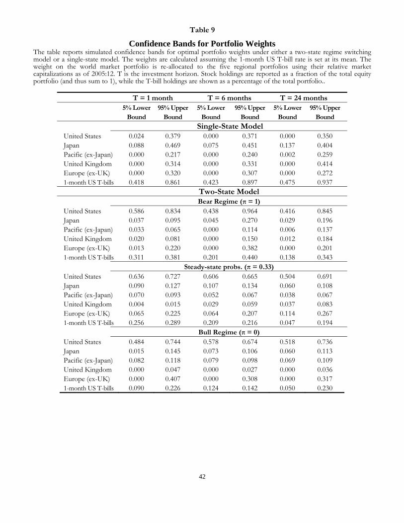
42

Table 9

Confidence Bands for Portfolio Weights The table reports simulated confidence bands for optimal portfolio weights under either a two-state regime switching model or a single-state model. The weights are calculated assuming the 1-month US T-bill rate is set at its mean. The weight on the world market portfolio is re-allocated to the five regional portfolios using their relative market capitalizations as of 2005:12. T is the investment horizon. Stock holdings are reported as a fraction of the total equity portfolio (and thus sum to 1), while the T-bill holdings are shown as a percentage of the total portfolio..

T = 1 month T = 6 months T = 24 months 5% Lower

Bound 95% Upper

Bound 5% Lower

Bound 95% Upper

Bound 5% Lower

Bound 95% Upper

Bound

Single-State Model United States 0.024 0.379 0.000 0.371 0.000 0.350 Japan 0.088 0.469 0.075 0.451 0.137 0.404 Pacific (ex-Japan) 0.000 0.217 0.000 0.240 0.002 0.259 United Kingdom 0.000 0.314 0.000 0.331 0.000 0.414 Europe (ex-UK) 0.000 0.320 0.000 0.307 0.000 0.272 1-month US T-bills 0.418 0.861 0.423 0.897 0.475 0.937

Two-State Model Bear Regime (π = 1) United States 0.586 0.834 0.438 0.964 0.416 0.845 Japan 0.037 0.095 0.045 0.270 0.029 0.196 Pacific (ex-Japan) 0.033 0.065 0.000 0.114 0.006 0.137 United Kingdom 0.020 0.081 0.000 0.150 0.012 0.184 Europe (ex-UK) 0.013 0.220 0.000 0.382 0.000 0.201 1-month US T-bills 0.311 0.381 0.201 0.440 0.138 0.343

Steady-state probs. (π = 0.33) United States 0.636 0.727 0.606 0.665 0.504 0.691 Japan 0.090 0.127 0.107 0.134 0.060 0.108 Pacific (ex-Japan) 0.070 0.093 0.052 0.067 0.038 0.067 United Kingdom 0.004 0.015 0.029 0.059 0.037 0.083 Europe (ex-UK) 0.065 0.225 0.064 0.207 0.114 0.267 1-month US T-bills 0.256 0.289 0.209 0.216 0.047 0.194

Bull Regime (π = 0) United States 0.484 0.744 0.578 0.674 0.518 0.736 Japan 0.015 0.145 0.073 0.106 0.060 0.113 Pacific (ex-Japan) 0.082 0.118 0.079 0.098 0.069 0.109 United Kingdom 0.000 0.047 0.000 0.027 0.000 0.036 Europe (ex-UK) 0.000 0.407 0.000 0.308 0.000 0.317 1-month US T-bills 0.090 0.226 0.124 0.142 0.050 0.230

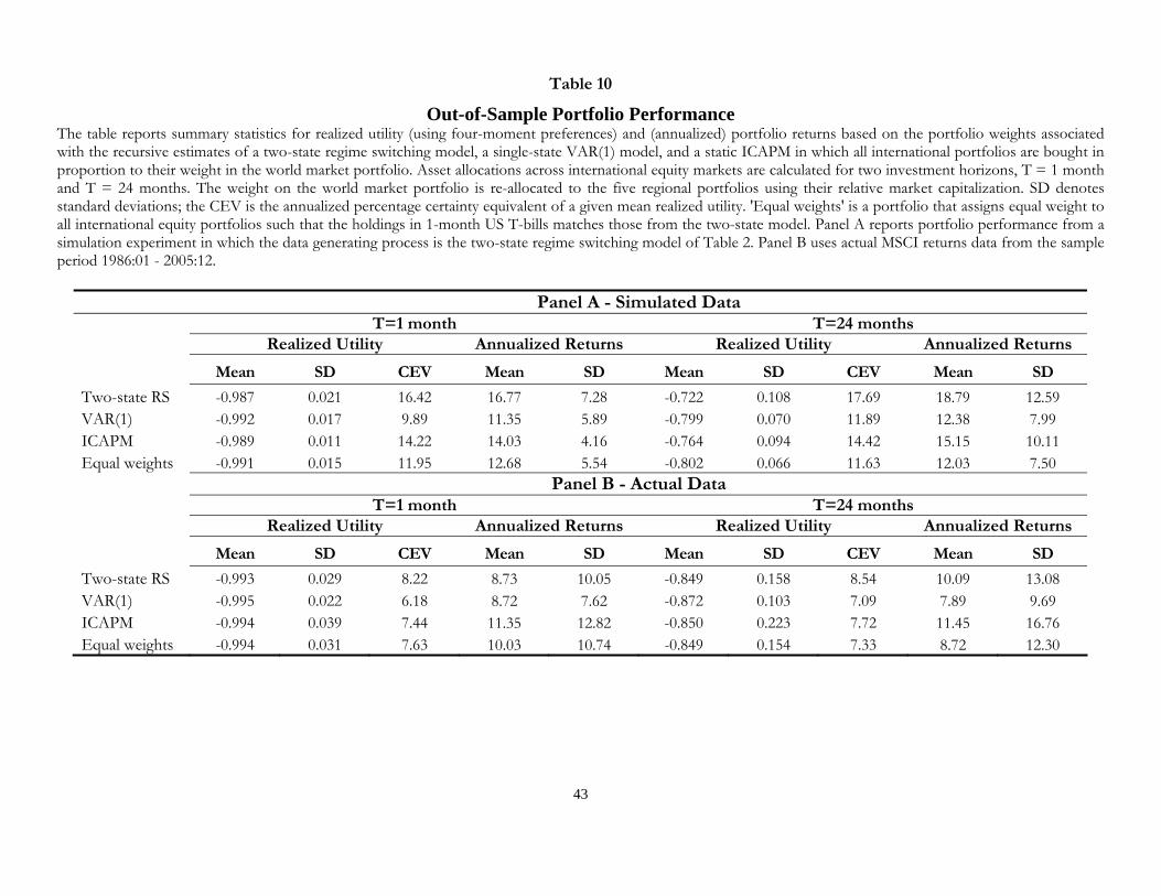
43

Table 10

Out-of-Sample Portfolio Performance The table reports summary statistics for realized utility (using four-moment preferences) and (annualized) portfolio returns based on the portfolio weights associated with the recursive estimates of a two-state regime switching model, a single-state VAR(1) model, and a static ICAPM in which all international portfolios are bought in proportion to their weight in the world market portfolio. Asset allocations across international equity markets are calculated for two investment horizons, T = 1 month and T = 24 months. The weight on the world market portfolio is re-allocated to the five regional portfolios using their relative market capitalization. SD denotes standard deviations; the CEV is the annualized percentage certainty equivalent of a given mean realized utility. 'Equal weights' is a portfolio that assigns equal weight to all international equity portfolios such that the holdings in 1-month US T-bills matches those from the two-state model. Panel A reports portfolio performance from a simulation experiment in which the data generating process is the two-state regime switching model of Table 2. Panel B uses actual MSCI returns data from the sample period 1986:01 - 2005:12.

Panel A - Simulated Data T=1 month T=24 months Realized Utility Annualized Returns Realized Utility Annualized Returns

Mean SD CEV Mean SD Mean SD CEV Mean SD

Two-state RS -0.987 0.021 16.42 16.77 7.28 -0.722 0.108 17.69 18.79 12.59 VAR(1) -0.992 0.017 9.89 11.35 5.89 -0.799 0.070 11.89 12.38 7.99 ICAPM -0.989 0.011 14.22 14.03 4.16 -0.764 0.094 14.42 15.15 10.11 Equal weights -0.991 0.015 11.95 12.68 5.54 -0.802 0.066 11.63 12.03 7.50 Panel B - Actual Data T=1 month T=24 months Realized Utility Annualized Returns Realized Utility Annualized Returns

Mean SD CEV Mean SD Mean SD CEV Mean SD

Two-state RS -0.993 0.029 8.22 8.73 10.05 -0.849 0.158 8.54 10.09 13.08 VAR(1) -0.995 0.022 6.18 8.72 7.62 -0.872 0.103 7.09 7.89 9.69 ICAPM -0.994 0.039 7.44 11.35 12.82 -0.850 0.223 7.72 11.45 16.76 Equal weights -0.994 0.031 7.63 10.03 10.74 -0.849 0.154 7.33 8.72 12.30

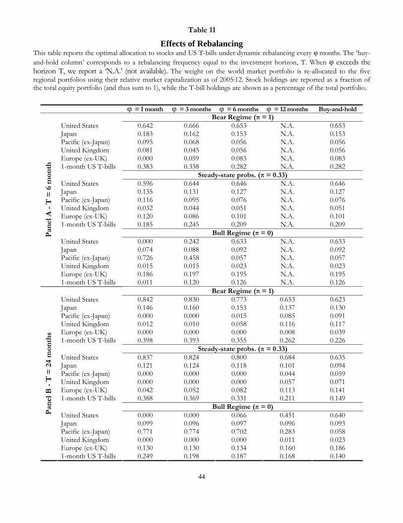
44

Table 11

Effects of Rebalancing This table reports the optimal allocation to stocks and US T-bills under dynamic rebalancing every months. The ‘buy-and-hold column’ corresponds to a rebalancing frequency equal to the investment horizon, T. When exceeds the horizon T, we report a ‘N.A.’ (not available). The weight on the world market portfolio is re-allocated to the five regional portfolios using their relative market capitalization as of 2005:12. Stock holdings are reported as a fraction of the total equity portfolio (and thus sum to 1), while the T-bill holdings are shown as a percentage of the total portfolio.

= 1 month = 3 months = 6 months = 12 months Buy-and-hold Bear Regime (π = 1) United States 0.642 0.666 0.653 N.A. 0.653 Japan 0.183 0.162 0.153 N.A. 0.153 Pacific (ex-Japan) 0.095 0.068 0.056 N.A. 0.056 United Kingdom 0.081 0.045 0.056 N.A. 0.056 Europe (ex-UK) 0.000 0.059 0.083 N.A. 0.083 1-month US T-bills 0.383 0.338 0.282 N.A. 0.282 Steady-state probs. (π = 0.33) United States 0.596 0.644 0.646 N.A. 0.646 Japan 0.135 0.131 0.127 N.A. 0.127 Pacific (ex-Japan) 0.116 0.095 0.076 N.A. 0.076 United Kingdom 0.032 0.044 0.051 N.A. 0.051 Europe (ex-UK) 0.120 0.086 0.101 N.A. 0.101 1-month US T-bills 0.185 0.245 0.209 N.A. 0.209 Bull Regime (π = 0) United States 0.000 0.242 0.633 N.A. 0.633 Japan 0.074 0.088 0.092 N.A. 0.092 Pacific (ex-Japan) 0.726 0.458 0.057 N.A. 0.057 United Kingdom 0.015 0.015 0.023 N.A. 0.023 Europe (ex-UK) 0.186 0.197 0.195 N.A. 0.195

Pan

el A

- T

= 6

mon

th

1-month US T-bills 0.011 0.120 0.126 N.A. 0.126 Bear Regime (π = 1) United States 0.842 0.830 0.773 0.653 0.623 Japan 0.146 0.160 0.153 0.137 0.130 Pacific (ex-Japan) 0.000 0.000 0.015 0.085 0.091 United Kingdom 0.012 0.010 0.058 0.116 0.117 Europe (ex-UK) 0.000 0.000 0.000 0.008 0.039 1-month US T-bills 0.398 0.393 0.355 0.262 0.226 Steady-state probs. (π = 0.33) United States 0.837 0.824 0.800 0.684 0.635 Japan 0.121 0.124 0.118 0.101 0.094 Pacific (ex-Japan) 0.000 0.000 0.000 0.044 0.059 United Kingdom 0.000 0.000 0.000 0.057 0.071 Europe (ex-UK) 0.042 0.052 0.082 0.113 0.141 1-month US T-bills 0.388 0.369 0.331 0.211 0.149 Bull Regime (π = 0) United States 0.000 0.000 0.066 0.451 0.640 Japan 0.099 0.096 0.097 0.096 0.093 Pacific (ex-Japan) 0.771 0.774 0.702 0.283 0.058 United Kingdom 0.000 0.000 0.000 0.011 0.023 Europe (ex-UK) 0.130 0.130 0.134 0.160 0.186

Pan

el B

- T

= 2

4 m

onth

s

1-month US T-bills 0.249 0.198 0.187 0.168 0.140

45

Figure 1

Bear state probabilities

0.0

0.2

0.4

0.6

0.8

1.0

1975 1980 1985 1990 1995 2000 2005

46

Figure 2

Mean excess returns (per annum) in the two-state model

-.01

.00

.01

.02

.03

.04

.05

.06

.07

.08

1980 1985 1990 1995 2000 2005

United States

-.01

.00

.01

.02

.03

.04

.05

.06

.07

.08

1980 1985 1990 1995 2000 2005

Japan

-.01

.00

.01

.02

.03

.04

.05

.06

.07

.08

1980 1985 1990 1995 2000 2005

Pacific (ex-Japan)

-.01

.00

.01

.02

.03

.04

.05

.06

.07

.08

1980 1985 1990 1995 2000 2005

Europe (ex-UK)

-.01

.00

.01

.02

.03

.04

.05

.06

.07

.08

1980 1985 1990 1995 2000 2005

United Kingdom

.00

.02

.04

.06

.08

.10

.12

1980 1985 1990 1995 2000 2005

World market

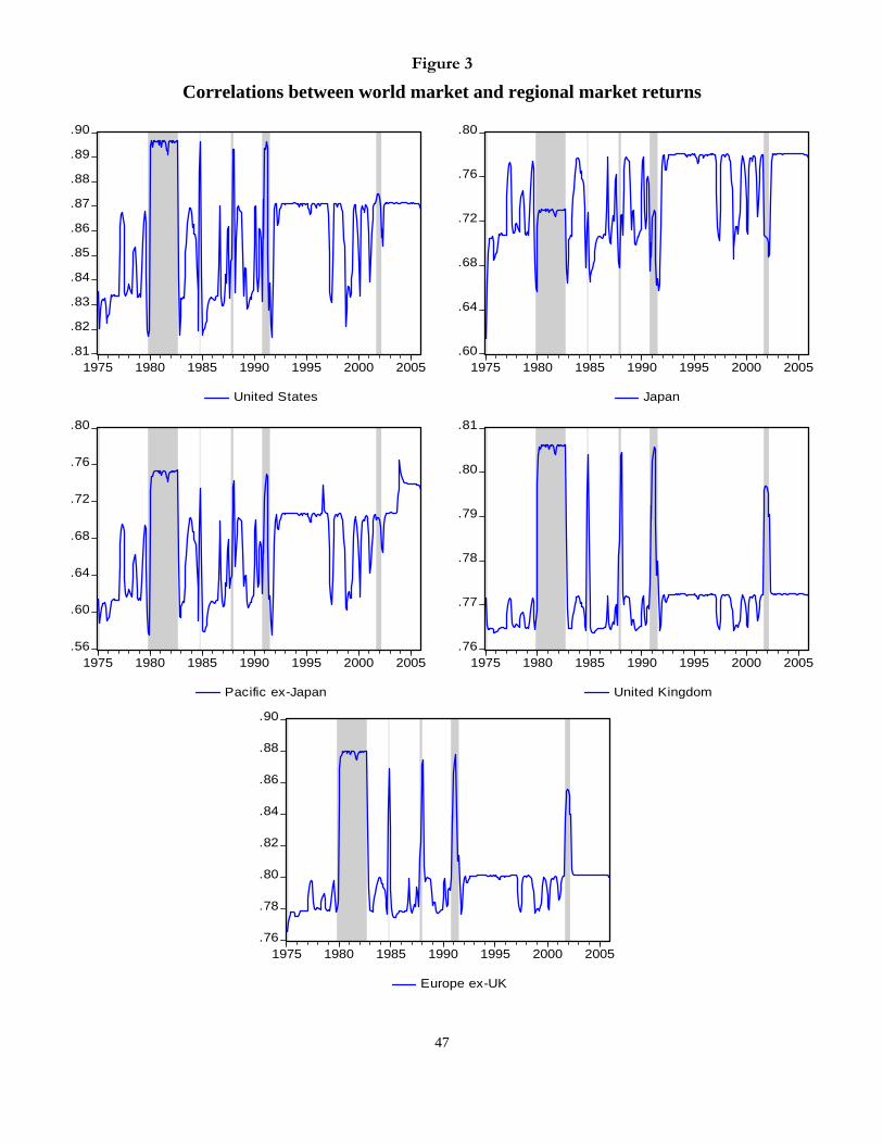
47

Figure 3

Correlations between world market and regional market returns

.81

.82

.83

.84

.85

.86

.87

.88

.89

.90

1975 1980 1985 1990 1995 2000 2005

United States

.60

.64

.68

.72

.76

.80

1975 1980 1985 1990 1995 2000 2005

Japan

.56

.60

.64

.68

.72

.76

.80

1975 1980 1985 1990 1995 2000 2005

Pacific ex-Japan

.76

.77

.78

.79

.80

.81

1975 1980 1985 1990 1995 2000 2005

United Kingdom

.76

.78

.80

.82

.84

.86

.88

.90

1975 1980 1985 1990 1995 2000 2005

Europe ex-UK

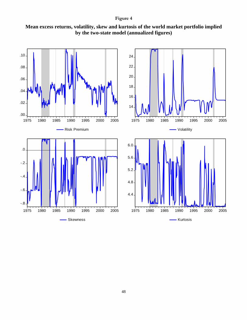
48

Figure 4

Mean excess returns, volatility, skew and kurtosis of the world market portfolio implied by the two-state model (annualized figures)

.00

.02

.04

.06

.08

.10

1975 1980 1985 1990 1995 2000 2005

Risk Premium

14

16

18

20

22

24

1975 1980 1985 1990 1995 2000 2005

Volatility

-.8

-.6

-.4

-.2

.0

1975 1980 1985 1990 1995 2000 2005

Skewness

4.4

4.8

5.2

5.6

6.0

1975 1980 1985 1990 1995 2000 2005

Kurtosis

International Asset Allocation under Regime Switching, Skew and

Documents

Transcript of International Asset Allocation under Regime Switching, Skew and