1

INTERNAL PROMOTION AND EXTERNAL RECRUITMENT: A THEORETICAL AND EMPIRICAL ANALYSIS

by

Jed DeVaro* Department of Management and Department of Economics

College of Business and Economics California State University, East Bay

Hayward, CA 94542 E-mail: jed.devaro@csueastbay.edu

and

Hodaka Morita

School of Economics Australian School of Business

The University of New South Wales Sydney 2052, Australia

E-mail: h.morita@unsw.edu.au

May 15, 2009 Abstract: A crucial personnel decision employers face is whether to fill a limited number of managerial positions with internal hires or external recruits. We present a theoretical and empirical analysis of this decision and how it relates to wage setting and the provision of general training. The theoretical framework is a promotion tournament involving M competing firms with heterogeneous productivities, two-level job hierarchies, and a fixed number of managerial positions. Employers provide general training to their workers, some of whom are promoted internally or raided by competing firms. We also consider an alternative model based on variation in the quality of the worker-employer match. Both models predict the following results: As the number of workers at the lower level of the hierarchy increases, holding fixed the number of managers at the top, 1) internal promotion increases relative to external recruitment, 2) employers provide more general training, 3) the percentage of employees in the upper tail of the wage distribution decreases, 4) profitability increases. We test these predictions using data from the 2004 wave of the WERS, a nationally-representative cross section of British establishments. The empirical results are supportive and contribute to the literature some new stylized facts concerning how key employer decisions vary with both the size and shape of the organizational hierarchy. Keywords: Internal Promotion, External Recruitment, General Training, Tournaments, Fixed Slots, Job Hierarchies

* The authors acknowledge the Department of Trade and Industry, the Economic and Social Research Council, the Advisory, Conciliation and Arbitration Service and the Policy Studies Institute as the originators of the 2004 Workplace Employee Relations Survey data, and the Data Archive at the University of Essex as the distributor of the data. None of these organizations bears any responsibility for the authors’ analysis and interpretations of the data. We thank Jonathan Lim for research assistance and numerous colleagues for helpful comments, including seminar participants at the 2009 Society of Labor Economists meeting, Hitotsubashi University, USC Marshall School of Business, UC Merced, and the 2008 conference on Tournaments, Contests, and Relative Performance in Raleigh, NC.

2

1. Introduction The number of managerial positions is limited in most organizations, and employers fill

those limited positions with either internal hires or external recruits. This external-versus-

internal-hiring decision is important, because managerial capability is a critical determinant of the

profitability of an organization. Our objective is to explore how this decision is related to the

shape of the organizational hierarchy, presenting a new theoretical model that describes the

interconnections among employers’ competition for scarce managerial talent, their profitability,

the shape of their organizational hierarchy, the distribution of wages within the organization, and

their incentives to train workers. Our model delivers testable implications concerning how these

concepts are related, and we test these predictions empirically using the British WERS, a large-

scale, nationally-representative, cross section of employers surveyed in 2004. Our results support

each of the model’s predictions and introduce a new set of empirical results to the literature on

internal hiring versus external recruitment. We find that, controlling for employer characteristics,

increases in establishment size that make the job hierarchy more “bottom heavy” are associated

with: 1) a greater likelihood of hiring internally versus recruiting externally, 2) a higher level of

profit, 3) a lower fraction of workers in the upper tail of the organization’s wage distribution, and

4) a greater likelihood of providing training to workers.

Our analysis contributes to the theoretical and empirical literatures on promotions in

general and internal hiring versus external recruitment in particular.1 Given that two important

functions of promotions are creating worker incentives and assigning workers to jobs, the two

main building blocks for theoretical analyses of promotions are tournament models and job

assignment models (Baker, Jensen, and Murphy 1988; Gibbons and Waldman 1999a). Ours is a

job-assignment model that incorporates a central feature of tournament models, namely a

hierarchy with a fixed number of managerial positions. In contrast, most job assignment models

assume flexible job slots in which any number of workers could be promoted to CEO, given

sufficiently strong job performance. The notion of fixed job slots is an important feature of most

within-firm job hierarchies, as discussed in DeVaro (2006), so it is worthwhile exploring the job-

assignment aspect of promotions under the realistic assumption of fixed managerial job slots. On

the other hand, the notion of an active outside market in which competing firms bid for a worker’s

1 A survey of the literature on internal promotion versus external recruitment is contained in Waldman (2007).

3

services is a plausible feature of employment relationships that is captured in many job

assignment models (including ours) but that is absent from traditional tournament theory, except

insofar as a participation constraint in the worker’s utility maximization affects how the employer

sets wages across hierarchical levels. Furthermore, an important distinguishing feature of our

model is that, unlike most existing models of promotion, ours explicitly analyzes strategic

interactions among heterogeneous employers in their efforts to fill their managerial positions with

capable candidates. In our model, firms’ hierarchical structures are endogenously determined,

where firms with higher returns from their managers adopt more bottom-heavy hierarchical

structures. This results in a set of novel testable predictions concerning internal promotion versus

external recruitment and the shape of the job hierarchy.

To see the model’s main ideas, consider a labor market consisting of M (≥ 2) firms, each

of which has a two-tier hierarchy consisting of one managerial position and a variable number of

subordinate positions. The firms are heterogeneous in that they have different returns from their

managers’ capabilities. Each firm decides how many young workers to hire and makes initial

wage offers to a large number of ex ante identical young workers that choose between

employment and self-employment. When the hired young workers become old, their managerial

capabilities (which are transferable across any firms in the market and modeled as random draws

from a known distribution function) are revealed to themselves, to their employers, and to all

other employers in the labor market.2 We assume that employers have symmetric information

about managerial capability and that employers compete against each other by simultaneously

making wage offers to employ one worker in the managerial position. Productive workers who

are not hired as managers remain with their current employers as subordinates, while

unproductive workers exit the market to pursue some outside option (e.g. self employment).

Our model, and an extension that incorporates firm-sponsored general training, yields the

following set of testable predictions: As the number of subordinate workers at the lower level of

the hierarchy increases (holding fixed the number of managers at the top): 1) internal promotion

2 The symmetric learning assumption in which a particular worker’s ability is revealed during the course of his career to all employers in the labor market at the same rate has appeared in a number of models in the job assignment literature (e.g. Gibbons and Waldman 1999b, 2003). An alternative strand of the literature focuses on asymmetric learning in which a worker’s current employer obtains information about his ability at a faster rate than competing employers (e.g. Waldman 1984; Milgrom and Oster 1987; Ricart i Costa 1987; Waldman 1990; Bernhardt 1995; Zabojnik and Bernhardt 2001; Owan 2004; Golan 2005; DeVaro and Waldman 2007; DeVaro, Ghosh, and Zoghi 2008).

4

increases relative to external recruitment, 2) profitability increases, 3) the percentage of

employees in the upper tail of the within-establishment wage distribution decreases, 4) employers

provide more general training.3 The logic behind these predictions can be explained as follows:

As the number of productive workers in the industry increases, each employer can hire a manager

with a greater managerial capability. This benefit is increasing in the return from managerial

capability, and hence an employer with a higher return from managerial capability has a greater

incentive to increase the number of its productive workers by employing more trainees and

providing them with a higher level of general training. An employer with a larger number of

productive workers, in turn, has a greater probability of filling its managerial position with an

internal hire, with a larger number of productive workers remaining as subordinates.

Our analysis relates to the literature on raiding (e.g. Lazear, 1986; Bernhardt and Scoones,

1993; Kim, 2007). Lazear (1986) explored a model consisting of two firms, with a raid occurring

when a worker is worth more to a competing employer than to the current employer, and

demonstrated that an informational asymmetry between the two firms concerning the worker’s

productivity gives rise to a number of implications on raiding and offer-matching. Building on

Lazear’s model, Kim (2007) explored a model that links employee movement and product-market

competition, demonstrating that a firm may poach its rival’s key employees in order to induce the

rival’s exit. Bernhardt and Scoones (1993) examined the strategic promotion and wage decisions

of employers when employees may be more valuable to competing firms. In all of these models,

the fundamental driving force for raiding is the quality of worker-employer match. In contrast, in

our model the driving force for raiding is the combination of fixed managerial job slots and

employers’ heterogeneity in their returns from managerial capability, though, as in the models

based on match quality, our model also captures the idea that raiding occurs when a worker is

worth more to a competing employer than to his current employer. In Section 3, we present an

alternative model based on match quality that yields the same predictions as our main model, and

we discuss how both models compare.

In our main model, returns from managerial capability are assumed to be different across

firms. In the equilibrium, firms with higher returns employ more young workers, yielding our

key prediction that an employer with a more bottom-heavy hierarchical structure is more likely to

3 The fourth prediction offers a new explanation for the existence of firm-sponsored general training, a topic of recent interest in the training literature. Alternative explanations for this practice have been offered in earlier work (e.g. Acemoglu and Pischke 1998, 1999a, 1999b).

5

hire its manager from its internal candidates. A similar assumption was made by Zábojník and

Bernhardt (2001), which proposed an asymmetric learning model in which tournament prizes are

determined competitively. That analysis incorporated firm heterogeneity by assuming a fixed

number of high-productivity firms and free entry of low-productivity firms. As in our model,

high-productivity firms in their model adopt a more bottom-heavy hierarchical structure than low-

productivity firms in the equilibrium. However, the Zábojník and Bernhardt model does not yield

predictions concerning internal promotion versus external recruitment; there is no labor turnover

in the equilibrium, and all promotions are internal in their model.4

Another purely theoretical analysis that relates to ours is Demougin and Siow (1994),

which incorporates training in a similar manner to the extension of our main model. Demougin

and Siow consider an overlapping-generations structure in which firms are infinitely lived and

each cohort of workers participates in the labor market for two periods. In any period, a firm

employs a single manager and an endogenously-determined number of unskilled workers. The

firm can train any or all of its young workers, where a higher level of training increases the

probability that an unskilled worker becomes skilled and therefore capable of becoming a

manager. In the equilibrium, each firm promotes internally if at least one young worker’s training

succeeds, and promotes externally otherwise. A fundamental difference between the Demougin

and Siow model and ours is that in theirs the equilibrium hierarchical structure (bottom-

heaviness) is the same across firms, whereas in ours it is different. This is crucial, because the

focus of our analysis is on deriving and empirically testing new predictions concerning how

variation in hierarchical structures across firms affects the likelihood of internal promotion,

profitability, wage structure, and training intensity. In contrast, the focus of their theoretical

analysis is explaining a pre-existing pattern of evidence concerning career mobility, up-or-out

rules, internal labor markets, the span of control, and seniority wage premia.

Other theoretical analyses of internal hiring include Chan (1996) and Waldman (2003),

and a recent empirical analysis is Chan (2006). These analyses differ from ours in their 4 Our model also predicts that an employer with a more bottom-heavy hierarchical structure makes more profit, has a greater fraction of workers appear in the upper tail of the firm’s wage distribution, and provides more training. Although these additional predictions also arise from the Zábojník and Bernhardt analysis, our work offers a contribution in two ways (apart from our unique theoretical prediction concerning internal hiring). First, our model establishes the robustness of these additional predictions in the context of a model with a very different focus; whereas Zábojník and Bernhardt focus on the incentive mechanisms of promotions with asymmetric learning, we focus on the job-assignment mechanisms of promotions with symmetric learning. Second, whereas the Zábojník and Bernhardt analysis is purely theoretical, we empirically test all of our model’s predictions.

6

motivations and in that they do not focus on the implications of employer heterogeneity. In

particular, they aim to explain why internal candidates are frequently preferred for promotion

over equally-qualified external candidates. Chan’s (1996) model consists of two ex ante identical

risk-neutral firms, while Waldman’s (2003) model considers a single risk-neutral firm. In

contrast, our study focuses on the implications of employer heterogeneity in the returns from

managerial capability, and this yields a set of new predictions concerning how a firm’s tendency

to hire internally, its profitability, its within-firm wage distribution, and its decisions regarding

training relate to its chosen shape of the job hierarchy.

Before presenting our main model in the next section, we note that our theory offers a

potential explanation for a well-established empirical finding that internal hiring of CEOs is more

prevalent than external recruitment in large firms (e.g. Dalton and Kesner, 1983; Lauterbach and

Weisberg, 1994; Parrino, 1996; Lauterbach, Vu, and Weisberg, 1999; Agrawal, Knoeber, and

Tsoulouhas, 2004. See Murphy, 1999 for a survey). Although this “internal succession – firm

size” relationship has been documented empirically, to our knowledge, no theoretical models

have been proposed that yield this prediction. Our model’s first prediction relates to this stylized

fact, though we emphasize that our prediction pertains to changes in size of a particular type,

namely increases in size at the lower (i.e. non-managerial) levels of the hierarchy. Thus,

increases in firm size in our model also imply changes in the shape of the hierarchy, in particular

a flattening of the hierarchy or an increase in “bottom heaviness”. However, the empirical

regularity pertaining to firm size in general might well be consistent with the predictions of our

model to the extent that “firm size” in general is positively correlated with size in the lower levels

of the hierarchy, and thus our model can be interpreted as offering a theoretical explanation for

the “internal succession – firm size” relationship for CEOs. Whereas the previous empirical

studies simply focused on firm size without distinguishing how this size was distributed across

hierarchical levels, the data we use allow us to investigate empirically the more refined prediction

regarding size (and shape) from our theoretical model. We find clear support for this prediction,

thereby introducing a new stylized fact to the literature as well as a theoretical rationale for it.

2. A Theoretical Model of Internal Promotion Versus External Recruitment In the following subsections we present our model, analysis, testable predictions, and an

extension to consider employer-sponsored training.

7

A. Model Consider an industry consisting of M (≥ 2) firms in a two-period setup. Heterogeneous

firms are characterized by parameters Vi, where i indexes firms and V1 > V2 > … > VM. The parameter Vi determines firm i’s return from its manager, as described later.5 In reality, firms in the same industry adopt different strategies to satisfy needs of different types of customers. For example, some firms produce lower quality, standardized products while others produce higher-quality products tailored to specific customer demands. For the latter type of firm, a manager's ability to understand the changing nature of customer needs and to propose corresponding changes in the firm’s business strategy (such as product design, product delivery, advertisement, etc.) is more important than in the former type of firm. Our mode captures this important difference across firms by assuming that the returns from managerial capabilities are different across firms.

In the beginning of period 1, a large number of ex ante identical individuals exist. Every firm i (= 1, 2, …, M) simultaneously makes take-it-or-leave-it first-period wage offer wi

1 > 0 to

in̂ ≥ 0 individuals. If an individual accepts firm i’s offer, he is employed by firm i in period 1. Let

ni denote the number of firm i’s first-period employees (call them young workers). If an individual is not employed by a firm, he becomes self-employed. To simplify the description of the model, assume that such an individual stays self-employed until the end of period 2, earning w > 0 per period. Firms and individuals are both risk neutral and do not discount the future.

Every young worker is assigned to a subordinate position. Due to lack of experience, each young worker requires supervision from the employer. Assume that each firm i’s young worker’s output is η – s(ni), where η > 0 is a given constant and s(.) is a differentiable function with s′(.) > 0. That is, as the number of young workers increases, each young worker’s output declines because each young worker receives less supervision from the employer.6 To simplify the analysis, let s(Z) = bZ where b > 0.7

At the end of period 1, each young worker j exhibits managerial capability mj, which is randomly drawn from a uniform distribution between α and β, 0 ≤ α < β. To keep the analysis simple and the notation compact, let α = 0 and β = 1. If worker j is assigned to a subordinate position, his second-period output is y ≥ η, requiring no supervision from the employer. Each

5 For simplicity, we assume that every employer knows its own V and those of the other employers in the market. This assumption can be relaxed a bit, so that employers observe their location in the distribution with some error, and our qualitative predictions would remain unchanged. The assumption that employers would have a fairly accurate sense of where they fall in the distribution of returns to managerial capability seems reasonable. 6 See Zábojník and Bernhardt (2001) for a similar specification. 7 We allow the possibility that a young worker’s output is negative. This can be avoided by interpreting η to be each young worker’s (positive) output and s(ni) to be a per-worker supervision cost that firm i must incur in period 1 when it employs ni young workers.

8

worker’s productivity is completely transferable across firms in the market, and the realization of each worker’s managerial ability is observable by all M firms. In period 2, each firm can fill one managerial position and an unlimited number of subordinate positions. Each firm’s gross output from its manager is given by Vi(mi + q), where mi denotes the managerial capability of the manager in firm i, and q denotes firm i's manager's productivity if he has zero managerial capability. Assume VM > y/q, which implies that each firm’s gross output from any worker is higher when the worker is assigned as a manager than when he is assigned as a subordinate. Each firm’s period-2 gross output is then given by Vi(mi + q) + ni

Oy, where niO denotes the number of firm i’s subordinates (the superscript “O” stands for

old workers) in period 2. Firm i’s overall profit is the gross output minus wage bills. The timing of the game can be summarized as follows: Stage 1: Every firm i (= 1, 2, …, M) simultaneously makes take-it-or-leave-it first-period wage offer wi

1 > 0 to in̂ ≥ 0 individuals. Individuals that are not employed by a firm become self-

employed. Stage 2: Each young worker exhibits managerial capability, mj, which is a random draw from a uniform distribution between α and β. The realization of each worker’s managerial capability is common knowledge. Stage 3: Each firm i simultaneously makes wage offers, denoted wir, to every young worker r

(including the workers employed at other firms). Each worker chooses the highest wage offer,

and in case of a tie stays with his current employer.8 Each firm then assigns one worker to its

managerial position and all others to subordinate positions. Finally, each firm realizes output.

The job assignment literature makes an important distinction between asymmetric and

symmetric learning, and influential models have been proposed under either set of assumptions.

Although we assume symmetric learning, the basic logic underlying our results should also apply

in an asymmetric learning model. Suppose that the current employer observes its old workers’

managerial capabilities after the first period of employment, whereas competing employers only

observe a noisy signal of these managerial capabilities. In that case, our results should hold in

expectation, though there would be some mistaken bids by outside employers, resulting in some

inefficient separations and job assignments. Another important issue in the job assignment

literature concerns the timing of the wage offer process, in particular whether offers are

simultaneous or allow for counteroffers from the current employer. The simultaneous offer

assumption has been criticized by Golan (2005) who showed that outcomes can be first-best 8 The results are qualitatively unchanged under an alternative assumption that each worker incurs an infinitesimally small moving cost when changing employers.

9

efficient even in the presence of asymmetric information (where the outside firms are less

informed than the current employer regarding worker productivity) when the current employer is

allowed to match outside offers with counteroffers. In our symmetric learning model, it makes no

difference whether wage bids are simultaneous or if the current employer can make a counteroffer.

However, it is unclear how an assumption of asymmetric learning combined with a counteroffer

from the current employer might affect the analysis, since in that case an offer made by a current

employer reveals some relevant information to other potential employers.

B. Equilibrium and Analysis We now derive Subgame Perfect Nash Equilibria in pure strategies. To focus our analysis

and simplify the description of the results, we assume that an old worker’s second-period output,

y, is sufficiently high so that every firm employs at least one young worker in period 1 in the

equilibrium. A sufficient condition for this is y > 2(w + b) – η, which we assume throughout our

analysis.9 Note that we focus on equilibria in which ni = in̂ holds: that is, in equilibrium, every

firm employs all individuals to whom it made a first-period wage offer.

Suppose that each of the M firms employs at least one young worker at stage 1. Let N (≥

M) denote the total number of young workers in the market and m(k|N) (k = 1, 2, …, N) denote

the kth highest realization of managerial capability in the market, across the young workers in all

M firms. It can be shown that, in the equilibrium of the subsequent Stage 3 subgame, each firm i

employs a worker with m(i|N) as its manager at the wage of wim (N), where

(1) ∑−

=+ +−+=

1

1 )]|1()|([)(M

i

mi NmNmVyNw

ψψ ψψ for i = 1, 2, …, M – 1, and ( )m

Mw N y= .

This result can be explained as follows. Since firm 1 has the highest return from its manager, it

hires the worker with m(1|N), the highest realization of the managerial capability, and firm 2 hires

the worker with m(2|N), and so on. We find that w1m(N) = w2

m(N) + V2[m(1|N) – m(2|N)] holds

in the equilibrium. Note that V2[m(1|N) – m(2|N)] captures the increment of firm 2’s gross profit

9 Suppose that firm i employs ni young workers at the first-period wage wi. If a young worker is assigned to a subordinate position in period 2, his second-period output is y, and hence Bertrand wage competition implies that the worker’s second-period wage is y. Also, if a young worker is assigned as a manager, the worker’s second period wage is at least y. This implies that wi ≤ 2w – y, given that any individual can earn w per period by choosing self-employment. Hence, firm i’s period-1 profit is at least ni[η – bni – (2w – y)] = ni[y + η – 2w – bni], which is maximized when ni = (y + η – 2w)/2b. Then, (y + η – 2w)/2b > 1 ⇔ y > 2(w + b) – η guarantees that every firm employs at least one young worker in any equilibrium of the game.

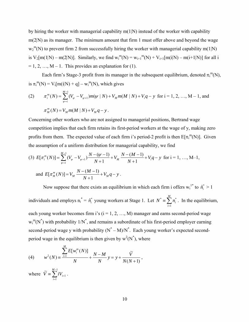
10

by hiring the worker with managerial capability m(1|N) instead of the worker with capability

m(2|N) as its manager. The minimum amount that firm 1 must offer above and beyond the wage

w2m(N) to prevent firm 2 from successfully hiring the worker with managerial capability m(1|N)

is V2[m(1|N) – m(2|N)]. Similarly, we find wim(N) = wi+1

m(N) + Vi+1[m(i|N) – m(i+1|N)] for all i

= 1, 2, …, M – 1. This provides an explanation for (1).

Each firm’s Stage-3 profit from its manager in the subsequent equilibrium, denoted πim(N),

is πim(N) = Vi[m(i|N) + q] – wi

m(N), which gives

(2) ∑−

=+ −++−=

1

1 )|()|()()(M

iiM

mi yqVNMmVNmVVN

ψψψ ψπ for i = 1, 2, …, M – 1, and

yqVNMmVN MMmM −+= )|()(π .

Concerning other workers who are not assigned to managerial positions, Bertrand wage

competition implies that each firm retains its first-period workers at the wage of y, making zero

profits from them. The expected value of each firm i’s period-2 profit is then E[πim(N)]. Given

the assumption of a uniform distribution for managerial capability, we find

(3) 1

1( 1) ( 1)[ ( )] ( )

1 1

Mmi M i

i

N N ME N V V V V q yN Nψ ψ

ψ

ψπ−

+=

− − − −= − + + −

+ +∑ for i = 1, …, M–1,

and ( 1)[ ( )]1

mM M M

N ME N V V q yN

π − −= + −

+.

Now suppose that there exists an equilibrium in which each firm i offers wi1* to *ˆin > 1

individuals and employs ni* = *ˆin young workers at Stage 1. Let * *

1

M

ii

N n=

≡∑ . In the equilibrium,

each young worker becomes firm i’s (i = 1, 2, …, M) manager and earns second-period wage

wim(N*) with probability 1/N*, and remains a subordinate of his first-period employer earning

second-period wage y with probability (N* – M)/N*. Each young worker’s expected second-

period wage in the equilibrium is then given by w2(N*), where

(4) )1(

~)]([)( 12

++=

−+≡

∑=

NNVyy

NMN

N

NwENw

M

i

mi

,

where ∑−

=+≡

1

11

~ M

iiiVV .

11

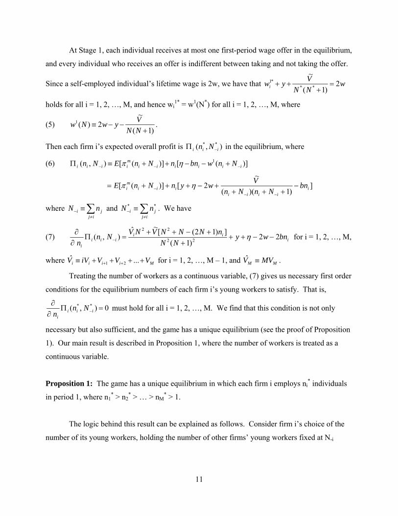
At Stage 1, each individual receives at most one first-period wage offer in the equilibrium,

and every individual who receives an offer is indifferent between taking and not taking the offer.

Since a self-employed individual’s lifetime wage is 2w, we have that wNNVywi 2

)1(

~**

*1 =+

++

holds for all i = 1, 2, …, M, and hence wi1* = w1(N*) for all i = 1, 2, …, M, where

(5) )1(

~2)(1

+−−≡

NNVywNw .

Then each firm i’s expected overall profit is ),( **iii Nn −Π in the equilibrium, where

(6) )]([)]([),( 1iiiiii

miiii NnwbnnNnENn −−− +−−++≡Π ηπ

])1)((

~2[)]([ i

iiiiiii

mi bn

NnNnVwynNnE −

++++−+++=

−−− ηπ

where ∑≠

− ≡ij

ji nN and ∑≠

− ≡ij

ji nN ** . We have

(7) iii

iiii

bnwyNN

nNNNVNVNnn

22)1(

])12([~ˆ),( 22

22

−−+++

+−++=Π

∂∂

− η for i = 1, 2, …, M,

where Miiii VVViVV ++++≡ ++ ...ˆ21 for i = 1, 2, …, M – 1, and MM MVV ≡ˆ .

Treating the number of workers as a continuous variable, (7) gives us necessary first order

conditions for the equilibrium numbers of each firm i’s young workers to satisfy. That is,

0),( ** =Π∂∂

−iiii

Nnn

must hold for all i = 1, 2, …, M. We find that this condition is not only

necessary but also sufficient, and the game has a unique equilibrium (see the proof of Proposition

1). Our main result is described in Proposition 1, where the number of workers is treated as a

continuous variable.

Proposition 1: The game has a unique equilibrium in which each firm i employs ni* individuals

in period 1, where n1* > n2

* > … > nM* > 1.

The logic behind this result can be explained as follows. Consider firm i’s choice of the

number of its young workers, holding the number of other firms’ young workers fixed at N-i

12

(≥ M – 1). The minimum possible wage at which firm i can employ ni young workers is w1(ni +

N-i) where w1(.) is as defined in (5), because each individual is indifferent between being

employed by firm i at w1(ni + N-i) and being self-employed. Firm i’s period-1 profit is then

(8) 1[ ( ) ( )] [ 2 / ( )( 1)]i i i i i i i i i in s n w n N n y w bn V n N n Nη η− − −− − + = + − − + + + +% ,

and (y + η – 2w)/2 > b implies that each firm i employs at least one young worker given any N-i.

In Period 2, firm i employs a worker with m(i|N), the ith highest realization of managerial

capability in the market, as its manager at the second-period wage of wim(ni + N-i). Since m(i|N)

is the ith order statistic among N = ni + N-i young workers in the industry, firm i can increase the

expected managerial capability of its manager by increasing the number of its young workers ni,

holding N-i constant. Comparing firm i and firm j where i < j, firm i’s incremental profit from

employing an additional young worker is greater than firm j’s incremental profit, because firm i’s

return from managerial capability is greater than firm j’s return from it (that is, Vi > Vj). On the

other hand, the incremental first-period profit (the increment can be negative) from employing an

additional young worker is the same across all M firms. Hence, the incremental overall expected

profit from employing an additional young worker is also higher for a firm with a higher return

from managerial ability, while the incremental cost of employing an additional young worker is

the same for all M firms. This implies that a firm with a higher return from managerial ability

employs a larger number of young workers in period 1, so n1* > n2

* > … > nM* > 1.

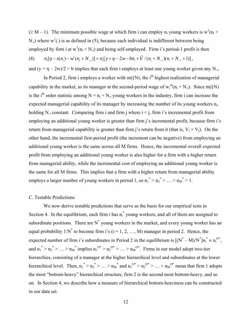
C. Testable Predictions

We now derive testable predictions that serve as the basis for our empirical tests in

Section 4. In the equilibrium, each firm i has ni* young workers, and all of them are assigned to

subordinate positions. There are N* young workers in the market, and every young worker has an

equal probability 1/N* to become firm i’s (i = 1, 2, …, M) manager in period 2. Hence, the

expected number of firm i’s subordinates in Period 2 in the equilibrium is [(N* – M)/N*]ni* ≡ ni

O*,

and n1* > n2

* > … > nM* implies n1

O* > n2O* > … > nM

O*. Firms in our model adopt two-tier

hierarchies, consisting of a manager at the higher hierarchical level and subordinates at the lower

hierarchical level. Then, n1* > n2

* > … > nM* and n1

O* > n2O* > … > nM

O* mean that firm 1 adopts

the most “bottom-heavy” hierarchical structure, firm 2 is the second most bottom-heavy, and so

on. In Section 4, we describe how a measure of hierarchical bottom-heaviness can be constructed

in our data set.

13

The following three testable predictions emerge from our model.

Testable prediction 1: An employer with more bottom-heavy hierarchical structure is more likely

to hire its manager from its internal candidates.

Testable prediction 2: An employer with more bottom-heavy hierarchical structure makes more

profit.

Testable prediction 3: An employer with more bottom-heavy hierarchical structure has a lower

percentage of its employees located in the upper tail of the within-firm wage distribution.

Since every young worker in the market has an equal probability, 1/N*, of becoming firm

i’s manager, the probability that firm i hires its manager from its internal candidate is ni*/N* ≡ Pi

*,

and n1* > n2

* > … > nM* > 1 implies P1

* > P2* > … > PM

*, yielding prediction 1. Regarding

profitability, given V1 > V2 > … > VM we find ∏1(n1*, N-1

*) > ∏2(n2*, N-2

*) > … > ∏M(nM*, N-M

*),

yielding prediction 2. Finally, given the natural assumption that managers are located in the

upper tail of the firms’ wage distributions and subordinates are in the lower tail, we have

prediction 3.

D. An Extension: Firm-sponsored training

Employers often provide training, at their own cost, to their employees. In this subsection,

we consider an extension of the model that incorporates firm-sponsored training to explore the

robustness of our theoretical predictions in the presence of training and to obtain an additional

testable prediction.10

Suppose that every firm i (= 1, 2, …, M) simultaneously makes take-it-or-leave-it offers

(wi1, xi) to in̂ ≥ 0 individuals at Stage 1. After the first-period employment is settled, each firm i

provides a level of training, xi ∈ [0, 1], to its young workers at a training cost of c(xi) per worker,

where c(.) is a standard, twice-differentiable cost function satisfying c(0) = 0, c′(.) > 0, and c′′(.) >

0. To simplify the analysis, let c(Z) = aZ2, where a > 0. Given the training, φ(xini) trainees

become productive workers and the others become unproductive workers in period 2, where φ(X)

denotes the integer closest to X ∈ ℜ satisfying φ(X) ≤ X. Thus, training increases the number of

productive workers. Each firm i’s young worker’s output is η – s(ni) as in the original model,

10 The full description of the extension is presented in a Supplementary Note that is available upon request.

14

where η > 0 is a given constant and s(.) is a differentiable function with s′(.) > 0. Assume η < w;

that is, each young worker’s output is lower than his self-employment output.11

At the end of period 1, each productive worker j exhibits managerial capability mj, which

is randomly drawn from a uniform distribution between 0 and 1, as in the original model. Each

productive worker’s output in a subordinate position is y, where y > w. On the other hand,

unproductive workers do not exhibit managerial capability and their output in a subordinate

position is η (< w) in any firms in the market, and hence unproductive workers leave the market

and become self-employed in period 2. Human capital is general and information is symmetric.

That is, each worker’s productivity is transferable across firms in the market, and the realization

of each worker’s managerial ability is observable by all M firms in the market.

We consider the Subgame Perfect Nash Equilibria, treating the number of workers as a

continuous variable. Let ni* and xi

* denote the number of firm i’s young workers and the level of

training firm i provides, respectively, in the equilibrium. If ni* > 1 and 0 < xi

* < 1 for all i = 1, 2,

…, M, we say that the equilibrium is an “interior equilibrium.” It can be shown that in the case of

M = 2, there exists a range of parameterizations for which interior equilibria exist. Details of the

analysis are available in the Supplementary Note.

If an interior equilibrium exists, it can be shown that n1* > n2

* > … > nM* > 1 and 1 > x1

* >

x2* > … > xM

* > 0 both hold in the equilibrium. The logic behind this result, which is similar to

the logic behind Proposition 1 of the original model, can be explained as follows. Let

1

M

P i ii

N x n=

≡∑ denote the total number of productive workers in the market, and let ,P i j jj i

N x n−≠

≡∑

denote the total number of productive workers in the market that are not employed by firm i. In

Period 2, firm i employs a worker with m(i|NP), the ith highest realization of managerial capability

in the market, as its manager. Since m(i|NP) is the ith order statistic among NP = xini + NP,-i

productive workers in the market, firm i can increase the expected managerial capability of its

manager by increasing the number of its productive workers, xini, holding NP,-i constant.

Comparing firm i and firm j, where i < j, firm i’s incremental profit from increasing the number of

its productive workers is greater than firm j’s incremental profit, because firm i enjoys a higher

return from managerial capability (i.e., Vi > Vj). This implies that the incremental first-period

profit from increasing the number of productive workers is higher for a firm with a higher return

11 For example, the need for learning-by-doing may reduce young workers’ output below the self-employment wage.

15

from managerial ability, while its incremental cost is the same across M firms. This results in

xi*ni

* > xj*nj

* for i < j. That is, a firm with a higher return from managerial ability has a larger

number of productive workers in the equilibrium, and the convex costs for training and

supervision of young workers result in xi* > xj

* and ni* > nj

* for all i and j such that i < j.

In the equilibrium, each firm i has xi*ni

* productive workers, and there are three

employment possibilities for each productive worker: (i) employment as a manager for the

current employer, (ii) employment as a manager for a competing employer, or (iii) employment as

a subordinate for the current employer. The expected number of firm i’s subordinates in Period 2

in the equilibrium, denoted niO*, is then given by

(9) *

* * **

Oi i i

N Mn x nN−

= for i = 1, 2, …, M,

where * * *

1

M

i ii

N x n=

= ∑ . It can then be shown that x1*n1

* > x2*n2

* > … > xM*nM

* implies n1O* > n2

O*

> … > nMO*, which in turn implies, as in the original model’s equilibrium, that firm 1 adopts the

most “bottom-heavy” hierarchical structure, firm 2 adopts the second most bottom-heavy

structure, and so on.

Concerning internal promotion and external recruitment, each firm i hires a worker with

the ith highest managerial capability as its manager. Given that there are * *

1

M

i ii

x n=∑ productive

workers in the industry and xi*ni

* of them are in firm i, the probability of internal promotion in

each firm i is xi*ni

*/ * *

1

M

i ii

x n=∑ , which is strictly decreasing in i. Hence Testable predictions 1-3 are

robust in this extension of the original model. In addition, the extension yields the following

testable prediction, since x1* > x2

* > … > xM* holds in the equilibrium.

Testable prediction 4: An employer with a more bottom-heavy hierarchical structure provides a

higher level of general training to its employees.

3. An Alternative Model: Managerial Match Quality In our model, stochasticity in managerial capability plays an important role in inducing

external recruiting. In an alternative model, the stochastic component might instead represent

16

firm-specific managerial match quality. To explore such an alternative model, consider the two-

firm case (M = 2). Suppose that if firm 1 employs young worker k in period 1, worker k’s match

quality with firm 1, denoted mk1, is realized by both firms and by the worker at the end of period

1. However, worker k’s match quality with firm 2, mk2, is still unknown to both firms and to the

worker. Assume that mk1 and mk2 are both randomly drawn from a uniform distribution between

0 and 1, where each worker’s match quality with firm 1 is independent of his match quality with

firm 2. If firm i employs worker k as its manager, firm i’s gross output from that manager is

Vi(mki + q). The other specifications of the model are the same as in our original model.

We now derive Subgame Perfect Nash Equilibria in pure strategies of this alternative

model, assuming throughout that an old worker’s second-period output as a subordinate, y, is

sufficiently high so that each firm employs at least two young workers in period 1 in the

equilibrium. A sufficient condition for this is y > 2(w + 2b) – η, which we assume throughout

our analysis.

Suppose that there exists an equilibrium in which each firm employs at least two young

workers (that is, ni ≥ 2, i = 1, 2) at stage 1. Let mi(1|ni) denote the highest realization of match

quality among firm i’s ni young workers. If firm i employs one of firm j’s (j ≠ i) young workers

as its manager, the manager’s expected match quality with firm i is 1/2. This implies that each

firm i employs the worker with mi(1|ni) as its period-2 manager at the wage y if mi(1|ni) ≥ 1/2, and

employs one of firm j’s (j ≠ i) young workers as its period-2 manager at the wage of y if mi(1|ni) <

1/2. Hence, the expected match quality of each firm i’s period-2 manager in the equilibrium is

g(ni) where

(10) 11/2 11 1

0 1/2

1 (1/ 2)( )2 1

nn n ng n nz dz znz dz

n

+− − +

≡ + =+∫ ∫ ,

and each firm i’s expected profit from its period-2 manager in the equilibrium is

(11) ( ( ) ) .i iV g n q y+ −

For workers who are not assigned to managerial positions, Bertrand wage competition

implies that each firm retains its first-period workers at the wage of y, making zero profits from

them. Each firm i’s period-2 expected profit is then ( ( ) )i iV g n q y+ − . At stage 1, each individual

anticipates that, if he is employed by a firm, his second-period wage will be y. Hence, each firm i

employs ni young workers at the wage of 2w – y at stage 1 in the equilibrium, and each firm i’s

expected overall profit in the equilibrium is πi(ni), where

17

(12) ( ) ( ( ) ) [ (2 ) ].i in V g n q y n w y bnπ η≡ + − + − − −

Treating the number of workers as a continuous variable, we find that πi(n) is strictly

concave for all n ≥ 1, and that there exists a unique value ni* > 0 (i = 1, 2) satisfying πi(ni

*) > πi(n)

for all n ≥ 1, n ≠ ni*, where V1 > V2 ⇒ n1

* > n2*. This implies the result analogous to Proposition

1 of our original model: that is, the alternative model has a unique equilibrium in which each firm

i employs ni* individuals in period 1, where n1

* > n2* > 2. In the equilibrium, firm i employs its

period-2 manager internally with probability Pi*, where

(13) ** 1 (1/ 2) in

iP = − .

Since n1* > n2

* ⇒ P1* > P2

*, the alternative model yields qualitatively the same prediction as

Testable prediction 1 of our original model. Also, V1 > V2 and n1* > n2

* together imply π1(n1*) >

π2(n2*), which yields qualitatively the same prediction as Testable prediction 2 of our original

model.

While Testable predictions 1 and 2 of the original model also hold in the alternative model

based on firm-specific managerial match quality, Testable prediction 3 does not hold in the

alternative model, because all managers and old workers earn the same wage, y, in equilibrium.

This is because of our assumption that firms make take-it-or-leave-it offers to workers. If we

consider an alternative wage-setting process in which an employer and its manager share the

surplus associated with the employment, then the expected wage of managers will be higher than

y, and this will in turn imply that the prediction 3 also holds. Furthermore, although we do not

show it formally here, an extension of this alternative model could also yield our Testable

prediction 4 concerning training.

In summary, the four testable implications arising from our model based on employer

heterogeneity in the returns to managerial capability could also arise from a model based on

heterogeneity in the quality of worker-employer matches. While from a theoretical standpoint the

predictions can be generated from either source of heterogeneity taken alone, in the real world we

suspect that both sources are relevant and important. It is reasonable to expect that an integrative

model that incorporates both sources of heterogeneity would also yield the same four predictions,

and such a model would likely be more realistic than either the model of Section 2 that neglects

heterogeneity in match qualities or the model in Section 3 that neglects employer heterogeneity in

the returns to managerial capability. Nonetheless, an important result of this paper is that either

18

heterogeneity in match quality (taken alone) or employer heterogeneity in returns to managerial

capability (taken alone) is sufficient to generate the four testable implications for which we find

empirical support in the following section.

4. Data and Empirical Analysis

Our data source is the management questionnaire from the 2004 British Workplace

Employee Relations Survey (WERS), jointly sponsored by the Department of Trade and Industry,

ACAS, the Economic and Social Research Council, and the Policy Studies Institute. Distributed

via the UK Data Archive in November 2005, the WERS data are a nationally representative

stratified random sample covering British workplaces with at least 5 to 9 employees, except for

local units in Northern Ireland and those in the following 2003 Standard Industrial Classification

(SIC) divisions: agriculture, hunting, and forestry; fishing; mining and quarrying; private

households with employed persons; and extra-territorial organizations. The 2004 WERS was the

fifth such survey, following earlier waves in 1980, 1984, 1990, and 1998. The sampling frame

used for WERS 2004 is the Inter-Departmental Business Register (IDBR) which is maintained by

the Office for National Statistics (ONS). As noted by Chaplin et al. (2005), “The IDBR is

undoubtedly the highest quality sample frame of organisations and establishments in Britain. The

frame is continuously up-dated from VAT and PAYE records and establishments that no longer

exist are removed reasonably quickly.”

Some of the workplaces targeted were found to be out of scope, and the final sample size

of 2295 implies a net response rate of 64%, or 64.8% among establishments having 10 or more

workers, after excluding the out-of-scope cases (Chaplin et al., 2005). Data were collected via

personal interviews of approximately 2 hours in average duration, between February 2004 and

April 2005, using Computer Aided Personal Interviewing. The respondent in the management

questionnaire was usually “the senior manager dealing with personnel, staff or employment

relations” at the workplace. In the vast majority of cases this respondent was identified and

interviewed at the location of the sampled establishment, though in some cases the interview

occurred elsewhere in the parent organization (though still focusing on the sampled

establishment).

Our theory requires a measure of “bottom heaviness” of the hierarchy, and the WERS

contains this information in the form of numbers of workers employed in various types of

19

positions in the organization. We define Managers to be the number of workers at the

establishment in the occupations described in the WERS as either “Managers and senior officials”

or “Professionals”, and Subordinates to be the number of workers at the establishment in the

following (typically) lower-level occupations: “Associate professional and technical”,

“Administrative and secretarial”, “Skilled trades”, “Caring, leisure, and personal service”, “Sales

and customer service”, “Process, plant, and machine operatives and drivers”, “Routine unskilled”.

The occupational categories underlying Managers and Subordinates are described in detail in

Appendix B along with all of the other variables used in the analysis.

Observing both Managers and Subordinates for each establishment allows us to measure

the notion of “bottom heaviness” that is relevant to our theory. In particular, holding constant

Managers, increasing Subordinates amounts to an increase in the “bottom heaviness” of the

hierarchy. We therefore include both variables on the right-hand side of all of our empirical

models, and the sign of the coefficient of Subordinates is of interest from the standpoint of testing

the theoretical predictions. Alternative functional forms would be less appropriate for addressing

our theory. For example, a control for firm size cannot be included in the model along with

Managers and Subordinates, due to perfect multi-collinearity since Size = Managers +

Subordinates. Furthermore, including the ratio Managers/Subordinates on the right-hand side,

either alone or in conjunction with a control for size, would also be problematic from the

standpoint of the theory. The coefficient of such a ratio in the presence of a control for size

would capture the effect of changes in the hierarchy’s shape in a way that leaves size unchanged

(i.e. redistributing a fixed size across the levels of the hierarchy), and the coefficient in the

absence of a size control would simply capture the effect of a change in hierarchical shape. None

of these alternatives captures what our model addresses, which is an increase in size of a

particular type, namely an increase in size that makes the hierarchy more bottom heavy. Thus,

the appropriate functional form is one in which size appears on the right-hand side disaggregated

into its two subcomponents (Subordinates and Managers), in which case the coefficient of

Subordinates pertains to changes that broaden the bottom of the hierarchy (and therefore

increasing firm size) while holding the top fixed.

Our empirical results are based on the full sample of establishments, though we drop the

relatively small number of observations for which the respondent employer reports that the

establishment’s largest occupational group is either “managers and senior officials” or

20

“professionals”, since this situation suggests a top-heavy hierarchy whereas our theoretical model

is designed to explain internal hiring decisions, training decisions, and within-establishment wage

structures for the more typical cases involving a fixed small number of managers supervising a

larger number of subordinates. This reduces the sample size to 2003. To a large extent our

results still hold, though a bit less strongly, even in the absence of this sample selection criterion.

Imposing this selection rule, we also conducted the analyses on the subsample of 1567

establishments in the private sector, producing results that are qualitatively similar to those we

report using the full sample and including in our multivariate statistical models a binary control

variable indicating “private sector”. Descriptive statistics for all variables in the analysis are

displayed in Table 1; we use establishment sampling weights when computing the statistics in this

table and in all of our subsequent analyses. Some of the variables in our multivariate statistical

models contain missing values, and we estimate all of our models using list-wise deletion.12 Our

analyses include controls for industry and employer characteristics, and we define these in

Appendix B.

Testable prediction 1 we view as the central prediction of our model. It states that

organizations that choose more bottom-heavy hierarchical structures are more likely to promote

internally rather than recruit externally. We address this prediction by estimating ordered probit

models that use the following WERS measure as a dependent variable:

Internal Hiring: qualitative response to the question “Which of these statements best describes your approach to filling vacancies at this workplace?” 1 = “External applicants are only source, no internal recruitment”, 2 = “External applicants are given preference, other things being equal, over internal applicants”, 3 = “Applications from internal and external applicants are treated equally”, 4 = “Internal applicants are given preference, other things being equal, over external applicants”, 5 = “Internal applicants are only source, no external recruitment”

As seen in Table 2, this prediction is empirically supported in that the coefficient of Subordinates

is positive and statistically significant at conventional levels. To interpret the magnitudes implied

by the reported ordered probit coefficients, consider an increase of 100 in the number of

Subordinates at an establishment. On average, in the most controlled specification, this change is

associated with decreases in the probability that Internal Hiring = 1, 2, or 3, an increase of 1.6

12 In Table 1, we use all available observations for each variable to compute summary statistics. Analogous tables that compute summary statistics based on the smaller subsamples on which the multivariate statistical models are estimated closely match Table 1.

21

percentage points in the probability that Internal Hiring = 4, and an increase of 0.04 percentage

points in the probability that Internal Hiring = 5.

Testable prediction 2 states that organizations with more bottom-heavy hierarchical

structures earn higher profit. To address this prediction we use a qualitative dependent variable,

Financial Performance, indicating the employer’s rating of the establishment’s financial

performance relative to that of other establishments in the same industry, with 1 = “a lot below

average”, 2 = “below average”, 3 = “average”, 4 = “above average”, 5 = “a lot above average”.

We estimate ordered probit models using Financial Performance as the dependent variable,

Managers and Subordinates as the key independent variables, and a set of controls for industry

and employer characteristics. Testable prediction 2 implies that the estimated coefficient of

Subordinates should be positive and statistically significant; in other words, holding constant the

number of managers at the top of the organizational hierarchy, increasing the number of workers

lower down in the hierarchy implies higher profit.

As revealed in Table 3, in all specifications this result is strongly supported empirically.

To interpret the magnitudes implied by the reported ordered probit coefficients, consider an

increase of 100 in the number of Subordinates at an establishment. On average, in the most

controlled specification (column 3), this change is associated with decreases in the probability

that Financial Performance = 1, 2, or 3, an increase of 1.6 percentage points in the probability

that Financial Performance = 4, and an increase of 1.1 percentage points in the probability that

Financial Performance = 5.13

Testable prediction 2 pertains to “profit”, whereas the preceding empirical test pertains to

“financial performance” as interpreted by the respondent employer. In some cases, the employer

might interpret financial performance to mean something other than profit. Following the survey

question pertaining to financial performance, the WERS asks the employer to state how financial

performance is interpreted. The distribution of responses to this clarifying question is displayed

in Table 4. Since Testable prediction 2 pertains to “profit”, we estimated the financial

performance ordered probit models on the subsample for which the employer interpreted

“financial performance” to mean “profit”, finding again that the coefficient of Subordinates is

positive and statistically significant as our theory predicts. Results are displayed in Table 5. To

13 These marginal effects, and others we report throughout the analysis, were computed using STATA’s mfx command, in which other covariates are evaluated at their mean values.

22

interpret the magnitudes implied by the reported ordered probit coefficients, consider an increase

of 100 in the number of Subordinates at an establishment. On average, in the most controlled

specification (column 3), this change is associated with decreases in the probability that Financial

Performance = 1, 2, or 3, an increase of 2.2 percentage points in the probability that Financial

Performance = 4, and an increase of 1.9 percentage points in the probability that Financial

Performance = 5.

Testable prediction 3 states that organizations with more bottom-heavy hierarchical

structure have a lower percentage of workers in the upper tail of the within-organization wage

distribution. To address this prediction we rely on the following WERS measure:

Fraction High Wage: fraction of workers at the establishment earning £15.00 per hour or more

Since this variable is a fraction and therefore bounded between 0 and 1, we use the natural

logarithm of its log-odd ratio as the dependent variable in least squares regression models

reported in Table 6. In the most controlled specification, the magnitude of interest that is

associated with an increase of 100 in Subordinates is exp(-0.19518) ≈ 0.823, which is the odds of

being in the upper tail of the within-establishment wage distribution. This is less than 1 as

predicted by our model, meaning increases in bottom heaviness are associated with less weight in

the upper tail of the within-establishment wage distribution.

Testable prediction 4, emerging from the extension of our model, states that organizations

with more bottom-heavy hierarchical structures provide subordinates with higher levels of general

training. We rely on the following three measures of training in the WERS:

Off-Job Training: proportion of experienced workers in the establishment’s largest occupational group that were given time off from their normal daily work duties to receive off-the-job training during the previous 12 months (1 = “none, 0%”; 2 = “Just a few, 1-19%”, 3 = “Some, 20-39%”, 4 = “Around half, 40-59%”, 5 = “Most, 60-79%”, 6 = “Almost all, 80-99%”, 7 = “All, 100%”)

Training Days: number of days of training that experienced workers in the

establishment’s largest occupational group had on average during the previous 12 months (1 = “No time”, 2 = “Less than one day”, 3 = “1 to less than 2 days”, 4 = “2 to less than 5 days”, 5 = “5 to less than 10 days”, 6 = “10 days or more”)

Induction Training: binary 0/1 variable equaling 1 if the establishment has a standard induction programme designed to introduced new workers in the establishment’s largest occupational group to the workplace

23

Although we present results for all three measures of training, we suspect that the activities

described by Induction Training might in many cases involve merely orientation (and are likely to

be firm-specific) as opposed to general training.

For each of these dependent variables for general training we estimated ordered probit

models, or a binary probit model in the case of Induction Training, including Managers and

Subordinates as the key independent variables and controlling for employer characteristics. Our

theory predicts that, controlling for Managers, the coefficient on Subordinates should be positive

and statistically significant, implying that an increase in bottom heaviness yields an increase in

employer-sponsored general training. Estimation results appear in Tables 7-9 and support or

model’s prediction, though in some cases the magnitudes are small in economic significance.

In the most controlled specification, an increase of 100 in Subordinates yields decreases in

the predicted probability that Off-Job Training assumes values of 1, 2, or 3, and increases in the

probability that it assumes values of 4 or 5, though in all cases the changes in predicted

probabilities are less than one percentage point in magnitude. For Training Days the analogous

marginal effects in percentage points (for an increase of 100 in Subordinates) corresponding to

values of the dependent variable from 1 to 5, respectively, are -1.6, -0.16, -0.27, 0.64, 0.62.

Finally, for the most controlled specification of the Induction Training binary probit model, an

increase of 100 in Subordinates is associated with an increase of 14.5 percentage points in the

predicted probability of induction training.

5. Conclusion We have proposed a new theory to explain employer decisions to promote managers

internally versus recruiting them externally. Ours is a job assignment model involving fixed-slot

job hierarchies, symmetric learning about worker ability, and firm heterogeneity in the returns to

managerial talent. Our model yields four testable implications: Controlling for the number of

managers at the highest level of the job hierarchy, increasing the number of subordinates implies:

1) a greater tendency to promote internally versus recruit from the outside, 2) a greater number of

workers in the upper tail of the within-establishment wage distribution, 3) higher profit, 4) more

firm-sponsored general training. We found empirical support for all four testable implications in

a broad, nationally-representative employer cross section of British establishments surveyed in

2004. In addition, we showed that these four testable predictions can also arise from a model

24

based on heterogeneous worker-employer match qualities as opposed to employer heterogeneities

in the returns to managerial capability. While either source of heterogeneity, taken alone, is

sufficient to generate the four testable predictions, the most plausible scenario in the real world is

a combination of both forces operating simultaneously.

An interesting direction for extending this work is to enrich the model along the

dimension of worker behavior. For example, the model could be extended so that worker effort is

endogenous and a determinant of output. This would bring the model closer to tournament theory

in which worker effort levels are typically modeled as endogenous choices. Our model, like most

other job-assignment models, does not do this, though (unlike traditional tournament models) we

consider a large number of competing employers that determines wage outcomes. Our model

incorporates some appealing features of tournament models (e.g. fixed-slot job hierarchies) that

are usually absent from job assignment models, but even more could be done in future work,

potentially yielding an even richer set of testable implications. We think that another interesting

direction for future work would be to link the return (or importance) of managerial capability to

some characteristics of the employer’s product. Our focus in this paper was on firms competing

in the same industry, and our most controlled empirical specifications held industry constant. But

to the extent that product characteristics influence the return to managerial capability, our

theoretical framework has the potential to explain differences across industries in the key firm

policies and outcomes analyzed in this study (i.e. internal promotion versus external recruiting,

firm profit, firm-sponsored general training, and within-establishment wage distributions).

Finally, it would be worthwhile addressing our new theory with other data sets. While the

2004 WERS has some very attractive features for our purposes, it also has some limitations. The

cross sectional nature does not allow us to control for unobserved employer heterogeneity in our

models, as would be possible in a panel. Another limitation of the WERS is that it does not

contain information on turnover rates by hierarchical level; although we did not focus on turnover

in the paper (because our data are not rich enough to address this) our model has predictions for

how turnover relates to hierarchical shape.14 Data sets such as the Scandinavian matched worker-

firm panels might offer useful vehicles for addressing our model’s implications for managerial

14 Since firms that are more bottom heavy provide more training, the percentage of productive workers are higher in such firms. Unproductive workers leave the industry and hence not retained by any firms, while a fraction of productive workers are retained. Hence, firms that are more bottom-heavy are predicted to have lower turnover rates.

25

turnover. On the theoretical side, the issue of turnover would be particularly interesting to

address in an extended version of our model that includes endogenous worker effort choices. The

reason is that turnover has clear implications for worker effort levels in models with fixed job-

hierarchies, in that managerial positions need to vacate if subordinate workers are to be promoted

internally into them, so when turnover is higher at the managerial level this has positive

implications for effort levels lower down in the hierarchy. In summary, we see this study as the

starting point for a fruitful research agenda that draws on the positive features of both the

tournament/incentives literature and the job assignment literature to better understand internal

promotions versus external recruitment and a host of related issues.

26

Appendix A

Proof of Proposition 1

Suppose that each firm i employs at least one young worker at Stage 1. Let N (≥ M)

denote the total number of young workers in the industry, and let m(k|N) (k = 1, 2, …, N) denote

the kth highest realization of managerial capability. We refer to a worker with m(k|N) as worker k.

Recall that mi denotes the managerial capability of the manager in firm i.

Claim 1: In the equilibrium of the subsequent Stage 2 subgame, ms ≥ mg must hold if s < g.

Proof: Suppose, to the contrary, ms < mg and s < g hold in the equilibrium. Let wim denote the

equilibrium wage for the manager at firm i. Then, Vsms – wsm ≥ Vsmg – wg

m and Vgmg – wgm ≥

Vgms – wsm must hold. This implies (Vs – Vg)(ms – mg) ≥ 0. This is a contradiction, given Vs >

Vg and ms < mg. Q.E.D.

Claim 2: Suppose that, in the subsequent equilibrium, workers 1, 2, …, M are employed as

managers by firms. Then each worker k (= 1, 2, …, M) is employed by firm k as its manager at

the wage of wkm, where wi

m is given by (1) in the text.

Proof: Claim 1 implies that each worker k (= 1, 2, …, M) is employed by firm k as its manager.

Then (A1) must hold for all i = 1, 2, …, M.

(A1) Vim(i|N) – wim ≥ Vim(j|N) – wj

m, j = 1, 2, …, M, and wim ≥ y.

For every i = 1, 2, …, M, (A1) is equivalent to

(A2) wim ≥ wj

m + Vj(m(i|N) – m(j|N)) for j = 1, 2, …, i-1, i+1, …, M, and wim ≥ y.

In the equilibrium, given (w2m, w3

m, …, wMm), firm 1 chooses a minimum possible w1

m that

satisfies (A2) with i = 1. Suppose w1m = w3

m + V3(m(1|N) – m(3|N)) holds in the equilibrium.

This implies w3m + V3(m(1|N) – m(3|N) ) ≥ w2

m + V2(m(1|N) – m(2|N) ). But from (2) with i = 2,

we have w2m ≥ w3

m + V3(m(2|N) – m(3|N) ). This is a contradiction, given V2 > V3. Analogously

we find w1m = wj

m + Vj(m(1|N) – m(j|N)) j = 3, 4, …, M cannot hold in the equilibrium and w1m =

y also cannot hold. Hence w1m = w2

m + V2(m(1|N) – m(2|N)) must hold in the equilibrium.

Similarly, we find that wim = wi+1

m + Vi+1(m(i|N) – m(i+1|N)) and wMm = y must hold in the

equilibrium for all i = 1, 2, …, M-1. Q.E.D.

27

Claim 3: In the subsequent equilibrium, workers 1, 2, …, M are employed as managers.

Proof: Suppose Claim 3 is not true. Then, Claim 1 implies that there are at least two workers r

and t (r < M < t), such that worker r is not employed as a manager while worker t is employed as

firm M’s manager. Through a procedure analogous to the proof of Claim 2, we find that worker

t’s equilibrium wage is y, which is equal to worker r’s equilibrium wage. Then, since Vr > Vt,

firm M is strictly better off by hiring worker r as its manager, this is a contradiction. Q.E.D.

Claims 1-3 together imply that, in the subsequent equilibrium, each firm i (= 1, 2, …, M) employs

worker i as its manager at the wage wim given by (1) in the text. Then, as stated in the text, firm

i’s expected overall profit is Πim(N), which is given by (6) in the text.

We now establish Claims 4 and 5, which together complete the proof.

Claim 4: Suppose that the game has an equilibrium. The equilibrium is unique and n1* > n2

* > …

> nM* > 1 holds in the equilibrium, where ni

* denotes the number of young workers employed by

frm i.

Proof: Suppose the game has an equilibrium. Each firm employs more than one young worker in

the equilibrium, given y > 2(w + b) – η (see Footnote 4). Then necessary first order conditions

* *( , )i i ii

n Nn −∂

Π∂

= 0 must hold for all i = 1, 2, …, M. Adding up M first order conditions implies

that (A3) must hold.

(A3) 02)2()(),( **

1

** =−−++=Π∂∂∑

=− bNwyMNFNn

n

M

iiii

i

η ,

where .)1(

~]1)2[(ˆ)( 2

1

+

−+−+≡

∑=

NN

VMNMVNNF

M

ii

We have that F′(N) < – [2(M – 2)N2 + (M –

1)(3N+1)]/[N2(N+1)3] < 0 for all N > 0. Then y > 2(w + b) – η ⇒ y + η – 2w > 0 implies that

(A3) uniquely determines N* > 0. Define G(ni, K) by 2 2

2 2

ˆ [ (2 1) ]( , ) 2 2( 1)

i ii i

V K V K K K nG n K y w bnK K

η+ + − +≡ + + − −

+

%. Since G(ni, K) is strictly decreasing

in ni, G(ni*, N*) = 0 uniquely determines ni

* > 0 given y + η – 2w > 0. This implies that there

exists a unique vector (n1*, n2

*, …, nM*) such that the necessary first order conditions

28

0),( ** =Π∂∂

−iiii

Nnn

hold for all i. Also, we have that 1 2ˆ ˆ ˆ... 0MV V V> > > > and y + η – 2w – 2b >

0, which together imply n1* > n2

* > … > nM* > 1. Q.E.D.

Claim 5: Suppose that each firm j (≠ i) offers w1(N*) to nj*= *ˆ jn individuals at Stage 1, where no

individual receives more than one offer from firm j ≠ i. Firm i’s optimal strategy at Stage 1 is to

offer w1(N*) to ni*= *ˆin individuals who receive no offers from firm j ≠i. Every individual who

receives an offer from a firm at Stage 1 takes the offer.

Proof: Suppose that each firm j (≠ i) employs nj* individuals at Stage 1. Firm i can employ ni

individuals at the first-period wage of wi1 ≥ w1(ni + N-i

*). Hence firm i maximizes its overall

expected profit by choosing ni that maximizes Πi(ni + N-i*). We have

(A4) 2

2 3 3

2 ( )( , )( 1)

ii i i

i

g nn Nn N N−∂

Π =∂ +

,

where 2 3 2 3 3 3ˆ( ) (3 3 1) (2 3 ) ( 1)i i ig n V N N n V N N N V N bN N≡ + + − + + − − +% % . We find that g′′′′(ni)

< 0 for all ni > 0, and g(0) < 0, g′(0) < 0, g′′(0) < 0, and g′′′(0) < 0. Hence 2 2 *( / ) ( , )i i i in n N−∂ ∂ Π <

0 for all ni > 0. This implies that ni = ni* is the unique value that maximizes Πi(ni, N-i

*).

Now suppose that firm i offers w1(ni*, N-i

*) = w1(N*) to ni*= *ˆin individuals who receive no

offers from firm j ≠i. Then every individual who receives an offer takes the offer because w1(N)

+ w2(N*) ≥ 2w for all N ≤ N*. This implies that firm i can make the expected overall profit Πi(ni*,

N-i*) by offering w1(N*) to ni

*= *ˆin individuals who receive no offers from firm j ≠i. Q.E.D.

29

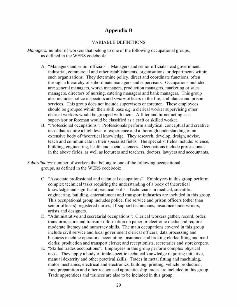
Appendix B

VARIABLE DEFINITIONS

Managers: number of workers that belong to one of the following occupational groups, as defined in the WERS codebook: A. “Managers and senior officials”: Managers and senior officials head government,

industrial, commercial and other establishments, organisations, or departments within such organisations. They determine policy, direct and coordinate functions, often through a hierarchy of subordinate managers and supervisors. Occupations included are: general managers, works managers, production managers, marketing or sales managers, directors of nursing, catering managers and bank managers. This group also includes police inspectors and senior officers in the fire, ambulance and prison services. This group does not include supervisors or foremen. These employees should be grouped within their skill base e.g. a clerical worker supervising other clerical workers would be grouped with them. A fitter and turner acting as a supervisor or foreman would be classified as a craft or skilled worker.

B. “Professional occupations”: Professionals perform analytical, conceptual and creative tasks that require a high level of experience and a thorough understanding of an extensive body of theoretical knowledge. They research, develop, design, advise, teach and communicate in their specialist fields. The specialist fields include: science, building, engineering, health and social sciences. Occupations include professionals in the above fields, as well as lecturers and teachers, doctors, lawyers and accountants.

Subordinates: number of workers that belong to one of the following occupational

groups, as defined in the WERS codebook: C. “Associate professional and technical occupations”: Employees in this group perform

complex technical tasks requiring the understanding of a body of theoretical knowledge and significant practical skills. Technicians in medical, scientific, engineering, building, entertainment and transport industries are included in this group. This occupational group includes police, fire service and prison officers (other than senior officers), registered nurses, IT support technicians, insurance underwriters, artists and designers.

D. “Administrative and secretarial occupations”: Clerical workers gather, record, order, transform, store and transmit information on paper or electronic media and require moderate literacy and numeracy skills. The main occupations covered in this group include civil service and local government clerical officers; data processing and business machine operators; accounting, insurance and broking clerks; filing and mail clerks; production and transport clerks; and receptionists, secretaries and storekeepers.

E. “Skilled trades occupations”: Employees in this group perform complex physical tasks. They apply a body of trade-specific technical knowledge requiring initiative, manual dexterity and other practical skills. Trades in metal fitting and machining, motor mechanics, electrical and electronics, building, printing, vehicle production, food preparation and other recognised apprenticeship trades are included in this group. Trade apprentices and trainees are also to be included in this group.

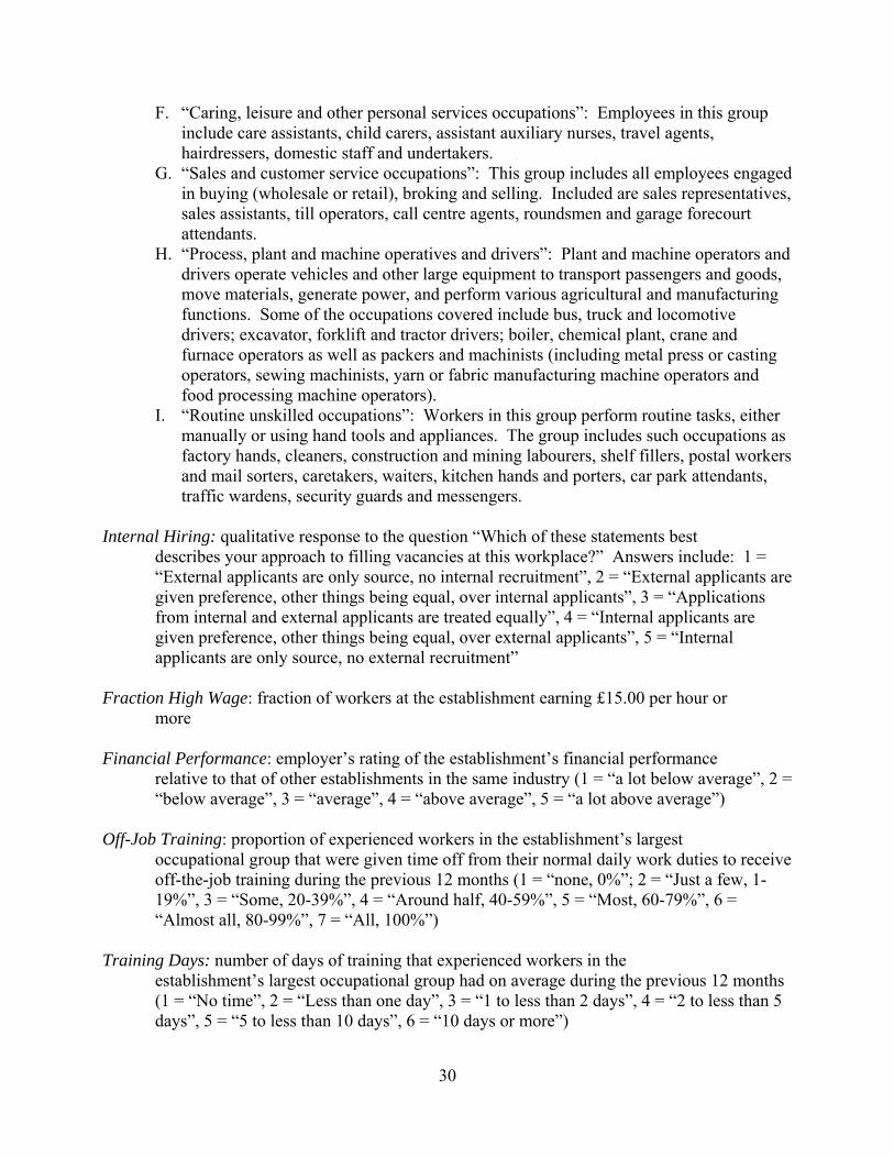
30

F. “Caring, leisure and other personal services occupations”: Employees in this group include care assistants, child carers, assistant auxiliary nurses, travel agents, hairdressers, domestic staff and undertakers.

G. “Sales and customer service occupations”: This group includes all employees engaged in buying (wholesale or retail), broking and selling. Included are sales representatives, sales assistants, till operators, call centre agents, roundsmen and garage forecourt attendants.

H. “Process, plant and machine operatives and drivers”: Plant and machine operators and drivers operate vehicles and other large equipment to transport passengers and goods, move materials, generate power, and perform various agricultural and manufacturing functions. Some of the occupations covered include bus, truck and locomotive drivers; excavator, forklift and tractor drivers; boiler, chemical plant, crane and furnace operators as well as packers and machinists (including metal press or casting operators, sewing machinists, yarn or fabric manufacturing machine operators and food processing machine operators).

I. “Routine unskilled occupations”: Workers in this group perform routine tasks, either manually or using hand tools and appliances. The group includes such occupations as factory hands, cleaners, construction and mining labourers, shelf fillers, postal workers and mail sorters, caretakers, waiters, kitchen hands and porters, car park attendants, traffic wardens, security guards and messengers.

Internal Hiring: qualitative response to the question “Which of these statements best

describes your approach to filling vacancies at this workplace?” Answers include: 1 = “External applicants are only source, no internal recruitment”, 2 = “External applicants are given preference, other things being equal, over internal applicants”, 3 = “Applications from internal and external applicants are treated equally”, 4 = “Internal applicants are given preference, other things being equal, over external applicants”, 5 = “Internal applicants are only source, no external recruitment”

Fraction High Wage: fraction of workers at the establishment earning £15.00 per hour or

more Financial Performance: employer’s rating of the establishment’s financial performance

relative to that of other establishments in the same industry (1 = “a lot below average”, 2 = “below average”, 3 = “average”, 4 = “above average”, 5 = “a lot above average”)

Off-Job Training: proportion of experienced workers in the establishment’s largest

occupational group that were given time off from their normal daily work duties to receive off-the-job training during the previous 12 months (1 = “none, 0%”; 2 = “Just a few, 1-19%”, 3 = “Some, 20-39%”, 4 = “Around half, 40-59%”, 5 = “Most, 60-79%”, 6 = “Almost all, 80-99%”, 7 = “All, 100%”)

Training Days: number of days of training that experienced workers in the

establishment’s largest occupational group had on average during the previous 12 months (1 = “No time”, 2 = “Less than one day”, 3 = “1 to less than 2 days”, 4 = “2 to less than 5 days”, 5 = “5 to less than 10 days”, 6 = “10 days or more”)

31

Induction Training: binary 0/1 variable equaling 1 if the establishment has a standard induction programme designed to introduced new workers in the establishment’s largest occupational group to the workplace

Union: binary 0/1 variable equaling 1 if there are union members at the establishment Fraction of Part Time Workers: number of part time workers at the establishment as a

fraction of establishment size (i.e. number of workers on payroll at establishment at the time of the survey)

Temporary Workers: binary 0/1 variable equaling 1 if the establishment has any temporary workers

Fraction of Temporary Workers: number of temporary workers at the establishment as a fraction of establishment size (i.e. number of workers on payroll at establishment at the time of the survey)

Fixed Term: binary 0/1 variable equaling 1 if establishment has any workers on fixed

term contracts Fixed Term Percentage: percentage of workers on fixed term contracts Percent Union: percentage of workers at the establishment belonging to a union Number of Recognized Unions: Total number of recognized unions at the workplace Owner Manager: binary 0/1 variable equaling 1 if employer responds “yes” to “Are any

of the controlling owners actively involved in day-to-day management of this workplace on a full-time basis?”

Foreign Owned: binary 0/1 variable equaling 1 if employer states that the establishment is “predominantly foreign owned” (i.e. 51% or more)

Age Less Than 5: binary 0/1 variable equaling 1 if establishment is less than 5 years old Age 5 to 9: binary 0/1 variable equaling 1 if establishment is 5 to 9 years old Age 10 to 14: binary 0/1 variable equaling 1 if establishment is 10 to 14 years old Age 15 to 20: binary 0/1 variable equaling 1 if establishment is 15 to 20 years old Age 21 to 24: binary 0/1 variable equaling 1 if establishment is 21 to 24 years old Age 25 plus: binary 0/1 variable equaling 1 if establishment is at least 25 years old Franchise: binary 0/1 variable equaling 1 if employer reports that the workplace is part of

a franchise operation

32

Private: binary 0/1 variable equaling 1 if establishment is in private sector Largest Occupational Group Categories: (managers and senior officials; professionals;

associate professional and technical; administrative and secretarial; skilled trades; caring, leisure, and personal service; sales and customer service; process, plant and machine operatives and drivers; routine unskilled

Industry Categories: (Manufacturing; Electricity, Gas, and Water; Construction;

Wholesale and Retail; Hotels and Restaurants; Transport and Communication; Financial Services; Other Business Services; Public Administration; Education; Health; Other Community Services)

33

References Acemoglu, Daron, and Steve Pischke. 1998. “Why Do Firms Train? Theory and Evidence”

Quarterly Journal of Economics, vol. 113, pp. 79-119.

Acemoglu, Daron, and Steve Pischke. 1999a. “The Structure of Wages and Investment in

General Training.” Journal of Political Economy, vol. 107, pp. 539-572.

Acemoglu, Daron, and Steve Pischke. 1999b. “Beyond Becker: Training in Imperfect Labor

Markets.” Economic Journal Features, vol. 109, pp. F112-F142.

Agrawal, Anup, Charles R. Knoeber and Theofanis Tsoulouhas. 2006. “Are outsiders

handicapped in CEO Successions?” Journal of Corporate Finance, vol. 12, pp. 619–644.

Baker, George, M.C. Jensen, and Kevin J. Murphy. 1988. “Compensation and Incentives:

Practice versus Theory.” Journal of Finance, Vol. 43, pp. 593-616.

Bernhardt, Dan. 1995. “Strategic Promotion and Compensation.” Review of Economic Studies,

vol. 62, pp. 315–339.

Bernhardt, Dan and David Scoones. 1993. “Promotion, Turnover, and Preemptive Wage

Offers.” American Economic Review, vol. 83, pp 771–791.

Chan, William. 1996. “External Recruitment versus Internal Promotion.” Journal of Labor

Economics, vol.14, pp. 555–570.

Chan, William. 2006. “External Recruitment and Intrafirm Mobility.” Economic Inquiry, vol. 44,

pp. 169–184.

Chaplin, Joanna, Jane Mangla, Susan Purdon, and Colin Airey. “The Workplace

Employment Relations Survey (WERS) 2004 Technical Report (Cross-section and Panel

Surveys)”, Prepared for Department of Trade and Industry, November 2005.

Demougin, Dominique, and Aloysius Siow. 1994. “Careers in Ongoing Hierarchies.”

American Economic Review, vol. 84, pp. 1261-1277.

Department of Trade and Industry, Advisory, Conciliation and Arbitration Service,

Workplace Employee Relations Survey: 2004 [computer file]. Colchester, Essex: The Data

Archive [distributor], December 2004.

DeVaro, Jed. 2006. “Internal Promotion Competitions in Firms.” The RAND Journal of

Economics, vol. 37, pp. 521–541.

DeVaro, Jed, Suman Ghosh, and Cindy Zoghi. 2008. “Job Characteristics and Labor Market

Discrimination in Promotions: New Theory and Empirical Evidence”. Mimeo.

34

DeVaro, Jed, and Michael Waldman. 2007. “The Signaling Role of Promotions: Further

Theory and Empirical Evidence.” Mimeo.

Gibbons, Robert and Michael Waldman. 1999a. “Careers in Organizations: Theory and

Evidence.” In Orley C. Ashenfelter and David Card, eds., Handbook of Labor Economics, vol.

IIIb, pp. 2373–2437. Amsterdam: North-Holland.

Gibbons, Robert and Michael Waldman. 1999b. “A Theory of Wage and Promotion Dynamics

Inside Firms.” Quarterly Journal of Economics, vol. 114, pp. 1321–1358.

Gibbons, Robert and Michael Waldman. 2006. “Enriching a Theory of Wage and Promotion

Dynamics inside Firms.” Journal of Labor Economics, vol. 24, pp. 59–107.

Golan, Limor. “Counteroffers and Efficiency in Labor Markets with Asymmetric Information,”

Journal of Labor Economics, 23, 2005, 373-393.

Kim, Jin-Hyuk. 2007, “Employee Poaching, Predatory Hiring, and Covenants Not to Compete.”

Mimeo, Cornell University.

Lauterbach, Beni and Jacob Weisberg. 1994. “Top management successions: the choice

between internal and external sources.” International Journal of Human Resource

Management, vol. 5, pp. 51–65

Lauterbach, Beni, Joseph Vu and Jacob Weisberg. 1999. “Internal vs. External Successions

and Their Effect on Firm Performance.” Human Relations, vol.52, pp. 1485–1504.

Lazear, Edward P. and Sherwin Rosen. 1981. “Rank-Order Tournaments as Optimum Labor

Contracts.” Journal of Political Economy, vol. 89, pp. 841–864.

Lazear, Edward P. 1986. “Raids and Offer Matching.” Research in Labor Economics, vol. 8,

pp. 141–165.

Milgrom, Paul and Sharon Oster. 1987. “Job Discrimination, Market Forces, and the

Invisibility Hypothesis.” Quarterly Journal of Economics, vol. 102, pp. 453–476.

Murphy, Kevin J. 1999. “Executive Compensation.” In Orley C. Ashenfelter and David Card,

eds., Handbook of Labor Economics, vol. IIIb, pp. 2485–2564. Amsterdam: North-Holland.

Owan, Hideo. “Promotion, Turnover, Earnings, and Firm-Sponsored Training,” Journal of

Labor Economics, 22, 2004, 955-978.

Parrino, Robert. 1997. “CEO Turnover and Outside Succession A Cross-sectional Analysis.”

Journal of Financial Economics, vol.46, pp. 165–197

Ricart i Costa, J. “Managerial Task Assignment and Promotion,” Econometrica, 56, 1988, 449

35

-466.

Waldman, Michael. 1984. “Job Assignments, Signalling, and Efficiency” The RAND Journal of

Economics, vol. 15, pp. 255–267.

Waldman, Michael. “Up-or-Out Contracts: A Signaling Perspective,” Journal of Labor

Economics, 8, 1990, 230-250.

Waldman, Michael. 2003. “Ex Ante Versus Ex Post Optimal Promotion Rules: The Case of

Internal Promotion.” Economic Inquiry, vol. 41, pp. 27–41.

Waldman, Michael. 2007. “Contracting Theory and Patterns of Evidence in Internal Labor

Markets.” Forthcoming Chapter in the Handbook of Organizational Economics.

Zábojník, Ján and Dan Bernhardt. 2001. “Corporate Tournaments, Human Capital Acquisition,

and the Firm Size-Wage Relation.” Review of Economic Studies, vol. 68, pp. 693–716.

Zábojník, Ján. 2007. “Promotion Tournaments as Relational Contracts in a Market Equilibrium

Setting.” Mimeo. Queen’s University.

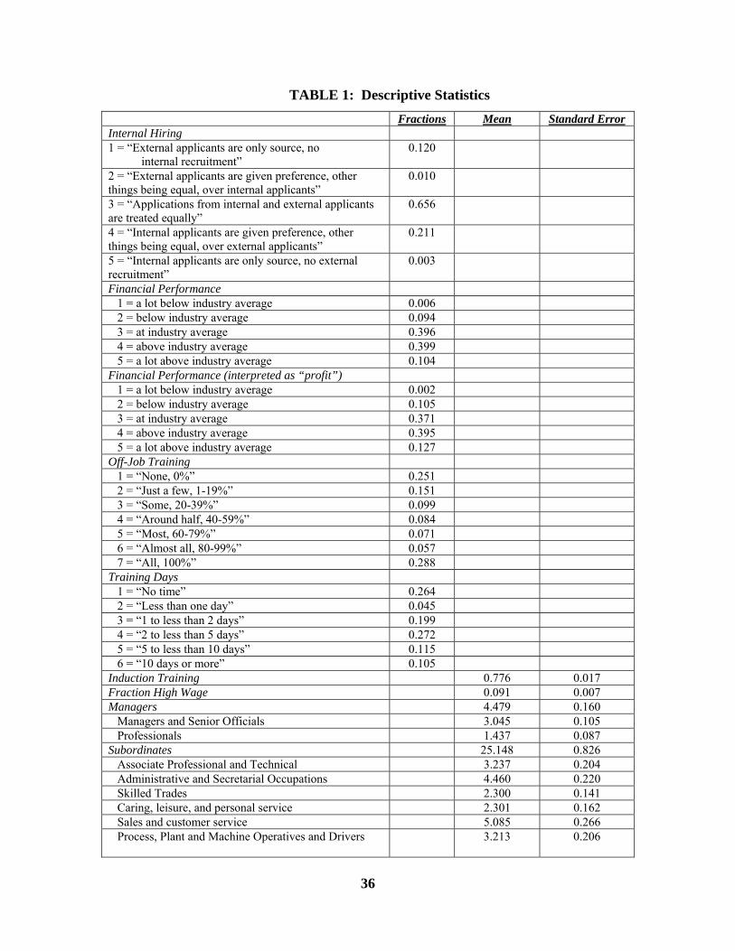
36

TABLE 1: Descriptive Statistics Fractions Mean Standard Error Internal Hiring 1 = “External applicants are only source, no internal recruitment”

0.120

2 = “External applicants are given preference, other things being equal, over internal applicants”

0.010

3 = “Applications from internal and external applicants are treated equally”

0.656

4 = “Internal applicants are given preference, other things being equal, over external applicants”

0.211

5 = “Internal applicants are only source, no external recruitment”

0.003

Financial Performance 1 = a lot below industry average 0.006 2 = below industry average 0.094 3 = at industry average 0.396 4 = above industry average 0.399 5 = a lot above industry average 0.104 Financial Performance (interpreted as “profit”) 1 = a lot below industry average 0.002 2 = below industry average 0.105 3 = at industry average 0.371 4 = above industry average 0.395 5 = a lot above industry average 0.127 Off-Job Training 1 = “None, 0%” 0.251 2 = “Just a few, 1-19%” 0.151 3 = “Some, 20-39%” 0.099 4 = “Around half, 40-59%” 0.084 5 = “Most, 60-79%” 0.071 6 = “Almost all, 80-99%” 0.057 7 = “All, 100%” 0.288 Training Days 1 = “No time” 0.264 2 = “Less than one day” 0.045 3 = “1 to less than 2 days” 0.199 4 = “2 to less than 5 days” 0.272 5 = “5 to less than 10 days” 0.115 6 = “10 days or more” 0.105 Induction Training 0.776 0.017 Fraction High Wage 0.091 0.007 Managers 4.479 0.160 Managers and Senior Officials 3.045 0.105 Professionals 1.437 0.087 Subordinates 25.148 0.826 Associate Professional and Technical 3.237 0.204 Administrative and Secretarial Occupations 4.460 0.220 Skilled Trades 2.300 0.141 Caring, leisure, and personal service 2.301 0.162 Sales and customer service 5.085 0.266 Process, Plant and Machine Operatives and Drivers

3.213 0.206

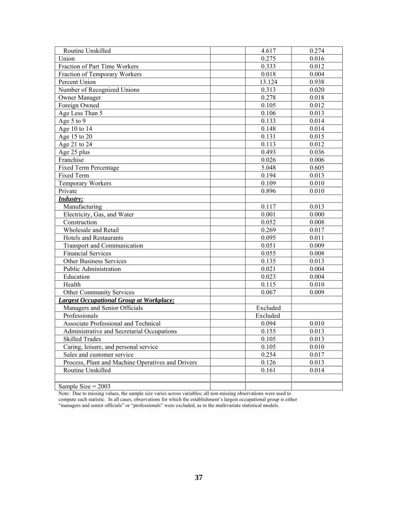
37

Routine Unskilled 4.617 0.274 Union 0.275 0.016 Fraction of Part Time Workers 0.333 0.012 Fraction of Temporary Workers 0.018 0.004 Percent Union 13.124 0.938 Number of Recognized Unions 0.313 0.020 Owner Manager 0.278 0.018 Foreign Owned 0.105 0.012 Age Less Than 5 0.106 0.013 Age 5 to 9 0.133 0.014 Age 10 to 14 0.148 0.014 Age 15 to 20 0.131 0.015 Age 21 to 24 0.113 0.012 Age 25 plus 0.493 0.036 Franchise 0.026 0.006 Fixed Term Percentage 5.048 0.605 Fixed Term 0.194 0.013 Temporary Workers 0.109 0.010 Private 0.896 0.010 Industry: Manufacturing 0.117 0.013 Electricity, Gas, and Water 0.001 0.000 Construction 0.052 0.008 Wholesale and Retail 0.269 0.017 Hotels and Restaurants 0.095 0.011 Transport and Communication 0.051 0.009 Financial Services 0.055 0.008 Other Business Services 0.135 0.013 Public Administration 0.021 0.004 Education 0.023 0.004 Health 0.115 0.010 Other Community Services 0.067 0.009 Largest Occupational Group at Workplace: Managers and Senior Officials Excluded Professionals Excluded Associate Professional and Technical 0.094 0.010 Administrative and Secretarial Occupations 0.155 0.013 Skilled Trades 0.105 0.013 Caring, leisure, and personal service 0.105 0.010 Sales and customer service 0.254 0.017 Process, Plant and Machine Operatives and Drivers 0.126 0.013 Routine Unskilled 0.161 0.014 Sample Size = 2003 Note: Due to missing values, the sample size varies across variables; all non-missing observations were used to compute each statistic. In all cases, observations for which the establishment’s largest occupational group is either “managers and senior officials” or “professionals” were excluded, as in the multivariate statistical models.

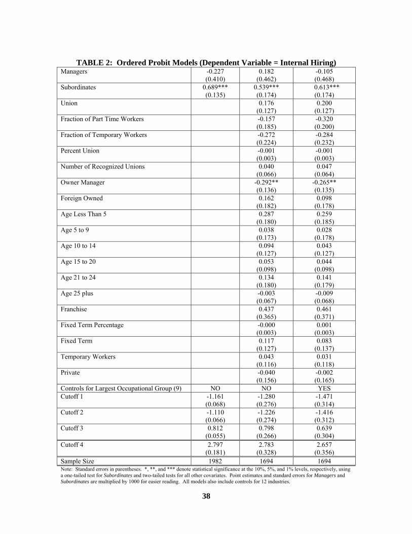
38

TABLE 2: Ordered Probit Models (Dependent Variable = Internal Hiring)

Managers -0.227 (0.410)

0.182 (0.462)

-0.105 (0.468)

Subordinates 0.689*** (0.135)

0.539*** (0.174)

0.613*** (0.174)

Union 0.176 (0.127)

0.200 (0.127)

Fraction of Part Time Workers -0.157 (0.185)

-0.320 (0.200)

Fraction of Temporary Workers -0.272 (0.224)

-0.284 (0.232)

Percent Union -0.001 (0.003)

-0.001 (0.003)

Number of Recognized Unions 0.040 (0.066)

0.047 (0.064)

Owner Manager -0.292** (0.136)

-0.265** (0.135)

Foreign Owned 0.162 (0.182)

0.098 (0.178)

Age Less Than 5 0.287 (0.180)

0.259 (0.185)

Age 5 to 9 0.038 (0.173)

0.028 (0.178)

Age 10 to 14 0.094 (0.127)

0.043 (0.127)

Age 15 to 20 0.053 (0.098)

0.044 (0.098)

Age 21 to 24 0.134 (0.180)

0.141 (0.179)

Age 25 plus -0.003 (0.067)

-0.009 (0.068)

Franchise 0.437 (0.365)

0.461 (0.371)

Fixed Term Percentage -0.000 (0.003)

0.001 (0.003)

Fixed Term 0.117 (0.127)

0.083 (0.137)

Temporary Workers 0.043 (0.116)

0.031 (0.118)

Private -0.040 (0.156)

-0.002 (0.165)

Controls for Largest Occupational Group (9) NO NO YES Cutoff 1 -1.161

(0.068) -1.280 (0.276)

-1.471 (0.314)

Cutoff 2 -1.110 (0.066)

-1.226 (0.274)

-1.416 (0.312)

Cutoff 3 0.812 (0.055)

0.798 (0.266)

0.639 (0.304)

Cutoff 4 2.797 (0.181)

2.783 (0.328)

2.657 (0.356)

Sample Size 1982 1694 1694 Note: Standard errors in parentheses. *, **, and *** denote statistical significance at the 10%, 5%, and 1% levels, respectively, using a one-tailed test for Subordinates and two-tailed tests for all other covariates. Point estimates and standard errors for Managers and Subordinates are multiplied by 1000 for easier reading. All models also include controls for 12 industries.

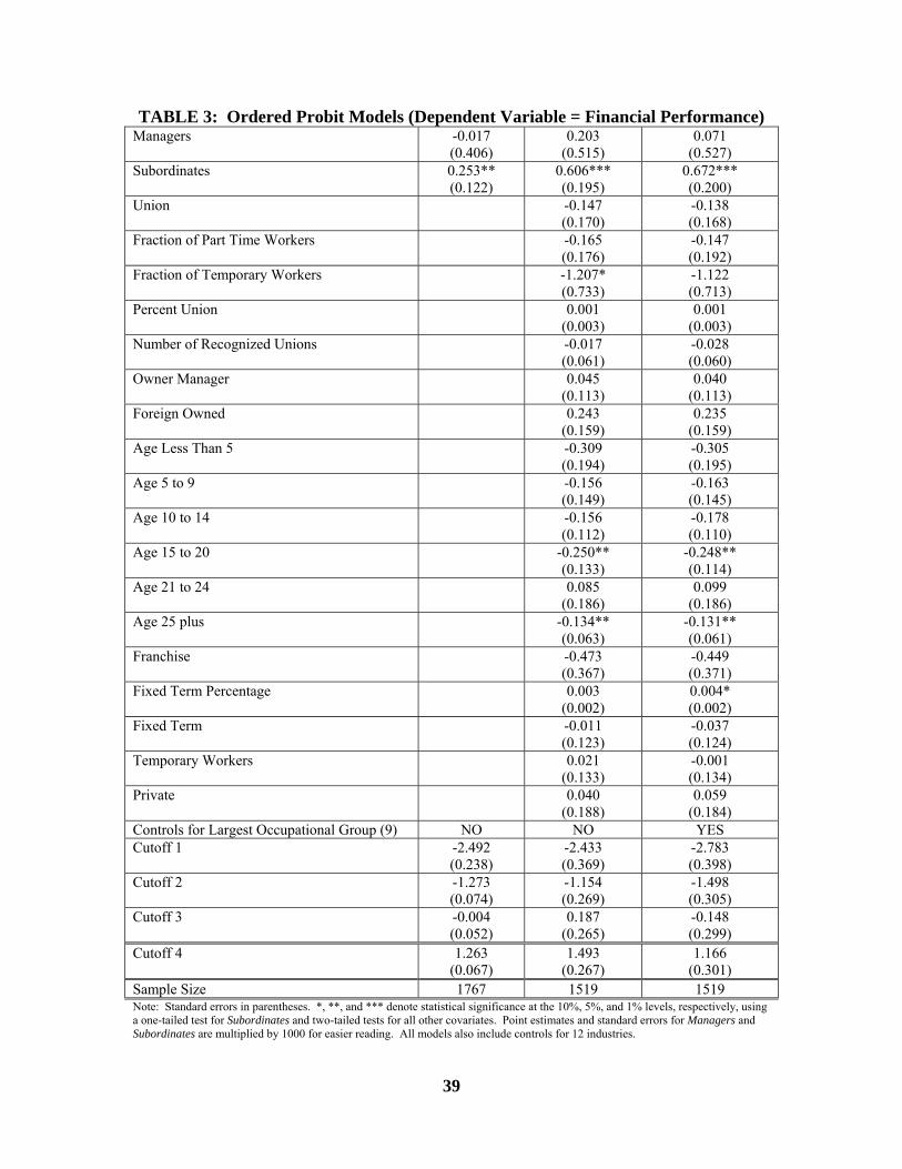
39

TABLE 3: Ordered Probit Models (Dependent Variable = Financial Performance) Managers -0.017

(0.406) 0.203

(0.515) 0.071

(0.527) Subordinates 0.253**

(0.122) 0.606*** (0.195)

0.672*** (0.200)

Union -0.147 (0.170)

-0.138 (0.168)

Fraction of Part Time Workers -0.165 (0.176)

-0.147 (0.192)

Fraction of Temporary Workers -1.207* (0.733)

-1.122 (0.713)

Percent Union 0.001 (0.003)

0.001 (0.003)

Number of Recognized Unions -0.017 (0.061)

-0.028 (0.060)

Owner Manager 0.045 (0.113)

0.040 (0.113)

Foreign Owned 0.243 (0.159)

0.235 (0.159)

Age Less Than 5 -0.309 (0.194)

-0.305 (0.195)

Age 5 to 9 -0.156 (0.149)

-0.163 (0.145)

Age 10 to 14 -0.156 (0.112)

-0.178 (0.110)

Age 15 to 20 -0.250** (0.133)

-0.248** (0.114)

Age 21 to 24 0.085 (0.186)

0.099 (0.186)

Age 25 plus -0.134** (0.063)

-0.131** (0.061)

Franchise -0.473 (0.367)

-0.449 (0.371)

Fixed Term Percentage 0.003 (0.002)

0.004* (0.002)

Fixed Term -0.011 (0.123)

-0.037 (0.124)

Temporary Workers 0.021 (0.133)

-0.001 (0.134)

Private 0.040 (0.188)

0.059 (0.184)

Controls for Largest Occupational Group (9) NO NO YES Cutoff 1 -2.492

(0.238) -2.433 (0.369)

-2.783 (0.398)

Cutoff 2 -1.273 (0.074)

-1.154 (0.269)

-1.498 (0.305)

Cutoff 3 -0.004 (0.052)

0.187 (0.265)

-0.148 (0.299)

Cutoff 4 1.263 (0.067)

1.493 (0.267)

1.166 (0.301)

Sample Size 1767 1519 1519 Note: Standard errors in parentheses. *, **, and *** denote statistical significance at the 10%, 5%, and 1% levels, respectively, using a one-tailed test for Subordinates and two-tailed tests for all other covariates. Point estimates and standard errors for Managers and Subordinates are multiplied by 1000 for easier reading. All models also include controls for 12 industries.

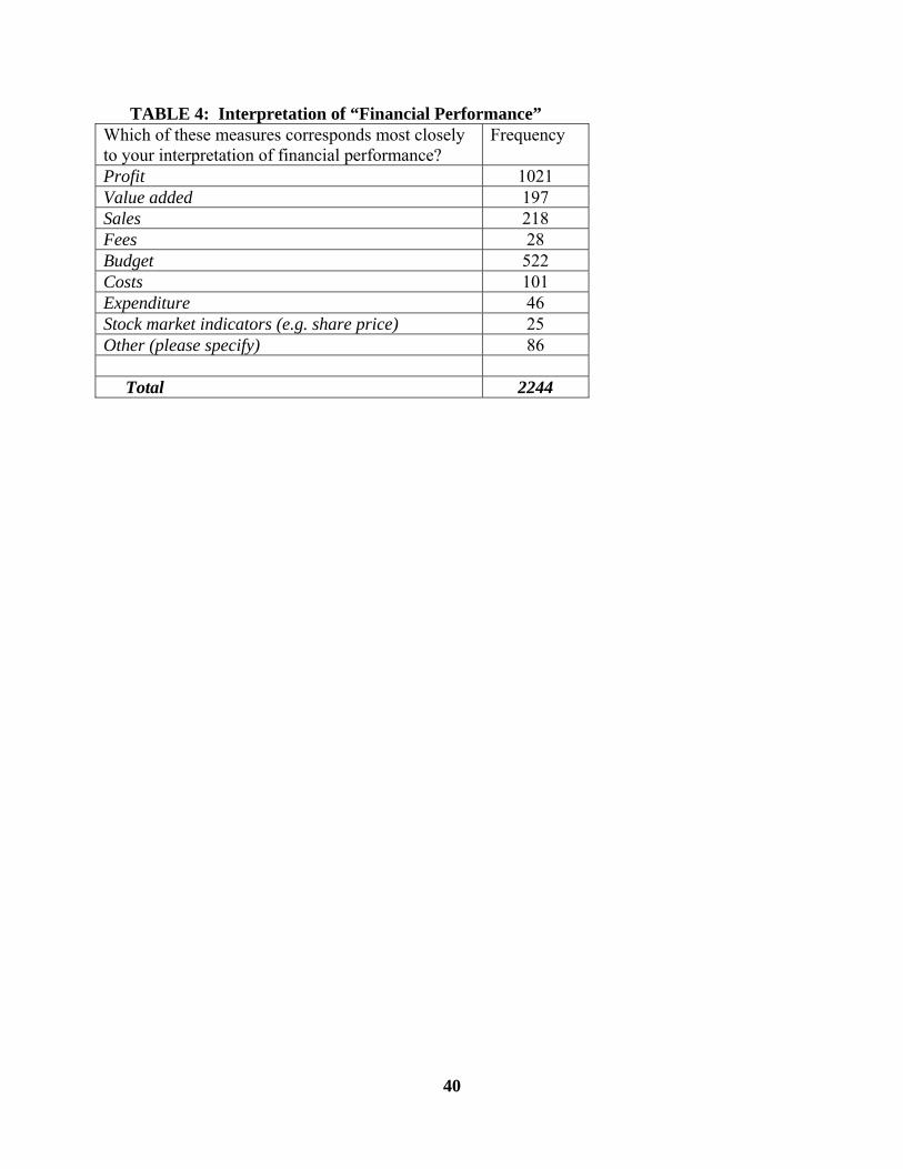
40

TABLE 4: Interpretation of “Financial Performance” Which of these measures corresponds most closely to your interpretation of financial performance?

Frequency

Profit 1021 Value added 197 Sales 218 Fees 28 Budget 522 Costs 101 Expenditure 46 Stock market indicators (e.g. share price) 25 Other (please specify) 86 Total 2244

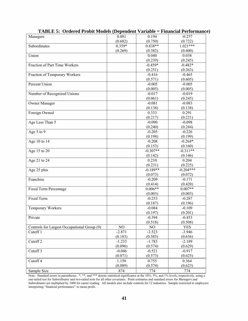
41

TABLE 5: Ordered Probit Models (Dependent Variable = Financial Performance) Managers 0.081

(0.682) 0.194

(0.750) -0.257 (0.722)

Subordinates 0.359* (0.269)

0.838** (0.382)

1.021*** (0.400)

Union 0.040 (0.239)

0.038 (0.245)

Fraction of Part Time Workers -0.459* (0.251)

-0.482* (0.263)

Fraction of Temporary Workers -0.416 (0.571)

-0.465 (0.605)

Percent Union -0.005 (0.005)

-0.005 (0.005)

Number of Recognized Unions -0.017 (0.061)

-0.019 (0.245)

Owner Manager -0.081 (0.138)

-0.083 (0.138)

Foreign Owned 0.333 (0.217)

0.291 (0.221)

Age Less Than 5 -0.090 (0.240)

-0.098 (0.244)

Age 5 to 9 -0.205 (0.198)

-0.226 (0.199)

Age 10 to 14 -0.208 (0.153)

-0.264* (0.160)

Age 15 to 20 -0.307** (0.142)

-0.311** (0.146)

Age 21 to 24 0.210 (0.231)

0.204 (0.225)

Age 25 plus -0.189** (0.073)

-0.204*** (0.072)

Franchise -0.209 (0.414)

-0.171 (0.420)

Fixed Term Percentage 0.006** (0.003)

0.007** (0.003)

Fixed Term -0.253 (0.187)

-0.287 (0.196)

Temporary Workers -0.084 (0.197)

-0.109 (0.201)

Private -0.394 (0.518)

-0.453 (0.508)

Controls for Largest Occupational Group (9) NO NO YES Cutoff 1 -2.871

(0.183) -3.523 (0.585)

-3.946 (0.636)

Cutoff 2 -1.233 (0.096)

-1.783 (0.574)

-2.189 (0.629)

Cutoff 3 -0.046 (0.071)

-0.521 (0.573)

-0.917 (0.625)

Cutoff 4 1.150 (0.089)

0.755 (0.574)

0.364 (0.623)

Sample Size 874 774 774 Note: Standard errors in parentheses. *, **, and *** denote statistical significance at the 10%, 5%, and 1% levels, respectively, using a one-tailed test for Subordinates and two-tailed tests for all other covariates. Point estimates and standard errors for Managers and Subordinates are multiplied by 1000 for easier reading. All models also include controls for 12 industries. Sample restricted to employers interpreting “financial performance” to mean profit.

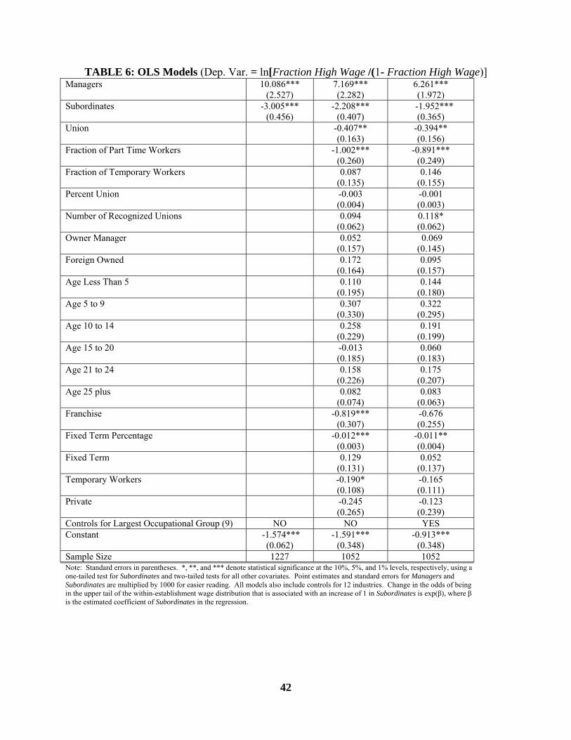
42

TABLE 6: OLS Models (Dep. Var. = ln[Fraction High Wage /(1- Fraction High Wage)] Managers 10.086***

(2.527) 7.169*** (2.282)

6.261*** (1.972)

Subordinates -3.005*** (0.456)

-2.208*** (0.407)

-1.952*** (0.365)

Union -0.407** (0.163)

-0.394** (0.156)

Fraction of Part Time Workers -1.002*** (0.260)

-0.891*** (0.249)

Fraction of Temporary Workers 0.087 (0.135)

0.146 (0.155)

Percent Union -0.003 (0.004)

-0.001 (0.003)

Number of Recognized Unions 0.094 (0.062)

0.118* (0.062)

Owner Manager 0.052 (0.157)

0.069 (0.145)

Foreign Owned 0.172 (0.164)

0.095 (0.157)

Age Less Than 5 0.110 (0.195)

0.144 (0.180)

Age 5 to 9 0.307 (0.330)

0.322 (0.295)

Age 10 to 14 0.258 (0.229)

0.191 (0.199)

Age 15 to 20 -0.013 (0.185)

0.060 (0.183)

Age 21 to 24 0.158 (0.226)

0.175 (0.207)

Age 25 plus 0.082 (0.074)

0.083 (0.063)

Franchise -0.819*** (0.307)

-0.676 (0.255)

Fixed Term Percentage -0.012*** (0.003)

-0.011** (0.004)

Fixed Term 0.129 (0.131)

0.052 (0.137)

Temporary Workers -0.190* (0.108)

-0.165 (0.111)

Private -0.245 (0.265)

-0.123 (0.239)

Controls for Largest Occupational Group (9) NO NO YES Constant -1.574***

(0.062) -1.591***

(0.348) -0.913***

(0.348) Sample Size 1227 1052 1052 Note: Standard errors in parentheses. *, **, and *** denote statistical significance at the 10%, 5%, and 1% levels, respectively, using a one-tailed test for Subordinates and two-tailed tests for all other covariates. Point estimates and standard errors for Managers and Subordinates are multiplied by 1000 for easier reading. All models also include controls for 12 industries. Change in the odds of being in the upper tail of the within-establishment wage distribution that is associated with an increase of 1 in Subordinates is exp(β), where β is the estimated coefficient of Subordinates in the regression.

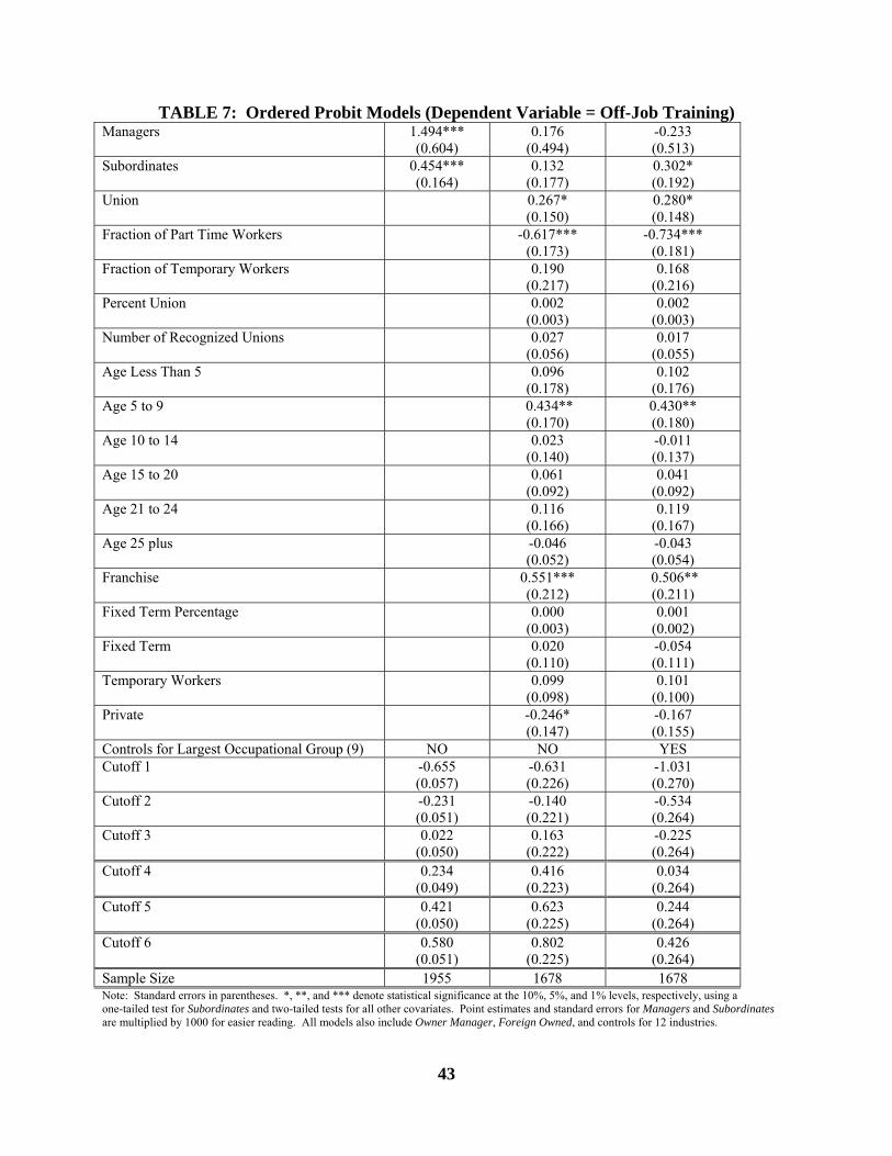
43

TABLE 7: Ordered Probit Models (Dependent Variable = Off-Job Training) Managers 1.494***

(0.604) 0.176

(0.494) -0.233 (0.513)

Subordinates 0.454*** (0.164)

0.132 (0.177)

0.302* (0.192)

Union 0.267* (0.150)

0.280* (0.148)

Fraction of Part Time Workers -0.617*** (0.173)

-0.734*** (0.181)

Fraction of Temporary Workers 0.190 (0.217)

0.168 (0.216)

Percent Union 0.002 (0.003)

0.002 (0.003)

Number of Recognized Unions 0.027 (0.056)

0.017 (0.055)

Age Less Than 5 0.096 (0.178)

0.102 (0.176)

Age 5 to 9 0.434** (0.170)

0.430** (0.180)

Age 10 to 14 0.023 (0.140)

-0.011 (0.137)

Age 15 to 20 0.061 (0.092)

0.041 (0.092)

Age 21 to 24 0.116 (0.166)

0.119 (0.167)

Age 25 plus -0.046 (0.052)

-0.043 (0.054)

Franchise 0.551*** (0.212)

0.506** (0.211)

Fixed Term Percentage 0.000 (0.003)

0.001 (0.002)

Fixed Term 0.020 (0.110)

-0.054 (0.111)

Temporary Workers 0.099 (0.098)

0.101 (0.100)

Private -0.246* (0.147)

-0.167 (0.155)

Controls for Largest Occupational Group (9) NO NO YES Cutoff 1 -0.655

(0.057) -0.631 (0.226)

-1.031 (0.270)

Cutoff 2 -0.231 (0.051)

-0.140 (0.221)

-0.534 (0.264)

Cutoff 3 0.022 (0.050)

0.163 (0.222)

-0.225 (0.264)

Cutoff 4 0.234 (0.049)

0.416 (0.223)

0.034 (0.264)

Cutoff 5 0.421 (0.050)

0.623 (0.225)

0.244 (0.264)

Cutoff 6 0.580 (0.051)

0.802 (0.225)

0.426 (0.264)

Sample Size 1955 1678 1678 Note: Standard errors in parentheses. *, **, and *** denote statistical significance at the 10%, 5%, and 1% levels, respectively, using a one-tailed test for Subordinates and two-tailed tests for all other covariates. Point estimates and standard errors for Managers and Subordinates are multiplied by 1000 for easier reading. All models also include Owner Manager, Foreign Owned, and controls for 12 industries.

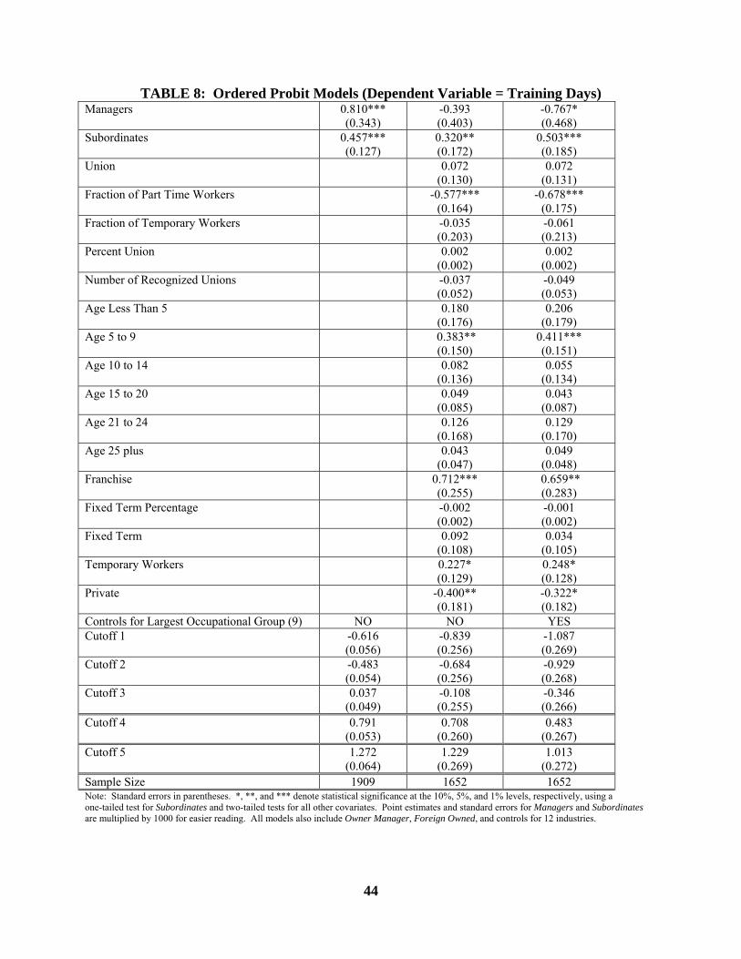
44

TABLE 8: Ordered Probit Models (Dependent Variable = Training Days) Managers 0.810***

(0.343) -0.393 (0.403)

-0.767* (0.468)

Subordinates 0.457*** (0.127)

0.320** (0.172)

0.503*** (0.185)

Union 0.072 (0.130)

0.072 (0.131)

Fraction of Part Time Workers -0.577*** (0.164)

-0.678*** (0.175)

Fraction of Temporary Workers -0.035 (0.203)

-0.061 (0.213)

Percent Union 0.002 (0.002)

0.002 (0.002)

Number of Recognized Unions -0.037 (0.052)

-0.049 (0.053)

Age Less Than 5 0.180 (0.176)

0.206 (0.179)

Age 5 to 9 0.383** (0.150)

0.411*** (0.151)

Age 10 to 14 0.082 (0.136)

0.055 (0.134)

Age 15 to 20 0.049 (0.085)

0.043 (0.087)

Age 21 to 24 0.126 (0.168)

0.129 (0.170)

Age 25 plus 0.043 (0.047)

0.049 (0.048)

Franchise 0.712*** (0.255)

0.659** (0.283)

Fixed Term Percentage -0.002 (0.002)

-0.001 (0.002)

Fixed Term 0.092 (0.108)

0.034 (0.105)

Temporary Workers 0.227* (0.129)

0.248* (0.128)

Private -0.400** (0.181)

-0.322* (0.182)

Controls for Largest Occupational Group (9) NO NO YES Cutoff 1 -0.616

(0.056) -0.839 (0.256)

-1.087 (0.269)

Cutoff 2 -0.483 (0.054)

-0.684 (0.256)

-0.929 (0.268)

Cutoff 3 0.037 (0.049)

-0.108 (0.255)

-0.346 (0.266)

Cutoff 4 0.791 (0.053)

0.708 (0.260)

0.483 (0.267)

Cutoff 5 1.272 (0.064)

1.229 (0.269)

1.013 (0.272)

Sample Size 1909 1652 1652 Note: Standard errors in parentheses. *, **, and *** denote statistical significance at the 10%, 5%, and 1% levels, respectively, using a one-tailed test for Subordinates and two-tailed tests for all other covariates. Point estimates and standard errors for Managers and Subordinates are multiplied by 1000 for easier reading. All models also include Owner Manager, Foreign Owned, and controls for 12 industries.

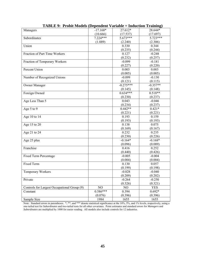
45

TABLE 9: Probit Models (Dependent Variable = Induction Training) Managers -17.168*

(10.666) 27.612* (17.537)

28.644* (17.697)

Subordinates 7.224*** (1.889)

5.673*** (2.240)

5.723*** (2.306)

Union 0.330 (0.235)

0.344 (0.244)

Fraction of Part Time Workers 0.127 (0.232)

-0.248 (0.257)

Fraction of Temporary Workers -0.099 (0.227)

-0.181 (0.220)

Percent Union 0.003 (0.005)

0.003 (0.005)

Number of Recognized Unions -0.099 (0.121)

-0.130 (0.115)

Owner Manager -0.275*** (0.145)

-0.357** (0.148)

Foreign Owned 0.634*** (0.230)

0.518** (0.237)

Age Less Than 5 0.043 (0.234)

-0.046 (0.237)

Age 5 to 9 0.442** (0.221)

0.421* (0.221)

Age 10 to 14 0.193 (0.193)

0.159 (0.193)

Age 15 to 20 0.138 (0.169)

0.075 (0.167)

Age 21 to 24 0.232 (0.230)

0.235 (0.226)

Age 25 plus -0.164* (0.096)

-0.168* (0.089)

Franchise 0.416 (0.440)

0.252 (0.426)

Fixed Term Percentage -0.005 (0.004)

-0.004 (0.004)

Fixed Term 0.130 (0.199)

0.057 (0.198)

Temporary Workers -0.028 (0.209)

-0.040 (0.202)

Private -0.264 (0.326)

-0.250 (0.321)

Controls for Largest Occupational Group (9) NO NO YES Constant 0.586***

(0.076) 0.394

(0.396) 0.692* (0.396)

Sample Size 1984 1655 1655 Note: Standard errors in parentheses. *, **, and *** denote statistical significance at the 10%, 5%, and 1% levels, respectively, using a one-tailed test for Subordinates and two-tailed tests for all other covariates. Point estimates and standard errors for Managers and Subordinates are multiplied by 1000 for easier reading. All models also include controls for 12 industries.