
Intermediate Public Economics
588
Intermediate Public Economics Jean Hindriks and Gareth D. Myles First version November 2000 This version June 2004
Transcript of Intermediate Public Economics

Intermediate Public Economics
Jean Hindriks and Gareth D. Myles
First version November 2000This version June 2004

ii
Contents
I Public Economics and the Public Sector 1
1 An Introduction to Public Economics 31.1 Public Economics . . . . . . . . . . . . . . . . . . . . . . . . . . . 31.2 Methods . . . . . . . . . . . . . . . . . . . . . . . . . . . . . . . . 41.3 Analyzing Policy . . . . . . . . . . . . . . . . . . . . . . . . . . . 51.4 Preview . . . . . . . . . . . . . . . . . . . . . . . . . . . . . . . . 61.5 Scope . . . . . . . . . . . . . . . . . . . . . . . . . . . . . . . . . 8
2 Government 112.1 Introduction . . . . . . . . . . . . . . . . . . . . . . . . . . . . . . 112.2 Historical Development . . . . . . . . . . . . . . . . . . . . . . . 112.3 Composition of Expenditure . . . . . . . . . . . . . . . . . . . . . 142.4 Revenue . . . . . . . . . . . . . . . . . . . . . . . . . . . . . . . . 162.5 Measuring the Government . . . . . . . . . . . . . . . . . . . . . 232.6 Conclusions . . . . . . . . . . . . . . . . . . . . . . . . . . . . . . 25
II Political Economy 27
3 Theories of the Public Sector 293.1 Introduction . . . . . . . . . . . . . . . . . . . . . . . . . . . . . . 293.2 Justification for the Public Sector . . . . . . . . . . . . . . . . . . 29
3.2.1 The Minimal State . . . . . . . . . . . . . . . . . . . . . . 303.2.2 Market versus Government . . . . . . . . . . . . . . . . . 313.2.3 Equity . . . . . . . . . . . . . . . . . . . . . . . . . . . . . 323.2.4 Efficiency and Equity . . . . . . . . . . . . . . . . . . . . 32
3.3 Public Sector Growth . . . . . . . . . . . . . . . . . . . . . . . . 333.3.1 Development Models . . . . . . . . . . . . . . . . . . . . . 333.3.2 Wagner’s Law . . . . . . . . . . . . . . . . . . . . . . . . . 343.3.3 Baumol’s Law . . . . . . . . . . . . . . . . . . . . . . . . . 353.3.4 A Political Model . . . . . . . . . . . . . . . . . . . . . . . 353.3.5 Ratchet Effect . . . . . . . . . . . . . . . . . . . . . . . . 37
3.4 Excessive Government . . . . . . . . . . . . . . . . . . . . . . . . 383.4.1 Bureaucracy . . . . . . . . . . . . . . . . . . . . . . . . . 39
iii

iv CONTENTS
3.4.2 Budget-Setting . . . . . . . . . . . . . . . . . . . . . . . . 413.4.3 Monopoly Power . . . . . . . . . . . . . . . . . . . . . . . 423.4.4 Corruption . . . . . . . . . . . . . . . . . . . . . . . . . . 433.4.5 Government Agency . . . . . . . . . . . . . . . . . . . . . 433.4.6 Cost Diffusion . . . . . . . . . . . . . . . . . . . . . . . . 45
3.5 Conclusions . . . . . . . . . . . . . . . . . . . . . . . . . . . . . . 46
4 Voting 494.1 Introduction . . . . . . . . . . . . . . . . . . . . . . . . . . . . . . 494.2 Stability . . . . . . . . . . . . . . . . . . . . . . . . . . . . . . . . 494.3 Impossibility . . . . . . . . . . . . . . . . . . . . . . . . . . . . . 504.4 Majority Rule . . . . . . . . . . . . . . . . . . . . . . . . . . . . . 53
4.4.1 May’s Theorem . . . . . . . . . . . . . . . . . . . . . . . . 534.4.2 Condorcet Winner . . . . . . . . . . . . . . . . . . . . . . 544.4.3 Median Voter Theorems . . . . . . . . . . . . . . . . . . . 544.4.4 Multi-Dimensional Voting . . . . . . . . . . . . . . . . . . 584.4.5 Agenda Manipulation . . . . . . . . . . . . . . . . . . . . 60
4.5 Alternatives to Majority Rule . . . . . . . . . . . . . . . . . . . . 634.5.1 Borda Voting . . . . . . . . . . . . . . . . . . . . . . . . . 634.5.2 Plurality Voting . . . . . . . . . . . . . . . . . . . . . . . 644.5.3 Approval Voting . . . . . . . . . . . . . . . . . . . . . . . 644.5.4 Runoff Voting . . . . . . . . . . . . . . . . . . . . . . . . . 65
4.6 The Paradox of Voting. . . . . . . . . . . . . . . . . . . . . . . . 664.7 The “Alabama” Paradox . . . . . . . . . . . . . . . . . . . . . . . 714.8 Conclusions . . . . . . . . . . . . . . . . . . . . . . . . . . . . . . 72
5 Rent-Seeking 755.1 Introduction . . . . . . . . . . . . . . . . . . . . . . . . . . . . . . 755.2 Definitions . . . . . . . . . . . . . . . . . . . . . . . . . . . . . . . 765.3 Rent-Seeking Games . . . . . . . . . . . . . . . . . . . . . . . . . 78
5.3.1 Deterministic game . . . . . . . . . . . . . . . . . . . . . . 785.3.2 Probabilistic game . . . . . . . . . . . . . . . . . . . . . . 815.3.3 Free-Entry . . . . . . . . . . . . . . . . . . . . . . . . . . 835.3.4 Risk Aversion . . . . . . . . . . . . . . . . . . . . . . . . . 845.3.5 Conclusions . . . . . . . . . . . . . . . . . . . . . . . . . . 85
5.4 Social Cost of Monopoly . . . . . . . . . . . . . . . . . . . . . . . 855.5 Equilibrium Effects . . . . . . . . . . . . . . . . . . . . . . . . . . 875.6 Government Policy . . . . . . . . . . . . . . . . . . . . . . . . . . 89
5.6.1 Lobbying . . . . . . . . . . . . . . . . . . . . . . . . . . . 915.6.2 Rent Creation . . . . . . . . . . . . . . . . . . . . . . . . . 935.6.3 Conclusions . . . . . . . . . . . . . . . . . . . . . . . . . . 94
5.7 Informative lobbying . . . . . . . . . . . . . . . . . . . . . . . . . 955.8 Controlling Rent-Seeking . . . . . . . . . . . . . . . . . . . . . . 985.9 Conclusions . . . . . . . . . . . . . . . . . . . . . . . . . . . . . . 99
CONTENTS v
III Equilibrium and Efficiency 101
6 Competitive Economies 1036.1 Introduction . . . . . . . . . . . . . . . . . . . . . . . . . . . . . . 1036.2 The Exchange Economy . . . . . . . . . . . . . . . . . . . . . . . 104
6.2.1 Endowments, Budgets and Preferences . . . . . . . . . . . 1046.2.2 The Edgeworth Box . . . . . . . . . . . . . . . . . . . . . 1056.2.3 Equilibrium . . . . . . . . . . . . . . . . . . . . . . . . . . 1066.2.4 Normalizations and Walras’ Law . . . . . . . . . . . . . . 109
6.3 Production and Exchange . . . . . . . . . . . . . . . . . . . . . . 1116.3.1 Firms and Consumers . . . . . . . . . . . . . . . . . . . . 1116.3.2 Equilibrium . . . . . . . . . . . . . . . . . . . . . . . . . . 115
6.4 Diagrammatic Illustration . . . . . . . . . . . . . . . . . . . . . . 1166.5 Discussion of Assumptions . . . . . . . . . . . . . . . . . . . . . . 1186.6 Conclusions . . . . . . . . . . . . . . . . . . . . . . . . . . . . . . 119
7 Efficiency of Competition 1217.1 Introduction . . . . . . . . . . . . . . . . . . . . . . . . . . . . . . 1217.2 Efficiency . . . . . . . . . . . . . . . . . . . . . . . . . . . . . . . 1227.3 Single Consumer . . . . . . . . . . . . . . . . . . . . . . . . . . . 1227.4 Pareto Efficiency . . . . . . . . . . . . . . . . . . . . . . . . . . . 1257.5 Efficiency in an Exchange Economy . . . . . . . . . . . . . . . . . 1267.6 Extension to Production . . . . . . . . . . . . . . . . . . . . . . . 1297.7 Lump-Sum Taxation . . . . . . . . . . . . . . . . . . . . . . . . . 1317.8 Summary . . . . . . . . . . . . . . . . . . . . . . . . . . . . . . . 133
IV Departures from Efficiency 135
8 Public Goods 1378.1 Introduction . . . . . . . . . . . . . . . . . . . . . . . . . . . . . . 1378.2 Definitions . . . . . . . . . . . . . . . . . . . . . . . . . . . . . . . 1388.3 Private Provision . . . . . . . . . . . . . . . . . . . . . . . . . . . 1398.4 Optimal Provision . . . . . . . . . . . . . . . . . . . . . . . . . . 1438.5 Voting . . . . . . . . . . . . . . . . . . . . . . . . . . . . . . . . . 1458.6 Personalized Prices . . . . . . . . . . . . . . . . . . . . . . . . . . 1488.7 Mechanism Design . . . . . . . . . . . . . . . . . . . . . . . . . . 151
8.7.1 Examples of Preference Revelation . . . . . . . . . . . . . 1528.7.2 Clarke-Groves Mechanism . . . . . . . . . . . . . . . . . . 1548.7.3 Clarke Tax . . . . . . . . . . . . . . . . . . . . . . . . . . 1568.7.4 Further Comments . . . . . . . . . . . . . . . . . . . . . . 157
8.8 More on Private Provision . . . . . . . . . . . . . . . . . . . . . . 1588.8.1 Neutrality and Population Size . . . . . . . . . . . . . . . 1588.8.2 Experimental Evidence . . . . . . . . . . . . . . . . . . . 1618.8.3 Modifications . . . . . . . . . . . . . . . . . . . . . . . . . 163
8.9 Fund-Raising Campaigns . . . . . . . . . . . . . . . . . . . . . . 164
vi CONTENTS
8.9.1 The Contribution Campaign . . . . . . . . . . . . . . . . 1658.9.2 The Subscription Campaign . . . . . . . . . . . . . . . . . 167
8.10 Conclusions . . . . . . . . . . . . . . . . . . . . . . . . . . . . . . 168
9 Club Goods and Local Public Goods 1719.1 Introduction . . . . . . . . . . . . . . . . . . . . . . . . . . . . . . 1719.2 Definitions . . . . . . . . . . . . . . . . . . . . . . . . . . . . . . . 1729.3 Single Product Clubs . . . . . . . . . . . . . . . . . . . . . . . . . 173
9.3.1 Fixed Utilization . . . . . . . . . . . . . . . . . . . . . . . 1739.3.2 Variable Utilization . . . . . . . . . . . . . . . . . . . . . 1759.3.3 Two-Part Tariff . . . . . . . . . . . . . . . . . . . . . . . . 177
9.4 Clubs and the Economy . . . . . . . . . . . . . . . . . . . . . . . 1789.4.1 Small Clubs . . . . . . . . . . . . . . . . . . . . . . . . . . 1789.4.2 Large Clubs . . . . . . . . . . . . . . . . . . . . . . . . . . 1799.4.3 Conclusion . . . . . . . . . . . . . . . . . . . . . . . . . . 184
9.5 Local Public Goods . . . . . . . . . . . . . . . . . . . . . . . . . . 1869.6 The Tiebout Hypothesis . . . . . . . . . . . . . . . . . . . . . . . 1899.7 Empirical Tests . . . . . . . . . . . . . . . . . . . . . . . . . . . . 1919.8 Conclusions . . . . . . . . . . . . . . . . . . . . . . . . . . . . . . 193
10 Externalities 19510.1 Introduction . . . . . . . . . . . . . . . . . . . . . . . . . . . . . . 19510.2 Externalities Defined . . . . . . . . . . . . . . . . . . . . . . . . . 19610.3 Market Inefficiency . . . . . . . . . . . . . . . . . . . . . . . . . . 19710.4 Externality Examples . . . . . . . . . . . . . . . . . . . . . . . . 199
10.4.1 River Pollution . . . . . . . . . . . . . . . . . . . . . . . . 19910.4.2 Traffic Jams . . . . . . . . . . . . . . . . . . . . . . . . . . 20110.4.3 Pecuniary externality . . . . . . . . . . . . . . . . . . . . 20110.4.4 The Rat Race Problem . . . . . . . . . . . . . . . . . . . 20310.4.5 The Tragedy of the Commons . . . . . . . . . . . . . . . . 20410.4.6 Bandwagon Effect . . . . . . . . . . . . . . . . . . . . . . 205
10.5 Pigouvian Taxation . . . . . . . . . . . . . . . . . . . . . . . . . . 20710.6 Licences . . . . . . . . . . . . . . . . . . . . . . . . . . . . . . . . 21010.7 Internalization . . . . . . . . . . . . . . . . . . . . . . . . . . . . 21310.8 The Coase Theorem . . . . . . . . . . . . . . . . . . . . . . . . . 21410.9 Non-Convexity . . . . . . . . . . . . . . . . . . . . . . . . . . . . 21810.10Conclusions . . . . . . . . . . . . . . . . . . . . . . . . . . . . . . 220
11 Imperfect Competition 22311.1 Introduction . . . . . . . . . . . . . . . . . . . . . . . . . . . . . . 22311.2 Concepts of Competition . . . . . . . . . . . . . . . . . . . . . . . 22411.3 Market structure . . . . . . . . . . . . . . . . . . . . . . . . . . . 225
11.3.1 Defining the Market . . . . . . . . . . . . . . . . . . . . . 22511.3.2 Measuring Competition . . . . . . . . . . . . . . . . . . . 226
11.4 Welfare . . . . . . . . . . . . . . . . . . . . . . . . . . . . . . . . 22811.4.1 Inefficiency . . . . . . . . . . . . . . . . . . . . . . . . . . 228
CONTENTS vii
11.4.2 Incomplete Information . . . . . . . . . . . . . . . . . . . 23111.4.3 Measures of Welfare Loss . . . . . . . . . . . . . . . . . . 232
11.5 Tax Incidence . . . . . . . . . . . . . . . . . . . . . . . . . . . . . 23511.6 Specific and Ad Valorem Taxation . . . . . . . . . . . . . . . . . 24111.7 Regulation of Monopoly . . . . . . . . . . . . . . . . . . . . . . . 24311.8 Regulation of Oligopoly . . . . . . . . . . . . . . . . . . . . . . . 248
11.8.1 Detecting Collusion . . . . . . . . . . . . . . . . . . . . . 24811.8.2 Merger Policy . . . . . . . . . . . . . . . . . . . . . . . . . 248
11.9 Unions and Taxation . . . . . . . . . . . . . . . . . . . . . . . . . 25011.10Monopsony . . . . . . . . . . . . . . . . . . . . . . . . . . . . . . 25111.11Conclusions . . . . . . . . . . . . . . . . . . . . . . . . . . . . . . 253
12 Asymmetric Information 25712.1 Introduction . . . . . . . . . . . . . . . . . . . . . . . . . . . . . . 25712.2 Hidden Knowledge and Hidden Action . . . . . . . . . . . . . . . 26012.3 Actions or Knowledge? . . . . . . . . . . . . . . . . . . . . . . . . 26112.4 Market Unravelling . . . . . . . . . . . . . . . . . . . . . . . . . . 262
12.4.1 Government Intervention . . . . . . . . . . . . . . . . . . 26312.5 Screening . . . . . . . . . . . . . . . . . . . . . . . . . . . . . . . 266
12.5.1 Perfect Information Equilibrium . . . . . . . . . . . . . . 26712.5.2 Imperfect Information Equilibrium . . . . . . . . . . . . . 26812.5.3 Government Intervention . . . . . . . . . . . . . . . . . . 271
12.6 Signalling . . . . . . . . . . . . . . . . . . . . . . . . . . . . . . . 27212.6.1 Educational Signalling . . . . . . . . . . . . . . . . . . . . 27412.6.2 Implications . . . . . . . . . . . . . . . . . . . . . . . . . . 279
12.7 Moral Hazard (Hidden Action) . . . . . . . . . . . . . . . . . . . 28012.7.1 Moral Hazard in Insurance . . . . . . . . . . . . . . . . . 28112.7.2 Effort Observable . . . . . . . . . . . . . . . . . . . . . . . 28212.7.3 Effort Unobservable . . . . . . . . . . . . . . . . . . . . . 28312.7.4 Second-Best Contract . . . . . . . . . . . . . . . . . . . . 28412.7.5 Government Intervention . . . . . . . . . . . . . . . . . . 286
12.8 Public provision of Health care . . . . . . . . . . . . . . . . . . . 28612.8.1 Efficiency Arguments . . . . . . . . . . . . . . . . . . . . . 28612.8.2 Redistributive Politics Argument . . . . . . . . . . . . . . 289
12.9 Evidence . . . . . . . . . . . . . . . . . . . . . . . . . . . . . . . . 29012.10Conclusions . . . . . . . . . . . . . . . . . . . . . . . . . . . . . . 292
V Equity and Distribution 295
13 Optimality and Comparability 29713.1 Introduction . . . . . . . . . . . . . . . . . . . . . . . . . . . . . . 29713.2 Social Optimality . . . . . . . . . . . . . . . . . . . . . . . . . . . 29713.3 Lump-Sum Taxes . . . . . . . . . . . . . . . . . . . . . . . . . . . 30013.4 Aspects of Pareto Efficiency . . . . . . . . . . . . . . . . . . . . . 30313.5 Social Welfare Functions . . . . . . . . . . . . . . . . . . . . . . . 306
viii CONTENTS
13.6 The Impossibility . . . . . . . . . . . . . . . . . . . . . . . . . . . 30813.7 Interpersonal Comparability . . . . . . . . . . . . . . . . . . . . . 30913.8 Comparability and Social Welfare . . . . . . . . . . . . . . . . . . 31213.9 Conclusions . . . . . . . . . . . . . . . . . . . . . . . . . . . . . . 315
14 Inequality and Poverty 31714.1 Introduction . . . . . . . . . . . . . . . . . . . . . . . . . . . . . . 31714.2 Measuring Income . . . . . . . . . . . . . . . . . . . . . . . . . . 31814.3 Equivalence Scales . . . . . . . . . . . . . . . . . . . . . . . . . . 32014.4 Inequality Measurement . . . . . . . . . . . . . . . . . . . . . . . 325
14.4.1 The Setting . . . . . . . . . . . . . . . . . . . . . . . . . . 32614.4.2 Statistical Measures . . . . . . . . . . . . . . . . . . . . . 32614.4.3 Inequality and Welfare . . . . . . . . . . . . . . . . . . . . 33314.4.4 An Application . . . . . . . . . . . . . . . . . . . . . . . . 337
14.5 Poverty . . . . . . . . . . . . . . . . . . . . . . . . . . . . . . . . 33914.5.1 Poverty and the Poverty Line . . . . . . . . . . . . . . . . 33914.5.2 Poverty Measures . . . . . . . . . . . . . . . . . . . . . . . 34014.5.3 Two Applications . . . . . . . . . . . . . . . . . . . . . . . 344
14.6 Conclusions . . . . . . . . . . . . . . . . . . . . . . . . . . . . . . 345
VI Taxation 349
15 Commodity Taxation 35115.1 Introduction . . . . . . . . . . . . . . . . . . . . . . . . . . . . . . 35115.2 Deadweight Loss . . . . . . . . . . . . . . . . . . . . . . . . . . . 35215.3 Optimal Taxation . . . . . . . . . . . . . . . . . . . . . . . . . . . 35415.4 Production Efficiency . . . . . . . . . . . . . . . . . . . . . . . . . 35915.5 Tax Rules . . . . . . . . . . . . . . . . . . . . . . . . . . . . . . . 361
15.5.1 The Inverse Elasticity Rule . . . . . . . . . . . . . . . . . 36215.5.2 The Ramsey Rule . . . . . . . . . . . . . . . . . . . . . . 363
15.6 Equity Considerations . . . . . . . . . . . . . . . . . . . . . . . . 36715.7 Applications . . . . . . . . . . . . . . . . . . . . . . . . . . . . . . 368
15.7.1 Reform . . . . . . . . . . . . . . . . . . . . . . . . . . . . 36915.7.2 Optimality . . . . . . . . . . . . . . . . . . . . . . . . . . 371
15.8 Efficient Taxation . . . . . . . . . . . . . . . . . . . . . . . . . . . 37215.9 Public Sector Pricing . . . . . . . . . . . . . . . . . . . . . . . . . 37415.10Conclusions . . . . . . . . . . . . . . . . . . . . . . . . . . . . . . 375
16 Income Taxation 37716.1 Introduction . . . . . . . . . . . . . . . . . . . . . . . . . . . . . . 37716.2 Taxation and Labor Supply . . . . . . . . . . . . . . . . . . . . . 37916.3 Empirical Evidence . . . . . . . . . . . . . . . . . . . . . . . . . . 38116.4 Modeling Income Taxation . . . . . . . . . . . . . . . . . . . . . . 38516.5 Rawlsian Tax . . . . . . . . . . . . . . . . . . . . . . . . . . . . . 39416.6 Numerical Results . . . . . . . . . . . . . . . . . . . . . . . . . . 396
CONTENTS ix
16.7 Voting Over a Flat Tax . . . . . . . . . . . . . . . . . . . . . . . 39816.8 Conclusions . . . . . . . . . . . . . . . . . . . . . . . . . . . . . . 400
17 The Limits to Redistribution 40317.1 Introduction . . . . . . . . . . . . . . . . . . . . . . . . . . . . . . 40317.2 Revelation Principle . . . . . . . . . . . . . . . . . . . . . . . . . 40517.3 Impossibility of Lump-Sum Taxes . . . . . . . . . . . . . . . . . . 40917.4 Tax Principle . . . . . . . . . . . . . . . . . . . . . . . . . . . . . 41217.5 Quasi-Linearity . . . . . . . . . . . . . . . . . . . . . . . . . . . . 41817.6 Tax Mix: Separation Principle . . . . . . . . . . . . . . . . . . . 42117.7 Non-tax redistribution . . . . . . . . . . . . . . . . . . . . . . . . 422
17.8 Conclusions . . . . . . . . . . . . . . . . . . . . . . . . . . . . . . 424
18 Tax Evasion 42718.1 Introduction . . . . . . . . . . . . . . . . . . . . . . . . . . . . . . 42718.2 The Extent of Evasion . . . . . . . . . . . . . . . . . . . . . . . . 42818.3 The Evasion Decision . . . . . . . . . . . . . . . . . . . . . . . . 43018.4 Auditing and Punishment . . . . . . . . . . . . . . . . . . . . . . 43718.5 Evidence on Evasion . . . . . . . . . . . . . . . . . . . . . . . . . 43918.6 Effect of Honesty . . . . . . . . . . . . . . . . . . . . . . . . . . . 44118.7 Tax Compliance Game . . . . . . . . . . . . . . . . . . . . . . . . 44318.8 Compliance and Social Interaction . . . . . . . . . . . . . . . . . 44518.9 Conclusions . . . . . . . . . . . . . . . . . . . . . . . . . . . . . . 448
VII Multiple Jurisdictions 451
19 Fiscal Federalism 45319.1 Introduction . . . . . . . . . . . . . . . . . . . . . . . . . . . . . . 45319.2 Arguments for Multi-Level Government . . . . . . . . . . . . . . 454
19.2.1 The Costs of Uniformity . . . . . . . . . . . . . . . . . . . 45519.2.2 The Tiebout Hypothesis . . . . . . . . . . . . . . . . . . . 45719.2.3 Distributive Arguments . . . . . . . . . . . . . . . . . . . 457
19.3 Optimal Structure: Efficiency versus Stability . . . . . . . . . . . 45819.4 Accountability . . . . . . . . . . . . . . . . . . . . . . . . . . . . 46119.5 Risk sharing . . . . . . . . . . . . . . . . . . . . . . . . . . . . . . 463
19.5.1 Voluntary risk sharing . . . . . . . . . . . . . . . . . . . . 46419.5.2 Insurance versus Redistribution . . . . . . . . . . . . . . . 466
19.6 Evidence on decentralization . . . . . . . . . . . . . . . . . . . . 46719.6.1 Decentralization around the World . . . . . . . . . . . . . 46719.6.2 Decentralization by Functions . . . . . . . . . . . . . . . . 46819.6.3 Determinants of Decentralization . . . . . . . . . . . . . . 469
19.7 Conclusions . . . . . . . . . . . . . . . . . . . . . . . . . . . . . . 470
x CONTENTS
20 Fiscal Competition 47320.1 Introduction . . . . . . . . . . . . . . . . . . . . . . . . . . . . . . 47320.2 Tax Competition . . . . . . . . . . . . . . . . . . . . . . . . . . . 473
20.2.1 Competitive Behavior . . . . . . . . . . . . . . . . . . . . 47420.2.2 Strategic Behavior . . . . . . . . . . . . . . . . . . . . . . 47520.2.3 Size Matters . . . . . . . . . . . . . . . . . . . . . . . . . 47920.2.4 Tax Overlap . . . . . . . . . . . . . . . . . . . . . . . . . 48020.2.5 Tax Exporting . . . . . . . . . . . . . . . . . . . . . . . . 48220.2.6 Efficient Tax Competition . . . . . . . . . . . . . . . . . . 484
20.3 Income Distribution . . . . . . . . . . . . . . . . . . . . . . . . . 48520.3.1 Perfect Mobility . . . . . . . . . . . . . . . . . . . . . . . 48520.3.2 Imperfect Mobility . . . . . . . . . . . . . . . . . . . . . . 48620.3.3 The Race to the Bottom . . . . . . . . . . . . . . . . . . . 489
20.4 Inter-Governmental Transfers . . . . . . . . . . . . . . . . . . . . 48920.4.1 Efficiency . . . . . . . . . . . . . . . . . . . . . . . . . . . 48920.4.2 Redistribution . . . . . . . . . . . . . . . . . . . . . . . . 49120.4.3 Flypaper Effect . . . . . . . . . . . . . . . . . . . . . . . . 493
20.5 Evidence . . . . . . . . . . . . . . . . . . . . . . . . . . . . . . . . 49320.6 Conclusions . . . . . . . . . . . . . . . . . . . . . . . . . . . . . . 496
VIII Issues of Time 501
21 Intertemporal Efficiency 50321.1 Introduction . . . . . . . . . . . . . . . . . . . . . . . . . . . . . . 50321.2 Overlapping Generations . . . . . . . . . . . . . . . . . . . . . . . 505
21.2.1 Time and Generations . . . . . . . . . . . . . . . . . . . . 50521.2.2 Consumers . . . . . . . . . . . . . . . . . . . . . . . . . . 50621.2.3 Production . . . . . . . . . . . . . . . . . . . . . . . . . . 507
21.3 Equilibrium . . . . . . . . . . . . . . . . . . . . . . . . . . . . . . 50921.3.1 Intertemporal Equilibrium . . . . . . . . . . . . . . . . . . 51021.3.2 Steady State . . . . . . . . . . . . . . . . . . . . . . . . . 510
21.4 Optimality and Efficiency . . . . . . . . . . . . . . . . . . . . . . 51321.4.1 The Golden Rule . . . . . . . . . . . . . . . . . . . . . . . 51321.4.2 Pareto Efficiency . . . . . . . . . . . . . . . . . . . . . . . 515
21.5 Testing Efficiency . . . . . . . . . . . . . . . . . . . . . . . . . . . 51921.6 Conclusions . . . . . . . . . . . . . . . . . . . . . . . . . . . . . . 519
22 Social Security and Debt 52122.1 Introduction . . . . . . . . . . . . . . . . . . . . . . . . . . . . . . 52122.2 Types of System . . . . . . . . . . . . . . . . . . . . . . . . . . . 52222.3 The Pensions Crisis . . . . . . . . . . . . . . . . . . . . . . . . . . 52422.4 The Simplest Program . . . . . . . . . . . . . . . . . . . . . . . . 52722.5 Social Security and Production . . . . . . . . . . . . . . . . . . . 52822.6 Population Growth . . . . . . . . . . . . . . . . . . . . . . . . . . 53222.7 Sustaining a Program . . . . . . . . . . . . . . . . . . . . . . . . 534
CONTENTS xi
22.8 Ricardian Equivalence . . . . . . . . . . . . . . . . . . . . . . . . 53822.9 Social Security Reform . . . . . . . . . . . . . . . . . . . . . . . . 54122.10Conclusions . . . . . . . . . . . . . . . . . . . . . . . . . . . . . . 544
23 Economic Growth 54723.1 Introduction . . . . . . . . . . . . . . . . . . . . . . . . . . . . . . 54723.2 Exogenous Growth . . . . . . . . . . . . . . . . . . . . . . . . . . 548
23.2.1 Constant Saving Rate . . . . . . . . . . . . . . . . . . . . 54823.2.2 Optimal Taxation . . . . . . . . . . . . . . . . . . . . . . 554
23.3 Endogenous Growth . . . . . . . . . . . . . . . . . . . . . . . . . 55923.3.1 Models of Endogenous Growth . . . . . . . . . . . . . . . 55923.3.2 Government Expenditure . . . . . . . . . . . . . . . . . . 561
23.4 Policy Reform . . . . . . . . . . . . . . . . . . . . . . . . . . . . . 56423.5 Empirical Evidence . . . . . . . . . . . . . . . . . . . . . . . . . . 56723.6 Conclusions . . . . . . . . . . . . . . . . . . . . . . . . . . . . . . 572

xii CONTENTS
Preface
This book has been prepared as the basis for a final-year undergraduate orfirst-year graduate course in Public Economics. It is based on lectures given bythe authors at several institutions over many years. It covers the traditionaltopics of efficiency and equity but also emphasizes more recent developments ininformation, games and, especially, political economy.The book should be accessible to anyone with a background of intermediate
microeconomics and macroeconomics. We have deliberately kept the quantityof math as low as we could without sacrificing intellectual rigor. Even so, thebook remains analytical rather than discursive.To support the content, further reading is given for each chapter. This read-
ing is intended to offer a range of material from the classic papers in each areathrough recent contributions to surveys and critiques. Exercises are included foreach chapter. Most of these should be prove possible for a good undergraduatebut some may prove challenging.There are many people who have contributed directly or indirectly with the
preparation of this book. Nigar Hashimzade is entitled to special thanks formaking incisive comments on the entire text and for assisting with the analy-sis in Chapters 4 and 23. Thanks are also due to Paul Belleflamme, TimBesley, Chuck Blackorby, Christopher Bliss, Craig Brett, John Conley, RichardCornes, Philippe De Donder, Sanjit Dhami, Peter Diamond, Jean Gabszewicz,Peter Hammond, Arye Hillman, Norman Ireland, Michael Keen, Jack Mintz,James Mirrlees, Frank Page Jr., Susana Peralta, Pierre Pestieau, Pierre Picard,Ian Preston, Maria Racionero, Antonio Rangel, Les Reinhorn, Elena del Rey,Todd Sandler, Kim Scharf, Hyun Shin, Michael Smart, Stephen Smith, JacquesThisse, John Weymark, and Myrna Wooders.Public Economics is about the government and the economic effects of its
policies. This book offers an insight into what Public Economics says and whatit can do. We hope that you enjoy it.Jean HindriksLouvain La NeuveGareth MylesExeterJuly 2004
xiii

xiv PREFACE

Part I
Public Economics and thePublic Sector
1

Chapter 1
An Introduction to PublicEconomics
1.1 Public Economics
Public economics studies the government and how its policies affect the economy.It considers how the choices of the government are made and how they canimprove or hinder economic efficiency. Public economics also investigates theextent to which it is possible for the government to influence the distribution ofincome and wealth and whether this is desirable. In undertaking these tasks,public economics draws upon influences from many areas of economics. This isreflected in the diversity of its subject matter which ranges from the traditionalstudy of the effects of taxation to public-choice explanations of bureaucracy.There are many sides to public economics, and we hope that this book providesan interesting insight into the richness of the subject.The study of public economics has a long tradition. It developed out of
the original political economy of Mill and Ricardo, through the public financetradition of tax analysis into public economics, and has now returned to itsroots with the development of the new political economy. From the inceptionof economics as a scientific discipline, public economics has always been one ofits core branches. The explanation for why it has always been so central is thefoundation that it provides for practical policy analysis. This has always beenthe motivation of public economists, even if the issues studies and the analyticalmethods employed have evolved over time. We intend the theory described inthis book to provide an organized and coherent structure for addressing eco-nomic policy.In the broadest interpretation, public economics is the study of economic
efficiency, distribution, and government economic policy. The subject encom-passes topics as diverse as responses to market failure due to the existence ofexternalities, the motives for tax evasion, and the explanation of bureaucraticdecision making. In order to reach into all of these areas, public economics
3

4 CHAPTER 1. AN INTRODUCTION TO PUBLIC ECONOMICS
has developed from its initial narrow focus upon the collection and spending ofgovernment revenues, to its present concern with every aspect of governmentinteraction with the economy. Public economics attempts to understand bothhow the government makes decisions and what decisions it should make.To understand how the government makes decisions it is necessary to inves-
tigate the motives of decisions makers within government, how they are chosenand how they are influenced by outside parties. Determining what decisionsshould be made involves studying the effects of the alternative policies that areavailable and evaluating the outcomes to which they lead. These aspects areinterwoven throughout the text. By pulling them together, this book providesan accessible introduction to both these aspects of public economics.
1.2 Methods
The feature that most characterizes modern public economics is the use madeof economic models. These models are employed as a tool to ensure that argu-ments are conducted coherently with a rigorous logical basis. Models are usedfor analysis because the possibilities for experimentation are limited and pastexperience cannot always be relied upon to provide a guide to the consequencesof new policies. Each model is intended to be a simplified description of the partof the economy that is relevant for the analysis. What distinguishes economicmodels from models in the natural sciences is the incorporation of indepen-dent decision making by the firms, consumers and politicians that populate theeconomy. These actors in the economy do not respond mechanically but aremotivated by personal objectives and are strategic in their behavior. Capturingthe implications of this complex behavior in a convincing manner is one of thekey skills of a successful economic theorist.Once a model has been chosen its implications have to be derived. These
implications are obtained by applying logical arguments that proceed from theassumptions of the model to a set of formally correct conclusions. Those con-clusions then need to be given an interpretation in terms that can be related tothe original question of interest. Policies recommendations can then be derivedbut with a recognition of the limitations of the model.The institutional setting for the study of public economics is invariably the
mixed economy where individual decisions are respected, but the governmentattempts to affect these through the policies it implements. Within this envi-ronment, many alternative objectives can be assigned to the government. Forinstance, the government can be assumed to care about the aggregate level ofwelfare in the economy and to act selflessly in attempting to increase this. Sucha viewpoint is the foundation of optimal policy analysis that enquires how thegovernment should behave. But there can be no presumption that actual gov-ernments act in this way. An alternative, and sometimes more compelling view,is that the government is composed of a set of individuals, each of whom ispursuing their own selfish agenda. Such a view provides a very different inter-pretation of the actions of the government and often provides a foundation for
1.3. ANALYZING POLICY 5
understanding how governments actually choose their policies. This perspectivewill also be considered in this book.The focus upon the mixed economy makes the analysis applicable to most
developed and developing economies. It also permits the study of how the gov-ernment behaves and how it should behave. To provide a benchmark from whichto judge the outcome of the economy under alternative policies, the commandeconomy with an omniscient planner is often employed. This, of course, is justan analytical abstraction.
1.3 Analyzing Policy
The method of policy analysis in public economics is to build a model of theeconomy and to find its equilibrium. The positive aspect of policy analysisdetermines the effect of a policy by tracing through the ways in which it changesthe equilibrium of the economy relative to some status quo. Alternative policiesare contrasted by comparing the equilibria to which they lead.In conducting the assessment of policy, it is often helpful to emphasize the
distinction between positive and normative analysis. The positive analysis ofgovernment investigates topics such as why there is a public sector, the emer-gence of government objectives and how government policies are chosen. It isalso about understanding what effects policies have upon the economy. In con-trast, normative analysis investigates what the best policies are, and aims toprovide a guide to good government. These are not entirely disjoint activities.To proceed with a normative analysis it is first necessary to conduct the positiveanalysis: it is not possible to say what is the best policy without knowing theeffects of alternative policies upon the economy. It could also be argued that apositive analysis is of no value until used as a guide to policy.Normative analysis is conducted under the assumption that the government
has a specified set of objectives and its action are chosen in the way that bestachieves these. Alternative policies (including the policy of laissez faire or,literally “leave to do”) are compared by using the results of the positive analy-sis. The optimal policy is that which best meets the government’s objective.Hence, the equilibria for different policies are determined and the government’sobjective is evaluated for each equilibrium.In every case restrictions are placed upon the set of policies from which
the government may choose. These restrictions are usually intended to capturelimits upon the information that the government has available. The informationthe government can obtain on the consumers and firms in the economy restrictsthe degree of sophistication that policy can have. For example, the extent towhich taxes can be differentiated between different taxpayers depends on theinformation the government can acquire about each individual. Administrativeand compliance costs are also relevant in generating restrictions upon possiblepolicies.When the government’s objective is taken to be some aggregate level of social
welfare in the economy, important questions are raised as to how welfare can be
6 CHAPTER 1. AN INTRODUCTION TO PUBLIC ECONOMICS
measured. This issue is discussed in some detail in a later chapter, but it canbe noted here that the answer involves invoking some degree of comparabilitybetween the welfare levels of different individuals. It has been the willingness toproceed on the basis that such comparisons can be made that has allowed thedevelopment of public economics. Whilst differences of opinion exist upon theextent to which these comparisons are valid, it is still scientifically justifiable toinvestigate what they would imply if they could be made. Furthermore, generalprinciples can be established that apply to any degree of comparability.
1.4 Preview
Part I of the book, including this chapter and Chapter 2, introduces publiceconomics and provides an overview of the public sector. Chapter 2 begins bycharting the historical growth of public sector expenditure over the previouscentury. It then reviews statistics on the present size of the public sector inseveral of the major developed economies. The division of expenditure and thecomposition of income are then considered. Finally, issues involved in measuringthe size of the public sector are addressed.Part II provides an analysis of the public sector and its decision-making
processes. This can be seen as a dose of healthy scepticism before proceeding intothe body of normative analysis. The issues raised by the statistics of Chapter2 are addressed by the discussion in Chapter 3 of theories of the public sector.Reasons for the existence of the public sector are considered, as are theoriesthat attempt to explain its growth. A positive analysis of how the governmentmay have its objectives and actions determined is undertaken. An emphasis isgiven to arguments for why the observed size of government may be excessive.An important practical method for making decisions and choosing governmentsis voting. Chapter 4 analyses the success of voting as a decision mechanismand the tactical and strategic issues it involves. The main results that emergeare the Median Voter Theorem and the shortcomings of majority voting. Theconsequences of rent seeking are then analyzed in Chapter 5. The theory of rent-seeking provides an alternative perspective upon the policy-making process thatis highly critical of the actions of government.Following the discussion of methodology, it is clear that a necessary starting
point for the development of the theory of policy analysis is an introductionto economic modelling. This represents the content of Chapter 6 in which thebasic model of a competitive economy is introduced. The chapter describes theagents involved in the economy and characterizes economic equilibrium. Anemphasis is placed upon the assumptions on which the analysis is based sincemuch of the subject matter of public follows from how the government shouldrespond if these are not satisfied. Having established the basic model, Chapter 7investigates the efficiency of the competitive equilibrium. This generates severalfundamentally important results.The focus of Part IV is upon relaxing the assumptions on which the competi-
tive economy is based. Chapter 8 introduces public goods into the economy and
1.4. PREVIEW 7
contrasts the allocation that is achieved when these are privately provided withthe optimal allocation. Mechanisms for improving the allocation are consideredand methods of preference revelation are also addressed. This is followed by ananalysis of clubs and local public goods, which are special cases of public goodsin general, in Chapter 9. The focus in this chapter returns to an assessmentof the success of market provision. The treatment of externalities in Chapter10 relaxes another of the assumptions. It is shown why market failure occurswhen externalities are present and reviews alternative policy schemes designedto improve efficiency. Imperfect competition and its consequences for taxationis the subject of Chapter 11. The measurement of welfare loss is discussed andemphasis is given to the incidence of taxation. A distinction is also drawn be-tween the effects of specific and ad valorem taxes. A symmetry of informationis required to sustain efficiency. When it is absent, inefficiency can arise. Theimplications of informational asymmetries and potential policy responses areconsidered in Chapter 12.Parts III and IV focus upon economic efficiency. Part V complements this
by considering issues of equity. Chapter 13 analyses the policy implications ofequity considerations and addresses the important restrictions placed on gov-ernment actions by limited information. Several other fundamental results inwelfare economics are also developed including the implications of alternativedegrees of interpersonal comparability. Chapter 14 considers the measurementof economic inequality and poverty. The economics of these measures ultimatelyreemphasizes the fundamental importance of utility theory.Part VI is concerned with taxation. It analysis the basic tax instruments
and the economics of tax evasion. Chapters 15 and 16 consider commodity taxa-tion and income taxation respectively which are the two main taxes levied uponconsumers. In both of these chapters the economic effects of the instrumentsare considered and rules for setting the taxes optimally are derived. The resultsillustrate the resolution of the equity/efficiency trade-off in the design of policyand the consequences of the limited information available to the government.In addition to the theoretical analysis, the results of application of the methodsto data are considered. The numerical results are useful since the theoreticalanalysis leads only to characterizations of optimal taxes rather than explicitsolutions. Chapter 17 determines the degree to which taxation can achieve re-distribution and contrasts this to other economic allocation mechanisms. Thesechapters all assume that the taxes which are levied are paid honestly and in full.This empirically-doubtful assumption is corrected in Chapter 18 which looks atthe extent of the hidden economy and analyses the motives for tax evasion andits consequences.Part VII studies public economics when there is more than one decision-
making body. Chapter 19 on fiscal federalism addresses why there should bemultiple levels of government and discusses the optimal division of responsi-bilities between different levels. The concept of tax competition is studied inChapter 20. It is shown how tax competition can limit the success of delegatingtax-setting powers to independent jurisdictions.Part VIII concentrates upon intertemporal issues in public economics. The
8 CHAPTER 1. AN INTRODUCTION TO PUBLIC ECONOMICS
first chapter, 21, describes the overlapping generations economy that is themain analytical tool of this part. The concept of the Golden Rule is introducedfor economies with production and capital accumulation, and the potential foreconomic inefficiency is discussed. Chapter 22 analyses social security policyand relates this to the potential inefficiency of the competitive equilibrium.Both the motivation for the existence of social security programmes and thedetermination of the level of benefits are addressed. Ricardian equivalence islinked to the existence of gifts and bequests. Finally, the book is completed byChapter 23 which considers the effects of taxation and public expenditure uponeconomic growth. Alternative models of economic growth are introduced andthe evidence linking government policy to the level of growth is discussed.
1.5 Scope
This book is essentially an introduction to the theory of public economics. Itpresents a unified view of this theory and introduces the most significant resultsof the analysis. As such, it provides a broad review of what constitutes thepresent state of public economics.What will not be found in the book are many details of actual institutions
for the collection of taxes or discussion of existing tax codes and other economicpolicies though we do present relevant data where it illuminates the argument.There are several reasons for this. This book is much broader than a textfocusing on taxation and to extend the coverage in this way, something elsehas to lost. Primarily, however, the book is about understanding the effects ofpublic policy and how economists think about the analysis of policy. This willgive an understanding of the consequences of existing policies but to benefitfrom it does not require a detailed knowledge of these.Furthermore, tax codes and tax law are country-specific and pages spent
discussing in detail the rules of one particular country will have little value forthose resident elsewhere. In contrast, the method of reasoning and the analyticalresults described here have value independent of country-specific detail. Finally,there are many texts available that describe in detail tax law and tax codes.These are written for accountants and lawyers and have a focus rather distinctthan that adopted by economists.
Further ReadingThe history of political economy is described in the classic volume:Blaug, M. (1996) Economic Theory in Retrospect (Cambridge: Cambridge
University Press).Two classic references on economic modelling are:Friedman, M. (1953) Essays on Positive Economics (Chicago: University of
Chicago Press),Koopmans, T.C. (1957) Three Essays on the State of Economic Science
(New York: McGraw-Hill).The issues involved in comparing individual welfare levels are explored in:

1.5. SCOPE 9
Robbins, L. (1935) An Essay on the Nature and Significance of EconomicScience (London: Macmillan).

10 CHAPTER 1. AN INTRODUCTION TO PUBLIC ECONOMICS

Chapter 2
Government
2.1 Introduction
In 1913 the 16th Amendment to the US Constitution gave Congress the legalauthority to tax income. By doing so, it made income taxation a permanentfeature of the US tax system and provided a significant source of additional taxrevenues. Revenue collection passed the $1bn mark in 1918, increased to $5.4bn. by 1920 and reached $43bn in 1945. It was not until the tax cut of 1981that this process of growth showed any marked sign of slowing. This growth intax revenues in the US mirrors the events in all western economies.The purpose of this chapter is to provide an introduction to the nature of
the public sector in modern markets economies and to provide a historical per-spective upon this. A review of data on the public sector which looks at itssize, sources of income, and expenditure shows the extent and range of activ-ities that the public sector undertakes. It also demonstrates the similarity inpublic sector behavior in countries that are otherwise very different culturally.The fundamental justifications for the existence of the public sector are thenconsidered, as are theories that explain the steady growth of the public sectorover the last century.
2.2 Historical Development
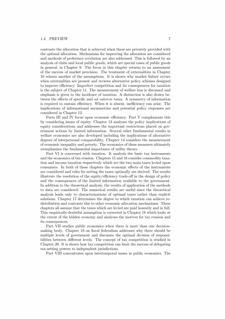
The historical development of the public sector over the past century can bebriefly described as one of significant growth. In most western economies gov-ernment expenditure was around 10% of gross domestic product in 1900. Ex-penditure then rose steadily over the next sixty years, levelling out in the latterpart of the century. This pattern of growth is illustrated in the following figures.Figure 2.1 displays the growth of public spending during the last century in
five developed economies. Only a selection of years are plotted — the years ofthe Second World War are left out for example — but the figure provides a clearimpression of the overall trend. There is a persistent difference in the levels of
11
12 CHAPTER 2. GOVERNMENT
1870 1900 1950 2000
0
20
40
60
1870 1900 1950 2000
0
20
40
60
US
UK
Germany
France
Japan
Figure 2.1: Growth of Total Expenditure
expenditure between the three European countries and the non-European coun-tries but the pattern of growth is the same for all. The economies have a clearlong-run upward path in public spending relative to gross domestic product.Starting at a level of public spending around 10% of gross domestic product
in the late nineteenth century, the share increased markedly at around the timeof the First World War and then continued to rise afterwards. It now exceeds athird of gross domestic product in all cases and, for France, exceeds one half. Anumber of explanations have been offered for this long-run increase and theseare discussed in Chapter 3.A more detailed representation of expenditure in the last thirty years is
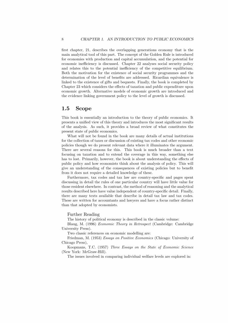
provided in Figure 2.2. The picture this presents is of a slowing, or even astagnation, of the growth in public sector expenditure. Although expenditureis higher in 2002 for the six countries shown, the increases for the UK andthe US are very small. For the UK especially, expenditure was clearly higherin the early 1980s than in 2002. The figure also suggests that there has beenconvergence in the level of expenditure between the countries. For example, in1970 expenditure in Japan was only half that in France, Germany and the UKbut by 2002 it almost matched that in the UK.The major implication of Figure 2.2 is that it clearly justifies the claim that
the public sector is significant in the economies of the industrialized countries.The mixed economies of these countries are characterized by substantial govern-ment involvement and are far from being free-market with minimal governmentintervention. The size of the public sector alone is justification for the study ofhow it should best choose its means of revenue collection and its allocation of
2.2. HISTORICAL DEVELOPMENT 13
0
10
20
30
40
50
60
1970
1973
1976
1979
1982
1985
1988
1991
1994
1997
2000
France
Germany
United Kingdom
United States
Japan
Australia
Figure 2.2: Total Outlays as a Percentage of GDP
expenditure. It is also worth noting that data on expenditure typically under-states the full influence of the public sector upon the economy. For instance,regulations such as employment laws or safety standards infringe upon economicactivity but without generating any measurable government expenditure or in-come.
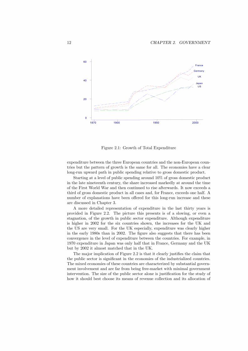
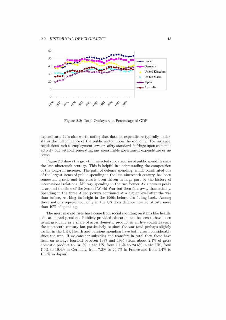
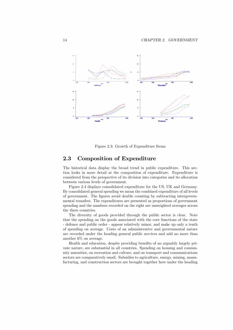
Figure 2.3 shows the growth in selected subcategories of public spending sincethe late nineteenth century. This is helpful in understanding the compositionof the long-run increase. The path of defence spending, which constituted oneof the largest items of public spending in the late nineteenth century, has beensomewhat erratic and has clearly been driven in large part by the history ofinternational relations. Military spending in the two former Axis powers peaksat around the time of the Second World War but then falls away dramatically.Spending in the three Allied powers continued at a higher level after the warthan before, reaching its height in the 1960s before also falling back. Amongthose nations represented, only in the US does defence now constitute morethan 10% of spending.
The most marked rises have come from social spending on items like health,education and pensions. Publicly-provided education can be seen to have beenrising gradually as a share of gross domestic product in all five countries sincethe nineteenth century but particularly so since the war (and perhaps slightlyearlier in the UK). Health and pensions spending have both grown considerablysince the war. If we consider subsidies and transfers in total then these haverisen on average fourfold between 1937 and 1995 (from about 2.1% of grossdomestic product to 13.1% in the US, from 10.3% to 23.6% in the UK, from7.0% to 19.4% in Germany, from 7.2% to 29.9% in France and from 1.4% to13.5% in Japan).
14 CHAPTER 2. GOVERNMENT
DefenceYear
1870 1900 1950 2000
0
5
10
15
DefenceYear
1870 1900 1950 2000
0
5
10
15
P
EducationYear
1870 1900 1950 2000
0
5
10
15
P
EducationYear
1870 1900 1950 2000
0
5
10
15
HealthYear
1870 1900 1950 2000
0
5
10
15
HealthYear
1870 1900 1950 2000
0
5
10
15
PensionsYear
1870 1900 1950 2000
0
5
10
15
PensionsYear
1870 1900 1950 2000
0
5
10
15
Figure 2.3: Growth of Expenditure Items
2.3 Composition of Expenditure
The historical data display the broad trend in public expenditure. This sec-tion looks in more detail at the composition of expenditure. Expenditure isconsidered from the perspective of its division into categories and its allocationbetween various levels of government.Figure 2.4 displays consolidated expenditure for the US, UK and Germany.
By consolidated general spending we mean the combined expenditure of all levelsof government. The figures avoid double counting by subtracting intergovern-mental transfers. The expenditures are presented as proportions of governmentspending and the numbers recorded on the right are unweighted averages acrossthe three countries.The diversity of goods provided through the public sector is clear. Note
that the spending on the goods associated with the core functions of the state- defence and public order - appear relatively minor, and make up only a tenthof spending on average. Costs of an administrative and governmental natureare recorded under the heading general public services and add no more thananother 6% on average.Health and education, despite providing benefits of an arguably largely pri-
vate nature, are substantial in all countries. Spending on housing and commu-nity amenities, on recreation and culture, and on transport and communicationssectors are comparatively small. Subsidies to agriculture, energy, mining, manu-facturing, and construction sectors are brought together here under the heading

2.3. COMPOSITION OF EXPENDITURE 15
6% Defence16% Health11% Education4% Public order & safety3% Housing & community1% Recreation, culture etc4% Transport & communication3% Other econ affairs34% Social security & welfare6% General public services12% Other
US 1996 UK 1998
Germany 1996
Figure 2.4: Composition of Consolidated General Spending
of other economic affairs and also appear relatively minor on average.Social security and welfare spending is the largest single item in all countries,
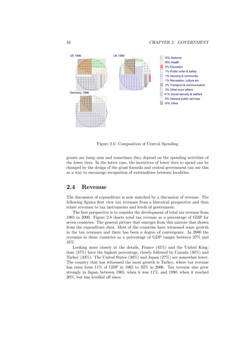
under this classification. This is so even in the US where it is noticeably smallerthan in the three European countries. On average it constitutes over a third ofspending.Figure 2.5 to 2.7 show how spending responsibilities are allocated between
different tiers of government in the US, UK and Germany. This provides aninteresting contrast since Germany and the US are federal countries with highlydevolved government whereas the UK is not. Nonetheless, some common obser-vations can be made. Certain items such as defence are always allocated to thecentre. Redistributive functions also tend to be concentrated centrally for thegood reason that redistribution between poor and rich regions is only possiblethat way and also that attempts at redistribution at lower levels are vulnerableto frustration through migration of richer individuals away from localities withinternally redistributive programs.Education on the other hand seems in all these countries to be largely de-
volved to lower levels — either to the states or to local government. Public orderis also typically dealt with at lower levels. Health spending, on the other hand,is always substantial at the central level but can also be important at lowertiers, for example in Germany.The fact that spending is made at lower levels need not mean that it is
financed from taxes levied locally. In most multiple-tier systems, central gov-ernment partly finances lower-tier functions by means of grants. These havemany purposes, including correcting for imbalances of resources between locali-ties and between tiers given the chosen allocation of tax instruments. Sometimes
16 CHAPTER 2. GOVERNMENT
10% Defence18% Health2% Education1% Public order & safety1% Housing & community1% Recreation, culture etc2% Transport & communication3% Other econ affairs
41% Social security & welfare6% General public services
14% Other
US 1996 UK 1998
Germany 1996
Figure 2.5: Composition of Central Spending
grants are lump sum and sometimes they depend on the spending activities ofthe lower tiers. In the latter case, the incentives of lower tiers to spend can bechanged by the design of the grant formula and central government can use thisas a way to encourage recognition of externalities between localities.
2.4 Revenue
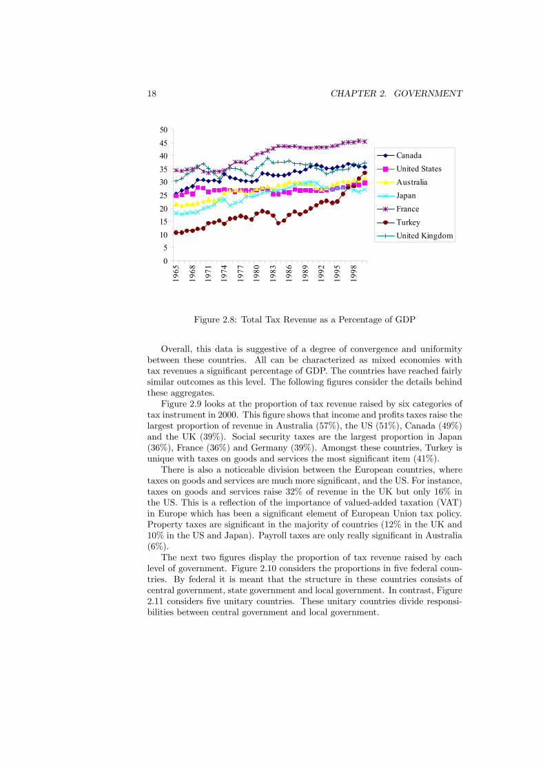
The discussion of expenditure is now matched by a discussion of revenue. Thefollowing figures first view tax revenues from a historical perspective and thenrelate revenues to tax instruments and levels of government.The first perspective is to consider the development of total tax revenue from
1965 to 2000. Figure 2.8 charts total tax revenue as a percentage of GDP forseven countries. The general picture that emerges from this mirrors that drawnfrom the expenditure data. Most of the countries have witnessed some growthin the tax revenues and there has been a degree of convergence. In 2000 therevenues in these countries as a percentage of GDP ranges between 27% and45%.Looking more closely at the details, France (45%) and the United King-
dom (37%) have the highest percentage, closely followed by Canada (36%) andTurkey (33%). The United States (30%) and Japan (27%) are somewhat lower.The country that has witnessed the most growth is Turkey, where tax revenuehas risen form 11% of GDP in 1965 to 33% in 2000. Tax revenue also grewstrongly in Japan between 1965, when it was 11%, and 1990, when it reached30%, but has levelled off since.

2.4. REVENUE 17
0% Defence21% Health23% Education8% Public order & safety3% Housing & community1% Recreation, culture etc7% Transport & communication3% Other econ affairs
19% Social security & welfare6% General public services9% Other
US 1996 Germany 1996
Figure 2.6: Composition of State Spending by Country. Source: IMF 2001.
0% Defence8% Health29% Education9% Public order & safety7% Housing & community4% Recreation, culture etc6% Transport & communication2% Other econ affairs22% Social security & welfare6% General public services8% Other
US 1996 UK 1998
Germany 1996
Figure 2.7: Composition of Local Spending
18 CHAPTER 2. GOVERNMENT
05
101520253035404550
1965
1968
1971
1974
1977
1980
1983
1986
1989
1992
1995
1998
CanadaUnited StatesAustraliaJapanFranceTurkeyUnited Kingdom
Figure 2.8: Total Tax Revenue as a Percentage of GDP
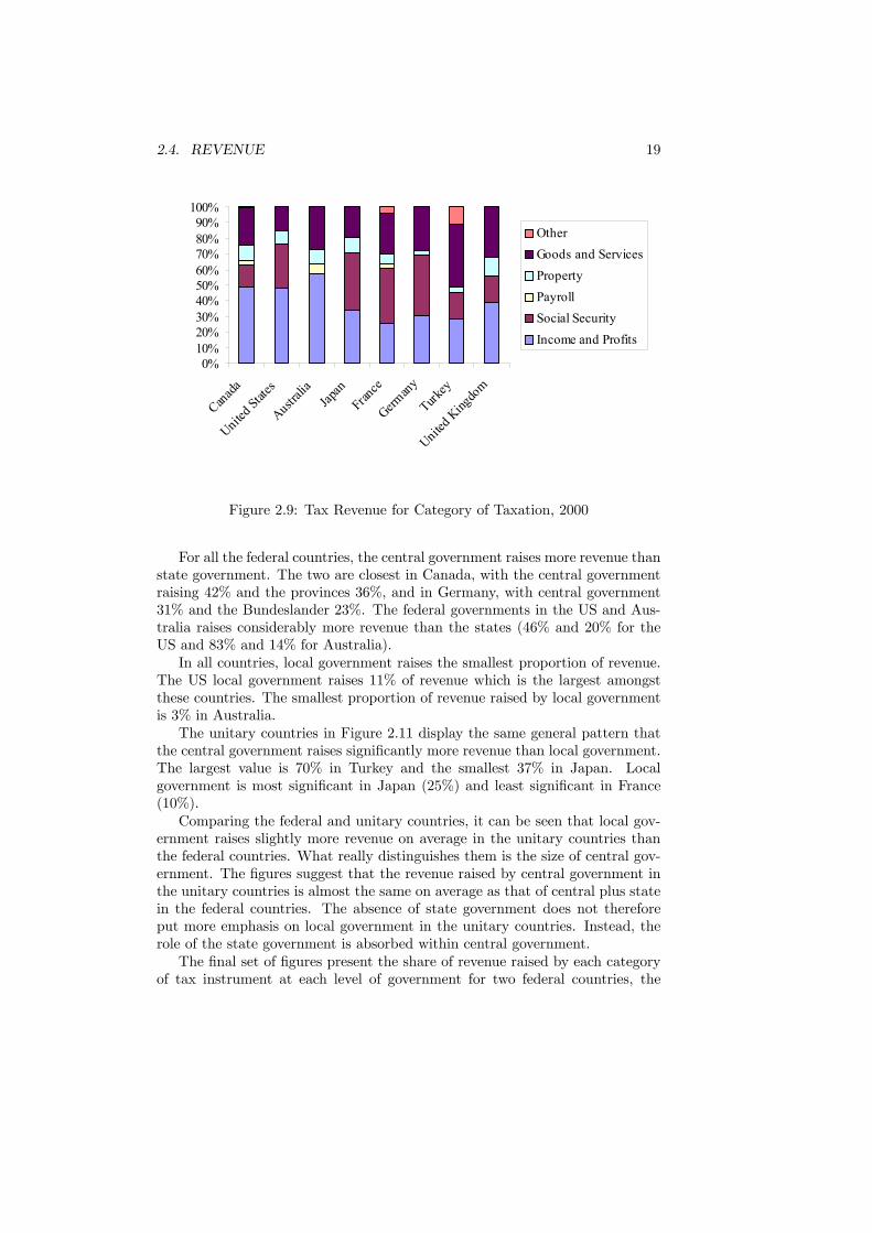
Overall, this data is suggestive of a degree of convergence and uniformitybetween these countries. All can be characterized as mixed economies withtax revenues a significant percentage of GDP. The countries have reached fairlysimilar outcomes as this level. The following figures consider the details behindthese aggregates.Figure 2.9 looks at the proportion of tax revenue raised by six categories of
tax instrument in 2000. This figure shows that income and profits taxes raise thelargest proportion of revenue in Australia (57%), the US (51%), Canada (49%)and the UK (39%). Social security taxes are the largest proportion in Japan(36%), France (36%) and Germany (39%). Amongst these countries, Turkey isunique with taxes on goods and services the most significant item (41%).There is also a noticeable division between the European countries, where
taxes on goods and services are much more significant, and the US. For instance,taxes on goods and services raise 32% of revenue in the UK but only 16% inthe US. This is a reflection of the importance of valued-added taxation (VAT)in Europe which has been a significant element of European Union tax policy.Property taxes are significant in the majority of countries (12% in the UK and10% in the US and Japan). Payroll taxes are only really significant in Australia(6%).The next two figures display the proportion of tax revenue raised by each
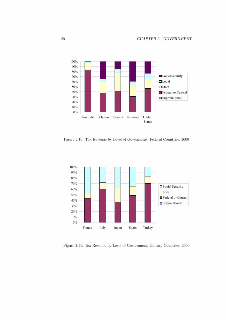
level of government. Figure 2.10 considers the proportions in five federal coun-tries. By federal it is meant that the structure in these countries consists ofcentral government, state government and local government. In contrast, Figure2.11 considers five unitary countries. These unitary countries divide responsi-bilities between central government and local government.
2.4. REVENUE 19
0%10%20%30%40%50%60%70%80%90%
100%
Canada
United S
tates
Australi
aJap
anFran
ce
Germany
Turkey
United K
ingdo
m
OtherGoods and ServicesPropertyPayrollSocial SecurityIncome and Profits
Figure 2.9: Tax Revenue for Category of Taxation, 2000
For all the federal countries, the central government raises more revenue thanstate government. The two are closest in Canada, with the central governmentraising 42% and the provinces 36%, and in Germany, with central government31% and the Bundeslander 23%. The federal governments in the US and Aus-tralia raises considerably more revenue than the states (46% and 20% for theUS and 83% and 14% for Australia).In all countries, local government raises the smallest proportion of revenue.
The US local government raises 11% of revenue which is the largest amongstthese countries. The smallest proportion of revenue raised by local governmentis 3% in Australia.The unitary countries in Figure 2.11 display the same general pattern that
the central government raises significantly more revenue than local government.The largest value is 70% in Turkey and the smallest 37% in Japan. Localgovernment is most significant in Japan (25%) and least significant in France(10%).Comparing the federal and unitary countries, it can be seen that local gov-
ernment raises slightly more revenue on average in the unitary countries thanthe federal countries. What really distinguishes them is the size of central gov-ernment. The figures suggest that the revenue raised by central government inthe unitary countries is almost the same on average as that of central plus statein the federal countries. The absence of state government does not thereforeput more emphasis on local government in the unitary countries. Instead, therole of the state government is absorbed within central government.The final set of figures present the share of revenue raised by each category
of tax instrument at each level of government for two federal countries, the
20 CHAPTER 2. GOVERNMENT
0%10%20%30%40%50%60%70%80%90%
100%
Australia Belgium Canada Germany UnitedStates
Social SecurityLocalStateFederal or CentralSupranational
Figure 2.10: Tax Revenue by Level of Government, Federal Countries, 2000
0%10%20%30%40%50%
60%70%80%90%
100%
France Italy Japan Spain Turkey
Social SecurityLocalFederal or CentralSupranational
Figure 2.11: Tax Revenue by Level of Government, Unitary Countries, 2000
2.4. REVENUE 21
0%10%20%30%40%50%
60%70%80%90%
100%
Central State Local
Taxes on Use
Other Taxes
Specific Goods andServicesGeneral Taxes
Property
Income and Profits
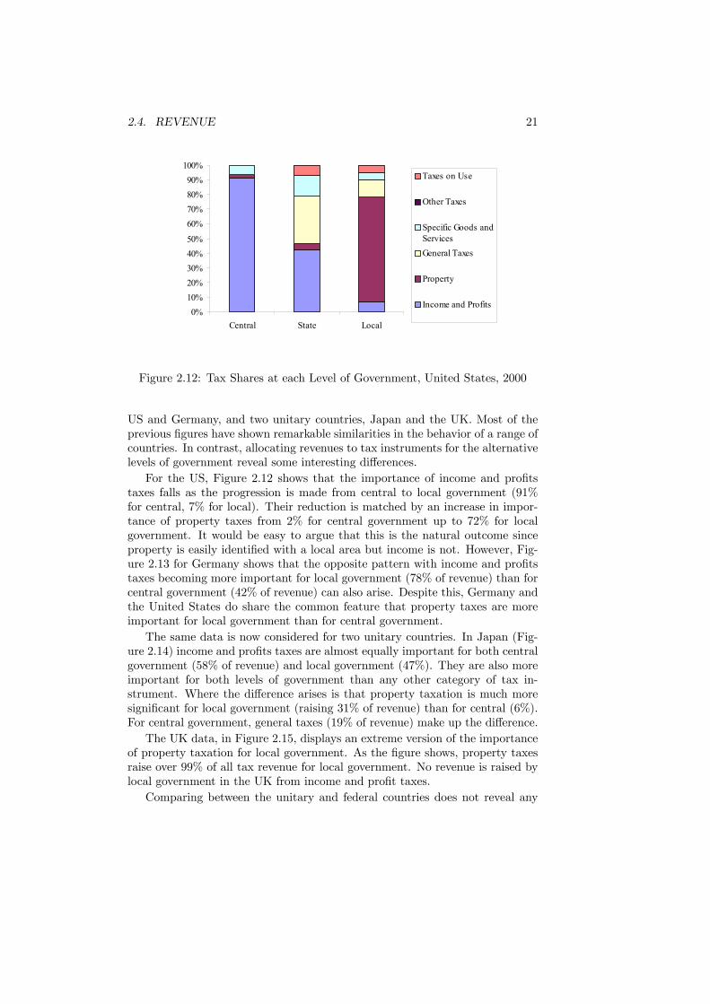
Figure 2.12: Tax Shares at each Level of Government, United States, 2000
US and Germany, and two unitary countries, Japan and the UK. Most of theprevious figures have shown remarkable similarities in the behavior of a range ofcountries. In contrast, allocating revenues to tax instruments for the alternativelevels of government reveal some interesting differences.For the US, Figure 2.12 shows that the importance of income and profits
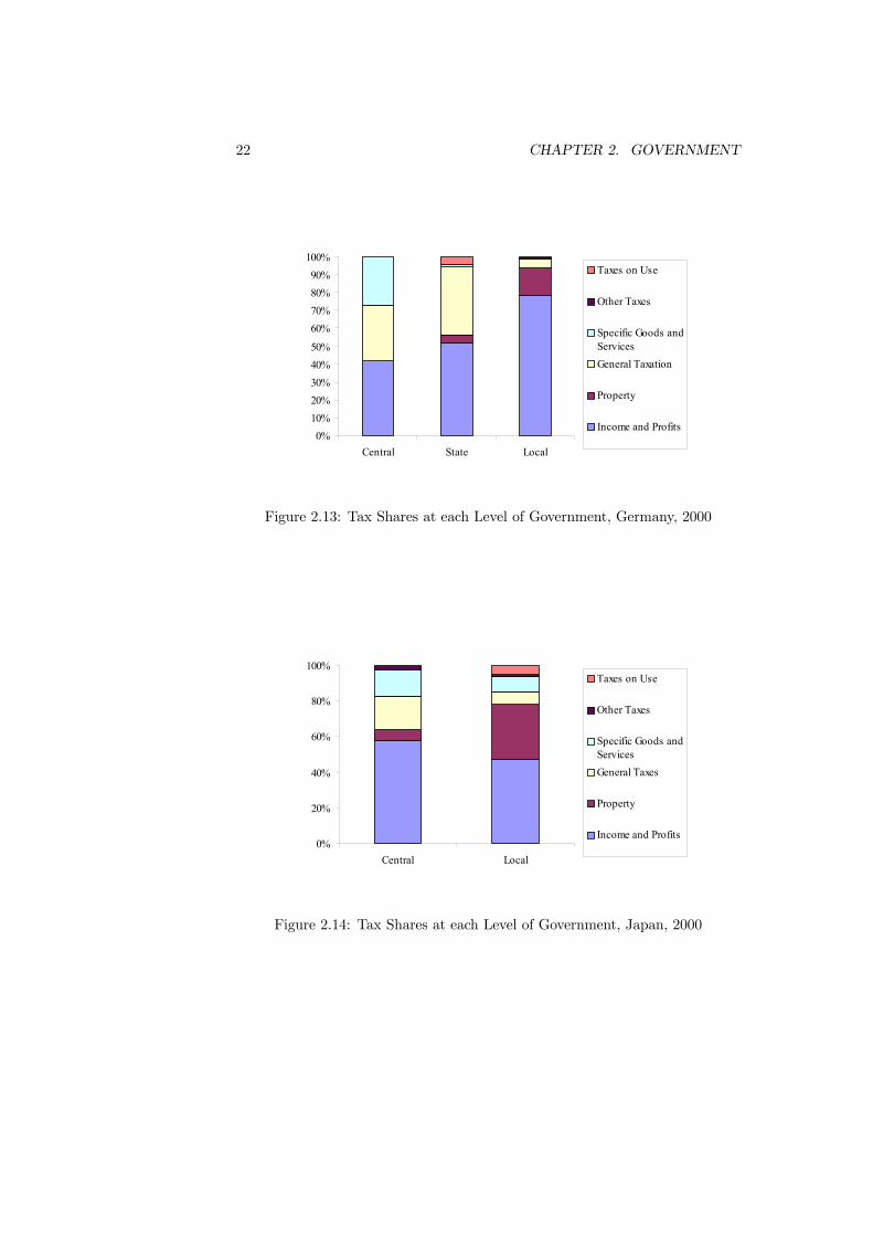
taxes falls as the progression is made from central to local government (91%for central, 7% for local). Their reduction is matched by an increase in impor-tance of property taxes from 2% for central government up to 72% for localgovernment. It would be easy to argue that this is the natural outcome sinceproperty is easily identified with a local area but income is not. However, Fig-ure 2.13 for Germany shows that the opposite pattern with income and profitstaxes becoming more important for local government (78% of revenue) than forcentral government (42% of revenue) can also arise. Despite this, Germany andthe United States do share the common feature that property taxes are moreimportant for local government than for central government.The same data is now considered for two unitary countries. In Japan (Fig-
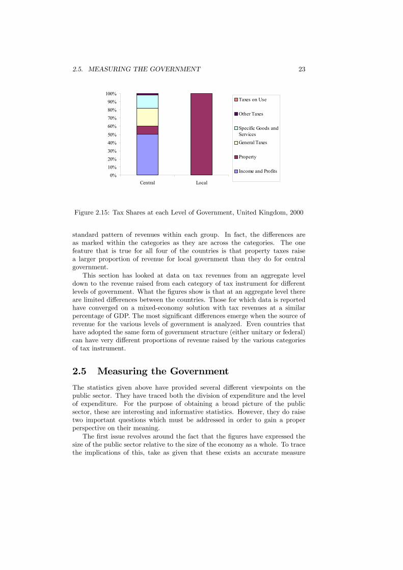
ure 2.14) income and profits taxes are almost equally important for both centralgovernment (58% of revenue) and local government (47%). They are also moreimportant for both levels of government than any other category of tax in-strument. Where the difference arises is that property taxation is much moresignificant for local government (raising 31% of revenue) than for central (6%).For central government, general taxes (19% of revenue) make up the difference.The UK data, in Figure 2.15, displays an extreme version of the importance
of property taxation for local government. As the figure shows, property taxesraise over 99% of all tax revenue for local government. No revenue is raised bylocal government in the UK from income and profit taxes.Comparing between the unitary and federal countries does not reveal any
22 CHAPTER 2. GOVERNMENT
0%10%20%30%40%50%
60%70%80%90%
100%
Central State Local
Taxes on Use
Other Taxes
Specific Goods andServicesGeneral Taxation
Property
Income and Profits
Figure 2.13: Tax Shares at each Level of Government, Germany, 2000
0%
20%
40%
60%
80%
100%
Central Local
Taxes on Use
Other Taxes
Specific Goods andServicesGeneral Taxes
Property
Income and Profits
Figure 2.14: Tax Shares at each Level of Government, Japan, 2000
2.5. MEASURING THE GOVERNMENT 23
0%10%20%30%40%50%
60%70%80%90%
100%
Central Local
Taxes on Use
Other Taxes
Specific Goods andServicesGeneral Taxes
Property
Income and Profits
Figure 2.15: Tax Shares at each Level of Government, United Kingdom, 2000
standard pattern of revenues within each group. In fact, the differences areas marked within the categories as they are across the categories. The onefeature that is true for all four of the countries is that property taxes raisea larger proportion of revenue for local government than they do for centralgovernment.This section has looked at data on tax revenues from an aggregate level
down to the revenue raised from each category of tax instrument for differentlevels of government. What the figures show is that at an aggregate level thereare limited differences between the countries. Those for which data is reportedhave converged on a mixed-economy solution with tax revenues at a similarpercentage of GDP. The most significant differences emerge when the source ofrevenue for the various levels of government is analyzed. Even countries thathave adopted the same form of government structure (either unitary or federal)can have very different proportions of revenue raised by the various categoriesof tax instrument.
2.5 Measuring the Government
The statistics given above have provided several different viewpoints on thepublic sector. They have traced both the division of expenditure and the levelof expenditure. For the purpose of obtaining a broad picture of the publicsector, these are interesting and informative statistics. However, they do raisetwo important questions which must be addressed in order to gain a properperspective on their meaning.The first issue revolves around the fact that the figures have expressed the
size of the public sector relative to the size of the economy as a whole. To tracethe implications of this, take as given that these exists an accurate measure
24 CHAPTER 2. GOVERNMENT
of the expenditure level of the public sector. The basic question is then: whatshould this expenditure be expressed as a proportion of? The standard approachis to use nominal gross domestic product (i.e. gross domestic product measuredusing each year’s own prices) but this is very much an arbitrary choice whichcan have a significant impact upon the interpretation of the final figure.Recall from basic national income accounting that the size of the economy
can be measured in either nominal or real terms using gross output or net out-put. Domestic or national product can be employed. Outputs can be valued atmarket prices or factor prices. For many purposes, as long as the basis of mea-surement is made clear, this does not make much real difference. Where it canmake a critical difference is in the impression it gives about the size of the publicsector. By adopting the smallest measure of the size of the economy (which thisis depends on a number of factors such as the level of new investment relativeto depreciation, the structure of the tax system and income from abroad), theapparent size of the public sector can be increased by several percent over thatfrom using the largest.Whilst not changing anything of real economic significance, such manipula-
tion of the figures can be very valuable in political debate. There is a degree offreedom for those who are supportive of the public sector, or are opponents ofit, to present a figure that is more favorable for their purposes. This may usefulfor those wishing to push a particular point of view, but it hinders informeddiscussion. Consequently, as long as the figures are calculated in a consistentway it does not matter for comparative purposes which precise definition of out-put is used. In contrast, for an assessment of whether the public sector is “toolarge” it can matter significantly.The second issue of measurement concerns what should be included within
the definition of government. To see what is involved here, consider the questionof whether should state-run industries be included. Assume that these areallowed to function as if they were private firms, so that they follow the objectiveof profit maximization, and simply remit their profits to the government. In thiscase they should certainly not be included since the government is simply actingas if it were a private shareholder. The only difference between the state-runfirm and any other private firm in which the government was a shareholderwould be the extent of the shareholding. Conversely, assume that the state-run firm was directed by the government to follow a policy of investment inimpoverished areas and to use cross-subsidization to lower the prices of some ofits products. In this case, there are compelling reasons to include the activitiesof the firm within the measure of government.What this example illustrates is that it is not government expenditure per se
that is interesting to the economist. Instead, what is really relevant is the de-gree of influence the government has over the economy. When the government issimply a shareholder, it is not directly influencing the firm’s decisions. The con-verse is true when it directs the firm’s actions. Looked at in this way, measuringthe size of government via its expenditure is a means of estimating governmentinfluence using an easily observable statistic. In fact, the extent of governmentinfluence is somewhat broader than just its expenditure. What must also be

2.6. CONCLUSIONS 25
included are the economic consequences of government-backed regulations andrestrictions on economic behavior. Minimum wage laws, weights and measuresregulation, health and safety laws are all examples of government interventionin the economy. However none of these would feature in any observation ofgovernment expenditure.What this discussion shows is that there is a degree of flexibility in interpret-
ing measures of government expenditure. Furthermore, government influence onthe economy is only approximately captured by the expenditure figure. The trueextent, including all relevant laws and regulations, is most certainly much larger.
2.6 ConclusionsThis chapter has reviewed the growth and activities of the public sector usingdata from a range of countries. Despite there clear cultural differences thesecountries have all experienced the same phenomenon of significant public sectorgrowth in the last century. From being only a minor part of the economy at thestart of the Twentieth Century, the public sector has grown to be significant inall developed countries at the start of the Twenty-First. There may be muchvariation within the figures for the exact size but the pattern of growth is thesame for all. There is also evidence that the growth has now ceased and, unlessthere is a some major upheaval, the size of the public sector will remain fairlyconstant for some time.In terms of the composition of public sector income and expenditure it can be
noted that there are differences in the details between countries. However thereis common reliance on similar tax instruments and spending patterns are notall that dissimilar. It is these commonalities that make the ideas and conceptsof public economics so broadly applicable.
Further ReadingDetailed evaluations of the different areas of public expenditure can be found
inMiles, D., Myles, G.D. and Preston, I. (2003) The Economics of Public
Spending (Oxford: Oxford University Press).The data for Figure 2.1 and 2.3 are taken from:Tanzi, V. and Schuknecht, L. (2000) Public Spending in the 20th Century:
A Global Perspective (Cambridge: Cambridge University Press).Figure 2.2 is compiled using data from:OECD Economic Outlook, Volumes 51 and 73.The expenditure data in Figures ?? to 2.7 uses data from:IMF (2001a) Government Finance Statistics Yearbook (Washington: IMF),andIMF (2001b) Government Finance Statistics Manual (Washington: IMF).Data on revenues in Figures 2.8 to 2.15 is drawn from:OECD (2002) Revenue Statistics 1965 - 2001 (Paris: OECD).

26 CHAPTER 2. GOVERNMENT

Part II
Political Economy
27

Chapter 3
Theories of the PublicSector
3.1 Introduction
The statistics of Chapter 2 have described the size, growth and compositionof the public sector in a range of developed and developing countries. Theseillustrated that the pattern of growth was similar across countries, as was thecomposition of expenditure. Although there is some divergence in the size of thepublic sector, it is significant in all the countries. Such observations raise twointer-related questions. First, why is there a public sector at all - would it notbe possible for economic activity to function satisfactorily without governmentintervention? Second, is it possible to provide a theory that explains the increasein size of the public sector and the composition of expenditure? The purpose ofthis chapter is to consider possible answers to these questions.The chapter begins with a discussion of the justifications that have been
proposed for the public sector. These show how the requirements of efficiencyand equity lead to a range of motives for public sector intervention. Alternativeexplanations for the growth in the size of the public sector are then assessed. Asa by-product, they also provide an explanation for the composition of expendi-ture. Finally, some economists would argue that the public sector is excessivelylarge. Several arguments for why this may be so are considered.
3.2 Justification for the Public Sector
Two basic lines of argument can be advanced to justify the role of the publicsector. These can be grouped under the headings of efficiency and equity. Effi-ciency relates to arguments concerning the aggregate level of economic activitywhereas equity refers to the distribution of economic benefits. In consideringthem, it is natural to begin with efficiency since this is essentially the more
29
30 CHAPTER 3. THEORIES OF THE PUBLIC SECTOR
fundamental concept.
3.2.1 The Minimal State
The most basic motivation for the existence of a public sector follows from theobservation that entirely unregulated economic activity could not operate in avery sophisticated way. In short, an economy would not function effectively ifthere were no property rights (the rules defining the ownership of property) orcontract laws (the rules governing the conduct of trade).Without property rights, satisfactory exchange of commodities could not
take place given the lack of trust that would exist between contracting parties.This argument can be traced back to Hobbes, who viewed the government as asocial contract that enabled people to escape from the anarchic “state of nature”where their competition in pursuit of self-interest would lead to a destructive“war of all against all”. The institution of property rights is a first step awayfrom this anarchy. In the absence of property rights, it would not be possibleto enforce any prohibition against theft. Theft discourages enterprise since thegains accrued may be appropriated by others. It also results in the use ofresources in the unproductive business of theft prevention.Contract laws determine the rules of exchange. They exist to ensure that
the participants in a trade receive what they expect from that trade or, ifthey do not, have open an avenue to seek compensation. Examples of contractlaws include the formalization of weights and measures and the obligation tooffer product warranties. These laws encourage trade by removing some of theuncertainty in transactions.The establishment of property rights and contract laws is not sufficient in
itself. Unless they can be policed and upheld in law, they are of limited con-sequence. Such law enforcement cannot be provided free of cost. Enforcementofficers must be employed and courts must be provided in which redress canbe sought. In addition, an advanced society would also face a need for theenforcement of more general criminal laws. Moving beyond this, once a coun-try develops its economic activity it will need to defend its gains from beingstolen by outsiders. This implies the provision of defence for the nation. As thestatistics made clear, national defence is also a costly activity.Consequently, even if only the minimal requirements of the enforcement of
contract and criminal laws and the provision of defence are met, a source ofincome must be found to pay for them. This need for income requires thecollection of revenue, whether these services are provided by the state or byprivate sector organizations. But they are needed in any economy that wishesto develop beyond the most rudimentary level. Whether it is most efficient fora central government to collect the revenue and provide the services could bedebated. Since there are some good reasons for assuming this is the case, thecoordination of the collection of revenue and the provision of services to ensurethe attainment of efficient functioning of economic activity provides a naturalrole for a public sector.
3.2. JUSTIFICATION FOR THE PUBLIC SECTOR 31
This reasoning illustrates that to achieve even a most minimal level of eco-nomic organization, some unavoidable revenue requirements are generated andrequire financing. From this follows the first role of the public sector which is toassist with the attainment of economic efficiency by providing an environmentin which trade can take place. The minimal state provides contract law, policesit, and defends the economy against outsiders. The minimal state does nothingmore than this, but without it organized economic activity could not take place.These arguments provide a justification for at least a minimal state and hencethe existence of a public sector and of public expenditure.Having concluded that the effective organization of economic activity gener-
ates a need for public expenditure, one role for public economics is to determinehow this revenue should be collected. The collection should be done with aslittle cost as possible imposed upon the economy. Such costs arise from thedistortion in choice that arise from taxation. Public economics aims to under-stand these distortions and to describe the methods of keeping them as low aspossible.
3.2.2 Market versus Government
Moving beyond the basic requirements for organized economic activity, thereare other situations where intervention in the economy can potentially increasewelfare. Unlike the minimal provision and revenue requirements however, therewill always be a degree of contentiousness about additional intervention what-ever the grounds on which it is motivated. The situations where interventionmay be warranted can be divided into two categories: those that involve marketfailure and those that do not.When market failure is present, the argument for considering whether in-
tervention would be beneficial is compelling. For example, if economic activitygenerated externalities (effects that one economic agent imposes on anotherwithout their consent), so that there is divergence between private and socialcosts and the competitive outcome is not efficient, it may be felt necessary forthe state to intervene to limit the inefficiency that results. This latter point canalso be extended to other cases of market failure, such as those connected tothe existence of public goods and of imperfect competition. Reacting to suchmarket failures is intervention motivated on efficiency grounds.It must be stressed that this reasoning does not imply that intervention
will always be beneficial. In every case, it must be demonstrated that thepublic sector actually has the ability to improve upon what the unregulatedeconomy can achieve. This will not be possible if the choice of policy tools islimited or government information is restricted. It will also be undesirable if thegovernment is not benevolent. These various imperfections in public interventionwill be a recurrent theme of this book.While some useful insights follow from the assumption of an omnipotent, om-
niscient and benevolent policy maker, in reality it can give us very misleadingideas about the possibilities of beneficial policy intervention. It must be recog-nized that the actions of the state, and the feasible policies that it can choose,
32 CHAPTER 3. THEORIES OF THE PUBLIC SECTOR
are often restricted by the same features of the economy that make the marketoutcome inefficient. One role for public economics is therefore to determine thedesirable extent of the public sector or the boundaries of state intervention.For instance, if we know that markets will fail to be efficient in the presenceof imperfect information, to establish the merit of government intervention it iscrucial to know if a government subject to the same informational limitationscan achieve a better outcome.Furthermore, a government managed by non-benevolent officials and subject
to political constraints may fail to correct market failures and may insteadintroduce new costs of its own creation. It is important to recognize that thispotential for government failure is as important as market failure and that bothare often rooted in the same informational problems. At a very basic level, theforce of coercion must underlie every government intervention in the economy.All policy acts take place, and in particular taxes are collected and industryis regulated, with this force in the background. But the very power to coerceraises the possibility of its misuse. Although the intention in creating this poweris that its force should serve the general interest, nothing can guarantee thatonce public officials are given this monopoly of force, they will not try to abusethis power in their own interest.
3.2.3 Equity
In addition to market failure, government intervention can also be motivated bythe observation that the economy may have widespread inequality of income,opportunity or wealth. This can occur even if the economy is efficient in anarrow economic sense. In such circumstances, the level of economic welfare asviewed by the government may well be raised by a policy designed to alleviatethese inequalities. This is the reasoning through which the provision of stateeducation, social security programmes and compulsory pension schemes are jus-tified. It should be stressed that the gains from these policies are with respectto normative assessments of welfare, unlike the positive criterion lying behindthe concept of economic efficiency.In the cases of both market failure and welfare-motivated policies, policy
intervention concerns more than just the efficient collection of revenue. Thereasons for the failure of the economy to reach the optimal outcome have to beunderstood and a policy that can counteract these has to be designed. Extendingthe scope of the public economics to address such issues provides the breadthto the subject.
3.2.4 Efficiency and Equity
When determining economic policy, governments are faced with two conflictingaims. They are all concerned with organizing economic activity so that the bestuse is made of economic resources. This is the efficiency side of policy design.To varying degrees, governments are also concerned to see that the benefits

3.3. PUBLIC SECTOR GROWTH 33
of economic activity are distributed fairly. This is the equity aspect of policydesign.The difficulty facing the government is that the requirements of equity and
efficiency frequently conflict. It is often the case that the efficient policy is highlyinequitable, whilst the equitable policy can introduce significant distortions anddisincentives. Given this fact, the challenge for policy design is to reach thecorrect trade-off between equity and efficiency. Quite where on the trade-off thegovernment should locate is dependent upon the relative importance it assignsto equity over efficiency.In this context, it is worth adding one final note concerned with the nature
of the arguments often used in this book. A standard simplification is to assumethat there is a single consumer or that all consumers are identical. In such asetting there can be no distributional issues, so any policy recommendationsderived within it relate only to efficiency and not to equity. The reason forproceeding in this way is that it usually permits a much simpler analysis to beundertaken and for the conclusions to be much more precise. When interpretingsuch conclusions in terms of practical policy recommendations, their basis shouldnever be overlooked.
3.3 Public Sector Growth
The data of Chapter 2 showed quite clearly the substantial growth of the publicsector in a range of countries during the past century. There are numeroustheories that have been advanced to explain why this has occurred. These differin their emphasis and perspective and are not mutually exclusive. In fact, it isreasonable to argue that a comprehensive explanation would involve elementsdrawn from all.
3.3.1 Development Models
The basis of the development models of public sector growth is that the econ-omy experiences changes in its structure and needs as it develops. Tracingthe nature of the development process from the beginning of industrializationthrough to the completion of the development process, a story of why publicsector expenditure increases can be told.It is possible to caricature the main features of this story in the following
way. The early stage of development is viewed as the period of industrializationduring which the population moves from the countryside to the urban areas.To meet the needs that result from this, there is a requirement for significantinfrastructural expenditure in the development of cities. The typically rapidgrowth experienced in this stage of development results in a significant increasein expenditure and the dominant role of infrastructure determines the nature ofexpenditure.In what are called the middle stages of development, the infrastructural
expenditure of the public sector becomes increasingly complementary with ex-

34 CHAPTER 3. THEORIES OF THE PUBLIC SECTOR
penditure from the private sector. Developments by the private sector, suchas factory construction, are supported by investments from the public sector,e.g. the building of connecting roads. As urbanization proceeds and cities in-crease in size, so does population density. This generates a range of externalitiessuch as pollution and crime. An increasing proportion of public expenditure isthen diverted away from spending upon infrastructure to the control of theseexternalities.Finally, in the developed phase of the economy, there is less need for in-
frastructural expenditure or for the correction of market failure. Instead, ex-penditure is driven by the desire to react to issues of equity. This results intransfer payments, such as social security, health and education, becoming themain items of expenditure. Of course, once such forms of expenditure becomeestablished, they are difficult to ever reduce. They also increase with heightenedexpectations and through the effect of an ageing population.Although this theory of the growth of expenditure concurs broadly with
the facts, it has a number of weaknesses. Most importantly, it is primarily adescription rather than an explanation. From an economist’s perspective, thetheory is lacking in that it does not have any behavioral basis but is essentiallymechanistic. What an economist really would wish to see is an explanation inwhich expenditure is driven by the choices of the individuals that constitute theeconomy. In the development model the change is just driven by the exogenousprocess of economic progress. Changes in expenditure should be related to howchoices change as preferences or needs evolve over time.
3.3.2 Wagner’s Law
Wagner was a 19th century economist who analyzed data on public sector ex-penditure for several European countries, Japan, and the US. This data revealedthe fact that was shown in the data of Chapter 2: the share of the public sectorin GDP had been increasing over time. The content of Wagner’s Law was anexplanation of this trend and a prediction that it would continue. In contrastto the basic developments models, Wagner’s analysis provided a theory ratherthen just a description and an economic justification for the predictions.The basis for the theory consisted of three distinct components. Firstly, it
was observed that the growth of the economy resulted in an increase in complex-ity. This required continuous introduction of new laws and development of thelegal structure. These implied continuing increases in public sector expenditure.Secondly, there was the process of urbanization and the increased externalitiesassociated with it. These two factors have already been discussed in connectionwith the development models.The final component underlying the Wagner’s Law is the most behavioral of
the three and is what distinguishes it from other explanations. Wagner arguedthat the goods supplied by the public sector have a high income elasticity ofdemand. This claim appears reasonable, for example, for education, recreationand health care. Given this fact, economic growth which raised incomes wouldlead to an increase in demand for these products. In fact, the high elasticity

3.3. PUBLIC SECTOR GROWTH 35
would imply that public sector expenditure would rise as a proportion of income.This conclusion is the substance of Wagner’s Law.In many ways, Wagner’s Law provides a good explanation of public sector
growth. Its main failing is that it concentrates solely on the demand for publicsector services. What must determine the level is some interaction betweendemand and supply. The supply side is explicitly analyzed in the next model.
3.3.3 Baumol’s Law
Rather than work from the observed data, Baumol’s Law starts from an obser-vation about the nature of the production technology in the public sector. Thebasic hypothesis is that the technology of the public sector is labor-intensiverelative to that of the private sector. In addition, the type of production under-taken leaves little scope for increases in productivity and that makes it difficultto substitute capital for labor. As examples, hospitals need minimum numbersof nurses and doctors per patient and maximum class sizes place lower limits onteacher numbers in schools.Competition on the labor market ensures that labor costs in the public sector
are linked to those in the private sector. Although there may be some frictions intransferring between the two, wage rates cannot be too far out of line. However,in the private sector it is possible to substitute capital for labor when the relativecost of labor increases. Furthermore, technological advances in the private sectorlead to increases in productivity. These increases in productivity result in thereturn to labor rising. The latter claim is simply a consequence of optimal inputuse in the private sector resulting in the wage rate being equated to the marginalrevenue product.Since the public sector cannot substitute capital for labor, the wage increases
in the private sector feed through into cost increases in the public sector. Main-taining a constant level of public sector output must therefore result in publicsector expenditure increasing. If public sector output/private sector output re-main in the same proportion, public sector expenditure rises as a proportion oftotal expenditure. This is Baumol’s Law which asserts the increasing propor-tional size of the public sector.There are a number of problems with this theory. It is entirely technology-
driven and does not consider aspects of supply and demand or political processes.There are also reasons for believing that substitution can take place in the publicsector. For example, additional equipment can replace nurses and less-qualifiedstaff can take on more mundane tasks. Major productivity improvements havealso been witnessed in universities and hospitals. Finally, there is evidence ofa steady decline in public sector wages relative to those in the private sector.This reflects lower-skilled labor being substituted for more skilled.
3.3.4 A Political Model
A political model of public sector expenditure needs to capture the conflict inpublic preferences between those who wish to have higher expenditure and those

36 CHAPTER 3. THEORIES OF THE PUBLIC SECTOR
who wish to limit the burden of taxes. It must also incorporate the resolution ofthis conflict and show how the size and composition of actual public spendingreflects the preferences of the majority of citizens as expressed through thepolitical process. The political model we now describe is designed to achievethese aims. The main point that emerges is that the equilibrium level of publicspending can be related to the income distribution, and more precisely that thegrowth of government is closely related to the rise of income inequality.To illustrate this, consider an economy with H consumers whose incomes
fall into a range between a minimum of 0 and a maximum of by. The governmentprovides a public good which is financed by the use of a proportional incometax. The utility of consumer i who has income yi is given by
ui(t,G) = [1− t] yi + b(G), (3.1)
where t is the income tax rate and G the level of public good provision. Thefunction b(·) represents the benefit obtained from the public good and it isassumed to be increasing (so the marginal benefit is positive) and concave (sothe marginal benefit is falling) as G increases. Denoting the mean income levelin the population of consumers by µ, the government budget constraint is
G = tHµ. (3.2)
Using this budget constraint, a consumer with income yi will enjoy utility fromprovision of a quantity G of the public good of
ui(G) =
·1− G
Hµ
¸yi + b(G). (3.3)
The ideal level of public good provision for the consumer is given by thefirst-order condition
∂ui(G)
∂G≡ − yi
Hµ+ b0(G) = 0 (3.4)
This condition relates the marginal benefit of an additional unit of the publicgood, b0(G), to its marginal cost yi
Hµ . The quantity of the public good demandedby the consumer depends upon their income relative to the mean since thisdetermines the marginal cost.The marginal benefit of the public good has been assumed to be a decreasing
function of G, so it follows that the preferred public good level is decreasing asincome rises. The reason for this is that with a proportional income tax the richpay a higher share of the cost of public good than the poor. Thus public goodprovision will disproportionately benefit the poor.The usual way to resolve the disagreement over the desired level of public
good is to choose by majority voting. If the level of public good is to be de-termined by majority voting which level will be chosen? In the context of thismodel the answer is clear-cut because all consumers would prefer the level ofpublic good to be as close as possible to their preferred level. Given any pairof alternatives, consumers will vote for that which is closest to their preferred

3.3. PUBLIC SECTOR GROWTH 37
alternative. The alternative that is closest for the largest number of consumerswill receive maximal support. There is in fact only one option that will satisfythis requirement: the option preferred by the consumer with the median income.The reason is that exactly one half of the electorate, above the median income(the rich), would like less public good and the other half, below the median (thepoor), would like more public good. Any alternative that is better for one groupwould be opposed by the other group with opposite preferences. (We explorethe theory of voting in detail in Chapter 4.)The political equilibrium G∗, determined by the median voter, is then the
solution to
b0(G∗) =ymHµ
, (3.5)
where ym/µ is the income of the median voter relative to the mean. Sincethe marginal benefits decrease as public good provision increases, the politicalequilibrium level of public good increases with income inequality as measuredby the ratio of the median to mean income. Accordingly, more inequality asmeasured by a lower ratio of the median to mean income would lead the decisivemedian voter to require more public spending.Government activities are perceived as redistributive tools. Redistribution
can be explicit, such as social security and poverty alleviation programs, or itcan take a more disguised form like public employment which is probably themain channel of redistribution from rich to poor in many countries. Because ofits nature, and interaction with the tax system, the demand for redistributionwill increase as income inequality increases as demonstrated by this politicalmodel.
3.3.5 Ratchet Effect
Models of the ratchet effect develop the modeling of political interaction ina different direction. They assume that the preference of the government isto spend money. Explanations of why this should be so can be found in theeconomics of bureaucracy which is explored in the next section. For now, thefact is just taken as given. In contrast, it is assumed that the public do not wantto pay taxes. Higher spending can only come from taxes, so by implication thepublic partially resists this; they do get some benefit from the expenditure. Thetwo competing objectives are moderated by the fact that governments desirere-election. This makes it necessary for it to take some account of the public’spreferences.The equilibrium level of public sector expenditure is determined by the bal-
ance between these competing forces. In the absence of any exogenous changesor of changes in preferences, the level of expenditure will remain relatively con-stant. In the historical data on government expenditure, the periods prior to1914, between 1920 and 1940 and post-1945 can be interpreted as displayingsuch constancy. Occasionally, though, economies go through periods of signif-icant upheaval such as occurs during wartime. During these periods normal

38 CHAPTER 3. THEORIES OF THE PUBLIC SECTOR
economic activity is disrupted. Furthermore, the equilibrium between the gov-ernment and the taxpayers becomes suspended. Ratchet models argue that thispermits the government to raise expenditure with the consent of the taxpayerson the understanding that this is necessary to meet the exceptional needs thathave arisen.
The final aspect of the argument is that the level of expenditure does notfall back to its original level after the period of upheaval. Several reasons canbe advanced for this. Firstly, the taxpayers could become accustomed to thehigher level of expenditure and perceive this as the norm. Secondly, debts maybe incurred during the period of upheaval which have to be paid-off later. Thisrequires the raising of finance. Thirdly, promises could be made by the govern-ment to the taxpayers during periods of upheaval which then have to be met.These can jointly be termed ratchet effects that sustain a higher level of spend-ing. Finally, there may also be an inspection effect after an upheaval, meaningthat the taxpayers and government reconsider their positions and priorities. Thediscovery of previously unnoticed needs then provides further justification forhigher public sector spending.
The prediction of the ratchet-effect model is that spending remains relativelyconstant unless disturbed by some significant external event. When these eventsoccur they lead to substantial increases in expenditure. The ratchet and inspec-tion effects work together to ensure that expenditure remains at the higher leveluntil the next upheaval.
Referring to data of Chapter 2, it can be seen that the description of expendi-ture growth given by this political model is broadly consistent with the evidence.Before 1914, between 1918 and 1940 and post-1945 the level of expenditure isfairly constant but steps-up between these periods. Whether this provides sup-port for the explanation is debatable because the model was constructed toexplain these known facts. In other words, the data cannot be employed as ev-idence that the model is correct, given that the model was designed to explainthat data.
3.4 Excessive Government
The theories of the growth of public sector expenditure described above attemptto explain the facts but do not offer comment on whether the level of expenditureis deficient or excessive. They merely describe processes and do not attempt toevaluate the outcome. In fact, there are many economists who would argue thatpublic sector expenditure is too large and represents a growing burden on theeconomy. While the evidence on this issue is certainly not conclusive, there are anumber of explanations of why this should be so and several are now described.These reach their conclusions not through a cost-benefit analysis of expenditurebut via an analysis of the functioning of government.
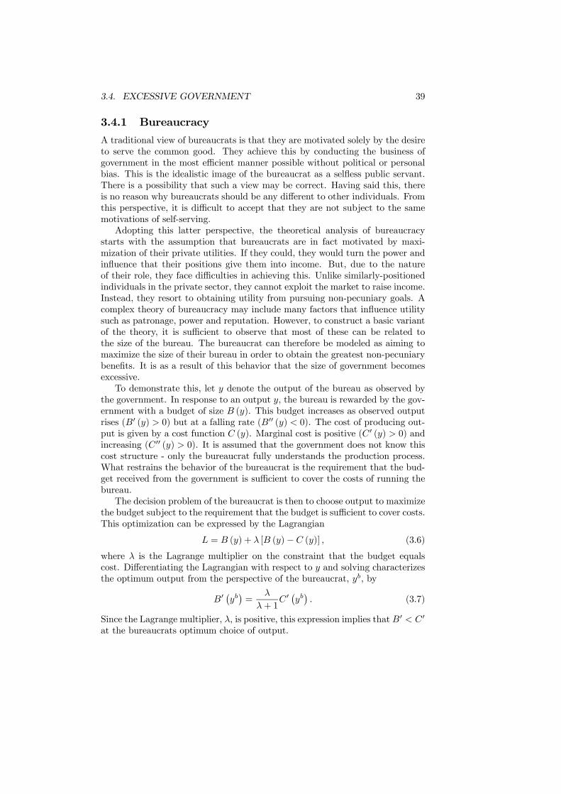
3.4. EXCESSIVE GOVERNMENT 39
3.4.1 Bureaucracy
A traditional view of bureaucrats is that they are motivated solely by the desireto serve the common good. They achieve this by conducting the business ofgovernment in the most efficient manner possible without political or personalbias. This is the idealistic image of the bureaucrat as a selfless public servant.There is a possibility that such a view may be correct. Having said this, thereis no reason why bureaucrats should be any different to other individuals. Fromthis perspective, it is difficult to accept that they are not subject to the samemotivations of self-serving.Adopting this latter perspective, the theoretical analysis of bureaucracy
starts with the assumption that bureaucrats are in fact motivated by maxi-mization of their private utilities. If they could, they would turn the power andinfluence that their positions give them into income. But, due to the natureof their role, they face difficulties in achieving this. Unlike similarly-positionedindividuals in the private sector, they cannot exploit the market to raise income.Instead, they resort to obtaining utility from pursuing non-pecuniary goals. Acomplex theory of bureaucracy may include many factors that influence utilitysuch as patronage, power and reputation. However, to construct a basic variantof the theory, it is sufficient to observe that most of these can be related tothe size of the bureau. The bureaucrat can therefore be modeled as aiming tomaximize the size of their bureau in order to obtain the greatest non-pecuniarybenefits. It is as a result of this behavior that the size of government becomesexcessive.To demonstrate this, let y denote the output of the bureau as observed by
the government. In response to an output y, the bureau is rewarded by the gov-ernment with a budget of size B (y). This budget increases as observed outputrises (B0 (y) > 0) but at a falling rate (B00 (y) < 0). The cost of producing out-put is given by a cost function C (y). Marginal cost is positive (C0 (y) > 0) andincreasing (C00 (y) > 0). It is assumed that the government does not know thiscost structure - only the bureaucrat fully understands the production process.What restrains the behavior of the bureaucrat is the requirement that the bud-get received from the government is sufficient to cover the costs of running thebureau.The decision problem of the bureaucrat is then to choose output to maximize
the budget subject to the requirement that the budget is sufficient to cover costs.This optimization can be expressed by the Lagrangian
L = B (y) + λ [B (y)− C (y)] , (3.6)
where λ is the Lagrange multiplier on the constraint that the budget equalscost. Differentiating the Lagrangian with respect to y and solving characterizesthe optimum output from the perspective of the bureaucrat, yb, by
B0¡yb¢=
λ
λ+ 1C 0¡yb¢. (3.7)
Since the Lagrange multiplier, λ, is positive, this expression implies that B0 < C0
at the bureaucrats optimum choice of output.

40 CHAPTER 3. THEORIES OF THE PUBLIC SECTOR
Output
Marginal Budgetand Marginal Cost
( )yB'( )yC '
*y by
Figure 3.1: Excessive Bureaucracy
We wish to contrast the outcome with the bureaucrat in charge that whichoccurs when the government has full information. With full information thereexists a variety of different ways to model efficiency. On way would be to placethis bureau within a more general setting and consider its output as one compo-nent of overall government intervention. A benefit/cost calculation for govern-ment intervention would then determine the efficient level of bureau output. Asimpler alternative, and the one we choose to follow, is to determine the efficientoutput by drawing an analogy between the bureau and a profit-maximizing firm.The firm would choose its output to ensure that the difference between revenueand costs was made as large as possible. Applying this analogy, the bureaushould choose output to maximize its budget less costs, B (y)− C (y). For thebureau, this is the equivalent of profit maximization.Differentiating with respect to y, the efficient output, y∗, equates the mar-
ginal effect of output on the budget to marginal cost, so B0 (y∗) = C0 (y∗).The output level chosen by the bureaucrat can easily be shown to be abovethe efficient level. This argument is illustrated in Figure 3.1. The increasingmarginal cost curve and declining marginal benefit curve are consequences ofthe assumptions already made. The efficient output occurs at the intersec-tion of these curves. In contrast, the output chosen by the bureaucrat satisfiesB0¡yb¢< C0
¡yb¢, so it must lie to the right of y∗. In fact, the budget covers
costs when the area under the marginal budget curve equals the area under themarginal cost curve. It is clear from this figure that the size of the bureaucracyis excessive when it is determined by the choice of a bureaucrat.This simple model shows how the pursuit of personal objectives by bureau-
crats can lead to an excessive size of bureaucracy. Adding together the individual

3.4. EXCESSIVE GOVERNMENT 41
bureaus that comprise the public sector makes this excessive in aggregate. Thisexcessive size is simply an inefficiency since money is spent on bureaus whichare not generating sufficiently valuable results.The argument just given is enticing in its simplicity but it is restricted by
the fact that it is assumed that the bureaucrats have freedom to set the sizeof the bureau. There are various ways this limitation can be addressed. Usefulextensions are to have the freedom constrained by political pressure or througha demand function. Although doing either of these would lessen the excess,the basic moral that bureaucrats have incentives to overly enlarge their bureauswould still remain. Whether they do so in practice is dependent upon theconstraints placed upon them.
3.4.2 Budget-Setting
An alternative perspective upon excessive bureaucracy can be obtained by con-sidering a different process of budget determination. A motivation for this isthe fact that each government department is headed by a politician who obtainssatisfaction from the size of the budget. Furthermore, in many government sys-tems, budgets for departments are determined annually by a meeting of cabinet.This meeting takes the budget bids from the individual departments and allo-cates a central budget on the basis of these. Providing a model incorporatingthese points then determines how departments’ budgets evolve over time.A simple process of this form can be the following. Let the budget for year
t be given by Bt. The budget claim for year t+ 1 is then given by
Bct+1 = [1 + α]Bt, (3.8)
where α > 0. Such a rule represents a straightforward mechanical method ofupdating the budget claim - last year’s is taken and a little more added. It is,of course, devoid of any basis in efficiency. The meeting of cabinet then takesthese bids and proportionately reduces them to reach the final allocation. Theagreed budget is then
Bt+1 = [1− γ]Bct+1 = [1− γ] [1 + α]Bt. (3.9)
The expression above gives a description of the change in the budget over time.It can be seen that if α > γ, then the budget will grow over time. Its
development bears little relationship to needs, so that there is every possibilitythat expenditure will eventually become excessive even if it initially begins atan acceptable level. When α < γ the budget will fall over time. Although eithercase is possible, the observed pattern of growth lends some weight to the formerassumption.This form of model could easily be extended to incorporate more complex
dynamics but these would not really enhance the content of the simple story ittells. The modeling of budget determination as a process entirely independentof what is good for the economy provides an important alternative perspectiveon how the public sector may actually function. Even if the truth is not quite
42 CHAPTER 3. THEORIES OF THE PUBLIC SECTOR
this stark, reasoning of this kind does put into context models that are basedon the assumption that the government is informed and efficient.
3.4.3 Monopoly Power
The basis of elementary economics is that market equilibrium is determined viathe balance of supply and demand. Those supplying the market are assumedto be distinct from those demanding the product. In the absence of monopolypower, the equilibrium that is achieved will be efficient. If the same reasoningcould be applied to the goods supplied by the public sector, then efficiencywould also arise there. Unfortunately, there are two reasons why this is notpossible. Firstly, the public sector can award itself a monopoly in the supplyof its goods and services. Secondly, this monopoly power may be extended intomarket capture.
Generally, a profit-maximizing monopolist will always want to restrict itslevel of output below the competitive level, so that monopoly power will providea tendency for too little government rather than the converse. This would bea powerful argument were it not for the fact that the government can choosenot to exercise its monopoly power in this way. If it is attempting to achieveefficiency, then it will certainly not do so. Furthermore, since the governmentmay not be following a policy of profit maximization, it might actually exploitits monopoly position to over-supply its output. This takes the analysis back inthe direction of the bureaucracy model.
The idea of market capture is rather more interesting and arises from thenature of goods supplied by the public sector. Rather than being standardmarket goods, many of them are complex in nature and not fully understoodby those consuming them. Natural examples of such goods would be educationand health care. In both cases, the consumer may not understand quite whatthe product is, nor what is best for them. Although this is important, it isalso true of many other goods. The additional feature of the public sectorcommodities is that demand is not determined by the consumers and expressedthrough a market. Instead it is delegated to specialists, such as teachers ordoctors. Furthermore, these same specialists are also responsible for setting thelevel of supply. In this sense, they can be said to capture the market.
The consequence of this market capture is that the specialists can set thelevel of output for the market that most meets their objectives. Naturally, sincemost would benefit from an expansion of their profession, within limits, thisgives a mechanism which leads to supply in excess of the efficient level. Thelimits arise because they won’t want to go so far that competition reduces thepayment received or lowers standards too far. Effectively, they are reaching atrade-off between income and power, where the latter arises through the sizeof the profession. The resulting outcome has no grounds in efficiency and maywell be too large.

3.4. EXCESSIVE GOVERNMENT 43
3.4.4 Corruption
Corruption does not emerge as a moral aberration, but as a general consequenceof government officials using their power for personal gain. Corruption distortsthe allocation of resources away from productive toward rent-seeking occupa-tions. Rent-seeking (studied in Chapter 5) is the attempt to obtain a returnabove what is judged adequate by the market. Monopoly profit is one example,but the concept is much broader. Corruption is not just redistributive (takingwealth from others to give it to some special interests) but it can also have enor-mous efficiency costs. By discouraging the entrepreneurs on whom they prey,corruptible officials may have the effect of stunting economic growth.Perhaps the most important form of corruption in many countries is preda-
tory regulation. This describes the process of the government intentionallycreating regulations that entrepreneurs will have to pay bribes to get around.Because it raises the cost of productive activity, corruption reduces efficiency.The damage is particularly large when several government officials, acting inde-pendently, create distinct obstacles to economic activity so that each can collecta separate bribe in return for removing the obstacle (such as creating the needfor a license and then charging for it). When entrepreneurs face all these in-dependent regulatory obstacles, they eventually cease trying, or else move intothe underground economy to escape regulation altogether. Thus corruption ispurely harmful in this perspective.How could we give a positive role for a bribe-based corruption system? One
possibility is that bribery is like an auction mechanism that directs resourcesto their best possible use. For example, corruption in procurement is similar toauctioning off the contract to the more efficient entrepreneurs who can afford thehighest bribes. However there are some problems with this bribery-based system.First, we care about the means as well as the ends. Bribery is noxious. Allowingbribery will destroy much of the goodwill that supports the system. Second,people should not be punished for their honesty. Indeed, honest governmentofficials can be used to create benchmarks by which to judge the performanceof the more opportunistic officials. Third, it is impossible to optimize or evenmanage underground activities such as bribery.
3.4.5 Government Agency
Another explanation for excessive government is the lack of information availableto voters. The imperfect information of voters enables the government to growlarger by increasing the tax burden. From this perspective government growthreflects the abuse of power by greedy bureaucrats. The central question is thenhow to set incentives which encourage the government to work better and tocost less, subject to the information available.To illustrate this point, consider a situation in which the cost to the gov-
ernment of supplying a public good can vary. The unit cost is either low, at c`,or is high, at ch. The gross benefit to the public from a level G of public goodis given by the function b(G) which is increasing and concave. The net benefit
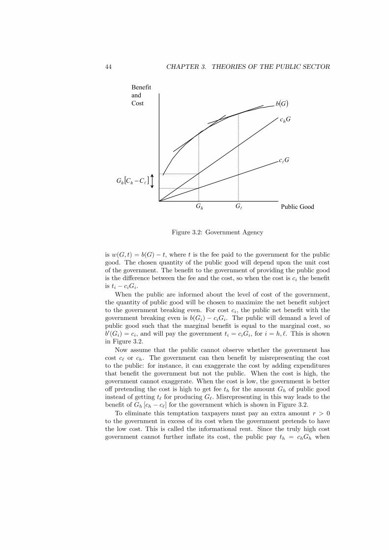
44 CHAPTER 3. THEORIES OF THE PUBLIC SECTOR
Public Good
Benefitand Cost
lGhG
[ ]lCCG hh −
( )Gb
Gch
Gcl
Figure 3.2: Government Agency
is w(G, t) = b(G) − t, where t is the fee paid to the government for the publicgood. The chosen quantity of the public good will depend upon the unit costof the government. The benefit to the government of providing the public goodis the difference between the fee and the cost, so when the cost is ci the benefitis ti − ciGi.When the public are informed about the level of cost of the government,
the quantity of public good will be chosen to maximize the net benefit subjectto the government breaking even. For cost ci, the public net benefit with thegovernment breaking even is b(Gi) − ciGi. The public will demand a level ofpublic good such that the marginal benefit is equal to the marginal cost, sob0(Gi) = ci, and will pay the government ti = ciGi, for i = h, `. This is shownin Figure 3.2.Now assume that the public cannot observe whether the government has
cost c` or ch. The government can then benefit by misrepresenting the costto the public: for instance, it can exaggerate the cost by adding expendituresthat benefit the government but not the public. When the cost is high, thegovernment cannot exaggerate. When the cost is low, the government is betteroff pretending the cost is high to get fee th for the amount Gh of public goodinstead of getting t` for producing G`. Misrepresenting in this way leads to thebenefit of Gh [ch − c`] for the government which is shown in Figure 3.2.To eliminate this temptation taxpayers must pay an extra amount r > 0
to the government in excess of its cost when the government pretends to havethe low cost. This is called the informational rent. Since the truly high costgovernment cannot further inflate its cost, the public pay th = chGh when
3.4. EXCESSIVE GOVERNMENT 45
the government reports a high cost. If the reported cost is low, the taxpayersdemand the amount G` of public good defined by b0(G`) = c` and pay thegovernment t` = c`G` + r where r is exactly the extra revenue the governmentcould have made if it had pretended to have high cost. To give a governmentwith a low cost just enough revenue to offset its temptation to pretend to havehigher cost it is necessary that r = [ch − cl]Gh. This is the rent required toinduce truthful revelation of the cost and have the provision of the public goodequal to that when the public are fully informed.It is possible for the taxpayers to reduce this excess payment by demanding
that the high-cost government supply less than it would with full information.Assume that cost is low with probability p` and high with probability ph = 1−p`.By maximizing their expected benefit subject to the government telling thetruth, it can be shown that revelation can be obtained at the least cost bydemanding an amount Gh of public services defined by
b0(Gh) = ch +p`
1− p` [ch − c`]. (3.10)
This quantity is lower than that with full information. The distortion of thequantity demanded from the high-cost government results from a simple cost-benefit argument. It trades off the benefit of reducing the rent, which is propor-tional to the cost difference [ch − c`], and the probability that the governmentis of the low cost type p`, against the cost of imposing the distortion of thequantity on the high-cost government with probability 1− p`.Therefore if the government is truly low cost it need not be given the high
tax, but in order to eliminate the temptation for cost inflation taxpayers haveto provide the government just enough of the rent as a reward for reportingtruthfully when its cost of public services is low. The ability of the governmentto misrepresent its costs therefore allows it to earn rents and can distort thelevel of provision.
3.4.6 Cost Diffusion
The last explanation we present for the possibility of excessively large govern-ment is the common resource problem. The idea is that spending authoritiesare dispersed while the treasury has the responsibility of collecting enough rev-enue to balance the overall budget. Each of the spending authorities has itsown spending priorities, with few consideration for others’ priorities, which itcan better meet by raiding the overall budget. This is the common resourceproblem, just like that of several oil companies tapping into a common poolunderground or fishermen netting in a single lake. In all cases it leads to excesspressure on the common resource. From this perspective a single committeewith expenditure authority would have a much better sense of the opportunitycost of public funds, and can better compare the merits of alternative propos-als, than the actual dispersed spending authorities. The current trend towardfederalism and devolution aggravates this common pool problem. The reasonis essentially that each district can impose projects whose cost is shared by all
46 CHAPTER 3. THEORIES OF THE PUBLIC SECTOR
other districts and so they support higher size projects than they would if theyhad to cover the full costs. We discuss in more detail the various aspects offederalism in Chapter 19.The problem can also be traced down to the individual level. Consider public
services like pensions, health care, schools and infrastructure work like bridges,roads and railtracks. It is clear that for these public services, and in fact manyothers, the government does not charge the direct users the full marginal cost,but subsidizes these activities partly or wholly from tax revenues. There is anobvious equity concern behind this fact. But it is then also natural that users whodo not bear the full cost will support more public services than they would if theyhad to cover the full cost. The same argument applies in the opposite directionwhen contemplating some cut in public spending: contributors who are asked tomake concessions are concentrated and possibly organized through a lobby withlarge per capita benefits from continued provision of specific public services.In contrast the beneficiaries of downsizing public spending, the taxpayers as awhole, are diffuse with small per capita stakes. This makes it less likely thatthey can offer organized support for the reform. To sum up, many public servicesare characterized by the concentration of benefits to a small group of users orrecipients and the diffusion of costs to the large group of taxpayers. This resultsin biases toward continuous demand for more public spending.
3.5 Conclusions
This chapter has provided a number of theories of public sector growth whichhave been designed to explain the growth patterns exhibited in Chapter 2. Eachof these has some points to commend it but none is entirely persuasive. It is fairto say that all provide a partial insight and have some element of truth. A moregeneral story drawing together the full set of components, including the ratcheteffect, income effect, political process, production technology and bureaucracy,would have much in its favor. This would be especially so if combined with thevoting models of the next chapter.The bureaucracy models are particularly attractive since they show how
economic analysis can be applied to what appears to be a non-economic problem.In doing so they generate an interesting conclusion which casts doubt on theefficiency of government. This illustrates how the method of economic reasoningcan be applied to understand the outcome of what is at first sight a non-economicproblem.The perennial question of whether the government has grown too large is
difficult to answer. The reason is that the government is both complementary tothe market and a competitor of the market. As a major employer, the govern-ment competes with any business looking to hire talented people. The possibilitythat the best and brightest become public officials and politicians, rather thanentrepreneurs, is considered by many as very costly to society because they areseen as devoting their talents to taking wealth from others rather than creatingit. When people pay taxes, they have less money to spend on other goods and
3.5. CONCLUSIONS 47
services provided by the market. Likewise when the government borrows money,it competes with companies looking to raise capital. In some areas like healthcare and education, public and private services are competing with each other.But at the same time, the government also serves as useful complement to everybusiness activity by providing basic infrastructure and civil order. Every busi-ness depends on the government for things like protection of life and property,a transportation network, civil courts, a stable currency, and so on. Withoutthese things, people couldn’t do business. Finally whether an activity is carriedout in the public sector or the private sector is itself endogenous.As in architecture, the functions suggest the form. Take the example of
education where the goals are multiple (literacy, vocational skills, citizenship,equality of chance, preparation for life) and not precisely measurable and severalstakeholders are involved (parents, employers, students, teachers, taxpayers)with possibly conflicting preferences. It is not immediately clear that the marketwith its single-minded focus can cope adequately with all these aspects, and therisk is that the market could bias the activity toward dimensions that mattermore for profit-making. For example, teaching various skills to the most ablestudents may conflict with teaching the same things to the least able ones. Inthe United States voucher programs are creating more competition from privateschools but for the vast majority of the population, the local public schoolremains the monopoly provider. The net result of switching to the market canwell be detrimental for the society as a whole. To sum up, there is potential forthe government to step in when the market is likely to fail.
Further ReadingAn account of Wagner’s law can be found in:Bird, R.M. (1971) ”Wagner’s law of expanding state activity”, Public Fi-
nance, 26, 1 - 26.The classic study of public sector growth is:Peacock, A.K. and Wiseman, J. (1961) The Growth of Public Expenditure
in the UK (Princeton: Princeton University Press).An non-technical account on corruption and government is:Rose-Ackerman, S. (1999), Corruption and Government: Causes, Conse-
quences and Reform (Cambridge: Cambridge University Press).The theory of bureaucracy was first developed in:Niskanen, W.A. (1974) ”Non-market decision making: the peculiar eco-
nomics of bureaucracy”, American Economic Review, 58, 293 - 305.A fascinating book on bureaucracy from a political scientist is:Wilson, J.Q., (1989) Bureaucracy: What Government Agencies Do and Why
They Do It (New York: Basic Books).The political theory of the size of the government is based on:Meltzer, A. and Richard, S. (1981) A rational theory of the size of govern-
ment, Journal of Political Economy 89, 914-27The main reference on government agency is:Laffont, J.-J. (2001) Incentives and Political Economy (Oxford: Oxford Uni-
versity Press)

48 CHAPTER 3. THEORIES OF THE PUBLIC SECTOR
Chapter 4
Voting
4.1 Introduction
Voting is the most commonly employed method of resolving a diversity of viewsor eliciting expressions of preference. It is used to determine the outcome ofelections from local to supra-national level. Within organizations, voting deter-mines who is elected to committees and it governs the decision-making of thosecommittees. Voting is a universal tool that is encountered in all spheres of life.The prevalence of voting, its use in electing governments, and its use by thosegovernments elected to reach decisions, is the basis for the considerable interestin the properties of voting.The natural question to ask of voting is whether it is a good method of
making decisions. There are two major properties to look for in a good method.First is the success or failure of the method in achieving a clear-cut decision.Second is the issue of whether voting always produces an outcome that is effi-cient. Voting would be of limited value if it frequently left the choice of outcomeunresolved or lead to a choice that was clearly inferior to other alternatives.Whether voting satisfies these properties is shown to be somewhat dependentupon the precise method of voting adopted. Ordinary majority voting is veryfamiliar but it is only one amongst a number of ways of voting. Several of thesemethods of voting will be introduced and analyzed alongside the standard formof majority voting.
4.2 Stability
Voting is an example of collective choice - the process through which a group(or collective) reaches a decision. A major issue of collective choice is stability.By stability we mean the tendency of the decision-making process to eventuallyreach a settled conclusion, and not to keep jumping around between alternatives.We begin this chapter by a simple illustration of the central fact that whenyou have a large group of people, with conflicting preferences, stability is not
49
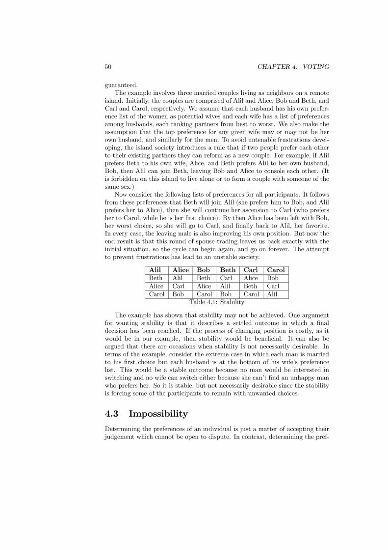
50 CHAPTER 4. VOTING
guaranteed.The example involves three married couples living as neighbors on a remote
island. Initially, the couples are comprised of Alil and Alice, Bob and Beth, andCarl and Carol, respectively. We assume that each husband has his own prefer-ence list of the women as potential wives and each wife has a list of preferencesamong husbands, each ranking partners from best to worst. We also make theassumption that the top preference for any given wife may or may not be herown husband, and similarly for the men. To avoid untenable frustrations devel-oping, the island society introduces a rule that if two people prefer each otherto their existing partners they can reform as a new couple. For example, if Alilprefers Beth to his own wife, Alice, and Beth prefers Alil to her own husband,Bob, then Alil can join Beth, leaving Bob and Alice to console each other. (Itis forbidden on this island to live alone or to form a couple with someone of thesame sex.)Now consider the following lists of preferences for all participants. It follows
from these preferences that Beth will join Alil (she prefers him to Bob, and Alilprefers her to Alice), then she will continue her ascension to Carl (who prefersher to Carol, while he is her first choice). By then Alice has been left with Bob,her worst choice, so she will go to Carl, and finally back to Alil, her favorite.In every case, the leaving male is also improving his own position. But now theend result is that this round of spouse trading leaves us back exactly with theinitial situation, so the cycle can begin again, and go on forever. The attemptto prevent frustrations has lead to an unstable society.
Alil Alice Bob Beth Carl CarolBeth Alil Beth Carl Alice BobAlice Carl Alice Alil Beth CarlCarol Bob Carol Bob Carol Alil
Table 4.1: Stability
The example has shown that stability may not be achieved. One argumentfor wanting stability is that it describes a settled outcome in which a finaldecision has been reached. If the process of changing position is costly, as itwould be in our example, then stability would be beneficial. It can also beargued that there are occasions when stability is not necessarily desirable. Interms of the example, consider the extreme case in which each man is marriedto his first choice but each husband is at the bottom of his wife’s preferencelist. This would be a stable outcome because no man would be interested inswitching and no wife can switch either because she can’t find an unhappy manwho prefers her. So it is stable, but not necessarily desirable since the stabilityis forcing some of the participants to remain with unwanted choices.
4.3 ImpossibilityDetermining the preferences of an individual is just a matter of accepting theirjudgement which cannot be open to dispute. In contrast, determining the pref-

4.3. IMPOSSIBILITY 51
erences of a group of people is not a simple matter. And that’s what socialchoice theory (including voting as a one particular method) is all about. Socialchoice takes a given set of individual preferences and tries to aggregate theminto a social preference.The central result of the theory of social choice, Arrow’s Impossibility The-
orem, says that there is no way to devise a collective decision-making processthat satisfies a few commonsense requirements and works in all circumstances.If there are only two options, majority voting works just fine, but with morethan two we can get into trouble. Despite all the talk about the ”will of thepeople”, it is not easy - in fact the theorem proves it impossible - to always de-termine what that will is. This is the remarkable fact of Arrow’s ImpossibilityTheorem.Before presenting the theorem, a taste of it can be obtained with the simplest
case of three voters with the following (conflicting) rankings over three options.
Voter 1 Voter 2 Voter 3a c bb a cc b aTable 4.2: Condorcet Paradox
Every voter has preferences over the three options which are transitive; forexample voter 1 prefers a to b to c, and therefore a to c. As individuals, thevoters are entirely self-consistent in their preferences. Now suppose we usemajority rule to select of one of these options. We see that two out of threevoters prefer a to b, while two out of three prefer b to c, and two out of threeprefer c to a. At the collective level there is a cycle in preference and no decisionis possible. We say that such preferences are intransitive, meaning that thatthe preference for a over b and for b over c does not imply a is preferred to c.As the example shows, intransitivity of group preferences can arise even whenindividual preferences are transitive. This generation of social intransitivityfrom individual transitivity is called the Condorcet Paradox.The general problem addressed by Arrow in 1951 was to seek a way of ag-
gregating individual rankings over options into a collective ranking. In doing so,difficulties such as the Condorcet paradox had to be avoided. Arrow’s approachwas to start from a set of requirements that a collective ranking must satisfyand then consider if any ranking could be found that met them all.
Condition 1 (I) Independence of Irrelevant Alternatives. Adding new optionsshould not affect the initial ranking of the old options; so the collective rankingover the old options should be unchanged.
For example, assume the group prefers option A to option C, and the newoption B is introduced. Wherever it fits into each individual’s ranking, Condi-tion I requires that the group preference should not switch to C over A. Theymay like or dislike the new option B, but their relative preferences for other
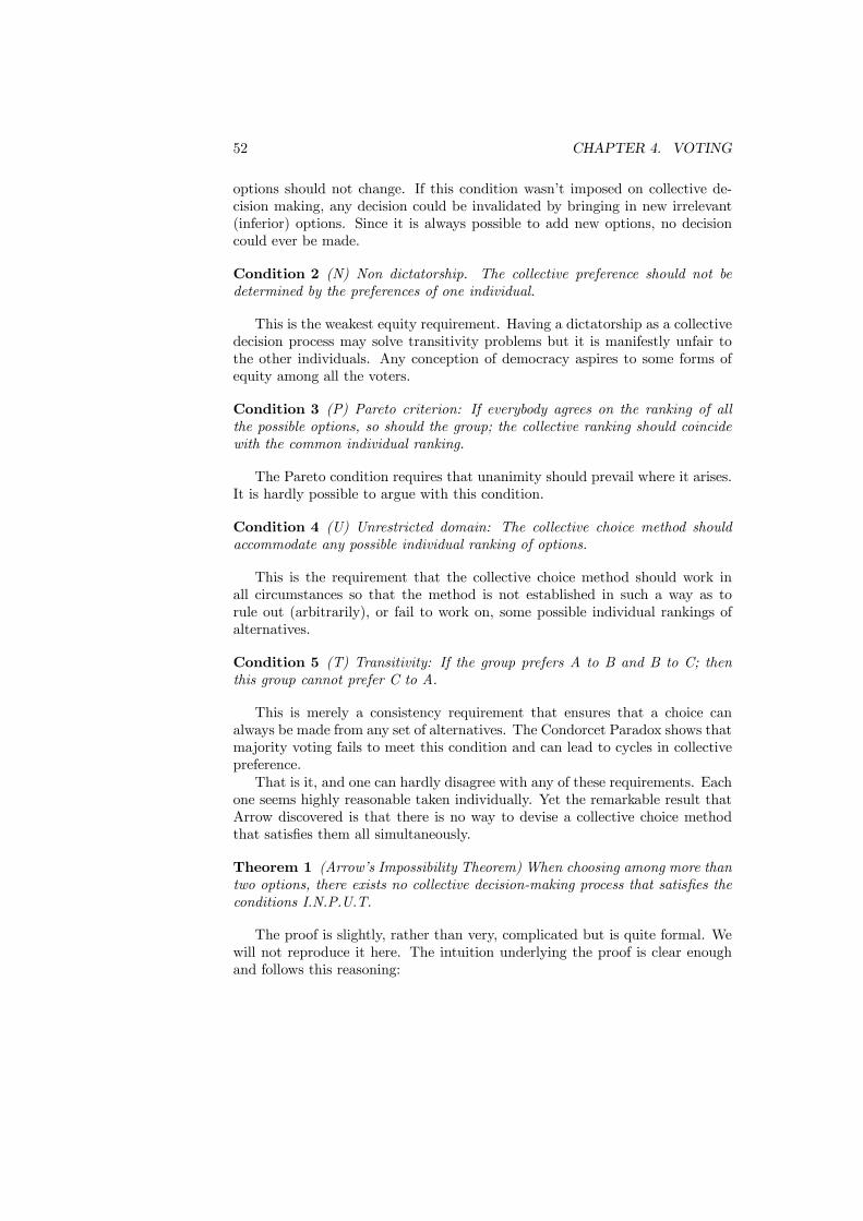
52 CHAPTER 4. VOTING
options should not change. If this condition wasn’t imposed on collective de-cision making, any decision could be invalidated by bringing in new irrelevant(inferior) options. Since it is always possible to add new options, no decisioncould ever be made.
Condition 2 (N) Non dictatorship. The collective preference should not bedetermined by the preferences of one individual.
This is the weakest equity requirement. Having a dictatorship as a collectivedecision process may solve transitivity problems but it is manifestly unfair tothe other individuals. Any conception of democracy aspires to some forms ofequity among all the voters.
Condition 3 (P) Pareto criterion: If everybody agrees on the ranking of allthe possible options, so should the group; the collective ranking should coincidewith the common individual ranking.
The Pareto condition requires that unanimity should prevail where it arises.It is hardly possible to argue with this condition.
Condition 4 (U) Unrestricted domain: The collective choice method shouldaccommodate any possible individual ranking of options.
This is the requirement that the collective choice method should work inall circumstances so that the method is not established in such a way as torule out (arbitrarily), or fail to work on, some possible individual rankings ofalternatives.
Condition 5 (T) Transitivity: If the group prefers A to B and B to C; thenthis group cannot prefer C to A.
This is merely a consistency requirement that ensures that a choice canalways be made from any set of alternatives. The Condorcet Paradox shows thatmajority voting fails to meet this condition and can lead to cycles in collectivepreference.That is it, and one can hardly disagree with any of these requirements. Each
one seems highly reasonable taken individually. Yet the remarkable result thatArrow discovered is that there is no way to devise a collective choice methodthat satisfies them all simultaneously.
Theorem 1 (Arrow’s Impossibility Theorem) When choosing among more thantwo options, there exists no collective decision-making process that satisfies theconditions I.N.P.U.T.
The proof is slightly, rather than very, complicated but is quite formal. Wewill not reproduce it here. The intuition underlying the proof is clear enoughand follows this reasoning:
4.4. MAJORITY RULE 53
(i) The unrestricted domain condition allows for preferences such that nooption is unanimously preferred.(ii) The independence of irrelevant alternatives forces the social ranking over
any two options to be based exclusively on the individual preferences over thosetwo options only.(iii) From the Condorcet Paradox, we know that a cycle can emerge from
three successive pair-wise comparisons.(iv) The transitivity requirement forces a choice among the three options.(v) The only method for deciding must give one individual all the power,
thus contradicting the non-dictatorship requirement.The implication of Arrow’s Impossibility Theorem is that any search for a
“perfect” method of collective decision-making is doomed to failure. Whateverprocess is devised, a situation can be constructed in which it will fail to deliveran outcome that satisfies one or more of the conditions I.N.P.U.T. As a conse-quence, all collective decision-making must make the most of imperfect decisionrules.
4.4 Majority Rule
In any situation involving only two options, majority rule simply requires thatthe option with the majority of votes is chosen. Unless unanimity is possible,asking that the few give way to the many is a very natural alternative to dic-tatorship. The process of majority voting is now placed into context and itsimplications determined.
4.4.1 May’s Theorem
Non-dictatorship is a very weak interpretation of the principles of democracy. Awidely held view is that democracy should treat all the voters in the same way.This symmetry requirement is called Anonymity. It requires that permutingthe names of any two individuals does not change the group preference. ThusAnonymity implies that there cannot be any dictator. Another natural symme-try requirement is that the collective decision-making process should treat allpossible options alike. No apparent bias in favor of one option should be intro-duced. This symmetric treatment of the various options is called Neutrality.Now a fundamental result due to May is that majority rule is the obvious
way to implement these principles of democracy (Anonymity and Neutrality)in social decision-making when only two options are considered at a time. Thetheorem asserts that majority rule is the unique way of doing so if the conditionsof Decisiveness (i.e., the social decision rule must pick a winner) and PositiveResponsiveness (i.e., increasing the vote for the winning option should not leadto the declaration of another option the winner) are also imposed.
Theorem 2 (May’s theorem) When choosing among only two options, thereis only one collective decision-making process that satisfies the requirements of

54 CHAPTER 4. VOTING
Anonymity, Neutrality, Decisiveness and Positive Responsiveness. This processis majority rule.
Simple majority rule is the best social choice procedure if we consider onlytwo options at a time. Doing so is not at all unusual in the real world. Forinstance, when a vote is called in a legislative assembly there are usually onlytwo possible options: to approve or to reject some specific proposal that is onthe floor. Also in a situation of two-party political competition, voters againface a binary choice. Therefore interest in other procedures arises only whenthere are more than two options to consider.
4.4.2 Condorcet Winner
When there are only two options, majority rule is a simple and compellingmethod for social choice. When there are more than two options to be consideredat a time, we can still apply the principle of majority voting by using binaryagendas which allow us to reduce the problem of choosing among many optionsto a sequence of votes each of which is binary.For example, one simple binary agenda for choosing among the three options
{a, b, c} in the Condorcet Paradox is as follows. First, there is a vote on a againstb. Then, the winner of this first vote is opposed to c. The winner of this secondvote is the chosen option. The most famous pair-wise voting method is theCondorcet method. It consists of a complete round-robin of majority votes,opposing each option against all of the others. The option which defeats allothers in pair-wise majority voting is called a Condorcet winner, after Condorcetsuggested that such an option should be declared the winner. That is, using to denote majority preference, a Condorcet winner is an option x such thatx  y for every other option y in the set of possible options X.The problem is that the existence of a Condorcet winner requires very special
configurations of individual preferences. For instance, with the preferences givenin the Condorcet paradox, there is no Condorcet winner. So a natural questionto ask is under what conditions a Condorcet winner does exist.
4.4.3 Median Voter Theorems
When the policy space is one-dimensional, sufficient (but not necessary) con-ditions for the existence of a Condorcet winner are given by the Median VoterTheorems. One version of these theorems refers to single-peaked preferences,while the other version refers to single-crossing preferences. The two conditionsof single-peaked and single-crossing are logically independent but both condi-tions give the same conclusion that the median position is a Condorcet winner.As an example of single-peaked preferences, consider a population of con-
sumers who are located at equally-spaced positions along a straight road. Alongthis road there is to be located a bus stop. It is assumed that all consumerswould prefer this to be located as close as possible to their own location. If the
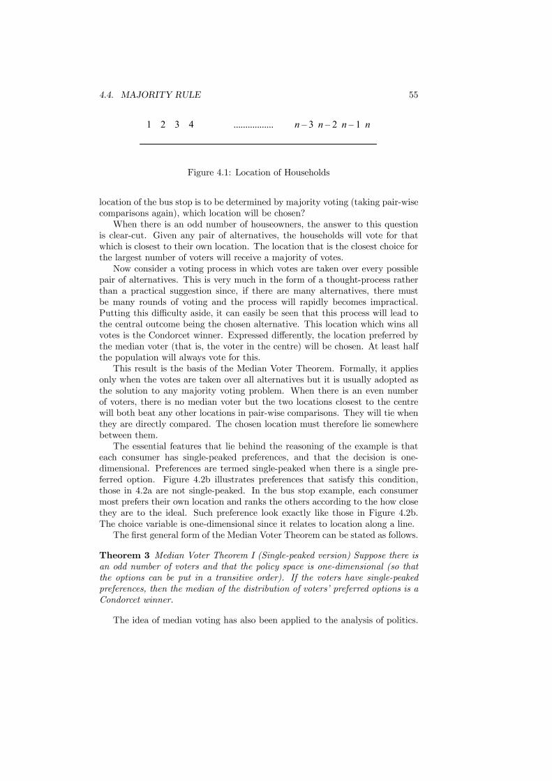
4.4. MAJORITY RULE 55
1 2 3 4 ................. n – 3 n – 2 n – 1 n
Figure 4.1: Location of Households
location of the bus stop is to be determined by majority voting (taking pair-wisecomparisons again), which location will be chosen?When there is an odd number of houseowners, the answer to this question
is clear-cut. Given any pair of alternatives, the households will vote for thatwhich is closest to their own location. The location that is the closest choice forthe largest number of voters will receive a majority of votes.Now consider a voting process in which votes are taken over every possible
pair of alternatives. This is very much in the form of a thought-process ratherthan a practical suggestion since, if there are many alternatives, there mustbe many rounds of voting and the process will rapidly becomes impractical.Putting this difficulty aside, it can easily be seen that this process will lead tothe central outcome being the chosen alternative. This location which wins allvotes is the Condorcet winner. Expressed differently, the location preferred bythe median voter (that is, the voter in the centre) will be chosen. At least halfthe population will always vote for this.This result is the basis of the Median Voter Theorem. Formally, it applies
only when the votes are taken over all alternatives but it is usually adopted asthe solution to any majority voting problem. When there is an even numberof voters, there is no median voter but the two locations closest to the centrewill both beat any other locations in pair-wise comparisons. They will tie whenthey are directly compared. The chosen location must therefore lie somewherebetween them.The essential features that lie behind the reasoning of the example is that
each consumer has single-peaked preferences, and that the decision is one-dimensional. Preferences are termed single-peaked when there is a single pre-ferred option. Figure 4.2b illustrates preferences that satisfy this condition,those in 4.2a are not single-peaked. In the bus stop example, each consumermost prefers their own location and ranks the others according to the how closethey are to the ideal. Such preference look exactly like those in Figure 4.2b.The choice variable is one-dimensional since it relates to location along a line.The first general form of the Median Voter Theorem can be stated as follows.
Theorem 3 Median Voter Theorem I (Single-peaked version) Suppose there isan odd number of voters and that the policy space is one-dimensional (so thatthe options can be put in a transitive order). If the voters have single-peakedpreferences, then the median of the distribution of voters’ preferred options is aCondorcet winner.
The idea of median voting has also been applied to the analysis of politics.
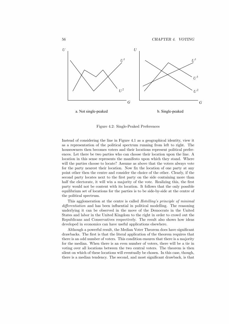
56 CHAPTER 4. VOTING
a. Not single-peaked b. Single-peaked
U
1U
2U
U
1U
2U
3U
G G
Figure 4.2: Single-Peaked Preferences
Instead of considering the line in Figure 4.1 as a geographical identity, view itas a representation of the political spectrum running from left to right. Thehouseowners then becomes voters and their locations represent political prefer-ences. Let there be two parties who can choose their location upon the line. Alocation in this sense represents the manifesto upon which they stand. Wherewill the parties choose to locate? Assume as above that the voters always votefor the party nearest their location. Now fix the location of one party at anypoint other then the centre and consider the choice of the other. Clearly, if thesecond party locates next to the first party on the side containing more thanhalf the electorate, it will win a majority of the vote. Realizing this, the firstparty would not be content with its location. It follows that the only possibleequilibrium set of locations for the parties is to be side-by-side at the centre ofthe political spectrum.This agglomeration at the centre is called Hotelling’s principle of minimal
differentiation and has been influential in political modelling. The reasoningunderlying it can be observed in the move of the Democrats in the UnitedStates and labor in the United Kingdom to the right in order to crowd out theRepublicans and Conservatives respectively. The result also shows how ideasdeveloped in economics can have useful applications elsewhere.Although a powerful result, the Median Voter Theorem does have significant
drawbacks. The first is that the literal application of the theorem requires thatthere is an odd number of voters. This condition ensures that there is a majorityfor the median. When there is an even number of voters, there will be a tie invoting over all locations between the two central voters. The theorem is thensilent on which of these locations will eventually be chosen. In this case, though,there is a median tendency. The second, and most significant drawback, is that
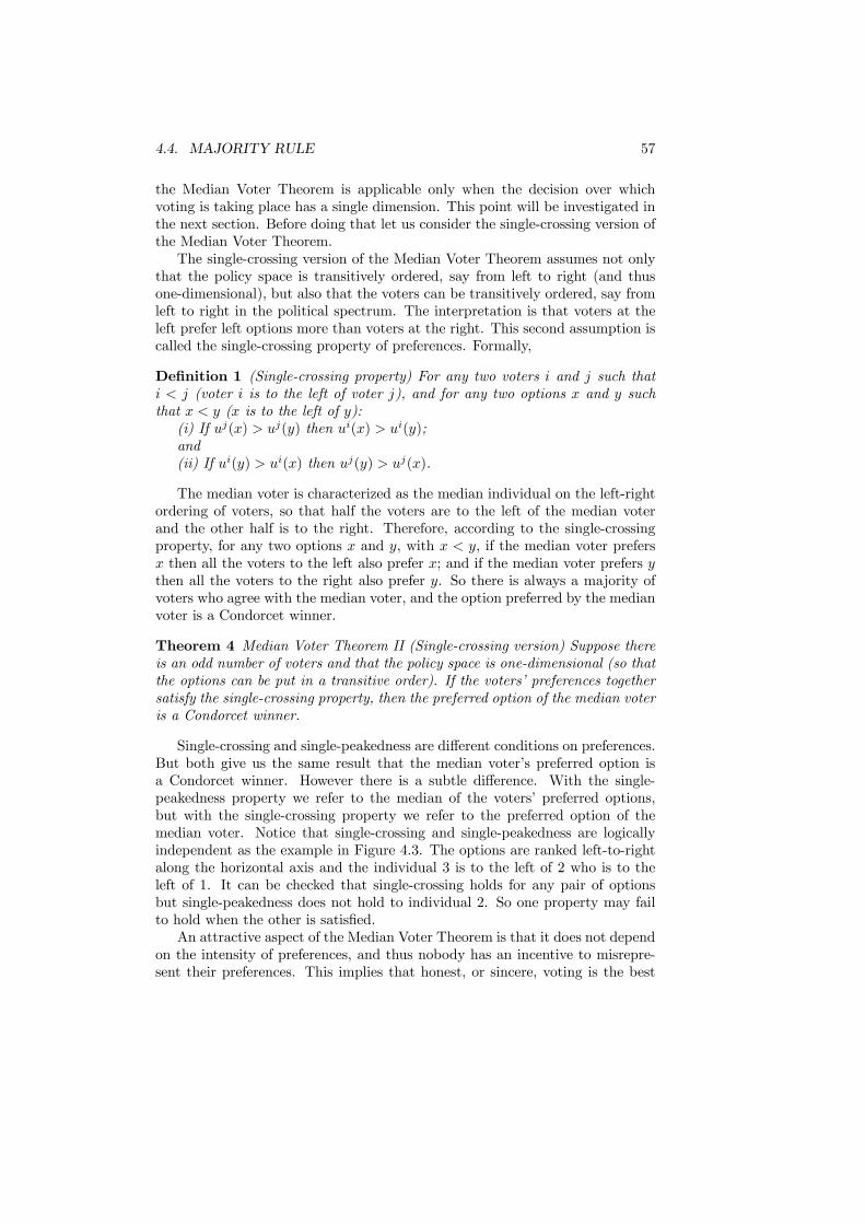
4.4. MAJORITY RULE 57
the Median Voter Theorem is applicable only when the decision over whichvoting is taking place has a single dimension. This point will be investigated inthe next section. Before doing that let us consider the single-crossing version ofthe Median Voter Theorem.The single-crossing version of the Median Voter Theorem assumes not only
that the policy space is transitively ordered, say from left to right (and thusone-dimensional), but also that the voters can be transitively ordered, say fromleft to right in the political spectrum. The interpretation is that voters at theleft prefer left options more than voters at the right. This second assumption iscalled the single-crossing property of preferences. Formally,
Definition 1 (Single-crossing property) For any two voters i and j such thati < j (voter i is to the left of voter j), and for any two options x and y suchthat x < y (x is to the left of y):(i) If uj(x) > uj(y) then ui(x) > ui(y);and(ii) If ui(y) > ui(x) then uj(y) > uj(x).
The median voter is characterized as the median individual on the left-rightordering of voters, so that half the voters are to the left of the median voterand the other half is to the right. Therefore, according to the single-crossingproperty, for any two options x and y, with x < y, if the median voter prefersx then all the voters to the left also prefer x; and if the median voter prefers ythen all the voters to the right also prefer y. So there is always a majority ofvoters who agree with the median voter, and the option preferred by the medianvoter is a Condorcet winner.
Theorem 4 Median Voter Theorem II (Single-crossing version) Suppose thereis an odd number of voters and that the policy space is one-dimensional (so thatthe options can be put in a transitive order). If the voters’ preferences togethersatisfy the single-crossing property, then the preferred option of the median voteris a Condorcet winner.
Single-crossing and single-peakedness are different conditions on preferences.But both give us the same result that the median voter’s preferred option isa Condorcet winner. However there is a subtle difference. With the single-peakedness property we refer to the median of the voters’ preferred options,but with the single-crossing property we refer to the preferred option of themedian voter. Notice that single-crossing and single-peakedness are logicallyindependent as the example in Figure 4.3. The options are ranked left-to-rightalong the horizontal axis and the individual 3 is to the left of 2 who is to theleft of 1. It can be checked that single-crossing holds for any pair of optionsbut single-peakedness does not hold to individual 2. So one property may failto hold when the other is satisfied.An attractive aspect of the Median Voter Theorem is that it does not depend
on the intensity of preferences, and thus nobody has an incentive to misrepre-sent their preferences. This implies that honest, or sincere, voting is the best
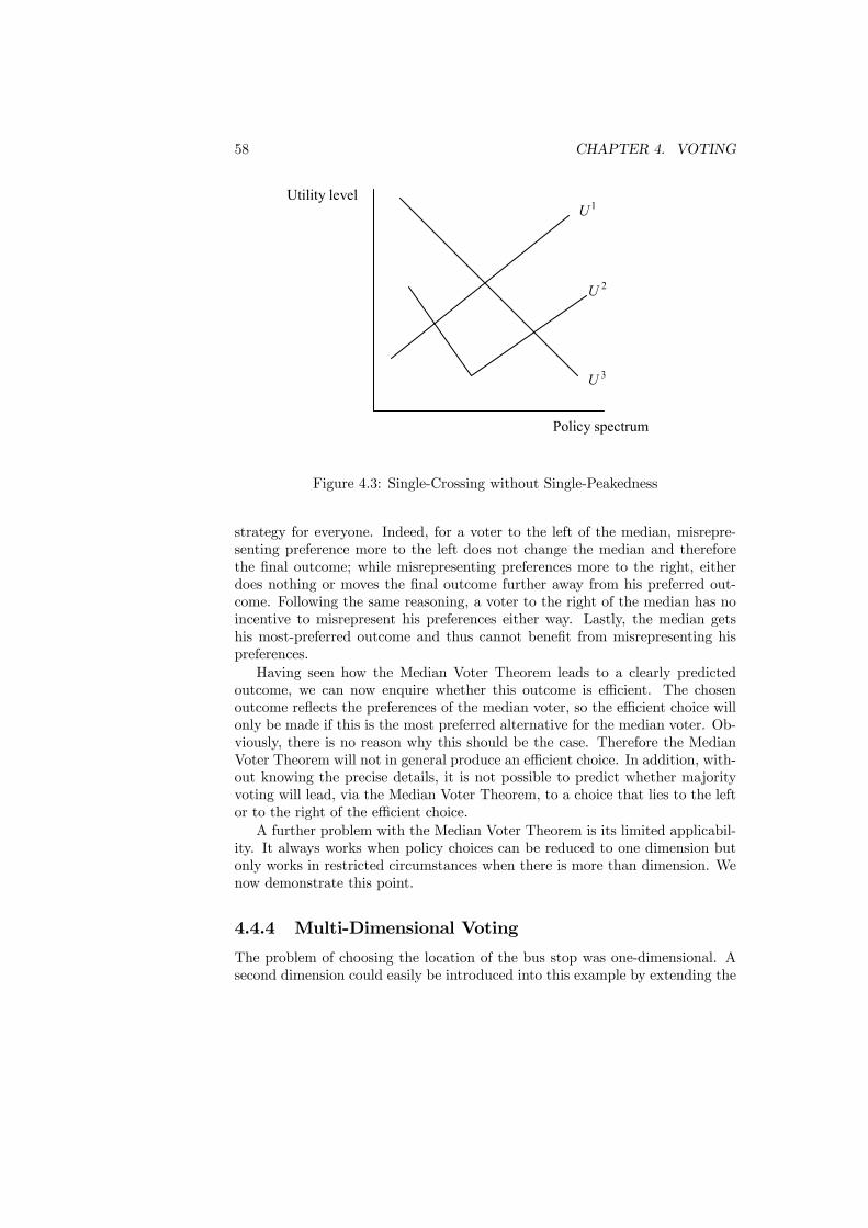
58 CHAPTER 4. VOTING
Policy spectrum
Utility level1U
2U
3U
Figure 4.3: Single-Crossing without Single-Peakedness
strategy for everyone. Indeed, for a voter to the left of the median, misrepre-senting preference more to the left does not change the median and thereforethe final outcome; while misrepresenting preferences more to the right, eitherdoes nothing or moves the final outcome further away from his preferred out-come. Following the same reasoning, a voter to the right of the median has noincentive to misrepresent his preferences either way. Lastly, the median getshis most-preferred outcome and thus cannot benefit from misrepresenting hispreferences.Having seen how the Median Voter Theorem leads to a clearly predicted
outcome, we can now enquire whether this outcome is efficient. The chosenoutcome reflects the preferences of the median voter, so the efficient choice willonly be made if this is the most preferred alternative for the median voter. Ob-viously, there is no reason why this should be the case. Therefore the MedianVoter Theorem will not in general produce an efficient choice. In addition, with-out knowing the precise details, it is not possible to predict whether majorityvoting will lead, via the Median Voter Theorem, to a choice that lies to the leftor to the right of the efficient choice.A further problem with the Median Voter Theorem is its limited applicabil-
ity. It always works when policy choices can be reduced to one dimension butonly works in restricted circumstances when there is more than dimension. Wenow demonstrate this point.
4.4.4 Multi-Dimensional Voting
The problem of choosing the location of the bus stop was one-dimensional. Asecond dimension could easily be introduced into this example by extending the

4.4. MAJORITY RULE 59
Location
Time1
2
32x
1x
3x• •
•
Figure 4.4: Single-Peakedness in Multi-Dimensions
vote to determine both the location of the bus stop and the time at which thebus is to arrive. The important observation for majority voting is that whenthis extension is made there is no longer any implication that single-peakedpreferences will lead to a transitive ranking of alternatives.This finding can be illustrated by considering the consumer’s indifference
curves over the two-dimensional space of location and time. To do this, considerlocation as the horizontal axis and time as the vertical axis with the origin at thefar-left of the street and midnight respectively. The meaning of single-peakedpreferences in this situation is that a consumer has a most-preferred location andany move in a straight line away from this must lead to a continuous decreasein utility. This is illustrated in Figure 4.4 where xi denotes the most preferredlocation of i and the oval around this point is one of the consumer’s indifferencecurves.Using this machinery, it is now possible to show that the Median Voter The-
orem can fail with majority voting failing to generate a transitive outcome. Thethree voters, denoted 1, 2 and 3, have preferred locations x1, x2 and x3. Assumethat voting is to decide which of these three locations is to be chosen (this is notnecessary for the argument as will become clear but it does simplify it). Therankings of the three consumers of these alternatives in Table 4.3 are consistentwith the preferences represented by the ovals in Figure 4.4. Contrasting theseto Table 4.2, one can see immediately that these are exactly the rankings thatgenerate an intransitive social ordering through majority voting. Consequently,even though preferences are single peaked, the social ordering is intransitive andthe Median Voter Theorem fails. Hence, the theorem does not extend beyondone-dimensional choice problems.

60 CHAPTER 4. VOTING
Voter 1 Voter 2 Voter 3x1 x2 x3x2 x3 x1x3 x1 x2
Table 4.3: Rankings
4.4.5 Agenda Manipulation
In a situation in which there is no Condorcet winner, the door is opened toagenda manipulation. This is because changing the agenda, meaning the orderin which the votes over pairs of alternatives are taken, can change the votingoutcome. Thus the agenda-setter may have substantial power to influence thevoting outcome. To determine the degree of the agenda-setter’s power, we mustfind the set of outcomes that can be achieved through agenda manipulations.To see how agenda-setting can be effective, suppose there are three voters
with preferences as in the Condorcet paradox (described in Figure 4.2). Thenthere is a majority (voters 1 and 2) who prefer a over b, there is a majority(voters 2 and 3) who prefer c over a, and there is a majority (voters 1 and 3)who prefer b over c. Given these voters’ preferences, what will be the outcome ofdifferent binary agendas? The answer is that when voters vote sincerely, then itis possible to set the agenda so that any of the three options can be the ultimatewinner. For example, to obtain option a as the final outcome it suffices to firstoppose b against c (knowing that b will defeat c) and then at the second stage tooppose the winner b against a (knowing that a will defeat b). Similarly, to getb as the final outcome, it suffices to oppose a against c at the first stage (giventhat c will defeat a) and then the winner c against b (given that b will defeatc). These observations show how the choice of agenda can affect the outcome.This reasoning is based on the assumption that voters vote sincerely. How-
ever, the voters may respond to agenda manipulation by misrepresenting theirpreferences. That is, they may vote strategically. Voters can choose to vote foroptions that are not actually their most-preferred options if they believe thatsuch behavior in the earlier ballots can affect the final outcome in their favor.For example, if we first oppose b against c then voter 2 may vote for c ratherthan b. This ensures that c then goes on to oppose a. Option c will then win, anoutcome preferred by voter 2 to the victory for a that emerges with sincere vot-ing. So, voters may not vote for their preferred option in order to prevent theirworst option from winning. The question is then how strategic voting affects theset of options that could be achieved by agenda-manipulation. Such outcomesare called sophisticated outcomes of binary agendas, because voters anticipatewhat the ultimate result will be, for a given agenda, and vote optimally in earlierstages.A remarkable result, due to Miller, is that strategic voting (relative to sincere
voting) does not alter the set of outcomes that can be achieved by agenda-manipulation when the agenda-setter can design any binary-agendas, providedonly that every option must be included in the agenda. Miller called the setthat can be achieved the top cycle.

4.4. MAJORITY RULE 61
[b]
[b][c]
ba
bcca
Figure 4.5: Binary Agenda
When there exists a Condorcet winner, the top cycle reduces to that singleoption. With preferences as in the Condorcet Paradox, the top cycle contains allthree options {a, b, c}. For example, option b can be obtained by the followingagenda (different from the agenda under sincere voting): at the first stage, a isopposed to b, then the winner is opposed to c. This binary agenda is representedin Figure 4.5.
The agenda begins at the top, and at each stage the voters must vote withthe effect of moving down the agenda tree along the branch that will defeatthe other with a sophisticated majority vote. To resolve this binary agenda,sophisticated voters must anticipate the outcome of the second stage and voteoptimally in the first stage. Either the second stage involves c against a, andthus c will beat a, or the second stage involves c against b and thus b will beatc. So the voters should anticipate that in the first stage voting for a will infact lead to the ultimate outcome c while voting for b will lead to the ultimateoutcome b (as displayed in parentheses). So in voting for a in the first stagethey vote in effect for c while voting for b in the first stage effectively leads tothe choice of b as the ultimate outcome. Because b is preferred by a majority toc, it follows that a majority of voters should vote for b at the first stage (eventhough a majority prefers a over b).
The problem with the top cycle is that it can contain options that are Paretodominated. To see this, suppose preferences are as in the Condorcet paradoxand let us add a fourth alternative d that falls just below c in every individual’spreference. The resulting rankings are give in Table 4.4. We see that there is acycle since two out of three prefer b to c, while two out of three prefer a to b,and two out of three prefer d to a, and lastly all prefer c to d, making it a fullcircle. So d is included in the top cycle, even though d is Pareto dominated byc.
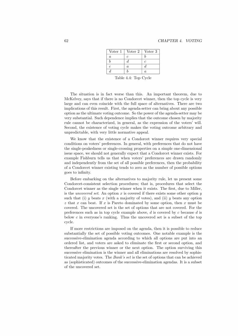
62 CHAPTER 4. VOTING
Voter 1 Voter 2 Voter 3a c bb d cc a dd b a
Table 4.4: Top Cycle
The situation is in fact worse than this. An important theorem, due toMcKelvey, says that if there is no Condorcet winner, then the top cycle is verylarge and can even coincide with the full space of alternatives. There are twoimplications of this result. First, the agenda-setter can bring about any possibleoption as the ultimate voting outcome. So the power of the agenda-setter may bevery substantial. Such dependence implies that the outcome chosen by majorityrule cannot be characterized, in general, as the expression of the voters’ will.Second, the existence of voting cycle makes the voting outcome arbitrary andunpredictable, with very little normative appeal.
We know that the existence of a Condorcet winner requires very specialconditions on voters’ preferences. In general, with preferences that do not havethe single-peakedness or single-crossing properties on a simple one-dimensionalissue space, we should not generally expect that a Condorcet winner exists. Forexample Fishburn tells us that when voters’ preferences are drawn randomlyand independently from the set of all possible preferences, then the probabilityof a Condorcet winner existing tends to zero as the number of possible optionsgoes to infinity.
Before embarking on the alternatives to majority rule, let us present someCondorcet-consistent selection procedures; that is, procedures that select theCondorcet winner as the single winner when it exists. The first, due to Miller,is the uncovered set. An option x is covered if there exists some other option ysuch that (i) y beats x (with a majority of votes), and (ii) y beats any optionz that x can beat. If x is Pareto dominated by some option, then x must becovered. The uncovered set is the set of options that are not covered. For thepreferences such as in top cycle example above, d is covered by c because d isbelow c in everyone’s ranking. Thus the uncovered set is a subset of the topcycle.
If more restrictions are imposed on the agenda, then it is possible to reducesubstantially the set of possible voting outcomes. One notable example is thesuccessive-elimination agenda according to which all options are put into anordered list, and voters are asked to eliminate the first or second option, andthereafter the previous winner or the next option. The option surviving thissuccessive elimination is the winner and all eliminations are resolved by sophis-ticated majority votes. The Bank’s set is the set of options that can be achievedas (sophisticated) outcomes of the successive-elimination agendas. It is a subsetof the uncovered set.
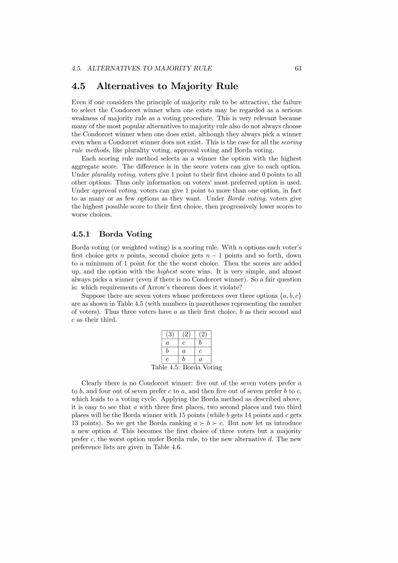
4.5. ALTERNATIVES TO MAJORITY RULE 63
4.5 Alternatives to Majority Rule
Even if one considers the principle of majority rule to be attractive, the failureto select the Condorcet winner when one exists may be regarded as a seriousweakness of majority rule as a voting procedure. This is very relevant becausemany of the most popular alternatives to majority rule also do not always choosethe Condorcet winner when one does exist, although they always pick a winnereven when a Condorcet winner does not exist. This is the case for all the scoringrule methods, like plurality voting, approval voting and Borda voting.Each scoring rule method selects as a winner the option with the highest
aggregate score. The difference is in the score voters can give to each option.Under plurality voting, voters give 1 point to their first choice and 0 points to allother options. Thus only information on voters’ most preferred option is used.Under approval voting, voters can give 1 point to more than one option, in factto as many or as few options as they want. Under Borda voting, voters givethe highest possible score to their first choice, then progressively lower scores toworse choices.
4.5.1 Borda Voting
Borda voting (or weighted voting) is a scoring rule. With n options each voter’sfirst choice gets n points, second choice gets n − 1 points and so forth, downto a minimum of 1 point for the the worst choice. Then the scores are addedup, and the option with the highest score wins. It is very simple, and almostalways picks a winner (even if there is no Condorcet winner). So a fair questionis: which requirements of Arrow’s theorem does it violate?Suppose there are seven voters whose preferences over three options {a, b, c}
are as shown in Table 4.5 (with numbers in parentheses representing the numberof voters). Thus three voters have a as their first choice, b as their second andc as their third.
(3) (2) (2)a c bb a cc b a
Table 4.5: Borda Voting
Clearly there is no Condorcet winner: five out of the seven voters prefer ato b, and four out of seven prefer c to a, and then five out of seven prefer b to c,which leads to a voting cycle. Applying the Borda method as described above,it is easy to see that a with three first places, two second places and two thirdplaces will be the Borda winner with 15 points (while b gets 14 points and c gets13 points). So we get the Borda ranking a  b  c. But now let us introducea new option d. This becomes the first choice of three voters but a majorityprefer c, the worst option under Borda rule, to the new alternative d. The newpreference lists are given in Table 4.6.

64 CHAPTER 4. VOTING
(3) (2) (2)d c ba d cb a dc b a
Table 4.6: Independence of Irrelevant Alternative
If we compute the scores with Borda method (now with points from oneto four), the election results are different: d will be the Borda winner with 22points, c will be second with 17 points, b will be third with 16 points and a willbe fourth with 15 points. So, the introduction of the new option d has reversedthe Borda ranking between the original alternatives to a ≺ b ≺ c. This reversalof the ranking shows that the Borda rule violates the independence of irrelevantalternatives and should be unacceptable in a voting procedure.This example illustrates the importance of the Arrow’s Condition I. Without
imposing this requirement it would be easy to manipulate the voting outcomeby adding or removing irrelevant alternatives without any real chance of themwinning the election in order to alter the chance of real contenders winning.
4.5.2 Plurality Voting
Under Plurality voting only the first choice of each voter matters and is givenone point. Choices other than the first do not count at all. These scores areadded and the option with the highest score is the plurality winner. Therefore,the Plurality winner is the option which is ranked first by the largest numberof voters.Consider the voters’ preferences over the three options given in Table 4.7.
Clearly a majority of voters rate c as worst option but it also has a dedicatedminority who rate if best (four out of nine voters). Under plurality voting cis the winner, with four first-place votes, while b and a have three and two,respectively.
(2) (3) (4)a b cb a ac c b
Table 4.7: Plurality Voting
The example illustrates the problem that plurality rule fails to select theCondorcet winner which, in this case, is a. The reason for this is that pluralityvoting dispenses with all information other than about the first choices.
4.5.3 Approval Voting
One problem with plurality rule is that voters don’t always have an incentiveto vote sincerely. Any rule that limits each voter to cast a vote for only oneoption forces the voters to consider the chance that their first-choices will win
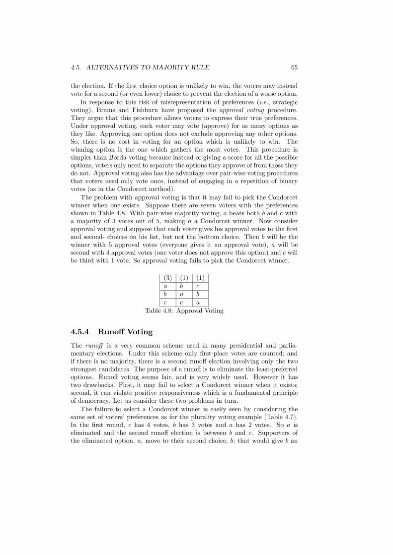
4.5. ALTERNATIVES TO MAJORITY RULE 65
the election. If the first choice option is unlikely to win, the voters may insteadvote for a second (or even lower) choice to prevent the election of a worse option.In response to this risk of misrepresentation of preferences (i.e., strategic
voting), Brams and Fishburn have proposed the approval voting procedure.They argue that this procedure allows voters to express their true preferences.Under approval voting, each voter may vote (approve) for as many options asthey like. Approving one option does not exclude approving any other options.So, there is no cost in voting for an option which is unlikely to win. Thewinning option is the one which gathers the most votes. This procedure issimpler than Borda voting because instead of giving a score for all the possibleoptions, voters only need to separate the options they approve of from those theydo not. Approval voting also has the advantage over pair-wise voting proceduresthat voters need only vote once, instead of engaging in a repetition of binaryvotes (as in the Condorcet method).The problem with approval voting is that it may fail to pick the Condorcet
winner when one exists. Suppose there are seven voters with the preferencesshown in Table 4.8. With pair-wise majority voting, a beats both b and c witha majority of 3 votes out of 5, making a a Condorcet winner. Now considerapproval voting and suppose that each voter gives his approval votes to the firstand second- choices on his list, but not the bottom choice. Then b will be thewinner with 5 approval votes (everyone gives it an approval vote), a will besecond with 4 approval votes (one voter does not approve this option) and c willbe third with 1 vote. So approval voting fails to pick the Condorcet winner.
(3) (1) (1)a b cb a bc c a
Table 4.8: Approval Voting
4.5.4 Runoff Voting
The runoff is a very common scheme used in many presidential and parlia-mentary elections. Under this scheme only first-place votes are counted; andif there is no majority, there is a second runoff election involving only the twostrongest candidates. The purpose of a runoff is to eliminate the least-preferredoptions. Runoff voting seems fair, and is very widely used. However it hastwo drawbacks. First, it may fail to select a Condorcet winner when it exists;second, it can violate positive responsiveness which is a fundamental principleof democracy. Let us consider these two problems in turn.The failure to select a Condorcet winner is easily seen by considering the
same set of voters’ preferences as for the plurality voting example (Table 4.7).In the first round, c has 4 votes, b has 3 votes and a has 2 votes. So a iseliminated and the second runoff election is between b and c. Supporters ofthe eliminated option, a, move to their second choice, b; that would give b an
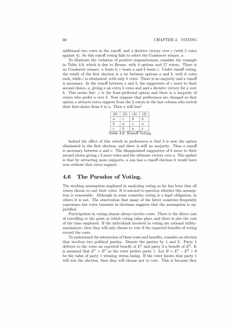
66 CHAPTER 4. VOTING
additional two votes in the runoff, and a decisive victory over c (with 5 votesagainst 4). So this runoff voting fails to select the Condorcet winner, a.To illustrate the violation of positive responsiveness, consider the example
in Table 4.9, which is due to Brams, with 4 options and 17 voters. There isno Condorcet winner: a beats b, c beats a and b beats c. Under runoff voting,the result of the first election is a tie between options a and b, with 6 voteseach, while c is eliminated, with only 5 votes. There is no majority and a runoffis necessary. In the runoff between a and b, the supporters of c move to theirsecond choice, a, giving a an extra 5 votes and and a decisive victory for a overb. This seems fair: c is the least-preferred option and there is a majority ofvoters who prefer a over b. Now suppose that preferences are changed so thatoption a attracts extra support from the 2 voters in the last column who switchtheir first-choice from b to a. Then a will lose!
(6) (5) (4) (2)a c b bb a c ac b a c
Table 4.9: Runoff Voting
Indeed the effect of this switch in preferences is that b is now the optioneliminated in the first election; and there is still no majority. Thus a runoffis necessary between a and c. The disappointed supporters of b move to theirsecond choice giving c 5 more votes and the ultimate victory over a. The upshotis that by attracting more supports, a can lose a runoff election it would havewon without that extra support.
4.6 The Paradox of Voting.The working assumption employed in analyzing voting so far has been that allvoters choose to cast their votes. It is natural to question whether this assump-tion is reasonable. Although in some countries voting is a legal obligation, inothers it is not. The observation that many of the latter countries frequentlyexperience low voter turnouts in elections suggests that the assumption is un-justified.Participation in voting almost always involve costs. There is the direct cost
of travelling to the point at which voting takes place and there is also the costof the time employed. If the individuals involved in voting are rational utility-maximizers, then they will only choose to vote if the expected benefits of votingexceed the costs.To understand the interaction of these costs and benefits, consider an election
that involves two political parties. Denote the parties by 1 and 2. Party 1delivers to the voter an expected benefit of E1 and party 2 a benefit of E2. Itis assumed that E1 > E2 so the voter prefers party 1. Let B = E1 − E2 > 0be the value of party 1 winning versus losing. If the voter knows that party 1will win the election, then they will choose not to vote. This is because they
4.6. THE PARADOX OF VOTING. 67
gain no benefit from doing so but still bear a cost. Similarly, they will also notvote if they expect party 2 to win. In fact, the rational voter will only everchoose to vote if they expect that they can affect the outcome of the election.Denoting the probability of breaking a tie occurring by P , then the expectedbenefit of voting is given by PB. The voting decision is then based on whetherPB exceeds the private cost of voting C. Intuition suggests that the probabilityof being pivotal decreases with the size of the voting population and increaseswith the predicted closeness of the election. This can be demonstrated formallyby considering the following coin-toss model of voting.There is a population of potential voters of sizeN . Each of the voters chooses
to cast a vote with probability p (so they don’t vote with probability 1 − p).This randomness in the decision to vote is the “coin toss” aspect of the model.There are two political parties contesting the election which we will call party1 and party 2. A proportion σ1 of the population support party 1, meaningthat if they did vote they would vote for party 1. Similarly, a proportion σ2 ofthe population support party 2. It must be the case that 0 ≤ σ1 + σ2 ≤ 1. Ifσ1 + σ2 < 1 then some of the potential voters do not support either politicalparty and abstain from the election. The number of votes cast for party 1 isdenoted X1 and the number for party 2 by X2.Now assume that the election is conducted. The question we want to answer
is: what is the probability that an additional voter can affect the outcome? Anadditional person casting a vote can affect the outcome in two circumstances:
• If the vote had resulted in a tie with X1 = X2. The additional vote canthen break the tie in favor of the party they support.
• If the party the additional person supports was 1 vote short of a tie. Theadditional vote will then lead to a tie.
Now assume that the additional voter supports party 1. (The argument isidentical if they support party 2.) The first case arises when X1 = X2 so theadditional vote will break the tie in favor of party 1. The second case occurs ifX1 = X2 − 1, so the additional vote will ensure a tie. The action in the eventof a tie is now important. We assume, as is the case in the UK, that a tie isbroken by the toss of a fair coin. Then when a tie occurs each party has a50/50chance of winning the vote.Putting these points together, the probability of being pivotal can be cal-
culated. If the original vote resulted in a tie, the additional vote will lead to aclear victory. Without the additional vote the tie would have been broken infavor of party 1 just 1/2 of the time so the additional vote leads to a reversalof the outcome with probability 1/2. If the original vote had concluded withparty 1 having 1 less vote than party 2, the addition of another vote for party 1will lead from defeat to a tie. The tie is won party 1 just 1/2 of the time. Theprobability, P, of being pivotal and affecting the outcome can then be calculatedas
P =1
2Pr (X1 = X2) +
1
2Pr (X1 = X2 − 1) . (4.1)

68 CHAPTER 4. VOTING
Figure 4.6: Probabilities of Election Outcomes
To see how result works, take the simple case of N = 3,σ1 =13 ,σ2 =
23 and
p = 12 . The probabilities of the various outcomes of the election are summarized
in Figure 4.6. These are calculated by observing that with 3 voters and 2alternatives for each voter (vote or not vote), there are 8 possible outcomes.Since 2 of the 3 voters prefer party 2, the probability of party 2 receiving 1 voteis twice that of party 1 receiving 1 vote.Using these probabilities, the probability of the additional voter affecting
the outcome can be calculated as
P =1
2[Pr (X1 = X2 = 0) + Pr (X1 = X2 = 1)]
+1
2[Pr (X1 = 0,X2 = 1) + Pr (X1 = 1,X2 = 2)]
=1
2
·1
8+2
8
¸+1
2
·2
8+1
8
¸=
3
8. (4.2)
With this probability, the voter will choose to vote in the election if
V =3
8B − C > 0. (4.3)
In an election with a small number of voters the benefit does not have to bemuch higher than the cost to make it worthwhile to vote.The calculation of the probability can be generalized to determine the de-
pendence of P upon the values of N,σ1,σ2 and p. This is illustrated in thefollowing two figure. Figure 4.7 displays the probability of being pivotal againstthe number of potential voters for three values of p given that σ1 = σ2 = 0.5.We can interpret the value of p as being the willingness to participate in theelection. The figures show clearly how an increase in the number of voters re-duces the probability of being pivotal. Although the probability tends to zeroas N becomes very large, is still significantly above zero at N = 100.

4.6. THE PARADOX OF VOTING. 69
Figure 4.7: Participation and the Probability of being Pivotal
Figure 4.8 confirms the intuition that the probability of being pivotal ishighest when the population is evenly divided between the parties. If the pop-ulation is more in favor of party 2 (the case of σ1 = 0.25,σ2 = 0.75) then theprobability of the additional voter being pivotal in favor of party 1 falls to 0very quickly. If the initial population is evenly divided, the probability of a tieremains significant for considerably larger values of N.The probability of a voter being pivotal can be aprroximated by a reasonably
simple formula if the number of potential voters, N , is large and the probabilityof each one voting, p, is small. Assume that this is so, and that the value ofpN tends to the limit of n. The term n is the number of potential voters thatactually choose to vote. The probability of being pivotal is then
P =en(2
√σ1σ2−σ1−σ2)
4
qπn (σ1σ2)
1/2
µ√σ1 +
√σ2√
σ1
¶, (4.4)
where π is used in its standard mathematical sense. From this equation can beobserved three results:
• The probability is a decreasing function of n. This follows from the factsthat 2
√σ1σ2 − σ1 − σ2 ≤ 0, so the power on the exponential is negative,
and that n is also in the denominator. Hence as the number of votersparticipating in the election increases, the probability of being pivotalfalls.
• For any given value of σ1, the probability increases the closer is σ2 toσ1. Hence, the probability of being pivotal is increased the more evenlydivided is support for the parties.
70 CHAPTER 4. VOTING
Figure 4.8: Closeness and the Probability of being Pivotal
• For a given value of n, the probability of being pivotal is at its maximumwhen σ1 = σ2 = 1/2 and the expression for P simplifies toP = 1√
2πn. In
this case the effect of increasing n is clear.
The bottom line of this analysis is that the probability that someone’s votewill change the outcome is essentially zero when the voting population is largeenough and so if voting is costly, the cost-benefit model, should imply almostno participation. The small probability of a large change is not enough to coverthe cost of voting. Each person’s vote is like a small voice in a very large crowd.
The following table presents the results of an empirical analysis of the partic-ipation rate to test the basic implications of the pivotal-voter theory (i.e., thatvoting should depend on the probability of a tie). It uses a linear regression overaggregate state-by-state data for the 11 US presidential elections (1948-1988)to estimate the empirical correlation between the participation rate and thestrategic variables (population size and electoral closeness). The analysis alsoreveals other main variables relevant for participation. As the table reveals thereis strong empirical support for the pivotal-agent argument: smaller populationand closer election are correlated with higher participation. It also reveals thatblack participation is 48 percent lower, that new residents are 1.2 percent lesslikely to vote, and that rain on the election day decreases participation by 3.4percent.
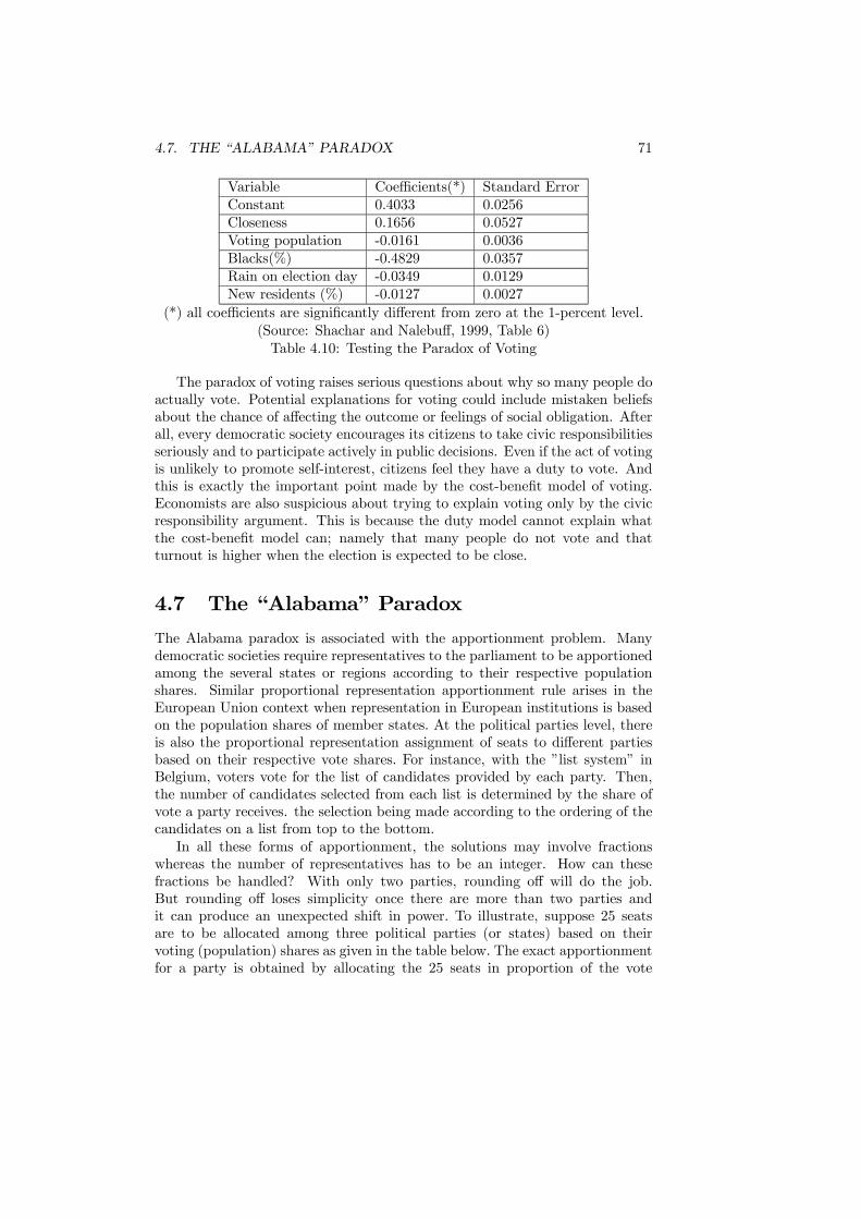
4.7. THE “ALABAMA” PARADOX 71
Variable Coefficients(*) Standard ErrorConstant 0.4033 0.0256Closeness 0.1656 0.0527Voting population -0.0161 0.0036Blacks(%) -0.4829 0.0357Rain on election day -0.0349 0.0129New residents (%) -0.0127 0.0027
(*) all coefficients are significantly different from zero at the 1-percent level.(Source: Shachar and Nalebuff, 1999, Table 6)Table 4.10: Testing the Paradox of Voting
The paradox of voting raises serious questions about why so many people doactually vote. Potential explanations for voting could include mistaken beliefsabout the chance of affecting the outcome or feelings of social obligation. Afterall, every democratic society encourages its citizens to take civic responsibilitiesseriously and to participate actively in public decisions. Even if the act of votingis unlikely to promote self-interest, citizens feel they have a duty to vote. Andthis is exactly the important point made by the cost-benefit model of voting.Economists are also suspicious about trying to explain voting only by the civicresponsibility argument. This is because the duty model cannot explain whatthe cost-benefit model can; namely that many people do not vote and thatturnout is higher when the election is expected to be close.
4.7 The “Alabama” Paradox
The Alabama paradox is associated with the apportionment problem. Manydemocratic societies require representatives to the parliament to be apportionedamong the several states or regions according to their respective populationshares. Similar proportional representation apportionment rule arises in theEuropean Union context when representation in European institutions is basedon the population shares of member states. At the political parties level, thereis also the proportional representation assignment of seats to different partiesbased on their respective vote shares. For instance, with the ”list system” inBelgium, voters vote for the list of candidates provided by each party. Then,the number of candidates selected from each list is determined by the share ofvote a party receives. the selection being made according to the ordering of thecandidates on a list from top to the bottom.In all these forms of apportionment, the solutions may involve fractions
whereas the number of representatives has to be an integer. How can thesefractions be handled? With only two parties, rounding off will do the job.But rounding off loses simplicity once there are more than two parties andit can produce an unexpected shift in power. To illustrate, suppose 25 seatsare to be allocated among three political parties (or states) based on theirvoting (population) shares as given in the table below. The exact apportionmentfor a party is obtained by allocating the 25 seats in proportion of the vote
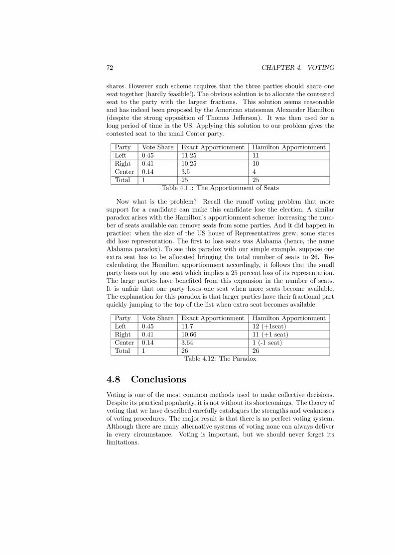
72 CHAPTER 4. VOTING
shares. However such scheme requires that the three parties should share oneseat together (hardly feasible!). The obvious solution is to allocate the contestedseat to the party with the largest fractions. This solution seems reasonableand has indeed been proposed by the American statesman Alexander Hamilton(despite the strong opposition of Thomas Jefferson). It was then used for along period of time in the US. Applying this solution to our problem gives thecontested seat to the small Center party.
Party Vote Share Exact Apportionment Hamilton ApportionmentLeft 0.45 11.25 11Right 0.41 10.25 10Center 0.14 3.5 4Total 1 25 25
Table 4.11: The Apportionment of Seats
Now what is the problem? Recall the runoff voting problem that moresupport for a candidate can make this candidate lose the election. A similarparadox arises with the Hamilton’s apportionment scheme: increasing the num-ber of seats available can remove seats from some parties. And it did happen inpractice: when the size of the US house of Representatives grew, some statesdid lose representation. The first to lose seats was Alabama (hence, the nameAlabama paradox). To see this paradox with our simple example, suppose oneextra seat has to be allocated bringing the total number of seats to 26. Re-calculating the Hamilton apportionment accordingly, it follows that the smallparty loses out by one seat which implies a 25 percent loss of its representation.The large parties have benefited from this expansion in the number of seats.It is unfair that one party loses one seat when more seats become available.The explanation for this paradox is that larger parties have their fractional partquickly jumping to the top of the list when extra seat becomes available.
Party Vote Share Exact Apportionment Hamilton ApportionmentLeft 0.45 11.7 12 (+1seat)Right 0.41 10.66 11 (+1 seat)Center 0.14 3.64 1 (-1 seat)Total 1 26 26
Table 4.12: The Paradox
4.8 ConclusionsVoting is one of the most common methods used to make collective decisions.Despite its practical popularity, it is not without its shortcomings. The theory ofvoting that we have described carefully catalogues the strengths and weaknessesof voting procedures. The major result is that there is no perfect voting system.Although there are many alternative systems of voting none can always deliverin every circumstance. Voting is important, but we should never forget itslimitations.

4.8. CONCLUSIONS 73
Further ReadingSome of the fundamental work on collective choice can be found in:Arrow, K.J. (1963) Social Choice and Individual Values (New York: John
Wiley and Sons).Black, D. (1958) The Theory of Committees and Election (Cambridge: Cam-
bridge University Press).Brams, S.J. and Fishburn, P.C. (1978) “Approval voting”, American Politi-
cal Science Review, 72, 831 - 847.Grandmont, J.M. (1978) “Intermediate preferences and the majority rule”,
Econometrica, 46, 317 - 330.May, K. (1952) “A set of independent, necessary and sufficient conditions
for simple majority decision”, Econometrica, 20, 680 - 684.McKelvey, R.D. (1976) “Intransitivities in multidimensional voting models
and some implications for agenda control”, Journal of Economic Theory, 12,472 - 482.Riker, W.H. (1986) The Art of Political Manipulation (New Haven: Yale
University Press).Two excellent books providing comprehensive surveys of the theory of voting
are:Mueller, D.C. (1989) Public Choice II (Cambridge: Cambridge University
Press).Ordeshook, P.C. (1986) Game Theory and Political Theory (Cambridge:
Cambridge University Press).A geometrical and very original presentation of voting theory isSaari, D.G (1995), Basic geometry of voting, (Springer-Verlag Berlin, Ger-
many)The voting paradox is based on:Feddersen, T.J. (2004) “Rational choice theory and the paradox of not vot-
ing”, Journal of Economic Perspectives, 18, 99 - 112.Myerson, R.B. (2000) “Large Poisson games”, Journal of Economic Theory,
94, 7 - 45.Shachar R. and B. Nalebuff (1999) “Follow the leader: theory and evidence
on political participation”, American Economic Review, 89, 525- - 547.

74 CHAPTER 4. VOTING
Chapter 5
Rent-Seeking
5.1 Introduction
The United States National Lobbyist Directory records there to be over 40,000state registered lobbyists and a further 4,000 federal government lobbyists reg-istered in Washington. Some estimates put the total number, including thosewho are on other registers or are unregistered, as high as 100,000. Althoughthe number of lobbyists in the United States dwarfs those elsewhere, there arelarge numbers of lobbyists in all major capitals.These lobbyists are not engaged directly in production. Instead, their role
is to seek favorable government treatment for the organizations that employthem. Viewed from the United States perspective, the economy has at least40,000 (presumably skilled) individuals who are contributing no net value tothe economy but are merely attempting to influence government policy andshift the direction of income flow.The behavior that the lobbyists are engaged in has been given the name of
rent-seeking in the economic literature. Precisely what constitutes rent-seekingis discussed in Section 5.2, but for the purpose of this introduction it is sufficientto distinguish it from profit-seeking which is activity that is economically usefuland creates additional income. What troubles economists about rent-seeking isthat it uses valuable resources unproductively and can push the government intoinefficient decisions. This places the economy within its production possibilityfrontier and implies that efficiency-improvements will be possible. As such,rent-seeking can be viewed as a potential cause of economic inefficiency.The chapter will first consider the nature and definition of rent-seeking. It
will then proceed onto the analysis of a simple game which demonstrates theessence of rent-seeking. This game will generate the fundamental results onthe consequences of rent-seeking and forms a basis on which the later analysisis developed. The insights generated from the game are then applied to rent-seeking in the context of monopoly. The basic point made there is that thestandard measure of monopoly welfare loss understates the true loss to society
75
76 CHAPTER 5. RENT-SEEKING
if rent-seeking behavior is present. This partial equilibrium analysis of monopolyis then extended to a general equilibrium setting. The emphasis is then placedon how and why rents are created. Government policy is analyzed and therelationship between lobbying and economic welfare is characterized in detail.The motives for a government to allow itself to be swayed by lobbyists are thendetailed. Finally, possible policies for containing rent-seeking are considered.
5.2 DefinitionsRent seeking has received a number of different definitions in the literature.These differ only in detail, particularly in whether the resources used in rent-seeking are directly wasted and in whether the term can be applied only to rentscreated by government. It is not the purpose here to catalogue these definitionsbut instead to motivate the concept of rent-seeking by example and to draw outthe common strands of the definitions.The ideas that lie behind rent-seeking can be seen by considering the follow-
ing two situations:
• A firm is engaged in research intended to develop a new product. If theresearch is successful, the product will be unique and the firm will have amonopoly position, and extract some rent from this, until rival productsare introduced.
• A firm has introduced a new product to the home market. A similar prod-uct is produced overseas. The firm hires lawyers to lobby the governmentto prevent imports of the overseas product. If it is successful, it will enjoya monopoly position from which it will earn rents.
What is the difference between these two situations? Both will give the firma monopoly position, at least in the short run, from which it can earn monopolyrents. The first, though, would be seen by many economists as something to bepraised but the second as something to be condemned. In fact, the fundamentaldifference is that the first case, with the firm expending resources to develop anew product, will lead to monopoly rent only if the product is successful andvalued by consumers. Hence, the resources used in research may ultimately leadto an increase in economic welfare. In contrast, the resources used in the secondcase are reducing economic welfare. If the lawyers are successful, consumerswill be denied a choice between products and the lack of competition will meanthat they face higher prices. Their welfare is reduced and some of their income,via the higher prices, is diverted to the monopolist. There is also (implicitly) atransfer from the overseas producers to the monopolist. Some of the monopolyrents are transferred to the lawyers via their fees (we will clarify how much inSection 5.3). In short, although the research and the lawyers are both directedto attaining a monopoly position, in the first case research increases economicwelfare but in the second the lawyers reduce it.These comments now allow us to distinguish between two concepts:
5.2. DEFINITIONS 77
• Profit-seeking is the expenditure of resources to create a profitable positionthat is ultimately beneficial to society. Profit seeking, as exemplified bythe example of research, is what drives progress in the economy and is themotivating force behind competition.
• Rent-seeking is the expenditure of resources to create a profitable oppor-tunity that is ultimately damaging to society. Rent-seeking, as exemplifiedby the use of lawyers, hinders the economy and limits competition.
There are some other points that can be drawn out of these definitions.Notice that the scientists and engineers employed in research are being produc-tive. If their work is successful, then new products will emerge that raise theeconomy’s output. On the other hand, the lawyers engaged in lobbying thegovernment are doing nothing productive. Their activity does not raise output.At best it simply redistributes what there already is, and generally it reduces it.Furthermore, output would be higher if they were usefully employed in a pro-ductive capacity rather than working as lawyers. In this respect, rent-seekingalways reduces total output since the resources engaged in rent-seeking can beexpected to have alternative productive uses.It can be seen from this discussion that rent-seeking can take many forms.
All lobbying of government for beneficial treatment, be it protection from com-petition or the payment of subsidies, is rent-seeking. Expenditure on advertisingor the protection of property rights is rent-seeking. And so is arguing for tar-iffs to protect infant industries. These activities are rife in most economies, sorent-seeking is a widespread and important issue.One of the factors that will feature strongly in the discussion below is the
level of resources wasted in the lobbying process. At first sight, there appears tobe a clear distinction between the time a lobbyist uses talking to a politician anda bribe passed to a politician. The time is simply lost to the economy - it couldhave been used in some productive capacity but has not. This is a resourcewasted. In contrast, the bribe is just a transfers of resources. Beyond theminimal costs needed to deliver the bribe, there appear to be no other resourcecosts. Hence it is tempting to conclude that lobbying time has a resource costwhereas bribes do not. Thus if rent-seeking is undertaken entirely by bribes itappears to have no resource cost.Before reaching this conclusion, it is necessary to take a further step back.
Consider the position of the politician receiving the bribe. How did they achievetheir position of authority? Clearly, resources would have been expended toobtain election. If potential politicians believed they would receive bribes onceelected, they would be willing to expend more resources to become a politician -they are in fact rent-seeking themselves. Much of the resources used in seekingelection will simply be a cost to the economy with no net output resulting fromthem. Through this process a bribe which is just a transfer actually becomestransformed further down the line into a resource loss caused by rent-seeking.These arguments suggest that caution is required in judging between lobby costswhich seem to be transfers and those which are clearly resource costs.

78 CHAPTER 5. RENT-SEEKING
So far the discussion has concentrated upon rent-seeking. The economicliterature has also dealt with the very closely related concept of directly unpro-ductive activities. The distinction between the two is not always that clear andmany economists use them interchangeably. If there is a precise distinction, itis in the fact that directly unproductive activities are by definition a waste ofresources whereas the activity of rent-seeking may not always involves activitieswhich waste resources. The focus below will be placed on rent-seeking thoughalmost all of what is said could be rephrased in terms of directly unproductiveactivities.
5.3 Rent-Seeking Games
This section considers several variants of a simple game that is designed tocapture the essential aspects of rent-seeking. From the analysis emerge severalimportant conclusions which will form the basis of more directly economic ap-plications in the following sections. The game may appear at first sight to beextreme but on reflection its interpretation in terms of rent-seeking will becomeclear.The basic structure of the game is as follows. Consider the offer of a prize of
$10,000. Competitors enter the game by simultaneously placing a sum of moneyon a table and setting it alight. The prize is awarded to the competitor thatburns the most money. Assuming that the competitors are all identical and risk-neutral, how much money will each one burn? This question will be answeredwhen there is either a fixed number of competitors or the number of competitorsis endogenously determined through free-entry into the competition.Before conducting the analysis, it is worth detailing how this game relates
to rent-seeking. The prize to be won is the rent - think of this as the profit thatwill accrue if awarded a monopoly in the supply of a product. The money that isburnt represents the resources used in lobbying for the award of the monopoly.Instead of burning money, it could be fees paid to a lobby company for theprovision of their services. The game can then be seen as representing a numberof companies each wishing to be granted the monopoly and employing lobbyiststo make their case. We consider two different games. In the deterministicgame, the prize is awarded to the firm that spends most on lobbying. In theprobabilistic game, the chance of obtaining the prize is an increasing functionof one’s share in the total spending on lobbying so that spending the most doesnot necessarily secure a win.
5.3.1 Deterministic game
A game of this form is solved by constructing its equilibrium. In this case welook for the Nash equilibrium which occurs when each competitor’s action isoptimal given the actions of all other competitors. Consequently, at a Nashequilibrium no variation in one competitor’s choice can be beneficial for thatcompetitor. It is this latter property that allows potential equilibria to be tested.
5.3. RENT-SEEKING GAMES 79
Assume initially that there are 2 competitors for the prize. To apply theNash equilibrium argument, the method is to fix the strategy choice of onecompetitor and to consider what the remaining competitor will do. Strategiesfor the game can be of two types. There are pure strategies which involve thechoice of a single quantity of money to burn. There are also mixed strategies inwhich the competitor uses a randomizing device to select their optimal strategy.For instance, labelling six possible strategies from 1 to 6 and then using the rollof a dice to choose which one to play is a mixed strategy. The central componentof finding a mixed strategy equilibrium is to determine the probabilities assignedto each pure strategy. The argument will first show that there can be no purestrategy equilibrium for the game. The mixed strategy equilibrium will then beconstructed.To show that there can be no pure strategy equilibrium, let one competitor
burn an amount B∗. Then if the remaining competitor burns B∗ + ² they willwin the contest and receive the prize of value V . This argument applies forany values of B∗ < V and any positive value of ² no matter how small. Sincethey have lost the contest, burning B∗ cannot be an equilibrium choice for theother competitor: they would wish to burn slightly more than B∗ + ². Fromthis reasoning, no amount of burning less than V can be an equilibrium. Theonly way the other competitor can prevent this “leapfrogging“ argument is byburning exactly V . The second competitor must then also burn V .However, burning V each is still not an equilibrium. If both competitors
burn V then each has an equal chance of winning. This chance of winning is 12 ,so their expected payoff, EP, is equal to the expected value of the prize minusthe money burnt
EP =1
2V − V = −1
2V < 0. (5.1)
Clearly, given that the other burns V , a competitor would be better off to burn0 and make an expected payoff of 0 rather than burn V and make an expectedloss of −V/2. So, the strategies of both burning V are not an equilibrium.The conclusion of this reasoning is that the game has no equilibrium in purestrategies. Therefore to find an equilibrium it becomes necessary to look for onein mixed strategies.The calculation of the mixed strategy for the game is easily motivated. It
is first noted that each player can obtain a payoff of at least 0 by burningnothing. Therefore, the equilibrium strategy must yield a payoff of at least 0.No player can ever burn a negative amount of money nor is there any point inburning more than V . Hence the strategy must assign positive probability onlyto amounts in the range 0 to V .It turns out that the equilibrium strategy is to assign the same probability to
all amounts in the range 0 to V . This probability, denoted f (B), must then begiven by f (B) = 1
V . Given that the other competition plays this mixed strategy,the probability of winning when burning an amount B is the probability thatthe other competitor burns less than B. This can be calculated as F (B) = B
V .
80 CHAPTER 5. RENT-SEEKING
Burning B then gives an expected payoff of
EP =
µB
V
¶V −B = 0. (5.2)
Therefore, whatever amount the random device suggests should be played, theexpected payoff from that choice will be zero. In total, the mixed strategiesused in this equilibrium give both players an expected payoff of zero.In the context of rent-seeking, the important quantity is the total sum of
money burnt since this can be interpreted as the value wasted. The mixed strat-egy makes each value between 0 and V equally likely so the expected burningfor each player is V/2. Adding these together, the total amount burnt is V -which is exactly equal to the value of the prize. This conclusions forms the basisof the important result that the effort put into rent-seeking will be exactly equalto the rent to be won.The argument can now be extended to any number of players. With three
players, the strategy of giving the same probability to each value between 0 andV is not the equilibrium. To see this, observe that with this mixed strategy theaverage amount burnt remains at V/2 but the probability of winning now thatthere are three players is reduced to 1
3 . The expected payoff is therefore
EP = (1
3)V − V
2= −V
6, (5.3)
so an expected loss is made. This strategy gives too much weight to higherlevels of burning now that there are three players. Consequently, the optimalstrategy must give less weight to higher values of burning so that the level ofexpected burning must match the expected winnings.The probability distribution for the mixed strategy equilibrium when the are
n players can be found as follows. Let the probability of beating one of the othercompetitors when B is burnt be F (B) . There are n−1 other competitors, so theprobability of beating them all is F (B)n−1. The expected payoff in equilibriummust be zero, so F (B)n−1 V = B for any value of B between 0 and V . Solvingthis equation for F (B) gives the equilibrium probability distribution as
F (B) =
µB
V
¶ 1n−1
. (5.4)
This distribution has the property that the probability applied to higher levelsof B falls relative to that on lower levels as n increases. It can also be seen thatwhen n = 2 it gives the solution found earlier.What is important for the issue of rent-seeking is the expected amount burnt
by each competitor. Given that the expected payoff in equilibrium is zero andthat everyone is equally likely to win V with probability 1
n , the expected amountburnt by each competitor is
EB =V
n. (5.5)
5.3. RENT-SEEKING GAMES 81
Using this result, the expected amount burnt by all the competitors is nEB = V,which again is exactly equal to the prize being competed for. This finding issummarized as a theorem.
Theorem 5 (Complete Dissipation Theorem) If there are two or more competi-tors in a deterministic rent-seeking game, the total expected value of resourcesexpended by the competitors in seeking a prize of V is exactly V.
The interpretation of this is that between them the set of competitors willburn (in expected terms) a sum of money exactly equal to the value of the prize.The theorem is just a restatement of the fact that the expected payoff from thegame is zero.This theorem has been very influential in the analysis of rent-seeking. Orig-
inally demonstrated in the context of monopoly (we will look at its applicationin this context later), the theorem provides the conclusion that from a socialperspective there is nothing gained from the existence of the prize. Instead, allthe possible benefits of the prize are wasted through the burning of money. Inthe circumstances in which it is applicable, the finding of complete dissipationprovides an exact answer to the question of how many resources are expendedin rent-seeking.It is important to note before proceeding that the theorem holds whatever
the value of n (provided it is at least 2). Early analyses of rent-seeking con-cluded that rents would be completely dissipated if there were large numbers ofcompetitors for the rent. This conclusion was founded on standard argumentsthat competition between many would drive the return down to zero. Prior tothe proof of the complete dissipation theorem it had been suspected that thiswould not be the case with only a small number of competitors and that somerent would be undissipated. However, the theorem proves that this reasoningis false and that even with only two competitors attempting to win the prize,rents are completely dissipated.
5.3.2 Probabilistic game
The key feature of the complete dissipation theorem is that it takes only a slightadvantage over your competitors to obtain a sure win. This is the situation whenthe rent-seeking contest takes the form of a race or an auction with maximalcompetition. However in many cases there is inevitable uncertainty in rentseeking so that higher effort increases the probability of obtaining the prize butdoes not ensure a win. A natural application is political lobbying where lobbyingexpenditures involves real resources that seek to influence public decision. Evenif a lobby can increase its chance of success by spending more, it cannot obtaina sure win by simply spending more that its competitors. We now show thatsuch uncertainty will reduce the equilibrium rent-seeking efforts, preventing fulldissipation of the rent.Consider the payoff function modified to let the probability of anyone ob-
taining the prize be equal to her share of the total rent-seeking expenditures of
82 CHAPTER 5. RENT-SEEKING
all contestants
EPi =
µBi
Bi + (n− 1)B−i
¶V −Bi, (5.6)
where (n − 1)B−i is the total effort of the other contestants. So the expectedpayoff of contestant i is the probability of obtaining the prize, which is hisspending as a proportion of the total amount spent in the competition, timesthe value of the rent, V , minus his own spending.A Nash equilibrium in this game is an expenditure level for each contestant
such that nobody would want to alter their expenditure given that of the othercontestants. Because all contestants are identical, we should expect a symmetricNash equilibrium in which rent-seeking activities are the same for all and every-one is equally likely to win the prize. To find this Nash equilibrium we proceedin two steps. First we derive the optimal response of contestant i as a function ofthe total efforts of the other contestants. Second we use the symmetry propertyto obtain the Nash equilibrium.To find player i’s best response when the others are choosing B−i, we must
take the derivative of player i’s expected payoff and set it equal to zero (this isthe first-order condition). To facilitate the derivative, let express the probabilityof winning as a power function in the expected payoff,
EPi = Bi [Bi + (n− 1)B−i]−1 V −Bi. (5.7)
Using the product rule for the derivative of a power function (derivative of thefirst function times the second, plus the first function times the derivative of thesecond), the first order condition is given by
[Bi + (n− 1)B−i]−1 V −Bi [Bi + (n− 1)B−i]−2 V − 1 = 0. (5.8)
Next we use the fact that in a symmetric equilibrium Bi = B−i = B. Makingthis substitution in the first-order condition, gives
[B + (n− 1)B]−1 V −B [B + (n− 1)B]−2 V − 1 = 0, (5.9)
or(nB)
−1V −B (nB)−2 V = 1. (5.10)
Finally multiplying both sides by n2B we obtain
nV − V = n2B. (5.11)
Hence the equilibrium level of rent-seeking expenditure is
B =(n− 1)n2
V, (5.12)
and the total expenditure of all contestants in equilibrium is
nB =(n− 1)n
V. (5.13)
5.3. RENT-SEEKING GAMES 83
Thus the fraction of the rent that is dissipated is (n − 1)/n < 1, whichis an increasing function of the number of contestants. With two contestantsonly one half of the rent is dissipated in a Nash equilibrium, and the fractionincreases to 1 as the number of contestants gets large. In equilibrium eachcontender is equally likely to obtain the prize (with probability 1/n) and usingthe equilibrium value of B, their expected payoff is EP =
¡1n
¢V −B = V/n.
Theorem 6 (Partial Dissipation Theorem) If there are two or more competi-tors in a probabilistic rent-seeking game, the total expected value of resourcesexpended by the competitors in seeking a prize of V is a fraction (n − 1)/n ofthe prize value V, and is increasing with the number of competitors.
It follows that the total costs of rent seeking activity are significant, and aregreater than one half of the rent value in all cases. Notice that the rate of rentdissipation is independent of the value of the rent. It is also worth mentioningthat in the Nash equilibrium, contestants play a pure strategy and do not ran-domize as in the previous deterministic rent seeking game. This is because theprobability of obtaining the rent is a continuous function of the person’s ownrent-seeking activity. Finally, in equilibrium, no single person would spend moreon rent seeking than the prize is worth, but with a large number of contenders,there is the disturbing possibility that the total expenditure on rent seeking ac-tivities may dissipate a substantial fraction of the prize value. This destructionof value is often innocuous because the contestants participate willingly expect-ing to gain. However as in any competition where the winner takes all there isonly one winner who may earn large profits, but many losers who bear the fullcost of the destruction of value.
5.3.3 Free-Entry
Beginning with a fixed number of competitors does not capture the idea of apotential pool of competitors who may opt to enter the competition if there is arent to be obtained. It is therefore of interest to consider what the equilibriumwill be if there is free-entry into the competition. In the context of the game,free-entry means that competitors enter to bid for the prize until there is noexpected benefit from further entry. This has the immediate implication thatthe expected payoff has to be driven to zero in any free-entry equilibrium.How can the game be solved with free-entry? The analysis of the determin-
istic game showed that the expected payoff of each competitor is zero in themixed strategy equilibrium. From this it follows that once at least two playershave entered the competition, the expected payoff is zero. The free-entry equi-librium concept is therefore compatible with any number of competitors greaterthat or equal to two, and all competitors who enter play the mixed strategy.There is an important distinction between this equilibrium and the one con-
sidered for fixed numbers. In the former case it was assumed (but without beingexplicitly stated) that all competitors played the same strategy and only suchsymmetric equilibria were considered. If this is applied to the free-entry case, it

84 CHAPTER 5. RENT-SEEKING
means that all the unlimited set of potential competitors must enter the gameand play the mixed strategy given by (5.4) as n → ∞ . An alternative to thiscumbersome equilibrium is to consider an asymmetric equilibrium in which dif-ferent competitors play different strategies. An asymmetric equilibrium of thegame is for some competitors to choose not to enter while some (at least 2) enterand play the mixed strategy in (5.4). All competitors (both those who enterand those who do not) have an expected payoff of 0.The other important feature of the both the symmetric and asymmetric
free-entry equilibria is that there is again complete dissipation of the rent. Thisfinding is less surprising in this case than it is with no entry, since the entrycould be expected to reduce the net social value of the competition to zero.In the probabilistic game, contestants get a positive expected payoff from
their rent-seeking activities of Vn . Such a gain from rent seeking will attract newcontestants until the rent value is fully dissipated, that is n → ∞ and V
n → 0.So free entry will make the two games equivalent with full dissipation of therent.
5.3.4 Risk Aversion
The analysis so far has relied on the assumption that competitors for the prizecare only about the expected amount of money with which they will leave thecontest. This is a consequence of the assumption that they are risk neutral andhence indifferent about accepting a fair gamble. Although risk neutrality maybe appropriate in some circumstances, such as for governments and large firmsthat can diversify risk, it is not usually felt to correctly describe the behaviorof individual consumers. It is therefore worth reflecting on how the results aremodified by the incorporation of risk aversion.The first effect of risk aversion is that the expected monetary gain from
entering the contest must be positive in order for a competitor to take part -this is the compensation required to induce the risk-averse competitors to takeon risk. In terms of the deterministic game with mixed strategy equilibrium, fora given number of competitors this means that less probability must be given tohigh levels of money burning and more to lower levels. However, the expectedutility gain of the contest will be zero, since competition will bid away any excessutility.In contrast to the outcome with risk neutrality there will not be complete
dissipation of the rent. This is a consequence of the expected monetary gainbeing positive which implies that something must be left to be captured. Withrisk aversion, the resources expended on rent-seeking will be strictly less thanthe value of the rent. But note carefully that this does not say that societyhas benefited. Since the expected utility gain of each competitor is zero, theavailability of the rent still does not raise society’s welfare.The same reasoning applies for the probabilistic game with more risk averse
individuals tending to expend less on rent seeking activities. As a result a lowerfraction of the rent will be dissipated. The effect of free entry will be to drivethe expected utility of each contender to zero.
5.4. SOCIAL COST OF MONOPOLY 85
5.3.5 Conclusions
This section has analyzed a simple game that can be interpreted as representingthe most basic of rent-seeking situations. The burning of money captures theuse of resources in lobbying and the fact that these resources are not being pro-ductive. The fundamental conclusion is that when competitors are risk neutral,competition leads to the complete or at least significant dissipation of the rent.This applies no matter how many competitors there are (provided there are atleast two) and whether or not the number of competitors is fixed or variable.This fundamental conclusion of the rent-seeking literature shows that the exis-tence of a rent does not benefit society since a significant amount of resources(possibly equal in value to that rent) will be exhausted in capturing it. Thisconclusion has to be slightly modified with risk aversion. In this case there isless expenditures on rent seeking and thus less rent dissipation. However theexpected utility gain of the competition is zero. In welfare terms, society doesnot benefit from the rent.
5.4 Social Cost of Monopoly
Monopoly is one of the causes of economic inefficiency. A monopolist restrictsoutput below the competitive level in order to raise price and earn monopolyprofits. This causes some consumer surplus to be turned into profit and someto become deadweight loss. Standard economic analysis views this deadweightloss to be the cost of monopoly power. The application of rent-seeking conceptssuggests that the cost may actually be much greater.Consider Figure 5.1. This depicts a monopoly producing with constant mar-
ginal cost c and no fixed costs. Its average revenue is denoted AR and marginalrevenueMR. The monopoly price and output are pm and ym respectively whilethe competitive output would be yc. Monopoly profit is the rectangle π anddeadweight loss the triangle d. In a static situation the deadweight loss d isthe standard measure of the cost of monopoly. (The emphasis on “static“ isnecessary here because there may be dynamic gains through innovation fromthe monopoly that offset the deadweight loss.)How can the introduction of rent-seeking change this view of the cost of
monopoly? There are two scenarios in which it can do so. Firstly, the monopolyposition may have been created by the government. An example would bethe government deciding that an airline route can be served only by a singlecarrier. If airlines must then compete in lobbying for the right to fly this routethe situation is just like the money-burning competition of Section 5.3. Therent-seeking here comes from the bidders for the monopoly position. Anotherexample is the allocation in the late 1980’s by the U.S. Federal CommunicationsCommission of regional cell phone licenses. The lure of extremely high potentialprofits was strong enough to attract many contenders. There were about 320,000contestants competing for 643 licenses. Hazlett and Michaels (1993) estimatedthe total cost of all applications (due to the technical expertise required) to
86 CHAPTER 5. RENT-SEEKING
Figure 5.1: Monopoly Deadweight Loss
be about $400,000. Each winner earned very large profits well in excess of theirapplication costs, but the costs incurred by others were lost, and the total cost ofthe allocation of licenses was estimated to be about forty percent of the marketvalue of the license.Secondly, the monopoly may be already in existence but having to defend
itself from potential competitors. Such defence could involve lawyers or an effec-tive lobbying presence attempting to prevent the production of similar productsusing copyright or patent law or it could mean advertising to stifle competition.Or it could even mean direct action to intimidate potential competitors.Whichever case applies, the implications are the same. The value of having
the monopoly position is given by the area π. If there are a number of potentialmonopolists bidding for the monopoly, then the analysis of money-burning canbe applied to show that, if they are risk neutral, the entire value will be dissi-pated in lobbying. Alternatively, if an incumbent monopolist is defending theirposition, they will expend resources up to value π to do so. In both cases thecosts of rent-seeking will be π.Combining these rent-seeking costs with the standard deadweight loss of
monopoly, the conclusion of the analysis is that the total cost of the monopolyto society is at least d and may be as high as π+ d. What determines the totalcost is the nature of the rent-seeking activity. We can conclude that resources ofvalue π will be expended but not how much is actually waste. As the discussionof Section 5.2 noted, some of the costs may just be transfer payments (or, moresimply, bribes) to officials. These are not directly social costs but, again referringto Section 5.2, may become so if they induce rent-seeking in obtaining officialpositions. In contrast, if all the rent-seeking costs are expended on unproductive
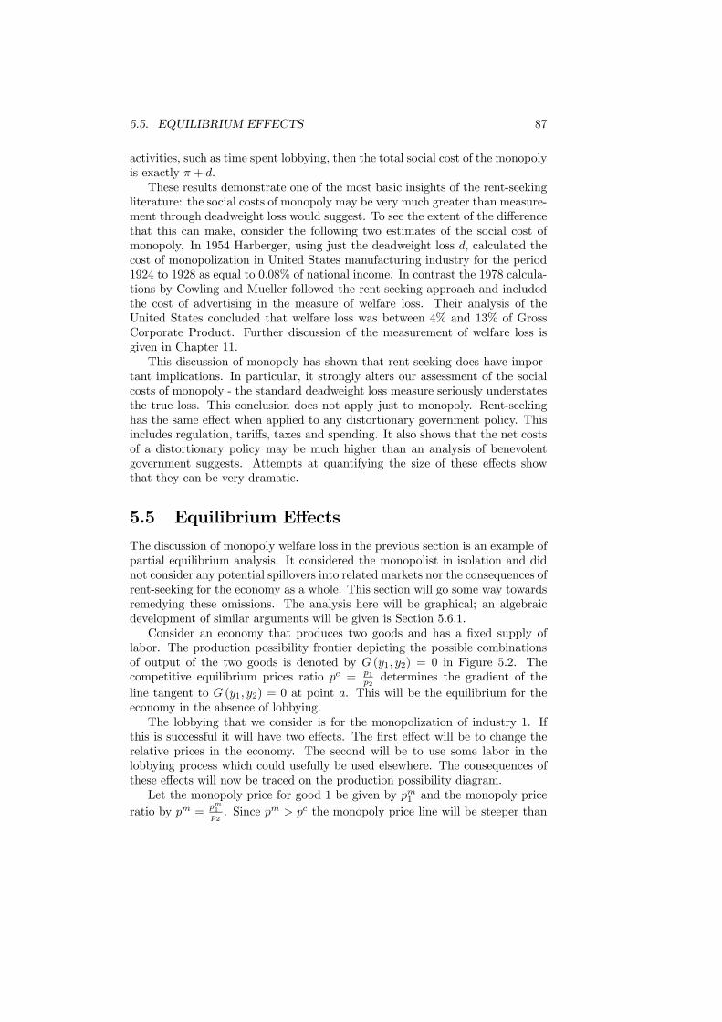
5.5. EQUILIBRIUM EFFECTS 87
activities, such as time spent lobbying, then the total social cost of the monopolyis exactly π + d.These results demonstrate one of the most basic insights of the rent-seeking
literature: the social costs of monopoly may be very much greater than measure-ment through deadweight loss would suggest. To see the extent of the differencethat this can make, consider the following two estimates of the social cost ofmonopoly. In 1954 Harberger, using just the deadweight loss d, calculated thecost of monopolization in United States manufacturing industry for the period1924 to 1928 as equal to 0.08% of national income. In contrast the 1978 calcula-tions by Cowling and Mueller followed the rent-seeking approach and includedthe cost of advertising in the measure of welfare loss. Their analysis of theUnited States concluded that welfare loss was between 4% and 13% of GrossCorporate Product. Further discussion of the measurement of welfare loss isgiven in Chapter 11.This discussion of monopoly has shown that rent-seeking does have impor-
tant implications. In particular, it strongly alters our assessment of the socialcosts of monopoly - the standard deadweight loss measure seriously understatesthe true loss. This conclusion does not apply just to monopoly. Rent-seekinghas the same effect when applied to any distortionary government policy. Thisincludes regulation, tariffs, taxes and spending. It also shows that the net costsof a distortionary policy may be much higher than an analysis of benevolentgovernment suggests. Attempts at quantifying the size of these effects showthat they can be very dramatic.
5.5 Equilibrium Effects
The discussion of monopoly welfare loss in the previous section is an example ofpartial equilibrium analysis. It considered the monopolist in isolation and didnot consider any potential spillovers into related markets nor the consequences ofrent-seeking for the economy as a whole. This section will go some way towardsremedying these omissions. The analysis here will be graphical; an algebraicdevelopment of similar arguments will be given is Section 5.6.1.Consider an economy that produces two goods and has a fixed supply of
labor. The production possibility frontier depicting the possible combinationsof output of the two goods is denoted by G (y1, y2) = 0 in Figure 5.2. Thecompetitive equilibrium prices ratio pc = p1
p2determines the gradient of the
line tangent to G (y1, y2) = 0 at point a. This will be the equilibrium for theeconomy in the absence of lobbying.The lobbying that we consider is for the monopolization of industry 1. If
this is successful it will have two effects. The first effect will be to change therelative prices in the economy. The second will be to use some labor in thelobbying process which could usefully be used elsewhere. The consequences ofthese effects will now be traced on the production possibility diagram.Let the monopoly price for good 1 be given by pm1 and the monopoly price
ratio by pm = pm1p2. Since pm > pc the monopoly price line will be steeper than

88 CHAPTER 5. RENT-SEEKING
Good 1
Good 2
a
b
( ) 0, 21 =yyG
Figure 5.2: Competitive and Monopoly Equilibria
the competitive price line. The price effect alone move the economy from pointa to point b around the initial production possibility frontier - see Figure 5.2.Evaluated at the competitive prices, the value of output can be seen to havereduced.The effect of introducing lobbying can be seen by realizing that the labor
of lobbyists does not produce either good 1 or good 2 but is effectively lost tothe economy. With labor used in lobbying the potential output of the economymust fall. Hence, the production possibility frontier with lobbying must lieinside that without lobbying. This is shown in Figure 5.3 where the productionpossibility frontier with lobbying is denoted GL (y1, y2) = 0. When faced withthe monopoly price line the equilibrium with monopoly and lobbying will be atpoint c in Figure 5.3.The outcome in Figure 5.3 is what might have been expected. The move to
monopoly pricing shifts the equilibrium around the frontier and lobbying shiftsthe frontier inward. The value at competitive prices of output at a is higherthan at b, and value at b is higher than at c. Hence the lobbying has resultedin a diminution of the value of output. At the aggregate level, this is damagingfor the economy. At the micro-level there will be income transfers towards theowners of the monopoly and the lobbyists, and away from the consumers so theoutcome is not necessarily bad for all individuals.In contrast, Figure ?? displays a surprising outcome. In this case the value
of output at c is actually higher than it is at b when evaluated at the competitiveprices. The cause of this is the way in which the labor used in lobbying hasaffected the shape of the production possibility frontier. When this happens,the value of output at competitive prices is higher with monopoly and lobbyingthan it is with just monopoly. This could be construed to be a positive argumentin favour of lobbying, but before it could be taken as such the conditions under
5.6. GOVERNMENT POLICY 89
Figure 5.3: Monopoly and Lobbying
which it could arise would require very careful elaboration.The final comparison that can be made is between the equilibrium with
unsuccessful lobbying where the resources costs are spent but the prices remainat the competitive level (point d in Figure 5.5) and monopoly with no lobbying(point b). As Figures 5.5a and 5.5b show, either of these could have the highestvalue at competitive prices. From this it can be concluded that there may besituations (as shown in 5.5b) when it may be better to concede to the threatof lobbying and allow the monopoly (without the lobbying taking place) ratherthan refuse to concede to the lobby.This section has extended the partial equilibrium analysis of lobbying to
illustrate the combined effects of the distortions generated by successful lobbyingand the waste of the resources used in the lobbying process. While some of theresults are unsurprising, particularly the finding that lobbying reduces the totalvalue of the economy’s output, the comparisons between different equilibria arenot always as expected. In fact, it would rarely be suspected that equilibriumwith monopoly could lead to a lower value of output than equilibrium withmonopoly and lobbying. But once again, this is a reflection of the fact that whenmultiple distortions are added to an economy the outcome is not necessarily clearcut.
5.6 Government Policy
Rent-seeking may be important for the study of private-sector monopoly, butmost proponents of rent-seeking would see its application to government asbeing far more significant. Much analysis of policy choice sees the governmentas benevolent and trying to make the best choices it can. The rent-seeking

90 CHAPTER 5. RENT-SEEKING
Figure 5.4: Lobbying Raises Value of Output
Figure 5.5: The Threat of Lobbying
5.6. GOVERNMENT POLICY 91
model of government is very different. This takes the view of the governmentas a creator of rents and those involved in government as seeking rent whereverpossible. Chapter 3 touched upon some of these issues in the discussion ofbureaucracy, but that discussion can be extended much further.There are two channels through which the government is connected with
rent-seeking. These are:
• Lobbying The introduction noted that the United States may have up to100,000 professional lobbyists. These lobbyists attempt to change govern-ment policy in favour of the interests that employ them. If the lobbyistsare successful, rents are created.
• Politicians and bureaucrats Politicians and bureaucrats in government areable to create rents through their policy choices. These rents can be “sold“to the parties that benefit. Selling rents generates income for the sellerand gives an incentive for careers to be made in politics and bureaucracy.
These two channels of rent-seeking are now discussed in turn.
5.6.1 Lobbying
The discussion so far has frequently referred to lobbying but without going intogreat detail about its economic effects. Section 5.4 showed graphically how theuse of labor in lobbying shifted the production possibility frontier inward buta graphical analysis of that kind could not provide an insight into the size ofthe effects. The purpose now is to analyze an example that can quantify thepotential size of the economic loss resulting from the use of labor in lobbying.Many of the implications of lobbying can be found by analyzing the use of
productive labor to lobby for a tariff. The effect of a tariff is to make importsmore expensive, so allowing the home firm to charge a higher price and earngreater profits. The potentially higher profit gives an incentive for lobbying. Forexample, the owners of textile firms will benefit from a lobby-induced tariff onimported clothing. Also, the U.S. steel industry is a well organized group andhas long been active in encouraging tariffs on competing imports. The resourcesused for lobbying have a social value (equal to their productivity elsewhere inthe economy) so the lobbying is not without cost. The calculations below willreveal the extent of this cost.Consider a small economy in which two consumption goods are produced. In
the absence of tariffs, the world prices of these commodities are both equal to 1and the assumption that the economy is small means that it treats these pricesas fixed. Some output is consumed and some is exported. A quantity, ¯, of laboris supplied inelastically by consumers. This is divided between production ofthe two goods and lobbying. Good 2 is produced with constant returns to scaleand one unit of labor produces one unit of output. This implies that the wagerate, w, must equal 1 (if it were higher the firms would make a loss producinggood 2, if it were lower their profit would be unlimited since the price is fixedat the world level).
92 CHAPTER 5. RENT-SEEKING
The cost function for the firm producing good 1 is assumed to be
C (y1;w) =1
2wy21 =
1
2y21, (5.14)
where y1 is output. With a tariff τ , which may be zero, the price of good 1 onthe domestic market becomes 1+ τ . Assuming that all of the output of the firmis sold on the domestic market, the profit level of the firm is
π1 (τ) = y1 (1 + τ)− 12y21. (5.15)
Profit is maximized at output level
y1 = 1 + τ . (5.16)
The resulting level of profit is given by
π1 (τ) =1
2[1 + τ ]
2, (5.17)
and labor demand from the firm is
`1 =1
2[1 + τ ]2 . (5.18)
Equilibrium on the labor market requires that labor supply must equal the useof labor in the production of good 1, `1 , plus that used in the production ofgood 2, `2, plus that used for lobbying, `L. Hence
¯= `1 + `2 + `L. (5.19)
The only value not yet determined is the labor used in lobbying. To find this,the complete dissipation result of Section 5.3 is applied. That is, it is assumedthat resources are used in lobbying up to the point at which the extra profitthey generate is exactly equal to the resource cost. Without lobbying, profitis π1 (0). After a successful lobby with a tariff implemented it becomes π1 (τ).The value of labor that the firm will devote to lobbying is therefore
w`L = π1 (τ)− π1 (0) =1
2
£2τ + τ2
¤. (5.20)
Since the production of each unit of good 2 requires one unit of labor, the outputof good 2 equals the labor input into the production of that good, so `2 = y2.Using these results, (5.16), (5.18) and (5.19) give
y1 = 1 + τ , y2 = ¯− 12
£1 + 4τ + 2τ2
¤, `L =
1
2
£2τ + τ2
¤. (5.21)
It can be seen from (5.21) that the output of good 1 is increasing in the valueof the tariff, that output of good 2 is decreasing as the square of the tariff, andlabor wasted in lobbying is increasing as the square of the tariff. From theseobservations it can be judged that the rent-seeking is damaging the economy

5.6. GOVERNMENT POLICY 93
since resources are being diverted at a rapid rate from the production of good2 but only increasing the production of good 1 slowly.One way of calculating the effect of this process is to determine the value of
national output at world prices. World prices are used since these are the truemeasure of value. Doing this gives
y1 + y2 = ¯− 12
£2τ2 + 2τ − 1¤ . (5.22)
Hence national income is reduced at the rate of the tariff squared.The conclusion in (5.22) shows just how damaging rent-seeking can be. The
possible availability of a tariff sees resources devoted to lobbying for it. Theseresources are withdrawn from the production of good 2 and national income,evaluated at world prices, declines.
5.6.2 Rent Creation
The analysis so far has focused primarily on the effects of rent-seeking in thepresence of pre-existing rents. We now turn to study the other side of the issue:the motives for the deliberate creation of rents. Such rent-creation is importantsince the existence of a rent implies a distortion in the economy. Hence theeconomic cost of a created rent is the total of the rent-seeking costs plus thecost of the economic distortion - this is the sum of deadweight loss plus profitidentified in the Section 5.4.To be in a position to create rents requires the power to make policy deci-
sions. In most political systems, this authority is formally vested in politicians.Assuming that they are solely responsible for decision-making would, though,be short-sighted. Politicians are advised and informed by bureaucrats. Many ofthe responsibilities for formulating policy options and for clarifying the vaguepolicy notions of politicians are undertaken by bureaucrats. By carefully lim-iting the policies suggested or by choosing their advice carefully, a bureaucratmay well be able to wield implicit political power. It therefore cannot be judgedin advance whether it is the politicians or the bureaucrats who actually makepolicy decisions. This does not matter unduly. For the purpose of the analysis,all that is necessary is that there is someone in a position to make decisions thatcan create rents, be it a politician or a bureaucrat. When the arguments applyto both politicians and bureaucrats, the generic term “decision-maker“ will beadopted.How are rents created? To see this most clearly, consider an initial position
where there is a uniform rate of corporation tax applicable to all industries. Arent can then be created by making it known that sufficient lobbying will be metby a reduction in the rate of tax. For instance, if the oil sector were to expendresources on lobbying then they would be made a special case and permitted alower corporation tax. The arguments already applied several times show thatthe oil sector will be willing to lobby up to a value equal to the benefit of thetax reduction. The monopoly airline route mentioned in Section 5.4 is anotherexample of rent-creation.
94 CHAPTER 5. RENT-SEEKING
The reason for the rent-creation can now be made clear. By ensuring that thenature of the lobbying is in a form that they find beneficial, the decision-makerwill personally gain. Such benefits could take many forms ranging from meals,to gifts, through to actual bribes in the form of cash payments. Contributionsto campaign funds are an especially helpful form of lobbying for politicians, asare lucrative appointments after a term of office is completed. All of these formsof lobbying are observed to greater or lesser degrees in political systems acrossthe world.It has already been noted that this rent-creation leads to the economic costs
of the associated rent-seeking. There are also further costs. Since there arerents to be gained from being a politician or a bureaucrat - the returns from thelobbying - there will be excessive resources devoted to securing these positions.Political office will be highly sought after with too many candidates spendingtoo much money in seeking election. Bureaucratic positions will be valued far inexcess of the contribution that bureaucrats make to economic welfare. Basically,if there are rents to be had as a politician or a bureaucrat then this will generateits own rent-seeking as these positions are competed for. In short, the abilityto create rents has cumulative effects throughout the system. The completedissipation theorem can again be applied here: in expected terms these rentsare dissipated. But it is important to bear in mind that the winner of the rentdoes gain: the politician who is elected or the bureaucrat who secures theirposition will personally benefit from the rent. The losses accrue to those whocompeted but failed to win.Two further effects arise. Firstly, there will be an excessive number of dis-
tortions introduced into the economy. Distortions will be created until there isno further potential for the decision-maker to extract additional benefits fromlobbyists. Secondly, there will be an excessive number of changes in policy.Decision-makers will constantly seek new methods of creating rents and thiswill involve policy being continually revised. One simple way for a new decision-maker to obtain rents is to make tax rates uniform with a broad base on ap-pointment, and then gradually auction off exemptions throughout the term ofoffice. The broader the chosen base, the greater the number of exemptions thatcan be sold.
5.6.3 Conclusions
The discussion of this section has presented a very negative view of governmentand economic policy making. The rent-seeking perspective argues that decisionsare not made for reasons of economic efficiency but are made on the basis ofhow much can be earned for making them. As a result of this, the economyis damaged by inefficient and distortionary policies. In addition, resources arewasted in the process of rent-seeking. Both lobbying and attempting to obtaindecision-making positions waste resources. When these are combined, the dam-age to the economy is significant. It suggests that political power is sought afternot as an end in itself but simply as a means to access rent.
5.7. INFORMATIVE LOBBYING 95
5.7 Informative lobbyingThe discussion so far has presented a picture of lobbyists as a group who con-tribute nothing to the economy and are just a source of welfare loss. To providesome balance, it is important to note that circumstances can arise in whichlobbyists do make a positive contribution. Lobbyists may be able to benefit theeconomy if they, or the interest groups they represent, have superior informa-tion about the policy environment than the decision maker. By transmittingthis information to the policy-maker, they can assist in the choice of a betterpolicy.Several issues arise in this process of information transmission. To provide a
simple description of these, assume that a policy has to be chosen for the nexteconomic period. At the time the policy has to be chosen, the policy-maker isuncertain what the economic environment will. This uncertainty is modeled byassuming that environment will one of several alternative “states of the world”.Here, a state of the world is a summary of all relevant economic information.The policy-maker knows that different states of the world require different policychoices to be mad, but they do not know what the state of the world will be.Without any additional information, the policy-maker would have to base policychoice upon some prior beliefs about the probability of alternative states of theworld. Unfortunately, if the chosen policy is not correct for the state of the worldwhich is realized, welfare will not be maximized.Now assume that there is a lobbyist who knows which state of the world
will occur. It seems that if they were just to report this information to thepolicy-maker then the correct policy would be chosen and welfare maximized.But this misses the most important point: the objectives of the lobbyists. If thelobbyists had the same preferences as the policy-maker there would be no prob-lem. The policy-maker would accept the information that was offered knowingthat the lobbyists were pursuing the same ends. In contrast, if the lobbyistshave different preferences then they may have an incentive to reveal false in-formation about the future state of the world with the intention of distortingpolicy in a direction that they find beneficial. Therefore the policy-maker facesthe problem of determining when the information they receive from lobbyists iscredible and correct, and when it represents a distortion of the truth.To see how these issues are resolved, consider an model in which there are
only two possible values for the future state of the world. Let these values bedenoted θh and θ` with θ` < θh, where we term θh the ”high state” and θ` isthe “low state”. The policy-maker seeks to maximize a social welfare functionthat depends on the state of the world and the policy choice, π. Suppose thisobjective function takes the form
W (π, θ) = −(π − θ)2. (5.23)
If the policy-maker had perfect information, when the high state was known tooccur a high policy level πh = θH is required and, when the state was knownto be low, a low policy level π` = θ` is required. If instead the policy-maker isuninformed about the state of the world and initially regards the two states as
96 CHAPTER 5. RENT-SEEKING
equally likely. In this case, the policy-maker will choose a policy based on theexpected state of the world, so
πe =θ` + θh2
. (5.24)
That is, the policy-maker sets the policy equal to the expected value of θ.Now we introduce a lobbyist who knows what the state of the world will be.
The welfare of the lobby also depends on the policy level and the state of theworld. However the lobbyist does not share the same view as the policy-makerabout the ideal policy level in each state of the world. We assume that the idealpolicy for the lobbyist exceeds the ideal policy of the policy-maker by an amount∆ in both states of the world. We can refer to such difference in the ideal policyas the extent of the disagreement between the policy-maker and the lobbyist.Such a lack of agreement can be obtained by adopting preferences for the groupgiven by
U(π, θ) = −(π − θ −∆)2. (5.25)
To see the condition under which the lobbyist can credibly transmit informa-tion about the state of the world, we must investigate the incentives the lobbyisthas to truthfully report the state of the world. First note that the lobbyist canonly report either θh or θ` and, if he is trusted by the policy-maker, the policychoice will be respectively πh or π`. If the true state is θh the lobbyist has noincentive to missreport the information. Indeed the lobbyist has a bias towardsa high policy level, so misreporting the state as being low would lead to a policyπ` which is worse than its ideal policy πh +∆ when the state is high. On theother hand, if the state is θ` the lobbyist has a potential incentive to missreportbecause a truthful report, if trusted by the policy-maker, leads to a policy levelπ` that is below the ideal policy of the lobbyist π` +∆. The lobbyist may thenprefer to claim that the state is high to exploit the trust and obtain policy πhinstead of π`. However it may be that πh is too large for the lobbyist when thestate is θ`, in which case the lobbyist will report truthfully. The latter is thecase if π` is closer to the ideal policy of the lobbyist in the low state than πh,which occurs if the following inequality is satisfied
(θ` +∆)− θ` ≤ θh − (θ` +∆) . (5.26)
This inequality reduces to
∆ ≤ θh − θ`2
. (5.27)
This condition says that policy-maker can expect the lobbyist to reporttruthfully the state of the world if the extent of the disagreement is not toolarge. The equilibrium that results is then fully revealing because the lobbyistcan credibly transmit information about the state of the world. Lobbying is theninformative and desirable for the society. If in contrast the above inequality isnot satisfied, the extent of the disagreement is too large for the policy-makerto expect truthful reporting when the state is low. The lobbyist’s report lacks
5.7. INFORMATIVE LOBBYING 97
credibility because the policy-maker knows that the lobbyist prefers reportinghigh state no matter what the true state happened to be. The report is thenuninformative and the policy-maker will rightly ignore it. The policy-makerthen sets the policy equal to the expected value πe = θ`+θh
2 . This policy choiceis suboptimal for society because it is too large when the state is low and toosmall when the state is high. Note that the lobbyist is also worse off with theuninformative outcome because policy choice πe is smaller than its ideal policyπh +∆ when the state is high.The problem of securing credibility is magnified when there are more than
two states of the world. As the number of possible states increases, honest infor-mation revelation becomes ever more difficult to obtain. This is easily demon-strated. For a lobbyist to credibly report the true state, ∆ must be smaller thanone-half of the distance between any two adjacent states - this is the content of(5.27). With n states, θ1 < ... < θi < ... < θn, the conditions for truthtellingare for all i = 1, ..., n− 1
∆ ≤ θi+1 − θi2
. (5.28)
Evidently, as the number of states grows, intermediate states are addedwhich reduces the distance between any two states. Eventually the states be-come too close to each other for the lobbyist to be able to credibly communicatethe true state, even if ∆ is small. Full revelation is then impossible. What canthe lobbyist do in such a situation? The answer is to reveal partial information.Suppose the states is partitioned into two sets, L = (θ1, ..., θi) and H =
(θi+1, ..., θn). Then the lobbyist can report the interval in which the true stateis, instead of reporting the precise state - we term this partial revelation. Ifhe reports ΘL then it means that θ1 ≤ θ ≤ θi. If all states are equallylikely, then a trusty policy-maker sets the policy equal to the expected valueon this interval π(L) = θ1+θi
2 . Similarly, the report ΘH induces a policy choiceπ(H) = θi+1+θn
2 ). The question is whether the lobbyist has any incentive to lie.Among the states in the interval L, the greatest temptation to lie (by report-ing ΘH) is when the true state is close to θi: if the lobbyist does not want toclaim H when θ = θi then he will not wish to do so when θ < θi, because itwould push the policy choice further away from his ideal policy. Hence we canrestrict attention to the incentive to report truthfully L when the true stateis θi. Truthful reporting induces policy π(L) and misreporting induces policyπ(H). The lobbyist will report truthfully if the former policy is closer than thelatter from his ideal policy θi +∆ given the true state θi. This is the case if
(θi +∆)− π(L) ≤ π(H)− (θi +∆) , (5.29)
which reduces to
θi +∆ ≤ π(H) + π(L)
2(5.30)
Now suppose that θ actually is in H. We must check the incentive of thelobbyist to truthfully report H instead of L. The temptation is highest to

98 CHAPTER 5. RENT-SEEKING
missreport when true state is close to θi+1. In such a case, to sustain truthfulreporting it is required that it must induce a policy π(H) that is closer to theideal policy θi+1 + ∆ than the policy that would be induced by misreportingπ(L). That is
(θi+1 +∆)− π(L) ≥ π(H)− (θi+1 +∆) , (5.31)
which reduces to
θi+1 +∆ ≥ π(H) + π(L)
2(5.32)
Combining the two incentive constraints (5.30) and (5.32), truthtelling requires
π(H) + π(L)
2− θi+1 ≤ ∆ ≤ π(H) + π(L)
2− θi
This condition puts both a lower bound and an upper bound on the extent ofthe disagreement for the lobbyist to be able to communicate credibly partialinformation about the state to the policy-maker.The outcome of this analysis is that lobbyists can raise welfare if they are
able to credibly report information to the policy-maker. Unfortunately, thisargument is limited by the potential for incentives to report false informationwhen there is divergence between the preferences of the lobbyist and the policy-maker. With a limited number of states, credible correct transmission can besustained if the divergence is not too great. However, as the number of statesof the world increases, credible transmission cannot be sustained if there is anydivergence at all in preferences. In this latter case, though, it is possible to havepartial information credibly released - again provided the divergence is limited.In conclusion, informed lobbyists can be beneficial through the advice they canoffer a policy-maker, but this can be undermined by their incentives to revealfalse information.
5.8 Controlling Rent-Seeking
Much has been made of the economic cost of rent-seeking. These insights areinteresting (and also depressing for those who may believe in benevolent gov-ernment) but are of little value unless they suggest methods of controlling thephenomenon. This section gathers together a number of proposals that havemade in this respect.There are two channels through which rent-seeking can be controlled. The
first channel is to limit the efforts that can be put into rent-seeking. The secondis to restrict the process of rent-creation.Beginning with the latter, rent-creation relies on the unequal treatment of
economic agents. For instance, the creation of a monopoly is based on oneeconomic agent being given the right to operate in the market and all otheragents being denied. Equally, offering a tax concession for one industry treatsthe agents in that industry more favorably than those outside. Consequently,
5.9. CONCLUSIONS 99
a first step in controlling rent-seeking would be to disallow policies that dis-criminate between economic agents. The restriction to the implementation ofnon-discriminatory policies only would forbid the creation of tax-breaks for spe-cial interests or the imposition of tariffs on particular imports. If restricted inthis way, the decision-maker could not auction off rents - if all parties gain, nonehas the incentive to pay.The drawback of a rule preventing discrimination is that sometimes it is
economically efficient to discriminate. As an example, the theory of optimalcommodity taxation (see Chapter 15) describes circumstances in which it isefficient for necessities to be taxed more heavily than luxuries. This would notbe possible with non-discrimination since the industries producing necessitieswould have grounds for complaint. Similarly, the theory of income taxation(see Chapter 16) finds that in general it is optimal to have a marginal rate ofincome tax that is not uniform. If implemented, the taxpayers facing a highermarginal rate would have grounds for alleging discrimination. Hence a non-discrimination ruling would result in uniform commodity and income taxes.These would not usually be efficient, so there would be a trade-off betweeneconomic losses through restrictions on feasible policy choices and losses throughrent-seeking. It is not unlikely that the latter will outweigh the former.There are other ways in which the process of rent-seeking can be lessened but
all of these are weaker than a non-discrimination rule. These primarily focus onensuring that the policy-making process is as transparent as possible. Amongstthem would be policies such as limiting campaign budgets, insisting on therevelation of names of donors, requiring registration of lobbyists, regulating andlimiting gifts, and reviewing bureaucratic decisions. Policing can be improvedto lessen the use of bribes. Unlike non-discrimination, none of these policies hasany economic implications other than their direct effect on rent-seeking.
5.9 Conclusions
Lobbyists are very numerous in number; they are also engaged in a non-productiveactivity. The theory of rent-seeking provides an explanation for this apparentparadox and looks at the consequences for the economy. The fundamental in-sight of the literature is the Complete Dissipation Theorem: competition for arent will result in resources being expended up until the expected gain of societyfrom the existence of the rent is zero. If competitors for the rent are risk-neutral,this implies that the resources used in rent-seeking are exactly equal in valueto the size of the rent. The applications of these rent-seeking ideas show thatthe losses caused by distortions are potentially much larger than the standardmeasure of deadweight loss.The other aspect of rent-seeking is that economic decision makers have an
incentive to create distortions. They do this in order to receive benefits fromthe resulting rent-seeking. This leads to a perspective of policy driven not bywhat is good for the economy but by what the decision maker can get out of itand of a politics corrupted by self-interest. If this view is the correct description
100 CHAPTER 5. RENT-SEEKING
of the policy-making process, the response should be to limit the discretion forpolicy-makers. Lastly, lobbying can be desirable when the lobbyists have betterinformation about policy-relevant variable than the policy-maker. The questionis then how the lobbyists can credibly communicate this information when thereis some disagreement about the ideal policy choice.
ReadingThe classic analysis of rent-seeking is in:Krueger, A. (1974), American Economic ReviewTullock, G. (1967) “The welfare costs of tariffs, monopolies and theft“,West-
ern Economic Journal, 5, 224 - 232.The second article is reprinted in:Buchanan, J.M., Tollison, R.D. and Tullock, G. (1980) Towards a Theory of
the Rent-Seeking Society (College Station: Texas A and M Press),which also contains other interesting reading. For more discussion of the
definition of rent-seeking and a survey of the literature see:Brooks, M.A. and Heijdra, B.J. (1989) “An exploration of rent-seeking“,
Economic Record, 65, 32 - 50.The complete analysis of the rent-seeking game is in:Hillman, A. and Samet, D. (1987) “Dissipation of contestable rents by small
numbers of contenders“, Public Choice, 54, 63 - 82.Estimates of the social costs of monopoly are taken from:Cowling, K.G. and Mueller, D.C. (1978) “The social costs of monopoly
power“, Economic Journal, 88, 727 - 748,andHarberger, A.C. (1954) “Monopoly and resource allocation“, American Eco-
nomic Review, 45, 77 - 87.Another important paper in this area is:Posner, R.A. (1975) “The social cost of monopoly and regulation“, Journal
of Political Economy, 83, 807 - 827.More on interest groups and lobbying can be found in:Austen-Smith, D. (1997) “Interest groups: money, information and influ-
ence“, in D. Mueller (ed.), Perspectives on Public Choice (Cambridge: Cam-bridge University Press).Grossman G. and Helpman E. (2001) Special Interest Politics (Cambridge:
MIT Press)A debate about the relative merits of rent-seeking and the traditional public
finance approach is found in:Buchanan, J.M. andMusgrave, R.A. (1999) Public Finance and Public Choice:
Two Contrasting Visions of the State (Cambridge: MIT Press).

Part III
Equilibrium and Efficiency
101

Chapter 6
Competitive Economies
6.1 Introduction
To make predictions about the effects of economic policies, economists constructand analyze models. Such models, while inevitably being simplifications ofthe real economy, are designed to capture the essential aspects of the problemunder study. Models are used because of problems of conducting experiments oneconomic systems and because the system is too large and complex to analyzein its entirety.Although many different models will be studied in this book, there are impor-
tant common features which apply to all. Most models used in public economicsspecify the objectives of the individual agents (such as firms and consumers) inthe economy, and the constraints they face, and then aggregate individual deci-sions to arrive at market demand and supply. The equilibrium of the economyis then determined and, in a policy analysis, the effects of government choicevariables upon this are calculated. This is done with various degrees of detail.Sometimes only a single market is studied - which is the case of partial equi-librium analysis. At other times, many markets are analyzed simultaneously.Similarly, the number of firms and consumers varies from one or two to verymany.An essential consideration in the choice of the level of detail for a model
is that its equilibrium must demonstrate a dependence upon policy that givesinsight into the functioning of the actual economy. If the model is too highlyspecified it may not be capable of capturing important forms of response. On theother hand, if it is too general it may not be able to provide any clear prediction.Achieving a successful compromise between these competing objectives is the”art” of economic modelling. The theory described in this book will show howthis trade-off can be successfully resolved.The focus of this chapter is on the basic model of the competitive economy.
Variants of this model will see extensive service in later chapters. In particular,it is used to develop the fundamental results of welfare economics and the basic
103

104 CHAPTER 6. COMPETITIVE ECONOMIES
principles of tax theory. The essential feature of competition is that the con-sumers and firms in the economy do not consider their actions to have any effectupon prices. Consequently, in making decisions they treat the market prices asfixed. This assumption can be justified when all consumers and firms are trulynegligible in size relative to the market. But it can be imposed as a modelingtool even in an economy with a single consumer and a single firm.This definition of competition places a focus upon the role of prices which is
maintained throughout the chapter. Prices measure values and are the signalswhich guide the decisions of firms and consumers. The adjustment of pricesequates supply and demand to ensure that equilibrium is achieved. It wasthe exploration of the determinants of the relative values of different goodsand services that lead to the formulation of the models. The role of prices incoordinating the decisions of independent economic agents is also crucial for theattainment of economic efficiency.Two forms of the competitive model are introduced in this chapter. The
first is concerned with an exchange economy in which there is no production.Initial stocks of goods are held by consumers and economic activity occursthrough the trade of these stocks to mutual advantage. The second form ofcompetitive economy introduces production. This is undertaken by firms withgiven technologies who use inputs to produce outputs and distribute their profitsas dividends to consumers.
6.2 The Exchange Economy
The model of the exchange economy considers the simplest form of economicactivity: the trade of commodities between two parties in order to obtain mutualadvantage. Despite the simplicity of this model, it is a surprisingly instructivetool for obtaining fundamental insights about taxation and tax policy. This willbecome evident in later chapters.This section will present a description of a two-consumer, two-good exchange
economy. The restriction on the number of goods and consumers does notalter any of the conclusions that will be derived - they will all extend to largernumbers. What restricting the numbers does is allow the economy to be depictedand analyzed in a simple diagram.
6.2.1 Endowments, Budgets and Preferences
Each of the two consumers has an initial stock, or endowment, of the economy’stwo goods. The endowments can be interpreted literally as stocks of goodsor less literally as human capital and are the quantities that are available fortrade. Given the absence of production, these quantities remains constant.The consumers exchange quantities of the two commodities in order to achieveconsumption levels that are preferred to their initial endowments. The rate atwhich one commodity can be exchanged for the other is given by the marketprices. Both consumers believe that their behavior cannot affect these prices.
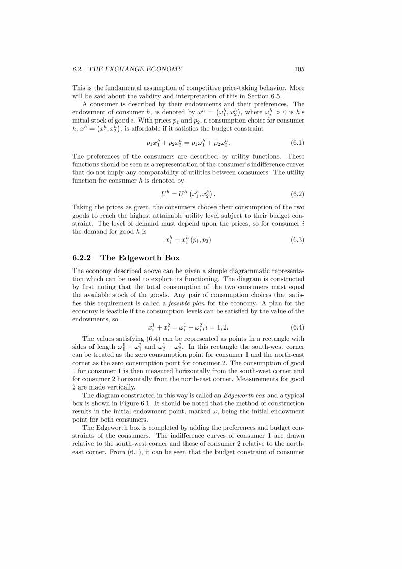
6.2. THE EXCHANGE ECONOMY 105
This is the fundamental assumption of competitive price-taking behavior. Morewill be said about the validity and interpretation of this in Section 6.5.A consumer is described by their endowments and their preferences. The
endowment of consumer h, is denoted by ωh =¡ωh1 ,ω
h2
¢, where ωhi > 0 is h’s
initial stock of good i. With prices p1 and p2, a consumption choice for consumerh, xh =
¡xh1 , x
h2
¢, is affordable if it satisfies the budget constraint
p1xh1 + p2x
h2 = p1ω
h1 + p2ω
h2 . (6.1)
The preferences of the consumers are described by utility functions. Thesefunctions should be seen as a representation of the consumer’s indifference curvesthat do not imply any comparability of utilities between consumers. The utilityfunction for consumer h is denoted by
Uh = Uh¡xh1 , x
h2
¢. (6.2)
Taking the prices as given, the consumers choose their consumption of the twogoods to reach the highest attainable utility level subject to their budget con-straint. The level of demand must depend upon the prices, so for consumer ithe demand for good h is
xhi = xhi (p1, p2) (6.3)
6.2.2 The Edgeworth Box
The economy described above can be given a simple diagrammatic representa-tion which can be used to explore its functioning. The diagram is constructedby first noting that the total consumption of the two consumers must equalthe available stock of the goods. Any pair of consumption choices that satis-fies this requirement is called a feasible plan for the economy. A plan for theeconomy is feasible if the consumption levels can be satisfied by the value of theendowments, so
x1i + x2i = ω1i + ω2i , i = 1, 2. (6.4)
The values satisfying (6.4) can be represented as points in a rectangle withsides of length ω11 + ω21 and ω12 + ω22. In this rectangle the south-west cornercan be treated as the zero consumption point for consumer 1 and the north-eastcorner as the zero consumption point for consumer 2. The consumption of good1 for consumer 1 is then measured horizontally from the south-west corner andfor consumer 2 horizontally from the north-east corner. Measurements for good2 are made vertically.The diagram constructed in this way is called an Edgeworth box and a typical
box is shown in Figure 6.1. It should be noted that the method of constructionresults in the initial endowment point, marked ω, being the initial endowmentpoint for both consumers.The Edgeworth box is completed by adding the preferences and budget con-
straints of the consumers. The indifference curves of consumer 1 are drawnrelative to the south-west corner and those of consumer 2 relative to the north-east corner. From (6.1), it can be seen that the budget constraint of consumer
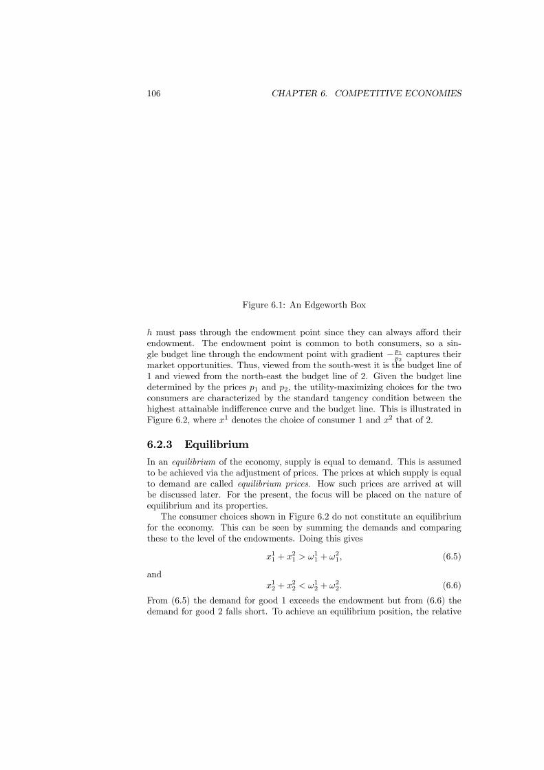
106 CHAPTER 6. COMPETITIVE ECONOMIES
Figure 6.1: An Edgeworth Box
h must pass through the endowment point since they can always afford theirendowment. The endowment point is common to both consumers, so a sin-gle budget line through the endowment point with gradient −p1p2 captures theirmarket opportunities. Thus, viewed from the south-west it is the budget line of1 and viewed from the north-east the budget line of 2. Given the budget linedetermined by the prices p1 and p2, the utility-maximizing choices for the twoconsumers are characterized by the standard tangency condition between thehighest attainable indifference curve and the budget line. This is illustrated inFigure 6.2, where x1 denotes the choice of consumer 1 and x2 that of 2.
6.2.3 Equilibrium
In an equilibrium of the economy, supply is equal to demand. This is assumedto be achieved via the adjustment of prices. The prices at which supply is equalto demand are called equilibrium prices. How such prices are arrived at willbe discussed later. For the present, the focus will be placed on the nature ofequilibrium and its properties.The consumer choices shown in Figure 6.2 do not constitute an equilibrium
for the economy. This can be seen by summing the demands and comparingthese to the level of the endowments. Doing this gives
x11 + x21 > ω11 + ω21, (6.5)
andx12 + x
22 < ω12 + ω22. (6.6)
From (6.5) the demand for good 1 exceeds the endowment but from (6.6) thedemand for good 2 falls short. To achieve an equilibrium position, the relative
6.2. THE EXCHANGE ECONOMY 107
Figure 6.2: Preferences and Demand
prices of the goods must change. An increase in the relative price of good 1raises the absolute value of the gradient −p1p2 of the budget line, making thebudget line steeper. It becomes flatter if the relative price of good 1 falls. At allprices, it continues to pass through the endowment point so a change in relativeprices sees the budget line pivot about the endowment point.The effect of a relative price change upon the budget constraint is shown
in Figure ??. In the figure the price of good 1 has increased relative to theprice of good 2. This causes the budget constraint to pivot upwards aroundthe endowment point. As a consequence of this change the consumers will nowselect consumption plans off this new budget constraint.Using the demand functions, demand is equal to supply for this economy
when the prices ensure that
x1i (p1, p2) + x2i (p1, p2) = ω1i + ω2i , i = 1, 2. (6.7)
Study of the Edgeworth box shows that such an equilibrium is achieved whenthe prices determine a budget line on which the indifference curves of the con-sumers have a common point of tangency. An equilibrium is shown in Figure??. Having illustrated an equilibrium, this raises the question of whether suchan equilibrium is guaranteed to exist. In fact, under reasonable assumptions, itwill always do so and Exercise ?? gives an indication of why. More important forpublic economics is the issue of whether the equilibrium has any desirable fea-tures from a welfare perspective. This is discussed in depth in the next chapterin which the Edgeworth box sees substantial use.This completes the description of the Edgeworth box diagram. Using this
tool it is possible to see the effect upon the equilibrium of changing the en-dowment point for given preferences and of changing preferences for a givenendowment. Some exercises of this kind are given at the end of the chapter.

108 CHAPTER 6. COMPETITIVE ECONOMIES
Figure 6.3: Relative Price Change
Figure 6.4: Equilibrium
6.2. THE EXCHANGE ECONOMY 109
6.2.4 Normalizations and Walras’ Law
Two points now need to be made that are important for understanding thefunctioning of the model. These concern the number of prices that can bedetermined and the number of independent equilibrium equations.In the equilibrium conditions (6.7) there are two equations to be satisfied by
the two equilibrium prices. It is now argued that the model can determine onlythe ratio of prices and not the actual prices. Accepting this, we would seem to bein a position where there is one price ratio attempting to solve two equations. Ifthis were the case, a solution would be unlikely and we would be in the positionof having a model that generally did not have an equilibrium. This situationis resolved by noting that there is a relationship between the two equilibriumconditions which ensures that there is only one independent equation. Thesingle price ratio then has to solve a single equation, thus making it possible forthere to be always a solution.The first point is developed by observing that the budget constraint always
passes through the endowment point and its gradient is determined by the priceratio. The consequence of this is that only relative prices matter, rather than theabsolute level, in determining demands and supplies. This can be seen takingthe budget constraint (6.1) and solving for the quantity of good 2
xh2 =
·p1p2ωh1 + ωh2
¸− p1p2xh1 . (6.8)
Only the ratio of prices, not their levels, enters (6.8). It follows that if bothprices are increased by a factor λ the budget opportunities for the consumer donot alter because λp1
λp2= p1
p2. The economic explanation for this result is that
consumers are only concerned with the real purchasing power embodied in theirendowment, and not with the level of prices. Since their nominal income is equalto the value of the endowment, any change in the level of prices raises nominalincome just as much as it raises the cost of purchases. This leaves real incomesunchanged.The fact that only relative prices matter is also reflected in the demand
functions. If xhi (p1, p2) is the level of demand at prices p1 and p2, then it mustbe that case that
xhi (p1, p2) = xhi (λp1,λp2) , for λ > 0. (6.9)
A demand function having the property shown in (6.9) is said to be homogeneousof degree 0. In terms of what can be learnt from the model, the homogeneityshows that only relative prices can be determined at equilibrium not the level ofprices. So, given a set of equilibrium prices any scaling up, or down, of these willalso be equilibrium prices since the change will not alter the level of demand.This is as it should be, since all that matters for the consumers is the rateat which they can exchange one commodity for another, and this is measuredby the relative prices. This can be seen in the Edgeworth box. The budgetconstraint always goes through the endowment point so only its gradient canchange and this is determined by the relative prices.

110 CHAPTER 6. COMPETITIVE ECONOMIES
In order to analyze the model the indeterminacy of the level of prices needsto be removed. This is achieved by adopting a price normalization which issimply a method of fixing a scale for prices. There are numerous ways to dothis. The simplest way is to select a commodity as numeraire, which meansthat its price is fixed at 1 and measure all other prices relative to this. Thenumeraire chosen in this way can be thought of as the unit of account for theeconomy. This is the role usually played by money but, formally, there is nomoney in this economy.The next step is to demonstrate the dependence between the two equilib-
rium equations. It can be seen that at the disequilibrium position described inequations (6.5) and (6.6) the demand for good 1 exceeds its supply whereas thesupply of good 2 exceeds demand. Considering other budget lines and indif-ference curves in the Edgeworth box, it can be seen that whenever there is anexcess of demand for one good there is a corresponding deficit of demand forthe other. There is, in fact, a very precise relationship between the excess andthe deficit which can be captured in the following way. Let the level of excessdemand for good i be determined by
Zi = x1i + x
2i − ω1i − ω2i . (6.10)
Using (6.10)
p1Z1 + p2Z2 =2Xi=1
pi£x1i + x
2i − ω1i − ω2i
¤=
2Xh=1
£p1x
h1 + p2x
h2 − p1ωh1 − p2ωh2
¤= 0, (6.11)
where the second equality is a consequence of the budget constraints in (6.1).The relationship in (6.11) is known as Walras’ Law and states that the valueof excess demand is zero. This must hold for any set of prices so it provides aconnection between the extent of disequilibrium and prices. In essence, Walras’Law is simply an aggregate budget constraint for the economy. Since all con-sumers are equating their expenditure to their income, so must the economy asa whole.Walras’ Law implies that the equilibrium equations are interdependent. Since
p1Z1 + p2Z2 = 0, if Z1 = 0 then Z2 = 0 (and vice versa). That is, if demandis equal to supply for good 1 then demand must also equal supply for good 2.Equilibrium in one market necessarily implies equilibrium in the other. Thisobservation allows the construction of a simple diagram to illustrate equilib-rium. Choose good 1 as the numeraire (so p1 = 1) and plot the excess demandfor good 2 as a function of p2. The equilibrium for the economy is then foundwhere the graph of excess demand crosses the horizontal axis. At this point,excess demand for good 2 is zero so, by Walras’ Law, it must also be zero forgood 1. This is illustrated in Figure 6.5 for an economy that has 3 equilibria.

6.3. PRODUCTION AND EXCHANGE 111
Figure 6.5: Equilibrium and Excess Demand
Finally, it should be noted that the arguments made above can be extendedto include additional consumers and additional goods. Income, in terms of anendowment of many goods, and expenditure, defined in the same way, mustremain equal for each consumer. The demand functions that result from themaximization of utility are homogeneous of degree zero in prices. The value ofexcess demand remains zero, so Walras’ Law continues to hold. The number ofprice ratios and the number of independent equilibrium conditions are alwaysone less than the number of goods.
6.3 Production and Exchange
The addition of production to the exchange economy provides a complete modelof economic activity. Such an economy allows a wealth of detail to be included.Some goods can be present as initial endowments (such as labor), others can beconsumption goods produced from the initial endowments, while some goods,intermediates, can be produced by one productive process and used as inputsinto another. The fully-developed model of the competitive economy is calledthe Arrow-Debreu economy in honor of its original constructors.
6.3.1 Firms and Consumers
An economy with production consists of consumers (or households) and pro-ducers (or firms). The firms use inputs to produce outputs with the intentionof maximizing their profits. Each firm has available a production technologywhich describes the ways in which it can use inputs to produce outputs. Theconsumers have preferences and initial endowments as for the exchange economy,but they now also hold shares in the firms. The firms’ profits are distributedas dividends in proportion to the shareholdings. The consumers receive incomefrom the sale of their initial endowments and from the dividends from firms.When the economy is competitive both firms and consumers treat prices as out-
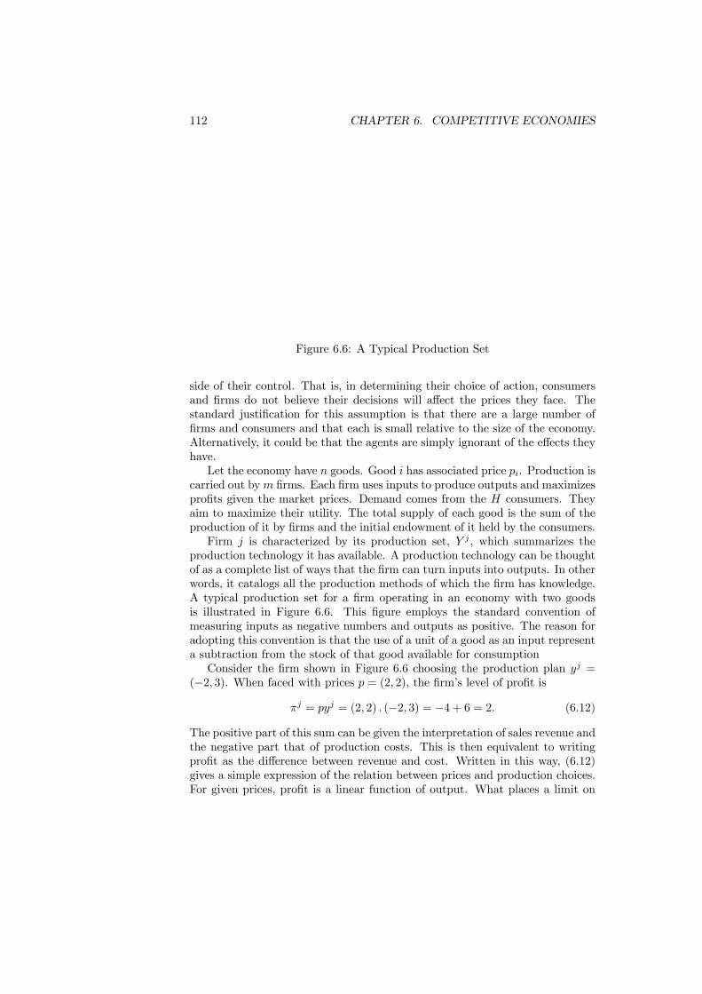
112 CHAPTER 6. COMPETITIVE ECONOMIES
Figure 6.6: A Typical Production Set
side of their control. That is, in determining their choice of action, consumersand firms do not believe their decisions will affect the prices they face. Thestandard justification for this assumption is that there are a large number offirms and consumers and that each is small relative to the size of the economy.Alternatively, it could be that the agents are simply ignorant of the effects theyhave.Let the economy have n goods. Good i has associated price pi. Production is
carried out bym firms. Each firm uses inputs to produce outputs and maximizesprofits given the market prices. Demand comes from the H consumers. Theyaim to maximize their utility. The total supply of each good is the sum of theproduction of it by firms and the initial endowment of it held by the consumers.Firm j is characterized by its production set, Y j , which summarizes the
production technology it has available. A production technology can be thoughtof as a complete list of ways that the firm can turn inputs into outputs. In otherwords, it catalogs all the production methods of which the firm has knowledge.A typical production set for a firm operating in an economy with two goodsis illustrated in Figure 6.6. This figure employs the standard convention ofmeasuring inputs as negative numbers and outputs as positive. The reason foradopting this convention is that the use of a unit of a good as an input representa subtraction from the stock of that good available for consumptionConsider the firm shown in Figure 6.6 choosing the production plan yj =
(−2, 3). When faced with prices p = (2, 2), the firm’s level of profit isπj = pyj = (2, 2) . (−2, 3) = −4 + 6 = 2. (6.12)
The positive part of this sum can be given the interpretation of sales revenue andthe negative part that of production costs. This is then equivalent to writingprofit as the difference between revenue and cost. Written in this way, (6.12)gives a simple expression of the relation between prices and production choices.For given prices, profit is a linear function of output. What places a limit on

6.3. PRODUCTION AND EXCHANGE 113
Figure 6.7: Profit Maximization
achievable profit is the technological possibilities open to the firm.The process of profit maximization is illustrated in Figure 6.7. Under the
competitive assumption the firm takes the prices p1 and p2 as given. Theseprices are used to construct isoprofit curves, which show all production plansthat give a specific level of profit. For example, all the production plans onthe isoprofit curve labelled π = 0 will lead to a profit level of 0. Productionplans on higher isoprofit curves lead to progressively larger profits and thoseon lower curves to negative profits. Since doing nothing (which means choosingy1 = y2 = 0) earns zero profit, the π = 0 isoprofit curve always passes throughthe origin.The profit-maximizing firm will choose a production plan that places it upon
the highest attainable isoprofit curve. What restricts the choice is the technol-ogy that is available as described by the production set. In Figure 6.7 theproduction plan that maximizes profit is shown by y∗ which is located at apoint of tangency between the isoprofit curve and the production set. There isno other technologically-feasible plan which can attain higher profit.It should be noted that the isoprofit curves are determined by the prices. In
fact, the geometry is that the isoprofit curves are at right-angles to the pricevector. The angle of the price vector is determined by the price ratio, p1p2 , so thata change in relative prices will alter the gradient of the isoprofit curves. Thefigure can be used to predict the effect of relative price changes. For instance,if p1 increases relative to p2, which can be interpreted as the price of the input(good 1) rising in comparison to the price of the output (good 2), the pricevector become flatter. This makes the isoprofit curves steeper, so the optimalchoice must move round the boundary of the production set towards the origin.The use of the input and the production of the output both fall.In the economy with n-goods, each firm will choose a production plan

114 CHAPTER 6. COMPETITIVE ECONOMIES
yj =³yj1, ..., y
jn
´.This production plan is chosen to maximize profits, πj = pyj ,
subject to the constraint that the chosen plan must be in the production set.From this maximization can be determined firm j’s supply function for good ias
yji = yji (p) . (6.13)
If good i is an output, then the level of supply in (6.13) is positive. If it is aninput, the “supply” is negative. The interpretation of the sign convention hereis that a positive supply adds to the economy’s stock of the good. In contrast,a negative supply reduces it and captures the idea of the input being used upin the production process. Using (6.13), the level of profit is
πj = pyj (p) = πj (p) , (6.14)
which also depends upon prices.Aggregate supply from the production sector of the economy is obtained
from the individual supply decisions of the individual firms by summing acrossthe firms. This gives aggregate supply as
Yi =mXj=1
yji (p) = Yi (p) . (6.15)
Since some goods must be inputs, and others outputs, the aggregate supplyY (p) = (Y1(p), ..., Yn(p)) will have some positive elements and some negative.Each consumer has an initial endowment of commodities and also a set of
shareholdings in firms. The latter assumption makes this a private ownershipeconomy in which the means of production are ultimately owned by individuals.In the present version of the model, these shareholdings are exogenously givenand remain fixed. A more-developed version would introduce a stock marketand allow them to be traded. For consumer h the initial endowment is denotedωh and the shareholding in firm j is θhj . The firms must be fully owned by the
consumers soPH
h=1 θhj = 1. That is, the shares in the firms must sum to one.
The preferences of consumer h are given by the utility function
Uh = Uh¡xh¢. (6.16)
Consumer h chooses a consumption plan xh to maximize their utility subject tothe budget constraint
nXi=1
pixhi =
nXi=1
piωhi +
mXj=1
θhj πj . (6.17)
This budget constraint requires that the value of expenditure is not more thanthe value of the endowment plus income received from dividends. Since firmsalways have the option of going out of business (and hence earning zero profit),the dividend income must be non-negative. The profit level of each firm is

6.3. PRODUCTION AND EXCHANGE 115
dependent upon prices. A change in prices therefore affects a consumer’s budgetconstraint through a change in the value of their endowment and through achange in profit income.The maximization of utility by the consumer results in the demand for good
i from consumer h taking the form
xhi = xhi (p1, ..., pn) . (6.18)
The level of aggregate demand is found by summing the individual demands ofthe consumers to give
Xi =nXi=1
xhi (p1, ..., pn) = Xi (p1, ..., pn) . (6.19)
6.3.2 Equilibrium
The same notion of equilibrium that was used for the exchange economy canbe applied in this economy with production. That is, equilibrium occurs whensupply is equal to demand. The distinction between the two is that supply,which was fixed in the exchange economy, is now variable and dependent uponthe production decisions of firms. Although this adds a further dimension tothe question of the existence of equilibrium, the basic argument why such anequilibrium always exists is essentially the same as that for the exchange econ-omy.As already noted, the equilibrium of the economy occurs when demand is
equal to supply or, equivalently, when excess demand is zero. Excess demandfor good i, Zi (p), can be defined by
Zi (p) = Xi (p)− Yi (p)−HXh=1
ωhi . (6.20)
Here excess demand is the difference between demand and the sum of initialendowment and firms’ supply. The equilibrium occurs when Zi (p) = 0 for allof the goods i = 1, ..., n. There are standard theorems that prove such anequilibrium must exist under fairly weak conditions.The properties established for the exchange economy also apply to this econ-
omy with production. Demand is determined only by relative prices (so it ishomogeneous of degree zero). Supply is also homogeneous of degree zero. To-gether, these imply that excess demand is also homogeneous of degree zero. Todetermine the equilibrium prices that equate supply to demand, a normalizationmust again be used. Typically, one of the goods will be chosen as numeraireand its price set to one. Equilibrium prices are then those which equate excessdemand to zero.
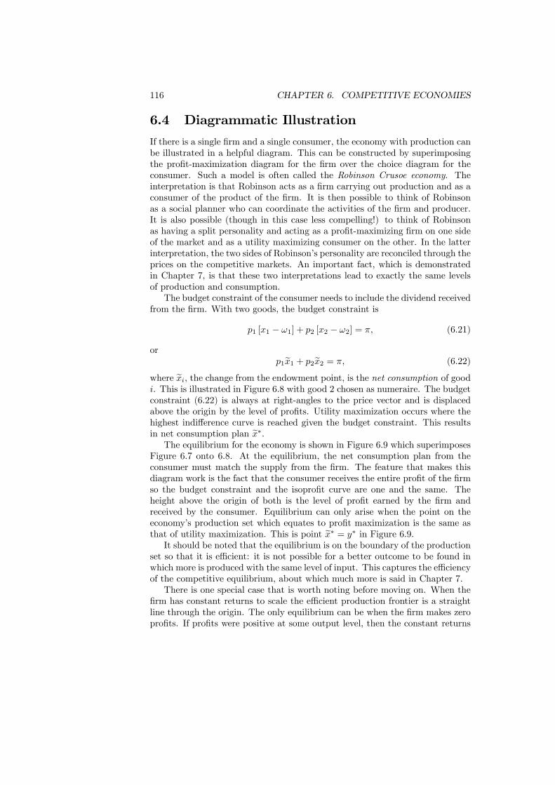
116 CHAPTER 6. COMPETITIVE ECONOMIES
6.4 Diagrammatic IllustrationIf there is a single firm and a single consumer, the economy with production canbe illustrated in a helpful diagram. This can be constructed by superimposingthe profit-maximization diagram for the firm over the choice diagram for theconsumer. Such a model is often called the Robinson Crusoe economy. Theinterpretation is that Robinson acts as a firm carrying out production and as aconsumer of the product of the firm. It is then possible to think of Robinsonas a social planner who can coordinate the activities of the firm and producer.It is also possible (though in this case less compelling!) to think of Robinsonas having a split personality and acting as a profit-maximizing firm on one sideof the market and as a utility maximizing consumer on the other. In the latterinterpretation, the two sides of Robinson’s personality are reconciled through theprices on the competitive markets. An important fact, which is demonstratedin Chapter 7, is that these two interpretations lead to exactly the same levelsof production and consumption.The budget constraint of the consumer needs to include the dividend received
from the firm. With two goods, the budget constraint is
p1 [x1 − ω1] + p2 [x2 − ω2] = π, (6.21)
orp1ex1 + p2ex2 = π, (6.22)
where exi, the change from the endowment point, is the net consumption of goodi. This is illustrated in Figure 6.8 with good 2 chosen as numeraire. The budgetconstraint (6.22) is always at right-angles to the price vector and is displacedabove the origin by the level of profits. Utility maximization occurs where thehighest indifference curve is reached given the budget constraint. This resultsin net consumption plan ex∗.The equilibrium for the economy is shown in Figure 6.9 which superimposes
Figure 6.7 onto 6.8. At the equilibrium, the net consumption plan from theconsumer must match the supply from the firm. The feature that makes thisdiagram work is the fact that the consumer receives the entire profit of the firmso the budget constraint and the isoprofit curve are one and the same. Theheight above the origin of both is the level of profit earned by the firm andreceived by the consumer. Equilibrium can only arise when the point on theeconomy’s production set which equates to profit maximization is the same asthat of utility maximization. This is point ex∗ = y∗ in Figure 6.9.It should be noted that the equilibrium is on the boundary of the production
set so that it is efficient: it is not possible for a better outcome to be found inwhich more is produced with the same level of input. This captures the efficiencyof the competitive equilibrium, about which much more is said in Chapter 7.There is one special case that is worth noting before moving on. When the
firm has constant returns to scale the efficient production frontier is a straightline through the origin. The only equilibrium can be when the firm makes zeroprofits. If profits were positive at some output level, then the constant returns

6.4. DIAGRAMMATIC ILLUSTRATION 117
Figure 6.8: Utility Maximization
Figure 6.9: Efficient Equilibrium
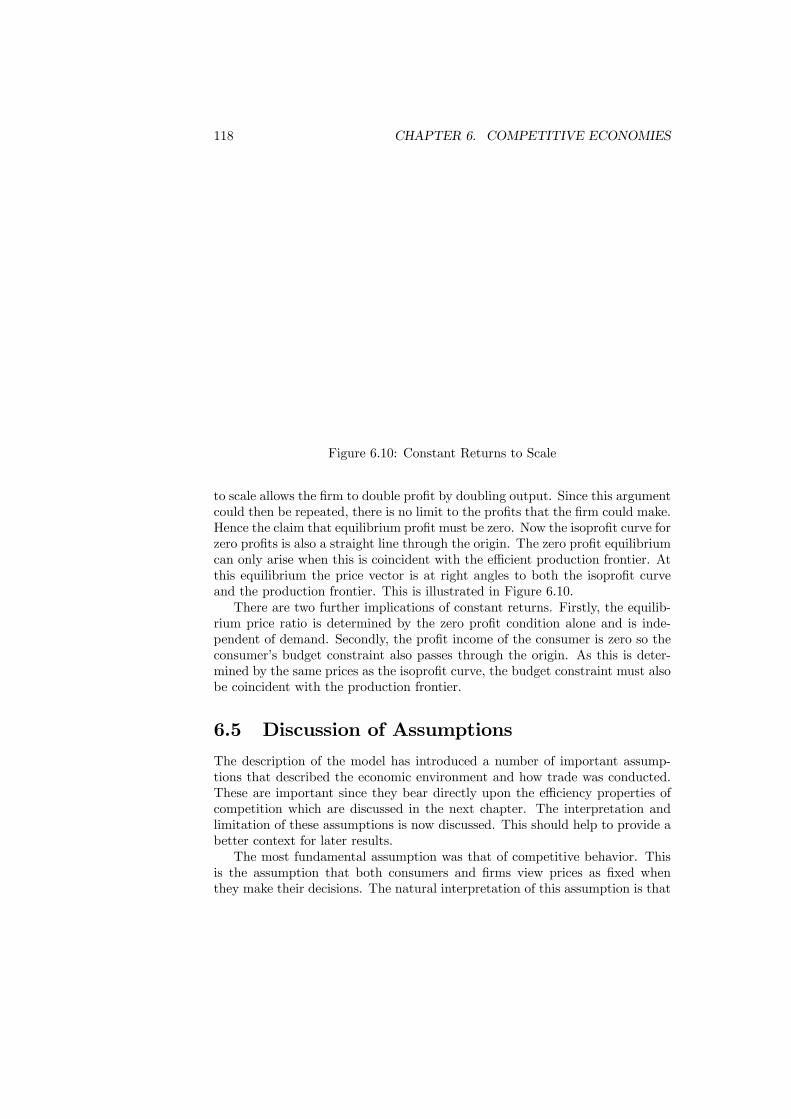
118 CHAPTER 6. COMPETITIVE ECONOMIES
Figure 6.10: Constant Returns to Scale
to scale allows the firm to double profit by doubling output. Since this argumentcould then be repeated, there is no limit to the profits that the firm could make.Hence the claim that equilibrium profit must be zero. Now the isoprofit curve forzero profits is also a straight line through the origin. The zero profit equilibriumcan only arise when this is coincident with the efficient production frontier. Atthis equilibrium the price vector is at right angles to both the isoprofit curveand the production frontier. This is illustrated in Figure 6.10.There are two further implications of constant returns. Firstly, the equilib-
rium price ratio is determined by the zero profit condition alone and is inde-pendent of demand. Secondly, the profit income of the consumer is zero so theconsumer’s budget constraint also passes through the origin. As this is deter-mined by the same prices as the isoprofit curve, the budget constraint must alsobe coincident with the production frontier.
6.5 Discussion of Assumptions
The description of the model has introduced a number of important assump-tions that described the economic environment and how trade was conducted.These are important since they bear directly upon the efficiency properties ofcompetition which are discussed in the next chapter. The interpretation andlimitation of these assumptions is now discussed. This should help to provide abetter context for later results.The most fundamental assumption was that of competitive behavior. This
is the assumption that both consumers and firms view prices as fixed whenthey make their decisions. The natural interpretation of this assumption is that
6.6. CONCLUSIONS 119
the individual economic agents are small relative to the total economy. Whenthey are small, they naturally have no consequence. This assumption rules outany kind of market power such as monopolistic firms or trade unions in labormarkets.Competitive behavior leads to the problem of who actually sets prices in the
economy. In the exchange model it can be thought that equilibrium prices areachieved via a process of barter and negotiation between the trading parties.However barter cannot be a credible explanation of price determination in anadvanced economic environment. The theoretical route out of this difficultyis to assume the existence of a fictitious Walrasian auctioneer who literallycalls out prices until equilibrium is achieved. At this point trade is allowed totake place. Obviously, this does not provide a credible explanation of reality.Although there are other theoretical explanation of price setting, none is entirelyconsistent with the competitive assumption. How to integrate the two remainsan unsolved puzzle.The second important assumption is the focus upon equilibrium positions.
This emphasis can be given several explanations. Historically, economists viewedthe economy as self-correcting so that, if it were ever away from equilibrium,forces existed that move it back towards equilibrium. In the long run, equilib-rium would then always be attained. Although such adjustment can be justifiedin simple single-market contexts, both the practical experience of sustainedhigh levels of unemployment and the theoretical study of the stability of suchprocesses have shown that it is not generally justified. The present justificationsfor focusing upon equilibrium are more pragmatic. The analysis of a model mustbegin somewhere, and the equilibrium has much merit as a starting point. Inaddition, even if the final focus is on disequilibrium, there is much to be gainedfrom comparing the properties of points of disequilibrium to those of the equi-librium. Finally, no positions other than those of equilibrium have any obviousclaim to prominence.
6.6 Conclusions
This chapter has introduced models of competitive economies involving the ex-change and production of commodities. It has been shown how the individualdecisions of consumers and producers are determined. The individual decisionshave been aggregated and a description of equilibrium given. Arguments wereadvanced as to why such equilibria would usually exist.These basic models will see much service in this book. They will be used to
derive some basic results in welfare theory and as the foundation for the analysisof taxation. They will be extended to introduce market imperfections and tointroduce time. In short, an understanding of the basic facts outlined above isessential to what follows.
Further readingThe two fundamental texts on the competitive economy are:

120 CHAPTER 6. COMPETITIVE ECONOMIES
Arrow, K.J. and Hahn, F.H. (1971) General Competitive Analysis (Amster-dam: North-Holland),andDebreu, G. (1959) The Theory of Value (Yale: Yale University Press).A textbook treatment can be found in:Ellickson, B. (1993) Competitive Equilibrium: Theory and Applications (Cam-
bridge: Cambridge University Press).The competitive economy has frequently been used as a practical tool for
policy analysis. A survey of applications is in:Shoven, J.B. and Whalley, J. (1992) Applying General Equilibrium Theory
(Cambridge: Cambridge University Press).A historical survey of the development of the model is given in:Duffie, D. and Sonnenschein, H. (1989) ”Arrow and General Equilibrium
Theory”, Journal of Economic Literature, 27, 565 - 598.Some questions concerning the foundations of the model are addressed in:Koopmans, T.C. (1957) Three Essays on the State of Economic Science
(New York: McGraw-Hill).

Chapter 7
Efficiency of Competition
7.1 Introduction
The discussion of Chapter 6 showed how the competitive model combined in-dependent decision-making of consumers and firms into a complete model ofthe economy. Equilibrium was achieved in the economy by prices adjusting toequate demand and supply. The purpose of this chapter is to demonstrate thatthe competitive equilibrium can be shown to possess properties of efficiency, afact that has been known to economists for some considerable time. The rootsof this analysis can be traced back at least to Adam Smith’s 18th century de-scription of the workings of the invisible hand of competition. The formalizationof the efficiency argument and the deeper understanding that comes with it, isa more recent innovation.That equilibrium prices can always be found which simultaneously equate
demand and supply for all goods is surprising. What is even more remarkableis that the equilibrium so obtained also has properties of efficiency. Why thisis remarkable is that individual households and firms are all pursuing theirindependent objectives with no apparent coordination other than through theprice system. Even so, the final state which emerges achieves efficiency solelythrough the coordinating role played by prices.The chapter first looks at the single consumer Robinson-Crusoe economy. It
is shown that the competitive equilibrium achieves the outcome that is unam-biguously best for the economy. To reach a similar conclusion in an economywith more that one consumer it is necessary to be more sophisticated in theanalysis. This is because what is good for one consumer need not be so foranother; so it is rarely possible to define a measure of what is unambiguouslygood. This reasoning motivates the introduction of the concept of Pareto effi-ciency which is the measure by which the efficiency of competitive equilibriumis judged. Given this concept, the efficiency theorems are described for boththe exchange economy and the production economy. The discussion then turnsto the role of lump-sum taxes and transfers in achieving a chosen equilibrium.
121
122 CHAPTER 7. EFFICIENCY OF COMPETITION
This provides one of the foundations for the normative analysis of public policy.
7.2 Efficiency
Economics is often defined as the study of scarcity. This viewpoint is reflectedin the concern with the efficient use of resources that runs throughout the coreof the subject. Efficiency would seem to be a simple concept to characterize: ifmore cannot be achieved then the outcome is efficient.When an individual decision maker is considered the problem of determining
what is efficient and what is not is this simple. The individual will employ theirresources to maximize utility subject to the constraints they face. When utilityis maximized, the efficient outcome has been achieved. Problems arise whenthere is more than one decision maker. To be unambiguous about efficiency it isnecessary to resolve the potentially competing needs of different decision makers.Efficiency has to be defined with respect to a set of aggregate preferences.The difficulty of progressing from individual to social preferences has already
been met in Chapter 4. There the limitations of voting as a method of collectivechoice were observed. These limitations are representative of the more generalissues analyzed in Chapter 13. The conclusion will remain that determinationof aggregate preferences is not simple. So defining a criteria for efficiency is nota simple question to answer though it is core to what we try to do.One route to a solution is to look at a single-consumer economy or an econ-
omy of identical consumers. Then there is no conflict between competing pref-erences. But with different consumers some creativity has to be used to describeefficiency. How this is done will be shown in Section 7.4 where the concept ofPareto efficiency is introduced. The trouble with such creativity is that it leavesthe definition of efficiency open to debate. We will postpone further discussionof this until Chapter 13.Before proceeding some definitions are need. A first-best outcome is achieved
when only the production technology and limitations on endowments restrict thechoice of the decision maker. Essentially, the first-best is what would be chosenby an omniscient planner with complete command over resources. A second-best arises whenever constraints other than technology and resources are placedupon what the planner can do. Such constraints could be limits on incomedistribution or an inability to remove monopoly power.
7.3 Single Consumer
With a single consumer there is no doubt as to what is good and bad from asocial perspective: the single individual’s preferences can be taken as the socialpreferences. To do otherwise would be to deny the validity of the consumer’sjudgements. Formally, it would involve violation of Condition P, the Paretoprinciple of Chapter 4. Hence, if the individual prefers one outcome to an-other, then so must society. The unambiguous nature of preferences provides

7.3. SINGLE CONSUMER 123
Figure 7.1: Optimal Allocation
significant simplification of the discussion of efficiency in the single-consumereconomy.
The issue of efficiency with a single consumer can be studied by using theRobinson Crusoe economy of Chapter 6. We assume that a set of preferencesand a production technology are given for the economy. Using these the ”best”outcome for the economy is determined and this is then compared to the outcomeobtained through competitive behavior. In this case the ”best” outcome mustbe first-best since no constraints on policy choices have not been invoked nor isthere an issue of income distribution to consider.
The first-best outcome for the single-consumer economy achieves the highestindifference curve possible subject to the restriction that it is feasible under thetechnology. This is illustrated in Figure 7.1 where the most preferred outcomeis determined as the tangency between the indifference curve and the efficientfrontier of the production set. Point ex∗ is the net level of consumption relativeto the endowment point and the production plan for the firm in the first-best.
A simple characterization of this first-best allocation can be given by usingthe fact that it is at a tangency point between two curves. The gradient ofthe indifference curve is equal to the ratio of the marginal utilities of the twogoods and is called the marginal rate of substitution. This measures the rateat which good 1 must be traded for good 2 to maintain constant utility. Usingsubscripts to denote the marginal utilities of the two goods, the marginal rateof substitution is given by MRS1,2 = U1
U2. Similarly, the gradient of the produc-
tion possibility set is termed the marginal rate of transformation and denotedMRT1,2. The MRT1,2 measures the rate at which good 1 has to be given upto allow an increase in production of good 2. At the tangency point, the two

124 CHAPTER 7. EFFICIENCY OF COMPETITION
gradients are equal so
MRS1,2 =MRT1,2. (7.1)
The reason why this equality characterizes the first-best equilibrium can beexplained as follows: The MRS captures the marginal value of good 1 to theconsumer relative to the marginal value of good 2 while theMRT measures themarginal cost of good 1 relative to the marginal cost of good 2. The first-bestis achieved when the marginal value is equal to the marginal cost.Having characterized the first-best outcome it is necessary to contrast this
with what the market achieves. This can be done by comparing Figure 7.1 whichdisplays the competitive market equilibrium to Figure 6.9 . Doing this makesit immediately apparent that the same allocation is reached in both cases: thesame tangency point is achieved so the market equilibrium is also the first-bestoutcome for the economy.The market achieves efficiency through the coordinating role of prices. The
consumer maximizes utility subject to their budget constraint. The optimalchoice occurs when the budget constraint is tangential to highest attainableindifference curve. The condition describing this is that ratio of marginal utilitiesis equal to the ratio of prices. Expressed in terms of the MRS this is
MRS1,2 =p1p2. (7.2)
Similarly, profit maximization by the firm occurs when the production possibilityset is tangential to the highest isoprofit curve. Using the MRT , the profit-maximization condition is
MRT1,2 =p1p2. (7.3)
Combining these conditions the competitive equilibrium satisfies
MRS1,2 =p1p2=MRT1,2. (7.4)
The condition in (7.4) demonstrates that the competitive equilibrium satisfiesthe same condition as the first-best and reveals the essential role of prices. Underthe competitive assumption, both the consumer and the producer are guidedin their decisions by the same price ratio. Each optimizes relative to the priceratio, hence their decisions are mutually efficient.In this single consumer context the equilibrium reached by the market simply
cannot be bettered. Such a strong statement cannot be made when furtherconsumers are introduced since issues of distribution between consumers thenarise. However, what will remain is the finding that the competitive marketensures that firms produce at an efficient point on the frontier of the productionset and that the chosen production plan is what is demanded at the equilibriumprices by the consumer. The key to this coordination are the prices that providethe signals guiding choices.

7.4. PARETO EFFICIENCY 125
7.4 Pareto Efficiency
When there is more than one consumer the simple analysis of the RobinsonCrusoe economy does not apply. Since consumers can have differing views aboutthe success of an allocation, there is no single, simple measure of efficiency. Theessence of the difficulty is that of judging between allocations with differentdistributional properties. What is needed is some measure that can take accountof the potentially diverse views of the consumers and separate efficiency fromdistribution.To achieve this, economists employ the concept of Pareto efficiency. The
philosophy behind this concept is that efficiency means there must be no un-exploited economic gains. Testing the efficiency of an allocation then involveschecking whether there are any such gains available. Pareto efficiency judgesan allocation by considering whether it is possible to undertake a reallocationof resources that can benefit at least one consumer without harming any. If itwere possible to do so, then there would exist unexploited gains. When no suchimproving reallocation can be found, then the initial position is deemed to bePareto efficient. An allocation that satisfies this test can be viewed as havingachieved an efficient distribution of resources. For the present chapter this con-cept will be used uncritically. The interpretations and limitations of this formof efficiency will be discussed in Chapter 13.To provide a precise statement of Pareto efficiency that applies in a compet-
itive economy it is first necessary to extend the idea of feasible allocations ofresources that was used in (6.4) to define the Edgeworth box. When productionis included, an allocation of consumption is feasible if it can be produced giventhe economy’s initial endowments and production technology. Given the initialendowment, ω, the consumption allocation x is feasible if there is productionplan y such that
x = y + ω. (7.5)
Pareto efficiency is then tested using the feasible allocations. A feasibleconsumption allocation bx is Pareto efficient if there does not exist an alternativefeasible allocation x such that:(i) Allocation x gives all consumers at least as much utility as bx;(ii) Allocation x gives at least one consumer more utility than bx.These two conditions can be summarized as saying that allocation bx is Pareto
efficient if there is no alternative allocation (a move from bx to x) that can makesomeone better-off without making anyone worse-off. It is this idea of beingable to make someone better-off without making someone else worse-off thatrepresents the unexploited economic gains in an inefficient position.It should be noted even at this stage how Pareto efficiency is defined by
the negative property of being unable to find anything better than the allo-cation. This is somewhat different to a definition of efficiency that looks forsome positive property of the allocation. Pareto efficiency also sidesteps issuesof distribution rather than confronting them. More will be said about this inChapter 13 when the construction of social welfare indicators is discussed.

126 CHAPTER 7. EFFICIENCY OF COMPETITION
Figure 7.2: Pareto Efficiency
7.5 Efficiency in an Exchange Economy
The welfare properties of the economy, which are commonly known as the TwoTheorems of Welfare Economics, are the basis for claims concerning the desir-ability of the competitive outcome. In brief, the First Theorem states that acompetitive equilibrium is Pareto efficient and the Second Theorem that anyPareto efficient allocation can be decentralized as a competitive equilibrium.Taken together, they have significant implications for policy and, at face value,they seem to make a compelling case for the encouragement of competition.The Two Theorems are easily demonstrated for a two-consumer exchange
economy by using the Edgeworth box diagram. The first step is to isolate thePareto efficient allocations. Consider Figure 7.2 and the allocation at pointa. To show that a is not a Pareto efficient allocation it is necessary to findan alternative allocation which gives at least one of the consumers a higherutility level and neither consumer a lower level. In this case, moving to theallocation at point b raises the utility of both consumers when compared to a.This establishes that a is not Pareto efficient. Although b improves upon a itis not Pareto efficient either: the allocation at c provides higher utility for bothconsumers than b.The allocation at c is Pareto efficient. Beginning at c any change in the
allocation must lower the utility of at least one of the consumers. The specialproperty of point c is that it lies at a point of tangency between the indifferencecurves of the two consumers. As it is a point of tangency, moving away fromit must lead to a lower indifference curve for one of the consumers if not both.Since the indifference curves are tangential, their gradients are equal so
MRS11,2 =MRS21,2. (7.6)
Hence the rate at which consumer 1 will exchange good 1 for good 2 is equal tothe rate at which consumer 2 will exchange the two goods. It is this equality

7.5. EFFICIENCY IN AN EXCHANGE ECONOMY 127
Figure 7.3: The First Theorem
of marginal values at the tangency point that results in there being no furtherunexploited gains and so makes c Pareto efficient.The Pareto efficient allocation at c is not unique. In fact, there are many
points of tangency between the two consumers’ indifference curves. A secondPareto Efficient allocation is at point d in Figure 7.2. Taken together, all thePareto efficient allocations form a locus in the Edgeworth box which is calledthe contract curve. This is illustrated in Figure 7.3. With this construction itis now possible to demonstrate the First Theorem.Referring back to Figure 6.4, a competitive equilibrium is given by a price line
through the initial endowment point, ω, which is tangential to both indifferencecurves at the same point. The common point of tangency results in consumerchoices that lead to the equilibrium levels of demand. Such an equilibrium isindicated by point e in Figure 7.3. As the equilibrium is a point of tangency ofindifference curves, it must also be Pareto efficient. For the Edgeworth box, thiscompletes the demonstration that a competitive equilibrium is Pareto efficient.The alternative way of seeing this result is to recall that the consumer max-
imizes utility at the point where their budget constraint is tangential to thehighest indifference curve. Using the MRS, this condition can be written forconsumer h as MRSh1,2 =
p1p2. The competitive assumption is that both con-
sumers react to the same set of prices so it follows that
MRS11,2 =p1p2=MRS11,2. (7.7)
Comparing this condition with (7.6) provides an alternative demonstration thatthe competitive equilibrium is Pareto efficient. It also shows again the role ofprices in coordinating the independent decisions of different economic agents toensure efficiency.This discussion can be summarized in the precise statement of the theorem.
128 CHAPTER 7. EFFICIENCY OF COMPETITION
Theorem 7 (The First Theorem of Welfare Economics) The allocation of com-modities at a competitive equilibrium is Pareto efficient.
This theorem can be formally proved by assuming that the competitive equi-librium is not Pareto efficient and deriving a contradiction. Assuming the com-petitive equilibrium is not Pareto efficient implies there is a feasible alternativethat is at least as good for all consumers and strictly better for at least one.Now take the consumer who is made strictly better off. Why did they notchoose the alternative consumption plan at the competitive equilibrium? Theanswer has to be because it was more expensive than their choice at the com-petitive equilibrium and not affordable with their budget. Similarly, for allother consumers the new allocation has to be at least as expensive as theirchoice at the competitive equilibrium. (If it were cheaper, they could afford aneven better consumption plan which made them strictly better-off than at thecompetitive equilibrium.) Summing across the consumers, the alternative allo-cation has to be strictly more expensive than the competitive allocation. Butthe value of consumption at the competitive equilibrium must equal the value ofthe endowment. Therefore the new allocation must have greater value than theendowment which implies it cannot be feasible. This contradiction establishesthat the competitive equilibrium must be Pareto efficient.The theorem demonstrates that the competitive equilibrium is Pareto effi-
cient but it is not the only Pareto efficient allocation. Referring back to Figure7.3, any point on the contract curve is also Pareto efficient since all are definedby a tangency between indifference curves. The only special feature of e is thatit is the allocation reached through competitive trading from the initial endow-ment point ω. If ω were different, then another Pareto efficient allocation wouldbe achieved. In fact there is an infinity of Pareto efficient allocations. Observingthese points motivates the Second Theorem of Welfare Economics.The Second Theorem is concerned with whether a given Pareto efficient al-
location can be made into a competitive equilibrium by choosing a suitablelocation for the initial endowment. Expressed differently, can a competitiveeconomy be constructed which has a selected Pareto efficient allocation as itscompetitive equilibrium? In the Edgeworth box, this involves being able tochoose any point on the contract curve and turning it into a competitive equi-librium.Using the Edgeworth Box diagram it can be seen that this is possible in the
exchange economy if the households’ indifference curves are convex. The com-mon tangent to the indifference curves at a Pareto efficient allocation providesthe budget constraint that each consumer must face if they are to afford thechosen point. The convexity ensures that, given this budget line, the Pareto ef-ficient point will also be the optimal choice of the consumers. The constructionis completed by choosing a point on this budget line as the initial endowmentpoint. This process of constructing a competitive economy to obtain a selectedPareto efficient allocation is termed decentralization.This process is illustrated in Figure 7.4 where the Pareto efficient allocation
e0 is made a competitive equilibrium by selecting ω0 as the endowment point.

7.6. EXTENSION TO PRODUCTION 129
Figure 7.4: The Second Theorem
Starting from ω0, trading by consumers will take the economy to its equilibriumallocation e0. This is the Pareto efficient allocation that it was intended shouldbe reached. Note that if the endowments of the households are initially givenby ω and the equilibrium at e0 is to be decentralized, it is necessary to adjustthe initial endowments of the consumers in order to begin from ω0.The construction described above can be given a formal statement as the
Second Theorem of Welfare Economics.
Theorem 8 (The Second Theorem of Welfare Economics) With convex prefer-ences, any Pareto efficient allocation can be made a competitive equilibrium.
The statement of the Second Theorem provides a conclusion but does notdescribe the mechanism involved in the decentralization. The important stepin decentralizing a chosen Pareto efficient allocation is placing the economy atthe correct starting point. For now it is sufficient to observe that behind theSecond Theorem lies a process of redistribution of initial wealth. How this canbe achieved is discussed later. Furthermore, the Second Theorem determines aset of prices that make the chosen allocation an equilibrium. These prices maywell be very different from those that would have been obtained in the absenceon the wealth redistribution.
7.6 Extension to Production
The extension of these theorems to an economy with production is straightfor-ward. The major effect of production is to make supply variable: it is now thesum of the initial endowment plus the net outputs of the firms. In addition, aconsumer’s income includes the profit derived from their shareholdings in firms.Section 7.3 has already described the Two Theorems for the Robinson Cru-
soe economy which included production. It was shown that the competitive
130 CHAPTER 7. EFFICIENCY OF COMPETITION
equilibrium achieved the highest attainable indifference curve given the produc-tion possibilities of the economy. Since the single consumer cannot be madebetter off by any change, the equilibrium is Pareto efficient and the First Theo-rem applies. The Second Theorem is of limited interest with a single consumersince there is only one Pareto efficient allocation and this is attained by thecompetitive economy.When there is more than one consumer the proof of the First Theorem follows
the same lines as for the exchange economy. Given the equilibrium prices, eachconsumer is maximizing utility so their marginal rate of substitution is equatedto the price ratio. This is true for all consumers and all goods, so
MRShi,j =pipj=MRSh
0i,j , (7.8)
for any pair of consumers h and h0 and any pair of good i and j. This istermed efficiency in consumption. In an economy with production this conditionalone is not sufficient to guarantee efficiency and it is also necessary to considerproduction. The profit-maximization decision of each firm will ensure that itequates its marginal rate of transformation between any two goods to the ratioof prices. For any two firms m and m0 this give
MRTmi,j =pipj=MRTm
0i,j , (7.9)
a condition that characterizes efficiency in production. The price ratio alsocoordinates consumers and firms giving
MRShi,j =MRTmi,j , (7.10)
for any consumer and any firm for all pairs of goods. As for the Robinson-Crusoeeconomy, the interpretation of this condition is that it equates the relative mar-ginal values to the relative marginal costs. Since (7.8) - (7.10) are the conditionsrequired for efficiency, this shows that the First Theorem extends to the economywith production.The formal proof of this claim mirrors that for the exchange economy, ex-
cept for the fact that the value of production must also be taken into account.Given this, the basis of the argument remains that since the consumers chosethe competitive equilibrium quantities anything that is preferred must be moreexpensive and hence can be shown not to be feasible.The extension of the Second Theorem to include production is illustrated
in Figure 7.5. The set W describes the feasible consumption plans for theeconomy with each point in w equal to the sum of a production plan and theinitial endowment, w = ω+y. Set Z denotes the consumption plans that wouldallow a Pareto improvement over the allocation bx1 to consumer 1 and bx2 toconsumer 2. If W and Z are convex, which occurs when firms’ production setsand preferences are convex, then a common tangent to W and Z can be found.This would make bx an equilibrium. Individual income allocations, the sum ofthe value of endowment plus profit income, can be placed anywhere on the
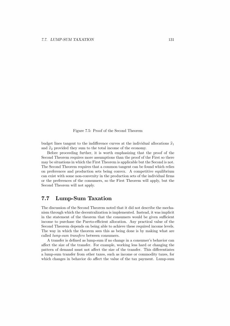
7.7. LUMP-SUM TAXATION 131
Figure 7.5: Proof of the Second Theorem
budget lines tangent to the indifference curves at the individual allocations bx1and bx2 provided they sum to the total income of the economy.Before proceeding further, it is worth emphasizing that the proof of the
Second Theorem requires more assumptions than the proof of the First so theremay be situations in which the First Theorem is applicable but the Second is not.The Second Theorem requires that a common tangent can be found which relieson preferences and production sets being convex. A competitive equilibriumcan exist with some non-convexity in the production sets of the individual firmsor the preferences of the consumers, so the First Theorem will apply, but theSecond Theorem will not apply.
7.7 Lump-Sum Taxation
The discussion of the Second Theorem noted that it did not describe the mecha-nism through which the decentralization is implemented. Instead, it was implicitin the statement of the theorem that the consumers would be given sufficientincome to purchase the Pareto-efficient allocation. Any practical value of theSecond Theorem depends on being able to achieve these required income levels.The way in which the theorem sees this as being done is by making what arecalled lump-sum transfers between consumers.A transfer is defined as lump-sum if no change in a consumer’s behavior can
affect the size of the transfer. For example, working less hard or changing thepattern of demand must not affect the size of the transfer. This differentiatesa lump-sum transfer from other taxes, such as income or commodity taxes, forwhich changes in behavior do affect the value of the tax payment. Lump-sum
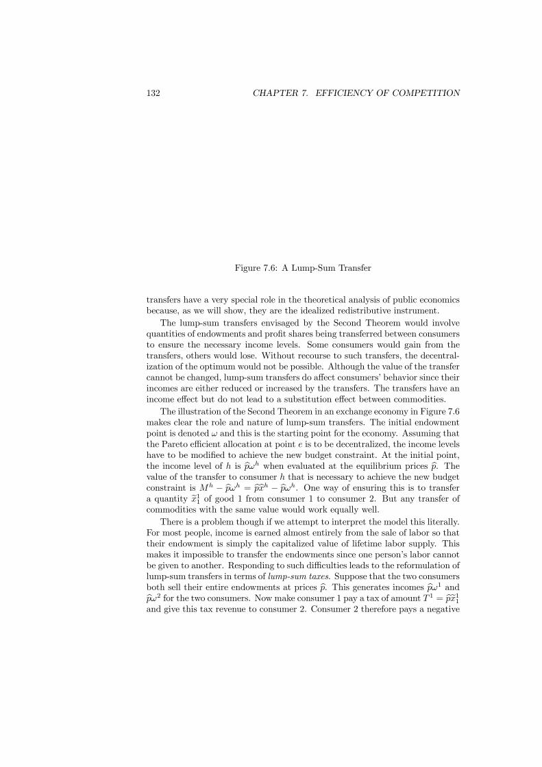
132 CHAPTER 7. EFFICIENCY OF COMPETITION
Figure 7.6: A Lump-Sum Transfer
transfers have a very special role in the theoretical analysis of public economicsbecause, as we will show, they are the idealized redistributive instrument.The lump-sum transfers envisaged by the Second Theorem would involve
quantities of endowments and profit shares being transferred between consumersto ensure the necessary income levels. Some consumers would gain from thetransfers, others would lose. Without recourse to such transfers, the decentral-ization of the optimum would not be possible. Although the value of the transfercannot be changed, lump-sum transfers do affect consumers’ behavior since theirincomes are either reduced or increased by the transfers. The transfers have anincome effect but do not lead to a substitution effect between commodities.The illustration of the Second Theorem in an exchange economy in Figure 7.6
makes clear the role and nature of lump-sum transfers. The initial endowmentpoint is denoted ω and this is the starting point for the economy. Assuming thatthe Pareto efficient allocation at point e is to be decentralized, the income levelshave to be modified to achieve the new budget constraint. At the initial point,the income level of h is bpωh when evaluated at the equilibrium prices bp. Thevalue of the transfer to consumer h that is necessary to achieve the new budgetconstraint is Mh − bpωh = bpbxh − bpωh. One way of ensuring this is to transfera quantity ex11 of good 1 from consumer 1 to consumer 2. But any transfer ofcommodities with the same value would work equally well.There is a problem though if we attempt to interpret the model this literally.
For most people, income is earned almost entirely from the sale of labor so thattheir endowment is simply the capitalized value of lifetime labor supply. Thismakes it impossible to transfer the endowments since one person’s labor cannotbe given to another. Responding to such difficulties leads to the reformulation oflump-sum transfers in terms of lump-sum taxes. Suppose that the two consumersboth sell their entire endowments at prices bp. This generates incomes bpω1 andbpω2 for the two consumers. Now make consumer 1 pay a tax of amount T 1 = bpex11and give this tax revenue to consumer 2. Consumer 2 therefore pays a negative

7.8. SUMMARY 133
tax (or, in simpler terms, receives a subsidy) of T 2 = −bpex11 = −T 1. This pairof taxes can be seen to move the budget constraint in exactly the same wayas the lump-sum transfer of endowment. The pair of taxes and the transfer ofendowment are therefore economically equivalent and have the same effect uponthe economy. The taxes are also lump-sum since they are determined withoutreference to either consumers’ behavior and their values cannot be affected byany change in behavior.Lump-sum taxes have a central role in public economics due to their effi-
ciency in achieving distributional objectives. It should be clear from the discus-sion above that the economy’s total endowment is not reduced by the applicationof the lump-sum taxes. This point applies to lump-sum taxes in general. Ashouseholds cannot affect the level of the tax by changing their behavior, lump-sum taxes do not lead to any inefficiency. There are no resources lost due to theimposition of lump-sum taxes and redistribution is achieved with no efficiencycost. In short, if they can be employed in the manner described they are theperfect taxes.
7.8 SummaryThis chapter has described and proved the Two Theorems of Welfare Economics.To do this it was necessary to introduce the concept of Pareto efficiency. Whilstthis was simply accepted in this chapter, it will be considered very criticallyin Chapter 13. The Two Theorems characterize the efficiency properties of thecompetitive economy and state when a selected Pareto efficient allocation canbe decentralized. The role of lump-sum transfers or taxes in supporting theSecond Theorem has been highlighted. These transfers constitute the ideal taxsystem since they have no resource costs.The subject matter of this chapter has very strong implications which are
investigated fully in later chapters. An understanding of them, and of theirlimitations, is fundamental to appreciating many of the developments of publiceconomics. Since claims about the efficiency of the competition feature routinelyin economic debate it is important to subject it to the most careful of scrutiny.
Further readingThe classic proof of these theorems is inDebreu, G. (1959) Theory of Value, (New York: Wiley).A formal analysis of lump-sum taxation can be found in:Mirrlees, J.A. (1986) “The theory of optimal taxation“ in K.J. Arrow and
M.D. Intrilligator (eds.), Handbook of Mathematical Economics (Amsterdam:North-Holland).An extensive textbook treatment of Pareto efficiency is:Ng, Y.-K. (2003) Welfare Economics, (Basingstoke: Macmillan).

134 CHAPTER 7. EFFICIENCY OF COMPETITION

Part IV
Departures from Efficiency
135

Chapter 8
Public Goods
8.1 Introduction
When a government provides a level of national defense sufficient to make acountry secure, all inhabitants are simultaneously protected. Equally, when aradio program is broadcast it can be received simultaneously by all listeners inrange of the transmitter. The possibility for many consumers to benefit from asingle unit of provision violates the assumption of the private nature of goodsunderlying the efficiency analysis of Chapter 7. The Two Theorems relied onall goods being private in nature, so that they could only be consumed by asingle consumer. If there are goods such as national defense in the economy,market failure occurs and the unregulated competitive equilibrium will fail to beefficient. This inefficiency implies that there is a potential role for governmentintervention.The chapter begins by defining a public good and distinguishing between
public goods and private goods. Doing so provides considerable insight intowhy market failure arises when there are public goods. The inefficiency is thendemonstrated by analyzing the equilibrium that is achieved when it is left tothe market to provide public goods. The Samuelson rule characterizing theoptimal level of the public good is then derived. This permits a comparison ofequilibrium and optimum.The focus of the chapter then turns to the consideration of methods through
which the optimum can be achieved. The first of these, the Lindahl equilibrium,is based on observation that the price each consumer pays for the public goodshould reflect their valuation of it. The Lindahl equilibrium achieves optimalitybut, since the valuations are private information, it generates incentives for con-sumers to provide false information. Mechanisms designed to elicit the correctstatement of these valuations are then considered. The theoretical results arethen contrasted with the outcomes of experiments designed to test the extentof false statement of valuations and the use of market data to calculate valua-tions. These results are primarily static in nature. To provide some insight into
137
138 CHAPTER 8. PUBLIC GOODS
the dynamic aspects of public good provision, the chapter is completed by theanalysis of two different forms of fund-raising campaign which permit sequentialcontributions.
8.2 Definitions
The pure public good has been the subject of most of the economic analysisof public goods. In some ways, the pure public good is an abstraction that isadopted to provide a benchmark case against which other, more realistic, casescan be assessed. A pure public good has the following two properties.
• Non-excludability. If the public good is supplied, no consumer can beexcluded from consuming it.
• Non-rivalry. Consumption of the public good by one consumer does notreduce the quantity available for consumption by any other.
In contrast, a private good is excludable at no cost and is perfectly rivalrous:if it is consumed by one person then none of it remains for any other. Althoughthey were not made explicit, these properties of a private good have been implicitin how we have analyzed market behavior in earlier chapters. As we will see,the efficiency of the competitive economy is dependent upon them.The two properties that characterize a public good have important impli-
cations. Consider a firm that supplies a pure public good. Since the good isnon-excludable, if the firm supplies one consumer then it has effectively sup-plied the public good to all. The firm can charge the initial purchaser butcannot charge any of the subsequent consumers. This prevents it from obtain-ing payment for the total consumption of the public good. The fact that there isno rivalry in consumption implies that the consumers should have no objectionto multiple consumption. These features prevent the operation of the marketequalizing marginal valuations as it does to achieve efficiency in the allocationof private goods.In practice, it is difficult to find any good that perfectly satisfies both the con-
ditions of non-excludability and non-rivalry precisely. For example, the trans-mission of a television signal will satisfy non-rivalry but exclusion is possible atfinite cost by scrambling the signal. Similar comments apply, for example, todefense spending which will eventually be rivalrous as a country of fixed sizebecomes crowded and from which exclusion is possible by deportation. Mostpublic goods eventually suffer from congestion when too many consumers tryto use them simultaneously. For example, parks and roads are public goodswhich can become congested. The effect of congestion is to reduce the benefitthe public good yields to each user. Public goods which are excludable, but ata cost, or suffer from congestion beyond some level of use are called impure.The properties of impure public goods place them between the two extremes ofprivate goods and pure public goods.

8.3. PRIVATE PROVISION 139
Figure 8.1: Typology of Goods
A simple diagram summarizing the different types of good and the namesgiven to them is shown in Figure 8.1. These goods vary in the properties ofexcludability and rivalry. In fact, it is helpful to envisage a continuum of goodswhich gradually vary in nature as they become more rivalrous or more easilyexcludable. The pure private good and the pure public good have already beenidentified. An example of a common property good is a lake which can be usedfor fishing by anyone who wishes, or a field that can be used for grazing by anyfarmer. This class of goods (usually called the commons) are studied in Chapter10. The problem with the commons is the tendency of overusing them, andthe usual solution is to establish property rights to govern access. This is whathappened in the sixteenth century in England where common land was enclosedand became property of the local landlords. The landlords then charged grazingfees, and so cut back the use. In some instances property rights are hard todefine and enforce, as is the case of the control over the high seas or air quality.For this reason, only voluntary cooperation can solve the international problemof overfishing, acid rain and greenhouse effect. Club goods are public goods forwhich exclusion is possible. The terminology is motivated by sport clubs whosefacilities are a public good for members but from which non-members can beexcluded. Clubs are studied in Chapter 9.
8.3 Private Provision
Public goods do not conform to the assumptions required for a competitive econ-omy to be efficient. Their characteristics of non-excludability and non-rivalrylead to the wrong incentives for consumers. Since they can share in consump-tion, each consumer has an incentive to rely on others to make purchases of thepublic good. This reliance on others to purchase is call free-riding and it is thisthat leads to inefficiency.To provide a model that can reveal the motive for free-riding and its con-
140 CHAPTER 8. PUBLIC GOODS
sequences, consider two consumers who have to allocate their incomes betweenpurchases of a private good and of a public good. Assume that the consumerstake the prices of the two goods as fixed when they make their decisions. If thegoods were both private, we could move immediately to the conclusion that anefficient equilibrium would be attained. What makes the public good differentis that each consumers derives a benefit from the purchases of the other. Thislink between the consumers, which is absent with private goods, introduces astrategic interaction into the decision processes. With the strategic interaction,the consumers are involved in a game so equilibrium is found using the conceptof a Nash equilibrium.The consumers have income levels M1 and M2. Income must be divided
between purchases of the private good and the public good. Both goods areassumed to have a price of 1. Using xh to denote purchase of the private goodby consumer h and gh to denote purchase of the public good, the choices mustsatisfy the budget constraintMh = xh+gh. The link between consumers comesfrom the fact that the consumption of the public good for each consumer isequal to the total quantity purchased, g1+g2. Hence, when making the purchasedecision, each consumer must take account of the decision of the other.This interaction is captured in the preferences of consumer h by writing the
utility function asUh¡xh, g1 + g2
¢. (8.1)
The standard Nash assumption is now imposed that each consumer takes thepurchase of the other as given when they make their decision. Under this as-sumption, consumer 1 chooses g1 to maximize utility given g2, while consumer2 chooses g2 given g1. This can be expressed by saying that the choice of con-sumer 1 is the best reaction to g2 and that of consumer 2 the best reaction tog1. The Nash equilibrium occurs when these reactions are mutually compatible,so that the choice of each is the best reaction to the choice of the other.The Nash equilibrium can be displayed by analyzing the preferences of the
two consumers over different combination of g1 and g2. Consider consumer 1.Using the budget constraint, their utility can be written as U1
¡M1 − g1, g1 + g2¢.
The indifference curves of this utility function are shown in Figure 8.2. Thesecan be understood by noting that an increase in g2 will always lead to a higherutility level for any value of g1. For given g2, an increase in g1 will initiallyincrease utility as more preferred combination of private and public good areachieved. Eventually, further increases in g1 will reduce utility as the level ofprivate good consumption becomes too small relative to that of public good.The income level places an upper limit upon g1.Consumer 1 takes the provision of 2 as given when making their choice.
Consider consumer 2 having chosen g2. The choices open to consumer 1 then liealong the horizontal line drawn at g2 in Figure 8.2. The choice that maximizesthe utility of consumer 1 occurs at the tangency of an indifference curve andthe horizontal line - this is the highest indifference curve they can reach. Thisis shown as the choice bg1. In the terminology we have chosen, bg1 is the bestreaction to g2. Varying the level of g2 will lead to another best reaction for

8.3. PRIVATE PROVISION 141
Figure 8.2: Preferences and Choice
consumer 1. Doing this for all possible g2 traces out the optimal choices of g1
shown by the locus through the lowest point on each indifference curve. Thislocus is known as the Nash reaction function and depicts the value of g1 thatwill be chosen in response to a value of g2. This construction can be repeatedfor consumer 2 and leads to Figure 8.3. For consumer 2, utility increases with g1
and thus indifference curves further to the right reflect higher utility levels. Thebest reaction for consumer 2 is shown by bg2 which occurs where the indifferencecurve is tangential to the vertical line at g1. The Nash reaction function linksthe points where the indifference curves are vertical.
The Nash equilibrium occurs where the choices of the two consumers arethe best reactions to each other so neither has an incentive to change theirchoice. This can only hold at a point at which the Nash reaction functionscross. The equilibrium is illustrated in Figure 8.4 in which the reaction functionsare simultaneously satisfied at their intersection. By definition, bg1 is the bestreaction to bg2 and bg2 is the best reaction to bg1. The equilibrium is privatelyoptimal: if a consumer were to unilaterally raise or reduce their purchase thenthey would move to a lower indifference curve.
Having determined the equilibrium, its welfare properties can now be ad-dressed. From the construction of the reaction functions, it follows that at theequilibrium the indifference curve of consumer 1 is horizontal and that of con-sumer 2 is vertical. This is shown in Figure 8.5. It can be seen that all thepoints in the shaded area are Pareto-preferred to the equilibrium - moving toone of these points will make both consumers better-off. Starting at the equi-librium, these points can be achieved by both consumers simultaneously raising

142 CHAPTER 8. PUBLIC GOODS
Figure 8.3: Best Reaction for 2
Figure 8.4: Nash Equilibrium
8.4. OPTIMAL PROVISION 143
Figure 8.5: Inefficiency of Equilibrium
their purchase of the public good. The Nash equilibrium is therefore not Paretoefficient although it is privately efficient. No further Pareto improvements canbe made when a point is reached where the indifference curves are tangential.The locus of these tangencies, which constitutes the set of Pareto efficient allo-cations, is also shown in Figure 8.5.The analysis has demonstrated that the outcome when individuals privately
choose the quantity of the public goods they purchase is Pareto inefficient. APareto improvement can be achieved by all consumers increasing the purchasesof public goods. Consequently, compared to Pareto preferred allocations, thetotal level of the public good consumed is too low. Why is this so? The answercan be attributed to strategic interaction and the free-riding that results. Thefree-riding emerges from each consumer relying on the other to provide thepublic good and thus avoiding the need to provide themselves. Since bothconsumers are attempting to free-ride in this way, too little of the public goodis ultimately purchased. In the absence of government intervention or voluntarycooperation, inefficiency arises.
8.4 Optimal Provision
Efficiency in consumption for private goods is guaranteed by each consumerequating their marginal rate of substitution to the price ratio. The strategicinteraction inherent with public goods does not ensure such equality. At a Paretoefficient allocation with the public good the indifference curves are tangential.However, this does not imply equality of the marginal rates of substitutionbecause the indifference curves are defined over different combinations of public
144 CHAPTER 8. PUBLIC GOODS
good purchased by the two consumers. As will soon be shown, the efficiencycondition involves the sum of marginal rates of substitution and is termed theSamuelson rule in honour of its discoverer.The basis for deriving the Samuelson rule is to observe that in Figure 8.5 the
locus of Pareto efficient allocations has the property that the indifference curvesof the two consumers are tangential. The gradient of these indifference curvesis given by the rate at which g2 can be traded for g1 keeping utility constant.The tangency conditions can then be expressed by requiring that the gradientsare equal so
dg2
dg1|U1const. =
dg2
dg1|U2const.. (8.2)
Calculating the derivatives using the utility functions (8.1), the efficiency con-dition (8.2) can be written as
U1x − U1GU1G
=U2G
U2x − U2G. (8.3)
The marginal rate of substitution between the private and the public good for
consumer h is defined by MRSh = UhG
Uhx. This can be used to re-arrange (8.3) in
the form ·1
MRS1− 1¸ ·
1
MRS2− 1¸= 1. (8.4)
Multiplying across by MRS1 × MRS2, (8.4) can be solved to give the finalexpression
MRS1 +MRS2 = 1. (8.5)
This is the two-consumer version of the Samuelson rule.To interpret this rule, the marginal rate of substitution should be viewed
as a measure of the marginal benefit of another unit of the public good. Themarginal cost of a unit of public good is one unit of private good. Therefore therule says that an efficient allocation is achieved when the total marginal benefitof another unit of the public good, which is the sum of the individual benefits,is equal to the marginal cost of another unit. The rule can easily be extendedto incorporate additional consumers: the total benefit remains the sum of theindividual benefits.Further insight into the Samuelson rule can be obtained by contrasting it
with the corresponding rule for efficient provision of two private goods. For twoconsumers, 1 and 2, and two private goods this is
MRS1 =MRS2 =MRT, (8.6)
where MRT denotes the marginal rate of transformation, the number of unitsof one good the economy has to given up to obtain an extra unit of the othergood (The MRT between public and private good was assumed to be equal to1 in the derivation of the Samuelson rule). The difference between (8.5) and(8.6) arises because an extra unit of the public good increases the utility of all

8.5. VOTING 145
consumers, so that the social benefit of this extra unit is found by summing themarginal benefits. This does not require equalization of the marginal benefitof all consumers. In contrast, an extra unit of private good can only be givento one consumer or another. Efficiency then occurs when it does not matterwho the extra unit is given to so that the marginal benefits of all consumers areequalized.The Samuelson rule provides a very simple description of the efficient out-
comes but this does not mean that efficiency is easily achieved. It has alreadybeen shown that it will not be if there is no government intervention and agentsact non-cooperatively (i.e. adopt Nash behavior). But what form should govern-ment intervention take? The most direct solution would be for the governmentto take total responsibility for provision of the public good and to finance itthrough lump-sum taxation. Because lump-sum taxes do not cause any dis-tortions, this would ensure satisfaction of the rule. However, the difficulties ofusing lump-sum taxation have been explored in Chapter 7. The same shortcom-ings apply here. The use of other forms of taxation would introduce their owndistortions, and these would prevent efficiency being achieved. In addition, toapply the Samuelson rule the government must know individual benefits frompublic good provision. In practice, this information is not readily available andthe government must rely on what individuals choose to reveal.The consequence of these observations is that efficiency will not be attained
through direct public good provision with the use of any of the forms of taxationdiscussed so far. This finding provides the motivation for considering alterna-tive allocation mechanisms that can provide the correct level of public good byeliciting preferences from consumers.
8.5 Voting
The failure of private actions to provide a public good efficiently suggests thatalternative allocation mechanisms need to be considered. There are a range ofresponses that can be adopted to counteract the market failure, ranging fromintervention with taxation through to direct provision by the government. Inpractice, the level of provision for public goods is frequently determined by thepolitical process with competing parties in electoral systems differing in the levelof public good provision they promise. The selection of one of the parties byvoting then determines the level of public good provision.We have already obtained a first insight into the provision of public goods
by voting in Chapter 3. That analysis focused upon voting over the tax rate asa proxy for government size when people have different income levels. What wewish to do here is provide a contrast between the voting outcome and the efficientlevel of public good provision when people differ in tastes and income levels.Consider a population of consumers who determine the quantity of public goodto be provided by a majority vote. The cost of the public good is shared equallybetween the consumers so, if G units of the public good are supplied, the costto each consumer is G
H . With income Mh, the consumer can purchase private

146 CHAPTER 8. PUBLIC GOODS
goods to the value of Mh − GH after paying for the public good. This provides
an effective price of 1H for each unit of the public good and a level of utility
Uh¡Mh − G
H , G¢. The budget constraint, the highest attainable indifference
curves and the most-preferred quantity of public good is shown in the upperpart of Figure 8.6.So that the Median Voter Theorem of Chapter 4 can be applied, assume
that there is an odd number, H, of consumers where H > 2 and that each ofthe consumers has single-peaked preferences for the public good. This secondassumption implies that when the level of utility is graphed against the quantityof public good there will be a single value of Gh that maximizes utility forconsumer h. Such preferences are illustrated in the lower panel of Figure 8.6.The consumers are numbered so that their preferred levels of public good satisfyG1 < G2 < ... < GH .Under these assumptions, the Median Voter Theorem ensures that the con-
sumer with the median preference for the public good will be decisive in themajority vote. The median preference belongs to the consumer at position H+1
2in the ranking. We label the median consumer as m and denote their chosenquantity of the public good by Gm. A remarkable feature of the majority votingoutcome is that nobody is able to manipulate the outcome to their advantageby misrepresenting their preference and so sincere voting is the best strategy.The reason is that anyone to the left of the median can only affect the finaloutcome by voting to the right of the median which would move the outcomefurther away from his preferred position, and vice versa for anyone to the rightof the median.Having demonstrated that voting will reveal preferences and that the voting
outcome will be the quantity Gm, it now remains to ask whether the votingoutcome is efficient. The value Gm is the preferred choice of consumer m so itsolves
max{G}
UmµMm − G
H,G
¶. (8.7)
where Mm denotes the income of the median voter which can differ from themedian income with heterogenous preferences. Calculating the first-order con-dition for the maximization, this can be expressed in terms of the marginal rateof substitution to show that the voting outcome is described by
MRSm =1
H, (8.8)
In contrast, because the marginal rate of transformation is equal to 1, the effi-cient outcome satisfies the Samuelson rule
HXh=1
MRSh = 1. (8.9)
Contrasting these, the voting outcome is efficient only if
MRSm =HXh=1
MRSh
H. (8.10)

8.5. VOTING 147
Figure 8.6: Allocation through Voting

148 CHAPTER 8. PUBLIC GOODS
Therefore majority voting leads to efficient provision of the public good onlyif the median voter’s MRS is equal to the mean MRS of the population ofvoters. There is no reason to expect that it will, so it must be concluded thatmajority voting will not generally achieve an efficient outcome. This is becausethe voting outcome does not take account of preferences other than those ofthe median voter: changing all the preferences except those of the median voterdoes not affect the voting outcome (although it would affect the optimal publicgood provision).Can any comments be offered on whether majority voting typically leads
to too much or too little public good? In general the answer has to be no,since no natural restrictions can be appealed to and the median voter’s MRSmay be lower or higher than the mean. If it is lower, then too little publicgood will provided. The converse holds if it is higher. The only approach thatmight give an insight is to note that the distribution of income has a very longright tail. If the MRS is higher for lower income voters, then the nature of theincome distribution suggests that the median MRS is higher than the mean.Thus, voting will lead to an excess quantity of public good being provided.Alternatively, if the MRS is increasing with income, then voting would lead tounderprovision.
8.6 Personalized Prices
We have now studied two allocation mechanisms that lead to inefficient out-comes. The private market fails because of free-riding and voting fails becausethe choice of the decisive median voter need not match the efficient choice.What these have in common is that the consumers face incorrect incentives. Inboth cases the decision makers take account only of the private benefit of thepublic good rather than the broader social benefit (i.e., that public good contri-bution also benefits others). As a general rule, efficiency will only be attainedby modifying the incentives to align private and social benefits.The first method for achieving efficiency involves using an extended pricing
mechanism for the public good. This mechanism uses prices which are “person-alized”, with each consumer paying a price that is designed to fit their situation.These personalized prices modify the actual price in two ways. Firstly, they ad-just the price of the public good to align social and private benefits. Secondly,they further adjust the price to capture each consumer’s individual valuation ofthe public good.This latter aspect can be further understood by considering the differences
between public and private goods. With private goods, consumers face a com-mon price but choose to purchase different quantities according to their prefer-ences. In contrast, with a pure public good, all consumers consume the samequantity. This can only be efficient if the consumers wish to purchase the samegiven quantity of the public good. They can be induced to do so by correctlychoosing the price they face. For instance, a consumer who places a low value onthe public good should face a low price whilst a consumer with a high valuation
8.6. PERSONALIZED PRICES 149
should face a high price. This reasoning is illustrated in Table 8.1.
Private Good Public GoodPrice Same DifferentQuantity Different Same
Table 8.1: Prices and Quantities
The idea of personalized pricing can be captured by assuming that the gov-ernment announces the share of the cost of the public good that each consumermust bear. For example, it may say that each of two consumers must pay halfthe cost of the public good. Having heard the announcement of these shares, theconsumers then state how much of the public good they wish to have supplied.If they both wish to have the same level, then that level is supplied. If theirwishes differ, the shares are adjusted and the process repeated. The adjust-ment continues until shares are reached at which both wish to have the samequantity. This final point is called a Lindahl equilibrium. It can easily be seenhow this mechanism overcomes the two sources of inefficiency. The fact that theconsumers only pay a share of the cost reduces the perceived unit price of thepublic good. Hence the private cost appears lower and the consumers increasetheir demands for the public good. Additionally, the shares can be tailored tomatch the individual valuations.To make this reasoning concrete, let the share of the public good that has to
paid by consumer h be denoted τh. The scheme must be self-financing so, withtwo consumers, τ1+τ2 = 1 . Now let Gh denote the quantity of the public goodthat household h would choose to have provided when faced with the budgetconstraint
xh + τhGh =Mh. (8.11)
The Lindahl equilibrium shares©τ1, τ2
ªare found when G1 = G2. The reason
why efficiency is attained can be seen in the illustration of the Lindahl equi-librium in Figure 8.7. The indifference curves reflect preferences over levels ofthe public good and shares in the cost. The shape of these captures the factthat each consumer prefers more of the public good but dislikes an increasedshare. The highest indifference curve for consumer 1 is to the north west andthe highest for consumer 2 to the north-east. Maximizing utility for a givenshare (which gives a vertical line in the figure), the highest level of utility isachieved where the indifference curve is vertical. Below this point the consumeris willing to pay a higher share for more public good and above it is just theother way around. Hence the indifference curves are backward-bending. TheLindahl reaction functions are then formed as the loci of the vertical points ofthe indifference curve. The equilibrium requires that both consumers demandthe same level of the public good; this occurs at the intersection of the reac-tions functions. At this point, the indifference curves of the two consumers aretangential and the equilibrium is Pareto efficient.To derive the efficiency result formally, note that utility is given by the
function Uh¡Mh − τhGh,Gh
¢. The first-order condition for the choice of the

150 CHAPTER 8. PUBLIC GOODS
Figure 8.7: The Lindahl Equilibrium
quantity of public good is
UhGUhx
= τh, h = 1, 2. (8.12)
Summing these conditions for the two consumers
U1GU1x
+U2GU2x≡MRS1 +MRS2 = τ1 + τ2 = 1. (8.13)
This is the Samuelson rule for the economy and establishes that the equilibriumis efficient. The personalized prices equate the individual valuations of thesupply of public goods to the cost of production in a way that uniform pricingcannot. They also correct for the divergence between private and social benefits.Although personalized prices seems a very simple way of resolving the pub-
lic good problem, when considered more closely a number of difficulties arise inactually applying them. Firstly, there is the very practical problem of determin-ing the prices in an economy with many consumers. The practical difficultiesinvolved in announcing and adjusting the individual shares are essentially in-surmountable. Secondly, there are also issues raised concerning the incentivesfor consumers to reveal their true demands.The analysis assumed that the consumers were honest in revealing their
reactions to the announcement of cost shares i.e. they simply maximize utilityby taking the share of cost as given. However, there will in fact be a gain toany consumer who attempts to cheat, or manipulate, the allocation mechanism.By announcing preferences that do not coincide with their true preferences, itis possible for a consumer to shift the outcome in their favor, provided that the
8.7. MECHANISM DESIGN 151
Figure 8.8: Gaining by False Announcement
other does not do likewise. To see this, assume that consumer 1 acts honestlyand that consumer 2 knows this and knows the reaction function of 1. In Figure8.8, an honest announcement on the part of consumer 2 would lead to theequilibrium eL where the two Lindahl reaction functions cross. However, byclaiming their preferences to be given by the dashed Lindahl reaction functionrather than the true function, the equilibrium can be driven to point eM whichrepresents the maximization of 2’s utility given the Lindahl reaction function of1. This improvement for consumer 2 reveals the incentive for dishonest behavior.The use of personalized prices can achieve efficiency but only if the consumers
act honestly. If a consumers acts strategically, they are able to manipulatethe outcome to their advantage. This suggests that the search for a means ofattaining the Samuelson rule should be restricted to allocation mechanisms thatcannot be manipulated in this way. This is the focus of the next section.
8.7 Mechanism Design
The previous section has shown how consumers have an incentive to reveal falsedemand information when personalized prices are being determined. That aconsumer will behave dishonestly if it is in their interests to do so follows fromthe consistent application of the assumption of utility maximization. This ob-servation has lead to the search for allocation mechanisms that are immune fromattempted manipulation. As will be shown, the design of some of these mech-anisms leads households to reveal their true preferences. From this propertyis derived the description of these mechanisms as preference revelation mecha-nisms.
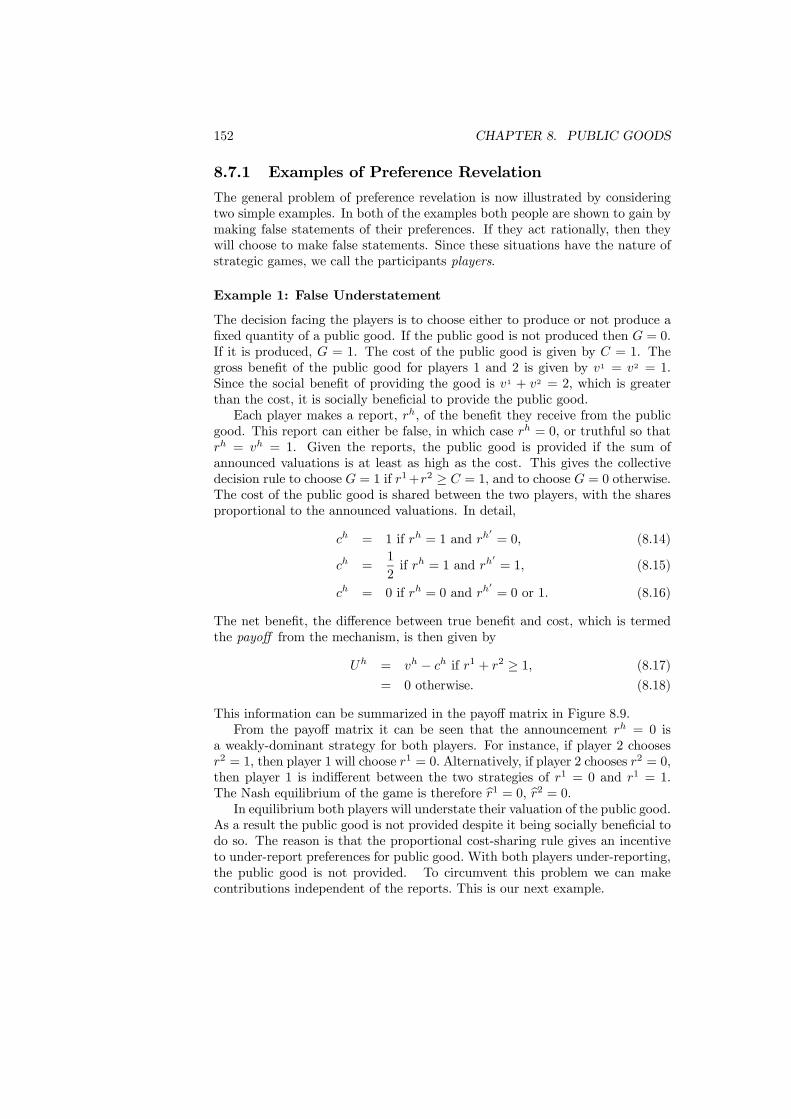
152 CHAPTER 8. PUBLIC GOODS
8.7.1 Examples of Preference Revelation
The general problem of preference revelation is now illustrated by consideringtwo simple examples. In both of the examples both people are shown to gain bymaking false statements of their preferences. If they act rationally, then theywill choose to make false statements. Since these situations have the nature ofstrategic games, we call the participants players.
Example 1: False Understatement
The decision facing the players is to choose either to produce or not produce afixed quantity of a public good. If the public good is not produced then G = 0.If it is produced, G = 1. The cost of the public good is given by C = 1. Thegross benefit of the public good for players 1 and 2 is given by v1 = v2 = 1.Since the social benefit of providing the good is v1 + v2 = 2, which is greaterthan the cost, it is socially beneficial to provide the public good.Each player makes a report, rh, of the benefit they receive from the public
good. This report can either be false, in which case rh = 0, or truthful so thatrh = vh = 1. Given the reports, the public good is provided if the sum ofannounced valuations is at least as high as the cost. This gives the collectivedecision rule to choose G = 1 if r1+r2 ≥ C = 1, and to choose G = 0 otherwise.The cost of the public good is shared between the two players, with the sharesproportional to the announced valuations. In detail,
ch = 1 if rh = 1 and rh0= 0, (8.14)
ch =1
2if rh = 1 and rh
0= 1, (8.15)
ch = 0 if rh = 0 and rh0= 0 or 1. (8.16)
The net benefit, the difference between true benefit and cost, which is termedthe payoff from the mechanism, is then given by
Uh = vh − ch if r1 + r2 ≥ 1, (8.17)
= 0 otherwise. (8.18)
This information can be summarized in the payoff matrix in Figure 8.9.From the payoff matrix it can be seen that the announcement rh = 0 is
a weakly-dominant strategy for both players. For instance, if player 2 choosesr2 = 1, then player 1 will choose r1 = 0. Alternatively, if player 2 chooses r2 = 0,then player 1 is indifferent between the two strategies of r1 = 0 and r1 = 1.The Nash equilibrium of the game is therefore br1 = 0, br2 = 0.In equilibrium both players will understate their valuation of the public good.
As a result the public good is not provided despite it being socially beneficial todo so. The reason is that the proportional cost-sharing rule gives an incentiveto under-report preferences for public good. With both players under-reporting,the public good is not provided. To circumvent this problem we can makecontributions independent of the reports. This is our next example.

8.7. MECHANISM DESIGN 153
Figure 8.9: Announcements and Payoffs
Example 2: False Overstatement
The second example is distinguished from the first by considering a public goodwhich is socially non-desirable with a cost greater than the social benefit. Thepossible announcements and the charging scheme are also changed.It is assumed that the gross payoffs when the public good is provided are
v1 = 0 < v2 =3
4. (8.19)
With the cost of the public good remaining at 1, these payoffs imply that
v1 + v2 =3
4< C = 1, (8.20)
so the social benefit from the public good is less than its cost.The possible announcements of the two players are given by r1 = 0 or 1 and
r2 = 34 or 1. These announcements permit the players to either tell the truth
or overstate the benefit so as to induce public good provision. Assume thatthere is also a uniform charge for the public good if it is provided so ch = 1
2 ifr1 + r2 ≥ c = 1, and ch = 0 otherwise. These valuations and charges imply thenet benefits
Uh = vh − ch if r1 + r2 ≥ 1, (8.21)
Uh = 0 otherwise. (8.22)
These can be used to construct the payoff matrix in Figure 8.10.The weakly-dominant strategy for player 1 is to play r1 = 0 and the best
response of player 2 is to select r2 = 1 (which is also a dominant strategy).Therefore the Nash equilibrium is r1 = 0, r2 = 1 which results in the provi-sion of a socially non-desirable public good. The combination of payoffs andcharging scheme has resulted in overstatement and unnecessary provision. Theexplanation for this is that the player 2 is able to guarantee the good is providedby announcing r2 = 1. Their private gain is 1
4 but this is more than offset bythe loss of −12 for player 1.
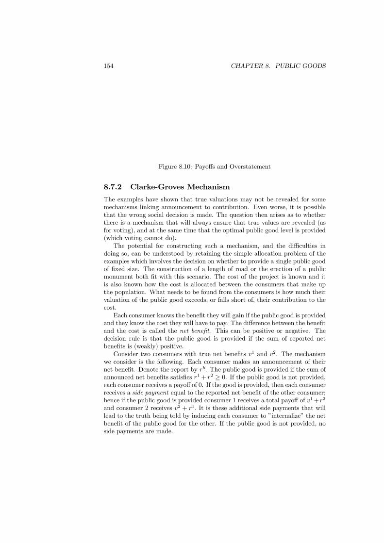
154 CHAPTER 8. PUBLIC GOODS
Figure 8.10: Payoffs and Overstatement
8.7.2 Clarke-Groves Mechanism
The examples have shown that true valuations may not be revealed for somemechanisms linking announcement to contribution. Even worse, it is possiblethat the wrong social decision is made. The question then arises as to whetherthere is a mechanism that will always ensure that true values are revealed (asfor voting), and at the same time that the optimal public good level is provided(which voting cannot do).The potential for constructing such a mechanism, and the difficulties in
doing so, can be understood by retaining the simple allocation problem of theexamples which involves the decision on whether to provide a single public goodof fixed size. The construction of a length of road or the erection of a publicmonument both fit with this scenario. The cost of the project is known and itis also known how the cost is allocated between the consumers that make upthe population. What needs to be found from the consumers is how much theirvaluation of the public good exceeds, or falls short of, their contribution to thecost.Each consumer knows the benefit they will gain if the public good is provided
and they know the cost they will have to pay. The difference between the benefitand the cost is called the net benefit. This can be positive or negative. Thedecision rule is that the public good is provided if the sum of reported netbenefits is (weakly) positive.Consider two consumers with true net benefits v1 and v2. The mechanism
we consider is the following. Each consumer makes an announcement of theirnet benefit. Denote the report by rh. The public good is provided if the sum ofannounced net benefits satisfies r1 + r2 ≥ 0. If the public good is not provided,each consumer receives a payoff of 0. If the good is provided, then each consumerreceives a side payment equal to the reported net benefit of the other consumer;hence if the public good is provided consumer 1 receives a total payoff of v1+r2
and consumer 2 receives v2 + r1. It is these additional side payments that willlead to the truth being told by inducing each consumer to ”internalize” the netbenefit of the public good for the other. If the public good is not provided, noside payments are made.

8.7. MECHANISM DESIGN 155
Figure 8.11: Clarke-Groves Mechanism
Figure 8.12: Payoffs for Player 1
To see how this mechanism works, assume that the true net benefits andthe reports can take the values of either −1 or +1. The public good will not beprovided if both report a value of −1, but if at least one reports +1 it will beprovided. The payoffs to the mechanism are summarized in the payoff matrixin Figure 8.11.The claim we now wish to demonstrate is that this mechanism provides no
incentive to make a false announcement of the net benefit. To do this it isenough to focus on player 1 and show that they will report truthfully whenv1 = −1 and when v1 = +1. The payoffs relating to the true values are in thetwo payoff matrices in Figure 8.12.Take the case of v1 = −1. Then consumer 1 finds the true announcement to
be weakly dominant - the payoff from being truthful (the top row) is greater ifr2 = −1 and equal if r2 = +1. Next take the case of r1 = +1. Consumer 1 isindifferent between truth and non-truth. But the point is that there is now noincentive to provide a false announcement. Hence truth should be expected.The problem with this mechanism is the side payments that have to be
156 CHAPTER 8. PUBLIC GOODS
made. If the public good is provided and v1 = v2 = +1, then the total sidepayments are equal to 2 - which amounts to the total net benefit of the publicgood. These side payments are money that has to be put into the system tosupport the telling of truth. Obtaining the truth is possible, but it is costly.
8.7.3 Clarke Tax
The problems caused by the existence of the side payments can be reduced, butthey can never be eliminated. The reason it cannot be eliminated entirely issimply that the mechanism is extracting information and this can never be donefor free. The way in which the side payments can be reduced is to modify thestructure of the mechanism.One way to do this is for side payments to be made only if the announcement
of a player changes the social decision. To see what this implies, considercalculating the sum of the announced benefits of all players but one. Whetherthis is positive or negative will determine a social decision for those players. Nowadd the announcement of the final player. Does this change the social decision?If it does, then the final player is said to be pivotal, and a set of side paymentsare implemented that requires taxing the pivotal agent for the cost inflicted onthe other agent through the changed social decision. This process is repeated foreach player in turn. These side payments are the Clarke taxes which ensure thatthe correct decision is made so that the public good is produced if it is sociallydesirable and not otherwise. The use of Clarke taxes reduces the number ofcircumstances in which the side payments are made.In a game with only two players, the payoffs for player 1 are when the Clarke
taxes are used are
v1 if r1 + r2 ≥ 0 and r2 ≥ 0, (8.23)
v1 − t1 if r1 + r2 ≥ 0 and r2 < 0,with t1 = −r2 > 0, (8.24)
−t1 if r1 + r2 < 0 and r2 ≥ 0,with t1 = r2 ≥ 0, (8.25)
0 if r1 + r2 < 0 and r2 < 0. (8.26)
Only in the second and third cases is player 1 pivotal (respectively„ by providingand not providing the public good) and for these a tax is levied on him reflectingthe cost to the other agent of changing public good provision (t1 = −r2 > 0for the cost of imposing provision, and t1 = r2 ≥ 0 for the cost of stoppingprovision).The Clarke taxes induce truthtelling and guarantee that the public good
is produced if and only if it is socially desirable. The explanation is that anymisreport that changes the decision about the public good would induce thepayment of a tax in excess of the benefit from the change in decision. Indeed,suppose the public good is socially desirable, so v1 + v2 ≥ 0, but that player1 dislikes it, so v1 < 0. Then, given an honest announcement from player 2with r2 = v2, by underreporting sufficiently to prevent provision of the publicgood (so r1 < −r2) player 1 becomes pivotal and will have to pay a tax oft1 = r2 = v2 which is in excess of the gain from non provision, −v1 (since
8.7. MECHANISM DESIGN 157
v1 + v2 ≥ 0 ⇒ v2 ≥ −v1). Hence player 1 is better off telling the truth and,given this truthtelling, player 2 is also better off telling the truth (although inthis case he is the pivotal agent, inducing provision and paying a tax equal tothe damage of public good provision for player 1, t2 = −r1 = −v1).The conclusion is that the Clarke tax induces preference revelation, and by
restricting side payments to pivotal agents only, it lowers the cost of informationrevelation.
8.7.4 Further Comments
The theory of mechanism design shows that it is possible to construct schemeswhich ensure the truth will be revealed and correct social decision made. Thesemechanisms may work but they are undoubtedly complex to implement. Puttingthis objection aside, it can still be argued that such revelation mechanisms arenot actually needed in practice. Two major reasons can be provided to supportthis contention.Firstly, the mechanisms are built on the basis that the players will be rational
and precise in their strategic calculations. In practice, many people may not actas strategically as the theory suggests. As in the theory of tax evasion in Chapter18, non-monetary benefits may be derived simply from acting honestly. Thesebenefits may provide a sufficient incentive that the true valuation is reported.In such circumstances, the revelation mechanism will not be needed.Secondly, the market activities of consumers often indirectly reveal the valu-
ation of public goods. To give an example of what is meant by this, consider thecase of housing. A house is a collection of characteristics, such as the number ofrooms, size of garden and access to amenities. The price that a house purchaseris willing to pay is determined by their assessment of the total value of thesecharacteristics. Equally, the cost of supplying a house is also dependent uponthe characteristics supplied. By observing the equilibrium prices of houses withdifferent characteristics, it is possible to determine the value assigned to eachcharacteristic separately. If one of the characteristics relates to a public good,for example the closeness to a public park, the value of this public good canthen be inferred. Such implicit valuation methods can be applied to a broadrange of public goods by carefully choosing the related private good. Since con-sumers have no incentive to act strategically in purchasing private goods, thetrue valuations should be revealed.The fact that consumers may have an incentive to falsely reveal their valua-
tions can also be exploited to obtain an approximation of the true value. Thiscan be done by running two preference revelation mechanisms simultaneously.If one is designed to lead to an under-reporting of the true valuation and theother one to over-reporting, then the true value of the public good can be takenas lying somewhere between the over- and under-reports. The Swedish econo-mist Bohm has conducted an experimental implementation of this procedure.In the experiment, 200 people from Stockholm had to evaluate the benefit ofseeing a previously unshown TV program. The participants were divided intofour groups which faced the following payment mechanisms: (i) pay stated val-
158 CHAPTER 8. PUBLIC GOODS
uation; (ii) pay a fraction of stated valuation such that costs are covered fromall payments; (iii) pay a low flat fee and (iv) no payment. Although the firsttwo provide an incentive to under-report and the latter two to over-report, theexperiment found that there was no significant difference in the stated valua-tions, suggesting that misrevelation may not be as important as suggested bythe theory.
8.8 More on Private Provision
The analysis of the private purchase of a public good in Section 8.3 focused uponthe issue of efficiency. The analysis showed that a Pareto improvement could bemade from the equilibrium point if both consumers simultaneously raised theircontributions, so that the equilibrium could not be efficient. This finding wassufficient to develop the contrast with efficient provision and for investigatingmechanism design.Although useful, these are not the only results that emerge from the pri-
vate purchase model. The model actually generates several remarkably precisepredictions about the effect of income transfers and increases in the number ofpurchasers. These results are now described and then contrasted with empiricaland experimental evidence.
8.8.1 Neutrality and Population Size
The first result concerns the effect of redistributing income. Consider transfer-ring an amount of income ∆ from consumer 1 to consumer 2, so the incomeof consumer 1 falls to M1 − ∆ and that of consumer 2 rises to M2 + ∆. Wewish to calculate the effect that this transfer has upon the equilibrium level ofpublic good purchases. To do this, notice that the equilibrium in Figure 8.5 isidentified by the fact that it occurs where an indifference curve for consumer 1crosses an indifference curve for consumer 2 at right angles. Hence the effect ofthe transfer upon the equilibrium can be found by determining how it affectsthe indifference curve.Consider consumer 1 who has their income reduced by ∆. If we also reduce
their public good purchase by ∆ and raise that of consumer 2 by ∆, the utilityof consumer 1 is unchanged because
U1¡M1 − g1, g1 + g2¢ = U1 ¡£M1 −∆¤− £g1 −∆¤ , £g1 −∆¤+ £g2 +∆¤¢ .
(8.27)This determines that the transfer of income causes the indifference curves andthe best-reaction function of consumer 1 to move as illustrated in Figure 8.13.The indifference curve through any point g1, g2 before the income transfer shiftsto pass through the point g1−∆, g2+∆ after the income transfer. The transferof income has the same effect upon the indifference curves and best-reactionfunction consumer 2. By considering the reduction in purchase of consumer 1

8.8. MORE ON PRIVATE PROVISION 159
Figure 8.13: Effect of Income Transfer
and the increase by consumer 2 it follows that
U2¡M2 − g2, g1 + g2¢ = U2 ¡£M2 +∆
¤− £g2 +∆¤ , £g1 −∆¤+ £g2 +∆¤¢ .(8.28)
For consumer 2, the indifference curve through g1, g2 before the income transferbecomes that through g1 −∆, g2 +∆ after the transfer.These shifts in the indifference curves result in the equilibrium moving as in
Figure 8.14. The point where the indifference curves cross at right angles shiftsin the same way as the individual indifference curves. If the equilibrium wasinitially at bg1, bg2 before the income transfer, it is located at bg1−∆, bg2+∆ afterthe transfer.The important result now comes from noticing that in the move from the
original to the new equilibrium, consumer 1 reduces their purchase of the pub-lic good by ∆ but consumer 2 increases their by the same amount ∆. Thesechanges in the value of purchases exactly match the change in income level. Thenet outcome is that the levels of private consumption remain unchanged for thetwo consumers and the total supply of the public good is also unchanged. Asa consequence, the income transfer does not affect the levels of consumption inequilibrium - all it does is to redistribute the burden of purchase. Income re-distribution is entirely offset by opposite redistribution of private contributions.This result, known as income distribution invariance, is a consequence of thefact that the utility levels of the consumers are linked via the quantity of publicgood.The second interesting result is that the transfer of income leaves the utility

160 CHAPTER 8. PUBLIC GOODS
Figure 8.14: New Equilibrium
levels of the two consumers unchanged. This has to be so since we have just seenthe consumption levels do not change. Therefore, the redistribution of incomehas not affected the distribution of welfare because the transfer is simply offsetby the change in public good purchases. This is an example of policy neutrality:by changing their behavior the individuals in the economy are able to undo whatthe government is trying to do. Income redistribution will always be neutraluntil the point is reached at which one of the consumers no longer purchasesthe public good. Only then will further income transfers affect the distributionof utility.
A third result follows easily from income invariance. Let both consumershave the same utility function but possibly different income levels. Since thequantity of public good consumed by both must be the same, the first-orderconditions require that both must also consume the same quantity of privategood; hence x1 = x2. Further, these common levels of consumption implythat the consumers must have the same utility levels even if there is an initialincome disparity. The private provision model therefore implies that, when theconsumers have identical utilities, contribution behavior will equalize utilitieseven in the face of income differentials. The poor will cut their contributionsrelative to the rich to a sufficient extent to makes them equally well off.
This model can also be used to consider the consequence of variations inthe number of households. Maintaining the assumption that all the consumersare identical in terms of both preferences and income, for an economy with H
consumers the total provision of the public good is G =HPh=1
gh and the utility
of h is
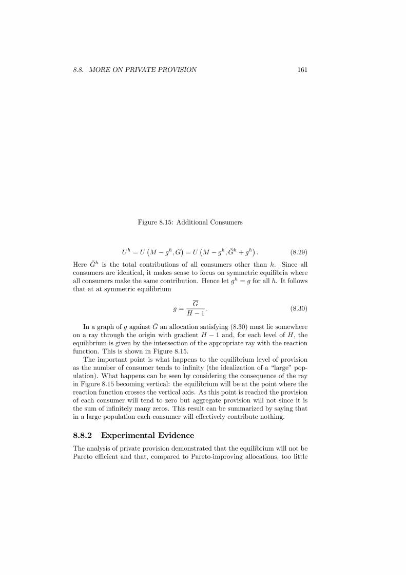
8.8. MORE ON PRIVATE PROVISION 161
Figure 8.15: Additional Consumers
Uh = U¡M − gh, G¢ = U ¡M − gh, Gh + gh¢ . (8.29)
Here Gh is the total contributions of all consumers other than h. Since allconsumers are identical, it makes sense to focus on symmetric equilibria whereall consumers make the same contribution. Hence let gh = g for all h. It followsthat at at symmetric equilibrium
g =G
H − 1 . (8.30)
In a graph of g against G an allocation satisfying (8.30) must lie somewhereon a ray through the origin with gradient H − 1 and, for each level of H, theequilibrium is given by the intersection of the appropriate ray with the reactionfunction. This is shown in Figure 8.15.The important point is what happens to the equilibrium level of provision
as the number of consumer tends to infinity (the idealization of a “large” pop-ulation). What happens can be seen by considering the consequence of the rayin Figure 8.15 becoming vertical: the equilibrium will be at the point where thereaction function crosses the vertical axis. As this point is reached the provisionof each consumer will tend to zero but aggregate provision will not since it isthe sum of infinitely many zeros. This result can be summarized by saying thatin a large population each consumer will effectively contribute nothing.
8.8.2 Experimental Evidence
The analysis of private provision demonstrated that the equilibrium will not bePareto efficient and that, compared to Pareto-improving allocations, too little

162 CHAPTER 8. PUBLIC GOODS
Figure 8.16: Public Good Experiment
of the public good will be purchased. A simple explanation of this result canbe given in terms of each consumer relying on others to purchase and hencedeciding to purchase too little themselves. Each consumer is free-riding onothers’ purchases and, since all attempt to free-ride, the total value of purchasesfails to reach the efficient level. This conclusion has been subjected to closeexperimental scrutiny.The basic form of experiment is to give participants a number of tokens that
can be invested in either a private good or a public good. Each participantmakes a single purchase decision. The private good provides a benefit only forits purchaser while purchase of public good provides a benefit to all participants.These values are set so that the private benefit is less than the social benefit.The benefits are known to the participants and the total benefit from purchasesis the payoff to the participant at the end of the experiment. It is therefore inthe interests of each participant to maximize their payoff.To see how this works in detail, assume that there are 10 participants in the
game. Allow each participant to have 10 tokens to spend. A unit of the privategood costs 1 token and provides a benefit of 5 units (private benefit=socialbenefit=5). A unit of the public good also costs 1 token but provides a benefit of1 unit to all the participants in the game (private benefit=1<social benefit=10).The returns are summarized in Figure 8.16.If the game is played once (a one-shot game), the Nash equilibrium strategy
is to purchase only the private good since each token spent on the private goodyields a return five times higher than for the public good. In equilibrium, thetotal return to each player is 50. In contrast, the socially-efficient outcome isfor all players to purchase only the public good and to generate a payoff of 100to each player. The fact that the Nash equilibrium differs from the efficientoutcome is because the private benefits diverge from the social benefits. Thus,in the one-shot game, all tokens should be spent on the private good.In experimental implementations of this game, the average value of pur-
chases of the public good has been approximately 30% to 90% of tokens, withmost observations falling in the 40%-50% range. (Among student participants,contributions have been lowest for those studying economics and fall with thenumber of years of economics taken! Clearly, instructors have some success inteaching how to play strategic games.) Since the purchase of public good is sig-nificantly different from 0, these results clearly do not support the predictionsof the private-purchase model.
8.8. MORE ON PRIVATE PROVISION 163
Some experiments have repeated the purchase decision over several roundswith the view that this should allow time for the participants to learn aboutfree-riding and develop the optimal strategy. The results from such experi-ments are not as clear and a wider range of purchases occur. Free-riding is notcompletely supported, but instances have been reported in which it does occur.However, this finding should be treated with caution since having several roundsof the game introduces aspects of repeated game theory. While it remains truethat the only credible equilibrium of the repeated game is the private-purchaseequilibrium of the corresponding single-period game, it is possible that in theexperiments some participants may have been attempting to establish cooper-ative equilibria by playing in a fashion that invited cooperation. Additionally,those not trained in game theory may have been unable to derive the optimalstrategy even though they could solve the single-period game.Other results show that increasing group size leads to increased divergence
from the efficient outcome when accompanied by a decrease in marginal returnfrom the public good but the results do not support a pure numbers-in-groupeffect. This finding is compatible with the theoretical finding that the effect ofgroup size on the divergence from optimality was in general indeterminate.These results indicate that there is little evidence of free-riding in single-
period, or one-shot, games but in the repeated games the purchases fall towardsthe private-purchase level as the game is repeated. In total, these experimentsdo not provide great support for the equilibrium based on the private-purchasemodel with Nash behavior. In the single-period games free-riding is unambigu-ously rejected. Although it appears after several rounds in repeated games,the explanation for the strategies involved is not entirely apparent. Neither astrategic nor a learning hypothesis is confirmed. What seems to be occurringis that the participants are initially guided more by a sense of fairness than byNash behavior. When this fairness is not rewarded, the tendency is then tomove towards the Nash equilibrium. The failure of experimentation to supportfree-riding lends some encouragement to the views that although such behaviormay be individually optimal, it is not actually observed in practice.
8.8.3 Modifications
The empirical and experimental evidence has produced a number of conflictswith the predictions of the theoretical model. The analysis of private-purchasehas been based on two fundamental assumptions. The utility of consumerswas assumed to depend only upon the consumption of the private good and thetotal supply of the public good. This ensures that consumers do not care directlyabout the size of their own contribution nor do they care about the behavior ofother consumers except for how it affects the total level of the public good. Thesecond assumption was that the consumers acted non-cooperatively and playedaccording to the assumptions of Nash equilibrium.The simplest modification that can be made to the model is to consider the
game being played in a different way. The foundation of the Nash equilibriumis that each player takes the behavior of the others as given when optimizing.

164 CHAPTER 8. PUBLIC GOODS
One way to change this is to consider “conjectural variations” so that eachplayers forms an opinion as to how their choice will affect that of others. Ifthe conjectural variation is positive, each player predicts that the others willrespond to an increase in purchase by also making additional purchases. Sucha positive conjecture can be interpreted as being more cooperative than thezero conjecture that arises in the Nash equilibrium and leads to the equilibriumhaving greater total public good supply than the Nash equilibrium.Moving to non-Nash conjectures may alter the equilibrium level of the public
good but it does not eliminate the neutrality properties. Furthermore, the majorobjection to this approach is that it is entirely arbitrary. There are sensiblereasons founded in game theory for focusing upon the Nash equilibrium andno other set of conjectures can appeal to similar justification. If the Nashequilibrium of the private purchase model does not agree with observations,it would seem that the objectives of the households and the social rules theyobserve should be reconsidered not the conjectures they hold when maximizing.One approach to modified preferences is to assume that the consumer de-
rives utility directly from the contribution they make. For instance, making adonation to charity can make a consumer feel good about themself; they areacting as a “good citizen”. This is often referred to as the “warm glow” effect.With a warm glow, a purchase of the public good provides a return from directconsumption of the public good and a further return from the warm glow. Theprivate warm glow effect increases the value of the purchase and so raises theequilibrium level of total purchases. The equilibrium also no longer has thesame invariance properties. This seems a significant advance were it not thatthe specification of the warm glow is entirely arbitrary.A final modification is to remove the individualism and allow for social in-
teraction by modifying the rules of social behavior. In the same way that socialeffects can arise with tax evasion, they can also occur with public goods. Oneway to do this is to introduce reciprocity under which each consumer considersthe contributions of others and contrasts them to what they feel they shouldhave made. If the contributions of others match, or exceed, what is expectedthen the consumer is assumed to feel under an obligation to make a similarcontribution. This again raises the equilibrium level of contribution.
8.9 Fund-Raising Campaigns
The model of voluntary provision that we have considered so far has involveda single one-off contribution decision. It is easy to appreciate that once thesecontributions have been made the consumers may look again at the situationand realize it is inefficient. This could give them an incentive to conduct a sec-ond round of contribution which will move the equilibrium closer to efficiency.Repeatedly applying this argument suggests that it may be possible to eventu-ally reach efficiency. We now assess this claim by addressing it within a simplefund-raising game.The basis of the fund-raising game is that target level of funds must be

8.9. FUND-RAISING CAMPAIGNS 165
achieved before a public good can be provided. For example, consider the tar-get the minimum cost of construction for a public library. Subscribers to thecampaign take it in turn to make either a contribution or a pledge to con-tribute. Only when the target is met does the process cease. The basic questionis whether such a fund-raising campaign can be successful given the possibilityof free-riding.We model a campaign as a game with an infinite horizon, meaning that
solicitation for donations can continue until the goal is met. There is one publicgood (or joint project) whose production cost is C and two identical players Xand Y . These players derive the same benefit, B, from public good, so the totalbenefit is 2B. Both also have the same discount rate δ, 0 < δ < 1, for delayingcompletion of the project by one period.The players alternate in making contributions. The sequential (marginal)
contributions are denoted (..., xt−1, yt, xt+1, ...) where xt−1 denotes the contri-bution of player X at time t− 1 and yt denotes the contribution of player Y attime t. The game ends, and the public good is provided, only when the totalcontributions cover the cost of the public good. Individuals derive no benefitsfrom the public good before completion of the fund raising so the marginal con-tributions yield no return until the cost is met. It follows that the incentive ofeach player to wait for the other one to contribute (free riding) must be bal-anced against the cost of delaying completion of the project. We suppose thatthe public good is “socially desirable”, so C < 2B, but that no single playervalues the public good enough to bear the full cost, so B < C. We now contrasttwo different forms of fund-raising campaigns. In the first, the contribution cam-paign, the contributions are paid at the time they are made. In the second, thesubscription campaign, players are asked in sequence to make donation pledgesthat are not be paid until the cost is met.
8.9.1 The Contribution Campaign
In the contribution campaign, contributions are sunk at the time they are madebecause a credible commitment cannot be made to make contributions later.The lack of commitment leads each player to back his contribution to assurethat the other player contributes their share. This is because past contributionsare sunk and cannot influence the division of the remaining cost between theplayers. As a result, we show that it is never possible to raise the money eventhough the project is worthwhile.The two players are asked in sequence to make a contribution. While there is
no natural end period, there is a total contribution level that is close enough tothe cost C that the contributor whose turn it is should complete the fund-raisingrather than waiting for the other one to make up the difference. Suppose that itis playerX’s turn to make a contribution offer at that final round T . There existsa deficit C − xT sufficiently small that player X is indifferent between makingup the difference and getting a payoff of B−xT or waiting in the expectation (atbest) that player Y will make up the difference in the next round and producinga payoff with delayed completion of δB. Hence, the maximal contribution of
166 CHAPTER 8. PUBLIC GOODS
player 1 in the final round T is
xT = (1− δ)B, (8.31)
so the contribution is equal to the benefit of speeding up completion of theproject. We suppose that (1−δ)B < C so that such a contribution cannot coverthe full cost and a donation from player Y must be solicited. Working backward,it is now player Y ’s turn to make a contribution at time T − 1. Player Y antic-ipates that in bringing (total) contributions up to C − xT at date T − 1, playerX will complete the project the next period. So there exists a sufficiently smalldeficit such that player Y is indifferent between bringing total contributions upto that level giving a payoff δB − yT−1or waiting for the other player to makesuch contribution while making himself the final contribution xT which pro-duces a payoff δ2 [B − xT ] (i.e., two periods later you get the completed projectbenefit B and pay the last contribution xT ). Hence, substituting for xT , thecontribution at time T − 1 that makes player Y indifferent is
yT−1 = δ(1− δ2)B. (8.32)
Proceeding backward to date T − 2, it is now the turn of player X to make acontribution. Using the same line of argument, there exists a total contributionlevel at date T − 2 such that player X is indifferent between bringing totalcontribution up to that level to get a payoff δ2 [B − xT ]−xT−2 from completionin two periods or waiting and delaying completion to get a payoff δ3B−δ2yT−1(inwhich from the switching position it becomes worthwhile to contribute yT−1).Substituting for xT and yT−1 gives
xT−2 = δ3(1− δ2)B. (8.33)
Moving back to round T − 3 and following the same reasoning, the potentialcontribution at time T − 3 from player Y is
yT−3 = δ5(1− δ2)B, (8.34)
and the potential contribution at time T − 4 isxT−4 = δ7(1− δ2)B, (8.35)
Going back further it is possible to calculate how much each player is willing tocontribute at each stage. This is illustrated in Figure 8.17.Summing these contributions starting from the end of the campaign, the
total potential for contributions is
(1−δ)B+δ(1−δ2)B+δ3(1−δ2)B+δ5(1−δ2)B+δ7(1−δ2)B+ ... = B, (8.36)where we have used the geometric progression fact that 1 + δ2 + δ4 + δ6 + ... =1/(1− δ2). The remarkable feature is that the total potential for contributionsnever exceeds the individual benefit from the project and thus it cannot bepossible to raise sufficient contributions for a successful campaign because B <C.

8.9. FUND-RAISING CAMPAIGNS 167
Figure 8.17: A Contribution Campaign
8.9.2 The Subscription Campaign
In the subscription game, agents alternate in making donation pledges and bearthe cost of their contribution only when and if enough contributions are pledgedto complete the project. In a sense, agents are able to make certain conditionalcommitments to contribute in the future. This possibility to commit modifiesthe strategic structure of the game and alters the total amount that can beraised. As we now show, in this case it becomes possible to raise an amountequal to the total valuation of all the contributors.Once again, we start when the fund-raising operation is over and work back-
ward. Fix an arbitrary end-point T with player X’s turn to make a donationpledge at date T . There must exists a contribution deficit sufficiently small tomake player X indifferent between financing the deficit himself to obtain a pay-off B−xT , or waiting for player Y to make up the difference in the next periodwith a delayed completion payoff of δB. So, the potential pledge of player X atdate T is
xT = (1− δ)B. (8.37)
We continue to assume that (1 − δ)B < C so that we must solicit player Y ’sdonation. Working back it is then player Y to pledge at date T − 1. PlayerY anticipates that in bringing the total amount pledged up to C − xT at dateT − 1, player X will complete the project in the next period. So there existsa sufficiently small deficit such that player Y is indifferent between making upthe difference to get a payoff δ [B − yT−1] , or leaving player X to make up thedifference and thereby delaying completion to get a payoff of δ2 [B − xT ] (in

168 CHAPTER 8. PUBLIC GOODS
which case it becomes worthwhile for Y to pledge himself xT at date T ). Hence,substituting for xT , we obtain
yT−1 = (1− δ2)B. (8.38)
Going back to date T−2, it is then playerX to pledge. Again, there exists a totalamount pledged close enough to C−xT −yT−1 such that player X is indifferentbetween bringing the total contribution up to that level anticipating completionin two rounds with a payoff δ2 [B − xT − xT−2] , or waiting for Y to pledgeinstead with a payoff from switching position of δ3 [B − yT−1]. Substituting forxT and yT−1 gives
xT−2 = δ(1− δ2)B. (8.39)
Proceeding likewise we can go back further and calculate how much player Ywill pledge at date T − 3 as
yT−3 = δ2(1− δ2)B, (8.40)
and player X will pledge at date T − 4 the amount
xT−4 = δ3(1− δ2)B.
Going back further, calculating how much each player is willing to pledge ateach stage and summing up potential pledges we get
(1−δ)B+(1−δ2)B+δ(1−δ2)B+δ2(1−δ2)B+δ3(1−δ2)B+ ... = 2B. (8.41)
This maximum amount that can be raised is just equal to the total valuationsof all the contributors. Hence it is always possible to raise enough money forany worthwhile project because C < 2B.These results have shown how allowing contributions to be repeated may
lead to efficient private provision of the public good. But this conclusion issensitive to the assumptions made upon the ability of contributors to makebinding commitments.
8.10 Conclusions
This chapter has reviewed the standard analysis of the efficient level of provisionof a public good leading to the Samuelson rule and the fact that private contri-butions do not achieve this outcome. The efficiency rule describes an allocationthat can only be achieved if the government is unrestricted in its policy toolsor, as the Lindahl equilibrium demonstrates, using prices that are personalizedfor each consumer.One aspect of public goods that prevents the government from making effi-
cient decisions is the government’s lack of knowledge of households’ preferencesand their willingness to pay for public goods. Mechanisms were constructedthat provide the right incentives for households to correctly reveal their true
8.10. CONCLUSIONS 169
valuation of the public good. Experimental evidence suggests that householdbehavior when confronted with decision problems involving public goods doesnot fully conform with the theoretical prediction and that the private provisionequilibrium may not be as inefficient as theory suggests. Furthermore, misrev-elation has not been confirmed as the inevitable outcome.
Further readingThe classic paper on the efficient provision of public goods is:Samuelson, P.A. (1954) ”The pure theory of public expenditure”, Review of
Economics and Statistics, 36, 387 - 389.The private provision model is developed fully in:Bergstrom, T.C., L. Blume and H. Varian (1986) ”On the private provision
of public goods”, Journal of Public Economics, 29, 25 - 49.Itaya, J.-I., D. de Meza and G.D. Myles (2002) ”Income distribution, tax-
ation and the private provision of public goods”, Journal of Public EconomicTheory, 4, 273 — 297.Mechanism design for public goods was first described in:Groves, T. and J. Ledyard (1977) “Optimal allocation of public goods: a
solution to the “free rider“ problem“, Econometrica, 45, 783 - 809.The sequential private provision is based on:Admati, A.R. and M. Perry (1991) ”Joint projects without commitment”,
Review of Economic Studies, 58, 259 - 276.Experimental results are surveyed in:Bohm, P. (1972) “Estimating demand for public goods: an experiment“,
European Economic Review, 3, 55 - 66.Isaac, R.M., K.F. McCue and C.R. Plott (1985) ”Public goods in an exper-
imental environment”, Journal of Public Economics, 26, 51 - 74.

170 CHAPTER 8. PUBLIC GOODS

Chapter 9
Club Goods and LocalPublic Goods
9.1 Introduction
One of the defining features of the public goods of Chapter 8 was non-rivalry:once the good was provided, its use by one consumer did not affect the quantityavailable for any other. This is clearly an extreme assumption. Many commodi-ties, such as parks, roads and sports facilities, satisfy non-rivalry to a point butare eventually subject to congestion. Although not pure public goods, thesegoods cannot be classed as private goods either.A good which has some degree of non-rivalry but for which excludability
is possible is called a club good. The name is intended to reflect the fact thatthere are benefits to groups of consumers forming a club to coordinate provisionand that the group size may be less than the total population. The name alsocaptures the fact that the clubs we observe in practice are formed by groupsof consumers to coordinate the provision of such goods. For instance, a tennisclub provides courts which are excludable and non-rival for users at differenttimes. International bodies, such as NATO, can also be interpreted as clubs:NATO provides defence for its members which is again partly non-rivalrousand partly excludable (only partly because if the existence of NATO detersaggression generally, non-members will also benefit).The description of economic activity that we have employed in the previous
chapters has not paid any attention to the geography of trade. In effect, wehave been assuming that there is either a single market place with consumerslocated close to it or that travel to markets is costless. It is a fact of actualeconomic activity that consumers and markets are dispersed, and that travelcosts can be significant. As a consequence, public goods provided in a particulargeographical location need not be available except for those in the close vicinity.For instance, radio and television signals can only be received within range of thetransmitter and a police service may only patrol a limited jurisdiction. Provided
171
172 CHAPTER 9. CLUB GOODS AND LOCAL PUBLIC GOODS
a consumer is located within the relevant area, they can benefit from the publicgood, otherwise the public good is unavailable to them because the cost oftravelling to enjoy it exceeds the benefit. Such goods are again not pure publicgoods as defined in Chapter 8 and are termed local public goods, with the namecapturing the idea of geographical restriction. The geographical restriction onavailability can also be accompanied by congestion within the region.The issues that the chapter addresses are similar to those involved with
pure public goods. It begins by defining club goods and local public goodsand investigating the relationships between them. The efficiency question isthen addressed for single-product clubs, and is related to the charging schemerequired to support efficiency. The clubs are then placed within an economyto consider whether efficiency is achieved at this level. Local public goods areintroduced and the efficiency question is again addressed. The extension is thenmade to consider heterogeneous consumers which leads into a discussion of theinfluential Tiebout hypothesis of preference matching for local public goods. Thechapter is completed by a review of the empirical evidence on this hypothesis.
9.2 Definitions
The purpose of this section is to provide precise definitions of the classes ofgoods under discussion. Once this is done, it is possible to describe how theseclasses are related.The essential aspect of a club good is that it is possible for those who pay
for its provision to exclude those who do not. This is in contrast to the purepublic good which was defined by the impossibility of exclusion. In addition,club goods are often assumed to suffer from congestion but this is not strictlynecessary. However, congestion provides a motive for exclusion and for theforming of a club to supply the good.A formal definition can be given as follows.
Definition 2 (Club good) A club good is a good which is either non-rivalrousor partly rivalrous but for which exclusion by the providers is possible.
The exclusion aspect of a club good can be taken literally, such as a checkon membership credentials at the door to the club, or taken as representingsome more general legal authority to bar non-members. Its consequence is thatissues of preference revelation are not important for club goods. The benefits ofthe club can only be obtained by voluntarily choosing to become a member anddoing so immediately reveals preferences. This observation is clearly importantfor the potential attainment of efficiency by the market.The defining feature of a local public good is one of geography and the need
to locate within a specific geographical area in order to benefit from the good.Once outside this area, the benefit of the good is no longer obtained. Thisgeographical constraint may also be linked with congestion which causes partialrivalry.
9.3. SINGLE PRODUCT CLUBS 173
Definition 3 (Local public good) A local public good can only benefit thosewithin a given geographical area. It may be non-rivalrous within that area orit may be partially rivalrous.
This definition of a local public good makes clear that the unique feature isthe geographic restriction. It leaves open the question of whether a local publicgood is excludable or not. This is important for the following reason. As will beseen, the focus of local public good theory is the analysis of local government anddecisions on taxation and expenditure. Whether the local public goods providedare excludable or not then becomes a matter of policy rather than an inherentfeature of the good. By this it is meant that local governments can use a varietyof regulations to control access to the public goods they offer. As examples,registration at schools can be restricted by policy choice to pupils in the localarea and the size of the local population can be controlled by prohibition onnew building.Consequently, there are large overlaps between clubs and local public goods
and the terms have often been used interchangeably. What has mostly distin-guished the two in the literature has been the issues that have been addressedusing each concept. The discussion of club goods has focussed more upon issuesof efficiency with homogeneous populations. In contrast, local public goods havefound their most prominent use in the analysis of heterogeneous populations andpreference revelation. Furthermore, local public goods have been used to un-derstand the role and structure of local government whereas club goods havebeen more about the market. Even these distinctions are not always binding.
9.3 Single Product ClubsThe analysis of efficiency for a pure public good involved determining how muchof it should be provided. With a club good, it is not just the quantity of thegood that needs to be decided but also the size of the club membership. Thelatter is important because of the effect of congestion. Adding a new memberallows the cost of providing a given quantity of public good to be spread amongstmore members but reduces the benefit obtained by each existing member. Witha club good that suffers from congestion there is a second efficiency conditioninvolved concerning the correct level of membership.
9.3.1 Fixed Utilization
Consider now the simplest model of a club. There is a homogeneous populationof consumers who are identical in terms of tastes and of income. One privategood is available and one club good. The club good can potentially suffer fromcongestion. The focus of attention is on the decision of a single club. It isassumed that a club has formed with the intention of supplying the club good(imagine a small committee of founder members setting out its constitution)and is now in the process of deciding how much of the good to supply and howmany member to admit.

174 CHAPTER 9. CLUB GOODS AND LOCAL PUBLIC GOODS
To complete the description of the decision problem, it is necessary to con-sider the financing of the club. Since the club has the ability to exclude non-members, it is able to charge members for the privilege of membership. Unlikea pure public good, there is then no barrier to financing provision of the clubgood provided enough potential members are willing to pay for membership.The most natural assumption to make on the method of charging is that thecost of the club is divided equally amongst the members. This charging policywill ensure the club just breaks even.Let each consumer have the utility function U (x,G, n), where x is the con-
sumption of a private good, G provision of the club good and n the numberof club members. Utility increases in x and G, and decreases in n if there iscongestion. If the cost of providing G units of the club good is C (G), thenthe budget constraint of a member with income M when the cost of the club isshared equally between members will be
M = x+C (G)
n. (9.1)
The decision problem for those in charge of the club involves choosing G andn to maximize the welfare of a typical member. Putting together the budgetconstraint and the utility function, this can be expressed as
max{G,n}
U(M − C (G)n
,G, n). (9.2)
The first-order conditions for this optimization produce the following pair ofequations that characterize efficiency:
nMRSG,x ≡ nUGUx
= CG, (9.3)
and
MRSn,x ≡ UnUx
= − Cn2. (9.4)
The first of these conditions, (9.3), is the version of the Samuelson rule (8.5)and describes the level of public good, G, that the club should supply. It statesthat the sum of marginal rates of substitution between the public good and theprivate good for the n members of the club should be equated to the marginalrate of transformation (or the marginal cost), CG, of another unit of the clubgood. What it is most important to observe from this condition is that theprocess of decision-making within the club ensures that this efficiency conditionis satisfied. The ability to exclude non-members from consuming the club goodpermits the club to achieve the correct level of provision. A club thereforeachieves efficient public good provision for its members.To interpret (9.4) it should first be noted that Un ≤ 0, with Un < 0 if there
is congestion, and an increase in the number of club members for a given level ofprovision will reduce the utility of each through congestion effects. We can treat
9.3. SINGLE PRODUCT CLUBS 175
UnUxas the marginal utility cost of another member of the club. This marginal
utility cost is then equated to the extent to which another club member reducesthe share of the cost for each existing member.
With Un < 0, (9.4) will determine an efficient level of membership for theclub which is positive and finite. Again, the club will achieve efficiency throughits internal decision-making. In the absence of congestion Un = 0 so the optimalclub membership will be infinite. In practice this can be interpreted as the clubencompassing the entire population. However, in contrast to the pure publicgood, the ability to exclude permits the levy of a membership fee which canfinance the cost of the club. The club therefore achieves an efficient level ofmembership.
The arguments to this point can be summarized as follows. A club is ableto exclude non-members from consumption of the public good and can levy acharge on members. If all consumers are identical, then the club will achievean efficient level of the club good and an efficient level of membership. If theclub good suffers from congestion, then the optimum membership will be finite.Without congestion, the entire population will be members of the club. Thecollection of membership fees by the club will ensure that it breaks even in itsfinancing of the provision of the club good. This fundamental insight that clubscan attain efficiency in the provision of public goods is attributed to the seminalwork of Buchanan who was the first to develop the theory of clubs. In terms ofthe earlier discussion, Buchanan observed that joining a club constitutes an actof preference revelation which permits the attainment of efficiency.
9.3.2 Variable Utilization
The model of the club used above does not probe too deeply into the natureof the good that the club supplies. When this is considered further, it becomesapparent that it is not the number of club members that matters for congestionbut how frequently the facilities of the club are used. Retaining the assumptionthat all club members are identical, the total use of the club is equal to theproduct of the number of members and the number of visits that each membermakes to the club. In determining its provision, a club will wish to optimize thenumber of visits in addition to the size of facility and the membership.
The model can be easily extended to incorporate a variable rate of visitationinto the analysis. Let v be the number of visits that each member makes tothe club. An increase in the number of visits raises the utility of the membermaking those visits, but causes congestion through the total number of visits ofall members. Letting the total number of visits be V = nv, the utility function iswritten U = U (x,G, v, V ) with the marginal utility to a visit, Uv, positive andthe marginal congestion effect, UV , negative. The cost function for providingthe club is also modified to make it dependent upon the total number of visits,nv.
176 CHAPTER 9. CLUB GOODS AND LOCAL PUBLIC GOODS
With this extension, the optimization problem for the club becomes
max{x,G,v,n}
U (x,G, v, V ) subject to M = x+C (G,nv)
n. (9.5)
The necessary condition for optimal provision of the public good by the club is
nUGUx
= CG, (9.6)
which is again the Samuelson rule for the club equating the sum of marginalrates of substitution to the marginal cost of provision. The necessary conditionfor optimal club membership is
vUVUx
= − Cn2+vCVn. (9.7)
In this condition, vUVUx is the marginal loss of utility through the congestioncaused by an additional club member. This is equated to the reduction in costof membership, − C
n2 , offset by the increased cost of servicing the increased visits,vCVn . The third optimality condition determines the number of visits to the clubthat each member should make. This is given by
UvUx
= CV − nUVUx, (9.8)
which equates the marginal benefit of an additional visit to the marginal main-tenance cost plus the marginal congestion cost an extra visit imposes upon allmembers of the club.As with the case of fixed visits, if the decision making of the club satisfies
these three optimality conditions then it will ensure an efficient allocation ofresources for its members. It will accept the correct number of members, providethe correct quantity of public good and set visit levels correctly. Thereforeintroducing a variable visitation rate does not affect the basic conclusion thatclubs will supply excludable public goods efficiently.However, there is a very important distinction between the cases of variable
and fixed utilization. This analysis of variable utilization retained the assump-tion that there is a fixed charge for membership but no further charges for visits.Consequently, once someone has become a member of the club, the price for eachadditional visit is zero. In choosing visits, each member will only take accountof the private cost of the increase in congestion and not the cost they impose onother members. Therefore, they will make an excessive number of visits to theclub. In brief, the fixed charge does not impose the correct incentives on mem-bers to decentralize the efficient outcome. To implement the optimum defined,it is therefore necessary for a club charging a fixed fee to directly regulate thenumber of visits. This is rather strong restriction on the behavior of the cluband motivates the study of an alternative pricing scheme.

9.3. SINGLE PRODUCT CLUBS 177
9.3.3 Two-Part Tariff
To provide a starting point for the study of a more sophisticated pricing scheme,it is worth formalizing the final subsection of the previous subsection. Assumethat the club has chosen its optimal provision, G∗, membership, n∗, and visits,v∗, and that its membership fee, which is based on all members abiding bythe number of visits, is given by F ∗ = C(G∗,n∗v∗)
n∗ . Now consider the incentivesfacing a member of the club who believes all other members will make v∗ visits.Putting together the budget constraint, M = x+ F ∗, and the utility function,then the club member faces the optimization
max{v}
U (M − F ∗, G∗, v, [n∗ − 1] v∗ + v) . (9.9)
The choice of v, taking the choices of G∗, n∗v∗ and F ∗ as given, then satisfiesthe necessary condition
Uv + UV = 0. (9.10)
Consequently, they will choose to make visits to the point at which the marginalutility of visits is completely offset by the marginal disutility of congestion. Thisis not the optimal condition as given by (9.8) and in fact leads to a higher numberof visits. This demonstrates how the membership fee fails to place the correctincentives in place, so that it can only be optimal if visits are directly regulated.Assume that instead of a membership fee, the club charges a price per visit.
If the price is denoted p and the membership fee is set at F = 0, then thenumber of visits is chosen to solve
max{x,v}
U (x,G∗, v, [n∗ − 1] v∗ + v) subject to M = x+ pv. (9.11)
The necessary conditions for this is that
p =UvUx
+ nUVUx.
Given the price, visits will be made up to the point at which the price is equalto the marginal benefit of another visit less the additional congestion cost itcauses. Contrasting this to (9.8) shows that the optimal number of visits willbe sustained if the price is set so
p = CV . (9.12)
However, it follows from optimal membership condition (9.7) that at this pricethe total revenue raised falls short of the cost of the club since
vnCV = C + n2vUVUx
< C, (9.13)
using the fact that UV < 0. This inequality shows the important result thata membership fee alone cannot both generate the correct number of visits andallow the club to break-even.
178 CHAPTER 9. CLUB GOODS AND LOCAL PUBLIC GOODS
The charging scheme that is required to finance the club and control visitsis a two-part tariff consisting of a membership fee and a charge for each visit.Let the fixed part of the two-part tariff be given by F and the charge for eachvisit be p. With this tariff the club solves
max{x,v,G,n}
U (x,G, v, nv) subject to M = x+F + pv, and nF + pnv = C (G,nv) ,
(9.14)where both the individual budget constraint and the break-even constraint forthe club have been imposed. The necessary conditions for this optimizationreadily yield the efficiency conditions (9.6) and (9.8), while the charging condi-tion becomes
F + pv = vCV − nvUVUx,
which is the analogue of (9.7). Taken together, these observations show thatthe two-part tariff allows the club to break-even and attain efficiency.This section has addressed the issue of charging when the number of visits to
the club cannot be controlled directly. It has shown that with variable utilizationa two-part tariff is required. The cost-per-visit is used to control the numberof visits whilst the fixed fee covers any residual payment needed for the club tobreak even.
9.4 Clubs and the EconomyThe analysis of the decision process of an individual club demonstrated thatthe club will ensure efficiency of provision for its membership. It is temptingto conclude from this observation that the argument can be extended to theeconomy as a whole, with efficiency in public good provision attained by thepopulation of consumers separating themselves into a series of efficient clubs.This was the conclusion reached by Buchanan. We now argue that althoughthis may sometimes be so, it is by no means guaranteed.There are two settings in which in which the issue of economy-wide efficiency
can be considered. The first setting, and the analytically simpler of the two, isto consider an economy where the efficient size of club is small relative to thetotal population. This situation applies when the club suffers from significantcongestion, so its optimal size is relatively small, and population size is large.The second setting is when the efficient size of the club is large relative to thetotal population. This can arise either through limited congestion or throughhaving a small population. Either of these settings can potentially occur, andthey give very different perspectives upon the efficiency of clubs at the level ofthe economy.
9.4.1 Small Clubs
Consider first an economy in which the size of the efficient membership of a clubis small relative to the size of the total population. This allows some very clear

9.4. CLUBS AND THE ECONOMY 179
conclusions to be obtained.To understand the effect of this assumption, consider what happens as pop-
ulation size increases. Initially, with a small population, there will either besome of the population who are not in an optimal-sized club or else every clubwill differ slightly in size from the optimum. In the first case, as the size ofthe population increases, the number of those not in an optimal size clubs be-comes trivial compared to the total population, so the deviation from efficiencytends to zero. In the second case, as the population increases the deviation ofeach club from the optimum size becomes less and less, so again the inefficiencytends to zero. Therefore, increases in population size eventually wipe out thedeviation from efficiency.The limiting interpretation of a large population is one which is infinite in
number. Assuming an infinite population allows the standard “tricks” that canbe played with an infinity In particular, if the population size is infinite thenit can be divided exactly into an infinite number of optimal size clubs. Theprovision of public goods by clubs is then efficient for each club and for theeconomy as a whole.The conclusion of this analysis is that if the efficient membership of each
club is small relative to the total population, then the outcome for the economywill be that a very large number of clubs will form each with the correct numberof members and each providing the efficient level of service. Hence efficiencywill be attained for the economy as a whole. In this case, the efficiency of eachindividual club is reflected at the aggregate level.
9.4.2 Large Clubs
The second and more interesting case, from both a practical and an analyticalperspective, arises when the optimal membership of each club is relatively largecompared to the total population. In this case the population size can supportonly a limited number of optimally-sized clubs.Two outcomes are then possible. It may be that the total population size
is an integer multiple of the number of clubs. The population is then dividedneatly between the clubs and efficiency is achieved. However, such a neat matchbetween club size and population is very unlikely. The more likely outcomeis that there will be some remainder when the total population is divided byoptimum club size. The outcome in this situation requires some careful analysis.To focus the analysis, assume that the total population is more than the
optimum size of a club but less than twice the optimum. Denoting the totalpopulation by N and the optimum club size by n∗, utility as a function of thesize of the club can be graphed as in Figure 9.1.To determine the equilibrium, it is necessary to be clear about what is pos-
sible and what is not in terms of membership fees. For reasons that will becomeclear, it is necessary to distinguish between cases in which all members of a clubmust pay the same fee and cases in which fees can be different between members.The latter case can also be interpreted as all club members paying the same fee

180 CHAPTER 9. CLUB GOODS AND LOCAL PUBLIC GOODS
Figure 9.1: Utility and Club Size
but making transfers, or “compensation“ payments, between themselves. If thisoccurs the fees net of transfers will differ.
Equal Fees
Assume that all members of each club must pay the same fee. In this case itis easy to show that two clubs of size N
2 cannot be an equilibrium. To do this,start from such a position and consider the individual motives involved. Eachmember would rather be in a larger club since this raises their utility. Assumingall the other individuals stay in the same clubs, which is the application of theconcept of Nash equilibrium, then an individual will have an incentive to changeclub. This raises the size of the one they move to and, because existing memberswill also benefit from larger club, they will be welcomed as a new member. Sincethere is an incentive to change club, the initial position cannot have been anequilibrium. In fact, the equilibrium must have two clubs, with one of efficientsize n∗ and the other of size N−n∗. In this position, the members of the largestclub have a higher level of utility. Consequently, they have no motive to moveto the smaller club. All the members of the smaller club would like to move butcannot do so because they are excluded by the members of the larger club.The next question is whether this outcome is efficient from the viewpoint of
society. The actual outcome will be dependent upon the precise situation but forthe example in Figure 9.1 the possibilities can be grouped into four categories.To see this, note that the social decision must be to choose between havingeither one club or two clubs. When there is a single club, it may be beneficialto exclude some individuals from the club altogether. Alternatively, the singleclub may contain the entire population. If it is optimal to have two clubs, these
9.4. CLUBS AND THE ECONOMY 181
may be equally sized or may be dissimilar. Summarizing this discussion givesthe following breakdown of potential optimum configurations:
• A single club, some of the population excluded;• A single club containing the entire population;• Two equally-sized clubs;• Two unequal clubs.Outcome 1 will occur if it is too costly to form a new club for a small number
of members and additional membership of the single club reduces the benefitof existing members significantly. The contrast between outcomes 2, 3 and 4depends on the costs of congestion relative to the gains from being closer tooptimality. For instance in outcome 2, with two equally-sized clubs, both musthave less than the optimum membership. The question then has to be askedwhether it is better to take one closer to the optimum (moving to outcome3). Those in the larger club will gain while those left in the smaller club willlose. Contrasting option 4 to option 2, the question has to be asked whetherthe smaller club in option 4 should be closed completely and the population allplaced in a single club. This will cause a congestion cost for those initially inthe larger club, but may benefit those who were in the smaller club since theper capita cost will be lower and public good provision higher.At this level of generality it is not possible to proceed to identify the nature of
the optimal allocation without being completely specific about the relationships(the utility function and congestion function) that underlie the model. Whatcan be concluded is that there is no necessity for the equilibrium position withtwo dissimilar sized clubs to be the efficient outcome. So, from the perspectiveof the entire economy, the actions of the clubs though individually efficient donot guarantee social efficiency. The reason is that both clubs are competing tobecome larger and so when one club attracts new members in order to grow,it does not take into account the cost inflicted upon the members of the otherclub which is becoming smaller.To illustrate this point consider the following example. The total population,
N, is normalized to have size one (N = 1) and this population has to be allocatedbetween two clubs in proportions n and 1− n (with 0 ≤ n ≤ 1). The utility ofbeing in a club of size n is given by
U (n) = n3 (1− n) , (9.15)
so that the utility maximizing club size is 34 of the population (which is greaterthan half the population, so giving the situation illustrated in Figure 9.1). Clubswith either the entire population as members or with no members provide zeroutility.We graph the utility of each club member for each partition of the population
between the two clubs in Figure 9.2. The figure measures the membership n inclub A from the left-corner and the population 1 − n in the club B from the

182 CHAPTER 9. CLUB GOODS AND LOCAL PUBLIC GOODS
Figure 9.2: Optimum with Unequally-Sized Clubs
right-corner. The width of the figure is the total population which is normalizedto one. Utility in club A begins at 0 when n = 0 and rises to a maximum whenn = 3
4 . Reading from the right-corner, utility in club B begins at 0 when n = 1and rises to a maximum at n = 1
4 . The equilibrium outcome occurs when oneclub is optimal, with 3
4 of the population, and the other is inefficient with just14 .The key feature of this example is that population is too small to allow
both clubs to reach their utility maximizing size of 34 . The efficient outcome isobtained by maximizing total welfare
W (n) = nU(n) + (1− n)U(1− n). (9.16)
The necessary condition for efficiency is then
U(n) + nU 0(n) = U(1− n) + (1− n)U 0(1− n), (9.17)
which requires that the marginal the gains of another member are the samefor both clubs. The average level of welfare, W (n)
n , is depicted by twin-peakedcurve in Figure 9.2. It is then readily seen that efficiency is achieved at oneof the two peaks where there are two unequally-sized clubs. Furthermore, themembership allocation at either of these peaks has one club that exceeds theoptimal membership and another club falls below. The attainment of efficiencyrequires that the size of the larger club is pushed beyond the size that maximizesthe utility of each member. The reason for this is that welfare is concerned withthe product of n and U (n), so that there is always an incentive to raise themembership of the club generating the higher utility for its members.Although this incentive always exists, it is not always the dominant effect.
Changing the utility function can affect the efficient outcome, but it will preserve
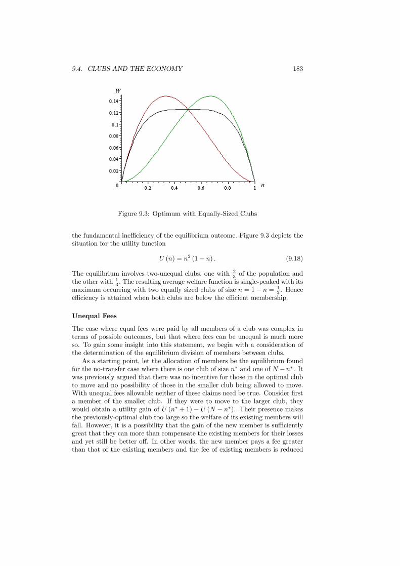
9.4. CLUBS AND THE ECONOMY 183
n
W
Figure 9.3: Optimum with Equally-Sized Clubs
the fundamental inefficiency of the equilibrium outcome. Figure 9.3 depicts thesituation for the utility function
U (n) = n2 (1− n) . (9.18)
The equilibrium involves two-unequal clubs, one with 23 of the population and
the other with 13 . The resulting average welfare function is single-peaked with its
maximum occurring with two equally sized clubs of size n = 1− n = 12 . Hence
efficiency is attained when both clubs are below the efficient membership.
Unequal Fees
The case where equal fees were paid by all members of a club was complex interms of possible outcomes, but that where fees can be unequal is much moreso. To gain some insight into this statement, we begin with a consideration ofthe determination of the equilibrium division of members between clubs.As a starting point, let the allocation of members be the equilibrium found
for the no-transfer case where there is one club of size n∗ and one of N −n∗. Itwas previously argued that there was no incentive for those in the optimal clubto move and no possibility of those in the smaller club being allowed to move.With unequal fees allowable neither of these claims need be true. Consider firsta member of the smaller club. If they were to move to the larger club, theywould obtain a utility gain of U (n∗ + 1) − U (N − n∗). Their presence makesthe previously-optimal club too large so the welfare of its existing members willfall. However, it is a possibility that the gain of the new member is sufficientlygreat that they can more than compensate the existing members for their lossesand yet still be better off. In other words, the new member pays a fee greaterthan that of the existing members and the fee of existing members is reduced
184 CHAPTER 9. CLUB GOODS AND LOCAL PUBLIC GOODS
more than sufficiently to compensate them for the additional crowding. If thisis compensation is possible, then the move between clubs will be allowed andthe initial position cannot be an equilibrium.Now consider reversing the argument and considering the incentive for a
member of the optimal club to move to the smaller club. With equal fees, thiswould never happen. Now let unequal fees be allowed. If the move did occur,the club member moving would lose utility of value U (n∗) − U (N − n∗ + 1)but the existing members of the smaller club would each gain U (N − n∗ + 1)−U (N − n∗). If they could collectively agree to pay compensation to the newmember (meaning let them pay a lower membership fee), then it is possiblethat the existing members could more than compensate the new member forthe loss incurred in their move whilst still remaining better-off themselves.These arguments reveal that members of the optimal club may be enticed
to the smaller club and that members of the smaller club may be able to “buy“themselves into the optimal club. Both of these mechanisms may even be func-tioning simultaneously. The outcome of this reasoning is that it may not bepossible to find any equilibrium and, even if an equilibrium exists, it is not easyto characterize. Furthermore, there is even less reason to expect any equilibriumthat is achieved to be efficient. All of this occurs because the population cannotbe allocated to a set of clubs each with optimal membership except in unlikelycases when population size is a integer multiple of the optimal membership level.This problem does not diminish even when population size increases.There is one situation in which this argument does not apply. Consider
again the graph of utility as a function of club size drawn in Figure 9.1. Theproblems of dividing the population into optimal clubs resulted from the factthat there was a unique value for optimal club membership. If the graph wereinstead like Figure 9.4, with a flat section at its peak, then there would be arange of optimal sizes. To see the effect of this, let the optimal club size rangefrom 2 to 3. Then a population of 11 consumers could be divided into threeclubs of size 3 and one of size 2 and the economy would achieve efficiency. Ofcourse, with a population of size 11, this could not be done if optimal club sizewas unique (unless it was 11). Furthermore, any population size greater than11 can be divided into optimal size clubs.The general version of this argument is illustrated in Figure 9.5. For a single
club, the range of optimal memberships is between n0 and n00. When thereare two clubs, optimality can occur for the range 2n0 to 2n00. This extensionof the range continues as additional clubs are introduced. Eventually, if thetotal population is large enough, the ranges of values of total population forwhich optimality cannot be achieved shrinks to zero (alternatively, the rangesof optimal size overlap) and all consumers can be placed in optimal clubs.
9.4.3 Conclusion
The conclusion of this section has to be that the efficiency of the individual clubdoes not always translate into efficiency for the economy. In a large population,approximate efficiency will be achieved and individual utility will be virtually

9.4. CLUBS AND THE ECONOMY 185
Figure 9.4: Non-Unique Club Size
Figure 9.5: Achieving Efficiency

186 CHAPTER 9. CLUB GOODS AND LOCAL PUBLIC GOODS
equal to maximal attainable utility. However, when there are small-numberproblems efficiency will not be achieved by the equilibrium allocation of membersbetween clubs. This should not be surprising since small numbers introduceproblems akin to those found in oligopoly problems. What occurs is that smallgroups of consumers are able to affect their own utility levels by choosing to formoptimal size clubs. Therefore they possess market power and this is reflected inthe inefficiency. These problems are eliminated if there are a range of optimalclub sizes.
9.5 Local Public Goods
The concept of a local public good has already been introduced in Section 9.2.A local public good has the feature that its benefits are restricted to a particulargeographical area and it cannot be enjoyed outside of that area. Relating thisidea to the analysis of club goods, one can think of local communities as clubswhich are formed to provide local public goods. To become a member of a localcommunity, a consumer must move into the area (i.e. join the club) and paywhatever local taxes are levied in that community (i.e. pay the membershipfee). Once they have done this, they can then enjoy the local public goods thatare provided.An important feature of the club good was that exclusion was possible and
it is interesting to discuss whether this is the case with local public goods.There are two points at which exclusion may be possible. Firstly, a consumermust become resident in an area in order to benefit from the local public good.Although few (if any) local authorities have the right to prevent the resale ofhouses or to forcibly evict existing occupants, they do have the power to preventadditional new building. Consequently, reductions in population may be hard toachieve (unlike expulsions in an ordinary club), exclusion of additional membersis possible. Secondly, there is the payment of taxes. Any resident who refuses topay local taxes can be either forced to pay or excluded from the club since localauthorities have legal authority to collect taxation. If we impose the possibilityof exclusion, then the analysis of local public goods becomes exactly that ofthe clubs we have already considered. However, the analysis of non-exclusion isalso of interest with local public goods since this captures the idea of a freely-operating market in which individuals have the freedom to select their preferredresidential location. We now focus upon non-exclusion.The concept of local public goods can be applied to the provision of public
services by local regions in order to understand the allocation of a populationbetween different localities. Intuitively, we can think of localities competing forpopulation by setting the package of public good provision and taxation theyoffer. Members of the population look at what is offered in different localitiesand selects the one that offers the highest utility level. This will cause populationflows until no-one can gain by moving locality. This is similar to the adjustmentprocess for club goods except for the fact that there is free access (i.e., nopossibility of barring access to new migrants even if the existing population
9.5. LOCAL PUBLIC GOODS 187
would lose from the migration).In this framework it is natural to question whether an efficient equilibrium
will be attained. The localities are competing for population and no restrictionsare imposed upon the freedom of the population to move between regions. Withclubs, efficiency was achieved at least within the clubs. To see whether the sameis true for local public goods, it is necessary to consider a model of the situation.Consider a total population of H consumers that is to be divided between
two localities with h being the population of a locality (we use different notationto avoid confusion with club membership). Each locality provides a local publicgood financed through a charge on the population. As the population increases,the unit cost of the public good per resident is reduced. This is the benefitfrom increased population. There is also a cost to increasing population. Thiscan be motivated by assuming that there is a fixed resource in each region sothat income per person falls as the population rises and this resource has to beshared between a greater number.These assumptions imply that income can be written as a decreasing func-
tion, M(h), of the population of a locality. Think of wages or welfare benefitsreducing with increased migration. If the locality provides G units of the publicgood, the charge per resident is G
h . Combining these, the income left to spendon private goods isM(h)− G
h , and the resulting level of utility U(M(h)− Gh ,G).
It is assumed that localities choose the level of public good optimally giventheir population. This eliminates the possibility of inefficiency through a levelof provision that does not satisfy the Samuelson rule. Given a population h, thelevel of public good provision satisfies the Samuelson rule
hUGUx
= 1. (9.19)
This condition can be solved to find the level of public good, G(h), which de-pends upon the population of the locality. Substituting the level of the publicgood into the utility function determines the level of utility as a function ofpopulation. This relationship is written in brief as U (h) . The implications ofthe model follow from the fact that an increase in h can increase or decreaseutility. Differentiating U (h) with respect to h shows that
U 0 = UxM 0 + Ux
µG
h2
¶. (9.20)
The first term of this is negative, since an increase in population reduces incomeM , while the second term is positive because the cost of the public good isreduced. It is therefore unclear what the net effect will be. To analyze themodel further, assume that utility initially increases with the population untilit reaches a maximum and then decreases. In addition, let U (H) > U (0) , sothat having all the population leads to higher utility than having no population.This can be motivated by the fact that a small number of people find it veryexpensive to provide the public good but the income is not reduced too far whenthe entire population is in one locality.
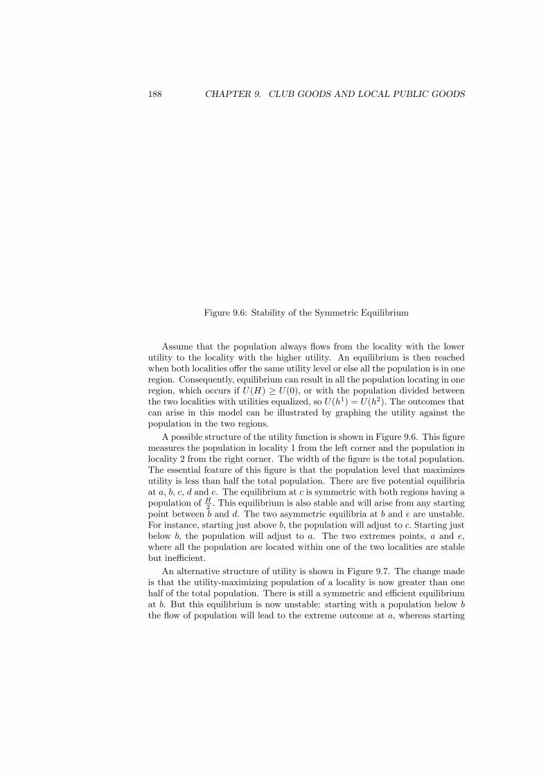
188 CHAPTER 9. CLUB GOODS AND LOCAL PUBLIC GOODS
Figure 9.6: Stability of the Symmetric Equilibrium
Assume that the population always flows from the locality with the lowerutility to the locality with the higher utility. An equilibrium is then reachedwhen both localities offer the same utility level or else all the population is in oneregion. Consequently, equilibrium can result in all the population locating in oneregion, which occurs if U(H) ≥ U(0), or with the population divided betweenthe two localities with utilities equalized, so U(h1) = U(h2). The outcomes thatcan arise in this model can be illustrated by graphing the utility against thepopulation in the two regions.
A possible structure of the utility function is shown in Figure 9.6. This figuremeasures the population in locality 1 from the left corner and the population inlocality 2 from the right corner. The width of the figure is the total population.The essential feature of this figure is that the population level that maximizesutility is less than half the total population. There are five potential equilibriaat a, b, c, d and e. The equilibrium at c is symmetric with both regions having apopulation of H2 . This equilibrium is also stable and will arise from any startingpoint between b and d. The two asymmetric equilibria at b and e are unstable.For instance, starting just above b, the population will adjust to c. Starting justbelow b, the population will adjust to a. The two extremes points, a and e,where all the population are located within one of the two localities are stablebut inefficient.
An alternative structure of utility is shown in Figure 9.7. The change madeis that the utility-maximizing population of a locality is now greater than onehalf of the total population. There is still a symmetric and efficient equilibriumat b. But this equilibrium is now unstable: starting with a population below bthe flow of population will lead to the extreme outcome at a, whereas starting
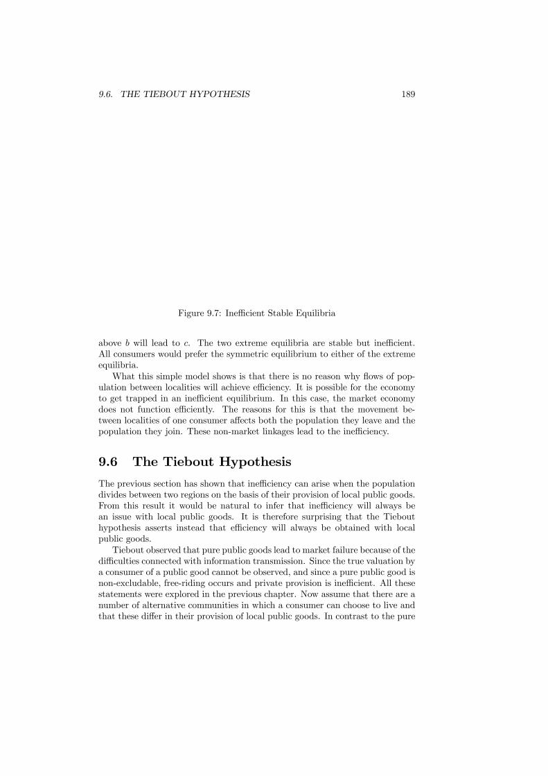
9.6. THE TIEBOUT HYPOTHESIS 189
Figure 9.7: Inefficient Stable Equilibria
above b will lead to c. The two extreme equilibria are stable but inefficient.All consumers would prefer the symmetric equilibrium to either of the extremeequilibria.What this simple model shows is that there is no reason why flows of pop-
ulation between localities will achieve efficiency. It is possible for the economyto get trapped in an inefficient equilibrium. In this case, the market economydoes not function efficiently. The reasons for this is that the movement be-tween localities of one consumer affects both the population they leave and thepopulation they join. These non-market linkages lead to the inefficiency.
9.6 The Tiebout Hypothesis
The previous section has shown that inefficiency can arise when the populationdivides between two regions on the basis of their provision of local public goods.From this result it would be natural to infer that inefficiency will always bean issue with local public goods. It is therefore surprising that the Tiebouthypothesis asserts instead that efficiency will always be obtained with localpublic goods.Tiebout observed that pure public goods lead to market failure because of the
difficulties connected with information transmission. Since the true valuation bya consumer of a public good cannot be observed, and since a pure public good isnon-excludable, free-riding occurs and private provision is inefficient. All thesestatements were explored in the previous chapter. Now assume that there are anumber of alternative communities in which a consumer can choose to live andthat these differ in their provision of local public goods. In contrast to the pure
190 CHAPTER 9. CLUB GOODS AND LOCAL PUBLIC GOODS
public good case, a consumer’s choice of which location to live in provides a veryclear signal of preferences. The chosen location is obviously the one offering theprovision of local public goods closest to the consumer’s ideal. Hence, throughcommunity choice, preference revelation takes place. Misrepresenting preferencecannot help a consumer here since the choice of a non-optimal location merelyreduces their welfare level. The only rational choice is to act honestly.The final step in the argument can now be constructed. Since preference
revelation is taking place, it follows that if there are enough different types ofcommunity and enough consumers with each kind of preference, then all con-sumers will allocate themselves to a community that is optimal for themselvesand each community will be optimally sized. Thus, the market outcome willbe fully efficient and the inefficiencies discussed in connection with pure publicgoods will not arise. Phrased more prosaically, consumers reveal their prefer-ences by voting with their feet and this ensures the construction of optimalcommunities. This also shows why the analysis of the previous section failed tofind efficiency. The existence of at most two localities violated the large-numberassumption of the Tiebout hypothesis.The significance of this efficiency result, which is commonly called the Tiebout
hypothesis, has been much debated. Supporters view it as another demonstra-tion of the power of the market in allocating resources. Critics denounce it assimply another empty demonstration of what is possible under unrealistic as-sumptions. Certainly, the Tiebout hypotheses has much the same foundationsas the Two Theorems of Welfare Economics since both concern economies withno rigidities and large numbers of participants. But there is one importantcontrast between the two: formalizing the Tiebout hypothesis proves a difficulttask.To obtain an insight into these difficulties, some of the steps in the previous
argument need to be retraced. It was assumed that consumers could move be-tween communities or at least choose between them with no restrictions on theirchoice. If housing markets function efficiently there should not be a problemin terms of actually finding accommodation. Where problems do arise is in thelink between income and location. An assumption that can justify the previousanalysis is that consumers obtain all their income from “rents” e.g. from theownership of land, property or shares. In this case it does not matter where theychoose to reside since the rents will accrue regardless of location. Once someincome is earned from employment, then the Tiebout hypothesis only holds ifall employment opportunities are also replicated in all communities. Otherwisecommunities with better employment prospects will appear more attractive evenif they offer a slightly less appealing set of local public goods. If the two issuesbecome entangled in this way then the Tiebout hypothesis will naturally fail.Further difficulties with the hypothesis arise when the numbers of commu-
nities and individuals is considered. When these are both finite the problemsalready discussed above with achieving efficiency through market behavior ariseagain. These are compounded when individuals of different types are needed tomake communities work. For example, assume that community A needs 10 doc-tors and 20 teachers to provide the optimal combination of local public goods
9.7. EMPIRICAL TESTS 191
whilst community B requires 10 policemen and 20 teachers. If doctors, teachersand policemen are not found in the proportions 1 : 4 : 1 then efficiency in alloca-tion between the communities cannot be achieved. Furthermore, if all teachershave different tastes to doctors and to policemen, then none of the communitiescan supply the ideal local public good combination to meet all tastes.The efficiency of the allocation can then be recovered in two steps. Firstly,
if we appeal again to the large population assumption the issue of achieving theprecise mix of different types is eliminated - there will always be enough peopleof each type to populate the localities in the correct proportions. Secondly, evenif tastes are different it is still possible to obtain agreement upon the level ofdemand through the use of personalized prices. This issue has already beendiscussed for public goods in connection with the Lindahl equilibrium. Thesame idea can be applied to local public goods in which case it would be thelocal taxes which are differentiated between residents to equalize the level ofpublic good demand and to attain efficiency with a heterogeneous population.The Tiebout hypothesis depends upon the freedom of consumers to move
to preferred locations. This is only possible if there are no transactions costsinvolved in changing location. In practice such transactions costs arise in thecommission that has to be paid to estate agents, legal fees and in the physicalcosts of shipping furniture and belongings. These can be significant and willcause friction in the movement of consumers to the extent that non-optimallevels of provision will be tolerated to avoid paying these costs.To sum up, the Tiebout hypothesis provides support for allowing the market,
by which is meant the free movement of consumers, to determine the provisionof local public goods. By choosing communities, consumers reveal their tastes.They also abide to local tax law so free-riding is ruled out. Hence efficiency isachieved. Although apparently simple, there are a number of difficulties whenthe practical implementation of this hypothesis is considered. The populationmay not partition neatly into the communities envisaged and employment tiesmay bind consumers to localities whose local public good supply is not to theirliking. Transactions costs in housing markets are significant and these will limitthe freedom of movement that is key to the hypothesis. The hypothesis providesan interesting insight into the forces at work in the formation of communitiesbut it does not guarantee efficiency.
9.7 Empirical Tests
The Tiebout hypothesis provides the reassuring conclusion that efficiency willbe attained by local communities providing public goods efficiently. If correct,the forces of economics and local politics can be left to work unrestricted bygovernment intervention. Given the strength of this conclusion, and some of thedoubts cast upon whether the Tiebout argument really works, it is natural toconduct empirical tests of the hypothesis.In testing any hypothesis it is first necessary to determine what the observa-
tional implications of the hypothesis will be. For Tiebout, this means isolating

192 CHAPTER 9. CLUB GOODS AND LOCAL PUBLIC GOODS
what will be different between an economy in which the Tiebout hypothesisapplies and one in which it does not. Empirical testing has been handicappedby the difficulty of establishing quite what this difference will be.The earlier empirical studies focussed upon property taxes, public good pro-
vision and house prices. The reason for this was made clear by Oates whoinitiated this line of research in 1969: local governments fund their activitiesprimarily through property taxes and the manner in which these taxes are re-flected in house prices provides evidence on the Tiebout hypothesis. Assumethat all local governments provide the same level of public goods. Then the ju-risdictions with higher property tax rates will be less attractive and have lowerhouse prices. Now let the provision of public goods vary. Holding tax rates con-stant, house prices should be higher in areas with more public good provision.These effects offset each other, and if the public good effect is sufficiently strongjurisdictions with higher tax rates will actually have higher property prices.Oates considered evidence on house prices, property tax rates and educationalprovision for 53 primarily residential municipalities in New Jersey. These mu-nicipalities were chosen because the majority of residents commuted to workand hence were not tied by employment to a particular location. The analysisof the house prices were reduced by high property taxes but increased by greaterpublic good provision.Whether these results were evidence in favor of the Tiebout hypothesis be-
came the subject of a debate which focused on the implications of the theory.Whereas Oates took differences in property prices as an indication of the Tiebouthypothesis at work (on the grounds that more attractive locations would witnessincreased competition for the housing stock), an alternative argument suggestedthat a given quality of house would have the same price in all jurisdictions ifTiebout applied. The argument for uniform prices is based on the view thatproperty taxes are the price paid for the bundle of public goods provided by thelocal government. If this price reflects the benefit enjoyed from the public goods,as it should if the Tiebout hypothesis is functioning, then it should not impactupon property prices. Uniform property prices should therefore be expected ifthe Tiebout hypothesis applies - an observation that lead to a series of stud-ies looking for uniform house prices across jurisdictions with different levels ofpublic good provision. Unfortunately, as Epple, Zelenitz and Visscher show, thesame conclusion is true even when the Tiebout hypothesis does not hold so thatnet-of-tax property prices should be uniform in all jurisdictions in all circum-stances. Instead, they argue that when the Tiebout hypothesis applies housingdemand is not affected by the property tax rate but when Tiebout does notapply it is affected. Looking at prices, which are equilibrium conditions, cannotthen provide a test of Tiebout. Instead, a test has to be based on the structuralequations of the demand for quantity of housing and of location demand andtheir dependence, or otherwise, upon tax rates. This conclusion undermines theearlier work on property values but does not provide and easily implementabletest.As a response to these difficulties, alternative tests of the hypothesis have
been constructed. One approach to determining whether the Tiebout hypothesis
9.8. CONCLUSIONS 193
applies is to consider the level of demand for public goods from the residents ofeach locality. If the Tiebout hypothesis applies, residents should have selecteda residential location that provides a level of public goods in line with theirpreferences. Hence, within each locality, there should be a degree of homogeneityin the level of demand for public goods. Note carefully that this does notassert that all residents have the same preferences, but only that given thetaxes and other local charges they pay, their demands are equalized. The testof the hypothesis is then to consider the variance in demand within regionsrelative to the variance in demand across regions. Such a test was conductedby Gramlich and Rubinfeld who studied households in Michigan suburbs andprovided compelling evidence that there was less variation within regions thanacross regions.It is necessary to note that these results do not confirm that the Tiebout
hypothesis is completely operating, but only that some sorting of residents isoccurring. It is supportive evidence for the hypothesis but not complete confir-mation. This conclusion is only to be expected since, given the extent of frictionsin the housing market, the freedom of movement necessary for the hypothesisto hold exactly is lacking.Overall, the empirical work is suggestive that the right forces are at work to
push the economy towards the efficient outcome of Tiebout but that there areresidual frictions that prevent the complete sorting required for the efficiency.Having said this, the tests have been limited to data from suburban areas whichhave the highest chance of producing the right outcome. In other locations,where the separation between work and location is not so simple, the hypothesiswould have less chance of applying.
9.8 Conclusions
The chapter has discussed the nature of club goods and local public goods, anddrawn the distinction between these and pure public goods. For a club good,the essential feature is the possibility of exclusion and it has been shown howexclusion allows an individual club to attain efficiency. Although it is temptingto extend this argument to the economy as a whole, a series of new issues arisewhen the allocation of a population between clubs is analyzed. Efficiency maybe attained, but it is not guaranteed.Many of these same issues arise with local public goods whose benefits are
restricted to a given geographical area. We have treated local public goodsas a model of provision by localities where each locality is described by thepackage of public good and taxation that it offers. When there is no exclusionfrom membership, there is no implication that efficiency will be attained whenresidential choice can be made from only a small number of localities.In contrast to this, the Tiebout hypothesis evokes a large-number assumption
to argue that the population will be able to sort itself into a set of localities,each of which is optimal for its residents. At the heart of this argument is thatchoice of locality reveals preferences about public goods so efficiency becomes
194 CHAPTER 9. CLUB GOODS AND LOCAL PUBLIC GOODS
attainable. The Tiebout hypothesis has been subjected to empirical testing butthe evidence is at best inconclusive. It shows some degree of sorting and iscertainly not a rejection of Tiebout but it does not go as far as confirming thatthe promised efficiency is delivered.
ReadingThe potential for clubs to achieve efficiency in the provision of public goods
was first identified in:Buchanan, J. (1965) ”An economic theory of clubs”, Economica, 32, 1 - 14.A more extensive discussion of many of these issues can be found in:Cornes, R.C. and Sandler, T. (1996) The Theory of Externalities, Public
Goods and Club Goods (Cambridge: Cambridge University Press).Sandler, T, and Tschirhart, J. (1980) ”The economic theory of clubs: an
evaluative survey”, Journal of Economic Literature, 18, 1481 - 1521.The problems of attaining efficiency in a club economy are explored by:Wooders, M.H. (1978) ”Equilibria, the core and jurisdiction structures in
economies with a local public good”, Journal of Economic Theory, 18, 328 -348.The influential Tiebout hypothesis was first stated in:Tiebout, C.M. (1956) ”A pure theory of local expenditure”, Journal of Po-
litical Economy, 64, 416 - 424.A strong critique of the hypothesis is in:Bewley, T.F. ”A critique of Tiebout’s theory of local public expenditure”,
Econometrica, 49, 713 -740.Tests of the Tiebout hypothesis are can be found in:Epple, D., Zelenitz, A., and Visscher, M. (1978) ”A search for testable im-
plications of the Tiebout hypothesis”, Journal of Political Economy, 86, 405 -425.Hamilton, B.W. (1976) ”The effects of property taxes and local public spend-
ing on property values: a theoretical comment”, Journal of Political Economy,84, 647 - 650.Oates, W.E. (1969) ”The effects of property taxes and local public spending
on property values: an empirical study of tax capitalization and the Tiebouthypothesis”, Journal of Political Economy, 77, 957 - 971.
Chapter 10
Externalities
10.1 Introduction
An externality is a link between economic agents that lies outside the pricesystem of the economy. Everyday examples include the pollution from a factorywhich harms a local fishery and the envy that is felt when a neighbor proudlydisplays a new car. Such externalities are not controlled directly by price -the fishery cannot choose to buy less pollution nor can you choose to buy yourneighbor a worse car. This prevents the efficiency theorems described in Chapter7 from applying. Indeed, the demonstration of market efficiency was based onthe following two presumptions:(a) the welfare of each consumer depended solely on her own consumption
decision;(b) the production of each firm depended only on its own input/output
choice.In reality a consumer or a firm may be directly affected by the actions of other
agents in the economy; that is, there may be external effects from the actions ofother consumers or firms. In the presence of such externalities the outcome ofa competitive market is unlikely to be Pareto efficient because agents will nottake account the external effects of their (consumption/production) decisions.Typically, the economy will display too great a quantity of “bad” externalitiesand too small a quantity of “good” externalities.The control of externalities is an issue of increasing practical importance.
Global warming and the destruction of the ozone layer are two of the mostsignificant examples but there are numerous others, from local to global envi-ronmental issues. Some of these may not appear immediately to be economicproblems but economic analysis can expose why they occur and investigate theeffectiveness of alternative policies. It can generate surprising conclusions andchallenge presumptions. In particular, economic analysis shows how govern-ment intervention that induces agents to internalize the external effects of theirdecisions can achieve a Pareto improvement.
195
196 CHAPTER 10. EXTERNALITIES
The starting point for the chapter is to provide a working definition of anexternality. Using this it is shown why market failure arises and the nature of theresulting inefficiency. The design of the optimal set of corrective, or Pigouvian,taxes is then addressed and related to missing markets for externalities. Theuse of taxes are then contrasted with direct control through tradable licences.Internalization as a solution to externalities is then considered. Finally, thesemethods of solving the externality problem are contrasted to the claim of theCoase theorem that efficiency will be attained by trade even when there areexternalities.
10.2 Externalities Defined
An externality has already been described as an effect upon one agent caused byanother. This section expresses this description as a formal definition and thenuses this to classify the various forms of externality. The way of representingthese forms of externalities in economic models is then introduced.There have been several attempts at defining externalities, and of providing
classifications of various types of externality. From amongst these, the followingdefinition is the most commonly adopted. Its advantages are that it placesthe emphasis on recognizing externalities through their effects and it leads to anatural system of classification.
Definition 4 (Externality) An externality is present whenever some economicagent’s welfare (utility or profit) is directly affected by the action of anotheragent (consumer or producer) in the economy.
By “directly” we exclude any effects that are mediated by prices. That is, anexternality is present if a fishery’s productivity is affected by the river pollutionof an upstream oil refinery, but not if the fishery’s profitability is affected by theprice of oil (which may depend on the oil refinery’s output of oil). The latter typeof effect (also called a pecuniary externality) is present in any competitive marketbut creates no inefficiency (since price mediation through competitive marketsleads to a Pareto efficient outcome). We shall present later an illustration of apecuniary externality.The definition of externality implicitly distinguishes between two broad cat-
egories of externality. A production externality occurs when the effect of theexternality is upon a profit relationship and a consumption externality whenevera utility level is affected. Clearly, an externality can be both a consumption anda production externality simultaneously. For example, pollution from a factorymay affect the profit of a commercial fishery and the utility of leisure anglers.Using this definition of an externality, it is possible to move on to how they
can be incorporated into the analysis of behavior. Denote, as in Chapter 6,the consumption levels of the households by x =
©x1, ..., xH
ªand the produc-
tion plans of the firms by y =©y1, ..., ym
ª. It is assumed that consumption
externalities enter the utility functions of the households and that production
10.3. MARKET INEFFICIENCY 197
externalities enter the production sets of the firms. At the most general level,this assumption implies that the utility functions take the form
Uh = Uh (x, y) , h = 1, ...,H, (10.1)
and the production set is described by
Y j = Y j (x, y) , j = 1, ...,m. (10.2)
In this formulation the utility functions and the production sets are possiblydependent upon the entire arrays of consumption and production levels. Theexpressions in (10.1) and (10.2) represent the general form of the externalityproblem and in some of the discussion below a number of further restrictionswill be employed.It is immediately apparent from (10.1) and (10.2) that the actions of the
agents in the economy will no longer be independent or determined solely byprices. The linkages via the externality result in the optimal choice of each agentbeing dependent upon the actions of others. Viewed in this light, it becomesapparent why the efficient functioning of the competitive economy will generallynot be observed in an economy with externalities.
10.3 Market InefficiencyIt has been accepted throughout the discussion above that the presence of exter-nalities will result in the competitive equilibrium failing to be Pareto efficient.The immediate implication of this fact is that incorrect quantities of goods, andhence externalities, will be produced. It is also clear that a non-Pareto efficientoutcome will never maximize welfare. This provides scope for economic policyto raise welfare. The purpose of this section is to demonstrate how inefficiencycan arise in a competitive economy. Cases where externalities do not lead toinefficiency will also be described. The results are developed in the context ofa simple two-consumer model since this is sufficient for the purpose and alsomakes the relevant points as clear as possible.Consider a two-household two-good economy where the households have util-
ity functionsU1 = x1 + u1(z
1) + v1(z2), (10.3)
andU2 = x2 + u2(z
2) + v2(z1). (10.4)
The externality effect in (10.4) and (10.4) is generated by consumption of goodz by households. The externality will be positive if vh(·) is increasing in theconsumption level of the other consumer and negative if it is decreasing.To complete the description of the economy, it is assumed that the supply
of good x comes from an endowment ωh to the household h whereas good z isproduced from good x by a competitive industry that uses one unit of good x toproduce one unit of good z. Normalizing the price of good x at 1, the structure
198 CHAPTER 10. EXTERNALITIES
of production ensures that the equilibrium price of good z must also be one.Given this, all that needs to be determined for this economy is the division ofthe initial endowment into quantities of the two goods.Incorporating this assumption into the maximization decision of the house-
holds, the competitive equilibrium of the economy is described by the equations
u0h(zh) = 1, h = 1, 2, (10.5)
xh + zh = ωh, h = 1, 2, (10.6)
andx1 + z1 + x2 + z2 = ω1 + ω2. (10.7)
It is equations (10.5) that are of primary importance at this point. For house-hold h these state that the private marginal benefit from each good, determinedby the marginal utility, is equated to the of private marginal cost. The ex-ternal effect does not appear directly in the determination of the equilibrium.The question we now address is whether this competitive market equilibrium isefficient.The Pareto efficient allocations are found by maximizing the total utility of
household 1 and 2, subject to the production possibilities. The equations thatresult from this will then be contrasted to (10.5). In detail, a Pareto efficientallocation solves
max{xh,zh}
U1 + U2 =£x1 + u1(z
1) + v1(z2)¤+£x2 + u2(z
2) + v2(z1)¤, (10.8)
subject toω1 + ω2 − x1 − z1 − x2 − z2 ≥ 0. (10.9)
The solution is characterized by the conditions
u01(z1) + v02(z
1) = 1, (10.10)
andu02(z
2) + v01(z2) = 1. (10.11)
In (10.10) and (10.11) the externality effect can be seen to affect the optimalallocation between the two goods via the derivatives of utility with respect tothe externality. If the externality is positive then v0h > 0 and the externalityeffect will raise the value of the left-hand terms. It will decrease them if thereis a negative externality with v0h < 0. It can then be concluded that at theoptimum with a positive externality the marginal utilities of both households arebelow their value in the market outcome. The converse is true with a negativeexternality. It can be seen that the externality leads to a divergence betweenthe private valuations of consumption given by (10.5) and the correspondingsocial valuations in (10.10) and (10.11). This observation has the implicationthat the market outcome is not Pareto efficient.In general, it can also be concluded that if the externality is positive then
more of good z will be consumed at the optimum than under the market out-come. The converse holds for a negative externality. This situation is illustrated
10.4. EXTERNALITY EXAMPLES 199
Figure 10.1: Deviation of Private from Social Benefits
in Figure 10.1. The market outcome is represented by the equality between pri-vate marginal benefit of the good and its marginal cost. The Pareto efficientoutcome equates the sum of the private marginal benefit and the marginal ex-ternal effect of the good to its marginal cost. The market failure is characterizedby too much consumption of a good causing a negative externality and too littleconsumption of a good generating a positive externality .
10.4 Externality Examples
The previous section has discussed externalities at a somewhat abstract level.We now consider some more-concrete examples of externalities. These will illus-trate the range of situations that fall under the general heading of externalities.
10.4.1 River Pollution
This is one of the simplest examples that can be described using only two agents.Assume that two firms are located along the same river. The upstream firm, u,pollutes the river which reduces the production (say the output of fish) of thedownstream firm, d. Both firms produce the same output which they sell at aconstant unit price of 1.Labor and water are used as inputs. Water is free but a wage w is paid
for each unit of labor. The labor market is competitive so w is the equilibriumprice of labor. The production technologies of the firms are given by Fu (Lu)and F d
¡Ld, Lu
¢, with ∂Fd
∂Ld< 0 to reflect that the pollution reduces downstream
output. Decreasing returns to scale is assumed with respect to own labor input.
200 CHAPTER 10. EXTERNALITIES
Figure 10.2: Equilibrium with River Pollution
Each firm acts independently and seeks to maximize it own profit πi = F i (·)−wLi taking prices as given.
The equilibrium is illustrated in Figure 10.2. The total stock of labor isallocated between the two firms. Each point on the horizontal axis then repre-sents a different allocation between the firms. The labor input of the upstreamfirm is measured from the left, that of the downstream from the right. Theupstream firm’s profit maximization process is represented in the upper part ofthe diagram and the downstream firm’s in the lower part. As the input of theupstream firm increases the production function of the downstream firm movesprogressively in towards the horizontal axis. Given the profit maximizing inputlevel of the upstream firm, denoted Lu∗, the downstream firm can do no betterthan choose Ld∗. At these choices, the firms earn profits πu and πd respectively.This is the competitive equilibrium We now show that this is inefficient andthat reallocating labor between the firms can increase total profit and reducepollution.
Consider starting at the competitive equilibrium and make a small reductionin the labor input to the upstream firm. Since the choice was optimal for theupstream firm, the change has no effect on profit for the upstream firm (recallthat ∂πu
∂Lu = 0). However, it leads to an outward shift of the downstream firm’sproduction function. This raises its profits. Hence the change raises aggregateprofit. This demonstrates that the competitive equilibrium is not efficient andthat the externality results in the upstream firm using too much labor and thedownstream too little.
10.4. EXTERNALITY EXAMPLES 201
Figure 10.3: Choice of Commuting Mode
10.4.2 Traffic Jams
The next example considers the externalities imposed by drivers on each other.Let there by N commuters who have the choice of commuting by train or bycar. Commuting by train always takes 40 minutes regardless of the numberof travellers. The commuting time by car increases as the number car usersincreases. This congestion effect which raises the commuting time is the ex-ternality between travellers. Each individual makes their decision to minimizetheir own transportation time.The equilibrium is depicted in Figure 10.3. The number of car users will
adjust until the travel time by car is exactly equal to the travel time by train.For the car travel time depicted in the figure, the equilibrium occurs when 40%of commuters travel by car. The optimum occurs when the aggregate timesaving is maximized. This occurs when only 20% of commuters use a car.The externality in this situation is that each car driver takes into account
only their own travel time but not the fact that they will increase the traveltime for all other drivers. As a consequence, too many commuters choose todrive.
10.4.3 Pecuniary externality
Consider a set of students who must decide whether to be an economist or alawyer. Being an economist is great when there are few economists, and not sogreat when the labor market becomes crowded with economists (due to pricecompetition). If the number of economists grows high enough, they will eventu-
202 CHAPTER 10. EXTERNALITIES
Figure 10.4: Job Choice
ally earn less than their lawyer counterparts. Suppose each person chooses theprofession with the best earnings prospects. The externality (a pecuniary one!)comes from the fact that when one more person decides to become a economist,he lowers all other economists’ incomes (through competition), imposing a coston the existing economists. When making his decision, he ignores this externaleffect imposed on others. The question is whether the invisible hand will leadto the correct allocation of students across different jobs.
The equilibrium is depicted in Figure 10.4. The number of economists willadjust until the earnings prospect for an economist is exactly equal to the earn-ings of a lawyer. The equilibrium is given by the percentage of economists atpoint E. To the right of point E, lawyers would earn more and the numberof economists would decrease. Alternatively, to the left of point E economistsare relatively few in number and will earn more than lawyers, attracting moreeconomists into the profession.
The laissez-faire equilibrium is efficient because the external effect is a changein price and income so that the economists’ cost of a lower income is a benefit toemployers. Employers’ benefit equals employees’ cost. There is zero net effect.The policy implication is that there is no need for government intervention toregulate the access to some professions. It follows that any public policy thataims to limit the access to some profession (like the numerus claususis) is notjustified. Market forces will correctly allocate the right number of people toeach of the different professions.
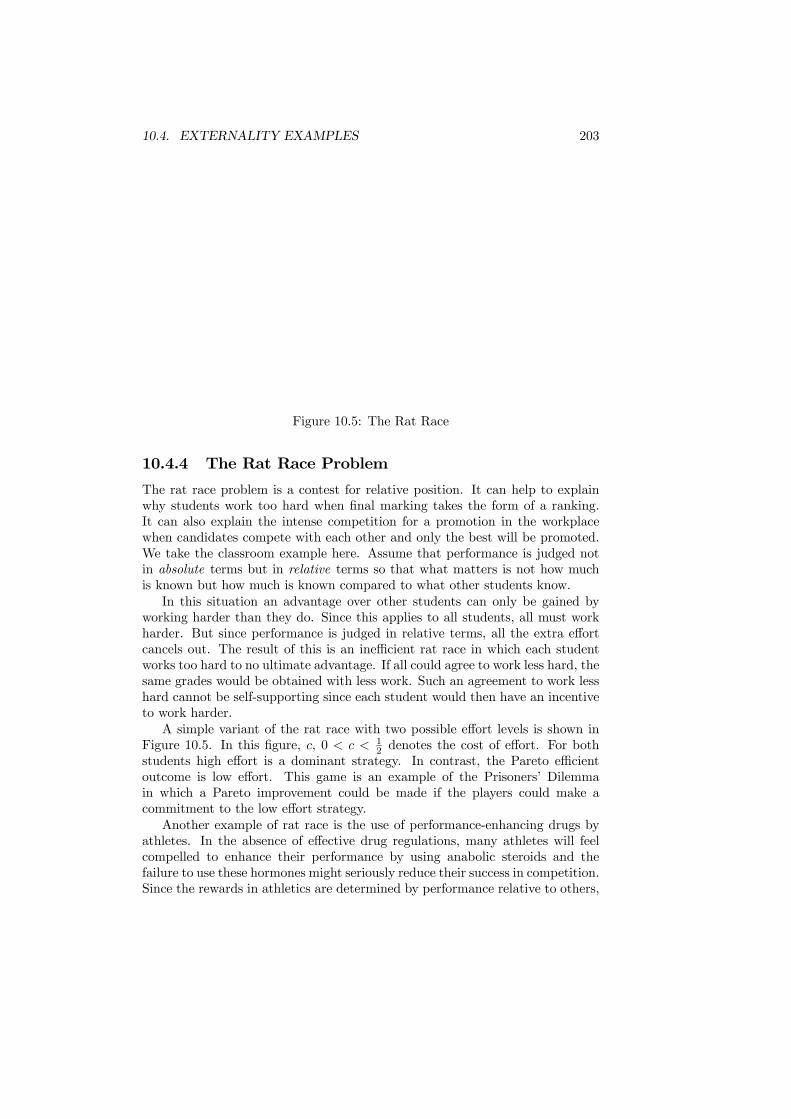
10.4. EXTERNALITY EXAMPLES 203
Figure 10.5: The Rat Race
10.4.4 The Rat Race Problem
The rat race problem is a contest for relative position. It can help to explainwhy students work too hard when final marking takes the form of a ranking.It can also explain the intense competition for a promotion in the workplacewhen candidates compete with each other and only the best will be promoted.We take the classroom example here. Assume that performance is judged notin absolute terms but in relative terms so that what matters is not how muchis known but how much is known compared to what other students know.In this situation an advantage over other students can only be gained by
working harder than they do. Since this applies to all students, all must workharder. But since performance is judged in relative terms, all the extra effortcancels out. The result of this is an inefficient rat race in which each studentworks too hard to no ultimate advantage. If all could agree to work less hard, thesame grades would be obtained with less work. Such an agreement to work lesshard cannot be self-supporting since each student would then have an incentiveto work harder.A simple variant of the rat race with two possible effort levels is shown in
Figure 10.5. In this figure, c, 0 < c < 12 denotes the cost of effort. For both
students high effort is a dominant strategy. In contrast, the Pareto efficientoutcome is low effort. This game is an example of the Prisoners’ Dilemmain which a Pareto improvement could be made if the players could make acommitment to the low effort strategy.Another example of rat race is the use of performance-enhancing drugs by
athletes. In the absence of effective drug regulations, many athletes will feelcompelled to enhance their performance by using anabolic steroids and thefailure to use these hormones might seriously reduce their success in competition.Since the rewards in athletics are determined by performance relative to others,
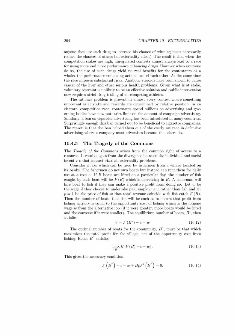
204 CHAPTER 10. EXTERNALITIES
anyone that use such drug to increase his chance of winning must necessarilyreduce the chances of others (an externality effect). The result is that when thecompetition stakes are high, unregulated contests almost always lead to a racefor using more and more performance enhancing drugs. However when everyonedo so, the use of such drugs yield no real benefits for the contestants as awhole: the performance-enhancing actions cancel each other. At the same timethe race imposes substantial risks. Anabolic steroids have been shown to causecancer of the liver and other serious health problems. Given what is at stake,voluntary restraint is unlikely to be an effective solution and public interventionnow requires strict drug testing of all competing athletes.The rat race problem is present in almost every contest where something
important is at stake and rewards are determined by relative position. In anelectoral competition race, contestants spend millions on advertising and gov-erning bodies have now put strict limit on the amount of campaign advertising.Similarly, a ban on cigarette advertising has been introduced in many countries.Surprisingly enough this ban turned out to be beneficial to cigarette companies.The reason is that the ban helped them out of the costly rat race in defensiveadvertising where a company must advertises because the others do.
10.4.5 The Tragedy of the Commons
The Tragedy of the Commons arises from the common right of access to aresource. It results again from the divergence between the individual and socialincentives that characterizes all externality problems.Consider a lake which can be used by fishermen from a village located on
its banks. The fishermen do not own boats but instead can rent them for dailyuse at a cost c. If B boats are hired on a particular day, the number of fishcaught by each boat will be F (B) which is decreasing in B. A fisherman willhire boat to fish if they can make a positive profit from doing so. Let w bethe wage if they choose to undertake paid employment rather than fish and letp = 1 be the price of fish so that total revenue coincide with fish catch F (B).Then the number of boats that fish will be such as to ensure that profit fromfishing activity is equal to the opportunity cost of fishing which is the forgonewage w from the alternative job (if it were greater, more boats would be hiredand the converse if it were smaller). The equilibrium number of boats, B∗, thensatisfies
π = F (B∗)− c = w (10.12)
The optimal number of boats for the community, B◦, must be that which
maximizes the total profit for the village, net of the opportunity cost fromfishing. Hence B
◦satisfies
max{B}
B [F (B)− c− w] . (10.13)
This gives the necessary condition
F³B◦´− c− w +BpF 0 ³B◦´ = 0. (10.14)
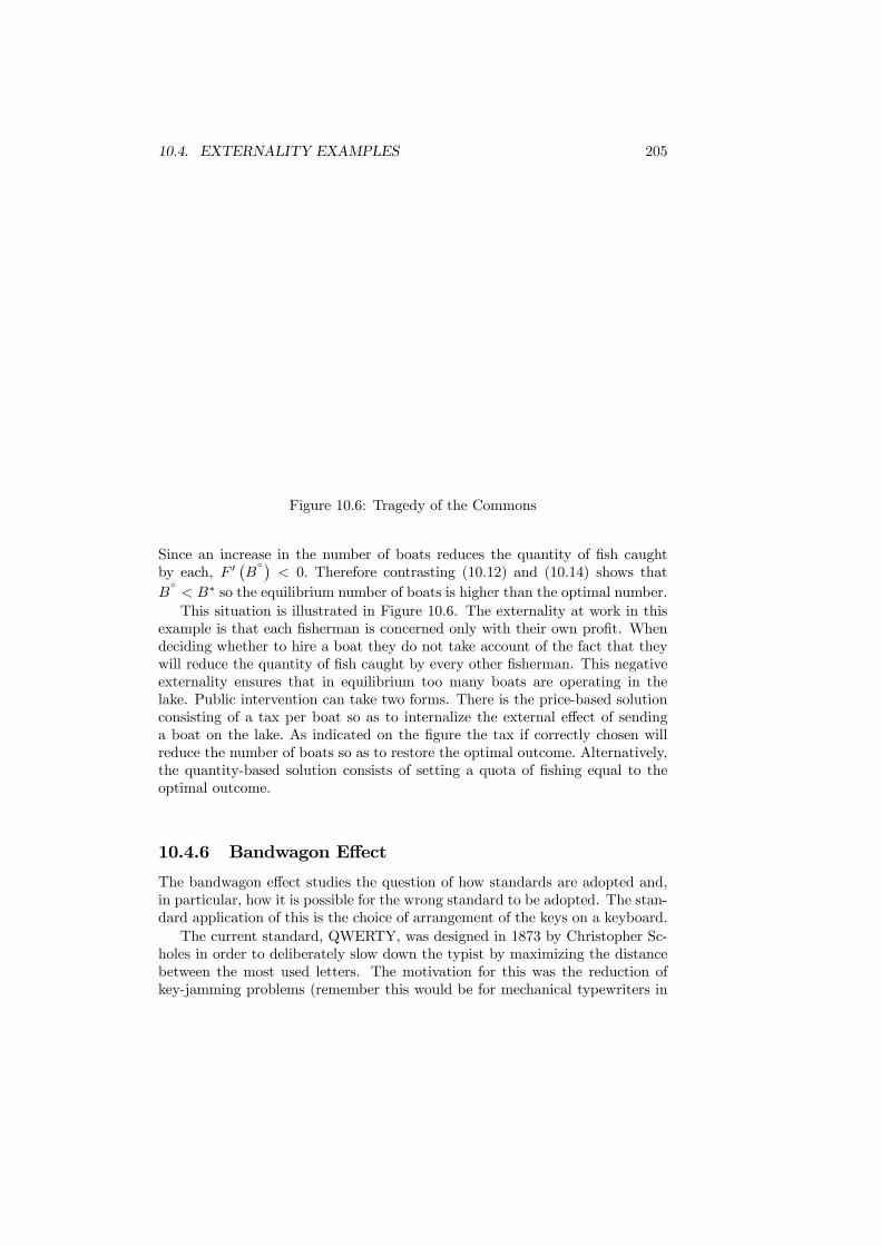
10.4. EXTERNALITY EXAMPLES 205
Figure 10.6: Tragedy of the Commons
Since an increase in the number of boats reduces the quantity of fish caughtby each, F 0
¡B◦¢< 0. Therefore contrasting (10.12) and (10.14) shows that
B◦< B∗ so the equilibrium number of boats is higher than the optimal number.This situation is illustrated in Figure 10.6. The externality at work in this
example is that each fisherman is concerned only with their own profit. Whendeciding whether to hire a boat they do not take account of the fact that theywill reduce the quantity of fish caught by every other fisherman. This negativeexternality ensures that in equilibrium too many boats are operating in thelake. Public intervention can take two forms. There is the price-based solutionconsisting of a tax per boat so as to internalize the external effect of sendinga boat on the lake. As indicated on the figure the tax if correctly chosen willreduce the number of boats so as to restore the optimal outcome. Alternatively,the quantity-based solution consists of setting a quota of fishing equal to theoptimal outcome.
10.4.6 Bandwagon Effect
The bandwagon effect studies the question of how standards are adopted and,in particular, how it is possible for the wrong standard to be adopted. The stan-dard application of this is the choice of arrangement of the keys on a keyboard.The current standard, QWERTY, was designed in 1873 by Christopher Sc-
holes in order to deliberately slow down the typist by maximizing the distancebetween the most used letters. The motivation for this was the reduction ofkey-jamming problems (remember this would be for mechanical typewriters in
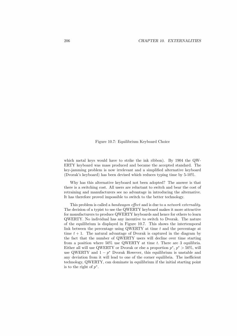
206 CHAPTER 10. EXTERNALITIES
Figure 10.7: Equilibrium Keyboard Choice
which metal keys would have to strike the ink ribbon). By 1904 the QW-ERTY keyboard was mass produced and became the accepted standard. Thekey-jamming problem is now irrelevant and a simplified alternative keyboard(Dvorak’s keyboard) has been devised which reduces typing time by 5-10%.
Why has this alternative keyboard not been adopted? The answer is thatthere is a switching cost. All users are reluctant to switch and bear the cost ofretraining and manufacturers see no advantage in introducing the alternative.It has therefore proved impossible to switch to the better technology.
This problem is called a bandwagon effect and is due to a network externality.The decision of a typist to use the QWERTY keyboard makes it more attractivefor manufacturers to produce QWERTY keyboards and hence for others to learnQWERTY. No individual has any incentive to switch to Dvorak. The natureof the equilibrium is displayed in Figure 10.7. This shows the intertemporallink between the percentage using QWERTY at time t and the percentage attime t + 1. The natural advantage of Dvorak is captured in the diagram bythe fact that the number of QWERTY users will decline over time startingfrom a position where 50% use QWERTY at time t. There are 3 equilibria.Either all will use QWERTY or Dvorak or else a proportion p∗, p∗ > 50%, willuse QWERTY and 1 − p∗ Dvorak However, this equilibrium is unstable andany deviation from it will lead to one of the corner equilibria. The inefficienttechnology, QWERTY, can dominate in equilibrium if the initial starting pointis to the right of p∗.

10.5. PIGOUVIAN TAXATION 207
Figure 10.8: Pigouvian Taxation
10.5 Pigouvian Taxation
The description of market inefficiency has shown that its basic source is thedivergence between social and private benefits (or between private costs andsocial costs). This fact has been reinforced by the examples. A natural meansof eliminating such divergences is to employ appropriate taxes or subsidies. Bymodifying the decision problems of the firms and consumers these can move theeconomy closer to an efficient position.To see how a tax can enhance efficiency consider the case of a negative con-
sumption externality. With a negative externality the private marginal benefitof consumption is always in excess of the social marginal benefit. These bene-fits are depicted by the PMB and SMBcurves respectively in Figure 10.8. Inthe absence of intervention, the equilibrium occurs where the PMB intersectsthe private marginal cost (PMC). This gives a level of consumption xm. Theefficient consumption level equates the PMC with the SMB; this is at pointxo. As already noted, with a negative externality the market outcome involvesmore consumption of the good than is efficient.The market outcome can be improved by placing a tax upon consumption.
What it is necessary to do is to raise the PMC so that it intersects the SMBvertically above xo. This is what happens for the curve PMC 0 which has beenraised above PMC by a tax of value t. This process, often termed Pigouviantaxation, allows the market to attain efficiency for the situation shown in Figure10.8Based on arguments like that exhibited above, Pigouvian taxation has been
proposed as a simple solution to the externality problem. The logic is that the
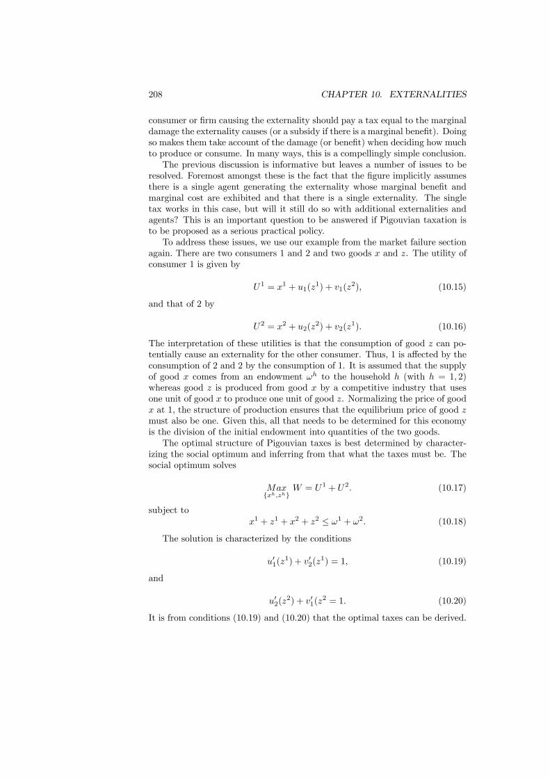
208 CHAPTER 10. EXTERNALITIES
consumer or firm causing the externality should pay a tax equal to the marginaldamage the externality causes (or a subsidy if there is a marginal benefit). Doingso makes them take account of the damage (or benefit) when deciding how muchto produce or consume. In many ways, this is a compellingly simple conclusion.The previous discussion is informative but leaves a number of issues to be
resolved. Foremost amongst these is the fact that the figure implicitly assumesthere is a single agent generating the externality whose marginal benefit andmarginal cost are exhibited and that there is a single externality. The singletax works in this case, but will it still do so with additional externalities andagents? This is an important question to be answered if Pigouvian taxation isto be proposed as a serious practical policy.To address these issues, we use our example from the market failure section
again. There are two consumers 1 and 2 and two goods x and z. The utility ofconsumer 1 is given by
U1 = x1 + u1(z1) + v1(z
2), (10.15)
and that of 2 by
U2 = x2 + u2(z2) + v2(z
1). (10.16)
The interpretation of these utilities is that the consumption of good z can po-tentially cause an externality for the other consumer. Thus, 1 is affected by theconsumption of 2 and 2 by the consumption of 1. It is assumed that the supplyof good x comes from an endowment ωh to the household h (with h = 1, 2)whereas good z is produced from good x by a competitive industry that usesone unit of good x to produce one unit of good z. Normalizing the price of goodx at 1, the structure of production ensures that the equilibrium price of good zmust also be one. Given this, all that needs to be determined for this economyis the division of the initial endowment into quantities of the two goods.The optimal structure of Pigouvian taxes is best determined by character-
izing the social optimum and inferring from that what the taxes must be. Thesocial optimum solves
Max{xh,zh}
W = U1 + U2. (10.17)
subject tox1 + z1 + x2 + z2 ≤ ω1 + ω2. (10.18)
The solution is characterized by the conditions
u01(z1) + v02(z
1) = 1, (10.19)
and
u02(z2) + v01(z
2 = 1. (10.20)
It is from conditions (10.19) and (10.20) that the optimal taxes can be derived.
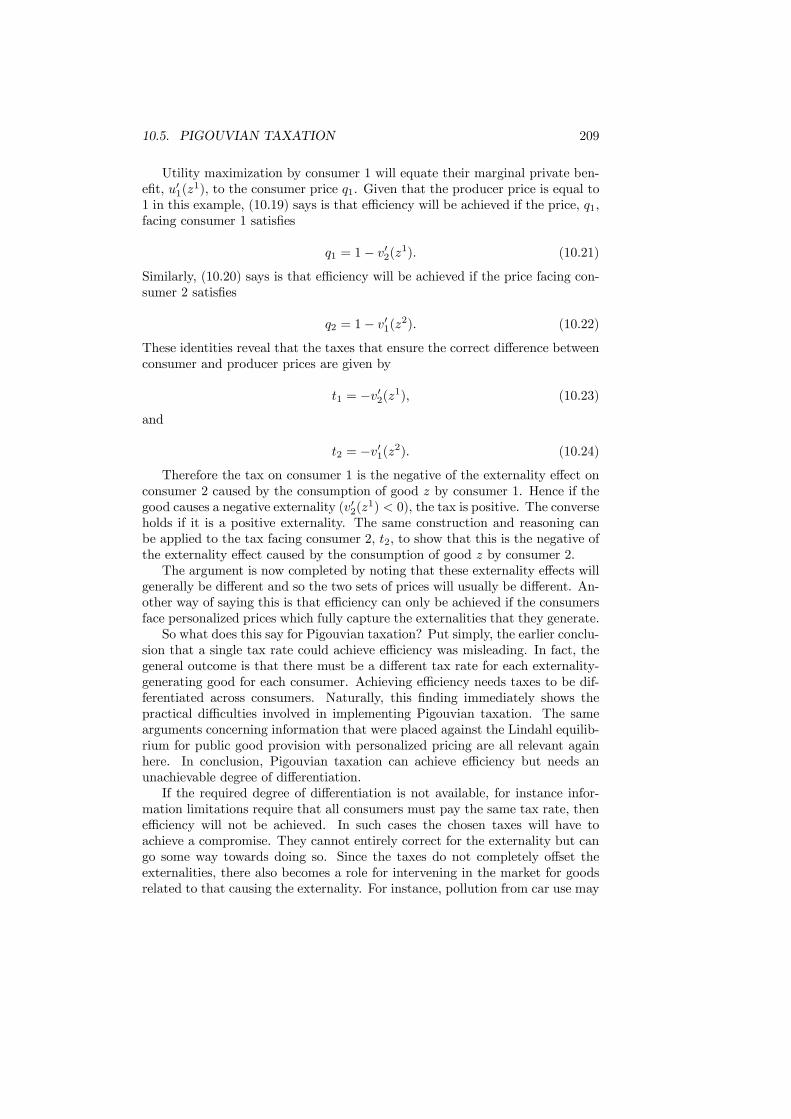
10.5. PIGOUVIAN TAXATION 209
Utility maximization by consumer 1 will equate their marginal private ben-efit, u01(z1), to the consumer price q1. Given that the producer price is equal to1 in this example, (10.19) says is that efficiency will be achieved if the price, q1,facing consumer 1 satisfies
q1 = 1− v02(z1). (10.21)
Similarly, (10.20) says is that efficiency will be achieved if the price facing con-sumer 2 satisfies
q2 = 1− v01(z2). (10.22)
These identities reveal that the taxes that ensure the correct difference betweenconsumer and producer prices are given by
t1 = −v02(z1), (10.23)
and
t2 = −v01(z2). (10.24)
Therefore the tax on consumer 1 is the negative of the externality effect onconsumer 2 caused by the consumption of good z by consumer 1. Hence if thegood causes a negative externality (v02(z1) < 0), the tax is positive. The converseholds if it is a positive externality. The same construction and reasoning canbe applied to the tax facing consumer 2, t2, to show that this is the negative ofthe externality effect caused by the consumption of good z by consumer 2.The argument is now completed by noting that these externality effects will
generally be different and so the two sets of prices will usually be different. An-other way of saying this is that efficiency can only be achieved if the consumersface personalized prices which fully capture the externalities that they generate.So what does this say for Pigouvian taxation? Put simply, the earlier conclu-
sion that a single tax rate could achieve efficiency was misleading. In fact, thegeneral outcome is that there must be a different tax rate for each externality-generating good for each consumer. Achieving efficiency needs taxes to be dif-ferentiated across consumers. Naturally, this finding immediately shows thepractical difficulties involved in implementing Pigouvian taxation. The samearguments concerning information that were placed against the Lindahl equilib-rium for public good provision with personalized pricing are all relevant againhere. In conclusion, Pigouvian taxation can achieve efficiency but needs anunachievable degree of differentiation.If the required degree of differentiation is not available, for instance infor-
mation limitations require that all consumers must pay the same tax rate, thenefficiency will not be achieved. In such cases the chosen taxes will have toachieve a compromise. They cannot entirely correct for the externality but cango some way towards doing so. Since the taxes do not completely offset theexternalities, there also becomes a role for intervening in the market for goodsrelated to that causing the externality. For instance, pollution from car use may
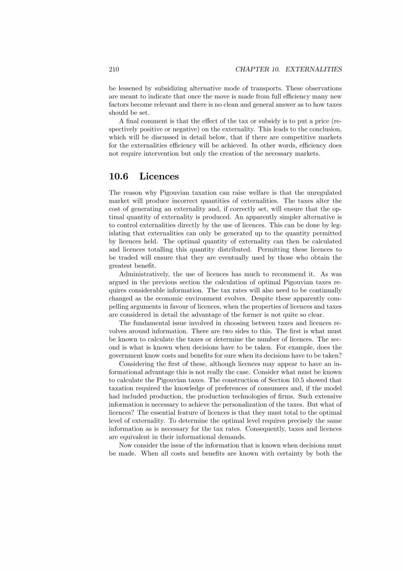
210 CHAPTER 10. EXTERNALITIES
be lessened by subsidizing alternative mode of transports. These observationsare meant to indicate that once the move is made from full efficiency many newfactors become relevant and there is no clean and general answer as to how taxesshould be set.A final comment is that the effect of the tax or subsidy is to put a price (re-
spectively positive or negative) on the externality. This leads to the conclusion,which will be discussed in detail below, that if there are competitive marketsfor the externalities efficiency will be achieved. In other words, efficiency doesnot require intervention but only the creation of the necessary markets.
10.6 Licences
The reason why Pigouvian taxation can raise welfare is that the unregulatedmarket will produce incorrect quantities of externalities. The taxes alter thecost of generating an externality and, if correctly set, will ensure that the op-timal quantity of externality is produced. An apparently simpler alternative isto control externalities directly by the use of licences. This can be done by leg-islating that externalities can only be generated up to the quantity permittedby licences held. The optimal quantity of externality can then be calculatedand licences totalling this quantity distributed. Permitting these licences tobe traded will ensure that they are eventually used by those who obtain thegreatest benefit.Administratively, the use of licences has much to recommend it. As was
argued in the previous section the calculation of optimal Pigouvian taxes re-quires considerable information. The tax rates will also need to be continuallychanged as the economic environment evolves. Despite these apparently com-pelling arguments in favour of licences, when the properties of licences and taxesare considered in detail the advantage of the former is not quite so clear.The fundamental issue involved in choosing between taxes and licences re-
volves around information. There are two sides to this. The first is what mustbe known to calculate the taxes or determine the number of licences. The sec-ond is what is known when decisions have to be taken. For example, does thegovernment know costs and benefits for sure when its decisions have to be taken?Considering the first of these, although licences may appear to have an in-
formational advantage this is not really the case. Consider what must be knownto calculate the Pigouvian taxes. The construction of Section 10.5 showed thattaxation required the knowledge of preferences of consumers and, if the modelhad included production, the production technologies of firms. Such extensiveinformation is necessary to achieve the personalization of the taxes. But what oflicences? The essential feature of licences is that they must total to the optimallevel of externality. To determine the optimal level requires precisely the sameinformation as is necessary for the tax rates. Consequently, taxes and licencesare equivalent in their informational demands.Now consider the issue of the information that is known when decisions must
be made. When all costs and benefits are known with certainty by both the
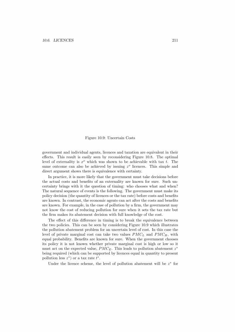
10.6. LICENCES 211
Figure 10.9: Uncertain Costs
government and individual agents, licences and taxation are equivalent in theireffects. This result is easily seen by reconsidering Figure 10.8. The optimallevel of externality is xo which was shown to be achievable with tax t. Thesame outcome can also be achieved by issuing zo licences. This simple anddirect argument shows there is equivalence with certainty.In practice, it is more likely that the government must take decisions before
the actual costs and benefits of an externality are known for sure. Such un-certainty brings with it the question of timing: who chooses what and when?The natural sequence of events is the following. The government must make itspolicy decision (the quantity of licences or the tax rate) before costs and benefitsare known. In contrast, the economic agents can act after the costs and benefitsare known. For example, in the case of pollution by a firm, the government maynot know the cost of reducing pollution for sure when it sets the tax rate butthe firm makes its abatement decision with full knowledge of the cost.The effect of this difference in timing is to break the equivalence between
the two policies. This can be seen by considering Figure 10.9 which illustratesthe pollution abatement problem for an uncertain level of cost. In this case thelevel of private marginal cost can take two values PMCL and PMCH , withequal probability. Benefits are known for sure. When the government choosesits policy it is not known whether private marginal cost is high or low so itmust act on the expected value, PMCE . This leads to pollution abatement z∗
being required (which can be supported by licences equal in quantity to presentpollution less z∗) or a tax rate t∗.Under the licence scheme, the level of pollution abatement will be z∗ for

212 CHAPTER 10. EXTERNALITIES
sure - there is no uncertainty about the outcome. With the tax, the level ofabatement will depend upon the realized level of cost since the firm chooses afterthis is known. Therefore if the cost turns out to be PMCL the firm will chooseabatement level zL. If its is PMCH , abatement is zH . This is shown in Figure10.9. Two observations emerge from this. Firstly, the claim that licences andtaxation will not be equivalent when there is uncertainty is confirmed. Secondly,when cost is realized to be low, taxation leads to abatement in excess of z∗. Theconverse holds when cost is high.The analysis of Figure 10.9 may be taken as suggesting that licences are
better since they do not lead to the variation in abatement that is inherent intaxation. However, it should also be realized that the choices made by the firmin the tax case are responding to the actual cost of abatement so there is somejustification for what the firm is doing. In general, there is no simple answer towhich is better.Some insight into the factors which are relevant can be obtained from the
following analysis. Let the cost of abatement be given by
CL = [c1 − θ] z + c2z2, (10.25)
with probability 1/2 and
CH = [c1 + θ] z + c2z2, (10.26)
with probability 1/2.Assuming that c1 > 0 and c2 > 0 and θ < c1, the marginalcost is increasing MC = [c1 ± θ] + 2c2z.Similarly, benefits are with probability 1/2
BL = [b1 − η] z − b2z2, (10.27a)
or with probability 1/2
BH = [b1 + η] z − b2z2, (10.28)
Assuming that b1 > 0, b2 > 0 and η < b1 the marginal benefit is decreasingMB = [b1 ± η]− 2b2z.The optimal licence is chosen to maximize the expected value of benefits
minus costs. Hence it solves
max{z}
E [B − C] = 1
2[BH +BL − CH − CL] . (10.29)
Substituting in from (10.25) - (10.28) the optimization problem is
max{z}
E [B − C] = (b1 − c1)z − (b2 + c2)z2, (10.30)
and carrying out the maximization shows that
z∗ =b1 − c1b2 + c2
. (10.31)
10.7. INTERNALIZATION 213
For simplicity it is assumed that z∗ = 0, which implies that b1 = c1.With taxation, the firm optimizes by choosing the level of abatement that
equates the marginal cost of abatement MB with the tax rate t. Hence, with alow cost
zL =t− c1 + θ
2c2, (10.32)
and with a high cost
zH =t− c1 − θ
2c2. (10.33)
The government therefore chooses the rate of tax to maximize expectedbenefits less costs taking account of the decision of the firm captured in (10.32)and (10.33). The government decision is
max{t}
E [B − C] = θzL2− θzH
2− 12[b2 + c2]
£z2H + z
2L
¤. (10.34)
After substituting for zL and zH , it follows from (10.34) that the optimal taxrate is
t∗ = c1. (10.35)
Using these solutions, the level of E [B − C] with the optimal quantity of licenceis
E [B − C] (z∗) = 0, (10.36)
and with taxation
E [B − C] (t∗) = θ2
2c2− [b2 + c2] θ
2
4c22. (10.37)
Hence taxation is preferable to the licence if
c2 > b2. (10.38)
When there is uncertainty, taxes and licenses will not be equivalent in theireffects. This analysis has established that neither licenses nor taxes are alwayssuperior - there are situations where each may be better. Factors such as theslope of the marginal cost and benefit curves are relevant to the choice betweenthe two.
10.7 Internalization
Consider the example of a bee keeper located next door to an orchard. Thebees pollinate the trees and the trees provide food for the bees, so a positive

214 CHAPTER 10. EXTERNALITIES
production externality runs in both directions between the two producers. Ac-cording to the theory developed above, the producers acting independently willnot take account of this externality. This leads to too few bees being kept andtoo few trees being planted.The externality problem could be resolved by using taxation or insisting that
both producers raise their quantities. Although both these would work, thereis another simpler solution. Imagine the two producers merging and forminga single firm. If they were to do so, profit maximization for the combinedenterprise would naturally take into account the externality. By so doing, theinefficiency is eliminated. This method of controlling externalities by formingsingle units out of the parties affected is called internalization and it ensuresthat private and social costs become the same. It works for both productionand consumption externalities whether they are positive or negative.Internalization seems a simple solution but it is not without its difficulties.
To highlight the first of these, consider an industry in which the productiveactivity of each firm in the industry causes an externality for the other firms inthe industry. In this situation the internalization argument would suggest thatthe firms become a single monopolist. If this were to occur, welfare loss wouldthen arise due to the monopolistic behavior and this may actually be greaterthan the initial loss due to the externality. Although this is obviously an extremeexample, the internalization argument always implies the construction of largereconomic agents and a consequent increase in market power. The welfare lossdue to market power then has to be offset against the gain from eliminating theeffect of the externality.The second difficulty is that the economic agents involved may simply not
wish to be amalgamated into a single unit. This objection is particularly truewhen applied to consumption externalities since if a household generates anexternality for their neighbor it is not clear that they would wish to form asingle household unit, particularly if the externality is a negative one.In summary, internalization will eliminate the consequences of an externality
in very direct manner by ensuring that private and social costs are equated.However it is unlikely to be a practical solution when many distinct economicagents contribute separately to the total externality and has the disadvantageof leading to increased market power.
10.8 The Coase Theorem
After identifying externalities as a source of market failure, this chapter hastaken the standard approach of then discussing policy remedies. In contrast tothis, there has developed a line of reasoning that questions whether such inter-vention is necessary. The focal point for this is the Coase Theorem which sug-gests that economic agents may resolve externality problems themselves withoutthe need for government intervention. This conclusion runs against the stan-dard assessment of the consequences of externalities and explains why the CoaseTheorem has been of considerable interest.
10.8. THE COASE THEOREM 215
The Coase Theorem asserts that if the market is allowed to function freelythen it will achieve an efficient allocation of resources. This claim can be statedformally as follows.
Theorem 9 (The Coase Theorem) In a competitive economy with complete in-formation and zero transaction costs, the allocation of resources will be efficientand invariant with respect to legal rules of entitlement.
The legal rules of entitlement, or property rights, are of central importanceto the Coase Theorem. Property rights are the rules which determine ownershipwithin the economy. For example, property rights may be state that all agentsare entitled to unpolluted air or the right to enjoy silence (they may also state theopposite). Property rights also determine the direction in which compensationpayments will be made if a property right is violated.The implication of the Coase theorem is that there is no need for policy
intervention with regard to externalities except to ensure that property rightsare clearly defined. When they are, the theorem presumes that those affectedby an externality will find it in their interest to reach private agreements withthose causing it to eliminate any market failure. These agreements will involvethe payment of compensation to the agent whose property right is being vio-lated. The level of compensation will ensure that the right price emerges forthe externality and a Pareto efficient outcome will be achieved. These compen-sation payments can be interpreted in the same way as the personalized pricesdiscussed in Section 10.5.As well as claiming the outcome will be efficient, the Coase Theorem also
asserts the equilibrium will be invariant to the how property rights are assigned.This is surprising since a natural expectation would be, for example, that thelevel of pollution under a polluter-pays system (i.e. giving property rights topollutees) will be less than that under a pollutee-pays (i.e. giving propertyrights to the polluter). To show how the invariance argument works, considerthe example of a factory that is polluting the atmosphere of a neighboringhouse. When the firm has the right to pollute, the householder can only reducethe pollution by paying the firm a sufficient amount of compensation to makeit worthwhile to stop production or to find an alternative means of production.Let the amount of compensation the firm requires be C. Then the cost to thehouseholder of the pollution, G, will either be greater than C, in which casethey will be willing to compensate the firm and the externality will cease, or itwill be less than C and the externality will be left to continue. Now considerthe outcome with the polluter pays principle. The cost to the firm stopping theexternality now becomes C and the compensation required by the household isG. If C is greater than G the firm will be willing to compensate the householdand continue producing the externality, if it is less thanG it stops the externality.Considering the two cases, it can be seen the outcome is determined only by Grelative to C and not by the assignment of property rights’ which is essentiallythe content of the Coase theorem.There is a further issue before invariance can be confirmed. The change in
property rights between the two cases will cause differences in the final distrib-
216 CHAPTER 10. EXTERNALITIES
ution of income due to the direction of compensation payments. Invariance canonly hold if this redistribution of income does not cause a change in the level ofdemand. This requires there to be no income effects or, to put it another way,the marginal unit of income must be spent in the same way by both parties.When the practical relevance of the Coase Theorem is considered, a number
of issues arise. The first lies with the assignment of property rights in the market.With commodities defined in the usual sense it is clear who is the purchaser andwho is the supplier and, therefore, the direction in which payment should betransferred. This is not the case with externalities. For example, with airpollution it may not be clear that the polluter should pay, with the implicitrecognition of the right to clean air, or whether there is a right to pollute, withclean air something that should have to be paid for. This leaves the direction inwhich payment should go unclear. Without clearly specified property rights, thebargaining envisaged in the Coase Theorem does not have a firm foundation:neither party would willingly accept that they were the party that should pay.If the exchange of commodities would lead to mutually beneficial gains for
two parties, the commodities will be exchanged unless the cost of doing sooutweighs the benefits. Such transactions costs may arise from the need forthe parties to travel to a point of exchange or from the legal costs involved informalizing the transactions. They may also arise due to the search requiredto find a trading partner. Whenever they arise, transactions costs represent ahindrance to trade and, if sufficiently great, will lead to no trade at all takingplace. The latter results in the economy having a missing market.The existence of transactions costs is often seen as the most significant reason
for the non-existence of markets in externalities. To see how they can arise,consider the problem of pollution caused by car emissions. If the reasoning ofthe Coase Theorem is applied literally, then any driver of a car must purchasepollution rights from all of the agents that are affected by the car emissionseach time, and every time, that the car is used. Obviously, this would take anabsurd amount of organization and, since considerable time and resources wouldbe used in the process, transactions costs would be significant. In many casesit seems likely that the welfare loss due to the waste of resources in organizingthe market would outweigh any gains from having the market.When external effects are traded, there will generally only be one agent on
each side of the market. This thinness of the market undermines the assump-tion of competitive behavior needed to support the efficiency hypothesis. Insuch circumstances, the Coase theorem has been interpreted as implying thatbargaining between the two agents will take place over compensation for exter-nal effects and that this bargaining will lead to an efficient outcome. Such aclaim requires substantiation.Bargaining can be interpreted as taking the form of either a cooperative
game between agents or as a non-cooperative game. When it is viewed ascooperative, the tradition since Nash has been to adopt a set of axioms whichthe bargain must satisfy and to derive the outcomes that satisfy these axioms.The requirement of Pareto efficiency is always adopted as one of the axiomsso that the bargained agreement is necessarily efficient. If all bargains over
10.8. THE COASE THEOREM 217
compensation payments were placed in front of an external arbitrator, then theNash bargaining solution would have some force as descriptive of what such anarbitrator should try and achieve. However, this is not what is envisaged in theCoase theorem which focuses on the actions of markets free of any regulation.Although appealing as a method for achieving an outcome agreeable to bothparties, the fact that Nash bargaining solution is efficient does not demonstratethe correctness of the Coase theorem.The literature on bargaining in a non-cooperative context is best divided
between games with complete information and those with incomplete informa-tion, since this distinction is of crucial importance for the outcome. One ofthe central results of non-cooperative bargaining with complete information isdue to Rubinstein who considers the division of a single object between twoplayers. The game is similar to the fund raising game presented in the publicgood chapter. The players take it in turns to announce a division of the objectand each period an offer and an acceptance or rejection are made. Both playersdiscount the future so are impatient to arrive at an agreed division. Rubinsteinshows that the game has a unique (subgame perfect) equilibrium with agreementreached in the first period. The outcome is Pareto efficient.The important point is the complete information assumed in this represen-
tation of bargaining. The importance of information for the nature of outcomeswill be extensively analyzed in Chapter 12, and it is equally important for bar-gaining. In the simple bargaining problem of Rubinstein the information thatmust be known are the preferences of the two agents, captured by their ratesof time discount. When these discount rates are private information the at-tractive properties of the complete information bargain are lost and there aremany potential equilibria with the equilibria being dependent upon the precisespecification of the structure of bargaining.In the context of externalities it seems reasonable to assume that information
will be incomplete since there is no reason why the agents involved in bargainingan agreement over compensation for an external effect should be aware of theother’s valuation of the externality. When they are not, there is always theincentive to try to exploit a supposedly weak opponent or to pretend to be strongand make excessive demands. This results in the possibility that agreement maynot occur even when it is in the interests of both parties to trade.To see this most clearly, consider the following bargaining situation. There
are two agents: a polluter and a pollutee. They bargain over the decision toallow or not the pollution. The pollutee cannot observe the benefit of pollutionB but knows that it is drawn from a distribution F (B). On the other hand, thepolluter cannot observe the cost of pollution C but knows that it is drawn froma distribution G(C). Obliviously, the benefit is known to the polluter and thecost is known to the pollutee. Let us give the property rights to the pollutee, sothat he has the right to a pollution free environment. Pareto efficiency requiresthat pollution be allowed whenever B ≥ C. Now the pollutee (with all thebargaining power) can make a take-it-or-leave-it offer to the polluter. Whatwill be the bargaining outcome?The pollutee will ask a compensation T > 0 (since C > 0) for permission

218 CHAPTER 10. EXTERNALITIES
to pollute. The producer will only accept to pay T if his benefit from pollutingexceeds the compensation he has to pay B ≥ T . Hence the probability that thepolluter will accept the offer is equal to 1 − F (T ); that is the probability thatB ≥ T . The best deal for the pollutee is to ask for compensation that maximizesher expected payoff defined as the probability that the offer is accepted times thenet gain if the offer is accepted. Therefore the pollutee asks for compensationT ∗ which solves
max{T}
(1− F (T )) [T − C] ,
clearlyT ∗ > C.
But then bargaining can result (with strictly positive probability) in aninefficient outcome. This is the case for all realizations of C and B such thatC < B < T ∗ which implies that the offer is rejected (since the compensationdemanded exceeds the benefit) and thus pollution is not allowed, while Paretoefficiency requires permission to pollute to be granted (since its cost is less thanits benefit).The efficiency thesis of the Coase theorem relies on agreements being reached
on the compensation required for external effects. The results above suggest thatwhen information is incomplete, bargaining between agents will not lead to anefficient outcome.
10.9 Non-ConvexityOne of the basic assumptions that supports economic analysis is that of convex-ity. Convexity gives indifference curves their standard shape, so consumers al-ways prefer mixtures to extremes. It also ensures that firms have non-increasingreturns so that profit-maximization is well defined. Without convexity, manyproblems arise with both the decisions of individual decisions of firms and con-sumers, and with the aggregation of these decisions to find an equilibrium forthe economy.Externalities can be a source of non-convexity. Consider the case of a nega-
tive production externality. The left-hand part of Figure 10.10 displays a firmwhose output is driven to zero by an externality regardless of the level of otherinputs. An example would be a fishery where sufficient pollution of the fish-ing ground by another firm can kill all the fish. In the right-hand diagram azero output level is not reached but output tends to zero as the level of theexternality is increased. In both these case the production set of the firm is notconvex.In either case the economy will fail to have an equilibrium if personalized
taxes are employed in an attempt to correct the externality. Suppose the firmwere to receive a subsidy for accepting externalities. Its profit-maximizing choicewould then be to produce an output level of zero and to offer to accept an arbi-trarily large quantity of externalities. Since its output is zero, the externalitiescan do it no further harm so this plan will lead to unlimited profits. If the price
10.9. NON-CONVEXITY 219
Figure 10.10: Non-Convexity
for accepting externalities were zero, the same firm would not accept any. Thedemand for externalities is therefore discontinuous and an equilibrium need notexist.
There is also a second reason for non-convexity with externalities. It is oftenassumed that once all inputs are properly accounted for, all firms will haveconstant returns to scale since behavior can always be replicated. That is, if afixed set of inputs (i.e. a factory and staff) produce output y, doubling all thoseinputs must produce output 2y since they can be split into two identical sub-units (e.g. two factories and staff) producing an amount y each. Now consider afirm subject to a negative externality and assume that it has constant returns toall inputs including the externality. From this view, there are constant returnsfrom the perspective of society. Now consider the firm doubling all its inputs butwith the externality held at a constant level. Since the externality is a negativeone, it becomes diluted by the increase in other inputs and output must morethan double. The firm therefore faces private increasing returns to scale. Withsuch increasing returns, the firm’s profit maximizing decision may not have awell-defined finite solution and market equilibrium may again fail to exist.
These arguments provide some fairly powerful reasons why an economy withexternalities may not share some of the desirable properties of economies with-out. The behavior that follows from non-convexity can prevent some of thepricing tools that are designed to attain efficiency from functioning in a sat-isfactory manner. At worst, non-convexity cause even cause there to be noequilibrium in the economy.
220 CHAPTER 10. EXTERNALITIES
10.10 Conclusions
Externalities are a prevalent feature of economic life and their existence canlead to inefficiency in an unregulated competitive economy. Although the Coasetheorem suggests that such inefficiencies will be eliminated by private tradingin competitive markets, number objections can be raised to this conclusion.Amongst these are the lack of well-defined property rights, the thinness of mar-kets and the incomplete information of market participants. Each of theseimpediments to efficient trading undermines the practical value of the Coasetheorem.The obvious policy response to the externality problem is the introduction
of a system of corrective Pigouvian taxes with the tax rates being proportionalto the marginal damage inflicted by externality generation. When sufficientdifferentiation of these taxes is possible between different agents, the first-bestoutcome can be sustained but such a system is not practical due to its informa-tional requirements. Restricting the taxes to be uniform across agents allowsthe first-best to be achieved in some special cases but, generally, leads to asecond-best outcome. An alternative system of control is to employ marketablelicences. These have administrative advantages over taxes and lead to an iden-tical outcome in conditions of certainty. With uncertainty, licences and taxeshave different effects and combining the two can lead to a superior outcome.
Further readingThe classic analysis of externalities is in:Meade, J.E. (1952) ”External economies and diseconomies in a competitive
situation”, Economic Journal, 62, 54 - 76.The externality analysis is carried further in a more rigorous and complete
analysis inBuchanan, J.M. and C. Stubblebine (1962) ”Externality”, Economica, 29,
371 - 384.A persuasive argumentation for the use of corrective taxes is inPigou, A.C. (1918) The Economics of Welfare (London: Macmillan)The problem of social cost and the bargaining solution with many legal
examples is developed inCoase, R.H. (1960) ”The problem of social cost”, Journal of Law and Eco-
nomics, 3, 1 - 44.An illuminating classification of externalities and non-market interdepen-
dences is inBator, F.M. (1958) ”The anatomy of market failure”, Quarterly Journal of
Economics, 72, 351 - 378.A comprehensive and detail treatment of the theory of externalities can be
found inLin, S. (ed.) (1976), Theory and Measurement of Economic Externalities
(New York: Academic Press).The efficient non-cooperative bargaining with perfect information is in

10.10. CONCLUSIONS 221
Rubinstein A. (1982) ”Perfect equilibrium in a bargaining model”, Econo-metrica, 50, 97 - 110The general theory of bargaining with complete and incomplete information
and many applications is inMuthoo, A., (1999) Bargaining Theory with Applications, (Cambridge: Cam-
bridge University Press)The non-convexity problem with externalities was first pointed out inStarrett, D. (1972) ”Fundamental non-convexities in the theory of external-
ities”, Journal of Economic Theory, 4, 180 - 199.

222 CHAPTER 10. EXTERNALITIES

Chapter 11
Imperfect Competition
11.1 Introduction
The analysis of economic efficiency in Chapter 7 demonstrated the significanceof the competitive assumption that no economic agent has the ability to affectmarket prices. Under this assumption, prices reveal true economic values andact as signals that guide agents to mutually consistent decisions. As the TwoTheorems of Welfare Economics showed, they do this so well that Pareto effi-ciency is attained. Imperfect competition arises whenever an economic agenthas the ability to influence prices. To be able to do so requires that the agentmust be large relative to the size of the market in which they operate. It followsfrom the usual application of economic rationality that those agents who canaffect prices will aim to do so to their own advantage. This must be detrimentalto other agents and to the economy as a whole. This basic feature of imperfectcompetition, and its implications for economic policy, will be explored in thischapter.Imperfect competition can take many forms. It can arise due to monopoly
in product markets and through monopsony in labor markets. Firms withmonopoly power will push price above marginal cost in order to raise theirprofits. This will reduce the equilibrium level of consumption below what itwould have been had the market been competitive and will transfer surplusfrom consumers to the owners of the firm. Unions with monopoly power canensure that the wage rate is increased above its competitive level and secure asurplus for their members. The increase in wage rate reduces employment andoutput. Firms (and even unions) can engage in non-price competition by choos-ing the quality and characteristics of their products, undertaking advertisingand blocking the entry of competitors.Each of these forms of behavior can be interpreted as an attempt to increase
market power and obtain a greater surplus. When they can occur the assump-tion of price-taking behavior used to prove the Two Theorems is violated andan economy with imperfect competition will not achieve an efficient equilibrium
223

224 CHAPTER 11. IMPERFECT COMPETITION
(with one special exception which is detailed later). It then becomes possi-ble that policy intervention can improve upon the unregulated outcome. Thepurpose of this chapter is to investigate how the conclusions derived in earlierchapters need to be modified and to look at some additional issues specific toimperfect competition.The first part of the chapter focuses upon imperfect competition in product
markets. After categorizing types of imperfect competition, defining the marketstructure and measuring the intensity of competition, the failure of efficiency isdemonstrated when there is a lack of competition. This is followed by a discus-sion of tax incidence in competitive and imperfectly competitive markets. Theeffects of specific and ad valorem taxes are then distinguished and their relativeefficiency is assessed. The policies used to regulate monopoly and oligopoly inpractice are also described. There is also a discussion of the recent Europeanpolicy on the regulation of mergers. The final part of the chapter focuses on mar-ket power on the two sides of the labor market. Market power from the supplyside (monopoly power of a labor union) is contrasted with monopsony powerfrom the demand side. It is shown that both cases lead to underemploymentwith wages, respectively above and below competitive wages.
11.2 Concepts of Competition
Imperfect competition arises whenever an economic agent exploits the fact thathe has the ability to influence the price of a commodity. If the influence uponprice can be exercised by the sellers of a product then there is monopoly power.If it is exercised by the buyers then there is monopsony power, and if by bothbuyers and sellers there is bilateral monopoly. A single seller is a monopolistand a single buyer a monopsonist. Oligopoly arises with two or more sellers whohave market power, with duopoly being the special case of two sellers.An agent with market power can set either the price at which they sell,
with the market choosing quantity, or can set the quantity they supply withthe market determining price. When there is either monopoly or monopsony, itdoes not matter whether price or quantity is chosen: the equilibrium outcomewill be the same. If there is more than one agent with market power, then thechoice variable does make a difference. Cournot behavior refers to the use ofquantity as the strategic variable and Bertrand behavior to the use of prices.Typically, Bertrand behavior is more competitive in that it leads to a lowermarket price. Entry by new firms may be impossible, so that an industry iscomposed of a fixed number of firms, it may be unhindered or incumbent firmsmay be following a policy of entry deterrence.Forms of imperfect competition also vary with respect to the nature of prod-
ucts sold. These may be homogeneous, so that the output of different firms isindistinguishable by the consumer, or differentiated, so that each firm offers adifferent variant. With homogeneous products, at an equilibrium there must bea single price in the market. Differentiation of products can either be vertical(so products can be unambiguously ranked in terms of quality) or horizontal
11.3. MARKET STRUCTURE 225
(so consumers differ in which specification they prefer). Equilibrium prices canvary across specifications in markets with differentiated products. The notion ofproduct differentiation captures the idea that consumers make choices betweencompeting products on the basis of factors other than price. The exact natureof the differentiation is very important for the market outcome. What differen-tiation implies is that the purchases of a product do not fall off to zero when itsprice is raised above that of competing products. The greater the differentiation,the lower the willingness of consumers to switch among sellers when one sellerchanges its price. The theory of monopolistic competition relates to this compe-tition between many differentiated sellers who can enjoy some limited monopolypower if tastes differ markedly from one consumer to the next.When products are differentiated, firms may engage in non-price competi-
tion. This is the use of variables other than price to gain profit. For example,firms may compete by choosing the specification of their product and the quan-tity of advertising used to support it. The level of investment can also be astrategic variable if this can deter entry by making credible a threat to raiseoutput.To limit the number of cases to be considered, this chapter will focus upon
Cournot behavior, so quantity is the strategic variable, with homogeneous prod-ucts. Although only one of many possible cases, this perfectly illustrates mostof the significant implications of imperfect competition. It also has monopolyas a special case (when there is a single firm) and competition as another (whenthe number of firms tends to infinity).
11.3 Market structure
The structure of the market describes the number and size of firms that competewithin it and the intensity of this competition. To describe the structure of themarket, it is first necessary to define the market.
11.3.1 Defining the Market
A market consists of the buyers and sellers whose interactions determine theprice and quantity of the good that is traded. Generally, two sellers will beconsidered to be in the same market if their products are close substitutes.Measuring the own-price elasticity of demand for a product tells us whetherthere are close substitutes available, but it does not identify what those sub-stitutes might be. To identify the close substitutes one must study cross-priceelasticities of demand between products. When the cross-price elasticity is pos-itive, it indicates that consumers increase their demand for one good when theprice of the other good increases. The two products are thus close substitutes.Another approach to defining markets is to use the standard industry classifica-tion that identifies products as close competitors if they share the same productcharacteristics. Although products with the same classification number are of-ten close competitors this is not always true. For example, all drugs share the

226 CHAPTER 11. IMPERFECT COMPETITION
same classification number but not all drugs are close substitute for each other.Markets are also defined by geographic areas, since otherwise identical prod-
ucts will not be close substitutes if they are sold in different areas and the costof transporting the product from one area to another is large. Given this rea-soning, one would expect close competitors to locate as far as possible fromeach other and it therefore seems quite peculiar to see them located close toone another in some large cities. This reflects a common trade-off between mar-ket size and market share. For instance, antique stores in Brussels are locatednext to one another around the Place du Grand Sablon. The reason is that thebunching effect helps to attract customers in the first place (market size), evenif they become closer competitors in dividing up the market (market sharing).By locating close together, Brussels’ antique stores make it more convenient forshoppers to come and browse around in search of some antiques. In other wordsthe bunching of sellers creates a critical mass that makes it easier to attractshoppers.
11.3.2 Measuring Competition
We now proceed on the basis that the market has been defined. What does itthen mean to say that there is “more” or “less competition” in this market?Three distinct dimensions are widely used and need to be clearly distinguished.The first dimension is contestability that represents the freedom of rivals to
enter an industry. It depends on legal monopoly rights (e.g., patent protection,operating licenses, ...) or other barriers to entry (such as economies of scaleand scope, the marketing advantage of incumbents, and entry-deterring strate-gies). Entry barriers protect the market leader from serious competition fromnewcomers. Contestability theory shows how the threat of entry can constrainincumbents from raising prices even if there is only one firm currently operat-ing on the market. However when markets are not perfectly contestable, thethreat of potential competition is limited which allows the incumbents to reapadditional profits.A second dimension is the degree of concentration that represents the number
and distribution of rivals currently operating in the same market. As we willsee, the performance of a market depends on whether it is concentrated (havingfew sellers) or unconcentrated (having many sellers). A widespread measure ofmarket concentration is the n-firm concentration ratio. This is defined as theconsolidated market share of the n largest firms in the market. For example, thefour-firm concentration index ratio in the US cigarette industry is 0.92 whichmeans that the four largest cigarette firms have a total market share of 92percent (with the calculation of market share usually based on sales revenue).Table 11.1 shows the four-firm concentration ratios for some U.S. industries in1987.The problem with the n-firm concentration index is that it is insensitive to
the distribution of market shares between the largest firms. For example a four-firm concentration index does not change if the first largest firm increases itsmarket share at the expense of the second largest firm. To capture the relative

11.3. MARKET STRUCTURE 227
size of the largest firms, another commonly used measure is the Herfindahl index.This index is defined as the sum of the squared market shares of all the firmsin the market. Letting si be the market share of firm i, the Herfindahl indexis given by H =
Pi s2i . Notice that the Herfindahl index in a market with two
equal-size firms is 12 and with n equal-size firms is
1n . For this reason a market
with Herfindahl index of 0.20 is also said to have a numbers-equivalent of 5. Asan example, if there is one dominant firm with a market share of 44% and 100identical small firms with a total market share of 56%, the Herfindahl is
H =Xi
s2i = (0.44)2 + 100(
0.56
100)2 = 0.197. (11.1)
This market structure is then interpreted as being equivalent to one with 5identical firms. Herfindahls associated to some U.S. industries are indicated inTable 11.1. These numbers show that the market for laundry firms, which has anumbers-equivalent less than 4, is more concentrated that the book publishingwhich has a numbers-equivalent of 38.
The third dimension of the market structure is collusiveness. This is re-lated to the degree of independence of firms’ strategies within the market or itsreciprocal which is the possibility for sellers to agree to raise prices in unison.Collusion can be either explicit (such as a cartel agreement) or tacit (when it isin each firm’s interest to refrain from aggressive price cutting). Explicit collu-sion is illegal and more easily detected than the tacit collusion. However tacitcollusion is more difficult to sustain. Experience has shown that it is unusual formore than a handful of sellers to raise prices much above costs for a sustainedperiod. One common reason is that a small firm may view the collusive bargainamong larger rivals as an opportunity to steal their market shares by undercut-ting the collusive price which in turn triggers a price war. The airline industry isa good example in recent years of frequent price wars. The additional problemwith the airline industry is that fixed cost is high relative to variable cost. Thismeans that once a flight is scheduled, airlines face tremendous pressure to filltheir planes and they are willing to fly passengers at prices close to marginalcosts but far below average costs. Thus with such pricing practices, airlines canmake large financial losses during price wars.
The three dimensions of market structure and the resulting intensity of com-petition may be related. The freedom to enter on a market may result in a largernumber of firms operating and thus a less concentrated market which in turnmay lead to the breakdown of collusive agreement to raise prices.
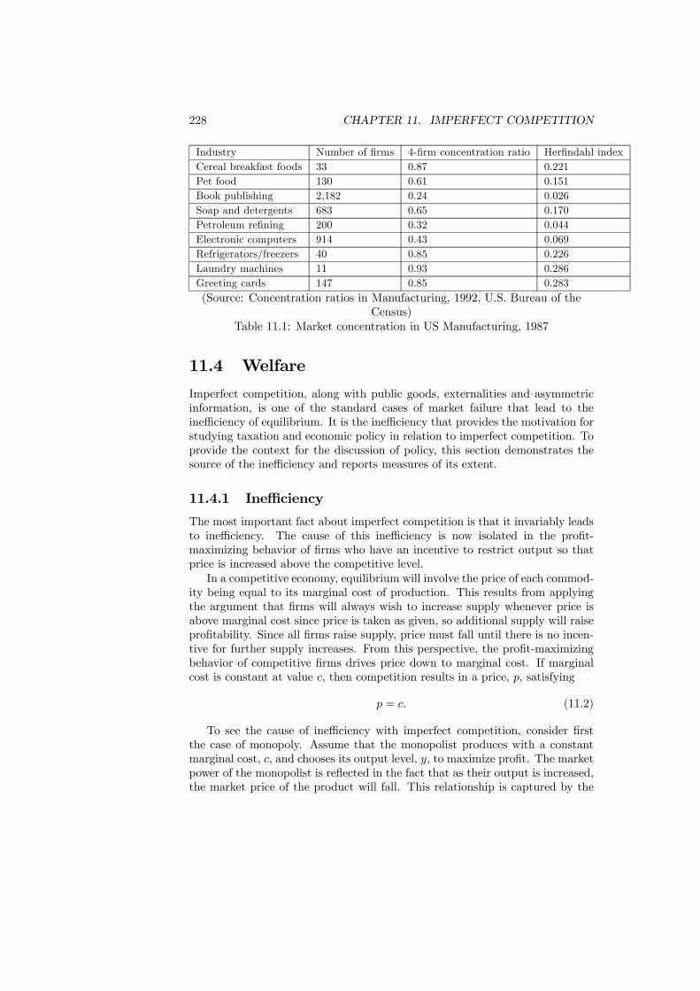
228 CHAPTER 11. IMPERFECT COMPETITION
Industry Number of firms 4-firm concentration ratio Herfindahl indexCereal breakfast foods 33 0.87 0.221Pet food 130 0.61 0.151Book publishing 2,182 0.24 0.026Soap and detergents 683 0.65 0.170Petroleum refining 200 0.32 0.044Electronic computers 914 0.43 0.069Refrigerators/freezers 40 0.85 0.226Laundry machines 11 0.93 0.286Greeting cards 147 0.85 0.283(Source: Concentration ratios in Manufacturing, 1992, U.S. Bureau of the
Census)Table 11.1: Market concentration in US Manufacturing, 1987
11.4 Welfare
Imperfect competition, along with public goods, externalities and asymmetricinformation, is one of the standard cases of market failure that lead to theinefficiency of equilibrium. It is the inefficiency that provides the motivation forstudying taxation and economic policy in relation to imperfect competition. Toprovide the context for the discussion of policy, this section demonstrates thesource of the inefficiency and reports measures of its extent.
11.4.1 Inefficiency
The most important fact about imperfect competition is that it invariably leadsto inefficiency. The cause of this inefficiency is now isolated in the profit-maximizing behavior of firms who have an incentive to restrict output so thatprice is increased above the competitive level.In a competitive economy, equilibrium will involve the price of each commod-
ity being equal to its marginal cost of production. This results from applyingthe argument that firms will always wish to increase supply whenever price isabove marginal cost since price is taken as given, so additional supply will raiseprofitability. Since all firms raise supply, price must fall until there is no incen-tive for further supply increases. From this perspective, the profit-maximizingbehavior of competitive firms drives price down to marginal cost. If marginalcost is constant at value c, then competition results in a price, p, satisfying
p = c. (11.2)
To see the cause of inefficiency with imperfect competition, consider firstthe case of monopoly. Assume that the monopolist produces with a constantmarginal cost, c, and chooses its output level, y, to maximize profit. The marketpower of the monopolist is reflected in the fact that as their output is increased,the market price of the product will fall. This relationship is captured by the
11.4. WELFARE 229
inverse demand function, p (y), which determines price as a function of output.As y increases, p (y) decreases. Using the inverse demand function which themonopolist is assumed to know, the profit level of the firm is
π = [p (y)− c] y. (11.3)
The first-order condition describing the profit-maximizing output level is
p+ ydp
dy− c = 0, (11.4)
which, since dpdy < 0 (price falls as output increases), implies that p > c. The
condition in (11.4) shows that the monopolist will set price above marginal costand that the monopolist’s price does not satisfy the efficiency requirement ofbeing equal to marginal cost. The fact that the monopolist perceives that theiroutput choice affects price, so dp
dy is not zero, results directly in the divergenceof price and marginal cost.The condition describing the choice of output can be re-arranged to provide
further insight into degree of divergence between price and marginal cost. Usingthe elasticity of demand, ε = dy
dppy < 0, the profit-maximization condition can
be written asp− cp
=1
|ε| (11.5)
This equilibrium condition of the monopoly is called the inverse elasticity pricingrule. In words, this condition says that the percentage deviation between theprice and the marginal cost is equal to the inverse elasticity of demand. Theexpression p−c
p is the Lerner index and will be shown shortly to be strictlybetween zero and one (i.e. |ε| > 1). The monopoly pricing rule can also bewritten as
p = µc, (11.6)
where µ = 11− 1
|ε|> 1 is called the monopoly mark-up and measures the extent
to which price is raised above marginal cost. This pricing rule shows that thedeviation of price from marginal cost is inversely related to the absolute valueof the elasticity of demand. The higher is the absolute value of the elasticity,the smaller is the monopoly mark-up.In the extreme case, if demand were perfectly elastic, which equates to the
firm having no market power, then price would be equal to marginal cost. Forthe mark-up µ to be finite, so price is well-defined, it must be the case that|ε| > 1 so the monopolist locates on the elastic part of the demand curve. Ifdemand is inelastic, with |ε| ≤ 1, then the monopolist makes maximum profitby selling the smallest possible quantity at an arbitrarily high price. Since themonopolist operates on the elastic part of the demand curve with |ε| > 1, theLerner index p−c
p = 1|ε| ∈ (0, 1) provides a simple measure of market power
ranging from zero for a perfectly competitive market to one for maximal marketpower. Therefore a firm might have a monopoly but its market power might

230 CHAPTER 11. IMPERFECT COMPETITION
still be low because it is constrained by competition from substitute productsoutside the market. By differentiating its product a monopolist can insulate itsproduct from the competition of substitute products and thereby expands itsmarket power.This relation of the monopoly mark-up to the elasticity of demand can be
easily extended from monopoly to oligopoly. Assume that there are m firms inthe market and denote the output of firm j by yj . The market price of output
is now dependent upon the total output of the firms, y =mPj=1
yj . With output
level yj , the profit level of firm j is
πj = [p− c] yj . (11.7)
Adopting the Cournot assumption that each firms regards its competitors’ out-puts as fixed when it optimizes, the choice of output for firm j satisfies
p+ yjdp
dy− c = 0. (11.8)
Now assume that the firms are identical and each produces the same outputlevel, y
m . The first-order condition for choice of output (11.8) can then be re-arranged to obtain the Lerner index
p− cp
=1
m
1
|ε|and the oligopoly pricing is given by
p = µ◦c,
where µ◦ = mm− 1
|ε|> 1 is the oligopoly mark-up. Thus, in the presence of several
firms on the market, the Lerner index of market power is deflated according tothe market share. As for monopoly, the value of the mark-up is related to theinverse of the elasticity of demand. The Lerner index can be used to show thatan oligopoly becomes more competitive as the number of firms in the industryincreases. This claim follows from the fact thatp−cp must tend to 0 as m tendsto infinity. Hence, as the number of firms increases, the Cournot equilibriumbecomes more competitive and price tends to marginal cost. The limiting po-sition with an infinite number of firms can be viewed as the idealization of thecompetitive model.There is one special case of monopoly for which the equilibrium is efficient.
Let the firm be able to charge each consumer the maximum price that theyare able to pay. To do so obviously requires the firm to have considerableinformation about its customers. The consequence is that the firm extractsall consumer surplus and translates it into profit. It will keep supplying thegood whilst price is above marginal cost, so total supply will be equal to thatunder the competition. This scenario, known as perfect price discrimination,results in all the potential surplus in the market being turned into monopoly
11.4. WELFARE 231
profit. No surplus is lost due to the monopoly, but all surplus is transferredfrom the consumers to the firm. Of course, this scenario can only arise with anexceedingly well-informed monopolist.
11.4.2 Incomplete Information
Monopoly inefficiency can also arise from the firm having incomplete informa-tion, even in situations where there would be efficiency with complete informa-tion. To see this, suppose a monopolist with constant marginal cost c faces abuyer whose willingness to pay for a unit of the firm’s output is v. If there wascomplete information, the firm and buyer would agree a price between c and vand the product would be traded. The surplus from the transaction would beshared between the two.The difference that imperfect competition can make is that trade will some-
times not take place even though both parties would gain if they did trade.Assume now that the monopolist cannot observe v but knows from experiencethat it is drawn from a distribution F (v) which is the probability that thebuyer’s valuation is less or equal to v. The function (1 − F (v)) is analogousto the expected demand when a purchaser buys at most one unit because theprobability that there is a demand at price v is the probability that the buyer’svaluation is higher than the price. Assume that there are potential gains fromtrade so v > c for at least a range of v. Pareto efficiency requires trade to occurif and only if v ≥ c.The monopolist’s problem is to offer a price p that maximizes its expected
profit (anticipating that the buyer will not accept the offer if v < p). This pricemust fall between c and v for trade to occur. The monopolist sets a price p∗ thatsolves
Maxp
[1− F (p)]| {z }prob trade
[p− c]| {z }profit if trade
From the assumption that there is a potential gain from trade, there must bea range of values of v higher than c and thus it is possible for the monopolistto charge a price in excess of the marginal cost with the offer being accepted.Clearly, the price that maximizes expected profit must be p∗ > c, so the standardconclusion of monopoly holds that price is in excess of marginal cost. When tradetakes place (so a value of v occurs with c < p∗ < v), the outcome is an efficienttrade. However, when a value of v occurs with c < v < p∗ trade does not takeplace. This is inefficient since trade should occur because the benefit exceedsthe cost (v > c). The effect of the monopolist setting price above marginal costis to eliminate some of the potential trades.For instance, assume the willingness to pay v is uniformly distributed on
the interval [0, 1] with the marginal cost 0 < c < 1. Then the probability thattrade takes place at price p (expected demand) is 1− F (p) = 1− p which givesexpected revenue [1− F (p)] p = (1 − p)p and marginal revenue MR = 1 − 2p.The expected profit is π = (1 − p)(p − c) and the profit maximizing pricingsatisfies the first-order condition (1 − 2p) + c = 0 which can be re-arranged to
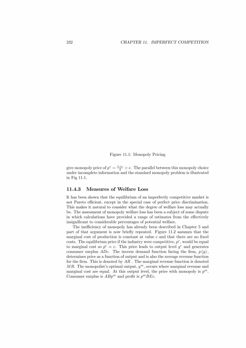
232 CHAPTER 11. IMPERFECT COMPETITION
Figure 11.1: Monopoly Pricing
give monopoly price of p∗ = 1+c2 > c. The parallel between this monopoly choice
under incomplete information and the standard monopoly problem is illustratedin Fig 11.1.
11.4.3 Measures of Welfare Loss
It has been shown that the equilibrium of an imperfectly competitive market isnot Pareto efficient, except in the special case of perfect price discrimination.This makes it natural to consider what the degree of welfare loss may actuallybe. The assessment of monopoly welfare loss has been a subject of some disputein which calculations have provided a range of estimates from the effectivelyinsignificant to considerable percentages of potential welfare.The inefficiency of monopoly has already been described in Chapter 5 and
part of that argument is now briefly repeated. Figure 11.2 assumes that themarginal cost of production is constant at value c and that there are no fixedcosts. The equilibrium price if the industry were competitive, pc, would be equalto marginal cost so pc = c. This price leads to output level yc and generatesconsumer surplus ADc. The inverse demand function facing the firm, p (y) ,determines price as a function of output and is also the average revenue functionfor the firm. This is denoted by AR . The marginal revenue function is denotedMR. The monopolist’s optimal output, ym, occurs where marginal revenue andmarginal cost are equal. At this output level, the price with monopoly is pm.Consumer surplus is ABpm and profit is pmBEc.
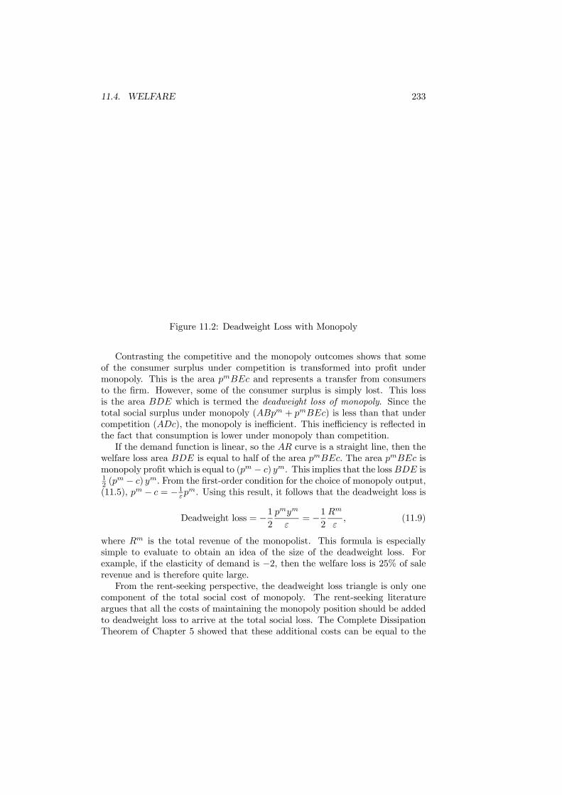
11.4. WELFARE 233
Figure 11.2: Deadweight Loss with Monopoly
Contrasting the competitive and the monopoly outcomes shows that someof the consumer surplus under competition is transformed into profit undermonopoly. This is the area pmBEc and represents a transfer from consumersto the firm. However, some of the consumer surplus is simply lost. This lossis the area BDE which is termed the deadweight loss of monopoly. Since thetotal social surplus under monopoly (ABpm + pmBEc) is less than that undercompetition (ADc), the monopoly is inefficient. This inefficiency is reflected inthe fact that consumption is lower under monopoly than competition.If the demand function is linear, so the AR curve is a straight line, then the
welfare loss area BDE is equal to half of the area pmBEc. The area pmBEc ismonopoly profit which is equal to (pm − c) ym. This implies that the lossBDE is12 (p
m − c) ym. From the first-order condition for the choice of monopoly output,(11.5), pm − c = −1εpm. Using this result, it follows that the deadweight loss is
Deadweight loss = −12
pmym
ε= −1
2
Rm
ε, (11.9)
where Rm is the total revenue of the monopolist. This formula is especiallysimple to evaluate to obtain an idea of the size of the deadweight loss. Forexample, if the elasticity of demand is −2, then the welfare loss is 25% of salerevenue and is therefore quite large.From the rent-seeking perspective, the deadweight loss triangle is only one
component of the total social cost of monopoly. The rent-seeking literatureargues that all the costs of maintaining the monopoly position should be addedto deadweight loss to arrive at the total social loss. The Complete DissipationTheorem of Chapter 5 showed that these additional costs can be equal to the

234 CHAPTER 11. IMPERFECT COMPETITION
value of monopoly profit. The total social loss can therefore be as great as thearea pmBEc+BDE.Numerous studies have been published that provide measures of the degree
of monopoly welfare loss. A selection of these results is given in Table 11.2.The smaller values are obtained by calculating only the deadweight loss tri-angle. If these were correct, then we could conclude that monopoly power isnot a significant economic issue. This was the surprising conclusion of the ini-tial study of Harberger in 1954 which challenged the conventional wisdom thatmonopoly must be damaging to the economy. In contrast, the larger valuesof loss are obtained by following the rent-seeking approach and including theadditional components of welfare loss. These values reveal monopoly loss to bevery substantial.
Author Sector Welfare Loss (%) CommentsHarberger US Manufacturing 0.08Gisser US Manufacturing 0.11 - 1.82 Cournot - price leadershipPeterson and Connor US Food Manufacturing 0.16 - 5.15 Variety of markets structuresMasson and Shaanan 37 US Industries 3 Deadweight loss
16 Including monopoly profitMcCorriston UK Agricultural Inputs 1.6 - 2.5 Deadweight loss
20 - 40 Including monopoly profitCowling and Mueller US 4 - 13 Includes advertising
UK 3.9 - 7.2 Includes advertisingTable 11.2: Monopoly Welfare Loss
It can be appreciated from Table 11.2 that a broad range of estimates ofmonopoly welfare loss have been produced. Some studies conclude welfare lossis insignificant, others conclude that it is very important. What primarily dis-tinguishes these differing estimates is whether it is only the deadweight lossthat is counted, or the deadweight loss plus the cost of rent seeking. Which isone correct is an unresolved issue that involves two competing perspectives oneconomic efficiency.There is one further point that needs to be made. The calculations above
have been based upon a static analysis in which there is a single time period. Thedemand function, the product traded and the costs of production are all given.The firm makes a single choice and then the equilibrium is attained. What thisignores are all the dynamic aspects of economic activity such as investment andinnovation. When these factors are taken into account, as Schumpeter forcefullyargued, it is even possible for monopoly to generate dynamic welfare gains ratherthan losses. This claim is based on the argument that investment and innovationwill only be undertaken if firms can expect to earn a sufficient return. In acompetitive environment, any gains will be competed away so the incentivesare eliminated. Conversely, holding a monopoly position allows gains to berealized. This provides the incentive to undertake investment and innovation.Furthermore, the incentive is strengthened by the intention of maintaining the

11.5. TAX INCIDENCE 235
position of monopoly. The dynamic gains can more than offset the static losses,giving a positive argument for the encouragement of monopoly. We return tothis issue in the discussion of regulation in Section ??.
11.5 Tax Incidence
The study of tax incidence is about determining the changes in prices and profitsthat follow the imposition of a tax. The formal or legal incidence of a tax refersto who is legally responsible for paying the tax. The legal incidence can be verydifferent to the economic incidence which relates to who ultimately has to altertheir behavior because of the tax.To see this distinction, consider the following. A tax of $1 is levied on
a commodity that costs $10 and this tax must be paid by the retailer. Thelegal incidence is simple: for each unit sold the retailer must pay $1 to the taxauthority. The economic incidence is much more complex. The first questionhas to be: what does the price of the commodity become after the tax? It maychange to $11, but this would be an exception rather than the norm. Instead,it may for example rise only to $10.50. If it does, $0.50 of the tax falls upon theconsumer to pay. What of the other $0.50? This depends on how the producerresponds to the tax increase. They may lower the price at which they sell tothe retailer from $9 to $8.75. If they do, then they bear $0.25 of the tax. Theremaining $0.25 of the tax is then paid by the retailer. The economic incidenceof a tax can therefore be very distinct from the legal incidence.This example raises the question of what determines the economic incidence.
The answer to this is found in the demand and supply curves for the good that istaxed. Economic incidence will first be determined for the competitive case andthen it is shown how the conclusions are modified by imperfect competition. Infact, imperfect competition can result in very interesting conclusions concerningtax incidence.Tax incidence analysis is at its simplest when there is competition and the
marginal cost of production is constant. In this case, the supply curve in theabsence of taxation must be horizontal at a level equal to marginal cost; seeFigure 11.3. This gives the pre-tax price p = c. The introduction of a tax ofamount t will raise this curve by exactly the amount of the tax. The post-taxprice, q, is at the intersection of demand and the new supply curve. It can beseen that q = p+ t so price will rise by an amount equal to the tax. Hence thetax is simply passed forward by the firms onto consumers since price is alwaysset equal to tax-inclusive marginal cost.When marginal cost is not constant and the supply curve slopes upward,
the introduction of a tax still shifts the curve vertically upwards by the amountequal to the tax. The extent to which price rises is then determined by theslopes of the supply and demand curve. If the demand curve is vertical, pricerises by the full amount of the tax; otherwise it will rise by less. See Figure11.4.In summary, if the supply curve is horizontal (so supply is infinitely elastic)

236 CHAPTER 11. IMPERFECT COMPETITION
Figure 11.3: Tax Incidence with Perfectly Elastic Supply
Figure 11.4: Tax Incidence in the General Case

11.5. TAX INCIDENCE 237
Figure 11.5: Tax Under-Shifting
or the demand curve is vertical (so demand is completely inelastic), then pricewill rise by exactly the amount of the tax. In all other cases it will rise by less,with the exact rise being determined by the elasticities of supply and demand.When the price increase is equal to the tax, the entire tax burden is passedby the firm onto the consumers. Otherwise the burden of the tax is sharedbetween firms and consumers. Consequently, the extent to which the price isshifted forwards from the producer onto the consumers is dependent upon theelasticities of supply and demand.There are two reasons why tax incidence with imperfect competition is dis-
tinguished from the analysis for the competitive case. Firstly, prices on im-perfectly competitive markets are set at a level above marginal cost. Secondly,imperfectly competitive firms may also earn non-zero profits so taxation canalso affect profit. To trace the effects of taxation it is necessary to work throughthe profit-maximization process of the imperfectly competitive firms. Such anexercise involves characterizing the optimal choices of the firms and then seeinghow they are affected by a change in the tax rate.The incidence of a tax upon output can be demonstrated by returning to the
diagram for monopoly profit maximization. A tax of value t on output changesthe tax-inclusive marginal cost from c to c + t. In Figure 11.5 this is shownto move the intersection between the marginal revenue curve and the marginalcost curve from a to b. Output falls from yo to yt and price rises from p to q.In this case, price rises by less than the tax imposed - the difference between qand p is less than t. This is called the case of tax under-shifting. What it meansis that the monopolist is absorbing some of the tax and not passing it on to theconsumer.
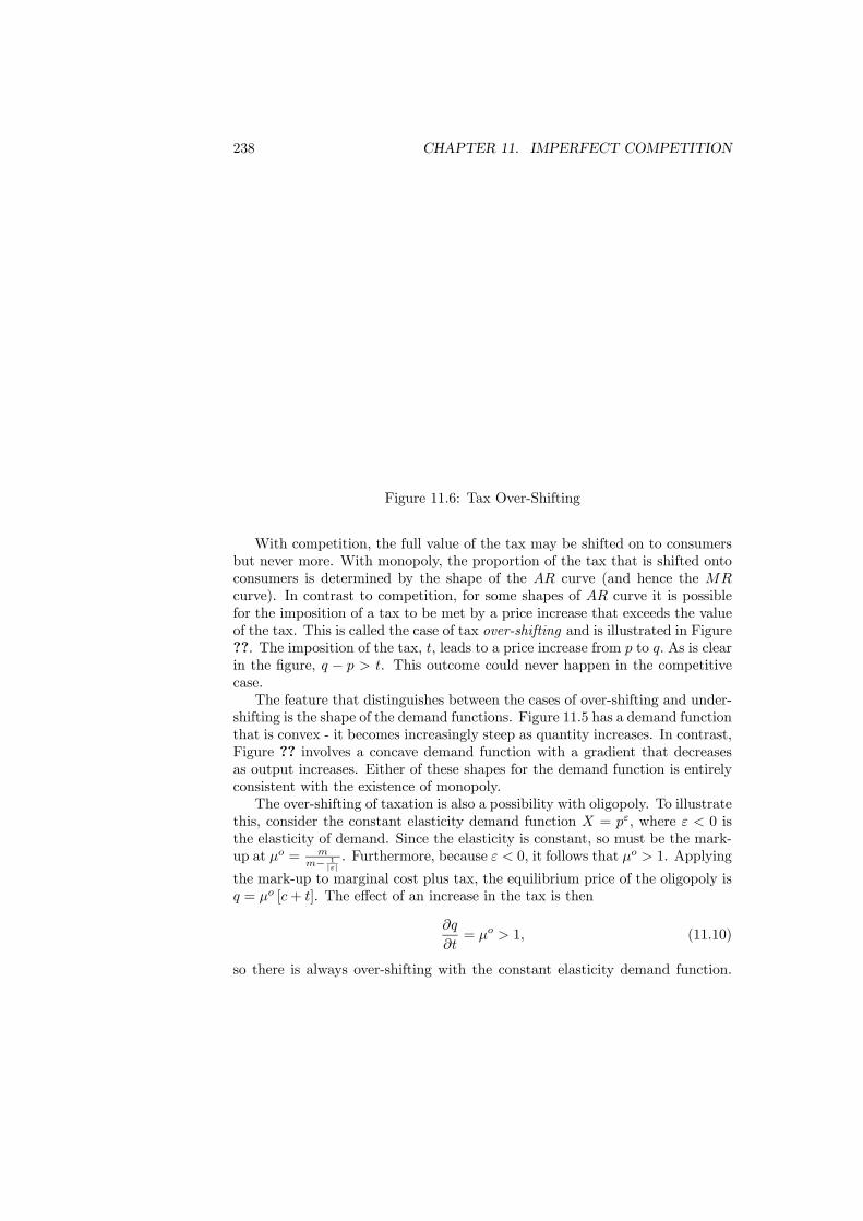
238 CHAPTER 11. IMPERFECT COMPETITION
Figure 11.6: Tax Over-Shifting
With competition, the full value of the tax may be shifted on to consumersbut never more. With monopoly, the proportion of the tax that is shifted ontoconsumers is determined by the shape of the AR curve (and hence the MRcurve). In contrast to competition, for some shapes of AR curve it is possiblefor the imposition of a tax to be met by a price increase that exceeds the valueof the tax. This is called the case of tax over-shifting and is illustrated in Figure??. The imposition of the tax, t, leads to a price increase from p to q. As is clearin the figure, q − p > t. This outcome could never happen in the competitivecase.The feature that distinguishes between the cases of over-shifting and under-
shifting is the shape of the demand functions. Figure 11.5 has a demand functionthat is convex - it becomes increasingly steep as quantity increases. In contrast,Figure ?? involves a concave demand function with a gradient that decreasesas output increases. Either of these shapes for the demand function is entirelyconsistent with the existence of monopoly.The over-shifting of taxation is also a possibility with oligopoly. To illustrate
this, consider the constant elasticity demand function X = pε, where ε < 0 isthe elasticity of demand. Since the elasticity is constant, so must be the mark-up at µo = m
m− 1|ε|. Furthermore, because ε < 0, it follows that µo > 1. Applying
the mark-up to marginal cost plus tax, the equilibrium price of the oligopoly isq = µo [c+ t]. The effect of an increase in the tax is then
∂q
∂t= µo > 1, (11.10)
so there is always over-shifting with the constant elasticity demand function.

11.5. TAX INCIDENCE 239
This holds for any value of m ≥ 1, and hence applies to both monopoly (m = 1)and oligopoly (m ≥ 2). In addition, as m increases and the market becomesmore competitive µo will tend to 1, as will ∂q
∂t , so the competitive outcome ofcomplete tax shifting will arise.Some estimates of the value of the tax-shifting term are given in Table 11.3
for the beer and tobacco industries. Both of these industries have a small numberof dominant firms and an oligopolistic market structure. The figures show thatalthough under-shifting arises in most cases, there is evidence of over-shiftingin the tobacco industry.
Baker and Brechling UK Beer 0.696 UK Tobacco 0.568Delipalla and O’Donnell, Tobacco “Northern” EU 0.92 “Southern” EU 2.16Tasarika, Beer UK 0.665
Table 11.3: Calculations of Tax Shifting
There is an even more surprising effect that can occur with oligopoly: anincrease in taxation can lead to an increase in profit. The analysis of the constantelasticity case can be extended to demonstrate this result. Since the equilibriumprice is q = µo [c+ t] , using the demand function the output of each firm is
x =[µo]
ε[c+ t]
ε
m. (11.11)
Using these values for price and output results in a profit level for each firm of
πi =[µo − 1] [µo]ε [c+ t]ε+1
m. (11.12)
The effect of an increase in the tax upon the level of profit is then given by
∂πi∂t
=[µo − 1] [µo]ε [ε+ 1] [c+ t]ε
m. (11.13)
The possibility of the increase in tax raising profit follows by observing thatif ε > −1, then [ε+ 1] > 0, so ∂πi
∂t > 0. When the elasticity satisfies thisrestriction, an increase in the tax will raise the level of profit. Put simply, thefirms find the addition to their costs to be profitable.It should be observed that such a profit increase cannot occur with monopoly,
because a monopolist must produce on the elastic part of the demand curve withε < −1. With oligopoly, the mark-up remains finite provided m − 1
|ε| > 0 or
ε < − 1m . Therefore profit can be increased by an increase in taxation if there is
oligopoly.The mechanism that makes this outcome possible is shown in Figure 11.7
which displays the determination of the Cournot equilibrium for a duopoly. Thefigure is constructed by first plotting the isoprofit curves. The curves denote setsof output levels for the two firms that give a constant level of profit. The profitof firm 1 is highest on the curves closest to the horizontal axis and it reachesits maximum at the output level, m1, which is the output firm 1 would produce
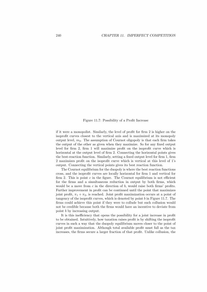
240 CHAPTER 11. IMPERFECT COMPETITION
Figure 11.7: Possibility of a Profit Increase
if it were a monopolist. Similarly, the level of profit for firm 2 is higher on theisoprofit curves closest to the vertical axis and is maximized at its monopolyoutput level, m2. The assumption of Cournot oligopoly is that each firm takesthe output of the other as given when they maximize. So for any fixed outputlevel for firm 2, firm 1 will maximize profit on the isoprofit curve which ishorizontal at the output level of firm 2. Connecting the horizontal points givesthe best-reaction function. Similarly, setting a fixed output level for firm 1, firm2 maximizes profit on the isoprofit curve which is vertical at this level of 1’soutput. Connecting the vertical points gives its best reaction function.The Cournot equilibrium for the duopoly is where the best reaction functions
cross, and the isoprofit curves are locally horizontal for firm 1 and vertical forfirm 2. This is point c in the figure. The Cournot equilibrium is not efficientfor the firms and a simultaneous reduction in output by both firms, whichwould be a move from c in the direction of b, would raise both firms’ profits.Further improvement in profit can be continued until the point that maximizesjoint profit, π1 + π2, is reached. Joint profit maximization occurs at a point oftangency of the isoprofit curves, which is denoted by point b in Figure 11.7. Thefirms could achieve this point if they were to collude but such collusion wouldnot be credible because both the firms would have an incentive to deviate frompoint b by increasing output.It is this inefficiency that opens the possibility for a joint increase in profit
to be obtained. Intuitively, how taxation raises profit is by shifting the isoprofitcurves in such a way that the duopoly equilibrium moves closer to the point ofjoint profit maximization. Although total available profit must fall as the taxincreases, the firms secure a larger fraction of that profit. Unlike collusion, the
11.6. SPECIFIC AND AD VALOREM TAXATION 241
tax is binding on the firms and produces a credible reduction in output.
11.6 Specific and Ad Valorem TaxationThe analysis of tax incidence has so far considered only specific taxation. Withspecific taxation, the legally-responsible firm has to pay a fixed amount of taxfor each unit of output. The amount that has to be paid is independent ofthe price of the commodity. Consequently, the price the consumer pays is theproducer price plus the specific tax. This is not the only way in which taxes canbe levied. Commodities can alternatively be subject to ad valorem taxation,so that the tax payment is defined as a fixed proportion of the producer price.Consequently, as price changes, so does the amount paid in tax.The fact that incidence has been analyzed only for specific taxation in not a
limitation when firms are competitive since the two forms are entirely equivalent.The meaning of equivalence here is that a specific tax and an ad valorem taxthat lead to the same consumer price will raise the same amount of tax revenue.Their economic incidence is therefore identical.This equivalence can be shown as follows. Let t be the specific tax on a
commodity. Then the equivalent ad valorem tax rate τ must satisfy the equation
q = p+ t = [1 + τ ] p. (11.14)
Solving this equation, shows τ = tp is the ad valorem tax rate that leads to the
same consumer price as the specific tax. In terms of the incidence diagrams,both taxes would shift the supply curve for the good in exactly the same way.The demonstration of equivalence is completed by showing that the taxes raiseidentical levels of tax revenue. The revenue raised by the ad valorem tax isR = τpX. Using the fact that τ = t
p , this revenue level can be written astppX = tX, which is the revenue raised by the specific tax. This completes thedemonstration that the specific and ad valorem taxes are equivalent.With imperfect competition this equivalence between the two forms of tax-
ation breaks down: specific and ad valorem taxes that generate the same con-sumer price generate different levels of revenue. The reason for this breakdownof equivalence, and its consequences, are now explored.The fact that specific and ad valorem taxes have different effects can be seen
very easily in the monopoly case. Assume that the firm sells at price q and thateach unit of output is produced at marginal production cost, c. With a specifictax, the consumer price and producer price are related by q = p+ t. This allowsthe profit level with a specific tax to be written as
π = [q − t]x− cx = qx− [c+ t]x. (11.15)
The definition of this profit levels shows that the specific tax acts as an additionto the marginal cost for the firm. Now consider instead the payment of anad valorem tax at rate τ . Since an ad valorem tax is levied as a proportionof the producer price, the consumer price and producer price are related by

242 CHAPTER 11. IMPERFECT COMPETITION
Figure 11.8: Contrasting Taxes
q = [1 + τ ] p; hence the consumers pay price q and the firm receives p = 11+τ q.
The profit level with the ad valorem tax is then
π =1
1 + τqx− cx. (11.16)
The basic difference between the two taxes can be seen by comparing thesealternative specifications of profit. From the perspective of the firm, the specifictax raises marginal production cost from c to c+ t. In contrast, the ad valoremtax reduces the revenue received by the firm from qx to 1
1+τ qx. Hence thespecific tax works via the level of costs whereas the ad valorem tax operates viathe level of revenue. With competition, this difference is of no consequence. Butthe very basis of imperfect competition is that the firms recognize the effect theiractions has upon revenue - so the ad valorem tax interacts with the expressionof monopoly power.The consequence of this difference is illustrated in Figure 11.8. In the left-
hand figure the effect of a specific tax is shown. In the right-hand figure theeffect of an ad valorem tax is shown. The specific tax leads to an upward shiftin the tax-inclusive marginal cost curve. This moves the optimal price from p toq. The ad valorem tax leads to a downward shift in marginal revenue net of taxas shown in Figure 11.8. The ad valorem tax leads from price p in the absenceof taxation to q with taxation. The resulting price increase is dependent on theslope of the marginal revenue curve.What is needed to make a firm comparison between the effects of the tax
is some common benchmark. The benchmark chosen is to choose values of thespecific and ad valorem taxes which lead to the same consumer price and deter-mine which raises the most tax revenue. This comparison is easily conducted
11.7. REGULATION OF MONOPOLY 243
by returning to the definition of profit in (11.16). With the ad valorem tax, theprofit level can be expressed as
π =1
1 + τqx− cx = 1
1 + τ[qx− [c+ τc]x] . (11.17)
The second term of (11.17) shows that the ad valorem tax is equivalent to thecombined use of a specific tax of value τc plus a profits tax at rate 1
1+τ . Sincea profits tax has no effect upon the firm’s choices but does raise revenue, if thefirm is making a positive profit level an ad valorem tax with its rate set so that
τc = t, (11.18)
must lead to the same post-tax price as the specific tax. However, the ad valoremtax must raise more revenue. This is because the component τc collects the samerevenue as the specific tax t but the ad valorem tax also collects revenue fromthe profit-tax component. Hence the ad valorem tax must collect more revenuefor the same consumer price. This result can alternatively be expressed as thefact that for a given level of revenue, an ad valorem tax leads to lower consumerprice than a specific tax.In conclusion, ad valorem taxation is more effective than specific taxation
when there is imperfect competition. The intuition behind this conclusion isthat the ad valorem tax lowers marginal revenue and this reduces the perceivedmarket power of the firm. Consequently, the ad valorem tax has the helpfuleffect of reducing monopoly power, thus offsetting some of the costs involved inraising revenue through commodity taxation.
11.7 Regulation of Monopoly
Up until this point the focus has been placed upon the welfare loss caused byimperfect competition and upon tax incidence. As we have shown, there are twocompeting views about the extent of the welfare loss but even if the lower valuesare accepted, it would still be beneficial to reduce the loss as far as possible.This raises the issue of the range of policies that are available to reduce theadverse effects of monopoly.When faced with imperfect competition, the most natural policy response
is to try to encourage an enhanced degree of competition. There are severalways in which this can be done. The most dramatic example is US anti-trustlegislation which has been used to enforce the division of monopolies into sep-arate competing firms. This policy was applied to the Standard Oil Companywhich was declared a monopoly and broken-up into competing units in 1911.More recently, the Bell System telephone company was broken up in 1984. Thispolicy of breaking-up monopolists represents extreme legislation and, once en-acted, leaves a major problem of how the system should be organized followingthe break-up. Typically the industry will require continuing regulation, a themeto which we return below.

244 CHAPTER 11. IMPERFECT COMPETITION
Less dramatic than directly breaking-up firms is to provides aids to com-petition. A barrier to entry is anything that allows a monopoly to sustain itsposition and prevent new firms from competing effectively. Barriers to entrycan be legal restrictions such as the issue of a single licence permitting onlyone firm to be active. They can also be technological in the sense of superiorknowledge, the holding of patents or the structure of the production function.Furthermore, some barriers can be erected deliberately by the incumbent mo-nopolist specifically to deter entry. For a policy to encourage competition, itmust remove or at least reduce the barriers to entry. The appropriate policyresponse depends upon the nature of the barrierIf a barrier to entry is created by a legal restriction it can equally be removed
by a change to the law. But here it is necessary to enquire as to why therestriction was created initially. One possible answer returns us to the concept ofrent-creation discussed in Chapter 5 where the introduction of a restriction wasseen as a way of generating rent. An interesting example of the creation of suchrestrictions are the activities of MITI (the Ministry of International Trade andIndustries) in Japan. In 1961 MITI produced its “Concentration Plan” whichaimed to concentrate the mass-production automakers into 2 to 3 groups. Theintention behind this was to cope with the international competition that ensuedafter the liberalization of auto imports into Japan and to place the Japanese carindustry in a stronger position for exporting. These intentions were never fullyrealized and the plan was ultimately undermined by developments in the autoindustry, especially the emergence of Honda as a major manufacturer. Despitethis, the example still stands of a good example of a deliberate policy attemptto restrict competition.If barriers to entry relate to technological knowledge, then it is possible for
the government to insist upon the sharing of this knowledge. Both the concernover the bundling of Internet Explorer with Windows in the US and the bundlingof Media Player with Windows in Europe are pertinent examples. In the US theoutcome has been that Microsoft will be obliged to provide rival software firmswith information that allows them to develop competing products, and to ensurethat these products work with the Windows operating system. Microsoft’s rivalsare pushing for a similar solution in the EU. The existence of patents to protectthe use of knowledge is also a barrier to entry. The reasoning behind patentsis that they allow a reward for innovation: new discoveries are only valuable ifthe products in which they are embedded can be exploited without competitorsimmediately copying them. The production of generic drugs is one of the better-known examples of product copying. Without patents, the incentive to innovatewould be much reduced and aggregate welfare would fall. The policy issue thenbecomes the choice of the length of a patent. It must be long enough to allowinnovation to be adequately rewarded but not so long that it stifles competition.Current practice in the US is that the term of a patent is 20 years from the dateat which the application is filed.Barriers to entry can also be erected as a deliberate part of a corporate
strategy designed to deter competitors. Such barriers can be within the law,such as sustained advertising campaigns to build brand loyalty or the building
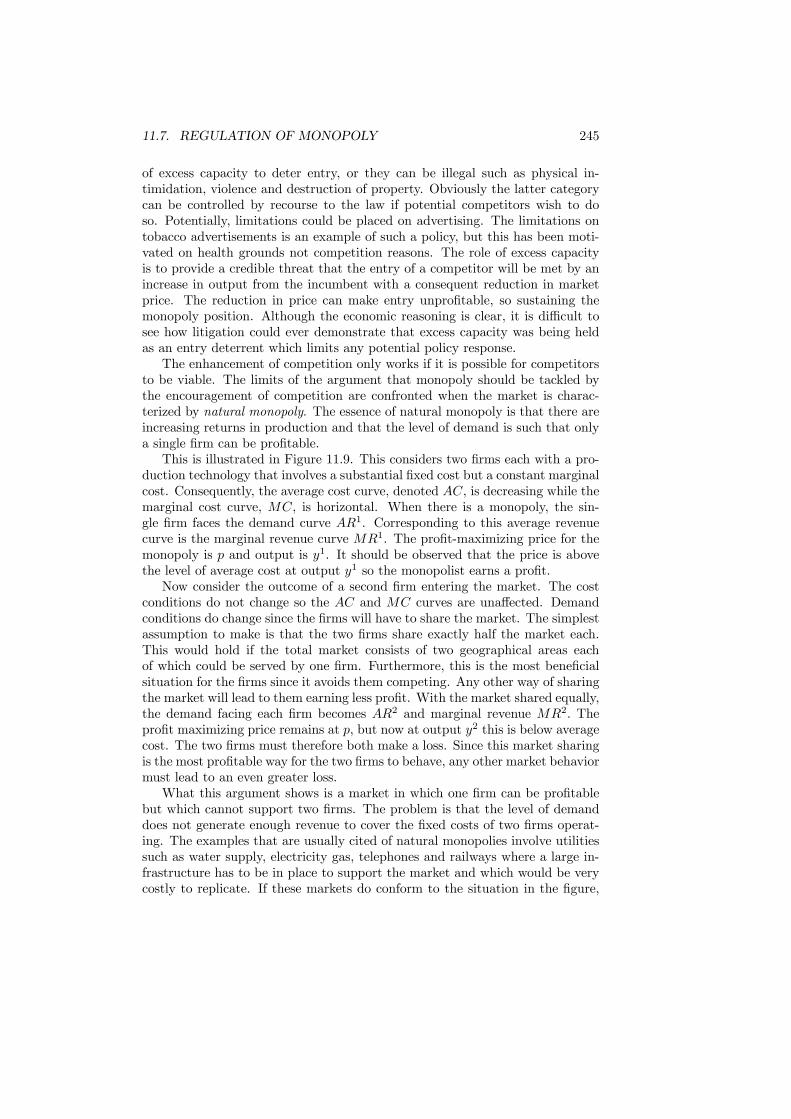
11.7. REGULATION OF MONOPOLY 245
of excess capacity to deter entry, or they can be illegal such as physical in-timidation, violence and destruction of property. Obviously the latter categorycan be controlled by recourse to the law if potential competitors wish to doso. Potentially, limitations could be placed on advertising. The limitations ontobacco advertisements is an example of such a policy, but this has been moti-vated on health grounds not competition reasons. The role of excess capacityis to provide a credible threat that the entry of a competitor will be met by anincrease in output from the incumbent with a consequent reduction in marketprice. The reduction in price can make entry unprofitable, so sustaining themonopoly position. Although the economic reasoning is clear, it is difficult tosee how litigation could ever demonstrate that excess capacity was being heldas an entry deterrent which limits any potential policy response.The enhancement of competition only works if it is possible for competitors
to be viable. The limits of the argument that monopoly should be tackled bythe encouragement of competition are confronted when the market is charac-terized by natural monopoly. The essence of natural monopoly is that there areincreasing returns in production and that the level of demand is such that onlya single firm can be profitable.This is illustrated in Figure 11.9. This considers two firms each with a pro-
duction technology that involves a substantial fixed cost but a constant marginalcost. Consequently, the average cost curve, denoted AC, is decreasing while themarginal cost curve, MC, is horizontal. When there is a monopoly, the sin-gle firm faces the demand curve AR1. Corresponding to this average revenuecurve is the marginal revenue curve MR1. The profit-maximizing price for themonopoly is p and output is y1. It should be observed that the price is abovethe level of average cost at output y1 so the monopolist earns a profit.Now consider the outcome of a second firm entering the market. The cost
conditions do not change so the AC and MC curves are unaffected. Demandconditions do change since the firms will have to share the market. The simplestassumption to make is that the two firms share exactly half the market each.This would hold if the total market consists of two geographical areas eachof which could be served by one firm. Furthermore, this is the most beneficialsituation for the firms since it avoids them competing. Any other way of sharingthe market will lead to them earning less profit. With the market shared equally,the demand facing each firm becomes AR2 and marginal revenue MR2. Theprofit maximizing price remains at p, but now at output y2 this is below averagecost. The two firms must therefore both make a loss. Since this market sharingis the most profitable way for the two firms to behave, any other market behaviormust lead to an even greater loss.What this argument shows is a market in which one firm can be profitable
but which cannot support two firms. The problem is that the level of demanddoes not generate enough revenue to cover the fixed costs of two firms operat-ing. The examples that are usually cited of natural monopolies involve utilitiessuch as water supply, electricity gas, telephones and railways where a large in-frastructure has to be in place to support the market and which would be verycostly to replicate. If these markets do conform to the situation in the figure,
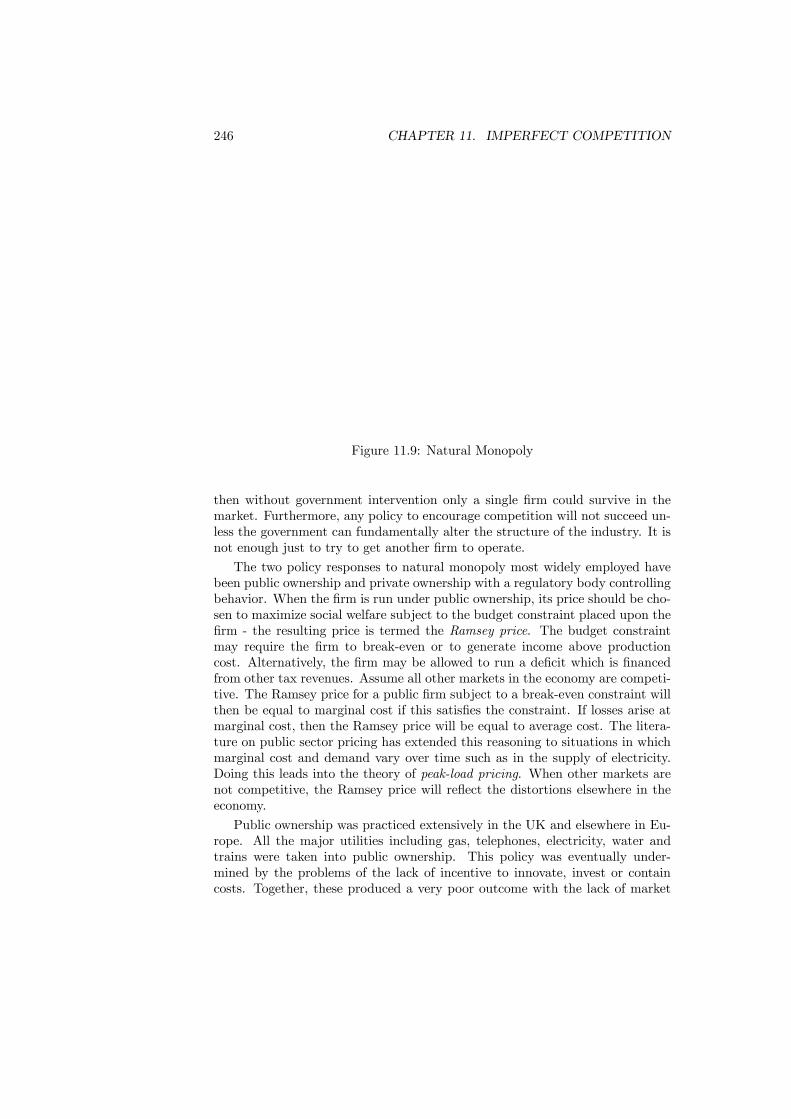
246 CHAPTER 11. IMPERFECT COMPETITION
Figure 11.9: Natural Monopoly
then without government intervention only a single firm could survive in themarket. Furthermore, any policy to encourage competition will not succeed un-less the government can fundamentally alter the structure of the industry. It isnot enough just to try to get another firm to operate.
The two policy responses to natural monopoly most widely employed havebeen public ownership and private ownership with a regulatory body controllingbehavior. When the firm is run under public ownership, its price should be cho-sen to maximize social welfare subject to the budget constraint placed upon thefirm - the resulting price is termed the Ramsey price. The budget constraintmay require the firm to break-even or to generate income above productioncost. Alternatively, the firm may be allowed to run a deficit which is financedfrom other tax revenues. Assume all other markets in the economy are competi-tive. The Ramsey price for a public firm subject to a break-even constraint willthen be equal to marginal cost if this satisfies the constraint. If losses arise atmarginal cost, then the Ramsey price will be equal to average cost. The litera-ture on public sector pricing has extended this reasoning to situations in whichmarginal cost and demand vary over time such as in the supply of electricity.Doing this leads into the theory of peak-load pricing. When other markets arenot competitive, the Ramsey price will reflect the distortions elsewhere in theeconomy.
Public ownership was practiced extensively in the UK and elsewhere in Eu-rope. All the major utilities including gas, telephones, electricity, water andtrains were taken into public ownership. This policy was eventually under-mined by the problems of the lack of incentive to innovate, invest or containcosts. Together, these produced a very poor outcome with the lack of market

11.7. REGULATION OF MONOPOLY 247
forces producing industries that were over-manned and inefficient. As a conse-quence, in the UK all have these industries have now been returned to privatesector.
The treatment of the various industries illustrates different responses to theregulation of natural monopoly. The water industry is broken into regional sup-pliers which do not compete directly but are closely regulated. With telephones,the network is owned by British Telecom but other firms are permitted accessagreements to the network. This can allow them to offer a service without theneed to undertake the capital investment. In the case of the railways, the own-ership of the track, which is the fixed cost, has been separated from the rights tooperate trains, which generates the marginal cost. Both the track owner and thetrain operators remain regulated. With gas and electricity, competing suppliersare permitted to supply using the single existing network.
The most significant difference between public ownership and private own-ership with regulation is that under public ownership the government is as in-formed as the firm about demand and cost conditions. This allows the govern-ment to determine the behavior of the firm using the best available information.Although this information may not be complete, so policy can only maximizethe objective function in an expected sense, the best that is possible will beachieved. In contrast, when the firm is in private ownership, the government,via the regulatory body, may well be far less informed about the operating con-ditions of the firm than the firm itself. Information about cost structures andmarket conditions are likely to remain private and the firm may have strategicreasons for not revealing this accurately.
As an alternative to public ownership, a firm may remain under private own-ership but be made subject to the control of a regulatory body. This introducespossible asymmetries in information between the firm and the regulator. Facedwith limited information, one approach considered in the theoretical literatureis for the regulator to design an incentive mechanism that achieves a desirableoutcome. An example of such a regulatory scheme is the two-part tariff in whichthe payment for a commodity involves a fixed fee to permit consumption fol-lowed by a price per unit of consumption, with these values being set by theregulator. Alternatively, the regulator may impose a constraint on some ob-servable measure of the firm’s activities such as that it must not exceed a givenrate of return upon the capital employed. Even more simple are the regulatoryschemes in the UK which involve restricting prices to rise at a slower rate thanan index of the general price level.
The analysis has looked at a range of issues concerned with dealing withmonopoly power and how to regulate industries. The essence of policy is tomove the economy closer to the competitive outcome but there can be distinctproblems in achieving this. Monopoly can arise because of the combination ofcost and demand conditions and this can place limitations on what policies arefeasible. Natural monopoly results in the need for regulation.
248 CHAPTER 11. IMPERFECT COMPETITION
11.8 Regulation of Oligopoly
11.8.1 Detecting Collusion
In oligopolistic markets firms can collectively act as a monopolist and are con-sequently able to increase their prices. The problem for a regulatory agency isthat such collusion is often tacit and so difficult to detect. However, from an eco-nomic viewpoint, there is no real competition and a high price is the prima facieevidence of collusion. The practical question for the regulator is whether a highprice is the natural outcome of competition in a market in which there is sig-nificant product differentiation (and so little pricing constraint from substituteproducts) or whether it reflects price collusion.Nevo (2001) studied this question for the Breakfast Cereal industry in which
the four leaders Kellogg, Quaker, General Mills and Post were accused by Con-gressman Schumer (March 1995) of charging “caviar prices for corn flakes qual-ity”. After estimating price elasticities of demand for each brand of cereal, Nevoused these price elasticities to calculate the Lerner index for each brand, p−cp ,that would prevail in the industry if producers were colluding and acting as amonopolist. Nevo then calculated the Lerner index of each brand if producerswere really competing with each other.Given the estimated demand elasticities, Nevo found that with collusion the
Lerner index of each brand would be on average around 65 to 75 percent. Whenfirms are competing, the Lerner index would be on average around 40 to 44percent. The next step was to compare these estimations of the Lerner index forthe hypothetical collusive and competing industry with the actual Lerner indexfor the Breakfast Cereal industry to see which hypothesis is the most likely.According to Nevo, the actual Lerner index for the Breakfast Cereal market wasabout 45 percent in 1995. This market power index is far below the 65-75 percenthypothetical Lerner index that would prevail in a colluding industry and muchcloser to the Lerner index in the competing hypothesis. Nevo concludes thatmarket power is significant in this industry not because of collusion, but becauseof product differentiation that limits competition from substitute products (afterall, what is the substitute for a “healthy” cereal breakfast?).
11.8.2 Merger Policy
In its recent reform of Merger Regulation, the European Commission has recog-nized that, in oligopolistic markets, a merger may harm competition and con-sequently increase prices. Under the original European Commission MergerRegulation (ECMR) a merger was incompatible with the common market ifand only if it “creates or strengthens a dominant position as a result of whichcompetition would be significantly impeded”. The problem with this two-partcumulative test was that unless a merger was likely to create or strengthen adominant position, the question of whether it could lessen competition did notarise and so could not be used to challenge a merger. However one can easilythink of oligopoly situations where a merger would substantially lessen com-
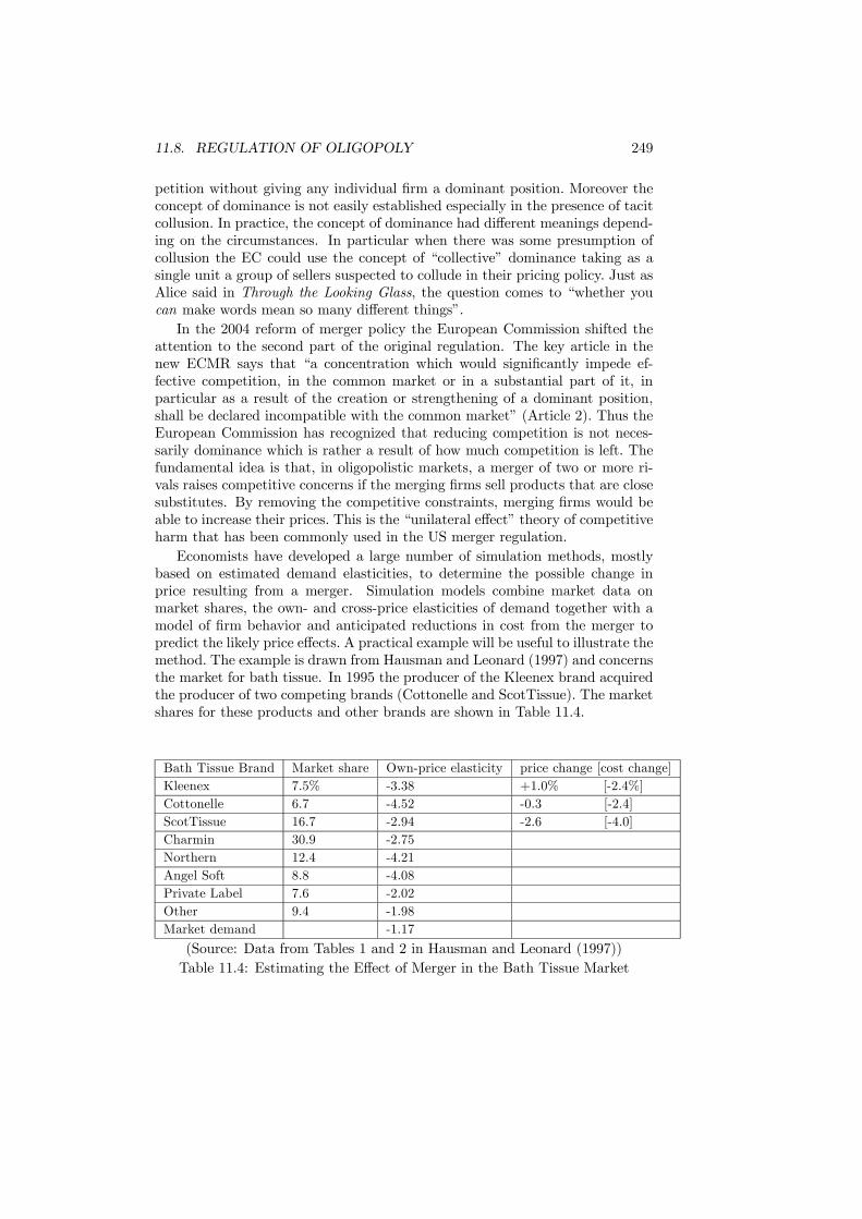
11.8. REGULATION OF OLIGOPOLY 249
petition without giving any individual firm a dominant position. Moreover theconcept of dominance is not easily established especially in the presence of tacitcollusion. In practice, the concept of dominance had different meanings depend-ing on the circumstances. In particular when there was some presumption ofcollusion the EC could use the concept of “collective” dominance taking as asingle unit a group of sellers suspected to collude in their pricing policy. Just asAlice said in Through the Looking Glass, the question comes to “whether youcan make words mean so many different things”.In the 2004 reform of merger policy the European Commission shifted the
attention to the second part of the original regulation. The key article in thenew ECMR says that “a concentration which would significantly impede ef-fective competition, in the common market or in a substantial part of it, inparticular as a result of the creation or strengthening of a dominant position,shall be declared incompatible with the common market” (Article 2). Thus theEuropean Commission has recognized that reducing competition is not neces-sarily dominance which is rather a result of how much competition is left. Thefundamental idea is that, in oligopolistic markets, a merger of two or more ri-vals raises competitive concerns if the merging firms sell products that are closesubstitutes. By removing the competitive constraints, merging firms would beable to increase their prices. This is the “unilateral effect” theory of competitiveharm that has been commonly used in the US merger regulation.Economists have developed a large number of simulation methods, mostly
based on estimated demand elasticities, to determine the possible change inprice resulting from a merger. Simulation models combine market data onmarket shares, the own- and cross-price elasticities of demand together with amodel of firm behavior and anticipated reductions in cost from the merger topredict the likely price effects. A practical example will be useful to illustrate themethod. The example is drawn from Hausman and Leonard (1997) and concernsthe market for bath tissue. In 1995 the producer of the Kleenex brand acquiredthe producer of two competing brands (Cottonelle and ScotTissue). The marketshares for these products and other brands are shown in Table 11.4.
Bath Tissue Brand Market share Own-price elasticity price change [cost change]Kleenex 7.5% -3.38 +1.0% [-2.4%]Cottonelle 6.7 -4.52 -0.3 [-2.4]ScotTissue 16.7 -2.94 -2.6 [-4.0]Charmin 30.9 -2.75Northern 12.4 -4.21Angel Soft 8.8 -4.08Private Label 7.6 -2.02Other 9.4 -1.98Market demand -1.17
(Source: Data from Tables 1 and 2 in Hausman and Leonard (1997))Table 11.4: Estimating the Effect of Merger in the Bath Tissue Market
250 CHAPTER 11. IMPERFECT COMPETITION
Using weekly retail scanner data that tracks household purchases in retailstores in major US cities, it was possible to estimate own-price elasticities asshown in Table 11.4. The key cross-price elasticities were estimated to be 0.19(Kleenex relative to Cotonelle); 0.18 (Kleenex relative to ScotTissue); 0.14 (Cot-tonelle relative to Kleenex); and 0.06 (ScotTissue relative to Kleenex). In ad-dition, it was anticipated that the acquisition would reduce the marginal costof production for ScotTissue, Cottonelle, and Kleenex by 4 percent, 2.4 per-cent and 2.4 percent respectively. With these estimates of demand elasticities,information about market shares and the anticipated cost saving from the ac-quisition of Cottonelle and ScotTissue by the Kleenex brand, it was possible toevaluate the price effects of the merger. A simulation model based on these mar-ket estimations and other assumptions about firm and market behavior (Nashequilibrium and constant marginal costs) produced the following prices changes.The acquisition would lead to a reduction in the price of ScotTissue and Cot-tonelle by 2.6 percent and 0.3 percent, respectively, and an increase in the priceof Kleenex by 1.0 percent. Not surprisingly the Antitrust did not challenge themerger.
11.9 Unions and Taxation
As well as monopoly on product markets, it is possible to have unions creatingmarket power for their members on input markets. By organizing labor intoa single collective organization, unions are able to raise the wage above thecompetitive level and generate a surplus for their members. The issue of taxincidence is also of interest when there are unions since they can employ theirmarket power to reduce the effect of a tax on the welfare of members.The role of trade unions is to ensure that they secure the best deal possible
for their members. In achieving this, the union faces a trade-off between thewage rate and the level of employment since a higher wage will invariably lead tolower employment. This trade-off has to be resolved by the union’s preferences.A standard way of representing the preferences of a union is to assume that
it has a fixed number, m, of members. Each employed member receives a wagew [1− t] , where t is the tax on wage income. The unemployed members receiveb, which can represent either unemployment benefit or the payment in a non-unionized occupation. The level of employment is determined by a labor demandfunction n (w), with higher values of w leading to lower values of employment.If the wage rate is w, the probability of any particular member being employedand receiving w [1− t] is n(w)
m . Consequently, if all members are assumed tohave the same preferences, the expected utility of a typical union member is
U =n (w)
mu (w [1− t]) + m− n (w)
mu (b) . (11.19)
Since all union members have identical preferences, this utility function can alsobe taken to represent the preferences of the union.

11.10. MONOPSONY 251
The union chooses the wage rate to maximize utility, so that the chosen wagesatisfies the first-order condition
n0 (w) [u (w [1− t])− u (b)] + n (w) [1− t]u0 (w [1− t]) = 0. (11.20)
The interpretation of this condition is that the optimal wage rate balances themarginal utility of a higher wage against the value of the marginal loss of em-ployment. Now define the elasticity of labor demand by εn = ∆n
∆wwn < 0 and the
elasticity of utility by εu = ∆u∆w[1−t]
w[1−t]u > 0. The first-order condition (11.20)
can then be written asu (w [1− t]) = µuu (b) , (11.21)
where µu = 11− εu
|εn|> 1 is the union mark-up relating the utility of an employed
member to that of an unemployed member. This mark-up is a measure of theunions market power. Given a value for the utility elasticity, εu, the mark-upincreases the lower is the elasticity of labor demand εn. At the other extreme aslabor demand becomes perfectly elastic, as it does if the labor market is perfectlycompetitive, then µu tends to 1 and the union can achieve no advantage for itsmembers.The incidence of taxation can now be determined. To simplify, assume that
the two elasticities - and hence the mark-up - are constant. Then the utility ofthe post-tax wage must always bear the same relation to the utility of unem-ployment benefit. Consequently, w [1− t] must be constant whatever the taxrate. This can only be achieved if the union negates any tax increase by securingan increase in the wage rate that exactly offsets the tax change. Consequently,those who retain employment are left unaffected by the tax change but, sincethe wage has risen, employment must fall. Overall, the union members must beworse-off. This argument can easily be extended to see that if the elasticities arenot constant there is the potential for over-shifting of the tax, or under-shifting,of any tax increase. In this respect, tax incidence with trade unions has verysimilar features to incidence with monopoly.
11.10 Monopsony
A monopsony market is a market consisting of a single buyer who can purchasefrom many sellers. The single buyer (or monopsonist) could be a firm thatconstitutes the only potential buyer of an input. It could also be an individualor public organization that is the only buyer of a product. For example, inmany countries the government is the monopsonist in the teaching and nursingmarkets. In local markets with only one large employer, the local employermight literally be the only employment option in the local community (e.g., acoal mine, supermarket, government agency ...) so it might make sense thatthe local employer would act as a monopsonist in reducing the wage below thecompetitive level. In larger markets with more than one employer, employersassociation often have opportunities to coordinate their wage offers. This wage

252 CHAPTER 11. IMPERFECT COMPETITION
coordination allows employers to act as a “demand” cartel in the labour marketand thus replicate the monopsony outcome.
Just as monopoly results in supply reduction with a price or wage abovecompetitive levels, monopsony will result in demand reduction with price orwage below competitive levels.
In a perfectly competitive market in which many firms purchase labor ser-vices, each firm takes the price of labor as given. Each firm maximizes its profitsby choosing the employment level that equates the marginal revenue productof labor with the wage rate. In contrast, in a monopsony labor market, themonopsony firm pays a wage below the competitive wage. The result is a short-age of employment relative to the competitive level. The idea is that since themarginal revenue product from additional employment exceeds the wage costin a monopsony labour market, the monopsonist employer might want to hiremore people at the prevailing wage. However, it would not want to increase thewage to attract more workers because the gain from hiring additional workers(the marginal revenue product) is outweighed by the higher wage bill it wouldface for its existing workforce.
Figure 11.10 shows the equilibrium in a monopsony labor market. The com-petitive equilibrium occurs at a market clearing wage wc, where the labor supplycurve intersects the demand curve. Suppose now there is a single buyer on thislabor market. The marginal revenue of labor is the additional revenue that thefirm gets when it employs an additional unit of labor. Suppose that the firm’soutput as a function of its labor use is Q(L) and that the firm is a price taker onthe output market so its output price p is independent of the amount of outputQ. Then the marginal revenue of labor is MRL = p
∆Q∆L which is decreasing due
to decreasing returns to labor. This marginal revenue is depicted in Figure 11.10as the downward sloping labor demand curve. The supply of labor is describedby the “inverse” supply curve. The inverse supply curve w(L) describes thewage required to induce any given quantity of labor to be supplied. Since thesupply curve is upward sloping ∆w∆L > 0. The total labor cost of the monop-sonist is Lw(L) and the marginal cost of labor is the extra cost that comesfrom hiring one more worker MCL = w+ L∆w∆L . This additional cost can bedecomposed into two parts; the cost from employing more workers at the exist-ing wage (w) and the cost from raising the wage for all workers (L∆w∆L ). Since∆w∆L > 0, the marginal labor cost curve lies everywhere above the labor sup-ply curve, as indicated on Figure 11.10. The monopsonist will maximize profitπ = pQ(L)−w(L)L at the point at which marginal revenue of labor is equal tomarginal cost p∆Q∆L = w + L∆w∆LThe choice that gives maximum profit occurs in Figure 11.10 at the inter-
section between the marginal cost curve and the labor demand curve yieldingemployment level Lm and wage rate wm. Therefore in a monopsony labor mar-ket the monopsony firm pays a wage that is less than the competitive wage withemployment level below the competitive level. The monopsony equilibrium con-dition can also be expressed as an inverse elasticity pricing rule. Indeed, theelasticity of labor supply is εL = ∆L
∆wwL and the profit maximization condition
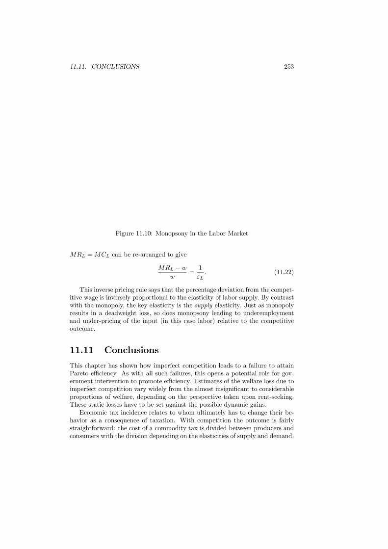
11.11. CONCLUSIONS 253
Figure 11.10: Monopsony in the Labor Market
MRL =MCL can be re-arranged to give
MRL − ww
=1
εL. (11.22)
This inverse pricing rule says that the percentage deviation from the compet-itive wage is inversely proportional to the elasticity of labor supply. By contrastwith the monopoly, the key elasticity is the supply elasticity. Just as monopolyresults in a deadweight loss, so does monopsony leading to underemploymentand under-pricing of the input (in this case labor) relative to the competitiveoutcome.
11.11 Conclusions
This chapter has shown how imperfect competition leads to a failure to attainPareto efficiency. As with all such failures, this opens a potential role for gov-ernment intervention to promote efficiency. Estimates of the welfare loss due toimperfect competition vary widely from the almost insignificant to considerableproportions of welfare, depending on the perspective taken upon rent-seeking.These static losses have to be set against the possible dynamic gains.Economic tax incidence relates to whom ultimately has to change their be-
havior as a consequence of taxation. With competition the outcome is fairlystraightforward: the cost of a commodity tax is divided between producers andconsumers with the division depending on the elasticities of supply and demand.

254 CHAPTER 11. IMPERFECT COMPETITION
Imperfect competition introduces two additional factors. Taxes may be over-shifted so that price rises by more than the value of the tax. In addition, anincrease in taxation may even raise the profits of firms. In contrast to the com-petitive case, specific and ad valorem taxation are not equivalent with imperfectcompetition. In a choice between the instruments, ad valorem taxation is moreeffective since it has the effect of reducing perceived monopoly power.To reduce the welfare loss, policy should attempt to encourage competition.
In some circumstances this can work, but when there is natural monopoly thispolicy has to be carefully considered. A natural monopoly could be taken intopublic ownership or run as a private firm with regulation. Recent policy hasconcentrated upon the latter.
Further readingThe measurement of welfare loss began withHarberger, A.C. (1954) “Monopoly and resource allocation“, American Eco-
nomic Review, 45, 77 - 87.The other values in Table 11.1 are taken fromCowling, K.G. and D.C. Mueller (1978) “The social costs of monopoly power“,
Economic Journal, 88, 727 - 748.Gisser, M. (1986) ”Price leadership and welfare losses in U.S. manufactur-
ing”, American Economic Review, 76, 756 - 767.Masson, R.T. and J. Shaanan (1984) ”Social costs of oligopoly and the value
of competition”, Economic Journal, 94, 520 - 535.McCorriston, S. (1993) ”The welfare implications of oligopoly in agricultural
input markets”, European Review of Agricultural Economics, 20, 1 - 17.Peterson. E.B. and J.M. Connor (1995) ”A comparison of oligopoly welfare
loss estimates for U.S. food manufacturing”, American Journal of AgriculturalEconomics, 77, 300 - 308.The basics of oligopoly theory are covered in:Waterson, M. (1983) Oligopoly Theory (Cambridge: Cambridge University
Press).The analysis of tax incidence with oligopoly can be traced back to:Seade, J. (1985) “Profitable cost increases“, Warwick Economic Research
Paper, No. 260.The results in Table 11.3 are compiled from:Baker, P. and V. Brechling (1992) ”The impact of excise duty changes on
retail prices in the UK”, Fiscal Studies, 13, 48 - 65.Delipalla, S. and O. O’Connell (2001) ”Estimating tax incidence, market
power and market conduct: the European cigarette industry”, InternationalJournal of Industrial Organization, 19, 885 - 908.Tasarika, E. (2001) Aspects of International Taxation (PhD. dissertation,
University of Exeter)Results on comparison of specific and ad valorem tax are in:Delipalla, S. and M. Keen (1992) “The comparison between ad valorem and
specific taxation under imperfect competition“, Journal of Public Economics,49, 351 - 367.

11.11. CONCLUSIONS 255
Myles, G.D. (1996) ”Imperfect competition and the optimal combination ofad valorem and specific taxation”, International Tax and Public Finance, 3, 29- 44.The example on detecting collusion is drawn fromNevo, A. (2001) ”Measuring market power in the ready-to-eat breakfast
cereal industry” Econometrica, 69, 307 - 342.The merger simulation model for bath tissue is drawn fromHausman J. A. and G. K. Leonard (1997) ”Economic analysis of differen-
tiated product mergers using real world data”, George Mason Law Review, 5,321 - 346.A further discussion of merger simulation analysis can be found inEpstein R.J. and D.L. Rubinstein (2002), ”Merger simulation: a simplified
approach with new applications”, Antitrust Law Journal, 69, 883 - 919.A presentation of the various concepts of competition is inVickers, J. (1995), ”Concepts of competition”, Oxford Economic Papers, 47,
1-23.A good perspective on the inefficiency resulting from market power with
special attention on information problem isVickers, J. (1996), ”Market power and inefficiency: a contract perspective”,
Oxford Review of Economic Policy, 12, 11 - 26The basic and first paper on product differentiation isHotelling, H., (1929) ”Stability in competition”, Economic Journal, 39, 41
- 47and the other classic paper isd’Aspremont, C., J. Gabszewicz, and J.-F. Thisse (1979) ”On Hotelling’s
stability in competition”, Econometrica, 17, 1145 - 1151The economic analysis of regulation policies with special attention to the
UK isArmstrong, M., S. Cowans and J. Vickers (1994) Regulatory Reform: Eco-
nomic Analysis and British Experience (Cambridge: MIT Press)Recent European merger regulation guidelines (28 January 2004) are avail-
able at http://europa.eu.int/comm/competition/mergers/review

256 CHAPTER 11. IMPERFECT COMPETITION

Chapter 12
Asymmetric Information
12.1 Introduction
A key feature of the real world is asymmetric information. Most people wantto find the right partner, who is caring, kind, healthy, intelligent, attractive,trustworthy and so on. While attractiveness may be easily verified at a glance,many other traits people seek in a partner are difficult to observe, and peopleusually rely on behavioral signals that convey partial information. There may begood reasons to avoid a potential mate who is too eager to start a relationshipwith you, as this may suggest unfavorable traits. Similarly, it is hard not toinfer that people who participate in dating services must be on average lessworth meeting, and the consensus appears to be that these services are a badinvestment. The reason is that the decision to resort to a dating agency identifiespeople who have trouble initiating their own relationships, which is indicativeof other unwelcome traits.In economics asymmetric information arises when the two sides of the mar-
ket have different information about the goods and services being traded. Inparticular, sellers typically know more about what they are selling than buyersdo. This can lead to adverse selection where bad-quality goods drive out good-quality goods, at least if other actions are not taken. Adverse selection is theprocess by which buyers or sellers with “unfavorable” traits are more likely toparticipate in the exchange. Adverse selection is important in economics be-cause it often eliminates exchange possibilities that would be beneficial to bothconsumers and sellers alike. There might seem some easy way to resolve theproblem of information asymmetry: let everyone tells what he knows. Unfortu-nately, individuals do not necessarily have the incentive to tell the truth (thinkabout the mating example or the market identification of high- and low-abilitypeople).Information imperfections are pervasive in the economy and in some sense
it is an essential feature of a market economy that different people know differ-ent things. While such information asymmetries inevitably arise, the extent to
257

258 CHAPTER 12. ASYMMETRIC INFORMATION
which they do so and their consequences depend on how the market is organized,and the anticipation that they will arise affects market behavior. In this chapterwe discuss the ways by which information asymmetries affect the market func-tioning and how they can be partially overcome though policy intervention. Wedo not consider how the agents can create information problems, for examplein an attempt to exploit market power by differentiating products or by tak-ing actions to increase information asymmetries as in the general governanceproblem.One fundamental lesson of information imperfections is that actions convey
information. This is a commonplace observation in life but it took some timefor economists to fully appreciate its profound effects on how markets function.Many examples can be given. A willingness to purchase insurance at a givenprice conveys information to an insurance company, because those most likelyto decide the insurance is not worthwhile are those who are least likely to havean accident. The quality of a guarantee offered by a firm conveys informationabout the quality of its products as only firms with reliable products are willingto offer a good guarantee. The years of schooling may also convey informationabout the ability of an individual. More able people may go to school longer andthe higher wage associated with more schooling may simply reflect the sortingthat occurs rather than the ability-augmenting effect of schooling itself. Thewillingness of an investor to self-finance a large fraction of the cost of a projectconveys information about his belief in the project. The size of deductibles andco-payments that an individual chooses in an insurance contract may conveyinformation that he is less risk prone. The process by which individuals revealinformation about themselves through the choices that they make is called self-selection.Upon recognizing that actions convey information, two important results
follow. First, when making decisions, agents will not only think about whatthey prefer, but they will also think about how their choice will affect others’beliefs about them. So, I may choose longer schooling not because I value whatis being taught, but because it changes others’ beliefs concerning my ability.Secondly, it may be possible to design a set of choices which would induce thosewith different characteristics to effectively reveal their characteristics throughtheir choices. As long as some actions are more costly for some types thanothers, it is an easy matter to construct choices which separate individuals intoclasses: self-selection mechanisms could, and would, be employed to screen. Forexample, insurance companies may offer a menu of transaction terms that willseparate out different classes of risk into preferring different parts of the menu.In equilibrium both sides of the market are aware of the informational conse-
quences of their actions. In the case where the insurance company or employertakes the initiatives, self-selection is the main screening device. In the casewhere the insured, or the employee, takes the initiative to identify himself as abetter type, then it is usually considered as signalling device. So the differencesbetween screening and signalling lies in whether the informed or uninformedside of the market moves first.Whatever the actions taken, the theory predicts that the types of transac-

12.1. INTRODUCTION 259
tions that will arise in practice will be different from those that would emerge ina perfect-information context. The fact that actions convey information affectsequilibrium outcomes in a profound way. Since quality increases with price inadverse selection models, it may be profitable to pay a price in excess of themarket clearing price. In credit market the supply of loans may be rationed. Inthe labor market, the wage rate may be higher than the market clearing wage,leading to unemployment. There may exist multiple equilibria. Two forms ofequilibria are possible: pooling equilibria in which the market cannot distinguishamong the types, and separating equilibria in which the different types separateout by taking different actions. On the other hand, under plausible conditions,equilibrium might not exist (in particular if the cost of separation is to great).
Another set of issues arise when actions are not easily observable. An em-ployer would like to know how hard his employee is working; a lender wouldlike to know the actions which borrower undertake that might affect the chanceof reimbursement. These asymmetries of information about actions are as im-portant as the situations of hidden knowledge. They lead to what is referred toas the moral hazard problem. This term originates from the insurance industrywhich recognized early that more insurance reduces precaution from insured(and not taking appropriate risk was viewed to be immoral, hence the name).One way to solve this problem is to try to induce desired behavior through thesetting of contract terms. Borrower’s risk taking behavior may be controlled bythe interest rate charged by the lender. The insured can exert more care whenfacing contracts with large deductibles. But in competing for risk averse cus-tomers, the insurance companies face an interesting trade-off. The insurance hasto be complete enough so that the individual will buy insurance. At the sametime, deductibles have to be significant enough to provide adequate incentivesfor insured parties to take care.
This chapter will explore the consequences of asymmetric information in anumber of different market situations. It will describe the inefficiencies thatarise and discuss possible government intervention to correct these. Interpretedin this way, asymmetric information is one of the classic reasons for marketfailure and will prevent trading partners from realizing all the gains of trade.In addition to asymmetric information between trading parties, it can also arisebetween the government and the consumers and firms in the economy. When itdoes, it restricts the policies that the government can implement. Some aspectsof how this affects the effectiveness of the government will be covered in thischapter, others will become apparent in later chapters. The main implicationthat will emerge for public intervention is that even if the government too facesinformational imperfections, the incentives and constraints facing governmentdiffer from those facing the private sector. Even when government faces exactlythe same informational problems, welfare could be improved by market inter-vention. There are interventions in the market that could make all parties betteroff.
260 CHAPTER 12. ASYMMETRIC INFORMATION
12.2 Hidden Knowledge and Hidden Action
There are two basic forms of asymmetric information that can be distinguished.Hidden knowledge refers to a situation in which one party has more informationthan the other party on the quality (or “type”) of a traded good or contractvariable. Hidden action is when one party can affect the “quality” of a tradedgood or contract variable by some action and this action cannot be observed bythe other party.Examples of hidden knowledge abound. Workers know more about their
own abilities than the firm does; doctors know more about their own skills,the efficacy of drugs and what treatment the patients need than do either thepatients themselves or the insurance companies; the person buying life insuranceknows more about his health and life expectancy, than the insurance firm; whenan automobile insurance company insures an individual, the individual mayknow more than the company about her inherent driving skill and hence abouther probability of having an accident; the owner of a car kbnows more aboutthe quality of the car than potential buyers; the owner of a firm knows moreabout the firm than a potential investor; the borrower knows more about theriskiness of his project than the lender does; and not least, in the policy world,the policymakers know more about their competence than the electorate.Hidden knowledge leads to the adverse selection problem. To introduce this,
suppose a firm knows that there are high productivity and low productivityworkers and that it offers a high wage with the intention of attracting high-productivity workers. Naturally, this high wage will also prove attractive to low-productivity workers so the firm will attract a combination of both types. If thewage is above the average productivity, the firm will make a loss and be forced tolower the wage. This will result in high-productivity workers leaving and averageproductivity falling. Consequently, the wage must again be lowered. Eventually,the firm will be left with only low-productivity workers. The adverse selectionproblem is that the high wage attracts the workers the firm wants (the highproductivity) and the ones it does not (the low productivity). The observationthat the firm will eventually be left with only lowproductivity workers reflectsthe old maxim that “The bad drives out the good”.There are also plenty of examples of hidden action. The manager of a firm
does not seek to maximize the return for shareholders but instead trades offher remuneration for less work effort, when it does not simply divert someprofit. Firms may find most profitable to make unsafe products when quality isnot easily observed. Employers also want to know how hard their workers work.Insurers want to know what care their insured take to avoid an accident. Lenderswant to know what risks their borrowers take. Patients want to know if doctorsdo the right things or if, in an attempt to protect themselves from malpracticesuits, they choose conservative medicine, ordering tests and procedures thatmay not be in the patient’s best interests, and surely not worth the costs. Thetax authority wants to know if taxing more may induce people to work less orto conceal more income. Government wants to know if more generous pensionreplacement rates may induce people to retire earlier. A welfaristic government
12.3. ACTIONS OR KNOWLEDGE? 261
will worry about the recipient of welfare spending too much and investing toolittle, thus being more likely in need in the future. This concern will alsobe present among altruistic parents who cannot commit not to help out theirchildren when needy and government who cannot commit not to bail out firmswith financial difficulties.From hidden actions arises the moral hazard problem. This refers to the
inefficiency that arises due to the difficulties in designing incentive schemes thatensure the right actions are taken. For instance, the price charged for insurancemust take into account of the fact that an insured person may become morecareless once they have the safety net of insurance cover.
12.3 Actions or Knowledge?
Although the definitions given above make moral hazard and adverse selectionseem quite distinct, in practice it may be quite difficult to determine which is atwork. The following example, due to Milgrom and Roberts, serves to illustratethis point.A radio story in the summer of 1990 reported a study on the makes and
models of cars that were observed going through intersections in theWashington,D.C. area without stopping at the stop signs. According to the story, Volvoswere heavily over-represented: the fraction of cars running stop signs that wereVolvos was much greater than the fraction of Volvos in the total populationof cars in the D.C. area. This is initially surprising because Volvo has built areputation as an especially safe car that appeals to sensible, safety-consciousdrivers. In addition, Volvos are largely bought by middle-class couples withchildren. How then is this observation explained?One possibility is that people driving Volvos feel particularly safe in this
sturdy, heavily built, crash-tested car. Thus they are willing to take risks thatthey would not take in another, less safe car. This implies that driving a Volvoleads to a propensity to run stop signs. This is essentially a moral hazardexplanation: the car is a form of insurance, and having the insurance altersbehavior in a way that is privately rational but socially undesirable.A second possibility is that the people who buy Volvos know that they are
bad drivers who are apt, for example, to be paying more attention to theirchildren in the back seat than to stop signs. The safety that a Volvo promisesis then especially attractive to people who have this private information abouttheir driving, and so they buy this safe car in disproportionately large numbers.Hence, a propensity for running stop signs leads to the purchase of a Volvo.This is essentially a self-selection story: Volvo buyers are privately informedabout their driving habits and abilities and choose the car accordingly.This self-selection is not necessarily adverse selection. It only becomes ad-
verse selection if it imposes costs on Volvo. Quite the opposite may in fact betrue and the self-selection of customers can be very profitable.It is also typically difficult to disentangle the moral hazard problem from the
adverse selection problem in anti-poverty programmes because it is difficult to
262 CHAPTER 12. ASYMMETRIC INFORMATION
decide whether poverty is due to a lack of productivity skill (adverse selection)or rather to a lack of effort from the poor themselves who know they will getwelfare assistance anyway (moral hazard).
12.4 Market UnravellingThe Introduction noted that asymmetric information could lead to a break-down in trade as the less-informed party began to realize that the less desirablepotential partners are those who are more willing to exchange with him. Thispossibility is now explored more formally in a model of the insurance marketin which individuals differ in their accident probabilities. The basic conclusionto emerge is that in equilibrium some consumers do not to purchase insuranceeven though they could profitably be sold by insurance companies if accidentprobabilities were observable to them.Assume that there is a large number of insurance companies and that the
insurance market is competitive. The insurance premium is based on the levelof expected risk among those who accept insurance offers. Competition ensuresthat profits are zero in equilibrium through entry and exit. Furthermore, ifthere is any new insurance contract that can be offered which will make apositive profit given the contracts already available, then one of the companieswill choose to offer it.The demand for insurance comes from a large number of individuals. These
can be broken down into many different types of individual who differ in theirprobability of incurring damage of value d = 1. The probability of damage foran individual is given by θ. Different individuals have different values of θ, butall values lies between 0 and 1. If θ = 1 the individual is certain to have an ac-cident. Asymmetric information is introduced by assuming that each individualknows their own value of θ but that it is not observable by the insurance com-panies. The insurance companies do know (correctly) that risks are uniformlydistributed in the population over the interval [0, 1].All of the individuals are risk averse, meaning that they are willing to pay
an insurance premium to avoid facing the cost of damage. For each type themaximal insurance premium that they are willing to pay, π(θ), is given by
π(θ) = (1 + α)θ, (12.1)
where α > 0 measures the level of risk aversion.The assumption of competition for the insurance companies implies that in
equilibrium they must earn zero profits. Now assume that insurance companiesjust offer a single insurance policy to all customers. Given the premium (orprice) of the policy, π, the policy will be purchased by all the individuals whoseexpected value of damage is greater than or equal to this. That is, an individualwill purchase the policy if
π (θ) ≥ π. (12.2)
If a policy is to breakeven with zero profits, the premium for this policy mustjust equal the average value of damage for those who choose to purchase the
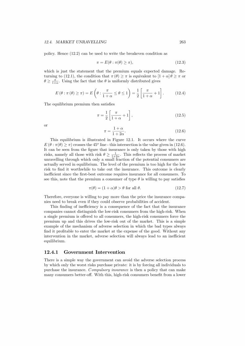
12.4. MARKET UNRAVELLING 263
policy. Hence (12.2) can be used to write the breakeven condition as
π = E(θ : π(θ) ≥ π), (12.3)
which is just the statement that the premium equals expected damage. Re-turning to (12.1), the condition that π (θ) ≥ π is equivalent to [1 + α] θ ≥ π orθ ≥ π
1+α . Using the fact that the θ is uniformly distributed gives
E (θ : π (θ) ≥ π) = E
µθ :
π
1 + α≤ θ ≤ 1
¶=1
2
·π
1 + α+ 1
¸. (12.4)
The equilibrium premium then satisfies
π =1
2
·π
1 + α+ 1
¸, (12.5)
orπ =
1 + α
1 + 2α. (12.6)
This equilibrium is illustrated in Figure 12.1. It occurs where the curveE (θ : π(θ) ≥ π) crosses the 45o line - this intersection is the value given in (12.6).It can be seen from the figure that insurance is only taken by those with highrisks, namely all those with risk θ ≥ 1
1+2α . This reflects the process of marketunravelling through which only a small fraction of the potential consumers areactually served in equilibrium. The level of the premium is too high for the lowrisk to find it worthwhile to take out the insurance. This outcome is clearlyinefficient since the first-best outcome requires insurance for all consumers. Tosee this, note that the premium a consumer of type θ is willing to pay satisfies
π(θ) = (1 + α)θ > θ for all θ. (12.7)
Therefore, everyone is willing to pay more than the price the insurance compa-nies need to break even if they could observe probabilities of accident.This finding of inefficiency is a consequence of the fact that the insurance
companies cannot distinguish the low-risk consumers from the high-risk. Whena single premium is offered to all consumers, the high-risk consumers force thepremium up and this drives the low-risk out of the market. This is a simpleexample of the mechanism of adverse selection in which the bad types alwaysfind it profitable to enter the market at the expense of the good. Without anyintervention in the market, adverse selection will always lead to an inefficientequilibrium.
12.4.1 Government Intervention
There is a simple way the government can avoid the adverse selection processby which only the worst risks purchase private: it is by forcing all individuals topurchase the insurance. Compulsory insurance is then a policy that can makemany consumers better-off. With this, high-risk consumers benefit from a lower
264 CHAPTER 12. ASYMMETRIC INFORMATION
Figure 12.1: Equilibrium in the Insurance Market
premium than the actual risk they face and lower than the level in (12.6) - itwill actually be π = 1
2 <1+α1+2α . The benefit for some of the low-risk is that
they can now purchase a policy at a more favorable premium than that offeredif only high-risk people purchased it. This benefits those close to the averagewho, although paying more for the policy than level of their expected damage,prefer to have insurance at this price than no insurance at all. Only the verylow-risk are made worse off - they would prefer to have no insurance than paythe average premium.The imposition of compulsory insurance may seem a very strong policy since
in few circumstances are consumers forced by the government to make specificpurchases. But it is the policy actually used for many insurance markets. Forinstance, both automobile insurance and employee protection insurance are com-pulsory. Health care insurance and unemployment insurance also are compul-sory. Aircraft also have to be insured. Pleasure boats have to be compulsorilyinsured in some countries (e.g. France) but not in others (e.g. the UK), despitethem representing a much greater capital investment than automobiles. Oneargument that could be advanced to explain this difference is the operation ofself-selection into boating as a leisure activity: those who choose to do it are bytheir nature either low probability of accident or sufficiently cautious to insurewithout compulsion.There is another role for government intervention. So far, the arguments
have concentrated upon one of the simplest cases. Particularly restrictive wasthe assumption that the probability of damage was uniformly distributed acrossthe population. It was this assumption (together with the proportional reserva-tion premium) that ensured the curve E (θ : π(θ) ≥ π) was a straight line with a

12.4. MARKET UNRAVELLING 265
Figure 12.2: Multiple Equilibria
single intersection with the 45o line. When the uniform distribution assumptionis relaxed, E (θ : π(θ) ≥ π) will have a different shape and the nature of equi-librium may be changed. In fact, there exist distribution functions F (θ) for thedistribution of types that lead to multiple equilibria. Such a case is illustratedin Figure 12.2. In this figure E (θ : π(θ) ≥ π) crosses the 45o line three timesso that there are three equilibria which differ in the size of the premium. Atthe low premium equilibrium, E1, most of the population is able to purchaseinsurance but at the high premium equilibrium, E3, very few can.Each of these equilibria is based on correct but different self-fulfilling beliefs.
For example, if the insurance companies are pessimistic and expect that onlyhigh-risk consumers will take out insurance, they will set a high premium. Givena high premium, only the high-risk will choose to accept the policy. The beliefsof the insurance companies are therefore confirmed and the economy becomestrapped in a high-premium equilibrium with very few consumers covered byinsurance. This is clearly a bad outcome for the economy since there are alsoequilibria with lower premiums and wider insurance coverage.When there are multiple equilibria, the one with the lowest premium is
Pareto preferred - it gives more consumers insurance cover and at a lower price.Consequently, if one of the other equilibria is achieved, there is a potentialbenefit from government intervention. The policy the government should adoptis simple: it can induce the best equilibrium (that with the lowest premium) byimposing a limit on the premium that can be charged. If we are at the wrongequilibrium the corresponding premium reduction (from E2 → E1 or E3 → E1)will attract the good risks making the cheaper insurance policy E1 sustainable.This policy is not without potential problems. To see these, assume that the
266 CHAPTER 12. ASYMMETRIC INFORMATION
government slightly miscalculates and sets the maximum premium below thepremium of policy E1. No insurance company can make a profit at this priceand all offers of insurance will be withdrawn. The policy will then worsen theoutcome. If set too high, one of the other equilibria may be established. Tointervene successfully in this way requires considerable knowledge on the partof the government.This analysis of the insurance market has shown how asymmetric information
can lead to market unravelling with the bad driving out the good, eventuallyleading to a position where fewer consumers participate in the market than isefficient. In addition, asymmetric information can lead to multiple equilibria.These equilibria can also be Pareto ranked. For each of these problems, apolicy response was suggested. The policy of making insurance compulsory isstraightforward to implement and requires little information on the part of thegovernment. Its only drawback is that it cannot benefit all consumers since thevery low risk are forced to purchase insurance they do not find worthwhile. Incontrast the policy of a maximum premium requires considerable informationand has significant potential pitfalls.
12.5 Screening
If insurance companies are faced with consumers whose probabilities of havingaccidents differ, then it will be to their advantage if they can find some mecha-nism that allows them to distinguish between the high risk and low risk. Doingso allows them to tailor insurance policies for each type and hence avoid thepooling of risks that causes market unravelling.The mechanism that can be used by the insurance companies is to offer
a menu of different contracts designed so that each risk type self-selects thecontract designed for it. By self-select we mean that the consumers find it intheir own interest to select the contract aimed at them. As we will show, self-selection will involve the bad risks being offered full insurance coverage at ahigh premium while the low risks are offered partial coverage at a low premiumrequiring them to bear part of the loss. The portion they have to bear consists ofa deductible (an initial amount of the loss) and coinsurance (an extra fraction ofthe loss beyond the deductible). An equilibrium like this where different typespurchase different contracts is called a separating equilibrium. This shouldbe contrasted to the pooling equilibrium of the previous section in which allconsumers purchasing insurance purchased the same contract. Obviously thebad risks will lose from this separation since they will no longer benefit fromthe lower premium resulting from their pooling with the low risks.To model self-selection, we again assume the insurance market is competitive,
so that in equilibrium insurance companies will earn zero profits. Rather thanhave a continuous range of different types, we now simplify by assuming thereare just two types of agents. The high-risk agents have a probability of anaccident occurring of ph, and the low-risks probability p`, with ph > p`. Thetwo types form proportions λh and λ` of the total population, where λh+λ` = 1.

12.5. SCREENING 267
Both types have the same fixed income, r, and, in the event of an accident sufferthe same fixed-damage, d, in the case of accident.If a consumer of type i buys an insurance policy with a premium π and
payout (or coverage) δ , their expected utility is given by
Vi(δ,π) = piu(r − d+ δ − π) + (1− pi)u(r − π). (12.8)
When they purchase no insurance (so π = 0 and δ = 0), expected utility is
Vi(0, 0) = piu(r − d) + (1− pi)u(r). (12.9)
It is assumed that the consumer is risk averse, so the utility function, u (·) , isconcave.The timing of the actions in the model is described by the following two
stages:Stage 1: firms simultaneously choose a menu of insurance contracts Si =
(δi,πi) with contract i intended for consumers of type i.Stage 2: agents choose their most preferred contract (not necessarily the one
the insurance companies intended for them!).We now analyze the equilibrium of this insurance market under a number of
different assumptions on information.
12.5.1 Perfect Information Equilibrium
The perfect information equilibrium assumes that the insurance companies canobserve the type of each consumer; that is they know exactly the accidentprobability of each customer. This case is used as a benchmark to isolate theconsequences of the asymmetric information that is soon to be introduced.Figure 12.3 illustrates the equilibrium with perfect information. The curved
lines are indifference curves - one curve is drawn for each type. The steepercurve is that of the high risk. The indifference curves are positively slopedbecause consumers are willing to trade-off greater coverage for a higher premium.They are concave because of risk aversion. It is assumed that willingness topay for extra coverage increases with the probability of having an accident.This makes the indifference curves of the high-risk steeper at any point thanthose of the low-risk so that the indifference curves satisfy the single-crossingproperty. With full information, the insurance companies know the accidentprobability. They can then offer contracts which trade off a higher premiumfor increased coverage at the rate of the accident probability. That is, low risktypes can be offered any contract {π, δ} satisfying π = p`δ and the high riskcontracts satisfying π = phδ. These equations give the two straight lines inFigure 12.3. These are the equilibrium contracts that will be offered. To seethis, note that if an insurance company offers a contract which is more generous(charges a lower premium for the same coverage) this contract must make a lossand will be withdrawn. Conversely, if a less generous contract is offered (so ahigher premium for the same coverage), other companies will be able to betterit without making a loss. Therefore it will never be chosen.

268 CHAPTER 12. ASYMMETRIC INFORMATION
Figure 12.3: Perfect Information Equilibrium
Given this characterization of the equilibrium contracts, the final step is toobserve that when these contracts are available, both types will choose to un-dertake full insurance cover. They will choose δ = d and pay the correspondingpremium. Hence the competitive equilibrium when types are observable by thecompanies is a pair of insurance contracts S∗h, S
∗` , where
S∗h = (d, phd) , (12.10)
andS∗` = (d, p`d) , (12.11)
so there is full coverage and actuarially-fair premia are charged. As for anycompetitive equilibrium with full (hence symmetric) information, this outcomeis Pareto efficient.
12.5.2 Imperfect Information Equilibrium
Imperfect information is introduced by assuming that the insurance companiescannot distinguish a low-risk consumer from a high-risk. We also assume thatit cannot employ any methods of investigation to elicit further information. Aswe will discuss later, insurance companies routinely do try to obtain furtherinformation. The reasons why they do and the consequences of doing so willbecome clear once it is understood what happens if they don’t.Given these assumptions, the insurance companies cannot offer the contracts
that arose in the full-information competitive equilibrium. The efficient contractfor the low risk provides any given degree of coverage at a lower premium thanthe contract for the high risk. Hence both types will prefer the contract intendedfor the low risk (this is adverse selection again!). If offered, it will charge a

12.5. SCREENING 269
premium based on the low-risk accident probability but have to pay claims atthe population average probability. It will therefore make a loss and have tobe withdrawn. This argument suggests what the insurance companies have todo: if they wish to offer a contract that will attract the low-risk type, it mustbe designed in such a way that it does not also attract the high risk. Thisrequirement places constraints upon the contracts that can be offered and iswhat prevents the attainment of the efficient outcome.Assume now that insurance companies offer a contract Sh designed for the
high risk and a contract S` designed for the low risk. To formally express thecomments in the previous paragraph, we say that when types are not observ-able, the contracts Sh and S` have to satisfy the self-selection (or incentive-compatibility) constraints. These constraints require the low risk to find thatthe contract S` offers them at least as much utility as the contract Sh, withthe converse holding for the high risk. If these constraints are satisfied, thelow risk will choose the contract designed for them, as will the high risk. Theself-selection constraints can be written as
V`(S`) ≥ V`(Sh) (ICu), (12.12)
andVh(Sh) ≥ Vh(S`) (ICd). (12.13)
(These are labelled ICu and ICd because the first has the low-risk types looking“up” at the contract of the high risk, the second has the high-risk looking“down” at the contract of the low-risk. This becomes clear in Figure 12.4.) Aswe have already remarked, the contracts S∗h, S
∗` arising in the full information
equilibrium do not satisfy (ICd): the high-risk will always prefer the low-risk’scontract S∗` .There is only one undominated pair of contracts that achieve the desired sep-
aration. By undominated we mean that no other pair of separating contracts canbe introduced that make a positive profit in competition with . The propertiesof the pair are that the high-risk type receives full insurance at an actuariallyfair rate. The low-risk do not receive full insurance. They are restricted topartial cover with the extent of the cover determined by where the indifferencecurve of the high risk crosses the actuarially-fair insurance line for the low risk.In addition the constraint (12.13) is binding while the constraint (12.12) is not.This feature, that the “good” type (here the low-risk) are constrained by the“bad” type (here the high-risk) is common to all incentive problems of this kind.It can easily be seen that the insurance contracts are undominated by any
other pair of separating contracts and make zero profit for the insurance com-panies. To see that no contract can be introduced which will appeal to onlyone type and yield positive profit, assume on one hand that such a contractwere aimed at the high risk. Then it must be more favorable than the existingcontract otherwise it will never be chosen. But is actuarially fair so any con-tract which is more favorable must make a loss. On the other hand, a contractaimed at the low risk will either attract the high risk too, and so not separate,or, if it attracts only low risk, will be unprofitable. There remains though the
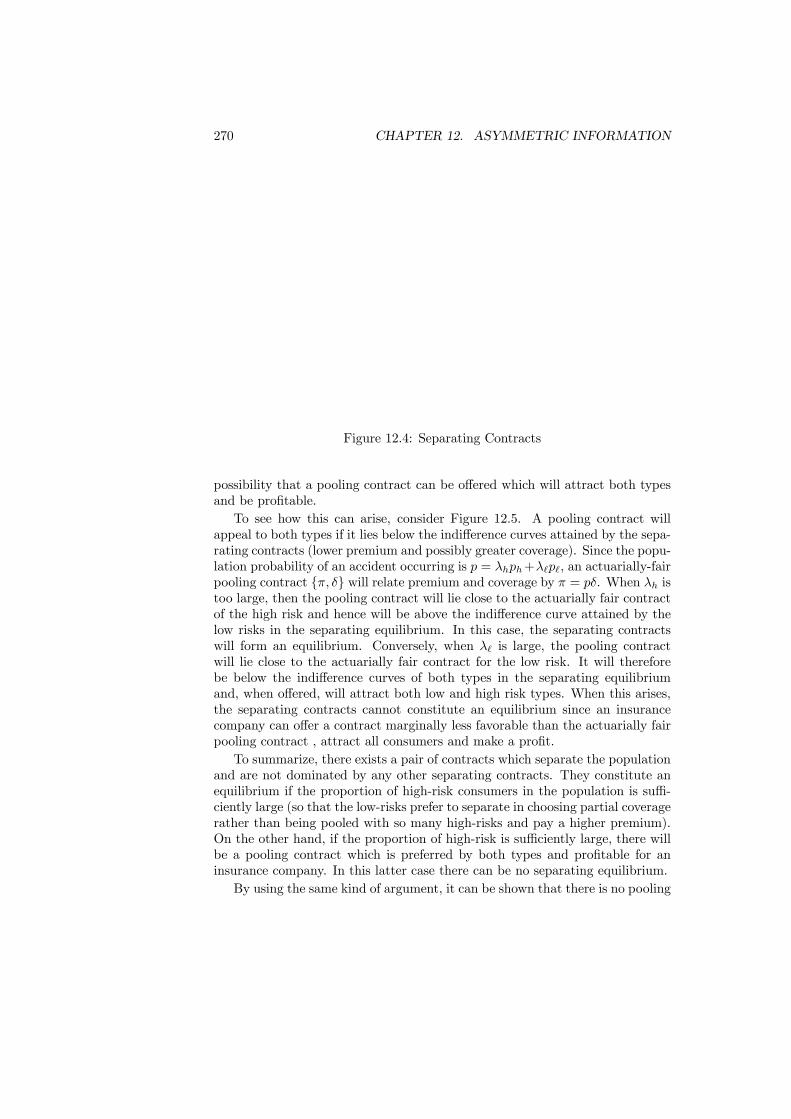
270 CHAPTER 12. ASYMMETRIC INFORMATION
Figure 12.4: Separating Contracts
possibility that a pooling contract can be offered which will attract both typesand be profitable.To see how this can arise, consider Figure 12.5. A pooling contract will
appeal to both types if it lies below the indifference curves attained by the sepa-rating contracts (lower premium and possibly greater coverage). Since the popu-lation probability of an accident occurring is p = λhph+λ`p`, an actuarially-fairpooling contract {π, δ} will relate premium and coverage by π = pδ. When λh istoo large, then the pooling contract will lie close to the actuarially fair contractof the high risk and hence will be above the indifference curve attained by thelow risks in the separating equilibrium. In this case, the separating contractswill form an equilibrium. Conversely, when λ` is large, the pooling contractwill lie close to the actuarially fair contract for the low risk. It will thereforebe below the indifference curves of both types in the separating equilibriumand, when offered, will attract both low and high risk types. When this arises,the separating contracts cannot constitute an equilibrium since an insurancecompany can offer a contract marginally less favorable than the actuarially fairpooling contract , attract all consumers and make a profit.To summarize, there exists a pair of contracts which separate the population
and are not dominated by any other separating contracts. They constitute anequilibrium if the proportion of high-risk consumers in the population is suffi-ciently large (so that the low-risks prefer to separate in choosing partial coveragerather than being pooled with so many high-risks and pay a higher premium).On the other hand, if the proportion of high-risk is sufficiently large, there willbe a pooling contract which is preferred by both types and profitable for aninsurance company. In this latter case there can be no separating equilibrium.By using the same kind of argument, it can be shown that there is no pooling
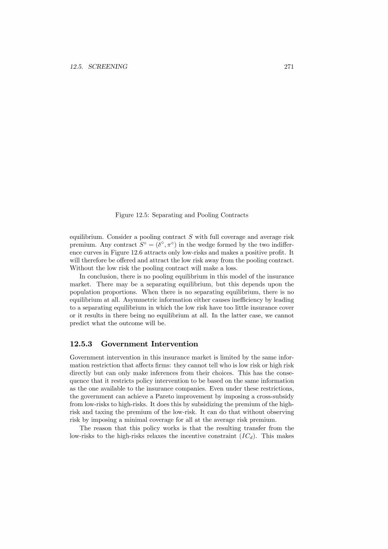
12.5. SCREENING 271
Figure 12.5: Separating and Pooling Contracts
equilibrium. Consider a pooling contract S with full coverage and average riskpremium. Any contract S◦ = (δ◦,π◦) in the wedge formed by the two indiffer-ence curves in Figure 12.6 attracts only low-risks and makes a positive profit. Itwill therefore be offered and attract the low risk away from the pooling contract.Without the low risk the pooling contract will make a loss.In conclusion, there is no pooling equilibrium in this model of the insurance
market. There may be a separating equilibrium, but this depends upon thepopulation proportions. When there is no separating equilibrium, there is noequilibrium at all. Asymmetric information either causes inefficiency by leadingto a separating equilibrium in which the low risk have too little insurance coveror it results in there being no equilibrium at all. In the latter case, we cannotpredict what the outcome will be.
12.5.3 Government Intervention
Government intervention in this insurance market is limited by the same infor-mation restriction that affects firms: they cannot tell who is low risk or high riskdirectly but can only make inferences from their choices. This has the conse-quence that it restricts policy intervention to be based on the same informationas the one available to the insurance companies. Even under these restrictions,the government can achieve a Pareto improvement by imposing a cross-subsidyfrom low-risks to high-risks. It does this by subsidizing the premium of the high-risk and taxing the premium of the low-risk. It can do that without observingrisk by imposing a minimal coverage for all at the average risk premium.The reason that this policy works is that the resulting transfer from the
low-risks to the high-risks relaxes the incentive constraint (ICd). This makes
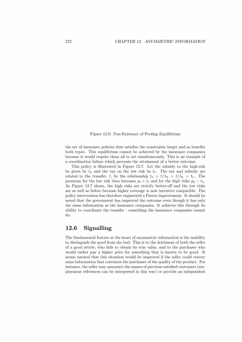
272 CHAPTER 12. ASYMMETRIC INFORMATION
Figure 12.6: Non-Existence of Pooling Equilibrium
the set of insurance policies that satisfies the constraints larger and so benefitsboth types. This equilibrium cannot be achieved by the insurance companiesbecause it would require them all to act simultaneously. This is an example ofa coordination failure which prevents the attainment of a better outcome.This policy is illustrated in Figure 12.7. Let the subsidy to the high-risk
be given by th and the tax on the low risk be t`. The tax and subsidy arerelated to the transfer, t, by the relationship th = t/λh = t/λh = t`. Thepremium for the low risk then becomes p` + t` and for the high risks ph − th.As Figure 12.7 shows, the high risks are strictly better-off and the low risksare as well as before because higher coverage is now incentive compatible. Thepolicy intervention has therefore engineered a Pareto improvement. It should benoted that the government has improved the outcome even though it has onlythe same information as the insurance companies. It achieves this through itsability to coordinate the transfer - something the insurance companies cannotdo.
12.6 Signalling
The fundamental feature at the heart of asymmetric information is the inabilityto distinguish the good from the bad. This is to the detriment of both the sellerof a good article, who fails to obtain its true value, and to the purchaser whowould rather pay a higher price for something that is known to be good. Itseems natural that this situation would be improved if the seller could conveysome information that convinces the purchaser of the quality of the product. Forinstance, the seller may announce the names of previous satisfied customers (em-ployment references can be interpreted in this way) or provide an independent

12.6. SIGNALLING 273
Figure 12.7: Market Intervention
guarantee of quality (such as a report on the condition of a car by a motoringorganization). Warranties can also serve as signals of quality of durable goodsbecause if a product is of higher quality it is less costly for the seller to offera longer warranty on it. Such information, generally termed signals, can bemutually beneficial.It is worth noting the difference between screening and signalling. The less-
informed players (like the insurance companies) use screening (different insur-ance contracts) to find out what the better-informed players (insurance cus-tomer) know (their own risk). In contrast, more-informed players use signals tohelp the less-informed players find out the truth.For a signal to work it must satisfy certain criteria. Firstly, it must be
verifiable by the receiver (i.e., the less-informed agent). Being given the nameof a satisfied customer is not enough - it must be possible to check back thatthey are actually satisfied. Secondly, it must be credible. In the case of anemployment reference this is dependent partly upon the author of the referencehaving a reputation to maintain and partly upon the possibility of legal action iffalse statements are knowingly made. Finally, the signal must also be costly forthe sender (i.e., the better-informed agent) to obtain and the cost must differbetween various qualities of sender. In the case of an employment reference, thisis obtained by a record of quality work. Something which is either costlesslyobtainable by both the senders of low- and high-quality or equally costly cannothave any value in distinguishing between them. We now model such signals andsee the effect that they have on the equilibrium outcome.The modelling of signalling revolves around the timing of actions. The ba-
sic assumption is that the informed agent moves first and invests in acquiringa costly signal. The uninformed party then observes the signals of different
274 CHAPTER 12. ASYMMETRIC INFORMATION
agents and forms inferences about quality on the basis of these signals. Anequilibrium is reached when the chosen investment in the signal is optimal foreach informed agent and the inferences of the uninformed about the meaning ofsignals are justified by the outcomes. As we will see, the latter aspect involvesself-supporting beliefs: they may be completely irrational but the equilibriumthey generate does not provide any evidence to falsify them.
12.6.1 Educational Signalling
To illustrate the consequences of signalling, we shall consider a model of pro-ductivity signalling in the labor market. The model has two identical firms whocompete for workers through the wages they offer. The set of workers can be di-vided into two types according to their productivity levels. Some of the workersare innately low-productivity in the form of employment offered by the firms,whilst the others are high-productivity. Without any signalling, the firms areassumed to be unable to judge the productivity of a worker.The firms cannot directly observe a worker’s type before hiring, but high-
productivity workers can signal their productivity by getting educated. Edu-cation itself does not alter productivity but it is costly to acquire. Firms canobserve the level of education of a potential worker and condition their wageoffer upon this. Hence, education is a signal. Investment in education will beworthwhile if it earns a higher wage. To make it an effective signal, it must beassumed that obtaining education is more costly for the low productivity thanit is for the high productivity otherwise both will have the same incentive foracquiring it.Formally, let θh denote the productivity of a high-productivity worker and θ`
that of a low-productivity worker, with θh > θ`. The workers are present in thepopulation in proportions λh and λ`, so λh + λ` = 1. The average productivityin the population is given by
E(θ) = λhθh + λ`θ`. (12.14)
Competition between the two firms ensures that this is the wage that wouldbe paid if there were no signalling so the firms could not distinguish betweenworkers. For a worker of productivity level θ, the cost of obtaining educationlevel e is
C(e, θ) =e
θ, (12.15)
which satisfies the property that any given level of education is more costly fora low productivity worker to obtain.The firms offer wages that are (potentially) conditional upon the level of
education; potentially is added since there may be equilibria in which the firmsignore the signal. The wage schedule is denoted by w(e). Given the offeredwage schedule, the workers aim to maximize utility which is defined as wagesless the cost of education. Hence their decision problem is
max{e}
w (e)− eθ. (12.16)
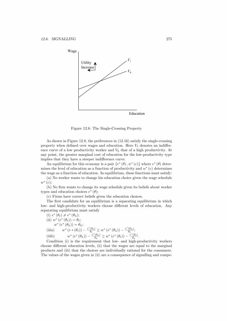
12.6. SIGNALLING 275
lV
hV
Education
Wage
UtilityIncrease
Figure 12.8: The Single-Crossing Property
As shown in Figure 12.8, the preferences in (12.16) satisfy the single-crossingproperty when defined over wages and education. Here V` denotes an indiffer-ence curve of a low productivity worker and Vh that of a high productivity. Atany point, the greater marginal cost of education for the low-productivity typeimplies that they have a steeper indifference curve.An equilibrium for this economy is a pair {e∗ (θ) , w∗ (e)} where e∗ (θ) deter-
mines the level of education as a function of productivity and w∗ (e) determinesthe wage as a function of education. In equilibrium, these functions must satisfy:(a) No worker wants to change his education choice given the wage schedule
w∗ (e);(b) No firm wants to change its wage schedule given its beliefs about worker
types and education choices e∗ (θ);(c) Firms have correct beliefs given the education choices.The first candidate for an equilibrium is a separating equilibrium in which
low- and high-productivity workers choose different levels of education. Anyseparating equilibrium must satisfy(i) e∗ (θ`) 6= e∗ (θh);(ii) w∗ (e∗ (θ`)) = θ`;
w∗ (e∗ (θh)) = θh;
(iiia) w∗ (e ∗ (θ`))− e∗(θ`)θ`≥ w∗ (e∗ (θh))− e∗(θh)
θ`;
(iiib) w∗ (e∗ (θh))− e∗(θh)θh≥ w∗ (e∗ (θ`))− e∗(θ`)
θh.
Condition (i) is the requirement that low- and high-productivity workerschoose different education levels, (ii) that the wages are equal to the marginalproducts and (iii) that the choices are individually rational for the consumers.The values of the wages given in (ii) are a consequence of signalling and compe-
276 CHAPTER 12. ASYMMETRIC INFORMATION
tition between firms. Signalling implies workers of different productivities arepaid different wages. If either paid a wage above the marginal product, it wouldmake a loss on each worker employed. This cannot be profit maximizing. Al-ternatively, if one paid a wage below the marginal productivity, the other wouldhave an incentive to set its wage incrementally higher. This would capture allthe workers of that productivity level and would be the more profitable strategy.Therefore, the only equilibrium values for wages when signalling occurs are theproductivity levels. This leaves only the levels of education to be determined.The equilibrium level of education for the low-productivity workers is found
by noting that if they choose not to act like the high-productivity, then thereis no point in obtaining any education - education is simply a cost which doesnot benefit them. Hence e∗ (θ`) = 0. Using this fact and that wages are equalto productivities, the level of education for the high-productivity workers canbe found from the incentive compatibility constraints. From (iiia)
θ` ≥ θh − e∗ (θh)θ`
, (12.17)
ore∗ (θh) ≥ θ` [θh − θ`] . (12.18)
Condition (12.18) provides the minimum level of education that will ensure thelow-productivity choose not to be educated. Now using (iiib), it follows that
θh − e ∗ (θh)θh
≥ θ`, (12.19)
orθh [θh − θ`] ≥ e ∗ (θh) . (12.20)
Hence a complete description of the separating equilibrium is
e∗ (θ`) = 0, θ` [θh − θ`] ≤ e∗ (θh) ≤ θh [θh − θ`] , (12.21)
w (e∗ (θ`)) = θ`, w (e∗ (θh)) = θh, (12.22)
so the low-productivity workers obtain no education, the high-productivity haveeducation somewhere between the two limits and both are paid their marginalproducts. An equilibrium satisfying these conditions is illustrated in Figure ??.Since there is a range of possible values for e∗ (θh), there is not a unique
equilibrium but a set of equilibria differing in the level of education obtained bythe high-productivity. This set of separating equilibria can be ranked accordingto criterion of Pareto preference. Clearly, changing the level of education e∗ (θh)within the specified range does not affect the low-productivity workers. Onthe other hand, the high-productivity workers always prefer a lower level ofeducation since education is costly. Therefore, equilibria with lower e∗ (θh)are Pareto-preferred and the most preferred equilibrium is that with e∗ (θh) =θ` [θh − θ`]. The Pareto-dominated separating equilibria are supported by thehigh-productivity worker’s fear choosing less education will give an unfavorableimpression of her productivity to the firm and thus lead to a lower wage.

12.6. SIGNALLING 277
Figure 12.9: Separating Equilibrium

278 CHAPTER 12. ASYMMETRIC INFORMATION
There are arguments (called refinements of equilibrium) to suggest that thismost-preferred equilibrium will actually be the one that emerges. Let the equi-librium level of education for the high-productivity type, e∗ (θh), be above theminimum required to separate. Denote this minimum e0. Now consider the firmobserving a worker with an education level at least equal to e0 but less thane∗ (θh). What should a firm conclude about this worker? Clearly, the workercannot be low ability since such a choice is worse for them than choosing no ed-ucation. Hence the firm must conclude that the worker is of high productivity.Realizing this, it then pays the worker to deviate since it would reduce the costof their education. This argument can be repeated until e∗ (θh) is driven downto e0.Signalling allows the high-productivity to distinguish themselves from the
low-productivity. It might be thought that this improvement in informationtransmission would make signalling socially beneficial. However, this need notbe the case since the act of signalling is costly and does not add to productiv-ity. The alternative to the signalling equilibrium is pooling where both typespurchase no education and are paid a wage equal to the average productivity.The low-productivity would prefer this equilibrium as it raises their wage fromθ` to E(θ) = λhθh + λ`θ`. For the high-productivity pooling is preferred if
E(θ) = λhθh + λ`θ` > θh − θ` [θh − θ`]
θh. (12.23)
Since λ` = 1− λh, this inequality will be satisfied if
λh > 1− θ`θh. (12.24)
Hence when there are sufficiently many high-productivity workers, so that theaverage wage is close the high productivity level, the separating equilibriumis Pareto-dominated by the pooling equilibrium. In these cases, signalling isindividually rational but socially unproductive. Again, the Pareto-dominatedseparating equilibrium is sustained by the high-productivity workers’ fear thatlowering their education would give a bad impression of their ability to the firmsand thus lead to lower wage. Actually the no-signalling pooling equilibrium isnot truly available to the high-productivity workers. If they get no education,firms will believe they are low-productivity workers and then offer a wage of θ`.So we get this paradoxical situation that high-productivity workers choose tosignal although they are worse off when signalling.If the government were to intervene in this economy, it has two basic policy
options. The first is to allow signalling to occur but to place an upper limit onthe level of education equal to θ` [θh − θ`]. It might choose to do this in thosecases where the pooling equilibrium does not Pareto dominate the separatingequilibrium. There is though, one problem with banning signalling and enforcinga pooling equilibrium. The pooling equilibrium requires the firms to believe thatall workers have the same ability. If the firms were to “test“ this belief by offeringa higher wage for a higher level of education, they would discover that the belief
12.6. SIGNALLING 279
Figure 12.10: Unreasonable Beliefs
was incorrect. This is illustrated in Figure 12.10. A low-productivity workerwould be better off getting no education than she would getting education abovee whatever the firm’s belief and the resulting wage. Therefore the firm shouldbelieve that any worker choosing education level above e has high productivityand should be offered a wage θh. But if this is so, the high-productivity workercould do better than the pooling equilibrium by deviating to an education levelslightly in excess of e to get a wage θh. Therefore the pooling equilibrium isunlikely since it involves unreasonable beliefs from the firms.
12.6.2 Implications
The model of educational signalling shows how an unproductive but costly signalcan be used to distinguish between quality levels through a set of self-supportingbeliefs. There will be a set of Pareto-ranked equilibria with the lowest level ofsignal the most preferred. Although there is an argument that the economymust achieve the Pareto-dominating signalling equilibrium, it is possible thatthis may not happen. If it does not, the economy may become settled in aPareto-inferior separating equilibrium. Even if it does not, it is still possible forthe pooling equilibrium to Pareto dominate the separating equilibrium. Thiswill occur when the high productivity workers are relatively numerous in thepopulation since in that case almost every worker is getting unproductive but

280 CHAPTER 12. ASYMMETRIC INFORMATION
costly education to separate themselves from few bad workers.There are several policy implications of these results. In a narrow interpreta-
tion, they show how the government can increase efficiency and make everyonebetter off by restricting the size of signals that can be transmitted. Alterna-tively the government could improve the welfare of everyone by organizing across-subsidy from the good to the bad workers. This can take the form of aminimum wage for the low-productivity workers in excess of their productivityfinanced by wage limit for the high-productivity workers which is below theirproductivity. Notice that a ban on signalling is an extreme form of such cross-subsidization since it forces a same wage for all. When the pooling equilibriumis Pareto-preferred, they should be eliminated entirely. More generally, themodel demonstrated how market solutions may endogenously arise to combatthe problems of asymmetric information. These solutions can never remove theproblems entirely - someone must be bearing the cost of improving informationflows - and can even exacerbate the situation.The basic problem for the government in responding to these kinds of prob-
lems is that it does not have a natural informational advantage over the privateagents. In the model of education there is no reason to suppose the governmentis any more able to tell the low-productivity workers from the high-productivity(in fact, there is every reason to suspect that the firms would be better equippedto do this). Faced with these kinds of problems, the government may have littleto offer beyond the cross-subsidization we have just mentioned.
12.7 Moral Hazard (Hidden Action)
Amoral hazard problem arises when an agent can affect the “quality” of a tradedgood or contract variable by some action which is not observed by other agents.For instance, a houseowner once insured may become lax in their attention tosecurity (such as leaving windows open) in the knowledge that if burgled theywill be fully compensated. Or a worker, once in employment, may not fullyexert themself reasoning that their lack of effort may be hidden amongst theeffort of the workforce as a whole. Such possibilities provide the motive forcontracts to be designed that embody incentives to lessen these effects.In the case of the worker, the employment contract could provide for a wage
that is dependent upon some measure of the worker’s performance. Ideally, themeasure would be their exact productivity but, except for the simplest cases,this can be difficult to measure. Difficulties can arise because production takesplace in teams (a production line can often be interpreted as a team) with theeffort of the individual team member impossible to distinguish from the outputof the team as a whole. They can also arise through randomness in the relationbetween effort and output As examples, agricultural output is driven by theweather, maintenance tasks can depend upon the (variable) condition of theitem being maintained, and production can be dependent upon the randomquality of other inputs.We now consider the design of incentive schemes in a situation with moral
12.7. MORAL HAZARD (HIDDEN ACTION) 281
hazard. The model we choose embodies the major points of the previous dis-cussion: effort cannot be measured directly so a contract has to be based onsome observable variable which roughly measures effort.
12.7.1 Moral Hazard in Insurance
The moral hazard problem that can arise in an insurance market is that efforton accident prevention is reduced when consumers become insured. If accident-prevention effort is costly, for instance driving more slowly is time consumingor eating a good diet is less enjoyable, then a rational consumer will seek toreduce such effort when it is beneficial to do so (and the benefits are raisedonce insurance is offered). Insurance companies must counteract this tendencythrough the design of their contracts.To model this situation, assume an economy populated by many identical
agents. The income of an agent is equal to r with probability 1 - p and r - d withprobability p. Here p is interpreted as the probability of an accident occurringand d the monetary equivalent of the accident damage. Moral hazard is intro-duced by assuming that the agents are able to affect the accident probabilitythrough their prevention efforts.To simplify, it is assumed that effort, e, can take one of two values. If
e = 0 an agent is making no effort at accident prevention and the probabilityof an accident is p (0). Alternatively, if e = 1, the agent is making maximumeffort at accident prevention and the probability is p (1). In line with theseinterpretations, it is assumed that p (0) > p (1), so the probability of the accidentis higher when no effort is undertaken. The cost of effort for the agents, measuredin utility terms, is c (e) ≡ ce.In the absence of insurance, the preferences of the agent are described by
the expected utility function
Uo (e) = p (e)u (r − d) + (1− p (e)))u (r)− ce. (12.25)
where u(r−d) is the utility if there is an accident and u(r) is the utility if thereis no accident. It is assumed that the agent is risk averse, so the utility functionu (·) is concave.The value of e, either 0 or 1, is chosen to maximize this utility. Effort to
prevent the accident will be undertaken (e = 1) if
Uo (1) > Uo (0) . (12.26)
Evaluating these and rearranging shows e = 1 if
c ≤ c0 ≡ [p (0)− p (1)] [u (r)− u (r − d)] . (12.27)
Here c0 is the critical value of effort cost. If effort cost is below this value,effort will be undertaken. Therefore, in the absence of insurance, effort will beundertaken to prevent accidents if the cost of doing so is sufficiently small.Consider now the introduction of insurance contracts. A contract consists
of a premium π paid by the consumer and an indemnity δ, δ ≤ d, paid to the
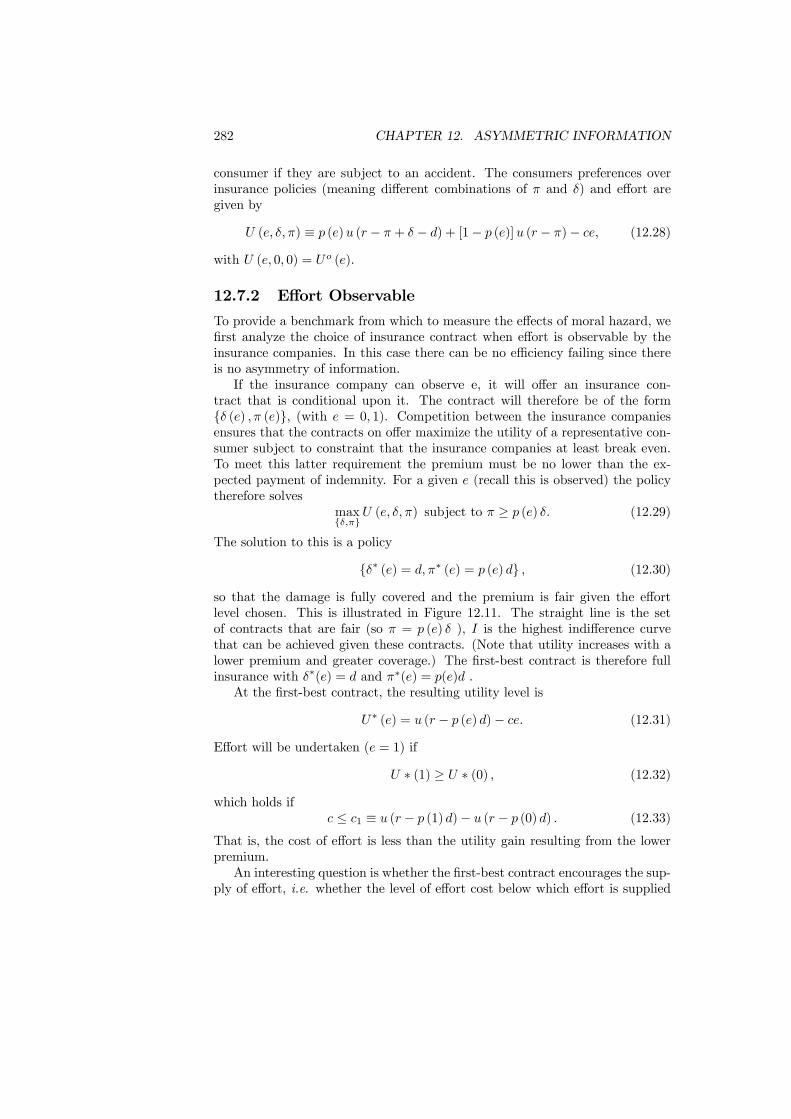
282 CHAPTER 12. ASYMMETRIC INFORMATION
consumer if they are subject to an accident. The consumers preferences overinsurance policies (meaning different combinations of π and δ) and effort aregiven by
U (e, δ,π) ≡ p (e)u (r − π + δ − d) + [1− p (e)]u (r − π)− ce, (12.28)
with U (e, 0, 0) = Uo (e).
12.7.2 Effort Observable
To provide a benchmark from which to measure the effects of moral hazard, wefirst analyze the choice of insurance contract when effort is observable by theinsurance companies. In this case there can be no efficiency failing since thereis no asymmetry of information.If the insurance company can observe e, it will offer an insurance con-
tract that is conditional upon it. The contract will therefore be of the form{δ (e) ,π (e)}, (with e = 0, 1). Competition between the insurance companiesensures that the contracts on offer maximize the utility of a representative con-sumer subject to constraint that the insurance companies at least break even.To meet this latter requirement the premium must be no lower than the ex-pected payment of indemnity. For a given e (recall this is observed) the policytherefore solves
max{δ,π}
U (e, δ,π) subject to π ≥ p (e) δ. (12.29)
The solution to this is a policy
{δ∗ (e) = d,π∗ (e) = p (e) d} , (12.30)
so that the damage is fully covered and the premium is fair given the effortlevel chosen. This is illustrated in Figure 12.11. The straight line is the setof contracts that are fair (so π = p (e) δ ), I is the highest indifference curvethat can be achieved given these contracts. (Note that utility increases with alower premium and greater coverage.) The first-best contract is therefore fullinsurance with δ∗(e) = d and π∗(e) = p(e)d .At the first-best contract, the resulting utility level is
U∗ (e) = u (r − p (e) d)− ce. (12.31)
Effort will be undertaken (e = 1) if
U ∗ (1) ≥ U ∗ (0) , (12.32)
which holds ifc ≤ c1 ≡ u (r − p (1) d)− u (r − p (0) d) . (12.33)
That is, the cost of effort is less than the utility gain resulting from the lowerpremium.An interesting question is whether the first-best contract encourages the sup-
ply of effort, i.e. whether the level of effort cost below which effort is supplied
12.7. MORAL HAZARD (HIDDEN ACTION) 283
Figure 12.11: First-Best Contract
in the absence of the contract, c0, is less than that with the contract, c1. Cal-culations show that the outcome may go in either direction depending on theaccident probabilities associated with effort and no effort.
12.7.3 Effort Unobservable
When effort is unobservable, the insurance companies cannot condition the con-tract upon it. Instead, they must evaluate the effect of the policies upon thechoices of the consumers and choose the policy taking this into account.The preferences of the consumer over contracts are determined by the highest
level of utility they can achieve with that contract given that they have madethe optimal choice of effort. Formally, the utility V (δ,π) arising from contract(δ,π) is determined by
V (δ,π) ≡ maxe={0,1}
U (e, δ,π) . (12.34)
The basic analytical difficulty in undertaking the determination of the con-tract is the non-convexity of preferences in the contract space (δ,π). This non-convexity arises at the point in the contract space where the consumers switchfrom no effort (e = 0) to full effort (e = 1). When supplying no effort their pref-erences are determined by U (0, δ,π) and when they supply effort by U (1, δ,π).
At any point (δ, π) where U³0, δ, π
´= U
³1, δ, π
´, the indifference curve of
U³0, δ, π
´is steeper than that of U
³1, δ, π
´because the willingness to pay for
extra coverage is higher when there is no effort and thus a high risk of accident.This is illustrated in Figure ??, where δ∗ (π) denotes the locus of points where
284 CHAPTER 12. ASYMMETRIC INFORMATION
Figure 12.12: Switching Line
the consumer is indifferent to e = 0 and e = 1. This locus has the propertiesdescribed in Lemma 1.
Lemma 1 For each premium π, there exists an indemnity level δ∗ (π) such that:(i) if δ < δ∗ (π), e = 1;(ii)if δ ≥ δ∗ (π), e = 0.where δ∗ (π) is increasing.
In words, if the coverage rate for any given premium is too high, agent willno longer find profitable to undertake effort.
12.7.4 Second-Best Contract
The second-best contract maximizes the consumer’s utility subject to the con-straint that it must at least break even. The optimization problem describingthis can be written as max V (δ,π) subject toi. π ≥ p (1) δ for δ < δ∗ (π),ii. π ≥ p (0) δ for δ∗ (π) ≤ δ < d.The first constraint applies if the consumer chooses to supply effort (e = 1)
and requires that the contract break even. The second constraint is the breakeven condition if the consumer chooses to supply no effort (e = 0).The problem is solved by calculating the solution under the first constraint
and evaluating the resulting level of utility. The solution is then found underthe second constraint and utility again evaluated. The two levels of utility arethen compared and the one yielding the highest utility is the optimal second-best contract. This reasoning provides two contracts that are candidates for
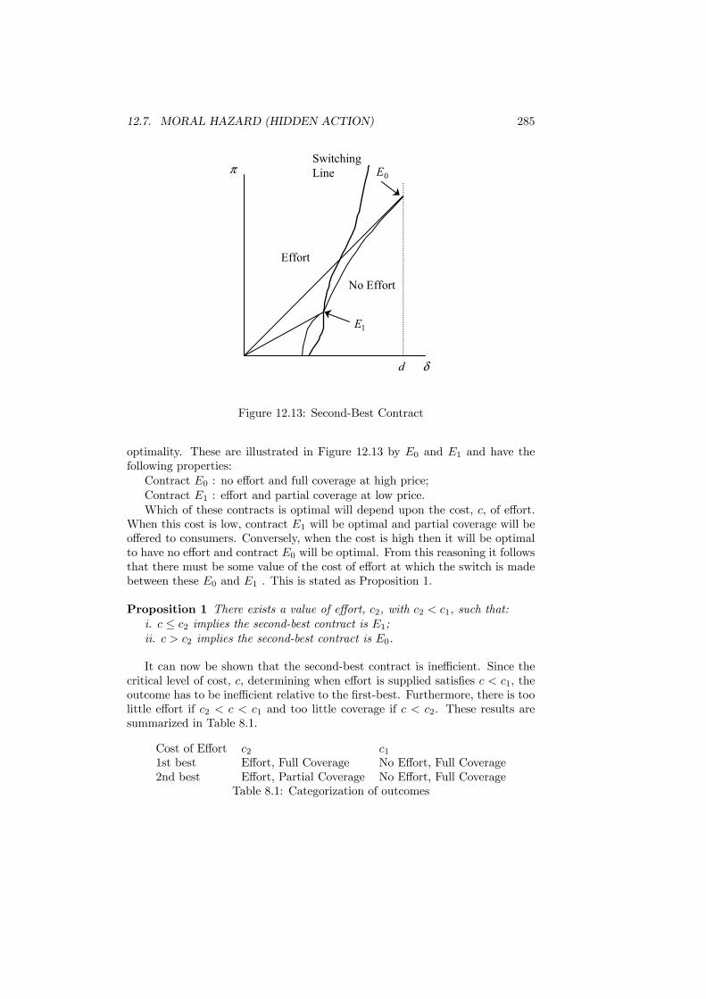
12.7. MORAL HAZARD (HIDDEN ACTION) 285
δ
π
d
Effort
No Effort
SwitchingLine 0E
1E
Figure 12.13: Second-Best Contract
optimality. These are illustrated in Figure 12.13 by E0 and E1 and have thefollowing properties:Contract E0 : no effort and full coverage at high price;Contract E1 : effort and partial coverage at low price.Which of these contracts is optimal will depend upon the cost, c, of effort.
When this cost is low, contract E1 will be optimal and partial coverage will beoffered to consumers. Conversely, when the cost is high then it will be optimalto have no effort and contract E0 will be optimal. From this reasoning it followsthat there must be some value of the cost of effort at which the switch is madebetween these E0 and E1 . This is stated as Proposition 1.
Proposition 1 There exists a value of effort, c2, with c2 < c1, such that:i. c ≤ c2 implies the second-best contract is E1;ii. c > c2 implies the second-best contract is E0.
It can now be shown that the second-best contract is inefficient. Since thecritical level of cost, c, determining when effort is supplied satisfies c < c1, theoutcome has to be inefficient relative to the first-best. Furthermore, there is toolittle effort if c2 < c < c1 and too little coverage if c < c2. These results aresummarized in Table 8.1.
Cost of Effort c2 c11st best Effort, Full Coverage No Effort, Full Coverage2nd best Effort, Partial Coverage No Effort, Full Coverage
Table 8.1: Categorization of outcomes
286 CHAPTER 12. ASYMMETRIC INFORMATION
12.7.5 Government Intervention
The market failure associated with moral hazard is very profound. The moralhazard problem arises from the non-observability of the level of care. Whenindividuals are fully insured they tend to exert too little precaution but alsoto overuse insurance. Consider, for instance, a patient who may be either sickwith probability 0.09 or very sick with probability 0.01. In the two events,his medical expenses will be $1000 and $10000. At a fair premium of $190the patient will not have to pay anything if he gets sick and would buy suchinsurance if risk averse. But then suppose that when he is a little sick, there issome chance, however small, that he can be very sick. Then he would choosethe expensive treatment given that there is no extra cost to the patient and allthe extra cost is borne by the insurance company. Each individual ignores theeffect of his reckless behavior and overconsumption on the premium; but whenthey all act like that, the premium increases. The lack of care by each inflatesthe premium which generates a negative externality on others. An importantimplication is that market cannot be efficient. Another way to see this genericmarket inefficiency is that the provision of insurance in the presence of moralhazard causes the insured individual to receive less than the full social benefit ofhis care. As a result, not only will the individual expend less than the sociallyoptimal level of care, but also there will be an insurance-induced externality.This implies that the potential scope for government intervention with moralhazard is substantial. Can the government improve efficiency by interventionwhen moral hazard is present? In answering this question it is important tospecify what information is available to the government. For a fair evaluationof government intervention it is natural to assume that the government has thesame information as private sector. In this case it can be argued that efficientgovernment intervention is still possible. The beneficial effects of governmentintervention stem from the government’s capacity to tax and subsidize. To takean example, the government cannot monitor smoking which has an adverseeffect on health, any better than the insurance company. But the governmentcan impose taxes, not only on cigarettes, but also on commodities that arecomplements and subsidize substitutes which have less adverse effect. Also thetaxation of insurance induces firms to offer insurance at less than fair price.As a consequence, individuals buy less insurance and expend more effort (asefficiency requires).
12.8 Public provision of Health care
12.8.1 Efficiency Arguments
Economists do not expect private insurance market for health care to functionwell. Our previous discussion suggests that informational problems would leavethe private provision of health insurance coverage incomplete and inefficient.The existence of asymmetric information between insurers and insured leadsto adverse selection, which can result in the market break down, and the non-
12.8. PUBLIC PROVISION OF HEALTH CARE 287
existence of certain types of insurance. The moral hazard problem can lead toincomplete insurance in the form of copayments and deductibles for those whohave insurance. Another problem caused by the presence of moral hazard isthat the insured who get sick will want to overconsume and doctors will want tooversupply health care since it is a third party who pays. It is not surprising,therefore, that the government may usefully intervene in the provision of healthcare.There is strong evidence that in the OECD countries the public sector plays
an important role in the provision of insurance for health care. Following OECDHealth data, in 1994 the proportion of publicly provided health expenses was44 percent in the US, 70 percent in Germany, 73 percent in Italy, 75 percent inFrance, 83 percent in Sweden and the UK. The question is why the governmentintervenes so extensively in the health care field. In answering the questionone must bear in mind that the government faces many of same informationalproblems that the private sector would. Like a private insurance, it faces themoral hazard where the patients who get insurance exert too little risk-reducingactivities and overconsume health services; and the doctors have the incentiveto oversupply health services at too high of a cost.One advantage of public provision is to prevent the adverse selection problem
by making health coverage compulsory and universal. It is tempting to believethat the actual provision of insurance need not be public to accomplish thiseffect. Indeed the actual provision of health insurance could remain privateand the government could have a mandate requiring all individuals to purchasehealth insurance and requiring private insurers to insure anyone who appliesfor insurance. However mandates may be difficult to enforce at the individuallevel and incentive for private firms to accept only the good risks is a permanentconcern. Another advantage of public provision is that as a predominant insurer,it can exert monopsony power with considerable leverage over health suppliersin influencing the prices they set or the amount of services they prescribe.The fact that private insurance is subject to the problem of moral hazard is
less helpful in explaining government provision. Indeed it is questionable thatgovernment has any advantage in dealing with the problem of moral hazardsince it cannot observe (hidden) activities of the insured any better than canthe private insurers. One possible form of advantageous government interventionis by taxing and subsidizing consumption choices that influence the insured’sdemand of health care (like subsidy for health club membership and taxes forsmoking). This argument, as noticed by Prescott and Townsend (1984), is basedon a presumption that government can monitor these consumption choices bet-ter than private market, otherwise private insurance could condition contractson their clients’ consumption choices and government would have no advan-tage over markets. So the potential scope for government provision with moralhazard is seemingly limited.However there is a more subtle form of moral-hazard which provides a reason
for direct government delivery of health care: the time consistency problem.Imagine that health insurance is provided by the private sector only. Eachindividual must decide how much insurance to purchase. In a standard insurance
288 CHAPTER 12. ASYMMETRIC INFORMATION
situation, risk averse individuals would fully insure if they can get fair price.However, in this case, they may recognize that if they do not fully insure, awelfaristic cannot commit government to provide for them if they become ill anduninsured. They have thus an incentive to buy to little insurance and to relyon the government to finance their health care should they become sick. Thisphenomenon is called the Samaritan’s Dilemma and implies that people wouldunderinvest any resources he has available in the present, knowing that thetruly welfaristic government will come to his rescue in the future. The problemis particularly acute for life-threatening diseases where denial of insurance istantamount to a death sentence for the patient.A similar time-consistency problem arises from the insurer side: insurance
companies cannot commit to guaranteeing that the rate will not change as theydiscover progressively more about the health condition of their clients. Com-petition will force insurance companies to update their rate to reflect any newinformation about an individual’s medical condition. Insurance could then be-come so expensive for some individuals that they could not afford to pay it.With recent advances in genetic testing and other long-range diagnoses, thisuninsured problem is likely to grow on future. With no insurance against unfa-vorable test results or for renewing insurance when a policy terminates, thosemore desperate to get insurance will find it increasingly harder to get it fromthe private market. The supply and demand-side time-consistency problem wereexplicitly recognized in the US by President Clinton, and used as a reason tomake participation in health insurance compulsory. In response to the uninsuredproblem, government provides a substitutes for insurance by directly fundinghealth care to the poor and long term sick (Medicaid in the US).Another advantage of public provision of insurance is to achieve pooling on
a much larger scale with improved risk sharing. By including every person ina nation-wide insurance scheme and pooling health insurance with other formsof insurance (unemployment, pension, etc) public insurance comes closer to the”ideal” optimal insurance which requires to pool all the risks faced by individualsand defining a single contract covering them jointly (with a single deductibleagainst all risks).Both adverse selection and moral hazard have been central in the debates
over health care reform in Europe and North America. Consider for example thedebate about medical savings accounts (MSA) in the US. They were intendedto encourage people to buy insurance with more deductibles and co-payments,thereby reducing the risk of moral hazard. But critics argued that it will triggera process of adverse selection where those less likely to need medical care willavail themselves of MSA. So those opting for the MSA with larger deductiblesmight indeed face higher total medical cost in spite of improved incentives (theytake more care), simply because of the self-selection process. Another responseto moral hazard problems in the US is the mandatory pre-admission referral byPeer Review Organizations before hospitalization. The increasing popularityof Health Maintenance Organization can also be viewed as a response to moralhazard by attracting cost-conscious patients who wish to lower the cost of in-surance. Finally the increasing use of co-payments in many countries appears

12.8. PUBLIC PROVISION OF HEALTH CARE 289
to be the effective method of cost-containment.
12.8.2 Redistributive Politics Argument
Government provision not only requires mandatory insurance to eliminate theadverse selection problem; but it also involves socializing insurance. Once in-surance is compulsory and financed (at least partly) by taxation, redistributiveconsideration plays a central role to explain the extensive public provision ofinsurance. Government programmes which provide the same amount of publicservices to all households may still be redistributive. In fact, the amount of re-distribution depends on how the programmes are financed, and how valuablethe services are to individuals with different income levels.First, a public health care programme offering services available to all fi-
nanced by a proportional income tax will redistribute income form the rich tothe poor. If there is no too much diversity of tastes and if consumption of healthcare is independent of income, all those with income below the average are sub-sidized by those above the average. Given the empirical fact that a majority ofvoters has income below the average, a majority of voters would approve publicprovision. With diversity of tastes, different individuals prefer different levels ofconsumption even when income is the same and the ”one-size-fit-all” public pro-vision may no longer be desirable for the majority. So the trade-off is betweenincome redistribution and preference-matching. However in so far as consump-tion of medical care is mostly the responsibility of doctors, reflecting standardmedical practices, the preference matching concern is likely to be negligible.The second way redistribution occurs is from the healthy to the sick (or the
young to the aged). Tax payments of any particular individual do not depend onthat individual’s morbidity. It follows that higher morbidity individuals receivean insurance in the public system that is less expensive that the insurance theywould get in the private market. So if a taxpayer has either high morbidity or lowincome then his tax price of insurance is lower than the price of private insurance.This taxpayer will vote for public provision. The negative correlation betweenmorbidity and income suggests that the majority below average income is alsomore likely to be in relatively poor health and so to favour public insurance.The third way of redistribution is through opting out. Universal provision
of health care by the government can redistribute welfare from the rich to thepoor because the rich refuse the public health care and buy a higher qualityprivate health services financed by private insurance. For example, individualsmay have to wait to receive treatment in the public system, whereas privatetreatment is immediate. In opting out, they lose the value of the taxes they paytowards public insurance, and the resources available for those who remain inthe public sector increases and the overall pressure on the system decreases (i.e.waiting list). So redistribution is taking place because the rich are more likelyto use private health care even though free public health care is available. Thisredistribution will arise even if everyone was contributing the same amount tothe public health insurance.Fourth, a redistribution via health care is more effective to target some needy
290 CHAPTER 12. ASYMMETRIC INFORMATION
groups than redistribution in cash. The majority may wish to redistributefrom those who inherit good health to those who inherit poor health, whichcan be thought of as a form of social insurance. If individual health statuscould be observed, the government would simply redistribute in cash and noreason for public health insurance would arise. But because it cannot observean individual’s poor state of health, providing health care in kind is a better wayto target those individuals. The healthy individuals are less likely to pretendto be unhealthy when health care is provided in kind, than if government wereto offer cash compensation to everyone claiming to be in poor health. This isthe self-selection benefit of in kind redistribution.
12.9 Evidence
Information asymmetries have profound implications for the working of compet-itive markets and the scope for government intervention. Detailed policy rec-ommendations for alleviating these problems also differ depending on whetherwe face the adverse selection or moral hazard problems. It is crucial to test indifferent markets the empirical relevance either of adverse selection or moralhazard. Such a test is surprisingly simple in the insurance market because bothadverse selection and moral hazard predict a positive correlation between thefrequency of accident and the insurance coverage. This prediction turns out tobe very general and to extent to a variety of more general contexts (imperfectcompetition, multidimensional heterogeneity, ...). The key problem is that suchcorrelation can be given two different interpretations (depending on the direc-tion of the causality). Under adverse selection high risk agents, knowing theyare more likely to have an accident, self-select by choosing more extensive cov-erage. Alternatively, under moral hazard,agents facing more extensive coverageare also less motivated to exert precaution, which may result in higher accidentrates. The difference matters a lot for health insurance if we want to assess theimpact of co-payments and deductibles on consumption and its welfare implica-tions. Indeed it is well-documented fact that better coverage is correlated withhigher medical expenses. If moral hazard is the main reason, deductibles andco-payments are likely to be desirable, since they reduce overconsumption. Butif adverse selection is the main explanation, then limiting coverage can onlyreduce the amount of insurance available to risk averse agents with little welfaregains. Evidence on election versus incentives can be tested in a number of waysand we briefly describe some of them.Manning et al. (1987) separate moral hazard from adverse selection by using
a random experiment in which individuals are exogenously allocated to differ-ent contracts. This is the Rand Health Insurance Experiment. Between 1974and 1977, households in the US were randomly assigned to one out of 14 differ-ent insurance plans with different coinsurance rates and upper limits on annualout-of-pocket expenses. Compensation were paid in order to guarantee that nohousehold would lose by participating in the experiment. Since individuals arerandomly assigned to contracts, differences in observed behavior can be inter-
12.9. EVIDENCE 291
preted as response to the different incentive structure of the different contracts.This experiment has provided some of the most interesting and robust test ofmoral hazard about the sensitivity of the consumption of medical services toout-of-pocket expenditures. The demand of medical services was found to berespond significantly to changes in the amount paid by the insuree. The largestdecrease in the use of services arises between a free service and a contractinvolving a 25 percent copayment rate.
Chiappori et al (1998) exploit a 1993 change in French regulation, to whichhealth insurance companies responded by modifying their coverage rates in anon uniform way. Some companies increased the level of deductibles, while otherdid not. They test for moral hazard by using groups of patients belonging todifferent companies, who where confronted to different changes in copaymentsand whose use for medical services was observed before and after the regulationchange. They find that the number of general practitioner home visits signifi-cantly decreased for the patients who experienced the increase in copaymentsbut not for those whose coverage remains constant.
Another interesting study is Cardon and Hendel (2001) who test for moral-hazard versus adverse selection in the US employer-provided health insurance.As argued before, a contract with larger co-payments is likely to involve lesshealth expenditures, either because of the incentive effect of co-payments orbecause high risk self-select by choosing contract with less co-payments. Thekey identifying argument is that agents do no select their employer on the basisof the health insurance coverage. As a consequence, the differences in behavioracross employer plans can be attributed to incentive effects. They find strongevidence that incentives matter.
Another way to circumvent the difficulty to distinguish empirically betweenadverse selection and moral hazard is to consider the annuity market. Annuitymarket provides insurance against the risk of outliving accumulated resources. Itis more valuable to those who expect to live longer. In this market we can safelyexpect that individuals will not substantially modify their behavior in responseto annuity income (like exerting more effort to extend length of life). It followsthat differential mortality rates for annuitants who purchase different types ofannuities is convincing evidence that selection occurs. Finkesltein and Poterba(2004) obtain evidence of the following selections patterns. First, those who buyback-loaded annuities are longer-lived (controlling for all observables) than otherannuitants; which is consistent with the fact that an annuitant with a longerlife expectancy is more likely to be alive in later years when the back-loadedannuity pays out more than the flat annuity. Second, those who buy annuitiesmaking payments to the estate are shorter-lived than other annuitants, whichis consistent with the fact that the possibility of payments to the annuitant’sestate in the event of early death is more valuable to a short-lived annuitant.
292 CHAPTER 12. ASYMMETRIC INFORMATION
12.10 Conclusions
The efficiency of competitive equilibrium is based on the assumption of symmet-ric information (or the very strong requirement of perfect information). Thischapter has explored some of the consequences of relaxing this assumption.The basic points are that asymmetric information leads to inefficiency and thatthe inefficiency can take a number of different forms. Under certain circum-stances appropriate government intervention can make everyone better off eventhough the government does not have better information than the private sector.Moreover, the role of the government may also be limited by restrictions on itsinformation. Welfare and public policy implications of the two main forms of in-formation asymmetries are not the same and it has been an empirical challengeto distinguish between adverse selection and moral hazard. Health insurance isa good illustration of the problem with extensive public intervention.
Further readingAkerlof, G., (1970) “The market for lemons: quality uncertainty and the
market mechanism”, Quarterly Journal of Economics, 89, 488 - 500.Arnott, R. and J.E. Stiglitz, (1988) “The basic analytics of moral hazard”,
Scandinavian Journal of Economics, 90, 383 - 413.Arrow, K.J., (1963) “Uncertainty and the welfare economics of medical care”,
American Economic Review, 53, 942 - 973.Blackorby, C. and D. Donaldson, (1988) “Cash versus kind, self-selection,
and efficient transfers”, American Economic Review, 78, 691 - 700.Besley, T. and S. Coate, (1991) “Public provision of private goods and the
redistirbution of income”, American Economic Review, 81, 979 - 984.Besley, T. and M. Gouveia, (1994) “Alternative system of health care pro-
vision”, Economic Policy, 19, 199 - 258.Bruce, N. and M. Waldman, (1991) “Transfer in kind: why they can be
efficient and nonpaternalistic”, American Economic Review, 81, 1345 - 1351.Buchanan, J. (1975) “The Samaritan’s dilemma”, in Altruism, Morality and
Economic Theory, E.S. Phelps (ed. ), 71 - 85, (New york: Russel Sage Founda-tion).Cardon, J. and I. Hendel, (2001) “Asymmetric information in health insur-
ance: evidence from the national health expenditure survey”, Rand Journal ofEconomics, 32, 408 - 427.Chiappori, P.A., F. Durand and P.Y. Geoffard, (1998) “Moral hazard and the
demand for physicians services: first lessons from a French natural experiment”,European Economic Review, 42, 499 - 511.Finkesltein, A., and J. Poterba, (2004) “Adverse selection in insurance mar-
kets: policyholder evidence from the UK annuity market”, Journal of PoliticalEconomy, 112, 183 - 208.Greenwald, B. and J.E. Stiglitz, (1986) “Externalities in economies with im-
perfect information and incomplete markets”, Quarterly Journal of Economics,100, 229 - 264.
12.10. CONCLUSIONS 293
Hindriks, J. and P. De Donder, (2003) “The politics of redistributive socialinsurance”, Journal of Public Economics, 87, 2639 - 2660 .Manning, W., J. Newhouse, N. Duan, E. Keeler and A. Leibowitz, (1987)
“Health insurance and the demand for medical care: evidence from the random-ized experiment”, American Economic Review, 77, 257 - 277.Poterba, J., (1994) “Government intervention in the markets for education
and health care: how and why?” NBER Working Paper No 4916.Prescott, E. and R. Townsend, (1984) “Pareto optima and competitive equi-
librium with adverse selection and moral hazard”, Econometrica, 52, 21 - 46.Rothschild, M., and J. E. Stiglitz, (1976) “Equilibrium in competitive insur-
ance markets: An essay in the economics of imperfect information”, QuarterlyJournal of Economics, 80, 629 - 649.Spence, M., (1973) “Job market signaling”, Quarterly Journal of Economics,
87, 355 - 374.Spence, M, (1974)Market Signaling (Cambridge: Harvard University Press).Usher, D., (1977) “The welfare economics of the socialization of commodi-
ties”, Journal of Public Economics, 8, 151 - 168

294 CHAPTER 12. ASYMMETRIC INFORMATION

Part V
Equity and Distribution
295


Chapter 13
Optimality andComparability
13.1 Introduction
The Second Theorem of Welfare Economics has very strong policy implications.These were touched upon in Chapter 7 but were not developed in detail at thatpoint. This was because the primary value of the theorem is what it says aboutissues of equity and distribution. To fully appreciated the Second Theorem itis necessary to develop the argument from an equity perspective and to assessit in the light of its distributional implications.This chapter will first investigate the implications of the Second Theorem
for economic policy. This is initially undertaken accepting that a social planneris able to make judgements between different allocations of utility. The conceptof an optimal allocation is developed and the Second Theorem is employed toshow how this can be achieved. Once this has been accomplished, questionswill be raised about the applicability of lump-sum taxes and the value of Paretoefficiency as a criterion for social decision-making. This provides a basis forre-assessing the interpretation of the First Theorem of Welfare Economics.The major deficiency of Pareto efficiency is identified as its inability to trade
utility gains for one consumer against losses for another. To proceed further theinformational basis for making welfare comparisons has to be addressed. Wedescribe different forms of utility and different degrees of comparability of utilitybetween consumers. These concepts are then related to Arrow’s ImpossibilityTheorem and the construction of social welfare functions.
13.2 Social Optimality
The importance of the Second Theorem for policy analysis is very easily ex-plained. In designing economic policy, a policy maker will always aim to achieve
297
298 CHAPTER 13. OPTIMALITY AND COMPARABILITY
a Pareto efficient allocation. If an allocation that was not Pareto efficient wasselected, then it would be possible to raise the welfare of at least one consumerwithout harming any other. It is hard to imagine why any policy maker wouldwant to leave such gains unexploited. Applying this argument, the set of allo-cations from which a policy maker will choose reduces to the Pareto efficientallocations.Suppose that a particular Pareto efficient allocation has been selected as the
policy-maker’s preferred outcome. The Second Theorem shows that this allo-cation can be achieved by making the economy competitive and providing eachhousehold with the level of income needed to purchase the consumption bundleassigned to them in the chosen allocation. In achieving this, only two policytools are employed: the encouragement of competition and a set of lump-sumtaxes to ensure that each household has the required income. If this approachcould be applied in practice, then economic policy analysis reduces to the for-mulation of a set of rules that guarantee competition and the calculation andredistribution of the lump-sum taxes. The subject matter of public economics,and economic policy in general, would then be closed.Looking at this process in detail, the first point that arises is the question of
selecting the most preferred allocation. There are a number of ways to imaginethis being done. An obvious one would be to consider voting, either over thealternative allocations directly or else for the election of a body (a “government”)to make the choice. Alternatively, the consumers could agree for it to be chosenat random or else they might hold unanimous views, perhaps via conceptionsof fairness, about what the outcome should be. Rather then consider either ofthese, the method that is adopted here is to assume that there is a social planner(which could be the elected government). This planner forms preferences overthe alternative allocations by taking into account the utility functions of theconsumers. The most preferred allocation according to these preferences is theone that is chosen.To see how this method functions, consider the set of Pareto efficient alloca-
tions described by the contract curve in the left-hand part of Figure 13.1. Eachpoint on the contract curve is associated with an indifference curve for consumer1 and an indifference curve for consumer 2. These indifference curves correspondto a pair of utility levels
©U1, U2
ªfor the two consumers. As the move is made
from the south-west corner of the Edgeworth box to the north-east corner, theutility of consumer 1 rises and that of 2 falls. Plotting these utility changes, theutility levels on the contract curve can be represented as a locus in utility space- usually called the utility possibility frontier. This is shown in the right-handpart of Figure 13.1 where the utility values corresponding to the points a, b, andc are plotted. Points such as a and b lie on the frontier: they are Pareto efficientso it is not possible to raise both consumers’ utilities simultaneously. Point cis off the contract curve and is inefficient according to the Pareto criterion. Ittherefore lies inside the utility possibility frontier.The utility possibility frontier describes the options from which the social
planner will choose. It is now necessary to describe how the choice is made.To do this, it is assumed that the social planner measures the welfare of soci-
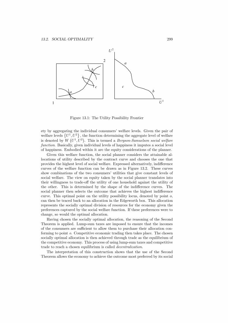
13.2. SOCIAL OPTIMALITY 299
a
bc
2U
1U1
2
a
b
c
Figure 13.1: The Utility Possibility Frontier
ety by aggregating the individual consumers’ welfare levels. Given the pair ofwelfare levels
©U1, U2
ª, the function determining the aggregate level of welfare
is denoted by W¡U1, U2
¢. This is termed a Bergson-Samuelson social welfare
function. Basically, given individual levels of happiness it imputes a social levelof happiness. Embodied within it are the equity considerations of the planner.Given this welfare function, the social planner considers the attainable al-
locations of utility described by the contract curve and chooses the one thatprovides the highest level of social welfare. Expressed alternatively, indifferencecurves of the welfare function can be drawn as in Figure 13.2. These curvesshow combinations of the two consumers’ utilities that give constant levels ofsocial welfare. The view on equity taken by the social planner translates intotheir willingness to trade-off the utility of one household against the utility ofthe other. This is determined by the shape of the indifference curves. Thesocial planner then selects the outcome that achieves the highest indifferencecurve. This optimal point on the utility possibility locus, denoted by point o,can then be traced back to an allocation in the Edgeworth box. This allocationrepresents the socially optimal division of resources for the economy given thepreferences captured by the social welfare function. If these preferences were tochange, so would the optimal allocation.Having chosen the socially optimal allocation, the reasoning of the Second
Theorem is applied. Lump-sum taxes are imposed to ensure that the incomesof the consumers are sufficient to allow them to purchase their allocation con-forming to point o. Competitive economic trading then takes place. The chosensocially optimal allocation is then achieved through trade as the equilibrium ofthe competitive economy. This process of using lump-sum taxes and competitivetrade to reach a chosen equilibrium is called decentralization.The interpretation of this construction shows that the use of the Second
Theorem allows the economy to achieve the outcome most preferred by its social

300 CHAPTER 13. OPTIMALITY AND COMPARABILITY
o
1U
2U
Figure 13.2: Social Optimality
planner. Given the economy’s limited initial stock of resources, the sociallyoptimal allocation is both efficient and, relative to the social welfare function,equitable. In this way, the application of the Second Theorem can be saidto solve the economic problem since the issues of both efficiency and equityare resolved to the greatest extent possible and there is no better outcomeattainable. Clearly, if this reasoning is applicable, all that a policy maker needdo is choose the allocation, implement the required lump-sum taxes and ensurethat the economy is competitive. No further policy or action is needed. Oncethe incomes are set, the economy will take itself to the optimal outcome.
13.3 Lump-Sum Taxes
The role of lump-sum taxes has been made very explicit in describing the appli-cation of the Second Theorem. In the economic environment envisaged, lump-sum taxes are the only tool of policy that is required beyond an active compe-tition policy. To justify the use of policies other than lump-sum taxes, it mustbe established that such taxes are either not feasible or else are restricted inthe way in which they can be employed. This is the purpose of this section.The results described are important in their own right, but they also provideimportant insights into the design of other forms of taxation. The argument isdeveloped further in Section 17.3.In order for a tax to be lump-sum, the consumer on whom the tax is levied
must not be able to affect the size of the tax by changing their behavior. Mosttax instruments encountered in practice are not lump-sum. Income taxes cannotbe lump-sum by this definition since a consumer can work more or less hard andvary income in response to the tax. Similarly, commodity taxes cannot be lump-sum since consumption patterns can be changed. Estate duties are lump-sum at
13.3. LUMP-SUM TAXES 301
the point at which they are levied (since by definition the person on which theyare levied is dead and unable to choose any other action) but can be affected bychanges in behavior prior to death (for instance by making gifts earlier in life).There are some taxes though that are close to being lump-sum. For exam-
ple, by taxing every consumer some fixed amount a lump-sum tax is imposed.Setting aside minor details, this was effectively the case of the United KingdomPoll Tax levied in the late 1980s as a source of finance for local government.This tax was unsuccessful for two reasons. Firstly, taxpayers could avoid payingthe tax by ensuring that their names did not appear on any official registers.Usually this was achieved by moving house and not making any official dec-laration of the new address. It appears large numbers of taxpayers did this(unofficial figures put the number as high as 1 million). This ”disappearance”is a change in behavior that reduces the tax burden. Secondly, the theoreticalefficiency of lump-sum taxes rests partly on the fact that their imposition iscostless but this was far from the case with the Poll Tax. In fact, the difficultiesof actually collecting and maintaining information on the residential address ofall households made the imposition of a uniform lump-sum tax prohibitivelyexpensive. The mobility of taxpayers proved to be much greater than had beenexpected. Therefore, although the structure of lump-sum taxes makes themappear deceptively simple to collect, this may not be the case in practice sincethe tax base, people, is highly mobile and keen to evade. Consequently, even auniform lump-sum tax proved difficult and costly to administer in practice.However, the costs of collection are only part of the issue. What is the pri-
mary concern here is the use of optimal lump-sum taxes. Optimal here meansa tax which is chosen, via application of the Second Theorem, to achieve theincome distribution necessary to decentralize a chosen allocation. The optimallump-sum tax system is unlikely to be a uniform tax upon each consumer be-cause the role of the taxes is fundamentally redistributive so they will be highlydifferentiated across consumers. Since uniform lump-sum taxes have difficultiesin implementation, the use of differentiated taxes will be faced with even greaterproblems.The extent of these problems can be seen by considering the information
needed to calculate the taxes. First, the social planner must be able to con-struct the contract curve of Pareto-efficient allocations so that they can selectthe social optimum. Secondly, the planner needs to predict the equilibriumthat will emerge for all possible income levels so that they can determine theincomes needed to decentralize the chosen allocation. Both of these steps re-quire knowledge of the consumers’ preferences. Finally, the social planner mustalso know the value of each consumer’s endowment in order to calculate theirincomes before tax and hence the lump-sum taxes that must be imposed. Thefundamental difficulty is that these economic characteristics, preferences andendowments, are private information. As such, they are known only to the in-dividual consumers and are not directly observed by the social planner. Thecharacteristics may be partly revealed through market choices, but these choicescan be changed if the consumers perceive any link with taxation. The fact thatlump-sum taxes are levied on private information is the fundamental difficulty
302 CHAPTER 13. OPTIMALITY AND COMPARABILITY
that hinders their use.Some characteristics of the consumers are public information, or at least can
be directly observed. Lump-sum taxes can then be levied upon these character-istics. For example, it may be possible to differentiate lump-sum taxes accordingto characteristics of the consumers such as sex, age or eye-color. However, thesecharacteristics are not those which are directly economically relevant as theyconvey neither preference information nor relate to the value of endowment.Although we could differentiate taxes on this basis, there is no reason why weshould want to do so.This returns us to the problem of private information. Since the relevant
characteristics such as ability are not observable, the social planner must ei-ther rely on consumers honestly reporting them or the characteristics must beinferred from the observed economic choices of consumers. If the planner re-lies upon the observation of choices, there is invariably scope for consumersto change their market behavior which then implies that the taxes cannot belump-sum. When reports are the sole source of information, unobserved char-acteristics cannot form a basis for taxation unless the tax scheme is such thatindividuals are faced with incentives to report truthfully.As an example of the interaction between taxes and reporting, consider the
following: Let the quality of a consumer’s endowment of labor be determined bytheir IQ level. Given a competitive market for labor, the value of the endowmentis then related to IQ. Assume there are no economically-relevant variables otherthan IQ, so that any set of optimal lump-sum taxes must be levied on IQ. If thelevel of lump-sum tax was inversely related to IQ and if all households had tocomplete IQ tests, then the tax system would not be cheated since the incentivewould always be to maximize the score on the test. In this case, the lump-sum taxes are said to be incentive compatible, meaning that they give incentivesto behave honestly. In contrast, if the taxes were positively related to IQ, atesting procedure could easily be manipulated by the high-IQ consumers whowould intentionally choose to perform poorly. If such a system were put intoplace, the mean level of tested IQ would be expected to fall considerably. Thisindicates the potential for misrevelation of characteristics and the system wouldnot be incentive compatible. Clearly, if a high-IQ results in higher earningsand, ultimately, greater utility a redistributive policy would require the use oflump-sum taxes that increased with IQ. The tax policy would not be incentivecompatible. Such problems will always be present in any attempt to base lump-sum taxes on unobservable characteristics.The main points of the argument can now be summarized. To implement
the Second Theorem as a practical policy tool it is necessary to employ optimallump-sum taxes. Such taxes are unlikely to be available in practice or to satisfyall the criteria required of them. The taxes may be costly to collect and thecharacteristics upon which they need to be based may not be observable. Whencharacteristics are not observable, the relationship between taxes and character-istics can give consumers the incentive to make false revelations. It is thereforebest to treat the Second Theorem as being of considerable theoretical interestbut of very limited practical relevance. The theorem shows us what could be
13.4. ASPECTS OF PARETO EFFICIENCY 303
possible, not what is possible.It is the impracticality of lump-sum taxation that provides the motive for
studying the properties of other tax instruments. The income taxes and com-modity taxes which are analyzed in Chapters 15 and 16 are second-best solutionsthat are used because the first-best solution, lump-sum taxation, is not avail-able. Lump-sum taxes are used as a benchmark from which to judge the relativesuccess of these alternative instruments. They also help to clarify what it is thatwe are really trying to tax.
13.4 Aspects of Pareto Efficiency
The analysis of lump-sum taxation has raised questions about the practical valueof the Second Theorem. The theorem shows how an optimal allocation can bedecentralized but the means to achieve the decentralization may be missing. Ifthe use of lump-sum taxes is restricted, then the government must resort toalternative policy instruments. All alternative instruments will be distortionaryand will not achieve the first-best.These criticisms do not extend to the First Theorem which states only that
a competitive equilibrium is Pareto efficient. Consequently, the First Theoremimplies no policy intervention, so it is safe from the restrictions on lump-sumtaxes. However, at the heart of the First Theorem is the use of Pareto efficiencyas a method for judging the success of an economic allocation. The value ofthe First Theorem can only be judged once a deeper understanding of Paretoefficiency has been developed.The Pareto criterion was introduced into economics by the Italian economist
Vilfredo Pareto at the beginning of the 20th century. This was during a period ofreassessment in economics during which the concept of utility as a measurablequantity was rejected. Alongside this rejection of measurability, the abilityto compare utility levels between consumers also had to be rejected. Paretoefficiency was therefore constructed explicitly to allow comparisons of allocationswithout the need to make any interpersonal comparisons of utility. As will beseen, this avoidance of interpersonal comparisons is both its strength and itsmain weakness.To assess Pareto efficiency, it is helpful to develop the concept in three
stages. The first stage defines the idea of making a Pareto improvement whenmoving from one allocation to another. From this can be constructed the Paretopreference order which judges whether one allocation is preferred to another.The final stage is to use Pareto preference to find the most preferred stateswhich are then defined as Pareto efficient. Reviewing each of these steps thenallows us to assess the meaning and value of the concept.Consider a move from economic state s1 to state s2. This is defined as a
Pareto improvement if it makes some consumers strictly better-off and noneworse-off. If there are H consumers, this definition can be stated formally bysaying a Pareto improvement is made in going from s1 to s2 if
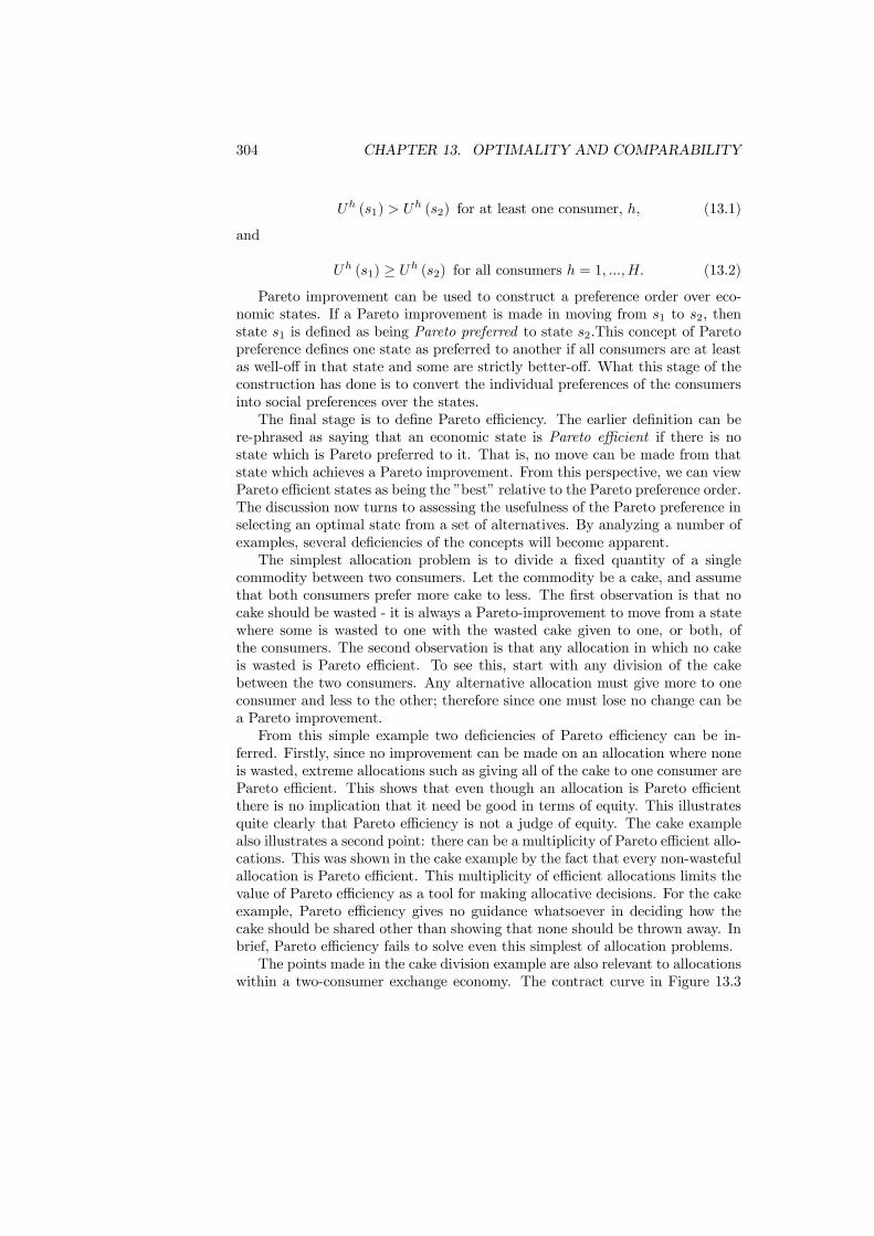
304 CHAPTER 13. OPTIMALITY AND COMPARABILITY
Uh (s1) > Uh (s2) for at least one consumer, h, (13.1)
and
Uh (s1) ≥ Uh (s2) for all consumers h = 1, ...,H. (13.2)
Pareto improvement can be used to construct a preference order over eco-nomic states. If a Pareto improvement is made in moving from s1 to s2, thenstate s1 is defined as being Pareto preferred to state s2.This concept of Paretopreference defines one state as preferred to another if all consumers are at leastas well-off in that state and some are strictly better-off. What this stage of theconstruction has done is to convert the individual preferences of the consumersinto social preferences over the states.The final stage is to define Pareto efficiency. The earlier definition can be
re-phrased as saying that an economic state is Pareto efficient if there is nostate which is Pareto preferred to it. That is, no move can be made from thatstate which achieves a Pareto improvement. From this perspective, we can viewPareto efficient states as being the ”best” relative to the Pareto preference order.The discussion now turns to assessing the usefulness of the Pareto preference inselecting an optimal state from a set of alternatives. By analyzing a number ofexamples, several deficiencies of the concepts will become apparent.The simplest allocation problem is to divide a fixed quantity of a single
commodity between two consumers. Let the commodity be a cake, and assumethat both consumers prefer more cake to less. The first observation is that nocake should be wasted - it is always a Pareto-improvement to move from a statewhere some is wasted to one with the wasted cake given to one, or both, ofthe consumers. The second observation is that any allocation in which no cakeis wasted is Pareto efficient. To see this, start with any division of the cakebetween the two consumers. Any alternative allocation must give more to oneconsumer and less to the other; therefore since one must lose no change can bea Pareto improvement.From this simple example two deficiencies of Pareto efficiency can be in-
ferred. Firstly, since no improvement can be made on an allocation where noneis wasted, extreme allocations such as giving all of the cake to one consumer arePareto efficient. This shows that even though an allocation is Pareto efficientthere is no implication that it need be good in terms of equity. This illustratesquite clearly that Pareto efficiency is not a judge of equity. The cake examplealso illustrates a second point: there can be a multiplicity of Pareto efficient allo-cations. This was shown in the cake example by the fact that every non-wastefulallocation is Pareto efficient. This multiplicity of efficient allocations limits thevalue of Pareto efficiency as a tool for making allocative decisions. For the cakeexample, Pareto efficiency gives no guidance whatsoever in deciding how thecake should be shared other than showing that none should be thrown away. Inbrief, Pareto efficiency fails to solve even this simplest of allocation problems.The points made in the cake division example are also relevant to allocations
within a two-consumer exchange economy. The contract curve in Figure 13.3
13.4. ASPECTS OF PARETO EFFICIENCY 305
Household 1
Household 2
Figure 13.3: Efficiency and Inequity
shows the set of Pareto efficient allocations and there is generally an infinitenumber of these. Once again the Pareto preference ordering does not select aunique optimal outcome. In addition, the competitive equilibrium may be asthe one illustrated in the bottom left corner of the box. This has the property ofbeing Pareto efficient but it is highly inequitable and may not find much favourusing other criteria for judging optimality.Another failing of the Pareto preference ordering is that it is not always able
to compare alternative states. In formal terms, it does not provide a completeordering of states. This is illustrated in Figure 13.4 where the allocations s1and s2 cannot be compared although both can be compared to s3 (s3 is Paretopreferred to both s1 and s2). When faced with a choice between s1 and s2, thePareto preference order is silent about which should be chosen. It should benoted that this incomparability is not the same as indifference. If the preferenceorder were indifferent between two states, then they are judged as equally good.Incomparability means the pair of states simply cannot be ranked.The basic mechanism at work behind this example is that the Pareto pref-
erence order can only rank alternative states if there are only gainers or losersas the move is made between the states. If some gain and some lose, as inthe choice between s1 and s2 in Figure 13.4, then the preference order is of novalue. Such gains and losses are invariably a feature of policy choices and muchof policy analysis consists of weighing-up the gains and losses. In this respect,the Pareto efficiency is inadequate as a basis for policy choice.To summarize these arguments, Pareto efficiency does not embody any con-
cept of justice and highly inequitable allocations can be efficient under the crite-rion. In many situations, the number of Pareto efficient allocations is infinite in

306 CHAPTER 13. OPTIMALITY AND COMPARABILITY
Household 1
Household 2
1s2s•
•
•
3s
Figure 13.4: Incompleteness of Pareto Ranking
which case the criterion then provides little guidance for policy choice. Finally,the Pareto efficiency may not provide a complete ordering of states so that somestates will be incomparable under the criterion. The source of all these failing isthat the Pareto criterion avoids weighing gains against losses but it is just suchjudgements that have to be made in most allocation decisions. To then makea choice of allocation the evaluation of the gains and losses have to be faceddirectly.
13.5 Social Welfare Functions
The social welfare function was employed in Section 13.2 to introduce the con-cept of a socially optimal allocation. At that point it was simply described asa means by which different allocations of utilities between consumers could besocially ranked. What was not done was to provide a convincing description ofwhere such a ranking could come from or of how it could be constructed. Threealternative interpretations will now be given, each of which provides a differentperspective upon the social welfare function.The first possibility is that the social welfare function captures the distribu-
tive preferences of a central planner or dictator. Under this interpretation, therecan be two meanings of the individual utilities that enter the function. One isthat they are the planner’s perception of the utility achieved by each consumerfor their level of consumption. This provides a consistent interpretation of thesocial welfare function but problems arise in its relation to the underlying model.To see why this is so, recall that the Edgeworth box, and the contract curvewithin it, were based upon the actual preferences of the consumers. This leads
13.5. SOCIAL WELFARE FUNCTIONS 307
to a potential inconsistency between this construction and the evaluation usingthe planner’s preferences. For example, what is a Pareto optimum under thetrue preferences may not be one under the planner’s (it need not even be anequilibrium). So, although this approach can justify the social welfare functionit is not internally consistent with the other components of the model.The alternative meaning of the utilities is that they are the actual utilities
of the consumers. This leads directly into the central difficulty faced in theconcept of social welfare. In order to evaluate all allocations of utility it mustbe possible to evaluate the social value of an increase in one consumer’s utilityagainst the loss in another’s. This is only possible if the utilities are comparableacross the consumers. More will be said about this below.An alternative interpretation of the social welfare function is that it captures
some ethical objective that society should be pursuing. Here the social welfarefunctions is determined by what is viewed as the just objective of society. Thereare two major examples of this. The utilitarian philosophy of aiming to achievethe greatest good for society as a whole translates into a social welfare func-tion that is the sum of individual utilities. In this formulation, only the totalsum of utilities counts, so it does not matter how utility is distributed betweenconsumers in the society. Alternatively, the Rawlsian philosophy of caring onlyfor the worst-off member of society leads to a level of social welfare determinedentirely by the minimum of that in society. With this objective, the distributionof utility is of paramount importance. Gains in utility achieved by anyone otherthan the worst-off consumer do not improve social welfare.Although this approach to the social welfare function is internally consistent
it is still not entirely satisfactory. The utilitarian approach requires that theutilities of the consumers are added in order to arrive at the total sum of socialwelfare. The Rawlsian approach necessitates the utility levels being comparedin order to find the lowest. The nature of comparability between utility may bedifferent for the two approaches (being able to add utilities is different to beingable to compare) but both do rely on some form of comparability. This againleads directly into the issue of utility comparisons.The final view that can be taken of the social welfare function is that it takes
the preferences of the individual consumers (represented by their utilities) andaggregates these into a social preference. This aggregation process would beexpected to obey certain rules; for instance if all consumers prefer one state toanother, it should be the case that the social preference also prefers the samestate. The structure of the social welfare function then emerges as a consequenceof the rules the aggregation must obey.Although this arrives at the same outcome as the other two interpretations,
it does so by a distinctly different process. In this case it is the set of rulesfor aggregation that are foremost rather than the form of social welfare. Thatis, the philosophy here would be that if the aggregation rules are judged assatisfactory then society should accept the social welfare function that emergesfrom their application, whatever its form. An example of this is that if the rulesof majority voting are chosen as the method of aggregating preferences (despitethe failings already identified in Chapter 4), then the minority must accept what
308 CHAPTER 13. OPTIMALITY AND COMPARABILITY
the majority chooses.The consequences of constructing a social welfare function by following this
line of reasoning are of fundamental importance in the theory of welfare eco-nomics. In fact, doing so leads straight back into Arrow’s Impossibility Theoremwhich was described in Chapter 4. The next section is dedicated to interpretingthe theorem and its implications in this new setting.
13.6 The Impossibility
Although they appear very distinct in nature, both majority voting and thePareto criterion are examples of procedures for aggregating individual prefer-ences into a social preference. It has been shown that neither is perfect. ThePareto preference order can be incomplete and is unable to rank some of thealternatives. Majority voting always leads to a complete social preference or-der but this may not be transitive. What Arrow’s theorem has shown is thatsuch failings are not specific to these aggregation procedures. All methods ofaggregation will fail to meet one or more of its conditions so it identifies a fun-damental problem at the heart of generating social preferences from individualpreferences.The conditions of Arrow’s theorem were stated in terms of the rankings
induced by individual preferences. However, since individual preferences canusually be represented by a utility function, the theorem also applies to theaggregation of individual utility functions into a social welfare function. Apply-ing the theorem, its implication is that a social welfare function does not existthat can aggregate individual utilities without conflicting with one, or more, ofthe conditions I.N.P.U.T . This means that whatever social welfare function isproposed, there will be some set of utility functions for which it conflicts withat least one of the conditions. An alternative way of looking at this is to viewif as saying that no ideal social welfare function can be found. No matter howsophisticated the aggregation mechanism is, it cannot overcome this theorem.Since the publication of Arrow’s theorem there has been a great deal of
research attempting to find a way out of the dead-end into which it leads.One approach that has been tried is to consider alternative sets of aggregationrules. For instance, transitivity of the social preference ordering can be relaxedto quasi-transitivity (only strict preference is transitive) or weaker versions ofCondition I and Condition P can be used. Most such changes just lead to furtherimpossibility theorems for these different sets of rules. Modifying the rules doesnot therefore really seem to be the way forward out of the impossibility.What is at the heart of the impossibility is the limited information contained
in individual utility functions. Effectively, all that is known are the individuals’rankings of the alternative - which is best, which is worst, and how they lineup in between. What it does not give is any strength of feeling either betweenalternatives for a given individual or across individuals for a given option. Suchstrength of feeling is an essential art of any attempt to make social decisions.Consider, for instance, a group of people choosing where to dine. In this sit-

13.7. INTERPERSONAL COMPARABILITY 309
uation a strong preference in one direction (”I don’t really want to eat fish”)usually counts for more than a mild preference (”I don’t really mind, but I wouldprefer fish”). Arrow’s theorem rules out any information of this kind.Using information on how strongly individuals feel about the alternatives
can be successful in choosing where to dine. It is interesting that strength ofpreference comparisons can be used in informal situations, but this does notdemonstrate that it can be incorporated within a scientific theory of socialpreferences. This issue is now addressed in detail.
13.7 Interpersonal Comparability
Earlier in this chapter it was noted that Pareto efficiency was originally proposedbecause it provided a means by which it was possible compare alternative allo-cations without requiring interpersonal comparisons of welfare. It is also fromthis avoidance of comparability that the failures of Pareto efficiency emerge.This point is also at the core of the impossibility theorem. To proceed further,this section first reviews the development of utility theory in order to provide acontext and then describes alternative degrees of utility comparability.Nineteenth century economists viewed utility, the level of happiness of an in-
dividual, as something that was potentially measurable. Advances in psychologywere expected to deliver the machinery for conducting the actual measurement.If utility were measurable, it follows naturally that it would be comparable be-tween individuals. This ability to measure utility, combined with the philosophythat society should aim for the greatest good, combined to provide the under-pinnings of utilitarianism. The measurability of utility permitted social welfareto be expressed by the sum of individual utilities. Ranking states by the value ofthis sum they achieved then gave a means of aggregating individual preferencesthat satisfied all of the conditions of the impossibility theorem except for theinformation content. If the envisaged degree of measurability could be achievedthen the restrictions of the impossibility theorem are overcome.This concept of measurable and comparable utility began to be dispelled in
the early Twentieth century. There were two grounds for this rejection. Firstly,no means of measuring utility had been discovered and it was becoming clearthat the earlier hopes would not be realized. Secondly, advances in economictheory showed that there was no need to have measurable utility in order todeduce a coherent theory of consumer choice. In fact, the entire theory ofthe consumer could be derived by specifying only the consumer’s preferenceordering. The role of utility then became strictly secondary - it could be invokedas a convenient functional representation of preferences if necessary, but wasotherwise redundant. Since utility had no deeper meaning attached to it, anyincreasing monotonic transformation of a utility function representing a set ofpreferences would also be an equally valid utility function. Utility was simplyan ordinal concept, with no natural zero or units of measurement. By the veryconstruction of utility, comparability between different consumers’ utilities wasa meaningless concept. This situation therefore left no scientific basis upon
310 CHAPTER 13. OPTIMALITY AND COMPARABILITY
which to justify the comparability of different consumer’s utility levels.This perspective on utility, and the consequent prevention of utility com-
parisons between consumers, created the necessity of developing concepts forsocial comparisons, such as Pareto efficiency, that were free of interpersonalcomparisons. However the weaknesses of these criteria soon became obvious.The analytical trend since the 1960’s has been to explore the consequencesof re-admitting interpersonal comparability into the analysis. The procedureadopted is basically to assume that comparisons are possible. This permits thederivation of results from which interpretations can be obtained. These arehoped to provide some general insights into policy which can be applied eventhough utility is not actually comparable in the way assumed.There are even some economists who would argue that comparisons are actu-
ally possible. One basis for this is the claim that all consumers have very similarunderlying preference orderings. All prefer to have more income to less, and con-sumers with equal incomes make very similar divisions of expenditures betweenalternative groups of commodities. That is, expenditure on food is similar, eventhose the actual foodstuffs purchased may be very different. In modelling suchconsumers it is possible to assert that they all have the same utility functionguiding their choices. This makes their utilities directly comparable.So far comparability has been used as a catch-all phrase for being able to
draw some contrast between the utility levels of consumers. In fact, manydifferent degrees of comparability can be envisaged. For instance, the claimthat one household has a higher level of utility than another requires ratherless comparability than claiming it has 15% more utility. Different degrees ofcomparability have implications for the way in which they can be aggregatedinto a social preference ordering.The starting point is to define the two major forms of utility. The first is
ordinal utility which is the familiar concept from consumer theory. Essentially,an ordinal utility function is no more than just a numbering of a consumer’s in-difference curves, with the numbering chosen so that higher indifference curveshave higher utility numbers. These numbers can be subjected to any formof transformation without altering their meaning provided the transformationleaves the ranking of the numbers unchanged - higher indifference curves muststill have larger utility numbers attached. Because they can be so freely trans-formed, there is no meaning to differences in utility levels between two situationsfor a single consumer except which of the two provides the higher utility.The second form of utility is cardinal utility. Cardinal utility imposes re-
strictions beyond those of ordinal utility. With cardinal utility you can onlytransform utility numbers by multiplying by a constant and then adding a con-stant, so an initial utility function U becomes the transformed utility U = a+bUwhere a and b are the constants. Any other form of transformation will affectthe meaning of a cardinal utility function. The typical place in which cardi-nal utility is found is in the economics of uncertainty since an expected utilityfunction is cardinal. This cardinal is a consequence of the fact that an expectedutility function must provide a consistent ranking for different probability dis-tributions of the outcomes and this consistency imposes cardinality. A second,

13.7. INTERPERSONAL COMPARABILITY 311
non-economic, example of a cardinal scale is temperature. It is possible to con-vert Celsius to Fahrenheit by multiplying by 9
5 and adding 32 (and the conversetransformation from Fahrenheit to Celsius is to multiply by 5
9 and subtract 32).With these definitions it now becomes possible to talk in detail about compa-rability and non-comparability.
Non-comparability can arise with both ordinal and cardinal utility. Whatnon-comparability means is that we can apply different transformations to dif-ferent consumers’ utilities. To express this in formal terms, let U1 be the utilityfunction of consumer 1 and U2 the utility function of consumer 2. Then non-comparability arises if the transformation f1 can be applied to U1 and a differenttransformation f2 to U2, with no relationship between f1 and f2. Why is thisnon-comparable? Because by suitably choosing f1 and f2 it is always possi-ble to one ranking of the initial utilities and to arrive at a different rankingof the transformed utilities. The utility information therefore does not providesufficient information to make a comparison of the two utility levels.
Comparability exists when the transformations that can be applied to theutility functions are restricted. With ordinal utility there is only one possibledegree of comparability. This occurs when the ordinal utilities for differentconsumers can be subjected only to the same transformation. The implicationof this is that the transformation preserves the ranking of utilities betweendifferent consumers, so if one consumer has a higher utility than the other beforethe transformation, they will have a higher utility after the transformation.Letting this transformation be denoted by f , then if U1 ≥ U2 it must be thecase that f
¡U1¢ ≥ f ¡U2¢ . This form of comparability is called ordinal level
comparability.
If the underlying utility functions are cardinal, then there are two forms ofcomparability that are worth discussing. The first form of comparability is toassume that the constant multiplying utility in the transformation must be thesame for all consumers, but the constant that is added can differ. Hence, for twoconsumers the transformed utilities are U1 = a1 + bU1 and U2 = a2 + bU2, sothe constant b is the same for both. This is called cardinal unit comparability.The implication of this transformation is that it now becomes meaningful totalk about the effect of changes in utility, meaning that gains to one consumercan be measured against losses to another - and whether the gain exceeds theloss is not affected by the transformation.
The second degree of comparability for cardinal utility is to further restrictthe constant a in the transformation to be the same for both consumers. Forall consumers the transformed utility becomes eUh = a+ bUh. It is now possiblefor both changes in utility and levels of utility to be compared. This is form ofcomparability is called cardinal full comparability.
The next step is to explore the implications of these comparabilities for theconstruction of social welfare functions. It will be shown that each form ofcomparability implies different permissible social welfare functions.

312 CHAPTER 13. OPTIMALITY AND COMPARABILITY
13.8 Comparability and Social WelfareThe discussion of Arrow’s Impossibility showed that the failure to successfullygenerate a social preference ordering from a set of individual preference orderingswas the result of limited information. The information content of an individual’spreference order involves nothing more than knowing how they rank the alter-natives. A preference order does not convey any information on the strength ofpreferences or allow comparison of utility levels across consumers. When moreinformation is available then it becomes possible to find social preference order-ings that satisfy the conditions I.N.P.U.T . Such information can be introducedby building social preferences upon individual utility functions that allow forcomparability.What this section shows is that for each form of comparability there is a
specification of social welfare function that is consistent with the informationcontent of the comparable utilities. To explain what is meant by consistent,recall that comparability is described by a set of permissible transformations ofutility. A social welfare function is consistent if it ranks the set of alternativesocial states in the same way for all permissible transformations of the utilityfunctions. Since increasing the degree of comparability reduces the number ofpermissible transformations, it has the effect of increasing the set of consistentsocial welfare functions.Let the utility obtained by consumer h from allocation s be Uh (s) . A trans-
formation of this basic utility function is denoted by Uh (s) = fh¡Uh (s)
¢.
The value of social welfare at allocation s using the basic utilities is W (s) =W¡U1 (s) , ..., UH (s)
¢and that from using the transformed utilities is W (s) =
W³U1 (s) , ..., UH (s)
´. Given alternative allocations A and B, the social wel-
fare function is consistent with the transformation (and hence the form of com-parability) if W (A) ≥W (B) implies W (A) ≥ W (B). In words, if A generateshigher social welfare than B for the basic utilities, it will also do so for thetransformed utilities.To demonstrate these points, assume there are two consumers with the basic
utility functions U1 =¡x1¢ 12¡y1¢ 12 and U2 = x2 + y2, where xh and yh are
the consumption levels of goods x and y. Further assume that there are twoallocations A and B with the consumption levels, and the resulting utilities, asshown in Table 13.1.
x1 y1 U1 x2 y2 U2
A 4 9 6 3 2 5B 16 1 4 2 5 7Table 13.1: Allocations and Utility
The first point to establish is that it is possible to find a social welfarefunction that is consistent with ordinal level comparability but that none thatis consistent with ordinal non-comparability. What level comparability allowsis the ranking of consumers by utility level (think of placing the consumers ina line with the lowest utility level first). A position in this line (e.g. the first,
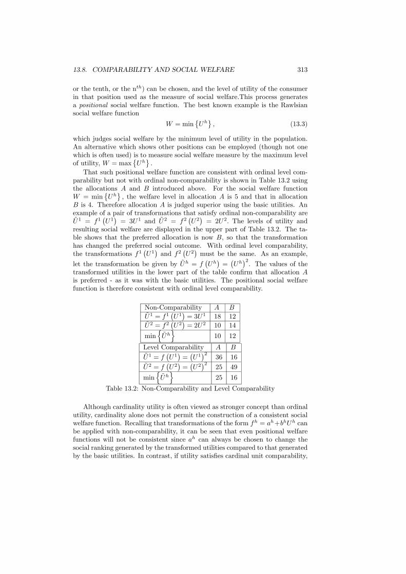
13.8. COMPARABILITY AND SOCIAL WELFARE 313
or the tenth, or the nth) can be chosen, and the level of utility of the consumerin that position used as the measure of social welfare.This process generatesa positional social welfare function. The best known example is the Rawlsiansocial welfare function
W = min©Uhª, (13.3)
which judges social welfare by the minimum level of utility in the population.An alternative which shows other positions can be employed (though not onewhich is often used) is to measure social welfare measure by the maximum levelof utility, W = max
©Uhª.
That such positional welfare function are consistent with ordinal level com-parability but not with ordinal non-comparability is shown in Table 13.2 usingthe allocations A and B introduced above. For the social welfare functionW = min
©Uhª, the welfare level in allocation A is 5 and that in allocation
B is 4. Therefore allocation A is judged superior using the basic utilities. Anexample of a pair of transformations that satisfy ordinal non-comparability areU1 = f1
¡U1¢= 3U1 and U2 = f2
¡U2¢= 2U2. The levels of utility and
resulting social welfare are displayed in the upper part of Table 13.2. The ta-ble shows that the preferred allocation is now B, so that the transformationhas changed the preferred social outcome. With ordinal level comparability,the transformations f1
¡U1¢and f2
¡U2¢must be the same. As an example,
let the transformation be given by Uh = f¡Uh¢=¡Uh¢2. The values of the
transformed utilities in the lower part of the table confirm that allocation Ais preferred - as it was with the basic utilities. The positional social welfarefunction is therefore consistent with ordinal level comparability.
Non-Comparability A B
U1 = f1¡U1¢= 3U1 18 12
U2 = f2¡U2¢= 2U2 10 14
minnUho
10 12
Level Comparability A B
U1 = f¡U1¢=¡U1¢2
36 16
U2 = f¡U2¢=¡U2¢2
25 49
minnUho
25 16
Table 13.2: Non-Comparability and Level Comparability
Although cardinality utility is often viewed as stronger concept than ordinalutility, cardinality alone does not permit the construction of a consistent socialwelfare function. Recalling that transformations of the form fh = ah+bhUh canbe applied with non-comparability, it can be seen that even positional welfarefunctions will not be consistent since ah can always be chosen to change thesocial ranking generated by the transformed utilities compared to that generatedby the basic utilities. In contrast, if utility satisfies cardinal unit comparability,
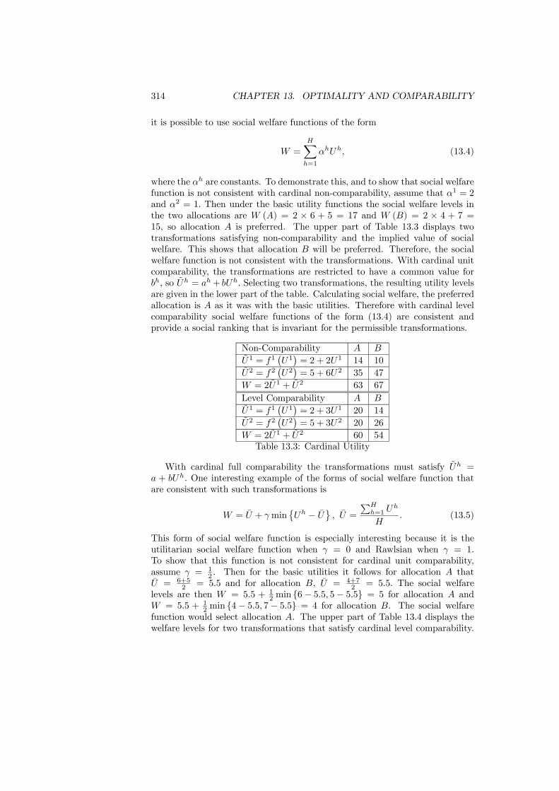
314 CHAPTER 13. OPTIMALITY AND COMPARABILITY
it is possible to use social welfare functions of the form
W =HXh=1
αhUh, (13.4)
where the αh are constants. To demonstrate this, and to show that social welfarefunction is not consistent with cardinal non-comparability, assume that α1 = 2and α2 = 1. Then under the basic utility functions the social welfare levels inthe two allocations are W (A) = 2 × 6 + 5 = 17 and W (B) = 2 × 4 + 7 =15, so allocation A is preferred. The upper part of Table 13.3 displays twotransformations satisfying non-comparability and the implied value of socialwelfare. This shows that allocation B will be preferred. Therefore, the socialwelfare function is not consistent with the transformations. With cardinal unitcomparability, the transformations are restricted to have a common value forbh, so Uh = ah+ bUh. Selecting two transformations, the resulting utility levelsare given in the lower part of the table. Calculating social welfare, the preferredallocation is A as it was with the basic utilities. Therefore with cardinal levelcomparability social welfare functions of the form (13.4) are consistent andprovide a social ranking that is invariant for the permissible transformations.
Non-Comparability A B
U1 = f1¡U1¢= 2 + 2U1 14 10
U2 = f2¡U2¢= 5 + 6U2 35 47
W = 2U1 + U2 63 67Level Comparability A B
U1 = f1¡U1¢= 2 + 3U1 20 14
U2 = f2¡U2¢= 5 + 3U2 20 26
W = 2U1 + U2 60 54Table 13.3: Cardinal Utility
With cardinal full comparability the transformations must satisfy Uh =a + bUh. One interesting example of the forms of social welfare function thatare consistent with such transformations is
W = U + γmin©Uh − Uª , U = PH
h=1 Uh
H. (13.5)
This form of social welfare function is especially interesting because it is theutilitarian social welfare function when γ = 0 and Rawlsian when γ = 1.To show that this function is not consistent for cardinal unit comparability,assume γ = 1
2 . Then for the basic utilities it follows for allocation A thatU = 6+5
2 = 5.5 and for allocation B, U = 4+72 = 5.5. The social welfare
levels are then W = 5.5 + 12 min {6− 5.5, 5− 5.5} = 5 for allocation A and
W = 5.5 + 12 min {4− 5.5, 7− 5.5} = 4 for allocation B. The social welfare
function would select allocation A. The upper part of Table 13.4 displays thewelfare levels for two transformations that satisfy cardinal level comparability.

13.9. CONCLUSIONS 315
With these transformed utilities the welfare function would select allocation B,so the social welfare function is not valid for these transformations. The lowerpart of the table displays a transformation that satisfies cardinal full compara-bility. For this transformation the social welfare function selects allocation A forboth the basic and the transformed utilities. This demonstrates the consistency.
Level Comparability A B
U1 = f1¡U1¢= 7 + 3U1 25 19
U2 = f2¡U2¢= 1 + 3U2 16 22
W = U + 12 min
©Uh − Uª 18.25 19.75
Full Comparability A B
U1 = f1¡U1¢= 1 + 3U1 19 13
U2 = f2¡U2¢= 1 + 3U2 16 22
W = U + 12 min
©Uh − Uª 16.75 15.25
Table 13.4: Full Comparability
These calculations have demonstrated that if we can compare utility levelsbetween consumers then a consistent social welfare function can be constructed.The resulting social welfare function must agree with the information content inthe utilities, so each form of comparability leads to a different consistent socialwelfare function. As the information increases, so does the range of consistentsocial welfare functions. Expressed differently, for each of the cases of compara-bility the problem of aggregating individual preferences leads to a well-definedform of social welfare function. All of these social welfare functions will gen-erate a social preference ordering that completely ranks the alternative states.They are obviously stronger in content than majority voting or Pareto efficiency.The drawback is that they are reliant on stronger utility information that maysimply not exist.
13.9 Conclusions
This chapter has cast a critical eye over the efficiency theorems of Chapter 7.Although these theorems are important for providing a basic framework in whichto think about policy, they are not an end in their own right. This perspective isbased on the limited practical applicability of the lump-sum transfers needed tosupport the decentralization in the Second Theorem and the weakness of Paretoefficiency as a method of judging between economic states.Although at first sight the theorems apparently have very strong implica-
tions, they become weakened when placed under critical scrutiny. But they arenot without value. Much of the subject matter of public economics takes asits starting point the practical shortcomings of these theorems and attemptsto find a way forward to something that is applicable. A knowledge of whatcould be achieved if the optimal lump-sum transfers were available provides ameans of assessing the success of what can be achieved and shows ways in whichimprovements in policy can be made.
316 CHAPTER 13. OPTIMALITY AND COMPARABILITY
The other aspect involved in the Second Theorem is the selection of theoptimal allocation to be decentralized. This choice requires a social welfarefunction that can be used to judge between different allocations of utility be-tween consumers. Such a social welfare function can only be constructed ifthe consumers’ utilities are comparable. The chapter described several differentforms of comparability and the social welfare functions that are consistent withthese.
Further readingArrow’s Impossibility Theorem was first demonstrated in:Arrow, K.J. (1950) “A difficulty in the concept of social welfare“, Journal
of Political Economy, 58, 328 - 346,and further elaborated in:Arrow, K.J. (1951) Social Choice and Individual Values (New York: Wiley).A comprehensive textbook treatment is given by:Kelly, J. (1987) Social Choice Theory: An Introduction (Berlin: Springer
Verlag).The concept of a social welfare function was first introduced by:Bergson, A. (1938) “A reformulation of certain aspects of welfare economics“,
Quarterly Journal of Economics, 68, 233 - 252.An analysis of limitations upon the use of lump-sum taxation is contained
in:Mirrlees, J.A. (1986) “The theory of optimal taxation“ in K.J. Arrow and
M.D. Intrilligator (eds.), Handbook of Mathematical Economics, Amsterdam:North-Holland.An economic assessment of the UK poll tax is conducted in:Besley, T., I. Preston and M. Ridge (1997) ”Fiscal anarchy in the UK: mod-
elling poll tax noncompliance”, Journal of Public Economics, 64, 137 - 152.Comparability of utility is discussed in:Ng, Y.-K. (2003) Welfare Economics, (Basingstoke: Macmillan).A discussion of the relation between social welfare functions and Arrow’s
theorem can be found in:Samuelson, P.A. (1977) “Reaffirming the existence of “reasonable“ Bergson-
Samuelson social welfare functions“, Economica, 44, 81 - 88.Several of Sen’s papers that discuss these issues are collected in:Sen, A.K. (11982) Choice, Welfare and Measurement, Oxford: Basil Black-
well.

Chapter 14
Inequality and Poverty
14.1 Introduction
A social welfare function permits the evaluation of economic policies that causeredistribution between consumers - a task that Pareto efficiency can never ac-complish. Although the concept of a social welfare function is a simple one,previous chapters have identified numerous difficulties on the path between in-dividual utility and aggregate social welfare. The essence of these difficultiesis that if the individual utility function corresponds with what is theoreticallyacceptable, then its information content is too limited for social decision making.The motivation for employing a social welfare function was to be able to
address issues of equity as well as issues of efficiency. Fortunately, a socialwelfare function is not the only way to do this and, as this chapter will show,we can construct measures of the economic situation that relate to equity andwhich are based on observable and measurable information. This provides a setof tools which can be, and frequently are, applied in economic policy analysis.They may not meet some of the requirements of the ideal social welfare functionbut they have the distinct advantage of being practically implementable.Inequality and poverty provide two alternative perspectives upon the equity
of the income distribution. Inequality of income means that some householdshave higher incomes than others - which is a basic source for an inequity in wel-fare. Poverty exists when some households are too poor to achieve an acceptablestandard of living. An inequality measure is a means of assigning a single num-ber to the observed income distribution that reflects its degree of inequality. Apoverty measure achieves the same for poverty. Although measures of inequalityand poverty are not themselves social welfare functions, the chapter will revealthe closeness of the link between the two concepts.The starting point of the chapter is a discussion of income. There are two
aspects to this: the definition of income and the comparison of income acrossfamilies with different compositions. In a setting of certainty, income is a clearlydefined concept. When there is uncertainty, differences can arise between ex ante
317

318 CHAPTER 14. INEQUALITY AND POVERTY
and ex post definitions. Given this, we look at alternative definitions and relatethese to the treatment of income for tax purposes. If two households differ intheir composition (for example, one household is a single person and the otheris a family of four), a direct comparison of their income levels will reveal littleabout the standard of living they achieve. Instead the incomes must be adjustedto take account of composition and then compared. The tool use to make theadjustment is an equivalence scale. We review the use of equivalence scales andsome of the issues that they raise.Having arrived at a set of correctly defined income levels which have been
adjusted for family composition using an equivalence scale, it becomes possibleto evaluate inequality and poverty. A number of the commonly-used measuresof each of these concepts are discussed and their properties investigated. Im-portantly, the link is drawn between measures of inequality and the welfareassumptions that are implicit within them. This leads into the idea of makingthe welfare assumptions explicit and building the measure up from these. Tomeasure poverty it is necessary to determine who is “poor” which is achievedby choosing a level of income as the poverty line and labelling as poor all thosewho fall below it. As well as discussing measures of poverty, we also reviewissues concerning the definition of the poverty line and the concept of povertyitself.Although the aim of this chapter was to move away from utility concepts
towards practical tools, it is significant that we keep returning to utility in theassessment and improvement of the tools. In attempting to refine, for example,an equivalence scale or a measure of inequality it is found that it is necessaryto comprehend the utility-basis of the measure. Despite intentionally startingin a direction away from utility, the theory returns us back to utility on everyoccasion.
14.2 Measuring Income
What is income? The obvious answer is that it is the additional resources aconsumer receives over a given period of time. The reference to a time periodis important here since income is a flow, so the period over which measurementtakes place must be specified. Certainly, evaluating the receipt of resources isthe basis of the definition used in the assessment of income for tax purposes.This definition works in a practical setting, but only in a backward-lookingsense. What an economist needs in order to understand behavior, especiallywhen choices are made in advance of income being received, is a forward-lookingmeasure of income. If the flow of income is certain, then there is no distinc-tion between backward- and forward-looking measures. It is when income isuncertain that differences emerge.The relevance of this issue is that both inequality and poverty measures use
income data as their basic input. The resulting measures will only be as accurateas the data that is employed to evaluate them. The data will be accurate wheninformation is carefully collected and a consistent definition is used of what is
14.2. MEASURING INCOME 319
to be measured. To evaluate the level of inequality or poverty, a necessary firststep is to resolve the issues surrounding the definition of income.The classic backward-looking definition of income was provided by Simons in
1938. This definition is “Personal income may be defined as the algebraic sumof (1) the market value of rights exercised in consumption and (2) the change inthe value of the store of property rights between the beginning and end of theperiod in question”. The essential feature of this definition is that it makes anattempt to be inclusive so as to incorporate all income regardless of the source.Although income definitions for tax purposes also adopt the backward-looking
viewpoint, they do not precisely satisfy the Simons’ definition. The divergencearises through the practical difficulties of assessing some sources of income es-pecially those arising from capital gains. According to the Simons’ definition,the increase in the value of capital assets should be classed as income. However,if the assets are not liquidated, the capital gain will not be realized during theperiod in question and will not be received as an income flow. For this reason,capital gains are taxed only upon realization. In the converse situation whencapital losses are made, most tax codes place limits upon the extent to whichthey can be offset against income.We have so far worked with the natural definition of income as the flow
of additional resources. To proceed further it becomes more helpful to adopta different perspective and to view the level of income by the benefits it candeliver. Since income is the means to achieve consumption, the flow of incomeduring a fixed time period can be measured as the value of consumption thatcan be undertaken while leaving the household with the same stock of wealthat the end of the period as it had at the start of the period. The benefit of thisperspective is that it extends naturally to situations where the income flow isuncertain. Building upon it, in 1939 Hicks provided what is generally taken asthe standard definition of income with uncertainty. This definition states that“income is the maximum value which a man can consume during a week andstill expect to be as well-off at the end of the week as he was at the beginning”.
This definition can clearly cope with uncertainty since it operates in expec-tational terms. But this advantage is also its major shortcoming when a move ismade towards applications. Expectations may be ill-defined or even irrational,so evaluation of the expected income flow may be unreasonably high or low. Aliteral application of the definition would not count windfall gains, such as un-expected gifts or lottery wins, as income because they are not expected despitesuch gains clearly raising the potential level of consumption. For these reasons,the Hicks definition of income is informative but not perfect.These alternative definitions of income have highlighted the distinctions be-
tween ex ante and ex post measures. Assessments of income for tax purposes usethe backward-looking viewpoint and measure income as all relevant paymentsreceived over the measurement period. Practical issues limit the extent to whichsome sources of income can be included, so the definition of income in tax codesdoes not precisely satisfy any of the formal definitions. This observation justreflects the fact that there is no unambiguously perfect definition of income.

320 CHAPTER 14. INEQUALITY AND POVERTY
14.3 Equivalence Scales
The fact that households differ in size and age distribution means that welfarelevels cannot be judged just by looking at their income levels. A household ofone adult with no children needs less income to achieve a given level of welfarethan a household with two adults and one child. In the words of the economistGorman, “When you have a wife and a baby, a penny bun costs threepence”.A larger household obviously needs more income to achieve a given level ofutility but the question is how much more income? Equivalence scales are theeconomist’s way of answering this question and provide the means of adjustingmeasured incomes into comparable quantities.Differences between households arise in the number of adults and the number
and ages of dependants. These are called demographic variables. The generalproblem in designing equivalence scales is to achieve the adjustment of observedincome to take account of demographic differences in household composition.Several ways exist to do this and these are now discussed.The first approach to equivalence scales is based on the concept of minimum
needs. A bundle of goods and services that is seen as representing the mini-mum needs for the household is identified. The exact bundle will differ betweenhouseholds of varying size but typically involves only very basic commodities.The cost of this bundle for families with different compositions is then calculatedand the ratio of these costs for different families provides the equivalence scale.The first application of this approach was by Rowntree in 1901 in his pioneeringstudy of poverty. The bundle of goods employed was just a minimum accept-able quantity of food, rent and a small allowance for “household sundries”. Theequivalence scale was then constructed by assigning the expenditure for a two-adult household with no children the index of 100 and measuring costs for allother household compositions relative to this. The scale obtained from expen-ditures calculated by Rowntree are given in the first column of Table 14.1. Theinterpretation of these figures is that the minimum needs of a couple with onechild cost 24% more than for a couple with no children.A similar approach was taken by Beveridge in his construction of the expen-
diture requirements that provided the foundation for the introduction of socialassistance in the UK. In addition to the goods in the bundle of Rowntree, Bev-eridge added fuel, light and a margin for “inefficiency” in purchasing. Also, thecost assigned to children increased with their age. The values of the BeveridgeScale in the second column of Table 14.1 are for children in the 5 - 10 age group.The final column of the table is generated from the income levels that are
judged to represent poverty in the US for families with different compositions.The original construction of these poverty levels was undertaken by Orshanskyin 1963. The method she used was to evaluate the cost of food for the eachfamily composition using the 1961 Economy Food Plan. Next, it was observedthat if expenditure upon food, F, constituted θ% of the family’s budget thentotal needs would be 1θF. For a family of two, θ was taken as 3.7 and for a familyof three or more θ was 3. The exception to this process was to evaluate the costfor a single person as 80% of that of a couple. The minimum expenditures
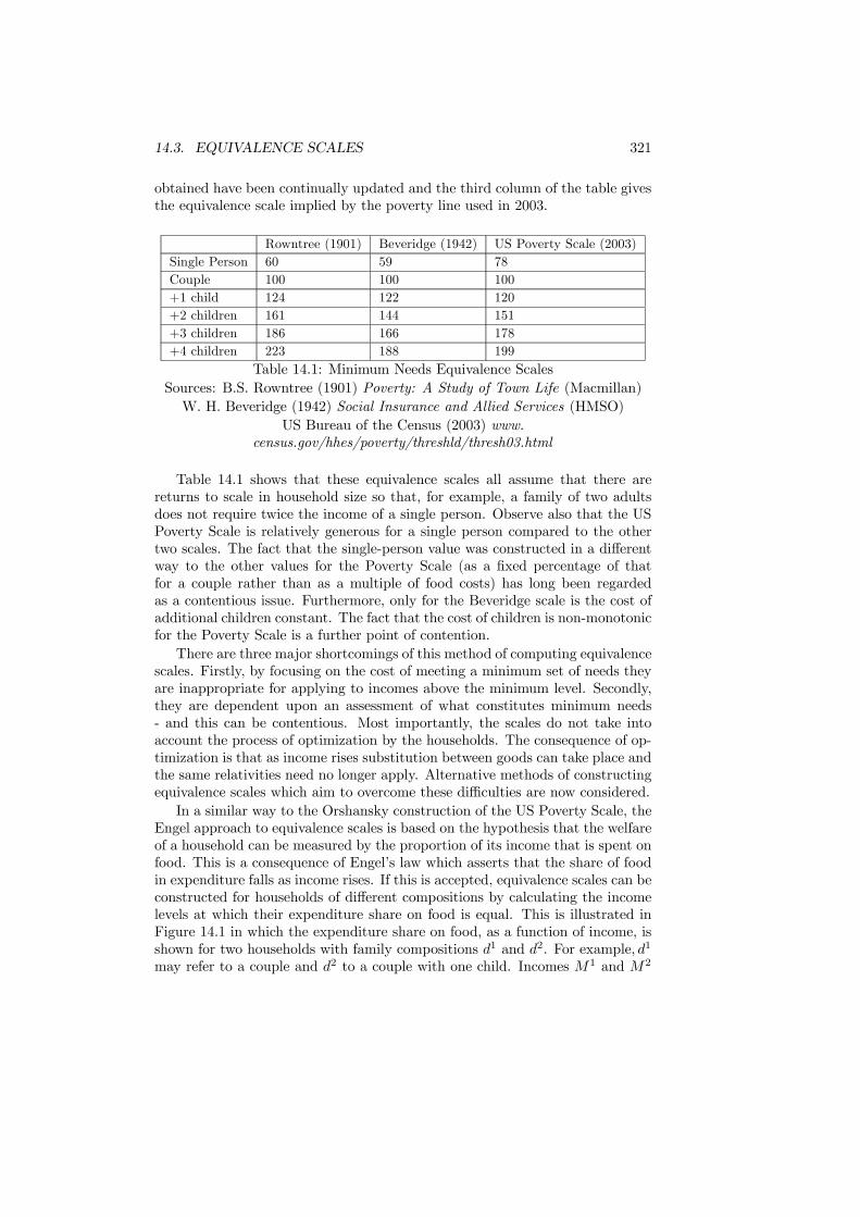
14.3. EQUIVALENCE SCALES 321
obtained have been continually updated and the third column of the table givesthe equivalence scale implied by the poverty line used in 2003.
Rowntree (1901) Beveridge (1942) US Poverty Scale (2003)Single Person 60 59 78Couple 100 100 100+1 child 124 122 120+2 children 161 144 151+3 children 186 166 178+4 children 223 188 199
Table 14.1: Minimum Needs Equivalence ScalesSources: B.S. Rowntree (1901) Poverty: A Study of Town Life (Macmillan)W. H. Beveridge (1942) Social Insurance and Allied Services (HMSO)
US Bureau of the Census (2003) www.census.gov/hhes/poverty/threshld/thresh03.html
Table 14.1 shows that these equivalence scales all assume that there arereturns to scale in household size so that, for example, a family of two adultsdoes not require twice the income of a single person. Observe also that the USPoverty Scale is relatively generous for a single person compared to the othertwo scales. The fact that the single-person value was constructed in a differentway to the other values for the Poverty Scale (as a fixed percentage of thatfor a couple rather than as a multiple of food costs) has long been regardedas a contentious issue. Furthermore, only for the Beveridge scale is the cost ofadditional children constant. The fact that the cost of children is non-monotonicfor the Poverty Scale is a further point of contention.There are three major shortcomings of this method of computing equivalence
scales. Firstly, by focusing on the cost of meeting a minimum set of needs theyare inappropriate for applying to incomes above the minimum level. Secondly,they are dependent upon an assessment of what constitutes minimum needs- and this can be contentious. Most importantly, the scales do not take intoaccount the process of optimization by the households. The consequence of op-timization is that as income rises substitution between goods can take place andthe same relativities need no longer apply. Alternative methods of constructingequivalence scales which aim to overcome these difficulties are now considered.In a similar way to the Orshansky construction of the US Poverty Scale, the
Engel approach to equivalence scales is based on the hypothesis that the welfareof a household can be measured by the proportion of its income that is spent onfood. This is a consequence of Engel’s law which asserts that the share of foodin expenditure falls as income rises. If this is accepted, equivalence scales can beconstructed for households of different compositions by calculating the incomelevels at which their expenditure share on food is equal. This is illustrated inFigure 14.1 in which the expenditure share on food, as a function of income, isshown for two households with family compositions d1 and d2. For example, d1
may refer to a couple and d2 to a couple with one child. Incomes M1 and M2
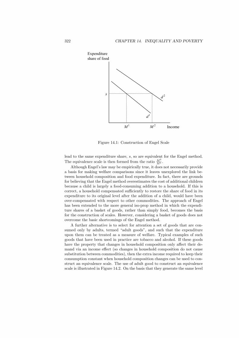
322 CHAPTER 14. INEQUALITY AND POVERTY
Income
Expenditure share of food
1d
2d
2M1M
s
Figure 14.1: Construction of Engel Scale
lead to the same expenditure share, s, so are equivalent for the Engel method.The equivalence scale is then formed from the ratio M2
M1 .Although Engel’s law may be empirically true, it does not necessarily provide
a basis for making welfare comparisons since it leaves unexplored the link be-tween household composition and food expenditure. In fact, there are groundsfor believing that the Engel method overestimates the cost of additional childrenbecause a child is largely a food-consuming addition to a household. If this iscorrect, a household compensated sufficiently to restore the share of food in itsexpenditure to its original level after the addition of a child, would have beenover-compensated with respect to other commodities. The approach of Engelhas been extended to the more general iso-prop method in which the expendi-ture shares of a basket of goods, rather than simply food, becomes the basisfor the construction of scales. However, considering a basket of goods does notovercome the basic shortcomings of the Engel method.A further alternative is to select for attention a set of goods that are con-
sumed only by adults, termed “adult goods”, and such that the expenditureupon them can be treated as a measure of welfare. Typical examples of suchgoods that have been used in practice are tobacco and alcohol. If these goodshave the property that changes in household composition only affect their de-mand via an income effect (so changes in household composition do not causesubstitution between commodities), then the extra income required to keep theirconsumption constant when household composition changes can be used to con-struct an equivalence scale. The use of adult good to construct an equivalencescale is illustrated in Figure 14.2. On the basis that they generate the same level
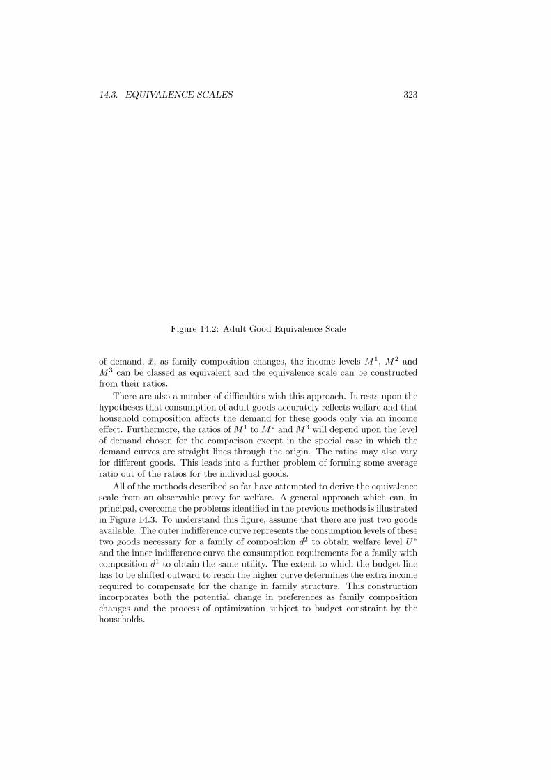
14.3. EQUIVALENCE SCALES 323
Figure 14.2: Adult Good Equivalence Scale
of demand, x, as family composition changes, the income levels M1, M2 andM3 can be classed as equivalent and the equivalence scale can be constructedfrom their ratios.There are also a number of difficulties with this approach. It rests upon the
hypotheses that consumption of adult goods accurately reflects welfare and thathousehold composition affects the demand for these goods only via an incomeeffect. Furthermore, the ratios ofM1 toM2 andM3 will depend upon the levelof demand chosen for the comparison except in the special case in which thedemand curves are straight lines through the origin. The ratios may also varyfor different goods. This leads into a further problem of forming some averageratio out of the ratios for the individual goods.All of the methods described so far have attempted to derive the equivalence
scale from an observable proxy for welfare. A general approach which can, inprincipal, overcome the problems identified in the previous methods is illustratedin Figure 14.3. To understand this figure, assume that there are just two goodsavailable. The outer indifference curve represents the consumption levels of thesetwo goods necessary for a family of composition d2 to obtain welfare level U∗
and the inner indifference curve the consumption requirements for a family withcomposition d1 to obtain the same utility. The extent to which the budget linehas to be shifted outward to reach the higher curve determines the extra incomerequired to compensate for the change in family structure. This constructionincorporates both the potential change in preferences as family compositionchanges and the process of optimization subject to budget constraint by thehouseholds.

324 CHAPTER 14. INEQUALITY AND POVERTY
Good 1
Good 2
1|*dU
2|*dU
Budget linewith income 2M
Budget linewith income 1M
Figure 14.3: General Equivalence Scale
To formalize this process, let the household have preferences described bythe utility function U (x1, x2; d) where xi is the level of consumption of good iand d denotes information on family composition. For example, d will describethe number of adults, the number and ages of children and any other relevantinformation. The consumption plan needed to attain a given utility level, U , atleast cost is the solution to
min{x1,x2}
p1x1 + p2x2 subject to U (x1, x2; d) ≥ U∗. (14.1)
Denoting the (compensated) demand for good i by xi (U∗, d), the minimum costof attaining utility U with characteristics d is then given by
M (U∗, d) = p1x1 (U∗, d) + p2x2 (U∗, d) . (14.2)
The equivalent incomes at utility U∗ for two households with compositions d1
and d2 are then given by M¡U∗, d1
¢and M
¡U∗, d2
¢. The equivalence scale
is then derived by computing their ratio. The important point obtained bypresenting the construction in this way is the observation that the equivalencescale will generally depend upon the level of utility at which the comparison ismade. If it does, there can be no single equivalence scale which works at alllevels of utility.The construction of an equivalence scale from preferences makes two fur-
ther issues become apparent. Firstly, the minimum needs and budget shareapproaches do not take account of how changes in family structure may shift

14.4. INEQUALITY MEASUREMENT 325
the indifference map. For instance, the pleasure of having children may raise theutility obtained from any given consumption plan. With the utility approachit then becomes cheaper to attain each indifference curve, so that value of theequivalence scale falls as family size increases. This conclusion then conflictswith the basic sense that it is more expensive to support a larger family.
The second problem centres around the use of a household utility function.Many economists would argue that a household utility function cannot exist;instead they would observe that households are composed of individuals withindividual preferences. Under the latter interpretation, the construction of ahousehold utility function suffers from the difficulties of preference aggregationidentified by Arrow’s Impossibility Theorem. Among the solutions to this prob-lem now being investigated is to look within the functioning of the householdand to model its decisions as the outcome of an efficient resource allocationprocess.
14.4 Inequality Measurement
Inequality is a concept which has immediate intuitive implications. The exis-tence of inequality is easily perceived: differences in living standards betweenthe rich and poor are only too obvious both across countries and, sometimes toa surprising extent, within countries. The obsession of the media with wealthand celebrity provides a constant reminder of just how rich the rich can be. Anincrease in inequality can also be understood at a basic level. If the rich becomericher, and the poor become poorer, then inequality must have increased.
The substantive economic questions about inequality arise when we try tomove beyond these generalizations to construct a quantitative measure of in-equality. Without a quantitative measure it is not possible to provide a preciseanswer to questions about inequality. For example, a measure is required todetermine which of a range of countries has the greatest level of inequality andto determine whether inequality has risen or fallen over time.
What an inequality measure must do is to take data on the distributionof income and generate a single number that captures the inequality in thatdistribution. A first approach to constructing such a measure is to adopt astandard statistical index. We describe the most significant of these indices.Looking at the statistical measures reveals that there are properties, particularlyhow the measure is affected by transfers of income between households, that wemay wish an inequality measure to possess. These properties can also be usedto assess the acceptability of alternative measures. It is also shown that implicitwithin a statistical measure are a set of welfare implications. Rather than justaccept these implications, the alternative approach is explored of making thewelfare assumptions explicit and building the inequality measure upon them.
326 CHAPTER 14. INEQUALITY AND POVERTY
14.4.1 The Setting
The intention of an inequality measure is to assign a single number to an incomedistribution that represents the degree of inequality. This section sets out thenotation employed for the basic information that is input into the measure anddefines precisely what is meant by a measure.We assume that there are H households and label these h = 1, ...,H. The
labelling of the households is chosen so that the lower is the label, the lower isthe household’s income. The incomes, Mh, then form an increasing sequencewith
M1 ≤M2 ≤M3 ≤ . . . ≤MH . (14.3)
The list©M1, ...,MH
ªis the income distribution whose inequality we wish to
measure. Given the income distribution, the mean level of income, µ, is definedby
µ =1
H
HXh=1
Mh. (14.4)
The purpose of an inequality measure is to assign a single number to the dis-tribution
©M1, ...,MH
ª. Let I
¡M1, ...,MH
¢be an inequality measure. Then
income distributionsnM1, ..., MH
ohas greater inequality than distributionn
M1, ..., MHoif I(M1, ..., MH) > I(M1, ..., MH). Typically, the inequality
measure is constructed so that a value of 0 represents complete equality (theposition where all incomes are equal) and a value of 1 represents maximuminequality (all income is received by just one household).The issues that arise in inequality measurement are encapsulated in deter-
mining the form that the function I(M1, ...,MH) should take. We now investi-gate some alternative forms and explore their implications.
14.4.2 Statistical Measures
Under the heading of “statistical” fall inequality measures that are derived fromthe general statistical literature. That is, the measures have been constructedto characterize the distribution of a set of numbers without thought of anyexplicit economic application or motivation. Even so, the discussion will latershow that these statistical measures make implicit economic value judgements.Accepting any one of these measures as the “correct” way to measure inequalitymeans the acceptance of these implicit assumptions. The following measuresare present in approximate order of sophistication. Each is constructed to takea value between 0 and 1, with a value of 0 occurring when all households haveidentical income levels.Probably the simplest conceivable measure, the range calculates inequality
as being the difference between the highest and lowest incomes expressed as aproportion of total income. As such, it is a very simple measure to compute.
14.4. INEQUALITY MEASUREMENT 327
The definition of the range, R, is
R =MH −M1
Hµ. (14.5)
The division by Hµ in (14.5) is a normalization that ensures the index is inde-pendent of the scale of incomes (or the units of measurement of income). Anyindex that has this property of independence is called a relative index.As an example of the use of the range, consider the income distribution
{1, 3, 6, 9, 11}. For this distribution µ = 6 and
R =11− 15× 6 = 0.3333. (14.6)
The failure of the range to take account of the intermediate part of the dis-tribution can be illustrated by taking income from the second household inthe example and giving it to the fourth to generate new income distribution{1, 1, 6, 11, 11}. This new distribution appears to be more unequal than thefirst yet the value of the range remains at R = 0.3333.Given the simplicity of its definition, it is not surprising that the range has
number of deficiencies. Most importantly, the range takes no account of the dis-persion of the income distribution between the highest and the lowest incomes.Consequently it is not sensitive to any features of the income distribution be-tween these extremes. For instance an income distribution with most of thehouseholds receiving close to the maximum income would be judged just as un-equal as one in which most received the lowest income. An ideal measure shouldpossess more sensitivity to the value of intermediate incomes than the range.The relative mean deviation, D, takes account of the deviation of each in-
come level from the mean so that it is dependent upon intermediate incomes. Itdoes this by calculating the absolute value of the deviation of each income levelfrom the mean and then summing. This summation process gives equal weightto deviations both above and below the mean and implies that D is linear inthe size of deviations. Formally, D is defined by
D =
HPh=1
¯µ−Mh
¯2 [H − 1]µ . (14.7)
The division by 2 [H − 1]µ again ensures that D takes values between 0 and 1.The advantage of the relative mean deviation over the range is that it takes
account of the entire income distribution and not just the endpoints. Takingthe example used for the range, the inequality in the distribution {1, 3, 6, 9, 11}as measured by D is
D =|−5|+ |−3|+ |0|+ |3|+ |5|
2× 4× 6 = 0.3333, (14.8)
and the inequality of {1, 1, 6, 11, 11} is
D =|−5|+ |−5|+ |0|+ |5|+ |5|
2× 4× 6 = 0.4167. (14.9)
328 CHAPTER 14. INEQUALITY AND POVERTY
Unlike the range, the relative mean deviation measures the second distributionas having more inequality.Although it does take account of the entire distribution of income, the lin-
earity of D has the implication it is insensitive to transfers from richer to poorerhouseholds, or vice versa, when the households involved in the transfer remainon the same side of the mean income level. To see an example of this, as-sume that the mean income level is µ = 20, 000. Now take two households withincome 25, 000 and 100, 000. Transferring 4, 000 from the poorer of these twohouseholds to the richer, so the income levels become 21, 000 and 104, 000, doesnot change the value of D - one term in the summation rises by 4, 000 and theother falls by 4, 000. (Notice that if the two households were on different sidesof the mean then a similar transfer would raise two terms in the summation by4, 000 which would increase inequality.) The fact that D can be insensitive totransfers seems unsatisfactory since it is natural to expect that a transfer froma poorer household to a richer one should raise inequality.This line of reasoning is enshrined in the Pigou-Dalton Principle of Transfers
which is a central concept in the theory of inequality measurement. The basisof this principle is precisely the requirement that any transfer from a poorhousehold to a rich one must increase inequality regardless of where the twohouseholds are located in the income distribution.
Definition 5 (Pigou-Dalton Principle of Transfers) The inequality index mustdecrease if there is a transfer of income from a richer household to a poorerhousehold which preserves the ranking of the two households in the income dis-tribution and leaves total income unchanged.
Any inequality measure that satisfies this principle is said to be sensitive totransfers. The Pigou-Dalton Principle is generally viewed as a feature that anyacceptable measure of inequality should possess and is therefore expected in aninequality measure. Neither the range nor the relative mean deviation satisfythis principle.The reason why D is not sensitive to transfers is its linearity in deviations
from the mean. The removal of the linearity provides the motivation for con-sidering the coefficient of variation which is defined using the sum of squareddeviations. The procedure of forming the square places more weight on ex-treme observations and so introduces a sensitivity to transfers. The coefficientof variation, C, is defined by
C =σ
µ [H − 1]1/2, (14.10)
where σ2 =
HPh=1[Mh−µ]2
H is the variance of the income distribution so σ is its stan-
dard deviation. The division by µ [H − 1]1/2 ensures the C lies between 0 and 1.For the income distribution {1, 3, 6, 9, 11}, σ2 = [−5]2+[−3]2+[0]2+[3]2+[5]2
5 = 13.6,

14.4. INEQUALITY MEASUREMENT 329
so
C =[13.6]
1/2
6 [4]1/2
= 0.3073, (14.11)
and for {1, 1, 6, 11, 11} ,σ2 = 20.0 giving
C =[20]1/2
6 [4]1/2
= 0.3727. (14.12)
To see that the coefficient of variation satisfies the Pigou-Dalton Principle,consider a transfer of an amount of income d² from household i to household j,with the households chosen so that M i < M j . Then
dC
d²=
1
µ [H − 1]1/2dσ
d²=
2£M i −M j
¤σHµ [H − 1]1/2
> 0, (14.13)
so the transfer from the poorer household to the richer household decreasesmeasured inequality as required by the Pigou-Dalton Principle. It should benoted that the value of the change in C depends upon the difference betweenthe incomes of the two households. This has the consequence that a transferof 100 units of income from a household with an income of 1,000,100 to onewith an income of 999,900 produces the same change in C as a transfer of 100units between households with incomes 1100 and 900. Most interpretations ofequity would suggest that the latter transfer should be of greater consequencefor the index since it involves two households of relatively low incomes. Thisreasoning suggests that satisfaction of the Pigou-Dalton Principle may not bea sufficient requirement for an inequality measure; the manner in which themeasure satisfies it may also matter.Before moving on to further inequality measures, it is worth describing the
Lorenz curve. The Lorenz curve is a helpful graphical device for presenting asummary representation of an income distribution and it has played an impor-tant role in the measurement of inequality. Although not strictly an inequalitymeasure as defined above, Lorenz curves are considered because of their use inillustrating inequality and the central role they play in the motivation of otherinequality indices.The Lorenz curve is constructed by arranging the population in order of
increasing income and then graphing the proportion of income going to eachproportion of the population. The graph of the Lorenz curve therefore has theproportion of population on the horizontal axis and the proportion of incomeon the vertical axis. If all households in the population had identical incomesthe Lorenz curve would then be the diagonal line connecting the points (0, 0)and (1, 1). If there is any degree of inequality, the ordering in which the house-holds are taken ensures that the Lorenz curve lies below the diagonal since,for example, the poorest half of the population must have less than half totalincome.To see how the Lorenz curve is plotted consider a population of 10 with
income distribution {1, 2, 3, 4, 5, 6, 7, 8, 9, 10} . The total quantity of income is
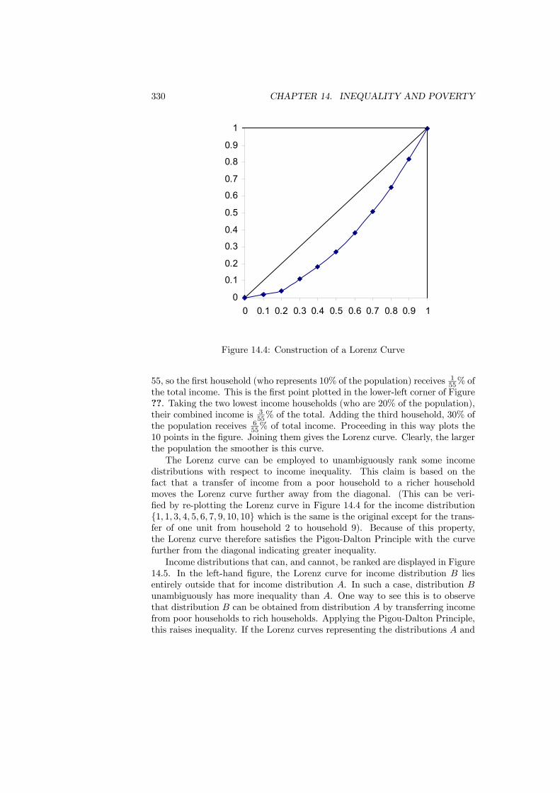
330 CHAPTER 14. INEQUALITY AND POVERTY
0
0.1
0.2
0.3
0.4
0.5
0.6
0.7
0.8
0.9
1
0 0.1 0.2 0.3 0.4 0.5 0.6 0.7 0.8 0.9 1
Figure 14.4: Construction of a Lorenz Curve
55, so the first household (who represents 10% of the population) receives 155% of
the total income. This is the first point plotted in the lower-left corner of Figure??. Taking the two lowest income households (who are 20% of the population),their combined income is 3
55% of the total. Adding the third household, 30% ofthe population receives 6
55% of total income. Proceeding in this way plots the10 points in the figure. Joining them gives the Lorenz curve. Clearly, the largerthe population the smoother is this curve.The Lorenz curve can be employed to unambiguously rank some income
distributions with respect to income inequality. This claim is based on thefact that a transfer of income from a poor household to a richer householdmoves the Lorenz curve further away from the diagonal. (This can be veri-fied by re-plotting the Lorenz curve in Figure 14.4 for the income distribution{1, 1, 3, 4, 5, 6, 7, 9, 10, 10} which is the same is the original except for the trans-fer of one unit from household 2 to household 9). Because of this property,the Lorenz curve therefore satisfies the Pigou-Dalton Principle with the curvefurther from the diagonal indicating greater inequality.Income distributions that can, and cannot, be ranked are displayed in Figure
14.5. In the left-hand figure, the Lorenz curve for income distribution B liesentirely outside that for income distribution A. In such a case, distribution Bunambiguously has more inequality than A. One way to see this is to observethat distribution B can be obtained from distribution A by transferring incomefrom poor households to rich households. Applying the Pigou-Dalton Principle,this raises inequality. If the Lorenz curves representing the distributions A and
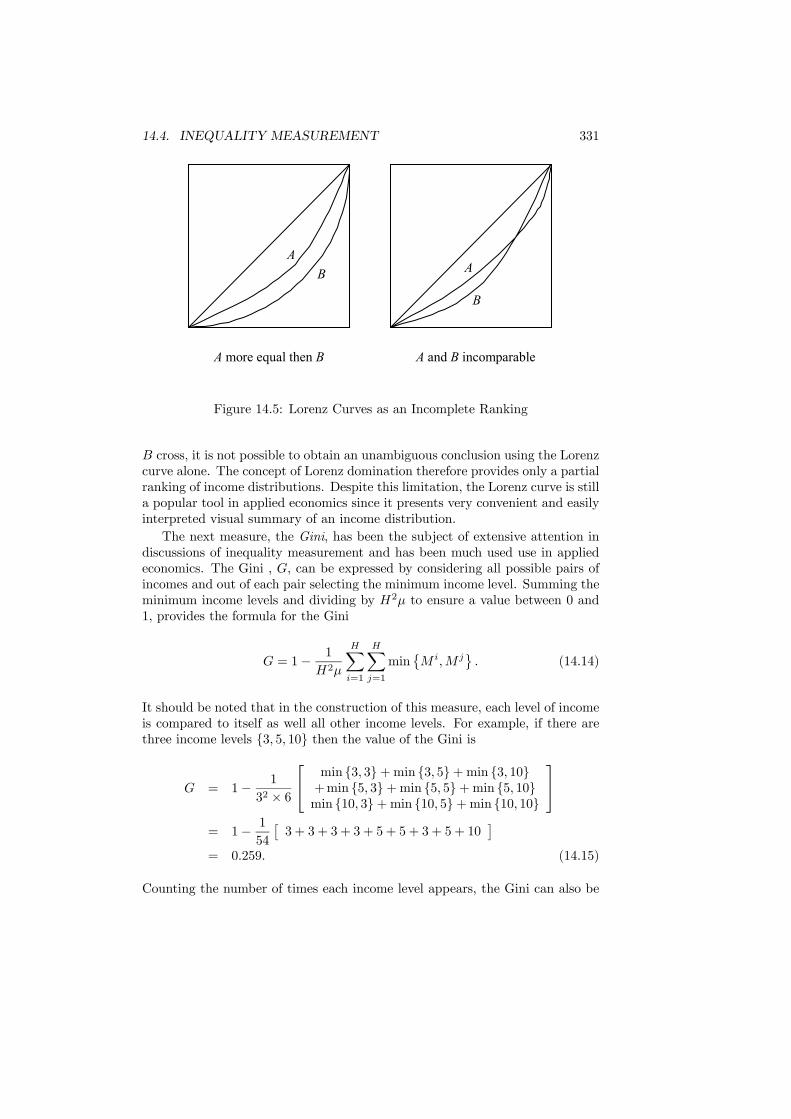
14.4. INEQUALITY MEASUREMENT 331
AB
A more equal then B
A
B
A and B incomparable
Figure 14.5: Lorenz Curves as an Incomplete Ranking
B cross, it is not possible to obtain an unambiguous conclusion using the Lorenzcurve alone. The concept of Lorenz domination therefore provides only a partialranking of income distributions. Despite this limitation, the Lorenz curve is stilla popular tool in applied economics since it presents very convenient and easilyinterpreted visual summary of an income distribution.The next measure, the Gini, has been the subject of extensive attention in
discussions of inequality measurement and has been much used use in appliedeconomics. The Gini , G, can be expressed by considering all possible pairs ofincomes and out of each pair selecting the minimum income level. Summing theminimum income levels and dividing by H2µ to ensure a value between 0 and1, provides the formula for the Gini
G = 1− 1
H2µ
HXi=1
HXj=1
min©M i,M j
ª. (14.14)
It should be noted that in the construction of this measure, each level of incomeis compared to itself as well all other income levels. For example, if there arethree income levels {3, 5, 10} then the value of the Gini is
G = 1− 1
32 × 6
min {3, 3}+min {3, 5}+min {3, 10}+min {5, 3}+min {5, 5}+min {5, 10}min {10, 3}+min {10, 5}+min {10, 10}
= 1− 1
54
£3 + 3 + 3 + 3 + 5 + 5 + 3 + 5 + 10
¤= 0.259. (14.15)
Counting the number of times each income level appears, the Gini can also be

332 CHAPTER 14. INEQUALITY AND POVERTY
Lorenz Curve
Figure 14.6: Relating Gini to Lorenz
written as
G = 1− 1
H2µ
£[2H − 1]M1 + [2H − 3]M2 + [2H − 5]M3 + ...+MH
¤.
(14.16)This second form of the Gini makes its computation simpler but hides the con-struction behind the measure.The Gini also satisfies the Pigou-Dalton Principle. This can be seen by
considering a transfer of income of size ∆M from household i to household j,with the households chosen so that M j > M i. From the ranking of incomesthis implies j > i. Then
∆G =2
H2µ[j − i]∆M > 0, (14.17)
as required. In the case of the Gini, the effect of the transfer of income uponthe measure depends only on the locations of i and j in the income distribution.For example, a transfer from the household at position i = 1 to the householdat position j = 11 counts as much as one from position i = 151 to positionj = 161. It might be expected that an inequality should be more sensitive totransfers between households low in the income distribution.There is an important relationship between the Gini and the Lorenz curve.
As shown in Figure 14.6, the Gini is equal to the area between the Lorenz curveand the line of equality as a proportion of the area of the triangle beneath theline of equality. As the area of the box is 1, the Gini is twice the area betweenthe Lorenz curve and the equality line. This definition of the Gini makes it clearthat the Gini, in common with R, C and D, can be used to rank distributionswhen the Lorenz curves cross since the relevant area is always well defined.Since all these measures provide a stronger ranking of income distributions thanthe Lorenz curve, they must each impose additional restrictions which allow acomparison to be made between distributions even when their Lorenz curvescross.

14.4. INEQUALITY MEASUREMENT 333
A final statistical measure that displays a different form of sensitivity is theTheil entropy measure. This measure is drawn from information theory and isused in that context to measure the average information content of a system ofinformation. The definition of the Theil entropy measure, T , is given by
T =1
logH
HXh=1
Mh
Hµ
·log
Mh
Hµ− log 1
H
¸
=1
H logH
HXh=1
Mh
µlog
Mh
µ. (14.18)
In respect of the Pigou-Dalton Principle, the effect of an income transfer, d²,between households i and j upon the entropy index is given by
dT
d²=
1
H logHlog
M j
M i< 0, (14.19)
so that the entropy measure also satisfies the criterion. For the Theil entropymeasure, the change is dependent upon the relative incomes of the two house-holds involved in the transfer. This provides an alternative form of sensitivityto transfers.
14.4.3 Inequality and Welfare
The analysis of the statistical measures of inequality has made reference to“acceptable” criteria for a measure to possess. One of these was made explicit inthe Pigou-Dalton Principle, whilst other criteria relating to additional desirablesensitivity properties have been implicit in the discussion. To be able to saysomething is acceptable or not implies that there is some notion of distributivejustice or social welfare underlying the judgement. It is then interesting toconsider the relationship between inequality measures and welfare.The first issue to address is the extent to which income distributions can be
ranked in terms of welfare with minimal restrictions imposed upon the socialwelfare function. To investigate this, let the level of social welfare be determinedby the function W = W
¡M1, . . . ,MH
¢. It is assumed that this social welfare
function is symmetric and concave. Symmetry means that the level of welfare isunaffected by changing the ordering of the households. This is just a requirementthat all households are treated equally. Concavity ensures that the indifferencecurves of the welfare function have the standard shape with mixtures preferredto extremes. This assumption imposes a concern for equity upon the welfarefunction.The critical theorem relating the ranking of income distributions to social
welfare is now given.
Theorem 10 Consider two distributions of income with the same mean. If theLorenz curves for these distributions do not cross, every symmetric and concavesocial welfare function will assign a higher level of welfare to the distributionwhose Lorenz curve is closest to the main diagonal.
334 CHAPTER 14. INEQUALITY AND POVERTY
The proof of this theorem is very straightforward. Since the welfare functionis symmetric and concave, it follows that ∂W
∂Mi ≥ ∂W∂Mj if M i < M j . Hence the
marginal social welfare of income is greater for a household lower in the incomedistribution. If the two Lorenz curves do not cross, the income distribution rep-resented by the inner one (that closest to the main diagonal) can be obtainedfrom that of the outer one by transferring income from richer to poorer house-holds. Since the marginal social welfare of income to the poorer households isnever less than that from richer, this transfer must raise welfare as measured byany symmetric and concave social welfare function.The converse of this theorem is that if the Lorenz curves for two distrib-
utions cross, then two symmetric and concave social welfare functions can befound that will rank the two distributions differently. This is because the in-come distributions of two Lorenz curves that cross are not related by simpletransfers from rich to poor. This permits the construction of the two socialwelfare functions, with different marginal social welfares, that will rank themdifferently. So, if the Lorenz curves do cross the income distributions cannot beunambiguously ranked without specifying the social welfare function.Taken together, the theorem and its converse show that the Lorenz curve
provides the most complete ranking of income distributions that is possiblewithout making assumptions on the form of the social welfare other than sym-metry and concavity. To achieve a complete ranking when the Lorenz curvescross requires restrictions to be placed upon the structure of the social welfarefunction. In addition, any measure of inequality is necessarily stronger than theLorenz curve since it generates a complete ranking of distributions. This is trueof all the statistical measures, which is why it can be argued that they all carryimplicit welfare judgements.This argument can be taken a stage further. It is in fact possible to construct
the social welfare function that is implied by an inequality measure. To seehow this can be done, consider the Gini. Assume that the total amount ofincome available is constant. Any redistribution of this that leaves the Giniunchanged must leave the implied level of welfare unchanged. A redistributionof income will not affect the Gini if the term
£[2H − 1]M1 + ...+MH
¤remains
constant. The welfare function must thus be a function of this expression.Furthermore, the Gini is defined to be independent of the total level of income,but a welfare function will increase if total income rises and distribution isunaffected. This can be incorporated by not dividing through by the mean levelof income. Putting these arguments together, the welfare function implied bythe Gini is given by
WG (M) =1
H2
£[2H − 1]M1 + [2H − 3]M2 + ...+MH
¤. (14.20)
The form of WG (M) is interesting since it shows that the Gini implies a socialwelfare function that is linear in incomes. It also has a clear structure of in-creasing welfare weights for lower income consumers. Also, the welfare functionhas indifference curves which are straight lines above and below the line of equalincomes, but kinked on this line. This is illustrated in Figure 14.7.

14.4. INEQUALITY MEASUREMENT 335
1M
2M
Figure 14.7: The Gini Social Welfare Function
In the same way a welfare function can be constructed for all of the statisticalmeasures. Therefore acceptance of the measure is acceptance of the impliedwelfare function. As shown by the linear social indifference curves and increasingwelfare weights, the implied welfare functions can have a very restrictive form.Rather than just accept such welfare restrictions, the fact that each inequalitymeasure implies a social welfare function suggests that the relationship can beinverted to move from a social welfare function to an inequality measure. Byassuming a social welfare function at the outset, it is possible to make welfarejudgements explicit and, by deriving the inequality measure from the socialwelfare function, ensure these are incorporated in the inequality measure.
To implement this approach, assume that the social welfare function is util-itarian with
W =HXh=1
U¡Mh
¢. (14.21)
The household utility of income function, U (M), is taken to satisfy the condi-tions that U 0 (M) > 0 and U 00 (M) < 0. The utility function U (M) can eitherbe the households’ true cardinal utility function or it can be chosen by the policyanalyst as their evaluation of the utility of income to each household. In thissecond interpretation, since social welfare is obtained by summing the individ-ual utilities, the importance given to equity can be captured in the choice ofU (M). This is because increasing the concavity of the utility function places arelatively higher weight on low incomes in the social welfare function.
A measure of inequality can be constructed from the social welfare function
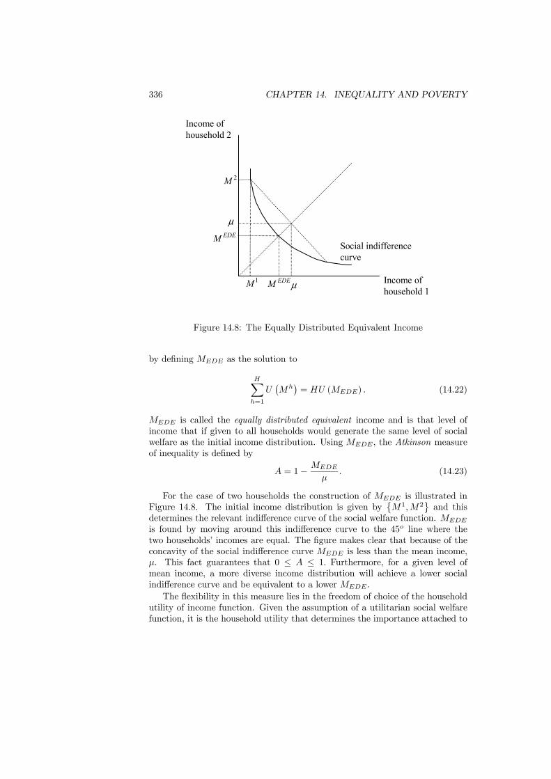
336 CHAPTER 14. INEQUALITY AND POVERTY
1M
2M
µ
µ
EDEM
EDEM
Income ofhousehold 1
Income ofhousehold 2
Social indifferencecurve
Figure 14.8: The Equally Distributed Equivalent Income
by defining MEDE as the solution to
HXh=1
U¡Mh
¢= HU (MEDE) . (14.22)
MEDE is called the equally distributed equivalent income and is that level ofincome that if given to all households would generate the same level of socialwelfare as the initial income distribution. Using MEDE, the Atkinson measureof inequality is defined by
A = 1− MEDE
µ. (14.23)
For the case of two households the construction of MEDE is illustrated inFigure 14.8. The initial income distribution is given by
©M1,M2
ªand this
determines the relevant indifference curve of the social welfare function. MEDE
is found by moving around this indifference curve to the 45o line where thetwo households’ incomes are equal. The figure makes clear that because of theconcavity of the social indifference curve MEDE is less than the mean income,µ. This fact guarantees that 0 ≤ A ≤ 1. Furthermore, for a given level ofmean income, a more diverse income distribution will achieve a lower socialindifference curve and be equivalent to a lower MEDE.The flexibility in this measure lies in the freedom of choice of the household
utility of income function. Given the assumption of a utilitarian social welfarefunction, it is the household utility that determines the importance attached to
14.4. INEQUALITY MEASUREMENT 337
inequality by the measure. One commonly used form of utility function is
U (M) =M1−ε
1− ε, ε 6= 1, (14.24)
which allow the welfare judgements of the policy analyst to be contained inthe chosen value of the parameter ε. The value of ε determines the degree ofconcavity of the utility function: it becomes more concave as ε increases. Anincrease in concavity raises the relative importance of low incomes because itcauses the marginal utility of income to decline at a faster rate. The utilityfunction is isoelastic, and concave if ε ≥ 0. When ε = 1, U (M) = logM andwhen ε = 0, U (M) =M .The Atkinson measure can be illustrated using the example of the income
distribution {1, 3, 6, 9, 11}. If ε = 12 the household utility function is U = M
12
2so the level of social welfare is
W =112
2+312
2+612
2+912
2+11
12
2= 5.7491. (14.25)
The equally distributed equivalent income then solves
5× [M ]12
2= 5.7491, (14.26)
so MEDE = 5.2883. This gives the value of the Atkinson measure as
A = 1− 5.28836
= 0.1186. (14.27)
14.4.4 An Application
As has been noted in the discussion, these inequality measures are frequentlyused in practical policy analysis. Table 14.2 summarizes the results of an OECDstudy into the change in inequality over time in wide range of countries. Thisis undertaken by calculating inequality at two points in time and determiningthe percentage change in the measure. If the change is positive, then inequalityhas increased. The converse holds if it is negative. The study also calculatesinequality for income before taxes and transfers and for income after taxes andtransfers. The difference between the inequality of these two gives an insightinto the extent to which the tax and transfer system succeeds in redistributingincome.Looking at the results, in all cases inequality is smaller after taxes and
transfers than before so that the tax systems in the countries studied are redis-tributive. For instance, in Denmark inequality is .0420 when measured by Ginibefore taxes and transfers but only 0.0217 after. The second general message ofthe results is that inequality has tended to rise in these countries - only in threecases has it been reduced and in every case this is after taxes and transfers.
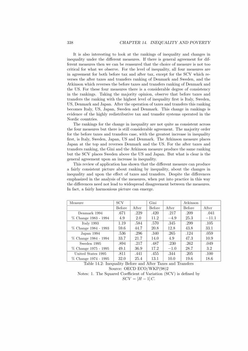
338 CHAPTER 14. INEQUALITY AND POVERTY
It is also interesting to look at the rankings of inequality and changes ininequality under the different measures. If there is general agreement for dif-ferent measures then we can be reassured that the choice of measure is not toocritical for what we observe. For the level of inequality, all four measures arein agreement for both before tax and after tax, except for the SCV which re-verses the after taxes and transfers ranking of Denmark and Sweden, and theAtkinson which reverses the before taxes and transfers ranking of Denmark andthe US. For these four measures there is a considerable degree of consistencyin the rankings. Taking the majority opinion, observe that before taxes andtransfers the ranking with the highest level of inequality first is Italy, Sweden,US, Denmark and Japan. After the operation of taxes and transfers this rankingbecomes Italy, US, Japan, Sweden and Denmark. This change in rankings isevidence of the highly redistributive tax and transfer systems operated in theNordic countries.The rankings for the change in inequality are not quite as consistent across
the four measures but there is still considerable agreement. The majority orderfor the before taxes and transfers case, with the greatest increase in inequalityfirst, is Italy, Sweden, Japan, US and Denmark. The Atkinson measure placesJapan at the top and reverses Denmark and the US. For the after taxes andtransfers ranking, the Gini and the Atkinson measure produce the same rankingbut the SCV places Sweden above the US and Japan. But what is clear is thegeneral agreement upon an increase in inequality.This review of application has shown that the different measure can produce
a fairly consistent picture about ranking by inequality, about the changes ininequality and upon the effect of taxes and transfers. Despite the differencesemphasized in the analysis of the measures, when put into practice in this waythe differences need not lead to widespread disagreement between the measures.In fact, a fairly harmonious picture can emerge.
Measure SCV Gini AtkinsonBefore After Before After Before After
Denmark 1994% Change 1983 - 1994
.6714.9
.2292.0
.42011.2
.217−4.9
.20925.3
.041−11.1
Italy 1993% Change 1984 - 1993
1.1959.6
.58444.7
.57020.8
.34512.8
.29943.8
.10533.1
Japan 1994% Change 1984 - 1994
.53633.7
.29621.7
.34014.0
.2654.9
.12447.3
.05910.9
Sweden 1995% Change 1975 - 1995
.89449.1
.21736.9
.48717.2
.230−1.0
.26228.7
.0493.2
United States 1995% Change 1974 - 1995
.81132.0
.44125.4
.45513.1
.34410.0
.20519.6
.10018.6
Table 14.2: Inequality Before and After Taxes and TransfersSource: OECD ECO/WKP(98)2
Notes: 1. The Squared Coefficient of Variation (SCV) is defined bySCV = [H − 1]C.
14.5. POVERTY 339
2. For the Atkinson measure, ε = 0.5.
14.5 Poverty
The essential feature of poverty is the possession of fewer resources than arerequired to achieve an acceptable standard of living. What constitutes povertycan be understood in the same intuitive way as what constitutes inequality, butsimilar issues about the correct measure arise again once we attempt to providea quantification. This section first discusses concepts of poverty and the povertyline, and then proceeds to review a number of common poverty measures.
14.5.1 Poverty and the Poverty Line
Before measuring poverty, it is first necessary to define it. It is obvious thatpoverty refers to a situation involving a lack of income and a consequent low levelof consumption and welfare. What is not so clear is the standard against whichthe level of income should be judged. Two possibilities arise in this context: anabsolute conception of poverty and a relative one. The distinction between thesehas implications for changes in the level of poverty over time and the success ofpolicy in alleviating poverty.The concept of absolute poverty assumes that there is some fixed minimum
level of consumption (and hence of income) that constitutes poverty and isindependent of time or place. Such a minimum level of consumption can be adiet that is just sufficient to maintain health and limited housing and clothing.Under the concept of absolute poverty, if the incomes of all households rise,there will eventually be no poverty. Although a concept of absolute poverty wasprobably implicit in early studies of poverty, such as that of Rowntree in 1901,the appropriateness of absolute poverty has since generally been rejected. In itsplace has been adopted the notion of relative poverty.Relative poverty is not a recent concept. Even in 1776 Adam Smith was
defining poverty as the lack of necessities, where necessities are defined as “whatever the custom of the country renders it indecent for creditable people, evenof the lowest order, to be without“. This definition makes it clear that rela-tive poverty is defined in terms of the standards of a given society at a giventime and, as the income of that society rises, so does the level that representspoverty. Operating under a relative standard, it becomes much more difficult toeliminate poverty. Relative poverty has also been defined in terms of the abilityto “participate” in society. Poverty then arises whenever a household possessesinsufficient resources to allow it to participate in the customary activities of itssociety.The starting point for the measurement of poverty is to set a poverty line
which separates those in viewed as living in poverty from those who are not.Of course, this poverty line applies to the incomes levels after application ofan equivalence scale. Whether poverty is viewed as absolute or relative matterslittle for setting a poverty line at any particular point in time (though advocates

340 CHAPTER 14. INEQUALITY AND POVERTY
of an absolute poverty concept may choose to set it lower). Where the distinctionmatters is whether and how the poverty line is adjusted over time. If an absolutepoverty standard were adopted, then there would be no revision. Conversely,with relative poverty the level of the line would rise or fall with in line withaverage incomes.In practice, poverty lines have often been determined by following the mini-
mum needs approach that was discussed in connection with equivalence scales.As noted in Section 14.3, this is the case with the US poverty line that was fixedin 1963 and has since been updated annually. As the package of minimum needshas not changed, the underlying concept is that of an absolute poverty measure.In the UK, the poverty line has been taken as the level of income which is 120%or 140% of the minimum supplementary benefit level. As this level of benefitis determined by minimum needs, this implies a minimum needs poverty line.In addition, benefits have risen with increases in average income so causing thepoverty line to rise. This represents the use of a relative concept of poverty.That there is a precise switch between poverty and non-poverty as the
poverty line is crossed is a very strong assumption. Instead, it would seemmuch more natural for there to be a gradual move out of poverty as incomeincreases. Such precision of the poverty line may also lead to difficulty in de-termining where it should lie if the level of poverty is critically dependent onthe precise choice. Both of these difficulties can be overcome by observing thatoften it is not the precise level of poverty that matters but changes in the levelof poverty over time and across countries. In these instances the poverty valueis not too important but only the rankings. This suggest the procedure of cal-culating poverty for a range of poverty lines. If poverty is higher today for allpoverty lines than it was yesterday, then it seems unambiguous that povertyhas risen. In this sense, the poverty line may not actually be of critical impor-tance for the uses to which poverty measurement is often put. An applicationillustrating this argument is given below.
14.5.2 Poverty Measures
The poverty line is now taken as given and we proceed to discuss alternativemeasures of poverty. The basic issue in this discussion is how best to combinetwo pieces of information (how many households are poor, and how poor theyare) into a single quantitative measure of poverty. By describing a number ofmeasures, the discussion will draw out the properties that it is desirable for apoverty measure to possess.Throughout the discussion, the poverty line is denoted by the income level
z, so that a household with an income level below or equal to z is classed asliving in poverty. For a household with income Mh, income gap of household hmeasures how far their income is below the poverty line. Denoting the incomegap for household h by gh, it follows that gh = z −Mh. Given the poverty linez and an income distribution
©M1, ...,MH
ª, where M1 ≤ M2 ≤ ... ≤ MH ,
the number of households in poverty is denoted by q. The value of q is definedby the facts that the income of household q is on or below the poverty line, so

14.5. POVERTY 341
Mq ≤ z, but that of the next household is above Mq+1 > z.The simplest measure of poverty is the headcount ratio which determines
the extent of poverty by counting the number of households whose incomesare not above the poverty line. Expressing the number as a proportion of thepopulation, the headcount ratio is defined by
E =q
H. (14.28)
This measure of poverty was first used by Rowntree in 1901 and has been em-ployed in many subsequent studies. The major advantage of the headcount ratiois its simplicity of calculation.The headcount ratio is clearly limited because it is not affected by how far
below the poverty line the household are. For example, with a poverty line ofz = 10 the income distributions {1, 1, 20, 40, 50} and {9, 9, 20, 40, 50} would bothhave a headcount ratio of E = 2
5 . A policy maker may well see these incomedistributions differently since the income required to alleviate poverty in thesecond case (2 units) is much less then that required for the first (18 units).The headcount ratio is also not affected by any transfer of income from a poorhousehold to one that is richer if both households remain on the same side ofthe poverty line. Even worse, observe that if we change the second distributionto {7, 11, 20, 40, 50} the headcount ratio falls to E = 1
5 , so a regressive transferhas actually reduced the headcount ratio. This will happen whenever a transfertakes income of the recipient of the transfer above the poverty line.The headcount uses only one of the two pieces on information on poverty.
A measure that uses only information on how far below the poverty line arethe incomes of the poor households is the aggregate poverty gap. This is definedas the simple sum of the income gaps of the households that are in poverty.Recalling that it is the first q households that are in poverty, the aggregatepoverty gap is
V =
qXh=1
gh. (14.29)
The interpretation of this measure is that it is the additional income for the poorthat is required to eliminate poverty. It provides some information but is limitedby the fact that it does not sensitive to changes in the number in poverty. Inaddition, the aggregate poverty gap gives equal weight to all income shortfallsregardless of how far they are from the poverty line. It is therefore insensitiveto transfers unless the transfer takes one of the households out of poverty. Tosee this latter point, for the poverty line of z = 10 the income distributions{5, 5, 20, 40, 50} and {1, 9, 20, 40, 50} have an aggregate poverty gap of V = 10.The distribution between the poor is somewhat different in the two cases.One direct extension of the aggregate poverty gap is to adjust the measure
by taking into account the number in poverty. The income gap ratio does thisby calculating the aggregate poverty gap and then dividing by the number inpoverty. Finally, the value obtained is divided by the value of the poverty line,
342 CHAPTER 14. INEQUALITY AND POVERTY
z, to obtain a measure whose value falls between 0 (the absence of poverty) and1 (all households in poverty have no income).
I =1
z
Pqh=1 ghq
. (14.30)
For the income distribution {1, 9, 20, 40, 50} , the income gap ratio whenz = 10 is
I =1
10
9 + 1
2= 0.5. (14.31)
However, when this income distribution changes to {1, 10, 20, 40, 50} , so onlyone household is now in poverty, the measure become
I =1
10
9
1= 0.9. (14.32)
This example reveals that the income gap ratio has the unfortunate propertyof being able to report increased poverty when the income of household crossesthe poverty line and the number in poverty is reduced.These observations suggest that it is necessary to reflect more carefully upon
the properties that a poverty measure should possess. In 1976 Sen suggestedthat a poverty measure should have the following properties:
• Transfers of income between households above the poverty line should notaffect the amount of poverty.
• If a household below the poverty line becomes worse off, poverty shouldincrease.
• The poverty measure should be anonymous i.e. should not depend on whois poor.
• A regressive transfer among the poor should raise poverty.These are properties that have already been highlighted by the discussion.
Two further properties were also proposed:
• The weight given to a household should depends on their ranking amongthe poor i.e. more weight should be given to those furthest from thepoverty line.
• The measure should reduce to the headcount if all the poor have the samelevel of income.
On poverty measure that satisfies all of these conditions is the Sen measure
S = E
·I + [1− I]Gp
·q
q + 1
¸¸, (14.33)
whereGp is the Gini measure of income inequality amongst the households belowthe poverty line. This poverty measure combines a measure of the number in
14.5. POVERTY 343
poverty (the headcount ratio), a measure of the shortfall in income (the incomegap ratio) and a measure of the distribution of income between the poor (theGini). Applying this to the income distribution {1, 9, 20, 40, 50} , we have E = 2
5and I = 0.5. The Gini is calculated for the distribution of income of the poor{1, 9} , so Gp = 1− 1
22×5 [3× 1 + 9] = 410 . These values give
S =2
5
·0.5 + [1− 0.5] 4
10
·2
2 + 1
¸¸= 0.2533. (14.34)
In contrast, for the distribution {1, 10, 20, 40, 50} which was judged worse usingthe income gap ratio, there is no inequality among the poor (since there is asingle poor person) so the Sen measure is
S =1
5
·0.9 + [1− 0.9] 0
·1
1 + 1
¸¸= 0.18, (14.35)
which is simply the headcount ratio and records a lower level of poverty.There is a further desirable property that leads into an alternative and im-
portant class of poverty measures. Consider a population that can be brokendown into distinct subgroups. For instance, imagine dividing the populationinto rural and urban dwellers. The property we want is for the measure to beable to assign a poverty level for each of the groups and to aggregate these grouppoverty levels into a single level of the total society. Further, we will also wantthe aggregate measure to increase if poverty rises in one of the subgroups anddoes not fall any of the others. So, if rural poverty rises while urban povertyremains the same, aggregate poverty must rise. Any poverty measures thatsatisfies this condition is termed subgroup consistent.Before introducing a form of measure that is subgroup consistent, it is pro-
viding additional discussion of the effect of transfers. The measures discussedso far have all had the property that the effect of a transfer has been indepen-dent of the income levels of the loser and gainer (except when the transfer wasbetween households on different sides of the poverty line or changed the num-ber in poverty). In the same way that in inequality measurement we argued formagnifying the effect of deviations far from the mean, we can equally argue thatthe effect of a transfer in poverty measurement should be dependent upon theincomes of those involved in the transfer. For example, a transfer away from thelowest income household should have more effect on measured poverty than atransfer away from a household close to the poverty line. A poverty measure willsatisfy this sensitivity to transfers if the increase in measured poverty caused bya transfer of income from a poor household to a poor household with a higherincome is smaller the larger is the income of the lowest income household.Let the total population remain at H. Assume that this population can be
divided into Γ separate subgroups. Let gγh be the income gap of a poor memberof subgroup γ and qγ be the number of poor in that subgroup. Using thisnotation, a poverty measure that satisfies the property of subgroup consistency
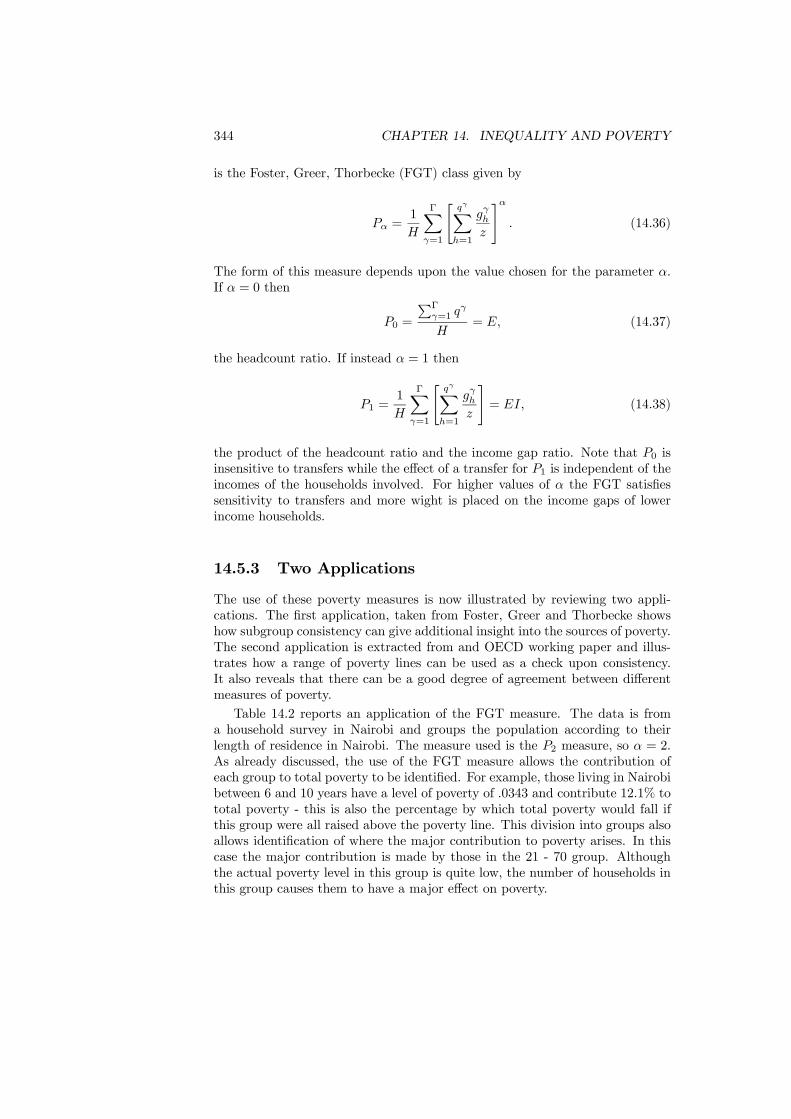
344 CHAPTER 14. INEQUALITY AND POVERTY
is the Foster, Greer, Thorbecke (FGT) class given by
Pα =1
H
ΓXγ=1
"qγXh=1
gγhz
#α. (14.36)
The form of this measure depends upon the value chosen for the parameter α.If α = 0 then
P0 =
PΓγ=1 q
γ
H= E, (14.37)
the headcount ratio. If instead α = 1 then
P1 =1
H
ΓXγ=1
"qγXh=1
gγhz
#= EI, (14.38)
the product of the headcount ratio and the income gap ratio. Note that P0 isinsensitive to transfers while the effect of a transfer for P1 is independent of theincomes of the households involved. For higher values of α the FGT satisfiessensitivity to transfers and more wight is placed on the income gaps of lowerincome households.
14.5.3 Two Applications
The use of these poverty measures is now illustrated by reviewing two appli-cations. The first application, taken from Foster, Greer and Thorbecke showshow subgroup consistency can give additional insight into the sources of poverty.The second application is extracted from and OECD working paper and illus-trates how a range of poverty lines can be used as a check upon consistency.It also reveals that there can be a good degree of agreement between differentmeasures of poverty.Table 14.2 reports an application of the FGT measure. The data is from
a household survey in Nairobi and groups the population according to theirlength of residence in Nairobi. The measure used is the P2 measure, so α = 2.As already discussed, the use of the FGT measure allows the contribution ofeach group to total poverty to be identified. For example, those living in Nairobibetween 6 and 10 years have a level of poverty of .0343 and contribute 12.1% tototal poverty - this is also the percentage by which total poverty would fall ifthis group were all raised above the poverty line. This division into groups alsoallows identification of where the major contribution to poverty arises. In thiscase the major contribution is made by those in the 21 - 70 group. Althoughthe actual poverty level in this group is quite low, the number of households inthis group causes them to have a major effect on poverty.
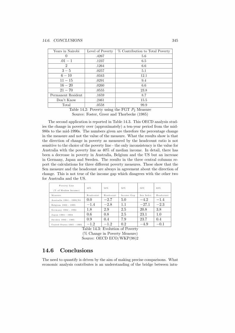
14.6. CONCLUSIONS 345
Years in Nairobi Level of Poverty % Contribution to Total Poverty0 .4267 5.6
.01− 1 .1237 6.52 .1264 6.6
3− 5 .0257 5.16− 10 .0343 12.111− 15 .0291 9.416− 20 .0260 6.621− 70 .0555 23.8
Permanent Resident .1659 8.7Don’t Know .2461 15.5
Total .0558 99.9Table 14.2: Poverty using the FGT P2 MeasureSource: Foster, Greer and Thorbecke (1985)
The second application is reported in Table 14.3. This OECD analysis stud-ies the change in poverty over (approximately) a ten-year period from the mid-980s to the mid-1990s. The numbers given are therefore the percentage changein the measure and not the value of the measure. What the results show is thatthe direction of change in poverty as measured by the headcount ratio is notsensitive to the choice of the poverty line - the only inconsistency is the value forAustralia with the poverty line as 40% of median income. In detail, there hasbeen a decrease in poverty in Australia, Belgium and the US but an increasein Germany, Japan and Sweden. The results in the three central columns re-port the calculations for three different poverty measures. These show that theSen measure and the headcount are always in agreement about the direction ofchange. This is not true of the income gap which disagrees with the other twofor Australia and the US.
Pove r ty L in e
(% o f M ed ia n In c om e )4 0% 5 0% 5 0% 5 0% 6 0%
M ea su r e H e a d c o u n t H ea d c o u n t In c om e G a p S en In d e x H e a d c o u n t
A u s t ra l i a 1 9 8 4 - 1 9 9 3 / 9 4 0.0 −2.7 5.0 −4.2 −1.4B e lg ium 1 9 8 3 - 1 9 9 5 −1.4 −2.8 1.1 −27.1 −2.3G e rm any 1 9 8 4 - 1 9 9 4 1.8 2.9 2.5 20.8 3.8J a p a n 1 9 8 4 - 1 9 9 4 0.6 0.8 2.5 23.1 1.0S w ed e n 1 9 8 3 - 1 9 9 5 0.9 0.4 7.9 23.7 0.4U n it e d S t a t e s 1 9 8 5 - 1 9 9 5 −1.2 −1.2 0.2 −4.9 −0.1
Table 14.3: Evolution of Poverty(% Change in Poverty Measure)Source: OECD ECO/WKP(98)2
14.6 ConclusionsThe need to quantify is driven by the aim of making precise comparisons. Whateconomic analysis contributes is an understanding of the bridge between intu-

346 CHAPTER 14. INEQUALITY AND POVERTY
itive concepts of inequality and poverty, and specific measures of these phenom-ena. Analysis can reveal the implications of alternative measures and provideprinciples that a good measure should satisfy.The first problem we challenged in this chapter was the comparison of in-
comes between households of different compositions. It is clearly more expensiveto support a large family than a small family, but exactly how much more ex-pensive is more difficult to determine. Equivalence scales were introduced asthe analytical tool to solve this problem. These scales were initially based uponthe cost of achieving a minimum standard of living. Though simple, such anapproach does not easily generalize to higher income levels nor does it takemuch account of economic optimization. In principle, equivalence scales couldbe built directly from utility functions but to do so issues must be addressed ofhow the preferences of the individual members of a household are aggregatedinto a household preference order.Inequality occurs when some households have a higher income (after the
incomes have been equivalized for household composition) than others. TheLorenz curve provides a graphical device for contrasting income distributions.Some income distributions can be ranked directly by the Lorenz curve, in whichcase there is no ambiguity about which has more inequality, but not all distribu-tions can be. Inequality measures provide a quantitative assessment of inequalityby imposing restrictions beyond those incorporated in the Lorenz curve. Thechapter investigated the properties of a number of measures of inequality. Ofparticular importance was the observation that all inequality measures embodyimplicit welfare judgements. Given this, the Atkinson measure is constructed onthe basis that the welfare judgements should be made explicit and the inequalitymeasure constructed upon these judgements. In principle, alternative measurescan generate different rankings of income distributions but, as the applicationshowed, they can in practice yield very consistent rankings.In many ways the measurement of poverty raises similar issues to that of in-
equality. The additional feature of poverty is the necessity to determine whetherhouseholds can be classed as living in poverty or not. The poverty line whichprovides the division between the two groups plays a central role in poverty mea-surement. Where and how the to locate this poverty line is important, but morefundamental is how it should be adjusted over time. At stake here is the keyquestion of whether poverty should be viewed in absolute or relative terms. Thepractice in developed countries is to use relative poverty. The chapter revieweda number of poverty measures from the headcount ratio to the FGT measure.These measures are also distinguished by a range of sensitivity properties. Theapplications showed how they could be used and that the different measurescould provide a consistent picture of the development of poverty despite theirdifferent conceptual bases.The chapter has revealed how economic analysis is able to provide insights
into what we are assuming when we employ a particular inequality or povertymeasure. It has also revealed how we can think about the process of improvingour measures. Inequality and poverty are significant issues and better measure-ment is a necessary starting point for better policy.
14.6. CONCLUSIONS 347
Further readingThe relationship between inequality measures and social welfare was first
explored in:Atkinson, A.B. (1970) “On the measurement of inequality“, Journal of Eco-
nomic Theory, 2, 244 - 263.A comprehensive survey of the measurement of inequality is given by:Sen, A.K. (1997) On Economic Inequality, Oxford: Oxford University Press.A textbook treatment is in:Lambert, P. (1989) The Distribution and Redistribution of Income: A Math-
ematical Analysis, Oxford: Basil Blackwell.Issues surrounding the definition and implications of the poverty line are
treated in:Atkinson, A.B. (1987) “On the measurement of poverty“, Econometrica, 55,
749 - 764.Callan, T. and B. Nolan (1991) “Concepts of poverty and the poverty line“,
Journal of Economic Surveys, 5, 243 - 261.The derivation of the Sen measure, and a general discussion of constructing
measures from a set of axioms is given by:Sen, A.K. (1976) “Poverty: an ordinal approach to measurement“, Econo-
metrica, 44, 219 - 231.The FGT measure was first discussed in:Foster, J.E., J. Greer and E. Thorbecke (1984) “A class of decomposable
poverty measures“, Econometrica, 52, 761 - 767.An in-depth survey of poverty measure is:Foster, J.E. (1984) “On economic poverty: a survey of aggregate measures”,
Advances in Econometrics, 3, 215 - 251.

348 CHAPTER 14. INEQUALITY AND POVERTY
Part VI
Taxation
349

Chapter 15
Commodity Taxation
15.1 Introduction
Commodity taxes are levied on transactions involving the purchase of goods.The necessity for keeping accounts ensures that such transactions are generallypublic information. This makes them a good target for taxation. The drawback,however, is that their use introduces distortions into the economy. The taxesdrive a wedge between the price producers receive and the price consumers pay.This leads to inefficiency and reduces the attainable level of welfare comparedto what could be achieved using lump-sum taxes. This is the price that has tobe paid for implementable taxation.The effects of commodity taxes are quite easily understood - the imposition
of a tax raises the price of a good. On the consumer side of the market, thestandard analysis of income and substitution effects predicts what will happen todemand. For producers, the tax is a cost increase and they respond accordingly.What is more interesting is the choice of the best set of taxes for the government.There are several interesting settings for this question. The simplest version canbe described as follows: There is a given level of government revenue to be raisedwhich must be financed solely by taxes upon commodities. How must the taxesbe set so as to minimize the cost to society of raising the required revenue? Thisis the Ramsey problem of efficient taxation, first addressed in the 1920s. Theinsights its study gives are still at the heart of the understanding of choosingoptimal commodity taxes. More general problems introduce equity issues inaddition to those of efficiency.The chapter begins by discussing the deadweight loss that is caused by the
introduction of a commodity tax. A diagrammatic analysis of optimal com-modity taxation is then presented. This diagram is also used to demonstratethe Diamond-Mirrlees Production Efficiency result. Following this, the Ramseyrule is derived and an interpretation of this is provided. The extension to manyconsumers is then made and the resolution of the equity/efficiency trade-off isemphasized. This is followed by a review of some numerical calculations of
351

352 CHAPTER 15. COMMODITY TAXATION
Quantity
Price
p
tpq +=
0X1X
DWL
a
bc d
ef
Figure 15.1: Deadweight Loss
optimal taxes based on empirical data.
15.2 Deadweight Loss
Lump-sum taxation was described as the perfect tax instrument becuase it doesnot cause any distortions. The absence of disortions is due to the fact thata lump-sum tax is defined by the condition that no change in behaviour canaffect the level of the tax. Commodity taxation does not satisfy this definition.It is always possible to change a consumption plan if commodity taxation isintroduced. Demand can shift from goods subject to high taxes to goods withlow taxes and total consumption reduced by earning less or saving more. Itis these changes at the margin, which we call substitution effects, that are thetax-induced distortions.The introduction of a commodity tax causes raises tax revenue but causes
consumer welfare to be reduced. The deadweight loss of the tax is the extentto which the reduction in welfare exceeds the revenue raised. This concept isillustrated in Figure 15.1.Before the tax is introduced, the price of the good is p and the quantity
consumed is X0. At this price the level of consumer surplus is given by thetriangle abc. A specific tax of amount t is then levied on the good, so the pricerises to q = p+ t and quantity consumed falls to X1. This fall in consumptionreduces consumer surplus to aef . The tax raises revenue equal to tX1 which isgiven by the area cdef . The part of the original consumer surplus that is notturned into tax revenue is the deadweight loss, DWL, given by the triangle bde.
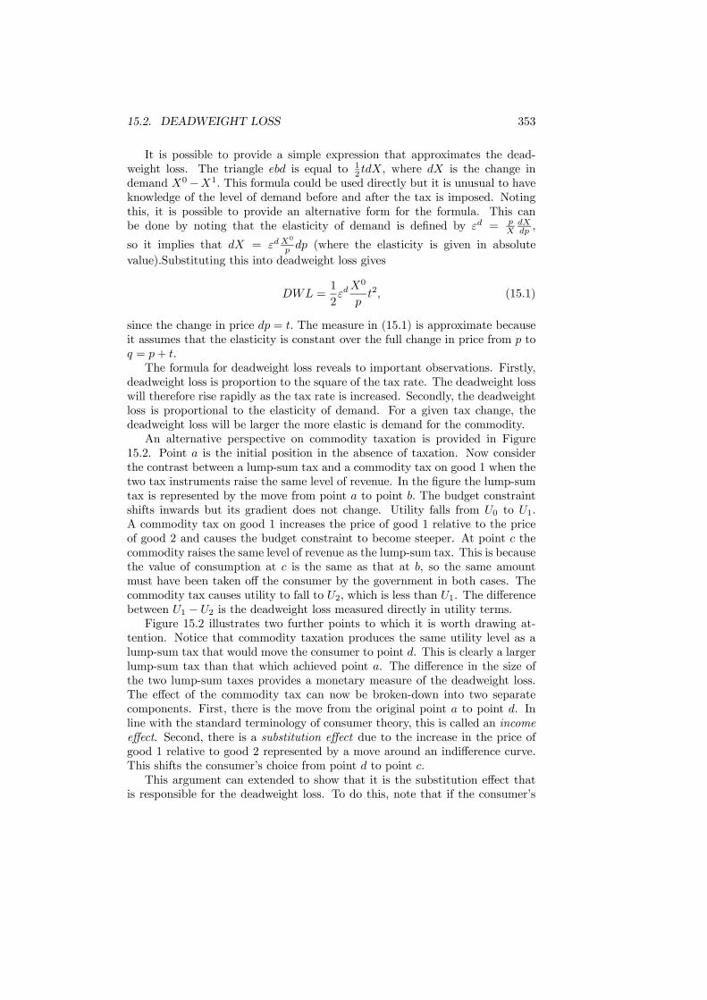
15.2. DEADWEIGHT LOSS 353
It is possible to provide a simple expression that approximates the dead-weight loss. The triangle ebd is equal to 1
2 tdX, where dX is the change indemand X0−X1. This formula could be used directly but it is unusual to haveknowledge of the level of demand before and after the tax is imposed. Notingthis, it is possible to provide an alternative form for the formula. This canbe done by noting that the elasticity of demand is defined by εd = p
XdXdp ,
so it implies that dX = εd X0
p dp (where the elasticity is given in absolutevalue).Substituting this into deadweight loss gives
DWL =1
2εdX0
pt2, (15.1)
since the change in price dp = t. The measure in (15.1) is approximate becauseit assumes that the elasticity is constant over the full change in price from p toq = p+ t.The formula for deadweight loss reveals to important observations. Firstly,
deadweight loss is proportion to the square of the tax rate. The deadweight losswill therefore rise rapidly as the tax rate is increased. Secondly, the deadweightloss is proportional to the elasticity of demand. For a given tax change, thedeadweight loss will be larger the more elastic is demand for the commodity.An alternative perspective on commodity taxation is provided in Figure
15.2. Point a is the initial position in the absence of taxation. Now considerthe contrast between a lump-sum tax and a commodity tax on good 1 when thetwo tax instruments raise the same level of revenue. In the figure the lump-sumtax is represented by the move from point a to point b. The budget constraintshifts inwards but its gradient does not change. Utility falls from U0 to U1.A commodity tax on good 1 increases the price of good 1 relative to the priceof good 2 and causes the budget constraint to become steeper. At point c thecommodity raises the same level of revenue as the lump-sum tax. This is becausethe value of consumption at c is the same as that at b, so the same amountmust have been taken off the consumer by the government in both cases. Thecommodity tax causes utility to fall to U2, which is less than U1. The differencebetween U1 − U2 is the deadweight loss measured directly in utility terms.Figure 15.2 illustrates two further points to which it is worth drawing at-
tention. Notice that commodity taxation produces the same utility level as alump-sum tax that would move the consumer to point d. This is clearly a largerlump-sum tax than that which achieved point a. The difference in the size ofthe two lump-sum taxes provides a monetary measure of the deadweight loss.The effect of the commodity tax can now be broken-down into two separatecomponents. First, there is the move from the original point a to point d. Inline with the standard terminology of consumer theory, this is called an incomeeffect. Second, there is a substitution effect due to the increase in the price ofgood 1 relative to good 2 represented by a move around an indifference curve.This shifts the consumer’s choice from point d to point c.This argument can extended to show that it is the substitution effect that
is responsible for the deadweight loss. To do this, note that if the consumer’s
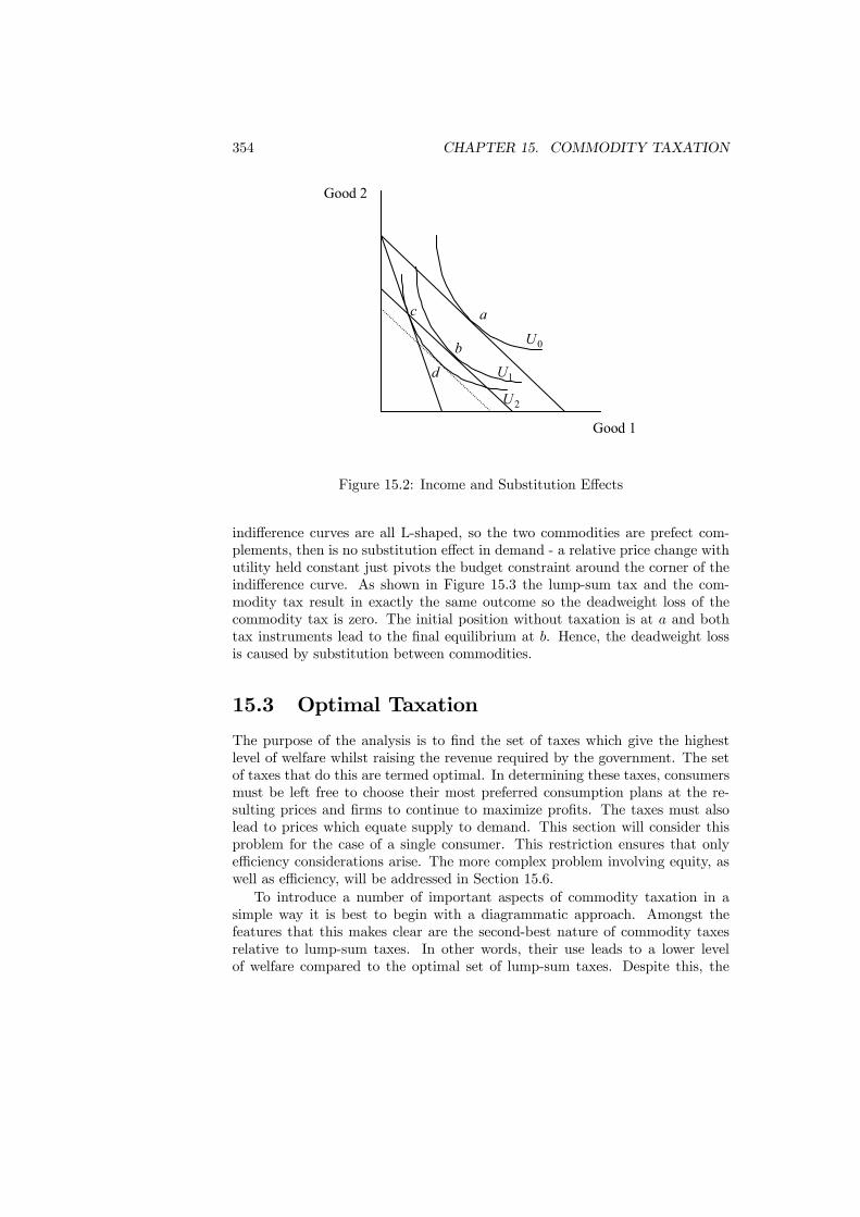
354 CHAPTER 15. COMMODITY TAXATION
Good 1
Good 2
a
b
c
d
0U
1U
2U
Figure 15.2: Income and Substitution Effects
indifference curves are all L-shaped, so the two commodities are prefect com-plements, then is no substitution effect in demand - a relative price change withutility held constant just pivots the budget constraint around the corner of theindifference curve. As shown in Figure 15.3 the lump-sum tax and the com-modity tax result in exactly the same outcome so the deadweight loss of thecommodity tax is zero. The initial position without taxation is at a and bothtax instruments lead to the final equilibrium at b. Hence, the deadweight lossis caused by substitution between commodities.
15.3 Optimal Taxation
The purpose of the analysis is to find the set of taxes which give the highestlevel of welfare whilst raising the revenue required by the government. The setof taxes that do this are termed optimal. In determining these taxes, consumersmust be left free to choose their most preferred consumption plans at the re-sulting prices and firms to continue to maximize profits. The taxes must alsolead to prices which equate supply to demand. This section will consider thisproblem for the case of a single consumer. This restriction ensures that onlyefficiency considerations arise. The more complex problem involving equity, aswell as efficiency, will be addressed in Section 15.6.To introduce a number of important aspects of commodity taxation in a
simple way it is best to begin with a diagrammatic approach. Amongst thefeatures that this makes clear are the second-best nature of commodity taxesrelative to lump-sum taxes. In other words, their use leads to a lower levelof welfare compared to the optimal set of lump-sum taxes. Despite this, the
15.3. OPTIMAL TAXATION 355
Good 1
Good 2
a
b0U
1U
Figure 15.3: Absence of Deadweight Loss
observability of transactions makes commodity taxes feasible whereas optimallump-sum taxes are generally not for the reasons explored in Chapter 13.
Consider a two-good economy with a single consumer and a single firm (theRobinson Crusoe economy of Chapter 6). One of the goods, labor is used asan input (so it is supplied by the consumer to the firm) and the output is soldby the firm to the consumer. In Figure ?? the horizontal axis measures laboruse and the vertical axis output. The shaded area is the firm’s production set,which in this case is also the production set for the economy. This is displacedfrom the origin by the distance R which equals the tax revenue requirementof the government. The interpretation is that the government takes out of theeconomy R units of labor for its own purposes. After the revenue requirementhas been met, the economy then has constant returns to scale in turning laborinto output. The commodity taxes have to be chosen to attain this level ofrevenue.
Normalizing the wage rate to 1, the only output price for the firm that leadsto zero profit is shown by p. This is the only level of profit consistent with theassumption of competitive behavior and p must be the equilibrium price for thefirm. Given this price, the firm is indifferent to where it produces on the frontierof its production set.
Figure 15.5 shows the budget constraint and the preferences of the consumer.With the wage rate of 1, the budget constraint for the consumer is constructedby setting the consumer’s price for the output to q. The difference between qand p is the tax upon the consumption good. It should be noticed that labor isnot taxed. As will become clear, this is not a restriction on the set of possibletaxes. With these prices, the consumer’s budget constraint can be written
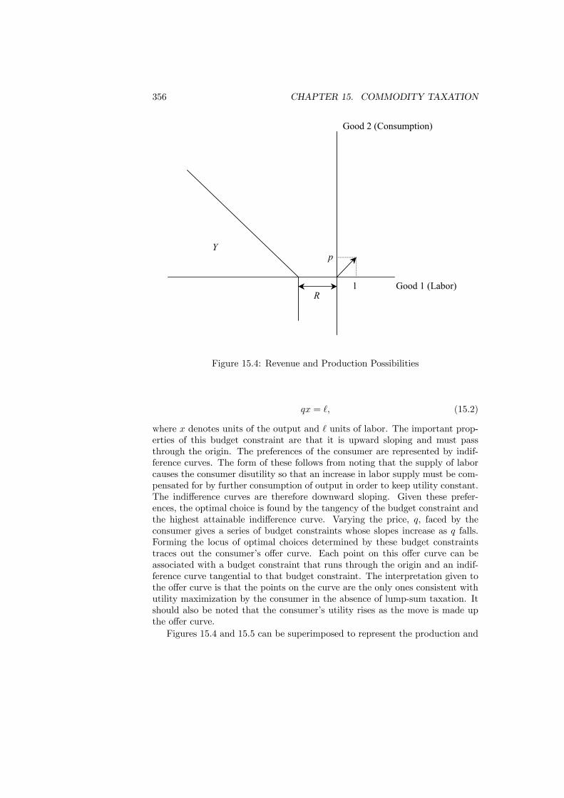
356 CHAPTER 15. COMMODITY TAXATION
Good 1 (Labor)
Good 2 (Consumption)
R
Y
1
p
Figure 15.4: Revenue and Production Possibilities
qx = `, (15.2)
where x denotes units of the output and ` units of labor. The important prop-erties of this budget constraint are that it is upward sloping and must passthrough the origin. The preferences of the consumer are represented by indif-ference curves. The form of these follows from noting that the supply of laborcauses the consumer disutility so that an increase in labor supply must be com-pensated for by further consumption of output in order to keep utility constant.The indifference curves are therefore downward sloping. Given these prefer-ences, the optimal choice is found by the tangency of the budget constraint andthe highest attainable indifference curve. Varying the price, q, faced by theconsumer gives a series of budget constraints whose slopes increase as q falls.Forming the locus of optimal choices determined by these budget constraintstraces out the consumer’s offer curve. Each point on this offer curve can beassociated with a budget constraint that runs through the origin and an indif-ference curve tangential to that budget constraint. The interpretation given tothe offer curve is that the points on the curve are the only ones consistent withutility maximization by the consumer in the absence of lump-sum taxation. Itshould also be noted that the consumer’s utility rises as the move is made upthe offer curve.Figures 15.4 and 15.5 can be superimposed to represent the production and
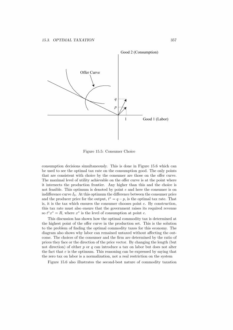
15.3. OPTIMAL TAXATION 357
Good 1 (Labor)
Good 2 (Consumption)
1
p
q
Offer Curve
Figure 15.5: Consumer Choice
consumption decisions simultaneously. This is done in Figure 15.6 which canbe used to see the optimal tax rate on the consumption good. The only pointsthat are consistent with choice by the consumer are those on the offer curve.The maximal level of utility achievable on the offer curve is at the point whereit intersects the production frontier. Any higher than this and the choice isnot feasible. This optimum is denoted by point e and here the consumer is onindifference curve I0. At this optimum the difference between the consumer priceand the producer price for the output, t∗ = q− p, is the optimal tax rate. Thatis, it is the tax which ensures the consumer chooses point e. By construction,this tax rate must also ensure that the government raises its required revenueso t∗x∗ = R, where x∗ is the level of consumption at point e.This discussion has shown how the optimal commodity tax is determined at
the highest point of the offer curve in the production set. This is the solutionto the problem of finding the optimal commodity taxes for this economy. Thediagram also shows why labor can remained untaxed without affecting the out-come. The choices of the consumer and the firm are determined by the ratio ofprices they face or the direction of the price vector. By changing the length (butnot direction) of either p or q can introduce a tax on labor but does not alterthe fact that e is the optimum. This reasoning can be expressed by saying thatthe zero tax on labor is a normalization, not a real restriction on the system
Figure 15.6 also illustrates the second-best nature of commodity taxation

358 CHAPTER 15. COMMODITY TAXATION
Good 1 (Labor)
Good 2 (Consumption)
Y
1
p
0Ie
q*t
*e
1I
- R
⋅⋅
fg
Figure 15.6: Optimal Commodity Taxation

15.4. PRODUCTION EFFICIENCY 359
relative to lump-sum taxation. It can be seen that there are points above theindifference curve I0 (the best achievable by commodity taxation) which arepreferred to e and which are also productively feasible. The highest attainableindifference curve for the consumer given the production set is I1 and utility ismaximized at e∗. This point would be chosen by the consumer if they faced abudget constraint which was coincident with the production frontier. A budgetconstraint of this form would cross the horizontal axis to the left of the originand would have the form
qx = `−R, (15.3)
where R represents a lump-sum tax equal to the revenue requirement. Thislump-sum tax would decentralize the first-best outcome at e∗. Commoditytaxation can only achieve the second-best at e.
15.4 Production Efficiency
The diagrammatic illustration of optimal taxation in the one-consumer econ-omy also shows another important result. This result, known as the Diamond-Mirrlees production efficiency lemma, states the production must be efficientwhen the optimal taxes are employed. In other words, the optimum with com-modity taxation must be on the boundary of the production set. This providesa demonstration of the efficiency lemma and discusses its implications.Production efficiency occurs when an economy is maximizing the output
attainable from its given set of resources. This can only happen when theeconomy is on the boundary of its production possibility set. Starting at aboundary point, no reallocation of inputs amongst firms can increase the outputof one good without reducing that of another (compare this with the Paretoefficiency criteria of Chapter 7). In the special case in which each firm employssome of all of the available inputs, a necessary condition for production efficiencyis that the marginal rate of substitution (MRS) between any two inputs is thesame for all firms. Such a position of equality is attained, in the absence oftaxation, by the profit maximization of firms in competitive markets. Each firmsets the marginal rate of substitution equal to the ratio of factor prices and,since factor prices are the same for all firms, this induces the necessary equalityin the MRSs. The same is true when there is taxation provided all firms facethe same post-tax prices for inputs, that is, inputs taxes are not differentiatedbetween firms.To see that the optimum with commodity taxation must be on the frontier of
the production set, consider interior points f and g. If the equilibrium were atf , the consumer’s utility could be raised by reducing the use of the input whilstkeeping output constant. Since this is feasible, f cannot be an optimum. Fromg, output could be increased without employing more labor so that g cannot bean optimum. Since this reasoning can be applied to any point that is interiorto the production set, the optimum must be on the boundary.
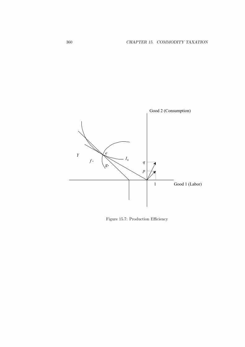
360 CHAPTER 15. COMMODITY TAXATION
Good 1 (Labor)
Good 2 (Consumption)
Y
1
p
0Ie
q⋅⋅
fg
Figure 15.7: Production Efficiency
15.5. TAX RULES 361
Although Figure 15.7 was motivated by considering the input to be labor,a slight re-interpretation can introduce intermediate goods. Assume that thereis an industry that uses one unit of labor to produce one unit of an intermedi-ate good and that the intermediate good is then used to produce final output.Figure 15.7 then depicts the intermediate good (the input) being used to pro-duce the output. Although the household actually has preferences over laborand final output and acts only on the markets for these goods, the direct linkbetween units of labor and of intermediate good allows preferences and the bud-get constraint to be depicted as if they were defined directly on those variables.The production efficiency argument then follows directly as before and now im-plies that intermediate goods should not be taxed since this would violate theequalization of MRSs between firms.The logic of the single-consumer economy can be adapted to show that the
efficiency lemma still holds when there are many consumers. What makes theresult so obvious in the single-consumer case is that a reduction in labor use oran increase in output raises the consumer’s utility. With many consumers, sucha change would have a similar effect if all consumer’s supply labor or prefer tohave more, rather than less, of the consumption good. This will be hold if thereis some agreement in the tastes of the consumers. If this is so, a direction ofmovement can be from an interior point in the production set to an exteriorpoint that is unanimously welcomed. The optimum must then be exterior.In summary, the Diamond-Mirrlees lemma provides a persuasive argument
for the non-taxation of intermediate goods and the non-differentiation of inputtaxes between firms. These are results of immediate practical importance sincethey provide a basic property that an optimal tax system must possess. Aswill become clear, it is rather hard to make precise statements about the opti-mal levels of tax but what the efficiency lemma provides is a clear and simplestatement about the structure of taxation.
15.5 Tax Rules
The diagrammatic analysis has shown the general principle behind the deter-mination of the optimal taxes. What is has not shown is how the tax burdenshould be allocated across different commodities. The optimal tax problem is toset the taxes upon the commodities to maximise social welfare subject to raisinga required level of revenue. This section looks at tax rules that characterize thesolution to this problem.To derive the rules it is first necessary to precisely specify a model of the
economy. Let there be n goods, each of which is produced with constant returnsto scale by competitive firms. Since the firms are competitive, the price theysell at must be equal to the marginal cost of production. Under the assump-tion of constant returns, this marginal cost is also independent of the scale ofproduction. Labor is assumed to be the only input into production.With the wage rate as numeraire, these assumptions imply that the producer
(or pre-tax) price of good i is determined by
362 CHAPTER 15. COMMODITY TAXATION
pi = ci, i = 1, ..., n, (15.4)
where ci denotes the number of units of labor required to produce good i. Theconsumer (or post-tax) prices are equal to the pre-tax prices plus the taxes. Forgood i the consumer price qi is
qi = pi + ti, i = 1, ..., n. (15.5)
Writing xi for the consumption level of good i, the tax rates on the n consump-tion goods must be chosen to raise the required revenue. Denoting the revenuerequirement by R, the revenue constraint can be written
R =nXi=1
tixi. (15.6)
In line with this numbering convention, labor is denoted as good 0, so x0 is thesupply of labor.This completes the description of the economy. The simplifying feature is
that the assumption of constant returns to scale fixes the producer prices via(15.4) so that equilibrium prices are independent of the level of demand. Fur-thermore, constant returns also implies that whatever demand is forthcomingat these prices will be met by the firms. If the budget constraints (both govern-ment and consumer), any demand must be backed by sufficient labor supply tocarry out the necessary production.
15.5.1 The Inverse Elasticity Rule
The first tax rule considers a simplified situation that delivers a very precisesolution. This solution, the inverse elasticity rule, provides a foundation forproceeding to the more general case. The simplifying assumption is that thegoods are independent in demand so that there are no cross-price effects betweenthe taxed goods. This independence of demands is a strong assumption so thatit is not surprising that a clear result can be derived. The way the analysis isset is to choose the optimal allocation and infer the tax rates from this. This isthe argument used in the diagram to locate the intersection of the offer curveand the frontier of the production set and then work back to the tax rates.Consider a consumer who buys the two taxed goods and supplies labor. Their
preferences are U (x0, x1, x2) and the budget constraint is q1x1+q2x2 = x0. Theprocess of utility maximization gives the first-order condtions Ui = αqi, whereUi is the marginal utility of good i and α is the marginal utility of income, andU0 = −α.The government revenue constraint is R = t1x1+ t2x2 but since ti = qi− pi,
this can be written as
q1x1 + q2x2 = R+ p1x1 + p2x2. (15.7)
15.5. TAX RULES 363
Using this the optimal tax rates are found from the Lagrangean
max{x1,x2}
L = U (x0, x1, x2) + λ [q1x1 + q2x2 −R− p1x1 − p2x2] (15.8)
The basic assumption that demands are independent can be used to writeqi = qi (xi). Using this and the consumer’s budget constraint to replace `, thefirst-order condition for the quantity of good i is
Ui + U0
·qi + xi
∂qi∂xi
¸+ λ
·qi + xi
∂qi∂xi− pi
¸= 0. (15.9)
The conditions Ui = αqi and U0 = −α can be used to write this as
−αxi ∂qi∂xi
+ λqi + λxi∂qi∂xi− λpi = 0. (15.10)
Now note that xiqi∂qi∂xi
= 1εdi, where εdi is the elasticity of demand for good i. The
first-order condition can then be solved to write
tipi + ti
=
·α− λ
λ
¸1
εdi. (15.11)
Equation (15.11) is the inverse elasticity rule. To interpret it must be notedthat α is the marginal utility of another unit of income for the consumer andλ is the utility cost of another unit of government revenue. Since taxes aredistortionary, λ > α. Therefore α − λ is negative. Since εdi is negative, thismakes the tax rate positive.This states that the proportional rate of tax on good k should be inversely
related to its price elasticity of demand. Furthermore, the constant of propor-tionality is the same for all goods. Recalling the discussion of the deadweightloss of taxation, it can be seen that this places proportionately more of the taxburden on goods where the deadweight loss is low. Its implication is clearlythat necessities, which by definition have low elasticities of demand, should behighly taxed.Limitations of this is that it rules out any linkages across the demands of dif-
ferent commodities. Also not clear how this can be extended to many consumersto take account of equity effects.
15.5.2 The Ramsey Rule
The diagram has shown some of the features that the optimal set of commoditytaxes will have. What the single-good formulation cannot do is give any insightinto how that tax burden should be spread across different goods. For example,should all goods have the same rate of tax or should taxes be related to thecharacteristics of the goods? This section will provide a derivation of a formulathat goes a long way to answering this question. This formula is called Ramseyrule and is one of the oldest results in the theory of optimal taxation. It provides

364 CHAPTER 15. COMMODITY TAXATION
a description of the optimal taxes for an economy with a single consumer inwhich there are no equity considerations.To derive the Ramsey rule it is necessary to change from choosing the optimal
quantities to choosing the taxes. Assume that there are just two consumptiongoods in order to simplify the notation and let the demand function for good ibe xi = xi (q) where q = q1, q2. The fact that the prices of all the commoditiesenter this demand function shows that the full range of interactions betweenthe demands is allowed. Using these demand functions, the preferences of theconsumer can be written
U = U (x0 (q) , x1 (q) , x2 (q)) . (15.12)
The optimal commodity taxes are those which give the highest level of utilityto the consumer while ensuring that the government reaches its revenue targetof R > 0. The government’s problem in choosing the tax rates can then besummarized by the Lagrangean
max{t1,t2}
L = U (x0 (q) , x1 (q) , x2 (q)) + λ
"2Xi=1
tixi (q)−R#, (15.13)
where it is recalled that qi = pi + ti. Differentiating (15.13) with respect to thetax on good k, the first-order necessary condition is
∂L
∂tk≡
2Xi=0
Ui∂xi∂qk
++λ
"xk +
2Xi=1
ti∂xi∂qk
#= 0 (15.14)
This first-order condition needs some manipulation to place it in the formwe want. The first step is to note that the budget constraint of the consumer is
q1x1 (q) + q2x2 (q) = x0 (q) . (15.15)
Any change in price of good k must result in demands that still satisfy thisconstraint so
q1∂x1∂qk
+ q2∂x2∂qk
+ xk =∂x0∂qk
. (15.16)
In addition, the conditions for optimal consumer choice are U0 = −α and Ui =αqi. Using these optimality conditions and (15.16), the forst-order condition forthe optimal tax, (15.14), becomes
αxk = λ
"xk +
2Xi=1
ti∂xi∂qk
#. (15.17)
Notice how this first-order condition involves quantities rather than the pricesthat appeared in the inverse elasticity rule. After rearrangement (15.17) be-comes
2Xi=1
ti∂xi∂qk
= −·λ− α
λ
¸xk. (15.18)
15.5. TAX RULES 365
The next step in the derivation is to employ the Slutsky equation whichbreaks the change in demand into the income and substition effects. The effectof an increase in the price of good k upon the demand for good i is determinedby the Slutsky equation as
∂xi∂qk
= Sik − xk ∂xi∂I, (15.19)
where Sik is the substitution effect of the price change (the move around anindifference curve) and−xk ∂xi∂I is the income effect of the price change (I denoteslump-sum income). Substituting from (15.19) into (15.18) gives
2Xi=1
ti
·Sik − xk ∂xi
∂I
¸= −
·λ− α
λ
¸xk (15.20)
(15.20) is now simplified by extracting the common factor xk which yields
2Xi=1
tiSik = −"1− α
λ−
2Xi=1
ti∂xi∂I
#xk. (15.21)
The substitution effect of a change in the price of good i on the demand for goodk is exactly equal to the substitution effect of a change in the price of good k onthe demand for good i because both are determined by movement around thesame indifference curve. This symmetry property implies Ski = Sik which canbe used to rearrange (15.21) to give the expression
2Xi=1
tiSki = −θxk, (15.22)
where θ =
·1− α
λ −2Pi=1
ti∂xi∂I
¸is a positive constant. Equation (15.22) is the
Ramsey rule describing a system of optimal commodity taxes and an equationof this form must hold for all goods, k = 1, ..., n.The optimal tax rule described by (15.22) can be used in two ways. If
the details of the economy are specified (the utility function and productionparameters) then the actual tax rates can be calculated. Naturally, the precisevalues would be a function of the structure chosen. Although this is the directionthat heads towards practical application of the theory (and more is said later),it is not the route that will be currently taken. The second use of the rule isto derive some general conclusions about the determinants of tax rates. This isdone by analyzing and understanding the individual components of (15.22).To provide with this, the focus upon the typical good k is maintained. Recall
that a substitution term meausres the change in demand with utility held con-stant. Demand defined in this way is termed compensated demand. Now beginin an initial position with no taxes. From this point, the tax ti is the change inthe tax rate on good i. Then tiSki is a first-order approximation to the change

366 CHAPTER 15. COMMODITY TAXATION
in compensated demand for good k due to the introduction of the tax ti. Ifthe taxes are small, this will be a good approximation to the actual change.Extending this argument to take account of the full set of taxes, it follows that2Pi=1tiSki is an approximation to the total change in compensated demand for
good k due to the introduction of the tax system from the initial no-tax position.Employing this approximation, the Ramsey rule can be interpreted as sayingthat the optimal tax system should be such that the compensated demand foreach good is reduced in the same proportion relative to the pre-tax position.This is the standard interpretation of the Ramsey rule.
The importance of this observation is reinforced when it is set against thealternative, but incorrect, argument that the optimal tax system should raisethe prices of all goods by the same proportion in order to minimize the distortioncaused by the tax system. This is shown be the Ramsey rule to be false. Whatthe Ramsey rule says is that it is the distortion in terms of quantities, ratherthan prices, that should be minimized. Since it is the level of consumption thatactually determines utility, it is not surprising that what happens to prices issecondary to what happens to quantities. Prices only matter so far as theydetermine demands.
Although the actual tax rates are only implicit in the Ramsey rule, some gen-eral comments can still be made. Employing the approximation interpretation,the rule suggests that as the proportional reduction in compensated demandmust be the same for all goods, those goods whose demand is unresponsive toprice changes must bear higher taxes in order to achieve this. Although broadlycorrect, this statement can only be completely justified when all cross-price ef-fects are accounted for. One simple case that overcomes this difficulty is thatin which there are no cross-price effects between the taxed goods. This specialcase, which leads to the inverse elasticity rule, will be considered in the nextsection.
Returning to the general case, goods that are unresponsive to price changesare typically necessities such as food and housing. Consequently, the implemen-tation of a tax system based on the Ramsey rule would lead to a tax systemthat would bear most heavily on these necessities. In contrast, the lowest taxrates would fall on luxuries. If put into practice, such a tax structure would in-volve low income consumers paying disproportionately larger fractions of theirincomes in taxes relative to rich consumers. The inequitable nature of this issimply a reflection of the single household assumption: the optimization doesnot involve equity and the solution reflects only efficiency criteria.
The single-household framework is not accurate as a description of realityand leads to an outcome that is unacceptable on equity grounds. The value ofthe Ramsey rule therefore arises primarily through the framework and method ofanalysis it introduces. This can easily be generalized to more relevant settings.It shows how taxes are determined by efficiency considerations and hence givesa baseline from which to judge the effects of introducing equity.

15.6. EQUITY CONSIDERATIONS 367
15.6 Equity ConsiderationsThe lack of equity in the tax structure determined by the Ramsey rule is in-evitable given its single-consumer basis. The introduction of further consumerswith differences in incomes makes it possible to see how equity can affect theconclusions. Although the method that is now discussed can cope with any num-ber of consumers, it is sufficient to consider just two. Restricting the number inthis way has the merit of making the analysis especially transparent.Consider, then, an economy which consists of two consumers. Each consumer
h, h = 1, 2, is described by their utility function
Uh = Uh¡xh0 (q) , x
h1 (q) , x
h2 (q)
¢. (15.23)
These utility functions may vary amongst the households. Labor remains theuntaxed numeraire and all households supply only the single form of labor ser-vice.The government revenue constraint is now given by
R =2Xi=1
tix1i (q) +
2Xi=1
tix2i (q) . (15.24)
The government’s policy is guided by a social welfare function which aggregatesthe individual consumers’ utilities. This social welfare function is denoted by
W =W¡U1¡x10, x
11, x
12
¢, U2
¡x20, x
21, x
22
¢¢. (15.25)
Combining (15.24) and (15.25) into a Lagrangean expression (as in (15.13)), thefirst-order condition for the choice of the tax on good k is
− ∂W
∂U1α1x1k −
∂W
∂U2α2x2k + λ
"2X
h=1
"xhk +
2Xi=1
ti∂xhi∂qk
##= 0. (15.26)
To obtain a result that is easily comparable to the Ramsey rule, define
βh =∂W
∂V hαh. (15.27)
βh is formed as the product of the effect of an increase in consumer h’s utility onsocial welfare and their marginal utility of income. It measures the increase insocial welfare that results from a marginal increase in the income of consumer h.Consequently, βh is termed the social marginal utility of income for consumer h.Employing the definition of βh and the substitutions used to obtain the Ramseyrule, the first-order condition (15.26) becomes
2Pi=1
tiS1ki +
2Pi=1
tiS1ki
x1k + x2k
=1
λ
β1x1k + β2x2kx1k + x
2k
− 1 +
·2Pi=1
ti∂x1i∂I1
¸x1k +
·2Pi=1
ti∂x2i∂I2
¸x2k
x1k + x2k
.
(15.28)

368 CHAPTER 15. COMMODITY TAXATION
The tax structure that is described by (15.28) can be interpreted in the sameway as the Ramsey rule. The left-hand side is approximately the proportionalchange in aggregate compensated demand for good k caused by the introductionof the tax system from an initial position with no taxes. When a positive amountof revenue is to be raised (so R > 0), the level of demand will be reduced bythe tax system so this term will be negative.The first point to observe about the right-hand side is that, unlike the Ram-
sey rule, the proportional reduction in demand is not the same for all goods.It then becomes possible to discuss the factors that influence the extent of thereduction and it is through doing this that the consequences of equity can beseen. The essential component in this regard is the first term on the right-handside. The proportional reduction in demand for good k will be smaller the largeris the value of β1 x1k
x1k+x2k+ β2
x2kx1k+x
2k. The value of this will be large if a high βh
is correlated with a high xhkx1k+x
2k. The meaning of this is clear when it is recalled
that a consumer will have a high value of βh when their personal marginal util-ity of income, αh, is large and when that ∂W
∂V h is also large so the social plannergives them a high weight in social welfare. If the social welfare function is con-cave, both of these will be satisfied by low utility consumers with low incomes.
The term xhkx1k+x
2kwill be large when good k is consumed primarily by consumer
h. Putting these points together, the proportional reduction in demand for agood will be reduced if it is consumed primarily by the poor household. This isthe natural reflection of equity considerations.The second term on the right-hand side shows that the proportional reduc-
tion in demand for good k will be smaller if its demand comes mainly fromthe consumer whose tax payments change most as income changes. This termis related to the efficiency aspects of the tax system. If taxation were to beconcentrated on goods consumed by those whose tax payments fell rapidly withreductions in income, then increased taxation, and consequently greater distor-tion, would be required to meet the revenue target.This has shown how the introduction of equity modifies the conclusions of the
Ramsey rule. Rather then all goods having their compensated demand reducedin the same proportion, equity results in the goods consumed primarily by thepoor facing less of a reduction. In simple terms, this should translate into lowerrates of tax on the goods consumed by the poor relative to those determinedsolely by efficiency. Equity therefore succeeds in moderating the hard-edge ofthe efficient tax structure.
15.7 Applications
At this point in the discussion it should be recalled that fundamental motivefor the analysis is to provide practical policy recommendations. The resultsthat have been derived do give some valuable insights: the need for productionefficiency and the non-uniformity of taxes being foremost amongst them. Ac-
15.7. APPLICATIONS 369
cepting this, the analysis is only of real values if the tax rules are capable of beingapplied to data and the actual values of the resulting optimal taxes calculated.The numerical studies that have been undertaken represent the development ofa technology for achieving this aim and also provide further insights into thestructure of taxation.Referring back to (15.28) it can be seen that two basic pieces of informa-
tion are needed in order to calculate the tax rates. The first is knowledge ofthe demand functions of the consumers. This provides the levels of demand
xhk and the demand derivatives∂xhk∂qi. The second piece of information are the
social marginal utilities of income, βh. Ideally, these should be calculated froma specified social welfare function and individual utility functions for the con-sumers. The problem with this is the same as that raised in previous chapters:the construction of some meaningful utility concept. The difficulties are furthercompounded in the present case by the requirement that the demand functionsalso be consistent with the utility functions.In practice, the difficulties are circumvented rather than solved. The ap-
proach that has been adopted is to first ignore the link between demand andutility and then impose a procedure to obtain the social welfare weights. Thedemand functions are then estimated using standard econometric techniques.One common procedure to find the social welfare weights is to employ the util-ity function defined by (14.24) to measure the social utility of income to eachconsumer. That is, Uh = KMh1−²
1−² . The social marginal utility is then given by
βh = KMh−². (15.29)
The value of the parameterK can then be fixed by, for instance, setting the valueof βh equal to 1 for the lowest income consumer. With ² > 0 the social marginalutility declines as income rises. It decreases faster as ² rises so relatively moreweight is given to low income consumers. In this way, the value of ² can betreated as a measure of the concern for equity.
15.7.1 Reform
The first application of the analysis is to consider marginal reforms of tax rates.By a marginal reform is meant a small change from the existing set of tax ratesthat moves the system closer to optimality. This should be distinguished froman optimization of tax rates which might imply a very significant change fromthe initial set of taxes.Marginal reforms are much easier to compute than optimal taxes since it is
only necessary to evaluate effect of changes not of the whole move. An analogycan be drawn with hill-climbing: to climb higher you only need to know whichdirection leads upwards and do not need to know where the top is. Essentially,studying marginal reforms reduces the informational requirement.Return to the analysis of the optimal taxes in the economy with two con-
sumers. Then the effect upon welfare of a marginal increase in the tax on good
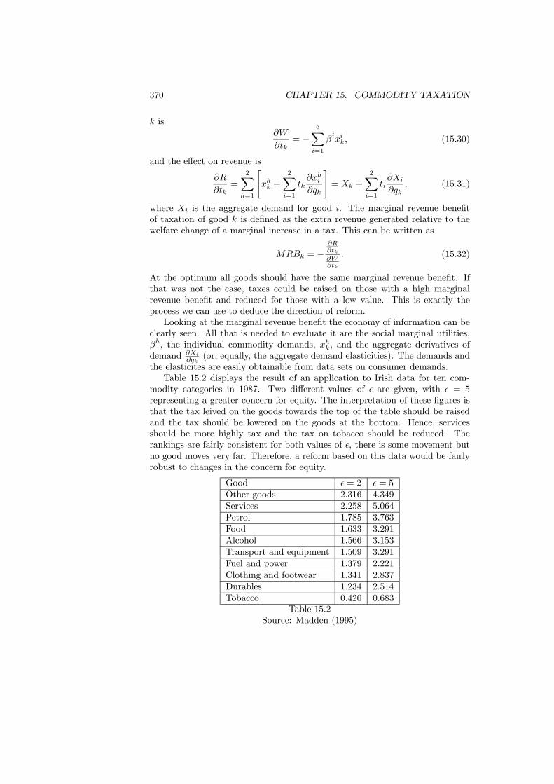
370 CHAPTER 15. COMMODITY TAXATION
k is∂W
∂tk= −
2Xi=1
βixik, (15.30)
and the effect on revenue is
∂R
∂tk=
2Xh=1
"xhk +
2Xi=1
tk∂xhi∂qk
#= Xk +
2Xi=1
ti∂Xi∂qk
, (15.31)
where Xi is the aggregate demand for good i. The marginal revenue benefitof taxation of good k is defined as the extra revenue generated relative to thewelfare change of a marginal increase in a tax. This can be written as
MRBk = −∂R∂tk∂W∂tk
. (15.32)
At the optimum all goods should have the same marginal revenue benefit. Ifthat was not the case, taxes could be raised on those with a high marginalrevenue benefit and reduced for those with a low value. This is exactly theprocess we can use to deduce the direction of reform.Looking at the marginal revenue benefit the economy of information can be
clearly seen. All that is needed to evaluate it are the social marginal utilities,βh, the individual commodity demands, xhk , and the aggregate derivatives ofdemand ∂Xi
∂qk(or, equally, the aggregate demand elasticities). The demands and
the elasticites are easily obtainable from data sets on consumer demands.Table 15.2 displays the result of an application to Irish data for ten com-
modity categories in 1987. Two different values of ² are given, with ² = 5representing a greater concern for equity. The interpretation of these figures isthat the tax leived on the goods towards the top of the table should be raisedand the tax should be lowered on the goods at the bottom. Hence, servicesshould be more highly tax and the tax on tobacco should be reduced. Therankings are fairly consistent for both values of ², there is some movement butno good moves very far. Therefore, a reform based on this data would be fairlyrobust to changes in the concern for equity.
Good ² = 2 ² = 5Other goods 2.316 4.349Services 2.258 5.064Petrol 1.785 3.763Food 1.633 3.291Alcohol 1.566 3.153Transport and equipment 1.509 3.291Fuel and power 1.379 2.221Clothing and footwear 1.341 2.837Durables 1.234 2.514Tobacco 0.420 0.683
Table 15.2Source: Madden (1995)

15.7. APPLICATIONS 371
15.7.2 Optimality
The most developed set of results derived in this way have been constructedusing data from the Indian National Sample Survey. Defining θ to be the wageas a proportion of expenditure, a selection of these results are given in Table 15.2for ² = 2. The table shows that these tax rates achieve a degree of redistributionsince cereals and milk products, both basic foodstuffs, are both subsidized. Suchredistribution results from the concern for equity embodied in a value of ² of 2.Interesting as they are, these results are limited, as are other similar analyses,by the degree of commodity aggregation that leads to the excessively generalother non-food category.
Item θ = 0.05 θ = 0.1Cereals -0.015 -0.089Milk and milk products -0.042 -0.011Edible oils 0.359 0.342Meat, fish and eggs 0.071 0.083Sugar and tea 0.013 0.003Other food 0.226 0.231Clothing 0.038 0.014Fuel and light 0.038 0.014Other non-food 0.083 0.126
Table 15.2: Optimal Tax Rates
This framework has also been used to analyze the redistributive impact ofIndian commodity taxes. This can be done by calculating the total paymentof commodity tax, Th, by consumer h relative to the expenditure, µh, of thatconsumer. The net gain from the tax system for h is then be defined by
−Th
µh. (15.33)
The consumer gains from the tax system if −Thµh
is positive since this impliesthat a net subsidy is being received. Contrasting the gains of consumer h fromthe existing tax system with those of the optimal system then provides anindication of both the success of the existing system and the potential gainsfrom the optimal system. The calculations for the existing Indian tax systemgive the gains shown in Table 15.3.
Rrual UrbanExpenditure level −Th
µh−Thµh
Rs. 20 0.105 0.220Rs. 50 0.004 0.037
Table 15.3: Redistribution of Indian commodity taxes
The expenditure levels of Rs. 20 and Rs. 50 place consumers with theseincomes in the lower 30% of the income distribution. The table shows a net
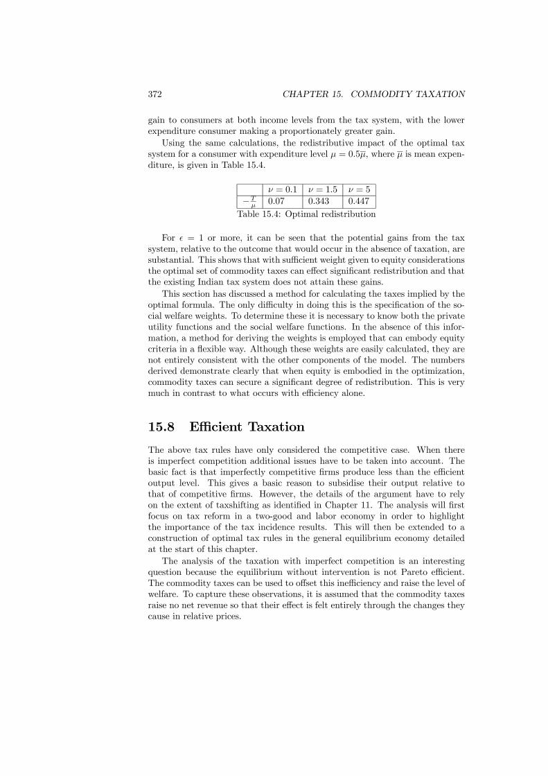
372 CHAPTER 15. COMMODITY TAXATION
gain to consumers at both income levels from the tax system, with the lowerexpenditure consumer making a proportionately greater gain.Using the same calculations, the redistributive impact of the optimal tax
system for a consumer with expenditure level µ = 0.5µ, where µ is mean expen-diture, is given in Table 15.4.
ν = 0.1 ν = 1.5 ν = 5
−Tµ 0.07 0.343 0.447Table 15.4: Optimal redistribution
For ² = 1 or more, it can be seen that the potential gains from the taxsystem, relative to the outcome that would occur in the absence of taxation, aresubstantial. This shows that with sufficient weight given to equity considerationsthe optimal set of commodity taxes can effect significant redistribution and thatthe existing Indian tax system does not attain these gains.This section has discussed a method for calculating the taxes implied by the
optimal formula. The only difficulty in doing this is the specification of the so-cial welfare weights. To determine these it is necessary to know both the privateutility functions and the social welfare functions. In the absence of this infor-mation, a method for deriving the weights is employed that can embody equitycriteria in a flexible way. Although these weights are easily calculated, they arenot entirely consistent with the other components of the model. The numbersderived demonstrate clearly that when equity is embodied in the optimization,commodity taxes can secure a significant degree of redistribution. This is verymuch in contrast to what occurs with efficiency alone.
15.8 Efficient Taxation
The above tax rules have only considered the competitive case. When thereis imperfect competition additional issues have to be taken into account. Thebasic fact is that imperfectly competitive firms produce less than the efficientoutput level. This gives a basic reason to subsidise their output relative tothat of competitive firms. However, the details of the argument have to relyon the extent of taxshifting as identified in Chapter 11. The analysis will firstfocus on tax reform in a two-good and labor economy in order to highlightthe importance of the tax incidence results. This will then be extended to aconstruction of optimal tax rules in the general equilibrium economy detailedat the start of this chapter.The analysis of the taxation with imperfect competition is an interesting
question because the equilibrium without intervention is not Pareto efficient.The commodity taxes can be used to offset this inefficiency and raise the level ofwelfare. To capture these observations, it is assumed that the commodity taxesraise no net revenue so that their effect is felt entirely through the changes theycause in relative prices.
15.8. EFFICIENT TAXATION 373
The analysis of tax design can be understood by considering the followingsimple economy in which the tax analysis consists of characterizing the welfare-improving tax reform starting from an initial position with no commodity tax-ation. The economy has a single consumer and a zero revenue requirement sothe taxes are used merely to correct for the distortion introduced by the im-perfect competition. There are two consumption goods, each produced usinglabor alone. Good 1 is produced with constant returns to scale by a competitiveindustry with post-tax price q1 = p1 + t1. It follows from these assumptionsthat ∂q1
∂t1= 1.
It is assumed that there is a single household in the economy whose prefer-ences can be represented by an indirect utility function
U = U (x0 (q1, q2) , x1 (q1, q2) , x2 (q1, q2)) , (15.34)
where w is the wage rate. Profits are assumed to be taxed at a rate of 100%and the revenue used to purchase labor. This assumption closes the model andavoids the need to worry about profit affecting the demand for consumptiongoods.Now take from the tax incidence analysis of Chapter 11 the direct and in-
duced effects of taxation. They are then denoted
∂q2∂t1≡ h1, (15.35)
and∂q2∂t2≡ h2. (15.36)
The expression of these effects at a general level has the advantage that it isunnecessary to specify the particular model of imperfect competition in orderto derive results. A specific formulation is only needed when the results requireevaluation.The tax reform problem now involves finding a pair of tax changes dt1, dt2
that raise welfare whilst collecting zero revenue. If the initial position is takento be one where both commodity taxes are zero initially, so t1 = t2 = 0, theproblem can be phrased succinctly as finding , from an initial position with suchthat dU > 0, dR = 0, where tax revenue, R, is defined by
R = t1x1 + t2x2. (15.37)
This framework ensures that one of the taxes will be negative and the otherpositive. The aim is to provide a simple characterization of the determinationof the relative rates. It should be noted that if both industries were competitivethe initial equilibrium would be Pareto efficient and the solution to the taxproblem would have dt1 = dt2 = 0. So non-zero tax rates will be a consequenceof the distortion caused by the imperfect competition.From differentiating the utility function and applying first-order condition
for consumer choice, it follows that the effect of the tax change upon welfare is
dU = −αx1 ∂q1∂t1
dt1 − αx2∂q2∂t1
dt1 − αx2∂q2∂t2
dt2. (15.38)
374 CHAPTER 15. COMMODITY TAXATION
Using the definition of the tax incidence terms h1 and h2
dU = − [αx1 + αx2h1] dt1 − αx2h2dt2 (15.39)
From the revenue constraint
dR = 0 = x1dt1 + x2dt2, (15.40)
where the fact that t1 = t2 = 0 initially has been used. Solving (15.40) for dt1gives
dt1 = −x2x1dt2. (15.41)
Substituting (15.41) into the welfare expression determines the welfare changeas dependent upon dt2 alone
dU =
·−αx2h2 + αx2 + α
x22x1h1
¸dt2. (15.42)
It is condition (15.42) that provides the key to understanding the determi-nation of the relative tax rates. Since we wish to choose the tax change dt2to ensure that dU > 0, it follows that the sign of the tax change must be thesame as that of
h−αx2h2 + αx2 + α
x22x1h1
i. From this observation follows the
conclusion that
x1 [1− h2] + x2h1 > 0⇒ dt2 > 0, (15.43)
x1 [1− h2] + x2h1 < 0⇒ dt2 < 0. (15.44)
The discussion will focus on the second of these two conditions. From (15.44),the output of the imperfectly competitive industry should be subsidized and thecompetitive industry taxed when h2 is large, so that overshifting is occurring,and h1 is negative. These are, of course, sufficient conditions. In general,the greater the degree of tax shifting the more likely is subsidization. Theexplanation for this result is that if firms overshift taxes, they will also do thesame for any subsidy. Hence a negative dt2 will be reflected by an even greaterreduction in price. If h1 is also negative, the tax on the competitive industrysecures a further reduction in the price of good 2.The conclusion of this analysis is that the rate of tax shifting is important
in the determination of relative rates of taxation. Although the economy issimplified by abstracting away from profit effects, it does demonstrate thatwith imperfect competition commodity taxation can be motivated on efficiencygrounds alone.
15.9 Public Sector PricingThe theory that has been developed in the previous sections also has a secondapplication. This arises because there are close connections between the theory

15.10. CONCLUSIONS 375
of commodity taxation and that of choosing optimal public sector prices. Firmsoperated by the public sector can be set the objective of choosing their pricingpolicy to maximize social welfare subject to some revenue target. If the firmshave increasing returns to scale, which is often the reason they are operatedby the public sector, then marginal cost pricing will lead to a deficit. Thegovernment will then want to find the optimal deviation from marginal costpricing that ensures break-even.For both commodity taxation and public sector pricing, the government is
choosing the set of consumer prices that maximize welfare subject to a rev-enue constraint. Under the commodity taxation interpretation these prices areachieved by setting the level of tax to be included in each consumer price whereaswith public sector pricing the prices are chosen directly. However the choice oftax rate is equivalent to the choice of consumer price.In the context of public sector pricing, the optimal prices are generally known
as Ramsey prices. The constraint on the optimization with commodity taxationrequires the raising of a specified level of revenue. With public sector pricingthis can be reinterpreted as the need to raise a given level of revenue in excess ofmarginal cost. The tax rates of the commodity taxation problem then translateinto the mark-up over marginal cost in the public sector pricing interpretation.The rules for optimal taxation derived above then characterize the public sectorprices.
15.10 Conclusions
This chapter has reviewed the determination of optimal commodity taxes. Ithas been shown how an efficient system places the burden of taxation primarilyupon necessities. If implemented such a system would be very damaging tolow income consumers. When equity is introduced this outcome is modified toreduce the extent to which goods consumed primarily by those with low incomeare affected by the tax system. These interpretations were borne out by thenumerical calculations.As well as providing these insights into the structure of taxes, it has also been
shown that the optimal tax system should ensure production efficiency. Theimplication of this finding is that there should be no taxes upon intermediategoods. This is a very strong and clear prediction. It is also a property thatactual tax systems adhere to.
Further readingDiamond, P.A. (1975) “A many-person Ramsey tax rule”, Journal of Public
Economics, 4, 227 - 244.Diamond, P.A. and J. A. Mirrlees (1971) “Optimal taxation and public pro-
duction 1: Production efficiency and 2: Tax rules“, American Economic Review,61, 8 - 27 and 261 - 278.Madden, D., 1995, ”An analysis of indirect tax reform in Ireland in the
1980s”, Fiscal Studies, 16, 18-37.
376 CHAPTER 15. COMMODITY TAXATION
Murty, M.N. and R. Ray (1987) “Sensitivity of optimal commodity taxes torelaxing leisure/goods separability and to the wage rate“, Economics Letters,24, 273 - 277.Myles, G.D. (1987) “Tax design in the presence of imperfect competition:
an example“, Journal of Public Economics, 34, 367 - 378.Ray, R. (1986a) “Sensitivity of “optimal” commodity tax rates to alternative
demand functional forms”, Journal of Public Economics, 31, 253 - 268.Ray, R. (1986b) “Redistribution through commodity taxes: the non-linear
Engel curve case”, Public Finance, 41, 277 - 284.Deaton, A.S. and N.H. Stern (1986) “Optimally uniform commodity taxes,
taste difference and lump-sum grants”, Economics Letters, 20, 263-266.Dreze, J.H. (1964) “Some postwar contributions of French economists to the-
ory and public policy with special emphasis on problems of resource allocation“,American Economic Review, 54, 1 - 64.
Chapter 16
Income Taxation
16.1 Introduction
As the discussion of Chapter 2 showed, the taxation of income is a major sourceof government revenue. This fact, coupled with the taxpayers’ direct observa-tion of income tax payments, make the structure of income tax the subject ofmuch political discussion. The arguments that are aired in such debate reflectthe two main perspectives upon income taxation. The first views the tax pri-marily as a disincentive to effort and enterprise. On these grounds, it followsthat the rate of tax should be kept as low as possible in order to avoid suchdiscouragement. This is essentially the expression of an efficiency argument.The competing perspective is that income taxation is well-suited for the task ofredistributing income. Hence notions of equity require that high earners shouldpay proportionately more tax on their incomes than low earners. The deter-mination of the optimal structure of income taxation involves the resolution ofthese contrasting views.These arguments introduce the two major issues in the analysis of income
taxation. The first is the effect of taxation upon the supply of labor. Taxationalters the choices that consumers make by affecting the trade-off between laborand leisure. In this respect, a particularly important question is whether anincrease in the rate of tax necessarily reduces the supply of labor. If this isthe case, support would be provided for the argument that taxes should bekept low to meet the needs of efficiency. Both theoretical and empirical resultson this issue will be discussed. The second issue that has been studied is thedetermination of the optimal level of income taxation. For reasons which willbecome clear, this is a complex question since if involves constructing a modelwith a meaningful trade-off between efficiency and equity. Having said this, ithas proved a fruitful avenue of investigation.The essential idea in the chapter it is a capital mistake to analyze the equity
of the tax structure without taking into account its impact on work efforts.To see why, consider the naive solution of setting the marginal tax rate at
377

378 CHAPTER 16. INCOME TAXATION
100 percent for all incomes above some threshold z◦ and zero tax rate for allincomes below this threshold. We can expect such tax structure to maximize theredistribution from the rich (above the income threshold) to the poor (belowthe threshold). However, this conclusion is incorrect when taxpayers respondto the tax structure. The confiscatory tax at the top removes the incentive toearn more than the threshold z◦ and everyone above this level will choose toearn exactly that amount of income. This sets a vicious circle in motion. Thegovernment must lower the threshold, inducing everyone above the new levelto lower again their incomes, and so forth until nobody chooses to work andincome is zero. Therefore it stands to reason that we must analyze the equityof the tax structure in tandem with its effect on work incentives. The idea isto find the tax schedule that meets some social objective, as captured by thesocial welfare function (see Chapter 13), given the adjustment in work effort andparticipation by taxpayers. Such a tax scheme is said to be optimal conditionalto a given objective. The results need to be interpreted with caution, however,since they are very sensitive to the distibution of abilities in the population andto the form of the utility function. More importantly, they depend on the formof the equity criterion itself.
In this chapter we will only consider welfaristic equity criterion (like the util-itarian and rawlsian social welfare functions). So inso far as the social objectiveis entirely based on individual welfare, we are not assessing the tax structure onthe basis of its capacity of either redressing inequality, or eliminating poverty.We do not either consider egalitarian social objective like equal sacrifice orequality of opportunities. There is indeed a interesting literature on fair incometax examining the distribution of taxes that imposes the same loss of utility toeveryone, either in absolute or relative terms. It is related to the ability to payprinciple according to which $1 tax is less painful for a rich than for a poor(due to the decreasing marginal value of income). This equal sacrifice approachpredicts that the resulting tax struture must be progressive (in the sense thateveryone sacrifices equally if they pay increasing percent of their income in taxas their income rises).
The chapter begins by conducting an analysis of the interaction betweenincome taxation and labor supply. A number of theoretical results are derivedand these are related to the empirical evidence. This evidence makes clear howdifferent are the responses of male and female labor supply to taxation. A modelthat permits the efficiency and equity aspects of taxation to be incorporated intothe design of the optimal tax is then described. A series of results describingthe optimal tax are then derived using this model and these are interpreted interms of practical policy recommendations. The chapter is pursued by reviewingcalculations of the optimal tax rates that emerge from the model. Finally, thechapter is completed by a discussion of the political economy aspects of incometaxation.
16.2. TAXATION AND LABOR SUPPLY 379
16.2 Taxation and Labor Supply
The effect of income taxation upon labor supply can be investigated using thestandard model of consumer choice. The analysis will begin with the generalquestion of labor supply and then move on to a series of specific analyses con-cerning the effect of variations in the tax system. The major insight this giveswill be to highlight the importance of competing income and substitution effects.As is standard, it is assumed that the consumer has a given set of preferences
over allocations of consumption and leisure. The consumer also has a fixed stockof time available which can be divided between labor supply and time spent asleisure. The utility function representing the preferences can then be defined by
U = U (x, T − `) = U (x, `) , (16.1)
where T is the stock of time, ` is labor supply and x is consumption. Conse-quently, leisure time is T − `. labor is assumed to be unpleasant for the workerso utility is reduced as more labor is supplied, implying that ∂U
∂` < 0. Let eachhour of labor supplied earn the wage rate w so that income, in the absence oftaxation is w`. Letting the rate of tax be t, the budget constraint facing theconsumer is px = [1− t]w`, where p is the price of the consumption good.This choice problem is shown in Figure 16.1a, which graphs consumption
against leisure. The indifference curves and budget constraint are as standardfor utility maximization. The optimal choice is at the tangency of the bud-get constraint and the highest attainable indifference curve. This results inconsumption x∗ and leisure T − `∗.There is also an alternative way to represent the utility function. Let pre-tax
income be denoted by z, so z = w`. Since ` = zw , utility can then be written in
terms of pre-tax income as
U = U³x,z
w
´. (16.2)
These preferences can be depicted on a graph of pre-tax income against con-sumption. The budget constraint then becomes px = [1− t] z. This is shownin Figure 16.1b. The optimal choice is shown as the tangency at point betweenthe highest attainable indifference curve and the budget constraint, with con-sumption x∗ and pre-tax income w`∗. The feature of this representation is thatthe budget constraint is not affected as w changes, so it is the same whateverwage the consumer earns, but the indifference curves do change since it is z
wthat enters the utility function. How they change is described below.This model can now be used to understand the effects of variations in the
wage rate. Consider the effect of an increase in the wage rate which is shown inthe Figure 16.2a by the move to the higher budget line and the new tangency atc. The move from a to c can be broken down into a substitution effect (a→ b)and an income effect (b→ c). The direction of the substitution effect can alwaysbe signed since it is given by a move around the indifference curve. In contrast,the income effect cannot be signed: it may be positive or negative. Consequentlythe net effect is ambiguous so an increase in the wage can raise or lower labor
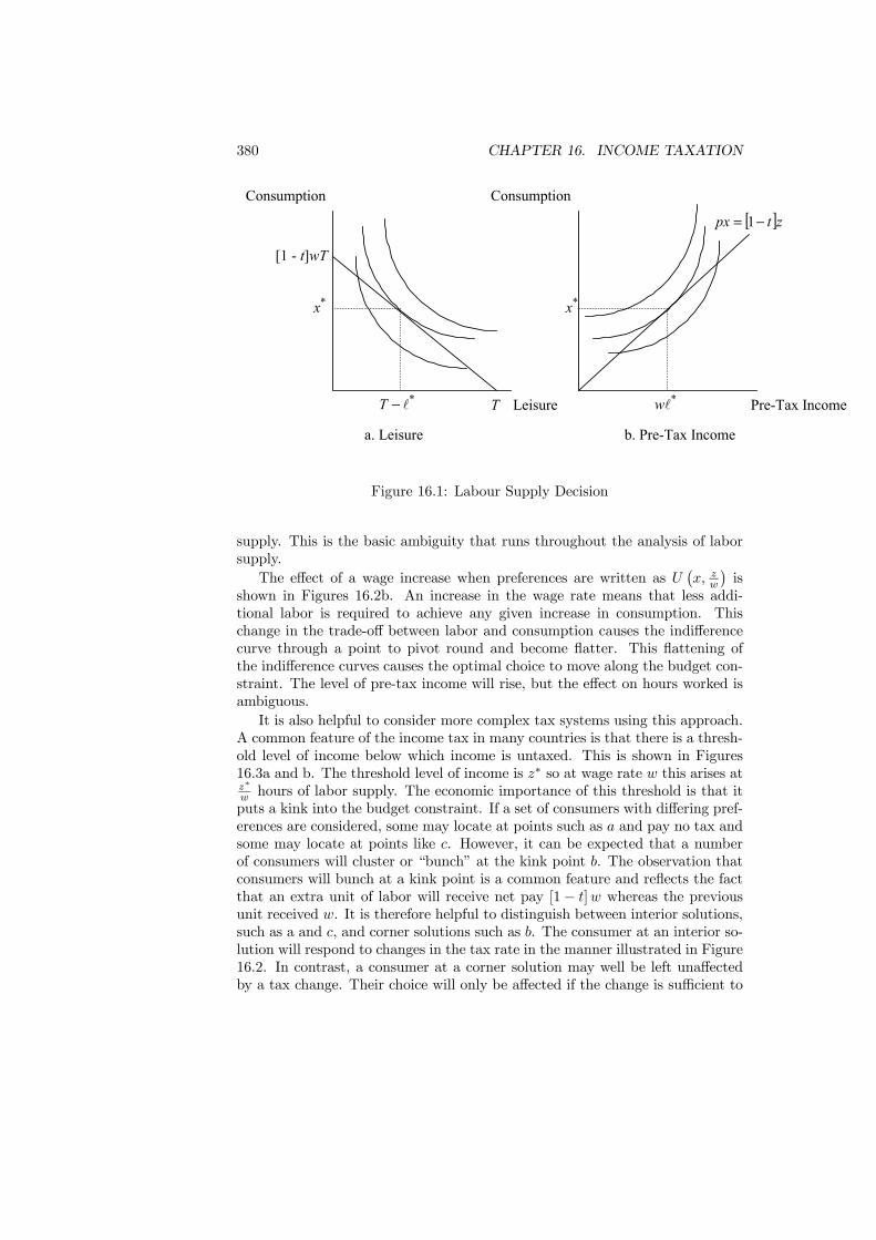
380 CHAPTER 16. INCOME TAXATION
Consumption Consumption
Leisure Pre-Tax IncomeT
[1 - t]wT
*x
*l−T
[ ]ztpx −= 1
*x
*lw
a. Leisure b. Pre-Tax Income
Figure 16.1: Labour Supply Decision
supply. This is the basic ambiguity that runs throughout the analysis of laborsupply.The effect of a wage increase when preferences are written as U
¡x, zw
¢is
shown in Figures 16.2b. An increase in the wage rate means that less addi-tional labor is required to achieve any given increase in consumption. Thischange in the trade-off between labor and consumption causes the indifferencecurve through a point to pivot round and become flatter. This flattening ofthe indifference curves causes the optimal choice to move along the budget con-straint. The level of pre-tax income will rise, but the effect on hours worked isambiguous.It is also helpful to consider more complex tax systems using this approach.
A common feature of the income tax in many countries is that there is a thresh-old level of income below which income is untaxed. This is shown in Figures16.3a and b. The threshold level of income is z∗ so at wage rate w this arises atz∗w hours of labor supply. The economic importance of this threshold is that itputs a kink into the budget constraint. If a set of consumers with differing pref-erences are considered, some may locate at points such as a and pay no tax andsome may locate at points like c. However, it can be expected that a numberof consumers will cluster or “bunch” at the kink point b. The observation thatconsumers will bunch at a kink point is a common feature and reflects the factthat an extra unit of labor will receive net pay [1− t]w whereas the previousunit received w. It is therefore helpful to distinguish between interior solutions,such as a and c, and corner solutions such as b. The consumer at an interior so-lution will respond to changes in the tax rate in the manner illustrated in Figure16.2. In contrast, a consumer at a corner solution may well be left unaffectedby a tax change. Their choice will only be affected if the change is sufficient to

16.3. EMPIRICAL EVIDENCE 381
Consumption Consumption
Leisure Pre-Tax Income
a. Leisure b. Pre-Tax Income
a a
ccb
Figure 16.2: Effect of a Wage Increase
allow the attainment of a utility level higher than at the kink.More generally, an income tax system may have a number of thresholds with
the marginal tax rate rising at each. Such a tax system appears as in Figure16.4. Again, with preferences varying across consumers the expectation is thatthere will tend to be collections of consumers at each kink point.The final issue that is worth investigating in this framework is that of partic-
ipation in the labor force. The basic assumption so far has been that the workercan continuously vary the number of working hours in order to arrive at themost preferred outcome. In practice it is often the case that hours are eitherfixed or else there is minimum that must be undertaken with the possibilityof more. Either case leads to a discontinuity in the budget constraint at thepoint of minimum hours. The choice for the consumer is then between eitherundertaking no work or working at least the minimum. This is the participationdecision: whether or not to join the workforce.The participation decision and it relation to taxation is shown in Figure
16.5 where `m denotes the minimum working time. The effect of an increasein taxation is to lower the budget constraint. A consumer that was previouslyindifferent between working and not (both points being on the same indifferencecurve) now strictly prefers to not do so. At this margin there is no conflictbetween income and substitution effects. An increase in taxation strictly reducesparticipation in the labor force.
16.3 Empirical Evidence
The theoretical analysis of Section 16.2 has identified the three major issues inthe study of labor supply. These are the potential conflict between income and
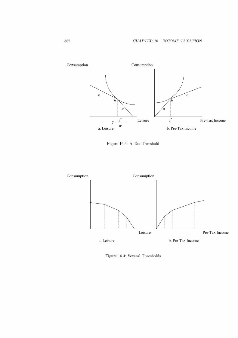
382 CHAPTER 16. INCOME TAXATION
Consumption Consumption
Leisure Pre-Tax Income
a. Leisure b. Pre-Tax Income
a a
c cbb
wzT
*−
*z
Figure 16.3: A Tax Threshold
Consumption Consumption
Leisure Pre-Tax Income
a. Leisure b. Pre-Tax Income
Figure 16.4: Several Thresholds
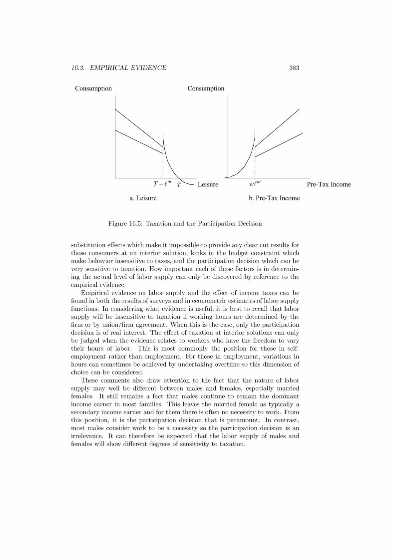
16.3. EMPIRICAL EVIDENCE 383
Consumption Consumption
Leisure Pre-Tax Income
a. Leisure b. Pre-Tax Income
TmT l− mwl
Figure 16.5: Taxation and the Participation Decision
substitution effects which make it impossible to provide any clear cut results forthose consumers at an interior solution, kinks in the budget constraint whichmake behavior insensitive to taxes, and the participation decision which can bevery sensitive to taxation. How important each of these factors is in determin-ing the actual level of labor supply can only be discovered by reference to theempirical evidence.Empirical evidence on labor supply and the effect of income taxes can be
found in both the results of surveys and in econometric estimates of labor supplyfunctions. In considering what evidence is useful, it is best to recall that laborsupply will be insensitive to taxation if working hours are determined by thefirm or by union/firm agreement. When this is the case, only the participationdecision is of real interest. The effect of taxation at interior solutions can onlybe judged when the evidence relates to workers who have the freedom to varytheir hours of labor. This is most commonly the position for those in self-employment rather than employment. For those in employment, variations inhours can sometimes be achieved by undertaking overtime so this dimension ofchoice can be considered.These comments also draw attention to the fact that the nature of labor
supply may well be different between males and females, especially marriedfemales. It still remains a fact that males continue to remain the dominantincome earner in most families. This leaves the married female as typically asecondary income earner and for them there is often no necessity to work. Fromthis position, it is the participation decision that is paramount. In contrast,most males consider work to be a necessity so the participation decision is anirrelevance. It can therefore be expected that the labor supply of males andfemales will show different degrees of sensitivity to taxation.

384 CHAPTER 16. INCOME TAXATION
Surveys on labor supply have normally arrived at the conclusion that changesin the tax rate have little effect on the labor supply decision. For instance, asurvey of the disincentive effect of high tax rates upon solicitors and accountantsin the UK, 63% of whom were subject to marginal tax rates above 50%, con-cluded that as many of the respondents were working harder because of the taxrates as were working less hard. A group such as this are ideal candidates forstudy for the reasons outlined above: they can be expected to have flexibility inthe choice of working hours and should be well-informed about the tax system.A similar conclusion was also found in a survey of the effect of income taxationon the level of overtime worked by a sample of weekly paid workers: little neteffect of taxation on working hours was found.These results suggest the conclusion that labor supply does not vary signifi-
cantly with the tax rate. If this were correct, the labor supply function would beapproximately vertical. In terms of the theoretical analysis the survey resultspoint to an income effect that almost entirely offsets the substitution effect.However, the discussion has already suggested that different groups in the pop-ulation may have different reactions to changes in the tax system. This issue isnow considered by considering the findings of some econometric analyses.Tables 16.1a - c present some summary econometric estimates of labor supply
elasticities. These are divided into those for married men, married women andunmarried women. Each gives the overall elasticity and its breakdown intosubstitution and income effects. Estimates for both the UK and the US aregiven.
Married Women Married Men Lone MothersUS UK US UK US UK
Uncompensated Wage 0.45 0.43 0.03 -0.23 0.53 0.76Compensated Wage 0.9 0.65 0.95 0.13 0.65 1.28Income -0.45 -0.22 -0.98 -0.36 -0.18 -0.52
Table 16.1: Labor supply elasticities
Since these results relate to the effect of a wage increase, theory would predictthat the substitution effect should be positive. This is what is found in all cases.The income effect, which theoretically can be positive or negative, is found tobe always negative. Consequently this offsets the substitution effect, sometimesmore than completely. Whilst there are a range of estimates for each category,some general observations can be made. The estimated elasticity for marriedmen is the lowest and is the only one that is ever estimated to be negative.This implies that the labor supply curve for married men is close to verticaland may even slopes backward. One explanation for these results could be thatthe working hours of this group are constrained by collective agreements whichleave little flexibility for variation.The labor supply of unmarried women is on average the largest of the three
sets. These results are probably a consequence of the participation effect. Forsingle women part-time work is an unattractive option since this usually impliesthe loss of state benefits. Consequently, labor supply becomes an all or nothing

16.4. MODELING INCOME TAXATION 385
decision. Married women represent the intermediate case. For them part-timework is quite common and this often opens the way to some degree of flexibilityin hours of work. As expected these factors lead to a labor supply elasticitygreater than that of married men but lower than that of unmarried women.Although the estimates vary widely within the groups, indicating some im-
precision in the estimates, some general conclusions can still be drawn. Firstly,the elasticity of labor supply is not uniform across the population of workers. Itclearly varies between the three groups identified in this discussion and probablyvaries within these groups. Despite this, it is still clearly apparent that the laborsupply elasticity for married men is small with estimates grouped around zero.Such a finding has immediate implications for the efficiency consequences of atax rate increase. In contrast, the elasticity of women is higher and reflects theparticipation effect and the greater flexibility they have in the choice of hours.
16.4 Modeling Income Taxation
The analysis of the chapter to this point has considered the positive questionof how income taxation affects labor supply. Having completed this, it is nowpossible to turn to the normative question of how the income tax structureshould be determined. This is by nature a complex issue. As has already beennoted income tax systems in practice generally have a number of thresholds atwhich the marginal tax rate rises. An investigation of the optimal system mustat least be flexible enough to consider such tax systems without limiting thenumber of thresholds or the rates of tax at each. In fact, it must do more muchthan this.These comments imply that it is necessary to construct a model that has
several important attributes. Firstly, there must be an unequal distribution ofincome in order for their to be equity motivations for taxation. Secondly, theincome tax must affect the labor supply decisions of the consumers so that it hasefficiency effects. Thirdly, in view of the comments above, the structure mustalso be sufficiently flexible that no prior restrictions are placed on the optimaltax functions that may arise.The simplest model that is able to meet all these is now described. In this
all the consumers have identical preferences but differ in their level of skill inemployment. The hourly wage received by each consumer is determined bytheir level of skill. This combines with the labor supply decision to determineincome. The economy is competitive so the wage rate is also equal to themarginal product of labor and firms price their output at marginal cost.The interesting feature of the model is that the level of skill is private in-
formation and so cannot be observed by the government. As the discussion ofChapter 13 showed, this makes it impossible to tax directly. Since the gov-ernment cannot observe a consumer’s skill level (which is essentially the initialendowment of the consumer), it employs an income tax as a second-best policy.A tax levied on skill would be the first-best policy as it would be a lump-sumtax on the unalterable characteristic which differentiates different consumers.
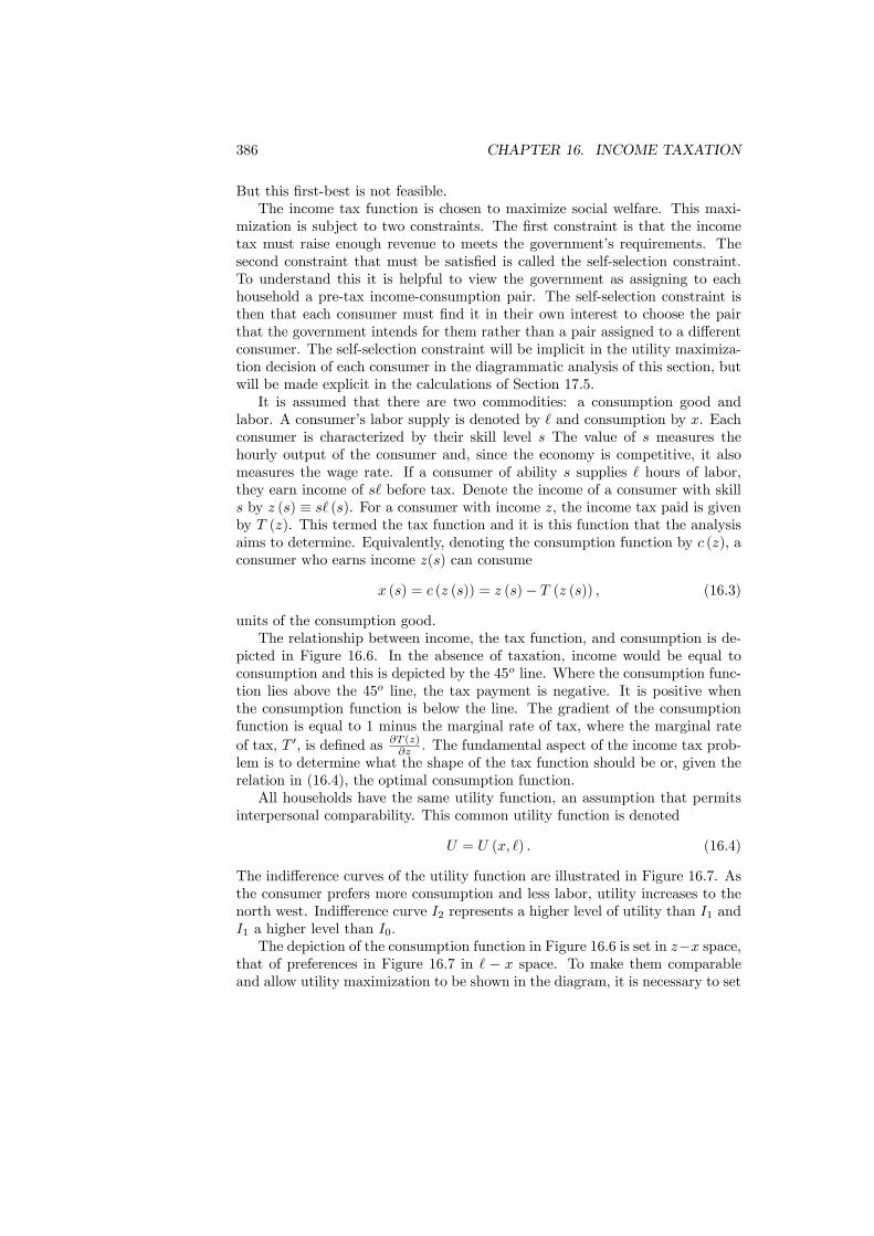
386 CHAPTER 16. INCOME TAXATION
But this first-best is not feasible.The income tax function is chosen to maximize social welfare. This maxi-
mization is subject to two constraints. The first constraint is that the incometax must raise enough revenue to meets the government’s requirements. Thesecond constraint that must be satisfied is called the self-selection constraint.To understand this it is helpful to view the government as assigning to eachhousehold a pre-tax income-consumption pair. The self-selection constraint isthen that each consumer must find it in their own interest to choose the pairthat the government intends for them rather than a pair assigned to a differentconsumer. The self-selection constraint will be implicit in the utility maximiza-tion decision of each consumer in the diagrammatic analysis of this section, butwill be made explicit in the calculations of Section 17.5.It is assumed that there are two commodities: a consumption good and
labor. A consumer’s labor supply is denoted by ` and consumption by x. Eachconsumer is characterized by their skill level s The value of s measures thehourly output of the consumer and, since the economy is competitive, it alsomeasures the wage rate. If a consumer of ability s supplies ` hours of labor,they earn income of s` before tax. Denote the income of a consumer with skills by z (s) ≡ s` (s). For a consumer with income z, the income tax paid is givenby T (z). This termed the tax function and it is this function that the analysisaims to determine. Equivalently, denoting the consumption function by c (z), aconsumer who earns income z(s) can consume
x (s) = c (z (s)) = z (s)− T (z (s)) , (16.3)
units of the consumption good.The relationship between income, the tax function, and consumption is de-
picted in Figure 16.6. In the absence of taxation, income would be equal toconsumption and this is depicted by the 45o line. Where the consumption func-tion lies above the 45o line, the tax payment is negative. It is positive whenthe consumption function is below the line. The gradient of the consumptionfunction is equal to 1 minus the marginal rate of tax, where the marginal rateof tax, T 0, is defined as ∂T (z)
∂z . The fundamental aspect of the income tax prob-lem is to determine what the shape of the tax function should be or, given therelation in (16.4), the optimal consumption function.All households have the same utility function, an assumption that permits
interpersonal comparability. This common utility function is denoted
U = U (x, `) . (16.4)
The indifference curves of the utility function are illustrated in Figure 16.7. Asthe consumer prefers more consumption and less labor, utility increases to thenorth west. Indifference curve I2 represents a higher level of utility than I1 andI1 a higher level than I0.The depiction of the consumption function in Figure 16.6 is set in z−x space,
that of preferences in Figure 16.7 in ` − x space. To make them comparableand allow utility maximization to be shown in the diagram, it is necessary to set
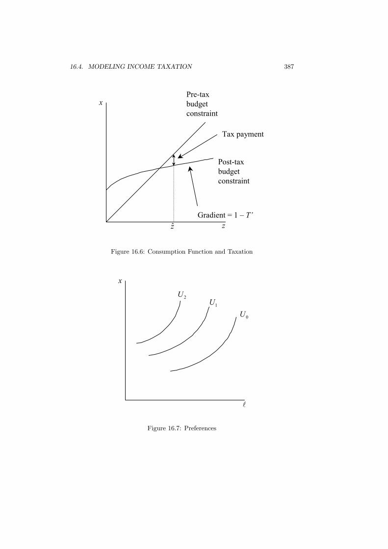
16.4. MODELING INCOME TAXATION 387
z
x
z
Pre-tax budget constraint
Post-tax budget constraint
Tax payment
Gradient = 1 – T’
Figure 16.6: Consumption Function and Taxation
x
l
0U1U
2U
Figure 16.7: Preferences

388 CHAPTER 16. INCOME TAXATION
x
l
1Ux
z
( )1 1 <sU ( )1 1 =sU ( )1 1 >sU
Figure 16.8: Translation of Indifference Curves
them in the same space. Since the consumption function is the object of primaryinterest, it is best to keep this in its natural form and to translate preferencesinto the new space. This can be done by taking the utility function and writing
U = U (x, `) = U³x,z
s
´= u (x, z, s) . (16.5)
The indifference curves of u (x, z, s), drawn in z − x space are dependent uponthe ability level of the household since it takes a high-ability household lesslabor time to achieve any given level of income. In fact, the indifference curvesare constructed from those in `− x space by multiplying by the relevant valueof s. This construction is shown in Figure 16.8 for the single indifference curveI0 and consumers of three different ability levels.Combining the preferences and consumption function it is now possible to
display the utility maximization decision of a consumer. Each consumer makesthe choice of income (which is equivalent to choosing labor supply) and consump-tion demand to maximize their utility subject to the satisfying the consumptionfunction. Hence a consumer of ability s chooses x and z to
maxu (x, z, s) subject to x = c (z) = z − T (z) . (16.6)
This optimization is shown in Figure 16.9 in which the utility maximizingchoice occurs on the highest indifference curve attainable given the consumptionfunction. Except for the additional factor that skill level is also involved here,this is essentially the same diagram that was used in Section 16.2.To derive results from the model requires that one further assumption be
placed upon preferences. This involves relating the gradient of the indifferencecurves through a given consumption-income point for consumers of differentabilities. The required assumption is termed agent monotonicity. This imposesthe condition that at any point in z−x space the indifference curve of a household
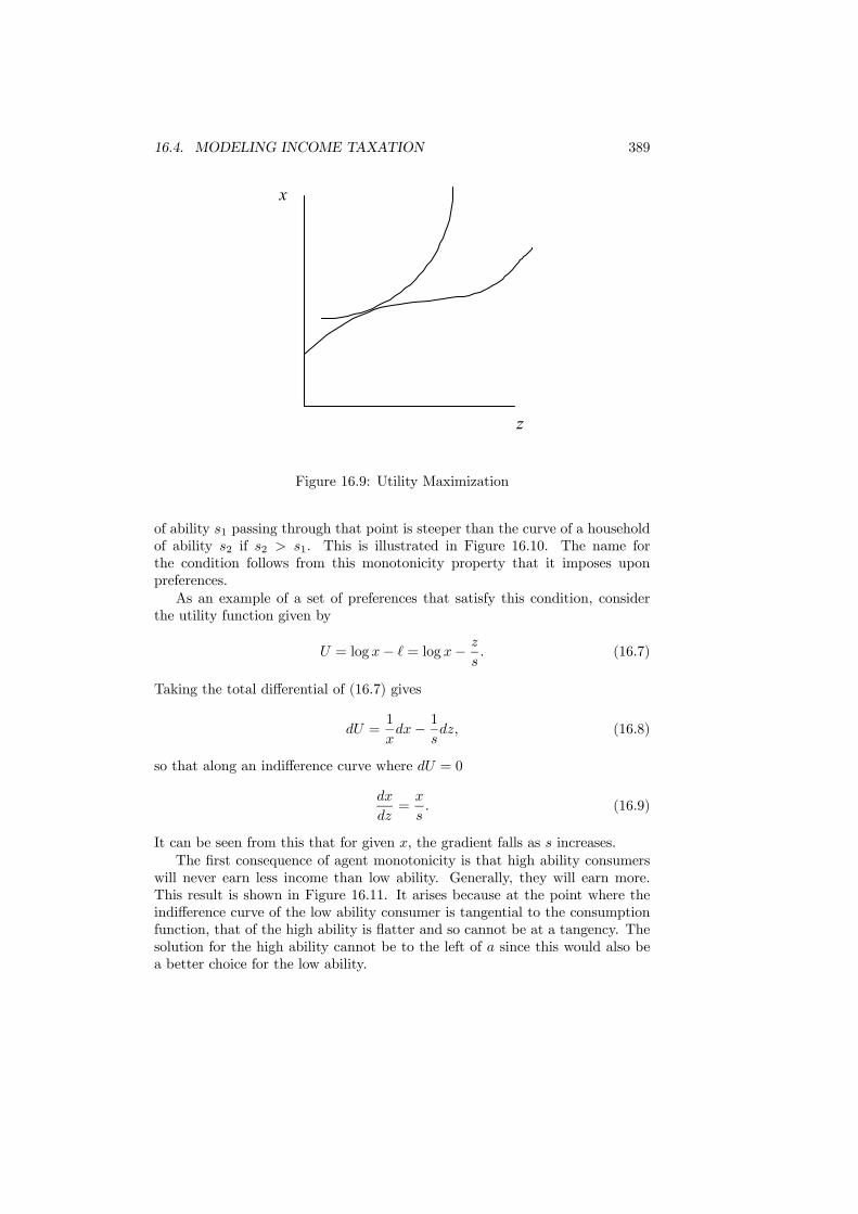
16.4. MODELING INCOME TAXATION 389
x
z
Figure 16.9: Utility Maximization
of ability s1 passing through that point is steeper than the curve of a householdof ability s2 if s2 > s1. This is illustrated in Figure 16.10. The name forthe condition follows from this monotonicity property that it imposes uponpreferences.As an example of a set of preferences that satisfy this condition, consider
the utility function given by
U = log x− ` = log x− zs. (16.7)
Taking the total differential of (16.7) gives
dU =1
xdx− 1
sdz, (16.8)
so that along an indifference curve where dU = 0
dx
dz=x
s. (16.9)
It can be seen from this that for given x, the gradient falls as s increases.The first consequence of agent monotonicity is that high ability consumers
will never earn less income than low ability. Generally, they will earn more.This result is shown in Figure 16.11. It arises because at the point where theindifference curve of the low ability consumer is tangential to the consumptionfunction, that of the high ability is flatter and so cannot be at a tangency. Thesolution for the high ability cannot be to the left of a since this would also bea better choice for the low ability.

390 CHAPTER 16. INCOME TAXATION
x
z
1ss = 2ss =
Figure 16.10: Agent Monotonicity
x
z
a
low high
Figure 16.11: Income and Ability
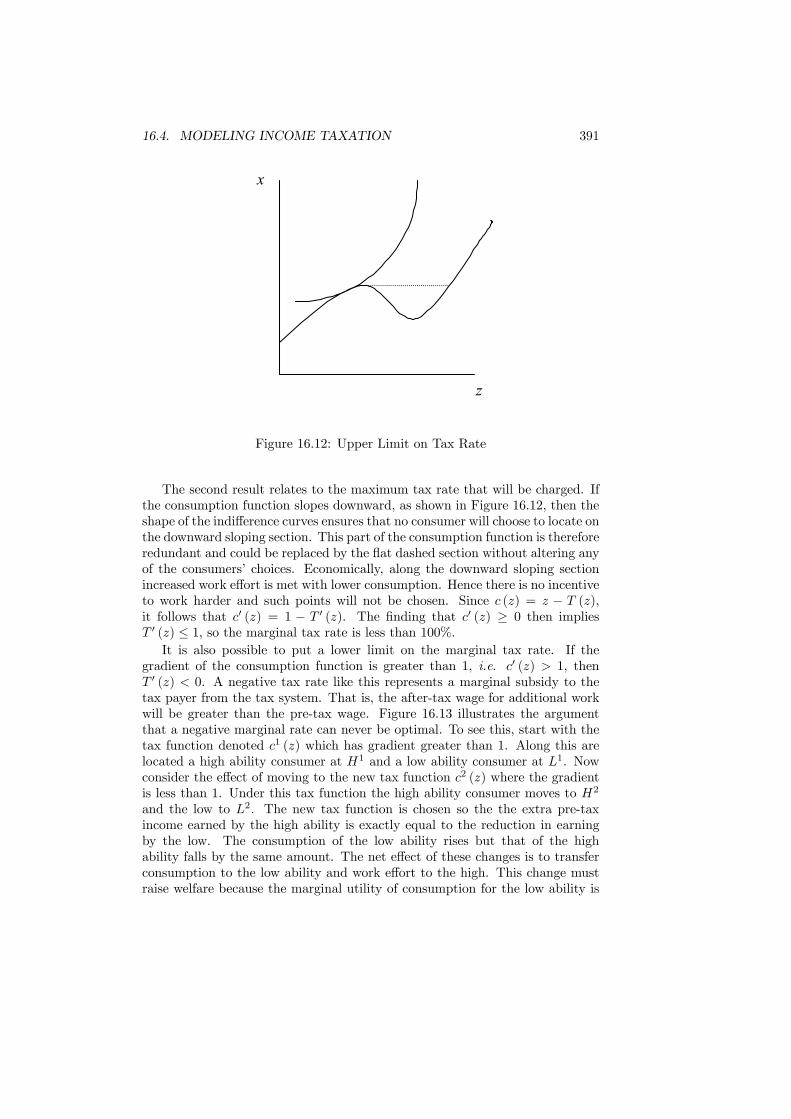
16.4. MODELING INCOME TAXATION 391
x
z
Figure 16.12: Upper Limit on Tax Rate
The second result relates to the maximum tax rate that will be charged. Ifthe consumption function slopes downward, as shown in Figure 16.12, then theshape of the indifference curves ensures that no consumer will choose to locate onthe downward sloping section. This part of the consumption function is thereforeredundant and could be replaced by the flat dashed section without altering anyof the consumers’ choices. Economically, along the downward sloping sectionincreased work effort is met with lower consumption. Hence there is no incentiveto work harder and such points will not be chosen. Since c (z) = z − T (z),it follows that c0 (z) = 1 − T 0 (z). The finding that c0 (z) ≥ 0 then impliesT 0 (z) ≤ 1, so the marginal tax rate is less than 100%.It is also possible to put a lower limit on the marginal tax rate. If the
gradient of the consumption function is greater than 1, i.e. c0 (z) > 1, thenT 0 (z) < 0. A negative tax rate like this represents a marginal subsidy to thetax payer from the tax system. That is, the after-tax wage for additional workwill be greater than the pre-tax wage. Figure 16.13 illustrates the argumentthat a negative marginal rate can never be optimal. To see this, start with thetax function denoted c1 (z) which has gradient greater than 1. Along this arelocated a high ability consumer at H1 and a low ability consumer at L1. Nowconsider the effect of moving to the new tax function c2 (z) where the gradientis less than 1. Under this tax function the high ability consumer moves to H2
and the low to L2. The new tax function is chosen so the the extra pre-taxincome earned by the high ability is exactly equal to the reduction in earningby the low. The consumption of the low ability rises but that of the highability falls by the same amount. The net effect of these changes is to transferconsumption to the low ability and work effort to the high. This change mustraise welfare because the marginal utility of consumption for the low ability is
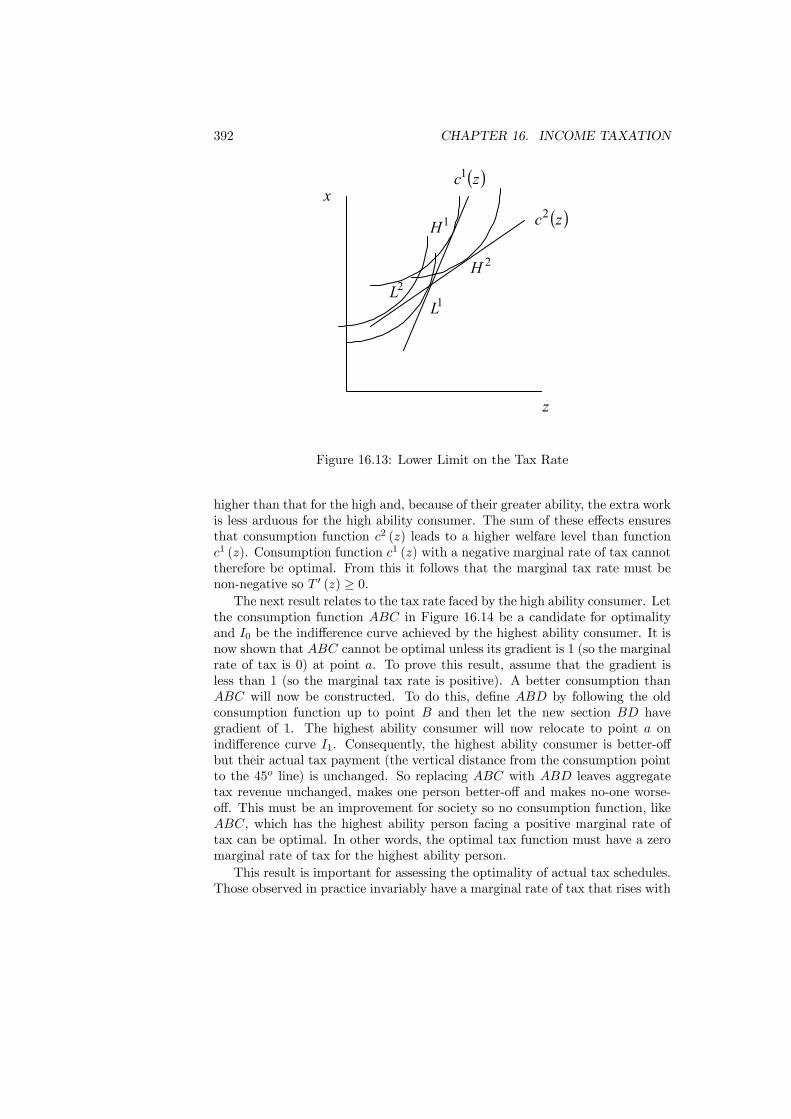
392 CHAPTER 16. INCOME TAXATION
x
z
( )zc1
( )zc21H
2H2L
1L
Figure 16.13: Lower Limit on the Tax Rate
higher than that for the high and, because of their greater ability, the extra workis less arduous for the high ability consumer. The sum of these effects ensuresthat consumption function c2 (z) leads to a higher welfare level than functionc1 (z). Consumption function c1 (z) with a negative marginal rate of tax cannottherefore be optimal. From this it follows that the marginal tax rate must benon-negative so T 0 (z) ≥ 0.The next result relates to the tax rate faced by the high ability consumer. Let
the consumption function ABC in Figure 16.14 be a candidate for optimalityand I0 be the indifference curve achieved by the highest ability consumer. It isnow shown that ABC cannot be optimal unless its gradient is 1 (so the marginalrate of tax is 0) at point a. To prove this result, assume that the gradient isless than 1 (so the marginal tax rate is positive). A better consumption thanABC will now be constructed. To do this, define ABD by following the oldconsumption function up to point B and then let the new section BD havegradient of 1. The highest ability consumer will now relocate to point a onindifference curve I1. Consequently, the highest ability consumer is better-offbut their actual tax payment (the vertical distance from the consumption pointto the 45o line) is unchanged. So replacing ABC with ABD leaves aggregatetax revenue unchanged, makes one person better-off and makes no-one worse-off. This must be an improvement for society so no consumption function, likeABC, which has the highest ability person facing a positive marginal rate oftax can be optimal. In other words, the optimal tax function must have a zeromarginal rate of tax for the highest ability person.This result is important for assessing the optimality of actual tax schedules.
Those observed in practice invariably have a marginal rate of tax that rises with
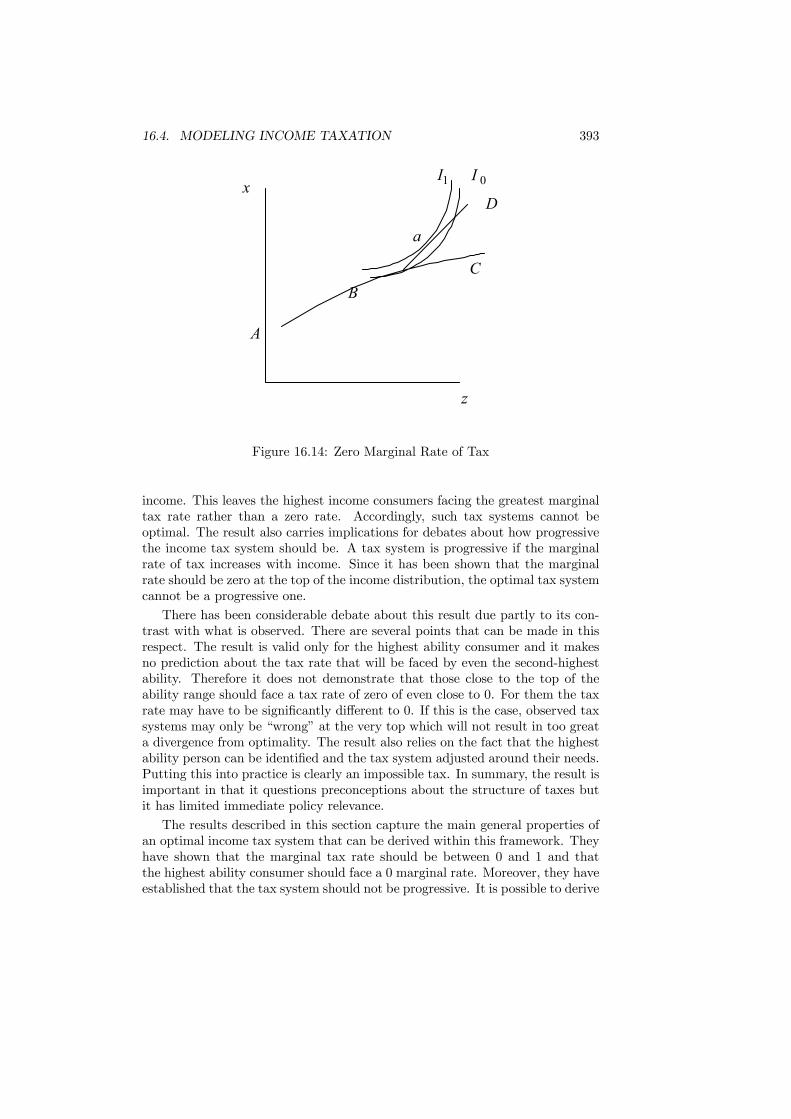
16.4. MODELING INCOME TAXATION 393
x
z
A
BC
D0I1I
a
Figure 16.14: Zero Marginal Rate of Tax
income. This leaves the highest income consumers facing the greatest marginaltax rate rather than a zero rate. Accordingly, such tax systems cannot beoptimal. The result also carries implications for debates about how progressivethe income tax system should be. A tax system is progressive if the marginalrate of tax increases with income. Since it has been shown that the marginalrate should be zero at the top of the income distribution, the optimal tax systemcannot be a progressive one.There has been considerable debate about this result due partly to its con-
trast with what is observed. There are several points that can be made in thisrespect. The result is valid only for the highest ability consumer and it makesno prediction about the tax rate that will be faced by even the second-highestability. Therefore it does not demonstrate that those close to the top of theability range should face a tax rate of zero of even close to 0. For them the taxrate may have to be significantly different to 0. If this is the case, observed taxsystems may only be “wrong” at the very top which will not result in too greata divergence from optimality. The result also relies on the fact that the highestability person can be identified and the tax system adjusted around their needs.Putting this into practice is clearly an impossible tax. In summary, the result isimportant in that it questions preconceptions about the structure of taxes butit has limited immediate policy relevance.
The results described in this section capture the main general properties ofan optimal income tax system that can be derived within this framework. Theyhave shown that the marginal tax rate should be between 0 and 1 and thatthe highest ability consumer should face a 0 marginal rate. Moreover, they haveestablished that the tax system should not be progressive. It is possible to derive
394 CHAPTER 16. INCOME TAXATION
further results only by adding further specification. The next section looks at theRawlsian optimal tax which is one way of proceeding in this direction. However,even adopting this does not provide entirely transparent insights into the levelof optimal tax rates. This can only be done through the use of numerical resultsand these are the subject matter of Section ??.
16.5 Rawlsian Tax
In Chapter 13 we introduced the Rawlsian social objective function, where so-ciety is concerned about the welfare of the worst-off individuals. The worst-offpersons are typically those at the bottom of the income distribution, and theirwelfare depends on the extent of redistribution. Assuming tax revenue are en-tirely redistributed in the form of lump sum grants; for a Rawlsian government,the optimal income tax is simply that which maximizes the lump-sum grant,that is, which maximizes the revenue that can be extracted from taxpayers.Given a tax schedule T (z), each consumer of skill level s makes the choice
of income z (which is equivalent to choosing labor supply l = z/s) and con-sumption demand x to maximize their utility u(x, z, s) subject to the satisfyingthe consumption function x = z − T (z). Let z(s) denote the optimal incomechoice of type s (conditional on tax scheme T ). It has been seen that agentmonotonicity implies that high ability consumers will never earn less incomethan low ability. So z(s) is increasing and can be inverted to give the increasinginverse function z−1(s), that is, the skill s associated to any income choice z.Different tax shemes will induce different income distributions from the sameunderlying distribution of skills.Consider skill levels are continuously distributed in the population according
to a cumulative distribution function F (s) (indicating the percentage of thepopulation below any skill level s) with associated density function f(s) > 0representing the probability associated with a small interval of the continuousskill. The tax scheme T (z) induces the following income distribution G(z) =F (z−1(s)) with density g(z) = f(z−1(s)).Now we are in a position to derive the optimal income tax associated to a
Rawlsian social welfare function. Recall that the Rawlsian optimal tax is therevenue maximizing tax schedule. Revenue maximizing tax scheme is one suchthat there exists no alternative tax structure which can raise more revenue fromthe taxpayers given their optimal work response to that new tax structure. Fromthe first order condition of the revenue maximization problem, small deviationfrom the optimal tax scheme must have no effect on total tax revenue (andlarger deviations must lower tax revenue). It follows that small change of thetax rate at any given income level z does not change total revenue. Using htissimple argument we can derive the optimal tax structure. Take income levelz, and consider a small increase in the marginal tax rate at that point by theamount ∆T 0. This change has two effects on tax revenue. First fixing laboursupply, it will increase tax payment by the amount z∆T 0 for all those taxpayerswith an income above or equal to the level at which the higher marginal tax
16.5. RAWLSIAN TAX 395
rate set in z. They represnet a proportion 1−G(z) of the population. Thereforethe revenue gain from this marginal tax change is
[1−G(z)] z∆T 0. (16.10)
Obviously, labour supply is not fixed and it is expected to vary in responeto change in tax rates. Those facing higher marginal tax rate are expectedto reduce their labour supply. Let εs denote the (uncompensated) elasticity oflabour supply to the net price of labour (the percent work reduction in responseto one percent reduction in the net price of labour). Under perfect competitionon the labour market, the price of labour decreases by the amount of the tax rate(i.e., there is no shifting of the tax burden to the employers in the form of highergross wage). Now the marginal tax rate increase ∆T 0 at income level z inducesa percentage reduction ∆T 0/1 − T 0 of the price of labour. Only those facingthis marginal tax rate change will reduce their labour supply by εs∆T
0/1− T 0percent inducing a reduction of their taxable income equal to zεs∆T 0/1 − T 0.They represent a proportion g(z) of the population (since those with an incomelevel above the level at which higher marginal tax rate set in continue to facethe same marginal tax rate). Therefore the revenue loss associated with theincentive effect of tax change is
[g(z)]T 0zεs∆T 0
1− T 0 . (16.11)
The revenue maximizing tax scheme (Rawlsian tax) requires to equate therevenue loss with the revenue gain from marginal tax change for any incomelevel. This yields
[1−G(z)] z∆T 0 = [g(z)]T 0zεs ∆T0
1− T 0 , (16.12)
and the optimal Rawlsian tax is easily seen to be such that for all income levelz
T 0(z)1− T 0(z) =
1−G(z)εsg(z)
. (16.13)
This expression has the following interpretation. High marginal tax ratesover some middle-income interval [z; z + dz] mean that for these middle-incomeindividuals but also for the upper-income individuals, the government is col-lecting more taxes. All together they represent a proportion 1 − G(z) that isdecreasing with z and converging to zero for the highest income level (hence,zero marginal tax rate at the top). The cost of the high marginal tax rates overthis interval is greater distortions for those with income in the range [z; z + dz].The total distortion (and revenue loss) will be low, however, if there are rela-tively few taxpayers in this interval (low g(z)), or if those in it have a relativelylow labour supply elasticity (low εs). Interestingly enough, even though theredistribution motive is maximal under rawlsian criterion, the optimal tax stru-ture does not require marginal progressivity. Indeed, since we do not really know

396 CHAPTER 16. INCOME TAXATION
how the labour supply elasticity changes with income, suppose that it is con-stant. Next, take the Pareto distribution of income which is supposed to bea good fit of the empirical distribution of income. For the pareto distribution,the hazard rate g(z)/1−G(z) is increasing almost everywhere. Therefore, fromthe optimal tax structure given above, it follows that marginal tax rate mustdecrease everywhere as the labor supply elasticity increases and that marginaltax rates are decreasing when the hazard rate is decreasing. Maximal redistrib-ution is better achieved when the tax schedule is regressive (concave) instead ofprogressive (convex). Such result is now extended to more general social welfarefunction through numerical analysis.
16.6 Numerical ResultsThe standard analysis of optimal income taxation has been introduced aboveand a number of results have been derived that provide some characterizationof the shape of the tax schedule. It has been seen that the marginal rate isbetween 0 and 1 but as yet no idea has been developed, except for the endpoints,of how close it should be to either. Similarly, although equity considerations areexpected to raise the marginal rate, this has not been demonstrated formallynor has consideration been given to how efficiency criteria, particularly theeffect of taxation upon labor supply, affects the choice of tax schedule. Due tothe analytical complexity of the model, these questions are best addressed vianumerical analysis.To generate numerical results, it is assumed that the social welfare function
takes the form
W =
Z ∞0
1
²e−²Uγ (s) ds, ² > 0,=
Z ∞0
Uγ (s) ds, ² = 0. (16.14)
The form of this social welfare function permits variations in the degree ofconcern for equity by changes in ². Higher values of ² represent greater concernfor equity, with ² = 0 representing the utilitarian case. (This is an alternativespecification to that of (14.24)). The individual utility function has the constantelasticity of substitution form
U =hα [L− `]−ρ + [1− α]x−ρ
i− 1ρ
, (16.15)
with elasticity of substitution ρ, ρ = 1µ+1 , equal to 1/2. The skill distribution
is log-normal so
γ (s) =1
sexp
"− log (s+ 1)
2
2
#. (16.16)
A selection of the numerical results obtained from this model are given inTables 16.2 and 16.3. In Table 16.2 ² = 0 so this is the case of a utilitarian socialwelfare function. Table 16.3 introduces equity considerations by using ² = 1.In both cases government expenditure is set at 10% of national income. The

16.6. NUMERICAL RESULTS 397
parameter σ is the standard deviation of the skill distribution. The larger is σthe more dispersed are skills or. equivalently, the greater is inherent inequality.The value of σ = 0.39 corresponds approximately to the value found in a studyof incomes. If the skill distribution matches the income distribution then thisis a value of particular interest. Γ (s) is the cumulative distribution of ability.
Income Consumption Average Tax (%) Marginal Tax (%)zG = 0.013 ν = 0
0 0.03 - 230.055 0.07 -34 260.10 0.10 -5 240.20 0.18 9 210.30 0.26 13 190.40 0.34 14 180.50 0.43 15 16
Table 16.2: The Utilitarian CaseIncome Consumption Average Tax (%) Marginal Tax (%)
zG = 0.003 ν = 10 0.05 - 300.05 0.08 -66 340.10 0.12 -34 320.20 0.19 7 280.30 0.26 13 250.40 0.34 16 220.50 0.41 17 20
Table 16.3: Some Equity Considerations
The first fact to be noticed from these results is that the average rate of taxfor low ability consumers is negative. These consumers are receiving an incomesupplement from the government. This is in the nature of a negative incometax where income below a chosen cut-off are supplemented by the governmentthrough the tax system. The average rate of tax then increases with ability.For the value of σ = 0.39 the maximum average rate of tax is actually quitesmall. The value of 34% in Table 16.3 is not far out of line with the actual ratein many countries.The behavior of the marginal rate of tax is rather different to that of the
average rate. When σ = 0.39 it is greatest at low abilities and then falls. For thetwo other values of σ it first rises and then falls. In these cases the maximum rateis reached around the median of the skill distribution. Except at the extremesof the skill distribution, there is not actually much variation in the marginaltax rate. To a first approximation, the optimal tax systems reported in thesefigures have a basically constant marginal rate of tax so that the consumptionfunction is close to being a straight line. This is one of the most surprisingconclusions of the analysis of income taxation: the model allows non-constancyin the marginal rate but this does not feature to a great degree in the optimal
398 CHAPTER 16. INCOME TAXATION
solution. Finally, the zero tax for the highest ability consumer is reflected in thefall of the marginal rate at high abilities but this is not really significant untilclose to the top of the skill distribution.Reading across the tables shows the effect of increasing the dispersion of
skills. This raises the marginal tax rates but these remain fairly constant acrossthe income range. This occurs despite the greater inequality of skills leads toa greater possible role for redistribution via the income tax. This increase inskill dispersion also has the effect of moving the maximum tax rate up theincome range, so that the marginal tax rate is increasing over the majority ofhouseholds.These results provide an interesting picture of the optimal income tax func-
tion. They suggest that it should subsidize low skill households through anegative income tax but should still face them with a high marginal rate of tax.The maximum marginal rate of tax should not be at the top of the skill dis-tribution but should occur much lower. Generally the marginal rate should befairly constant. These are not results that would have been discovered withoutthe use of this model.
16.7 Voting Over a Flat Tax
Having identified the optimal tax structure, we now need to look at how it isdetermined. To do this we consider a distribution of income and let peoplevote over tax schedules which have some degree of redistribution. Because it isdifficult to model voting on non-linear tax schemes given the high dimensionalityof the problem, we will restrict attention to a linear tax structure as originallyproposed by Romer (1975). We specify the model further with quasi-linearpreferences to avoid unnecessary complications and to simplify the analysis ofthe voting equilibrium.Consider as before that individuals differ in only their level of skill. We
assume that skills are distributed in the population according to a cumulativedistribution function F (s) that is known to everybody, with mean skill s and me-dian sm. Individuals work and consume. They also vote on a linear tax schemethat pays a lump sum benefit b to each individual, financed by a proportionalincome tax t. The individual utility function has the quasi-linear form
u(x, z, s) = x− 12
³zs
´2, (16.17)
where x and z denote consumption and income respectively. As s is the skilllevel, z/s denotes effective labour supply. The individual budget constraint is
x = (1− t)z + b. (16.18)
It is easy to verify that in this simple model the optimal income choice of types individual is
z(s) = (1− t)s2. (16.19)
16.7. VOTING OVER A FLAT TAX 399
Quasi-linear preferences imply that there is no income effect on labour supply(i.e. z(s) is independent of the lump-sum benefit b). This simplifies the effectof tax distortions and makes the analysis of the voting equilibrium easier. Lesssurprisingly, a higher tax rate induces taxpayers to work less and earn lessincome.The lump-sum transfer b is constrained by the government budget balance
condition,b = tE(z(s)) = t(1− t)E(s2), (16.20)
where E(.) is the mathematical expectation and we used the optimal incomechoice to derive the second equality. This constraint says that the lump-sumbenefit paid to each individual must be equal to the expected tax paymenttE(z(s)). This expression is termed the Dupuit-Laffer curve and describes taxrevenue as a function of the tax rate. In this simple model, the Dupuit-Laffercurve is bell shaped with a peak at t = 1/2 and no tax collected at the endst = 0 and t = 1. We can now derive individual preferences over tax schedules bymeans of indirect utility functions. Substituting (16.18) and (16.19) into (??)and rearranging, the indirect utility function becomes
V (t, b, s) = b+1
2(1− t)2s2. (16.21)
Taking the total differential of (16.21) gives
dV = db− (1− t)s2dt, (16.22)
so that along an indifference curve where dV = 0
db
dt= (1− t)s2. (16.23)
It can be seen from this that for given t, the indifference curve becomessteeper in (t, b) space as s increases. The consequence of this monotonicityis the single-crossing property of the indifference curves. As we have seen inChapter 4, the single crossing property is a sufficient condition for the medianvoter theorem to apply. It follows that there is only one tax policy that can resultfrom a majority voting: it is the policy preferred by the median voter (half thevoters are poorer than the median and prefer higher tax rates, and the other halfis richer and prefers lower tax rates). Letting tm be the tax rate preferred by themedian voter, then tm is implicitely defined by the solution to the first-ordercondition for maximizing the median voter’s utility. We differentiate (16.21)with respect to t taking into account the goverment budget constraint (16.20)to obtain
∂V
∂t= (1− 2t)E(s2)− (1− t)s2. (16.24)
Setting this expression equal to zero for the median skill level sm yields the taxrate preferred by the median voter
tm =E(s2)− s2m2E(s2)− s2m
, (16.25)
400 CHAPTER 16. INCOME TAXATION
or using the optimal income choice (16.19)
tm =E(z)− zm2E(z)− zm . (16.26)
This simple model predicts that the political equilibrium tax rate is de-termined by the position of the median voter in the income distribution. Thegreater is income inequality as measured by the distance between median andmean income, the higher the tax rate. If the median voter is relatively worseoff, with income well below the mean income, then equilibrium redistribution islarge. In practice, the income distribution has a median income below the meanincome, so that a majority of voters would favour redistribution through pro-portional income taxation. More general utility function would also predict thatthe extent of this redistribution decreases with the elasticity of labour supply.
16.8 ConclusionsThis chapter introduced the issues surrounding the effects and design of theincome tax structure. It was first shown how income and substitution effectsleft the theoretical impact of a tax increase upon labor supply indeterminate. Ifthe income effect is sufficiently strong, it is possible for a tax increase to lead tomore labor being supplied. The participation decision was also discussed and itwas argued that taxation could be significant in affecting this choice.This lack of theoretical predictions places great emphasis on empirical re-
search for determining the actual effects of taxation. It was discussed how thelabor supply responses of different groups in the population may be related totaxation. These observations were borne out by the empirical results whichshowed a very small or negative elasticity of supply for married men but a muchlarge positive elasticity for unmarried women. The latter can be interpreted asa reflection of the participation decision.A model that was able to incorporate the important issues of efficiency and
equity in income taxation was then introduced. A number of results were de-rived capturing general features of the optimal tax system.. Most notably, themarginal rate of tax facing the highest ability person should be 0 and the op-timal tax rate is bounded between 0 and 1. This model was then specializedto Rawlsian social welfare function and some further insights obtained. Numer-ical simulation results were given which showed that the marginal rate of taxshould remain fairly constant whilst the average rate of tax should be negativefor low-skill consumers. Finally the political economy of taxation was presentedby means of a simple model of voting over linear income tax schedules.
Further readingThe economics of taxation and labor supply are surveyed in:Blundell paperFeldstein, M., (1995), The effect of marginal tax rates on taxable income:
a panel study of the 1986 tax reform act, Journal of Political Economy 103,551-72.
16.8. CONCLUSIONS 401
The initial analysis of the problem of nonlinear income taxation was givenin:Mirrlees, J.A. (1971) “An exploration in the theory of optimum income tax”,
Review of Economic Studies, 38, 175 - 208.Be warned, the analytical parts of this paper are exceptionally complex.
Even so, the numerical simulation is easily understood.Further numerical simulations are discussed in:Kanbur, S.M.R. and M. Tuomala (1994) “Inherent inequality and the opti-
mal graduation of marginal tax rates”, Scandinavian Journal of Economics, 96,275 - 282.Tuomala, M. (1990)Optimal Income Tax and Redistribution, Oxford: Claren-
don Press.For a comprehensive survey of recent income tax policy in the US seePechman, J.E., (1987), Federal State Policy, 5th ed., Washington, D.C., The
Brooking Institution.The zero marginal tax rate at the top was first presented inSeade, J.K., (1977), On the shape of optimal tax schedules, Journal of Public
Economics, 7, 203-35.The properties of the quasi-linear model are explored in:Weymark, J.A. (1986) “A reduced-form optimal income tax problem”, Jour-
nal of Public Economics, 30, 199 - 217.An alternative form of quasi-linearity is used to discuss potential patterns
of marginal tax rates in:Diamond, P.A. (1998) “Optimal income taxation: an example with a U-
shaped pattern of optimal marginal tax rates”, American Economic Review,88, 83 — 95.Another consideration of the pattern of marginal rates of tax is:Myles, G.D. (2000) “On the optimal marginal rate of income tax”, Eco-
nomics Letters, 66, 113 - 119.Saez, E., (2001), Using elasticities to derive optimal tax rates, Review of
Economic Studies 68, 205-29.Voting over linear income tax was originally developed inRomer, T., (1975), Individual welfare, majority voting and the properties of
a linear income tax, Journal of Public Economics 7, 163-68.Roberts, K. , (1977), Voting over income tax schedules, Journal of Public
Economics 8, 329-40.Voting over non-linear income tax schedule is inSnyder, J., and G. Kramer, (1988), Fairness, self-interest and the politics of
the progressive income tax, Journal of Public Economics 36, 197-230.Marhuenda, F., and I. Ortuno-Ortin, (1995), Popular support for progressive
taxation, Economics Letters 48, 319-24.Hindriks, J., (2001), Is there a demand for income tax progressivity?, Eco-
nomics Letters 73, 43-50.A comprehensive and more advanced presentation of the optimal taxation
theory isSalanie, B., 2003, Economics of Taxation, Cambridge, MIT press

402 CHAPTER 16. INCOME TAXATION
A bargaining approach to the income tax problem is inAumann, R.J., and M. Kurz, (1977), Power and taxes, Econometrica 45,
1137-61.For the relationship between existing income tax systems and the equal
sarifice principle see:Young, H.P., (1990), Progressive taxation and equal sacrifice, American Eco-
nomic Review 80, 253-66.

Chapter 17
The Limits toRedistribution
17.1 Introduction
In this chapter we step back from the specific models used in the previous twochapters in order to consider taxation from a broader perspective. We havealready stressed that the role of taxation is to allow the government to achievean allocation of resources that is preferred to that which would arise in the ab-sence of intervention. The mixed economy approach we have adopted, by whichis meant the combination of competitive trading alongside intervention by thegovernment, is not the only means of organizing economic activity. Many alter-natives exist, such as the command economy with direct government resourceallocation or economies based on workers’ cooperatives.All forms of economy can be interpreted as allocation mechanisms: they
provide a mechanism for allocating the economy’s resources between competinguses. From this viewpoint, the mixed-economy model of taxation upon whichwe have focused represents just one form of allocation mechanism from amonga very broad set of potential allocation mechanisms. This line of reasoningleads to some important questions. For instance, how effective is taxation inachieving the government’s aims? Expressed differently, are there any allocationmechanisms that can achieve those aims better than the mixed economy withtaxation? If there are, what is the nature of these alternatives? By consideringthe issue of the choice between allocation mechanisms, with the mixed economyas one option among many, this chapter will provide clear answers to thesequestions.To provide the motivation for the approach we take, it is necessary to clarify
some basic issues. As we have noted many times already, government policyaims to resolve the trade-off between efficiency and equity in order to maximizeits objective function. Improving efficiency is uncontentious since it implies aPareto improvement, and therefore will be unanimously supported. In contrast,
403

404 CHAPTER 17. THE LIMITS TO REDISTRIBUTION
attaining aims of equity implies redistribution, so there will be some consumersthat lose from this (but others that gain). Those that stand to lose will havean incentive to take actions to reduce the loss. Such changes in action providelimits on the amount of redistribution that can be undertaken. Different al-location mechanisms will face different limits, so the effectiveness of taxationas an allocation mechanism can be measured against its success in achievingredistribution. More generally, it is possible to determine the limit to whichredistribution can be undertaken and enquire to whether taxation can achievethis limit.The prime obstacle to redistribution is its deleterious effect on the incentive
to create wealth. Naturally, a greater incentive to create and accumulate wealthis linked with a greater inequality of income. The cause of inequality can takeeither of two forms. Firstly, inequality can follow simply from luck. Some peopleare born with higher innate talent than others - such talents can be assigned tothe outcome of the “genetic lottery”. In addition, among those who start equal,fortune favors the endeavors of some more than others. Many people may thinkit perfectly legitimate to tax away the economic benefits that arise from luckas a source of inequality. But the ability to do so depends on the possibility ofthe government observing the innate talents and inducing their owner to bringthem to full fruition despite the knowledge that the resulting income will betaxed away. For example, even if born with the talent to become a concertpianist, a person will only choose to endure the hours of necessary practice ifthey can foresee future benefits from doing so. The second cause of inequality isthe effort that is applied to gain wealth, given the level of ability. Some peoplechoose to work harder than others, and allowing them to keep the fruits of theirown effort seems legitimate. Put another way, there can be little justificationfor redistributing from those who incomes are high because of their efforts tothose whose incomes are low solely because they choose to supply little effort.If the government could determine what part of inequality was due to differ-
ences in effort and what part due to luck, these differences present no problemsfor redistribution. In such circumstances the tax system could be finely ad-justed to elicit the correct effort level from all consumers by imposing a harshpunishment for realizing an income that is too low. In practice, effort is not ob-servable and people can pretend to work when they do not. A high income maybe the result of hard work or it may be due to chance (better natural talent),but without detailed information the government cannot infer which. Redress-ing inequality with respect to one dimension but not the other then becomes adifficult task. Higher innate talent must be judged, faute de mieux, indirectlyby income which itself depends on effort. Taxing income is then a blunt toolfor attacking the symptom, but not the cause. There is as a result a conflictbetween the redistributive and the incentive effects of the tax system that de-termines the scope for redistribution. These ideas were the basis of the analysisof optimal income taxation in Chapter 16 and the idea that a tax system hadto be incentive compatible.The purpose of this chapter is to describe how incentive compatibility, which
is the requirement that the allocation mechanism must be consistent with the in-

17.2. REVELATION PRINCIPLE 405
centives for the truthful revelation of information, places limits upon the abilityof the government to undertake redistribution. The fact that an optimal allo-cation mechanism will be consistent with truth-telling is called the revelationprinciple. We will also explain why taxation is typically the best mechanism,from among the set of incentive compatible mechanisms, for achieving redistri-bution. This conclusion is termed the tax principle. This result is interestinggiven that the notion of taxing income directly was for a long time rejected onthe grounds that the collection of the necessary information would be costlyand constitute a risk of invasion of privacy. The UK did not adopt a permanentincome tax until the 1870s and the US Congress established the same form oftaxation in the 1890s. Even today, the use of income taxation is not widespreadand has a negligible role in many developing countries. While income tax is animportant instrument of redistribution, there are additional instruments thatcan be used. Among them are commodity taxes tilted towards the poor. Weshall then describe under what circumstances differential commodity taxationcan usefully supplement the income tax and expand the possibilities for redis-tribution. This is the issue of the tax mix.
17.2 Revelation Principle
Any economic system is essentially a general allocation mechanism that deter-mines the economic allocation for each possible economic environment. The eco-nomic allocation includes the bundle of commodities each consumer receives, theproduction activities that are undertaken in the economy and the public goodsthat are provided. The economic environment is a specification of each person’sexogenous characteristics (i.e., their endowments, needs, tastes, talents, etc.) aswell as the production possibilities.The competitive economy is one form of allocation mechanism. In Chapter
6 the competitive economy was described by the preferences and endowments ofconsumers and the firms’ production technologies; this was the economic envi-ronment. Given this information, resources were allocated via the competitivetrading mechanism: taking prices as given, each consumer chose demand tomaximize utility and each firm chose output to maximize profit. Prices wereadjusted until supply and demand were equal and then trading took place toallocate commodities. We have also discussed some alternative allocation mech-anisms; two examples were the personalized pricing model in Chapter 10 andthe Clarke-Groves mechanism in Chapter 8.These allocation mechanisms have been judged by their success in allocating
resources. The First Theorem of Welfare Economics says that the competitiveeconomy is a successful allocation mechanism because it leads (under certainconditions) to a Pareto-efficient allocation. We have also seen the circumstancesunder which the competitive economy fails and government intervention canachieve a Pareto improvement. But this is not the end of the story, becausean allocation can be efficient and at the same time extremely unfair. Thecompetitive economy is indeed blind to injustice and the allocation achieved by

406 CHAPTER 17. THE LIMITS TO REDISTRIBUTION
the mechanism can involve extreme manifestations of inequity in the form ofpoverty and starvation.In response to this problem, the Second Theorem of Welfare Economics says
that (under certain conditions) any Pareto-efficient allocation can be reachedthrough competitive trading by means of lump-sum redistribution. Lump-sumredistribution does not interfere with the working of the competitive marketbecause it is based on the unalterable characteristics of the economic agents.The problem is that the personal characteristics relevant for redistribution neednot be publicly observable (i.e., tastes, talents, needs, abilities, etc.). Therefore,redistribution has to be based on information that people choose to reveal.These issues were introduced in Chapter 13.The basis of a mechanism is that the agents in the economy make a report of
information. This report could, for example, be a statement of their preferences(such as the valuation reported in the Clarke-Groves mechanism) or of theirdemands (as in the competitive economy). Alternatively, it could take the formof a direct statement of their characteristics. Given these announcements, themechanism determines the economic allocation. For the Clarke-Groves mecha-nism, the allocation was a choice to provide the public good or not and set ofside payments. In the competitive economy the allocation was determined bythe market equilibrium given the announced demands.A desirable economic allocation is defined as an achievable allocation that
maximizes a social choice function. For example, a utilitarian social choicefunction will select the allocation that maximizes the sum of utilities. The im-plementation problem is to design the allocation mechanism so that it producesa desirable economic allocation, even when agents attempt to manipulate it totheir advantage. Manipulation means reporting false characteristics in order toobtain an advantage - in Chapter 8 such manipulation arose in connection withthe Lindahl equilibrium. The scope for manipulation arises because some (orall) of the characteristics that are relevant for the proper allocation of resourcesare not publicly observable.To be more explicit, consider an economy populated by a set of agents I =
{1, ..., i, ..., n}. Each agent, i, is described by θi which is a list of all the personalcharacteristics that can be economically relevant. Let Θi be the set of possiblecharacteristics for agent i, so θi has to be drawn from the alternatives in Θi.The corresponding profile of characteristics for the set of agents in the economyis denoted θ = (θ1, ..., θn). Finally, let X be the set of economic allocations thatare technically possible using the economy’s resources.Given the characteristics for the agents the optimal allocation, that which
is best according to the social choice function, is selected. Formally, the socialchoice function determines an allocation for every possible profile of the agents’characteristics. Specifically, if the profile of characteristics is θ = (θ1, ..., θn),the social choice function selects the allocation x = f(θ). It must be the casethat x is one of the allocations in X.The central idea of mechanism design is the construction of an allocation
mechanism that implements the social choice function. That is, if the socialchoice function selects the allocation x = f(θ), then given the characteristics
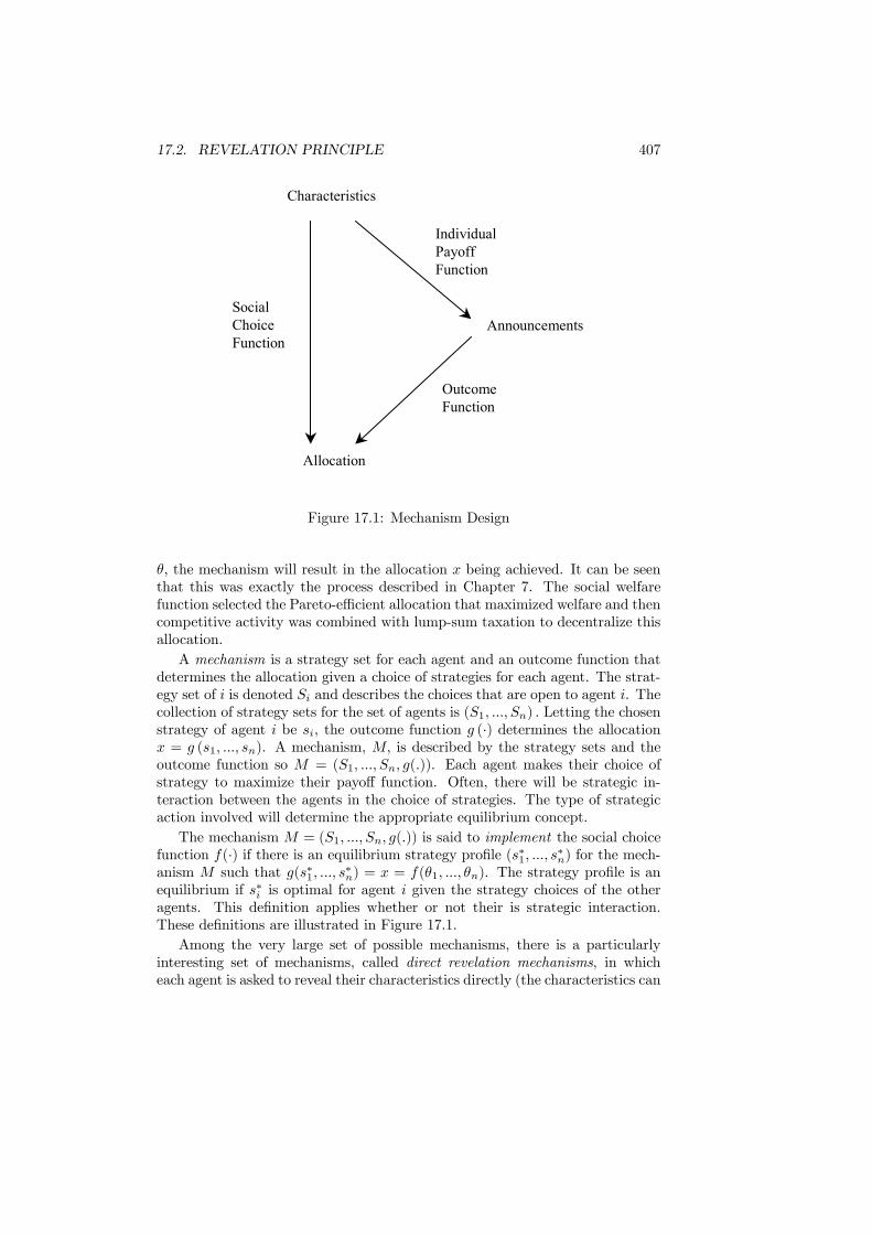
17.2. REVELATION PRINCIPLE 407
Characteristics
SocialChoiceFunction
Allocation
IndividualPayoffFunction
Announcements
OutcomeFunction
Figure 17.1: Mechanism Design
θ, the mechanism will result in the allocation x being achieved. It can be seenthat this was exactly the process described in Chapter 7. The social welfarefunction selected the Pareto-efficient allocation that maximized welfare and thencompetitive activity was combined with lump-sum taxation to decentralize thisallocation.A mechanism is a strategy set for each agent and an outcome function that
determines the allocation given a choice of strategies for each agent. The strat-egy set of i is denoted Si and describes the choices that are open to agent i. Thecollection of strategy sets for the set of agents is (S1, ..., Sn) . Letting the chosenstrategy of agent i be si, the outcome function g (·) determines the allocationx = g (s1, ..., sn). A mechanism, M, is described by the strategy sets and theoutcome function so M = (S1, ..., Sn, g(.)). Each agent makes their choice ofstrategy to maximize their payoff function. Often, there will be strategic in-teraction between the agents in the choice of strategies. The type of strategicaction involved will determine the appropriate equilibrium concept.The mechanism M = (S1, ..., Sn, g(.)) is said to implement the social choice
function f(·) if there is an equilibrium strategy profile (s∗1, ..., s∗n) for the mech-anism M such that g(s∗1, ..., s∗n) = x = f(θ1, ..., θn). The strategy profile is anequilibrium if s∗i is optimal for agent i given the strategy choices of the otheragents. This definition applies whether or not their is strategic interaction.These definitions are illustrated in Figure 17.1.Among the very large set of possible mechanisms, there is a particularly
interesting set of mechanisms, called direct revelation mechanisms, in whicheach agent is asked to reveal their characteristics directly (the characteristics can
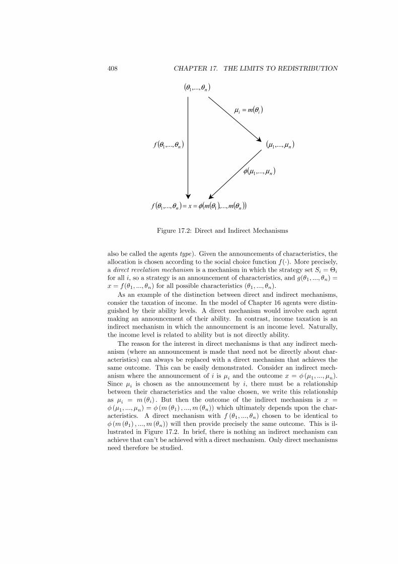
408 CHAPTER 17. THE LIMITS TO REDISTRIBUTION
( )ii m θµ =
( )nθθ ,...,1
( )nµµ ,...,1
( )nµµφ ,...,1
( )nf θθ ,...,1
( ) ( ) ( )( )nn mmxf θθφθθ ,...,,..., 11 ==
Figure 17.2: Direct and Indirect Mechanisms
also be called the agents type). Given the announcements of characteristics, theallocation is chosen according to the social choice function f(·). More precisely,a direct revelation mechanism is a mechanism in which the strategy set Si = Θifor all i, so a strategy is an announcement of characteristics, and g(θ1, ..., θn) =x = f(θ1, ..., θn) for all possible characteristics (θ1, ..., θn).As an example of the distinction between direct and indirect mechanisms,
consier the taxation of income. In the model of Chapter 16 agents were distin-guished by their ability levels. A direct mechanism would involve each agentmaking an announcement of their ability. In contrast, income taxation is anindirect mechanism in which the announcement is an income level. Naturally,the income level is related to ability but is not directly ability.The reason for the interest in direct mechanisms is that any indirect mech-
anism (where an announcement is made that need not be directly about char-acteristics) can always be replaced with a direct mechanism that achieves thesame outcome. This can be easily demonstrated. Consider an indirect mech-anism where the announcement of i is µi and the outcome x = φ (µ1, ..., µn).Since µi is chosen as the announcement by i, there must be a relationshipbetween their characteristics and the value chosen, we write this relationshipas µi = m (θi) . But then the outcome of the indirect mechanism is x =φ (µ1, ..., µn) = φ (m (θ1) , ...,m (θn)) which ultimately depends upon the char-acteristics. A direct mechanism with f (θ1, ..., θn) chosen to be identical toφ (m (θ1) , ...,m (θn)) will then provide precisely the same outcome. This is il-lustrated in Figure 17.2. In brief, there is nothing an indirect mechanism canachieve that can’t be achieved with a direct mechanism. Only direct mechanismsneed therefore be studied.

17.3. IMPOSSIBILITY OF LUMP-SUM TAXES 409
The interesting issue here is whether mechanisms can be designed suchthat it is optimal for the agents to announce their true characteristics. Inthis respect, the social choice function f(·) is truthfully implementable in dom-inant strategies (or incentive compatible) if the direct revelation mechanismM = (Θ1, ...,Θn, f(·)) has a dominant strategy equilibrium (s∗1, ..., s
∗n) in which
truthtelling is optimal so s∗i = θi for any value of θi in the set Θi. By a domi-nant strategy equilibrium, it is meant that truthtelling is optimal for all agentsregardless of what the other agents choose to do.We are now almost in a position to state the fundamental result of this
section but one final definition is necessary before this can be done. A trulyfeasible allocation is defined as one which is both technically feasible (giventhe endowments and endowments and technology of the economy) and whichis informationally feasible given that the characteristics on which redistributionis based are not publicly observable. The following theorem is the RevelationPrinciple that is key to analyzing allocation mechanisms.
Theorem 11 Revelation Principle (Dasgupta, Hammond, Maskin and My-erson) The set of allocations that are truly feasible when agents’ characteristicsare not observable is the set of allocations that are incentive compatible (ortruthfully implementable in dominant strategies).
There are two aspects to this theorem. Firstly, it tells us that there is nothingto be gained by constructing mechanisms in which agents are deliberately leadto reveal false information. Instead, we can confine attention to mechanisms inwhich the best strategy is to tell the truth. Secondly, it reveals that we needonly study mechanisms where the equilibrium is found in dominant strategies.There have been several previous occasions in the text where we have analyzedthe Nash equilibrium of games and it may seem that restricting attention todominant strategies must reduce the set of allocations that can be achieved.This is not true for the following simple reason: the mechanism must be designedso that truth is the Nash equilibrium strategy for each agent whatever are thecharacteristics of the other agents. Now consider agent i. Since truth is his Nashequilibrium strategy for all possible characteristics of agents other than i, thisimplies that it must be chosen in response to any announcement by the others(whether these are truthful or not). Therefore, if it is always a Nash strategy,truth must be a dominant strategy.
17.3 Impossibility of Lump-Sum TaxesImagine that each individual in a society can be described by a list of per-sonal attributes upon which the society wishes to condition taxes and transfers(e.g. tastes, needs, talents and endowments). Individuals are also identifiedby their names and possibly other publicly-observable attributes (such as eyecolor) which are not judged to be relevant attributes for taxation. The list ofpersonal attributes associated to every agent is not publicly known but is theprivate information of each individual. This implies that the lump-sum taxes the
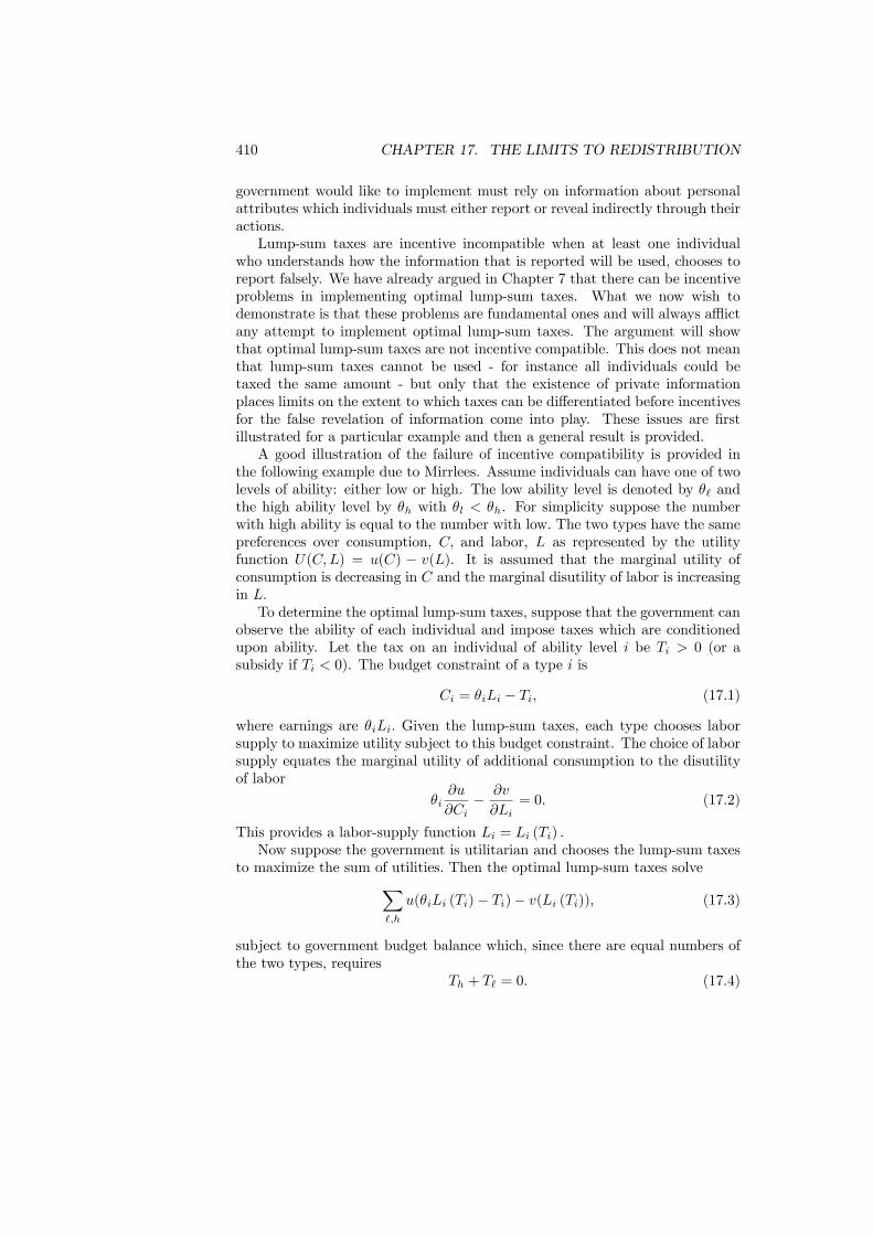
410 CHAPTER 17. THE LIMITS TO REDISTRIBUTION
government would like to implement must rely on information about personalattributes which individuals must either report or reveal indirectly through theiractions.Lump-sum taxes are incentive incompatible when at least one individual
who understands how the information that is reported will be used, chooses toreport falsely. We have already argued in Chapter 7 that there can be incentiveproblems in implementing optimal lump-sum taxes. What we now wish todemonstrate is that these problems are fundamental ones and will always afflictany attempt to implement optimal lump-sum taxes. The argument will showthat optimal lump-sum taxes are not incentive compatible. This does not meanthat lump-sum taxes cannot be used - for instance all individuals could betaxed the same amount - but only that the existence of private informationplaces limits on the extent to which taxes can be differentiated before incentivesfor the false revelation of information come into play. These issues are firstillustrated for a particular example and then a general result is provided.A good illustration of the failure of incentive compatibility is provided in
the following example due to Mirrlees. Assume individuals can have one of twolevels of ability: either low or high. The low ability level is denoted by θ` andthe high ability level by θh with θl < θh. For simplicity suppose the numberwith high ability is equal to the number with low. The two types have the samepreferences over consumption, C, and labor, L as represented by the utilityfunction U(C,L) = u(C) − v(L). It is assumed that the marginal utility ofconsumption is decreasing in C and the marginal disutility of labor is increasingin L.To determine the optimal lump-sum taxes, suppose that the government can
observe the ability of each individual and impose taxes which are conditionedupon ability. Let the tax on an individual of ability level i be Ti > 0 (or asubsidy if Ti < 0). The budget constraint of a type i is
Ci = θiLi − Ti, (17.1)
where earnings are θiLi. Given the lump-sum taxes, each type chooses laborsupply to maximize utility subject to this budget constraint. The choice of laborsupply equates the marginal utility of additional consumption to the disutilityof labor
θi∂u
∂Ci− ∂v
∂Li= 0. (17.2)
This provides a labor-supply function Li = Li (Ti) .Now suppose the government is utilitarian and chooses the lump-sum taxes
to maximize the sum of utilities. Then the optimal lump-sum taxes solveX`,h
u(θiLi (Ti)− Ti)− v(Li (Ti)), (17.3)
subject to government budget balance which, since there are equal numbers ofthe two types, requires
Th + T` = 0. (17.4)

17.3. IMPOSSIBILITY OF LUMP-SUM TAXES 411
Now use this budget constraint to substitute for T`, in (17.3). Differentiatingthe resulting expression with respect to the tax Th and using the first-ordercondition (17.2) for the choice of labor supply, the optimal lump-sum taxes arecharacterized by the condition
∂u
∂Ch=
∂u
∂C`. (17.5)
Since the marginal utility of consumption is decreasing in C, the optimalitycondition (17.5) implies that there is equality of consumption for the two types;Ch = C`. When this conclusion is combined with (17.2) and the fact θ` < θh,it follows that
∂v
∂L`= θ`
∂u
∂C`< θh
∂u
∂Ch=
∂v
∂Lh. (17.6)
Under the assumption of an increasing marginal disutility of labor, this inequal-ity shows that the optimal lump-sum taxes should induce the outcome Lh > L`,so the more able work harder than the less able. The motivation for this outcomeis that working the high-ability type harder is the most efficient way to raise thelevel of total income for the society which can then be redistributed using thelump-sum taxes. Thus, the high-ability type works harder than the low-abilitytype but they only get to consume the same. Therefore, the high-ability type isleft with a lower utility level than the low-ability type after redistribution.Now suppose that the government can observe incomes but cannot observe
the ability of each individual. Assume it still attempts to implement the optimallump-sum taxes. The taxes are obviously not incentive compatible because, ifthe high-ability type understand the outcome, they can always choose to earnas little as the low-ability type. Doing so then qualifies the high-ability type forthe redistribution aimed at the low-ability type. This will provide them with ahigher utility level than if they did not act strategically. The optimal lump-sumtaxes cannot then be implemented with private information.Who would work hard if the government stood ready to tax away the result-
ing income? Optimal (utilitarian) lump-sum redistribution makes the more ableindividuals worse off because it requires them to work harder but does not re-ward them with additional consumption. In this context, it is profitable for themore able individuals to make themselves seem incapable. Many people believethere is something unfair about inequality that arises from the fact that somepeople are born with superior innate ability or similar advantage over others.But many people also think it morally right that one should be able to keepsome of the fruits of one’s own effort. This example may have been simple butits message is far-reaching. The Soviet Union and other communist economieshave shown us that it is impossible to generate wealth without offering ade-quate material incentives. Incentive constraints inevitably limit the scope forredistribution.The observations of the example are now shown to reflect a general prin-
ciple concerning the incentive compatibility of optimal lump-sum taxes. Westate the formal version of this result for a “large economy” which is one where

412 CHAPTER 17. THE LIMITS TO REDISTRIBUTION
every individual is insignificant and so powerless to affect the distribution ofannouncements. In other words, there is a continuum of different agents whichis the idealization of a competitive economy with a very large number of smallagents with no market power. The theorem shows that optimal lump-sum tax-ation is never incentive compatible.
Theorem 12 (Hammond) In a large economy, redistribution through optimallump-sum taxes is always incentive incompatible.
The logic behind this theorem is surprisingly simple. A system of optimallump-sum taxes is used to engineer a distribution of endowments that will de-centralize the first-best allocation. The endowments after redistribution mustbe based on the agents’ characteristics (recall that in the analysis of the SecondTheorem the taxes were based on knowledge of endowments and preferences), soassume the endowment of an agent with characteristics θi is given by ei = e (θi).For those characteristics which are not publicly observable, the government mustrely on an announcement of the values by the agents. Assume for simplicity thatnone of the characteristics can be observed. Then the incentive exists for eachagent to announce the set of characteristics that maximize the value of the en-dowment at the equilibrium prices p. This is illustrated in Figure 17.3 where θ1and θ2 are two potential announcements, with related endowments e (θ1) ande (θ2) , and θ∗ is the announcement that maximizes pe (θ) . The announcementof θ∗ leads to the highest budget constraint from amongst the set of possibleannouncements and, by giving the agent maximum choice, allows the highestlevel of utility to be attained. Consequently, all agents will announce θ∗ andthe optimal lump-sum taxes are not incentive compatible.In conclusion, lump-sum taxes can achieve the optimal allocation of resources
provided all information is public. If some of the characteristics which arerelevant for taxation are private information then the optimal lump-sum taxesare not incentive compatible. Information limitations therefore place a limitupon the extent to which redistribution can be undertaken using lump-sumtaxation.
17.4 Tax PrincipleIf optimal lump-sum taxes could be employed, the first-best allocation wouldbe achieved. There is no allocation mechanism that can achieve more than this.However, optimal lump-sum taxes are not incentive compatible so they do notfunction as an allocation mechanism. Other forms of taxation, such as incomeand commodity taxation, are incentive compatible but achieve only a second-best allocation. There is therefore a gap between what the economy couldachieve at the first-best and what taxation achieves at the second-best. Thisobservation raises the question which this section answers: can we improve uponthe allocation achieved with taxation? In other words, is there any allocationmechanism that can locate the economy somewhere between the second-bestachieved by taxation and the first-best?
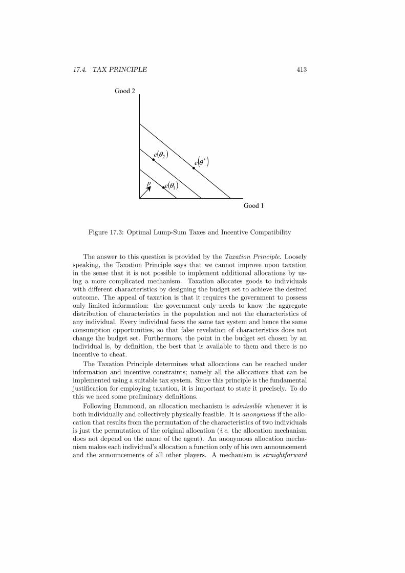
17.4. TAX PRINCIPLE 413
•
••
( )1θe
( )2θe ( )*θe
Good 1
Good 2
p
Figure 17.3: Optimal Lump-Sum Taxes and Incentive Compatibility
The answer to this question is provided by the Taxation Principle. Looselyspeaking, the Taxation Principle says that we cannot improve upon taxationin the sense that it is not possible to implement additional allocations by us-ing a more complicated mechanism. Taxation allocates goods to individualswith different characteristics by designing the budget set to achieve the desiredoutcome. The appeal of taxation is that it requires the government to possessonly limited information: the government only needs to know the aggregatedistribution of characteristics in the population and not the characteristics ofany individual. Every individual faces the same tax system and hence the sameconsumption opportunities, so that false revelation of characteristics does notchange the budget set. Furthermore, the point in the budget set chosen by anindividual is, by definition, the best that is available to them and there is noincentive to cheat.The Taxation Principle determines what allocations can be reached under
information and incentive constraints; namely all the allocations that can beimplemented using a suitable tax system. Since this principle is the fundamentaljustification for employing taxation, it is important to state it precisely. To dothis we need some preliminary definitions.Following Hammond, an allocation mechanism is admissible whenever it is
both individually and collectively physically feasible. It is anonymous if the allo-cation that results from the permutation of the characteristics of two individualsis just the permutation of the original allocation (i.e. the allocation mechanismdoes not depend on the name of the agent). An anonymous allocation mecha-nism makes each individual’s allocation a function only of his own announcementand the announcements of all other players. A mechanism is straightforward

414 CHAPTER 17. THE LIMITS TO REDISTRIBUTION
whenever it implements a given allocation in dominant truthtelling strategies.A dominant strategy is a strategy that an individual, given his information,is willing to play regardless of what he believes others know and the way hebelieves others behave. The Tax Principle can now be stated.
Theorem 13 Tax Principle (Guesnerie and Hammond) In a large economy,an allocation is implementable by an admissible tax mechanism if and only if itis implementable by an admissible straightforward allocation mechanism.
The intuition behind this result is quite simple. The first step is to showthat if an allocation is implementable by taxation it can be implemented byan admissible straightforward allocation mechanism. The justification for thisresult is that a tax system is an indirect mechanism which has a dominantstrategy solution consisting of the announcements of each individual’s trades.In fact, a tax schedule confronts each individual with the same budget set sothat the bundle allocated to them depends only on their strategy. Thus, byappealing to the Revelation Principle, there exists a direct mechanism (in whichindividuals announce their characteristics) that is equivalent to the (indirect)tax mechanism.The second step requires the demonstration that any allocation which is
implementable by a straightforward allocation mechanism is implementable bytaxation. Since the allocation must be incentive compatible, each individualmust find the consumption bundle allocated to them at least as good as thatallocated to any other individual (if they did not, they would make a falsestatement of characteristics in order to secure the alternative). A budget setcan then be constructed which contains the consumption bundle allocated toeach of the individuals but excludes any preferable bundles. This budget setimplicitly defines a tax system. Faced with this budget set, the individuals willalways choose the consumption bundle allocated by the mechanism. Taxationtherefore achieves the same outcome as the alternative allocation mechanism.Therefore, tax systems yield in general the best allocations that can be achievedin a private information world! The only truly feasible allocations are thosewhich can be decentralized by some non-linear income and commodity taxes(with everybody facing the same non-linear tax schedule).We now illustrates this Taxation Principle in our economy composed of two
ability types (θl < θh) and two goods (C and L). This example allows usto clarify the extent to which incentive considerations limit redistribution. Wecontinue to assume, for simplicity, an equal number of individuals of both abilitytypes. Assume the government observes only income Y = θL and consumptionC. From the preferences over consumption and labor can be derived differentpreferences over consumption and income given by
U(C,L) = U(C,Y
θ).
(This construction was explored in detail in Chapter 16.) The indifference curvesof both types are depicted in Figure 17.4 in income/consumption space. They
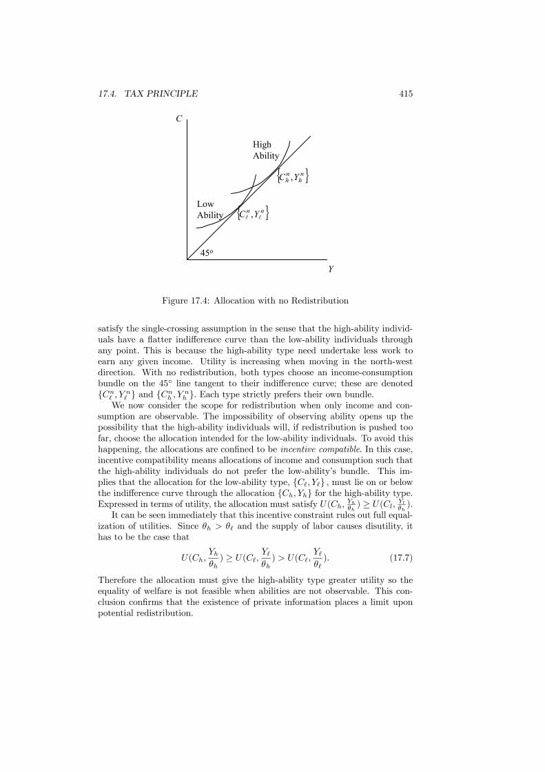
17.4. TAX PRINCIPLE 415
45o
Y
C
LowAbility
HighAbility
{ }nn YC ll ,
{ }nh
nh YC ,
Figure 17.4: Allocation with no Redistribution
satisfy the single-crossing assumption in the sense that the high-ability individ-uals have a flatter indifference curve than the low-ability individuals throughany point. This is because the high-ability type need undertake less work toearn any given income. Utility is increasing when moving in the north-westdirection. With no redistribution, both types choose an income-consumptionbundle on the 45◦ line tangent to their indifference curve; these are denoted{Cn` , Y n` } and {Cnh , Y nh }. Each type strictly prefers their own bundle.We now consider the scope for redistribution when only income and con-
sumption are observable. The impossibility of observing ability opens up thepossibility that the high-ability individuals will, if redistribution is pushed toofar, choose the allocation intended for the low-ability individuals. To avoid thishappening, the allocations are confined to be incentive compatible. In this case,incentive compatibility means allocations of income and consumption such thatthe high-ability individuals do not prefer the low-ability’s bundle. This im-plies that the allocation for the low-ability type, {C`, Y`} , must lie on or belowthe indifference curve through the allocation {Ch, Yh} for the high-ability type.Expressed in terms of utility, the allocation must satisfy U(Ch, Yhθh ) ≥ U(Cl, Ylθh ).It can be seen immediately that this incentive constraint rules out full equal-
ization of utilities. Since θh > θ` and the supply of labor causes disutility, ithas to be the case that
U(Ch,Yhθh) ≥ U(C`, Y`
θh) > U(C`,
Y`θ`). (17.7)
Therefore the allocation must give the high-ability type greater utility so theequality of welfare is not feasible when abilities are not observable. This con-clusion confirms that the existence of private information places a limit uponpotential redistribution.
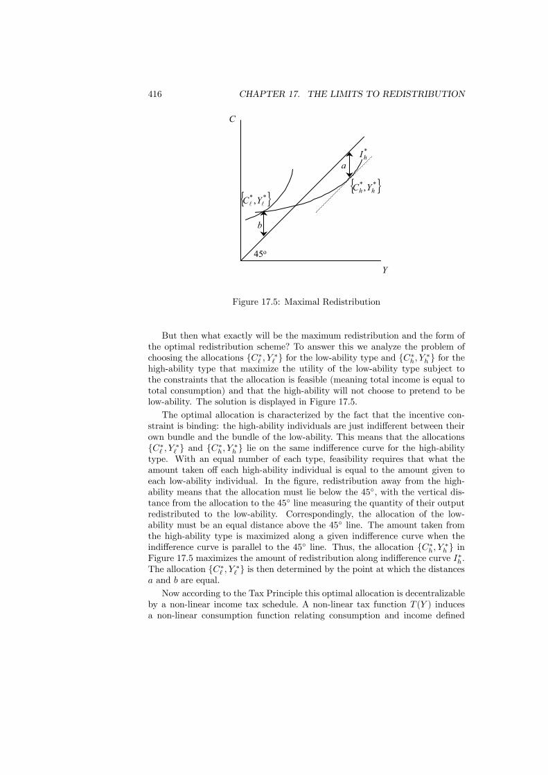
416 CHAPTER 17. THE LIMITS TO REDISTRIBUTION
45o
Y
C
{ }**, ll YC{ }**, hh YC
a
b
*hI
Figure 17.5: Maximal Redistribution
But then what exactly will be the maximum redistribution and the form ofthe optimal redistribution scheme? To answer this we analyze the problem ofchoosing the allocations {C∗` , Y ∗` } for the low-ability type and {C∗h, Y ∗h } for thehigh-ability type that maximize the utility of the low-ability type subject tothe constraints that the allocation is feasible (meaning total income is equal tototal consumption) and that the high-ability will not choose to pretend to below-ability. The solution is displayed in Figure 17.5.The optimal allocation is characterized by the fact that the incentive con-
straint is binding: the high-ability individuals are just indifferent between theirown bundle and the bundle of the low-ability. This means that the allocations{C∗` , Y ∗` } and {C∗h, Y ∗h } lie on the same indifference curve for the high-abilitytype. With an equal number of each type, feasibility requires that what theamount taken off each high-ability individual is equal to the amount given toeach low-ability individual. In the figure, redistribution away from the high-ability means that the allocation must lie below the 45◦, with the vertical dis-tance from the allocation to the 45◦ line measuring the quantity of their outputredistributed to the low-ability. Correspondingly, the allocation of the low-ability must be an equal distance above the 45◦ line. The amount taken fromthe high-ability type is maximized along a given indifference curve when theindifference curve is parallel to the 45◦ line. Thus, the allocation {C∗h, Y ∗h } inFigure 17.5 maximizes the amount of redistribution along indifference curve I∗h.The allocation {C∗` , Y ∗` } is then determined by the point at which the distancesa and b are equal.Now according to the Tax Principle this optimal allocation is decentralizable
by a non-linear income tax schedule. A non-linear tax function T (Y ) inducesa non-linear consumption function relating consumption and income defined
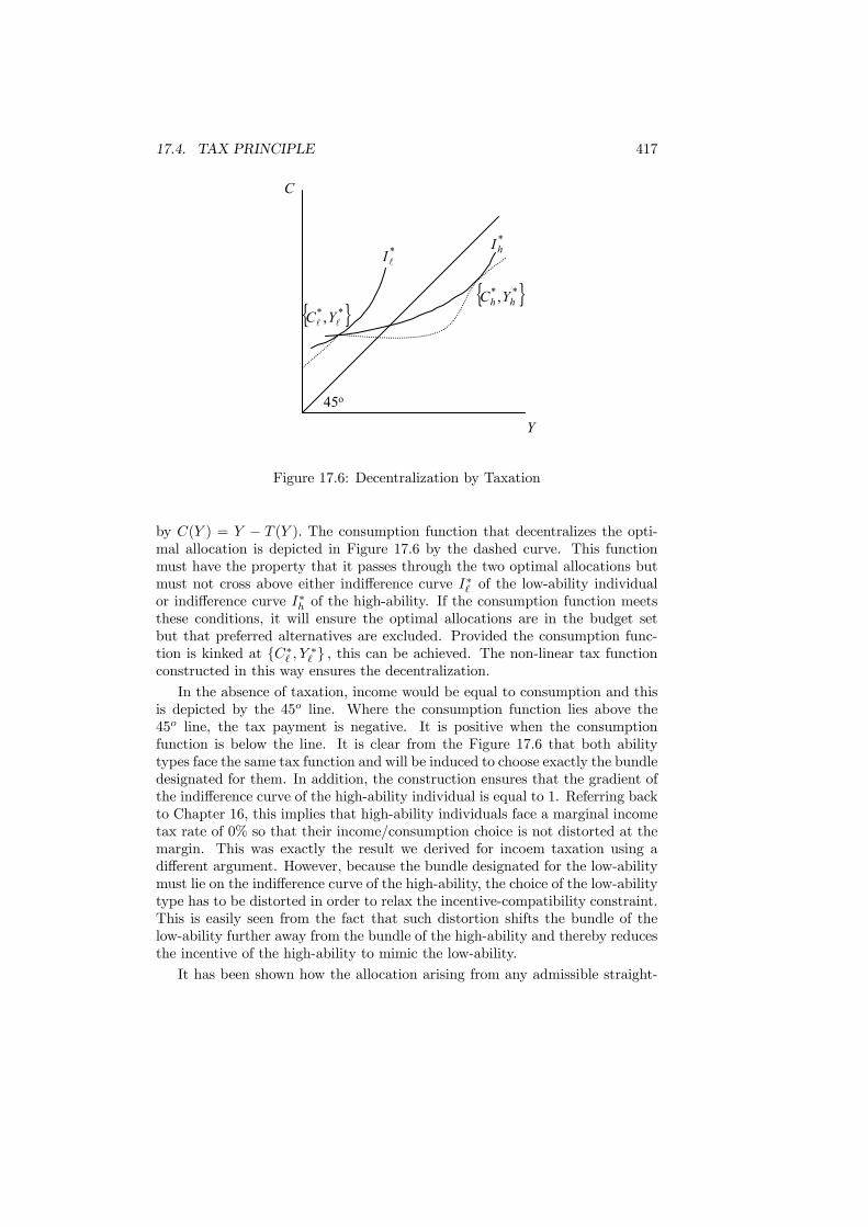
17.4. TAX PRINCIPLE 417
45o
Y
C
{ }**, ll YC{ }**, hh YC
*hI*
lI
Figure 17.6: Decentralization by Taxation
by C(Y ) = Y − T (Y ). The consumption function that decentralizes the opti-mal allocation is depicted in Figure 17.6 by the dashed curve. This functionmust have the property that it passes through the two optimal allocations butmust not cross above either indifference curve I∗` of the low-ability individualor indifference curve I∗h of the high-ability. If the consumption function meetsthese conditions, it will ensure the optimal allocations are in the budget setbut that preferred alternatives are excluded. Provided the consumption func-tion is kinked at {C∗` , Y ∗` } , this can be achieved. The non-linear tax functionconstructed in this way ensures the decentralization.
In the absence of taxation, income would be equal to consumption and thisis depicted by the 45o line. Where the consumption function lies above the45o line, the tax payment is negative. It is positive when the consumptionfunction is below the line. It is clear from the Figure 17.6 that both abilitytypes face the same tax function and will be induced to choose exactly the bundledesignated for them. In addition, the construction ensures that the gradient ofthe indifference curve of the high-ability individual is equal to 1. Referring backto Chapter 16, this implies that high-ability individuals face a marginal incometax rate of 0% so that their income/consumption choice is not distorted at themargin. This was exactly the result we derived for incoem taxation using adifferent argument. However, because the bundle designated for the low-abilitymust lie on the indifference curve of the high-ability, the choice of the low-abilitytype has to be distorted in order to relax the incentive-compatibility constraint.This is easily seen from the fact that such distortion shifts the bundle of thelow-ability further away from the bundle of the high-ability and thereby reducesthe incentive of the high-ability to mimic the low-ability.It has been shown how the allocation arising from any admissible straight-
418 CHAPTER 17. THE LIMITS TO REDISTRIBUTION
forward allocation mechanism can be decentralized by means of a non-lineartax schedule. More importantly, a non-linear tax schedule can attain the maxi-mum redistribution that is possible given limitations on information. There is nofurther redistributive instruments that can expand the possibilities of redistrib-ution. Therefore, having analyed taxation in earlier chapters, we have exhaustedthe possibilities for achieving redistribution.
17.5 Quasi-Linearity
To provide insights additional to the general results derived above it is worthconsidering a specialization of the model. This specialization is noteworthy forthe very clear view it gives into the models functioning. It is assumed that thereare just two consumers and that utility is linear in labor supply. The latter isstrictly necessary for the analysis, the former is not. These assumptions permitan explicit solution to be derived to the optimal tax problem.With only two consumers the problem of choosing the optimal tax (or con-
sumption) function can be given the following formulation. Whatever consump-tion function is chosen, the fact that there are only two consumers ensures thatat most two locations on it will ever be selected. Having observed this, it isapparent that instead of choosing the consumption function itself it is possi-ble to restrict attention to choosing only these two locations. The rest of theconsumption function can then be chosen to ensure that it is no better for theconsumers than the two chosen locations. Essentially the consumption functionjust needs to link the two points, whilst elsewhere remaining below the indif-ference curves through the points. This procedure reduces the choice of taxfunction to a simple maximization problem involving the two locations.The quasi-linear utility function has the form
U(C,Y, θ) = u (C)− Yθ, (17.8)
so that the marginal disutility of labor L = Y/θ is constant and u(C) is in-creasing and concave. The marginal rate of substitution between consumptionand income can be calculated to be MRS = 1/θu0 (C), so that it is consistentwith the requirements of agent monotonicity. As discussed previously, the in-centive compatibility constraint requires that each consumer should prefer theirown location to that of the other. Denoting the location intended for low abilityconsumer by {Cl, Yl} and that for high-ability by {Ch, Yh}, self-selection impliesthat
u (Cl)− Ylθl≥ u (Ch)− Yh
θl, (17.9)
and
u (Ch)− Yhθh≥ u (Cl)− Yl
θh, (17.10)
17.5. QUASI-LINEARITY 419
where θi is the ability level of consumer i = l, h. It is assumed that θl < θh < 3θl(the reason for this is apparent later).Equation (17.9) is the requirement that the consumer l prefers their location
to that of consumer h. The converse requirement is given in (??). Putting thesetogether, the full optimization facing the utilitarian government is
max{Cl,Ch,Yl,Yh}
u (Cl)− Ylθl+ u (Ch)− Yh
θh, (17.11)
subject to the incentive compatibility constraints (17.9) and (??) and the pro-duction constraint
Cl + Ch = Yl + Yh. (17.12)
The production constraint makes the simplifying assumption that zero revenueis to be raised. What is now shown is that this maximization problem can beconsiderably simplified. The simplification then permits a simple and explicitsolution to be given.The first step is to consider which of the incentive compatibility constraints
will hold at the optimum. They cannot both be equalities. If they were, the dif-ference in the slopes of the indifference curves resulting from agent monotonicityimplies that both consumers must have the same income and consumption lev-els. This cannot be optimal since consumer h earns income with less effort. Areallocation that made consumer h work harder and consumer l less hard wouldthen raise welfare. Now assume that both are strict inequalities. Consider hold-ing incomes levels constant and transferring consumption from consumer h toconsumer l. There will always be a transfer ∆ > 0 that satisfies
u (Ch −∆)− Yhθh= u (Cl +∆)− Yl
θh, (17.13)
that is, it makes consumer h indifferent between {Ch −∆, Yh} and {Cl +∆, Yl}.The change must also raise welfare since it transfers consumption to consumerl who has a lower consumption level and hence higher marginal utility. Theinitial position could not therefore be optimal. Consequently, the only remainingpossibility is that at any optimum, (17.10) must be an equality so that consumerh is indifferent between the two locations and (17.9) an inequality.Given that (17.10) is an equality, it can be solved to write
Yh = θh [u (Ch)− u (Cl)] + Yl. (17.14)
Using the revenue constraint and eliminating Yh by using (17.14)
Yl =1
2[Cl + Ch − θh [u (Ch)− u (Cl)]] . (17.15)
This can now be used with the revenue constraint to give
Yh =1
2[Cl + Ch + θh [u (Ch)− u (Cl)]] . (17.16)

420 CHAPTER 17. THE LIMITS TO REDISTRIBUTION
These solution for the pre-tax income levels can be then be substituted intothe objective function (17.11). Doing this shows that the original constrainedoptimization is equivalent to
max{Cl,Ch}
βlu (Cl) + βhu (Ch)−·θl + θh2θlθh
¸[Cl + Ch] , (17.17)
where βl =3θl−θh2θl
and βh =θl+θh2θl
.Comparing (17.11) and (17.17) allows a new interpretation of the optimal
tax problem. The construction undertaken has turned the maximization of theutilitarian social welfare function subject to constraint into the maximization ofa weighted welfare function without constraints. The constraints have becomeequivalent to placing a greater weight on the welfare of the high ability consumer(since βh > βl) which, in turn, ensures that their consumption level must begreater at the optimum. From (17.15) and (17.16), this feeds back into a higherlevel of pre-tax income for consumer h. It can also be seen that as the abilitydifference between the two consumers increases, so does the relative weight givento consumer h.Carrying out the optimization in (17.17), the consumption levels of consumer
i = h, l satisfy the first-order conditions
βiu0 (Ci)− θl + θh
2θlθh= 0 (17.18)
which shows how the consumption levels are proportional to the welfare weights.For consumer h, substituting in the value of βh gives
u0 (Ch) =1
θh. (17.19)
Consequently the marginal utility of consumer h is inversely proportional totheir ability level. With u00 < 0 (decreasing marginal utility) this implies thatconsumption is proportional to ability. Using this result it follows thatMRSh =1 at the optimum. The fact that the marginal rate of substitution is 1 showsthat consumer h is facing a zero marginal tax rate. This is the no-distortion-at-the-top result already derived in Chapter 16. For consumer l
u0 (Cl) =θl + θh
θh [3θl − θh], (17.20)
and MRSl =θh[3θl−θh]θl[θl+θh]
< 1. These show that consumer l faces a positivemarginal rate of tax.The use of quasi-linear utility allows the construction of an explicit solution
which shows how the general findings of the previous section translate intothis special case. It is interesting to note the simple dependence of consumptionlevels upon the relative abilities and the manner in which the constraints becometranslated into a higher effective welfare weight for the high ability consumer.This is showing that this consumer needs to be encouraged to supply more laborthrough the reward of additional consumption.

17.6. TAX MIX: SEPARATION PRINCIPLE 421
17.6 Tax Mix: Separation Principle
Tax systems must be based on observable variables. In practice governmentsuse income and consumption as the basis of taxation, even if they are imper-fect measures of individual earning ability. From a lifetime perspective, savingsare future consumption and thus, as consumption must equal income, a tax onthe value of consumption is equivalent to a tax on income. From this perspec-tive, it does not matter whether taxes are levied on income or on the value ofconsumption.In the simple models we have used so far in this chapter, we have assumed
that there is a single consumption good When there are two or more consump-tion goods, the commodity taxes levied upon then need not be uniform. Aswe showed in Chapter 15, when there is no income tax the Ramsey rule saysthat the tax on each commodity should be inversely related to the elasticity ofdemand. We now consider how this conclusion can be modified when incomeand commodity taxes can be simultaneously employed.The central question is whether there should be differential commodity tax-
ation when combined with a nonlinear income tax. There is a sense in whichcommodity taxation can usefully supplement income taxation by reducing thedistortion in the labor/consumption choice induced by income tax. If we taxcommodities that are substitutes for work and subsidize those that are com-plements we can encourage people to work more and thus reduce the workdiscouraging effect of income tax. The optimal differentiation depends on howthe preferences for some goods vary with labor supply. Turning this argumentaround, if the preference between commodities does not vary with labor supply,then there seems to be no argument for differential commodity taxes.Preferences over commodities are independent of labor supply if the utility
function is separable. What separable means is that utility can be written asU = U (u(C), L) , so that the marginal rate of substitution between any pairof goods depends only on u(C) and is independent of labor supply. We nowdemonstrate this if labor and goods are separable in utility then there is noneed to supplement an optimal nonlinear income tax with differential commoditytaxation.The result that commodity taxation is not needed with separability between
labor and goods is easily demonstrated in the two-ability model we have beenusing in this chapter. We now interpret Ci as a vector describing the consump-tion levels of n goods, Ci =
¡Ci1, ..., C
in
¢. We already know that the optimal
allocation {C∗i , Y ∗i } is constrained by the incentive of high-ability individuals to“disguise” themselves as low-ability. That is, the downward incentive constraint,U (u(C∗h), Y
∗h /θh) ≥ U (u(C∗` ), Y
∗` /θh), is binding at the optimum because it
requires less work for a high-ability individual to earn the income Y ∗` of a low-ability individual, Lh = Y ∗` /θh < L` = Y
∗` /θ`. The only difference between then
two types at any given level of income arises from the difference in the amountof work. This feeds into a utility difference, U (u(C∗` ), L`) 6= U (u(C∗` ), Lh) ,when the high-ability mimic the low-ability. With separable preferences, sucha difference does not affect the indifference curves between commodities (since

422 CHAPTER 17. THE LIMITS TO REDISTRIBUTION
2C
1hI
lI
1C
p
'p
2hI
Figure 17.7: Differential Taxation and Non-Separability
u(C∗` ) is the same for both types), so that we cannot use differential taxation toseparate the types (i.e. to make the consumption bundle of the low-ability indi-vidual less attractive to high-ability individual). The fact that differential taxesdo not help in relaxing the incentive constraint renders their use unnecessary.With a non-separable utility function, U(C,L), the indifference curves be-
tween commodities differ and we can tax more heavily the good that the high-ability person values more in the low-ability consumption bundle. This reducesthe incentive for the high-ability to mimic the low-ability. Figure 17.7 illustrateshow differential commodity taxation (changing prices from p to p0) can be usedto make the consumption bundle of the low-ability type less attractive for thehigh-ability type. The change in prices from the budget constraint labelled pto the budget constraint labelled p0 does not affect the utility of the low-ability(the budget constraint pivots around their indifference curve I`) but it causesa reduction in utility of the high-ability (shown by the new budget constraintchanging the location of the choice from initial indifference curve I1h to the lowerindifference curve I2h). This reduction in utility for the high-ability type relaxesthe incentive constraint.
17.7 Non-tax redistribution
The principal implication of the previous analysis, as reflected in the tax princi-ple, is that society cannot improve redistribution possibilities by using non-fiscalinstruments. The question is then why non-fiscal forms of redistribution are sowidely used. Governments frequently provide for goods such as education orhealth services at less than their costs, which may be viewed as redistributional
17.7. NON-TAX REDISTRIBUTION 423
policies. One may expect that a cash transfer of the same value would havemore redistributional power than such in-kind transfer programmes. This ismistaken. There are three reasons why such transfers in kind may be superiorto cash transfers as achieved through standard tax-transfer programmes.One reason is political. Rather than voting for a tax-transfer scheme which
benefits the poor, i might impose my own preferences and vote for providingcertain services such as education, even though the recipient would have pre-ferred another use. Voters may support redistributional policies if in kind butnot if in cash with use at the discretion of the recipient. Such preference forredistribution in kind. Political considerations dictate that many governmentprovision programmes like education, pension and basic health insurance, beuniversal. Without such feature the programmes would not have the politicalsupport required to be adopted or continued. For instance, public pensions andhealth care would be far more vulnerable politically if they were targeted to thepoor and not available to others. It should be noted that it is not because somegovernment programmes are universal that there is no redistribution. First ifthe programme is financed by proportional inome taxation, the rich contributemore than the poor. Second, even if everyone contributes the same to the pro-gramme, it is possible that the rich will not use the publicly provided good. Totake an example, consider public provision of basic health care which is avail-able to everyone for free. The programme is financed by a uniform tax on allhouseholds. There exists a private health care alternative with higher qualitybut at some cost. Since the rich can afford a better quality, they will use theprivate health even though free public health care is available. These rich house-holds still pay their contribution to the public programme and thus the poorhouseholds derive a net benefit from this cross subsidization.Another reason is self-selection. What ultimately sets the limit to redistrib-
ution is when its becomes advantageous for higher ability persons to earn lowerincome by expending less effort and thereby paying taxes (or receiving trans-fers) intended for the lower ability groups. The limits to redistribution is reachedwhen persons a person of a given ability would be just as well off earning theincome of other with lesser ability. The self-selection argument is that anythingwhich makes it less attractive for persons to mimic those with lesser abilitycould extend the limits to redistribution. As seen in the previous section, if thegovernment could supplement non-linear income tax with differential commod-ity taxes, it will do so in certain cases (namely, if the shares of income devotedto the consumption of each good depend are not independent of the amountof leisure). For our discussion of non-fiscal redistibutive instruments, the useof in-kind transfers to supplement standard taxation can be optimal. This isan efficiency based argument. Basically, a given degree of redistribution can bemore efficiently achieved by using in-kind transfers as supplement ot incometaxes. The argument, unlike the separability argument just used for differentialcommodity taxes, relies on differences in preferences among different incomegroups. Consider two individuals who differ not only in their ability but also intheir health status. Suppose that lesser ability means also poorer health so thatthe less able also spend more on health. Then both income and health expen-

424 CHAPTER 17. THE LIMITS TO REDISTRIBUTION
ditures act as a signal of ability. It follows that the limits to redistribution canbe relaxed if transfers are made partly in the form of provision of health care(or equivalently with full subsidization of health expenditures). The reason issimply that the more able individual (with less tendency to become ill) is lesslikely to claim in-kind benefits in the form of health care provision, than hewould be to claim cash benefits. To take another example, suppose the govern-ment is considering redistribution either in cash or in the form of low-incomehousing. All households, needy or not would like the cash transfer. Howeverfew non-needy households may want living in low-income housing. They canafford better housing. Thus self-selection arises by which the non-needy dropout of the housing programme and only the needy take up. In short, transfersin kind invite people to self-select in a way which reveals their neediness. Whenneed is correlated to income-earning ability, then in-kind transfers can relax in-centive and selection constraints, thereby improving the government ability toredistribute income. Interestingly universal government provision provisionA third reason is time consistency. Here the argument for in-kind transfers
relies on the inability of government to commit to its future actions. UnlikeStrotz (1956) earliest argument on government time inconsistency, it does notarise from a change in government objective over time ((e.g. because of elec-tion) nor from the fact that the government is not welfaristic or rational. Thetime consistency problem arises from a perfectly rational government who doesfully respect individual preferences, but who does not have the power to com-mit its policy on the long run. The time-consistency problem is obvious withpensions. To the extent that households expect governments to provide somebasic pensions to those with too little savings, their incentive to save for retire-ment consumption and provide for themselves is reduced. Anticipating that, thegovernment may prefer to provide public pensions itself. A related time con-sistency problem can explain why transfer programmes, such as social security,education and job training are in kind. If a welfaristic government cannot com-mit not to come to the rescue of those in need in the future, potential recipientswill have little reason to invest in their education or to undertake job training,because the government will help them out anyway. Again, the government canimprove both economic efficiency and redistribution by making education andjob training available at less than their cost, rather than making cash transfersof equivalent value.
17.8 Conclusions
We addressed the important question of what limits the extent of redistributionin a society. We began the chapter with the very general concept of selectingthe allocation mechanism that achieved the best possible outcome given theconstraint that some relevant individual characteristics are private information.This information restriction requires that the characteristics must be reported,either directly or indirectly, as part of the mechanism. The competitive economywith taxation is just one example of a mechanism. What we wished to discover
17.8. CONCLUSIONS 425
is whether there were any better mechanisms.When there are no informational problems, lump-sum transfers combined
with competitive economic activity can take the economy to the first-best out-come. No mechanism can perform better than this. When there is privateinformation the situation is considerably changed: optimal lump-sum taxes arenot incentive compatible. All other forms of taxation (such as income taxesor commodity taxes) are distortionary, so will only ever allow attain alloca-tions strictly worse than the first-best. These observations raise the possibilitythat there may be allocation mechanisms that can achieve outcomes which arestrictly better than those arising from distortionary taxation. Perhaps surpris-ingly, the Tax Principle shows this is not the case. The taxation of observablevariables is as good as any other allocation mechanism.These are very general and very powerful results. What they do is emphasize
from a fresh perspective just how successful is the competitive economy as anallocation mechanism. When combined with intervention via taxation, thereis no other allocation mechanism that can better it. But it should always berecalled that the intervention has to be well-intended and that politics can alsoshape the outcome and constraint further the possibilities of redistribution. Forexample with political determination of redistribution, increasing the numberof the rich can actually leave the poor worse off: as the rich becomes politicallymore influencial, the extent of redistribution from each rich person may fallby so much as to more than offset the increase in the relative number of richredistributing to the poor.The arguments developed in the chapter are also based on welfaristic ob-
jectives (i.e. social objectives only but fully respect individual preferences).Recently there has been growing emphasis on non-welfaristic objectives that in-clude equality of chance and capability, fairness, poverty alleviation, inequality.This poses a real challenge not just in the value judgments associated with thedifferent objectives themselves, but also because welfaristic and non-welfaristicobjectives are typically in conflict as the social choice theory has convincinglyshown. Resolving the conflict itself involves a value judgment that ultimately isleft to the political process.
Further readingFor a more complete theoretical treatment of the information constraint to
redistribution seeGuesnerie, R., (1995) A Contribution to the Pure Theory of Taxation, Cam-
bridge: Cambridge University PressHammond, P. (1979) “Straightforward incentive compatibility in large economies”,
Review of Economic Studies 46, 263-82.Roberts, K. (19684), The theoretical limits to redistribution, Review of Eco-
nomic Studies 51, 177-95.Two excellent reviews of the central issues that arise with redistributionStiglitz, J., (1987) “Pareto efficient and optimal taxation and the new wel-
fare economics”, in A. Auerbach and M. Feldstein (eds.) Handbook of PublicEconomics, Vol. 2, Amsterdam: North Holland, 991-1042.

426 CHAPTER 17. THE LIMITS TO REDISTRIBUTION
Boadway, R. and M. keen, (2000), Redistribution, in A.B. Atkinson and F.Bourguignon (eds.) Handbook of Income Distribution, Vol 1, Amsterdam: NorthHolland, 677-789.The relevance of indirect taxation to supplement income tax is inAtkinson, A.B., and J.E. Stiglitz, (1976), The design of the the tax structure:
direct versus indirect taxation, Journal of Public Economics 6, 55-75.Christiansen, V. (1984), Which commodity taxes should supplement the
income tax, Journal of Public Economics 24, 195-220.Cremer, H., P. Pestieau, and J.-C Rochet, (2001), Direct versus indirect tax-
ation: the design of the tax structure revisited, International Economic Review,42, 781-800.The self-selection argument for in-kind redistribution is inBlackorby, C. and D. Donaldson, 1988, Cash versus kind, self-selection and
efficient transfers, American Economic Review 78, 691-700.Garfinkel, I., (1973), Is in-kind redistribution efficient? Quarterly Journal of
Economics 87, 320-30.Besley, T. and S. Coate, (1991), Public provision of private goods and the
redistribution of income, American Economic Review 81, 979-84.Akerlof, G., (1978), The economics of tagging as applied to the optimal
income tax, welfare programmes and manpower planning, American EconomicReview 68, 8-19.Estimation of the incentive effect of welfare programmes is inEissa, N. and J. Liebman, (1996), Labour supply response to the earned
income tax credit, Quarterly Journal of Economics,111, 605-37Gruber, J. ,(2000), Disability, insurance benefits and labor supply, Journal
of Political Economy, 108, 1162-1183.Government time consistency problem is inStrotz, R.H., 1956, Myopia and inconsistency in dynamic utility maximiza-
tion, Review of Economic Studies 24, 165-80.Hillier, B. and J.M. Malcomson, 1984, Dynamic inconsistency, rational ex-
pectations and optimal government policy, Econometrica 52, 1437-52.Bruce, N. and M. Waldman, 1991, Transfer in kind: why they can be efficient
and non paternalistic, American Economic Review 81, 1345-51.
Chapter 18
Tax Evasion
18.1 Introduction
It is not unusual to offered a discount for payment in cash. This is almostroutine in the employment of the services of builders, plumbers and decorators.It is less frequent, but still occurs, when major purchases are made in shops.While the expense of banking checks and the commissions charged by creditcard companies may explain some of these discounts, the usual explanation isthat payment in cash makes concealment of the transaction much easier. Incomethat can be concealed need not be declared to the tax authorities.The same motivation can be provided for exaggeration in claims for ex-
penses. By converting income into expenses that are either exempt from tax ordeductible from tax, the total tax bill can be reduced. Second jobs are also alucrative source of income that can be concealed from taxation. A declarationthat reports no income, or at least a very low level, is likely to attract moreattention to one which declares earnings from primary employment but fails tomention income from secondary employment.In contrast to these observations on tax evasion, the analysis of taxation
in the previous chapters assumed that firms and consumers honestly reportedtheir taxable activities. Although acceptable for providing simplified insightsinto the underlying issues, this assumption is patently unacceptable when con-fronted with reality. The purpose of this chapter can therefore be seen as theintroduction of practical constraints upon the free choice of tax policy. Taxevasion, the intentional failure to declare taxable economic activity, is pervasivein many economies as the evidence given in the following section makes clearand is therefore a subject of practical as well as theoretical interest.The chapter begins by considering how tax evasion can be measured. Evi-
dence on the extent of tax evasion in a range of countries is then reviewed. Thechapter then proceeds to try to understand the factors involved in the decisionto evade tax. Initially, this decision is represented as a choice under uncer-tainty. The analysis predicts the relationship between the level of evasion, tax
427
428 CHAPTER 18. TAX EVASION
rates and punishments. Within this framework, the optimal degree of auditingand of punishment is considered. Evidence that can be used to assess the mod-els predictions is then reviewed. In light of this, some extensions of the basicmodel are then considered. Then a game-theoretic approach of tax complianceis presented where taxpayers and governments interact strategically. The lastsection is about the importance of social interaction on compliance decisions.
18.2 The Extent of Evasion
Tax evasion is illegal, so those engaging in it have every reason to seek toconceal what they are doing. This introduces a fundamental difficulty into themeasurement of tax evasion. Even so, the fact that the estimates that areavailable show evasion to constitute a significant part of total economic activityunderline the importance of measurement. They also emphasize the value ofdeveloping a theory of evasion which can be used to design a tax structure thatminimizes evasion and ensures that the policy is optimal given that evasionoccurs.Before proceeding, it is worth making some distinctions. Firstly, tax evasion
is the failure to declare taxable activity. Tax evasion should be distinguishedfrom tax avoidance, which is the reorganization of economic activity, possiblyat some cost, to lower tax payment. Tax avoidance is legal, tax evasion is not.In practice, the distinction is not this clear cut since tax avoidance schemesfrequently need to be tested in court to clarify their legality. Secondly, theterms black, shadow or hidden economy refer to all economic activities for whichpayment is made but are not officially declared. Under these headings would beincluded illegal activities, such as the drug trade, and unmeasured activity suchas agricultural output by smallholders. They would also incorporate the legal,but undeclared, income which constitutes tax evasion. Finally, the unmeasuredeconomy would be the shadow economy plus activities such as do-it-yourselfwhich are economically valuable but do not involve any transaction.This discussion reveals that there are several issues concerning how economic
activity should be divided between the regular economy and the shadow econ-omy. For instance, most systems of national accounts do not include criminalactivity (although Italy, for example, does make some adjustment for smug-gling). In principle, the UN System of National Accounts includes both legaland illegal activities and it has been suggested that criminal activity should bemade explicit when the system is revised. Although this chapter is primarilyabout tax evasion, when an attempt is made at the measurement of tax eva-sion the figures obtained may also include some or all of the components of theshadow economy.The simplest measure of tax evasion is to use the difference between the
income and expenditure measures of national income. The standard analysis ofthe circular flow of income suggests that these two should be equal: what is spentmust be earned. However, the existence of tax evasion can destroy this identity.Income that is undeclared will not figure in the measure of national income but
18.2. THE EXTENT OF EVASION 429
will appear on the expenditure side. This suggests that an expenditure figurein excess of an income figure is an indication of the degree of tax evasion. Thismethod is a useful first step but suffers from the problem that both incomesand expenditures may be undeclared, so it can only place a lower limit on theextent of evasion.The essential problem involved in the measurement of tax evasion is that
the illegality provides an incentive for individuals to keep the activity hidden.Furthermore, by its very nature, tax evasion does not appear in any official sta-tistics. This implies that the extent of tax evasion cannot be measured directlybut must be inferred from economic variables that can be observed.A first method for measuring tax evasion is to use survey evidence. This
can be employed either directly or indirectly as an input into an estimationprocedure. The obvious difficulty with this is that respondents who are activein the hidden economy have every incentive to conceal the truth. There are twoways in which this issue can be circumvented. Firstly, information collected forother purposes can be employed. One example of this is the use of data from theFamily Expenditure Survey in the UK. This survey involves consumers recordingtheir incomes and expenditures in a diary. Participants in this have no reason tofalsely recorded information. The relation between income and expenditure canbe derived from the respondents whose entire income is obtained in employmentwhich cannot escape tax. This can then be used to infer, from the expenditurerecorded, the income of those who do have an opportunity to evade. Althoughthey are not surveys in the normal sense, studies of taxpayer compliance con-ducted by revenue collection agencies, such as the Internal Revenue Service, canbe treated as survey evidence and have some claim to accuracy.The second general method is to infer the extent of tax evasion, or the hidden
economy generally, from the observation of another economic variable. This isdone by determining total economic activity then subtracting measured activityto gives the hidden economy. The direct input approach observes the use of aninput to production and from this predicts what output must be. An input whichis often used for this purpose is electricity since this universally employed andaccurate statistics are kept on energy consumption. The monetary approachemploys the demand for cash to infer the size of the hidden economy on thebasis that transactions in the hidden economy are financed by cash rather thancheques or credit. Given a relationship between the quantity of cash and thelevel of economic activity. This allows estimation of the hidden economy.What distinguishes alternative studies that fall under the heading of mone-
tary approaches is the method used to derive the total level of economic activityfrom the observed use of cash. One way to do this is to assume that there wasa base year in which the hidden economy did not exist. The ratio of cash tototal activity is then fixed by that year. This ratio allows observed cash use inother years to be compounded up into total activity. An alternative has been tolook at the actual use of bank notes. The issuing authorities know the expectedlifespan of a note (that is, how many transactions it can finance). Multiplyingthe number of notes used by the number of transactions gives the total value ofactivity financed.
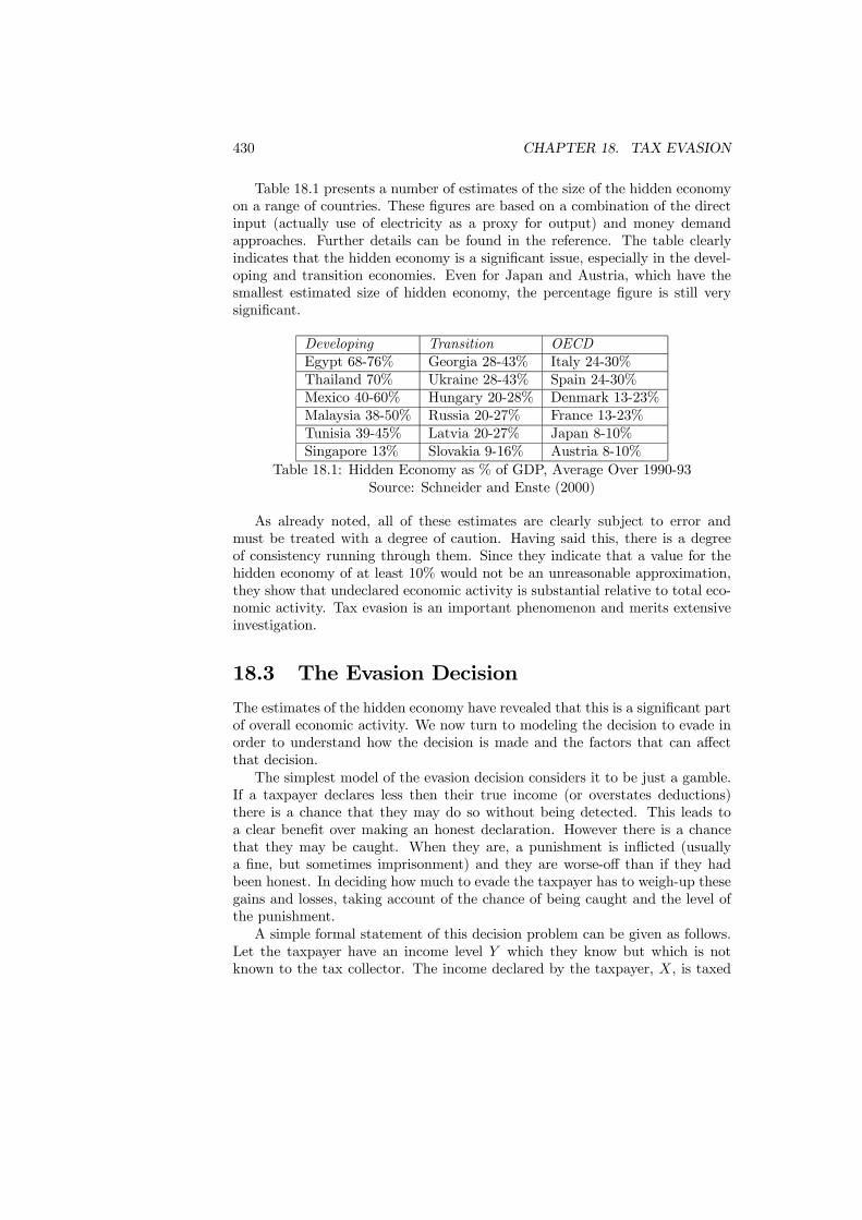
430 CHAPTER 18. TAX EVASION
Table 18.1 presents a number of estimates of the size of the hidden economyon a range of countries. These figures are based on a combination of the directinput (actually use of electricity as a proxy for output) and money demandapproaches. Further details can be found in the reference. The table clearlyindicates that the hidden economy is a significant issue, especially in the devel-oping and transition economies. Even for Japan and Austria, which have thesmallest estimated size of hidden economy, the percentage figure is still verysignificant.
Developing Transition OECDEgypt 68-76% Georgia 28-43% Italy 24-30%Thailand 70% Ukraine 28-43% Spain 24-30%Mexico 40-60% Hungary 20-28% Denmark 13-23%Malaysia 38-50% Russia 20-27% France 13-23%Tunisia 39-45% Latvia 20-27% Japan 8-10%Singapore 13% Slovakia 9-16% Austria 8-10%
Table 18.1: Hidden Economy as % of GDP, Average Over 1990-93Source: Schneider and Enste (2000)
As already noted, all of these estimates are clearly subject to error andmust be treated with a degree of caution. Having said this, there is a degreeof consistency running through them. Since they indicate that a value for thehidden economy of at least 10% would not be an unreasonable approximation,they show that undeclared economic activity is substantial relative to total eco-nomic activity. Tax evasion is an important phenomenon and merits extensiveinvestigation.
18.3 The Evasion Decision
The estimates of the hidden economy have revealed that this is a significant partof overall economic activity. We now turn to modeling the decision to evade inorder to understand how the decision is made and the factors that can affectthat decision.The simplest model of the evasion decision considers it to be just a gamble.
If a taxpayer declares less then their true income (or overstates deductions)there is a chance that they may do so without being detected. This leads toa clear benefit over making an honest declaration. However there is a chancethat they may be caught. When they are, a punishment is inflicted (usuallya fine, but sometimes imprisonment) and they are worse-off than if they hadbeen honest. In deciding how much to evade the taxpayer has to weigh-up thesegains and losses, taking account of the chance of being caught and the level ofthe punishment.A simple formal statement of this decision problem can be given as follows.
Let the taxpayer have an income level Y which they know but which is notknown to the tax collector. The income declared by the taxpayer, X, is taxed
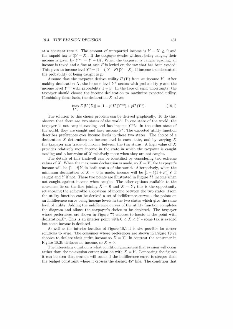
18.3. THE EVASION DECISION 431
at a constant rate t. The amount of unreported income is Y − X ≥ 0 andthe unpaid tax is t[Y −X]. If the taxpayer evades without being caught, theirincome is given by Y nc = Y − tX. When the taxpayer is caught evading, allincome is taxed and a fine at rate F is levied on the tax that has been evaded.This gives an income level Y c = [1− t]Y −Ft [Y −X]. If income is understated,the probability of being caught is p.Assume that the taxpayer derives utility U (Y ) from an income Y . After
making declaration X, the income level Y c occurs with probability p and theincome level Y nc with probability 1 − p. In the face of such uncertainty, thetaxpayer should choose the income declaration to maximize expected utility.Combining these facts, the declaration X solves
max{X}
E [U (X)] = [1− p]U (Y nc) + pU (Y c) . (18.1)
The solution to this choice problem can be derived graphically. To do this,observe that there are two states of the world. In one state of the world, thetaxpayer is not caught evading and has income Y nc. In the other state ofthe world, they are caught and have income Y c. The expected utility functiondescribes preferences over income levels in these two states. The choice of adeclaration X determines an income level in each state, and by varying Xthe taxpayer can trade-off income between the two states. A high value of Xprovides relatively more income in the state in which the taxpayer is caughtevading and a low value of X relatively more when they are not caught.The details of this trade-off can be identified by considering two extreme
values of X. When the maximum declaration is made, so X = Y , the taxpayer’sincome will be [1− t]Y in both states of the world. Alternatively, when theminimum declaration of X = 0 is made, income will be [1− t (1 + F )]Y ifcaught and Y if not. These two points are illustrated in Figure ?? income whennot caught against income when caught. The other options available to theconsumer lie on the line joining X = 0 and X = Y ; this is the opportunityset showing the achievable allocations of income between the two states. Fromthe utility function can be derived a set of indifference curves - the points onan indifference curve being income levels in the two states which give the samelevel of utility. Adding the indifference curves of the utility function completesthe diagram and allows the taxpayer’s choice to be depicted. The taxpayerwhose preferences are shown in Figure ?? chooses to locate at the point withdeclarationX∗. This is an interior point with 0 < X < Y - some tax is evadedbut some income is declared.As well as the interior location of Figure 18.1 it is also possible for corner
solutions to arise. The consumer whose preferences are shown in Figure 18.2achooses to declare their entire income so X = Y . In contrast the consumer inFigure 18.2b declares no income, so X = 0.The interesting question is what condition guarantees that evasion will occur
rather than the no-evasion corner solution with X = Y . Comparing the figuresit can be seen that evasion will occur if the indifference curve is steeper thanthe budget constraint where it crosses the dashed 45o line. The condition that
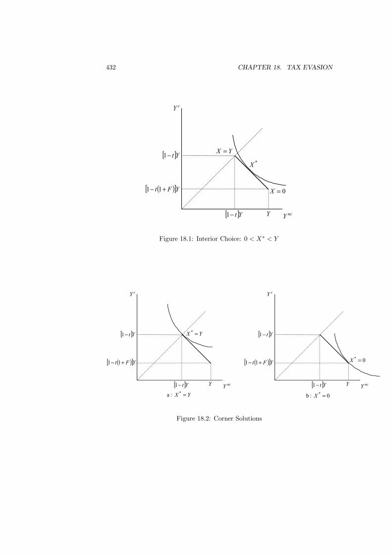
432 CHAPTER 18. TAX EVASION
cY
ncY
[ ]Yt−1
[ ]Yt−1 Y
( )[ ]YFt +− 11 0=X
YX =*X
Figure 18.1: Interior Choice: 0 < X∗ < Y
cY
ncY
[ ]Yt−1
[ ]Yt−1 Y
( )[ ]YFt +− 11
YX =*
cY
ncY
[ ]Yt−1
[ ]Yt−1 Y
0* =X
YX =* :a 0 :b * =X
( )[ ]YFt +− 11
Figure 18.2: Corner Solutions
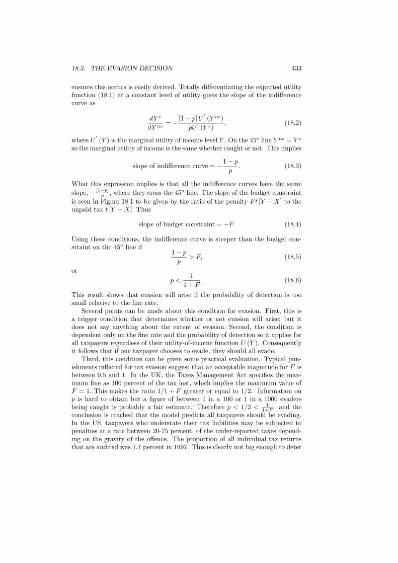
18.3. THE EVASION DECISION 433
ensures this occurs is easily derived. Totally differentiating the expected utilityfunction (18.1) at a constant level of utility gives the slope of the indifferencecurve as
dY c
dY nc= − [1− p]U
0(Y nc)
pU 0 (Y c). (18.2)
where U0(Y ) is the marginal utility of income level Y . On the 45o line Y nc = Y c
so the marginal utility of income is the same whether caught or not. This implies
slope of indifference curve = −1− pp. (18.3)
What this expression implies is that all the indifference curves have the sameslope, − [1−p]p , where they cross the 45o line. The slope of the budget constraintis seen in Figure 18.1 to be given by the ratio of the penalty Ft [Y −X] to theunpaid tax t [Y −X]. Thus
slope of budget constraint = −F (18.4)
Using these conditions, the indifference curve is steeper than the budget con-straint on the 45◦ line if
1− pp
> F, (18.5)
or
p <1
1 + F. (18.6)
This result shows that evasion will arise if the probability of detection is toosmall relative to the fine rate.Several points can be made about this condition for evasion. First, this is
a trigger condition that determines whether or not evasion will arise; but itdoes not say anything about the extent of evasion. Second, the condition isdependent only on the fine rate and the probability of detection so it applies forall taxpayers regardless of their utility-of-income function U (Y ). Consequentlyit follows that if one taxpayer chooses to evade, they should all evade.Third, this condition can be given some practical evaluation. Typical pun-
ishments inflicted for tax evasion suggest that an acceptable magnitude for F isbetween 0.5 and 1. In the UK, the Taxes Management Act specifies the max-imum fine as 100 percent of the tax lost, which implies the maximum value ofF = 1. This makes the ratio 1/1 + F greater or equal to 1/2. Information onp is hard to obtain but a figure of between 1 in a 100 or 1 in a 1000 evadersbeing caught is probably a fair estimate. Therefore p < 1/2 < 1
1+F and theconclusion is reached that the model predicts all taxpayers should be evading.In the US, taxpayers who understate their tax liabilities may be subjected topenalties at a rate between 20-75 percent of the under-reported taxes depend-ing on the gravity of the offence. The proportion of all individual tax returnsthat are audited was 1.7 percent in 1997. This is clearly not big enough to deter

434 CHAPTER 18. TAX EVASION
cY
ncY
[ ]Yt−1
[ ]Yt−1 Y
( )[ ]YFt +− 11
new
old
Figure 18.3: Increase in Detection Probability
cheating and everyone should be under-reporting taxes. In fact the TaxpayerCompliance Measurement Program reveals that 40 percent of US taxpayers un-derpaid their taxes. This is a sizeable minority, but not as widespread evasionas the theoretical model would predict. So taxpayers appears to be more honestthan might be expected.The next step is to determine the amount of tax evasion and how it is affected
by changes in the model’s variables. There are four such variables that are ofinterest: the income level Y , the tax rate t, the probability of detection p andthe fine rate F . These effects can be explored by using the figure depicting thechoice of evasion level.Take the probability of detection first. The probability of detection does not
affect the opportunity set but does affect preferences. The effect of an increasein p is to make the indifference curves flatter where they cross the 45o line. Asshown in Figure 18.3, this moves the optimal choice closer to the point X = Y ofhonest declaration. The amount of income declared rises, so an increase in theprobability of detection reduces the level of evasion. This is a clearly expectedresult since an increase in the likelihood of detection lowers the payoff fromevading and makes evasion a less attractive proposition.A change in the fine rate only affects income when the taxpayer is caught
evading. The consequence of an increase in F is that the budget constraintpivots round the honest report point and becomes steeper. Since the indifferencecurve is unaffected by the penalty change, the optimal choice must again movecloser to the honest declaration point. This is shown in Figure 18.4 by the movefrom the initial choice of Xold when the fine rate if F to the choice Xnew whenthe fine rate increases to bF . An increase in the fine rate therefore leads to areduction in the level of tax evasion. This, and the previous result, shows that
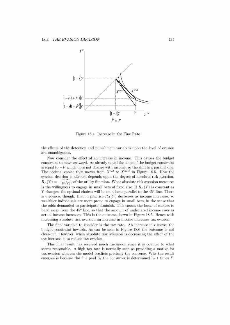
18.3. THE EVASION DECISION 435
cY
ncY
[ ]Yt−1
[ ]Yt−1 Y
FF >ˆ
oldXnewX( )[ ]YFt +− 11
( )[ ]YFt ˆ11 +−
Figure 18.4: Increase in the Fine Rate
the effects of the detection and punishment variables upon the level of evasionare unambiguous.Now consider the effect of an increase in income. This causes the budget
constraint to move outward. As already noted the slope of the budget constraintis equal to −F which does not change with income, so the shift is a parallel one.The optimal choice then moves from Xold to Xnew in Figure 18.5. How theevasion decision is affected depends upon the degree of absolute risk aversion,RA(Y ) = −U
00(Y )U 0(Y ) , of the utility function. What absolute risk aversion measures
is the willingness to engage in small bets of fixed size. If RA(Y ) is constant asY changes, the optimal choices will be on a locus parallel to the 45o line. Thereis evidence, though, that in practice RA(Y ) decreases as income increases, sowealthier individuals are more prone to engage in small bets, in the sense thatthe odds demanded to participate diminish. This causes the locus of choices tobend away from the 45o line, so that the amount of undeclared income rises asactual income increases. This is the outcome shown in Figure 18.5. Hence withincreasing absolute risk aversion an increase in income increases tax evasion.The final variable to consider is the tax rate. An increase in t moves the
budget constraint inwards. As can be seen in Figure 18.6 the outcome is notclear-cut. However, when absolute risk aversion is decreasing the effect of thetax increase is to reduce tax evasion.This final result has received much discussion since it is counter to what
seems reasonable. A high tax rate is normally seen as providing a motive fortax evasion whereas the model predicts precisely the converse. Why the resultemerges is because the fine paid by the consumer is determined by t times F .
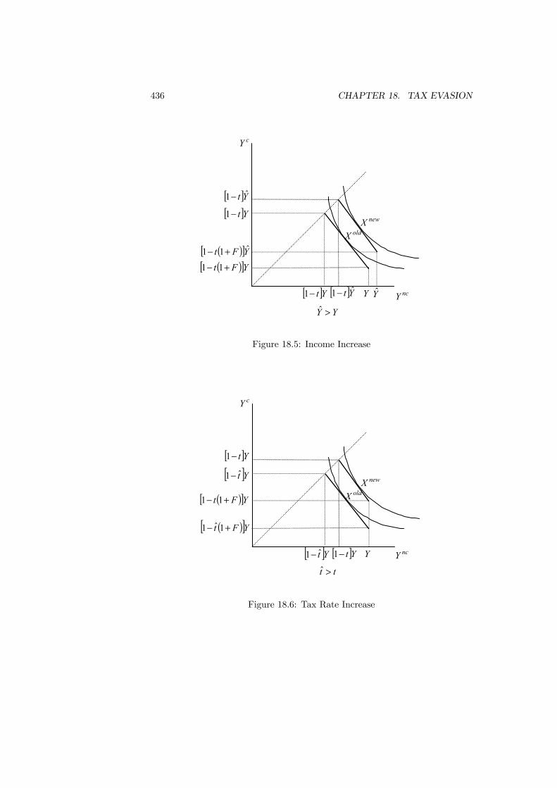
436 CHAPTER 18. TAX EVASION
cY
ncY
[ ]Yt−1
[ ]Yt−1 Y
( )[ ]YFt +− 11
YY >ˆ
oldX
newX
Y
( )[ ]YFt ˆ11 +−
[ ]Yt ˆ1−
[ ]Yt ˆ1−
Figure 18.5: Income Increase
cY
ncY[ ]Yt1− Y
( )[ ]YFt +− 1ˆ1
tt >ˆ
oldX
newX
( )[ ]YFt +− 11
[ ]Yt−1
[ ]Yt−1
[ ]Yt1−
Figure 18.6: Tax Rate Increase
18.4. AUDITING AND PUNISHMENT 437
An increase in the tax rate thus has the effect of raising the penalty. This takesincome away from the taxpayer when they are caught - the state in which theyhave least income. It is through this mechanism that a higher tax rate canreduce evasion.This completes the analysis of the basic model of tax evasion. It has been
shown how the level of evasion is determined and how this is affected by theparameters of the model. The next section turn to the issue of determiningthe optimal levels of auditing and punishment when the behavior of taxpayerscorresponds to the predictions of this model. Some empirical and experimentalevidence is then considered and the model is assessed in the light of this.
18.4 Auditing and PunishmentThe analysis of the tax evasion decision assumed that the probability of detec-tion and the rate of the fine levied when caught evading were fixed. This is asatisfactory assumption from the perspective of the individual taxpayer. Fromthe government’s perspective, though, these are variables that can be chosen.The probability of detection can be raised by the employment of additional tax-payers and the fine can be legislated or set by the courts. The purpose of thissection is to analyze the issues involved in the government’s decision.It has already been shown that an increase in either p or F will reduce the
amount of undeclared income. The next step is consider how they affect thelevel of revenue raised by the government. Revenue in this context is defined astaxes paid plus the money received from fines. From a taxpayer with income Ythe expected value (it is expected since there is only a probability the taxpayerwill be fined) of the revenue collected is
R = tX + p(1 + F )t [Y −X] . (18.7)
Differentiating with respect to p shows that the effect upon revenue of an in-crease in the probability of detection is
∂R
∂p= (1 + F )t [Y −X] + t [1− p− pF ] ∂X
∂p> 0, (18.8)
whenever pF < 1 − p. Recalling (18.6), if pF ≥ 1 − p there is no evasion andso p has no effect on revenue. Carrying out the differentiation for the fine rateshows that if pF < 1− p
∂R
∂F= pt [Y −X] + t [1− p− pF ] ∂X
∂F> 0. (18.9)
Again, the fine has no effect if pF ≥ 1 − p. These expressions show that ifevasion is taking place, an increase in either the probability of detection or ofthe fine will increase the revenue the government receives.The choice problem of the government can now be addressed. It has already
been noted that an increase in the probability of detection can be achieved by
438 CHAPTER 18. TAX EVASION
the employment of additional tax inspectors. Tax inspectors require paymentso, as a consequence, an increase in p is costly to achieve. In contrast, thereis no cost involved in raising or lowering the fine. Effectively, increases in Fare costless to produce. From these observations, the optimal policy can bedetermined.Since p is costly and F is free, the interests of the government are best
served by reducing p close to zero whilst raising F towards infinity. This hasbeen termed the policy of “hanging taxpayers with probability zero”. Expressedin words, the government should put virtually no effort into attempting to catchtax evaders but should severely punish those it apprehends. This is an extremeform of policy and nothing like it is observed in practice. Surprising as it is, itdoes follow from the logical application of the model.Numerous comments can be made in respect of this result. The first begins
with the objective of the government. In previous chapters it has been assumedthat the government is guided in its policy choice by a social welfare function.There will be clear differences between a policy designed to maximize revenueand one that maximizes welfare. For instance, inflicting an infinite fine upona taxpayer caught evading will have a significantly detrimental effect on wel-fare. Even if the government does not pursue welfare maximization, it may beconstrained by political factors such as the need to ensure re-election. A policyof severely punishing tax evaders may be politically damaging especially if taxevasion is a widely-established phenomenon.One could think that such argument is not relevant because if the punishment
is large enough to deter cheating, it should not matter how dire it is. Thefear keeps everyone from cheating, hence the punishment never actually occursand its costs is irrelevant. The problem with this argument is that it ignoresthe risk of mistakes. The detection process may go wrong or the taxpayer canmistakenly understate taxable income. If punishment are as large as possible,even for small tax underpayments, then mistakes will be very costly. To reducethe cost of mistakes, the punishment should be of the smallest size required todeter cheating. Minimal deterrence accomplishes this purpose.A further observation, and one whose consequences will be investigated in
detail, concerns the policy instruments under the government’s control. Theview of the government so far is that it a single entity that chooses the level ofall its policy instruments simultaneously. In practice, the government consistsof many different departments and agencies. When it comes to taxation and taxpolicy, a reasonable breakdown would be to view the tax rate as set by centralgovernment as part of a general economic policy. The probability of detection iscontrolled by a revenue service whose objective is the maximization of revenue.Finally, the punishment for tax evasion is set by the judiciary.This breakdown shows why the choice of probability and fine may not be
chosen in a cohesive manner by a single authority. What it does not do isprovide any argument for why the fine should not be set infinitely high to deterevasion. An explanation for this can be found by applying reasoning fromthe economics of crime. This would view tax evasion as just another crime,and the punishment for it should fit with the scheme of punishments for other
18.5. EVIDENCE ON EVASION 439
crimes. The construction of these punishments relies on the argument that theyshould provide incentives that lessen the overall level of crime. To see what thismeans, imagine that crimes can be ranked from least harmful to most harmful.Naturally, if someone is going to commit a crime, the authorities wish that theycommit a less harmful one rather than a more harmful one. If more harmfulones are also more rewarding (think of robbing a bank whilst armed comparedto merely attempting to snatch cash), then a scheme of equal punishments willnot provide any incentive for committing the less harmful crime. What willprovide the right incentive is for the more harmful crime to also have a heavierpunishment. So the extent of punishment should be related to the harmfulnessof the crime. Punishment should fit the crime.This framework has two implications. First of all, the punishment for tax
evasion will not be varied freely in order to maximized revenue. Instead itwill be set as part of a general crime policy. The second implication is thatthe punishment will also be quite modest since tax evasion is not an especiallyharmful crime. Arguments such as these are reflected in the fact that the finerate on evasion is quite low - a figure in the order of 1.5 to 2 would not beunrealistic. As already noted, the maximum fine in the UK is 100% of theunpaid tax, but the Inland Revenue may accept a lesser fine depending on the“size and gravity” of the offence.Putting all of these arguments together suggests adopting a different per-
spective on choosing the optimal probability of detection. With the tax rate setas a tool of economic policy and the fine set by the judiciary, the only instru-ment under the control of the revenue service is the probability of detection. Asalready seen, an increase in this raises revenue but only does so at a cost. Theoptimal probability is found when the marginal gain in revenue just equals themarginal cost - and this could occur at a very low value of p.
18.5 Evidence on Evasion
The model of tax evasion has predicted the effect that changes in various para-meters will have upon the level of tax evasion. In some cases, such as the effectof the probability of detection and the fine, these are unambiguous. In others,particularly the effect of changes in the tax rate, the effects depend upon theprecise specification of the tax system and upon assumptions concerning atti-tudes towards risk. These uncertainties make it valuable to investigate furtherevidence to see how the ambiguities are resolved in practice. The analysis ofevidence also allows the investigation of the relevance of other parameters, suchas the source of income, and other hypotheses on tax evasion, for example theimportance of social norms.There have been two approaches taken in studying tax evasion. The first
has been to collect survey or interview data and use econometric analysis toprovide a quantitative determination of the relationships. The second has beento use experiments to provide an opportunity of designing the environment topermit the investigation of particular hypotheses.

440 CHAPTER 18. TAX EVASION
The results that have been found can be summarized as follows. Whenincome levels ascertained from interviews has been contrasted to that given onthe tax returns of the same individuals, a steady decline of declared incomeas a proportion of reported income occurs as income rises. This finding is inagreement with the comparative statics analysis. Table 18.2 provides a sample ofdata to illustrate this. Interviewees were placed in income intervals according totheir responses to interview questions. The information on their tax declarationwas then used to determine assessed income. The percentage is then found bydividing the assessed income by the midpoint of the income interval.
Income Interval 17-20 20-25 25-30 30-35 35-40Midpoint 18.5 22.5 27.5 32.5 37.5
Assessed Income 17.5 20.6 24.2 28.7 31.7Percentage 94.6 91.5 88.0 88.3 84.5
Table 18.2: Declaration and IncomeSource: Mork (1975)
Econometrics and survey methods have been used to investigate the impor-tance of attitudes and social norms in the evasion decision. The study reportedin Table 18.3 shows that the propensity to evade taxation is reduced by an in-creased probability of detection and an increase in age. An increase in incomereduces the propensity to evade. With respect to the attitude and social vari-ables, both an increase in the perceived inequity of taxation and of the numberof other tax evaders known to the individual make evasion more likely. Theextent of tax evasion is also increased by the attitude and social variables butwas also increased by the experience of the tax payer with previous tax audits.The social variables are clearly important in the decision to evade tax.
Propensity to Evade Extent of EvasionInequity 0.34 0.24
No. of Evaders Known 0.16 0.18Probability of Detection -0.17
Age -0.29Experience of Audits 0.22 0.29
Income Level -0.27Income from Wages and Salaries 0.20
Table 18.3: Explanatory FactorsSource: Spicer and Lundstedt (1976)
As far as the effect of the tax rate is concerned, data from the InternalRevenue Services Taxpayer Compliance Measurement Program survey of 1969shows that tax evasion increases as the marginal tax rates increases but is de-creased when wages where a significant proportion of income. This result issupported by employing the difference between income and expenditure figuresin National Accounts as a measure of evasion. In contrast a study, of Belgiandata found precisely the converse conclusion with tax increases leading to lower
18.6. EFFECT OF HONESTY 441
evasion. Therefore these studies do not resolve the ambiguity about the relationbetween marginal tax rates and tax evasion.Turning now to experimental studies, tax evasion games have shown that
evasion increases with the tax rate and that evasion falls as the fine is increasedand the detection probability reduced. Further results have shown that womenevade more often than men but evade lower amounts and that purchasers oflottery tickets, presumed to be less risk averse, were no more likely to evadethan non-purchasers but evaded greater amounts when they did evade. Finally,the very nature of the tax evasion decision has been tested by running two setsof experiments. One was framed as a tax evasion decision and the other asa simple gamble with the same payoffs. For the tax evasion experiment sometaxpayers chose not to evade even when they would under the same conditionswith the gambling experiment.There are two important lessons to be drawn from this brief review of the
empirical and experimental results. Firstly, the theoretical predictions are gen-erally supported except for the effect of the tax rate. The latter remains uncer-tain with conflicting conclusions from the evidence. Secondly it appears thattax evasion is more than the simple gamble portrayed in the basic model. Inaddition to the basic element of risk, there are attitudinal and social aspects tothe evasion decision.
18.6 Effect of HonestyThe evidence discussed in the previous section has turned up a number of factorsthat are not explained by the basic model of tax evasion. Foremost amongstthese are that some taxpayers choose not to evade even when they would acceptan identical gamble and that there are social aspects of the evasion decision.The purpose of this section is to show how simple modifications to the modelcan incorporate these factors and can change the conclusions concerning theeffect of the tax rate.The feature that distinguishes tax evasion from a simple gamble is that
taxpayers submitting incorrect returns feel varying degrees of anxiety and regret.To some, being caught would represent a traumatic experience which woulddo immense damage to their self-image. To others, it would be only a slightinconvenience. The innate belief in honesty of some taxpayers is not capturedby representing tax evasion as just a gamble nor are the non-monetary costs ofdetection and punishment captured by preferences defined on income alone. Thefirst intention of this section is to incorporate these features into the analysisand to study their consequences.A preference for honesty can be introduced into the utility function by writ-
ing utility asU = U (Y )− χE,
where χ is the measure of the taxpayers honesty and, with E = Y −X the extentof evasion, χE is the utility cost of deviating from complete honesty. To see theconsequence of this assumption, assume that taxpayers differ in their value of χ
442 CHAPTER 18. TAX EVASION
but are identical in all other respects. Those with higher values of χ will sufferfrom a greater utility reduction for any given level of evasion. In order for themto evade, the utility gain from evasion must exceed this utility reduction. Thepopulation is therefore separated into two parts with some taxpayers choosingnot to evade (those with high values of χ) while others will evade (those withlow χ). It is tempting to label those who do not evade as honest, but this is notreally appropriate since they will evade if the benefit is sufficiently great.Let the value of χ that separates the evaders from the non-evaders be denotedbχ. A change in one of the parameters of the model (p, F and t) now has two
effects. Firstly, it changes the benefit from evasion so alters the value of bχ. Forinstance, an increase in the rate of tax raises the benefit of evasion so increasesbχ with the consequence that more taxpayers evade. Secondly, the change inthe parameter affects the evasion decision of all existing tax evaders. Puttingtogether these effects together, it becomes possible for an increase in the taxrate to lead to more evasion in aggregate. This is in contrast to the basic modelwhere it would reduce evasion.The discussion of the empirical evidence has drawn attention to the positive
connection between the number of tax evaders known to a taxpayer and thelevel of that taxpayer’s own evasion. This observation suggests that the evasiondecision is not made in isolation by each taxpayer but is made with referenceto the norms and behavior of the general society of the taxpayer. Given theempirical significance of such norms, the second part of this section focuses ontheir implications.Social norms have been incorporated into the evasion decision in two dis-
tinct ways. It can be introduced as an additional element of the utility cost toevasion. The additional utility cost is assumed to be an increasing function ofthe proportion of taxpayers who do not evade. This formulation is intended tocapture the fact that more utility will be lost, in terms of reputation, the moreout of step the taxpayer is with the remainder of society. The consequence ofthis modification is to reinforce the separation of the population into evadersand non-evaders.An alternative approach is to explicitly impose a social norm upon behavior.
One such social norm can be based on the concept of Kantian morality and,effectively, has each individual assessing their fair contribution in tax paymentstowards the provision of public goods. This calculation then provides an upperbound on the extent of tax evasion. To calculate the actual degree of tax evasioneach taxpayer then performs the expected utility maximization calculation, asin (18.1), and evades whichever is the smaller out of this quantity and thepreviously determined upper bound. This formulation is also able to provide apositive relation between the tax rate and evaded tax for some range of taxesand to divide the population into those who evade tax and those who do not.The introduction of psychic costs and of social norms is capable of explaining
some of the empirically observed features of tax evasion which are not explainedby the standard expected utility maximization hypothesis. It does this modify-ing the form of preferences but the basic nature of the approach is unchanged.The obvious difficulty with these changes is that there is little to suggest pre-

18.7. TAX COMPLIANCE GAME 443
cisely how social norms and utility costs of dishonesty should be formalized.
18.7 Tax Compliance Game
An initial analysis of the choice of audit probability was undertaken in Section18.4. It was argued there that the practical situation involves a revenue servicethat chooses the probability to maximize total revenue taking as given the taxrate and the punishment. The choice of probability in this setting requiresan analysis of the interaction between the revenue service and the taxpayers.The revenue service reacts to the declarations of taxpayers, and taxpayers makedeclarations on the basis of the detection probability.Such interaction is best analyzed by formalizing the structure of the game
that is being played between the revenue service and the taxpayers. The choiceof a strategy for the revenue service is the probability with which it chooses toaudit any given value of declaration. This probability need not be constant fordeclarations of different values and is based on its perception of the behaviourof taxpayers. For the taxpayers, a strategy is a choice of declaration given theaudit strategy of the revenue service. At a Nash equilibrium of the game, thestrategy choices must be mutually optimal: the audit strategy must maximisethe revenue collected, net of the costs of auditing, given the declarations andthe declaration must maximize utility given the audit strategy.Even without specifying details of the game, it is possible to make a general
observation: predictability in auditing cannot be an equilibrium strategy. Thiscan be seen in several stages. First, no auditing at all cannot be a optimal be-cause it would mean maximal tax evasion. Secondly, auditing of all declarationscannot be a solution either because no revenue service would incur the cost ofauditing knowing that full enforcement induces everyone to comply. Finally, pre-specified limits on the range of delarations that will be audited are also flawed.Taxpayers who are considering under-reporting income will make sure that theystay just outside the audit limit, and those who cannot avoid being audited willchoose to report truthfully. Exactly the wrong set of taxpayers will be audited.This establishes that the equilibrium strategy must be unpredictable.To be unpredictable, the audit strategy must be random. But how should
the probability of audit depend on the information available on the tax return?Since the incentive of a taxpayer is to understate income to reduce their taxliabilities, it seems to require that the probability of an audit should be higherfor low income reports. More precisely, the probability of an audit should behigh for an income report that is low compared to what one would expect fromsomeone in that taxpayer’s occupation or given the information on previous taxreturns for that taxpayer. This is what theory predicts and what is done inpractice.A simple version of the strategic interaction between the revenue service and
a taxpayer is depicted in Figure ??. The taxpayer with true income Y can eitherevade (reporting zero income) or not (truthful income report) By reportingtruthfully the taxpayer pays tax T to the revenue service (with T < Y ). The
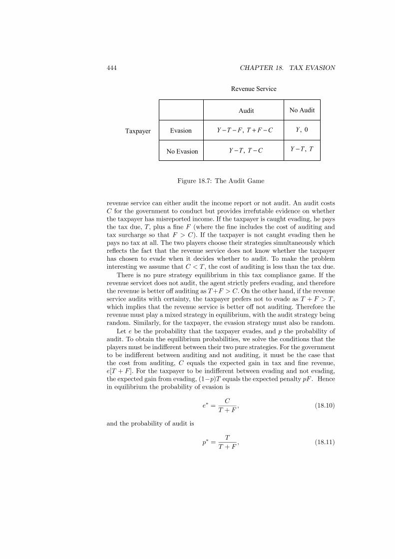
444 CHAPTER 18. TAX EVASION
CFTFTY −+−− ,
CTTY −− ,
0 ,Y
TTY ,−
No AuditAudit
Evasion
No Evasion
Taxpayer
Revenue Service
Figure 18.7: The Audit Game
revenue service can either audit the income report or not audit. An audit costsC for the government to conduct but provides irrefutable evidence on whetherthe taxpayer has misreported income. If the taxpayer is caught evading, he paysthe tax due, T, plus a fine F (where the fine includes the cost of auditing andtax surcharge so that F > C). If the taxpayer is not caught evading then hepays no tax at all. The two players choose their strategies simultaneously whichreflects the fact that the revenue service does not know whether the taxpayerhas chosen to evade when it decides whether to audit. To make the probleminteresting we assume that C < T , the cost of auditing is less than the tax due.There is no pure strategy equilibrium in this tax compliance game. If the
revenue servicet does not audit, the agent strictly prefers evading, and thereforethe revenue is better off auditing as T+F > C. On the other hand, if the revenueservice audits with certainty, the taxpayer prefers not to evade as T + F > T ,which implies that the revenue service is better off not auditing. Therefore therevenue must play a mixed strategy in equilibrium, with the audit strategy beingrandom. Similarly, for the taxpayer, the evasion strategy must also be random.Let e be the probability that the taxpayer evades, and p the probability of
audit. To obtain the equilibrium probabilities, we solve the conditions that theplayers must be indifferent between their two pure strategies. For the governmentto be indifferent between auditing and not auditing, it must be the case thatthe cost from auditing, C equals the expected gain in tax and fine revenue,e[T + F ]. For the taxpayer to be indifferent between evading and not evading,the expected gain from evading, (1−p)T equals the expected penalty pF . Hencein equilibrium the probability of evasion is
e∗ =C
T + F, (18.10)
and the probability of audit is
p∗ =T
T + F, (18.11)
18.8. COMPLIANCE AND SOCIAL INTERACTION 445
where both e∗ and p∗ belong to the interval (0, 1) so that both evasion and auditstrategies are random.The equilibrium probabilities are determined by the strategic interaction be-
tween the taxpayer and the revenue service. For instance, the audit probabilitydeclines with the fine, though a higher fine may be expected to make auditingmore profitable. The reason is that a higher fine discourages evasion, thus mak-ing auditing less useful. Similarly, evasion is less likely with high tax becausethe higher tax induces the government to audit more. Note that these resultsare obtained without specifying the details of the fine function which could beeither a lump sum amount or something proportional to evaded tax. Evasion isalso more likely the more costly is auditing, since the revenue service is willingto audit at a higher cost only if the taxpayer is more likely to have evaded tax.The equilibrium payoffs are
u∗ = Y − T + e∗[T − p∗[T + F ]], (18.12)
for the taxpayer and
v∗ = (1− e∗)T + p∗[e∗[T + F ]− C], (18.13)
for the revenue service. Substituting into these payoffs the equilibrium proba-bilities of evasion and audit gives
u∗ = Y − T, (18.14)
v∗ = T − C
T + FT. (18.15)
Because the taxpayer is indifferent between evading or not evading, his equi-librium payoff is equal to his truthful payoff Y −T . This means that the unpaidtaxes and the fine cancel out in expected terms. Increasing the fine does notaffect the taxpayer. However a higher fine increases the payoff of the revenueservice since it reduces the amount of evasion. Hence increasing the penalty isPareto improving in this model. The equilibrium payoffs also reflect the costfrom evasion. Indeed for any tax T paid by the taxpayer, the revenue serviceeffectively receives T −∆ where ∆ = C
T+F T is the deadweight loss from evasion.Thus evasion involves a deadweight loss that is increasing with the tax rate.
18.8 Compliance and Social InteractionIt has been assumed so far that the decision by any taxpayer to comply withthe tax law is independent of what the other taxpayers are doing. This decisionis based entirely on the enforcement policy (penalty and auditing) and the eco-nomic opportunity (tax rates and income). In practice, however, we may expectthat someone is more likely to break the law when non-compliance is alreadywidespread than when it is confined to a small segment of the population. Thisobservation is supported by the evidence in Table 18.3 which shows that taxcompliance is susceptible to social interaction.
446 CHAPTER 18. TAX EVASION
The reasoning behind this social interaction can be motivated along the fol-lowing lines. The amount of stigma or guilt I feel if I do not comply may dependon what others do and think. Whether they also underpay taxes may determinehow I feel if I do not comply. As we now show, this simple interdependence be-tween taxpayers can trigger a dynamic process that moves the economy towardeither full compliance or no compliance at all.
To see this, consider a set of taxpayers. Each taxpayer has to decide whetherto evade taxes or not. Fixing the enforcement parameters, the payoff from evad-ing taxes depends on the number of non-compliers. In particular, the payofffrom non-compliance is increasing with the number of non-compliers becausethen the chances of getting away with the act of evasion increase. On the otherhand, the payoff from compliance decreases with the number of non-compliers.The reason can be that you suffer some resentment cost from abiding with thelaw when so many are breaking the law. Therefore individuals care about theoverall compliance in the group when choosing to comply themselves.
It follows from this that the choice of tax evasion becomes more attractivewhen more taxpayers make the same choice of breaking the law. Because ofthe way interactions work, the aggregate compliance tendency is toward oneof the extremes: only the worst outcome of nobody complying or the bestoutcome of full compliance are possible. This is illustrated in the Figure 18.8depicting the payoff from compliance and non-compliance (vertical axis) againstthe non-compliance rate in the group (horizontal axis). At the intersection ofthe two payoff functions taxpayers are indifferent between compliance or non-compliance. Starting from this point, a small reduction in non-compliance wouldbreak the indifference in favour of compliance and trigger a chain reaction towardincreasing compliance. Alternatively a small increase in non-compliance triggersa chain reaction in the opposite direction making non-compliance progressivelymore and more attractive.
In this situation, how do we get to encourage taxpayers to abide by the lawwhen the dynamic is pushing in the opposite direction? The solution is to get acritical mass of individuals complying to reverse the dynamic. This requires ashort but intense audit policy backed by a harsh punishment in order to changethe decisions of enough taxpayers that the dynamics switch toward full compli-ance. When at this new full compliance equilibrium, it is then possible to cutdown on audit costs because compliance is self-sustained by the large numbersof taxpayers who comply. It follows from this simple argument that moderateenforcement policy with few audits and light penalties over a long period isineffective. Another interesting implication of this model is that two countrieswith similar enforcement policies can end up with very different compliancerates. Social interaction can be a crucial explanation for the astoundingly highvariance of compliance rates across locations and over time: much higher thanwhat can be predicted by differences in local enforcement policies.

18.8. COMPLIANCE AND SOCIAL INTERACTION 447
01
Noncompliance rate
Compliance payoff
Noncompliancepayoff
Figure 18.8: Compliance Rate
448 CHAPTER 18. TAX EVASION
18.9 Conclusions
Tax evasion is an important and significant phenomenon that affects both de-veloped and developing economies. Although there is residual uncertainty sur-rounding the accuracy of measurements, even the most conservative estimatessuggest the hidden economy in the UK and US to be at least ten per cent of themeasured economy. There are many countries where it si very much higher. Thesubstantial size of the hidden economy, and the tax evasion that accompaniesit, requires understanding so that the effects of policies that interact with it canbe correctly forecast.The predictions of the standard representation of tax evasion as a choice with
risk were derived and contrasted with empirical and experimental evidence.This showed that although it is valuable as a starting point for a theory ofevasion, the model did not incorporate some key aspects of the evasion decision,most notably the effects of a basic wish to avoid dishonesty and the the socialinteraction between taxpayers. The analysis was then extended to incoporporateboth of these issues.
Further readingOne of the earliest model of tax compliance:AllinghamM. and A. Sandmo, 1972, Income tax evasion: a theoretical analy-
sis, Journal of Public Economics, 1, 323-38.Becker, G., 1968, Crime and punishment: an economic approach, Journal of
Political Economy, 76, 169-217.Cowell, F.A., 1990, Cheating the Government, (Cambridge: MIT Press).For a comprehensive survey of the extent of tax evasion in wide range of
countries:Schneider F., and Enste D.H., 2000, ”Shadow economies: Size, causes, and
consequences”, Journal of Economic Literature, 38, 77-114.Empirical and experimental evidence is found inBaldry, J.C., 1986, “Tax evasion is not a gamble“, Economics Letters, 22,
333 - 335.Mork, K.A., 1975, “Income tax evasion: some empirical evidence“, Public
Finance, 30, 70-76.Spicer, M.W. and S.B. Lundstedt, 1976, “Understanding tax evasion“, Public
Finance, 31, 295-305.On the effect of social interaction on law complianceGlaeser, E.L., B. Sacerdote and J.A. Scheinkman, 1996, Crime and social
interaction, Quarterly Journal of Economics, 111, 506-548.Game theoretic model of the strategic interaction between taxpayer and
enforcement agency, including honest taxpayers:Graetz, M., Reinganum, J. and L. Wilde, 1986, The tax compliance game:
towards an interactive theory of law enforcement, Journal of Law, Economicsand Organization, 2, 1-32.Scotchmer, S., 1987, Audit classes and tax enforcement policy, American
Economic Review, 77, 229-233.

18.9. CONCLUSIONS 449
On the effect of fiscal corruption and the desirability of flat taxHindriks, J., Keen M., and A. Muthoo, 1999, Corruption, extortion and
evasion, Journal of Public Economics, 74, 395-430.

450 CHAPTER 18. TAX EVASION

Part VII
Multiple Jurisdictions
451

Chapter 19
Fiscal Federalism
19.1 Introduction
Fiscal federalism is the division of revenue collection and expenditure respon-sibilities between different levels of government. Most countries have a central(or federal) government, state or county governments, town councils and, at thelowest level, parish councils. Each level has restrictions on the tax instrumentsit can employ and the expenditures that it can make. Together they consti-tute the multi-levelled and overlapping administration that governs a typicaldeveloped country.The central government can usually choose whatever tax instruments it
pleases and, although it has freedom in its expenditure, it usually focuses uponnational defence, the provision of law and order, infrastructure and transferpayments. The taxation powers of state governments are more restricted. Inthe UK they can levy only property taxes; in the US both commodity andlocal income taxes are allowed. Their responsibilities include education, localinfrastructure and the provision of health care. Local governments provide ser-vices such as rubbish collection and parks. The responsibility for the police andfire service can be at either the state or local level. These levels of governmentare connected by overlapping responsibilities and transfers payments betweenlevels.The issue of fiscal federalism is not restricted to the design of government
within countries. Indeed, the recent impetus for the advancement of this theoryhas been issues involving the design of institutional structures for the EuropeanUnion. The progress made towards economic and monetary integration hasbegun to raise questions about subsidiarity, which is the degree of independencethat individual countries will maintain in the setting of taxes. Such argumentsjust involve the application of fiscal federalism, albeit at a larger scale.These observations lead to a number of interesting economic questions.
Firstly, why should there be more than one level of government? Using thelogic of economic reasoning, multi-level government can only be justified if it
453
454 CHAPTER 19. FISCAL FEDERALISM
can achieve something that a single-level cannot. Explanations of what this canbe must revolve around access to information and how this can be best utilized.If this argument is accepted, and it is explored in detail below, then a secondquestion arises. How are the functions of government allocated between thelevels? A brief sketch of how this works in practice has already been given; isthis outcome efficient or does it reflect some other factors?The next section of the chapter will consider the rationale for multi-level
government, focussing upon the availability of information. Section 2 providesan overview of arguments in favour of multi-level government. A more detailedanalysis of some of the key issues is given in Section 3 and the concept of an op-timal structure is investigated. The issue of accountability and decentralizationis analyzed in Section 4. The essential elements of inter-regional risk sharing arepresented in Section 5 and the distinction between insurance and redistributionis discussed. Section 6 provides empirical evidence on the extent of decentral-ization by countries and functions, and the main determinants of the observeddecentralization. Concluding comments are in Section 7.
19.2 Arguments for Multi-Level Government
The economic arguments for having government are founded on the two prin-ciples outlined in Chapter 6. If there is market failure, the government canintervene in the economy to increase efficiency. It can also intervene to improveequity, regardless of whether the economy is efficient or not. These argumentsjustify intervention; to justify multi-level government the case must be madeobjectives of efficiency and equity are better-served by a combination of localand central government.If the correct decisions are made about the level of public good provision and
about taxes, then it does not matter at which level of government they are taken.Provided that there are no resources wasted in overlapping responsibilities, thenumber of levels of government is a matter of indifference. A case for multi-levelgovernment must therefore be sought in differences in information and politicalprocess that allow some structures to achieve better outcomes than others.Decisions should be taken at a national level if they involve public goods
which serve the entire economy. The obvious example here would be defence,the benefits of which cannot be assigned to any particular community within theeconomy. It is common to argue that all citizens should have the same accessto the law, have the same rights under the law and be subject to the samerestrictions. An application of this equity argument supports a legal systemthat is organized and administered from the centre. Given the central provisionof these services, it is natural to support them through centrally-organized taxes.Other public goods, namely the local public goods of Chapter 16, benefit
only those resident within a defined geographic area. The level of supply ofthese goods could be determined and financed at the national level but thereare three arguments to suggest a lower-level decision is preferable.Firstly, determination at the local level can take account of more precise
19.2. ARGUMENTS FOR MULTI-LEVEL GOVERNMENT 455
information available on local preferences. In this context, local ballots andknowledge of local circumstances may help in reaching a more efficient deci-sion. Secondly, if a decision were to be made at the national level politicalpressures may prevent there from being any differentiation of provision betweencommunities, whereas it might be efficient to have different levels of local publicgood provision in different areas. Finally, the Tiebout hypothesis investigatedin Chapter 16 argued that if consumers have heterogenous preferences then effi-ciency requires numerous communities to form and offer different levels of publicgood provision. This will not be possible if decisions are taken at a nationallevel.If these arguments for determining and providing public goods at a local
level are accepted, then it follows almost inevitably that financing should bedetermined at the same level. To do otherwise, and to set a tax policy that wasuniform across the economy, would result in transfers between regions. Thoseregions choosing levels of public good provision that were high relative to theirtax base would not generate sufficient tax revenue to finance their provisionwhilst those with relatively low levels would raise excessive revenue. Thesedeficits and surpluses result in implicit transfers between regions. Such transfersmay not be efficient, equitable or politically acceptable.Similar arguments can be repeated for the other roles of government such
as the control of externalities and some aspects of the reallocation of income.The provision of services, even if they have the nature of private goods (suchas garbage disposal), can be subject to the same reasoning. This suggests thatdifferent levels of government should be constructed to ensure that decisionsare made at the most appropriate level. This process has a limit, though, inthat duplication of effort and wasted resources should be avoided. The precisedesign of the structure of government then emerges from the trade-off betweenincreasing the number of levels to ensure decisions are made at the correct pointand the resource benefits of having fewer levels.The general observations made above can now be refined into more detailed
arguments. We first explore the costs of imposing uniformity and then considerpositive arguments for decentralization.
19.2.1 The Costs of Uniformity
Uniform provision of public goods and services by all jurisdictions will only everexactly meet the needs of the entire population when preferences are homoge-neous. When they are not, any form of uniform provision must be a compromisebetween competing levels of demand. As such, it must involve some loss in wel-fare relative to differentiated provision.This argument can be illustrated by considering an economy in which there
are two groups of consumers who have different tastes for the economy’s singlepublic good. Assume that the public good is financed by the use of an incometax. Denoting the two groups by A and B, the utility of a typical consumer of
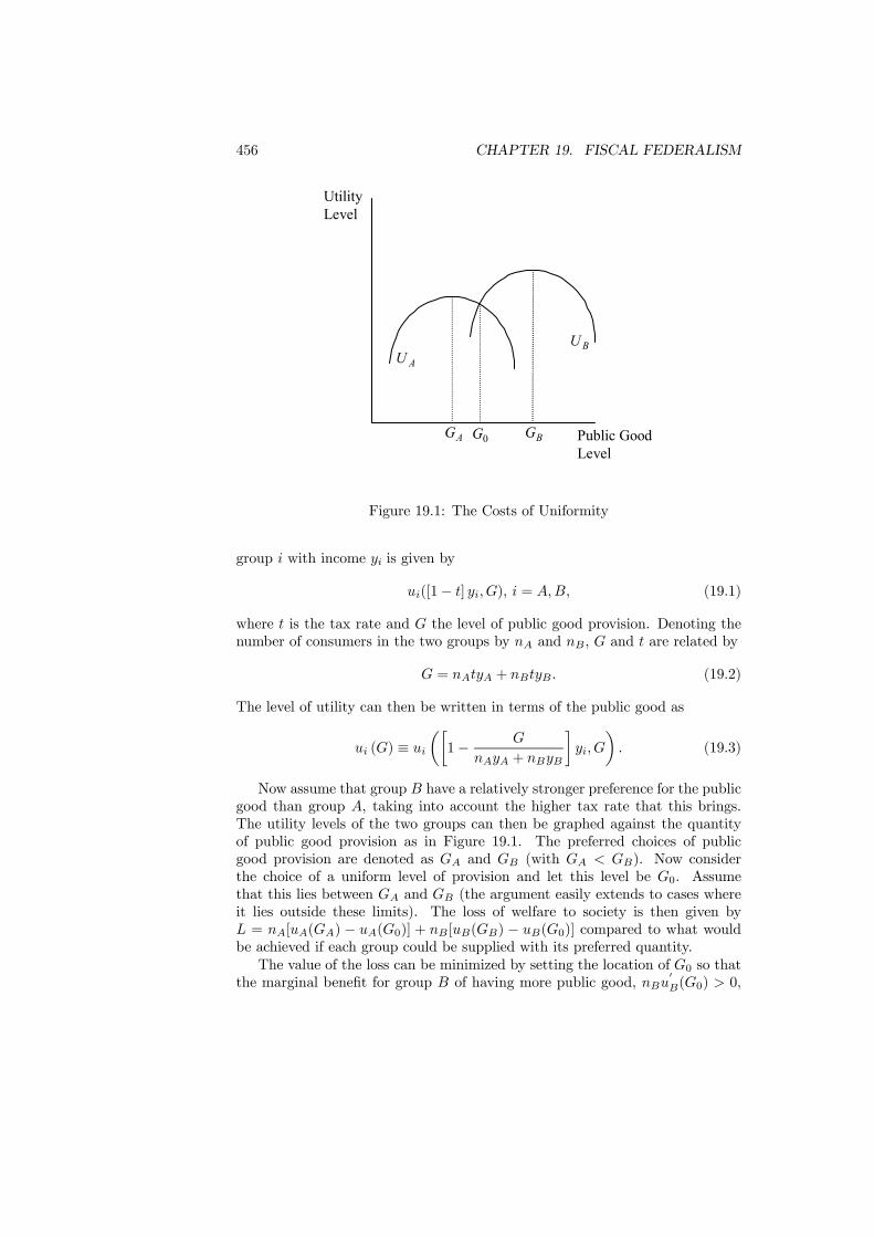
456 CHAPTER 19. FISCAL FEDERALISM
0GAG BG Public GoodLevel
UtilityLevel
AUBU
Figure 19.1: The Costs of Uniformity
group i with income yi is given by
ui([1− t] yi, G), i = A,B, (19.1)
where t is the tax rate and G the level of public good provision. Denoting thenumber of consumers in the two groups by nA and nB, G and t are related by
G = nAtyA + nBtyB. (19.2)
The level of utility can then be written in terms of the public good as
ui (G) ≡ uiµ·1− G
nAyA + nByB
¸yi, G
¶. (19.3)
Now assume that group B have a relatively stronger preference for the publicgood than group A, taking into account the higher tax rate that this brings.The utility levels of the two groups can then be graphed against the quantityof public good provision as in Figure 19.1. The preferred choices of publicgood provision are denoted as GA and GB (with GA < GB). Now considerthe choice of a uniform level of provision and let this level be G0. Assumethat this lies between GA and GB (the argument easily extends to cases whereit lies outside these limits). The loss of welfare to society is then given byL = nA[uA(GA) − uA(G0)] + nB [uB(GB) − uB(G0)] compared to what wouldbe achieved if each group could be supplied with its preferred quantity.The value of the loss can be minimized by setting the location of G0 so that
the marginal benefit for group B of having more public good, nBu0B(G0) > 0,

19.2. ARGUMENTS FOR MULTI-LEVEL GOVERNMENT 457
just offsets the marginal loss of group A, nAu0A(G0) < 0; but the essential point
is that the loss remains positive. Furthermore, the loss increases the more widelydispersed are preferences and the more members there are of each group.This analysis shows how uniformity can be costly in terms of foregone wel-
fare. A policy of uniformity can then only be supported if the costs of differenti-ation exceed the benefit. Such costs could arise in the collection of informationto determine the differentiation and in the administration costs of a differenti-ated system. These arguments will be explored further below. The next sectionthough considers the limit of the benefits that can arise from differentiation.
19.2.2 The Tiebout Hypothesis
Although the costs of uniformity as illustrated above are indisputable, it isanother step to show that decentralization is justified. The route to doingthis is to exploit the Tiebout hypothesis that was analyzed in Section 16.5 inconnection with the theory of local public goods. The exact same arguments areapplicable here. Each community can be treated as an independent provider oflocal public goods. If the consumers in the economy have heterogeneous tastes,then there will be clear advantages to jurisdictions having different levels ofprovision. Each can design what it offers (its tax rates, level of provision andtype of provision) to appeal to particular groups within society. By choosingthe jurisdiction in which to live (i.e., by voting with their feet) the consumersreveal their tastes for public goods. In the absence of transactions costs, or otherimpediments to freedom of movement, an efficient equilibrium must ensue.The limits to this argument explored in the context of local public goods are
also applicable here. Transactions costs are relevant in practice, and the problemof optimally dividing a finite population into a limited number of jurisdictionswill arise. The fact that the first-best allocation will not be achieved does notnecessarily undermine the argument for decentralization. There are clearly stillbenefits to decentralization even when this cannot be taken to the level requiredby the Tiebout hypothesis. Starting from a uniform level of services that is toolittle for some consumers, and too much for others, then a move away fromthis uniform level by some jurisdictions must benefit some of the consumers.In this way, even restricted decentralization can be efficiency-increasing. Thisargument can be easily understood from Figure 19.1.The Tiebout hypothesis shows the benefits achievable by decentralization.
Although these will not be fully realizable, a limited version of the same argu-ment suggests that even restricted decentralization will improve upon uniformprovision.
19.2.3 Distributive Arguments
The regions that constitute any economy are endowed with different stocks ofresources. Some may be rich in natural resources, such as oil and coal, othersmay have a well-educated workforce with high levels of human capital. Such
458 CHAPTER 19. FISCAL FEDERALISM
differences in endowments will be reflected in disparities in living standardsbetween regions.The ability to differentiate public good provision between the regions then
allows more accurate targeting of resources to where they are required. Thisis an equity argument for not having uniform provision. Decentralized decisionmaking allows each region to communicate its needs to the centre and permitsthe centre to make differential allocations to the regions.This process will be designed to offset the differences in living standards
caused by endowments. Typically there will be no compensation for differencesin preference for public good provision such as giving more to a region wishing tospend more on public goods. This form of redistribution between regions is calledan equalization formula and will be explored in Chapter 20 when discussinginter-governmental grants.
19.3 Optimal Structure: Efficiency versus Sta-bility
The previous arguments have explored a number of advantages of fiscal decen-tralization. These have involved both efficiency and equity aspects. The issuethat remains is what is the optimal structure or the correct number of levels ofadministration.The difficulty that arises here is that the optimal division may be different
between public goods. The examples in the introduction have discussed howfire services are organized at a very local level, education at a higher level anddefence at an even higher one. There are many other public goods providedby the federal government. If each were to be allocated at the correct level ofdecentralization, this would imply an equally large number of levels of govern-ment.To understand whether this will be done, it is now necessary to consider an
important aspect of decentralization that has not yet been introduced. So faronly the advantages have been considered, now it is time to introduce the costs.Each level of government brings with it additional costs. These involve all thefactors that are necessary to provide administration. Buildings, staff and equip-ment will all be required, as will elections to choose politicians. The politicianswill also require compensation for the time devoted to political activity. Thesecosts are replicated each time an additional level of government is introduced.Consequently, introducing further levels of government is not costless. The
choice of the optimal degree of decentralization must take these costs into ac-count and balance them against the benefits. From such a process will emergethe optimal structure. This will depend on the relative sizes of costs and ben-efits but is most likely to result in a level of decentralization such that somedecisions are taken at a higher level than would be best if decentralization werecostless.This argument is now illustrated in a simple location model that trades off
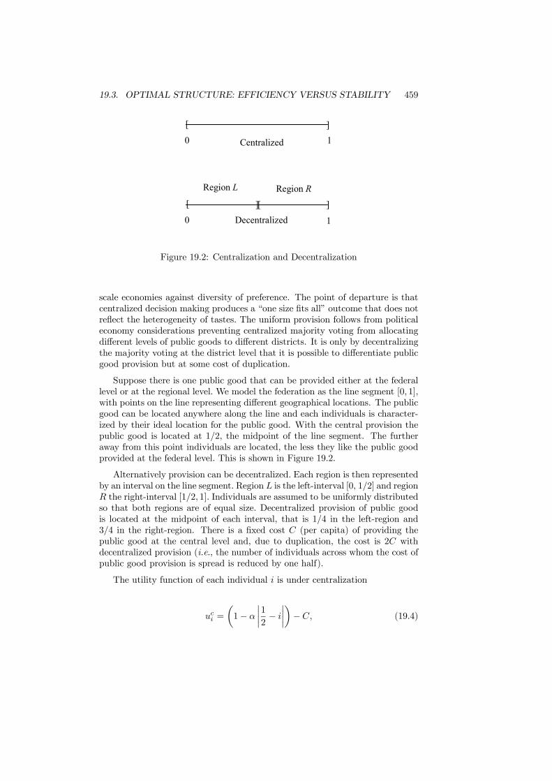
19.3. OPTIMAL STRUCTURE: EFFICIENCY VERSUS STABILITY 459
[ [ ]]
[ ]
Centralized
Decentralized
Region L Region R
0
0
1
1
Figure 19.2: Centralization and Decentralization
scale economies against diversity of preference. The point of departure is thatcentralized decision making produces a “one size fits all” outcome that does notreflect the heterogeneity of tastes. The uniform provision follows from politicaleconomy considerations preventing centralized majority voting from allocatingdifferent levels of public goods to different districts. It is only by decentralizingthe majority voting at the district level that it is possible to differentiate publicgood provision but at some cost of duplication.
Suppose there is one public good that can be provided either at the federallevel or at the regional level. We model the federation as the line segment [0, 1],with points on the line representing different geographical locations. The publicgood can be located anywhere along the line and each individuals is character-ized by their ideal location for the public good. With the central provision thepublic good is located at 1/2, the midpoint of the line segment. The furtheraway from this point individuals are located, the less they like the public goodprovided at the federal level. This is shown in Figure 19.2.
Alternatively provision can be decentralized. Each region is then representedby an interval on the line segment. Region L is the left-interval [0, 1/2] and regionR the right-interval [1/2, 1]. Individuals are assumed to be uniformly distributedso that both regions are of equal size. Decentralized provision of public goodis located at the midpoint of each interval, that is 1/4 in the left-region and3/4 in the right-region. There is a fixed cost C (per capita) of providing thepublic good at the central level and, due to duplication, the cost is 2C withdecentralized provision (i.e., the number of individuals across whom the cost ofpublic good provision is spread is reduced by one half).
The utility function of each individual i is under centralization
uci =
µ1− α
¯1
2− i¯¶− C, (19.4)
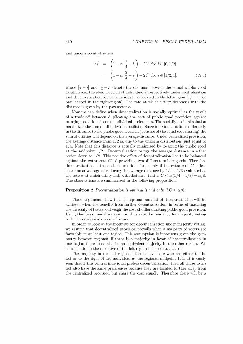
460 CHAPTER 19. FISCAL FEDERALISM
and under decentralization
udi =
µ1− α
¯1
4− i¯¶− 2C for i ∈ [0, 1/2]
=
µ1− α
¯3
4− i¯¶− 2C for i ∈ [1/2, 1], (19.5)
where¯12 − i
¯and
¯14 − i
¯denote the distance between the actual public good
location and the ideal location of individual i, respectively under centralizationand decentralization for an individual i is located in the left-region (
¯34 − i
¯for
one located in the right-region). The rate at which utility decreases with thedistance is given by the parameter α.Now we can define when decentralization is socially optimal as the result
of a trade-off between duplicating the cost of public good provision againstbringing provision closer to individual preferences. The socially optimal solutionmaximizes the sum of all individual utilities. Since individual utilities differ onlyin the distance to the public good location (because of the equal cost sharing) thesum of utilities will depend on the average distance. Under centralized provision,the average distance from 1/2 is, due to the uniform distribution, just equal to1/4. Note that this distance is actually minimized by locating the public goodat the midpoint 1/2. Decentralization brings the average distance in eitherregion down to 1/8. This positive effect of decentralization has to be balancedagainst the extra cost C of providing two different public goods. Thereforedecentralization is the optimal solution if and only if the extra cost C is lessthan the advantage of reducing the average distance by 1/4− 1/8 evaluated atthe rate α at which utility falls with distance; that is C ≤ α (1/4− 1/8) = α/8.The observations are summarized in the following proposition.
Proposition 2 Decentralization is optimal if and only if C ≤ α/8.
These arguments show that the optimal amount of decentralization will beachieved when the benefits from further decentralization, in terms of matchingthe diversity of tastes, outweigh the cost of differentiating public good provision.Using this basic model we can now illustrate the tendency for majority votingto lead to excessive decentralization.In order to look at the incentive for decentralization under majority voting,
we assume that decentralized provision prevails when a majority of voters arefavorable in at least one region. This assumption is innocuous given the sym-metry between regions: if there is a majority in favor of decentralization inone region there must also be an equivalent majority in the other region. Weconcentrate on the incentive of the left region for decentralization.The majority in the left region is formed by those who are either to the
left or to the right of the individual at the regional midpoint 1/4. It is easilyseen that if this central individual prefers decentralization, then all those to hisleft also have the same preferences because they are located further away fromthe centralized provision but share the cost equally. Therefore there will be a

19.4. ACCOUNTABILITY 461
majority in favour of decentralization in the left-region if the decisive individuali = 1/4 prefers decentralization, that is if
uci = (1− α
¯1
2− 14
¯)− C ≤ udi = (1− α
¯1
4− 14
¯)− 2C. (19.6)
From this follows the next proposition.
Proposition 3 Decentralization is a majority voting equilibrium if and only ifC ≤ α/4.
This result suggests excessive decentralization under majority voting becausethe critical cost level under majority voting is higher than the critical cost levelfor optimality. In particular for any cost C ∈ (α/8,α/4), majority voting leadsto decentralization (C < α/4) although it is not socially optimal (C > α/8).Therefore under majority voting there is too much decentralization: voters whoare located at the extreme have an incentive to support decentralized provisionto get a public good closer to what they want, but the democratic process doesnot internalize the negative externalities imposed on voters located in the center.
19.4 AccountabilityPoliticians may pursue a range of different objectives. At times, they may bepublic-spirited and dedicate themselves fully to furthering public interest. Butthey may also pursue their own ideas, even if these differ from those of theirconstituents. Some may want to derive private gains while in office or activelyseek perks of office. Some may extend clientilistic favors to their families andfriends. But the most important way in which they can act against the bestinterests of their constituents is by choosing policies that advance their owninterests or those of special groups to which they are beholden.A government is “accountable” if voters can discern whether it is acting in
their interest and sanction them appropriately if they are not, so that incum-bents anticipate that they will have to render accounts for their past actions.The problem is then to confront politicians with a trade-off between divertingrents and losing office or doing what voters want and getting re-elected. In thisview, elections can be seen as an accountability mechanism for controlling andsorting good from bad incumbents. By “good incumbent”, we mean someonewho is honest, competent and not easily bought-off by special interests.The standard view of how electoral accountability works is that voters set
some standard of performance to evaluate governments and they vote out theincumbent unless these criteria are fulfilled. However elections do not work wellin controlling and sorting politicians. There are severe problems in monitoringand evaluating the incumbent’s behavior in order to make informed decisionsabout whether to re-elect or not. Voters face a formidable agency problembecause they are inevitably poorly informed about politicians’ behavior andtype. Moreover, the electoral sanction (pass or fail) is such a crude instrumentthat it can hardly induce the politicians to do what the public wants.

462 CHAPTER 19. FISCAL FEDERALISM
State a State b
Policy A
Policy B
0, 3 r, 0
r, 1 0, 1
Figure 19.3: Political Accountability and Voter Welfare
In this perspective, it might be reasonable to try to organize competitionamong politicians in order to control them. In this respect, the Brennan andBuchanan (1980) view is that decentralization is an effective mechanism to con-trol governments’ expansive tendencies. The basic argument is that competitionamong different decentralized governments can exercise a disciplinary force andbreak the monopoly power of a large central government. Comparing perfor-mance in office among different incumbents helps in sorting good types frombad types as well as controlling the quality of their decisions. Hence one votesagainst an incumbent if his performance is bad relative to others, in order toinduce each incumbent to behave in the public interest.To see the logic of the argument, consider a simple example. Suppose that
the circumstances under which politicians make decisions can be good (state a)or bad (state b). Governments decide to adopt policy A, which is better for theirconstituents in the good state a, or policy B, which is better in the bad state b.Governments need not pursue the public interest and can rather advance theirown interests by choosing policy A in state b and policy B in state a to get someprivate gains (say a rent r > 0). Suppose that politicians value being re-electedand that such value is V > r. The payoff matrix is shown in Figure 19.3: thefirst number in each cell is the government payoff and the second number isvoters welfare. If the government is re-elected it gets the extra value V . Thegovernment knows the prevailing conditions (i.e., whether a or b has occurred)but all that citizens observe is their current welfare.To induce politicians to act as well as they can under this information struc-
ture, voters must set their re-election rule. If voters set the standard the incum-bent must meet in order to be re-elected too high (such as committing to votefor the incumbent if the welfare level is at least 3), then the incumbent cannotbe re-elected whatever he does if conditions turn out to be bad (state b). Con-sequently, the incumbent has the incentive to obtain the rent r and leave office.Alternatively, if the voters set the standard for re-election lower, say at 1, the
19.5. RISK SHARING 463
incumbent will be able to divert rent when conditions happen to be good (statea) and be re-elected by giving voters less than what they could obtain. Thenvoters are in a quandary because whatever they decide to do, the politicianswill sometimes escape from their control and divert rent.Suppose now that the electorate can compare the outcome of its incum-
bent with other incumbents (in different constituencies) facing exactly the samecircumstances. Then from the observation of outcomes elsewhere, voters canpotentially infer whether the prevailing conditions are good or bad and therebyget the most they can under either conditions. The information will be revealedif there is at least one government that chooses a different policy from that ofthe others. When conditions are good, vote for the incumbent if the outcomeis at least 3. When conditions are bad, vote for the incumbent if the outcomeis at least 1. Otherwise vote the incumbent out. Hence, a government facinggood conditions a knows that by choosing the appropriate policy A, it will bere-elected for sure and get V which is more than the rent r he can get by choos-ing B and being voted out. In turn a government facing bad conditions b knowsthat by choosing B it will be re-elected and get V which is better than whatit would get by adopting the wrong policy A to get the rent r but no chanceof being re-elected. Therefore, comparing the performance of their incumbentwith other incumbents facing similar circumstances, voters can gain increasedcontrol over their politicians and deduce what is attributable to circumstancesas opposed to government actions.Another argument for why decentralization should lead to greater efficiency
and accountability is that a central decision maker does not need to please alljurisdictions to get re-elected but simply a majority of them. However this argu-ment is usually balanced against the fact that the value of holding office is largerin a centralized arrangement and thus politicians are more eager to win election,which in a conventional political agency model may increase accountability andefficiency.
19.5 Risk sharing
Inter-regional insurance is fundamentally about sharing risk among a groupof regions so that no region bears an undue amount of risk. Because of this,insurance can arise even when all parties are risk averse. What is necessary forthis to happen is that the risks the parties bear are, to some degree, independentof each other. That is, when one region suffers a loss, there are other regions (orgroup of regions) that do not suffer a loss. While such independence is usuallytrue of almost all individual risks for which standard forms of insurance exist(fires, car accidents, sicknesses ...) it is less obvious at the regional level.There are some fundamental principles in mutual insurance. First, risk-
sharing is more effective the broader the basis on which risks are pooled. Thisis a consequence of Borch’s theorem on mutual insurance. Second, it is moreadvantageous for any region to engage in mutual insurance with other regionswhen risks are negatively correlated across regions. Third, there must be min-
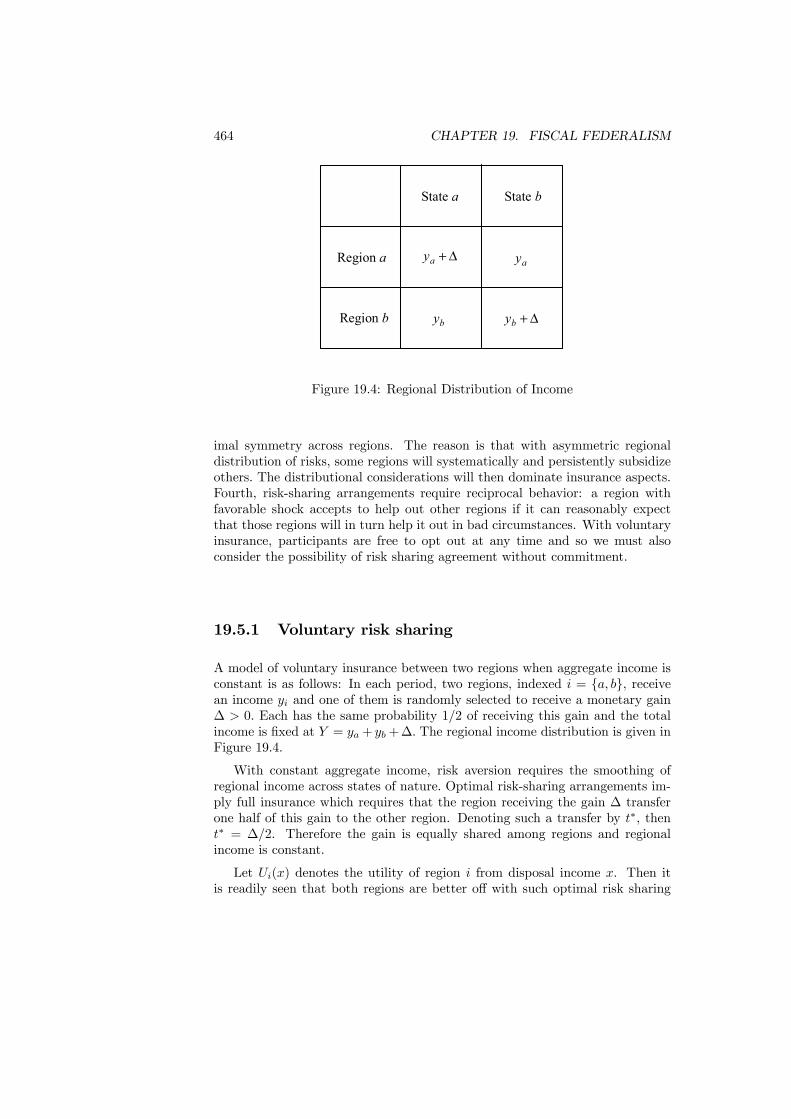
464 CHAPTER 19. FISCAL FEDERALISM
State a State b
Region a
Region b
∆+ay ay
by ∆+by
Figure 19.4: Regional Distribution of Income
imal symmetry across regions. The reason is that with asymmetric regionaldistribution of risks, some regions will systematically and persistently subsidizeothers. The distributional considerations will then dominate insurance aspects.Fourth, risk-sharing arrangements require reciprocal behavior: a region withfavorable shock accepts to help out other regions if it can reasonably expectthat those regions will in turn help it out in bad circumstances. With voluntaryinsurance, participants are free to opt out at any time and so we must alsoconsider the possibility of risk sharing agreement without commitment.
19.5.1 Voluntary risk sharing
A model of voluntary insurance between two regions when aggregate income isconstant is as follows: In each period, two regions, indexed i = {a, b}, receivean income yi and one of them is randomly selected to receive a monetary gain∆ > 0. Each has the same probability 1/2 of receiving this gain and the totalincome is fixed at Y = ya+ yb+∆. The regional income distribution is given inFigure 19.4.
With constant aggregate income, risk aversion requires the smoothing ofregional income across states of nature. Optimal risk-sharing arrangements im-ply full insurance which requires that the region receiving the gain ∆ transferone half of this gain to the other region. Denoting such a transfer by t∗, thent∗ = ∆/2. Therefore the gain is equally shared among regions and regionalincome is constant.
Let Ui(x) denotes the utility of region i from disposal income x. Then itis readily seen that both regions are better off with such optimal risk sharing

19.5. RISK SHARING 465
arrangement since
ua(ya +∆
2) ≥ 1
2ua(ya +∆) +
1
2ua(ya), (19.7)
ub(yb +∆
2) ≥ 1
2ub(yb +∆) +
1
2ub(yb). (19.8)
Without commitment, complete risk sharing is not guaranteed. We must takeinto account the possibility that the region receiving the gain may refuse totransfer some of the gain to the other region. Risk-sharing agreement withoutcommitment must be “self-enforcing” in the sense that no region has incentiveto defect unilaterally from the agreement. To be self-enforcing, the risk-sharingarrangement must be such that the expected net benefits from participatingis at any time larger than the one time gain from defection (by not makingtransfer when call upon). If full insurance is not possible, it is still possible todesign partial insurance by limiting transfers when the participation constraintis binding. Let ti be the transfer made by region i to the other region whenregion i receives the gain ∆. Upon receiving the gain ∆, region i can tradeoff the immediate gain of defecting by refusing to make the transfer ti, againstthe cost of being excluded from any future insurance arrangement and to bearregional income variation alone. Taking region a, the gain from defection whenreceiving ∆ is
ua(ya +∆)− ua(ya +∆− ta). (19.9)
The cost of losing insurance in the next period (discounted at rate δ < 1) is
·1
2ua(ya +∆− ta) + 1
2ua(ya + tb)
¸−·1
2ua(ya +∆) +
1
2ua(ya)
¸. (19.10)
The participation constraint holds if the cost of defecting exceeds the gainfrom future insurance (discounted at rate δ < 1) . Comparing the two valuesand rearranging we find that region a has no incentive to defect if
(1− δ
2)ua(ya+∆− ta)+ δ
2ua(ya+ tb) ≥ (1− δ
2)ua(ya+∆)+
δ
2ua(ya), (19.11)
and similarly region b has no incentive to defect if
(1− δ
2)ub(yb +∆− tb) + δ
2ub(yb + ta) ≥ (1− δ
2)ub(yb +∆) +
δ
2ub(yb). (19.12)
We can draw several implications from this simple model of risk-sharingwithout commitment. First, the time horizon will influence the amount ofmutual insurance that is sustainable. Indeed the value attached to continuedinsurance depends on the discount rate (reflecting the time horizon). At oneextreme when δ −→ 0 (extremely short horizon) the value of future insurance iszero and regions always defect. No insurance is possible. At the other extremewhen δ −→ 1 (very long horizon) the value of future insurance is sufficiently

466 CHAPTER 19. FISCAL FEDERALISM
high that full insurance is possible (ti = ∆/2). And by a continuity argument,for intermediate discounting values δ ∈ (δ, δ), with 0 < δ < δ < 1, only limitedinsurance is possible (ti < ∆/2). Therefore the expected time horizon limits theamount of risk sharing. For values δ ≥ δ complete risk sharing can be achieved.For intermediate values δ < δ < δ there is partial risk sharing. And for valuesδ < δ no risk sharing is possible.The second implication is that the level of risk sharing that regions can
achieve increases with risk aversion. The reason is that regions put more weighton the gain from long-term insurance against the short-term gain from defecting.This is immediately seen from the participation constraints. Indeed the incomedistribution on the left-hand side is less uncertain than the income distributionon the right-hand side which makes the participation constraints more likely tobe satisfied under increased risk aversion.A third implication is about the effect of income inequality. Intuition would
suggest that mutual insurance is more likely if regions are ex-ante identical andthat regional inequality limits the scope for insurance. But this is not true. Thereason is that risk-sharing redistributes ex-post from the region with positiveshock to the other region, but it does not redistribute ex-ante from the rich tothe poor regions. More surprisingly, it is even possible that increased inequality,while maintaining constant the aggregate income and the variance of income,would improve insurance. To see this, start from income equality ya = yb. Usingthe participation constraint it is possible to calculate the level of risk sharingthat is possible. Then, increase ya and reduce yb by the same amount. Supposingthe same positive shock ∆, aggregate income and the intra-regional varianceof income are unchanged. However the participation constraints are affectedbecause income levels influence the demand for insurance. It is then possibleto show that for some standard utility functions, the likelihood of completeinsurance and the amount of risk sharing under constrained insurance haveincreased with inequality.
19.5.2 Insurance versus Redistribution
In practice inter-regional insurance is organized in a federation through federaltaxes and transfers. The effect of such a federal tax system is to redistributeincome from high- to low-income regions. By pooling income risk across theregions, the federal tax system provide insurance against region-specific shocks.However to the extent that there is ex-ante income inequality between regions,federal taxes also provide ex-ante regional redistribution. We ignore the sta-bilizing effect of federal taxation which refers to the possibility of smoothingshocks over time (between bad years and good years). The insurance motive forthe federal tax system is explicitly recognized in many countries. For instancein the UK part of the tax system is actually called “National Insurance”. Toappreciate the amount of insurance federal taxes can provide it is necessaryto disentangle redistribution from insurance components. Redistribution actson the initial income distribution, while insurance responds to income shocks(either permanent or temporary).
19.6. EVIDENCE ON DECENTRALIZATION 467
Assume region i’s income at time t is subject to permanent shock ψti andtemporary shock ηti. Both shocks are assumed to be mean zero. Thus regionalincome at time t can be written
yti = y0i +
tXs=1
ψsi + ηti. (19.13)
Suppose the federal tax system taxes all regions’ incomes at the same rate τand redistributes total tax revenue as a uniform transfer to all regions. It followsthat region i at time t pays taxes τyti and receives transfers from the federationbased on the average tax payment
τEi
"y0i +
tXs=1
ψsi + ηti
#= τEi
£y0i¤= τy0. (19.14)
The after tax and transfer regional income is
xti = y0i + τ(y0 − y0i ) + (1− τ)
£Σψsi + ηti
¤. (19.15)
The income change can be decomposed into an insurance part and a redistrib-ution part as follows
xti − yti = τ(y0 − y0i )| {z }redistribution
+ τ£Σψsi + ηti
¤| {z }insurance
. (19.16)
Using this decomposition, it is interesting to measure the extent of insuranceprovided by federal taxation in practice. Empirical studies for the US federaltax system clearly suggest the presence of intranational insurance. Though thereis disagreement about the exact magnitude of the insurance, all studies find thatthe redistribution effect largely dominates the insurance effect. They also findthat insurance is rather modest in the sense that it cannot smooth more than10 cents on a dollar change in state income caused by asymmetric shocks.
19.6 Evidence on decentralization
19.6.1 Decentralization around the World
The degree of decentralization of government activity can be measured in severaldifferent ways. Oates (1972) distinguishes three measures of fiscal decentraliza-tion: (i) share of total public revenue collected by the central government; (ii)share of the central government in all public expenditures (including incomeredistribution payments); (iii) share of the central government in current gov-ernment consumption expenditures.The first measure based on revenue collection raises the problem that the
center may collect revenue for regions. It underestimates the degree of decen-tralization to the extent that regions get back substantial portions of revenue
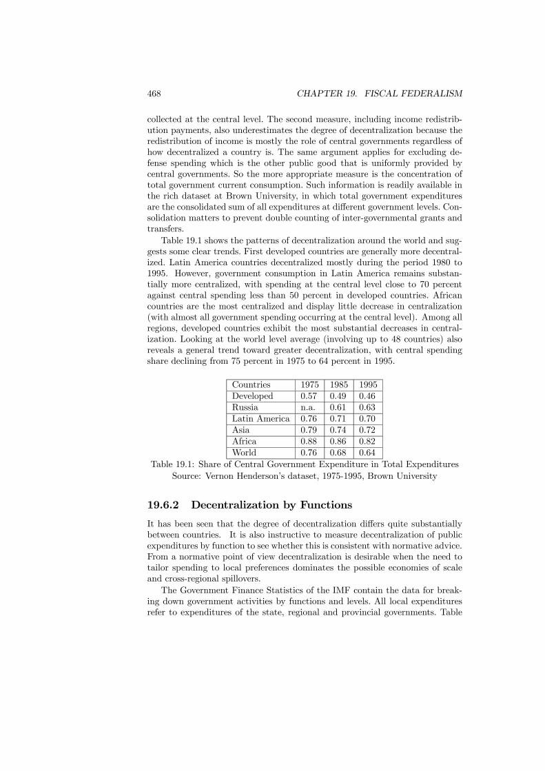
468 CHAPTER 19. FISCAL FEDERALISM
collected at the central level. The second measure, including income redistrib-ution payments, also underestimates the degree of decentralization because theredistribution of income is mostly the role of central governments regardless ofhow decentralized a country is. The same argument applies for excluding de-fense spending which is the other public good that is uniformly provided bycentral governments. So the more appropriate measure is the concentration oftotal government current consumption. Such information is readily available inthe rich dataset at Brown University, in which total government expendituresare the consolidated sum of all expenditures at different government levels. Con-solidation matters to prevent double counting of inter-governmental grants andtransfers.Table 19.1 shows the patterns of decentralization around the world and sug-
gests some clear trends. First developed countries are generally more decentral-ized. Latin America countries decentralized mostly during the period 1980 to1995. However, government consumption in Latin America remains substan-tially more centralized, with spending at the central level close to 70 percentagainst central spending less than 50 percent in developed countries. Africancountries are the most centralized and display little decrease in centralization(with almost all government spending occurring at the central level). Among allregions, developed countries exhibit the most substantial decreases in central-ization. Looking at the world level average (involving up to 48 countries) alsoreveals a general trend toward greater decentralization, with central spendingshare declining from 75 percent in 1975 to 64 percent in 1995.
Countries 1975 1985 1995Developed 0.57 0.49 0.46Russia n.a. 0.61 0.63Latin America 0.76 0.71 0.70Asia 0.79 0.74 0.72Africa 0.88 0.86 0.82World 0.76 0.68 0.64
Table 19.1: Share of Central Government Expenditure in Total ExpendituresSource: Vernon Henderson’s dataset, 1975-1995, Brown University
19.6.2 Decentralization by Functions
It has been seen that the degree of decentralization differs quite substantiallybetween countries. It is also instructive to measure decentralization of publicexpenditures by function to see whether this is consistent with normative advice.From a normative point of view decentralization is desirable when the need totailor spending to local preferences dominates the possible economies of scaleand cross-regional spillovers.The Government Finance Statistics of the IMF contain the data for break-
ing down government activities by functions and levels. All local expendituresrefer to expenditures of the state, regional and provincial governments. Table
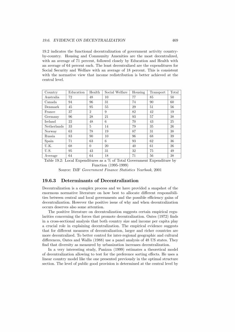
19.6. EVIDENCE ON DECENTRALIZATION 469
19.2 indicates the functional decentralization of government activity country-by-country. Housing and Community Amenities are the most decentralized,with an average of 71 percent, followed closely by Education and Health withan average of 64 percent each. The least decentralized are the expenditures forSocial Security and Welfare with an average of 18 percent. This is consistentwith the normative view that income redistribution is better achieved at thecentral level.
Country Education Health Social Welfare Housing Transport TotalAustralia 72 48 10 77 85 50Canada 94 96 31 74 90 60Denmark 45 95 55 29 51 56France 37 2 9 82 42 19Germany 96 28 21 93 57 38Ireland 22 48 6 70 43 25Netherlands 33 5 14 79 35 26Norway 63 78 19 87 31 38Russia 83 90 10 96 68 39Spain 71 63 6 93 62 36U.K. 68 0 20 40 61 26U.S. 95 43 31 32 75 49Average 64 64 18 71 56 38Table 19.2: Local Expenditures as a % of Total Government Expenditure by
Function (1995-1999)Source: IMF Government Finance Statistics Yearbook, 2001
19.6.3 Determinants of Decentralization
Decentralization is a complex process and we have provided a snapshot of theenormous normative literature on how best to allocate different responsibili-ties between central and local governments and the possible efficiency gains ofdecentralization. However the positive issue of why and when decentralizationoccurs deserves also some attention.The positive literature on decentralization suggests certain empirical regu-
larities concerning the forces that promote decentralization. Oates (1972) findsin a cross-sectional analysis that both country size and income per capita playa crucial role in explaining decentralization. The empirical evidence suggeststhat for different measures of decentralization, larger and richer countries aremore decentralized. To better control for inter-regional geographic and culturaldifferences, Oates and Wallis (1988) use a panel analysis of 48 US states. Theyfind that diversity as measured by urbanization increases decentralization.In a very interesting study, Panizza (1999) estimates a theoretical model
of decentralization allowing to test for the preference sorting effects. He uses alinear country model like the one presented previously in the optimal structuresection. The level of public good provision is determined at the central level by

470 CHAPTER 19. FISCAL FEDERALISM
majority voting (i.e. by the median voter’s preference). The central governmentprovides a uniform public good level whose value decreases with the spatialdistance between the citizens and the central government. Local governmentprovision is closer to the preferences of citizens and so more valuable. Since vot-ers benefit more from local provision, increasing central provision reduces overalldemand for the public good. Central government decides its share in provisionof the public good anticipating how that share influences overall demand for thepublic good. Using cross-sectional analysis and standard measures of decentral-ization, Panizza finds that decentralization increases with country size, incomeper capita, the level of democracy and ethno-linguistic fractionalization.A important limit of the existing empirical testing of decentralization is that
it ignores a central force in the process of decentralization, namely the threatof separation. The possibility of secession has been a powerful force to limit theability of the central government to exploit peripheral minorities of voters forthe sake of the majority of the population. The idea is that unitary governmentis more willing to devolve more power and responsibility when the threat ofsecession is more credible. It has been a recurrent feature in Europe that thedecision to decentralize is not necessarily guided by efficiency considerations, butis also driven by distributional and political forces. When rich regions, whichtoday transfer large amount of income to poorer regions, demand more decen-tralization it is to limit their net contributions. They often do that becausethey do not believe anymore in the mutual insurance effect that such transfersmight change directions in a near future. Also the size of the regional redistrib-ution has become so visible that it creates an insurmountable political problem.The perception is that rich regions would become better off by seceding and, toprevent such countries from breaking apart, concessions in the form of larger de-volution of responsibilities and resources to regions have been taking place. Italyand Belgium are two good illustrations of the sort of decentralization forced bythe pressing demand of the rich regions Lombardy and Flanders, respectively. Itis clear that in those cases, the efficiency argument that decentralization allowspolicy choices that better reflect local preference was not the key force. Richerregions demand more autonomy because the regional income inequality is suchthat mutual insurance becomes pure redistribution. Moreover, the demand formore autonomy is exacerbated, rightly or wrongly, by the perceptions in therich regions that the regional transfers are very much influenced by opportunis-tic behavior of the receiving regions (i.e. some form of moral hazard problemat the regional level).
19.7 Conclusions
There is a considerable controversy as to what public activities should be decen-tralized or centralized. There is also empirical evidence of increasing decentral-ization around the world. In this chapter we have seen the costs and benefits ofdecentralization. One important advantage of a decentralized system is the tai-loring of the provision of public goods and services to local preferences. The idea
19.7. CONCLUSIONS 471
is that local government is closer to the people and so more responsive to theirpreferences than central governments. Another advantage of decentralization isto foster intergovernmental competition making government more efficient andmore accountable to their electorate.There are also disadvantages of decentralized system. Some of them, like
fiscal competition, will be covered in the next chapter. The main disadvantageof decentralization is probably its failure to exploit all the economies of scalein the provision of public goods. Another disadvantage is to limit the scope forinterregional risk sharing through the federal fiscal system.Optimal federalism results from the trade off between these various costs
and benefits from decentralization. It provides normative conclusions about theallocation of responsibilities between central and local levels. However from amore positive perspective, political and distributional considerations can leadto different conclusions. The best illustration is that too much decentralizationwill result from a democratic choice.
Further readingThe optimal government structure with overlapping jurisdictions is inCasella, A. and B. Frey (1992) “Federalism and clubs: toward an economic
theory of overlapping political jurisdictions”, European Economic Review, 36,635 - 646.Hochman, O., D. Pines and J. Thisse (1995) “On the optimal structure of
local governments”, American Economic Review, 85, 1224 - 1240.The excessive decentralization with majority rule is in:Alesina, A. and E. Spolaore (1997) “On the number and size of nations”,
Quarterly Journal of Economics, 112, 1028 - 1056.Cremer, H., A.-M de Kerchove and J. Thisse (1985) “A economic theory of
public facilities in space”, Mathematical Social Sciences, 9, 249 - 262.The empirical analysis of the determinants of decentralization is inOates, W.E. (1972) Fiscal Federalism, New York: Harcourt Brace Jovanovich,
Academic Press.Oates, W.E. and J. Wallis (1988) “Decentralization in the public sector: an
empirical study and local governments”, in Fiscal Decentralization: QuantitativeStudies, H.S. Rosen (ed.), Chicago: University of Chicago Press.Panizza, U. (1999) “On the determinant of fiscal centralization: theory and
evidence”, Journal of Public Economics, 74, 97 - 139.The study of secession and break up of nations is in:Buchanan, J. and R. Faith (1987) “Secession and the limits of taxation:
toward a theory of internal exit”, American Economic Review, 77, 1023 - 1031.Bolton, P. and G. Roland (1997) “The break up of nations: a political
economy analysis”, Quarterly Journal of Economics, 112, 1057 - 1090.The government accountability is inBesley, T., “Political agency and accountability”, (forthcoming).Brennan, G, and J. Buchanan (1980) The Power to Tax, New York: Cam-
bridge University press.
472 CHAPTER 19. FISCAL FEDERALISM
Przeworski, A., S. Stokes and B. Manin (eds) (1999) Democracy, Account-ability, and Representation, Cambridge: Cambridge University press.Seabright, P. (1996) “Accountability and decentralization in government: an
incomplete contracts model”, European Economic Review, 40, 61 - 89.The risk sharing is inGenicot, G. and D. Ray (2003) “Endogenous group formation in risk sharing
arrangements”, Review of Economic Studies, 70, 87 - 113.Kocherlakota, N. (1996) “Implications of efficient risk sharing without com-
mitment”, Review of Economic Studies, 63, 595 - 609.Lockwood, B, (1999) “Inter-regional insurance”, Journal of Public Eco-
nomics, 72, 1 - 37Persson, T. and G. Tabellini (1996) “Federal fiscal constitutions: risk sharing
and moral hazard”, Econometrica, 64, 623 - 646Persson, T. and G. Tabellini (1996) “Federal fiscal constitutions: risk sharing
and redistribution”, Journal of Political Economy, 104, 979 - 1009.Federal fiscal system and insurance is inSorensen, B.E., and O. Yosha (1997) “Federal insurance of US states: an
empirical investigation”, in A. Razin and E. Sadka (eds.), Globalization: PublicEconomics Policy Perspectives, Cambridge: Cambridge University Press.
Chapter 20
Fiscal Competition
20.1 Introduction
What is the role of competition between governments? If competition is thefundamental force of efficient economic performance in the private sector, whyshould it be different for the public sector? Why cannot the same discipliningeffect of competition be applied to the public sector as well? In the private sectorcompetition will promote efficiency because firms which best satisfy consumers’preferences will survive and prosper, while others will lose customers and fail.Extending this argument to the public sector, competition among governmentsand jurisdictions should induce them to best serve the will of their residents.If they fail to do so, residents will vote with their feet and leave for otherjurisdictions which offer a better deal.The purpose of this chapter is to show that if the private competition anal-
ogy has some merit, it also needs to be seriously qualified. The chapter isorganized as follows. First the efficiency aspects of fiscal competition are pre-sented. Second, the distributional aspects of residential mobility are evaluated.The key issue is how mobility limits the possibility of redistributing income.Third, the role of inter-governmental transfers is discussed both in terms ofefficiency and redistribution. Fourth, some evidence on fiscal competition andinter-governmental interactions is given. Lastly, the main results from the fiscalcompetition theory are summarized and evaluated in the concluding section.
20.2 Tax Competition
Tax competition refers to the interaction between governments due to interjuris-dictional mobility of the tax base. It does not include fiscal interaction betweengovernments resulting from public good spillovers, where residents of one juris-diction consume the public goods provided by neighboring jurisdictions. Taxcompetition arises because jurisdictions finance provision of a public good with atax on locally employed capital. Capital moves across jurisdictions in response to
473

474 CHAPTER 20. FISCAL COMPETITION
tax differentials, while residents are typically immobile (or at least less mobile).In the competitive version of tax competition, jurisdictions are “too small”
(relative to the economy) to affect the net return to capital that is determinedworldwide. As a result, each jurisdiction sets its tax on locally employed capitaltaking as given the net-of-tax price of capital. Tax rates in other jurisdictions donot matter and there is no strategic interaction among jurisdictions when settingtheir taxes. We say that jurisdictions behave competitively. When jurisdictionsare “large” relative to the economy, each jurisdiction can affect the net returnto capital by varying its own tax rate. In this case, the tax rate chosen in onejurisdiction varies with the taxes in other jurisdictions. Jurisdictions behavestrategically: they set their tax in response to the tax rates in other jurisdictions.Both the competitive and strategic version of the tax competition model
produce the same important conclusion, namely, that public goods are under-provided relative to the efficient Samuelson rule level. The reason is that eachjurisdiction perceives the mobility of capital and keeps its tax low to preserveits tax base. To understand the inefficiency from inter-governmental competi-tion, it is useful to consider a simple model in which we assume in turn thatjurisdictions behave competitively and then strategically.
20.2.1 Competitive Behavior
The assumption of perfect competition means that the mobile factor of produc-tion is available to the “small” jurisdiction at a fixed price. Suppose capital isthe mobile factor of production and that the jurisdiction seeks to impose a taxon capital and to use the revenue to provide public goods and services to its res-idents, or to directly transfer cash to them. If capital were perfectly immobile, alocal source-based tax on capital would reduce the net rate of return to capitalby the exact amount of the tax. This capital tax would make the residents betteroff at the expense of capital owners (who are not necessarily residents).In contrast, when capital is costlessly mobile, local capital taxation cannot
affect the net return to capital. The reason is that the imposition of the local taxdrives capital out of the jurisdiction until the increase in before-tax rate of returnis sufficient to compensate capital owners for local taxes. However the outflowof capital from the jurisdiction reduces the remuneration of labor. The resultingloss of income to the residents will exceed the value of the tax revenue collectedfrom capital taxation. Except if public expenditures have greater value to localresidents than the tax revenue used to finance them, the net effect of capitaltaxation is to harm immobile residents. Therefore with perfect competitionand costless mobility, the taxation of capital is impossible whereas it may bedesirable without mobility. Capital taxes that help immobile residents whencapital is immobile harm them when this factor is perfectly mobile.Assume that the local production process uses mobile capital k, and immo-
bile labor. Let f(k) denote the production function in the jurisdiction, wheref(k) is strictly increasing f 0(k) > 0 and concave f”(k) < 0. The concavity ofthe production function reflects diminishing returns to capital as it is combinedwith the immobile stock of labor. Let ρ denote the net return to capital outside

20.2. TAX COMPETITION 475
the jurisdiction, and let t denote the per-unit tax on the capital employed inthe jurisdiction. With costless mobility of capital, the local supply of capitalequates its net return in the jurisdiction with its net return elsewhere
f 0(k)− t = ρ. (20.1)
With exogenously fixed ρ, the fact that f 0(k) is decreasing in k implies that ahigher tax drives capital away so ∆k/∆t < 0. Assuming that the net revenuecollected from local capital taxation accrues to workers in the form of cashtransfers or public goods of the same value, the net income of workers will be
y = f(k)− f 0(k)k + tk= f(k)− ρk, (20.2)
where the second equality follows from the arbitrage condition f 0(k) = ρ + t.Because taxation reduces the amount of capital in the jurisdiction, it is theneasily seen that the welfare of the workers, as measured by their net income x,is maximized by setting t = 0.
20.2.2 Strategic Behavior
It is now assumed that jurisdictions behave strategically. The strategic inter-action makes the equilibrium analysis more delicate and it is useful to describethe equilibrium outcome rigorously. Consequently this section will use morecalculus than usual and can be skipped with little loss of continuity by thosewho wish to.Consider two countries (i = 1, 2) that levy a tax upon the return to capital.
Capital is mobile and is used together with some fixed amount of labor toproduce output. The production function is F (Ki, L), where Ki is the aggregatecapital and Li is aggregate labor employed in country i. The quantity of laboravailable and the production technology are the same for the two countries, andeach worker is endowed with one unit of labor. Under constant returns to scale,F (Ki, Li) = LiF (
Ki
Li, 1) = Lif(ki) where ki is the capital-labor ratio. The
production function f(ki) gives the per capital output, which is increasing andconcave (f”(ki) < 0 < f 0(ki)). There is a fixed stock of capital k which allocatesitself between the two countries, so k1 + k2 = k. Each country levies a per-unittax ti on the capital that is employed within its boundaries. The revenue raisedis used to supply a level of public services of Gi = tiki. Due to capital mobility,the tax choice of one jurisdiction affects the size of the tax base available to theother country.Given the pair of tax rates, costless mobility implies the equality of after-tax
return to capital across countries
f 0(k1)− t1 = f 0(k2)− t2= f 0(k − k1)− t2. (20.3)
This arbitrage condition produces an allocation of capital across countries de-pending on tax rates, as illustrated in Figure 20.1.
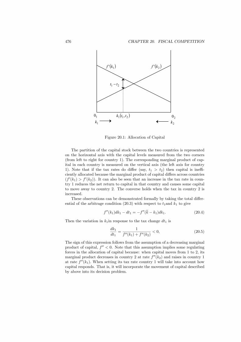
476 CHAPTER 20. FISCAL COMPETITION
( )1' kf ( )2' kf
2010
1k 2k
21 tt −
( )211 , ttk
Figure 20.1: Allocation of Capital
The partition of the capital stock between the two countries is representedon the horizontal axis with the capital levels measured from the two corners(from left to right for country 1). The corresponding marginal product of cap-ital in each country is measured on the vertical axis (the left axis for country1). Note that if the tax rates do differ (say, t1 > t2) then capital is ineffi-ciently allocated because the marginal product of capital differs across countries(f 0(k1) > f 0(k2)). It can also be seen that an increase in the tax rate in coun-try 1 reduces the net return to capital in that country and causes some capitalto move away to country 2. The converse holds when the tax in country 2 isincreased.These observations can be demonstrated formally by taking the total differ-
ential of the arbitrage condition (20.3) with respect to t1and k1 to give
f 00(k1)dk1 − dt1 = −f 00(k − k1)dk1. (20.4)
Then the variation in k1in response to the tax change dt1 is
dk1dt1
=1
f 00(k1) + f 00(k2)< 0, (20.5)
The sign of this expression follows from the assumption of a decreasing marginalproduct of capital, f 00 < 0. Note that this assumption implies some regulatingforces in the allocation of capital because: when capital moves from 1 to 2, itsmarginal product decreases in country 2 at rate f 00(k2) and raises in country 1at rate f 00(k1). When setting its tax rate country 1 will take into account howcapital responds. That is, it will incorporate the movement of capital describedby above into its decision problem.
20.2. TAX COMPETITION 477
Assuming that the net revenue collected from local capital taxation accruesto workers in the form of cash transfers or public goods of the same value, thenet income of workers (or residents) in country 1 will be
y1 = f(k1)− f 0(k1)k1 + t1k1. (20.6)
Each country maximizes the net income of its residents taking into account cap-ital flows resulting from tax changes. Because the amount of capital employedin each country also depends on the other country’s tax rate, there is strate-gic fiscal interaction among countries: neither can set its own tax rate withouttaking into account what the other is doing.The optimal choice of each country is found by applying the usual Nash
assumption: each takes the tax rate of the other as given when maximizing.Applying this reasoning, the best response of country 1 to the other country’stax t2 is described by the following first-order condition
dy1(t1, t2)
dt1= −k1f 001
dk1dt1
+ k1 + t1dk1dt1
= [k1f002 + t1]
dk1dt1
= 0, (20.7)
where the second equality is obtained by using (20.5) to substitute for k1 =k1 [f
001 + f
002 ]
dk1dt1. Therefore the best response function for country 1 can be
written ast1 = −k1f 002 = r1(t2), (20.8)
and similarly for country 2
t2 = −k2f 001 = r2(t1). (20.9)
A Nash equilibrium is a pair (t∗1, t∗2) such that the tax choice of each country
is a best response to the other country’s tax choice, t∗1 = r1(t∗2) and t∗2 = r2(t∗1).The symmetry of the model implies that both countries choose the same taxes inequilibrium, so t∗1 = t
∗2, and that consequently the capital is evenly distributed
between jurisdictions with k1 = k2 = k/2. The Nash equilibrium in taxes is thus
t∗1 = t∗2 = −
k
2f 00µk
2
¶. (20.10)
We can also find the slope of the best response function r1(t2) to evaluate thenature of strategic interdependency between the two countries. The first-ordercondition ψ1(t1, t2) = k1f
002 + t1 = 0 implicitly defines t1 as a function of t2, and
we need to know how the optimum choice of t1 will respond to changes in t2.Differentiating the first-order condition totally, we have
∂ψ1∂t1
dt1 − ∂ψ1∂t2
dt2 = 0. (20.11)

478 CHAPTER 20. FISCAL COMPETITION
21 tt =
( )12 tr
( )21 tr
1t
2t
Figure 20.2: Symmetric Nash Equilibrium
This gives the slope of the best-response as
dr1dt2
=
³f 002 − k1f
0002
´dk1/dt1
1 +¡f 002 − k1f 0002
¢dk1/dt1
, (20.12)
where dk1/dt1 < 0 and f 00 < 0. It follows that for f 000 ≥ 0 the slope of the bestresponse function satisfies 0 < dr1
dt2< 1. Tax rates are strategic complements: a
lower tax in country 2 attracts capital away from country 1 which in responsecuts its own tax rate.It is now easily seen that such a Nash equilibrium t∗1 = t
∗2 = t
∗ involves inef-ficiently low taxes and that jointly increasing taxes to t > t∗ is beneficial to bothcountries. First, observe that from the perspective of the two countries together,the stock of capital is fixed at k. Hence it is simply a fixed factor. Providedboth countries levy the same tax rate t = t1 = t2 , half of the capital, k/2, willbe located in each country regardless of the level of the taxes. The welfare of theworkers in each country, as measured by their net income y = f(k)−f 0(k)k+tk,is then improved since tk/2 > t∗k/2. In fact, with the cooperative tax setting,the countries can maximize the net income of their residents by fully taxing themobile factor, whereas the non-cooperative equilibrium leads to a lower rate oncapital. Welfare is higher with cooperation. This loss in potential welfare is theefficiency cost of fiscal competition.Although the model just considered leads to the extreme conclusion that the
tax is pushed to its maximum with cooperation, this was not the major pointof the analysis. What the model does illustrate are the forces that are at workwhen an attempt is made to tax a mobile factor of production. The movementof the factor generates an externality between countries which is not internalized
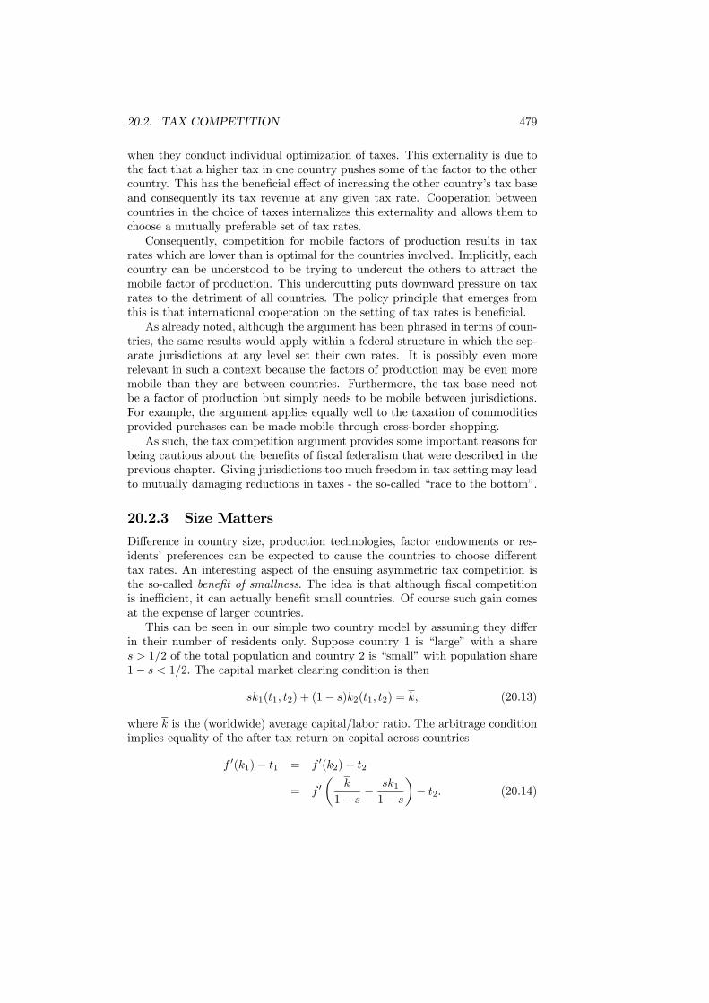
20.2. TAX COMPETITION 479
when they conduct individual optimization of taxes. This externality is due tothe fact that a higher tax in one country pushes some of the factor to the othercountry. This has the beneficial effect of increasing the other country’s tax baseand consequently its tax revenue at any given tax rate. Cooperation betweencountries in the choice of taxes internalizes this externality and allows them tochoose a mutually preferable set of tax rates.Consequently, competition for mobile factors of production results in tax
rates which are lower than is optimal for the countries involved. Implicitly, eachcountry can be understood to be trying to undercut the others to attract themobile factor of production. This undercutting puts downward pressure on taxrates to the detriment of all countries. The policy principle that emerges fromthis is that international cooperation on the setting of tax rates is beneficial.As already noted, although the argument has been phrased in terms of coun-
tries, the same results would apply within a federal structure in which the sep-arate jurisdictions at any level set their own rates. It is possibly even morerelevant in such a context because the factors of production may be even moremobile than they are between countries. Furthermore, the tax base need notbe a factor of production but simply needs to be mobile between jurisdictions.For example, the argument applies equally well to the taxation of commoditiesprovided purchases can be made mobile through cross-border shopping.As such, the tax competition argument provides some important reasons for
being cautious about the benefits of fiscal federalism that were described in theprevious chapter. Giving jurisdictions too much freedom in tax setting may leadto mutually damaging reductions in taxes - the so-called “race to the bottom”.
20.2.3 Size Matters
Difference in country size, production technologies, factor endowments or res-idents’ preferences can be expected to cause the countries to choose differenttax rates. An interesting aspect of the ensuing asymmetric tax competition isthe so-called benefit of smallness. The idea is that although fiscal competitionis inefficient, it can actually benefit small countries. Of course such gain comesat the expense of larger countries.This can be seen in our simple two country model by assuming they differ
in their number of residents only. Suppose country 1 is “large” with a shares > 1/2 of the total population and country 2 is “small” with population share1− s < 1/2. The capital market clearing condition is then
sk1(t1, t2) + (1− s)k2(t1, t2) = k, (20.13)
where k is the (worldwide) average capital/labor ratio. The arbitrage conditionimplies equality of the after tax return on capital across countries
f 0(k1)− t1 = f 0(k2)− t2= f 0
µk
1− s −sk11− s
¶− t2. (20.14)

480 CHAPTER 20. FISCAL COMPETITION
Differentiating the arbitrage condition gives the capital outflow in response toa domestic tax increase
dk1dt1
=1− s
(1− s)f 00(k1) + sf 00(k2) < 0, (20.15)
and by analogy for the small country
dk2dt2
=s
(1− s)f 00(k1) + sf 00(k2) < 0. (20.16)
From (20.15) and (20.16), it follows that both countries face a capital outflowafter an increase in their own tax rate, but this outflow is less severe in the largecountry. Indeed when t1 = t2 , we have k1 = k2, f 00(k1) = f 00(k2) and thusdk2dt2
< dk1dt1
< 0 for s > 1−s. The larger country faces a less elastic tax base andthereby chooses a higher tax rate than the smaller country, so in equilibriumt1 > t2. Because the small country charges a lower tax on capital, it willemploy more capital per unit of labor, (k2 > k1) increasing per capita incomeand making its residents better off than the residents of the large country. Itis even possible that for a sufficiently large difference in size, the small countrywill be better off than it would be without tax competition.This benefit of smallness is illustrated in Figure 20.3, where for country
i = 1, 2 per capita income is denoted ci = f(ki) − f 0(ki)ki and tax revenueis denoted gi = tiki. The net-return to capital, denoted by R, is the samefor both countries by arbitrage and is adjusted to tax choices in order to clearthe market. It is then readily seen that the residents of the small country arebetter-off taxing less since c2 + g2 > c1 +G1.We can obviously extend this reasoning to show that if the number of coun-
tries competing for capital increases, each country having a lower populationshare will perceive a greater elasticity of its tax base and choose lower taxes:the larger the number of countries, the more intense the competition and thelower the equilibrium taxes.
20.2.4 Tax Overlap
A common feature of fiscal federalism is that higher- and lower-levels of govern-ment share the same tax base. This tax base overlap gives rise to vertical fiscalexternalities. With tax competition between jurisdictions, the horizontal fiscalexternality upon other regions is positive - an increase in tax rate by one regionraises the tax base of others. In contrast, if different levels of government sharethe same tax base, then the tax levied by one government will reduce the taxbase available to other levels of governments. This introduces a negative verticalexternality. Not surprisingly such vertical externalities lead to over-taxation inequilibrium because each level of government neglects the negative effect of itstaxation on the other levels of government.The joint taxation of cigarettes by Canadian federal and provincial govern-
ments is a good example. Figure 20.4 illustrates this tax overlap problem. The
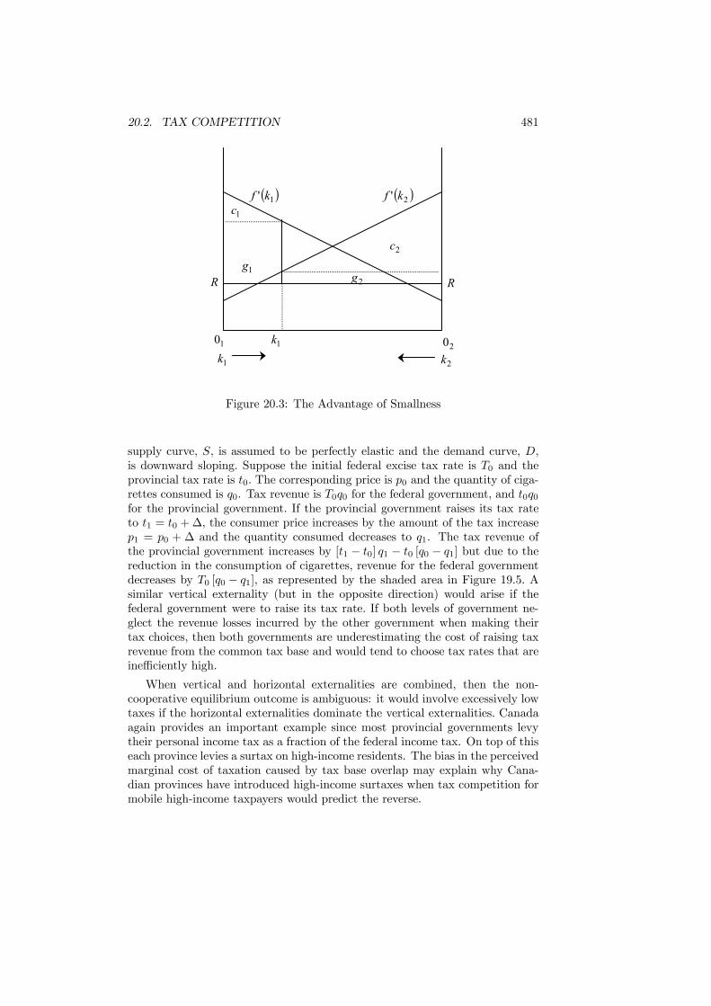
20.2. TAX COMPETITION 481
( )1' kf ( )2' kf
2010
1k 2k1k
R R1g
1c
2c
2g
Figure 20.3: The Advantage of Smallness
supply curve, S, is assumed to be perfectly elastic and the demand curve, D,is downward sloping. Suppose the initial federal excise tax rate is T0 and theprovincial tax rate is t0. The corresponding price is p0 and the quantity of ciga-rettes consumed is q0. Tax revenue is T0q0 for the federal government, and t0q0for the provincial government. If the provincial government raises its tax rateto t1 = t0 +∆, the consumer price increases by the amount of the tax increasep1 = p0 + ∆ and the quantity consumed decreases to q1. The tax revenue ofthe provincial government increases by [t1 − t0] q1 − t0 [q0 − q1] but due to thereduction in the consumption of cigarettes, revenue for the federal governmentdecreases by T0 [q0 − q1], as represented by the shaded area in Figure 19.5. Asimilar vertical externality (but in the opposite direction) would arise if thefederal government were to raise its tax rate. If both levels of government ne-glect the revenue losses incurred by the other government when making theirtax choices, then both governments are underestimating the cost of raising taxrevenue from the common tax base and would tend to choose tax rates that areinefficiently high.
When vertical and horizontal externalities are combined, then the non-cooperative equilibrium outcome is ambiguous: it would involve excessively lowtaxes if the horizontal externalities dominate the vertical externalities. Canadaagain provides an important example since most provincial governments levytheir personal income tax as a fraction of the federal income tax. On top of thiseach province levies a surtax on high-income residents. The bias in the perceivedmarginal cost of taxation caused by tax base overlap may explain why Cana-dian provinces have introduced high-income surtaxes when tax competition formobile high-income taxpayers would predict the reverse.
482 CHAPTER 20. FISCAL COMPETITION
Price
Quantity
0t
0T
0p
0q1q
1p
D
S
Figure 20.4: Tax Overlap
20.2.5 Tax Exporting
In any country, some commodities that are sold within its borders will be pur-chased by non-residents. This will be particularly true if the country is especiallyimportant in the context of international tourism. It will also be encouragedunder fiscal federalism with a single market covering all jurisdictions. Similarly,some of the productive activity carried out in a country will be undertaken byfirms that repatriate their profits to another country. Whenever there is sucheconomic activity by non-residents, the possibility for tax exporting arises.Tax exporting is the levying of taxes that discriminate against non-residents.
A simple example would be the imposition of a higher level of VAT upon restau-rants located in centers of tourism. The motive for such tax exporting is to shiftsome of the burden of revenue collection onto non-residents and lower it on resi-dents. All else held constant, this is clearly of benefit to residents. However, allelse is not constant in practice and the same argument will apply to all coun-tries. As for tax overlap, tax exporting provides an argument for why tax ratesmay be set too high when countries compete.Another form of tax exporting is the taxation of capital employed in the
country but owned by non-residents. The simplest version of this form of taxexporting can be described with the previous model of tax competition by as-suming that country 1’s residents have a capital endowment k1 > 0 that differsfrom that of country 2, k1 6= k2. Capital owners in each country are free to investtheir capital in their home country or abroad. The level of social welfare in coun-try 1, is measured by the net income of its workers y1 = f(k1)− f 0(k1)k1+ t1k1plus the net income of its capital owners ρk1; where k1 is the amount of capital
20.2. TAX COMPETITION 483
employed in country 1. The capital market clearing condition requires
k1 − k1 = −¡k2 − k2
¢. (20.17)
That is, when k1 < k1 country 1 is employing less capital than its endowment, itsnet export of capital has to be equal to the net import of capital from country 2.For country 1 the problem is to set its tax t1 on capital given the tax of country2 so as to maximize
f(k1)− f 0(k1)k1 + t1k1 + ρk1, (20.18)
where k1 = k1(t1, t2) is the amount of capital employed in country 1 given taxrates t1, t2 and ρ = ρ(t1, t2) is the net return to capital. Using ρ = f 0(k1)− t1,the objective function can be written as follows
W1 = f(k1) + ρ(k1 − k1),
that is, country welfare is the total production f(k1) plus the net return tocapital export (k1 − k1). When deriving the first-order condition, we must dif-ferentiateW1 with respect to t1 taking into account the change in capital supplydk1dt1
and the change in the net return to capital dρdt1. This gives
dW
dt1= (f 0(k1)− ρ)
dk1dt1
+ (k1 − k1) dρdt1
= t1dk1dt1
+ (k1 − k1)(f 001dk1dt1− 1) = 0. (20.19)
To solve this first-order condition, we can use (20.5) to get f 001dk1dt1−1 = −f 002 dk1dt1
,this gives
t1 = f002 (k1 − k1), (20.20)
and by analogy for country 2, using (20.17)
t2 = −f 001 (k1 − k1), (20.21)
with f 00 < 0. Therefore in any equilibrium, if country 1 has the larger endowmentof capital, k1 > k2, it will export capital k1 > k1 and so it will prefer to subsidizecapital t1 < 0. The reason is the term of trade effect. By subsidizing capital,the country with large endowment of capital can raise the net-return to capital.Because the other country will import capital from country 1, it will tax capitalt2 > 0 as a means to tax non-residents. This is the tax exporting effect. Next,note that the initial asymmetry in capital endowments leads countries to setdifferent tax rates. This non-uniform tax equilibrium has important implicationsin terms of productive efficiency. Indeed efficient allocation of capital requiresits marginal product to be equalized across countries. But because country 1subsidizes capital and country 2 taxes it, it follows that the marginal productof capital is higher in country 2 than in country 1, f 02 > f 01. Therefore, inequilibrium, country 1 attracts too much capital and country 2 too little, relativeto what efficiency recommends.

484 CHAPTER 20. FISCAL COMPETITION
20.2.6 Efficient Tax Competition
Tax competition has been seen as producing wasteful competition. There arecircumstances however where tax competition may be welfare enhancing. Weconsider two examples.The first example is the case where countries seek to give a competitive
advantage to their own firms by offering wasteful subsidies. In equilibrium allcountries will do this, so each country’s subsidy cancels out with of others.Since they cancel, none gains any advantage and all countries would be betteroff giving no subsidy. This is the Prisoners’ Dilemma once again. Tax competi-tion may help solve this inefficient outcome by allowing firms to locate whereverthey choose and preventing governments from discriminating between domes-tic and foreign firms operating within a country. The mobility of the firms willforce governments to recognize that their subsidy will not only give a compet-itive advantage to their domestic firms but that it will also attract firms fromother countries. Because the government cannot discriminate between all firmsoperating within its borders, it will have to pay the subsidy to both the domes-tic and foreign firms, thereby eliminating the competitive advantage. Thereforemobility eliminates the potential gains from the subsidy and raises its cost byextending its payment to foreign firms.Tax competition can therefore improve welfare by reducing the incentive for
countries to resort to wasteful subsidies to protect their own industries. Noticethat the non-discrimination requirement plays a crucial role in making tax com-petition welfare improving. If discrimination were possible, then governmentscould continue to give wasteful subsidies to their domestic firms.The second example is the use of tax competition as a commitment device. In
the tax competition model, governments independently announce tax rates andthen the owners of capital choose where to invest. A commitment problem ariseshere because the governments are able to revise their tax rates after investmentdecisions are made. If there were a single government and investment decisionwere irreversible, then this government would have an incentive to tax awayall profits. The capital owner would anticipate this incentive when making itsinitial investment decision and choose not to invest capital in such a country.Tax competition may help to solve this commitment problem. The reason
is that inter-governmental competition for capital would deter each governmentfrom taxing away profits within its borders because it would induce realloca-tion of capital between countries in response to difference in tax rates. Taxcompetition is a useful commitment device as it induces governments to foregotheir incentive to tax investment in an effort to attract further investment or tomaintain the existing investment level.The original insight that tax competition leads to inefficiently low taxes and
public good provision was obtained in models with benevolent decision makers.An alternative approach is to consider public officials that seek in their deci-sion making to maximize their own welfare and not necessarily that of theirconstituencies. From this perspective, tax competition may help discipline non-benevolent governments. For instance if we view governments as ”leviathan”

20.3. INCOME DISTRIBUTION 485
mainly concerned with maximizing the size of the public sector, then tax compe-tition may improve welfare by limiting taxation possibilities and thereby cuttingdown the size of government that would be otherwise excessive. This argumentsuggests that the public sector should be smaller, the greater the extent towhich taxes and expenditures are decentralized. The evidence on this is, how-ever, mixed. In fact there is not much evidence on the relationship betweenfiscal decentralization and the overall size of the public sector.An analogous argument applies to governments with some degree of benev-
olence, possibly due to electoral concerns. When political agency problems areintroduced, this inefficiency of competition among governments is no longer soclear. Inter-governmental competition makes the costs of public programs morevisible, as well as their benefits in ways that make public officials accountablefor their decisions. Stated briefly, competition may induce government officialsto reduce waste and thus reduce the effective price of public goods.
20.3 Income Distribution
When the powers for tax setting are devolved to individual jurisdictions, theTiebout hypothesis asserts that the outcome will be efficient. The basis for thisargument is that there are enough jurisdictions for individuals to sort themselvesinto optimal locations. For practical purposes it is not possible to appeal to thislarge-numbers assumption and questions need to be asked about the outcomethat will emerge when only a small, and predetermined, number of jurisdictionsexist. The Tiebout hypothesis is also silent about how the policy of a jurisdic-tion emerges. It is possible that equilibrium results in all the residents of anyjurisdiction being identical, so that there is no need to resolve different pointsof view. More generally, though, it is necessary to explore the consequences ofpolitical-decision making, expressed through elections, on the choice of policy.An important set of issues revolve around income distribution and the role
that this has in determining the composition of the population in jurisdictions.For instance, will it always be the case that the rich wish to detach themselvesfrom the poor so that they can avoid being subject to redistributive taxation?And, if they have the option, would the poor wish to live with the rich? Thesequestions are now explored under perfect and imperfect mobility.
20.3.1 Perfect Mobility
The difficulty that mobility poses for redistribution is seen most strongly inthe following example. Consider individuals who differ only in income level yand who can choose to reside in one of the two available jurisdictions. Thejurisdictions independently set a constant tax rate t ∈ [0, 1] and pay a lumpsum transfer g subject to a budget balance constraint. Individuals care onlyabout their income after taxes and transfers, so their preferences are given by
v(t, g; y) = g + [1− t] y. (20.22)
486 CHAPTER 20. FISCAL COMPETITION
The tax-transfer pair (t, g) in each jurisdiction is chosen by some unspecifiedcollective decision rule (e.g. majority voting). We are looking for an equilibriumin which the two jurisdictions differ and offer different tax and transfer schemes,thereby inducing the sorting of types across jurisdictions (as the Tiebout hy-pothesis would predict).With no loss of generality, suppose it is jurisdiction 1 that sets the higher
tax rate. Then to attract any individuals, it must also provide a higher level oftransfer, that is (t1, g1) > (t2, g2). Individuals with different income levels differin their preferences for redistribution. From (20.22), if a type y prefers the hightax jurisdiction 1, then all those with lower income levels will also prefer thisjurisdiction. And if a type y prefers the low tax jurisdiction 2, then all thosewith higher income levels will also prefer this jurisdiction. Therefore if bothjurisdictions are occupied in equilibrium, there must exist a separating type y∗
who is just indifferent between the two tax schemes and all those who are poorer,with y ≤ y∗, join jurisdiction 1 and all those who are richer, with y > y∗, joinjurisdiction 2. That is the jurisdiction undertaking more redistribution attractsthe poorest individuals.However this cannot be an equilibrium, because the richest individual in the
poor jurisdiction loses out from intra-jurisdictional redistribution and will preferto move to the rich jurisdiction and become a net beneficiary of redistributionas its poorest resident. Therefore there cannot be an equilibrium with differenttax-transfer schemes.There remains the possibility of a symmetric equilibrium with individuals
evenly divided between the two jurisdictions. In other words, perfect mobilityleads to harmonization of tax-transfer schemes, even though agents differ intheir preferences. The mobility does not lead to the sorting of types across ju-risdictions as Tiebout predicts. The possibility for the rich to detach themselvesfrom the poor to escape redistributive taxation induces jurisdictions either toabandon any taxation or to choose the same tax rate.
20.3.2 Imperfect Mobility
Suppose now that consumers have one of two income levels. Those with thehigher income level are termed the “rich” and those with the lower income arethe “poor”. The two groups are imperfectly mobile but to different degrees. Therich (group 1) have income 1 and poor (group 0) have income 0. For simplicity,there is an equal number of poor and rich in the total population. The focusis placed on one of the jurisdictions (say region 1) and the proportions fromeach group residing there are denoted x1 and x0 , where the index denotesincome group. The remainder (1 − x1) and (1 − x0) are located in the otherjurisdiction. Redistribution implies that the rich are subject to taxation andthe poor recipients of transfer. Accordingly, each jurisdiction levies a head tax ton its rich residents to pay a transfer b to each of its poor residents. The feasiblechoices are restricted by the budget constraint tx1 = bx0.In addition to income differences, each individual is characterized by a pref-
erence for location x ∈ [0, 1] where a low x implies preference for region 1 and
20.3. INCOME DISTRIBUTION 487
a high x implies preference for region 2. Individuals care only about their netincome and their location. Given the pair of transfers (b, b∗) in the two regions,the payoff of a poor individual with preference x ∈ [0, 1] is
b− d0x in region 1,
b∗ − d0(1− x) in region 2, (20.23)
where d0 > 0 measures the degree of attachment to location of the poor withhigher attachment equivalent to lower mobility.Given the tax pair (t, t∗) the payoff of a rich individual with preference
x ∈ [0, 1] is(1− t)− d1x in region 1,
(1− t∗)− d1(1− x) in region 2. (20.24)
It is assumed that x is uniformly distributed within income groups.Given the tax policies, the population is divided between the two regions.
The proportion of poor joining region 1, x = x0, is defined by the type that isindifferent between the two regions so
b− d0x0 = b∗ − d0(1− x0), (20.25)
and thus
x0 =1
2+ µ0
·b− b∗2
¸, (20.26)
with µ0 = 1/d0 denoting the mobility of the poor. Higher mobility of the poorincreases their migration in response to transfer differential. The poor are evenlydistributed across regions with uniform transfers b = b∗.Similarly, the proportion of rich, x = x1 joining region 1 is given by the
indifference condition
(1− t)− d1x1 = (1− t∗)− d1(1− x1). (20.27)
Defining the mobility of the rich by µ1 = 1/d1, this yields
x1 =1
2+ µ1
·t∗ − t2
¸.
with equal taxes inducing equal division of the rich between the two regions,x1 = 1/2. Taxing more drives out some of the rich (i.e., x1 decreases with t).Budget balance implies that the transfer you can afford to pay depends on
who you attract. The transfer paid to each poor resident is
b =tx1x0
in region 1, (20.28)
b∗ =t∗(1− x1)1− x0 in region 2. (20.29)

488 CHAPTER 20. FISCAL COMPETITION
Assume that both governments follow a policy of maximal redistribution.Then region 1 sets its tax rate t taking as given the tax rate of the other, t∗, soas to maximize the transfer given to its poor residents, b, correctly anticipatingthe induced migration. The migration response of the rich to a small tax changeis proportional to their mobility
dx1dt
= −µ12< 0. (20.30)
How the poor respond to a small tax change depends on the migration responseof the rich and is given by total differentiation
dx0 =µ02
µd(b− b∗)dt
dt+d(b− b∗)dx0
dx0
¶. (20.31)
Evaluating this expression around t = t∗ (i.e., with xi = 1/2) for separatechanges in t and x0 gives
d(b− b∗)dt
=x1 + t
dx1dt
x0− t∗ d(1−x1)
dt
1− x0 = 1− 2tµ1, (20.32)
d(b− b∗)dx0
=−tx1(x0)
2 −t∗(1− x1)(1− x0)2
= −4t. (20.33)
Therefore the migration response of the poor to a domestic tax change is
dx0dt
=12 − tµ11µ0+ 2t
≷ 0. (20.34)
It is worth noting that the migration response of the poor to tax change cango either way. In particular higher tax can drive out the poor: dx0/dt < 0 fort > 1
2µ1. The reason is that if the rich are sufficiently mobile (high µ1), a tax
increase induces so many rich to leave that the poor would find it better tofollow them. In such circumstances, the poor will chase the rich.Putting these points together the (symmetric) equilibrium tax choice can be
determined. Region 1 chooses its tax rate t so as to maximize the transfer to itspoor residents b taking as given the tax choice of the other region and correctlyanticipating the migration responses of the rich and the poor. The necessaryfirst-order condition is
db
dt=x1x0+
µt
x0
¶dx1dt
+db
dx0
µdx0dt
¶= 0 (20.35)
Using the migration changes as given by (20.30) and (20.34) and evaluatingthe condition at the symmetric outcome in which both regions pick the sametax-transfer scheme and each group divides evenly between the two regions, thefirst-order condition becomes
db
dt= 1− tµ1 − 2t
Ã12 − tµ11µ0+ 2t
!= 0. (20.36)

20.4. INTER-GOVERNMENTAL TRANSFERS 489
This gives the following symmetric equilibrium
t = t∗ =1
µ1 − µ0. (20.37)
Consequently, the equilibrium level of redistributive taxation is inverselyproportional to the difference in the mobility of the rich and the poor. Highermobility of the rich reduces taxation but this is partially offset by the mobilityof the poor. The reasoning behind this is that in equilibrium the poor chase therich and so it is not possible for the rich to detach themselves from the poor.The logic of the conclusion also applies in a model with capital and labor
mobility. With this extension, it implies that the possibility to tax capital in-creases with the mobility of labor. So the problem of tax competition is notonly the excessive mobility of capital but also the lack of mobility of labor.
20.3.3 The Race to the Bottom
In a context where there are no legal barriers to migration, so that the forcesof fiscal competition are at work, any attempt at redistribution or the provisionof social insurance in a country would be impossible because it would induceemigration of those who were supposed to give (the rich) and immigration ofthose who were supposed to receive (the poor). The most extreme predictions ofthis form imply a “race to the bottom” but receive little theoretical or empiricalsupport. This is probably due to the presence of significant costs and barriersto migration.For example, welfare shopping has been discouraged in Europe by limiting
portability between member states and requiring, for eligibility, previous em-ployment in the country. However we believe that under-provision of socialinsurance in an integrated market is an issue that cannot be ignored in the EU.Even if it has not been a pressing issue to date, fiscal competition for capital andlabor factors has already arrived. The Irish experience of the success of reducedcorporation taxes is evidence of this. And with the prospect of enlargement,this issue will become even more pressing.
20.4 Inter-Governmental Transfers
The reasons for organizing inter-governmental transfers are twofold: efficiencyand redistribution. We consider the two in turn.
20.4.1 Efficiency
A critical insight from the analysis of tax competition is that increasing thetax rate in one region benefits other regions by increasing their tax bases. If wetake the tax base to be the capital stock and the aggregate supply of capital tobe fixed, then the tax-induced outflow of capital from the region taxing morerepresents an inflow of capital to the other regions.
490 CHAPTER 20. FISCAL COMPETITION
In particular, another region j benefits from increased revenue by the amounttj∆kj, where tj is its tax rate and ∆kj the fiscally-induced capital inflow. Theproblem facing each region is to choose the tax rate on capital to finance thepublic good level that maximizes the welfare of its residents subject to thebudget constraint G = tk(t). The optimal regional level of public good is givenby the fact that the marginal benefit of public good MB must be high enoughto not only cover its marginal cost, MC, but also to offset the negative impactof capital outflow on tax revenue, denoted by t∆k < 0. Then we obtain thefollowing modified Samuelson rule
MB =MC − t∆k. (20.38)
The context of identical regions provides a useful reference for isolating thefiscal-externality inefficiency from other equity and efficiency aspects that wouldarise when regions differ and choose different tax rates and public good levels.With identical tax rates, t, the cost of a capital outflow from one region isexactly offset by the benefits from the resulting capital inflows to other regions.It follows that if regions were to take into account such external benefits theywould no longer perceive capital outflows as a cost and the efficient provision ofpublic good (as given by the usual Samuelson rule) would obtain with
MB =MC. (20.39)
The central authority can achieve this efficient outcome by means of revenuematching grants. The idea is to correct the externality by providing a subsidy tothe revenue raised by each region. The matching rate to a region is the additionalrevenue that accrues to other regions when this region raises its tax rate. Thenregions are correctly compensated for the positive externalities of raising theirtaxes.Differences among regions bring about a second inefficiency from tax com-
petition, namely that different tax rates induce a misallocation of capital acrossregions, such that the marginal product of capital is relatively high in high-taxregions (see Figure 20.3). It follows that matching rates should be differenti-ated to induce all regions to choose the same tax rate and at the same timeto internalize the fiscal externality. Tax harmonization requires the paymentof a higher subsidy to regions with a low preference for taxation and publicgoods. In practice, however, the central government may not have the politicalauthority or the information required to impose differentiated matching grants.The information problem is rather severe because all regions can claim to beof the low-tax type in order to obtain a higher subsidy. With tax overlap, thematching rate will be negative to represent the reduction in tax revenues forother levels of government when the region raises additional revenue from thecommon tax base (see Figure 20.4).Expenditure externalities can also be corrected with expenditure matching
grants. For example, spending by a local government on education or publicinfrastructure improves the potential earnings of its residents by making themmore productive and this will increase the federal government’s revenue from
20.4. INTER-GOVERNMENTAL TRANSFERS 491
income, payroll and sales taxes. To induce the local government to internalizethis vertical expenditure externality, the federal authority can use expenditurematching grants. Matching grant programs specify that the federal governmentmatches on a dollar-for-dollar basis local expenditure up to some maximum. Theeffect is to lower the price of local public goods and thereby offset the tendencyfor local governments to under-provide public expenditures generating positiveexternalities.An important example of vertical expenditure externalities in Canada is the
substitutability between expenditures on unemployment benefits at the federallevel and welfare benefits at the provincial levels. If the federal governmentreduces unemployment benefits or their duration, more people will apply forwelfare benefits, increasing spending at the provincial level. Conversely, em-ployment programs by provincial government which allow welfare recipients toregain eligibility to unemployment benefits will lead to higher spending at thefederal level.In the US, until 1996, the federal government could bear 50-80 percent of
the cost of some welfare expenditures undertaken by states (like the Aid toFamilies with Dependent Children, Food stamp and Medicaid programs). In1996 the AFDC matching system was replaced by a lump-sum grant (i.e., theTANF programme). This is intriguing because as illustrated in Figure 20.5,the matching system is more effective in stimulating local public expendituresthan a lump-sum subsidy of the same amount. The reason is simply that thelump-sum grant can be used in any way the recipient wishes, in contrast to thematching grant that is increasing with the amount of public spending. In thatperspective matching grants are also called ”conditional” grants because theyplace some restrictions on their use by the recipient, and the lump-sum grantsare called ”unconditional” grants. Figure 20.5 also indicates the distortionaryeffect of matching grants: higher welfare could be attained at the same costwith lump-sum grants. This is the advantage of the freedom of choice that”unconditional” grants provide.The attraction of matching grants is to internalize expenditure externalities.
However lump-sum grants also have their own attraction which is to maintainfiscal discipline (at the heart of the EMU). The idea here is that by creatinga hard budget constraint, they impose a very useful discipline on decentralizedexpenditure decisions. More generally, a hard budget constraint implies thatdecentralized governments must place a basic reliance on their own sourcesof revenue and must not be overly dependent on transfers from the federalgovernment. Self-financing is a powerful incentive device and it is essential thatlocal governments do not turn to the federal authority to bail them out of fiscaldifficulties by resorting to expansible matching grants.
20.4.2 Redistribution
Inter-governmental grants are also used to channel resources from wealthy ju-risdictions to poorer ones. Such transfers are based on equalization formulathat measure the fiscal need and fiscal capacity of each jurisdiction, locality or
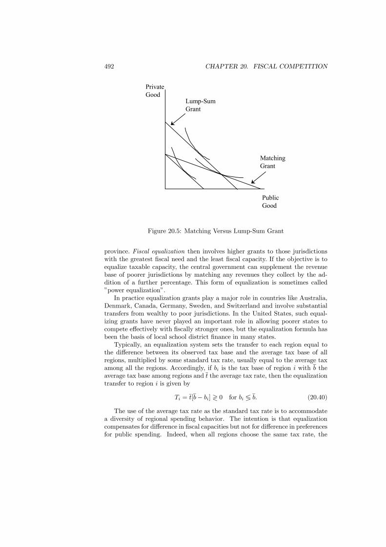
492 CHAPTER 20. FISCAL COMPETITION
PrivateGood
PublicGood
Lump-SumGrant
MatchingGrant
Figure 20.5: Matching Versus Lump-Sum Grant
province. Fiscal equalization then involves higher grants to those jurisdictionswith the greatest fiscal need and the least fiscal capacity. If the objective is toequalize taxable capacity, the central government can supplement the revenuebase of poorer jurisdictions by matching any revenues they collect by the ad-dition of a further percentage. This form of equalization is sometimes called”power equalization”.In practice equalization grants play a major role in countries like Australia,
Denmark, Canada, Germany, Sweden, and Switzerland and involve substantialtransfers from wealthy to poor jurisdictions. In the United States, such equal-izing grants have never played an important role in allowing poorer states tocompete effectively with fiscally stronger ones, but the equalization formula hasbeen the basis of local school district finance in many states.Typically, an equalization system sets the transfer to each region equal to
the difference between its observed tax base and the average tax base of allregions, multiplied by some standard tax rate, usually equal to the average taxamong all the regions. Accordingly, if bi is the tax base of region i with b theaverage tax base among regions and t the average tax rate, then the equalizationtransfer to region i is given by
Ti = t[b− bi] ≷ 0 for bi ≶ b. (20.40)
The use of the average tax rate as the standard tax rate is to accommodatea diversity of regional spending behavior. The intention is that equalizationcompensates for difference in fiscal capacities but not for difference in preferencesfor public spending. Indeed, when all regions choose the same tax rate, the
20.5. EVIDENCE 493
formula guarantees equal revenues. The equalization formula can also correctfor fiscal externalities. A tax cut by one region increases not only its tax base atthe expense of other regions, but also relative to the average tax base, therebyreducing the entitlement of this region to equalization grants.Fiscal equalization is a contentious issue. In some cases, as in Canada, it
may provide the cement that holds the bricks of the federation together. Inother cases, like Italy or Belgium, it may become the source of division, whererich regions weary of large and durable transfers to poor regions, actually seekthe break up of the federation.
20.4.3 Flypaper Effect
When considering the budgetary decisions of the recipients of inter-governmentalgrants, models of rational choice suggest that the response to a lump-sum grantshould be roughly the same as the response to an equal increase in income result-ing from a federal tax cut. But empirical studies of the response to grants haverejected this equivalence. There are indeed strong evidence that local govern-ment spending is more sensitive to grants than it is to increasing income throughtax cut. Among the best estimates of this in the US: the marginal propensityfor state local governments to spend out of personal income in the state is about10 percent. But the marginal propensity for state local governments to spendout of grants from the federal level is around 80-90 percent. This has beenknown as the ”flypaper effect” to say that money sticks where it hits. This isintriguing because it suggests that the same budget could give rise to differentchoices depending on what form the increment to the budget takes. It has beensuggested that this may reflect the behavioral regularity that money on hand(from grants) has different effect on spending than where the money must beraised (by taxation). This is can be understood with the following thought ex-periment. Consider you have lost your ticket for the cinema and you must decidewhether to buy a new one. Now suppose instead that you lose the same amountof money, would you be as willing to buy the ticket in the first place. Althoughin both cases you face exactly the same budget constraint, it is less likely thatyou will buy the new ticket after losing the original one than if you were losingthe equivalent amount of money. The fly paper effect also casts serious doubton the idea that local governments are more responsive to local demand. Indeedtaking the estimates above, one might think that if the local government werestrictly responding to local demand, $100 per capita of federal grants wouldlead to about $90 per capita tax reduction and $10 additional spending, but itis entirely the other way around with about $90 additional spending and $10 ofreduced local taxes.
20.5 Evidence
Race to the bottom: The central result of the tax competition model is thatincreasing mobility of capital will drive down the equilibrium tax on capital.

494 CHAPTER 20. FISCAL COMPETITION
This canonical model is at the heart of concerns about capital tax competitionwithin the EU. In response to this growing concern, the OECD published areport (OECD, 1998) comprising about 20 recommendations to counter whatwas perceived as ”harmful” tax competition of capital income. This issue wasalso taken seriously by the EU in December 1997. The EU commission agreedwith a ”Code of Conduct” in business taxation, as part of a ”package to tackleharmful tax competition”. The Code is aimed at identifying tax measures thatreduce the level of tax paid below the ”usual” level. In particular, a measure isconsidered as ”harmful” if the tax advantage is restricted only to non-residents,or if it is ”ring-fenced” from the domestic market, or if the tax break is grantedwithout any real economic activity taking place. The central motivation forthese reforms is the race to the bottom in capital taxation. To appreciate therelevance of this we must evaluate the existence and magnitude of this race tothe bottom. The following table shows the statutory corporate income tax ratesbetween 1982 and 2001 for a group of countries in the EU and G7. The statutorytax rate includes local tax rates and any supplementary charges made. Exceptfor Italy and Ireland, all countries have significantly reduced their statutory taxrate. In 1982 Ireland had the lowest rate at 10 percent and Germany the highestrate at 64 percent, while both the US and the UK had a rate around 50 percent.In 2001, Ireland had still the lowest rate at 10 percent but both Germany andthe US had reduced their rate just below 40 percent, and the rate in the UKwas down to 30 percent. Over this period Austria, Finland and Sweden havecut their statutory rate by more than one half.
1982 2001Austria 61 34Belgium 45 40Canada 45 35Finland 60 28France 50 35UK 53 30Germany 62 38Greece 42 38Ireland 10 10Italy 38 40Japan 52 41Netherlands 48 35Portugal 55 36Sweden 61 28USA 50 49
Table 20.1: Statutory Corporate Income TaxSource: Devereux et al. (2002)
Table 20.2 shows the fall in the median statutory corporate income tax ratesover the last two decades for the same group of countries. Between 1982 and2001, the median statutory tax rate for this group fell from 50 percent to about

20.5. EVIDENCE 495
35 percent. The statutory tax rate is likely to be important in determining theincentive for firms to shift investment between countries. However the tax base isalso likely to be relevant. A higher tax rate does not necessarily imply higher taxpayment, since effective tax payments also depend on the definition of the taxbase. Governments with different tax rates can also adjust their rates of depre-ciation allowances for capital expenditure. The rate allowed for firms to spreadthe cost of capital against tax varies considerably across countries. Adjustingthe statutory tax rate to take account of this effect and other difference in taxbase, we obtain the “effective” average tax rate. It measures the proportion oftotal profit taken in tax. The evolution of the “effective” rate does not replicatethe statutory rate. There is a decline from 43 percent in 1982 to 32 percent in2001, but the fall is less pronounced as for statutory rate. The lower fall inthe effective rates indicates that the reduction in the statutory rates has beenpartially offset by less generous allowances for capital expenditures (broader taxbase).
82 84 86 88 90 92 94 96 98 01MedianStatutory
50 48 46 43 39 38 37 36 37 35
AverageEffective
43 42 41 38 36 37 36 36 34 32
Table 20.2: Statutory and Effective Corporate Income Tax RatesSource: Devereux et al. (2002)
Race to the top: It is natural for economists to think that competitionamong jurisdictions should stimulate public decision makers to act more ef-ficiently and limit their discretion to pursue objectives that are not congru-ent with the interest of their constituency. Test of this hypothesis led to sub-stantial empirical research investigating whether inter-governmental competi-tion through fiscal decentralization affects public expenditures. The evidenceas reviewed in Oates (1999), supports strongly the conclusion that increasedcompetition tends to restrict government spending. But the fact that spendingfalls with more competition does not mean that resources are more efficientlyallocated as competition increases. The problem is that it is hard to come upwith measures of the quality of locally provided public services. However, thereis one notable exception which is education where standardized test scores andpost-graduating earnings provide performance measures that are easily compa-rable across districts. Following this strategy, Hoxby (2000) finds that greatercompetition among school districts has a significant effect both in improvingeducational performances and reducing expenditures per student. Besley andCase (1995) develop and test a political model of yardstick competition in whichvoters are poorly informed about the true cost of public good provision. Theyuse data on state taxes and gubernatorial election outcomes in the US. Thetheoretical idea is that to see how much of a tax increase is due to the economicenvironment or to the quality of their local government, voters can use the per-formance in others jurisdictions as a ”yardstick” to obtain an assessment of the
496 CHAPTER 20. FISCAL COMPETITION
relative performance of their own government. The empirical evidence supportsthe prediction that yardstick competition does indeed influence local tax set-ting. From that perspective intergovernmental competition is good to disciplinepoliticians and limit wasteful public spending.Tax mimicking: A substantial body of empirical studies has emerged test-
ing for interdependence among jurisdictions in tax and expenditure choices.One of the first and very influential work is by Case et al. (1993) who test amodel in which state’s expenditure may generate spillovers to nearby states.The great novelty of this work is to allow for spatially correlated shocks as wellas spillovers. Using data from a group of states, strong evidence of fiscal inter-dependence emerges and the effects arising from interdependence are large. Adollar increase in spending in one state induces neighboring states to increasetheir own spending by seventy cents. Brueckner and Saavedra (2001) test forthe presence of strategic competition among local governments using data of70 cities in the Boston metropolitan area. Taking capital as the mobile factorand population as fixed, local jurisdictions choose property tax rates takinginto account the mobility of capital in response to tax differentials. Propertytaxes are the only important local revenue. The authors use spatial econometricmethods to relate the property tax rate in one community to its own character-istics and to the tax rates in competing communities. They find that tax ratein one locality is positively and significantly related to tax rates in contiguouslocalities. This means that the tax interdependence generates upward slopingreaction functions. Same conclusion has been obtained with similar methodol-ogy by Heyndels and Vuchelen (1998) in their study of property-tax mimickingamong Belgian municipalities. Turning to welfare migration, Saavedra (1998)uses spatial econometric estimates of cross sections welfare benefits (AFDC) forthe year 1985, 1990 and 1995 of all states in the continental US. She find strongevidence that a given state’s welfare benefit choice is affected by benefit levels innearby states for each year. Moreover the findings show significant and positivespatial interdependence, suggesting that a given state would increase its benefitlevel as nearby-state benefits rise.
20.6 Conclusions
The role of competition may be thought as a device to secure better fiscal perfor-mance, or at least to detect fiscal inefficiency. If market competition by privatefirms provides households with what they want at least cost, why intergovern-mental competition cannot lead to better governmental activities? Poorly per-forming governments will lose out and better performing ones will be rewarded.Though appealing, the analogy can be misleading and the competitive model isnot directly transferable to fiscal competition among governments. Once thereis more than one jurisdiction, the possibility is opened for a range of fiscal exter-nalities to emerge. Such externalities can be positive, as with tax competition,and lead to tax rates that are too low. Competition among governments to ren-der high quality services may give way to competition for under cutting tax rates
20.6. CONCLUSIONS 497
to attract mobile factors always from neighboring jurisdictions. Given capitalmobility, any attempt by local government to impose a net tax on capital willdrive out capital until its net return is raised to that available elsewhere. Therevenue gain from higher tax rate would be more than offset by an income loss toworkers due to the reduction in the locally employed capital stock. Fiscal har-monization across jurisdiction would be unanimously preferred. Alternatively,the externalities can be negative, as with tax overlapping, and put upward pres-sure on tax rates. This is the common pool problem leading to overspendingand overtaxation. Interestingly when there is no clear division of power, thereis competition between central and local governments not only for the same taxbase but also for the same local voter base. The federal government is competingwith the local government for the provision of what might otherwise be localgovernment services (child care, education, police ...). The implication of that isthe overexpansion of public spending. To make things worse, tax bases as wellas consumers of public services are mobile and need not move together. Insteadof voting with their feet to sanction inefficient government, consumers of publicservices can move to escape fiscal obligations rather than to obtain efficient pub-lic services. At the extreme, given household mobility, public services may usedand benefits may be received in one region, while income is derived and taxesare paid in another. Such externalities can be corrected, and inter-governmentaltransfers are one means of doing so. Grants may be either conditional (match-ing grants and categorical grants) or unconditional (lump sum block grants).Each type of grants involves different incentives and induces different behav-iors for local governments. The final mix of increased expenditure versus lowerlocal taxes depends on the preferences guiding local choices. Empirical studiesare essential to compare the costs and benefits of intergovermental competition.Evidence of the presence of fiscal interaction between jurisdictions is not com-pelling evidence of harmful tax competition. Tax interaction can also be due topolitical effect where the electoral concern induces local governments to mimictax setting in neighboring jurisdictions. In such case competition can be aneffective instrument to discipline and control officials.We can conclude with the question raised at the beginning of this chapter
on the analogy between market competition and government competition. Themain lesson from the fiscal competition theory is that intergovernmental compe-tition limits the set of actions and policies available to each government. Thereis no doubt that such constraints that are imposed on the authority of govern-ments do, indeed, constraint or limit actions, and, in so doing, both ”good”and ”bad” actions may be forestalled. So, whether we view such competition asharmful or not reflects our perception of the quality of governments. Uncon-strained actions of a benevolent governments is good, but it can be very costlywhen governments can abuse power.Further readingFirst studies on fiscal interaction due to interjurisdictional spillover areWilliams, A., (1966), “The optimal provision of public goods in a system of
local governments”, Journal of Political Economy, 74, 18 - 33.Pauly, M.V., (1970), “Optimality, public goods and local governments: a
498 CHAPTER 20. FISCAL COMPETITION
general theoretical analysis”, Journal of Political Economy, 78, 572 - 585.Oates, W.E., 1972, Fiscal Federalism (New York: Harcourt Brace Jovanovich,
Inc).The competitive version of tax competition was first analyzed byBeck, J.H., (1983), “Tax competition, uniform assessment, and the benefit
principle”, Journal of Urban Economics, 13, 127 - 146.Wilson, J.D., (1986), “A theory of interregional tax competition”, Journal
of Urban Economics, 19, 296 - 315.Zodrow, G. and P. Mieszkowski, (1986), “Pigou, Tiebout, property taxation
and the underprovision of local public goods”, Journal of Urban Economics, 19,356 - 370.The pioneering studies of strategic tax competition areMintz, J. and H. Tulkens, (1986), “Commodity tax competition between
member states of a federation: equilibrium and efficiency”, Journal of PublicEconomics, 29, 133 - 172.Wildasin, D., (1988), “Nash equilibria in models of fiscal competition”, Jour-
nal of Public Economics, 35, 229 - 240.Asymmetric tax competition is inBucovetsky, S., (1991), “Asymmetric tax competition”, Journal of Urban
Economics, 30, 167 - 181.DePater and G. Myers, (1994), “Strategic capital tax competition: a pecu-
niary externality and a corrective device”, Journal of Urban Economics, 36, 66- 78.Wilson, J.D., (1991), “Tax competition with interregional differences in fac-
tor endowments”, Regional Science and Urban Economics, 21, 423 - 451.Wilson, J.D., (1999), “Theories of tax competition”, National Tax Journal,
52, 269 - 304Mobility and community formation is inTiebout, C., (1956), “A pure theory of local expenditures”, Journal of Po-
litical Economy, 64, 416 - 424.Caplin, A. and B. Nalebuff, (1997), “Competition among institutions”, Jour-
nal of Economic Theory, 2, 306 -342.Westhoff, F., (1977), “Existence of equilibria in economies with local public
good”, Journal of Economic Theory, 14, 84 - 112.Mobility and redistributionEpple, D., and T. Romer, (1991), “Mobility and redistribution”, Journal of
Political Economy, 99, 828 - 858.Hindriks, J., (1999), “The consequences of labor mobility for redistribution:
tax versus transfer competition”, Journal of Public Economics, 74, 215 - 234.On the design of intergovernmental transfers:Inman, R. and D. Rubinfeld, (1996), “Designing tax policy in federalist
economies: an overview”, Journal of Public Economics, 60, 307 - 334.Hines, J. and R. Thaler, (1995), “The flypaper effect”, Journal of Economic
Perspectives, 9, 217 - 226.Testing the Tiebout hypothesis
20.6. CONCLUSIONS 499
Epple, D., and H. Sieg, (1999), “Estimating equilibrium models of localjurisdictions”, Journal of Political Economy, 107, 645 - 681Epple, D. and T. Romer, (2001), “Interjurisdictional sorting and majority
rule: an empirical analysis”, Econometrica, 69, 1437 - 1466.Rhode, P. and K Strumpf, (2003), “Assessing the importance of the Tiebout
hypothesis: local heterogeneity from 1850 to 1990”, American Economic Review,forthcoming.Evidence on fiscal competitionDevereux, M, R. Griffith and A. Klemm, (2002), “Corporate income tax
reforms and international tax competition”, Economic Policy, 17, 450 - 495.OECD, 1998, Harmful Tax Competition: An Emerging Global Issue (Paris:
OECD).Baldwin, R. and P. Krugman, (2004), “Agglomeration, interaction, and tax
harmonization”, European Economic Review, 48, 1 - 23.Hines, J., (1999), “Lessons from behavioral responses to international taxa-
tion”, National Tax Journal, 52, 305 - 322.Evidence on efficiency enhancing competitionBesley T. and A. Case, (1995), “Incumbent behavior: vote seeking, tax
setting and yardstick competition”, American Economic Review, 85, 25 - 45.Hoxby, C.M., (2000), “Does competition among public schools benefit stu-
dents and taxpayers?” American Economic Review, 90, 1209-38.Evidence on strategic fiscal interactionCase, A., H. Rosen, and J. Hines, (1993), “Budget spillovers and fiscal policy
interdependence: evidence from the States”, Journal of Public Economics, 52,285 - 307.Saavedra, L. (2000), “A model of welfare competition with empirical evi-
dence from AFDC”, Journal of Urban Economics, 47, 248 - 279Heyndels, B. and J. Vuchelen, (1998), “Tax mimicking among Belgian mu-
nicipalities”, National Tax Journal, 51, 89 - 101.Brueckner, J. and L. Saavedra, (2001), “Do local governments engage in
strategic tax competition”, National Tax Journal, 54, 203 - 229.

500 CHAPTER 20. FISCAL COMPETITION

Part VIII
Issues of Time
501


Chapter 21
Intertemporal Efficiency
21.1 Introduction
Time is an essential component of economic activity. The passage of time seesthe birth and death of consumers and the purchase, depreciation and eventualobsolescence of capital. It sees new products and production processes intro-duced, and provides a motive for borrowing and saving. Time also brings withit new and important issues in public economics such as the benefits from theprovision of social security (pensions) and the effect of government policy uponeconomic growth. The remaining chapters of the book are devoted to exploringthese issues.The competitive economy described in Chapter 6 provided a firm founda-
tion for the discussion of economic efficiency and equity in a static setting. Thiseconomy also underpinned the analysis of efficiency failures and the policy re-sponses to them. It also taught a number of important lessons about economicmodelling. For all these reasons, it has been one of the most influential anddurable models in economics. Despite this, the model has shortcomings whenit is applied to economic issues involving time. We presented the competitiveeconomy as being atemporal - having an absence of any time structure. A tem-poral structure can be added by interpreting commodities as being available atdifferent times, so that the commodity “bread for delivery today” is a distinctcommodity from “bread available tomorrow”. The list of commodities traded isthen extended to include all commodities at all points in time. Since only thelabelling of commodities has changed, all the results derived for the economy -the efficiency theorems in particular - remain valid.Although analyzing time in this way has the benefit of simplicity it also has
one major shortcoming. This shortcoming is best understood by consideringthe implications of the equilibrium concept we applied to the model. Equilib-rium was found by selecting a set of prices that equate supply and demand onall markets. Moreover, it was assumed that no trade took place until theseequilibrium prices were announced. The implication of this structure is that all
503
504 CHAPTER 21. INTERTEMPORAL EFFICIENCY
agreements to trade present commodities, and commodities to be consumed inthe future, have to be made at the start of the economy. That is, contracts haveto be negotiated and agreed, and equilibrium prices determined, before produc-tion and consumption can take place. This produces a poor representation ofan intertemporal economy that misses the gradual unfolding of trade which isthe very essence of time. It is also an untenable one: the need to make tradesnow for all commodities into the future requires all consumers and firms to bepresent at the start of the economy and to know what all future products willbe. Consequently, if issues of time are to be properly addressed, a better modelis needed. We consider two alternative models of time: the overlapping gener-ations economy, whose focus is upon population structure, in this chapter andan alternative set of models, focusing on growth through capital accumulationand technological innovation, in Chapter 23.
The overlapping generation economy is one alternative to the competitiveeconomy that introduces time in a more convincing manner. This model hasthe basic feature that the economy evolves over time with new consumers beingborn at the start of each period and old ones dying. At any point in timethe population consists of a mix of old and young consumers. The lifespans ofthese generations of young and old overlap, which gives the model its name,and provides a motive for trade between generations at different points in theirlife-cycle. This evolution of the population allows the overlapping generationseconomy to address many issues of interest in public economics.
Overlapping generations economies are important not only because theygives a simple yet realistic model of the lifecycle, but also because of theirmany surprising properties. Foremost amongst these, and the one that is focusof this chapter, is that the competitive equilibrium can fail to be Pareto effi-cient despite the absence of any of the sources of market failure identified inPart IV. The potential failure of Pareto efficiency provides an efficiency-basedjustification for assessing the benefits of government intervention. Among suchinterventions, the one with the most important policy implications is social se-curity (or pensions). Social security can transfer wealth across points in thelifecycle and between the generations. Given the impending “pensions crises”that are slowly developing in many advanced economies as the elderly popula-tion increases relative to the number of workers, social security is an issue ofmajor policy concern.
This chapter sets out the structure of a basic overlapping generations econ-omy with production. It presents the decision problems facing the consumersand the producers in the economy. The solutions to these problems are thenused to characterize the equilibrium of the economy and to determine the steady-state equilibrium in which consumption and output per capita are constant.Both Pareto-efficient steady states and the optimal Golden Rule steady stateare characterized. It is then shown that the economy can settle into an ineffi-cient steady state which is the important result from a policy perspective. Thenature of the inefficiency and the reason why it arises are discussed.
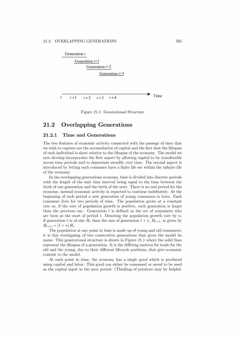
21.2. OVERLAPPING GENERATIONS 505
Timet 1+t 2+t 3+t 4+t
Generation t
Generation t+1Generation t+2
Generation t+3
Figure 21.1: Generational Structure
21.2 Overlapping Generations
21.2.1 Time and Generations
The two features of economic activity connected with the passage of time thatwe wish to capture are the accumulation of capital and the fact that the lifespanof each individual is short relative to the lifespan of the economy. The model wenow develop incorporates the first aspect by allowing capital to be transferableacross time periods and to depreciate steadily over time. The second aspect isintroduced by letting each consumer have a finite life set within the infinite lifeof the economy.In the overlapping generations economy, time is divided into discrete periods
with the length of the unit time interval being equal to the time between thebirth of one generation and the birth of the next. There is no end period for theeconomy, instead economic activity is expected to continue indefinitely. At thebeginning of each period a new generation of young consumers is born. Eachconsumer lives for two periods of time. The population grows at a constantrate so, if the rate of population growth is positive, each generation is largerthan the previous one. Generation t is defined as the set of consumers whoare born at the start of period t. Denoting the population growth rate by n,if generation t is of size Ht then the size of generation t+ 1, Ht+1, is given byHt+1 = [1 + n]Ht.The population at any point in time is made up of young and old consumers;
it is this overlapping of two consecutive generations that gives the model itsname. This generational structure is shown in Figure 21.1 where the solid linesrepresent the lifespan of a generation. It is the differing motives for trade for theold and the young, due to their different lifecycle positions, that give economiccontent to the model.At each point in time, the economy has a single good which is produced
using capital and labor. This good can either be consumed or saved to be usedas the capital input in the next period. (Thinking of potatoes may be helpful.
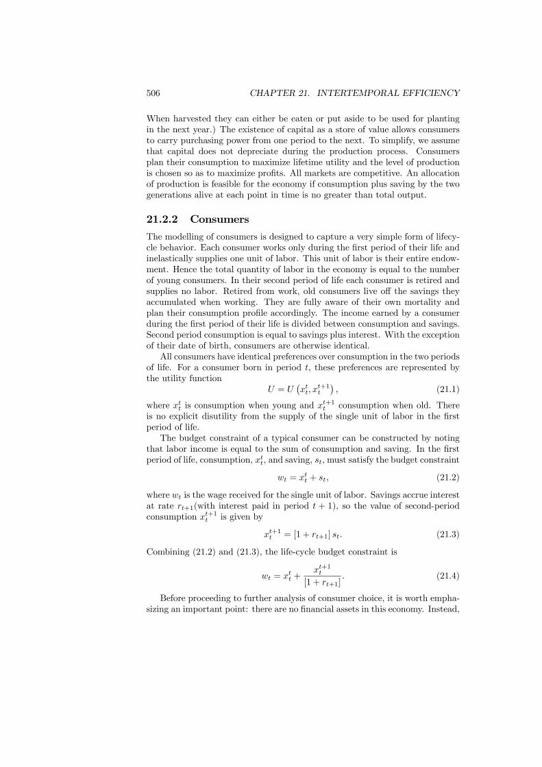
506 CHAPTER 21. INTERTEMPORAL EFFICIENCY
When harvested they can either be eaten or put aside to be used for plantingin the next year.) The existence of capital as a store of value allows consumersto carry purchasing power from one period to the next. To simplify, we assumethat capital does not depreciate during the production process. Consumersplan their consumption to maximize lifetime utility and the level of productionis chosen so as to maximize profits. All markets are competitive. An allocationof production is feasible for the economy if consumption plus saving by the twogenerations alive at each point in time is no greater than total output.
21.2.2 Consumers
The modelling of consumers is designed to capture a very simple form of lifecy-cle behavior. Each consumer works only during the first period of their life andinelastically supplies one unit of labor. This unit of labor is their entire endow-ment. Hence the total quantity of labor in the economy is equal to the numberof young consumers. In their second period of life each consumer is retired andsupplies no labor. Retired from work, old consumers live off the savings theyaccumulated when working. They are fully aware of their own mortality andplan their consumption profile accordingly. The income earned by a consumerduring the first period of their life is divided between consumption and savings.Second period consumption is equal to savings plus interest. With the exceptionof their date of birth, consumers are otherwise identical.All consumers have identical preferences over consumption in the two periods
of life. For a consumer born in period t, these preferences are represented bythe utility function
U = U¡xtt, x
t+1t
¢, (21.1)
where xtt is consumption when young and xt+1t consumption when old. There
is no explicit disutility from the supply of the single unit of labor in the firstperiod of life.The budget constraint of a typical consumer can be constructed by noting
that labor income is equal to the sum of consumption and saving. In the firstperiod of life, consumption, xtt, and saving, st, must satisfy the budget constraint
wt = xtt + st, (21.2)
where wt is the wage received for the single unit of labor. Savings accrue interestat rate rt+1(with interest paid in period t + 1), so the value of second-periodconsumption xt+1t is given by
xt+1t = [1 + rt+1] st. (21.3)
Combining (21.2) and (21.3), the life-cycle budget constraint is
wt = xtt +
xt+1t
[1 + rt+1]. (21.4)
Before proceeding to further analysis of consumer choice, it is worth empha-sizing an important point: there are no financial assets in this economy. Instead,
21.2. OVERLAPPING GENERATIONS 507
ttx
1+ttx
tw
[ ]11 ++ tt rw
Consumptionwhen young
Consumption when old
Figure 21.2: Consumer Choice
saving takes the form of investment in real capital. The interest rate is thereforeequal to the return on capital, and the same interest rate guides the investmentin capital by firms.From (21.1) and (21.4) the utility-maximizing consumption plan satisfies the
first-order condition ‘∂U∂xtt∂U
∂xt+1t
= [1 + rt+1] . (21.5)
In (21.5) the left-hand side is the intertemporal marginal rate of substitutionbetween consumption in the two periods of life. The right-hand side is the in-tertemporal marginal rate of transformation. The solution to this choice prob-lem is illustrated in Figure 21.2.
21.2.3 Production
The productive sector of the economy is assumed to consist of many compet-itive firms all producing with the same constant-returns-to-scale productiontechnology. These assumptions allow the firms to be aggregated into one sin-gle representative firm modelled by an aggregate production function. Using arepresentative firm greatly simplifies the presentation.It has been assumed that the capital used in production does not depreciate
(this simplifies matters, but has no significant economic consequences). At theend of the production process in each period, the firm has: (a) the (undepreci-ated) capital used in production and (b) new output. The sum of these is the

508 CHAPTER 21. INTERTEMPORAL EFFICIENCY
total output of the economy which is divided between saving (to be re-investedas capital) and consumption. To be consistent, the aggregate production func-tion is defined to measure the gross output of the firm which is the sum ofnew output plus the undepreciated capital. Denote this production functionby F (Kt, Lt), where Kt is the capital stock in period t and Lt is aggregatelabor supply. An allocation is feasible if gross output is equal to the sum ofconsumption for the two generations alive at time t plus savings
F (Kt, Lt) = Htxtt +Ht−1x
tt−1 +Htst. (21.6)
The representative firm chooses its use of capital and labor to maximizeprofits, πt, where
πt = F (Kt, Lt)− wtLt − rtKt. (21.7)
Note that this expression for profit values net output and the undepreciatedcapital equally and assigns a rental rate of rt for the use of capital. The necessarycondition for choice of the level of capital is
FK = rt. (21.8)
This is just the usual statement that capital should be employed up to thepoint at which its marginal product, FK , is equal to its cost, rt. The first-ordercondition for the quantity of labor input is
FL = wt, (21.9)
so labor is employed up to the point at which its marginal product, FL, is equalto the wage, wt.This development of the firm’s decision problem allows the results to be
related to standard results from microeconomics. However an alternative pre-sentation is more helpful in the context of an overlapping generations economywith a possibly variable population. In this case what matters for economicwelfare is not just how much is produced but, instead, how much is producedper unit of labor. An increase in production per unit of labor (with labor equalto the number of young consumers) can allow an unambiguous increase in wel-fare, provided it is correctly distributed, but an increase in production, withoutreference to the size of population, can not. To capture these observations, it ispreferable to re-phrase the formulation of the production function.It is now assumed that the production function satisfies constant returns to
scale. This assumption makes it possible to write
Yt = LtF
µKt
Lt, 1
¶= Ltf
µKtLt
¶, (21.10)
where Kt
Ltis the capital/labour ratio. Defining yt = Yt
Ltand kt = Kt
Lt, net output
per unit of labor is determined by a function that has the capital/labor ratio asits sole argument
yt = f (kt) . (21.11)
21.3. EQUILIBRIUM 509
It is assumed that this function satisfies f (0) = 0, f 0 > 0 and f 00 < 0 so that nooutput can be produced without capital and the marginal product is positivebut decreasing. Using (21.10) it follows that the marginal product of capital is
∂Yt∂Kt
≡ FK = f 0, (21.12)
and the marginal product of labor
∂Yt∂Lt
≡ FL = f − KtLtf 0 = f − ktf 0. (21.13)
These derivatives can be used to re-write (21.8) and (21.9) as
f 0 (kt) = rt, (21.14)
and
f (kt)− ktf 0 (kt) = wt. (21.15)
Conditions (21.14) and (21.15) represent the optimal choice of capital and laborfor the firm when the production function is expressed in terms of the capi-tal/labor ratio. This pair of conditions characterize the choices arising fromprofit maximization by the firm.
21.3 Equilibrium
At an equilibrium for the overlapping generations economy it is necessary thatconsumers maximize utility, that the representative firm maximizes profit, andthat all markets clear. Since there is a single good which can be used as capitalor consumed, market clearing can be captured by the equality of demand andsupply on the capital market.Granted this fact, there are two ways in which equilibrium can be viewed.
The first is to consider the intertemporal equilibrium of the economy. By this ismeant a sequence of values for the economic variables that ensure markets are inequilibrium in every time period. This intertemporal equilibrium determines thefull time-path for the endogenous variables (xtt, x
t+1t , kt, wt and rt) and hence
their changes from one period to the next. The alternative form of equilibrium isto consider the steady-state of the economy. The steady state is the situation inwhich the endogenous variables remain constant over time. Such an equilibriumcan be thought of as a long-run position for the economy. By definition, oncethe economy reaches a steady-state it never leaves it.To describe either of the forms of equilibrium, it is first necessary to char-
acterize equilibrium on the capital market. Equilibrium is achieved when thequantity of capital used in production is equal to the level of savings, since cap-ital is the only store of value for saving. By definition, saving is labor incomeless consumption so st = wt − xtt. Hence, as there are Ht young consumers in
510 CHAPTER 21. INTERTEMPORAL EFFICIENCY
period t, the equality of total savings in period t with capital used in periodt+ 1 requires that
Ht£wt − xtt
¤= Kt+1. (21.16)
Dividing through byHt, recalling thatHt+1 = [1 + n]Ht andHt = Lt, expressesthis in terms of the capital/labor ratio as
wt − xtt = kt+1 [1 + n] . (21.17)
When (21.17) is satisfied, there is equilibrium in the capital market.
21.3.1 Intertemporal Equilibrium
An intertemporal equilibrium is a sequence©xtt, x
t+1t , kt, wt, rt
ªof the endoge-
nous variables that attain equilibrium in every time period t. In each time period,all consumers must maximize utility, the representative firm must maximizeprofit and the capital market must be in equilibrium. Putting these together,the set of conditions that must be simultaneously satisfied for the economy tobe in equilibrium are:
• Utility maximization: (21.5), (21.4);• Profit maximization: (21.14), (21.15);• Market clearing: (21.17).
The equilibrium determined by these conditions should be seen as one inwhich the economy develops over time. The way that this works can be under-stood by following the economy from its very beginning. Let the economy havean initial capital stock, k1, in period 1. This capital stock is endowed by natureand belongs to consumers who are already in the second period of life at thestart of economic activity. The level of capital and the initial labor force deter-mine the interest rate, r1, and wage rate, w1, from (21.14) and (21.15). Usingthese, (21.5), (21.4) and (21.17) simultaneously determine x11, x
21 and k2. Start-
ing with k2, the process can be repeated for the next time period. Continuingforward in this way, generates the entire equilibrium path of the economy.Although the intertemporal behavior of the overlapping generations economy
is of great analytical interest, it will not be pursued in detail here. Instead, ourfocus will be upon steady state from this point onwards.
21.3.2 Steady State
In the steady state, all variables are constant. Consequently consumers in allgenerations must have the same lifetime consumption plan. The quantity ofcapital per worker must also remain constant. These observations suggest aninterpretation of the steady state as the long-run equilibrium in which the econ-omy has reached the limit of its development (but note that this interpretationis only strictly true if the economy converges to the steady state).

21.3. EQUILIBRIUM 511
Since all variables are constant in the steady state, the notation can be sim-plified by dropping the subscripts referring to time. The steady-state equationsdetermining the wage and the interest rate are w = f(k)−kf 0(k) and r = f 0(k),where k, w and r are the (constant) capital/labor ratio, wage rate and interestrate. Each consumer’s budget constraint can then be written as
x1 +x2
1 + f 0 (k)= f (k)− kf 0 (k) , (21.18)
where x1 and x2 are the steady-state consumption levels in the first-period andsecond-period of the consumer’s life. The steady-state capital market equilib-rium condition becomes
f (k)− kf 0 (k)− x1 = [1 + n] k. (21.19)
These equations can be used to provide a helpful means of displaying the steadystate equilibrium. Solving (21.18) and (21.19) for the consumption levels x1 andx2 gives
x1 = f (k)− kf 0 (k)− [1 + n] k, (21.20)
andx2 = [1 + n] k [1 + f 0 (k)] . (21.21)
The interpretation of (21.20) and (21.21) is that each value of the steady-state capital/labor ratio k implies a steady-state level of first-period consump-tion from (21.20) and of second-period consumption from (21.21). As k is varied,this pair of equations generates a locus of
©x1, x2
ªpairs. This is termed the
consumption possibility frontier. It shows the steady-state consumption plansthat are possible for alternative capital/labor ratios.There are basic economic reasons for expecting the consumption possibility
frontier to describe a non-monotonic relationship between x1 and x2 as illus-trated in Figure 21.3. When k = 0 it can be seen immediately that x1 and x2
are both zero - no output can be produced without capital. This is illustratedby the frontier beginning at the origin in the figure. When k becomes positive,x1 and x2 also become positive. As k is increased, we move further around thefrontier with both x1 and x2 increasing. For large values of k, x1 may beginto fall and can even become zero since f (k) increases at an ever slower ratewhile [1 + n] k increases at a constant rate. The actual shape of the frontierdepends on how quickly the returns to capital decrease as the capital input isincreased whilst holding labor input constant. What is underlying this is thatlow values of k do not allow much to be produced so consumption must be low.As k increases, more consumption becomes possible. However, at high valuesof k decreasing returns to capital become important and consumption must bedecreased in order to support the reproduction of a very high capital stock.The importance of this construction is the following interpretation. All
points on the frontier are potentially steady-state equilibria. Each point de-termines a pair
©x1, x2
ªand an implied value of the capital/labor ratio, k. The

512 CHAPTER 21. INTERTEMPORAL EFFICIENCY
1x
2x
0=k
large k
increases k
Figure 21.3: Consumption Possibilities
steady-state that will actually arise as the competitive equilibrium of the econ-omy is determined by the interaction of consumer preferences and the consump-tion possibility frontier. The question then arises as to the efficiency propertiesof the consumption pair
©x1, x2
ªor equivalently of the value of k. That is, are
all values of k equally good or are some preferable to others? If some are prefer-able, will the competitive economic activity result in an optimal value of k inequilibrium? The answers to these questions are given in the following sections.Before proceeding to these, we first look at how the competitive equilibrium isdetermined.
The optimal choice of the consumer is a point where the indifference curveis tangential to the budget constraint. The budget constraint has gradient− [1 + r]. In a steady-state equilibrium the consumption plan
©x1, x2
ªmust
also be on the consumption possibility frontier and tangential to the budgetconstraint. The equilibrium is found by moving around the frontier until avalue of k is reached at which the indifference curve is tangent to the budgetconstraint defined by the rate of interest, r = f 0 (k) , at that level of capital.A steady-state equilibrium satisfying this condition and two non-equilibriumallocations, at a and b, are shown in Figure 21.4.
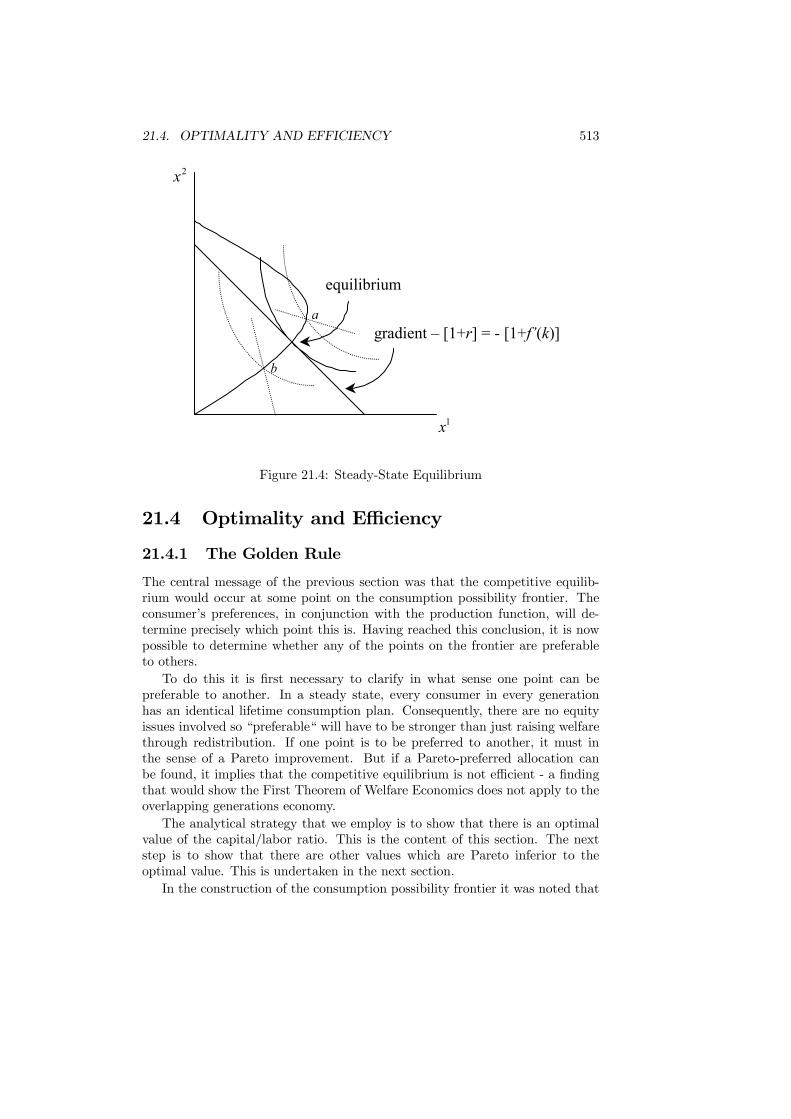
21.4. OPTIMALITY AND EFFICIENCY 513
1x
2x
gradient – [1+r] = - [1+f’(k)]
equilibrium
a
b
Figure 21.4: Steady-State Equilibrium
21.4 Optimality and Efficiency
21.4.1 The Golden Rule
The central message of the previous section was that the competitive equilib-rium would occur at some point on the consumption possibility frontier. Theconsumer’s preferences, in conjunction with the production function, will de-termine precisely which point this is. Having reached this conclusion, it is nowpossible to determine whether any of the points on the frontier are preferableto others.To do this it is first necessary to clarify in what sense one point can be
preferable to another. In a steady state, every consumer in every generationhas an identical lifetime consumption plan. Consequently, there are no equityissues involved so “preferable“ will have to be stronger than just raising welfarethrough redistribution. If one point is to be preferred to another, it must inthe sense of a Pareto improvement. But if a Pareto-preferred allocation canbe found, it implies that the competitive equilibrium is not efficient - a findingthat would show the First Theorem of Welfare Economics does not apply to theoverlapping generations economy.The analytical strategy that we employ is to show that there is an optimal
value of the capital/labor ratio. This is the content of this section. The nextstep is to show that there are other values which are Pareto inferior to theoptimal value. This is undertaken in the next section.In the construction of the consumption possibility frontier it was noted that
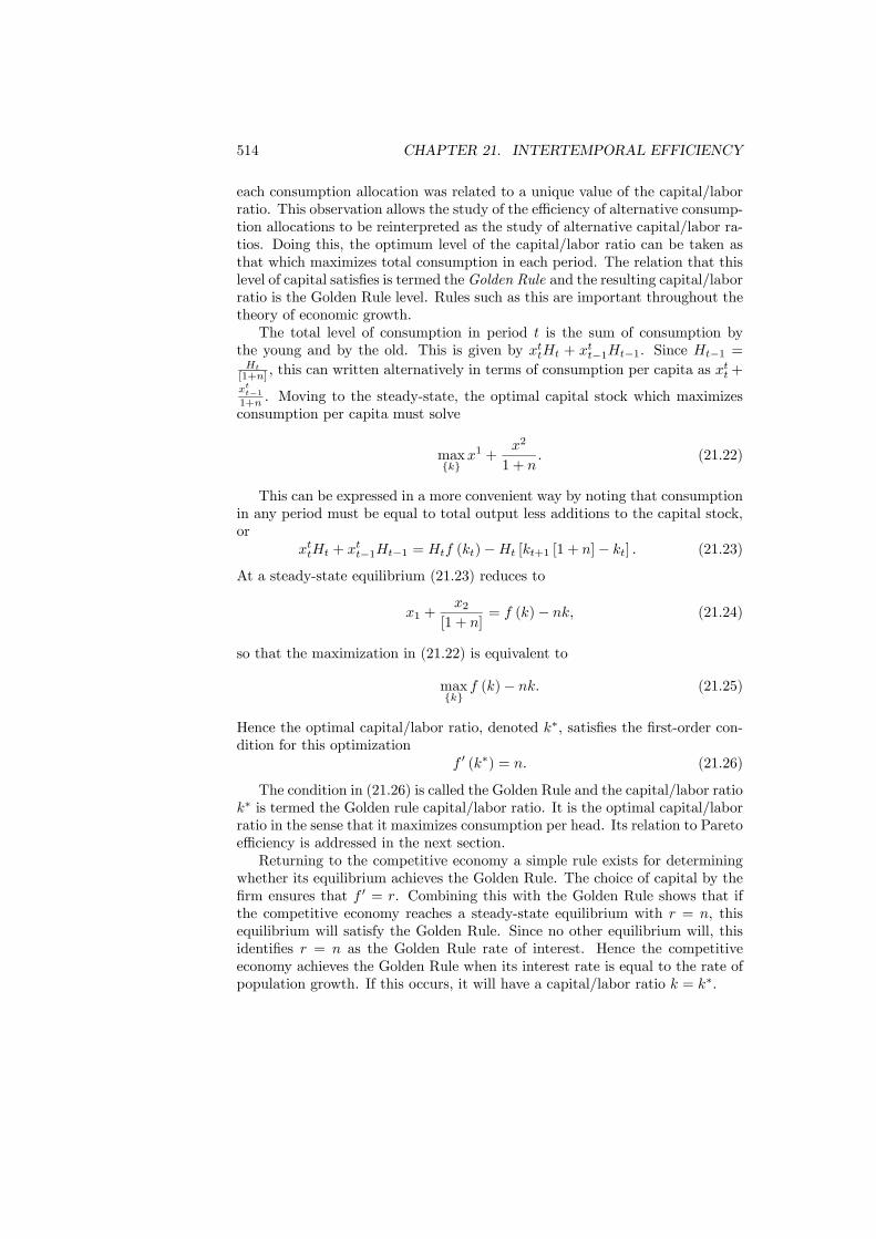
514 CHAPTER 21. INTERTEMPORAL EFFICIENCY
each consumption allocation was related to a unique value of the capital/laborratio. This observation allows the study of the efficiency of alternative consump-tion allocations to be reinterpreted as the study of alternative capital/labor ra-tios. Doing this, the optimum level of the capital/labor ratio can be taken asthat which maximizes total consumption in each period. The relation that thislevel of capital satisfies is termed theGolden Rule and the resulting capital/laborratio is the Golden Rule level. Rules such as this are important throughout thetheory of economic growth.The total level of consumption in period t is the sum of consumption by
the young and by the old. This is given by xttHt + xtt−1Ht−1. Since Ht−1 =
Ht
[1+n] , this can written alternatively in terms of consumption per capita as xtt+
xtt−11+n . Moving to the steady-state, the optimal capital stock which maximizesconsumption per capita must solve
max{k}
x1 +x2
1 + n. (21.22)
This can be expressed in a more convenient way by noting that consumptionin any period must be equal to total output less additions to the capital stock,or
xttHt + xtt−1Ht−1 = Htf (kt)−Ht [kt+1 [1 + n]− kt] . (21.23)
At a steady-state equilibrium (21.23) reduces to
x1 +x2
[1 + n]= f (k)− nk, (21.24)
so that the maximization in (21.22) is equivalent to
max{k}
f (k)− nk. (21.25)
Hence the optimal capital/labor ratio, denoted k∗, satisfies the first-order con-dition for this optimization
f 0 (k∗) = n. (21.26)
The condition in (21.26) is called the Golden Rule and the capital/labor ratiok∗ is termed the Golden rule capital/labor ratio. It is the optimal capital/laborratio in the sense that it maximizes consumption per head. Its relation to Paretoefficiency is addressed in the next section.Returning to the competitive economy a simple rule exists for determining
whether its equilibrium achieves the Golden Rule. The choice of capital by thefirm ensures that f 0 = r. Combining this with the Golden Rule shows that ifthe competitive economy reaches a steady-state equilibrium with r = n, thisequilibrium will satisfy the Golden Rule. Since no other equilibrium will, thisidentifies r = n as the Golden Rule rate of interest. Hence the competitiveeconomy achieves the Golden Rule when its interest rate is equal to the rate ofpopulation growth. If this occurs, it will have a capital/labor ratio k = k∗.
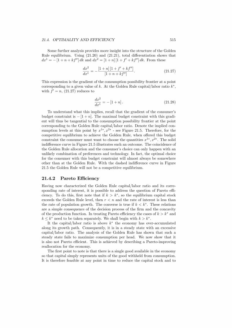
21.4. OPTIMALITY AND EFFICIENCY 515
Some further analysis provides more insight into the structure of the GoldenRule equilibrium. Using (21.20) and (21.21), total differentiation shows thatdx1 = − [1 + n+ kf 00] dk and dx2 = [1 + n] [1 + f 0 + kf 00] dk. From these
dx2
dx1= − [1 + n] [1 + f
0 + kf 00][1 + n+ kf 00]
. (21.27)
This expression is the gradient of the consumption possibility frontier at a pointcorresponding to a given value of k. At the Golden Rule capital/labor ratio k∗,with f 0 = n, (21.27) reduces to
dx2
dx1= − [1 + n] . (21.28)
To understand what this implies, recall that the gradient of the consumer’sbudget constraint is − [1 + n]. The maximal budget constraint with this gradi-ent will thus be tangential to the consumption possibility frontier at the pointcorresponding to the Golden Rule capital/labor ratio. Denote the implied con-sumption levels at this point by x1∗, x2∗ - see Figure 21.5. Therefore, for thecompetitive equilibrium to achieve the Golden Rule, when offered this budgetconstraint the consumer must want to choose the quantities x1∗, x2∗. The solidindifference curve in Figure 21.5 illustrates such an outcome. The coincidence ofthe Golden Rule allocation and the consumer’s choice can only happen with anunlikely combination of preferences and technology. In fact, the optimal choicefor the consumer with this budget constraint will almost always be somewhereother than at the Golden Rule. With the dashed indifference curve in Figure21.5 the Golden Rule will not be a competitive equilibrium.
21.4.2 Pareto Efficiency
Having now characterized the Golden Rule capital/labor ratio and its corre-sponding rate of interest, it is possible to address the question of Pareto effi-ciency. To do this, first note that if k > k∗, so the equilibrium capital stockexceeds the Golden Rule level, then r < n and the rate of interest is less thanthe rate of population growth. The converse is true if k < k∗. These relationsare a simple consequence of the decision process of the firm and the concavityof the production function. In treating Pareto efficiency the cases of k > k∗ andk ≤ k∗ need to be taken separately. We shall begin with k > k∗.It the capital/labor ratio is above k∗ the economy has over-accumulated
along its growth path. Consequently, it is in a steady state with an excessivecapital/labor ratio. The analysis of the Golden Rule has shown that such asteady state fails to maximize consumption per head. We now show that itis also not Pareto efficient. This is achieved by describing a Pareto-improvingreallocation for the economy.The first point to note is that there is a single good available in the economy
so that capital simply represents units of the good withheld from consumption.It is therefore feasible at any point in time to reduce the capital stock and to
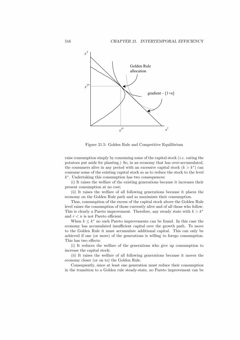
516 CHAPTER 21. INTERTEMPORAL EFFICIENCY
1x
2x
gradient – [1+n]
Golden Rule allocation
*1x
*2x
Figure 21.5: Golden Rule and Competitive Equilibrium
raise consumption simply by consuming some of the capital stock (i.e. eating thepotatoes put aside for planting.) So, in an economy that has over-accumulated,the consumers alive in any period with an excessive capital stock (k > k∗) canconsume some of the existing capital stock so as to reduce the stock to the levelk∗. Undertaking this consumption has two consequences:(i) It raises the welfare of the existing generations because it increases their
present consumption at no cost;(ii) It raises the welfare of all following generations because it places the
economy on the Golden Rule path and so maximizes their consumption.Thus, consumption of the excess of the capital stock above the Golden Rule
level raises the consumption of those currently alive and of all those who follow.This is clearly a Pareto improvement. Therefore, any steady state with k > k∗
and r < n is not Pareto efficient.When k ≤ k∗ no such Pareto improvements can be found. In this case the
economy has accumulated insufficient capital over the growth path. To moveto the Golden Rule it must accumulate additional capital. This can only beachieved if one (or more) of the generations is willing to forego consumption.This has two effects:(i) It reduces the welfare of the generations who give up consumption to
increase the capital stock;(ii) It raises the welfare of all following generations because it moves the
economy closer (or on to) the Golden Rule.Consequently, since at least one generation must reduce their consumption
in the transition to a Golden rule steady-state, no Pareto improvement can be
21.4. OPTIMALITY AND EFFICIENCY 517
made from the initial position. Therefore all states with k ≤ k∗ are Paretoefficient.In summary, any steady state with k > k∗ and r < n is not Pareto efficient.
Such states are called dynamically inefficient. Those with k ≤ k∗ are Paretoefficient and are termed dynamically efficient. The fact that steady-states whichare not Pareto efficient can exist despite the model satisfying all the standardbehavioral and informational assumptions that describe a competitive economyshows that the First Theorem of Welfare Economics cannot be extended toinclude overlapping generations economies. Therefore, these economies demon-strate the competition need not always lead to efficiency even when none of thestandard causes of inefficiency (such as monopoly) are present. This observationis one of the most fundamental to emerge out of the analysis of overlapping gen-erations economies. As we will see, it provides the motive for studying numerousforms of policy intervention.The discussion has concluded that a steady-state equilibrium with r < n is
not Pareto efficient despite the economy satisfying all the standard competitiveassumptions. However, it might still be suspected that to arrive at a steady-state with r < n requires some unusual structure to be placed on the economy.To show that this is not so, consider the following example. The utility functionof the single consumer in each generation is given by
U¡x1, x2
¢= β log x1 + [1− β] log x2, (21.29)
and the production function is y = Akα. Using the five equations describinga steady-state, the interest rate can be calculated to be (the derivation of thisresult is undertaken in Exercise 21.14)
r =α [1 + n]
[1− β] [1− α]. (21.30)
This will only be equal to the Golden Rule rate when
n =α
[1− β] [1− α]− α. (21.31)
If preferences and production do not satisfy this condition, and there is noreason why they should, the economy will not grow on the Golden Rule growthpath. This example illustrates that a Golden Rule economy will be the exceptionrather than the norm. A dynamically inefficient steady-state occurs when r < n.Using the solution for r in (21.30), this inequality can be written as
α
1− α<
n
1 + n[1− β] . (21.32)
From (21.32) it can been seen that this is most likely to arise when:(i) The increase in output following a marginal increase in the capital/labor
ratio is small (α low);(ii) The rate of population growth is high (n large);
518 CHAPTER 21. INTERTEMPORAL EFFICIENCY
(iii) The consumer places a high weight on second-period consumption (1−βlarge).
In conclusion, the efficiency of the steady-state equilibrium is dependentupon the relation of the capital stock to the Golden Rule level. The economymay reach an equilibrium at a dynamically inefficient steady-state which is notPareto efficient. In such a case, a Pareto improvement can be achieved byconsuming some of the capital stock. A Cobb-Douglas example illustrates thefactors that may lead to dynamic inefficiency.
Now that it has been demonstrated that the competitive equilibrium of theoverlapping generations economy need not be Pareto efficient, it remains to ex-plain why. There is a significant difficulty in doing this: there is no agreedexplanation for the inefficiency. To explore this further, consider a very sim-ple variant of the economy. In this variant there is no production, and henceno capital. Instead each young consumer is endowed with one unit of a con-sumption good while old consumers are endowed with nothing. Clearly, eachconsumer would like to even out consumption over the lifespan and so wouldtrade some consumption when young for consumption when old. But such atrade is not possible. The young could give the old some consumption butthe old have nothing to trade in exchange. Therefore, the only equilibrium isthat no trade takes place (a position called autarky) whereas a Pareto efficientallocation would have consumption in both periods of life.
It was in this setting that the inefficiency result was initially discovered.At first sight it might seem that it is just the structure of the economy - inparticular, the lack of any way of transferring purchasing power across periods- that prevents the attainment of Pareto efficiency. There are two responsesto this. First, in the standard competitive economy the efficiency result holdsindependent of any particular details of the economy. Second, the analysis ofthis chapter has already shown that inefficiency can hold even if consumers areable to hold savings which transfer purchasing power across periods. Inefficiencyusually arises when the market provides the wrong price signals. This is the case,for example, with monopoly and externalities. This might lead one to suspectthat the inefficiency can be explained because the interest rate provides thewrong signal for investment. But this cannot be the explanation since in themodel without production there is no interest rate.
There is one point that is agreed upon. As the overlapping generationseconomy has no end, over its lifespan it has an infinite number of consumersand, counting the good in each period as a different good, an infinite number ofgoods. The inefficiency can only arise if there is this double infinity of consumersand goods. We have already seen that the competitive economy with a finitenumber of goods and consumers is Pareto efficient. If the number of consumers isinfinite, but the number of goods finite, we have the idealized competitive modelwith each consumer being insignificant relative to the market and efficiencyagain holds. Finally, with a finite number of consumers but an infinite numberof goods, the economy is again efficient.

21.5. TESTING EFFICIENCY 519
21.5 Testing EfficiencyThe Golden Rule, and the characterization of dynamic efficiency, provide condi-tions which are very simple to evaluate. Before this can be done credibly, thereis an important issue concerning the assumptions describing the economy thatneed to be addressed. The most significant assumption was that of a constantgrowth rate in the population. The importance of this emerges in the fact thatthe Golden Rule is determined by the equality of the interest rate to the growthrate of population. If the growth rate is not constant, then this simple conditioncannot be used. To provide a general means of testing efficiency, an extensionmust be made to the analysis.A more general condition can be motivated as follows. In the economy
we have described, the growth rate of capital is equal to the growth rate ofpopulation in the steady state. Observing this, new investment in each periodis given by nK. The total payments to the owners of capital are rK. Thedifference between these, rK − nK measures the total flows out of the firm -which we can call dividend payments. The economy is dynamically efficient ifr ≥ n, which implies that dividend payments are positive so that funds areflowing out of the firm to the consumption sector. Conversely, the economy isdynamically inefficient if r < n so funds are flowing to the firm. The logic oflooking at the flows in or out of firms provides a more general method of testingefficiency than comparing the interest rate to the population growth rate sinceit holds under much less restrictive assumptions.The general version of the test is to look at the difference between gross
profit (the generalization of rK) and investment (the generalization of nK).The value of this difference, as a proportion of GDP, for a selection of countriesis presented in Table 21.1. All of the values in the table are positive which showsclear evidence that the countries are dynamically efficient. However, given thehigh values reported in the table, these countries remain some distance fromachieving the Golden Rule.
Year England France Germany Italy Japan US1965 9.4 13.6 8.5 22.9 15.2 6.91970 7.5 11.8 7.8 18.9 11.6 5.61975 6.0 10.9 12.4 16.6 6.8 14.41980 10.1 8.3 8.4 12.9 7.5 10.21984 13.9 12.9 13.8 17.3 9.4 6.7
Table 21.1: Gross Profit minus Investment as a Proportion of GDPSource: Abel, Mankiw, Summers and Zeckhauser (1989)
21.6 ConclusionsThe overlapping generations economy provides a very flexible representation ofhow an economy evolves through time. It captures the natural features thatconsumers’ lives are short relative to the lifespan of the economy and that con-sumers allocate consumption in a rational way over their lifecycle. Using the
520 CHAPTER 21. INTERTEMPORAL EFFICIENCY
concept of the steady state also gives a description of equilibrium that is simpleto apply.The most interesting feature of the economy is that its lack of an ending
means that there is a double infinity of goods and consumers. This is responsiblefor creating a potential inefficiency of the competitive equilibrium. This is aresult in complete contrast to the static model. The chapter has characterizedboth efficient and optimal steady state equilibria. These produce a simple test ofdynamic efficiency which the evidence suggests is met by a range of economies.
Further readingThe classic paper which introduced the overlapping generations economy isSamuelson, P.A. (1958) “An exact consumption-loan model of interest with
or without the social contrivance of money“, Journal of Political Economy, 66,467 - 482.It must be noted that the focus of this paper is on providing an intertem-
poral model that determines the interest rate endogenously. The inefficiencyresult, which has generated an immense literature since, falls out as an almostunintentional by-product of this.The model used here was introduced in:Diamond, P.A. (1965) “National debt in a neo-classical growth model“, Jour-
nal of Political Economy, 55, 1126 - 1150.Two interesting discussions (but note the first is very technical) of the inef-
ficiency result are:Geanakoplos, J. (1987) ”Overlapping generations model of general equilib-
rium” in J. Eatwell, M. Milgate and P. Newman (eds.) The New Palgrave: ADictionary of Economics (London: Macmillan).Shell, K. (1971) “Notes on the economics of infinity“, Journal of Political
Economy, 79, 1002 - 1011.For a study of the role of money in overlapping generations, see:Hahn, F.H. (1982) Money and inflation, Oxford: Basil Blackwell.The empirical analysis of efficiency is taken from:Abel, A.B., N.G. Mankiw, L.H. Summers and R.J. Zeckhauser (1989) ”As-
sessing dynamic efficiency”, Review of Economic Studies, 56, 1 - 19.

Chapter 22
Social Security and Debt
22.1 Introduction
A typical social security system provides income during periods of unemploy-ment, ill-health or disability and financial support, in the form of pensions, tothe retired. Although the generosity of systems varies between countries, theseelements are present in all developed economies. The focus of this chapter isthe economic implications of financial assistance to the retired. The overlappinggenerations economy proves to be ideal for this purpose.In economic terms, the analysis of that part of the social security system
which provide assistance during unemployment or ill-health is concerned withissues of uncertainty and insurance. Specifically, unemployment and ill-healthcan be viewed as events which are fundamentally uncertain and the provision ofsocial security is insurance cover against bad outcomes. In contrast retirementis an inevitable outcome, or at least an option, once the retirement age has beenreached. Insurance is therefore not the main issue (except for the problem ofliving for longer than accumulated wealth can finance). Instead, the issues thatare raised with pensions are the potential transfers of resources between genera-tions and the effect upon savings behavior in the economy. Both of these issuesrequire a treatment that is set within an explicitly intertemporal framework.The pensions systems in many developed economies are coming under pres-
sure in a process that has become known as the ”pensions crisis”. The roots ofthis crisis can be found in the design of the systems and the process of change inpopulation structure. The potential extent of this crisis provides strong groundsfor holding the view that reform of the pension system is currently one of themost pressing economic policy challenges.After describing alternative forms of pension systems, the nature of the
pensions crisis is described. This introduces the concept of the dependencyratio and the how this ratio links pensions and pension contributions. Theeconomic analysis of social security begins with a study of their effect upon theequilibrium of the economy. Chapter 21 introduced the overlapping generations
521
522 CHAPTER 22. SOCIAL SECURITY AND DEBT
economy and showed how its competitive equilibrium may be inefficient. Thepotential for inefficiency opens up the possibility of efficiency-enhancing policyinterventions. From this perspective, we consider whether social security canenhance efficiency. The fact that it may can be understood from the effect ofsocial security upon the level of the capital stock. If a social security programhas the form of forced saving, so that consumers are provided with greatersecond-period income than they would naturally choose, then the program mayraise the capital stock through the increased savings it generates. This will bebeneficial in an undercapitalized economy. Conversely, if the program simplytransfers earnings from those who are working to those who are retired, savingsand hence the level of capital will fall. These observations motivate the searchfor a social security program that can guide the economy to the Golden Rule.The fall in the birth rate is one of the causes of the pensions crisis. It is
an interesting question to consider how a change in the birth rate affects thelevel of welfare at the steady-state of an overlapping generations economy. Wepursue this issue by considering how the birth rate affects the structure of theconsumption possibility frontier, both in the absence and in the presence ofa social security program. Social security may be beneficial for the economy,but there are issues of political economy connected with the continuation of aprogram. The introduction of a program with the structure observed in practiceresults in a transfer of resources towards the first generation of retired (theyreceive but do not contribute) and away from some of the generations thatfollow. This raises question of how such a program is ever sustained since eachgeneration has incentive to receive but not to contribute. The final analyticalissue is to review the concept of Ricardian equivalence and its implications forsocial security. Ricardian equivalence is the observation that by changing theirbehavior consumers are able to offset the actions of the government. We showthe consequences this can have for social security and address the limitationsof the argument. Finally, after having completed the analytical material, wereturn to address some of the proposals that have been made for the reform ofsocial security programs.
22.2 Types of System
One defining characteristic of a social security system is whether pensions arepaid from an accumulated fund or from current tax contributions. This featureforms the distinction between fully-funded and pay-as-you-go social securitysystems. The economic effects, both in terms of efficiency and distribution,between these two polar forms of system are markedly different.In a pay-as-you-go social security program the current contributions through
taxation of those in employment provide the pensions of those who are retired.At any point in time, the contributions to the system must match the pensionpayments made by the system. The social security systems presently in opera-tion in the US, the UK, and numerous other countries are broadly of this form.The qualifier ”broadly” is used because, for example, though the US system
22.2. TYPES OF SYSTEM 523
owns some assets and could afford a short-term deficit, the assets would fundonly a very short period of payments. At each point in time, a pay-as-you-gosystem satisfies the equality
benefits received by retired = contributions of workers (22.1)
This equality can be expressed in terms of the number of workers and pensionersby
βR = τE, (22.2)
where τ is the average social security contribution of each worker, β is theaverage pension received, E the number of workers in employment and R thenumber of retired. If there is a constant rate of growth of population, so theworkforce is a constant multiple of retired population, then E = [1 + n]R. Usingthis in (22.2), βR = τ [1 + n]R or
β = [1 + n] τ . (22.3)
This relationship implies that the tax paid when young earns interest at raten before being returned as a pension when old. Hence in a pay-as-you-go pen-sion system the return on contributions is determined by the growth rate ofpopulation.In a fully-funded system each worker makes a contributions toward social
security via the social security tax and the contributions are invested by thesocial security program. The program therefore builds up a pension fund foreach worker. The total pension benefits received by the worker when retired arethen equal to their contribution to the program plus the return received on theinvestment. Such a program satisfies the equalities
pensions = social security tax plus interest = investment plus return. (22.4)
The implication of this constraint is that the fund earns interest at rate r, sothe pension and the tax are related by
β = [1 + r] τ . (22.5)
A fully-funded social security system forces each worker to save an amountat least equal to the tax they pay. It remains possible for workers to savemore if they choose to do so. If, in the absence of social security, all workerschose to save an amount in excess of the taxed levied by the program then,holding all else constant, a fully-funded system will simply replace some of theprivate saving by an equivalent amount of public saving. In this case, a fully-funded system will have no effect upon the equilibrium outcome. We explore thisobservation further when we discuss Ricardian Equivalence in Section 22.8. Inmore general settings with a variety of investment opportunities, the possibilitymust be considered that the rate of return on private savings may differ fromthat on public savings. When it does, a fully-funded system may affect theequilibrium. This point arises again in the analysis of pension reform.

524 CHAPTER 22. SOCIAL SECURITY AND DEBT
Contrasting these two forms of system, it can be observed that a pay-as-you-go system leads to an intergenerational transfer of resources, from currentworkers to current retired, whereas a fully-funded system can at most cause anintertemporal reallocation for each generation. This observation suggests thatthe two systems will have rather different welfare implications; these will beinvestigated in the following sections. In addition, the pay-as-you-go systemhas a return of n on contributions and the fully-funded system has a return ofr. These returns will differ unless the economy is at the Golden Rule allocation.Systems that fall between these two extremes will be termed non-fully-
funded. Such systems make some investments but the payments made in anygiven period may be greater than or less than the revenue, composed of taxpayments plus return on investment, received in that period. The differencebetween payments and revenue will comprise investment, or disinvestment, inthe pension fund.
22.3 The Pensions Crisis
Many countries face a pensions crisis which will require that their pensionssystems are significantly reformed. This section identifies the nature and con-sequences of this crisis. Once the analysis of social security is completed, wereturn in Section 22.9 to review a range of proposals for reform of the systemin the light of this crisis.The basis of the pensions crisis is three-fold. Firstly, most developed economies
have witnessed a reduction in their birth rates. Although immigration has par-tially offset the effect of this in some countries, there has still been a net effectof a steady reduction in the addition of new workers. The second effect is thatlongevity is increasing so that people are on average living longer. For any givenretirement age, this is increasing the number of retired. Thirdly, there is also atendency for the retirement age to fall.The net effect of these three is that the proportion of retired in the population
is growing and it is this that is problematic. In general terms, as the proportionof the population that is retired increases, the output of each worker mustsupport an ever larger number of people. Output per capita must increasejust to keep consumption per capita constant. If output does not rise quicklyenough, then productivity gains will be diluted and output per capita will fall.Furthermore, supporting the retired at a given standard of living will imposean increasing burden upon the economy.The size of this effect can be seen by looking at forecasts for the dependency
ratio. The dependency ratio measures the relative size of the retired populationand is defined as the size of the retired population relative to the size of theworking population. Table 22.1 reports the dependency ratio for a range ofcountries over the recent past and forecasts for its development into the future.The countries in the table are typical with the dependency ratio forecast toincrease substantially - in all cases the ratio more than doubles from 1980 to2040. This means that those working have to support an increasing propor-
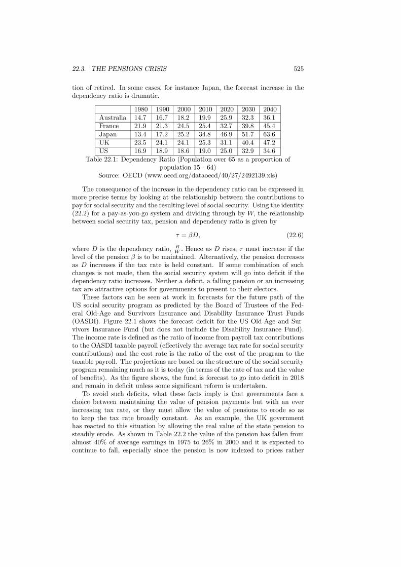
22.3. THE PENSIONS CRISIS 525
tion of retired. In some cases, for instance Japan, the forecast increase in thedependency ratio is dramatic.
1980 1990 2000 2010 2020 2030 2040Australia 14.7 16.7 18.2 19.9 25.9 32.3 36.1France 21.9 21.3 24.5 25.4 32.7 39.8 45.4Japan 13.4 17.2 25.2 34.8 46.9 51.7 63.6UK 23.5 24.1 24.1 25.3 31.1 40.4 47.2US 16.9 18.9 18.6 19.0 25.0 32.9 34.6
Table 22.1: Dependency Ratio (Population over 65 as a proportion ofpopulation 15 - 64)
Source: OECD (www.oecd.org/dataoecd/40/27/2492139.xls)
The consequence of the increase in the dependency ratio can be expressed inmore precise terms by looking at the relationship between the contributions topay for social security and the resulting level of social security. Using the identity(22.2) for a pay-as-you-go system and dividing through by W, the relationshipbetween social security tax, pension and dependency ratio is given by
τ = βD, (22.6)
where D is the dependency ratio, RW . Hence as D rises, τ must increase if the
level of the pension β is to be maintained. Alternatively, the pension decreasesas D increases if the tax rate is held constant. If some combination of suchchanges is not made, then the social security system will go into deficit if thedependency ratio increases. Neither a deficit, a falling pension or an increasingtax are attractive options for governments to present to their electors.These factors can be seen at work in forecasts for the future path of the
US social security program as predicted by the Board of Trustees of the Fed-eral Old-Age and Survivors Insurance and Disability Insurance Trust Funds(OASDI). Figure 22.1 shows the forecast deficit for the US Old-Age and Sur-vivors Insurance Fund (but does not include the Disability Insurance Fund).The income rate is defined as the ratio of income from payroll tax contributionsto the OASDI taxable payroll (effectively the average tax rate for social securitycontributions) and the cost rate is the ratio of the cost of the program to thetaxable payroll. The projections are based on the structure of the social securityprogram remaining much as it is today (in terms of the rate of tax and the valueof benefits). As the figure shows, the fund is forecast to go into deficit in 2018and remain in deficit unless some significant reform is undertaken.To avoid such deficits, what these facts imply is that governments face a
choice between maintaining the value of pension payments but with an everincreasing tax rate, or they must allow the value of pensions to erode so asto keep the tax rate broadly constant. As an example, the UK governmenthas reacted to this situation by allowing the real value of the state pension tosteadily erode. As shown in Table 22.2 the value of the pension has fallen fromalmost 40% of average earnings in 1975 to 26% in 2000 and it is expected tocontinue to fall, especially since the pension is now indexed to prices rather
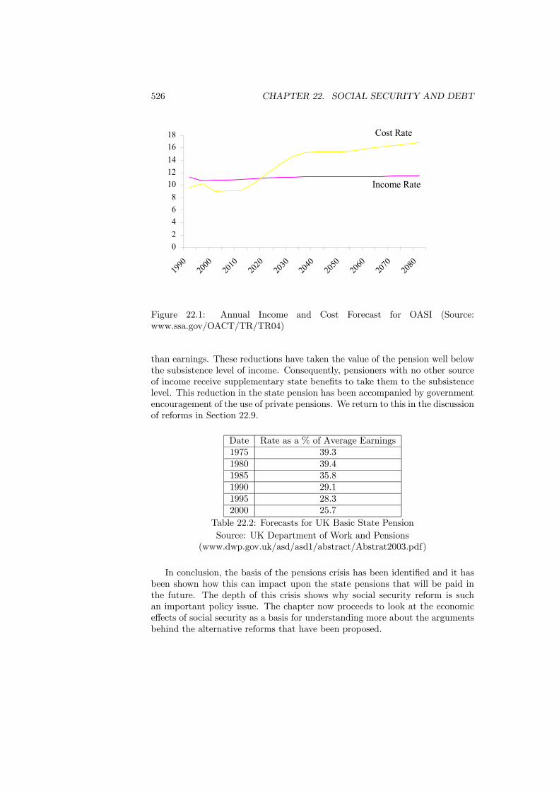
526 CHAPTER 22. SOCIAL SECURITY AND DEBT
02468
1012141618
1990
2000
2010
2020
2030
2040
2050
2060
2070
2080
Income Rate
Cost Rate
Figure 22.1: Annual Income and Cost Forecast for OASI (Source:www.ssa.gov/OACT/TR/TR04)
than earnings. These reductions have taken the value of the pension well belowthe subsistence level of income. Consequently, pensioners with no other sourceof income receive supplementary state benefits to take them to the subsistencelevel. This reduction in the state pension has been accompanied by governmentencouragement of the use of private pensions. We return to this in the discussionof reforms in Section 22.9.
Date Rate as a % of Average Earnings1975 39.31980 39.41985 35.81990 29.11995 28.32000 25.7
Table 22.2: Forecasts for UK Basic State PensionSource: UK Department of Work and Pensions
(www.dwp.gov.uk/asd/asd1/abstract/Abstrat2003.pdf)
In conclusion, the basis of the pensions crisis has been identified and it hasbeen shown how this can impact upon the state pensions that will be paid inthe future. The depth of this crisis shows why social security reform is suchan important policy issue. The chapter now proceeds to look at the economiceffects of social security as a basis for understanding more about the argumentsbehind the alternative reforms that have been proposed.
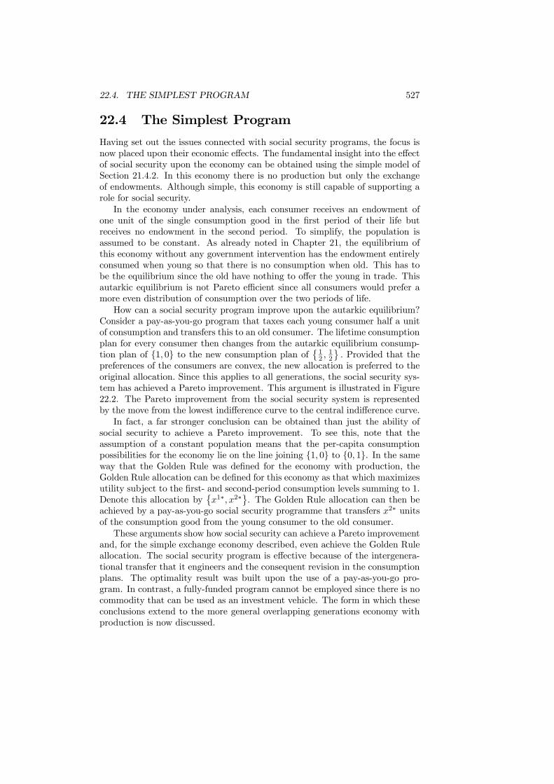
22.4. THE SIMPLEST PROGRAM 527
22.4 The Simplest Program
Having set out the issues connected with social security programs, the focus isnow placed upon their economic effects. The fundamental insight into the effectof social security upon the economy can be obtained using the simple model ofSection 21.4.2. In this economy there is no production but only the exchangeof endowments. Although simple, this economy is still capable of supporting arole for social security.In the economy under analysis, each consumer receives an endowment of
one unit of the single consumption good in the first period of their life butreceives no endowment in the second period. To simplify, the population isassumed to be constant. As already noted in Chapter 21, the equilibrium ofthis economy without any government intervention has the endowment entirelyconsumed when young so that there is no consumption when old. This has tobe the equilibrium since the old have nothing to offer the young in trade. Thisautarkic equilibrium is not Pareto efficient since all consumers would prefer amore even distribution of consumption over the two periods of life.How can a social security program improve upon the autarkic equilibrium?
Consider a pay-as-you-go program that taxes each young consumer half a unitof consumption and transfers this to an old consumer. The lifetime consumptionplan for every consumer then changes from the autarkic equilibrium consump-tion plan of {1, 0} to the new consumption plan of ©12 , 12ª . Provided that thepreferences of the consumers are convex, the new allocation is preferred to theoriginal allocation. Since this applies to all generations, the social security sys-tem has achieved a Pareto improvement. This argument is illustrated in Figure22.2. The Pareto improvement from the social security system is representedby the move from the lowest indifference curve to the central indifference curve.In fact, a far stronger conclusion can be obtained than just the ability of
social security to achieve a Pareto improvement. To see this, note that theassumption of a constant population means that the per-capita consumptionpossibilities for the economy lie on the line joining {1, 0} to {0, 1}. In the sameway that the Golden Rule was defined for the economy with production, theGolden Rule allocation can be defined for this economy as that which maximizesutility subject to the first- and second-period consumption levels summing to 1.Denote this allocation by
©x1∗, x2∗
ª. The Golden Rule allocation can then be
achieved by a pay-as-you-go social security programme that transfers x2∗ unitsof the consumption good from the young consumer to the old consumer.These arguments show how social security can achieve a Pareto improvement
and, for the simple exchange economy described, even achieve the Golden Ruleallocation. The social security program is effective because of the intergenera-tional transfer that it engineers and the consequent revision in the consumptionplans. The optimality result was built upon the use of a pay-as-you-go pro-gram. In contrast, a fully-funded program cannot be employed since there is nocommodity that can be used as an investment vehicle. The form in which theseconclusions extend to the more general overlapping generations economy withproduction is now discussed.
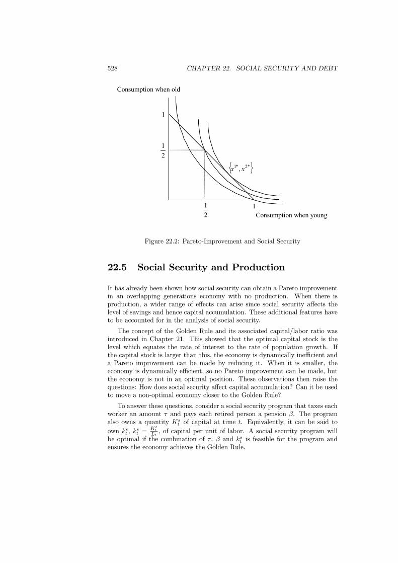
528 CHAPTER 22. SOCIAL SECURITY AND DEBT
Consumption when young
Consumption when old
21
21
1
1
{ }*2*1 , xx
Figure 22.2: Pareto-Improvement and Social Security
22.5 Social Security and Production
It has already been shown how social security can obtain a Pareto improvementin an overlapping generations economy with no production. When there isproduction, a wider range of effects can arise since social security affects thelevel of savings and hence capital accumulation. These additional features haveto be accounted for in the analysis of social security.
The concept of the Golden Rule and its associated capital/labor ratio wasintroduced in Chapter 21. This showed that the optimal capital stock is thelevel which equates the rate of interest to the rate of population growth. Ifthe capital stock is larger than this, the economy is dynamically inefficient anda Pareto improvement can be made by reducing it. When it is smaller, theeconomy is dynamically efficient, so no Pareto improvement can be made, butthe economy is not in an optimal position. These observations then raise thequestions: How does social security affect capital accumulation? Can it be usedto move a non-optimal economy closer to the Golden Rule?
To answer these questions, consider a social security program that taxes eachworker an amount τ and pays each retired person a pension β. The programalso owns a quantity Ks
t of capital at time t. Equivalently, it can be said toown kst , k
st =
Kst
Lt, of capital per unit of labor. A social security program will
be optimal if the combination of τ , β and kst is feasible for the program andensures the economy achieves the Golden Rule.

22.5. SOCIAL SECURITY AND PRODUCTION 529
A feasible social security program must satisfy the budget identity
βLt−1 = τLt + rtkstLt −
£kst+1Lt+1 − kstLt
¤, (22.7)
which states that pension payments must be equal to tax revenue plus the returnon capital holdings less investment in new capital. Since the population growsat rate n, in a steady state the identities Lt−1 = Lt
1+n , Lt+1 = [1 + n]Lt andkst+1 = k
st ≡ ks can be used in (22.7) to generate the steady state budget identity
β
1 + n= τ + [r − n] ks. (22.8)
Noting that the pension, β, which is received in the second period of life, isdiscounted in a consumer’s budget constraint (since x1+s = w−τ and [1 + r] s+β = x2, it follows that s = x2−β
1+r ), the budget constraint under the program canbe written
x1 +x2
1 + r= w − τ +
β
1 + r. (22.9)
The condition describing consumer choice remains
U1¡x1, x2
¢U2 (x1, x2)
= 1 + r. (22.10)
Equilibrium on the capital market requires that private savings are equal to totalcapital less the capital owned by the social security program. This conditioncan be expressed as
w − x1 − τ = [1 + n] [k − ks] . (22.11)
The choices of the representative firm do not change, so the conditions relatingfactor prices to capital still apply with
f 0(k) = r, (22.12)
f (k)− kf 0 (k) = w. (22.13)
The steady-state equilibrium with the pension program is the solution to equa-tions (22.8) to (22.13).The aim now is to investigate the effect that the social security policy can
have upon the equilibrium. To see why it may be possible to design a programthat can achieve the Golden Rule, it should be noted that the failure of thecompetitive equilibrium without intervention to achieve efficiency results fromthe savings behavior of individuals leading to over- or under-accumulation ofcapital. With the correct choice of social security program the government caneffectively force-save for individuals. This alters the steady state level of thecapital stock and hence the growth path of output.In equations (22.8) to (22.13) there are five private-sector choice variables
(k,x1, x2, w and r) which are treated as endogenous, plus the three variables(β, τ and ks) that describe the social security program. Given that there are six

530 CHAPTER 22. SOCIAL SECURITY AND DEBT
equilibrium conditions, the pension system can choose any two of the variablesdescribing the program with the third determined alongside the endogenousvariables. To analyze the system, it is simplest to treat β as endogenous and τand ks as exogenous.The method of analysis is to assume that the Golden Rule is achieved and
then to work back to the implications of this assumption. Consequently, letr = n. From the firm’s choice of capital, the Golden Rule is consistent witha capital stock that solves f 0(k∗) = n and hence a wage rate that satisfiesw = f (k∗) − k∗f 0 (k∗). The important observation is that with r = n, thebudget constraint for the social security program collapses to
β
1 + n= τ + [r − n] ks = τ , (22.14)
so a program attaining the Golden Rule must have the form of a pay-as-you-gosystem with β = [1 + n] τ . It is important to observe that any value of ks isconsistent with (22.14) when r = n, including positive values. This observationseems to conflict with the definition of a pay-as-you-go program. These com-ments are rationalized by the fact that we are working with the steady state ofthe economy. The social security program may own a stock of capital, ks > 0,but operating the pay-as-you-go-system it does not add to or subtract from thislevel of capital. Instead, the return on the capital it owns is just sufficient tomaintain it at a constant level. It remains true that along any growth path,including the steady state, a pay-as-you-go system cannot increase its capitalholdings.The values of the tax and capital stock of the program required to support
the Golden Rule can now be found by using the fact that the program is pay-as-you-go to reduce the consumer’s budget constraint to
x1 +x2
1 + r= w. (22.15)
Combining this constraint with the condition describing consumer choice, thedemand for first-period consumption must depend only on the wage rate andthe interest rate, so x1 = x1 (w, r). Using the conditions for the choice of thefirm, the wage rate and interest rate depend on the level of capital, so demandfor first-period consumption can be written as
x1 = x1 (w, r) = x1 (f (k)− kf 0 (k) , f 0 (k)) = x1 (k) . (22.16)
The capital market clearing condition can then be written as
w − x1 (k)− τ = [1 + n] [k − ks] . (22.17)
Using the conditions for the choice of the firm and evaluating at the GoldenRule level,
τ =£f (k∗)− k∗f 0 (k∗)− x1 (k∗)− [1 + n] k∗¤+ [1 + n] ks. (22.18)

22.5. SOCIAL SECURITY AND PRODUCTION 531
The condition determines pairs of values {τ , ks} that will achieve the GoldenRule.Any pair {τ , ks} that satisfies (22.18) will generate the Golden Rule, pro-
vided that the capital stock held by the program is not negative. For instance,if the program holds no capital, so ks = 0, then the value of the social securitytax will be
τ = f (k∗)− k∗f 0 (k∗)− x1 (k∗)− [1 + n] k∗. (22.19)
Although the discussion to this point has implicitly been based on the tax, τ ,being positive, it is possible that the optimal program may require it to benegative. If it is negative, the social security program will generate a transferfrom the old to the young.
As an example, if x1 (w, r) = w2 and f (k) = kα, then k∗ =
¡αn
¢ 11−α (see
Exercise 22.8 for the details of this derivation). Substituting into these valuesinto (22.19)
τ =³αn
´ 11−α
·[1− α]n
2α− [1 + n]
¸. (22.20)
If the rate of population growth is 5%, then the tax will be negative whenever
1
43< α. (22.21)
For this example, the tax rate is positive only for very small values of α.The results have shown that attainment of the Golden Rule requires a pay-
as-you-go social security system. By implication, a fully-funded program willfail to attain the Golden Rule. In fact, an even stronger result can be shown: afully-funded program will have no effect upon the equilibrium. To demonstratethis result, observe that a fully-funded program must satisfy the identity thatthe value of pension paid must equal the value of tax contributions plus interest,or
βLt−1 = τLt−1 [1 + rt] = ksLt [1 + rt] . (22.22)
Evaluated at a steady state
β = τ [1 + r] = ks [1 + n] [1 + r] . (22.23)
The substitution of (22.23) into the equilibrium conditions (22.8) to (22.13)shows that they reduce to the original market equilibrium conditions describedin (21.18) to (21.21). The fully-funded system therefore replaces private savingby public saving and does not affect the consumption choices of individual con-sumers. It therefore has no real effect upon the equilibrium and, if the initialsteady state were not at the Golden Rule, the fully-funded social security pro-gram will not restore efficiency. This observation is discussed further in Section22.8.This analysis has demonstrated how a correctly designed social security pro-
gram can generate the Golden Rule equilibrium, provided that it is not of thefully-funded kind. A fully-funded system does not affect the growth path. In
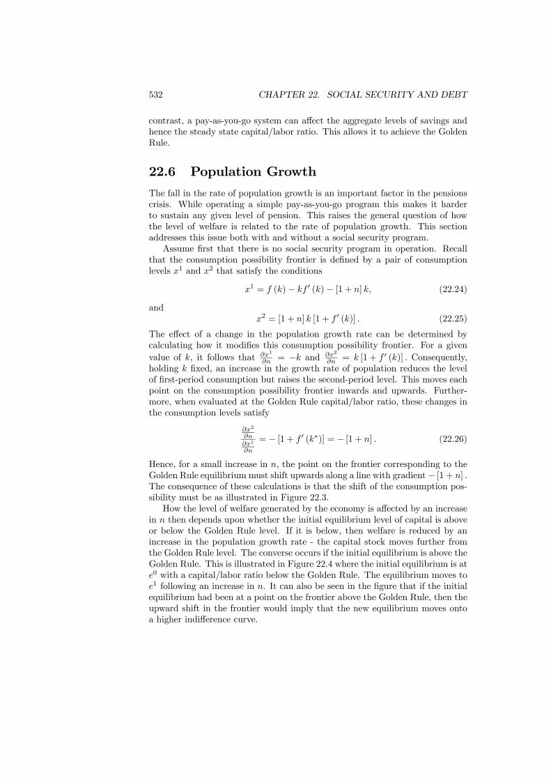
532 CHAPTER 22. SOCIAL SECURITY AND DEBT
contrast, a pay-as-you-go system can affect the aggregate levels of savings andhence the steady state capital/labor ratio. This allows it to achieve the GoldenRule.
22.6 Population GrowthThe fall in the rate of population growth is an important factor in the pensionscrisis. While operating a simple pay-as-you-go program this makes it harderto sustain any given level of pension. This raises the general question of howthe level of welfare is related to the rate of population growth. This sectionaddresses this issue both with and without a social security program.Assume first that there is no social security program in operation. Recall
that the consumption possibility frontier is defined by a pair of consumptionlevels x1 and x2 that satisfy the conditions
x1 = f (k)− kf 0 (k)− [1 + n] k, (22.24)
andx2 = [1 + n] k [1 + f 0 (k)] . (22.25)
The effect of a change in the population growth rate can be determined bycalculating how it modifies this consumption possibility frontier. For a givenvalue of k, it follows that ∂x1
∂n = −k and ∂x2
∂n = k [1 + f 0 (k)] . Consequently,holding k fixed, an increase in the growth rate of population reduces the levelof first-period consumption but raises the second-period level. This moves eachpoint on the consumption possibility frontier inwards and upwards. Further-more, when evaluated at the Golden Rule capital/labor ratio, these changes inthe consumption levels satisfy
∂x2
∂n∂x1
∂n
= − [1 + f 0 (k∗)] = − [1 + n] . (22.26)
Hence, for a small increase in n, the point on the frontier corresponding to theGolden Rule equilibriummust shift upwards along a line with gradient− [1 + n] .The consequence of these calculations is that the shift of the consumption pos-sibility must be as illustrated in Figure 22.3.How the level of welfare generated by the economy is affected by an increase
in n then depends upon whether the initial equilibrium level of capital is aboveor below the Golden Rule level. If it is below, then welfare is reduced by anincrease in the population growth rate - the capital stock moves further fromthe Golden Rule level. The converse occurs if the initial equilibrium is above theGolden Rule. This is illustrated in Figure 22.4 where the initial equilibrium is ate0 with a capital/labor ratio below the Golden Rule. The equilibrium moves toe1 following an increase in n. It can also be seen in the figure that if the initialequilibrium had been at a point on the frontier above the Golden Rule, then theupward shift in the frontier would imply that the new equilibrium moves ontoa higher indifference curve.
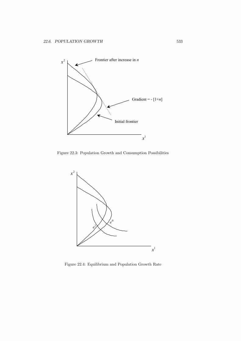
22.6. POPULATION GROWTH 533
1x
2x
Initial frontier
Frontier after increase in n
Gradient = - [1+n]
Figure 22.3: Population Growth and Consumption Possibilities
1x
2x
0e1e
Figure 22.4: Equilibrium and Population Growth Rate
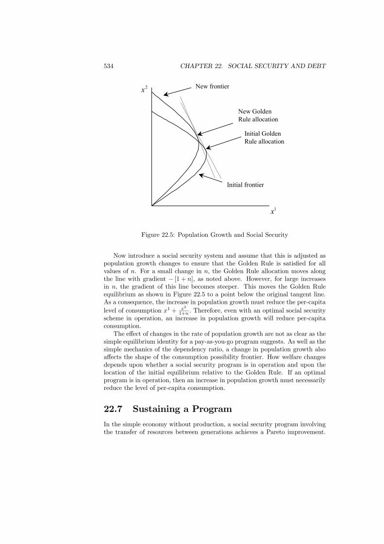
534 CHAPTER 22. SOCIAL SECURITY AND DEBT
1x
2x
Initial frontier
New frontier
Initial Golden Rule allocation
New Golden Rule allocation
Figure 22.5: Population Growth and Social Security
Now introduce a social security system and assume that this is adjusted aspopulation growth changes to ensure that the Golden Rule is satisfied for allvalues of n. For a small change in n, the Golden Rule allocation moves alongthe line with gradient − [1 + n], as noted above. However, for large increasesin n, the gradient of this line becomes steeper. This moves the Golden Ruleequilibrium as shown in Figure 22.5 to a point below the original tangent line.As a consequence, the increase in population growth must reduce the per-capitalevel of consumption x1 + x2
1+n . Therefore, even with an optimal social securityscheme in operation, an increase in population growth will reduce per-capitaconsumption.The effect of changes in the rate of population growth are not as clear as the
simple equilibrium identity for a pay-as-you-go program suggests. As well as thesimple mechanics of the dependency ratio, a change in population growth alsoaffects the shape of the consumption possibility frontier. How welfare changesdepends upon whether a social security program is in operation and upon thelocation of the initial equilibrium relative to the Golden Rule. If an optimalprogram is in operation, then an increase in population growth must necessarilyreduce the level of per-capita consumption.
22.7 Sustaining a Program
In the simple economy without production, a social security program involvingthe transfer of resources between generations achieves a Pareto improvement.

22.7. SUSTAINING A PROGRAM 535
This raises the obvious question of why such a program will not always beintroduced.The basic nature of the pay-as-you go pension program described above is
that the young make a transfer to the old without receiving anything directlyfrom those old in return. Instead, they must wait until their own old age beforereceiving the compensating payment. Although these transfers do give rise to aPareto improvement, it can be argued not to be in the young consumer’s privateinterest to make the transfer provided they expect to receive a transfer. If theydo not give their transfer, but still expect to receive, then their consumptionlevel will be increased. Clearly, this makes them better off and so they will notwish to make the transfer. Since the social security system is not individually-rational, how can the young be persuaded to consent to the imposition of thesocial security program?Two different answers to this question will be considered. The first answer
is based upon altruism on the part of the young - they are willing to providethe transfer because they care about the old. This rationalizes the existenceof a social security program but only by making an assumption that moveoutside the standard economic framework of individual self-interest. The secondanswer works with the standard neoclassical model of self-interest but showshow the program can be sustained by the use of ”punishment strategies” in anintertemporal game. It should be stressed that the fact that participation ina social security program is mandatory is not by itself a valid explanation ofthe existence of the program. Any program has to have willing participants toinitiate them (so that they must be individually-rational at their introduction)and need continuing support to sustain them.Altruism refers to feelings of concern for others beside oneself. It is natural
to think that altruism applies to close family members but it may also apply toconcern for people generally. Feelings of altruism can also be held with respectto animals, plants and even non-sentient objects.Although the existence of altruism takes us outside the standard perspective
of behavior driven by narrow self-interest, it need not affect the tools we employto analyze behavior. What is meant by this is that altruism alters the natureof preferences but does not affect the fact that a consumer will want to achievethe highest level of preference possible. Consequently, given a set of altruisticpreferences the consumer will still choose the action that best satisfies thosepreferences subject to the constraint placed upon their choices. The standardtools remain valid but operate on different preferences.There are numerous ways to represent altruism but one of the simplest is
to view it as consumption externality. Writing the utility of a consumer ingeneration t in the form
Ut = U¡xtt, x
t+1t , xtt−1
¢, (22.27)
gives an interpretation of altruism as concern for the consumption level, xtt−1,achieved by a member of the earlier generation (which is usually interpreted as
536 CHAPTER 22. SOCIAL SECURITY AND DEBT
the parent of the consumer). A very similar alternative would be to assume that
Ut = U¡xtt, x
t+1t , Ut−1
¢, (22.28)
so that altruism is reflected in a concern for the utility of the member of theearlier generation.Both of these forms of altruism can be seen to provide a motive for a social
security program that transfers resources from the young to the old. Consider(22.27). A consumer with this utility function can be thought of as choosingtheir personal consumption levels xtt, x
t+1t and a transfer, τ , to the old consumer.
The effect of the transfer is to raise the consumption level xtt−1 since the budgetconstraint of the old consumer is
xtt−1 = [1 + rt] st + τ . (22.29)
Provided the marginal utility generated by an increase in xtt−1 is sufficientlyhigh, the consumer will willingly choose to make a positive transfer. In thissense, the provision of social security has become individually rational.The rationality for participating in a social security program can be found
in the fact that each young person expects a similar transfer when they areold. They can then be threatened with having this removed if they do notthemselves act in the appropriate manner. This punishment can sometimes(but not always) be sufficient to ensure that compliance with the social securityprogram is maintained.To give substance to these observations, it is best to express the argument
using the language of game theory. The analysis so far has shown that thestrategy to provide a transfer is not a Nash equilibrium. Recall that in thedetermination of a Nash equilibrium each individual holds the strategies of allothers constant as they consider their own choice. So, if all others are providingtransfers, it will be a better strategy not to do so but to still receive. If othersare not transferring, then it is also best not to do so. Therefore not providing atransfer is a dominant strategy and the individually-rational Nash equilibriummust be for no transfers to take place.These simple Nash strategies are not the only ones that can be played.
To motivate what else can be done, it is best to think about repeated gamesand the more sophisticated strategies that can be played in them. A repeatedgame is one where the same “stage” game is played once each period for anendless number of periods by the same players. The prisoner’s dilemma givenin the matrix in Figure ?? has the general features of the social security model.Although it is not exactly the same since the social security model has manygenerations of consumers, not just the two given in the game.If both players contribute to social security, then a payoff of 5 is attained.
If neither contributes, the payoff is only 2. This reflects the fact that the socialsecurity equilibrium is Pareto preferred to the equilibrium without. However,the highest payoff is obtained if a player chooses not to contribute but the otherdoes. When played a single time, the unique Nash equilibrium is for both playersto choose Don’t Contribute - if the other contributes, then it pays not to. This

22.7. SUSTAINING A PROGRAM 537
Contribute Don’t contribute
Contribute
Don’t contribute
5, 5
2, 2
0, 10
10, 0
Player 1
Player 2
Figure 22.6: Social Security Game
reasoning applies to both players and hence the equilibrium. This equilibriumis inefficient and is Pareto dominated by {Contribute, Contribute}.The situation is completely changed if the game is repeated indefinitely and
the efficient equilibrium {Contribute, Contribute} can be sustained. The strat-egy that supports this is for each player to choose Contribute until their oppo-nent chooses Don’t Contribute. Once this has happened, they should continueto play Don’t Contribute from that point onwards.To evaluate the payoffs from this strategy, assume that the discount rate
between periods is δ. The payoff from always playing Contribute is then
5 + 5δ + 5δ2 + 5δ3 + . . . = 5
·1
1− δ
¸. (22.30)
Alternatively, if Don’t Contribute is played a temporary gain will be obtainedbut the payoff will then fall back to that at the Nash equilibrium of the single-period game once the other player switches to Don’t Contribute. This gives thepayoff
10 + 2δ + 2δ2 + 2δ3 + . . . = 10 + 2
·δ
1− δ
¸. (22.31)
Contrasting these, playing Contribute in every period will give a higherpayoff if
5
·1
1− δ
¸> 10 + 2
·δ
1− δ
¸, (22.32)
or
δ >5
8. (22.33)
That is, {Contribute, Contribute} will be an equilibrium if the players are suf-ficiently patient. The reason behind this is that a patient player will put a highvalue on payoffs well into the future. Therefore the reduction to a payoff of 2
538 CHAPTER 22. SOCIAL SECURITY AND DEBT
after the first period will be very painful. For a very impatient player, only thepayoff of 10 will really matter and they are driven to Don’t Contribute.The strategy just described is known as a “punishment strategy”: the de-
viation from Don’t Contribute is punished by reversion to the inefficient Nashequilibrium. Although the punishment will hurt both the players, the point isthat will not happen in equilibrium since the optimal play with these strate-gies is always to play Contribute. In summary, in an infinitely repeated game,punishment strategies can be used to support efficient equilibria.The same line of reasoning can be applied to the analysis of social security.
What is different in this context is that the same players do not interact everyperiod. Instead, it is a different pair of old and young consumers that meetin each period. However, the punishment strategy can still be employed in thefollowing way: each consumer when young will provide a transfer of size x to theold consumer that overlaps with them provided the old person they coexist withprovided a transfer in the previous period; otherwise no transfer is provided. Ifall generations of consumers play according to this strategy then the transferscan be made self-supporting.There remains one important limitation to this use of punishment strategies
in the social security environment. In order to implement the strategy, eachyoung consumer must know whether the transfer was made in the period be-fore they were alive. This issue does not arise in the standard application ofpunishment strategies since the players are alive in all periods — they need onlyremember what happened in the previous period. Consequently, some form ofverification device is necessary to support the punishment strategy. Withoutthe verification, the only equilibrium is for there to be no transfers which is aPareto inferior outcome.This discussion of pay-as-you-go social security has shown how such a system
can be sustained even when there is a short-run incentive for consumers not tomake the required transfers. The basis for this claim is that social security inan overlapping generations economy has the nature of a repeated game so that]strategies which punish the failure to provide a transfer can be employed. Whatthis analysis shows is that an apparent act of generosity — the gift of a transferto the older generation — can be made to be rational for each individual. Sothe provision of social security may occur not through altruism but throughrationality.
22.8 Ricardian Equivalence
Ricardian Equivalence refers to the proposition that the government can alter aneconomic policy and yet the equilibrium of the economy can remain unchanged.This occurs if consumers can respond to the policy by making off-setting changesin their behavior which neutralize the effect of the policy change. In terms of thepresent chapter, Ricardian equivalence holds when the government introduces,or changes, a social security system and yet the changes in individual behaviorrender the policy change ineffectual.
22.8. RICARDIAN EQUIVALENCE 539
Such equivalence results have already featured twice in the text. On thefirst occasion, in the analysis of the private purchase of public goods, it wasshown that, by changing their purchases, the individuals could offset the effectof income redistribution. Furthermore, it was also rational for the individualsto make the off-setting changes. The second case of equivalence arose in thederivation of the optimal social security program where it was noted that afully-funded system would not affect the capital/labor ratio. The explanationfor this equivalence was that consumers react to a fully-funded social securityprogram by making a reduction in their private saving which ensures total savingis unchanged.The common feature of these examples is that the effect of the policy change
and the off-setting reaction involve the same individuals. It is this that providesthem with a direct incentive to modify their behavior. Clearly, this is trueonly of a social security system that is fully-funded with a return equal to thaton private savings. If social security is anything but fully-funded, a changein the system will affect a number of generations since the system must beredistributive over time. In the case of pay-as-you-go, social security is purelyredistributive over time. A change in a program can therefore affect consumersin different generations who need not be alive at the time the program is changednor even be alive at the same time. At first sight, this would seem to mean thatit cannot be possible for equivalence to hold. This argument is in fact correctgiven the assumptions made so far.To give a basis for eliminating the effect of policy it is necessary to link the
generations across time so that something that affects one generation directlysomehow affects all generations indirectly. The way that this can be done isto return to the idea of altruism and intergenerational concern. Intuitivelywe can think of each consumer as having familial forebears and descendents(or parents and children in simple language). This time we assume that eachparent is concerned with the welfare of their children, and that their children areconcerned with the welfare of the grandchildren. Indirectly, although they arenot alive at the same time in the model, this makes the parents concerned aboutthe grandchildren. What effect does this have? It makes each family act as ifit was a dynasty stretching through time, and its decisions at any one momenttake into account all later consequences. A change in a social security programthen causes a reaction right through the decision process of the dynasty.To provide some details, let the utility of the generation born at time t be
Ut = U³xtt, x
t+1t , eUt+1´ . (22.34)
It is the term eUt+1 that represents the concern for the next generation. HereeUt+1 is defined as the maximum utility that will be obtained by the children,who are born at t+1, of the parent born in t. The fact that the family will actas a dynasty can the be seen by substituting for eUt+1 to give
Ut = U³xtt, x
t+1t , U
³xt+1t+1, x
t+2t+1,
eUt+2´´ . (22.35)
540 CHAPTER 22. SOCIAL SECURITY AND DEBT
If this substitution is continually repeated then the single parent born at tultimately cares about consumption levels in all future time periods.Using this fact, it is now possible to demonstrate that Ricardian Equivalence
applies to social security in these circumstances. Consider an initial positionwith no social security program. The consumer at t reflects their concern forthe descendent by making a bequest of value bt. Hence the consumption levelin the second period of life is
xt+1t = st [1 + rt+1]− bt, (22.36)
and that of their descendent is
xt+1t+1 = wt+1 + bt − st+1. (22.37)
Now assume that each consumer has one descendent and that the young con-sumers are taxed and amount τ to pay a pension of equal value to old consumersThen the consumption level of each parent satisfies
xt+1t = st [1 + rt+1] + τ −bbt, (22.38)
and that of their descendent
xt+1t+1 = wt+1 +bbt − τ − st+1. (22.39)
But now note that if the bequest is changed so that bbt = bt + τ , the sameconsumption levels can be achieved for both the parent and the child as forthe case with no pension. Furthermore, since these consumptions levels werethe optimal choice initially, they will still be the optimal choice. So the oldconsumer will make this change to their bequest and the social security schemewill have no effect.The conclusion of this analysis is that the change in the bequest can offset
the intertemporal transfer caused by a social security system. Although thiswas only a two period system, it can easily be seen that the same logic canbe applied to any series of transfers. All that the dynasty has to do is adjusteach bequest to offset the effect of the social security system between any twogenerations. The outcome is that the policy has no effect. This is the basicpoint of Ricardian Equivalence.It must be noted that there are limitations to this argument. Firstly, it is
necessary that there be active intergenerational altruism. Without this thereis no dynastic structure and the offsetting changes in bequests will not occur.In addition, the argument only works if the initial bequest is sufficiently largethat it can be changed to offset the policy without becoming negative. Doesit apply in practice? We clearly observe bequests but many of these may beunintentional and occur due to premature death.The concept of Ricardian Equivalence can be extended into other areas of
policy. Closely related to social security is the issue of government debt, whichis also an intergenerational transfer (but from children to parents), and its
22.9. SOCIAL SECURITY REFORM 541
effects upon the economy. This was the initial area of application for RicardianEquivalence, with changes in bequests offsetting changes in government debtpolicy. Furthermore, if links are made across households it becomes possiblefor changes in household choices to offset a policy that causes transfers betweenhouseholds. This has lead to the question of whether “everything is neutral?”.The answer depends upon the extent of the links.
22.9 Social Security Reform
The basic nature of the pensions crisis facing a range of economies was identi-fied in Section 22.3: increasing longevity and the decline in the birth rate arecombining to increase the dependency ratio. Without major reform or an un-acceptably high increase in tax rates, the pension programs will either go intodeficit or pay a much reduced pension. A variety of reforms have been proposedin response to this crisis. Some of these are now briefly reviewed.Underlying the crisis is the fact that the pension systems are essentially of
the pay-as-you-go form. With such a structure an increase in the dependencyratio will always put pressure upon the pension system. The reform most oftendiscussed in the US is for the social security system to move towards a fully-funded structure. Once the system reaches the point of being fully-funded,pensions are paid from the pension fund accumulated by each worker. Thisbreaks the identity relating pensions to the dependency ratio. A fully-fundedsystem can operate either as a government-run scheme of on the basis of privatepensions. We comment on this choice below. For now, we note that as well asreducing the real value of the pension, the UK government has moved in thedirection of a fully-funded program by encouraging the use of private pensions.The difficulty with this approach is that it relies on workers making adequateprovision for their retirement - and there is much evidence that this is not thecase.If an economy were to reform its pension system, it would take some time to
transit from the pay-as-you-go system to the fully-funded system. The reformrequires that a capital fund is established which takes a period of investment.Furthermore, the pay-as-you-go system cannot be terminated abruptly. Thosealready retired will still require to provide their pensions and those close toretirement will have too little time to invest in a pension fund and so willrequire the continuation of the pay-as-you-go element. These facts imply thatthose who are in work during the transition process will be required to bothpay the pensions of the retired and pay to finance their own pension fund. Insimple terms, they are paying for two sets of pensions and fare badly during thereform process. At the very least, this suggests that there could be significantpolitical pressure against the proposed reform.The distributional effects of a reform from a pay-as-you-go system to a fully-
funded system are illustrated by the simulation reported in Table 22.3. Thissimulation determines the growth path of the economic model for a referencecase in which the state pension is held constant. Applied to the UK, the model

542 CHAPTER 22. SOCIAL SECURITY AND DEBT
assumes that the value of the pension is 20% of average earnings. For theapplication to Europe, the value is taken to be 40%. A reform is then consideredwhere an announcement is made in 1997 (the year the research was conducted)that the state pension will be steadily reduced from the year 2020 until beingphased out in 2040. The aim of the long period between announcement andreduction is to allow for adjustment in private behavior. The removal of thestate pension implies that private savings will have to increase to compensate.The negative ages in the first column of Table 22.3 refer to consumers who
had not yet been born in 1997, so a consumer with age - 10 in 1997 will be bornin 2007. The numbers in the second and third columns shows the percentageby which the lifetime wage of that age group would need to be changed in thereference case to give the same level of welfare as in the reform case. Hence thevalue of -1.1 for the age group 40-50 in the UK shows that they are worse offwith the reform - a reduction of 1.1% of their wage in the base case would givethen the same welfare level as in the reform case.
Age in 1997 UK Europe> 57 0 050 - 57 - 0.09 - 0.640 - 50 - 1.1 - 2.330 - 40 - 3.0 - 5.720 - 30 - 3.8 - 7.210 - 20 - 2.3 - 4.20 - 10 0.7 1.7-10 - 0 3.95 9.2-20 - -10 6.5 15.7-40 - -30 7.4 18.7< -40 7.2 18.9
Table 22.3: Gains and Losses in transitionSource: Miles (1998)
The values in Table 22.3 show that the pension reform hurts those early inlife who must pay the pensions of the retired and pay into their own retirementfund. Ultimately, the reform benefits consumers in the long run. The long-rungain comes from the fact that the reduction in the pension leads to an increasein private saving. Private saving has to be invested, so there is also an increasein the capital stock. The consequence of this capital stock increase depends onthe initial level of capital compared to the Golden Rule level. In the simulations,capital is initially below the Golden Rule level and remains so throughout thetransition. But since this is moving the economy closer to the Golden Rule,there is ultimately a gain in welfare for later generations. The structure of thegains and losses also illustrates the political problem involved in implementingthe reform: those who must vote in favor of its implementation are those wholose the most. This political problem will be exacerbated by the aging of theelectorate that is expected over the next 50 years. Estimates of the age of themedian voter are given in Table 22.4. These reveal that the age of the median

22.9. SOCIAL SECURITY REFORM 543
voter is likely to rise from the mid-40s to the mid-50s, so the electorate willbecome dominated by the age group that will lose most if the pension systemreform were undertaken.
Country Year Age of Median VoterFrance 2000 43
2050 53Germany 2000 46
2050 55Italy 1992 44
2050 57Spain 2000 44
2050 57UK 2000 45
2050 53US 2000 47
2050 53Table 22.4: Age of the Median VoterSource: Galasso and Profeta (2004)
It has already been noted that a fully-funded scheme run by the governmentis equivalent to a system of private pension provision. This is only strictly true inan economy, like the overlapping generations model we have studied, that has asingle capital good. In a more practical setting with a range of investment assets,the equivalence will only hold if the same portfolio choices are made. Movingfrom a pay-as-you-go system to a fully-funded system run by the governmentraises the issue of the portfolio of investments made by the pension fund. Inthe US, the assets of the fund are invested entirely in long-term Treasury Debt.Such debt is very low risk but as a consequence it also has a low return. Thisis not a portfolio that any private sector institution would choose, except onethat is especially risk-averse. Nor is it one that many private investors wouldchoose. Permitting the social security fund to invest in a wider portfolio opensthe possibility for a higher return to be obtained but introduces questions aboutthe degree of investment risk that the pension fund could accept. In addition,changing the portfolio structure of the social security fund could have significantmacroeconomic consequences because of its potential size.A further issue in the design of a pensions system is the choice between a
defined contributions system and a defined benefits system. In a defined contri-bution scheme, social security contributions are paid into an investment fundand, at the time of retirement, the accumulated fund is annuitized. Whatannuitized means is that the fund purchases an annuity which is a financial in-strument that pays a constant income to the purchaser until their date of death.In a defined benefits scheme, contributions are made at a constant proportionof income whereas the benefit is a known fraction of income at retirement (orsome average over income levels in years close to retirement).
544 CHAPTER 22. SOCIAL SECURITY AND DEBT
The consequences of these differences are most apparent in the apportion-ment of risk under the two types of system. With a defined contributions system,the level of payment into the pension fund is certain for the worker. What isnot certain is the maturity value of the pension fund, since this depends onthe return earned on the fund, or the pension that will be received, since thisdepends on the rate offered on annuities at retirement. All risk therefore fallsupon the worker. With a defined benefits system, the risk is placed entirelyupon the pension fund since it must meet the promises that have been made.The pension fund receives contributions which it can invest but it runs the riskthat the returns on these may not meet pension commitments. This is currentlythe situation of the US fund where the forecast deficit is a consequence of thedefined benefits it has promised.Assuming that a defined contributions scheme is chosen, there is a further
reform that can be made. In the discussion of the simulation it was noted thatthe reform involved a move from a state pension scheme to private pensionschemes. In a defined contribution system there is no real distinction betweenstate and private schemes in principal. When put into practice, distinctions willarise in the choice of investment portfolio, the returns earned on the portfolioand the transactions costs incurred in running the scheme. If moving to a fully-funded system pensions, the choice between state and private become a realissue. One option is to use a public fund, either directly administered or runprivately after a competitive tendering process. Alternatively, a limited rangeof approved private funds could be made available. Both choices would lead to aproblem of monitoring the performance of the schemes given the fundamentallyuncertain nature of financial markets. In addition, seeking low transactionscosts could prove detrimental to other areas of performance. A final option is tomake use of an open selection of private investment funds. Doing so relies uponinvestors making informed choices between the providers and between the fundson offer to ensure the risk characteristics of the fund match their preferences.Such a scheme will not work with poorly informed investors and may run foulof high transactions costs. Both of these have been significant problems in theUK where “mis-selling” - the selling of inappropriate pensions plans - and highcosts have accompanied the move toward the private financing of pensions.The reform of pensions systems is an issue with much current policy rele-
vance. A range of reforms have been suggested to cope with the forecast changein the dependency ratio. Some of these represent adjustments to the structureof pension schemes whereas others envisage a major reorganization of pensionprovision. The UK is probably further down the path of reform than most coun-tries, but its increasing reliance on private rather than state pension schemes isa model that other countries should judge carefully before electing to follow.
22.10 Conclusions
Social security in the form of pensions is important both in policy and for itseffect upon the economy. The generosity of a pension scheme has implications
22.10. CONCLUSIONS 545
for individual saving behavior and, in the aggregate, for capital accumulation.Since an economy may reach an inefficient steady state, the design of pensionscheme can impact upon economic efficiency.Demographic changes and changes in employment behavior are currently
putting existing state pension schemes under pressure because of their funda-mentally pay-as-you-go nature. Reform proposals have focused upon a move toa fully-funded system, but such a reform can have a detrimental impact uponthe welfare level of consumers living during the transition period.
ReferencesThe data on the dependency ratio is taken from:Bos, E., M.T. Vu, E. Massiah and R.A. Bulatao (1994) World Population
Predictions 1994-95 Edition: Estimates and Projections with Related Demo-graphic Statistics (Baltimore: Johns Hopkins University Press).A survey of policy issues in social security is:Banks, J. and C. Emmerson (2000) ”Public and private pension spending:
principles, practice and the need for reform”, Fiscal Studies, 21, 1 - 63.The original analysis of an optimal program can be found in:Samuelson, P.A. (1975a) “Optimum social security in a life-cycle growth
model”, International Economic Review, 16, 539 - 544.The forecasts on the effect of pension reform are taken fromMiles, D. (1998) ”The implications of switching from unfunded to funded
pension systems”, National Institute Economic Review, 71 - 86.The forecasts of the age of the median voter are fromGalasso, V. and P. Profeta (2004) “Lessons for an aging society: the political
sustainability of social security systems”, Economic Policy, 38, 63 - 115.Discussion of reform proposals are inDiamond, P.A. (1997) ”Macroeconomic aspects of social security reform”,
Brookings Papers on Economic Activity, 1 - 87.Diamond, P.A. (2001) ”Issues in Social Security Reform” in S. Friedman and
D. Jacobs (eds.) The Future of the Safety Net: Social Insurance and EmployeeBenefits (Ithaca: Cornell Univeristy Press).

546 CHAPTER 22. SOCIAL SECURITY AND DEBT
Chapter 23
Economic Growth
23.1 Introduction
Economic growth is the basis of increased prosperity. Growth comes from theaccumulation of capital (both human and physical) and from innovation whichleads to technical progress. These advances raise the productivity of labor andincrease the potential for consumption. The rate of growth can be affected bypolicy through the effect that taxation has upon on the return to investments.Taxation can also finance public expenditures that enhance productivity. Inmost developed countries the level of taxes has risen steadily over the courseof the last century: an increase from about 5%-10% of GDP at the turn ofthe century to 20% - 30% at present is typical. Such significant increases raiseserious questions about the effect taxation has upon economic growth.Until recently, economic models that could offer convincing insights into this
question were lacking. Much of the growth literature focused on the long-runequilibrium where output per head was constant or modelled growth through ex-ogenous technical progress. By definition, when technical progress is exogenousit cannot be affected by policy. The development of endogenous growth the-ory has overcome these limitations by explicitly modelling the process throughwhich growth is generated. This allows the effects of taxation to be tracedthrough the economy and predictions made about its effects on growth.The chapter begins with a review of exogenous growth models. The concept
of the steady state is introduced and it is shown why growth is limited unlessthere is some external process of technical progress. The exogenous growthmodel is employed to prove the important result that the optimal long-run taxrate on capital income should be zero. Actual tax systems are some way fromthis ideal position, so the welfare cost of the non-optimality is also addressed.Endogenous growth models are then considered. A brief survey is given of
the various ways in which endogenous growth has been modelled. The focusis then placed upon endogenous growth arising from the provision of a publicinput for private firms. It is shown that there is an optimal level of public
547
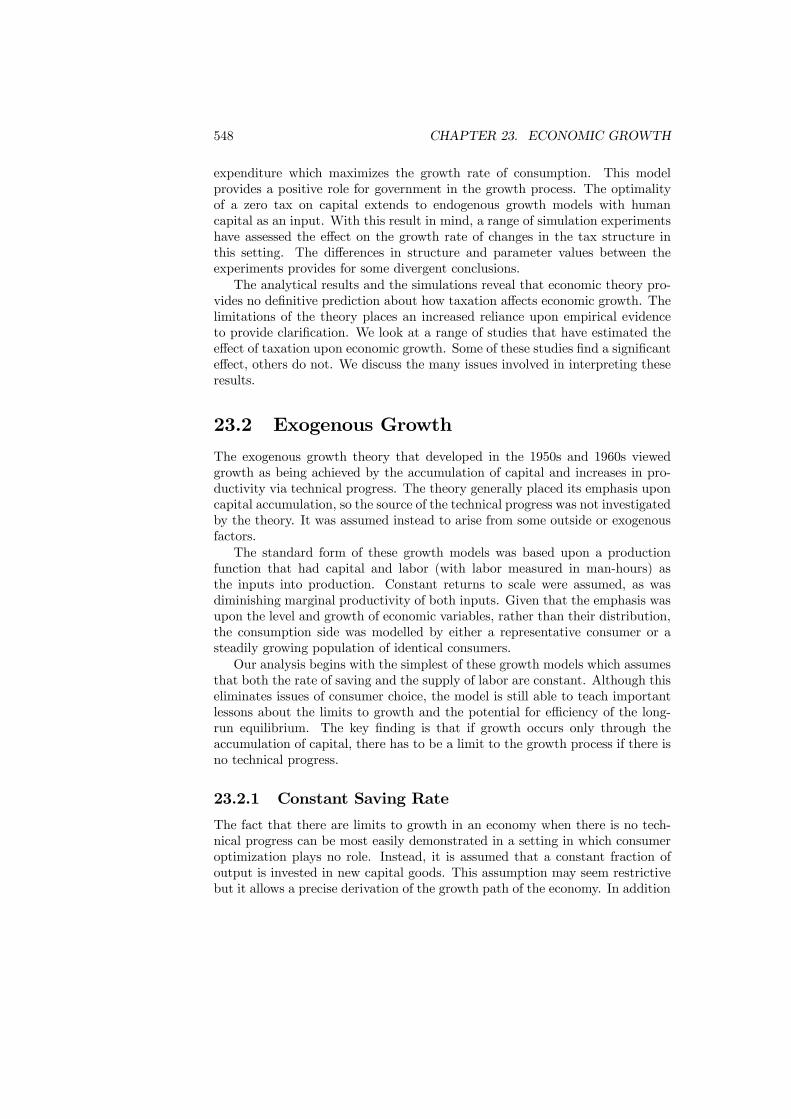
548 CHAPTER 23. ECONOMIC GROWTH
expenditure which maximizes the growth rate of consumption. This modelprovides a positive role for government in the growth process. The optimalityof a zero tax on capital extends to endogenous growth models with humancapital as an input. With this result in mind, a range of simulation experimentshave assessed the effect on the growth rate of changes in the tax structure inthis setting. The differences in structure and parameter values between theexperiments provides for some divergent conclusions.The analytical results and the simulations reveal that economic theory pro-
vides no definitive prediction about how taxation affects economic growth. Thelimitations of the theory places an increased reliance upon empirical evidenceto provide clarification. We look at a range of studies that have estimated theeffect of taxation upon economic growth. Some of these studies find a significanteffect, others do not. We discuss the many issues involved in interpreting theseresults.
23.2 Exogenous Growth
The exogenous growth theory that developed in the 1950s and 1960s viewedgrowth as being achieved by the accumulation of capital and increases in pro-ductivity via technical progress. The theory generally placed its emphasis uponcapital accumulation, so the source of the technical progress was not investigatedby the theory. It was assumed instead to arise from some outside or exogenousfactors.The standard form of these growth models was based upon a production
function that had capital and labor (with labor measured in man-hours) asthe inputs into production. Constant returns to scale were assumed, as wasdiminishing marginal productivity of both inputs. Given that the emphasis wasupon the level and growth of economic variables, rather than their distribution,the consumption side was modelled by either a representative consumer or asteadily growing population of identical consumers.Our analysis begins with the simplest of these growth models which assumes
that both the rate of saving and the supply of labor are constant. Although thiseliminates issues of consumer choice, the model is still able to teach importantlessons about the limits to growth and the potential for efficiency of the long-run equilibrium. The key finding is that if growth occurs only through theaccumulation of capital, there has to be a limit to the growth process if there isno technical progress.
23.2.1 Constant Saving Rate
The fact that there are limits to growth in an economy when there is no tech-nical progress can be most easily demonstrated in a setting in which consumeroptimization plays no role. Instead, it is assumed that a constant fraction ofoutput is invested in new capital goods. This assumption may seem restrictivebut it allows a precise derivation of the growth path of the economy. In addition

23.2. EXOGENOUS GROWTH 549
the main conclusions relating to limits on growth are little modified even whenan optimizing consumer is introduced.Consider an economy with a population that is growing at a constant rate.
Each person works a fixed number of hours and capital depreciates partiallywhen used. There is a single good in the economy which can be consumedor saved. The only source of saving is investment in capital. Under theseassumptions, the output that is produced at time t, Yt, must be divided betweenconsumption, Ct, and investment, It. In equilibrium, the level of investmentmust be equal to the level of saving.With inputs of capital Kt and labor Lt employed in production, the level of
output isYt = F (Kt, Lt) . (23.1)
This output can be either consumed or saved. The fundamental assumptionof the model is that the level of saving is a fixed proportion s, 0 < s < 1, ofoutput. As saving must equal investment in equilibrium, at time t investmentin new capital is given by
It = sF (Kt, Lt) . (23.2)
The use of capital in production results in its partial depreciation. We assumethat this depreciation is a constant fraction δ, so the capital available in periodt+ 1 is given by new investment plus the undepreciated capital, or
Kt+1 = It + (1− δ)Kt
= sF (Kt, Lt) + (1− δ)Kt. (23.3)
This equation is the basic capital accumulation relationship that determineshow the capital stock evolves through time.The fact that the population is growing makes it preferable to express vari-
ables in per capita terms. This can be done by exploiting the assumption of
constant returns to scale in the production function to write Yt = LtF³Kt
Lt, 1´=
Ltf (kt) where kt = Kt
Lt. Dividing (23.3) through by Lt, the capital accumulation
relation becomesKt+1
Lt= sf (kt) +
(1− δ)Kt
Lt. (23.4)
Denoting the constant population growth rate by n, labor supply grows accord-ing to Lt+1 = (1+n)Lt. Using this growth relationship, the capital accumulationrelation shows that the dynamics of the capital/labor ratio are governed by
(1 + n)kt+1 = sf (kt) + (1− δ) kt. (23.5)
The relation in (23.5) will trace the development of the capital stock overtime from an initial stock k0 = K0
Lo. To see what this implies, consider an exam-
ple where the production function has the form f (kt) = kαt . The capital/labor
ratio must then satisfy
kt+1 =skαt + (1− δ) kt
1 + n. (23.6)
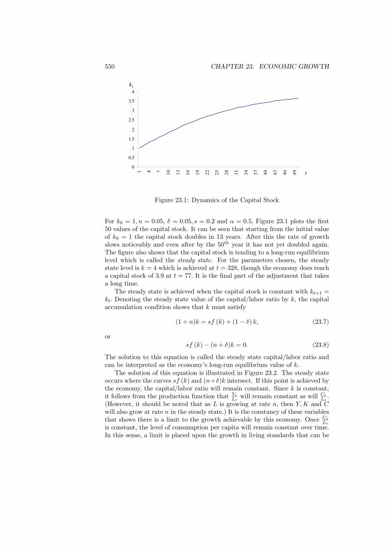
550 CHAPTER 23. ECONOMIC GROWTH
0
0.5
1
1.5
2
2.5
3
3.5
4
1 4 7 10 13 16 19 22 25 28 31 34 37 40 43 46 49 t
tk
Figure 23.1: Dynamics of the Capital Stock
For k0 = 1, n = 0.05, δ = 0.05, s = 0.2 and α = 0.5, Figure 23.1 plots the first50 values of the capital stock. It can be seen that starting from the initial valueof k0 = 1 the capital stock doubles in 13 years. After this the rate of growthslows noticeably and even after by the 50th year it has not yet doubled again.The figure also shows that the capital stock is tending to a long-run equilibriumlevel which is called the steady state. For the parameters chosen, the steadystate level is k = 4 which is achieved at t = 328, though the economy does reacha capital stock of 3.9 at t = 77. It is the final part of the adjustment that takesa long time.The steady state is achieved when the capital stock is constant with kt+1 =
kt. Denoting the steady state value of the capital/labor ratio by k, the capitalaccumulation condition shows that k must satisfy
(1 + n)k = sf (k) + (1− δ) k, (23.7)
orsf (k)− (n+ δ)k = 0. (23.8)
The solution to this equation is called the steady state capital/labor ratio andcan be interpreted as the economy’s long-run equilibrium value of k.The solution of this equation is illustrated in Figure 23.2. The steady state
occurs where the curves sf (k) and (n+δ)k intersect. If this point is achieved bythe economy, the capital/labor ratio will remain constant. Since k is constant,it follows from the production function that Yt
Ltwill remain constant as will CtLt .
(However, it should be noted that as L is growing at rate n, then Y,K and Cwill also grow at rate n in the steady state.) It is the constancy of these variablesthat shows there is a limit to the growth achievable by this economy. Once Ct
Ltis constant, the level of consumption per capita will remain constant over time.In this sense, a limit is placed upon the growth in living standards that can be
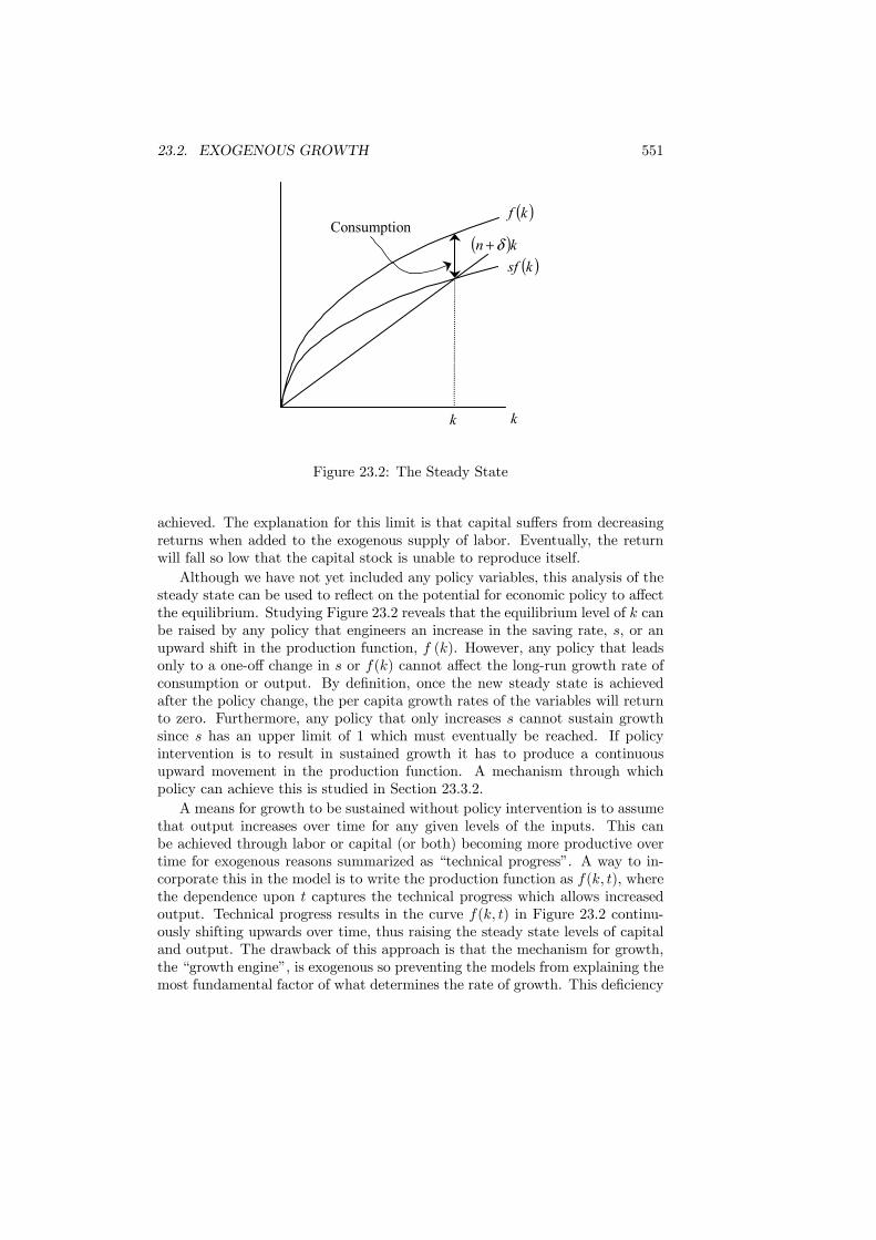
23.2. EXOGENOUS GROWTH 551
( )kf
( )ksf
k
( )kn δ+
k
Consumption
Figure 23.2: The Steady State
achieved. The explanation for this limit is that capital suffers from decreasingreturns when added to the exogenous supply of labor. Eventually, the returnwill fall so low that the capital stock is unable to reproduce itself.Although we have not yet included any policy variables, this analysis of the
steady state can be used to reflect on the potential for economic policy to affectthe equilibrium. Studying Figure 23.2 reveals that the equilibrium level of k canbe raised by any policy that engineers an increase in the saving rate, s, or anupward shift in the production function, f (k). However, any policy that leadsonly to a one-off change in s or f(k) cannot affect the long-run growth rate ofconsumption or output. By definition, once the new steady state is achievedafter the policy change, the per capita growth rates of the variables will returnto zero. Furthermore, any policy that only increases s cannot sustain growthsince s has an upper limit of 1 which must eventually be reached. If policyintervention is to result in sustained growth it has to produce a continuousupward movement in the production function. A mechanism through whichpolicy can achieve this is studied in Section 23.3.2.A means for growth to be sustained without policy intervention is to assume
that output increases over time for any given levels of the inputs. This canbe achieved through labor or capital (or both) becoming more productive overtime for exogenous reasons summarized as “technical progress”. A way to in-corporate this in the model is to write the production function as f(k, t), wherethe dependence upon t captures the technical progress which allows increasedoutput. Technical progress results in the curve f(k, t) in Figure 23.2 continu-ously shifting upwards over time, thus raising the steady state levels of capitaland output. The drawback of this approach is that the mechanism for growth,the “growth engine”, is exogenous so preventing the models from explaining themost fundamental factor of what determines the rate of growth. This deficiency

552 CHAPTER 23. ECONOMIC GROWTH
is addressed by the endogenous growth models of the next section which explorethe mechanisms that can drive technical progress.Returning to the basic model without technical progress, condition (23.8)
shows the steady state capital/labor ratio is dependent upon the saving rates. This raises the question as to whether some saving rates are better thanothers. To address this question, it is noted first that for each value of s thereis a corresponding steady-state capital/labor ratio at the intersection of sf(k)and (n+ δ) k. It is clear from Figure 23.2 that for low values of s, the curvesf(k) will intersect the curve (n+ δ) k at low values of k. As s is increased,sf(k) shifts upwards and the steady state level of k will rise. The relationshipbetween the capital/labor ratio and the saving rate implied by this constructionis denoted by k = k (s) . We have observed that k (s) is an increasing functionof s up until the maximum value of s = 1.Taking account of the link between s and k, the level of consumption per
capita can be written
c (s) = (1− s) f (k (s)) = f (k (s))− (n+ δ) k(s), (23.9)
where the second equality follows from definition (23.8) of a steady state. Whatis of interest are the properties of the saving rate that maximizes consump-tion. The first-order condition for defining this saving rate can be found bydifferentiating c(s) with respect to s. Doing so gives
dc (s)
ds= [f 0 (k (s))− (n+ δ)] k0 (s) = 0. (23.10)
Since k0(s) is positive, the saving rate, s∗, that maximizes consumption is definedby
f 0 (k(s∗)) = n+ δ. (23.11)
The saving rate s∗ determines a level of capital k∗ = k(s∗) which is calledthe Golden Rule capital/labor ratio. If the economy achieves this capital/laborratio at its steady state it is maximizing consumption per capita. The samelogic applies here as it did in the derivation of the steady state in Chapter 21(though δ was assumed to be zero in the overlapping generations economy).The nature of the Golden Rule is illustrated in Figure 23.3. For any level of
the capital/labor ratio, the steady state level of consumption per capita is givenby the vertical distance between the curve (n + δ)k and the curve f(k). Thisdistance is maximized when the gradient of the production function is equalto (n + δ) which gives the Golden Rule condition. The figure also shows thatconsumption will fall if the capital/labor ratio is either raised or lowered fromthe Golden Rule level. In line with the definitions of Chapter 21, an economywith a steady-state capital stock below the Golden Rule level, k∗, is dynamicallyefficient - it requires a sacrifice of consumption now in order to raise k so a Paretoimprovement cannot be found. An economy with a capital stock in excess of k∗
is dynamically inefficient since immediate consumption of the excess would raisecurrent welfare and place the economy on a path with higher consumption.

23.2. EXOGENOUS GROWTH 553
( )kf
k
( )kn δ+
*k
Consumption
Figure 23.3: The Golden Rule
As an example of these calculations, let the production function be given byy = kα, with α < 1. For a given saving rate s the steady state is defined by thesolution to
skα = (n+ δ) k. (23.12)
Solving this equation determines the steady state capital/labor ratio as k =³s
n+δ
´1/(1−α). Using this solution, the per capita level of consumption follows
as
c(s) = kα − (n+ δ) k =
µs
n+ δ
¶α/(1−α)− (n+ δ)
µs
n+ δ
¶1/(1−α). (23.13)
Adopting the parameter values n = 0.025, δ = 0.025 and α = 0.75, the levelof consumption is plotted in Figure 23.4 as a function of s. The figure showsthat consumption rises with s until the saving rate is reached at which theequilibrium capital stock is equal to the Golden Rule level and then falls againfor higher values.
Formally, the fact that the saving rate is fixed leaves little scope for policyanalysis. However, studying the effect of changes in the saving rate revealsthe factors that would be at work in a more general model in which the level ofsaving is a choice variable that can be affected by policy variables. By definition,the per capita level of the variables are constant once the steady state has beenachieved. The living standards in the economy reach a limit and then cannotgrow any further unless the production function is continually raised. Changesin the saving rate affect the level of consumption but not its growth rate.

554 CHAPTER 23. ECONOMIC GROWTH
Figure 23.4: Consumption and the Saving Rate
23.2.2 Optimal Taxation
The analysis of the fixed saving model has touched upon some of the potentialconsequences of policy intervention. As a tool for policy analysis, the model isvery limited given the lack of choice variables that can be affected by policy. Thisshortcoming is now overcome by studying a variant of the Ramsey growth modelin which a representative consumer chooses an intertemporal consumption planto maximize lifetime utility. Using this model, we analyze the optimal taxesupon labor and capital income.The Ramsey model has a single representative consumer who chooses the
paths of consumption, labor and capital over time. The single consumer assump-tion is adopted to eliminate issues concerning distribution between consumers ofdiffering abilities and tastes and to place the focus entirely upon efficiency. Forsimplicity, it is also assumed that the growth rate of labor, n, is zero. There is arepresentative firm that chooses its use of capital and labor to maximize profits.Given that the market must be in equilibrium, the choices of the consumer drivethe rest of the economy through the level of saving, and hence capital, that theyimply. The supply of labor and capital from the consumer combine with thefactor demands of the firm to determine the equilibrium factor rewards.The aim is to characterize the optimal tax structure in this economy. We
assume there is a government that requires revenue of amount gt at time t. Itraises this revenue through taxes on capital and labor, which are denoted byτKt and τLt respectively. The government chooses these tax rates in the mostefficient manner.The choices of the consumer are made to maximize the discounted sum of
the flow of utility. Letting 0 < β < 1 be the discount factor on future utility,
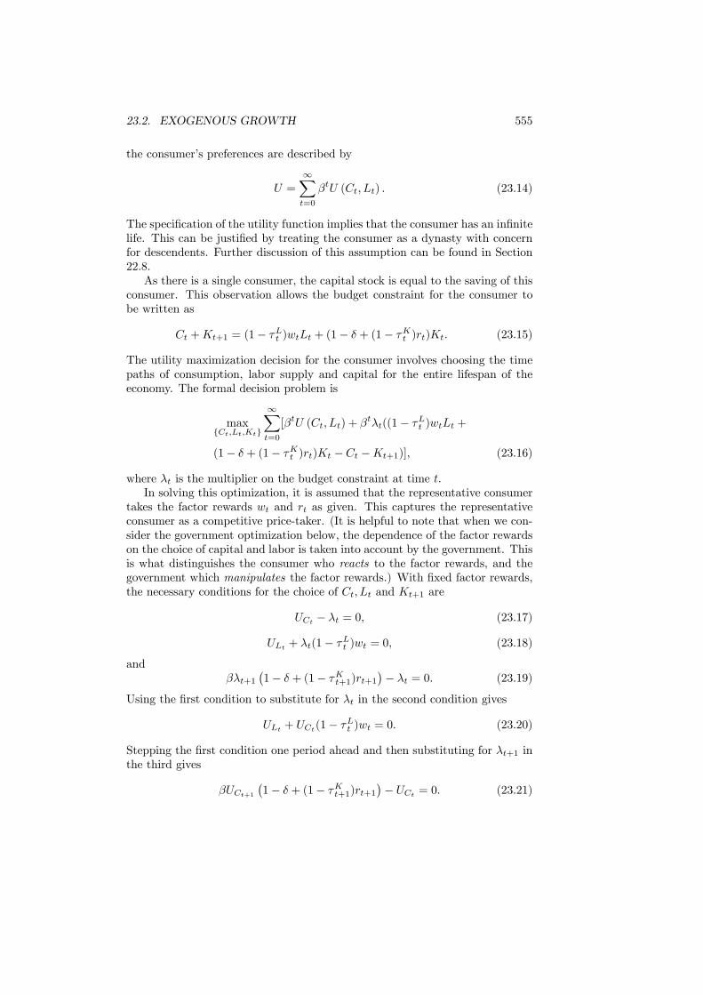
23.2. EXOGENOUS GROWTH 555
the consumer’s preferences are described by
U =∞Xt=0
βtU (Ct, Lt) . (23.14)
The specification of the utility function implies that the consumer has an infinitelife. This can be justified by treating the consumer as a dynasty with concernfor descendents. Further discussion of this assumption can be found in Section22.8.As there is a single consumer, the capital stock is equal to the saving of this
consumer. This observation allows the budget constraint for the consumer tobe written as
Ct +Kt+1 = (1− τLt )wtLt + (1− δ + (1− τKt )rt)Kt. (23.15)
The utility maximization decision for the consumer involves choosing the timepaths of consumption, labor supply and capital for the entire lifespan of theeconomy. The formal decision problem is
max{Ct,Lt,Kt}
∞Xt=0
[βtU (Ct, Lt) + βtλt((1− τLt )wtLt +
(1− δ + (1− τKt )rt)Kt − Ct −Kt+1)], (23.16)
where λt is the multiplier on the budget constraint at time t.In solving this optimization, it is assumed that the representative consumer
takes the factor rewards wt and rt as given. This captures the representativeconsumer as a competitive price-taker. (It is helpful to note that when we con-sider the government optimization below, the dependence of the factor rewardson the choice of capital and labor is taken into account by the government. Thisis what distinguishes the consumer who reacts to the factor rewards, and thegovernment which manipulates the factor rewards.) With fixed factor rewards,the necessary conditions for the choice of Ct, Lt and Kt+1 are
UCt − λt = 0, (23.17)
ULt + λt(1− τLt )wt = 0, (23.18)
andβλt+1
¡1− δ + (1− τKt+1)rt+1
¢− λt = 0. (23.19)
Using the first condition to substitute for λt in the second condition gives
ULt + UCt(1− τLt )wt = 0. (23.20)
Stepping the first condition one period ahead and then substituting for λt+1 inthe third gives
βUCt+1¡1− δ + (1− τKt+1)rt+1
¢− UCt = 0. (23.21)

556 CHAPTER 23. ECONOMIC GROWTH
Conditions (23.20) and (23.21) describe utility maximization by the con-sumer. To interpret these it should be observed that there are two aspects tothe consumer’s decision. Firstly, within each period the consumer needs to op-timize over the levels of consumption and labor supply. The efficient solution tothis within-period decision is described by (23.20) which ensures that the mar-ginal utilities are proportional to the relative prices. Secondly, the consumer hasto allocate their resources efficiently across time. Condition (23.21) describesefficiency in this process by linking the marginal utility of consumption in twoadjacent periods to the rate at which consumption can be transferred throughtime via investments in capital. Taken together for every time period t, thesenecessary conditions describe the optimal paths of consumption, labor supplyand capital investment for the consumer.The representative firm is assumed to maximize profit by choosing its use
of capital and labor. Since the firm rents capital from the consumer, it makesno irreversible decisions so it need do no more than maximize profit in each pe-riod. The standard efficiency conditions for factor use then apply which equatemarginal products to factor rewards. Hence the interest rate and the wage ratesatisfy
FKt = rt, (23.22)
andFLt = wt. (23.23)
Following these preliminaries, it is possible to state the government opti-mization problem. The sequence of government expenditures {gt} is taken asgiven. It is assumed that these expenditures are used for a purpose which doesnot directly affect utility. Formally, the government chooses the tax rates andthe levels of consumption, labor supply and capital to maximize the level ofutility. The values of these variables must be chosen for each point in time,so the government decision is a sequence
©τKt , τ
Lt , Ct, Lt,Kt
ª. The choices of
Ct, Lt and Kt must be identical to what would be chosen by the consumer giventhe tax rates τKt and τLt . This can be achieved by imposing conditions (23.20)and (23.21) as constraints upon the optimization. When these constraints aresatisfied it is as if the consumer were making the choice. As already noted, thegovernment explicitly takes into account the endogenous determination of thefactor rewards.The optimization also has to be constrained by the budget constraints of the
consumer and government, and by aggregate production feasibility. However,if any two of these constraints hold the third must also hold. Therefore one ofthem need not be included as a separate constraint for the optimization. In thiscase it is the consumer’s budget constraint which is dropped. The governmentbudget constraint that taxes must equal expenditure is given by
τKt rtKt + τLt wtLt = gt. (23.24)
In addition, the aggregate production condition for the economy is that
Ct + gt + It = F (Kt, Lt) . (23.25)
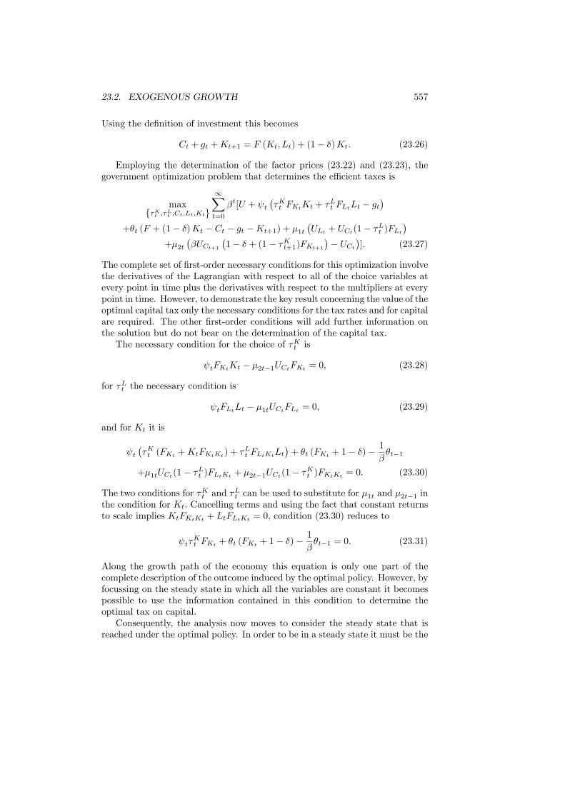
23.2. EXOGENOUS GROWTH 557
Using the definition of investment this becomes
Ct + gt +Kt+1 = F (Kt, Lt) + (1− δ)Kt. (23.26)
Employing the determination of the factor prices (23.22) and (23.23), thegovernment optimization problem that determines the efficient taxes is
max{τKt ,τLt ,Ct,Lt,Kt}
∞Xt=0
βt[U + ψt¡τKt FKt
Kt + τLt FLtLt − gt¢
+θt (F + (1− δ)Kt − Ct − gt −Kt+1) + µ1t¡ULt + UCt(1− τLt )FLt
¢+µ2t
¡βUCt+1
¡1− δ + (1− τKt+1)FKt+1
¢− UCt¢]. (23.27)
The complete set of first-order necessary conditions for this optimization involvethe derivatives of the Lagrangian with respect to all of the choice variables atevery point in time plus the derivatives with respect to the multipliers at everypoint in time. However, to demonstrate the key result concerning the value of theoptimal capital tax only the necessary conditions for the tax rates and for capitalare required. The other first-order conditions will add further information onthe solution but do not bear on the determination of the capital tax.The necessary condition for the choice of τKt is
ψtFKtKt − µ2t−1UCtFKt = 0, (23.28)
for τLt the necessary condition is
ψtFLtLt − µ1tUCtFLt = 0, (23.29)
and for Kt it is
ψt¡τKt (FKt +KtFKtKt) + τLt FLtKtLt
¢+ θt (FKt + 1− δ)− 1
βθt−1
+µ1tUCt(1− τLt )FLtKt+ µ2t−1UCt(1− τKt )FKtKt
= 0. (23.30)
The two conditions for τKt and τLt can be used to substitute for µ1t and µ2t−1 in
the condition for Kt. Cancelling terms and using the fact that constant returnsto scale implies KtFKtKt + LtFLtKt = 0, condition (23.30) reduces to
ψtτKt FKt + θt (FKt + 1− δ)− 1
βθt−1 = 0. (23.31)
Along the growth path of the economy this equation is only one part of thecomplete description of the outcome induced by the optimal policy. However, byfocussing on the steady state in which all the variables are constant it becomespossible to use the information contained in this condition to determine theoptimal tax on capital.Consequently, the analysis now moves to consider the steady state that is
reached under the optimal policy. In order to be in a steady state it must be the
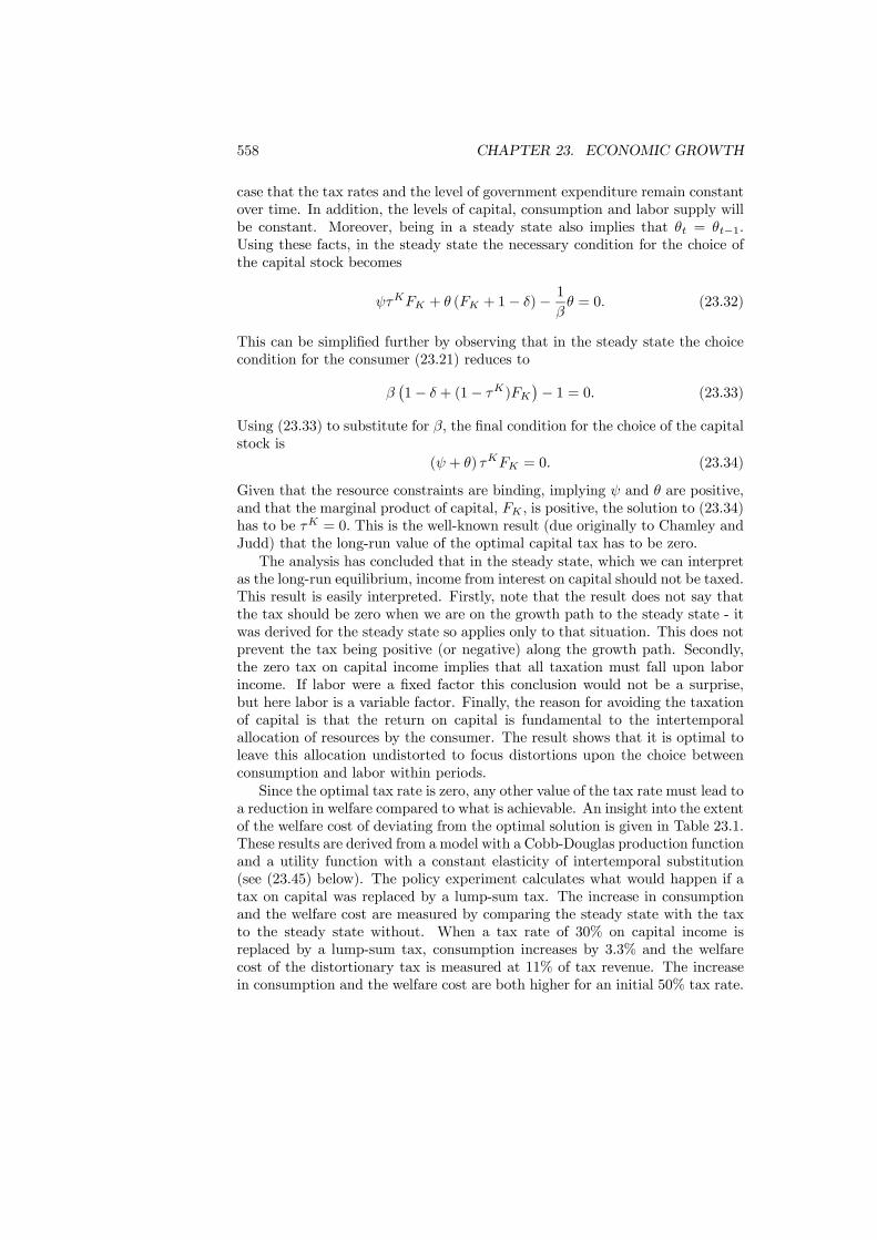
558 CHAPTER 23. ECONOMIC GROWTH
case that the tax rates and the level of government expenditure remain constantover time. In addition, the levels of capital, consumption and labor supply willbe constant. Moreover, being in a steady state also implies that θt = θt−1.Using these facts, in the steady state the necessary condition for the choice ofthe capital stock becomes
ψτKFK + θ (FK + 1− δ)− 1βθ = 0. (23.32)
This can be simplified further by observing that in the steady state the choicecondition for the consumer (23.21) reduces to
β¡1− δ + (1− τK)FK
¢− 1 = 0. (23.33)
Using (23.33) to substitute for β, the final condition for the choice of the capitalstock is
(ψ + θ) τKFK = 0. (23.34)
Given that the resource constraints are binding, implying ψ and θ are positive,and that the marginal product of capital, FK , is positive, the solution to (23.34)has to be τK = 0. This is the well-known result (due originally to Chamley andJudd) that the long-run value of the optimal capital tax has to be zero.The analysis has concluded that in the steady state, which we can interpret
as the long-run equilibrium, income from interest on capital should not be taxed.This result is easily interpreted. Firstly, note that the result does not say thatthe tax should be zero when we are on the growth path to the steady state - itwas derived for the steady state so applies only to that situation. This does notprevent the tax being positive (or negative) along the growth path. Secondly,the zero tax on capital income implies that all taxation must fall upon laborincome. If labor were a fixed factor this conclusion would not be a surprise,but here labor is a variable factor. Finally, the reason for avoiding the taxationof capital is that the return on capital is fundamental to the intertemporalallocation of resources by the consumer. The result shows that it is optimal toleave this allocation undistorted to focus distortions upon the choice betweenconsumption and labor within periods.Since the optimal tax rate is zero, any other value of the tax rate must lead to
a reduction in welfare compared to what is achievable. An insight into the extentof the welfare cost of deviating from the optimal solution is given in Table 23.1.These results are derived from a model with a Cobb-Douglas production functionand a utility function with a constant elasticity of intertemporal substitution(see (23.45) below). The policy experiment calculates what would happen if atax on capital was replaced by a lump-sum tax. The increase in consumptionand the welfare cost are measured by comparing the steady state with the taxto the steady state without. When a tax rate of 30% on capital income isreplaced by a lump-sum tax, consumption increases by 3.3% and the welfarecost of the distortionary tax is measured at 11% of tax revenue. The increasein consumption and the welfare cost are both higher for an initial 50% tax rate.
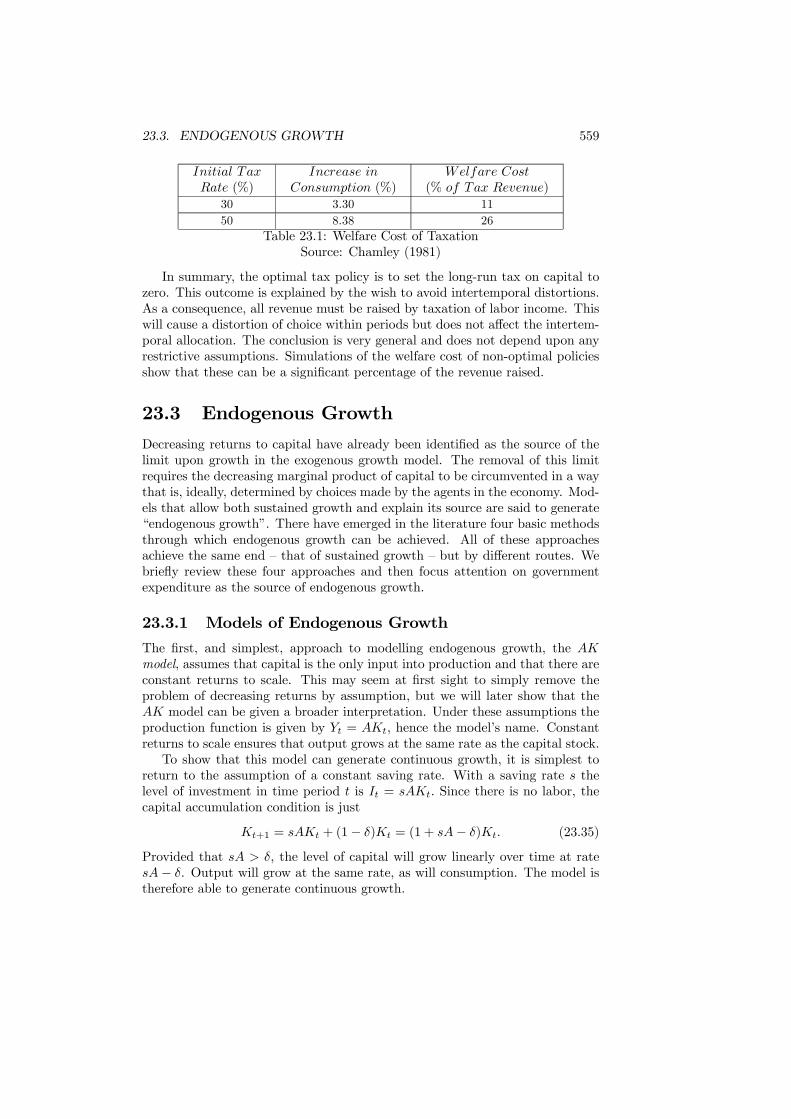
23.3. ENDOGENOUS GROWTH 559
Initial TaxRate (%)
Increase inConsumption (%)
Welfare Cost(% of Tax Revenue)
30 3.30 1150 8.38 26
Table 23.1: Welfare Cost of TaxationSource: Chamley (1981)
In summary, the optimal tax policy is to set the long-run tax on capital tozero. This outcome is explained by the wish to avoid intertemporal distortions.As a consequence, all revenue must be raised by taxation of labor income. Thiswill cause a distortion of choice within periods but does not affect the intertem-poral allocation. The conclusion is very general and does not depend upon anyrestrictive assumptions. Simulations of the welfare cost of non-optimal policiesshow that these can be a significant percentage of the revenue raised.
23.3 Endogenous GrowthDecreasing returns to capital have already been identified as the source of thelimit upon growth in the exogenous growth model. The removal of this limitrequires the decreasing marginal product of capital to be circumvented in a waythat is, ideally, determined by choices made by the agents in the economy. Mod-els that allow both sustained growth and explain its source are said to generate“endogenous growth”. There have emerged in the literature four basic methodsthrough which endogenous growth can be achieved. All of these approachesachieve the same end — that of sustained growth — but by different routes. Webriefly review these four approaches and then focus attention on governmentexpenditure as the source of endogenous growth.
23.3.1 Models of Endogenous Growth
The first, and simplest, approach to modelling endogenous growth, the AKmodel, assumes that capital is the only input into production and that there areconstant returns to scale. This may seem at first sight to simply remove theproblem of decreasing returns by assumption, but we will later show that theAK model can be given a broader interpretation. Under these assumptions theproduction function is given by Yt = AKt, hence the model’s name. Constantreturns to scale ensures that output grows at the same rate as the capital stock.To show that this model can generate continuous growth, it is simplest to
return to the assumption of a constant saving rate. With a saving rate s thelevel of investment in time period t is It = sAKt. Since there is no labor, thecapital accumulation condition is just
Kt+1 = sAKt + (1− δ)Kt = (1 + sA− δ)Kt. (23.35)
Provided that sA > δ, the level of capital will grow linearly over time at ratesA− δ. Output will grow at the same rate, as will consumption. The model istherefore able to generate continuous growth.

560 CHAPTER 23. ECONOMIC GROWTH
The second approach is to match increases in capital with equal growth inother inputs. One way to do this is to consider human capital as an inputrather than just raw labor time. The level of the human capital input is thenthe product of the quality of labor and labor time. Doing so allows labor time tobe made more productive by investment in education and training which raisehuman capital. Technical progress is then embodied in the quality of labor. Themodel requires two investment processes: one for investment in physical capitaland another for investment in human capital. There can either be one sector,with human capital produced by the same technology as physical capital, or twosectors with a separate production process for human capital. The standardform of production function for such a model would be
Yt = F (Kt,Ht) , (23.36)
where Ht is the level of human capital. If the production function has constantreturns to scale in human capital and physical capital jointly, then investmentin both can raise output without limit even if the quantity of labor time is fixed.The one-sector model with human capital actually reduces to the AK model
- this is the broader interpretation of the AK model referred to above. To seethis, note that the one-sector assumption means that output can be used forconsumption or invested in physical capital or invested in human capital. Thismeans that the two capital goods are perfect substitutes for the consumer inthe sense that a unit of output can become one unit of either. The perfectsubstitutability implies that in equilibrium the two factors must have the samerate of return. Combining this with the constant returns to scale in the pro-duction function results in the two factors always being employed in the sameproportions. Therefore the ratio Ht
Ktis constant for all t. Denoting this constant
value by HK , the production function becomes
Yt = Ktf
µH
K
¶= AKt, (23.37)
where A ≡ f ¡HK ¢. This returns us to the AK form.A two-sector model can have different production functions for the creation
of the two types of capital good. This eliminates the restriction that theyare perfect substitutes and moves away from the AK setting. In a two-sectormodel different human and physical capital intensities can be incorporated inthe production of the two types of capital. This can make it consistent withthe observation that human capital production tends to be more intensive inhuman capital - through the requirement for skilled teaching staff etc.The next two approaches focus on inputs other than labor. If output depends
upon labor use and a range of other inputs, technological progress can take theform of the introduction of new inputs into the production function withoutany of the old inputs being dropped. This allows production to increase sincethe expansion of the input range prevents the level of use of any one of theinputs becoming too large relative to the labor input. An alternative view of
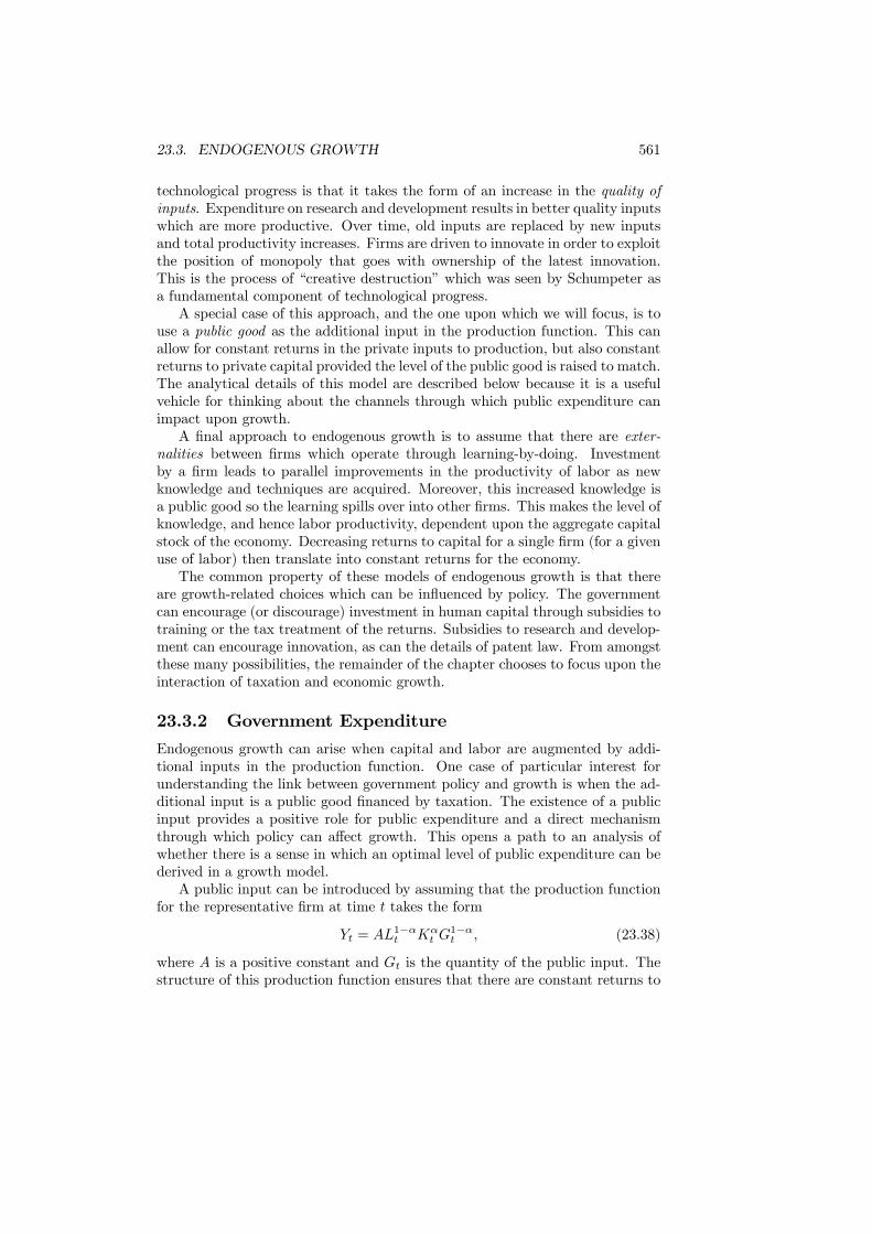
23.3. ENDOGENOUS GROWTH 561
technological progress is that it takes the form of an increase in the quality ofinputs. Expenditure on research and development results in better quality inputswhich are more productive. Over time, old inputs are replaced by new inputsand total productivity increases. Firms are driven to innovate in order to exploitthe position of monopoly that goes with ownership of the latest innovation.This is the process of “creative destruction” which was seen by Schumpeter asa fundamental component of technological progress.A special case of this approach, and the one upon which we will focus, is to
use a public good as the additional input in the production function. This canallow for constant returns in the private inputs to production, but also constantreturns to private capital provided the level of the public good is raised to match.The analytical details of this model are described below because it is a usefulvehicle for thinking about the channels through which public expenditure canimpact upon growth.A final approach to endogenous growth is to assume that there are exter-
nalities between firms which operate through learning-by-doing. Investmentby a firm leads to parallel improvements in the productivity of labor as newknowledge and techniques are acquired. Moreover, this increased knowledge isa public good so the learning spills over into other firms. This makes the level ofknowledge, and hence labor productivity, dependent upon the aggregate capitalstock of the economy. Decreasing returns to capital for a single firm (for a givenuse of labor) then translate into constant returns for the economy.The common property of these models of endogenous growth is that there
are growth-related choices which can be influenced by policy. The governmentcan encourage (or discourage) investment in human capital through subsidies totraining or the tax treatment of the returns. Subsidies to research and develop-ment can encourage innovation, as can the details of patent law. From amongstthese many possibilities, the remainder of the chapter chooses to focus upon theinteraction of taxation and economic growth.
23.3.2 Government Expenditure
Endogenous growth can arise when capital and labor are augmented by addi-tional inputs in the production function. One case of particular interest forunderstanding the link between government policy and growth is when the ad-ditional input is a public good financed by taxation. The existence of a publicinput provides a positive role for public expenditure and a direct mechanismthrough which policy can affect growth. This opens a path to an analysis ofwhether there is a sense in which an optimal level of public expenditure can bederived in a growth model.A public input can be introduced by assuming that the production function
for the representative firm at time t takes the form
Yt = AL1−αt Kα
t G1−αt , (23.38)
where A is a positive constant and Gt is the quantity of the public input. Thestructure of this production function ensures that there are constant returns to
562 CHAPTER 23. ECONOMIC GROWTH
scale in Lt and Kt for the firm given a fixed level of the public input. Althoughreturns are decreasing to private capital as the level of capital is increased forfixed levels of labor and public input, there are constant returns to scale inpublic input and private capital together. For a fixed level of Lt, this propertyof constant returns to scale in the other two inputs permits endogenous growthto occur.It is assumed that the public input is financed by a tax upon output. As-
suming that capital does not depreciate in order to simplify the derivation, theprofit level of the firm is
πt = (1− τ)AL1−αt Kαt G
1−αt − rtKt − wtLt, (23.39)
where rt is the interest rate, wt the wage rate and τ the tax rate. From thisspecification of profit, the choice of capital and labor by the firm satisfy
(1− τ)αAL1−αt Kα−1t G1−αt = rt, (23.40)
and(1− τ) (1− α)AL−αt Kα
t G1−αt = wt. (23.41)
The government budget constraint requires that tax revenue equals the cost ofthe public good provided, so
Gt = τYt. (23.42)
Now assume that labor supply is constant at Lt = L for all t. Without thepublic input, it would not be possible given this assumption to sustain growthbecause the marginal product of capital would decrease as the capital stockincreased. With the public input, growth can now be driven by a joint increasein private and public capital even though labor supply is fixed. Using (23.38)and (23.42), the level of public input can be written as
Gt = (τA)1/α
L(1−α)/αKt. (23.43)
This result can be substituted into (23.40) to obtain an expression for the in-terest rate as a function of the tax rate
rt = (1− τ)αA1/α (Lτ)(1−α)/α . (23.44)
The economy’s representative consumer is assumed to have preferences de-scribed by the utility function
U =∞Xt=1
βtC1−σt − 11− σ
. (23.45)
This specific form of utility is adopted to permit an explicit solution for thesteady state. The consumer chooses the path {Ct} over time to maximize utility.The standard condition for intertemporal choice must hold for the optimization,
23.3. ENDOGENOUS GROWTH 563
so the ratio of the marginal utilities of consuming at t and at t+ 1 must equalthe gross interest rate. Hence
∂U/∂Ct∂U/∂Ct+1
≡ C−σtβC−σt+1
= (1 + rt+1) . (23.46)
By solving for Ct+1Ct
and then subtracting CtCtfrom both sides of the resulting
equation, this optimality condition can be written in terms of the growth rateof consumption
Ct+1 − CtCt
= (β (1 + rt+1))1/σ − 1. (23.47)
Finally, using the solution (23.44) to substitute for the interest rate, the growthrate of consumption is related to the tax rate by
Ct+1 − CtCt
= β1/σ³1 + (1− τ)αA1/α (Lτ)
(1−α)/α´1/σ − 1. (23.48)
The result in (23.48) demonstrates the two channels through which the taxrate affects consumption growth. Firstly, taxation reduces the growth rate ofconsumption through the term (1− τ) which represents the effect on the mar-ginal return of capital reducing the amount of capital used. Secondly, the taxrate increases growth through the term τ (1−α)/α which represents the gainsthrough the provision of the public input.Further insight into these effects can be obtained by plotting the relationship
between the tax rate and consumption growth. This is shown in Figure 23.5under the assumption that A = 1, L = 1, α = 0.5,β = 0.95 and σ = 0.5. Thefigure displays several notable features. First, for low levels of the public inputgrowth is negative, so a positive tax rate is required for there to be consumptiongrowth. Secondly, the relationship between growth and the tax rate is non-monotonic: growth initially increases with the tax rate, reaches a maximum,and then decreases. Finally, there is a tax rate which maximizes the growthrate of consumption. Differentiating (23.48) with respect to τ , the tax rate thatmaximizes consumption growth is
τ = 1− α. (23.49)
For the values in the figure, this optimal tax rate is τ = 0.5. To see what thistax rate implies, observe that
∂Yt∂Gt
= (1− α)YtGt
= 1, (23.50)
using Gt = τYt and τ = 1−α. Hence the tax rate that maximizes consumptiongrowth ensures that the marginal product of the public input is equal to 1 whichis also its marginal cost.This model reveals a positive role for government in enhancing growth through
the provision of a public input. It illustrates a sense in which there can be an
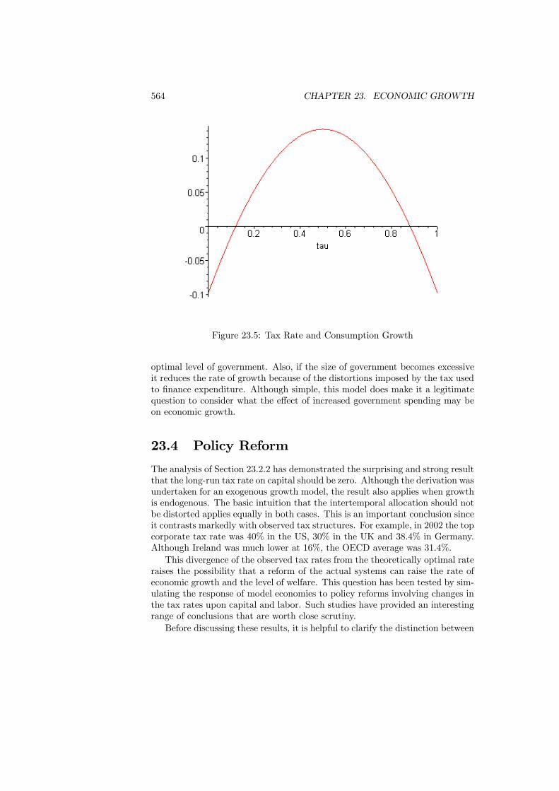
564 CHAPTER 23. ECONOMIC GROWTH
Figure 23.5: Tax Rate and Consumption Growth
optimal level of government. Also, if the size of government becomes excessiveit reduces the rate of growth because of the distortions imposed by the tax usedto finance expenditure. Although simple, this model does make it a legitimatequestion to consider what the effect of increased government spending may beon economic growth.
23.4 Policy Reform
The analysis of Section 23.2.2 has demonstrated the surprising and strong resultthat the long-run tax rate on capital should be zero. Although the derivation wasundertaken for an exogenous growth model, the result also applies when growthis endogenous. The basic intuition that the intertemporal allocation should notbe distorted applies equally in both cases. This is an important conclusion sinceit contrasts markedly with observed tax structures. For example, in 2002 the topcorporate tax rate was 40% in the US, 30% in the UK and 38.4% in Germany.Although Ireland was much lower at 16%, the OECD average was 31.4%.This divergence of the observed tax rates from the theoretically optimal rate
raises the possibility that a reform of the actual systems can raise the rate ofeconomic growth and the level of welfare. This question has been tested by sim-ulating the response of model economies to policy reforms involving changes inthe tax rates upon capital and labor. Such studies have provided an interestingrange of conclusions that are worth close scrutiny.Before discussing these results, it is helpful to clarify the distinction between
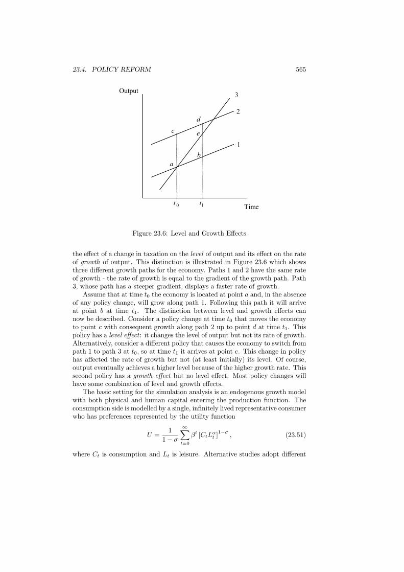
23.4. POLICY REFORM 565
Time
Output
1
2
3
a
c
b
e
d
0t 1t
Figure 23.6: Level and Growth Effects
the effect of a change in taxation on the level of output and its effect on the rateof growth of output. This distinction is illustrated in Figure 23.6 which showsthree different growth paths for the economy. Paths 1 and 2 have the same rateof growth - the rate of growth is equal to the gradient of the growth path. Path3, whose path has a steeper gradient, displays a faster rate of growth.Assume that at time t0 the economy is located at point a and, in the absence
of any policy change, will grow along path 1. Following this path it will arriveat point b at time t1. The distinction between level and growth effects cannow be described. Consider a policy change at time t0 that moves the economyto point c with consequent growth along path 2 up to point d at time t1. Thispolicy has a level effect : it changes the level of output but not its rate of growth.Alternatively, consider a different policy that causes the economy to switch frompath 1 to path 3 at t0, so at time t1 it arrives at point e. This change in policyhas affected the rate of growth but not (at least initially) its level. Of course,output eventually achieves a higher level because of the higher growth rate. Thissecond policy has a growth effect but no level effect. Most policy changes willhave some combination of level and growth effects.The basic setting for the simulation analysis is an endogenous growth model
with both physical and human capital entering the production function. Theconsumption side is modelled by a single, infinitely lived representative consumerwho has preferences represented by the utility function
U =1
1− σ
∞Xt=0
βt [CtLαt ]1−σ
, (23.51)
where Ct is consumption and Lt is leisure. Alternative studies adopt different

566 CHAPTER 23. ECONOMIC GROWTH
values for the parameters α and σ. The second area of differentiation betweenstudies is the range of inputs into the production process for human capital, inparticular whether it requires only human capital and time or whether it alsoneeds physical capital. The analytical process is to specify the initial tax rates,which usually take values close to the actual position in the US, then calculatethe initial growth path. The tax rates are then changed and the new steadystate growth path calculated. The two steady states are then contrasted with afocus placed upon the change in growth rate and in levels of the variables.Figure 23.7 summarizes some of the policy experiments and their conse-
quences. The experiment of Lucas involves elimination of the capital tax withan increase in the labor tax to balance the government budget. This policychange has virtually no growth effect (it is negative but very small) but a signif-icant level effect. In contrast, King and Rebelo and Jones et al. find very stronggrowth and level effects. King and Rebelo consider the effect of an increasein the capital tax by 10% whereas Jones et al. mirror Lucas by eliminatingthe capital tax. What distinguishes the King and Rebelo analysis is that theyhave physical capital entering into the production of human capital. Jones etal. employ a higher value for the elasticity of labor supply than other studies.The model of Pecorino has the feature that capital is a separate commodity tothe consumption good. This permits different factor intensities in the produc-tion of human capital, physical capital and the consumption good. Completeelimination of the capital tax raises the growth rate, in contrast to the findingof Lucas.The importance of each of the elements in explaining the divergence be-
tween the results is studied in Stokey and Rebelo (1995). Using a model thatencompasses the previous three, they show that the elasticity of substitutionin production matters little for the growth effect but does have implicationsfor the level effect - with a high elasticity of substitution, a tax system thattreats inputs asymmetrically will be more distortionary. The elimination of thedistortion then leads to a significant welfare increase. What are important arethe factor shares in production of human capital and physical capital, the in-tertemporal elasticity of substitution in utility and the elasticity of labor supply.Stokey and Rebelo conclude that the empirical evidence provides support forvalues of these parameters which justify Lucas’ claim that the growth effect issmall.
A range of estimates have been given for the effects of taxation upon growthinvolving several different policy experiments. Some of the models predict thatthe growth effect is insignificant, others predict it could be very significant.What distinguishes the models are a number of key parameters, particularlythe share of physical capital in human capital production, the elasticities in theutility function and the depreciation rates. In principal, these could be isolatedempirically and a firm statement of the size of the growth effect given. To doso and thus claim an “answer” would be to overlook several important issuesabout the restrictiveness of the model. Moreover, it would not be justifiable to
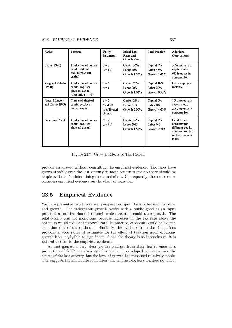
23.5. EMPIRICAL EVIDENCE 567
Capital 0%Labor 0%Growth 2.74%
Capital 0%Labor 0%Growth 4.00%
Capital 30%Labor 20%Growth 0.50%
Capital 0%Labor 46%Growth 1.47%
Final Position Additional Observations
Initial Tax Rates and Growth Rate
Utility Parameters
FeaturesAuthor
Capital and consumption different goods, consumption tax replaces income taxes
Capital 42%Labor 20%Growth 1.51%
σ = 2α = 0.5
Production of human capital requires physical capital
Pecorino (1993)
10% increase in capital stock29% increase in consumption
Capital 21%Labor 31%Growth 2.00%
σ = 2α= 4.99α calibrated given σ
Time and physical capital produce human capital
Jones, Manuelli and Rossi (1993)
Labor supply is inelastic
Capital 20%Labor 20%Growth 1.02%
σ = 2α = 0
Production of human capital requires physical capital (proportion = 1/3)
King and Rebelo (1990)
33% increase in capital stock6% increase in consumption
Capital 36%Labor 40%Growth 1.50%
σ = 2α = 0.5
Production of human capital did not require physical capital
Lucas (1990)
Figure 23.7: Growth Effects of Tax Reform
provide an answer without consulting the empirical evidence. Tax rates havegrown steadily over the last century in most countries and so there should beample evidence for determining the actual effect. Consequently, the next sectionconsiders empirical evidence on the effect of taxation.
23.5 Empirical Evidence
We have presented two theoretical perspectives upon the link between taxationand growth. The endogenous growth model with a public good as an inputprovided a positive channel through which taxation could raise growth. Therelationship was not monotonic because increases in the tax rate above theoptimum would reduce the growth rate. In practice, economies could be locatedon either side of the optimum. Similarly, the evidence from the simulationsprovides a wide range of estimates for the effect of taxation upon economicgrowth from negligible to significant. Since the theory is so inconclusive, it isnatural to turn to the empirical evidence.At first glance, a very clear picture emerges from this: tax revenue as a
proportion of GDP has risen significantly in all developed countries over thecourse of the last century, but the level of growth has remained relatively stable.This suggests the immediate conclusion that, in practice, taxation does not affect
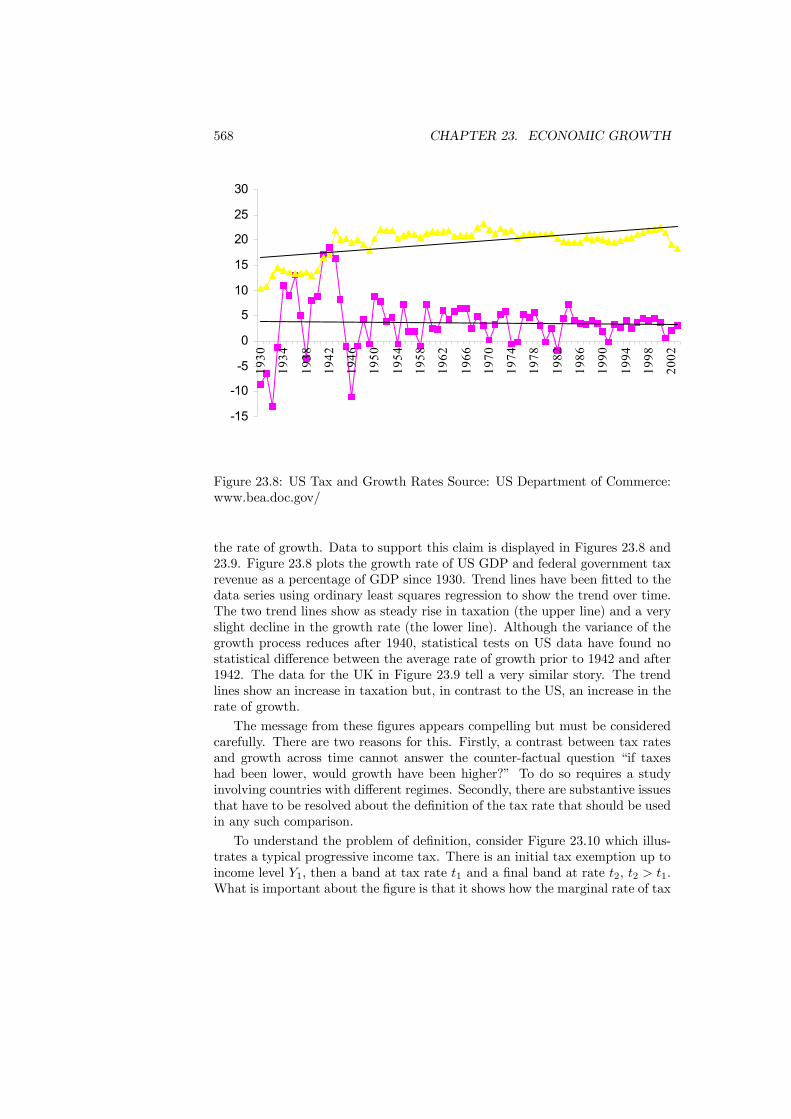
568 CHAPTER 23. ECONOMIC GROWTH
-15
-10
-5
0
5
10
15
20
25
30
1930
1934
1938
1942
1946
1950
1954
1958
1962
1966
1970
1974
1978
1982
1986
1990
1994
1998
2002
Figure 23.8: US Tax and Growth Rates Source: US Department of Commerce:www.bea.doc.gov/
the rate of growth. Data to support this claim is displayed in Figures 23.8 and23.9. Figure 23.8 plots the growth rate of US GDP and federal government taxrevenue as a percentage of GDP since 1930. Trend lines have been fitted to thedata series using ordinary least squares regression to show the trend over time.The two trend lines show as steady rise in taxation (the upper line) and a veryslight decline in the growth rate (the lower line). Although the variance of thegrowth process reduces after 1940, statistical tests on US data have found nostatistical difference between the average rate of growth prior to 1942 and after1942. The data for the UK in Figure 23.9 tell a very similar story. The trendlines show an increase in taxation but, in contrast to the US, an increase in therate of growth.
The message from these figures appears compelling but must be consideredcarefully. There are two reasons for this. Firstly, a contrast between tax ratesand growth across time cannot answer the counter-factual question “if taxeshad been lower, would growth have been higher?” To do so requires a studyinvolving countries with different regimes. Secondly, there are substantive issuesthat have to be resolved about the definition of the tax rate that should be usedin any such comparison.
To understand the problem of definition, consider Figure 23.10 which illus-trates a typical progressive income tax. There is an initial tax exemption up toincome level Y1, then a band at tax rate t1 and a final band at rate t2, t2 > t1.What is important about the figure is that it shows how the marginal rate of tax
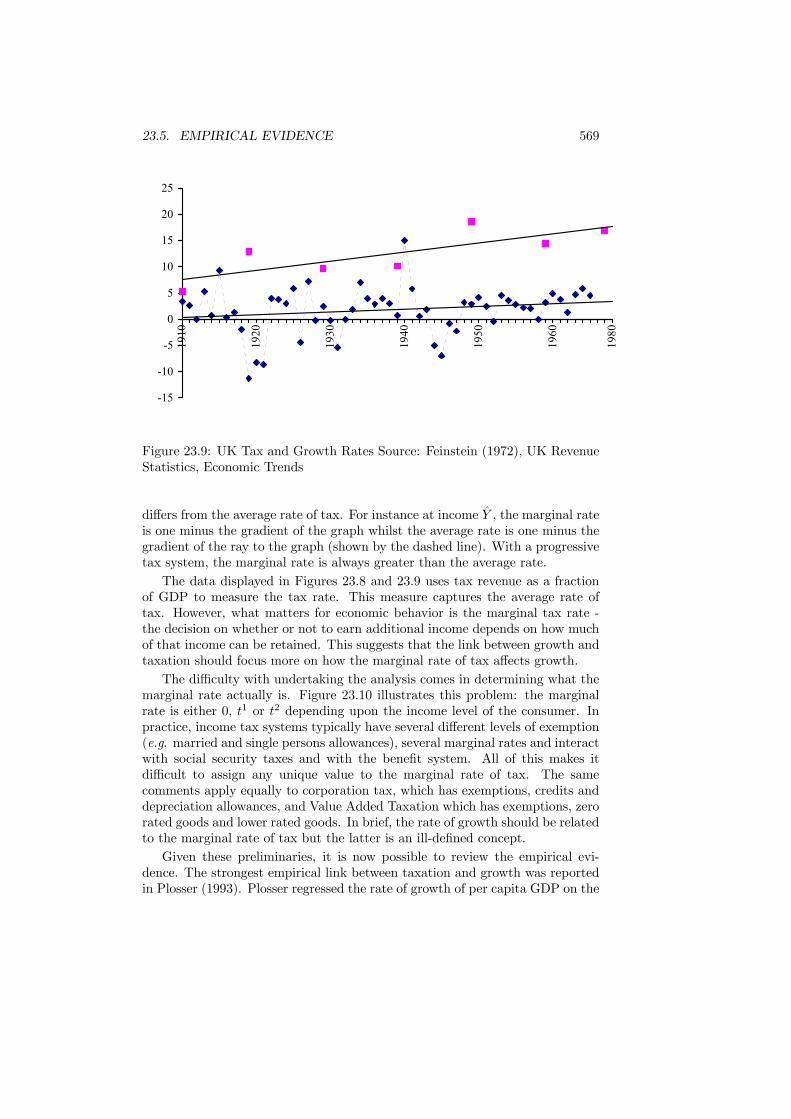
23.5. EMPIRICAL EVIDENCE 569
-15
-10
-5
0
5
10
15
20
2519
10
1920
1930
1940
1950
1960
1980
Figure 23.9: UK Tax and Growth Rates Source: Feinstein (1972), UK RevenueStatistics, Economic Trends
differs from the average rate of tax. For instance at income Y , the marginal rateis one minus the gradient of the graph whilst the average rate is one minus thegradient of the ray to the graph (shown by the dashed line). With a progressivetax system, the marginal rate is always greater than the average rate.The data displayed in Figures 23.8 and 23.9 uses tax revenue as a fraction
of GDP to measure the tax rate. This measure captures the average rate oftax. However, what matters for economic behavior is the marginal tax rate -the decision on whether or not to earn additional income depends on how muchof that income can be retained. This suggests that the link between growth andtaxation should focus more on how the marginal rate of tax affects growth.The difficulty with undertaking the analysis comes in determining what the
marginal rate actually is. Figure 23.10 illustrates this problem: the marginalrate is either 0, t1 or t2 depending upon the income level of the consumer. Inpractice, income tax systems typically have several different levels of exemption(e.g. married and single persons allowances), several marginal rates and interactwith social security taxes and with the benefit system. All of this makes itdifficult to assign any unique value to the marginal rate of tax. The samecomments apply equally to corporation tax, which has exemptions, credits anddepreciation allowances, and Value Added Taxation which has exemptions, zerorated goods and lower rated goods. In brief, the rate of growth should be relatedto the marginal rate of tax but the latter is an ill-defined concept.Given these preliminaries, it is now possible to review the empirical evi-
dence. The strongest empirical link between taxation and growth was reportedin Plosser (1993). Plosser regressed the rate of growth of per capita GDP on the
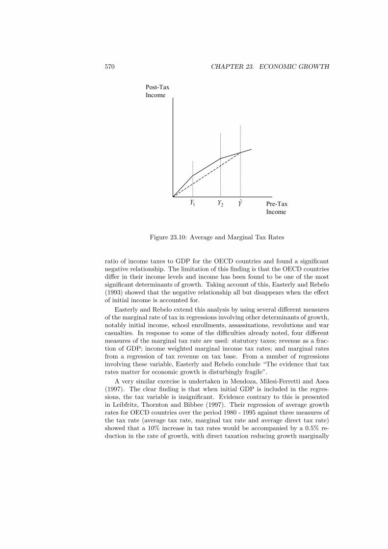
570 CHAPTER 23. ECONOMIC GROWTH
1Y 2Y Y
Post-TaxIncome
Pre-TaxIncome
Figure 23.10: Average and Marginal Tax Rates
ratio of income taxes to GDP for the OECD countries and found a significantnegative relationship. The limitation of this finding is that the OECD countriesdiffer in their income levels and income has been found to be one of the mostsignificant determinants of growth. Taking account of this, Easterly and Rebelo(1993) showed that the negative relationship all but disappears when the effectof initial income is accounted for.Easterly and Rebelo extend this analysis by using several different measures
of the marginal rate of tax in regressions involving other determinants of growth,notably initial income, school enrollments, assassinations, revolutions and warcasualties. In response to some of the difficulties already noted, four differentmeasures of the marginal tax rate are used: statutory taxes; revenue as a frac-tion of GDP; income weighted marginal income tax rates; and marginal ratesfrom a regression of tax revenue on tax base. From a number of regressionsinvolving these variable, Easterly and Rebelo conclude “The evidence that taxrates matter for economic growth is disturbingly fragile”.A very similar exercise is undertaken in Mendoza, Milesi-Ferretti and Asea
(1997). The clear finding is that when initial GDP is included in the regres-sions, the tax variable is insignificant. Evidence contrary to this is presentedin Leibfritz, Thornton and Bibbee (1997). Their regression of average growthrates for OECD countries over the period 1980 - 1995 against three measures ofthe tax rate (average tax rate, marginal tax rate and average direct tax rate)showed that a 10% increase in tax rates would be accompanied by a 0.5% re-duction in the rate of growth, with direct taxation reducing growth marginally
23.5. EMPIRICAL EVIDENCE 571
more than indirect taxation.
One possible route out of the difficulties of defining the appropriate tax rateis to adopt a different method of determining the effect of fiscal policy. Engenand Skinner (1996) label the regressions described above as “top-down” sincethey work with aggregate measures of taxation. Instead of doing this, theypropose a “bottom-up” method which involves calculating the effect of taxationon labor supply, investment and productivity, and then summing these to obtaina total measure. Doing this suggests that a cut of 5% in all marginal rates oftax and 2.5% in average rates would raise the growth rate by 0.22%
An alternative line of literature (Barro (1991), Dowrick (1993) and de laFuente (1997)) has considered the more general issue of how fiscal policy hasaffected growth. In particular, the relation of growth to the composition andlevel of public sector spending is investigated. The results of de la Fuente showthat if public spending (measured as the share of total government expenditurein GDP) increases, growth is reduced (an increase in government spending of5% of GDP reduces growth by 0.66%) whereas an increase in public investmentwill raise growth. There are four significant points to be made about thesefindings. Firstly, government spending may just be a proxy for the entire setof government non-price interventions - including, for example, employmentlegislation, health and safety rules and product standards - and that it may bethese, not expenditure, that actually reduce growth. Secondly, since the shareof public spending in GDP is very closely correlated to the average tax rate, itis not clear which hypothesis is being tested.
The final points are more significant. Levine and Renelt (1992) have shownthat the finding of a negative relationship is not robust to the choice of condi-tioning variables. Finally, as noted by Slemrod (1995), the method of the regres-sions is to use national income, Y , as the left-hand-side variable and governmentexpenditure, G, as the right-hand-side variable. In contrast, economic theoryusually views the causality as running in the opposite direction: governmentexpenditure is seen as being determined by the preferences of the population asexpressed through the political system. An extreme version of this view is cap-tured in Wagner’s law which relates government expenditure to national incomevia the income elasticity of demand for government-provided goods and services.If Y (or the growth of Y ) and G are related via an equilibrium relationship, thena simple regression of one on the other will not identify this.
This review of the empirical evidence leads to the following observations.A visual inspection of tax rates and growth rates suggests that there is littlerelationship between the two. This is weak evidence but it does find supportin some more detailed investigations in which regression equations that includepreviously identified determinants of growth, especially initial income, revealthat tax rates are insignificant as an explanatory variable. Other regressionsfind a small but significant tax effect. All of these results are hampered bythe difficulties in actually defining marginal rates of tax and in their lack of anequilibrium relationship.
572 CHAPTER 23. ECONOMIC GROWTH
23.6 Conclusions
Growth is important since without it living standards must stagnate. The effectof even small changes in the growth rate can be dramatic. With a growth rateof 2% it takes 35 years to double the level of income but at a rate of 5% it takesjust 14 years. Even if economic policy only succeeds in increasing the growthrate from 2% to 3%, it will reduce the time taken to double income by 12 years.The cumulative effect of a policy that affects the growth rate will eventuallydominate anything achieved by a policy that affects only the level of economicvariables.In an exogenous growth model the economy must eventually reach a limit
to its growth unless there is technical progress. The effects of policy are limitedin this form of model because in the long-run they cannot affect the growthrate. Nonetheless, these models still provide some insight into what policy mustachieve in order for it to have a lasting effect upon economic growth. In partic-ular, the exogenous growth model provides a simple setting for demonstratingthe important result that efficiency requires that the tax rate on capital incomemust be zero in the long-run.The limitations of the exogenous growth model lead to the development of
theories of endogenous growth. The literature on endogenous growth has pro-vided a range of mechanisms through which taxation can impact upon economicgrowth. This chapter has described the range of models and has discussed theresults that have been obtained. In quantitative terms, a wide range of theo-retical predictions arose for the size of the tax effect from the insignificant toconsiderable. The size of the growth rate effect depends just about equally onthe structure of the model and on the parameter values within the model. Theproduction process for human capital is also critical, as are the elasticities inthe utility function and the rates of depreciation. A fair summary is that thetheoretical models introduce a range of issues that must be considered, but donot provide any convincing or definitive answers.The conclusions of the empirical evidence are not quite as diverse as for the
theory. Although there are some disagreements, the picture that emerges is thatthe effect of taxation, if there is any at all, is relatively minor. However, theestimates have to be judged taking into account to the difficulty of defining theappropriate measure of the tax rate and the choice of appropriate regressors.These problems may prove to be significant but that is unlikely. As far aspolicy is concerned, this is a reassuring conclusion since it removes the need tobe overly concerned about growth effects when tax reforms are planned.
ReadingThe classic summary of exogenous growth theory can be found in:Solow, R.M. (1970) Growth Theory: An Exposition (Oxford: Oxford Uni-
versity Press).The data in Table 23.1 are taken from:Chamley, C. (1981) “The welfare const of capital income taxation in a grow-
ing economy”, Journal of Political Economy, 89, 468 - 496.
23.6. CONCLUSIONS 573
Three detailed surveys of growth theory which differ in their emphasis are:Aghion, P. and Howitt, P. (1998) Endogenous Growth Theory (Cambridge:
MIT Press).andBarro, R.J. and Sala—I-Martin, X. (1995) Economic Growth (New York:
McGraw-Hill).De La Croix, D. and P. Michel (2002) A Theory of Economic Growth (Cam-
bridge: Cambridge University Press).The proof that the optimal capital tax rate is zero can be found in:Chamley, C. (1986) “Optimal taxation of capital income in general equilib-
rium with infinite lives”, Econometrica, 54, 607 - 622.Judd, K. (1985) “Redistributive taxation in a simple perfect foresight model”,
Journal of Public Economics, 28, 59 - 83.The model of endogenous growth with a public input was first proposed by:Barro, R.J. (1990) “Government spending in a simple model of endogenous
growth”, Journal of Political Economy, 98, S103-S125.The simulations of the effect upon growth of changes in the tax rate are
taken from:Lucas, R.E. (1990) “Supply-side economics: an analytical review”, Oxford
Economic Papers, 42, 293 - 316.Jones, L.E., Manuelli, R.E., and Rossi, P.E. (1993) “Optimal taxation in
models of endogenous growth”, Journal of Political Economy, 101, 485 - 517.King, R.G. and Rebelo, S. (1990) “Public policy and endogenous growth:
developing neoclassical implications”, Journal of Political Economy, 98, S126 -S150.Pecorino, P. (1993) “Tax structure and growth in a model with human cap-
ital”, Journal of Public Economics, 52, 251 - 271.Stokey, N.L. and Rebelo, S. (1995) Growth effects of flat-rate taxes”, Journal
of Political Economy, 103, 519 - 550.Some of the data in Figure 23.9 are from:Feinstein, C.H. (1972) National Income, Expenditure and Output of the
United Kingdom, 1855 — 1965, (Cambridge: Cambridge University Press).For empirical evidence on the effect of taxation upon economic growth:Barro, R.J. (1991) “Economic growth in a cross section of countries”, Quar-
terly Journal of Economics, 106, 407 - 444.Easterly, W. and Rebelo, S. (1993)“Fiscal policy and economic growth”,
Journal of Monetary Economics, 32, 417 - 458.Dowrick, S. (1993) “Government consumption: its effects on productivity
growth and investment” in N. Gemmel (ed.) The Growth of the Public Sector.Theories and Evidence (Aldershot: Edward Elgar).Easterly, W. (1993) “How much do distortions affect growth?”, Journal of
Monetary Economics, 32, 187 - 212.Engen, E.M. and Skinner, J. (1996) “Taxation and economic growth”, NBER
Working Paper No. 5826.de la Fuente, A. (1997) “Fiscal policy and growth in the OECD”, CEPR
Discussion Paper No. 1755.

574 CHAPTER 23. ECONOMIC GROWTH
Leibfritz, W, Thornton, J. and Bibbee, A. (1997) “Taxation and economicperformance”, OECD Working Paper No. 176.Levine, R. and Renelt, D. (1992) “A sensitivity analysis of cross-country
growth models”, American Economic Review, 82, 942 - 963.Mendoza, E., Milesi-Ferretti, G.M and Asea, P. (1997) “On the ineffec-
tiveness of tax policy in altering long-run growth: Harberger’s superneutralityconjecture”, Journal of Public Economics, 66, 99 - 126.Plosser, C. (1993) “The search for growth”, in Federal Reserve of Kansas
City symposium series, Policies for Long Run Growth, 57 - 86, (Kansas City).Slemrod, J. (1995) “What do cross-country studies teach about government
involvement, prosperity, and economic growth”, Brookings Papers on EconomicActivity, 373 - 431.