Interim Analysis in Clinical Trials and Early Stoppingfor Futility

John M. Lachin

The Biostatistics Center

The George Washington University

jml@biostat.bsc.gwu.edu

Interim Analysis in Clinical Trials

Effectiveness Monitoring:Group sequential upper one-sided, or outer two-sided bounds, for rejecting H0.Lan-DeMets α-spending function preserves overall type I error probability α.Allows early termination due to beneficial effect.Fixed sample size power preserved with O’Brien-Fleming bound, not a Pocock bound.

Safety Monitoring:No formal sequential procedures usually applied.

Futility Monitoring:Formal lower one-sided, or inner two-sided bounds, for accepting H0.

ORComputation of conditional power

Futility Monitoring

Conditional Power (CP ):The probability that the final study result will be statistically significant, given the dataobserved thus far and a specific assumption about the future data.

Stochastic Curtailing refers to a decision to terminate a trial based on CPHalperin, Lan, Ware, Johnson and DeMets. Controlled Clinical Trials 1982.Lan, Simon and Halperin. Comm. Statist. 1982.

Futility Monitoring refers to monitoring for lack of effectiveness based on low CPWare, Muller and Braunwald. Am. J. Medicine 1985.

Sequential MonitoringBounds on Type I and II error probabilities α and β

Lan, Simon and Halperin (1982) under continuous monitoringDavis and Hardy (Comm. Statist., 1990, 1992) when monitored at discrete points in

time.

Single Interim Futility Assessment at a Pre-Specified Time

Industry trials with "mid-study" futility assessmentSample size re-estimation procedures with a simultaneous futility assessment atpre-specified time τ , e.g. Lan-Trost (1997)

Simple Example: The Lupus Nephritis Collaborative Study

Lachin and Lan, Controlled Clinical Trials, 1992Effects of Plasmapheresis versus Standard therapy on renal failure in lupusnephritis.With two years remaining in the study the following data had been observed

Response

GroupP S

+ 11 10 21− 29 36 5540 46 86

bπP = 0.275 (11/40)bπS = 0.2174p = 0.66 (two-sided)

Recruitment closed.Question: Conditional Power

What is the probability that the study would yield a significant result (one-sided) in favor of Plasmapheresis if the study were to be continued for two years,given what has been observed to date?

Possible Future Data

All 2× 2 tables with the following values

Response

GroupP S

+ 11 + a 10 + b 21 + a + b− 29− a 36− b 55− a− b

40 46 86

0 ≤ a ≤ 290 ≤ b ≤ 36

To compute the conditional power (one-sided):1. Identify those tables where bπP < bπS and p ≤ 0.05 (one-sided).2. Specify probabilities to apply to the future data: πP and πS.

3. Compute the probability of each table with values (a, b) given (πP , πS),P (table) = P (a|πP )× P (b|πS) = B(a|πP , 29)×B(b|πS, 36)

4. Sum these probabilities

CP (πP , πS) =X29

a=0

X36

b=0I [bπP < bπS] I [p ≤ 0.05]B(a|πP, 29)×B(b|πS, 36)

The Lupus Nephritis Collaborative Study

Current Trend:Control group: πS = pS = 0.22

Plasmapheresis group: πP = pP = 0.28,

CP < 0.01 (one-sided)Design Effect Size: 50% reduction

Control group: πS = pS = 0.22

Plasmapheresis group: πP = 0.11,CP = 0.01

Study stopped for futility

Generalizations

Exact CP for test for proportions with additional recruitment (Lachin, Lan, 1992)Large Sample CP for tests for proportions with or without additional recruitment(Halperin, et al. 1982)Lan and Wittes (Biometrics, 1988) B-value (Brownian Motion)

Applicable to any test with "independent increments" in informationAny test based on an efficient estimator of the parameter of interest

Lachin (Statistics in Medicine, 2005)Operating Characteristics

Probability of stoppingType I and II error probabilities

Information Time (Fraction)Test H0: θ = 0 versus H1: θ 6= 0

Zt = Z-test value at “information time” t, Zt = bθt/qV (bθt)Simple cases (means or proportions)

Planned total sample sizes: NE and NC in groups E and C.

Variance ∝£N−1E +N−1C

¤, e.g. V

£X1 −X2

¤= σ2

h1NE+ 1

NC

iAs Variance decreases, information increasesInformation ∝

£N−1E +N−1C

¤−1Accrued sample sizes: nE and nC

t =

£n−1E + n−1C

¤−1£N−1E +N−1C

¤−1= n/N if nE = nC and NE = NC

Logrank test

Expected number of events: E(DE) and E(DC)

Information ∝£E(DE)

−1 +E(DC)−1¤−1

Accrued events: dE and dC

t =

£d−1E + d−1C

¤−1[E(DE)−1 +E(DC)−1]

−1

=dC

E(DC)under H0 for groups of equal size

Drift ParameterStatistic S:

H0: S ∼ N(0, σ2/N)

H1: S ∼ N(φ, σ2/N)

Z = S√N/σ

αD = design type I error probabilityβD = design type II error probability, 1− βD = Φ(Z1−βD

) = power

N =

∙(Z1−αD

+ Z1−β)σ

φ

¸2Drift Parameter θ is the non-centrality parameter

θ = E[Z|H1] =

√N |φ|σ

= Z1−αD+ Z1−β

For α = 0.05 (two-sided), β = 0.15, then θ = 1.96 + 1.04 = 3

The B-valueA transform of the Z-test value that facilitates computation of CP

Lan and Wittes. Biometrics 1988.Lan and Zucker. Statistics in Medicine 1993.

B-value,Bt = Zt

√t, 0 < t ≤ 1.

Asymptotically, 0 < t ≤ 1

Bt ∼ N(tθ, t)

Zt ∼ N(θ√t, 1)bθt = Bt/t ∼ N(θ, 1/t)

The B-value Shows the Trend in the Data

Bt ∼ N(tθ, t), θ = E[Z|H1] =

√N |φ|σ

Example, Mantel logrank TestαD = 0.05 (two-sided), 1− βD = 0.85

Relative hazard φD = 0.6

Control group hazard rate of 0.35 per year5% losses to follow-up per year1 year recruitment and 2.5 year total durationN = 355, Lachin and Foulkes (Biometrics, 1986)θD = Z0.975 + Z0.85 = 1.96 + 1.04 = 3

E(DC) = 85 events in the control groupt = dc/85

Conditional PowerθF = drift parameter for the future data

B1|(Bt, θF ) ∼ N(eθ, 1− t)

where eθ = tbθt + θF (1− t) = Bt + θF (1− t).

CP (t, θF ) = Φ[Z1−β(t, θF )] where

Z1−β(t, θF ) =eθ − Z1−αD√1− t

CPD under the original design, θF = θD

CPT under the current trend, θF = bθtCPN under H0, θF = 0

Conditional Power - DistributionθI = drift parameter assumed for the initial data up to interim assessment

= E(bθt) = E(Bt/t)

Since Z1−β is a funciton of bθt, or of Bt or Zt, then

Z1−β(t, θF ) ∼ N

∙tθI + (1− t)θF − Z1−αD√

1− t,

t

1− t

¸Provides distribution of Z1−β, and of CP , for given α, θI, θF , and t.

Con

ditio

nal P

ower

Low Conditional Power (< 0.3) at t = 0.5Under the Design, Current Trend and Null

As a Function of the B-value and θt

B0.5

Desig

n

Tren

d

Null

θ0.5∧

0.30

0.25

0.20

0.15

0.10

0.05

-2 -1 0 1 2 3 4

-1 0 1 2

∧

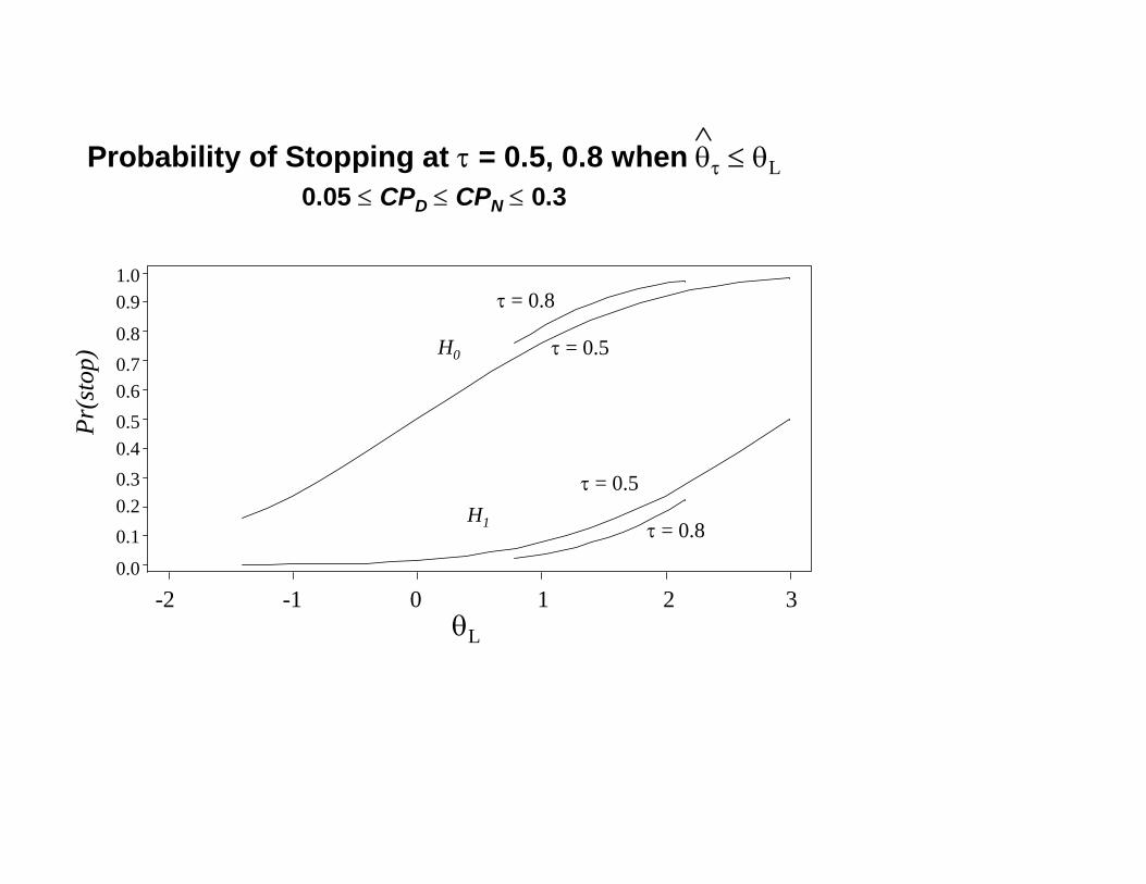
Futility StoppingPre-specified time t = τ

Stop for futility if CP ≤ CL

P (Stop)

PL = P [CP (τ , θF ) ≤ CL]

= P [Bτ ≤ BL]

= P [bθτ ≤ θL]

Pr(s

top)

θL

τ = 0.5

τ = 0.8

H0

H1

τ = 0.5

τ = 0.8

Probability of Stopping at τ = 0.5, 0.8 when θτ ≤ θL0.05 ≤ CPD ≤ CPN ≤ 0.3

1.00.9

0.80.70.60.50.40.30.20.1

0.0

-2 -1 0 1 2 3

∧

Type II Error Probabilityβ = β1 + β2

β1 = PL1 = P (stop for futility |H1)

β2 = Prob continuation and the final result is not significantβ2 = P (B1 < Z1−αD

∩ Bτ > BL|H1)

β ≤ β1 + βD

Example

Design power = 0.85, βD = 0.15 when φ = 0.6

Stop for futility at τ = 0.5 if CPD(0.5) ≤ 0.3B0.5 ≤ BL = 0.08916bθ0.5 ≤ θL = 0.17831.

Under H1: θ = θD, P (stop) = P (CPD(0.5) ≤ 0.3) = 0.023.Total type II error probability given θ = θD

β = P (CPD(0.5) ≤ 0.3) + P [(CPD(0.5) > 0.3) ∩ (|Z1| < 1.96)]= 0.023 + 0.131 = 0.154.

Type II Error ProbabilityθF = θD = 3

0.05 ≤ CPD ≤ CPN ≤ 0.3

β

θ(τ)L

τ = 0.5

τ = 0.80.150.20

0.30

0.40

0.50

-2 -1 0 1 2 3

Type I Error Probabilityα = α1 + α2

α1 = P (reject when stop for futility |H0) = 0.α2 = is the probability of continuation and significance at the final analysis

under H0: θ = 0.For a one-sided test at level αD

α2 = P (Bt > BL ∩ B1 ≥ Z1−αD| H0)

Type I Error Probability0.05 ≤ CPD ≤ CPN ≤ 0.3

α

τ = 0.8

τ = 0.5

0.01

0.02

0.03

0.04

0.05

θ(τ)L-2 -1 0 1 2 3

Fixing The Error ProbabilitiesAs P(Stop) increases

β increases from design level βD

α decreases from design level αD

For given boundary BL can iteratively determine final critical value ZF < Z1−αD

such that α2 = αD

Example:BL = 0.9 (θL = 1.8) at τ = 0.5, ZF = 1.7535 provides α = 0.05 two-sided.

For given β ≥ βD can iteratively determine BL and ZF such that α2 = αD

Example: Slight Inflation in P(Type II error)θD = 3, αD = 0.05 (two-sided), βD = 0.15 and β = 0.175, at τ = 0.5,

ZF = 1.8954 and BL = 0.5673 for which θL = 1.135.

P (stop | H0) = 0.789, P (stop | θ = 3) = 0.094.

Fixing The Error ProbabilitiesExample: No Inflation in P(Type II error)

θD = 3, αD = 0.05 (two-sided), βD = β = 0.15, at τ = 0.5,ZF = 1.95996 and BL = −1.1794 for which θL = −2.359.P (stop | H0) = 0.047, P (stop | θ = 3) = 0.000076.

ConclusionsWhile CP is a useful construct, the properties of futility monitoring depend on the

bounds on the interim statistics: either Zt, Bt, or bθt.Conservative to employ CP under designCP under the current trend has a higher probability of stopping for futility,

greater inflation in β

Regardless of how CP is computed, the probability of stopping is a function ofthe true drift parameter θthe critical value BL or the corresponding θL

The greater the probability of stopping the greater the potential inflation β.

Inflation in β can be reduced by adjustment of final critical value ZF .As the time of the futility assessment increases:

Probability of stopping under H1 decreasesInflation in β decreases

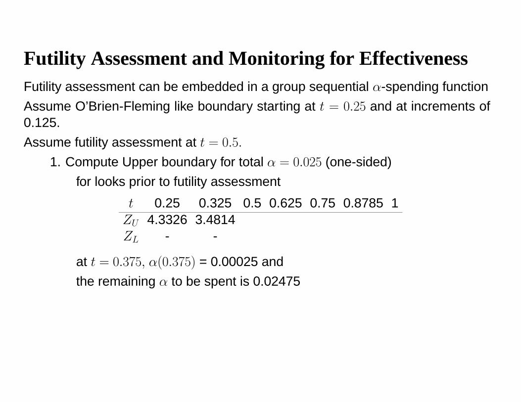
Futility Assessment and Monitoring for EffectivenessFutility assessment can be embedded in a group sequential α-spending functionAssume O’Brien-Fleming like boundary starting at t = 0.25 and at increments of0.125.Assume futility assessment at t = 0.5.

1. Compute Upper boundary for total α = 0.025 (one-sided)for looks prior to futility assessment

t 0.25 0.325 0.5 0.625 0.75 0.8785 1ZU 4.3326 3.4814ZL - -

at t = 0.375, α(0.375) = 0.00025 andthe remaining α to be spent is 0.02475

2. Compute futility bound and critical value for αD = 0.02475,βD = 0.15, and total β = 0.20 for θ = 3

t 0.25 0.325 0.5 0.625 0.75 0.8785 1ZU 4.3326 3.4814ZL - - 1.06427

ZF = 1.84009 with nominal αF = 0.032877

2. Compute futility bound and critical value for αD = 0.02475,βD = 0.15, and total β = 0.20 for θ = 3

t 0.25 0.325 0.5 0.625 0.75 0.8785 1ZU 4.3326 3.4814ZL - - 1.06427

ZF = 1.84009 with nominal αF = 0.032877

3. Compute remaining O-Brien-Fleming boundary using α = 0.032877 startingat t = 0.5

t 0.25 0.325 0.5 0.625 0.75 0.8785 1ZU 4.3326 3.4814 2.8006 2.5013 2.2725 2.0963 1.9554ZL - - 1.06427 - - - -

4. Check actual probabilities using the Lan-DeMets program,α = 0.0266 one sided (0.0532 two-sided) and 1− β = 0.7957.

If futility assessment at τ = 0.75, then α = 0.02461 and 1− β = 0.7817.An exact calculation could be done using successive multivariate integration forthe sequence of interim analyses.

Related WorkSnappin (Stat in Med, 1992) reject H0 based on CP (Trend), accept H0 based onCP (Design)

Pepe and Anderson (Appl Stat, 1992) similar for conservative estimate undercurrent trend for survival data.Ellenberg and Eisenberg (Cancer Treat Rep, 1985), Wieand et al. (Stat in Med,1994):

Stop for futility in PH model if bβ < 0

P (stop|H1) very small, minimal impact on α, βPampalonna and Tsiatis (J Stat Plan and Inf, 1994),

α and β spending outer and inner bounds for effectiveness and futility (EAST)Other related methodsExact α, β only for a fixed pre-specified sequence of looks

Kittleson and Emerson (Biometrics, 1999)Inner and outer boundaries for α = 0.05 (2-sided), β = 0.20

Inner boundary corresponds to CL = CPD = 0.50

Tante Grazie!