Rollins CollegeRollins Scholarship Online

Student-Faculty Collaborative Research

3-2006

Interferometric studies of a piano soundboardThomas R. MooreDepartment of Physics, Rollins College, TMOORE@rollins.edu

Sarah A. ZietlowDepartment of Physics, Rollins College

Follow this and additional works at: http://scholarship.rollins.edu/stud_fac

Part of the Physics Commons

This Article is brought to you for free and open access by Rollins Scholarship Online. It has been accepted for inclusion in Student-FacultyCollaborative Research by an authorized administrator of Rollins Scholarship Online. For more information, please contact rwalton@rollins.edu.

Published InSarah A. Zietlow, and Thomas R. Moore. 2006. Interferometric studies of a piano soundboard. The Journal of the Acoustical Society ofAmerica 119 (3): 1783-93.

Interferometric studies of a piano soundboardThomas R. Moore and Sarah A. ZietlowDepartment of Physics, Rollins College, Winter Park, Florida 32789

�Received 15 June 2005; revised 11 December 2005; accepted 13 December 2005�

Electronic speckle pattern interferometry has been used to study the deflection shapes of a pianosoundboard. A design for an interferometer that can image such an unstable object is introduced, andinterferograms of a piano soundboard obtained using this interferometer are presented. Deflectionshapes are analyzed and compared to a finite-element model, and it is shown that the force thestrings exert on the soundboard is important in determining the mode shapes and resonantfrequencies. Measurements of resonance frequencies and driving-point impedance made using theinterferometer are also presented. © 2006 Acoustical Society of America.�DOI: 10.1121/1.2164989�

PACS number�s�: 43.75.Mn, 43.40.At, 43.20.Ks �NHF� Pages: 1783–1793

I. INTRODUCTION

A complete understanding of how the dynamics of themodern piano creates its unique sound is unlikely without athorough understanding of the soundboard. Probably themost important parameter associated with the soundboard isthe impedance at the point where the strings meet the bridge,and there are several reports of investigations of the depen-dence of the driving-point impedance on frequency.1–6 How-ever, there are parameters beyond the mere value of the im-pedance at the terminating point of the strings that areimportant. Of particular interest are the soundboard deflec-tion shapes. These shapes have been reported to be similar tothe shapes of the normal modes for frequencies below ap-proximately 200 Hz; above this limit the resonances of thesoundboard are believed to be broad and closely spaced sothat the deflection shapes do not necessarily resemble themode shapes.7,8 Understanding the deflection shapes is im-portant not only because they provide some insight into thephysical basis for the impedance structure at the bridge, butalso because they can provide insight into effects, such asacoustic short circuiting, which may not affect the drivingpoint impedance but may significantly affect the sound per-ceived by the listener.

The most common methods for determining the deflec-tion shapes of objects include observing Chladni patterns,measuring the acoustic power as a function of position, mak-ing impact measurements, and performing holographic orspeckle pattern interferometry. However, each of these tech-niques is difficult to use in determining the deflection shapesof a piano soundboard.

In principle Chladni patterns are simple to create, butthey are extremely difficult to obtain on a fully assembledpiano for several reasons. Although some Chladni patternshave been obtained on a soundboard isolated from thepiano,3 the utility of this method is limited by the necessityto physically access the entire soundboard, the requirementthat the soundboard be oriented horizontally, and the fact thatthere are ribs and other attachments that segment the surface.

Recently, acoustic measurements have yielded informa-tion on the shapes of the lowest modes of a piano sound-board; however, these measurements have very low spatial

resolution.9,10 Likewise, mechanical measurements of the de-flection of a soundboard have been made by physically plac-ing accelerometers on an isolated soundboard as it is struck.This technique is limited by the necessity for physical accessto all points of the soundboard, and it is therefore not fea-sible to perform the measurements on a fully assembled pi-ano. Furthermore, the measurement process can potentiallychange the resonance structure and the spatial resolution isquite low.2,7,8,11

Time-averaged holographic or speckle pattern interfer-ometry both provide interferograms that can reveal the de-flection shape of a vibrating object, and both techniques havebeen used often to determine deflection shapes of musicalinstruments. However, the size and mass of a fully assembledpiano make both types of interferometry a very difficult un-dertaking. Specifically, these interferometric techniques re-quire extensive vibration isolation. A good estimate of therequirement for vibration isolation is that the movement ofthe object due to ambient vibrations must be significantlyless than one-tenth of the wavelength of the light used toimage the object. This stability must be maintained over theentire time it takes to perform the experiment. The high cen-ter of mass, large surface area, and wooden construction of apiano make this level of isolation problematic. Even whenenclosed within a soundproof room, and mounted on sup-ports with active vibration control mechanisms, vibrationsthat are transmitted through the support structure usuallymake such large objects too unstable to be effectively studiedusing these techniques.

To investigate the deflection shapes of a piano sound-board, we have modified the common form of the specklepattern interferometer so that ambient vibrations that are dif-ficult to eliminate do not degrade the time-averaged inter-ferogram. In fact, when using this interferometer the decor-relation of the speckle pattern actually increases the precisionof the measurements. This modification, combined with arecently reported modification that reduces the complexity ofthe interferometer while simultaneously reducing the neces-sary laser power,12,13 has enabled us to optically investigatethe deflection shapes of a fully strung piano soundboard insitu.

J. Acoust. Soc. Am. 119 �3�, March 2006 © 2006 Acoustical Society of America 17830001-4966/2006/119�3�/1783/11/$22.50

In what follows we describe this interferometer, thetheory of its operation, and its application to the study of apiano soundboard. We begin by discussing the most commonform of the electronic speckle pattern interferometer andhighlight the problems associated with using it to investigatethe soundboard. We then describe a modification to the in-terferometer and present a theory showing that with thismodification a slow decorrelation of the speckle pattern en-hances the sensitivity. Next, we present some interferogramsof the deflection shapes of the soundboard of a fully as-sembled piano that were made using this method, discusstheir implications, and compare interferograms of the lowestmodes with finite-element models. Finally, we demonstratethat data obtained using this interferometer can be used todetermine the resonance curves of the soundboard, as well asmake measurements of the driving-point impedance.

II. THEORY OF TIME-AVERAGED ELECTRONICSPECKLE PATTERN INTERFEROMETRYWITH DECORRELATION

The arrangement of the electronic speckle pattern inter-ferometer used in our experiments is shown in Fig. 1. It is amodified version of the more common arrangement and adetailed description can be found in Refs. 12 and 13. Tocreate an interferogram, a beam of coherent light is reflectedfrom an object and imaged through a beamsplitter onto acharge-coupled device �CCD� array. A reference beam is di-rected through a delay leg and illuminates a piece of groundglass, which is also in the view of the imaging lens throughreflection from the beamsplitter. To study harmonically vi-brating objects, the image present on the CCD array is digi-tally stored prior to the onset of harmonic motion of theobject. Once the object is executing harmonic motion, theimage on the array is then subtracted from the initial imagein real time.

This situation can be described theoretically by assum-ing that the object under investigation is moving with simpleharmonic motion, with an angular frequency of �0 and anamplitude of �z. Assuming that the size of the speckle isapproximately the size of a single pixel element, the intensityof the light on a pixel is given by

I = Ir + I0 + 2�IrI0 cos � , �1�

where Ir and I0 are the intensities of the reference and objectbeam, respectively, and

� = �0 + � sin��0t� . �2�

In this equation

� =2��z

��cos �i + cos �r� , �3�

and �0 is the initial difference in phases of the two beams atthe pixel element. In Eq. �3�, �i and �r represent the incidentand reflected angles of the object beam measured from thenormal to the surface of the object under study, and � is thewavelength of the light.

For the case considered here the integration time of thedetector is long compared to the period of the motion; there-fore, it records only the time-averaged intensity of the inter-ference. Assuming that the intensities of the two beams areconstant in time, the recorded intensity is given by

�I� = Ir + I0 + 2�IrI0�cos��0 + � sin��0t��� , �4�

where the angled brackets indicate a time average. Perform-ing the time average explicitly reduces Eq. �4� to14

�I� = Ir + I0 + 2�IrI0 J0��� cos �0, �5�

where J0 represents the zero-order Bessel function of the firstkind.

The most common method of viewing the amplitude ofdisplacement is to record an initial image before the onset ofvibration of the object and subtract it from an image re-corded subsequent to the onset of harmonic motion; the ab-solute value of the difference is then displayed on a computermonitor. In this case the intensity recorded by the first frameis given by

I1 = Ir + I0 + 2�IrI0 cos �0, �6�

and the intensity recorded after the onset of vibration of theobject is given by Eq. �5�. When the two are subtracted, theintensity of the pixel displayed on the monitor after the nthframe is given by

In = �n�1 − J0���� , �7�

where �n is a positive constant with a value that dependsupon the relative intensities of the image and referencebeams, as well as the details of the display.

For the interferometer to provide the results indicated byEq. �7�, the object must be stable enough such that thespeckle pattern does not decorrelate in the time between ob-taining the initial and final image. Therefore, the interferom-eter and the object under study are typically isolated fromambient vibrations.

When the object under investigation is large or flimsy,adequate isolation from ambient vibrations can become dif-ficult. Any displacement due to motion of the structure uponwhich the object rests increases linearly with height, and anobject with a high center of mass, such as a piano, enhancesthe effects of any slight motion. Even when the interferom-eter and the piano sit on tables with active pneumatic vibra-

FIG. 1. �Color online� Diagram of the electronic speckle pattern interferom-eter.

1784 J. Acoust. Soc. Am., Vol. 119, No. 3, March 2006 T. R. Moore and S. A. Zietlow: Piano soundboard

tion isolation, and the entire apparatus is enclosed within aroom without circulating air, we have found that the specklecan decorrelate on a time scale significantly less than1 second. This decorrelation may occur even more quickly ifthe interferometer and the object under study are indepen-dently supported, which may be required to image large ob-jects such as pianos.

To include the decorrelation due to ambient vibration, anextra term must be added to Eq. �2�. While the ambient vi-brations may contain many frequencies, it is most difficult toisolate a large object from vibrations with long periods;therefore, we assume that the period of the movement re-sponsible for speckle decorrelation is significantly greaterthan the period of the oscillation of interest. Under this con-dition,

� = �0 +2�

�� sin�t� + � sin��0t� , �8�

where � is the amplitude of the oscillation and it is assumedthat �0.

If the integration time of the detector is short comparedto −1, the small angle approximation may be applied and themovement can be approximated as a slow linear movementover the integration time of the detector. In this case Eq. �8�becomes

� = �0 + t + � sin��0t� . �9�

Equation �9� can also be written as

� = �0 + ��0t + � sin��0t� , �10�

where �1. If the integration time of the detector is shortcompared to −1, the intensity of the light incident on a pixelof the recording array is given by

�In� = Ir + I0 + 2�IrI0�cos��0 + ��0t + � sin��0t��� . �11�

When integrated, the function within the angled brackets inthe above equation is a form of the equation known as An-ger’s function, which is a generalization of the Bessel func-tion of the first kind.14 When � is an integer, Anger’s func-tion reduces to a Bessel function of order �.

Since we have assumed that �1, we can approximatethe time-averaged term in Eq. �11� as Anger’s function with�=0. In this case Eq. �11� reduces to Eq. �5�. However, sincethe small-angle approximation used to obtain Eq. �10� is notvalid for times that are not short compared to −1, �0 cannotbe considered to be constant over long periods of time. Thatis, although we may assume that � is approximately zero forthe purpose of evaluating Eq. �11�, any nonzero value of �will result in a time-varying value of �0 that cannot be ig-nored over time periods that are not short compared to −1.

If the time between the collection of images in electronicspeckle pattern interferometry is long compared to −1, andthe integration time of the detector is short compared to thisvalue, subtracting the pixel value recorded after the onset ofvibration from the value of the same pixel recorded beforethe onset of vibration will generally provide a nonzero result.This nonzero result will occur even when the object has notbeen intentionally set into motion. Therefore, speckle pattern

interferometry yields no usable information about the har-monic movement of the object unless the time between im-ages is short compared to −1.

However, when the initial image and the final image areboth recorded while the object is oscillating at frequency �0,rather than the initial frame being recorded prior to the onsetof vibration, Eq. �11� describes the intensity of both images.Under these circumstances the intensity shown on the com-puter monitor is proportional to the absolute value of thedifference between the pixel values in the mth and nth im-ages, i.e.,

Imn = �mn�J0���� , �12�

where in this case the value of �mn depends not only uponthe details of the monitor settings, but also on the value ofthe phase angle �0, which is slowly varying in time andtherefore changes slightly between the mth and nth frames.That is,

�mn �cos �m − cos �n� , �13�

where �m and �n represent the value of the initial phase anglefor the mth and nth image, respectively.

If the object is too stable, such that cos �m=cos �n, theresulting interferogram will be uniformly black and yield noinformation despite any harmonic movement of the object. Inthis case it is necessary to subtract an image taken after theonset of vibration from one taken before vibration begins forthe interferogram to provide any useful information. Like-wise, if the movement that produces the decorrelation is notwell approximated by a linear function over the integrationtime of the detector, then Eq. �12� is not valid.

In the case where there is a slow decorrelation of thelight, such that over the integration time of the detectorcos �m�cos �n and �1, then the brightness of the pixeldisplayed on the screen will be proportional to �J0����, andlines of equal displacement will occur when

J0��� = 0, �14�

where � is defined by Eq. �3�. Averaging over several frameswill eliminate the possibility of a spurious result due tocos �m and cos �n being equal simply by chance.

Note that Eq. �12� indicates that nodes in the soundboardwill appear white on the monitor, while black lines indicatecontours of equal amplitude of vibration. In the case wherethe initial frame is recorded before the onset of harmonicvibration, Eq. �7� indicates that areas of no movement appearas black, while white lines indicate contours of equal ampli-tude. Note also that the resolution of the system described byEq. �12� is twice that described by Eq. �7�, because Eq. �12�indicates that minima in the interferogram occur at everypoint where the Bessel function has a value of zero. Equation�7� indicates that minima occur only at the maxima of theBessel function.

In the case where the object under investigation is stableso that cos �m=cos �n, a slow linear shift can be added toeither the reference beam or the object beam; similarly, aslow physical motion of the object can be induced artificially.Either of these techniques will ensure that � is nonzero butsignificantly less than unity, and will result in the increased

J. Acoust. Soc. Am., Vol. 119, No. 3, March 2006 T. R. Moore and S. A. Zietlow: Piano soundboard 1785

precision of the interferometer. Yet, precision is seldom theproblem when attempting electronic speckle pattern interfer-ometry in the laboratory.

As noted above, large objects such as pianos are nor-mally not stable enough to image using electronic specklepattern interferometry due to the presence of small ambientmotions transmitted through the support structure. However,if the ambient motion is slow compared to the driving fre-quency �0, the motion will decorrelate the speckle within theconstraints outlined above. In this case, speckle pattern inter-ferometry can be used to study the motion of these objects.That is, as long as there is some slowly varying motion of theobject, even if the motion is caused by ambient vibrationsthat normally precludes the use of interferometry, useful in-terferograms can be obtained.

Before concluding this section we note that assuming�0 ensures that we can approximate the time average inEq. �11� as a zero-order Bessel function of the first kind.However, this is not a necessary approximation since Eq.�11� can be calculated explicitly for any value of �. Interfero-grams can be obtained even for large values of �; however,knowledge of its value is necessary to make measurementsof the amplitude of the motion. We address this issue furtherin Sec. IV.

III. EXPERIMENTAL ARRANGEMENT

All of the experiments reported here were performed ona Hallet and Davis piano manufactured circa 1950. The pianowas a spinet model, with a soundboard measuring approxi-mately 1.4�0.63 meters. The soundboard was of varyingthickness, as is usually the case; however, precise measure-ments of the thickness were not possible without signifi-cantly altering the piano and were therefore not made. Theprofile of the bottom of the soundboard could be unambigu-ously measured, and it was found that the thickness variedfrom 4.4±0.1 to 6.9±0.1 mm.

The soundboard of the piano was made of solid spruce,with the grain direction being 32° from the horizontal, diag-onal from the upper left to lower right as viewed from theback of the piano. There were 12 ribs made of pine and gluedto the back of the soundboard in an orientation perpendicularto the grain. The ribs had a width of approximately 25 mm,were spaced approximately 80 mm apart, and ranged inlength from approximately 217 to 725 mm.

There were two bridges on the front of the soundboardover which the strings passed. A treble bridge, approximately1.12 m in length was placed diagonally from the lower rightto the upper left, as viewed from the back. A bass bridge,approximately 0.37 m long, was attached near the bottom ofthe soundboard. The edges of the soundboard were sand-wiched between the case and retaining timbers, resulting inthe edges being strongly clamped. Figure 2 contains a draw-ing of the soundboard, as viewed from the back, indicatingthe location of the bridges and orientation of the ribs.

Except where it is explicitly noted below, the pianosoundboard remained completely strung and attached to thepiano frame. No modification of the structure of the pianowas made except that the hammers were removed for easier

access to the treble bridge. The strings were all damped intwo or three places by weaving strips of cloth between themto ensure that vibrations of the strings in no way affected thesoundboard vibrations.

The piano was mounted on an optical table with activepneumatic vibration-isolating legs, and attached to the tablewith a 3-in. nylon strap. The back of the piano was paintedwhite to efficiently reflect light.

The interferometer was made from discrete optical com-ponents mounted on a separate actively isolated optical table.The entire experimental arrangement, with the exception ofthe laser, was contained within a 10�12�7 ft. room, whichwas tiled with anechoic foam on all surfaces except for theportions of the floor that supported the optical tables.

The laser used to illuminate the piano was a frequency-doubled Nd:YVO4 laser with a wavelength of 532 nm and amaximum power of 5 W. It was mounted outside of theanechoic room on an optical table with active pneumaticvibration isolation. The light entered the anechoic roomthrough a small hole in the wall. A commercial CCD camerawith a 768�494 pixel array and the standard 30-Hz framerate was used to record the images. The illuminating beamand the imaging system were oriented perpendicular to thesoundboard, so that cos �i and cos �r were both very close tounity.

Since the mass of the tables and the piano exceeded1000 Kg, and the stability required for interferometry re-stricts the relative movement of the interferometer and pianoto less than 50 nm, the floor of the chamber was not made ofa suspended wire mesh as is common. Rather, the floor of thechamber was a portion of a concrete slab that comprised thefloor of the building. Although the interferometer and thepiano were mounted on tables with active vibration isolation,and both were housed in a chamber tiled with anechoic foam,there was a slight independent motion of the two tables atlow frequencies. This motion was transmitted to the tablesthrough the floor, with the peak transmissibility occurring atapproximately 1 Hz.

Under normal circumstances the motion of the tablesdecorrelates the speckle and precludes the use of specklepattern interferometry. However, since the method outlinedabove requires some decorrelation, the motion of the tableswas advantageous. Thus, the technique described above al-lowed the use of speckle pattern interferometry in a situationin which it is normally impossible.

As outlined in the theory above, an image from the cam-era was digitally stored after the soundboard was set into

FIG. 2. Drawing of the orientation of the bridges and ribbing of the sound-board as viewed from the back. The bridges are attached to the front of thesoundboard and the ribs are attached to the back.

1786 J. Acoust. Soc. Am., Vol. 119, No. 3, March 2006 T. R. Moore and S. A. Zietlow: Piano soundboard

harmonic motion. Each subsequent frame was then digitallysubtracted in real time from the previous image. Black linesappeared on the interferogram when the condition set forth inEq. �14� was met.

During the experiments, vibrations of the soundboardwere induced at an angular frequency of �0. The two mo-tions, one harmonic with angular frequency �0 and oneslowly varying so that it appeared linear over the integrationtime of the detector, were completely independent of oneanother. The slower vibrations occurred continually, regard-less of the presence or absence of the driven harmonic mo-tion.

Since the decorrelation time due to the ambient vibra-tions was on the order of the integration time of the CCDarray, good interferograms were obtained by subtracting con-tiguous frames, thus allowing real-time viewing of the inter-ferograms. Some higher frequency ambient vibrations re-sulted in noticeable noise in the interferograms, which wasmanifest as a series of lines unrelated to the harmonic motionof the piano. To eliminate these effects, and produce unam-biguous interferograms for later analysis, up to 200 interfero-grams were averaged before the image was digitally stored.The total time of data collection for a single image, includingpostprocessing, was less than 10 s.

To obtain interferograms showing the deflection shapesof a piano soundboard, the apparatus described above wasused to study the soundboard as it was driven harmonically.The driving force was provided by a speaker placed approxi-mately 2 m from the soundboard. A high-quality functiongenerator provided a sinusoidal signal, which was subse-quently amplified and sent to the speaker. Typical deflectionsof the soundboard were less than a few wavelengths of theilluminating light �i.e., 0.1–2 �m� and required a soundintensity level on the order of 50 dB.

In some cases an electromagnetic shaker was used todrive the soundboard vibrations. The shaker was mounted onan adjustable magnetic base so that the driving mechanismcould impinge upon any desired part of the soundboard.

IV. RESULTS AND ANALYSIS

A. Deflection shapes of a piano soundboard

Typical interferograms obtained using the apparatus de-scribed above are shown in Fig. 3. Three vertical braces andtwo carrying handles are visible in the interferograms, inaddition to the soundboard and the rectangular frame towhich it is mounted. The braces and handles are not physi-cally touching the soundboard.

The interferograms in Fig. 3 show the deflection shapesof the soundboard at three different frequencies ranging from219 Hz to 2.8 kHz. The total amplitude of the deflection atany point can be determined by counting the lines of equaldisplacement from a nodal point. Table I lists the displace-ment from the equilibrium position represented by each con-tour line.

From observations of the interferograms at frequenciesbetween 60 Hz and 3 kHz, it appears that most of the reso-nances of the soundboard are broad and overlapping. How-ever, the lower resonances appear to be significantly sepa-

rated in frequency and therefore amenable to study. Thisconclusion has also been reached by others.3,7,8 Interfero-grams of the deflection shapes of the lowest three resonancesof the piano are shown in Figs. 4�a�, 5�a�, and 6�a�. Theresonant frequencies are shown in the second column ofTable II. The bandwidth of the resonances are on the order of20 Hz; however, the peak response is easily discerned byviewing the interferograms in real time while changing thedriving frequency.

The simplest model of a piano soundboard is that of anisotropic rectangular plate clamped at the edges. Leissa hasreprinted the frequency parameters necessary for finding theresonant frequencies of rectangular plates with several aspectratios.15 The frequency parameter is defined as

� = 2�fa2� �

D, �15�

where f is the resonant frequency, a is the length of theshortest side of the plate, � is the area density, and D is therigidity of the plate, which is defined as

FIG. 3. Interferograms of the soundboard of a spinet piano. The vibrationsare driven acoustically from a speaker placed approximately 2 m away.

TABLE I. The total amplitude of vibration represented by the number ofdark lines traversed from a nodal point in an interferogram. Each line rep-resents a point where Eq. �14� is valid.

Contour Displacement �nm�

1 1022 2343 3664 4995 6326 7657 8988 10319 1164

10 1297

J. Acoust. Soc. Am., Vol. 119, No. 3, March 2006 T. R. Moore and S. A. Zietlow: Piano soundboard 1787

D =Eh3

12�1 − �2�, �16�

where E is Young’s modulus, h is the thickness of the plate,and � is Poisson’s ratio. Knowing the frequency parameterfor any mode uniquely determines the frequency of thatmode.

The aspect ratio of this particular soundboard is 0.45,which is very close to the aspect ratio of 0.5, for which thefrequency parameters are reported by Leissa derived fromwork by Bolotin.16 A good estimate of the correct value ofthe frequency parameters can be determined from these val-ues by interpolation, which yields frequency parameters of23.9, 29.9, and 40.7 for the first three modes of the sound-board.

Using Eq. �15�, the frequencies of the lowest modes ofan isotropic soundboard were calculated. The values for thedensity, Young’s modulus, and Poisson’s ratio were takenfrom the literature; all other parameters were measured.17

These calculated frequencies are shown in the third columnof Table II. This model is adequate to predict the approxi-mate frequencies of the two lowest resonant modes of this

soundboard; however, there are significant variances betweenthe observed mode shapes and those of an isotropic rectan-gular plate clamped at the edges.

An analysis of the mode shapes shown in Figs. 4�a�,5�a�, and 6�a� leads one to believe that the soundboard is notmodeled well by a simple isotropic rectangular plateclamped at the edges, even though the resonant frequenciesof the two lowest modes can be estimated using this model.Since the ribs are oriented in the direction perpendicular tothe wood grain of the soundboard, and the spacing betweenthem is much smaller than the wavelengths of the bendingwaves that are associated with the lowest modes in the wood,the soundboard should present an almost isotropic mediumfor the lower modes.2 However, the soundboard under inves-tigation exhibits some large-scale anisotropy, which can bededuced because the antinodes of all of the lowest threemodes are noticeably shifted from their expected, symmetricpositions.

Since the wavelength of the flexural waves in the sound-board at these low frequencies is on the order of the size ofthe soundboard, and there are no obvious small-scale aberra-

FIG. 4. Deflection shape of the first mode of the piano soundboard �a�observed interferometrically; �b� predicted by finite-element analysis of anisotropic soundboard; �c� predicted by finite-element analysis of an isotropicsoundboard with bridges attached; �d� predicted by finite-element analysis ofan orthotropic soundboard with ribs and bridges attached; and �e� observedinterferometrically with no string tension. The resonant frequencies arelisted in Table II.

FIG. 5. Deflection shape of the second mode of the piano soundboard �a�observed interferometrically; �b� predicted by finite-element analysis of anisotropic soundboard; �c� predicted by finite-element analysis of an isotropicsoundboard with bridges attached; �d� predicted by finite-element analysis ofan orthotropic soundboard with ribs and bridges attached; and �e� observedinterferometrically with no string tension. The resonant frequencies arelisted in Table II.

1788 J. Acoust. Soc. Am., Vol. 119, No. 3, March 2006 T. R. Moore and S. A. Zietlow: Piano soundboard

tions in the mode shapes, it is likely that the cause of theasymmetry in the mode shapes is not due to small asymme-tries in the soundboard. Indeed, it is likely that the observedasymmetries of the mode shapes are due to the presence ofthe bridges.

To test this hypothesis a finite-element model was con-structed using a commercially available software program.The soundboard was assumed to be an isotropic board ofsitka spruce with a thickness of 5.6 mm, which was the av-erage thickness at the bottom of the actual soundboard. Themodel had approximately 39 000 elements and the edges

were assumed to be clamped. The results of the model areshown in Figs. 4�b�, 5�b�, and 6�b�. The resonant frequenciesof the soundboard predicted by this model are found in thefourth column of Table II. As expected, the modes are sym-metric and the predicted resonant frequencies are similar tothose found analytically.

When the two bridges are added to the model the fre-quencies of the two lowest resonances change little, but themodal shapes of all three modes change significantly. Theresonant frequencies of the soundboard predicted by thismodel are found in the fifth column of Table II. Figures 4�c�,5�c�, and 6�c� show the shapes of the first three modes pre-dicted by this model. Note that the antinodes and the nodallines are shifted from the positions predicted by the simplemodel of an isotropic board. However, comparing these pre-dictions with the interferograms shown in Figs. 4�a�, 5�a�,and 6�a� reveals that these mode shapes do not compare wellwith the experimental data. In particular, the antinode of thefirst mode and the nodal line of the second mode are bothshifted to the incorrect side of the center of the soundboard.Additionally, the predicted deflection shape of the third moderemains significantly different than the experimentally ob-served shape.

Despite the poor agreement between the observed andpredicted deflection shapes, the frequencies of the modespredicted by this model agree quite well with the observedfrequencies. In particular, the addition of the bridges to themodel has a significant effect on the frequency of the thirdmode. However, the large-scale anisotropy of the modeshapes, which does not appear to be accounted for by thepresence of the bridges, indicates that it may be necessary toinclude the orthotropic nature of the wood and the presenceof the ribs in the model.

The predictions of the mode shapes from a model thatincludes the orthotropy of the wood, the ribs, and the bridgesare shown in Figs. 4�d�, 5�d�, and 6�d�. The resonant frequen-cies of the soundboard predicted by this model are found inthe sixth column of Table II. Note that the predictions of thismodel show better agreement with the experimentally ob-served mode shape of the second mode than the previousmodel, but the poor agreement between the predictions forthe first and third modes remains. Additionally, the predictedfrequencies for all modes are significantly changed, showingpoor agreement with the experimentally derived values.

From this analysis one may conclude that by addingcomplexity to the model, and thus making it more similar tothe actual piano, the predicted resonant frequencies are

FIG. 6. Deflection shape of the third mode of the piano soundboard �a�observed interferometrically; �b� predicted by finite-element analysis of anisotropic soundboard; �c� predicted by finite-element analysis of an isotropicsoundboard with bridges attached; �d� predicted by finite-element analysis ofan orthotropic soundboard with ribs and bridges attached; and �e� observedinterferometrically with no string tension. The resonant frequencies arelisted in Table II.

TABLE II. The measured and calculated resonant frequencies �in Hz� of the soundboard. See the text fordetails.

ModeMeasured�±1 Hz� Analytical

FEAisotropic

FEAisotropic

with bridges

FEAorthotropic

with ribs and bridges

Measuredwithout strings

�±1 Hz�

1 112 93 99 92 74 802 129 116 123 126 90 1103 204 158 168 198 101 170

J. Acoust. Soc. Am., Vol. 119, No. 3, March 2006 T. R. Moore and S. A. Zietlow: Piano soundboard 1789

shifted further from the actual frequencies. Furthermore, themode shapes predicted by the model are significantly differ-ent from those observed experimentally.

The poor agreement between the model and the inter-ferograms leads one to believe that one or more importantparameters are still missing from the model, despite the factthat all of the obvious physical parts have been included. Wehave determined that one of these parameters is the forceexerted by the strings on the bridge.

As noted by Conklin, the total force of the strings on amodern piano is approximately 200 kN, and the bearingforce on the bridges is between one-half and 3 percent of thestring force.3 Thus, the total force on the bridges is in excessof 2000 N. Although this force is distributed along the lengthof the bridges, it is unlikely that a force of this magnitudewill not have an effect on the motion of the soundboard.

To determine if the bearing force of the strings doesindeed have a large enough effect on the frequencies andmode shape to account for the differences between the modeland the experimentally derived shapes and frequencies, thetension of each string was reduced until the string lay slack.Once the strings were no longer exerting a force on thesoundboard, the experiments described above were againperformed. The resulting interferograms are shown in Figs.4�e�, 5�e�, and 6�e�, and the measured resonant frequenciesare shown in the final column of Table II.

Comparing Fig. 4�d� with Fig. 4�e�, and Fig. 5�d� withFig. 5�e� indicates that the finite-element computer model ofthe soundboard predicts the mode shapes and resonant fre-quencies quite well, as long as there is no significant pressureexerted by the strings. From this we may conclude that, al-though work on experiments and modeling that has beenreported in the literature has largely ignored the pressure ofthe strings on the soundboard, it does have a significant ef-fect on the mode shape and resonant frequencies of the low-est modes.

It is not clear, however, that the force due to the stringshas a significant impact on the deflection shapes at higherfrequencies. This can be seen by comparing the interfero-grams shown in Fig. 3, made with the strings at full tension,with those in Fig. 7, which were obtained with the sound-board vibrating at the same frequencies after the strings hadbeen removed. The similarity of the interferograms indicatesthat the effects of the string force on the deflection shape isnot as important at higher frequencies as it is at the lowerfrequencies.

Eliminating the pressure on the bridges due to the stringsdoes have a significant effect on the shape and frequency ofthe third mode, but the mode shape predicted by the modelstill does not agree well with the interferogram of this mode.Currently, we do not know why there is such poor agreementbetween the model and the experiment for the frequency andshape of the third mode.

It is interesting to note that once the pressure of thestrings is removed from the soundboard, the effects of theindividual ribs becomes apparent at low frequencies. Note,for example, that the node of the second mode is parallel tothe side of the soundboard when the bridges are under thepressure exerted by the strings, but without this pressure the

node follows the direction of the ribs. This indicates that thesoundboard of a piano can be modeled as an isotropic plateat low frequencies only when the pressure due to the stringsis present. Evidently, it is not only the ribs that compensatefor the orthotropy of the wood at low frequencies, but thepressure placed on the bridges by the strings appears to alsohelp in this regard.

As noted above, at frequencies above those of the lowerresonances, the pressure on the soundboard due to the stringsappears to be less important. One reason for this may be thatat higher frequencies the antinodes are small compared to thesize of the soundboard, and except for the antinodes verynear the bridges, the effect of the pressure on the bridge isunimportant.

In closing we note that, while the discussion above dealsalmost exclusively with the lowest two modes of the sound-board, the motion of the soundboard at these frequencies isextremely important in determining the overall tonal qualityof the sound. For example, the asymmetry in the secondmode, evident in Fig. 5�a�, reduces the efficiency of acousticshort-circuiting between the two antinodes. This causes thelower frequencies to be radiated more efficiently than wouldbe possible with a completely symmetric mode shape.

B. Comparison of the vibrational patterns of anacoustically driven and a point-driven soundboard

Although the deflection shapes of the soundboard aredependent only upon frequency when driven by a distributedacoustic signal, they can vary significantly when driven me-chanically at a specific point. Since several resonances maybe excited at any frequency, the position of the excitationwill determine which resonances will be most efficiently ex-cited. Therefore, excitation may occur at a node of a mode atone point but at an antinode at another, leading to the factthat the point of excitation will determine the deflectionshape to a great extent.

FIG. 7. Interferograms of the piano soundboard with the strings removed.The frequencies of vibration are the same as those in Fig. 3.

1790 J. Acoust. Soc. Am., Vol. 119, No. 3, March 2006 T. R. Moore and S. A. Zietlow: Piano soundboard

To demonstrate the extent to which this can affect thedeflection shape of the soundboard, an electromechanicalshaker was placed so that it impacted the bridge near theterminating point of the C4 string on the treble bridge of thepiano. Figure 8�a� shows the deflection shape of the sound-board when driven mechanically at a frequency of 328 Hz.For comparison Fig. 8�b� shows the deflection shape whenthe soundboard is driven acoustically at the same frequencyby a speaker placed 2 m away. The difference between thetwo images in Fig. 8 leads one to ask if the shape of thebridge is actually designed to take advantage of the modeshapes of the soundboard.

Giordano has proposed that the shape of the bridge isdesigned to ensure that each string terminates near a locationsuch that it cannot strongly excite a resonance in the sound-board at the fundamental frequency of the string.4 This im-plies that each string terminates near a node in the sound-board, thus ensuring a slow transfer of energy to thesoundboard from the string, and a commensurate lengtheningof the decay time. We have investigated this conjecture byacoustically driving the motion of the soundboard at the fun-damental frequency of each string using a speaker placedapproximately 2 m away, and observing the deflection shapeat the terminating point of the string associated with thatfrequency. In almost every case, the terminating point of thestring lies extremely close to a node in the soundboard. Ofall 88 strings, only the termination of the D5 string was notclose to a node when the soundboard was driven at the fun-damental frequency of the string. The termination of the D5string was approximately midway between a node and anti-node.

Preliminary experiments on other instruments indicatethat not all pianos are designed so that the strings terminatenear nodes in the soundboard at the fundamental frequencyof vibration. Observations on a 6-ft. grand piano show thatmany of its strings terminate near antinodes.

C. Resonance measurements

Using the interferometer it is also possible to determinethe resonance curve of the soundboard as long as a singleantinode can be associated with an individual resonance. To

do this it is only necessary to plot the amplitude of the de-flection of one antinode of the mode as a function of fre-quency. Figure 9 contains such a plot of the lowest threemodes of the soundboard without the strings.

The data shown in Fig. 9 were derived by driving thevibrations of the soundboard with a speaker placed approxi-mately 2 m from the piano. The amplitude of the motion wasdetermined using the interferometer as the driving frequencywas varied. Using this technique it is possible to determinethe frequency at which the modes begin to overlap signifi-cantly, thus setting an upper limit on modeling the sound-board as having individually isolated resonances. The datashown in Fig. 9 indicate that below approximately 200 Hzthe modes are spaced widely enough to analyze them inde-pendently, although there is some overlap between the firstand second modes far from resonance. Above this frequencythe positions of the antinodes begin to shift noticeably withslight changes in frequency, indicating that there is signifi-cant overlap of the modes.

D. Measurement of the driving point impedance

The driving-point impedance determines much about theinteraction of the string with the soundboard. It is defined asthe driving force divided by the velocity, and to determinethe driving-point impedance both of these quantities must bemeasured simultaneously. In the past, an impedance headthat simultaneously measures the applied force and the ac-celeration has been used to determine the driving-point im-pedance; however, this arrangement has some disadvantages.The size and shape of these devices make it difficult to makemeasurements in the confined spaces of many pianos; there-fore, only a limited number of measurements have beenmade on a fully assembled piano. Also, there have been re-ports of discrepancies in measurements that may be traceableto the construction and application of these devices.1,6

We have used an electronic speckle pattern interferom-eter to measure the driving-point impedance at several pointson the soundboard, and at several different frequencies, with-out the use of an accelerometer. The interferometer was usedto determine the velocity of the driving point while a shakervibrated the soundboard at the point of interest. To measure

FIG. 8. Interferograms of the soundboard �a� when driven at a point on thebridge, and �b� when driven by a distributed acoustic source.

FIG. 9. Plot of amplitude of vibration vs frequency for the lowest threeresonances of the piano soundboard.

J. Acoust. Soc. Am., Vol. 119, No. 3, March 2006 T. R. Moore and S. A. Zietlow: Piano soundboard 1791

the force applied to the soundboard, a force-dependent resis-tor was placed on the bridge at the point where the shakertouched it. An operational amplifier produced a voltage thatwas linearly proportional to the force exerted on the resistor.

Since the soundboard was driven harmonically at an an-gular frequency �0, the velocity of the driving point wasgiven by

v = A0�0 cos �0t , �17�

where A0 is the amplitude of the displacement. As the forcewas increased from zero, a black spot appeared at the posi-tion of the driving point when observed through the interfer-ometer each time Eq. �14� was satisfied. This spot migratedinto a ring as the driving amplitude was increased, and even-tually a new spot appeared at the driving point. This processprogressed until the limit of the driver was reached.

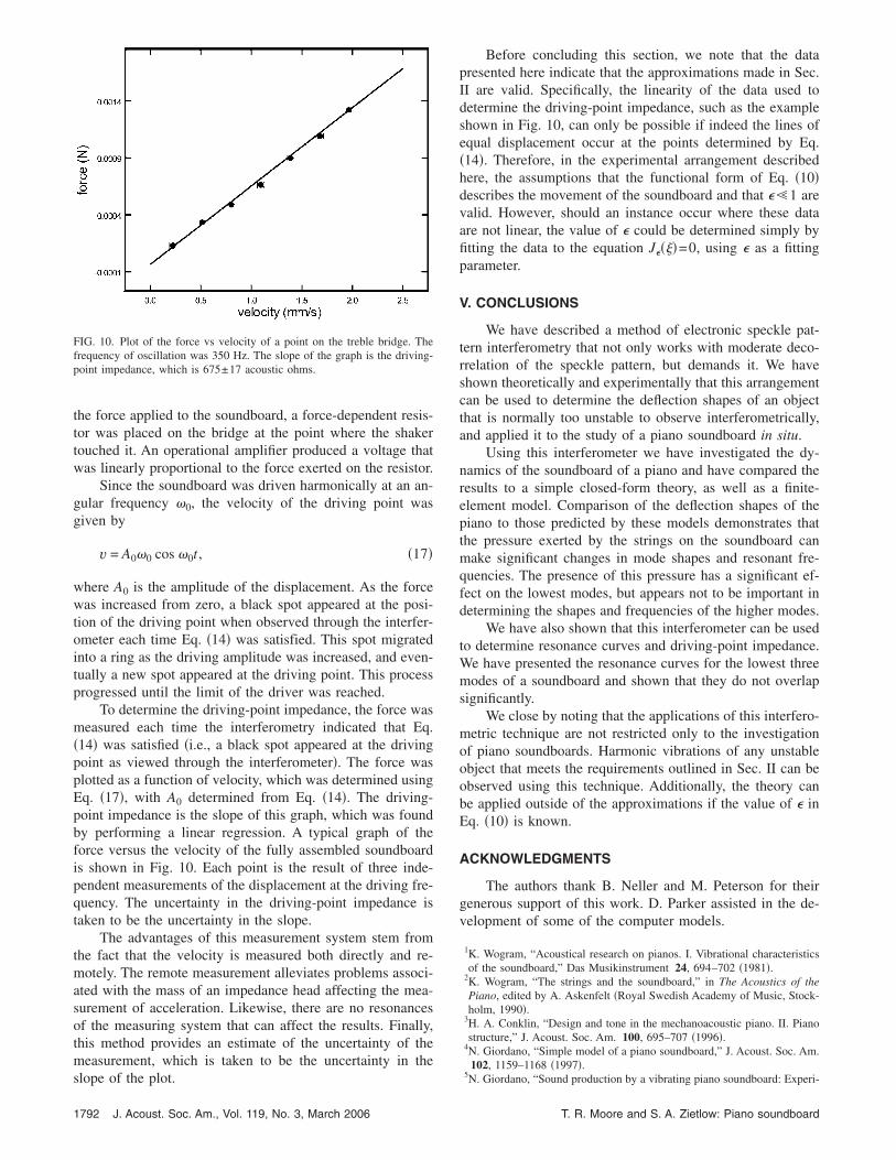
To determine the driving-point impedance, the force wasmeasured each time the interferometry indicated that Eq.�14� was satisfied �i.e., a black spot appeared at the drivingpoint as viewed through the interferometer�. The force wasplotted as a function of velocity, which was determined usingEq. �17�, with A0 determined from Eq. �14�. The driving-point impedance is the slope of this graph, which was foundby performing a linear regression. A typical graph of theforce versus the velocity of the fully assembled soundboardis shown in Fig. 10. Each point is the result of three inde-pendent measurements of the displacement at the driving fre-quency. The uncertainty in the driving-point impedance istaken to be the uncertainty in the slope.

The advantages of this measurement system stem fromthe fact that the velocity is measured both directly and re-motely. The remote measurement alleviates problems associ-ated with the mass of an impedance head affecting the mea-surement of acceleration. Likewise, there are no resonancesof the measuring system that can affect the results. Finally,this method provides an estimate of the uncertainty of themeasurement, which is taken to be the uncertainty in theslope of the plot.

Before concluding this section, we note that the datapresented here indicate that the approximations made in Sec.II are valid. Specifically, the linearity of the data used todetermine the driving-point impedance, such as the exampleshown in Fig. 10, can only be possible if indeed the lines ofequal displacement occur at the points determined by Eq.�14�. Therefore, in the experimental arrangement describedhere, the assumptions that the functional form of Eq. �10�describes the movement of the soundboard and that �1 arevalid. However, should an instance occur where these dataare not linear, the value of � could be determined simply byfitting the data to the equation J����=0, using � as a fittingparameter.

V. CONCLUSIONS

We have described a method of electronic speckle pat-tern interferometry that not only works with moderate deco-rrelation of the speckle pattern, but demands it. We haveshown theoretically and experimentally that this arrangementcan be used to determine the deflection shapes of an objectthat is normally too unstable to observe interferometrically,and applied it to the study of a piano soundboard in situ.

Using this interferometer we have investigated the dy-namics of the soundboard of a piano and have compared theresults to a simple closed-form theory, as well as a finite-element model. Comparison of the deflection shapes of thepiano to those predicted by these models demonstrates thatthe pressure exerted by the strings on the soundboard canmake significant changes in mode shapes and resonant fre-quencies. The presence of this pressure has a significant ef-fect on the lowest modes, but appears not to be important indetermining the shapes and frequencies of the higher modes.

We have also shown that this interferometer can be usedto determine resonance curves and driving-point impedance.We have presented the resonance curves for the lowest threemodes of a soundboard and shown that they do not overlapsignificantly.

We close by noting that the applications of this interfero-metric technique are not restricted only to the investigationof piano soundboards. Harmonic vibrations of any unstableobject that meets the requirements outlined in Sec. II can beobserved using this technique. Additionally, the theory canbe applied outside of the approximations if the value of � inEq. �10� is known.

ACKNOWLEDGMENTS

The authors thank B. Neller and M. Peterson for theirgenerous support of this work. D. Parker assisted in the de-velopment of some of the computer models.

1K. Wogram, “Acoustical research on pianos. I. Vibrational characteristicsof the soundboard,” Das Musikinstrument 24, 694–702 �1981�.

2K. Wogram, “The strings and the soundboard,” in The Acoustics of thePiano, edited by A. Askenfelt �Royal Swedish Academy of Music, Stock-holm, 1990�.

3H. A. Conklin, “Design and tone in the mechanoacoustic piano. II. Pianostructure,” J. Acoust. Soc. Am. 100, 695–707 �1996�.

4N. Giordano, “Simple model of a piano soundboard,” J. Acoust. Soc. Am.102, 1159–1168 �1997�.

5N. Giordano, “Sound production by a vibrating piano soundboard: Experi-

FIG. 10. Plot of the force vs velocity of a point on the treble bridge. Thefrequency of oscillation was 350 Hz. The slope of the graph is the driving-point impedance, which is 675±17 acoustic ohms.

1792 J. Acoust. Soc. Am., Vol. 119, No. 3, March 2006 T. R. Moore and S. A. Zietlow: Piano soundboard

ment,” J. Acoust. Soc. Am. 104, 1648–1653 �1998�.6N. Giordano, “Mechanical impedance of a piano soundboard,” J. Acoust.Soc. Am. 103, 2128–2133 �1998�.

7H. Suzuki, “Vibration and sound radiation of a piano soundboard,” J.Acoust. Soc. Am. 80, 1573–1582 �1986�.

8J. Berthaut, M. Ichchou, and L. Jézéquel, “Piano soundboard: Structuralbehavior, numerical and experimental study in the modal range,” Appl.Acoust. 64, 1113–1136 �2003�.

9J. Skala, “The piano soundboard behavior in relation with its mechanicaladmittance,” in Proc. of Stockholm Music Acoustics Conference (SMAC03), 6–9 August, Royal Institute of Technology �KTH� �Royal Institute ofTechnology, Stockholm, 2003�, pp. 171–174.

10E. J. Hansen, I. Bork, and T. D. Rossing, “Relating the radiated pianosound field to the vibrational modes of the soundboard,” J. Acoust. Soc.Am. 114, 2383 �2003�.

11J. Kindel and I. Wang, “Modal analysis and finite element analysis of a

piano soundboard,” in Proc. of 5th International Modal Analysis Confer-ence, 6–9 April, Imperial College of Science and Technology, London�Union College, Schenectady, NY, 1987�, pp. 1545–1549.

12T. R. Moore, “A simple design for an electronic speckle pattern interfer-ometer,” Am. J. Phys. 72, 1380 �2004�.

13T. R. Moore, “Erratum: A simple design for an electronic speckle patterninterferometer,” Am. J. Phys. 73, 189 �2004�.

14M. Abramowitz and I. A. Stegun, Handbook of Mathematical Functions�Dover, New York, NY, 1972�.

15A. Leissa, Vibrations of Plates �Acoustical Society of America, Melville,NY, 1993�.

16V. V. Bolotin, B. P. Makarov, G. V. Mishenkov, and Y. Y. Shveiko,“Asymptotic method of investigating the natural frequency spectrum ofelastic plates,” Raschetna Prochnost, Mashgiz 6, 231–253 �1960�.

17Wood Handbook �University Press of the Pacific, Honolulu, HI, 1974�.

J. Acoust. Soc. Am., Vol. 119, No. 3, March 2006 T. R. Moore and S. A. Zietlow: Piano soundboard 1793