Interference & Diffraction: Applications to the...

$: Interference & Diffraction: Applications to the ...ww3.haverford.edu/physics-astro/Amador/links/documents/HCDNACr… · Interference & Diffraction: Applications to the crystallography$
DNA Crystallography 1 Physics 102

Interference & Diffraction: Applications to the crystallography of macromolecules

Adapted from Tim McKay, University of Michigan, and the Institute for Chemical Education—Suzanne Amador Kane, 4/2010. (Ed. By WFS 3-30-11)

Introduction

In this lab you will determine the wavelength of a light source and observe the wave properties of light,

especially interference and diffraction, which were crucial in establishing a link between light and electric

and magnetic phenomena. You also will learn how these phenomena can allow us to determine the

structures of complex molecules like DNA.

You should read chapter 25 in Hecht carefully before coming to lab, noting especially those parts

needed to perform the experiments listed below. You may find it useful to bring your textbook to lab.

Interference techniques are among the most widely used methods for studying a variety of physical

systems:

a) X-ray diffraction has taught us most of what we know about the arrangements of atoms and

molecules in crystals and complex molecules, including proteins and DNA.

b) Optical interference is at the core of holography, which has become a widely used industrial

technique for detecting defects in manufactured objects such as aircraft tires.

c) Interference techniques are widely used in spectroscopic instruments of all kinds. These

instruments serve as our primary source of information about distant stars and also the

electron orbitals in atoms.

d) Mapping by interferometry is widely used in astronomy, making it possible to create high-

resolution images of extended galactic and extragalactic objects, which would be impossible

with single telescopes due to the intrinsic resolution limits of waves.

Today you will investigate several interference and diffraction phenomena by observing the distribution

of laser light after it passes through arrays of parallel slits and models of DNA. The structure of DNA

One of the great discoveries of biochemistry is the close connection between protein structure and

function. Much of the business of life within the cell is carried out using such large macromolecules. The

“primary structure” of these molecules is a simple map of connectivity, a network showing which other

atoms each atom in the molecule is attached to. While information about primary structure is central to

the identity and nature of a molecule, it tells us remarkably little about how it will function. Function is


often determined by the so‐called “tertiary structure”, the full three dimensional distribution of atoms in

the equilibrium state of the molecule.

Since this 3D shape plays such a central role in the function of biomolecules, determining structure is an

essential task for the life sciences. There are several different ways to do this, all of which depend on

fundamental physics principles. The most important of these, both historically and today, is X‐ray

diffraction. Since it is so important, we will spend a little time going over the basic principles of this

method, using as our central example the most famous determination of the structure of a biomolecule:

the discovery of the DNA double helix. More recently, the 2009 Nobel Prize in Chemistry was awarded

for x‐ray crystallography studies of the ribosome, the body’s machine for protein production.

We saw in lecture and your textbook that light with a known wavelength could be used to determine the

structure of a diffraction grating with unknown slit spacing. The same essential approach allows us to

determine the microstructural arrangement of atoms in molecules. However, if you want to see

diffraction from individual atoms, you need to use X‐rays: light waves with wavelengths about the size

of the spacing between atoms, on the order of 10‐10 m. Bouncing X‐rays off of atoms and looking at the

diffraction patterns they produce can tell us how the atoms are arranged. Examining the X‐ray diffraction

pattern of DNA taken by Rosalind Franklin allowed Watson and Crick to determine its double‐helical

structure. In what follows we will see, in some detail, how they did this.

Actual crystallography involves, not the geometry discussed for interference from slits, but interference

from a 3 dimensional array of atoms or molecules, as shown in Figure 1. The resulting constructive and

destructive interference phenomena, however, are very similar. Interference and diffraction patterns in

our experimental geometry are called Fraunhoeffer diffraction patterns, while those used in x‐ray

crystallography from 3D crystals are called Bragg diffraction patterns. However, since the constructive

and destructive intereference phenomena are so similar, we can learn about crystallography using

Fraunhoeffer diffraction today. Only some details of the relationships between scattering angle,

wavelength and diffraction peak index change.


Figure 1

What happens if you don’t have a crystal in which all the atoms are lined up, but instead have something

with no regular order, like a liquid? In this case, there is no regular interference‐grating‐like order and the

“diffraction pattern” disappears. If you want to use X‐ray diffraction to determine all the spacings

between the atoms, you need a perfectly ordered crystal of the protein or other molecule of interest.

Often this is the limiting factor in the measurement of structure for new biological molecules.

Because of the importance of protein structure for so many topics in the life sciences, knowledge about

them is shared online in “protein data banks”. If you look here, you can see one current count:

http://www.rcsb.org/pdb/statistics/holdings.do As of 2009, about 60,000 proteins have known

structures, most determined through X‐ray diffraction methods.

Getting to DNA

To do X‐ray crystallography of DNA, a regular oriented array of the molecules was required. In the early

1950’s, it was not known how to create this with DNA. Rosalind Franklin, a physical chemist and an early

expert at structure studies, discovered around 1951 that DNA took on two forms, then called “A” and

“B”. The A form, which is produced when the DNA is at low humidity, is not the form found in the cell.

The B form, fully hydrated, is what we now know to be a double helix. Preparation of long, ordered,

fibers of this B form required great care, but they enabled Franklin to obtain the crucial X‐ray diffraction

pictures which revealed the famous double‐helix structure.


Franklin’s original X‐ray diffraction pattern for B‐DNA is shown below in Figure 2 at left. It was obtained

by shining X‐rays with a wavelength of 0.15 nm perpendicular to a long thin fiber containing many DNA

molecules all lined up in the vertical direction. Photographic film was used to capture the resulting

diffraction pattern. Undeflected x‐rays hit the center of the film (this is white only because it was snipped

out and removed), while the darker regions of film indicate the location of x‐ray interference and

diffraction maxima. This crude arrangement is shown schematically in the picture below (top of Figure.

2) Franklin’s blurry diffraction pattern contained all the features which were needed to infer the

structure of DNA. As such, it is one of the most important images in biology.

Figure 2: (left) Rosalind Franklin’s original x‐ray diffraction pattern for DNA. The darker regions

correspond the higher intensities of x‐rays. (middle) schematic diagram indicating the key points of the

diffraction pattern; (right) Double‐helical structure of DNA, showing the basic double helical geometry.

(top) Schematic geometry for the experiment.

Our discussion of the Franklin image and its interpretation relies heavily on an article by Lucas, Lambin,

Mairesse, and Mathot in the Journal of Chemical Education, 1999, 76, 378. There are four aspects of this

Picture from Lucas et al., 1999, JCE, 76,

Picture from Lucas et al., 1999, JCE, 76, 378

Incident X-rays


image that we want you to notice and try to explain experimentally. To recognize these features, compare

the schematic diagram in the center to the actual X‐ray diffraction pattern on the left. The four key

features are:

1. The “layer lines”: Starting from the center, there are a series of dots along regularly spaced

horizontal lines.

2. The “cross” in the middle: The bright spots which define the horizontal layer lines are found at

increasing distances from a vertical centerline as you move away from the center of the image.

3. The outer “diamond”: the bright points at the top and bottom and the sides of the image are

connected by a diamond shaped continuous structure

4. The “missing 4th layer line”: When you look at the layer lines you can see that the fourth line from

the center is missing.

Every one of these features provides important information about the structure of DNA, so the following

experiments go through each in turn and uncover its origin.

It will help in understanding this to refer to the model shown in the picture on the right in Figure 2,

which emphasizes several key spacings in the structure of the DNA double helix. All are expressed in

terms to the spiral spacing “P”, or pitch, which is the distance along the strand you have to go before one

of the two helices returns back around to where it started. The other two distances are 3/8P, the distance

between the two intertwined helices, P/10, the distance between base pairs along the chains, and 0.3P, the

radius from the center to the outer edge of the helix. Given this background, we will guide you through

experiments that probe each of the features in the Franklin image. But, first let’s start with some simple

interference and diffraction exercises to get oriented.


EXPERIMENTAL PROCEDURE

EXPERIMENT 1: INTERFERENCE FROM MULTIPLE SLITS (ABOUT HALF A LAB PERIOD)

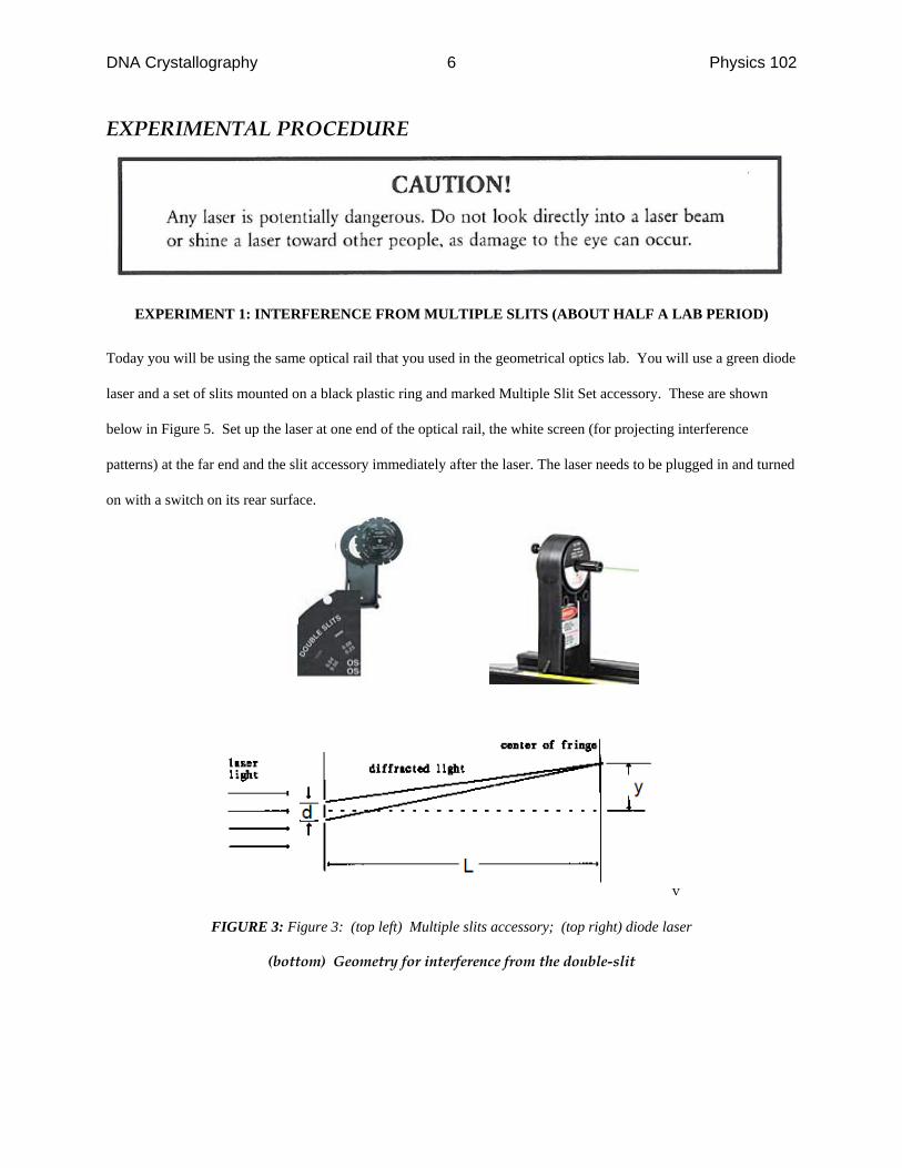
Today you will be using the same optical rail that you used in the geometrical optics lab. You will use a green diode

laser and a set of slits mounted on a black plastic ring and marked Multiple Slit Set accessory. These are shown

below in Figure 5. Set up the laser at one end of the optical rail, the white screen (for projecting interference

patterns) at the far end and the slit accessory immediately after the laser. The laser needs to be plugged in and turned

on with a switch on its rear surface.

v

FIGURE 3: Figure 3: (top left) Multiple slits accessory; (top right) diode laser

(bottom) Geometry for interference from the double-slit


1) Pass the green diode laser light through a pair of slits. These are marked DOUBLE

SLITS on the Multiple Slit Set accessory. You may need to steer the laser beam a little using

the two knobs on the rear of the laser so it passes through the slits. To find the distance d

between the slits you will need to look on the face of the slit accessory. Use the pair of slits

labeled a=0.04mm, d=0.25mm, where a = slit width and d = slit spacing.

Look carefully at the pattern on the screen. You should see something that looks like

the product of two patterns: one has a “slow” variation (over length scales of 1-2 cm), and the

other has a much “faster” variation (over length scales of a few mm).

Go to the front of the room where we have set up two similar optical rails. One has

the laser light shining through the same double slit you used above. The other has the same

type of laser shining through a single slit with the same slit width. The screens are the same

distance from the slits in either case. Sketch the two interference patterns (be sure you know

which is which!) and explain what is similar and what is different. Which features relate to

the slit width, a? Which features relate to the slit spacing, d?

Measure the displacement y between the peaks of adjacent interference maxima and

the distance L from the slit to the screen. (How can you get the best accuracy? Record all

your uncertainties.) You have directly measured or estimated your uncertainties in d, y and

L. To get your uncertainty in wavelength, , you will use the relationship discussed in pre-

lab lecture between the uncertainties in measured quantities and a computed quantity of

interest.

Now use this information to determine the wavelength of the laser light and its

uncertainty; compare to the manufacturer’s specification of 532 nm—does your result agree

to within your uncertainty?

2) Make qualitative observations of the effect of spacing on the interference pattern. You may

use the “variable double slit” that has continuously variable spacing on your Multiple Slit

Accessory to see this. Qualitatively, how is the distance between interference maxima related

to the spacing between the slits?

3) Look at the interference pattern from the pair of slits labeled a=0.04mm, d=0.25mm using the

red laser (670 nm), the green (532 nm) laser and the blue/purple (405 nm) laser. (When

comparing the red and the green, you will probably need to make some measurements,

because the differences are a little subtle. The differences should be more apparent for the

blue/purple laser.) Describe what features change as you change the wavelength, and what

features remain the same.


4) Using your red diode laser now, sketch the interference patterns produced by the three, four,

and five slits sets on the Multiple Slit set accessory. Comment on what happens to the

spacing and width of the interference maxima when you keep the slit spacing fixed, but

increase the number of slits. You will want to use as large a separation between the screen

and slits as possible and look very carefully at the maxima and the region in between the

maxima. (You may even wish to project your interference pattern on the wall!) Again, use

sketches to explain your results.

5) (Optional—do only if you are finished before 2:30) Now take the accessory marked SINGLE

SLIT ACCESSORY and put it on your optical rail in place of the multiple slit accessory; you

may keep using the red diode laser for now. Look at the Circular Aperture marked 0.2mm

(you will again need to steer your laser to go through the hole) to see its diffraction pattern.

Sketch in your report, then observe diffraction from the larger hole on the same assembly.

What changes?

Experiment 2: DNA Crystallography with visible light

Now you will explore how the DNA diffraction pattern arises from the double‐helical structure of B‐

DNA. Your only tools will be a laser and an “optical transform” slide (similar to your multiple slits

above) that has a variety of arrays of regular structures printed on transparent film. These structures

mimic various features of B‐DNA, although at sizes over a thousand times greater than real DNA

molecules. Their visible light interference pattern mimics the x‐ray diffraction pattern from B‐DNA,

enabling you do perform an experiment with visible light that avoids the complications and safety issues

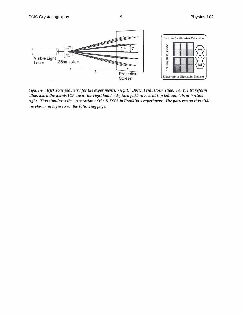
involved with x‐ray diffraction. Your experimental geometry is shown in Figure 4 below. Set up your

laser, slide and screen on your optical rail now and try aiming your laser through the slide to make sure

you can see at least one interference pattern. Your experimental geometry is the same as for the double

and multiple slit experiments above, with the optical transform slide replacing the slits. As before, put

your green diode laser at one end of your optical rail and your white screen on the other, and the slide as

close to the laser as possible. You can either hold the slide by hand, or use the mount provided to hold it

in place.

Figure 5 on the following page shows the patterns used to mimic the structure of DNA, with the simplest

analogous structures at top going to increasingly detailed structures at bottom. We will explain what

each of these patterns represents in the exercises to come.


Figure 4: (left) Your geometry for the experiments. (right) Optical transform slide. For the transform

slide, when the words ICE are at the right hand side, then pattern A is at top left and L is at bottom

right. This simulates the orientation of the B‐DNA in Franklin’s experiment. The patterns on this slide

are shown in Figure 5 on the following page.


Figure 5: Illustration of the various optical transform patterns on the slide.


6: Understanding the closely spaced layer lines (about half a lab period)

Now, look again at the DNA diffraction pattern in Figure 2. To understand the regularly spaced layer

lines, remember that as the helix of DNA spirals around it goes through repeated cycles, once for each

time it spirals around. This makes a repeated pattern of X‐ray scattering centers lined up along the

vertical direction, spaced by a distance P. In other words, they act like the many slits with spacing d = P in

your first experiment. Such a line of sources will produce an array of interference maxima on a screen at a

distance L located at positions y = nL/P, where (n = 1, 2, 3,…) Pattern A on your slide captures this

behavior. (Figure 5 & 6 below)

Remember from above how the spacings of the diffraction maxima (“bright spots”) are “reciprocal”

to the slit spacing (that is, they vary as y ~ 1/slit spacing)? Now this same relationship holds, for the

regular spacings in the molecule: y ~ 1/P. An arrangement with large separations will produce

diffraction spots close together. Since this is the largest repetition scale in the DNA structure, it

produces the diffraction features which are closest together. Imagine now what would happen to

your diffraction pattern if the patterns on your slides started shrinking down to molecular

dimensions. How would using a shorter wavelength of light correct this problem? (Answer keeping

in mind your results from the exercise above about looking at interference using different wavelength

of light.)

Look at the interference pattern for pattern A on your DNA optical transform card using your green

diode laser. Sketch its interference pattern, and explain it qualitatively. Also, explain how you could

use measurements of the interference pattern to determine the vertical spacing between the horizontal

rows of dashes on the slide, and also to determine the horizontal spacing between the vertical rows of

dashes. (We do not ask you to actually make these measurements.)

Figure 6 The first set of patterns for Experiments 2 and 3


7. Understanding the central cross

For reasons that will soon become apparent, we are interested in diffraction from a set of equally spaced

lines that are tilted, such as optical transform patterns B and C. Observe the diffraction patterns from B

and C now and sketch them in your report. What is similar to the diffraction from A? (Look at the

diffraction from A, B and C alternatively to see.) What is different? What would happen if you added the

diffraction patterns from B and C together? (Note that the array of lines in C is more tilted than in B, but

for now assume they are tilted by the same amount.) Sketch and explain what diffraction pattern would

result then. Is the spacing between interference maxima for B and C the same as that for A?

We can now see how this relates to the helical structure of DNA. Consider Figure 7 below, which

resembles optical transform H. Each element in these patterns looks like a sine wave—and also like a

single helix projected onto the flat slide. Note how the sine wave can be decomposed into two alternating

sets of evenly‐spaced lines at an angle to each other.

Figure 7: Optical transform pattern for H

Given your answers above, what do you think the diffraction pattern should be from pattern H? Now

sketch the actual diffraction pattern from H. How did it compare to your prediction?


8. Understanding the fourth missing layer line

Now look again at the optical transforms in Figure 5. Patterns F, I and L all have double helices, not just

single helices like H. Let’s now see how this affects the diffraction pattern. In F, I and L, one helix is

shifted vertically by an integer number of eighths of a period P relative to the other helix. These shifted

double helices will result in additional interference that will show up in the diffraction pattern. That is

because the light diffracted from each individual helix will interfere with the other helix’s light, leading to

destructive interference at some angle. In pre‐lab lecture we derived the resulting condition for

destructive interference using path lengths and phase shifts.

Figure 8: Optical transform pattern for analyzing diffraction from the double‐helical patterns H, F, I and

L. Use to identify which layer lines are missing for each pattern.

Using Figure 8 as a guide, compare the diffraction pattern for H with that for F, I and L. You may want to

bring your screen in closer to see this better (We found a distance of about 30 to 40 cm worked for us.)

Which layer lines are missing for each pattern? Which of these diffraction patterns in Figure 5 is most

similar to Franklin’s image, and hence best represents B‐DNA?

9. Understanding the diamond pattern

Our optical transforms so far have consisted of continuous lines, but DNA is made up of individual

atoms. What happens if we look at patterns that include increasing amounts of chemical accuracy?

Consider patterns L and J now in Figure 5; each has the same shift so they are missing the same layer

lines. Look at these patterns in the optical microscope. You should see that L has double helices made up

of continuous lines, while J has regularly spaced horizontal lines representing the base pairs (the chemical

groups that bond the double helices together.) What effect do we get from including these atomic level


features in our diffraction pattern? Remember that features that are far apart on the diffraction pattern,

must correspond to some repeated features in the molecule which are close together. First, thinking of the

“reciprocal” arguments about diffraction from a linear array, see if you can guess the answer of how this

affects the diffraction pattern, and write down your best guess.

Now, sketch the diffraction patterns from L and J, labeling each carefully and noting what changes as you

go from L to J. How does this relate to features of the actual B‐DNA x‐ray diffraction pattern reproduced

in Figure 2? Which of these most resembles Franklin’s diffraction pattern?

Note that the brightest spots in the diffraction pattern of K form the corners of diamonds. How many

layer lines are present from top to bottom of one of these diamonds? This number represents the number

of repeating monomer units per period of each helix. Record and check whether this agrees with the

actual pattern on the slide. (You can look at the actual patterns on the slide under the microscope

provided to determine this.) What is the value for DNA?

Interference & Diffraction: Applications to the...

Documents

Transcript of Interference & Diffraction: Applications to the...