Interest Rate Risk in the Banking Book: The trade-off ... · sheet data made available by a Dutch...
113
U NIVERSITY OF T WENTE GRADUATION T HESIS Interest Rate Risk in the Banking Book: The trade-off between delta EVE and delta NII Author: Philip J.F. ENGBERSEN BS C. Supervisors: Dr. B. ROORDA Drs. Ir. A.C.M. DE BAKKER P. ABELING MS C. B. KLEIN MS C. A thesis submitted in fulfillment of the requirements for the degree of Master of Science in the Industrial Engineering and Management -Financial Engineering July 14, 2017
Transcript of Interest Rate Risk in the Banking Book: The trade-off ... · sheet data made available by a Dutch...
UNIVERSITY OF TWENTE
GRADUATION THESIS
Interest Rate Risk in the Banking Book:The trade-off between delta EVE and delta
NII
Author:Philip J.F. ENGBERSEN BSC.
Supervisors:Dr. B. ROORDA
Drs. Ir. A.C.M. DE BAKKER
P. ABELING MSC.B. KLEIN MSC.
A thesis submitted in fulfillment of the requirementsfor the degree of Master of Science
in the
Industrial Engineering and Management-Financial Engineering
July 14, 2017

iii
University of Twente
Abstract
Faculty of Behavioural, Management and Social sciences
-Financial Engineering
Master of Science
Interest Rate Risk in the Banking Book: The trade-off between delta EVE anddelta NII
by Philip J.F. ENGBERSEN BSC.
The low interest rate environment has made Interest Rate in the Banking Book (IR-RBB) an interesting topic. The Basel Comittee on Banking Supervision (BCBS) madenew guidelines for regulations available in April 2016. It stated that both deltaEVE and delta NII as economic value and earnings perspectives to IRRBB shouldbe taken into account when assessing IRRBB. Several studies have shown that theseperspectives relate to each other and can even cause a trade-off when minimisingboth. Present study is performed to investigate this trade-off and the use of deltaEVE and delta NII measures is investigated. By means of a case study and balancesheet data made available by a Dutch bank this trade-off was assessed. A LinearProgramming (LP) model was constructed to optimise the hedging portfolio basedon IRRBB constraints. The results indicate that for this specific data set the delta EVEand delta NII had very little impact on each other. It also can be derived that plainvanilla swaps could effectively hedge the delta EVE and delta NII.

v
Contents
Abstract iii
1 Introduction 11.1 Background . . . . . . . . . . . . . . . . . . . . . . . . . . . . . . . . . . 1
1.1.1 Basic banking structure and activities . . . . . . . . . . . . . . . 11.1.2 Overview of IRRBB practices at banks . . . . . . . . . . . . . . . 21.1.3 Changing regulatory landscape on IRRBB . . . . . . . . . . . . . 4
1.2 Research purposes . . . . . . . . . . . . . . . . . . . . . . . . . . . . . . 41.3 Research questions . . . . . . . . . . . . . . . . . . . . . . . . . . . . . . 41.4 Methodology . . . . . . . . . . . . . . . . . . . . . . . . . . . . . . . . . 5
2 Theoretical Framework and Literature Research 72.1 Introduction . . . . . . . . . . . . . . . . . . . . . . . . . . . . . . . . . . 72.2 Interest Rate Risk in the Banking Book . . . . . . . . . . . . . . . . . . . 7
2.2.1 Definition of Interest Rate Risk . . . . . . . . . . . . . . . . . . . 72.2.2 Banking Book versus Trading Book . . . . . . . . . . . . . . . . 82.2.3 Sources of Interest Rate Risk . . . . . . . . . . . . . . . . . . . . 8
2.3 Common practices to measure IRRBB . . . . . . . . . . . . . . . . . . . 92.3.1 Introduction . . . . . . . . . . . . . . . . . . . . . . . . . . . . . . 92.3.2 Earnings perspective to IRRBB . . . . . . . . . . . . . . . . . . . 102.3.3 Economic value perspective on IRRBB . . . . . . . . . . . . . . . 112.3.4 Commonalities and differences . . . . . . . . . . . . . . . . . . . 12
Commonalities . . . . . . . . . . . . . . . . . . . . . . . . . . . . 13Differences . . . . . . . . . . . . . . . . . . . . . . . . . . . . . . . 13
3 Analysis of relevant aspects in calculating delta EVE and delta NII 153.1 Introduction . . . . . . . . . . . . . . . . . . . . . . . . . . . . . . . . . . 153.2 Methodology . . . . . . . . . . . . . . . . . . . . . . . . . . . . . . . . . 16
3.2.1 Aspect 1: Yield curve used for delta EVE and delta NII calcu-lations . . . . . . . . . . . . . . . . . . . . . . . . . . . . . . . . . 16
3.2.2 Aspect 2: Maturity profile of assets and liabilities . . . . . . . . 173.2.3 Aspect 3: Type of banking business model . . . . . . . . . . . . 173.2.4 Measuring exposure to interest rate risk . . . . . . . . . . . . . . 183.2.5 Calculation of delta EVE and delta NII figures . . . . . . . . . . 19
Calculation of delta EVE . . . . . . . . . . . . . . . . . . . . . . . 19
vi
Calculation of delta NII . . . . . . . . . . . . . . . . . . . . . . . 203.3 Data . . . . . . . . . . . . . . . . . . . . . . . . . . . . . . . . . . . . . . . 22
Data source . . . . . . . . . . . . . . . . . . . . . . . . . . . . . . 223.3.1 Balance sheet data . . . . . . . . . . . . . . . . . . . . . . . . . . 233.3.2 Balance sheet retail banking . . . . . . . . . . . . . . . . . . . . . 23
3.4 Results . . . . . . . . . . . . . . . . . . . . . . . . . . . . . . . . . . . . . 253.4.1 Results of the yield curve used in calculating delta EVE and
delta NII . . . . . . . . . . . . . . . . . . . . . . . . . . . . . . . . 25Delta EVE . . . . . . . . . . . . . . . . . . . . . . . . . . . . . . . 25Delta NII . . . . . . . . . . . . . . . . . . . . . . . . . . . . . . . . 27
3.4.2 Results of the maturity profile used in the calculation of deltaEVE and delta NII . . . . . . . . . . . . . . . . . . . . . . . . . . 28Delta EVE . . . . . . . . . . . . . . . . . . . . . . . . . . . . . . . 29Delta NII . . . . . . . . . . . . . . . . . . . . . . . . . . . . . . . . 29
3.4.3 Results banking business model used in the calculation of deltaEVE and delta NII . . . . . . . . . . . . . . . . . . . . . . . . . . 31Delta EVE . . . . . . . . . . . . . . . . . . . . . . . . . . . . . . . 32Delta NII . . . . . . . . . . . . . . . . . . . . . . . . . . . . . . . . 32
3.5 Concluding remarks . . . . . . . . . . . . . . . . . . . . . . . . . . . . . 33
4 Constructing a model to change exposure to IRRBB 354.1 Introduction . . . . . . . . . . . . . . . . . . . . . . . . . . . . . . . . . . 354.2 LP model constraints and assumptions . . . . . . . . . . . . . . . . . . . 37
4.2.1 LP model design . . . . . . . . . . . . . . . . . . . . . . . . . . . 37Decision variables . . . . . . . . . . . . . . . . . . . . . . . . . . 37Target function . . . . . . . . . . . . . . . . . . . . . . . . . . . . 38Constraints . . . . . . . . . . . . . . . . . . . . . . . . . . . . . . 38
4.2.2 Data used . . . . . . . . . . . . . . . . . . . . . . . . . . . . . . . 394.2.3 Methodology and assumptions in the LP model . . . . . . . . . 40
Interest rate shocks . . . . . . . . . . . . . . . . . . . . . . . . . . 40Min-max theory . . . . . . . . . . . . . . . . . . . . . . . . . . . . 41Assumptions in calculation of delta NII . . . . . . . . . . . . . . 41
4.3 Mathematical formulation of the LP problem . . . . . . . . . . . . . . . 434.3.1 Target function . . . . . . . . . . . . . . . . . . . . . . . . . . . . 434.3.2 Balance sheet constraint . . . . . . . . . . . . . . . . . . . . . . . 444.3.3 Hedging portfolio volume constraints . . . . . . . . . . . . . . . 444.3.4 Delta EVE constraint . . . . . . . . . . . . . . . . . . . . . . . . . 444.3.5 Delta NII constraint . . . . . . . . . . . . . . . . . . . . . . . . . 454.3.6 Duration of equity constraint . . . . . . . . . . . . . . . . . . . . 464.3.7 Key Rate Duration constraint . . . . . . . . . . . . . . . . . . . . 474.3.8 Hedging portfolio . . . . . . . . . . . . . . . . . . . . . . . . . . 48
Calculating the value of the interest rate swap . . . . . . . . . . 49
vii
Calculating the earnings of the swaps . . . . . . . . . . . . . . . 504.4 Concluding remarks . . . . . . . . . . . . . . . . . . . . . . . . . . . . . 51
5 Results LP problem 535.1 Introduction . . . . . . . . . . . . . . . . . . . . . . . . . . . . . . . . . . 535.2 Example of LP model and results . . . . . . . . . . . . . . . . . . . . . . 535.3 Changing exposure to both delta EVE and delta NII . . . . . . . . . . . 57
5.3.1 Initial IRRBB exposure . . . . . . . . . . . . . . . . . . . . . . . . 575.3.2 Changing IRRBB exposure of the bank . . . . . . . . . . . . . . . 58
Effect payer and receiver swaps on return . . . . . . . . . . . . . 58General results changing exposure to delta EVE and delta NII . 61Delta EVE, delta NII and return in point 1 . . . . . . . . . . . . . 63Delta EVE, delta NII and return in point 2 . . . . . . . . . . . . . 65Delta EVE, delta NII and return in point 3 . . . . . . . . . . . . . 66Delta EVE, delta NII and return in point 4 . . . . . . . . . . . . . 67
5.4 Difference in one and two year time horizon for delta NII . . . . . . . . 685.5 Concluding remarks . . . . . . . . . . . . . . . . . . . . . . . . . . . . . 70
6 Conclusion 736.1 Introduction . . . . . . . . . . . . . . . . . . . . . . . . . . . . . . . . . . 736.2 Conclusions to the first research question . . . . . . . . . . . . . . . . . 736.3 Conclusions to the second research question . . . . . . . . . . . . . . . 746.4 Conclusion to the third research question . . . . . . . . . . . . . . . . . 756.5 Conclusion . . . . . . . . . . . . . . . . . . . . . . . . . . . . . . . . . . . 76
7 Future Research 777.1 Introduction . . . . . . . . . . . . . . . . . . . . . . . . . . . . . . . . . . 777.2 Recommendations . . . . . . . . . . . . . . . . . . . . . . . . . . . . . . 77
Bibliography 79
A Modelling of interest rate scenarios Chapter 3 81A.0.1 Modelling of interest rate scenarios . . . . . . . . . . . . . . . . 81
B Mathematical derivation of LP optimisation problem 85B.1 Introduction . . . . . . . . . . . . . . . . . . . . . . . . . . . . . . . . . . 85
B.1.1 Delta EVE constraint . . . . . . . . . . . . . . . . . . . . . . . . . 85B.2 Delta NII constraint . . . . . . . . . . . . . . . . . . . . . . . . . . . . . . 87
B.2.1 Duration of equity constraint . . . . . . . . . . . . . . . . . . . . 88B.2.2 Key rate duration constraint . . . . . . . . . . . . . . . . . . . . . 91
C Tables 95
D Data Chapter 3 97

ix
List of Figures
3.1 Delta EVE per yield curve for retail business model . . . . . . . . . . . 263.2 Delta EVE per yield curve for wholesale business model . . . . . . . . 263.3 Delta EVE per yield curve for investment business model . . . . . . . . 273.4 Delta NII per yield curve for retail business model . . . . . . . . . . . . 273.5 Delta NII per yield curve for investment business model . . . . . . . . 283.6 Delta NII per yield curve for wholesale business model . . . . . . . . . 283.7 Delta EVE of the duration analysis for retail business model, reference
rate: EONIA . . . . . . . . . . . . . . . . . . . . . . . . . . . . . . . . . . 293.8 Delta EVE of the duration analysis for investment business model,
reference rate: EONIA . . . . . . . . . . . . . . . . . . . . . . . . . . . . 303.9 Delta NII of the duration analysis for investment business model, ref-
erence rate: EONIA . . . . . . . . . . . . . . . . . . . . . . . . . . . . . . 303.10 Delta NII of the duration analysis for retail business model, reference
rate: EONIA . . . . . . . . . . . . . . . . . . . . . . . . . . . . . . . . . . 313.11 Delta NII of the duration analysis for wholesale business model, ref-
erence rate: EONIA . . . . . . . . . . . . . . . . . . . . . . . . . . . . . . 313.12 Delta EVE per shock per business model, reference rate: EONIA . . . . 323.13 Delta NII per shock per business model, reference rate: EONIA . . . . 33
5.1 Return, delta EVE and delta NII per number of payer swaps . . . . . . 545.2 Return, delta EVE and delta NII per number of payer swaps with fea-
sible region . . . . . . . . . . . . . . . . . . . . . . . . . . . . . . . . . . . 565.3 Return, delta EVE and delta NII per number of payer swaps with ad-
justed feasible region . . . . . . . . . . . . . . . . . . . . . . . . . . . . . 565.4 Composition of hedging portfolio over maturity with original target
function . . . . . . . . . . . . . . . . . . . . . . . . . . . . . . . . . . . . 595.5 Trade-off surface delta EVE, delta NII and return . . . . . . . . . . . . . 615.6 Trade-off surface delta EVE, delta NII and return, feasible solutions only 625.7 Number of payer and receiver swaps for point 1 on the trade-off surface 645.8 Number of payer and receiver swaps for point 2 on the trade-off surface 665.9 Number of payer and receiver swaps for point 3 on the trade-off surface 675.10 Number of payer and receiver swaps for point 3 on the trade-off surface 68
A.1 EONIA Interest rate scnenarios . . . . . . . . . . . . . . . . . . . . . . . 83

xi
List of Tables
1.1 Typical balance sheet retail bank . . . . . . . . . . . . . . . . . . . . . . 21.2 Preliminary analysis of interest rate risk management practises across
European Banks . . . . . . . . . . . . . . . . . . . . . . . . . . . . . . . . 3
3.1 19 time buckets as defined by the BCBS . . . . . . . . . . . . . . . . . . 193.2 Asset and liability categorisation to maturity . . . . . . . . . . . . . . . 213.3 Largest assets and liabilities of the 4 largest Dutch banks in percentage 243.4 Typical balance sheet retail bank . . . . . . . . . . . . . . . . . . . . . . 243.5 Relative distribution of assets and liabilities over time . . . . . . . . . . 25
4.1 Overview asset and liability classes bank’s balance sheet . . . . . . . . 394.2 Valuation of a 1 year swap in terms of FRA’s . . . . . . . . . . . . . . . 50
5.1 Overview of initial delta EVE and delta NII on the bank’s balance sheet 585.2 Total cost analysis interest rate swap over time . . . . . . . . . . . . . . 605.3 Values of delta EVE and delta NII for point 1 on the trade-off surface . 645.4 Values of delta EVE and delta NII for point 2 on the trade-off surface . 655.5 Values of delta EVE and delta NII for point 3 on the trade-off surface . 665.6 Values of delta EVE and delta NII for point 4 on the trade-off surface . 675.7 Values of one- and two-year delta NII for point 1 on the trade-off surface 695.8 Values of one- and two-year delta NII for point 2 on the trade-off surface 695.9 Values of one- and two-year delta NII for point 3 on the trade-off surface 705.10 Values of one- and two-year delta NII for point 4 on the trade-off surface 70
A.1 Specified size of interest rate shocks Rshocktype,c in basis points . . . . . 81A.2 Overview changes first five time buckets . . . . . . . . . . . . . . . . . 82
C.1 Overview shock size per currency . . . . . . . . . . . . . . . . . . . . . 96C.2 Overview changes per rate per maturity . . . . . . . . . . . . . . . . . . 96
D.1 Data wholesale business model . . . . . . . . . . . . . . . . . . . . . . . 97D.2 Typical balance sheet wholesale business model . . . . . . . . . . . . . 98D.3 Data balance sheet wholesale business model over time . . . . . . . . . 98D.4 Data investment business model . . . . . . . . . . . . . . . . . . . . . . 98D.5 Typical balance sheet investment business model . . . . . . . . . . . . . 99D.6 Data balance sheet investment business model over time . . . . . . . . 99


xiii
List of Abbreviations
BCBS Basel Committee on Banking SupervisionBIS Bank of International Settlementsbp basis pointsDCF Dicounted Cash FlowDF Discount FactorDoE Duration of EquityEBA European Banking AuthorityEONIA European OverNight Indexed Aggregated rateEuribor Euro InterBank Offered RateEV Economic ValueEVE Economic Value of EquityFRA Forward Rate AgreementFRM Financial Risk ManagementFSI Financial Services IndustryIRB Internal Ratings Based approachIRR Interest Rate RiskIRRBB Interest Rate Risk in the Banking BookKRD Key Rate DurationLIBOR London InterBank Offered RateLP Linear ProgrammingNII Net Interest IncomeNIM Net Interest MarginNPV Net Present ValueOBS Off Balance SheetOIS Overnight Indexed SwapPV Present Value

1
Chapter 1
Introduction
1.1 Background
1.1.1 Basic banking structure and activities
Traditionally banks have a mediating role between groups of people and businessesthat have money, and groups that need it (Asmundson, 2011). This redistributionis done via deposit and savings accounts where clients can store money they don’tneed and earn interest on it. Money acquired on these accounts is loaned to cus-tomers in need of money via loans and mortgages. This process is called transfor-mation (SVV, 2013). Generally the margin between the interest paid on deposits andearned on loans result in a profit for the bank. This margin is often called the NetInterest Margin (NIM).
These activities of lending and taking deposits is typical for commercial banks (Hull,2012a). Commercial banks can be divided into two sub categories: retail and whole-sale. The retail banks tend to lend relatively little amounts and take deposits ofprivate customers and small businesses, where wholesale banks provide bankingservices to larger corporate clients, fund managers and other financial institutions(Hull, 2012a). Besides commercial banks, investment banking is a second categoryof banks. Investment banks assist companies in raising debt and equity, providingadvice on mergers and acquisitions, restructurings and other corporate finance de-cisions (Hull, 2012a). These banks are often also more involved in the trading ofsecurities (Hull, 2012a).
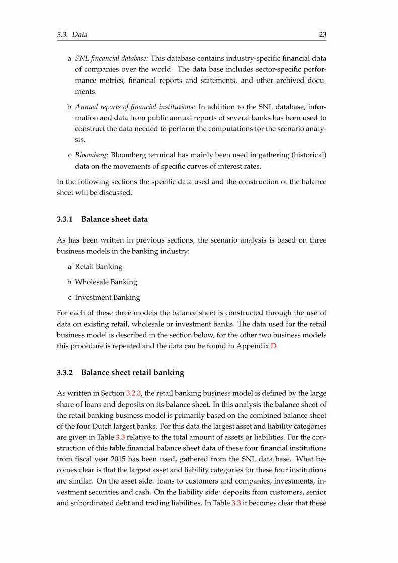
In Table 1.1 a simplified example of a typical retail bank’s balance sheet is given.For retail banks loans are the largest part of their assets, deposits the largest liability.This is represented by the percentages of 72% and 70.5% respectively for loans andmortgages and deposits. The composition of assets and liabilities given in Table 1.1is based on aggregated public data of the balance sheets of 4 of the largest retailbanks in the Netherlands in fiscal year 2015.
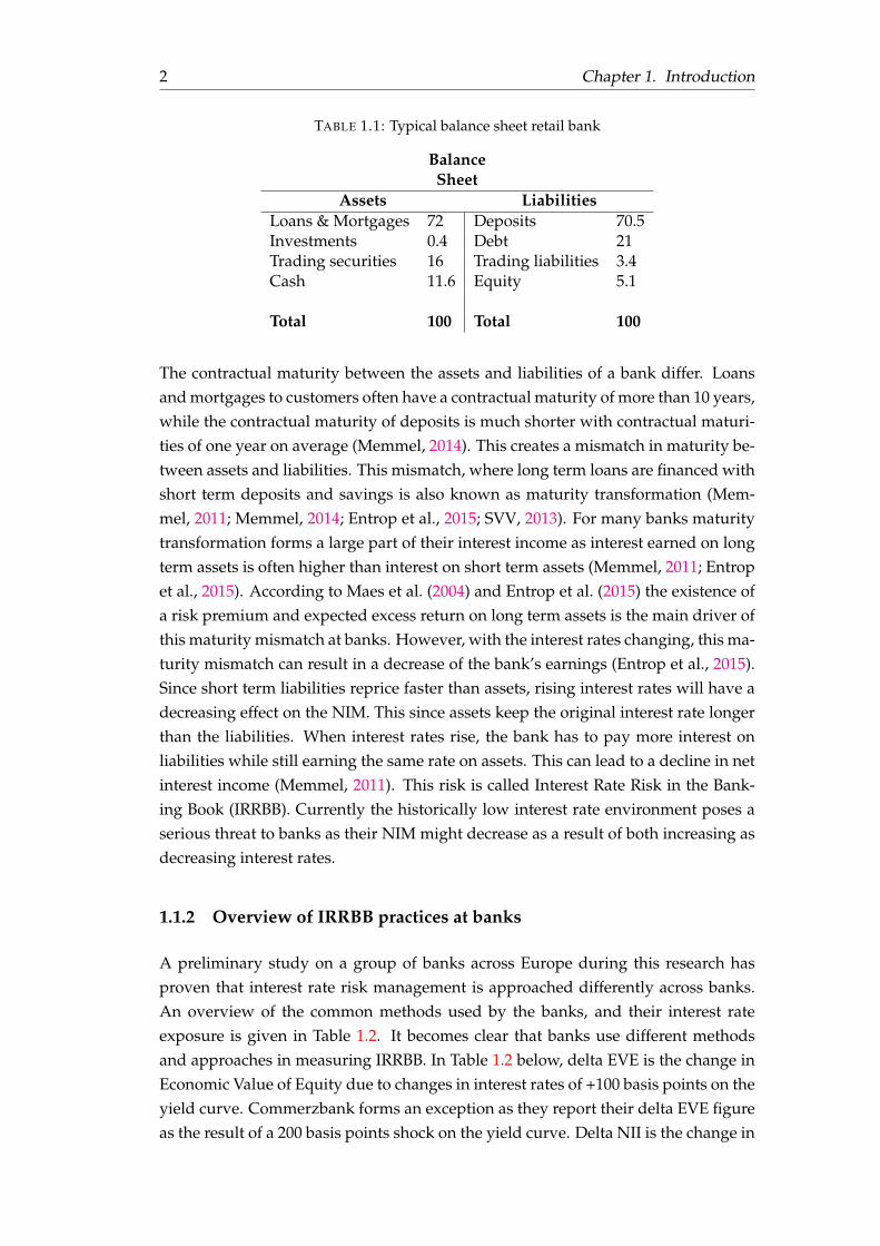
2 Chapter 1. Introduction
TABLE 1.1: Typical balance sheet retail bank
BalanceSheet
Assets LiabilitiesLoans & Mortgages 72 Deposits 70.5Investments 0.4 Debt 21Trading securities 16 Trading liabilities 3.4Cash 11.6 Equity 5.1
Total 100 Total 100
The contractual maturity between the assets and liabilities of a bank differ. Loansand mortgages to customers often have a contractual maturity of more than 10 years,while the contractual maturity of deposits is much shorter with contractual maturi-ties of one year on average (Memmel, 2014). This creates a mismatch in maturity be-tween assets and liabilities. This mismatch, where long term loans are financed withshort term deposits and savings is also known as maturity transformation (Mem-mel, 2011; Memmel, 2014; Entrop et al., 2015; SVV, 2013). For many banks maturitytransformation forms a large part of their interest income as interest earned on longterm assets is often higher than interest on short term assets (Memmel, 2011; Entropet al., 2015). According to Maes et al. (2004) and Entrop et al. (2015) the existence ofa risk premium and expected excess return on long term assets is the main driver ofthis maturity mismatch at banks. However, with the interest rates changing, this ma-turity mismatch can result in a decrease of the bank’s earnings (Entrop et al., 2015).Since short term liabilities reprice faster than assets, rising interest rates will have adecreasing effect on the NIM. This since assets keep the original interest rate longerthan the liabilities. When interest rates rise, the bank has to pay more interest onliabilities while still earning the same rate on assets. This can lead to a decline in netinterest income (Memmel, 2011). This risk is called Interest Rate Risk in the Bank-ing Book (IRRBB). Currently the historically low interest rate environment poses aserious threat to banks as their NIM might decrease as a result of both increasing asdecreasing interest rates.
1.1.2 Overview of IRRBB practices at banks
A preliminary study on a group of banks across Europe during this research hasproven that interest rate risk management is approached differently across banks.An overview of the common methods used by the banks, and their interest rateexposure is given in Table 1.2. It becomes clear that banks use different methodsand approaches in measuring IRRBB. In Table 1.2 below, delta EVE is the change inEconomic Value of Equity due to changes in interest rates of +100 basis points on theyield curve. Commerzbank forms an exception as they report their delta EVE figureas the result of a 200 basis points shock on the yield curve. Delta NII is the change in
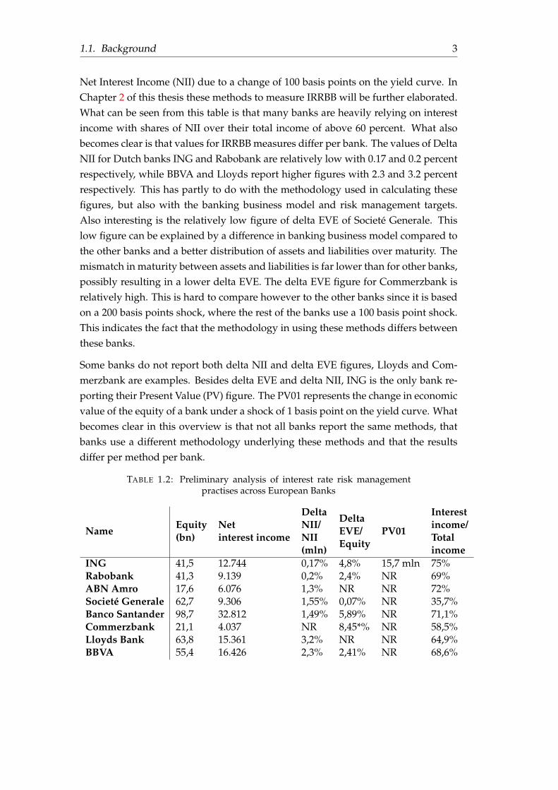
1.1. Background 3
Net Interest Income (NII) due to a change of 100 basis points on the yield curve. InChapter 2 of this thesis these methods to measure IRRBB will be further elaborated.What can be seen from this table is that many banks are heavily relying on interestincome with shares of NII over their total income of above 60 percent. What alsobecomes clear is that values for IRRBB measures differ per bank. The values of DeltaNII for Dutch banks ING and Rabobank are relatively low with 0.17 and 0.2 percentrespectively, while BBVA and Lloyds report higher figures with 2.3 and 3.2 percentrespectively. This has partly to do with the methodology used in calculating thesefigures, but also with the banking business model and risk management targets.Also interesting is the relatively low figure of delta EVE of Societé Generale. Thislow figure can be explained by a difference in banking business model compared tothe other banks and a better distribution of assets and liabilities over maturity. Themismatch in maturity between assets and liabilities is far lower than for other banks,possibly resulting in a lower delta EVE. The delta EVE figure for Commerzbank isrelatively high. This is hard to compare however to the other banks since it is basedon a 200 basis points shock, where the rest of the banks use a 100 basis point shock.This indicates the fact that the methodology in using these methods differs betweenthese banks.
Some banks do not report both delta NII and delta EVE figures, Lloyds and Com-merzbank are examples. Besides delta EVE and delta NII, ING is the only bank re-porting their Present Value (PV) figure. The PV01 represents the change in economicvalue of the equity of a bank under a shock of 1 basis point on the yield curve. Whatbecomes clear in this overview is that not all banks report the same methods, thatbanks use a different methodology underlying these methods and that the resultsdiffer per method per bank.
TABLE 1.2: Preliminary analysis of interest rate risk managementpractises across European Banks
NameEquity(bn)
Netinterest income
DeltaNII/NII(mln)
DeltaEVE/Equity
PV01
Interestincome/Totalincome
ING 41,5 12.744 0,17% 4,8% 15,7 mln 75%Rabobank 41,3 9.139 0,2% 2,4% NR 69%ABN Amro 17,6 6.076 1,3% NR NR 72%Societé Generale 62,7 9.306 1,55% 0,07% NR 35,7%Banco Santander 98,7 32.812 1,49% 5,89% NR 71,1%Commerzbank 21,1 4.037 NR 8,45*% NR 58,5%Lloyds Bank 63,8 15.361 3,2% NR NR 64,9%BBVA 55,4 16.426 2,3% 2,41% NR 68,6%
4 Chapter 1. Introduction
1.1.3 Changing regulatory landscape on IRRBB
In April 2016 the Basel Committee on Banking Supervision (BCBS) published a pa-per with new guidelines and standards for interest rate risk management called:"Standards on Interest Rate Risk in the Banking Book" (BCBS, 2016a). This paper is aresponse of the committee on the current low interest rate environment and hetero-geneous practices on the measurement and management of interest rate risk.
In these new guidelines, aimed at more standardisation and comparison of man-agement of IRRBB between banks, the use of two methods in measuring interestrate risk is advocated: an earnings based method and an economic value basedmethod (BCBS, 2016a). The earnings based method measures the change in NII dueto changes in the interest rates, where the economic value based measures focus onthe change in net present value of the bank’s balance sheet. Banks have to complywith these new regulations from the 1st of January 2018.
1.2 Research purposes
The two methods for measuring IRRBB are the main subject of this research. Earn-ings and economic value based methods to measure IRRBB are different in someaspects. The most important aspect is the time horizon over which IRRBB is as-sessed. The earnings based methods have a short term focus of 1 to 3 years (BCBS,2016a; Memmel, 2014; EBA, 2013a). The economic value measures often have anextended focus of more than 5 years. The few literature that is published on thesetopics claim that a trade-off between both methods occurs when minimising the in-terest rate risk measured with both these methods. It is not possible to minimise theinterest rate risk measured by both of the methods at the same time. In this researchthe relationship between these two methods is investigated, is determined how thistrade-off occurs and how banks should manage their assets and liabilities based onthese results.
1.3 Research questions
In order to aid the purposes mentioned in the previous section, and to guide theresearch, the following research questions is used:
How can banks best change their levels of exposure to interest rate risk, measured from aneconomic value and earnings perspective, given their risk appetite and business model?
This research is structured through the use of three sub research questions. Thesethree sub research questions will each form a different phase in this research, leading
1.4. Methodology 5
to the answer to the main research question. The three sub research questions arestated as follows:
1. What are important aspects and differences between delta NII as earnings and deltaEVE as economic value based methods to measure IRRBB?
2. What are important aspects to take into account in the calculation of delta EVE anddelta NII?
(a) What is the effect of the yield curve used on the exposure to IRRBB measuredfrom both perspectives?
(b) What is the impact of changes in duration of assets and liabilities on the exposureto interest rate risk measured from both perspectives?
(c) What is the impact of the business model of the bank on the calculation of deltaEVE and delta NII?
3. When is the exposure to interest rate risk measured from both perspectives consideredoptimal?
(a) How can a bank best change its exposure to interest rate risk?
1.4 Methodology
In this thesis the main research question will be answered by the answers obtainedfrom the research questions defined in the previous section. The methods and ap-proach used to gather answers to these questions will be described in this section.
The first research question, aimed at getting more understanding of the concepts ofIRRBB, economic value and earnings based methods will be answered by extensiveliterature research in Chapter 2.
The understanding of the basic concepts regarding IRRBB, delta EVE and delta NIIwill be used during the second step of this research: determining the relevant aspectsin this research and their impact on interest rate risk measured. By conducting quan-titative analyses on the levels of delta NII as earnings, and delta EVE as economicvalue perspectives on IRRBB, the second research question will be answered. Rele-vant aspects that will be dealt with are the yield curves used in computing the levelsof delta NII and delta EVE, the duration of assets and liabilities and banking busi-ness models. The process of inding thse answers and the results will be described inChapter 3.
The third research question is aimed at answering the main research question: "Howcan a bank best change its exposure to IRRBB measured through both delta EVE and deltaNII?" This question will be answered through the use of a case study. A Dutchbank provided data that is used for this purpose. In cooperation with this bank a
6 Chapter 1. Introduction
model is developed that optimally distributes payer and receiver swaps based ondelta EVE and delta NII measures in order to hedge IRRBB. The bank has providedan extensive data set containing detailed information on the positions of assets andliabilities, IRRBB appetite and risk limits set by the management of the bank. Thisdata, information and expert input of the bank is used to construct the LP model andto determine the optimal allocation of payer and receiver swaps given a certain riskappetite. This model is described in Chapter 4.
In order to examine the best direction for banks to change their exposure to IRRBB,linear programming theory is used to optimise the balance sheet given certain expo-sures to IRRBB. Knowledge gathered from research question 2 is used to constructthis model. In this research the simplex method will be used to optimise the linearproblem. More on the methodology of this optimisation problem is found in Chap-ter 4. The results of this model and the answers to research question 3 and the mainresearch question are discussed in Chapter 5.
7
Chapter 2
Theoretical Framework andLiterature Research
2.1 Introduction
In order to obtain a proper understanding of the concepts relating to IRRBB and bothearnings and economic value based methods, in this chapter literature available onthese topics is reviewed. The purpose of this chapter is to lay a theoretical founda-tion from which the research will be built. At the end of this chapter the followingresearch question will be answered:
1. What are important aspects and differences between delta NII as earnings and deltaEVE as economic value based methods to measure IRRBB?
This is achieved by elaborating on the general literature that is reviewed. First IRRBBin general will be described, further on the focus will be on delta NII and delta EVEas earnings and economic value perspectives on IRRBB.
2.2 Interest Rate Risk in the Banking Book
2.2.1 Definition of Interest Rate Risk
The BCBS defines in its "Principles for the Management and Supervision of InterestRate Risk", Interest Rate Risk as "the current or prospective risk to the bank’s capitaland earnings arising from adverse movements in interest rates that affect the bank’sbanking book positions" (BCBS, 2016a). Changes in interest rates affect a bank’searnings. As stated in Section 1.1 a mismatch between the maturity of assets andliabilities may cause changes in a bank’s earnings when interes rates increase ordecrease. Also changes in interest rates may cause the clients of a bank to withdrawtheir money, or prepay their loans earlier, affecting its NII (BCBS, 2015).
8 Chapter 2. Theoretical Framework and Literature Research
Besides affecting a bank’s earnings, changes in interest rates also have an impacton the underlying value of the bank’s assets, liabilities and off-balance-sheet (OBS)positions. The interest rate is an input variable in the net present value calculationof cash flows. Changing interest rates have therefore an impact on the net presentvalue calculations of assets and liabilities (BCBS, 2004; Memmel, 2014). When inter-est rates increase, both the value of assets and liabilities decrease. However, since thematurity of the assets is often longer than the maturity of the liabilities, the losseson the assets side are higher than on the liability side. The economic value of eq-uity, the difference between the present value of assets and liabilities, then decreases(Memmel, 2014).
A distinction is made between interest rate risk resulting from trading activities andbanking activities. The focus of this thesis lies on Interest Rate Risk in the BankingBook (IRRBB): interest rate risk resulting from other activities than trading activitiesand market risk (EBA, 2015; BCBS, 2016a). In the next section the difference betweenthese interest rate risks will be elaborated.
2.2.2 Banking Book versus Trading Book
After the financial crisis in 2008 a distinction has been made between interest raterisk in the trading and the banking book. Banking book instruments are generallyintended to be held to maturity. Changes in market value are therefore not neces-sarily reflected in profit and loss accounts (BCBS, 2015). Instruments held in thetrading book are often not meant to be held to maturity, and changes in the fairvalue impact profit and loss accounts. Before and during the crisis banks could des-ignate instruments with observable market prices to the trading book by claimingtrading intent. During the crisis many of these positions became illiquid. To avoidthe impact of these instruments on profit and loss accounts, many banks transferredinstruments to the banking book subjecting them to minimum capital requirements(BCBS, 2015). After the crisis the BCBS started a fundamental review of the tradingbook where different capital charges for the same types of products in the tradingand banking book were addressed. In addition, more strict boundaries were set toprevent transferring trading instruments to the banking book and vice versa (BCBS,2015; BCBS, 2016b). Both trading and banking book products are subject to interestrate risk. In this thesis however, the focus will be on interest rate risk on bankingbook products.
2.2.3 Sources of Interest Rate Risk
In general four sources of interest rate risk in the banking book are defined (Charu-mathi, 2008; Seetanah and Thakoor, 2013; BCBS, 2004; BCBS, 2015):
2.3. Common practices to measure IRRBB 9
• Repricing Risk: Risk arising from timing differences in the maturity and rollingover of a bank’s assets, liabilities and OBS positions (BCBS, 2004). When a banklends for a long term at a fixed rate, while funding this with deposits with afloating rate, this margin can be compressed when interest rates rise.
• Yield Curve Risk: A bank’s exposure to changes in the slope and shape of theyield curve. This risk arises when unanticipated shifts in the yield curve haveadverse effects on a bank’s income or underlying economic value (BCBS, 2004).
• Basis Risk: The risk from the imperfect correlation in the adjustment of therates on different financial instruments that initially have similar repricingcharacteristics. In a situation where a one-year loan that reprices monthlybased on the one-month US Treasury bill rate is funded with a one-year de-posit repricing monthly on the one-month LIBOR, the institution is exposedto unexpected changes in the spread between the two indexes. This type ofinterest rate risk is called basis risk (BCBS, 2004).
• Optionality Risk: Many banking products have embedded options. An optionprovides the buyer the right, but not the obligation to perform a certain action.Examples of options in assets of banks can be for instance the prepayment op-tion for customers on a loan or mortgage, or for liabilities a bank changing itsinterest rates on deposits. If these options are not adequately managed, in-struments with optionality features can pose a risk to a bank’s business (BCBS,2004).
In the "Standards on Interest Rate Risk In the Banking Book" which is the most re-cent publication on guidelines and regulation of IRRBB by the BCBS, the sourcesrepricing Risk and yield curve risk are replaced by the broader term "Gap risk". Thisterm describes all risks related to the timing differences in bank’s instruments’ ratechanges according to the BCBS (BCBS, 2016a). In gap risk both parallel shocks asnon-parallel shocks to the yield curve are taken into account. Regarding the foursources of interest rate risk, during this research, the focus will mainly lie on repric-ing Risk, yield curve risk and optionality risk.
2.3 Common practices to measure IRRBB
2.3.1 Introduction
In this section the practices and methods often used by banks to measure IRRBBwill be described. In literature many methods are found. One of the first methods tomeasure interest rate risk was the approach suggested by Flannery and James (1984).In this method the interest rate risk is measured by the sensitivity of a banks’ stockprices to changes in interest rates. A negative coefficient means that the value ofbank’s equity would decrease as a result of changing interest rates. The focus of the
10 Chapter 2. Theoretical Framework and Literature Research
method is primarily on the short term since the changing stock price of the bank istaken as an indicator of risk (Esposito, Nobili, and Ropele, 2015).
As stated in section 2.2 changes in interest rates can affect both a bank’s earningsand economic value. Literature proposes methods to measure IRRBB that fall intothese two categories (Seetanah and Thakoor, 2013; Memmel, 2011; Memmel, 2014;Drehmann, Sorensen, and Stringa, 2008; Abdymomunov and Gerlach, 2014; Maeset al., 2004). Also from a regulatory perspective the use of both perspectives is ad-vocated (BCBS, 2004; BCBS, 2015; BCBS, 2016a; CEBS, 2006; EBA, 2013b). It is statedthat an interest rate transaction cannot minimise both earnings risk and economicvalue risk. The longer the duration of an interest rate transaction, the lesser theearnings risk. However, the long duration of the transaction causes more economicvalue risk. More cash flows take place in the future where the impact of discountingis larger (EBA, 2015). When a bank only minimises its economic value at risk by en-gaging mostly in short term interest rate transactions, it could run the risk of shortterm earnings volatility (BCBS, 2016a).
In the following subsections of this chapter the two perspectives on measuring in-terest rate risk in the banking book will elaborated further. Here the focus will lie ondelta NII as earnings perspective, and delta EVE as economic value perspective onIRRBB.
2.3.2 Earnings perspective to IRRBB
NII is still one of the most important sources of income for a bank (Racic, Stanisic,and Racic, 2014). Research in interest rate risk on the Belgian sector have proventhat interest income still contributes over 60 percent of the total income for banks(Maes et al., 2004). The short analysis of the European banks in Chapter 1 Table1.2 indicates that this is not only true for Belgian banks. The earnings perspectiveon IRRBB is in line with the internal management of assets and liability objectivessince it represents the ability of the bank to generate stable earnings over a short tomedium horizon. These stable earnings provide the bank a stable profit generationand allows the bank to pay a stable level of dividend (BCBS, 2016a).
Measures under the earnings perspective to IRRBB differ to the extend of the com-plexity of the calculations of expected income. In general, literature identifies twotypes of measures (EBA, 2015):
1. GAP Analysis
2. Delta NII (Earnings at risk)
To carry out a GAP analysis, a gap report is constructed by classifying all interestsensitive cash flows of assets and liabilities in time buckets according to their repric-ing or maturity date. Per time bucket cash flows of interest rates earned and paid
2.3. Common practices to measure IRRBB 11
over assets and liabilities are netted to give an exposure per time bucket. GAP anal-ysis is a static measure for interest rate risk in the banking book as it does not adjustthe assumptions in the model and calculations under different interest rate scenarios(Charumathi, 2008; EBA, 2015).
The delta NII calculates the change in NII as the difference between the expectednet interest income of a base scenario and an alternative scenario (EBA, 2015; BCBS,2016a). Here the base case scenario reflects the bank’s current corporate plan in pro-jecting volume, pricing and repricing dates of future business transactions. Againthe method requires allocation of all the relevant assets and liabilities to maturitybuckets by maturity or repricing date. In order to construct a NII forecast, the bankhas to make assumptions on the future earnings under both the base and shockedscenario. This suggests that the delta NII measure often assumes a going-concern ofthe balance sheet, meaning that items that reprice or mature within the assessmenthorizon are replaced with items that have identical features.
The going concern assumption implies that more assumptions have to be made onthe future earnings of the bank. These assumptions range from simple scenarios tomore complex dynamic models reflecting changes in volumes and types of businessunder different interest rate scenarios (EBA, 2013b). With stress test scenarios themethod is a more comprehensive and dynamic measure for earnings than the GAPanalysis (EBA, 2015).
The delta NII measure normally has a time horizon that focuses on the short term,typically one to three years. This is due to the fact that longer time horizons increasethe complexity of calculations. Also the quality of the assumptions underlying thecalculations decreases when the time horizon is extended since it is harder to predictthe future business production of the bank (BCBS, 2016a; EBA, 2013b).
2.3.3 Economic value perspective on IRRBB
The second perspective on IRRBB is the economic value perspective. The economicvalue of an instrument represents the assessment of the present value of its expectednet cash flows. The economic value of a bank can be viewed as the present valueof its expected net cash flows defined as the expected cash flows on assets minusliabilities plus the cash flows on Off Balance Sheet (OBS) positions. In this sense itreflects the sensitivity of the net worth of the bank to changes in interest rates (BCBS,2016a). The Economic Value of Equity (EVE) is also viewed as the amount of futureearnings capacity residing in the bank’s balance sheet (Payant, 2007). In contrast tothe earnings perspective that has a short term focus on IRRBB, the economic valueperspective has a longer time horizon. The economic value perspective evaluatesthe net worth of a bank’s exposure to changes in all interest rate sensitive portfoliosacross the full maturity spectrum (Maes et al., 2004).
12 Chapter 2. Theoretical Framework and Literature Research
In literature the following measures are used to determine the sensitivity of a bank’seconomic value to changes in interest rates:
• Duration of equity: Method that measures the change in value of bank’s equitydue to small parallel changes in the yield curve (EBA, 2015).
• Partial Duration of equity (key rate duration): Method that measures the changein value of equity due to small parallel changes in interest rates at specific ma-turities (EBA, 2015).
• Delta EVE (capital at risk): Method that measures the change in value of equitydue to changes in interest rates under several scenarios (EBA, 2015).
• Value at Risk: Method that measures the maximum loss of capital under nor-mal market situations and given a specific confidence level (EBA, 2015).
The calculations of delta EVE can either be done with or without the inclusion ofequity. In the earnings adjusted economic value calculation, equity is included inthe calculation at the same duration as the assets which it is financing. In the stan-dard delta EVE calculation equity is left out of the computations and the outcomeis viewed as the theoretical change in economic value of equity (BCBS, 2016a). Inthis research, the main focus of economic value perspective on IRRBB will be on thestandard delta EVE method.
Where the use of EVE is advocated by literature and regulators, there are certaindisadvantages in the method. Instruments that are truly meant to be held to maturityare not affected by swings or changes in the market value of the instrument sincethey will pull back to their original value. The presence or absence of higher/loweraccounting values for instruments held at amortising cost is therefore ignored. Theeconomic value perspective can then be misleading. Also, it may be difficult to finda reliable measure since markets for some instruments are highly illiquid or non-existent (Maes et al., 2004).
Additionally, the heterogeneous margins on loans and embedded optionality on as-sets and liabilities make the determination of delta EVE rather complex. In order toovercome these problems, banks typically determine the delta EVE through the netpresent value of relevant balance sheet items and contractual or existing cash flows(BCBS, 2016a).
2.3.4 Commonalities and differences
In the sections above it became clear that there are certain differences between deltaNII and delta EVE as earnings and economic value perspective on IRRBB. In thissection the most important commonalities and differences will be summarised inorder to give an answer to the first research question: What are important aspects and
2.3. Common practices to measure IRRBB 13
differences between delta NII as earnings and delta EVE as economic value based methods tomeasure IRRBB?
Commonalities
The most important commonality between the two methods is that both methodsmeasure the effect of changes in interest rates through the use of several scenarios.The original amount of income and EVE in a base scenario is compared with theamount of earnings and EVE as a result of several stressed scenarios.
An other commonality is that both measures can be calculated as the result of dy-namic of static assumptions on the balance sheet and future business production.
Differences
Next to the commonalities there are also several differences between the two meth-ods. The most important is the difference in outcome of the measure. As stated inthe sections above, the delta NII method measures the change in net interest incomeover a certain horizon due to changes in interest rates. The delta EVE method mea-sures the change in net present value of the balance sheet due to changes in interestrates. So value on the one hand and future profitability on the other.
Another difference is the time horizon used by the two methods. The nature of thedelta EVE method calculating the net present value of all interest sensitive assets andliabilities implies a run-off scenario where all cash flows are incorporated across thefull maturity spectrum. The delta NII method on the other hand uses a more shortertime horizon due to increasing complexity of calculations with longer maturities andmore uncertainty over future cash flows and business production (EBA, 2015; BCBS,2016a).
The third and last difference between delta NII and delta EVE methods is the as-sumption on the future business production. The delta EVE method focuses only oncash flows of products that are already on the balance sheet. Therefore implying arun-off balance sheet. The delta NII method uses a continuous balance sheet whereitems are replaced with items with identical features after reaching their maturityor repricing date. Here a distinction made between a constant balance sheet and adynamic balance sheet:
1. Constant Balance sheet: The assets and liabilities that are on the balance sheet aremaintained assuming like-for-like replacements as assets and liabilities run off.
2. Dynamic Balance sheet: Incorporating future business expectations on the basisof specific economic scenarios.

15
Chapter 3
Analysis of relevant aspects incalculating delta EVE and delta NII
3.1 Introduction
In the previous chapter an introduction to IRRBB and the earnings and economicvalue perspectives on IRRBB is given. Differences and commonalities between deltaNII and delta EVE came forward. In this chapter the purpose is to make the nextstep in this research by investigating the impact of some of these aspects. The secondresearch question will be answered in this chapter:
2. What are important aspects to take into account in the calculation of delta EVE anddelta NII?
In order to determine how levels of delta NII and delta EVE relate to changes inrelevant aspects, the delta EVE and delta NII levels are computed on an aggregatedbalance sheet under changing assumptions on: the yield curve, the maturity profileof assets and liabilities and the banking business model. This is reflected in thesubsidiary research questions of research question 2:
a What is the effect of the yield curve used on the impact of both methods on interestrate exposure?
b What is the impact of changes in duration of assets and liabilities on the exposure tointerest rate risk from both perspectives?
c How does the banking business model affects the exposure to IRRBB measured fromthe economic value and earnings perspective?
Previous research has pointed out that the exposure to interest rate risk from bothan economic value and earnings perspective differs with the composition of assetsand liabilities of a bank (Memmel, 2011). Besides the composition of the portfolioof assets and liabilities, also the maturity profile appears to impact economic valuecomputations to IRRBB (Memmel, 2011). Changing assumptions on these three as-pects are made in order to determine the impact on delta EVE and delta NII.
16 Chapter 3. Analysis of relevant aspects in calculating delta EVE and delta NII
In this chapter first the methodology of this analysis will be described. The assump-tions regarding the three aspects will be elaborated, and the methods to measure thedelta NII and delta EVE risk measures will be addressed. After the methodology,the results of the analysis will be described. In the end, preliminary conclusions thatcan be drawn will be covered.
3.2 Methodology
To determine the impact of the aspects mentioned in the previous section, the levelsof delta NII and delta EVE are calculated under different situations and assumptionson the yield curve used, the maturity profile of assets and liabilities and the businessmodel of the bank. In total there will be three aspects:
a Aspect 1: Type of yield curve used in delta NII and delta EVE calculations
b Aspect 2: Maturity profile of assets and liabilities
c Aspect 3: Type of banking business model
These three aspects can have different settings as will be described in the sectionsbelow. By changing one of these three aspects while keeping the others fixed, theimpact of the aspect on interest rate risk exposure will be determined. In this section,the different assumptions on each of the three aspects are addressed. Besides thethree aspects, also assumptions underlying the computations of the delta EVE anddelta NII is given, as is the data used for this analysis.
3.2.1 Aspect 1: Yield curve used for delta EVE and delta NII calculations
In order to determine the impact of the yield curve on the levels of delta EVE andNII to assess IRRBB, four yield curves are used in this analysis. General literaturestates that LIBOR and Overnight rates often are used as a proxy for the risk free rate.Treasury rates are viewed too low as a proxy for the risk free rate since regulatorycapital requirements on treasury bonds is far lower and tax advantages reduce thecost of treasury bills (Hull, 2012a). However, to create a complete view of the impactof the yield curve used, treasury rates are incorporated in this analysis besides theEuropean Overnight Index (EONIA). Also curves from both European and US cur-rencies are taken into account as they differ in their current level. Hence, in total thefollowing curves are incorporated in this analysis:
a European Overnight Indexed Rate Average (EONIA)
b German Treasury rate
c US treasury rate
d Federal Funds rate
3.2. Methodology 17
The curves are extracted from Bloomberg at date: 01-07-2016.
3.2.2 Aspect 2: Maturity profile of assets and liabilities
Previous research pointed out that the maturity of an asset or liability has an effecton the level of delta EVE calculated (Memmel, 2011). It is stated that the longer thematurity, the greater the impact on the present value calculation (Memmel, 2011). Inorder to test this and to determine the effect on both delta EVE and delta NII calcu-lations, the following four situations with changing assumptions on the maturity ofassets and liabilities is examined in this analysis:
a Shorter duration of both assets and liabilities: In this scenario the maximum matu-rity of both assets and liabilities is assumed to be short. The maximum matu-rity will be fixed at 6 years.
b Longer durations for both assets and liabilities: In this scenario the opposite of theprevious scenario is assumed. Instead of a maximum duration of 6 years, nowall the assets and liabilities that in the previous assumption were assumed tohave a maturity of 6 years, are here estimated to have a maturity of 25 years.
c Duration of assets matched with liabilities: In this scenario the distribution of as-sets across the maturity ladder is matched with the distribution of the liabili-ties across the maturity ladder. This means that the distribution of the assetsacross the maturity buckets is matched with the profile of the distribution ofthe liabilities.
d Duration of liabilities matched with assets: In this scenario the distribution of theliabilities across the maturity buckets is matched with the existing profile ofthe distribution of the assets across the maturity ladder.
The first two assumptions are to determine the maturity effect of assets and liabili-ties. The second two assumptions test the statement by literature that when assetsand liabilities are perfectly matched, a change in economic value can still be present(BCBS, 2016a).
3.2.3 Aspect 3: Type of banking business model
In previous research the relative importance of maturity of assets and liabilities cameforward, but the impact could be different depending on the banking business model(Memmel, 2014). Therefore in this research, the type of banking business modelwill be incorporated, since this may affect the the impact of the aspects describedabove. In general many banking business models are recognised, in this analysishowever, the three business models mentioned in Chapter 1 are examined. Thesethree business models are also in line with recent research on this topic, where on
18 Chapter 3. Analysis of relevant aspects in calculating delta EVE and delta NII
the basis of balance sheet data and statistical analysis of 222 banks (Roengpitya,Tarashev, and Tsatsaronis, 2014), the following three banking business models arerecognised as the main banking business models:
a Retail Banking: This class of banks is characterised by its high share of loans onthe balance sheet and its stable funding characteristics as deposits (Roengpitya,Tarashev, and Tsatsaronis, 2014).
b Wholesale Banking: The funding profile of this class of banks strongly resemblesthe profile of the retail banks in that it also depends on deposits and loans.However, the share of inter-bank liabilities and wholesale debt is much higherthan in the previous class (Roengpitya, Tarashev, and Tsatsaronis, 2014).
c Investment Banking: This last class labelled as investment or investment bankholds most of its assets in the form of tradable securities and is predomi-nately funded in the wholesale markets (Roengpitya, Tarashev, and Tsatsaro-nis, 2014).
When calculating these scenarios, the structure of a bank’s balance sheet is basedupon data from the SNL database that contains aggregated financial data of corpo-rations and financial institutions. More on this data can be found in Section 3.3.1.
3.2.4 Measuring exposure to interest rate risk
The calculation of the exposures to IRRBB in the analysis described above will bedone through the use of six interest rate scenarios. These six interest rate scenariosare described in the "Standards on IRRBB" by the BCBS (BCBS, 2016a). In researchpublished by the BCBS it proved that these six interest rate scenarios are most likelyto occur and have the largest impact on the interest rate risk measured by banks(BCBS, 2015; BCBS, 2016a). Hence these interest rate scenarios will be used in thisresearch:
a Parallel up shock: A parallel shock on the yield curve of +200 basis points.
b Parallel down shock: A parallel shock on the yield curve of -200 basis points.
c Steepener: A shock where the yield curve is rotated to get a steeper version ofthe base curve.
d Flattener: A shock where the yield curve is rotated to get a flattener version ofthe base curve.
e Short rate up: The short rates of the yield curve up to 1,5 year are increased.The rest of the curve is held equal to the base curve.
f Short rate down: The short rates of the yield curve up to 1,5 year are decreased.The rest of the curve is held equal to the base curve.
3.2. Methodology 19
3.2.5 Calculation of delta EVE and delta NII figures
The delta EVE and delta NII is calculated over the six interest rate scenarios men-tioned in section 3.2.4. In this section the computations for delta EVE and delta NIIis described.
Calculation of delta EVE
The delta EVE interest rate risk figure will be calculated according to the methodoutlined in the paper published by the BCBS (BCBS, 2016a).
The only difference in the approach by the BCBS and this research is that in thisresearch the EVE of the base scenario is subtracted from the EVE of the shocked sce-nario. In the paper by the BCBS delta EVE is calculated by subtracting the shockedEVE from the base EVE. In the latter case positive values have a negative meaningsince the amount that remains is the amount with what the value of equity is de-creased. For instance the EVE of the base scenario is 10, and the EVE of the shockedscenario is 2. In the approach by the BCBS then the delta EVE is 8, a decrease of 8.In this approach, it would be -8. To keep the figures and outcomes of the analysisintuitive therefore in this research the EVE of the base scenario is subtracted fromthe EVE of the shocked scenario.
The first step in the process of calculating the delta EVE is by slotting the repricingcash flows of the assets and liabilities in 19 time buckets in which they belong accord-ing to their contractual maturity. The 19 time buckets are given in table 3.1. In orderto be consistent with the method used in the "Standards on IRRBB" (BCBS, 2016a) 19time buckets are chosen, identically defined as in the paper by the BCBS. To allocatethe cash flows to these buckets this research makes use of the EDTF 20 publicationsby Dutch retail banks. This EDTF 20 table contains all notional and coupon cashflows resulting from assets and liabilities and off balance sheet positions organisedon their contractual maturity date.
Short term rates Medium term rates Long term ratesOvernight 2Y to ≤3Y 7Y to ≤8Y≤1M 3Y to ≤4Y 8Y to ≤9Y1M to ≤ 3M 4Y to ≤5Y 9Y to ≤10Y3M to ≤6M 5Y to ≤6Y 10Y to ≤15Y6M to ≤9M 6Y to ≤7Y 15Y to ≤20Y9M to ≤1Y >20Y1Y to ≤1.5Y1.5Y to ≤2Y
TABLE 3.1: 19 time buckets as defined by the BCBS
For the calculation of delta EVE all interest sensitive cash flows that are slotted intothe 19 time buckets are discounted using a risk free rate. With DF (t) being the
20 Chapter 3. Analysis of relevant aspects in calculating delta EVE and delta NII
discount factor of time bucket t and Rk,c the interest rate for a certain interest ratescenario k and currency c. Since in this research all calculations are done in the eurocurrency the c is left out of the equations:
DF (t) = e−Rk×t (3.1)
Multiplying these discount factors with the net cash flows of assets and liabilities pertime bucket midpoint t gives the economic value of equity for interest rate scenariok and currency c:
EV Ek =
19∑t=1
CFk(t)×DFk(t) (3.2)
In order to determine the change in economic value of equity, the same process asabove is repeated with each interest rate scenario. The change in economic value isthe difference between the base scenario and one of the six interest rate scenarios:
∆EV E =
19∑t=1
CFk(t)×DFk(t)−19∑t=1
CF0(t)×DF0(t) (3.3)
For example: take a zero coupon bond with a maturity of 3 years and a principalof 100 euros. To get the original value the bond is discounted at a rate of 0.5%.The Discount factor is then according to equation 3.1: e−0.005×3 = 0.985. Followingequation 3.2, this gives an original economic value for the base scenario of: 100 ×0.985 = 98.5. Suppose that in the parallel up scenario the interest rate is increasedwith two percent to 2.5%. This gives an economic value of: 100 × e−0.25×3 = 100 ×0.927 = 92.7. This gives a change in economic value of: 92.7− 98.5 = −5.8 euro.
Calculation of delta NII
For the calculation of delta NII the same data on the distribution of cash flows is usedas in the calculation of delta EVE. In the paper published by the BCBS, the calculationof delta NII is made over a time horizon of one year (BCBS, 2016a). In this researchdelta NII will be assessed on a time horizon of 3 years in order to get a better viewof the measure over time. Therefore the assets and liabilities are categorised in thefollowing six maturities:
After the assets and liabilities are allocated to these six buckets, the cash flows perbucket per month over a time horizon of three years are determined. t representsthe month ranging from 1 to 36. The cash flows are determined through the notionalof assets and liabilities per maturity bucket j and the interest rate earned and paidover assets and liabilities. This interest rate consists of the risk free rate in interestrate scenario k: Rk,c and the commercial margin for assets per asset class i: Massets,i.For liabilities it exists out of the risk free rate and the cost of funds represented as a
3.2. Methodology 21
Category j Contractual Maturity1 More than 3 years2 2-3 years3 1-2 years4 3-12 months5 1-3 months6 less than a month
TABLE 3.2: Asset and liability categorisation to maturity
margin per liability class i: Mliabilities,i. In the data used the assets and liabilities areclassified into 5 asset and liability classes. The currency in the calculations is just likein the delta EVE calculation in Section 3.2.5 assumed to be the euro. Therefore the c
is left out of the equations. This gives the following equation for interest earned onassets:
Rassets,k,i(t) = Rk(t) + Massets,i (3.4)
The calculation of the cash flows for the liabilities follows the same logic, giving thefollowing formula for the interest paid over liabilities:
Rliabilities,k,i(t) = Rk(t) + Mliabilities,i (3.5)
For the assets the Interest Received (IR) per month IRassets,i(t) are then determinedby multiplying the amount of assets per asset class in maturity bucket j: Ai,j by theinterest rate:
IRassets,k,j(t) =
5∑i=1
(Ai,j ×Rassets,k,i(t)
)(3.6)
For the liabilities the same holds but then the notional per maturity bucket j is givenby: Li,j . This gives the following formula for the Interest Paid (IP) of liabilities:
IPliabilities,k,j(t) =5∑
i=1
(Li,j ×Rliabilities,k,i(t)
)(3.7)
NII in the base scenario is defined by the summation of the difference in cash flowsof assets and liabilities per maturity bucket per month:
NII0 =36∑t=1
( 6∑j=1
IRassets,0,j(t)−6∑
j=1
IPliabilities,0,j(t))
(3.8)
To determine the net interest income for the different interest rate scenarios k thesame procedure is repeated. However at each of the first repricing dates of the dif-ferent j categories of assets and liabilities the shocked interest rate of scenario k istaken in stead of the interest rate of the base scenario. The delta NII can then be
22 Chapter 3. Analysis of relevant aspects in calculating delta EVE and delta NII
calculated by taking the difference of the NII of the base scenario and the interestrate scenario k:
∆NIIk = NIIk −NII0 (3.9)
In order to clarify the computations the following example is examined. Suppose aloan is on the balance sheet with a notional of 100 euros and a contractual maturityof four years. The risk free rate at one year is -0.05%, and the commercial margin is2.5%. The total rate earned on the loan per year is then 2.45%. The loan is fundedwith a deposit that has the same notional but has a contractual maturity of one year.The deposit’s margin is 1%. This gives a total interest paid over the deposit per yearof 0.95%
The net interest income per year is thus: 2.45% × 100 − 0.95% × 100 = 1.50 euros.Since the NII is assessed over a horizon of three years, this gives 4.50 euros overthree years.
Suppose a parallel shock takes place which increases the risk free rate with 2%. Theloan reprices after four years meaning that the interest on the loan within the threeyear horizon is left unchanged at 2.45%. The interest on the deposit in the first yearis 0.95%. After the first year it matures and is replaced for a deposit with the samecharacteristics, except for the fact that the risk free rate has increased with 2%. Thenew interest on the deposit is calculated at: −0.05% + 2% + 1% = 2.95%. Thismeans that for the second and the third year the net interest income over the loanand deposit is: 2.45%× 100− 2.95%× 100 = −0.50 euros. So the NII over the threeyear horizon is 100×1.5% + 2× (−0.5%×100) = 1 euro. Delta NII is then calculatedas: 1− 4.5 = −3.5, meaning the NII has decreased with 3.50 euros.
In the determination of the cash flows a time horizon of three years is assumed. Cashflows are examined per month. In the calculations of changes in net interest incomea constant balance sheet is assumed, meaning that assets and liabilities are replacedat the features as before the repricing moment.
3.3 Data
During the scenario analysis several possible situations have been examined in or-der to map the effect and the relation between delta EVE and delta NII measuresto IRRBB. This scenario analysis has made use of data of typical balance sheets ofbanks. In this section the data that has been used in this research is described inmore detail.
Data source
The data that is used in this research has three sources:
3.3. Data 23
a SNL fincancial database: This database contains industry-specific financial dataof companies over the world. The data base includes sector-specific perfor-mance metrics, financial reports and statements, and other archived docu-ments.
b Annual reports of financial institutions: In addition to the SNL database, infor-mation and data from public annual reports of several banks has been used toconstruct the data needed to perform the computations for the scenario analy-sis.
c Bloomberg: Bloomberg terminal has mainly been used in gathering (historical)data on the movements of specific curves of interest rates.
In the following sections the specific data used and the construction of the balancesheet will be discussed.
3.3.1 Balance sheet data
As has been written in previous sections, the scenario analysis is based on threebusiness models in the banking industry:
a Retail Banking
b Wholesale Banking
c Investment Banking
For each of these three models the balance sheet is constructed through the use ofdata on existing retail, wholesale or investment banks. The data used for the retailbusiness model is described in the section below, for the other two business modelsthis procedure is repeated and the data can be found in Appendix D
3.3.2 Balance sheet retail banking
As written in Section 3.2.3, the retail banking business model is defined by the largeshare of loans and deposits on its balance sheet. In this analysis the balance sheet ofthe retail banking business model is primarily based on the combined balance sheetof the four Dutch largest banks. For this data the largest asset and liability categoriesare given in Table 3.3 relative to the total amount of assets or liabilities. For the con-struction of this table financial balance sheet data of these four financial institutionsfrom fiscal year 2015 has been used, gathered from the SNL data base. What be-comes clear is that the largest asset and liability categories for these four institutionsare similar. On the asset side: loans to customers and companies, investments, in-vestment securities and cash. On the liability side: deposits from customers, seniorand subordinated debt and trading liabilities. In Table 3.3 it becomes clear that these
24 Chapter 3. Analysis of relevant aspects in calculating delta EVE and delta NII
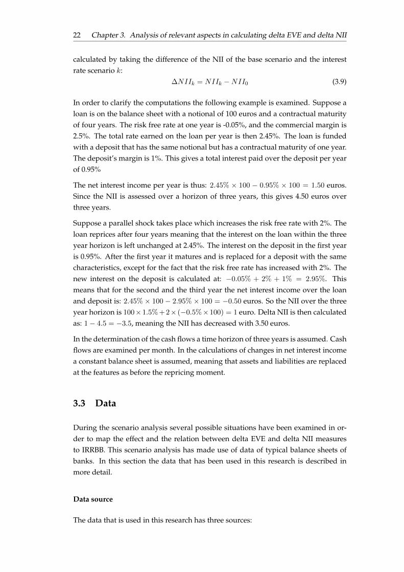
eight components together sum up to approximately 98 percent of the assets and lia-bilities. So when focusing on these components the balance sheet is a representativesubstitute of a retail bank’s balance sheet.
ABN Amro ING De Volksbank Rabobank Row AverageAssetsLoans 0.677 0.762 0.785 0.686 0.728Investments 0.008 0.003 0.002 0.006 0.005Trading securities 0.201 0.167 0.133 0.136 0.159Cash 0.103 0.051 0.069 0.143 0.092Total 0.989 0.983 0.990 0.972 0.983LiabilitiesDeposits 0.671 0.771 0.816 0.574 0.708Debt 0.251 0.162 0.125 0.323 0.215Trading liabilities 0.059 0.051 0.037 0.088 0.059Total 0.980 0.984 0.978 0.984 0.982Equity 0.043 0.048 0.053 0.062 0.051
TABLE 3.3: Largest assets and liabilities of the 4 largest Dutch banksin percentage
The data in Table 3.3 is combined to form one balance sheet that matches the char-acteristics of the four banks mentioned above. This balance sheet is given in Table3.4.
BalanceSheet
Assets LiabilitiesLoans 72 Deposits 70.5Investments 0.4 Debt 21Trading securities 16 Trading liabilities 3.4Cash 11.6 Equity 5.1
Total 100 Total 100
TABLE 3.4: Typical balance sheet retail bank
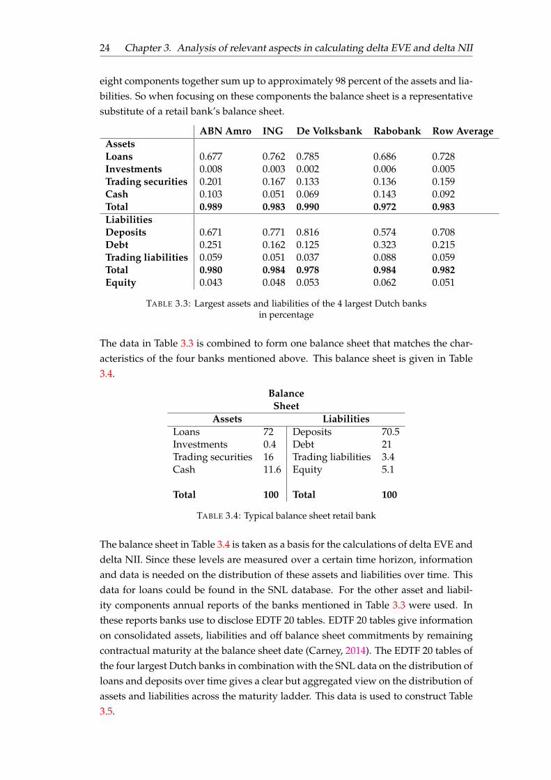
The balance sheet in Table 3.4 is taken as a basis for the calculations of delta EVE anddelta NII. Since these levels are measured over a certain time horizon, informationand data is needed on the distribution of these assets and liabilities over time. Thisdata for loans could be found in the SNL database. For the other asset and liabil-ity components annual reports of the banks mentioned in Table 3.3 were used. Inthese reports banks use to disclose EDTF 20 tables. EDTF 20 tables give informationon consolidated assets, liabilities and off balance sheet commitments by remainingcontractual maturity at the balance sheet date (Carney, 2014). The EDTF 20 tables ofthe four largest Dutch banks in combination with the SNL data on the distribution ofloans and deposits over time gives a clear but aggregated view on the distribution ofassets and liabilities across the maturity ladder. This data is used to construct Table3.5.
3.4. Results 25
Assets Loans Securities Investments Cash<1 M 0,05 0,405 0,014 11-3M 0,1 0,145 0,0193-12M 0,05 0,131 0,0921-5Y 0,2 0,151 0,456>5Y 0,6 0,169 0,419
Liabilities Deposits Debt Trading Liabilities<1 M 0,070 0,3911-3M 0,94 0,035 0,0983-12M 0,03 0,105 0,0991-5Y 0,02 0,070 0,207>5Y 0,01 0,720 0,206
TABLE 3.5: Relative distribution of assets and liabilities over time
The data in Table 3.5 describes the distribution of assets and liabilities across thematurity ladder. In the calculations of delta EVE this data is still too aggregated.Therefore, it is assumed that the assets and liabilities are equally distributed overtime within the time buckets given in Table 3.5. However in the situation where theaspect maturity profile is changed, other assumptions are made as can be found inSection 3.2.2.
3.4 Results
In this section the results of the analysis is described. The results are dealt with peraspect. First the results of the different yield curves used in the calculations of deltaEVE and delta NII will be discussed, then the maturity profile and last the businessmodel.
3.4.1 Results of the yield curve used in calculating delta EVE and deltaNII
In this section the results of the analysis of the impact of the first aspect on the deltaEVE and delta NII levels measured is described. In this analysis four yield curves,set out in Section 3.2.1, are used to compute the levels of delta EVE and delta NII.This is done for the three business models in Section 3.2.3. First the results on deltaEVE are described, thereafter the delta NII results will be elaborated.
Delta EVE
In Figures 3.1, 3.2 and 3.3 the results for the delta EVE figures for respectively theretail, trade and wholesale business models are given. Here the values on the Y axis
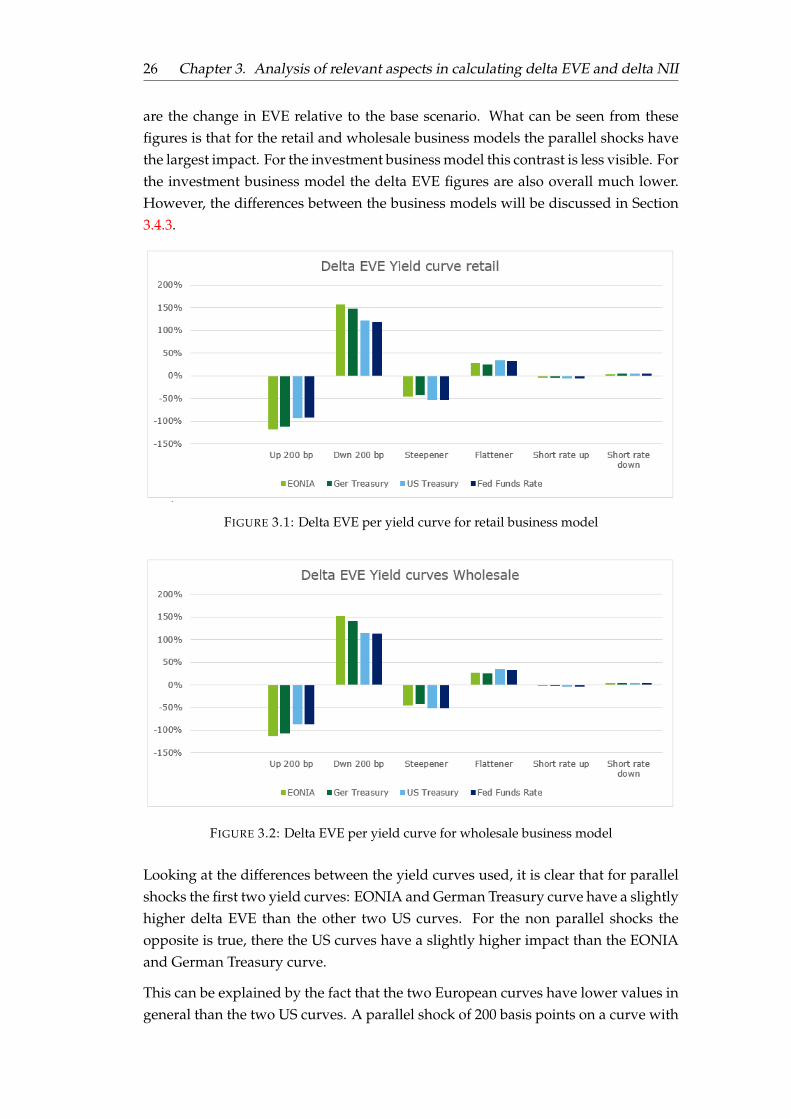
26 Chapter 3. Analysis of relevant aspects in calculating delta EVE and delta NII
are the change in EVE relative to the base scenario. What can be seen from thesefigures is that for the retail and wholesale business models the parallel shocks havethe largest impact. For the investment business model this contrast is less visible. Forthe investment business model the delta EVE figures are also overall much lower.However, the differences between the business models will be discussed in Section3.4.3.
FIGURE 3.1: Delta EVE per yield curve for retail business model
FIGURE 3.2: Delta EVE per yield curve for wholesale business model
Looking at the differences between the yield curves used, it is clear that for parallelshocks the first two yield curves: EONIA and German Treasury curve have a slightlyhigher delta EVE than the other two US curves. For the non parallel shocks theopposite is true, there the US curves have a slightly higher impact than the EONIAand German Treasury curve.
This can be explained by the fact that the two European curves have lower values ingeneral than the two US curves. A parallel shock of 200 basis points on a curve with
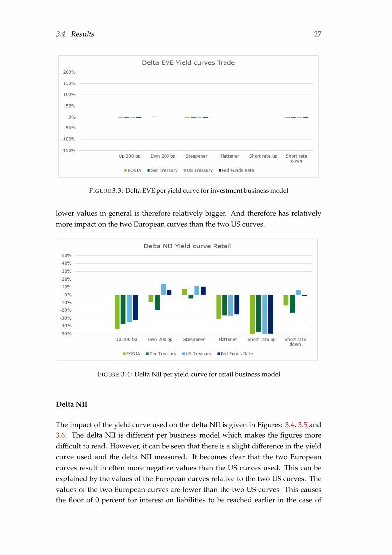
3.4. Results 27
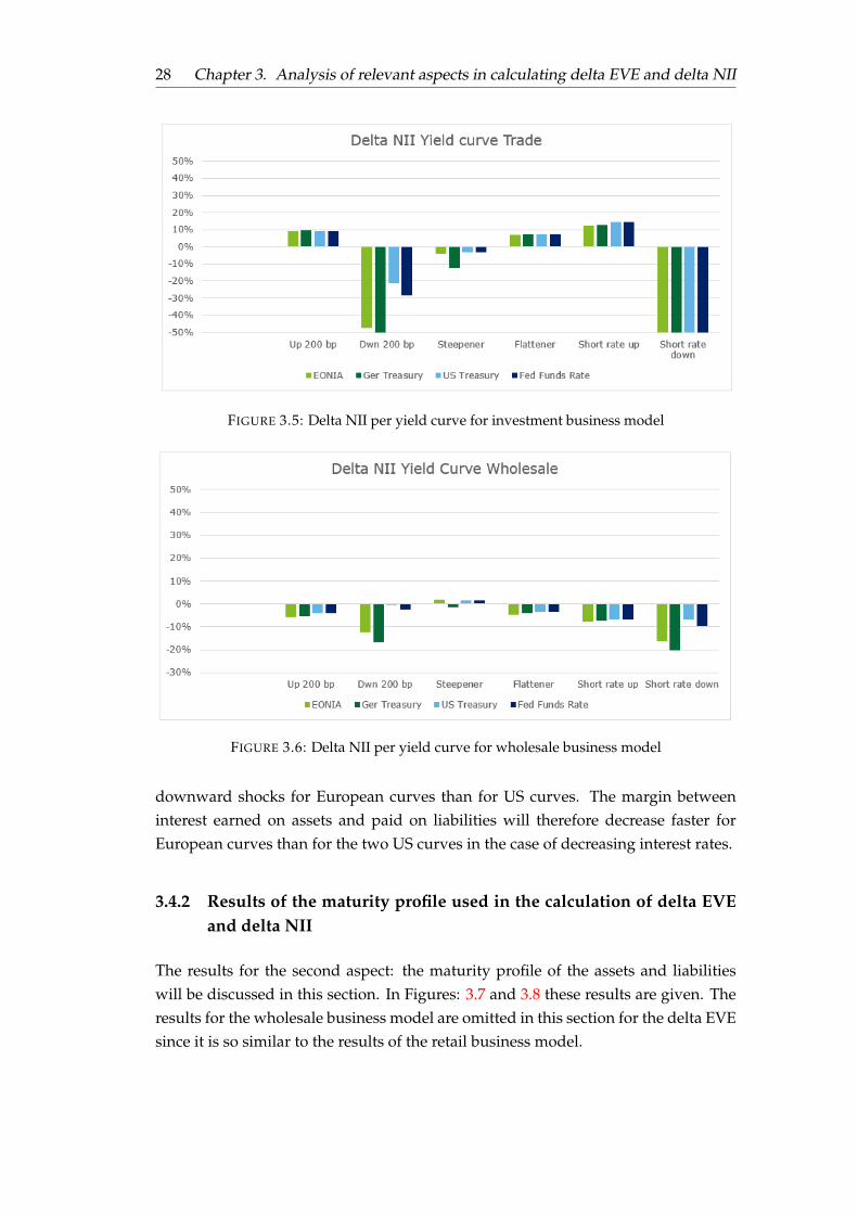
FIGURE 3.3: Delta EVE per yield curve for investment business model
lower values in general is therefore relatively bigger. And therefore has relativelymore impact on the two European curves than the two US curves.
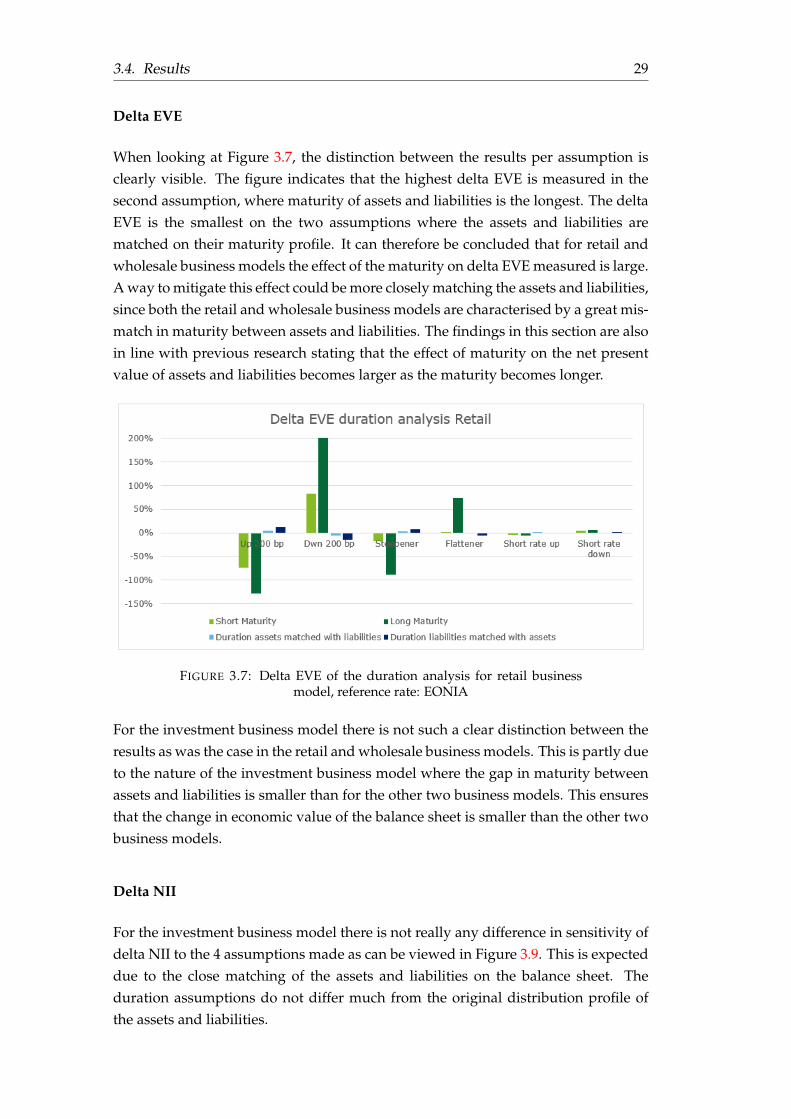
FIGURE 3.4: Delta NII per yield curve for retail business model
Delta NII
The impact of the yield curve used on the delta NII is given in Figures: 3.4, 3.5 and3.6. The delta NII is different per business model which makes the figures moredifficult to read. However, it can be seen that there is a slight difference in the yieldcurve used and the delta NII measured. It becomes clear that the two Europeancurves result in often more negative values than the US curves used. This can beexplained by the values of the European curves relative to the two US curves. Thevalues of the two European curves are lower than the two US curves. This causesthe floor of 0 percent for interest on liabilities to be reached earlier in the case of
28 Chapter 3. Analysis of relevant aspects in calculating delta EVE and delta NII
FIGURE 3.5: Delta NII per yield curve for investment business model
FIGURE 3.6: Delta NII per yield curve for wholesale business model
downward shocks for European curves than for US curves. The margin betweeninterest earned on assets and paid on liabilities will therefore decrease faster forEuropean curves than for the two US curves in the case of decreasing interest rates.
3.4.2 Results of the maturity profile used in the calculation of delta EVEand delta NII
The results for the second aspect: the maturity profile of the assets and liabilitieswill be discussed in this section. In Figures: 3.7 and 3.8 these results are given. Theresults for the wholesale business model are omitted in this section for the delta EVEsince it is so similar to the results of the retail business model.
3.4. Results 29
Delta EVE
When looking at Figure 3.7, the distinction between the results per assumption isclearly visible. The figure indicates that the highest delta EVE is measured in thesecond assumption, where maturity of assets and liabilities is the longest. The deltaEVE is the smallest on the two assumptions where the assets and liabilities arematched on their maturity profile. It can therefore be concluded that for retail andwholesale business models the effect of the maturity on delta EVE measured is large.A way to mitigate this effect could be more closely matching the assets and liabilities,since both the retail and wholesale business models are characterised by a great mis-match in maturity between assets and liabilities. The findings in this section are alsoin line with previous research stating that the effect of maturity on the net presentvalue of assets and liabilities becomes larger as the maturity becomes longer.
FIGURE 3.7: Delta EVE of the duration analysis for retail businessmodel, reference rate: EONIA
For the investment business model there is not such a clear distinction between theresults as was the case in the retail and wholesale business models. This is partly dueto the nature of the investment business model where the gap in maturity betweenassets and liabilities is smaller than for the other two business models. This ensuresthat the change in economic value of the balance sheet is smaller than the other twobusiness models.
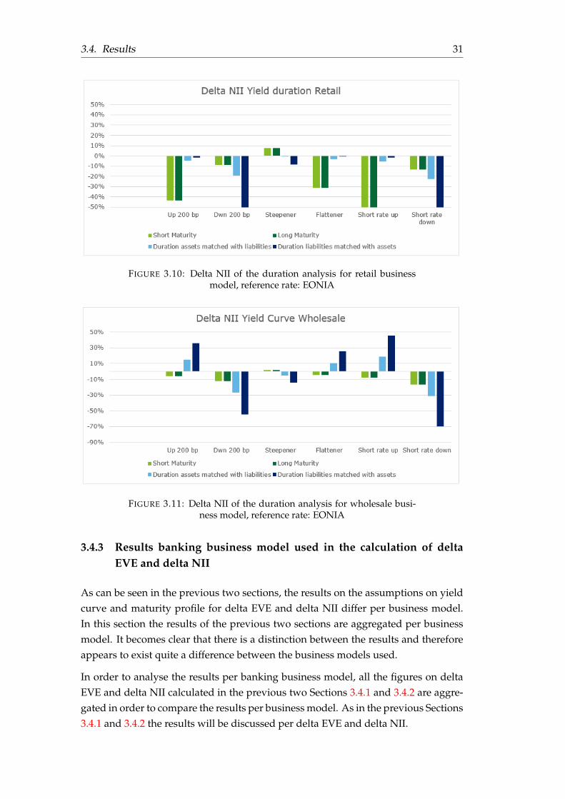
Delta NII
For the investment business model there is not really any difference in sensitivity ofdelta NII to the 4 assumptions made as can be viewed in Figure 3.9. This is expecteddue to the close matching of the assets and liabilities on the balance sheet. Theduration assumptions do not differ much from the original distribution profile ofthe assets and liabilities.
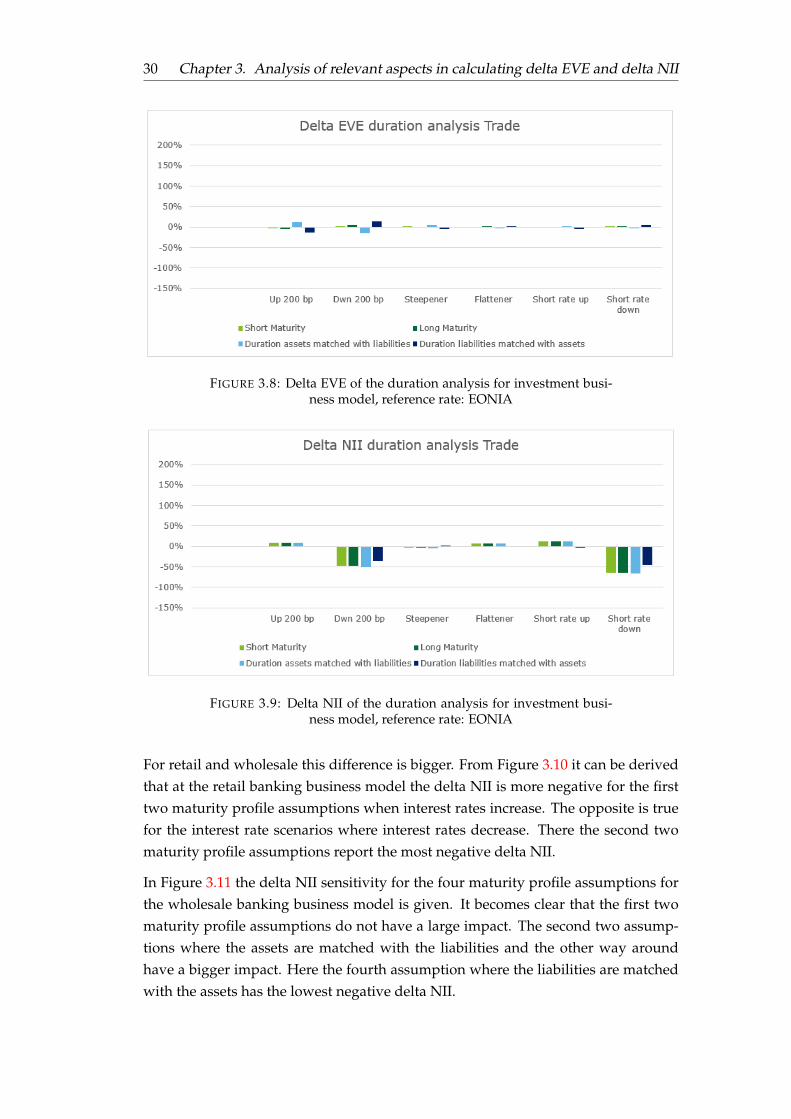
30 Chapter 3. Analysis of relevant aspects in calculating delta EVE and delta NII
FIGURE 3.8: Delta EVE of the duration analysis for investment busi-ness model, reference rate: EONIA
FIGURE 3.9: Delta NII of the duration analysis for investment busi-ness model, reference rate: EONIA
For retail and wholesale this difference is bigger. From Figure 3.10 it can be derivedthat at the retail banking business model the delta NII is more negative for the firsttwo maturity profile assumptions when interest rates increase. The opposite is truefor the interest rate scenarios where interest rates decrease. There the second twomaturity profile assumptions report the most negative delta NII.
In Figure 3.11 the delta NII sensitivity for the four maturity profile assumptions forthe wholesale banking business model is given. It becomes clear that the first twomaturity profile assumptions do not have a large impact. The second two assump-tions where the assets are matched with the liabilities and the other way aroundhave a bigger impact. Here the fourth assumption where the liabilities are matchedwith the assets has the lowest negative delta NII.
3.4. Results 31
FIGURE 3.10: Delta NII of the duration analysis for retail businessmodel, reference rate: EONIA
FIGURE 3.11: Delta NII of the duration analysis for wholesale busi-ness model, reference rate: EONIA
3.4.3 Results banking business model used in the calculation of deltaEVE and delta NII
As can be seen in the previous two sections, the results on the assumptions on yieldcurve and maturity profile for delta EVE and delta NII differ per business model.In this section the results of the previous two sections are aggregated per businessmodel. It becomes clear that there is a distinction between the results and thereforeappears to exist quite a difference between the business models used.
In order to analyse the results per banking business model, all the figures on deltaEVE and delta NII calculated in the previous two Sections 3.4.1 and 3.4.2 are aggre-gated in order to compare the results per business model. As in the previous Sections3.4.1 and 3.4.2 the results will be discussed per delta EVE and delta NII.
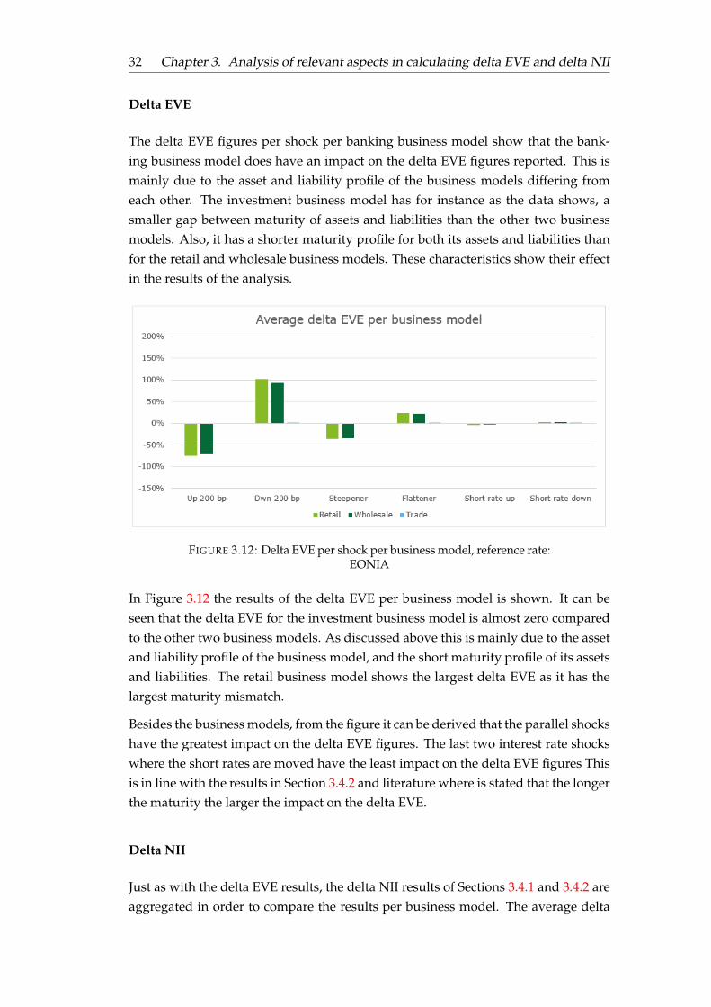
32 Chapter 3. Analysis of relevant aspects in calculating delta EVE and delta NII
Delta EVE
The delta EVE figures per shock per banking business model show that the bank-ing business model does have an impact on the delta EVE figures reported. This ismainly due to the asset and liability profile of the business models differing fromeach other. The investment business model has for instance as the data shows, asmaller gap between maturity of assets and liabilities than the other two businessmodels. Also, it has a shorter maturity profile for both its assets and liabilities thanfor the retail and wholesale business models. These characteristics show their effectin the results of the analysis.
FIGURE 3.12: Delta EVE per shock per business model, reference rate:EONIA
In Figure 3.12 the results of the delta EVE per business model is shown. It can beseen that the delta EVE for the investment business model is almost zero comparedto the other two business models. As discussed above this is mainly due to the assetand liability profile of the business model, and the short maturity profile of its assetsand liabilities. The retail business model shows the largest delta EVE as it has thelargest maturity mismatch.
Besides the business models, from the figure it can be derived that the parallel shockshave the greatest impact on the delta EVE figures. The last two interest rate shockswhere the short rates are moved have the least impact on the delta EVE figures Thisis in line with the results in Section 3.4.2 and literature where is stated that the longerthe maturity the larger the impact on the delta EVE.
Delta NII
Just as with the delta EVE results, the delta NII results of Sections 3.4.1 and 3.4.2 areaggregated in order to compare the results per business model. The average delta
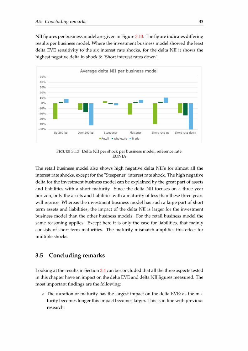
3.5. Concluding remarks 33
NII figures per business model are given in Figure 3.13. The figure indicates differingresults per business model. Where the investment business model showed the leastdelta EVE sensitivity to the six interest rate shocks, for the delta NII it shows thehighest negative delta in shock 6: "Short interest rates down".
FIGURE 3.13: Delta NII per shock per business model, reference rate:EONIA
The retail business model also shows high negative delta NII’s for almost all theinterest rate shocks, except for the "Steepener" interest rate shock. The high negativedelta for the investment business model can be explained by the great part of assetsand liabilities with a short maturity. Since the delta NII focuses on a three yearhorizon, only the assets and liabilities with a maturity of less than these three yearswill reprice. Whereas the investment business model has such a large part of shortterm assets and liabilities, the impact of the delta NII is larger for the investmentbusiness model than the other business models. For the retail business model thesame reasoning applies. Except here it is only the case for liabilities, that mainlyconsists of short term maturities. The maturity mismatch amplifies this effect formultiple shocks.
3.5 Concluding remarks
Looking at the results in Section 3.4 can be concluded that all the three aspects testedin this chapter have an impact on the delta EVE and delta NII figures measured. Themost important findings are the following:
a The duration or maturity has the largest impact on the delta EVE: as the ma-turity becomes longer this impact becomes larger. This is in line with previousresearch.
34 Chapter 3. Analysis of relevant aspects in calculating delta EVE and delta NII
b The banking business model has an impact on the delta EVE measured. Thisis largely because of the difference in maturity profile between the businessmodels, and can thus be related to the duration effect. Retail and wholesalebusiness models are characterised by a larger mismatch in maturity of assetsand liabilities, and their economic value of equity is therefore more sensitiveto changes in interest rates.
c The delta NII is bigger for European curves, or curves that have lower values,than for curves that have higher values, since the floor on interest on liabilitiesis reached earlier. This means that the margin between assets and liabilities willdecrease faster than with curves that have higher values such as the Americancurves used in this analysis.
These findings are based on the aggregated data of a small group of large systemicbanks. What has to be incorporated in the understanding of these findings is thatthe results are calculated without incorporation of hedging effects. The results ofthe calculations can therefore be more extreme than they would be when hedgingwould be incorporated. Also the results are calculated on a static balance sheet as-sumption. Including optionality assumptions in the different interest rate scenariosmight exacerbate the results discussed in the previous sections. More on these twotopics can be found in Chapter 7.
35
Chapter 4
Constructing a model to changeexposure to IRRBB
4.1 Introduction
The next step in this research is to determine how banks can change their levels ofinterest rate risk exposure. In Chapter 4 and 5 this step is discussed. Ultimately, inthese two chapters an answer to the third research question and the main researchquestion is given:
3. When is the exposure to interest rate risk measured from both earnings and economicvalue perspectives considered optimal?
And the main research question:
How can banks best change their levels of exposure to interest rate risk, measured from aneconomic value and earnings perspective, given their risk appetite and business model?
As stated in Section 1.4, the answer to these research questions will be found byconstructing a Linear Programming (LP). The construction of the LP model will bediscussed in this chapter. The results of the optimisation will be described in Chapter5.
An LP model is an optimisation algorithm that maximises or minimises a targetfunction while being subject to certain constraints (Winston, 2004). Th LP modelin this research will optimise the balance sheet via constraints on interest rate riskmeasured through delta EVE and delta NII.
Literature defines two sets of LP models that are often used for optimising the bal-ance sheet and the management of assets and liabilities:
• Deterministic Models: Models that use Linear Programming, assume specific re-alisations for random events and are computationally tractable for large prob-lems (Zopounidis, Doumpos, and Pardalos, 2010).
36 Chapter 4. Constructing a model to change exposure to IRRBB
• Stochastic Models: The use of probability constrained Linear Programming, dy-namic programming and Linear Programming under uncertainty (Zopouni-dis, Doumpos, and Pardalos, 2010).
George B. Dantzig was in 1947 the first to lay a foundation for the simplex methodthat is mostly used in solving LP problems (Dantzig, 1990). Chambers and Charneswere pioneers in applying deterministic Linear Programming in the management ofassets and liabilities with their model on the analysis and optimisation of bank port-folios (Zopounidis, Doumpos, and Pardalos, 2010; Kusy and Ziemba, 1986). All de-terministic and many of the stochastic models applied to banking portfolios followthe approach of Chambers and Charnes’ Linear Programming model. Discountednet returns are maximised, subject to budget and liquidity constraints (Kusy andZiemba, 1986). Deterministic models are often criticised because of their incapabil-ity to incorporate uncertainty in their models. Probability distributions can be ob-tained for different economic scenarios and Linear Programming formulations canbe applied to each scenario to determine optimal solutions. However research haspointed out that these approaches will not generate optimal solutions to the totalproblem (Kusy and Ziemba, 1986).
The main goal of asset and liability management is controlling the net interest mar-gin (Al Shubiri et al., 2010). This is why in the linear (stochastic) programming mod-els this is often the main target function. Other target functions used in models areminimising the penalty cost when achieving a certain goal: "Goal programming"(Zopounidis, Doumpos, and Pardalos, 2010).
In an extensive stochastic Linear Programming problem that has been implementedat the Vancouver City Savings Credit Union (Kusy and Ziemba, 1986), the authorsuse a maximisation target function that is based on the following components: dis-counted returns and capital gains on assets, discounted cost of deposits and other lia-bilities, and expected penalty costs for the violation of constraints (Kusy and Ziemba,1986; Oguzsoy, Gu, et al., 1997).
This part of the research is executed in cooperation with a Dutch bank. This bankprovided data of their asset and liability positions over the fiscal year 2016. Thesepositions were viewed on a time horizon of 30 years. Besides this gapping profile,information on the average coupon earned and paid on their assets and liabilitieswas incorporated.
In this chapter the main assumptions, data and mathematical formulation of the LPmodel will be covered in detail.
4.2. LP model constraints and assumptions 37
4.2 LP model constraints and assumptions
The purpose of the LP model is to determine how the bank can best change its levelsof delta EVE and delta NII, and how this impacts the return of the bank. This is doneby optimising the return of the balance sheet via the target function, while subject tocertain constraints, of which delta EVE and delta NII for example. These constraintsare used to steer the interest rate risk exposures. This can be done by moving thelower bound for the negative delta EVE or delta NII constraints upwards and thusconstraining the IRRBB exposures. Besides the delta EVE and delta NII constraints,other constraints are incorporated in this model as well. In this section the design ofthe LP model, the data used and the methodology and assumptions underlying themodel will be discussed.
4.2.1 LP model design
Decision variables
The bank stated that their interest rate risk position is mainly managed through theirhedging portfolio and not through balance sheet restructuring. This is incorporatedin the LP model by making the composition of the hedging portfolio the main deci-sion variable in the LP model.
The previous chapter described that one of the most important factors in the deter-mination of delta EVE and delta NII is the maturity profile of assets and liabilities.To make sure that the maturity profile can be adjusted, the number of swaps overtime buckets can be changed. Suppose a bank may decide how many swaps with amaturity of one year, two years or three years it needs to obtain a certain interest raterisk profile. TThe decision variables are the number of swaps per maturity bucket.
The hedging portfolio is assumed to consist out of plain vanilla interest rate swaps.A distinction is made between payer swaps: where the fixed rate is paid and thefloating rate is received, and receiver swaps: where the fixed rate is received andfloating rate is paid. The decision variables in this model are therefore the numberof payer and receiver swaps per maturity.
Both the payer and receiver swaps have the same floating leg: the 3 month Euriborcurve extracted from Bloomberg at date 30-06-2016. The swaps have also the samefixed rate leg. The values for this fixed leg per maturity are chosen such that the netpresent value of the swaps is 0 for all maturities. It is assumed that the swaps can bepurchased with maturities ranging from 0.25 up to 30 years, the same time horizonas the balance sheet of the bank. The bank stated that its hedging portfolio is onlyused for hedging purposes and not for speculation on interest rate scenarios.
38 Chapter 4. Constructing a model to change exposure to IRRBB
Target function
The Lp model requires a target function that has to be minimised or optimised. Inthis research the interest is mainly on the exposure to IRRBB measured through deltaEVE and delta NII. However, since the measurement of delta EVE and delta NIIthrough the six interest rate shocks is hard to put in one linear format, the delta EVEand delta NII are therefore put as constraints in the model. A third criterion that isused to determine the optimal allocation of the swaps is then the return earned ormissed through a specific solution. Therefore the target function of this LP model isto maximise return earned over the hedging portfolio while subject to constraints oninterest rate risk and other constraints.
Constraints
This target function will be subject to constraints. Some of these are set due to prac-tical considerations, other such as the interest rate risk constraints are to monitorthe relationship between interest rate risk and the return made on the assets andliabilities. The following constraints will apply to the model:
a Balance sheet constraint: This constraint is set to make sure that the asset andliability side of the balance sheet remain equal.
b Decision variables volume constraint: A constraint limiting the maximum volumeof the number of swaps.
c Delta EVE constraint: A constraint putting a limit to changes in EVE due tochanges of the interest rate.
d Delta NII constraint: A constraint putting a limit to changes in earnings due tochanges in interest rates.
e Duration of equity constraint: A constraint putting a limit on the duration ofequity as stated in the risk appetite of the bank.
f Key rate or partial duration constraints: A constraint putting a limit on the partialduration or Key Rate Duration per year as stated in the risk appetite of thebank.
g Non-negativity constraint: The LP model requires all variables to be non-negative.
The first constraint ensures that the asset and liability side of the balance sheet areequal to each other. The second constraint puts a limit on the number of swaps aban can obtain. With maximising the return as target funcion, the model will take aninfinite number of swaps on the balance sheet as there is no limit on the number ofswaps and a small positive return can be made per swap. Since the swaps are usedfor hedging IRRBB and not speculating on the interest rate scenarios a limit on thevolume of swaps will be set in terms of notional.
4.2. LP model constraints and assumptions 39
The third and fourth constraint are delta EVE and delta NII constraints on IRRBB.The purpose of the LP model is to determine the optimal distribution of payer andreceiver swaps given a certain risk appetite and the impact on the return. The levelsof delta EVE and delta NII will be calculated through six interest rate shocks that thebank uses for their IRRBB assessment.
Constraints on the duration of equity and the Key Rate Duration per year comple-ment the interest rate risk constraints mentioned above. The duration of equity is akey economic value measure for IRRBB and is frequently used by the bank to steerits IRRBB profile. The Key Rate Duration constraint (KRD) is set in cooperation withthe bank in order to measure interest rate risk per maturity individually. These con-straints will prevent the model allocating too many payer and receiver swaps to oneor more specific time buckets.
The last constraint is to prevent values to have a value lower than zero. The LPmodel doesn’t allow variables to become negative. Short selling is however stillpossible since the pay-off and value of the payer and receiver swaps are the oppositeof each other. If a receiver swap with maturity x has a value of y, the value of thepayer swap with the same maturity x has a value of -y. The decision variable inthe LP problem cannot be negative. Its characteristics however can be achieved bymultiplying the decision variable with -1.
4.2.2 Data used
The data provided by the bank contained information on the asset and liability po-sitions over a time horizon of 30 years considering a run-off balance sheet. The datawas available on a quarterly basis, beyond 30 years no data was available. For bothassets and liabilities 5 classes are considered in this model that form the main partof the balance sheet of the bank. Due to confidentiality reasons the exact figures willnot be disclosed in this thesis. The balance sheet used is given in 4.1:
Assets Liabilities1 Mortgages Fixed 1 Term Deposits2 Mortgages Floating 2 Sight Deposits3 Bonds and Non-commercial loans 3 Wholesale Funding4 Receiver Swaps 4 Payer Swaps5 Cash 5 Equity
TABLE 4.1: Overview asset and liability classes bank’s balance sheet
For each asset and liability class the following data was available and taken intoaccount:
• Average coupon earned or paid over the asset or liability class;
• Distribution over maturity buckets per asset and liability class;
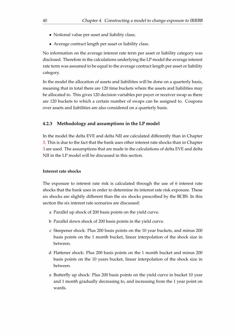
40 Chapter 4. Constructing a model to change exposure to IRRBB
• Notional value per asset and liability class;
• Average contract length per asset or liability class.
No information on the average interest rate term per asset or liability category wasdisclosed. Therefore in the calculations underlying the LP model the average interestrate term was assumed to be equal to the average contract length per asset or liabilitycategory.
In the model the allocation of assets and liabilities will be done on a quarterly basis,meaning that in total there are 120 time buckets where the assets and liabilities maybe allocated to. This gives 120 decision variables per payer or receiver swap as thereare 120 buckets to which a certain number of swaps can be assigned to. Couponsover assets and liabilities are also considered on a quarterly basis.
4.2.3 Methodology and assumptions in the LP model
In the model the delta EVE and delta NII are calculated differently than in Chapter3. This is due to the fact that the bank uses other interest rate shocks than in Chapter3 are used. The assumptions that are made in the calculations of delta EVE and deltaNII in the LP model will be discussed in this section.
Interest rate shocks
The exposure to interest rate risk is calculated through the use of 6 interest rateshocks that the bank uses in order to determine its interest rate risk exposure. Thesesix shocks are slightly different than the six shocks prescribed by the BCBS. In thissection the six interest rate scenarios are discussed:
a Parallel up shock of 200 basis points on the yield curve.
b Parallel down shock of 200 basis points in the yield curve.
c Steepener shock: Plus 200 basis points on the 10 year buckets, and minus 200basis points on the 1 month bucket, linear interpolation of the shock size inbetween.
d Flattener shock: Plus 200 basis points on the 1 month bucket and minus 200basis points on the 10 years bucket, linear interpolation of the shock size inbetween.
e Butterfly up shock: Plus 200 basis points on the yield curve in bucket 10 yearand 1 month gradually decreasing to, and increasing from the 1 year point onwards.
4.2. LP model constraints and assumptions 41
f Butterfly down shock: Minus 200 basis points on the yield curve in buckets 10year and 1 month, and gradually increasing to, and decreasing from the 1 yearpoint on wards.
These six interest rate shocks are different from the six shocks used in Chapter 3,but are the interest rate scenarios used by the bank. The difference is the way thesteepener and flattener shocks are calculated. For the steepener shock the shortestrate is decreased with -200 basis points, and the longest rate is increased with +200basis points. For the time buckets in between the change in interest rate is calculatedvia linear interpolation. For the flattener interest rate scenario this is the other wayaround. This is more simplistic as the way it was determined in Chapter 3 wherescalars where used in orde rto determine the decay of the shock over time.
Additionally, where the BCBS uses "short rate up" and "short rate down" shocks, thebank uses "butterfly up" and "butterfly down" shocks. The butterfly shocks haveexcept for a shock of ±200 bp on the rate with the shortest maturity also the sameshock on the longest maturity with linear interpolation for maturities in between.The one-year time bucket is the rotation point of this shock type.
Min-max theory
For each of these six interest rate shocks the delta EVE and delta NII will be cal-culated. The values of these interest rate exposures will be constrained by a lowerbound. This lower bound will be the same for all these six shocks. So the lowerbound of the delta EVE by a parallel up shock will be the same as all the other 5shocks. This enables a min-max theory where the maximum loss in change of eco-nomic value is minimised for all of these six shocks. For example: suppose that thelower bound for delta EVE is set at -15 percent. Results might show a parallel upshock causes the lowest negative delta of -14,5 percent, while the other shocks havehigher values. When moving the lower bound of the delta EVE constraint to -13percent, the LP model optimises the mixture of swaps such that the lowest nega-tive delta EVE falls within this boundary. In the new situation, results might showthat delta EVE for the parallel up shock is -12 percent, and the steepener shock hasa value -13 percent. This is the min-max theory. By gradually moving the lowerbound upwards the maximum negative delta EVE value can be minimised.
The same methodology is used for the delta NII constraint.
Assumptions in calculation of delta NII
For the delta NII calculation, some assumptions are made. In contrast to the deltaEVE calculation which assumes a run-off balance sheet, the delta NII assumes aconstant balance sheet where assets and liabilities that mature are replaced with
42 Chapter 4. Constructing a model to change exposure to IRRBB
items with identical features. However, there are some assumptions underlying thismethod. These will be discussed in this section.
Time horizon: The time horizon is one of the first assumptions of importance. Inthe analysis, the delta NII is calculated on a time horizon of one year. This is in linewith current practice of the bank and the paper of the BCBS (BCBS, 2016a). Since thedelta NII over two-years might be different than the delta NII measured over oneyear in the model, the delta NII is also calculated over a time-horizon of two years inorder to compare the results. Repricing features: The assumption on the repricingmoments of the assets and liabilities in the delta NII computation is also of impor-tance. As stated in Section 4.2.2, data on the distribution of assets and liabilities over30 years is used to determine the repricing moments. Here the interest rate term andcontractual maturity are assumed to be equal. Therefore the contractual maturity isconsidered as the repricing moment of the asset or liability.
The new rate at which an asset or liability reprices is determined as follows: theheight of the new rate is the normal coupon plus the interest rate shocks. For instancean asset with a coupon of 5%, is assumed to be 5% + 2% = 7% after a parallel upshock.
For non-parallel shocks, as for instant the "Steepener" shock, the average contractlength of an asset class is used to determine the repriced rate of the shock. For non-parallel shocks these rates differ with maturity. For instance: the shock size for the"Steepener" shock the maturity of 1 month is -200 bp, but for two years it is +22bp. The average contract length of an asset or liability class is used to determinethe maturity of the new repriced item and the corresponding shock size. Take forinstance an asset with average contract length of 2 years, that reprices within oneyear and has a coupon of 5%. The new coupon is then set at 5% + 0.22% = 5.22%
Two year delta NII: For the delta NII with a time horizon of two years the repricingis carried out in the same way as for the delta NII with the horizon of one year, butthen two times. Here the asset and liabilities can be categorised in three categories:
a An asset or liability that reprices in the first year and earns two shocked coupons;
b An asset or liability that reprices in the second year and earns a normal couponplus a shocked coupon;
c An asset or liability that doesn’t reprice within two years and earns two initialcoupons.
The shocked coupons are determined in the same way as for the one year delta NII.In order to match market practices the cash flows in the delta NII calculations arenot discounted. In order to determine the two year delta NII the change in NII over2 years is calculated relative to the two year NII forecast of the base scenario. TheNII in the base scenario consists of assets and liabilities of the third category only.
4.3. Mathematical formulation of the LP problem 43
4.3 Mathematical formulation of the LP problem
The mathematical formulation of the target function and the constraints is elabo-rated in this section. The LP model requires all constraints to be in a linear format.Since some computations of these constraints are not linear such as for instance theduration of equity and Key Rate Duration constraints, these have to be rewrittento linear form to fit the format of the LP model. The derivation of the linear con-straints as they are stated in this chapter and the following sections can be found inAppendix B .
4.3.1 Target function
The target of the model is, as stated in section 4.2, to maximise the return earnedon payer and receiver swaps plus a constant of the return on assets and liabilitiesof the original balance sheet. Therefore the target function of the LP model can bedefined as the interest earned or paid on receiver swaps plus the interest earned orpaid on payer swaps. Since the interest rate swaps are the only decision variables inthe model, this can be stated as follows:
Maxz =
120∑t=1
(xtRt) +
120∑t=1
(ytct) + C (4.1)
Where:
xt = The number of receiver swaps in time bucket t
yt = The number of payer swaps in time bucket t
Rt = The interest rate earned over receiver swaps allocated to time bucket t
ct = The interest rate paid over the amount of payer swaps allocated to time bucket t
t ∈ (1, 120) = The number of time buckets, divided quarterly over 30 years
C = A constant representing the interest income earned over the assets and liabilitiesother than the interest rate swaps
The coupons Rt and ct are the first year cash flows of the receiver and payer swaps.Although the values of the swaps are all 0, the first year cash flows may be non-negative (Hull, 2012b). Therefore, in the first year NII a positive or negative cashflow may result from a position in payer or receiver swaps. These coupons originallyare considered to be quarterly since the data of the bank is also on a quarterly basis.In order to display the return over one year these coupons are multiplied by four.
44 Chapter 4. Constructing a model to change exposure to IRRBB
4.3.2 Balance sheet constraint
The balance sheet constraints are set to keep the two sides of the balance sheet equal.Since only the interest rate swaps are decision variables and the rest of the balancesheet is kept fixed, the total value of the receiver swaps on the asset side must equalthe total value of the payer swaps on the liability side of the balance sheet:
120∑t=1
Vtxt −120∑t=1
Vtyt = 0 (4.2)
with: Vt = the value of the swap in time bucket t.
As the value of the swaps is set at or close to 0 it will be expected that this constrainthas a minimum effect on the optimal solution.
4.3.3 Hedging portfolio volume constraints
In order to prevent the LP model to take too many swaps on the balance sheet as aresult of the maximisation of the target function, a limit on the total volume of payerand receiver swaps is set. This limit is set on the total volume of the notional ofthe payer and receiver swaps. With each swap having a notional of 2 million euros,the number of payer and receiver swaps is both limited at 30. With a total balancesheet volume of 100 million the notional for payer and receiver swaps is limited at60% of the balance sheet. This value is chosen as it represents a large part of thebalance sheet and therefore allows the hedging portfolio to be sufficiently large tohedge all risks. But at the same time this limit prevents the balance sheet to becomeunrealistically large. This gives two constraints. One for the receiver swaps:
120∑t=1
xt ≤ 30 (4.3)
And one for the payer swaps:
120∑t=1
yt ≤ 30 (4.4)
4.3.4 Delta EVE constraint
The delta EVE constraint is the fourth constraint that will be discussed. According toliterature the change in economic value of equity can be calculated as follows (BCBS,2015; BCBS, 2016a; EBA, 2015):
4.3. Mathematical formulation of the LP problem 45
∆EV Ek = (NPVAssets,k −NPVLiabilities,k)− (NPVAssets,0 −NPVLiabilities,0) (4.5)
With k ∈ (1, 6) the indicator of the interest rate shock and 0 the basis interest ratescenario. Equity is left out of the equations as it is the difference between the assetsand liabilities. This gives then following constraint:
∆EV Ek =
5∑i=1
120∑t=1
(( 1
(1 + rk,t)t+(
t∑t∗=1
1
(1 + rk,t∗)t∗Rk,t∗)
)−
( 1
(1 + r0,t)t+ (
t∑t∗=1
1
(1 + r0,t∗)t∗R0,t∗)
))xi,t−
5∑i=1
120∑t=1
(( 1
(1 + rk,t)t+(
t∑t∗=1
1
(1 + rk,t∗)t∗ck,t∗)
)−
( 1
(1 + r0,t)t+ (
t∑t∗=1
1
(1 + r0,t∗)t∗c0,t∗)
))yi,t ≥ −25%
(4.6)
The value for the right-hand side of the equation is here chosen at random. In thefollowing chapters the right-hand side of this equation will be used in order to obtaindifferent values for delta EVE.
The derivation of the delta EVE constraint can be found in Appendix B section B.2
4.3.5 Delta NII constraint
Besides the delta EVE constraint, the delta NII constraint is an important factor inthis model as it constrains the interest rate risk measured from an earnings perspec-tive. According to literature, the change in net interest income can be calculated asfollows (BCBS, 2015; BCBS, 2016a; EBA, 2015):
∆NIIk = NIIk −NII0 (4.7)
With k ∈ (1, 6) the indicator of the interest rate shock applied, and 0 being the basescenario.
Negative values of the delta NII will indicate a decrease in NII due to a change ininterest rates, and positive values an increase in NII.
Since the horizon of delta NII is one year, the shock in interest rates will only beapplied to the first 4 time buckets, representing the four first quarters. The other
46 Chapter 4. Constructing a model to change exposure to IRRBB
buckets will remain unchanged since assets and liabilities with a maturity of morethan one year will not reprice within the one year at which the delta NII is assessedand therefore will keep their original coupon.
Since the LP model requires the constraints to be in linear format, rewriting givesthe following result:
∆NIIk =
5∑i=1
4∑t=1
((Rk,t −R0,t)xi,t − (ck,t − c0,t)yi,t
)≥ −10% (4.8)
Again the right-hand side of this equation is chosen at random. In the followingchapters this right-hand side will be varied in order to obtain different results fordelta NII.
4.3.6 Duration of equity constraint
Duration of equity is a widely used risk measure for the exposure of a portfolioto movements in the yield curve. Duration measures the sensitivity of percentagechanges in an asset’s or liability’s price to changes in its yield (Hull, 2012a). A du-ration of equity constraint is incorporated in the LP model since it is part of the riskappetite of the bank and since it is an indication of the economic value sensitivity ofthe balance sheet. The duration of equity can be viewed as the difference in durationof assets and liabilities (Cummins et al., 2009):
DoE = DurationAssets − (assets/liabilities)DurationLiabilities (4.9)
The duration of an asset or liability can also be viewed as the weighted average ofall the cash flows of assets and liabilities multiplied with the time they occur (Hull,2012a).
These weights are calculated by dividing the cash payment at time t with the totalnet present value of the asset or liability (Hull, 2012a). The value of the boundaryfor the duration of equity constraint is given by 2.1. For confidentiality purposes thisfigure can not be disclosed but replaced by an indiactive figure. The linear format ofthis equation is given in the following formula:
Duration =
n∑t=1
t(Rt
1(1+r0,t)t
NPVasset
)(4.10)
In the LP model the constraint will be defined as:
4.3. Mathematical formulation of the LP problem 47
DoE =
( 120∑t=1
((Ri,t
1
(1 + r0,t)t)(t− 2.1)
)+
1
(1 + r0,t)t(t− 2.1)
)xi,t
−( 120∑
t=1
((Ri,t
1
(1 + r0,t)t)(t− 2.1)
)+
1
(1 + r0,t)t(t− 2.1)
)yi,t ≤ 0
(4.11)
The mathematical derivation of equation 4.11 can be found in Appendix B, sectionB.2.1.
4.3.7 Key Rate Duration constraint
In order to constrain the Key Rate Duration per year, a set of 30 Key Rate Durationconstraints is constructed to prevent peaks of allocations of swaps in specific timebuckets. Key Rate Duration is defined as the change in value of assets and liabilitiesdue to a shock to the yield curve at a specific maturity (Hull, 2012a). It is given as:
KRDT = − 1
P
∆PT
∆rT
Where P is the total price or value of an asset/liability, and ∆PT is the correspondingchange in value of the asset. Just like the duration constraint and the calculation ofthe delta EVE constraint, the ∆PT is calculated as the difference between the originalprice and the price after the change in value due to the small shock of the interestrate: ∆PT = PT −P0. The small change in interest rates ∆rT is determined as 1 basispoint, or 0,01 percent. Any change could be chosen here. However, due to convexitywith greater changes a small change of 1 basis point is chosen (Hull, 2012a).
This change is applied to a one year period of the yield curve. Since the assets andliabilities can be allocated to a total of 120 time buckets (30 years), there are 30 KeyRate Duration constraints where for each constraint a different period of one yearon the yield curve is shocked. Each of these constraints then have to comply withequation 4.12.
In the risk appetite statements of the bank, values for the bounds on the KRD con-straints were given. This information is confidential, therefore the following valueis chosen to replace it: 1.5. This gives the following Key Rate Duration KRDT withT the year on the yield curve that is shocked to determine the Key Rate Duration:
48 Chapter 4. Constructing a model to change exposure to IRRBB
KRDT = − 1
P
∆PT
∆rT≤ 1.5 (4.12)
Literature considers liabilities as a short position in a bond (Hull, 2012b). In line withthe duration of equity calculations, the net Key Rate Duration position per year isdefined as:
KRDT = KRDassets,T −KRDliabilities,T (4.13)
Implementing equations B.30, B.31 and B.2.2 in equation 4.13 for T = 1 gives theequation for the Key Rate Duration of assets, where:
KRDassets,1 =
(( 5∑i=1
4∑t=1
( 1
(1 + r0,t + ∆rt)t+ (
t∑t∗=1
1
(1 + r0,t∗ + ∆rt∗)t∗ck,t∗)
)+
5∑i=1
120∑t=4
( 1
(1 + r0,t)t+ (
t∑t∗=1
1
(1 + r0,t∗)t∗ck,t∗)
))−(
5∑i=1
120∑t=1
( 1
(1 + r0,t)t+ (
t∑t∗=1
1
(1 + r0,t∗)t∗ck,t∗)
)(1 + ∆rtxx)
))xi,t
(4.14)
and:
KRDliabilities,1 =
(( 5∑i=1
4∑t=1
( 1
(1 + r0,t + ∆rt)t+ (
t∑t∗=1
1
(1 + r0,t∗ + ∆rt∗)t∗ck,t∗)
)+
5∑i=1
120∑t=4
( 1
(1 + r0,t)t+ (
t∑t∗=1
1
(1 + r0,t∗)t∗ck,t∗)
))−(
5∑i=1
120∑t=1
( 1
(1 + r0,t)t+ (
t∑t∗=1
1
(1 + r0,t∗)t∗ck,t∗)
)(1 + ∆rtxx)
))yi,t
(4.15)
4.3.8 Hedging portfolio
The decision variables in this model are the number of payer and receiver swapsto buy. As was stated in previous sections, these swaps are used by the bank tomanage its interest rate risk exposure. In order to give some more information onthe assumptions and calculations underlying these payer and receiver swaps, theyare discussed here in this section.
4.3. Mathematical formulation of the LP problem 49
A swaps has two legs: one floating leg and a fixed leg. The floating leg of the swapis based on the 3 month Euribor forward curve at 30-06-2016. This curve is annuallycompounded. The fixed leg is chosen such that the value of the swap for each matu-rity is 0 or close to 0. The both legs of the swaps are discounted using the OIS curveat date 30-06-2016.
Calculating the value of the interest rate swap
In the calculation of delta EVE the value of swaps has a big impact. When interestrates rise, the rates of the floating leg will rise at the same time, while the fixed ratesremain fixed. This results in a difference in earnings and thus in a higher value forpayer swaps and a lower value for receiver swaps. The opposite holds for decreasinginterest rates. The change in value of the swaps will be incorporated in the delta EVEand delta NII computations to model the effect.
The value of an interest rate swap can be calculated according to the following twoapproaches:
a Valuation in terms of Bond prices: The value of the swap is the differencebetween a fixed and a floating bond that represents the fixed and floating legsof the swap (Hull, 2012b).
b Valuation in terms of Forward Rate Agreements (FRA’s): The value of the swapis calculated as the value of a portfolio of FRA’s (Hull, 2012b).
In this research the second approach is used: valuation in terms of FRA’s. A ForwardRate Agreement is a contract where the specifics of a certain interest rate, applied toeither borrowing or lending a certain principle in the future, are determined (Hull,2012b). An example of an FRA is the situation where a company agrees that it re-ceives a fixed rate of 4% on a principal of 100 million for a 3-month period starting inthree years and in exchange pays LIBOR. If the 3-month LIBOR is 4.5% for the threemonth period, the cash flow to the lender will be: 100,000,000 × (0.04-0.045) × 0.25= -$125,000 (Hull, 2012b).
A swap can be viewed as a portfolio of FRA’s, since in an interest rate swap a cer-tain interest rate applies to a certain principal at multiple times in the future (Hull,2012b). Key in the valuation of an FRA is the assumption that forward interest ratesare realised. The interest rate swap therefore also makes use of this assumption.
The first step is determining the forward curve that applies to the floating leg. Inthis case the Euribor curve extracted from Bloomberg is the forward curve that canbe applied. The second step is to use the assumption that floating rates equal theEuribor forward rates to calculate the cash flows of the two legs of the swap. In thefinal step the swaps cash flows are discounted in order to determine the value. Thisprocedure is given in the following formula:
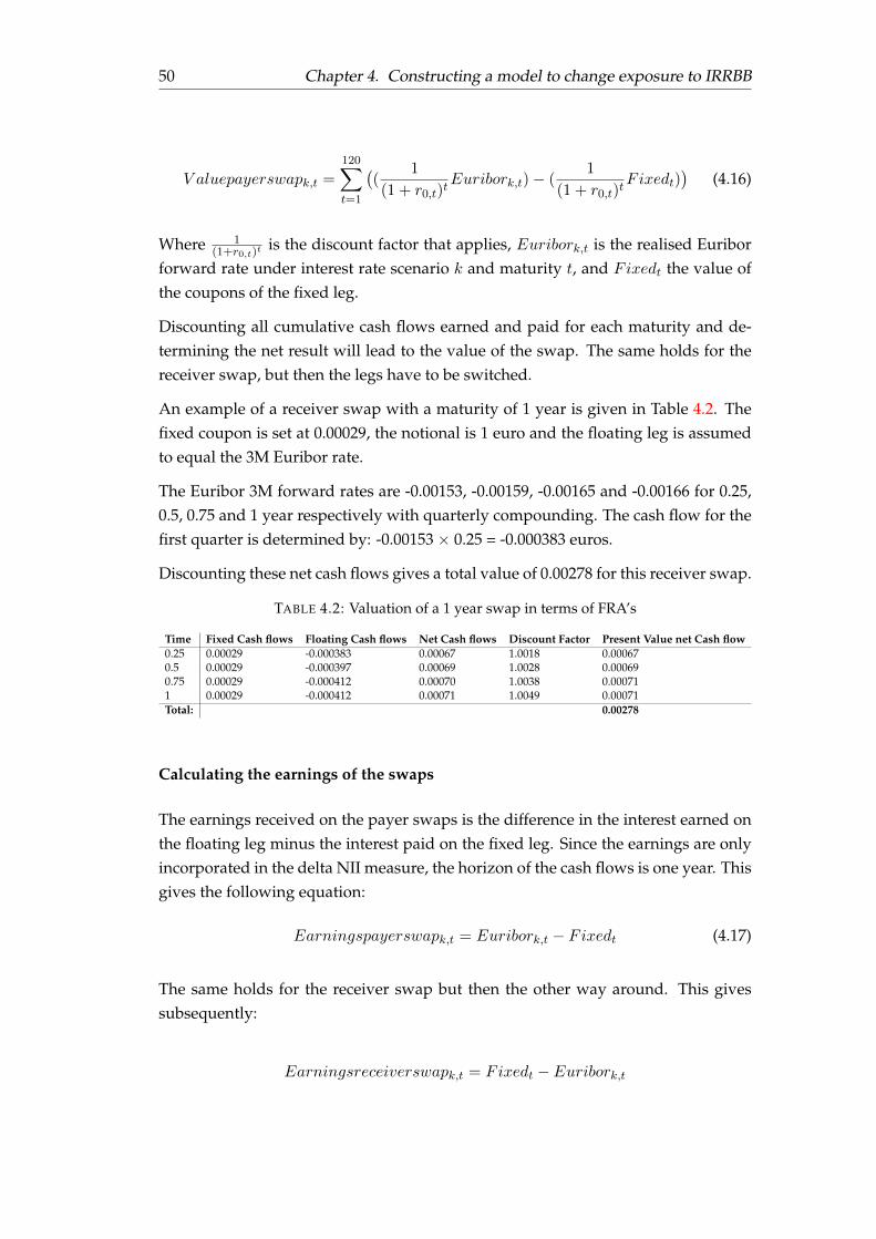
50 Chapter 4. Constructing a model to change exposure to IRRBB
V aluepayerswapk,t =
120∑t=1
((
1
(1 + r0,t)tEuribork,t)− (
1
(1 + r0,t)tFixedt)
)(4.16)
Where 1(1+r0,t)t
is the discount factor that applies, Euribork,t is the realised Euriborforward rate under interest rate scenario k and maturity t, and Fixedt the value ofthe coupons of the fixed leg.
Discounting all cumulative cash flows earned and paid for each maturity and de-termining the net result will lead to the value of the swap. The same holds for thereceiver swap, but then the legs have to be switched.
An example of a receiver swap with a maturity of 1 year is given in Table 4.2. Thefixed coupon is set at 0.00029, the notional is 1 euro and the floating leg is assumedto equal the 3M Euribor rate.
The Euribor 3M forward rates are -0.00153, -0.00159, -0.00165 and -0.00166 for 0.25,0.5, 0.75 and 1 year respectively with quarterly compounding. The cash flow for thefirst quarter is determined by: -0.00153 × 0.25 = -0.000383 euros.
Discounting these net cash flows gives a total value of 0.00278 for this receiver swap.
TABLE 4.2: Valuation of a 1 year swap in terms of FRA’s
Time Fixed Cash flows Floating Cash flows Net Cash flows Discount Factor Present Value net Cash flow0.25 0.00029 -0.000383 0.00067 1.0018 0.000670.5 0.00029 -0.000397 0.00069 1.0028 0.000690.75 0.00029 -0.000412 0.00070 1.0038 0.000711 0.00029 -0.000412 0.00071 1.0049 0.00071Total: 0.00278
Calculating the earnings of the swaps
The earnings received on the payer swaps is the difference in the interest earned onthe floating leg minus the interest paid on the fixed leg. Since the earnings are onlyincorporated in the delta NII measure, the horizon of the cash flows is one year. Thisgives the following equation:
Earningspayerswapk,t = Euribork,t − Fixedt (4.17)
The same holds for the receiver swap but then the other way around. This givessubsequently:
Earningsreceiverswapk,t = Fixedt − Euribork,t
4.4. Concluding remarks 51
4.4 Concluding remarks
In this chapter the construction of the LP model is discussed. The target functionof the LP model is to maximise the return earned over payer and receiver swaps.The target function is constrained by delta EVE, delta NII, (key rate) duration andbalance sheet constraints.
The design of the LP model gives an answer to the third research question: 3. Whenis the exposure to interest rate risk measured from both earnings and economic value perspec-tives considered optimal? The model uses boundaries for the levels of delta EVE anddelta NII measured. The height of these boundaries differ per bank and their riskappetite. In this research the min max theory will be used together with sensitivityanalysis in order to determine how low the boundaries of these constraints can beset. The answer to the third research question is then that the exposure to IRRBB isconsidered optimal as it its minimum. The target of the LP model is however to max-imise the return over the hedging portfolio. In that case the most optimal solutionwould be the solution that maximises the return given the IRRBB constraints.

53
Chapter 5
Results LP problem
5.1 Introduction
In this chapter the results of the optimisation of the hedging portfolio through theLP problem will be discussed as they present the key findings of this thesis. Whendiscussing these results, an answer to the main research question will be provided.
Before describing the results of the LP problem outlined in Chapter 4, this chap-ter will start with a simple example to explain the LP model. This example willshow how the LP model selects the optimal solution and how the results should beinterpreted. Next, the results of the optimisation of the hedging portfolio will bedescribed. Here the lower boundaries of delta EVE and delta NII are increased si-multaneously in order to confine the delta EVE and delta NII exposure in the model.For each combination of values for these lower bounds the return will be plotted ina surface. In the trade-off surface that results from this operation, several points willbe compared with each other on levels of delta EVE, delta NII and return achieved.Also these levels will be compared to the values of the original balance sheet. Furtherit will be described how these levels of IRRBB exposure are achieved by examiningthe composition of the hedging portfolio.
The LP model has a constraint on the one-year delta NII, meaning that earnings riskis limited by the model over a one year horizon. However, the earnings risk forlonger time horizons is not limited which may cause a unilateral view on the deltaNII. The last section of this chapter addresses this problem and compares the resultsof the one-year delta NII with the two-year delta NII.
5.2 Example of LP model and results
In the previous chapter it became clear that the LP model is quite complex and thatunderstanding the results can be difficult. The target function of the model is tomaximise the return while subject to multiple constraints on IRRBB. The levels ofdelta EVE and delta NII are calculated through with six interest rate shocks which

54 Chapter 5. Results LP problem
makes the interpretation of the outcome of the levels of delta EVE and delta NII evenmore complex. This since the six interest rate shocks each have a different impacton the delta EVE and delta NII levels. In this section therefore a simple graphicalexample of the LP model is given in order to aid the understanding of the LP modeland the results in the next sections.
In this example a simple balance sheet is taken consisting out of one loan with a ma-turity of five years. The loan has a notional of 100 million euros and a yearly couponof 3.9%. After five years the notional is paid back to the bank. In this example thedecision variables of the model are the number of payer or receiver swaps with amaturity of five years to take on the balance sheet. The model is constrained bythe maximum level of negative delta EVE and delta NII, measured through the sixinterest rate shocks described in Section 4.2.3.
In Figure 5.1 the amount of return, delta EVE and delta NII for this simple exampleis given per number of payer swaps. In this figure a negative amount of payer swapsrepresents the number of receiver swaps as they have opposite characteristics.
FIGURE 5.1: Return, delta EVE and delta NII per number of payerswaps
The green line represents the one year return earned over the combination of theloan and the number of payer swaps. This line shows a decreasing trend when thenumber of payer swaps increases. This is due to the fact that the earnings from payerswaps in the first year are negative, meaning that the more payer swaps are takenon the balance sheet, the more the return decreases. This is the other way aroundwhen receiver swaps are taken on the balance sheet.
The blue and yellow lines show the levels of minimum delta EVE and delta NIIresulting from the loan and the number of swaps, measured through the six interest
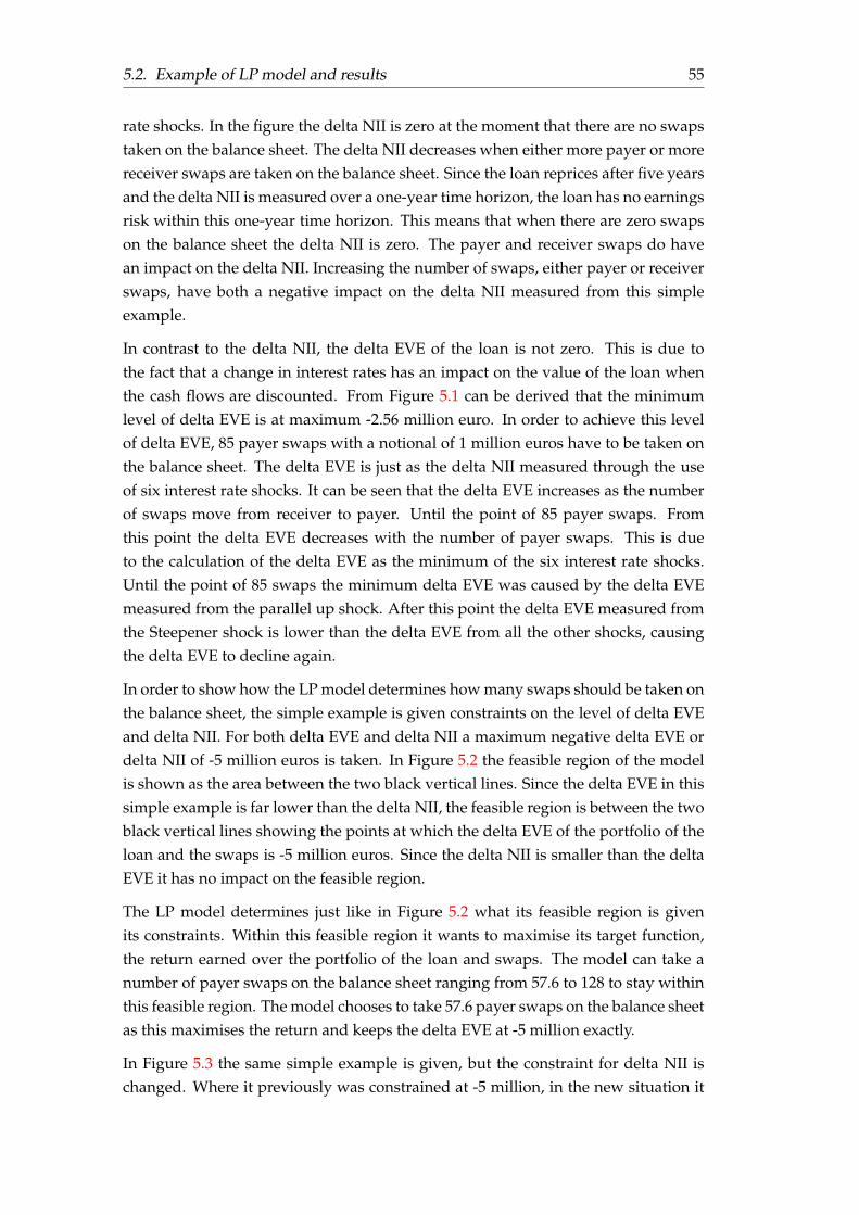
5.2. Example of LP model and results 55
rate shocks. In the figure the delta NII is zero at the moment that there are no swapstaken on the balance sheet. The delta NII decreases when either more payer or morereceiver swaps are taken on the balance sheet. Since the loan reprices after five yearsand the delta NII is measured over a one-year time horizon, the loan has no earningsrisk within this one-year time horizon. This means that when there are zero swapson the balance sheet the delta NII is zero. The payer and receiver swaps do havean impact on the delta NII. Increasing the number of swaps, either payer or receiverswaps, have both a negative impact on the delta NII measured from this simpleexample.
In contrast to the delta NII, the delta EVE of the loan is not zero. This is due tothe fact that a change in interest rates has an impact on the value of the loan whenthe cash flows are discounted. From Figure 5.1 can be derived that the minimumlevel of delta EVE is at maximum -2.56 million euro. In order to achieve this levelof delta EVE, 85 payer swaps with a notional of 1 million euros have to be taken onthe balance sheet. The delta EVE is just as the delta NII measured through the useof six interest rate shocks. It can be seen that the delta EVE increases as the numberof swaps move from receiver to payer. Until the point of 85 payer swaps. Fromthis point the delta EVE decreases with the number of payer swaps. This is dueto the calculation of the delta EVE as the minimum of the six interest rate shocks.Until the point of 85 swaps the minimum delta EVE was caused by the delta EVEmeasured from the parallel up shock. After this point the delta EVE measured fromthe Steepener shock is lower than the delta EVE from all the other shocks, causingthe delta EVE to decline again.
In order to show how the LP model determines how many swaps should be taken onthe balance sheet, the simple example is given constraints on the level of delta EVEand delta NII. For both delta EVE and delta NII a maximum negative delta EVE ordelta NII of -5 million euros is taken. In Figure 5.2 the feasible region of the modelis shown as the area between the two black vertical lines. Since the delta EVE in thissimple example is far lower than the delta NII, the feasible region is between the twoblack vertical lines showing the points at which the delta EVE of the portfolio of theloan and the swaps is -5 million euros. Since the delta NII is smaller than the deltaEVE it has no impact on the feasible region.
The LP model determines just like in Figure 5.2 what its feasible region is givenits constraints. Within this feasible region it wants to maximise its target function,the return earned over the portfolio of the loan and swaps. The model can take anumber of payer swaps on the balance sheet ranging from 57.6 to 128 to stay withinthis feasible region. The model chooses to take 57.6 payer swaps on the balance sheetas this maximises the return and keeps the delta EVE at -5 million exactly.
In Figure 5.3 the same simple example is given, but the constraint for delta NII ischanged. Where it previously was constrained at -5 million, in the new situation it
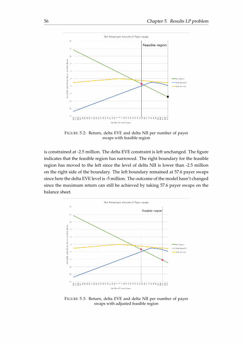
56 Chapter 5. Results LP problem
FIGURE 5.2: Return, delta EVE and delta NII per number of payerswaps with feasible region
is constrained at -2.5 million. The delta EVE constraint is left unchanged. The figureindicates that the feasible region has narrowed. The right boundary for the feasibleregion has moved to the left since the level of delta NII is lower than -2.5 millionon the right side of the boundary. The left boundary remained at 57.6 payer swapssince here the delta EVE level is -5 million. The outcome of the model hasn’t changedsince the maximum return can still be achieved by taking 57.6 payer swaps on thebalance sheet.
FIGURE 5.3: Return, delta EVE and delta NII per number of payerswaps with adjusted feasible region
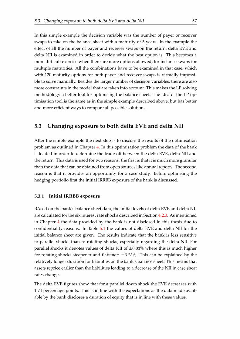
5.3. Changing exposure to both delta EVE and delta NII 57
In this simple example the decision variable was the number of payer or receiverswaps to take on the balance sheet with a maturity of 5 years. In the example theeffect of all the number of payer and receiver swaps on the return, delta EVE anddelta NII is examined in order to decide what the best option is. This becomes amore difficult exercise when there are more options allowed, for instance swaps formultiple maturities. All the combinations have to be examined in that case, whichwith 120 maturity options for both payer and receiver swaps is virtually impossi-ble to solve manually. Besides the larger number of decision variables, there are alsomore constraints in the model that are taken into account. This makes the LP solvingmethodology a better tool for optimising the balance sheet. The idea of the LP op-timisation tool is the same as in the simple example described above, but has betterand more efficient ways to compare all possible solutions.
5.3 Changing exposure to both delta EVE and delta NII
After the simple example the next step is to discuss the results of the optimisationproblem as outlined in Chapter 4. In this optimisation problem the data of the bankis loaded in order to determine the trade-off between the delta EVE, delta NII andthe return. This data is used for two reasons: the first is that it is much more granularthan the data that can be obtained from open sources like annual reports. The secondreason is that it provides an opportunity for a case study. Before optimising thehedging portfolio first the initial IRRBB exposure of the bank is discussed.
5.3.1 Initial IRRBB exposure
BAsed on the bank’s balance sheet data, the initial levels of delta EVE and delta NIIare calculated for the six interest rate shocks described in Section 4.2.3. As mentionedin Chapter 4 the data provided by the bank is not disclosed in this thesis due toconfidentiality reasons. In Table 5.1 the values of delta EVE and delta NII for theinitial balance sheet are given. The results indicate that the bank is less sensitiveto parallel shocks than to rotating shocks, especially regarding the delta NII. Forparallel shocks it denotes values of delta NII of ±0.03% where this is much higherfor rotating shocks steepener and flattener: ±6.25%. This can be explained by therelatively longer duration for liabilities on the bank’s balance sheet. This means thatassets reprice earlier than the liabilities leading to a decrease of the NII in case shortrates change.
The delta EVE figures show that for a parallel down shock the EVE decreases with1.74 percentage points. This is in line with the expectations as the data made avail-able by the bank discloses a duration of equity that is in line with these values.
58 Chapter 5. Results LP problem
TABLE 5.1: Overview of initial delta EVE and delta NII on the bank’sbalance sheet
Shock Type Delta EVE Delta NIIParallel Up 1.41% -0.03%Parallel Down -1.74% 0.03%Butterfly Up -0.81% 6.25%Butterfly Down 0.51% -6.25%Steepener 1.83% -6.17%Flattener -2.13% 6.17%
Just as for delta NII, for delta EVE the bank is more sensitive to non-parallel shocksthan to parallel shocks. The delta EVE measured through the flattener shock is lowerthan for the parallel down shock meaning more decrease in economic value. This canbe explained by the maturity profile of the assets and liabilities on the balance sheet.The longer duration for liabilities leads to a larger decrease in value in the case ofrising interest rates for liabilities than assets. So a rotating shock, where the shortrates increase and the long rates decrease, leads to a decrease in value of assets andan increase in value of liabilities. Resulting in a lower EVE. In the case of parallelshocks this effect is less strong as the assets increase or decrease in value at the sametime as the liabilities increase or decrease in value. This shows the importance of themeasurement of IRRBB through the use of multiple shocks since the parallel shocksonly don’t give a complete view on the exposure to IRRBB.
5.3.2 Changing IRRBB exposure of the bank
The exposure to IRRBB as given in Table 5.1 can be changed by increasing the lowerboundaries of the delta EVE and delta NII constraints. In this case the model searchesfor a combination of payer and receiver swaps to take on the balance sheet such thatit satisfies these new constraints. Releasing the constraints of delta EVE and deltaNII allows more exposure to IRRBB on the balance sheet.
In the following sections the impact of higher and lower values for the boundariesof the delta EVE and delta NII constraints will be discussed. Here the impact ofdifferent values for these boundaries on the composition of the hedging portfolioand the level of return is examined. This will be done in two steps: first the trade-offsurface between boundary levels for the delta EVE, delta NII and the return will beconstructed. Secondly, different points in the surface will be compared in order todetermine the possible strategies for the bank and how to achieve them.
Effect payer and receiver swaps on return
Before going through the results, a change in target function is discussed. During theanalysis it appeared that the way the return on the hedging portfolio was calculated
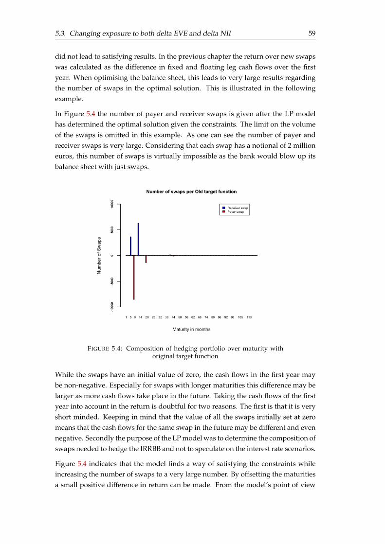
5.3. Changing exposure to both delta EVE and delta NII 59
did not lead to satisfying results. In the previous chapter the return over new swapswas calculated as the difference in fixed and floating leg cash flows over the firstyear. When optimising the balance sheet, this leads to very large results regardingthe number of swaps in the optimal solution. This is illustrated in the followingexample.
In Figure 5.4 the number of payer and receiver swaps is given after the LP modelhas determined the optimal solution given the constraints. The limit on the volumeof the swaps is omitted in this example. As one can see the number of payer andreceiver swaps is very large. Considering that each swap has a notional of 2 millioneuros, this number of swaps is virtually impossible as the bank would blow up itsbalance sheet with just swaps.
FIGURE 5.4: Composition of hedging portfolio over maturity withoriginal target function
While the swaps have an initial value of zero, the cash flows in the first year maybe non-negative. Especially for swaps with longer maturities this difference may belarger as more cash flows take place in the future. Taking the cash flows of the firstyear into account in the return is doubtful for two reasons. The first is that it is veryshort minded. Keeping in mind that the value of all the swaps initially set at zeromeans that the cash flows for the same swap in the future may be different and evennegative. Secondly the purpose of the LP model was to determine the composition ofswaps needed to hedge the IRRBB and not to speculate on the interest rate scenarios.
Figure 5.4 indicates that the model finds a way of satisfying the constraints whileincreasing the number of swaps to a very large number. By offsetting the maturitiesa small positive difference in return can be made. From the model’s point of view
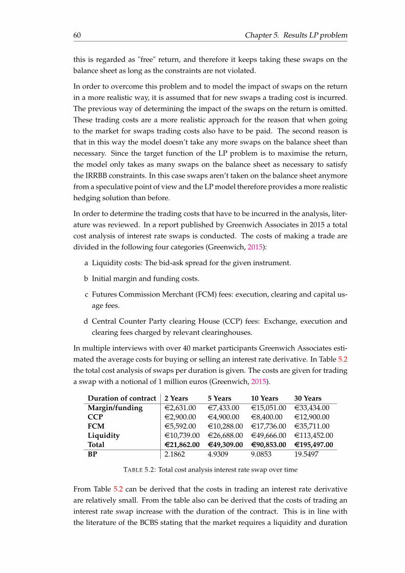
60 Chapter 5. Results LP problem
this is regarded as "free" return, and therefore it keeps taking these swaps on thebalance sheet as long as the constraints are not violated.
In order to overcome this problem and to model the impact of swaps on the returnin a more realistic way, it is assumed that for new swaps a trading cost is incurred.The previous way of determining the impact of the swaps on the return is omitted.These trading costs are a more realistic approach for the reason that when goingto the market for swaps trading costs also have to be paid. The second reason isthat in this way the model doesn’t take any more swaps on the balance sheet thannecessary. Since the target function of the LP problem is to maximise the return,the model only takes as many swaps on the balance sheet as necessary to satisfythe IRRBB constraints. In this case swaps aren’t taken on the balance sheet anymorefrom a speculative point of view and the LP model therefore provides a more realistichedging solution than before.
In order to determine the trading costs that have to be incurred in the analysis, liter-ature was reviewed. In a report published by Greenwich Associates in 2015 a totalcost analysis of interest rate swaps is conducted. The costs of making a trade aredivided in the following four categories (Greenwich, 2015):
a Liquidity costs: The bid-ask spread for the given instrument.
b Initial margin and funding costs.
c Futures Commission Merchant (FCM) fees: execution, clearing and capital us-age fees.
d Central Counter Party clearing House (CCP) fees: Exchange, execution andclearing fees charged by relevant clearinghouses.
In multiple interviews with over 40 market participants Greenwich Associates esti-mated the average costs for buying or selling an interest rate derivative. In Table 5.2the total cost analysis of swaps per duration is given. The costs are given for tradinga swap with a notional of 1 million euros (Greenwich, 2015).
Duration of contract 2 Years 5 Years 10 Years 30 YearsMargin/funding e2,631.00 e7,433.00 e15,051.00 e33,434.00CCP e2,900.00 e4,900.00 e8,400.00 e12,900.00FCM e5,592.00 e10,288.00 e17,736.00 e35,711.00Liquidity e10,739.00 e26,688.00 e49,666.00 e113,452.00Total e21,862.00 e49,309.00 e90,853.00 e195,497.00BP 2.1862 4.9309 9.0853 19.5497
TABLE 5.2: Total cost analysis interest rate swap over time
From Table 5.2 can be derived that the costs in trading an interest rate derivativeare relatively small. From the table also can be derived that the costs of trading aninterest rate swap increase with the duration of the contract. This is in line withthe literature of the BCBS stating that the market requires a liquidity and duration
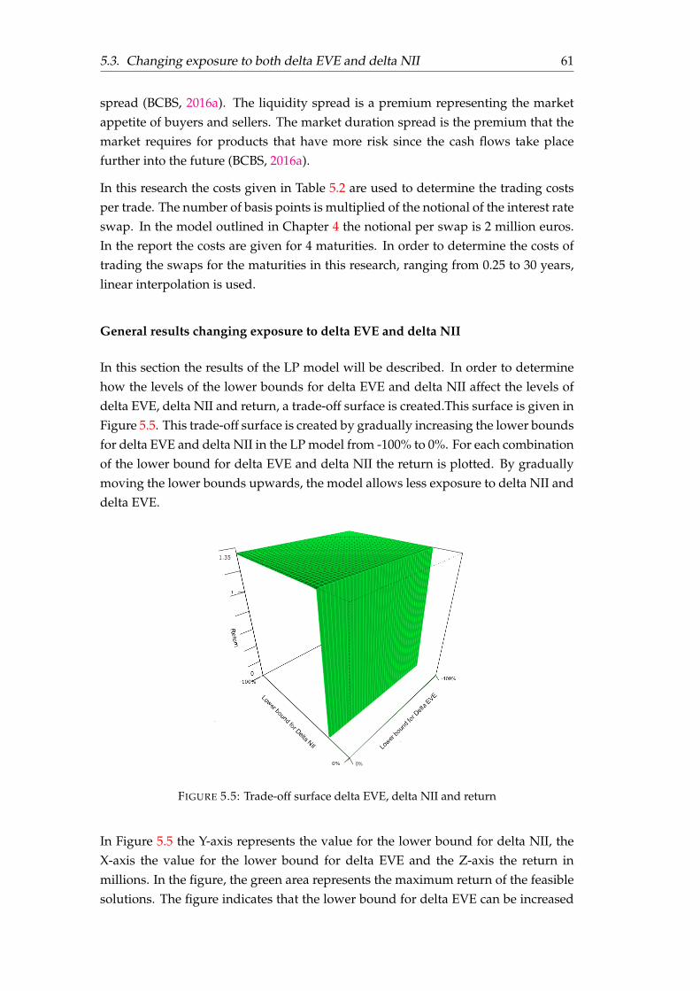
5.3. Changing exposure to both delta EVE and delta NII 61
spread (BCBS, 2016a). The liquidity spread is a premium representing the marketappetite of buyers and sellers. The market duration spread is the premium that themarket requires for products that have more risk since the cash flows take placefurther into the future (BCBS, 2016a).
In this research the costs given in Table 5.2 are used to determine the trading costsper trade. The number of basis points is multiplied of the notional of the interest rateswap. In the model outlined in Chapter 4 the notional per swap is 2 million euros.In the report the costs are given for 4 maturities. In order to determine the costs oftrading the swaps for the maturities in this research, ranging from 0.25 to 30 years,linear interpolation is used.
General results changing exposure to delta EVE and delta NII
In this section the results of the LP model will be described. In order to determinehow the levels of the lower bounds for delta EVE and delta NII affect the levels ofdelta EVE, delta NII and return, a trade-off surface is created.This surface is given inFigure 5.5. This trade-off surface is created by gradually increasing the lower boundsfor delta EVE and delta NII in the LP model from -100% to 0%. For each combinationof the lower bound for delta EVE and delta NII the return is plotted. By graduallymoving the lower bounds upwards, the model allows less exposure to delta NII anddelta EVE.
FIGURE 5.5: Trade-off surface delta EVE, delta NII and return
In Figure 5.5 the Y-axis represents the value for the lower bound for delta NII, theX-axis the value for the lower bound for delta EVE and the Z-axis the return inmillions. In the figure, the green area represents the maximum return of the feasiblesolutions. The figure indicates that the lower bound for delta EVE can be increased
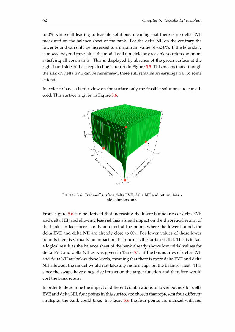
62 Chapter 5. Results LP problem
to 0% while still leading to feasible solutions, meaning that there is no delta EVEmeasured on the balance sheet of the bank. For the delta NII on the contrary thelower bound can only be increased to a maximum value of -5.78%. If the boundaryis moved beyond this value, the model will not yield any feasible solutions anymoresatisfying all constraints. This is displayed by absence of the green surface at theright-hand side of the steep decline in return in Figure 5.5. This means that althoughthe risk on delta EVE can be minimised, there still remains an earnings risk to someextend.
In order to have a better view on the surface only the feasible solutions are consid-ered. This surface is given in Figure 5.6.
FIGURE 5.6: Trade-off surface delta EVE, delta NII and return, feasi-ble solutions only
From Figure 5.6 can be derived that increasing the lower boundaries of delta EVEand delta NII, and allowing less risk has a small impact on the theoretical return ofthe bank. In fact there is only an effect at the points where the lower bounds fordelta EVE and delta NII are already close to 0%. For lower values of these lowerbounds there is virtually no impact on the return as the surface is flat. This is in facta logical result as the balance sheet of the bank already shows low initial values fordelta EVE and delta NII as was given in Table 5.1. If the boundaries of delta EVEand delta NII are below these levels, meaning that there is more delta EVE and deltaNII allowed, the model would not take any more swaps on the balance sheet. Thissince the swaps have a negative impact on the target function and therefore wouldcost the bank return.
In order to determine the impact of different combinations of lower bounds for deltaEVE and delta NII, four points in this surface are chosen that represent four differentstrategies the bank could take. In Figure 5.6 the four points are marked with red
5.3. Changing exposure to both delta EVE and delta NII 63
dots. The four points are characterised by the following values for the lower boundsof delta EVE and delta NII:
• Point 1: At this point the lower bound for delta EVE is 0% and for delta NII is-15%.
• Point 2: At this point the lower bound for delta EVE is 0% and for delta NII is-5.93%.
• Point 3: At this point the lower bound for delta EVE is -10% and for delta NIIis -5.78%.
• Point 4: At this point the lower bound for delta EVE is -1.50% and for delta NIIis -7.4%
These first three points are specifically chosen as they represent the points at whicheither the delta EVE, delta NII or both are minimised by putting the lower bound fordelta EVE and delta NII at the maximum level possible. By looking at these threepoints in more detail, insight in the strategy in minimising either delta EVE, deltaNII or both can be gained. The fourth point is examined as this point is characterisedby a relatively high return and low corresponding levels for delta EVE and delta NII.With the target function of maximising the return this point is specifically interest-ing. In the following sections the results of the LP model at the four points on thetrade-off surface will be discussed.
Delta EVE, delta NII and return in point 1
In Table 5.3 the levels of delta EVE and delta NII for the six interest rate shocksmeasured in point 1 in the trade-off surface are given. The first point is characterisedby a lower bound for delta EVE of 0% and a lower bound for delta NII of -15%.The results in Table 5.3 indeed give a minimum of 0% for the level of delta EVEmeasured on three shocks. The maximum delta EVE is 2.58% on the butterfly downand steepener shock. The values in the table indicate that it is possible to completelymitigate a negative change in EVE resulting from the six interest rate shocks. Stillthree shocks result in a positive change in EVE, meaning that the balance sheet isn’tcompletely insensitive to interest rate shocks measured through delta EVE.
The lower boundary for the delta NII constraint is set at -15%. The results howevershow that the minimum delta NII is just -7.96% meaning that the lower boundaryfor delta NII is not constraining the solution of the LP model. The minimum valuefor delta NII has decreased from -6.25% in the original balance sheet to -7.67%. Thereturn that the bank is able to achieve however has decreased to 1.348 million euros,where previously it was 1.355 million for the original balance sheet.
These levels of delta EVE, delta NII and return are achieved by taking a hedgingportfolio on the balance sheet as given in Figure 5.7. In this figure the number of
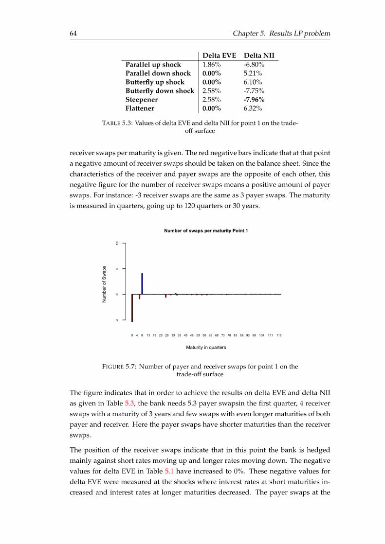
64 Chapter 5. Results LP problem
Delta EVE Delta NIIParallel up shock 1.86% -6.80%Parallel down shock 0.00% 5.21%Butterfly up shock 0.00% 6.10%Butterfly down shock 2.58% -7.75%Steepener 2.58% -7.96%Flattener 0.00% 6.32%
TABLE 5.3: Values of delta EVE and delta NII for point 1 on the trade-off surface
receiver swaps per maturity is given. The red negative bars indicate that at that pointa negative amount of receiver swaps should be taken on the balance sheet. Since thecharacteristics of the receiver and payer swaps are the opposite of each other, thisnegative figure for the number of receiver swaps means a positive amount of payerswaps. For instance: -3 receiver swaps are the same as 3 payer swaps. The maturityis measured in quarters, going up to 120 quarters or 30 years.
FIGURE 5.7: Number of payer and receiver swaps for point 1 on thetrade-off surface
The figure indicates that in order to achieve the results on delta EVE and delta NIIas given in Table 5.3, the bank needs 5.3 payer swapsin the first quarter, 4 receiverswaps with a maturity of 3 years and few swaps with even longer maturities of bothpayer and receiver. Here the payer swaps have shorter maturities than the receiverswaps.
The position of the receiver swaps indicate that in this point the bank is hedgedmainly against short rates moving up and longer rates moving down. The negativevalues for delta EVE in Table 5.1 have increased to 0%. These negative values fordelta EVE were measured at the shocks where interest rates at short maturities in-creased and interest rates at longer maturities decreased. The payer swaps at the
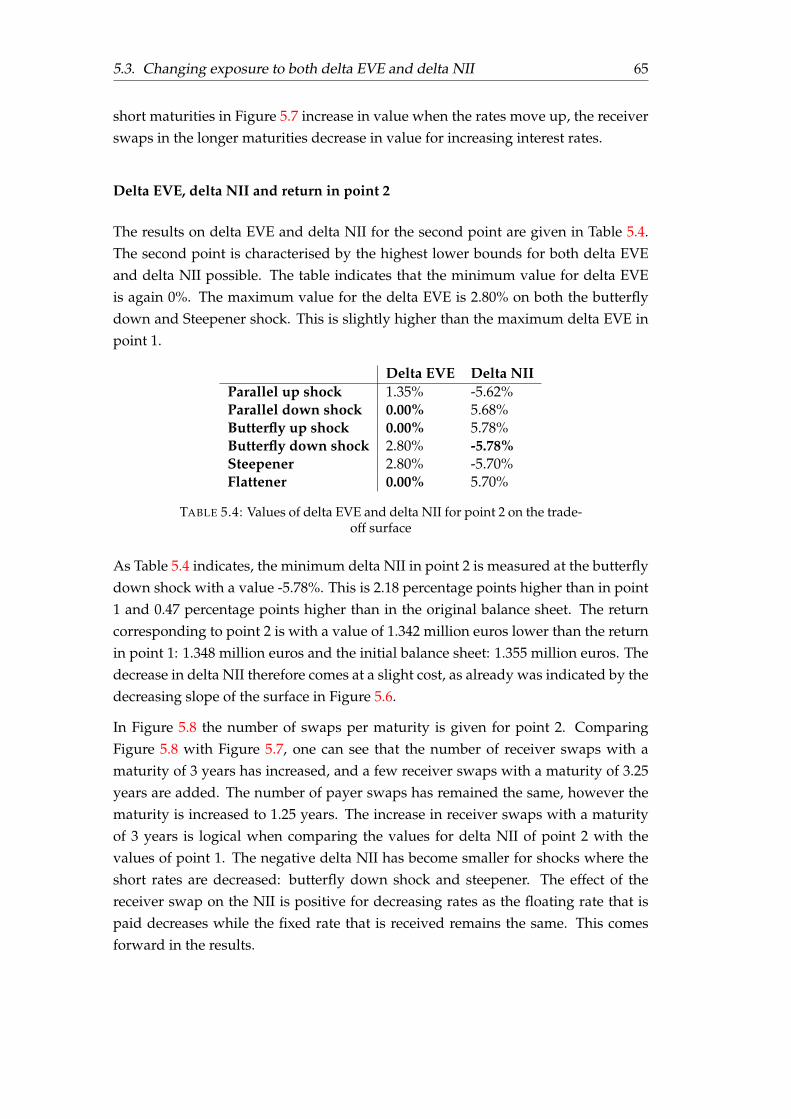
5.3. Changing exposure to both delta EVE and delta NII 65
short maturities in Figure 5.7 increase in value when the rates move up, the receiverswaps in the longer maturities decrease in value for increasing interest rates.
Delta EVE, delta NII and return in point 2
The results on delta EVE and delta NII for the second point are given in Table 5.4.The second point is characterised by the highest lower bounds for both delta EVEand delta NII possible. The table indicates that the minimum value for delta EVEis again 0%. The maximum value for the delta EVE is 2.80% on both the butterflydown and Steepener shock. This is slightly higher than the maximum delta EVE inpoint 1.
Delta EVE Delta NIIParallel up shock 1.35% -5.62%Parallel down shock 0.00% 5.68%Butterfly up shock 0.00% 5.78%Butterfly down shock 2.80% -5.78%Steepener 2.80% -5.70%Flattener 0.00% 5.70%
TABLE 5.4: Values of delta EVE and delta NII for point 2 on the trade-off surface
As Table 5.4 indicates, the minimum delta NII in point 2 is measured at the butterflydown shock with a value -5.78%. This is 2.18 percentage points higher than in point1 and 0.47 percentage points higher than in the original balance sheet. The returncorresponding to point 2 is with a value of 1.342 million euros lower than the returnin point 1: 1.348 million euros and the initial balance sheet: 1.355 million euros. Thedecrease in delta NII therefore comes at a slight cost, as already was indicated by thedecreasing slope of the surface in Figure 5.6.
In Figure 5.8 the number of swaps per maturity is given for point 2. ComparingFigure 5.8 with Figure 5.7, one can see that the number of receiver swaps with amaturity of 3 years has increased, and a few receiver swaps with a maturity of 3.25years are added. The number of payer swaps has remained the same, however thematurity is increased to 1.25 years. The increase in receiver swaps with a maturityof 3 years is logical when comparing the values for delta NII of point 2 with thevalues of point 1. The negative delta NII has become smaller for shocks where theshort rates are decreased: butterfly down shock and steepener. The effect of thereceiver swap on the NII is positive for decreasing rates as the floating rate that ispaid decreases while the fixed rate that is received remains the same. This comesforward in the results.
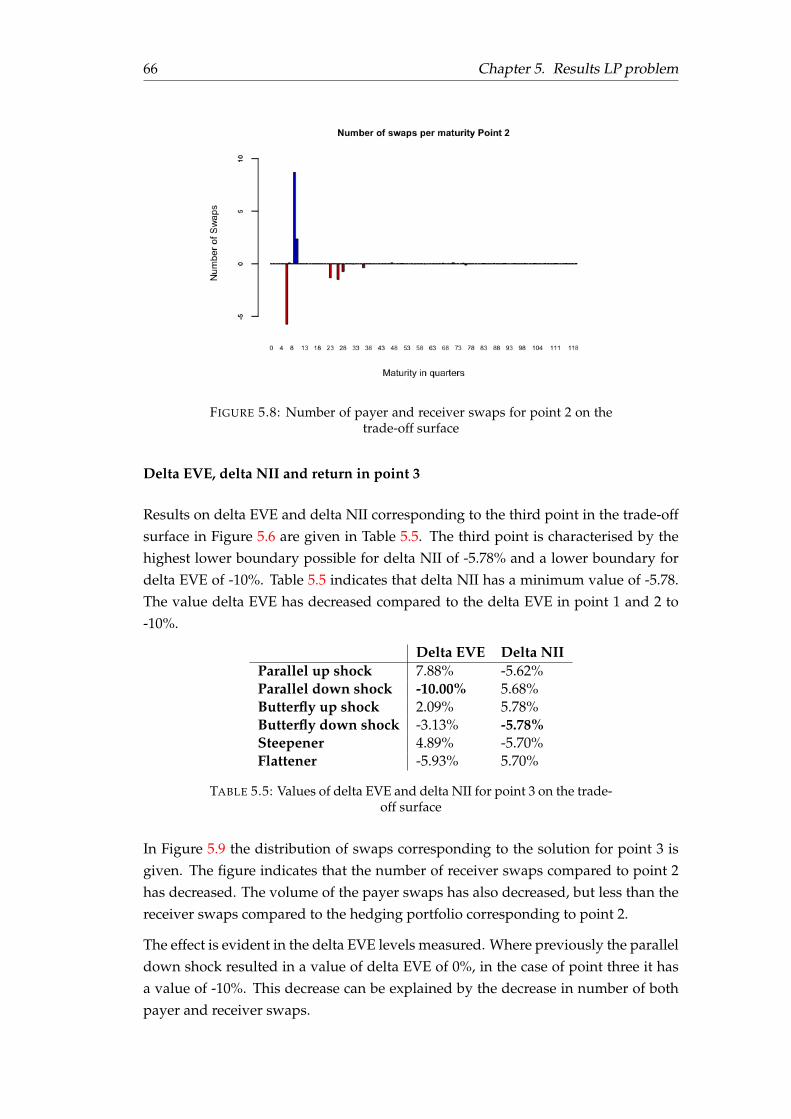
66 Chapter 5. Results LP problem
FIGURE 5.8: Number of payer and receiver swaps for point 2 on thetrade-off surface
Delta EVE, delta NII and return in point 3
Results on delta EVE and delta NII corresponding to the third point in the trade-offsurface in Figure 5.6 are given in Table 5.5. The third point is characterised by thehighest lower boundary possible for delta NII of -5.78% and a lower boundary fordelta EVE of -10%. Table 5.5 indicates that delta NII has a minimum value of -5.78.The value delta EVE has decreased compared to the delta EVE in point 1 and 2 to-10%.
Delta EVE Delta NIIParallel up shock 7.88% -5.62%Parallel down shock -10.00% 5.68%Butterfly up shock 2.09% 5.78%Butterfly down shock -3.13% -5.78%Steepener 4.89% -5.70%Flattener -5.93% 5.70%
TABLE 5.5: Values of delta EVE and delta NII for point 3 on the trade-off surface
In Figure 5.9 the distribution of swaps corresponding to the solution for point 3 isgiven. The figure indicates that the number of receiver swaps compared to point 2has decreased. The volume of the payer swaps has also decreased, but less than thereceiver swaps compared to the hedging portfolio corresponding to point 2.
The effect is evident in the delta EVE levels measured. Where previously the paralleldown shock resulted in a value of delta EVE of 0%, in the case of point three it hasa value of -10%. This decrease can be explained by the decrease in number of bothpayer and receiver swaps.
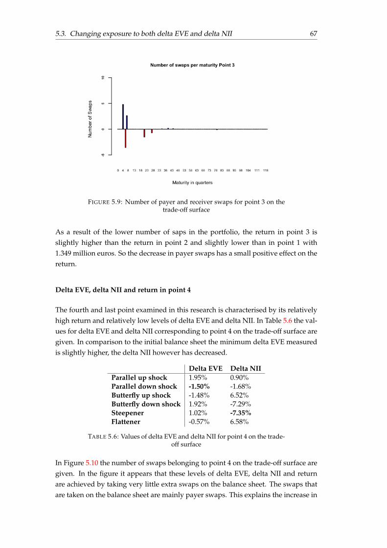
5.3. Changing exposure to both delta EVE and delta NII 67
FIGURE 5.9: Number of payer and receiver swaps for point 3 on thetrade-off surface
As a result of the lower number of saps in the portfolio, the return in point 3 isslightly higher than the return in point 2 and slightly lower than in point 1 with1.349 million euros. So the decrease in payer swaps has a small positive effect on thereturn.
Delta EVE, delta NII and return in point 4
The fourth and last point examined in this research is characterised by its relativelyhigh return and relatively low levels of delta EVE and delta NII. In Table 5.6 the val-ues for delta EVE and delta NII corresponding to point 4 on the trade-off surface aregiven. In comparison to the initial balance sheet the minimum delta EVE measuredis slightly higher, the delta NII however has decreased.
Delta EVE Delta NIIParallel up shock 1.95% 0.90%Parallel down shock -1.50% -1.68%Butterfly up shock -1.48% 6.52%Butterfly down shock 1.92% -7.29%Steepener 1.02% -7.35%Flattener -0.57% 6.58%
TABLE 5.6: Values of delta EVE and delta NII for point 4 on the trade-off surface
In Figure 5.10 the number of swaps belonging to point 4 on the trade-off surface aregiven. In the figure it appears that these levels of delta EVE, delta NII and returnare achieved by taking very little extra swaps on the balance sheet. The swaps thatare taken on the balance sheet are mainly payer swaps. This explains the increase in
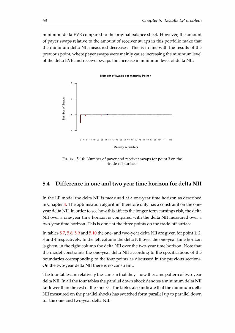
68 Chapter 5. Results LP problem
minimum delta EVE compared to the original balance sheet. However, the amountof payer swaps relative to the amount of receiver swaps in this portfolio make thatthe minimum delta NII measured decreases. This is in line with the results of theprevious point, where payer swaps were mainly cause increasing the minimum levelof the delta EVE and receiver swaps the increase in minimum level of delta NII.
FIGURE 5.10: Number of payer and receiver swaps for point 3 on thetrade-off surface
5.4 Difference in one and two year time horizon for delta NII
In the LP model the delta NII is measured at a one-year time horizon as describedin Chapter 4. The optimisation algorithm therefore only has a constraint on the one-year delta NII. In order to see how this affects the longer term earnings risk, the deltaNII over a one-year time horizon is compared with the delta NII measured over atwo-year time horizon. This is done at the three points on the trade-off surface.
In tables 5.7, 5.8, 5.9 and 5.10 the one- and two-year delta NII are given for point 1, 2,3 and 4 respectively. In the left column the delta NII over the one-year time horizonis given, in the right column the delta NII over the two-year time horizon. Note thatthe model constraints the one-year delta NII according to the specifications of theboundaries corresponding to the four points as discussed in the previous sections.On the two-year delta NII there is no constraint.
The four tables are relatively the same in that they show the same pattern of two-yeardelta NII. In all the four tables the parallel down shock denotes a minimum delta NIIfar lower than the rest of the shocks. The tables also indicate that the minimum deltaNII measured on the parallel shocks has switched form parallel up to parallel downfor the one- and two-year delta NII.
5.4. Difference in one and two year time horizon for delta NII 69
Delta NII one-year Delta NII two-yearParallel up shock -6.80% 12.90%Parallel down shock 5.21% -12.79%Butterfly up shock 6.10% 6.51%Butterfly down shock -7.75% -6.40%Steepener -7.96% -5.72%Flattener 6.32% 5.82%
TABLE 5.7: Values of one- and two-year delta NII for point 1 on thetrade-off surface
There are two reasons why the parallel shocks denote more extreme values for thetwo-year delta NII than the other shocks. The first is the way the shocks are calcu-lated. In the rotational shocks the rotating point of the shock is in the one year timebucket. This means that in the second year the effect of the shock is the opposite ofthe effect in the first year, and less strong since the height of the shock is interpolatedover more time buckets than the height of the shock before the rotating point of oneyear. This means that the effect of the receiver swaps is also the opposite. Parallelshocks don’t have this rotating point and have the same shock over the whole yieldcurve.
Delta NII one-year Delta NII two-yearParallel up shock -5.62% 10.23%Parallel down shock 5.68% -10.19%Butterfly up shock 5.78% 6.31%Butterfly down shock -5.78% -6.31%Steepener -5.70% -5.65%Flattener 5.70% 5.65%
TABLE 5.8: Values of one- and two-year delta NII for point 2 on thetrade-off surface
A second reason for the high values of parallel down shocks in the two-year deltaNII is the high volume of swaps with a maturity of one year. In the second year all ofthese swaps reprice their fixed leg resulting in a lower impact on the delta NII in thesecond year. The swaps that do have a maturity of more than two years are mainlyreceiver swaps. These swaps still have an impact on the delta NII as they don’treprice in the first or second year on which the delta NII is assessed. The receiverswaps have a negative effect in the case of decreasing rates as the floating rate that ispaid decreases while the fixed rate that is received remains the same. This explainsthe change in negative delta NII from the parallel up to the parallel down shock forthe two-year delta NII.
From the results is appears that the lowest minimum two-year delta NII is achievedin the fourth point examined on the trade-off surface. This makes sense as this pointsis characterised by its high return, but low amount of swaps. The lack of swapsresults in a low minimum value for the two-year delta NII.
70 Chapter 5. Results LP problem
Delta NII one-year Delta NII two-yearParallel up shock -5.62% 11.65%Parallel down shock 5.68% -11.63%Butterfly up shock 5.78% 6.43%Butterfly down shock -5.78% -6.43%Steepener -5.70% -5.76%Flattener 5.70% 5.76%
TABLE 5.9: Values of one- and two-year delta NII for point 3 on thetrade-off surface
Delta NII one-year Delta NII two-yearParallel up shock 0.90% 14.05%Parallel down shock -1.68% -14.00%Butterfly up shock 6.52% 6.62%Butterfly down shock -7.29% -6.57%Steepener -7.35% -5.90%Flattener 6.58% 5.94%
TABLE 5.10: Values of one- and two-year delta NII for point 4 on thetrade-off surface
The results on the two-year delta NII indicate that the high volume of short termreceiver swaps compared to the longer term payer swaps is the main cause of thelarger delta NII values for the parallel down shocks. The increasing costs for swapswith longer maturities in our target function is the main cause of this result. Sincethe delta NII is limited for a one-year time horizon only, the model is better off byputting as less swaps as possible in longer maturities. When also a constraint onthe two-year delta NII or longer time horizons is set, the model would allocate moreswaps to longer maturities at a higher cost meaning that the return would be lower.
5.5 Concluding remarks
In the analysis in this chapter a few points came forward. The first conclusion is thatthe negative change in delta EVE can be limited to 0% for this data set. For the deltaNII the highest minimum level is at -5.78%.
The second conclusion is that the hedging portfolio is composed such that it min-imises the delta EVE measured from rotational shocks where the short rates increaseand the longer rates on the yield curve decrease. This fits the original distribution ofthe balance sheet where the liabilities have a longer duration than the assets, mean-ing that in these rotational shocks the delta EVE is the largest.
Decreasing the delta NII measured is mainly done by increasing the number of re-ceiver swaps with a maturity just over 3 years. This has the effect that the delta NIIover a one-year time horizon can be lowered to some extend. However, the fact thatmany swaps are allocated in the first year has the effect that the delta NII assessed
5.5. Concluding remarks 71
over a two-year time horizon for all the four points examined in the trade-off surfaceis larger than the one-year horizon. To overcome this problem the bank would haveto take more swaps with longer maturities on the balance sheet which would have anegative impact on the return.
In the introduction of Chapter 4 the aim of the model was described. This chapterwas aimed at finding an answer to the third and main research questions by opti-mising the balance sheet:
How can banks best change their levels of exposure to interest rate risk, measured from aneconomic value and earnings perspective, given their risk appetite and business model?
The IRRBB limits differ per bank, as does the balance sheet. So it depends per bankhow they want to change their IRRBB exposure. In this chapter based on the data ofa specific bank a trade-off surface was created in order to compare several differentcombinations of delta EVE, delta NII and return.
The results indicated that the exposure to IRRBB can be changed effectively usingplain vanilla swaps. The negative delta EVE could be minimised to a level 0%, wherethe delta NII could be minimised to -5.78%. The analysis that was carried out inthis chapter on the data of a bank indicated that this bank was mainly exposed toIRRBB resulting from rotational shocks. The hedging portfolio was therefore mainlydirected to overcome the negative values resulting from these shocks.

73
Chapter 6
Conclusion
6.1 Introduction
In this research many topics relating to interest rate in the banking book were ad-dressed, especially focusing on the measurement of IRRBB through delta EVE anddelta NII as economic value and earnings based perspectives. The aim was to de-termine the dynamics of these two methods, and their relationship to the steeringof assets and liabilities. In the process this research has been partly conducted incooperation with a Dutch bank. In this chapter the main findings of this researchwill be presented and concluded. This will be done at the hand of the three researchquestions that were designed to guide this research and to find the answer to themain research question:.
How can banks best change their levels of exposure to interest rate risk, measured from aneconomic value and earnings perspective, given their risk appetite and business model?
In the next three sections the main conclusions to the three research questions willbe discussed.
6.2 Conclusions to the first research question
The first research question was designed to get more knowledge on the concepts ofinterest rate risk in the banking book and the relationship between the two perspec-tives on IRRBB:
What are important aspects and differences between delta NII as earnings and delta EVE aseconomic value based methods to measure IRRBB?
In the literature review that is conducted in Chapter 2, the basic concepts betweenIRRBB, economic value and earnings perspectives to IRRBB were elaborated on.
In order to give an answer to the research question, it can be stated that the mostimportant conclusions from this stage of the research are the following:
74 Chapter 6. Conclusion
• Earnings and economic value measures are linked in the fact that earnings af-fect the net present value of assets and liabilities, and thus the economic valueof assets and liabilities;
• Economic value and earnings based perspectives on IRRBB differ in the timehorizon at which IRRBB is measured. Delta NII is assessed on a short termhorizon where delta EVE has a longer time horizon. The methods also differ inthe use of different assumptions on the future business production of the bank.
6.3 Conclusions to the second research question
The second research question was aimed to get more insight in the assumptionsunderlying the delta NII and delta EVE calculations: What are important aspects to takeinto account in the calculation of delta EVE and delta NII? The target was to determinehow assumptions on three different aspects in the calculation of delta EVE and deltaNII would impact the exposure measured. In order to do so the levels of delta NIIand delta EVE were calculated under different assumptions on the following threeaspects:
• The yield curve used in the calculations of delta EVE and delta NII;
• The impact of maturity profile of assets and liabilities on the calculations ofdelta EVE and delta NII;
• The impact of the banking business model used in the calculation of delta EVEand delta NII.
Looking at the results in Section 3.4, it can be concluded that all the three aspectstested in that chapter have an impact on the delta EVE and delta NII figures mea-sured:
a The duration or maturity profile of assets and liabilities has the largest impacton the delta EVE measure to IRRBB: as the maturity becomes longer, this im-pact becomes larger.
b The banking business model has an impact on the delta EVE measured. Thisis largely because of the difference in gapping profile between assets and lia-bilities for the business models, and can therefore be related to the maturityprofile of assets and liabilities. Retail and wholesale business models are char-acterised by a much larger maturity mismatch, and their economic value ofequity is therefore more sensitive to changes in interest rates.
c The negative delta NII is bigger for European curves, or curves that have lowervalues, than for curves that have higher values, since the floor is hit earlier.This means that the margin between assets and liabilities will fall earlier than
6.4. Conclusion to the third research question 75
with curves that have higher values such as the American curves used in thisanalysis.
6.4 Conclusion to the third research question
The third research question was designed to make the link between interest rate riskin the banking book and the management of assets and liabilities:
When is the exposure to interest rate risk measured from both perspectives considered opti-mal?
a How can a bank best change their exposure to interest rate risk?
In Chapter 4 a linear programming model was constructed that through the use ofconstraints on delta EVE, delta NII and (key rate) durations determines the optimaldistribution of the hedging portfolio in order to maximise the return on assets andliabilities. A real answer to the third research question was not found. The designof the model and the methodology used imply that the less delta EVE and delta NIImeasured the better. So the optimal exposure would be the solution with the leastexposure to IRRBB.
In Chapter 5 a trade-off surface was created where delta EVE, delta NII and thereturn were displayed. This surface was formed by plotting the return for each com-bination of lower bound f delta EVE and delta NII. In the surface four points wereexamined to show the effect of the position of the lower bounds for delta EVE anddelta NII on the theoretical maximum return earned on the balance sheet.
In the analysis several conclusions came forward. The first conclusion is that theexposure to negative delta EVE can be mitigated so that the minimum value fordelta EVE is 0%. For the delta NII this is possible only to a certain level given thisdata set.
The second conclusion that can be made is the fact the hedging portfolio is directedsuch that it minimises the delta EVE measured from rotational shocks where theshort rates increase and the longer rates on the yield curve decrease. This fits theoriginal distribution of the balance sheet where the liabilities have a longer durationthan the assets, meaning that in these rotational shocks the delta EVE is the largest.
Decreasing the measured delta NII is mainly done by increasing the number of re-ceiver swaps with a maturity just over three years. This has the effect that the deltaNII over a one-year time horizon can be lowered to some extend. The delta NII as-sessed over a two-year time horizon for all the four points examined in the trade-offsurface is much larger than the one-year horizon. Therefore it can be concluded thatlimiting the one-year delta NII can have the opposite effect on longer maturities. To
76 Chapter 6. Conclusion
overcome this problem the bank would have to take more swaps with longer matu-rities on the balance sheet which would have a negative impact on the return.
6.5 Conclusion
In this research many different conclusions and aspects of earnings and economicvalue based measures to interest rate in the banking book have come across. It canbe concluded that the maturity profile of assets and liabilities plays an importantrole in the interest rate risk exposure measured. In the optimisation problem this istaken into account in order to address the main research question:
How can banks best change their levels of exposure to interest rate risk, measured from aneconomic value and earnings perspective, given their risk appetite and business model?
The IRRBB risk appetite differs per bank. It depends per bank how they want tochange their IRRBB exposure. On the basis of data made available by a Dutch banka trade-off surface was created in order to compare several different combinationsof delta EVE, delta NII and return.
The results indicated that the exposure to IRRBB can be changed effectively usingplain vanilla swaps. The minimum Delta EVE measured on the basis of six interestrate shocks amounts 0% where the minimum delta NII measured amounted to -5.78%. The analysis that was carried out on data of the bank indicated that thisbank was mainly exposed to IRRBB resulting from rotational shocks. The hedgingportfolio was therefore primarily directed to overcome the negative values resultingfrom these shocks.
77
Chapter 7
Future Research
7.1 Introduction
The research that is conducted and outlined in this thesis contained many assump-tions. These assumptions have a large impact on the results. Some of these resultsalso lead to new questions that were not addressed in this research. In order to ad-dress these issues in future research, the most important aspects are mentioned inthis chapter.
7.2 Recommendations
In the modelling of the linear programming problem to investigate the effect of thedelta EVE and delta NII constraints on management of IRRBB some assumptions aremade that influenced the results and may be interesting for future research. The LPmodel is mainly focused on repricing risk and yield curve risk. Optionality of termdeposits or mortgages or other assets and liabilities is not incorporated in the model.It is assumed that these assumptions will have an impact on the exposure to interestrate risk as the term deposits or mortgages reprice earlier and to a different rate thanexpected. This may have an impact on the composition of the hedging portfolio. Itmight be interesting for future research to investigate how optionality of the balancesheet affects the composition of the hedging portfolio.
The current research uses linear programming as optimisation method. Researchpointed out that stochastic programming models are quite often used in the man-agement of assets and liabilities. The use of stochastic programming models canenable the use of stochastic interest rate scenarios and even more dynamic stresstesting of interest rate risk exposure than in the current research. It would be inter-esting for future research to determine how IRRBB is impacted by more and heavierinterest rate scenarios. The use of stochastic programming could be used in order todetermine this purpose. By assigning a probability to a certain interest rate scenario,a stress test and Value at Risk (VAR) figure could possibly be generated. This would
78 Chapter 7. Future Research
be a different point of view on IRRBB measurement as chance is not incorporated inthis research.
In this research, during the optimisation of the balance sheet, the hedging portfo-lio is used as decision variable. This is to represent current practices at the bank.However, from both a scientific as practical point of view it would be interesting tosee current constraints on IRRBB and target function to be applied on a completebalance sheet in combination with other constraints on liquidity, solvency and other.In that case it would give a more broader view on the management of assets andliabilities in general instead of only focusing on the hedging portfolio and interestrate risk constraints only. It could also be an interesting comparison in the manage-ment of IRRBB on balance sheet via restructuring of assets and liabilities versus offbalance sheet via swaps.
Besides this integrated approach, there is also another topic that is left out in thisresearch but forms a major part of interest rate risk: basis risk. It would be inter-esting to see how interest rate risk measures from an earnings and economic valueperspective are impacted by, or have an impact on the basis risk measured.
79
Bibliography
Abdymomunov, Azamat and Jeffrey Gerlach (2014). “Stress testing interest rate riskexposure”. In: Journal of Banking & Finance 49, pp. 287–301.
Al Shubiri, Faris Nasif et al. (2010). “Impact of bank asset and liability managementon profitability: Empirical investigation”. In: Journal of Applied Research in Finance(JARF) 2.4, pp. 101–109.
Asmundson, Irena (2011). “What are financial services”. In: Finance & Development,March, pp. 46–47.
BCBS, Basel Committee on Banking Supervision (2004). Principles for the Managementand Supervision of Interest Rate Risk.
– (2015). Consultative Document on Interest Rate in the Banking Book.– (2016a). Interest Rate Risk in the Banking Book - Standards. BIS.– (2016b). Minimum capital requirements for market risk. BIS.Carney (2014). “Enhancing the Risk Disclosures of Banks”. In:CEBS (2006). Technical Aspects of the Management of Interest Rate Risk Arising from Non-
Trading Activities Under the Supervisory Review Process.Charumathi, B (2008). “Asset Liability Management in Indian Banking Industry-
with special reference to Interest Rate Risk Management in ICICI Bank”. In: Pro-ceedings of the World Congress on Engineering 2008 vol II.
Cummins, J David et al. (2009). “Efficiency of insurance firms with endogenous riskmanagement and financial intermediation activities”. In: Journal of ProductivityAnalysis 32.2, pp. 145–159.
Dantzig, George B (1990). Origins of the simplex method. ACM.Drehmann, Mathias, Steffen Sorensen, and Marco Stringa (2008). “The integrated
impact of credit and interest rate risk on banks: an economic value and capitaladequacy perspective”. In:
EBA, European Banking Association (2013a). Consultation paper on revision of the "guide-lines on Technical aspects of the management of interest rate risk". EBA.
– (2013b). Consultation paper on revision of the "guidelines on Technical aspects of themanagement of interest rate risk".
– (2015). Guidelines on the Management of Interest Rate Risk. EBA.Entrop, Oliver et al. (2015). “Determinants of bank interest margins: Impact of ma-
turity transformation”. In: Journal of Banking & Finance 54, pp. 1–19.
80 BIBLIOGRAPHY
Esposito, Lucia, Andrea Nobili, and Tiziano Ropele (2015). “The management of in-terest rate risk during the crisis: evidence from Italian banks”. In: Journal of Banking& Finance 59, pp. 486–504.
Flannery, Mark J and Christopher M James (1984). “The effect of interest rate changeson the common stock returns of financial institutions”. In: The Journal of Finance39.4, pp. 1141–1153.
Greenwich, Associates (2015). Total cost analysis of interest-rate swaps vs. futures.Hull, John (2012a). Risk Management and Financial Institutions,+ Web Site. Vol. 733.
John Wiley & Sons.Hull, John C. (2012b). Options, Futures and other derivatives. Pearson.Kusy, Martin I and William T Ziemba (1986). “A bank asset and liability management
model”. In: Operations Research 34.3, pp. 356–376.Maes, Konstantijn et al. (2004). “Interest rate risk in the Belgian banking sector”. In:
Financial Stability Review 2.1, pp. 157–179.Memmel, Christoph (2011). “Banks’ exposure to interest rate risk, their earnings
from term transformation, and the dynamics of the term structure”. In: Journalof Banking & Finance 35.2, pp. 282–289.
– (2014). “Banks’ interest rate risk: the net interest income perspective versus themarket value perspective”. In: Quantitative Finance 14.6, pp. 1059–1068.
Oguzsoy, Cemal Berk, Sibel Gu, et al. (1997). “Bank asset and liability managementunder uncertainty”. In: European Journal of Operational Research 102.3, pp. 575–600.
Payant (2007). “Economic Value of Equity - the Essentials”. In:Racic, Zeljko, Nemanja Stanisic, and Marijana Racic (2014). “A Comparative Analy-
sis of the Determinants of Interest Rate Risk Using the Example of Banks fromDeveloped and Developing Financial Markets”. In: Engineering Economics 25.4,pp. 395–400.
Roengpitya, Rungporn, Nikola A Tarashev, and Kostas Tsatsaronis (2014). “Bankbusiness models”. In: BIS Quarterly Review December.
Seetanah, B and P Thakoor (2013). “Interest Rate Risk Management: Evidence fromMauritian Commercial Banks”. In: Cambridge Business Economics Conferece.
SVV, NIBE (2013). Algemene Opleiding Bankbedrijf. NIBE SVV.Winston, Wayne L. (2004). Operation Research: applications and algorithms. Thomson,
Brooks Cole tm.Zopounidis, Constantin, Michael Doumpos, and Panos M Pardalos (2010). Handbook
of financial engineering. Vol. 18. Springer Science & Business Media.
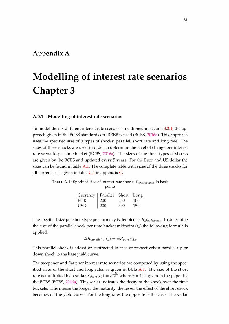
81
Appendix A
Modelling of interest rate scenariosChapter 3
A.0.1 Modelling of interest rate scenarios
To model the six different interest rate scenarios mentioned in section 3.2.4, the ap-proach given in the BCBS standards on IRRBB is used (BCBS, 2016a). This approachuses the specified size of 3 types of shocks: parallel, short rate and long rate. Thesizes of these shocks are used in order to determine the level of change per interestrate scenario per time bucket (BCBS, 2016a). The sizes of the three types of shocksare given by the BCBS and updated every 5 years. For the Euro and US dollar thesizes can be found in table A.1. The complete table with sizes of the three shocks forall currencies is given in table C.1 in appendix C.
TABLE A.1: Specified size of interest rate shocks Rshocktype,c in basispoints
Currency Parallel Short LongEUR 200 250 100USD 200 300 150
The specified size per shocktype per currency is denoted as Rshocktype,c. To determinethe size of the parallel shock per time bucket midpoint (tk) the following formula isapplied:
∆Rparallel,c(tk) = ±Rparallel,c
This parallel shock is added or subtracted in case of respectively a parallel up ordown shock to the base yield curve.
The steepener and flattener interest rate scenarios are composed by using the spec-ified sizes of the short and long rates as given in table A.1. The size of the shortrate is multiplied by a scalar Sshort(tk) = e
−tkx where x = 4 as given in the paper by
the BCBS (BCBS, 2016a). This scalar indicates the decay of the shock over the timebuckets. This means the longer the maturity, the lesser the effect of the short shockbecomes on the yield curve. For the long rates the opposite is the case. The scalar
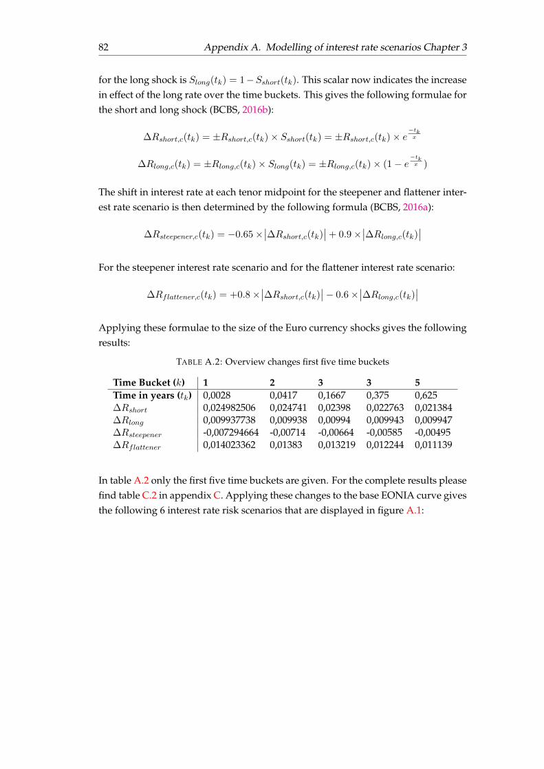
82 Appendix A. Modelling of interest rate scenarios Chapter 3
for the long shock is Slong(tk) = 1−Sshort(tk). This scalar now indicates the increasein effect of the long rate over the time buckets. This gives the following formulae forthe short and long shock (BCBS, 2016b):
∆Rshort,c(tk) = ±Rshort,c(tk)× Sshort(tk) = ±Rshort,c(tk)× e−tkx
∆Rlong,c(tk) = ±Rlong,c(tk)× Slong(tk) = ±Rlong,c(tk)× (1− e−tkx )
The shift in interest rate at each tenor midpoint for the steepener and flattener inter-est rate scenario is then determined by the following formula (BCBS, 2016a):
∆Rsteepener,c(tk) = −0.65×∣∣∆Rshort,c(tk)
∣∣+ 0.9×∣∣∆Rlong,c(tk)
∣∣For the steepener interest rate scenario and for the flattener interest rate scenario:
∆Rflattener,c(tk) = +0.8×∣∣∆Rshort,c(tk)
∣∣− 0.6×∣∣∆Rlong,c(tk)
∣∣Applying these formulae to the size of the Euro currency shocks gives the followingresults:
TABLE A.2: Overview changes first five time buckets
Time Bucket (k) 1 2 3 3 5Time in years (tk) 0,0028 0,0417 0,1667 0,375 0,625∆Rshort 0,024982506 0,024741 0,02398 0,022763 0,021384∆Rlong 0,009937738 0,009938 0,00994 0,009943 0,009947∆Rsteepener -0,007294664 -0,00714 -0,00664 -0,00585 -0,00495∆Rflattener 0,014023362 0,01383 0,013219 0,012244 0,011139
In table A.2 only the first five time buckets are given. For the complete results pleasefind table C.2 in appendix C. Applying these changes to the base EONIA curve givesthe following 6 interest rate risk scenarios that are displayed in figure A.1:
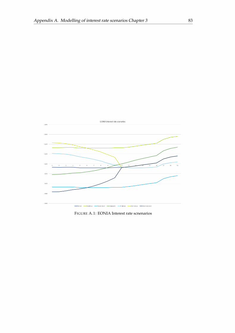
Appendix A. Modelling of interest rate scenarios Chapter 3 83
FIGURE A.1: EONIA Interest rate scnenarios

85
Appendix B
Mathematical derivation of LPoptimisation problem
B.1 Introduction
In this appendix the mathematical derivations of the constraints in the LP model areelaborated. Most of the constraints that are used in the LP optimisation problemand are stated in Chapter 4 are of a non-linear form. Since the LP package used inR only recognises constraints of a linear form, these formulae have to be rewrittenin order to fit the requirements. The constraints as stated in Chapter 4 are writtenin linear form. Since the computations are quite complex, the mathematical deriva-tion of these constraints will be dealt with in this appendix. In total the followingconstraints will be dealt with in this appendix:
• Delta EVE constraint;
• Delta NII constraint;
• Duration of equity constraint;
• Key rate duration constraint.
B.1.1 Delta EVE constraint
The delta EVE constraint is the first constraint that will be dealt with. According toliterature the change in economic value of equity can be calculated as follows (BCBS,2015; BCBS, 2016a; EBA, 2015):
∆EV Ek = (NPVAssets,k −NPVLiabilities,k)− (NPVAssets,0 −NPVLiabilities,0) (B.1)
Where k is one of the 6 interest rate scenarios mentioned in Chapter 4 section 4.2 and0 is the base scenario.
86 Appendix B. Mathematical derivation of LP optimisation problem
The difference in net present value of assets between a shocked interest rate scenarioand the base scenario is the change in economic value of assets. The change in netpresent value of liabilities is subtracted to get the net change in economic value ofequity. In a linear form the delta EVE calculation looks as follows:
∆EV Ek = (NPVAssets,k −NPVAssets,0)− (NPVLiabilities,k −NPVLiabilities,0) (B.2)
The net present value of assets and liabilities can be calculated by multiplying all thecash flows and notional repricing cash flows per maturity bucket with a discountfactor corresponding to the risk free rate at that time. The sum of these discountedcash flows is then the net present value.
The payer and receiver swaps are the only decision variables in this LP model. How-ever, all asset and liability classes as set in Chapter 4 section 4.2 are taken into ac-count in the calculation of the delta EVE constraint. The notional repricing cashflows in this thesis are based on the gapping information provided by the bank.This notional repricing cash flow is represented in the model by xi,j where i is oneof the 5 asset classes set in Chapter 4 section 4.2 and j one of the 120 maturity buck-ets the asset can be allocated to. The liabilities are represented by yi,j with class i inmaturity bucket j.
The discount factors are computed via continuously compounding. This is done bythe following formula: exp−rk,jtj , with rk,j being the risk free rate under scenariok at time bucket j, and tj the time at time bucket j. The net present value of thenotional repricing cash flows are then: exp−rk,jtj xi,j for assets and exp−rk,jtj yi,j forliabilities.
Besides the notional cash flows, the coupon payments that are made on assets andliabilities are also incorporated in this model. An asset in a certain time bucket j,has earned jRi,j until the moment of repricing at moment j. In order to determinethe net present value of these coupon payments, they should be discounted withthe rate at which they occur. To do this, the first coupon Ri,1 should be discountedwith discount factor exp−rk,1t1 . The second coupon Ri,2 should be discounted withthe discount factor corresponding with the discount factor at time t2: exp−rk,2t2 etc.When we consider asset 2 in time bucket 3, this gives the following computation forthe total net present value of the coupon payments:
∑3j=1(x2,3R2,3 exp−rk,jtj ).
The total net present value for asset 2 in time bucket 3 is thus:
NPVnotional + NPVcouponpayments = (exp−rk,3t3 x2,3) +3∑
j=1
(x2,3R2,3 exp−rk,jtj ) (B.3)
B.2. Delta NII constraint 87
The linear format requires the notional repricing cash flow to be kept outside brack-ets. This gives:
NPVasset2,3 =(
exp−rk,3t3 +
3∑j=1
(R2,3 exp−rk,jtj ))x2,3 (B.4)
Repeating this for every asset class i and all time buckets j gives the total net presentvalue of assets and liabilities:
NPVassets,k =5∑
i=1
120∑j=1
( 1
(1 + rk,t)t+ (
j∑j∗=1
1
(1 + rk,t)tRk,j∗)
)xi,j (B.5)
NPVliabilities,k =
5∑i=1
120∑j=1
( 1
(1 + rk,t)t+ (
j∑j∗=1
1
(1 + rk,t)tck,j∗)
)yi,j (B.6)
NPVassets,0 =
5∑i=1
120∑j=1
( 1
(1 + rk,t)t+ (
j∑j∗=1
1
(1 + rk,t)tR0,j∗)
)xi,j (B.7)
NPVliabilities,0 =
5∑i=1
120∑j=1
( 1
(1 + rk,t)t+ (
j∑j∗=1
1
(1 + rk,t)tc0,j∗)
)yi,j (B.8)
Implementing these four in equation B.2 gives the total delta EVE calculation inlinear format:
∆EV E =
5∑i=1
120∑j=1
(( 1
(1 + rk,t)t+(
j∑j∗=1
1
(1 + rk,t)tRk,j∗)
)−
( 1
(1 + r0,t)t+ (
j∑j∗=1
1
(1 + r0,t)tR0,j∗)
))xi,j−
5∑i=1
120∑j=1
(( 1
(1 + rk,t)t+(
j∑j∗=1
1
(1 + rk,t)tck,j∗)
)−
( 1
(1 + r0,t)t+ (
j∑j∗=1
1
(1 + r0,t)tc0,j∗)
))yi,j
(B.9)
B.2 Delta NII constraint
As mentioned in Chapter 2, the delta NII constraint is set as the difference in netinterest income of a base scenario, and one of the six interest rate shocks as described
88 Appendix B. Mathematical derivation of LP optimisation problem
in the Chapter 4. According to literature the change in net interest income can becalculated as follows (BCBS, 2015; BCBS, 2016a; EBA, 2015):
∆NIIk = NIIk −NII0 (B.10)
Here negative values of the delta NII will indicate a decrease in NII due to a changein interest rates, and positive values an increase in NII.
Since the time horizon on which the delta NII is monitored is one year, the shock ininterest rates will only be applied to the first 4 time buckets. This since assets andliabilities with a maturity of more than one year will not reprice within that one yearat which the delta NII is assessed and thus will keep their original coupon. This thengives the following computations for the components of equation B.10:
NIIk =5∑
i=1
4∑j=1
((xi,jRk,j)− (yi,jck,j)
)(B.11)
and
NII0 =
5∑i=1
4∑j=1
((xi,jR0,j)− (yi,jc0,j)
)(B.12)
Here Rk,j is the interest earned on assets in interest rate scenario k and time bucketj. R0,j is the original coupon of the base scenario. Note that interest rate earned Rk,j
is not the same as the risk free rate.
Implementing these components in equation B.10 gives the following equation:
∆NIIk =
5∑i=1
4∑j=1
(((xi,jRk,j)− (yi,jck,j)
)−((xi,jR0,j)− (yi,jc0,j)
))(B.13)
Rewriting to linear format gives:
∆NIIk =
5∑i=1
4∑j=1
((Rk,j −R0,j)xi,j − (ck,j − c0,j)yi,j
)(B.14)
B.2.1 Duration of equity constraint
The duration of equity is the difference that can be viewed as the difference in dura-tion of assets and liabilities (Cummins et al., 2009):
DoE = DurationAssets − (assets/liabilities)DurationLiabilities (B.15)
B.2. Delta NII constraint 89
The duration of an asset or liability can also be viewed as the weighted average ofall the cash flows of assets and liabilities multiplied with the time they occur. Theseweights are calculated by dividing the cash payment at time tj with the total netpresent value of the asset or liability (Hull, 2012a). This is given in the followingformula:
Duration =n∑
j=1
tj
(Rj1
(1+rt)t
NPVasset
)(B.16)
Here Rj is the coupon at time j, and rj the risk free rate at time j.
In the LP model the duration of equity constraint will be calculated in a similarmanner. However since the LP model requires a linear format for the constraints,equation B.16 has to be rewritten to fit this purpose. In the next few steps this pro-cess will be elaborated. During this process, the duration of assets will be taken asexample, for the duration of liabilities this however works exactly the same, but forsimplicity it is omitted.
In equation B.16 Rj contains both coupon and principal payments (Hull, 2012a). Inour linear format this is not the case, and Ri,j only represents the coupon payments.The principal payment is in the case of our LP format denoted with xi,j . Just like inthe delta EVE computations, the linear format requires us to deal with the couponpayments and the principal payment separately.
Let’s begin with the coupon payments. As in our delta EVE calculation, couponsare earned on a quarterly basis until the moment that the asset reaches its maturity.This means that asset 2 in maturity bucket 3 earns 3 quarterly coupons during thattime. These coupons have to be discounted at the rate corresponding to the timethey occur. This gives for asset 2 in time bucket 3:
∑3j=1(x2,3R2,j
1(1+r0,tj )
tj). In order
to determine the weighted average cash flows, first the coupon cash flows have tobe multiplied with the time tj at which they occur. This gives:
3∑j=1
(x2,3R2,j1
(1 + r0,t)ttj) (B.17)
Besides the coupon cash flows, the notional payment also has to be discounted andmultiplied with the time tj at which it occurs:
x2,3 exp−r0,3t3 t3
In total the cash flows can be written as:
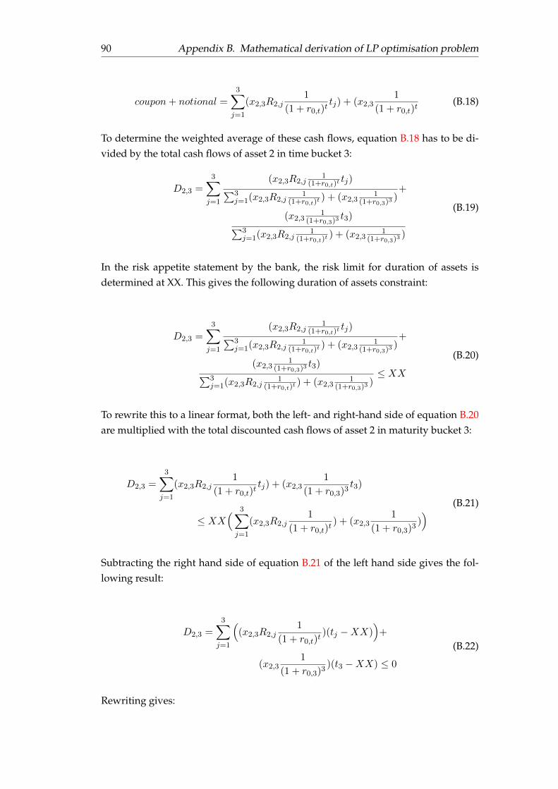
90 Appendix B. Mathematical derivation of LP optimisation problem
coupon + notional =3∑
j=1
(x2,3R2,j1
(1 + r0,t)ttj) + (x2,3
1
(1 + r0,t)t(B.18)
To determine the weighted average of these cash flows, equation B.18 has to be di-vided by the total cash flows of asset 2 in time bucket 3:
D2,3 =3∑
j=1
(x2,3R2,j1
(1+r0,t)ttj)∑3
j=1(x2,3R2,j1
(1+r0,t)t) + (x2,3
1(1+r0,3)3
)+
(x2,31
(1+r0,3)3t3)∑3
j=1(x2,3R2,j1
(1+r0,t)t) + (x2,3
1(1+r0,3)3
)
(B.19)
In the risk appetite statement by the bank, the risk limit for duration of assets isdetermined at XX. This gives the following duration of assets constraint:
D2,3 =
3∑j=1
(x2,3R2,j1
(1+r0,t)ttj)∑3
j=1(x2,3R2,j1
(1+r0,t)t) + (x2,3
1(1+r0,3)3
)+
(x2,31
(1+r0,3)3t3)∑3
j=1(x2,3R2,j1
(1+r0,t)t) + (x2,3
1(1+r0,3)3
)≤ XX
(B.20)
To rewrite this to a linear format, both the left- and right-hand side of equation B.20are multiplied with the total discounted cash flows of asset 2 in maturity bucket 3:
D2,3 =
3∑j=1
(x2,3R2,j1
(1 + r0,t)ttj) + (x2,3
1
(1 + r0,3)3t3)
≤ XX( 3∑
j=1
(x2,3R2,j1
(1 + r0,t)t) + (x2,3
1
(1 + r0,3)3)) (B.21)
Subtracting the right hand side of equation B.21 of the left hand side gives the fol-lowing result:
D2,3 =
3∑j=1
((x2,3R2,j
1
(1 + r0,t)t)(tj −XX)
)+
(x2,31
(1 + r0,3)3)(t3 −XX) ≤ 0
(B.22)
Rewriting gives:
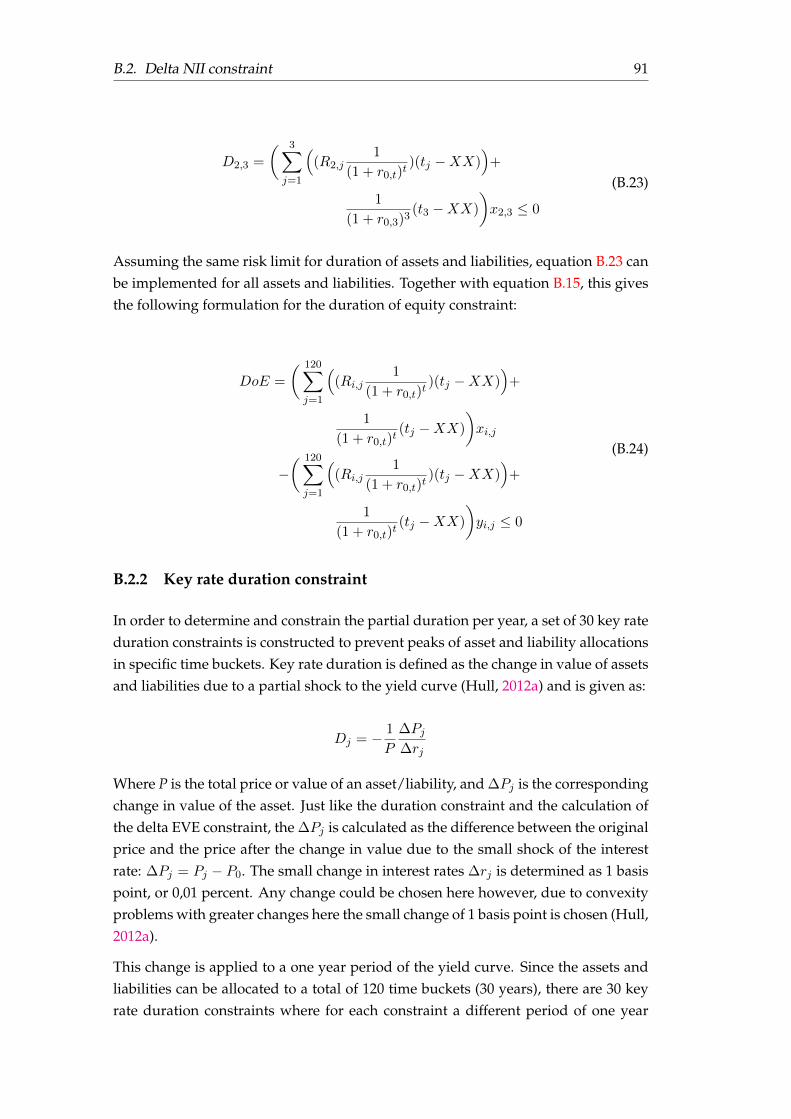
B.2. Delta NII constraint 91
D2,3 =
( 3∑j=1
((R2,j
1
(1 + r0,t)t)(tj −XX)
)+
1
(1 + r0,3)3(t3 −XX)
)x2,3 ≤ 0
(B.23)
Assuming the same risk limit for duration of assets and liabilities, equation B.23 canbe implemented for all assets and liabilities. Together with equation B.15, this givesthe following formulation for the duration of equity constraint:
DoE =
( 120∑j=1
((Ri,j
1
(1 + r0,t)t)(tj −XX)
)+
1
(1 + r0,t)t(tj −XX)
)xi,j
−( 120∑
j=1
((Ri,j
1
(1 + r0,t)t)(tj −XX)
)+
1
(1 + r0,t)t(tj −XX)
)yi,j ≤ 0
(B.24)
B.2.2 Key rate duration constraint
In order to determine and constrain the partial duration per year, a set of 30 key rateduration constraints is constructed to prevent peaks of asset and liability allocationsin specific time buckets. Key rate duration is defined as the change in value of assetsand liabilities due to a partial shock to the yield curve (Hull, 2012a) and is given as:
Dj = − 1
P
∆Pj
∆rj
Where P is the total price or value of an asset/liability, and ∆Pj is the correspondingchange in value of the asset. Just like the duration constraint and the calculation ofthe delta EVE constraint, the ∆Pj is calculated as the difference between the originalprice and the price after the change in value due to the small shock of the interestrate: ∆Pj = Pj − P0. The small change in interest rates ∆rj is determined as 1 basispoint, or 0,01 percent. Any change could be chosen here however, due to convexityproblems with greater changes here the small change of 1 basis point is chosen (Hull,2012a).
This change is applied to a one year period of the yield curve. Since the assets andliabilities can be allocated to a total of 120 time buckets (30 years), there are 30 keyrate duration constraints where for each constraint a different period of one year
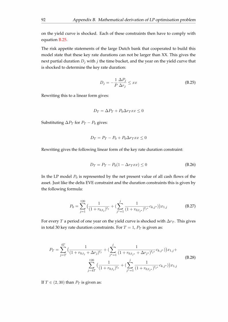
92 Appendix B. Mathematical derivation of LP optimisation problem
on the yield curve is shocked. Each of these constraints then have to comply withequation B.25.
The risk appetite statements of the large Dutch bank that cooperated to build thismodel state that these key rate durations can not be larger than XX. This gives thenext partial duration Dj with j the time bucket, and the year on the yield curve thatis shocked to determine the key rate duration:
Dj = − 1
P
∆Pj
∆rj≤ xx (B.25)
Rewriting this to a linear form gives:
DT = ∆PT + P0∆rTxx ≤ 0
Substituting ∆PT for PT − P0 gives:
DT = PT − P0 + P0∆rTxx ≤ 0
Rewriting gives the following linear form of the key rate duration constraint:
DT = PT − P0(1−∆rTxx) ≤ 0 (B.26)
In the LP model P0 is represented by the net present value of all cash flows of theasset. Just like the delta EVE constraint and the duration constraints this is given bythe following formula:
P0 =
120∑j=1
( 1
(1 + r0,tj )tj
+ (
j∑j∗=1
1
(1 + r0,tj∗ )tj∗ck,j∗)
)x1,j (B.27)
For every T a period of one year on the yield curve is shocked with ∆rT . This givesin total 30 key rate duration constraints. For T = 1, PT is given as:
PT =
4T∑j=T
( 1
(1 + r0,tj + ∆rj)tj+ (
j∑j∗=1
1
(1 + r0,tj∗ + ∆rj∗)tj∗ck,j∗)
)x1,j+
120∑j=4T
( 1
(1 + r0,tj )tj
+ (
j∑j∗=1
1
(1 + r0,tj∗ )tj∗ck,j∗)
)x1,j
(B.28)
If T ∈ (2, 30) than PT is given as:
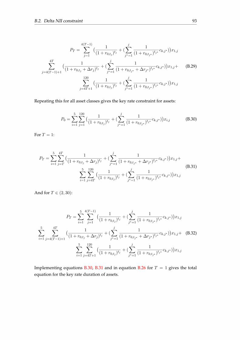
B.2. Delta NII constraint 93
PT =
4(T−1)∑j=1
( 1
(1 + r0,tj )tj
+ (
j∑j∗=1
1
(1 + r0,tj∗ )tj∗ck,j∗)
)x1,j
4T∑j=4(T−1)+1
( 1
(1 + r0,tj + ∆rj)tj+ (
j∑j∗=1
1
(1 + r0,tj∗ + ∆rj∗)tj∗ck,j∗)
)x1,j+
120∑j=4T+1
( 1
(1 + r0,tj )tj
+ (
j∑j∗=1
1
(1 + r0,tj∗ )tj∗ck,j∗)
)x1,j
(B.29)
Repeating this for all asset classes gives the key rate constraint for assets:
P0 =5∑
i=1
120∑j=1
( 1
(1 + r0,tj )tj
+ (
j∑j∗=1
1
(1 + r0,tj∗ )tj∗ck,j∗)
)xi,j (B.30)
For T = 1:
PT =5∑
i=1
4T∑j=T
( 1
(1 + r0,tj + ∆rj)tj+ (
j∑j∗=1
1
(1 + r0,tj∗ + ∆rj∗)tj∗ck,j∗)
)x1,j+
5∑i=1
120∑j=4T
( 1
(1 + r0,tj )tj
+ (
j∑j∗=1
1
(1 + r0,tj∗ )tj∗ck,j∗)
)x1,j
(B.31)
And for T ∈ (2, 30):
PT =5∑
i=1
4(T−1)∑j=1
( 1
(1 + r0,tj )tj
+ (
j∑j∗=1
1
(1 + r0,tj∗ )tj∗ck,j∗)
)x1,j
5∑i=1
4T∑j=4(T−1)+1
( 1
(1 + r0,tj + ∆rj)tj+ (
j∑j∗=1
1
(1 + r0,tj∗ + ∆rj∗)tj∗ck,j∗)
)x1,j+
5∑i=1
120∑j=4T+1
( 1
(1 + r0,tj )tj
+ (
j∑j∗=1
1
(1 + r0,tj∗ )tj∗ck,j∗)
)x1,j
(B.32)
Implementing equations B.30, B.31 and in equation B.26 for T = 1 gives the totalequation for the key rate duration of assets.
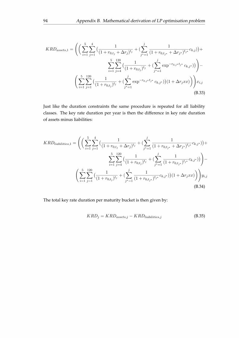
94 Appendix B. Mathematical derivation of LP optimisation problem
KRDassets,1 =
(( 5∑i=1
4∑j=1
( 1
(1 + r0,tj + ∆rj)tj+ (
j∑j∗=1
1
(1 + r0,tj∗ + ∆rj∗)tj∗ck,j)
)+
5∑i=1
120∑j=4
( 1
(1 + r0,tj )tj
+ (
j∑j∗=1
exp−r0,j∗ tj∗ ck,j∗)))−
(5∑
i=1
120∑j=1
( 1
(1 + r0,tj )tj
+ (
j∑j∗=1
exp−r0,j∗ tj∗ ck,j∗))(1 + ∆rjxx)
))xi,j
(B.33)
Just like the duration constraints the same procedure is repeated for all liabilityclasses. The key rate duration per year is then the difference in key rate durationof assets minus liabilities:
KRDliabilities,1 =
(( 5∑i=1
4∑j=1
( 1
(1 + r0,tj + ∆rj)tj+ (
j∑j∗=1
1
(1 + r0,tj∗ + ∆rj∗)tj∗ck,j∗)
)+
5∑i=1
120∑j=4
( 1
(1 + r0,tj )tj
+ (
j∑j∗=1
1
(1 + r0,tj∗ )tj∗ck,j∗)
))−
(5∑
i=1
120∑j=1
( 1
(1 + r0,tj )tj
+ (
j∑j∗=1
1
(1 + r0,tj∗ )tj∗ck,j∗)
)(1 + ∆rjxx)
))yi,j
(B.34)
The total key rate duration per maturity bucket is then given by:
KRDj = KRDassets,j −KRDliabilities,j (B.35)

95
Appendix C
Tables
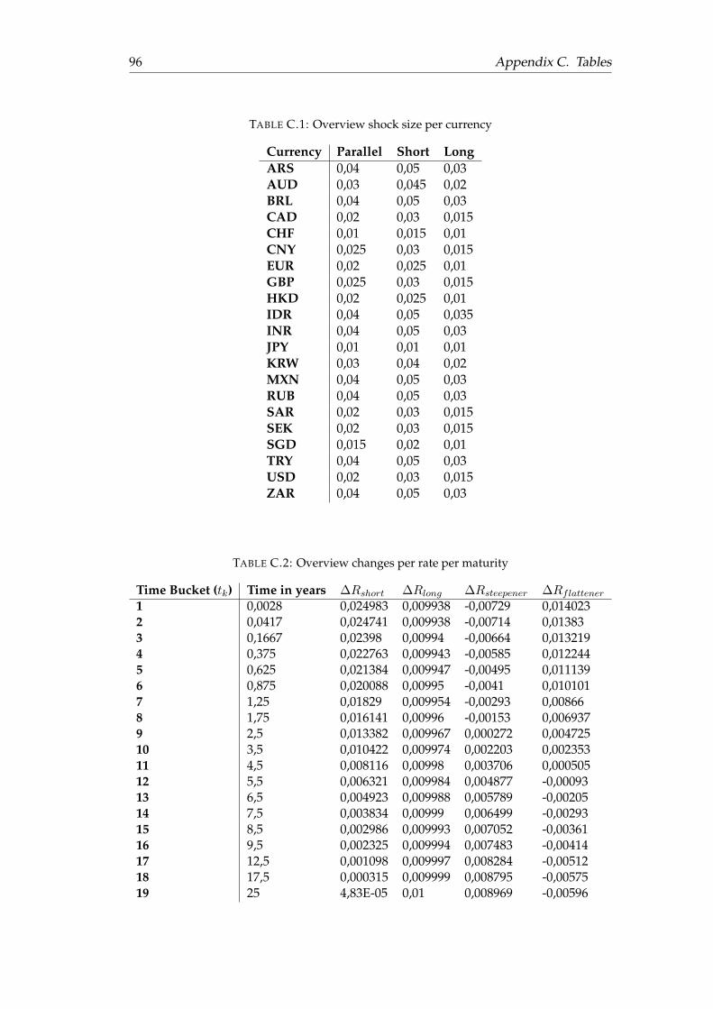
96 Appendix C. Tables
TABLE C.1: Overview shock size per currency
Currency Parallel Short LongARS 0,04 0,05 0,03AUD 0,03 0,045 0,02BRL 0,04 0,05 0,03CAD 0,02 0,03 0,015CHF 0,01 0,015 0,01CNY 0,025 0,03 0,015EUR 0,02 0,025 0,01GBP 0,025 0,03 0,015HKD 0,02 0,025 0,01IDR 0,04 0,05 0,035INR 0,04 0,05 0,03JPY 0,01 0,01 0,01KRW 0,03 0,04 0,02MXN 0,04 0,05 0,03RUB 0,04 0,05 0,03SAR 0,02 0,03 0,015SEK 0,02 0,03 0,015SGD 0,015 0,02 0,01TRY 0,04 0,05 0,03USD 0,02 0,03 0,015ZAR 0,04 0,05 0,03
TABLE C.2: Overview changes per rate per maturity
Time Bucket (tk) Time in years ∆Rshort ∆Rlong ∆Rsteepener ∆Rflattener
1 0,0028 0,024983 0,009938 -0,00729 0,0140232 0,0417 0,024741 0,009938 -0,00714 0,013833 0,1667 0,02398 0,00994 -0,00664 0,0132194 0,375 0,022763 0,009943 -0,00585 0,0122445 0,625 0,021384 0,009947 -0,00495 0,0111396 0,875 0,020088 0,00995 -0,0041 0,0101017 1,25 0,01829 0,009954 -0,00293 0,008668 1,75 0,016141 0,00996 -0,00153 0,0069379 2,5 0,013382 0,009967 0,000272 0,00472510 3,5 0,010422 0,009974 0,002203 0,00235311 4,5 0,008116 0,00998 0,003706 0,00050512 5,5 0,006321 0,009984 0,004877 -0,0009313 6,5 0,004923 0,009988 0,005789 -0,0020514 7,5 0,003834 0,00999 0,006499 -0,0029315 8,5 0,002986 0,009993 0,007052 -0,0036116 9,5 0,002325 0,009994 0,007483 -0,0041417 12,5 0,001098 0,009997 0,008284 -0,0051218 17,5 0,000315 0,009999 0,008795 -0,0057519 25 4,83E-05 0,01 0,008969 -0,00596
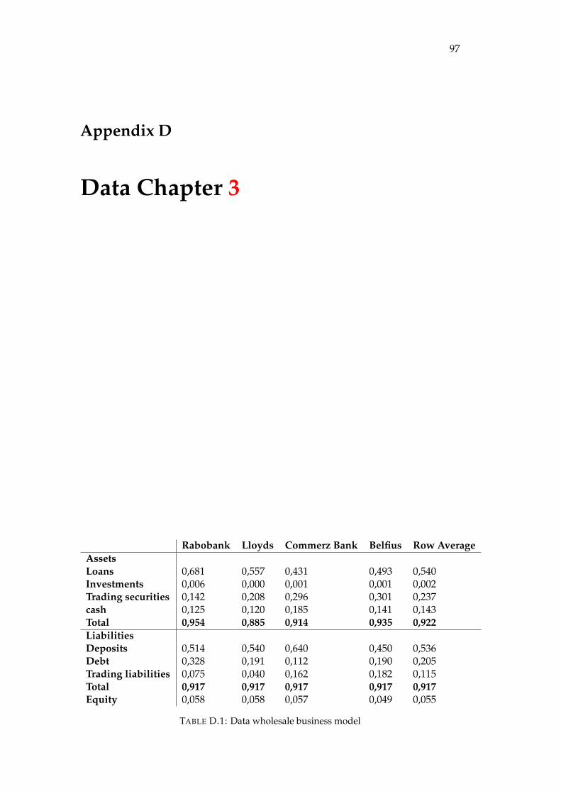
97
Appendix D
Data Chapter 3
Rabobank Lloyds Commerz Bank Belfius Row AverageAssetsLoans 0,681 0,557 0,431 0,493 0,540Investments 0,006 0,000 0,001 0,001 0,002Trading securities 0,142 0,208 0,296 0,301 0,237cash 0,125 0,120 0,185 0,141 0,143Total 0,954 0,885 0,914 0,935 0,922LiabilitiesDeposits 0,514 0,540 0,640 0,450 0,536Debt 0,328 0,191 0,112 0,190 0,205Trading liabilities 0,075 0,040 0,162 0,182 0,115Total 0,917 0,917 0,917 0,917 0,917Equity 0,058 0,058 0,057 0,049 0,055
TABLE D.1: Data wholesale business model
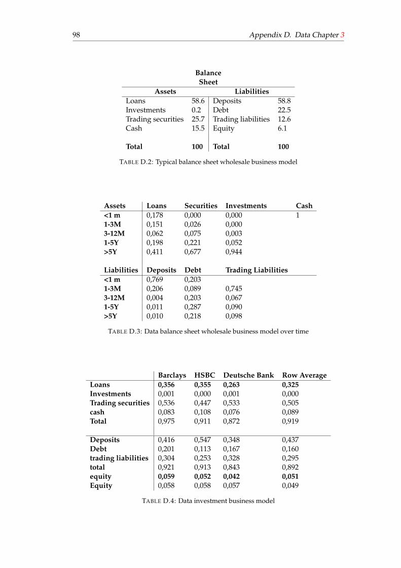
98 Appendix D. Data Chapter 3
BalanceSheet
Assets LiabilitiesLoans 58.6 Deposits 58.8Investments 0.2 Debt 22.5Trading securities 25.7 Trading liabilities 12.6Cash 15.5 Equity 6.1
Total 100 Total 100
TABLE D.2: Typical balance sheet wholesale business model
Assets Loans Securities Investments Cash<1 m 0,178 0,000 0,000 11-3M 0,151 0,026 0,0003-12M 0,062 0,075 0,0031-5Y 0,198 0,221 0,052>5Y 0,411 0,677 0,944
Liabilities Deposits Debt Trading Liabilities<1 m 0,769 0,2031-3M 0,206 0,089 0,7453-12M 0,004 0,203 0,0671-5Y 0,011 0,287 0,090>5Y 0,010 0,218 0,098
TABLE D.3: Data balance sheet wholesale business model over time
Barclays HSBC Deutsche Bank Row AverageLoans 0,356 0,355 0,263 0,325Investments 0,001 0,000 0,001 0,000Trading securities 0,536 0,447 0,533 0,505cash 0,083 0,108 0,076 0,089Total 0,975 0,911 0,872 0,919
Deposits 0,416 0,547 0,348 0,437Debt 0,201 0,113 0,167 0,160trading liabilities 0,304 0,253 0,328 0,295total 0,921 0,913 0,843 0,892equity 0,059 0,052 0,042 0,051Equity 0,058 0,058 0,057 0,049
TABLE D.4: Data investment business model
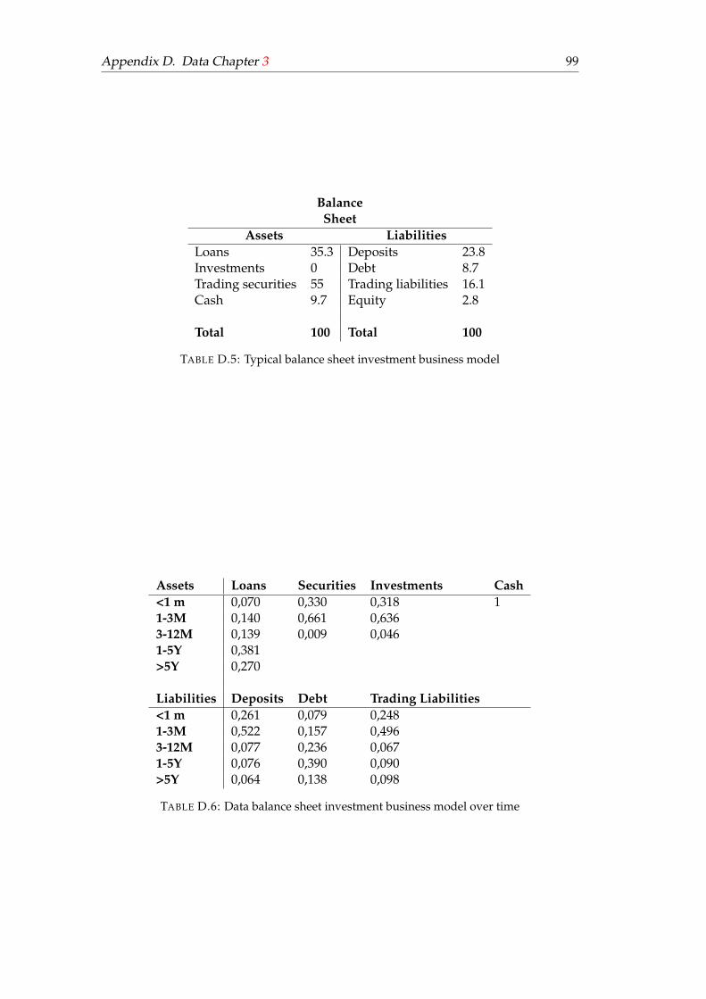
Appendix D. Data Chapter 3 99
BalanceSheet
Assets LiabilitiesLoans 35.3 Deposits 23.8Investments 0 Debt 8.7Trading securities 55 Trading liabilities 16.1Cash 9.7 Equity 2.8
Total 100 Total 100
TABLE D.5: Typical balance sheet investment business model
Assets Loans Securities Investments Cash<1 m 0,070 0,330 0,318 11-3M 0,140 0,661 0,6363-12M 0,139 0,009 0,0461-5Y 0,381>5Y 0,270
Liabilities Deposits Debt Trading Liabilities<1 m 0,261 0,079 0,2481-3M 0,522 0,157 0,4963-12M 0,077 0,236 0,0671-5Y 0,076 0,390 0,090>5Y 0,064 0,138 0,098
TABLE D.6: Data balance sheet investment business model over time