Interest-Rate Risk Factor and Stock Returns: A Time...

Interest-Rate Risk Factor and Stock Returns:

A Time-Varying Factor-Loadings Model

Peng Huang

Department of Economics Ripon College, U.S.A.

C. James Hueng*

Department of Economics Western Michigan University, U.S.A.

Abstract

We extend the Fama-French three-factor model to include a new risk factor that proxies for

interest-rate risk faced by firms, in an attempt to reduce the pricing errors that the three-factor

model cannot explain. These pricing errors are observed especially in small size and low book-

to-market ratio firms, which are in general more sensitive to interest-rate risk. In addition, the

factor loadings are modeled as time-varying so that the investors’ learning process can be taken

into account. The results show that our time-varying-loadings four-factor model significantly

reduces the pricing errors.

Key words: factor model; interest-rate risk factor; time-varying factor loadings; Kalman Filter.

JEL Classifications: G11, G12

*Correspondence to: Professor C. James Hueng

5412 Friedmann Hall Western Michigan University Kalamazoo, MI 49008-5330 U.S.A. Phone: 0021-269-387-5558 Fax: 0021-269-387-5637 Email: [email protected]

1

I. Introduction

Modeling the cross-sectional average stock returns has been the focal point of finance for many

years. The most influential asset-pricing model in the 1990s is the three-factor model proposed by

Fama and French (1993). This model consists of three portfolios constructed to mimic

underlying common risk factors in returns. The portfolios include the zero-investment portfolios

formed on firm size (SZ) and book-to-market ratio (BM), as well as the excess return of a value-

weighted market portfolio. The risk factors constructed from these portfolios are denoted as SMB

(Small-SZ Minus Big-SZ), HML (High-BM Minus Low-BM), and MKT, respectively. Their

results show that these three factors seem to explain the excess returns on a full set of BM- and

SZ-sorted portfolios.

Although the three-factor model has generated impressive performance, empirical

evidence indicates that it is still not able to completely capture the cross-sectional returns. In

particular, statistically significant pricing errors that cannot be explained by these three factors

still exist in several portfolios. For example, using monthly data on the U.S. common stocks

from 1963:7 to 1990:12, Fama and French (1993) show that in the five-by-five SZ/BM double-

sorted portfolios, there are three portfolios of which the pricing errors are significantly different

from zero. Two of them are located in the lowest BM quintile. Petkova (2006) extends the

sample to include the data after 1990 (up to 2001:12) and finds that six out of the 25 portfolios

have pricing errors that are significantly different from zero. Four of them are located in the

lowest BM or the smallest SZ quintile. Adrian and Franzoni (2005) report similar results using

quarterly data from 1963 to 2004: five portfolios located in either the lowest BM quintile or the

smallest SZ quintile have statistically significant pricing errors. This inefficiency of the three-

factor model, in fact, is not limited to the U.S. data. Chiao and Hueng (2005) use the Japanese

data and find that six out of the nine lowest BM and/or smallest SZ portfolios have pricing errors

that are significantly different from zero.

2

Apparently, most of the pricing errors that cannot be explained by the three-factor model

appear in the portfolios with either the lowest BM (denoted as the “growth” portfolio) or the

smallest SZ (denoted as the “small” portfolio). Therefore, to improve the model’s ability to

explain the cross-sectional returns, we add a risk factor that is most likely to capture the risk faced

especially by small firms and firms with a low BM. Studies such as Cornell (1999) and Campbell

and Vuolteenaho (2004) claim that small firms and firms with a low BM are more sensitive to

interest rate (discount rate) risk. To capture this risk, the TERM factor, defined as the yield

spread between the ten-year and the three-month treasury rates, is incorporated into our model.

As suggested by Campbell and Shiller (1991), Diebold, Rudebush, and Aruoba (2006), and Chen,

Roll, and Ross (1986), this term spread represents a good proxy for risk caused by shifts in

interest rates. Since the discount rate is an average of interest rates over time, a change in interest

rates can lead to a change in the discount rate. Therefore, the TERM factor should capture

information about risk related to changes in the discount rate.

In addition to the TERM factor, the second modification we make on the three-factor

model is to model the factor loadings as time varying. Under the CAPM framework, studies such

as Harvey (1989), Ferson and Harvey (1991, 1993), and Jagnnathan and Wang (1996)

demonstrate that beta in the CAPM tends to be volatile through time. Franzoni (2006) shows that

portfolios, especially those with small firms, exhibit considerable long-run variations in beta.

Adrian and Franzoni (2004, 2005) argue that the main reason for the failure of the unconditional

CAPM is that the model does not mimic investors’ learning process. The unobservable time-

varying beta should induce the investors’ learning process. However, the OLS regression used in

constant-loadings factor models cannot successfully mimic the investors’ learning process, which

leads to a difference between the investors’ true expectation of the loadings and the constant

factor loadings estimated by OLS. Indeed, Fama and French (1997) show that loadings on MKT,

HML, and SMB of industry-sorted portfolios exhibit strong time variations. Ferson and Havey

(1999) also show that loadings on the Fama-French three factors of the five-by-five SZ/BM

3

double-sorted portfolios tend to be time-varying. Therefore, following Adrian and Franzoni’s

research, we use the Kalman Filter procedure to estimate the movements of the factor loadings

and replicate the investors’ learning process.

To evaluate the performance of our time-varying-loadings four-factor model, thereafter

the “TVL4 model”, we apply the model to the five-by-five SZ/BM double-sorted portfolios

formed by U.S. stocks from the period 1963:7-2004:12. In addition, the time-varying-loadings

three-factor model estimated by the Kalman Filter and the constant-loadings four-factor model

estimated by OLS are also examined to analyze the sole contribution of the learning process and

of the TERM factor, respectively. This paper focuses on the pricing error in each individual

portfolio as well as the aggregate pricing error generated by each model.

The results show that both the time-varying-factor-loadings specification and the TERM

factor reduce the pricing errors. The most impressive result is that the combination of these two

modifications, the TVL4 model, remarkably reduces both the individual and the aggregate pricing

errors generated by the Fama-French three-factor model. Those statistically significant pricing

errors in the Fama-French model almost all become insignificant in the TVL4 model. The root

mean squared error (RMSE) and the composite pricing error (CPE), two measures for the

aggregate pricing errors, are reduced by 60% and 50%, respectively, from the Fama-French

model to the TVL4 model.

To check for possible data mining problems, we further evaluate the performances of the

TVL4 model in other portfolio formations. Specifically, we first experiment with the model in

industry-sorted portfolios. Both the individual and the aggregate pricing errors in the Fama-

French three-factor model are largely reduced in the TVL4 model. Furthermore, we use only the

data prior to 1963 to form the SZ/BM double-sorted portfolios and evaluate the performances of

the TVL4 model. Again, the TVL4 model outperforms the Fama-French three-factor model by

greatly reducing both the individual and the aggregate pricing errors.

4

To further check the robustness of our results, we also experiment with another time-

varying-loadings four-factor model where the TERM factor is replaced by the momentum factor,

a risk factor that has been found to be important in the literature. It turns out that the momentum

factor does not help to reduce the pricing errors in the five-by-five SZ/BM double-sorted

portfolios. Therefore, we conclude that the success of the TVL4 model lies on the facts that it

successfully mimics the investors’ evolutional learning process of loadings, and that it

incorporates into the estimation process more information about risks related to changes in

discount rates.

The remainder of the paper is organized as follows. The next section details our

motivation for constructing the TVL4 model and the specification of the model. Section III

describes the data and the methodology. Section IV shows the estimation results for the five-by-

five SZ/BM double-sorted portfolios. Robustness checks are presented in Section V. Finally,

Section VI concludes the paper.

II. The time-varying-loadings four-factor model

A. The TERM factor

Since statistically significant pricing errors are found mostly in the small/growth

portfolios, it is natural for us to investigate this problem by concentrating on specific

characteristics of firms in these portfolios. Previous studies have indicated that both the small

and growth portfolios are more sensitive to changes in the discount rates. Based on the

relationship between risk and the duration of projects, Cornell (1999) argues that the relatively

higher risk of long-term projects arises from variations in the discount rate rather than variations

in the cash flows. Since small and growth firms usually generate cash flows in a longer duration,

their returns are likely to respond more strongly to shocks to the discount rate than the large and

value (high BM) firms do. This is very similar to the case that long-term bonds are more sensitive

than short-term bonds to shocks to the discount rates because of their longer durations.

5

A recent study by Campbell and Vuolteenaho (2004) provides further evidence. They

decompose the market beta of a portfolio into the cash-flow beta and the discount-rate beta.

Their results indicate that the discount-rate betas of the small/growth portfolios are larger than

those of the large/value portfolios after 1960s. That is, the small/growth portfolios are likely to

be more sensitive to the discount rate during this period. They attribute the relatively higher

discount-rate betas to long durations of cash flows, future investment opportunities, and

dependence on external fund raising. Like Cornell (1999), they think that small and growth firms,

usually with negative current cash flows but valuable future investment opportunities, react more

to the discount rate news. Furthermore, in line with Perez-Quiros and Timmermann (2000), they

argue that small and young firms with little collateral rely more heavily on external financing

such as bank loans. This is because these firms do not have easy access to other credit sources

and therefore, are more sensitive to interest costs and external financial conditions.

Hence, we believe that the information about shocks to the discount rates plays an

important role in explaining returns of the small/growth portfolios. Indeed, Cornell (1999)

suggests that taking account of changes in the discount rates may improve the tests of an asset-

pricing model and help to explain some anomalies in returns, especially for small or growth firms.

This inspires us to add the TERM factor, the spread between ten-year and three-month Treasury

rates, to the three-factor model.1

It is well-known that the term spread is a variable that contains information about future

movements in interest rates [e.g., Campbell and Shiller (1991)]. When building a three-factor

yield curve model, Diebold, Rudebusch and Aruoba (2006) assert that the yield spread between

1 Studies that also realize the importance of the information connected to the discount rate include

Elton, Gruber, and Blake (1995) and Ferson and Harvey (1999). They both suggest that the

Fama-French three-factor model may leave out some important information reflected by interest-

rate factors.

6

the ten-year bond and the three-month Treasury bill, which is highly correlated with their “slope”

factor, responds significantly to innovations in Federal funds rate. Since the discount rate is an

average of interest rates over time, changes in interest rates affect the value of the discount rate,

and in turns affect the stock returns. Chen, Roll and Ross (1986) also claim that the discount rate

changes with the term spread across different maturities.

In the factor model literature, it has been suggested that the term spread may play an

important role.2 For example, Petkova (2006) illustrates that SMB is positively and significantly

related to the term spread, but only a very small portion (about 5%) of the surprises in the term

spread can be explained by the Fama-French three factors. On the other hand, to improve the

performance of their conditional CAPM, Adrian and Franzoni (2005) show that, in addition to the

MKT and HTM factors, the term spread should be included as a state variable for beta. Both of

these studies hint that the term spread carries information beyond the Fama-French three factors.

B. The time-varying factor-loadings model

Time-varying factor loadings have been suggested in recent asset pricing literature. For

example, Franzoni (2006) finds that portfolios with small firms exhibit considerable long-run

variations in market beta. Adrian and Franzoni (2004, 2005) argue that the unobservability of

time-varying betas should induce the investors’ learning process, and that the main reason for the

failure of the unconditional CAPM is that the constant-beta model does not mimic the investors’

learning process. However, the OLS regression used in the constant-loadings factor models

cannot successfully mimic the investors’ learning process. Therefore, they use the Kalman Filter

procedure to estimate the movements of the time-varying market beta. The Kalman Filter

2 Chen, Roll and Ross (1986), Fama and French (1993), Aretz, Bartram and Pope (2005), and

Petkova (2006) use the term spread directly as a factor, while Campbell and Vuolteenaho (2004)

and Adrian and Franzoni (2005) use it as a state variable for the other factors.

7

updates the time-varying parameters through learning from prediction errors. Their results show

that the learning type of CAPM outperforms the unconditional CAPM.

Motivated by Adrian and Franzoni (2004, 2005), we implement the learning type model

in the case of multiple factor loadings. Previous studies that try to document time-varying risk

loadings often use conditional models. For example, Jaganathan and Wang (1996) develop a

conditional CAPM in which the evolution of beta is a function of lagged state variables.

Similarly, Ferson and Havery (1999) propose a conditional multi-risk-loadings model that

specifies time-varying risk loadings as linear functions of lagged instrumental variables. Fama

and French (1997) model a conditional three-factor model by assuming that the risk loadings on

SMB and HML for a portfolio vary with the average size and book-to-market ratios of the firms in

that portfolio. Different from these papers, we focus on tracking the evolution of risk loadings

with an emphasis on mimicking the investors’ learning process of unobservable variables, rather

than using additional state variables in the model. Thus, following Adrian and Franzoni, we

assume that the time-varying factor loadings are mean-reverting and that each loading has an

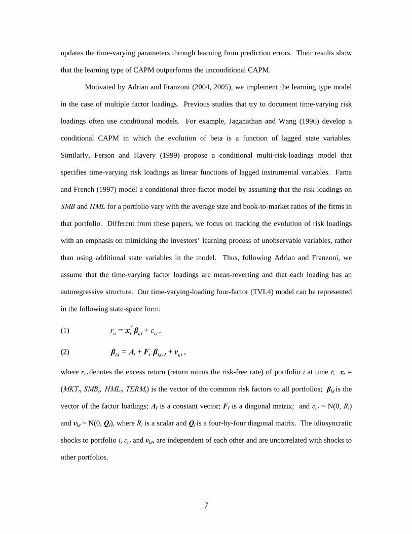
autoregressive structure. Our time-varying-loading four-factor (TVL4) model can be represented

in the following state-space form:

(1) i,t i,tr = + ε′t i,tx β ,

(2) = + +i,t i i i,t -1 i,tβ A F β ν ,

where ri,t denotes the excess return (return minus the risk-free rate) of portfolio i at time t; xt =

(MKTt, SMBt, HMLt, TERMt) is the vector of the common risk factors to all portfolios; βi,t is the

vector of the factor loadings; Ai is a constant vector; Fi is a diagonal matrix; and εi,t ~ N(0, Ri)

and vi,t ~ N(0, Qi), where Ri is a scalar and Qi is a four-by-four diagonal matrix. The idiosyncratic

shocks to portfolio i, εi,t and vi,t, are independent of each other and are uncorrelated with shocks to

other portfolios.

8

Equations (1) and (2) are estimated by the Kalman Filter. The Kalman Filter is a

dynamic procedure that updates unobservable factor loadings by learning through prediction

errors in returns that contain the most updated information. Since the factor loadings are affected

by idiosyncratic shocks and change over time, the Kalman Filter is a better methodology than the

OLS in capturing the dynamics of the factor loadings.

The Kalman Filter consists of two steps: prediction and updating. Since the factor

loadings are not observable, investors need to form their expectations based on available

information. In the prediction step, the one-period ahead forecast of iβ at time t-1 can be

expressed as:

(3) = + i,t | t -1 i i i,t -1 | t -1β A F β .

Based on the expectations of the risk loadings, the expected excess return of portfolio i is:

(4) i,t|t -1r = ′t i,t|t -1x β .

After ri,t is realized at time t, the prediction error can be expressed as:

(5) i,t | t-1 i,t i,t | t-1η = r - r ,

where i,t | t-1η contains new information about i,tβ beyond i,t | t -1β .

In the updating step, based on the prediction error, the inference of risk loading i,tβ ,

denoted as i,t | tβ , can be updated with information up to time t:

(6) = + × i,t | t -1ηi, t | t i, i,tt | t -1β β K ,

where Ki,t is the Kalman gain, which determines how much weigh to be assigned to the prediction

error i,t | t-1η .3 In practice, investors continue to adjust their inference about risk loadings through

3 The Kalman gain = -1

i,t | t -1fi,t i,t | t -1 tK P X , where = E[( )( ) ]′i,t | t -1 i,t i,t | t -1 i,t i,t | t -1P β - β β - β and

= +i,t|t -1 if R′t i, t | t -1 tX P X .

9

learning new information. The dynamic process in equation (6) mimics the investors’ learning

process on the unobservable risk loadings. After incorporating the new information from the

prediction error i,t | t-1η , the updated risk loadings i,t | tβ can be used to form the expectation of the

risk loadings at time t+1, i,t +1| tβ . Here we only briefly introduce the idea of how the Kalman

Filter mimics the investors’ learning process of time-varying risk loadings. For details on the

Kalman Filter methodology, see Hamilton (1994) and Kim and Nelson (2001).

III. Data and methodology

A. Data

The data used in this paper are kindly provided by Professor Kenneth R. French on his

website at Dartmouth. They are monthly returns of 25 portfolios double-sorted by size (SZ) and

book-to-market ratio (BM) covering the period from July 1963 to December 2004. A portfolio’s

BM in year t is the sum of book equities of the firms in the portfolio for the fiscal year ending in

year t-1 divided by the sum of their SZ in December of year t-1. A portfolio’s SZ is the average

of the logarithms of market equities of the firms in the portfolio at the end of June in year t. On

the formation dates (the beginning of July from 1963 to 2004), all NYSE, AMEX, and NASDAQ

stocks are sorted into five groups based on their SZ. The breakpoints are the NYSE market equity

quintiles at the end of June in each year. These stocks are then divided independently into five

equal BM groups. Twenty-five portfolios are constructed from the intersections of the five SZ

and five BM groups. The average monthly return is calculated over the period from July in year t

to June in year t+1. All stocks in a portfolio are value weighted on the formation date. The five-

by-five SZ and BM double-sorted portfolios are a standard set for testing asset pricing models.

Previous empirical results show that the returns of the small (the smallest SZ) and growth (the

lowest BM) portfolios cannot be adequately explained by the Fama-French three-factor model.

10

The Fama-French three-factor model consists of three portfolios constructed to mimic

underlying risk factors in returns. The portfolios include the zero-investment portfolios formed

on SZ (denoted as SMB) and BM (denoted as HML), as well as the excess return of a value-

weighted market portfolio (denoted as MKT). The TERM factor we propose is defined as the

yield spread between the ten-year government bond and the three-month Treasury bill.4 The data

of these two variables are taken from the Federal Reserve Bank of St. Louis website.

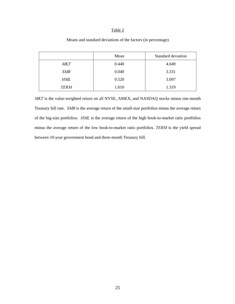
Table 1 reports the time-series means and the standard deviations of the monthly returns

of the five-by-five SZ/BM double-sorted portfolios, and Table 2 reports those of the four factors.5

Table 1 exhibits a familiar pattern: Within a specific BM (SZ) group, the average return increases

as SZ falls (BM rises). The only exception is at the lowest BM quintile. This exception shows the

first signal that Fama-French’s risk factors constructed by SZ (SMB) and BM (HML) may not be

able to explain the cross-sectional returns in these growth portfolios (the portfolios in the lowest

BM quintile).

The other signal that may hint on the possible failure of the Fama-French model is that

the standard deviations of the small portfolios (the portfolios in the smallest SZ quintile) and the

growth portfolios are larger compared to the other portfolios. This suggests that the returns of the

small/growth portfolios are more volatile than those of the other portfolios. Since the values of

the risk factors are the same across different portfolios, relatively higher volatilities in the returns

4 Studies using yield spread between a long-term bond and a short-term treasury bill as a proxy

for interest rate risk include Chen, Roll, and Ross (1986), Fama and French (1993), Adrian and

Franzoni (2005), and Petkova (2006).

5 Since estimating the time-varying parameter model via the Kalman Filter needs wild guess for

initial values of parameters, the first five years of estimates (1963:7 to 1968:12) are eliminated to

offset the effect of the wild guess. Thus, Tables 1 and 2 report the statistics for the data from

1968:7 to 2004:12.

11

of these portfolios imply that these factors may not be able to explain the cross-sectional returns

in these portfolios.

B. Measurement of the pricing errors

In the constant-loadings models, the pricing error is defined as the excess portfolio return

that cannot be explained by the proposed risk factors:

(7) i,t i,t= r α ′− t ix β ,

where xt is the vector of the common risk factors and βi is the vector of the corresponding factor

loadings. Jensen (1968) suggests a time series regression to estimate the pricing error. That is,

the excess return is regressed on a constant and the risk factors by OLS. The estimated intercept

is the estimated pricing error ( îα ). This estimated intercept should not be statistically different

from zero if the model can well explain the returns of portfolio i. A t-test can be used to check

the statistical significance.

In our time-varying-loadings setup, following Adrian and Franzoni (2005), the pricing

error at time t of portfolio i is estimated as:

(8) ˆî,t i,t= r α ′− t i,t|t -1x β ,

where î,t|t -1β is estimated by the Kalman Filter [see equations (1)-(6) in Section II]. Then the

estimated pricing error of portfolio i ( îα ) is the time-series mean of î,tα :

(9) 2

1ˆ ˆ-1

T

i i,tt=

α = αT ∑ .

The standard deviation of îα is:

(10) 21 ˆ ˆˆ ( )- 2

T

i i,t it=2

σ α - αT

= ∑ .

12

In a well-specified asset-pricing model, the pricing error ˆiα should be insignificantly different

from zero. The standard t-statistics can be used to check the statistical significance.

There are two measures of the overall performance of the model across all portfolios.

The first one is the root mean squared error (RMSE), which gives equal weight to the pricing

errors of individual portfolios:

(12) RMSE = 2

=1

1 ˆN

ii

αN ∑ ,

where N is the number of portfolios. The second measure is the composite pricing error (CPE)

suggested by Campbell and Vuolteenaho (2004):

(13) CPE = -1ˆˆ ˆα'Ω α

where α is the N×1 vector consists of the individual estimated pricing errors and Ω is a N×N

diagonal matrix with ˆ 2iσ ’s on its diagonal. The weighting matrix -1Ω places less weight on more

volatile portfolios.6

IV. Results

Table 3 reports the individual and aggregate pricing errors from the four models considered in

this paper, (1) the constant-loadings three-factor model (the Fama-French model), (2) the

constant-loadings four-factor model, (3) the time-varying-loadings three-factor model, and (4) the

time-varying-loadings four-factor model (the TVL4 model), in Panels (A)-(D), respectively. The

constant-loadings models are estimated by OLS and the time-varying-loadings models are

estimated by the Kalman Filter (with Maximum Likelihood Estimations).

6 The composite pricing error suggested by Campbell and Vuolteenaho (2004) is -1ˆˆ ˆα'Ω α . We

take a squared root of the measure to express the pricing errors in levels.

13

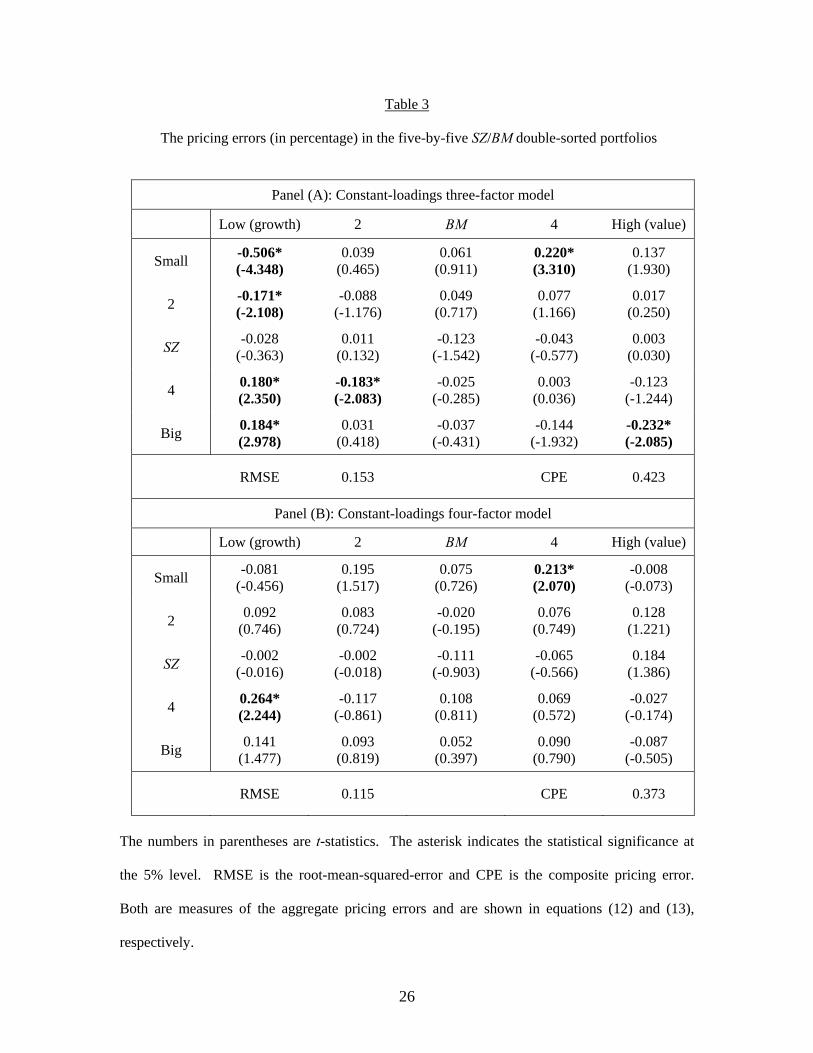
Panel (A) shows that, among the 25 portfolios, seven portfolios have a pricing error that

is significantly different from zero at the 5% level. Five of these seven portfolios are located

either in the small (smallest SZ) portfolios quintile or in the growth (lowest BM) portfolios

quintile. The findings are in line with previous studies [e.g., Petkova (2006) and Adrian and

Franzoni (2005)] in that the returns of the small and the growth portfolios cannot be successfully

explained by the Fama-French three-factor model.

Incorporating the TERM factor into the conventional Fama-French model, Panel (B)

shows that the number of significant individual pricing errors is decreased from seven to two, one

of which is located in the lowest BM quintile. For the aggregate pricing errors, the RMSE and the

CPE are reduced from 0.153 % and 0.423% in Panel A to 0.115% and 0.373% in Panel (B),

respectively. Since the TERM factor represents a proxy for the risk related to the innovations in

the discount rates, the results confirm our conjectures that the returns of the small or growth

portfolios are sensitive to such risk, and that the TERM factor documents the information about

risk related to changes in the discount rates that the Fama-French factors cannot fully capture.

Adding the TERM factor into the conventional Fama-French model can help to reduce the

abnormal returns in the small and growth portfolios.

Panel (C) reports the pricing errors for the three-factor model with time-varying factor-

loadings. Compared with Panel (A), even though those small/growth portfolios with significant

pricing errors in Panel (A) still show significant pricing errors in Panel (C), those two portfolios

with significant pricing error in the other quintiles do not show significant pricing errors in Panel

(C). The overall performance of the time-varying loadings model is better than that of the

constant-loadings model: both the RMSE and the CPE are reduced by about 10%. The better

performance of the time-varying loadings model implies that the learning process mimicked by

the Kalman Filter improves the accuracy of forecasts for risk loadings. This is consistent with the

findings of Adrian and Franzoni (2005) in their time-varying beta model.

14

Comparing Panel (C) and Panel (D), which reports the pricing errors for the TVL4 model,

we can see the importance of the TERM factor again. The performance of the TVL4 model is

very impressive. The null hypothesis that the pricing error of individual portfolio is equal to zero

can only be rejected at the 5% level in one growth portfolio. For the overall performance, the

RMSE and the CPE are reduced by 57% and 50%, respectively, when the TERM factor is added

to the time-varying loadings model.

Similarly, comparing Panel (D) and Panel (B), we also see an improvement by modeling

the factor loadings as time-varying. Although the additional TERM factor conveys information

beyond the Fama-French factors, the OLS regression is still not able to track the time-varying

factor-loadings, which leads to imprecise estimates of the loadings. Under the framework of a

learning process, the accuracy of the estimates of risk loadings improves as the Kalman Filter

captures the dynamics of the risk loadings.

Finally, the improvement of the performances from the Fama-French model to the TVL4

model can be seen by comparing Panel (A) and Panel (D). The number of portfolios with

significant pricing errors drops from seven to one. The TVL4 model reduces the aggregate

pricing error in the Fama-French model by more than 50%.

V. Robustness Checks

The above results confirm our hypotheses that (1) the TERM factor contains information related

to innovations to discount rates for which the Fama-French three factors cannot fully account; and

that (2) the Kalman filter improves the accuracy of the estimation of factor-loadings since the

learning process mimicked by the filter captures the dynamics of the factor-loadings that the

common OLS estimation cannot.

However, we have only focused on the five-by-five SZ/BM double-sorted portfolios

because these are where our motivation is derived from. These portfolios are also the most

commonly used ones in the literature. Whether or not our TVP4 model derived from this

15

particular portfolio design can still perform well in other samples, that is, the data mining

problem, may be an issue of concerns. Therefore, it is necessary to investigate the performance

of our model in other samples.

A. An alternative portfolio formation

Daniel and Titman (1997) argue that it could be wrongful to examine asset pricing

models only within portfolios sorted by characteristics known to be related to average returns.

Therefore, to check the importance of the two modifications we make on the three-factor model

in general, we further evaluate the performances of the models in industry-sorted portfolios.

Fama and French (1997) find that the risk loadings of the industry-sorted portfolios exhibit great

time variation and are difficult to be estimated precisely. Therefore, it would be interesting to see

whether our TVL4 model can solve this problem. We use the ten industry-sorted portfolios

provided by Professor Kenneth R. French on his website. The industries are categorized by the

firms’ four-digit SIC codes at the time of the portfolio formation. Panel (A) of Table 4 shows the

means and the standard deviations of these portfolios.

Panel (B) of Table 4 reports the pricing errors from those four models considered in this

paper. In the constant-loadings three-factor model, statistically significant pricing errors are

shown in the Consumer Durables and the Healthcare industries. Adding the TERM factor into the

model does not improve the model like it does in the SZ/BM double-sorted portfolios. This is not

too surprising because firms that are more sensitive to the interest rate risk do not particularly

reside in any specific industry. However, the time-varying-loadings specification does improve

the performance of the model. Especially, when combined with the addition of the TERM factor,

our TVL4 model does not generate any statistically significant pricing error for any individual

16

industry. The model’s overall performance is also much better than the traditional Fama-French

model. Both the RMSE and the CPE are reduced by more than 40%.7

B. An alternative sample period

Previous studies have intensively explored the post-1963:7 sample for the five by five

SZ/BM double-sorted portfolios. This is because first of all, the book values for firms are not

generally available in the pre-1963 COMPUSTAT dataset. Secondly, the COMPUSTAT has a

serious selection bias prior to 1963, which are tilted toward big historically successful firms [see

Fama and French (1992)]. Finally, the CAPM is usually found to fail in explaining cross-

sectional returns, especially the book-to-market anomaly, in the post-1963:7 sample [see

Campbell and Vuolteenaho (2004) and Adrian and Franzoni (2005)].

Since many researchers investigate the asset pricing model with the same dataset, data

mining has become a potential problem. Ferson and Harvey (1999) suggest that out-of-sample

studies may reduce the risk of data mining. A good example is Davis, Fama, and French (1998),

who extend the analysis of the U.S. data back to 1929. Campbell and Vuolteenaho (2004) argue

that pre-1963 sample provides an opportunity for an out-of-sample test because this sample is

relatively untouched in comparison with the well mined post-1963 sample. Therefore, in this

subsection, we experiment with the pre-1963:7 data of the five-by-five SZ/BM double-sorted

7 We also experiment with 30 and 48 industry-sorted portfolios provided by Professor Kenneth R.

French on his website. The results, not shown here but available upon requests, confirm the

superiority of our TVL4 model. When the constant three-factor model is used, six of the 30

industry-sorted portfolios, and nine of the 48 industry-sorted portfolios, have a statistically

significant pricing error. When the TVL4 model is used, there is no statistically significant

pricing error existing in either set of portfolios. Both the RMSE and the CPE are reduced by

more than 30%.

17

portfolios. Due to the availability of the bond return data, we can only extend our experiment

back to 1953.

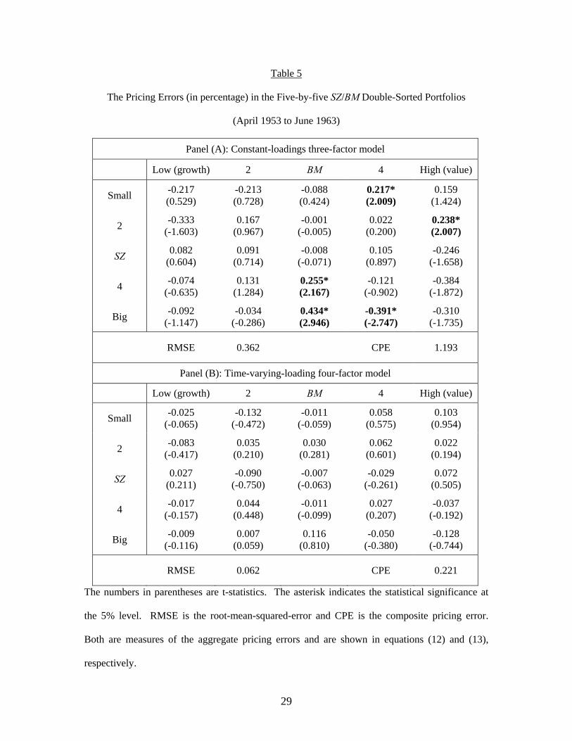
Table 5 shows the results of the five-by-five SZ/BM double-sorted portfolios for the

period 1953:4-1963:6. Panel (A) shows the pricing errors from the Fama-French constant-

loadings three-factor model and Panel (B) shows those from the TVL4 model. There are five

individual pricing errors that are significantly different from zero in Panel (A). Note that these

significant pricing errors are not observed particularly in the lowest BM or the smallest SZ

portfolios. Although these observations are not where our original motivation is derived from,

they can be explained by the selection bias (toward big historically successful firms) prior to

1963.8 Nonetheless, our TVL4 model still eliminates all these pricing errors. The model does not

produce any significant individual pricing errors for all 25 portfolios. Both the RMSE and the

CPE are reduced by more than 80% from the Fama-French three-factor model to our TVL4

model.

C. An alternative factor

As a robustness check, we further compare the effect of the TERM factor to that of a

popular factor that has been shown to explain abnormal stock returns in the literature. The

momentum factor is the average of the returns on high prior-return portfolios minus the average

of the returns on low prior-return portfolios. This factor is to pick up the short-run delayed price

reactions to firm-specific information. Jegadeesh and Titman (1993) argue that the moment

8 Small-size and low-book-to-market-ratio portfolios prior to 1963 likely include those successful

firms independent of external financial conditions (interest rates). Furthermore, Campbell and

Vuolteenaho (2004) suggest that the NYSE has very strict profitability requirements for a firm to

be listed on the exchange in earlier years, and therefore growth portfolios tend to be consistently

profitable and insensitive to external financing.

18

effect is distinct from the value effect captured by BM. Fama and French (1996) show that their

three factors cannot successfully explain the returns of portfolios formed on short-term (two to 12

months) past returns. Carhart (1997) is the first to add the momentum factor into the Fama-

French three-factor model. He finds that, compared to the Fama-French three-factor model, his

four-factor model noticeably reduces the average pricing errors of portfolios sorted by past

returns. Here we evaluate the performance of the momentum factor in the five-by-five SZ/BM

double-sorted portfolios and compare it to the performance of the TERM factor in such portfolios.

Data on the momentum factor and the method of constructing it are provided by

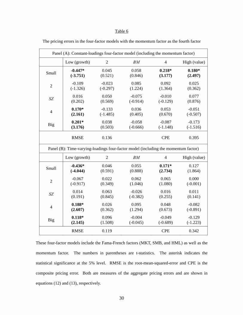
Professor Kenneth R. French on his website. Panel (A) of Table 6 shows the pricing errors from

the constant-loadings four-factor model and Panel (B) shows those from the time-varying-

loadings four-factor model. Both use the momentum factor as the fourth factor. Comparing

Panel (A) of Table 6 and Panel (A) of Table 3, we can see that the addition of the momentum

factor only reduces the number of pricing errors from seven to five; while Panel (B) of Table 3

shows that the addition of the TERM factor reduces the number of pricing errors from seven to

two. Incorporating the time-varying-loadings specification, Panel (B) of Table 6 shows that there

are still four portfolios with significant pricing errors when the momentum factor is used. Recall

that in Panel (D) of Table 3, there is only one portfolio with a significant pricing error when the

TERM factor is used. Comparing the RMSEs and the CPEs, the models with the TERM factor

have smaller aggregate pricing errors than the models with the momentum factor. Therefore, the

TERM factor outperforms the momentum factor in explaining the abnormal returns in the SZ/BM

sorted portfolios.

V. Conclusion

Fama and French’s three-factor model has produced an influential impact on the development of

asset pricing models. However, empirical studies show that this model cannot fully capture the

cross-sectional average stock returns in the SZ/BM double-sorted portfolios, especially in the

19

small and the growth portfolios. The three-factor model generates unexplained pricing errors in

several of these 25 portfolios. A special characteristic of small and growth firms is that they are

more sensitive to interest rate risk. Therefore, we are motivated to add into the model the TERM

factor, which proxies for risk caused by shifts in interest rates. In addition, since it has been

shown in the literature that factor loadings exhibit time variations, we use the Kalman Filter

procedure to estimate the movements of our factor loadings and to replicate investors’ learning

processes.

Using U.S. stock market data, we show that both modifications are essential to improving

the performance of the three-factor model in the SZ/BM double-sorted portfolios. Especially, our

time-varying-loadings four-factor (TVL4) model explains the cross-sectional returns without any

statistically significant pricing error in 24 out of the 25 SZ/BM double-sorted portfolios. Our

model also reduces the aggregate pricing errors generated by the three-factor model by more than

50%. These results confirm our hypotheses that (1) the TERM factor contains information related

to innovations to discount rates that the Fama-French three factors cannot fully account for; and

that (2) the Kalman filter improves the accuracy of the estimation of the loading because the

learning process mimicked by the filter captures the dynamics of the factor loadings that the

common OLS estimation cannot.

To check the robustness of our results, we further experiment with an alternative portfolio

formation, with a different sample period, and with an alternative risk factor. We first evaluate

the performance of the TVL4 model in industry-sorted portfolios. It is shown that no statistically

significant pricing error is observed when the TVL4 model is used. The aggregate pricing error is

also reduced significantly. The second experiment is an out-of-sample test suggested by Ferson

and Harvey (1999). We check the performances of the TVL4 model on the five-by-five SZ/BM

double-sorted portfolios for the sample period 1953:4-1963:6. The results show that the TVL4

model remarkably reduces both the individual and aggregate pricing errors in comparison with

the Fama-French three-factor model. Finally, we replace the TERM factor with the momentum

20

factor and evaluate the models in the SZ/BM double-sorted portfolios. The results show that, in

contrast to the outstanding performance of the TVL4 model with the TERM factor, the TVL4

model with the momentum factor only moderately improves the Fama-French three-factor model.

The focus of this paper is to test whether the TERM factor and the time-varying-loadings

specification are able to eliminate the pricing errors generated by the Fama-French three-factor

model, especially in the small and the growth portfolios. We successfully prove that these two

modifications improve the three-factor model in these portfolios. However, it is not proper to

claim a full victory of our TVL4 model because it needs to be tested in other types of portfolio

formations and/or in other samples. Due to the limitation on publicly available data, we only

experiment with several industry-sorted portfolios and a different sample period. Further

robustness checks, such as investigations of data from other countries, should be a topic of

interest for future studies. Nonetheless, this paper provides a good starting point and shows that

future studies should not ignore the effects of the interest-rate risk and the investors’ learning

process.

21

References:

Adrian, T. and F. Franzoni, 2004. “Learning about beta: a new look at CAPM tests.” Staff

reports of Federal Reserve Bank of New York, No.193.

Adrian, T. and F. Franzoni, 2005. “Learning about beta: time-varying factor loadings, expected

returns, and the conditional CAPM.” Working paper, HEC School of Management, Paris.

Aretz, K., S. Bartram, and P. Pope, 2005. “Macroeconomic risks and the Fama and French

model.” Working paper, Lancaster University, Department of Accounting and Finance.

Campbell, J. and R. Shiller, 1991. “Yield spreads and interest rate movements: a bird eye view.”

Review of Economic Studies, 58, 495-514.

Campbell, J. and T. Vuolteenaho, 2004. “Bad beta, Good beta.” American Economic Review,

Vol. 94, No. 5.

Carhart, M., 1997. “On persistence in mutual fund performance.” Journal of Finance, 52, 57-82.

Cornell, B., 1999. “Risk, duration, and capital budgeting: new evidence on some old questions.”

Journal of Business, 72, 183-200.

Chen, N., R. Roll, and S. Ross, 1986. “Economic forces and the stock market.” Journal of

Business, 59, 383-403.

Chiao, C. and C. J. Hueng, 2005. “Overreaction effects independent of risk and characteristics:

Evidence from the Japanese stock market.” Japan and the World Economy, 17, 431-455.

Daniel, K. and S. Titman, 1997. “Evidence on the characteristics of cross sectional variation in

stock returns.” Journal of Finance, 52, 1-33.

Davis J., E. Fama, and K. French, 2000. “Characteristics, Covariances, and Average Returns:

1929 to 1997.” Journal of Finance, 55, 389-406.

Diebold, F., G. Rudebusch, and B. Aruoba, 2006. “The macroeconomy and the yield curve: a

dynamic latent factor approach.” Journal of Econometrics, 131, 309-338.

Elton, E., M. Gruber, and C. Blake, 1995. “Fundamental Economic Variables, Expected Returns,

and Bond Fund Performance.” Journal of Finance, 50, 1229-1256.

22

Fama, E. and K. French, 1992. “The cross-section of expected stock returns.” Journal of

Finance, 47, 427-465.

Fama, E. and K. French, 1993. “Common risk factors in the returns on stocks and bonds.”

Journal of Financial Economics, 33, 3-56.

Fama, E. and K. French, 1996. “Multifactor explanations of asset pricing anomalies.” Journal of

Finance, 51, 55-84.

Fama, E. and K. French, 1997. “Industry costs of equity.” Journal of Financial Economics, 43,

153-193.

Ferson, W. and C. Harvey, 1991. “The variation of economic risk premiums.” Journal of

Political Economy, 99, 385-415.

Ferson, W. and C. Harvey, 1993. “The risk of predictability of international equity

returns.” Review of Financial Studies, 6, 527-566.

Ferson, W. and C. Harvey, 1999. “Conditioning Variables and the Cross Section of Stock

Returns.” Journal of Finance, 54, 1325-1360.

Franzoni, F., 2006. “Where is beta going? The riskiness of value and small stocks.” Working

paper, HEC School of Management, Paris.

Hamilton, J., 1994. Time Series Analysis. New Jersey: Prentice Hall.

Harvey, C., 1989. “Time-varying conditional covariance in tests of asset pricing models.”

Journal of Financial Economics, 24, 289-317.

Jagannathan, R. and Z. Wang, 1996. “The conditional CAPM and the cross-section of expected

returns.” Journal of Finance, 51, 3-54.

Jegadeesh, N. and S. Titman, 1993. “Returns to buying winners and selling losers: implications

for stock market efficiency.” Journal of Finance, 48, 65-91.

Jensen, M., 1968. “The performance of mutual funds in the period of 1945-1954.” Journal of

Finance, 23, 389-416.

23

Kim, C. and C. Nelson, 1999. State-space Models with Regime Switching: Classical and Gibbs-

sampling Approaches with Applications. Cambridge, Mass: MIT Press.

Perez-Quiros, G. and A. Timmermann, 2000. “Firm size and cyclical variations in stock returns.”

Journal of Finance, 55, 1229-1262.

Petkova, R., 2006. “Do the Fama-French factors proxy for innovations in predictive variables?”

Journal of Finance, 61, 581-612.

24

Table 1

Means and standard deviations of the returns in the five-by-five SZ/BM double-sorted portfolios

Mean

Low (growth) 2 BM 4 High (value)

Small 0.490 1.166 1.253 1.458 1.530

2 0.762 1.075 1.282 1.377 1.471

SZ 0.832 1.160 1.130 1.267 1.456

4 0.986 0.971 1.208 1.273 1.314

Big 0.873 1.037 1.010 1.051 1.080

Standard deviation


Small 8.407 7.161 6.091 5.620 5.956

2 7.656 6.200 5.384 5.196 5.794

SZ 7.067 5.606 5.038 4.800 5.436

4 6.304 5.376 4.987 4.723 5.440

Big 4.968 4.749 4.493 4.344 4.909 The monthly returns (in percentage) cover the period from July 1968 to December 2004. A

portfolio’s BM in year t is the sum of book equities of the firms in the portfolio for the fiscal year

ending in year t-1 divided by the sum of their SZ in December of year t-1. A portfolio’s SZ is the

average of the logarithms of market equities of the firms in the portfolio at the end of June in year

t. On the formation dates, all NYSE, AMEX, and NASDAQ stocks are sorted into five groups

based on their SZ. The breakpoints are the NYSE market equity quintiles at the end of June in

each year. These stocks are then divided independently into five equal BM groups. Twenty-five

portfolios are constructed from the intersections of the five SZ and five BM groups. The average

monthly return is calculated over the period from July in year t to June in year t+1. All stocks in

a portfolio are value weighted on the formation date.

25

Table 2

Means and standard deviations of the factors (in percentage)

Mean Standard deviation

MKT 0.440 4.649

SMB 0.040 3.331

HML 0.520 3.097

TERM 1.610 1.319 MKT is the value-weighted return on all NYSE, AMEX, and NASDAQ stocks minus one-month

Treasury bill rate. SMB is the average return of the small-size portfolios minus the average return

of the big-size portfolios. HML is the average return of the high book-to-market ratio portfolios

minus the average return of the low book-to-market ratio portfolios. TERM is the yield spread

between 10-year government bond and three-month Treasury bill.

26

Table 3

The pricing errors (in percentage) in the five-by-five SZ/BM double-sorted portfolios

Panel (A): Constant-loadings three-factor model


Small -0.506* (-4.348)

0.039 (0.465)

0.061 (0.911)

0.220* (3.310)

0.137 (1.930)

2 -0.171* (-2.108)

-0.088 (-1.176)

0.049 (0.717)

0.077 (1.166)

0.017 (0.250)

SZ -0.028 (-0.363)

0.011 (0.132)

-0.123 (-1.542)

-0.043 (-0.577)

0.003 (0.030)

4 0.180* (2.350)

-0.183* (-2.083)

-0.025 (-0.285)

0.003 (0.036)

-0.123 (-1.244)

Big 0.184* (2.978)

0.031 (0.418)

-0.037 (-0.431)

-0.144 (-1.932)

-0.232* (-2.085)

RMSE 0.153 CPE 0.423

Panel (B): Constant-loadings four-factor model


Small -0.081 (-0.456)

0.195 (1.517)

0.075 (0.726)

0.213* (2.070)

-0.008 (-0.073)

2 0.092 (0.746)

0.083 (0.724)

-0.020 (-0.195)

0.076 (0.749)

0.128 (1.221)

SZ -0.002 (-0.016)

-0.002 (-0.018)

-0.111 (-0.903)

-0.065 (-0.566)

0.184 (1.386)

4 0.264* (2.244)

-0.117 (-0.861)

0.108 (0.811)

0.069 (0.572)

-0.027 (-0.174)

Big 0.141 (1.477)

0.093 (0.819)

0.052 (0.397)

0.090 (0.790)

-0.087 (-0.505)

RMSE 0.115 CPE 0.373

The numbers in parentheses are t-statistics. The asterisk indicates the statistical significance at

the 5% level. RMSE is the root-mean-squared-error and CPE is the composite pricing error.

Both are measures of the aggregate pricing errors and are shown in equations (12) and (13),

respectively.

27

Table 3 (continued)

Panel (C): Time-varying-loadings three-factor model


Small -0.475* (-4.234)

0.032 (0.399)

0.060 (0.953)

0.216* (3.446)

0.138* (2.000)

2 -0.113 (-1.545)

-0.023 (-0.358)

0.061 (1.020)

0.077 (1.274)

0.024 (0.381)

SZ -0.006 (-0.084)

0.050 (0.664)

-0.070 (-1.035)

-0.014 (-0.213)

0.042 (0.528)

4 0.208* (2.825)

-0.086 (-1.174)

-0.001 (-0.011)

0.012 (0.160)

-0.104 (-0.119)

Big 0.156* (2.690)

0.062 (0.969)

-0.012 (-0.152)

-0.102 (-1.446)

-0.197 (-1.847)

RMSE 0.137 CPE 0.390

Panel (D): Time-varying-loading four-factor model


Small -0.017 (-0.151)

0.092 (1.160)

0.057 (0.904)

0.096 (1.505)

0.019 (0.280)

2 0.035 (0.484)

0.007 (0.106)

-0.069 (-1.170)

-0.015 (-0.256)

0.070 (1.102)

SZ 0.003 (0.038)

-0.055 (-0.732)

-0.084 (-1.242)

-0.062 (-0.946)

0.062 (0.791)

4 0.162* (2.193)

-0.038 (-0.523)

-0.012 (-0.166)

-0.006 (-0.077)

-0.054 (-0.585)

Big 0.002 (0.034)

0.033 (0.508)

0.026 (0.323)

0.041 (0.589)

-0.025 (-0.237)

RMSE 0.058 CPE 0.197




respectively.

28

Table 4

The results for the ten industry-sorted portfolios

Industry

Sample Statistics Estimated Pricing Errors

Mean Standard deviation

Constant-loadings

three-factor model

Constant-loadings

four-factor model

Time-varying-loadings

three-factor model

Time-varying-loadings

four-factor model

(1) 1.102 4.681 0.088 (0.687)

0.088 (0.446)

0.105 (0.966)

-0.045 (-0.415)

(2) 0.909 5.857 -0.373* (-2.270)

-0.613* (-2.420)

-0.288 (-1.802)

-0.188 (-1.175)

(3) 0.929 4.998 -0.143 (-1.522)

-0.250 (-1.728)

-0.094 (-1.132)

-0.099 (-1.198)

(4) 1.115 5.438 0.107 (0.546)

0.201 (0.666)

0.122 (0.656)

0.148 (0.796)

(5) 0.920 7.070 0.258 (1.640)

0.028 (0.115)

0.128 (0.892)

-0.082 (-0.575)

(6) 0.960 4.848 0.065 (0.435)

0.166 (0.726)

-0.008 (-0.056)

0.016 (0.113)

(7) 1.021 5.543 -0.047 (-0.354)

0.033 (0.159)

-0.010 (-0.088)

-0.082 (-0.692)

(8) 1.100 5.203 0.450* (2.899)

0.850* (3.574)

0.405* (2.996)

0.249 (1.836)

(9) 0.900 4.245 -0.184 (-1.274)

-0.167 (-0.749)

-0.134 (-0.963)

-0.039 (-0.288)

(10) 1.063 5.245 -0.084 (-1.042)

-0.025 (-0.197)

-0.016 (-0.224)

0.012 (0.170)

RMSE 0.223 0.356 0.178 0.121

CPE 0.232 0.369 0.194 0.134

The industries are: (1) Consumer Nondurables; (2) Consumer Durables; (3) Manufacturing; (4)

Energy; (5) High Technology; (6) Telecommunication; (7) Wholesale and Retail; (8) Healthcare;

(9) Utilities; and (10) Other Industries (firms that are not included in the first nine industries). The

numbers in parentheses are t-statistics. The asterisk indicates the statistical significance at the 5%

level. RMSE is the root-mean-squared-error and CPE is the composite pricing error. Both are

measures of the aggregate pricing errors and are shown in equations (12) and (13), respectively.

29

Table 5

The Pricing Errors (in percentage) in the Five-by-five SZ/BM Double-Sorted Portfolios

(April 1953 to June 1963)

Panel (A): Constant-loadings three-factor model


Small -0.217 (0.529)

-0.213 (0.728)

-0.088 (0.424)

0.217* (2.009)

0.159 (1.424)

2 -0.333 (-1.603)

0.167 (0.967)

-0.001 (-0.005)

0.022 (0.200)

0.238* (2.007)

SZ 0.082 (0.604)

0.091 (0.714)

-0.008 (-0.071)

0.105 (0.897)

-0.246 (-1.658)

4 -0.074 (-0.635)

0.131 (1.284)

0.255* (2.167)

-0.121 (-0.902)

-0.384 (-1.872)

Big -0.092 (-1.147)

-0.034 (-0.286)

0.434* (2.946)

-0.391* (-2.747)

-0.310 (-1.735)

RMSE 0.362 CPE 1.193

Panel (B): Time-varying-loading four-factor model


Small -0.025 (-0.065)

-0.132 (-0.472)

-0.011 (-0.059)

0.058 (0.575)

0.103 (0.954)

2 -0.083 (-0.417)

0.035 (0.210)

0.030 (0.281)

0.062 (0.601)

0.022 (0.194)

SZ 0.027 (0.211)

-0.090 (-0.750)

-0.007 (-0.063)

-0.029 (-0.261)

0.072 (0.505)

4 -0.017 (-0.157)

0.044 (0.448)

-0.011 (-0.099)

0.027 (0.207)

-0.037 (-0.192)

Big -0.009 (-0.116)

0.007 (0.059)

0.116 (0.810)

-0.050 (-0.380)

-0.128 (-0.744)

RMSE 0.062 CPE 0.221




respectively.

30

Table 6

The pricing errors in the four-factor models with the momentum factor as the fourth factor

Panel (A): Constant-loadings four-factor model (including the momentum factor)


Small -0.447* (-3.751)

0.045 (0.521)

0.058 (0.846)

0.218* (3.177)

0.180* (2.497)

2 -0.109 (-1.326)

-0.023 (-0.297)

0.085 (1.224)

0.092 (1.364)

0.025 (0.362)

SZ 0.016 (0.202)

0.050 (0.569)

-0.075 (-0.914)

-0.010 (-0.129)

0.077 (0.876)

4 0.170* (2.161)

-0.133 (-1.485)

0.036 (0.405)

0.053 (0.670)

-0.051 (-0.507)

Big 0.201* (3.176)

0.038 (0.503)

-0.058 (-0.666)

-0.087 (-1.148)

-0.173 (-1.516)

RMSE 0.136 CPE 0.395

Panel (B): Time-varying-loadings four-factor model (including the momentum factor)


Small -0.436* (-4.044)

0.046 (0.591)

0.055 (0.888)

0.171* (2.734)

0.127 (1.864)

2 -0.067 (-0.917)

0.022 (0.349)

0.062 (1.046)

0.065 (1.080)

0.000 (-0.001)

SZ 0.014 (0.191)

0.063 (0.845)

-0.026 (-0.382)

0.016 (0.255)

0.011 (0.141)

4 0.188* (2.607)

0.026 (0.362)

0.095 (1.294)

0.048 (0.673)

-0.082 (-0.891)

Big 0.118* (2.145)

0.096 (1.508)

-0.004 (-0.045)

-0.049 (-0.689)

-0.129 (-1.223)

RMSE 0.119 CPE 0.342 These four-factor models include the Fama-French factors (MKT, SMB, and HML) as well as the

momentum factor. The numbers in parentheses are t-statistics. The asterisk indicates the

statistical significance at the 5% level. RMSE is the root-mean-squared-error and CPE is the

composite pricing error. Both are measures of the aggregate pricing errors and are shown in

equations (12) and (13), respectively.

Interest-Rate Risk Factor and Stock Returns: A Time...

Documents

Transcript of Interest-Rate Risk Factor and Stock Returns: A Time...