Interactive Spreadsheets for

Celestial Navigation

Copyright 2009 - 2011. Navigation Spreadsheets℠. All rights reserved.

TABLE OF CONTENTSIntroduction! 1

Lines of position (two-body) fix! 3

Lines of position (many-body) fix! 5

Running fix! 7

Noon sight ! 9

Noon curve! 11

Noon curve on a moving vessel! 14

Meridian transit on a moving vessel! 15

Ex-meridian latitude calculation! 16

Latitude from Polaris! 17

Dead reckoning position! 19

Dead reckoning fix of Estimated Position along LOP ! 20

Set and drift! 22

Closest point of approach! 24

Sextant altitude corrections! 26

Precomputed sextant altitude! 28

Averaging of sights: 1) precomputed slope! 29

Averaging of sights: 2) fitted slope! 30

Dip short of the horizon! 32

Distance by vertical angle! 33

Altitude correction for motion of the vessel! 34

Sight reduction using the intercept method! 35

The one-body fix! 38

Great-circle and rhumb-line sailings! 40

Copyright 2009 - 2011. Navigation Spreadsheets℠. All rights reserved.

Composite sailing! 42

Amplitude! 44

Almanac data! 45

Lunar distance clearing and UT recovery! 49

Precomputed lunar distance! 51

Alphabetical list of spreadsheets! 52

Literature! 53 Worksheet 54

Web: http://www.navigation-spreadsheets.com http://www.t-plotter.com

Blog: http://blog.navigation-spreadsheets.com

E-mail: pmh099@yahoo.com

Copyright 2009 - 2011. Navigation Spreadsheets℠. All rights reserved.

Introduction

In our world of ever expanding technology, many people have reached to the past to rediscover

the traditions of navigation on the high seas by using the sun, the moon, the planets, and the

stars. Even today in the age of the Internet, telecommunication satellites, and the Global

Positional System (GPS), there still are people who have reconnected with the earth and the sun

through the art and science of celestial navigation. Just as sailors did in the days of tall ships and

billowing sails, we also are able to determine our position on the earth by looking at the sky

armed with just a sextant, a chronometer, and some tables.

The spreadsheets available through this website are designed to increase the accuracy, reliability,

and the speed with which you can derive your position from observations of the heavens. First,

you take a sight with a sextant, make the appropriate corrections to the measured altitude, and

retrieve the necessary astronomical data from an almanac spreadsheet. Then you enter the data

into the appropriate sight reduction spreadsheet - and you're done! The use of these spreadsheets

finds a middle ground between manually doing all the steps needed to plot your line of position

on a chart and simply pushing a button to read your location on a GPS receiver.

Our spreadsheets are programmed to provide and process several types of sight data commonly

acquired in celestial navigation:

• Intersections of lines of position

• Running fix

• Noon sight, noon curve, and meridian transits

• Dead reckoning (DR) position and a DR fix along a line of position

• Sextant altitude corrections

• Solutions of the navigation triangle (the intercept method and sailings calculations)

• Almanac data (calculation of Geographical Positions of main celestial bodies)

• Lunar distance (UT recovery)

1

In all spreadsheets the cells expecting the user’s input data are formatted in italics on green

background and the results are displayed with the normal font in cyan cells, all next to labels in

bold. Cells marked yellow are used for both input and output (i.e. intermediate results). Except

in the spreadsheet aries_stars.xls, the cells containing angular input data are formatted as

compound fractions with three-digit denominators; thus the angle of 27° 31.1´ is to be entered as

27 311/600. These angular input data are accompanied by grey cells displaying the fractional

portion of the data value in minutes of arc. This way you can verify that the input value was

entered correctly. You may also use the minispreadsheet minutes.xls for the same purpose.

Enter the fractional value in cell B1, or the decimal value in cell B5, and inspect the equivalent

angular value in arcminutes. Cells containing time data (with the exception of cell B6 in

running_fix.xls, dr.xls, and dr_fix_lop.xls) are formatted using the 24-hour clock as HH:MM:SS.

(For times between 12 and 1 o’clock make sure that the cell ends up with the correct AM/PM

value.) All other cell contents represent partial results of the computations and can be ignored,

unless you want to get into the nitty-gritty details. Our adopted sign convention marks north

latitudes and east longitudes as positive; south latitudes and west longitudes are considered

negative. On output, fractions of degrees (minutes of arc) are displayed without their sign. We

also provide a simple worksheet in which you may record intermediate results, such as output of

almanac spreadsheets that need to be transferred into the input of the sight reduction

spreadsheets. OpenOffice seems to have a problem here; you may need to reformat these cells

using only two-digit fractions and therefore round angles to whole minutes. Another alternative

is to enter these values using the formula bar as: =27+311/600. If the value is negative (e.g.

declination S 27° 31.1´), then in the formula you must use minus signs for both the whole degree

component and its fraction: =-27-311/600. The formatting of some results does not explicitly

separate the sign on output from the integer degree value. Therefore, for results between -1° and

+1° be sure to pick up the correct sign from the decimal value of the result in a neighboring cell,

because zeroes are usually displayed unsigned. The spreadsheets are protected against accidental

changes of data and formulae by locking all but the input cells. You do have the option of

unlocking everything, since there is no password, although this is not recommended.

2

Lines of position (two-body) fix

If, for instance, both the sun and the

moon are simultaneously visible in the

sky it is possible to obtain your

position by finding the intersection of

the two lines of position (LOP)

obtained from each sight. Typically

there are two distinct possible

positions and it should be very easy to

decide which one is the correct one.

The measured sextant altitude is

corrected for index error, refraction,

parallax, and semidiameter which

results in the observed altitude (Ho).

The Universal Time (UT) of the sight

is used to determine the Geographical

Position (GP) with the help of an

almanac. The declination and Greenwich Hour Angle (GHA) of the GP plus the Ho for the two

sights are entered in row 3 of the spreadsheet. The solutions are displayed in rows 8 and 10.

3

The following image shows the spreadsheet lops.xls.

Summary for spreadsheet lops.xls:Input cells: A3, B3, C3, D3, E3, F3

Output cells: A8, B8, C8, D8, E8, F8, A10, B10, C10, D10, E10, F10

The problem preset in this spreadsheet is treated in The Celestial Navigation Mystery Solved by

David Owen Bell on p. 79.

The spreadsheet two_body_fix.xls has the same interface as lops.xls and solves the same problem

using a different method. Whereas lops.xls employs the techniques of spatial geometry (Van

Allen paper), two_body_fix.xls applies the equations of spherical trigonometry (John Karl,

Celestial Navigation in the GPS Age, pp. 78-79). The latter reference also discusses the

applicability of this approach to finding the latitude without a meridian sight or knowledge of

UT (the double-altitude method).

4

Lines of position (many-body) fix

Spreadsheet many_body_fix.xls implements a procedure for computing a location from multiple

lines of position obtained on a moving vessel. This navigation problem typically arises from a

round of observations acquired during twilight. Enter the desired UT of the fix in cell A2, vessel

speed in knots in cell B2, and course (track) in cell C2. The initial best guess for the position

goes into cells E2 and F2. The observational and GP data start in line 9 and are entered into

columns A (name), B (UT of observation), C (observed altitude Ho), E (GHA), and G

(declination). The computed coordinates are displayed in row 6. The spreadsheet performs a

block of four iterations of this procedure. On output, the value d in cell D4 should be less than

20 nautical miles; if that is not the case, copy cells A6 and D6 into cells E2 and F2 and repeat

this procedure until convergence is reached.

5

The following image shows the spreadsheet many_body_fix.xls.

Summary for spreadsheet many_body_fix.xls:Input cells: A2, B2, C2, E2, F2, from row 9 down columns A, B, C, E, G

Output cells: D4, B6, C6, E6, F6

The method and the problem preset in this spreadsheet were taken from pp. 282-283 of the

Nautical Almanac, 2010 Commercial Edition.

6

Running fix

If two different celestial bodies are not available for simultaneous measurements, it is possible to

obtain the two lines of position by observing the same body twice within a few hours. The first

observed LOP then has to be displaced by the distance and direction traveled during the time

interval between observations. The spreadsheet running_fix.xls is an extended version of

two_body_fix.xls and is used the same way. Additional input information consists of the average

speed in knots (cell A7), time interval in hours (cell B7, formatted as a regular floating-point

number), and course (cell C7 - track, measured from true north clockwise). The solutions are

displayed in rows 10 and 12. The distance traveled (in nautical miles) is in cell D7.

7

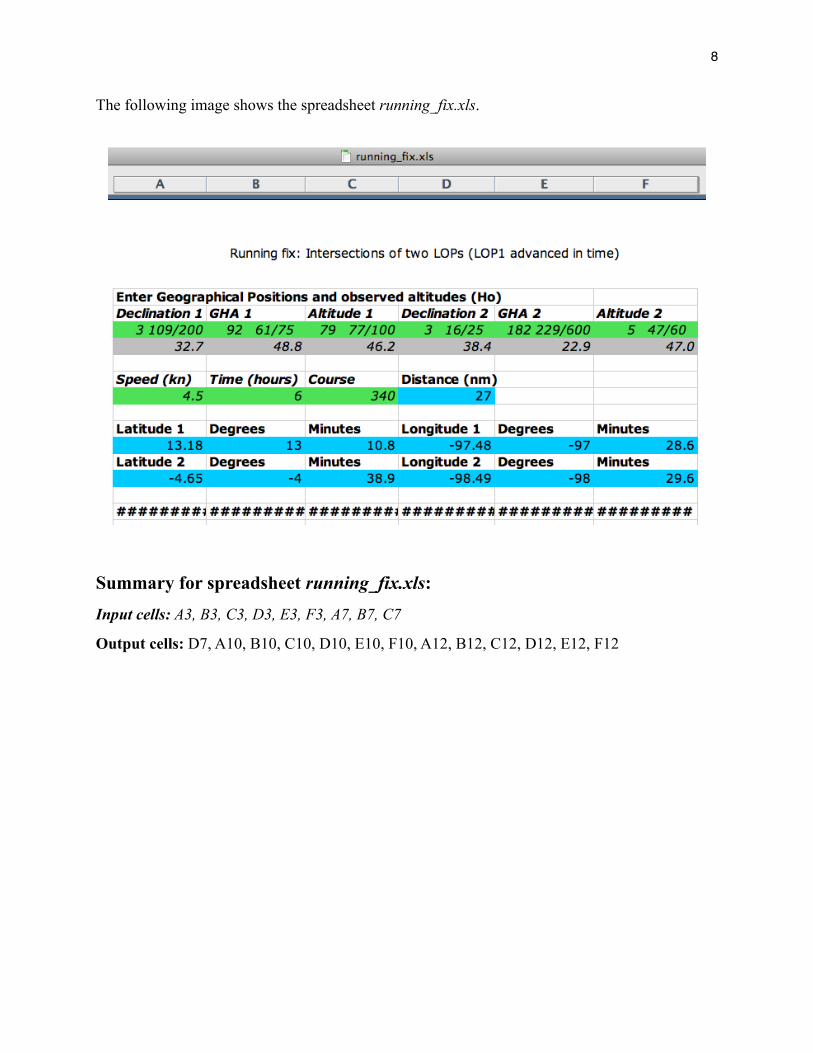
The following image shows the spreadsheet running_fix.xls.

Summary for spreadsheet running_fix.xls:Input cells: A3, B3, C3, D3, E3, F3, A7, B7, C7

Output cells: D7, A10, B10, C10, D10, E10, F10, A12, B12, C12, D12, E12, F12

8

Noon sight

Observing the sun at LAN (local apparent noon) allows you to determine the position from a

single sight. The need for a second line of position is eliminated by the additional piece of

information implicitly contained in a noon sight: i.e. that the sun and the observer are on the

same meridian. Thus the geometric arrangement is reduced to a 1-dimensional problem along

this meridian, with the sun bearing either directly north or south from the observer. In the

spreadsheet noon_sight.xls the Ho at LAN is entered in cell D1 and the UT in cell D13. From an

almanac you find the sun’s declination (D3) and the correction for equation of time; the latter is

entered in D14 if positive, or in D15 if negative (without its sign). This correction is always less

than one hour, therefore it is to be entered as 00:MM:SS. It can be (optionally) copied from cell

B16 that interpolates between cells B14, B15; therein you may enter the equation of time values

(without their signs) for the 00h and 12h instants that straddle your noon UT in cell D13. (This

interpolator works in the vast majority of cases when the two equation of time values are of the

same sign.) The final two entries identify the observer’s hemisphere (D4) and the sun’s bearing

9

(D5); enter N for north and S for south. In the special case of the sun in zenith (Ho = F1 = 90°)

your position is the sun’s GP and the sun’s bearing (D5) is as unimportant as it is undefined. The

latitude of the position is displayed in cells D9, D10, D11 and cells D16, D17, D18 contain the

longitude.

The following image shows the spreadsheet noon_sight.xls.

Summary for spreadsheet noon_sight.xls:Input cells: D1, D3, D4, D5, D13, D14, D15, (B14, B15 optional)

Output cells: D9, D10, D11, D16, D17, D18

Intermediate cell: B16

10

Noon curve

The noon sight in principle allows you to determine the position and indeed the latitude can be

measured to a good accuracy. However, in practice the inferred longitude is often inaccurate due

to the difficulty of marking the precise moment of LAN. The sun hangs at its maximum altitude

for a couple of minutes and every four seconds of uncertainty in the time of LAN introduce an

error of 1 arc minute of longitude.

In order to mitigate this problem with the noon sight it is recommended to make several

observations around the time of LAN, fit the measurements with a “noon curve” and infer the Ho

and UT from this fit. The spreadsheet noon_curve.xls does precisely that. It is an extended

version of the noon_sight.xls spreadsheet with the difference that the Ho (H1) and UT (H13) at

LAN are computed from the noon curve instead of being entered by the user.

11

The noon curve is constructed via the following steps:

• Enter the UT’s of your sights in column A and the corresponding Ho’s in column B. You will

need at least three observations for the noon curve (which is a quadratic fit) to be defined.

• Insert a Chart (XY scatter type) with column B as the Y axis (“Data range” tab) and column A

for X-values (“Series” tab).

• Right-click on the plotted curve and select “Add Trendline” from the context menu. In the

“Type” tab select “polynomial” of order 2; in the “Options” tab check “Display equation on

chart.”

• Find the noon curve fitting equation of the type y = ax² + bx + c on the plot, retrieve the a, b, c

coefficients (complete with signs) and enter them into cells F1, F2, and F3.

• The entries for Hemisphere (H4), Sun bearing (H5), and Equation of time (H14 or H15, plus

the optional interpolation data in cells F14, F15) are entered as in the noon_sight.xls

spreadsheet.

• The position is displayed in cells H9, H10, H11 (latitude) and in cells H16, H17, H18

(longitude).

Alternatively, you may also use the spreadsheet noon_motion.xls (see below), which produces

the same results without the need for plotting a chart. That spreadsheet computes the coefficients

a, b, and c of the quadratic fit automatically. Extra pieces of information on input include the

number of observations in cell F4. Also, in this context set F1 cell value to zero and enter a

solstice day (June or December 21) in cells F6 and F7.

12

The following image shows the spreadsheet noon_curve.xls.

Summary for spreadsheet noon_curve.xls:Input cells: column A, column B, F1, F2, F3, H3, H4, H5, H14, H15, (F14, F15 optional)

Output cells: H9, H10, H11, H16, H17, H18

Intermediate cell: F16

13

Noon curve on a moving vessel

The movement of the observer and Sun’s declination change both distort the idealized parabolic

noon-curve shape treated by the noon_curve.xls spreadsheet. The spreadsheet noon_motion.xls

accounts for both of these effects assuming a uniform speed (F1) and course (F2) of the vessel

for the duration of the procedure. The number of observations goes to cell F4 and the date is

entered in cells F6 and F7. All other cells have the same meaning as in the noon_curve.xls

spreadsheet with important clarifications. The coordinates of the fix (H9-11 and H16-18) pertain

to the vessel’s position at the moment of the last observation; it is this moment for which the

declination of the Sun (H3) should be entered. The equation-of-time value (H14 or H15),

however, applies to the computed instant of local apparent noon (H13).

The following image shows the spreadsheet noon_motion.xls.

Summary for spreadsheet noon_motion.xls:Input cells: columns A and B, F1, F2, F4, F6, F7, H3, H4, H5, H14, H15, (F14, F15 optional)

Output cells: H9, H10, H11, H16, H17, H18

Intermediate cells: F16, H13

14

Meridian transit on a moving vessel

The spreadsheet transit.xls is a generalization of noon_motion.xls that can process meridian

transit data (both upper and lower) for any celestial body. The rate of change of declination (in

arc minutes per hour) is entered in cell F7. In cell H15 enter “U” for upper and “L” for lower

meridian transit.

The following image shows the spreadsheet transit.xls.

Summary for spreadsheet transit.xls:Input cells: column A, column B, F1, F2, F4, F7, H3, H4, H5, H14, H15

Output cells: H9, H10, H11, H16, H17, H18

Intermediate cell: H13

15

Ex-meridian latitude calculation

The ex-meridian.xls spreadsheet has the same general format of input and output cells as the

other meridian-transit-category spreadsheets. The one extra input data point is in cell B11

marking the time away from the actual meridian transit in the hours:minutes:seconds

(HH:MM:SS) format. Cell B12 displays the intermediate results: (altitude factor) from

Bowditch Table 24, and cell B13 shows the absolute value of the resulting change in altitude/

latitude from Bowditch Table 25.

The following image shows the spreadsheet ex-meridian.xls.

Summary for spreadsheet ex-meridian.xls:Input cells: B1, B3, B4, B5, B9, B11, B15

Output cells: B16, B17, B18

Intermediate cells: B12, B13

16

Latitude from Polaris

In the northern hemisphere, the observed altitude of Polaris indicates your latitude. This value is

only approximate because Polaris does not sit exactly above the North Pole. If you know your

longitude, you may use the polaris.xls spreadsheet to improve your latitude determination by

accounting for the small distance of Polaris from the Pole. Enter Universal Time (UT) of your

observation in row 2, longitude in cell A5, and observed altitude (Ho) of Polaris in cell B5. Your

latitude is displayed in cells D5 and E5. Cell F5 contains the azimuth of Polaris. In row 10 you

may see the Geographical Position of Polaris, which is computed from the UT. The SHA may

differ a little from published almanacs but this does not affect the spreadsheet’s latitude result.

17

The following image shows the spreadsheet polaris.xls.

Summary for spreadsheets polaris.xls:Input cells: A2, B2, C2, D2, E2, F2, A5, B5

Output cells: D5, E5, F5

Intermediate cells: B10, C10, E10, F10

The example preset in this spreadsheet is taken from p. 275 of the Nautical Almanac, 2009

Commercial Edition.

If your longitude is unknown, you may instead use the polaris_lha.xls spreadsheet with the LHA

of Polaris as input in cell A5. This LHA can be estimated by inspecting the relative orientation

of nearby star patterns (most likely the Ursa Minor constellation) with respect to the horizon. All

other data are placed in the same cells as in the polaris.xls spreadsheet.

18

Dead reckoning position

Spreadsheet dr.xls computes the dead reckoning

(DR) position (row 11) from the previous known

position (cells A3 and B3), average speed in knots

(cell A7), time interval in hours (cell B7, formatted

as a regular floating point number), and course

(cell C7).

The following image shows the spreadsheet dr.xls.

Summary for spreadsheet dr.xls:Input cells: A3, B3, A7, B7, C7

Output cells: A11, B11, C11, D11, E11, F11

19

Dead reckoning fix of Estimated Position along LOP

When only one line of position (LOP) is available, it is possible to find your estimated position

(EP) by using the dead reckoning position (DRP) as a guide. Spreadsheet dr_fix_lop.xls finds

the EP as the point along the LOP which is closest to the DRP. The previous known position is

entered in cells A3 and B3, average speed in knots in cell A7, time interval in hours in cell B7

(formatted as a regular floating point number), and course in cell C7. The LOP is defined as

usual by the GP and Ho (cells D3, E3, and F3). The EP is displayed in row 11. The distance (in

nautical miles) and bearing from the DRP to the EP are shown in cells C13 and F13, respectively.

20

The following image shows the spreadsheet dr_fix_lop.xls.

Summary for spreadsheet dr_fix_lop.xls:Input cells: A3, B3, D3, E3, F3, A7, B7, C7

Output cells: A11, B11, C11, D11, E11, F11, C13, F13

The problem preset in this spreadsheet is a variation on the one treated in The Celestial

Navigation Mystery Solved by David Owen Bell on p. xliii (Problem 1).

The auxiliary minispreadsheet time.xls can be used to add and subtract time data and also to

perform conversions between the HH:MM:SS and hours-decimal formats.

21

Set and drift

The following four spreadsheets

solve a number of variations of the

set and drift problem. The preset

values are taken from the end of

the "Dead Reckoning" chapter in

Bowditch.

set_and_drift.xls:

Calculation of set and drift from the difference between dead-reckoning and estimated positions.

22

ground_speed.xls:

Calculation of the ground speed from the current’s speed and direction (i.e. set and drift) and the

vessel speed relative to the water.

course_to_steer.xls:

Given the set and drift, the vessel's speed and the intended direction relative to ground, this

spreadsheet calculates the required vessel course and the resulting ground speed. If the vessel's

speed is too small to counteract the current, an error message is displayed in row 4.

23

course_and_speed.xls:

Calculation of the required vessel speed and course from the set and drift and the desired ground

speed and track.

Closest point of approach

24

The spreadsheet cpa.xls computes the closest point of approach (CPA) of another vessel. This

type of computation is useful for collision avoidance. All bearings and ranges (in nautical miles)

are relative to your vessel’s heading. The calculation encoded into this spreadsheet works with a

locally flat Earth’s surface (i.e. it is only valid for small distances) and assumes that both vessels

in question move with constant speeds and tracks during the relevant time interval. The vessel is

observed at two different ranges (cells A2 and C2) and relative bearings (cells B2 and D2)

separated by time interval entered into cell E2 in the HH:MM:SS format. From this information

the spreadsheet calculates the relative speed of the other vessel in knots (cell A5), range (cell B5)

and relative bearing (cell C5) at the CPA, and the time interval between the second observation

and the moment of the CPA (cell D5, in the HH:MM:SS format). If the range at CPA (cell A5) is

close to zero, and if the “at” time (cell D5) is positive, the two vessels are headed for collision.

The following image shows the spreadsheet cpa.xls.

Summary for spreadsheet cpa.xls:Input cells: A2, B2, C2, D2, E2

Output cells: A5, B5, C5, D5

25

Sextant altitude corrections

The spreadsheet alt_corr.xls performs the corrections to the sextant altitude Hs (cell B1) that are

needed to produce the apparent altitude Ha (cells B6, B7, B8) and the observed altitude Ho (cells

B12, B13, B14). The index correction goes to cell B2. Cell B4 contains a yes/no (Y/N) answer

to the question whether a reflecting artificial horizon was used. The semidiameter correction is

entered in cell B9; this is positive for lower limb and negative for upper limb observations. The

hight of eye in cell E1 (enter “ft” for feet or “m” for meters in cell F1) determines the dip

correction. Cells E2 and E3 control the refraction correction; the standard values are

Temperature = 10 ºC and Pressure = 1010 mb. Cell E6 contains the value of the horizontal

parallax (HP) in arc minutes. The Moon parallax can also be corrected for the oblateness of the

Earth by entering the latitude (E8) and azimuth (E9). The semidiameter value from either cell

E11 (Sun - typical preset value, or from the almanac) or E12 (Moon - computed from the HP) is

to be copied (with the appropriate sign characterizing the limb) into cell B11.

26

The following image shows the spreadsheet alt_corr.xls.

Summary for spreadsheet alt_corr.xls:Input cells: B1, B2, B4, B11, E1, F1, E2, E3, (E6, E8, E9 optional)

Output cells: B6, B7, B8, B12, B13, B14

Input/Output cells: E11, E12

The preset example contained in the spreadsheet is the upper limb Moon sight from p. 281 of the

Nautical Almanac, 2009 Commercial Edition.

27

Precomputed sextant altitude

The spreadsheet alt_prec.xls is a reversed version of alt_corr.xls. It provides the altitude Hs to

which the sextant may be preset before an observation. The observed altitude Ho (computed

with intercept.xls) is now input in cell B12 and the sextant altitude is displayed in cells B1 and

C1. The remaining cells have the same meaning as in alt_corr.xls.

The following image shows the spreadsheet alt_prec.xls.

Summary for spreadsheet alt_prec.xls:Input cells: B2, B4, B11, B12, E1, F1, E2, E3, (E6, E8, E9 optional)

Output cells: B1, C1, B6, B7, B8

Input/Output cells: E11, E12

28

Averaging of sights: 1) precomputed slope

Random errors can affect every individual sight. This problem can be mitigated by taking a set

of measurements and averaging them. The spreadsheet average1.xls can perform this function

for sextant altitude data (Hs). Enter the UT set in column A and the corresponding Hs set (in

degrees) in column B. In cells F1 and F2 enter the expected sextant altitudes based on your

position (dr.xls, almanac, intercept.xls, and alt_prec.xls spreadsheets are relevant here). This

spreadsheet then calculates a weighted least-squares straight-line fit to the data, whose slope is

derived from values in cells F2 and F3. From this fit it then extracts the average UT (cell G5)

and Hs (cells G6, G7, G8). You also have the option of evaluating the average Hs (cells F6, F7,

F8) at the UT of your choice (cell F5). Column D contains the weights (maximum=1.000) with

which each particular data point is influencing the final result. The “Scatter” parameter (cell

F13, in arcminutes) should be adjusted so that cell F14 is as close to 1 as possible and the

weights in column D end up neither all 1.000, nor all (but one) much smaller than 1.000. Cells

F10, F11, F12 should be small as they indicate the convergence of the encoded iterative

procedure and the closeness of the fit to the original data. (Further details about the technique

and the meaning of these cells are available upon request.) The time interval over which the

average is computed should be short (about 5 minutes maximum), so that the assumed straight-

line approximation remains justified. The resulting average altitude is a sextant altitude Hs and

therefore should be processed with alt_corr.xls to yield the observed altitude Ho.

29

The following image shows the spreadsheet average1.xls.

Summary for spreadsheet average1.xls:Input cells: column A, column B, F1, F2, F5, F13

Output cells: column D, F6, F7, F8, F10, F11, F12, F14, G5, G6, G7, G8

Averaging of sights: 2) fitted slope

The spreadsheet average2.xls performs the same function as average1.xls, but for observed

altitude data (Ho) in column B, while allowing the procedure to also choose the slope of the fit.

Additional input data include the speed (cell F1) and course (cell F2) of the vessel, the hourly

declination change rate (cell F5, in arcminutes), and azimuth (cell F7, in degrees) of the observed

body. The remaining cells serve the same function as in average1.xls. The weights in column D

should come out neither all 1.000, nor all (but two) very small.

30

The following image shows the spreadsheet average2.xls.

Summary for spreadsheet average2.xls:Input cells: column A, column B, F1, F2, F5, F7, F9, F17

Output cells: column D, F10, F11, F12, F14, F15, F16, F18, G9, G10, G11, G12

31

Dip short of the horizon

The spreadsheet dip_short.xls implements the formula behind Table 14 in Bowditch. The height

of eye can be entered in meters or feet (enter "m" or "ft" in cell C1). The distance to the

waterline in cell B2 is in nautical miles. The resulting dip is output in cell B3 in nautical miles.

The following image shows the spreadsheet dip_short.xls.

Summary for spreadsheet dip_short.xls:Input cells: B1, C1, B2

Output cells: B3

32

Distance by vertical angle

The spreadsheet distance.xls implements the formula from Bowditch to calculate the distance by

vertical angle between the waterline and the top of an object. Select "ft" or "m" in cells C1 and

C2, and enter the corrected vertical angle in cell B3. The distance in nautical miles is displayed

in cell B4.

The following image shows the spreadsheet distance.xls.

Summary for spreadsheet distance.xls:Input cells: B1, C1, B2, C2, B3

Output cells: B4

33

Altitude correction for motion of the vessel

The spreadsheet alt_move.xls calculates the effective observed altitude associated with a line of

position that is advanced or retarded by dead reckoning. In this technique of compensating for

the vessel motion the assumed position is unchanged and only the final adjusted LOP needs to be

plotted. Enter the original observed altitude and azimuth from spreadsheet intercept.xls in cells

A2 and B2. Enter ground speed and course made good in cells C2 and D2. The time interval in

cell E2 is positive to advance the LOP and negative to retard the LOP. The (signed) distance

traveled in nautical miles is displayed in cell F2. Reenter the adjusted observed altitude from

row 6 in cell E2 of intercept.xls to obtain the new intercept.

The following image shows the spreadsheet alt_move.xls.

Summary for spreadsheet alt_move.xls:Input cells: A2, B2, C2, D2, E2

Output cells: A6, B6, C6

Intermediate cell: F2

34

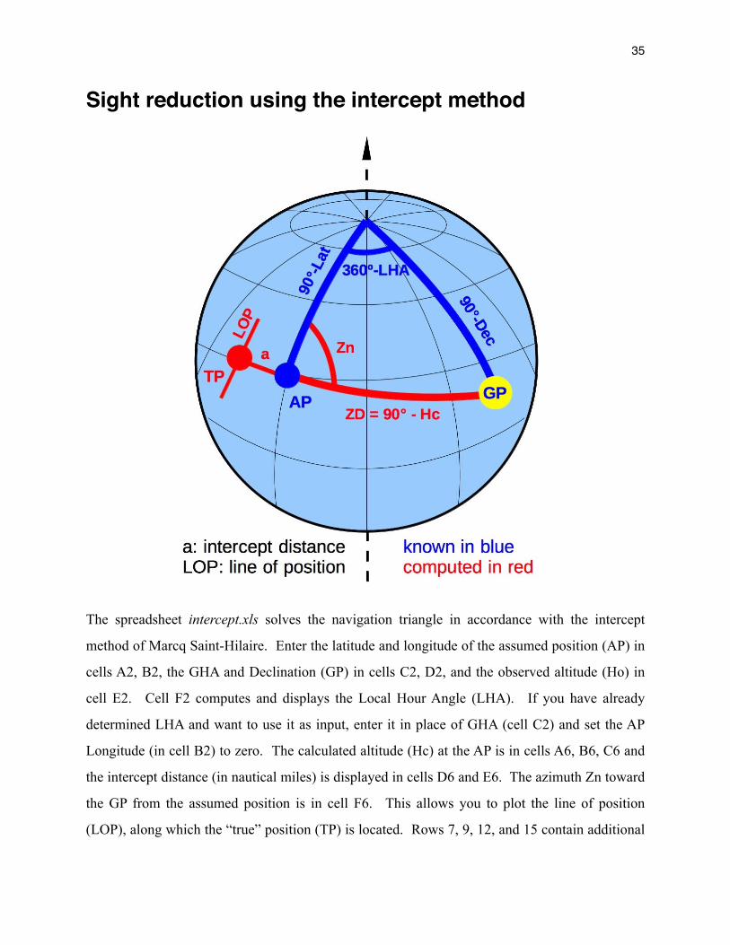
Sight reduction using the intercept method

The spreadsheet intercept.xls solves the navigation triangle in accordance with the intercept

method of Marcq Saint-Hilaire. Enter the latitude and longitude of the assumed position (AP) in

cells A2, B2, the GHA and Declination (GP) in cells C2, D2, and the observed altitude (Ho) in

cell E2. Cell F2 computes and displays the Local Hour Angle (LHA). If you have already

determined LHA and want to use it as input, enter it in place of GHA (cell C2) and set the AP

Longitude (in cell B2) to zero. The calculated altitude (Hc) at the AP is in cells A6, B6, C6 and

the intercept distance (in nautical miles) is displayed in cells D6 and E6. The azimuth Zn toward

the GP from the assumed position is in cell F6. This allows you to plot the line of position

(LOP), along which the “true” position (TP) is located. Rows 7, 9, 12, and 15 contain additional

35

information about LOP properties that allow the plotting of the LOP without the azimuth line

using the T-Plotter™. This reduces the clutter on the chart when multiple LOP’s are plotted.

The following image shows the spreadsheet intercept.xls.

Summary for spreadsheet intercept.xls:Input cells: A2, B2, C2, D2

Output cells: A6-F6, D7-F7, D9, E9, C12-F12, C15-F15

Intermediate cell: F2

It is also possible to use this spreadsheet to precompute altitudes before an observation. For that

purpose the computed altitude Hc displayed in cell A6 can be further matched to the actual

observation conditions with spreadsheet alt_prec.xls (enter Hc in cell B12), which corrects for

refraction, semidiameter, parallax, and index error.

36

The calculated LOP on a plotting sheet:

37

The one-body fix

If both the azimuth (Zn) and the altitude (Ho) of a celestial body is known, then it is possible to

obtain a fix for the “true” position (TP) from observing that one body alone. The spreadsheet

one_body_fix.xls solves the navigation triangle in this scenario. The GP is characterized by its

declination (cell A2) and Greenwich Hour Angle (B2). The azimuth (Zn) is entered in cell C2,

and the observed altitude (Ho) goes into cell D2. The TP coordinates are displayed in row 6.

38

The following image shows the spreadsheet one_body_fix.xls.

Summary for spreadsheet one_body_fix.xls:Input cells: A2, B2, C2, D2

Output cells: A6, B6, C6, D6, E6, F6

The preset data in this spreadsheet define an inverse problem to the one preset in intercept.xls.

39

Great-circle and rhumb-line sailings

This group of spreadsheets (sailings.xls, waypoints.xls, composite.xls) can assist you in planning

your trip from the point of Departure to Destination. The example preset in these spreadsheets

pertains to a trip from San Francisco (USA) to Yokohama (Japan). This choice is inspired by

Figure 2404 in Bowditch (p. 347).

In spreadsheet sailings.xls you enter the coordinates of the Departure and Destination points in

row 2. The spreadsheet calculates the distances and courses from Departure to Destination along

the resulting great circle (columns B, C) and rhumb line (columns E, F). The results are

displayed both assuming a perfectly spherical (row 6) as well as a flattened (row 7) Earth model.

The initial great-circle course in the yellow cell C6 is displayed with (otherwise unrealistic) three

decimal places in order to minimize numerical round-off errors when that value is subsequently

copied into the D2 input cell of the spreadsheet waypoints.xls. Finally, row 11 displays the

coordinates of the great-circle vertex on the path from Departure toward Destination..

The following image shows the spreadsheet sailings.xls.

40

Summary for spreadsheet sailings.xls:Input cells: B2, C2, E2, F2

Output cells: B6, C6, E6, F6, B7, C7, E7, F7, row 11

The spreadsheet waypoints.xls takes the coordinates of the Departure point (cells B2, C2) and (in

cell D2) the initial course (e.g. from cell C6 in sailings.xls). Row 7 displays the great-circle

vertex. Starting in row 11 you can use column A to specify the longitude of each waypoint along

the great circle. The spreadsheet then calculates the corresponding latitude (columns C, D, E)

and the (flattened Earth model) rhumb-line distance (column F) and the constant course (column

G) from the previous waypoint. The total length of this path is shown in cell F2.

The following image shows the spreadsheet waypoints.xls.

Summary for spreadsheet waypoints.xls:Input cells: B2, C2, D2, column A starting in row 11

Output cells: F2, row 7, columns C, D, E, F, G starting in row 11

For more information on the preset example please visit the SAILINGS entry on our blog.

41

Composite sailing

The spreadsheet composite.xls takes the initial great-circle course from sailings.xls (cell C6) and

modifies this calculated great-circle route from the point of Departure (cells B2, C2) to

Destination (cells E2, F2) so as not to go beyond the chosen limiting parallel of latitude (cell

B9). The resulting two waypoints along this limiting parallel (plus the third waypoint, which is

the Destination) are displayed in rows 12, 13, and 14. The courses shown in cells F12 and F14

are the initial great-circle (spherical Earth) courses to the first waypoint and to the Destination,

respectively. The constant course in cell F13 reflects the east or west direction of the latitude

sailing along the limiting parallel from the first to the second waypoint. If needed, waypoints

along the two great-circle legs of this trip can be calculated with waypoints.xls.

Yellow cells in rows 5 and 9 display text messages about the result and status of the composite

sailing calculation. These messages are:

cell D9: INVALID: the limiting parallel was chosen between the equator and either the Departure

or the Destination point. Composite sailing path cannot be computed in this case. Rows 12, 13,

and 14 are zeroed out.

cell F9: Composite OK: Non-trivial composite sailing path is successfully calculated.

cell E9: Unconstrained gc (great circle): The limiting parallel is between the vertex and its Pole

and therefore does not affect the originally computed great-circle sailing path. The first and

second waypoints are identical as they coincide with the vertex.

cell C5: Vertex beyond destination: This happens for relatively close Departure and Destination

points, which are not separated by the vertex. The choice of limiting parallel is voided in this

case and rows 13 and 14 are zeroed out. A great-circle sailing calculation is displayed in row 12.

The Unconstrained gc message is also displayed in cell E9 in this case.

42

The following image shows the spreadsheet composite.xls.

Summary for spreadsheet composite.xls:Input cells: B2, C2, E2, F2, B9

Output cells: row 7, block B12 through F14, E15

43

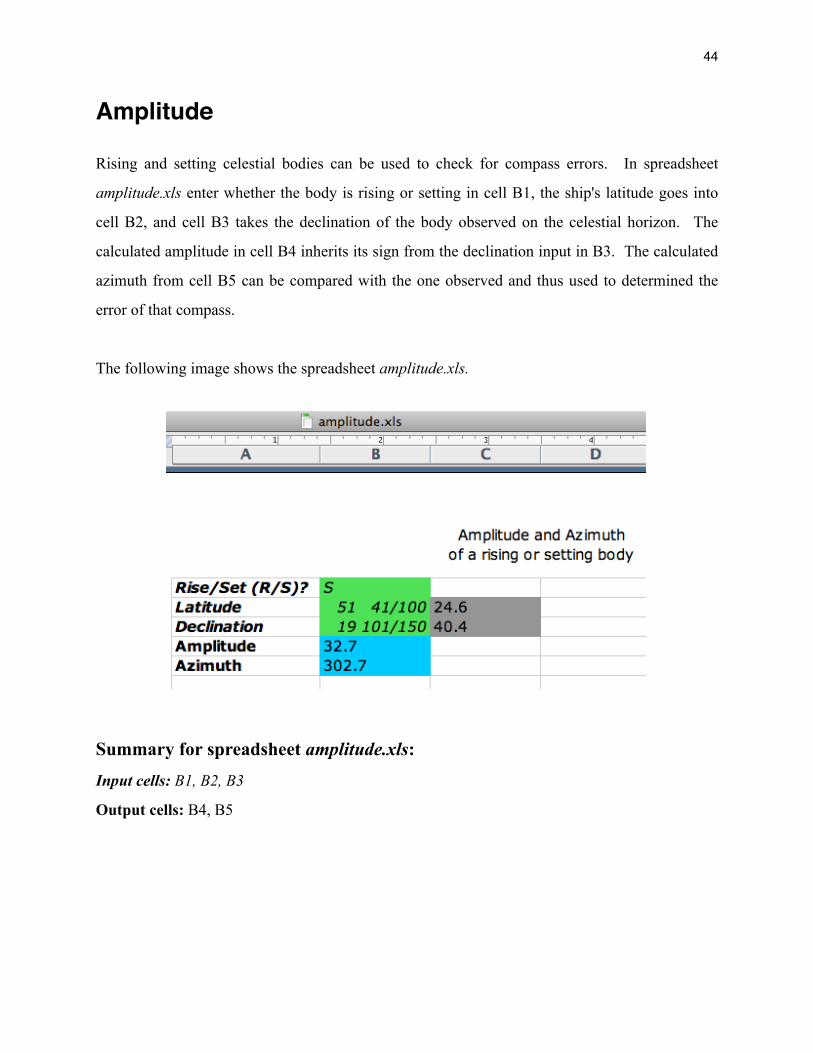
Amplitude

Rising and setting celestial bodies can be used to check for compass errors. In spreadsheet

amplitude.xls enter whether the body is rising or setting in cell B1, the ship's latitude goes into

cell B2, and cell B3 takes the declination of the body observed on the celestial horizon. The

calculated amplitude in cell B4 inherits its sign from the declination input in B3. The calculated

azimuth from cell B5 can be compared with the one observed and thus used to determined the

error of that compass.

The following image shows the spreadsheet amplitude.xls.

Summary for spreadsheet amplitude.xls:Input cells: B1, B2, B3

Output cells: B4, B5

44

Almanac data

The Geographical Position (GP) of a celestial body is the location on the surface of the Earth

from which this body appears directly overhead (at a given point in time). The measurement of

the body’s altitude above the horizon (Ho) with a sextant tells us how far we are from the GP

(Zenith distance = ZD = 90° - Ho). Therefore, in order to derive our position we need to know

the observed body’s GP at the moment its altitude was measured. The GP’s and other data are

published in almanacs as a function of Universal Time (UT). The spreadsheets sun.xls, moon.xls,

mercury.xls, venus.xls, mars.xls, jupiter.xls, saturn.xls, uranus.xls, neptune.xls, and

aries_stars.xls calculate the GP’s of these bodies from the year, month, day, hour, minute, and

second of UT. Thus there is no need for interpolation (increments and corrections). Data

calculated by the solar system spreadsheets also include the semidiameter (SD) and horizontal

parallax (HP) data. The equation of time is provided by the sun.xls spreadsheet.

45

The following image shows the spreadsheet moon.xls.

Summary for the Sun, Moon, and planetary spreadsheets:Input cells: A2, B2, C2, D2, E2, F2 (Universal Time)

Output cells: B5, C5, E5, F5 (GP); A8 (SD), C8 (HP, both in arcminutes); E8, F8

The spreadsheet aries_stars.xls provides the GHA of Aries from which the GHA of any star can

be determined by adding it to its SHA (sidereal hour angle). The UT is entered in row 2. The

GHA of Aries is displayed in cells B5 and C5. You may enter the SHA of the observed star in

cells E10, F10 (compound fractions are not used here) and retrieve its GHA from cells B11, C11.

If the observed star is one of the 57 main navigation stars you may also scroll down the

spreadsheet and find its GP there. The SHA’s and declinations of these main stars are in columns

E, F. The spreadsheet calculates these quantities from the UT taking into account the effects of

light aberration, Earth’s precession and nutation, and the star’s proper motion. The SHA for each

star is then added to the GHA of Aries resulting in the star’s GHA in columns B, C. The

numbers next to the star’s name are its almanac ID (column B) and magnitude (column C).

46

The following image shows the spreadsheet aries_stars.xls. Data in rows 10, 11 are for Markab.

Summary for spreadsheet aries_stars.xls:Input cells (in green): A2, B2, C2, D2, E2, F2 (Universal Time), E10, F10 (SHA)

Output cells (in cyan): columns B and C (GHA), columns E and F (declination)

Intermediate cells (in yellow): columns E and F (SHA) - from row 15 down

The Sun and planetary data are computed using the VSOP87 theory by Bretagnon and Francou.

The Moon data are calculated from the improved Chapront ELP-2000/82 lunar theory.

47

What star is this?

The spreadsheet what_star.xls is the combination of the aries_stars.xls and intercept.xls

spreadsheets. It allows the identification of the observed star based on UT (row 2), your known

location (cells A5, B5), observed altitude (cell C5), and azimuth (D5) of the star. Working with

the catalog of the 57 main navigation stars, in cell E5 the spreadsheet displays the star that is the

closest match to the input data.

The following image shows the spreadsheet what_star.xls.

Summary for spreadsheet what_star.xls:Input cells: A2, B2, C2, D2, E2, F2 (Universal Time), A5, B5, C5, D5Output cell: E5

48

Lunar distance clearing and UT recovery

The lunar distance technique allows you to determine Universal Time (UT) in case you cannot

rely on a chronometer. This method is not all that accurate by modern standards but it is rigorous

and can serve as a viable backup option. The spreadsheet lunar_distance.xls clears the lunar

distance and then performs the interpolation that yields an improved UT. Start by entering your

best estimate of UT in row 3. Select Time1 and Time2 instants on opposite sides of this estimate

and enter the corresponding GPs of the Moon and the other body in rows 7 and 12. The apparent

and observed altitudes go to row 17. Enter the observed lunar distance (corrected for index error

only) into cell B22. The objects’ semidiameters are placed in cells C22 and E22 (enter near-limb

values as positive, and far-limb values as negative). The computed UT is displayed in cell C30,

which is Time1 + T_add (i.e. the sum of cells A7 and B30). Verify that the interpolation factor

IntF (cell A30) lies between 0 and 1. If that is not the case then the two instants Time1 and

Time2 do not “bracket” the “true” UT and need to be changed accordingly.

49

The following image shows the spreadsheet lunar_distance.xls.

Summary for spreadsheet lunar_distance.xls:Input cells: row 3, A7-E7, A12-E12, B17, C17, E17, F17, B22, C22, E22

Output cells: A30, B30, C30

Intermediate lunar distance cells: F7, F12 (computed), F22 (centered), E27, F27 (cleared)

The method and example preset in this spreadsheet can be found in Celestial Navigation in the

GPS Age by John Karl, pp. 93-95.

50

Precomputed lunar distance

The spreadsheet ld_comp.xls allows the calculation of the center-to-center (i.e. no semidiameter)

geocentric lunar distance (cells A10, B10, C10) from almanac data (row 2). The topocentric

result in cells D10, E10, F10 includes the effect of Moon’s parallax on the lunar distance, when

observed from an assumed position (cells E6, F6). While these results do not include the effects

of refraction, they are close enough for your sextant to be preset to an angle that is sufficiently

close to the actual observed value. The values are preset for a Sun lunar on January 8, 2011,

UT = 22:00:00.

The following image shows the spreadsheet ld_prec.xls.

Summary for spreadsheet ld_prec.xls:Input cells: A2, B2, C2, E2, F2, E6, F6

Output cells: A10, B10, C10, D10, E10, F10

51

Alphabetical list of spreadsheets

1. alt_corr: sextant altitude corrections 2. alt_move: correction of observed altitude for motion of the vessel 3. alt_prec: precomputed sextant altitude 4. amplitude: amplitude and azimuth of a rising or a setting body 5. aries_stars: GHA of Aries and GPs of 57 main navigation stars 6. average1: averaging of sights (precomputed slope) 7. average2: averaging of sights (fitted slope) 8. composite: composite sailing calculation 9. course_and_speed: ground speed from the vessel speed and speed of current10. course_to_steer: vessel course from set and drift and desired ground track11. cpa.xls: closest point of approach from two ranges and relative bearings12. dip_short: dip short of the horizon13. distance: distance by vertical angle14. dr: dead reckoning position (DRP)15. dr_fix_lop: estimated position (EP) from a DRP and a celestial LOP16. ex_meridian: ex-meridian latitude calculation17. ground_speed: ground speed from vessel speed and set and drift18. intercept: intercept and azimuth for the St. Hilaire method19. jupiter: almanac data for Jupiter20. ld_prec: geocentric and topocentric lunar distance from almanac data21. lops: two-body fix (using spatial geometry)22. lunar_distance: LD clearing and chronometer resetting23. many_body_fix: multiple LOP fix calculation24. mars: almanac data for Mars25. mercury: almanac data for Mercury26. minutes: conversion of fractional angles into minutes of arc27. moon: almanac data for Moon28. neptune: almanac data for Neptune29. noon_curve: Sun LAN curve fix30. noon_motion: Sun LAN curve fix with motion of the vessel31. noon_sight: Sun LAN fix32. one_body_fix: fix from a zenith distance and azimuth33. polaris: latitude from Polaris (UT input)34. polaris_lha: latitude from Polaris (LHA input)35. running_fix: running fix (LOP1 advanced in time)36. sailings: great-circle and rhumb-line sailings37. saturn: almanac data for Saturn38. set_and_drift: set and drift from the difference between DRP and EP39. sun: almanac data for Sun40. time: conversion of time data between formats41. transit: fix from a meridian transit on a moving vessel42. two_body_fix: two-body fix (using spherical trigonometry)43. uranus: almanac data for Uranus44. venus: almanac data for Venus45. waypoints: rhumb-line sailing between great-circle waypoints46. what_star: star identification based on altitude and azimuth

52

Copyright 2009 - 2011. Navigation Spreadsheets℠. All rights reserved.

Literature

Jean Meeus, Astronomical Algorithms, Second Edition, Willmann-Bell (2005).

Nautical Almanac, 2009 Commercial Edition, United Kingdom Hydrographic Office (2008).

Nautical Almanac, 2010 Commercial Edition, United Kingdom Hydrographic Office (2009).

Nautical Almanac, 2011 Commercial Edition, United Kingdom Hydrographic Office (2010).

Nautical Almanac, 2012 Commercial Edition, United Kingdom Hydrographic Office (2011).

The Astronomical Almanac for the year 2009, The Stationery Office, United Kingdom (2007).

Explanatory Supplement to the Astronomical Almanac, University Science Books (2006).

The American Practical Navigator, (Bowditch 2002, 2004 revised PDF version).

Thomas J. Cutler, Dutton’s Nautical Navigation, 15th Edition, Naval Institute Press (2004).

John Karl, Celestial Navigation in the GPS Age, Paradise Cay Publications (2007).

David Burch, Emergency Navigation, Second Edition, McGraw-Hill (2008).

David Owen Bell, The Celestial Navigation Mystery Solved, Landfall Navigation (1999).

Hewitt Schlereth, Celestial Navigation in a Nutshell, Sheridan House (2000).

James A. Van Allen, An Analytical Solution of the Two Star Problem, Navigation 28 (1), (1981).

http://eclipse.gsfc.nasa.gov/SEhelp/deltatpoly2004.html

http://simbad.u-strasbg.fr/

http://www.absoluteastronomy.com/stars/

http://www.navigation-spreadsheets.com

53

Copyright 2009 - 2011. Navigation Spreadsheets℠. All rights reserved.

Worksheet for _________________ http://www.navigation-spreadsheets.com

Universal Time (UT)

Year Month Day Hours Minutes Seconds

Geographical Position (GP), semidiameter (SD), horizontal parallax (HP), Eq. of Time

GHA Declination SD HP Eq. of Time

Sextant altitude corrections

Hs IC AH? (Y/N) Ha Ho

Notes:

54

Copyright 2009 - 2011. Navigation Spreadsheets℠. All rights reserved.