Interactive Feedback between the Tropical Paciﬁc Decadal...

Interactive Feedback between the Tropical Pacific Decadal Oscillationand ENSO in a Coupled General Circulation Model

JUNG CHOI AND SOON-IL AN

Department of Atmospheric Sciences, Global Environmental Laboratory, Yonsei University, Seoul, South Korea

BORIS DEWITTE

Laboratoire d’Etude en Geophysique et Oceanographie Spatiale, Toulouse, France

WILLIAM W. HSIEH

Department of Earth and Ocean Sciences, University of British Columbia, Vancouver, British Columbia, Canada

(Manuscript received 8 August 2008, in final form 7 July 2009)

ABSTRACT

The output from a coupled general circulation model (CGCM) is used to develop evidence showing that the

tropical Pacific decadal oscillation can be driven by an interaction between the El Nino–Southern Oscillation

(ENSO) and the slowly varying mean background climate state. The analysis verifies that the decadal changes

in the mean states are attributed largely to decadal changes in ENSO statistics through nonlinear rectification.

This is seen because the time evolutions of the first principal component analysis (PCA) mode of the decadal-

varying tropical Pacific SST and the thermocline depth anomalies are significantly correlated to the decadal

variations of the ENSO amplitude (also skewness). Its spatial pattern resembles the residuals of the SST and

thermocline depth anomalies after there is uneven compensation from El Nino and La Nina events. In ad-

dition, the stability analysis of a linearized intermediate ocean–atmosphere coupled system, for which the

background mean states are specified, provides qualitatively consistent results compared to the CGCM in

terms of the relationship between changes in the background mean states and the characteristics of ENSO. It

is also shown from the stability analysis as well as the time integration of a nonlinear version of the in-

termediate coupled model that the mean SST for the high-variability ENSO decades acts to intensify the

ENSO variability, while the mean thermocline depth for the same decades acts to suppress the ENSO activity.

Thus, there may be an interactive feedback consisting of a positive feedback between the ENSO activity and

the mean state of the SST and a negative feedback between the ENSO activity and the mean state of the

thermocline depth. This feedback may lead to the tropical decadal oscillation, without the need to invoke any

external mechanisms.

1. Introduction

The Pacific decadal oscillation (PDO) pattern is usu-

ally defined by the leading principal component analy-

sis (PCA) mode of the sea surface temperature (SST)

anomalies in the Pacific Ocean north of 208N. Although

the PDO was initially defined over the North Pacific, the

global SST pattern associated with the PDO index shows

an El Nino–Southern Oscillation (ENSO)-like pattern

over the tropical Pacific (Zhang et al. 1997). Hence, it

is likely that there is a dynamical linkage between the

extratropical PDO and the tropical PDO. Regardless of

its main driver [i.e., an unstable air–sea interaction mode

proposed by Latif and Barnett (1994) or a stochastically

excited resonance mode proposed by Saravanan and

McWilliams (1997) and a combined process of that ex-

ternally forced by ENSO known as ‘‘reemergence’’ and

that driven by atmospheric white noise proposed by

Alexander et al. (1999) and Newman et al. (2003)], the

extratropical PDO signals were considered to be trans-

ported into the tropics (e.g., Gu and Philander 1997;

Vimont et al. 2003; Kleeman et al. 1999; Nonaka et al.

2002). On the other hand, tropical Pacific variability due

Corresponding author address: Prof. Soon-Il An, Department

of Atmospheric Sciences, Yonsei University, 134 Shinchon-dong,

Seodaemun-gu, Seoul 120-749, South Korea.

E-mail: [email protected]

15 DECEMBER 2009 C H O I E T A L . 6597

DOI: 10.1175/2009JCLI2782.1

� 2009 American Meteorological Society

to ENSO also communicates into the extratropics and

generates the extratropical PDO through teleconnec-

tion (Cane and Evans 2000; Newman et al. 2003; An

et al. 2007; Holland et al. 2007). Thus, a debate is un-

derway regarding whether the extratropical PDO drives

the tropical PDO (TPDO), or vice versa.

Recently, it has been suggested that the TPDO could

be generated through an internal process of the tropi-

cal Pacific without invoking any extratropical influences

(Timmermann and Jin 2002; Rodgers et al. 2004; Dewitte

et al. 2007b). In other words, TPDO is either stochasti-

cally excited (Kirtman and Schopf 1998; Yeh and Kirtman

2004; Burgman et al. 2008; Yeh and Kirtman 2009) or it

results from deterministic dynamical processes that are

possibly driven by a simple atmosphere–ocean coupling

(Timmermann et al. 2003). Although these two mecha-

nisms have different theoretical bases, they share a com-

mon feature. That is, the TPDO is characterized by the

ENSO-like patterns of anomalous sea surface temper-

atures (SSTA) and subsurface temperatures, with a time

scale of 10–20 yr. Thus, a close relationship between

TPDO and ENSO is expected intuitively.

As mentioned above, the TPDO can be generated

by intrinsic nonlinear processes. Timmermann and Jin

(2002) and Timmermann et al. (2003) emphasized that

nonlinearities in the tropical Pacific heat budget could

generate El Nino bursting with 10–20-yr time scales,

without any external influence or stochastic forcing. The

decadal occurrences of strong El Nino events (i.e., El Nino

bursting) indicate a stronger El Nino and a weaker

La Nina over a long period. This El Nino–La Nina

asymmetry enables the ENSO cycle to exert a nonzero

forcing on the tropical mean background states, possibly

modifying them. For example, Rodgers et al. (2004)

used a coupled general circulation model (CGCM) out-

put to show that the SST anomaly pattern of TPDO

resembles the residual SST anomaly pattern of El Nino

and La Nina, which indicates that the TPDO resulted

from the El Nino–La Nina asymmetry. Their point was

further supported by Sun and Yu (2009), based on an

analysis of observational data. Accordingly, the TPDO

is likely to be tightly linked to the intrinsic characteris-

tics of ENSO.

Conversely, the phase change of the TPDO (the change

of the mean background climate states) can modify

ENSO characteristics such as the amplitude, the period,

and the propagation pattern (Wang and Ropelewski

1995; Ye and Hsieh 2006). This phenomenon is referred

to as the decadal modulation of ENSO properties. For

example, the remarkable climate shift that occurred in

the late 1970s had a significant impact on ENSO ampli-

tude and frequency (An and Wang 2000). Also, Fedorov

and Philander (2000) stressed the importance of the mean

thermocline depth in modifying ENSO characteristics.

This mean state’s influence on ENSO was confirmed by

An and Jin (2000) and Wang and An (2001). Using an

intermediate-type coupled model, they showed that ob-

served changes in the mean background state would alter

the characteristics of ENSO. Timmermann et al. (1999)

concluded that the strengthening of the equatorial ther-

mocline gradient due to global warming very strongly

influences the ENSO statistics. On the whole, the TPDO

is likely to be an intrinsic mode in the tropical Pacific,

and it both affects ENSO and is influenced by ENSO

concurrently.

Many physical processes have been proposed to de-

scribe the nature of the relationship between the TPDO

and ENSO. Jin (2001) and Knutson and Manabe (1998)

suggested that the TPDO has essentially the same phys-

ical nature as the interannual modes in the tropical ocean

dynamics. Also, Kirtman and Schopf (1998) noted that

the various mechanisms of ENSO operate depending

on the characteristics of the mean state; for example,

the delayed oscillator mechanism drives SST anomalies

during decades when ENSO variability is high, and at-

mospheric noise drives SST anomalies when ENSO

variability is low. Obviously, the TPDO and ENSO can

be dynamically linked under a coupled nonlinear dy-

namical framework, but they do not interact in a simple

linear cause-and-effect relationship (Timmermann 2003).

Nevertheless, the previous studies omitted some aspects

of the physical mechanisms associated with the cyclic

nature of the TPDO. They tended to focus on a unidi-

rectional mechanism in which either the TPDO affects

ENSO or the reverse.

Our primary interest in this paper is to address this

issue in a fully coupled context that accounts for the

interactive feedback mechanism between the TPDO

and ENSO using the outputs of a CGCM that exhibits

realistic characteristics in terms of decadal variability

and ENSO modulation. In light of the results of sensi-

tivity experiments with an intermediate coupled model

in which the mean state is prescribed from the CGCM

outputs, we propose a mechanism through an asym-

metric nature of the ENSO cycle (An et al. 2005a,b;

Dewitte et al. 2007b; An 2009) and a modification of the

linear stability of ENSO by change in the mean state

(An and Jin 2000; An and Wang 2000; Fedorov and

Philander 2000).

This paper is organized as follows. The CGCM dataset

is outlined in section 2. In section 3, the correlation be-

tween the decadal modulations of the ENSO amplitude

and the slowly varying mean state is analyzed. The

asymmetric structures of ENSO within the different

mean states are described in section 4. Also within this

section, the modification of the ENSO amplitude by the

6598 J O U R N A L O F C L I M A T E VOLUME 22

mean states is investigated using an intermediate ocean–

atmosphere coupled model. Section 5 is devoted to a

discussion and concluding remarks.

2. Data and model

The oceanic component of the coupled model is taken

from the global configuration ORCA2 of the Ocean

Parallelise (OPA) 8.2 ocean general circulation model

(OGCM) (Madec et al. 1998). The horizontal resolution

is 28 in longitude, and it varies meridionally from 0.58

around the equator to 28 in the higher latitude. The

meridional grid resolution is increased near the equator

to improve the modeling of the equatorial dynamics. The

model includes a full thermodynamic sea ice component:

the Hibler-type dynamic–thermodynamic Louvain-La-

Neuve sea ice model that was developed at the Uni-

versite Catholique de Louvain (UCL) by Fichefet and

Morales Maqueda (1997). The atmospheric component

comes from the third version of the Action de Recherche

Petite Echelle Grande Echelle (ARPEGE)-climate at-

mospheric general circulation model developed at Meteo-

France (Deque et al. 1994). The climate version in its

standard configuration uses a T63 triangular horizontal

truncation. The vertical direction is discretized into 31

levels (20 levels in the troposphere) using a progressive

vertical hybrid coordinate that extends from the ground

to a height of about 34 km (7.35 hPa). The model time

step is 30 min for this resolution and time discretization

scheme. Detailed descriptions of the model are provided

by Cibot et al. (2005).

The ARPEGE and ORCA/Louvain Ice Model

(ORCALIM) models are coupled using the Ocean–

Atmosphere–Sea Ice–Soil (OASIS) 2.5 coupler developed

at the Centre Europeen de Recherche et de Formation

Avancee en Calcul Scientifique (CERFACS) (Valcke

et al. 2000). All concentrations of greenhouse gases are

fixed at preindustrial levels, and no flux corrections are

applied. The atmospheric initial state is set to January

conditions that are taken from an uncoupled integration

of ARPEGE. The initial ocean temperature and salinity

fields are taken from Levitus et al. (1998), and the ve-

locity field is set to zero. We integrated the coupled

model over 260 yr. We only considered the latest 200-yr

period in our subsequent analyses. The model variability

has been analyzed in previous studies (Cibot et al. 2005;

Dewitte et al. 2007a,b), with a focus on some of the as-

pects of the seasonal-to-decadal variability. The reader

is invited to refer to these studies for an assessment of

the realism of the simulation regarding the ENSO mode

and decadal variability. Despite a tendency for overly

energetic westward mean currents that enhance a near-

annual mode and a quasi-biennial ENSO (Dewitte et al.

2007a), the model variability is realistic, particularly

since its decadal mode shares many characteristics with

observations (Cibot et al. 2005). Dewitte et al. (2007b)

focused on the analysis of the vertical structure vari-

ability at decadal time scales. As mentioned above in

the introduction, the present study complements these

previous works by providing a dynamical description

and an interpretation of the rectification processes that

lead to the low-frequency ENSO modulation.

3. Correlation between ENSO amplitude and meanclimate state

To determine the frequency and locality of the ENSO

variation, we applied a wavelet analysis to an ENSO

index, that is, the time series of the Nino-3 SST anomaly

(i.e., SST anomaly averaged over the region 58S–58N,

1508–908W; anomalies are relative to the monthly cli-

matology). The real part of the wavelet transform of the

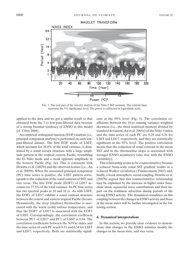
ENSO index is shown in Fig. 1. In this figure, which

covers the entire period, the large loadings occur around

the 2-yr period, which means that the ENSO period is

dominated by a biennial cycle (e.g., Cibot et al. 2005).

The biennial tendency of ENSO is a common feature

seen in many CGCM results (Guilyardi 2006). Using the

wavelet spectrum, we characterize the low-frequency

modulation of the ENSO amplitude by computing the

interannual (2–7 yr) wavelet variance of a Nino-3 SST

anomaly (hereafter referred to as the N3Var index),

as described in Torrence and Webster (1998). The

N3Var index strongly fluctuates on a decadal time scale

with about a 16-yr period, yet it has irregular variabil-

ity. Consistent with Cibot et al. (2005), large fluctua-

tions of N3Var obviously indicate large amplitudes of

ENSO.

The goal of this work is to explore the underlying

mechanisms leading to the relationship between the

N3Var index and the decadal change in the mean state.

The ‘‘mean state’’ in this study does not refer to a sta-

tionary state but instead refers to the tropical state over

decades or over longer time scales than the interan-

nual time scale. To identify the decadal changes, a 7-yr

low-pass filter was applied to the 178C isotherm depth

(a proxy for the thermocline depth) and the SST anom-

alies (hereafter LD17 and LSST, respectively). Note

that we take the 178C isotherm depth rather than the

208C isotherm depth as a proxy for the thermocline

depth to avoid a possible outcropping of the 208C iso-

therm that may occur because of the cold bias of this

CGCM. However, the decadal mode extracted from

the 178C isotherm depth shares a great similarity with

that from 208C isotherm depth (see Fig. 6a of Cibot

et al. 2005). Also, the 10-yr low-pass filter has been


applied to the data and we got a similar result to that

obtained from the 7-yr low-pass-filtered data because

of a strong biennial tendency of ENSO in this model

(cf. Cibot 2004).

An empirical orthogonal function (EOF) analysis (i.e.,

principal component analysis) is performed on each low-

pass-filtered dataset. The first EOF mode of LSST,

which accounts for 38.0% of the total variance, is dom-

inated by a zonal seesaw structure with a large ampli-

tude pattern in the tropical eastern Pacific, resembling

the El Nino mode and a weak opposite amplitude in

the western Pacific (Fig. 2a). This is consistent with

Dewitte et al. (2007b) and the observed feature (i.e., An

et al. 2005b). When the associated principal component

(PC) time series is positive, the LSST pattern corre-

sponds to the reduction of the zonal contrast of SST, and

vice versa. The first EOF mode (EOF1) of LD17 ac-

counts for 27.3% of the total variance. Its PC time series

has two spectral peaks at 10 and 16 yr. As with LSST,

the EOF1 of LD17 exhibits a zonal contrast structure

between the central and eastern tropical Pacific Oceans.

Dynamically, the deep (shallow) thermocline is asso-

ciated with the warm (cold) surface temperature, and

thus the EOF1 of LD17 is associated with the EOF1

of LSST. Correspondingly, the correlation coefficient

between PC1 of LD17 and PC1 of LSST is 0.94. The

correlation coefficients between the N3Var index and

the time series of each PC reach 0.51 and 0.54 for LSST

and LD17, respectively. Both are statistically signifi-

cant at the 99% level (Fig. 3). The correlation co-

efficients between the 10-yr running variance–weighted

skewness (i.e., the third statistical moment divided by

standard deviation; An et al. 2005a) of the Nino-3 index

and the time series of each PC are 0.29 and 0.26 for

LSST and LD17, respectively, and they are statistically

significant at the 95% level. The positive correlation

means that the reduction of zonal contrast in the mean

SST and in the thermocline slope is associated with

stronger ENSO asymmetry (also true with the ENSO

variability).

This relationship seems to be counterintuitive because

a reduced basin-scale zonal SST gradient results in a

reduced Walker circulation (Timmermann 2003) and,

finally, a weak atmosphere–ocean coupling. Dewitte et al.

(2007b) argued that this counterintuitive relationship

may be explained by the increase in higher-order baro-

clinic mode equatorial wave contributions and their im-

pact on the nonlinear advection during periods of the

strong ENSO activity. The dynamical causalities on this

coupling between the changes in ENSO activity and those

in the mean states will be further investigated in the fol-

lowing section.

4. Dynamical interpretations

In this section, we provide clear evidence to demon-

strate that changes in the ENSO statistics modify the

changes in the mean state, and vice versa.

FIG. 1. The real part of the wavelet analysis of the Nino-3 SST anomaly. The contour lines

represent the 5% significance level. The power is calibrated in logarithmic scale.


a. Nonlinear rectification of ENSO onto a mean state

An upscale energy transport, that is, from high-

frequency variability to low-frequency variability, is pos-

sible through a nonlinear process. For example, the

residual from an incomplete compensation between a

larger El Nino and a smaller La Nina, associated with

the nonlinear process of ENSO (or asymmetric oscilla-

tory behavior of ENSO), can be rectified into the mean

state (Jin et al. 2003; Timmermann 2003; Rodgers et al.

2004; Yeh and Kirtman 2004; Schopf and Burgman

2006; Sun and Zhang 2006; An 2009; Sun and Yu 2009;

see also the appendix, which elucidates a nonlinear rec-

tification process of ENSO in a simply dynamical system

context). In this work, we test whether the rectification

is significant in our model. First, we define two regimes

based on the leading PC of LD17, each of which in-

dicates different mean state conditions. The first regime

is the high-ENSO variability regime, which occurs when

the values of the normalized PC of LD17 are greater

than 0.5 (hereafter High-Var regime). The second is the

low-ENSO variability regime, which occurs when the

values for the normalized PC of LD17 are smaller than

20.5 (hereafter Low-Var regime). The choice of a higher

threshold, that is, one standard deviation, does not change

the composite result (not shown).

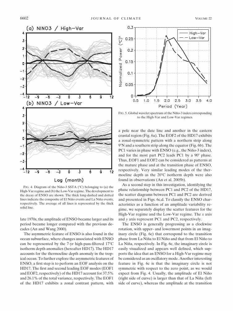
Figure 4 shows the evolutions of every El Nino and

La Nina event through the Nino-3 SSTA index, and their

composite values, for periods during the High-Var re-

gime (Fig. 4a) and periods during the Low-Var regime

(Fig. 4b). The ‘‘lag 0’’ refers to each January, when

events achieve their maximum phase. In the High-Var

regime, the peak amplitudes of the Nino-3 SST anoma-

lies are approximately 628C, whereas the peak ampli-

tudes in the Low-Var regime are approximately 618C.

As expected, the amplitude of ENSO in the High-Var

regime is larger than the amplitude in the Low-Var

regime. The residual heat (i.e., the average of the

El Nino and La Nina composites) is positive in the High-

Var regime (greater than 0.288C is statistically signifi-

cant enough to be a nonzero value with 90% confidence

level) but is weakly negative in the Low-Var regime (less

than 20.268C is statistically significant enough to be a

nonzero value with 90% confidence level). Accordingly,

El Nino (La Nina) events are stronger than La Nina

(El Nino) events in the High-Var regime (Low-Var re-

gime). Previous observational studies suggested this

asymmetric characteristic of ENSO (An and Jin 2004;

An 2009; Sun and Yu 2009).

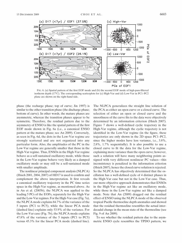
The dominant periods of ENSO for both regimes are

obtained by computing a global wavelet spectrum of the

Nino-3 index corresponding to each regime (Fig. 5). A

global wavelet spectrum corresponds to the average of

all the wavelet spectrums with respect to each period.

To facilitate the comparison, each variance is normal-

ized by the total variance over each mean state. The

spectrum of ENSO associated with the Low-Var regime

sharply peaks around 1.9 yr, while the High-Var regime

peaks around 2.3 yr. The strongest variability (when the

normalized power is strongest than 0.2) has a range from

1.8 to 2.3 yr in the Low-Var regime; it is relatively

broader for the High-Var regime ranging from 1.8 to

2.7 yr. This model agrees with the observed tendency of

a direct proportionality between the period and ampli-

tude of ENSO. For example, after the climate shift in the

FIG. 2. Spatial pattern of the first EOF mode of (a) the

low-pass-filtered SST and (b) the 178C isotherm depth anomalies.

FIG. 3. Gray solid line: time series of the N3Var index. Black

short-dashed line: PC time series of first EOF mode for the low-

pass-filtered 178C isotherm depth (see Fig. 2b). Black long-dashed

line: PC time series of first EOF mode for the low-pass-filtered SST

(see Fig. 2a). Time series has been normalized.


late 1970s, the amplitude of ENSO became larger and its

period became longer compared with the previous de-

cades (An and Wang 2000).

The asymmetric feature of ENSO is also found in the

ocean subsurface, where changes associated with ENSO

can be represented by the 7-yr high-pass-filtered 178C

isotherm depth anomalies (hereafter HD17). The HD17

accounts for the thermocline depth anomaly in the trop-

ical ocean. To further explore the asymmetric features of

ENSO, a first step is to perform an EOF analysis on the

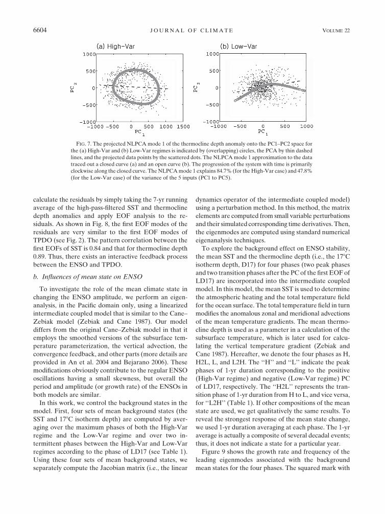
HD17. The first and second leading EOF modes (EOF1

and EOF2, respectively) of the HD17 account for 37.5%

and 26.1% of the total variance, respectively. The EOF1

of the HD17 exhibits a zonal contrast pattern, with

a pole near the date line and another in the eastern

coastal region (Fig. 6a). The EOF2 of the HD17 exhibits

a zonal-symmetric pattern with a northern strip along

98N and a southern strip along the equator (Fig. 6b). The

PC1 varies in phase with ENSO (e.g., the Nino-3 index),

and for the most part PC2 leads PC1 by a 908 phase.

Thus, EOF1 and EOF2 can be considered as patterns at

the mature phase and at the transition phase of ENSO,

respectively. Very similar leading modes of the ther-

mocline depth as the 208C isotherm depth were also

found in observations (An et al. 2005b).

As a second step in this investigation, identifying the

phase relationship between PC1 and PC2 of the HD17,

the scatter diagrams between PC1 and PC2 are derived

and presented in Figs. 6c,d. To classify the ENSO char-

acteristics as a function of an amplitude variability re-

gime, we separately display the scatter features for the

High-Var regime and the Low-Var regime. The x axis

and y axis represent PC1 and PC2, respectively.

The ENSO is generally progressing as a clockwise

rotation, with upper- and lowermost points in an imag-

inary circle (Fig. 6c) that correspond to the transition

phase from La Nina to El Nino and that from El Nino to

La Nina, respectively. In Fig. 6c, the imaginary circle is

easily visualized and appears well defined, which sup-

ports the idea that an ENSO for a High-Var regime may

be considered as an oscillatory mode. Another interesting

feature in Fig. 6c is that the imaginary circle is not

symmetric with respect to the zero point, as we would

expect from Fig. 4. Usually, the amplitude of El Nino

(right side of curve) is larger than that of La Nina (left

side of curve), whereas the amplitude at the transition

FIG. 4. Diagram of the Nino-3 SSTA (8C) belonging to (a) the

High-Var regime and (b) the Low-Var regime. The development to

the decay of ENSO are shown. The thick long-dashed and dotted

lines indicate the composite of El Nino events and La Nina events,

respectively. The average of all lines is represented by the thick

solid line.

FIG. 5. Global wavelet spectrum of the Nino-3 index corresponding

to the High-Var and Low-Var regimes.


phase (the recharge phase; top of curve; Jin 1997) is

similar to the other transition phase (the discharge phase;

bottom of curve). In other words, the mature phases are

asymmetric, whereas the transition phases appear to be

symmetric. Therefore, the residual pattern due to the

asymmetry of ENSO is like the spatial pattern of the first

EOF mode shown in Fig. 6a (i.e., a canonical ENSO

pattern at the mature phase; see An 2009). Conversely,

as seen in Fig. 6d, the dots in the Low-Var regime are

strongly scattered and are not organized into any

particular form. Also, the amplitudes of the PC in the

Low-Var regime are generally smaller that those in the

High-Var regime. Thus, ENSOs in the High-Var regime

behave as a self-sustained oscillatory mode, while those

in the Low-Var regime behave very likely as a damped

oscillatory mode or may still be a self-sustained mode

with smaller amplitude.

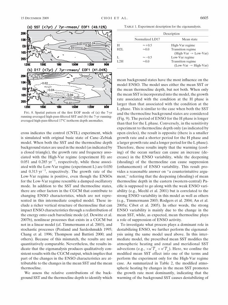
The nonlinear principal component analysis (NLPCA)

(Hsieh 2001, 2004, 2007) of HD17 is used to confirm and

complement the above interpretation. It first reveals

a canonical oscillatory trajectory in the PC time series

space in the High-Var regime, as mentioned above. As

in An et al. (2005b), the NLPCA was applied to the

leading 5 PCs of the EOFs, separately for the High-Var

and the Low-Var regimes. For the High-Var case (Fig. 7a),

the NLPCA mode explains 84.7% of the variance of the

5 inputs (PC1 to PC5), while the linear PCA mode

(dashed line) explains only 53.9% of the variance. For

the Low-Var case (Fig. 7b), the NLPCA mode explains

47.8% of the variance of the 5 inputs (PC1 to PC5)

versus 45.3% for the linear PCA mode (dashed line).

The NLPCA generalizes the straight line solution of

the PCA as either an open curve or a closed curve. The

selection of either an open or closed curve and the

smoothness of the curve fits to the data were objectively

determined by an information criterion (Hsieh 2007).

Figure 7 shows a well-defined cyclic trajectory in the

High-Var regime, although the cyclic trajectory is not

identified in the Low-Var regime (in the figure, these

trajectories are only shown in the 2D space PC1–PC2,

since the higher modes have less variance, i.e., 3.8%,

2.8%, 1.7% sequentially). It is also possible to use a

closed curve to fit the data for the Low-Var regime,

explaining more variance than the open curve; however,

such a solution will have many neighboring points as-

signed with very different nonlinear PC values—this

inconsistency is penalized in the information criterion

(Hsieh 2007), hence the closed curve solution is rejected.

So the NLPCA has objectively determined that the os-

cillation has a well-defined cycle of 4 distinct phases in

the High-Var case but not in the Low-Var case. Thus,

our more objective approach demonstrates that ENSOs

in the High-Var regime act like an oscillatory mode,

while those in the Low-Var regime act like a damped

mode. Note that An (2009) dragged out the residual

effect of ENSO using the NLPCA mode of the observed

tropical Pacific thermocline depth anomalies and showed

that the residual thermocline resembles the actual inter-

decadal change in the mean state of the thermocline (see

Fig. 9 of An 2009).

To see whether the residual pattern due to the asym-

metric ENSO cycle resembles the TPDO pattern, we

FIG. 6. (a) Spatial pattern of the first EOF mode and (b) the second EOF mode of high-pass-filtered

isotherm depth (178C). The corresponding scatterplots for (c) High-Var and (d) Low-Var in PC1–PC2

plane are shown on the right-hand side.


calculate the residuals by simply taking the 7-yr running

average of the high-pass-filtered SST and thermocline

depth anomalies and apply EOF analysis to the re-

siduals. As shown in Fig. 8, the first EOF modes of the

residuals are very similar to the first EOF modes of

TPDO (see Fig. 2). The pattern correlation between the

first EOFs of SST is 0.84 and that for thermocline depth

0.89. Thus, there exists an interactive feedback process

between the ENSO and TPDO.

b. Influences of mean state on ENSO

To investigate the role of the mean climate state in

changing the ENSO amplitude, we perform an eigen-

analysis, in the Pacific domain only, using a linearized

intermediate coupled model that is similar to the Cane–

Zebiak model (Zebiak and Cane 1987). Our model

differs from the original Cane–Zebiak model in that it

employs the smoothed versions of the subsurface tem-

perature parameterization, the vertical advection, the

convergence feedback, and other parts (more details are

provided in An et al. 2004 and Bejarano 2006). These

modifications obviously contribute to the regular ENSO

oscillations having a small skewness, but overall the

period and amplitude (or growth rate) of the ENSOs in

both models are similar.

In this work, we control the background states in the

model. First, four sets of mean background states (the

SST and 178C isotherm depth) are computed by aver-

aging over the maximum phases of both the High-Var

regime and the Low-Var regime and over two in-

termittent phases between the High-Var and Low-Var

regimes according to the phase of LD17 (see Table 1).

Using these four sets of mean background states, we

separately compute the Jacobian matrix (i.e., the linear

dynamics operator of the intermediate coupled model)

using a perturbation method. In this method, the matrix

elements are computed from small variable perturbations

and their simulated corresponding time derivatives. Then,

the eigenmodes are computed using standard numerical

eigenanalysis techniques.

To explore the background effect on ENSO stability,

the mean SST and the thermocline depth (i.e., the 178C

isotherm depth, D17) for four phases (two peak phases

and two transition phases after the PC of the first EOF of

LD17) are incorporated into the intermediate coupled

model. In this model, the mean SST is used to determine

the atmospheric heating and the total temperature field

for the ocean surface. The total temperature field in turn

modifies the anomalous zonal and meridional advections

of the mean temperature gradients. The mean thermo-

cline depth is used as a parameter in a calculation of the

subsurface temperature, which is later used for calcu-

lating the vertical temperature gradient (Zebiak and

Cane 1987). Hereafter, we denote the four phases as H,

H2L, L, and L2H. The ‘‘H’’ and ‘‘L’’ indicate the peak

phases of 1-yr duration corresponding to the positive

(High-Var regime) and negative (Low-Var regime) PC

of LD17, respectively. The ‘‘H2L’’ represents the tran-

sition phase of 1-yr duration from H to L, and vice versa,

for ‘‘L2H’’ (Table 1). If other compositions of the mean

state are used, we get qualitatively the same results. To

reveal the strongest response of the mean state change,

we used 1-yr duration averaging at each phase. The 1-yr

average is actually a composite of several decadal events;

thus, it does not indicate a state for a particular year.

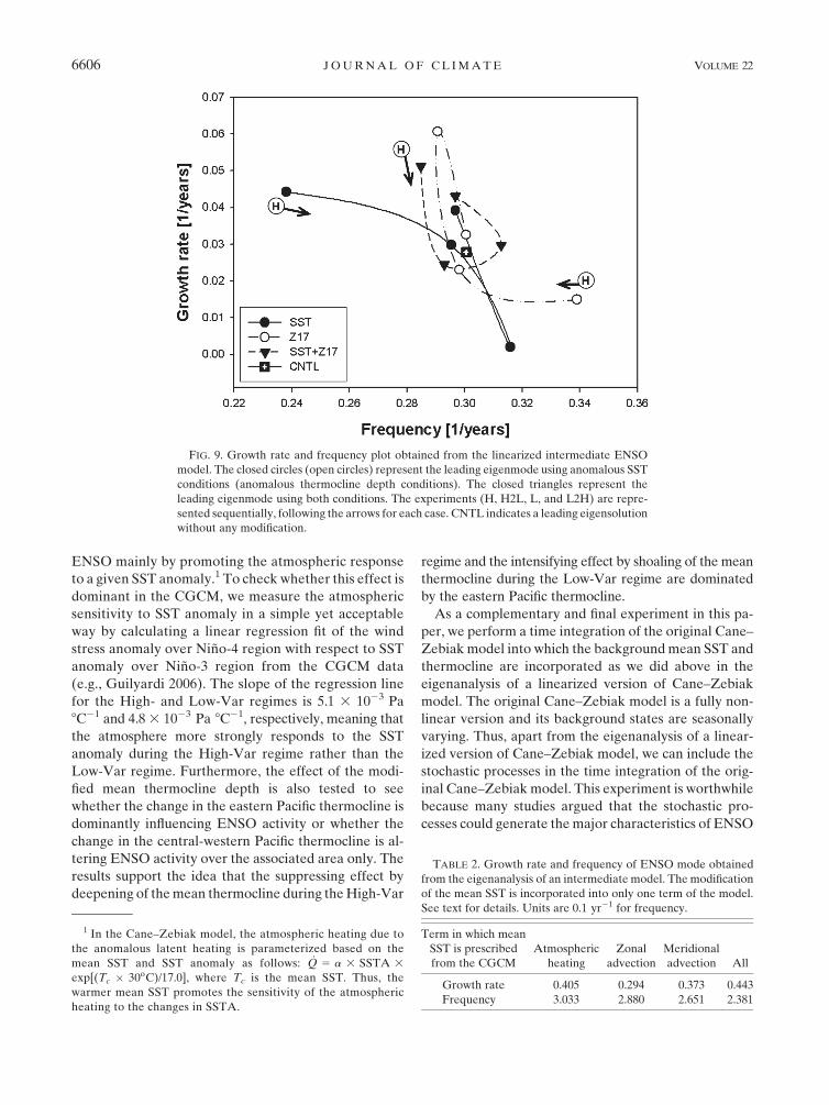
Figure 9 shows the growth rate and frequency of the

leading eigenmodes associated with the background

mean states for the four phases. The squared mark with

FIG. 7. The projected NLPCA mode 1 of the thermocline depth anomaly onto the PC1–PC2 space for

the (a) High-Var and (b) Low-Var regimes is indicated by (overlapping) circles, the PCA by thin dashed

lines, and the projected data points by the scattered dots. The NLPCA mode 1 approximation to the data

traced out a closed curve (a) and an open curve (b). The progression of the system with time is primarily

clockwise along the closed curve. The NLPCA mode 1 explains 84.7% (for the High-Var case) and 47.8%

(for the Low-Var case) of the variance of the 5 inputs (PC1 to PC5).


cross indicates the control (CNTL) experiment, which

is simulated with original basic state of Cane–Zebiak

model. When both the SST and the thermocline depth

background states are used in the model (as indicated by

a closed triangle), the growth rate and frequency asso-

ciated with the High-Var regime (experiment H) are

0.051 and 0.285 yr21, respectively, while those associ-

ated with the Low-Var regime (experiment L) are 0.030

and 0.313 yr21, respectively. The growth rate of the

Low-Var regime is positive, even though the ENSOs

for the Low-Var regime resemble a damped oscillatory

mode. In addition to the SST and thermocline states,

there are other factors in the CGCM that contribute to

changing ENSO characteristics, which are not repre-

sented in this intermediate coupled model. These in-

clude a richer vertical structure of thermocline that can

impact ENSO characteristics through a redistribution of

the energy onto each baroclinic mode (cf. Dewitte et al.

2007b), nonlinear processes that exists in a CGCM but

not in a linear model (cf. Timmermann et al. 2003), and

stochastic processes (Penland and Sardeshmukh 1995;

Chang et al. 1996; Thompson and Battisti 2000; and

others). Because of this mismatch, the results are not

quantitatively comparable. Nevertheless, the results in-

dicate that the eigenanalysis produces qualitatively con-

sistent results with the CGCM output, which implies that

part of the changes in the ENSO characteristics are at-

tributable to the changes in the mean SST and the mean

thermocline.

We assess the relative contributions of the back-

ground SST and the thermocline depth to identify which

mean background states have the most influence on the

model ENSO. The model uses either the mean SST or

the mean thermocline depth, but not both. When only

the mean SST is incorporated into the model, the growth

rate associated with the condition at the H phase is

larger than that associated with the condition at the

L phase. This is similar to the case when both the SST

and the thermocline background states are considered

(Fig. 9). The period of ENSO for the H phase is longer

than that for the L phase. Conversely, in the sensitivity

experiment to thermocline depth only (as indicated by

open circles), the result is opposite (there is a smaller

growth rate and a shorter period for the H phase and

a larger growth rate and a longer period for the L phase).

Therefore, these results imply that the warming (cool-

ing) of the ocean surface can cause an increase (de-

crease) in the ENSO variability, while the deepening

(shoaling) of the thermocline can cause suppression

(enhancement) of ENSO variability. This result pro-

vides a reasonable answer on ‘‘a counterintuitive argu-

ment,’’ referring that the deepening (shoaling) of mean

thermocline depth in the eastern (western-central) Pa-

cific is supposed to go along with the weak ENSO vari-

ability (e.g., Meehl et al. 2001) but is correlated to the

strong ENSO variability in this model as well as others

(e.g., Timmermann 2003; Rodgers et al. 2004; An et al.

2005a; Cibot et al. 2005). In other words, the strong

ENSO variability is mainly due to the change in the

mean SST, while, as expected, mean thermocline plays

a role of suppression of ENSO activity.

To investigate what process plays a dominant role in

destabilizing ENSO, we further perform the eigenanal-

ysis using the same model used above. In this inter-

mediate model, the prescribed mean SST modifies the

atmospheric heating and zonal and meridional SST

advections (e.g., �u9Tx� y9T

y). Here, we confine the

modified mean SST effect into one of the terms and

perform the experiment only for the High-Var regime

case. As summarized in Table 2, the modified atmo-

spheric heating by changes in the mean SST promotes

the growth rate most dominantly, indicating that the

warming of the background SST causes destabilizing of

TABLE 1. Experiment description for the eigenanalysis.

Description

Normalized LD17 Mean state

H ’10.5 High-Var regime

H2L ’0.0 Transition regime

(High-Var / Low-Var)

L ’20.5 Low-Var regime

L2H ’0.0 Transition regime

(Low-Var / High-Var)

FIG. 8. Spatial pattern of the first EOF mode of (a) the 7-yr

running-averaged high-pass-filtered SST and (b) the 7-yr running-

averaged high-pass-filtered 178C isotherm depth anomalies.


ENSO mainly by promoting the atmospheric response

to a given SST anomaly.1 To check whether this effect is

dominant in the CGCM, we measure the atmospheric

sensitivity to SST anomaly in a simple yet acceptable

way by calculating a linear regression fit of the wind

stress anomaly over Nino-4 region with respect to SST

anomaly over Nino-3 region from the CGCM data

(e.g., Guilyardi 2006). The slope of the regression line

for the High- and Low-Var regimes is 5.1 3 1023 Pa

8C21 and 4.8 3 1023 Pa 8C21, respectively, meaning that

the atmosphere more strongly responds to the SST

anomaly during the High-Var regime rather than the

Low-Var regime. Furthermore, the effect of the modi-

fied mean thermocline depth is also tested to see

whether the change in the eastern Pacific thermocline is

dominantly influencing ENSO activity or whether the

change in the central-western Pacific thermocline is al-

tering ENSO activity over the associated area only. The

results support the idea that the suppressing effect by

deepening of the mean thermocline during the High-Var

regime and the intensifying effect by shoaling of the mean

thermocline during the Low-Var regime are dominated

by the eastern Pacific thermocline.

As a complementary and final experiment in this pa-

per, we perform a time integration of the original Cane–

Zebiak model into which the background mean SST and

thermocline are incorporated as we did above in the

eigenanalysis of a linearized version of Cane–Zebiak

model. The original Cane–Zebiak model is a fully non-

linear version and its background states are seasonally

varying. Thus, apart from the eigenanalysis of a linear-

ized version of Cane–Zebiak model, we can include the

stochastic processes in the time integration of the orig-

inal Cane–Zebiak model. This experiment is worthwhile

because many studies argued that the stochastic pro-

cesses could generate the major characteristics of ENSO

TABLE 2. Growth rate and frequency of ENSO mode obtained

from the eigenanalysis of an intermediate model. The modification

of the mean SST is incorporated into only one term of the model.

See text for details. Units are 0.1 yr21 for frequency.

Term in which mean

SST is prescribed

from the CGCM

Atmospheric

heating

Zonal

advection

Meridional

advection All

Growth rate 0.405 0.294 0.373 0.443

Frequency 3.033 2.880 2.651 2.381

FIG. 9. Growth rate and frequency plot obtained from the linearized intermediate ENSO

model. The closed circles (open circles) represent the leading eigenmode using anomalous SST

conditions (anomalous thermocline depth conditions). The closed triangles represent the

leading eigenmode using both conditions. The experiments (H, H2L, L, and L2H) are repre-

sented sequentially, following the arrows for each case. CNTL indicates a leading eigensolution

without any modification.

1 In the Cane–Zebiak model, the atmospheric heating due to

the anomalous latent heating is parameterized based on the

mean SST and SST anomaly as follows: _Q 5 a 3 SSTA 3

exp[(Tc � 30oC)/17.0], where Tc is the mean SST. Thus, the

warmer mean SST promotes the sensitivity of the atmospheric

heating to the changes in SSTA.


as much as the chaotic dynamics could (e.g., Penland and

Sardeshmukh 1995; Chang et al. 1996; Thompson and

Battisti 2000; Burgman et al. 2008; Yeh and Kirtman

2009). Therefore we can test the ENSO modulation by

changes in the background state under a stable regime of

ENSO. Before starting to run the model, we reduce the

coupling parameter down to the stable regime so that

the model cannot produce a self-sustained oscillation on

its own. To generate ENSO, a random noise is added

whose spatial pattern is a bell shape centered at the

equatorial western Pacific. The random noise amplitude

is given as 0.035 dyne cm22, which is known to be the

amplitude of the surface zonal wind stress associated

with the Madden–Julian oscillation in the tropical Pa-

cific (Kessler and Kleeman 2000). Time integration for

each experiment is performed for 500 yr. The ENSO

activity of each experiment is measured by calculating

the standard deviation of Nino-3 index. When changes

in the mean SST and the thermocline depth associated

with High-Var regime are adopted separately into the

model, the standard deviation of the simulated Nino-3

index are 0.828 and 0.188C, respectively, while counter-

parts associated with the Low-Var regime are 0.0388C

(mean SST modified) and 1.668C (mean thermocline

modified), respectively. Thus, warming in the mean

SST and deepening of the mean thermocline during

the High-Var regime promote intensification and sup-

pression of ENSO activities, respectively, and opposite

cases associated with the Low-Var regime are also true.

Moreover, the intensified ENSO is simulated with a

relatively longer period (not shown). These time in-

tegrations of the original Cane–Zebiak model are con-

sistent with the eigenanalysis. Thus, the ENSO activity

subjected to stochastic processes in a stable regime is

modified by changes in the mean states in a similar

manner as shown in the eigenanalysis.

5. Discussion and conclusions

We use the outputs of a coupled general circulation

model (CGCM) to investigate the interaction mecha-

nism between a low-frequency modulation of ENSO

statistics and the slowly varying mean state in the trop-

ical Pacific. First, we provide evidence that the most

dominant decadal changes in both the mean SST and

the thermocline depth (i.e., the first EOF modes) are sig-

nificantly correlated to the decadal modulation of ENSO

statistics, including its variance and skewness. We pro-

pose that the nonlinear dynamical process initiates this

strong correlation. Second, using the intermediate cou-

pled model, we verify that the dominant decadal changes

in the mean states (here, the SST and thermocline are

used) represented by the first EOF mode can effectively

modify the ENSO statistics. Combining these two find-

ings, we conclude that there very likely exists an inter-

active feedback mechanism between the slowly varying

mean state and the ENSO variability in this CGCM.

More specifically, there exists a positive feedback with

the mean SST and a negative feedback with the mean

thermocline depth.

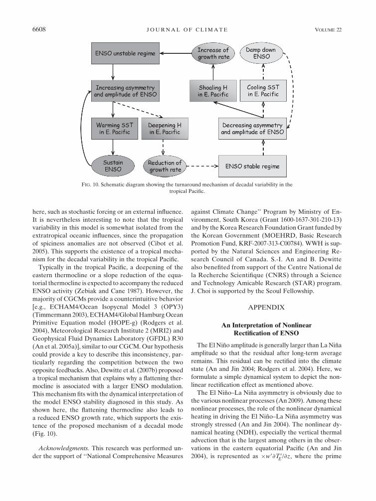
The above findings lead us to the following hypothesis

on the tropical Pacific decadal oscillation, which to

a certain extent was raised by Sun and Yu (2009), but

here we provide more convincing evidence. As depicted

on the schematic of Fig. 10, this oscillation is possibly

generated through the following sequential processes.

First, in the unstable regime, the ENSO amplitude and

asymmetry increase. Residual heat in both the ocean

surface and subsurface associated with the asymmetric

nonlinear ENSO cycle then leads to the warming of the

sea surface and to the deepening of the thermocline

depth in the tropical eastern Pacific. The warmed mean

SST plays a role in amplifying the ENSO variability,

while the deepened mean thermocline in the eastern

Pacific tends to reduce the ENSO variability. Because

of the negative feedback between mean thermocline

depth and this ENSO variability, the stability of ENSO

shifts toward the stable regime. In the stable regime,

the ENSO cycle becomes symmetric, so that there is

no further accumulation of heat. As a result, the mean

thermocline should shoal back to a normal condition,

and the mean surface temperature should return to its

normal condition. The shallow thermocline provides a

favorable condition for a larger variability in ENSO, so

that ENSO returns to the unstable regime. Accordingly,

the combined effect of the positive feedback between

ENSO activity and the SST climate state, and the neg-

ative feedback between ENSO activity and the ther-

mocline climate state, can generate the tropical Pacific

decadal oscillation.

However, there are several caveats to our hypothesis.

Our eigenanalysis does not account for a circumstance

when the negative feedback overwhelms the positive

feedback. This turning point between two opposite feed-

backs could provide a potential key component for reg-

ulating the time scale of the tropical Pacific decadal

oscillation. Jin et al. (2001) suggested that oceanic

Rossby waves play an important role in the decadal

mode in the tropics. However, we did not consider any

factors that control the period of the decadal oscillation.

Therefore, further validations are needed to understand

the regulation of the time scale of the TPDO. Another

caveat to our approach is that we have prescribed a

mean state while neglecting other forcing mechanisms.

In fact, the amplitude of ENSO can be changed by

a number of other mechanisms not fully considered


here, such as stochastic forcing or an external influence.

It is nevertheless interesting to note that the tropical

variability in this model is somewhat isolated from the

extratropical oceanic influences, since the propagation

of spiciness anomalies are not observed (Cibot et al.

2005). This supports the existence of a tropical mecha-

nism for the decadal variability in the tropical Pacific.

Typically in the tropical Pacific, a deepening of the

eastern thermocline or a slope reduction of the equa-

torial thermocline is expected to accompany the reduced

ENSO activity (Zebiak and Cane 1987). However, the

majority of CGCMs provide a counterintuitive behavior

[e.g., ECHAM4/Ocean Isopycnal Model 3 (OPY3)

(Timmermann 2003), ECHAM4/Global Hamburg Ocean

Primitive Equation model (HOPE-g) (Rodgers et al.

2004), Meteorological Research Institute 2 (MRI2) and

Geophysical Fluid Dynamics Laboratory (GFDL) R30

(An et al. 2005a)], similar to our CGCM. Our hypothesis

could provide a key to describe this inconsistency, par-

ticularly regarding the competition between the two

opposite feedbacks. Also, Dewitte et al. (2007b) proposed

a tropical mechanism that explains why a flattening ther-

mocline is associated with a larger ENSO modulation.

This mechanism fits with the dynamical interpretation of

the model ENSO stability diagnosed in this study. As

shown here, the flattening thermocline also leads to

a reduced ENSO growth rate, which supports the exis-

tence of the proposed mechanism of a decadal mode

(Fig. 10).

Acknowledgments. This research was performed un-

der the support of ‘‘National Comprehensive Measures

against Climate Change’’ Program by Ministry of En-

vironment, South Korea (Grant 1600-1637-301-210-13)

and by the Korea Research Foundation Grant funded by

the Korean Government (MOEHRD, Basic Research

Promotion Fund, KRF-2007-313-C00784). WWH is sup-

ported by the Natural Sciences and Engineering Re-

search Council of Canada. S.-I. An and B. Dewitte

also benefited from support of the Centre National de

la Recherche Scientifique (CNRS) through a Science

and Technology Amicable Research (STAR) program.

J. Choi is supported by the Seoul Fellowship.

APPENDIX

An Interpretation of NonlinearRectification of ENSO

The El Nino amplitude is generally larger than La Nina

amplitude so that the residual after long-term average

remains. This residual can be rectified into the climate

state (An and Jin 2004; Rodgers et al. 2004). Here, we

formulate a simple dynamical system to depict the non-

linear rectification effect as mentioned above.

The El Nino–La Nina asymmetry is obviously due to

the various nonlinear processes (An 2009). Among these

nonlinear processes, the role of the nonlinear dynamical

heating in driving the El Nino–La Nina asymmetry was

strongly stressed (An and Jin 2004). The nonlinear dy-

namical heating (NDH), especially the vertical thermal

advection that is the largest among others in the obser-

vations in the eastern equatorial Pacific (An and Jin

2004), is represented as �w9›TE9/›z, where the prime

FIG. 10. Schematic diagram showing the turnaround mechanism of decadal variability in the

tropical Pacific.


indicates anomaly. In the following, the rectified effect

due to this nonlinear vertical advection term will be

depicted by using a box-averaged SST equation over the

equatorial eastern Pacific. The SST equation is similar to

that in Jin (1997) but was modified to include the non-

linear vertical advection term. The nonlinear SST equa-

tion is

›TE

›t5 � � � �aT

E� w

›TE

›z, (A1)

where the subscript ‘‘E’’ indicates the equatorial eastern

Pacific. To make the case simpler, other thermal ad-

vection terms are omitted. Equation (A1) is separated

into the slowly varying mean (i.e., mean quantities) and

deviation (i.e., ENSO quantities) equations by adopting

the rule of TE9 5 0. After some manipulations, we have

›TE

›t5 � � � �aT

E� w

›TE

›z� w9

›TE9

›z; (A2)

›TE9

›t5 � � � �aT

E9� w

›TE9

›z� w9

›TE

›z

� w9›T

E9

›z1 w9

›TE9

›z. (A3)

Equations (A2) and (A3) indicate the slowly varying

mean SST tendency and the anomalous SST tendency

(i.e., ENSO) equations, respectively, and they are linked

through the nonlinear advection term. Thus, the non-

zero �w9›TE9/›z, which is driven by the nonlinear pro-

cess of ENSO, will be rectified into the mean (i.e., TE).

Now, we convert the NDH term�w9›TE9/›z to a finite-

difference form to understand its role:

�w9›T

E9

›z’�w9

(TE9� T

sub9 )

HS

, (A4)

where the upwelling velocity w9 is proportional to the

surface zonal wind stress anomaly (the westerly drives

the downwelling anomaly) and the surface zonal wind

stress along the equator is also approximately pro-

portional to the zonal gradient of the SST anomaly

(Lindzen and Nigam 1987) such that w9 } 2t9X } 2T9E.

Here T9sub is a subsurface temperature where the water is

entrained into the ocean surface layer, and it can be

parameterized by the oceanic vertical stratification and

thermocline depth anomaly; that is, T9sub ’ gh9E [see

appendix B of An et al. (2008) and Jin (1997)]. Thus,

after applying the above rules, Eq. (A4) becomes

�w9(T

E9� T

sub9 )

HS

’1

HS

(TE92 � gT

E9h

E9). (A5)

Theoretically (Wang and Fang 1996, hereafter WF96),

as well as in the observation (Zelle et al. 2004), h9Eslightly leads T9E in time, and their correlation is positive.

Equation (A5) is almost identical to Eq. (3.5a) of WF96.

According to WF96, the reasonable value of g is slightly

greater than one, when the above system is normalized.

Note that Dewitte and Perigaud (1996) also showed that

g can depend on the sign of h9E, g being larger for posi-

tive h9E than for negative h9E in the eastern equatorial

Pacific. Therefore, (A5) usually has a negative value

indicating that the nonlinear dynamical advection term

promotes the negative SST anomaly tendency. Thus, the

cooling due to this second-order—that is, nonlinear—

term results in a negative skewness of T9E (i.e., weaker

El Nino and stronger La Nina), which will be rectified

into the climate state. The negative skewness is a solu-

tion obtained from a prototype ENSO model of WF96

(see their Figs. 5 and 7), while the observed ENSO

usually has a positive skewness (An and Jin 2004). This

contradiction may be due to immoderate simplifica-

tion or possibly inadequate parameterization of a pro-

totype ENSO model in treating the ocean wave dynamics.

A clearer explanation will be addressed in a future

study.

REFERENCES

Alexander, M. A., C. Deser, and M. S. Timlin, 1999: The reemergence

of SST anomalies in the North Pacific Ocean. J. Climate, 12,

2419–2431.

An, S.-I., 2009: A review on interdecadal changes in the non-

linearity of the El Nino–Southern Oscillation. Theor. Appl.

Climatol., 97, 29–40.

——, and F.-F. Jin, 2000: An eigen analysis of the interdecadal

changes in the structure and frequency of ENSO mode.

Geophys. Res. Lett., 27, 2573–2576.

——, and B. Wang, 2000: Interdecadal change of the structure of

the ENSO mode and its impact on the ENSO frequency.

J. Climate, 13, 2044–2055.

——, and F.-F. Jin, 2004: Nonlinearity and asymmetry of ENSO.

J. Climate, 17, 2399–2412.

——, A. Timmermann, L. Bejarano, F.-F. Jin, F. Justino, Z. Liu,

and A. W. Tudhope, 2004: Modeling evidence for enhanced

El Nino–Southern Oscillation amplitude during the Last

Glacial Maximum. Paleoceanography, 19, PA4009, doi:10.1029/

2004PA001020.

——, Y.-G. Ham, J.-S. Kug, F.-F. Jin, and I.-S. Kang, 2005a:

El Nino–La Nina asymmetry in the Coupled Model Inter-

comparison Project simulations. J. Climate, 18, 2617–2627.

——, W. W. Hsieh, and F.-F. Jin, 2005b: A nonlinear analysis of

the ENSO cycle and its interdecadal change. J. Climate, 18,3229–3239.

——, J.-S. Kug, A. Timmermann, I.-S. Kang, and O. Timm, 2007:

The influence of ENSO on the generation of decadal vari-

ability in the North Pacific. J. Climate, 20, 667–680.

——, ——, Y.-G. Ham, and I.-S. Kang, 2008: Successive modula-

tion of ENSO to the future greenhouse warming. J. Climate,

21, 3–21.


Bejarano, L., 2006: Coexistence of leading equatorial coupled

modes for ENSO. Ph.D. dissertation, The Florida State Uni-

versity, 118 pp.

Burgman, R. J., P. S. Schopf, and B. P. Kirtman, 2008: Decadal

modulation of ENSO in a hybrid coupled model. J. Climate,

21, 5482–5500.

Cane, M. A., and M. Evans, 2000: Climate variability—Do the

tropics rule? Science, 290, 1107–1108.

Chang, P., L. Ji, H. Li, and M. Flugel, 1996: Chaotic dynamics

versus stochastic processes in El Nino–Southern Oscillation

in coupled ocean–atmosphere models. Physica D, 98,

301–320.

Cibot, C., 2004: Variabilite decennale dans le Pacifique tropical et

modulation basse frequence de l’activite ENSO. Ph.D. thesis,

Universite Paul Sabatier, Toulouse, France, 164 pp.

——, E. Maisonnave, L. Terray, and B. Dewitte, 2005: Mechanisms

of tropical Pacific interannual-to-decadal variability in the

ARPEGE/ORCA global coupled model. Climate Dyn., 24,

823–842.

Deque, M., C. Dreveton, A. Braun, and D. Cariolle, 1994: The

ARPEGE/IFS atmosphere model: A contribution to the

French community climate modeling. Climate Dyn., 10,

249–266.

Dewitte, B., and C. Perigaud, 1996: El Nino–La Nina events sim-

ulated with Cane and Zebiak’s model and observed with sat-

ellite or in situ data. Part II: Model forced with observations.

J. Climate, 9, 1188–1207.

——, C. Cibot, C. Perigaud, S.-I. An, and L. Terray, 2007a:

Interaction between near-annual and ENSO modes in a

CGCM simulation: Role of equatorial background mean state.

J. Climate, 20, 1035–1052.

——, S.-W. Yeh, B.-K. Moon, C. Cibot, and L. Terray, 2007b:

Rectification of the ENSO variability by interdecadal changes

in the equatorial background mean state in a CGCM simula-

tion. J. Climate, 20, 2002–2021.

Fedorov, A. V., and S. G. Philander, 2000: Is El Nino changing?

Science, 288, 1997–2002.

Fichefet, T., and M. A. Morales Maqueda, 1997: Sensitivity of a

global sea ice model to the treatment of ice thermodynamics

and dynamics. J. Geophys. Res., 102, 12 609–12 646.

Gu, D., and S. G. H. Philander, 1997: Interdecadal climate fluctu-

ations that depend on exchanges between the tropics and ex-

tratropics. Science, 275, 805–807.

Guilyardi, E., 2006: El Nino–mean state–seasonal cycle inter-

actions in a multi-model ensemble. Climate Dyn., 26, 329–348.

Holland, C. L., R. B. Scott, S.-I. An, and F. W. Taylor, 2007:

Propagating decadal sea surface temperature signal identified

in modern proxy records of the tropical Pacific. Climate Dyn.,

28, 163–179.

Hsieh, W. W., 2001: Nonlinear principal component analysis by

neural networks. Tellus, 53A, 599–615.

——, 2004: Nonlinear multivariate and time series analysis by neural

network methods. Rev. Geophys., 42, RG1003, doi:10.1029/

2002RG000112.

——, 2007: Nonlinear principal component analysis of noisy data.

Neural Networks, 20, 434–443.

Jin, F.-F., 1997: An equatorial ocean recharge paradigm for ENSO.

Part I: Conceptual model. J. Atmos. Sci., 54, 811–829.

——, 2001: Low-frequency modes of tropical ocean dynamics.

J. Climate, 14, 3874–3881.

——, M. Kimoto, and X. Wang, 2001: A model of decadal ocean–

atmosphere interaction in the North Pacific basin. Geophys.

Res. Lett., 28, 1531–1534.

——, S.-I. An, A. Timmermann, and J. Zhao, 2003: Strong El Nino

events and nonlinear dynamical heating. Geophys. Res. Lett.,

30, 1120.

Kessler, W. S., and R. Kleeman, 2000: Rectification of the Madden–

Julian oscillation into the ENSO cycle. J. Climate, 13, 3560–

3575.

Kirtman, B. P., and P. S. Schopf, 1998: Decadal variability in

ENSO predictability and prediction. J. Climate, 11, 2804–

2822.

Kleeman, R., J. P. McCreary, and B. A. Klinger, 1999: A mecha-

nism for generating ENSO decadal variability. Geophys. Res.

Lett., 26, 1743–1746.

Knutson, T. R., and S. Manabe, 1998: Model assessment of decadal

variability and trends in the tropical Pacific Ocean. J. Climate,

11, 2273–2296.

Latif, M., and T. P. Barnett, 1994: Causes of decadal climate vari-

ability over the North Pacific and North America sector. Sci-

ence, 266, 634–637.

Levitus, S., and Coauthors, 1998: Introduction. Vol. 1, World Ocean

Database 1998, NOAA Atlas NESDIS 18, 346 pp.

Lindzen, R. S., and S. Nigam, 1987: On the role of sea surface

temperature gradients in forcing low-level winds and conver-

gence in the tropics. J. Atmos. Sci., 44, 2418–2436.

Madec, G., P. Delecluse, M. Imbard, and C. Levy, 1998: OPA 8.1

ocean general circulation model reference manual. Note du

Pole de modelisation 11, Institut Pierre-Simon Laplace, 91 pp.

Meehl, G. A., P. R. Gent, J. M. Arblaster, B. L. Otto-Bliesner,

E. C. Brady, and A. Craig, 2001: Factors that affect amplitude

of El Nino in global coupled climate models. Climate Dyn., 17,

515–526.

Newman, M., G. P. Compo, and M. A. Alexander, 2003: ENSO-

forced variability of the Pacific decadal oscillation. J. Climate,

16, 3853–3857.

Nonaka, M., S.-P. Xie, and J. P. McCreary, 2002: Decadal variations

in the subtropical cells and equatorial pacific SST. Geophys.

Res. Lett., 29, 1116, doi:10.1029/2001GL013717.

Penland, C., and P. D. Sardeshmukh, 1995: The optimal growth

of tropical sea surface temperature anomalies. J. Climate, 8,

1999–2024.

Rodgers, K. B., P. Friederichs, and M. Latif, 2004: Tropical Pacific

decadal variability and its relation to decadal modulations of

ENSO. J. Climate, 17, 3761–3774.

Saravanan, R., and J. C. McWilliams, 1997: Stochasticity and spa-

tial resonance in interdecadal climate fluctuations. J. Climate,

10, 2299–2320.

Schopf, P. S., and R. J. Burgman, 2006: A simple mechanism

for ENSO residuals and asymmetry. J. Climate, 19, 3167–3179.

Sun, D.-Z., and T. Zhang, 2006: A regulatory effect of ENSO on the

time-mean thermal stratification of the equatorial upper ocean.

Geophys. Res. Lett., 33, L07710, doi:10.1029/2005GL025296.

Sun, F., and J.-Y. Yu, 2009: A 10–15-year modulation cycle of

ENSO intensity. J. Climate, 22, 1718–1735.

Thompson, C. J., and D. S. Battisti, 2000: A linear stochastic dy-

namical model of ENSO. Part I: Model development. J. Cli-

mate, 13, 2818–2832.

Timmermann, A., 2003: Decadal ENSO amplitude modulations: A

nonlinear paradigm. Global Planet. Change, 37, 135–156.

——, and F.-F. Jin, 2002: A nonlinear mechanism for decadal

El Nino amplitude changes. Geophys. Res. Lett., 29, 1003,

doi:10.1029/2001GL013369.

——, M. Latif, A. Bacher, J. Oberhuber, and E. Roeckner, 1999:

Increased El Nino frequency in a climate model forced by

future greenhouse warming. Nature, 398, 694–697.


——, F.-F. Jin, and J. Abshagen, 2003: A nonlinear theory for

El Nino bursting. J. Atmos. Sci., 60, 152–165.

Torrence, T., and P. J. Webster, 1998: Interdecadal changes in the

ENSO–monsoon system. J. Climate, 12, 2679–2690.

Valcke, S., L. Terray, and A. Piacentini, 2000: The OASIS cou-

pled user guide version 2.4. Tech. Rep. TR/CMGC/00-10,

CERFACS, 85 pp.

Vimont, D. J., D. S. Battisti, and A. C. Hirst, 2003: The seasonal

footprinting mechanism in the CSIRO general circulation

models. J. Climate, 16, 2653–2667.

Wang, B., and Z. Fang, 1996: Chaotic oscillations of tropical climate: A

dynamic system theory for ENSO. J. Atmos. Sci., 53, 2787–2802.

——, and S.-I. An, 2001: Why the properties of El Nino changed

during the late 1970s. Geophys. Res. Lett., 28, 3709–3712.

Wang, X. L., and C. F. Ropelewski, 1995: An assessment of ENSO-

scale secular variability. J. Climate, 8, 1584–1599.

Ye, Z., and W. W. Hsieh, 2006: The influence of climate regime

shift on ENSO. Climate Dyn., 26, 823–833.

Yeh, S.-W., and B. Kirtman, 2004: Tropical Pacific decadal vari-

ability and ENSO amplitude modulation in a CGCM. J. Geo-

phys. Res., 109, C11009, doi:10.1029/2004JC002442.

——, and ——, 2009: Internal atmospheric variability and interannual-

to-decadal ENSO variability in a CGCM. J. Climate, 22,

2335–2355.

Zebiak, S. E., and M. A. Cane, 1987: A model El Nino–Southern

oscillation. Mon. Wea. Rev., 115, 2262–2278.

Zelle, H., G. Appeldoorn, G. Burgers, and G. J. V. Oldenborgh,

2004: The relationship between sea surface temperature and

thermocline depth in the eastern equatorial Pacific. J. Phys.

Oceanogr., 34, 643–655.

Zhang, Y., J. M. Wallace, and D. S. Battisti, 1997: ENSO-like in-

terdecadal variability: 1900–93. J. Climate, 10, 1004–1020.


Interactive Feedback between the Tropical Paciﬁc Decadal...

Documents

Transcript of Interactive Feedback between the Tropical Paciﬁc Decadal...