Interactions, Specifications, DLR probabilitiesand the Ruelle Operator in the

One-Dimensional Lattice

Leandro Cioletti† and Artur O. Lopes‡

† Dep. Matematica - Universidade de Brasılia, 70910-900 Brasilia-DF, Brazil‡ Inst. Matematica UFRGS, 91.500 Porto Alegre-RS, Brazil

Abstract

In this paper we consider general continuous potentials on the symbolicspace (the one-dimensional lattice N with a finite number of spins). Weshow a natural way to associate potentials of Thermodynamic Formalismwith Interactions. Using properties of the Ruelle operator we show the re-lation of the Gibbs Measures of Holder and Walters potentials consideredin Thermodynamic Formalism with the Dobrushin-Lanford-Ruelle Gibbsmeasures and also with Gibbs measures obtained via the ThermodynamicLimit with boundary conditions. We prove some uniform convergence the-orems for finite volume Gibbs measures, we analyze the Long-Range IsingModel and we show that it belongs to the Walters class for certain parame-ters. This paper also provides a kind of “dictionary” so one of our purposesis to clarify for both the Dynamical Systems and Mathematical StatisticalMechanics communities how these (seemingly distinct) concepts of Gibbsmeasures are related.

Contents1 Introduction .............................................................................................. 22 The Ruelle Operator ................................................................................. 33 Interactions on the Lattice N .................................................................... 94 The Hamiltonian and Interactions ............................................................ 145 Long-Range Ising Model and Walters Condition ...................................... 166 Boundary conditions ................................................................................. 187 Gibbs Specifications for Continuous Functions ......................................... 218 Thermodynamic Limit .............................................................................. 219 DLR - Gibbs Measures.............................................................................. 2210 Equivalence on the Walters Class.............................................................. 3311 Concluding Remarks ................................................................................. 38

1

1 Introduction

The basic idea of the Ruelle Operator remounts to the transfer matrix methodintroduced by Kramers and Wannier and (independently) by Montroll, on an ef-fort to compute the partition function of the Ising model. In a very famous work[26] published by Lars Onsager in 1944, the transfer matrix method was gener-alized to the two-dimensional lattice and was employed to successfully computethe partition function for the first neighbors Ising model. As a byproduct, heobtained the critical point at which the model passes through a phase transition.These two historical and remarkable chapters of the theory of transfer operatorsare related to the study of their actions on finite-dimensional vector spaces.

In a seminal paper in 1968, David Ruelle [30] introduced the transfer oper-ator for an one-dimensional statistical mechanics model with infinite range in-teractions. This paved the way to the study of transfer operators in infinite-dimensional vector spaces. In this paper, Ruelle proved the existence and unique-ness of the Gibbs measure for a lattice gas system with a potential depending oninfinitely many coordinates.

Nowadays, the transfer operators are called Ruelle operators (mainly in Ther-modynamic Formalism) and play an important role in Dynamical Systems andMathematical Statistical Mechanics. They are actually useful tools in severalother branches of mathematics.

Roughly speaking, the famous Ruelle-Perron-Frobenius Theorem states thatthe Ruelle operator for a potential with a certain regularity, in a suitable Banachspace, has a unique simple positive eigenvalue (equal to the spectral radius) and apositive eigenfunction. For Holder continuous potentials the proof of this theoremcan be found in [30, 2]. In 1978, Walters obtained the Ruelle-Perron-FrobeniusTheorem for a more general setting [38], allowing expansive and mixing dynamicalsystems together with potentials with summable variation. After the 80’s, theliterature on Ruelle’s theorem became abundant ([2, 12, 20, 27, 3, 33]).

The Ruelle operator was successfully used to study equilibrium measures for avery general class of potentials f . For a normalized potential f on such class theunique probability measure which is the fixed point for the dual of Ruelle operatorassociated to f it is sometimes called Gibbs probability in Thermodynamic For-malism. Some people on this area can use a different terminology. By the otherhand the equilibrium probability for f is the solution of the variational problem(1) of pressure of the potential f . Under some regularity conditions one canshow that the unique probability measure which is the solution of the variationalproblem is also the Gibbs measure associated to the potential f . Some impor-tant properties of the equilibrium probability can be derived from the formalismof the Ruelle operator approach. This study turns out to be a very importanton topological dynamics and differentiable dynamical systems, with applicationson the study of invariant measures for an Anosov diffeomorphism [32] and themeromorphy of Zelberg’s zeta function [31].

2

The so called DLR Gibbs measures were introduced in 1968 and 1969 indepen-dently by Dobrushin [8] and Lanford and Ruelle [22]. The abstract formulationin terms of specifications was developed five years latter in [9, 13, 28]. An im-portant stage in the development of the theory was established by the works ofPreston, Gruber, Hintermann and Merlini around 1977, Ruelle (1978) and Israel(1979). Preston’s work was more focused on the abstract measure theory, whileGruber et. al. concentrated on specific methods for Ising type models, Israel dealtwith the variational principle and Ruelle worked towards Gibbsian formalism inErgodic Theory.

Dobrushin began the study of non-uniqueness of the DLR Gibbs measure andproposed its interpretation as a phase transition. He proved the famous Do-brushin Uniqueness Theorem in 1968, ensuring the uniqueness of the Gibbs mea-sures for a very general class of interactions at very high temperatures (β 1).This result, together with the rigorous proof of non-uniqueness of the Gibbs mea-sures for the two-dimensional Ising model at low temperatures, is a great triumphof the DLR approach in the study of phase transition in Statistical Mechanics.Some accounts of the general results on the Gibbs Measure theory (from theStatistical Mechanics’ viewpoint) can be found in [17, 11, 34, 5, 16, 1].

This work aims to explain the relationship of DLR-Gibbs measures with theusual Gibbs measures considered in the Thermodynamic Formalism. We alsopresent the details of the construction of specifications for continuous functions.In particular, we show how to construct an absolutely uniformly summable spec-ification for any Holder potential. En route to the proof of this work’s maintheorem, we show that the DLR approach extends the construction usually con-sidered in Thermodynamics Formalism and then introduce the concept of dualGibbs measure (which is natural for Ruelle formalism) and show that these mea-sures are equivalent to the DLR-Gibbs measures for the lattice N. We also analyzethe relation with the thermodynamic limit with boundary conditions.

2 The Ruelle Operator

Consider the symbolic space Ω ≡ 1, 2, .., dN and let σ : Ω→ Ω be the left shift.As usual we consider Ω as metric space endowed with a metric d defined by

d(x, y) = 2−N , where N = infi ∈ N : xi 6= yi.

The Ruelle operator on the space of continuous function is defined as follows.

Definition 1. Fix a continuous function f : Ω → R. The Ruelle operator Lf :C(Ω,R)→ C(Ω,R) is defined on the function ψ as follows

Lf (ψ)(x) =∑y∈Ω;σ(y)=x

ef(y) ψ(y).

3

Normally we call f a potential and Lf the transfer operator associated to thepotential f .

Definition 2. For a continuous potential f the Pressure of f is defined by

P (f) = supν∈M(σ)

h(ν) +

∫Ω

f dν

,

whereM(σ) is the set of σ-invariant probabilities measures and h(ν) the Shannon-Kolmogorov entropy of ν.

A probability µ ∈ M(σ) is called an equilibrium state for f if it solves theabove variational problem, i.e.,

h(µ) +

∫Ω

f dµ = P (f). (1)

Several properties of the equilibrium probability can be obtained via the Ruelleoperator approach under some regularity assumptions on f .

From a compactness argument one can show that if f is a continuous potentialthen there exists at least one equilibrium state, see [35]. In such generality it ispossible to exhibit examples where the equilibrium state is not unique, see [19].

A simple and important class where uniqueness holds is the class of Holdercontinuous potentials. In this paper, we use this class to exemplify how to dealwith problems in Thermodynamic Formalism using the DLR approach. A Holderfunction is defined as follows. Fix 0 < γ ≤ 1. A function f : Ω→ R is γ-Holdercontinuous if

supx 6=y

|f(x)− f(y)|dγ(x, y)

< +∞.

The space of all the γ-Holder continuous functions is denote by Holγ. When wesay that f : Ω → R is Holder continuous function we mean f ∈ Holγ for some0 < γ ≤ 1.

A classical theorem in Thermodynamic Formalism assures that for any Holderpotential f the equilibrium state is unique.

Definition 3. Given f : Ω→ R the n-variation of f is

varn(f) = sup |f(x)− f(y)| : x, y ∈ Ω and xi = yi for all 0 ≤ i ≤ n− 1.

Definition 4. We say that f : Ω→ R is in the Walters class if

limp→∞

[ supn≥1varn+p( f(x) + f(σ(x)) + ...+ f(σn−1(x)) ) ] = 0.

4

Remark. Any Holder potential is in the Walters class.We shown in the Section 4 that the potential f : −1, 1N → R associated

to the Long-Range Ising model with interactions of type 1/rα is in the Waltersclass if α > 2. We remark that if f is in the Walters class the equilibrium stateis unique and all nice properties of the Ruelle operator still valid as for Holderpotentials [37]. When f is just a continuous potential there are examples wheremore than one equilibrium state exists. We present one of such examples later.

In what follows we present the first definition of Gibbs measure which is com-mon on the dynamical system community. For this one needs introduce beforethe dual Ruelle operator.

Definition 5. Given a continuous potential f : Ω→ R let L∗f be the operator onthe set of Borel Measures on Ω defined so that L∗f (ν), for each Borel measure ν,satisfies: ∫

Ω

ψ dL∗f (ν) =

∫Ω

Lf (ψ) dν,

for all continuous functions ψ.

Remark. The existence of the above operator is guaranteed by the Riesz-MarkovTheorem. In fact, for any fixed Borel measure ν we have that ψ 7→

∫ΩLf (ψ) dν

is a positive linear functional.

Theorem 6 (Ruelle-Perron-Frobenius). If f : Ω → R is in the Walters class,then there exist a strictly positive function ψf (called eigenfunction) and a strictlypositive eigenvalue λf such that Lf (ψf ) = λfψf . The eigenvalue λf is simple andit is equal to the spectral radius of the operator. Moreover, there exists a uniqueprobability νf on Ω such that L∗f (νf ) = λf νf . After proper normalization theprobability µf = ψf νf is invariant and it is also the equilibrium probability for f .

Suppose f is in the Walters class. If ϕ is positive and β > 0 satisfies Lf (ϕ) =β ϕ, then β = λf (the spectral radius) and ϕ is multiple of ψf . We also assumethat νf is a probability measure and ψf is chosen in such way that µf is also aprobability. The main point is: if for some potential f (in the Walters class ornot) it is possible to find a positive eigenfunction for the Ruelle operator, thenseveral interesting properties of the system can be obtained, see section 9.

If a potential f satisfies for all x ∈ Ω the equation Lf (1)(x) = 1, we say that f isa normalized potential. If f is in Walters class using the Ruelle-Perron-FrobeniusTheorem we can construct a normalized potential f given by

f ≡ f + logψf − logψf σ − log λf . (2)

We remark that if f is Holder then f is Holder. For some particular casesof non Holder potentials one can show the existence of the main eigenvalue and

5

the main positive eigenfunction, see [19] and [36], for instance. As far as weknow there is no general result about existence of the main eigenfunction for acontinuous potential.

Theorem 7. Let f : Ω → R be a potential in the Walters class and f given by(2). Then there is a unique Borel probability measure µf such that L∗

f(µf ) = µf .

The probability measure µf is σ invariant and for all Holder functions ψ we havethat, in the uniform convergence topology,

Lnfψ →∫

Ω

ψ dµf .

Definition 8 (Gibbs Measures). Let f : Ω → R be in the Walters class and fits normalization as in (2). The unique fixed point µf of the dual operator L∗

fis

called the Gibbs Measure for the potential f .

If we denote g = log f , any fixed point probability for L∗f

is also called a

g-measure (see [7, 29]).One of the main accomplishments of Thermodynamic Formalism was to show

that the equilibrium probability and the Gibbs probability are the same [27].Several important properties of the equilibrium probability measure such as decayof correlation, central limit theorem, large deviations and others can be inferedfrom the analysis of the Ruelle operator.

We remark that nowadays there are several definitions of Gibbs measure. In[33], the author presents some of them and some ideas which are relevant to thegeneral problem we treat.

The definition of Gibbs measure given above is based on the Ruelle-Perron-Frobenius Theorem, which is well known when the potential is Holder or Walters.The aim of this work is to present a generalization of the concept of Gibbs measurethat extends this definition.

A natural way to do this is to prove a better version of the Ruelle-Perron-Frobenius Theorem, but our efforts are not in this direction. In the next section,we shall introduce the concept of interaction and then Gibbs Measures will beconstructed using the DLR formalism. We proceed to compare both definitions,showing that the DLR approach is more general and constructive, which meansthat, given a potential, we can directly define the Gibbs measures without study-ing the spectral properties of the Ruelle Operator.

Note that for a given continuous potential f one can define the associated Ru-elle operator Lf , which acts on continuous functions. Using a standard argument(Thychonov-Schauder Theorem), one can show that in this case there exists atleast one probability measure ν and λ > 0 such that L∗f (ν) = λ ν. If the potentialf is continuous, we consider the transformation T : M(Ω) → M(Ω) such that

6

T (µ) = ρ, where for any continuous function g we have∫Ω

g dT (µ) =

∫Ω

gdρ =

∫ΩLf (g) dµ∫

ΩLf (1)dµ

.

By the Thychonov-Schauder Theorem there exists a fixed point ν for T . Inthis case λ =

∫ΩLf (1)dν.

For a general continuous potential f , it seems natural to enlarge the set of theso called Gibbs probabilities in the context of Ruelle operators. As we will see,this generalization agrees with the definition of Gibbs measures used in StatisticalMechanics.

Definition 9 (Dual-Gibbs Measures). Let f : Ω → R be a continuous function.We call a probability measure ν a Dual-Gibbs probability for f if there exists apositive λ > 0 such that L∗f (ν) = λ ν. We denote the set of such probabilities byG∗(f).

Notice that, in general, G∗(f) 6= ∅, although a probability measure on G∗(f)needs not be shift-invariant, even if f is Holder. If f is a Walters potential, it isonly possible to get associated eigenprobabilities when λ is the maximal eigen-value of the Ruelle operator Lf . In this case the eigenprobability ν associated tothe maximal eigenvalue is unique.

A natural question is: for a Holder continuous potential f is it possible to havedifferent eigenprobabilities ν1, ν2 ∈ G∗(f) for L∗f , associated to different eigenval-ues λ1 and λ2? This is not possible due to properties of the involution kernel (see[25]). These two eigenprobabilities would determine via the involution kernel twopositive eigenfunctions for another Ruelle operator Lf∗ , with the eigenvalues λ1

and λ2 (see [18]), where f ∗ is the dual potential for f . This is not possible (seefor instance [27] or Proposition 1 in [25]). Anyway, eigendistributions for L∗f mayexist (see [18]).

Now we introduce some more notations. The elements in the space 1, 2, ..., dNshall be denoted by (x0, x1, x2, ..), while the elements of Ω = 1, 2, ..., dZ will bedenoted by (...x−2, x−1 |x0, x1, x2, ...). So the image of the left shift on σ onΩ = 1, 2, ..., dZ will be written as

σ(..., x−2, x−1 |x0, x1, x2, ...) = (..., x−2, x−1, x0 |x1, x2, ...).

Suppose we initially consider a potential f : Ω = 1, 2, ..., dZ → R and we

want to find the equilibrium state µ for the potential described by f , that is,

P (f) = supν∈M(σ)

h(ν) +

∫Ω

f dν

= h(µ) +

∫Ω

f dµ.

7

The Bowen-Ruelle-Sinai approach (see [2] and [27]) to the problem is the fol-lowing: since there is no reason for the site 0 ∈ Z to have privileged status inthe lattice, we shall consider shift-invariant probability measures. As we are in-terested in such probabilities, we point out that the equilibrium probabilities forf and g : 1, 2, .., dZ → R, satisfying f = g + h − h σ for some continuoush : 1, 2, .., dZ → R are the same. The main point is that under some regular-ity assumptions on the potential f , one can get a special g which depends juston future coordinates, that is, for any pair x = (..., x−2, x−1 |x0, x1, x2, ...) andy = (..., y−2, y−1 |x0, x1, x2, ...) ∈ Ω, we have g(x) = g(y). We abuse notationby simply writing g(x) = g(x0, x1, x2, ...)., so we can think of g as a functionon 1, 2, .., dN. Therefore, we can apply the formalism of the Ruelle operatorLg to study the properties of µ (a probability measure on 1, 2, .., dN), whichis the equilibrium state for g : 1, 2, .., dN → R. One can show that the equi-

librium state for f is the probability measure µ (a probability on 1, 2, .., dZ),which is given by the natural extension of µ (see [2] and [27]). Let us elab-orate on that: what we call the natural extension of the shift-invariant prob-ability measure µ on 1, 2, .., dN is the probability measure µ on 1, 2, .., dZdefined in the following way: for any given cylinder set on the space Ω ofthe form [ak, ak+1, ..., a−2, a−1 | a0, a1, a2, ..ak+n], where aj ∈ 1, 2, .., d and j ∈k, k + 1, .., k + n ⊂ Z, we define

µ(

[ak, ak+1, ..., a−1 | a0, a1, ..., ak+n])

= µ(

[ak, ak+1, ..., a−1, a0, a1, ..ak+n]),

where [ak, ak+1, ..., a−1, a0, a1, ..., ak+n] is now a cylinder on Ω. Notice that if µ isshift-invariant, then µ is shift-invariant.

If we initially consider a potential f : Ω→ R, then it is natural to denote G∗(f)as the set of natural extensions ν of the probabilities ν which are eigenprobabil-ities of the Ruelle operator Lg (where g was the coboundary associated by theprocedure we just described).

The strategy described above works well if f is Holder (and the g we get is also

Holder). In some cases where f (or g) is not Holder, part of the above formalismalso works (see Example 15).

We shall remind that in order to use the Ruelle operator formalism we haveto work with potentials f which are defined on the symbolic space Ω, i.e.,f : Ω = 1, 2, ..., dN → R.

We point out that the setting we consider here for DLR, Thermodynamic Limitand such is for problems which are naturally defined on the lattice N, and not onthe lattice Z. The theory in Z could, in principle, differ and we do not addressthis issue here.

8

3 Interactions on the Lattice NFrom now on the notation A b N is used meaning that A is an empty or finitesubset of N. If to each A b N is associated a function ΦA : Ω→ R then we have afamily of functions defined on Ω. We denote such family simply by Φ = ΦAAbNand Φ will be called an interaction. We shall remark that it is very commonfor an interaction Φ having several finite subsets A’s for which the associatedfunction ΦA is identically zero and another important observation is that in thiswork we only treat interactions defined in the lattice N.

The space of interactions has natural structure of a vector space where the sumof two interactions Φ and Ψ, is given by the interaction (Φ+Ψ) ≡ ΦA+ΨAAbN.If λ ∈ R then λΦ = λΦAAbN. This vector space is too big to our our purposesso we concentrated in a proper subspace which is defined below.

We can also consider interactions defined over a general countable set V . IfV = Z, for example, then the family Φ is now indexed over the collection ofall A b Z. In this case we say that the interaction is defined on the lattice Z.We focus here on interactions Φ defined on the lattice N, in order to relate theDLR-Gibbs measures and the Thermodynamic Formalism.

Definition 10 (Uniformly Absolutely Summable Interaction). An interactionΦ = ΦAAbN is uniformly absolutely summable if satisfies:

1. for each A b N the function ΦA : Ω → R depends only on the coordinatesthat belongs to the set A, for example, if A = 1, . . . , n then ΦA(x) =ΦA(x1, . . . , xn).

2. Φ satisfies the following regularity condition

‖Φ‖ ≡ supn∈N

∑AbN;A3n

supx∈Ω|ΦA(x)| <∞.

We remark that ‖Φ‖ is a norm on the space of all uniformly absolutely summableinteractions and this space endowed with this norm is a Banach Space.

We now present two simple examples of uniformly absolutely summable Inter-actions.

Example 11. Let Ω = 0, 1N and Φ an interaction given by the following ex-pression: for any n ∈ N

ΦA(x) =

xnxn+1 − 1, if A = n, n+ 1;0, otherwise.

is an uniformly absolutely summable interaction. In fact, for any A b N we havethat ΦA ≡ 0 if A is not of the form n, n+ 1. If A = n, n+ 1 is clear from the

9

definition of ΦA that this function depends only on the coordinates xn and xn+1.The regularity condition in this example is satisfied once

‖Φ‖ ≡ supn∈N

∑AbN;A3n

supx∈Ω|ΦA(x)| = sup

n∈Nsupx∈Ω|Φn,n+1(x)| = 1.

Example 12. If Ω = 0, 1N, and α > 1 is a fixed parameter, then the interactionΦ given by

ΦA(x) =

1

|n−m|α(xnxm − 1), if A = n,m and m 6= n;

0, otherwise,

is an uniformly absolutely summable interaction. In fact, for any A b N we havethat ΦA ≡ 0 if #A 6= 2. On the other hand if A = m,n with m 6= n we have,similarly to the previous example, that ΦA depends only on the coordinates xnand xm. The regularity condition is verified as follows

‖Φ‖ ≡ supn∈N

∑AbN;A3n

supx∈Ω|ΦA(x)| = sup

n∈N

∑m∈N\n

supx∈Ω

∣∣∣∣xnxm − 1

|m− n|α

∣∣∣∣≤ sup

n∈N

∑m∈N\n

1

|m− n|α

≤ 2ζ(α).

Remark. The interactions in the Examples 11 and 12 are the interactions of theshort (first neighbors) and long range Ising model on the lattice N, respectively.

Now are ready to state the main theorem of this section. The interactionobtained there will be used in the next section to construct the Gibbs measurefor a Holder potential f using the Specification theory.

Theorem 13. Let f : Ω → R be a continuous potential. For each integersk ≥ 1 and n ≥ 0 consider the arithmetic progression A(k, n) ≡ k, . . . , 2k + nand the function gA(k,n) : Ω→ R defined by

gA(k,n)(x) = f(xk, . . . , x2k+n, 0, 0, . . .)− f(xk, . . . , x2k+n−1, 0, 0, . . .),

if n ≥ 1 and in the case n = 0 this function is defined by

gA(k,0)(x) = f(xk, . . . , x2k, 0, 0, . . .)− f(0, 0, 0, . . .).

Let Φf = ΦfAAbN be the interaction on the lattice N given by

ΦfA(x) =

gA(k,n)(x), if A = A(k, n);

0, otherwise,

10

then we havef(x)− f(0, 0, . . .) =

∑AbN;A31

ΦfA(x).

Moreover if f is Holder then Φf is uniformly absolutely summable interaction.

Proof. We first observe that from the definition of ΦA(1,n)(x) we have

f(0, 0, . . .) +∑

AbN;A31

ΦfA(x) = f(0, 0, . . .) +

∞∑n=0

ΦfA(1,n)(x). (3)

The partial sums of the r.h.s. above are given by

f(0, 0, . . .) +n∑j=0

ΦfA(1,j)(x) =

f(0, 0, . . .) +(f(x1, x2, 0, . . .)− f(0, 0, . . .)

)+(f(x1, x2, x3, 0, . . .)− f(x1, x2, 0, . . .)

)+ . . .+

(f(x1, x2, . . . , x2+n, 0, 0, . . .)− f(x1, x2, . . . , x1+n, 0, 0, . . .)

)= f(x1, x2, . . . , x2+n, 0, 0, . . .).

Therefore, the partial sums are given by

f(0, 0, . . .) +n∑k=0

ΦfA(1,k)(x) = f(0, 0, . . .) + f(x1, x2, . . . , x2+n, 0, 0, . . .)

Since f is continuous, we get that

f(x1, x2, . . . , x2+n, 0, 0, , . . .)− f(x1, x2, . . .)→ 0

and the first statement follows. Now if we assume that f is Holder we have

|f(x1, x2, . . . , x2+n, 0, 0, , . . .)− f(x1, x2, . . .)| ≤ K(f)2−γ(n+2),

where K(f) is the Holder constant of f and γ ∈ (0, 1]. This proves that

limn→∞

f(x1, x2, . . . , xn, 0, 0, , . . .) = f(x). (4)

The next step is to prove that Φf is uniformly absolutely summable. So weneed to upper bound the sum

‖Φf‖ ≡ supn∈N

∑AbN;A3n

supx∈Ω|Φf

A(x)|.

11

In order to bound this sum we observe that the r.h.s above is equal to

supn∈N

(∞∑k=1

supx∈Ω

∣∣∣ΦfA(n,k)(x)

∣∣∣+∞∑k=2

supx∈Ω

∣∣∣ΦfA(n−1,k)(x)

∣∣∣+ . . .+∞∑k=n

supx∈Ω

∣∣∣ΦfA(1,k)(x)

∣∣∣)

The general term in the first sum is

supx∈Ω

∣∣∣ΦfA(n,k)(x)

∣∣∣ = supx∈Ω|gA(k,n)(x)|

which is, by definition of gA(k,n) and because of f is Holder, bounded by

supx∈Ω|f(xk, ..., x2k+n, 0, ..)−f(xk, ..., x2k+n−1, 0, ...)| ≤ K(f)2−γ(k+n−1).

So for any n ∈ N the first sum in the above supremun is bounded by

∞∑k=1

supx∈Ω

∣∣∣ΦfA(n,k)(x)

∣∣∣ ≤ K(f)∞∑k=1

2−γ(k+n−1) = 2K(f)2−γn.

This upper bound allows us to conclude that the above supremum is bounded by2K(f)

∑nj=1 2−γj from where we get that

‖Φf‖ ≡ supn∈N

∑AbN;A3n

supx∈Ω|Φf

A(x)| ≤ supn∈N

2K(f)n∑j=1

2−γj ≤ 4K(f)ζ(2γ).

By a direct inspection of the expression below

ΦfA(x) =

gA(k,n)(x), if A = A(k, n);

0, otherwise

and from definition of gA(k,n)(x), we can verify that ΦfA(x) depends only on the

coordinates in A thus we finally complete the proof.

Remark 1. The above proof works the same for a continuous potential f : Ω→R, if we consider interactions Φ on the lattice Z. In this case we would considerarithmetic progressions of the form A(k, n), k ∈ Z, n ∈ N.

Remark 2. The Holder hypothesis considered above can be weakened and thetheorem still valid as long as the potential f satisfies∑

n∈N

sup|f(x)− f(y)| : xi = yi, ∀i ≤ n <∞

12

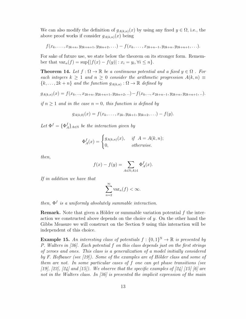
We can also modify the definition of gA(k,n)(x) by using any fixed y ∈ Ω, i.e., theabove proof works if consider gA(k,n)(x) being

f(xk, . . . , x2k+n, y2k+n+1, y2kn+2, . . .)− f(xk, . . . , x2k+n−1, y2k+n, y2k+n+1, . . .).

For sake of future use, we state below the theorem on its stronger form. Remem-ber that varn(f) = sup|f(x)− f(y)| : xi = yi, ∀i ≤ n.

Theorem 14. Let f : Ω→ R be a continuous potential and a fixed y ∈ Ω . Foreach integers k ≥ 1 and n ≥ 0 consider the arithmetic progression A(k, n) ≡k, . . . , 2k + n and the function gA(k,n) : Ω→ R defined by

gA(k,n)(x) = f(xk, .., x2k+n, y2k+n+1, y2kn+2, ..)−f(xk, .., x2k+n−1, y2k+n, y2k+n+1, ..).

if n ≥ 1 and in the case n = 0, this function is defined by

gA(k,0)(x) = f(xk, . . . , x2k, y2k+1, y2k+2, . . .)− f(y).

Let Φf = ΦfAAbN be the interaction given by

ΦfA(x) =

gA(k,n)(x), if A = A(k, n);

0, otherwise.

then,

f(x)− f(y) =∑

AbN;A31

ΦfA(x).

If in addition we have that∞∑n=2

varn(f) <∞.

then, Φf is a uniformly absolutely summable interaction.

Remark. Note that given a Holder or summable variation potential f the inter-action we constructed above depends on the choice of y. On the other hand theGibbs Measure we will construct on the Section 9 using this interaction will beindependent of this choice.

Example 15. An interesting class of potentials f : 0, 1N → R is presented byP. Walters in [36]. Each potential f on this class depends just on the first stringsof zeroes and ones. This class is a generalization of a model initially consideredby F. Hofbauer (see [19]). Some of the examples are of Holder class and some ofthem are not. In some particular cases of f one can get phase transitions (see[19], [23], [24] and [15]). We observe that the specific examples of [24] [15] [6] arenot in the Walters class. In [36] is presented the implicit expression of the main

13

eigenfunction λ of the Ruelle operator (page 1342) and the explicit expression ofthe eigenfunction (page 1341).

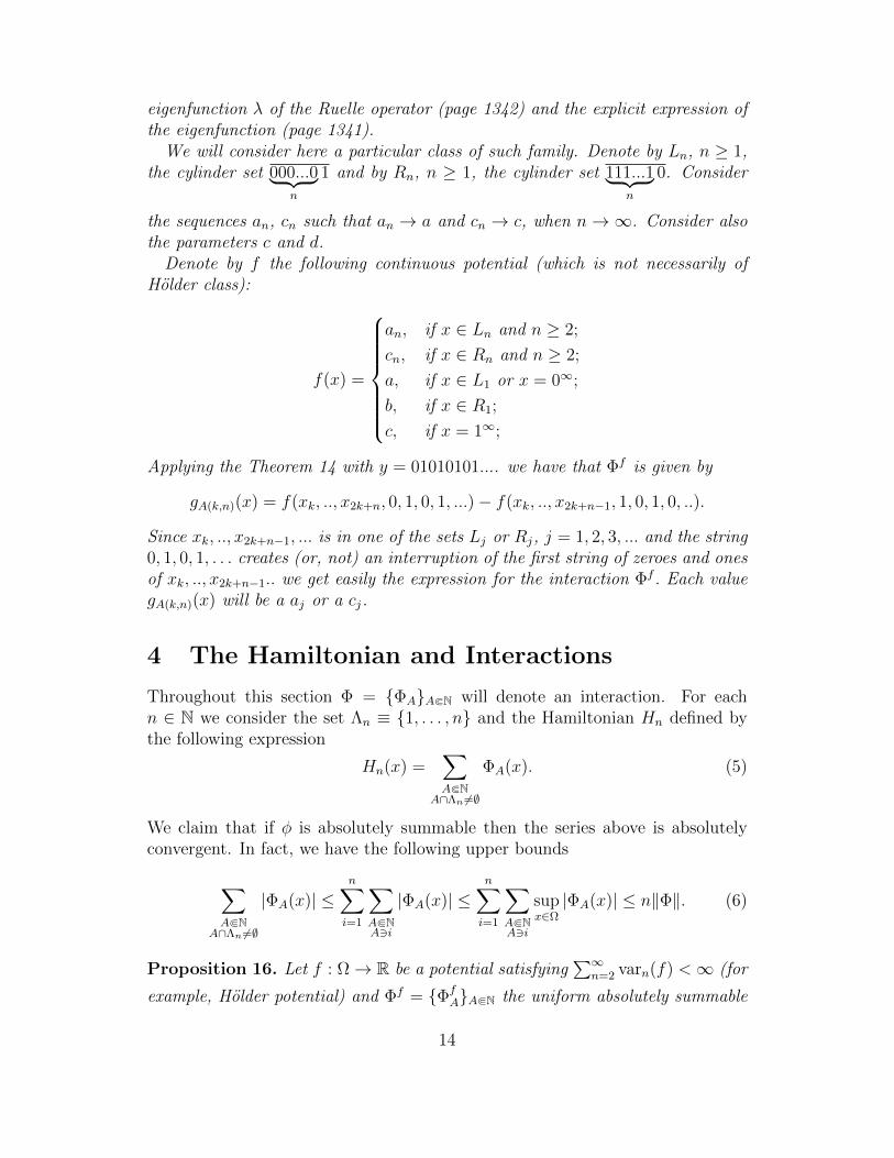
We will consider here a particular class of such family. Denote by Ln, n ≥ 1,the cylinder set 000...0︸ ︷︷ ︸

n

1 and by Rn, n ≥ 1, the cylinder set 111...1︸ ︷︷ ︸n

0. Consider

the sequences an, cn such that an → a and cn → c, when n→∞. Consider alsothe parameters c and d.

Denote by f the following continuous potential (which is not necessarily ofHolder class):

f(x) =

an, if x ∈ Ln and n ≥ 2;

cn, if x ∈ Rn and n ≥ 2;

a, if x ∈ L1 or x = 0∞;

b, if x ∈ R1;

c, if x = 1∞;

Applying the Theorem 14 with y = 01010101.... we have that Φf is given by

gA(k,n)(x) = f(xk, .., x2k+n, 0, 1, 0, 1, ...)− f(xk, .., x2k+n−1, 1, 0, 1, 0, ..).

Since xk, .., x2k+n−1, ... is in one of the sets Lj or Rj, j = 1, 2, 3, ... and the string0, 1, 0, 1, . . . creates (or, not) an interruption of the first string of zeroes and onesof xk, .., x2k+n−1.. we get easily the expression for the interaction Φf . Each valuegA(k,n)(x) will be a aj or a cj.

4 The Hamiltonian and Interactions

Throughout this section Φ = ΦAAbN will denote an interaction. For eachn ∈ N we consider the set Λn ≡ 1, . . . , n and the Hamiltonian Hn defined bythe following expression

Hn(x) =∑AbN

A∩Λn 6=∅

ΦA(x). (5)

We claim that if φ is absolutely summable then the series above is absolutelyconvergent. In fact, we have the following upper bounds

∑AbN

A∩Λn 6=∅

|ΦA(x)| ≤n∑i=1

∑AbNA3i

|ΦA(x)| ≤n∑i=1

∑AbNA3i

supx∈Ω|ΦA(x)| ≤ n‖Φ‖. (6)

Proposition 16. Let f : Ω→ R be a potential satisfying∑∞

n=2 varn(f) <∞ (for

example, Holder potential) and Φf = ΦfAAbN the uniform absolutely summable

14

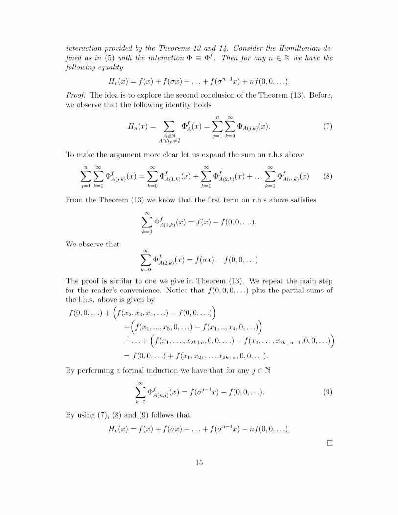
interaction provided by the Theorems 13 and 14. Consider the Hamiltonian de-fined as in (5) with the interaction Φ ≡ Φf . Then for any n ∈ N we have thefollowing equality

Hn(x) = f(x) + f(σx) + . . .+ f(σn−1x) + nf(0, 0, . . .).

Proof. The idea is to explore the second conclusion of the Theorem (13). Before,we observe that the following identity holds

Hn(x) =∑AbN

A∩Λn 6=∅

ΦfA(x) =

n∑j=1

∞∑k=0

ΦA(j,k)(x). (7)

To make the argument more clear let us expand the sum on r.h.s above

n∑j=1

∞∑k=0

ΦfA(j,k)(x) =

∞∑k=0

ΦfA(1,k)(x) +

∞∑k=0

ΦfA(2,k)(x) + . . .

∞∑k=0

ΦfA(n,k)(x) (8)

From the Theorem (13) we know that the first term on r.h.s above satisfies

∞∑k=0

ΦfA(1,k)(x) = f(x)− f(0, 0, . . .).

We observe that∞∑k=0

ΦfA(2,k)(x) = f(σx)− f(0, 0, . . .)

The proof is similar to one we give in Theorem (13). We repeat the main stepfor the reader’s convenience. Notice that f(0, 0, 0, . . .) plus the partial sums ofthe l.h.s. above is given by

f(0, 0, . . .) +(f(x2, x3, x4, . . .)− f(0, 0, . . .)

)+(f(x1, ..., x5, 0, . . .)− f(x1, .., x4, 0, . . .)

)+ . . .+

(f(x1, . . . , x2k+n, 0, 0, . . .)− f(x1, . . . , x2k+n−1, 0, 0, . . .)

)= f(0, 0, . . .) + f(x1, x2, . . . , x2k+n, 0, 0, . . .).

By performing a formal induction we have that for any j ∈ N∞∑k=0

ΦfA(n,j)(x) = f(σj−1x)− f(0, 0, . . .). (9)

By using (7), (8) and (9) follows that

Hn(x) = f(x) + f(σx) + . . .+ f(σn−1x)− nf(0, 0, . . .).

15

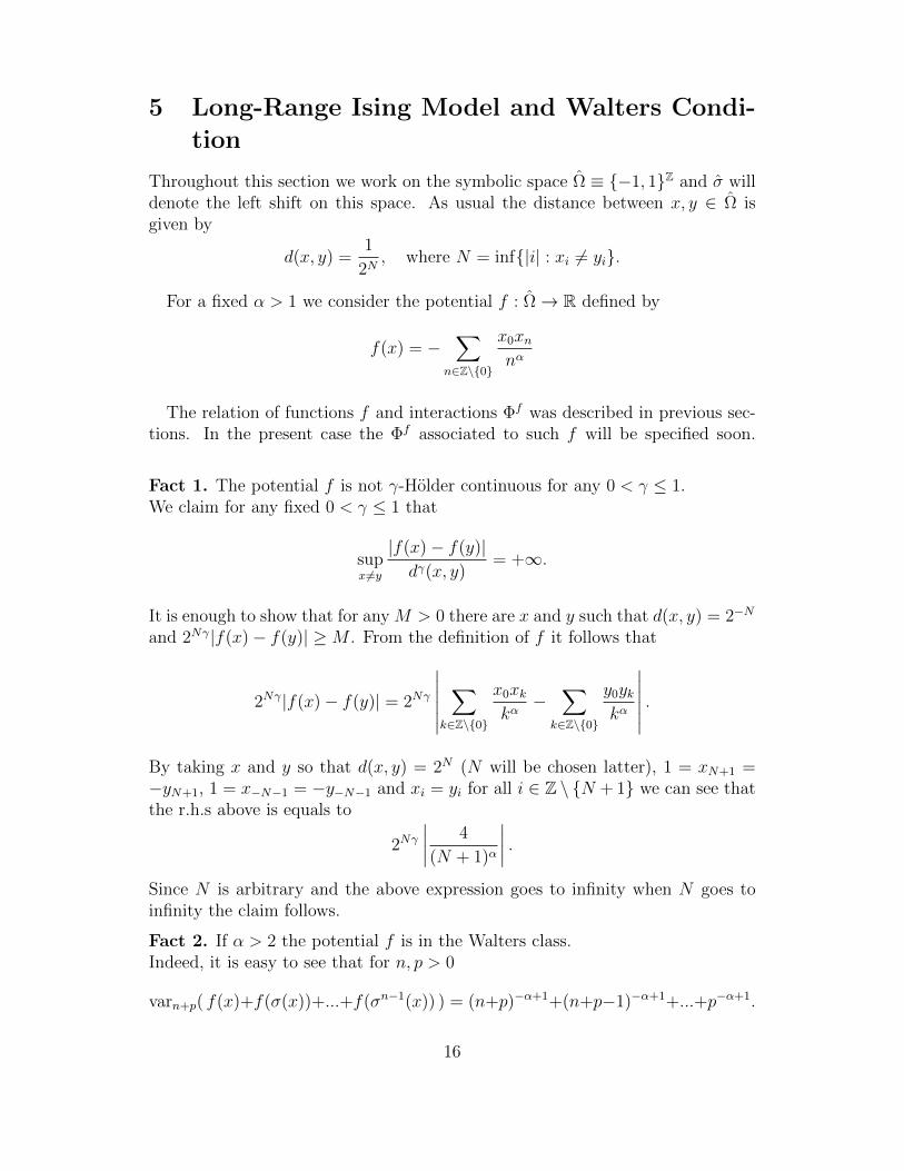
5 Long-Range Ising Model and Walters Condi-

tion

Throughout this section we work on the symbolic space Ω ≡ −1, 1Z and σ willdenote the left shift on this space. As usual the distance between x, y ∈ Ω isgiven by

d(x, y) =1

2N, where N = inf|i| : xi 6= yi.

For a fixed α > 1 we consider the potential f : Ω→ R defined by

f(x) = −∑

n∈Z\0

x0xnnα

The relation of functions f and interactions Φf was described in previous sec-tions. In the present case the Φf associated to such f will be specified soon.

Fact 1. The potential f is not γ-Holder continuous for any 0 < γ ≤ 1.We claim for any fixed 0 < γ ≤ 1 that

supx 6=y

|f(x)− f(y)|dγ(x, y)

= +∞.

It is enough to show that for any M > 0 there are x and y such that d(x, y) = 2−N

and 2Nγ|f(x)− f(y)| ≥M . From the definition of f it follows that

2Nγ|f(x)− f(y)| = 2Nγ

∣∣∣∣∣∣∑

k∈Z\0

x0xkkα−

∑k∈Z\0

y0ykkα

∣∣∣∣∣∣ .By taking x and y so that d(x, y) = 2N (N will be chosen latter), 1 = xN+1 =−yN+1, 1 = x−N−1 = −y−N−1 and xi = yi for all i ∈ Z \ N + 1 we can see thatthe r.h.s above is equals to

2Nγ∣∣∣∣ 4

(N + 1)α

∣∣∣∣ .Since N is arbitrary and the above expression goes to infinity when N goes toinfinity the claim follows.

Fact 2. If α > 2 the potential f is in the Walters class.Indeed, it is easy to see that for n, p > 0

varn+p( f(x)+f(σ(x))+...+f(σn−1(x)) ) = (n+p)−α+1+(n+p−1)−α+1+...+p−α+1.

16

Therefore, for each fixed p > 0 we have that

supn∈N

[varn+p( f(x) + f(σ(x)) + ...+ f(σn−1(x)) )

]∼

∞∑j=p

j−α+1 ∼ p−α+2,

which proves that the Walters condition is satisfied as long as α > 2.The potential f is associated to the following absolutely uniformly summable

interaction

ΦA(x) =

xnxm|n−m|α

, if A = n,m and m 6= n;

0, otherwise,

meaning that

Hn(x) =∑AbZ

A∩Λn 6=∅

ΦA(x) = f(x) + f(σx) + . . .+ f(σn−1x).

Fact 3. The interaction Φ = ΦAAbZ is absolutely uniformly summable inter-action for any α > 1.

This fact can be proved working in the same way we have done in the Example12.

We can ask if the above potential f is cohomologous with a potential g whichdepends just on future coordinates? Note that the Sinai’s Theorem can not bedirectly applied here to answer this question, because the fact we shown above (fis not Holder). For the other hand in this case by keep tracking the cancellationswe actually can construct the transfer function (Definition 1.11 in [33]) usingSinai’s idea, see Proposition 1.2 in [27]. This means: there exists g : −1, 1Z → Rand h : −1, 1Z → R, such that:

1. for any x = (..., x−2, x−1, x0, x1, x2, ...) we have that g(x) = g(x0, x1, x2, ...),

2. f = g + h− h σ.

We first define ϕ : −1, 1Z → −1, 1Z by the expression

ϕ(. . . , x−2, x−1 |x0, x1, x2, . . .) =

(. . . ,−1,−1 |x0, x1, x2, . . .), if x0 = −1;

(. . . , 1, 1 |x0, x1, x2, . . .), if x0 = 1.

Now we define the transfer function h by

h(x) =∞∑j=0

f(σn(x))− f(σn(ϕ(x))).

17

Suppose, for instance, that x satisfies x0 = −1, then,

h(x) = [ f (. . . , x−2, x−1 |x0, x1, x2, . . .) − f (. . . , x0, x0 |x0, x1, x2, . . .) ]

+ [ f (. . . , x−2, x−1, x0 |x1, x2, . . .) − f (. . . , x1, x1, x1 |x1, x2, . . .) ]

+ [ f (. . . , x−2, x−1, x0, x1 |x2, . . .) − f (. . . , x2, x2, x2, x2 |x2, . . .) ] + ...

The case x0 = 1 is similar. Note that if we show that this series is absolutelyconvergent then it is easy to see that 1) and 2) above holds by taking g =f − h+ h σ. By the definition of ϕ and f we have that

∞∑j=0

|f(σn(x))− f(σn(ϕ(x))| =∞∑m=0

∣∣∣∣∣xm(∞∑n=1

x−n(m+ n)α

−∞∑n=1

1

(m+ n)α

)∣∣∣∣∣≤2

∞∑m=0

∞∑n=1

1

(m+ n)α

which is finite as long as α > 2. In this case we can also obtain g in explicit formas:

g(x0, x1, x2, ...) = −x0

∞∑j=1

xjjα− ζ(α).

Remark. The potential f : −1, 1Z → R is very well known on the Mathe-matical Statistical Mechanics community. Two classical theorems state that if1 < α ≤ 2, then there exists a finite positive βc(α) such that if β > βc(α) thenfor the potential βf the set DLR Gibbs measures has at least two elements andif β < βc(α) there is exactly one DLR Gibbs Measure. This is a very non-trivialtheorem. The case 1 < α < 2 it was proved by Freeman Dyson in [10] and thefamous borderline case α = 2 was proved by Frolich and Spencer in [14].

In a future work we will analyze properties which can be derived from theabove g : −1, 1N → R via the Ruelle operator formalism.

6 Boundary conditions

Now we introduce the concept of Gibbsian specification for the lattice N. Thepresentation will not be focused on general aspects of the theory and we restrictourselves to the aspect needed to present our main theorem.

Let Ω be the symbolic space, F the product σ-algebra on Ω and Φ = ΦAAbNbe an interaction defined on Ω and obtained from a continuous f : Ω → R.For some results we will need some more regularity like uniformly absolutelysummability.

18

In what follows we introduce the so called finite volume Gibbs measures witha boundary condition y ∈ Ω (see [33]). Fixed β > 0, y ∈ Ω and n ∈ N. Considerthe probability measure in (Ω,F ) so that for any F ∈ F , we have

µyn(F ) =1

Zyn(β)

∑x∈Ω;

σn(x)=σn(y)

1F (x) exp(−βHn(x)),

where Zyn(β) is a normalizing factor called partition function given by

Zyn(β) =

∑x∈Ω;

σn(x)=σn(y)

exp(−βHn(x)).

It follows from (6) that the above expression is finite. So straightforwardcomputations shows that µyn(·) is a probability measure.

The above expression can be written in the Ruelle operator formalism in thefollowing way. Given a potential f and −Hn(x) = f(x)+f(σ(x)+ ..+f(σn−1(x)),then, for n ∈ N

µyn(F ) =1

Zyn(β)

∑x∈Ω;

σn(x)=σn(y)

1F (x) exp(−βHn(x)) =Lnβf (1F ) (σn(y))

Lnβ f (1) (σn(y)). (10)

In another way

µyn =1

Lnβ f (1)(σn(y))[ (Lβ f )∗ ]n (δσn(y)).

Note that if f is in the Walters class then

Lnf (1) (σn(y)) = λn ϕ(σn(y))Lnf

(1

ϕ

)(σn(y)), (11)

where λ is the eigenvalue, ϕ the eigenfunction of the Ruelle operator Lf andf = f + log(ϕ) − log(ϕ σ) − log λ is the normalized potential associated to f .So for any n ∈ N we have when β = 1

µyn(F ) =Lnf (1F ) (σn(y))

λn ϕ(σn(y))Lnf

( 1ϕ

) (σn(y))=Lnf

(1Fϕ

) (σn(y))

Lnf

( 1ϕ

) (σn(y)). (12)

Which implies that for any given cylinder set F and any y ∈ Ω, we have thatthere exists the limit

limn→∞

µyn(F ) = ν(F ), (13)

where ν is the eigenprobability for L∗f .

19

Gibbs Specifications

Proposition 17. For any fixed n ∈ N and F ∈ F , the mapping y 7→ µyn(F ) ismeasurable with respect the σ-algebra σnF .

Proof. It is enough to note that a function y 7→ z(y) is σnF measurable iff it isof the form z(y) = v(σn(y)) for some F measurable function v.

Definition 18 (Gibbs Specification Determined by Φ). Given a general interac-tion Φ and the associated Hamiltonian, for each n ∈ N and y ∈ Ω, consider thefunction Kn : (F ,Ω)→ R defined by

Kn(F, y) =1

Zyn(β)

∑x∈Ω;

σn(x)=σn(y)

1F (x) exp(−βHn(x)),

where Zyn(β) is

Zyn(β) =

∑x∈Ω;

σn(x)=σn(y)

exp(−βHn(x)).

The collection Knn∈N is known as the Gibbsian specification determined bythe interaction Φ.

Theorem 19. Let Knn∈N be a Gibbsian specification determined by an inter-action Φ, then: for n ∈ N

a) y → Kn(F, y) is σnF -measurable

b) F 7→ Kn(F, y) is a probability measure;

Proof. The proof of a) follows from the Proposition 17 and b) is straightforward.

Proposition 20. Let Φ = ΦAAbN and Ψ = ΨAA∈bN two uniformly absolutelysummable interactions. Suppose that there exist a sequence of real numbers (an)such that

Hn(x) =∑AbN

A∩Λn 6=∅

ΦA(x) and Hn(x) + an =∑AbN

A∩Λn 6=∅

ΨA(x).

Then both interactions determines the same Gibbsian specification.

20

Proof. Let Kn, Kn be the Gibbsian specifications determined by Φ and Ψ throughHn and Hn+an, respectively. If Zy

n(β) is the partition function associated to Kn,i.e.,

Kn(F, y) =1

Zyn(β)

∑x∈Ω;

σn(x)=σn(y)

1F (x) exp(−βHn(x) + an),

then Zyn(β) = exp(an)Zy

n(β), recall that Zyn(β) is obtained taking the numerator

of the above expression with F = Ω. Therefore we have

Kn(F, y) =1

Zyn(β)

∑x∈Ω;

σn(x)=σn(y)

1F (x) exp(−βHn(x) + an)

=1

exp(an)Zyn(β)

∑x∈Ω;

σn(x)=σn(y)

1F (x) exp(−βHn(x)) exp(an)

= Kn(F, y).

7 Gibbs Specifications for Continuous Functions

Given a continuous potential f we consider the following Hamiltonian

Hn(x) = f(x) + f(σx) + . . .+ f(σn−1x).

Note that we are not assuming in this section that the potential f is associatedto any interaction. Even though we can define a Gibbsian specification as in theprevious section, i.e., for n ∈ N

Kn(F, y) =1

Zyn(β)

∑x∈Ω;

σn(x)=σn(y)

1F (x) exp(−βHn(x)), (14)

since we are assuming that f is continuous the two conclusions of the Theorem19 holds and in this case we will say that Knn∈N is the Gibbs specificationassociated to the continuous function f .

8 Thermodynamic Limit

We consider Knn∈N a Gibbsian Specification determined by an uniformly abso-lutely summable interaction Φ or by a continuous potential f . By definition for

21

any measurable set F ⊂ Ω we have

Kn(F, y) =1

Zyn(β)

∑x∈Ω;

σn(x)=σn(y)

1F (x) exp(−βHn(x)).

Let (yn) be a sequence in Ω and (Kn(·, yn)) a sequence of Borel probabilitiesmeasures on Ω. From the compactness of M(Ω) follows that there is at leastone subsequence (nk) so that ynk → y ∈ Ω and Knk(·, ynk) µy, i.e., for allcontinuous function g we have

limk→∞

∫Ω

g(x) dKnk(x, ynk) =

∫Ω

g dµy.

So the probability measure µy is a cluster point in the weak topology of the set

C ≡ Kn(·, yn) : n ∈ N and yn ∈ Ω ⊂ M(Ω).

Definition 21. (Thermodynamic Limit Gibbs probability) The set GTL(Φ) orGTL(f) is defined as being the closure of the convex hull of the set of the clusterpoints of C in M(Ω), where

C ≡ Kn(·, yn) : n ∈ N and yn ∈ Ω.

Any probability in GTL(Φ) will be called Thermodynamic Limit Gibbs probability.

Proposition 22. If f is in the Walters class then GTL = G∗.Proof. This follows from expression (13).

9 DLR - Gibbs Measures

In this section we show how to extend the concept of Gibbs measures beyond theHolder and Walters classes given in the Definition 8. This is done by followingthe Dobrushin-Lanford-Ruelle approach. We will present this concept of Gibbsmeasures for an interaction Φ and for a general continuous potential f .

Finite Volume DLR-equations

Let Knn∈N be a specification determined by and interaction Φ or a continuouspotential f . Before present the DLR-equations let us introduce the followingnotation ∫

Ω

g dKn(·, y) ≡∫

Ω

g(x) dKn(x, y),

where g is any bounded measurable function y ∈ Ω and x = (x1, x2, ...) is just anintegration variable which runs over the space Ω.

22

Theorem 23 (Finite Volume DLR-equations). Let Knn∈N be a specificationdetermined by a continuous potential f . Then for any continuous function g :Ω→ R, and any z ∈ Ω fixed, we have∫

Ω

[∫Ω

g(x) dKn(x, y)

]dKn+r(y, z) =

∫Ω

g(y) dKn+r(y, z).

Before prove the theorem we prove some facts. The first one is the followinglemma.

Lemma 24. For any n, r ∈ N, x = (x1, x2, .., xn), y = (y1, .., yn, yn+1, .., yn+r)and z = (z1, z2, zn, ..) ∈ Ω we have

Hn+r(y1, .., yn, yn+1, .., yn+r, zn+r+1, ..)−Hn(y1, .., yn, yn+1, .., yn+r, zn+r+1, ..)=

Hn+r(x1, .., xn, yn+1, .., yn+r, zn+r+1, ..)−Hn(x1, .., xn, yn+1, .., yn+r, zn+r+1, ..).

In other words, the above difference does not depends on the first n variables.

Proof. By the definition of Hn we have

Hn+r(y1, .., yn, yn+1, .., yn+r, zn+r+1, ..)−Hn(y1, .., yn, yn+1, .., yn+r, zn+r+1, ..)=

n+r−1∑j=n

f(σj(y1, .., yn, yn+1, .., yn+r, zn+r+1, ..)).

By a simple inspection on the above expression the lemma follows.

Corollary 25. For any x, y, z ∈ Ω and n, k ∈ N we have

Hn+r(y1, .., yn, yn+1, .., yn+r, zn+r+1, ..) +Hn(x1, .., xn, yn+1, .., yn+r, zn+r+1, ..)=

Hn+r(x1, .., xn, yn+1, .., yn+r, zn+r+1, ..) +Hn(y1, .., yn, yn+1, .., yn+r, zn+r+1, ..).

Proof of Theorem 23. Observe that∫Ω

g(x) dKn(x, (y1, . . . , yn+1, . . . , yn+r, zn+r+1, zn+r+2, . . .) )

=

1

Z(y1,..,yn+r,zn+r+1,..)n (β)

×∑x∈Ω

σn(x)=(yn+1,..,yn+r,zn+r+1,..)

g(x) exp(−βHn(x))

≡h(y1, . . . , yn+r, zn+r+1, . . .).

23

Note that the statement of the theorem is equivalent to

1

Zzn+r(β)

∑y∈Ω

σn+r(y)=σn+r(z)

h(y) exp(−βHn+r(y)) =1

Zzn+r(β)

∑y∈Ω

σn+r(y)=σn+r(z)

g(y) exp(−βHn+r(y)).

Since Zzn+r(β) > 0, the above equation is equivalent to∑

y∈Ωσn+r(y)=σn+r(z)

h(y) exp(−βHn+r(y)) =∑y∈Ω

σn+r(y)=σn+r(z)

g(y) exp(−βHn+r(y)). (15)

From the definition of h follows that the l.h.s above is given by∑y∈Ω

σn+r(y)=σn+r(z)

1

Z(y1,..,yn+r,zn+r+1,..)n (β)

∑x∈Ω

σn(x)=(yn+1,..,yn+r,zn+r+1,..)

g(x) exp(−βHn(x)) exp(−βHn+r(y))

Using the Corollary 25 we can interchange the n first coordinates of the variableson the above exponentials showing that the above expression is equals to∑

y∈Ωσn+r(y)=σn+r(z)

exp(−βHn(y1, .., yn+k, zn+r+1, ..))

Z(y1,..,yn+r,zn+r+1,..)n (β)

×

∑x∈Ω

σn(x)=(yn+1,..,yn+r,zn+r+1,..)

g(x) exp(−βHn+r(x1, .., xn, yn+1, .., yn+r, zn+r+1, ..)).

Note that the above expression is equals to∑y1,...,yn+r

exp(−βHn(y1, .., yn+r, zn+r+1, ..))

Z(y1,..,yn+r,zn+r+1,..)n (β)

×∑x1,...,xn

g(x) exp(−βHn+r(x1, .., xn, yn+1, .., yn+r, zn+r+1, ..)).

By changing the order of the sums we get∑yn+1,...,yn+r

∑y1,...,yn

exp(−βHn(y1, .., yn+r, zn+r+1, ..))

Z(y1,..,yn+r,zn+r+1,..)n (β)

×∑x1,...,xn

g(x) exp(−βHn+r(x1, .., xn, yn+1, .., yn+r, zn+r+1, ..)).

Observe that Z(y1,..,yn+r,zn+r+1,..)n (β) does not depends on y1, . . . , yn, so from its

definition we have ∑y1,...,yn

exp(−βHn(y1, .., yn+r, zn+r+1, ..))

Z(y1,..,yn+r,zn+r+1,..)n (β)

= 1,

24

implying that the previous expression is equals to∑yn+1,...,yn+r

∑x1,...,xn

g(x) exp(−βHn+r(x1, .., xn, yn+1, .., yn+k, zn+r+1, ..))

=∑y∈Ω

σn+r(y)=σn+r(z)

g(y) exp(−βHn+r(y)).

Therefore the Equation (15) holds and the theorem is proved.In terms of the Ruelle operator the above theorem claims that for any z, and

n, r ≥ 0,

Ln+rf (h)(σn+r(z)) = Ln+r

f

(Lnf (h)(σn(·) )

Lnf (1)(σn(·) )

)(σn+r(z)).

DLR-equations

Theorem 26 (DLR-equations). Let Knn∈N be a specification determined by anabsolutely summable interaction or by a continuous potential f . If the sequenceKnr(·, z) µz, when r → ∞, then for any continuous function g : Ω → R, wehave ∫

Ω

[∫Ω

g(x) dKn(x, y)

]dµz(y) =

∫Ω

g dµz

Proof. In both cases, whereKn is determined by an absolutely uniformly summableinteraction or continuous potential f , the mapping

y 7→∫

Ω

g(x) dKn(x, y)

is continuous for any continuous function g. Taking r large enough the prooffollows from the Theorem 23 and the definition of weak topology.

Definition 27 (DLR-Gibbs Measures). Let Knn∈N be the Gibbsian Specifica-tion on the lattice N determined by an interaction Φ obtained from a continu-ous potential f constructed as in the two previous sections. The set of the DLRGibbs measures for the interaction Φ (or for potential f) is denoted by GDLR(Φ)(GDLR(f)) and given by

µ ∈M(Ω) : µ(F |σnF )(y) = Kn(F, y) for any y, µ−a.e. ∀F ∈ F and ∀n ∈ N.

Remark. We observe that the set GDLR(Φ) or GDLR(f) for a general uniformlyabsolutely summable interaction Φ or continuous potential, respectively, is not

25

necessarily an unitary set. But in any case it is a convex and compact subset ofM(Ω) in the weak topology. We also observe that for the lattice Z even in thecase where #GDLR(Φ) = 1 or #GDLR(f) = 1 the unique probability measure onsuch sets are not necessarily shift invariant. For the lattice Z, assuming thehypothesis of uniformly absolutely summability and the shift invariant propertyin the lattice Z for the interaction Φ, then, we get that the unique element inGDLR(Φ) is invariant for the action of the shift in 1, 2..., dZ (see Corollary 3.48 in[16]). For the lattice N and a continuous potential the corresponding results arenot necessarily the same: the difference between the action by automorphismsand endomorphisms has to be properly considered. Theorems 30 and 34 areexamples where results on N and Z match.

Theorem 28. Let Knn∈N be the Gibbsian Specification determined by an in-teraction Φ obtained from a continuous potential f . A Borel probability measureµ belongs to GDLR(Φ) or GDLR(f) if and only if for all n ∈ N and any continuousfunction g : Ω→ R, we have∫

Ω

[∫Ω

g(x) dKn(x, y)

]dµ(y) =

∫Ω

g dµ.

In other words, µ ∈ GDLR(Φ) or GDLR(f) iff µ satisfies the DLR-equations.

Proof. The proof for GDLR(Φ) is very classical on the Statistical Mechanics lit-erature. We mimic this proof for GDLR(f). Suppose that µ ∈ GDLR(f) then itfollows from the definition of GDLR(f) and the basic properties of the conditionalexpectation that for all n ∈ N we have∫

Ω

g dµ =

∫Ω

µ(g|σnF )(y) dµ(y) =

∫Ω

[∫Ω

g(x) dKn(x, y)

]dµ(y).

Conversely, we assume that the DLR-equations are valid for all n ∈ N and forany continuous function g. By taking g = 1Eh, where E ∈ σnF is a cylinder setand h is an arbitrary continuous function, we have g is continuous and∫

E

[∫Ω

h(x) dKn(x, y)

]dµ(y) =

∫E

h dµ.

It follows from the Dominate Convergence Theorem and Monotone Class The-orem that above identity holds for any measurable set E ∈ σnF . Since themapping

y 7→∫

Ω

h(x) dKn(x, y)

is σn(F )-measurable and E ∈ σn(F ) is an arbitrary measurable set, we havefrom the definition of conditional expectation that∫

Ω

h(x) dKn(x, y) = µ(h|σnF )(y) µ− a.e..

26

Using again the dominate convergence theorem for conditional expectation andmonotone class theorem we can show that the above equality holds for h = 1Fwhere F is a measurable set on Ω, so the result follows.

Theorem 29. For any absolutely uniformly summable interaction Φ or a con-tinuous potential f we have that

GTL(Φ) ⊂ GDLR(Φ) and GTL(f) ⊂ GDLR(f).

Proof. Suppose that Knk(·, znk) µ, i.e., µ ∈ GTL(f). Since f is continuouspotential we have that for any continuous function g : Ω→ R the mapping

y 7→∫

Ω

g(x) dKn(x, y)

is continuous. Using the definition of weak convergence, the finite volume DLR-equations and continuity of g, respectively, we have∫

Ω

[∫Ω

g(x) dKn(x, y)

]dµ(y) = lim

k→∞

∫Ω

[∫Ω

g(x) dKn(x, y)

]dKnk(y, znk)

= limr→∞

∫Ω

g(y) dKnk(y, znk)

=

∫Ω

g(y) dµ(y).

The above equation prove that the probability measure µ satisfies the DLR-equation for any continuous function g. By applying the Theorem 28 we concludethat µ ∈ GDLR(f).

Theorem 30. Let Φ be an interaction obtained from a continuous potential fWe consider the Gibbs specification Knn∈N, associated to this interaction Φ orto the function f . Then, in the general case GDLR(Φ) = GTL(Φ). In particular,GDLR(f) = GTL(f).

Proof. We borrow the proof from [5]. We first remark that GTL(Φ) ⊂ GDLR(Φ)is the content of the Theorem 29. Suppose by contradiction that there existsµ ∈ GDLR(Φ) which is not in the compact set GTL(Φ).

Any open neighborhood V ⊂ M(Ω) of µ in the weak topology contains anbasis element B(g, ε), where g is some continuous function and ε > 0, of the form

B(g, ε) =

ν ∈M(Ω) :

∣∣∣∣∫Ω

g d ν −∫

Ω

g dµ

∣∣∣∣ < ε

.

Assume for some B(g, ε), that we have B(g, ε) ∩ GTL(Φ) = ∅. Note that themapping ν 7→

∫Ωg dν is continuous and convex as a function defined on the

convex set GTL(Φ).

27

Without loss of generality we can assume for any ν ∈ GTL(Φ) that∫

Ωg dν >∫

Ωgdµ+ ε. By Theorem 28 we have for any n ∈ N that∫

Ω

[∫Ω

g(x) dKn(x, y)

]dµ(y) =

∫Ω

g dµ.

For each n, there exist at least one yn such that∫

Ωg(x) dKn(x, yn) <

∫Ωgdν + ε.

Now, by considering a convergent subsequence limk→∞Knk(., ynk) = µ ∈ GTL(Φ)we reach a contradiction. Therefore, GDLR(Φ) = GTL(Φ).

Note that when f is a Walters potential, for any z ∈ Ω we have from (13) thatKn(., z) → ν, where ν ∈ G∗(f). Therefore, ν is a DLR-Gibbs Measure for thepotential f .

There is another direct way to prove this result for a general continuous poten-tial f which needs not to be on the Bowen or Walters class. To prove this resultin such generality is useful to deal with the potentials appearing on [6] and [36].

Theorem 31. Suppose f is continuous and there exists a positive eigenfunctionψ for the Ruelle operator Lf . Then, G∗(f) ⊂ GDLR.

Proof. Suppose ν is an eigenprobability in G∗(f). Then µ = ψ ν is a shift-invariantprobability measure. Given a function g : Ω → R, consider the expected valueof g with respect to the finite volume Gibbs measure with boundary condition y,given by ∫

Ω

g(x)Kn(x, y) dx =Lnβf (g) (σn(y))

Lnβ f (1) (σn(y)).

Note thatLnβf (g) (σn(y))

Lnβ f (1) (σn(y))is σnF measurable. From the Theorem 23 we have for

any n, r ≥ 0 and z that

Ln+rf (h)(σn+r(z)) = Ln+r

f

(Lnf (h)(σn(·) )

Lnf (1)(σn(·) )

)(σn+r(z)). (16)

Given n ∈ N and measurable functions g and v we have that

28

∫Ω

(g σn)(z)Lnf (v) (σn(z))

Lnf (1) (σn(z))d ν(z) =

∫Ω

Lnf (v (g σn)) (σn(z))

Lnf (1) (σn(z))d ν(z)

=

∫Ω

1

λnLnf

[Lnf (v (g σn)) (σn(·))Lnf (1) (σn(·))

](z) d ν(z)

=

∫Ω

1

λnLnf

[Lnf (v (g σn)) (σn(·))Lnf (1) (σn(·))

](z)

1

ψ(z)d µ(z)

since the measure µ is translation invariant the r.h.s above is equals to∫Ω

1

λnLnf

[Lnf (v (g σn)) (σn(·))Lnf (1) (σn(·))

](σn)(z)

1

ψ(σn(z))d µ(z).

Using the equation (16) we can see that the above expression is equals to∫Ω

1

λnLnf [(v (g σn))(·)] (σn)(z)

1

ψ(σn(z))d µ(z).

Using again the translation invariance of µ we get that the above expression isequals to∫

Ω

1

λnLnf [(v (g σn))(·)] (z)

1

ψ(z)d µ(z) =

∫Ω

1

λnLnf [(v (g σn))(·)] (z) d ν(z)

=

∫Ω

(g σn) (z) v(z) d ν(z)

so for each n ∈ N follows from the identities we obtained above that

ν(F |σnF )(y) =Lnf (IF ) (σn(y))

Lnβ f (1) (σn(y)), ν − almost surely.

Which immediately implies that ν is DLR-Gibbs measure for f .

In the next section we address the question of uniqueness of the Gibbs Mea-sures. We provide sufficient conditions for a specification defined by an interactionΦ or by a continuous potential f to have a unique DLR-Gibbs measure. In thesequel we use this theorem to prove that the specification Φf for a Holder poten-tial f as defined in Theorem 13 or the specification for f in Walter class, has aunique Gibbs Measure.

29

We shown that the unique DLR-Gibbs measure associated to Φf is the uniquefixed point of L∗

fthe same for f in the Walter class. Since we have a unique Gibbs

measure for any Holder potential or for any f in Walter class follows that theDLR point of view give us a direct and convenient way to define Gibbs Measuresfor a very large class of potentials and extends the concept of Gibbs measureusually considered in Thermodynamic Formalism. We also explain the relationbetween the DLR Gibbs measures for Φf and Φf in the Holder class and theanalogous statement for the Walter class.

Uniqueness and Walters Condition

We say that a specification presents phase transition in the DLR, TL or dual senseif, respectively, the sets GDLR(Φ), GTL(Φ), or G∗(Φ) has more than one element.In [6] several examples of such phenomena are described for one-dimensionalsystems.

We begin this section recalling a classical theorem of the Probability theory.Consider the following decreasing sequence of σ-algebras

F ⊃ σF ⊃ σ2F ⊃ · · · ⊃ σnF ⊃ · · · ⊃∞⋂j=1

σjF

the Backward Martingale Convergence Theorem states that for all f : Ω → Rbounded measurable function we have

µ(f |σnF )→ µ(f | ∩∞j=1 σjF ), a.s. and in L1.

Theorem 32. Let Knn∈N be an specification determined by an absolutely uni-formly summable interaction Φ or a continuous function f . Let µ ∈ GDLR(Φ)or µ ∈ GDLR(f). In any of both cases the following conditions are equivalentcharacterizations of extremality.

1. µ is extremal;

2. µ is trivial on⋂∞j=1 σ

jF ;

3. Any⋂∞j=1 σ

jF -measurable functions g is constant µ-almost surely.

Proof. The proof can be found on [17] and [16, p. 151].

Theorem 33. Let Knn∈N be an specification determined by an interaction Φobtained from a continuous function f . Let µ be an extremal element of theconvex space GDLR(Φ) or GDLR(f). Then for µ-almost all y we have

Kn(·, y) µ.

30

Proof. We will prove convergence and not just convergence of subsequence. Wewill borrow the proof from [16].

Note that it is enough to prove that for µ-almost all y we have

Kn(C, y)→ µ(C) ∀C cylinder set.

The crucial fact is that the of all cylinder set is countable. Fix a cylinder C andn ∈ N then by the definition of GDLR(Φ) or GDLR(f) there is a set Ωn,C withµ(Ωn,C) = 1 and such that Kn(C, y) = µ(C|σnF )(y) for all y ∈ Ωn,C . By theitem 3 of the Theorem 32 and definition of conditional expectation it is possibleto find a measurable set ΩC so that µ(C) = µ(C|∩∞j=1σ

jF )(y) for all y ∈ ΩC andµ(ΩC) = 1. By the Backward Martingale Convergence Theorem with f = 1C , wehave that there is a measurable set Ω′C with µ(Ω′C) = 1 so that

µ(C|σnF )(y)→ µ(C| ∩∞j=1 σjF )(y) ∀y ∈ Ω′C .

Therefore ify ∈

⋂n∈N

C cylinder set

(ΩC ∩ Ω′C ∩ Ωn,c)

which is a set of µ measure one, we have the desired convergence.

Theorem 34. Let Φ be an absolutely uniform summable potential and f a con-tinuous potential. Consider the Hamiltonian

Hn(x) =∑AbN

A∩Λn 6=∅

ΦA(x) or Hn(x) = f(x) + f(σx) + . . .+ f(σn−1x)

IfD ≡ sup

n∈Nsupx,y∈Ω;

d(x,y)≤2−n

|Hn(x)−Hn(y)| <∞

then #GDLR(Φ) = 1 or #GDLR(f) = 1, respectively.

Before presenting the proof of this theorem we need one more lemma.

Lemma 35. Let D be the constant defined on the above theorem. Then, for allx, y ∈ Ω, all cylinders C and for n large enough, we have

e−2DβKn(C, z) ≤ Kn(C, y) ≤ e2DβKn(C, z).

Proof. The proof presented here follow closely [16]. By the definition of D, uni-formly in n ∈ N, x, y, z ∈ Ω, we have

−D ≤ Hn(x1, . . . , xn, zn+1, . . .)−Hn(x1, . . . , xn, yn+1, . . .) ≤ D

31

which implies the following two inequalities:

exp(−Dβ) exp(−βHn(x1, ..., xn, zn+1, ...)) ≤ exp(−Hn(x1, ..., xn, yn+1, ...))

and

exp(−Hn(x1, ..., xn, yn+1, ...)) ≤ exp(Dβ) exp(−βHn(x1, ..., xn, zn+1, ...)).

Using theses inequalities we get that

e−βDZzn(β) ≤ Zy

n(β) ≤ eβDZzn(β).

Let C be a cylinder set and suppose that its basis is contained in the set 1, . . . , p.For every n ≥ p we have 1C(x1, . . . , xn, zn+1, . . .) = 1C(x1, . . . , xn, yn+1, . . .).Therefore

Kn(C, y) =1

Zyn(β)

∑x∈Ω;

σn(x)=σn(y)

1C(x) exp(−βHn(x))

≤ 1

e−βDZzn(β)

∑x∈Ω;

σn(x)=σn(z)

1C(x) exp(Dβ) exp(−βHn(x))

=e2DβKn(C, z).

The proof of the inequality e−2DβKn(C, z) ≤ Kn(C, y) is similar.

Proof of the Theorem 34. The strategy is to prove that G(Φ) or G(f) has aunique extremal measure and use the Choquet Theorem to conclude the unique-ness of the Gibbs measures.

We give the argument for G(f), the proof is the same for G(Φ). Let µ and νbe extremal measures on G(f). By the Theorem 33 there exists y, z ∈ Ω suchthat both measures µ and ν are thermodynamic limits of Kn(·, y) and Kn(·, z),respectively, when n→∞. Using the Lemma 35 we have for any cylinder set Cthat

µ(C) = limnKn(C, y) ≤ e2Dβ lim

nKn(C, z) = e2Dβν(C).

Clearly the collection D = E ∈ F : µ(E) ≤ e2Dβν(E) is a monotone class.Since it contains the cylinder set, which is stable under intersections, we havethat D = F . Therefore µ ≤ e2Dβν, in particular µ ν. This contradict the factthat two distinct extremal gibbs measures are mutually singular, see [17, Theo.7.7, pag 118]. So have proved that µ = ν.

Remark. Note that the condition imposed over D is more general than theWalters condition. In fact, we just have proved uniqueness in the Bowen class(see definition in [36]). Note that for a continuous f we have that G∗(f) andGTL(f) are not empty. We just show that the cardinality of GTL(f) is equal toone.

32

Theorem 36. Let f : Ω → R be a Holder potential and Φf the interactionconstructed in the Theorem 13. If

Hn(x) =∑AbN

A∩Λn 6=∅

ΦfA(x)

then the hypothesis of Theorem 34 holds and therefore Φf has a unique DLRGibbs measure measures for the interaction Φf .

Proof. By Proposition 16 and the triangular inequality we have that

|Hn(x)−Hn(y)| = |f(x) + . . .+ f(σnx)− f(y)− . . .− f(σny)|

≤ |f(x)− f(y)|+ . . .+ |f(σnx)− f(σny)|.

Given n ∈ N if d(x, y) ≤ 2−n then the r.h.s above is bounded by K(f)2−n +K(f)2−n+1 + . . .+K(f). So

D ≡ supn∈N

supx,y∈Ω;

d(x,y)≤2−n

|Hn(x)−Hn(y)| < K(f).

Remark. We point out the following a criteria of [21] for the uniqueness of theeigenprobability of the normalized potential f (which is stronger than [4]): Forany ε > 0 we have that

∞∑n=1

exp

[− (

1

2+ ε) (var1(f) + var2(f) + ...+ varn(f))

]=∞.

10 Equivalence on the Walters Class

Now we consider a potential f in the Walters class and the specification Knn∈Ndetermined by f . We will show, following the steps in [3], that the unique Gibbsmeasure µ ∈ GDLR(f) satisfies L∗

f(µ) = µ. Next, we show that if f belongs to

the Walters class, then

G∗(f) = GDLR(f) = GTL(f).

We will express al the concepts and results described in previous sections inthe language of Ruelle operators. When f is in the Walters class there exist themain eigenfunction and this sometimes simplifies some proofs.

33

Theorem 37. Let f : Ω → R be a potential in the Walters class and f itsnormalization given by (2). Let µ be the unique probability belonging to the setGDLR(Φf ) then L∗

fµ = µ. In other words GDLR(f) ⊂ G∗(f).

Proof. We first prove that for any continuous function g : Ω → R and y ∈ Ωfixed, we have ∑

x∈Ωσnx=y

g(x)Kn(x, y) = Lnf (f)(σn(y)).

It follows directly from the definition of the Ruelle operator that

Lnf (1)(σn(y)) =∑x∈Ω

σnx=σny

exp(f(x) + . . .+ f(σn−1x)).

Since the potential is normalized we have that above sum is equal to one. IfKnn∈N is the specification associated to the interaction Φf then for any con-tinuous potential g we have∑

x∈Ωσnx=y

g(x)Kn(x, y) =1

Zyn

∑x∈Ω

σnx=σny

g(x) exp(f(x) + . . .+ f(σn−1x))

Note we have canceled the term nf(0, 0, . . .) in the numerator and denominatorin the above expression. It is immediate to check that Zy

n = Lnf(1)(σn(y)) = 1,

therefore ∑x∈Ωσnx=y

g(x)Kn(x, y) = Lnf (g)(σn(y))

By the Theorem 30 and a classical result from Thermodynamic Formalism wehave that (up to subsequence)∫

Ω

g dµ = limn→∞

∑x∈Ωσnx=y

g(x)Kn(x, y) = limn→∞

Lnf (g)(σn(y)) =

∫Ω

gdm,

where m is the fixed point of the Ruelle operator. By observing that the g isan arbitrary continuous function it follows from the Riesz-Markov Theorem thatµ = m.

Given a potential f and −Hn(x) = f(x) + f(σ(x) + ..+ f(σn−1(x)), then

Kn(F, y) =1

Zyn(β)

∑x∈Ω;

σn(x)=σn(y)

1F (x) exp(−βHn(x)) =Lnβf (1F ) (σn(y))

Lnβ f (1) (σn(y)).

34

As long as f is in the Walters class we have

Lnf (1) (σn(y)) = λn ϕ(σn(y))Lnf

(1

ϕ

)(σn(y))

and we can also rewrite Kn(F, y) as follows:

Kn(·, y) =1

Lnβ f (1)(σn(y))[ (Lβ f )∗ ]n (δσn(y)). (17)

Note that if the potential f is normalized, that is Lf1 = 1, and Hn = f(x) +

f(σ(x)+. . .+f(σn(x)), then for all n and all y we have Zy,fn (1) = Ln

f(1) (σn(y)) =

1. Moreover,

Kn(F, y) =∑x∈Ω;

σn(x)=σn(y)

1F (x) exp(−Hn(x)) = Lnf (1F ) (σn(y))

or alternatively Kn(·, y) = [ (L f )∗ ]n (δσn(y)). Assuming that f is in the Waltersclass we have for any continuous function g : Ω→ R, and any fixed y ∈ Ω that

limn→∞

Ln+1f

(g) (σn(y)) = limn→∞

Lnf (g) (σn(y)) =

∫Ω

g dµ,

where µ is the fix point for L∗f.

Remark: From the above expression follows that if f is just continuous butnormalized (Lf (1) = 1) and such that for a certain y ∈ Ω there exists the limitm = limn→∞ µ

yn, then,

L∗f (m) = L∗f ( limn→∞

µy,fn ) =L∗f ( limn→∞

[ (L f )∗ ]n (δσn(y)) )

= limn→∞

L∗f [ (L f )∗ ]n (δσn(y) )

=m.

In other words: G∗(f) = GTL(f).

Theorem 38. Let f : Ω → R be a potential in the Walters class and f itsnormalization given by (2). Then

1. For any y ∈ Ω we have that µy,fn = [ (L f )∗ ]n (δσn(y)) converges when n→∞in the weak topology to the unique equilibrium state for f (or f).

35

2. Moreover, for any y ∈ Ω, we have that

µy,fn =1

Lnf (1)(σn(y))[ (L f )∗ ]n (δσn(y))

converges when n → ∞ to the unique eigenprobability ν for L∗f , associatedto the principal eigenvalue.

3. As the set GTL(Φf ) is the closure of the convex hull of the set of weak limitsof subsequences µy,fnk , k →∞, we get that GDLR(Φf ) has cardinality 1.

Proof. 1. If f is normalized and in the Walters class there is a unique fixedprobability µ for L∗

f. Given any y ∈ Ω we have, for any continuous function g,

that

(L f )n(g)(σn(y))→∫

Ω

gdµ,

as n→∞. Since∫

Ωg dµy,fn = (L f )n(g)(σn(y)) the first claim follows.

2. Since the equilibrium state µ = ϕ ν, where ϕ is the eigenfunction and ν isthe eigenprobability. Given a non-normalized f in the Walters class and ϕ themain eigenfunction of Lf considering the normalized potential f = f + logϕ −log(ϕ σ)− log λ, we have

(L f )n(

1

ϕ

)(σn(y))→

∫Ω

1

ϕdµ =

∫Ω

1 dν.

From this convergence and the coboundary property we get that

ϕ(σn(y))−1 Lnf ( 1 )(y)

λn→ 1.

Analogously for any given continuous function g : Ω→ R, we have that

(L f+logϕ−log(ϕσ)−log λ)n

(g

ϕ

)(σn(y)) = (L f )n

(g

ϕ

)(σn(y))→

∫g

ϕdµ =

∫g dν.

andϕ(σn(y))−1 Lnf ( g )(σn(y))

λn→∫gdν,

when n→∞. So taking the limit when n→∞ we obtain∫Ω

g µy,fn =1

Lnf (1)(σn(y))(L f )n (g)(σn(y)) ∼ (L f )n (g)(σn(y))

1λn

ϕ(σn(y))−1

→∫gdν,

36

The above proof also shows that GDLR(f) ⊂ G∗(f). That is, if f is in theWalters class we have that ν = GDLR(f) where ν is the unique eigenprobabilityfor L∗f . Moreover, if f is normalized and in the Walters class we have that µ =

GDLR(f) where µ is the unique fixed point for L∗f.

If the potential f does not satisfies the hypothesis of the Theorem 34 the limitµy,fn , when n→∞, can depends on y. We Remark that there is a certain optimal-ity in Theorem 34 because of the long-range Ising model. When the parameterα > 2 in this model, we have shown that the Hypothesis of the Theorem 34 aresatisfied and we have only one Gibbs measure for any y. For 1 < α ≤ 2 (wherethe hypothesis is broken) Dyson, Frolich and Spencer (see [10, 14]) shows thatthere is more than one Gibbs measure for sufficiently low temperatures. Moreexamples of this phenomenon can also be found in [6, 17].

Theorem 39. Let f : Ω → R be a potential in the Walters class and f itsnormalization given by (2). If ν ∈ GDLR(f) and µ ∈ GDLR(f) then for anycontinuous function g we have that∫

Ω

g dν =

∫Ω

g

ϕdµ.

Proof. Let ϕ be the main eigenfunction associated to the main eigenvalue λ of theoperator Lf . Let Hn and Hn the Hamiltonians associated to f and f , respectively

−Hy

n(x) =n−1∑j=0

f(σjx) and −Hyn(x) =

n−1∑j=0

f(σjx)

By a simple computation follows that

n−1∑j=0

f(σjx) =n−1∑j=0

f(σjx) + logϕ(x)− logϕ(σnx)− n log λ.

Therefore, we have

Hn(x)−Hn(x) = logϕ(σnx)− logϕ(x) + n log λ. (18)

Note that for any g : Ω→ R we have∑x∈Ω;σnx=σny

g(x)e−βHn(x)

∑x∈Ω;σnx=σny

e−βHn(x)=

∑x∈Ω;σnx=σny

g(x)e−βHn(x)+β logϕ(σnx)−β logϕ(x)

∑x∈Ω;σnx=σny

e−βHn(x)+β logϕ(σnx)−β logϕ(x)

37

In the sums on the r.h.s. above the terms exp(β logϕ(σnx)) are constant equalto exp(β logϕ(y)). So they cancel each other and r.h.s of the above expression isequal to

∑x∈Ω;σnx=σny

g(x)e−βHn(x)−β logϕ(x)

∑x∈Ω;σnx=σny

e−βHn(x)−β logϕ(x)=

∑x∈Ω;σnx=σny

g(x)

ϕ(x)e−βHn(x)

∑x∈Ω;σnx=σny

1

ϕ(x)e−βHn(x)

.

By dividing and multiplying by the partition function of the Hamiltonian Hn andtaking the limit when n→∞ we get from the two previous equations that∫

Ω

g dν =

∫Ω

g

ϕdµ

Remark. From (18) for any Holder or Walters potential f we have

supn∈N

supx∈Ω|Hn(x)−Hn(x)| = sup

n∈Nsupx∈Ω| logϕ(x)− logϕ(σnx)| <∞,

where in the last inequality we use that ϕ is positive everywhere, continuous andΩ is compact. So the specifications Kn and Kn are “physically” equivalent, see[17, p.136]. As we already said µ is always σ-invariant for any Holder potentialf . Although µ and ν are associated to equivalent specifications there are caseswhere ν is not σ invariant. For the other hand in any case µ = ν on the tailσ-algebra, i.e., ∩n∈NσnF , see Theorem 7.33 in [17].

11 Concluding Remarks

In this paper we have compared the definitions of Gibbs measures defined interms of the Ruelle operator and DLR specifications. We show how to obtain forpotentials in the Walters and Holder class the Gibbs measures usually consideredin the Thermodynamic Formalism via the DLR formalism and prove that themeasures obtained from both approaches are the same.

Both approaches have their advantages. For example, using the Ruelle operatorwe were able to prove some uniform convergence theorems about the finite volumeGibbs measures.

The literature about absolutely uniformly summable interactions is vast andthis approach allow us to consider non translation invariant potentials and alsoon systems other than the lattices Z or N. We also show that the long rangeIsing model on N can be studied using the Ruelle operator, at least when the

38

interaction is of the form 1/rα with α > 2. In these cases, we have proved thatthe unique Gibbs measure of this model satisfies GDLR(Φ) = GTL(Φ) = G∗(f),but on the other hand it is not clear how to treat the cases 1 < α ≤ 2 by using theRuelle operator and what kind of information is obtainable through this approach.It is worth pointing out that treating this model with the DLR approach isfairly standard, so the connection made here suggests that more understandingof the DLR Specification theory can shed light on more general spaces whereone can efficiently use the Ruelle Operator. Another important feature of theDLR-measure Theory is that it is also readily appliable to standard Borel spaces,which includes compact and non-compact spaces [17]. Thus the results obtainedhere can be extended to compact spaces, but some measurability issues have tobe taken into account and some convergence theorems have to be completelyrewritten, although the main ideas are contained here. We will approach thisissue in the near future.

Acknowledgments

We would like to express our thanks to Aernout van Enter, Anthony Quas, JoseSiqueira, Renaud Leplaideur and Rodrigo Bissacot for their careful reading ofthis paper, and their many helpful comments which have helped improve theexposition. The authors thanks CNPq and FEMAT by the financial support.

Keywords: DLR-Gibbs Measures, Ruelle Operator, eigenprobabilities, Ther-modynamic Limit, One-Dimensional Systems, Symbolic Dynamics, StatisticalMechanics.

References

[1] A. Bovier. Statistical Mechanics of Disordered Systems. A MathematicalPerspective. Cambridge University Press (2006).

[2] R. Bowen. Equilibrium States and the Ergodic Theory of Anosov Diffeomor-phisms, Lecture Notes in Math., vol. 470. Springer, Berlin (1975).

[3] A. T. Baraviera, L. Cioletti, A. O. Lopes, J. Mohr and R. R. Souza. On thegeneral one-dimensional XY model: positive and zero temperature, selectionand non-selection. Rev.Math. Phys. 23 n.10, 1063-1113 (2011).

[4] H. Berbee. Uniqueness of Gibbs measures and absortion probabilities, TheAnnals of Prob., Vol 17, N. 4, 1416-1431 (1989).

[5] R. Bissacot and L. Cioletti. Introducao as medidas de Gibbs, Notes USP(2013).

39

[6] L. Cioletti and A. O. Lopes. Phase Transitions in One-dimensional Transla-tion Invariant Systems: a Ruelle Operator Approach, preprint (2014).

[7] Z. Coelho and A. Quas. A criteria for d-continuity, Trans. AMS, Volume 350,Number 8, 3257-3268 (1998).

[8] R.L. Dobrushin. The description of a random field by means of conditionalprobabilities and conditions of its regularity. Theor. Prob. Appl. 13, 197-224(1968).

[9] R.L. Dobrushin. Prescribing a system of random variables by conditionaldistributions. Th. Prob. Appl. 15, 458-486 (1970).

[10] F. J. Dyson. Existence of a phase-transition in a one-dimensional Ising fer-romagnet. Comm. Math. Phys. 12, no. 2, 91-107 (1969).

[11] R. Ellis. Entropy, Large Deviations, and Statistical Mechanics. Springer Ver-lag. (2005).

[12] A.H. Fan. A proof of the Ruelle theorem. Reviews Math. Phys., Vol 7, n8,1241-1247 (1995).

[13] Follmer H. Phase transition and Martin boundary. In:Sem. Prob. StrasbourgIX, LNM 465 (1975).

[14] J. Frohlich, T. Spencer. The phase transition in the one-dimensional Isingmodel with 1/r2 interaction energy. Comm. Math. Phys. 84, no. 1, 87-101(1982).

[15] A. Fisher and A. O. Lopes. Exact bounds for the polynomial decay of cor-relation, 1/f noise and the CLT for the equilibrium state of a non-Holderpotential, Nonlinearity, Vol 14, Number 5, pp 1071-1104 (2001).

[16] Sacha Friedli and Yvan Velenik. Equilibrium Statistical Mechanics of Clas-sical Lattice Systems: a Concrete Introduction. Available at http://www.

unige.ch/math/folks/velenik/smbook/index.html

[17] H.O. Georgii. Gibbs Measures and Phase Transitions, Ed. de Gruyter, Berlin,(1988).

[18] P. Giulietti, A. Lopes and V. Pit Duality between Eigenfunctions andEigendistributions of Ruelle and Koopman operators via an integral kernel,preprint Arxiv (2014).

[19] F. Hofbauer. Examples for the non-uniqueness of the Gibbs states, Trans.AMS , (228), 133-141, (1977).

40

[20] Y. P. Jiang. A Proof of existence and simplicity of a maximal eigenvaluefor Ruelle-Perron-Frobenius operators. Letters in Mathematical Physics, 48,211-219 (1999).

[21] A. Johansson, A. Oberg and M. Pollicott. Unique Bernoulli g-measures, J.Eur. Math. Soc. (Journ of the Eur. Math. Soc) 14, no. 5, 1599-1615 (2012).

[22] Lanford, O.E. and D. Ruelle. Observables at infinity and states with shortrange correlations in Statistical Mechanics. Commun. Math. Phys. 13, 194-215 (1969).

[23] A. O. Lopes. A First-Order Level-2 Phase Transition in Thermodynamic For-malism, Journal of Statistical Physics, Vol. 60, N. 3/4, pp. 395-411, (1990).

[24] A. O. Lopes. The Zeta Function, Non-Differentiability of Pressure and theCritical Exponent of Transition, Advances in Mathematics, Vol. 101, pp.133-167, (1993).

[25] A. O. Lopes, J. K. Mengue, J. Mohr and R. R. Souza, Entropy and Varia-tional Principle for one-dimensional Lattice Systems with a general a-prioriprobability: positive and zero temperature, to appear in Erg. Theory andDyn. Systems, (2015).

[26] L. Onsager. Crystal Statistics. I. A Two-Dimensional Model with an Order-Disorder Transition. Phys. Rev. Vol 65, 117 (1944).

[27] W.Parry and M.Pollicott. Zeta functions and the periodic orbit structure ofhyperbolic dynamics. Asterisque, 187-188, (1990).

[28] C.J. Preston. Random Fields. LNM 534 (1976).

[29] A. Quas. Non-ergodicity for C1 expanding maps and g-measures. ErgodicTheory Dynam. Systems 16, no. 3, 531–543 (1996).

[30] D. Ruelle. Statistical mechanics of a one-dimensional lattice gas. Comm.Math. Phys. Vol.9, 267–278 (1968).

[31] D.Ruelle. Zeta-functions for expanding maps and Anosov flows. Invent.Math. 34, 231-242 (1976).

[32] Y. Sinai. Gibbsian measures in ergodic theory. Uspehi Mat. Nauk 27, 4,21-64 (1972). English translation, Russian Math. Surveys, 4, 21-69 (1972).

[33] O. Sarig. Lecture notes on thermodynamic formalism for topological Markovshifts. Penn State. (2009).

41

[34] A. C. D. van Enter, R. Fernandez and A. D. Sokal. Regularity properties andpathologies of position-space renormalization-group transformations: Scopeand limitations of Gibbsian theory. Journ. of Stat. Phys. V.72. N 5/6, 879-1187 (1993).

[35] P. Walters. An Introduction to Ergodic theory, Springer Verlag, (2000)

[36] P. Walters. A natural space of functions for the Ruelle operator theorem,Ergodic Theory and Dynamical Systems. 27, 1323-1348 (2007).

[37] P. Walters. Convergence of the Ruelle operator for a function satisfyingBowen’s condition. Trans. Amer. Math. Soc. 353, no. 1, 327–347 (2001).

[38] P. Walters. Invariant measures and equilibrium states for some mappingswhich expand distances. Trans. Amer. Math. Soc, 236, 121-153 (1978).

42