Inter Laboratory Variability

of the Marshall Test Method

for Asphalt Concrete

FINAL REPORT WVDOH RP #137

By John P. Zaniewski, Ph.D.

Michael Hughes

Harley O. Staggers National Transportation Center Department of Civil and Environmental Engineering

West Virginia University PO Box 6103

Morgantown, WV 26506

Submitted to:

West Virginia Department of Transportation Division of Highways

And U.S. Department of Transportation Federal Highway Administration

June 2003

Revised June 2006

i

NOTICE The contents of this report reflect the views of the author who is responsible for the facts and the accuracy of the data presented herein. The contents do not necessarily reflect the official views or policies of the State or the Federal Highway Administration. This report does not constitute a standard, specification, or regulation. Trade or manufacturer names which may appear herein are cited only because they are considered essential to the objectives of this report. The United States Government and the State of West Virginia do not endorse products or manufacturers. This report is prepared for the West Virginia Department of Transportation, Division of Highways, in cooperation with the US Department of Transportation, Federal Highway Administration.

ii

Technical Report Documentation Page

1. Report No. 2. Government Accociation No.

3. Recipient's catalog No.

4. Title and Subtitle

Inter Laboratory Variability of the Marshall Test Method for Asphalt Concrete

5. Report Date June 2006

6. Performing Organization Code

7. Author(s)

John P. Zaniewski, Michael Hughes 8. Performing Organization Report No.

9. Performing Organization Name and Address

Harley O. Staggers National Transportation Center Department of Civil and Environmental Engineering West Virginia University P.O. Box 6103 Morgantown, WV 26506-6103

10. Work Unit No. (TRAIS)

11. Contract or Grant No.

12. Sponsoring Agency Name and Address

West Virginia Division of Highways 1900 Washington St. East Charleston, WV 25305

13. Type of Report and Period Covered

14. Sponsoring Agency Code

15. Supplementary Notes

Performed in Cooperation with the U.S. Department of Transportation - Federal Highway Administration

16. Abstract

Statistical quality control measures, such as used by the West Virginia Division of Highways (WVDOH), require quantification of the variability of the test methods to set meaningful material acceptance parameters. The Division currently uses the Marshall method for asphalt concrete mix design and quality control. The objective of this project was to determine multi-laboratory precision statements for the Marshall method that the WVDOH can use in developing statistically based quality acceptance specifications.

An inter-laboratory study was performed in accordance with ASTM standards to evaluate the multi-laboratory variability of test methods. All WVDOH laboratories, two contractor laboratories and the Asphalt Technology Laboratory at West Virginia University (WVU) participated in the study. The experiment included three WVDOH asphalt concrete types. All samples were mixed at the WVU laboratory and shipped to the laboratories for compaction and testing using the Marshall method. From the results of these tests, within-laboratory and between laboratory precision statements were developed for 102mm and 152mm Marshall test specimens.

17. Key Words

Marshall Variability, Asphalt mix design 18. Distribution Statement

19. Security Classif. (of this report)

Unclassified

20. Security Classif. (of this page)

Unclassified

21. No. Of Pages

126

22. Price

Form DOT F 1700.7 (8-72) Reproduction of completed page authorized

iii

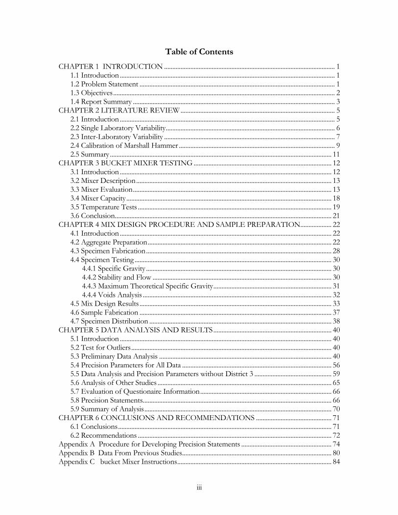
Table of Contents

CHAPTER 1 INTRODUCTION ........................................................................................................ 1 1.1 Introduction ................................................................................................................................... 1 1.2 Problem Statement ....................................................................................................................... 1 1.3 Objectives ....................................................................................................................................... 2 1.4 Report Summary ........................................................................................................................... 3

CHAPTER 2 LITERATURE REVIEW .............................................................................................. 5 2.1 Introduction ................................................................................................................................... 5 2.2 Single Laboratory Variability ....................................................................................................... 6 2.3 Inter-Laboratory Variability ........................................................................................................ 7 2.4 Calibration of Marshall Hammer ............................................................................................... 9 2.5 Summary ....................................................................................................................................... 11

CHAPTER 3 BUCKET MIXER TESTING .................................................................................... 12 3.1 Introduction ................................................................................................................................. 12 3.2 Mixer Description ....................................................................................................................... 13 3.3 Mixer Evaluation ......................................................................................................................... 13 3.4 Mixer Capacity ............................................................................................................................. 18 3.5 Temperature Tests ...................................................................................................................... 19 3.6 Conclusion.................................................................................................................................... 21

CHAPTER 4 MIX DESIGN PROCEDURE AND SAMPLE PREPARATION................... 22 4.1 Introduction ................................................................................................................................. 22 4.2 Aggregate Preparation ................................................................................................................ 22 4.3 Specimen Fabrication ................................................................................................................. 28 4.4 Specimen Testing ........................................................................................................................ 30

4.4.1 Specific Gravity ................................................................................................................. 30 4.4.2 Stability and Flow ............................................................................................................. 30 4.4.3 Maximum Theoretical Specific Gravity ........................................................................ 31 4.4.4 Voids Analysis ................................................................................................................... 32

4.5 Mix Design Results ..................................................................................................................... 33 4.6 Sample Fabrication ..................................................................................................................... 37 4.7 Specimen Distribution ............................................................................................................... 38

CHAPTER 5 DATA ANALYSIS AND RESULTS ........................................................................ 40 5.1 Introduction ................................................................................................................................. 40 5.2 Test for Outliers .......................................................................................................................... 40 5.3 Preliminary Data Analysis ......................................................................................................... 40 5.4 Precision Parameters for All Data ........................................................................................... 56 5.5 Data Analysis and Precision Parameters without District 3 ............................................... 59 5.6 Analysis of Other Studies .......................................................................................................... 65 5.7 Evaluation of Questionaire Information ................................................................................ 66 5.8 Precision Statements................................................................................................................... 66 5.9 Summary of Analysis .................................................................................................................. 70

CHAPTER 6 CONCLUSIONS AND RECOMMENDATIONS .............................................. 71 6.1 Conclusions .................................................................................................................................. 71 6.2 Recommendations ...................................................................................................................... 72

Appendix A Procedure for Developing Precision Statements ....................................................... 74 Appendix B Data From Previous Studies........................................................................................... 80 Appendix C bucket Mixer Instructions .............................................................................................. 84

iv

Appendix D Mix Design Charts ........................................................................................................... 85 APPENDIX E Laboratory Data ........................................................................................................... 94 APPENDIX F Laboratory Instructions, Questionnaire and Data Sheets ................................ 101

Questionnaire ................................................................................................................................... 103 APPENDIX G Variability Analysis Tables ....................................................................................... 107

List of Figures

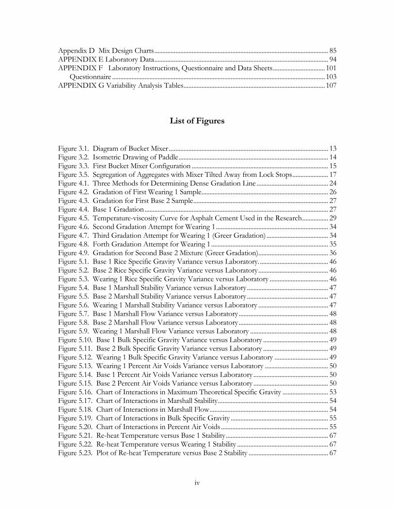
Figure 3.1. Diagram of Bucket Mixer .................................................................................................. 13 Figure 3.2. Isometric Drawing of Paddle ............................................................................................ 14 Figure 3.3. First Bucket Mixer Configuration .................................................................................... 15 Figure 3.5. Segregation of Aggregates with Mixer Tilted Away from Lock Stops ...................... 17 Figure 4.1. Three Methods for Determining Dense Gradation Line ............................................ 24 Figure 4.2. Gradation of First Wearing 1 Sample .............................................................................. 26 Figure 4.3. Gradation for First Base 2 Sample ................................................................................... 27 Figure 4.4. Base 1 Gradation ................................................................................................................. 27 Figure 4.5. Temperature-viscosity Curve for Asphalt Cement Used in the Research ................ 29 Figure 4.6. Second Gradation Attempt for Wearing 1 ..................................................................... 34 Figure 4.7. Third Gradation Attempt for Wearing 1 (Greer Gradation) ...................................... 34 Figure 4.8. Forth Gradation Attempt for Wearing 1 ........................................................................ 35 Figure 4.9. Gradation for Second Base 2 Mixture (Greer Gradation)........................................... 36 Figure 5.1. Base 1 Rice Specific Gravity Variance versus Laboratory. .......................................... 46 Figure 5.2. Base 2 Rice Specific Gravity Variance versus Laboratory ........................................... 46 Figure 5.3. Wearing 1 Rice Specific Gravity Variance versus Laboratory .................................... 46 Figure 5.4. Base 1 Marshall Stability Variance versus Laboratory .................................................. 47 Figure 5.5. Base 2 Marshall Stability Variance versus Laboratory .................................................. 47 Figure 5.6. Wearing 1 Marshall Stability Variance versus Laboratory ........................................... 47 Figure 5.7. Base 1 Marshall Flow Variance versus Laboratory ....................................................... 48 Figure 5.8. Base 2 Marshall Flow Variance versus Laboratory ....................................................... 48 Figure 5.9. Wearing 1 Marshall Flow Variance versus Laboratory ................................................ 48 Figure 5.10. Base 1 Bulk Specific Gravity Variance versus Laboratory ........................................ 49 Figure 5.11. Base 2 Bulk Specific Gravity Variance versus Laboratory ........................................ 49 Figure 5.12. Wearing 1 Bulk Specific Gravity Variance versus Laboratory ................................. 49 Figure 5.13. Wearing 1 Percent Air Voids Variance versus Laboratory ....................................... 50 Figure 5.14. Base 1 Percent Air Voids Variance versus Laboratory .............................................. 50 Figure 5.15. Base 2 Percent Air Voids Variance versus Laboratory .............................................. 50 Figure 5.16. Chart of Interactions in Maximum Theoretical Specific Gravity ............................ 53 Figure 5.17. Chart of Interactions in Marshall Stability .................................................................... 54 Figure 5.18. Chart of Interactions in Marshall Flow ......................................................................... 54 Figure 5.19. Chart of Interactions in Bulk Specific Gravity ............................................................ 55 Figure 5.20. Chart of Interactions in Percent Air Voids .................................................................. 55 Figure 5.21. Re-heat Temperature versus Base 1 Stability ............................................................... 67 Figure 5.22. Re-heat Temperature versus Wearing 1 Stability ........................................................ 67 Figure 5.23. Plot of Re-heat Temperature versus Base 2 Stability ................................................. 67

v

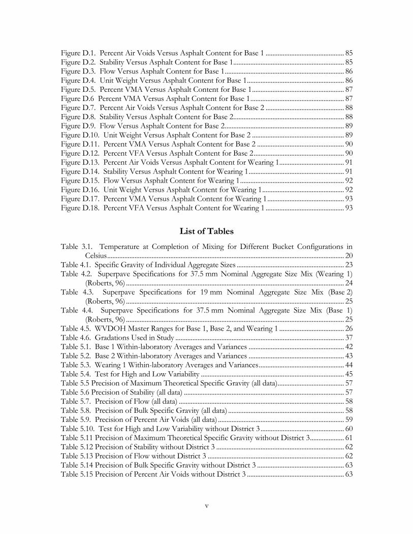
Figure D.1. Percent Air Voids Versus Asphalt Content for Base 1 .............................................. 85 Figure D.2. Stability Versus Asphalt Content for Base 1................................................................. 85 Figure D.3. Flow Versus Asphalt Content for Base 1 ...................................................................... 86 Figure D.4. Unit Weight Versus Asphalt Content for Base 1 ......................................................... 86 Figure D.5. Percent VMA Versus Asphalt Content for Base 1 ...................................................... 87 Figure D.6 Percent VMA Versus Asphalt Content for Base 1 ....................................................... 87 Figure D.7. Percent Air Voids Versus Asphalt Content for Base 2 .............................................. 88 Figure D.8. Stability Versus Asphalt Content for Base 2................................................................. 88 Figure D.9. Flow Versus Asphalt Content for Base 2 ...................................................................... 89 Figure D.10. Unit Weight Versus Asphalt Content for Base 2 ...................................................... 89 Figure D.11. Percent VMA Versus Asphalt Content for Base 2 ................................................... 90 Figure D.12. Percent VFA Versus Asphalt Content for Base 2 ..................................................... 90 Figure D.13. Percent Air Voids Versus Asphalt Content for Wearing 1...................................... 91 Figure D.14. Stability Versus Asphalt Content for Wearing 1 ........................................................ 91 Figure D.15. Flow Versus Asphalt Content for Wearing 1 ............................................................. 92 Figure D.16. Unit Weight Versus Asphalt Content for Wearing 1 ................................................ 92 Figure D.17. Percent VMA Versus Asphalt Content for Wearing 1 ............................................. 93 Figure D.18. Percent VFA Versus Asphalt Content for Wearing 1 .............................................. 93

List of Tables

Table 3.1. Temperature at Completion of Mixing for Different Bucket Configurations in Celsius ........................................................................................................................................... 20

Table 4.1. Specific Gravity of Individual Aggregate Sizes ............................................................... 23 Table 4.2. Superpave Specifications for 37.5 mm Nominal Aggregate Size Mix (Wearing 1)

(Roberts, 96) ................................................................................................................................ 24 Table 4.3. Superpave Specifications for 19 mm Nominal Aggregate Size Mix (Base 2)

(Roberts, 96) ................................................................................................................................ 25 Table 4.4. Superpave Specifications for 37.5 mm Nominal Aggregate Size Mix (Base 1)

(Roberts, 96) ................................................................................................................................ 25 Table 4.5. WVDOH Master Ranges for Base 1, Base 2, and Wearing 1 ...................................... 26 Table 4.6. Gradations Used in Study ................................................................................................... 37 Table 5.1. Base 1 Within-laboratory Averages and Variances ........................................................ 42 Table 5.2. Base 2 Within-laboratory Averages and Variances ........................................................ 43 Table 5.3. Wearing 1 Within-laboratory Averages and Variances .................................................. 44 Table 5.4. Test for High and Low Variability .................................................................................... 45 Table 5.5 Precision of Maximum Theoretical Specific Gravity (all data)....................................... 57 Table 5.6 Precision of Stability (all data) .............................................................................................. 57 Table 5.7. Precision of Flow (all data) ................................................................................................. 58 Table 5.8. Precision of Bulk Specific Gravity (all data) .................................................................... 58 Table 5.9. Precision of Percent Air Voids (all data) .......................................................................... 59 Table 5.10. Test for High and Low Variability without District 3 ................................................. 60 Table 5.11 Precision of Maximum Theoretical Specific Gravity without District 3 .................... 61 Table 5.12 Precision of Stability without District 3 ........................................................................... 62 Table 5.13 Precision of Flow without District 3 ................................................................................ 62 Table 5.14 Precision of Bulk Specific Gravity without District 3 ................................................... 63 Table 5.15 Precision of Percent Air Voids without District 3 ......................................................... 63

vi

Table 5.16 Percent change in precision statements without District 3 .......................................... 64 Table 5.17. Standard Deviations of Average Laboratory Results from Inter-laboratory Studies66 Table A.1 Approximate Values (Upper 5 percent Level) for the Ratio of the Largest Variance

to the Sum of the Variances ..................................................................................................... 77 Table A.2 Approximate Values (Upper 5 percent Level) for the Ratio of the Highest to

Lowest Variance ......................................................................................................................... 77 Table A.3. Example Calculation of Components of Variance ....................................................... 78 Table B.1. Precision Summary of Study by ASTM (Kanhdal, 96) ................................................. 80 Table B.2. Georgia Laboratory Comparison Study (Siddiqui, 95) ................................................. 81 Table B.3. Utah-Marshall Study, Same Operator, Different Equipment at Various

Laboratories (Siddiqui, 95) ........................................................................................................ 82 Table B.4. Utah-Marshall Study, Different Operator and Equipment at Various Laboratories

(Siddiqui, 95) ................................................................................................................................ 82 Table B.5. Canadian Mix Exchange, .................................................................................................... 83 Table E.1. Compacted Base 1 Samples Raw Data ............................................................................ 94 Table E.2. Compacted Base 2 Samples Raw Data ............................................................................ 95 Table E.3. Compacted Wearing 1 Samples Raw Data ..................................................................... 96 Table E.4. Base 1 Maximum Theoretical Specific GravitySamples Raw Data ............................ 97 Table E.5. Base 2 Maximum Theoretical Specific GravitySamples Raw Data ............................ 98 Table E.6. Wearing 1 Maximum Theoretical Specific Gravity Samples Raw Data .................... 99 Table E.7. Questionnaire Results ....................................................................................................... 100 Table G.1. Base 1, Maximum Theoretical Specific Gravity, Within-Laboratory Average and

Variance ...................................................................................................................................... 107 Table G.2. Base 2, Maximum Theoretical Specific Gravity, Within-Laboratory Average and

Variance ...................................................................................................................................... 107 Table G.3. Wearing 1, Maximum Theoretical Specific Gravity, Within-Laboratory Average

and Variance .............................................................................................................................. 108 Table G.4. Base 1, Stability, Within-Laboratory Average and Variance ..................................... 108 Table G.5. Base 2, Stability, Within-Laboratory Average and Variance ..................................... 109 Table G.6. Wearing 1 Stability, Within-Laboratory Average and Variance ................................ 109 Table G.7. Base 1, Flow, Within-Laboratory Average and Variance .......................................... 110 Table G.8. Base 2, Flow, Within-Laboratory Average and Variance .......................................... 110 Table G.9. Wearing 1, Flow, Within-Laboratory Average and Variance .................................... 111 Table G.10. Base 1, Bulk Specific Gravity, Within-Laboratory Average and Variance ........... 111 Table G.11. Base 2, Bulk Specific Gravity, Within-Laboratory Average and Variance ........... 112 Table G.12. Wearing 1, Bulk Specific Gravity, Within-Laboratory Average and Variance .... 112 Table G.13. Base 1, Percent Air Voids, Within-Laboratory Average and Variance ................. 113 Table G.14. Base 2, Percent Air Voids, Within-Laboratory Average and Variance ................. 113 Table G.15. Wearing 1, Percent Air Voids, Within-Laboratory Average and Variance .......... 114 Table G.16. Outlying Percentile for Maximum Theoretical Specific Gravity Specific Gravity115 Table G.17. Outlying Percentile for Marshall Stability ................................................................... 116 Table G.18. Outlying Percentile for Marshall Flow ........................................................................ 117 Table G.19. Outlying Percentile for Bulk Specific Gravity ........................................................... 118 Table G.20. Outlying Percentile for Percent Air Voids ................................................................. 119

1

CHAPTER 1

INTRODUCTION

1.1 INTRODUCTION

In the late 1860’s the first bituminous pavements were placed in Washington D.C. These

pavements were a significant improvement over the common earth road surfaces of the day.

However, with continuous growth in traffic, particularly during World War II, the need to

improve pavement quality became an important issue to highway agencies and the Department

of Defense. As a result, mix design methods were developed for improving the quality of

asphalt concrete. One of these methods, developed by Bruce Marshall, has been widely

adopted by state highway agencies, including West Virginia.

The West Virginia Division of Highways, WVDOH, uses statistical quality control methods.

Under these methods, the precision of all test procedures must be known in order to ensure

equitable evaluation of contractors’ products. Although the Marshall method has been in use

for approximately 50 years, the precision of the method is not quantified in the ASTM

standard test method. Hence, the WVDOH needs to quantify the precision of the Marshall

method as it is implemented in the state. This need defined the primary objective of this

research. In essence, this requires performing a test method precision experiment as described

in ASTM Standard C 802 “Standard Practice for Conducting and Inter-laboratory Test

Program to Determine the Precision of Test Methods for Construction Materials.” The

standard requires preparing and distributing at least 3 replicate samples of 3 material types to a

minimum of 10 laboratories. Obviously, sample preparation is a significant effort during this

type of experiment.

1.2 PROBLEM STATEMENT

Even though the Superpave procedures will eventually replace the Marshall procedure for mix

design and quality control, in the interim, WVDOH will continue to use the Marshall method.

For quality control, the inter-laboratory precision and variance in the Marshall method must be

2

quantified for statistical based quality control methods. In a previous project, single laboratory

precision of the Marshall method was evaluated (Head, 93). The current project expands on

the work of Head to include inter-laboratory precision.

1.3 OBJECTIVES

The objective of this research was to develop precision statements for Marshall parameters.

The Marshall parameters evaluated during this project were stability, flow, air void, maximum

theoretical specific gravity, and bulk specific gravity.

The precision statements must apply to all laboratories working for and with WVDOH,

therefore, all WVDOH district laboratories and the central laboratory participated in the study.

In addition, since contractors have a direct responsibility for quality control, contractors

laboratories were included in the study. The precision statements must be valid for all asphalt

concrete types, so three mix types were included in the research. To ensure the experiment

design and analysis fulfilled these objectives, ASTM standard practices for performing

precision statements were used during the research.

The Marshall method was developed to accommodate mixes with relatively small maximum

size aggregates. This permitted the use of a 102 mm diameter mold, which can accommodate

a 25 mm maximum aggregate size. Recently, in response to heavier traffic loads, highway

agencies have introduced mixes with larger maximum aggregate sizes to improve mix

durability. Consequently, there is a need to increase the Marshall sample size to accommodate

the larger size aggregates. The use of larger sample molds is also accommodated in more

modern mix design methods, such as the Superpave system developed during the Strategic

Highway Research Program. Both the large Marshall mold and the mold used for the

Superpave system require approximately 4,000 g of aggregate as opposed to the 1,200 g sample

needed for the standard Marshall mold.

Increasing the sample size significantly affects laboratory sample preparation. Due to the mass

of material required, it is difficult to prepare samples using traditional methods. In response to

this need, industry has introduced a large capacity mixer for asphalt concrete. Since the

3

objective of this project required preparation of many samples, the large capacity mixer was

evaluated.

1.4 REPORT SUMMARY

This report is organized into six chapters and seven appendices. Following the introduction

chapter is a summary of the literature. Given the fact that the Marshall method was developed

50 years ago and was the standard method for approximately seventy-five percent of the stated

highway agencies, the lack of information on the test method precision seems unusual. The

literature survey found two studies covering single-laboratory precision and two reports on

inter-laboratory precision. The studies indicate the variability of the Marshall method is

relatively high. Others have recognized this fact and studies of methods for reducing the

variability have been conducted. One such study was reviewed to highlight the difficulty in

reducing the variability of the seemingly simple Marshall mix design method.

One aspect of the standard Marshall test method is the small mold size which limits the

maximum aggregate size that can be considered for mix design. To overcome this limitation,

an ASTM test method for using a 152 mm diameter mold was developed. In addition, the

Superpave method uses large sample sizes. Chapter 3 outlines a method for mixing large

samples.

Chapter 4 presents the process used to select the specific aggregate gradations and asphalt

contents for the mixture types used during this research. The types of mixtures were selected

in concert with the project sponsor. Once the mixture types were selected, samples of

aggregate were obtained from Greer Industries. A Marshall mix design was preformed to

determine the optimum asphalt content. However, mixes with the Greer aggregates failed to

meet all the WVDOH Marshal criteria. Therefore the mix designs used by the Greer plant for

DOH projects were used for the research.

The samples were prepared in the WVU Asphalt Technology Laboratory and distributed to

the 10 WVDOH district laboratories, the WVDOH central laboratory, two contractor

laboratories, and the WVU Asphalt Technology Laboratory. The samples were tested using

4

standard Marshall methods adopted by WVDOH. The test results were returned to the

researchers and analyzed as reported in Chapter 5.

Chapter 6 presents the conclusions and recommendations for the research project. The

objective of the project was achieved with the presentation of precision statements, which the

WVDOH can implement. However, the research discovered two issues which should be

evaluated further. First, data from one of the laboratories was discarded as being too variable.

The reasons for this variability should be investigated and the equipment and testing technique

should be modified as needed. Second, when the research project was designed, three material

types were selected as specified by the ASTM standard for developing precision statements.

However, two of the material types are compacted in 102 mm molds and the other in 152 mm

molds. There were significant differences in the variability of test results obtained with

standard and large molds. In essence, the precision statements developed during this research

treated the standard and large molds as separate test methods.

5

CHAPTER 2 LITERATURE REVIEW

2.1 INTRODUCTION

The Marshall mix design method was developed approximately 50 years ago and was adopted

as the standard mix design for the majority of state highway agencies. Standard Marshall test

methods were published by both the American Society for Testing and Materials (ASTM), and

by the American Association of State Highway and Transportation Officials (AASHTO).

However, these standards lack quantified precision statements.

ASTM published standards for developing precision statements which were extensively used

for this project. These standards are summarized in Appendix A.

ASTM precision statements recognize the difference in precision that can be achieved within a

single laboratory and between multiple laboratories. Two studies were found which examined

the within, or single-laboratory variability. One examined the repeatability of the Marshall

stability test using a single technician but two “identical” Marshall hammers (Kovac, 62). The

other study examined the single laboratory variability for four asphalt concrete types used by

WVDOH (Head, 93). Two studies were found which evaluated the inter-laboratory variability.

One study was performed specifically to develop precision statements for Marshall stability

tests performed on 152 mm samples (Kandhal, 96). The other study presents a compilation of

inter-laboratory Marshall variability data that were collected, but not published, by several

agencies (Siddiqui, 95).

Each of these studies demonstrated considerable variability in the Marshall test method.

Therefore, although it is not directly related to the current project, information on ways to

reduce variability in the Marshall method was sought. The Federal Highway Administration

(FHWA) sponsored a study for calibrating the compaction effort of the Marshall hammer

(Sherton, 94).

6

2.2 SINGLE LABORATORY VARIABILITY

In 1962, Kovac expressed concern that publications in the proceedings of the Association of

Asphalt Paving Technologists, AAPT, indicated the standard deviation of the Marshall

Stability test was in the range of 1980 and 5930 N (Kovac, 62). Kovac preformed an

experiment to quantify the single operator standard deviation. Factors and levels in the

experiment were:

1. Compaction hammers – two “identical hammers,

2. Sample position – the hammers were capable of compacting two samples

simultaneously.

3. Molds – four molds were used in the experiment

A single mix design with a 9.5 mm maximum aggregate size and 85/100 penetration grade

binder was used for all samples. A total of 64 samples were prepared over a 4 week period.

The standard deviation for all samples was 304 N, which was considerably less than the

previously unpublished values. Kovac found significant differences in the compactive effort

produced by the two “identical” hammers. Also, the first sample made each day had the

highest variability. After the variability associated with experimental factors was removed from

the analysis, the resulting error standard deviation for the Marshall stability was 272 N.

The WVDOH sponsored a project at WVU to quantify the single laboratory precision for

Marshall mix design tests for 102 mm and 152 mm samples (Head, 93). Four mix types were

evaluated:

1. Patching and Leveling 2, 12.5 mm max aggregate size, 102 mm mold,

2. Wearing 3, 4.75 mm maximum aggregate size, 102 mm mold,

3. Base 1, 37.5 mm maximum aggregate size, 152 mm mold, and

4. Modified Base 1, 19 mm maximum aggregate size, 152 mm mold.

The gradation for each mix type was established by using the midpoint of the allowable range

for percent passing for each sieve size. The optimum asphalt content was determined in

accordance with provisions contained in the Asphalt Institute Manual MS-2, Pennsylvania

Department of Transportation (PennDOT) Marshall criteria for compacted specimens, and

WVDOH specifications. Ten samples were prepared for each mix type. A sample consisted of

7

the average of three results. The Marshall parameters evaluated in the study were stability,

flow, unit weight, and percent air voids.

The WVU research found the variability of the Marshall parameters was greater for the

152 mm samples than for the 102 mm samples. The mean value for stability, flow, and unit

weight were greater for the 152 mm samples than for the 102 mm samples (Head, 93). The

material types and sample size were confounded in the experiment, i.e., no material type was

tested at both sample sizes. Hence, the difference in the means and variability may be

attributed to either material type or sample size.

2.3 INTER-LABORATORY VARIABILITY

The precision of the Marshall procedure for 152 mm samples was evaluated when ASTM

published a standard test method for preparing and testing this size sample (Kandhal, 96). The

AASHTO Material Reference Laboratory (AMRL) distributed replicate samples to twelve

laboratories. The laboratories were instructed to follow ASTM D5581, “Test Method for

Resistance to Flow of Bituminous Mixtures Using Marshall Apparatus (6 inch Diameter

Specimen)”. The laboratories mixed and compacted samples, at temperatures specified by the

researchers, and then tested for Marshall stability and flow, air voids, and bulk specific gravity.

The laboratories were provided with a sufficient amount of 25 mm maximum size aggregates

and AC-20 to prepare 3 Marshall sampled, “butter” the mixer, and make samples for

determining the maximum theoretical specific gravity.

The data received from the laboratories were analyzed using ASTM Practice for Preparing

Precision and Bias Statements for Test Methods for Construction Materials (C 670), the

ASTM practice for Conducting an Inter-laboratory Test Program to Determine the Precision

of Test Methods for Construction Materials (C 802), and ASTM Practice for Use of the Terms

Precision and Bias in ASTM Test Methods (E 177) (Kandhal, 96). The parameters of

precision from this study are presented in Table B.1.

Siddiqui, Trethewey, and Anderson studied variables affecting Marshall test results (Siddiqui,

95). The primary objectives of the study were to identify the key equipment-related factors

associated with inconsistencies in test results obtained by using different compaction

8

equipment and to recommend calibration equipment and techniques for Marshall compaction

equipment.

Inter-laboratory variability results from differences in equipment characteristics, and the skill

of the technician. The variability of the Marshall procedures has been a concern since at least

1984 (Lee, 84). However, there are relatively few published studies which quantify the

precision of these procedures.

Siddiqui reported on experts’ and users’ opinions on the sources of variability in the Marshall

procedure. A questionnaire was used to capture the opinion of eleven experts concerning the

variables that significantly affect Marshall compaction. Analysis of the questionnaire identified

the rank order of the five most influential variables as:

1. Hammer alignment,

2. Pedestal support,

3. Height of free fall,

4. Hammer weight, and

5. Pedestal construction.

Users were then interviewed relative to the differences in brands of equipment and operator

technique. These users reported significant differences in pedestal construction, shape of the

hammer foot, hammer weight and dimensions of the breaking head used in the stability and

flow tests. In addition, the users identified concerns that experienced technicians were not

following the ASTM standard test procedure (Siddiqui, 95).

The experts’ and users’ opinions provide an expectation of high inter-laboratory variability.

This expectation was verified with data collected by highway agencies in Georgia, Utah, and

Canada. These agencies conducted inter-laboratory studies to examine Marshall variability

within their agency. These were unpublished studies prior to being reported by Siddiqui. The

data from these studies are presented in Appendix B. An analysis of these data for the ASTM

precision parameters is presented in Chapter 5.

Qualitative findings from these studies include (Siddiqui, 95):

9

1. Results from the Georgia Department of Transportation (GDOT) showed

samples prepared with mechanical hammers were consistently different from

samples prepared with manual hammers with respect to density.

2. The GDOT data showed most laboratories could operate within the desired levels

of precision, but some data indicated potential problems with either the equipment

or technician technique.

3. The Utah Department of Transportation (UDOT) data demonstrated that the

precision of the Marshall method was influenced by operator technique.

4. The Canadian data demonstrated the variability of mechanically compacted

samples was higher than the variability associated with manually compacted

samples.

2.4 CALIBRATION OF MARSHALL HAMMER

After research demonstrated the large variability in the Marshall procedure, especially for the

mechanical compaction hammers, the Federal Highway Administration (FHWA) sponsored

research on methods to calibrate these hammers (Sherton, 94). Since the WVDOH uses

mechanical Marshall hammers, the FHWA research was reviewed to determine if it was

applicable to the division’s procedures.

Sherton developed equipment to measure the compaction force applied to Marshall samples.

The equipment consisted of a power supply, data acquisition system and an elastic spring-mass

device with an integral force transducer. The basic premise behind the equipment was that the

compaction effort of the hammer could be measured with an elastic spring-mass device

positioned inside a standard Marshall mold. As the hammer impacts the device, the spring is

compressed. The rate of compression and maximum deformation is sent to the data

acquisition system. The force, impulse, and energy are then calculated for each individual

blow.

After the prototype device was developed, tests were performed to evaluate the potential of

reducing variability by calibrating each hammer. This laboratory evaluation program evaluated

conditions that produced scatter in Marshall test results. The topic of comparing different

hammers and standardization was indirectly examined. The main focus was on Marshall

10

equipment related variables such as variation in drop weight, friction, wear, and foundation

compliance.

Five different machine setups were evaluated:

1. New Pine Instruments Marshall compaction hammer,

2. Twenty year old Reinhart Testing Equipment Marshall compaction hammer,

3. The Pine Instruments hammer with the mass increased by 277 g,

4. The Reinhart Testing Equipment hammer with a rubber pad between the mold

and base plate, and

5. Manual Marshall compaction hammer.

Three samples were compacted in each of the five device setups. The samples were

compacted with fifty blows on each side of the sample. The bulk specific gravity, stability,

flow, air voids and height of each sample were determined. The standard deviation of each

parameter was computed from three replicate specimens prepared with each machine setup.

The machines were then calibrated using the calibration device. A standard cumulative

impulse value and cumulative energy value were computed. Calibration consisted of

computing the number of times each machine would have to drop the hammer to achieve

energy and impulse values theoretically computed for 50 blows per side. The “calibrated”

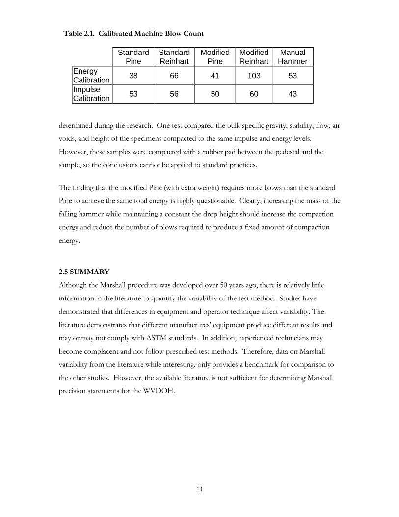
number of blows are shown in Table 2.1.

Three samples were then compacted in each machine with the impulse and energy modified

blow counts. The mean and standard deviation for the three samples were computed for each

of the Marshall parameters. In almost all cases, the standard deviation of the samples prepared

with the calibrated number of blows was less than the standard deviation for samples prepared

using the standard number of blows. Samples prepared using the number of blows computed

from the impulse calibration procedure had less variability than samples prepared using the

number of blows computed the energy calibration procedure (Sherton, 96).

Sherton claimed that since the standard deviations were reduced, the calibration method was

effective. However, this comparison was not made between hammers. The efficacy of the

calibration method to produce consistent results with different compaction machines was not

11

determined during the research. One test compared the bulk specific gravity, stability, flow, air

voids, and height of the specimens compacted to the same impulse and energy levels.

However, these samples were compacted with a rubber pad between the pedestal and the

sample, so the conclusions cannot be applied to standard practices.

The finding that the modified Pine (with extra weight) requires more blows than the standard

Pine to achieve the same total energy is highly questionable. Clearly, increasing the mass of the

falling hammer while maintaining a constant the drop height should increase the compaction

energy and reduce the number of blows required to produce a fixed amount of compaction

energy.

2.5 SUMMARY

Although the Marshall procedure was developed over 50 years ago, there is relatively little

information in the literature to quantify the variability of the test method. Studies have

demonstrated that differences in equipment and operator technique affect variability. The

literature demonstrates that different manufactures’ equipment produce different results and

may or may not comply with ASTM standards. In addition, experienced technicians may

become complacent and not follow prescribed test methods. Therefore, data on Marshall

variability from the literature while interesting, only provides a benchmark for comparison to

the other studies. However, the available literature is not sufficient for determining Marshall

precision statements for the WVDOH.

Table 2.1. Calibrated Machine Blow Count

Standard

Pine Standard Reinhart

Modified Pine

Modified Reinhart

Manual Hammer

Energy Calibration

38 66 41 103 53

Impulse Calibration

53 56 50 60 43

12

CHAPTER 3 BUCKET MIXER TESTING

3.1 INTRODUCTION

In the past, the size and capacity of a laboratory asphalt concrete mixer has been of little

concern due to the small quantities needed. Samples were mixed in a tabletop mechanical

mixer or by hand. These two methods sufficed because the Marshall and the Hveem mix

design method were the two predominant mix design methods. Both procedures use 102 mm

diameter by 63 mm high samples requiring approximately 1200 g of aggregate.

In recent years, new testing procedures have been accepted in the asphalt industry. In 1996,

ASTM introduced a testing procedure for 152 mm diameter Marshall apparatus. The Strategic

Highway Research Program (SHRP) developed a new system for asphalt concrete mix design

using the Superpave Gyratory Compactor. This machine, over the next several years, will

replace the Hveem and Marshall methods. The Superpave Gyratory Compactor uses a

150 mm diameter sample. The samples weigh more than 4500 g. This quantity of material is

difficult to mix with traditional methods. Since AASHTO and ASTM mix design test

standards for Marshall and Superpave only specify that the mixture have a uniform distribution

of asphalt binder, a different style mixer may be introduced.

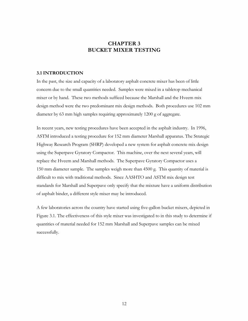
A few laboratories across the country have started using five-gallon bucket mixers, depicted in

Figure 3.1. The effectiveness of this style mixer was investigated to in this study to determine if

quantities of material needed for 152 mm Marshall and Superpave samples can be mixed

successfully.

13

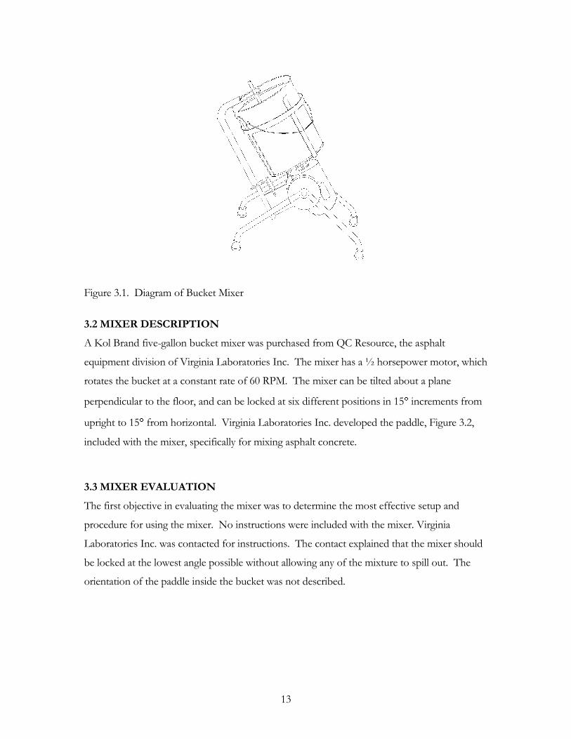
Figure 3.1. Diagram of Bucket Mixer

3.2 MIXER DESCRIPTION

A Kol Brand five-gallon bucket mixer was purchased from QC Resource, the asphalt

equipment division of Virginia Laboratories Inc. The mixer has a ½ horsepower motor, which

rotates the bucket at a constant rate of 60 RPM. The mixer can be tilted about a plane

perpendicular to the floor, and can be locked at six different positions in 15 increments from

upright to 15 from horizontal. Virginia Laboratories Inc. developed the paddle, Figure 3.2,

included with the mixer, specifically for mixing asphalt concrete.

3.3 MIXER EVALUATION

The first objective in evaluating the mixer was to determine the most effective setup and

procedure for using the mixer. No instructions were included with the mixer. Virginia

Laboratories Inc. was contacted for instructions. The contact explained that the mixer should

be locked at the lowest angle possible without allowing any of the mixture to spill out. The

orientation of the paddle inside the bucket was not described.

14

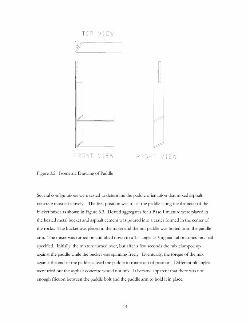
Figure 3.2. Isometric Drawing of Paddle

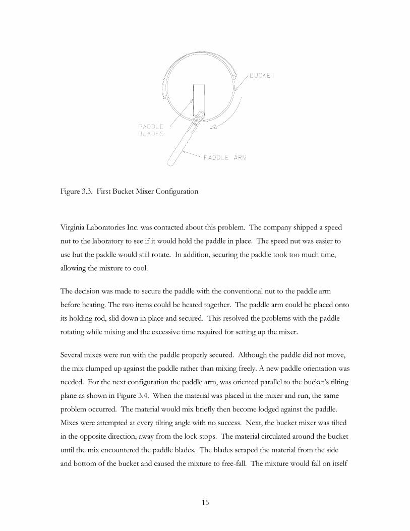
Several configurations were tested to determine the paddle orientation that mixed asphalt

concrete most effectively. The first position was to set the paddle along the diameter of the

bucket mixer as shown in Figure 3.3. Heated aggregates for a Base 1 mixture were placed in

the heated metal bucket and asphalt cement was poured into a crater formed in the center of

the rocks. The bucket was placed in the mixer and the hot paddle was bolted onto the paddle

arm. The mixer was turned on and tilted down to a 15 angle as Virginia Laboratories Inc. had

specified. Initially, the mixture turned over, but after a few seconds the mix clumped up

against the paddle while the bucket was spinning freely. Eventually, the torque of the mix

against the end of the paddle caused the paddle to rotate out of position. Different tilt angles

were tried but the asphalt concrete would not mix. It became apparent that there was not

enough friction between the paddle bolt and the paddle arm to hold it in place.

15

Figure 3.3. First Bucket Mixer Configuration

Virginia Laboratories Inc. was contacted about this problem. The company shipped a speed

nut to the laboratory to see if it would hold the paddle in place. The speed nut was easier to

use but the paddle would still rotate. In addition, securing the paddle took too much time,

allowing the mixture to cool.

The decision was made to secure the paddle with the conventional nut to the paddle arm

before heating. The two items could be heated together. The paddle arm could be placed onto

its holding rod, slid down in place and secured. This resolved the problems with the paddle

rotating while mixing and the excessive time required for setting up the mixer.

Several mixes were run with the paddle properly secured. Although the paddle did not move,

the mix clumped up against the paddle rather than mixing freely. A new paddle orientation was

needed. For the next configuration the paddle arm, was oriented parallel to the bucket’s tilting

plane as shown in Figure 3.4. When the material was placed in the mixer and run, the same

problem occurred. The material would mix briefly then become lodged against the paddle.

Mixes were attempted at every tilting angle with no success. Next, the bucket mixer was tilted

in the opposite direction, away from the lock stops. The material circulated around the bucket

until the mix encountered the paddle blades. The blades scraped the material from the side

and bottom of the bucket and caused the mixture to free-fall. The mixture would fall on itself

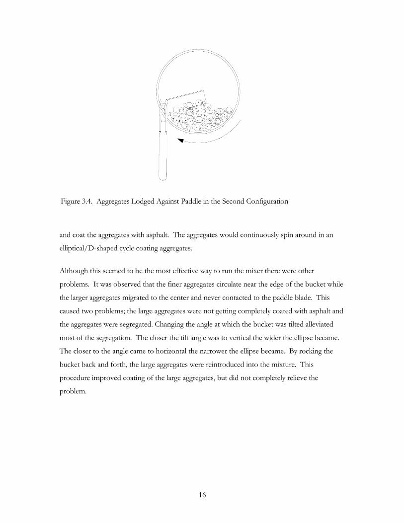
16

and coat the aggregates with asphalt. The aggregates would continuously spin around in an

elliptical/D-shaped cycle coating aggregates.

Although this seemed to be the most effective way to run the mixer there were other

problems. It was observed that the finer aggregates circulate near the edge of the bucket while

the larger aggregates migrated to the center and never contacted to the paddle blade. This

caused two problems; the large aggregates were not getting completely coated with asphalt and

the aggregates were segregated. Changing the angle at which the bucket was tilted alleviated

most of the segregation. The closer the tilt angle was to vertical the wider the ellipse became.

The closer to the angle came to horizontal the narrower the ellipse became. By rocking the

bucket back and forth, the large aggregates were reintroduced into the mixture. This

procedure improved coating of the large aggregates, but did not completely relieve the

problem.

Figure 3.4. Aggregates Lodged Against Paddle in the Second Configuration

17

Figure 3.5. Segregation of Aggregates with Mixer Tilted Away from Lock Stops

Different attempts were made to improve coating of the large aggregates. Specifications for

the gyratory compactor require heating the mixture in a shallow pan for a period of two hours

after mixing. This allowed the large aggregates to become completely coated as the heated

asphalt cement flowed to the uncoated surfaces. However, heating after mixing is not part of

the Marshall specifications, so a better mixing method was still needed.

It was observed that upon initial mixing, there was thorough coating of the fine aggregates but

inadequate coating of the largest aggregate. Hence, it was decided to try a two step mixing

process. In the first step, the coarse aggregate and asphalt were placed in the bucket and

mixed for about 10 seconds. Then the fine aggregates were introduced while the mixer was

running and the bucket was locked in the vertical position. The fine aggregates were poured

into the center of the mix, avoiding the bucket side and paddle. It was observed that after

another 20 seconds of mixing, all aggregates were thoroughly coated.

Different separations between large and small aggregates were attempted to see which

separations allowed for the fastest mixing time while still completely coating all aggregates. It

was discovered that for mixtures with a nominal maximum aggregate size of 9.5 mm or

smaller, aggregates retained on 2.36 mm sieves should be mixed first. Aggregates passing the

18

2.36 mm sieve are then introduced and mixed until all aggregates are uniformly coated. For

mixtures with a nominal maximum aggregate size of 12.5 mm or greater, aggregates retained

on a 4.75 mm sieve are mixed first, followed by the smaller aggregates.

An additional problem with the mixer was its inability to scrape the entire bucket. In the center

of the bucket, a 25 mm to 75 mm circle of asphalt cement and fines was never scraped from

the bottom of the bucket. The paddle was long enough but the bottom edge of the paddle

blade did not contact the bottom of the bucket at the center. As the bucket spun, the area of

the bucket not reached by the blade had a thin coating of asphalt and fine material. These

materials had to be scraped with a spoon and reintroduced with the rest of the material after

the mechanical mixing was complete. At the seam where the side of the bucket and the

bottom met there was a three millimeter wide two millimeter deep indent. While the mixer

was running, the end of a metal spatula was placed in this indent to dig out the fines and allow

them to be mixed.

3.4 MIXER CAPACITY

The next phase of the evaluation was to the bucket mixer’s capacity. In the previous phase of

the testing it was observed that the mixer could provide a homogeneous mixture for 4000 g

samples. It now needed to be seen if the mixer could handle mixes significantly smaller and

larger.

It was decided that the smallest size mixture that would be needed for asphalt concrete mix

design would be for a single Marshall sample, 1200 g. The mixing procedures developed for

the 4000 g samples were used for all of the samples. Both WVDOH Base 2 and Wearing 1

mix designs were evaluated at optimum asphalt content. With the 1200 g samples the paddle

was hardly touched by the material when the bucket was tilted to a steep angle. The material

mixed through centripetal acceleration and gravity, providing a uniform coating of the

aggregates. In mixing the smaller samples, segregation was not a problem.

Next, the ability of the bucket mixer to prepare large batch sizes was evaluated. An 18,000 g

batch was selected this would enable asphalt samples to be quartered into Superpave Gyratory

Compactor specimens of approximately 4500 g.

19

The first samples were run at the optimum asphalt content. The bucket was unable to be tilted

over very far because the mixture was approximately 70 mm from the top of the bucket. The

aggregates turned over very well and the mixer had no problem handling such a large batch.

Through visible inspection it was determined that all of the aggregates were evenly coated.

However, severe segregation was observed. The fine aggregates migrated to the bottom of the

bucket while the larger aggregates remained on top. No method could be seen to alleviate this.

Careful quartering of the batch into the required sample size should mitigate this segregation

problem.

Mixes were evaluated with low asphalt contents. For this particular aggregate gradation no

problems occurred in mixing at one percent below optimum asphalt content. When a mixture

was attempted at 1.5 percent below optimum asphalt content it was observed that not all of

the aggregates were evenly coated with asphalt. The fine aggregates that were introduced into

the mixture after the large aggregates were not being completely coated. The aggregates were

migrating to the bottom of the bucket forcing the coarse aggregates to surface. The large

aggregates that were thoroughly coated with asphalt were not coming in contact with the fine

aggregates at the bottom. Agitating the mixture with a hot spoon did not improve coating.

18000 g batches were run at high asphalt contents. The asphalt cement on the bucket and

aggregates acted as a lubricant. There was not enough friction between the aggregate and the

bucket to cause the mix to turn over. The mix would stop moving. When this occurred the

bucket was rocked back-and-forth vigorously and a hot spoon was used to agitate the stopped

mixture. This reactivated the mixing and good aggregate coating was achieved.

3.5 TEMPERATURE TESTS

Tests were run to see if different bucket setups would affect the temperature retained in a

sample after mixing. Three different five-gallon bucket configurations were evaluated, the

standard bucket, a 16 gauge steel bucket, and the standard bucket with a fiberglass insulated

wrap. Mixtures were run at optimum asphalt content on batch of sizes 18000 g, 4000 g and

1200 g.

20

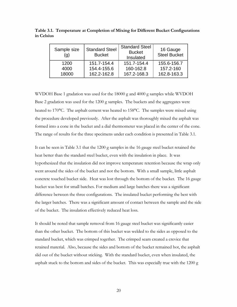
Table 3.1. Temperature at Completion of Mixing for Different Bucket Configurations in Celsius

Sample size (g)

Standard Steel Bucket

Standard Steel Bucket

Insulated

16 Gauge Steel Bucket

1200 4000

18000

151.7-154.4 154.4-155.6 162.2-162.8

151.7-154.4 160-162.8

167.2-168.3

155.6-156.7 157.2-160

162.8-163.3

WVDOH Base 1 gradation was used for the 18000 g and 4000 g samples while WVDOH

Base 2 gradation was used for the 1200 g samples. The buckets and the aggregates were

heated to 170 C. The asphalt cement was heated to 158 C. The samples were mixed using

the procedure developed previously. After the asphalt was thoroughly mixed the asphalt was

formed into a cone in the bucket and a dial thermometer was placed in the center of the cone.

The range of results for the three specimens under each condition is presented in Table 3.1.

It can be seen in Table 3.1 that the 1200 g samples in the 16 gauge steel bucket retained the

heat better than the standard steel bucket, even with the insulation in place. It was

hypothesized that the insulation did not improve temperature retention because the wrap only

went around the sides of the bucket and not the bottom. With a small sample, little asphalt

concrete touched bucket side. Heat was lost through the bottom of the bucket. The 16 gauge

bucket was best for small batches. For medium and large batches there was a significant

difference between the three configurations. The insulated bucket performing the best with

the larger batches. There was a significant amount of contact between the sample and the side

of the bucket. The insulation effectively reduced heat loss.

It should be noted that sample removal from 16 gauge steel bucket was significantly easier

than the other bucket. The bottom of this bucket was welded to the sides as opposed to the

standard bucket, which was crimped together. The crimped seam created a crevice that

retained material. Also, because the sides and bottom of the bucket remained hot, the asphalt

slid out of the bucket without sticking. With the standard bucket, even when insulated, the

asphalt stuck to the bottom and sides of the bucket. This was especially true with the 1200 g

21

samples. This is significant when preparing samples for the Marshall test method where the

sample goes directly from the mixer to the compaction mold.

3.6 CONCLUSION

Overall, the five-gallon bucket mixer performed extremely well at mixing asphalt. An effective

mixer configuration and procedure was developed for creating a well coated homogeneous

mixture. Sample sizes ranging from 1200 g to 18,000 g can be effectively mixed. Large

samples at low asphalt contents pose a problem in mixing and should be avoided. If heat loss

is critical either fiberglass insulating blanket or a high gauge steel bucket is recommended. If

individual Marshall specimens are going to be made a 16 gauge steel bucket is beneficial for

consistent sample preparation. A recommended bucket mixer operating procedure is

presented in Appendix C.

22

CHAPTER 4 MIX DESIGN PROCEDURE AND SAMPLE PREPARATION

4.1 INTRODUCTION

Three different WVDOH mixes were used in assessing the precision and repeatability of the

Marshall mix design method. The three mixes selected for the testing were WVDOT Wearing

1, Base 2 and Base 1. These mixes were selected because of their frequent use by the

WVDOH. The statistical evaluation is most meaningful when performed at the optimum

asphalt content. This chapter describes the procedures used to determine the optimum asphalt

content for each mix type.

4.2 AGGREGATE PREPARATION

All aggregates used for testing in this project were crushed limestone donated by Greer

Limestone in Sabraton, WV. The aggregates were sieved into the following sizes: 37.5 mm,

25 mm, 19 mm, 12.5 mm, 9.5 mm, 4.75 mm, 2.35 mm, 1.18 mm, 0.60 mm, 0.15 mm, and

0.075 mm. Once the aggregates were separated, the specific gravity of each sieve size was

determined in accordance with ASTM C128 and ASTM 127 for fine and coarse aggregates,

respectively (Table 4.1).

The Federal Highway Administration recommends using a 0.45 power gradation chart to find

the best gradation for a mix. Three methods are currently recognized in practice (Roberts, 96):

Method A: Draw a straight line from the origin to the maximum aggregate size.

Method B: Draw a straight line from the origin to the nominal maximum aggregate

size.

Method C: Draw a straight line from the origin to the percentage point for the

largest sieve that retains material.

23

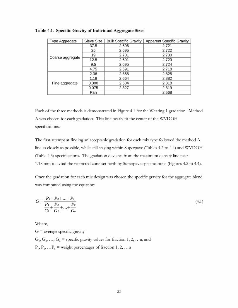
Table 4.1. Specific Gravity of Individual Aggregate Sizes

Type Aggregate Sieve Size Bulk Specific Gravity Apparent Specific Gravity

Coarse aggregate

37.5 2.696 2.721

25 2.695 2.722

19 2.701 2.730

12.5 2.691 2.729

9.5 2.695 2.724

4.75 2.691 2.718

Fine aggregate

2.36 2.658 2.825

1.18 2.664 2.882

0.300 2.504 2.818

0.075 2.327 2.619

Pan 2.568

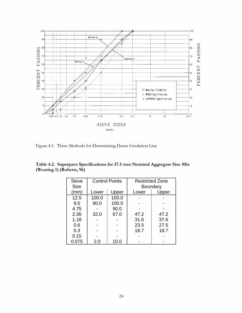
Each of the three methods is demonstrated in Figure 4.1 for the Wearing 1 gradation. Method

A was chosen for each gradation. This line nearly fit the center of the WVDOH

specifications.

The first attempt at finding an acceptable gradation for each mix type followed the method A

line as closely as possible, while still staying within Superpave (Tables 4.2 to 4.4) and WVDOH

(Table 4.5) specifications. The gradation deviates from the maximum density line near

1.18 mm to avoid the restricted zone set forth by Superpave specifications (Figures 4.2 to 4.4).

Once the gradation for each mix design was chosen the specific gravity for the aggregate blend

was computed using the equation:

n

n

n

G

P

G

P

G

P

PPPG

...

...

2

2

1

1

21 (4.1)

Where,

G = average specific gravity

G1, G2, …, Gn = specific gravity values for fraction 1, 2, …n; and

P1, P2, …Pn = weight percentages of fraction 1, 2, …n

24

Figure 4.1. Three Methods for Determining Dense Gradation Line

Table 4.2. Superpave Specifications for 37.5 mm Nominal Aggregate Size Mix (Wearing 1) (Roberts, 96)

Sieve Size

Control Points Restricted Zone Boundary

(mm) Lower Upper Lower Upper

12.5 100.0 100.0 - - 9.5 90.0 100.0 - - 4.75 - 90.0 - - 2.36 32.0 67.0 47.2 47.2 1.18 - - 31.6 37.6 0.6 - - 23.5 27.5 0.3 - - 18.7 18.7 0.15 - - - -

0.075 2.0 10.0 - -

25

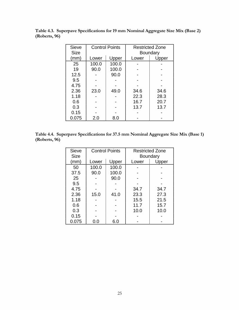
Table 4.3. Superpave Specifications for 19 mm Nominal Aggregate Size Mix (Base 2) (Roberts, 96)

Sieve Size

Control Points Restricted Zone Boundary

(mm) Lower Upper Lower Upper

25 100.0 100.0 - - 19 90.0 100.0 - -

12.5 - 90.0 - - 9.5 - - - - 4.75 - - - - 2.36 23.0 49.0 34.6 34.6 1.18 - - 22.3 28.3 0.6 - - 16.7 20.7 0.3 - - 13.7 13.7 0.15 - - - -

0.075 2.0 8.0 - -

Table 4.4. Superpave Specifications for 37.5 mm Nominal Aggregate Size Mix (Base 1) (Roberts, 96)

Sieve Size

Control Points Restricted Zone Boundary

(mm) Lower Upper Lower Upper

50 100.0 100.0 - - 37.5 90.0 100.0 - - 25 - 90.0 - - 9.5 - - - - 4.75 - - 34.7 34.7 2.36 15.0 41.0 23.3 27.3 1.18 - - 15.5 21.5 0.6 - - 11.7 15.7 0.3 - - 10.0 10.0 0.15 - - - -

0.075 0.0 6.0 - -

26

Table 4.5. WVDOH Master Ranges for Base 1, Base 2, and Wearing 1

Sieve Size

Base 1 Base 2 Wearing 1

(mm) Lower Upper Lower Upper Lower Upper

50 100 - - - - - 37.5 80 100 - - - - 25 - - 100 - - - 19 50 80 85 100 - -

12.5 - - - - 100 - 9.5 35 65 60 80 85 100 4.75 25 55 35 65 50 70 2.36 - - 20 50 30 50 1.18 10 35 - - 20 40 0.6 - - - - - - 0.3 4.0 20.0 4 20 5 20 0.15 - - - - - -

0.075 0 8 1 8 1 8

Figure 4.2. Gradation of First Wearing 1 Sample

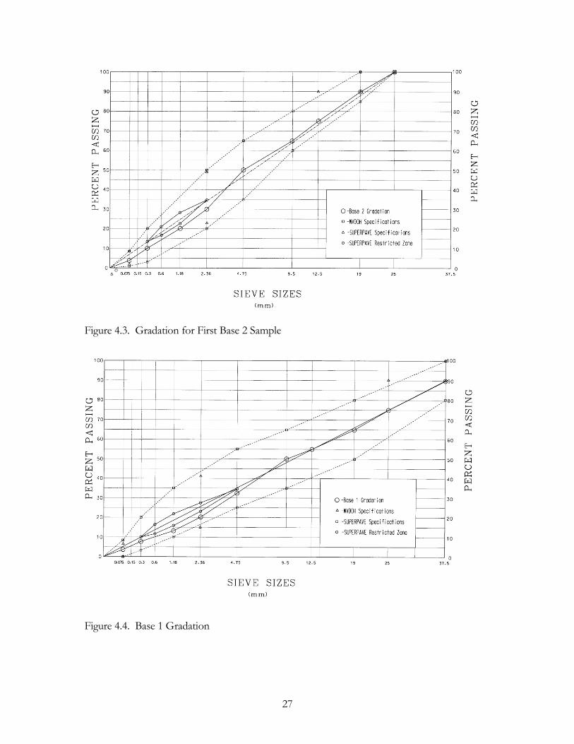
27

Figure 4.3. Gradation for First Base 2 Sample

Figure 4.4. Base 1 Gradation

28

4.3 SPECIMEN FABRICATION

Once each aggregate gradation was selected, the optimum asphalt content for each mix type

was determined using the Marshall method and the Asphalt Institute criteria (Roberts, 96).

The Asphalt Institute criteria requires averaging the asphalt content at maximum stability,

maximum density, and mid point of specified air void range (typically 4 percent) from plots of

stability, flow, air voids, and VMA versus asphalt content. The properties of the mix at this

asphalt content are then compared to mixture acceptance criteria.

Marshall testing for this project conformed to ASTM D 1559, for 102 mm samples and ASTM

D 5581 for 152 mm samples. ASTM D 1559 was followed for the Base 2 and Wearing 1

mixes and ASTM D 5581 was followed for the Base 1 mix.

For the 102 mm diameter Marshall samples WVDOH personnel recommended that

approximately 1200 g of hot mix asphalt be used to achieve the desired 63.5 mm high samples.

It was determined through trial and error that 1150 g of aggregates produced 63.5 mm sample

heights. Samples heights changed slightly from the varying asphalt cement content but not

enough to require changing the aggregate quantity. For the 152 mm samples, 3950 g of

aggregate were used in the mix to achieve the target 95.25 mm sample height.

The asphalt cement used in all testing was performance grade PG64-22 produced by Ashland

Petroleum Company. Greer Limestone, Sabraton, WV, donated the asphalt cement. The

proper mixing temperature and compaction temperatures were determined from a temperature

viscosity chart obtained from Ashland Petroleum Company. ASTM D 1559 specifies a

viscosity during mixing of 170 20 cSt. and a viscosity of 280 30 cSt. for compaction. This

corresponds to 153 C to 159 C and 142 C to147 C for asphalt cement used in this project

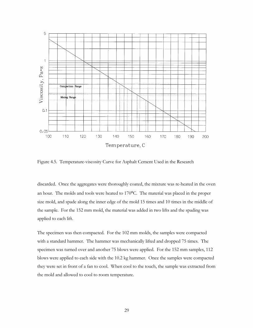
(Figure 4.5). The asphalt cement was heated to 158 C for mixing.

The aggregates were heated in an oven to 170 C as were the mixing tools, bucket, and mixing

paddle. When items were heated to their proper temperatures, the asphalt cement and

aggregate were mixed in accordance with the methods stated in the previous chapter. Each

day the first batch in the bucket mixer was used to “butter” the bucket and paddle and was

29

Figure 4.5. Temperature-viscosity Curve for Asphalt Cement Used in the Research

discarded. Once the aggregates were thoroughly coated, the mixture was re-heated in the oven

an hour. The molds and tools were heated to 170 C. The material was placed in the proper

size mold, and spade along the inner edge of the mold 15 times and 10 times in the middle of

the sample. For the 152 mm mold, the material was added in two lifts and the spading was

applied to each lift.

The specimen was then compacted. For the 102 mm molds, the samples were compacted

with a standard hammer. The hammer was mechanically lifted and dropped 75 times. The

specimen was turned over and another 75 blows were applied. For the 152 mm samples, 112

blows were applied to each side with the 10.2 kg hammer. Once the samples were compacted

they were set in front of a fan to cool. When cool to the touch, the sample was extracted from

the mold and allowed to cool to room temperature.

30

Mixes were made at five asphalt contents for each mix type; one at the estimated optimum

asphalt content, at 0.5 percent above and 0.5 percent below the estimated optimum asphalt

content, and at 1.0 percent above and 1.0 percent below the estimated optimum asphalt

content. The Greer Asphalt plant was contacted to obtain an estimate of the optimum asphalt

content. For Base 1, Base 2 and Wearing 1 the recommended asphalt contents were 3.9, 4.6,

and 5.5 percent, respectively. For the trial mix design the, for Base 1, Base, 2 and Wearing 1

the estimated optimum asphalt contents were 3.5, 4.5, and 5.5 percent, respectively.

4.4 SPECIMEN TESTING

4.4.1 Specific Gravity

The bulk specific gravity of the specimen was determined in accordance with ASTM D 2726.

The specimen was cooled to room temperature and weighed. The specimen was hung from a

scale and immersed in a water bath at 25 1 C for three to five minutes. The weight of the

specimen in water was then recorded. The sample was removed from the water bath, surface

dried with a towel and weighed again. The bulk specific gravity, Gmb, was determined as:

CB

AGmb (4.2)

Where:

A = Dry weight of specimen, grams

B = Surface Dried weight of specimen, grams

C = Weight of specimen in water, grams

The unit weight of the specimen was calculated by multiplying the bulk specific gravity by the

unit weight of water. The averages of the three specimens were the values recorded for unit

weight and bulk specific gravity.

4.4.2 Stability and Flow

Once the bulk specific gravity was determined, the heights of the samples were measured.

Following the height measurement the 102 mm specimens were immersed in a water bath at

60 C for 35 5 minutes while the 152 mm specimens were immersed for 45 5 minutes. A

31

specimen was removed from the water bath and quickly placed in the Marshall loading head

and then into a Pine Instrument Company brand Marshall stability apparatus. The Marshall

apparatus deformed the specimen at a constant rate of 50.8 mm per minute. The apparatus

automatically plotted load versus specimen deformation. Stability was identified as the

maximum load sustained by the sample. Flow was the deformation at maximum load. The

stability values were then adjusted with respect to sample height using the equations:

0.6016-0.0252CA

B (4.3)

0.6594-F*0.0174

ED (4.4)

Where :

A= Adjusted 102 mm Sample Stability

B= 102 mm Sample Stability

C= Sample Height

D= Adjusted 152 mm Sample Stability

E= 152 mm Sample Stability

F= Sample Height

These functions were developed by regression analysis of the correction factors given in

ASTM D 1559 and ASTM D 5581. It was verified that these equations produce the exact

values given in the tables to two decimal places.

4.4.3 Maximum Theoretical Specific Gravity

The maximum theoretical specific gravity of each mixture was determined in accordance with

ASTM D 2041. After the sample was properly mixed, it was spread on a table and allowed to

cool. The clumps of fine aggregate materials were then broken into particles ¼ inch in

diameter or smaller. Following separation of the coated fine and coarse aggregate particles, the

sample was weighed and then placed into a pycnometer and submerged in water at a

temperature of 25 1 C. The sample was subjected to a vacuum of 30 mmHg for 15 minutes

while the pycnometer was agitated on a vibrating table. The pycnometer was then filled

32

completely with water and the pycnometer and contents were weighed. The maximum

theoretical specific gravity, Gmm, was calculated as:

CBA

AGmm (4.5)

Where:

A = Weight of Dry Sample, grams

B = Weight of pycnometer completely filled with water, grams

C = Weight of pycnometer filled with water and sample, grams

4.4.4 Voids Analysis

The percent air voids, or voids in the total mix (VTM), in the compacted mixtures was found

in accordance ASTM D 2041. Percent air voids is the air voids in the compacted sample

expressed as a percentage of the total volume of the sample. Percent air voids was computed

as:

100A

BAVTM (4.6)

Where:

A = Average bulk specific gravity of three specimens

B = Maximum theoretical specific gravity of the mixture

The percent voids in the mineral aggregate (VMA) is the volume of space between the

aggregate particles (air voids of the compacted mixture) plus the volume of the asphalt not

absorbed into the aggregates. Percent voids in the mineral aggregate was computed as:

C

BAVMA

*100 (4.7)

Where:

A = Average bulk specific gravity of compacted mixture

B = Percent by weight of aggregate mixture

C = Bulk specific gravity of combined aggregate

33

The percent voids filled with asphalt (VFA) is the percentage of the VMA that is made up of

asphalt. The percent voids filled with asphalt was calculated using the following relationship:

100*VMA

VTMVMAVFA

(4.8)

4.5 MIX DESIGN RESULTS

Once the optimum asphalt contents for the three mix designs were determined the percent air

voids, bulk specific gravity, stability, flow, and VMA were compared to the values required by

WVDOH. The properties of the Wearing 1 mixture were acceptable except for the VMA.

For a mix with a maximum aggregate size of 9.5 mm, the minimum VMA is 15 percent.

Depending on the analytical method used, the VMA was low by 2.1 to 2.75 percent. The Base

2 mix met all criteria except for VMA. The VMA for the mix was low by 1.4 percent. The

Base 1 mix met all WVDOH specifications. The VMA specification for a mixture with a

maximum aggregate size of 37.5 mm was 11 percent and the mix had a VMA of 11.0 to 11.1

percent. In proportioning a mixture for constructed, the Base 1 mix might be redesigned

however, because the scope of this study was focused on the test variability the Base 1 mix

design was accepted. Since the Wearing 1 and Base 2 did not meet the VMA criteria, they

were redesigned.

To increase VMA the percent coarse aggregate in the Wearing 1 mix was increased, Figure 4.6.

However, samples made with the new gradation showed only a slight change in VMA; not

enough to meet the specifications. Greer Limestone was contacted to determine the gradation

they used for each of the mixes. The Greer Limestone gradation, Figure 4.7, was more

uniformly graded than the mixes previously attempted at the WVU laboratory. The Wearing 1

Greer Limestone gradation had 5 percent of the aggregate retained on the 9.5 mm sieve. This

gradation was evaluated. The VMA was under specification but very close to the minimum

limit. A final attempt was made to find a gradation that would provide a suitable VMA. A

more exaggerated uniformly graded blend was used while staying within WVDOH and

SUPERPAVE specifications, Figure 4.8. At four percent air voids the VMA was greater than

34

Figure 4.6. Second Gradation Attempt for Wearing 1

Figure 4.7. Third Gradation Attempt for Wearing 1 (Greer Gradation)

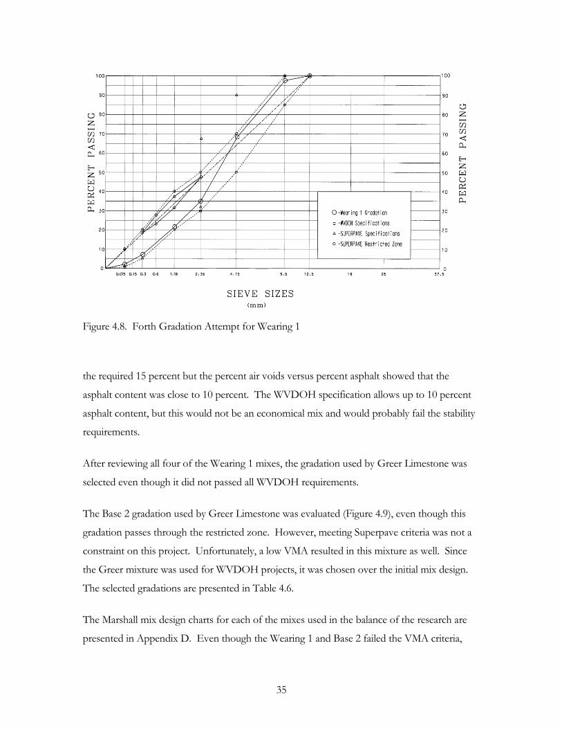
35

Figure 4.8. Forth Gradation Attempt for Wearing 1

the required 15 percent but the percent air voids versus percent asphalt showed that the

asphalt content was close to 10 percent. The WVDOH specification allows up to 10 percent

asphalt content, but this would not be an economical mix and would probably fail the stability

requirements.

After reviewing all four of the Wearing 1 mixes, the gradation used by Greer Limestone was

selected even though it did not passed all WVDOH requirements.

The Base 2 gradation used by Greer Limestone was evaluated (Figure 4.9), even though this

gradation passes through the restricted zone. However, meeting Superpave criteria was not a

constraint on this project. Unfortunately, a low VMA resulted in this mixture as well. Since

the Greer mixture was used for WVDOH projects, it was chosen over the initial mix design.

The selected gradations are presented in Table 4.6.

The Marshall mix design charts for each of the mixes used in the balance of the research are

presented in Appendix D. Even though the Wearing 1 and Base 2 failed the VMA criteria,

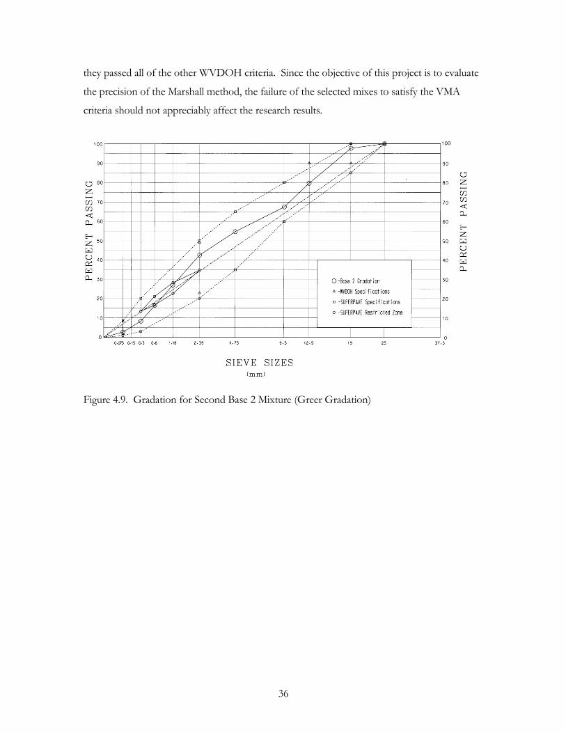
36

they passed all of the other WVDOH criteria. Since the objective of this project is to evaluate

the precision of the Marshall method, the failure of the selected mixes to satisfy the VMA

criteria should not appreciably affect the research results.

Figure 4.9. Gradation for Second Base 2 Mixture (Greer Gradation)

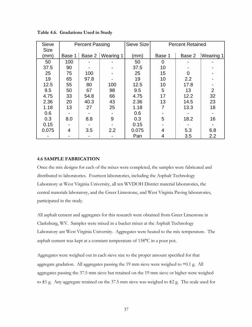
37

Table 4.6. Gradations Used in Study

Sieve Size

Percent Passing Sieve Size Percent Retained

(mm) Base 1 Base 2 Wearing 1 (mm) Base 1 Base 2 Wearing 1

50 100 - - 50 0 - - 37.5 90 - - 37.5 10 - - 25 75 100 - 25 15 0 - 19 65 97.8 - 19 10 2.2 -

12.5 55 80 100 12.5 10 17.8 - 9.5 50 67 98 9.5 5 13 2 4.75 33 54.8 66 4.75 17 12.2 32 2.36 20 40.3 43 2.36 13 14.5 23 1.18 13 27 25 1.18 7 13.3 18 0.6 - - - 0.6 - - - 0.3 8.0 8.8 9 0.3 5 18.2 16 0.15 - - - 0.15 - - - 0.075 4 3.5 2.2 0.075 4 5.3 6.8

- - - - Pan 4 3.5 2.2

4.6 SAMPLE FABRICATION

Once the mix designs for each of the mixes were completed, the samples were fabricated and

distributed to laboratories. Fourteen laboratories, including the Asphalt Technology

Laboratory at West Virginia University, all ten WVDOH District material laboratories, the

central materials laboratory, and the Greer Limestone, and West Virginia Paving laboratories,

participated in the study.

All asphalt cement and aggregates for this research were obtained from Greer Limestone in

Clarksburg, WV. Samples were mixed in a bucket mixer at the Asphalt Technology

Laboratory ant West Virginia University. Aggregates were heated to the mix temperature. The

asphalt cement was kept at a constant temperature of 158 C in a pour pot.

Aggregates were weighed out in each sieve size to the proper amount specified for that

aggregate gradation. All aggregates passing the 19 mm sieve were weighed to 0.1 g. All

aggregates passing the 37.5 mm sieve but retained on the 19 mm sieve or higher were weighed

to 1 g. Any aggregate retained on the 37.5 mm sieve was weighed to 2 g. The scale used for

38

weighing the asphalt cement would not allow for measurements more accurate than 0.1 g

because of the weight of the bucket and aggregate also being weighed.

Base 1 mixes were fabricated first followed by Wearing 1 and then Base 2 mixes. The order in

which the mixtures were made was deemed insignificant since comparisons of the variability

between different mixture types were not the focus of this project. Only variability between

the same type mixes was evaluated.

Originally, four specimens were to be sent to each laboratory for each of mix type. Three of

the samples were to be compacted and tested for voids, stability, and flow for each mixture

type. The fourth sample was to be used to determine maximum theoretical specific gravity.

After the Base 1 mixing was started, it was decided that two maximum theoretical specific

gravity tests should be performed to provide data on the within laboratory variability. This

created a problem because additional containers had to be ordered and would not arrive in

time to finish all of the Base 1 mixes at one time. For this reason 60 of the Base 1 samples

were prepared initially. The remaining Base 1 samples were prepared after the Base 2 and

Wearing 1 samples were mixed. .

The samples were placed in shipment containers and labeled. The samples were randomly

selected for each laboratory except for those used by the Asphalt Technology Laboratory at

WVU. The samples sent to each laboratory are identified in Appendix E. The samples tested

at WVU were prepared after the samples were shipped to the other laboratories. If significant

differences occurred in the results then all of the results for the WVU laboratory would be

disregarded since there was the potential for a bias in the sample preparation due to these

samples not being randomly selected.

4.7 SPECIMEN DISTRIBUTION

Two days after all of the samples were mixed the samples were mailed to the laboratories.

Instructions were also included with a cover letter, giving the compaction temperature range

and explanation of the code on each can. The package also included a survey form with brief

questions concerning the equipment and technician. A copy of the letter, survey form, and

data sheets are included in Appendix F.

39

After all of the samples were sent to the laboratories, each laboratory was contacted to review

the project requirements. The laboratories were also asked to return the results of the tests

within two weeks of receiving the samples. In response to questions from the technicians at

the laboratories, it was necessary to provide additional testing information requiring (1)

compacting the samples for a heavy traffic design, (2) use of the dryback method for the

maximum theoretical specific gravity test and (3) compaction of the samples at the middle

temperature of the allowable range..

40

CHAPTER 5 DATA ANALYSIS AND RESULTS

5.1 INTRODUCTION

The 14 laboratories returned the data within one month. The raw data were consolidated into

six tables presented in Appendix E. From this raw data the stability, flow, unit weight and

percent air voids were calculated and tabulated in Appendix G. These data were analyzed in

accordance with ASTM Standard C 802, “Conducting an Inter-laboratory Test Program to

Determine the Precision of Test Methods for Construction Materials.”

Once all of the data from this experiment were analyzed, select data from the literature review

were analyzed and compared to the data from this study. Finally, the data were evaluated for

correlation between different characteristics of the participating laboratories and technicians.

These characteristics were obtained through the survey form distributed with the samples.

The survey form is included in Appendix F.

5.2 TEST FOR OUTLIERS

ASTM C 802 specifies that no data may be ruled as an outlier in an inter-laboratory study

unless an assignable cause is identified. For this reason, in the first stage of the data analysis

only two results were discarded. The two discarded values came from the District 1 maximum

theoretical specific gravity tests for the Wearing 1 mix. The laboratory technician was

contacted to see if he could locate the source of the error but a cause could not be identified.

Since these two values obviously resulted from a gross blunder, they were discarded. Since the

calculation of percent air voids is dependent on the maximum theoretical specific gravity, the

Wearing 1 percent air voids results from the District 1 laboratory were discarded as well.

5.3 PRELIMINARY DATA ANALYSIS

The next stage in the research was to calculate the within-laboratory average and variance for

each characteristic of the three replicates. These results are presented in Tables 5.1, 5.2, and

41

5.3. Using the procedures in ASTM C 802, as outlined in Appendix A, the results in these

tables were evaluated for the acceptability of the amount of variance in the test results.

Statistical tests are used to test for both high and low variance. The high variance test is based

on the ratio of the highest variance in the set of tests divided by the sum of the variances for

all the labs. The low variance test uses the ratio of the highest to lowest variance for each set

of results. These ratios are compared to the statistical limit values in Tables A.1 and A.2.

The results of the variance evaluation are presented in Table 5.4. Results that do not meet the

criteria are shown in bold. These results indicate there are many issues with the amount of

variability in the test results. Investigation of the data demonstrated that a single abnormal

result can cause this statistical test to indicate problems in the data set. This is demonstrated

by examining the variability plots, Figures 5.1 to 5.15.

Table 5.4 indicates the variability of the maximum theoretical specific gravity is both too great

and too small. Figure 5.1 shows there is very low variability with one exception. District 5 had

a variance of 0.0039. The next highest variance for the Base 1 maximum theoretical specific

gravity was 0.00084. Table G1 shows the two test results for District 5 were 2.566 and 2.654.

This difference does not seem excessive, but when tested against the low variability produced

by the other labs, there is a statistical indication of high variability. The test for low variability

for the maximum theoretical specific gravity could not be computed as there was at least one

lab with zero variance. These statistics were computed using two replicate samples per lab. It

is difficult to make statistically valid statements with only two replicates. The fact that labs

measured the same results for two samples is not unreasonable.

The stability of the Wearing 1 mix also indicates the variance that is too high and too low.

Figure 5.6 shows the results from District 3 have a high variance. The District 3 Wearing 1

stability results were 12300, 6000 and 4300 N. The highest result in near the average value for

the other labs, but there is not explanation for the other two abnormally low results. The

consistency of the results produced by the other labs tends to indicate the District 3 results are an

aberration. Low variance is also identified as an issue. However, the test for low variance is

based on the ratio of the high variance divided by the low variance. A high result can be triggered

by either a high or low variance. In this case the indicator of low variance is actually triggered by

the high variance results from District 3. If these results are not considered, the high/low ratio

would be 48.5 which indicates low variance is not an issue.

42

Table 5.1. Base 1 Within-laboratory Averages and Variances

Gmm Stability Flow Gmb Percent Air

Voids

Lab Avg. Var. Avg. Var. Avg. Var. Avg. Var. Avg. Var.

DST. 1 2.558 0.0000180 25700 7860000 15.5 0.75 2.446 0.0000300 4.4 0.04

DST. 2 2.566 0.0000000 21600 2120000 13.9 5.13 2.451 0.0000280 4.5 0.05

DST. 3 2.562 0.0000050 25300 6330000 15.5 19.20 2.454 0.0000270 4.2 0.03

DST. 4 2.560 0.0000000 24000 4480000 17.5 5.25 2.451 0.0000160 4.3 0.03

DST. 5 2.610 0.0038720 11100 40000 11.3 0.44 2.415 0.0000420 7.5 0.06

DST. 6 2.563 0.0000050 21100 9400000 15.5 15.25 2.439 0.0000300 4.8 0.04

DST. 7 2.555 0.0000840 19700 1840000 14.1 2.21 2.446 0.0000650 4.2 0.09

DST. 8 2.563 0.0000050 14200 200000 12.7 2.33 2.403 0.0000480 6.3 0.08

DST. 9 2.565 0.0000000 25100 3940000 18.8 7.58 2.455 0.0002280 4.3 0.36

DST. 10 2.560 0.0000000 25500 15370000 15.1 0.90 2.447 0.0000400 4.4 0.05

Central 2.562 0.0000050 21800 1600000 12.7 0.33 2.462 0.0000330 3.9 0.05

Greer 2.560 0.0000020 16000 1920000 16.0 0.25 2.434 0.0000020 4.9 0.00

WV Paving 2.566 0.0000000 17200 440000 15.9 10.29 2.408 0.0000890 6.1 0.14

WVU 2.561 0.0000020 18700 160000 15.5 2.25 2.445 0.0000060 4.5 0.01

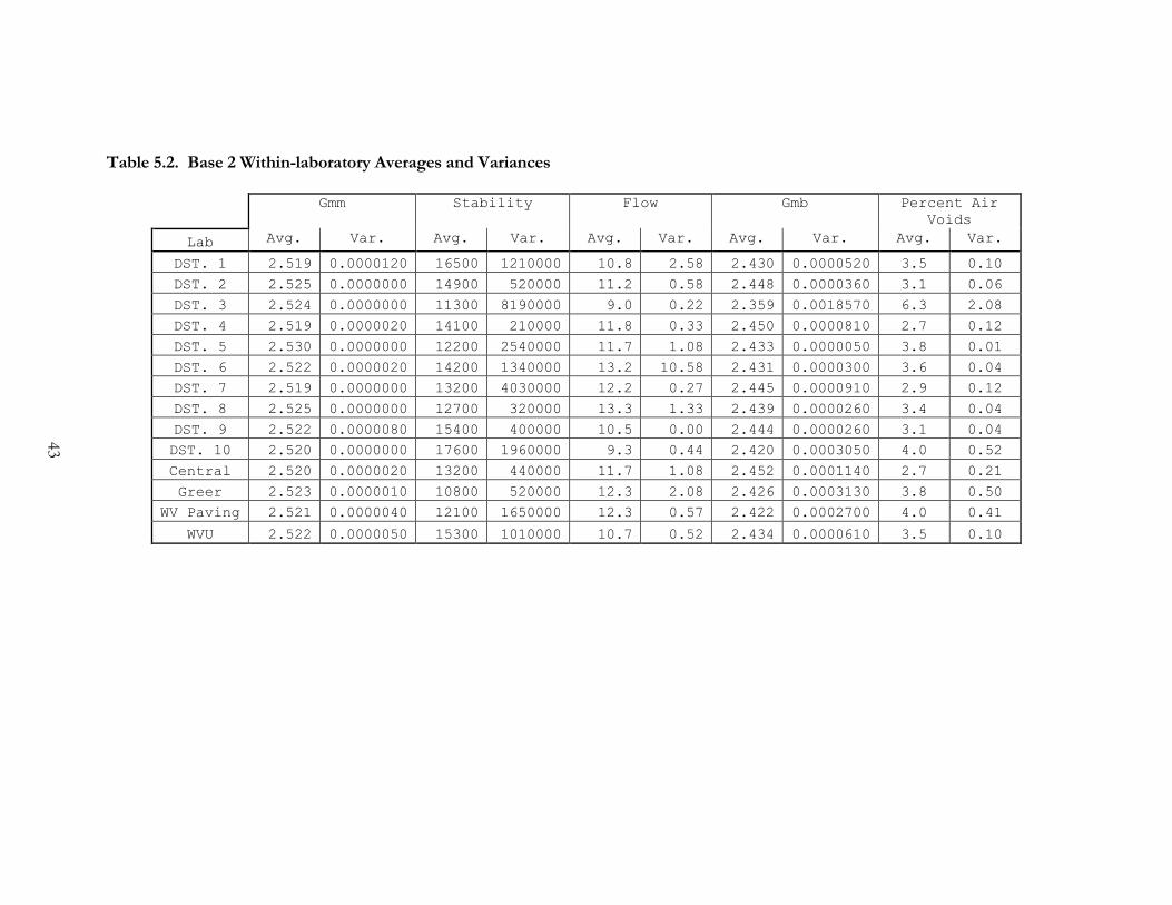
43

Table 5.2. Base 2 Within-laboratory Averages and Variances

Gmm Stability Flow Gmb Percent Air

Voids

Lab Avg. Var. Avg. Var. Avg. Var. Avg. Var. Avg. Var.

DST. 1 2.519 0.0000120 16500 1210000 10.8 2.58 2.430 0.0000520 3.5 0.10

DST. 2 2.525 0.0000000 14900 520000 11.2 0.58 2.448 0.0000360 3.1 0.06

DST. 3 2.524 0.0000000 11300 8190000 9.0 0.22 2.359 0.0018570 6.3 2.08

DST. 4 2.519 0.0000020 14100 210000 11.8 0.33 2.450 0.0000810 2.7 0.12

DST. 5 2.530 0.0000000 12200 2540000 11.7 1.08 2.433 0.0000050 3.8 0.01

DST. 6 2.522 0.0000020 14200 1340000 13.2 10.58 2.431 0.0000300 3.6 0.04

DST. 7 2.519 0.0000000 13200 4030000 12.2 0.27 2.445 0.0000910 2.9 0.12

DST. 8 2.525 0.0000000 12700 320000 13.3 1.33 2.439 0.0000260 3.4 0.04

DST. 9 2.522 0.0000080 15400 400000 10.5 0.00 2.444 0.0000260 3.1 0.04

DST. 10 2.520 0.0000000 17600 1960000 9.3 0.44 2.420 0.0003050 4.0 0.52

Central 2.520 0.0000020 13200 440000 11.7 1.08 2.452 0.0001140 2.7 0.21

Greer 2.523 0.0000010 10800 520000 12.3 2.08 2.426 0.0003130 3.8 0.50

WV Paving 2.521 0.0000040 12100 1650000 12.3 0.57 2.422 0.0002700 4.0 0.41

WVU 2.522 0.0000050 15300 1010000 10.7 0.52 2.434 0.0000610 3.5 0.10

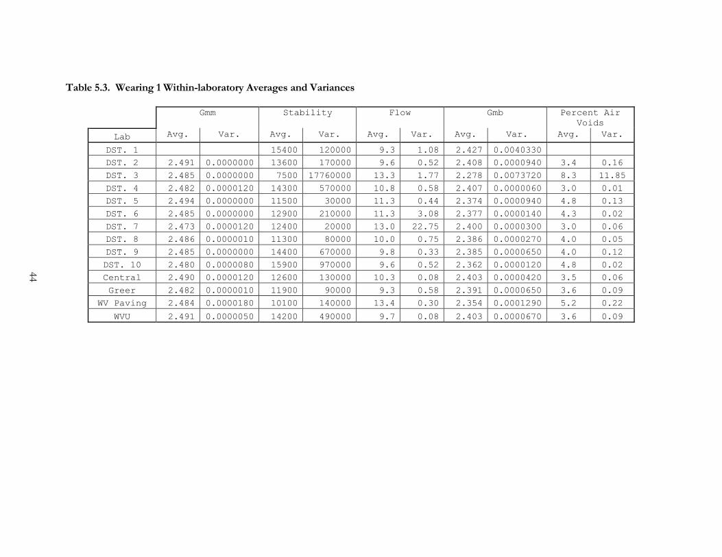
44

Table 5.3. Wearing 1 Within-laboratory Averages and Variances

Gmm Stability Flow Gmb Percent Air

Voids

Lab Avg. Var. Avg. Var. Avg. Var. Avg. Var. Avg. Var.

DST. 1 15400 120000 9.3 1.08 2.427 0.0040330

DST. 2 2.491 0.0000000 13600 170000 9.6 0.52 2.408 0.0000940 3.4 0.16

DST. 3 2.485 0.0000000 7500 17760000 13.3 1.77 2.278 0.0073720 8.3 11.85

DST. 4 2.482 0.0000120 14300 570000 10.8 0.58 2.407 0.0000060 3.0 0.01

DST. 5 2.494 0.0000000 11500 30000 11.3 0.44 2.374 0.0000940 4.8 0.13

DST. 6 2.485 0.0000000 12900 210000 11.3 3.08 2.377 0.0000140 4.3 0.02

DST. 7 2.473 0.0000120 12400 20000 13.0 22.75 2.400 0.0000300 3.0 0.06

DST. 8 2.486 0.0000010 11300 80000 10.0 0.75 2.386 0.0000270 4.0 0.05

DST. 9 2.485 0.0000000 14400 670000 9.8 0.33 2.385 0.0000650 4.0 0.12

DST. 10 2.480 0.0000080 15900 970000 9.6 0.52 2.362 0.0000120 4.8 0.02

Central 2.490 0.0000120 12600 130000 10.3 0.08 2.403 0.0000420 3.5 0.06

Greer 2.482 0.0000010 11900 90000 9.3 0.58 2.391 0.0000650 3.6 0.09

WV Paving 2.484 0.0000180 10100 140000 13.4 0.30 2.354 0.0001290 5.2 0.22

WVU 2.491 0.0000050 14200 490000 9.7 0.08 2.403 0.0000670 3.6 0.09

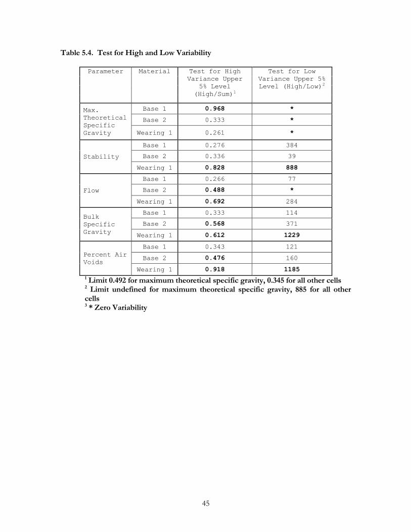
45

Table 5.4. Test for High and Low Variability

Parameter Material Test for High

Variance Upper

5% Level

(High/Sum)1

Test for Low

Variance Upper 5%

Level (High/Low)2

Max.

Theoretical

Specific

Gravity

Base 1 0.968 *

Base 2 0.333 *

Wearing 1 0.261 *

Stability

Base 1 0.276 384

Base 2 0.336 39

Wearing 1 0.828 888

Flow

Base 1 0.266 77

Base 2 0.488 *

Wearing 1 0.692 284

Bulk

Specific

Gravity

Base 1 0.333 114

Base 2 0.568 371

Wearing 1 0.612 1229

Percent Air

Voids

Base 1 0.343 121

Base 2 0.476 160

Wearing 1 0.918 1185

1 Limit 0.492 for maximum theoretical specific gravity, 0.345 for all other cells 2 Limit undefined for maximum theoretical specific gravity, 885 for all other

cells 3 * Zero Variability

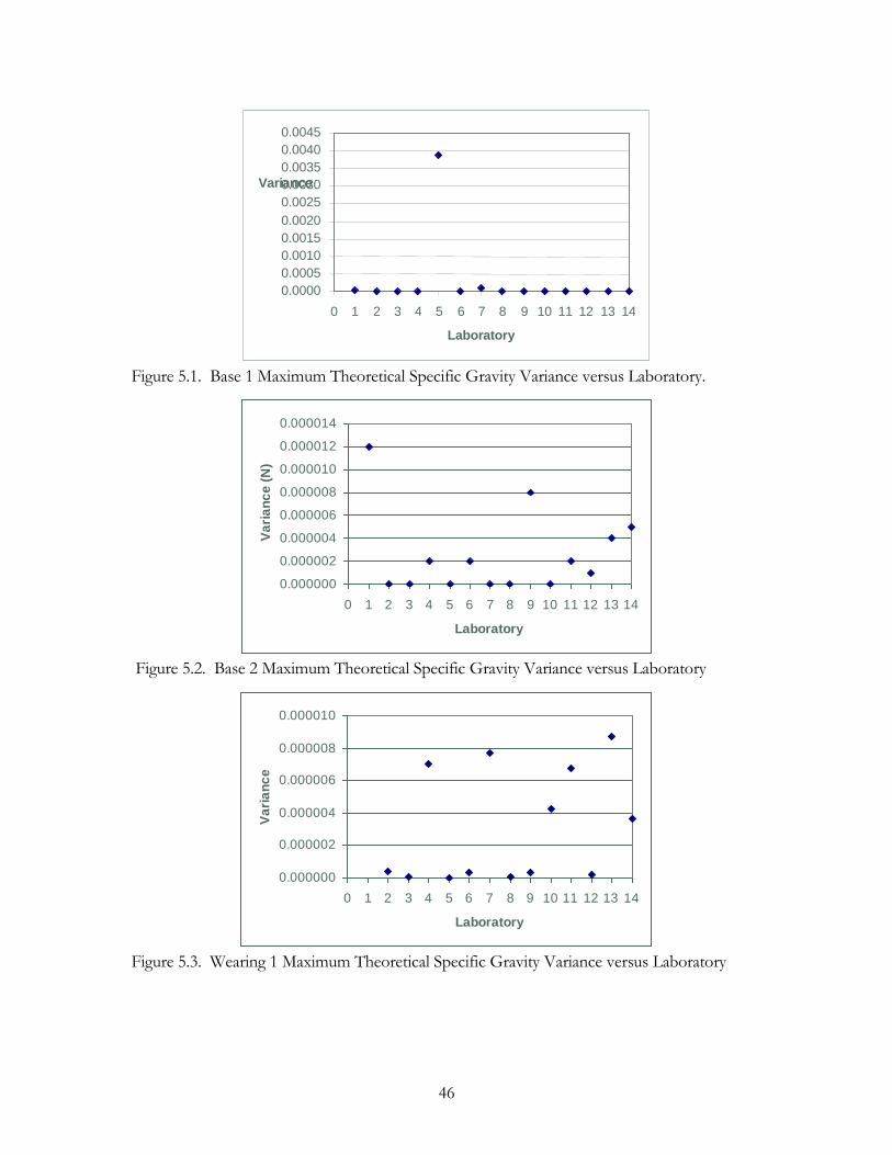
46

Figure 5.1. Base 1 Maximum Theoretical Specific Gravity Variance versus Laboratory.

0.000000

0.000002

0.000004

0.000006

0.000008

0.000010

0.000012

0.000014

0 1 2 3 4 5 6 7 8 9 10 11 12 13 14

Laboratory

Va

ria

nc

e (

N)

Figure 5.2. Base 2 Maximum Theoretical Specific Gravity Variance versus Laboratory

0.000000

0.000002

0.000004

0.000006

0.000008

0.000010

0 1 2 3 4 5 6 7 8 9 10 11 12 13 14

Laboratory

Va

ria

nc

e

Figure 5.3. Wearing 1 Maximum Theoretical Specific Gravity Variance versus Laboratory

0.0000 0.0005 0.0010 0.0015 0.0020 0.0025 0.0030 0.0035 0.0040 0.0045

0 1 2 3 4 5 6 7 8 9 10 11 12 13 14

Laboratory

Variance

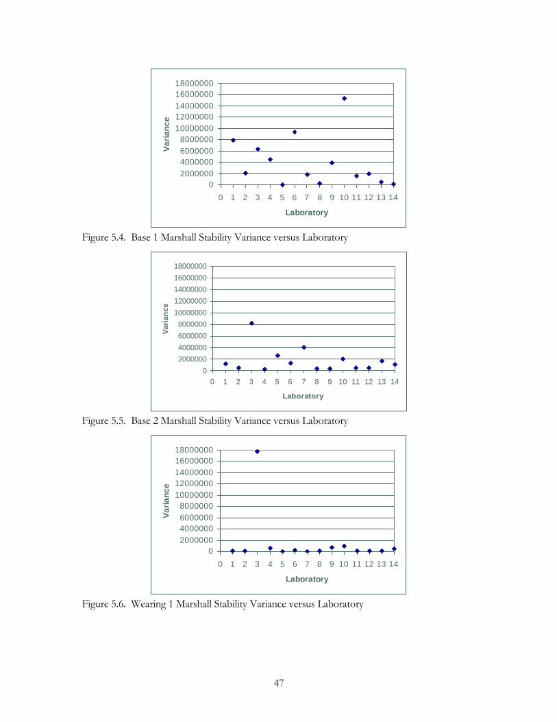
47

0

2000000

4000000

6000000

8000000

10000000

12000000

14000000

16000000

18000000

0 1 2 3 4 5 6 7 8 9 10 11 12 13 14

Laboratory

Va

ria

nc

e

Figure 5.4. Base 1 Marshall Stability Variance versus Laboratory

0

2000000

4000000

6000000

8000000

10000000

12000000

14000000

16000000

18000000

0 1 2 3 4 5 6 7 8 9 10 11 12 13 14

Laboratory

Vari

an

ce

Figure 5.5. Base 2 Marshall Stability Variance versus Laboratory

0

2000000

4000000

6000000

8000000

10000000

12000000

14000000

16000000

18000000

0 1 2 3 4 5 6 7 8 9 10 11 12 13 14

Laboratory

Va

ria

nc

e

Figure 5.6. Wearing 1 Marshall Stability Variance versus Laboratory

48

0

5

10

15

20

25

0 1 2 3 4 5 6 7 8 9 10 11 12 13 14

Laboratory

Va

ria

nc

e

Figure 5.7. Base 1 Marshall Flow Variance versus Laboratory

0

2

4

6

8

10

12

0 1 2 3 4 5 6 7 8 9 10 11 12 13 14

Laboratory

Va

ria

nc

e

Figure 5.8. Base 2 Marshall Flow Variance versus Laboratory

0

5

10

15

20

25

0 1 2 3 4 5 6 7 8 9 10 11 12 13 14

Laboratory

Va

ria

nc

e

Figure 5.9. Wearing 1 Marshall Flow Variance versus Laboratory

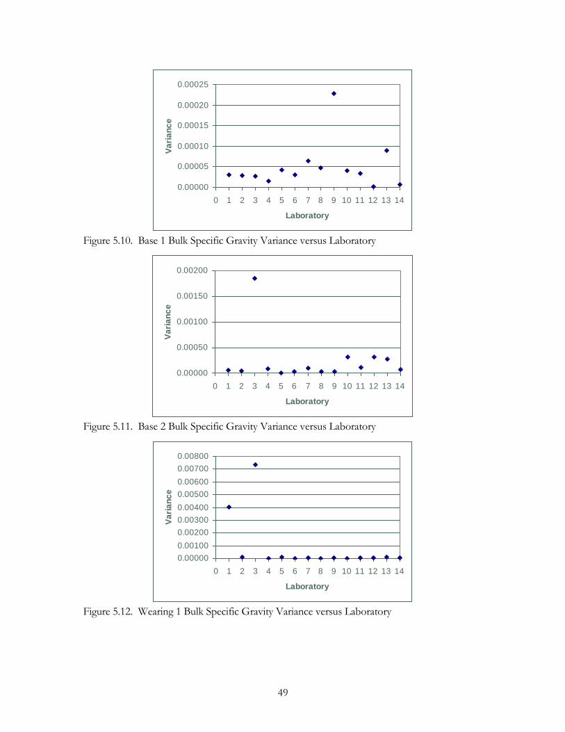
49

0.00000

0.00005

0.00010

0.00015

0.00020

0.00025

0 1 2 3 4 5 6 7 8 9 10 11 12 13 14

Laboratory

Va

ria

nc

e

Figure 5.10. Base 1 Bulk Specific Gravity Variance versus Laboratory

0.00000

0.00050

0.00100

0.00150

0.00200

0 1 2 3 4 5 6 7 8 9 10 11 12 13 14

Laboratory

Va

ria

nc

e

Figure 5.11. Base 2 Bulk Specific Gravity Variance versus Laboratory

0.00000

0.00100

0.00200

0.00300

0.00400

0.00500

0.00600

0.00700

0.00800

0 1 2 3 4 5 6 7 8 9 10 11 12 13 14

Laboratory

Va

ria

nc

e

Figure 5.12. Wearing 1 Bulk Specific Gravity Variance versus Laboratory

50

0.00

0.05

0.10

0.15

0.20

0.25

0.30

0.35

0.40

0 1 2 3 4 5 6 7 8 9 10 11 12 13 14

Laboratory

Va

ria

nc

e

Figure 5.13. Base 1 Percent Air Voids Variance versus Laboratory

0.00

0.05

0.10

0.15

0.20

0.25

0.30

0.35

0.40

0 2 4 6 8 10 12 14

Laboratory

Vari

an

ce

Figure 5.14. Base 2 Percent Air Voids Variance versus Laboratory

0.00

2.00

4.00

6.00

8.00

10.00

12.00

14.00

0 1 2 3 4 5 6 7 8 9 10 11 12 13 14

Laboratory

Va

ria

nc

e

Figure 5.15. Wearing 1 Percent Air Voids Variance versus Laboratory

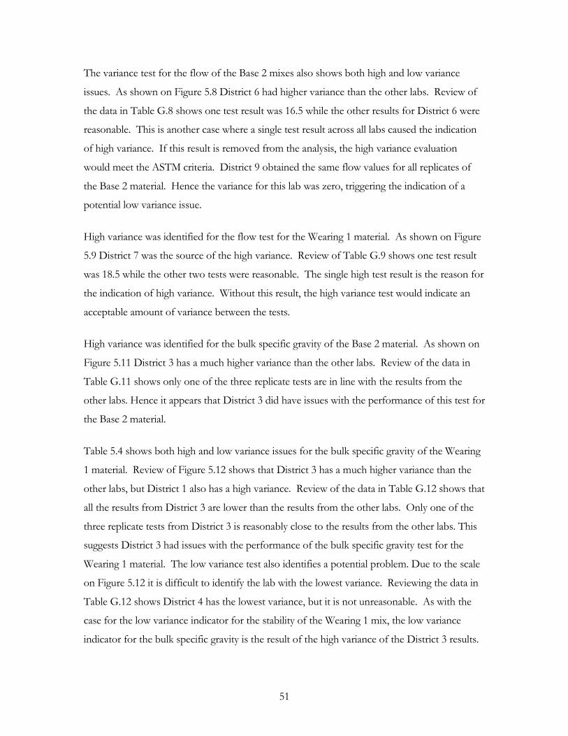
51

The variance test for the flow of the Base 2 mixes also shows both high and low variance

issues. As shown on Figure 5.8 District 6 had higher variance than the other labs. Review of

the data in Table G.8 shows one test result was 16.5 while the other results for District 6 were

reasonable. This is another case where a single test result across all labs caused the indication

of high variance. If this result is removed from the analysis, the high variance evaluation

would meet the ASTM criteria. District 9 obtained the same flow values for all replicates of

the Base 2 material. Hence the variance for this lab was zero, triggering the indication of a

potential low variance issue.

High variance was identified for the flow test for the Wearing 1 material. As shown on Figure

5.9 District 7 was the source of the high variance. Review of Table G.9 shows one test result

was 18.5 while the other two tests were reasonable. The single high test result is the reason for

the indication of high variance. Without this result, the high variance test would indicate an

acceptable amount of variance between the tests.

High variance was identified for the bulk specific gravity of the Base 2 material. As shown on

Figure 5.11 District 3 has a much higher variance than the other labs. Review of the data in

Table G.11 shows only one of the three replicate tests are in line with the results from the

other labs. Hence it appears that District 3 did have issues with the performance of this test for

the Base 2 material.

Table 5.4 shows both high and low variance issues for the bulk specific gravity of the Wearing

1 material. Review of Figure 5.12 shows that District 3 has a much higher variance than the

other labs, but District 1 also has a high variance. Review of the data in Table G.12 shows that

all the results from District 3 are lower than the results from the other labs. Only one of the

three replicate tests from District 3 is reasonably close to the results from the other labs. This

suggests District 3 had issues with the performance of the bulk specific gravity test for the

Wearing 1 material. The low variance test also identifies a potential problem. Due to the scale

on Figure 5.12 it is difficult to identify the lab with the lowest variance. Reviewing the data in

Table G.12 shows District 4 has the lowest variance, but it is not unreasonable. As with the

case for the low variance indicator for the stability of the Wearing 1 mix, the low variance

indicator for the bulk specific gravity is the result of the high variance of the District 3 results.

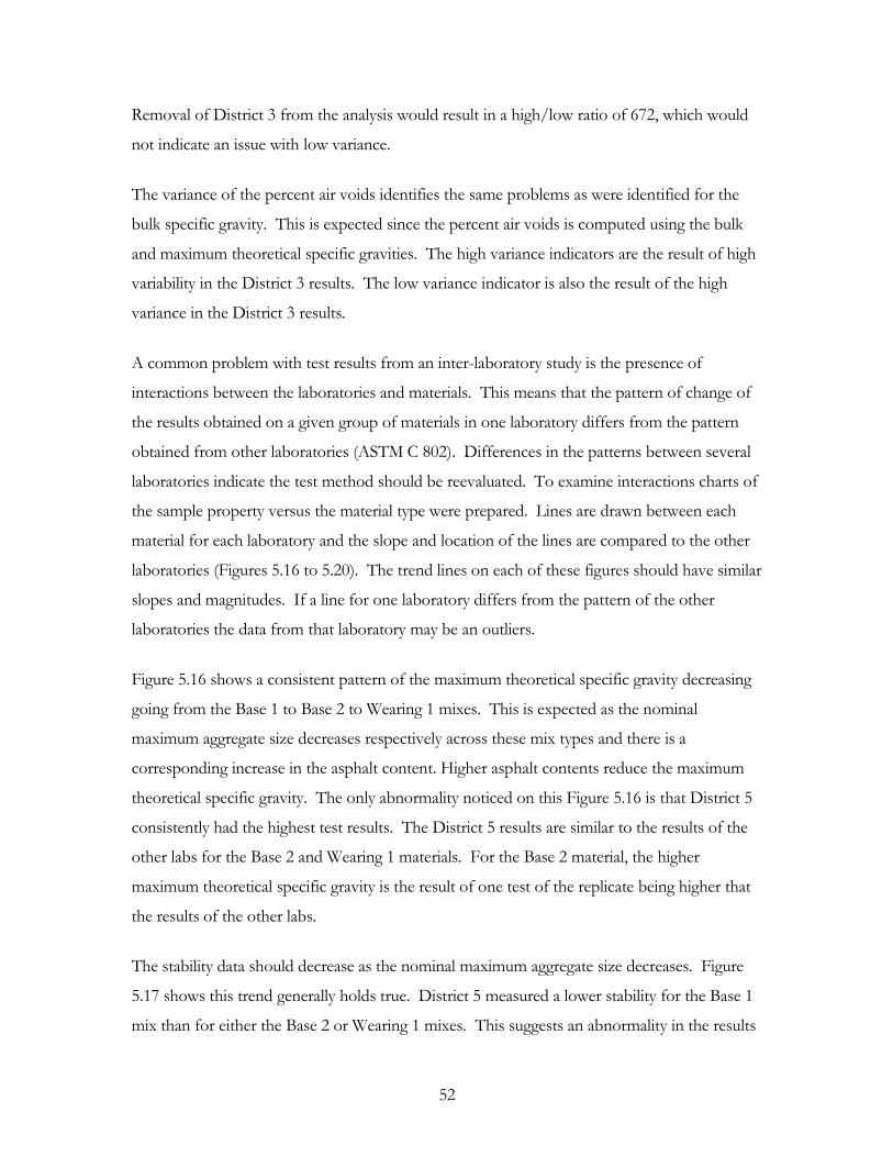
52

Removal of District 3 from the analysis would result in a high/low ratio of 672, which would

not indicate an issue with low variance.

The variance of the percent air voids identifies the same problems as were identified for the

bulk specific gravity. This is expected since the percent air voids is computed using the bulk

and maximum theoretical specific gravities. The high variance indicators are the result of high

variability in the District 3 results. The low variance indicator is also the result of the high

variance in the District 3 results.

A common problem with test results from an inter-laboratory study is the presence of

interactions between the laboratories and materials. This means that the pattern of change of

the results obtained on a given group of materials in one laboratory differs from the pattern

obtained from other laboratories (ASTM C 802). Differences in the patterns between several

laboratories indicate the test method should be reevaluated. To examine interactions charts of

the sample property versus the material type were prepared. Lines are drawn between each

material for each laboratory and the slope and location of the lines are compared to the other

laboratories (Figures 5.16 to 5.20). The trend lines on each of these figures should have similar

slopes and magnitudes. If a line for one laboratory differs from the pattern of the other

laboratories the data from that laboratory may be an outliers.

Figure 5.16 shows a consistent pattern of the maximum theoretical specific gravity decreasing

going from the Base 1 to Base 2 to Wearing 1 mixes. This is expected as the nominal

maximum aggregate size decreases respectively across these mix types and there is a

corresponding increase in the asphalt content. Higher asphalt contents reduce the maximum

theoretical specific gravity. The only abnormality noticed on this Figure 5.16 is that District 5

consistently had the highest test results. The District 5 results are similar to the results of the

other labs for the Base 2 and Wearing 1 materials. For the Base 2 material, the higher

maximum theoretical specific gravity is the result of one test of the replicate being higher that

the results of the other labs.

The stability data should decrease as the nominal maximum aggregate size decreases. Figure

5.17 shows this trend generally holds true. District 5 measured a lower stability for the Base 1

mix than for either the Base 2 or Wearing 1 mixes. This suggests an abnormality in the results

53

reported by District 5. District 4 and Greer reported the stability of the Base 2 mix was less

than the stability of the Wearing 1 mix. However, the magnitudes of the differences are not

large enough to cause concern.

Figure 5.18 shows a general trend for flow to decrease with a reduction in the nominal

maximum aggregate size. However two of the labs measured higher flow for the Base 2

material compared to the Base 1 material and four labs measured higher values for the

Wearing 1 than the Base 2. WVDOH specifications of flow allow a wide range of flow values

due to the high variance of this test.

Figures 5.19 and 5.20 show reasonable agreement and similar trends for bulk specific gravity

and percent air voids for all laboratories with the exception of District 3. The low bulk

specific gravity and high air void content of the Base 2 and Wearing 1 samples from District 3

indicate inadequate compaction. This could be a reason the Marshall stability of these samples

was relatively low, especially for the Wearing 1 samples.

2.40

2.45

2.50

2.55

2.60

2.65

Base 1 Base 2 Wearing 1

Material

Ma

xim

um

Th

eo

reti

ca

l S

pe

cif

Gra

vit

y

DST. 2

DST. 3

DST. 4

DST. 5

DST. 6

DST. 7

DST. 8

DST. 9

DST. 10

Central

Greer

WV Pav

WVU

Figure 5.16. Material type versus Maximum Theoretical Specific Gravity

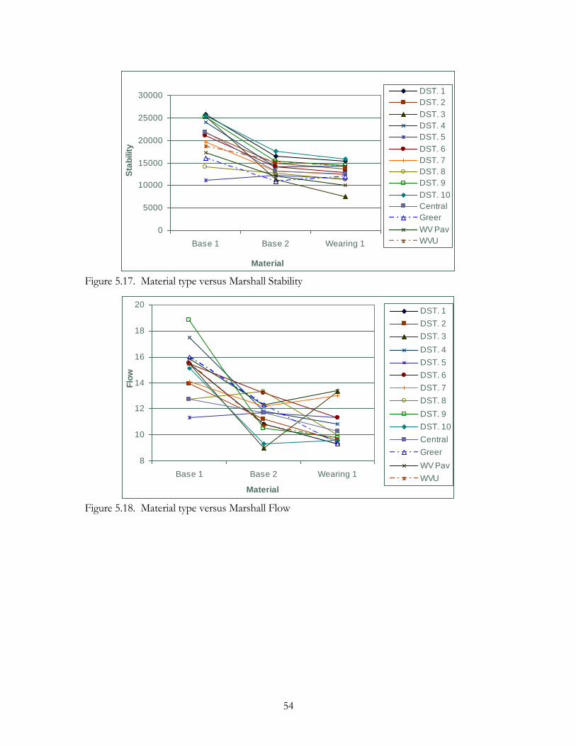
54

0

5000

10000

15000

20000

25000

30000

Base 1 Base 2 Wearing 1

Material

Sta

bilit

y

DST. 1

DST. 2

DST. 3

DST. 4

DST. 5

DST. 6

DST. 7

DST. 8

DST. 9

DST. 10

Central

Greer

WV Pav

WVU

Figure 5.17. Material type versus Marshall Stability

8

10

12

14

16

18

20

Base 1 Base 2 Wearing 1

Material

Flo

w

DST. 1

DST. 2

DST. 3

DST. 4

DST. 5

DST. 6

DST. 7

DST. 8

DST. 9

DST. 10

Central

Greer

WV Pav

WVU

Figure 5.18. Material type versus Marshall Flow

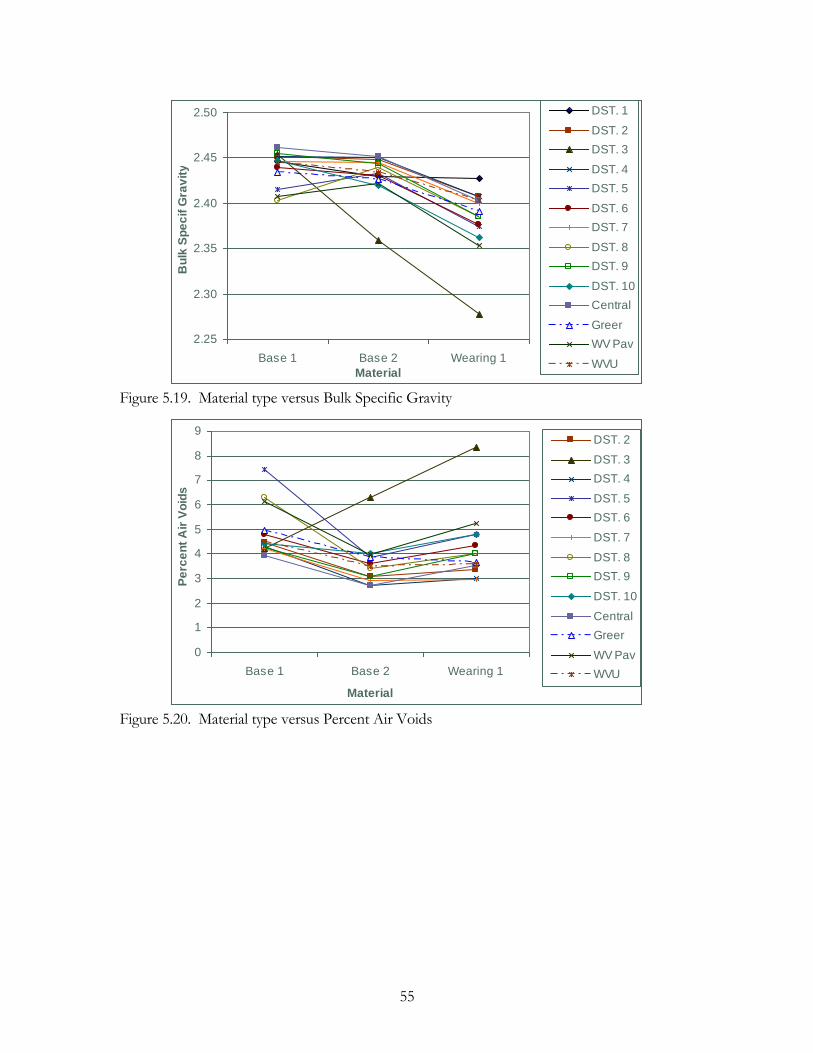
55

2.25

2.30

2.35

2.40

2.45

2.50

Base 1 Base 2 Wearing 1

Material

Bu

lk S

pe

cif

Gra

vit

y

DST. 1

DST. 2

DST. 3

DST. 4

DST. 5

DST. 6

DST. 7

DST. 8

DST. 9

DST. 10

Central

Greer

WV Pav

WVU

Figure 5.19. Material type versus Bulk Specific Gravity

0

1

2

3

4

5

6

7

8

9

Base 1 Base 2 Wearing 1

Material

Pe

rce

nt

Air

Vo

ids

DST. 2

DST. 3

DST. 4

DST. 5

DST. 6

DST. 7

DST. 8

DST. 9

DST. 10

Central

Greer

WV Pav

WVU

Figure 5.20. Material type versus Percent Air Voids

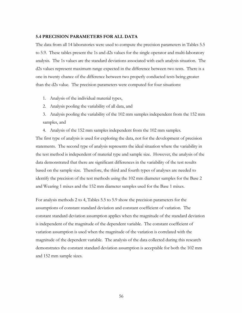
56

5.4 PRECISION PARAMETERS FOR ALL DATA

The data from all 14 laboratories were used to compute the precision parameters in Tables 5.5

to 5.9. These tables present the 1s and d2s values for the single operator and multi-laboratory

analysis. The 1s values are the standard deviations associated with each analysis situation. The

d2s values represent maximum range expected in the difference between two tests. There is a

one in twenty chance of the difference between two properly conducted tests being greater

than the d2s value. The precision parameters were computed for four situations:

1. Analysis of the individual material types,

2. Analysis pooling the variability of all data, and

3. Analysis pooling the variability of the 102 mm samples independent from the 152 mm

samples, and

4. Analysis of the 152 mm samples independent from the 102 mm samples.

The first type of analysis is used for exploring the data, not for the development of precision

statements. The second type of analysis represents the ideal situation where the variability in

the test method is independent of material type and sample size. However, the analysis of the

data demonstrated that there are significant differences in the variability of the test results

based on the sample size. Therefore, the third and fourth types of analyses are needed to

identify the precision of the test methods using the 102 mm diameter samples for the Base 2

and Wearing 1 mixes and the 152 mm diameter samples used for the Base 1 mixes.

For analysis methods 2 to 4, Tables 5.5 to 5.9 show the precision parameters for the

assumptions of constant standard deviation and constant coefficient of variation. The

constant standard deviation assumption applies when the magnitude of the standard deviation

is independent of the magnitude of the dependent variable. The constant coefficient of

variation assumption is used when the magnitude of the variation is correlated with the

magnitude of the dependent variable. The analysis of the data collected during this research

demonstrates the constant standard deviation assumption is acceptable for both the 102 mm

and 152 mm sample sizes.

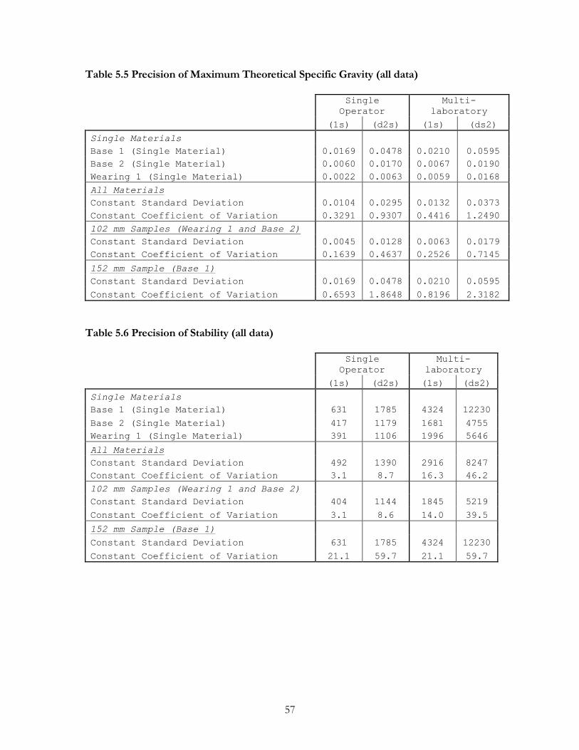
57

Table 5.5 Precision of Maximum Theoretical Specific Gravity (all data)

Single

Operator

Multi-

laboratory

(1s) (d2s) (1s) (ds2)

Single Materials

Base 1 (Single Material) 0.0169 0.0478 0.0210 0.0595

Base 2 (Single Material) 0.0060 0.0170 0.0067 0.0190

Wearing 1 (Single Material) 0.0022 0.0063 0.0059 0.0168

All Materials

Constant Standard Deviation 0.0104 0.0295 0.0132 0.0373

Constant Coefficient of Variation 0.3291 0.9307 0.4416 1.2490

102 mm Samples (Wearing 1 and Base 2)

Constant Standard Deviation 0.0045 0.0128 0.0063 0.0179

Constant Coefficient of Variation 0.1639 0.4637 0.2526 0.7145

152 mm Sample (Base 1)

Constant Standard Deviation 0.0169 0.0478 0.0210 0.0595

Constant Coefficient of Variation 0.6593 1.8648 0.8196 2.3182

Table 5.6 Precision of Stability (all data)

Single

Operator

Multi-

laboratory

(1s) (d2s) (1s) (ds2)

Single Materials

Base 1 (Single Material) 631 1785 4324 12230

Base 2 (Single Material) 417 1179 1681 4755

Wearing 1 (Single Material) 391 1106 1996 5646

All Materials

Constant Standard Deviation 492 1390 2916 8247

Constant Coefficient of Variation 3.1 8.7 16.3 46.2

102 mm Samples (Wearing 1 and Base 2)

Constant Standard Deviation 404 1144 1845 5219

Constant Coefficient of Variation 3.1 8.6 14.0 39.5

152 mm Sample (Base 1)

Constant Standard Deviation 631 1785 4324 12230

Constant Coefficient of Variation 21.1 59.7 21.1 59.7

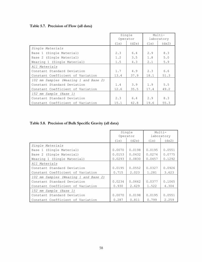
58

Table 5.7. Precision of Flow (all data)

Single

Operator

Multi-

laboratory

(1s) (d2s) (1s) (ds2)

Single Materials

Base 1 (Single Material) 2.3 6.4 2.9 8.3

Base 2 (Single Material) 1.2 3.5 1.8 5.0

Wearing 1 (Single Material) 1.5 4.3 2.1 5.9

All Materials

Constant Standard Deviation 1.7 4.9 2.3 6.6

Constant Coefficient of Variation 13.4 37.9 18.1 51.3

102 mm Samples (Wearing 1 and Base 2)

Constant Standard Deviation 1.4 3.9 1.9 5.5

Constant Coefficient of Variation 12.6 35.5 17.4 49.2

152 mm Sample (Base 1)

Constant Standard Deviation 2.3 6.4 2.9 8.3

Constant Coefficient of Variation 15.1 42.8 19.6 55.3

Table 5.8. Precision of Bulk Specific Gravity (all data)

Single

Operator

Multi-

laboratory

(1s) (d2s) (1s) (ds2)

Single Materials

Base 1 (Single Material) 0.0070 0.0198 0.0195 0.0551

Base 2 (Single Material) 0.0153 0.0432 0.0274 0.0775

Wearing 1 (Single Material) 0.0293 0.0830 0.0457 0.1292

All Materials

Constant Standard Deviation 0.0195 0.0552 0.0327 0.0926

Constant Coefficient of Variation 0.715 2.023 1.281 3.623

102 mm Samples (Wearing 1 and Base 2)

Constant Standard Deviation 0.0234 0.0662 0.0377 0.1065

Constant Coefficient of Variation 0.930 2.629 1.522 4.304

152 mm Sample (Base 1)

Constant Standard Deviation 0.0070 0.0198 0.0195 0.0551

Constant Coefficient of Variation 0.287 0.811 0.799 2.259

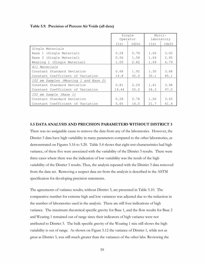
59

Table 5.9. Precision of Percent Air Voids (all data)

Single

Operator

Multi-

laboratory

(1s) (d2s) (1s) (ds2)

Single Materials

Base 1 (Single Material) 0.28 0.78 1.06 3.00

Base 2 (Single Material) 0.56 1.58 1.04 2.95

Wearing 1 (Single Material) 1.00 2.82 1.69 4.79

All Materials

Constant Standard Deviation 0.68 1.92 1.30 3.68

Constant Coefficient of Variation 14.8 42.0 30.1 85.1

102 mm Samples (Wearing 1 and Base 2)

Constant Standard Deviation 0.81 2.29 1.41 3.98

Constant Coefficient of Variation 19.44 55.0 34.3 97.0

152 mm Sample (Base 1)

Constant Standard Deviation 0.28 0.78 1.06 3.00

Constant Coefficient of Variation 5.65 16.0 21.7 61.4

5.5 DATA ANALYSIS AND PRECISION PARAMETERS WITHOUT DISTRICT 3

There was no assignable cause to remove the data from any of the laboratories. However, the

District 3 data have high variability in many parameters compared to the other laboratories, as

demonstrated on Figures 5.16 to 5.20. Table 5.4 shows that eight test characteristics had high

variance, of these five were associated with the variability of the District 3 results. There were

three cases where there was the indication of low variability was the result of the high

variability of the District 3 results. Thus, the analysis repeated with the District 3 data removed

from the data set. Removing a suspect data set from the analysis is described in the ASTM

specification for developing precision statements.

The agreements of variance results, without District 3, are presented in Table 5.10. The

comparative number for extreme high and low variances was adjusted due to the reduction in

the number of laboratories used in the analysis. There are still four indications of high

variance. The maximum theoretical specific gravity for Base 1, and the flow results for Base 2

and Wearing 1 remained out of range since their indicators of high variance were not

attributed to District 3. The bulk specific gravity of the Wearing 1 mix still shows the high

variability is out of range. As shown on Figure 5.12 the variance of District 1, while not as

great as District 3, was still much greater than the variances of the other labs. Reviewing the

60

Table 5.10. Test for High and Low Variability without District 3

Parameter Material

Test for High

Variance Upper

5% Level

(High/Sum)1

Test for Low

Variance Upper 5%

Level (High/Low)2

Max.

Theoretical

Specific

Gravity

Base 1 0.970 *

Base 2 0.333 *

Wearing 1 0.261 *

Stability

Base 1 0.311 384

Base 2 0.250 19

Wearing 1 0.263 49

Flow

Base 1 0.288 61

Base 2 0.493 *

Wearing 1 0.732 284

Bulk

Specific

Gravity

Base 1 0.347 114

Base 2 0.222 63

Wearing 1 0.862 672

Percent Air

Voids

Base 1 0.353 121

Base 2 0.227 40

Wearing 1 0.211 22

1 Limit 0.514 for maximum theoretical specific gravity, 0.363 for all other cells 2 Limit undefined for maximum theoretical specific gravity, 790 for all other

cells 3 * Zero Variability

data in Table G.12 shows two of the bulk specific gravity replicate tests for Wearing 1 by

District 1 were identical and near the average for all the labs. The third replicate result is much

higher. Looking at the raw data in Table E.3 shows the submerged weight for the third

replicate is out of line compared to the other results, demonstrating the impact of a single

erroneous measurement. However, since there is no assignable cause for removal of this data

point and since the results of District 1 are otherwise reasonable, there is no justification for

the removal of this data point from the analysis.

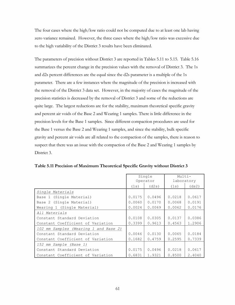
61

The four cases where the high/low ratio could not be computed due to at least one lab having

zero variance remained. However, the three cases where the high/low ratio was excessive due

to the high variability of the District 3 results have been eliminated.

The parameters of precision without District 3 are reported in Tables 5.11 to 5.15. Table 5.16

summarizes the percent change in the precision values with the removal of District 3. The 1s

and d2s percent differences are the equal since the d2s parameter is a multiple of the 1s

parameter. There are a few instances where the magnitude of the precision is increased with

the removal of the District 3 data set. However, in the majority of cases the magnitude of the

precision statistics is decreased by the removal of District 3 and some of the reductions are

quite large. The largest reductions are for the stability, maximum theoretical specific gravity

and percent air voids of the Base 2 and Wearing 1 samples. There is little difference in the

precision levels for the Base 1 samples. Since different compaction procedures are used for

the Base 1 versus the Base 2 and Wearing 1 samples, and since the stability, bulk specific

gravity and percent air voids are all related to the compaction of the samples, there is reason to

suspect that there was an issue with the compaction of the Base 2 and Wearing 1 samples by

District 3.

Table 5.11 Precision of Maximum Theoretical Specific Gravity without District 3

Single

Operator

Multi-

laboratory

(1s) (d2s) (1s) (ds2)

Single Materials

Base 1 (Single Material) 0.0175 0.0496 0.0218 0.0617

Base 2 (Single Material) 0.0060 0.0170 0.0068 0.0191

Wearing 1 (Single Material) 0.0024 0.0069 0.0062 0.0176

All Materials

Constant Standard Deviation 0.0108 0.0305 0.0137 0.0386

Constant Coefficient of Variation 0.3399 0.9613 0.4563 1.2906

102 mm Samples (Wearing 1 and Base 2)

Constant Standard Deviation 0.0046 0.0130 0.0065 0.0184

Constant Coefficient of Variation 0.1682 0.4759 0.2595 0.7339

152 mm Sample (Base 1)

Constant Standard Deviation 0.0175 0.0496 0.0218 0.0617

Constant Coefficient of Variation 0.6831 1.9321 0.8500 2.4040

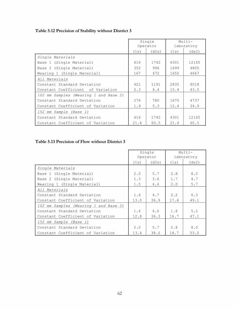
62

Table 5.12 Precision of Stability without District 3

Single

Operator

Multi-

laboratory

(1s) (d2s) (1s) (ds2)

Single Materials

Base 1 (Single Material) 616 1742 4301 12165

Base 2 (Single Material) 352 996 1699 4805

Wearing 1 (Single Material) 167 472 1650 4667

All Materials

Constant Standard Deviation 421 1191 2835 8018

Constant Coefficient of Variation 2.3 6.4 15.4 43.5

102 mm Samples (Wearing 1 and Base 2)

Constant Standard Deviation 276 780 1675 4737

Constant Coefficient of Variation 1.9 5.3 12.4 34.9

152 mm Sample (Base 1)

Constant Standard Deviation 616 1742 4301 12165

Constant Coefficient of Variation 21.4 60.5 21.4 60.5

Table 5.13 Precision of Flow without District 3

Single

Operator

Multi-

laboratory

(1s) (d2s) (1s) (ds2)

Single Materials

Base 1 (Single Material) 2.0 5.7 2.8 8.0

Base 2 (Single Material) 1.3 3.6 1.7 4.7

Wearing 1 (Single Material) 1.5 4.4 2.0 5.7

All Materials

Constant Standard Deviation 1.6 4.7 2.2 6.3

Constant Coefficient of Variation 13.0 36.9 17.4 49.1

102 mm Samples (Wearing 1 and Base 2)

Constant Standard Deviation 1.4 4.0 1.8 5.2

Constant Coefficient of Variation 12.8 36.3 16.7 47.1

152 mm Sample (Base 1)

Constant Standard Deviation 2.0 5.7 2.8 8.0

Constant Coefficient of Variation 13.4 38.0 18.7 53.0

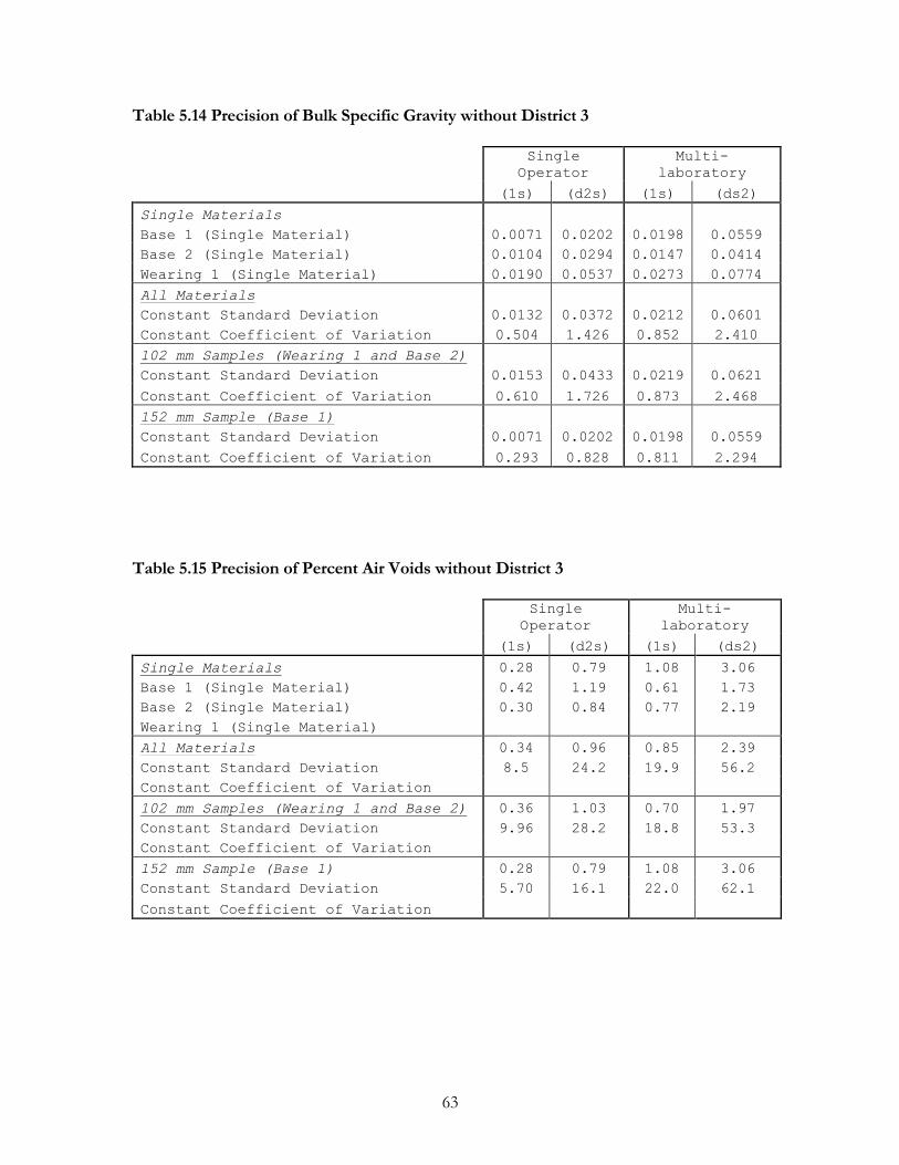
63

Table 5.14 Precision of Bulk Specific Gravity without District 3

Single

Operator

Multi-

laboratory

(1s) (d2s) (1s) (ds2)

Single Materials

Base 1 (Single Material) 0.0071 0.0202 0.0198 0.0559

Base 2 (Single Material) 0.0104 0.0294 0.0147 0.0414

Wearing 1 (Single Material) 0.0190 0.0537 0.0273 0.0774

All Materials

Constant Standard Deviation 0.0132 0.0372 0.0212 0.0601

Constant Coefficient of Variation 0.504 1.426 0.852 2.410

102 mm Samples (Wearing 1 and Base 2)

Constant Standard Deviation 0.0153 0.0433 0.0219 0.0621

Constant Coefficient of Variation 0.610 1.726 0.873 2.468

152 mm Sample (Base 1)

Constant Standard Deviation 0.0071 0.0202 0.0198 0.0559

Constant Coefficient of Variation 0.293 0.828 0.811 2.294

Table 5.15 Precision of Percent Air Voids without District 3

Single

Operator

Multi-

laboratory

(1s) (d2s) (1s) (ds2)

Single Materials 0.28 0.79 1.08 3.06

Base 1 (Single Material) 0.42 1.19 0.61 1.73

Base 2 (Single Material) 0.30 0.84 0.77 2.19

Wearing 1 (Single Material)

All Materials 0.34 0.96 0.85 2.39

Constant Standard Deviation 8.5 24.2 19.9 56.2

Constant Coefficient of Variation

102 mm Samples (Wearing 1 and Base 2) 0.36 1.03 0.70 1.97

Constant Standard Deviation 9.96 28.2 18.8 53.3

Constant Coefficient of Variation

152 mm Sample (Base 1) 0.28 0.79 1.08 3.06

Constant Standard Deviation 5.70 16.1 22.0 62.1

Constant Coefficient of Variation

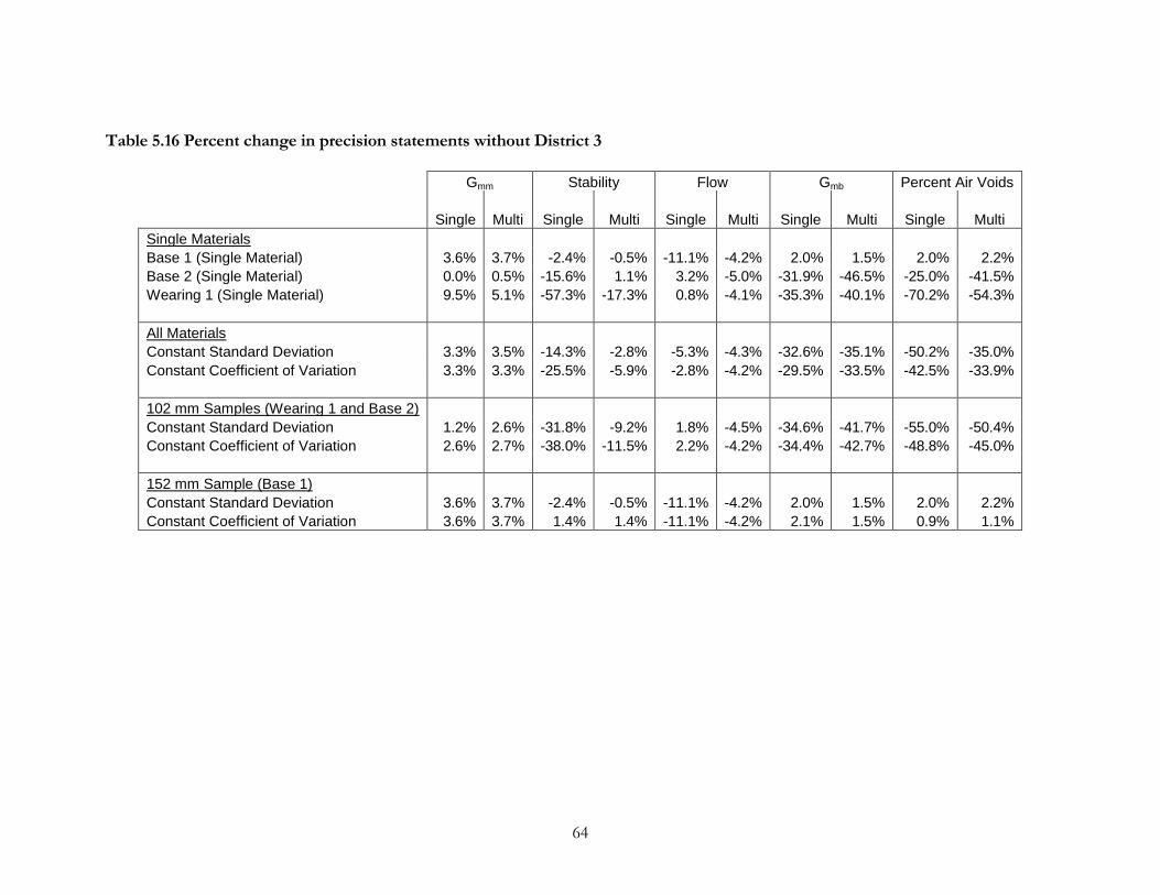
64

Table 5.16 Percent change in precision statements without District 3

Gmm Stability Flow Gmb Percent Air Voids

Single Multi Single Multi Single Multi Single Multi Single Multi

Single Materials

Base 1 (Single Material) 3.6% 3.7% -2.4% -0.5% -11.1% -4.2% 2.0% 1.5% 2.0% 2.2%

Base 2 (Single Material) 0.0% 0.5% -15.6% 1.1% 3.2% -5.0% -31.9% -46.5% -25.0% -41.5%

Wearing 1 (Single Material) 9.5% 5.1% -57.3% -17.3% 0.8% -4.1% -35.3% -40.1% -70.2% -54.3%

All Materials

Constant Standard Deviation 3.3% 3.5% -14.3% -2.8% -5.3% -4.3% -32.6% -35.1% -50.2% -35.0%

Constant Coefficient of Variation 3.3% 3.3% -25.5% -5.9% -2.8% -4.2% -29.5% -33.5% -42.5% -33.9%

102 mm Samples (Wearing 1 and Base 2)

Constant Standard Deviation 1.2% 2.6% -31.8% -9.2% 1.8% -4.5% -34.6% -41.7% -55.0% -50.4%

Constant Coefficient of Variation 2.6% 2.7% -38.0% -11.5% 2.2% -4.2% -34.4% -42.7% -48.8% -45.0%

152 mm Sample (Base 1)

Constant Standard Deviation 3.6% 3.7% -2.4% -0.5% -11.1% -4.2% 2.0% 1.5% 2.0% 2.2%

Constant Coefficient of Variation 3.6% 3.7% 1.4% 1.4% -11.1% -4.2% 2.1% 1.5% 0.9% 1.1%

65

5.6 ANALYSIS OF OTHER STUDIES

Next, the results from this research were compared to the results from similar studies. Table

B.1 is a summary of the precision found from a round-robin study between AMRL

laboratories, conducted for ASTM (Kandhal, 96). This study used 152 mm samples and a

25.4 mm maximum aggregate sized, so the results are compared to the Base 1 data from the

current study. The Kandhal results are similar to the Base 1 standard deviations for bulk

specific gravity, flow, and percent air voids to the current study. The Kandhal single operator

standard deviation for stability was 65 percent greater than the Base 1 results, while the multi-

laboratory standard deviation was 23 percent lower. Given the magnitude of the variability in

the stability testing, this amount of difference in two studies conducted at different times, with

different materials and laboratories, is not unreasonable.

The Georgia DOH study (Siddiqui, 95) provides results comparable to the Base 2 and Wearing

1 materials (Table B.2). The within laboratory and between-laboratory standard deviation of

stability for the Georgia Study were 968 N and 1232 N, respectively. These compare to values

of ??714 N and ??1931 N, respectively, for the current study.

Siddiqui also provided data from Canadian and Utah studies, but only the average test values

from each of the laboratories were reported. Thus, the precision statements cannot be

calculated. To compare the results of these studies to the current study, the standard deviation

of the average results from each laboratory, excluding District 3, were calculated (Table 5.17).

The magnitude of the standard deviation between laboratories is similar to the data in the

literature. The WVU Base 1 results correspond to the ASTM study. The Base 2 and

Wearing 1 results correspond to the Utah, Georgia, and Canadian studies.

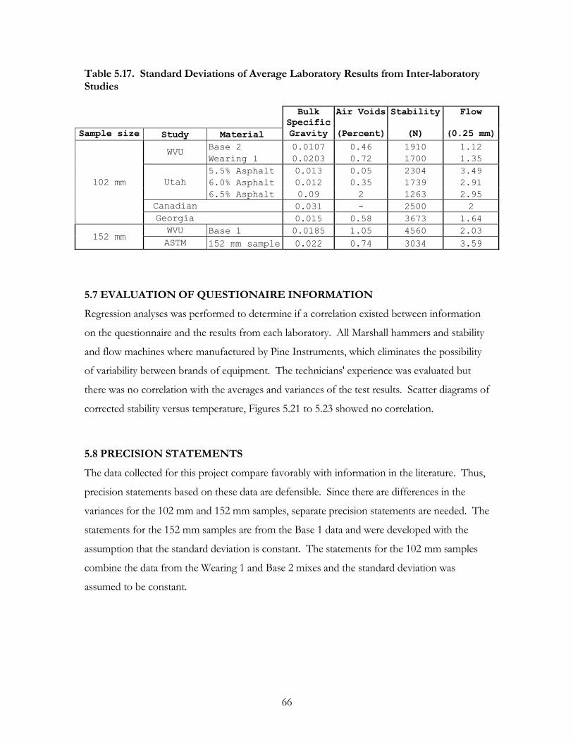
66

Table 5.17. Standard Deviations of Average Laboratory Results from Inter-laboratory Studies

Bulk

Specific

Air Voids Stability Flow

Sample size Study Material Gravity (Percent) (N) (0.25 mm)

102 mm

WVU Base 2 0.0107 0.46 1910 1.12

Wearing 1 0.0203 0.72 1700 1.35

Utah

5.5% Asphalt 0.013 0.05 2304 3.49

6.0% Asphalt 0.012 0.35 1739 2.91

6.5% Asphalt 0.09 2 1263 2.95

Canadian 0.031 - 2500 2

Georgia 0.015 0.58 3673 1.64

152 mm WVU Base 1 0.0185 1.05 4560 2.03

ASTM 152 mm sample 0.022 0.74 3034 3.59

5.7 EVALUATION OF QUESTIONAIRE INFORMATION

Regression analyses was performed to determine if a correlation existed between information

on the questionnaire and the results from each laboratory. All Marshall hammers and stability

and flow machines where manufactured by Pine Instruments, which eliminates the possibility

of variability between brands of equipment. The technicians' experience was evaluated but

there was no correlation with the averages and variances of the test results. Scatter diagrams of

corrected stability versus temperature, Figures 5.21 to 5.23 showed no correlation.

5.8 PRECISION STATEMENTS

The data collected for this project compare favorably with information in the literature. Thus,

precision statements based on these data are defensible. Since there are differences in the

variances for the 102 mm and 152 mm samples, separate precision statements are needed. The

statements for the 152 mm samples are from the Base 1 data and were developed with the

assumption that the standard deviation is constant. The statements for the 102 mm samples

combine the data from the Wearing 1 and Base 2 mixes and the standard deviation was

assumed to be constant.

67

0

5000

10000

15000

20000

25000

30000

35000

144 146 148 150 152 154 156 158

Temperature

Co

rrecte

d S

tab

ilit

y

Figure 5.21. Re-heat Temperature versus Base 1 Stability

0

5000

10000

15000

20000

144 145 146 147 148 149 150

Temperature

Co

rrecte

d S

tab

ilit

y

Figure 5.22. Re-heat Temperature versus Base 2 Stability

0

2000

4000

6000

8000

10000

12000

14000

16000

18000

140 142 144 146 148 150 152 154 156

Temperature

Co

rrecte

d S

tab

ilit

y

Figure 5.23. Plot of Re-heat Temperature versus Wearing 1 Stability

68

The treatment of the data from District 3 is a concern. A rigorous statistical analysis would

include these data since there was not an assignable cause to support their exclusion.

However, the fact that five of the nine stability values reported by District 3 were more than

two standard deviations from the mean for all the data indicates there is a problem with the

data and the cause was undiscovered. There is a one in twenty chance for one value to be

more than two standard deviations from the mean. When one laboratory has five values that

exceed this limit there is a strong indication that an undetected factor was affecting the results

produced at that lab. Using this reasoning, it is prudent to exclude the District 3 data when

developing the precision statements. Therefore, the following precision statements are

recommended based on the data in Tables 5.11 to 5.15.

Maximum Theoretical Specific Gravity (152 mm samples):

The single-operator standard deviation is 0.0175 for calculated maximum theoretical specific

gravities ranging from 2.555 to 2.610. Therefore, the results of two properly conducted tests by

the same operator on the same mix should not differ by more than the difference two-sigma limit

of 0.0496.

The multi-laboratory standard deviation is 0.0218. Therefore, the results of properly conducted

tests from two different laboratories on the same mix should not differ by more than 0.0617.

Maximum Theoretical Specific Gravity (102 mm samples):

The single-operator standard deviation is 0.0046 calculated maximum theoretical specific

gravities ranging from 2.473 to 2.530. Therefore, the results of two properly conducted tests by

the same operator on the same mix should not differ by more than the difference two-sigma limit

of 0.0130.

The multi-laboratory standard deviation is 0.0065. Therefore, the results of properly conducted

tests from two different laboratories on the same mix should not differ by more than 0.0184.

Marshall Stability (152 mm samples):

The single-operator standard deviation is 616 N for measured Marshall stability ranging from

11100 to 25700 N. Therefore, the results of two properly conducted tests by the same operator

on the same mix should not differ by more than the difference two-sigma limit of 1742 N.

69

The multi-laboratory standard deviation is 4301 N. Therefore, the results of properly

conducted tests from two different laboratories on the same mix should not differ by more than

12165 N.

Marshall Stability (102 mm samples):

The single-operator standard deviation is 276 N for Marshall stability ranging from 10100 to

15900 N. Therefore, the results of two properly conducted tests by the same operator on the

same mix should not differ by more than the difference two-sigma limit of 780.

The multi-laboratory standard deviation is 1675 N. Therefore, the results of properly

conducted tests from two different laboratories on the same mix should not differ by more than

4767 N.

Marshall Flow (152 mm samples):

The single-operator standard deviation is 2.0 (0.25 mm) for measured Marshall flow ranging

from 11.3 to 18.8 (0.25 mm). Therefore, the results of two properly conducted tests by the

same operator on the same mix should not differ by more than the difference two-sigma limit of

5.7 (0.25 mm).

The multi-laboratory standard deviation is 2.8 (0.25 mm). Therefore, the results of properly

conducted tests from two different laboratories on the same mix should not differ by more than

8.0 (0.25 mm).

Marshall Flow (102 mm samples):

The single-operator standard deviation is 1.4 (0.25 mm) for measured Marshall flow ranging

from 9.3 to 13.3 (0.25 mm). Therefore, the results of two properly conducted tests by the same

operator on the same mix should not differ by more than the difference two-sigma limit of 4.0

(0.25 mm).

The multi-laboratory standard deviation is 1.8 (0.25 mm). Therefore, the results of properly

conducted tests from two different laboratories on the same mix should not differ by more than

5.2 (0.25 mm).

Bulk Specific Gravity (152 mm samples):

The single-operator standard deviation is 0.0071 for calculated bulk specific gravities ranging

from 2.403 to 2.462. Therefore, the results of two properly conducted tests by the same

operator on the same mix should not differ by more than the difference two-sigma limit of

0.0202.

70

The multi-laboratory standard deviation is 0.0198. Therefore, the results of properly conducted

tests from two different laboratories on the same mix should not differ by more than 0.0559.

Bulk Specific Gravity (102 mm samples):

The single-operator standard deviation is 0.0153 calculated bulk specific gravities ranging from

2.354 to 2.452. Therefore, the results of two properly conducted tests by the same operator on

the same mix should not differ by more than the difference two-sigma limit of 0.0433.

The multi-laboratory standard deviation is 0.0198. Therefore, the results of properly conducted

tests from two different laboratories on the same mix should not differ by more than 0.0559.

Percent Air Voids (152 mm samples):

The single-operator standard deviation is 0.28 for percent air voids ranging from 3.9 to 7.5.

Therefore, the results of two properly conducted tests by the same operator on the same mix

should not differ by more than the difference two-sigma limit of 0.79.

The multi-laboratory standard deviation is 1.08. Therefore, the results of properly conducted

tests from two different laboratories on the same mix should not differ by more than 3.06.

Percent Air Voids (102 mm samples):

The single-operator standard deviation is 0.36 for percent air voids ranging 2.7 to 5.2.

Therefore, the results of two properly conducted tests by the same operator on the same mix

should not differ by more than the difference two-sigma limit of 1.03.

The multi-laboratory standard deviation is 0.70. Therefore, the results of properly conducted

tests from two different laboratories on the same mix should not differ by more than 1.97.

5.9 SUMMARY OF ANALYSIS

After performing analysis on the asphalt samples tested by the fourteen laboratories across the

state, precision parameters were computed. Comparing the results to those of similar studies

from the literature validated these results. Precision statements were developed for maximum

theoretical specific gravity, Marshall stability, Marshall flow, bulk specific gravity and percent

air voids. Due to the nature of the data provided by the District 3 laboratory, these data were

excluded from the recommended precision statements. Separate precision statements were

prepared for 102 mm and 152 mm samples. In all cases, the standard deviation was assumed

constant for each Marshall parameter.

71

CHAPTER 6 CONCLUSIONS AND RECOMMENDATIONS

6.1 CONCLUSIONS

The objective of this research, the development of precision statements for the Marshall

method, was accomplished. Of the 14 laboratories participating in the study, the data from 13

laboratories were of sufficient quality to include in the analysis to develop the precision

statements. Three WVDOH mixes were included in the study, Wearing 1, Base 1, and Base 2.

Due to the maximum aggregate size of these mixes, the Wearing 1 and Base 2 mixes were

evaluated in the standard 102 mm Marshall mold. The maximum aggregate size of the Base 2

mix requires use of the 152 mm mold. Evaluation of the variability of the data from these two

mold sizes demonstrated that separate precision statements are needed for each. Based on

these data, precision statements for each sample size, were prepared for:

Marshall stability,

Marshall flow,

Bulk specific gravity,

Percent air voids, and

Maximum theoretical specific gravity.

The results from this study were compared to data from the literature. Similar results were

found, indicating that the data used to develop the precision statements are reasonable when

compared to the results of other asphalt technologists. Thus, the WVDOH can implement

the results of this research with some assurance that all laboratories in the state should be

capable of achieving these levels of testing precision.

In a side issue, the 152 mm Marshall and the Superpave molds require sample sizes that are

difficult to prepare with conventional mixers. A bucket mixer was evaluated and operating

procedures were developed. The mixer and operating procedures were found to prepare the

larger sample size mixes efficiently.

72

6.2 RECOMMENDATIONS

It is recommended that precision statements based on the results found in this study be used

in the WVDOH specifications for asphalt concrete. These statements identify the variability

of the different parameters of the Marshall method. These precision statements will also aid in

the quality assurance process for reviewing the work performed by contractors on WVDOH

projects.

Further research could improve the precision statements for WVDOH. The results of this

project are based on single sources for the aggregates and asphalt cement. The study should

be expanded to include more aggregate and asphalt cement types. This will return more

representative precision statements of the mixes used the state.

The study was limited to three of the standard WVDOH mix types. To make precision

statements that better represent the variability of Marshall testing, an inter-laboratory study

could be conducted using all of the WVDOH mix types. Also, only one mix design was used

to develop precision statements for all 152 mm samples and only two mix designs were used

to develop 102 mm sample precision statements. ASTM C802 recommends a minimum of

three material types for developing precision statements. Since the magnitude of the variability

between the 102 mm and 152 mm samples required separate precision statements, the ASTM

recommendation of a minimum of three materials for each type of precision statement was

not followed. Data should be collected from at least one additional material using the 102 mm

mold and two additional materials using the 152 mm mold.

As the WVDOH implements the Superpave gyratory compactor, an experiment should be

performed to determine precision statements for the test parameters for this method.

73

R E F E R E N C E S

Head, W.J., Iskander, W.H., and Frisco, M.R., July 1993. “Development of Precision Statements and Tolerance Limits For test Parameters Associated with Four and Six-Inch Diameter Marshall Method Mix Design Specimens: A Feasibility Study,” West Virginia University, Morgantown, WV.

Kandhal, P.S., Wu, Y., Parker, F., Jr., and Spellerberg, P.A., 1996, “Precision of Marshall Stability and Flow Test Using 6-in. (152.4 mm) Diameter Specimens,” ASTM Journal of Testing and Evaluation, Vol. 24, No. 1, pp. 20-25.

Lee, G.J., and Arsenault, P.J., 1984. Report on the 1983 Canadian Asphalt Mix Exchange. Proc., Twenty-Ninth Annual Conference of Canadian Technical Asphalt Association, pp. 2-29.

Roberts, F. L., Kandhal, P.S., Brown, E.R., Lee, D., and Kennedy, T.W., 1996, Hot Mix Asphalt Materials, Mixture Design, and Construction.Lanham, MD.

Sherton, H., Cassidy, M., Spellerberg, P. and Savage, D., January 1994. “A System for Calibration of the Marshall Compaction Hammer,” FHWA Report. AASHTO Materials Reference Laboratory

Siddiqui, Z., Trethewey, M.W. and Anderson D.A., 1995. “Variables Affecting Marshall Test Results,” Transportation Research Record 1171, TRB, National Research Council, Washington D.C., pp. 139-148

Kovac, R., 1962. “Repeatability of Marshall Test by Analysis of Factorial Experiment Data,” Proceedings of the Association of Asphalt Paving Technologists Volume 31. pp. 533-562. New Orleans, LA.

West Virginia Department of Highways, Standard Specifications, Roads and Bridges, 1994, Charleston, WV.

74

APPENDIX A

PROCEDURE FOR DEVELOPING PRECISION STATEMENTS

The objective of this research is to determine precision statements for Marshall testing. A

similar study was performed for 152 mm size Marshall stability and flow parameters (Kandhal,

96). The resulting precision statement was used as a model for this study. The precision

statement was:

The single-operator standard deviation is 722 lbs (3212 N) for measured Marshall stabilities ranging from 4657 lbs (20,715 N) to 6852 lbs (30,524 N). Therefore, the results of two properly conducted tests by the same operator on the same mix should not differ by more than the difference of two-sigma limit of 2042 lbs (9083 N),

The multilaboratory standard deviation is 901 lbs (408 N). Therefore, the results of the properly conducted tests from two different laboratories on the same mix should not differ by more than 2548 lbs (11,334 N).

Developing this type of precision statement requires determining the single-operator and

multilaboratory standard deviations. In ASTM terminology, these are the 1s values. The two

sigma limit equals the standard deviation times 2 2 . In ASTM termonology, this is the d2s

values. This limit is used to represent 95 percent of the data. Thus, to develop the precision

statements requires collecting and analysing stat to quantify the single operator and

multilaboreatory standard deviations. The procedures for setting up the experiments and

performing the analysis are defined in several ASTM standards.

ASTM standard C 802 – “Standard Practice for Conduting an Inter-laboratory Test Program

to Determine the Precision of Test Methods of Construction Materials,” gives procedures for

designing the experiment and analysing the data for preparing precision statements. This

practice was closely followed during research. The experimental design requirement and

analytical procedures are summarized below. In addition, ASTM C 670 – “Practice for

Preparing Precison and Bias Statements for Test Methods for Construction Materials,”

provides detailed instrucions for preparing precision statements as needed for this research.

75

ASTM C 802 requires a minimum of ten laboratories participate in the study. Each laboratory

needs personnel with practiced knowledge of the test method being analysed. A minimum of

three materials with at least three replicates each are required for developing multi-laoreatory

precision statements. A replicate is defined as a materal samples which are faricated to have

“identical” characteristics and properties. Laboratories participatng in the study are instructed

to follow “normal” operating procedures when testing the samples. All materials should be

the “same” and no special instructions should be given on how to test them. The idea is to

compare how the tests are normally run.

Once the laboratories submit the test data, ASTM C 802 gives analytical methods for

evaluating the data quality prior to the calculation of the precision statement parameters. The

data are analysed for outliers, agreement of variance and interactions. To evaluate outliers

ASTM C 802 refers to ASTM E 178 “Dealing With Outlying Observations.” ASTM E 178

recommeds the Student’s t test for evaluating the sample population for outliers. InSudent’s t

test, the normalied difference between an observation and the mean for all observations in the

sample are the selected confidence level. The normalized difference is compted as:

Where:

ti = computed t value for observation i

xi = single observation from population

x = arithmetic average of all n values

s = estimate of population standard deviation based on the sample data

If the computed t value is greater than the corresponding table value, at that confidence level,

the data point is a potential outlier. The standard deviation emphasizes that values should not

be eliminated from the analysis simply because they fall outside of the selected confidence

range. Some samples will be outside this range through natural variability. For example, if a

confidence level of 95 percent was selected, one observation out of twenty will fall outside of

s

xxt

ii

)(

76

this range. However, the test is helpful in identifying obervations that can be investigated to

determine if there is an assignable cause for the abnormal observation.

Variance is a measure of the spread in the data. Variances are tested for being either too high,

indicating flawed testing methods, or too low, indicating a constraint on the actual material

variability. The test for high variance consists of comparing the ratio of the highest variance

within a laboratory to the sum of the variances from all of the laboratories. The ratio is then

compared to a value based on the number or replicates for each sample, the number of

laboratories, and a confidence limit (Table A.1). The test for low variance consists of

comparing the ratio of the highest variance within a laboratory to the lowest variance withn a

laboratory to a standard table (Table A.2). If the ratios from either test are greater than their

respective table values then the variance of the material parameter must be investigated more

closly by examinimg plots of the variance for each laboratory. If the plot shows one high or

low variance then that laboratory may be removed from the analysis. If the data points are

scattered then the test method may need to be re-evaluated.

Once the data has been evaluated for agreement of variance, the data must be checked for

interactions. Interactions are when “…the pattern of change of results obtained on a given

group of materials in one laboratory differs from the pattern obtained in another laboratory.

In extreme cases, different laboratories may even fail to rate materials in the same order.”

(ASTM C 802). Agreement of variance can be checked either by performing an analysis of

variance or by observing a plot of the material versus the parameter value. Looking at this

plot, the relationship between the materials may be compared to that of the other laboratories.

Similar slopes from one material to the next should be observed. If the relationship between

materials form one laboratory differ greatly from the other observations there may have been

some testing error ato that laboratory. The difference in interactions for this laboratory may

be cause to omit the results from the analysis.

Once outliers, agreement of variance and interactions have been checked within-laboratory

and between laboratory variances, standard deviations, and coefficient of variations should be

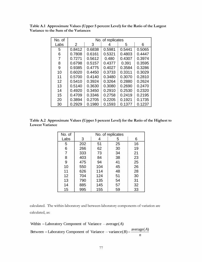
77

Table A.1 Approximate Values (Upper 5 percent Level) for the Ratio of the Largest Variance to the Sum of the Variances

No. of No. of replicates Labs 2 3 4 5 6

5 0.8412 0.6838 0.5981 0.5441 0.5065 6 0.7808 0.6161 0.5321 0.4803 0.4447 7 0.7271 0.5612 0.480 0.4307 0.3974 8 0.6798 0.5157 0.4377 0.391 0.3595 9 0.9385 0.4775 0.4027 0.3584 0.3286 10 0.6020 0.4450 0.3733 0.3311 0.3029 11 0.5700 0.4140 0.3480 0.3070 0.2810 12 0.5410 0.3924 0.3264 0.2880 0.2624 13 0.5140 0.3630 0.3080 0.2690 0.2470 14 0.4920 0.3450 0.2910 0.2530 0.2320 15 0.4709 0.3346 0.2758 0.2419 0.2195 20 0.3894 0.2705 0.2205 0.1921 0.1735 30 0.2929 0.1980 0.1593 0.1377 0.1237

Table A.2 Approximate Values (Upper 5 percent Level) for the Ratio of the Highest to Lowest Variance

No. of No. of replicates Labs 3 4 5 6

5 202 51 25 16 6 266 62 30 19 7 333 73 34 21 8 403 84 38 23 9 475 94 41 25 10 550 104 45 26 11 626 114 48 28 12 704 124 51 30 13 790 135 54 31 14 885 145 57 32 15 995 155 59 33

calculated. The within-laboratory and between-laboratory components of variation are

calculated, as:

)(averageVarianceofComponentLaboratoryWithin A

n

AB

)(average)(varianceVarianceofComponentLaboratoryBetween

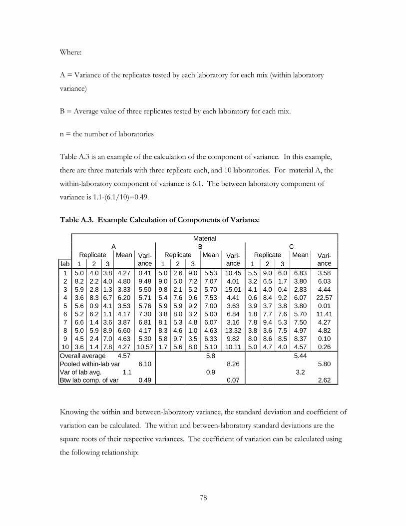
78

Where:

A = Variance of the replicates tested by each laboratory for each mix (within laboratory

variance)

B = Average value of three replicates tested by each laboratory for each mix.

n = the number of laboratories

Table A.3 is an example of the calculation of the component of variance. In this example,

there are three materials with three replicate each, and 10 laboratories. For material A, the

within-laboratory component of variance is 6.1. The between laboratory component of

variance is 1.1-(6.1/10)=0.49.

Table A.3. Example Calculation of Components of Variance

Material

A B C

Replicate Mean Vari- ance

Replicate Mean Vari- ance

Replicate Mean Vari- ance lab 1 2 3 1 2 3 1 2 3

1 5.0 4.0 3.8 4.27 0.41 5.0 2.6 9.0 5.53 10.45 5.5 9.0 6.0 6.83 3.58

2 8.2 2.2 4.0 4.80 9.48 9.0 5.0 7.2 7.07 4.01 3.2 6.5 1.7 3.80 6.03

3 5.9 2.8 1.3 3.33 5.50 9.8 2.1 5.2 5.70 15.01 4.1 4.0 0.4 2.83 4.44

4 3.6 8.3 6.7 6.20 5.71 5.4 7.6 9.6 7.53 4.41 0.6 8.4 9.2 6.07 22.57

5 5.6 0.9 4.1 3.53 5.76 5.9 5.9 9.2 7.00 3.63 3.9 3.7 3.8 3.80 0.01

6 5.2 6.2 1.1 4.17 7.30 3.8 8.0 3.2 5.00 6.84 1.8 7.7 7.6 5.70 11.41

7 6.6 1.4 3.6 3.87 6.81 8.1 5.3 4.8 6.07 3.16 7.8 9.4 5.3 7.50 4.27

8 5.0 5.9 8.9 6.60 4.17 8.3 4.6 1.0 4.63 13.32 3.8 3.6 7.5 4.97 4.82

9 4.5 2.4 7.0 4.63 5.30 5.8 9.7 3.5 6.33 9.82 8.0 8.6 8.5 8.37 0.10

10 3.6 1.4 7.8 4.27 10.57 1.7 5.6 8.0 5.10 10.11 5.0 4.7 4.0 4.57 0.26

Overall average 4.57 5.8 5.44

Pooled within-lab var 6.10 8.26 5.80

Var of lab avg. 1.1 0.9 3.2

Btw lab comp. of var 0.49 0.07 2.62

Knowing the within and between-laboratory variance, the standard deviation and coefficient of

variation can be calculated. The within and between-laboratory standard deviations are the

square roots of their respective variances. The coefficient of variation can be calculated using

the following relationship:

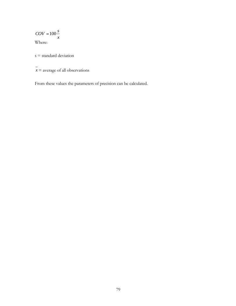
79

Where:

s = standard deviation

x = average of all observations

From these values the parameters of precision can be calculated.

x

sCOV 100

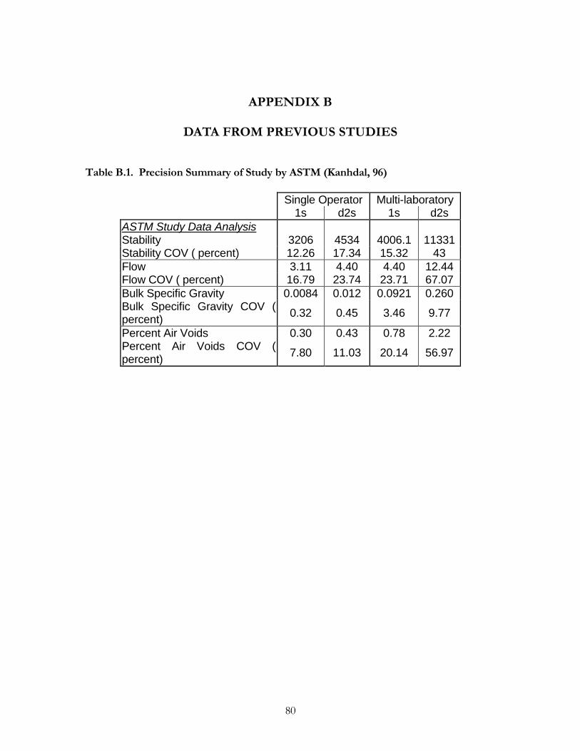
80

APPENDIX B

DATA FROM PREVIOUS STUDIES

Table B.1. Precision Summary of Study by ASTM (Kanhdal, 96)

Single Operator Multi-laboratory

1s d2s 1s d2s

ASTM Study Data Analysis Stability 3206 4534 4006.1 11331 Stability COV ( percent) 12.26 17.34 15.32 43

Flow 3.11 4.40 4.40 12.44 Flow COV ( percent) 16.79 23.74 23.71 67.07

Bulk Specific Gravity 0.0084 0.012 0.0921 0.260 Bulk Specific Gravity COV ( percent)

0.32 0.45 3.46 9.77

Percent Air Voids 0.30 0.43 0.78 2.22 Percent Air Voids COV ( percent)

7.80 11.03 20.14 56.97

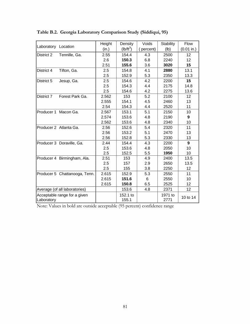
81

Table B.2. Georgia Laboratory Comparison Study (Siddiqui, 95)

Laboratory Location Height Density Voids Stability Flow

(in.) (lb/ft3) ( percent) (lb) (0.01 in.)

District 2 Tennille, Ga. 2.55 154.4 4.3 2500 12

2.6 150.3 6.8 2240 12

2.51 155.6 3.6 3020 15

District 4 Tifton, Ga. 2.5 154.8 4.1 2880 13.1

2.5 152.9 5.3 2350 13.3

District 5 Jesup, Ga. 2.5 154.6 4.2 2200 15

2.5 154.3 4.4 2175 14.8

2.5 154.6 4.2 2275 13.6

District 7 Forest Park Ga. 2.562 153 5.2 2100 12

2.555 154.1 4.5 2460 13

2.54 154.3 4.4 2520 11

Producer 1 Macon Ga. 2.567 153.1 5.1 2150 10

2.574 153.6 4.8 2190 9

2.562 153.6 4.8 2340 10

Producer 2 Atlanta Ga. 2.56 152.6 5.4 2320 11

2.56 153.2 5.1 2470 13

2.56 152.8 5.3 2330 13

Producer 3 Doraville, Ga. 2.44 154.4 4.3 2200 9

2.5 153.6 4.8 2050 10

2.5 152.5 5.5 1950 10

Producer 4 Birmingham, Ala. 2.51 153 4.9 2400 13.5

2.5 157 2.9 2650 13.5

2.5 155 3.8 2250 12

Producer 5 Chattanooga, Tenn. 2.615 152.9 5.3 2550 11

2.615 151.6 6 2550 10

2.615 150.8 6.5 2525 12

Average (of all laboratories) 153.6 4.8 2371 12

Acceptable range for a given Laboratory

152.1 to 155.1

1971 to 2771

10 to 14

Note: Values in bold are outside acceptable (95 percent) confidence range

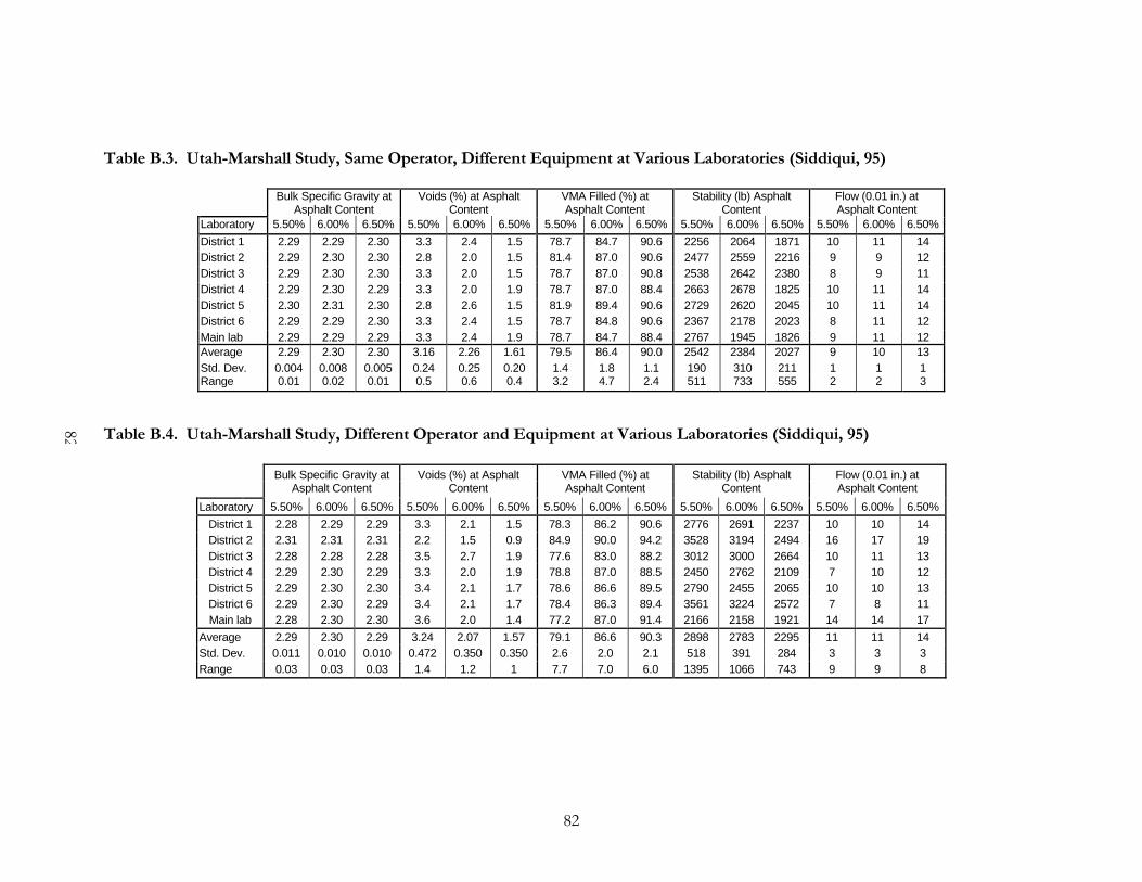
82

82

Table B.3. Utah-Marshall Study, Same Operator, Different Equipment at Various Laboratories (Siddiqui, 95)

Bulk Specific Gravity at Asphalt Content

Voids (%) at Asphalt Content

VMA Filled (%) at Asphalt Content

Stability (lb) Asphalt Content

Flow (0.01 in.) at Asphalt Content

Laboratory 5.50% 6.00% 6.50% 5.50% 6.00% 6.50% 5.50% 6.00% 6.50% 5.50% 6.00% 6.50% 5.50% 6.00% 6.50%

District 1 2.29 2.29 2.30 3.3 2.4 1.5 78.7 84.7 90.6 2256 2064 1871 10 11 14

District 2 2.29 2.30 2.30 2.8 2.0 1.5 81.4 87.0 90.6 2477 2559 2216 9 9 12

District 3 2.29 2.30 2.30 3.3 2.0 1.5 78.7 87.0 90.8 2538 2642 2380 8 9 11

District 4 2.29 2.30 2.29 3.3 2.0 1.9 78.7 87.0 88.4 2663 2678 1825 10 11 14

District 5 2.30 2.31 2.30 2.8 2.6 1.5 81.9 89.4 90.6 2729 2620 2045 10 11 14

District 6 2.29 2.29 2.30 3.3 2.4 1.5 78.7 84.8 90.6 2367 2178 2023 8 11 12

Main lab 2.29 2.29 2.29 3.3 2.4 1.9 78.7 84.7 88.4 2767 1945 1826 9 11 12

Average 2.29 2.30 2.30 3.16 2.26 1.61 79.5 86.4 90.0 2542 2384 2027 9 10 13

Std. Dev. 0.004 0.008 0.005 0.24 0.25 0.20 1.4 1.8 1.1 190 310 211 1 1 1 Range 0.01 0.02 0.01 0.5 0.6 0.4 3.2 4.7 2.4 511 733 555 2 2 3

Table B.4. Utah-Marshall Study, Different Operator and Equipment at Various Laboratories (Siddiqui, 95)

Bulk Specific Gravity at Asphalt Content

Voids (%) at Asphalt Content

VMA Filled (%) at Asphalt Content

Stability (lb) Asphalt Content

Flow (0.01 in.) at Asphalt Content

Laboratory 5.50% 6.00% 6.50% 5.50% 6.00% 6.50% 5.50% 6.00% 6.50% 5.50% 6.00% 6.50% 5.50% 6.00% 6.50%

District 1 2.28 2.29 2.29 3.3 2.1 1.5 78.3 86.2 90.6 2776 2691 2237 10 10 14

District 2 2.31 2.31 2.31 2.2 1.5 0.9 84.9 90.0 94.2 3528 3194 2494 16 17 19

District 3 2.28 2.28 2.28 3.5 2.7 1.9 77.6 83.0 88.2 3012 3000 2664 10 11 13

District 4 2.29 2.30 2.29 3.3 2.0 1.9 78.8 87.0 88.5 2450 2762 2109 7 10 12

District 5 2.29 2.30 2.30 3.4 2.1 1.7 78.6 86.6 89.5 2790 2455 2065 10 10 13

District 6 2.29 2.30 2.29 3.4 2.1 1.7 78.4 86.3 89.4 3561 3224 2572 7 8 11

Main lab 2.28 2.30 2.30 3.6 2.0 1.4 77.2 87.0 91.4 2166 2158 1921 14 14 17

Average 2.29 2.30 2.29 3.24 2.07 1.57 79.1 86.6 90.3 2898 2783 2295 11 11 14

Std. Dev. 0.011 0.010 0.010 0.472 0.350 0.350 2.6 2.0 2.1 518 391 284 3 3 3

Range 0.03 0.03 0.03 1.4 1.2 1 7.7 7.0 6.0 1395 1066 743 9 9 8

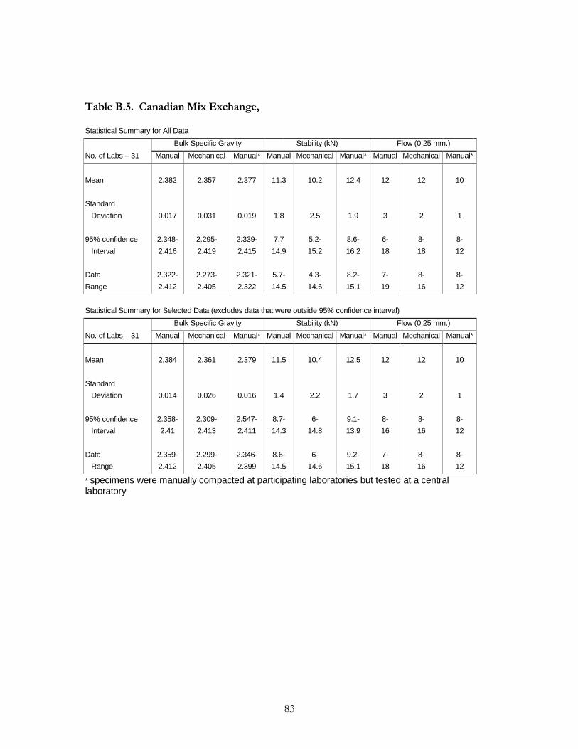
83

Table B.5. Canadian Mix Exchange,

Statistical Summary for All Data

Bulk Specific Gravity Stability (kN) Flow (0.25 mm.)

No. of Labs – 31 Manual Mechanical Manual* Manual Mechanical Manual* Manual Mechanical Manual*

Mean 2.382 2.357 2.377 11.3 10.2 12.4 12 12 10

Standard

Deviation 0.017 0.031 0.019 1.8 2.5 1.9 3 2 1

95% confidence 2.348- 2.295- 2.339- 7.7 5.2- 8.6- 6- 8- 8-

Interval 2.416 2.419 2.415 14.9 15.2 16.2 18 18 12

Data 2.322- 2.273- 2.321- 5.7- 4.3- 8.2- 7- 8- 8-

Range 2.412 2.405 2.322 14.5 14.6 15.1 19 16 12

Statistical Summary for Selected Data (excludes data that were outside 95% confidence interval)

Bulk Specific Gravity Stability (kN) Flow (0.25 mm.)

No. of Labs – 31 Manual Mechanical Manual* Manual Mechanical Manual* Manual Mechanical Manual*

Mean 2.384 2.361 2.379 11.5 10.4 12.5 12 12 10

Standard

Deviation 0.014 0.026 0.016 1.4 2.2 1.7 3 2 1

95% confidence 2.358- 2.309- 2.547- 8.7- 6- 9.1- 8- 8- 8-

Interval 2.41 2.413 2.411 14.3 14.8 13.9 16 16 12

Data 2.359- 2.299- 2.346- 8.6- 6- 9.2- 7- 8- 8-

Range 2.412 2.405 2.399 14.5 14.6 15.1 18 16 12

* specimens were manually compacted at participating laboratories but tested at a central laboratory

84

APPENDIX C

BUCKET MIXER INSTRUCTIONS

SETTING UP THE MIXER. Install paddle arm so arm sits parallel to the plane to which the bucket can rotate Secure paddle to paddle are so both back edges sit flush to the side of the bucket and blade touches bottom of bucket MIXING PROCEDURE Weigh out aggregates and separate into two containers: course and fine

Nominal maximum aggregate size 9.5 mm

Fine aggregate 2.36 mm

Coarse aggregate 2.36 mm

Nominal maximum aggregate size 9.5 mm

Fine aggregate 4.75 mm

Coarse aggregate 4.75 mm Heat 5-gallon bucket and paddle attached to paddle arm. Allow enough time for bucket and paddle to achieve proper temperature Remove bucket from oven and add coarse aggregate and asphalt to bucket Place bucket in mixer basket and turn mixer on Remove paddle and arm from oven and slide over rod With aggregates moving the paddle should slide down until touching the bucket bottom. Unlock mixer and tilt mixer away from paddle arm side. Hold on to paddle arm and tilt bucket as far as possible without spilling contents After 10 seconds lock bucket in upright position. Remove fine aggregate from oven and introduce into the mix. Pour fine aggregates into bucket with allowing aggregate to touch paddle or side of bucket Unlock bucket and tilt Rock bucket up-and-down to reduce segregation After about 20 seconds when the aggregate looks thoroughly coated take a hot spatula, and as the bucket is spinning, scrape all of the material out of the seam between the bottom and side of the bucket. Shut off mixer. Slide paddle off of the rod and with a hot spoon scrape the asphalt off the paddle into the bucket. Remove bucket from mixer and tilt bucket onto its side and scrape circle of asphalt and fines stuck to the center of the bucket bottom. Scrape material out of seem again. Dump bucket contents Scrape entire side and bottom of bucket.

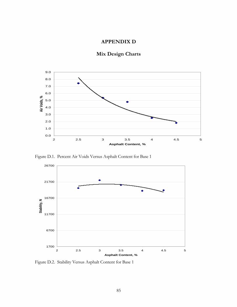
85

APPENDIX D

Mix Design Charts

0.0

1.0

2.0

3.0

4.0

5.0

6.0

7.0

8.0

9.0

2 2.5 3 3.5 4 4.5 5

Asphalt Content, %

Air

Void

s, %

Figure D.1. Percent Air Voids Versus Asphalt Content for Base 1

1700

6700

11700

16700

21700

26700

2 2.5 3 3.5 4 4.5 5

Asphalt Content, %

Sta

bilit

y, N

Figure D.2. Stability Versus Asphalt Content for Base 1

86

0.0

2.0

4.0

6.0

8.0

10.0

12.0

14.0

16.0

18.0

2 2.5 3 3.5 4 4.5 5

Asphalt Content, %

Flo

w, .

25cm

Figure D.3. Flow Versus Asphalt Content for Base 1

Figure D.4. Unit Weight Versus Asphalt Content for Base 1

2.400

2.410

2.420

2.430

2.440

2.450

2.460

2.470

2.480

2 2.5 3 3.5 4 4.5 5

Asphalt Content, %

Un

it W

eig

ht,

kg

/m^

3

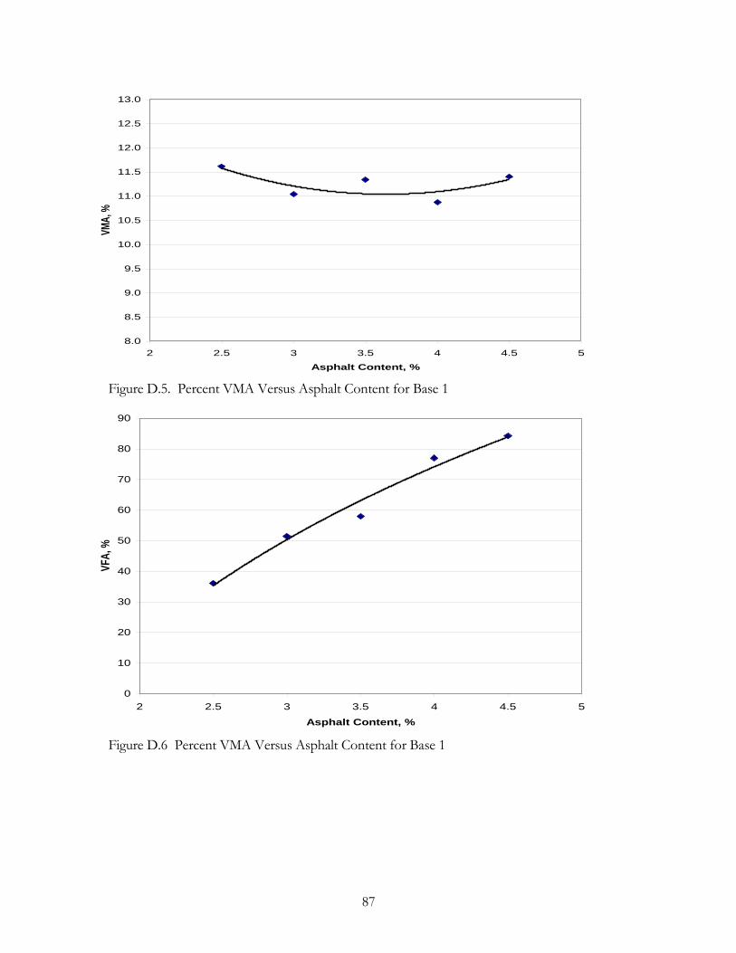
87

8.0

8.5

9.0

9.5

10.0

10.5

11.0

11.5

12.0

12.5

13.0

2 2.5 3 3.5 4 4.5 5

Asphalt Content, %

VMA

, %

Figure D.5. Percent VMA Versus Asphalt Content for Base 1

0

10

20

30

40

50

60

70

80

90

2 2.5 3 3.5 4 4.5 5

Asphalt Content, %

VFA

, %

Figure D.6 Percent VMA Versus Asphalt Content for Base 1

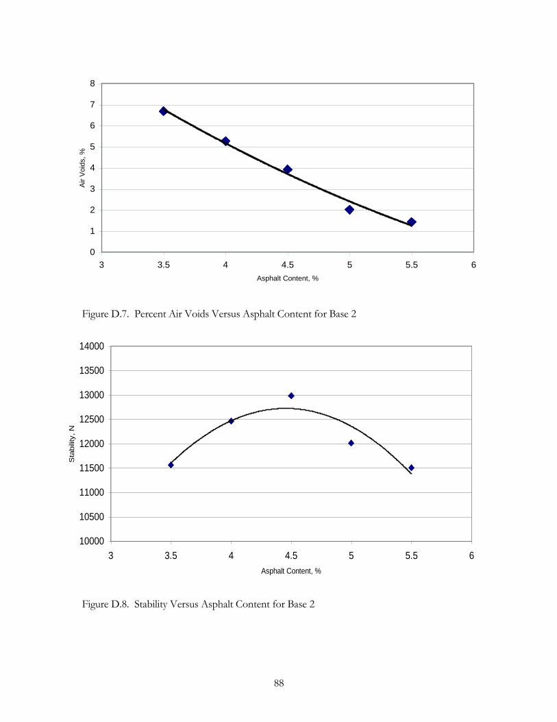
88

0

1

2

3

4

5

6

7

8

3 3.5 4 4.5 5 5.5 6

Asphalt Content, %

Air V

oid

s,

%

Figure D.7. Percent Air Voids Versus Asphalt Content for Base 2

Figure D.8. Stability Versus Asphalt Content for Base 2

10000

10500

11000

11500

12000

12500

13000

13500

14000

3 3.5 4 4.5 5 5.5 6

Asphalt Content, %

Sta

bili

ty, N

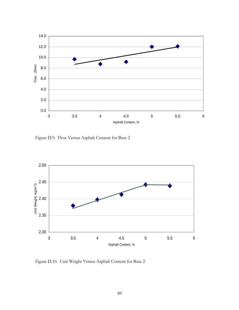
89

0.0

2.0

4.0

6.0

8.0

10.0

12.0

14.0

3 3.5 4 4.5 5 5.5 6

Asphalt Content, %

Flo

w,

.25m

m

Figure D.9. Flow Versus Asphalt Content for Base 2

2.30

2.35

2.40

2.45

2.50

3 3.5 4 4.5 5 5.5 6

Asphalt Content, %

Unit W

eig

ht,

kg/m

^3

Figure D.10. Unit Weight Versus Asphalt Content for Base 2

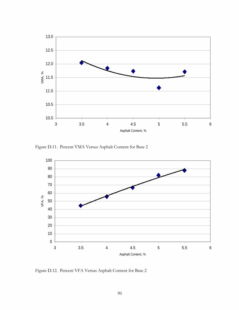
90

10.0

10.5

11.0

11.5

12.0

12.5

13.0

3 3.5 4 4.5 5 5.5 6

Asphalt Content, %

VM

A,

%

Figure D.11. Percent VMA Versus Asphalt Content for Base 2

0

10

20

30

40

50

60

70

80

90

100

3 3.5 4 4.5 5 5.5 6

Asphalt Content, %

VF

A,

%

Figure D.12. Percent VFA Versus Asphalt Content for Base 2

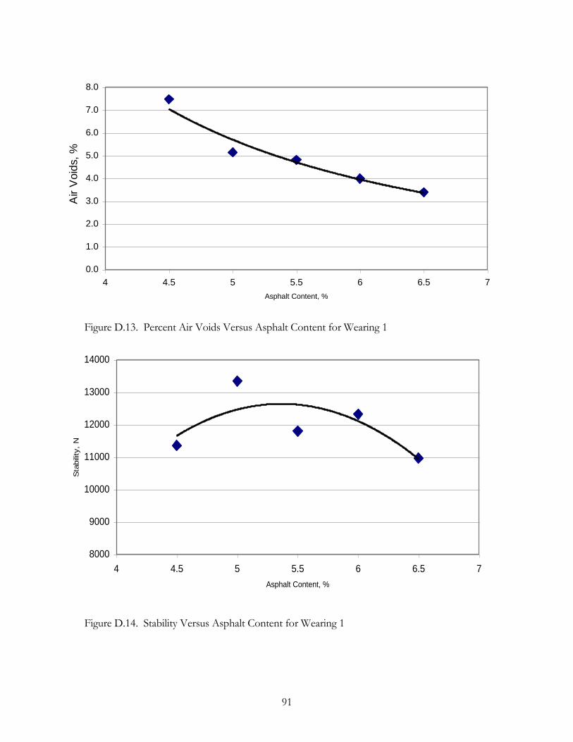
91

Figure D.13. Percent Air Voids Versus Asphalt Content for Wearing 1

8000

9000

10000

11000

12000

13000

14000

4 4.5 5 5.5 6 6.5 7

Asphalt Content, %

Sta

bili

ty,

N

Figure D.14. Stability Versus Asphalt Content for Wearing 1

0.0

1.0

2.0

3.0

4.0

5.0

6.0

7.0

8.0

4 4.5 5 5.5 6 6.5 7

Asphalt Content, %

Air V

oid

s, %

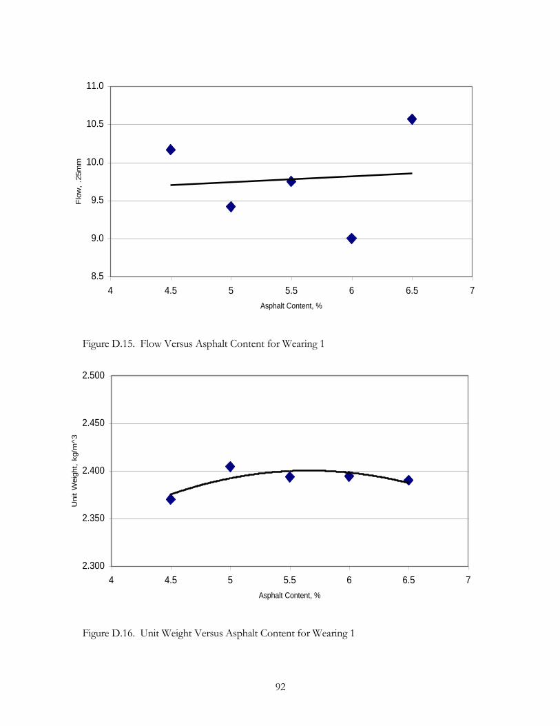
92

8.5

9.0

9.5

10.0

10.5

11.0

4 4.5 5 5.5 6 6.5 7

Asphalt Content, %

Flo

w,

.25m

m

Figure D.15. Flow Versus Asphalt Content for Wearing 1

2.300

2.350

2.400

2.450

2.500

4 4.5 5 5.5 6 6.5 7

Asphalt Content, %

Unit W

eig

ht,

kg/m

^3

Figure D.16. Unit Weight Versus Asphalt Content for Wearing 1

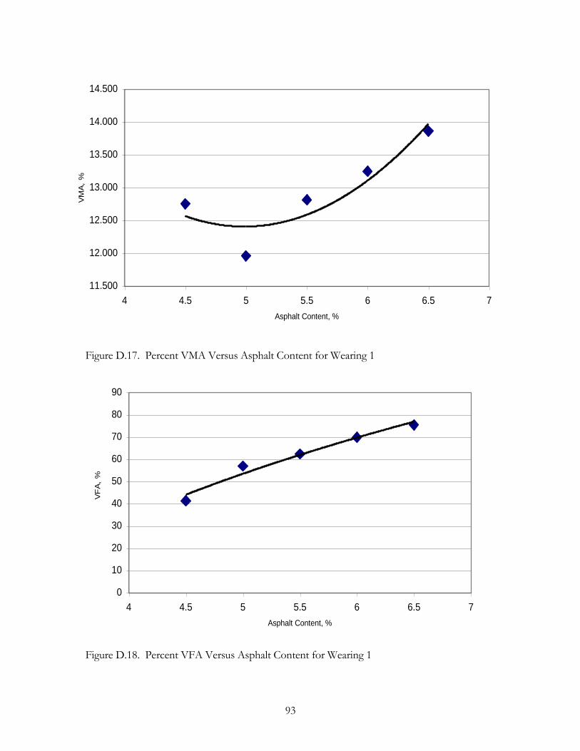
93

11.500

12.000

12.500

13.000

13.500

14.000

14.500

4 4.5 5 5.5 6 6.5 7

Asphalt Content, %

VM

A,

%

Figure D.17. Percent VMA Versus Asphalt Content for Wearing 1

0

10

20

30

40

50

60

70

80

90

4 4.5 5 5.5 6 6.5 7

Asphalt Content, %

VF

A,

%

Figure D.18. Percent VFA Versus Asphalt Content for Wearing 1

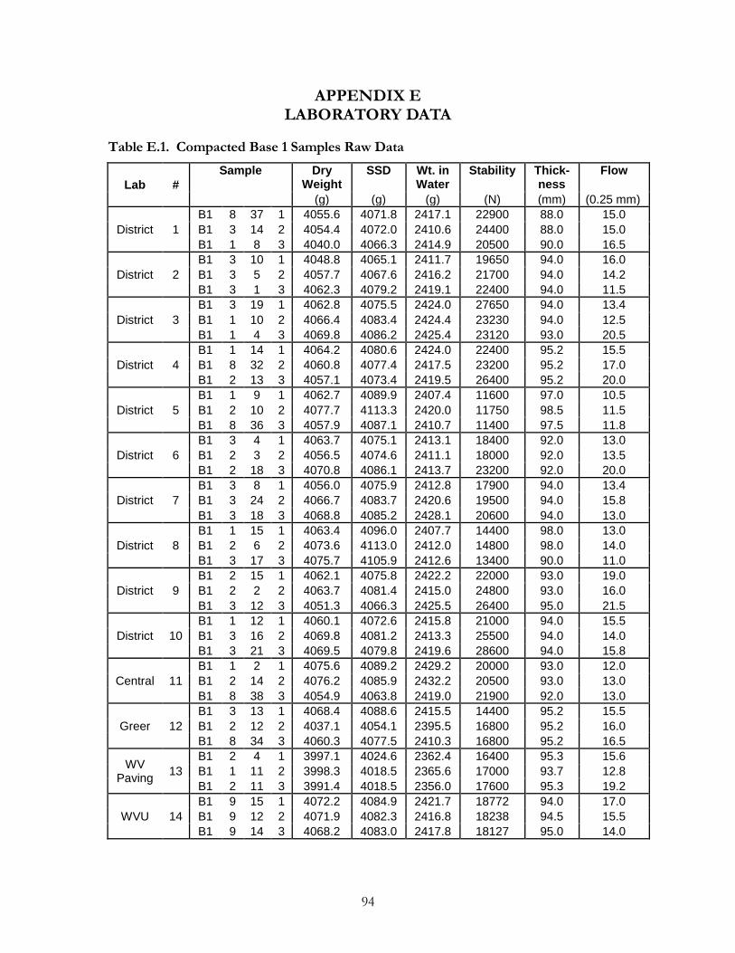
94

APPENDIX E LABORATORY DATA

Table E.1. Compacted Base 1 Samples Raw Data

Lab #

Sample Dry Weight

SSD Wt. in Water

Stability Thick-ness

Flow

(g) (g) (g) (N) (mm) (0.25 mm)

District 1

B1 8 37 1 4055.6 4071.8 2417.1 22900 88.0 15.0

B1 3 14 2 4054.4 4072.0 2410.6 24400 88.0 15.0

B1 1 8 3 4040.0 4066.3 2414.9 20500 90.0 16.5

District 2

B1 3 10 1 4048.8 4065.1 2411.7 19650 94.0 16.0

B1 3 5 2 4057.7 4067.6 2416.2 21700 94.0 14.2

B1 3 1 3 4062.3 4079.2 2419.1 22400 94.0 11.5

District 3

B1 3 19 1 4062.8 4075.5 2424.0 27650 94.0 13.4

B1 1 10 2 4066.4 4083.4 2424.4 23230 94.0 12.5

B1 1 4 3 4069.8 4086.2 2425.4 23120 93.0 20.5

District 4

B1 1 14 1 4064.2 4080.6 2424.0 22400 95.2 15.5

B1 8 32 2 4060.8 4077.4 2417.5 23200 95.2 17.0

B1 2 13 3 4057.1 4073.4 2419.5 26400 95.2 20.0

District 5

B1 1 9 1 4062.7 4089.9 2407.4 11600 97.0 10.5

B1 2 10 2 4077.7 4113.3 2420.0 11750 98.5 11.5

B1 8 36 3 4057.9 4087.1 2410.7 11400 97.5 11.8

District 6

B1 3 4 1 4063.7 4075.1 2413.1 18400 92.0 13.0

B1 2 3 2 4056.5 4074.6 2411.1 18000 92.0 13.5

B1 2 18 3 4070.8 4086.1 2413.7 23200 92.0 20.0

District 7

B1 3 8 1 4056.0 4075.9 2412.8 17900 94.0 13.4

B1 3 24 2 4066.7 4083.7 2420.6 19500 94.0 15.8

B1 3 18 3 4068.8 4085.2 2428.1 20600 94.0 13.0

District 8

B1 1 15 1 4063.4 4096.0 2407.7 14400 98.0 13.0

B1 2 6 2 4073.6 4113.0 2412.0 14800 98.0 14.0

B1 3 17 3 4075.7 4105.9 2412.6 13400 90.0 11.0

District 9

B1 2 15 1 4062.1 4075.8 2422.2 22000 93.0 19.0

B1 2 2 2 4063.7 4081.4 2415.0 24800 93.0 16.0

B1 3 12 3 4051.3 4066.3 2425.5 26400 95.0 21.5

District 10

B1 1 12 1 4060.1 4072.6 2415.8 21000 94.0 15.5

B1 3 16 2 4069.8 4081.2 2413.3 25500 94.0 14.0

B1 3 21 3 4069.5 4079.8 2419.6 28600 94.0 15.8

Central 11

B1 1 2 1 4075.6 4089.2 2429.2 20000 93.0 12.0

B1 2 14 2 4076.2 4085.9 2432.2 20500 93.0 13.0

B1 8 38 3 4054.9 4063.8 2419.0 21900 92.0 13.0

Greer 12

B1 3 13 1 4068.4 4088.6 2415.5 14400 95.2 15.5

B1 2 12 2 4037.1 4054.1 2395.5 16800 95.2 16.0

B1 8 34 3 4060.3 4077.5 2410.3 16800 95.2 16.5

WV Paving

13

B1 2 4 1 3997.1 4024.6 2362.4 16400 95.3 15.6

B1 1 11 2 3998.3 4018.5 2365.6 17000 93.7 12.8

B1 2 11 3 3991.4 4018.5 2356.0 17600 95.3 19.2

WVU 14

B1 9 15 1 4072.2 4084.9 2421.7 18772 94.0 17.0

B1 9 12 2 4071.9 4082.3 2416.8 18238 94.5 15.5

B1 9 14 3 4068.2 4083.0 2417.8 18127 95.0 14.0

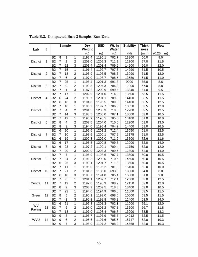
95

Table E.2. Compacted Base 2 Samples Raw Data

Lab #

Sample Dry Weight

SSD Wt. in Water

Stability Thick-ness

Flow

(g) (g) (g) (N) (mm) (0.25 mm)

District 1

B2 8 1 1 1192.4 1195.1 702.7 13200 56.0 9.0

B2 7 2 2 1203.0 1205.3 711.2 12800 57.0 11.5

B2 7 22 3 1201.4 1203.4 709.9 14200 56.0 12.0

District 2

B2 7 15 1 1191.4 1192.7 707.3 14990 61.5 10.5

B2 7 18 2 1193.9 1196.5 708.5 13990 61.5 12.0

B2 7 6 3 1197.0 1198.7 708.5 13580 61.5 11.0

District 3

B2 7 25 1 1195.4 1201.3 691.3 9000 65.0 8.6

B2 7 9 2 1199.8 1204.3 706.0 12000 67.0 8.8

B2 7 1 3 1187.2 1209.9 699.5 13340 61.0 9.5

District 4

B2 7 17 1 1202.9 1204.0 714.8 13600 63.5 11.5

B2 6 24 2 1199.7 1201.1 709.6 14400 63.5 11.5

B2 6 16 3 1194.8 1196.5 709.0 14400 63.5 12.5

District 5

B2 7 16 1 1195.2 1197.7 706.3 10050 62.5 12.0

B2 7 4 2 1201.5 1203.3 710.0 12200 62.5 12.5

B2 7 14 3 1198.5 1200.0 707.1 13000 62.0 10.5

District 6

B2 7 12 1 1195.9 1198.5 705.6 13100 61.0 10.0

B2 8 4 2 1202.5 1204.0 710.6 12200 61.0 13.0

B2 8 3 3 1194.0 1195.4 704.2 14400 61.0 16.5

District 7

B2 6 20 1 1199.6 1201.2 712.4 13650 61.0 12.5

B2 7 10 2 1198.6 1200.1 707.9 13175 61.0 12.5

B2 6 19 3 1200.3 1202.0 711.2 13500 72.6 11.6

District 8

B2 6 17 1 1198.5 1200.8 709.3 12000 62.0 14.0

B2 6 23 2 1197.2 1199.1 709.4 11750 62.0 12.0

B2 7 20 3 1202.0 1203.3 709.6 12800 62.0 14.0

District 9

B2 7 7 1 1196.9 1198.6 707.7 13600 60.0 10.5

B2 7 24 2 1198.2 1200.0 710.5 14600 60.0 10.5

B2 6 25 3 1199.1 1201.7 711.3 13600 60.0 10.5

District 10

B2 7 11 1 1195.0 1196.2 701.3 15400 62.0 10.0

B2 7 21 2 1181.3 1185.0 693.8 18900 64.0 8.8

B2 6 18 3 1193.7 1194.8 705.4 16800 61.0 9.0

Central 11

B2 7 8 1 1201.1 1202.7 712.4 12500 62.0 12.5

B2 7 19 2 1197.0 1198.9 708.9 12150 62.0 12.0

B2 8 2 3 1208.9 1209.5 718.8 13400 62.0 10.5

Greer 12

B2 7 23 1 1194.0 1194.9 706.0 11000 63.5 11.5

B2 8 5 2 1190.1 1193.0 698.6 10000 63.5 11.5

B2 7 3 3 1196.3 1198.8 706.2 11400 63.5 14.0

WV Paving

13

B2 6 21 1 1199.8 1201.3 702.1 11000 65.1 12.0

B2 7 5 2 1199.0 1201.2 707.3 13500 66.7 11.8

B2 7 13 3 1197.0 1198.4 706.7 13000 63.5 13.2

WVU 14

B2 9 8 1 1195.7 1197.9 705.6 14012 62.5 11.5

B2 9 6 2 1195.6 1197.6 705.5 15747 62.0 10.3

B2 9 7 3 1195.0 1197.2 708.0 14568 62.0 10.3

96

Table E.3. Compacted Wearing 1 Samples Raw Data

Lab #

Sample Dry Weight

SSD Wt. in Water

Stability Thick-ness

Flow

(g) (g) (g) (N) (mm) (0.25 mm)

District 1

W1 6 6 1 1191.6 1193.3 694.8 13000 57.0 10.5

W1 4 31 2 1202.1 1203.4 700.4 12900 58.0 8.5

W1 5 1 3 1203.5 1204.8 723.4 13000 57.0 9.0

District 2

W1 4 10 1 1202.5 1203.1 704.1 13200 62.0 9.4

W1 5 9 2 1203.9 1204.8 706.6 13400 62.0 10.4

W1 6 2 3 1210.0 1210.9 706.0 12620 62.0 9.0

District 3

W1 6 7 1 1211.6 1211.7 701.7 12380 64.0 12.4

W1 4 7 2 1207.6 1224.2 685.6 6020 64.0 14.8

W1 6 13 3 1209.2 1233.3 687.7 4770 68.0 12.6

District 4

W1 5 3 1 1208.7 1209.5 707.7 15200 63.5 10.0

W1 3 28 2 1206.1 1206.7 705.7 14000 63.5 11.0

W1 5 2 3 1207.5 1208.4 706.1 13800 63.5 11.5

District 5

W1 6 10 1 1197.0 1198.0 692.1 11600 63.5 10.5

W1 4 15 2 1208.9 1209.8 700.1 11750 64.0 11.5

W1 5 7 3 1210.4 1211.3 703.7 11400 64.0 11.8

District 6

W1 4 6 1 1210.3 1211.4 702.7 12700 63.0 9.5

W1 4 4 2 1206.8 1208.0 699.5 12400 63.0 11.5

W1 4 12 3 1205.2 1206.1 699.7 12900 62.0 13.0

District 7

W1 4 5 1 1210.7 1211.7 707.2 12400 63.0 18.5

W1 4 19 2 1208.0 1209.0 704.4 12300 63.0 10.5

W1 4 25 3 1206.4 1207.2 705.5 12050 63.0 10.0

District 8

W1 3 27 1 1208.9 1210.5 704.4 11050 63.5 9.5

W1 4 32 2 1209.6 1210.9 702.6 11050 63.5 9.5

W1 6 8 3 1212.7 1214.0 706.4 11600 63.5 11.0

District 9

W1 4 28 1 1207.3 1208.1 699.9 13000 60.2 9.5

W1 6 5 2 1208.3 1209.2 703.7 12600 60.2 9.5

W1 4 33 3 1209.8 1210.5 704.4 14000 60.2 10.5

District 10

W1 6 15 1 1202.1 1203.3 694.4 15600 64.0 8.8

W1 4 14 2 1202.6 1203.9 695.6 15400 64.0 10.0

W1 4 23 3 1210.4 1211.6 698.4 17200 64.0 10.0

Central 11

W1 4 2 1 1212.5 1213.3 707.3 12800 63.0 10.5

W1 4 17 2 1208.1 1208.7 705.9 12100 63.0 10.0

W1 5 12 3 1209.4 1209.9 707.9 12600 63.0 10.5

Greer 12

W1 4 8 1 1201.9 1202.4 698.3 12200 63.5 10.0

W1 4 13 2 1204.3 1205.1 701.3 11800 63.5 9.5

W1 4 30 3 1205.7 1206.7 704.4 11600 63.5 8.5

WV Paving

13

W1 5 13 1 1206.9 1208.8 695.1 10400 66.7 13.9

W1 4 21 2 1208.5 1209.7 699.2 10750 65.1 12.8

W1 5 4 3 1205.2 1207.0 693.3 11200 66.7 13.4

WVU 14

W1 9 3 1 1200.0 1200.4 702.5 14457 62.0 10.0

W1 9 2 2 1203.8 1204.9 702.1 13678 63.5 9.5

W1 9 5 3 1208.3 1209.0 706.5 13789 63.0 9.5

97

Table E.4. Base 1 Maximum Theoretical Specific Gravity Samples Raw Data

Lab # Sample Dry Weight

Asphalt+ Pycnometer+

Water

Pycnometer + Water

(g) (g) (g)

District 1 B1R 2 20 1 4090.4 3926.7 1433.8

B1R 3 25 2 4067.2 3909.1 1433.8

District 2 B1R 1 1 2 4064.1 3839.7 1359.8

B1R 2 5 1 4068.5 3842.5 1359.8

District 3

B1R 1 6 1 2013.3 2654.9 1429.3

2067.7 2690.4 1429.3

B1R 3 11 2 2209.7 2773.1 1429.3

1870.7 2574.1 1429.3

District 4 B1R 3 6 2 4014.4 3842.6 1396.6

B1R 8 33 1 4006.6 3838.2 1396.6

District 5

B1R 1 7 1 2251.6 2760.1 1386.1

1821.2 2497.7 1386.1

B1R 8 35 2 2347.5 2821.4 1386.1

1734.2 2494.6 1386.1

District 6 B1R 2 8 1 4064.1 3864.2 1387.2

B1R 2 19 2 4070.9 3870.3 1387.2

District 7 B1R 2 7 2 4063.3 3865.2 1388.6

B1R 3 7 1 4004.7 3821.6 1388.6

District 8 B1R 2 9 1 4089.5 5229.5 2735.0

B1R 3 22 2 4094.1 5230.4 2735.0

District 9 B1R 2 17 2 4061 5289.7 2812.4

B1R 3 15 1 4075.1 5298.6 2812.4

District 10 B1R 3 2 1 4066.4 3880.6 1402.6

B1R 3 3 2 4074.8 3885.3 1402.6

Central 11 B1R 1 3 1 4083.6 3809.7 1321.5

B1R 2 1 2 4074.4 3805.9 1321.5

Greer 12 B1R 1 5 1 4058.7 3828.4 1355.7

B1R 3 9 2 4081.8 3843.9 1355.7

WV Paving

13 B1R 1 13 2 4039.7 5454.4 2988.8

B1R 3 23 1 4061.6 5466.9 2988.8

WVU 14 B1R 9 11 1 4061.1 9956.2 7480.2

B1R 9 13 2 4087.1 9970.8 7480.2

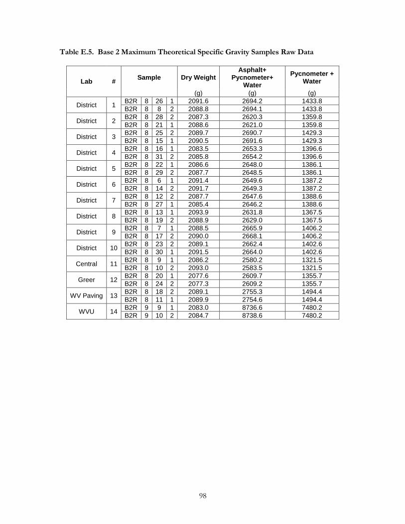
98

Table E.5. Base 2 Maximum Theoretical Specific Gravity Samples Raw Data

Lab # Sample Dry Weight

Asphalt+ Pycnometer+

Water

Pycnometer + Water

(g) (g) (g)

District 1 B2R 8 26 1 2091.6 2694.2 1433.8

B2R 8 8 2 2088.8 2694.1 1433.8

District 2 B2R 8 28 2 2087.3 2620.3 1359.8

B2R 8 21 1 2088.6 2621.0 1359.8

District 3 B2R 8 25 2 2089.7 2690.7 1429.3

B2R 8 15 1 2090.5 2691.6 1429.3

District 4 B2R 8 16 1 2083.5 2653.3 1396.6

B2R 8 31 2 2085.8 2654.2 1396.6

District 5 B2R 8 22 1 2086.6 2648.0 1386.1

B2R 8 29 2 2087.7 2648.5 1386.1

District 6 B2R 8 6 1 2091.4 2649.6 1387.2

B2R 8 14 2 2091.7 2649.3 1387.2

District 7 B2R 8 12 2 2087.7 2647.6 1388.6

B2R 8 27 1 2085.4 2646.2 1388.6

District 8 B2R 8 13 1 2093.9 2631.8 1367.5

B2R 8 19 2 2088.9 2629.0 1367.5

District 9 B2R 8 7 1 2088.5 2665.9 1406.2

B2R 8 17 2 2090.0 2668.1 1406.2

District 10 B2R 8 23 2 2089.1 2662.4 1402.6

B2R 8 30 1 2091.5 2664.0 1402.6

Central 11 B2R 8 9 1 2086.2 2580.2 1321.5

B2R 8 10 2 2093.0 2583.5 1321.5

Greer 12 B2R 8 20 1 2077.6 2609.7 1355.7

B2R 8 24 2 2077.3 2609.2 1355.7

WV Paving 13 B2R 8 18 2 2089.1 2755.3 1494.4

B2R 8 11 1 2089.9 2754.6 1494.4

WVU 14 B2R 9 9 1 2083.0 8736.6 7480.2

B2R 9 10 2 2084.7 8738.6 7480.2

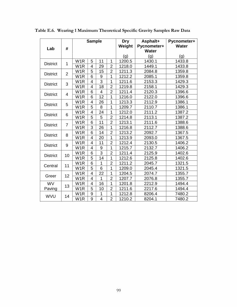
99

Table E.6. Wearing 1 Maximum Theoretical Specific Gravity Samples Raw Data

Lab #

Sample Dry Weight

Asphalt+ Pycnometer+

Water

Pycnometer+ Water

(g) (g) (g)

District 1 W1R 5 11 1 1200.5 1430.1 1433.8

W1R 4 29 2 1218.0 1449.1 1433.8

District 2 W1R 5 15 2 1211.3 2084.8 1359.8

W1R 6 9 1 1212.2 2085.1 1359.8

District 3 W1R 4 3 1 1211.6 2153.3 1429.3

W1R 4 18 2 1219.8 2158.1 1429.3

District 4 W1R 6 4 2 1211.4 2120.3 1396.6

W1R 6 12 1 1216.0 2122.0 1396.6

District 5 W1R 4 26 1 1213.3 2112.9 1386.1

W1R 5 8 1 1209.7 2110.7 1386.1

District 6 W1R 4 24 1 1212.0 2111.2 1387.2

W1R 5 5 2 1214.8 2113.1 1387.2

District 7 W1R 6 11 2 1213.1 2111.6 1388.6

W1R 3 26 1 1216.8 2112.7 1388.6

District 8 W1R 6 14 2 1213.2 2092.7 1367.5

W1R 4 20 1 1213.9 2093.0 1367.5

District 9 W1R 4 11 2 1212.4 2130.5 1406.2

W1R 4 9 1 1215.7 2132.7 1406.2

District 10 W1R 6 3 2 1211.4 2125.9 1402.6

W1R 5 14 1 1212.6 2125.8 1402.6

Central 11 W1R 6 1 2 1211.2 2045.7 1321.5

W1R 5 6 1 1209.0 2045.4 1321.5

Greer 12 W1R 4 22 1 1204.5 2074.7 1355.7

W1R 4 1 2 1207.7 2076.8 1355.7

WV Paving

13 W1R 4 16 1 1201.8 2212.9 1494.4

W1R 5 10 2 1211.6 2217.6 1494.4

WVU 14 W1R 9 1 1 1212.8 8206.4 7480.2

W1R 9 4 2 1210.2 8204.1 7480.2

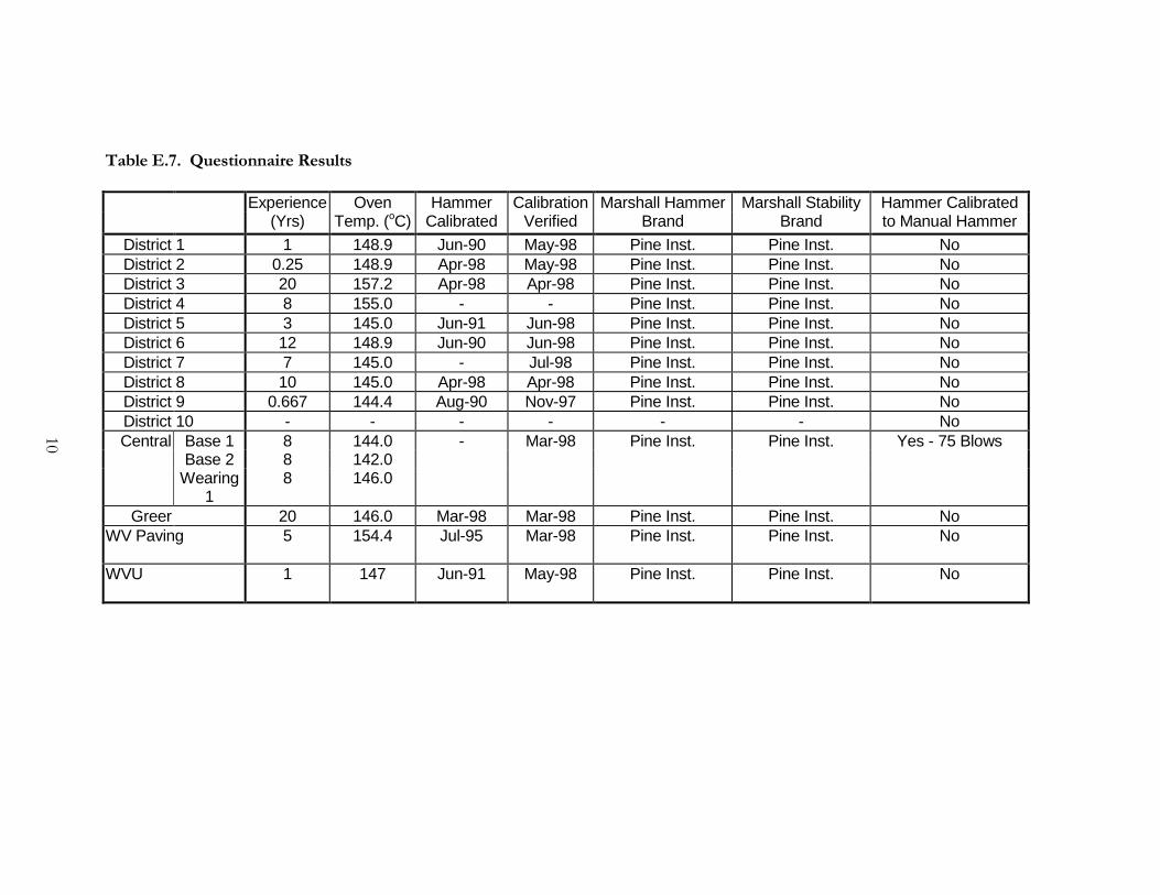
100

Table E.7. Questionnaire Results

Experience Oven Hammer Calibration Marshall Hammer Marshall Stability Hammer Calibrated (Yrs) Temp. (oC) Calibrated Verified Brand Brand to Manual Hammer

District 1 1 148.9 Jun-90 May-98 Pine Inst. Pine Inst. No

District 2 0.25 148.9 Apr-98 May-98 Pine Inst. Pine Inst. No

District 3 20 157.2 Apr-98 Apr-98 Pine Inst. Pine Inst. No

District 4 8 155.0 - - Pine Inst. Pine Inst. No

District 5 3 145.0 Jun-91 Jun-98 Pine Inst. Pine Inst. No

District 6 12 148.9 Jun-90 Jun-98 Pine Inst. Pine Inst. No

District 7 7 145.0 - Jul-98 Pine Inst. Pine Inst. No

District 8 10 145.0 Apr-98 Apr-98 Pine Inst. Pine Inst. No

District 9 0.667 144.4 Aug-90 Nov-97 Pine Inst. Pine Inst. No

District 10 - - - - - - No

Central Base 1 8 144.0 - Mar-98 Pine Inst. Pine Inst. Yes - 75 Blows Base 2 8 142.0 Wearing

1 8 146.0

Greer 20 146.0 Mar-98 Mar-98 Pine Inst. Pine Inst. No

WV Paving

5 154.4 Jul-95 Mar-98 Pine Inst. Pine Inst. No

WVU

1 147 Jun-91 May-98 Pine Inst. Pine Inst. No

101

APPENDIX F

LABORATORY INSTRUCTIONS, QUESTIONNAIRE AND DATA SHEETS

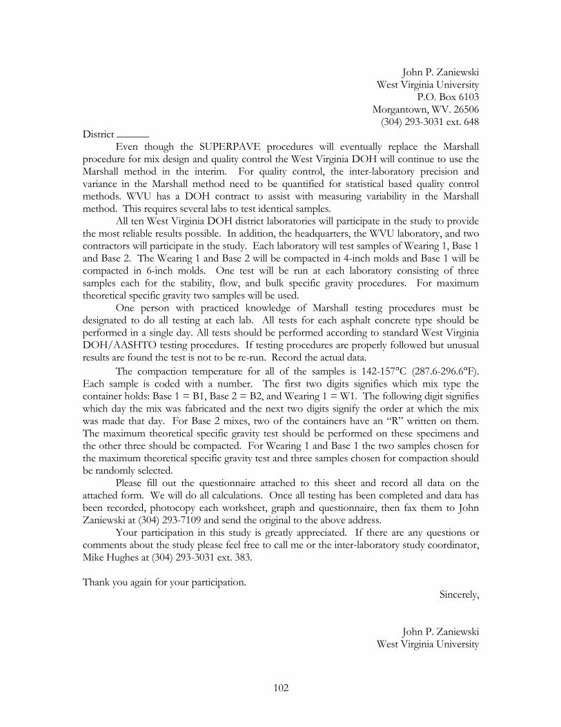
102

John P. Zaniewski West Virginia University P.O. Box 6103 Morgantown, WV. 26506 (304) 293-3031 ext. 648 District ______

Even though the SUPERPAVE procedures will eventually replace the Marshall procedure for mix design and quality control the West Virginia DOH will continue to use the Marshall method in the interim. For quality control, the inter-laboratory precision and variance in the Marshall method need to be quantified for statistical based quality control methods. WVU has a DOH contract to assist with measuring variability in the Marshall method. This requires several labs to test identical samples.

All ten West Virginia DOH district laboratories will participate in the study to provide the most reliable results possible. In addition, the headquarters, the WVU laboratory, and two contractors will participate in the study. Each laboratory will test samples of Wearing 1, Base 1 and Base 2. The Wearing 1 and Base 2 will be compacted in 4-inch molds and Base 1 will be compacted in 6-inch molds. One test will be run at each laboratory consisting of three samples each for the stability, flow, and bulk specific gravity procedures. For maximum theoretical specific gravity two samples will be used.

One person with practiced knowledge of Marshall testing procedures must be designated to do all testing at each lab. All tests for each asphalt concrete type should be performed in a single day. All tests should be performed according to standard West Virginia DOH/AASHTO testing procedures. If testing procedures are properly followed but unusual results are found the test is not to be re-run. Record the actual data.

The compaction temperature for all of the samples is 142-157 C (287.6-296.6 F). Each sample is coded with a number. The first two digits signifies which mix type the container holds: Base 1 = B1, Base 2 = B2, and Wearing 1 = W1. The following digit signifies which day the mix was fabricated and the next two digits signify the order at which the mix was made that day. For Base 2 mixes, two of the containers have an “R” written on them. The maximum theoretical specific gravity test should be performed on these specimens and the other three should be compacted. For Wearing 1 and Base 1 the two samples chosen for the maximum theoretical specific gravity test and three samples chosen for compaction should be randomly selected.

Please fill out the questionnaire attached to this sheet and record all data on the attached form. We will do all calculations. Once all testing has been completed and data has been recorded, photocopy each worksheet, graph and questionnaire, then fax them to John Zaniewski at (304) 293-7109 and send the original to the above address.

Your participation in this study is greatly appreciated. If there are any questions or comments about the study please feel free to call me or the inter-laboratory study coordinator, Mike Hughes at (304) 293-3031 ext. 383. Thank you again for your participation. Sincerely, John P. Zaniewski West Virginia University

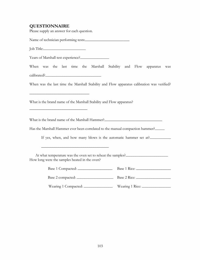
103

QUESTIONNAIRE Please supply an answer for each question. Name of technician performing tests:_______________________

Job Title:______________________

Years of Marshall test experience?_______________

When was the last time the Marshall Stability and Flow apparatus was

calibrated?_____________________________

When was the last time the Marshall Stability and Flow apparatus calibration was verified?

_______________________________

What is the brand name of the Marshall Stability and Flow apparatus?

______________________________

What is the brand name of the Marshall Hammer?______________________________

Has the Marshall Hammer ever been correlated to the manual compaction hammer?_____

If yes, when, and how many blows is the automatic hammer set at?___________

___________________________________

At what temperature was the oven set to reheat the samples?______________________ How long were the samples heated in the oven?

Base 1 Compacted: __________________ Base 1 Rice: __________________

Base 2 compacted: ___________________ Base 2 Rice: __________________

Wearing 1 Compacted: _______________ Wearing 1 Rice: _______________

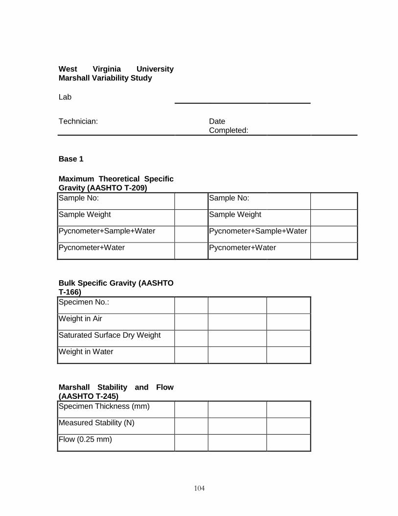
104

West Virginia University Marshall Variability Study

Lab

Technician: Date Completed:

Base 1

Maximum Theoretical Specific Gravity (AASHTO T-209)

Sample No: Sample No:

Sample Weight Sample Weight

Pycnometer+Sample+Water Pycnometer+Sample+Water

Pycnometer+Water Pycnometer+Water

Bulk Specific Gravity (AASHTO T-166)

Specimen No.:

Weight in Air

Saturated Surface Dry Weight

Weight in Water

Marshall Stability and Flow (AASHTO T-245)

Specimen Thickness (mm)

Measured Stability (N)

Flow (0.25 mm)

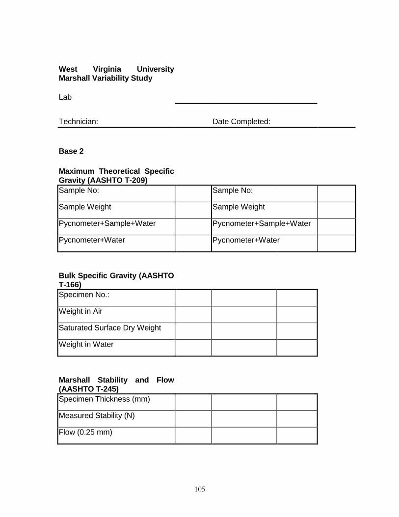
105

West Virginia University Marshall Variability Study

Lab

Technician: Date Completed:

Base 2

Maximum Theoretical Specific Gravity (AASHTO T-209)

Sample No: Sample No:

Sample Weight Sample Weight

Pycnometer+Sample+Water Pycnometer+Sample+Water

Pycnometer+Water Pycnometer+Water

Bulk Specific Gravity (AASHTO T-166)

Specimen No.:

Weight in Air

Saturated Surface Dry Weight

Weight in Water

Marshall Stability and Flow (AASHTO T-245)

Specimen Thickness (mm)

Measured Stability (N)

Flow (0.25 mm)

106

West Virginia University Marshall Variability Study

Lab

Technician: Date Completed:

Wearing 1

Maximum Theoretical Specific Gravity (AASHTO T-209)

Sample No: Sample No:

Sample Weight Sample Weight

Pycnometer+Sample+Water Pycnometer+Sample+Water

Pycnometer+Water Pycnometer+Water

Bulk Specific Gravity (AASHTO T-166)

Specimen No.:

Weight in Air

Saturated Surface Dry Weight

Weight in Water

Marshall Stability and Flow (AASHTO T-245)

Specimen Thickness (mm)

Measured Stability (N)

Flow (0.25 mm)

107

APPENDIX G VARIABILITY ANALYSIS TABLES

Table G.1. Base 1, Maximum Theoretical Specific Gravity, Within-Laboratory Average and Variance

Laboratory #

Sample 1

Sample 2

Average Within-Laboratory Variance

District 1 2.561 2.555 2.558 0.0000180

District 2 2.565 2.566 2.566 0.0000000

District 3 2.560 2.563 2.562 0.0000050

District 4 2.560 2.560 2.560 0.0000000

District 5 2.566 2.654 2.610 0.0038720

District 6 2.561 2.564 2.563 0.0000050

District 7 2.561 2.548 2.555 0.0000840

District 8 2.564 2.561 2.563 0.0000050

District 9 2.564 2.565 2.565 0.0000000

District 10 2.560 2.559 2.560 0.0000000

Central 11 2.560 2.563 2.562 0.0000050

Greer 12 2.559 2.561 2.560 0.0000020

WV Paving 13 2.566 2.565 2.566 0.0000000

WVU 14 2.562 2.560 2.561 0.0000020

Table G.2. Base 2, Maximum Theoretical Specific Gravity, Within-Laboratory Average and Variance

Laboratory Sample 1

Sample 2

Average Within-Laboratory Variance

District 1 2.516 2.521 2.519 0.0000120

District 2 2.525 2.524 2.525 0.0000000

District 3 2.523 2.524 2.524 0.0000000

District 4 2.520 2.518 2.519 0.0000020

District 5 2.530 2.530 2.530 0.0000000

District 6 2.523 2.521 2.522 0.0000020

District 7 2.519 2.519 2.519 0.0000000

District 8 2.524 2.525 2.525 0.0000000

District 9 2.520 2.524 2.522 0.0000080

District 10 2.519 2.520 2.520 0.0000000

Central 11 2.521 2.519 2.520 0.0000020

Greer 12 2.523 2.522 2.523 0.0000010

WV Paving 13 2.522 2.519 2.521 0.0000040

WVU 14 2.520 2.523 2.522 0.0000050

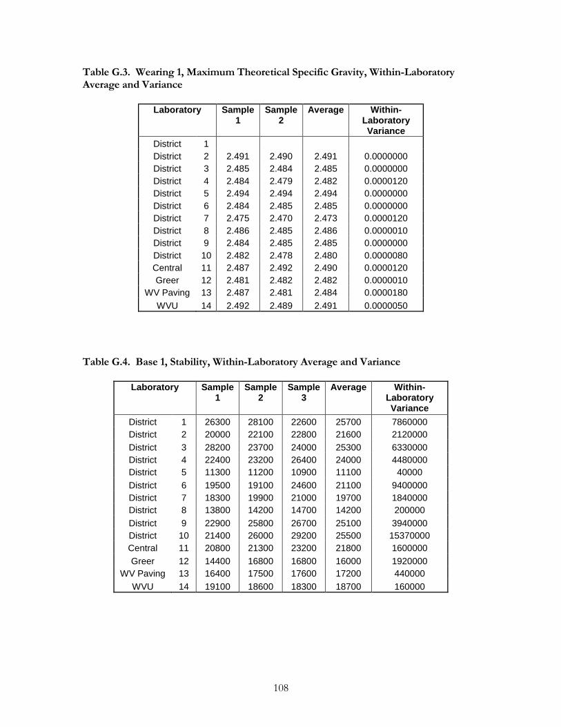
108

Table G.3. Wearing 1, Maximum Theoretical Specific Gravity, Within-Laboratory Average and Variance

Laboratory Sample 1

Sample 2

Average Within-Laboratory Variance

District 1

District 2 2.491 2.490 2.491 0.0000000

District 3 2.485 2.484 2.485 0.0000000

District 4 2.484 2.479 2.482 0.0000120

District 5 2.494 2.494 2.494 0.0000000

District 6 2.484 2.485 2.485 0.0000000

District 7 2.475 2.470 2.473 0.0000120

District 8 2.486 2.485 2.486 0.0000010

District 9 2.484 2.485 2.485 0.0000000

District 10 2.482 2.478 2.480 0.0000080

Central 11 2.487 2.492 2.490 0.0000120

Greer 12 2.481 2.482 2.482 0.0000010

WV Paving 13 2.487 2.481 2.484 0.0000180

WVU 14 2.492 2.489 2.491 0.0000050

Table G.4. Base 1, Stability, Within-Laboratory Average and Variance

Laboratory Sample 1

Sample 2

Sample 3

Average Within-Laboratory Variance

District 1 26300 28100 22600 25700 7860000

District 2 20000 22100 22800 21600 2120000

District 3 28200 23700 24000 25300 6330000

District 4 22400 23200 26400 24000 4480000

District 5 11300 11200 10900 11100 40000

District 6 19500 19100 24600 21100 9400000

District 7 18300 19900 21000 19700 1840000

District 8 13800 14200 14700 14200 200000

District 9 22900 25800 26700 25100 3940000

District 10 21400 26000 29200 25500 15370000

Central 11 20800 21300 23200 21800 1600000

Greer 12 14400 16800 16800 16000 1920000

WV Paving 13 16400 17500 17600 17200 440000

WVU 14 19100 18600 18300 18700 160000

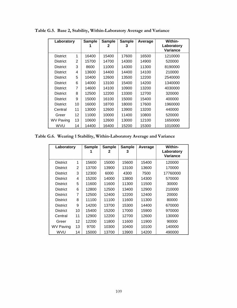
109

Table G.5. Base 2, Stability, Within-Laboratory Average and Variance

Laboratory Sample 1

Sample 2

Sample 3

Average Within-Laboratory Variance

District 1 16400 15400 17600 16500 1210000

District 2 15700 14700 14300 14900 520000

District 3 8600 11000 14300 11300 8190000

District 4 13600 14400 14400 14100 210000

District 5 10400 12600 13500 12200 2540000

District 6 14000 13100 15400 14200 1340000

District 7 14600 14100 10900 13200 4030000

District 8 12500 12200 13300 12700 320000

District 9 15000 16100 15000 15400 400000

District 10 16000 18700 18000 17600 1960000

Central 11 13000 12600 13900 13200 440000

Greer 12 11000 10000 11400 10800 520000

WV Paving 13 10600 12600 13000 12100 1650000

WVU 14 14400 16400 15200 15300 1010000

Table G.6. Wearing 1 Stability, Within-Laboratory Average and Variance

Laboratory Sample 1

Sample 2

Sample 3

Average Within-Laboratory Variance

District 1 15600 15000 15600 15400 120000

District 2 13700 13900 13100 13600 170000

District 3 12300 6000 4300 7500 17760000

District 4 15200 14000 13800 14300 570000

District 5 11600 11600 11300 11500 30000

District 6 12800 12500 13400 12900 210000

District 7 12500 12400 12200 12400 20000

District 8 11100 11100 11600 11300 80000

District 9 14200 13700 15300 14400 670000

District 10 15400 15200 17000 15900 970000

Central 11 12900 12200 12700 12600 130000

Greer 12 12200 11800 11600 11900 90000

WV Paving 13 9700 10300 10400 10100 140000

WVU 14 15000 13700 13900 14200 490000

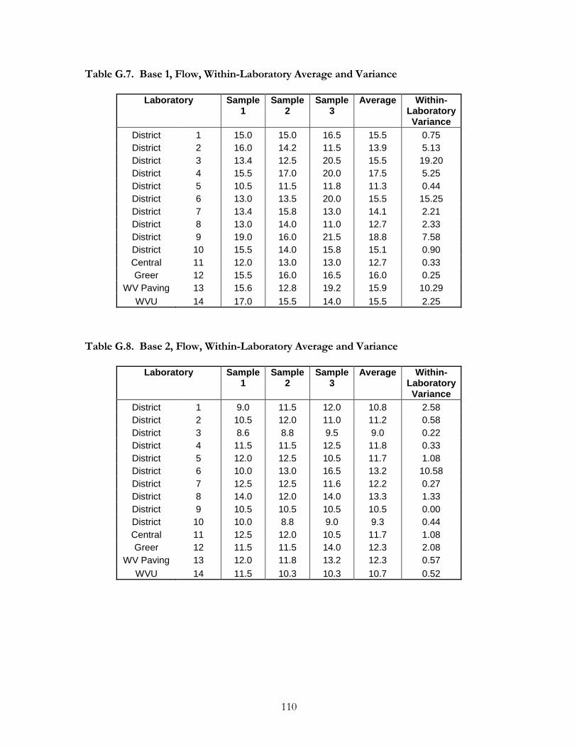
110

Table G.7. Base 1, Flow, Within-Laboratory Average and Variance

Laboratory Sample 1

Sample 2

Sample 3

Average Within- Laboratory Variance

District 1 15.0 15.0 16.5 15.5 0.75

District 2 16.0 14.2 11.5 13.9 5.13

District 3 13.4 12.5 20.5 15.5 19.20

District 4 15.5 17.0 20.0 17.5 5.25

District 5 10.5 11.5 11.8 11.3 0.44

District 6 13.0 13.5 20.0 15.5 15.25

District 7 13.4 15.8 13.0 14.1 2.21

District 8 13.0 14.0 11.0 12.7 2.33

District 9 19.0 16.0 21.5 18.8 7.58

District 10 15.5 14.0 15.8 15.1 0.90

Central 11 12.0 13.0 13.0 12.7 0.33

Greer 12 15.5 16.0 16.5 16.0 0.25

WV Paving 13 15.6 12.8 19.2 15.9 10.29

WVU 14 17.0 15.5 14.0 15.5 2.25

Table G.8. Base 2, Flow, Within-Laboratory Average and Variance

Laboratory Sample 1

Sample 2

Sample 3

Average Within-Laboratory Variance

District 1 9.0 11.5 12.0 10.8 2.58

District 2 10.5 12.0 11.0 11.2 0.58

District 3 8.6 8.8 9.5 9.0 0.22

District 4 11.5 11.5 12.5 11.8 0.33

District 5 12.0 12.5 10.5 11.7 1.08

District 6 10.0 13.0 16.5 13.2 10.58

District 7 12.5 12.5 11.6 12.2 0.27

District 8 14.0 12.0 14.0 13.3 1.33

District 9 10.5 10.5 10.5 10.5 0.00

District 10 10.0 8.8 9.0 9.3 0.44

Central 11 12.5 12.0 10.5 11.7 1.08

Greer 12 11.5 11.5 14.0 12.3 2.08

WV Paving 13 12.0 11.8 13.2 12.3 0.57

WVU 14 11.5 10.3 10.3 10.7 0.52

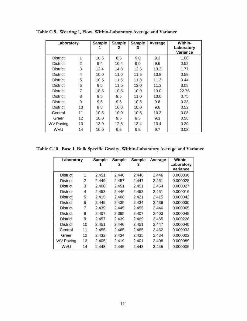
111

Table G.9. Wearing 1, Flow, Within-Laboratory Average and Variance

Laboratory Sample 1

Sample 2

Sample 3

Average Within-Laboratory Variance

District 1 10.5 8.5 9.0 9.3 1.08

District 2 9.4 10.4 9.0 9.6 0.52

District 3 12.4 14.8 12.6 13.3 1.77

District 4 10.0 11.0 11.5 10.8 0.58

District 5 10.5 11.5 11.8 11.3 0.44

District 6 9.5 11.5 13.0 11.3 3.08

District 7 18.5 10.5 10.0 13.0 22.75

District 8 9.5 9.5 11.0 10.0 0.75

District 9 9.5 9.5 10.5 9.8 0.33

District 10 8.8 10.0 10.0 9.6 0.52

Central 11 10.5 10.0 10.5 10.3 0.08

Greer 12 10.0 9.5 8.5 9.3 0.58

WV Paving 13 13.9 12.8 13.4 13.4 0.30

WVU 14 10.0 9.5 9.5 9.7 0.08

Table G.10. Base 1, Bulk Specific Gravity, Within-Laboratory Average and Variance

Laboratory Sample 1

Sample 2

Sample 3

Average Within-Laboratory Variance

District 1 2.451 2.440 2.446 2.446 0.000030

District 2 2.449 2.457 2.447 2.451 0.000028

District 3 2.460 2.451 2.451 2.454 0.000027

District 4 2.453 2.446 2.453 2.451 0.000016

District 5 2.415 2.408 2.421 2.415 0.000042

District 6 2.445 2.439 2.434 2.439 0.000030

District 7 2.439 2.445 2.455 2.446 0.000065

District 8 2.407 2.395 2.407 2.403 0.000048

District 9 2.457 2.439 2.469 2.455 0.000228

District 10 2.451 2.440 2.451 2.447 0.000040

Central 11 2.455 2.465 2.465 2.462 0.000033

Greer 12 2.432 2.434 2.435 2.434 0.000002

WV Paving 13 2.405 2.419 2.401 2.408 0.000089

WVU 14 2.448 2.445 2.443 2.445 0.000006

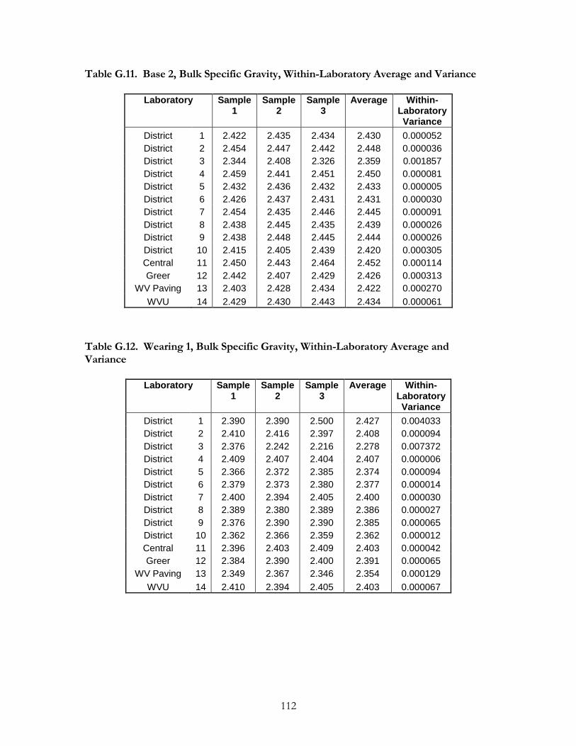
112

Table G.11. Base 2, Bulk Specific Gravity, Within-Laboratory Average and Variance

Laboratory Sample 1

Sample 2

Sample 3

Average Within-Laboratory Variance

District 1 2.422 2.435 2.434 2.430 0.000052

District 2 2.454 2.447 2.442 2.448 0.000036

District 3 2.344 2.408 2.326 2.359 0.001857

District 4 2.459 2.441 2.451 2.450 0.000081

District 5 2.432 2.436 2.432 2.433 0.000005

District 6 2.426 2.437 2.431 2.431 0.000030

District 7 2.454 2.435 2.446 2.445 0.000091

District 8 2.438 2.445 2.435 2.439 0.000026

District 9 2.438 2.448 2.445 2.444 0.000026

District 10 2.415 2.405 2.439 2.420 0.000305

Central 11 2.450 2.443 2.464 2.452 0.000114

Greer 12 2.442 2.407 2.429 2.426 0.000313

WV Paving 13 2.403 2.428 2.434 2.422 0.000270

WVU 14 2.429 2.430 2.443 2.434 0.000061

Table G.12. Wearing 1, Bulk Specific Gravity, Within-Laboratory Average and Variance

Laboratory

Sample 1

Sample 2

Sample 3

Average Within-Laboratory Variance

District 1 2.390 2.390 2.500 2.427 0.004033

District 2 2.410 2.416 2.397 2.408 0.000094

District 3 2.376 2.242 2.216 2.278 0.007372

District 4 2.409 2.407 2.404 2.407 0.000006

District 5 2.366 2.372 2.385 2.374 0.000094

District 6 2.379 2.373 2.380 2.377 0.000014

District 7 2.400 2.394 2.405 2.400 0.000030

District 8 2.389 2.380 2.389 2.386 0.000027

District 9 2.376 2.390 2.390 2.385 0.000065

District 10 2.362 2.366 2.359 2.362 0.000012

Central 11 2.396 2.403 2.409 2.403 0.000042

Greer 12 2.384 2.390 2.400 2.391 0.000065

WV Paving 13 2.349 2.367 2.346 2.354 0.000129

WVU 14 2.410 2.394 2.405 2.403 0.000067

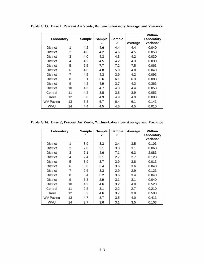
113

Table G.13. Base 1, Percent Air Voids, Within-Laboratory Average and Variance

Laboratory

Sample 1

Sample 2

Sample 3 Average

Within-Laboratory Variance

District 1 4.2 4.6 4.4 4.4 0.040

District 2 4.6 4.2 4.6 4.5 0.053

District 3 4.0 4.3 4.3 4.2 0.030

District 4 4.2 4.5 4.2 4.3 0.030

District 5 7.5 7.7 7.2 7.5 0.063

District 6 4.6 4.8 5.0 4.8 0.040

District 7 4.5 4.3 3.9 4.2 0.093

District 8 6.1 6.6 6.1 6.3 0.083

District 9 4.2 4.9 3.7 4.3 0.363

District 10 4.3 4.7 4.3 4.4 0.053

Central 11 4.2 3.8 3.8 3.9 0.053

Greer 12 5.0 4.9 4.9 4.9 0.003

WV Paving 13 6.3 5.7 6.4 6.1 0.143

WVU 14 4.4 4.5 4.6 4.5 0.010

Table G.14. Base 2, Percent Air Voids, Within-Laboratory Average and Variance

Laboratory Sample 1

Sample 2

Sample 3

Average Within-Laboratory Variance

District 1 3.9 3.3 3.4 3.5 0.103

District 2 2.8 3.1 3.3 3.1 0.063

District 3 7.1 4.6 7.1 6.3 2.083

District 4 2.4 3.1 2.7 2.7 0.123

District 5 3.9 3.7 3.9 3.8 0.013

District 6 3.8 3.4 3.6 3.6 0.040

District 7 2.6 3.3 2.9 2.9 0.123

District 8 3.4 3.2 3.6 3.4 0.040

District 9 3.3 2.9 3.1 3.1 0.040

District 10 4.2 4.6 3.2 4.0 0.520

Central 11 2.8 3.1 2.2 2.7 0.210

Greer 12 3.2 4.6 3.7 3.8 0.503

WV Paving 13 4.7 3.7 3.5 4.0 0.413

WVU 14 3.7 3.6 3.1 3.5 0.103

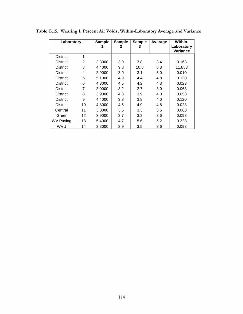
114

Table G.15. Wearing 1, Percent Air Voids, Within-Laboratory Average and Variance

Laboratory Sample 1

Sample 2

Sample 3

Average Within-Laboratory Variance

District 1

District 2 3.3000 3.0 3.8 3.4 0.163

District 3 4.4000 9.8 10.8 8.3 11.853

District 4 2.9000 3.0 3.1 3.0 0.010

District 5 5.1000 4.9 4.4 4.8 0.130

District 6 4.3000 4.5 4.2 4.3 0.023

District 7 3.0000 3.2 2.7 3.0 0.063

District 8 3.9000 4.3 3.9 4.0 0.053

District 9 4.4000 3.8 3.8 4.0 0.120

District 10 4.8000 4.6 4.9 4.8 0.023

Central 11 3.8000 3.5 3.3 3.5 0.063

Greer 12 3.9000 3.7 3.3 3.6 0.093

WV Paving 13 5.4000 4.7 5.6 5.2 0.223

WVU 14 3.3000 3.9 3.5 3.6 0.093

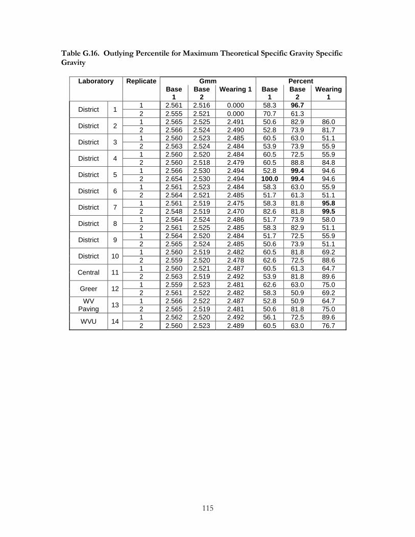
115

Table G.16. Outlying Percentile for Maximum Theoretical Specific Gravity Specific Gravity

Laboratory Replicate Gmm Percent

Base 1

Base 2

Wearing 1 Base 1

Base 2

Wearing 1

District 1 1 2.561 2.516 0.000 58.3 96.7

2 2.555 2.521 0.000 70.7 61.3

District 2 1 2.565 2.525 2.491 50.6 82.9 86.0

2 2.566 2.524 2.490 52.8 73.9 81.7

District 3 1 2.560 2.523 2.485 60.5 63.0 51.1

2 2.563 2.524 2.484 53.9 73.9 55.9

District 4 1 2.560 2.520 2.484 60.5 72.5 55.9

2 2.560 2.518 2.479 60.5 88.8 84.8

District 5 1 2.566 2.530 2.494 52.8 99.4 94.6

2 2.654 2.530 2.494 100.0 99.4 94.6

District 6 1 2.561 2.523 2.484 58.3 63.0 55.9

2 2.564 2.521 2.485 51.7 61.3 51.1

District 7 1 2.561 2.519 2.475 58.3 81.8 95.8

2 2.548 2.519 2.470 82.6 81.8 99.5

District 8 1 2.564 2.524 2.486 51.7 73.9 58.0

2 2.561 2.525 2.485 58.3 82.9 51.1

District 9 1 2.564 2.520 2.484 51.7 72.5 55.9

2 2.565 2.524 2.485 50.6 73.9 51.1

District 10 1 2.560 2.519 2.482 60.5 81.8 69.2

2 2.559 2.520 2.478 62.6 72.5 88.6

Central 11 1 2.560 2.521 2.487 60.5 61.3 64.7

2 2.563 2.519 2.492 53.9 81.8 89.6

Greer 12 1 2.559 2.523 2.481 62.6 63.0 75.0

2 2.561 2.522 2.482 58.3 50.9 69.2

WV Paving

13 1 2.566 2.522 2.487 52.8 50.9 64.7

2 2.565 2.519 2.481 50.6 81.8 75.0

WVU 14 1 2.562 2.520 2.492 56.1 72.5 89.6

2 2.560 2.523 2.489 60.5 63.0 76.7

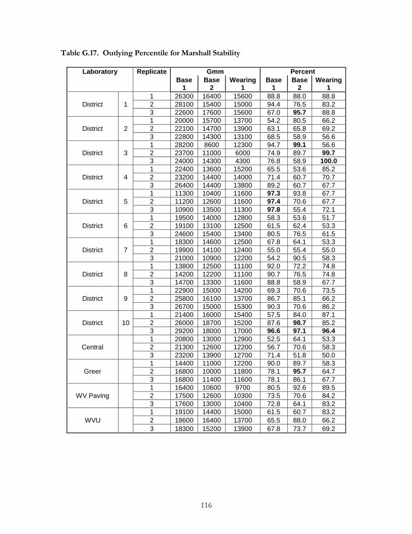
116

Table G.17. Outlying Percentile for Marshall Stability

Laboratory Replicate Gmm Percent

Base 1

Base 2

Wearing 1

Base 1

Base 2

Wearing 1

District 1

1 26300 16400 15600 88.8 88.0 88.8

2 28100 15400 15000 94.4 76.5 83.2

3 22600 17600 15600 67.0 95.7 88.8

District 2

1 20000 15700 13700 54.2 80.5 66.2

2 22100 14700 13900 63.1 65.8 69.2

3 22800 14300 13100 68.5 58.9 56.6

District 3

1 28200 8600 12300 94.7 99.1 56.6

2 23700 11000 6000 74.9 89.7 99.7

3 24000 14300 4300 76.8 58.9 100.0

District 4

1 22400 13600 15200 65.5 53.6 85.2

2 23200 14400 14000 71.4 60.7 70.7

3 26400 14400 13800 89.2 60.7 67.7

District 5

1 11300 10400 11600 97.3 93.8 67.7

2 11200 12600 11600 97.4 70.6 67.7

3 10900 13500 11300 97.8 55.4 72.1

District 6

1 19500 14000 12800 58.3 53.6 51.7

2 19100 13100 12500 61.5 62.4 53.3

3 24600 15400 13400 80.5 76.5 61.5

District 7

1 18300 14600 12500 67.8 64.1 53.3

2 19900 14100 12400 55.0 55.4 55.0

3 21000 10900 12200 54.2 90.5 58.3

District 8

1 13800 12500 11100 92.0 72.2 74.8

2 14200 12200 11100 90.7 76.5 74.8

3 14700 13300 11600 88.8 58.9 67.7

District 9

1 22900 15000 14200 69.3 70.6 73.5

2 25800 16100 13700 86.7 85.1 66.2

3 26700 15000 15300 90.3 70.6 86.2

District 10

1 21400 16000 15400 57.5 84.0 87.1

2 26000 18700 15200 87.6 98.7 85.2

3 29200 18000 17000 96.6 97.1 96.4

Central

1 20800 13000 12900 52.5 64.1 53.3

2 21300 12600 12200 56.7 70.6 58.3

3 23200 13900 12700 71.4 51.8 50.0

Greer

1 14400 11000 12200 90.0 89.7 58.3

2 16800 10000 11800 78.1 95.7 64.7

3 16800 11400 11600 78.1 86.1 67.7

WV Paving

1 16400 10600 9700 80.5 92.6 89.5

2 17500 12600 10300 73.5 70.6 84.2

3 17600 13000 10400 72.8 64.1 83.2

WVU

1 19100 14400 15000 61.5 60.7 83.2

2 18600 16400 13700 65.5 88.0 66.2

3 18300 15200 13900 67.8 73.7 69.2

117

Table G.18. Outlying Percentile for Marshall Flow

Laboratory Replicate Flow Percent

Base 1

Base 2

Wearing 1

Base 1

Base 2

Wearing 1

District 1

1 15.0 9.0 10.5 50.2 93.1 55.5

2 15.0 11.5 8.5 50.2 51.9 88.2

3 16.5 12.0 9.0 71.3 63.8 82.2

District 2

1 16.0 10.5 9.4 64.7 71.4 76.2

2 14.2 12.0 10.4 61.5 63.8 57.6

3 11.5 11.0 9.0 90.2 60.2 82.2

District 3

1 13.4 8.6 12.4 72.2 95.8 80.3

2 12.5 8.8 14.8 82.2 94.6 98.2

3 20.5 9.5 12.6 98.0 88.1 83.1

District 4

1 15.5 11.5 10.0 57.6 51.9 65.5

2 17.0 11.5 11.0 77.3 51.9 54.8

3 20.0 12.5 11.5 96.9 74.6 64.9

District 5

1 10.5 12.0 10.5 95.2 63.8 55.5

2 11.5 12.5 11.5 90.2 74.6 64.9

3 11.8 10.5 11.8 88.5 71.4 69.6

District 6

1 13.0 10.0 9.5 77.0 80.9 74.6

2 13.5 13.0 11.5 71.0 83.3 64.9

3 20.0 16.5 13.0 96.9 99.9 87.8

District 7

1 13.4 12.5 18.5 72.2 74.6 100.0

2 15.8 12.5 10.5 61.2 74.6 55.5

3 13.0 11.6 10.0 77.0 54.3 65.5

District 8

1 13.0 14.0 9.5 77.0 94.3 74.6

2 14.0 12.0 9.5 64.3 63.8 74.6

3 11.0 14.0 11.0 93.1 94.3 54.8

District 9

1 19.0 10.5 9.5 93.2 71.4 74.6

2 16.0 10.5 9.5 64.7 71.4 74.6

3 21.5 10.5 10.5 99.2 71.4 55.5

District 10

1 15.5 10.0 8.8 57.6 80.9 85.4

2 14.0 8.8 10.0 64.3 95.0 65.5

3 15.8 9.0 10.0 61.2 93.1 65.5

Central 11

1 12.0 12.5 10.5 86.6 74.6 55.5

2 13.0 12.0 10.0 77.0 63.8 65.5

3 13.0 10.5 10.5 77.0 71.4 55.5

Greer 12

1 15.5 11.5 10.0 57.6 51.9 65.5

2 16.0 11.5 9.5 64.7 51.9 74.6

3 16.5 14.0 8.5 71.3 94.3 88.2

WV Paving 13

1 15.6 12.0 13.9 59.1 63.8 94.9

2 12.8 11.8 12.8 79.2 59.2 85.6

3 19.2 13.2 13.4 94.2 86.2 91.5

WVU 14

1 17.0 11.5 10.0 77.3 51.9 65.5

2 15.5 10.3 9.5 57.6 76.4 74.6

3 14.0 10.3 9.5 64.3 76.4 74.6

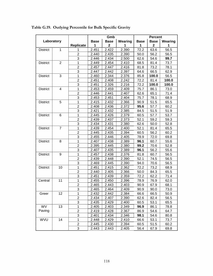
118

Table G.19. Outlying Percentile for Bulk Specific Gravity

Laboratory Replicate

Gmb Percent

Base 1

Base 2

Wearing 1

Base 1

Base 2

Wearing 1

District 1 1 2.451 2.422 2.390 72.2 63.6 56.5

2 2.440 2.435 2.390 50.0 56.2 56.5

3 2.446 2.434 2.500 62.6 54.6 99.7

District 2 1 2.449 2.454 2.410 68.5 81.4 73.7

2 2.457 2.447 2.416 81.8 73.2 78.1

3 2.447 2.442 2.397 64.6 66.5 62.9

District 3 1 2.460 2.344 2.376 85.8 100.0 56.5

2 2.451 2.408 2.242 72.2 81.4 100.0

3 2.451 2.326 2.216 72.2 100.0 100.0

District 4 1 2.453 2.459 2.409 75.7 86.1 73.0

2 2.446 2.441 2.407 62.6 65.1 71.4

3 2.453 2.451 2.404 75.7 78.1 68.9

District 5 1 2.415 2.432 2.366 90.9 51.5 65.5

2 2.408 2.436 2.372 95.6 57.7 60.2

3 2.421 2.432 2.385 84.5 51.5 51.9

District 6 1 2.445 2.426 2.379 60.5 57.7 53.7

2 2.439 2.437 2.373 52.1 59.2 59.3

3 2.434 2.431 2.380 62.6 50.0 52.8

District 7 1 2.439 2.454 2.400 52.1 81.4 65.5

2 2.445 2.435 2.394 60.5 56.2 60.2

3 2.455 2.446 2.405 78.9 72.0 69.8

District 8 1 2.407 2.438 2.389 96.1 60.7 55.6

2 2.395 2.445 2.380 99.2 70.6 52.8

3 2.407 2.435 2.389 96.1 56.2 55.6

District 9 1 2.457 2.438 2.376 81.8 60.7 56.5

2 2.439 2.448 2.390 52.1 74.5 56.5

3 2.469 2.445 2.390 94.0 70.6 56.5

District 10 1 2.451 2.415 2.362 72.2 73.2 68.9

2 2.440 2.405 2.366 50.0 84.3 65.5

3 2.451 2.439 2.359 72.2 62.2 71.4

Central 11 1 2.455 2.450 2.396 78.9 76.9 62.0

2 2.465 2.443 2.403 90.9 67.9 68.1

3 2.465 2.464 2.409 90.9 90.0 73.0

Greer 12 1 2.432 2.442 2.384 66.6 66.5 50.9

2 2.434 2.407 2.390 62.6 82.4 56.5

3 2.435 2.429 2.400 60.5 53.1 65.5

WV Paving

13 1 2.405 2.403 2.349 96.9 86.1 78.8

2 2.419 2.428 2.367 86.9 54.6 64.7

3 2.401 2.434 2.346 98.1 54.6 80.8

WVU 14 1 2.448 2.429 2.410 66.6 53.1 73.7

2 2.445 2.430 2.394 60.5 51.5 60.2

3 2.443 2.443 2.405 56.4 67.9 69.8

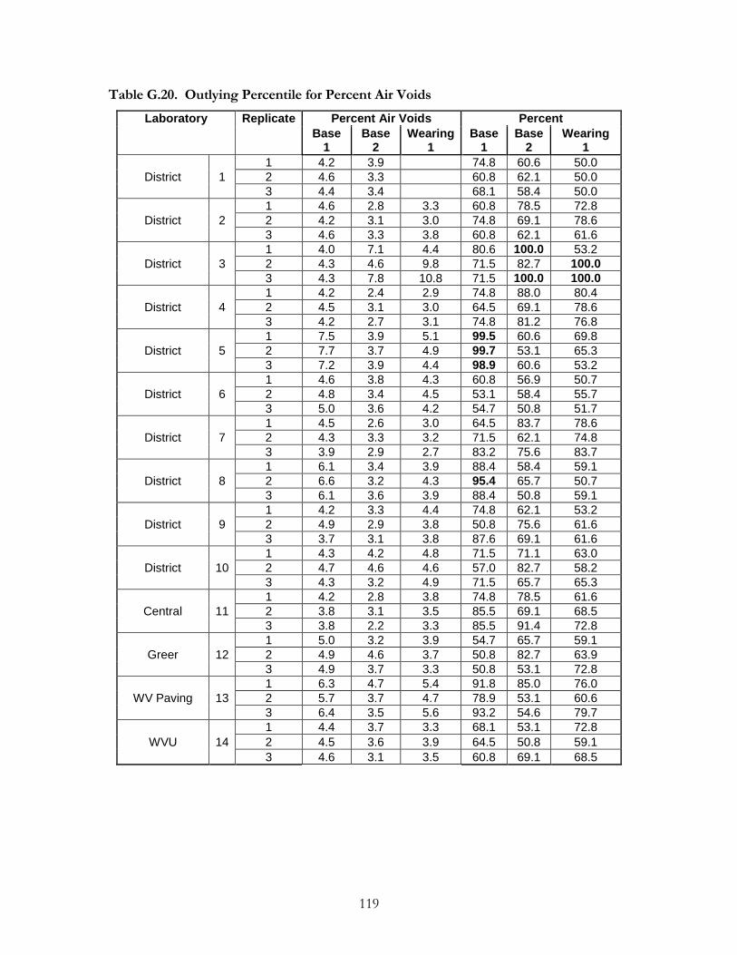
119

Table G.20. Outlying Percentile for Percent Air Voids

Laboratory Replicate Percent Air Voids Percent

Base 1

Base 2

Wearing 1

Base 1

Base 2

Wearing 1

District 1

1 4.2 3.9 74.8 60.6 50.0

2 4.6 3.3 60.8 62.1 50.0

3 4.4 3.4 68.1 58.4 50.0

District 2

1 4.6 2.8 3.3 60.8 78.5 72.8

2 4.2 3.1 3.0 74.8 69.1 78.6

3 4.6 3.3 3.8 60.8 62.1 61.6

District 3

1 4.0 7.1 4.4 80.6 100.0 53.2

2 4.3 4.6 9.8 71.5 82.7 100.0

3 4.3 7.8 10.8 71.5 100.0 100.0

District 4

1 4.2 2.4 2.9 74.8 88.0 80.4

2 4.5 3.1 3.0 64.5 69.1 78.6

3 4.2 2.7 3.1 74.8 81.2 76.8

District 5

1 7.5 3.9 5.1 99.5 60.6 69.8

2 7.7 3.7 4.9 99.7 53.1 65.3

3 7.2 3.9 4.4 98.9 60.6 53.2

District 6

1 4.6 3.8 4.3 60.8 56.9 50.7

2 4.8 3.4 4.5 53.1 58.4 55.7

3 5.0 3.6 4.2 54.7 50.8 51.7

District 7

1 4.5 2.6 3.0 64.5 83.7 78.6

2 4.3 3.3 3.2 71.5 62.1 74.8

3 3.9 2.9 2.7 83.2 75.6 83.7

District 8

1 6.1 3.4 3.9 88.4 58.4 59.1

2 6.6 3.2 4.3 95.4 65.7 50.7

3 6.1 3.6 3.9 88.4 50.8 59.1

District 9

1 4.2 3.3 4.4 74.8 62.1 53.2

2 4.9 2.9 3.8 50.8 75.6 61.6

3 3.7 3.1 3.8 87.6 69.1 61.6

District 10

1 4.3 4.2 4.8 71.5 71.1 63.0

2 4.7 4.6 4.6 57.0 82.7 58.2

3 4.3 3.2 4.9 71.5 65.7 65.3

Central 11

1 4.2 2.8 3.8 74.8 78.5 61.6

2 3.8 3.1 3.5 85.5 69.1 68.5

3 3.8 2.2 3.3 85.5 91.4 72.8

Greer 12

1 5.0 3.2 3.9 54.7 65.7 59.1

2 4.9 4.6 3.7 50.8 82.7 63.9

3 4.9 3.7 3.3 50.8 53.1 72.8

WV Paving 13

1 6.3 4.7 5.4 91.8 85.0 76.0

2 5.7 3.7 4.7 78.9 53.1 60.6

3 6.4 3.5 5.6 93.2 54.6 79.7

WVU 14

1 4.4 3.7 3.3 68.1 53.1 72.8

2 4.5 3.6 3.9 64.5 50.8 59.1

3 4.6 3.1 3.5 60.8 69.1 68.5