Inter-Domain Traffic Engineering

Manuel António Seixas Pinto

Thesis to obtain the Master of Science Degree in

Electrical and Computer Engineering

Supervisor: Prof. João Luís Costa Campos Gonçalves Sobrinho

Examination Committee

Chairperson: Prof. Nuno Cavaco Gomes HortaSupervisor: Prof. João Luís Costa Campos Gonçalves Sobrinho

Members of the Committee: Prof. Teresa Maria Sá Ferreira Vazão Vasques

November 2015

ii

Acknowledgments

First of all, I would like to thank my thesis advisor, Professor Joao Luis Sobrinho. His endless passion

for the thesis topics proved to be a source of continuous encouragement and inspiration. Also, when it

came to more challenging matters, he was always patient enough to make sure that I understood every

aspect.

University was not at all times a soft journey but it was sure made easier with the remarkable col-

leagues I met and all the help from my caring friends to whom I am deeply thankful.

Most importantly, I would like to express sincere gratitude to my family. Throughout these years, my

close family was always a big source of support. Even without fully understanding what I was going

through, they continually shared all my frustrations and accomplishments. I feel like I can never thank

them enough.

iii

iv

Abstract

Traffic Engineering (TE) techniques for inbound traffic control can seriously threaten the scalability of the

Internet’s global routing system. This work provides an in-depth study to TE practices with focus on the

scalability problem by doing an experimental assessment, impact evaluation and subsequently present

a mitigating solution.

We first provide the tools needed for the study by surveying the publicly available data sources and

creating the basic algorithms. Then, we portray the evolutionary and current state of the Internet with

an analysis to the address space and a prefix characterization. Given its importance for future studies,

a web platform was created in order for these and other interesting statistics to be publicly available.

The assessment study uses real BGP data in order to observe the prevalence of TE on the Internet

for both IPv4 and IPv6. We try to guess on its trending and briefly compare both IP versions. TE impact

is evaluated for global reachability, routing table sizes and the changes to the route type and path length.

Finally, we provide solutions to lighten the damaging consequences of TE by adapting and applying the

Distributed Route Aggregation (DRAGON) strategy to the Internet’s inferred topology with very promising

results.

Keywords: Traffic engineering, prefix deaggregation, BGP, scalability, DRAGON

v

vi

Resumo

Tecnicas de engenharia de trafego (ET) podem seriamente ameacar a escalabilidade do sistema de

encaminhamento da Internet. Neste trabalho e feito um estudo cuidado das praticas de ET com especial

foco no problema da escalabilidade passado por uma avaliacao experimental, estudo do impacto e de

seguida e exposta uma solucao. Primeiramente sao apresentadas as ferramentas para o estudo do

impacto e da solucao atraves de uma pesquisa por fontes publicas de dados e sao tambem criados os

algoritmos necessarios. Posteriormente, mostra-se a evolucao e estado actual da Internet atraves de

uma analise ao espaco de enderecos e e tambem feita uma caracterizacao dos prefixos. Dada a sua

importancia em estudos futuros, foi criada uma plataforma web onde estas e outras estatısticas podem

ser acedidas publicamente.

O estudo experimental usa dados reais de BGP de maneira a perceber a dimensao de ET na Internet

para IPv4 e IPv6. Tenta-se perceber a tendencia e e feita uma breve comparacao entre versoes. O

estudo do impacto visa perceber os efeitos da ET para a conectividade global, tamanho das tabelas de

encaminhamento e as mudancas no tipo de rotas e tamanho do caminho. Por ultimo, apresentam-se

solucoes capazes de atenuar as consequencias prejudiciais de ET adaptando e implementando uma

estrategia de agregacao de rotas distribuıda (DRAGON) na topologia inferida da Internet com resultados

bastante promissores.

Palavras-chave: Engenharia de Trafego, desagregacao de prefixos, BGP, escalabilidade,

DRAGON

vii

viii

Contents

Acknowledgments . . . . . . . . . . . . . . . . . . . . . . . . . . . . . . . . . . . . . . . . . . . iii

Abstract . . . . . . . . . . . . . . . . . . . . . . . . . . . . . . . . . . . . . . . . . . . . . . . . . v

Resumo . . . . . . . . . . . . . . . . . . . . . . . . . . . . . . . . . . . . . . . . . . . . . . . . . vii

List of Tables . . . . . . . . . . . . . . . . . . . . . . . . . . . . . . . . . . . . . . . . . . . . . . xi

List of Figures . . . . . . . . . . . . . . . . . . . . . . . . . . . . . . . . . . . . . . . . . . . . . xiv

List of Abbreviations . . . . . . . . . . . . . . . . . . . . . . . . . . . . . . . . . . . . . . . . . . 1

1 Introduction 1

1.1 Concepts of Inter-Domain Routing . . . . . . . . . . . . . . . . . . . . . . . . . . . . . . . 2

1.2 Traffic Engineering . . . . . . . . . . . . . . . . . . . . . . . . . . . . . . . . . . . . . . . . 4

1.3 Scalability . . . . . . . . . . . . . . . . . . . . . . . . . . . . . . . . . . . . . . . . . . . . . 5

1.4 Related Work . . . . . . . . . . . . . . . . . . . . . . . . . . . . . . . . . . . . . . . . . . . 6

1.5 Contributions . . . . . . . . . . . . . . . . . . . . . . . . . . . . . . . . . . . . . . . . . . . 7

2 Snapshot of the Internet 9

2.1 Data Sources . . . . . . . . . . . . . . . . . . . . . . . . . . . . . . . . . . . . . . . . . . . 9

2.1.1 Raw Data . . . . . . . . . . . . . . . . . . . . . . . . . . . . . . . . . . . . . . . . . 9

2.1.2 Processed data . . . . . . . . . . . . . . . . . . . . . . . . . . . . . . . . . . . . . . 12

2.2 Elected Route Algorithm . . . . . . . . . . . . . . . . . . . . . . . . . . . . . . . . . . . . . 13

2.2.1 Elected Route type . . . . . . . . . . . . . . . . . . . . . . . . . . . . . . . . . . . . 13

2.2.2 Elected Route with path length . . . . . . . . . . . . . . . . . . . . . . . . . . . . . 14

2.3 Statistics . . . . . . . . . . . . . . . . . . . . . . . . . . . . . . . . . . . . . . . . . . . . . 17

2.3.1 Address Space . . . . . . . . . . . . . . . . . . . . . . . . . . . . . . . . . . . . . . 17

2.3.2 Prefix type . . . . . . . . . . . . . . . . . . . . . . . . . . . . . . . . . . . . . . . . 17

2.4 InterSnap web platform . . . . . . . . . . . . . . . . . . . . . . . . . . . . . . . . . . . . . 22

3 Experimental Assessment of TE 23

3.1 Assessment methodology . . . . . . . . . . . . . . . . . . . . . . . . . . . . . . . . . . . . 23

3.1.1 Selective advertisements . . . . . . . . . . . . . . . . . . . . . . . . . . . . . . . . 24

3.1.2 Path Prepending . . . . . . . . . . . . . . . . . . . . . . . . . . . . . . . . . . . . . 25

3.1.3 Procedure . . . . . . . . . . . . . . . . . . . . . . . . . . . . . . . . . . . . . . . . . 26

3.2 Statistics and Analysis . . . . . . . . . . . . . . . . . . . . . . . . . . . . . . . . . . . . . . 28

ix

3.2.1 Path Prepending . . . . . . . . . . . . . . . . . . . . . . . . . . . . . . . . . . . . . 28

3.2.2 Prefix Deaggregation . . . . . . . . . . . . . . . . . . . . . . . . . . . . . . . . . . 29

4 Impact of TE on global routing 31

4.1 Impact analysis . . . . . . . . . . . . . . . . . . . . . . . . . . . . . . . . . . . . . . . . . . 31

4.1.1 Distortion to the route type . . . . . . . . . . . . . . . . . . . . . . . . . . . . . . . 31

4.1.2 Distortion to the path length . . . . . . . . . . . . . . . . . . . . . . . . . . . . . . . 33

4.1.3 Global Reachability . . . . . . . . . . . . . . . . . . . . . . . . . . . . . . . . . . . 35

4.1.4 FIB & RIB - Table size . . . . . . . . . . . . . . . . . . . . . . . . . . . . . . . . . . 38

4.2 Statistics . . . . . . . . . . . . . . . . . . . . . . . . . . . . . . . . . . . . . . . . . . . . . 39

4.2.1 Change in route type . . . . . . . . . . . . . . . . . . . . . . . . . . . . . . . . . . . 39

4.2.2 Changes in path length . . . . . . . . . . . . . . . . . . . . . . . . . . . . . . . . . 41

4.3 Impact Simulator . . . . . . . . . . . . . . . . . . . . . . . . . . . . . . . . . . . . . . . . . 42

5 Solution for scalable TE 45

5.1 Scalable TE using DRAGON . . . . . . . . . . . . . . . . . . . . . . . . . . . . . . . . . . 45

5.1.1 Equivalent model . . . . . . . . . . . . . . . . . . . . . . . . . . . . . . . . . . . . . 46

5.1.2 Provider delegation . . . . . . . . . . . . . . . . . . . . . . . . . . . . . . . . . . . 49

5.2 Statistics and analysis . . . . . . . . . . . . . . . . . . . . . . . . . . . . . . . . . . . . . . 51

5.2.1 Equivalent model . . . . . . . . . . . . . . . . . . . . . . . . . . . . . . . . . . . . . 51

5.2.2 Provider delegation . . . . . . . . . . . . . . . . . . . . . . . . . . . . . . . . . . . 53

6 Conclusions and future work 55

Bibliography 59

x

List of Tables

1.1 IP routes export policies . . . . . . . . . . . . . . . . . . . . . . . . . . . . . . . . . . . . . 3

2.1 Prefix subtype distribution . . . . . . . . . . . . . . . . . . . . . . . . . . . . . . . . . . . . 19

3.1 TE evaluation procedure . . . . . . . . . . . . . . . . . . . . . . . . . . . . . . . . . . . . . 27

3.2 TE percentages by practices . . . . . . . . . . . . . . . . . . . . . . . . . . . . . . . . . . 29

3.3 Number of providers used with prefix deaggregation and selective advertisements . . . . 30

4.1 Route type and the GR export policies . . . . . . . . . . . . . . . . . . . . . . . . . . . . . 32

4.2 Changes in route type due to prefix deaggregation . . . . . . . . . . . . . . . . . . . . . . 39

5.1 Average percentage of affected ASes for different gains in a situation of 2 TE providers . 51

5.2 Average percentage of affected ASes for different gains in a situation of 4 TE providers . 52

5.3 Percentage of found Aggregation Nodes by level and number of providers . . . . . . . . . 53

xi

xii

List of Figures

1.1 CIDR Notation . . . . . . . . . . . . . . . . . . . . . . . . . . . . . . . . . . . . . . . . . . 1

1.2 IP network example . . . . . . . . . . . . . . . . . . . . . . . . . . . . . . . . . . . . . . . 2

1.3 Unsusable paths . . . . . . . . . . . . . . . . . . . . . . . . . . . . . . . . . . . . . . . . . 3

1.4 Inter-Domain routing example . . . . . . . . . . . . . . . . . . . . . . . . . . . . . . . . . . 4

1.5 Traffic engineering example . . . . . . . . . . . . . . . . . . . . . . . . . . . . . . . . . . . 5

2.1 Monitoring architecture . . . . . . . . . . . . . . . . . . . . . . . . . . . . . . . . . . . . . . 10

2.2 Monitor data example . . . . . . . . . . . . . . . . . . . . . . . . . . . . . . . . . . . . . . 10

2.3 Hidden Links . . . . . . . . . . . . . . . . . . . . . . . . . . . . . . . . . . . . . . . . . . . 11

2.4 Increased visibility with multiple monitors . . . . . . . . . . . . . . . . . . . . . . . . . . . 11

2.5 Sample IRR query using the whois command . . . . . . . . . . . . . . . . . . . . . . . . . 12

2.6 Transformation to a DAG . . . . . . . . . . . . . . . . . . . . . . . . . . . . . . . . . . . . . 15

2.7 Address space distribution . . . . . . . . . . . . . . . . . . . . . . . . . . . . . . . . . . . . 17

2.8 Sample network . . . . . . . . . . . . . . . . . . . . . . . . . . . . . . . . . . . . . . . . . 18

2.9 Prefix Tree example . . . . . . . . . . . . . . . . . . . . . . . . . . . . . . . . . . . . . . . 19

2.10 Prefix type distribution . . . . . . . . . . . . . . . . . . . . . . . . . . . . . . . . . . . . . . 19

2.11 Aggregation prefixes example . . . . . . . . . . . . . . . . . . . . . . . . . . . . . . . . . . 20

2.12 IPv4 and IPv6 early phase prefix type comparison . . . . . . . . . . . . . . . . . . . . . . 20

2.13 InterSnap web architecture . . . . . . . . . . . . . . . . . . . . . . . . . . . . . . . . . . . 22

2.14 InterSnap screenshot . . . . . . . . . . . . . . . . . . . . . . . . . . . . . . . . . . . . . . 22

3.1 Prefix deaggregation without selective advertisements . . . . . . . . . . . . . . . . . . . . 24

3.2 Prefix deaggregation with selective advertisements . . . . . . . . . . . . . . . . . . . . . . 25

3.3 Path prepending monitoring . . . . . . . . . . . . . . . . . . . . . . . . . . . . . . . . . . . 25

3.4 Path prepending and prefix deaggregation monitoring . . . . . . . . . . . . . . . . . . . . 26

3.5 Binary prefix tree used for merging route data . . . . . . . . . . . . . . . . . . . . . . . . 27

3.6 Prefix type with prepending distribution . . . . . . . . . . . . . . . . . . . . . . . . . . . . . 28

3.7 Evolution of prefix deaggregation . . . . . . . . . . . . . . . . . . . . . . . . . . . . . . . . 29

3.8 Prefix deaggregation by Tier . . . . . . . . . . . . . . . . . . . . . . . . . . . . . . . . . . 30

4.1 Change in route type when using prefix deaggregation . . . . . . . . . . . . . . . . . . . . 32

4.2 Change in the forwarding path when using path prepending. . . . . . . . . . . . . . . . . . 34

xiii

4.3 Possible topologies with different outcomes to the path length . . . . . . . . . . . . . . . . 34

4.4 Prefix deaggregation and global reachability on not policy connected networks . . . . . . 35

4.5 Prefix deaggregation and global reachability on not policy connected networks with ag-

gregation node . . . . . . . . . . . . . . . . . . . . . . . . . . . . . . . . . . . . . . . . . . 36

4.6 Filtering deaggregated prefixes with a less preferred route. . . . . . . . . . . . . . . . . . 37

4.7 Lose of attractiveness by filtering prefixes with the same forwarding neighbor . . . . . . . 37

4.8 C2P distortion . . . . . . . . . . . . . . . . . . . . . . . . . . . . . . . . . . . . . . . . . . 40

4.9 R2P distortion . . . . . . . . . . . . . . . . . . . . . . . . . . . . . . . . . . . . . . . . . . 40

4.10 Change in path length from the use of TE. . . . . . . . . . . . . . . . . . . . . . . . . . . . 41

4.11 Screenshot of the Impact Simulator App and its main features . . . . . . . . . . . . . . . . 42

4.12 Impact Simulator example . . . . . . . . . . . . . . . . . . . . . . . . . . . . . . . . . . . . 43

5.1 Sample network to perform DRAGON . . . . . . . . . . . . . . . . . . . . . . . . . . . . . 46

5.2 Execution of DRAGON. (a) with Aggregation node, (b) without Aggregation node. . . . . . 47

5.3 DRAGON link Failure . . . . . . . . . . . . . . . . . . . . . . . . . . . . . . . . . . . . . . . 48

5.4 Filtering Delegation . . . . . . . . . . . . . . . . . . . . . . . . . . . . . . . . . . . . . . . . 49

5.5 FIB gain for 2 providers . . . . . . . . . . . . . . . . . . . . . . . . . . . . . . . . . . . . . 51

5.6 FIB gain for 2 providers . . . . . . . . . . . . . . . . . . . . . . . . . . . . . . . . . . . . . 52

xiv

Chapter 1

Introduction

The Internet is one of the world’s most remarkable engineering achievements. Its success results from

the numerous contributions throughout the years from different scientific areas of electrical and com-

puter engineering, mainly in the fields of Computer science and Telecommunications. The Internet is a

global system of interconnected computer networks that use the standard Internet protocol suite to com-

municate. This suite consists of two main protocols, Transmission Control Protocol (TCP) and Internet

Protocol (IP). Regarding IP, there are two versions in use: IP Version 4 (IPv4) and IP Version 6 (IPv6).

Nodes in the Internet communicate by exchanging small blocks of formatted data, called packets.

Routing is responsible for finding paths from source to destination. To make flow of traffic along paths

possible, each network node saves state information, known as routes, with instructions of where to for-

ward traffic. One of the many challenges of the Internet is to find reliable and efficient routing protocols.

Each interface of a device connected to the Internet has a unique IP (Internet Protocol) address.

In IPv4, addresses are strings of 32 bits, this limits the address space to 4 294 967 296 (232) different

addresses making it impossible to process that many routes. In reality, the address space is divided

into blocks, represented by IP prefixes, that can cover addresses in networks and subnetworks. An IP

prefix consists of a smaller set of bits from the address. A network mask specifies how many of the

most significant bits are used for the prefix, leaving the rest reserved for interface identification. The

Classless Inter-Domain Routing (CIDR) notation if often used to represent prefixes. The representation

divides the 32-bits in 4 bytes in dot decimal form and the corresponding network mask separated by a

slash character as figure 1.1 shows.

11000000 10101000 00000010 00000000

8 8# bits32-bit IP Address

192(10) 162(10) 2(10) 0(10). . .

8 7 1

prefix

/CIDR notation

+

23

Figure 1.1: CIDR notation for IPv4 prefixes

When speaking about prefixes it is usual to use specificity terms to refer to the size of their address

1

block. Longer prefixes covered by other shorter prefixes are said to be more specific as they have a

smaller block size thus are closer to interface’s address. Using the same logic, shorter prefixes are

referred as being less specific than their covered prefixes. The IP prefix can cover different number of

addresses, and different interfaces can have its address covered in prefixes of different specificity.

A

B

192.168.2.0/23

192.168.3.0/24

192.168.3.59/32B.1

(a) Network topology

192.168.2.0/23

192.168.2.0 192.168.3.255192.168.3.0

00000010

B

A

(…) (…)

192.168.3.59B.1

(b) Address space

Figure 1.2: IP network example

To better illustrate this concepts let us consider Figure 1.2 where network A, identified by the IP

prefix 192.168.4.0/22 has a subnetwork B with the assigned prefix 192.168.2.0/24. The address space

for the B network is covered by the shorter, less specific prefix of A. Address 192.168.2.1/32 of some

end-interface B.1 in network B is covered by both prefixes.

1.1 Concepts of Inter-Domain Routing

The internet can be seen as a dynamic interconnection of thousands of independently managed com-

puter networks known as Autonomous Systems (ASes). These smaller networks, also called domains,

may be operated by different entities such as Internet Service Providers (ISPs). Each AS must have an

officially registered Autonomous System Number (ASN). ASN is a unique identifier given by the Internet

Assigned Numbers Authority (IANA) and the Regional Internet Registries (RIRs) [2]. These entities are

also responsible for the assignment of prefixes to an AS. At inter-domain routing level, ASes are reached

through their announced prefixes.

Routing between ASes relies on the Border Gateway Protocol (BGP), responsible for the exchange

of reachability information and the selection of paths according to the routing policies specified by each

domain. Routes are exchanged between ASes and kept in the Routing Information Base (RIB). From

this learned routes, BGP offers customization options in order to control outbound traffic in the election of

a preferred route. Best path algorithm election in BGP relies on multiple parameters, the most important

of which being the LOCAL PREF. The AS can prefer to forward traffic to certain neighbors by assigning

a higher value of LOCAL PREF to routes learned from these ASes. The actual preference parameters

used are not known as they are part of each ASes’ business strategy. From the elected routes, the

elected neighbor is stored in the Forwarding Information Base (FIB). To know where to forward traffic

2

when there is more than one match in the FIB, IP also specifies the Longest-prefix match rule. It states

that if an IP packet has a destination address matching different prefix entries in a forwarding table, the

selected entry should be the one that has the longest subnet mask.

Although ASes collaborate to ensure connectivity, they have conflicting interests and compete for

economic reasons by selling and reselling traffic-delivery services. The standard model for the routing

policies in use is based on the work by Gao and Rexford [17] . Using the simplest version, commercial

relationships between domains can be summarized in two types, Customer-Provider (c2p) and Peer-

Peer (p2p). In c2p, the customer pays the provider for Internet access and reachability whereas in p2p,

traffic between the peering ASes’s customers is exchanged for free. It is usual to refer to routes by their

type. A destination that is reached through customers is a customer route, the same logic applies for

providers and peers. The route election process wants to mirror these relationships by increasing the

order of preference to routes that bring more economical benefits. An example of this is an AS that

will prefer to reach a destination AS through its customers (i.e. customer route) as it has associated

revenues, instead of having to pay a provider (i.e. provider route). In summary, customer routes are

preferred over peer routes and these are preferred over provider routes. Although there might exist

physical links connecting ASes, comercial relationships imply that these links are only usable if there is

an economical incentive in doing so. IP routes export policies shown at 1.1 summarize this behavior.

Origin/Destination Customers Peers ProvidersCustomer Routes Yes Yes YesPeer routes Yes No NoProvider routes Yes No No

Table 1.1: IP routes export policies

p2p<->p

p<->p

p2p<->p2p

Figure 1.3: Unusable paths between domains

One direct consequence of these policies is that not all paths are usable. An AS as no incentive to be

used as a transit AS between providers and peers as depicted in Figure 1.3. p2p links are represented

as dashed lines and c2p with solid lines where the customer is at a lower level.

To better understand these concepts using a global perspective, let us have a look at the next exam-

ple, based on figure 1.4.

In this simple example, AS3 has the assigned prefix p. AS3 doesn’t want to rely in only one provider

3

p: AS4->AS3

RIB

From: AS4 (Provider)

p: AS3->AS4

From: AS3 (Customer)

p: AS3

p->AS3

FIBAS2

Election

p: r

out

es

p

provider

customer

p: e

lect

ed r

ou

te

AS3AS5

AS2

AS4

Sample network Elected route process

pp

ASASc2p

p2p

Route adv.

prefix

Expedition of data-packets

prefix

Figure 1.4: Inter-Domain routing example

to have Internet access so it announces the route for prefix p to different providers, AS4 and AS2, in a

process known as multihoming. Each transit AS appends its ASN to the AS-PATH entry in the route.

AS2, which has AS3 as its customer and AS4 as provider, receives different routes for the same prefix

and stores them in its RIB. The route received from AS4 is stored in AS2’s RIB as a provider route and

the one from AS3 as a customer route. Next, AS2 needs to select from all the routes pertaining prefix

p,p-routes, which is the elected route to be processed in the FIB and propagated to AS’s neighbors

according to routing policies of table 1.1. Having only two routes for the same prefix, AS2 will prefer the

customer route learned from AS3. To account for this, the FIB creates an entry for prefix p with neighbor

AS3. This way, when packets arrive at AS2 destined to addresses covered by prefix p, they will be

automatically forwarded to AS3. Since the elected route is a customer route, AS2 will further announce

it to customer AS5 and provider AS4.

c2p links create a hierarchy on the Internet as providers, in general, exchange more traffic than its

customers. At the top of this tiered structure are ASes that do not have providers, called tier 1 networks

responsible for global coverage. Customers of these networks are tier-2 ASes and so on. On the other

end, ASes that do not have customers are called stubs. Although there are hundreds of stub networks,

only a couple more than a dozen of tier-1 ASes exist [1]. These establish peering relationships between

them in order to ensure connectivity between all nodes. When this happens, the network is said to be

policy-connected.

1.2 Traffic Engineering

Traffic engineering refers to the actions taken in order to control inbound IP traffic according to technical

and economical necessities. BGP offers ASes two techniques to control inbound traffic. One is AS-

PATH prepending (PP) where, by injecting redundancy of nodes in the route’s AS-PATH parameter, it is

able to make paths longer and by doing so decrease the order of preference of those routes. The other

technique is prefix deaggregation (PD). This method is characterized by an AS dividing its assigned

prefixes in longer, more specific, prefixes and advertising them to different subsets of providers. Due to

4

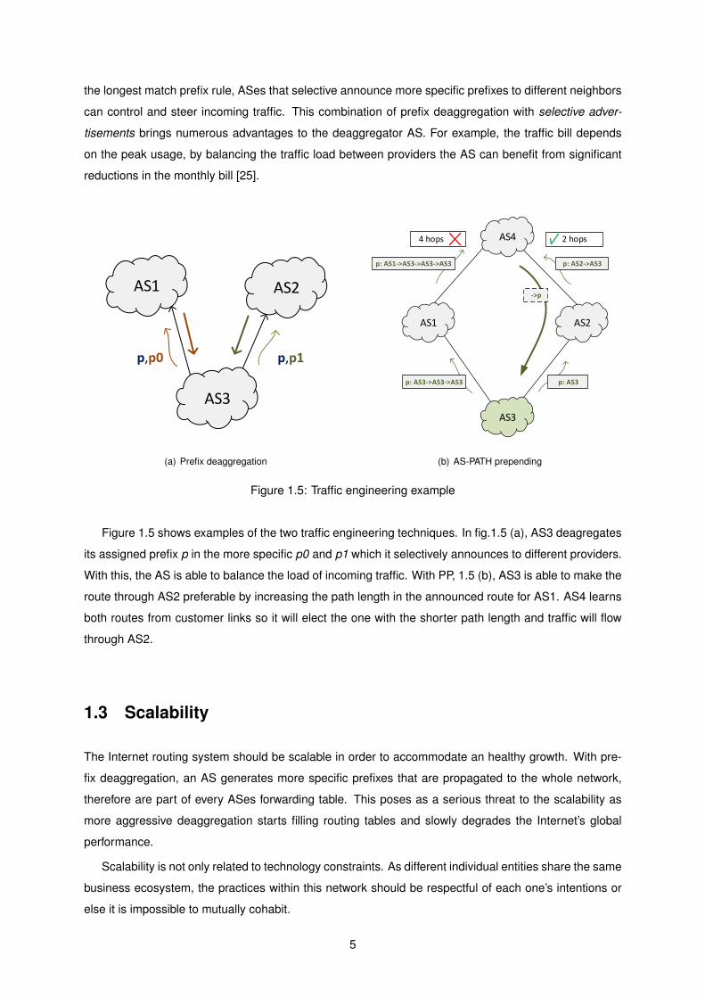
the longest match prefix rule, ASes that selective announce more specific prefixes to different neighbors

can control and steer incoming traffic. This combination of prefix deaggregation with selective adver-

tisements brings numerous advantages to the deaggregator AS. For example, the traffic bill depends

on the peak usage, by balancing the traffic load between providers the AS can benefit from significant

reductions in the monthly bill [25].

AS1 AS2

AS3

p,p0 p,p1

(a) Prefix deaggregation

2 hops

AS1 AS2

AS3

AS4

p: AS3p: AS3->AS3->AS3

p: AS1->AS3->AS3->AS3 p: AS2->AS3

->p

4 hops

(b) AS-PATH prepending

Figure 1.5: Traffic engineering example

Figure 1.5 shows examples of the two traffic engineering techniques. In fig.1.5 (a), AS3 deagregates

its assigned prefix p in the more specific p0 and p1 which it selectively announces to different providers.

With this, the AS is able to balance the load of incoming traffic. With PP, 1.5 (b), AS3 is able to make the

route through AS2 preferable by increasing the path length in the announced route for AS1. AS4 learns

both routes from customer links so it will elect the one with the shorter path length and traffic will flow

through AS2.

1.3 Scalability

The Internet routing system should be scalable in order to accommodate an healthy growth. With pre-

fix deaggregation, an AS generates more specific prefixes that are propagated to the whole network,

therefore are part of every ASes forwarding table. This poses as a serious threat to the scalability as

more aggressive deaggregation starts filling routing tables and slowly degrades the Internet’s global

performance.

Scalability is not only related to technology constraints. As different individual entities share the same

business ecosystem, the practices within this network should be respectful of each one’s intentions or

else it is impossible to mutually cohabit.

5

Route aggregation

Route aggregation refers to the practice of substituting a set of routes pertaining longer prefixes with a

aggregating route for a less specific prefix. This is achieved by filtering, but it should be done in a careful

way so that the filtered state is as consistent as possible with the standard state. For every filtered prefix,

q, the filtered state is said to be route consistent if the route type for every q-route does not change.

Good route aggregation strategies are able to filter a big portion of prefixes and still achieve a route

consistent state.

1.4 Related Work

The research community has devoted significant efforts to the study of the global impact of address

fragmentation. The negative impacts of an increasing number of announced prefixes have been known

for long [15] . Studies show that the growth of BGP routing tables pose a serious threat for scalability of

the global system with its decreasing packet forwarding speed and demand for more memory space.

Despite the negative side to it, prefix deaggregation can bring serious rewards. Recent works study

the economical incentives for prefix deaggregation. Lulu et al. [25] shows that prefix deaggregation

can have the advantageous side effect of reducing traffic expenses. Deaggregated prefixes allow for a

better control of inbound traffic lowering fluctuations that can cause peak traffic usage taxed at higher

rates. Lutu el al. [26] also showed in a followup work that prefix deaggregation by a customer can

negatively impact the business of the associated provider. Bangera et al. [14] analyses incentives of

transit providers for deaggregating customer’s prefixes in order to attract more traffic.

Some works explore the competitive economical interactions between domains using game-theoretic

perspectives. Kalogiros et al. [22] use a small scale example to show that if an AS decides to deaggre-

gate prefixes, others will have incentives to follow even if they all end with lower benefits.

With many studies showing incentives for prefix deaggregation it seems that one should expect

increasing popularity for prefix deaggregation or traffic engineering over time. Moreover, as in inter-

domain scenarios the local interests are preferred to the global ones, that seems like a fairly plausible

assumption. Cittadinni et al. [16] aimed to challenge widespread assumptions like this. The study is

mostly based on observation of experimental results, showing that there is no evidence to support such

claims.

In order to reduce the number of routes due to prefix deaggregation one can look at route aggrega-

tion strategies. The state of the art in terms of route-aggregation is DRAGON [21] (Distributed Route

Aggregation on the Global Network). DRAGON is able to achieve a set of goals that distances it from

previous approaches namely that it works with BGP, its incrementally deployable and provides algo-

rithms for reaching route consistent states, all of this while being able to reduce the number of prefixes

in each AS by up to 80%. It can also be adapted for TE, an option we will explore in chapter 5.

6

1.5 Contributions

This work provides an in-depth study to the TE practices with focus on the scalability problem by doing

an experimental assessment, impact evaluation and finally present a mitigating solution.

First, we survey the publicly available data sources and portrayed the evolutionary and current state

of the Internet with an analysis to the address space and a prefix characterization. Because these

statistics could be helpful for future studies we created a web platform in order for these results to be

publicly available and automatically updated.

In the assessment study we had to overcome the problem of working with large amounts of complex

BGP data. Its main challenge was to create efficient algorithms in order for this study to be computa-

tionally possible with our limited resources. Most assessment studies focus on the IPv4 network, we go

further and also evaluate the IPv6 case due to its growing popularity and importance in the future.

TE is then evaluated for the scalability impact, in particular for global reachability, routing table sizes

and the changes to the route type and path length. Specifically for prefix deaggregation, we simulated

the distortion to the route type and path length using the publicly available Internet’s inferred topology.

Given the multiple scenarios in which an AS can use TE to control inbound traffic, we also contributed

with an impact simulator application that allows the user to test TE configurations on real topologies and

instantly observe its global effects.

Route aggregation strategies are always looked by ASes with apprehension that, in order to obtain

significant global gains, these strategies may interfere with their businesses. Also, these may require

significant changes to today’s routing architecture which dramatically discourages adoption. With this

in mind, we showed how to adapt one of the most promising route aggregation strategies, DRAGON,

specifically for use with TE. When prefix deaggregation is applied, we were able keep the deaggregated

prefixes only for a small number of ASes making room for huge global gains while maintaining routing

consistency with just minimal and local policy changes.

7

8

Chapter 2

Snapshot of the Internet

The aim of this chapter is to provide the necessary tools to guide us on the TE study. First, we will

explore the characteristics of public data sources available, and how these can be used to serve our

purposes. Then, we will present some algorithms related to the BGP elected route process to be used

in the Internet’s characterization as well as part of the TE’s impact and solution study. The next step is to

compute some statistics to better understand the current state of the Internet, in particular its structure,

address space and prefix type. Finally, it is presented a web platform that automatically generates

some of these measurements and it is publicly available so it can be used for consultation in future

studies.

2.1 Data Sources

From the publicly available data sources it is possible to separate them in two groups, raw data and pro-

cessed data. The Internet relies on a number of protocols to function and these require the exchange

of state information as well as specific machine configurations that we can gather. In itself, this raw

data is not very useful for studying but can serve as basis to be further processed and serve multiple

applications.

2.1.1 Raw Data

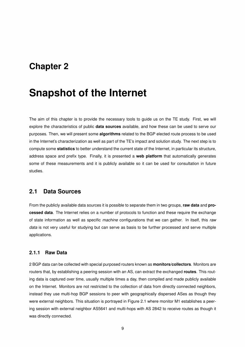
2 BGP data can be collected with special purposed routers known as monitors/collectors. Monitors are

routers that, by establishing a peering session with an AS, can extract the exchanged routes. This rout-

ing data is captured over time, usually multiple times a day, then compiled and made publicly available

on the Internet. Monitors are not restricted to the collection of data from directly connected neighbors,

instead they use multi-hop BGP sessions to peer with geographically dispersed ASes as though they

were external neighbors. This situation is portrayed in Figure 2.1 where monitor M1 establishes a peer-

ing session with external neighbor AS5641 and multi-hops with AS 2842 to receive routes as though it

was directly connected.

9

AS2842

AS5641

Multi-hop BGP

Route adv.

AS5641

AS5641

...

Peering ASesprefix 1

Routes

prefix nMonitor

Figure 2.1: Monitoring Architecture

The most popular sources for route data are the RouteViews[8] (RV) and RIPE-RIS [9] projects.

RIPE-RIS has 16 route monitors spread throughout the world. Each of these peer with dozens of ASes

directly or through multi-hop, creating a huge monitoring network. The RV project has a similar purpose

but most of the monitors (hosts) are in the United States, this is not an issue as with multi-hop, monitor’s

location is not a constraint for geographic diversity. The monitor that gathers more routes is host number

2[10] which offers merged routing data collected from 36 ASes. Each collection is updated every 2 hours

for routes and every 15 minutes for BGP updates, since 2001. Besides IPv4, they also provide data on

IPv6.

(a) Sample collected route

AS137

6939

AS40191

AS40191

Monitor

130.136.0.0/16

130.136.0.0/16

(b) Route path

Figure 2.2: Monitor data example

Figure 2.2 shows a simple example of the data format captured by one of these monitors. Route

for prefix 130.136.0.0/16 was originated by AS 137 (last in the ASPATH) and collected from AS 40191

(peering AS).

The fact that each route carries the AS-PATH parameter may lead us to believe that it is possible to

have a complete view of the Internet’s connections and easily infer it’s topology. That is not achievable as

the collected routes are the elected routes at the peering AS and the path associated with the routes

that were not elected do not reach the monitor and therefore some connections may be hidden[27].

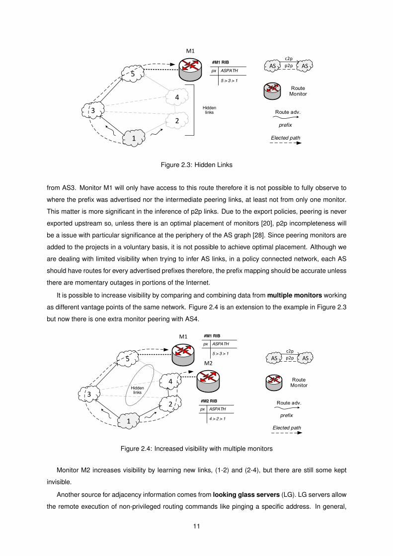
Figure 2.3 shows a simple demonstration of this problem.

AS1 advertises some prefix p to both providers AS3 and AS2. AS5 learns a customer route for p from

AS3 and AS4. Both routes are of the same type, so AS5 will elect the shorter which is the one learned

10

1

3

5

4

2

M1

ASASc2pp2p

Route Monitor

Route adv.

prefix

Elected path

#M1 RIB

px ASPATH

5 > 3 > 1

Hiddenlinks

Figure 2.3: Hidden Links

from AS3. Monitor M1 will only have access to this route therefore it is not possible to fully observe to

where the prefix was advertised nor the intermediate peering links, at least not from only one monitor.

This matter is more significant in the inference of p2p links. Due to the export policies, peering is never

exported upstream so, unless there is an optimal placement of monitors [20], p2p incompleteness will

be a issue with particular significance at the periphery of the AS graph [28]. Since peering monitors are

added to the projects in a voluntary basis, it is not possible to achieve optimal placement. Although we

are dealing with limited visibility when trying to infer AS links, in a policy connected network, each AS

should have routes for every advertised prefixes therefore, the prefix mapping should be accurate unless

there are momentary outages in portions of the Internet.

It is possible to increase visibility by comparing and combining data from multiple monitors working

as different vantage points of the same network. Figure 2.4 is an extension to the example in Figure 2.3

but now there is one extra monitor peering with AS4.

1

3

5

4

2

M1

ASASc2pp2p

Route Monitor

Route adv.

prefix

Elected path

#M1 RIB

px ASPATH

5 > 3 > 1

Hiddenlinks

M2

#M2 RIB

px ASPATH

4 > 2 > 1

Figure 2.4: Increased visibility with multiple monitors

Monitor M2 increases visibility by learning new links, (1-2) and (2-4), but there are still some kept

invisible.

Another source for adjacency information comes from looking glass servers (LG). LG servers allow

the remote execution of non-privileged routing commands like pinging a specific address. In general,

11

these servers do not allow full BGP table dumps as some information is intentionally kept secret.

A more reliable source for adjacency are the Internet Routing Registries (IRR). IRRs are public

databases where AS administrators manually register adjacency and policy information. The data is

inserted using the Routing Policy Specification Language (RPSL) [11]. The problem with this databases

is that they are used in a voluntary basis which may lead to inaccuracies or even intentional misinforma-

tion. From these, one of the more trustworthy source is the RIPE database. Usually, each RIR provides

a web interface to access its data but they can also be queried using the whois protocol.

RCCN

INESC

RCCN

GEANT

RCCN NOS

Customer

Provider

Peer

Figure 2.5: Sample IRR query using the whois command

Figure 2.5 shows a query from the RIPE database (whois.ripe.net) for AS 1930 belonging to FCCN,

a Portuguese foundation for national scientific computing. From the import/export rules it is possible to

infer on the relationships with the adjacent ASes. For example with INESC (AS5516) there is a rule for

exporting all the routes to this AS suggesting this to be a provider to customer relationship.

2.1.2 Processed data

Internet’s Inferred topology

One of the more demanded applications for the routing data is the inference of the Internet’s AS rela-

tionships. Research community has devoted significant efforts in the search for algorithms that better

portray the Internet’s topology, the ones with better results are the datasets provided by UCLA [12] and

CAIDA [5]. CAIDA’s algorithm was recently (2013) improved in a way that it outperforms all the existing

datasets, including UCLA’s [24]. Both use BGP data collected from RouteViews and RIPE-RIS.

As the main source for this algorithms is the BGP data collected from monitors, the problem with

hidden links is carried on to the topology making it particularly incomplete in p2p links. Giotsas et al.[19]

studied 13 large European IXP’s in search for p2p links by mining BGP communities used by Internet

eXange Points (IXPs) route servers to implement multilateral peering. The study produced four times

more peer links than what was directly observable from BGP data. IXPs are routing points where ASes

connect to establish peering relationships between them.

These algorithms have a similar structure. To give a general idea on how they work, they first infer the

Tier-1 clique (Tier-1 nodes that establish peering relationships between each pair). Then, route paths

12

from these nodes are analyzed because these should be related to customer routes as peer routes are

not exported upstream. So, in a top-down approach, c2p links are then inferred (customer cone) and the

remaining links are set as p2p.

These studies focus on the IPv4 network and the algorithms cannot be directly exported to infer the

IPv6 topology. IPv6 is still maturing and one important difference between networks is that the IPv6 has

long standing peering disputes between Tier-1 ASes [13] making the IPv6 graph not fully connected and

as such without an obvious clique. In a recent study [18] (2015), CAIDA proposed a way to infer the IPv6

topology by adapting the IPv4 algorithm to cope with IPv6’s constraints but unfortunately these datasets

are still not publicly available.

Prefix to AS mapping

In order to study the prefix distribution and better characterize how these are being generated one

can associate the advertised prefix to the origin AS. These mappings can be easily extracted from the

monitor’s BGP data by combining the PREFIX entry with the last AS (origin) on the ASPATH. CAIDA[4]

provides this prefix to AS mapping using the RV monitors as source.

2.2 Elected Route Algorithm

In order to simulate routing on the Internet one has to devise an algorithm that mimics the BGP elected

route procedure. Since in this process each attribute is sequentially evaluated, first the route type and

only after the path length, this algorithm can be divided in two parts. One that only calculates the elected

route type and other for the path length. There are advantages in breaking the problem this way, one is

that most of our statistics only care for the elected route type which is fairly simpler to compute than the

path length. Another aspect is that we can actually use the output from the elected route type to simplify

and more efficiently extract the path length.

2.2.1 Elected Route type

Throughout our study, we made some assumptions on the characteristics of the Internet topology,

namely that it is policy-connected (there is a route for every pair of nodes) as well as there are no

customer-provider cycles (elected route algorithms terminate). But, as pointed out from some studies

[30], there are some mismatching between our beliefs and the attributes of available datasets.

With this in mind, before jumping into the data sources, these must be corrected with minimum bias

to the network. A previous work [31] proposed an algorithm to overcome this issue. The main ideia

behind this algorithm is to transverse customer paths until an AS that is already present in the path

is detected thus forming a cycle and the corresponding link is removed. The output of this algorithm

creates a network without customer-provider cycles and ensures that it is policy connected even if some

nodes need to be removed.

13

The algorithm we will use for electing the route’s types assumes the GR routing policies. Since we

are only interested in evaluating the type, the only parameter that matters is the business relationship

with the forwarding neighbor.

The following is a all-to-one approach, as we want to reason on the global impact from the TE

practices of a single AS. In a policy connected network, every pair of nodes is joined by at least a

provider route. Since most ASes on the Internet are stubs [31], these can only elect provider and

possibly peer routes. So, it is expected that averaging on all nodes they will mostly be connected by

provider paths. With this uniqueness in mind, an efficient procedure is to focus in finding the ones that

do not have a provider route, which are therefore joined by customer or peer paths.

A node that can reach the destination using only customer links will always prefer a customer route.

This node, P-node, will be a provider to some degree of the destination. In the GR export policy, only

P-nodes export the destination route to peering neighbors. A peer node of a P-node will elect a peering

route only if it is not itself a P-node, in that case it prefers the customer route. Every other node that is

not a P-node or a peer of a P-node will maintain the provider route estimation.

Algorithm 1 Algorithm for computing the type of the elected route from all nodes to a single destination1: function ELECTEDROUTETYPE(Graph G, Node dest)2: Queue toVisit3: Array routeType[G.nNodes] . Array to store the route type of each starting node

4: for each v in G do5: routeType[v]← P . Initialize with the worst estimation

6: toVisit.add(dest)7: while toVisit is not empty do8: v← toVisit.deQueue()9: for each p in v.providers do . P-nodes of P-nodes know customer route

10: if routeType[p] is worse than C then11: routeType[p]← C12: toVisit.enQueue(p) . Add new P-node to visit13: for each r in v.peers do . peers of P-nodes know peer route14: if routeType[r] is worse than R then15: routeType[r]← R16: return routeType

For a single destination, the algorithm only visits each P-nodes once where it sweeps through all

its peering neighbors thus, the complexity of this algorithm is proportional to the product of these two

variables. It is expected that nodes down the Internet’s hierarchy will globally change more route type

estimations as there are more indirect providers to visit. On the opposite side, for tier-1 ASes only its

peering neighbors will change the estimation.

2.2.2 Elected Route with path length

The following is an approach to efficiently compute the distance from one-to-all nodes.

In order to transverse the Internet graph, one can do a Breath First Search (BFS) starting at a single

node and moving through the allowed links in a way that mimics the advertisement of routes. Note that

not all links are usable, for example if we reach a node via a peer link, we cannot further visit its peers or

14

providers because the route was only advertised to its customers. Our model assumes that there are no

customer-to-provider cycles and edges have same unitary weight. Note that peering links do not create

cycles, as routes learned from peers are only exported to customers and not to other peers or providers.

On the Internet, given its unique business dynamics, the elected route is not necessarily the shortest

in path length. Applying a BFS to this network would indeed return the shortest distance to a single

node, but it would possibly have to do multiple visits to a node before arriving at the final distance in

order to satisfy the elected route type. Imagine we transverse the network using a BFS and reach a

node via a peer link. The distance is propagated to its customers but, as the BFS progresses we reach

the same node at a longer but more preferred customer route. Therefore, we would then have to change

all of the customer’s distance estimations. If we knew beforehand that the node elects a customer route,

we wouldn’t bother to visit the node’s customers and would wait for a future iteration. As so, we can

take advantage in knowing what is the elected route type for each node before running the distance

algorithm. In fact, we can erase some of the neighbor links that are not possible given the elected type.

A node that elects a peer route must have learned it from a peering neighbor with customer route. There

is no point in using the provider links to reach this node since we already know that they are not part of

the elected route. If we give a direction to the links based on the direction of the route advertisements

we create a Directed Acyclic Graph (DAG). This is a graph that takes into consideration, not only the

policies but also the route types. A BFS on a DAG with edges of unitary weight gives at each iteration

the shortest distance to a single node.

To graphically visualize how the algorithm transforms the network let us take a look at the following

example.

C

C

C C

R

R

P

P

C

1

2

1 2

3

2

2

1

0

Origin Origin

C

P2P

R

C

C2P

C

P X

C R P

Route Type

N

Path length

Figure 2.6: Transformation to a DAG

The left of figure 2.6 exhibits a sample network showing at each node the elected route type. In the

center is shown how to assign directions to the links in order to create a DAG. These come from the

direction of the route advertisements. For instance, a node that elects a customer route further forwards

it to all its neighbors, so the direction should point away from this node. The right side shows the path

length at each node resulting from a BFS starting at the origin.

15

Taking all of this into consideration we are now in the position to create an algorithm to efficiently

compute the shortest distance for the elected route. Algorithm 1 is used to process the elected route

type. One way to implement the aforementioned algorithm is by using two queues, one for the current

level of the BFS and the other for the next level as they have different associated lengths. They switch

functions at each iteration. Nodes are marked as visited before being added to the queue in order to

prevent duplication that can originate unnecessary en/dequeuing. Neighbors are visited according to

the allowed connections as seen in figure 2.6.

Algorithm 2 Algorithm for computing the length of the elected route from all nodes to a single destination1: function ELECTEDROUTEDISTANCE(Graph G, Node dest)2: Array routeType[G.nNodes] = ElectedRouteType(G, dest)3: Queue toVisit[2] . One for each level4: Array routeDst[G.nNodes] . Array to store the shortest distances of the elected route

5: for each v in G do6: v.visited ← False7: len← 08: toVisit[len % 2].enQueue(dest)9: while toVisit[len % 2] is not empty do

10: v← toVisit[len % 2].deQueue()11: routeDst[v]← len12: if routeType[v] = C then . Only nodes with C type export to providers and peers13: for each p in v.providers do14: if p not visited then15: p.visited ← True16: toVisit[(len+1) % 2].enQueue(p)17: for each r in v.peers do18: if r not visited and routeType[r] = R then19: r.visited ← True20: toVisit[(len+1) % 2].enQueue(r)21: for each c in v.customers do22: if c not visited and routeType[c] = P then23: c.visited ← True24: toVisit[(len + 1) % 2].enQueue(c)25: if toVisit[len % 2] is empty then26: len++27: return routeDst

16

2.3 Statistics

2.3.1 Address Space

In order to understand the current state for the address space on both IP versions, figure 2.7 shows this

distribution by mask size and also from two previous years. Note that IPv4 space is near exhaustion

whereas IPv6 is still far from reaching its capacity.

0%5%

10%15%20%25%30%35%40%45%50%

/16 /17+/31 /32 /33+/47 /48

%-of-a

dvertised-prefixes

Mask

IPv6

2013 2014 2015

0%

10%

20%

30%

40%

50%

60%

/8 /9+/15 /16 /17+/23 /24

%-of-a

dvertised-prefixes

Mask

IPv4

2013 2014 2015

Figure 2.7: Address space distribution

The distribution by mask size for IPv4 and IPv6 is very different, IPv4 is mostly concentrated between

the mask size 16 and 24 (8 bits) whereas in IPv6 if falls into a much wider interval mostly from 32 to 48 (16

bits), meaning that in IPv6 there are 8 more bits to further deaggregate prefixes. If prefix deaggregation

is not performed in a responsible way this can lead into and even greater problem to the scalability than

the already observed for the IPv4 case. If this is not alarming enough, comparing the distribution from

previous years, it is possible to observe the slow increase of prefixes with the maximum mask size, a

sign of possible deaggregation.

2.3.2 Prefix type

Let us introduce classes of prefixes to help us with the characterization.

17

AS3

AS1 AS2

ASASc2pp2p

123.44.0.0/16123.44.0.0/24 123.45.0.0/16

123.44.1.0/24

Figure 2.8: Sample network

The prefix classes are:

• Lonely A prefix that is not itself covered by a less specific nor covers more specific prefixes.

(123.45.0.0/16)

• Top A prefix that is not itself covered by a less specific but covers at least one more specific prefixs.

(123.44.0.0/16)

• Deaggregated A prefix that is covered by a less specific prefix, and this less specific is originated

by the same AS as the deaggregated prefix. (123.44.0/24)

• Delegated A prefix that is covered by a less specific, and this less specific is not originated by the

same AS as the delegated prefix. (123.44.1/24)

The total number of announced prefixes is, as of October of 2015, of more than 512k, so in order to

assign the advertised prefixes to the aforementioned classes we need to find an efficient representation

of such a large number of entries. We will use as source the CAIDA’s prefix-to-AS mapping. This

dataset has some inaccuracies regarding the represented prefixes so it needs to be pre filtered, for

example prefixes with mask larger than 24 for IPv4 which is not allowed in BGP.

An approach to this problem is to explore the bitwise nature of the prefixes. The proposed way to

do it is by using a binary tree, called binary prefix tree. In this tree, nodes represent prefixes and have

two children, left and right, representing each bit state. A prefix is inserted in the tree by analyzing each

successive bit in the prefix and flowing through the left and right child until there are no bits left. Levels

in this tree are directly related to the length of the prefix. Each announced prefix has information about

the originating AS. This way, all leaf nodes are announced prefixes, but internal nodes can also be. For

a prefix p, the aggregated prefix of p is the announced more specific prefix that covers p. In example

2.8, 123.44.0.0/16 is the aggregated prefix of 123.44.0.0/24 and 123.44.1.0/24. In the data structure,

123.44.0.0/23 is the aggregated node that represents a prefix that is not announced, it is just used for

data structure convenience hence the origin parameter is left to none.

Figure 2.9 shows a graphical representation of this data structure for the example in Figure 2.8.

18

123.44.0.0/15Origin: - | Agg: -

.00101100.

123.44.0.0/16Origin: AS1 | Agg: -

.00101100. .00101101.

123.45.0.0/16Origin: AS2 | Agg: -

0 1

123.44.0.0/23Origin: - | Agg: AS1

.00000000.

123.44.0.0/24Origin: AS1 | Agg: AS1

.00000000. .00000001.

123.44.1.0/24Ori: AS2 | Agg: AS1

0 1 (…)

0

Figure 2.9: Prefix Tree example

Using this procedure we got the following distribution of prefixes by the different types.

TOP6% DEL

13%

LON44%

DEA37%

IPv4TOP6% DEL

9%

LON64%

DEA21%

IPv6

Figure 2.10: Prefix type distribution

Lonely class take the majority of the announced prefixes with an even bigger portion on IPv6. Scal-

ability threats are strongly related with deaggregation, the situation is more severe for IPv4 with 37% of

deaggregated prefixes. At this point it is hard to compare these two protocols and jump to conclusions

as IPv6 is in an early phase as IPv4 still announces 24 times more prefixes than its upgraded version.

For the purposes of this study it is also important to introduce the notion of aggregated and deaggre-

gated child prefixes. An aggregated prefix is a prefix that covers some more specific prefixes and these

prefixes are originated from the same AS. This separation is important because aggregated prefixes

are prefixes that were deagreated for some reason. From the previously defined classes, aggregated

prefixes are part of the Top and Delegated as portrayed on figure 2.11 using the prefix tree notation.

The actual portion of aggregated prefixes from these classes is shown in table 2.1

Type Subtype #IPv4 %IPv4 #IPv6 %IPv6

TOP Aggregated 28783 5.23% 1121 4.60%Lonely 5530 1.0% 256 1.05%

DELEGATED Aggregated 2663 0.48% 47 0.19%Lonely 71209 12.93% 2142 8.79%

Table 2.1: Prefix subtype distribution

Most of the aggregated prefixes come from the Top type. In IPv4, 5.71% of the total prefixes are ag-

19

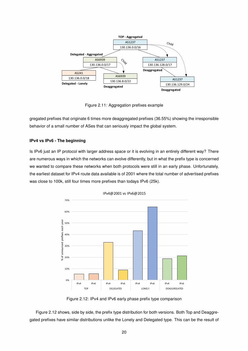
AS1237

130.136.0.0/16

AS6939

130.136.0.0/17

AS1237

130.136.128.0/17

AS1237

130.136.129.0/24

AS6939

130.136.8.0/22

TOP - Aggregated

Deaggregated

Deaggregated

Deaggregated

Delegated - Aggregated

AS241

130.136.0.0/18

Delegated - Lonely

Figure 2.11: Aggregation prefixes example

gregated prefixes that originate 6 times more deaggregated prefixes (36.55%) showing the irresponsible

behavior of a small number of ASes that can seriously impact the global system.

IPv4 vs IPv6 - The beginning

Is IPv6 just an IP protocol with larger address space or it is evolving in an entirely different way? There

are numerous ways in which the networks can evolve differently, but in what the prefix type is concerned

we wanted to compare these networks when both protocols were still in an early phase. Unfortunately,

the earliest dataset for IPv4 route data available is of 2001 where the total number of advertised prefixes

was close to 100k, still four times more prefixes than todays IPv6 (25k).

0%

10%

20%

30%

40%

50%

60%

70%

IPv4 IPv6 IPv4 IPv6 IPv4 IPv6 IPv4 IPv6

TOP DELEGATED LONELY DEAGGREGATED

%7of7a

nnounced7prefixes7each7year7

IPv4@20017vs7IPv6@2015

Figure 2.12: IPv4 and IPv6 early phase prefix type comparison

Figure 2.12 shows, side by side, the prefix type distribution for both versions. Both Top and Deaggre-

gated prefixes have similar distributions unlike the Lonely and Delegated type. This can be the result of

20

fundamental differences in the prefix assignment policy. IPv6 has a much larger address space so there

is plenty of unrelated space to assign.

21

2.4 InterSnap web platform

The Internet is a ever changing environment, that is why it is so important for related studies to first

assess on its current status. The public data sources discussed are automatically updated on a regular

basis. Using this material, some websites [6] provide automatically-generated statistics on the state of

the Internet. CAIDA has recently unveiled a project[3] aimed at providing a framework for Live BGP Data

Analysis. Still, these are very general results that may not apply to all applications. As so, we though

of publicly providing a web platform to show some statistics from this thesis through time as multiple

snapshots of the Internet. The project goals include automatic updates, appealing interface and room

for future integrations. Taking all of this into account the InterSnap [7] platform was created.

InterSnapwebserver

User

CAIDA web directories

HTT

P

SQL database

Query the database

Date

IPver

Stats

Retrieve Stat(Fast)

If not on the database

Fetch file and compute Stat

(Slow)

Figure 2.13: InterSnap web architecture

The InterSnap web server uses open source software hosted on a free cloud platform. As support,

it uses an SQL database with pre-processed data that is automatically updated every year by directly

fetching the files from the CAIDA’s directories and applying the statistics algorithms. It currently provides

statistics on the Address Space, Prefix type to both IP versions and Network information for IPv4.

Figure 2.14: InterSnap screenshot

22

Chapter 3

Experimental Assessment of TE

It is well known the TE techniques for inbound traffic control and its threats to scalability. However, only

by observing the prevalence and the way these practices are actually being used on the Internet can we

infer on its significance to better evaluate the real impact and try to propose a solution.

This chapter is responsible for the assessment of TE and it is divided in two parts. First we will

explore an assessment methodology to show how these practices can be extracted by studying the

footprints left on the Internet from real BGP data. Only after can we put into practice this methodology in

order to extract relevant statistics and better analyze its results. More specifically, we plan to examine

the use of both techniques, explore the relationship between TE and prefix deaggregation as well as

observe its evolution and trending given its implications on the Internet’s future.

3.1 Assessment methodology

It is not possible to have a full view of each AS advertisement policies in order to observe how TE is being

used. RIR registries are not mandatory and some special adjustments are key to the ASes business

strategy so they are kept secret. However, every AS has to speak BGP so, it is possible to get an idea

on how routes were advertised by doing an in-depth study on real BGP-route data collected from route

monitors even if that means working with gigabytes of raw information. From the elected RIB entries we

will analyze some of its route parameters, the PREFIX, FROM, and ASPATH.

We will use the data collected from host 2 of the RV project. We could also combine this with the

RIPE-RIS source, although with a different syntax, they show the same route parameters but there is

little gain in doing so. Data from the different sources are collected the same way, they do not result

from applying different algorithms as with the Internet’s inferred topology. For that reason, there is a high

level of redundancy between sources, although the more monitors indeed give a more complete view of

the Internet, one of the aims of the RV project is to provide enough diversity of monitors to serve a great

variety of studies. So, by merging data from different sources we are doubling the size of an already

complex data source only to slightly better our results, therefore we decided not to do it.

23

3.1.1 Selective advertisements

Deaggregation without selective advertisements

When deaggregation is used without TE intention, all the prefixes are advertised to all providers in order

for those links to be equally preferred. When this occurs, in every monitor, the elected route for all the

deaggregated as well as the aggregated prefixes must display the same last-hop neighbor. Figure 3.1

portrays how monitors may receive these routes in this circumstance.

AS1

M3

AS3

AS2

M2

p,p0

p,p0

p,p0 #M3 RIB

px ASPATH

p 3 > 1p,p0

#AS2 RIB

px typ len ASPATHp C 1 1 C 2 3>1

#AS3 RIB

px typ len ASPATH

p C 1 1

#M2 RIB

px ASPATH

p 2 > 1

p0 C 1 1 P 2 2>1

p0 C 1 1 C 3 3>1

P 2 2>1

p0 2 > 1

p0 3 > 1

ASASc2pp2p

Route Monitor

Route adv.

prefix

Figure 3.1: Prefix deaggregation without selective advertisements

A p-route and p0-route is advertised to both providers. In this way, the preference of routes is the

same for all the advertised prefixes so every node will elect routes that transversed the same paths.

Depending on the monitor’s position on the Internet, the last-hop neighbor will either be AS1 or AS2.

The only case when this is not true is if some nodes apply different policies based on the prefixes and

not only on the route attribute, which we believe to be an unlikely scenario.

Deaggregation with selective advertisements

In the case where deaggregation is combined with selective advertisements, routes for the advertised

prefixes may follow different paths. The consequence is that in every monitor, the elected route for the

deaggregated and selectively advertised prefix must display the same last-hop neighbor. Let us take on

the classic example portrayed in Figure 3.2 where an AS breaks down p’s address space in the more

specific p0 and selectively announces it to provider AS3.

24

AS1

M3

AS3

AS2

M2

p,p0

p,p0

#M3 RIB

px ASPATH

p 3 > 1p

#AS2 RIB

px typ len ASPATHp C 1 1 C 2 3>1

#AS3 RIB

px typ len ASPATH

p C 1 1

#M2 RIB

px ASPATH

p 2 > 1

p0 C 1 1

p0 C 1 3>1

P 2 2>1

p0 2 > 3 > 1

p0 3 > 1

p,p0

ASASc2pp2p

Route Monitor

Route adv.

prefix

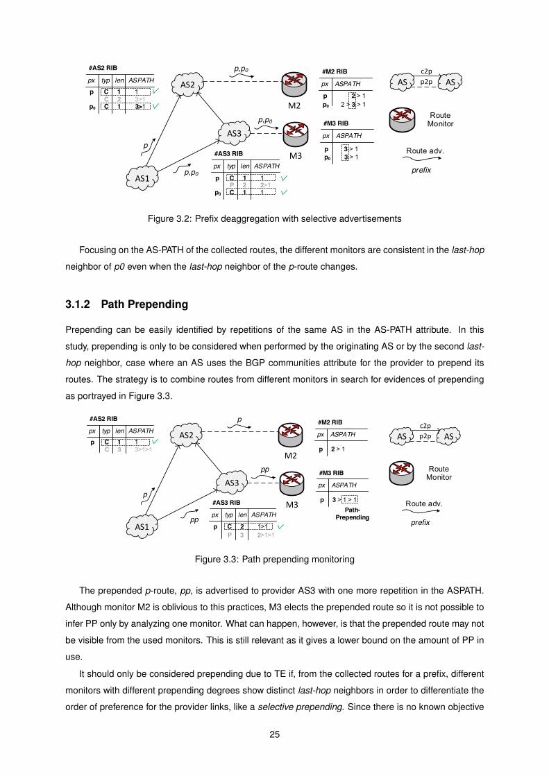
Figure 3.2: Prefix deaggregation with selective advertisements

Focusing on the AS-PATH of the collected routes, the different monitors are consistent in the last-hop

neighbor of p0 even when the last-hop neighbor of the p-route changes.

3.1.2 Path Prepending

Prepending can be easily identified by repetitions of the same AS in the AS-PATH attribute. In this

study, prepending is only to be considered when performed by the originating AS or by the second last-

hop neighbor, case where an AS uses the BGP communities attribute for the provider to prepend its

routes. The strategy is to combine routes from different monitors in search for evidences of prepending

as portrayed in Figure 3.3.

AS1

M3

AS3

AS2

M2

pp

p

pp #M3 RIB

px ASPATH

p 3 > 1 > 1p

Path-Prepending

#AS2 RIB

px typ len ASPATHp C 1 1 C 3 3>1>1

#AS3 RIB

px typ len ASPATH

p C 2 1>1

#M2 RIB

px ASPATH

p 2 > 1

P 3 2>1>1

ASASc2pp2p

Route Monitor

Route adv.

prefix

Figure 3.3: Path prepending monitoring

The prepended p-route, pp, is advertised to provider AS3 with one more repetition in the ASPATH.

Although monitor M2 is oblivious to this practices, M3 elects the prepended route so it is not possible to

infer PP only by analyzing one monitor. What can happen, however, is that the prepended route may not

be visible from the used monitors. This is still relevant as it gives a lower bound on the amount of PP in

use.

It should only be considered prepending due to TE if, from the collected routes for a prefix, different

monitors with different prepending degrees show distinct last-hop neighbors in order to differentiate the

order of preference for the provider links, like a selective prepending. Since there is no known objective

25

for PP besides TE, we expect this to be the majority of the cases.

Prepending and Deaggregation

A combination of both techniques can also be used to have a finer control of inbound traffic, but when

prepending is used, it is not possible to distinguish selective from unselective advertisements. The

problem arises from the fact that when prepending is used the preference of routes are altered in a way

that in some circumstances it may be confused with selective advertisement practices. Let us look at

the practical example of figure 3.4.

AS1

M3

AS3

AS2

M2

p,p0

p,p0

p,p0

#M3 RIB

px ASPATH

p 3 > 1

p,pp0

#AS2 RIB

px typ len ASPATH

p C 1 1 C 2 3>1

#AS3 RIB

px typ len ASPATH

p C 1 1

#M2 RIB

px ASPATH

p 2 > 1

p0 C 1 1

P 4 2>1>1>1

p0 C 2 3>1

C 3 1>1>1

P 2 2>1

p0 2 > 3 > 1

p0 3 > 1

≠

Selective Adv.

ASASc2p

p2p

Route Monitor

Route adv.

prefix

Figure 3.4: Path prepending and prefix deaggregation monitoring

Suppose that AS1 wants to reduce the order of preference of the provider link to AS2 only for a

specific address space covered by p0. The p-route is advertised to both providers as well as the p0-

route, but to the p0-route to AS2, 2 more repetitions of AS1 are injected in the ASPATH attribute.

Looking at the monitor’s output we see that it is exactly the same as the one from the example

with deaggregation and selective advertisements (fig. 3.2). The prepended route was never elected

at a monitor’s peering AS. AS2 elects a customer p0-route from both AS1 and AS3 but, although it

is directly connected to AS1 from where it also learns p, the fact that the route is prepended makes

the route less preferred to the one learned from AS3. This way, the p-route and p0-route are elected

at AS2 with distinct last-hop neighbors just like the situation where p0 is selectively advertised. We

cannot differentiate the techniques used but we can conclude that the routes were deaggregated for

traffic engineering purposes.

3.1.3 Procedure

In order to assess TE using that previous analysis, we relied on a set of data structures and computa-

tional procedures. The data structure used for storing information is similar to the binary prefix tree used

for prefix classification in section 2.3.2, for a fast access to specific prefix entries. In this case, each of

the tree-nodes has to store some ASPATH-related variables like the last-hop neighbor. For each monitor,

a tree of this kind is created and then, the combined results are stored in a master tree. For example

26

(fig. 3.5), imagine a prefix p and its deaggregated p0. When no prepending is observed, if a monitor

finds distinct last-hop neighbors for any of the prefixes we are in a situation of selective advertisements

therefore, the master -tree can be updated with this result.

M 2351 M 5412

Prefix : pL-H : 3 Prep : N

Prefix : p0L-H : 2 Prep : N

Master

Sele : Y GPrep : N

Prefix : pL-H : 3 Prep : N

Prefix : p0L-H : 3 Prep : N

Sele : N GPrep : N

Prefix : p

Prefix : p0Prep : N

Sele : Y GPrep : N

+

Figure 3.5: Binary prefix tree used for merging route data

Table 3.1 summarizes the conditions used to reason on the TE practices for the whole prefix family,

the aggregated and its deaggregated children. On the other hand, prepending is extracted per-prefix.

Selective Prepending Each Monitor Across MonitorsLast-hop Prepending

NO NO allequal no

YES NO >=1diff no

- YES - yes

Table 3.1: TE evaluation procedure

For example, as previously explored, to identify selective advertisements in an aggregated prefix

family we first need to make sure that none of them are advertised with prepending, situation that can

bias the results. This is obtained by analyzing, across all monitors, if there is no evidence of prepend-

ing for each of the family’s elements. In that case, if at least one family prefix shows a different last-hop

neighbor in a monitor we believe to be in the situation of selective advertisements. As one monitor may

limit our visibility, the last-hop computation is repeated for each monitor.

27

3.2 Statistics and Analysis

3.2.1 Path Prepending

Path prepending takes on a significant portion in today’s TE practices as we were able to observe

prepending in nearly half of the announced prefixes (41.38%) for IPv4 and a significantly less, 19.96%,

for IPv6. In order to better understand where this percentages come from and observe its evolution in

time let us take a look at figure 3.6.

1.04% 1.10%7.09% 5.08%

16.19% 19.95%

7.71%15.25%

0%5%

10%15%20%25%30%35%40%45%50%

2005 2015 2005 2015 2005 2015 2005 2015

TOP DELEGATED LONELY DEAGGREGATED

%8of8a

nnounced8prefixes8each8year8

IPv4

Prepended Not8Prepended

0.70% 0.69% 3.80% 2.29%6.71% 12.97%

2.77% 4.06%0%

10%

20%

30%

40%

50%

60%

70%

80%

90%

100%

2012 2015 2012 2015 2012 2015 2012 2015

TOP DELEGATED LONELY DEAGGREGATED

%8of8a

nnounced8prefixes8each8year8

IPv6

Prepended Not8Prepended

Figure 3.6: Prefix type with prepending distribution

This figure shows the prefix distribution with the percentage of prepended prefixes. Besides the

statistics for 2015 is is also shown the same results from a previous year. In IPv4 the gap used is of 10

years, on the other hand in IPv6 since only now this protocol is starting to mature, the chosen year for

comparison was 2012.

We see that most of the prepended prefixes come from the lonely class in both IP versions. Lonely

prefixes do not share address space with any other prefixes, in order to control traffic for this space, one

can only prepend. From the deaggregated prefixes, in 2015 for IPv4, 41.7% of these (15.25% of total)

28

show prepending. This can lead us to believe that deaggregation and prepending are significantly used

in combination.

To what the evolution is concerned, both IP versions show an increase in the amount of total prepend-

ing where it mainly grows in the deaggregated and lonely class.

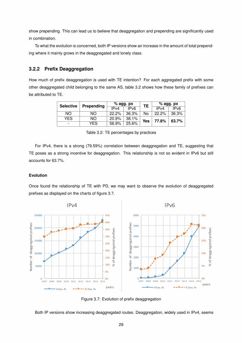
3.2.2 Prefix Deaggregation

How much of prefix deaggregation is used with TE intention? For each aggregated prefix with some

other deaggregated child belonging to the same AS, table 3.2 shows how these family of prefixes can

be attributed to TE.

Selective Prepending % agg. px TE % agg. pxIPv4 IPv6 IPv4 IPv6

NO NO 22.2% 36.3% No 22.2% 36.3%YES NO 20.9% 38.1% Yes 77.8% 63.7%- YES 56.9% 25.6%

Table 3.2: TE percentages by practices

For IPv4, there is a strong (79.59%) correlation between deaggregation and TE, suggesting that

TE poses as a strong incentive for deaggregation. This relationship is not so evident in IPv6 but still

accounts for 63.7%.

Evolution

Once found the relationship of TE with PD, we may want to observe the evolution of deaggregated

prefixes as displayed on the charts of figure 3.7.

0%

5%

10%

15%

20%

25%

30%

35%

40%

45%

0

50000

100000

150000

200000

250000

2007 2008 2009 2010 2011 2012 2013 2014 2015

%+of+deaggregated+prefixe

s

Number+of++deaggregated+prefixe

s

years

IPv4

#+Dea.+Px %+Dea.+Px

0%

5%

10%

15%

20%

25%

0

1000

2000

3000

4000

5000

6000

2007 2008 2009 2010 2011 2012 2013 2014 2015

%+of+deaggregated+prefixe

s

Number+of++deaggregated+prefixe

s

years

IPv6

#+Dea.+Px %+Dea.+Px

Figure 3.7: Evolution of prefix deaggregation

Both IP versions show increasing deaggregated routes. Deaggregation, widely used in IPv4, seems

29

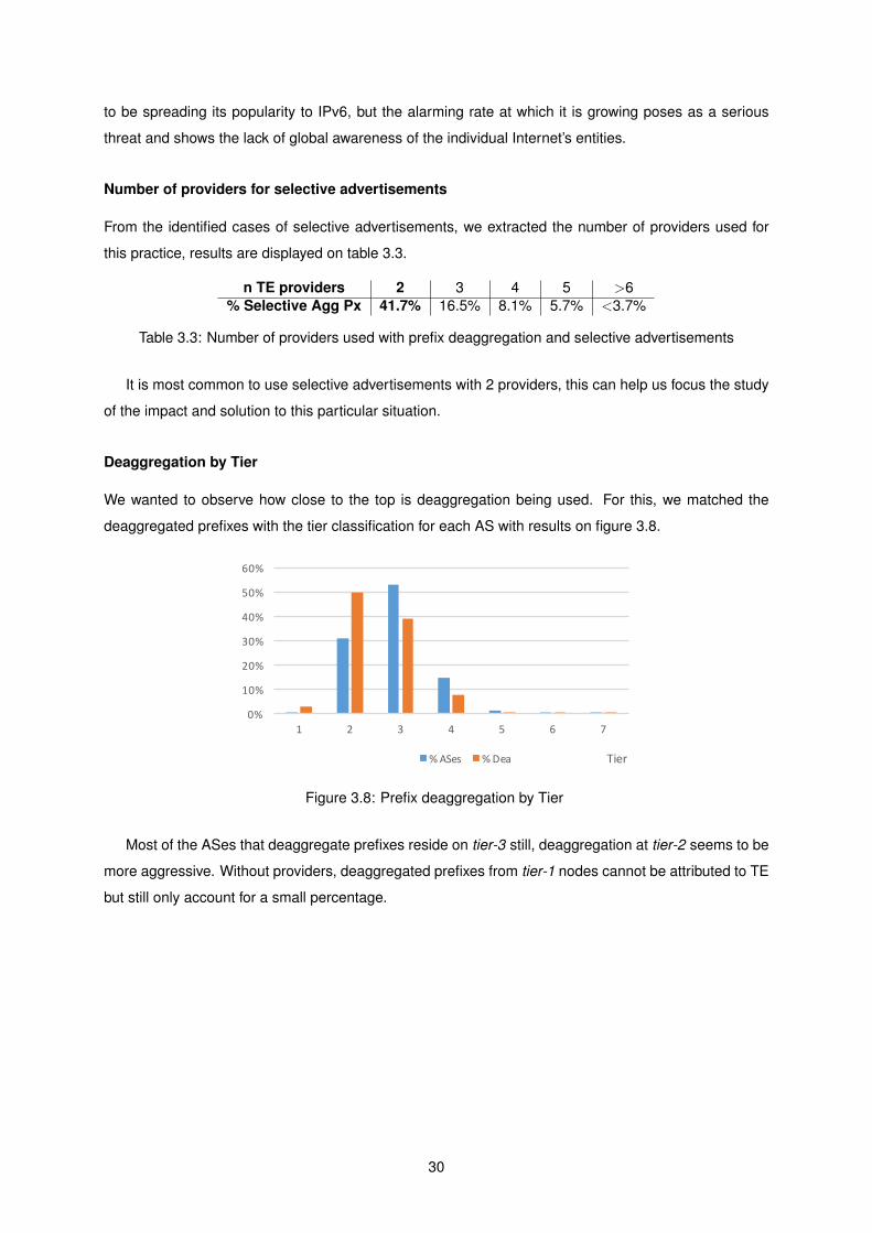
to be spreading its popularity to IPv6, but the alarming rate at which it is growing poses as a serious

threat and shows the lack of global awareness of the individual Internet’s entities.

Number of providers for selective advertisements

From the identified cases of selective advertisements, we extracted the number of providers used for

this practice, results are displayed on table 3.3.

n TE providers 2 3 4 5 >6% Selective Agg Px 41.7% 16.5% 8.1% 5.7% <3.7%

Table 3.3: Number of providers used with prefix deaggregation and selective advertisements

It is most common to use selective advertisements with 2 providers, this can help us focus the study

of the impact and solution to this particular situation.

Deaggregation by Tier

We wanted to observe how close to the top is deaggregation being used. For this, we matched the

deaggregated prefixes with the tier classification for each AS with results on figure 3.8.

0%

10%

20%

30%

40%

50%

60%

1 2 3 4 5 6 7

Tier%.ASes %.Dea

Figure 3.8: Prefix deaggregation by Tier

Most of the ASes that deaggregate prefixes reside on tier-3 still, deaggregation at tier-2 seems to be

more aggressive. Without providers, deaggregated prefixes from tier-1 nodes cannot be attributed to TE

but still only account for a small percentage.

30

Chapter 4

Impact of TE on global routing

TE is used as a way for an individual AS to better manage inbound traffic in order to maximize revenues.

Chapter 3 showed the widespread and increasing adoption of these techniques. In this chapter we are

interested in reasoning the collateral impact this practices have on aspects that pose a threat to the

Internet’s scalability. While being advantageous to the origin AS, can it negatively influence the business

of other ASes? To answer this question we will focus on analyzing the change in preference of the

engineered routes by studying the global distortion to the route type. Also, Is there any distortion

to the path length for the modified routes? If the number of hops a packet has to travel dramatically

increases, the negative consequences of longer paths can even surpass the economic advantages

behind the use of TE. We will also study the impact on the routers FIB and RIB table size that may

prevent a healthy growth of the Internet. Finally a major concern is tackled, the fear that TE may have

the striking effect of preventing global reachability. In this impact analysis, it is easier to to shift the

notation that represents the Internet as a modeled graph where ASes are represented by nodes and the

edges by the links connecting ASes, either c2p or p2p.

4.1 Impact analysis

4.1.1 Distortion to the route type

The route type could be customer, peer or provider based on the relationship with the AS from where

the route was learned from. Different types have different orders of preference as an AS favors sending

traffic to a customer where it has associated revenues than to pay a provider to reach a specific des-

tination. These relationships also shape how the learned routes are exported following the GR model.

Table 4.1 summarizes these elements.

31

Route GR export policylearned from type pref Customers Peers Providers

customer customer route C +++ yes yes yespeer peer route R ++ yes no no

provider provider route P + yes no no

Table 4.1: Route type and the GR export policies

For a given prefix, Path Prepending uses injections in the route ASPATH attribute to adjust the

attractiveness of a provider link regarding inbound traffic. In relation to the no-TE situation, this change

is felt in the route election process after the route type is evaluated when the modified path length is

used to help reason on the most preferred from routes of the same type. In conclusion PP does not add

distortion to the route type.

On the other hand, prefix deaggregation announces different, more specific prefixes to disjoint

subsets of providers. One consequence is that routes flow through distinct paths and may arrive at

nodes from links which have different associated route types. If this change is very significant, it can

seriously impact the global business relationships. A practice that is beneficial to one AS can glob-

ally have a negative impact and therefore create a serious threat to scalability. To demonstrate the

consequences of this action, let us take a look at the sample network depicted in figure 4.1.

u4p, p1

u3

u1

u2

Route adv.

C2P

prefix

u4p

u3

u1

u2

pExpedit ion of data-packets

p1

#2 RIB

px typ:nei

p C:4 P:1

#2 RIB

px typ:nei

p C:4 P:1p0 C:4

!

Without PD With PD

p, p0p1 P:1

Figure 4.1: Change in route type when using prefix deaggregation

In this simple network, node u4 deaggregates prefix p into p0 and p1 which it selectively advertises

to different providers u2 and u3 in order to balance incoming traffic. For reliability reasons we will study in

further sections, prefix p is also advertised to both providers. The situation with selective advertisements

is depicted on the right side of the figure where straight arrows also show the flow of traffic pertaining to

prefix p1. In contrast, the left side shows the no-TE situation with only p being advertised.

Let us take a closer look at the differences. The network is policy connected, each node learns

a route for every advertised prefix. In the TE situation, due to the longest match prefix rule, packets

destined to p’s address space are routed to the forwarding neighbors of the p0/p1-route. Focusing on

the expedition of packets for p1, node u2 has a provider route through u1 even though there is a usable

direct customer link from u2 to u4. Node u2 now has to pay for traffic that would otherwise flow directly

to its customer in the no-TE situation. Also, u2 even has a preferred customer p-route that it cannot use

unless p1 is filtered. In order to satisfy u4’s intention to balance traffic, u2 suffered negative impact by

32

the change in the route type from customer to provider regarding p1’s address space.

Considering that with PD we are restricting the paths of a prefix, each AS will have fewer route

options in the RIB entry from which to elect the preferred route so PD can only worsen the type.

4.1.2 Distortion to the path length

Since the Internet is a vastly dense network, a data-packet can travel to any destination in the world

having to transverse only through a small number of exchange points. Many services have strict Quality

of Service, QoS, requirements that can be affected by the enlargement of paths.

For example, Voice over IP, VoIP communications are very sensitive to delay. The transit delay for the

communication is a combination of several factors, but the biggest slice comes from the delay introduced

by routers and switches in the path [33]. Each intermediate stop has an associated switching delay for

table look up and also buffering delay because packets must wait in line before being processed.

The purpose of this part is to study the impact of TE on the change of the route’s path length. So

far, TE was always seen as profitable practices an AS engages in that can have negative impact to the

global system, here we are examining a situation that hurts the origin AS the most. To what QoS is con-

cerned, because many factors contribute to the quality of a connection and have different significances

depending on the nature of the service, a longer path doesn’t always mean that it is a worse path. The

aim of this analysis is not to go any further and test specific QoS requirements, but to give a general

understanding that they might be negatively affected.

In the route election process, learned routes of the same route type use the ASPATH attribute to

choose the most preferred route. Path prepending injects ASes in order to make the path longer and

therefore less appealing. Note that the path is not longer in the sense that it travels through more nodes

before arriving to the destination, the process blindly evaluates the path length and not the number of

hops that take up the real length. To avoid any confusion we will refer path length as the number of ASes

on the ASPATH attribute and use real length to the distinct number of ASes in the path attribute. For

example, the ASPATH composed of AS1-AS1-AS2-AS3 is of path length 4, but the real length is only

3. In this way, prepending may change the preference of routes and a node can elect routes with larger

real length thinking that it is electing a shorter path. Figure 4.2 portrays this situation.

Node u6 prepends 4 times its ASN in the path attribute before advertising to provider u4 in order to

discourage traffic on this link. Node u1 receives two customer routes for the same prefix and is therefore

left with the evaluation of the path length. The route from u4 is of path length 5 while the one from u2 is

4 thus u1 will choose u2’s learned route even though it is of longer real length.

There are no general guidelines for applying PP as it largely depends on the topology and the op-

erator’s goals for a particular situation. That is why PP is usually executed in a succession of trials in a

optimization process. Given the particularities of each case, it is not possible to conceive a simulation

test that represents a realistic situation in order to measure the impact and extract relevant conclusions.

However, we can still conclude that PP can only worsen the path length for a given prefix. When no PP

33

Route adv.

C2P

prefix: ASPATH

u6

u5

u1

u4

p: AS4Expedit ion of data-packets

p

#1 RIB

px typ/len:nei

p C/2:4 C/4:2

Without PP

u3

u2

p: AS4 u6

u1

u4

p: AS4x4

#1 RIB

px typ/len:nei

p C/5:4 C/4:2

With PP

u3

u2

p: AS4

u5

!

Figure 4.2: Change in the forwarding path when using path prepending.

is used, the elected route is the one with minimal real length. On the other hand with prepending, if the

route changes, we know that the election process was tricked into choosing a route of equal or worse

real length.

In the case of prefix deaggregation, we have already observed that the selective advertisements

can significantly change the elected route at a node. In extreme cases, it can even change the route

type, so it comes as no surprise that it also has an impact on the path length. Comparing to the no-TE

situation, if the route type is the same, the path is of equal or worse length. The explanation for this is

because in the no-TE situation, all routes of the same type were already evaluated and the one with

shorter length was chosen. On the other hand, if the route type changes, the path length could be

longer, equal or even shorter. Since in this case the route arrives via a different incoming link, it travels

through a distinct path and as such it is not possible to find a relationship between situations and predict

the outcome of the path length. Although the path could be shorter, because the route type is worse this

is usually seen as an unfavorable situation. Figure 4.3 portrays an example of this two cases.

Route adv.

C2P

prefix: ASPATH

u5

u1

u3

p

Expedit ion of data-packets

p0

#1 RIB

px typ/len:nei

p C/2:3 C/3:2

Len(p) - Len(p0) < 0

u2

p, p0

u4

p0 C/3:2

#2 RIB

px typ/len:nei

p C/3:3 P/2:1p0 P/2:1

Len(p) - Len(p0) > 0

u5

u4

u1

u3

u2

p, p0

p

Figure 4.3: Possible topologies with different outcomes to the path length

34

4.1.3 Global Reachability

One of the major concerns when applying TE is the fear that it may prevent routes from reaching portions

of the internet. Before any traffic control, the network operator is interested in assuring that global

reachability is satisfied so it is of most importance to understand in what circumstances TE can prevent

this from happening.

For a given prefix, Path Prepending uses injections in the route ASPATH attribute to adjust the

attractiveness of an incoming link. The different prepended routes are advertised to all providers. In

relation to the no-TE situation, this change is only felt in the route election process after LOCALPREF

attribute is evaluated. This means that the changed routes do not completely erase connections that

may prevent global reachability. A link that is very unappealing is still a valid link. As such, PP will not

change connectivity compared to the no-TE situation.

Prefix deaggregation is usually deployed by injecting different, more specific prefix routes to differ-

ent provider links. One direct implication is that routes flow through distinct paths that may reach different

sets of nodes in a network preventing global reachability. When the network is policy connected, this is

not an issue as every route announced to whichever node reaches the remaining nodes. Even though

we not advertising the prefixes to all providers, they will eventually receive the remaining routes. The

issue arises when the network is not policy connected because we may be limiting the reachability of

a given prefix by not advertising it to all the providers. In order to understand the connectivity change

regarding the more specific prefixes let us take a look to the following example.

D

u4

u6 u7 u8

u3

u2u1

u5

u9

p, p0 p, p1 D

u4

u6 u7

u3

u2u1

u5

u9

p, p0 p, p1

? ?

?

?

?

?

p1

p0

u8

?

Policy-connected Not Policy-connected

p1p0

p

Route advertisements

Expedition of data-packets

Figure 4.4: Prefix deaggregation and global reachability on not policy connected networks

Figure 4.4 shows an example of a policy connected (left) as well as a not policy connect (right)

network. Node u9 deaggregates its assigned prefix p into the more specific p0 and p1. Following

believed PD practices, p0 and p1 are announced to different upstream providers, u6 and u7 respectively.

Prefix p is also advertised to both providers. Looking at the left figure, the network is policy connected

35

meaning that every node learns routes for all the advertised prefixes, in particular u9’s p, p0 and p1.

Imagine now that there is a peering dispute between Tier-1 nodes u1 and u2, situation depicted on

the right side of the figure. The network lost its global connectivity and the more specific prefixes do not

reach every node in the network. For p0, this route is first advertised from u9 to u6 which it forwards to its

provider u1. Being a customer route, u1 exports the learned route to all its neighbors, u4 and u2. On u2’s

perspective, the p0-route learned from its peer u1 is a peering route, consequently it is only announced

to its customer u5 and not the peer u3. Node u3 has no other link in which to learn a p0-route and as

such will now match p0 destined packets to the neighbor that exported the p-route which is u7. Node u7

is also oblivious of p0-routes and forwards traffic matching p0’s space directly to u9. Similar conclusions

can be extracted for p1. Node u9 lost the ability to balance traffic as it may receive traffic on both links.

In conclusion, PD may not work on networks that are not policy connected.

Due to the less specific p-route being also advertised on all provider links, globally, connectivity is

not lost as every node knows at least one p-route that covers both p0 and p1. If this does not happen,

some nodes will simply discard packets because they do not know a route matching the deaggregated

space and as such decreasing reachability.

One question that comes to mind is if this is always the case for not globally connected networks. It

is not, the problem can be overcome by the existence of a node with unique characteristics.

p1p0

p

D

u4

u6 u7

u3

u2u1

u5

u9

p0 p1

u8

ANp1p0

p1

p0p0p1

D

u4

u6 u7

u3

u2u1

u5

u9

p0

u8

AN

Route advertisements

Expedition of data-packets

Figure 4.5: Prefix deaggregation and global reachability on not policy connected networks with aggre-gation node

Figure 4.5 is an extension of the previous example with one more node, customer os both u1 and u3.

In this example all nodes now know where to forward traffic regarding the more specific prefixes thus

preserving u9’s intention of balancing traffic. This works because there exists a node that has both a p1

and p0 customer route while also being a direct or indirect customer of the unconnected ASes. To nodes

with such features we will call aggregation nodes (AN). These play an important role in aggregating

prefixes as we will see further in this work. However, this does not mean that the network behaves like

it is policy connected, u1’s own routes still have no way of reaching u3.

36

Filtering by intermediate nodes

We have explored situations where nodes can experience negative business impact when forwarding

traffic of more specific prefixes to less preferred neighbors encouraging the node to filter those prefixes.

Figure 4.6 shows a situation where node u6 has a strong incentive to filter the deaggregated prefixes.

u5

p, p0p

u4

u3

u1

u2

D p, p0

p

u4

u3

u1

u2

F

!!!

#3 RIBpx typ:nei

p C:4 R:2p0 R:2 P:1

#4 RIBpx typ:nei

p C:5 P:3 P:1p0 P:3 P:1

#3 RIBpx typ:nei

p C:4 R:2p0 R:2 P:1

#4 RIBpx typ:nei

p C:5 P:3 P:1p0 P:3 P:1

Figure 4.6: Filtering deaggregated prefixes with a less preferred route.

On the left side, node u3 knows a customer p-route and a peer p0-route. Maybe u3 feels it is not

willing to forward traffic for p0 space pay-free to its peer when it can just match to the less specific p

and forward it to its customer u3 with increased revenues. From what we know, global connectivity is

not touched as the customer, on a policy connect network, knows some other route in which to forward

traffic for p0. Although this can happen, it is very unlikely that this situation is performed in reality due to

the strong damaging impact it has on the customer’s network.

Imagine u3 filters p0, now traffic for p0 is forwarded to u4 that has to pay to receive this traffic and

also pay again to forward it to its provider u1. It is acting as a transit node for traffic that is not his or

from its customers in a valley-like situation. Node u4 will hardly engane in a business relationship with a

provider that has such intentions.

Another interesting situation is when both p and p0 are learned from the same neighbor, depicted in

figure 4.7

u5

p, p0

u4

u3

u1

u2

#3 RIBpx typ/len:nei

p R/2:2 P/4:1p0 R/2:2 P/4:1

#4 RIBpx typ/len:nei

p P/4:1 P/3:3 p0 P/4:1 P/3:3

#3 RIBpx typ/len:nei

#4 RIBpx typ/len:nei

p, p0

u6 p R/2:2 P/4:1p0 R/2:2 P/4:1

p P/4:1 P/3:3 p0 P/4:1 P/3:3u5

u4

u3

u1

u2

u6

F!

Figure 4.7: Lose of attractiveness by filtering prefixes with the same forwarding neighbor

Node u3 now has a preferred peer p-route as well as a peer p0-route learned from the same neighbor,

u2. Filtering p0 in this situations does not damage the customer network as in the previous example and

may seem a good answer to save some routing space. Node u4, customer of u3, is multi-homed with

two providers u3 and u1. The traffic flow for p0 is depicted in figure 4.7 left.

37

Now, let us see what happens to the traffic flow for p0 when u3 filters (fig. 4.7 right). In this situation,

p0 is not advertised from u3 to u4 anymore. Node u4 is left with the p0-route learned from u1 to where

it now forwards all the p0 traffic. u3 loses u4’s traffic and is therefore left with decreased revenues, as a

result of being the only node to filter, it repulsed p0 traffic.

With this, we see that deaggregation is strongly associated with traffic attraction. [22]Karlogirous et

al. explored in a game-theory like example that it may beneficial to the global network to stop advertising

deaggregated prefixes if all nodes cooperate. As we know, it is not possible to achieve global participa-

tion as each node acts like individual entities. Furthermore, once the deaggregated prefix is advertised,

every node has an incentive to further propagate this route as falling to do so might attract the traffic

elsewhere. A recent study by Bangera [14] even explored a situation where providers deaggregated

customer’s prefixes in order to attract more traffic and boost earnings. Note that stubs are only inter-

ested in connectivity and as such do not care for traffic attraction. This puts them in a unique situation

to filter prefixes and have no impact in the global business dynamics of the network.

To what global connectivity is concerned, PD does not diminish connectivity as long as a more spe-

cific covering the deaggregated prefixes is also advertised to all providers. This is also true for the

filtering situations explained before, busyness dynamics may change but connectivity is assured.

4.1.4 FIB & RIB - Table size

All of the aforementioned aspects rely on the graph dynamics but nothing is more threatening to the

scalability than exceeding the physical constrains of the technology. Forwarding tables do not have

infinite capacity and take some time to process each entry that can be proportional to the number

of entries. So, the undisciplined increase in number of prefixes and routes can seriously lead to a

degradation in performance, routing instability, or impact availability of the global routing system.

FIB table size recently reached an important milestone. Some of the old deployed routers had a

memory limit of 512K prefixes, a boundary that was exceeded in May of 2014 creating partial outages

on the Internet. Although some workarounds are possible to extend capacity these are not responsible

practices in the long run. This section is focused on understanding how TE can impact FIB & RIB table

size.

Modified routes for path prepending pertain to a single prefix, which means they do not introduce

a new entry in the forwarding table nor increase the amount of advertised routes. Although different-

in-length routes are announced, each AS only advertises one elected route. On the other hand, prefix

deaggregation injects more specific prefixes to the network meaning that it takes space from the FIB

as well as the RIB. The severity of the impact dependents on the deaggregation factor.

From this we see that PD is much more damaging to the scalability of the Internet. The fact that PD

gives a better control over inbound traffic than PP, implicates that these techniques cannot be substituted

to achieve global scalability gains.

38

4.2 Statistics

4.2.1 Change in route type

Prefix deaggregation can impact the route type of ASes from the advertisement of a prefix to a subset

of providers instead of using all links. When a prefix is selectively advertised, some of the nodes might

experience a degradation on the type of route. Here we wish to reason on the change of routes that may

negatively impact the global system.

Candidate ASes to preform PD are those with more than one provider. For each PD-AS as destina-

tion, we compute the elected route on all ASes using every provider link, this corresponds to the best

route estimation and also the no-TE situation we want to compare. To simulate prefix deaggregation,

let us ignore all the provider links except for one. We then compute the elected route and compare the

differences. The process is repeated for each provider link and the differences are finally averaged.

1: procedure ROUTETYPEIMPACT(Graph G)2: for each v in G do3: if v.nProviders > 1 then . Deaggregating ASes candidates4: routeType = ElectedRouteType(G,v) . Computed for all ASes5: for each p in v.providers do6: G* := G - {v.providers - {p}} . Selectively announce to one provider7: routeTypeTE = ElectedRouteType(G*,v)8: diff += routeType - routeTypeTE9: averageStat[v]← diff/v.providers

Our simulation found that more than half (68.5%) of the ASes that deaggregated prefixes for TE

purposes experienced global changes in the route type. Although this percentage is high, the changes

on the other hand are not so severe. We already know that the estimation can only worsen the route

type, the following charts on Figures 4.8 and 4.9 particularize the changes from customer to provider,

C2P, customer to peer, C2R and peer to provider, R2P.

ASesDeaggregatingTotal Total with change without change

50086 29249 20033 (68.5%) 9216 (31.5%)

Table 4.2: Changes in route type due to prefix deaggregation

The worst case scenario, where nodes change the type from customer to provider only affects 2

ASes (0.004%) for more than half (56.23%) of the deaggregators. The change from customer to a peer

route has similar results with slightly higher impact.

From the chart analysis, one observation is that the impact is felt more intensively on the changes

from peer to provider. Still, half of the deaggregators only impact 634 (1.27%) ASes but some may reach

up to 5116 (10.21%) ASes. One explanation could be due to the great number of peering relationships

on the internet, these can become unavailable once the route is selectively advertised. This precise case

may slightly differ from reality since inferred topologies are particularly deficient on estimating peering

links. However, it is not possible to guess how it influences the results. The diminishing of nodes with

39

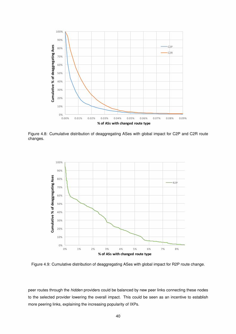
0%

10%

20%

30%

40%

50%

60%

70%

80%

90%

100%

0.00% 0.01% 0.02% 0.03% 0.04% 0.05% 0.06% 0.07% 0.08% 0.09%

Cumulative*%*of*d

eaggregatin

g*Ases

%*of*ASs*with*changed*route*type*

C2P

C2R

Figure 4.8: Cumulative distribution of deaggregating ASes with global impact for C2P and C2R routechanges.

0%

10%

20%

30%

40%

50%

60%

70%

80%

90%

100%

0% 1% 2% 3% 4% 5% 6% 7% 8%

Cumulative*%*of*d

eaggregatin

g*Ases

%*of*ASs*with*changed*route*type*

R2P

Figure 4.9: Cumulative distribution of deaggregating ASes with global impact for R2P route change.

peer routes through the hidden providers could be balanced by new peer links connecting these nodes

to the selected provider lowering the overall impact. This could be seen as an incentive to establish

more peering links, explaining the increasing popularity of IXPs.

40

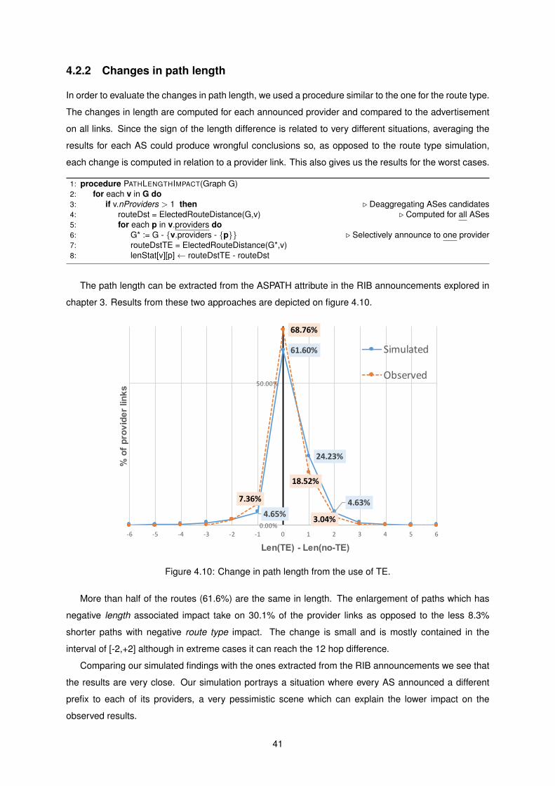
4.2.2 Changes in path length

In order to evaluate the changes in path length, we used a procedure similar to the one for the route type.

The changes in length are computed for each announced provider and compared to the advertisement

on all links. Since the sign of the length difference is related to very different situations, averaging the

results for each AS could produce wrongful conclusions so, as opposed to the route type simulation,

each change is computed in relation to a provider link. This also gives us the results for the worst cases.

1: procedure PATHLENGTHIMPACT(Graph G)2: for each v in G do3: if v.nProviders > 1 then . Deaggregating ASes candidates4: routeDst = ElectedRouteDistance(G,v) . Computed for all ASes5: for each p in v.providers do6: G* := G - {v.providers - {p}} . Selectively announce to one provider7: routeDstTE = ElectedRouteDistance(G*,v)8: lenStat[v][p]← routeDstTE - routeDst

The path length can be extracted from the ASPATH attribute in the RIB announcements explored in

chapter 3. Results from these two approaches are depicted on figure 4.10.

4.65%

61.60%

24.23%

4.63%7.36%

68.76%

18.52%

3.04%0.00%

50.00%

%6 %5 %4 %3 %2 %1 0 1 2 3 4 5 6

%"of"provider"links

Len(TE)"4 Len(no4TE)

Simulated

Observed

Figure 4.10: Change in path length from the use of TE.

More than half of the routes (61.6%) are the same in length. The enlargement of paths which has

negative length associated impact take on 30.1% of the provider links as opposed to the less 8.3%

shorter paths with negative route type impact. The change is small and is mostly contained in the

interval of [-2,+2] although in extreme cases it can reach the 12 hop difference.

Comparing our simulated findings with the ones extracted from the RIB announcements we see that

the results are very close. Our simulation portrays a situation where every AS announced a different

prefix to each of its providers, a very pessimistic scene which can explain the lower impact on the

observed results.

41

4.3 Impact Simulator

We have seen that TE can have a significant impact depending on how these techniques are used.

To better understand this effects we built an impact simulator application to test TE configurations and

immediately see the effects on the global routing system.

As input, the application uses the Internet’s inferred topology, from there it is possible to navigate to

a specific AS and test some TE configurations. Namely it is possible to simulate the changes in route

type from advertising only to a subset of the providers and it is also possible to prepend to a specific

amount some of the advertised routes routes and extract the number of ASes that will elect a route that

has an associated higher number of hops. All of this using a simple but effective interface, as portrayed

in figure 4.11.

Origin ASN

Internet topology dataset

Subset of providers for

selective advertisement

Prepending ammountn Cust. n Peer. n Prov.

All providers

Number of Ases with changed route type

Number of Ases with increased path length Simulate the global gains

from using DRAGON

Figure 4.11: Screenshot of the Impact Simulator App and its main features

Example

Let us consider a practical example to help us understand how this works. AS 38993 is registered

on the RIPE database as RENOVA-PT-AS, belonging to the Portuguese company that produces paper

consumption goods. An input in the Find field for this AS shows that this company gets its Internet

access from two providers, VODAFONE-PT (AS12353) and NOS-COMUNICACOES (AS2860). Imagine that

RENOVA wants to use TE to balance inbound traffic on both links.

One way to do it is by using PD with selective advertisements therefore, the route for the deaggre-

gated prefix is only advertised to one of the providers. To simulate this on the application, we click on

one provider and press the ADD button. If we then press the Scoped button, the elected route type is

42

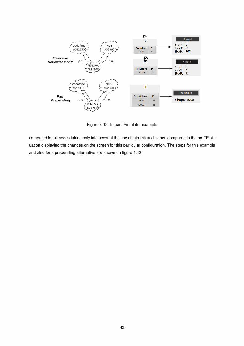
RENOVAAS38993

VodafoneAS12353

NOSAS2860

p,p0p,p1

RENOVAAS38993

VodafoneAS12353

NOSAS2860

pp, pp

p0

p1Selective Advertisements

Path Prepending

Figure 4.12: Impact Simulator example

computed for all nodes taking only into account the use of this link and is then compared to the no-TE sit-

uation displaying the changes on the screen for this particular configuration. The steps for this example

and also for a prepending alternative are shown on figure 4.12.

43

44

Chapter 5

Solution for scalable TE

Chapter 4 showed that TE practices are more harmful to the scalability of the Internet in the form of

prefix deaggregation due to the bloating of forwarding and routing tables as well as increasing BGP

route updates. A scalable approach to this problem should be focused on global gains and preferably

reach a solution with minimum changes from today’s deployed technologies in order to facilitate adop-

tion. Most academic findings for FIB [32, 29] and RIB [23] reduction rely on local software optimizations

to the table entries that only contribute to improve individual ASes and not the global system. Many

clean slate approaches aim to redesign the Internet’s architecture and are therefore difficult to deploy

without major changes which may not be feasible in the near future.

Inter-domain route aggregation strategies are of special interest as filtering gains propagate through

the Internet. For this approach we will consider DRAGON as it is TE compatible. With this in mind, we will

explore DRAGON with TE in a way that it is able to mitigate the negative impact of prefix deaggregation

and therefore pose as a scalable solution. We will also evaluate the side-effects that may arise from the

use of this approach, hoping that they seem insignificant given the global benefits that pave way for a

healthy Internet’s future.

5.1 Scalable TE using DRAGON

Dragon proposes a route-aggregation solution for inter-domain routing. Its mechanisms rely on two

basic rules:

For a prefix p containing in space some other more specific q prefixes:

• Filtering code: CR: If a node is not the origin of p and if attribute for elected q-route equals or is

less preferred than the attribute of the elected p-route→ filter q

• Rule of announcement: RA: The origin of p announces p with a route whose attribute is equal

or less preferred than the attribute of the elected q-route.

Applying this algorithm guarantees an optimal route-consistent state for GR export policies. However,

when using TE in the form of PD, DRAGON does not directly work as the q and p routes share the same

45

attribute and can therefore be filtered. In order to understand the implications let us look at figure 5.1

that portrays a sample network and the standard stable state for p0.

D

u4

u1

u3

p, p0 p, p1

u2

u5

u6

u7

C CC

R CC

P CC

C PC

P PP

P PP

p1p0

pRoute type

* Origin

Expedition of data-packets

p0

P2P

C2P

Route adv.

prefix

R CC

Figure 5.1: Sample network to perform DRAGON

In this Figure, node u7 deaggregates prefix p into p0 and p1. Node u7’s providers, u4 and u5, elect a

customer p-route. Executing DRAGON, CR filters the deaggregated prefixes because they are of a less

or equally preferred route compared to the p-route. In this way, p0/p1 are not propagated to the network

and u7 is unable to engineer its incoming traffic despite the global filtering gains.

DRAGON can still be used with prefix deaggregation by an adjustment to reach an equivalent model.

Another approach is to delegate the use of filtering to upstream providers.

5.1.1 Equivalent model

It is possible to achieve a DRAGON equivalent model by applying specific rules in a settlement with the

providers. The idea is for the providers to announce deaggregated routes as though they are the ones

originating those prefixes. In this way, DRAGON then can be deployed with its resulting advantages.

Provider’s settlement (PS)

If a customer deaggregating node, ud, wants to perform PD for a prefix p containing in space n

deaggregated prefixes, qn, each provider of un should obey the following rules in order to reach an

equivalent DRAGON model to respect ud’s TE intention.

1. Announce p according to RA, i.e. with a route whose attribute is equally or less preferred than the

elected qn routes (p0/p1-route in the example).

2. Prefer p-routes learned from other than ud (u7).

To see how this works let us look at the following figure 5.2 - (a). Node u4, provider of u7, elects both

a customer p0-route as well as a provider p1-route. In order to obey rule 1 of the PS, p is announced

as a provider route thus only to u4’s customers. Node u6 learns a provider p/p0/p1-route, executes CR

and filters p0/p1. Globally this has little to no effect but note that node u1 learns a customer p0/p1-route.

For that reason, u1 could originate aggregation prefix p as a customer route, therefore announcing p

to all neighbors. Node u5 follows rule 2 of PS and prefers u1’s p-route. Now, there are more filtering

opportunities and the final stable state is reached (fig. 5.2 right).

46

D

u4

u1

u3

p, p0 p, p1

u2

u5

u6

u7

C CC

R C

P CP*

C PP*

P PP

P P

p

p

pp

p

D

u4

u1

u3

p, p0 p, p1

u2

u5

u6

u7

C CC*

C

CP

CP

P

p

P

R

D

u4

u1

u3

p, p0 p, p1

u2

u5

u6

u7

C RR*

C

CP

CP

P

P

R*R

p

p p

(a) (b)

pp

pp

Figure 5.2: Execution of DRAGON. (a) with Aggregation node, (b) without Aggregation node.

Comparing figure 5.2-(a)-right with figure 5.1 we see that not only is u7’s TE intention respected but

also that the final state is route-consistent. DRAGON guarantees that route-consistency is met (for GR

policies), so by applying a model that falls into DRAGON’s conditions it also ensures consistency to the

final state.

An aggregation node, AN, is a node that elects a customer route for the selectively advertised deag-

gregated prefixes. Given the dense Internet graph, many nodes can fall into this category, for example

a provider of an AN will also be an AN as customer routes are exported upstream. For greater global

gains, we are interested in aggregating the closest as possible to the origin AS so that the aggregated

route reaches more nodes that do not need to keep table entries for the deaggregated prefixes in order

for those to be kept only within a small vicinity of the origin. Note that closest is in relation to the GR

policies and not necessary the shortest path. What this means is that the closest AN is the one where it

is impossible to reach another AN following only customer routes from this node to the origin.

In order to discover if a node is an AN, one can simulate selective advertisements by computing

the elected routes taking into consideration only one provider of the origin AS for each of the providers.

If a node has a customer route for every of these computed routes then it is an AN (function isAN()).

A provider of an AN is also an AN, as customer routes are exported to the providers so each AN will

have a customer AN unless it is the first to aggregated routes from different customers in which case

it is one of the shortest aggregation node. So, the algorithm for computing the shortest AN starts at

an arbitrary candidate AN and explores its customers. If at least one of the customers is an AN, it will

further evaluate this customer node and repeat the process. Has we keep on doing this, we are moving

towards the destination following customer links until the shortest AN is found. For our study we are only

interested in finding one shortest AN but multiple might exist.

The following is an sample algorithm for computing the shortest AN taking advantage of algorithm

1 for computing the elected route type. Note that the algorithm 1 evaluates provider nodes as well as

peers of those providers in order to compute customer and peer routes. In this situation we are only

using elected customer routes, so a slight modification to alg. 1 where peer links are not used could

improve performance.

47

Algorithm 3 Algorithm for computing shortest Aggregation Node1: function SHORTESTAN(Graph G, Node d)2: Array routeTypeTE[d.nProviders][G.nNodes]3: for each p in d.providers do4: routeTypeTE[p] = ElectedRoute(G - {d.providers - {p}}, d) . one for each selective advertisement

5: for each v in G do6: if isAN(v) then7: v.isAN← True

8: return findAN( getCandidateAN(G) ) . starts at an arbitrary AN

9: function ISAN(Node n, Array routeTypeTE)10: for each routeType in routeTypeTE do11: if routeType[n] is not ’C’ then12: return False13: return True

14: function FINDAN(Node AN)15: if AN is not null then16: for each c in c.customers do17: if c.isAN then18: return findAN(c)19: return AN

Without aggregation node

There are cases where there is no upstream provider capable of aggregating routes, situation repre-

sented in fig. 5.2-(b) where link {u1,u5} was removed, incapacitating u1 from generating aggregation

prefix p. In situation (a), node u1 could announce p as a customer route in accordance to RA. Here,

p could also be advertised but only as a peer or provider route meaning that it is exported only to the

customers. If every node prefers a p route learned from a neighbor instead of being the one to generate

p, tier-1 nodes receiving customer routes for the deaggregated prefixes will be the ones to generate p

but only to its customers. This creates filtering opportunities while maintaining route-consistency.

Robustness to link failures

Multi-homing could be used for load balancing but its main purpose is to increase reliability by ensuring

that the node stays connected to the Internet even if there is a failure in a provider link. Let us see what

happens to the previous network when the two-way link {u4,u7} fails.

D

u4

u1

u3

p, p1

u2

u5

u6

u7

C CC

C

CP

CP

P

p

P

R

pC

D

u4

u1

u3

p, p1

u2

u5

u6

u7

C C

CC*P

P

P

p

Figure 5.3: Link failure. Left Transition state. Right Stable state

48

Looking at the left of figure 5.3, prefix p0 stops being advertised, thus node u1 cannot originate

aggregation prefix p. Node u5 now has only a customer p1-route so it can now announce p with customer

route attribute exporting p to all neighbors. In this way, the stable state is reached and packets destined

to the p0 space arrive at u7 through u5, maintaining global reachability.

This equivalent model offers great advantages to the global system as it creates many filtering op-

portunities while maintaining route consistency. The major downside comes from the fact that its not a

completely distributed algorithm, as there needs to be a settlement with the providers in order to behave

with special conditions and also some coordination from the all the nodes to advertise the aggregation

prefix.

5.1.2 Provider delegation

One other way is simply to tell different levels of upstream providers not to filter. This can be achieved

for example using the BGP communities attribute that binds specific information to the routes so it can

be interpreted in whichever way, in our case could be used to propagate a node’s intention for some of

the providers to not deploy DRAGON’s filtering strategies.

D

u4

u1

u3

p, p0 p, p1

u2

u5

u6

u7

C CC

R CC

P CC

C PC

P

P

D

u4

u1

u3

p, p0 p, p1

u2

u5

u6

u7

C CC

CC

CC

CC

P

P

!

Figure 5.4: Filtering Delegation

Figure 5.4 portrays two possible outcomes from this alternative procedure. Starting with the left

side of the figure, node u7 informs nodes u4, u5 and u1 not to filter, therefore abiding by the standard

BGP protocol. Node u5 learns a customer p-route that forwards to all neighbors, namely its ’DRAGON ’

provider u2. Executing CR on node u2, with a customer p-route, both p0/p1-routes are filtered. With

focus on p0 space, node u2 forwards traffic to its customer u5 and is then rerouted to u1 via provider

link. Node u5 suffers from negative business impact by serving as a transit node in a valley-like situation,

in another perspective node u2 improved its elected route attribute for p0 space from peer to customer

route. Despite the distortion to the route type, u7 is able to successfully engineer incoming traffic while

keeping filtering opportunities thus reducing its global impact. We can conclude that this solution, while

being advantageous in a global perspective, may impact some nodes due to the change in route type,

losing route-consistency.

In the previous example, despite its negative impacts, u7 was able to apply TE but is this always true

or depends on the topology? To answer this question, let us take a look at the right side of figure 5.4.

Now, the nodes instructed not to filter are u4, u5 and u2. Node u1 filters p0 and p1, advertising only p

49

to u2 and u5 that are oblivious to the existence of p0. Therefore, traffic for p0 space is matched to the

p route and arrives at u7 via the forbiden provider link from u5 so, TE may not work using the provider

delegation strategy.

The significant change from the previous example is that in this case there is no aggregation node

from the set of providers that do not filter. This is the node who knows how to route packets for each

deaggregated route, if these routes are filtered due to the customer p-route there is no way to recover this

information and TE may not be accomplished. In conclusion, using the provider’s delegation approach,

TE is only possible if there exists an aggregation node from the set of non-filtering providers.

50

5.2 Statistics and analysis

5.2.1 Equivalent model

In order to evaluate the filtering gains from applying DRAGON with the model from section 5.1.1 the

FIBTE−gain was defined as the relative difference on the FIB entries for a prefix and its deaggregated

childs.

FIBTE−gain =FIBinitial − FIBafter

FIBinitial

For example, a multi-homed AS with 2 providers deaggregates its assigned prefix p into p0 and p1

which it selectively advertises to each provider. Without filtering, each AS will have a FIB entry for all the

advertised prefixes p/p0/p1. When DRAGON is deployed, an AS that is able to filter p0 but not p1 will

have FIB entries only for p/p1 resulting in a FIBTE−gain of (3-2)/3 (33%).

Figure 5.5 computes the gains for the common situation of a multi-homed AS with 2 providers where

a prefix is broke in two and these are selectively advertised to the different providers. Table 5.1 shows

the average results for this case.

0%

10%

20%

30%

40%

50%

60%

70%

80%

90%

100%

0% 2% 5% 7% 9% 12%

14%

16%

19%

21%

23%

26%

28%

30%

33%

35%

37%

40%

42%

44%

47%

49%

51%

54%

56%

58%

61%

63%

65%

68%

70%

72%

75%

77%

79%

81%

84%

86%

88%

91%

93%

95%

98%

%"of"ASes"

%"of"deaggregating"ASes"with"2"providers

0% 33% 67%

Figure 5.5: FIB gain for 2 providers

2 TE providers%gain 0% 33% 67%

Average%ASes 0.50% 3.09% 96.41%

Table 5.1: Average percentage of affected ASes for different gains in a situation of 2 TE providers

Observing the previous results we see tremendous global gains. On average, almost all of the

51

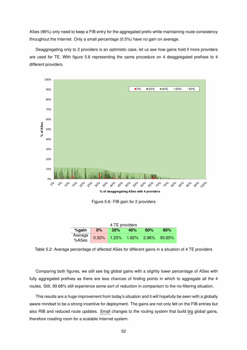
ASes (96%) only need to keep a FIB entry for the aggregated prefix while maintaining route-consistency

throughout the Internet. Only a small percentage (0.5%) have no gain on average.

Deaggregating only to 2 providers is an optimistic case, let us see how gains hold if more providers

are used for TE. With figure 5.6 representing the same procedure on 4 deaggregated prefixes to 4

different providers.

0%

10%

20%

30%

40%

50%

60%

70%

80%

90%

100%

%"of"ASes

%"of"deaggregating"ASes"with"4"providers"

0% 20% 40% 60% 80%

Figure 5.6: FIB gain for 2 providers

4 TE providers%gain 0% 20% 40% 60% 80%

Average%ASes 0.32% 1.25% 1.82% 2.96% 93.65%

Table 5.2: Average percentage of affected ASes for different gains in a situation of 4 TE providers

Comparing both figures, we still see big global gains with a slightly lower percentage of ASes with

fully aggregated prefixes as there are less chances of finding points in which to aggregate all the 4

routes. Still, 99.68% still experience some sort of reduction in comparison to the no-filtering situation.

This results are a huge improvement from today’s situation and it will hopefully be seen with a globally

aware mindset to be a strong incentive for deployment. The gains are not only felt on the FIB entries but

also RIB and reduced route updates. Small changes to the routing system that build big global gains,

therefore creating room for a scalable Internet system.

52

5.2.2 Provider delegation

In this strategy, prefix p is advertised without restrictions throughout the Internet just like the no-TE

situation. Each of the deaggregated q-routes selectively advertised to different providers arrives at

every node with a route attribute that is equal or less preferred than the elected route attribute for the p

prefix. Code CR of DRAGON filters these q-routes. Therefore, each AS that does not belong to the non-

filtering set of ASes will filter q-routes and maintain only a FIB entry for the p prefix. This blind filtering

causes changes from a route-consistent state. The changes cancel the TE route type impact identified

in section 4.2.1 of chapter 4, forwarding for these nodes is consistent with the no-TE situation while

being even possible for an AS to control inbound traffic. But who is paying the price for this seemingly

optimal solution? A side-effect from this approach is that nodes that do not filter may receive traffic

pertaining to a q-route from filtering neighbors on links to which a q-route was not advertised because

of the GR export policies. This is to show that the non-filtering ASes ir order to maintain consistency to

the q-routes suffer from a big negative impact.

The incentives for applying this solution rely on the compromise between sacrificing a small number

of ASes for the global gains.

Change in level

Using this approach one question that comes to mind is to how many levels of providers should the non-

filtering intention be propagated?. We want to keep this number as low as possible for greater global

gains but still be able to achieve TE. We have found that TE is respected as long as there is an AN from

the set of non filtering nodes, the next table shows the percentage of found ANs for the different levels.

n TEproviders

Total ASes withn providers

ASeswith AP Level ASes with AP

within level %

1 5576 37.8%2 14740 99.1%3 14746 99,9%2 20146 14752

>= 4 14752 100%1 969 33.2%2 2837 97.2%3 5341 2920

>= 3 2920 100%1 267 36.9%2 714 98.6%4 1962 724

>= 3 724 100%

Table 5.3: Percentage of found Aggregation Nodes by level and number of providers

From the table we see that there is a big incentive on propagating the no filtering intention further

than the first level as it dramatically increases the chances of finding an AN within the non filtering nodes

and therefore achieve inbound TE.

53

54

Chapter 6

Conclusions and future work

We showed great correlation between prefix deaggregation and traffic engineering. Also we observed

an upward trend towards deaggregation throughout the years for both IP versions. The dramatic rate in

which deaggregation is growing for IPv6 shows that if the lack of global awareness stays the same, IPv6

could face an even greater problem.

The two TE practices in study proved to have very different significances to the global impact. Path

prepending is almost harmless apart from possibly increasing the number of transversed hops. Prefix

deaggregation on the other hand is the core of the problem. For one, it can negatively impact the

business relationships of distant ASes although the extent in which it does was found to be not so

severe. The distortion to the route type mostly impacts changes from a peer to a provider route and

when this happens, the worst case only affects 10.21% of the total ASes. We even showed that if

deaggregation is not performed in a careful way, by also advertising as backup the aggregated prefix to

all providers it could decrease reachability in extreme cases.

The most damaging consequence of PD is the bloating of forwarding tables. With this in mind, we

showed that it is possible to achieve traffic engineering without overloading the routing system. By adapt-

ing the DRAGON aggregation strategy, one of the proposed solutions was not only capable of filtering

most of the deaggregated prefixes but did so without compromising the global business relationships

by maintaining a route consistent state. On average, 96.41% of the ASes were able to fully filter the

deaggregated prefixes for the most common case.

We hope that this study at least served as a wake up call to the alarming consequences of undisci-

plined TE to the scalability. It is becoming increasingly difficult to find reasons to dismiss route aggre-

gation strategies. Its global advantages far surpass the needed changes with deployment and should

serve as sufficient incentive for adoption.

In the future, the web platform could be further improved to incorporate new measurements in order

to serve a more complete range of studies. Also, we saw an increasing number of projects that aim to

provide new kinds of Internet monitoring data. This data sources could be explored in future studies to

maybe overcome the limitations of todays publicly available data sources.

As IPv6 keeps on maturing, soon academic studies will shift the attention from IPv4, as consequence

55

we believe there will be IPv6 inferred topologies in a near future. Although both IP version share many

features it is impossible to know if they will evolve in the same way so the results from this study that are

valid for IPv4 may need a reassessment for IPv6. Although it may seem that IPv6 is far from its end, the

sooner we start addressing scalability issues, the less likely they will become a serious problem.

56

Bibliography

[1] AS Rank: AS Ranking. Available: http://as-rank.caida.org. (Sep, 2015).

[2] Autonomous System (AS) numbers. Available: http://web.archive.org/web/20080207010024/

http://www.808multimedia.com/winnt/kernel.htm. (Sep, 2015).

[3] BGPStream - An Open Source Framework for Live/Historical BGP Data Analysis. Available: http:

//www.caida.org/publications/presentations/2015/bgpstream_ripe/. (Sep, 2015).

[4] CAIDA - RouteViews Prefix-to-AS mapping. Available: http://data.caida.org/datasets/

routing/. (Sep, 2015).

[5] CAIDA: Internet AS-Relationships. Available: http://www.caida.org/data/as-relationships/.

(Sep, 2015).

[6] CIDR - Report. Available: http://www.cidr-report.org/as2.0/. (Sep, 2015).

[7] InterSnap - A monitoring platform. Available: http://intersnap.herokuapp.com. (Sep, 2015).

[8] Oregon: routeviews. Available: http://www.routeviews.org. (Sep, 2015).

[9] RIPE-RIS. Available: http://www.ripe.net/data-tools/stats/ris. (Sep, 2015).

[10] RouteViews Host 2 bgp-data. Available: http://archive.routeviews.org/bgpdata/. (Sep,

2015).

[11] RPSL Standard (RFC2622. Available: https://tools.ietf.org/html/rfc2622. (Sep, 2015).

[12] UCLA: Internet AS-level Topology Archive. Available: http://irl.cs.ucla.edu/topology/. (Sep,

2015).

[13] Siddharth Bafna, Avichal Pandey, and Kshitiz Verma. Anatomy of the internet peering disputes.

arXiv preprint arXiv:1409.6526, 2014.

[14] Pradeep Bangera and Sergey Gorinsky. Economics of traffic attraction by transit providers. In

Networking Conference, 2014 IFIP, pages 1–9. IEEE, 2014.

[15] T. Bu, L. Gao, and D. Towsley. On characterizing BGP routing table growth. Computer Networks,

45-54(1):681–692, 2004.

57

[16] L. Cittadini, S. Uhlig W. Muahlbauer, R. Bush, P. Francois, and O. Maennel. Evolution of Internet

Address Space Deaggregation: Myths and Reality. IEEE Journal on Selected Areas in Communi-

cations, special issue on Internet Routing Scalability, 2010.

[17] L. Gao and J. Rexford. Stable Internet Routing without Global Coordination. IEEE Transactions on

Networking, (9):681–692, Dec 2001.

[18] V. Giotsas, M. Luckie, B. Huffaker, and k. claffy. IPv6 AS Relationships, Clique, and Congruence.

Passive and Active Network Measurement Workshop (PAM) , pages 111–122, Mar 2015.

[19] V. Giotsas, S. Zhou, M. Luckie, and k claffy. Inferring multilateral peering. ACM CoNEXT, page

247–258, Dec 2013.

[20] E. Gregoriand A. Improta, L. Lenzini, L. Rossi, and L. Sani. On the incompleteness of the AS-level

graph: a novel methodology for BGP route collector placement. IMC ’12, page 253–264, 2012.

[21] Joao Luis Sobrinho and Laurent Vanbever and Franck Le and Jennifer Rexford. Distributed Route

Aggregation on the Global Network. December 2014.

[22] C. Kalogiros, M. Bagnulo, and A. Kostopoulos. Understanding Incentives for Prefix Aggregation in

BGP. ReArch ’09, Dec 2009.

[23] E. Karpilovsky, M. Caesar, J. Rexford, A. Shaikh, and J. van der Merwe. Practical network-

wide compression of IP routing tables. IEEE Transactions on Network and Service Management,

9(4):446–458, Dec 2012.

[24] M. Luckie, B. Huffaker, k. claffy, A. Dhamdhere, and V. Giotsas. AS Relationships, Customer Cones,

and Validation. IMC ’13, page 243–256, 2013.

[25] A. Lutu, M. Bagnulo, and R. Stanojevic. An Economic Side-Effect for Prefix Deaggregation. NetE-

con, 2012.

[26] A. Lutu, C. Pelsser, M. Bagnulo, and K. Cho. The Aftermath of Prefix Deaggregation. Teletraffic

Congress (ITC), 2013.

[27] R. V. Oliveira, D. Pei, W. Willinger anda B. Zhang, and L. Zhang. The (in)completeness of the

observed Internet AS-level structure. EEE/ACM Transactions on Networking, page 109–122, 2008.

[28] R. V. Oliveira, D. Pei, W. Willinger, B. Zhang, and L. Zhang. In search of the elusive ground truth:

the Internet’s AS-level connectivity structure. SIGMETRICS 2008, 18:217–228, Feb 2008.

[29] G. Retvari, J. Tapolcai, A. Korosi, A. Majdan, and Z. Heszberger. Compressing IP forwarding tables:

towards entropy bounds and beyond. ACM SIGCOM, 2013.

[30] M. Roughan, W. Willinger, O. Maennel, D. Perouli, and R. Bush. 10 lessons from 10 years of

measuring and modeling the Internet’s autonomous systems. IEEE Journal on Selected Areas in

Communications, 24(9):1810–1821, Oct 2011.

58

[31] A. Sousa. Scaling the Internet Routing System through Route Aggregation. Master’s Thesis -

Instituto Superior Tecnico, 2014.

[32] Y.Liu, S. O. Amin, and L. Wang. An efficient FIB caching using minimal non-overlapping prefixes.

SIGCOMM Comput. Commun. Rev., 43(1):14–21, Jan 2012.

[33] Li Zheng, Liren Zhang, and Dong Xu. Characteristics of network delay and delay jitter and its effect

on voice over ip (voip). In Communications, 2001. ICC 2001. IEEE International Conference on,

volume 1, pages 122–126. IEEE, 2001.

59