Inter-calibrating multi-source, multi-platform backscatter data sets to

Proceedings of the Canadian Hydrographic Conference and National Surveyors Conference 2008

Paper 8-2 John E. Hughes Clarke

Inter-calibrating multi-source, multi-platform backscatter data sets to assist in compiling regional sediment type maps : Bay of Fundy

John E. Hughes Clarke(1)

, Kashka K. Iwanowska(1)

, Russell Parrott(2)

, Garret Duffy(3)

,

Mike Lamplugh(4)

and Jon Griffin(4)

(1) Ocean Mapping Group, Dept. Geodesy and Geomatics Engineering, Univ. New Brunswick

(2) Geological Survey of Canada-Atlantic, Natural Resources Canada, BIO

(3) Department of Earth and Ocean Sciences, National University of Ireland, Galway, IRELAND

(4) Canadian Hydrographic Service-Atlantic, Dept. Fisheries and Oceans, BIO

Abstract

The Bay of Fundy has seen ongoing multibeam mapping since 1992 as part of a series of local

projects, and in a major regional program in the last 2 years. The survey sensors include

Kongsberg EM1000, EM3000, EM1002, EM3002 and EM710 with centre frequencies ranging

from 70 to 300 kHz. All data is acquired through the Kongsberg standard backscatter data

reduction process that is supposed to generate estimates of seabed backscatter strength, ideally an

inherent property of the seafloor. To achieve this data reduction, assumptions are required about

absolute source level, pulse length, absolute and time varying receiver gains, seawater

attenuation coefficients and sonar transmission and reception sensitivities. Because of

uncertainty in all of these, the standard output value is effectively a relative measure. As a result

inter-survey consistency is poor. A method is therefore required to pick an arbitrary reference

(sonar hardware and software configuration) and adjust every other survey, through overlapping

coverage, to that reference. For each configuration, specific adjustments need to be made to both

absolute levels, variations by angle, by pulse length settings and correcting for applied

attenuation coefficients. Once all these corrections have been made, a second set of adjustments

needs to account for the spatially variable shape of the inherent seabed angular response curves.

Introduction

As part of the Geoscience for Ocean Management (GOM) program within Natural Resources

Canada, a regional multibeam mapping effort is underway (Fig. 1), designed to cover the

majority of the seafloor of the Bay of Fundy.

The mandate of the GOM program is to: “deliver the geoscience knowledge base for informed

decision making in Canada’s offshore lands, to ensure that natural resource development does

not harm the environment and that appropriate land-use decisions are made balancing social,

economic and environmental considerations”.

In the case of the Bay of Fundy, the prime land (seabed)-use issues relate to the fisheries (lobster,

scallop, aquaculture), aggregate extraction and, most recently, the potential for in-stream tidal

power (Hagerman et al., 2006). In all three cases, the concern is primarily with the surficial

substrate which in turn controls the benthic habitat; the available grain sizes and sorting; and the



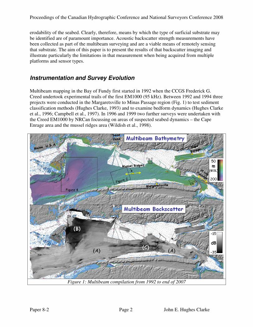
erodability of the seabed. Clearly, therefore, means by which the type of surficial substrate may

be identified are of paramount importance. Acoustic backscatter strength measurements have

been collected as part of the multibeam surveying and are a viable means of remotely sensing

that substrate. The aim of this paper is to present the results of that backscatter imaging and

illustrate particularly the limitations in that measurement when being acquired from multiple

platforms and sensor types.

Instrumentation and Survey Evolution

Multibeam mapping in the Bay of Fundy first started in 1992 when the CCGS Frederick G.

Creed undertook experimental trails of the first EM1000 (95 kHz). Between 1992 and 1994 three

projects were conducted in the Margaretsville to Minas Passage region (Fig. 1) to test sediment

classification methods (Hughes Clarke, 1993) and to examine bedform dynamics (Hughes Clarke

et al., 1996; Campbell et al., 1997). In 1996 and 1999 two further surveys were undertaken with

the Creed EM1000 by NRCan focussing on areas of suspected seabed dynamics – the Cape

Enrage area and the mussel ridges area (Wildish et al., 1998).

Figure 1: Multibeam compilation from 1992 to end of 2007



From 2000-2005, coastal surveys were undertaken using EM3000 (300 kHz) equipped launches

(Plover and Heron) along the New Brunswick shore extending from the border with the United

States to Saint John. These operations were in very shallow water, addressing coastal issues such

as disposal site dynamics (Parrott et al., 2002), Marine Protected Areas (Byrne et al., 2002),

aquaculture sites (Hughes Clarke et al., 2002, Wildish et al., 2004) and benthic habitat as well as

providing training for students (at UNB).

In 2006 and 2007 a much larger scale program was initiated as part of the Geoscience for Ocean

Management (GOM) and Ocean Action Plan (OAP) programs. These surveys have involved 5

multibeam-equipped platforms:

1. CCGS Frederick G. Creed EM1002 (98 & 93 kHz) 2006 2007

2. CSL Heron EM3002 (300 kHz) 2006 2007

3. CCGS Matthew EM710 (71, 74, 77, 83 & 97 kHz) 2007

4. CSL Plover EM3002 (300 kHz) 2007

5. CSL Pippit EM3002 (300 kHz) 2007

This most recent phase of these surveys has provided by far the greatest coverage. Almost all the

areas surveyed in 1992/3/4 have been resurveyed, in part due to data quality issues, but also in

order to directly monitor the > 13 years of change (Hughes Clarke, 2008). The 1996 and 1999

areas, however, have not been resurveyed.

The majority of the area surveyed in 2006 and 2007 was by the Creed EM1002 and Matthew

EM710 systems. The launches, equipped with EM3002 systems, focussed primarily on the near

coastal (<30m) regions, in which many of the land-use issues lie.

Backscatter Data Manipulation

The backscattering coefficient for a particular sediment at a given frequency is an inherent

property of that material and varies only with grazing angle. The backscattering coefficient is

calculated as a dimensionless ratio of the power backscattered by unit sold angle with respect to

the product of the incident intensity per unit area and the area instantaneously ensonified

(Mitchell and Somers, 1989). The backscatter strength (herein referred to as the BS) is most

often quoted and is just 10log10 of this ratio. While the definition is straight forward, arriving at

that dimensionless ratio is fraught with system calibration and normalization issues.

Most modern multibeam sonar systems provide a measure of the peak or average backscattered

intensity (measured as a voltage on the receiver array). This value is not an estimate of the

backscatter strength since it is a function of the system and geometric parameters. To reduce this

value to a measure of the bottom backscatter strength, the system must account for:

1. Sonar source levels, pulse lengths and receiver sensitivity.

2. The 3D beam patterns of the transmit and receive arrays.

3. Spherical spreading and particularly ocean attenuation coefficients at that frequency.

4. Applied real-time time-varying gains (TVG’s).

5. Local seabed slopes



All Kongsberg EM multibeam systems use a data reduction scheme (Hammerstad, 2000)

designed to reduce the received intensity values to a first-order measure of the bottom

backscatter strength by including corrections for all of the steps listed above. Such a data

reduction provides a stable relative value for a sonar system with a given set of hardware

(transducers and electronics). The validity of this data reduction, however, is limited by two

aspects (Hughes Clarke, 1993):

• there are usually discrepancies between the actual hardware performance and the

design (1,2,4)

• there are environmental assumptions in the calculation including (3,5)

Since these surveys have taken place using 5 different Kongsberg EM multibeam sonar types,

from 5 different survey platforms with over 15 years of software and hardware upgrades,

imperfections in each of these models and assumptions provide uncertainty in the absolute

estimate of bottom backscatter strength (see Fig. 2a). Even with this uncertainty the separation of

materials with strongly contrasting BS such as boulders and clay (> 30 dB contrast) is not an

issue, but the delineation of the variations between muddy sands and sandy muds and coarse and

fine gravels (< 5dB contrast) becomes a challenge.

Figure 2:

Example of the integration of multi-source

data. The data was collected in 105-60m of

water in the central bay

A: mosaic of backscatter data as acquired.

B: data adjusted according to the steps outlined

in this paper.

C: bathymetric surface derived from all the

same sonar systems.



In the absence of a robust absolute calibration method, empirical approaches through inter-sonar

comparisons have to be used as a proxy (Fig. 2b). This paper presents the main problems and

steps taken to resolve that. Each issue is presented in turn, with examples.

Coping with Source Level Uncertainty

From the data shown in Figure 2A it is clear that the absolute level of backscatter strength for a

given sediment type varies from sonar to sonar and model to model. In the absence of an

absolute calibration, we can only turn to the expected BS levels for the known sediments present

in the region as a proxy (table 1). Based on a compilation of calibrated BS observations, the

Applied Physics Laboratory at the University of Washington has developed a backscattering

model (APL, 1994). Using the output of this model typical sediment types have BS (at 80 and

100 kHz) in the following ranges at a grazing angle of 40° (50° off vertical):

Sediment type BS (40° grazing) 80 kHz BS (40° grazing) 100 kHz

Rough rock -4.4 -4.2

Rock -8.6 -8.2

Cobble -13.0 -12.6

Sandy Gravel -17.1 -16.8

Coarse Sand -19.6 -19.2

Medium Sand -22.0 -21.7

Very Fine Sand -24.9 -24.8

Silt (high volume) -28.7 -28.7

Silt (low volume) -33.9 -33.9

Table 1: modelled backscatter strength levels (dB) derived from the

Applied Physics Laboratory (UW, 1994) report.

40° was chosen as a representative grazing angle as this is the dominant angle of data visible in

the BS mosaics. All data were normalized for beam pattern and angular response (see later

discussion for methods) to a reference grazing angle in this range. From the APL (1994) report

(which relies on the Jackson et al. (1986) model), it is clear that around this grazing angle the

angular response (AR) curves are flattest.

The dominant sedimentary facies on the floor of the Bay of Fundy are “deflated tills” (Swift et

al., 1969, Fader et al. 1976) which represent seabed surface sediment in the range from coarse

sand and gravels to cobbles. This is represented by areas indicated by (A) in Fig. 1. Only in the

western region between Grand Manan and the New Brunswick shore do we find significant

accumulations of mud (the La Have Clay indicated by (B) in Fig. 1). Well sorted, mobile

medium to fine sand sheets are concentrated on the flanks of depressions along the central bay

(indicated by (C) in Fig. 1 and represented by the dark regions in Fig. 2 (top-right) and in the lee

of headlands.

From Figure 1 we note that the main range of BS levels seen in the Bay extend from -15 to -35

dB. This reasonably matches the APL (1994) predictions for Cobble/Sandy Gravel through to

Silt. We have decided to use the BS levels output by the 1992-1994 EM1000 surveys as our



reference levels for two reasons. Firstly they reasonably approximate the APL results without

apparent bias and secondly, they were the first data acquired and subsequent processing had used

them as a reference. These data (after empirical beam pattern corrections, which do not alter the

mean BS level) are taken as the nominal “truth”. All other surveys are adjusted by overlap to best

correspond to that truth. Particular complications with this method include calculating this source

level adjustment accounting for changing pulse lengths, changing attenuation coefficients (see

later discussion) and the fact that overlap is not always achieved.

The following table shows the currently-used dB shifts applied to each survey.

Platform Sonar Freq. year dB offset

Creed EM1000 95 kHz 1992-1994 reference

Creed EM1000 95 kHz 1996 0 (no overlap to

check)

Creed EM1000 95 kHz 1999 -2 dB

Plover EM3000 300 kHz 2000/1/2 0 dB

Heron EM3000 300 kHz 2002/3/4/5 -3dB

H. Queen EM3002 300 kHz 2005/6 -3 dB

Heron EM3002 300 kHz 2006/7 -3 dB

Creed EM1002 93/98 kHz 2006/7 -5 dB

Matthew EM710 71-97 kHz 2007 -11.5 dB

Plover EM3002 300 kHz 2007 -9 dB

Pipit EM3002 300 kHz 2007 -7 dB

Hawk EM3002 300 kHz 2007 -3 dB

Table 2: dB offsets for each sensor, platform and survey.

Note that EM3000/3002 results used to vary by only 3dB, until the most recent field season.

Note also that the EM710 results are the most significantly different. A noted tendency is for the

more recent Kongsberg systems to generate significantly higher BS levels (5-12dB stronger).

The newer sonar systems routinely report positive mean BS levels suggesting a false bias.

Note also that for sonar systems that show a systematic BS offset with changing pulse length (see

discussion below), table 2 represents the offset applied to the shorter pulse length data (0.2ms in

the case of the EM1002).

Once applied, these bulk offsets usually suffice for a specific sonar and platform during a survey

season. One notable exception to this was the EM1002 on the Creed. Figure 3 illustrates that,

from day to day, as the sonar system was turned off and on (the vessel operates only as a day

boat) the absolute BS values appear to shift within typically +/- 0.5 dB. To date this has not been

noted with the other sonar systems and is thus assumed to be a hardware malfunction problem.

The EM3000/3002 systems are routinely restarted on a daily basis whereas the EM710 system,

once turned on, tends to remain on for several days at a time.

In summary, empirically-derived BS offsets are necessary to be able to follow subtle

geologically-driven geographic variations in bottom backscatter strength across survey

boundaries. Even with an arbitrary reference however, BS levels with respect to that level should



not be relied upon to better than about +/-2dB. This has implications for robust seafloor

characterization.

Figure 3: Illustrating, uncompensated day-to-day +/-0.5 dB shifts in apparent EM1002 source

level. This was present for both 2006 and 2007 data and occurred superimposed on top of the

0.2-0.7ms pulse length shifts. Note that the greyscale represents only 5 dB range.

Coping with imperfectly Reduced Pulse Length effects.

To a first order, the Kongsberg data reduction routine (Hammerstad, 2000) is supposed to correct

automatically for the instantaneously ensonified area resulting from a change in pulse length.

The EM1000 and EM1002 sonars shift from a 0.2 to 0.7 ms pulse at depths ranging from 100 to

150m (the exact depth depends on the signal to noise ratio which depends on environmental

conditions, primarily controlled in low seastates by seabed BS). Depending of the specific

system however, this sometimes results in an apparent shift in the BS level.

For the case of 2006 and 2007 Creed EM1002 data, it is clear that the longer pulse length is

favoured in water depths greater that 150m (Fig. 4a and arrows on b). When the pulse length

shifts, there is an abrupt increase in apparent BS (Fig 5a). When comparing the BS level

immediately before and after the shifts (Fig. 5c) a 5dB apparent offset is seen. Interestingly the



~3.5x factor increase in ensonified area is nearly equivalent to the 5dB step which might suggest

there is no correction applied. However, equivalent work by the first author with other EM1002

systems indicates that the magnitude of this offset varies from installation to installation.

As the pulse length is recorded in every ping, a systematic offset can be applied which, together

with the source level offsets, result in a much improved regional image (Fig 4C and compare Fig.

5a and b). As the pulse length change is automatically done when a signal to noise threshold is

passed, one can note that the change tends to occur at a deeper depth when going down hill than

when steaming uphill.

Figure 4:

A : Bathymetric surface showing changing depths

that drive pulse-length changes

B : Compilation of BS measurements using as-

acquired Kongsberg TVG reduced data. (sonar

types indicated). Arrows indicate regions where

the EM1002 pulse length is changing.

C: After reduction for relative source level, pulse

lengths and sonar-specific empirical beam

patterns. Note the residual +/-0.5dB changes in

the EM1002 data (highlighted in Fig. 3).

There are two additional concerns with the EM1002 pulse length shifting. Firstly the change in

the apparent near-specular response (Fig 5c) shows up as residual nadir stripes in the mosaic data



after correction. This would lead to two different estimates of the shape of the near nadir AR

which would confound classification schemes that use this information (e.g.: deMoustier and

Alexandrou, 1991, Hughes Clarke, 1994).

The second concern is that, with the changing range sampling interval resulting from the change

in the pulse bandwidth, the spatial texture is notably different. For those seafloor characterization

methods that use texture including grey level co-occurrence matrices (Pace and Dyer, 1979;

Reed and Hussong, 1989), intensity probability density functions (deMoustier, 1985) or along-

trace spectra (Pace and Gao, 1988), a change in texture will result in different statistics.

Figure 5:

A: EM1002 backscatter data, as acquired,

showing abrupt, across-track shifts in BS level

at the pulse length is changed.

B : after arbitrary 5dB drop in data using 0.7

ms pulse length. Note the remaining abrupt

change in the character of the nadir stripe.

C: Showing change in mean BS and apparent

angular response with changing pulse length.

Note also that the spatial speckle texture is

significantly different (coarser for 0.7 ms

pulse).

In this case, the pulse length changes are unavoidable as the sonar is signal to noise limited at a

certain depth and thus must switch pulse lengths to maintain bottom lock. The EM3000 and

EM3002 normally only use one pulse length and thus are not affected by this (although there is

an optional operator override for this).

The EM710 shares similar source level and attenuation characteristics to the EM1002 and thus

also needs to change pulse length. An additional complication is that the EM710 changes sector

frequency when the pulse length is changed. The EM710 has 30 kHz of available bandwidth (70-

100 kHz) to accommodate several broad band pulses. In shallow water using a 0.2 ms pulse (5

kHz bandwidth) the full bandwidth is used with the three sectors set at : 71, 97 and 83 kHz (port



to starboard). As one goes deeper, and uses longer pulses, the required pulse bandwidth reduces

and thus the system can shift to the lower frequency (and thus lower attenuation) range. With a

0.5 ms pulse, the sectors are now 71, 83 and 77 kHz, and in the deeper water a 2.0 ms pulse is

used with sector frequencies of 71, 77 and 74 kHz. All these changes in ensonified area, and

centre frequency hold great potential for apparent shifts in BS if not properly compensated for.

In Figure 6a the EM710 coverage is presented, coded by used pulse length and frequency

combinations. The system automatically adjusts mode to suit depth range. Unlike the EM1002

though, once in a mode, the EM710 is more likely to stay in that mode. In the deepest water

(~200m) the EM710 switched to a 2.0ms pulse, unlike the EM1002 (which does have this

option), resulting in a third mode.

Figure 6b illustrates a region with adjacent and overlapping regions where each of the three

EM710 pulse length modes was used. As can be seen, unlike the EM1002, the BS levels for the

EM710 modes are within ~ +/- 1dB (and averages are obtained from non overlapping areas)

indicating that the pulse length corrections are reasonable. What one does clearly notice,

however is a change in the apparent speckle texture for the three modes. The change would

complicate using classification algorithms that in part rely on BS statistics (e.g.: Milvang et al.,

1993; Preston et al., 2001).

Figure 6a: EM710 coverage. Shades of grey

represent the three discrete pulse length and

sector frequency modes used.

Figure 6b: zoomed area, showing detail of

texture and slight BS shifts between pulse

length and frequency sector changes.

Coping with Beam Pattern Uncertainty

Each EM model sonar has a designed array directivity on both transmit and receive. Some of

these are vertically referenced beam patterns and some are sonar referenced. For those sonars

with multiple sectors (e.g. EM1002 and EM710), each sector has its own roll-stabilized beam

pattern (Kongsberg, 1998, 2005). For malfunctioning EM1002s it is possible to have both

vertically referenced and sonar referenced beam pattern issues (Hughes Clarke, 2008). Any

deviation from the designed beam pattern (reduced for by the Kongsberg standard algorithm)



will show up as a series of residual variations in BS projected on the seafloor as a function of

angle. As these small perturbations are unknown, an empirical estimate has to be made of these

by stacking the average BS values recorded as a function of vertically referenced angle (Hughes

Clarke et al., 1997). For multi-sector sonars, these statistics should be compiled separately for

each sector (Llewellyn, 2005). Such a stack combines the beam pattern residuals as well as the

combination of the true seafloor angular response and the Kongsberg compensation.

For an area of homogenous seabed type, this variation of BS by angle (e.g. Fig. 7a) can be used

to normalize the BS estimates across track to a common reference angle. As the beam pattern

residuals are unique to a hardware configuration, each vessel will have its own specific signature.

Fig 7a: Comparing reproducibility for systems

and years.

Fig 7b: Angular response curves derived

accounting for the local seabed grazing angle

(arrow indicates sector boundary).

In Figure 7a(i) the signature of two EM3002’s collected on the same day in the same area shows

a 2dB shift between the two installations that can be corrected for in the installation-specific

offsets (table 2). Superimposed on the average offset, however, there is a smaller variation by

angle that needs, also, to be accounted for. A common reference level for each profile is picked,

(usually the average BS value at ~ 40°) and all BS observations at other angles, are adjusted by

the average difference from that level.

In Figure 7a(ii) we see the patterns for a single system (Creed EM1002) in two years (2006 and

7) calculated in the same location. Characteristically the EM1002 has a much greater degree of

rippling in the beam pattern residuals than the EM3002 since the transmitter consists of multiple

staves and each roll-stabilized receiver channel has a separate amplifier. Notice too that there is

an abrupt step up of ~2-3 dB at + and – 50° that reflects the sector shift from the central 98 kHz



sector to the outer 93 kHz sectors. Interestingly the beam pattern ripples are stable from year to

year (as neither the transducer nor the transmitter and receiver electronics board have changed).

There is a 1dB apparent shift in the mean BS level, but this is probably due to the day to day

changes that were illustrated in Figure 3.

All these empirical beam pattern corrections implicitly assume that the shape of the seabed

angular response curve remains the same for different sediment types. The derived BS AR

curves for three common sediment types in the Bay of Fundy (Fig. 7b) show that the variation

with grazing angle is actually very pronounced and thus the empirical combined beam pattern

and AR curves will change with sediment type. A method needs to be put in place to account for

that.

Coping with variable shape of Angular Response

Figure 8a illustrates a survey line of BS data observed across contrasting sediment types. The

location of the line is indicated in Figure 10. Figure 7b shows the strongly contrasting angular

response of the sands and gravels where there is both a significant drop in mean BS (averaged

over all grazing angles) but also a strong change in the shape of the AR. The sandy sediments are

notable in that there is a particularly pronounced roll-off in BS from vertical incidence to 40°

incidence. From the regional BS mosaic presented in Figure 1 we note that the La Have Clay

regions (A) appear on average to have similar mean BS to the mobile sand sheets (C). When

compared over the full range of grazing angles though (Fig. 7b) it is seen that the La Have Clay

regions have a much flatter angular response curve. The two sediment types are thus clearly

separable based on their AR, even though their mean BS is very similar. This is important

information for seabed characterization, but needs to be suppressed for the purposes of regional

mean BS maps as the along-track striping is due to grazing angle, not sediment type changes

away from nadir.

When interpreting a map of mean BS (e.g. Fig. 10 showing the Scots Bay sand wave field), the

geologist would like to be able to delineate the bounds of the two sediment types. In the original

data, (Fig. 8a) one can see both the changing angular response (the bright zone at nadir only

present on the sand) as well as the system beam pattern (the sector boundaries most apparent in

the gravels at the mid range). If the method described previously, involving stacking the average

BS by vertically referenced angle, were utilised, the correction would depend on the seafloor

type used to acquire the stack. If the stacked data is collected within the gravel region, then the

reduced data will present an even grey level across the swath for sediment with an AR shape

similar to the gravels (left side of Fig. 8b). But the same empirical correction would leave a

strong BS stripe in the nadir regions of the sand area (right side of Fig. 8b). Inversely if the

empirical combined beam pattern and angular response estimate is made predominantly within

the sand areas (Fig. 8c), the sand seafloors will present an even grey level across the swath,

whereas the gravel regions will be over compensated, resulting in an artificially low apparent BS

in the near nadir regions.



Figure 8 : Illustrating empirical approaches for suppressing combined beam pattern and

angular response (AR) signatures.

(A) - as observed using Kongsberg default TVG.

(B) - Using statistics of gravel region – undercompensated sand AR (arrow).

(C) - Using statistics of well-sorted sand region – overcompensated gravel AR (arrow)

(D) - Using statistics derived from local 200 ping rolling average.

The solution to this is to acquire the empirical corrections locally, ideally within the same

sediment type. The problem here is that the method is circular. One needs to know the sediment

boundaries to define similar sediment types, yet the data reduction method is for the very

purpose of defining the sediment boundaries. Herein, a rolling local average is used that responds

to sediment variations within a few 100 pings of the region of interest (Iwanowska, 2005;

Hughes Clarke, 2008). This method is applied for the same data (Fig. 8d). It generally works

well (the image in Figure 10 used this approach), but can fail in regions where there is a local

(i.e. maintained within the few 100 ping averaging) abrupt across-track boundary in sediment

type.



Whether to reference to the local level or the local surface?

All the previously-described empirical approaches, compiled the BS with respect to the

vertically-referenced beam angle. For flat seafloors this closely approximates the grazing angle.

But where there are strong seafloor slopes, the two can differ. A common example of this is in

the presence of steep bedforms (Fig. 9) where much of the variation in the BS level is controlled

by slope rather than sediment type changes.

Figure 9: Showing progressive reduction of the backscatter data over the Quaco Ledges Sand

Wave field.

• A: sun-illuminated topography – showing true bathymetric relief (10m contours,

superimposed).

• B : showing data as acquired using the Kongsberg real-time time-varying gain that

assume a locally flat seafloor, and a model beam pattern.

• C: after empirical reduction using a 500 ping moving average of the variation in BS as a

function of vertical referenced angle.

• D : after empirical reduction using a line-averaged estimate of the variation by 3D local

grazing angle.



When using textural analysis, whether through grey-level occurrence matrixes (e.g. Reed and

Hussong, 1989) or directional spectra (e.g.: Pace and Gao, 1988), much of the apparent texture in

very low aspect ratio sidescan systems is a mixture of true patchiness in sediment types and

changes in seabed slope. Particularly for the case of bedforms, or rock outcrop, the presence of

shadows and the variation in the grazing angle strongly contribute to the apparent texture of a

backscatter image. For the case of sidescan imagery, there is no unambiguous way of separating

the slope effect from sediment type. For multibeam data, however, we have the opportunity to

separate out the two. This is of particular value when we wish to examine the distribution of

sediment types across large bedforms.

Figure 9 illustrates the observed BS variability about large scale bedforms. It is clear that much

of the BS pattern correlates with the bedform relief. By stacking the BS values with respect to

the local seabed slope rather than the vertically referenced angle, we can generate an improved

estimate of the angular response. We can then apply this estimate according to the local seabed

slope. As a result (Fig. 9d), we can see textural (sediment patchiness) variation about the

bedform independently of the slope. Significantly, the visibility of the bedform crests is

markedly reduced and the new image would exhibit different textural statistics.

This method only works well for those sonars that have weak beam pattern ripples, the signature

of which does not migrate with seafloor slope, as the ripple pattern would overprint the real slope

signal. The EM3000 and EM3002 have single line transmitters and single sectors and are thus

well suited to this.

Coping with imperfect Attenuation Coefficients.

As part of the data reduction steps described by the sonar equation (Urick, 1983), one has the

propagation terms including spherical spreading and path length attenuation. While the first is

environmentally invariant, the second strongly depends on temperature and salinity (and depth).

Thus for a given range and sediment type, the received intensity will vary as a function of the

water column properties. The Kongsberg data reduction scheme relies on a user-supplied

attenuation coefficient. The issue is then whether the correct attenuation coefficient is used.

April

4.5°C 32 ppt June

6.5°C 31.5 ppt August

11°C 32.5ppt October

11°C 33ppt

300 kHz 63.2 64.1 71.7 72.4

100 kHz 25.9 27.5 32.1 32.5

70 kHz 19.6 20.3 22.1 22.4

Table 3: Attenuation coefficients (dB/km) in seawater for the range of frequencies used in the

surveys. Calculated using the formulas of Francois and Garrison (1982). Values used are from

30m depth, at Station Prince 5 in the outer Bay of Fundy.

Table 3 illustrated typical attenuation coefficients for the range of frequencies used in the Bay of

Fundy multibeam surveys. The coefficients are calculated for four times of year during which the



data were acquired. For a depth of 100m, at an incidence angle of 60°, the two way travel

distance is approximately 400m. Thus the received echo could be in error by 0.4 dB for 1 dB/km

mismatch in the applied attenuation coefficient.

As one can see, between winter and summer conditions in the Bay of Fundy, there is a 9 dB/km

variation for 300 kHz, but only 3 dB/km variation at 70 kHz. Thus having the correct value is far

more important at the higher frequencies.

For the EM710 sonar system, there is an option to self-calculate the depth-integrated attenuation

coefficient if the user supplies a profile of temperature and salinity rather than just sound speed.

Since the CCGS Matthew routinely operates an MVP-200 CTD profiling system this was done

automatically. This is of particular importance for this system as the attenuation coefficient

changes by sector and the sector frequencies, in turn, change with pulse length.

For the EM3000/3002/1000/1002 sonar systems, however, determining the attenuation

coefficient is the responsibility of the operator. Unless adjusted, it is normally set to the default

of ~30 dB/km for 95 kHz and ~65 dB/km for 300 kHz. This was the case for most of the

surveys performed. Thus where the EM3002 was used in deeper waters (> 100m), the resulting

BS data would appear as stronger in the spring and weaker in the fall. To date this has not been

corrected for these data sets.

Where a slightly imperfect attenuation coefficient is used, an apparent depth dependence in the

BS data is generated. This has been a particular complication for the matching of relative BS

levels between the high and low frequency systems. If the source level offsets (Table 2) are

calculated at one depth, the two sonar system results may not match at other depths, either

shallower or deeper.

Coping with changing frequency of scattering

Even when all the above limitations are taken into consideration, there is still no particular

reason why the backscattering strength of a given seabed type should be independent of the

acoustic frequency. The scattering is strongly controlled by the relative scale of the wavelength

with respect to the dominant roughness scales on the surface (Ogilvy, 1991). For frequency

shifts of less than an octave such as those within EM1000/1002/710 family (all within 71-98 kHz

– 2.1-1.5 cm λ) it would be expected that the only fractional change in the wavelength would not

make the scattering strength vary significantly. But for the case of the 300 kHz family (EM3000,

EM3002 – 0.5cm λ), in which the wavelength changes by a factor of 3 to 4 over the

EM1000/1002/710 systems, the assumption is less likely to hold true.

As an example of where the scattering strength clearly do not map well, Figure 10 illustrates the

variation in BS from the deflated gravel pavements onto the mobile sand sheets across the Scots

Bay sand wave field (Swift et al., 1966; Miller and Fader, 1990). At 71-97 kHz (EM710) there is

clearly a strong contrast in BS (and the AR as shown in Fig. 8) between the two sediment types.

Note that where a subset of the sand wave field was surveyed at 300 kHz, the BS at 300 kHz

matches in the gravel regions but is different by more than 15dB in the mobile sand region.



Presumably either the surface or the volume scattering of the sand surface is markedly different

at 0.5cm v. 2.0cm wavelengths.

Interestingly, other lower BS sediment types such as the La Have Clay, appear much more

similar at the two wavelengths. Thus the frequency dependence is sediment type dependent. If

both frequencies were acquired in all areas, this would add a degree of freedom to the

characterization routines (equivalent to multi-spectral classification in remote sensing). In

practise this is not possible due to attenuation limits at the higher frequency in deeper water and

the inability of the small launches to carry the larger, lower frequency arrays.

Figure 10: showing backscatter strength estimates from 300 kHz and 71-97 kHz over a transition

from gravel to sand on the Scots Bay sand wave field. The white line represents the corridor of

data displayed in Fig. 8.



Conclusions

Multi-year, multi source multibeam acoustic backscatter data has been integrated into a single

regional coverage map. To do so has required a range of theoretical and empirical corrections.

Each one of these corrections has limitations and often depend on the fidelity of other

corrections.

Even after empirical matching between sonar systems, the relative level of confidence in the

mean backscatter strength is only likely to be within +/- 2 dB. As such, apparent subtle shifts in

apparent seabed physical properties that lie at survey boundaries should be treated with

suspicion. Because of slight variations in the residual beam pattern artefacts that are linked to

specific sonar configurations, classification schemes that rely on the shape of the angular

response curves must proceed with caution. The use of textural classification methods that rely

on the spatial statistics of the instantaneous backscatter strength values are also compromised by

the changing pulse lengths required to cover the range of depths in the Bay.

Due to the ship-time economies inherent in multiplatform deployment and the need for the

launches to work in the shallower regions, much of the Bay has been surveyed alternately with

100 or 300 kHz sonars. This creates a significant problem for data interpretation. Unless the

user’s attention is drawn to the patchwork quilt of sonar sources, they risk interpreting a

frequency switch as a potential sediment boundary.

Whilst these limitations will challenge the efficacy of automated seabed characterization

algorithms, with a proper understanding of the nature of the inter survey uncertainty, subjective

interpretation by trained marine geologists can still proceed. The reality of hydrographic survey

operations dictate that this imperfect situation will continue for many years. This is a result of

the fact that over 15 years of shallow water multibeam data has now been collected in Canadian

waters and the sonar systems used have been, and will continue to be, continually upgraded. We

can therefore expect to have these issues in compilation of seabed backscatter strength maps for

many years to come.

Future Directions

In 2008, the mapping program will continue using EM710, EM1002 and EM3002 multibeam

sonars. As well as adding on to the existing coverage there will be several instances where repeat

surveys will be performed to monitor both topographic and sediment variations over an annual or

multi-annual period. The confidence with which we can say whether the surficial sediment

distribution has changed will be strongly limited by the ability to match backscatter strength

estimates across different platforms and sensors.



Acknowledgements

This research has been primarily funded as part of the Geoscience for Ocean Management

Program and Ocean Action Plan through Natural Resources Canada. Addition financial support

has come from the sponsors of the Chair in Ocean Mapping at UNB including – U.S. Geological

Survey, Kongsberg Maritime, Royal (U.K.) Navy, Fugro Pelagos, Route Survey Office of the

Canadian Navy and Rijkswaterstaat.

References

Applied Physics Laboratory, 1994, High Frequency Ocean Environmental Acoustic Models

Handbook, Applied Physics Laboratory-University of Washington TR 9407-AEAS 9501, Oct

1994.

Byrne, T., Hughes Clarke, J.E., Nichols, S. and M-I, Buzeta, 2002, The delineation of the

seaward limits of a Marine Protected Area using non-terrestrial (submarine) boundaries – The

Musquash MPA : Canadian Hydrographic Conference Proceedings CDROM.

Campbell.J.W.M., Gray,A.L., Mattar,K.E., Hughes Clarke,J.E. and van der Kooij, M.W.A.,

1997, Ocean Surface Feature Detection with the CCRS Along-Track InSAR: Canadian Journal

of Remote Sensing, v.23, no. 1, p.24-37.

de Moustier, C. , 1985, "Beyond bathymetry: Mapping acoustic backscattering from the deep

seafloor with Sea Beam", Journal of the Acoustical Society of America, Vol. 79, No. 2.

de Moustier, C. , Alexandrou, D. , 1991, "Angular dependence of 12-kHz seafloor acoustic

backscatter", Journal of the Acoustical Society of America, Vol. 90, No. 1, pp. 522 - 531.

Ogilvy, J.A., Theory of wave scattering from random rough surfaces, Institute of Physics

Publishing, 1991, 273 pp.

Fader, G. B., L.,H, King and B,Maclean, 1977, Surficial geology of the eastern Gulf of Maine

and Bay of Fundy, Geol, Survey Can, Paper 76-17, 23 p.

Francois R. E., Garrison G. R., 1982a, "Sound absorption based on ocean measurements: Part

I:Pure water and magnesium sulfate contributions", Journal of the Acoustical Society of

America, 72(3), 896-907.

Francois R. E., Garrison G. R., 1982b, "Sound absorption based on ocean measurements: Part II:

Boric acid contribution and equation for total absorption", Journal of the Acoustical Society of

America, 72(6), 1879-1890.

Hagerman, G., G. Fader and R. Bedard, 2006, EPRI North American Tidal Flow Power

Feasibility Demonstration Project, Phase: 1 – Project Definition Study Reports: EPRI - TP- 003

NB Rev 1 and EPRI - TP- 003 NS Rev 1

Hammerstad, E. (2000). "EM Technical Note: Backscattering and Seabed Image Reflectivity":



Kongsberg Technical Documentation.

Hughes Clarke, J.E, 1993, The potential for seabed classification using backscatter from shallow

water multibeam sonars, in Pace, N. and Langhorne, D.N., Acoustic Classification and Mapping

of the Seafloor, Proc. of the Inst. of Acoustics, v. 15, pt. 2, p. 381- 388.

Hughes Clarke, J.E., 1994, Toward remote seafloor classification using the angular response of

acoustic backscattering: a case study from multiple overlapping GLORIA data: IEEE Journal of

Oceanic Engineering v.19, no.1, p.364-374.

Hughes Clarke, J.E., Mayer, L.A. and Wells, D.E., 1996, Shallow-water imaging multibeam

sonars: A new tool for investigating seafloor processes in the coastal zone and on the continental

shelf: Marine Geophysical Research, v.18, p.607-629.

Hughes Clarke, J.E., Danforth, B.W. and Valentine, P., 1997, Areal Seabed Classification using

Backscatter Angular Response at 95 kHz: NATO SACLANTCEN Conference Proceedings

Series CP-45, High Frequency Acoustics in Shallow Water, , p.243-250.

Hughes Clarke, J.E., 2008, Optimal use of multibeam technology in the study of shelf

morphodynamics : Sedimentology – Special Publication , Shelf Morphodynamics, Editors, Hill,

Li and Sherwood, reviewed.

Iwanowska, K., Hughes Clarke, J.E., Conway, K.W. and Barrie, V., 2005, Managing

systematic residual errors in multibeam backscatter data: GEOHAB 2005, Conference Victoria,

Abstracts and poster.

Jackson, D.R., Winebrenner, D.P. and Ishimaru, A., 1986, Application of the composite

roughness model to high-frequency bottom backscattering: Journal of the Acoustical Society of

America, v.79, p.1410-1422.

Kongsberg Simrad A/S 1998, EM1002 Multibeam Sonar Operators Manual, Horten, Norway.

Kongsberg Simrad Maritime, 2004, EM3002 Multibeam Sonar Operators Manual, Horten

Norway

Kongsberg Maritime, 2005, EM710 Multibeam Sonar Operators Manual, Horten Norway.

Llewellyn, K, 2005, Corrections for Beam Pattern Residuals in Backscatter Imagery from the

Kongsberg-Simrad EM300 Multibeam Echosounder MScEng Thesis, UNB.

Miller, R O; Fader, G B J , 1990, Phase C - Sand Wave Field - Scots Bay, F.R.V. Navicula:

Geological Survey of Canada, Open File 2298, 28 pages Bedford Institute of Oceanography,

Cruise Report 89-009.

Milvang, O, Huseby, R.B., Weisteen, K. and Solberg, A.S., 1993, : Feature extraction from

backscatter sonar data. Acoustic Classification and Mapping of the Seabed. International



Conference. Proceedings.

Mitchell, N. C., Somers, M. L. (1989) Quantitative Backscatter Measurements with a Long-

Range Side-Scan Sonar IEEE Journal of Oceanic Engineering 14(4), 368-374

Pace, N.G. and Dyer, C.M., 1979, “Machine Classification of Sedimentary Sea Bottoms”, IEEE

Transactions on Geoscience Electronics, vol. GE-17, no. 3, p. 52–56.

Pace, N.G. and Gao, H., 1988, “Swathe Seabed Classification”, IEEE Journal of Oceanic

Engineering, vol. 13, no. 2, p. 83–90.

Parrott, D.R., Cranston, R., Li, M., Parsons M.E. and Kostylev V.E., 2002, Monitoring and

Evaluation of Conditions at the Black Point Ocean Disposal Site Operations to March 2001.

Report to Environment Canada by Natural Resources Canada Geological Survey of Canada

(Atlantic). 165 pp.

Preston, J.M., A.C. Christney, S.F. Bloomer and I.L. Beaudet, 2001, "Seabed Classification of

Multibeam Sonar Images", MTS/IEEE Oceans 2001 Conference Proceedings, p. 2616-2623.

Reed, IV, T.B. and D. Hussong. 1989, Digital image processing techniques for enhancement

and classification of SeaMARC II side scan sonar imagery. Journal of Geophysical Research

94(B6): 7469-90.

Swift, D.J.P., A.E. Cok and A.K. Lyall, 1966, A Subtidal Sandbody in the Minas Channel,

Eastern Bay of Fundy: Maritime Sediments, v.2, p.175-180.

Swift, D. J. P., B. R. Pelletier, A. K. Lyall, and J. A. Miller, 1969. Sediments of the Bay of

Fundy, A Preliminary Report. Maritime Sediments, 5: 95-100.

.

Urick, Robert J., 1983, Principles of underwater sound: New York, McGraw-Hill Book

Company.

Wildish D.J., Fader G.B.J., Lawton P. and MacDonald A.J., 1998, The acoustic detection and

characterization of sublittoral bivalve reefs in the Bay of Fundy. Continental Shelf Research 18,

105–113.

Wildish, D.J., Hughes Clarke, J.E., Pohle, G.W., Hargrave,B.T., Mayer,L.M. 2004, Acoustic

detection of organic enrichment in sediments at a salmon farm is confirmed by independent

groundtruthing methods: Marine Ecology Progress Series, v.267, p.99-105



Author biographies

John E. Hughes Clarke is the Chair in Ocean Mapping at the University of New

Brunswick. With a background in marine geology and oceanography, his prime

interest is in taking advantage of the limits of resolution and accuracy achievable

with both the bathymetry and backscatter from swath sonar systems to examine

marine sediment transport.

Dept. Geodesy and Geomatics Engineering

University of New Brunswick

P.O. Box 4400, Fredericton, NB, E3B 5A3 Canada

Office - 506-453-4568, Fax. - 506-453-4943, [email protected]

Kashka Iwanowska is a GIS specialist in the Ocean Mapping Group at UNB responsible for the

Fundy multibeam backscatter and subbottom project. She has a degree in Geography from

University of Victoria and has previously worked as a GIS Specialist for multibeam operations

for the Geological Survey Pacific since 1998.

Russell Parrott is a marine geophysicist specializing in high resolution survey

techniques at the Geological Survey of Canada, Atlantic. He is the project leader for

the Bay of Fundy project. He holds an M.Eng degree in Applied Geophysics from

McGill University, Montreal.

Garret Duffy graduated with a Ph.D. in Ocean Mapping from the Dept. of Geodesy and

Geomatics Engineering, UNB in 2006. He then worked as Visiting Fellow at the Geological

Survey of Canada (Dartmouth) working on interpretation of various multibeam datasets. He is

currently employed as Researcher in the Biogeoscience Group at National University of Ireland

(Galway).

Michael Lamplugh has been a field hydrographer in CHS-Atlantic since 1977. He

was H-I-C aboard the F G Creed until he moved (2002) to the CCGS Matthew.

Starting in 2003 he worked hard to upgrade the sounding capability of the Matthew

from an EM100 to the high-resolution EM710, this was achieved in 2006 (& both

launches have EM3002 systems).

Jon Griffin is a hydrographer with the CHS-Atlantic, and is currently a Chief

Hydrographer aboard the CCGS Matthew for the 2008 survey season. Jon

joined the CHS in 1991, and has been primarily involved with field

programs in support of science and hydrography since then. He has a Masters

of Engineering from UNB.

Inter-calibrating multi-source, multi-platform backscatter data sets to

Documents

Transcript of Inter-calibrating multi-source, multi-platform backscatter data sets to