1

Intensity of Integrated Pest Management (IPM) Practices Adoption by U.S. Nursery Crop

Producers

Mahesh Pandit, Graduate Student

Department of Agricultural Economics and Agribusiness

101 Martin D. Woodin Hall

Louisiana State University and LSU AgCenter

Baton Rouge, LA 70803

Office: (225) 578-2728

Fax: (225) 578-2716

Email: mpandi2@tigers.lsu.edu

Krishna P. Paudel, Associate Professor

Department of Agricultural Economics and Agribusiness

225 Martin D. Woodin Hall

Louisiana State University and LSU AgCenter Baton Rouge, LA 70803

Office: (225) 578-7363

Fax: (225) 578-2716

Email: kpaudel1@lsu.edu

Roger Hinson, Professor

Department of Agricultural Economics and Agribusiness

101 Martin D. Woodin Hall,

Louisiana State University and LSU AgCenter Office: (225) 578-2753

Fax: (225) 578-2716

Email: rhinson@agcenter.lsu.edu

Selected Paper prepared for presentation at the Agricultural & Applied Economics

Association’s 2012 AAEA Annual Meeting, Seattle, Washington, August 12-14, 2012

Copyright 2012 by Pandit et al. All rights reserved. Readers may make verbatim copies of this

document for non-commercial purposes by any means, provided that this copyright notice

appears on all such copies.

2

Intensity of Integrated Pest Management (IPM) Practices Adoption by U.S. Nursery Crop

Producers

Abstract

We examined the intensity of integrated pest management (IPM) techniques adoption by U.S.

nursery crop producers using parametric and nonparametric methods. We used data collected

from 2009 National Nursery Survey to identify effects of variables associated with nursery

producers on the number of IPM techniques used. Our results indicated that Pacific and

Southeast regions, sales of trees, year farm was established, and number of trade shows were

positively related to the number of IPM techniques adopted, whereas sale volume of trees/shrubs

and foliage had opposite effects. We found a nonparametric specification superior compared to a

parametric specification in IPM intensity analysis.

Key words: IPM, Negative Binomial, Nonparametric, Plant Nursery, Quasi Likelihood, Zero

Inflated Negative Binomial

JEL Classifications: M31, L14

3

Intensity of Integrated Pest Management (IPM) Practices Adoption by U.S. Nursery

Crop Producers

Pest management is one of the most important decision components from the perspective of

cost and time involved in nursery crop production in the United States. Due to negative effects of

chemical application on human and environmental health, difficulty of finding right types of

chemicals given pest incidence and pest resistance, and increased regulations regarding

environmental impacts, integrated pest management (IPM) has been used as an alternative pest

management approach in plant nursery production. The National Coalition on IPM (1994)

defines IPM as ‘a sustainable approach to managing pests by combining biological, cultural,

physical, and chemical tools in a way that minimizes economic, health and environmental risks.

Since the inception of IPM in 1972, it has been combining various control methods in pest

suppressant technologies such as biological control, cultural control, mechanical and physical

control, chemical control, host plant resistance and regulatory control. Regions with higher

overall pest pressure due to warm and humid conditions, particularly the Southeast U.S., are

more amenable to IPM adoption (Sellmer et al., 2004). This area also happens to have the

highest number of plant nursery operations in the U.S.

Nursery producers benefit from adopting IPM as they can achieve acceptable control using

fewer pesticides. Although IPM might be costly at the beginning, nursery producers will benefit

from IPM adoption in a long run. At the beginning, nursery growers need to invest time to learn

different pest and related information; however compensation from cost savings from adoption

of IPM translates to better plant and environmental qualities. There are ample evidences of

producers being able to save chemical expenses from IPM use (Adkins et al. (2012)) .

4

There exists a plethora of studies (example includes (Fernandez-Cornejo and Ferraioli, 1999;

Rejesus et al., 2009; Sharma et al., 2011)) on IPM technology adoption in agriculture, but few

deal with IPM adoption in nursery production. Intensity of technology adoption has been studied

in other crops and livestock using count data model techniques (Mishra and Park, 2005; Paxton

et al., 2011; Rahelizatovo and Gillespie, 2004). Nursery producers may adopt multiple IPM

methods once they have positive experience and feel comfortable with the technology. To

understand the adoption intensity of multiple IPM techniques by plant nursery producers, we

used count data models. We utilized a combination of parametric and nonparametric methods to

calculate the effects of several pertinent variables on the intensity of IPM adoption by plant

nursery producers.

1. Method

Poisson models are a common choice to analyze count data under equi-dispersion (equal mean

and variance) assumption. Unobserved heterogeneity and concerns regarding the prediction of

probability of zero counts make a Poisson model less attractive in empirical estimation (Cameron

and Trivedi, 2010) . When an assumption of equi-dispersion is rejected, a negative binomial

model is used. A dispersion parameter in a negative binomial model addresses heterogeneity

present in the model but it is difficult to identify a true value for the dispersion parameter. For

example, Park and Lord (2008) make adjustment in the maximum likelihood method that

minimize or correct bias due to small sample size and low sample mean. They developed a

relationship between true and estimated dispersion parameters that reduces bias of estimated

parameters. Cadigan and Tobin (2010) used strata based negative binomial distribution to make

adjustment in dispersion parameters in their study.

5

There exists an alternative way to address heterogeneity in a count data model. Staub and

Winkelmann (2012) claim that zero-inflated maximum likelihood estimates have both consistent

and efficiency problems so they proposed an alternative Poisson quasi-likelihood estimator

(PQL). Zhou et al. (2012) proposed a log-normal based negative binomial distribution.

Additionally, some researchers such as Sharma et al. (2011) used nonparametric (NP) count data

models to study number of technology adoption and pest control strategies among UK cereal

farmers. They found that nonparametric model specification is preferred to parametric model.

Based on the summary of existing literature presented, we used both parametric and

nonparametric methods to study effects of different variables on the number of IPM practices

adopted.

1.1 Parametric method

The Poisson model specification is given as

( )

, n. (1)

Here, represents number of IPM adoption by a plant nursery producer. Count data is always

positive so the usual parameterization for mean in the Poisson model is ( ), such that

.

Unobserved heterogeneity which causes additional variability in the variable of interest can

be generated by adding multiplicative randomness, such that parameterization for mean is ,

where is random variable. A well-known distribution used in econometrics literature for

random variable is the gamma distribution, so ( ) where is the variance

parameter of the gamma distribution. Then the marginal distribution of y is the Poisson-gamma

6

mixture with a closed form, which is the negative binomial distribution with parameter ( )

with the following probability mass function

( | ) ( )

( ) ( )(

)

(

)

(2)

where ( ) denotes the gamma integral. The mean and variance of these probability mass

functions are and ( ).

Zero inflated model

As mentioned earlier in this section, another problem of the Poisson model is underestimation of

number of zeros in the sample data. An alternative is a hurdle model that relaxes the assumption

that zeros and the positives come from the same data generating process. According to Cameron

and Trivedi (2005) and Cameron and Trivedi (2010), zeros are determined by the density ( ),

so that ( ) ( ) and ( ) ( ). The positive count comes from the

truncated density ( | ) ( ( )), which is multiplied by ( ) to ensure that

probabilities sum to 1. This is a two stage model specification, each being a model of one

decision. Zero inflated negative binomial distribution is maximum likelihood estimation;

however, Staub and Winkelmann (2012) find that Poisson quasi likelihood (PQL) estimator is

robust to misspecification as it estimates the regression parameter consistently regardless of the

true distribution of the counts. The Poisson quasi likelihood can be presented as

( ) ∑ ( ) ( ) (3)

where ( ) ( ) ( ( )).

Test of over-dispersion

7

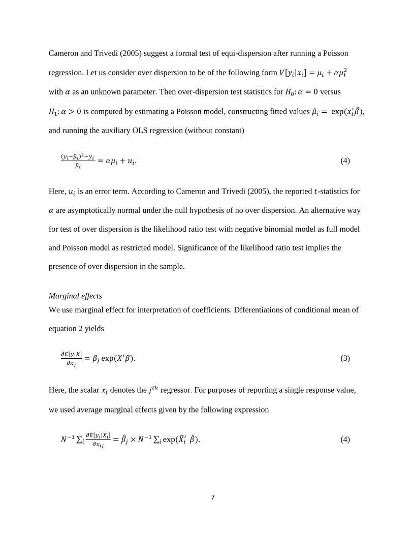
Cameron and Trivedi (2005) suggest a formal test of equi-dispersion after running a Poisson

regression. Let us consider over dispersion to be of the following form [ | ]

with as an unknown parameter. Then over-dispersion test statistics for versus

is computed by estimating a Poisson model, constructing fitted values ( ),

and running the auxiliary OLS regression (without constant)

( )

(4)

Here, is an error term. According to Cameron and Trivedi (2005), the reported -statistics for

are asymptotically normal under the null hypothesis of no over dispersion. An alternative way

for test of over dispersion is the likelihood ratio test with negative binomial model as full model

and Poisson model as restricted model. Significance of the likelihood ratio test implies the

presence of over dispersion in the sample.

Marginal effects

We use marginal effect for interpretation of coefficients. Dfferentiations of conditional mean of

equation 2 yields

[ | ]

( ). (3)

Here, the scalar denotes the regressor. For purposes of reporting a single response value,

we used average marginal effects given by the following expression

∑ [ | ]

∑ (

) . (4)

8

1.2 Nonparametric method

Use of a generalized kernel estimation in a nonparametric method allows incorporation of

both continuous and categorical variables ( Racine and Li (2004). We consider a nonparametric

model with both continuous ( ) and categorical ( ) explanatory variables

( ) (5)

where ( ) has an unknown functional form. We also assume that has mean zero and

variance ( | ) ( ). Suppose that ( ) represents a univariate kernel function so that

we can write the product kernel as

(

) ∏ (

)

(6)

where and are elements of and , and represents the smoothing parameter for all

the continuous variable. We used standard normal kernel function as our kernel type, expressed

as

( )

√

. (7)

The kernel function for discrete variable is expressed as

( ) {

(8)

where and are elements ( to ), is the smoothing parameter which lies in the

interval [0,1]. This indicates that the kernel function becomes indicator function when ,

9

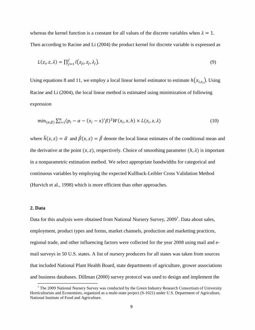
whereas the kernel function is a constant for all values of the discrete variables when .

Then according to Racine and Li (2004) the product kernel for discrete variable is expressed as

( ) ∏ ( ) (9)

Using equations 8 and 11, we employ a local linear kernel estimator to estimate ( ) Using

Racine and Li (2004), the local linear method is estimated using minimization of following

expression

( ) ∑ ( ( ) ) ( ) ( ) (10)

where ( ) and ( ) denote the local linear estimates of the conditional mean and

the derivative at the point ( ), respectively. Choice of smoothing parameter ( ) is important

in a nonparametric estimation method. We select appropriate bandwidths for categorical and

continuous variables by employing the expected Kullback-Leibler Cross Validation Method

(Hurvich et al., 1998) which is more efficient than other approaches.

2. Data

Data for this analysis were obtained from National Nursery Survey, 20091. Data about sales,

employment, product types and forms, market channels, production and marketing practices,

regional trade, and other influencing factors were collected for the year 2008 using mail and e-

mail surveys in 50 U.S. states. A list of nursery producers for all states was taken from sources

that included National Plant Health Board, state departments of agriculture, grower associations

and business databases. Dillman (2000) survey protocol was used to design and implement the

1 The 2009 National Nursery Survey was conducted by the Green Industry Research Consortium of University

Horticulturists and Economists, organized as a multi-state project (S-1021) under U.S. Department of Agriculture,

National Institute of Food and Agriculture.

10

survey, which was sent to 15,000 producers whereas email survey was sent to 1,900 producers in

12 states. A total of 3,044 valid responses were received with a 17% response rate. Out of these

samples 312 were obtained from e-mail survey.

The survey listed 22 different IPM techniques were adopted by nursery producers.

Details on specific technique and number of producers adopting these techniques are given in

Table 1. Use of techniques such as removing infested plants, hand weeding, inspecting incoming

stock was adopted by large percentage of nursery producers. Percentage of farmers adopting

each technique is provided in Figure 1, where 11% did not adopt any techniques. Most of the

nursery producers adopted four to ten IPM techniques. Pair-wise correlation coefficients for all

IPM techniques show that only a few practices were jointly adopted. For example, spot treatment

with pesticides was correlated with remove infested plants, alternate pesticides to avoid chemical

resistance, elevate or space plants for air circulation, and disinfect bench/ground cover. Further,

use cultivation- hand weeding was correlated with remove infested plants. However, these

correlation coefficients were close to 0.5 and only for a few IPM practices, so it is safe to analyze

data using count models.

Our dependent variable is the number of IPM techniques adopted by nursery growers.

The number of IPM techniques available to nursery producers ranged from 0 to 22. Explanatory

variables were regional dummies (Northeast, Midwest, Pacific, Southeast), and sales of plant

group (trees/shrubs, bedding plants, vines, foliage and other), contracted production (total sales

under contract, contract to other producers, to garden centers and to mass merchandiser), age,

computer management aids, channel diversity etc. Choice of these explanatory variables is

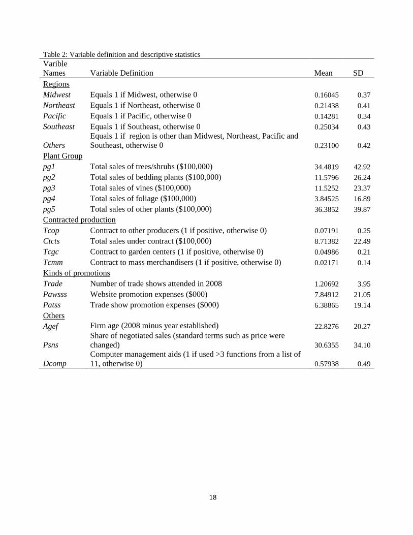
consistent with the study by Hinson et al. (2012). Explanatory variables and summary statistics

are provided in Table 2.

11

3. Results and Discussion

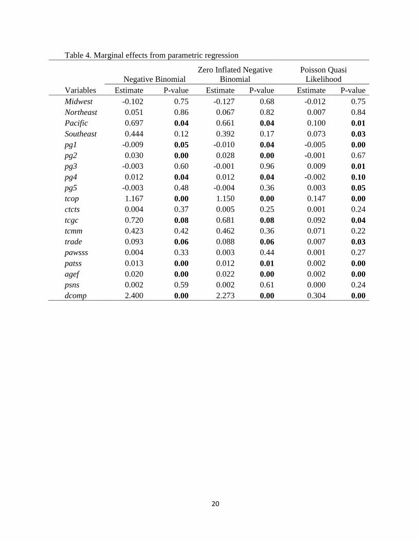
Parametric results of negative binomial, zero inflated negative binomial and PQL are provided in

Table 3 and corresponding model marginal effects are given in Table 4. We first tested for model

specification to interpret results obtained from these models. The coefficient of alpha parameter

was significant leading, to a decisive rejection of the null of equi-dispersion ( ). Consistent

with this, there was a large increase in the log-likelihood from -5930.43 to -5564.93 at the cost of

one additional parameter than the Poisson model. The highly significant LR test statistics

(731.37) indicated considerable improvement in the fit of the model. Figure 1 shows there were

many zeros, a potential problem as an NB model does not capture excess zeros. Hence, we also

tested the zero inflated model using the LR test of Vuong (1989) to identify a better model

between negative binomial and zero inflated negative binomial (ZINB) models. A large positive

test value favors a ZINB model whereas a large negative value favors an NB model (Cameron

and Trivedi, 2010). In our case, the test statistics was 3.01 and one-sided p-value of this test

statistics was 0.002, favoring the ZINB model. Staub and Winkelmann (2012) found that PQL

model was consistent compared to ZINB model, so our interpretation of results based on PQL

model is presented in following paragraphs. Parameter significance was measured at a 10%

level.

Results suggest those nursery growers located in Pacific and Southeast regions adopted more

IPM methods compared to others. Marginal effects indicated that nursery growers in the Pacific

region adopted 0.1 more practices compared to farmers in other regions, and nursery growers in

the Southeast region adopted 0.073 more practices compared to other regions. An increase in

sales of trees/shrubs (pg1) led to lower IPM adoption. These products tend to be less affected

12

with pests and diseases. We found similar effects for sale of foliage (pg4), but increase in sales

of vines (pg3) and other plants (pg5) increased the number of practices adopted.

We found that if production is contracted to other producers (tcop), IPM techniques adopted

increased. Marginal effect for this variable is 0.147 which indicates that IPM adoption is 0.147

higher among those producers who contracted to other producers. We found similar results for

contract to garden center (tcgc) and the number of IPM practices increased by 0.092. We also

found that number of trade shows attended in 2008 (trade) has a positive effect of 0.007 on

number of IPM techniques. Further, an increase in expenses on trade shows (patss) had a

positive effect on number of IMP technique adoption. We found that increase in farm age

increased the number of practices by 0.002. With respect to use of the computer as a

management aid (dcomp), the number of practices used increased by 0.304.

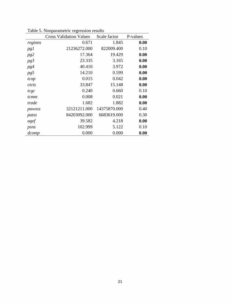
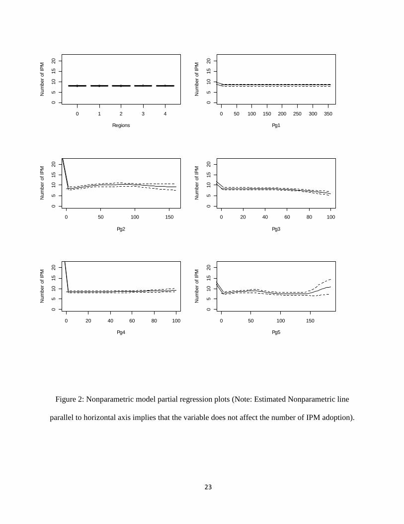
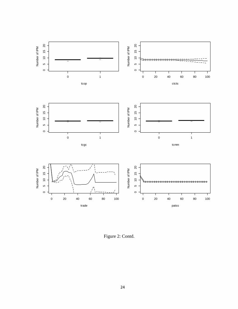
Nonparametric results

We used local-linear least squares cross-validation bandwidth selection method (Racine and Li,

2004)2 to estimate a nonparametric model. The value for a nonparametric model is 0.37

which is very high compared to parametric results. Therefore, in terms of model fit, a

nonparametric model performs better than the parametric models estimated. The cross validation

estimates, the associated scale factors and the P-values for our nonparametric regression are

presented in Table 5. These p-values are generated by employing and an iid bootstrap process.

The significance test is equivalent to a t-test for our parametric models. Table 5 shows that

regions, sales of bedding plants, vines, foliage and others, sales under contract, contract to other

producers, contract to mass merchandisers, number of trade shows and age of farm established

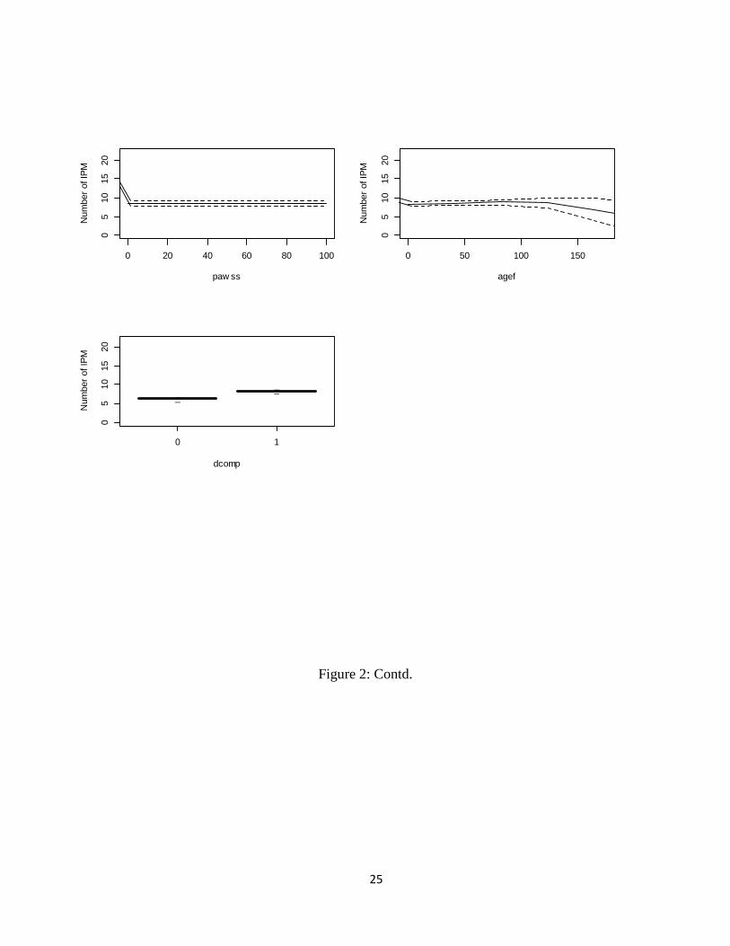
are all statistically significant. Figure 2 shows our results as a set of partial plots. The plot shows

2 All programming was done using R 2.15.0 and package np (see www.r.project.org; R, 2012).

13

relation between each explanatory variable against number of IPM techniques, assuming that all

other independent variables take their mean values. Nonparametric estimate with point-wise

confidence interval and bootstrap error are used to plot confidence interval.

We observed that regions are statistically significant where the labels indicate Midwest

(1), Northeast (2), Pacific (3) and Southeast (4). We can see that as sales of bedding plants (pg2)

increased, the number of practices adopted also increased; however, it decreases when sales

volume reached $100 million. We found that number of IPM practices decreased as sales of

vines (pg3), foliage (pg4) and other (pg5) increased. We found that nursery producers with

contract to other producers (tcop) and contract to mass merchandisers (tcmm) adopt more IPM

techniques. As total sales under contract (ctcts) increased the number of IPM adoption decreased.

We found that trade had a mixed effect on number of IPM practices - as number of trade shows

increased up around 20, the number of IPM adopted also increased and then decreases and likely

to remain constant. Our results also show that as age of the business increased (agef), the number

of IPM techniques adopted decreased. Finally, nursery producers who used computer as a

management aid (dcomp) had a higher number of IPM techniques adopted than those who do

not.

4. Conclusions

We examined the issue of IPM adoption, and our focus has been on the intensity of IPM

adoption rather than whether or not a specific IPM technology has been adopted by plant nursery

producers. By using 2009 National Nursery Survey data, we identified different factors on the

intensity of adoption of IPM practices to manage pests. We used better parametric model PQL

which is more consistent than ZINB. We found that nonparametric model is preferred over

14

parametric method. We employed cross-validation method and we were able to combine

categorical and continuous variables thereby avoiding a sample splitting problem. Although

nonparametric model is computationally intensive, we utilized it as it does not require a prior

functional form specification.

Overall, results from the parametric model indicated that Pacific and Southeast region,

sales of trees, farm age, number of trade shows have positive relation to the number of IPM

adopted, whereas sales of trees/ shrubs and foliage had opposite effects. Overall, our

nonparametric model gave slightly different results for some explanatory variables that are

statistically significant compared to the parametric models. In particular, the nonparametric

model indicated total sales under contract (ctcts) and contracts to mass merchandiser (tcmm) as

important variables in determining the number of IPM practices adopted, but these were not

significant in the parametric model. Contrasting results were found for some variables, namely

sales of vines (pg3) and firm age (agef) between parametric and nonparametric results.

15

REFERENCES

Adkins, C.R., J.R. Sidebottom, and A.F. Fulcher 2012. Overview of Ipm in Flowering &

Ornamental Shade Trees

http://www.clemson.edu/extension/horticulture/nursery/ipm/book_files/chapter_1

Cadigan, N.G., and J. Tobin. 2010. "Estimating the Negative Binomial Dispersion Parameter

with Highly Stratified Surveys." Journal of Statistical Planning and Inference

140(7):2138-2147.

Cameron, A.C., and P.K. Trivedi. 2005. Microeconometrics : Methods and Applications:

Cambridge University Press.

Cameron, A.C., and P.K. Trivedi. 2010. Microeconometrics Using Stata: Stata Press.

Dillman, D. 2000. Mail and Internet Surveys: The Tailored Design Method. New York: John

Wiley & Sons.

Fernandez-Cornejo, J., and J. Ferraioli. 1999. "The Environmental Effects of Adopting Ipm

Techniques: The Case of Peach Producers." Journal of Agricultural and Applied

Economics 31(3):551-564.

Hinson, R.A., K.P. Paudel, M. Velastegui, M.A. Marchant, and D.J. Bosch. 2012.

"Understanding Ornamental Plant Market Shares to Rewholesaler, Retailer, and

Landscaper Channels." Journal of Agricultural and Applied Economics 44(02):173–189.

Hurvich, C.M., J.S. Simonoff, and C.-L. Tsai. 1998. "Smoothing Parameter Selection in

Nonparametric Regression Using an Improved Akaike Information Criterion." Journal of

the Royal Statistical Society: Series B (Statistical Methodology) 60(2):271-293.

Mishra, A.K., and T.A. Park. 2005. "An Empirical Analysis of Internet Use by U.S. Farmers."

Agricultural and Resource Economics Review 34(2):253-264.

Park, B.J., and D. Lord. 2008. "Adjustment for Maximum Likelihood Estimate of Negative

Binomial Dispersion Parameter." Transportation Research Record: Journal of the

Transportation Research Board 2061(-1):9-19.

Paxton, K.W., A.K. Mishra, S. Chintawar, J.A. Larson, R.K. Roberts, B.C. English, D.M.

Lambert, M.C. Marra, S.L. Larkin, J.M. Reeves, and S.W. Martin. 2011. "Intensity of

Precision Agriculture Technology Adoption by Cotton Producers." Agricultural and

Resource Economics Review 40(1):133-144.

16

Racine, J., and Q. Li. 2004. "Nonparametric Estimation of Regression Functions with Both

Categorical and Continuous Data." Journal of Econometrics 119(1):99-130.

Rahelizatovo, N.C., and J.M. Gillespie. 2004. "The Adoption of Best-Management Practices by

Louisiana Dairy Producers." Journal of Agricultural and Applied Economics 36(1):229-

240.

Rejesus, R.M., F.G. Palis, A.V. Lapitan, T.T.N. Chi, and M. Hossain. 2009. "The Impact of

Integrated Pest Management Information Dissemination Methods on Insecticide Use and

Efficiency: Evidence from Rice Producers in South Vietnam." Applied Economic

Perspectives and Policy 31(4):814-833.

Sellmer, J.C., N. Ostiguy, K. Hoover, and K.M. Kelley. 2004. "Assessing the Integrated Pest

Management Practices of Pennsylvania Nursery Operations." HortScience 39(2):297-302.

Sharma, A., A. Bailey, and I. Fraser. 2011. "Technology Adoption and Pest Control Strategies

among Uk Cereal Farmers: Evidence from Parametric and Nonparametric Count Data

Models." Journal of Agricultural Economics 62(1):73-92.

Staub, K.E., and R. Winkelmann. 2012. "Consistent Estimation of Zero-Inflated Count Models."

Health Economics. DOI: 10.1002/hec.2844

Vuong, Q.H. 1989. "Likelihood Ratio Tests for Model Selection and Non-Nested Hypotheses."

Econometrica 57:307-333.

Zhou, M., L. Li, D. Dunson, and L. Carin 2012. Lognormal and Gamma Mixed Negative

Binomial Regression http://people.ee.duke.edu/~lcarin/Mingyuan_ICML_2012.pdf

17

Table 1: IPM technology and percentage of nursery producers adopting the technology

IPM Technology

Percentage of

Nursery Producers

Adopting the

Technology

Remove infested plants 69

Alternate pesticides to avoid chemical resistance 46

Elevate or space plants for air circulation 47

Use cultivation, hand weeding 64

Disinfect benches/ground cover 35

Use sanitized water foot baths 4

Soil solarization/sterilization 12

Monitor pest populations with tarp or sticky boards 25

Adjust pesticide application to protect beneficial 30

Use mulches to suppress weeds 37

Beneficial insect identification 34

Inspect incoming stock 57

Manage irrigation to reduce pests 43

Spot treatment with pesticides 58

Ventilate greenhouses 36

Use of beneficial insects 22

Keep pest activity records 19

Adjust fertilization rates 32

Use screening/barriers to exclude pests 12

Use bio pesticides/ lower toxicity 25

Treat retention pond water 4

Use pest resistant varieties 30

18

Table 2: Variable definition and descriptive statistics

Varible

Names Variable Definition Mean SD

Regions

Midwest Equals 1 if Midwest, otherwise 0 0.16045 0.37

Northeast Equals 1 if Northeast, otherwise 0 0.21438 0.41

Pacific Equals 1 if Pacific, otherwise 0 0.14281 0.34

Southeast Equals 1 if Southeast, otherwise 0 0.25034 0.43

Others

Equals 1 if region is other than Midwest, Northeast, Pacific and

Southeast, otherwise 0 0.23100 0.42

Plant Group

pg1 Total sales of trees/shrubs ($100,000) 34.4819 42.92

pg2 Total sales of bedding plants ($100,000) 11.5796 26.24

pg3 Total sales of vines ($100,000) 11.5252 23.37

pg4 Total sales of foliage ($100,000) 3.84525 16.89

pg5 Total sales of other plants ($100,000) 36.3852 39.87

Contracted production

Tcop Contract to other producers (1 if positive, otherwise 0) 0.07191 0.25

Ctcts Total sales under contract ($100,000) 8.71382 22.49

Tcgc Contract to garden centers (1 if positive, otherwise 0) 0.04986 0.21

Tcmm Contract to mass merchandisers (1 if positive, otherwise 0) 0.02171 0.14

Kinds of promotions Trade Number of trade shows attended in 2008 1.20692 3.95

Pawsss Website promotion expenses ($000) 7.84912 21.05

Patss Trade show promotion expenses ($000) 6.38865 19.14

Others

Agef Firm age (2008 minus year established) 22.8276 20.27

Psns

Share of negotiated sales (standard terms such as price were

changed) 30.6355 34.10

Dcomp

Computer management aids (1 if used >3 functions from a list of

11, otherwise 0) 0.57938 0.49

19

Table 3. Parametric regression results

Negative Binomial

Zero Inflated Negative

Binomial

Poisson Quasi

Likelihood

Variables Estimate P-value Estimate P-value Estimate P-value

Intercept 1.696 0.00 1.761 0.00 1.981 0.00

Midwest -0.013 0.75 -0.016 0.69 -0.012 0.75

Northeast 0.006 0.86 0.008 0.82 0.007 0.84

Pacific 0.085 0.03 0.081 0.04 0.100 0.01

Southeast 0.055 0.12 0.049 0.16 0.073 0.03

pg1 -0.001 0.05 -0.001 0.01 -0.005 0.00

pg2 0.004 0.00 0.003 0.00 -0.001 0.67

pg3 0.000 0.60 0.000 0.62 0.009 0.01

pg4 0.001 0.04 0.001 0.06 -0.002 0.10

pg5 0.000 0.48 -0.001 0.16 0.003 0.05

Tcop 0.138 0.00 0.137 0.00 0.147 0.00

Ctcts 0.000 0.37 0.001 0.25 0.001 0.24

Tcgc 0.087 0.06 0.082 0.07 0.092 0.04

Tcmm 0.052 0.41 0.056 0.34 0.071 0.22

Trade 0.012 0.06 0.011 0.06 0.007 0.03

pawsss 0.001 0.33 0.000 0.44 0.001 0.27

Patss 0.002 0.00 0.001 0.01 0.002 0.00

Agef 0.002 0.00 0.003 0.00 0.002 0.00

Psns 0.000 0.59 0.000 0.61 0.000 0.24

dcomp 0.322 0.00 0.304 0.00 0.304 0.00

ln alpha -1.822

-2.0188

Pseudo R2 0.029

LL -5564.930

-5536.509 -5824.839

Note: Over dispersion test coefficient is 0.124 with p-value equal to 0.00.

Likelihood ratio (LR) test for over-dispersion is 731.37 with p-value equal to 0.00

Vuong test of ZINB vs. standard negative binomial: z = 3.01 Pr > z = 0.00

20

Table 4. Marginal effects from parametric regression

Negative Binomial

Zero Inflated Negative

Binomial

Poisson Quasi

Likelihood

Variables Estimate P-value Estimate P-value Estimate P-value

Midwest -0.102 0.75 -0.127 0.68 -0.012 0.75

Northeast 0.051 0.86 0.067 0.82 0.007 0.84

Pacific 0.697 0.04 0.661 0.04 0.100 0.01

Southeast 0.444 0.12 0.392 0.17 0.073 0.03

pg1 -0.009 0.05 -0.010 0.04 -0.005 0.00

pg2 0.030 0.00 0.028 0.00 -0.001 0.67

pg3 -0.003 0.60 -0.001 0.96 0.009 0.01

pg4 0.012 0.04 0.012 0.04 -0.002 0.10

pg5 -0.003 0.48 -0.004 0.36 0.003 0.05

tcop 1.167 0.00 1.150 0.00 0.147 0.00

ctcts 0.004 0.37 0.005 0.25 0.001 0.24

tcgc 0.720 0.08 0.681 0.08 0.092 0.04

tcmm 0.423 0.42 0.462 0.36 0.071 0.22

trade 0.093 0.06 0.088 0.06 0.007 0.03

pawsss 0.004 0.33 0.003 0.44 0.001 0.27

patss 0.013 0.00 0.012 0.01 0.002 0.00

agef 0.020 0.00 0.022 0.00 0.002 0.00

psns 0.002 0.59 0.002 0.61 0.000 0.24

dcomp 2.400 0.00 2.273 0.00 0.304 0.00

21

Table 5. Nonparametric regression results

Cross Validation Values Scale factor P-values

regions 0.671 1.845 0.00

pg1 21236272.000 822009.400 0.10

pg2 17.364 19.429 0.00

pg3 23.335 3.165 0.00

pg4 40.416 3.972 0.00

pg5 14.210 0.599 0.00

tcop 0.015 0.042 0.00

ctcts 33.847 15.148 0.00

tcgc 0.240 0.660 0.10

tcmm 0.008 0.021 0.00

trade 1.682 1.882 0.00

pawsss 32121211.000 14375870.000 0.40

patss 84203092.000 6683619.000 0.30

agef 39.582 4.218 0.00

psns 102.999 5.122 0.10

dcomp 0.000 0.000 0.00

22

Figure 1: Percentage of nursery producers adopting different numbers of IPM.

11.77

3.68

5.39

6.31

7.76 7.69

6.91 7 7.37

6.87

5.95

5.06 4.77

3.65 3.32

2.24 1.68

1.09 0.76

0.16 0.36 0.16 0.03 0

2

4

6

8

10

12

14

0 1 2 3 4 5 6 7 8 9 10 11 12 13 14 15 16 17 18 19 20 21 22

Pe

rce

nta

ge o

f p

rod

uce

r

Number of IPM

23

Figure 2: Nonparametric model partial regression plots (Note: Estimated Nonparametric line

parallel to horizontal axis implies that the variable does not affect the number of IPM adoption).

0 1 2 3 4

05

10

15

20

Regions

Num

ber

of IP

M

- - - - -- - - - -

0 50 100 150 200 250 300 350

05

10

15

20

Pg1

Num

ber

of IP

M

0 50 100 150

05

10

15

20

Pg2

Num

ber

of IP

M

0 20 40 60 80 100

05

10

15

20

Pg3

Num

ber

of IP

M

0 20 40 60 80 100

05

10

15

20

Pg4

Num

ber

of IP

M

0 50 100 150

05

10

15

20

Pg5

Num

ber

of IP

M

24

Figure 2: Contd.

0 1

05

10

15

20

tcop

Num

ber

of IP

M

_ ___

0 20 40 60 80 100

05

10

15

20

ctcts

Num

ber

of IP

M

0 1

05

10

15

20

tcgc

Num

ber

of IP

M

_ __ _

0 10

510

15

20

tcmm

Num

ber

of IP

M

_ __ _

0 20 40 60 80 100

05

10

15

20

trade

Num

ber

of IP

M

0 20 40 60 80 100

05

10

15

20

patss

Num

ber

of IP

M

25

Figure 2: Contd.

0 20 40 60 80 100

05

10

15

20

paw ss

Num

ber

of IP

M

0 50 100 150

05

10

15

20

agef

Num

ber

of IP

M

0 1

05

10

15

20

dcomp

Num

ber

of IP

M

____