No. 2008–43

INTENSITY OF COMPETITION AND MARKET STRUCTURE IN THE ITALIAN BANKING INDUSTRY

By Caterina Giannetti

April 2008

ISSN 0924-7815

Intensity of competition and Market structure in

the Italian Banking Industry

This version: April 2008

AbstractThis work tests the predictions of Sutton’s model of independent submarkets for the Italian

retail banking industry. In the first part of this paper, I develop a model of endogenous mergersto evidence the relationship between firms’ conduct, market entry and market structure. Inthe second part, I identify the submarket dimension and estimate the relationship betweenmarket size and market structure using data on bank branches. The size of the submarketsturned out to be at most provincial whereas the limiting concentration index - as argued bySutton for industries with exogenous sunk costs - goes to zero as the market becomes larger.

Keywords: Concentration, Truncated Poisson and Negative Binomial models, quantile regressions

JEL Classification: C24, D43, L11, L89

1Email: c.giannetti@uvt.nlI am grateful to Luigi Buzzacchi for his guidance and his precious indications. I also thank Marcello Messori,Giampiero M. Gallo, Elena Carletti, and Hans Degryse for valuable comments and suggestions. Special thanksto Paul Belleflamme and to participants at the IV Doctoral Workshop in Economics (Louvain-la-Neuve), the 34th

EARIE Conference (Valencia), the ESSID Workshop (Cargèse), as well as seminars participants at CES (Universityof Paris I).This paper was partly written while I was visiting CORE, and I am grateful to them for their hospitality. I alsoacknowledge the financial support from the EDNET Marie Curie fellowship program. All remaining errors are myresponsibility.

1 Introduction

Sutton’s model of independent submarkets emphasizes the strategic choice of sunk costs and,

unlike the traditional structure-conduct-performance approach, considers how changes in firms’

conduct affects the condition of entry, altering by consequence market structure. Under this scheme,

both homogeneous-horizontally differentiated products and advertising-R&D intensive (vertically

differentiated products) industries can be analysed. For the former type of industries, with fixed

sunk costs, it is possible to show an inverse relationship between market size and market structure.

For the latter type of industries, where sunk costs are endogenous, such a negative relationship does

not necessarily emerge as market size increases. This is because sunk costs, such as advertising or

R&D expenditure, raise with market size. Such expenditures are choice variables of (perceived)

quality: by increasing the level of advertising-R&D, firms are able to gain (or to maintain) market

share. Therefore, as market size becomes larger, an ‘escalation mechanism’ could raise fixed costs

per firm to such an extent that the negative relationship between market size and market structure

will break down. Sutton’s model offers therefore very clear and testable predictions about the

relationship between market-size and market-concentration.

The aim to this paper is to analyse the Italian retail banking industry as a special case of the

first type of industries, since products are rather standardized and there is a limited scope for cost-

decreasing or quality increasing investments. This industry can be viewed as made of a large number

of local markets that arise because there are many different geographical locations throughout the

country: in every submarket products are fairly good substitutes and banks compete against each

other by means of their branch locations. The degree of substitutability is substantially lower for

products and services offered in neighbour submarkets.

In the first part of this paper, relying on the model developed by Vasconcelos (2006), I examine

the firm strategic behaviour referring to a three-stage non cooperative game. In line with Sutton’s

theory, the aim is to highlight the relationship between firm conduct, entry and market structure

while explicitly allowing for a merger process in the industry. In so doing, it is possible to show

that the incentives to merge to a monopoly are lead by the intensity of competition and by the

degree of product substitution. This ultimately shows how the number of banks as well as the share

1

of the main bank are determined in each submarket, and offers indications on the variables to be

used in the empirical section. In the second part, I will estimate the market structure-market size

relationship in the Italian retail banking industry. Testing this relationship empirically requires

identifying a set of independent submarkets. In order to do that, I estimate the number of firms

in each province using data on the national bank branch location. To take into account that the

number of firms is discrete and greater than zero, a truncated Poisson and Negative Binomial

models are used. This analysis confirms that the province (at most) is the size of each submarket.

In fact, firm variables related to neighbour provinces turned out to be insignificant in determining

the number of bank in each province. Once the size of the submarket has been identified, I will

investigate the market structure-market size relationship by regressing the one firm concentration

ratio on market size variables. As the limiting concentration ratio approaches zero as market size

goes to infinity, the hypothesis of exogenous sunk costs for the retail banking industry can be

accepted.

The paper is organized as follows. The next section presents the theoretical framework to

analyse the relationship between firm conduct and concentration based on the Sutton approach.

Sections 3 and 4 respectively describe the banking industry referring to this framework and the

characteristic and the construction of the dataset. In section 5 the econometric model and results

are presented. Conclusions are in the final section.

2 The theoretical approach

Sutton (1991, 1997, 1998) describes the impact of firm conduct on market structure identifying two

key aspects: the intensity of competition and the level of endogenous sunk costs. Considering these

elements, he distinguishes between two general types of industry. One class is characterized by

industries that produce homogeneous and horizontally differentiated products. The other category

is composed of industries engaged in the production of vertically differentiated products. In the

first type of industries, the only important sunk costs are the exogenously determined setup costs,

given by the technology. In such industries Sutton (1998) predicts a lower bound to concentration,

which goes to zero as the market size increases and rises with the intensity of price competition.

2

The idea is that as market size increases, profits also increase, and given free entry, other firms will

enter the market until the last entrant just covers the exogenous cost for entry. Also, the higher the

competition, the higher the concentration index. In fact, as the competition gets stronger, the entry

becomes less profitable and the higher the level of concentration is to be in order to allow firms

to cover their entry cost1. It is important to underline that the intensity of competition will not

simply represent firm strategies but, rather, the functional relationship between market structure,

prices and profits. It is derived by institutional factors, and therefore is not only captured by the

price-cost margin. More generally, an increase in the intensity of competition could be represented

by any exogenous influence that makes entry less profitable, e.g the introduction of a competition

law (Symeodonis (2000), Symeodonis (2002)). In the second type of industries sunk costs are

endogenous. Firms pay some sunk cost to enter but can make further investments to enhance

their demand. As market size increases, the incentive to gain market share through advertising

and R&D expenditure also increases, leading to higher fixed cost per firm. Even though room

for other firms is potentially created, the ‘escalation mechanism’ will raise the endogenous fixed

costs, possibly breaking down the negative structure-size relationship that exists in the other type

of industries. For such industries Sutton’s model predicts that the minimum equilibrium value of

seller concentration remains positive as the market grows2.

Sutton’s model offers very clear predictions for the first group of industries whereas it is not

possible for industries where sunk costs are endogenous. Despite Sutton’s insights on the relation-

ship between market concentration and market size, there are few empirical works testing these

predictions. Previous works that test the Sutton approach are Sutton (1998) for the US Cement

Industry, Buzzacchi and Valletti (2005) for the Italian Motor Insurance Industry, Asplund and

Sandin (1999) for the Swedish Driving Schools Sector, (Walsh and Whelan (2002)) in Carbonated

Soft Drinks in the Irish retail market, Hutchinson et al. (2006) across manufacturing industries in

UK and Belgium, and Ellickson (2007) for the supermarket industry in the United States. These1A way to model an increase in the ‘toughness of price competition’ is to consider a movement from monopoly

model to Cournot and Bertrand model. For any given market size, the higher the competition at final stage, thelower the number of firms entering at stage 1, and the higher the concentration index (ex-post). See Sutton (2002).

2To be more precise, Sutton goes further in distinguishing within the endogenous cost categories between low-αand high-α industries. In the low-α type industries, due to R&D trajectories, we will still observe low level ofconcentration

3

papers mainly test Sutton’s predictions by typically looking if a measure of firm inequality - such

as the Gini coefficient - increases with the number of submarkets. Specific to the banking sector

are the works of Dick (2007) for the Banking Industry in the United States and de Juan (2003) for

the Spanish Retail Banking Sector. Although Dick (2007) investigated the relationship between

market size and market concentration, she considered the banking industry without distinguishing

the retail segment from the wholesale. In particular, she focused on banking quality through a

set of variables, such as geographic diversification, employees compensation and branch density,

finding a non-decreasing concentration ratio as market size gets larger. She concluded that endoge-

nous quality model characterized the industry. de Juan (2003) analysed instead another important

insight of Sutton’s analysis: the degree of concentration and the level of aggregation of submarkets.

Focusing on retail market only, and after having identified the individual submarkets, she tested

the bound on the inequality of firm size distribution at different levels, local, regional and national.

The purpose of this paper is to verify if empirical evidence for the Italian retail banking industry is

consistent with Sutton’s predictions. To apply this framework to the Italian banking industry is of

interest since during the nineties it experienced a deregulation and consolidation process. There-

fore, in order to identify the relationship proposed by Sutton, the choice of the year is crucial. I

will assume that the industry reached in 2005, the year of the analysis, an equilibrium. Similar to

de Juan (2003), I will make an effort to empirically test the size of the submarket but I will depart

from her work by investigating the market size- market concentration relationship. As the focus

is on the retail banking, this paper also differentiates from Dick (2007) as she considered both the

industry segments, wholesale and retail. The present paper is also strictly related to the theoret-

ical analysis developed by Cerasi (1996). Cerasi developed a model of retail banking competition

in which banks compete first in branching and then in prices. In line with Sutton’s analysis her

model predicts that deregulation should lead to an increase in the degree of concentration whereas,

with respect to branching, an increase in market size is followed by a decrease in the degree of

concentration in branching.

4

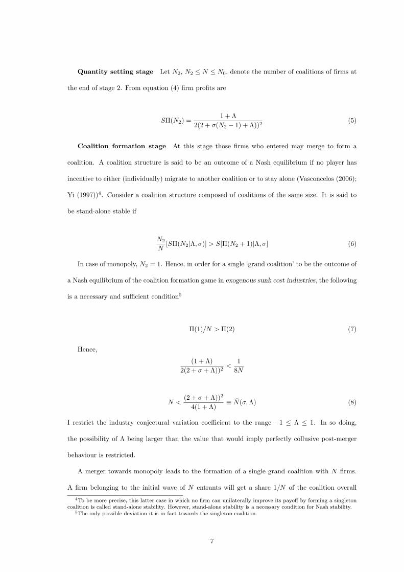
3 Exogenous sunk cost industries: the model

Using the model developed by Vasconcelos (2006), as modified in order to explicitly account for

the intensity of competition, this section analyses the market size-concentration relationship in

exogenous sunk cost industries. In such industries, firms will face some sunk cost to enter but

cannot make further investment in order to enhance their demand. Assuming that all consumers

have the same utility function over n substitute goods (or n varieties of the same product) as

follows:

U(x1, ....., xn;M) =∑

k

(xk − x2k)− 2σ

∑k

∑l<k

xkxl + M, (1)

where xk is the quantity of good k and M denotes expenditure on outside goods whose price

is fixed exogenously at unity. The parameter σ, 0 ≤ σ ≤ 1, measures the degree of substitution

between goods3. When σ = 0 the cross product term in the utility function vanishes so that

product varieties are independent in demand, whereas if σ = 1, the goods are perfect substitutes.

For the utility function (1), the individual demand for good k is:

pk = 1− 2xk − 2σ∑l 6=k

xl (2)

If there are S identical consumers in the market and we denote with xk the per-capita quantity

demanded of good k, market demand for this good is Sxk.

Considering now a three stage game. In the first stage, a sufficiently large number of ex-ante

identical firms, N0, simultaneously decide whether or not to enter the market incurring an entry

cost of ε. In the second stage, firms that have decided to enter decide to join a coalition. All the

firms that have decided to join the same coalition then merge. In the third stage, firms set their

output. All coalitions are assumed to face the same marginal cost of production c, which we can

normalize to zero.3This is a quadratic utility function and it has previously used by Spence(1976), Shaked and Sutton (1990),

Sutton (1997, 1998) and Symeodonis (2000). The banking sector is usually analysed under hotelling-type model.However, it is possible to show that any hotelling-type model is a special case of vertical production differentiation.See Cremer and Thisse (1991).

5

4 The game: equilibrium analysis

In stage 2, each firm i ∈ {1, ...., N} simultaneously announces a list of players that it wishes to

form a coalition with. Firms that make exactly the same announcement form a coalition together.

For example, if firms 1 an 2 both announced coalition {1, 2, 3}, while firm 3 announced something

different, then only players 1 and 2 form a coalition. Since all firms are initially symmetric, members

of each coalition are assumed to equally share the final stage profit.

Let λ = dxj

dxirepresent firm i’s conjectural variation, that is its expectation about the change in

its competitors production resulting from a change in its own production level, and assume that

this conjecture is identical for all firms (λi = dxj

dxi= λ).

Assuming that quantity is a strategic variable, profit maximization requires that ∂Πi/∂xi = 0.

In equilibrium:

xi =1

2(2 + (N − 1)σ(1 + λ))(3)

and the profit of each of the N firms is

SΠi = S1 + λ(N − 1)σ

2(2 + (N − 1)σ(1 + λ))2− F (4)

Let Λ be equal to σ(N−1)λ. It is possible to refer to Λ as the competitive intensity of the industry,

with lower values of Λ corresponding to more intense competition.

For F ≥ 0, N ≥ 2 and −1 ≤ Λ ≤ 1 , and 0 ≤ σ ≤ 1 each firm’s profit is a decreasing function of

the number of firms in the industry, its competitive intensity and the amount of fixed costs. Two

reasons could lead firms to merge: market power and efficiency. To maintain things simpler, I avoid

to account for efficiency gains. In this analysis, firms could not make any further investments to

enhance their quality (and hence the demand) of the product offered. So, it possible to set F = 0.

In any case, a clear picture in a similar framework is offered by Rodrigues (2001).

Following the traditional backward induction procedure, I analyze the condition under which I

get a monopoly in exogenous sunk cost industries model.

6

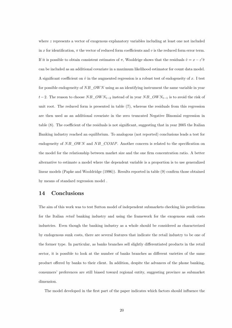
Quantity setting stage Let N2, N2 ≤ N ≤ N0, denote the number of coalitions of firms at

the end of stage 2. From equation (4) firm profits are

SΠ(N2) =1 + Λ

2(2 + σ(N2 − 1) + Λ))2(5)

Coalition formation stage At this stage those firms who entered may merge to form a

coalition. A coalition structure is said to be an outcome of a Nash equilibrium if no player has

incentive to either (individually) migrate to another coalition or to stay alone (Vasconcelos (2006);

Yi (1997))4. Consider a coalition structure composed of coalitions of the same size. It is said to

be stand-alone stable if

N2

N[SΠ(N2|Λ, σ)] > S[Π(N2 + 1)|Λ, σ] (6)

In case of monopoly, N2 = 1. Hence, in order for a single ‘grand coalition’ to be the outcome of

a Nash equilibrium of the coalition formation game in exogenous sunk cost industries, the following

is a necessary and sufficient condition5

Π(1)/N > Π(2) (7)

Hence,

(1 + Λ)2(2 + σ + Λ))2

<1

8N

N <(2 + σ + Λ))2

4(1 + Λ)≡ N̄(σ,Λ) (8)

I restrict the industry conjectural variation coefficient to the range −1 ≤ Λ ≤ 1. In so doing,

the possibility of Λ being larger than the value that would imply perfectly collusive post-merger

behaviour is restricted.

A merger towards monopoly leads to the formation of a single grand coalition with N firms.

A firm belonging to the initial wave of N entrants will get a share 1/N of the coalition overall4To be more precise, this latter case in which no firm can unilaterally improve its payoff by forming a singleton

coalition is called stand-alone stability. However, stand-alone stability is a necessary condition for Nash stability.5The only possible deviation it is in fact towards the singleton coalition.

7

profits, whereas by free-riding on its N-1 merging rivals it can obtain duopoly profits. Each time

in which the ‘grand coalition’ is unstable, as market size increases, more firms want to enter and

to free ride and form a duopoly instead of joining the grand coalition. That means, as the market

size rises, the concentration ratio goes down 6. This result shows how this process in turn affects

the one firm concentration ratio, C1 = qN2q = 1/N2.

When Λ lies in the range previously defined, and fixed costs are zero, N(σ,Λ) is strictly de-

creasing in Λ. Therefore, the weaker the competitive intensity, the larger the pre-merger market

concentration should be for a monopoly to emerge through merger.

In particular, if σ = 1, we can rewrite equation (8) as

N <1(Λ + 3)2

4(Λ + 1)(9)

The RHS is strictly decreasing in Λ. As Λ approaches -1, the value of perfect competition,

condition (9) is alway satisfied, and so, merger to monopoly would occur whatever the number

of firms in the industry. Hence, the higher the intensity of competition at stage 3, the lower the

pre-merger market concentration could be in order for a monopoly to emerge through merger.

When Λ = 0, that is firms behave as in Cournot, monopolization will occur only if σ ≥ 0.83. If

this condition is not met and more than two firms enter in stage 1, and merge in a single grand

coalition, that equilibrium might not be stable. As σ approaches 1, competition becomes tougher as

products are closer substitutes, and the lower bound to the one firm concentration ratio decreases

as market size increases. On the other hand, in perfectly cooperative industries, where Λ = 1,

or when demands are perfectly independent, where σ = 0, merger to monopolization will never

occur. However, it is important to remark that we are not considering cost efficiency gains that

would probably give an incentive to merge even in the case that market demands are completely

independent.

Entry stage At stage 1 firms decide to enter.

If σ = 1 products are perfect substitutes, a merger to monopoly will occur at the second stage

of the game if firms compete very toughly. Then, if firms anticipate that a monopoly coalition6It is valuable to remark that in this model it is implicitly assumed that the pre-merger behaviour is not affected

by the coalition formation stage.

8

structure is going to be formed at stage 2, firms will enter up to a point at which N is the largest

integer value satisfying

1N

(SΠ(1)) ≥ ε (10)

where ε > 0 is the entry fee. By the same reasoning, therefore, if the competitive intensity

is extremely strong, the firms will merge to monopoly. For any given level of market size, the

equilibrium level of concentration is higher. However, entry will occur at the first stage and the

lower bound to concentration goes down7. If products are imperfect substitutes - and Λ = 0 - a

merger to monopoly might not take place. In particular, when σ < 0.83, a merger to monopoly

might not take place since a firm could prefer to get all the profits of a duopolist. This means that

as the market size rises, more firms enter and this makes the monopoly unsustainable as individual

firms want to free ride and form a duopoly. Thus, there is an upper bound to concentration that

goes down as market size increases (Vasconcelos (2006)).

5 The Italian retail banking industry

The presence of different territorial dynamics is a characteristic of the Italian banking industry

(Guiso et al. (2004), Guiso et al. (2006); Colombo and Turati (2004)). I consider the retail Italian

banking industry as belonging to an industry of the first type, where sunk costs are exogenous

and the size of the submarkets is provincial. Since lending and borrowing take place mostly in

a narrow geographical place and operation are similar and repeated during time, this industry

can in fact be viewed as made of a large number of local markets, corresponding to different

provinces (geographical units close to US counts). These submarkets are independent both from

the supply and demand side. On the supply side, in each one of these independent submarkets,

banks’ goods are fairly substitute whereas banks’ products of neighbouring provinces are not. In

particular, in each province banks can mitigate price (interest rate) competition by means of their

branch location8. However, opening new branches, independently of the size of their operations,7Also, from the previous analysis, since ∂Π/∂N < 0 and ∂Π/∂Λ > 0, by applying the implicit function theorem,

one concludes that ∂N/∂Λ =−∂Π/∂Λ∂Π/∂N

> 0. The equilibrium number of firms is decreasing in the intensity ofcompetition at stage 3.

8See also Cerasi et al. (2002) and Cohen and Mazzeo (2004)

9

has fixed costs, for example the cost of hiring personnel, the cost of renting or buying facilities in

particular province and other province specific elements. As documented in (Cerasi et al. (2000)),

in Italy in the recent years, as a result of reforms on entry and branching regulation, the cost of

branching has decreased. On the demand side, despite the advances in home and phone banking,

preferences of customers seem to be still biased toward entities with strong regional and local

contents. A customer is likely to shop only at those banks that operate in the local area where he

lives and works. In other words, zero/small cross-elasticities are likely to characterize the demand

of geographically separated submarkets whereas positive elasticities are likely to characterize the

demand in each province.

6 Exogenous or endogenous sunk costs?

As we would expect both exogenous and endogenous sunk costs to be relevant in the banking

industry, with both horizontal and vertical differentiation, some point of remarks are deserved.

In this work I am considering the retail sector by looking at branches as the main distributional

channel of certain standardized banking products. Therefore, I am not looking as in Dick (2007) at

branches, as one of the costs in advertising and quality (employee compensation, branch staffing)

that banks will incur in order to enhance consumer willingness to pay. Indeed, as banks become

more and more visible through branches, one could consider branches as a form of advertising itself.

In other words, I am assuming that branches of different banks offer similar (bundle of) services

despite bank size and, hence, the number of branches in a given submarket could be considered

as the number of varieties of services offered by banks. Even in the case, however, there are

circumstances in which endogenous costs could arise. As pointed out by Petersen and Rajan (1995)

relationship lending may generate severe barriers to entry. However, the advent of information and

communication technologies increased the ability of banks to open branches in distant locations,

considerably reducing the cost of distance-related trade and enhancing competition in local banking

markets (Berger and Udell (2006), Affinito and Piazza (2005))9. In addition, developments in the9Besides, Berger himself has recently taken an opposite view with respect to his previous study (Berger et al.

(2003)) where it is claimed that services to small firms are likely to be provided by small banking institutionssince they meet the demands of informationally opaque SMEs that may be constrained in the financing by largeinstitutions. He now claims that this vision could be an oversimplification: new transaction technologies are nowavailable enabling large banks to overcome informational constraints.

10

financial industries with new contracts and new intermediaries are likely to reduce the role of close

bank-firm relationships (Rajan and Zingales (2003)). The opinions are not unique. Whatever the

conclusion might be, we can foresee that it will at least influence the structure of the banking

system in terms of the local nature of the banks but not the number of branches that could be

opened given market demand10. It is obvious that in the industry as a whole (retail and wholesale)

both endogenous and exogenous interact costs with one another to determine market structure.

The approach and conclusion could be very different (Dick (2007)).

7 Market equilibrium

The predictions of Sutton’s model apply to markets in equilibrium. However, discontinuities in the

normative (or economic) conditions can lead to process of consolidation. Unless we are observing

the market at the end of this process, it will be difficult to disentangle the relationship between

competition and concentration as predicted by Sutton from that caused by mergers and acquisi-

tions. This means that I am making the implicit assumption that the retail baking sector reached

an equilibrium in 2005, the year for which I collected the observations. This assumption - though

strong - seems reasonable. Beginning in the 1980s, the Italian Banking system underwent a series

of reforms aimed at increasing the competition in the market through liberalizing branching and

easing the geographical restrictions on lending. In fact, the opening of new branches had been

regulated by the ‘branch distribution plan’, issued every four years. The last distribution plan

was issued in 1986 and, since March 1990, the establishment of new branches has been completely

liberalized. The number of branches increased steadily, up to 31.081 in 2005, as well as the number

of people served by each branch, 47 per 100.000 inhabitants in 2004 (compared to 59 EU mean).

In particular, the number of banks mergers and acquisitions of control per year was 45 in 1990

and decreased substantially to 5 in 200511. At the same time, in more than 50% of the provinces,

new banks entered the market. This process of new entry, parallel to the process of consolidation,

made the average number of banks in each province rise from 29 in 1990 to 34 in 2005.10To have a picture of the role of local banks and how the probability of branching in a new market depends on

the features of both the local market and the potential entrant, see Di Salvo et al. (2004), Bofondi and Gobbi (2004)and Felici and Pagnini (2005).

11Referring to December 2005. It is important to remark that the process of consolidation with foreign banks isnow gaining relevance. See ICB (2004).

11

8 Characteristics and construction of the dataset

The dataset is composed of 103 Italian provinces and 784 banks. In total, there are 85 groups

of banks to which 230 banks belong. The greater part of banks, 554, does not belong to any

group. The Italian territory is divided into 20 regions and 103 provinces, which are geographical

units close to US counties. For each provinces, I have data on the number of banks and their

number of branches for the year 2005 as collected by the Italian Central Bank (Banca d’Italia)12.

I also have data about GDP, number of inhabitants, density of population as collected by National

Institute of Statistics (Istat). According to the criteria developed below, four provinces will be

excluded when estimating the submarket size since these are - by definition - considered ‘isolated’

provinces13. A description of the variables involved in the analysis follows, as well as indications

for the theoreticals variables they should account for. The name of the variable that will be used in

the empirical assessment is reported in square brackets. Summary statistics are reported in tables

(1).

• Concentration = C1

To measure concentration the ‘one-bank concentration ratio’, [C1], is used. The bank con-

centration ratio is defined as the fraction of the number of branches owned by the largest

bank within the market.

• Market size = S

It is likely to vary with the level of demand measured by GDP , [V A_pct], and by population,

[logPOP ], in the province considered14.

• Intensity of competition and product differentiation = Λ and σ

So as to control for different market features, I control for population density, [DENS],

measuring thousands of people per Km2. The higher the density, the lower the number of12http://siotec.bancaditalia.it/sportelli/main.do?function=language&language=ita.13These provinces are: Potenza, Palermo, Trapani and Sassari. Therefore, in that case I considered 573

banks or group of banks over 99 provinces for a total of 2673 observations. I do not consider in thiscount the number of branches belonging to foreign banks. For further information, see ICB (2005) andhttp://www.bancaditalia.it/pubblicazioni/ricec/relann/rel05/rel05it /vigilanza/rel05_attivita_vigilanza.pdf

14Since data on GDP for the year 2005 was not available,in the analysis I used the percentage of value added per-taining to each province for year 2004. The relative position of each province is unlikely to markedly changefrom one year to another. Regarding data on population for the year 2005 I relied on Istat forecasting athttp://demo.istat.it/stimarapida/

12

banks: comparing two submarkets with the same number of inhabitants, I expect that the

number of branches will be less in the submarket with a high population density.

To measure the intensity of competition and product differentiation, I computed three indices:

- [K] = Totalbranches/Km2. It represents the monopolistic power of each branch and could

be considered as a proxy of the (inverse of) transportation costs. More branches in the same

provinces means, for each consumer, a lower distance to cover to reach a branch, a weaker

power exerted by bank branch and an overall higher degree of competition.

- [P ] = Totalbranches/Population. It is the number of branches for a thousand inhabitants.

The higher P, the higher the competition. It can be considered as a proxy for the (inverse

of) queueing costs. The less the population served by each branch (or the higher the number

of branches for each individual), the lower the cost met by the customers15.

- [CV ] =standarddeviation/Branchesmean. It is the coefficient of variation. It is a di-

mensionless number and it is calculated by dividing the standard deviation by the mean

of branches in each province. The higher the CV, the higher the degree of differentiation

by branches opening, since some bank has smaller branch network size whereas others have

greater branch network size.

• Market Borders

Since the unit of observation is the bank (or group of banks), I also compute for each bank

in every submarket (province)

- the total number of its own branches [NB_OWNim]

- the total number of branches of its competitors [NB_COMPim]

The same quantities are also computed for all the ‘closest’ provinces (less than 100 Km)

[NB_OWN_OUTim] and [NB_COMP_OUTim

]16.15It is interesting to note that these two indices, K and P , split the information contained in the density of

population, DENS = population/Km2

16I performed an alternative analysis computing the number of branches of each bank, and those of its competitors,outside the province but in the same region. The reason for trying this specification is to test the alternative regionaldimension for market size that is, in general, used by the authorities or in similar studies. The results are substantiallyanalogous.

13

9 Intensity of competition and concentration: Empiricalmodel and results

According to Sutton’s model, the number of branches per submarket is a function of the relative

size of the submarket, of the intensity of competition and of the cost incurred to entry. As market

size increases, profits also increase, and given free entry, other firms will enter the market until

the last entrant just covers the exogenous cost of entry. As the previous analysis also showed, the

relationship between the number of firms (or concentration) and the market size will in general

depend on the intensity of competition and the degree of product differentiation.

The Italian Antitrust Authority defines the province as the market geographical scope. Prior

to analyse the relationship between the one-bank firm concentration ratio and market size, this

hypothesis is tested.

10 Model description: identifying the size of the submarket

In order to test the submarket dimension, I construct a model for the number of competitors in

each province. Given the data, no observations are possible for provinces with zero banks, since

a criterion for sample inclusion is that there is at least one banks in the province. This is to

be distinguished from datasets without 0 values, but which may have 0s. Thus, the dependent

variable of the model, the number of banks in each province, is truncated at zero, taking only

positive values. A zero-truncated Poisson and Negative Binomial models are therefore appropriate,

since these models allows us to take into account that the dependent variable, NFIRMS, is also

a non negative-integer. The truncated densities of these models are easily obtainable by slightly

modifying the untruncated models and have been presented in Cameron and Trivedi (1998), Gurmu

and Trivedi (1992) and Gurmu (1991).

The latent variable, NFIRMS∗, is assumed to be

NFIRMS∗im= X ′

imδ + eim

(11)

where m = 1...99 is the submarket, im is bank i in submarket m,

14

Xim≡ (NB_OWNim

, NB_COMPim, NB_OWN_OUTim

, NB_COMP_OUTim

, CVm, Pm,Km, V Am_pct)

and

NFIRMSim= NFIRMS∗im

if NFIRMS∗im> 0 (12)

Since not all of the 573 banks (or group of banks) are active in every province, the subscript

im goes, for each m, from Nm−1 + 1 to Nm, where the total numbers of banks, Nm = Nm−1 + nm,

gets incremented by nm, the total number of banks in each province and N0 = 0. The overall

sample size, n1 + .... + n99, is equal to 2673. Observations may be considered independent across

provinces (clusters), but not necessarily within groups. Cluster devices must be adopted. The

number of bank branches in each province, NB_OWNim is likely to vary with the level of demand.

Therefore, it is reasonable in the estimation to control for the level of demand, represented by

GDP, [V Am_pct], and the population spread, [DENSm]. Furthermore, to account for different

intensity of competition in the province, I computed two indices of competition, Km and Pm17.

Then, to take into account the border of submarkets, I consider the number of branches of each

bank in each province [NB_OWNim] and outside the province [NB_OWN_OUTim

], and the

number of branches of ‘other banks’, distinguishing them between competitors’ bank branches

in the same provinces [NB_COMPim] and competitors’ bank branches outside the provinces

[NB_COMP_OUTim]18. The degree of product differentiation is captured by the coefficient of

variation, [CVm], that measures how banks are differentiated in terms of total size of their network

of branches inside each province. For the Poisson model the probability that there are exactly N

firms in the market, conditional on N being greater than zero, is

Prob(NFIRMSim= N |N > 0) =

e−γim γNim

N !(1− eγim ), (13)

for N = 1, ......,∞ and γim = exp(δXim).

Unlike the Poisson distribution, the zero-truncated Poisson distribution does not present equidis-

persion (that is, the equality between the conditional mean and variance). In fact, the average of the17See section 4.18Please see note 14.

15

truncated distribution is higher than the average of non-truncated distribution while its variance

is smaller. In addition, contrary to the non-truncated case (Asplund and Sandin (1999)), the esti-

mates of the regression parameters will be biased and inconsistent in the presence of overdispersion

because consistency requires the proper specification of all the moments of the underlying relevant

cumulative distribution. These findings are similar to the result that the Tobit estimator, unlike

ordinary least squares, yields inconsistent parameter estimates in the presence of heteroscedasticity

(See Grogger and Carson (1992)). Given the importance of accounting for overdispersion in the

truncated context, I also present a model for truncated counts based on the Negative Binomial

distribution. The conditional distribution of a truncated Negative Binomial is

Prob(NFIRMSim = N |N > 0) =Γ(N + 1

α )Γ(N + 1)Γ 1

α

∗ 1

(1 + αγ)1α − 1

∗ (αγ

1 + αγ)N , (14)

As for the Poisson distribution, the average of the truncated negative binomial distribution is higher

than that of the non-truncated one. Though the truncated Poisson distribution no longer shows

the equidispersion characteristic, the truncated Negative Poisson model introduce overdispersion,

in the sense that its variance is higher than that of the Poisson19.

11 Model description: testing market size-market concen-tration relationship

In practice the relationship between market size and market concentration has been investigated

by estimating a lower bound where a concentration measure is regressed on market size variables.

In that case,

log(C1

1− C1) = a + b

1log(S/ε)

+ v (15)

The constant represents the value of the limiting concentration as the market size approaches

infinite, that is C∞ = exp(a)/1+exp(a). The most used approach is the Smith’s two step procedure,

where the error distribution is a two or three parameters assumed to be drawn from a Weibull19For the truncated Poisson distribution the first and the second moment are:• E(N |N > 0; X) = u = λ + σ

• V (N |N > 0; X) = σ2 = λ − σ(u − 1)

with σ = λ/(eλ − 1). The mean and the variance of the truncated negative binomial regression are the following:• E(N |N > 0; X) = u∗ = λ + σ∗

• V (N |N > 0; X) = σ∗2 = λ + αλ − σ∗(u∗ − 1)

with σ∗ = λ/((1 + α)α−1λ − 1).

16

distribution. See for example Marìn and Siotis (2007). Lyons and Matraves (1996) proposed to

use a stochastic (cost) frontier approach, allowing for disequilibrium deviations from the bound.

As estimating a stochastic lower bound by maximum likelihood methods is possible only when

the least squares residuals are positively skewed, Symeodonis (2000) suggest to simply use OLS

regressions. I will follow Giorgetti (2003) relying on quantile regression, as estimations obtained

with this procedure are robust to outliers. In particular, I will estimate the following lower bound

log(C1

1− C1) = a + a1TY PE1 + a2TY PE2 + a3REGION1 (16)

+a4REGION2 + b 1log(S/ε) + v

where TYPE and REGION are dummies variables, which account for different macro regions in

which the Italian territory can be divided and for the different type of banks. For example, the

limiting concentration ratio in a province in the NORTH, where the major bank is a cooperative,

will be equal to C∞ = exp(a + a1 + a3)/1 + exp(a + a1 + a3).

12 Results

The results of the zero truncated Poisson are reported in table (2). These results suggest that

province could be considered - in general - as an independent submarket. As expected, the value of

the coefficient is higher for branches in the same provinces [NB_OWNim] and [NB_COMPim

],

and lower and close to zero for banks outside [NB_COMP_OUTim]. Regression in column

2 and 3 in table (2) replicate the analysis in column 1 accounting for i) different macro-regions

(REGION1=Nord,REGION2=Centre, REGION3=South) in which it is possible to group provinces,

and ii) different types of banks (TY PE1=BCC, TY PE2=BP, TY PE3= S.p.A). The inclusions of

these variables improve the explanatory power of the model (likelihood ratio tests are significant).

In particular, supporting the point of independence among provincial submarkets, we can accept

the null hypothesis that both the coefficients of branches belonging to banks outside the province

are zero. The sign for the K coefficient is negative and significant whereas the value of the P

coefficient is smaller, positive and significant. These results suggest, as one could expect, that

transportation costs are more relevant in the retail market, and, therefore, a higher branch density

increases competition lowering the expected (ex-post) number of banks. The value of the coefficient

17

on CV is positive and significant. In accordance with the model developed in the previous section,

the higher the degree of differentiation, the higher the number of banks. Since consumers have

preferences about total number of branches, some banks have greater network size with respect to

other competitors and are able to capture more consumers by differentiating themselves by opening

more branches. In equilibrium, therefore, higher asymmetry in branch size (a higher value of CV)

is compatible with a large number of banks. On the contrary, the sign of the coefficient for the

density of population is significant with unexpected signs, where GPD is positive and insignificant.

This is probably due to the non-linear relationship between these variables and the dependent vari-

able, and to the fact that higher density will capture the same effect of GDP (since higher density

is associated with higher GDP ). Results for the zero Truncated Negative Binomial are reported

in table (3). These regressions are in line with those of the zero Truncated Poisson. However,

our interest lies in measuring the change in the conditional mean of NBANKS when regressors

X change by one unit, the so called marginal effects20. For reporting purposes, in tables (4) a

single response value - the mean of the independent variables - is used to evaluate the marginal

effects for regression 3 in table (2) and (3). At this point it is important to control for overdisper-

sion, since in context with truncation and censoring it leads to problems of inconsistency (Hilbe

(2007)). Several test procedures can be followed to test the (truncated and untruncated) Poisson

model against the Negative Binomial model. As the Negative Binomial model degenerate into a

Poisson model when α = 0, all tests (score test, Wald test, likelihood test) are based on testing the

overdispersion parameter α equal to zero (Yen and Adamowicz (1993)). Since both the Poisson

and the Negative Binomial model have been estimated a likelihood-ratio test is straightforward.

From the previous tables, it is possible to compute the likelihood-ratio test of α = 0. This is the

likelihood-ratio chi-square test that is equal to χ2(1) = −2(ll(Poisson) − ll(NegativeBinomial)).

The large test statistic would suggest that the response variable is over-dispersed and it is not suf-

ficiently described by the Poisson distribution. In all cases, this test is significant (for example, for

regressions (3) is equal to χ2(1) = 357.26, p < 0.001). In the end, these preliminary analysis allows

me to analyse the main relationship of interest, that is the one between the size of the market and20For linear regression marginal effects coincide with the estimated coefficients. For non linear regression this is

no longer true. In that case, E[NBANKS|X] = exp(X′β), then ∂E[NBANKS|X]/∂X = exp(X′β)β is a functionof both estimated parameters and regressors.

18

the one-firm concentration ratio at the provincial level, relying only on a subsample made of one

observation for each submarket. I will measure market size by means of two variables: the popu-

lation in each province and the number of banks as estimated in previous section. Concerning the

choice of this latter variables, it important to notice that in homogeneous industries, the number

of firms represents the ratio between market size and sunk costs, that is S/ε . In addition, I can

rely on 99 submarkets instead of 103 since four provinces have been excluded from the previous

regressions as were considered isolated by definition. Tables (5) and (6) report quantile regressions

for the fifth, tenth and fiftieth percentile. Results are very similar and support the hypothesis

that the retail banking industry is characterized by exogenous sunk costs: the estimated limiting

concentration, C∞, approaches zero as the market size approaches infinite. It would be better to

have an industry with endogenous costs so as to compare the value of the limiting concentration.

However, the quantile regressions, using both measures of market size, indicate that when market

size increases, the concentration index goes down. This result is weaker in provinces located in the

South and in the Centre whereas it is stronger in province where the main banks is a TYPE2 (that

is, Banche Popolari).

13 Robustness checks

The aim of this section is to control for issues that could weaken previous results, mainly endo-

geneity and model specifications. Endogeneity may be an important concern when testing the

size of each submarket, since there are variables that could be considered jointly determined with

the number of banks if the industry has not reached an equilibrium. In particular, at firm level,

a troubling variable could be the number of branches a bank has in the province (NB_OWN).

The easiest way to test for endogeneity is to use a method suggested by Wooldridge (1997) for

count models with endogenous explanatory variables along similar lines to those suggested in other

limited dependent variable contexts by Smith and Blundell (1986) and Rivers and Voung (1988).

For any given explanatory variable x which is potentially endogenous, it is possible to estimate a

reduced form regression of the form

x = z′π + v (17)

19

where z represents a vector of exogenous explanatory variables including at least one not included

in x for identification, π the vector of reduced form coefficients and v is the reduced form error term.

If it is possible to obtain consistent estimates of π, Wooldrige shows that the residuals v̂ = x− z′π̂

can be included as an additional covariate in a maximum likelihood estimator for count data model.

A significant coefficient on v̂ in the augmented regression is a robust test of endogeneity of x. I test

for possible endogeneity of NB_OWN using as an identifying instrument the same variable in year

t− 2. The reason to choose NB_OWNt−2 instead of in year NB_OWNt−1 is to avoid the risk of

unit root. The reduced form is presented in table (7), whereas the residuals from this regression

are then used as an additional covariate in the zero truncated Negative Binomial regression in

table (8). The coefficient of the residuals is not significant, suggesting that in year 2005 the Italian

Banking industry reached an equilibrium. To analogous (not reported) conclusions leads a test for

endogeneity of NB_OWN and NB_COMP . Another concern is related to the specification on

the model for the relationship between market size and the one firm concentration ratio. A better

alternative to estimate a model where the dependent variable is a proportion is to use generalized

linear models (Papke and Wooldridge (1996)). Results reported in table (9) confirm those obtained

by means of standard regression model .

14 Conclusions

The aim of this work was to test Sutton model of independent submarkets checking his predictions

for the Italian retail banking industry and using the framework for the exogenous sunk costs

industries. Even though the banking industry as a whole should be considered as characterized

by endogenous sunk costs, there are several features that indicate the retail industry to be one of

the former type. In particular, as banks branches sell slightly differentiated products in the retail

sector, it is possible to look at the number of banks branches as different varieties of the same

product offered by banks to their client. In addition, despite the advances of the phone banking,

consumers’ preferences are still biased toward regional entity, suggesting province as submarket

dimension.

The model developed in the first part of the paper indicates which factors should influence the

20

number of banks in each submarket, and as a consequence the one firm concentration ratio: the

initial number of banks, the intensity of competition and the degree of product differentiation.

In the second part, a truncated Poisson and Negative Binomial model have been used in order

to estimate the number of banks in each submarket. This way of proceeding allowed me to check

the hypothesis about the size and the independence among submarkets. In fact, the value of the

coefficient on the number of branches for banks outside the provinces, but within a radius of a

hundred of kilometers, turned out to be insignificant. These results permitted to examine the

one bank concentration ratio at provincial level. Interestingly, the limiting concentration ratio

approaches zero as market size goes to infinity. That means that exogenous sunk costs are involved

in the Italian retail banking industry. As argued by Sutton, as the dimension of the submarket

becomes larger, and given free entry, the value of concentration ratio has to go down.

21

References

Affinito, M. and Piazza, M. (2005), “What determines banking structure in European regions?”

Paper prepared for the XIV International Tor Vergata Conference on Banking and Finance.

Asplund, M. and Sandin, R. (1999), “The Number of Firms and Production Capacity in Relation

to Market Size,” The Journal of Industrial Economics, 69–85.

Berger, A.N. and Udell, G. (2006), “A More Complete Conceptual Framework for SME Finance,”

Journal of Banking and Finance, vol. 30, 2945–2966.

Berger, A., Dai, Q., Ongena, S. and Smith (2003), “To What Extent Will the Banking Industry be

Globalized? A study of bank nationality and reach in 20 European nations,” Journal of Banking

and Finance, vol. 27, 383–415.

Bofondi, M. and Gobbi, G. (2004), “Bad Loans and Entry into Local Credit Markets,” Banca

d’Italia Temi di discussione, No 509.

Buzzacchi, L. and Valletti, T. (2005), “Firm Size Distribution: Testing the Independent Submarkets

Model in the Italian Motor Insurance Industry,” International Journal of Industrial Organization,

vol. 24, 1–50.

Cameron, A.C. and Trivedi, P.K. (1998), Regression Analysis of Count Data, Cambridge University

Press.

Cerasi, V. (1996), “A model of Retail Banking Competition,” mimeo.

Cerasi, V., Chizzolini, B. and Ivaldi, M. (2000), “Branching and Competitiveness across Regions

in the Italian Banking Industry,” in “Industria Bancaria e Concorrenza,” Il Mulino, a cura di

Polo, M.

Cerasi, V., Chizzolini, B. and Ivaldi, M. (2002), “Branching and Competition in the European

Banking Industry,” Applied Economics, vol. 34, 2213–2225.

Cohen, M. and Mazzeo, M. (2004), “Market Structure and Competition Among Retail Depository

Institutions,” FEDS Working Paper, No 4.

22

Colombo, L. and Turati, G. (2004), “The role of local real and financial variables in banking

industry consolidation: the case of Italy,” Working Paper 80, Department of Economics and

Finance.

Cremer, H. and Thisse, J. (1991), “Location Models of Horizontal Differentation: a Special Case

of Vertical Differentiation, Models,” The Journal of Industrial Economics, vol. 39, 383–390.

de Juan, R. (2003), “The Independent Submarkets Model: an Application to the Spanish Retail

Banking Market,” International Journal of Industrial Organization, vol. 21, 1461–1487.

Di Salvo, R., Lopez, J.S. and Mazzilis, C. (2004), “I Processi Concorrenziali e l’Evoluzione del

Relationship Banking nei Mercati Creditizi locali,” in “La Competitività dell’Industria Bancaria

Italiana,” Nono Rapporto sul Sistema Finanziario Italiano. Fondazione Rosselli, a cura di Bracchi

G. e Masciandaro D., pages 87–118.

Dick, A.A. (2007), “Market Size, Service Quality and Competition in Banking,” Journal of Money,

Credit and Banking, vol. 39, 49–81.

Ellickson, P. (2007), “Does Sutton apply to supermarkets?” The RAND Journal of Economics,

vol. 38, 43–59.

Felici, R. and Pagnini, M. (2005), “Distance, bank heterogeneity, and entry in local banking mar-

ket,” Banca d’Italia Temi di discussione, No 557.

Giorgetti, M. (2003), “Lower Bound Estimation - Quantile Regression and Simplex Method: An

Application to Italian Manufacturing Sectors,” Journal of Industrial Economics, vol. 51, 113–120.

Grogger, J.T. and Carson, R.T. (1992), “Models for Truncated Counts,” Journal of Applied Econo-

metrics, vol. 6, 225–238.

Guiso, L., Sapienza, P. and Zingales, L. (2004), “Does Local Financial Development Matter?” The

Quarterly Journal of Economics, vol. 119, 929–969.

Guiso, L., Sapienza, P. and Zingales, L. (2006), “The Cost of Banking Regulation,” CEPR Discus-

sion Papers 5864, C.E.P.R. Discussion Papers.

23

Gurmu, S. (1991), “Tests for Detecting Overdispersion in the Positive Poisson Regression Model,”

Journal of Business and Economic Statistics, vol. 54, 347–370.

Gurmu, S. and Trivedi, P. (1992), “Overdispersion Test for Truncated Poisson Regression,” Journal

of Econometrics, vol. 54, 347–370.

Hilbe, J. (2007), Negative Binomial Regression, Cambridge University Press.

Hutchinson, J., Konings, J. and Walsh, P. (2006), “Company Size, Industry and Product Diversi-

fication. Evidence from the UK and Belgium,” mimeo.

ICB (2004), “Relazione Annuale,” Banca d’Italia.

ICB (2005), “Relazione Annuale,” Banca d’Italia.

Lyons, B. and Matraves, C. (1996), “Industrial Concentration,” in “Industrial Organization in

the European Union: Structure, Strategy, and the Competitive Mechanism,” Oxford University

Press, Lyons et al. (eds).

Marìn, P. and Siotis, G. (2007), “Innovation and Market Structure: an Empirical Evaluation of

the ’Bound Approach’ in the Chemical Industry’,” Journal of Industrial Economics, vol. 55.

Papke, L. and Wooldridge, J. (1996), “Econometric methods for fractional response variables with

an application to 401(k) plan participation rates,” Journal of Applied Econometrics, vol. 11,

619–632.

Petersen, M. and Rajan, R. (1995), “The Effect of Credit Market Competition on Lending Rela-

tionship,” Quarterly Journal of Economics, vol. 110, 407–43.

Rajan, R. and Zingales, L. (2003), “Banks and Markets: The Changing Character of European

Finance,” NBER Working paper series.

Rivers, D. and Voung, Q. (1988), “Limited Information Estimators and Exogeneity Tests for Si-

multaneous Probit Models,” Journal of Econometrics, vol. 39, 347–366.

Rodrigues, V. (2001), “Endogenous mergers and market structure,” International Journal of In-

dustrial Organization, vol. 47, 1245–1261.

24

Smith, R. and Blundell, R.W. (1986), “An Exogeneity Test for a Simultaneous Equation Tobit-

Model with an Application to Labor Supply,” Econometrica, vol. 54, 679–685.

Sutton, J. (1991), Sunk Costs and Market Structure, MIT Press.

Sutton, J. (1997), “Game Theoretic Models of Market Structure,” in “Advances in Economics and

Econometrics: Theory and Applications,” Cambridge Univ. Press, Kreps, D. M. and Wallis, K.

F (eds).

Sutton, J. (1998), Sunk Costs & Market Structure: Theory and History, MIT Press.

Sutton, J. (2002), “Market Structure. The Bound Approach,” LSE, Paper prepared for the Volume

3 of the Handbook of I.O.

Symeodonis, G. (2000), “Price Competition and Market Structure: The impact of Cartel Policy

on Concentration in the UK,” The Journal of Industrial Economics, vol. 48, 1–26.

Symeodonis, G. (2002), The Effect of Competition Cartel Policy and the Evolution of Strategy and

Structure in British Industry, MIT Press.

Vasconcelos, H. (2006), “Endogenous mergers in endogenous sunk cost industries,” International

Journal of Industrial Organization, vol. 24, 227–250.

Walsh, P. and Whelan, P. (2002), “Portfolio Effects and Firms Size Distribution: Carbonate Soft

Drinks,” The Economic and Social Review, vol. 33, 43–54.

Wooldridge, J. (1997), “Quasi-maximum Likelihood Methods for Count Data,” in “Handbook of

Applied Econometrics Vol II,” Oxford; Blackwells, Pesaran, H. and Schimdt, P. (eds), pages –.

Yen, S. and Adamowicz, W. (1993), “Statistical Properties of Welfare Measures from Count-Data

Models of Recreation Demand,” Review of Agricultural Economics, vol. 15, 203–215.

Yi, S. (1997), “Stable Coalition Structure with Externalities,” Game and Economic Behavior,

vol. 20, 201–237.

25

Table 1: Summary statisticsVariable Mean Std. Dev. Min. Max. N

Nbanks 34.598 19.096 8 86 2673C1 24.869 8.153 12.963 80.672 2673CV 1.626 0.419 0.691 2.648 2673DENS 0.033 0.044 0.004 0.264 2673K 0.002 0.002 0 0.012 2673P 0.06 0.019 0.022 0.104 2673NB_OWN 0.001 0.002 0 0.043 2673NB_COMP 0.045 0.048 0.002 0.231 2673NB_OWN_OUT 0.005 0.01 0 0.093 2673NB_COMP_OUT 0.177 0.156 0.002 0.631 2673

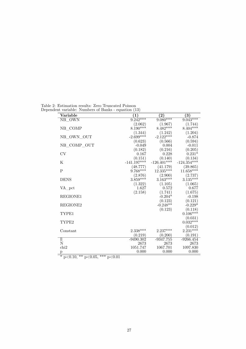
Table 2: Estimation results: Zero Truncated PoissonDependent variable: Numbers of Banks - equation (13)

Variable (1) (2) (3)NB_OWN 9.242*** 9.080*** 9.043***

(2.062) (1.967) (1.744)NB_COMP 8.190*** 8.482*** 8.404***

(1.344) (1.242) (1.204)NB_OWN_OUT -2.699*** -2.122*** -0.874

(0.623) (0.566) (0.594)NB_COMP_OUT -0.049 0.004 -0.011

(0.182) (0.216) (0.205)CV 0.167 0.228 0.231*

(0.151) (0.140) (0.134)K -141.197*** -126.401*** -124.354***

(48.777) (41.179) (39.865)P 9.768*** 12.335*** 11.658***

(2.876) (2.900) (2.737)DENS 3.859*** 3.163*** 3.135***

(1.322) (1.105) (1.065)VA_pct 1.627 0.572 0.677

(2.158) (1.741) (1.675)REGIONE1 -0.204* -0.198

(0.123) (0.121)REGIONE2 -0.248** -0.229*

(0.123) (0.118)TYPE1 0.106***

(0.031)TYPE2 0.032***

(0.012)Constant 2.338*** 2.237*** 2.231***

(0.219) (0.200) (0.191)ll -9490.302 -9347.755 -9266.454N 2673 2673 2673chi2 1051.747 1067.701 1097.830p 0.000 0.000 0.000* p<0.10, ** p<0.05, *** p<0.01

27

Table 3: Estimation results: Zero Truncated Negative BinomialDependent variable: Numbers of Banks

Variable (1) (2) (3)NB_OWN 9.227*** 8.933*** 9.042***

(2.278) (2.194) (1.890)NB_COMP 8.564*** 8.615*** 8.527***

(1.428) (1.279) (1.236)NB_OWN_OUT -2.559*** -2.121*** -0.843

(0.601) (0.562) (0.600)NB_COMP_OUT -0.032 0.026 0.010

(0.170) (0.206) (0.195)CV 0.163 0.219 0.222*

(0.142) (0.137) (0.132)K -141.481*** -124.063*** -121.415***

(48.087) (42.405) (40.864)P 8.761*** 11.128*** 10.515***

(2.610) (2.885) (2.751)DENS 3.729*** 3.081*** 3.045***

(1.294) (1.161) (1.115)VA_pct 1.479 0.557 0.647

(2.352) (1.846) (1.762)REGIONE1 -0.177 -0.173

(0.124) (0.121)REGIONE2 -0.209* -0.193

(0.123) (0.118)TYPE1 0.114***

(0.032)TYPE2 0.036***

(0.013)Constant 2.392*** 2.289*** 2.278***

(0.193) (0.189) (0.181)lnalpha -3.676*** -3.831*** -3.930***

(0.371) (0.425) (0.422)ll -9196.711 -9138.896 -9087.824N 2673 2673 2673chi2 600.999 641.091 657.921p 0.000 0.000 0.000* p<0.10, ** p<0.05, *** p<0.01

28

Table 4: Estimation results: Marginal effectsVariable (ztp) (ztnb) (Variable Mean)NB_OWN 283.1834 283.0865 .0011403

(52.357) (56.701)NB_COMP 263.1779 266.9689 .0447364

(36.787) (38.366)NB_OWN_OUT -27.37672 -26.40309 .005079

(18.463) (18.601)NB_COMP_OUT -.3452477 .2979915 .1772281

(6.431) (6.110)CV 7.227972 6.952858 1.625817

(4.238) (4.167)K -3894.202 -3801.284 .0018006

(1238.163) (1277.182)P 365.0903 329.2003 .0600712

(87.430) (87.960)DENS 98.17784 95.34141 .0327039

(32.976) (34.739)VA_pct 21.21327 20.25852 .0143725

(52.418) (55.120)REGIONE1 (d) -6.113763 -5.35278

(3.697) (3.708)REGIONE2 (d) -6.920037 -5.862967

(3.473) (3.508)TYPE1 (d) 3.423496 3.673721

(1.037) (1.093)TYPE2 (d) 1.002621 1.144445

(0.392) (0.417)(d)marginals for discrete change of dummy variable from 0 to 1

Table 5: Estimation results: QUANTILE REGRESSIONSVariable Quantile5% Quantile25% Quantile50%1/log(POP) 51.416*** 37.429*** 34.027***

(5.967) (12.168) (10.508)REGIONE1 0.186 0.070 0.005

(0.162) (0.160) (0.107)REGIONE2 0.253 0.035 -0.025

(0.180) (0.172) (0.114)TYPE1 -0.041 -0.122 -0.204*

(0.111) (0.179) (0.114)TYPE2 -0.046 0.094 -0.005

(0.116) (0.200) (0.129)Constant -5.737*** -4.225*** -3.644***

(0.455) (0.949) (0.817)C∞ REGION1 0.0039 0.0154 0.0256

(0.0021) (.0144) (0.0205)C∞ REGION2 0.0041 0.0149 0.0249

(0.0020) (0.0142) (0.0198)C∞ REGION3 0.00321 (0.0144) 0.0255

(0.0015) (0.0135) (.0203)N 103 103 103*p<0.10,**p<0.05,***p<0.01

29

Table 6: Estimation results: QUANTILE REGRESSIONSVariable Quantile5% Quantile25% Quantile50%1/log(banks) 7.556* 7.078 2.947

(4.440) (5.069) (3.001)REGIONE1 0.428*** 0.232 0.029

(0.099) (0.199) (0.100)REGIONE2 0.437*** 0.196 -0.022

(0.132) (0.202) (0.102)TYPE1 0.011 -0.108 -0.198**

(0.186) (0.203) (0.097)TYPE2 0.057 -0.019 -0.054

(0.089) (0.237) (0.116)Constant -3.123*** -2.498*** -1.500***

(0.719) (0.818) (0.489)C∞ REGION1 0.0633 0.0940 0.1824**

(0.0455) (0.0646) (0.0730)C∞ REGION2 0.0638 0.0909 0.1791***

(0.0441) (0.0655) (0.0679)C∞ REGION3 0.0422 0.0760 0.1868***

(0.0290) (0.0574) (0.0683)N 99 99 99*p<0.10,**p<0.05,***p<0.01

Table 7: Estimation results: OLS - Reduced form Dependent variable: NB_OWNVariable CoefficientNB_OWN_03 0.9798***

(0.008)NB_COMP 0.0003*

(0.000)NB_OWN_OUT 0.0002

(0.001)NB_COMP_OUT 0.0001

(0.000)CV -0.0000

(0.000)K -0.0025

(0.009)P 0.0002

(0.000)DENS 0.0002

(0.000)VA_pct 0.0003

(0.000)TYPE1 0.0000

(0.000)TYPE2 0.0001***

(0.000)REGION1 -0.0000

(0.000)REGION2 0.0000

(0.000)Constant 0.0000

(0.000)R2 .9883225N 2414.000p 0.000* p<0.10, ** p<0.05, *** p<0.01

30

Table 8: Estimation results: Augmented Zero Truncated Negative BinomialDependent variable: Numbers of Banks

Variable (1)NB_OWN 9.170***

(1.923)NB_COMP 8.556***

(1.255)NB_OWN_OUT -0.591

(0.587)NB_COMP_OUT 0.006

(0.203)CV 0.225*

(0.135)K -121.924***

(41.176)P 10.713***

(2.718)DENS 3.087***

(1.128)VA_pct 0.613

(1.770)TYPE1 0.121***

(0.032)TYPE2 0.034**

(0.014)REGION1 -0.181

(0.124)REGION2 -0.201*

(0.120)vhat -2.433

(8.790)Constant 2.260***

(0.186)-3.852***

(0.404)ll -8245.051N 2414.000chi2 666.529p 0.000* p<0.10, ** p<0.05, *** p<0.01

31

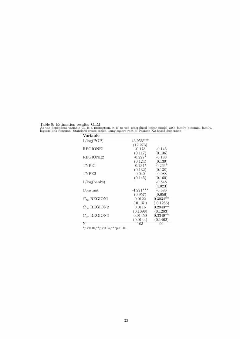
Table 9: Estimation results: GLMAs the dependent variable C1 is a proportion, it is to use generalized linear model with family binomial family,logistic link function. Standard errors scaled using square root of Pearson X2-based dispersion

Variable1/log(POP) 43.956***

(12.273)REGIONE1 -0.173 -0.145

(0.117) (0.136)REGIONE2 -0.227* -0.188

(0.124) (0.139)TYPE1 -0.234* -0.263*

(0.132) (0.138)TYPE2 0.040 -0.088

(0.145) (0.160)1/log(banks) -0.848

(4.023)Constant -4.221*** -0.686

(0.957) (0.656)C∞ REGION1 0.0122 0.3034**

(.0115 ) ( 0.1256)C∞ REGION2 0.0116 0.2943**

(0.1098) (0.1283)C∞ REGION3 0.01450 0.3349**

(0.0144) (0.1462)N 103 99*p<0.10,**p<0.05,***p<0.01

32