Intensional Associations in Dataspaces - Cornell …vmarcos/default_files/SDB10.pdf · Intensional...

Intensional Associations in DataspacesMarcos Antonio Vaz Salles #1, Jens Dittrich ∗2, Lukas Blunschi +3

#Cornell University ∗Saarland University +ETH [email protected] [email protected] [email protected]

Abstract— Dataspace applications necessitate the creation ofassociations among data items over time. For example, onceinformation about people is extracted from sources such aswebpages and blogs, associations among them may emerge asa consequence of different criteria, such as their city of origin,their elected hobbies, or their age group. In a set of personaldata sources, we may wish to associate documents and emailsbased on their modification dates or their authors. In thispaper, we advocate a declarative approach to specifying theseassociations. We propose that each set of associations be definedby an association trail. An association trail is a query-baseddefinition of how items are connected by intensional (i.e., virtual)association edges to other items in the dataspace. The benefitof this mechanism is the creation of an intensional graph ofassociations among previously disconnected data items comingfrom different data sources.

We study in detail the problem of processing neighborhoodqueries over these intensional association graphs. The naive ap-proach to neighborhood query processing over intensional graphsis to materialize the whole graph and then apply previous work ondataspace graph indexing to answer queries. As the intensionalgraph may have a number of edges quadratic in its numberof nodes, the naive approach has worst-case quadratic indexingcost. We develop in this paper a novel indexing technique, thegrouping-compressed index (GCI), that exploits association traildefinitions to materialize the same intensional graph with linearcost. In addition, we present a query answering algorithm overGCI that avoids decompressing the graph to its quadratic size. Inour experimental evaluation, GCI is shown to provide an orderof magnitude gain in indexing cost over the naive approach, whileremaining competitive in query processing time.

I. INTRODUCTION

Dataspace systems have been envisioned as a new archi-tecture for data management and information integration [1].The main goal of these systems is to model, query, andmanage relationships among disparate data sources. So far,relationships in these systems have been specified at the setor schema level [2], [3]. These relationships are exploitedto rewrite queries posed to the system, by reasoning onthe containment of queries or on the schema relationships.In several dataspace scenarios, however, it is important tomodel associations between individual data items across orwithin data sources. Such scenarios include scientific datamanagement [4], semantic web [5], [6], personal informationmanagement [7], social content management [8], and metadatamanagement [9]. In scientific applications, it is necessary tolink information about the same entity spread across severaldatabases; in social content management, it is fundamental tocreate relationships between persons; in personal informationmanagement, it is useful to associate messages and documentsreceived in the same context or timespan.

In this paper, we propose a declarative approach, calledassociation trails, to specifying associations among items in adataspace. An association trail is a query-based definition ofhow items in the dataspace are connected by virtual associationedges to other items. A set of association trails defines a logicalgraph of associations over the dataspace. As this graph ispurely logical and in principle does not need to be explicitlymaterialized, we call it in this paper an intensional graph. Inaddition, we term the edges of this graph intensional edgesor intensional associations. In contrast to solutions that defineassociations extensionally [4], [5], [6], [10], association trailsdefine associations logically and in bulk. As a consequence,association trails are especially useful in scenarios in whichdata sources have no explicit associations defined beforehand.

In addition to defining intensional graphs, we propose inthis paper novel techniques to process exploratory queriesover them. The queries we target are a generalization of theneighborhood queries defined by Dong and Halevy [10] tointensional graphs. A neighborhood query extends a searchquery’s results by obtaining their immediate neighborhood inthe graph. In the following, we first show example scenariosof association trails. We then discuss the challenges of neigh-borhood query processing over intensional graphs.

A. Examples

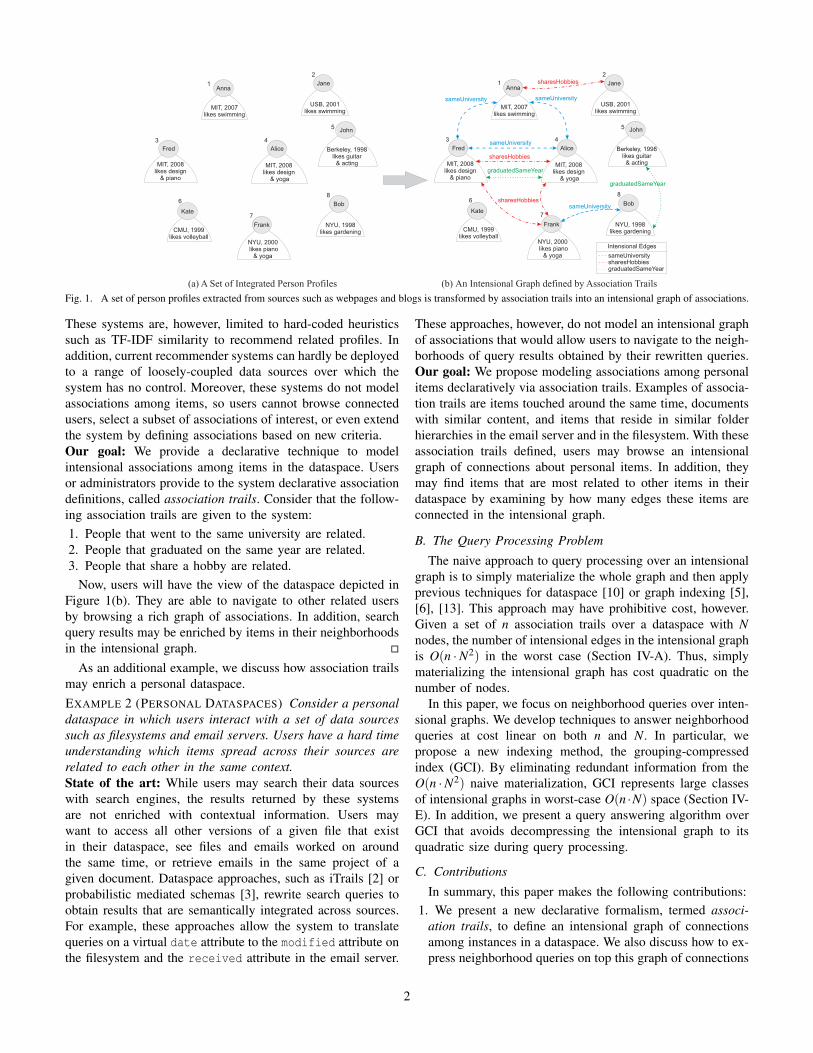
While our techniques are applicable to many dataspacescenarios, we will use as a running example for this paper themodeling of an implicit social network. Figure 1(a) shows aset of person profiles extracted from sources such as webpagesand blogs. Each profile states a person’s name, along with theuniversity she has attended, her year of graduation, and herhobbies. Such profiles can be obtained by applying informationextraction techniques [11].EXAMPLE 1 (IMPLICIT SOCIAL NETWORKS) Users wouldlike to navigate their social dataspaces to find other usersrelated to them or to their topics of interest. Unfortunately,data extracted from loosely-connected sources is poor inassociations among users.State of the art: Users may search their dataspaces withkeyword search engines. These systems have no knowlegdeabout associations between data items. As a consequence, theyreturn only items that match the user’s specific request andcannot enrich results with other relevant associated informa-tion. While some dataspace approaches extend search resultswith elements in a dataspace graph [10], they are of little usewhen connections are not explicitly defined as in Figure 1(a).Users could rely, instead, on a recommender system [12].

refs.bib

p425.pdf

bibliography

childOf

similarTime

similarContent

Association Trails

(a) Data Sources

inbox

Fw: Indexing paper

PIM

Latest Document

Re: Indexing Discussion

joe

(b) Logical Graph OverlayFiles & Folders Email

pim2006.tex

paper.tex

p618.pdf

projects

PIM

bibliography

refs.bib

p425.pdf

home

inbox

Fw: Indexing paper

PIM

Latest Document

Re: Indexing Discussion

joe

pim2006.tex

paper.tex

p618.pdf

projects

PIM

home

(modified = 25/04/2007)

(modified = 26/02/2007; title = "Indexing Dataspaces"; references = {"A Dataspace Odyssey"})

(modified = 21/04/2007)

citedPaperinproceedings(authors = {"Dong", "Halevy"}; title = "Indexing Dataspaces"; file = "p425.pdf")

inproceedings(authors = {"Blunschi", ...} title = "A Dataspace Odyssey"; file = "p618.pdf")

(received = 01/03/2007; title = "A Dataspace Odyssey")

(received = 01/03/2007; from = "Jane")



(received = 26/04/2007)

inproceedings

inproceedings

(modified = 25/04/2007)

(modified = 21/04/2007)

(authors = {"Dong", "Halevy"}; title = "Indexing Dataspaces"; file = "p425.pdf")

(authors = {"Blunschi", ...} title = "A Dataspace Odyssey"; file = "p618.pdf")

(modified = 26/02/2007; title = "Indexing Dataspaces"; references = {"A Dataspace Odyssey"})


(received = 26/04/2007)



(received = 01/03/2007; title = "A Dataspace Odyssey")

paperPdf

citedPaper

citedPaper

paperPdfpaperPdf

similarContent

similarTime

similarTime

similarTime

similarTime

childOf

childOf

childOf

childOf

childOf

childOf

childOf

childOf

childOf

childOf

1

2

3

4

5

6

7

8

9

10

11

12

13

14

15

16

17

isFriendsameUniversitysharesHobbies

Association Trails

graduatedSameYearpostedComment

university: ETHhobbies: design, piano

gradYear: 2008

university: ETHhobbies: design, yoga

gradYear: 2008

From: AliceTo: Design Community

Does anybody remember this boy who used to playthe piano?

university: Cornellhobbies: piano, pool

gradYear: 2000

university: PUC-Riohobbies: guitar, acting

gradYear: 1998

university: Cornellhobbies: gardening

gradYear: 1998university: CMU

hobbies: volleyballgradYear: 1999

university: ETHhobbies: swimming

gradYear: 2007

(a) A Social Network Today (b) A Social Network with aTrails

Frank

Bob

Fred

Alice

Kate

Fred

Anna


gradYear: 2008


gradYear: 2008


gradYear: 2000


gradYear: 1998





gradYear: 2007

Frank

Bob

Fred

Alice

Kate

Fred

Anna




gradYear: 1998

Bob

Bobuniversity: Cornellhobbies: gardeninggradYear: 1998...

sameUniversitysharesHobbies

Intensional Edges

graduatedSameYear

MIT, 2008likes design

& piano


& yoga

NYU, 2000 likes piano

& yoga

Berkeley, 1998likes guitar

& acting

NYU, likes gardening

1998CMU, 1999

likes volleyball

MIT, 2007likes swimming

sameUniversity

sameUniversity

sameUniversity

sameUniversity

sharesHobbies

sharesHobbies

graduatedSameYear

graduatedSameYear

(a) A Set of Integrated Person Profiles (b) An Intensional Graph defined by Association Trails

Frank

Bob

John

Alice

Kate

Fred

Anna


Association Trails



gradYear: 2008


gradYear: 2008




gradYear: 2000


gradYear: 1998





gradYear: 2007

isFriend

sameUniversity

sameUniversity

sameUniversity

sameUniversity

sharesHobbies

sharesHobbies

postedComment

graduatedSameYear

graduatedSameYear

isFriend

isFriend

isFriend

isFriend


Frank

Bob

Fred

Alice

Kate

Fred

Anna


gradYear: 2008


gradYear: 2008


gradYear: 2000


gradYear: 1998





gradYear: 2007

Frank

Bob

Fred

Alice

Kate

Fred

Anna




& piano


& yoga

, 2000 likes piano

& yoga

NYU

Berkeley, 1998likes guitar

& acting

, likes gardening

NYU 1998CMU, 1999

likes volleyball

MIT, 2007likes swimming

Frank

Bob

John

Alice

Kate

Fred

Anna


Association Trails


ETH, 2008likes design

& piano


& yoga

From: AliceTo: Design Community...

Cornell, 2000 likes piano

& pool

PUC-Rio, 1998likes guitar

& acting

Cornell, likes gardening

1998CMU, 1999

likes volleyball

ETH, 2007likes swimming

isFriend

sameUniversity

sameUniversity

sameUniversity

sameUniversity

sharesHobbies

sharesHobbies

postedComment

graduatedSameYear

graduatedSameYear

isFriend

isFriend

isFriend

isFriend


Frank

Bob

Fred

Alice

Kate

Fred

Anna


& piano


& yoga

From: AliceTo: Design Community...

Cornell, 2000 likes piano

& pool

PUC-Rio, 1998likes guitar

& acting

Cornell, likes gardening

1998CMU, 1999

likes volleyball

ETH, 2007likes swimming

Frank

Bob

Fred

Alice

Kate

Fred

Anna

isFriend

postedComment

isFriend

isFriend

isFriend

isFriend

1

2

4

5

6

7

8

3

1

4

6

7

8

3

, likes swimming

USB 2001

JanesharesHobbies2

, likes swimming

USB 2001

Jane

5

Fig. 1. A set of person profiles extracted from sources such as webpages and blogs is transformed by association trails into an intensional graph of associations.

These systems are, however, limited to hard-coded heuristicssuch as TF-IDF similarity to recommend related profiles. Inaddition, current recommender systems can hardly be deployedto a range of loosely-coupled data sources over which thesystem has no control. Moreover, these systems do not modelassociations among items, so users cannot browse connectedusers, select a subset of associations of interest, or even extendthe system by defining associations based on new criteria.Our goal: We provide a declarative technique to modelintensional associations among items in the dataspace. Usersor administrators provide to the system declarative associationdefinitions, called association trails. Consider that the follow-ing association trails are given to the system:1. People that went to the same university are related.2. People that graduated on the same year are related.3. People that share a hobby are related.

Now, users will have the view of the dataspace depicted inFigure 1(b). They are able to navigate to other related usersby browsing a rich graph of associations. In addition, searchquery results may be enriched by items in their neighborhoodsin the intensional graph. �

As an additional example, we discuss how association trailsmay enrich a personal dataspace.EXAMPLE 2 (PERSONAL DATASPACES) Consider a personaldataspace in which users interact with a set of data sourcessuch as filesystems and email servers. Users have a hard timeunderstanding which items spread across their sources arerelated to each other in the same context.State of the art: While users may search their data sourceswith search engines, the results returned by these systemsare not enriched with contextual information. Users maywant to access all other versions of a given file that existin their dataspace, see files and emails worked on aroundthe same time, or retrieve emails in the same project of agiven document. Dataspace approaches, such as iTrails [2] orprobabilistic mediated schemas [3], rewrite search queries toobtain results that are semantically integrated across sources.For example, these approaches allow the system to translatequeries on a virtual date attribute to the modified attribute onthe filesystem and the received attribute in the email server.

These approaches, however, do not model an intensional graphof associations that would allow users to navigate to the neigh-borhoods of query results obtained by their rewritten queries.Our goal: We propose modeling associations among personalitems declaratively via association trails. Examples of associa-tion trails are items touched around the same time, documentswith similar content, and items that reside in similar folderhierarchies in the email server and in the filesystem. With theseassociation trails defined, users may browse an intensionalgraph of connections about personal items. In addition, theymay find items that are most related to other items in theirdataspace by examining by how many edges these items areconnected in the intensional graph.

B. The Query Processing Problem

The naive approach to query processing over an intensionalgraph is to simply materialize the whole graph and then applyprevious techniques for dataspace [10] or graph indexing [5],[6], [13]. This approach may have prohibitive cost, however.Given a set of n association trails over a dataspace with Nnodes, the number of intensional edges in the intensional graphis O(n ·N2) in the worst case (Section IV-A). Thus, simplymaterializing the intensional graph has cost quadratic on thenumber of nodes.

In this paper, we focus on neighborhood queries over inten-sional graphs. We develop techniques to answer neighborhoodqueries at cost linear on both n and N. In particular, wepropose a new indexing method, the grouping-compressedindex (GCI). By eliminating redundant information from theO(n ·N2) naive materialization, GCI represents large classesof intensional graphs in worst-case O(n ·N) space (Section IV-E). In addition, we present a query answering algorithm overGCI that avoids decompressing the intensional graph to itsquadratic size during query processing.

C. Contributions

In summary, this paper makes the following contributions:1. We present a new declarative formalism, termed associ-

ation trails, to define an intensional graph of connectionsamong instances in a dataspace. We also discuss how to ex-press neighborhood queries on top this graph of connections

2

that is not given explicitly, but rather defined by associationtrails. Association trails are introduced in Section III.

2. We propose query processing techniques for neighborhoodqueries over the intensional graph defined by associationtrails. These techniques take advantage of different amountsof materialization of the intensional graph in order to makequery processing efficient. We discuss our query processingtechniques in Section IV.

3. In a set of experiments with real and synthetic datasets,we evaluate the performance of our query processing tech-niques over intensional graphs. Our best technique, thegrouping-compressed index, exhibits an order of magnitudeimprovement in indexing cost over the naive approach,while remaining competitive in terms of query processingtime. Experimental results are reported in Section V.

II. PRELIMINARIES

A. Data Model

We begin by defining the data model used to represent inthe dataspace the data extracted from the data sources.

DEFINITION 1 (DATA MODEL) The data in the dataspace isrepresented by a graph G := (N,E), where:1. N is a set of nodes {N1, . . . ,Nm}. Each node Ni is a set

of attribute-value pairs Ni := {(ai1,v

i1), . . . ,(a

ik,v

ik)}, where

each value is either atomic or a bag of words. We do notenforce a schema over the nodes, i.e., the set of attributesof each node may be different.

2. E is a set of directed edges (Ni,N j), s.t. Ni,N j ∈ N. �

EXAMPLE 3 The data in Figure 1(a) is represented in the datamodel of Definition 1. Node 4 has a set of attribute-value pairs{(name, Alice), (university, MIT), (gradYear, 2008), (hobbies,design & yoga)} (for better visibility, attribute names havebeen omitted in the figure). While E =∅ in the figure, it maycontain explicit source connections in general. For example,in a personal dataspace, E will contain explicit filesystemconnections between folders and files. �

B. Query Model

For the purposes of this paper, we will use the followingsimple keyword and path language.

DEFINITION 2 (QUERY) A query Q is an expression thatselects a set Q(G)⊆N. The possible query expressions are:1. Keyword Expression: denoted K, returns all nodes such

that keyword K occurs in some of their attribute-value pairs.2. Attribute-value Expression: denoted A op V, returns all

nodes such that the condition on attribute A with operatorop and value V is true.

3. Intersect Expression: denoted exp1 exp2, returns allnodes qualifying both exp1 and exp2.

4. Union Expression: denoted exp1 OR exp2, returns allnodes qualifying either exp1 or exp2. �

EXAMPLE 4 In the graph of Figure 1(a), the following queriesexemplify the expression types described in Definition 2:1. yoga returns Nodes 4 and 7.

2. university = NYU returns Nodes 7 and 8.3. yoga NYU returns Node 7.4. yoga OR NYU returns Nodes 4, 7, and 8. �

C. Basic Index Structures

Given the queries above, we assume two basic index struc-tures, commonly found in state-of-the-art search engines [14]:1. Inverted Index: a mapping from keyword to the list of

node identifiers of nodes containing that keyword. In orderto support both attribute-value and keyword expressions,the inverted index may be implemented by concatenatingkeywords with the attribute names in which those keywordsoccur. Keyword expressions are then translated to prefixqueries [15], [10]. Keywords can be of any data type witha total order (e.g., numbers, dates, or strings).

2. Rowstore (or repository): a mapping from node identifierto the information associated with that node. This includesthe set of attribute-value pairs of that node as well as anyexplicit edges that connect this node to other nodes.Search engines use ranking schemes, e.g., PageRank, to sup-

port top-K query processing over the data structures desbribedabove [14]. In our work, we are agnostic to the ranking schemeused by the search engine. We focus on efficient techniquesfor neighborhood query processing over intensional graphs.

III. ASSOCIATION TRAILS

This section formalizes association trails and neighborhoodqueries over intensional graphs.

A. Basic Form of an Association Trail

An association trail defines a set of edges in the intensionalgraph. For example, in Figure 1(b), a single association trailwould define all sharesHobbies edges. Defining more associ-ation trails adds more edges to the graph, potentially betweenthe same nodes. We may thus interpret each association trailas defining an intensional graph overlay on top of the originaldataspace graph. When we take a set of association trailstogether, they define an intensional multigraph, i.e., a graphin which nodes may be connected by multiple labeled edges(Figure 1(b)). The definition below formalizes this intuition.

DEFINITION 3 (ASSOCIATION TRAIL) A unidirectional asso-ciation trail is denoted as

A := QLθ(l,r)=⇒ QR,

where A is a label naming the association trail, QL,QR arequeries, and θ is a predicate. The query results QL(G) areassociated to QR(G) according to the predicate θ, whichtakes as inputs one query result from QL and one from QR.Thus, we conceptually introduce in the association graph oneintensional edge, directed from left to right and labeled A, foreach pair of nodes given by QL Zθ QR. We require that thenode on the left of the edge be different than the node on theright, i.e., no self-edges are allowed.

A bidirectional association trail is denoted as

A := QLθ(l,r)⇐⇒ QR.

3

The latter also means that the query results QR(G) are relatedto the query results QL(G) according to θ. �

An association trail relates elements from the data sourcesby a join predicate θ. Therefore, association trails coverrelational and non-relational theta-joins as special cases. Whileknowing the form of θ may allow us to improve performance(see Section IV-E), conceptually θ may be an arbitrarilycomplex function. This means that Definition 3 also modelsuse cases such as content equivalence and similar documents.

A straightforward extension to our model is to define θ as amatching function generating several edges between a pair ofnodes. This may be useful to model individual matches createdby multi-valued attributes, e.g., modeling each hobby matchin sharesHobbies by a separate intensional edge.A Word about Ranking. The attentive reader will noticethat it is easy to extend the definition of association trailsto incorporate edge weights. Each association trail may begiven a normalized weight value that represents the strengthof the association edges created by that trail. These weightsmay then be exploited for ranking of results obtained bynavigating intensional edges. While a detailed treatment ofranking exceeds the scope of this paper, our query processingtechniques compute information necessary as input to ranking,such as the edge in-degree of query results. More informationon association trail ranking can be found in [16].

B. Association Trail Use Cases

USE CASE 1 (SOCIAL NETWORKS) The intensional graph ofFigure 1(b) is defined by the following association trails:

sameUniversity := class=personθ1(l,r)⇐⇒ class=person,

θ1(l,r) := (l.university = r.university).

graduatedSameYear := class=personθ2(l,r)⇐⇒ class=person,

θ2(l,r) := (l.gradYear = r.gradYear).

sharesHobbies := class=personθ3(l,r)⇐⇒ class=person,

θ3(l,r) := (∃h ∈ l.hobbies : h ∈ r.hobbies).

The association trail sameUniversity (resp. graduated-SameYear) defines that given any two persons, there will bean edge between them if they have the same value for theuniversity (resp. gradYear) field. A more complex existentialpredicate is introduced in sharesHobbies, which defines thattwo people are related when they have at least one hobbyin common. These association trail examples show how todefine a logical graph of associations among elements inthe dataspace. This is achieved in terms of queries thatselect elements to be related and predicates that specify joinsemantics among those elements. When taken together, theassociation trails above result in a multigraph (displayed inFigure 1(b)). This intensional multigraph is actually a view,which can be refined over time by adding more associationtrails in a pay-as-you-go fashion. �

USE CASE 2 (PERSONAL DATASPACES) Consider the fol-lowing association trails defined over a personal dataspace:

similarTime := class=fileθ6(l,r)⇐⇒ class=file,

θ6(l,r) := (r.date−1≤ l.date≤ r.date+1).

relatedFolder := class=emailθ7(l,r)⇐⇒ class=file mimeType=pdf,

θ7(l,r) := (∃ f1, f2 : ( f1, l) ∈ E ∧ ( f2,r) ∈ E∧ f1.name = f2.name).

These association trails model the context of personal items asdiscussed in Example 2. They define, respectively, associationsamong items changed or received around the same time andemails and files that reside in similar folders in the emailserver and in the filesystem. The relatedFolder association trailrestricts intensional associations between files and emails tooccur only for pdf documents and not for any arbitrary file. �

C. Neighborhood Queries

The applications described in the Introduction must processexploratory queries over the intensional graph of associationsdefined by association trails. We focus on a special class ofexploratory queries termed neighborhood queries. For simplic-ity, our presentation in the following sections is focussed onunidirectional association trails, as it is simple to extend ourtechniques to the bidirectional case.

Neighborhood queries were used by Dong and Halevy toexplore a dataspace graph [10]. They assume that the dataspacegraph is given extensionally, i.e., each edge in the graph isexplicitly materialized, and that the original queries to thegraph are keyword or union expressions. Unfortunately, theirdefinition does not apply to intensional graphs. As such, wegeneralize neighborhood queries below to intensional graphsand to any original query described in Definition 2. We firstdefine what a neighborhood is in our context.

DEFINITION 4 (NEIGHBORHOOD) Given a query Q and aset of association trails A∗, the neighborhood NQ

A∗ of Q withrespect to A∗ is given by

NQA∗ :=

∅, if A∗ := ∅ ,

(Q ∩ QiL) Yθi Qi

R, if A∗ := {Ai} ,

NQ{A1} ∪ NQ

{A2} ∪ . . . ∪ NQ{An}, if A∗ := {A1,A2, . . . ,An}.

where QiL and Qi

R are the queries on the left and right sidesof trail Ai, respectively, and θi is the θ-predicate of Ai. �

The definition above states that the neighborhood includesall instances associated through A∗ to instances returned by Q.That is formalized in terms of a semi-join, as we wish to findall instances from Qi

R which are connected to some elementof Q also appearing on Qi

L. Note that in the definition above,nothing is said about self-edges. Self-edges are disallowed byDefinition 3. It is simple to exclude self-edges by removingfrom Qi

R all nodes in QiL ∩ Qi

R for which θi generates a self-edge and that do not have an edge to at least one other nodein Qi

L. For the remainder, we will not consider self-edges inorder to simplify our presentation.

4

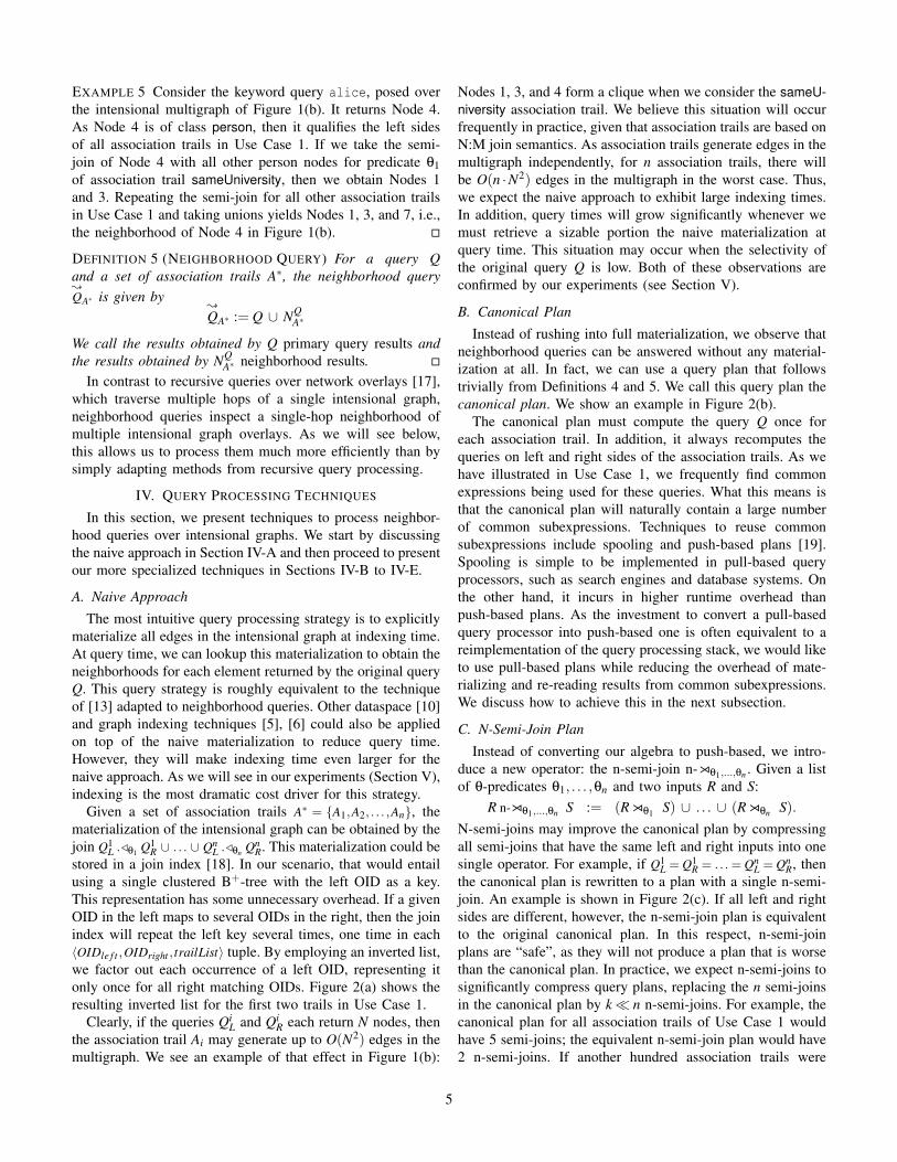
EXAMPLE 5 Consider the keyword query alice, posed overthe intensional multigraph of Figure 1(b). It returns Node 4.As Node 4 is of class person, then it qualifies the left sidesof all association trails in Use Case 1. If we take the semi-join of Node 4 with all other person nodes for predicate θ1of association trail sameUniversity, then we obtain Nodes 1and 3. Repeating the semi-join for all other association trailsin Use Case 1 and taking unions yields Nodes 1, 3, and 7, i.e.,the neighborhood of Node 4 in Figure 1(b). �

DEFINITION 5 (NEIGHBORHOOD QUERY) For a query Qand a set of association trails A∗, the neighborhood query{QA∗ is given by

{QA∗ := Q ∪ NQ

A∗

We call the results obtained by Q primary query results andthe results obtained by NQ

A∗ neighborhood results. �

In contrast to recursive queries over network overlays [17],which traverse multiple hops of a single intensional graph,neighborhood queries inspect a single-hop neighborhood ofmultiple intensional graph overlays. As we will see below,this allows us to process them much more efficiently than bysimply adapting methods from recursive query processing.

IV. QUERY PROCESSING TECHNIQUES

In this section, we present techniques to process neighbor-hood queries over intensional graphs. We start by discussingthe naive approach in Section IV-A and then proceed to presentour more specialized techniques in Sections IV-B to IV-E.

A. Naive Approach

The most intuitive query processing strategy is to explicitlymaterialize all edges in the intensional graph at indexing time.At query time, we can lookup this materialization to obtain theneighborhoods for each element returned by the original queryQ. This query strategy is roughly equivalent to the techniqueof [13] adapted to neighborhood queries. Other dataspace [10]and graph indexing techniques [5], [6] could also be appliedon top of the naive materialization to reduce query time.However, they will make indexing time even larger for thenaive approach. As we will see in our experiments (Section V),indexing is the most dramatic cost driver for this strategy.

Given a set of association trails A∗ = {A1,A2, . . . ,An}, thematerialization of the intensional graph can be obtained by thejoin Q1

L ./θ1 Q1R ∪ . . . ∪ Qn

L ./θn QnR. This materialization could be

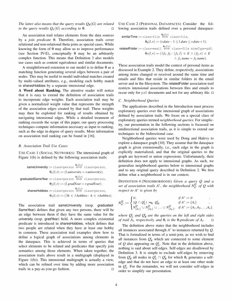
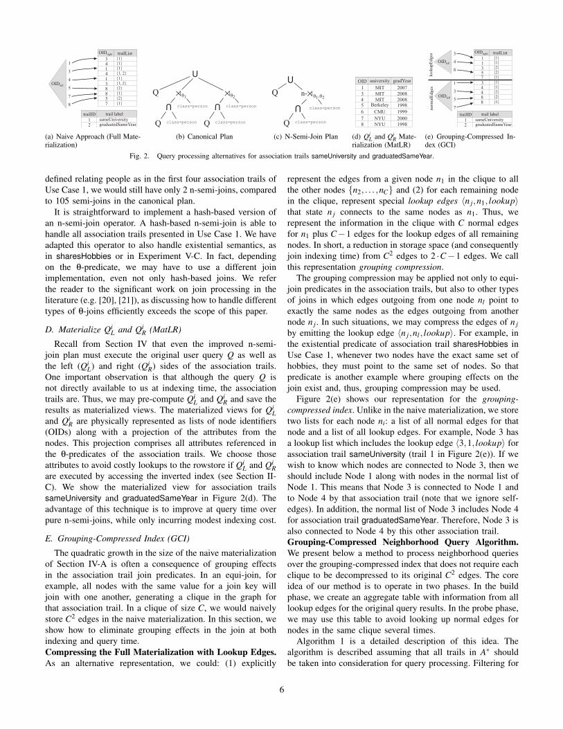
stored in a join index [18]. In our scenario, that would entailusing a single clustered B+-tree with the left OID as a key.This representation has some unnecessary overhead. If a givenOID in the left maps to several OIDs in the right, then the joinindex will repeat the left key several times, one time in each〈OIDle f t ,OIDright , trailList〉 tuple. By employing an inverted list,we factor out each occurrence of a left OID, representing itonly once for all right matching OIDs. Figure 2(a) shows theresulting inverted list for the first two trails in Use Case 1.

Clearly, if the queries QiL and Qi

R each return N nodes, thenthe association trail Ai may generate up to O(N2) edges in themultigraph. We see an example of that effect in Figure 1(b):

Nodes 1, 3, and 4 form a clique when we consider the sameU-niversity association trail. We believe this situation will occurfrequently in practice, given that association trails are based onN:M join semantics. As association trails generate edges in themultigraph independently, for n association trails, there willbe O(n ·N2) edges in the multigraph in the worst case. Thus,we expect the naive approach to exhibit large indexing times.In addition, query times will grow significantly whenever wemust retrieve a sizable portion the naive materialization atquery time. This situation may occur when the selectivity ofthe original query Q is low. Both of these observations areconfirmed by our experiments (see Section V).

B. Canonical Plan

Instead of rushing into full materialization, we observe thatneighborhood queries can be answered without any material-ization at all. In fact, we can use a query plan that followstrivially from Definitions 4 and 5. We call this query plan thecanonical plan. We show an example in Figure 2(b).

The canonical plan must compute the query Q once foreach association trail. In addition, it always recomputes thequeries on left and right sides of the association trails. As wehave illustrated in Use Case 1, we frequently find commonexpressions being used for these queries. What this means isthat the canonical plan will naturally contain a large numberof common subexpressions. Techniques to reuse commonsubexpressions include spooling and push-based plans [19].Spooling is simple to be implemented in pull-based queryprocessors, such as search engines and database systems. Onthe other hand, it incurs in higher runtime overhead thanpush-based plans. As the investment to convert a pull-basedquery processor into push-based one is often equivalent to areimplementation of the query processing stack, we would liketo use pull-based plans while reducing the overhead of mate-rializing and re-reading results from common subexpressions.We discuss how to achieve this in the next subsection.

C. N-Semi-Join Plan

Instead of converting our algebra to push-based, we intro-duce a new operator: the n-semi-join n-Yθ1,...,θn . Given a listof θ-predicates θ1, . . . ,θn and two inputs R and S:

R n-Yθ1,...,θn S := (R Yθ1 S) ∪ . . . ∪ (R Yθn S).N-semi-joins may improve the canonical plan by compressingall semi-joins that have the same left and right inputs into onesingle operator. For example, if Q1

L = Q1R = . . . = Qn

L = QnR, then

the canonical plan is rewritten to a plan with a single n-semi-join. An example is shown in Figure 2(c). If all left and rightsides are different, however, the n-semi-join plan is equivalentto the original canonical plan. In this respect, n-semi-joinplans are “safe”, as they will not produce a plan that is worsethan the canonical plan. In practice, we expect n-semi-joins tosignificantly compress query plans, replacing the n semi-joinsin the canonical plan by k� n n-semi-joins. For example, thecanonical plan for all association trails of Use Case 1 wouldhave 5 semi-joins; the equivalent n-semi-join plan would have2 n-semi-joins. If another hundred association trails were

5

(a) Naive Approach (Full Mate-rialization)

Q

ócontent ~

G G

UU

ócontent ~"pdf" "yesterday"

U

A1L.Q

A1R.Q

U

×è1Q

Q

U

AnL.Q

AnR.Q

×èn...

è

è,æ×

Q

U

U

×è1Q

Q

U

×è2

Q

U

U

×è1Q

1QL

1QR

Q

U

×è2

2QL

2QR

class=person

class=person

class=person

class=person

(b) Canonical Plan

ócontent ~

G G

U

ócontent ~"pdf" "yesterday"

U

U

è1Q

Q

U

× è2

è

è,æ×

,n-

U

è1Q

Q

U

× è2,n-

1,2QL

1,2QR

class=person

class=person

(c) N-Semi-Join Plan

OID university gradYear

1345

7

MIT 2007MIT 2008MIT 2008

Berkeley

1999

NYU 20008 NYU 1998

6 CMU

1998

(d) QiL and Qi

R Mate-rialization (MatLR)

(e) Grouping-Compressed In-dex (GCI)

Fig. 2. Query processing alternatives for association trails sameUniversity and graduatedSameYear.

defined relating people as in the first four association trails ofUse Case 1, we would still have only 2 n-semi-joins, comparedto 105 semi-joins in the canonical plan.

It is straightforward to implement a hash-based version ofan n-semi-join operator. A hash-based n-semi-join is able tohandle all association trails presented in Use Case 1. We haveadapted this operator to also handle existential semantics, asin sharesHobbies or in Experiment V-C. In fact, dependingon the θ-predicate, we may have to use a different joinimplementation, even not only hash-based joins. We referthe reader to the significant work on join processing in theliterature (e.g. [20], [21]), as discussing how to handle differenttypes of θ-joins efficiently exceeds the scope of this paper.

D. Materialize QiL and Qi

R (MatLR)

Recall from Section IV that even the improved n-semi-join plan must execute the original user query Q as well asthe left (Qi

L) and right (QiR) sides of the association trails.

One important observation is that although the query Q isnot directly available to us at indexing time, the associationtrails are. Thus, we may pre-compute Qi

L and QiR and save the

results as materialized views. The materialized views for QiL

and QiR are physically represented as lists of node identifiers

(OIDs) along with a projection of the attributes from thenodes. This projection comprises all attributes referenced inthe θ-predicates of the association trails. We choose thoseattributes to avoid costly lookups to the rowstore if Qi

L and QiR

are executed by accessing the inverted index (see Section II-C). We show the materialized view for association trailssameUniversity and graduatedSameYear in Figure 2(d). Theadvantage of this technique is to improve at query time overpure n-semi-joins, while only incurring modest indexing cost.

E. Grouping-Compressed Index (GCI)

The quadratic growth in the size of the naive materializationof Section IV-A is often a consequence of grouping effectsin the association trail join predicates. In an equi-join, forexample, all nodes with the same value for a join key willjoin with one another, generating a clique in the graph forthat association trail. In a clique of size C, we would naivelystore C2 edges in the naive materialization. In this section, weshow how to eliminate grouping effects in the join at bothindexing and query time.Compressing the Full Materialization with Lookup Edges.As an alternative representation, we could: (1) explicitly

represent the edges from a given node n1 in the clique to allthe other nodes {n2, . . . ,nC} and (2) for each remaining nodein the clique, represent special lookup edges 〈n j,n1, lookup〉that state n j connects to the same nodes as n1. Thus, werepresent the information in the clique with C normal edgesfor n1 plus C−1 edges for the lookup edges of all remainingnodes. In short, a reduction in storage space (and consequentlyjoin indexing time) from C2 edges to 2 ·C−1 edges. We callthis representation grouping compression.

The grouping compression may be applied not only to equi-join predicates in the association trails, but also to other typesof joins in which edges outgoing from one node nl point toexactly the same nodes as the edges outgoing from anothernode n j. In such situations, we may compress the edges of n jby emitting the lookup edge 〈n j,nl , lookup〉. For example, inthe existential predicate of association trail sharesHobbies inUse Case 1, whenever two nodes have the exact same set ofhobbies, they must point to the same set of nodes. So thatpredicate is another example where grouping effects on thejoin exist and, thus, grouping compression may be used.

Figure 2(e) shows our representation for the grouping-compressed index. Unlike in the naive materialization, we storetwo lists for each node ni: a list of all normal edges for thatnode and a list of all lookup edges. For example, Node 3 hasa lookup list which includes the lookup edge 〈3,1, lookup〉 forassociation trail sameUniversity (trail 1 in Figure 2(e)). If wewish to know which nodes are connected to Node 3, then weshould include Node 1 along with nodes in the normal list ofNode 1. This means that Node 3 is connected to Node 1 andto Node 4 by that association trail (note that we ignore self-edges). In addition, the normal list of Node 3 includes Node 4for association trail graduatedSameYear. Therefore, Node 3 isalso connected to Node 4 by this other association trail.Grouping-Compressed Neighborhood Query Algorithm.We present below a method to process neighborhood queriesover the grouping-compressed index that does not require eachclique to be decompressed to its original C2 edges. The coreidea of our method is to operate in two phases. In the buildphase, we create an aggregate table with information from alllookup edges for the original query results. In the probe phase,we may use this table to avoid looking up normal edges fornodes in the same clique several times.

Algorithm 1 is a detailed description of this idea. Thealgorithm is described assuming that all trails in A∗ shouldbe taken into consideration for query processing. Filtering for

6

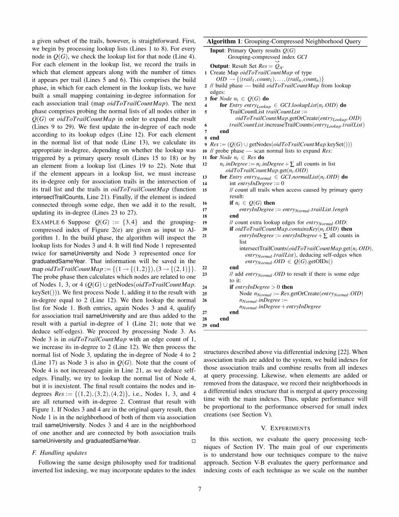
a given subset of the trails, however, is straightforward. First,we begin by processing lookup lists (Lines 1 to 8). For everynode in Q(G), we check the lookup list for that node (Line 4).For each element in the lookup list, we record the trails inwhich that element appears along with the number of timesit appears per trail (Lines 5 and 6). This comprises the buildphase, in which for each element in the lookup lists, we havebuilt a small mapping containing in-degree information foreach association trail (map oidToTrailCountMap). The nextphase comprises probing the normal lists of all nodes either inQ(G) or oidToTrailCountMap in order to expand the result(Lines 9 to 29). We first update the in-degree of each nodeaccording to its lookup edges (Line 12). For each elementin the normal list of that node (Line 13), we calculate itsappropriate in-degree, depending on whether the lookup wastriggered by a primary query result (Lines 15 to 18) or byan element from a lookup list (Lines 19 to 22). Note thatif the element appears in a lookup list, we must increaseits in-degree only for association trails in the intersection ofits trail list and the trails in oidToTrailCountMap (functionintersectTrailCounts, Line 21). Finally, if the element is indeedconnected through some edge, then we add it to the result,updating its in-degree (Lines 23 to 27).EXAMPLE 6 Suppose Q(G) := {3,4} and the grouping-compressed index of Figure 2(e) are given as input to Al-gorithm 1. In the build phase, the algorithm will inspect thelookup lists for Nodes 3 and 4. It will find Node 1 representedtwice for sameUniversity and Node 3 represented once forgraduatedSameYear. That information will be saved in themap oidToTrailCountMap := {(1→{(1,2)}),(3→{(2,1)}}.The probe phase then calculates which nodes are related to oneof Nodes 1, 3, or 4 (Q(G) ∪ getNodes(oidToTrailCountMap.keySet())). We first process Node 1, adding it to the result within-degree equal to 2 (Line 12). We then lookup the normallist for Node 1. Both entries, again Nodes 3 and 4, qualifyfor association trail sameUniversity and are thus added to theresult with a partial in-degree of 1 (Line 21; note that wededuce self-edges). We proceed by processing Node 3. AsNode 3 is in oidToTrailCountMap with an edge count of 1,we increase its in-degree to 2 (Line 12). We then process thenormal list of Node 3, updating the in-degree of Node 4 to 2(Line 17) as Node 3 is also in Q(G). Note that the count ofNode 4 is not increased again in Line 21, as we deduce self-edges. Finally, we try to lookup the normal list of Node 4,but it is inexistent. The final result contains the nodes and in-degrees Res := {(1,2),(3,2),(4,2)}, i.e., Nodes 1, 3, and 4are all returned with in-degree 2. Contrast that result withFigure 1. If Nodes 3 and 4 are in the original query result, thenNode 1 is in the neighborhood of both of them via associationtrail sameUniversity. Nodes 3 and 4 are in the neighborhoodof one another and are connected by both association trailssameUniversity and graduatedSameYear. �

F. Handling updates

Following the same design philosophy used for traditionalinverted list indexing, we may incorporate updates to the index

Algorithm 1: Grouping-Compressed Neighborhood QueryInput: Primary Query results Q(G)

Grouping-compressed index GCI

Output: Result Set Res ={QA∗

Create Map oidToTrailCountMap of type1OID →{(trail1,count1), . . . ,(trailn,countn)}

// build phase — build oidToTrailCountMap from lookup2edges:for Node ni ∈ Q(G) do3

for Entry entryLookup ∈ GCI.lookupList(ni.OID) do4TrailCountList trailCountList :=5

oidToTrailCountMap.getOrCreate(entryLookup.OID)trailCountList.increaseTrailCounts(entryLookup.trailList)6

end7end8Res := (Q(G) ∪ getNodes(oidToTrailCountMap.keySet()))9// probe phase — scan normal lists to expand Res:10for Node ni ∈ Res do11

ni.inDegree := ni.inDegree+∑ all counts in list12oidToTrailCountMap.get(ni.OID)

for Entry entryNormal ∈ GCI.normalList(ni.OID) do13int entryInDegree := 014// count all trails when access caused by primary query15result:if ni ∈ Q(G) then16

entryInDegree := entryNormal .trailList.length17end18// count extra lookup edges for entryNormal .OID:19if oidToTrailCountMap.containsKey(ni.OID) then20

entryInDegree := entryInDegree+∑ all counts in21listintersectTrailCounts(oidToTrailCountMap.get(ni.OID),

entryNormal .trailList), deducing self-edges whenentryNormal .OID ∈ Q(G).getOIDs()

end22// add entryNormal .OID to result if there is some edge23to it:if entryInDegree > 0 then24

Node nNormal := Res.getOrCreate(entryNormal .OID)25nNormal .inDegree :=26nNormal .inDegree+ entryInDegree

end27end28

end29

structures described above via differential indexing [22]. Whenassociation trails are added to the system, we build indexes forthose association trails and combine results from all indexesat query processing. Likewise, when elements are added orremoved from the dataspace, we record their neighborhoods ina differential index structure that is merged at query processingtime with the main indexes. Thus, update performance willbe proportional to the performance observed for small indexcreations (see Section V).

V. EXPERIMENTS

In this section, we evaluate the query processing tech-niques of Section IV. The main goal of our experimentsis to understand how our techniques compare to the naiveapproach. Section V-B evaluates the query performance andindexing costs of each technique as we scale on the number

7

of association trails. Section V-C explores the sensitivity of allmethods to the selectivity of the primary query Q.

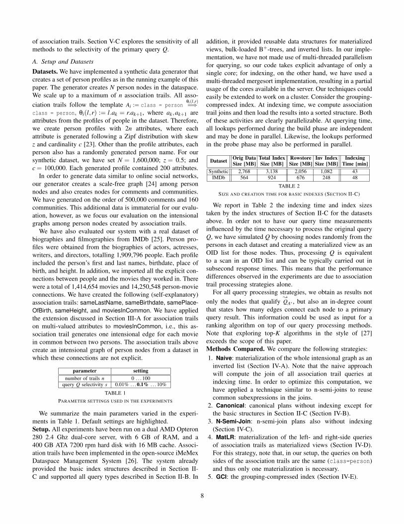
A. Setup and Datasets

Datasets. We have implemented a synthetic data generator thatcreates a set of person profiles as in the running example of thispaper. The generator creates N person nodes in the dataspace.We scale up to a maximum of n association trails. All asso-ciation trails follow the template Ai := class = person

θi(l,r)=⇒class = person, θi(l,r) := l.ak = r.ak+1, where ak,ak+1 areattributes from the profiles of people in the dataset. Therefore,we create person profiles with 2n attributes, where eachattribute is generated following a Zipf distribution with skewz and cardinality c [23]. Other than the profile attributes, eachperson also has a randomly generated person name. For oursynthetic dataset, we have set N = 1,600,000; z = 0.5; andc = 100,000. Each generated profile contained 200 attributes.

In order to generate data similar to online social networks,our generator creates a scale-free graph [24] among personnodes and also creates nodes for comments and communities.We have generated on the order of 500,000 comments and 160communities. This additional data is immaterial for our evalu-ation, however, as we focus our evaluation on the intensionalgraphs among person nodes created by association trails.

We have also evaluated our system with a real dataset ofbiographies and filmographies from IMDb [25]. Person pro-files were obtained from the biographies of actors, actresses,writers, and directors, totalling 1,909,796 people. Each profileincluded the person’s first and last names, birthdate, place ofbirth, and height. In addition, we imported all the explicit con-nections between people and the movies they worked in. Therewere a total of 1,414,654 movies and 14,250,548 person-movieconnections. We have created the following (self-explanatory)association trails: sameLastName, sameBirthdate, samePlace-OfBirth, sameHeight, and moviesInCommon. We have appliedthe extension discussed in Section III-A for association trailson multi-valued attributes to moviesInCommon, i.e., this as-sociation trail generates one intensional edge for each moviein common between two persons. The association trails abovecreate an intensional graph of person nodes from a dataset inwhich these connections are not explicit.

parameter settingnumber of trails n 0 . . . 100

query Q selectivity s 0.01% . . . 0.1% . . . 10%

TABLE 1PARAMETER SETTINGS USED IN THE EXPERIMENTS

We summarize the main parameters varied in the experi-ments in Table 1. Default settings are highlighted.Setup. All experiments have been run on a dual AMD Opteron280 2.4 Ghz dual-core server, with 6 GB of RAM, and a400 GB ATA 7200 rpm hard disk with 16 MB cache. Associ-ation trails have been implemented in the open-source iMeMexDataspace Management System [26]. The system alreadyprovided the basic index structures described in Section II-C and supported all query types described in Section II-B. In

addition, it provided reusable data structures for materializedviews, bulk-loaded B+-trees, and inverted lists. In our imple-mentation, we have not made use of multi-threaded parallelismfor querying, so our code takes explicit advantage of only asingle core; for indexing, on the other hand, we have used amulti-threaded mergesort implementation, resulting in a partialusage of the cores available in the server. Our techniques couldeasily be extended to work on a cluster. Consider the grouping-compressed index. At indexing time, we compute associationtrail joins and then load the results into a sorted structure. Bothof these activities are clearly parallelizable. At querying time,all lookups performed during the build phase are independentand may be done in parallel. Likewise, the lookups performedin the probe phase may also be performed in parallel.

Dataset Orig Data Total Index Rowstore Inv Index IndexingSize [MB] Size [MB] Size [MB] Size [MB] Time [min]

Synthetic 2,768 3,138 2,056 1,082 43IMDb 564 924 676 248 48

TABLE 2SIZE AND CREATION TIME FOR BASIC INDEXES (SECTION II-C)

We report in Table 2 the indexing time and index sizestaken by the index structures of Section II-C for the datasetsabove. In order not to have our query time measurementsinfluenced by the time necessary to process the original queryQ, we have simulated Q by choosing nodes randomly from thepersons in each dataset and creating a materialized view as anOID list for those nodes. Thus, processing Q is equivalentto a scan in an OID list and can be typically carried out insubsecond response times. This means that the performancedifferences observed in the experiments are due to associationtrail processing strategies alone.

For all query processing strategies, we obtain as results notonly the nodes that qualify

{QA∗ , but also an in-degree count

that states how many edges connect each node to a primaryquery result. This information could be used as input for aranking algorithm on top of our query processing methods.Note that exploring top-K algorithms in the style of [27]exceeds the scope of this paper.Methods Compared. We compare the following strategies:1. Naive: materialization of the whole intensional graph as an

inverted list (Section IV-A). Note that the naive approachwill compute the join of all association trail queries atindexing time. In order to optimize this computation, wehave applied a technique similar to n-semi-joins to reusecommon subexpressions in the joins.

2. Canonical: canonical plans without indexing except forthe basic structures in Section II-C (Section IV-B).

3. N-Semi-Join: n-semi-join plans also without indexing(Section IV-C).

4. MatLR: materialization of the left- and right-side queriesof association trails as materialized views (Section IV-D).For this strategy, note that, in our setup, the queries on bothsides of the association trails are the same (class=person)and thus only one materialization is necessary.

5. GCI: the grouping-compressed index (Section IV-E).

8

We would like to point out that techniques such as thoseproposed by Dong and Halevy [10] or graph indexing tech-niques [28], [5], [6] expect as input a fully materialized,extensional graph. As a consequence, any of these techniqueswill have indexing times that equal the Naive approach.

B. Scalability in Number of Association Trails

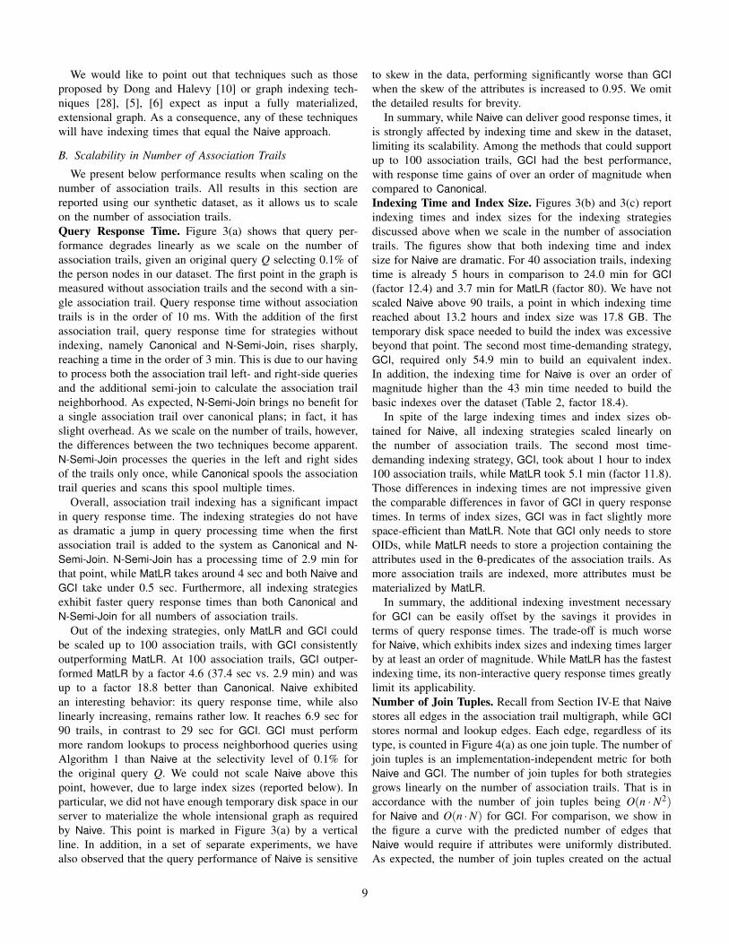
We present below performance results when scaling on thenumber of association trails. All results in this section arereported using our synthetic dataset, as it allows us to scaleon the number of association trails.Query Response Time. Figure 3(a) shows that query per-formance degrades linearly as we scale on the number ofassociation trails, given an original query Q selecting 0.1% ofthe person nodes in our dataset. The first point in the graph ismeasured without association trails and the second with a sin-gle association trail. Query response time without associationtrails is in the order of 10 ms. With the addition of the firstassociation trail, query response time for strategies withoutindexing, namely Canonical and N-Semi-Join, rises sharply,reaching a time in the order of 3 min. This is due to our havingto process both the association trail left- and right-side queriesand the additional semi-join to calculate the association trailneighborhood. As expected, N-Semi-Join brings no benefit fora single association trail over canonical plans; in fact, it hasslight overhead. As we scale on the number of trails, however,the differences between the two techniques become apparent.N-Semi-Join processes the queries in the left and right sidesof the trails only once, while Canonical spools the associationtrail queries and scans this spool multiple times.

Overall, association trail indexing has a significant impactin query response time. The indexing strategies do not haveas dramatic a jump in query processing time when the firstassociation trail is added to the system as Canonical and N-Semi-Join. N-Semi-Join has a processing time of 2.9 min forthat point, while MatLR takes around 4 sec and both Naive andGCI take under 0.5 sec. Furthermore, all indexing strategiesexhibit faster query response times than both Canonical andN-Semi-Join for all numbers of association trails.

Out of the indexing strategies, only MatLR and GCI couldbe scaled up to 100 association trails, with GCI consistentlyoutperforming MatLR. At 100 association trails, GCI outper-formed MatLR by a factor 4.6 (37.4 sec vs. 2.9 min) and wasup to a factor 18.8 better than Canonical. Naive exhibitedan interesting behavior: its query response time, while alsolinearly increasing, remains rather low. It reaches 6.9 sec for90 trails, in contrast to 29 sec for GCI. GCI must performmore random lookups to process neighborhood queries usingAlgorithm 1 than Naive at the selectivity level of 0.1% forthe original query Q. We could not scale Naive above thispoint, however, due to large index sizes (reported below). Inparticular, we did not have enough temporary disk space in ourserver to materialize the whole intensional graph as requiredby Naive. This point is marked in Figure 3(a) by a verticalline. In addition, in a set of separate experiments, we havealso observed that the query performance of Naive is sensitive

to skew in the data, performing significantly worse than GCIwhen the skew of the attributes is increased to 0.95. We omitthe detailed results for brevity.

In summary, while Naive can deliver good response times, itis strongly affected by indexing time and skew in the dataset,limiting its scalability. Among the methods that could supportup to 100 association trails, GCI had the best performance,with response time gains of over an order of magnitude whencompared to Canonical.Indexing Time and Index Size. Figures 3(b) and 3(c) reportindexing times and index sizes for the indexing strategiesdiscussed above when we scale in the number of associationtrails. The figures show that both indexing time and indexsize for Naive are dramatic. For 40 association trails, indexingtime is already 5 hours in comparison to 24.0 min for GCI(factor 12.4) and 3.7 min for MatLR (factor 80). We have notscaled Naive above 90 trails, a point in which indexing timereached about 13.2 hours and index size was 17.8 GB. Thetemporary disk space needed to build the index was excessivebeyond that point. The second most time-demanding strategy,GCI, required only 54.9 min to build an equivalent index.In addition, the indexing time for Naive is over an order ofmagnitude higher than the 43 min time needed to build thebasic indexes over the dataset (Table 2, factor 18.4).

In spite of the large indexing times and index sizes ob-tained for Naive, all indexing strategies scaled linearly onthe number of association trails. The second most time-demanding indexing strategy, GCI, took about 1 hour to index100 association trails, while MatLR took 5.1 min (factor 11.8).Those differences in indexing times are not impressive giventhe comparable differences in favor of GCI in query responsetimes. In terms of index sizes, GCI was in fact slightly morespace-efficient than MatLR. Note that GCI only needs to storeOIDs, while MatLR needs to store a projection containing theattributes used in the θ-predicates of the association trails. Asmore association trails are indexed, more attributes must bematerialized by MatLR.

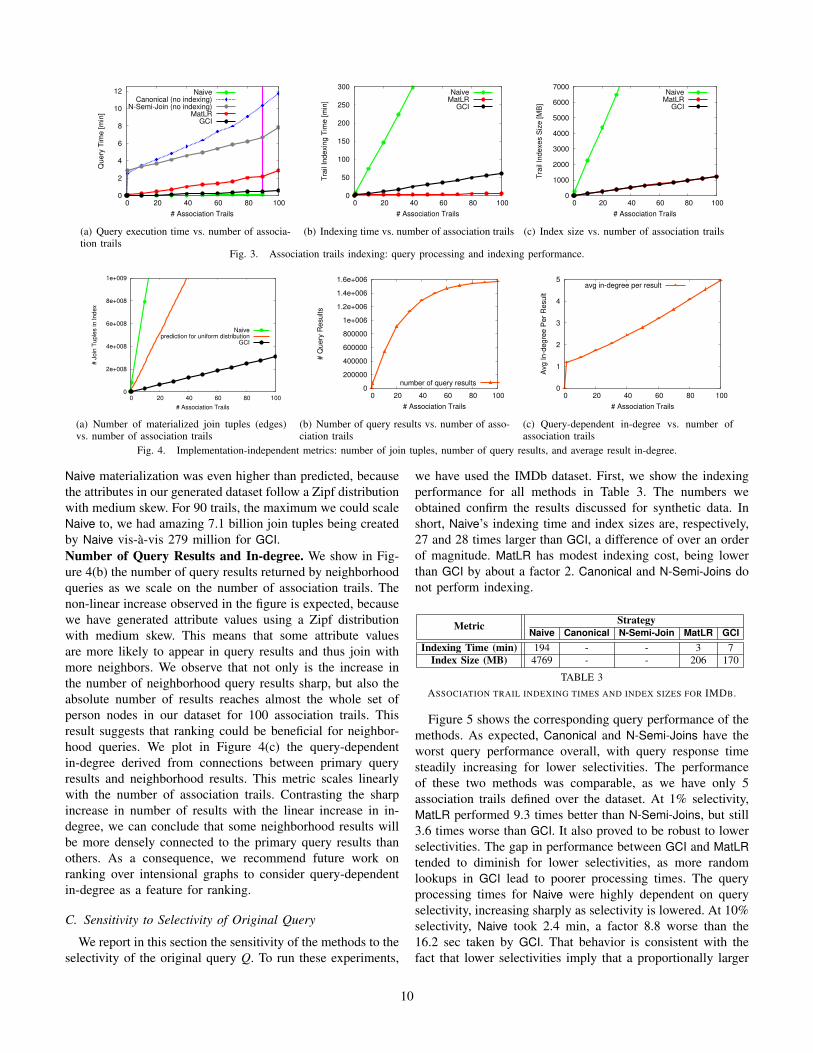
In summary, the additional indexing investment necessaryfor GCI can be easily offset by the savings it provides interms of query response times. The trade-off is much worsefor Naive, which exhibits index sizes and indexing times largerby at least an order of magnitude. While MatLR has the fastestindexing time, its non-interactive query response times greatlylimit its applicability.Number of Join Tuples. Recall from Section IV-E that Naivestores all edges in the association trail multigraph, while GCIstores normal and lookup edges. Each edge, regardless of itstype, is counted in Figure 4(a) as one join tuple. The number ofjoin tuples is an implementation-independent metric for bothNaive and GCI. The number of join tuples for both strategiesgrows linearly on the number of association trails. That is inaccordance with the number of join tuples being O(n ·N2)for Naive and O(n ·N) for GCI. For comparison, we show inthe figure a curve with the predicted number of edges thatNaive would require if attributes were uniformly distributed.As expected, the number of join tuples created on the actual

9

0

2

4

6

8

10

12

0 20 40 60 80 100

Query

Tim

e [m

in]

# Association Trails

NaiveCanonical (no indexing)

N-Semi-Join (no indexing)MatLR

GCI

(a) Query execution time vs. number of associa-tion trails

0

50

100

150

200

250

300

0 20 40 60 80 100

Tra

il In

dexin

g T

ime [m

in]


NaiveMatLR

GCI

(b) Indexing time vs. number of association trails

0

1000

2000

3000

4000

5000

6000

7000

0 20 40 60 80 100

Tra

il In

dexes S

ize [M

B]


NaiveMatLR

GCI

(c) Index size vs. number of association trails

Fig. 3. Association trails indexing: query processing and indexing performance.

0

2e+008

4e+008

6e+008

8e+008

1e+009

0 20 40 60 80 100

# J

oin

Tuple

s in Index


Naiveprediction for uniform distribution

GCI

(a) Number of materialized join tuples (edges)vs. number of association trails

0

200000

400000

600000

800000

1e+006

1.2e+006

1.4e+006

1.6e+006

0 20 40 60 80 100

# Q

uery

Results


number of query results

(b) Number of query results vs. number of asso-ciation trails

0

1

2

3

4

5

0 20 40 60 80 100

Avg In-d

egre

e P

er

Result


avg in-degree per result

(c) Query-dependent in-degree vs. number ofassociation trails

Fig. 4. Implementation-independent metrics: number of join tuples, number of query results, and average result in-degree.

Naive materialization was even higher than predicted, becausethe attributes in our generated dataset follow a Zipf distributionwith medium skew. For 90 trails, the maximum we could scaleNaive to, we had amazing 7.1 billion join tuples being createdby Naive vis-à-vis 279 million for GCI.Number of Query Results and In-degree. We show in Fig-ure 4(b) the number of query results returned by neighborhoodqueries as we scale on the number of association trails. Thenon-linear increase observed in the figure is expected, becausewe have generated attribute values using a Zipf distributionwith medium skew. This means that some attribute valuesare more likely to appear in query results and thus join withmore neighbors. We observe that not only is the increase inthe number of neighborhood query results sharp, but also theabsolute number of results reaches almost the whole set ofperson nodes in our dataset for 100 association trails. Thisresult suggests that ranking could be beneficial for neighbor-hood queries. We plot in Figure 4(c) the query-dependentin-degree derived from connections between primary queryresults and neighborhood results. This metric scales linearlywith the number of association trails. Contrasting the sharpincrease in number of results with the linear increase in in-degree, we can conclude that some neighborhood results willbe more densely connected to the primary query results thanothers. As a consequence, we recommend future work onranking over intensional graphs to consider query-dependentin-degree as a feature for ranking.

C. Sensitivity to Selectivity of Original Query

We report in this section the sensitivity of the methods to theselectivity of the original query Q. To run these experiments,

we have used the IMDb dataset. First, we show the indexingperformance for all methods in Table 3. The numbers weobtained confirm the results discussed for synthetic data. Inshort, Naive’s indexing time and index sizes are, respectively,27 and 28 times larger than GCI, a difference of over an orderof magnitude. MatLR has modest indexing cost, being lowerthan GCI by about a factor 2. Canonical and N-Semi-Joins donot perform indexing.

Metric StrategyNaive Canonical N-Semi-Join MatLR GCI

Indexing Time (min) 194 - - 3 7Index Size (MB) 4769 - - 206 170

TABLE 3ASSOCIATION TRAIL INDEXING TIMES AND INDEX SIZES FOR IMDB.

Figure 5 shows the corresponding query performance of themethods. As expected, Canonical and N-Semi-Joins have theworst query performance overall, with query response timesteadily increasing for lower selectivities. The performanceof these two methods was comparable, as we have only 5association trails defined over the dataset. At 1% selectivity,MatLR performed 9.3 times better than N-Semi-Joins, but still3.6 times worse than GCI. It also proved to be robust to lowerselectivities. The gap in performance between GCI and MatLRtended to diminish for lower selectivities, as more randomlookups in GCI lead to poorer processing times. The queryprocessing times for Naive were highly dependent on queryselectivity, increasing sharply as selectivity is lowered. At 10%selectivity, Naive took 2.4 min, a factor 8.8 worse than the16.2 sec taken by GCI. That behavior is consistent with thefact that lower selectivities imply that a proportionally larger

10

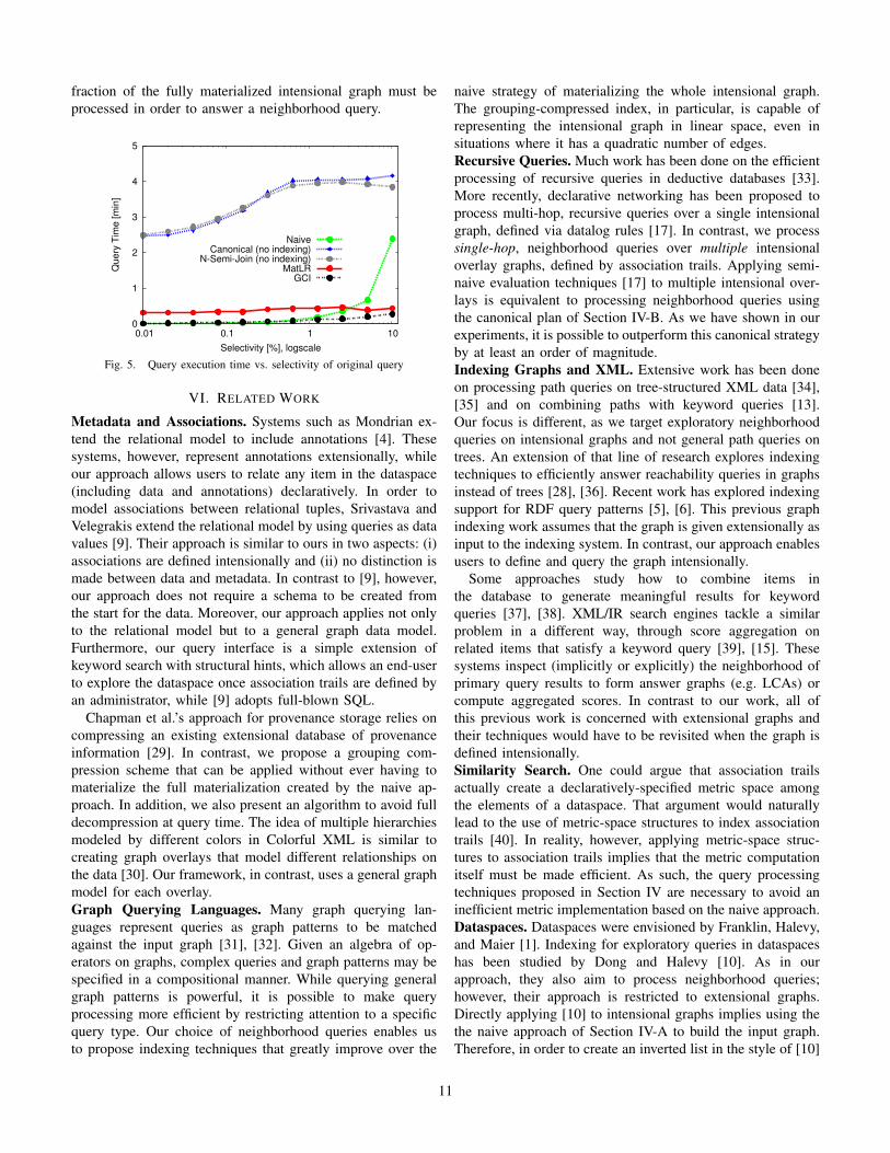
fraction of the fully materialized intensional graph must beprocessed in order to answer a neighborhood query.

0

1

2

3

4

5

0.01 0.1 1 10

Query

Tim

e [m

in]

Selectivity [%], logscale

NaiveCanonical (no indexing)

N-Semi-Join (no indexing)MatLR

GCI

Fig. 5. Query execution time vs. selectivity of original query

VI. RELATED WORK

Metadata and Associations. Systems such as Mondrian ex-tend the relational model to include annotations [4]. Thesesystems, however, represent annotations extensionally, whileour approach allows users to relate any item in the dataspace(including data and annotations) declaratively. In order tomodel associations between relational tuples, Srivastava andVelegrakis extend the relational model by using queries as datavalues [9]. Their approach is similar to ours in two aspects: (i)associations are defined intensionally and (ii) no distinction ismade between data and metadata. In contrast to [9], however,our approach does not require a schema to be created fromthe start for the data. Moreover, our approach applies not onlyto the relational model but to a general graph data model.Furthermore, our query interface is a simple extension ofkeyword search with structural hints, which allows an end-userto explore the dataspace once association trails are defined byan administrator, while [9] adopts full-blown SQL.

Chapman et al.’s approach for provenance storage relies oncompressing an existing extensional database of provenanceinformation [29]. In contrast, we propose a grouping com-pression scheme that can be applied without ever having tomaterialize the full materialization created by the naive ap-proach. In addition, we also present an algorithm to avoid fulldecompression at query time. The idea of multiple hierarchiesmodeled by different colors in Colorful XML is similar tocreating graph overlays that model different relationships onthe data [30]. Our framework, in contrast, uses a general graphmodel for each overlay.Graph Querying Languages. Many graph querying lan-guages represent queries as graph patterns to be matchedagainst the input graph [31], [32]. Given an algebra of op-erators on graphs, complex queries and graph patterns may bespecified in a compositional manner. While querying generalgraph patterns is powerful, it is possible to make queryprocessing more efficient by restricting attention to a specificquery type. Our choice of neighborhood queries enables usto propose indexing techniques that greatly improve over the

naive strategy of materializing the whole intensional graph.The grouping-compressed index, in particular, is capable ofrepresenting the intensional graph in linear space, even insituations where it has a quadratic number of edges.Recursive Queries. Much work has been done on the efficientprocessing of recursive queries in deductive databases [33].More recently, declarative networking has been proposed toprocess multi-hop, recursive queries over a single intensionalgraph, defined via datalog rules [17]. In contrast, we processsingle-hop, neighborhood queries over multiple intensionaloverlay graphs, defined by association trails. Applying semi-naive evaluation techniques [17] to multiple intensional over-lays is equivalent to processing neighborhood queries usingthe canonical plan of Section IV-B. As we have shown in ourexperiments, it is possible to outperform this canonical strategyby at least an order of magnitude.Indexing Graphs and XML. Extensive work has been doneon processing path queries on tree-structured XML data [34],[35] and on combining paths with keyword queries [13].Our focus is different, as we target exploratory neighborhoodqueries on intensional graphs and not general path queries ontrees. An extension of that line of research explores indexingtechniques to efficiently answer reachability queries in graphsinstead of trees [28], [36]. Recent work has explored indexingsupport for RDF query patterns [5], [6]. This previous graphindexing work assumes that the graph is given extensionally asinput to the indexing system. In contrast, our approach enablesusers to define and query the graph intensionally.

Some approaches study how to combine items inthe database to generate meaningful results for keywordqueries [37], [38]. XML/IR search engines tackle a similarproblem in a different way, through score aggregation onrelated items that satisfy a keyword query [39], [15]. Thesesystems inspect (implicitly or explicitly) the neighborhood ofprimary query results to form answer graphs (e.g. LCAs) orcompute aggregated scores. In contrast to our work, all ofthis previous work is concerned with extensional graphs andtheir techniques would have to be revisited when the graph isdefined intensionally.Similarity Search. One could argue that association trailsactually create a declaratively-specified metric space amongthe elements of a dataspace. That argument would naturallylead to the use of metric-space structures to index associationtrails [40]. In reality, however, applying metric-space struc-tures to association trails implies that the metric computationitself must be made efficient. As such, the query processingtechniques proposed in Section IV are necessary to avoid aninefficient metric implementation based on the naive approach.Dataspaces. Dataspaces were envisioned by Franklin, Halevy,and Maier [1]. Indexing for exploratory queries in dataspaceshas been studied by Dong and Halevy [10]. As in ourapproach, they also aim to process neighborhood queries;however, their approach is restricted to extensional graphs.Directly applying [10] to intensional graphs implies using thethe naive approach of Section IV-A to build the input graph.Therefore, in order to create an inverted list in the style of [10]

11

over intensional graphs, the techniques studied in this paperare a prerequisite.iTrails. One could argue that the set-level trails introduced bythe authors in previous work [2] could be used to representitem-level association trails. In order to do that, we wouldhave to create one set-level trail with a set of one item toanother set of one item for each intensional edge in theassociation trail multigraph. As a consequence, we would needto define a quadratic number of set-level trails to represent anintensional graph that could be alternatively specified with asingle association trail. Using the trails of [2] here would infact be equivalent to the naive approach (full materialization ofthe intensional graph). Apart from the incovenience of definingsuch a large number of trails, our experiments demonstrate thatthis approach is an order of magnitude less efficient than thegrouping-compressed index.

VII. CONCLUSIONS

In this paper, we have presented association trails, adeclarative technique to define a logical, intensional graph ofassociations among instances in a dataspace. Our techniqueis general and may be applied to model such intensionalgraphs on a variety of scenarios, such as social networksand personal dataspaces. We have shown how to processexploratory neighborhood queries on top of the intensionalgraph defined by association trails. Our query processingtechniques combine partial materialization of the intensionalgraph with specialized query processing algorithms in orderto avoid the naive approach of completely materializing theintensional graph.

Our evaluation showed that the grouping-compressed index(GCI), our best query processing technique, scales well whenthe number of association trails is increased and when theselectivity is varied. In addition, GCI may bring over an orderof magnitude gain in query response time when compared tothe canonical plan without indexing. At the same time, GCImay provide over an order of magnitude gain in indexing timewhen compared to the naive approach.

As future work, we plan to adapt our techniques to bettersupport top-K query processing in the style of [27]. In thatvein, we would like to compare different ranking schemeswhen computing top-K answers over the association trailmultigraph. In addition, we would like to evaluate how ourtechniques perform over large real social networks.

REFERENCES

[1] M. Franklin, A. Halevy, and D. Maier, “From Databases to Dataspaces:A New Abstraction for Information Management,” SIGMOD Record,vol. 34, no. 4, pp. 27–33, 2005.

[2] M. A. V. Salles et al., “iTrails: Pay-as-you-go Information Integrationin Dataspaces,” in VLDB, 2007.

[3] A. D. Sarma, X. Dong, and A. Halevy, “Bootstrapping Pay-As-You-GoData Integration Systems,” in ACM SIGMOD, 2008.

[4] F. Geerts, A. Kementsietsidis, and D. Milano, “MONDRIAN: Anno-tating and Querying Databases through Colors and Blocks,” in ICDE,2006.

[5] T. Neumann and G. Weikum, “RDF-3X: a RISC-style Engine for RDF,”JDMR (formerly Proc. VLDB), vol. 1, 2008.

[6] C. Weiss, P. Karras, and A. Bernstein, “Hexastore: Sextuple Indexingfor Semantic Web Data Management,” JDMR (formerly Proc. VLDB),vol. 1, 2008.

[7] J.-P. Dittrich and M. A. V. Salles, “iDM: A Unified and Versatile DataModel for Personal Dataspace Management,” in VLDB, 2006.

[8] S. Amer-Yahia, L. V. S. Lakshmanan, and C. Yu, “SocialScope: EnablingInformation Discovery on Social Content Sites,” in CIDR, 2009.

[9] D. Srivastava and Y. Velegrakis, “Intensional Associations Between Dataand Metadata,” in ACM SIGMOD, 2007.

[10] X. Dong and A. Halevy, “Indexing Dataspaces,” in ACM SIGMOD,2007.

[11] R. Grishman, “Information Extraction: Techniques and Challenges,” inSCIE, 1997.

[12] G. Adomavicius and A. Tuzhilin, “Toward the Next Generation ofRecommender Systems: A Survey of the State-of-the-Art and PossibleExtensions,” IEEE Transactions on Knowledge and Data Engineering,vol. 17, no. 6, pp. 734–749, 2005.

[13] R. Kaushik et al., “On the Integration of Structure Indexes and InvertedLists,” in ACM SIGMOD, 2004.

[14] R. Baeza-Yates and B. Ribeiro-Neto, Modern Information Retrieval.Addison-Wesley, 1999.

[15] D. Carmel et al., “Searching XML Documents via XML Fragments,” inACM SIGIR, 2003.

[16] M. V. Salles, “Pay-as-you-go Information Integration in Personal andSocial Dataspaces,” Ph.D. dissertation, ETH Zurich, 2008.

[17] B. T. Loo et al., “Declarative Networking: Language, Execution andOptimization,” in ACM SIGMOD, 2006.

[18] P. Valduriez, “Join Indices,” ACM Transactions on Database Systems(TODS), vol. 12, no. 2, pp. 218–246, 1987.

[19] T. Neumann, “Efficient Generation and Execution of DAG-StructuredQuery Graphs,” Ph.D. dissertation, University of Mannheim, 2005.

[20] P. Mishra and M. H. Eich, “Join Processing in Relational Databases,”ACM Computing Surveys, vol. 24, no. 1, pp. 63–113, 1992.

[21] E. H. Jacox and H. Samet, “Spatial Join Techniques,” ACM Transactionson Database Systems (TODS), vol. 32, no. 1, 2007.

[22] D. Severance and G. Lohman, “Differential Files: Their Application tothe Maintenance of Large Databases,” ACM Transactions on DatabaseSystems (TODS), vol. 1, no. 3, 1976.

[23] J. Gray et al., “Quickly Generating Billion-Record Synthetic Databases,”in ACM SIGMOD, 1994.

[24] A.-L. Barabási and R. Albert, “Emergence of Scaling in RandomNetworks,” Science, vol. 286, no. 5439, pp. 509–512, 1999.

[25] “IMDb. http://www.imdb.com/.”[26] iMeMex project web-site. http://www.imemex.org.[27] R. Fagin, “Combining Fuzzy Information: an Overview,” SIGMOD

Record, vol. 31, no. 2, pp. 109–118, 2002.[28] S. Trissl and U. Leser, “Fast and Practical Indexing and Querying of

Very Large Graphs,” in ACM SIGMOD, 2007.[29] A. Chapman, H. V. Jagadish, and P. Ramanan, “Efficient Provenance

Storage,” in ACM SIGMOD, 2008.[30] H. V. Jagadish et al., “Colorful XML: One Hierarchy Isn’t Enough,” in

ACM SIGMOD, 2004.[31] H. He and A. Singh, “Graphs-at-a-Time: Query Language and Access

Methods for Graph Databases,” in ACM SIGMOD, 2008.[32] M. Fernández, D. Florescu, A. Y. Levy, and D. Suciu, “Declarative

Specification of Web Sites with Strudel,” VLDB Journal, vol. 9, no. 1,pp. 38–55, 2000.

[33] F. Bancilhon and R. Ramakrishnan, “An Amateur’s Introduction toRecursive Query Processing Strategies,” in ACM SIGMOD, 1986.

[34] N. Bruno, N. Koudas, and D. Srivastava, “Holistic Twig Joins: OptimalXML Pattern Matching,” in ACM SIGMOD, 2002.

[35] T. Milo and D. Suciu, “Index Structures for Path Expressions,” in ICDT,1999.

[36] H. Wang et al., “Dual Labeling: Answering Graph Reachability Queriesin Constant Time,” in ICDE, 2006.

[37] C. Yu and H. V. Jagadish, “Querying Complex Structured Databases,”in VLDB, 2007.

[38] S. Agrawal, S. Chaudhuri, and G. Das, “DBXplorer: A System forKeyword-Based Search over Relational Databases,” in ICDE, 2002.

[39] S. Amer-Yahia and M. Lalmas, “XML Search: Languages, INEX andScoring,” SIGMOD Record, vol. 36, no. 7, pp. 16–23, 2006.

[40] E. Chávez et al., “Searching in Metric Spaces,” ACM ComputingSurveys, vol. 33, no. 3, pp. 273–321, 2001.

12

Intensional Associations in Dataspaces - Cornell …vmarcos/default_files/SDB10.pdf · Intensional...

Documents

Transcript of Intensional Associations in Dataspaces - Cornell …vmarcos/default_files/SDB10.pdf · Intensional...