
Intelligent Wind Turbine Using Fuzzy PID Control1160242/FULLTEXT01.pdf · controller with the Fuzzy...
90
IN DEGREE PROJECT TECHNOLOGY, FIRST CYCLE, 15 CREDITS , STOCKHOLM SWEDEN 2017 Intelligent Wind Turbine Using Fuzzy PID Control RICHARD HEDLUND NIKLAS TIMARSON KTH ROYAL INSTITUTE OF TECHNOLOGY SCHOOL OF INDUSTRIAL ENGINEERING AND MANAGEMENT
Transcript of Intelligent Wind Turbine Using Fuzzy PID Control1160242/FULLTEXT01.pdf · controller with the Fuzzy...

IN DEGREE PROJECT TECHNOLOGY,FIRST CYCLE, 15 CREDITS
, STOCKHOLM SWEDEN 2017
Intelligent Wind Turbine Using Fuzzy PID Control
RICHARD HEDLUND
NIKLAS TIMARSON
KTH ROYAL INSTITUTE OF TECHNOLOGYSCHOOL OF INDUSTRIAL ENGINEERING AND MANAGEMENT


Intelligent Wind Turbine Using Fuzzy PID Control
RICHARD HEDLUNDNIKLAS TIMARSON
Bachelor’s Thesis at ITMSupervisor: Baha Alhaj Hasan
Examiner: Nihad Subasic
MMK 2017:23 MDAB 641

AbstractThis thesis demonstrates how small wind turbines can con-tribute to a greener planet by using wind energy to gen-erate electrical power. It compares the conventional PIDcontroller with the Fuzzy PID controller, implemented ina small wind turbine that was constructed using variousmachines.
The concept of changing the gain parameters of the PIDcontroller with fuzzy logic, depending on the wind directionfor greater power generation, is explained and tested. This,with usage of a DC-motor that gets an output signal fromthe system which reads input values from an encoder anda wind vane. The construction included a powertrain inwhich a transmission, roller bearings and shafts were im-plemented in the yaw mechanism.
The tests resulted in showing that the Fuzzy PID con-troller performed better, minimizing the error, when theerror between the wind turbine and the wind itself, wassmall. The power generation was also increased when uti-lizing the Fuzzy PID controller. However, the PID con-troller performed similar to the Fuzzy PID controller whenexposed to larger errors.
Keywords: Intelligent Wind Turbine, Fuzzy PID Control, Power Generation
ReferatIntelligent vindkraftverk som använder
suddig PID reglering
Det har arbetet visar hur sma vindkraftverk kan bidra tillen gronare planet genom att omvandla vindenergi till elekt-risk energi. Det beskriver jamforelsen mellan den vanligtforekommande PID regulatorn och den suddiga PID regu-latorn, implementerad i ett litet vindkraftverk som konstru-erades med hjalp av flertalet maskiner.
Konceptet att andra pa parametrarna i PID regulatornmed hjalp av suddig logik, beroende pa vindriktningen,forklaras och testas med syfte att generera energi. Dettamed hjalp av en DC-motor som far utsignaler fran systemetsom laser insignaler fran en encoder och en vindflojt. Kon-struktionen av rotatonsmekanismen inneholl implementa-tion av en vaxel, kullager och axlar.
Testresultaten visade att den suddiga PID regleringenvar battre pa att minimera felet, nar felet mellan vindkraft-verket och vinden var litet. Aven vid generering av energi,visade det sig att den suddiga PID regleringen presteradebattre. Likval presterade PID regulatorn pa samma nivasom den suddiga, nar felet var storre.

Preface
For us to be able to achieve this project with success, we have had the privilege toreceive help from fellow students in the mechatronics lab. We would like to thank oursupervisor Baha Alhaj Hasan who have guided us in the right direction and helpedus with sharing of his great knowledge. We would also like to thank Tomas Ostbergand Staffan Qvarnstrom for providing us with both mechanical and electronic partsthat were crucial for our project. Without the help from our talented lab assistants,especially Marcus Olsson, we wouldn’t have been able to finish this project in time.We appreciate the time that you’ve shared with us and answering all our questions.Also a big thanks to the course responsible Nihad Subasic, for making this possible.Last but not least, we would like to thank our fellow students for sharing this springsemester with us and for making it a great one.
Richard Hedlund and Niklas TimarsonStockholm, May 2017


Nomenclature
Abbreviations
Boolean Two state variable (True/False)
C Programming language
DC Direct Current
I/O Input/Output
LCA Life Cycle Analysis
LCD Liquid Crystal Display
MOI Moment of Inertia
MOM Mean of Maximum
NB Negative Big
NS Negative Small
PB Positive Big
PS Positive Small
PWM Pulse-Width Modulation
ZO Zero
Symbols
η Gearing efficiency
µ Membership function
ω Angular velocity
ρ Density
Θ Angle in frequency domain

θ Angle
A Area
Cp Power coefficient of the wind turbine
de Derivative of the error
E Voltage over electrical motor
e Error
f Viscous friction
Gc Transfer function of the controller
Gplant Transfer function of the plant
I Current
i Instantaneous current
J Moment of inertia
K Torque constant
k Number of gear teeth
K2φ Constant of the electrical motor
KD Derivative gain
KI Integrating gain
KP Proportional gain
L Inductance
l, a, b, h Length
M , T Torque
n Revolutions per minute
P Effect
R Resistance
r Radius
S Set of x′
U Voltage

u Instantaneous voltage
v Velocity
x′ Point that has the highest degree of membership

Contents
1 Introduction 11.1 Background . . . . . . . . . . . . . . . . . . . . . . . . . . . . . . . . 11.2 Purpose . . . . . . . . . . . . . . . . . . . . . . . . . . . . . . . . . . 11.3 Scope . . . . . . . . . . . . . . . . . . . . . . . . . . . . . . . . . . . 21.4 Method . . . . . . . . . . . . . . . . . . . . . . . . . . . . . . . . . . 2
2 Theory 52.1 Control Theory . . . . . . . . . . . . . . . . . . . . . . . . . . . . . . 5
2.1.1 PID Control . . . . . . . . . . . . . . . . . . . . . . . . . . . 52.1.2 Transfer Function . . . . . . . . . . . . . . . . . . . . . . . . 62.1.3 Fuzzy Control . . . . . . . . . . . . . . . . . . . . . . . . . . . 72.1.4 Fuzzy PID Control . . . . . . . . . . . . . . . . . . . . . . . . 8
2.2 Power Generation . . . . . . . . . . . . . . . . . . . . . . . . . . . . . 92.2.1 Moment of Inertia . . . . . . . . . . . . . . . . . . . . . . . . 102.2.2 Transmission . . . . . . . . . . . . . . . . . . . . . . . . . . . 10
2.3 Electronics . . . . . . . . . . . . . . . . . . . . . . . . . . . . . . . . 112.3.1 H-bridge . . . . . . . . . . . . . . . . . . . . . . . . . . . . . . 122.3.2 Encoder . . . . . . . . . . . . . . . . . . . . . . . . . . . . . . 13
3 Demonstrator 153.1 Problem Formulation . . . . . . . . . . . . . . . . . . . . . . . . . . . 153.2 Hardware . . . . . . . . . . . . . . . . . . . . . . . . . . . . . . . . . 15
3.2.1 Transmission . . . . . . . . . . . . . . . . . . . . . . . . . . . 173.2.2 Moment of Inertia . . . . . . . . . . . . . . . . . . . . . . . . 18
3.3 Electronics . . . . . . . . . . . . . . . . . . . . . . . . . . . . . . . . 203.3.1 Arduino and LCD display . . . . . . . . . . . . . . . . . . . . 203.3.2 Sensors . . . . . . . . . . . . . . . . . . . . . . . . . . . . . . 223.3.3 Motor and H-bridge . . . . . . . . . . . . . . . . . . . . . . . 233.3.4 Effect Resistor . . . . . . . . . . . . . . . . . . . . . . . . . . 23
3.4 Software . . . . . . . . . . . . . . . . . . . . . . . . . . . . . . . . . . 243.5 Controller . . . . . . . . . . . . . . . . . . . . . . . . . . . . . . . . . 253.6 Results . . . . . . . . . . . . . . . . . . . . . . . . . . . . . . . . . . . 25
3.6.1 Tests . . . . . . . . . . . . . . . . . . . . . . . . . . . . . . . . 25

3.6.2 Control Performance . . . . . . . . . . . . . . . . . . . . . . . 27
4 Discussion and Conclusions 334.1 Discussion . . . . . . . . . . . . . . . . . . . . . . . . . . . . . . . . . 334.2 Conclusions . . . . . . . . . . . . . . . . . . . . . . . . . . . . . . . . 344.3 Environment Perspective . . . . . . . . . . . . . . . . . . . . . . . . . 34
5 Future Work 355.1 Hardware . . . . . . . . . . . . . . . . . . . . . . . . . . . . . . . . . 355.2 Software . . . . . . . . . . . . . . . . . . . . . . . . . . . . . . . . . . 365.3 Tests . . . . . . . . . . . . . . . . . . . . . . . . . . . . . . . . . . . . 36
Bibliography 37
Appendices 39
A Arduino Code i
B Matlab Code xiii
C CAD Drawings xv
D LCA Report xxv
E Membership Functions xxxiii
List of Figures
2.1 Block diagram of the closed loop system, created with draw.io. . . . . . 62.2 System of fuzzy control [21]. . . . . . . . . . . . . . . . . . . . . . . . . . 82.3 Voltage and current divider, created using Fritzing. . . . . . . . . . . . . 122.4 Scheme of the process made in an H-bridge [16]. . . . . . . . . . . . . . 122.5 Model of an encoder [28]. . . . . . . . . . . . . . . . . . . . . . . . . . . 13
3.1 Section view of the wind turbine showing the components that were used.Made in Solid Edge ST8 using KeyShot Render. . . . . . . . . . . . . . 16
3.2 Components inside the wind turbine, made in Solid Edge ST8 usingKeyShot Render. . . . . . . . . . . . . . . . . . . . . . . . . . . . . . . . 16
3.3 The constructed wind turbine shown in Solid Edge ST8 with renderingin KeyShot Render. . . . . . . . . . . . . . . . . . . . . . . . . . . . . . 17
3.4 The constructed small wind turbine shown in a holistic view. . . . . . . 183.5 Schematic figures of the two transmissions, made in Microsoft Paint. . . 193.6 Block diagram of the system, made in Microsoft Visio. . . . . . . . . . . 203.7 Circuit schem of the system, made using Fritzing. . . . . . . . . . . . . . 213.8 Anemometer, instrument to measure wind speed [7]. . . . . . . . . . . . 223.9 Voltage sensor, made using Fritzing. . . . . . . . . . . . . . . . . . . . . 233.10 Effect resistor [8]. . . . . . . . . . . . . . . . . . . . . . . . . . . . . . . . 233.11 Algorithm flowchart of the control system, made in Microsoft Visio. . . 243.12 Surface plots of Fuzzy PID gain parameters, made in Matlab R2017a
using the Fuzzy Logic Designer. . . . . . . . . . . . . . . . . . . . . . . . 263.13 PID controller in test one, made in Matlab R2017a. . . . . . . . . . . . 273.14 Fuzzy PID controller in test one, made in Matlab R2017a. . . . . . . . . 283.15 PID controller in test two, made in Matlab R2017a. . . . . . . . . . . . 283.16 Fuzzy PID controller in test two, made in Matlab R2017a. . . . . . . . . 293.17 PID controller in test three, made in Matlab R2017a. . . . . . . . . . . 293.18 Fuzzy PID controller in test three, made in Matlab R2017a. . . . . . . . 303.19 PID: step responses, made in Matlab R2017a. . . . . . . . . . . . . . . . 303.20 Fuzzy PID: step responses, made in Matlab R2017a. . . . . . . . . . . . 313.21 Power generated by PID and Fuzzy PID, made in Matlab R2017a. . . . 313.22 Error between the wind angle and the turbine angle for PID and Fuzzy
PID, made in Matlab R2017a. . . . . . . . . . . . . . . . . . . . . . . . . 32
List of Tables
2.1 Rules tables of the gain parameters. . . . . . . . . . . . . . . . . . . . . 9
3.1 Tables of the different parameters of the hardware components. . . . . . 193.2 Electronic component description. . . . . . . . . . . . . . . . . . . . . . 213.3 Electronic component description for the voltage sensor. . . . . . . . . . 233.4 Gain parameters used in the PID controller. . . . . . . . . . . . . . . . . 253.5 Explanation of tests. . . . . . . . . . . . . . . . . . . . . . . . . . . . . . 263.6 Average error of the control algorithms performed in the tests. . . . . . 32

Chapter 1
Introduction
The introduction will describe the background, state the research questions and showthe procedures made in this thesis.
1.1 BackgroundThe world is getting warmer every day and the humanity are in desperate need ofnew innovative ways to produce the power that is needed for a modern society. Newinnovations can also be to produce more power with existing green energy powerplants and one of them is the wind turbine power plants. One way of increasingpower generation is to implement an effective control method to maximize windsupply and prevent components of failure caused by fatigue. This is the key foreveryday people to implement such an energy source to make the planet a bitgreener. The Swedish energy authority, Energimyndigheten, states that wind energyplants have been implemented all around Sweden during the last years and that itproduces more than 10 % of the total electricity generation in the country. InSweden, the total energy generated by wind turbine power plants have increased ina steady pace the last decade [13], which shows that renewable energy is truly onthe rising front. That is why it is important to research further about smaller windturbines for everyday utilization.
This thesis will show how these smaller wind turbines can contribute to a greenerplanet and to help sustain its assets. This will be done by the demonstration ofhow a small wind turbine can be constructed and its implementation of an effectivecontrol method that handles the nonlinear properties of the wind, using conventionalPID control with fuzzy logic. This was made with the purpose of controlling theyaw mechanism of the wind turbine to generate as much power as possible.
1.2 PurposeThe purpose of this project is to present a way of generating power from a windturbine. The wind will make the rotor turn which starts the process of converting
1
CHAPTER 1. INTRODUCTION
kinetic energy into electrical energy that will be turned into heat, in this project.The wind turbine will utilize a wind vane and an anemometer, which respectivelydetects the angle and speed of the wind with purpose of maximizing the incomingwind supply. This requires a nonlinear control method that minimizes the errordefined as the misalignment of the wind turbine from the wind direction. This con-troller is crucial for maximizing the power generation, which leads to the followingheader research question and its sub research questions that will be covered in thisstudy:
• Which control technique is more suitable to be used in small wind turbineapplications?
– How much does the Fuzzy PID controller increase or decrease the re-sponsiveness for different magnitudes of errors, compared to the PIDcontroller in a small wind turbine?
– Which of the Fuzzy PID controller and the PID controller has the leastaverage error, used in a small wind turbine?
– Which of the Fuzzy PID controller and the PID controller performs bestin terms of generating power, compared to the theoretical value of windturbines?
1.3 ScopeDue to limits in time and resources, there has to be some limitations regarding thisproject. The wind turbine only needs to rotate in the horizontal direction, hence,the pitch angle of the blades are not included in this project. The goal of the windturbine is therefore to generate as much electricity as possible by utilization of yawcontrol. Since the sensors used for the controller is fairly cheap, they are not asaccurate as one may think, but enough, relative to the size of this project.
Furthermore, the project does not include calculations of the blades aerodynamicproperties and if the whole construction has enough strength to cope with strongwinds. It is basically constructed in a way that it should be stable enough to copewith relatively small winds and to have the appropriate motors and components atwhich controlling can be executed with.
The electricity generated by the system is not powering the yaw control. Instead,it is fed with external batteries. In addition, the constructed wind turbine has noimplemented breaking system, when exposed to strong winds.
1.4 MethodA literature study made ground for this project, which partly included readings ofcontrol theory, design of wind turbines and calculations of electronic components.When this was done, the whole wind turbine was modeled in Siemens Solid Edge ST8
2

1.4. METHOD
to make sure that the components match each other and to simplify the practicalwork later on. The majority of the parts were manufactured with 3D-printers whichsuits perfect for making engine mounts and gears.
The beginning of the project also included making an algorithm flowchart thatshows how the controller operates along with the systems sensors to fulfill its pur-pose. Alongside this, a block diagram including every electronic component werefinalized. Both of these diagrams were made using Microsoft Visio and the circuitscheme where made using Fritzing.
The interdisciplinary work then started, which consisted of assembly the me-chanical parts in parallel with implementing the control system and the electronics.The suitable gain parameters were determined by empirical tests with purpose ofhaving a system that works in practice. The test data were analyzed using Math-Works Matlab R2017a to get to the results and determine the conclusions of thethesis.
3

Chapter 2
Theory
This chapter describes the foundations of the project’s theory. Hence, the reader isexpected to have basic knowledge in mathematics and control theory.
2.1 Control TheoryOne of the main goals of this project was to construct a controller that regulatesthe direction pointed by the wind turbine in order to maximize the power genera-tion. Due to varying parameters of the wind such as direction and speed demandseffective control systems that can handle quick changes of these parameters. One ofthe most common ways to maximize the power output of which these parametersplay a very important role, is to control the yaw mechanism of the wind turbine.Since the parameters of the wind are nonlinear, the commonly used PID control isnot a perfect implementation because it relies on mathematical models in which itresponds to well. A more suitable way of controlling the yaw movement is to use amore intelligent controller such as the Fuzzy PID [14,24].
2.1.1 PID ControlThe PID controller is widely used in the industry and it has some interesting prop-erties. It consists of three parts: proportional-, integrating- and derivative controlthat respectively handles values in present-, past- and future time. The proportionalpart determines the system’s speed where as the integrating part complements itby decreasing the steady state error. To be able to counteract the upcoming er-ror caused by the system, it needs to include a derivative part that can improvestability. The input signal when using PID control is defined as
u(t) = KP e(t) +KI
∫ t
0e(τ)dτ +KD
d
dte(t) (2.1)
where e(t) is the error with respect to time t and KP ,KI and KD stands for the gainparameters for each part. These parameters are crucial for the system to functionproperly [15].
5
CHAPTER 2. THEORY
2.1.2 Transfer Function
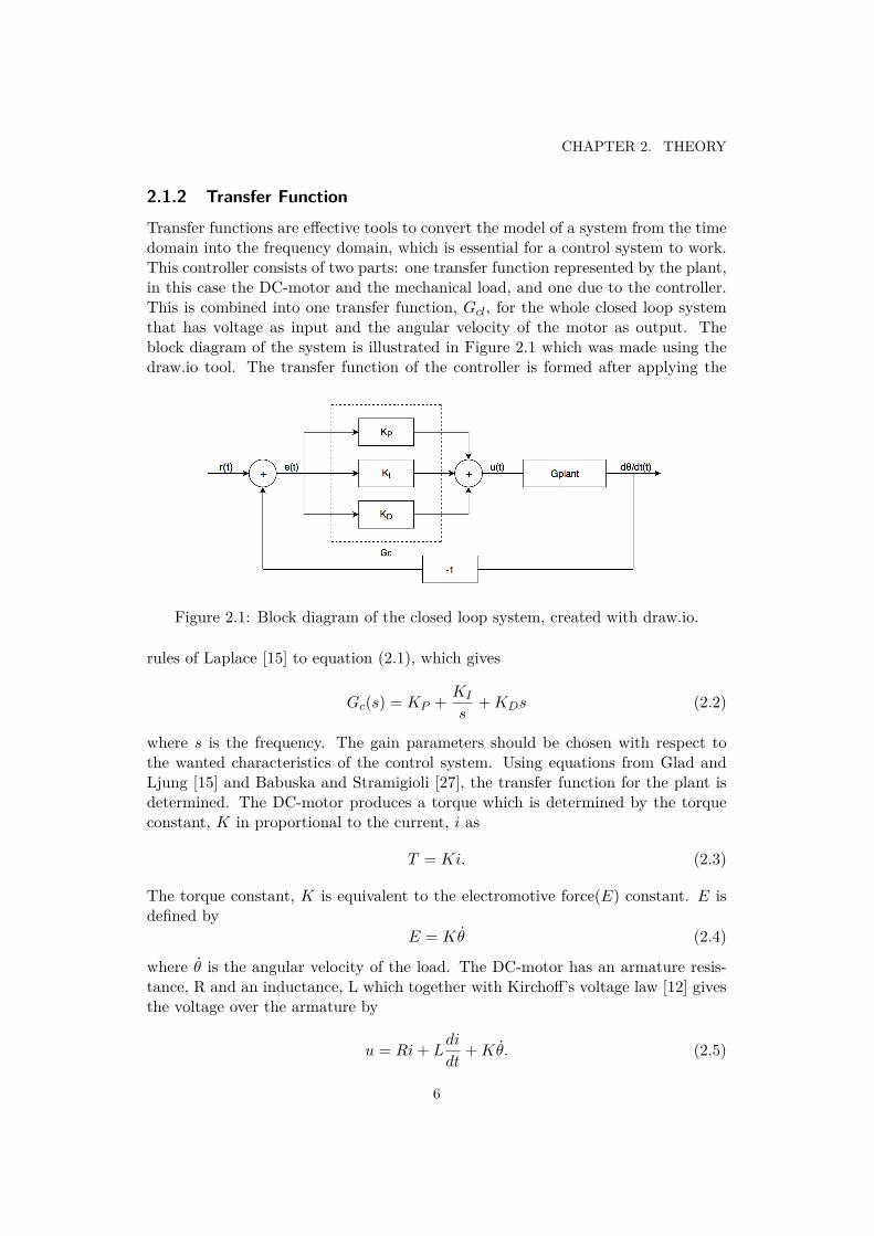
Transfer functions are effective tools to convert the model of a system from the timedomain into the frequency domain, which is essential for a control system to work.This controller consists of two parts: one transfer function represented by the plant,in this case the DC-motor and the mechanical load, and one due to the controller.This is combined into one transfer function, Gcl, for the whole closed loop systemthat has voltage as input and the angular velocity of the motor as output. Theblock diagram of the system is illustrated in Figure 2.1 which was made using thedraw.io tool. The transfer function of the controller is formed after applying the
Figure 2.1: Block diagram of the closed loop system, created with draw.io.
rules of Laplace [15] to equation (2.1), which gives
Gc(s) = KP + KI
s+KDs (2.2)
where s is the frequency. The gain parameters should be chosen with respect tothe wanted characteristics of the control system. Using equations from Glad andLjung [15] and Babuska and Stramigioli [27], the transfer function for the plant isdetermined. The DC-motor produces a torque which is determined by the torqueconstant, K in proportional to the current, i as
T = Ki. (2.3)
The torque constant, K is equivalent to the electromotive force(E) constant. E isdefined by
E = Kθ (2.4)
where θ is the angular velocity of the load. The DC-motor has an armature resis-tance, R and an inductance, L which together with Kirchoff’s voltage law [12] givesthe voltage over the armature by
u = Ri+ Ldi
dt+Kθ. (2.5)
6
2.1. CONTROL THEORY
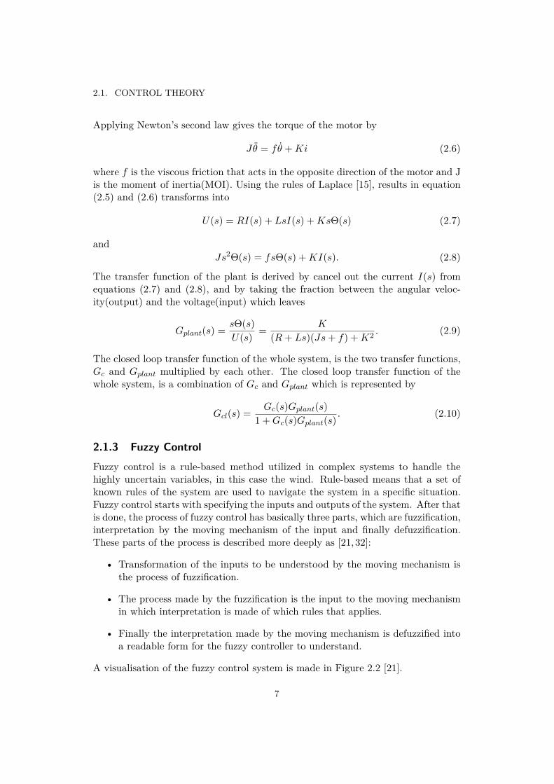
Applying Newton’s second law gives the torque of the motor by
Jθ = fθ +Ki (2.6)
where f is the viscous friction that acts in the opposite direction of the motor and Jis the moment of inertia(MOI). Using the rules of Laplace [15], results in equation(2.5) and (2.6) transforms into
U(s) = RI(s) + LsI(s) +KsΘ(s) (2.7)
andJs2Θ(s) = fsΘ(s) +KI(s). (2.8)
The transfer function of the plant is derived by cancel out the current I(s) fromequations (2.7) and (2.8), and by taking the fraction between the angular veloc-ity(output) and the voltage(input) which leaves
Gplant(s) = sΘ(s)U(s) = K
(R+ Ls)(Js+ f) +K2 . (2.9)
The closed loop transfer function of the whole system, is the two transfer functions,Gc and Gplant multiplied by each other. The closed loop transfer function of thewhole system, is a combination of Gc and Gplant which is represented by
Gcl(s) = Gc(s)Gplant(s)1 +Gc(s)Gplant(s)
. (2.10)
2.1.3 Fuzzy Control
Fuzzy control is a rule-based method utilized in complex systems to handle thehighly uncertain variables, in this case the wind. Rule-based means that a set ofknown rules of the system are used to navigate the system in a specific situation.Fuzzy control starts with specifying the inputs and outputs of the system. After thatis done, the process of fuzzy control has basically three parts, which are fuzzification,interpretation by the moving mechanism of the input and finally defuzzification.These parts of the process is described more deeply as [21,32]:
• Transformation of the inputs to be understood by the moving mechanism isthe process of fuzzification.
• The process made by the fuzzification is the input to the moving mechanismin which interpretation is made of which rules that applies.
• Finally the interpretation made by the moving mechanism is defuzzified intoa readable form for the fuzzy controller to understand.
A visualisation of the fuzzy control system is made in Figure 2.2 [21].
7
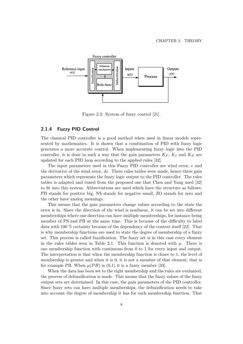
CHAPTER 2. THEORY
Figure 2.2: System of fuzzy control [21].
2.1.4 Fuzzy PID Control
The classical PID controller is a good method when used in linear models repre-sented by mathematics. It is shown that a combination of PID with fuzzy logicgenerates a more accurate control. When implementing fuzzy logic into the PIDcontroller, it is done in such a way that the gain parameters KP , KI and KD areupdated for each PID loop according to the applied rules [32].
The input parameters used in this Fuzzy PID controller are wind error, e andthe derivative of the wind error, de. Three rules tables were made, hence three gainparameters which represents the fuzzy logic output to the PID controller. The rulestables is adapted and tuned from the proposed one that Chen and Yang used [32]to fit into this system. Abbreviations are used which have the structure as follows:PB stands for positive big, NS stands for negative small, ZO stands for zero andthe other have analog meanings.
This means that the gain parameters change values according to the state theerror is in. Since the direction of the wind is nonlinear, it can be set into differentmemberships where one direction can have multiple memberships, for instance beingmember of PS and PB at the same time. This is because of the difficulty to labeldata with 100 % certainty because of the dependency of the context itself [22]. Thatis why membership functions are used to state the degree of membership of a fuzzyset. This process is called fuzzification. The fuzzy set is in this case every elementin the rules tables seen in Table 2.1. This function is denoted with µ. There isone membership function with continuum from 0 to 1 for every input and output.The interpretation is that when the membership function is closer to 1, the level ofmembership is greater and when it is 0, it is not a member of that element, that isfor example PB. When µ(PB) is (0,1) it is a fuzzy member [33].
When the data has been set to the right membership and the rules are evaluated,the process of defuzzification is made. This means that the fuzzy values of the fuzzyoutput sets are determined. In this case, the gain parameters of the PID controller.Since fuzzy sets can have multiple memberships, the defuzzification needs to takeinto account the degree of membership it has for each membership function. That
8
2.2. POWER GENERATION
Rules table of KP
ede NB NS ZO PS PB
NB PB PB PS PS ZONS PB PS PS ZO NSZO PB PS ZO NS NBPS PS ZO NS NS NBPB ZO NS NS NB NB
(a) Rules table for KP
Rules table of KI
ede NB NS ZO PS PB
NB NB NB NS NS ZONS NB NS NS ZO PSZO NB NS ZO PS PBPS NS ZO PS PS PBPB ZO PS PS PB PB
(b) Rules table for KI
Rules table of KD
ede NB NS ZO PS PB
NB PS NB NB NB PSNS ZO NS NS NS ZOZO ZO NS NS NS ZOPS ZO ZO ZO ZO ZOPB PB PS PS PS PB
(c) Rules table for KD
Table 2.1: Rules tables of the gain parameters.
can be made using different methods but the one that is suggested in this report isthe Mean of Maximum(MOM) method, since it is short and possible to implementon the Arduino. The two input variables determines the membership that theoutput variables belong to. MOM assigns the highest value of the fuzzy set A torepresent the crisp output value, which means that it is exact, unlike the fuzzyvalue. This is calculated by
y =
∑x′∈S
x′
S(2.11)
where x′ is the points that has the highest degree of membership and S the set ofwhich the x′ spans over [29]. For instance: if the membership function only has onehighest point, y will be assigned that x value, hence it is the MOM.
2.2 Power GenerationValidation of how the power generation system performs was compared to the theo-retical value of a wind turbine. According to Alexandersson [1], the annual averageof wind speed in Stockholm-Bromma during the years 1991-2004 was 3.4 m/s, whichis what the wind turbine will be exposed to in average. The power output of a windturbine is defined as
P = 12 · ρ ·A · v
3 · Cp. (2.12)
9

CHAPTER 2. THEORY
Here, v is equivalent to the mean value of the wind speed and ρ is the density ofair at 20 ◦C. The power coefficient, Cp is a fraction of how much energy that canbe converted by the wind turbine [24, 31]. It has a theoretical maximum value of59.3 %, called Betz’s limit [24]. The circular area covered by the wind blades isrepresented by
A = π · l2 (2.13)
in which l is the length of each blade. The value from equation (2.12) is the theo-retical value of which the power generation test will be compared to.
2.2.1 Moment of InertiaThe powertrain is the heart of the power generation system. In which, there are atransmission that transfer the power from the DC-motor to the gears, hence, makesthe wind turbine rotate. It may be intuitive that a particle with mass, have some sortof resistance against acceleration. This concept is called moment of inertia(MOI)and mathematically, it is described as
J =∫r2dm (2.14)
where r is the distance from origo and m, the mass. For this thesis, the rectangularparallelepiped and the bar will be the ones that are included which leaves the otherparts neglected. The MOI of the rectangular parallelepiped can be calculated with
JGx = m
12(a2 + h2) (2.15a)
JGy = m
12(b2 + h2) (2.15b)
JGz = m
12(a2 + b2) (2.15c)
where a, b and h are width, depth and height, respectively. And for the bar, theMOI is
JGx = m · r2
4 + m · h2
12 (2.16a)
JGz = m · r2
2 (2.16b)
where r is the radius and h the length [20].
2.2.2 TransmissionThe transmission was demanded because of the need for a high gear ratio due tolimitations in motor power. It also filled the purpose of making smooth transitionsto prevent fatigue and mechanical failure. The ratio can be calculated with
nout = −nin ·kin
kout. (2.17)
10

2.3. ELECTRONICS
The incoming speed nin is the speed in which the rotor is rotating with. The numberof gear teeth has k as its symbol [11]. Thanks to the transmission the effective MOIreduces to
Jred = J · n2
η(2.18)
where η is the efficiency of the transmission [10].
2.3 ElectronicsThree fundamental quantities in direct current(DC) electronics are voltage(U),current(I) and resistance(R). The three can be linked together with Ohm’s law [12]by
I = U
R. (2.19)
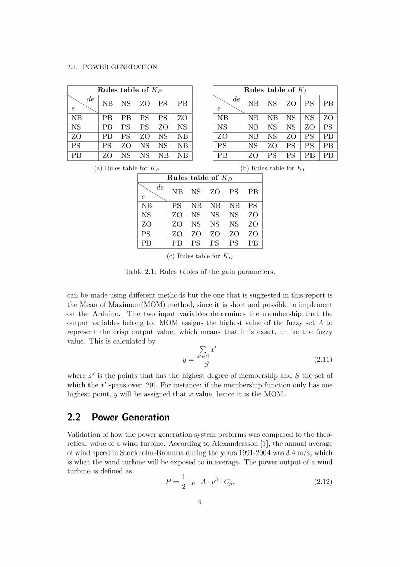
From Ohm’s law, the voltage divider and the current divider can be calculated. Thetwo equations will not be proven here but are defined as [12]
U1 = U · R1R1 +R2
(2.20a)
U2 = U · R2R1 +R2
(2.20b)
I1 = I · R2R1 +R2
(2.20c)
I2 = I · R1R1 +R2
(2.20d)
and the dividers are shown in Figure 2.3a and 2.3b which were made with Fritzing.With current and voltage, it is possible to calculate the total power in a circuit
with the following equationP = I · U (2.21)
where P is the power [12]. It may be intuitive to think that current and voltage thatgoes in to a circuit must come back in some way. The two laws made by Kirchhoffand also named by him are Kirchhoff’s voltage law and Kirchhoff’s current law [12].The two laws implies just that and they are defined as
n∑k=1
Ik = 0 (2.22a)
n∑k=1
Uk = 0 (2.22b)
where n represents the number of voltage and current components.
11
CHAPTER 2. THEORY
(a) Voltage divider.
(b) Current divider.
Figure 2.3: Voltage and current divider, created using Fritzing.
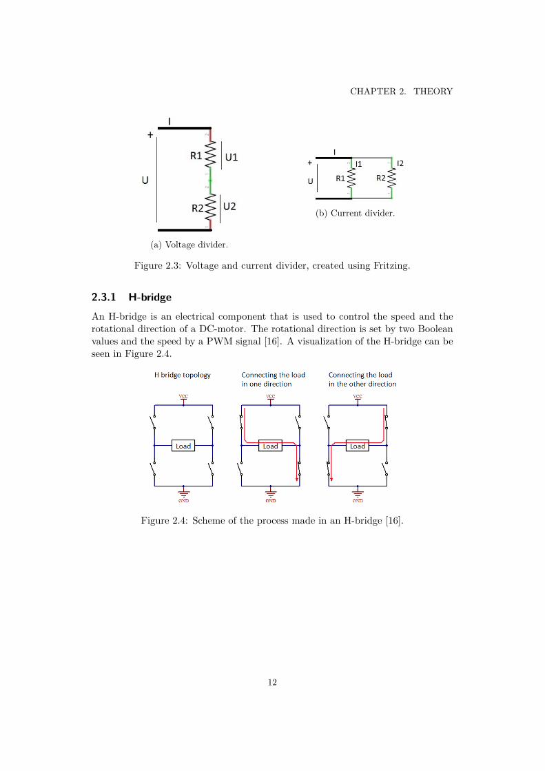
2.3.1 H-bridgeAn H-bridge is an electrical component that is used to control the speed and therotational direction of a DC-motor. The rotational direction is set by two Booleanvalues and the speed by a PWM signal [16]. A visualization of the H-bridge can beseen in Figure 2.4.
Figure 2.4: Scheme of the process made in an H-bridge [16].
12
2.3. ELECTRONICS
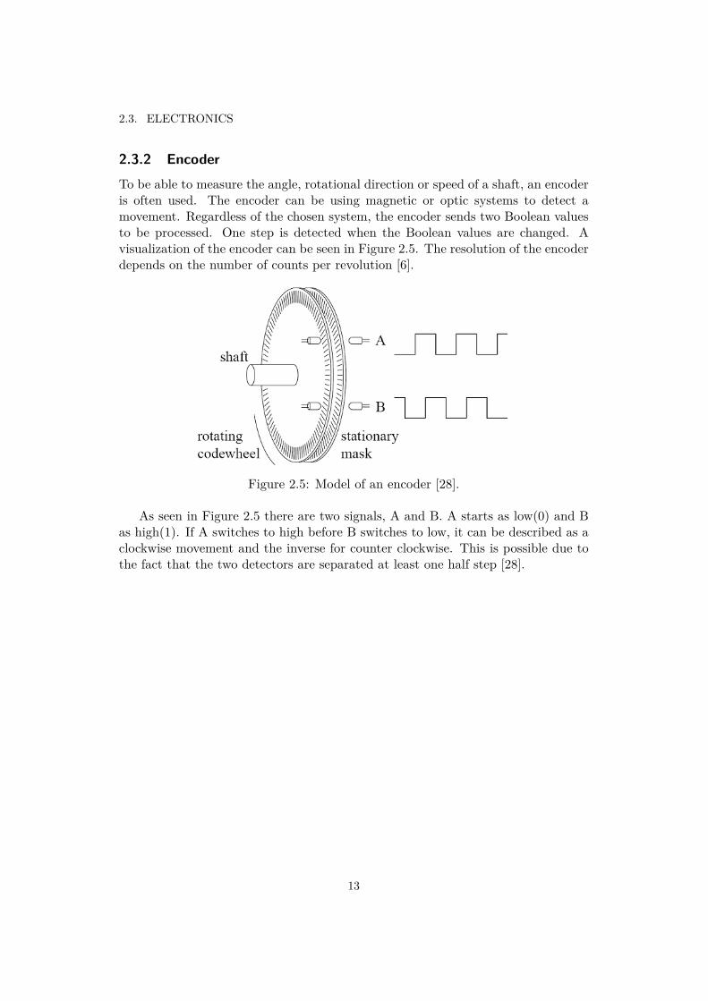
2.3.2 EncoderTo be able to measure the angle, rotational direction or speed of a shaft, an encoderis often used. The encoder can be using magnetic or optic systems to detect amovement. Regardless of the chosen system, the encoder sends two Boolean valuesto be processed. One step is detected when the Boolean values are changed. Avisualization of the encoder can be seen in Figure 2.5. The resolution of the encoderdepends on the number of counts per revolution [6].
Figure 2.5: Model of an encoder [28].
As seen in Figure 2.5 there are two signals, A and B. A starts as low(0) and Bas high(1). If A switches to high before B switches to low, it can be described as aclockwise movement and the inverse for counter clockwise. This is possible due tothe fact that the two detectors are separated at least one half step [28].
13

Chapter 3
Demonstrator
This chapter states the problem formulation as well as describing the construction,electronics and software used to get to the results.
3.1 Problem FormulationThis project aims to create a small wind turbine in which generation of power cantake place. This is subject to facing different problems that need to be solved, suchas:
• Control of the angle in which the wind turbine is pointing
• Mechanical design of the powertrain
• Power generation
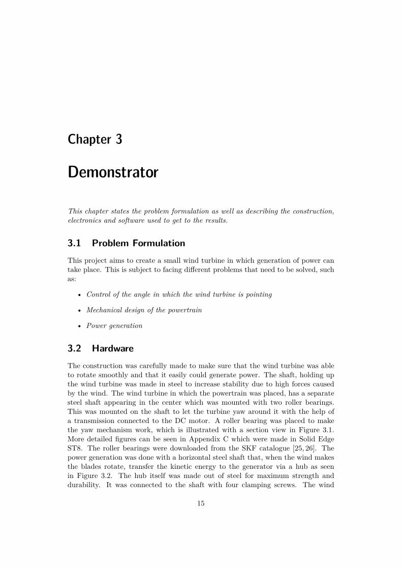
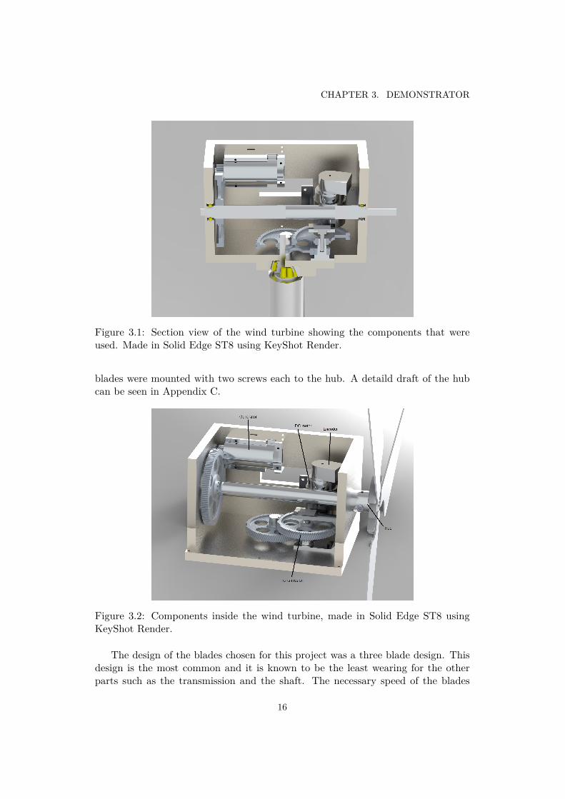
3.2 HardwareThe construction was carefully made to make sure that the wind turbine was ableto rotate smoothly and that it easily could generate power. The shaft, holding upthe wind turbine was made in steel to increase stability due to high forces causedby the wind. The wind turbine in which the powertrain was placed, has a separatesteel shaft appearing in the center which was mounted with two roller bearings.This was mounted on the shaft to let the turbine yaw around it with the help ofa transmission connected to the DC motor. A roller bearing was placed to makethe yaw mechanism work, which is illustrated with a section view in Figure 3.1.More detailed figures can be seen in Appendix C which were made in Solid EdgeST8. The roller bearings were downloaded from the SKF catalogue [25, 26]. Thepower generation was done with a horizontal steel shaft that, when the wind makesthe blades rotate, transfer the kinetic energy to the generator via a hub as seenin Figure 3.2. The hub itself was made out of steel for maximum strength anddurability. It was connected to the shaft with four clamping screws. The wind
15
CHAPTER 3. DEMONSTRATOR
Figure 3.1: Section view of the wind turbine showing the components that wereused. Made in Solid Edge ST8 using KeyShot Render.
blades were mounted with two screws each to the hub. A detaild draft of the hubcan be seen in Appendix C.
Figure 3.2: Components inside the wind turbine, made in Solid Edge ST8 usingKeyShot Render.
The design of the blades chosen for this project was a three blade design. Thisdesign is the most common and it is known to be the least wearing for the otherparts such as the transmission and the shaft. The necessary speed of the blades
16
3.2. HARDWARE
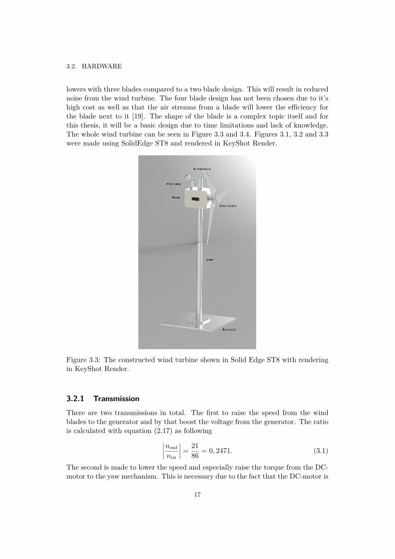
lowers with three blades compared to a two blade design. This will result in reducednoise from the wind turbine. The four blade design has not been chosen due to it’shigh cost as well as that the air streams from a blade will lower the efficiency forthe blade next to it [19]. The shape of the blade is a complex topic itself and forthis thesis, it will be a basic design due to time limitations and lack of knowledge.The whole wind turbine can be seen in Figure 3.3 and 3.4. Figures 3.1, 3.2 and 3.3were made using SolidEdge ST8 and rendered in KeyShot Render.
Figure 3.3: The constructed wind turbine shown in Solid Edge ST8 with renderingin KeyShot Render.
3.2.1 Transmission
There are two transmissions in total. The first to raise the speed from the windblades to the generator and by that boost the voltage from the generator. The ratiois calculated with equation (2.17) as following∣∣∣∣nout
nin
∣∣∣∣ = 2186 = 0, 2471. (3.1)
The second is made to lower the speed and especially raise the torque from the DC-motor to the yaw mechanism. This is necessary due to the fact that the DC-motor is
17

CHAPTER 3. DEMONSTRATOR
Figure 3.4: The constructed small wind turbine shown in a holistic view.
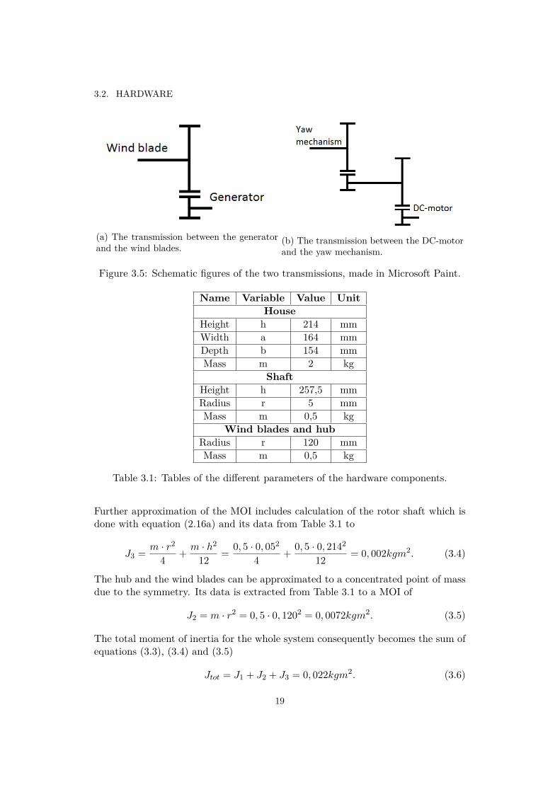
low on torque and the system have a high moment of inertia(MOI). The transmissionhave two steps to maximize the ratio without compromising on space. The twotransmissions can be seen in Figure 3.1, 3.2 and 3.5 as well as in Appendix C. Theschematic figure were made with Microsoft Paint. The total ratio is calculated againwith (2.17) into
n = nout
nin= 21
83 ·2183 = 0, 0640. (3.2)
3.2.2 Moment of Inertia
To be able to simulate the yaw system in a correct way, it is important to know theMOI of the system in total. The dimensions and the weight of the rotating housecan be seen in Table 3.1. With the help from equation (2.15a), the MOI of the boxcan be approximated to
J1 = m
12(a2 + h2) = 212(0, 1642 + 0, 2142) = 0, 012kgm2. (3.3)
18
3.2. HARDWARE
(a) The transmission between the generatorand the wind blades.
(b) The transmission between the DC-motorand the yaw mechanism.
Figure 3.5: Schematic figures of the two transmissions, made in Microsoft Paint.
Name Variable Value UnitHouse
Height h 214 mmWidth a 164 mmDepth b 154 mmMass m 2 kg
ShaftHeight h 257,5 mmRadius r 5 mmMass m 0,5 kg
Wind blades and hubRadius r 120 mmMass m 0,5 kg
Table 3.1: Tables of the different parameters of the hardware components.
Further approximation of the MOI includes calculation of the rotor shaft which isdone with equation (2.16a) and its data from Table 3.1 to
J3 = m · r2
4 + m · h2
12 = 0, 5 · 0, 052
4 + 0, 5 · 0, 2142
12 = 0, 002kgm2. (3.4)
The hub and the wind blades can be approximated to a concentrated point of massdue to the symmetry. Its data is extracted from Table 3.1 to a MOI of
J2 = m · r2 = 0, 5 · 0, 1202 = 0, 0072kgm2. (3.5)
The total moment of inertia for the whole system consequently becomes the sum ofequations (3.3), (3.4) and (3.5)
Jtot = J1 + J2 + J3 = 0, 022kgm2. (3.6)
19
CHAPTER 3. DEMONSTRATOR
Due to the transmission in the yaw mechanism, with zero losses, the MOI is reducedto
Jtot,red = Jtot · n2
η= 0, 022 · 0.06402
1 = 9, 01 · 10−5kgm2 (3.7)
according to equation (2.18).
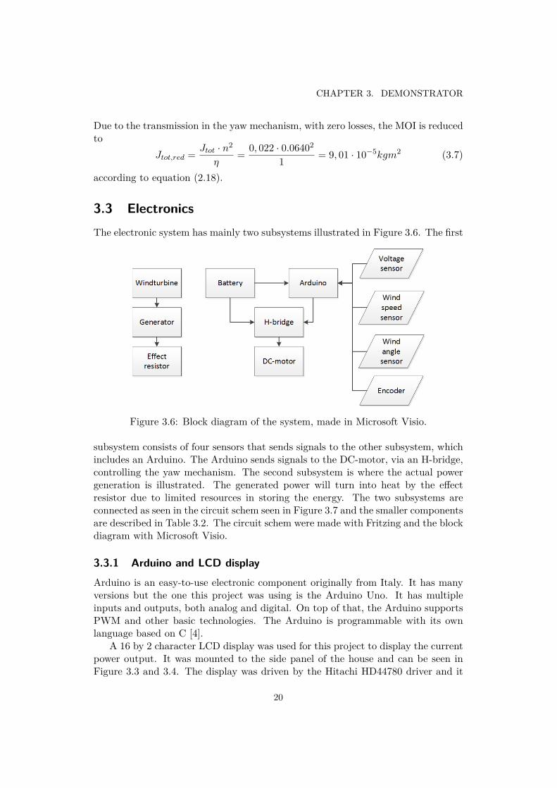
3.3 ElectronicsThe electronic system has mainly two subsystems illustrated in Figure 3.6. The first
Figure 3.6: Block diagram of the system, made in Microsoft Visio.
subsystem consists of four sensors that sends signals to the other subsystem, whichincludes an Arduino. The Arduino sends signals to the DC-motor, via an H-bridge,controlling the yaw mechanism. The second subsystem is where the actual powergeneration is illustrated. The generated power will turn into heat by the effectresistor due to limited resources in storing the energy. The two subsystems areconnected as seen in the circuit schem seen in Figure 3.7 and the smaller componentsare described in Table 3.2. The circuit schem were made with Fritzing and the blockdiagram with Microsoft Visio.
3.3.1 Arduino and LCD displayArduino is an easy-to-use electronic component originally from Italy. It has manyversions but the one this project was using is the Arduino Uno. It has multipleinputs and outputs, both analog and digital. On top of that, the Arduino supportsPWM and other basic technologies. The Arduino is programmable with its ownlanguage based on C [4].
A 16 by 2 character LCD display was used for this project to display the currentpower output. It was mounted to the side panel of the house and can be seen inFigure 3.3 and 3.4. The display was driven by the Hitachi HD44780 driver and it
20

3.3. ELECTRONICS
Figure 3.7: Circuit schem of the system, made using Fritzing.
Name Component Value UnitR1 Effect resistor 33 kW
R2, R3, R4 Resistor 330 kWP1 Wind vane(potentiometer) 10 kWP2 Anemometer - -P3 Potentiometer 30 kWF1 Fuse 1 AF2 Fuse 310 mAF3 Fuse 160 mA
Table 3.2: Electronic component description.
was able to be fed with a 4 or 8 bit data feed. The 4 bit interface is used due tothe limited number of digital I/Os of the Arduino [2].
21
CHAPTER 3. DEMONSTRATOR
3.3.2 Sensors
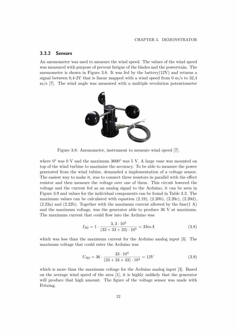
An anemometer was used to measure the wind speed. The values of the wind speedwas measured with purpose of prevent fatigue of the blades and the powertrain. Theanemometer is shown in Figure 3.8. It was fed by the battery(12V) and returns asignal between 0,4-2V that is linear mapped with a wind speed from 0 m/s to 32,4m/s [7]. The wind angle was measured with a multiple revolution potentiometer
Figure 3.8: Anemometer, instrument to measure wind speed [7].
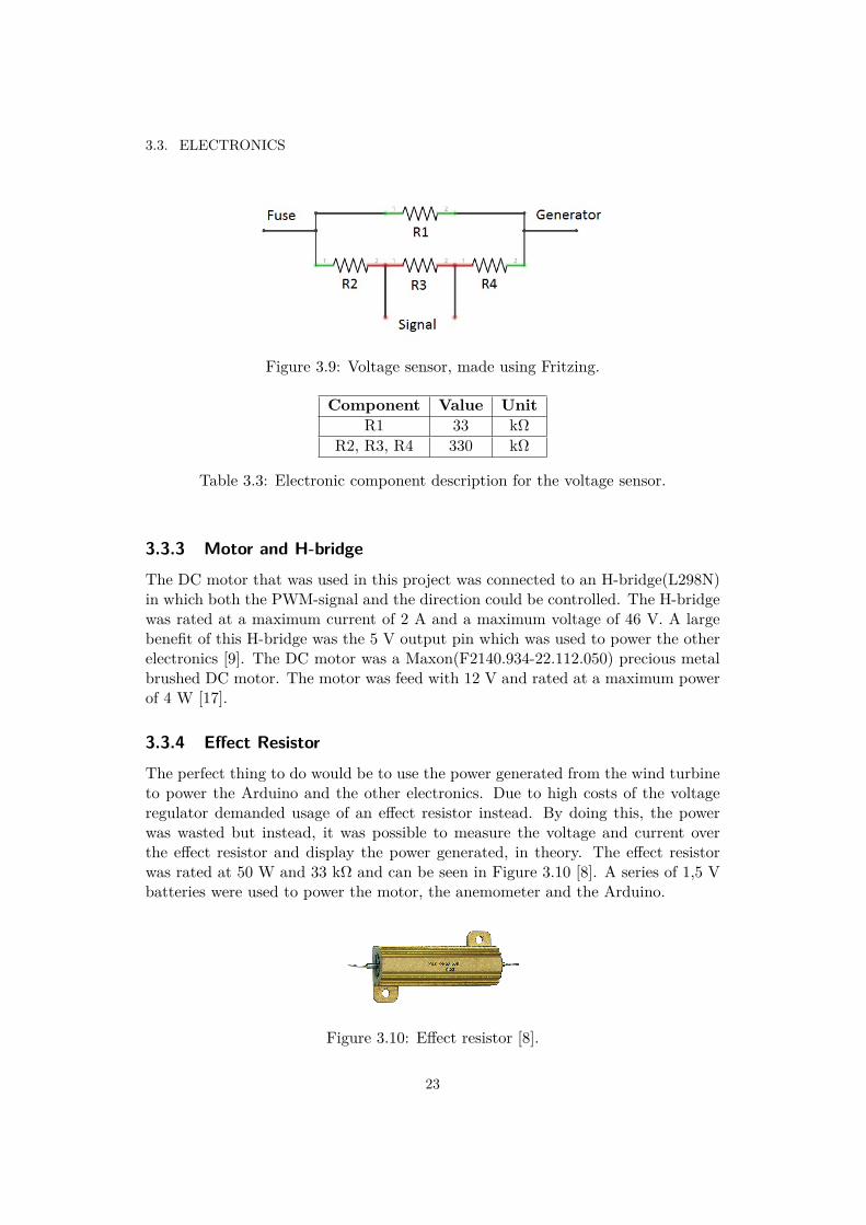
where 0° was 0 V and the maximum 3600° was 5 V. A large vane was mounted ontop of the wind turbine to maximize the accuracy. To be able to measure the powergenerated from the wind tubine, demanded a implementation of a voltage sensor.The easiest way to make it, was to connect three resistors in parallel with the effectresistor and then measure the voltage over one of them. This circuit lowered thevoltage and the current fed as an analog signal to the Arduino, it can be seen inFigure 3.9 and values for the individual components can be found in Table 3.3. Themaximum values can be calculated with equation (2.19), (2.20b), (2.20c), (2.20d),(2.22a) and (2.22b). Together with the maximum current allowed by the fuse(1 A)and the maximum voltage, was the generator able to produce 36 V at maximum.The maximum current that could flow into the Arduino was
IR2 = 1 · 3, 3 · 104
(33 + 33 + 33) · 104 = 33mA (3.8)
which was less than the maximum current for the Arduino analog input [3]. Themaximum voltage that could enter the Arduino was
UR2 = 36 · 33 · 104
(33 + 33 + 33) · 104 = 12V (3.9)
which is more than the maximum voltage for the Arduino analog input [3]. Basedon the average wind speed of the area [1], it is highly unlikely that the generatorwill produce that high amount. The figure of the voltage sensor was made withFritzing.
22
3.3. ELECTRONICS
Figure 3.9: Voltage sensor, made using Fritzing.
Component Value UnitR1 33 kW
R2, R3, R4 330 kW
Table 3.3: Electronic component description for the voltage sensor.
3.3.3 Motor and H-bridge
The DC motor that was used in this project was connected to an H-bridge(L298N)in which both the PWM-signal and the direction could be controlled. The H-bridgewas rated at a maximum current of 2 A and a maximum voltage of 46 V. A largebenefit of this H-bridge was the 5 V output pin which was used to power the otherelectronics [9]. The DC motor was a Maxon(F2140.934-22.112.050) precious metalbrushed DC motor. The motor was feed with 12 V and rated at a maximum powerof 4 W [17].
3.3.4 Effect Resistor
The perfect thing to do would be to use the power generated from the wind turbineto power the Arduino and the other electronics. Due to high costs of the voltageregulator demanded usage of an effect resistor instead. By doing this, the powerwas wasted but instead, it was possible to measure the voltage and current overthe effect resistor and display the power generated, in theory. The effect resistorwas rated at 50 W and 33 kW and can be seen in Figure 3.10 [8]. A series of 1,5 Vbatteries were used to power the motor, the anemometer and the Arduino.
Figure 3.10: Effect resistor [8].
23
CHAPTER 3. DEMONSTRATOR
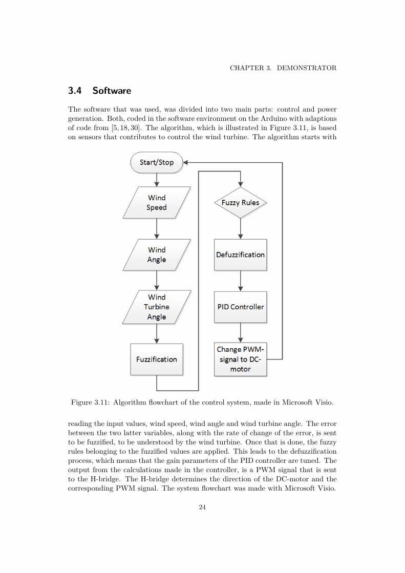
3.4 Software
The software that was used, was divided into two main parts: control and powergeneration. Both, coded in the software environment on the Arduino with adaptionsof code from [5, 18, 30]. The algorithm, which is illustrated in Figure 3.11, is basedon sensors that contributes to control the wind turbine. The algorithm starts with
Figure 3.11: Algorithm flowchart of the control system, made in Microsoft Visio.
reading the input values, wind speed, wind angle and wind turbine angle. The errorbetween the two latter variables, along with the rate of change of the error, is sentto be fuzzified, to be understood by the wind turbine. Once that is done, the fuzzyrules belonging to the fuzzified values are applied. This leads to the defuzzificationprocess, which means that the gain parameters of the PID controller are tuned. Theoutput from the calculations made in the controller, is a PWM signal that is sentto the H-bridge. The H-bridge determines the direction of the DC-motor and thecorresponding PWM signal. The system flowchart was made with Microsoft Visio.
24
3.5. CONTROLLER
3.5 ControllerThe final gain parameters that were used in the PID controller were producedusing empirical tests to see how the system performs in the real world. These gainparameters are shown in Table 3.4. The transfer function of the closed loop system
PIDKP KI KD
1.5 0.1 3.5
Table 3.4: Gain parameters used in the PID controller.
was determined using equation (2.10) with Matlab R2017a into
Gcl(s) = 0, 1932s2 + 0, 0828s+ 0, 005525, 695 · 10−8s3 + 0, 1937s2 + 0, 08585s+ 0, 00552 (3.10)
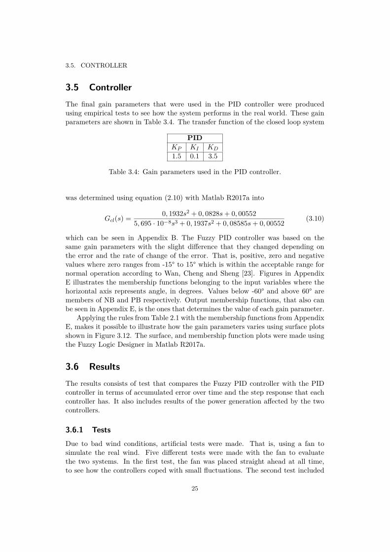
which can be seen in Appendix B. The Fuzzy PID controller was based on thesame gain parameters with the slight difference that they changed depending onthe error and the rate of change of the error. That is, positive, zero and negativevalues where zero ranges from -15° to 15° which is within the acceptable range fornormal operation according to Wan, Cheng and Sheng [23]. Figures in AppendixE illustrates the membership functions belonging to the input variables where thehorizontal axis represents angle, in degrees. Values below -60° and above 60° aremembers of NB and PB respectively. Output membership functions, that also canbe seen in Appendix E, is the ones that determines the value of each gain parameter.
Applying the rules from Table 2.1 with the membership functions from AppendixE, makes it possible to illustrate how the gain parameters varies using surface plotsshown in Figure 3.12. The surface, and membership function plots were made usingthe Fuzzy Logic Designer in Matlab R2017a.
3.6 ResultsThe results consists of test that compares the Fuzzy PID controller with the PIDcontroller in terms of accumulated error over time and the step response that eachcontroller has. It also includes results of the power generation affected by the twocontrollers.
3.6.1 TestsDue to bad wind conditions, artificial tests were made. That is, using a fan tosimulate the real wind. Five different tests were made with the fan to evaluatethe two systems. In the first test, the fan was placed straight ahead at all time,to see how the controllers coped with small fluctuations. The second test included
25
CHAPTER 3. DEMONSTRATOR
(a) Surface plot of KP . (b) Surface plot of KI .
(c) Surface plot of KD.
Figure 3.12: Surface plots of Fuzzy PID gain parameters, made in Matlab R2017ausing the Fuzzy Logic Designer.
continuous angular movement of 20-25°/20 s unlike the third test where discretesteps of 20-25°/20 s were done. When +/- 45-50° was reached, the direction waschanged to the opposite side. One long term(300 s) test was made to analyze thetotal power output. All tests were started with the fan in a straight ahead position, 4m from the wind turbine. Furthermore, a test was made which did not include wind,with purpose of analyzing the control algorithms more thoroughly. Specificationsof the tests can be found in Table 3.5.
Test # Duration [s] Explanation1 100 Steady placement2 100 20-25°/20 s continuously3 100 20-25°/20 s discrete steps4 150 Step responses without wind5 300 Steady placement, power generation
Table 3.5: Explanation of tests.
26

3.6. RESULTS
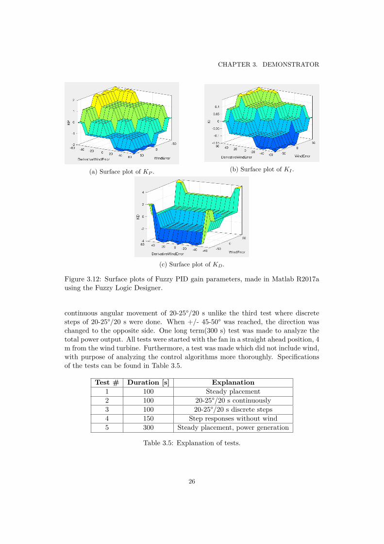
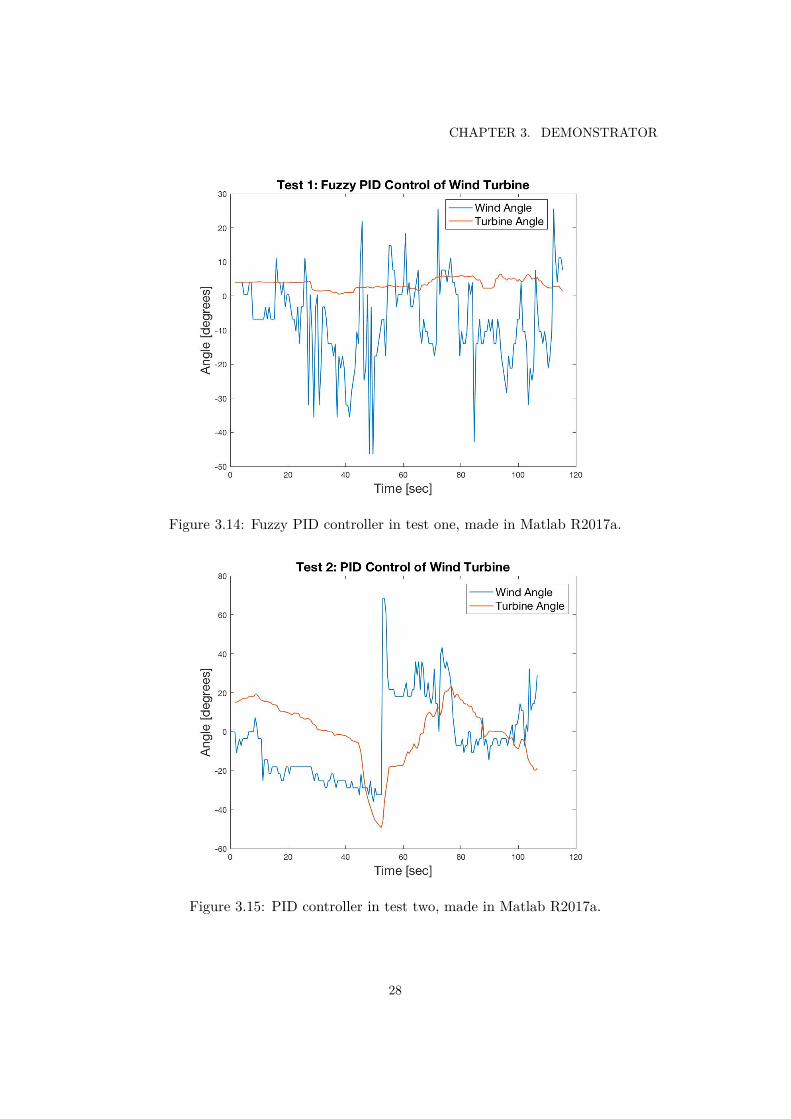
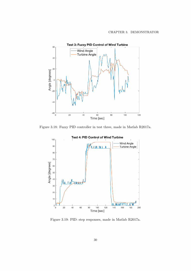
3.6.2 Control PerformanceThis section illustrates the performance of the tests described in Section 3.6.1 withplots made in Matlab R2017a. First of all is the steady placement test, whichcan be seen in Figure 3.13 and 3.14. Plots of the second test with the fan in
Figure 3.13: PID controller in test one, made in Matlab R2017a.
a continuously moving pace is illustrated in Figure 3.15 and 3.16. The discretetest is represented by Figure 3.17 and 3.18 and the results of the step responsesin test four is illustrated in Figure 3.19 and 3.20. Power generation was also partof the testing, which led to plots representing the power generated by each controlalgorithm as well as showing the error between the wind angle and the turbineangle. Using equation (2.12) and (2.13) with the average wind speed of 4.45 m/smeasured in the PID test and 4,12 m/s in the Fuzzy PID test, results in a maximumtheoretical power output of
PTP ID= 1
2 · 1, 2 · π · 0, 42 · 4, 453 · 0, 593 = 15, 8W (3.11)
andPTF uzzy
= 12 · 1, 2 · π · 0, 4
2 · 4, 123 · 0, 593 = 12, 5W. (3.12)
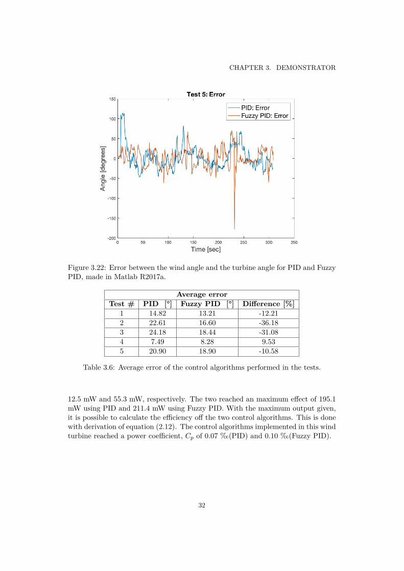
Here, 0.4 m is the length of the wind blades and the density of air is equal to 1.2kg/m3. The plots of test five are illustrated in Figure 3.21 and 3.22. The averageerror for every data point in these tests are summarized in Table 3.6 where theaverage power output using the PID controller and the Fuzzy PID controller were
27
CHAPTER 3. DEMONSTRATOR
Figure 3.14: Fuzzy PID controller in test one, made in Matlab R2017a.
Figure 3.15: PID controller in test two, made in Matlab R2017a.
28

3.6. RESULTS
Figure 3.16: Fuzzy PID controller in test two, made in Matlab R2017a.
Figure 3.17: PID controller in test three, made in Matlab R2017a.
29
CHAPTER 3. DEMONSTRATOR
Figure 3.18: Fuzzy PID controller in test three, made in Matlab R2017a.
Figure 3.19: PID: step responses, made in Matlab R2017a.
30

3.6. RESULTS
Figure 3.20: Fuzzy PID: step responses, made in Matlab R2017a.
Figure 3.21: Power generated by PID and Fuzzy PID, made in Matlab R2017a.
31
CHAPTER 3. DEMONSTRATOR
Figure 3.22: Error between the wind angle and the turbine angle for PID and FuzzyPID, made in Matlab R2017a.
Average errorTest # PID [°] Fuzzy PID [°] Difference [%]
1 14.82 13.21 -12.212 22.61 16.60 -36.183 24.18 18.44 -31.084 7.49 8.28 9.535 20.90 18.90 -10.58
Table 3.6: Average error of the control algorithms performed in the tests.
12.5 mW and 55.3 mW, respectively. The two reached an maximum effect of 195.1mW using PID and 211.4 mW using Fuzzy PID. With the maximum output given,it is possible to calculate the efficiency off the two control algorithms. This is donewith derivation of equation (2.12). The control algorithms implemented in this windturbine reached a power coefficient, Cp of 0.07 ‰(PID) and 0.10 ‰(Fuzzy PID).
32
Chapter 4
Discussion and Conclusions
This chapter includes analyzes and conclusions of the results with purpose of an-swering the research questions as well as summarizing the thesis.
4.1 Discussion
Since we have built a wind turbine in a relatively small scale, made it automaticallyhard for us to design and resemble the large ones used for power generation. Thechallenges that we have faced were mainly the drivetrain which included difficultiesin designing the transmission along with a small DC-motor. This was crucial for usto be able to compare the two control algorithms. Also, the power generation wasdifficult to measure, not due to bad sensors, but because of the trouble getting thewind blades to rotate continuously without moving too slow or too fast.
From the results, it is clear that the Fuzzy PID controller that we implementedperforms similar to the PID controller. One of the things that we wanted to seeif the Fuzzy PID performs better in, is when the wind fluctuates around -15° to15°. It would be unnecessary to rotate the wind turbine back and forth under thatcondition which is why the rules are determined in a way that the gain parametersbelongs to the ZO membership function. This was performed in test one wherewe can see from Figure 3.13 and 3.14 that the Fuzzy PID controller has a morestraight line, hence steadier than the PID controller. Even though it was morewind fluctuations in the test made for Fuzzy PID control.
Test two and three had more similar outcomes with a slight advantage by theFuzzy PID controller regarding more smooth curves and better tracking of the winddirection. Because of the difficulty to move around the fan and simultaneously aimit at the wind turbine, makes it hard to rate its reliability. The in-house test madeto analyze the two control algorithms deeper, seen in Figure 3.19 and 3.20, showsthat using bigger steps gives the Fuzzy PID controller advantage in terms of steadystate error and rise time. However, it is clear that the PID controller seems to haveabout the same overshoot performance.
Power generation performance, seen in Figure 3.21 and 3.22, are difficult to draw
33
CHAPTER 4. DISCUSSION AND CONCLUSIONS
conclusions from. This is since the test should be made in a more quantitative wayto make it statistical correct. However, from these plots, we can see that the FuzzyPID controller generates more power, probably because of that the controller seemsto have smaller errors more times than the PID controller, seen over the wholeduration of test five. It was also difficult to make sure that the conditions for bothcontrollers were the same, since the fan and the outside wind differ from time totime.
4.2 ConclusionsThe conclusions that can be drawn from the results and the discussion is that theFuzzy PID controller has better performance when the wind fluctuates around thesame angle due to the ZO membership function. Conclusion drawn from large winderrors and step responses is that the PID and the Fuzzy PID controller performsmore or less the same, except that the latter has smoother response, hence moresuitable for a wind turbine in terms of fatigue exposure.
Regarding the average error of the two control algorithms, the Fuzzy PID con-troller performs better in four of five tests with, according to us, significant im-provement. It also improves in terms of power generation. However, due to lowquantities of power generating tests, it is hard to conclude whether Fuzzy PID isbetter than PID implemented in a small wind turbine, or not. What is confirmed,is that Cp is very low for both control algorithms which might be caused by a toosmall generator and a mechanical design that needs improvement. However, thefinal conclusion is that Fuzzy PID is slightly more suitable to use in small windturbine applications.
4.3 Environment PerspectiveEven though a wind turbine is considered to be environment friendly and the powergenerated is renewable, the production of the turbine itself is not perfect. On topof that, the wind turbine might change the landscape and the conditions for theanimals and humans around it. A basic Life Cycle Analysis(LCA) report has beendone to estimate the energy usage and CO2 emissions of the turbine over a five-yearperiod. The report does not include all parts and processes but gives a good firstestimation. Transport and maintenance are not included as well. The report itselfcan be seen in Appendix D and it was made using CES Edupack.
34
Chapter 5
Future Work
This chapter states the future work that can be done to increase the accuracy of theresearch.
5.1 Hardware
There are three large fields of hardware improvement for this project. The firstis related to the yaw mechanism. The problem is that the inertia for the twodirections are not the same due to friction and unbalance of mass. We thus suggestthat it would be a good thing to solve this. The unbalance can be fixed with areconfiguration of the the internal systems, the batteries for example are a largepart of the total mass and are quite easy to move around.
The second thing to improve is the position of the anemometer and the windvane. Due to turbulence around the wind blades, the correct wind speed is notdetected. It is also a possibility for a wind blade to stop at a position that willblock the wind for the wind vane. Risk of collision between the anemometer andthe wind vane is also a problem with the current configuration. Different heightsfor the two sensors would therefore be a good and easy solution.
Friction between gears and miss fittings are the third problem that could besolved in future work. The transmission between the DC motor and the yaw mech-anism is too complex to build out of basic 3D printed parts. In addition, it is achallenge to match all parts together for assembly which leads to a recommendationof building all parts in a different machine with higher tolerance or/and a differ-ent material. To fully eliminate the assembly problem, a pre-built transmission issuggested to be the best choice. A more realistic solution would be to build a trans-mission as a separate assembly and then install it when the tolerances are undercontrol.
35
CHAPTER 5. FUTURE WORK
5.2 SoftwareIn order to perform a deeper comparison we could have included two more mem-bership functions e.g. PM(positive medium) and NM(negative medium), whichperhaps would have improved the characteristics of the Fuzzy PID controller bet-ter. We thought that the rules tables would have been too large and extensive forthis project. We could also have made more quantitative tests to be sure that theoutcomes were not just a coincident, but the limitations in time made that difficultto do.
5.3 TestsAlthough extensive tests were made considering the time frame, they are not com-plete and enough to be able to draw extensive conclusions. Many of the tests madeby us were theoretical and simulated, therefore a long term live test would be a goodthing to do in future work. Perhaps on a rooftop or even better in the archipelago.The follow up tests could also save data about the power consumption of the yawmechanism. In that way it would be easy to show positive(and negative) poweroutput in total.
36

Bibliography
[1] H. Alexandersson. Vindstatistik for sverige 1961-2004. http://www.smhi.se/polopoly_fs/1.113638!/meteorologi_121.pdf, 2006. [Accessed: 2017-02-15].
[2] Arduino. ”helloworld!”. https://www.arduino.cc/en/Tutorial/HelloWorld,2015. [Accessed: 2017-05-18].
[3] Arduino. Technical specs. https://www.arduino.cc/en/main/arduinoBoardUno, 2017. [Accessed: 2017-05-15].
[4] Arduino. What is arduino? https://www.arduino.cc/en/Guide/Introduction, 2017. [Accessed: 2017-02-20].
[5] B. Beauregard. Pid library. https://playground.arduino.cc/Code/PIDLibrary, 2015. [Accessed: 2017-05-21].
[6] E. Eitel. Basics of rotary encoders: Overview and newtechnologies. http://www.machinedesign.com/sensors/basics-rotary-encoders-overview-and-new-technologies-0, 2014.[Accessed: 2017-05-07].
[7] Electrokit. Anemometer vindsensor ana-log utgang. https://www.electrokit.com/anemometer-vindsensor-analog-utgang.52106?gclid=Cj0KEQiA56_FBRDYpqGa2p_e1MgBEiQAVEZ6-6fZ3qXEl6qC6kU6CYT6Nkv8ssMH\tG3IVo077-cMsHEaAvof8P8HAQ, 2017. [Accessed: 2017-02-21].
[8] Elfa. Tradlindat motstand 33 kohm 50 w ± 1, rh05033k00fe05, vishay. https://www.elfa.se/sv/tradlindat-motstand-33-kohm-50-vishay-rh05033k00fe05/p/16024595?queryFromSuggest=true, 2015. [Accessed: 2017-02-26].
[9] Elfa. Motordrivkrets multiwatt 15, l298n, st. https://www.elfa.se/Web/Downloads/t_/en/ofL298N_647108_dat_en.pdf?mime=application%2Fpdf,2017. [Accessed: 2017-05-15].
[10] D. Grieve. Acceleration of a geared system. http://www.tech.plym.ac.uk/sme/mech226/gearsys/gearaccel.htm, 2003. [Accessed: 2017-05-20].
37
BIBLIOGRAPHY
[11] KTH Institutionen for maskinkonstruktion. Maskinelement Handbok. Institu-tionen for maskinkonstruktion, KTH, Stockholm, Sweden, 2008.
[12] H. Johansson. Elektroteknik. KTH Institutionen for Maskinkonstruktion Meka-tronik, Stockholm, Sweden, 2013.
[13] M. Johansson. Vindkraft i sverige. http://www.energimyndigheten.se/fornybart/vindkraft/marknadsstatistik/ny-sida/, 2015-08-18, updated2016-10-26. [Accessed: 2017-04-20].
[14] S. Theodoropoulos, D. Kandris, M. Samarakou, G. Koulouras. Fuzzy regulatordesign for wind turbine yaw control. The Scientific World Journal, 2014, 2014.[Accessed: 2017-02-26].
[15] T. Glad, L. Ljung. Reglerteknik, Grundlaggande teori. Studentlitteratur, Lund,Sweden, 4 edition, 2006.
[16] P. Magnusson. Design of an h bridge. http://axotron.se/index_en.php?page=34, 2016. [Accessed: 2017-05-07].
[17] Maxon. F 2140 ø40 mm, precious metal brushes cll, 4 watt.http://www.maxonmotor.com/medias/sys_master/root/8807088979998/13-360-EN.pdf, 2013. [Accessed: 2017-04-23].
[18] D. Mellis. ”hello world!”. https://www.arduino.cc/en/Tutorial/HelloWorld, 2008, last updated: 2010-11-22. [Accessed: 2017-05-21].
[19] D. Milborrow. Are three blades really better thantwo? http://www.windpowermonthly.com/article/1083653/three-blades-really-better-two, 2011. [Accessed: 2017-03-01].
[20] C. Nyberg. Mekanik: Stelkroppsdynamik. Liber, Stockholm, Sweden, 2014.
[21] K. Passino. Intelligent control: An overview of techniques ∗. Technical re-port, Department of Electrical Engineering The Ohio State University, 2015.[Accessed: 2017-05-20].
[22] D. Dubois, H. Prade. Fuzzy Sets and Systems: Theory and Applications. NewYork, NY, Academic Press (HBJ), West Lafayette, Indiana, USA, 1978. [Ac-cessed: 2017-05-11].
[23] S. Wan, L. Cheng, X. Sheng. Effects of yaw error on wind turbine runningcharacteristics based on the equivalent wind speed model. Energies, 8, 2015.[Accessed: 2017-05-17].
[24] V. Calderaro , V. Galdi , A. Piccolo, P. Siano. A fuzzy controller for maximumenergy extraction from variable speed wind power generation systems. ElectricPower Systems Research, 78, 2008. [Accessed: 2017-02-26].
38
BIBLIOGRAPHY
[25] SKF. Deep groove ball bearings 6200. http://www.skf.com/us/products/bearings-units-housings/ball-bearings/deep-groove-ball-bearings/deep-groove-ball-bearings/index.html?designation=6200&unit=metricUnit. [Accessed: 2017-04-23].
[26] SKF. Tapered roller bearings, single row 32303 j2/q. http://www.skf.com/us/products/bearings-units-housings/roller-bearings/tapered-roller-bearings/single-row-tapered-roller-bearings/single-row/index.html?designation=32303%20J2%2FQ&unit=metricUnit.[Accessed: 2017-04-23].
[27] R. Babuska, S. Stramigioli. Matlab and simulink for modeling and control.Technical report, Faculty of Information Technology and Systems Delft Uni-versity of Technology, 1999. [Accessed: 2017-05-20].
[28] Northwestern University. Rotary encoder. http://hades.mech.northwestern.edu/index.php/Rotary_Encoder, 2010. [Accessed: 2017-05-07].
[29] Y. Bai, D. Wang. Fundamentals of Fuzzy Logic Control - Fuzzy Sets, FuzzyRules and Defuzzifications. In: Advanced Fuzzy Logic Technologies in IndustrialApplications. Springer, London, 2006.
[30] M. Wolf. Reading rotary encoders. http://playground.arduino.cc/Main/RotaryEncoders, 2006. [Accessed: 2017-05-21].
[31] D. Wood. Small Wind Turbines. Springer, Calgary, Alberta, Canada, 2011.
[32] F. Chen, J. Yang. Fuzzy pid controller used in yaw system of wind turbine. In3rd International Conference on Power Electronics Systems and Applications,2009. [Accessed: 2017-03-01].
[33] L. A. ZADEH. Fuzzy sets*. In Information and Control, volume 8, 1965.[Accessed: 2017-05-11].
39

Appendix A
Arduino Code
#inc lude <PID v1 . h>#inc lude <Liqu idCrys ta l . h>/∗School : KTH Royal I n s t i t u t e o f TechnologyCourse : MF133X Degree Pro j e c t in Mechatronics , F i r s t CyclePro j e c t : I n t e l l i g e n t Wind Turbine Using Fuzzy PID ControlMade by : Richard Hedlund and Nik las TimarsonDate f i n a l i z e d : 2017−05−19TRITA: MMK 2017:23 MDAB 641This code i s used to c o n t r o l the wind turb ine us ingPID c o n t r o l and Fuzzy PID c o n t r o l in the main loop .I t a l s o i n c l u d e s r ead ings o f the s e n s o r s and p r i n t i n gdata that can be analyzed .E l e c t r o n i c par t s inc luded :LCD−di sp lay , Encoder , Wind Speed Sensor , Wind Vane andVoltage Sensor∗///−−−−−−−−−−−−−−I n i t i a t e v a r i a b l e s−−−−−−−−−−−−−−−−unsigned long xtime ; // to measure time//−−−−−−−−−−−−−−−−−−−−LCD−−−−−−−−−−−−−−−−−−−−−−−−−Liqu idCrys ta l l cd (12 , 11 , 7 , 6 , 5 , 4) ; // p insi n t timeCount = 0 ;
//−−−−−−−−−−−−−−−−−−−−DC−motor−−−−−−−−−−−−−−−−−−−−i n t in1 = 9 ;i n t in2 = 8 ;i n t dcPin = 10 ; //dc motor to H−br idgei n t dcPWM;//−−−−−−−−−−−−−−−−−−−−−−−−−−−−−−−−−−−−−−−−−−−−−−−−
i
APPENDIX A. ARDUINO CODE
//−−−−−−−−−−−−−−−−−−−−Encoder−−−−−−−−−−−−−−−−−−−−−i n t encoderPinA = 2 ;i n t encoderPinB = 3 ;i n t encoderPinALast = LOW;i n t encoderPinACurrentVal = LOW;// the encoder shows the p o s i t i o n o f// the wind turb inef l o a t turbineAngle ;i n t counter = 0 ;//−−−−−−−−−−−−−−−−−−−−−−−−−−−−−−−−−−−−−−−−−−−−−−−−
//−−−−−−−−−−−−−−−−Wind speed sensor−−−−−−−−−−−−−−−f l o a t windSpeedValue = 0 ;i n t windSpeedPin = A2 ; //wind speed senso r input//−−−−−−−−−−−−−−−−−−−−−−−−−−−−−−−−−−−−−−−−−−−−−−−−
//−−−−−−−−−−−−−−−−−−−−Wind Vane−−−−−−−−−−−−−−−−−−−i n t windPot = A1 ; //wind potent iometer inputf l o a t windDir ;//−−−−−−−−−−−−−−−−−−−−−−−−−−−−−−−−−−−−−−−−−−−−−−−−
//−−−−−−−−−−−−−−−−−−−−−−−PID−−−−−−−−−−−−−−−−−−−−−−double Input , Output , Setpo int ;//Gain parametersdouble Kp = 1 . 5 ;double Ki = 0 . 1 ;double Kd = 3 . 5 ;// i n i t i a t e PID c o n t r o l l e rPID myPID(&Input , &Output , &Setpoint , Kp, Ki , Kd, DIRECT) ;//−−−−−−−−−−−−−−−−−−−−−−−−−−−−−−−−−−−−−−−−−−−−−−−−
//−−−−−−−−−−−−−−−−−Fuzzy PID−−−−−−−−−−−−−−−−−−−−−−double e r r o r = 0 ;double de = 0 ;double l a s t E r r o r = 0 ;unsigned long fuzzyTime ;unsigned long lastTime ;double PB = 45 ;double PS = 15 ;double ZO = 0 ;double NS = −15;double NB = −45;
//Gain parameters in the d i f f e r e n t membership f u n c t i o n s
ii
double KpPB = 2 ;double KpPS = 1 ;double KpZO = 0 ;double KpNS = −1;double KpNB = −2;
double KiPB = 0 . 1 5 ;double KiPS = 0 . 0 7 5 ;double KiZO = 0 ;double KiNS = −0.075;double KiNB = −0.15;
double KdPB = 4 ;double KdPS = 2 ;double KdZO = 0 ;double KdNS = −2;double KdNB = −4;//−−−−−−−−−−−−−−−−−−−−−−−−−−−−−−−−−−−−−−−−−−−−−−−−
//−−−−−−−−−−−−−−−−−Voltage Sensor−−−−−−−−−−−−−−−−−−i n t vo l tagePin = A3 ; // vo l tage s enso r inputf l o a t vo l tageSensorVal = 0 ;f l o a t vo l tageVal = 0 ;f l o a t r e s i s t a n c e = 31935;f l o a t currentVal = 0 ;//−−−−−−−−−−−−−−−−−−−−−−−−−−−−−−−−−−−−−−−−−−−−−−−−−
//−−−−−−−−−−−−−−−−−−−−Ef f ec t−−−−−−−−−−−−−−−−−−−−−−−f l o a t e f f e c t = 0 ;//−−−−−−−−−−−−−−−−−−−−−−−−−−−−−−−−−−−−−−−−−−−−−−−−−
void setup ( ) {S e r i a l . begin (9600) ;//−−−−−−−−−−−−−−−−−−−−LCD−−−−−−−−−−−−−−−−−−−−−−−−−//LCD code adapted from ://David A. Me l l i s , 2008 , l a s t updated : 2010−11−22//On webpage :// https : //www. arduino . cc /en/ Tutor i a l / HelloWorld// [ Accessed : 2017−05−21]l cd . begin (16 , 2) ; //two rows and 16 c h a r a c t e r s long// Pr int a message to the LCD.l cd . p r i n t ( ”Wind Turbine ” ) ;de lay (1000) ;l cd . c l e a r ( ) ;
iii
APPENDIX A. ARDUINO CODE
//−−−−−−−−−−−−−−−−−−−−−−−−−−−−−−−−−−−−−−−−−−−−−−−−
//−−−−−−−−−−−−−−−−−−−−DC−motor−−−−−−−−−−−−−−−−−−−−pinMode ( in1 , OUTPUT) ;pinMode ( in2 , OUTPUT) ;pinMode ( dcPin , OUTPUT) ;//−−−−−−−−−−−−−−−−−−−−−−−−−−−−−−−−−−−−−−−−−−−−−−−−
//−−−−−−−−−−−−−−−−−−−−Wind Vane−−−−−−−−−−−−−−−−−−windDir = analogRead ( windPot ) ∗ 3 . 6 ;i f ( windDir > 360) {
windDir = windDir − 360 ;}
//−−−−−−−−−−−−−−−−−−−−−−−−−−−−−−−−−−−−−−−−−−−−−−−−
//−−−−−−−−−−−−−−−−−−−−Encoder−−−−−−−−−−−−−−−−−−−−−pinMode ( encoderPinA ,INPUT) ;pinMode ( encoderPinB ,INPUT) ;turb ineAngle = windDir ;//−−−−−−−−−−−−−−−−−−−−−−−−−−−−−−−−−−−−−−−−−−−−−−−−
//−−−−−−−−−−−−−−−−Wind speed sensor−−−−−−−−−−−−−−−pinMode ( windSpeedPin , INPUT) ;windSpeedValue = analogRead ( windSpeedPin ) ;//−−−−−−−−−−−−−−−−−−−−−−−−−−−−−−−−−−−−−−−−−−−−−−−−
//−−−−−−−−−−−−−−−−−−−−−−−PID−−−−−−−−−−−−−−−−−−−−−−Input = turbineAngle ;Se tpo int = windDir ;myPID. SetMode (AUTOMATIC) ;myPID. SetOutputLimits (−255 , 255) ; // changes the l i m i t s//−−−−−−−−−−−−−−−−−−−−−−−−−−−−−−−−−−−−−−−−−−−−−−−−−−
//−−−−−−−−−−−−−−−−−−−Voltage Sensor−−−−−−−−−−−−−−−−−pinMode ( voltagePin , INPUT) ;//−−−−−−−−−−−−−−−−−−−−−−−−−−−−−−−−−−−−−−−−−−−−−−−−−−
S e r i a l . p r i n t ( ” windDir ” ) ;S e r i a l . p r i n t ( ” , ” ) ;S e r i a l . p r i n t ( ” turbineAngle ” ) ;
S e r i a l . p r i n t ( ” windSpeedValue ” ) ;S e r i a l . p r i n t ( ” , ” ) ;S e r i a l . p r i n t ( ” vo l tageVal ” ) ;
iv

S e r i a l . p r i n t ( ” currentVal ” ) ;S e r i a l . p r i n t ( ” , ” ) ;S e r i a l . p r i n t ( ” e f f e c t ” ) ;S e r i a l . p r i n t ( ” , ” ) ;S e r i a l . p r i n t ( ”Time” ) ;S e r i a l . p r i n t ( ”\n” ) ;
}
void loop ( ) {xtime = m i l l i s ( ) ; // measure the time from the s t a r t
//−−−−−−−−−−−−−−−−−Power Generation−−−−−−−−−−−−−−−readVoltageSensor ( ) ; // ge t s the generated vo l tage outputcurrentVal = 1000∗30∗ vo l tageVal / r e s i s t a n c e ; // in mAe f f e c t = vo l tageVal ∗ currentVal ; // in mW//−−−−−−−−−−−−−−−−−−−−−−−−−−−−−−−−−−−−−−−−−−−−−−−−−
//−−−−−−−−−−−−−−−−−−−−LCD−−−−−−−−−−−−−−−−−−−−−−−−−−checkTime ( ) ;//−−−−−−−−−−−−−−−−−−−−−−−−−−−−−−−−−−−−−−−−−−−−−−−−−
//−−−−−−−−−−−−−−−−Wind speed sensor−−−−−−−−−−−−−−−−readWindSpeed ( ) ; // ge t s the cur rent wind speed//−−−−−−−−−−−−−−−−−−−−−−−−−−−−−−−−−−−−−−−−−−−−−−−−−
//−−−−−−−−−−−−−−−−−−−−Encoder−−−−−−−−−−−−−−−−−−−−−−// ge t s the p o s i t i o n o f the dc motor which// i s the input to the c o n t r o l l e rreadEncoder ( ) ;//−−−−−−−−−−−−−−−−−−−−−−−−−−−−−−−−−−−−−−−−−−−−−−−−−
//−−−−−−−−−−−−−−−−−−−−Wind Vane−−−−−−−−−−−−−−−−−−−−// ge t s the wind ang le which// i s the s e t p o i n t f o r the c o n t r o l l e rreadWindAngle ( ) ;//−−−−−−−−−−−−−−−−−−−−−−−−−−−−−−−−−−−−−−−−−−−−−−−−−
//−−−−−−−−−−−−−−−−−−−−Fuzzy PID−−−−−−−−−−−−−−−−−−−−fuzz iAndDefuzz i ( ) ;//−−−−−−−−−−−−−−−−−−−−−−−−−−−−−−−−−−−−−−−−−−−−−−−−−
//−−−−−−−−−−−−−−−−−−−−−PID−−−−−−−−−−−−−−−−−−−−−−−−−//PID code adapted from :
v
APPENDIX A. ARDUINO CODE
// Brett Beauregard , 2015//On webpage :// https : // playground . arduino . cc /Code/PIDLibrary// [ Accessed : 2017−05−21]Input = turbineAngle ;Se tpo int = windDir ;myPID. Compute ( ) ;dcPWM = Output ;updatePWM( ) ;//−−−−−−−−−−−−−−−−−−−−−−−−−−−−−−−−−−−−−−−−−−−−−−−−−−
//−−−−−−−−−−−−−−−−−−−−Test Data−−−−−−−−−−−−−−−−−−−−−i f ( counter == 1000) {
S e r i a l . p r i n t ( windDir ) ;S e r i a l . p r i n t ( ” ” ) ;S e r i a l . p r i n t ( turb ineAngle ) ;S e r i a l . p r i n t ( ” ” ) ;S e r i a l . p r i n t ( windSpeedValue ) ;S e r i a l . p r i n t ( ” ” ) ;S e r i a l . p r i n t ( vo l tageVal ) ;S e r i a l . p r i n t ( ” ” ) ;S e r i a l . p r i n t ( currentVal ) ;S e r i a l . p r i n t ( ” ” ) ;S e r i a l . p r i n t ( e f f e c t ) ;S e r i a l . p r i n t ( ” ” ) ;S e r i a l . p r i n t ( xtime ) ;S e r i a l . p r i n t l n ( ) ;counter = 0 ;
}//−−−−−−−−−−−−−−−−−−−−−−−−−−−−−−−−−−−−−−−−−−−−−−−−−
}
void checkTime ( ) {timeCount = timeCount + 1 ;i f ( timeCount == 300) {
updateLCD ( ) ;timeCount = 0 ; // r e s e t the counter a f t e r update
}}void updateLCD ( ) {
l cd . se tCursor (0 , 0 ) ;l cd . p r i n t ( ”Wind : ” ) ;l cd . p r i n t ( windSpeedValue ) ;l cd . p r i n t ( ”m/ s ” ) ;
vi
l cd . se tCursor (0 , 1) ;l cd . p r i n t ( ”Output : ” ) ;l cd . p r i n t ( e f f e c t ) ;l cd . p r i n t ( ”mW” ) ;
}
void readWindSpeed ( ) {//minus 9 to get the 0 .4 V s i g n a l down to 0 m/windSpeedValue = map( analogRead ( windSpeedPin ) , 0 , 255 , 0 ,
3 2 . 4 ) − 9 . 0 0 ;}
void readEncoder ( ) {// Encoder code adapted from ://Max Wolf , 2006//On webpage :// http :// playground . arduino . cc /Main/ RotaryEncoders// [ Accessed : 2017−05−21]encoderPinACurrentVal = d ig i t a lRead ( encoderPinA ) ;counter = counter + 1 ;i f ( ( encoderPinALast == LOW) && ( encoderPinACurrentVal ==
HIGH) ) {i f ( d i g i t a lRead ( encoderPinB ) == LOW) {// 500 counts per rev and 16 in gear ra t i o , hence 0 .045
degree sturbineAngle = turbineAngle − 0 . 0 4 5 ;} e l s e {
// 500 counts per rev and 16 in gear ra t i o , hence0 .045 degree s
turbineAngle = turbineAngle + 0 . 0 4 5 ;}
}encoderPinALast = encoderPinACurrentVal ; // r e s e t the l a s t
va lue}
void readWindAngle ( ) {windDir = analogRead ( windPot ) ∗ 3 . 6 ; // the cur rent wind ang lei f ( windDir > 360) {
windDir = windDir − 360 ;}
}
vii
APPENDIX A. ARDUINO CODE
void updatePWM( ) {i f (dcPWM >= 0) {
d i g i t a l W r i t e ( in2 ,HIGH) ;d i g i t a l W r i t e ( in1 ,LOW) ;analogWrite ( dcPin , abs (dcPWM) ) ;
} e l s e i f (dcPWM < 0) {d i g i t a l W r i t e ( in2 ,LOW) ;d i g i t a l W r i t e ( in1 ,HIGH) ;analogWrite ( dcPin , abs (dcPWM) ) ;
}}
void readVoltageSensor ( ) {vo l tageSensorVal = analogRead ( vo l tagePin ) ;vo l tageVal = (5∗3∗ vo l tageSensorVal ) /1023 ; // in V
}
void fuzz iAndDefuzz i ( ) {fuzzyTime = m i l l i s ( ) ;e r r o r = windDir − turbineAngle ;de = ( er ror−l a s t E r r o r ) /( fuzzyTime−lastTime ) ;
//−−−−−−−−−−−−−−−−Row 1 in the r u l e s tab le−−−−−−−−−−−−−−−−i f ( e r r o r < NB && e r r o r > −180 && de < NB && de > −180){myPID. SetTunings (KpPB, KiNB, KdPS) ;}
e l s e i f ( e r r o r < NB && e r r o r > −180 && de < NS && de > NB) {myPID. SetTunings (KpPB, KiNB, KdNB) ;}
e l s e i f ( e r r o r < NB && e r r o r > −180 && de < PS && de > NS) {myPID. SetTunings (KpPS, KiNS , KdNB) ;}
e l s e i f ( e r r o r < NB && e r r o r > −180 && de < PB && de > PS) {myPID. SetTunings (KpPS, KiNS , KdNB) ;}
e l s e i f ( e r r o r < NB && e r r o r > −180 && de < 180 && de > PB){
myPID. SetTunings (KpZO, KiZO , KdPS) ;}
viii
//−−−−−−−−−−−−−−−−−−−−−−−−−−−−−−−−−−−−−−−−−−−−−−−−−−−−−−−−−
//−−−−−−−−−−−−−−Row 2 in the r u l e s tab le−−−−−−−−−−−−−−−−−−−
e l s e i f ( e r r o r > NB && e r r o r < NS && de < NB && de > −180){myPID. SetTunings (KpPB, KiNB, KdZO) ;}
e l s e i f ( e r r o r > NB && e r r o r < NS && de < NS && de > NB) {myPID. SetTunings (KpPS, KiNS , KdNS) ;}
e l s e i f ( e r r o r > NB && e r r o r < NS && de < PS && de > NS) {myPID. SetTunings (KpPS, KiNS , KdNS) ;}
e l s e i f ( e r r o r > NB && e r r o r < NS && de < PB && de > PS) {myPID. SetTunings (KpZO, KiZO , KdNS) ;}
e l s e i f ( e r r o r > NB && e r r o r < NS && de < 180 && de > PB) {myPID. SetTunings (KpNS, KiPS , KdZO) ;}
//−−−−−−−−−−−−−−−−−−−−−−−−−−−−−−−−−−−−−−−−−−−−−−−−−−−−−−−−−
//−−−−−−−−−−−−−−−Row 3 in the r u l e s tab le−−−−−−−−−−−−−−−−−−
e l s e i f ( e r r o r > NS && e r r o r < PS && de < NB && de > −180){myPID. SetTunings (KpPB, KiNB, KdZO) ;}
e l s e i f ( e r r o r > NS && e r r o r < PS && de < NS && de > NB) {myPID. SetTunings (KpPS, KiNS , KdNS) ;}
e l s e i f ( e r r o r > NS && e r r o r < PS && de < PS && de > NS) {myPID. SetTunings (KpZO, KiZO , KdNS) ;}
e l s e i f ( e r r o r > NS && e r r o r < PS && de < PB && de > PS) {myPID. SetTunings (KpNS, KiPS , KdNS) ;}
e l s e i f ( e r r o r > NS && e r r o r < PS && de < 180 && de > PB) {
ix

APPENDIX A. ARDUINO CODE
myPID. SetTunings (KpNB, KiPB , KdZO) ;}
//−−−−−−−−−−−−−−−−−−−−−−−−−−−−−−−−−−−−−−−−−−−−−−−−−−−−−−−−−−
//−−−−−−−−−−−−−−−Row 4 in the r u l e s tab le−−−−−−−−−−−−−−−−−−−
e l s e i f ( e r r o r > PS && e r r o r < PB && de < NB && de > −180){myPID. SetTunings (KpPS, KiNS , KdZO) ;}
e l s e i f ( e r r o r > PS && e r r o r < PB && de < NS && de > NB) {myPID. SetTunings (KpZO, KiZO , KdZO) ;}
e l s e i f ( e r r o r > PS && e r r o r < PB && de < PS && de > NS) {myPID. SetTunings (KpNS, KiPS , KdZO) ;}
e l s e i f ( e r r o r > PS && e r r o r < PB && de < PB && de > PS) {myPID. SetTunings (KpNS, KiPS , KdZO) ;}
e l s e i f ( e r r o r > PS && e r r o r < PB && de < 180 && de > PB) {myPID. SetTunings (KpNB, KiPB , KdZO) ;}
//−−−−−−−−−−−−−−−Row 5 in the r u l e s tab le−−−−−−−−−−−−−−−−−−−
e l s e i f ( e r r o r > PB && e r r o r < 180 && de < NB && de > −180){
myPID. SetTunings (KpZO, KiZO , KdPB) ;}
e l s e i f ( e r r o r > PB && e r r o r < 180 && de < NS && de > NB) {myPID. SetTunings (KpNS, KiPS , KdPS) ;}
e l s e i f ( e r r o r > PB && e r r o r < 180 && de < PS && de > NS) {myPID. SetTunings (KpNS, KiPS , KdPS) ;}
e l s e i f ( e r r o r > PB && e r r o r < 180 && de < PB && de > PS) {myPID. SetTunings (KpNB, KiPB , KdPS) ;}
x

e l s e i f ( e r r o r > PB && e r r o r < 180 && de < 180 && de > PB) {myPID. SetTunings (KpNB, KiPB , KdPB) ;}
//−−−−−−−−−−−−−−−−−−−−−−−−−−−−−−−−−−−−−−−−−−−−−−−−−−−−−−−−−−l a s t E r r o r = e r r o r ; // r e s e t the e r r o r f o r each looplastTime = fuzzyTime ; // r e s e t the time f o r each loop
}
xi


Appendix B
Matlab Code
c l e a r a l l , c l o s e a l l , c l c% Code that c a l c u l a t e s the c l o s e d loop t r a n s f e r func t i on%School : KTH Royal I n s t i t u t e o f Technology%Course : MF133X Degree Pro j e c t in Mechatronics , F i r s t Cycle%Pro j e c t : I n t e l l i g e n t Wind Turbine Using Fuzzy PID Control%Made by : Richard Hedlund and Nik las Timarson%Date : 2017−05−19%TRITA: MMK 2017:23 MDAB 641
% Ca l cu l a t i on o f t r a n s f e r func t i on o f PID c o n t r o l l e r
s = t f ( ’ s ’ ) ; %frequency domain%PID parameters :Kp = 1 . 5 ;Ki = 0 . 1 ;Kd = 3 . 5 ;
%DC motor parametersR = 40 ;J = 0 .0000851 ;K = 55.2∗10ˆ−3;f = 0 . 1 3 3 3 ;L = 0 . 0050 2 ;
%Trans fe r func t i on o f the p lantGplant = K/((R+L∗ s ) ∗( J∗ f ∗ s )+Kˆ2)
%Trans fer func t i on o f the PID c o n t r o l l e rF = (Kp + Ki/ s + Kd∗ s ) ;
xiii

APPENDIX B. MATLAB CODE
%Trans fer func t i on o f the c l o s e d loop systemCloop = feedback (F∗Gplant , 1 )
f i g u r es tep ( Cloop )legend ( ’PID−c o n t r o l l e r ’ )g r id on
xiv

Appendix C
CAD Drawings
xv

Niklas Timarson and Richard Hedlund
Generator attachement
Datum
Skapad av
Ritningsnr
MaterialGodkänd av Ersätter Ersatt av
2017-05-18
Skala
Ämne/Dimension
MF133X
Detaljnr Antal Benämning Material Anmärkning
R 17,5
R2
7
16
25
80
10
2
13
R2
R2
O3
4x
10
APPENDIX C. CAD DRAWINGS
xvi
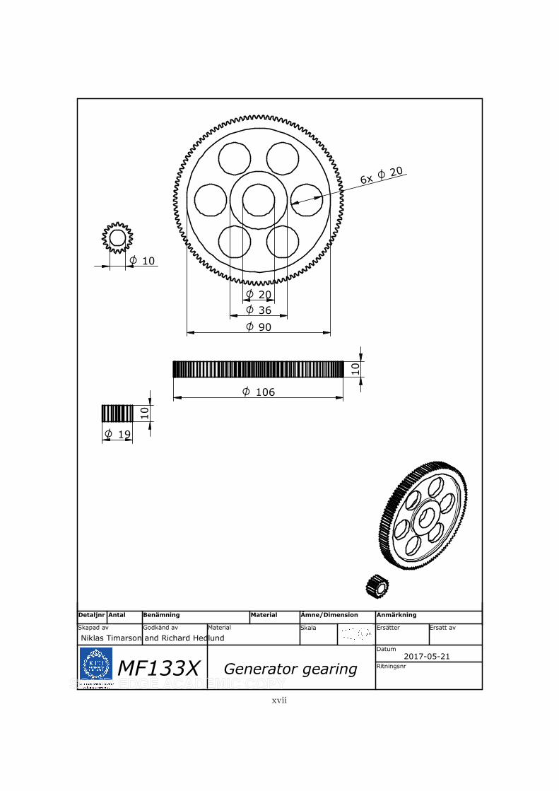
Niklas Timarson and Richard Hedlund
Generator gearing
Datum
Skapad av
Ritningsnr
MaterialGodkänd av Ersätter Ersatt av
2017-05-21
Skala
Ämne/Dimension
MF133X
Detaljnr Antal Benämning Material Anmärkning
O 10
O 20
O 36
O 90
O 206x
106O
19O
10
10
xvii
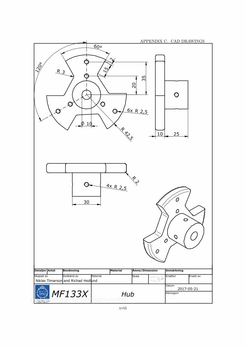
Niklas Timarson and Richad Hedlund
Hub
Datum
Skapad av
Ritningsnr
MaterialGodkänd av Ersätter Ersatt av
2017-05-21
Skala
Ämne/Dimension
MF133X
Detaljnr Antal Benämning Material Anmärkning
30
2510
R2
R 2,54x
O 10R
42,5
15
2
R 3
60°
120°
20
35
R 2,56x
APPENDIX C. CAD DRAWINGS
xviii

Niklas Timarson and Richard Hedlund
DC motor attachment
Datum
Skapad av
Ritningsnr
MaterialGodkänd av Ersätter Ersatt av
2017-05-18
ABS Plastic, medium impact
Skala
Ämne/Dimension
MF133X
Detaljnr Antal Benämning Material Anmärkning
40
74
R22R
20
1
R18
10
4,25
O4
4x
5
5
31
xix
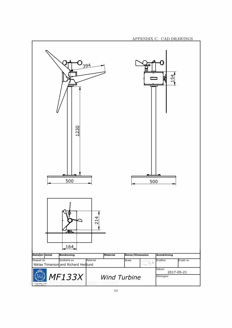
Niklas Timarson and Richard Hedlund
Wind Turbine
Datum
Skapad av
Ritningsnr
MaterialGodkänd av Ersätter Ersatt av
2017-05-21
Skala
Ämne/Dimension
MF133X
Detaljnr Antal Benämning Material Anmärkning
394
1230
500
214
164
500
154
APPENDIX C. CAD DRAWINGS
xx
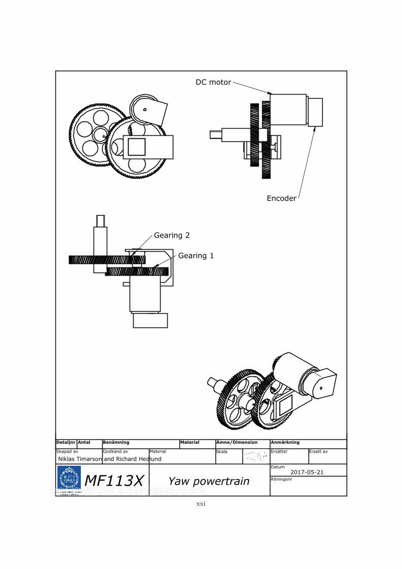
Niklas Timarson and Richard Hedlund
Yaw powertrain
Datum
Skapad av
Ritningsnr
MaterialGodkänd av Ersätter Ersatt av
2017-05-21
Skala
Ämne/Dimension
MF113X
Detaljnr Antal Benämning Material Anmärkning
DC motor
Encoder
Gearing 1
Gearing 2
xxi
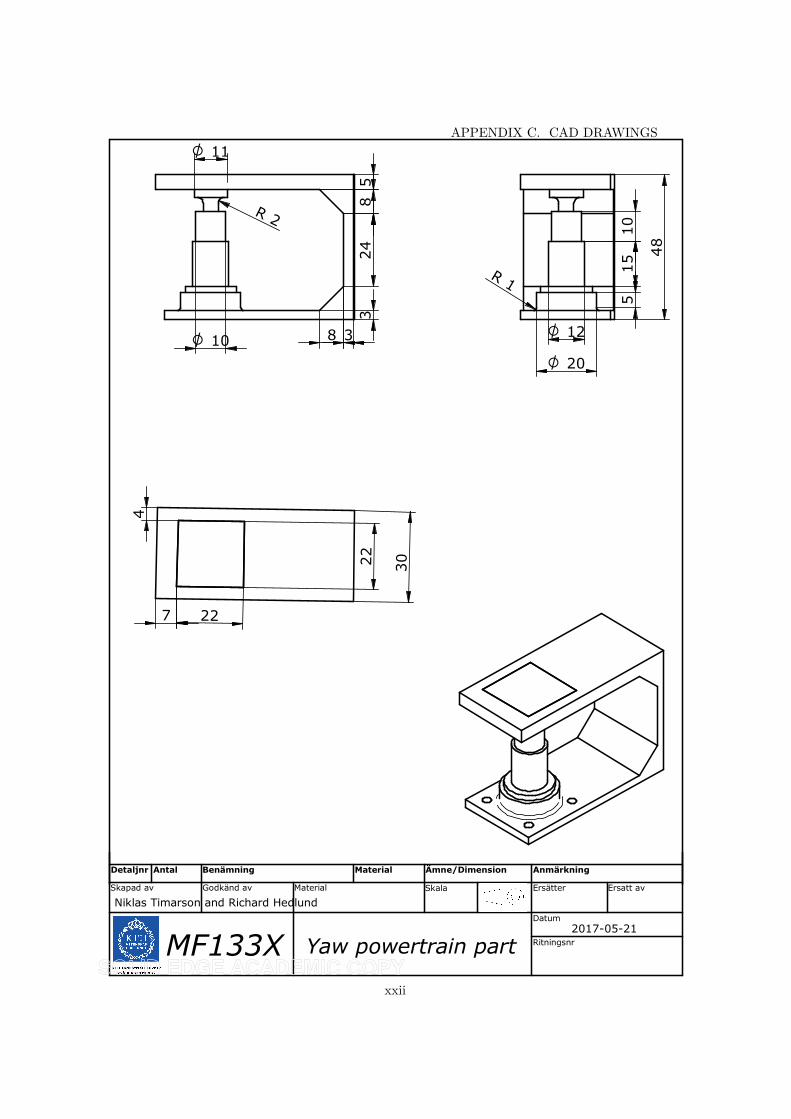
Niklas Timarson and Richard Hedlund
Yaw powertrain part
Datum
Skapad av
Ritningsnr
MaterialGodkänd av Ersätter Ersatt av
2017-05-21
Skala
Ämne/Dimension
MF133X
Detaljnr Antal Benämning Material Anmärkning
11O
10O
58
24
3
38 12O
20O
48
5
R2
R1
3022
7 22
4
15
10
APPENDIX C. CAD DRAWINGS
xxii
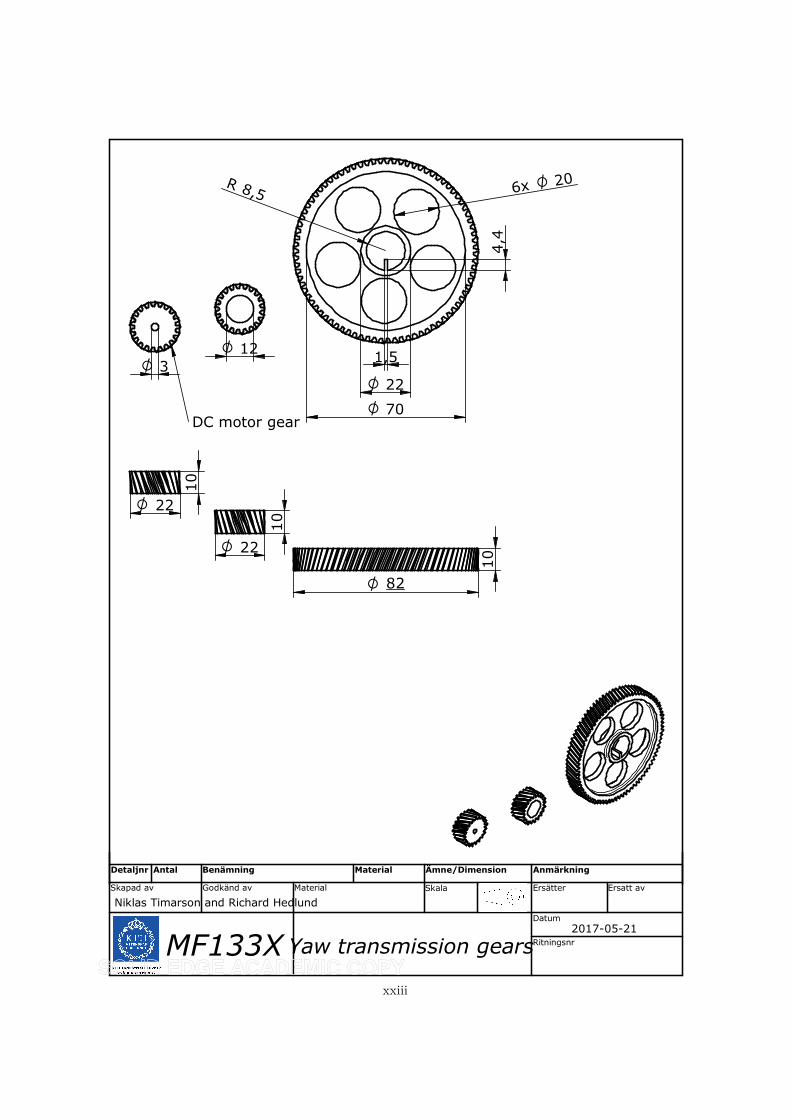
Niklas Timarson and Richard Hedlund
Yaw transmission gears
Datum
Skapad av
Ritningsnr
MaterialGodkänd av Ersätter Ersatt av
2017-05-21
Skala
Ämne/Dimension
MF133X
Detaljnr Antal Benämning Material Anmärkning
O 3
O 12
O 22
O 70
R 8,5
4,4
1,5
O 206x
10
10
10
22O
22O
82O
DC motor gear
xxiii


Appendix D
LCA Report
xxv
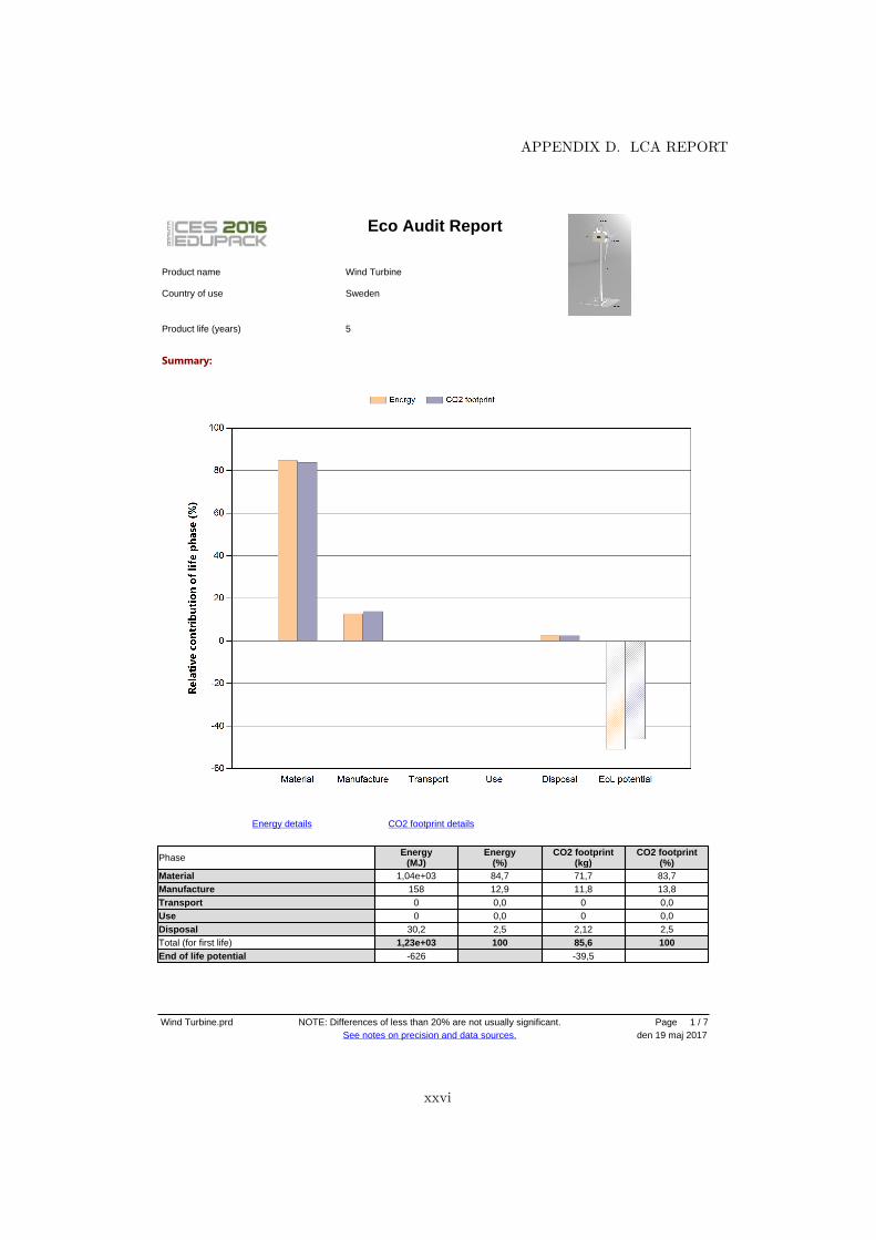
Wind Turbine
5
Product name
Product life (years)
Summary:
Eco Audit Report
Country of use Sweden
Phase Energy(MJ)
Energy(%)
CO2 footprint(kg)
CO2 footprint(%)
Material 1,04e+03 84,7 71,7 83,7Manufacture 158 12,9 11,8 13,8Transport 0 0,0 0 0,0Use 0 0,0 0 0,0Disposal 30,2 2,5 2,12 2,5Total (for first life) 1,23e+03 100 85,6 100End of life potential -626 -39,5
Energy details CO2 footprint details
See notes on precision and data sources.NOTE: Differences of less than 20% are not usually significant.
den 19 maj 2017Wind Turbine.prd Page 1 / 7
APPENDIX D. LCA REPORT
xxvi
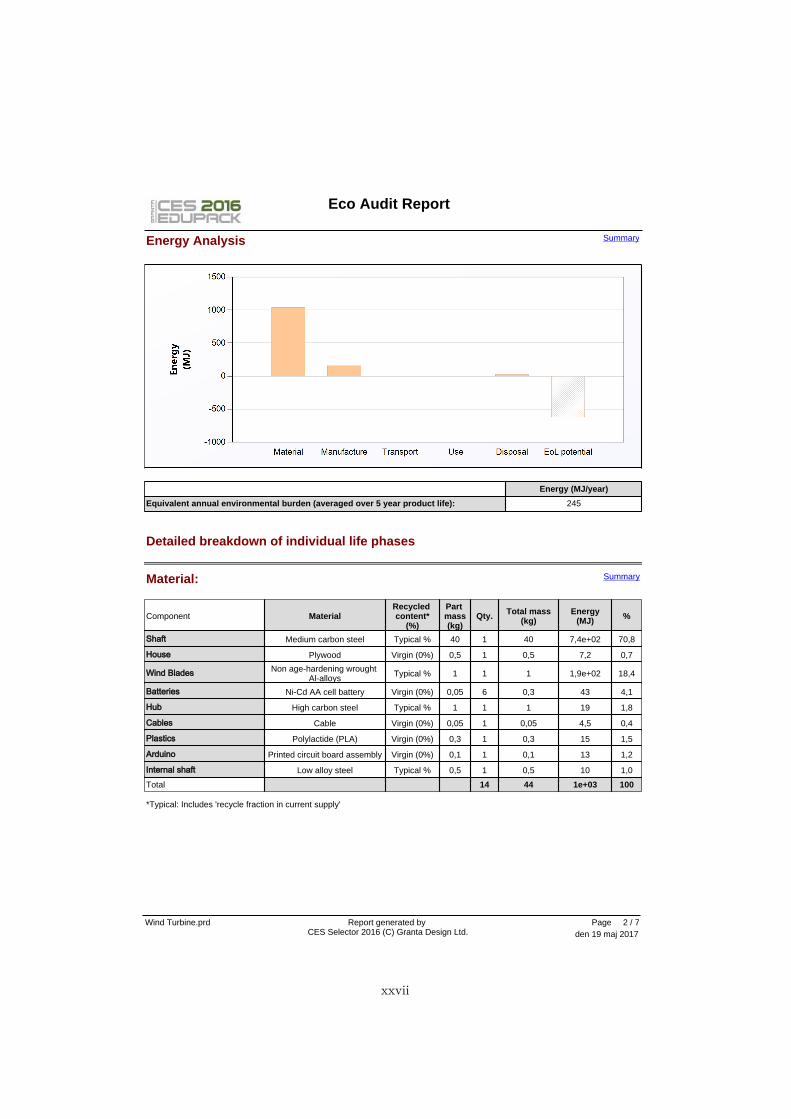
Energy (MJ/year)
Equivalent annual environmental burden (averaged over 5 year product life): 245
SummaryEnergy Analysis
Eco Audit Report
Material:
Component MaterialRecycled content*
(%)
Part mass(kg)
Qty. Total mass(kg)
Energy(MJ) %
Shaft Medium carbon steel Typical % 40 1 40 7,4e+02 70,8
House Plywood Virgin (0%) 0,5 1 0,5 7,2 0,7
Wind Blades Non age-hardening wrought Al-alloys Typical % 1 1 1 1,9e+02 18,4
Batteries Ni-Cd AA cell battery Virgin (0%) 0,05 6 0,3 43 4,1
Hub High carbon steel Typical % 1 1 1 19 1,8
Cables Cable Virgin (0%) 0,05 1 0,05 4,5 0,4
Plastics Polylactide (PLA) Virgin (0%) 0,3 1 0,3 15 1,5
Arduino Printed circuit board assembly Virgin (0%) 0,1 1 0,1 13 1,2
Internal shaft Low alloy steel Typical % 0,5 1 0,5 10 1,0
Total 14 44 1e+03 100
Detailed breakdown of individual life phases
Summary
*Typical: Includes 'recycle fraction in current supply'
Report generated by CES Selector 2016 (C) Granta Design Ltd. den 19 maj 2017
Wind Turbine.prd Page 2 / 7
xxvii
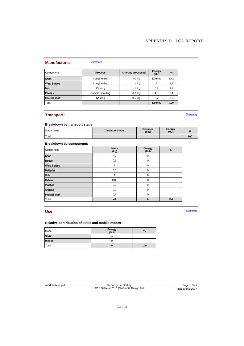
Manufacture: Summary
Component Process Amount processed Energy(MJ) %
Shaft Rough rolling 40 kg 1,3e+02 82,9
Wind Blades Rough rolling 1 kg 5 3,2
Hub Casting 1 kg 11 7,2
Plastics Polymer molding 0,3 kg 4,9 3,1
Internal shaft Casting 0,5 kg 5,7 3,6
Total 1,6e+02 100
Transport:
Breakdown by transport stage
Stage name Transport type Distance(km)
Energy(MJ) %
Total 100
Component Mass(kg)
Energy(MJ) %
Shaft 40 0
House 0,5 0
Wind Blades 1 0
Batteries 0,3 0
Hub 1 0
Cables 0,05 0
Plastics 0,3 0
Arduino 0,1 0
Internal shaft 0,5 0
Total 44 0 100
Breakdown by components
Summary
Use:
Mode Energy(MJ) %
Static 0
Mobile 0
Total 0 100
Relative contribution of static and mobile modes
Summary
Report generated by CES Selector 2016 (C) Granta Design Ltd. den 19 maj 2017
Wind Turbine.prd Page 3 / 7
APPENDIX D. LCA REPORT
xxviii
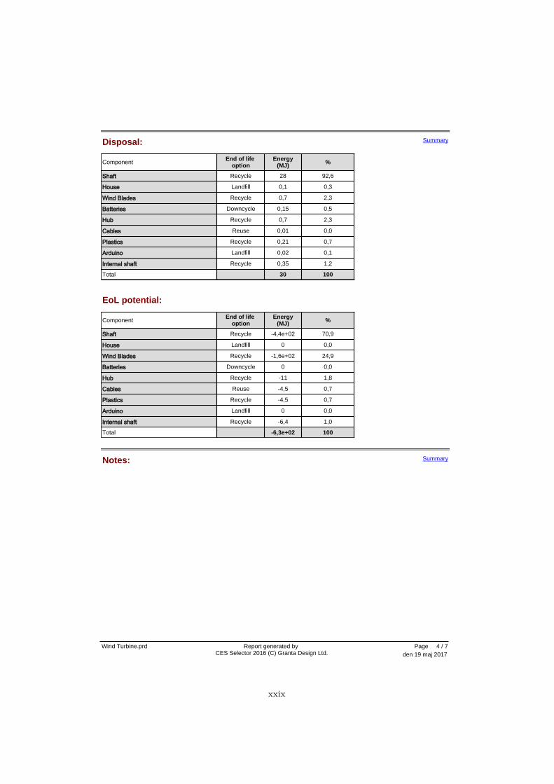
Disposal:
Component End of life option
Energy(MJ) %
Shaft Recycle 28 92,6
House Landfill 0,1 0,3
Wind Blades Recycle 0,7 2,3
Batteries Downcycle 0,15 0,5
Hub Recycle 0,7 2,3
Cables Reuse 0,01 0,0
Plastics Recycle 0,21 0,7
Arduino Landfill 0,02 0,1
Internal shaft Recycle 0,35 1,2
Total 30 100
Summary
Component End of life option
Energy(MJ) %
Shaft Recycle -4,4e+02 70,9
House Landfill 0 0,0
Wind Blades Recycle -1,6e+02 24,9
Batteries Downcycle 0 0,0
Hub Recycle -11 1,8
Cables Reuse -4,5 0,7
Plastics Recycle -4,5 0,7
Arduino Landfill 0 0,0
Internal shaft Recycle -6,4 1,0
Total -6,3e+02 100
EoL potential:
Notes: Summary
Report generated by CES Selector 2016 (C) Granta Design Ltd. den 19 maj 2017
Wind Turbine.prd Page 4 / 7
xxix
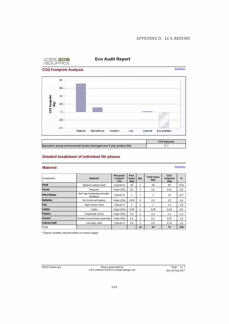
Material:
Component MaterialRecycled content*
(%)
Part mass(kg)
Qty. Total mass(kg)
CO2 footprint
(kg)%
Shaft Medium carbon steel Typical % 40 1 40 52 72,0
House Plywood Virgin (0%) 0,5 1 0,5 0,41 0,6
Wind Blades Non age-hardening wrought Al-alloys Typical % 1 1 1 12 16,7
Batteries Ni-Cd AA cell battery Virgin (0%) 0,05 6 0,3 3,2 4,5
Hub High carbon steel Typical % 1 1 1 1,3 1,8
Cables Cable Virgin (0%) 0,05 1 0,05 0,34 0,5
Plastics Polylactide (PLA) Virgin (0%) 0,3 1 0,3 1,1 1,5
Arduino Printed circuit board assembly Virgin (0%) 0,1 1 0,1 0,97 1,4
Internal shaft Low alloy steel Typical % 0,5 1 0,5 0,72 1,0
Total 14 44 72 100
Detailed breakdown of individual life phases
Summary
*Typical: Includes 'recycle fraction in current supply'
CO2 (kg/year)
Equivalent annual environmental burden (averaged over 5 year product life): 17,1
SummaryCO2 Footprint Analysis
Eco Audit Report
Report generated by CES Selector 2016 (C) Granta Design Ltd. den 19 maj 2017
Wind Turbine.prd Page 5 / 7
APPENDIX D. LCA REPORT
xxx
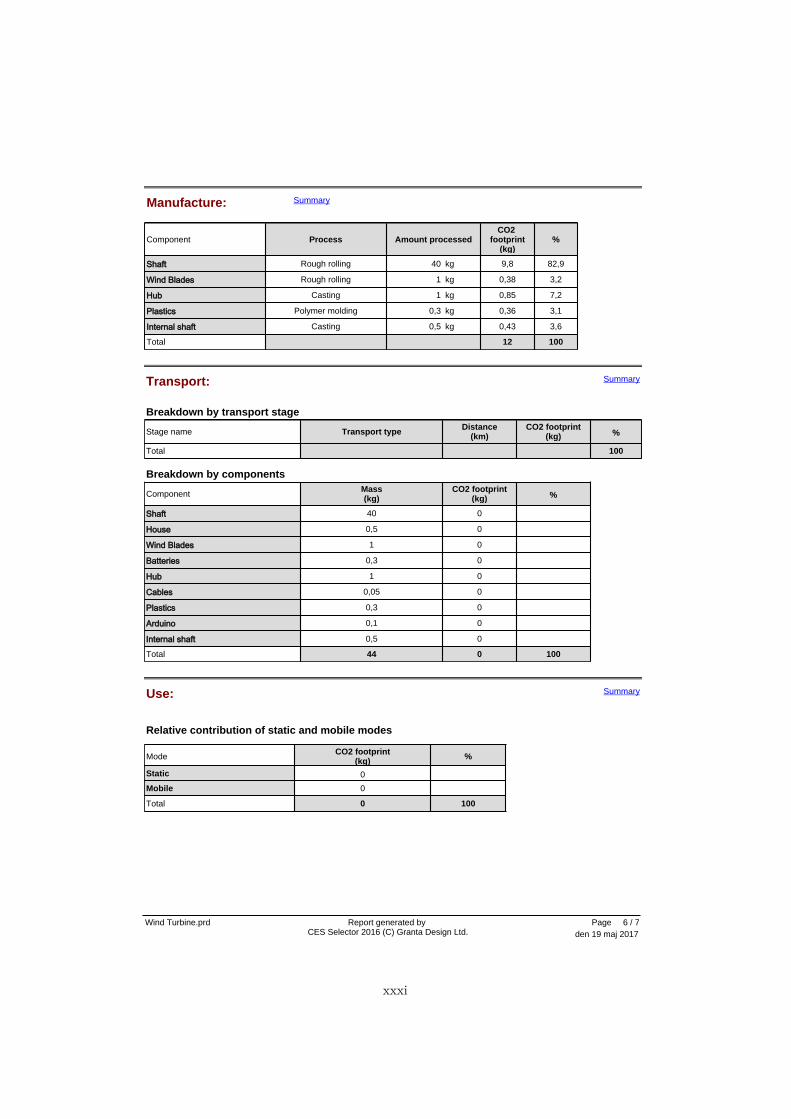
Use:
Mode CO2 footprint(kg) %
Static 0
Mobile 0
Total 0 100
Relative contribution of static and mobile modes
Summary
Transport:
Breakdown by transport stage
Stage name Transport type Distance(km)
CO2 footprint(kg) %
Total 100
Component Mass(kg)
CO2 footprint(kg) %
Shaft 40 0
House 0,5 0
Wind Blades 1 0
Batteries 0,3 0
Hub 1 0
Cables 0,05 0
Plastics 0,3 0
Arduino 0,1 0
Internal shaft 0,5 0
Total 44 0 100
Breakdown by components
Summary
Manufacture: Summary
Component Process Amount processedCO2
footprint(kg)
%
Shaft Rough rolling 40 kg 9,8 82,9
Wind Blades Rough rolling 1 kg 0,38 3,2
Hub Casting 1 kg 0,85 7,2
Plastics Polymer molding 0,3 kg 0,36 3,1
Internal shaft Casting 0,5 kg 0,43 3,6
Total 12 100
Report generated by CES Selector 2016 (C) Granta Design Ltd. den 19 maj 2017
Wind Turbine.prd Page 6 / 7
xxxi
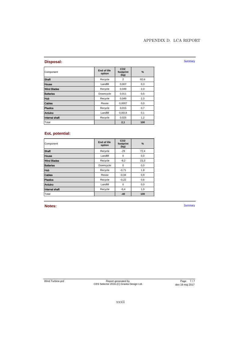
Notes: Summary
Disposal:
Component End of life option
CO2 footprint
(kg)%
Shaft Recycle 2 92,6
House Landfill 0,007 0,3
Wind Blades Recycle 0,049 2,3
Batteries Downcycle 0,011 0,5
Hub Recycle 0,049 2,3
Cables Reuse 0,0007 0,0
Plastics Recycle 0,015 0,7
Arduino Landfill 0,0014 0,1
Internal shaft Recycle 0,025 1,2
Total 2,1 100
Summary
Component End of life option
CO2 footprint
(kg)%
Shaft Recycle -29 72,4
House Landfill 0 0,0
Wind Blades Recycle -9,2 23,3
Batteries Downcycle 0 0,0
Hub Recycle -0,71 1,8
Cables Reuse -0,34 0,9
Plastics Recycle -0,22 0,6
Arduino Landfill 0 0,0
Internal shaft Recycle -0,4 1,0
Total -40 100
EoL potential:
Report generated by CES Selector 2016 (C) Granta Design Ltd. den 19 maj 2017
Wind Turbine.prd Page 7 / 7
APPENDIX D. LCA REPORT
xxxii

Appendix E
Membership Functions
Membership functions for the wind error, made using Fuzzy Logic Designer in Mat-lab R2017a.
Membership functions for the derivative of the wind error, made using Fuzzy LogicDesigner in Matlab R2017a.
xxxiii
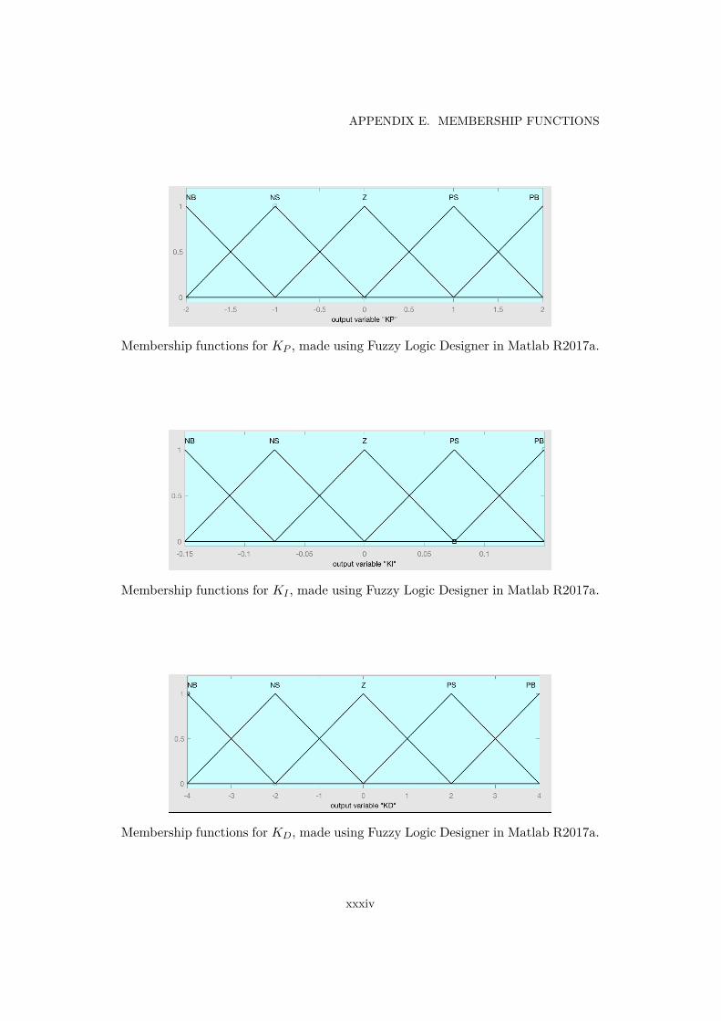
APPENDIX E. MEMBERSHIP FUNCTIONS
Membership functions for KP , made using Fuzzy Logic Designer in Matlab R2017a.
Membership functions for KI , made using Fuzzy Logic Designer in Matlab R2017a.
Membership functions for KD, made using Fuzzy Logic Designer in Matlab R2017a.
xxxiv

TRITA MMK 2017:23 MDAB 641
www.kth.se