Intelligent monitoring of jack arch structures · Wrought iron Wrought iron is nearly pure iron. It...
56
Intelligent monitoring of jack arch structures Prepared for Dr R Kimber, Research Director, Transport Research Foundation K C Brady and J Kavanagh TRL Report TRL546
Transcript of Intelligent monitoring of jack arch structures · Wrought iron Wrought iron is nearly pure iron. It...

Intelligent monitoring of jack archstructures
Prepared for Dr R Kimber, Research Director,Transport Research Foundation
K C Brady and J Kavanagh
TRL Report TRL546

First Published 2002ISSN 0968-4107Copyright TRL Limited 2002.
This report is prepared for the Research Director of the TransportResearch Foundation and must not be referred to in anypublication without the permission of the Transport ResearchFoundation. The views expressed are those of the authors andnot necessarily those of the Transport Research Foundation.
TRL is committed to optimising energy efficiency, reducingwaste and promoting recycling and re-use. In support of theseenvironmental goals, this report has been printed on recycledpaper, comprising 100% post-consumer waste, manufacturedusing a TCF (totally chlorine free) process.

CONTENTS
Page
Executive Summary 1
1 Introduction 3
2 Cast iron 3
2.1 Iron and steel alloys 3
2.2 Properties of cast iron 4
2.3 19th Century casting techniques 5
3 Jack arch structures 5
3.1 Description 5
3.2 Performance 6
3.3 Hythe End Bridge 6
4 Details of project 6
4.1 Monitoring techniques 6
4.2 Limitations of test programme 6
5 Acoustic emission 6
5.1 Equipment 8
5.2 Physical Acoustics AE monitoring equipment 9
5.2.1 Specification 9
5.2.2 Data capture 10
5.2.3 Output 10
5.3 SoundPrint monitoring system 10
5.3.1 Description 10
5.3.2 Components 10
5.3.3 Output 10
6 Details of test rig and instrumentation 12
7 Details of the test 12
7.1 The test beam 12
7.2 Procedure 12
8 Results of test 18
8.1 Load cycle 1 - peak load 51 kN 18
8.2 Load cycle 2 – peak load 68 kN 18
8.3 Load cycle 3 – peak load 73 kN 18
8.4 Load cycle 4 - peak load 52 kN 18
8.5 Load cycle 5 – peak load 87 kN 29
8.6 Load cycle 6 - peak load 104 kN 29
iii

iv
Page
8.7 Load cycle 7 - peak load 116 kN 29
8.8 Load cycle 8 - peak load 130 kN 29
8.9 Load cycle 9 - peak load 151 kN 29
8.10 Summary of results 42
8.11 Other forms of processing 46
9 Discussion 46
9.1 Interpretation of data 46
9.2 In-service load 49
9.3 Collapse load 49
9.4 In-service condition 50
10 Recommendations for further work 50
11 Conclusion 50
12 References 51
Abstract 52
Related publications 52

1
Executive Summary
As part of the Transport Research Foundation’sreinvestment programme, a research project was initiatedat TRL Limited to examine the feasibility of developing anintelligent system for monitoring the in-serviceperformance of jack arch structures. Ideally such a systemwould be capable of continuously monitoring a structureso that it would forewarn of structural deterioration andthereby trigger remedial works – for example the closureof a section of track or road.
This report provides and discusses the results of a loadtest conducted on a cast iron beam instrumented with straingauges, deflection gauges, and acoustic emission (AE)systems obtained from Physical Acoustics Ltd and fromPure Technology (their ‘SoundPrint’ system). The beamwas recovered from a jack arch bridge constructed in 1852and demolished in the late 1980s. The report providesinformation on the properties of cast iron and details ofjack arch structures.
AE systems have been used to monitor other types ofstructure, but it would seem that this is the first time theyhave been used for this type of beam. The objective of theproject was to assess the potential of the AE systems aspart of an intelligent monitoring system.
A series of nine load cycles with a generally increasingpeak load, were conducted on the cast iron beam. Detailsof the instruments, test beam and test set up are providedin the report. The beam was loaded to about 150 kN, andprobably in excess of the ‘equivalent’ maximum in-serviceload. The results of the load test show that the response ofthe beam was slightly asymmetric.
The data indicate generally increasing AE activity withincreasing peak load and, almost always, substantial activitywas only recorded once the previous peak load wasapproached. Activity seemed to be related to the duration ofapplication of the peak load. The rate of AE generationreduced following the attainment of the peak load, itreduced further during unloading and all but stopped onremoval of the load. The location of most of the recordedevents was around the mid-span of the beam. The resultsstrongly support the view that AE was generated via someload-related mechanism, perhaps related to micro-crackingof the cast iron. Further research is required to confirm andextend the findings of the test, but the results show that AEtechniques have good potential for forming the basis of anintelligent monitoring system.

2

3
1 Introduction
There are many jack arch structures still in service that areover 100 years old. These are formed from cast iron beamswith integral brickwork, and are usually found as short-spanroad bridges over canals and railways. Cast iron beamsmanufactured in the 19th century are also still in service inmajor public buildings in London, and in textile mills andwarehouses in northern England. The structural condition ofsuch beams is difficult to assess. Owners, and those chargedwith the maintenance of such structures, therefore have aproblem with managing such assets. On the one hand it isessential to identify sub-standard structures that pose a riskto users, but on the other it is desirable to minimiseexpenditure on the strengthening of perfectly adequatestructures. Jack arch structures supporting buildings andhighways commonly fail structural assessments, or aredeemed to be in a state of disrepair. This could lead to theimposition of weight or width restrictions, which in somecases might be unnecessary.
The aim of the project was to examine the feasibility ofdeveloping an intelligent system that could be used tomonitor the in-service performance of a cast iron jack archbridge. The system should be capable of continuouslymonitoring a structure so that it would forewarn ofstructural deterioration and thereby trigger remedial works– for example the closure of a section of track or road.Such a system might also be applicable to the assessmentand monitoring of other cast iron structural elements suchas bridge piers.
This report describes a load test conducted on a cast ironbeam instrumented with strain gauges, deflection gaugesand two acoustic monitoring systems. Such systems havebeen used to monitor other types of structure, but a searchof the literature indicates that this is the first time theyhave been used for a cast iron jack arch beam. The resultsof the test are presented and discussed, andrecommendations for further work are outlined.
2 Cast iron
2.1 Iron and steel alloys
There are numerous different types of iron and steel alloys.The physical properties of a particular alloy are largelydependent upon its chemical composition, although theycan be greatly affected by heating and working.
Although there is some overlap between them, iron alloyscan be classified into one of the following three groups.
Pig ironPig iron has an iron content of about 93 per cent, a carboncontent of about 3 to 4 per cent and smaller amounts of otherelements. Most pig iron is used to make steel, but a smallamount is used to make cast iron and wrought iron products.
Cast ironCast iron is any iron alloy that has a carbon content ofbetween 2 and 4 per cent and a silicon content of between
1 and 3 per cent. It might also contain trace amounts ofmanganese, phosphorus and sulphur. The high carboncontent means that the metal cannot be worked; but itsusability derives from its hardness, low cost and ability toabsorb shock loads.
Cast iron products are, as the name implies, made bycasting, a process in which the molten alloy is poured into amould and allowed to solidify. There are two basic types ofcast iron, the type that forms depends on the speed at whichthe molten alloy cools. Grey cast iron forms as a result ofrelatively slow cooling, in which case some of the carbonsolidifies as graphite flakes sitting in a matrix of whatapproximates to steel. Figure 1, from Swailes (1995),indicates the nature of the material. White cast iron (or chilliron) forms as a result of relatively rapid cooling, in whichthe carbon is unable to solidify as graphite flakes but insteadcombines completely with the iron. In general, white castiron has a higher tensile strength than grey cast iron.
Graphiteflakes
Ferrite/pearlitematrix
1.0mm
Figure 1 Structure of cast iron, from Swailes (1995)
The presence of trace elements, deliberately added orpresent as impurities, affects the physical properties of thematerial. In particular, the formation of grey cast iron ispromoted by the presence of silicon and phosphoruswhereas the formation of white cast iron is promoted bythe presence of sulphur.

4
Wrought iron
Wrought iron is nearly pure iron. It is malleable and hasbetter corrosion resistance than cast iron.
2.2 Properties of cast iron
The stress-strain behaviour of grey cast iron is dependenton the quantity and coarseness of the graphite flakes, thusit can vary considerably. The flakes act as planes ofweakness, resulting in low tensile strengths, but are able totransfer compressive forces so that the material has a nearelastic behaviour in compression. Figure 2, from Swailes(1995), shows a typical stress-strain curve for grey castiron, using Hodgkinson’s formulae obtained from his testsundertaken for the Iron Commission in the 19th century.
As a result of cooling from the molten alloy the tensile
and flexural strengths of a cast iron element vary withcross-sectional shape and size. Cooling is dictated by thevolume/surface area ratio and so different parts of a castingcool at different rates. A thin flange may cool relativelyquickly resulting in a stronger but more brittle cast iron:conversely, the material at the centre of large poor-qualitycastings can be spongy or porous in appearance. Theproperties of cast iron may be compromised by thepresence of chemical impurities, and the strength of largeelements may be much reduced by the higher frequencyand size of flaws.
Swailes (1995) considered a small sample of the resultsof an investigation into the strengths of different Britishiron alloys undertaken by Fairbairn in the 19th century.These are reproduced in Table 1 and confirm the commentof Swailes (1995) that ‘the properties varied considerably.’
Table 1 Selected results from Fairburn’s tests on British iron alloys, after Swailes (1995)
BreakingSpecific E* load**
Rank*** Name of iron gravity KN/mm2 kN Colour Quality
1 Ponkey, no. 3, cold-blast 7.122 119 2.584 Whitish grey Hard5 Beaufort, no. 3, hot-blast 7.069 116 2.300 Dullish grey Hard10 Beaufort, no.2, hot-blast 7.108 112 2.108 Dull grey Hard15 Oldberry, no.2, cold-blast 7.059 99 2.024 Dark grey Rather soft20 Blania, no.3, cold-blast 7.159 98 1.993 Bright grey Hard25 Carron, no.3, cold-blast 7.094 112 1.970 Grey Soft30 Wallbrook, no.3 6.979 106 1.957 Light grey Rather hard35 Level, no.2, hot-blast 7.031 105 1.908 Dull grey Soft40 Coltham, no. 1, hot-blast 7.128 107 1.886 Whitish grey Rather soft45 Coed-Talon, no. 2, cold-blast 6.955 99 1.837 Grey Rather soft
* E obtained from the deflection at about one sixth of the breaking load** Breaking load at centre of a 4ft 6in (1.37 m) span*** Ranking in terms of strength
-0.003 -0.002 -0.001 0.001 0.002
100
0
-100
-200
Compressive stress-strain curvefrom shortening of 3.05m long
bars with buckling prevented
Str
ess
N/m
m2
Average ultimate compressivestress 648 N/mm2
Tensile stress-strain curve fromextension of 28.6mm dia. bars15.25m long
Average ultimate tensile stress 108 N/mm2
Strain
Figure 2 Typical stress-strain curve for cast iron, plotted from Hodgkinson's formulae, from Swailes (1995)

5
2.3 19th Century casting techniques
Structural beams were cast in moulds of sand using aslightly oversized pattern to allow for shrinkage oncooling. Although dry sand moulds gave a better finish,they required baking before use. Moulds formed fromdamp sand were cheaper and, therefore, more commonlyused. Usually, I-beams would be cast on their sides, and T-beams cast with the flange uppermost. These arrangementsare shown schematically in Figure 3.
Although the importance of permitting the beam to coolat a sufficiently slow rate was appreciated, there isevidence that some smaller foundries removed red-hotcastings from the sand mould. Figure 3 illustrates twocommon flaws arising from poor casting. Firstly when themolten alloy came into contact with the sand, gas bubblesor pieces of slag would rise and, as a result of poorventing, become trapped just beneath the surface.Secondly, where an insufficient head of molten alloy wasprovided, progressive cooling from the outside of the castcould lead to the development of voids at the centre as thematerial shrank.
In the early 19th century, iron was smelted using coal,converted to coke, as fuel and supplying a blast of cold airto the furnace. But by the 1830s hot-blast iron was widelyavailable. The use of hot air permitted coal to be useddirectly as the fuel and more iron to be extracted from themelt. Both practices introduced impurities that could affectthe final casting.
3 Jack arch structures
3.1 Description
According to Hilton (1997), jack arch constructionoriginated in the UK in the early part of the 19th century:the first recorded structure was built in 1801. This form ofconstruction allowed short to medium span structures to bebuilt with a much shallower depth than was possible withmasonry.
Jack arch bridges usually comprise the longitudinal castiron beams, at say 1 to 1.5 metre centres, and brick arches,usually at least two courses thick, spanning transversely tothe beams. The brick arches spring from a mortar bed laidon the bottom flanges of the beams, and have a rise ofabout half the depth of the beams. The remaining spacebelow the running surface is filled with soil or, in newer orrenovated structures, with concrete. The arrangement isshown in Figure 4. Transverse steel ties may be providedbetween the beams at mid-span. The beams are commonlysupported on brick abutments and piers.
Gas bubbles, pieces of mould sand or slag float to the top ofthe mould to be trapped just below the surface of the metal
Surface pitting due to inadequateventing of mould gases
Softer, coarser grained materialin thicker sections of casting
Taper for withdrawal of patternfrom bottom part of mould
Mould joint
Pipe formed by contractionaway from centre of slow
cooling thicker part of section
T SECTIONI SECTION
Figure 3 19th Century cast iron casting techniques, from Swailes (1995)
Figure 4 Typical cross section, after Hilton (1997)
Apart from the bottom flange, the beams are usuallyburied within brickwork and fill, and so it is difficult todetermine the material condition and hence the structuralstability of jack arches.
Bituminous seal Road pavement(varying depth)
Infill deck
Brick arch
1525 mm24' x 7.5" x 100 lbsGirders TYP

6
3.2 Performance
Only a few failures of jack arch and cast iron girder roadbridges have been recorded. Swailes (1995) reported on anumber of failures of structures incorporating cast ironbeams and noted that most, if not all, failures appeared tohave been due to bad design, poor construction practice orbadly cast beams: to date corrosion does not appear to be amajor problem.
3.3 Hythe End bridge
The Hythe End bridge is a good example of a jack archstructure: the test on an edge beam from this structure isthe main focus of this investigation. The bridge wasconstructed in 1852 to cross the River Coln at Hythe Endnear Wraysbury, Berkshire. It was constructed as a two-span bridge incorporating four (grey) cast iron beams perspan supporting transverse brickwork and fill. The beamswere supported on brick abutments and a brick pier atmidstream to give two clear spans of 6.9 m; the width ofthe bridge between kerbs was 4.06 m. A view of the bridgeis shown in Figure 5.
In 1975, the bridge was repaired and strengthened, some ofthe brick arches were replaced with in situ concrete.Permanent traffic lights were installed to enforce single lanetraffic and an 11 ton weight restriction was placed on thebridge. In 1985, the bridge was assessed to BD 21 (DMRB3.4.3) by the owners, Berkshire County Council. Theydetermined that the structure had no capacity for highwayloading and immediately closed the bridge. Prior todemolition, it was offered for testing to the (then) TRRL:details of the test have been provided by Daly and Raggett(1991). The test involved the use of a loaded two-axlearticulated trailer: loads of 80, 143 and 195 kN were appliedat five points along each of four longitudinal axes across thespan, each longitudinal axis being at a different transverseposition, i.e. a total of 20 load points. Following the test, thebridge was then demolished: Figure 6, shows the demolitionworks in progress, and also reveals the inner structure of thebridge. All eight cast iron beams were subsequently recoveredand stored at TRL. Figure 7 shows elevations and sections ofboth the internal and external beams.
4 Details of project
The aim of the project was to examine the cost andpracticality of developing an intelligent system formonitoring the in-service performance of cast iron jackarch bridges. The system was to be capable ofcontinuously monitoring a structure so that it couldprovide advance warning of structural deterioration. Thisreport describes an investigation into the response of a castiron beam under load using techniques that wereconsidered to have the potential for further developmentinto a ‘smart’ system for use on site.
4.1 Monitoring techniques
Two AE systems were investigated as the potential basisfor a monitoring system. These were based on (a)
monitoring equipment supplied by Physical Acoustics and(b) Pure Technologies’ SoundPrint system. Bothtechniques employ sensors that can continuously monitor astructure, process and analyse data in real-time, andtherefore deliver an immediate message to a remoteterminal when some predefined criterion is met. Details ofboth systems are given in Section 5.
Because metal is a good propagator of acoustic stresswaves, almost any acoustic technique should be well suitedto the detection of cracking in a metallic element. In a castiron beam, energy released through the formation of afracture will radiate outwards from the source and propagatealong its length. Depending upon the frequencies monitoredby the acoustic system and the form of the structure, it maybe possible to monitor a single beam, or even multiplebeams, with a single acoustic sensor.
The description of grey cast iron, given in Section 2.2,suggests that the material could be a good generator of AE.It can be envisaged that, in response to an applied load,micro-cracking might be initiated by separation betweenthe graphite flakes and surrounding material: such flakesmay act as planes of weakness. Also the rate and extent ofcracking could reasonably be expected to be related to themagnitude of the load and, therefore, also to the AE signalsgenerated. However no evidence of this particularapplication has been found in a literature searchundertaken by the authors.
In this investigation, the cast iron beam was alsoinstrumented with deflection gauges and strain gauges. Incontrast to AE techniques, such gauges only measure achange at the point at which they are located and thismeasurement might not be representative of the structure asa whole. The readings from the deflection and strain gaugeswere used to corroborate the AE data, and to provideinformation on the stress-strain response of the beam.
4.2 Limitations of test programme
It is necessary at this stage to consider some of thelimitations of the test programme. As described in Section8, the test involved the application of a sequence of loadseach applied for a fixed time before being removed. Themaximum load generally increased through the sequence,but this does not replicate the loading history of an in-service structure. Furthermore, the results of load tests,such as that conducted by Daly and Raggett (1991), haveshown that the stability of jack arch structures isconsiderably enhanced by the support provided by theadjacent brick jack arches and fill. This support was notavailable in the test conducted on the single beam.
5 Acoustic emission
Many materials subjected to a load generate acoustic stresswaves: these waves are mechanical vibrations that radiateout from an energy source. The objective of an AEinvestigation is to capture and quantify the emission andthereby determine the extent of the deformation ordegradation of the material. Crack propagation in metalsand concrete, the debonding of fibres in composite

7
Figure 5 Hythe End bridge, from Daly and Raggett (1991)
Figure 6 Demolition of the Hythe End bridge, indicating the internal structure, from Daly and Raggett (1991)

8
90
30
35
25
380
450
Section B-B(Internal beam)
95
380
25
35
Section A-A(External beam)
7950270
450
B
B
Internal Beam
A
AExternal Beam
Figure 7 Hythe End bridge beam elevations and sections, after Daly and Raggett (1991)
materials, and sliding between particles of soil have allbeen shown to be mechanisms that can generate acousticstress waves.
The use of AE as a means of monitoring degradationand assessing structural integrity, has been, and still is, thefocus of research. For example, Lim and Koo (1989)related AE generation to crack growth in reinforcedconcrete beams under load; Li et al. (1998) examined theuse of AE to detect the corrosion of steel reinforcement inconcrete; Royles and Hendry (1991) conducted a numberof tests on model masonry arch bridges and related theload-deflection behaviour to the generated AE; and Dixonet al. (1996) described a field trial aimed at examining thepotential use of AE as a means of monitoring slopestability. Ghorbanpoor (1990) found that the AE signalsfrom growing fatigue cracks had distinct characteristics inboth the time and frequency domains, and that such crackscould be detected at a relatively early stage. Burdekin(1993) compared a range of non-destructive techniques,including AE, for the detection of flaws in weldedstructural steelwork.
5.1 Equipment
A conventional AE monitoring system is depicted inFigure 8. The sensor, a piezoelectric transducer, is attachedto the structure under examination. As the structuredeforms or deteriorates a mechanism (for example, theformation of a micro-crack) generates an emission whichpropagates through the structure as a series of mechanicalstress waves. The piezoelectric transducer detects themechanical stresses (or vibrations) and converts them intoa voltage. The output voltage is processed by filtering outunwanted frequency components and by amplifying theremaining signal. The analogue-to-digital conversionboard, under control of the PC, samples the signal andconverts it to a digital format: the data are then stored,usually on disk. An example of the resulting output isgiven in Figure 9 - this depicts a typical decayingsinusoidal transducer-generated response, termed an‘event’. Also indicated on this figure are a number of waysof defining the output. These include the peak amplitude,the rise time, and the ringdown count. (Note that the event
All dimensions in mm

9
TransducerPre-amplifier
Filter Amplifier
PC
Expansion box containingpower unit & analogue-digital conversion boardAE source
Structure
Figure 8 Typical AE monitoring system
0
+
–
Rise time
Pea
k am
plitu
de Threshold
Ringdown counts
Am
plitu
de
0 20 40 60 80
Sample number
Figure 9 Transducer response to an event and its definition
depicted in Figure 9 would record nine ringdown counts,but only three are highlighted as examples.) An emissionmay have a distinct ‘character’ in terms of its constituentfrequencies or some form of amplitude analysis, such thatwithin an environment perceived as ‘noisy’ it may still bepossible to capture and identify an emission generated by aparticular mechanism.
The SoundPrint system, described in Section 5.3, wasdeveloped by Pure Technologies Inc to detect wire breaksin steel tendons and has a good track record in that area. Itemploys a slightly different philosophy to that used inconventional acoustic emission, in that the mechanism
responsible for the generation of the acoustic stress wave isthe catastrophic break of a wire rather than one reflecting agradual deterioration in condition. But, through ‘tuning’the system, the sensors can respond to the release ofenergy from comparatively low energy events, such asmight be associated with micro-cracking.
5.2 Physical Acoustics AE monitoring equipment
5.2.1 SpecificationThe equipment consists of an analogue-to-digitalconversion board with digital signal processing

10
capabilities. The board is housed in a conventional PC andis used in conjunction with four 150 kHz peak resonancetransducers, each with an integral 40 dB preamplifier. Theboard has four AE channels and can sample an analoguesignal at a maximum rate of 10 MHz (i.e. 10 millionsamples per second), with 16 bit resolution. The board alsofeatures programmable filters and gains, and up to eightparametric inputs.
The supplied software can provide up to 100simultaneous real-time graphs on multiple screens. Eachgraph is user-defined from any combination of measuredparameters and may be 2D, or rotating 3D display, as bar,line or point with colour analysis, several types ofautoscale, cursors and zoom.
5.2.2 Data captureVarious parameters must be defined to detect, process andinterpret the data obtained from the sensor. For the testdescribed herein, the acquisition rate was set at 2 MHzwith a threshold of 40 dB and the signal was passedthrough software controlled filters - a low pass of 20 kHzand a high pass of 400 kHz. Three additional parametersalso require definition: the peak definition time (PDT) isthe time-window during which the peak amplitude of anevent is determined, the hit definition time (HDT) is thetime-window during which the end of an event isdetermined and the hit lock-out time (HLT) is the period oftime following the end of an event during which dataacquisition is inhibited, to eliminate reflections etc. that donot form part of the event. Values for the parameters aredependent upon the nature of the material, and thosequoted above were suggested by Physical Acoustics for thespecific conditions of the test.
The system is capable of extracting a number of AEfeatures in real-time including wave form amplitude,energy, counts, duration, rise time and average frequency.Two types of data set may be saved. The ‘hit driven’ data,is a set consisting of AE features such as those describedabove: these data are saved, along with the time ofacquisition, when an acoustic transducer is stimulated. Theother type of data set is ‘time driven’ and the data set aresaved periodically. Time driven data are usually governinginputs, for example the applied load, and are used mainlyto record the progress of a test when no substantial AE isbeing generated. However no such parametric inputs wereused in this investigation.
5.2.3 OutputThe system was designed to analyse large numbers ofacoustic events in real-time, extracting AE features such asamplitude and duration. These parameters can be displayedin graphical form thereby providing a useful means ofmonitoring structural integrity. An example of thegraphical output is shown in Figure 10. Although thePhysical Acoustics system used in this investigation doesnot capture waveforms, it is capable of extracting a largenumber of AE features from each event. Some of these areconsidered later but for most of the discussion that follows
acoustic events are described in terms of their constituentcounts: see Section 5.1. Although the sensors actindependently, it is possible to process the data fromindividual channels and also to locate the source of theevents along a sensor array.
5.3 SoundPrint monitoring system
5.3.1 DescriptionPure Technologies Inc developed, and holds a patent for,an acoustic monitoring system suitable for the continuousmonitoring of post-tensioned structures. A characteristic ofstressed high tensile steel elements (for example, wires,strands and bars) is a sudden release of energy at themoment of fracture. This energy is dissipated in the formof an acoustic response that can be detected by sensorsmounted, for example, on the surface of the structure. Eachsensor (a piezoelectric transducer) is connected to a dataacquisition system on site. The time taken for the signal toreach each sensor is used to locate the source of the signal.
TRL has successfully used the system to detect wirebreaks in a number of bridges. Details are given byWillmott et al. (1997), Stephens and Cullington (1998) andMacNeil and Cullington (1998).
The arrangement typically used for detecting wirebreaks was modified by TRL for this study. Thefrequency response was increased, by increasing thesampling rate of the data, and the trigger level was set tothe energy released by the crushing of a few grains ofsand. For the latter, the internal setting was adjusted untilthe crushing of the sand grains on top of the beam led toa triggering of the system.
5.3.2 ComponentsThe system comprises the following components:
Data acquisition computer with A/D boards, monitorand modem.
SoundPrint SPDAQ data acquisition software withAdaptive Logic Network recognition capability (offsite).
Windows NT 4.0 operating system software, SymantecPC Anywhere 32 for Windows and commercialanti-virus software.
SoundPrint hardware consisting of CA-16 chargeamplifiers, TR-4 trigger devices and primary filters,PS-2 power supply.
APC un-interruptible power supply unit, Power Stoneremote power activation unit.
SoundPrint acoustic sensors complete with cable andaccessories.
5.3.3 OutputThe SoundPrint system was designed to identify andcapture relatively infrequent but substantial acoustic eventsgenerated by significant fractures, such as a wire break. Itcan distinguish between different generation mechanismsprovided these give different waveform characteristics: it

11
Figure 10 Example of Physical Acoustics AE monitoring system real-time graphing
can also identify the location of the source. Triggering ofeven a single sensor will cause the system to acquire datafrom all sensors in the system. An example of an event isshown in Figure 11.
The recorded events were classified into one of four types:
i ‘confirmed’ cracking events – i.e. one where the eventwas confirmed either visually and/or audibly;
ii unconfirmed cracking event;
iii pencil lead breaks – these were introduced tosynchronise the internal clocks of the two acousticmonitoring systems;
iv noise event – generated in the background or by the testrig: mechanical or electrical source.
Only the first two need be discussed herein.
Figure 11 Example of SoundPrint captured event

12
6 Details of test rig and instrumentation
The test beam was fitted with six deflection gauges,eighteen strain gauges (in six triplets), five SoundPrintacoustic sensors and four Physical Acoustics acoustictransducers. The beam was loaded using a computercontrolled 500 kN test rig at the TRL. The computer alsorecorded the movement of the cross head of the rig and theapplied load, the latter was calculated as the average of theload cells housed in each of the four rig supports. Anadditional and more accurate load cell, of 450 kN capacity,was placed between the loading platen of the rig and thebeam. The data from the deflection gauges, strain gaugesand load cell were captured by an Orion data-logger.
The test set-up is illustrated in Figures 12 and 13, thelatter also shows acoustic sensors fixed to the side of thebeam. The deflection gauges and load cell were calibratedprior to the test. The acoustic sensors were fixed to thebeam using standard couplings.
The locations of the instruments are shown schematicallyin Figures 14 and 15. Figure 16 shows the deflection gaugesat the mid-span of the beam whilst Figure 17 shows the twosets of strain gauges and the SoundPrint sensor at the mid-span. Figure 18 shows a Physical Acoustics sensor fixed bya magnetic clamp to the side of the test beam. Figure 19shows the arrangement of the load cell located between therig and the spreader beam.
The orientation of the strain gauges is shown in Figure 20.For identification purposes, each strain gauge was referencedaccording to its relevant Orion data-logger channel numberand these are noted on Figures 15 and 20. The middle set ofstrain gauges (i.e. 3, 9, 15, 23, 29 and 35) were parallel withthe longitudinal axis of the test beam and would therefore beexpected to record the largest strains. The deflection gaugesand both types of acoustic sensors are also identified by codereferences and these are defined in Figure 14.
7 Details of the test
7.1 The test beam
The test was undertaken on an edge beam taken from theHythe End bridge: the beam was forged in 1852. (A briefdescription of the bridge is given in Section 3). The beamwas 7.95 m long and weighed approximately 15 kN: itsdimensions are given in Figure 7. Views of the edge beamare shown in Figures 5 and 6, whilst views of the beam inthe test set-up are shown in Figures 12 and 13.
7.2 Procedure
The beam was placed longitudinally and centrally underthe test rig. A load spreading plate was located into twobearings attached (using ‘chemical cement’) to the topflange of the beam. The bearings were 1 m apart, andarranged equidistant from the centre of the beam. Thisarrangement, shown in Figure 19, ensured that the beamwas subjected to a two-point loading regime, as illustratedin Figure 14. The beam was supported at both ends byconcrete blocks leaving an unsupported 7 m span between.To provide some acoustic insulation a thin sheet of rubberwas placed between each end of the beam and thesupporting concrete block.
The test consisted of a series of nine load cycles in whichthe maximum applied load generally increased in sequence.Prior to the application of load, the cross head of the loadingrig was moved downwards until it was close to the load cell.The rig was then placed under computer control and thecross head moved downwards at a constant loading rate of 3kN per minute, the slowest rate the rig would accommodate,until the target load was reached. The peak load was left onfor some time while monitoring continued. The load wasthen removed, usually rapidly, and monitoring continued fora short period following unloading.
Figure 12 Cast iron beam under test rig, and Orion data-logger

13
Figure 13 Cast iron beam under test rig. Note acoustic sensors along beam length
1000
End supports
Load spreader plate
A0 PAC1 A1 PAC2
Load cell
DG2 DG6 DG5 DG3 DG1 DG4
7950
450
7000
3500
8001500
200
1000
2500
A2 A4PAC3 PAC4
Physical Acoustics transducer
Deflection gauge - ‘string pot’ device
SoundPrint transducer
Line ofstrain gauges
All dimensions in mm
A3
Figure 14 Beam elevation showing location of instruments

14
380
450
35
25
28
178
178
10
150
375
50 50
20
Section through load spreader plate
190
Strain gauges (in sets of three)
Physical Acoustics transducer
Soundprint transducer
1-3-5 (identificationnumber of gauges)
7-9-11
13-15-17
21-23-25 27-29-31
33-35-37
Figure 15 Cross section through beam showing location of strain gauges and lines of acoustic transducers at mid-span.Also shown is cross section of the load spreader plate.
All dimensions in mm

15
Figure 16 Central deflection gauges under test beam

16
Figure 17 Two sets of strain gauges and the SoundPrint acoustic sensor located at the mid-span of the beam
Figure 18 Physical Acoustics acoustic transducer affixed to beam by a magnetic clamp

17
Figure 19 Arrangement of load cell and spreader beam
Beam longitudinal axis
1-7-13-21-27-33
3-9-15-23-29-35
5-11-17-25-31-37
Strain gauge identification numbers
Figure 20 Configuration of strain gauges

18
Whilst under computer control, but just prior to thecross head coming into contact with the load cell, theOrion data-logger and Physical Acoustics AE system wereprimed. The SoundPrint system ran continuously over theentire test period but its clock was synchronised with thePhysical Acoustics system. Thus it was possible to matchthe data from the rig computer with the other data setsthrough comparison of the load records. A manual recordnoting times, events, points of interest etc. of each loadcycle was also made.
Details of the load cycles are given below: calculationsindicated:
i the design load of the beam was about 72 kN; and
ii the collapse load was likely to be between about 150 kNand 220 kN.
8 Results of test
8.1 Load cycle 1 - peak load 51 kN
For this cycle, the readings from the deflection gauges areshown in Figure 21, the data from the strain gauges inFigure 22, individual AE events (measured in terms ofcounts) in Figure 23, cumulative AE counts for all foursensors in Figure 24 and cumulative AE counts for eachsensor in Figure 25. All data are plotted as a function of time.
Figure 21 shows that deflection increased reasonablylinearly with the applied load. Similarly, as shown inFigure 22, the strain measured by the gauges increasedreasonably linearly with load.
Figure 23 shows that the highest number of AE eventscoincided with the attainment of the peak load and Figure24 shows that the gradient of the cumulative AE line wassteepest at this point. The cumulative AE count on theattainment of the peak load was approximately 11,500. AEcontinued to be generated following attainment of the peakload, but at a lesser rate, although Figure 24 shows anincrease at about 1300 seconds. Thereafter generation ofAE reduced quickly, and only a small number of eventswere associated with the unloading of the beam.
The SoundPrint system did not record any events duringthis load cycle.
It will be noted that data were not captured during theearly part of this load cycle. The computer-control systemof the rig has a ‘fixed position’ option that is supposed to
ApproximateApproximate time monitoring
Peak time peak load continued afterLoad load left on hold load removedcycle (kN) (minutes) (minutes)
1 51 25 02 68 10 03 73 10 104 52 10 105 87 15 106 104 20 107 116 1020 908 130 20 159 151 15 15
hold the cross head of the rig stationary. However duringthe course of the second cycle it was found that with thisoption the cross head of the rig was still movingdownwards. As a result, in first load cycle the beam wasloaded to about 20 kN before the AE monitoring systemsand the Orion data-logger were operated.
8.2 Load cycle 2 – peak load 68 kN
The data from this cycle are shown, in the same sequenceas for the first cycle in Figures 26 to 30.
As for the first cycle, Figures 28 to 30 show a higherincidence of AE events coinciding with the attainment ofthe peak load, and also that AE was generated but at alesser rate following its attainment. The cumulative AEcount at the peak load was about 28,000.
It is interesting to note that there was little AE activityuntil the peak load attained in the first cycle (about 50 kN)was approached. It was this that alerted the operator to theproblem of the test rig mentioned above. Originally thissecond cycle had been planned as a repeat of the first, i.e.with a target peak load of 50 kN. The low generation of AEobserved was in accordance with that expected, but asudden increase in AE activity led to the discovery that theapplied load had crept up to about 68 kN. This also explainsthe gap in some of the test data between 50 and 68 kN.
The SoundPrint system picked up one event during thiscycle: but this event was not confirmed by other data.
8.3 Load cycle 3 – peak load 73 kN
The data for this cycle are shown, in the same sequence asthe previous cycles, in Figures 31 to 35.
There was little AE activity until the peak load attainedin the second cycle (about 68 kN) was approached. Thecumulative AE count at the attainment of the peak loadwas about 8,700. Compared to the other load cycles therewas relatively high AE activity following the attainment ofthe peak load. Following unloading, AE activity reducedrapidly and no AE was detected in the last three minutes orso of this cycle.
The SoundPrint system did not record any events in thisload cycle.
8.4 Load cycle 4 - peak load 52 kN
This cycle was designed as a repeat of load cycle 1. Thedata from this cycle are shown, in the same sequence asbefore in Figure 36 to 40.
The data given in Figure 36 show that the two centraldeflection gauges recorded a deflection of approximately5.1 mm at the maximum load: i.e. much the same as thedeflection of 5 mm for the first cycle. The maximum straingauge readings, recorded by No. 3 (central gauge on top oftop flange) and No. 29 (central gauge at centre underbottom flange), were approximately 300 uE (compression)and 154 uE (tension) respectively: i.e. almost identical tothe corresponding values recorded in the first cycle.
It is evident from the data in Figure 38 to 40 that thelevel of AE generated throughout this cycle wassignificantly less than in the first. Nonetheless, the patternof AE generation was similar to that found previously in

19
0
1
2
3
4
5
6
0 500 1000 1500 2000 2500Time (s)
Ver
tical
def
lect
ion
(mm
) (d
ownw
ard
posi
tive)
0
10
20
30
40
50
60
Load (kN)
DG1
DG2
DG3
DG4
DG5
DG6
Load cell
(Position of instruments shown in Figure 14)
Figure 21 Deflection and load plots for load cycle 1
-350
-300
-250
-200
-150
-100
-50
0
50
100
150
200
0 500 1000 1500 2000 2500Time (s)
Str
ain
(uE
) (t
ensi
on p
ositi
ve)
0
10
20
30
40
50
60
Load (kN)
SG1
SG3
SG5
SG7
SG9
SG11
SG13
SG15
SG17
SG21
SG23
SG25
SG27
SG29
SG31
SG33
SG35
SG37
Load cell
(Position of instruments shown in Figures 14 and 15)
Figure 22 Strain and load plots for load cycle 1

20
0
50
100
150
200
250
0 500 1000 1500 2000 2500
Time (s)
AE
cou
nt
0
10
20
30
40
50
60
Load (kN)
Individual counts for all four sensors
Load
0
2000
4000
6000
8000
10000
12000
14000
16000
18000
0 500 1000 1500 2000 2500
Time (s)
AE
cum
ulat
ive
coun
t
0
10
20
30
40
50
60
Load (kN)
Cumulative counts
Load
Figure 23 Generation of AE counts through load cycle 1
Figure 24 Cumulative AE counts through load cycle 1

21
0
2000
4000
6000
8000
10000
12000
0 500 1000 1500 2000 2500Time (s)
AE
cum
ulat
ive
coun
t
0
10
20
30
40
50
60
Load (kN)
Channel 1Channel 2
Channel 3Channel 4
Load cell
(Position of instruments shown in Figures 14 and 15)
0
1
2
3
4
5
6
7
8
0 500 1000 1500 2000 2500Time (s)
Ver
tical
def
lect
ion
(mm
) (d
ownw
ard
posi
tive)
0
10
20
30
40
50
60
70
80
Load (kN)
DG1
DG2
DG3
DG4
DG5
DG6
Load cell
(Position of instruments shown in Figure 14)
Figure 25 Cumulative AE counts for each sensor for load cycle 1
Figure 26 Deflection and load plots for load cycle 2

22
-500
-400
-300
-200
-100
0
100
200
300
0 500 1000 1500 2000 2500Time (s)
Str
ain
(uE
) (t
ensi
on p
ositi
ve)
0
10
20
30
40
50
60
70
80
Load (kN)
SG1
SG3
SG5
SG7
SG9
SG11
SG13
SG15
SG17
SG21
SG23
SG25
SG27
SG29
SG31
SG33
SG35
SG37
Load cell
(Position of instruments shown in Figures 14 and 15)
0
50
100
150
200
250
300
350
400
0 500 1000 1500 2000 2500
Time (s)
AE
cou
nt
0
10
20
30
40
50
60
70
80
Load (kN)
Individual counts for all four sensorsLoad cell
Figure 27 Strain and load plots for load cycle 2
Figure 28 Generation of AE counts through load cycle 2

23
0
5000
10000
15000
20000
25000
30000
35000
0 500 1000 1500 2000 2500Time (s)
AE
cum
ulat
ive
coun
t
0
10
20
30
40
50
60
70
80
Load (kN)
Cumulative countsLoad cell
0
5000
10000
15000
20000
25000
0 500 1000 1500 2000 2500Time (s)
AE
cum
ulat
ive
coun
t
0
10
20
30
40
50
60
70
80
Load (kN)
Channel 1Channel 2
Channel 3Channel 4
Load cell
(Positions of instruments shown in Figures 14 and 15)
Figure 29 Cumulative AE counts through load cycle 2
Figure 30 Cumulative AE counts for each sensor for load cycle 2

24
0
1
2
3
4
5
6
7
8
0 500 1000 1500 2000 2500Time (s)
Ver
tical
def
lect
ion
(mm
) (d
ownw
ard
posi
tive)
0
10
20
30
40
50
60
70
80
Load (kN)
DG1DG2DG3
DG4DG5DG6
Load cell
(Position of instruments shown in Figure 14)
-500
-400
-300
-200
-100
0
100
200
300
0 500 1000 1500 2000 2500Time (s)
Str
ain
(uE
) (t
ensi
on p
ositi
ve)
0
10
20
30
40
50
60
70
80
Load (Kn)
SG1
SG3
SG5
SG7
SG9
SG11
SG13
SG15
SG17
SG21
SG23
SG25
SG27
SG29
SG31
SG33
SG35
SG37
Load cell
(Position of instruments shown in Figures 14 and 15)
Figure 31 Deflection and load plots for load cycle 3
Figure 32 Strain and load plots for load cycle 3

25
0
50
100
150
200
250
300
350
0 500 1000 1500 2000 2500Time (s)
AE
cou
nt
0
10
20
30
40
50
60
70
80
Load (kN)
Individual counts for all four sensors
Load cell
0
2000
4000
6000
8000
10000
12000
14000
16000
0 500 1000 1500 2000 2500
Time (s)
AE
cum
ulat
ive
coun
t
0
10
20
30
40
50
60
70
80
Load (kN)
Cumulative countsLoad cell
Figure 33 Generation of AE counts through load cycle 3
Figure 34 Cumulative AE counts through load cycle 3

26
0
1000
2000
3000
4000
5000
6000
7000
8000
9000
0 500 1000 1500 2000 2500Time (s)
AE
cum
ulat
ive
coun
t
0
10
20
30
40
50
60
70
80
Load (kN)
Channel 1
Channel 2
Channel 3
Channel 4Load cell
(Position of instruments shown in Figures 14 and 15)
0
1
2
3
4
5
6
0 500 1000 1500 2000
Time (s)
Ver
tical
def
lect
ion
(mm
) (d
ownw
ard
posi
tive)
0
10
20
30
40
50
60
Load (kN)
DG1DG2DG3
DG4DG5DG6
Load cell
(Position of instruments shown in Figure 14)
Figure 35 Cumulative AE counts for each sensor for load cycle 3
Figure 36 Deflection and load plots for load cycle 4

27
-350
-300
-250
-200
-150
-100
-50
0
50
100
150
200
0 500 1000 1500 2000
Time (s)
Str
ain
(uE
) (t
ensi
on p
ositi
ve)
0
10
20
30
40
50
60
Load (kN)
SG1
SG3
SG5
SG7
SG9
SG11
SG13
SG15
SG17
SG21
SG23
SG25
SG27
SG29
SG31
SG33
SG35
SG37
Load cell
(Position of instruments shown in Figures 14 and 15)
0
20
40
60
80
100
120
140
160
0 500 1000 1500 2000
Time (s)
AE
cou
nt
0
10
20
30
40
50
60
Load (kN)
Individual counts for all four sensorsLoad cell
Figure 37 Strain and load plots for load cycle 4
Figure 38 Generation of AE counts through load cycle 4

28
0
200
400
600
800
1000
1200
1400
0 500 1000 1500 2000
Time (s)
AE
cum
ulat
ive
coun
t
0
10
20
30
40
50
60
Load (kN)
Cumulative counts
Load cell
0
100
200
300
400
500
600
700
800
0 500 1000 1500 2000
Time (s)
AE
cum
ulat
ive
coun
t
0
10
20
30
40
50
60
Load (kN)
Channel 1Channel 2
Channel 3Channel 4
Load cell
(Position of instruments shown in Figures 14 and 15)
Figure 39 Cumulative AE counts through load cycle 4
Figure 40 Cumulative AE counts for each sensor for load cycle 4

29
that there was a distinct increase in the AE generated as thepeak load was approached. The cumulative AE count asthe peak load was attained was about 700; i.e. about 6 percent of that attained in the first cycle. Following unloading,no AE activity was recorded during the last four minutesof the cycle.
The SoundPrint system did not record any events in thisload cycle.
8.5 Load cycle 5 – peak load 87 kN
Data from this load cycle are presented in Figures 41 to 45.The cumulative AE count as the peak load was attained wasabout 41,000. Four ‘unconfirmed cracking’ events werepicked up by the SoundPrint system during this cycle.
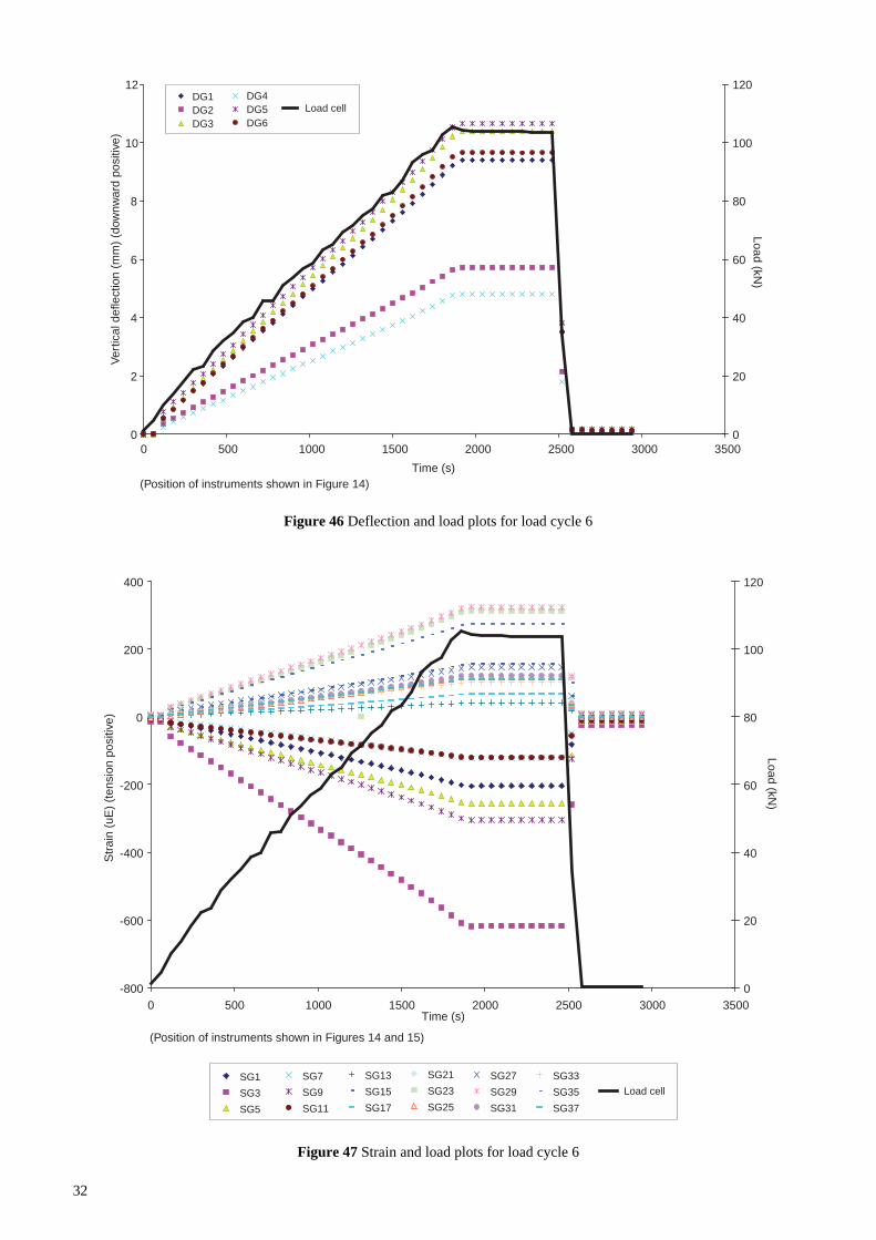
8.6 Load cycle 6 - peak load 104 kN
Data from this load cycle are presented in Figures 46 to 50.The cumulative AE count as the peak load was attainedwas about 77,800.
Following the attainment of the peak load a loud crackwas heard by those operating the equipment. This emissionwas picked up by both the SoundPrint and PhysicalAcoustics systems. It appears in Figure 48 as an eventconsisting of in excess of 4700 counts recorded by channel2, 950 counts by channel 3, and 530 counts by channel 1.The event is also evident in Figures 49 and 50. At thispoint there was no substantial change in either thedeflection or strain gauge readings. A visual examination
of the beam did not reveal the presence of any cracks orfractures, or of any slippage or other movement at thespreader-beam interface.
No other events were picked up by the SoundPrintsystem during this cycle.
8.7 Load cycle 7 - peak load 116 kN
The data for this cycle are shown in Figures 51 to 56.During this cycle, the peak load was left on hold for
about 17 hours, and after unloading monitoring continuedfor a further 90 minutes. Following attainment of the peakload, AE continued to be generated, albeit at a lesser rate,for the time that the load was applied. The cumulative AEcount as the peak load was attained was about 84,200.
Eight ‘unconfirmed cracking’ events were picked up bythe SoundPrint system during this cycle.
8.8 Load cycle 8 - peak load 130 kN
Data from this cycle of load are shown in Figures 57 to 61.The cumulative AE count as the peak load was attained wasabout 82,600. Two ‘unconfirmed cracking’ events werepicked up by the SoundPrint system during this cycle.
8.9 Load cycle 9 - peak load 151 kN
Data from this cycle are shown in Figures 62 to 66. Thecumulative AE count as the peak load was attained wasabout 146,000. Four ‘unconfirmed cracking’ events werepicked up by the SoundPrint system during this cycle.
0
1
2
3
4
5
6
7
8
9
10
0 500 1000 1500 2000 2500 3000 3500Time (s)
Ver
tical
def
lect
ion
(mm
) (d
ownw
ard
posi
tive)
0
10
20
30
40
50
60
70
80
90
100
Load (kN)
DG1DG2DG3
DG4DG5DG6
Load cell
(Position of instruments shown in Figure 14)
Figure 41 Deflection and load plots for load cycle 5

30
-600
-500
-400
-300
-200
-100
0
100
200
300
400
0 500 1000 1500 2000 2500 3000 3500Time (s)
Str
ain
(uE
) (t
ensi
on p
ositi
ve)
0
10
20
30
40
50
60
70
80
90
100
Load (kN)
SG1
SG3
SG5
SG7
SG9
SG11
SG13
SG15
SG17
SG21
SG23
SG25
SG27
SG29
SG31
SG33
SG35
SG37
Load cell
(Position of instruments shown in Figures 14 and 15)
0
100
200
300
400
500
600
0 500 1000 1500 2000 2500 3000 3500
Time (s)
AE
cou
nt
0
10
20
30
40
50
60
70
80
90
100
Load (kN)
Individual counts for all four sensors
Load cell
Figure 42 Strain and load plots for load cycle 5
Figure 43 Generation of AE counts through load cycle 5

31
0
5000
10000
15000
20000
25000
30000
35000
40000
45000
50000
0 500 1000 1500 2000 2500 3000 3500
Time (s)
AE
cum
ulat
ive
coun
t
0
10
20
30
40
50
60
70
80
90
100
Load (kN)
Cumulative counts
Load cell
0
5000
10000
15000
20000
25000
30000
0 500 1000 1500 2000 2500 3000 3500Time (s)
AE
cum
ulat
ive
coun
t
0
10
20
30
40
50
60
70
80
90
100
Load (kN)
Channel 1Channel 2
Channel 3Channel 4
Load cell
(Position of instruments shown in Figures 14 and 15)
Figure 44 Cumulative AE counts through load cycle 5
Figure 45 Cumulative AE counts for each sensor for load cycle 5
32
0
2
4
6
8
10
12
0 500 1000 1500 2000 2500 3000 3500
Time (s)
Ver
tical
def
lect
ion
(mm
) (d
ownw
ard
posi
tive)
0
20
40
60
80
100
120
Load (kN)
DG1DG2DG3
DG4DG5DG6
Load cell
(Position of instruments shown in Figure 14)
-800
-600
-400
-200
0
200
400
0 500 1000 1500 2000 2500 3000 3500Time (s)
Str
ain
(uE
) (t
ensi
on p
ositi
ve)
0
20
40
60
80
100
120
Load (kN)
SG1
SG3
SG5
SG7
SG9
SG11
SG13
SG15
SG17
SG21
SG23
SG25
SG27
SG29
SG31
SG33
SG35
SG37
Load cell
(Position of instruments shown in Figures 14 and 15)
Figure 46 Deflection and load plots for load cycle 6
Figure 47 Strain and load plots for load cycle 6

33
0
500
1000
1500
2000
2500
3000
3500
4000
4500
5000
0 500 1000 1500 2000 2500 3000 3500Time (s)
AE
cou
nt
0
20
40
60
80
100
120
Load (kN)
Individual counts for all four sensors
Load cell
0
10000
20000
30000
40000
50000
60000
70000
80000
90000
100000
0 500 1000 1500 2000 2500 3000 3500
Time (s)
AE
cum
ulat
ive
coun
t
0
20
40
60
80
100
120
Load (kN)
Cumulative counts
Load cell
Figure 48 Generation of AE counts through load cycle 6
Figure 49 Cumulative AE counts through the load cycle 6

34
0
10000
20000
30000
40000
50000
60000
0 500 1000 1500 2000 2500 3000 3500Time (s)
AE
cum
ulat
ive
coun
t
0
20
40
60
80
100
120
Load (kN)
Channel 1Channel 2
Channel 3Channel 4
Load cell
(Position of instruments shown in Figures 14 and 15)
0
2
4
6
8
10
12
14
0 10000 20000 30000 40000 50000 60000 70000 80000
Time (s)
Ver
tical
def
lect
ion
(mm
) (d
ownw
ard
posi
tive)
0
20
40
60
80
100
120
Load (kN)
DG1DG2DG3
DG4DG5DG6
Load cell
(Position of instruments shown in Figure 14)
Figure 50 Cumulative AE counts for each sensor for load cycle 6
Figure 51 Deflection and load plots for load cycle 7

35
-800
-600
-400
-200
0
200
400
600
0 10000 20000 30000 40000 50000 60000 70000 80000
Time (s)
Str
ain
(uE
) (t
ensi
on p
ositi
ve)
0
20
40
60
80
100
120
Load (kN)
SG1
SG3
SG5
SG7
SG9
SG11
SG13
SG15
SG17
SG21
SG23
SG25
SG27
SG29
SG31
SG33
SG35
SG37
Load cell
(Position of instruments shown in Figures 14 and 15)
0
100
200
300
400
500
600
700
800
0 10000 20000 30000 40000 50000 60000 70000Time (s)
AE
cou
nt
0
20
40
60
80
100
120
140
Load (kN)
Individual counts for all four sensors
Load cell
Figure 52 Strain and load plots for load cycle 7
Figure 53 Generation of AE counts through load cycle 7

36
0
20000
40000
60000
80000
100000
120000
140000
0 10000 20000 30000 40000 50000 60000 70000
Time (s)
AE
cum
ulat
ive
coun
t
0
20
40
60
80
100
120
140Load (kN
)Cumulative counts
Load cell
0
10000
20000
30000
40000
50000
60000
70000
80000
0 10000 20000 30000 40000 50000 60000 70000Time (s)
AE
cum
ulat
ive
coun
t
0
20
40
60
80
100
120
140
Load (kN)
Channel 1
Channel 2Channel 3
Channel 4Load cell
(Position of instruments shown in Figures 14 and 15)
Figure 54 Cumulative AE counts through load cycle 7
Figure 55 Cumulative AE counts for each sensor for load cycle 7

37
0
20000
40000
60000
80000
100000
120000
140000
0 500 1000 1500 2000 2500 3000 3500Time (s)
AE
cum
ulat
ive
coun
t
0
20
40
60
80
100
120
140Load (kN
)Cumulative countsLoad cell
0
2
4
6
8
10
12
14
16
0 500 1000 1500 2000 2500 3000 3500 4000 4500 5000
Time (s)
Ver
tical
def
lect
ion
(mm
) (d
ownw
ard
posi
tive)
0
20
40
60
80
100
120
140
Load (kN)
DG1DG2DG3
DG4DG5DG6
Load cell
(Position of instruments shown in Figure 14)
Figure 56 Cumulative AE counts through early stages of load cycle 7
Figure 57 Deflection and load plots for load cycle 8

38
-1000
-800
-600
-400
-200
0
200
400
600
0 500 1000 1500 2000 2500 3000 3500 4000 4500 5000
Time (s)
Str
ain
(uE
) (t
ensi
on p
ositi
ve)
0
20
40
60
80
100
120
140
Load (kN)
SG1
SG3
SG5
SG7
SG9
SG11
SG13
SG15
SG17
SG21
SG23
SG25
SG27
SG29
SG31
SG33
SG35
SG37
Load cell
(Positions of instruments shown in Figures 14 and 15)
0
50
100
150
200
250
300
350
400
450
500
0 500 1000 1500 2000 2500 3000 3500 4000 4500 5000
Time (s)
AE
cou
nt
0
20
40
60
80
100
120
140
Load (kN)
Individual counts for all four sensors
Load cell
Figure 58 Strain and load plots for load cycle 8
Figure 59 Generation of AE counts through load cycle 8

39
0
20000
40000
60000
80000
100000
120000
0 500 1000 1500 2000 2500 3000 3500 4000 4500 5000
Time (s)
AE
cum
ulat
ive
coun
t
0
20
40
60
80
100
120
140Load (kN
)Cumulative countsLoad cell
0
10000
20000
30000
40000
50000
60000
0 500 1000 1500 2000 2500 3000 3500 4000 4500 5000
Time (s)
AE
cum
ulat
ive
coun
t
0
20
40
60
80
100
120
140
Load (kN)
Channel 1Channel 2
Channel 3Channel 4
Load cell
(Position of instruments shown in Figures 14 and 15)
Figure 60 Cumulative AE counts through load cycle 8
Figure 61 Cumulative AE counts for each sensor for load cycle 8

40
0
2
4
6
8
10
12
14
16
18
0 500 1000 1500 2000 2500 3000 3500 4000 4500 5000
Time (s)
Ver
tical
def
lect
ion
(mm
) (d
ownw
ard
posi
tive)
0
20
40
60
80
100
120
140
160
180
Load (kN)
DG1DG2DG3
DG4DG5DG6
Load cell
(Position of instruments shown in Figure 14)
-1200
-1000
-800
-600
-400
-200
0
200
400
600
0 500 1000 1500 2000 2500 3000 3500 4000 4500 5000
Time (s)
Str
ain
(uE
) (t
ensi
on p
ositi
ve)
0
20
40
60
80
100
120
140
160
180
Load (kN)
SG1
SG3
SG5
SG7
SG9
SG11
SG13
SG15
SG17
SG21
SG23
SG25
SG27
SG29
SG31
SG33
SG35
SG37
Load cell
(Position of instruments shown in Figures 14 and 15)
Figure 62 Deflection and load plots for load cycle 9
Figure 63 Strain and load plots for load cycle 9

41
0
100
200
300
400
500
600
0 500 1000 1500 2000 2500 3000 3500 4000 4500 5000
Time (s)
AE
cou
nt
0
20
40
60
80
100
120
140
160
180
Load (kN)
Individual counts for all four sensorsLoad cell
0
20000
40000
60000
80000
100000
120000
140000
160000
180000
0 500 1000 1500 2000 2500 3000 3500 4000 4500 5000Time (s)
AE
cum
ulat
ive
coun
t
0
20
40
60
80
100
120
140
160
180
Load (kN)
Cumulative countsLoad cell
Figure 64 Generation of AE counts through load cycle 9
Figure 65 Cumulative AE counts through load cycle 9

42
0
20000
40000
60000
80000
100000
120000
0 500 1000 1500 2000 2500 3000 3500 4000 4500 5000
Time (s)
AE
cum
ulat
ive
coun
t
0
20
40
60
80
100
120
140
160
180Load (kN
)Channel 1Channel 2
Channel 3Channel 4
Load cell
(Positions of instruments shown in Figures 14 and 15)
Figure 66 Cumulative AE counts for each sensor for load cycle 9
8.10 Summary of results
The deflections recorded at the peak loads are plotted inFigure 67. It is evident that deflection of the beam wasslightly asymmetric, with marginally more deflectionoccurring on the left than the right hand side of the beam.As shown in Figure 68, there was a more or less linearrelationship between the recorded maximum deflectionand the peak load. The deflections plotted in Figures 67and 68 are those recorded from the start of each cycle ofload, but the beam did not return to its original position atthe end of each cycle. Figure 69 shows the change inposition at the start of the third and subsequent cycles,relative to the position at the start of the second cycle.There appears to be some asymmetry in the data, but therecorded maximum residual displacement was a little lessthan 1 mm.
Figure 70 also indicates reasonably linear relationsbetween the strains recorded in both the top and bottomflanges and the peak load. The maximum strain gaugereadings at the maximum load of about 150 kN, wererecorded by No. 3 (central gauge on top of top flange) andNo. 29 (central gauge at centre under bottom flange), thevalues were 946 uE (compression) and 508 uE (tension)respectively.
Figure 71 shows a plot of the cumulative AE count onthe attainment of the peak load as a function of load. Thecumulative count for cycle 4 (i.e. the repeat of the firstcycle) has been omitted and a best-fit least squares straightline drawn through the other data points. The choice ofplotting the cumulative AE count at the peak load issomewhat arbitrary.
Figure 72 plots the cumulative AE count as a functionof time. If the loading rate were the same for each test(as it was supposed to be), the time scale would beproportional to load. The peak loads are defined on thefigure but note that minor variations in the actualloading rate have led to some small inconsistencies inthe positions of the peak loads. A similar pattern ofbehaviour was detected by each of the four sensors butthe two centre sensors (numbers 2 and 3), and inparticular number 2, recorded much greater levels of AEthan numbers 1 and 4. In some cycles sensor 1 detectednoticeably greater levels of AE than sensor 4.
At first sight there are two apparent, but slight,anomalies in the data. Firstly, cycle 3 with a peak load ofabout 73 kN generated less AE than the first cycle whenthe peak load was only 50 kN. Secondly, the cumulativeAE recorded during the loading stages of cycles 6,7 and 8do not increase uniformly with the increase in the peakload. These are discussed in Section 9 below.
The data from the SoundPrint system are summarised inTable 2, and the calculated locations of the source of theevents are shown in Figure 73. Although the error in thelocation of most of the events should be within 300 mm,the error for a few might be up to 600 mm. The accuracyof the location could be improved in future tests bychanging the positions of the sensors and throughmodification of the software.

43
0 1 2 3 4 5 6 7 8
Distance along beam (m)
Ver
tical
def
lect
ion
(mm
) (d
ownw
ard
posi
tive)
51.268.273.452.387.3103.7115.6130.3151.2
Peak load (kN)
DG2 DG6 DG4DG3 DG1DG5
CL
0
2
4
6
8
10
12
14
16
18
SupportSupport
0
2
4
6
8
10
12
14
16
18
0 20 40 60 80 100 120 140 160
Peak load (kN)
Ver
tical
def
lect
ion
(mm
)(d
ownw
ard
posi
tive)
Figure 67 Maximum beam displacements during each load cycle
Figure 68 Relation between deflection and peak load

44
-0.4
-0.2
0.0
0.2
0.4
0.6
0.8
1.0
0 1 2 3 4 5 6 7 8
Distance along beam (m)
Ver
tical
def
lect
ion
(mm
)
68.273.452.387.3103.7115.6130.3151.2
Peak load (kN)
0
100
200
300
400
500
600
700
800
900
1000
0 20 40 60 80 100 120 140 160
Peak load (kN)
Str
ain
(uE
)
SG3
SG29
Position of instruments shown in Figures 14 and 15
Figure 69 Beam starting positions relative to position at load cycle 2
Figure 70 Relation between strain and peak load

45
0
20000
40000
60000
80000
100000
120000
140000
160000
180000
0 500 1000 1500 2000 2500 3000 3500 4000Time (s)
Cum
ulat
ive
AE
cou
nt
Load cycle 1
Load cycle 2
Load cycle 3
Load cycle 4
Load cycle 5
Load cycle 6
Load cycle 7
Load cycle 8
Load cycle 9
51 87 104 116 130 15168
Peak load
Figure 71 Relation between AE count and peak load
Figure 72 Cumulative AE counts for each load cycle
0
20000
40000
60000
80000
100000
120000
140000
160000
0 20 40 60 80 100 120 140 160Peak load (kN)
AE
cou
nt
Count
Linear (count)

46
Table 2 Number of cracking events detected duringeach load cycle
Max No. of No. oftest possible observedload cracking cracking
Test No. (kN) events events Total
1 51.2 0 0 02 68.2 1 0 13 73.4 0 0 04 52.3 0 0 05 87.3 4 0 46 103.7 0 1 17 115.6 8 0 88 130.3 2 0 29 151.2 4 0 4
A2A1A0 A3 A4
7950
450
All dimensions in mm
1000
2500
3975
SoundPrint transducer
Event location
Figure 73 Location of events picked up by Soundprint systems
8.11 Other forms of processing
The Physical Acoustics system is capable of extractingmany AE features from events in real-time. It is thereforepossible to plot other waveform parameters rather than justcounts as a function of time. This might be useful, forexample, where different fracture mechanisms generatedifferent waveforms and it is necessary to distinguishbetween them. By way of example, Figure 74 plots theamplitude of the waveform as a function of duration forthe AE event data obtained in load cycle 9.
9 Discussion
The discussion is divided into four parts, considering inturn (i) interpretation of the AE test data, (ii) assessment ofthe maximum in-service load, (iii) assessment of collapseload, and (iv) assessment of in-service condition.
It should be appreciated in what follows that theprincipal objective of the project was to determine whetherAE techniques had the potential to form the basis for anintelligent monitoring system. The data presented in theforegoing clearly show that AE has that potential. It wasexpected from the outset that further work following thetest would be required to determine how the technique(s)could be applied in practice. Potential applications ofvarious monitoring systems are covered in the followingbut at this stage discussion is, necessarily, rather
speculative and perhaps over-critical. Nonetheless someform of critical analysis is required to establishrecommendations for follow-up work.
It should also be appreciated that the loading conditionson the beam imposed during the test and in service werequite different. The imposition of a load at the centre of thespan (as in the test) cannot replicate both bending andshear effects of a reasonably distributed superimposeddead load combined with the effect of a live load (as inservice): the results of the two loading regimes aretherefore not directly comparable. Nonetheless to progressdiscussion such differences have been largely suspended inthe following.
9.1 Interpretation of data
In general, the rate of AE generated increased greatly asthe previously applied maximum load was approached andthen exceeded. The rate reduced substantially followingthe stabilisation of the (new) maximum load: it reducedfurther during unloading, and further still to a relativelyinsignificant level within a short space of time followingthe removal of the load.
The Physical Acoustic sensors at the centre of the beamrecorded far more AE activity than the sensors towards theend of the beam, showing that the supports were not amajor source of emission. Similarly the events recorded bythe SoundPrint system were located towards the mid-spanof the beam. It is of interest to note that the data from boththe AE sensors and the deflection gauges showed a slightlyasymmetric response of the beam.
There was no evidence of rust flaking from the beamduring the load cycles nor was there any visible evidenceof a reaction between the beam and the load spreader at thebearings. Thus it is probable that the AE activity resultedfrom some load-related mechanism. It is impossible to becertain of the source but, given the relation between AEactivity and load, it is likely that it was associated withmicro-fracturing of the cast iron beam, perhaps betweenthe graphite flakes and the surrounding matrix. It seemsreasonable to suppose that as the applied load wasincreased existing fractures would lengthen and new oneswould be created. Provided that failure was notapproached, at a constant load micro-fracturing, andtherefore AE activity, would continue but at a decreasing

47
rate with time until it ceased completely, indicating thatequilibrium had been attained. Removal of the appliedload would not be expected to generate much AE activity,other than, perhaps, some minor levels associated with theclosure of fractures. During reloading, existing fracturesmight reopen, but this would not be expected to generatemuch activity until the previous maximum load had beenexceeded. The above model of behaviour fits most of thedata reasonably well but, at first sight, there are twoanomalies in the AE data that require explanation.
Firstly, as shown in Figure 72, the cumulative AE countrecorded at the peak load of about 73 kN in the third loadcycle was (at 8,700) substantially lower than recorded(28,000) during the previous cycle where the peak loadwas a little lower at about 68 kN. However because of theproblems with the control system of the rig, the peak loadmight have been slightly underestimated during the secondcycle and in any case the difference in the peak loads wasonly about 5 kN. It is also relevant to note that the rate ofAE generated following the attainment of the peak load incycle 3 was relatively low compared to the rate generatedin other cycles. It is possible that AE activity in the secondcycle might have been boosted by a substantial acousticevent. A single event was recorded by the SoundPrintsystem in the second cycle but nothing was recorded in thethird (see Table 2).
Secondly, examination of the data presented in Figure 72,shows that there is relatively little difference in thecumulative AE counts recorded in load cycles 6, 7 and 8where the peak loads were about 104, 116 and 131 kNrespectively. As noted above, a significant audible eventwas noted in cycle 6, but eight events were also recordedby the SoundPrint system during cycle 7. In most of the
0
10
20
30
40
50
60
70
80
90
0 500 1000 1500 2000 2500 3000 3500 4000 4500 5000
Duration (uS)
Am
plitu
de (
dB)
Threshold = 40dB
Figure 74 Relation between the amplitude and duration of AE events through load cycle 9
cycles the peak load was maintained for between about 10and 25 minutes but it was applied for 17 hours in cycle 7.Data, given in Figures 54 to 56, show that the rate of AEwas still reducing at the end of this time indicating that thebeam had still not reached ‘equilibrium’ – at least in termsof micro-cracking and AE activity. By implication theother load cycles were terminated well before an‘equilibrium’ condition was approached (if indeed such astate would ever be reached). Thus the relation betweenAE (however quantified) and load might be stronglydependent on the rate of loading and the length of time aparticular load is applied for. (That the effect of a load on abeam varies with its rate of application and duration shouldnot be a surprise.) It is, therefore, feasible that the(relatively) low AE count for cycle 8 was due to damageinflicted in the previous cycle. An important inferencefrom this is that it might be possible to use AE to comparethe damaging effect of various live loads (for exampleheavy goods vehicles of varying weight and travelling atdifferent speeds) and dead loads. On the other handbecause the plots shown in Figures 71 and 72 are affectedby the rates of loading and unloading, by how long thepeak load is applied for, and perhaps also by the creationof significant flaws, it might be difficult to use AE data toassess the structural stability of an old structure,particularly one that supported substantial live loads.
As shown in Figure 75, there is a reasonably linearrelation between the rate of AE generated as the peak loadis approached and the peak load. Note that the data pointsfor cycles 3, 4 and 8 fall well below the best-fit line.Similarly, Figure 76 shows the relation between the rate ofAE generated immediately following the attainment of thepeak load and the peak load itself. In contrast to Figure 75,

48
0
50
100
150
200
250
300
350
400
450
0 20 40 60 80 100 120 140 160
Peak load (kN)
AE
(co
unts
/sec
ond)
app
roac
hing
pea
k lo
ad
1
2
3
4
5
6 7 8
9
Note: numbers refer to the test cycle
0
2
4
6
8
10
12
14
0 20 40 60 80 100 120 140 160Peak load (kN)
AE
(co
unts
/sec
ond)
follo
win
g at
tain
men
t of p
eak
load
14
32
5
6
7
7
8
9
Note:numbers refer to test cyclebest-fit line drawn through 1, 2, 3, 4, 5, 6 & 9 only
Figure 75 Rate of AE generation approaching peak load for each test cycle
Figure 76 Rate of AE generation following attainment of peak load for each load cycle

49
the data points for cycles 1 and 4 fall close together in Figure76. This might suggest that the rate following the attainmentof the peak is solely a function of the peak load but the time-dependency of the relation must be considered. The rate forcycle 8 is also quite depressed, perhaps again because of theprolonged application of the peak load in the previous cycle.Note that two data points are shown for cycle 7: the higherrate corresponds to the attainment of the peak load whilst thelower corresponds to the end of the loading cycle, i.e. aftersome 17 hours. The rates differ by an order of magnitude,thus again showing the time-dependency of the relation. It ispertinent to note that the lower rate is lower than that recordedat the maximum load imposed during cycle 4 – which was areloading cycle. Further tests are required to characterise theshape of the AE-load relations over much longer loadingtimes. (Note that for some of the load cycles it was difficult toaccurately define the shape of the relations between AEactivity and load - particularly where data points are sparsefor example on Figure 39.)
9.2 In-service load
An estimate of the maximum load sustained in-service frommeasurements of deflection and strain might be based on thepremise that there is some noticeable change in stiffness orsome permanent deflection as that load is exceeded. But it isquite likely that, in-service, the test beam was within its‘elastic recoverable’ range. According to the data from thetest (Figure 69), some permanent deflection was noted at anapplied load of about 70 kN, but this might just reflect achange in the position of the supports. Furthermore, there wassome small permanent strain induced by the applied load(more noticeably from the third cycle onwards). A bi-linearrelation fitted to the data points in Figure 70, such that thelower line passed through the origin, indicates a (slight)change of slope at a load of about 90 kN. However, the load-strain plots for the various cycles show no noticeable changein slope where a previous maximum load was exceeded.
At this stage, the damage commensurate with the AEactivity measured during the test cannot be translated intoother units (such as the extent of micro-cracking), but itwould seem that such damage did not much affect theload-deflection nor the load-strain relation for the beam.This suggests that neither deflection gauges nor straingauges would be of much use in determining the conditionof a cast iron jack arch bridge.
As discussed in Section 9.1, because of the effect ofloading history it might be difficult to determine the peakin-service load sustained by a structure from an analysis ofAE data. Figures 71, 75 and 76 show relations between AEactivity and peak load for the various load cycles. Anumber of the data points could be overlooked ininterpreting these relations - such as for the seventh andeighth cycles because the peak load applied in the seventhwas sustained for an extended period. Nonetheless,extrapolations for various selected combinations of pointsplotted in these figures suggest that the maximum previousload sustained by the beam was between about 40 and 50kN. Again it should be appreciated that:
i the load regime applied in the test and in-service werequite different; and
ii the AE relations are time-dependent and whilst the beamwas in-service for more than a century the first cyclewas completed in about an hour or so.
Further evidence of this might, therefore, be found froma close examination of the data from the first cycle, wherethe maximum applied load was a little over 50 kN. Acomparison of Figure 25 with, for example, Figure 30shows that the plots in the former have a much morepronounced S-shape than those in the latter. Much moreAE activity takes place at low loads during the first cyclethan in any of the others. It is, however, difficult to decidewhat rate or change in rate of AE could be taken torepresent a change in performance that might result fromthe application of a new peak load. The assumption that nosignificant AE is generated until the previous peak load isapproached leads to the conclusion (from Figure 25) thatthe maximum in-service load was less than about 20 kN,i.e. below the level for which data are available, seeSection 8.1.
9.3 Collapse load
It is improbable that a load-deflection relation, as shown inFigure 68 for example, could be used to estimate thecollapse load of a jack arch structure. A brittle failuremight show as a dramatic, and perhaps unpredictable,discontinuity in such a relation. A plastic failure would bepreceded by an upturn in the relation, but it is probable thata change in slope would be associated with a weakening ofthe structure: a load test should not venture this far.However such a relation might be extrapolated todetermine the (serviceability) load for some limiting andacceptable deflection. For example, according to Figure 68a limiting deflection of 0.1 per cent (or 1/1000) of the clearspan of the beam (7 metres) is generated at a load of about70 kN. It should be appreciated that rarely would such anextended load test as undertaken on the test beam befeasible for an in-service structure. Furthermore therelation for an in-service jack arch structure would beaffected by the interaction of the beams, brickwork, andbackfill and could not therefore be calculated particularlyaccurately.
It might be thought that an estimate of the collapse loadof a cast iron beam could be based on measured strains, asprovided for example in Figures 2 and 70. However thereare a number of interacting factors that make it well nighimpossible to do this, including:
i the origin of the relation cannot be defined for astructure;
ii the strain under load will vary with position;
iii the distribution of load might not be known well, or becontrollable;
iv the point of maximum strain might not be identifiable -and if it could it might not be possible to install straingauges at that point;
v the shape of the load-strain relation for any particularpoint on a structure will vary according to the pattern ofloading, and might not be known a priori;

50
vi due to the presence of flaws, the load-strain response ofa beam might be quite different to that of a small-scalelaboratory specimen.
According to Figure 2, the average ultimate tensilestress of cast iron is 108 N/mm2 and is developed at atensile strain of about 0.0017. At the maximum appliedload of 150 kN the maximum tensile strain recorded by thegauges attached to the beam was about 0.0005. This mightsuggest that there was a large margin of safety at this load,but the gauge would not have recorded the maximumstrain generated on the beam.
As shown for example in Figure 71, the amount of AEincreased, more or less, with increasing load. If AE activitywere related to the size or number of micro-cracks, whichcould be taken as a measure of damage, it might bepossible to extrapolate the load-AE relation to assess thecollapse load. However, an inherent problem is theapparent time-dependency of AE data. Furthermore, asdiscussed above, it is difficult to base predictions of failureon a linear relation as shown for example in Figure 71. It isnot known what level of AE could be set to represent an‘allowable level of damage’ - and even if one could be setfor this beam, or a range of test beams, it would notnecessarily be relevant to an in-service jack arch structure.Because the response of an in-service beam is affected(perhaps overwhelmingly so) by its interaction with thesurrounding backfill and brick arches, a good deal of workmight be required to establish empirical rules.
At this stage, it is not known whether the AE activitygenerated by reloading was due to the opening of existingmicro-cracks, the extension of existing cracks or the creationof new cracks - or what combination of these occurred. Insome load cycles, AE activity was not negligible duringreloading: as evidenced for example in Figures 39 and 56.This might indicate that cast iron beams are susceptible tocyclic loading. Long-term experiments are required to assesswhether or not the rate of AE during reloading could berelated to the residual fatigue life of a structure.
9.4 In-service condition
The aims of a structural assessment are to check that thestructure in question is performing adequately and that ithas an acceptable margin of safety against collapse. Butassessment via calculation alone is complicated by variousstructural interactions, which may or may not beunderstood particularly well. Furthermore there might notbe relevant information on structural form (for example as-built drawings) and material properties; such problemscould be expected to increase with the age of a structure.Instrumentation can be installed to quantify in some way(such as through measurements of deflection) in-serviceperformance, but there remains the problem of fixing aweight restriction at an appropriate level. Although strainand/or load-measuring devices and deflection gaugesmight have some role to play they do not necessarily warnthat a structure is deteriorating. On the other hand, AEtechniques can provide information on the damagesustained in service, which might not be picked-up byother methods of instrumentation, but the data from AE
devices has to be ‘calibrated’ in some way to be ofpractical use.
In many cases, the only way of estimating the level ofsafety of a structure is through analysis of a load test, asdescribed for example by Daly and Raggett (1991). But, asdescribed by them, analysis of the data from such tests iscomplicated by various structural interactions and there arealso limits on the magnitude of the load that can beapplied. Owners might be concerned that load tests woulddamage, and hence weaken, the structure. Againmeasurements of strain and deflection might have somerole to play in assessing the performance of a structureunder load, but they only provide information local to theposition of the instrument. As shown herein, AE has agood potential for site monitoring works. Its use mightreassure an owner of the safety of undertaking a load test.
10 Recommendations for further work
It is necessary to conduct further investigations to confirmthe findings of this test as well as to investigate thepractical application of the equipment to an intelligentmonitoring system.
The next step would be the investigation of the time-dependency of the relation between AE activity and load.A particular load cycle might have to be applied forseveral days, if not weeks, to determine whether or not an‘equilibrium’ status was achieved. It would also bedesirable to load the beam to failure, or close to it, toinvestigate AE behaviour as failure is approached.
As a second step, a load test could be undertaken onanother beam from the Hythe End bridge, using the samerig and sensors, to investigate the AE response at loadlevels up to and slightly in excess of the maximum (or its‘equivalent’) in-service load. Again the load cycles wouldneed to be over a much longer period than in the testdescribed herein. This might provide an insight to thechange in AE response at and around a load equivalent tothe maximum supported in-service.
In either of the above, if not both, the AE response to cyclicloading (to simulate live loading) should be examined.
Wherever possible, opportunity should be taken to collectAE data from in-service jack arch structures, and particularadvantage should be taken of any load tests conducted.
11 Conclusion
A series of nine load cycles with a generally increasingpeak load, were conducted on a cast iron beam recoveredfrom an in-service structure. The beam, instrumented withdeflection gauges, strain gauges and acoustic sensors, wasloaded to about 150 kN, and in excess of the ‘equivalent’maximum in-service load. The results of the load test showthat the response of the beam was slightly asymmetric.
AE activity generally increased with peak load and,almost always, substantial activity was only recorded oncethe previous peak load was approached. The activityseemed to be related to the period of application of thepeak load. The rate of AE reduced following the

51
attainment of the peak load, it reduced further duringunloading and all but stopped on removal of the load. Thelocation of most of the recorded activity was around themid-span of the beam.
The results strongly support the view that AE wasgenerated via some load-related mechanism, perhapsrelated to micro-cracking of the cast iron. Further researchis required to confirm and extend the findings of the test,but the results show that AE techniques have the potentialfor forming the basis of an intelligent monitoring system.
12 References
Burdekin F M (1993). Non-destructive testing of weldedstructural steelwork. Proc Inst Civ Engrs: Structures andBuildings, Vol 99, No 1, pp 89-95.
BD 21. The Assessment of Highway Bridges and Structures(DMRB 3.4.3). London: The Stationery Office.
Daly A F and Raggett S J (1991). Load test on a jackarch bridge with cast iron girders. Research ReportRR310. Crowthorne: TRL Limited.
Dixon N, Hill R and Kavanagh J (1996). The use ofacoustic emission to monitor the stability of soil slopes.Proc Int Conf Advances in Site Investigation Practice heldin London, March 1995. London: Thomas Telford.pp 739-749.
Ghorbanpoor A (1990). Monitoring steel bridges byacoustic emission. Transportation Research Record, No1268, January 1990. Washington DC. pp 148-155.
Hilton J (1997). Jack arch bridges investigation andrating. Sydney: Austroads Bridge Conference, 1997,Vol 2, pp 309 – 321.
Li Z, Li F, Zdunek A, Landis E and Shah S P (1998).Application of acoustic emission technique to detection ofreinforcing steel corrosion in concrete. ACI MaterialsJournal, American Concrete Institute, January 1998,Vol 95, No 1, pp 68-76.
Lim M K and Koo T K (1989). Acoustic emission fromreinforced concrete beams. Magazine of ConcreteResearch. December 1989, Vol 41, No 149. London:Thomas Telford. pp 229-234.
MacNeil D J and Cullington D W (1998). Acousticmonitoring of a railway viaduct, Huntingdon. ProjectReport PR/CE/256/98. Crowthorne: TRL Limited.(Unpublished report available on direct personalapplication only)
Royles R and Hendry A W (1991). Model tests onmasonry arches. Proc Inst Civ Eng, Part 2, June 1991,Vol 89. London: Thomas Telford. pp 299-321.
Stephens V A and Cullington D W (1998). Inspectionand testing of post-tensioned bridges: Progress report 8.Project Report PR/CE/89/98. Crowthorne: TRL Limited.(Unpublished report available on direct personalapplication only)
Swailes T (1995). 19th Century cast-iron beams: theirdesign, manufacture and reliability. Proc Inst Civ Engrs:Civ Engng, Vol 114, Feb, pp 25-35.
Willmott M P, Harrison K M and Frost A J (1997).Inspection and testing of post-tensioned bridges: Progressreport 7 (work in 1996/97). Project Report PR/CE/65/97.Crowthorne: TRL Limited. (Unpublished report availableon direct personal application only)

52
Abstract
A cast iron beam, instrumented with deflection gauges, strain gauges and two forms of acoustic monitoring system,was subjected to a series of nine load cycles of generally increasing maximum load. The aim of the test programmewas to determine whether acoustic emission (AE) techniques could be used to form the basis of an intelligentmonitoring system for structures. The results of the test are described in terms of a simple model and they supportthe view that AE was generated by a load-related mechanism, which was likely to be due to micro-fracturing of thecast iron. Thus AE techniques could form the basis of an intelligent monitoring system, but further work is requiredto develop a practical system. Recommendations for furthering the project are provided.
Related publications
TRL204 A guide to repair and strengthening of masonry arch highway bridges by J Page. 1996 (price £50, code L)
RR310 Load test on a jack arch bridge with cast iron girders by A F Daly and S J Raggett. 1991 (price £20, code B)
CR284 An assessment of repair and strengthening techniques for brick and stone masonry arch bridgesby D Ashhurst. 1992 (price £50, code N)
CR244 Masonry properties for assessing arch bridges by A W Hendrey. 1990 (price £20, code C)
CR155 Load tests on a full scale model four metre span masonry arch bridge by W J Harvey, A E Vardy,R F Craig, and F W Smith. 1989 (price £20, code C)
RR19 Finite element and mechanism methods for the analysis of masonry and brickwork archesby M A Crisfield. 1985 (price £20, code AA)
Prices current at October 2002
For further details of these and all other TRL publications, telephone Publication Sales on 01344 770783, or visitTRL on the Internet at www.trl.co.uk.