INTEGRATION OF MULTISPECTRAL SATELLITE … OF MULTISPECTRAL SATELLITE AND HYPERSPECTRAL FIELD DATA...
8
INTEGRATION OF MULTISPECTRAL SATELLITE AND HYPERSPECTRAL FIELD DATA FOR AQUATIC MACROPHYTE STUDIES John C. M a ., and Kavya Nath a,b . a Dr. R. Satheesh Centre for Remote Sensing and GIS, School of Environmental Sciences, Mahatma Gandhi University, Kottayam, Kerala, India – 686560. [email protected] b Indian Institute of Information Technology and Management-Kerala, Thiruvananthapuram – 699581. [email protected] KEY WORDS: Aquatic macrophytes, Spectral analysis, Principal Component analysis, Hyperspectral, Vegetation indices ABSTRACT: Aquatic macrophytes (AM) can serve as useful indicators of water pollution along the littoral zones. The spectral signatures of various AM were investigated to determine whether species could be discriminated by remote sensing. In this study the spectral readings of different AM communities identified were done using the ASD Fieldspec® Hand Held spectro-radiometer in the wavelength range of 325 – 1075nm. The collected specific reflectance spectra were applied to space borne multi-spectral remote sensing data from Worldview-2, acquired on 26 th March 2011. The dimensionality reduction of the spectro-radiometric data was done using the technique principal components analysis (PCA). Out of the different PCA axes generated, 93.472 % variance of the spectra was explained by the first axis. The spectral derivative analysis was done to identify the wavelength where the greatest difference in reflectance is shown. The identified wavelengths are 510, 690, 720, 756, 806, 885, 907 and 923 nm. The output of PCA and derivative analysis were applied to Worldview-2 satellite data for spectral subsetting. The unsupervised classification was used to effectively classify the AM species using the different spectral subsets. The accuracy assessment of the results of the unsupervised classification and their comparison were done. The overall accuracy of the result of unsupervised classification using the band combinations Red-Edge, Green, Coastal blue & Red-edge, Yellow, Blue is 100%. The band combinations NIR-1, Green, Coastal blue & NIR-1, Yellow, Blue yielded an accuracy of 82.35%. The existing vegetation indices and new hyper-spectral indices for the different type of AM communities were computed. Overall, results of this study suggest that high spectral and spatial resolution images provide useful information for natural resource managers especially with regard to the location identification and distribution mapping of macrophyte species and their communities. 1 INTRODUCTION 1.1 Remote sensing and GIS for aquatic plant studies Remote sensing data in combination with Geographic Information System (GIS) are effective tools for wetland conservation and management. Remote sensing techniques offer rapid acquisition of data with generally short turn-around time at lower costs than ground surveys (Tueller 1982). Multispectral airborne and satellite imagery have been used extensively to distinguish and map aquatic vegetation (Carter 1982, Martyn et al. 1986, Tiner 1997, Jakubauskas et al. 2002, Everitt et al. 2008, John 2010). Multispectral ground reflectance measurements have also been used to characterize and differentiate among wetland and aquatic plant species. Best et al. (1981) studied the multispectral reflectance of 10 wetland and emergent plant species and concluded that there were significantly different visible and near-infrared (NIR) spectra among the species. Everitt et al. (1999) reported that the 2 submersed species hydrilla (Hydrilla verticillata) and water stargrass (Heteranthera dubia) could be distinguished in the green (520 to 600 nm), red (630 to 690 nm), and NIR (750 to 900 nm) spectral bands. More recently, Everitt et al. (2007) reported that Eurasian water milfoil (Myriophyllum spicatum) could be differentiated from hydrilla in the green and red bands. Although these broadband systems and instrumentation have been widely used for wetland assessment, they are often constrained due to their coarse spatial and spectral resolution (Turner et al. 2003). More recently, hyper-spectral remote sensing including both imaging systems and ground-based radiometers, which can simultaneously acquire spectral data in many narrow contiguous spectral bands, has been used for a variety of natural resource management applications (Thenkabail et al. 2000, Fung et al. 2003, Ge et al. 2006, Yang et al. 2009). Hyper-spectral ground reflectance measurements have been used to develop spectral signatures of aquatic and wetland plant species and to ultimately identify the optimum bands to separate plant species. Ullah et al. (2000) studied the hyper- spectral reflectance of 3 emergent macrophytes and reported that the best separation among the species occurred at several bands in the NIR region (optimum bands: 882 and 885 nm). The study of aquatic macrophytes using remote sensing techniques has been less comprehensive than that of terrestrial vegetation because of the additional challenges associated with water reflectance, differentiating between different macrophyte species, and the small scale of freshwater aquatic environments compared to the resolution of most sensors (Underwood et al. 2006). It is known that different types of aquatic vegetation have subtly different spectral reflectance signatures, which differ greatly from open water and non-vegetated areas (Marshall and Lee 1994, Ozesmi and Bauer 2002, Penuelas et al. 1993). However, in the case of mixed beds, the varying contribution of each emergent macrophytes species to the total coverage remains difficult (Underwood et al. 2006, Vis et al. 2003). Mapping submerged aquatic vegetation with remote sensing can be problematic. The electromagnetic radiation reflected or radiating from submerged vegetation must cross the air-water interface (Wolter et al. 2005). In addition, because water absorbs much of the electromagnetic spectrum used in remote sensing, a major complication in remotely sensing of submerged vegetation is depth of the macrophyte canopy in the The International Archives of the Photogrammetry, Remote Sensing and Spatial Information Sciences, Volume XL-8, 2014 ISPRS Technical Commission VIII Symposium, 09 – 12 December 2014, Hyderabad, India This contribution has been peer-reviewed. doi:10.5194/isprsarchives-XL-8-581-2014 581
Transcript of INTEGRATION OF MULTISPECTRAL SATELLITE … OF MULTISPECTRAL SATELLITE AND HYPERSPECTRAL FIELD DATA...
INTEGRATION OF MULTISPECTRAL SATELLITE AND HYPERSPECTRAL FIELD DATA FOR AQUATIC MACROPHYTE STUDIES
John C. Ma., and Kavya Natha,b.
aDr. R. Satheesh Centre for Remote Sensing and GIS, School of Environmental Sciences, Mahatma Gandhi University, Kottayam,
Kerala, India – 686560. [email protected] bIndian Institute of Information Technology and Management-Kerala, Thiruvananthapuram – 699581. [email protected]
KEY WORDS: Aquatic macrophytes, Spectral analysis, Principal Component analysis, Hyperspectral, Vegetation indices ABSTRACT:
Aquatic macrophytes (AM) can serve as useful indicators of water pollution along the littoral zones. The spectral signatures of various AM were investigated to determine whether species could be discriminated by remote sensing. In this study the spectral readings of different AM communities identified were done using the ASD Fieldspec® Hand Held spectro-radiometer in the wavelength range of 325 – 1075nm. The collected specific reflectance spectra were applied to space borne multi-spectral remote sensing data from Worldview-2, acquired on 26th March 2011. The dimensionality reduction of the spectro-radiometric data was done using the technique principal components analysis (PCA). Out of the different PCA axes generated, 93.472 % variance of the spectra was explained by the first axis. The spectral derivative analysis was done to identify the wavelength where the greatest difference in reflectance is shown. The identified wavelengths are 510, 690, 720, 756, 806, 885, 907 and 923 nm. The output of PCA and derivative analysis were applied to Worldview-2 satellite data for spectral subsetting. The unsupervised classification was used to effectively classify the AM species using the different spectral subsets. The accuracy assessment of the results of the unsupervised classification and their comparison were done. The overall accuracy of the result of unsupervised classification using the band combinations Red-Edge, Green, Coastal blue & Red-edge, Yellow, Blue is 100%. The band combinations NIR-1, Green, Coastal blue & NIR-1, Yellow, Blue yielded an accuracy of 82.35%. The existing vegetation indices and new hyper-spectral indices for the different type of AM communities were computed. Overall, results of this study suggest that high spectral and spatial resolution images provide useful information for natural resource managers especially with regard to the location identification and distribution mapping of macrophyte species and their communities.
1 INTRODUCTION
1.1 Remote sensing and GIS for aquatic plant studies Remote sensing data in combination with Geographic Information System (GIS) are effective tools for wetland conservation and management. Remote sensing techniques offer rapid acquisition of data with generally short turn-around time at lower costs than ground surveys (Tueller 1982). Multispectral airborne and satellite imagery have been used extensively to distinguish and map aquatic vegetation (Carter 1982, Martyn et al. 1986, Tiner 1997, Jakubauskas et al. 2002, Everitt et al. 2008, John 2010). Multispectral ground reflectance measurements have also been used to characterize and differentiate among wetland and aquatic plant species. Best et al. (1981) studied the multispectral reflectance of 10 wetland and emergent plant species and concluded that there were significantly different visible and near-infrared (NIR) spectra among the species. Everitt et al. (1999) reported that the 2 submersed species hydrilla (Hydrilla verticillata) and water stargrass (Heteranthera dubia) could be distinguished in the green (520 to 600 nm), red (630 to 690 nm), and NIR (750 to 900 nm) spectral bands. More recently, Everitt et al. (2007) reported that Eurasian water milfoil (Myriophyllum spicatum) could be differentiated from hydrilla in the green and red bands. Although these broadband systems and instrumentation have been widely used for wetland assessment, they are often constrained due to their coarse spatial and spectral resolution (Turner et al. 2003). More recently, hyper-spectral remote sensing including both imaging systems and ground-based radiometers, which can simultaneously acquire spectral data in many narrow
contiguous spectral bands, has been used for a variety of natural resource management applications (Thenkabail et al. 2000, Fung et al. 2003, Ge et al. 2006, Yang et al. 2009). Hyper-spectral ground reflectance measurements have been used to develop spectral signatures of aquatic and wetland plant species and to ultimately identify the optimum bands to separate plant species. Ullah et al. (2000) studied the hyper-spectral reflectance of 3 emergent macrophytes and reported that the best separation among the species occurred at several bands in the NIR region (optimum bands: 882 and 885 nm). The study of aquatic macrophytes using remote sensing techniques has been less comprehensive than that of terrestrial vegetation because of the additional challenges associated with water reflectance, differentiating between different macrophyte species, and the small scale of freshwater aquatic environments compared to the resolution of most sensors (Underwood et al. 2006). It is known that different types of aquatic vegetation have subtly different spectral reflectance signatures, which differ greatly from open water and non-vegetated areas (Marshall and Lee 1994, Ozesmi and Bauer 2002, Penuelas et al. 1993). However, in the case of mixed beds, the varying contribution of each emergent macrophytes species to the total coverage remains difficult (Underwood et al. 2006, Vis et al. 2003). Mapping submerged aquatic vegetation with remote sensing can be problematic. The electromagnetic radiation reflected or radiating from submerged vegetation must cross the air-water interface (Wolter et al. 2005). In addition, because water absorbs much of the electromagnetic spectrum used in remote sensing, a major complication in remotely sensing of submerged vegetation is depth of the macrophyte canopy in the
The International Archives of the Photogrammetry, Remote Sensing and Spatial Information Sciences, Volume XL-8, 2014ISPRS Technical Commission VIII Symposium, 09 – 12 December 2014, Hyderabad, India
This contribution has been peer-reviewed. doi:10.5194/isprsarchives-XL-8-581-2014
581
water column (Han and Rundquist 2003, Penuelas et al. 1993, Wolter et al. 2005). Non-canopy forming submerged vegetative species are the most commonly misclassified submerged vegetation (Valta-Hulkkonen et al. 2005, Vis et al. 2003, Wolter et al. 2005). 1.2 Methods of RS data analysis Principal components analysis (PCA) is a multivariate method of statistical analysis and has been used widely with large, multi-dimensional data sets. PCA has been called, ‘one of the most important results from applied linear algebra’ and perhaps its most common use is as the first step in trying to analyse large data sets. Some of the other common applications include; de-noising signals, blind source separation, and data compression (Mark 2009). Principal component analysis calculated with the matrix of correlations and therefore not mean-correlated (e.g.: maximizing the weight of IR wavelengths) gave, as expected, a first principal component (PC1) that separates underwater from floating and emergent plants (Penuelas et al. 1993). Derivative analysis is an established technique for eliminating background signals, resolving interference from overlapping spectral features such as those from soil and water reflectance, and avoiding turbidity interference in the assessment of aquatic chlorophyll (Demetriades-Shah et al. 1990). Several spectral indices in the visible and near infrared were calculated with criteria based in the most outstanding features of the spectra, mainly those due to the absorbance of photosynthetic and protective pigments. The first derivative helps to locate the red edge, that is, the wavelength of maximum slope of the reflectance between 670nm and 800 nm (Penuelas et al. 1993). 1.3 Present study The present study was taken up in a selected portion of the Vembanad estuary in the western coast of peninsular India 1) to investigate the use of field based in-situ measurement of hyperspectral reflectance data in identifying and deriving new species specific hyperspectral indices of aquatic macrophytes 2) to compare among spectral reflectance characteristics of aquatic plants those are adapted to grow above water surface (emergent/floating vegetation) and below water surface (submerged aquatic vegetation) 3) to integrate in-situ measured hyperspectral reflectance data with the high spatial resolution multispectral satellite image and map the distribution of species-specific communities.
2 MATERIALS AND METHODS 2.1 Study area: Vembanad estuary A small portion of Vembanad estuary is selected for the study. The central point latitude and longitude of the area selected for the study is 9038’4.74”N and 76024’49.02”E. This test site was chosen because of its size, water depth, and similar abundance of dominant macrophyte species. The study area enjoys humid tropical monsoon climate and receive more than 300 cm rain fall annually. Annual temperature ranges from 21 to 350C (John 2010). This kind of monsoon climate played a crucial role in the diversity of fauna and flora of this lake. 2.2 Materials used 2.2.1 Spectro-radiometric data:
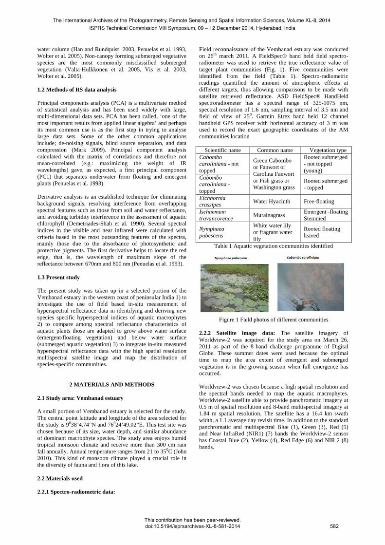
Field reconnaissance of the Vembanad estuary was conducted on 26th march 2011. A FieldSpec® hand held field spectro-radiometer was used to retrieve the true reflectance value of target plant communities (Fig. 1). Five communities were identified from the field (Table 1). Spectro-radiometric readings quantified the amount of atmospheric effects at different targets, thus allowing comparisons to be made with satellite retrieved reflectance. ASD FieldSpec® HandHeld spectroradiometer has a spectral range of 325-1075 nm, spectral resolution of 1.6 nm, sampling interval of 3.5 nm and field of view of 250. Garmin Etrex hand held 12 channel handheld GPS receiver with horizontal accuracy of 3 m was used to record the exact geographic coordinates of the AM communities location
Scientific name Common name Vegetation type Cabombo caroliniana - not topped
Rooted submerged - not topped (young)
Cabombo caroliniana - topped
Green Cabombo or Fanwort or Carolina Fanwort or Fish grass or Washington grass
Rooted submerged - topped
Eichhornia crassipes Water Hyacinth Free-floating
Ischaemum travancorence Murainagrass Emergent -floating
Stemmed
Nymphaea pubescens
White water lily or fragrant water lily
Rooted floating leaved
Table 1 Aquatic vegetation communities identified
Figure 1 Field photos of different communities
2.2.2 Satellite image data: The satellite imagery of Worldview-2 was acquired for the study area on March 26, 2011 as part of the 8-band challenge programme of Digital Globe. These summer dates were used because the optimal time to map the area extent of emergent and submerged vegetation is in the growing season when full emergence has occurred. Worldview-2 was chosen because a high spatial resolution and the spectral bands needed to map the aquatic macrophytes. Worldview-2 satellite able to provide panchromatic imagery at 0.5 m of spatial resolution and 8-band multispectral imagery at 1.84 m spatial resolution. The satellite has a 16.4 km swath width, a 1.1 average day revisit time. In addition to the standard panchromatic and multispectral Blue (1), Green (3), Red (5) and Near InfraRed (NIR1) (7) bands the Worldview-2 sensor has Coastal Blue (2), Yellow (4), Red Edge (6) and NIR 2 (8) bands.
The International Archives of the Photogrammetry, Remote Sensing and Spatial Information Sciences, Volume XL-8, 2014ISPRS Technical Commission VIII Symposium, 09 – 12 December 2014, Hyderabad, India
This contribution has been peer-reviewed. doi:10.5194/isprsarchives-XL-8-581-2014
582
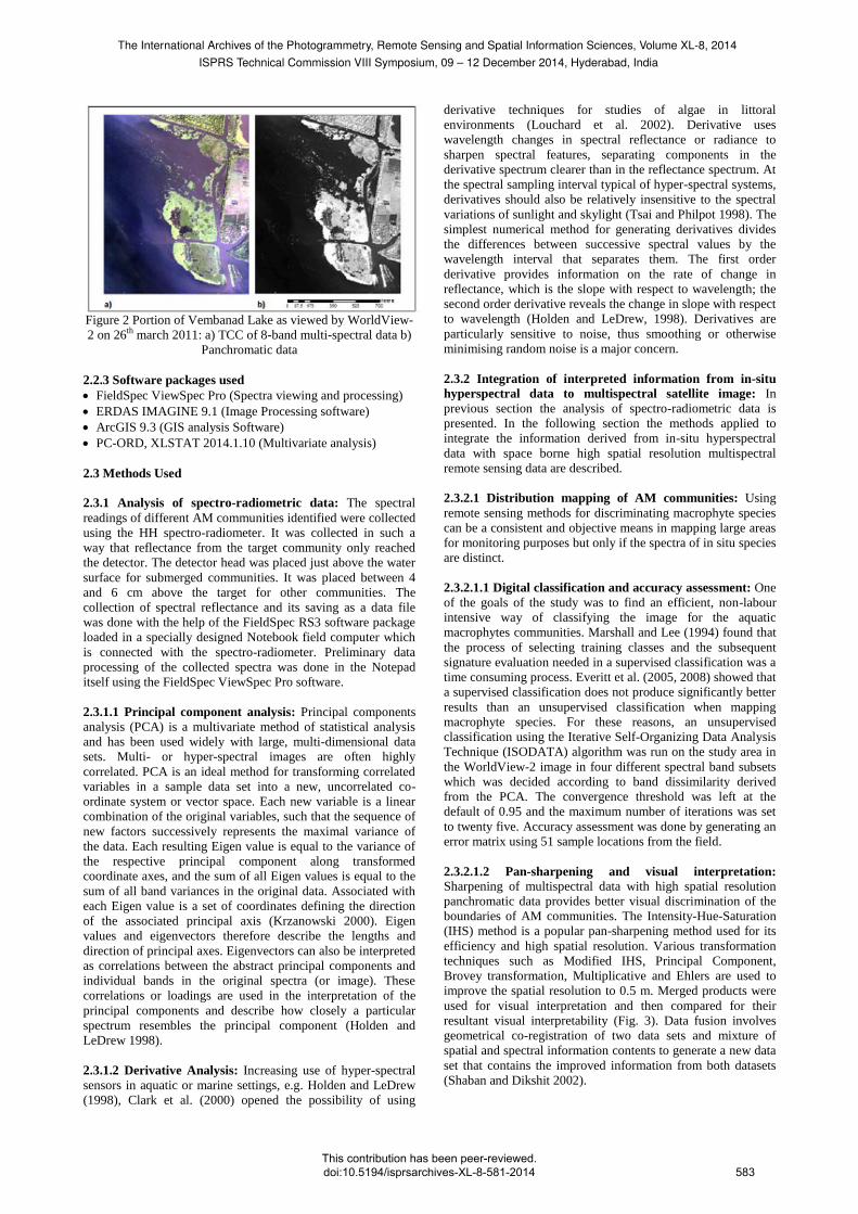
Figure 2 Portion of Vembanad Lake as viewed by WorldView-2 on 26th march 2011: a) TCC of 8-band multi-spectral data b)
Panchromatic data 2.2.3 Software packages used FieldSpec ViewSpec Pro (Spectra viewing and processing) ERDAS IMAGINE 9.1 (Image Processing software) ArcGIS 9.3 (GIS analysis Software) PC-ORD, XLSTAT 2014.1.10 (Multivariate analysis) 2.3 Methods Used 2.3.1 Analysis of spectro-radiometric data: The spectral readings of different AM communities identified were collected using the HH spectro-radiometer. It was collected in such a way that reflectance from the target community only reached the detector. The detector head was placed just above the water surface for submerged communities. It was placed between 4 and 6 cm above the target for other communities. The collection of spectral reflectance and its saving as a data file was done with the help of the FieldSpec RS3 software package loaded in a specially designed Notebook field computer which is connected with the spectro-radiometer. Preliminary data processing of the collected spectra was done in the Notepad itself using the FieldSpec ViewSpec Pro software. 2.3.1.1 Principal component analysis: Principal components analysis (PCA) is a multivariate method of statistical analysis and has been used widely with large, multi-dimensional data sets. Multi- or hyper-spectral images are often highly correlated. PCA is an ideal method for transforming correlated variables in a sample data set into a new, uncorrelated co-ordinate system or vector space. Each new variable is a linear combination of the original variables, such that the sequence of new factors successively represents the maximal variance of the data. Each resulting Eigen value is equal to the variance of the respective principal component along transformed coordinate axes, and the sum of all Eigen values is equal to the sum of all band variances in the original data. Associated with each Eigen value is a set of coordinates defining the direction of the associated principal axis (Krzanowski 2000). Eigen values and eigenvectors therefore describe the lengths and direction of principal axes. Eigenvectors can also be interpreted as correlations between the abstract principal components and individual bands in the original spectra (or image). These correlations or loadings are used in the interpretation of the principal components and describe how closely a particular spectrum resembles the principal component (Holden and LeDrew 1998). 2.3.1.2 Derivative Analysis: Increasing use of hyper-spectral sensors in aquatic or marine settings, e.g. Holden and LeDrew (1998), Clark et al. (2000) opened the possibility of using
derivative techniques for studies of algae in littoral environments (Louchard et al. 2002). Derivative uses wavelength changes in spectral reflectance or radiance to sharpen spectral features, separating components in the derivative spectrum clearer than in the reflectance spectrum. At the spectral sampling interval typical of hyper-spectral systems, derivatives should also be relatively insensitive to the spectral variations of sunlight and skylight (Tsai and Philpot 1998). The simplest numerical method for generating derivatives divides the differences between successive spectral values by the wavelength interval that separates them. The first order derivative provides information on the rate of change in reflectance, which is the slope with respect to wavelength; the second order derivative reveals the change in slope with respect to wavelength (Holden and LeDrew, 1998). Derivatives are particularly sensitive to noise, thus smoothing or otherwise minimising random noise is a major concern. 2.3.2 Integration of interpreted information from in-situ hyperspectral data to multispectral satellite image: In previous section the analysis of spectro-radiometric data is presented. In the following section the methods applied to integrate the information derived from in-situ hyperspectral data with space borne high spatial resolution multispectral remote sensing data are described. 2.3.2.1 Distribution mapping of AM communities: Using remote sensing methods for discriminating macrophyte species can be a consistent and objective means in mapping large areas for monitoring purposes but only if the spectra of in situ species are distinct. 2.3.2.1.1 Digital classification and accuracy assessment: One of the goals of the study was to find an efficient, non-labour intensive way of classifying the image for the aquatic macrophytes communities. Marshall and Lee (1994) found that the process of selecting training classes and the subsequent signature evaluation needed in a supervised classification was a time consuming process. Everitt et al. (2005, 2008) showed that a supervised classification does not produce significantly better results than an unsupervised classification when mapping macrophyte species. For these reasons, an unsupervised classification using the Iterative Self-Organizing Data Analysis Technique (ISODATA) algorithm was run on the study area in the WorldView-2 image in four different spectral band subsets which was decided according to band dissimilarity derived from the PCA. The convergence threshold was left at the default of 0.95 and the maximum number of iterations was set to twenty five. Accuracy assessment was done by generating an error matrix using 51 sample locations from the field. 2.3.2.1.2 Pan-sharpening and visual interpretation: Sharpening of multispectral data with high spatial resolution panchromatic data provides better visual discrimination of the boundaries of AM communities. The Intensity-Hue-Saturation (IHS) method is a popular pan-sharpening method used for its efficiency and high spatial resolution. Various transformation techniques such as Modified IHS, Principal Component, Brovey transformation, Multiplicative and Ehlers are used to improve the spatial resolution to 0.5 m. Merged products were used for visual interpretation and then compared for their resultant visual interpretability (Fig. 3). Data fusion involves geometrical co-registration of two data sets and mixture of spatial and spectral information contents to generate a new data set that contains the improved information from both datasets (Shaban and Dikshit 2002).
The International Archives of the Photogrammetry, Remote Sensing and Spatial Information Sciences, Volume XL-8, 2014ISPRS Technical Commission VIII Symposium, 09 – 12 December 2014, Hyderabad, India
This contribution has been peer-reviewed. doi:10.5194/isprsarchives-XL-8-581-2014
583
2.3.2.1.3 Generation of spectral indices: Normalized Difference Vegetation Index (NDVI) was calculated using the red and NIR bands of the satellite imagery with the following formula: NDVI = (NIR – RED) / (NIR + RED). The value range of an NDVI is -1 to 1 where healthy vegetation generally falls between values of 0.20 to 0.80. Previous studies have shown that NDVI has positive correlation with aquatic macrophyte plant cover (Jakubauskas et al. 2000, Penuelas et al. 1993) and can be used to help differentiate vegetation and other surfaces from one another (Ozesmi and Bauer 2002). Because the NDVI is a ratio, it reduces many forms of multiplicative noise such as shadows. In this study in addition to existing vegetation indices certain new indices were generated using NIR-1, RED and Red-edge bands. hyperspectral vegetation indices were manually calculated using the result of PCA to identify species-assemblage wise indices. Eichhornia crassipes and Ischaemum travancorense showed highest reflectance variance in 810 – 900 nm and is quantified by the following equation: NDVI (810-900) = R900-R810/R900+R810 SR (810-900) = R900/R810 Cabombo caroliniana (mature), Cabombo caroliniana (young) and Nymphaea pubescens showed highest variance in the reflectance values at 325- 327 nm, 702 – 717 nm and 739 - 741 respectively, and are quantified by the following equations: NDVI (325-327) = R327-R325/R327+R325 NDVI (702-717) = R717-R702/R717+R702 NDVI (739-741) = R741-R739/R741+R739 SR (325-327) = R327-R325 SR (702-717) = R717-R702 SR (741-7397) = R741/R739
Figure 3 Flowchart of the overall methodology adopted
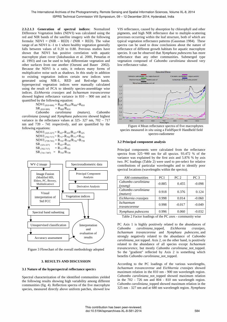
3. RESULTS AND DISCUSSION 3.1 Nature of the hyperspectral reflectance spectra Spectral characterization of the identified communities yielded the following results showing high variability among different communities (fig. 4). Reflection spectra of the five macrophyte species, measured directly above uniform patches, showed low
VIS reflectance, caused by absorption by chlorophyll and other pigments, and high NIR reflectance due to multiple-scattering processes occurring within the leaf structure, both of which are typical vegetation reflectance patterns (Gausman 1984). These spectra can be used to draw conclusions about the nature of reflectance of different growth habitats for aquatic macrophyte species. It can be observed that Nymphaea pubescens has more reflectance than any other communities. Submerged type vegetation composed of Cabombo caroliniana showed very low reflectance value.
Figure 4 Mean reflectance spectra of five macrophytes species measured in situ using a FieldSpec® Handheld field
spectro-radiometer
3.2 Principal component analysis Principal components were calculated from the reflectance spectra from 325−900 nm for all species. 93.472 % of the variance was explained by the first axis and 5.876 % by axis two. PC loadings (Table 2) were used to pre-select for relative contributions of particular wavelengths and to identify poor spectral locations (wavelengths within the spectra).
AM communities PC1 PC 2 PC 3 Cabombo caroliniana (young) -0.885 0.455 -0.098
Cabombo caroliniana (mature) 0.918 0.376 0.124
Eichhornia crassipes 0.998 0.014 -0.060 Ischaemum travancorense 0.998 -0.017 -0.049
Nymphaea pubescens 0.996 0.060 -0.032 Table 2 Factor loadings of the PC axes - community wise
PC Axis 1 is highly positively related to the abundances of Cabombo caroliniana_topped, Eichhornia crassipes, Ischaemum travancorense and Nymphaea pubescens, and strongly negatively related to the abundance of Cabombo caroliniana_not topped. Axis 2, on the other hand, is positively related to the abundance of all species except Ischaemum travancorence, but mostly Cabombo caroliniana_not_topped. So the "gradient" reflected by Axis 2 is something which benefits Cabombo caroliniana_not_topped. According to the PC loadings of the various wavelengths, Ischaemum travancorense and Eichhornia crassipes showed maximum relation in the 810 nm - 900 nm wavelength region. Cabombo caroliniana_not_topped showed maximum relation in the 702 - 726 nm and 804 - 810 nm wavelength region. Cabombo caroliniana_topped showed maximum relation in the 325 nm - 327 nm and at 680 nm wavelength region. Nymphaea
WV-2 image
Image Fusion (Modified HIS,
Ehlers, PC, Brovey, Multiplicative)
Visual interpretation of
Std FCC
Spectral band subsetting
Unsupervised classification
Accuracy assessment
Spectroradiometric data
Vegetation indices
Principal Component Analysis
Derivative Analysis
Interpretation and
evaluation of results
The International Archives of the Photogrammetry, Remote Sensing and Spatial Information Sciences, Volume XL-8, 2014ISPRS Technical Commission VIII Symposium, 09 – 12 December 2014, Hyderabad, India
This contribution has been peer-reviewed. doi:10.5194/isprsarchives-XL-8-581-2014
584
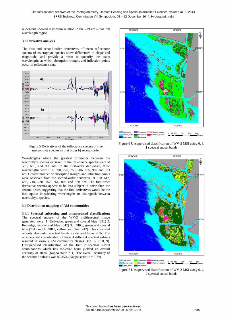
pubescens showed maximum relation in the 739 nm – 741 nm wavelength region. 3.3 Derivative analysis The first and second-order derivatives of mean reflectance spectra of macrophyte species show differences in shape and magnitude, and provide a mean to quantify the exact wavelengths at which absorption troughs and inflection points occur in reflectance data.
Figure 5 Derivatives of the reflectance spectra of five macrophyte species a) first order b) second-order
Wavelengths where the greatest difference between the macrophyte species occurred in the reflectance spectra were at 505, 685, and 930 nm. In the first-order derivative, these wavelengths were 510, 690, 720, 756, 806, 885, 907 and 923 nm. Greater number of absorption troughs and inflection points were observed from the second-order derivative, at 510, 612, 686, 710, 720, 752, 764, 802 and 930 nm. The first-order derivative spectra appear to be less subject to noise than the second-order, suggesting that the first derivatives would be the best option in selecting wavelengths to distinguish between macrophyte species.
3.4 Distribution mapping of AM communities
3.4.1 Spectral subsetting and unsupervised classification: The spectral subsets of the WV-2 multispectral image generated were: 1. Red-edge, green and coastal blue (631) 2. Red-edge, yellow and blue (642) 3. NIR1, green and coastal blue (731) and 4. NIR1, yellow and blue (742). This consisted of only dissimilar spectral bands as derived from PCA. The unsupervised classification of these 4 different spectral subsets resulted in various AM community classes (Fig. 6, 7, 8, 9). Unsupervised classification of the first 2 spectral subset combinations which has red-edge band yielded an overall accuracy of 100% (Kappa static = 1). The overall accuracy of the second 2 subsets was 82.35% (Kappa statistic = 0.79).
Figure 6 Unsupervised classification of WV-2 MSI using 6, 3,
1 spectral subset bands
Figure 7 Unsupervised classification of WV-2 MSI using 6, 4,
2 spectral subset bands
a)
b)
The International Archives of the Photogrammetry, Remote Sensing and Spatial Information Sciences, Volume XL-8, 2014ISPRS Technical Commission VIII Symposium, 09 – 12 December 2014, Hyderabad, India
This contribution has been peer-reviewed. doi:10.5194/isprsarchives-XL-8-581-2014
585
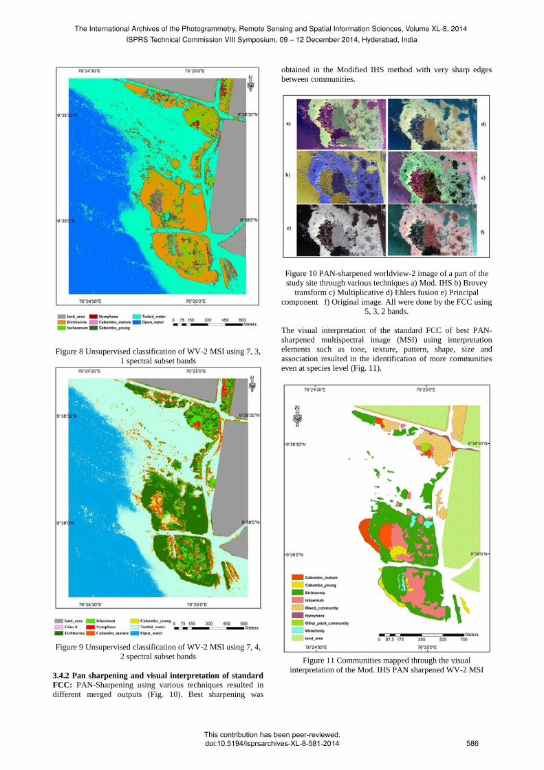
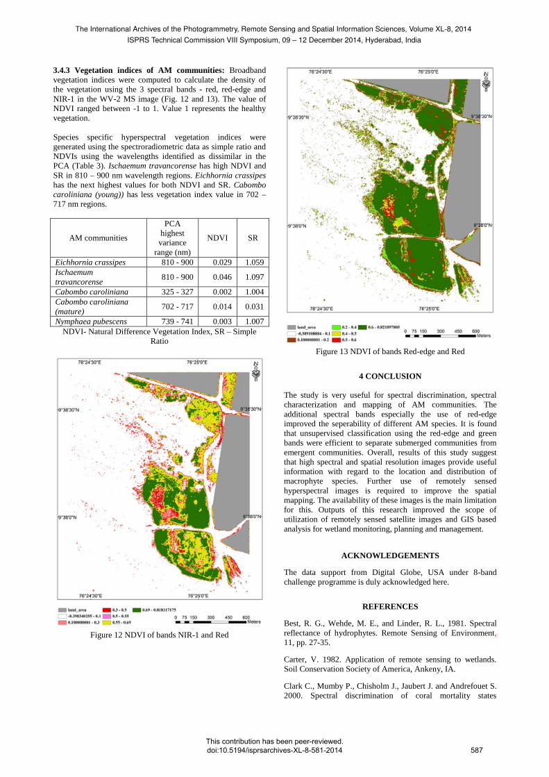
Figure 8 Unsupervised classification of WV-2 MSI using 7, 3,
1 spectral subset bands
Figure 9 Unsupervised classification of WV-2 MSI using 7, 4,
2 spectral subset bands 3.4.2 Pan sharpening and visual interpretation of standard FCC: PAN-Sharpening using various techniques resulted in different merged outputs (Fig. 10). Best sharpening was
obtained in the Modified IHS method with very sharp edges between communities.
Figure 10 PAN-sharpened worldview-2 image of a part of the study site through various techniques a) Mod. IHS b) Brovey
transform c) Multiplicative d) Ehlers fusion e) Principal component f) Original image. All were done by the FCC using
5, 3, 2 bands.
The visual interpretation of the standard FCC of best PAN-sharpened multispectral image (MSI) using interpretation elements such as tone, texture, pattern, shape, size and association resulted in the identification of more communities even at species level (Fig. 11).
Figure 11 Communities mapped through the visual
interpretation of the Mod. IHS PAN sharpened WV-2 MSI
The International Archives of the Photogrammetry, Remote Sensing and Spatial Information Sciences, Volume XL-8, 2014ISPRS Technical Commission VIII Symposium, 09 – 12 December 2014, Hyderabad, India
This contribution has been peer-reviewed. doi:10.5194/isprsarchives-XL-8-581-2014
586
3.4.3 Vegetation indices of AM communities: Broadband vegetation indices were computed to calculate the density of the vegetation using the 3 spectral bands - red, red-edge and NIR-1 in the WV-2 MS image (Fig. 12 and 13). The value of NDVI ranged between -1 to 1. Value 1 represents the healthy vegetation. Species specific hyperspectral vegetation indices were generated using the spectroradiometric data as simple ratio and NDVIs using the wavelengths identified as dissimilar in the PCA (Table 3). Ischaemum travancorense has high NDVI and SR in 810 – 900 nm wavelength regions. Eichhornia crassipes has the next highest values for both NDVI and SR. Cabombo caroliniana (young)) has less vegetation index value in 702 – 717 nm regions.
AM communities
PCA highest variance
range (nm)
NDVI SR
Eichhornia crassipes 810 - 900 0.029 1.059 Ischaemum travancorense 810 - 900 0.046 1.097
Cabombo caroliniana 325 - 327 0.002 1.004 Cabombo caroliniana (mature) 702 - 717 0.014 0.031
Nymphaea pubescens 739 - 741 0.003 1.007 NDVI- Natural Difference Vegetation Index, SR – Simple
Ratio
Figure 12 NDVI of bands NIR-1 and Red
Figure 13 NDVI of bands Red-edge and Red
4 CONCLUSION
The study is very useful for spectral discrimination, spectral characterization and mapping of AM communities. The additional spectral bands especially the use of red-edge improved the seperability of different AM species. It is found that unsupervised classification using the red-edge and green bands were efficient to separate submerged communities from emergent communities. Overall, results of this study suggest that high spectral and spatial resolution images provide useful information with regard to the location and distribution of macrophyte species. Further use of remotely sensed hyperspectral images is required to improve the spatial mapping. The availability of these images is the main limitation for this. Outputs of this research improved the scope of utilization of remotely sensed satellite images and GIS based analysis for wetland monitoring, planning and management.
ACKNOWLEDGEMENTS
The data support from Digital Globe, USA under 8-band challenge programme is duly acknowledged here.
REFERENCES Best, R. G., Wehde, M. E., and Linder, R. L., 1981. Spectral reflectance of hydrophytes. Remote Sensing of Environment, 11, pp. 27-35. Carter, V. 1982. Application of remote sensing to wetlands. Soil Conservation Society of America, Ankeny, IA. Clark C., Mumby P., Chisholm J., Jaubert J. and Andrefouet S. 2000. Spectral discrimination of coral mortality states
The International Archives of the Photogrammetry, Remote Sensing and Spatial Information Sciences, Volume XL-8, 2014ISPRS Technical Commission VIII Symposium, 09 – 12 December 2014, Hyderabad, India
This contribution has been peer-reviewed. doi:10.5194/isprsarchives-XL-8-581-2014
587
following a severe bleaching event. International Journal of Remote Sensing, 21: 2321–2327. Everitt, J. H., Yang, C., Escobar, D. E., Webster, C. F., Lonard, R. I. and Davis, M. R. 1999. Using remote sensing and spatial information technologies to detect and map two aquatic macrophytes. Journal of Aquatic Plant Management, 37, pp. 71-80. Everitt, J. H., Davis, M. R. and Nibling, F. L., 2007. Using spatial information technologies for detecting and mapping Eurasian water milfoil. Journal of Geocarto International, 22(1), pp. 49-61. Everitt, J. H., Fletcher, R. S., Elder, H. S. and Yang, C. 2008. Mapping Giant Salvinia with satellite imagery and image analysis. Environmental Monitoring and Assessment, 139, pp. 35-40. Fung T., Fung H., Ma Y. and Siu W. L. 2003. Band selection using hyper-spectral data of subtropical tree species. Journal of Geocarto International, 18(4), pp. 3-12. Gausman, H. 1984. Evaluation of factors causing reflectance differences between sun and shade leaves. Remote Sensing of Environment, 15, pp.177–181. Ge S, Everitt J. H., Carruthers R., Gong P. and Anderson G. 2006. Hyper-spectral characteristics of canopy components and structure for phenological assessment of an invasive weed. Environmental Monitoring and Assessment, 120: 109-126. Holden, H., and LeDrew, E., 1998. Spectral discrimination of healthy and non-healthy corals based on cluster analysis, principal components analysis, and derivative spectroscopy. Remote Sensing of Environment, 65, pp. 217–224. Jakubauskas M. E., Peterson D. L., Campbell S. W., Campbell S.D., Penny D. and deNoyelles F. Jr. 2002. Remote sensing of aquatic plant obstructions in navigable waterways. Proceedings of 2002 ASPRS-ACSM Annual Conference and FIG XXII Congress, April 22-25, 2002, Washington, D.C. John, C. M., 2010. A taxonomic and ecological study of the aquatic macrophytes of Kuttanad wetlands with special reference to spatial and temporal distribution using remote sensing and GIS techniques. PhD Thesis, Mahatma Gandhi University, Kottayam. Krzanowski, W., 2000. Principles of multivariate analysis. A user’s perspective. Number 22 in Oxford Statistical Science Series. Oxford University Press Inc., New York, USA. Mark Richardson. 2009. Principal Component Analysis. Oxford University Press Marshall, T., and Lee, P., 1994. Mapping aquatic macrophytes through digital image-analysis of aerial photographs - an assessment. Journal of Aquatic Plant Management, 32, pp. 61–66. Martyn, R. D., Noble, R. L., Bettoli, P. W. and Maggio, R. C. 1986. Mapping aquatic weeds with aerial color-infrared photography and evaluating their control by grass carp. Journal of Aquatic Plant Management, 24, pp. 46-56. Louchard E., Reid R., Stephens C., Davis C., Leathers R. and Downes, T. 2002. Derivative analysis of absorption features in
hyper-spectral remote sensing data of carbonate sediment. Optics Express, 10(26): 1573–1584. Ozesmi S. L. and Bauer M. E. 2002. Satellite remote sensing of wetlands. Wetlands Ecology and Management, 10: 381-402. Penuelas J., Gramon J. A., Griffin K. L. and Field C. B. 1993. Assessing community type, plant biomass, pigment composition and photosynthetic efficiency of aquatic vegetation from spectral reflectance. Remote Sensing of Environment, 46: 110-118. Shaban, M. A., and Dikshit, O., 2002. Evaluation of the merging of SPOT multispectral and panchromatic data for classification of an urban environment. International Journal of Remote Sensing, 23, pp. 249–262. Thenkabail P. S., Smith R. B. and De Pauw E. 2000. Hyper-spectral vegetation indices and their relationship with agricultural crops. Remote Sensing of Environment, 71: 158-182. Tiner R. W. 1997. Wetlands, pp. 475-494. In: W. R. Philipson (ed.), Manual of Photographic Interpretation, 2nd edition, American Society of Photogrammetry and Remote Sensing, Bethesda, MD. Tsai F. and Philpot W. 1998. Derivative analysis of hyper-spectral data. Remote Sensing of Environment, 66: 41–51. Tueller, P. T., 1982. Remote sensing for range management. Pages 125-140 in: Johannsen C. J. and Sanders J. L. (Eds.). Remote Sensing for Resource Management. Soil Conservation Society of America, Ankeny, IA. Turner W., Spectro S., Gardiner N., Fladeland M., Sterling E. and Sterninger M. 2003. Remote sensing for biodiversity science and conservation. Trends in Ecology & Evolution, 18: 306-314. Ullah A., Rundquist D. C. and Derry D. P. 2000. Characterizing spectral signatures for three selected emergent aquatic macrophytes: a controlled experiment. Geocarto International, 15(4): 29-39. Underwood E., M. J. Mulitsch, J. A. Greenberg, M. L. Whiting, S. L. Ustin and Kefauver S. C. 2006. Mapping invasive aquatic vegetation in the Sacramento-San Joaquin Delta using hyper-spectral imagery. Environmental Monitoring and Assessment, 121: 47-64. Vis C., C. Hudon. and R. Carignan. 2003. An evaluation of approaches used to determine the distribution and biomass of emergent and submerged aquatic macrophytes over large spatial scales. Aquatic Botany, 77: 187-201. Wolter P.T., C. A. Johnston. and Niemi G. J. 2005. Mapping submerged aquatic vegetation in the US Great Lakes using Quickbird satellite data. International Journal of Remote Sensing, 26(23), pp. 5255-5274. Yang C., Everitt J. H., Fletcher R. S., Jensen R. R. and Mausel P. W. 2009. Evaluating AISA+ hyper-spectral imagery for mapping black mangrove along the South Texas Gulf Coast. Journal of Photogrammetric Engineering & Remote Sensing, 75: 424-435.
The International Archives of the Photogrammetry, Remote Sensing and Spatial Information Sciences, Volume XL-8, 2014ISPRS Technical Commission VIII Symposium, 09 – 12 December 2014, Hyderabad, India
This contribution has been peer-reviewed. doi:10.5194/isprsarchives-XL-8-581-2014
588