Integration of Local Positioning System & Strapdown Inertial ...
137
Integration of Local Positioning System & Strapdown Inertial Navigation System for Hand-Held Tool Tracking by Neda Parnian A thesis presented to the University of Waterloo in fulfillment of the thesis requirement for the degree of Doctor of Philosophy in Electrical and Computer Engineering Waterloo, Ontario, Canada, 2008 ©Neda Parnian 2008
Transcript of Integration of Local Positioning System & Strapdown Inertial ...

Integration of Local Positioning System &
Strapdown Inertial Navigation System
for Hand-Held Tool Tracking
by
Neda Parnian
A thesis
presented to the University of Waterloo
in fulfillment of the
thesis requirement for the degree of
Doctor of Philosophy
in
Electrical and Computer Engineering
Waterloo, Ontario, Canada, 2008
©Neda Parnian 2008

ii
AUTHOR'S DECLARATION
I hereby declare that I am the sole author of this thesis. This is a true copy of the thesis, including any
required final revisions, as accepted by my examiners.
I understand that my thesis may be made electronically available to the public.
iii
Abstract
This research concerns the development of a smart sensory system for tracking a hand-held moving
device to millimeter accuracy, for slow or nearly static applications over extended periods of time.
Since different operators in different applications may use the system, the proposed design should
provide the accurate position, orientation, and velocity of the object without relying on the knowledge
of its operation and environment, and based purely on the motion that the object experiences. This
thesis proposes the design of the integration a low-cost Local Positioning System (LPS) and a low-
cost StrapDown Inertial Navigation System (SDINS) with the association of the modified EKF to
determine 3D position and 3D orientation of a hand-held tool within a required accuracy.
A hybrid LPS/SDINS combines and complements the best features of two different navigation
systems, providing a unique solution to track and localize a moving object more precisely. SDINS
provides continuous estimates of all components of a motion, but SDINS loses its accuracy over time
because of inertial sensors drift and inherent noise. LPS has the advantage that it can possibly get
absolute position and velocity independent of operation time; however, it is not highly robust, is
computationally quite expensive, and exhibits low measurement rate.
This research consists of three major parts: developing a multi-camera vision system as a reliable
and cost-effective LPS, developing a SDINS for a hand-held tool, and developing a Kalman filter for
sensor fusion.
Developing the multi-camera vision system includes mounting the cameras around the workspace,
calibrating the cameras, capturing images, applying image processing algorithms and features
extraction for every single frame from each camera, and estimating the 3D position from 2D images.
In this research, the specific configuration for setting up the multi-camera vision system is
proposed to reduce the loss of line of sight as much as possible. The number of cameras, the position
of the cameras with respect to each other, and the position and the orientation of the cameras with
respect to the center of the world coordinate system are the crucial characteristics in this
configuration. The proposed multi-camera vision system is implemented by employing four CCD
cameras which are fixed in the navigation frame and their lenses placed on semicircle. All cameras
are connected to a PC through the frame grabber, which includes four parallel video channels and is
able to capture images from four cameras simultaneously.
iv
As a result of this arrangement, a wide circular field of view is initiated with less loss of line-of-
sight. However, the calibration is more difficult than a monocular or stereo vision system. The
calibration of the multi-camera vision system includes the precise camera modeling, single camera
calibration for each camera, stereo camera calibration for each two neighboring cameras, defining a
unique world coordinate system, and finding the transformation from each camera frame to the world
coordinate system.
Aside from the calibration procedure, digital image processing is required to be applied into the
images captured by all four cameras in order to localize the tool tip. In this research, the digital
image processing includes image enhancement, edge detection, boundary detection, and morphologic
operations. After detecting the tool tip in each image captured by each camera, triangulation
procedure and optimization algorithm are applied in order to find its 3D position with respect to the
known navigation frame.
In the SDINS, inertial sensors are mounted rigidly and directly to the body of the tracking object
and the inertial measurements are transformed computationally to the known navigation frame.
Usually, three gyros and three accelerometers, or a three-axis gyro and a three-axis accelerometer are
used for implementing SDINS. The inertial sensors are typically integrated in an inertial
measurement unit (IMU). IMUs commonly suffer from bias drift, scale-factor error owing to non-
linearity and temperature changes, and misalignment as a result of minor manufacturing defects.
Since all these errors lead to SDINS drift in position and orientation, a precise calibration procedure is
required to compensate for these errors.
The precision of the SDINS depends not only on the accuracy of calibration parameters but also on
the common motion-dependent errors. The common motion-dependent errors refer to the errors
caused by vibration, coning motion, sculling, and rotational motion. Since inertial sensors provide
the full range of heading changes, turn rates, and applied forces that the object is experiencing along
its movement, accurate 3D kinematics equations are developed to compensate for the common
motion-dependent errors. Therefore, finding the complete knowledge of the motion and orientation
of the tool tip requires significant computational complexity and challenges relating to resolution of
specific forces, attitude computation, gravity compensation, and corrections for common motion-
dependent errors.

v
The Kalman filter technique is a powerful method for improving the output estimation and
reducing the effect of the sensor drift. In this research, the modified EKF is proposed to reduce the
error of position estimation. The proposed multi-camera vision system data with cooperation of the
modified EKF assists the SDINS to deal with the drift problem. This configuration guarantees the
real-time position and orientation tracking of the instrument. As a result of the proposed Kalman
filter, the effect of the gravitational force in the state-space model will be removed and the error
which results from inaccurate gravitational force is eliminated. In addition, the resulting position is
smooth and ripple-free.
The experimental results of the hybrid vision/SDINS design show that the position error of the tool
tip in all directions is about one millimeter RMS. If the sampling rate of the vision system decreases
from 20 fps to 5 fps, the errors are still acceptable for many applications.

vi
Acknowledgements
This thesis represents four years of research work. During these years, I have been encouraged and
supported by many people, and I take this opportunity to express my gratitude to them.
First, I would like to express my deep and sincere gratitude to my supervisor, Prof. Farid
Golnaraghi, for giving me the opportunity to work in his group and for providing an excellent
research environment. I cannot imagine having a better advisor and mentor for my PhD than Prof.
Farid Golnaraghi. His confidence in me and in my capabilities gave me the inspiration to pursue my
research with great intensity. Without his expertise and knowledge, his sharp perceptiveness, and his
tireless support, I would never have completed this thesis.
I would also like to thank the members of my PhD committee who read and provided valuable
comments on earlier versions of this thesis: Prof. Robert Gorbet, Prof. William W. Melek, Prof.
Hamid R. Tizhoosh, and Prof. Khashayar Khorasani – I thank you all.
I would like to extend my special thanks to Robert Wagner, CNC technician, for his broad
technical advice and support in configuring my test set-up. Also, my sincere appreciation goes to the
Jason Benninger and John Potzold, Engineering machine shop technicians, for their assistance in
creating the hand-held tool.
My warm thanks go to Steve Hitchman and Martha Morales, Computer Specialists, for their kind
support in configuring, installing required software on, and maintaining my project PC.
I wish to express my warm and sincere thanks to my friends who created a friendly and pleasant
atmosphere, including frequent social gatherings that helped my family and me not to feel lonely and
depressed at living far away from our home town.
I appreciate the Ministry of Science, Research, and Technology of the Islamic Republic of Iran for
sponsoring my PhD studies.
I cannot end without thanking my family for their constant encouragement and love. I wish to
express my deepest and warmest gratitude to my parents for giving me life in the first place, for
providing me the best education possible, and for their unconditional support and encouragement as I
pursued my interests – even when these interests went beyond boundaries of language and geography.

vii
My endless thanks are also extended to my brother, Navid, for his loving support. I am deeply
indebted to him for taking care of my parents and giving them additional love when I was absent.
I owe my loving thanks to my husband, Habib, for his love and patience during my PhD studies. I
am most grateful to him for leaving his job to give me the opportunity to continue my education, for
helping me in taking care of my children, for listening to my complaints and frustrations, and at last,
for believing in me. Without his encouragement and understanding it would have been impossible
for me to finish this work.
Last but not the least, I would like to extend my special love to my sons, Hatef and Aref, who
instill me with delightful energy and inspiration whenever I feel exhausted and frustrated – and fill
my life with charm, joy, and happiness.

viii
Dedication
I dedicate this thesis to my parents, my husband, and my sons. I would not have been able to
complete my PhD studies and this thesis without their unconditional love, support, encouragement,
and great patience. I deeply value their true love and concern.

ix
Table of Contents List of Figures ...................................................................................................................................... xii
List of Tables ........................................................................................................................................ xv
Chapter 1 Introduction ............................................................................................................................ 1
1.1 Thesis Overview ........................................................................................................................... 2
1.2 Literature Survey .......................................................................................................................... 3
1.2.1 Medical Application .............................................................................................................. 3
1.2.2 Sensor Drift and Solutions ..................................................................................................... 4
1.2.3 Local Positioning System (LPS)............................................................................................ 6
1.3 Research Objective ....................................................................................................................... 9
1.3.1 New Contribution ................................................................................................................ 10
1.3.2 Publications ......................................................................................................................... 13
1.4 Summary .................................................................................................................................... 14
Chapter 2 Strapdown Inertial Navigation System ................................................................................ 16
2.1 Inertial Measurement Unit (IMU) .............................................................................................. 17
2.1.1 IMU Calibration .................................................................................................................. 17
2.1.2 Rate Gyros and Accelerometers Output Modeling .............................................................. 18
2.1.3 Thermal Tests ...................................................................................................................... 20
2.2 Navigation Equations ................................................................................................................. 21
2.2.1 Reference Frames ................................................................................................................ 21
2.2.2 Motion Analysis .................................................................................................................. 22
2.2.3 Relative-Motion Analysis Using Translating and Rotating Axes ....................................... 25
2.2.4 Direction Cosine Matrix ...................................................................................................... 30
2.2.5 Quaternion ........................................................................................................................... 32
2.2.6 Attitude Compensation ........................................................................................................ 34
2.2.7 Effect of Earth Rotation ....................................................................................................... 35
2.2.8 Physiological Hand Tremor ................................................................................................. 35
2.2.9 State-Space of the System ................................................................................................... 36
2.3 Experimental Result ................................................................................................................... 37
2.3.1 IMU Calibration .................................................................................................................. 37
2.3.2 Noise and Physiological Hand Tremor Compensation ........................................................ 39
2.3.3 Compensation for the Common Motion-Dependent Errors ................................................ 41

x
2.3.4 Acceleration Computation .................................................................................................. 43
2.3.5 Attitude Computation .......................................................................................................... 46
2.4 Summary .................................................................................................................................... 48
Chapter 3 Local Positioning System .................................................................................................... 49
3.1 Multi-Camera Vision System..................................................................................................... 49
3.1.1 Configuration ...................................................................................................................... 50
3.1.2 Camera Modeling ................................................................................................................ 53
3.1.3 Single Camera Calibration .................................................................................................. 56
3.1.4 Stereo Camera Calibration .................................................................................................. 58
3.1.5 Defining the World Coordinate System .............................................................................. 58
3.2 Digital Image Processing ........................................................................................................... 59
3.2.1 Image Enhancement ............................................................................................................ 60
3.2.2 Edge Detection .................................................................................................................... 61
3.2.3 Boundary Extraction ........................................................................................................... 63
3.2.4 Morphologic Operations ..................................................................................................... 63
3.3 Experimental Results ................................................................................................................. 65
3.3.1 Configuration Setup ............................................................................................................ 66
3.3.2 Single Calibration ............................................................................................................... 67
3.3.3 Stereo Calibration ............................................................................................................... 77
3.3.4 Image Processing ................................................................................................................ 77
3.3.5 Tool Tracking ...................................................................................................................... 83
3.4 Summary .................................................................................................................................... 91
Chapter 4 Extended Kalman Filter ....................................................................................................... 92
4.1 General Extended Kalman Filter ................................................................................................ 93
4.1.1 System Model ..................................................................................................................... 93
4.1.2 Measurement Model ........................................................................................................... 94
4.1.3 Extended Kalman Filter Equations ..................................................................................... 94
4.2 Modified Extended Kalman Filter ............................................................................................. 96
4.2.1 System Model ..................................................................................................................... 96
4.2.2 Measurement Model ......................................................................................................... 100
4.3 Experimental Result ................................................................................................................. 101
4.4 Summary .................................................................................................................................. 105

xi
Chapter 5 Conclusion and Future Work ............................................................................................. 106
5.1 Conclusion ................................................................................................................................ 106
5.2 Contributions ............................................................................................................................ 107
5.3 Future Work and Research ....................................................................................................... 109
Bibliography ....................................................................................................................................... 111
Appendix A Detailed Specification for MicroStrain IMU ................................................................. 121

xii
List of Figures Figure 1 - Gyros and accelerometers misalignments ........................................................................... 17
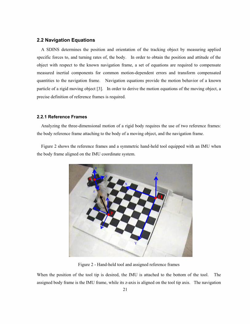
Figure 2 - Hand-held tool and assigned reference frames .................................................................... 21
Figure 3 - The effect of rotation about x-axis on the output of y-axis accelerometer. ......................... 23
Figure 4 - The effect of rotation about y-axis on the output of x-axis accelerometer. ......................... 23
Figure 5 - The effect of coning motion around z-axis on the output of x-axis accelerometer. ............ 24
Figure 6 - The effect of coning motion around z-axis on the output of y-axis accelerometer. ............ 24
Figure 7 - Relative position .................................................................................................................. 25
Figure 8 - Euler angels of the tool with respect to the NED frame ...................................................... 29
Figure 9 - Sensor’s output correction block diagram ........................................................................... 36
Figure 10 - Accelerometer bias without and with temperature compensation [ 80 79] ......................... 38
Figure 11 - Accelerometer gain without and with temperature compensation [ 79] ............................. 38
Figure 12 - Gyro bias without and with temperature compensation [ 79] ............................................ 38
Figure 13 - Gyro gain without and with temperature compensation [ 79] ............................................ 39
Figure 14 - The output of accelerometers: measured (left) denoised (right) ....................................... 40
Figure 15 - The output of gyros: measured (left) denoised (right)....................................................... 40
Figure 16 - Accelerometers outputs while the tool is experiencing the rotational motion around x-axis
............................................................................................................................................................. 41
Figure 17 - Accelerometers outputs while the tool is experiencing the rotational motion around y-axis
............................................................................................................................................................. 42
Figure 18 - Acceleration error when the tool rotating around x-axis ................................................... 42
Figure 19 - Acceleration error when the tool rotating around y-axis ................................................... 43
Figure 20 - Estimated acceleration vs. measured acceleration in x axis .............................................. 44
Figure 21 - Estimated acceleration vs. measured acceleration in y axis .............................................. 44
Figure 22 - Estimated acceleration vs. measured acceleration in z axis .............................................. 45
Figure 23 - Linear acceleration in x, y, and z axes .............................................................................. 46
Figure 24 - Quaternion: estimated (solid) vs. true (doted) .................................................................. 47
Figure 25 - Quaternion error ................................................................................................................ 47
Figure 26 - Euler angles error .............................................................................................................. 48
Figure 27 - Cameras configuration set up ............................................................................................ 50
Figure 28 - The field of view of a multi-camera vision system when the lenses of its cameras are
placed on a straight line ....................................................................................................................... 52
xiii
Figure 29 - The field of view of the proposed multi-camera vision system ......................................... 53
Figure 30 - Ideal camera imaging model .............................................................................................. 54
Figure 31 - Radial and tangential distortion ......................................................................................... 55
Figure 32 - Checkerboard with 5 cm×5 cm squares ............................................................................. 57
Figure 33 - The world coordinate system in the view of:
(a) camera #1 (b) camera #2 (c) camera #3 (d) camera #4 ................................................................... 59
Figure 34 - Spatial averaging window mask: (a) 3×3 window (b) 5-point weighted low-pass filter ... 60
Figure 35 - Edge operators: (a)&(b) pair gradient operators, (c)&(d) single Laplace operators .......... 62
Figure 36 - Pixel connectivity: (a) four-connected (b) eight-connected .............................................. 63
Figure 37 - Experimental setup for the multi-camera vision system .................................................... 66
Figure 38 - Calibration images for camera #1 as a left camera for camera #2 ..................................... 67
Figure 39 - Calibration images for camera #2 as a right camera for camera #1 ................................... 68
Figure 40 - Calibration images for camera #2 as a left camera for camera #3 ..................................... 68
Figure 41 - Calibration images for camera #3 as a right camera for camera #2 ................................... 69
Figure 42 - Calibration images for camera #3 as a left camera for camera #4 ..................................... 69
Figure 43 - Calibration images for camera #4 as a right camera for camera #3 ................................... 70
Figure 44 - Grid extraction for a sample image.................................................................................... 71
Figure 45 - Complete distortion model of camera #1 ........................................................................... 72
Figure 46 - Radial component of distortion model of camera #1 ......................................................... 73
Figure 47 - Tangential component of distortion model of camera #1 .................................................. 73
Figure 48 - Extrinsic parameters cam #1 in Figure 38: (left) camera-centered, (right) world-centered
.............................................................................................................................................................. 74
Figure 49 - Extrinsic parameters cam. #2 in Figure 39: (left) camera-centered, (right) world-centered
.............................................................................................................................................................. 74
Figure 50 - Extrinsic parameters cam. #2 in Figure 40: (left) camera-centered, (right) world-centered
.............................................................................................................................................................. 75
Figure 51 - Extrinsic parameters cam. #3 in Figure 41: (left) camera-centered, (right) world-centered
.............................................................................................................................................................. 75
Figure 52 - Extrinsic parameters cam. #3 in Figure 42: (left) camera-centered, (right) world-centered
.............................................................................................................................................................. 75
Figure 53 - Extrinsic parameters cam. #4 in Figure 43: (left) camera-centered, (right) world-centered
.............................................................................................................................................................. 76
xiv
Figure 54 - Original Image .................................................................................................................. 78
Figure 55 - Denoised image ................................................................................................................. 78
Figure 56 - Edge Enhancement ............................................................................................................ 79
Figure 57 - Contrast Enhancement....................................................................................................... 79
Figure 58 - Detected edge by gradient operator ................................................................................... 80
Figure 59 - Detected Edges .................................................................................................................. 81
Figure 60 - The effect of opening morphologic operations followed by closing operation ................. 81
Figure 61 - Extracted boundary of the tool tip ..................................................................................... 82
Figure 62 - Initial guess window mask for the position of tool tip ...................................................... 82
Figure 63 - Mask repositioning ............................................................................................................ 83
Figure 64 - Tool tip tracking by camera #1 ......................................................................................... 83
Figure 65 - Tool tip tracking by camera #2 ......................................................................................... 84
Figure 66 - Tool tip tracking by camera #3 ......................................................................................... 84
Figure 67 - Tool tip tracking by camera #4 ......................................................................................... 84
Figure 68 - Comparison of the positioning with the use of two cameras (1&2) and four cameras ..... 85
Figure 69 - Comparison of the positioning with the use of two cameras (2&3) and four cameras ..... 86
Figure 70 - Comparison of the positioning with the use of two cameras (3&4) and four cameras ..... 86
Figure 71 - The traced path by tool tip (red) in comparison with the pre-designed path (blue) .......... 88
Figure 72 - The location of the maximum errors occurred during video tracking ............................... 88
Figure 73 - Integration of SDINS and vision system with using EKF ................................................. 93
Figure 74 – The discrete difference of a Zero-mean Gaussian noise: .................................................. 98
Figure 75 - Estimated position by applying different estimation method: continuous EKF (left),
Switch EKF (center), and proposed EKF (right); when the sampling rate of the cameras is 16 fps. 103
Figure 76 - Estimated position by applying different estimation method: continuous EKF (left),
Switch EKF (center), and proposed EKF (right); when the sampling rate of the cameras is 5 fps. .. 104

xv
List of Tables Table 1 - Camera specifications ........................................................................................................... 65
Table 2 - Frame grabber specifications ................................................................................................ 66
Table 3 - Intrinsic parameters ............................................................................................................... 71
Table 4 - Transformation parameters from each camera frame to the world coordinate system ......... 76
Table 5 - Extrinsic parameters for each two adjacent cameras ............................................................ 77
Table 6 - The position error of the multi-camera vision system compared with each camera pair ...... 87
Table 7 - Magnified images of the maximum errors in the tool tip positioning ................................... 89
Table 8 - Positions estimated by different estimation methods are compared with the position
estimated by the multi-camera vision system ..................................................................................... 102
1
Chapter 1 Introduction
Over the past few decades, micro-electromechanical systems (MEMS) have been used in a wide
range of research areas. Recently, MEMS have found new applications in medicine, especially
surgery [ 1]. This technology provides real-time data, such as the surgical tool force, temperature,
position, or direction, to improve the functionality of the surgical devices. The real-time feedbacks
help surgeons to not only control the surgical procedure, but also develop new techniques for cutting
and extraction.
During a medical operation, a surgeon is interested in knowing the position and orientation of
surgical tools so as to control the surgery process with lowest possible risk. An endoscope is
traditionally used for localizing surgical instruments in a patient. The view of the tools is not always
ideal for estimating the position of an instrument precisely. Moreover, if the instrument is outside of
the camera’s view, then its position is unknown. Computer-aided surgery techniques deal with this
problem by providing 3D models. An imaging device, such as MRI or CAT, scans the patient body
during the operation and simulates 3D models with position and orientation to give a better view of
the surgical area.
Tracking system technologies in this area are solely optically-based. In these tracking system
techniques, two sets of markers are used for localization. Some markers are mounted on the surgical
tools for tracking, and some are located on the specific position on the body of the patient for
reference. Since the position of the reference markers are known, a computer can localize and align
the tools with the image of the patient’s body. The positions and orientations of the tool tips must be
estimated by extrapolating techniques; but because of bending of the tools as well as the compression
of tissues, these techniques are not precise and accurate. During a surgery, the markers must be in
the field of view of the camera system, and the surgeon must pay attention not to obstruct, with arms
or hands or surgical tools, the path from marker to cameras.
To deal with these issues, in this study a tracking system based on inertial sensors is proposed. As
the MEMS fabrication techniques miniaturize the inertial sensors in size and weight, then MEMS-
based inertial sensors can easily be mounted on a tool and do not interfere with the surgery.

2
The real-time states estimation of rigid bodies, including position, orientation, and velocity, has
been the focus of research for several decades. The principal reason for this interest is its application
in the guidance and navigation of aircraft and spacecraft and in robotics and automation. The best-
known way of deriving position and orientation in these systems is to use inertial navigation sensors,
which provide high frequency and continuous acceleration and rotation rate data. The inherent noise
and biases of the sensors lead to unbounded and exponential error that grows in time. Researchers
have long sought to aid inertial sensors with other sensors’ measurements [ 2, 3]. A hybrid Inertial
Navigation System (INS) can now provide a robust system with grouping of the best features of
different tracking technologies, and compensate for their limitations by using multiple measurements.
The integration of vision and inertial measurements is an attractive solution to address both system
problems. Vision measurements can be employed to reduce the INS drift that results from
integrating noisy and biased inertial measurements. However, a vision system can provide the
absolute position and velocity of a moving object independent of time, but, because of low
measurement rate, it is difficult to meet the high dynamic range of fast moving. In addition, the
image-based pose estimation is sensitive to the incorrect image feature tracking and camera modeling
errors. Nevertheless, highly precise cameras such as Optotrak [ 4] can track an object in a high
frequency and also provide the accurate position; these cameras are extremely expensive and are not
even easily portable for use in many applications. Besides, keeping the moving object in the field of
view requires the chaining of several of these cameras together.
This research proposes the integration of a low-cost multi-camera vision system and low-cost
MEMS-based inertial sensors to provide a robust and cost-effective system. The proposed multi-
camera vision system includes four common CCD cameras, with their lenses placed on an arc line.
Accordingly, the total workspace of the vision system is expanded compared with the straight line
configuration, an arrangement that reduces the possibility of the loss of the line-of-sight.
1.1 Thesis Overview
This thesis presents the development of the integration of the LPS/SDINS. The thesis is organized
as follows. The rest of Chapter 1 reviews previous related work and results. It also presents our
research and describes its application and its contribution to the state of knowledge. Chapter 2
describes the strapdown inertial navigation system, introduces the inertial measurement unit, and
3
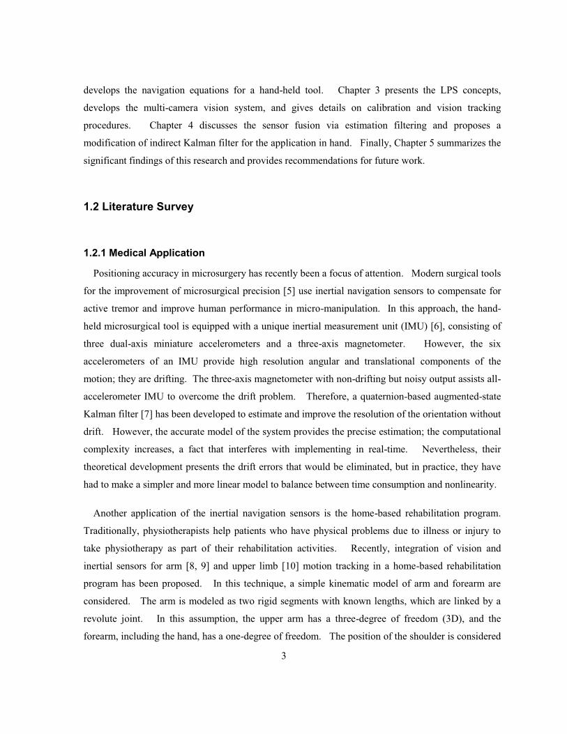
develops the navigation equations for a hand-held tool. Chapter 3 presents the LPS concepts,
develops the multi-camera vision system, and gives details on calibration and vision tracking
procedures. Chapter 4 discusses the sensor fusion via estimation filtering and proposes a
modification of indirect Kalman filter for the application in hand. Finally, Chapter 5 summarizes the
significant findings of this research and provides recommendations for future work.
1.2 Literature Survey
1.2.1 Medical Application
Positioning accuracy in microsurgery has recently been a focus of attention. Modern surgical tools
for the improvement of microsurgical precision [ 5] use inertial navigation sensors to compensate for
active tremor and improve human performance in micro-manipulation. In this approach, the hand-
held microsurgical tool is equipped with a unique inertial measurement unit (IMU) [ 6], consisting of
three dual-axis miniature accelerometers and a three-axis magnetometer. However, the six
accelerometers of an IMU provide high resolution angular and translational components of the
motion; they are drifting. The three-axis magnetometer with non-drifting but noisy output assists all-
accelerometer IMU to overcome the drift problem. Therefore, a quaternion-based augmented-state
Kalman filter [ 7] has been developed to estimate and improve the resolution of the orientation without
drift. However, the accurate model of the system provides the precise estimation; the computational
complexity increases, a fact that interferes with implementing in real-time. Nevertheless, their
theoretical development presents the drift errors that would be eliminated, but in practice, they have
had to make a simpler and more linear model to balance between time consumption and nonlinearity.
Another application of the inertial navigation sensors is the home-based rehabilitation program.
Traditionally, physiotherapists help patients who have physical problems due to illness or injury to
take physiotherapy as part of their rehabilitation activities. Recently, integration of vision and
inertial sensors for arm [ 8, 9] and upper limb [ 10] motion tracking in a home-based rehabilitation
program has been proposed. In this technique, a simple kinematic model of arm and forearm are
considered. The arm is modeled as two rigid segments with known lengths, which are linked by a
revolute joint. In this assumption, the upper arm has a three-degree of freedom (3D), and the
forearm, including the hand, has a one-degree of freedom. The position of the shoulder is considered
4
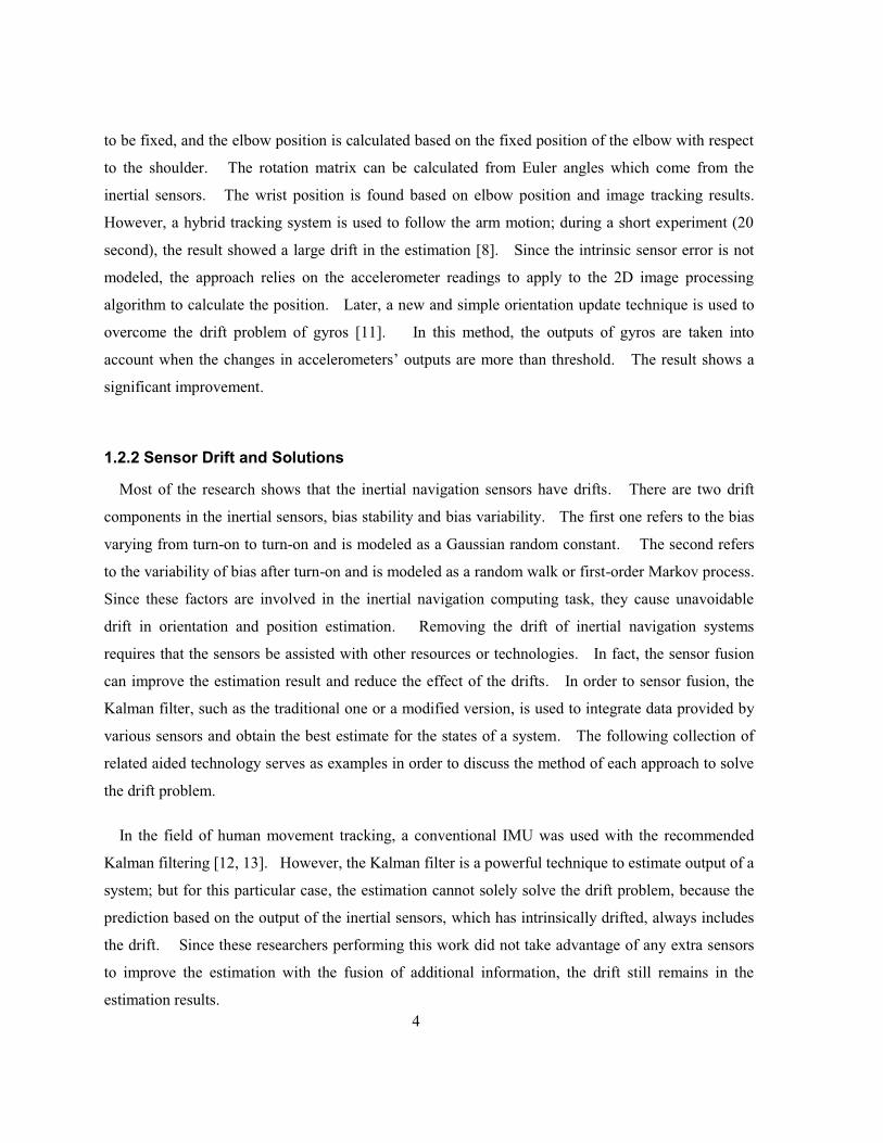
to be fixed, and the elbow position is calculated based on the fixed position of the elbow with respect
to the shoulder. The rotation matrix can be calculated from Euler angles which come from the
inertial sensors. The wrist position is found based on elbow position and image tracking results.
However, a hybrid tracking system is used to follow the arm motion; during a short experiment (20
second), the result showed a large drift in the estimation [ 8]. Since the intrinsic sensor error is not
modeled, the approach relies on the accelerometer readings to apply to the 2D image processing
algorithm to calculate the position. Later, a new and simple orientation update technique is used to
overcome the drift problem of gyros [ 11]. In this method, the outputs of gyros are taken into
account when the changes in accelerometers’ outputs are more than threshold. The result shows a
significant improvement.
1.2.2 Sensor Drift and Solutions
Most of the research shows that the inertial navigation sensors have drifts. There are two drift
components in the inertial sensors, bias stability and bias variability. The first one refers to the bias
varying from turn-on to turn-on and is modeled as a Gaussian random constant. The second refers
to the variability of bias after turn-on and is modeled as a random walk or first-order Markov process.
Since these factors are involved in the inertial navigation computing task, they cause unavoidable
drift in orientation and position estimation. Removing the drift of inertial navigation systems
requires that the sensors be assisted with other resources or technologies. In fact, the sensor fusion
can improve the estimation result and reduce the effect of the drifts. In order to sensor fusion, the
Kalman filter, such as the traditional one or a modified version, is used to integrate data provided by
various sensors and obtain the best estimate for the states of a system. The following collection of
related aided technology serves as examples in order to discuss the method of each approach to solve
the drift problem.
In the field of human movement tracking, a conventional IMU was used with the recommended
Kalman filtering [ 12, 13]. However, the Kalman filter is a powerful technique to estimate output of a
system; but for this particular case, the estimation cannot solely solve the drift problem, because the
prediction based on the output of the inertial sensors, which has intrinsically drifted, always includes
the drift. Since these researchers performing this work did not take advantage of any extra sensors
to improve the estimation with the fusion of additional information, the drift still remains in the
estimation results.
5
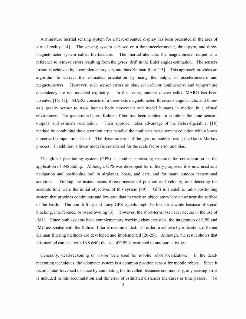
A miniature inertial sensing system for a head-mounted display has been presented in the area of
virtual reality [ 14]. The sensing system is based on a three-accelerometer, three-gyro, and three-
magnetometer system called InertiaCube. The InertiaCube uses the magnetometer output as a
reference to remove errors resulting from the gyros’ drift in the Euler angles estimation. The sensors
fusion is achieved by a complementary separate-bias Kalman filter [ 15]. This approach provides an
algorithm to correct the estimated orientation by using the output of accelerometers and
magnetometers. However, such sensor errors as bias, scale-factor nonlinearity, and temperature
dependency are not modeled explicitly. In this scope, another device called MARG has been
invented [ 16, 17]. MARG consists of a three-axis magnetometer, three-axis angular rate, and three-
axis gravity sensor to track human body movement and model humans in motion in a virtual
environment The quaternion-based Kalman filter has been applied to combine the nine sensors
outputs, and estimate orientation. Their approach takes advantage of the Gebre-Egziabher [ 18]
method by combining the quaternion error to solve the nonlinear measurement equation with a lower
numerical computational load. The dynamic error of the gyro is modeled using the Gauss-Markov
process. In addition, a linear model is considered for the scale factor error and bias.
The global positioning system (GPS) is another interesting resource for consideration in the
application of INS aiding. Although, GPS was developed for military purposes; it is now used as a
navigation and positioning tool in airplanes, boats, and cars, and for many outdoor recreational
activities. Finding the instantaneous three-dimensional position and velocity, and detecting the
accurate time were the initial objectives of this system [ 19]. GPS is a satellite radio positioning
system that provides continuous and low-rate data to track an object anywhere on or near the surface
of the Earth. The non-drifting and noisy GPS signals might be lost for a while because of signal
blocking, interference, or overcrowding [ 3]. However, the short-term loss never occurs in the use of
IMU. Since both systems have complementary working characteristics, the integration of GPS and
IMU associated with the Kalman filter is recommended. In order to achieve hybridization, different
Kalman filtering methods are developed and implemented [ 20- 25]. Although, the result shows that
this method can deal with INS drift; the use of GPS is restricted to outdoor activities.
Generally, dead-reckoning or vision were used for mobile robot localization. In the dead-
reckoning techniques, the odometer system is a common position sensor for mobile robots. Since it
records total traversed distance by cumulating the travelled distances continuously, any sensing error
is included in this accumulation and the error of estimated distances increases as time passes. To
6
prevent excessive error and obtain accurate estimations of position and orientation, dead-reckoning is
integrated with the inertial navigation sensors [ 26]. Owing to the intrinsic error of both IMU and
odometer, the data fusion requires precision calibration of the IMU [ 27]. The dead-reckoning
methods are not suitable for use in precise manipulation applications since small movements cannot
be sensed and slow signal processing does not allow real-time processing. In vision-based robot
localization, the robot equipped by camera finds its current location using different features extracted
from visual information of the environment. Each feature and its corresponding position are stored
in a database, and the robot retrieves its position by comparing the current extracted feature with the
database and finding the most similar vector. Lately, the inertial sensors have been playing a role in
robot positioning [ 28, 29] as well as augmented reality [ 30, 31].
Most vision-based hybrid INS systems are based on a monocular vision system [ 29, 30]. While
the inertial sensors measure the components of the motion, the current position of the moving object
is simultaneously determined by using visual information from the surrounding environment. In fact,
a camera is mounted on the object, and a database of various features corresponding to a landmark is
established. During object navigation, several images are captured and then different invariant
features are extracted. The extracted feature vector is compared with those in the database. The
current position can be retrieved once the optimum vector is found. Then, the sensor fusion
algorithm estimates the current state of the object. In many applications, land marking is not
practical or is hard to implement. Besides, mounting a camera on the tracking object is not possible
because of the size and weight of the camera compared with the dimensions of the object. However,
two-camera vision systems are used in particular applications [ 9, 10, 28, 32, 33]; they have a limited
field of view and accuracy.
Without considering the result of the above hybrid vision-inertial systems, the robot’s precision is
not satisfactory and reasonable in precise manipulation tasks.
1.2.3 Local Positioning System (LPS)
The Local Positioning System (LPS) is a system with the capability of detecting, tracking, and
localizing multiple targets accurately in real-time in an indoor environment. Typical applications of
LPS include resource management [ 34], robot localization [ 35, 36], environment monitoring [ 37], and
people-tracking for purposes of special supervision [ 38] and public safety [ 39].
7
The target or moving object is equipped with a small transmitter that includes a micro-controller
and an emitting device. The emitting device sends the identification of the target to the LPS receiver
with a unique sequence of on and off flashing.
The current localization systems can be classified by the core transmission techniques as IR, RF,
ultrasound, magnetic, or electromagnetic. Their distinctive characteristics make them popular for
different applications.
RF-based systems now have a low accuracy. However, they do not require a direct line of sight
between sender and receiver, and their accuracy is considerably reduced by multiple-path and fading
effects. Experience shows that the measurement results can be influenced even by the number of
targets and by varying the number of objects standing close to a target [ 40].
In the ultrasound technique, targets emit an ultrasonic pulse to a set of ceiling-mounted receivers,
such as the Active Bat system [ 41]. The objects can be located to within 9 cm of their true position.
The accuracy of ultrasound-based systems suffers from reflections and obstacles between senders and
receivers. However, the performance of these systems can be improved by establishing a dense
network of receivers; this requirement makes them expensive, as well as complex to install.
Magnetic-based tracking systems are commonly used in virtual reality and motion capture
applications. However, the magnetic tracking technique offers a high resolution; the use of
magnetic-based systems is limited to a small and precisely controlled environment.
The electromagnetic systems are based on a network of wire coils covering the area of tracking.
The accuracy of the electromagnetic systems is within a few millimeters in 3D; however, the large
metal objects affect the electromagnetic systems; to achieve good accuracy, therefore, a precise
calibration procedure is required. In addition, the infrastructure of these systems is such that it is
difficult to install them in rooms with high ceilings.
Ultra-WideBand systems (UWBs) [ 42] are wireless communications techniques based on very high
frequency signals, and their bandwidth is much wider than the conventional RF bandwidth.
Furthermore, a higher receiver density than that in traditional RF systems is required. UWBs are
capable to transmit pulses with duration as short as nanosecond or less. Since these systems are less
8
affected by multi-path than are conventional RF systems, they can be accurate to about 5 cm in 3D.
Besides, they can be installed much easier than ultrasound and electromagnetic systems.
Infrared (IR) optical-based systems cover a wide range of field [ 41], but they require a direct line of
sight between transmitter and receiver. This means that obstacles and surfaces cause the
communication linkage between senders and receivers to be missed. However, the emitters must be
mounted at uncovered places; this constraint does not severely limit their use.
Considering the complementary working characteristic of RF- and IR-localization systems,
researchers have started to focus attention on finding effective means to combine these two systems
into a hybrid localization system with higher accuracy and better performance than previous systems
[ 43, 44]. Thus, large rooms can be covered easily and positioning within the room is possible with
less limitation; however, the complexity of the system is drastically increased.
An IR-LPS for smart items and devices is designed for integration with a camera [ 40]. This
system covers a wide area (~100m2) and tracks a large number of targets with a constant sampling
rate without impacting on performance significantly. The result shows the accuracy is about 8 cm
over a small range and 16 cm over a wide range. As well, the multi-robot positioning experiment
[ 43], which takes advantage of the hybrid IR/RF communication system, shows that the measured
distance error is relative to the range of view; the target can be located within 3.25 cm to 15 cm of its
true position. In addition, bandwidth, sampling time, number of targets, and some hardware intrinsic
bottlenecks are restricted when using this system.
Typically available IR optical tracking systems, such as Optotrak [ 4] and Firefly [ 45], are used
mostly in precise applications, given that the accurate and instantaneous responses are two vital and
crucial factors. The IR optical systems can cover and bring up to the field of view a wide region,
while the Optotrak positional resolution and accuracy of positioning each marker in 3D is about 0.002
mm and 0.05 mm at 2.5 m respectively. Accordingly, even though IR optical systems are extremely
expensive, their use in medical applications has grown. On the other hand, in most vision-based
tracking systems including Optotrak, cameras are aligned on a straight line. When applications
require keeping the object in the field of view during all of its movement, several of these optical
systems must be chained together, creating an exceedingly expensive tracking system.
9
1.3 Research Objective
In this research, we propose a Local Positioning System (LPS)/SDINS for use in designing a hand-
held tool tracking system. At the beginning of using the tool, a stationary reference point is affixed
in the workspace. The ultimate goal here is to develop a hand-held tool, which is instrumented with
MEMS sensors for full six degrees of freedom (6D) tracking. The tool is placed in the reference
point in a mechanically stable and repeatable fashion. The measurement system is reset when the
tool is placed in the reference position. This position is considered the origin, where acceleration due
to gravity can be determined. The orientation is therefore determined relative to gravity. The tool
can then be removed from the reference point. It is moved by hand to a point of interest in the
workspace.
The end tip position and tool orientation must be tracked and be reported to a host computer for
further analysis. This end-tip measurement and the attitude of the tool must remain accurate to
better than one millimeter RMS and one degree RMS for duration of at least one minute as it is
required for many applications in medicine and industry. An audible or visual indication must be
made after such time that the system determines it can no longer accurately report the pose. The
user then returns the tool to the reference holder to re-establish the origin. Remaining accurate for a
time greater than one minute would be of great benefit as the operator does not require returning the
tool frequently. The local coordinate system of the tool can be established relative to the reference
holder by well-known registration techniques.
The LPS is designed to calculate the position and orientation of the tool. To implement the LPS,
we locate a multi-camera vision system around the workspace, which is connected to our own
computer to facilitate 6D position-orientation calculation during tool operation.
The proposed multi-camera vision system is implemented by employing CCD cameras which are
fixed in the navigation frame and their lenses placed on a semicircle. All cameras are connected to a
PC through the frame grabber, which includes four parallel video channels and is able to capture
images from four cameras simultaneously. Digital image processing algorithms are applied to detect
the tool with markers which are located on the body of the tool, determine the tool orientation, and
find the 3D position of the tool tip with respect to the navigation frame.

10
In the SDINS, three accelerometers and three gyros are mounted rigidly and directly to the body of
the tool in a three perpendicular axes frame. Since these sensors provide the full range of heading
changes, turn rates, and applied forces that the object is experiencing along its movement, accurate
3D kinematics equations are developed to compensate for the motion-dependent errors caused by
vibration, coning motion, sculling, and rotational motion.
In addition, the multi-camera vision system data with cooperation of the modified EKF aids the
inertial sensors to deal with the drift problem.
The specifications of a final solution for a hand-held tool tracking are as follows:
� Measuring Devices for 6D (translational and rotations) or 3D (only rotations)
� Update rate of 100 Hz.
� Inexpensive
� Light weight and ergonomically balanced for the human hand.
� Auto-cleavable for at least 10 cycles (withstand storage temperatures of 125� C and high
humidity).
� User-friendly push-buttons, LED indicators, and limited capacity programmable memory
device.
1.3.1 New Contribution
The objective of this research is to design a reliable and cost-effective positioning system which is
capable to locate precisely the position of the tool and determine accurately its orientation in real-
time.
The accurate available positioning systems such as Optotrak are expensive and not affordable to be
used in many applications such as industries. Therefore, the system is designed based on the cost-
effective factor.
11
The performance of the positioning systems is not only evaluated based on the accuracy but also
the measurement rate. The measurement rate of the existing positioning systems is reduced by
increasing the number of markers. Keeping the sampling rate of the system at the same measurement
rate that the system is operating with fewer markers requires extra hardware. Introducing more
hardware to the system adds more complexity in hardware and software design. This means the price
will be increased significantly.
One of the most important contributions of this research is that the proposed positioning system is
capable to respond at the highest measurement rate at all time of operation, which is at least 100 HZ
in order to response in real time.
The low-cost and high frequency features of the MEMS-based inertial sensors allow us to meet the
high measurement rate requirement. Besides of these features, they are miniaturized in size and
weight which allow them to be mounted on an object and without interfering with its operation. In
addition, they can provide full dynamic range of the motion that the target is experiencing during its
movement. All these characteristics make them popular in navigation applications; however, few
research studies have been done in the field of the tool tracking [ 5]. Current tool tracking systems
based on MEMS-based inertial sensors use 6 or 9 accelerometers and no rate gyros, which is call all-
accelerometer IMU or gyro free IMU. Magnetometers are introduced in these systems to assist the
accelerometers in estimating the 3D orientations. As the function of the magnetometers is affected
easily by metals around the workspace, they are not appropriate for many applications. To address
this problem, this research study proposes to employ a 3-axis accelerometer and a 3-axis rate gyro to
estimate the 6D positions and orientations.
Although, the general equations of the SDINS computing task are applied in many navigation
applications such as the navigation of land vehicles, airplanes, spacecrafts, and submarines;
introducing MEMS-based inertial sensors in the tool tracking system whose accuracy should be in the
range of few millimeters requires developing precise kinematics equations in order to minimize the
SDINS errors resulting from the common motion-dependent errors as much as possible. The relative
motion analysis and driven equations in the current research studies in this area are based on the gyro
free assumption. The 3D relative motion analysis and developing required 3D kinematics equations
for the hand-held tool including a three-axis rate gyro and a three-axis accelerometer is the other
essential contribution of this thesis.
12
Even though, the drift error of the SDINS is significantly reduced by developing 3D kinematics
equations and applying them into the general equations of the SDINS; but the SDINS still lose its
accuracy over the time. This thesis recommends that the SDINS is integrated with another local
positioning system associated with a sensor fusion technique to improve the accuracy of the system
and keep it in the desired range for a longer period of the time.
However, GPS is commonly used for integrating with INS and SDINS in many outdoor
applications; it is not recommended for indoor applications, since the satellite signals cannot penetrate
the buildings materials. Vision systems are one of the most popular indoor tracking systems. Aside
form Optotrak which is used three IR cameras and are not optical cameras, other research studies
employ monocular or stereo vision systems in order to video tracking. One of the shortcomings of
the vision systems is the loss of line of sight; which means the path between the target and the
cameras will be blocked by obstacles and the video tracking will be failed.
Another significant contribution of this research is the design of a multi-camera vision system with
individual configuration so as to prevent the loss of line of sight as much as possible. This
configuration proposes to place the cameras along a semicircle in order to expand the angle of view
and initiate a wide circular field of view.
As a matter of cost effectiveness, the low-cost CCD cameras are chosen to be employed in the
proposed vision system. The more inexpensive cameras the smaller angle of view. As a result of
smaller angle of view, more cameras are required to be employed to cover the entire circular
workspace. However, utilizing more cameras introduces more complexity in calibration procedures
and computer vision algorithms; the positioning error of the multi-camera vision system is
significantly reduced. The number of required cameras is directly relative to the angle of view of the
cameras. Since the angle of view of the chosen cameras in this project is �8 , four cameras are
necessary for achieving the proposed arrangement.
As a result of this arrangement, an individual calibration procedure is designed to estimate the
intrinsic and extrinsic parameters of the multi-camera vision system. In addition, the 3D position
estimated by SDINS is provided in the navigation frame, therefore, a 3D transformation is required in
order to map each point expressed in the world coordinate system of the multi-camera vision system
into the navigation frame. First, the calibration procedure assigns a unique world coordinate system
13
into the multi-camera vision system, and then provides a 3D homogenous transformation for each
single camera to transform each point in camera frame into the unique world coordinate system and a
3D homogenous transformation to map each point in world coordinate system into the navigation
frame.
Aside from the camera calibration, video tracking requires applying digital image processing and
computer vision algorithms. To address the computation load problem of the video tracking, the
simple and efficient algorithms for application in hand are selected.
Integration of the multi-camera vision system and SDINS requires an estimation method. Various
types of EKF are developed for different application. These methods provide an estimation of the
state variables or the errors. This research develops an EKF which offers the estimation of the
changes in the state variables. Then the current estimated values of changes in the variables are
added to the previous estimation. According to the general equations of the SDINS, the constant
value of the gravitational force is removed from the resulted equations and the resulting error from
the uncertainty value of the gravitational force is eliminated.
The inertial sensor noise is theoretically modeled with a zero-mean Gaussian random process. In
reality, the actual mean of the noise is not absolutely zero. As a result of the proposed EKF and due
to the inherent characteristic of the Gaussian random process, the average of the input noise is
decreased while its variance is increased. It is expected that the resulting drift from input noise is
reduced and smooth positioning is obtained.
1.3.2 Publications
Journals:
N. Parnian, M. F. Golnaraghi, 2007, “Integration of Vision and Inertial Sensors for Industrial Tools
Tracking,” Sensor Review, Vol. 27, No. 2.
N. Parnian, M. F. Golnaraghi, 2008, “Compensation for the Common Motion-Dependent Errors in
the Strapdown Inertial Navigation System in Application of a Hand-Held Tool Positioning,”
Submitted to: IEEE Journal of selected topics in Signal Processing, Paper Number: ASPGRN.103
14
N. Parnian, M. F. Golnaraghi, 2008, “Integration of the Multi-Camera Vision System and SDINS
with a modified EKF,” ready for submission.
N. Parnian, M. F. Golnaraghi, 2008, “A New Configuration for a Multi-Camera Vision System in
its Integration with the Strapdown Inertial Navigation System for Hand-held Tool Tracking,” ready
for submission.
Conferences:
N. Parnian, S.P. Won M. F. Golnaraghi, “Position Sensing Using Integration of a Vision System
and Inertial Sensors,” Proceeding of IECON2008, November 2008, Orlando, Florida, USA.
S.P. Won, N. Parnian, M. F. Golnaraghi, W. Melek, “A Quaternion-Based Tilt Angle Correction
Method for a Hand-Held Device Using an Inertial Measurement Unit,” Proceeding of IECON2008,
November 2008, Orlando, Florida, USA.
N. Parnian, M. F. Golnaraghi, “A Low-Cost Hybrid SDINS/Multi-Camera Vision System for a
Hand-held Tool Positioning,” Proceeding of IEEE/ION PLANS Conference, May 2008, Monterey,
California, USA.
N. Parnian, M. F. Golnaraghi, “Hybrid Vision/Inertial Tracking for a Surgical Application,”
NTC2007 Proceeding of the First Nano Technology Conference, February 2007, Shiraz, Iran.
N. Parnian, M. F. Golnaraghi, “Integration of Vision and Inertial Sensors for a Surgical Tool
Tracking,” Proceedings of IMECE2006 2006 ASME International Mechanical Engineering Congress
and Exposition, November 2006, Chicago, Illinois USA.
1.4 Summary
Our survey of the prior-art shows that there is a need for research in the area of precise positioning
and the proposed topic will advance the state of knowledge in this field. In particular, the
advancements from the proposed research will have the potential to benefit computer-assisted
surgical devices in medical applications. The research will provide innovations in sensor tracking of
devices utilizing the multi-camera vision system and inertial sensors, a new configuration and

15
calibration method for the proposed vision system, and integration of the vision system and SDINS
by introducing a new estimation algorithm.
16
Chapter 2 Strapdown Inertial Navigation System
Inertial navigation systems (INSs) were initially developed for military aviation applications.
INSs are widely used in the positioning of various types of vehicles such as land vehicles, aircrafts,
spacecrafts, and submarines. An INS is implemented based on two different techniques, gimbaling
and strapdown systems.
The first system requires complicated, power consuming, and massive structures for gimbaling the
inertial sensors on a mechanized-platform [ 46]. In the second system, inertial sensors are mounted
on the body of a moving object [ 2] rather than a mechanized-platform. As a result of MEMS
fabrication techniques, the inertial sensors such as accelerometers and angular rate gyros have been
manufactured in a small size and light weight, allowing them to be strapped onto the moving object.
Because MEMS fabrication techniques have made inertial sensors low-cost and inexpensive,
SDINS is allowed to be used for outdoor recreational activities, as well as for indoor environment
applications such as medicine, industry, robotics, sports, virtual reality, and human motion tracking.
In an SDINS, inertial sensors are mounted rigidly and directly to the body of the tracking object
and the inertial measurements are transformed computationally to the known navigation frame. The
SDINS can continuously monitor the position and orientation of a moving object with respect to the
known navigation reference frame, based on measuring its instantaneous linear acceleration and
angular velocity with respect to the body reference frame and knowing its initial position, velocity,
and attitude with respect to the navigation reference frame. Since the inertial measurements are in
the body reference frame, computing the position and orientation requires a set of guidance
navigation equations to transform the inertial measurements to the navigation reference frame.
In order to implement SDISN, three gyros and three accelerometers, or a three-axis gyro and a
three-axis accelerometer are employed. These sensors are typically integrated in a unit which is
referred to as inertial measurement unit (IMU).
17
2.1 Inertial Measurement Unit (IMU)
An Inertial Measurement Unit (IMU), includes gyros and accelerometers, is mounted on the
moving object to track its motion, attitude, and position. IMUs commonly suffer from bias drift,
scale-factor error owing to non-linearity and temperature changing, and misalignment as a result of
minor manufacturing defects. All these errors lead to SDINS drift in position and orientation.
Reducing the resulting drift in SDINS requires that the IMU be calibrated and parameters be
estimated before mounting the IMU on a mobile object.
2.1.1 IMU Calibration
Calibration is the process of comparing a sensor’s output with known reference quantities over the
range of output values. The precision of the SDINS depends on the accuracy of calibration
parameters such as scale factors and cross-coupling, measurement noise, and sensor bias.
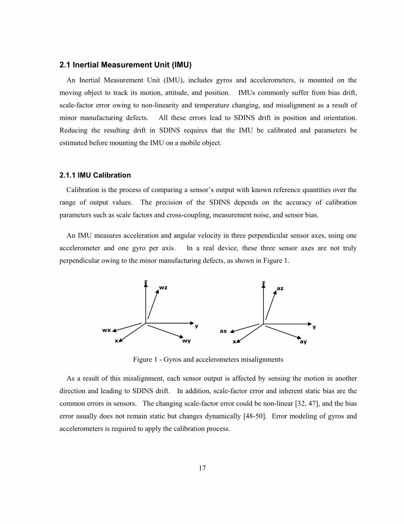
An IMU measures acceleration and angular velocity in three perpendicular sensor axes, using one
accelerometer and one gyro per axis. In a real device, these three sensor axes are not truly
perpendicular owing to the minor manufacturing defects, as shown in Figure 1.
As a result of this misalignment, each sensor output is affected by sensing the motion in another
direction and leading to SDINS drift. In addition, scale-factor error and inherent static bias are the
common errors in sensors. The changing scale-factor error could be non-linear [ 32, 47], and the bias
error usually does not remain static but changes dynamically [ 48- 50]. Error modeling of gyros and
accelerometers is required to apply the calibration process.
x
y
z
wx
wz
wy x
y
z
ax
az
ay
Figure 1 - Gyros and accelerometers misalignments
18
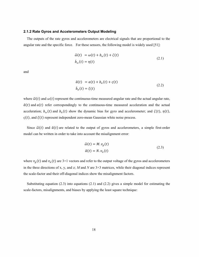
2.1.2 Rate Gyros and Accelerometers Output Modeling
The outputs of the rate gyros and accelerometers are electrical signals that are proportional to the
angular rate and the specific force. For these sensors, the following model is widely used [ 51]:
��(�) = �(�) + �� (�) + �(�) �� (�) = �(�)
(2.1)
and
(�) = (�) + � (�) + �(�) � (�) = �(�)
(2.2)
where ��(�) and �(�) represent the continuous-time measured angular rate and the actual angular rate, (�) and (�) refer correspondingly to the continuous-time measured acceleration and the actual
acceleration; �� (�) and � (�) show the dynamic bias for gyro and accelerometer; and �(�), �(�), �(�), and �(�) represent independent zero-mean Gaussian white noise process.
Since ��(�) and (�) are related to the output of gyros and accelerometers, a simple first-order
model can be written in order to take into account the misalignment error:
��(�) = . ��(�) (�) = �. � (�)
(2.3)
where ��(�) and � (�) are 3×1 vectors and refer to the output voltage of the gyros and accelerometers
in the three directions of x, y, and z; M and N are 3×3 matrices, while their diagonal indices represent
the scale-factor and their off-diagonal indices show the misalignment factors.
Substituting equation (2.3) into equations (2.1) and (2.2) gives a simple model for estimating the
scale-factors, misalignments, and biases by applying the least square technique:
19
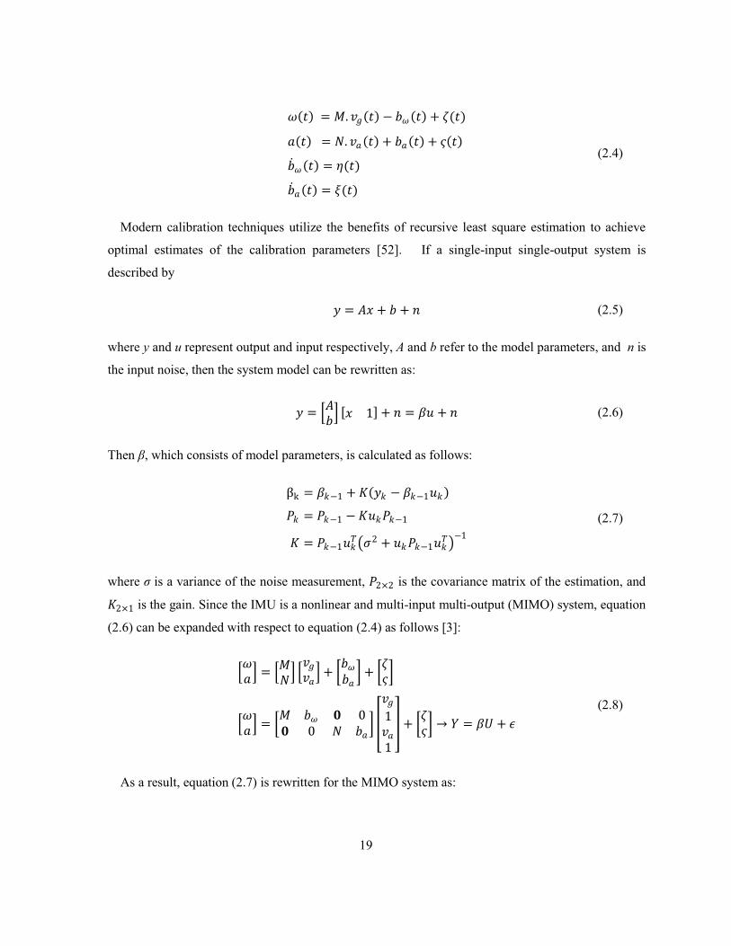
�(�) = . ��(�) − �� (�) + �(�) (�) = �. � (�) + � (�) + �(�) �� (�) = �(�) � (�) = �(�)
(2.4)
Modern calibration techniques utilize the benefits of recursive least square estimation to achieve
optimal estimates of the calibration parameters [ 52]. If a single-input single-output system is
described by
� = �� + � + � (2.5)
where y and u represent output and input respectively, A and b refer to the model parameters, and n is
the input noise, then the system model can be rewritten as:
� = ���� [� 1] + � = �� + � (2.6)
Then β, which consists of model parameters, is calculated as follows:
βk = ��−1 + �(�� − ��−1�� ) �� = ��−1 − ��� ��−1 � = ��−1�����2 + �� ��−1���!−1
(2.7)
where σ is a variance of the noise measurement, �2×2 is the covariance matrix of the estimation, and �2×1 is the gain. Since the IMU is a nonlinear and multi-input multi-output (MIMO) system, equation
(2.6) can be expanded with respect to equation (2.4) as follows [ 3]:
��� = � �� ���� � + "��� # + "��#
��� = " �� $ 0$ 0 � � # %��1�1 & + "��# → * = �, + - (2.8)
As a result, equation (2.7) is rewritten for the MIMO system as:
20
βk = ��−1 + �(*� − ��−1,� ) �� = ��−1 − �,� ��−1 � = ��−1,���/ + ,� ��−1,��!−1
(2.9)
where R is the noise measurement covariance matrix.
Determining the unknown parameters requires measuring the output of gyros and accelerometers in
different temperatures over the range when the actual angular rates and actual acceleration are known
or obtained from the precise device, such as a turntable.
It is well known that the scale factors of inertial sensors are changing with temperature. These
changes are considerable even the temperature is changing in the small range (see the result in the
section 2.3.1). Since the hand-held tool can operate in different environment for different
applications, then a wider range of temperature is considered for IMU calibration.
2.1.3 Thermal Tests
The thermal tests are employed to establish the variation in the calibration parameters with
temperature; when either the sensor is working at the lowest or highest operating temperature. The
sensor is usually placed in the thermal chamber allowing tests to be run at the sub-zero temperatures
and increased to the high temperatures. Various tests can be carried out to study the behavior of the
inertial sensors in different temperatures. Soak method and ramp method are two popular thermal
tests for MEMS inertial sensors [ 53 , 54].
In the soak method, the sensor is put in the chamber for sufficient time allowing the sensor to
establish its temperature at the temperature of the chamber. Then, the system records the output of the
sensor.
In the ramp method, the response of the sensor is recorded during different rates of temperatures.
The sensor is placed in the chamber with the variable temperature. The temperature is linearly
increased or decreased during a given period of time. During this period, the output of the sensor and
temperatures are recorded correspondingly.
21
2.2 Navigation Equations
A SDINS determines the position and orientation of the tracking object by measuring applied
specific forces to, and turning rates of, the body. In order to obtain the position and attitude of the
object with respect to the known navigation frame, a set of equations are required to compensate
measured inertial components for common motion-dependent errors and transform compensated
quantities to the navigation frame. Navigation equations provide the motion behavior of a known
particle of a rigid moving object [ 3]. In order to derive the motion equations of the moving object, a
precise definition of reference frames is required.
2.2.1 Reference Frames
Analyzing the three-dimensional motion of a rigid body requires the use of two reference frames:
the body reference frame attaching to the body of a moving object, and the navigation frame.
Figure 2 shows the reference frames and a symmetric hand-held tool equipped with an IMU when
the body frame aligned on the IMU coordinate system.
Figure 2 - Hand-held tool and assigned reference frames
When the position of the tool tip is desired, the IMU is attached to the bottom of the tool. The
assigned body frame is the IMU frame, while its z-axis is aligned on the tool tip axis. The navigation
X
Y
Z
X
Y
Z x
y
z
P
A
O
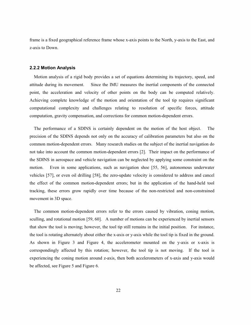
22
frame is a fixed geographical reference frame whose x-axis points to the North, y-axis to the East, and
z-axis to Down.
2.2.2 Motion Analysis
Motion analysis of a rigid body provides a set of equations determining its trajectory, speed, and
attitude during its movement. Since the IMU measures the inertial components of the connected
point, the acceleration and velocity of other points on the body can be computed relatively.
Achieving complete knowledge of the motion and orientation of the tool tip requires significant
computational complexity and challenges relating to resolution of specific forces, attitude
computation, gravity compensation, and corrections for common motion-dependent errors.
The performance of a SDINS is certainly dependent on the motion of the host object. The
precision of the SDINS depends not only on the accuracy of calibration parameters but also on the
common motion-dependent errors. Many research studies on the subject of the inertial navigation do
not take into account the common motion-dependent errors [ 2]. Their impact on the performance of
the SDINS in aerospace and vehicle navigation can be neglected by applying some constraint on the
motion. Even in some applications, such as navigation shoe [ 55, 56], autonomous underwater
vehicles [ 57], or even oil drilling [ 58], the zero-update velocity is considered to address and cancel
the effect of the common motion-dependent errors; but in the application of the hand-held tool
tracking, these errors grow rapidly over time because of the non-restricted and non-constrained
movement in 3D space.
The common motion-dependent errors refer to the errors caused by vibration, coning motion,
sculling, and rotational motion [ 59, 60]. A number of motions can be experienced by inertial sensors
that show the tool is moving; however, the tool tip still remains in the initial position. For instance,
the tool is rotating alternately about either the x-axis or y-axis while the tool tip is fixed in the ground.
As shown in Figure 3 and Figure 4, the accelerometer mounted on the y-axis or x-axis is
correspondingly affected by this rotation; however, the tool tip is not moving. If the tool is
experiencing the coning motion around z-axis, then both accelerometers of x-axis and y-axis would
be affected, see Figure 5 and Figure 6.
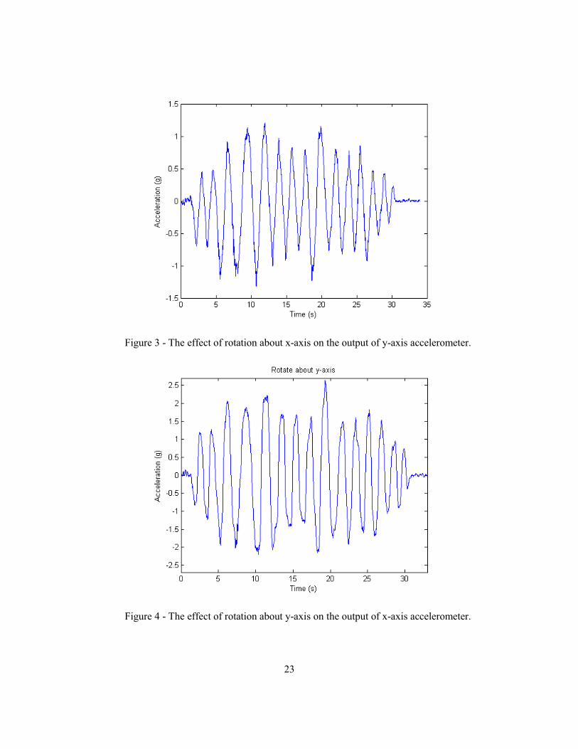
23
Figure 3 - The effect of rotation about x-axis on the output of y-axis accelerometer.
Figure 4 - The effect of rotation about y-axis on the output of x-axis accelerometer.
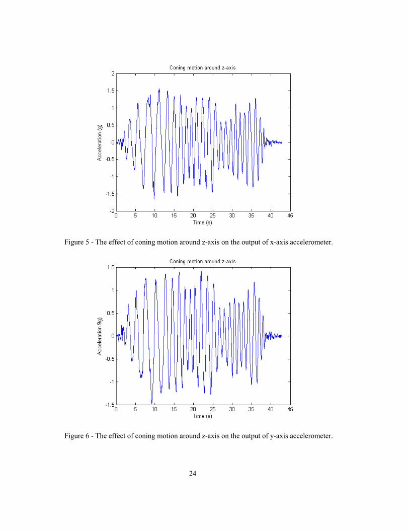
24
Figure 5 - The effect of coning motion around z-axis on the output of x-axis accelerometer.
Figure 6 - The effect of coning motion around z-axis on the output of y-axis accelerometer.
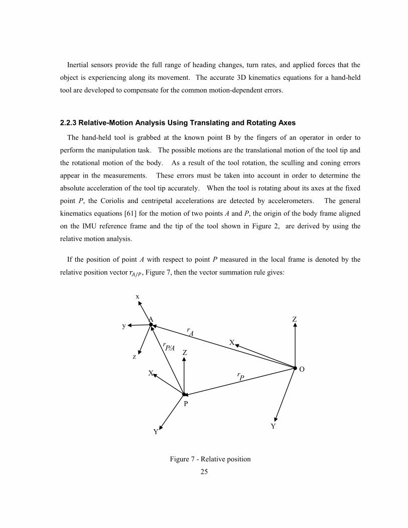
25
Inertial sensors provide the full range of heading changes, turn rates, and applied forces that the
object is experiencing along its movement. The accurate 3D kinematics equations for a hand-held
tool are developed to compensate for the common motion-dependent errors.
2.2.3 Relative-Motion Analysis Using Translating and Rotating Axes
The hand-held tool is grabbed at the known point B by the fingers of an operator in order to
perform the manipulation task. The possible motions are the translational motion of the tool tip and
the rotational motion of the body. As a result of the tool rotation, the sculling and coning errors
appear in the measurements. These errors must be taken into account in order to determine the
absolute acceleration of the tool tip accurately. When the tool is rotating about its axes at the fixed
point P, the Coriolis and centripetal accelerations are detected by accelerometers. The general
kinematics equations [ 61] for the motion of two points A and P, the origin of the body frame aligned
on the IMU reference frame and the tip of the tool shown in Figure 2, are derived by using the
relative motion analysis.
If the position of point A with respect to point P measured in the local frame is denoted by the
relative position vector 3�/�, Figure 7, then the vector summation rule gives:
Figure 7 - Relative position
rP
A
P
Y
X
Y
Z X
Z
O
rA
rP/A
x
y
z

26
3� = 3� + 3�/� (2.10)
where 3� and 3� are vectors defining position of points A and P with respect to the navigation frame.
The velocity of point A measured from navigation frame is obtained by taking the time derivative of
equation (2.10):
3� = 3� + 3�/� (2.11)
Since the body frame axes are rotating with respect to the navigation frame, the time derivative of
each arbitrary vector in the body frame must take into account the change not only in the vector’s
magnitude but also in the vector’s direction [ 62], meaning that:
� = ��!��5 + ω × � (2.12)
where k is an arbitrary vector in the body frame; � is its time derivative with respect to the fixed
navigation frame; ω is a vector referring to the angular rate of the body frame measured in the fixed
navigation frame; and “×” denotes the cross product operation.
By considering the angular velocity of body frame, ω, measured from navigation frame, the last
term in equation (2.11) yields:
3�/� = (3�/�)��5 + ω × 3�/� (2.13)
Then equation (2.11) is rewritten as:
3� = 3� + (3�/�)��5 + ω × 3�/� (2.14)
or
�� = �� + ω × 3�/� + (��/�)��5 (2.15)
where �� and �� represent the velocity of points A and P, and (��/�)��5 is the relative velocity of
point A with respect to point P measured from the body frame. As well, the acceleration of point A
measured form the navigation frame is calculated by taking the time derivative of equation (2.15):
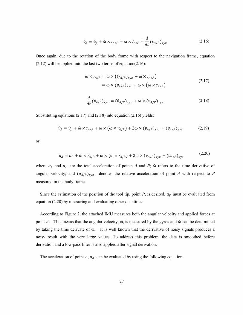
27
�� = �7 + ω × 3�/� + ω × 3�/� + 99� (��/�)��5 (2.16)
Once again, due to the rotation of the body frame with respect to the navigation frame, equation
(2.12) will be applied into the last two terms of equation (2.16):
ω × 3�/� = ω × �(3�/�)��5 + ω × 3�/�!= ω × (��/�)��5 + ω × �ω × 3�/�!
(2.17)
99� (��/�)��5 = (��/�)��5 + ω × (��/�)��5 (2.18)
Substituting equations (2.17) and (2.18) into equation (2.16) yields:
�� = �7 + ω × 3�/� + ω × �ω × 3�/�! + 2ω × (��/�)��5 + (��/�)��5 (2.19)
or
� = � + ω × 3�/� + ω × (ω × 3�/�) + 2ω × (��/�)��5 + (�/�)��5 (2.20)
where � and � are the total acceleration of points A and P; ω refers to the time derivative of
angular velocity; and (�/�)��5 denotes the relative acceleration of point A with respect to P
measured in the body frame.
Since the estimation of the position of the tool tip, point P, is desired, � must be evaluated from
equation (2.20) by measuring and evaluating other quantities.
According to Figure 2, the attached IMU measures both the angular velocity and applied forces at
point A. This means that the angular velocity, ω, is measured by the gyros and ω can be determined
by taking the time derivate of ω. It is well known that the derivative of noisy signals produces a
noisy result with the very large values. To address this problem, the data is smoothed before
derivation and a low-pass filter is also applied after signal derivation.
The acceleration of point A, �, can be evaluated by using the following equation:
28
� = :� + �� (2.21)
where :� denotes applied forces or the accelerometer measurements, and �� is the gravity vector
represented in the body frame.
Since both points P and A located on the same rigid body and moving along the motion of the tool,
the two terms (��;7 /�)��5 and (�;7 /�)��5 become zero. As demonstrated in Figure 7, 3�/� is
changing because of the rotation of the tool:
3�/� = − < > sin ?−> sin @>A1 − sin2 ? − sin2 @B = − C > sin ?−> sin @>D E (2.22)
Therefore, the total acceleration of the tool tip, � , is computed as:
� = :� − ω × 3�/� − ω × (ω × 3�/�) + �� (2.23)
The Euler angles corresponding to the roll, pitch, and yaw [ 63] are shown in Figure 8, and denoted
with the angles �, �, and �, respectively. The length of the line AP which connects the tool tip to the
origin of the body frame has a known value of L.
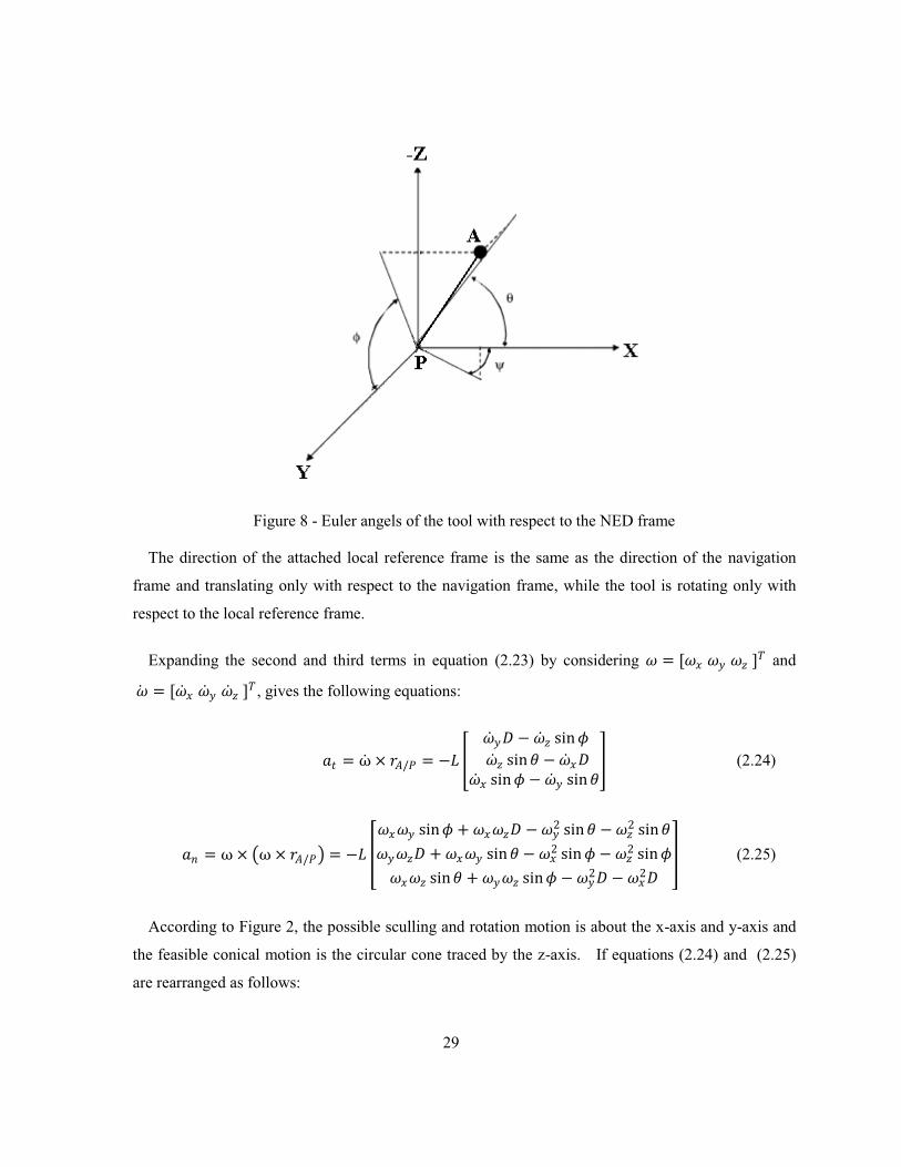
29
Figure 8 - Euler angels of the tool with respect to the NED frame
The direction of the attached local reference frame is the same as the direction of the navigation
frame and translating only with respect to the navigation frame, while the tool is rotating only with
respect to the local reference frame.
Expanding the second and third terms in equation (2.23) by considering � = [�� �� �5 ]� and � = [�� �� �5 ]� , gives the following equations:
� = ω × 3�/� = −> < �� D − �5 sin @ �5 sin ? − �� D�� sin @ − �� sin ?B (2.24)
� = ω × �ω × 3�/�! = −> %�� �� sin @ + �� �5D − ��2 sin ? − �52 sin ?�� �5D + �� �� sin ? − ��2 sin @ − �52 sin @�� �5 sin ? + �� �5 sin @ − ��2D − ��2D & (2.25)
According to Figure 2, the possible sculling and rotation motion is about the x-axis and y-axis and
the feasible conical motion is the circular cone traced by the z-axis. If equations (2.24) and (2.25)
are rearranged as follows:
30
� = −> C −�5 sin @ �5 sin ?0 E − > < �� D −�� D�� sin @ − �� sin ?B (2.26)
� = −> < �� �5D − �52 sin ?�� �5D + −�52 sin @0 B − > % �� �5D − ��2 sin ?�� �� sin ? − ��2 sin @�� �5 sin ? + �� �5 sin @ − ��2D − ��2D& (2.27)
then the first terms and the second terms of equations (2.26) and (2.27) introduce the effect of the
coning motion and the sculling/rotation motion, respectively. Therefore, equation (2.23) can be
rewritten as:
� = :� − � − � + �� (2.28)
Since the angular velocity, angular acceleration, and applied force in equation (2.28) are expressed
in the body frame, a transformation matrix [ 64] is required to convert the acceleration of the tool tip
from the body frame to the navigation frame.
2.2.4 Direction Cosine Matrix
The direction cosine matrix (DCM), F�� , is a 3×3 matrix that transforms any represented vector in
the body frame, 3� , to the corresponding vector in the navigation frame, 3� ,:
3� = F�� 3� (2.29)
Therefore, the acceleration of tool tip with respect to the navigation frame is computed as:
7 = F�� (:� − � − � ) + �� (2.30)
where �� denotes the gravity vector in the navigation frame [0 0 9.81]�.
Obviously, the body frame is rotating with respect to the navigation frame around three directions
during the movement of the tool, so the changes of direction cosine matrix should be calculated with
respect to time. The changes in the rate of F�� with time is given by:

31
F�� = limI� →0 IF��I� = limI� →0 F�� (� + I�) − F�� (�)I� (2.31)
where F�� (�) and F�� (� + I�) refer to the transformation matrix at times t, and (� + I�). F�� (� + I�)
can be considered a product of two sequent rotations: a transformation from body frame to navigation
frame and transformation from body frame at time t to body frame at time (� + I�). As a result,
F�� (� + I�) = F�� (�)D(�) (2.32)
The three rotations of body frame may be expressed as a transformation from one frame to another
frame as:
D =⎣⎢⎢⎢⎢⎡cos ? cos M − cos @ sin M sin @ sin M + sin @ sin ? cos M + cos @ sin ? cos Mcos ? sin M cos @ cos M − sin @ cos M + sin @ sin ? sin M + cos @ sin ? sin M− sin ? sin @ cos ? cos @ cos ? ⎦⎥⎥
⎥⎥⎤ (2.33)
where ψ, �, and � are represented the Euler rotation angles. For a small angle rotation of δψ, δ�, and
δ� which the body frame has rotated over the time interval δt about its yaw, pitch, and roll axes; sin IM → IM, sin I? → I?, and sin I@ → I@; and the cosines of these angles approach unity.
Making this substitution into equation (2.33) and ignoring the angles products, which are much
smaller than the angles itself, gives:
D = C 1 −IM I?IM 1 −I@−I? I@ 1 E = C1 0 00 1 00 0 1E + C 0 −M ?M 0 −@−? @ 0 E = Q + IΨ (2.34)
By substituting equation (2.34) into equation (2.32), the direction cosine matrix at time (� + I�) is expressed in terms of the changes in Euler angles:
F�� (� + I�) = F�� (�)[Q + IΨ] (2.35)
According to equation (2.31), the rate of changes of F�� (�) can be rewritten as:
F�� = F�� (�) limI�→0 IΨI� (2.36)
32
where
limI� →0 IΨI� = Ω��� (2.37)
In equation (2.37), ��� denotes the skew-symmetric form of the angular rate vector ���� = [�� �� �5]� , which refers to the turn rate of the body frame with respect to navigation
frame expressed in body axes and measured by gyros. As a result, the changes in the rate of
transformation matrix is calculated by the following equation:
F�� = F�� (�) Ω��� = F�� [ω��� ×] Ω��� = < 0 −�5 ���5 0 −��−�� �� 0 B
(2.38)
2.2.5 Quaternion
The three-dimensional Euler angles representations were applied for attitude estimation in the
SDINS, but these representations are singular or discontinuous for certain attitudes [ 65]. Since the
quaternion parameterization has the lowest dimensional possibility for a globally non-singular attitude
representation [ 51, 66], the quaternion is generally used for attitude estimation in the SDINS.
The direction cosine matrix,F�� , can be expressed in terms of the quaternion [ 2, 3] T = [T1 T2 T3 T4]� as:
F�� (T) = <T12 + T22 − T32 − T422(T2T3 + T1T4)�2(T2T4 − T1T3)� 2(T2T3 − T1T4)T12 − T22 + T32 − T42�2(T3T4 + T1T2)� �2(T2T4 + T1T3)�2(T3T4 − T1T2)T12 − T22 − T32 + T42B (2.39)
Since T12 + T22 + T32 + T42 = 1, equation (2.39) can be rewritten as:
F�� (T) = 2 × <T12 + T22 − 0.5�T2T3 + T1T4��T2T4 − T1T3� �T2T3 − T1T4�T12 + T32 − 0.5�T3T4 + T1T2�
�T2T4 + T1T3��T3T4 − T1T2�T12 + T42 − 0.5B (2.40)
33
Moreover, a quaternion vector for small angular displacements can be expressed in terms of the
direction cosine matrix as follows:
T1 = 12 A1 + Y11 + Y22 + Y33
T2 = 14T1 (Y32 − Y23)
T3 = 14T1 (Y13 − Y31)
T4 = 14T1 (Y21 − Y12)
(2.41)
The complete algorithm for the computation of quaternion parameters from the transformation
matrix can be found in [ 67].
On the other hand, the angular velocity is related to the quaternion [ 68], and can be written as:
�� = 2(−T2T1 + T1T2 + T4T3 − T3T4) �� = 2(−T3T1 − T4T2 + T1T3 + T2T4) �5 = 2(−T4T1 + T3T2 − T2T3 + T1T4)
(2.42)
Rearranging equation (2.42) gives:
T1 = − 12 �T2�� + T3�� + T4�5!
T2 = 12 �T1�� − T4�� + T3�5!
T3 = 12 �T4�� + T1�� − T2�5!
T4 = − 12 �T3�� − T2�� − T1�5!
(2.43)
This set of equations can be represented in two matrix forms:
T = 12 ��� T = 12 \(T) " 0���� # (2.44)
34
where Q(q) is a quaternion matrix representation and Λ��� is a 4×4 skew symmetric matrix of the
angular rate vector. These two matrices are described as follows:
Λ��� = C 0 −^���� _����� −^���� ×_E
\(T) = %T1 −T2 −T3 −T4T2 T1 −T4 T3T3 T4 T1 −T2T4 −T3 T2 T1&
(2.45)
where × denotes the cross product operator.
2.2.6 Attitude Compensation
While the angular velocity remains fixed over a computational update interval [2], the quaternion
vector update equation [ 59] may be written as:
T�+1 = `exp a12 b Λ dttk+1tk fg T� = exp hΣ2q T�
Σ = "0 −��� −[σ ×]# �9 � = b ω dttk+1tk
(2.46)
where σ represents the change in the rotation angle express in navigation frame over the computer
cycle �� to ��+1.
According to existing coning motion, the attitude cannot be computed solely based on the
measured angular velocity [ 69]. The rate of the rotation angle, �, is expressed as follows:
� = � + u (2.47)
where u is a component of � because of coning motion. By using the Bortz equation [ 69] and
neglecting the higher order terms [ 51, 70], the following approximation is obtained for equation
(2.47):
35
� ≅ � + 12 � × � + 112 � × (� × �) ≅ � + 12 w(�) × �
w(�) = b ω dτttk
(2.48)
2.2.7 Effect of Earth Rotation
Aside from the motion that the tool is experiencing during its operation, the entire system including
both the navigation frame and body frame are also rotating simultaneously along the Erath. Since the
accelerometers measure the total acceleration resulting from any rotational and translational motion
that they are sensing, the effect of Earth rotation must be taken into account and considered in the
relative motion analysis.
According to the relative motion equations, the acceleration of point A can be expressed in the
Earth frame as:
� = z + �{3� ℎ × 3�/z + ω{3� ℎ × �ω{3� ℎ × 3�/z! +2ω × (��/z)� + (�/z)� (2.49)
where O is the origin of the navigation frame. As the navigation frame is considered to be fixed to
the ground, the relative acceleration of the navigation frame with respect to the Earth, z, is zero.
Moreover, the angular acceleration of the Earth is almost zero [ 71] because of its constant angular
velocity. Since the angular velocity of the Earth is nearly 7.3 × 10⁻⁵ rad/s [ 72] and the relative
position and velocity of A with respect to the O is too small owing to description of on-hand
application, the effects of Coriolis and centripetal acceleration in equation (2.49) are too small to be
detected by available accelerometers. As a result, the acceleration of point A with respect to the
Earth reference frame is the same as its acceleration with respect to the navigation frame.
2.2.8 Physiological Hand Tremor
Physiological hand tremor introduces a linear and Gaussian random process to the output of the
inertial sensors [ 73, 74]. Generally, low pass filters (LPF) are added [ 75] to reduce the errors
resulting from noise and physiological hand tremor.
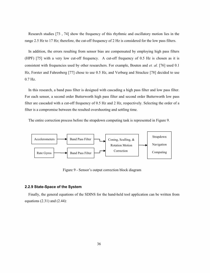
36
Research studies [ 73 , 74] show the frequency of this rhythmic and oscillatory motion lies in the
range 2.5 Hz to 17 Hz; therefore, the cut-off frequency of 2 Hz is considered for the low pass filters.
In addition, the errors resulting from sensor bias are compensated by employing high pass filters
(HPF) [ 75] with a very low cut-off frequency. A cut-off frequency of 0.5 Hz is chosen as it is
consistent with frequencies used by other researchers. For example, Bouten and et. al. [ 76] used 0.1
Hz, Forster and Fahrenberg [ 77] chose to use 0.5 Hz, and Verburg and Strackee [ 78] decided to use
0.7 Hz.
In this research, a band pass filter is designed with cascading a high pass filter and low pass filter.
For each sensor, a second order Butterworth high pass filter and second order Butterworth low pass
filter are cascaded with a cut-off frequency of 0.5 Hz and 2 Hz, respectively. Selecting the order of a
filter is a compromise between the resulted overshooting and settling time.
The entire correction process before the strapdown computing task is represented in Figure 9.
Figure 9 - Sensor’s output correction block diagram
2.2.9 State-Space of the System
Finally, the general equations of the SDINS for the hand-held tool application can be written from
equations (2.31) and (2.44):
Correction
Coning, Sculling, &
Rotation Motion
Accelerometers
Rate Gyros
Band Pass Filter
Band Pass Filter
Strapdown
Navigation
Computing
37
3� = �� �� = F�� (:� − � − � ) + ��
T = 12 ��� T = 12 \(T) " 0���� #
(2.50)
where 3� and �� denote the position and velocity of the tool tip with respect to the navigation frame.
2.3 Experimental Result
In this research, a 3DX-GX1 IMU from the Microstrain was used, which included three rate gyros
and three accelerometers with a sampling rate of 100 Hz and a noise density of 3.5 °/√ℎ~�3 and
0.4 ��/(3�� √�5), respectively [ 79]. Detailed specifications are found in Appendix A.
2.3.1 IMU Calibration
Microstrain Company has performed the calibration procedure for 3DX-GX1 IMU. This IMU is
calibrated for the scale factor, bias, misalignment, and even gyro G-sensitivity. In addition, the
performance of 3DX-GX1 is improved by full temperature compensation.
According to 3DX-GX1 documentation [ 79], the calibration parameters such as sensor gain and
bias are changed with temperature. Therefore, the calibration parameters must be calibrated with
respect to the operating temperature. Figure 10 through Figure 13 show the effect of temperature
compensation on the stability of the sensor gain and bias over the range of -20°C to 60°C. As shown
in these figures, the changes in the sensor gain and bias are considerable even the temperature is
changing in the small range. These results illustrated the importance of the parameter calibration
with respect to the temperature when it is hard to control the temperature of the environment that the
inertial sensors are operating.
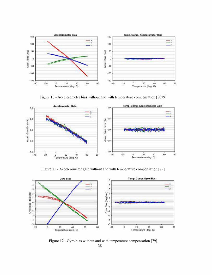
38
Figure 10 - Accelerometer bias without and with temperature compensation [ 80 79]
Figure 11 - Accelerometer gain without and with temperature compensation [ 79]
Figure 12 - Gyro bias without and with temperature compensation [ 79]
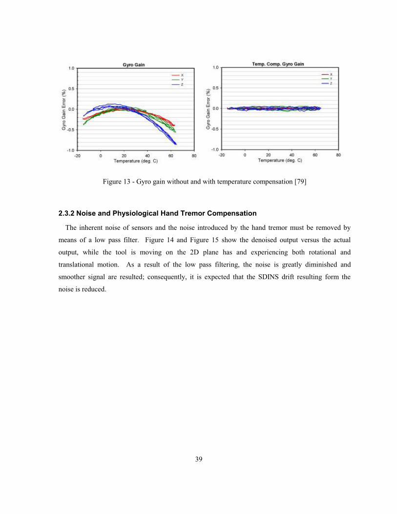
39
Figure 13 - Gyro gain without and with temperature compensation [ 79]
2.3.2 Noise and Physiological Hand Tremor Compensation
The inherent noise of sensors and the noise introduced by the hand tremor must be removed by
means of a low pass filter. Figure 14 and Figure 15 show the denoised output versus the actual
output, while the tool is moving on the 2D plane has and experiencing both rotational and
translational motion. As a result of the low pass filtering, the noise is greatly diminished and
smoother signal are resulted; consequently, it is expected that the SDINS drift resulting form the
noise is reduced.
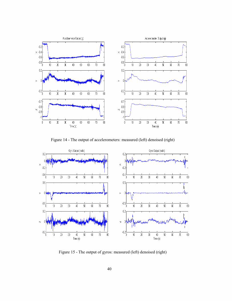
40
Figure 14 - The output of accelerometers: measured (left) denoised (right)
Figure 15 - The output of gyros: measured (left) denoised (right)
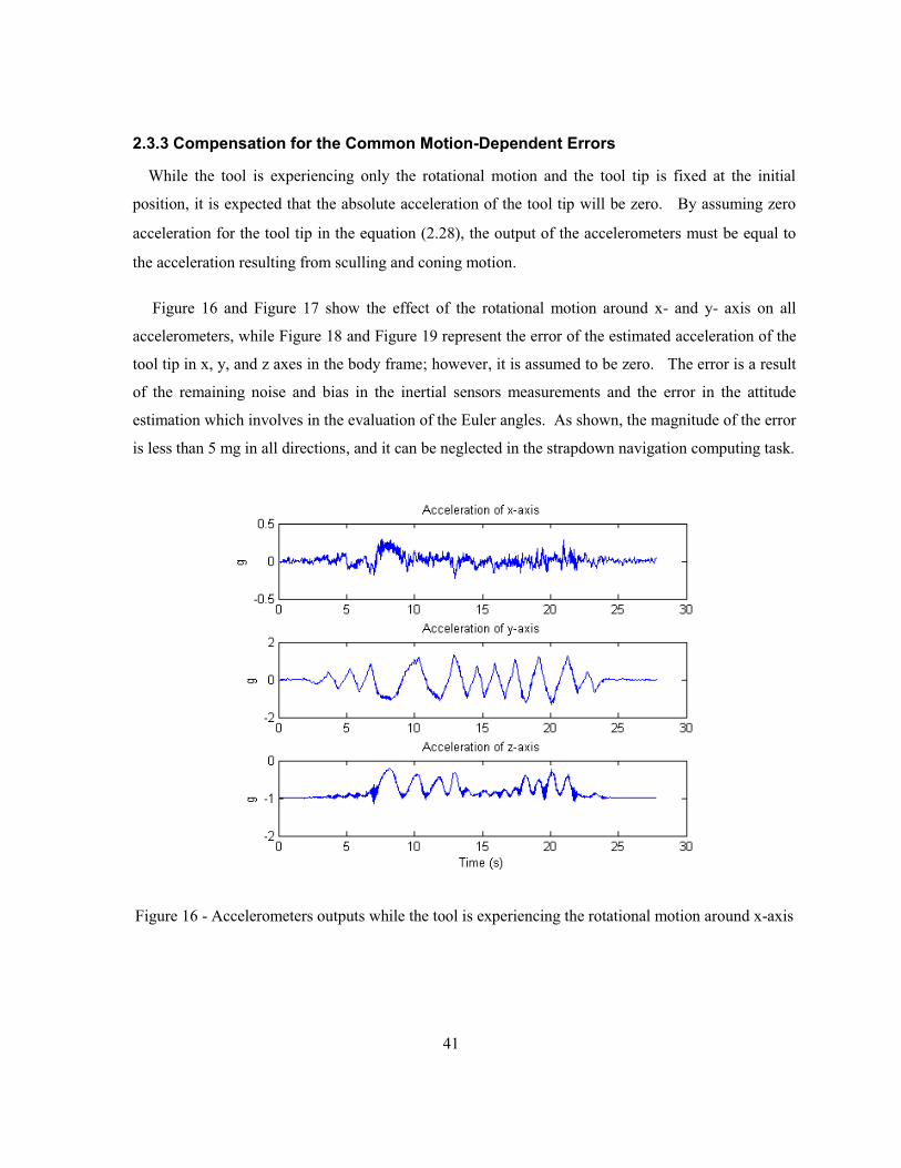
41
2.3.3 Compensation for the Common Motion-Dependent Errors
While the tool is experiencing only the rotational motion and the tool tip is fixed at the initial
position, it is expected that the absolute acceleration of the tool tip will be zero. By assuming zero
acceleration for the tool tip in the equation (2.28), the output of the accelerometers must be equal to
the acceleration resulting from sculling and coning motion.
Figure 16 and Figure 17 show the effect of the rotational motion around x- and y- axis on all
accelerometers, while Figure 18 and Figure 19 represent the error of the estimated acceleration of the
tool tip in x, y, and z axes in the body frame; however, it is assumed to be zero. The error is a result
of the remaining noise and bias in the inertial sensors measurements and the error in the attitude
estimation which involves in the evaluation of the Euler angles. As shown, the magnitude of the error
is less than 5 mg in all directions, and it can be neglected in the strapdown navigation computing task.
Figure 16 - Accelerometers outputs while the tool is experiencing the rotational motion around x-axis
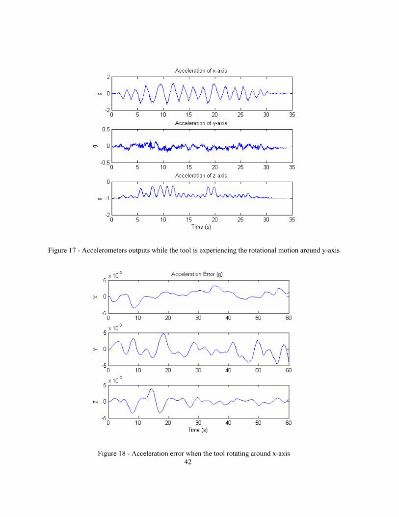
42
Figure 17 - Accelerometers outputs while the tool is experiencing the rotational motion around y-axis
Figure 18 - Acceleration error when the tool rotating around x-axis
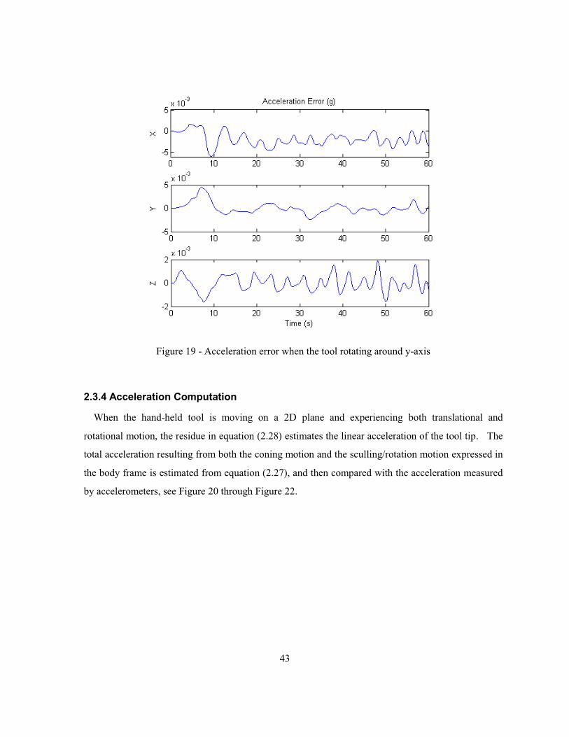
43
Figure 19 - Acceleration error when the tool rotating around y-axis
2.3.4 Acceleration Computation
When the hand-held tool is moving on a 2D plane and experiencing both translational and
rotational motion, the residue in equation (2.28) estimates the linear acceleration of the tool tip. The
total acceleration resulting from both the coning motion and the sculling/rotation motion expressed in
the body frame is estimated from equation (2.27), and then compared with the acceleration measured
by accelerometers, see Figure 20 through Figure 22.

44
Figure 20 - Estimated acceleration vs. measured acceleration in x axis
Figure 21 - Estimated acceleration vs. measured acceleration in y axis
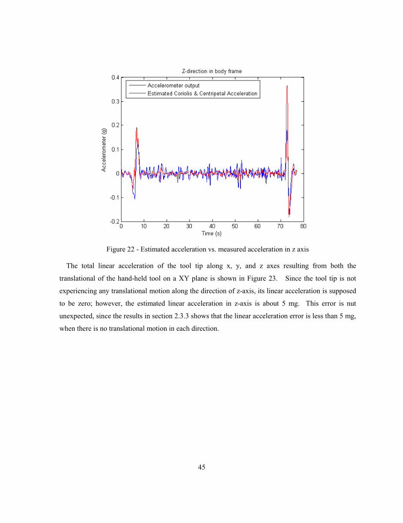
45
Figure 22 - Estimated acceleration vs. measured acceleration in z axis
The total linear acceleration of the tool tip along x, y, and z axes resulting from both the
translational of the hand-held tool on a XY plane is shown in Figure 23. Since the tool tip is not
experiencing any translational motion along the direction of z-axis, its linear acceleration is supposed
to be zero; however, the estimated linear acceleration in z-axis is about 5 mg. This error is nut
unexpected, since the results in section 2.3.3 shows that the linear acceleration error is less than 5 mg,
when there is no translational motion in each direction.
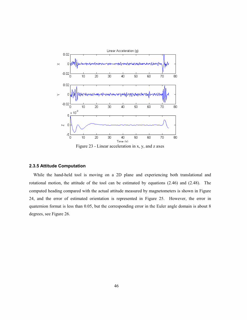
46
Figure 23 - Linear acceleration in x, y, and z axes
2.3.5 Attitude Computation
While the hand-held tool is moving on a 2D plane and experiencing both translational and
rotational motion, the attitude of the tool can be estimated by equations (2.46) and (2.48). The
computed heading compared with the actual attitude measured by magnetometers is shown in Figure
24, and the error of estimated orientation is represented in Figure 25. However, the error in
quaternion format is less than 0.05, but the corresponding error in the Euler angle domain is about 8
degrees, see Figure 26.
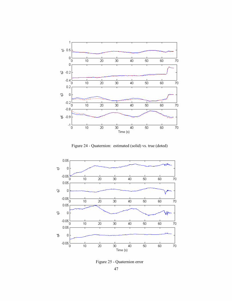
47
Figure 24 - Quaternion: estimated (solid) vs. true (doted)
Figure 25 - Quaternion error

48
Figure 26 - Euler angles error
2.4 Summary
This chapter presents an algorithm for reducing the effect of the common motion-dependent errors
in SDINS for a hand-held tool tracking system. The drift resulting from accelerometer bias is
reduced by applying a high-pass filter, while the error produced by the sensor noise and the tool
vibration is diminished by employing a low-pass filter. The common motion-dependent errors
including rotational and coning motion are taken into account not only in the calculation of the
effective acceleration but also in the computation of the attitude. The effects of the common motion-
dependent errors are reduced considerably, but the remaining attitude error is still great enough to
cause a drift in position estimation.
49
Chapter 3 Local Positioning System
The Local Positioning System (LPS) is a reliable and cost-effective tracking system for indoor
applications, designed to localize a moving object by estimating its three-dimensional position in real-
time. The LPS provides a small centralized version of the Global Positioning System (GPS) for
indoor environments, since the satellite signals are blocked easily by construction materials of
buildings.
Over the last few decades, the real-time video tracking systems have been used for a wide range of
applications such as robotics [ 35, 36], medicine [ 38], security [ 39], and even interactive games [ 80,
81]. Automated video analysis has been made possible by the easy access to high-powered
computers and high-quality but inexpensive video cameras.
In computer vision, object tracking refers to the detection of a desired object in each single frame
of sequential frames and the estimation of its trajectory as it moves around the scene. Video tracking
can be a complex and time-consuming process because of the noise in images, complex motion,
partial or full object occlusions, and loss of information because of projection of the 3D world on a
2D image.
Video tracking includes mounting the cameras around the workspace, calibrating the cameras,
capturing images, applying image processing algorithms and features extraction for every single
frame from each camera, and estimating the 3D position from 2D images.
In this chapter, the proposed multi-camera vision system, which includes four common CCD
cameras, is described with a new configuration set up and calibration procedure. In addition, the
required image processing techniques and feature extraction method is discussed.
3.1 Multi-Camera Vision System
The multi-camera systems generally include two or three digital cameras, while the positions of
their lens are placed in a straight line. However, the calibration procedure for the cameras is easier
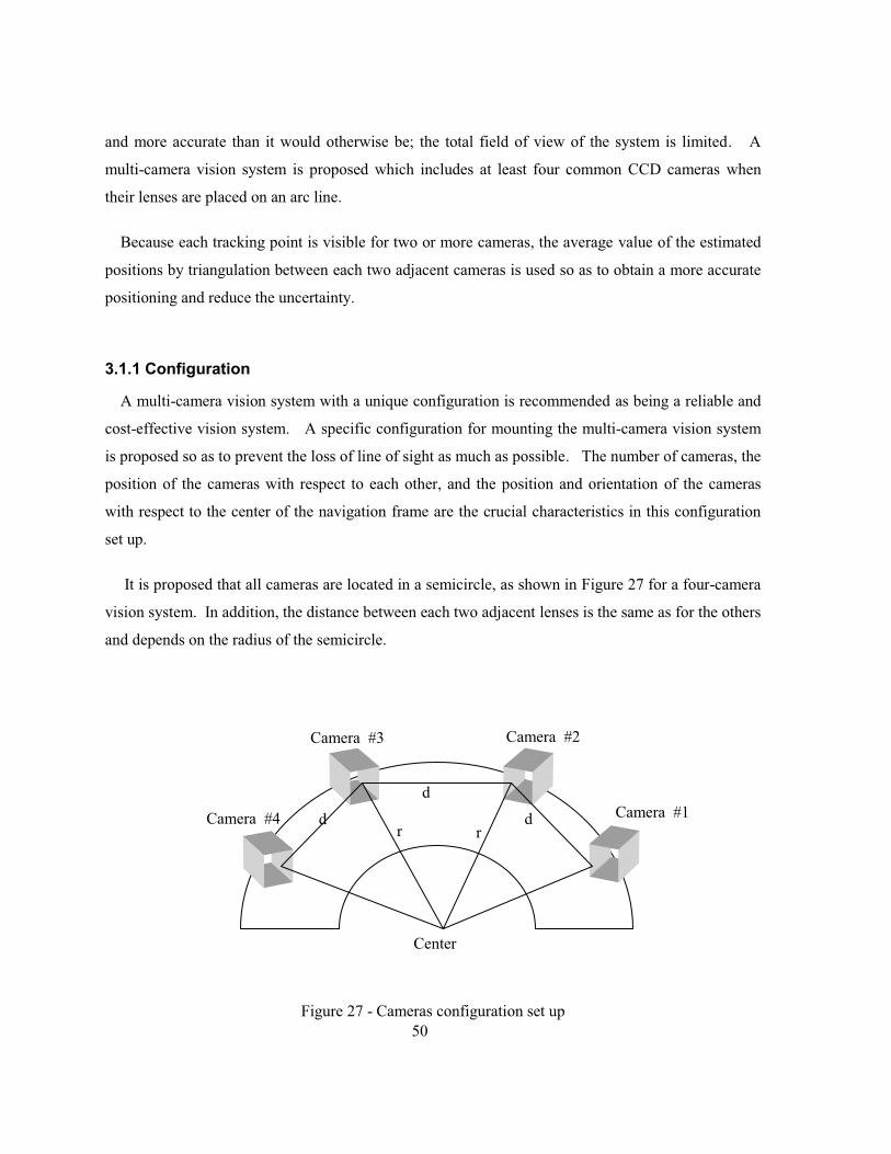
50
and more accurate than it would otherwise be; the total field of view of the system is limited. A
multi-camera vision system is proposed which includes at least four common CCD cameras when
their lenses are placed on an arc line.
Because each tracking point is visible for two or more cameras, the average value of the estimated
positions by triangulation between each two adjacent cameras is used so as to obtain a more accurate
positioning and reduce the uncertainty.
3.1.1 Configuration
A multi-camera vision system with a unique configuration is recommended as being a reliable and
cost-effective vision system. A specific configuration for mounting the multi-camera vision system
is proposed so as to prevent the loss of line of sight as much as possible. The number of cameras, the
position of the cameras with respect to each other, and the position and orientation of the cameras
with respect to the center of the navigation frame are the crucial characteristics in this configuration
set up.
It is proposed that all cameras are located in a semicircle, as shown in Figure 27 for a four-camera
vision system. In addition, the distance between each two adjacent lenses is the same as for the others
and depends on the radius of the semicircle.
Figure 27 - Cameras configuration set up
Center
d
d
d Camera #4
Camera #3 Camera #2
Camera #1 r r
51
According to Figure 27, the distance between each two cameras is calculated as follows:
9 = 2 3 tan ��8� (3.1)
Moreover, the tilt of the lenses toward the center and the length of the radius of semicircle depend
on the angle of view of each camera, the height of the cameras from the workspace, and the width of
the desired workspace.
As a result of this arrangement, a wide circular field of view is initiated with less loss of line-of-
sight. Figure 28 and Figure 29 show the field of view of the proposed multi camera vision systems
with a straight line and a semicircle configuration.
As shown in Figure 28, if the angle of view of each camera is α, the angle of view of the multi-
camera vision system with the straight line configuration is still equal to α with a forward-facing field
of view. However, the proposed multi-camera vision system initiates the wider angle of view which
is equal to (π – π/8). In addition, a circular field of view is provided with this configuration as
illustrated in Figure 29.
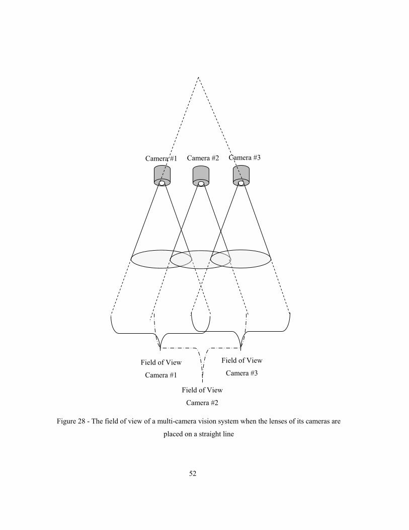
52
Figure 28 - The field of view of a multi-camera vision system when the lenses of its cameras are
placed on a straight line
Camera #2 Camera #1 Camera #3
Field of View
Camera #3 Field of View
Camera #1
Field of View
Camera #2
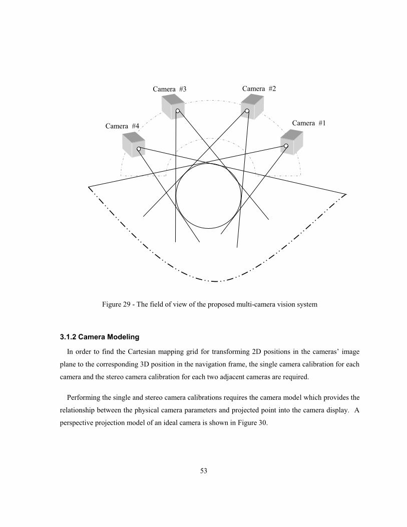
53
Figure 29 - The field of view of the proposed multi-camera vision system
3.1.2 Camera Modeling
In order to find the Cartesian mapping grid for transforming 2D positions in the cameras’ image
plane to the corresponding 3D position in the navigation frame, the single camera calibration for each
camera and the stereo camera calibration for each two adjacent cameras are required.
Performing the single and stereo camera calibrations requires the camera model which provides the
relationship between the physical camera parameters and projected point into the camera display. A
perspective projection model of an ideal camera is shown in Figure 30.
Camera #4
Camera #3 Camera #2
Camera #1

54
Figure 30 - Ideal camera imaging model
In this model, the image plane is located at the focal length of the lens on the optical axis z parallel
with the x-y plane of the camera frame [ 82]. Each point of an object in the navigation frame, � = [� � 5]� , is projected to the corresponding point p:
7 = �7�7� � = % �:�� �5 �: �5 & + "���� #
(3.2)
where f is the focal length of the camera lens, 1� and 1� denote the dimension of a pixel on the image
plane, �� represents the image scale factor [ 83], and the vector N is a zero-mean Gaussian random
measurement noise.
In a real digital camera, because of the lens distortion, the location of point p is not located exactly
on the projected line [ 84, 85]. As shown in Figure 31, two tangential and radial distortions relocate
the position of the projected point.
px py
Image Plane
z=f y
x P z
Object
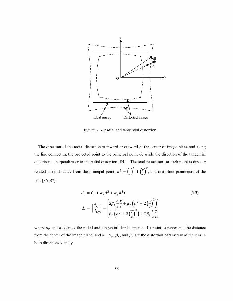
55
Figure 31 - Radial and tangential distortion
The direction of the radial distortion is inward or outward of the center of image plane and along
the line connecting the projected point to the principal point O, while the direction of the tangential
distortion is perpendicular to the radial distortion [ 84]. The total relocation for each point is directly
related to its distance from the principal point, 92 = ��5�2 + ��5�2, and distortion parameters of the
lens [ 86, 87]:
93 = (1 + w� 92 + w� 94)
9� = "9�,�9�,� # = %2�� �5 �5 + �� h92 + 2 ��5�2q�� h92 + 2 ��5�2q + 2�� �5 �5&
(3.3)
where 93 and 9� denote the radial and tangential displacements of a point; d represents the distance
from the center of the image plane; and w� , w� , �� , and �� are the distortion parameters of the lens in
both directions x and y.
Ideal image
β
α
y
x
Distorted image
O
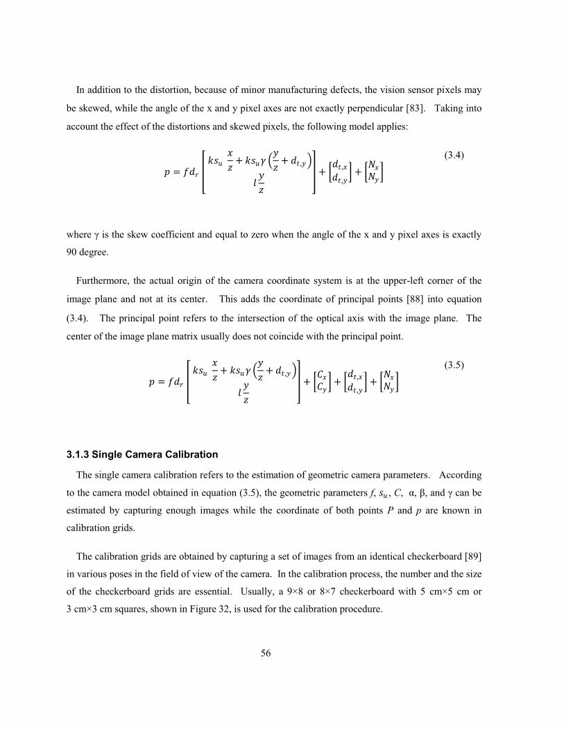
56
In addition to the distortion, because of minor manufacturing defects, the vision sensor pixels may
be skewed, while the angle of the x and y pixel axes are not exactly perpendicular [ 83]. Taking into
account the effect of the distortions and skewed pixels, the following model applies:
7 = :93 % ��� �5 + ��� � ��5 + 9�,� � � �5 & + "9�,�9�,� # + "���� #
(3.4)
where γ is the skew coefficient and equal to zero when the angle of the x and y pixel axes is exactly
90 degree.
Furthermore, the actual origin of the camera coordinate system is at the upper-left corner of the
image plane and not at its center. This adds the coordinate of principal points [ 88] into equation
(3.4). The principal point refers to the intersection of the optical axis with the image plane. The
center of the image plane matrix usually does not coincide with the principal point.
7 = :93 % ��� �5 + ��� � ��5 + 9�,� � � �5 & + "F�F� # + "9�,�9�,� # + "���� #
(3.5)
3.1.3 Single Camera Calibration
The single camera calibration refers to the estimation of geometric camera parameters. According
to the camera model obtained in equation (3.5), the geometric parameters f, �� , C, α, β, and γ can be
estimated by capturing enough images while the coordinate of both points P and p are known in
calibration grids.
The calibration grids are obtained by capturing a set of images from an identical checkerboard [ 89]
in various poses in the field of view of the camera. In the calibration process, the number and the size
of the checkerboard grids are essential. Usually, a 9×8 or 8×7 checkerboard with 5 cm×5 cm or
3 cm×3 cm squares, shown in Figure 32, is used for the calibration procedure.
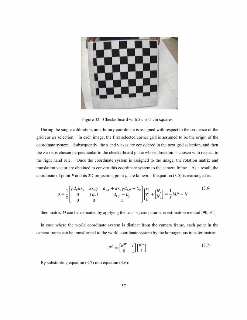
57
Figure 32 - Checkerboard with 5 cm×5 cm squares
During the single calibration, an arbitrary coordinate is assigned with respect to the sequence of the
grid corner selection. In each image, the first selected corner grid is assumed to be the origin of the
coordinate system. Subsequently, the x and y axes are considered in the next grid selection, and then
the z-axis is chosen perpendicular to the checkerboard plane whose direction is chosen with respect to
the right hand rule. Once the coordinate system is assigned to the image, the rotation matrix and
translation vector are obtained to convert this coordinate system to the camera frame. As a result, the
coordinate of point P and its 2D projection, point p, are known. If equation (3.5) is rearranged as:
7 = 15 <:93 ��� ��� � 9�,� + ��� �9�,� + F�0 :93 � 9�,� + F�0 0 1 B `��1g + "���� # = 15 � + � (3.6)
then matrix M can be estimated by applying the least square parameter estimation method [ 90, 91].
In case where the world coordinate system is distinct from the camera frame, each point in the
camera frame can be transformed to the world coordinate system by the homogenous transfer matrix:
�F = "/F� �0 1# ���1 � (3.7)
By substituting equation (3.7) into equation (3.6):

58
7 = 15 "/F� �0 1# ���1 � + � = 15 ℳ� + � (3.8)
where matrix ℳ includes intrinsic and extrinsic parameters; and then, the geometric parameter of
the camera can be obtained by estimating matrix ℳ.
3.1.4 Stereo Camera Calibration
Since the 3D position of each tracking point with respect to the navigation frame is desirable, aside
from the single camera calibration, the stereo camera calibration [ 92] for each two adjacent cameras
should be performed to make three-dimensional vision possible.
The stereo camera calibration refers to a procedure that provides the extrinsic parameters of two
adjacent cameras relative to each other. This procedure allows us to calculate depth by using
triangulation algorithm. Performing stereo camera calibration requires a set of images captured by
two neighboring cameras simultaneously. Going through the corner extraction process, the same set
of points must be selected in both the left and right image of the same scene. In addition, this is
crucial that the same grid must be selected as being the origin point for both images. This means the
identical pattern must be chosen for selecting the corner grids for all pair of images.
As a result of the stereo calibration, the homogenous transfer matrix is obtained, which transforms
each point in the right camera frame into the left camera frame and allows computing the 3D position
of each point in the image plane expressed in the both right and left camera frame.
3.1.5 Defining the World Coordinate System
Finding the 3D position of the tool tip with respect to the navigation frame requires that a unique
world coordinate system is considered for all cameras.
According to the single camera calibration procedure, a unique world coordinate system can be
considered for all four cameras as shown in Figure 33. This world coordinate system is also aligned
on the navigation frame which is defined in the SDINS.
First, all four cameras capture the image of the checkerboard simultaneously. Then a unique
corner of checkerboard in four images is chosen as the origin of the world coordinate system. Since

59
the direction of the x, y, and z axes are obtained with respect to the next grids selection, the next grids
must be selected in the same pattern in four images. Once the calibration procedure is performed for
all cameras, the homogenous transfer matrix is available to convert each point from each camera
frame to the world coordinate system.
Figure 33 - The world coordinate system in the view of:
(a) camera #1 (b) camera #2 (c) camera #3 (d) camera #4
3.2 Digital Image Processing
Digital image processing techniques are the two-dimensional digital signal processing which are
designed to enhance the quality of an image, restore information from a distorted image, and extract
required information.
x
y
z
O
x
y
z
O
x
y
z
O
(a) (b)
(c) (d)
y
z
x
O
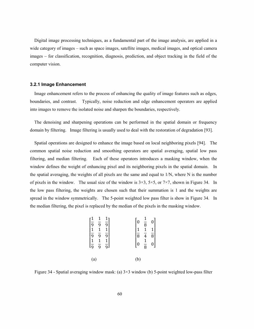
60
Digital image processing techniques, as a fundamental part of the image analysis, are applied in a
wide category of images – such as space images, satellite images, medical images, and optical camera
images – for classification, recognition, diagnosis, prediction, and object tracking in the field of the
computer vision.
3.2.1 Image Enhancement
Image enhancement refers to the process of enhancing the quality of image features such as edges,
boundaries, and contrast. Typically, noise reduction and edge enhancement operators are applied
into images to remove the isolated noise and sharpen the boundaries, respectively.
The denoising and sharpening operations can be performed in the spatial domain or frequency
domain by filtering. Image filtering is usually used to deal with the restoration of degradation [ 93].
Spatial operations are designed to enhance the image based on local neighboring pixels [ 94]. The
common spatial noise reduction and smoothing operators are spatial averaging, spatial low pass
filtering, and median filtering. Each of these operators introduces a masking window, when the
window defines the weight of enhancing pixel and its neighboring pixels in the spatial domain. In
the spatial averaging, the weights of all pixels are the same and equal to 1/N, where N is the number
of pixels in the window. The usual size of the window is 3×3, 5×5, or 7×7, shown in Figure 34. In
the low pass filtering, the weights are chosen such that their summation is 1 and the weights are
spread in the window symmetrically. The 5-point weighted low pass filter is show in Figure 34. In
the median filtering, the pixel is replaced by the median of the pixels in the masking window.
⎣⎢⎢⎢⎢⎡19 19 1919 19 1919 19 19⎦⎥
⎥⎥⎥⎤
⎣⎢⎢⎢⎢⎡0 18 018 14 180 18 0⎦⎥
⎥⎥⎥⎤
(a) (b)
Figure 34 - Spatial averaging window mask: (a) 3×3 window (b) 5-point weighted low-pass filter

61
The original image is blurred by applying the noise reduction and smoothing operators. The
unsharp masking operation is generally used to sharpen the edges. This operation can be
represented as:
�(�, �) = �(�, �) + ��(�, �) (3.9)
where u(m,n), v(m,n), and g(m,n) are the original, unsharp masked, and gradient image,
respectively; and λ is chosen to be greater than zero. The gradient is a discrete Laplacian operator:
�(�, �) = �(�, �)− 14 [�(� − 1, �) + �(�, � − 1) + �(� + 1, �) + �(�, � + 1)]
(3.10)
Besides the spatial domain, denoising and sharpening can be performed in the frequency domain.
Digital Fourier transform (DFT) or Discrete Wavelet transform (DWT) of an image is the
representation of the image in the frequency domain. Accordingly, various filters have been
designed to apply into the image in this domain. Displaying the resulting image in the spatial
domain requires inverse transformation of DFT or DWT. Studies show that the result of image
filtering in the frequency domain is more precise than it is in the spatial domain [ 95].
3.2.2 Edge Detection
The very first step of features extraction and segmentation is edge detection. Edges can be
considered the pixels that their luminous intensity or gray-level changes sharply with respect to their
neighboring pixels.
Edges can be localized by finding maximum local in the image derivatives [ 96]. Gradient and
Laplace operators are designed based on computing the first- and second-order derivatives of the
image. These operators include a mask or pair of masks, shown in Figure 35.
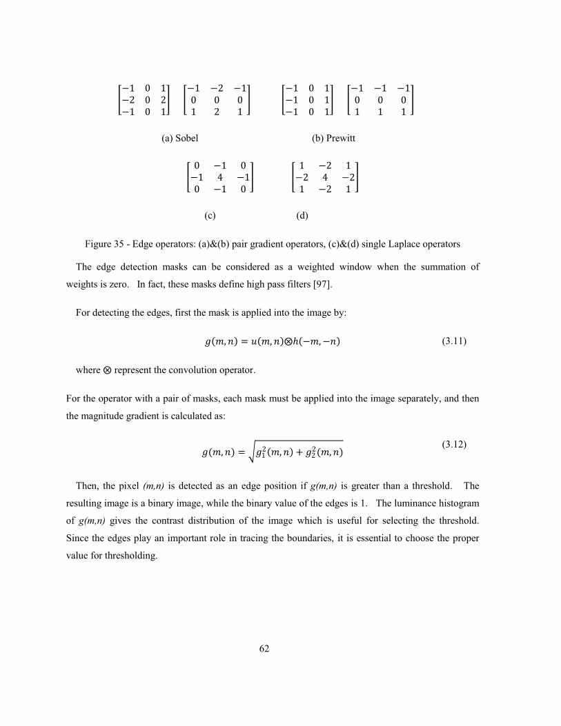
62
C−1 0 1−2 0 2−1 0 1E C−1 −2 −10 0 01 2 1 E C−1 0 1−1 0 1−1 0 1E C−1 −1 −10 0 01 1 1 E (a) Sobel (b) Prewitt
C 0 −1 0−1 4 −10 −1 0 E C 1 −2 1−2 4 −21 −2 1 E
(c) (d)
Figure 35 - Edge operators: (a)&(b) pair gradient operators, (c)&(d) single Laplace operators
The edge detection masks can be considered as a weighted window when the summation of
weights is zero. In fact, these masks define high pass filters [ 97].
For detecting the edges, first the mask is applied into the image by:
�(�, �) = �(�, �)⨂ℎ(−�, −�) (3.11)
where ⨂ represent the convolution operator.
For the operator with a pair of masks, each mask must be applied into the image separately, and then
the magnitude gradient is calculated as:
�(�, �) = ��12(�, �) + �22(�, �) (3.12)
Then, the pixel (m,n) is detected as an edge position if g(m,n) is greater than a threshold. The
resulting image is a binary image, while the binary value of the edges is 1. The luminance histogram
of g(m,n) gives the contrast distribution of the image which is useful for selecting the threshold.
Since the edges play an important role in tracing the boundaries, it is essential to choose the proper
value for thresholding.
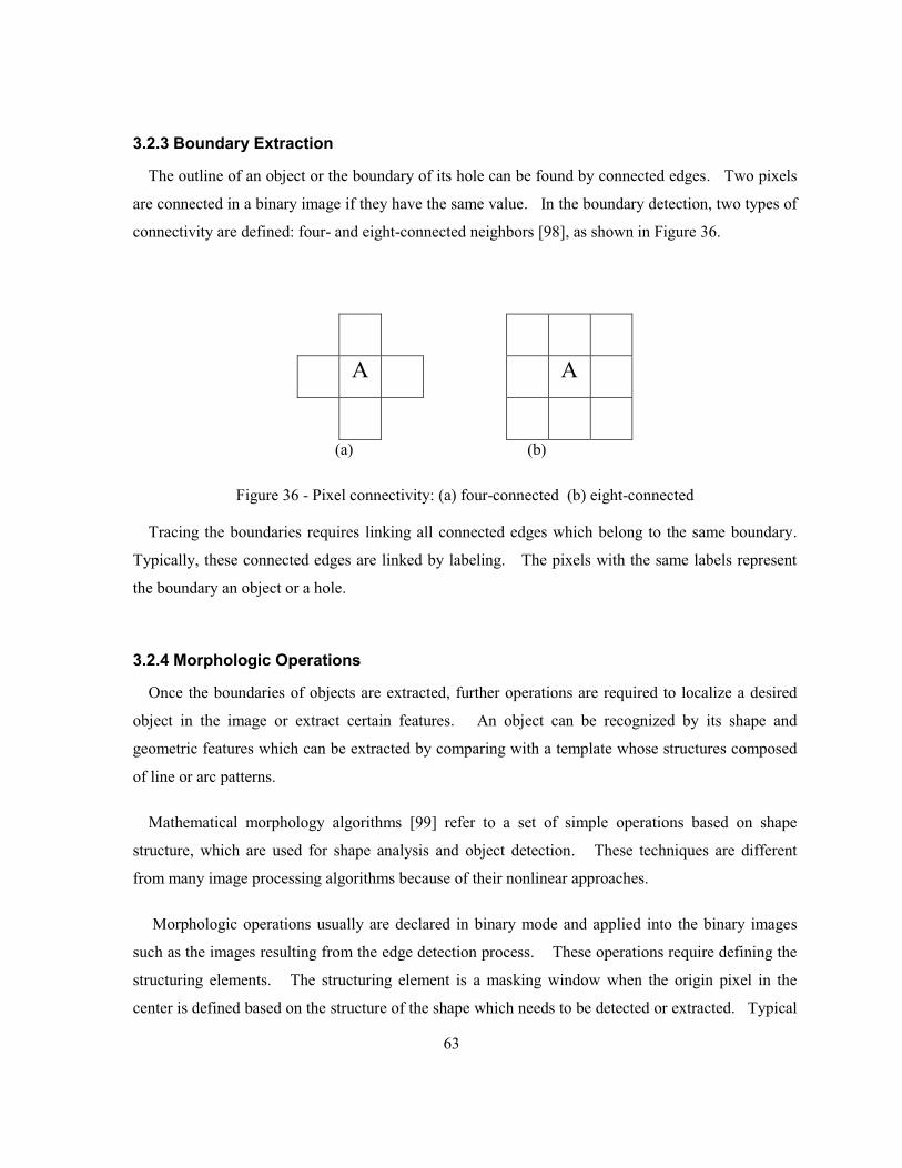
63
3.2.3 Boundary Extraction
The outline of an object or the boundary of its hole can be found by connected edges. Two pixels
are connected in a binary image if they have the same value. In the boundary detection, two types of
connectivity are defined: four- and eight-connected neighbors [ 98], as shown in Figure 36.
A A
(a) (b)
Figure 36 - Pixel connectivity: (a) four-connected (b) eight-connected
Tracing the boundaries requires linking all connected edges which belong to the same boundary.
Typically, these connected edges are linked by labeling. The pixels with the same labels represent
the boundary an object or a hole.
3.2.4 Morphologic Operations
Once the boundaries of objects are extracted, further operations are required to localize a desired
object in the image or extract certain features. An object can be recognized by its shape and
geometric features which can be extracted by comparing with a template whose structures composed
of line or arc patterns.
Mathematical morphology algorithms [ 99] refer to a set of simple operations based on shape
structure, which are used for shape analysis and object detection. These techniques are different
from many image processing algorithms because of their nonlinear approaches.
Morphologic operations usually are declared in binary mode and applied into the binary images
such as the images resulting from the edge detection process. These operations require defining the
structuring elements. The structuring element is a masking window when the origin pixel in the
center is defined based on the structure of the shape which needs to be detected or extracted. Typical
64
operations are dilation, erosion, opening, and closing, with the net effect of expanding, shrinking,
simplifying, and smoothing the shapes [ 100], respectively.
The dilation of set A by set B denoted by �⨁� and defined as:
�⨁� = ⟨max(5)| ��⏞�5 ∩ � ≠ ∅⟩ (3.13)
where sets A and B are members of the 2D integer space; ��⏞�5 is the translation of the reflection of
the set B by point 5 = (51, 52) and obtained by
�⏞ = {�|� = −�, :~3 � ∈ �} (�)5 = {�|� = � + 5, :~3 � ∈ �}
(3.14)
In other words, the origin pixel is replaced by the maximum value of all the neighboring pixels in
the structure window B. In a binary image, if the value of any of the neighboring pixels is 1, the
origin pixel is set to 1.
The erosion of set A by set B denoted by � ⊖ � and defined as:
� ⊖ � = {min(5)|(�)5 ⊆ �} (3.15)
where sets A and B are members of the 2-D integer space.
In other words, the value of origin pixel is set to the minimum value of all the neighboring pixels in
the structure window B. In a binary image, if the value of any of the neighboring pixels is 0, the
origin pixel is replaced by 0. The opening and closing operation are called dual operations.
An opening operation is defined by erosion followed by dilation with the same structuring element,
while a closing operation is defined by dilation followed by erosion with the same structuring
element.

65
3.3 Experimental Results
This section summarizes the experimental results based on the described multi-camera vision
system. The multi-camera vision includes four surveillance IR-CCD cameras; their specifications
are described in Table 1.
Table 1 - Camera specifications
Image Sensor 1/3" Color Sharp CCD
Effective Pixels NTSC: 510(H) X492(V)
Unit Cell Size 9.6μm (H) × 7.5μm (V)
Sensor Size 4.8mm (H) × 3.6 mm(V)
Scanning System 2:1 Interlace
Signal System NTSC
Infrared LED's 24 LED's
Infrared Illumination 60 ft
Minimum Luminance 0 Lux
Horizontal Resolution 420 TV Lines
S/N Ratio Less than 48 dB
Gamma 0.45
Video Out BNC
All cameras are connected to a PC through the IDS Falcon Quattro PCIe frame grabber, which
includes four parallel video channels and is capable of capturing simultaneously images from
four cameras with a sampling rate of 20 fps. Detailed characteristics of the frame grabber
are listed in Table 2.
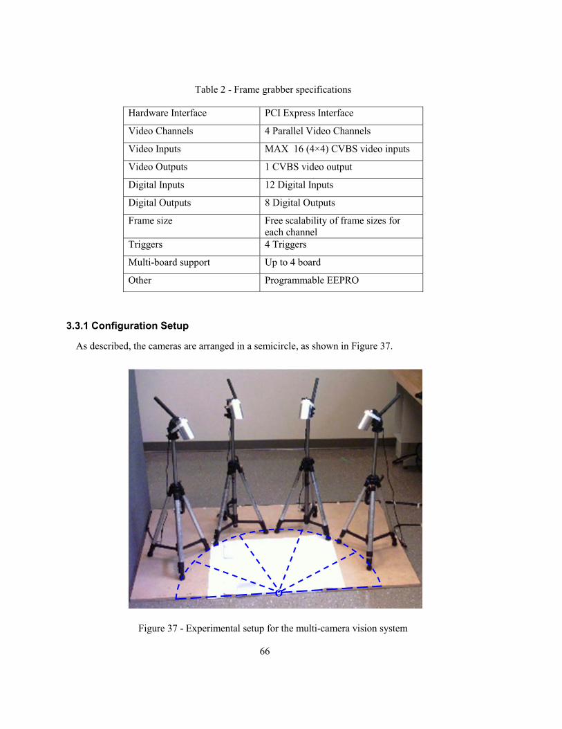
66
Table 2 - Frame grabber specifications
Hardware Interface PCI Express Interface
Video Channels 4 Parallel Video Channels
Video Inputs MAX 16 (4×4) CVBS video inputs
Video Outputs 1 CVBS video output
Digital Inputs 12 Digital Inputs
Digital Outputs 8 Digital Outputs
Frame size Free scalability of frame sizes for each channel
Triggers 4 Triggers
Multi-board support Up to 4 board
Other Programmable EEPRO
3.3.1 Configuration Setup
As described, the cameras are arranged in a semicircle, as shown in Figure 37.
Figure 37 - Experimental setup for the multi-camera vision system
O
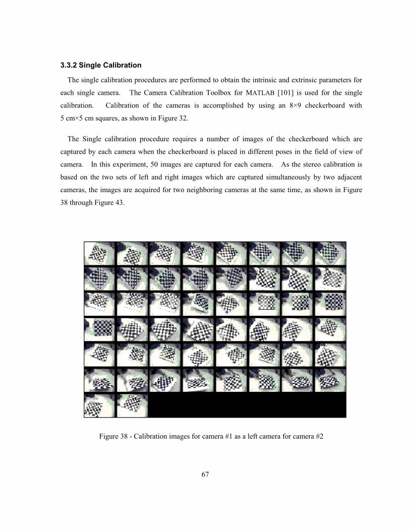
67
3.3.2 Single Calibration
The single calibration procedures are performed to obtain the intrinsic and extrinsic parameters for
each single camera. The Camera Calibration Toolbox for MATLAB [ 101] is used for the single
calibration. Calibration of the cameras is accomplished by using an 8×9 checkerboard with
5 cm×5 cm squares, as shown in Figure 32.
The Single calibration procedure requires a number of images of the checkerboard which are
captured by each camera when the checkerboard is placed in different poses in the field of view of
camera. In this experiment, 50 images are captured for each camera. As the stereo calibration is
based on the two sets of left and right images which are captured simultaneously by two adjacent
cameras, the images are acquired for two neighboring cameras at the same time, as shown in Figure
38 through Figure 43.
Figure 38 - Calibration images for camera #1 as a left camera for camera #2
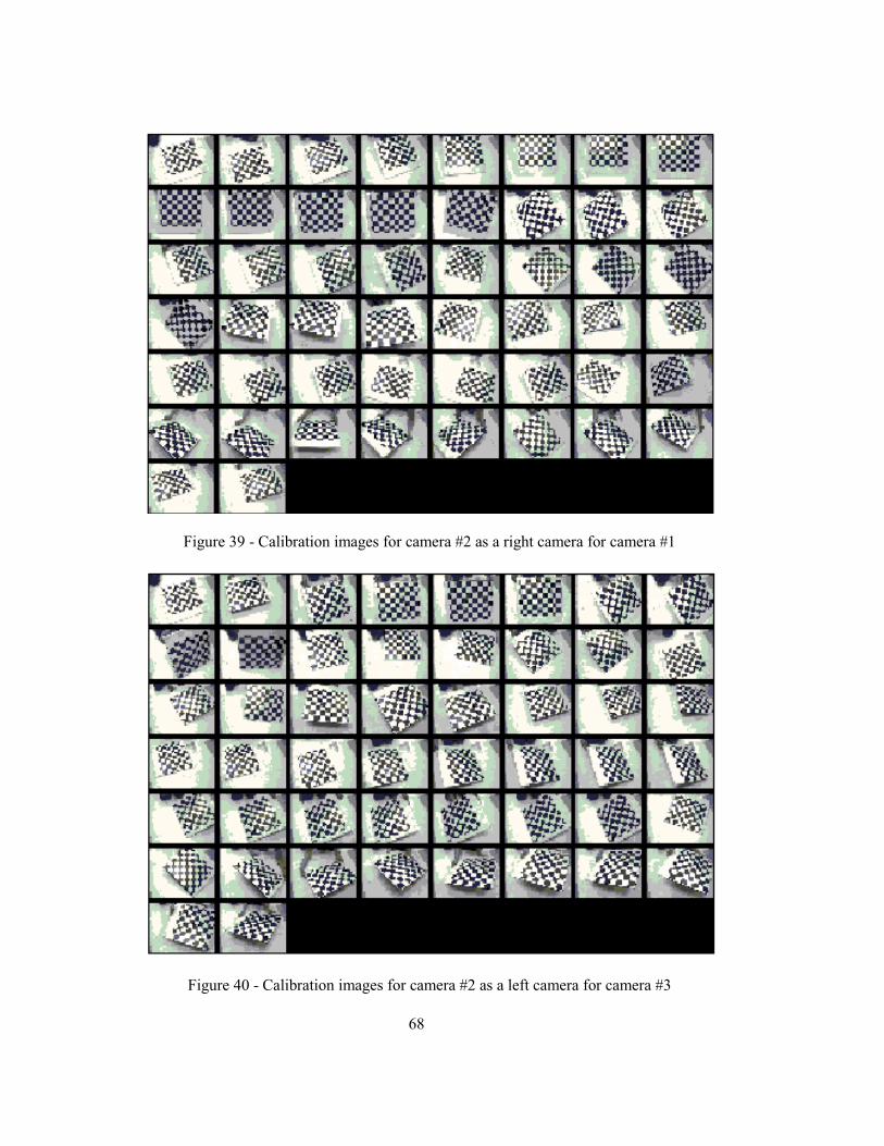
68
Figure 39 - Calibration images for camera #2 as a right camera for camera #1
Figure 40 - Calibration images for camera #2 as a left camera for camera #3

69
Figure 41 - Calibration images for camera #3 as a right camera for camera #2
Figure 42 - Calibration images for camera #3 as a left camera for camera #4
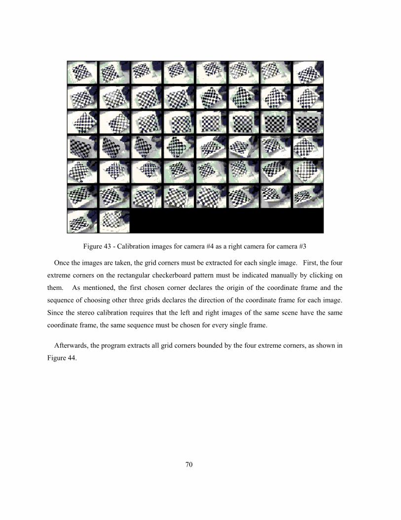
70
Figure 43 - Calibration images for camera #4 as a right camera for camera #3
Once the images are taken, the grid corners must be extracted for each single image. First, the four
extreme corners on the rectangular checkerboard pattern must be indicated manually by clicking on
them. As mentioned, the first chosen corner declares the origin of the coordinate frame and the
sequence of choosing other three grids declares the direction of the coordinate frame for each image.
Since the stereo calibration requires that the left and right images of the same scene have the same
coordinate frame, the same sequence must be chosen for every single frame.
Afterwards, the program extracts all grid corners bounded by the four extreme corners, as shown in
Figure 44.
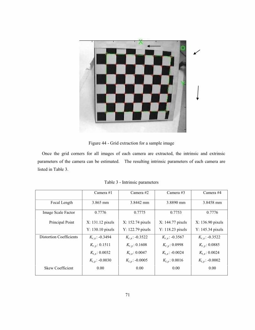
71
Figure 44 - Grid extraction for a sample image
Once the grid corners for all images of each camera are extracted, the intrinsic and extrinsic
parameters of the camera can be estimated. The resulting intrinsic parameters of each camera are
listed in Table 3.
Table 3 - Intrinsic parameters
Camera #1 Camera #2 Camera #3 Camera #4
Focal Length 3.865 mm 3.8442 mm 3.8890 mm 3.8458 mm
Image Scale Factor 0.7776 0.7775 0.7753 0.7776
Principal Point X: 131.12 pixels
Y: 130.10 pixels
X: 152.74 pixels
Y: 122.79 pixels
X: 144.77 pixels
Y: 118.23 pixels
X: 136.90 pixels
Y: 145.34 pixels
Distortion Coefficients
�3,� : -0.3494 �3,� : 0.1511 ��,� : 0.0032 ��,� : -0.0030
�3,� : -0.3522 �3,� : 0.1608 ��,� : 0.0047 ��,� : -0.0005
�3,� : -0.3567 �3,� : 0.0998 ��,� : -0.0024 ��,� : 0.0016
�3,� : -0.3522 �3,� : 0.0885 ��,� : 0.0024 ��,� : -0.0002
Skew Coefficient 0.00 0.00 0.00 0.00
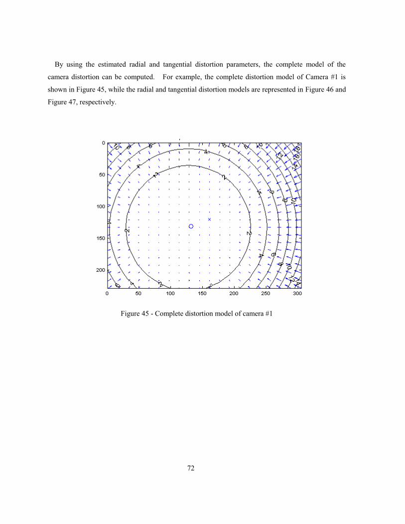
72
By using the estimated radial and tangential distortion parameters, the complete model of the
camera distortion can be computed. For example, the complete distortion model of Camera #1 is
shown in Figure 45, while the radial and tangential distortion models are represented in Figure 46 and
Figure 47, respectively.
Figure 45 - Complete distortion model of camera #1
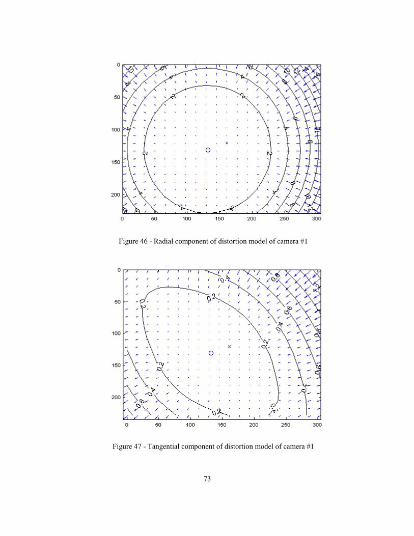
73
Figure 46 - Radial component of distortion model of camera #1
Figure 47 - Tangential component of distortion model of camera #1
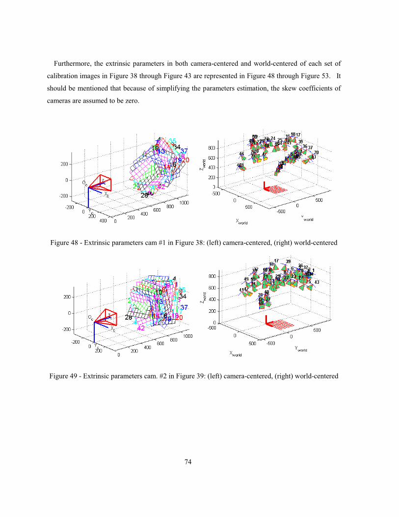
74
Furthermore, the extrinsic parameters in both camera-centered and world-centered of each set of
calibration images in Figure 38 through Figure 43 are represented in Figure 48 through Figure 53. It
should be mentioned that because of simplifying the parameters estimation, the skew coefficients of
cameras are assumed to be zero.
Figure 48 - Extrinsic parameters cam #1 in Figure 38: (left) camera-centered, (right) world-centered
Figure 49 - Extrinsic parameters cam. #2 in Figure 39: (left) camera-centered, (right) world-centered

75
Figure 50 - Extrinsic parameters cam. #2 in Figure 40: (left) camera-centered, (right) world-centered
Figure 51 - Extrinsic parameters cam. #3 in Figure 41: (left) camera-centered, (right) world-centered
Figure 52 - Extrinsic parameters cam. #3 in Figure 42: (left) camera-centered, (right) world-centered
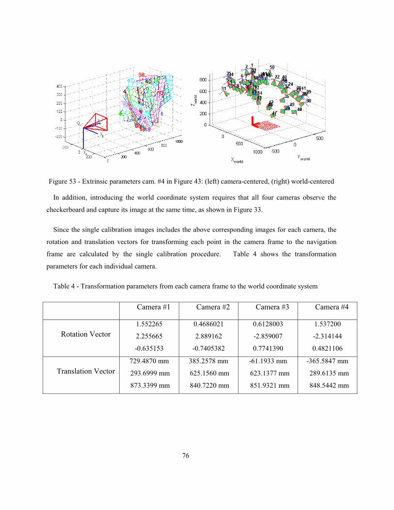
76
Figure 53 - Extrinsic parameters cam. #4 in Figure 43: (left) camera-centered, (right) world-centered
In addition, introducing the world coordinate system requires that all four cameras observe the
checkerboard and capture its image at the same time, as shown in Figure 33.
Since the single calibration images includes the above corresponding images for each camera, the
rotation and translation vectors for transforming each point in the camera frame to the navigation
frame are calculated by the single calibration procedure. Table 4 shows the transformation
parameters for each individual camera.
Table 4 - Transformation parameters from each camera frame to the world coordinate system
Camera #1 Camera #2 Camera #3 Camera #4
Rotation Vector 1.552265
2.255665
-0.635153
0.4686021
2.889162
-0.7405382
0.6128003
-2.859007
0.7741390
1.537200
-2.314144
0.4821106
Translation Vector 729.4870 mm
293.6999 mm
873.3399 mm
385.2578 mm
625.1560 mm
840.7220 mm
-61.1933 mm
623.1377 mm
851.9321 mm
-365.5847 mm
289.6135 mm
848.5442 mm
77
3.3.3 Stereo Calibration
The stereo calibration process refers to an algorithm of estimating extrinsic parameters of the right
camera with respect to the left camera for each two adjacent cameras. The result of the stereo
calibration allows applying the triangulation technique to estimate the depth of the desired object.
Since the captured images for each of two neighboring cameras in the single camera calibration
phase are followed the required rule for executing the stereo calibration procedure, the direct result of
the single calibration step can be employed in the stereo calibration algorithm. Table 5 shows the
rotation and translation vector for transforming each point in the right camera frame to the left camera
frame.
Table 5 - Extrinsic parameters for each two adjacent cameras
Camera #1 & #2 Camera #2 & #3 Camera #3 & #4
Rotation Vector 0.02865
0.42562
0.76695
-0.03225
0.42071
0.63442
0.09050
0.42463
0.64168
Translation Vector -431.649730 mm
-197.41507 mm
55.10179 mm
-410.24851 mm
-147.60000 mm
105.27998 mm
-419.84660 mm
-134.27390 mm
94.60045 mm
3.3.4 Image Processing
In this research, the image processing techniques are applied to every single frame from each
camera to localize the tool tip. The results of the image processing techniques are shown on a
selected image which is displayed in Figure 54.
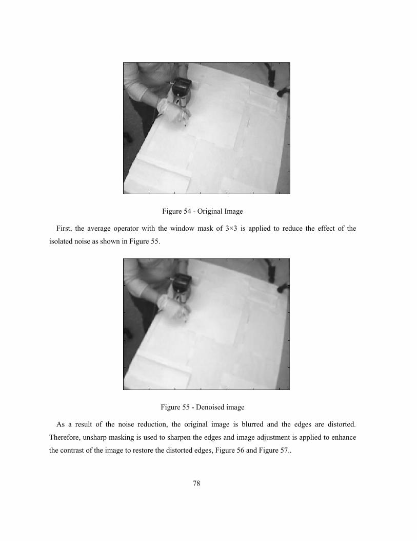
78
Figure 54 - Original Image
First, the average operator with the window mask of 3×3 is applied to reduce the effect of the
isolated noise as shown in Figure 55.
Figure 55 - Denoised image
As a result of the noise reduction, the original image is blurred and the edges are distorted.
Therefore, unsharp masking is used to sharpen the edges and image adjustment is applied to enhance
the contrast of the image to restore the distorted edges, Figure 56 and Figure 57..
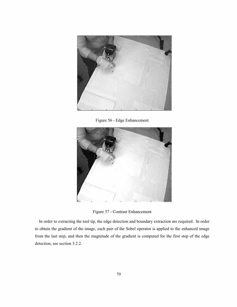
79
Figure 56 - Edge Enhancement
Figure 57 - Contrast Enhancement
In order to extracting the tool tip, the edge detection and boundary extraction are required. In order
to obtain the gradient of the image, each pair of the Sobel operator is applied to the enhanced image
from the last step, and then the magnitude of the gradient is computed for the first step of the edge
detection, see section 3.2.2.
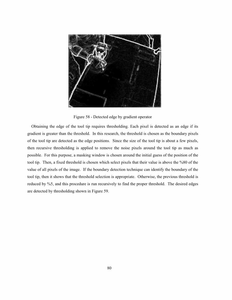
80
Figure 58 - Detected edge by gradient operator
Obtaining the edge of the tool tip requires thresholding. Each pixel is detected as an edge if its
gradient is greater than the threshold. In this research, the threshold is chosen as the boundary pixels
of the tool tip are detected as the edge positions. Since the size of the tool tip is about a few pixels,
then recursive thresholding is applied to remove the noise pixels around the tool tip as much as
possible. For this purpose, a masking window is chosen around the initial guess of the position of the
tool tip. Then, a fixed threshold is chosen which select pixels that their value is above the %80 of the
value of all pixels of the image. If the boundary detection technique can identify the boundary of the
tool tip, then it shows that the threshold selection is appropriate. Otherwise, the previous threshold is
reduced by %5, and this procedure is run recursively to find the proper threshold. The desired edges
are detected by thresholding shown in Figure 59.
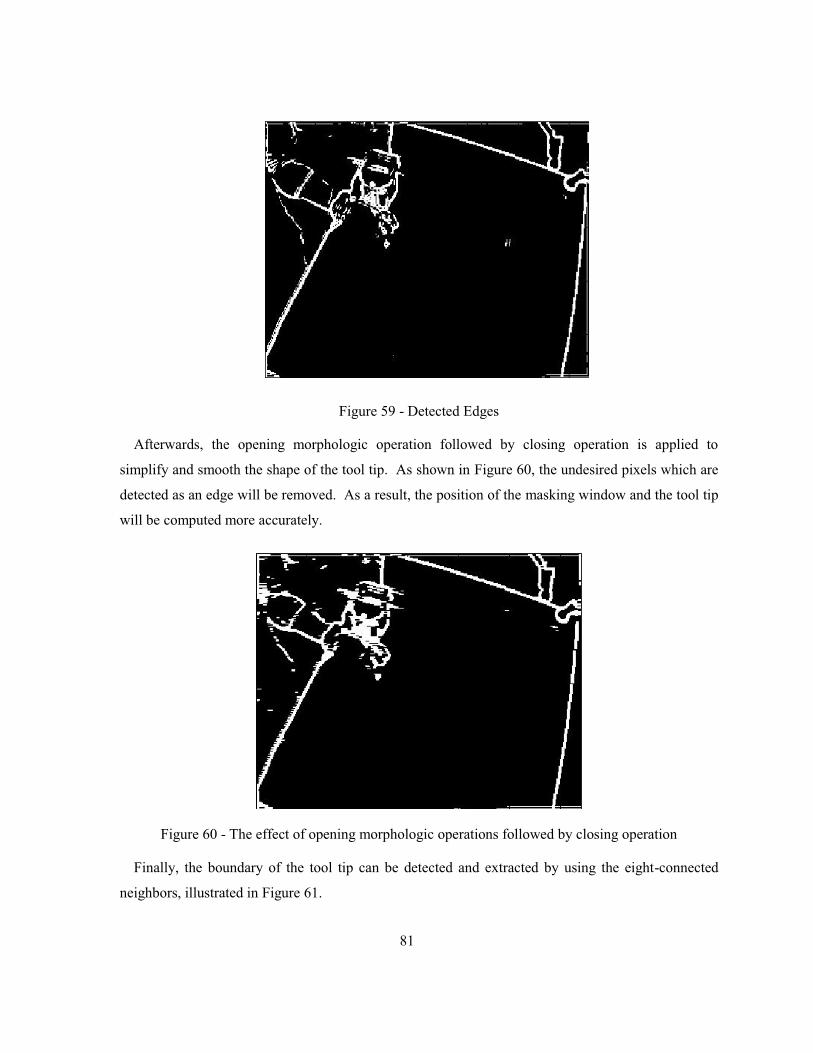
81
Figure 59 - Detected Edges
Afterwards, the opening morphologic operation followed by closing operation is applied to
simplify and smooth the shape of the tool tip. As shown in Figure 60, the undesired pixels which are
detected as an edge will be removed. As a result, the position of the masking window and the tool tip
will be computed more accurately.
Figure 60 - The effect of opening morphologic operations followed by closing operation
Finally, the boundary of the tool tip can be detected and extracted by using the eight-connected
neighbors, illustrated in Figure 61.
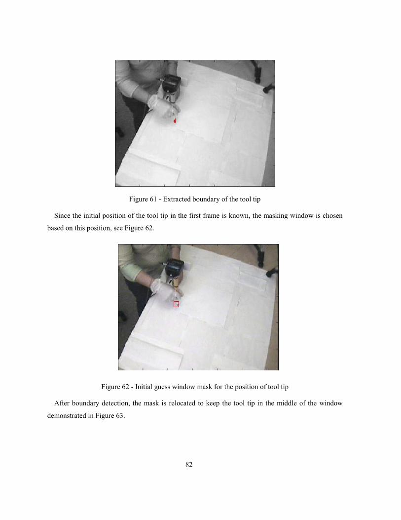
82
Figure 61 - Extracted boundary of the tool tip
Since the initial position of the tool tip in the first frame is known, the masking window is chosen
based on this position, see Figure 62.
Figure 62 - Initial guess window mask for the position of tool tip
After boundary detection, the mask is relocated to keep the tool tip in the middle of the window
demonstrated in Figure 63.
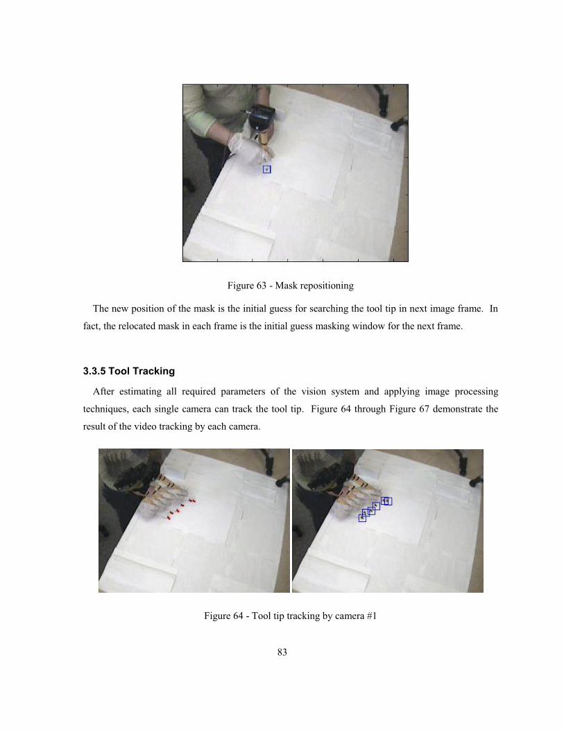
83
Figure 63 - Mask repositioning
The new position of the mask is the initial guess for searching the tool tip in next image frame. In
fact, the relocated mask in each frame is the initial guess masking window for the next frame.
3.3.5 Tool Tracking
After estimating all required parameters of the vision system and applying image processing
techniques, each single camera can track the tool tip. Figure 64 through Figure 67 demonstrate the
result of the video tracking by each camera.
Figure 64 - Tool tip tracking by camera #1
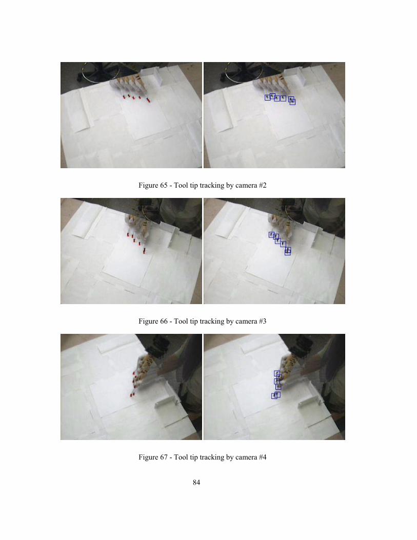
84
Figure 65 - Tool tip tracking by camera #2
Figure 66 - Tool tip tracking by camera #3
Figure 67 - Tool tip tracking by camera #4
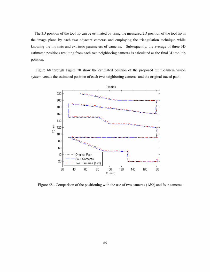
85
The 3D position of the tool tip can be estimated by using the measured 2D position of the tool tip in
the image plane by each two adjacent cameras and employing the triangulation technique while
knowing the intrinsic and extrinsic parameters of cameras. Subsequently, the average of three 3D
estimated positions resulting from each two neighboring cameras is calculated as the final 3D tool tip
position.
Figure 68 through Figure 70 show the estimated position of the proposed multi-camera vision
system versus the estimated position of each two neighboring cameras and the original traced path.
Figure 68 - Comparison of the positioning with the use of two cameras (1&2) and four cameras
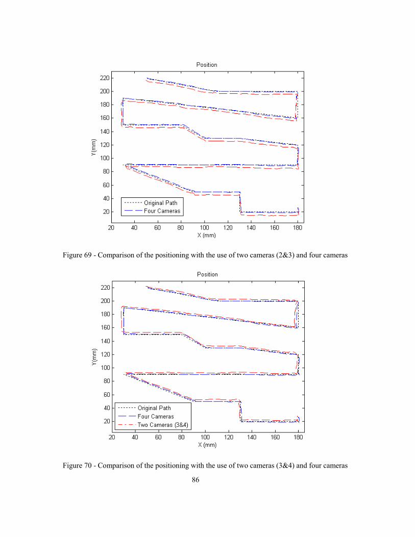
86
Figure 69 - Comparison of the positioning with the use of two cameras (2&3) and four cameras
Figure 70 - Comparison of the positioning with the use of two cameras (3&4) and four cameras
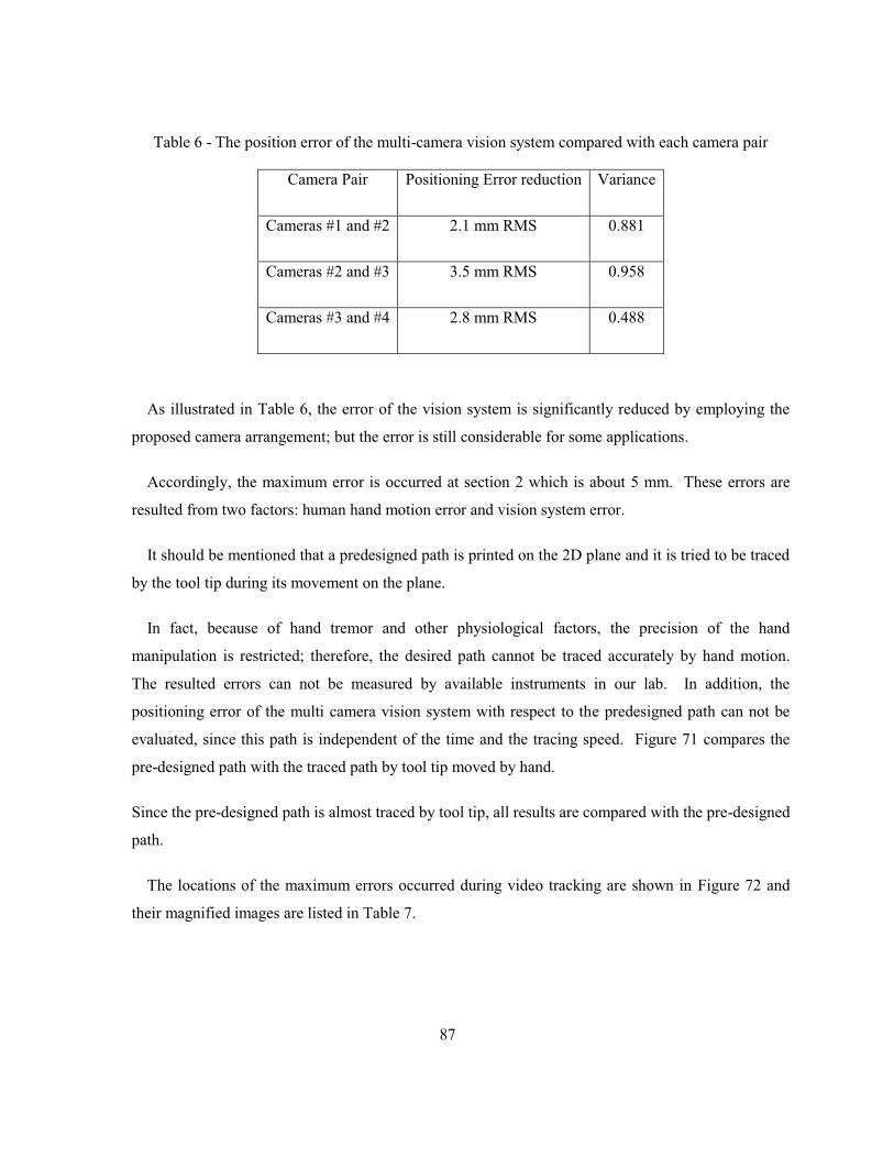
87
Table 6 - The position error of the multi-camera vision system compared with each camera pair
Camera Pair Positioning Error reduction Variance
Cameras #1 and #2 2.1 mm RMS 0.881
Cameras #2 and #3 3.5 mm RMS 0.958
Cameras #3 and #4 2.8 mm RMS 0.488
As illustrated in Table 6, the error of the vision system is significantly reduced by employing the
proposed camera arrangement; but the error is still considerable for some applications.
Accordingly, the maximum error is occurred at section 2 which is about 5 mm. These errors are
resulted from two factors: human hand motion error and vision system error.
It should be mentioned that a predesigned path is printed on the 2D plane and it is tried to be traced
by the tool tip during its movement on the plane.
In fact, because of hand tremor and other physiological factors, the precision of the hand
manipulation is restricted; therefore, the desired path cannot be traced accurately by hand motion.
The resulted errors can not be measured by available instruments in our lab. In addition, the
positioning error of the multi camera vision system with respect to the predesigned path can not be
evaluated, since this path is independent of the time and the tracing speed. Figure 71 compares the
pre-designed path with the traced path by tool tip moved by hand.
Since the pre-designed path is almost traced by tool tip, all results are compared with the pre-designed
path.
The locations of the maximum errors occurred during video tracking are shown in Figure 72 and
their magnified images are listed in Table 7.
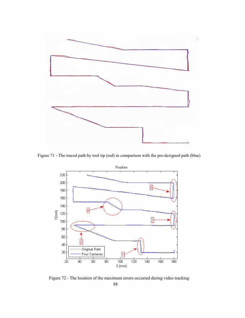
88
Figure 71 - The traced path by tool tip (red) in comparison with the pre-designed path (blue)
Figure 72 - The location of the maximum errors occurred during video tracking
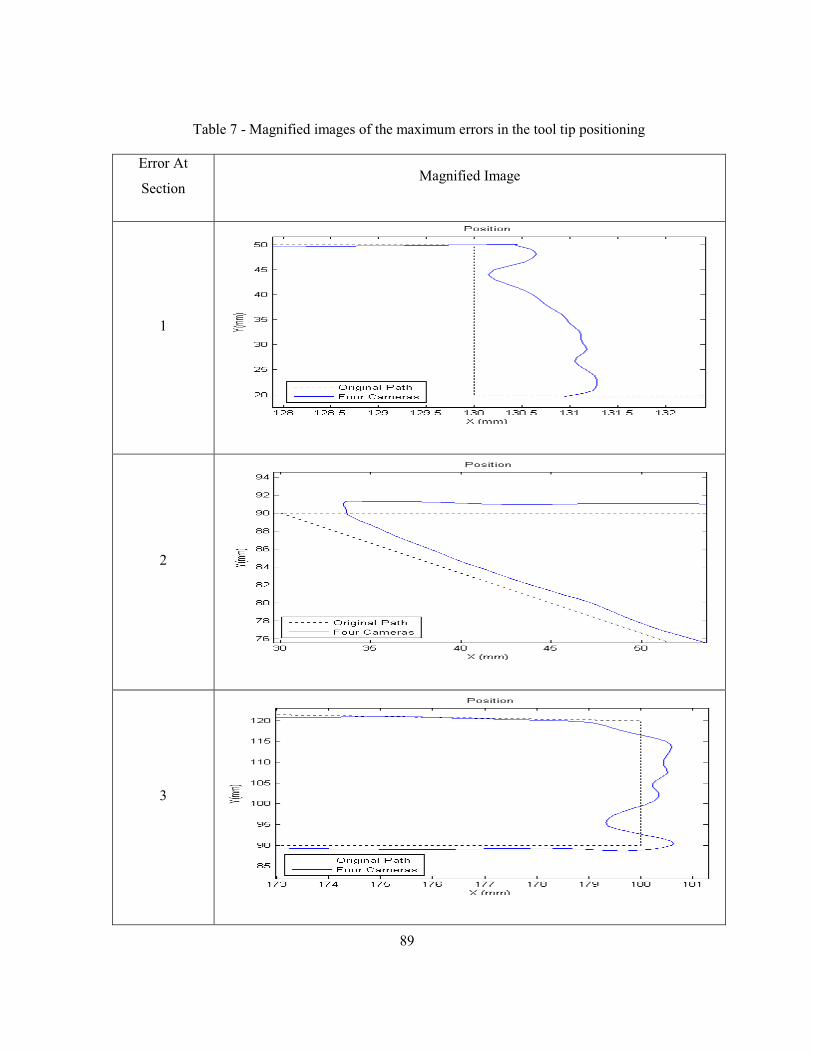
89
Table 7 - Magnified images of the maximum errors in the tool tip positioning
Error At
Section Magnified Image
1
2
3
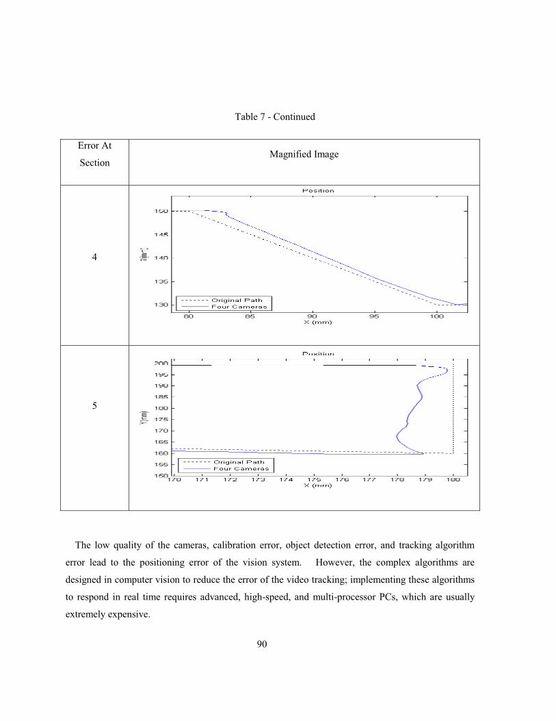
90
Table 7 - Continued
Error At
Section Magnified Image
4
5
The low quality of the cameras, calibration error, object detection error, and tracking algorithm
error lead to the positioning error of the vision system. However, the complex algorithms are
designed in computer vision to reduce the error of the video tracking; implementing these algorithms
to respond in real time requires advanced, high-speed, and multi-processor PCs, which are usually
extremely expensive.
91
3.4 Summary
This chapter details a multi-camera vision system. The proposed vision system includes
four cameras located in a semicircle instead of arranged in the classical pattern. As a result,
the entire workspace is covered by this configuration is expanded and a wide circular field of
view is provided. As a result, the possibility of the loss of line-of-sight is reduced.
Furthermore, the accuracy of the vision system increases by using multi-cameras; however,
its precision is affected by the low quality of the cameras, calibration error, object detection error,
and tracking algorithm error. Reducing the error of the video tracking requires applying complex
computer vision algorithms whose implementation algorithms needs advanced multi-processor PCs to
respond in real time.
However, low-quality cameras and simple image processing techniques are applied; the
experimental result shows that the accuracy of the multi-camera vision system is less than 5 mm and
acceptable for many applications.
92
Chapter 4 Extended Kalman Filter
Most research studies show that the inertial navigation sensors have drifts. There are two
components in the inertial sensor drift, bias stability and bias variability. These components are
involved in double integration in position calculation; so after a while, the output of the inertial
navigation system (INS) is not reliable. To remove the resulted drifts in position, the INS is assisted
by other positioning technologies such as GPS, vision system, or odometer.
The use of Kalman filters is a common method in the data fusion technique. The Kalman filter
technique is a powerful method for improving the output estimation and reducing the effect of the
sensor drift. Different Kalman filters are being developed in the area of the sensor fusion [ 20- 25].
In the past, the three-dimensional attitude representations were applied, but these representations
are singular or discontinuous for certain attitudes [ 65]. As a result, the quaternion parameterization
was proposed, which has the lowest dimensional possibility for a globally non-singular attitude
representation [ 51, 66].
In assisted inertial navigation systems, the state variables of a Kalman filter usually take one of two
forms: first, the sensed quantities such as acceleration, velocity, and attitude, etc.; and second, the
errors of these quantities. The first form is used by the centralized Kalman filter [ 25], unscented
Kalman filter [ 48, 102, 103], adaptive Kalman filter [ 50, 104], and sigma-point extended Kalman
filter [ 105], while the second one is used by the indirect Kalman filter [ 26, 27, 106].
A Kalman filter that operates on the error states is called an indirect or a complementary Kalman
filter. The optimal estimates of the errors are then subtracted from the sensed quantities to obtain the
optimal estimates. Since the 1960s, the complementary Kalman filter has become the standard
method of integrating non-inertial with inertial measurements in aircrafts and spacecrafts navigation.
This method requires dynamic models for both the navigation variable states and the error states [ 64].
In this chapter, a modified EKF is developed. In this filter method, the magnitude of the changes
in position and velocity are estimated and then added to the previous estimation of the position and
velocity, respectively.
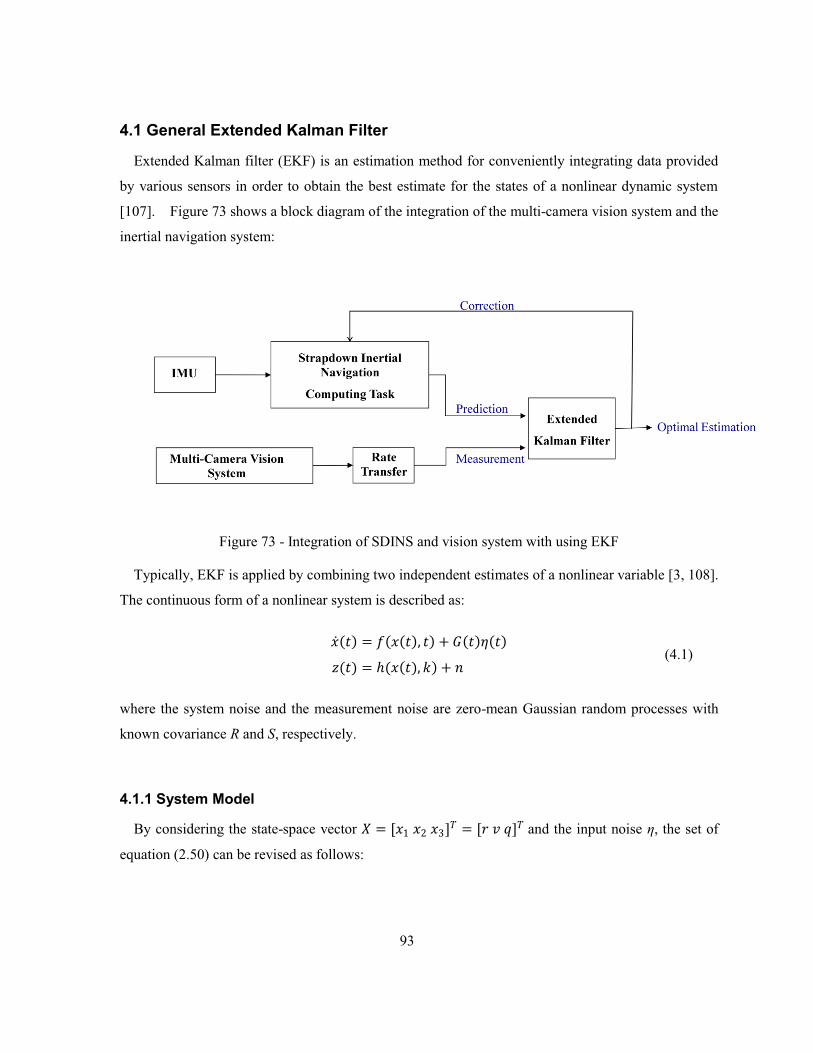
93
4.1 General Extended Kalman Filter
Extended Kalman filter (EKF) is an estimation method for conveniently integrating data provided
by various sensors in order to obtain the best estimate for the states of a nonlinear dynamic system
[ 107]. Figure 73 shows a block diagram of the integration of the multi-camera vision system and the
inertial navigation system:
Figure 73 - Integration of SDINS and vision system with using EKF
Typically, EKF is applied by combining two independent estimates of a nonlinear variable [ 3, 108].
The continuous form of a nonlinear system is described as:
�(�) = :(�(�), �) + �(�)�(�) 5(�) = ℎ(�(�), �) + �
(4.1)
where the system noise and the measurement noise are zero-mean Gaussian random processes with
known covariance R and S, respectively.
4.1.1 System Model
By considering the state-space vector � = [�1 �2 �3]� = [3 � T]� and the input noise η, the set of
equation (2.50) can be revised as follows:
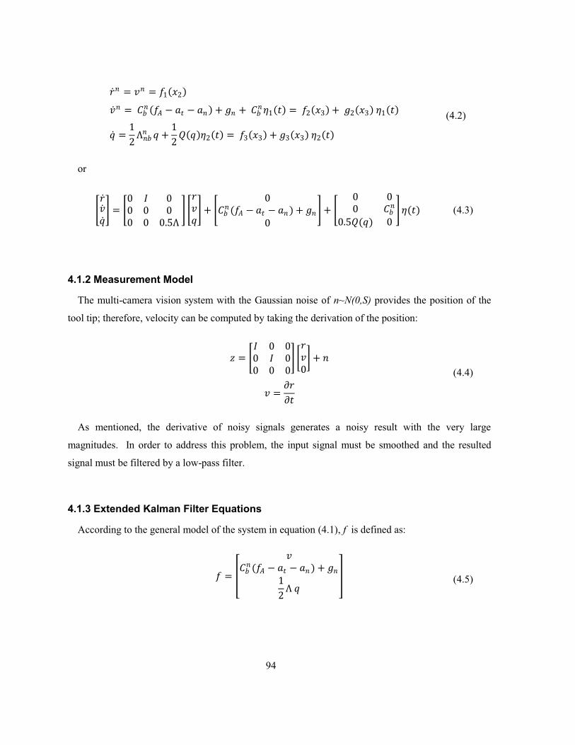
94
3� = �� = :1(�2) �� = F�� (:� − � − � ) + �� + F�� �1(�) = :2(�3) + �2(�3) �1(�) T = 12 Λ��� T + 12 \(T)�2(�) = :3(�3) + �3(�3) �2(�)
(4.2)
or
C3�TE = C0 Q 00 0 00 0 0.5Λ E C3�TE + C 0F�� (:� − � − � ) + ��0 E + C 0 00 F��0.5\(T) 0 E �(�) (4.3)
4.1.2 Measurement Model
The multi-camera vision system with the Gaussian noise of n~N(0,S) provides the position of the
tool tip; therefore, velocity can be computed by taking the derivation of the position:
5 = CQ 0 00 Q 00 0 0E `3�0g + �
� = �3��
(4.4)
As mentioned, the derivative of noisy signals generates a noisy result with the very large
magnitudes. In order to address this problem, the input signal must be smoothed and the resulted
signal must be filtered by a low-pass filter.
4.1.3 Extended Kalman Filter Equations
According to the general model of the system in equation (4.1), f is defined as:
: = % �F�� (:� − � − � ) + ��12 Λ T &
(4.5)
95
Applying the EKF requires obtaining the transition matrix by linearizing f about the current
estimated state [ 2, 109]. The following matrix F is computed by assuming the state-space vector � = [3 � T]�and = (:� − � − � ):
� ≡ ��:��¡�=�⏞ = %0 Q 00 0 ��T F�� 0 0 0.5Λ & (4.6)
where ��T F is computed as:
��T F = 2 C T11 − T42 + T33 T21 + T32 + T43 T41 + T12 − T43 T31 − T22 − T13−T31 + T22 + T13 T41 + T12 − T23�
�−T31 + T22 + T13 −T41 − T12 + T23 T21 + T32 + T43 T11 − T42 − T13−T11 + T42 − T33 T21 + T32 + T43E
(4.7)
Since the measurement model is a linear function, then the observation matrix is defined as:
� = CQ 0 00 Q 00 0 0E (4.8)
As a result, the predication and update steps of the EKF can be written as:
Prediction:
��+1 = :��⏞� , �! �¢ = �� �� ��� + �� /� ���
Update:
�⏞�+1 = ��+1 + �[5�+1 − ℎ(�� , �)] ��+1 = �¢ − ��� �¢ � = �¢���(£� + �� �¢���)−1
(4.9)
96
4.2 Modified Extended Kalman Filter
Since the sensor outputs are provided at discrete intervals of time, it is appropriate to express the
system modeling, shown in equation (4.1), in the form of discrete differential equations:
��+1 = @� �� + �� 5�+1 = ��+1��+1 + ��+1
(4.10)
where
@� = exp[�(��+1 − �� )] �(�� ) ≡ ��:��¡�=�⏞� (4.11)
4.2.1 System Model
According to equations (2.50), (4.10), and (4.11), the discrete form of the system is developed as:
3�+1 = 3� + �; �� ��+1 = �� + �;(F� � + �� + F� �1� ) T�+1 = (Q + 0.5�;Ω)T� + 0.5\(T� )�2� = :� + ω × 3�/� + ω × (ω × 3�/�)
(4.12)
where �; is the sampling rate of the inertial sensors. In this research, instead of estimating the actual
value of these quantities, we propose to estimate how much the position and the velocity will be
changed; that is,
Δ3�+1 = 3�+1 − 3� Δ��+1 = ��+1 − ��
(4.13)
Substituting equation (4.13) into equation (4.12) gives the following results:
Δ3�+1 = 3� + �;�� − 3�−1 − �;��−1 = (3� − ��−1) + �;(�� − ��−1)
⟹ Δ3�+1 = Δ3� + �;Δ�� (4.14)
97
and
Δ��+1 = �� + �; (F� � + �� + F� �1� ) − ��−1 − �; �F�−1�−1 + �� + F�−1�1(�−1)!= (�� − ��−1) + �;(F� � − F�−1�−1) + �;�F� �1� − F�−1�1(�−1)!= Δ�� + �;(F� �−1 − F�−1�−1 + F� � − F� �−1)+ �;�F� �1� − F�−1�1(�−1) + F�−1�1� − F�−1�1� !
⟹ Δ��+1 = Δ�� + �;(ΔF� �−1 + F� Δ� + ΔF� �1� + 2F� �1� )
(4.15)
As a consequence, the effect of the gravitational force is removed in the state-space model. In
fact, the error caused by inaccurate value of the gravitational force in the state-space model is
completely eliminated.
The inertial sensor noise is theoretically modeled with a zero-mean Gaussian random process. In
practice, the average of the noise is not absolutely zero. Due to the inherent characteristic of the
Gaussian random process, the discrete difference of a zero-mean Gaussian random process is also a
zero-mean Gaussian random process with very lower actual mean while its variance is twice of the
variance of the original process.
Figure 74 shows a zero-mean Gaussian random process with σ=0.01 when the actual mean is
-0.0012. While the program is generating this process, its discrete difference is calculated. As
illustrated in Figure 74, its discrete difference is also a zero-mean Gaussian random process with
σ=0.02 and actual mean=-0.000012. This shows that the average of the process is significantly
reduced. As a result, the drift resulting from the input noise is reduced and a smooth positioning is
expected.
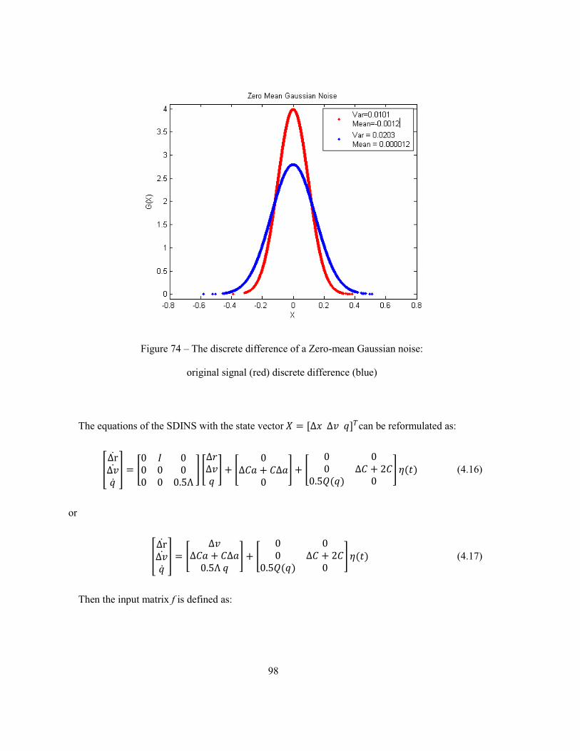
98
Figure 74 – The discrete difference of a Zero-mean Gaussian noise:
original signal (red) discrete difference (blue)
The equations of the SDINS with the state vector � = [Δ� Δ� T]�can be reformulated as:
<ΔrΔ�T B = C0 Q 00 0 00 0 0.5Λ E CΔ3Δ�T E + C 0ΔF + FΔ0 E + C 0 00 ΔF + 2F0.5\(T) 0 E �(�) (4.16)
or
<ΔrΔ�T B = C Δ�ΔF + FΔ0.5Λ T E + C 0 00 ΔF + 2F0.5\(T) 0 E �(�) (4.17)
Then the input matrix f is defined as:
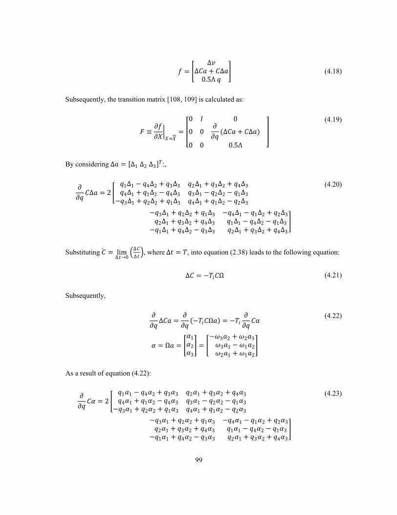
99
: = C Δ�ΔF + FΔ0.5Λ T E (4.18)
Subsequently, the transition matrix [ 108, 109] is calculated as:
� ≡ ��:��¡�=�⏞ = %0 Q 00 0 ��T (ΔF + FΔ)0 0 0.5Λ &
(4.19)
By considering Δ = [Δ1 Δ2 Δ3]�:,
��T FΔ = 2 C T1Δ1 − T4Δ2 + T3Δ3 T2Δ1 + T3Δ2 + T4Δ3 T4Δ1 + T1Δ2 − T4Δ3 T3Δ1 − T2Δ2 − T1Δ3−T3Δ1 + T2Δ2 + T1Δ3 T4Δ1 + T1Δ2 − T2Δ3�
�−T3Δ1 + T2Δ2 + T1Δ3 −T4Δ1 − T1Δ2 + T2Δ3 T2Δ1 + T3Δ2 + T4Δ3 T1Δ1 − T4Δ2 − T1Δ3−T1Δ1 + T4Δ2 − T3Δ3 T2Δ1 + T3Δ2 + T4Δ3 E
(4.20)
Substituting F = limΔ�→0 �ΔFΔ� �, where Δ� = �, into equation (2.38) leads to the following equation:
ΔF = −�;FΩ (4.21)
Subsequently,
��T ΔF = ��T (−�;FΩ) = −�; ��T Fα
w = Ω = Cw1w2w3E = C−�32 + �23 �31 − �12 �21 + �12E
(4.22)
As a result of equation (4.22):
��T Fw = 2 C T1w1 − T4w2 + T3w3 T2w1 + T3w2 + T4w3 T4w1 + T1w2 − T4w3 T3w1 − T2w2 − T1w3−T3w1 + T2w2 + T1w3 T4w1 + T1w2 − T2w3�
�−T3w1 + T2w2 + T1w3 −T4w1 − T1w2 + T2w3 T2w1 + T3w2 + T4w3 T1w1 − T4w2 − T1w3−T1w1 + T4w2 − T3w3 T2w1 + T3w2 + T4w3E
(4.23)
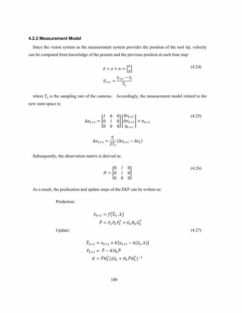
100
4.2.2 Measurement Model
Since the vision system as the measurement system provides the position of the tool tip, velocity
can be computed from knowledge of the present and the previous position at each time step:
5 = 5 + � = �3�� ��+1 = 3�+1 − 3���
(4.24)
where �� is the sampling rate of the cameras. Accordingly, the measurement model related to the
new state-space is:
Δ5�+1 = CQ 0 00 Q 00 0 0E CΔ3�+1Δ��+1T�+1 E + ��+1
Δ��+1 = �;2�� (Δ3�+1 − Δ3� )
(4.25)
Subsequently, the observation matrix is derived as:
� = C0 Q 00 Q 00 0 0E (4.26)
As a result, the predication and update steps of the EKF can be written as:
Prediction:
��+1 = :��⏞� , �! �¢ = �� �� ��� + �� /� ���
Update:
�⏞�+1 = ��+1 + �[5�+1 − ℎ(�� , �)] ��+1 = �¢ − ��� �¢ � = �¢���(2£� + �� �¢���)−1
(4.27)
101
4.3 Experimental Result
This section presents the experimental result of applying EKF and the proposed Kalman filter.
The experimental hardware includes a 3DX-GX1 IMU from Microstrain, an IDS Falcon Quattro PCIe
frame grabber from IDS Imaging Development Systems, and four surveillance IR-CCD cameras.
The integration of the SDINS and multi-camera vision system is accomplished by using classical
EKF and modified EKF described in section 4.2. The system model and measurement model, which
are derived in section 4.1 and 4.2, are substituted into the prediction and update steps.
The position estimated by both versions of Kalman filter is compared with the position estimated
by the vision system and the original path. The sensor fusion techniques allow us estimating the
states variables of the system at the sampling rate of the sensor with the highest measurement rate. In
this experiment, the sampling rate of cameras and inertial sensors are 20 fps and 100 Hz. As a result
of sensor fusion, the measurement rate of the proposed integrated system is 100 HZ. In addition, the
classical EKF is applied in both switch and continues modes. In the switch mode, the estimation of
the states variables is corrected whenever the measurement of the vision system is available.
Otherwise, the states are estimated only based on the SDINS.
In order to reduce the computational complexity of image processing algorithms, sensor fusion
allows that the sampling rate of the vision system can be reduced to 10 fps and 5 fps.
As illustrated in Table 8, the positioning error is increased by reducing the sampling rate of the
cameras. In addition, the error in proposed EKF grows faster than the other methods; since this
technique assumes that the rate of the changes in state variables is constant from one frame to another
frame. So, this assumption cannot be valid in lower measurement rates. Although, it is shown in
that the position error of the continuous EKF is less than the others; it should be mentioned that the
position obtained by the multi-camera vision system still has errors compared with the predesigned
path. As mentioned in section 3.3.5, the actual traced path is not measureable.
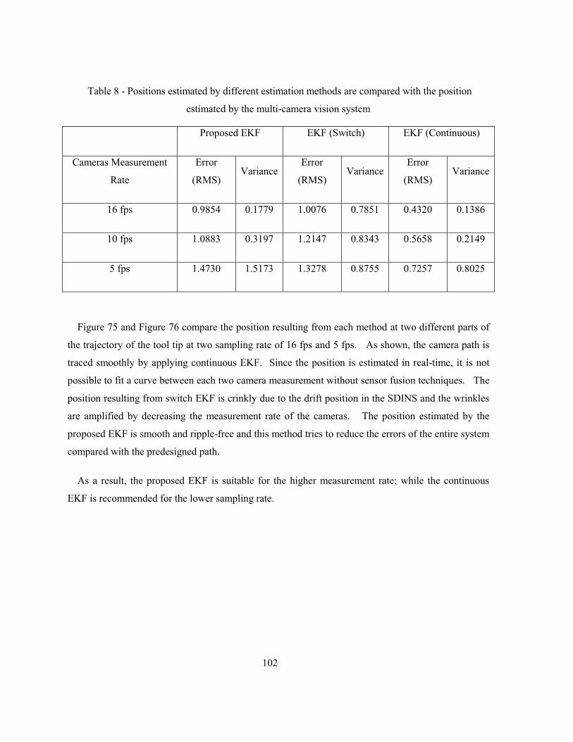
102
Table 8 - Positions estimated by different estimation methods are compared with the position
estimated by the multi-camera vision system
Proposed EKF EKF (Switch) EKF (Continuous)
Cameras Measurement
Rate
Error
(RMS) Variance
Error
(RMS) Variance
Error
(RMS) Variance
16 fps 0.9854 0.1779 1.0076 0.7851 0.4320 0.1386
10 fps 1.0883 0.3197 1.2147 0.8343 0.5658 0.2149
5 fps 1.4730 1.5173 1.3278 0.8755 0.7257 0.8025
Figure 75 and Figure 76 compare the position resulting from each method at two different parts of
the trajectory of the tool tip at two sampling rate of 16 fps and 5 fps. As shown, the camera path is
traced smoothly by applying continuous EKF. Since the position is estimated in real-time, it is not
possible to fit a curve between each two camera measurement without sensor fusion techniques. The
position resulting from switch EKF is crinkly due to the drift position in the SDINS and the wrinkles
are amplified by decreasing the measurement rate of the cameras. The position estimated by the
proposed EKF is smooth and ripple-free and this method tries to reduce the errors of the entire system
compared with the predesigned path.
As a result, the proposed EKF is suitable for the higher measurement rate; while the continuous
EKF is recommended for the lower sampling rate.
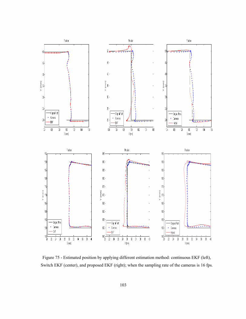
103
Figure 75 - Estimated position by applying different estimation method: continuous EKF (left),
Switch EKF (center), and proposed EKF (right); when the sampling rate of the cameras is 16 fps.
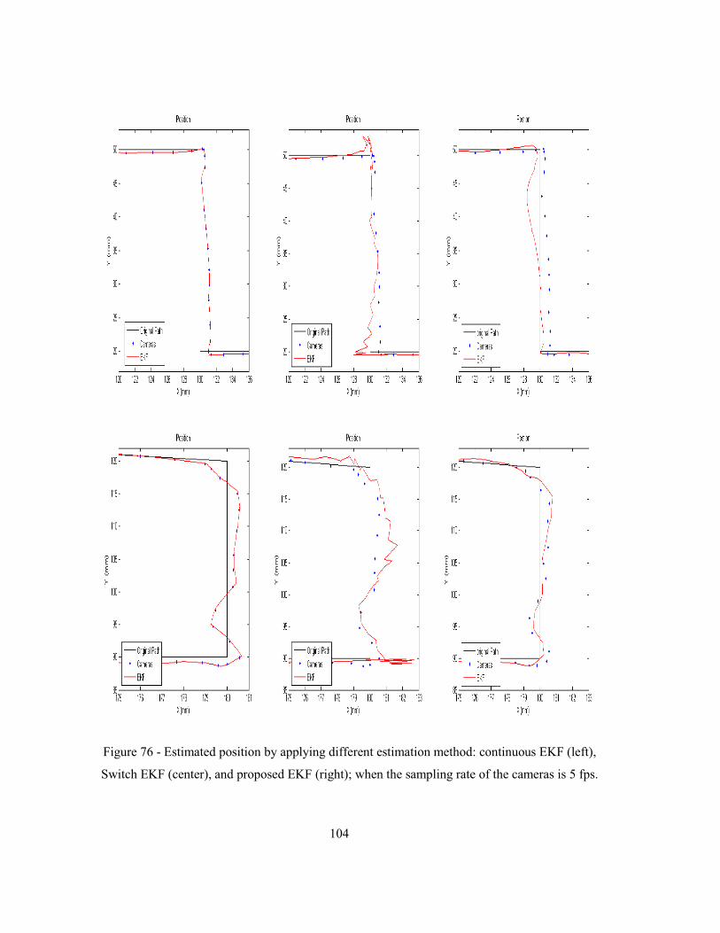
104
Figure 76 - Estimated position by applying different estimation method: continuous EKF (left),
Switch EKF (center), and proposed EKF (right); when the sampling rate of the cameras is 5 fps.
105
However, the error of inertial sensors resulting from noise and the common motion-dependent
errors are compensated according to chapter 2, but the remaining errors cause the position error
estimation in the integrated system. In addition, the video tracking errors lead to the position
estimation error as well. Since the vision data and inertial sensor outputs were not synchronized by
hardware but they were synchronized later manually, new errors were introduced in the system.
4.4 Summary
This chapter describes the use of the EKF to develop integration of the multi-camera vision system
and inertial sensors. The sensor fusion techniques allow estimating the state variables at the
sampling rate of the sensor with highest measurement rate. This helps to reduce the sampling rate of
the sensors with high computational load.
The classical EKF is designed for nonlinear dynamic system such as the strapdown inertial
navigation system. The performance of the classical EKF is reduced by lowering the sampling rate
of the cameras. When the sampling rate of the cameras is reduced, the rate of updating decreases and
the system must rely more on the inertial sensors output for estimating the position. Because of the
drift in the SDINS, the position error increases.
The modified EKF is proposed to obtain position estimation with less error. Furthermore, it
removes the effect of the gravitational force in the state-space model. In fact, the error resulting from
inaccuracy in the evaluation of the gravitational force is eliminated in the state-space model. In
addition, the estimated position is smooth and ripple-free. However; the proposed EKF is not
convincing at the lower measurement rate.
The error of the estimated position is resulted by inertial sensor errors, uncompensated common
motion-dependent errors, attitude errors, video tracking errors, and unsynchronized data.
106
Chapter 5 Conclusion and Future Work
This chapter reviews the material presented throughout the research and summarizes the major
findings and limitations of the study. It also discusses the contribution of this research to the state of
knowledge on the subject and provides suggestions for future work.
5.1 Conclusion
Chapter 1 discusses the problem of localization in the field of medical operation applications,
presents the available technologies, and describes their limitations in this area. It then introduces the
novel idea of the integration of the multi-camera vision system and strapdown inertial navigation
system by using a modified EKF, and compares it with other approaches. The chapter also previews
the organization of the thesis.
Chapter 2 describes the strapdown inertial navigation system and its implementation requirements.
It then introduces inertial sensors and inertial measurement units. The chapter also presents the
fundamental idea of the IMU design and its calibration procedure, which includes the computation of
the scale factors and compensations for the sensor misalignment, sensor bias, and sensor sensitivity to
temperature and gravitational force. In addition, it illustrates how the sensor outputs are impacted by
the common motion-dependent components and presents an algorithm to remove these components
from the measurements by applying the relative-motion analysis. This chapter also expresses that
physiological hand tremor adds Gaussian random noise to the system. Therefore, the errors produced
by the sensor noise and the tool vibration are diminished by applying a low pass filter, while the drift
resulted by the accelerometer bias is reduced by employing a high pass filter. Finally, the strapdown
inertial navigation computing task is developed to estimate the position and attitude of the hand-held
tool in addressing the common motion-dependent errors and noise problems. The experimental
results show the significant improvement of the system performance. The resulting errors are
reduced considerably, but the remaining attitude error is still great enough to cause a drift in the
position estimation.
Chapter 3 describes the Local Positioning Systems and available tracking technologies. It then
proposes a multi-camera vision system that includes four IR-CCD cameras which are aligned along a
107
semicircle. The chapter also describes the multi-camera vision system calibration procedure, which
includes single- and stereo-calibration processes for estimating the intrinsic and extrinsic cameras
parameters, and compares it with the calibration procedure for the straight line configuration. The
algorithm for aligning the world coordinate system on the navigation frame is also presented. The
experimental results of the proposed multi-camera vision system compared with those of the stereo
vision system show that the new configuration can cover the entire workspace, reduce the possibility
of the loss of line-of-sight, and increase the accuracy of the vision system. As usual, the precision of
the vision system depends on the quality of the cameras, precision of the calibration process, and
accuracy of the object detection algorithms. Reducing the error of video tracking requires the
complex computer vision algorithms. Employing these algorithms requires the use of advanced,
high-speed, and multi-processor PCs to respond in real time.
Chapter 4 presents two different extended Kalman filters for integration of the multi-camera vision
system and inertial sensors. These methods allow estimating position at the sampling rate of the
inertial sensors which have the higher measurement rate than the cameras’. The result of both version
of the Kalman filter shows improvement in the system performance. Since the modified EKF
removes the effect of the gravitational force in the state-space model, the error resulting from
inaccurate value of the gravitational force in the state-space model is eliminated. In addition, the
modified EKF reduces the error of the position estimation and results smooth and ripple free position.
Furthermore, the proposed integrated tracking system compared with the multi-camera vision
system allows a reduction of the sampling rate of the cameras without loss of accuracy. When the
sampling rate is reduced, the system implementation does not require a highly advanced PC and
system responses in real-time.
5.2 Contributions
The objective of this thesis is the design of a reliable and cost-effective positioning system with
capability of the tool localization by estimating its position and orientation in real-time. The major
contributions of this research are as follows:
108
The system is designed based on the cost-effective factor, since the precise available positioning
systems are not affordable to be used in many applications.
Responding in real time is one of the most important contributions of this research. The sampling
rate of the proposed positioning system is 100Hz at all time of its operation.
The low-cost MEMS-based IMU including three accelerometers and three rate gyros is introduced
to the system in order to provide high frequency and full dynamic range of the motion. Although, the
general equations of the SDINS computing task are applied in many navigation applications; but the
accuracy of the tool tracking system should be in the range of few millimeters. This requires
developing precise kinematics equations in order to minimize the SDINS errors resulting from the
common motion-dependent errors as much as possible. The 3D relative motion analysis and
developing required 3D kinematics equations for the hand-held tool is the other essential contribution
of this thesis.
Even though, the drift error of the SDINS is significantly reduced by developing 3D kinematics
equations; but the SDINS still lose its accuracy over the time. It is recommended that the SDINS is
integrated with a vision system associated with a sensor fusion technique to improve the accuracy of
the system and keep it in the desired range for a longer period of the time. As a matter of cost
effectiveness, it is proposed to employ the low-cost CCD cameras in the proposed vision system.
Another significant contribution of this research is the design of a multi-camera vision system with
individual configuration so as to prevent the loss of line of sight as much as possible. This
configuration proposes to place the cameras along a semicircle in order to expand the angle of view
and initiate a wide circular field of view. As a result of this arrangement, an individual calibration
procedure is designed to estimate the intrinsic and extrinsic parameters of the multi-camera vision
system, which includes the required 3D transformation to map each point expressed in the world
coordinate system of the multi-camera vision system into the SDINS navigation frame.
To address the computation load problem of the video tracking, the simple and efficient algorithms
for application in hand are selected.
Integration of the multi-camera vision system and SDINS requires an estimation method. This
research develops an EKF which offers the estimation of the changes in the state variables.

109
According to the general equations of the SDINS, the constant value of the gravitational force is
removed from the resulted equations and the resulting error from the uncertainty value of the
gravitational force is eliminated. As a result of the proposed EKF, it is expected that the resulting
drift from input noise is reduced and smooth positioning is obtained.
5.3 Future Work and Research
The design of the integrated multi-camera vision system and strapdown inertial navigation system
has not been completed in this research. More engineering efforts are required to overcome the
existing bottlenecks in the proposed system.
The performance of the system can be improved by making a few design changes in both the
hand-held tool and the multi-camera vision system.
Since the MEMS-based inertial sensors are quite small, the inertial sensors can be placed inside of
the tool and as close as possible to the tool tip. Redesigning the hand-held tool would help to reduce
the effect of the common motion-dependent errors. Besides, adding a magnetometer per axis, which
is not affected by these motions, would help to reduce the attitude errors, resulting in less error in the
position estimation. In addition, the resolution of available IMUs, which use a 16-bit analogue to
digital converter, is about 5 mg. However, the micromanipulation application requires a better
resolution, which can be provided by a 24-bit analogue-to-digital converter.
The performance of the multi-camera vision system can be increased by using eight CCD cameras
with a 45° field of view angle or twelve CCD cameras with a 30° field of view angle which can be
placed along a circle. However, a complex calibration procedure must be performed to obtain the
intrinsic and extrinsic parameters of the multi-camera vision system. Using the low-cost CCD
cameras with a higher resolution would help to reduce the error of video tracking algorithms.
In order to synchronize the multi-camera vision system and inertial sensors, additional hardware is
required to initiate both systems and obtain their outputs simultaneously.
Aside from the hardware design enhancement, improvement of the software is also required.
Future work can focus on reducing the position and attitude error by considering the effects of the

110
coning, sculling, and rotational motion more precisely in the position and attitude computation
equations in the strapdown inertial navigation computing task.
Also, the computer vision algorithms proposed in this research for object detection, image
segmentation, and object tracking can be enhanced by a few changes or be replaced by new simple
and efficient techniques. The orientation of the hand-held tool was not computed by using video
tracking algorithm in this research. This estimation can reduce the error of the attitude and position
estimation in SDINS by taking into account in the measurement model of the Kalman filter.
Finally, the classical or modified Kalman filter would be developed for the system through these
changes.
Although this research focuses on the hand-held tool tracking application, the concept of
performing compensation for the common motion-dependent errors, developing the multi-camera
vision system, and integrating the different sensors has enormous application in the localization tasks
that require accuracy enhancement.
The tracking system developed in this thesis can be applied in a variety of areas such as industry,
medicine, human motion tracking, and sports.
111
Bibliography
1 Rebello, K.J. 2004. “Applications of MEMS in Surgery,” Proceedings of the IEEE, Vol. 92,
No. 1, pp 43-55.
2 Titterton, D.H., and Weston, J.L., 2004. Strapdown Inertial Navigation Technology. The
institution of Electrical Engineers, 2nd Edition.
3 J. Farrell, J., and Barth, M., 1999. Global Positioning System and Inertial Navigation,
McGraw-Hill.
4 Northern Digital Inc., Optotrak, http://www.ndigital.com/
5 Ang, W.T., Riviere, C.N., and Khosla, K. 2001. “Design and Implementation of Active Error
Cancelling in Hand-held Microsurgical Instrument,” Proceedings of IEEE/RSJ International
Con. on Intelligent Robots and Systems, pp. 1106-1111.
6 Ang, W.T. 2004, “Active Tremor Compensation in Handheld Instrument for Microsurgery,”
PhD Thesis, tech. report CMU-RI-TR-04-28, Robotics Institute, Carnegie Mellon University,
May, 2004.
7 Ang, W.T., Khosla, K., and Riviere, C.N. 2004. “Kalman Filtering for Real-Time Orientation
Tracking of Handheld Microsurgical Instrument,” Proceedings of IEEE/RSJ International
Con. on Intelligent Robots and Systems, pp. 2574-2580.
8 Tao, Y., and Hu, H. 2008. “A Novel Sensing and Data Fusion System for 3D Arm Motion
Tracking in Tele-Rehabilitation,” IEEE Transaction on Instrumentation and Measurements,
Vol. 75, No. 5, pp. 1029-1040.
9 Tao, Y., Hu, H., and Zhou, H. 2007. “Integration of Vision and Inertial Sensors for 3D Arm
Motion Tracking in Home-based Rehabilitation,” International Journal of Robotics Research,
Vol. 26, No. 6, pp. 607-624.
10 Zhang, S.M., Hu, H., and Zhou, H. 2008. “An Interactive Internet-based System for Tracking
Upper Limb Motion in Home-based Rehabilitation,” Journal of Medical Biological
Engineering and Computing, Vol. 46, No. 3, pp. 241-249.
112
11 Zhou, H., and Hu, H., 2007. “Inertial Sensors for Motion Detection of Human Upper Limbs,”
Journal of Sensor Review, Vol. 27, No. 2, pages 151-158.
12 Rehbinder, H., and Hu, X. 2001. “Drift-Free Attitude Estimation for Accelerated Rigid
Bodies,” Proceedings of IEEE International Conference on Robotics & Automation, pp.
4244-4249.
13 Luinge, H.J. 2002. “Inertial Sensing of Human Movement,” PhD. Thesis, University of
Twente, University Press.
14 Foxlin E., Harrington M., and Altshuler Y. 1998. “Miniature 6-DOF Inertial System for
Tracking HMDs,” In SPIE Vol. 3362, Helmet and Head-Mounted Displays III, AeroSense 98,
pp. 214-228.
15 Foxlin E. 1996, “Inertial Head-Tracker Sensor Fusion by a Complementary Separate-Bias
Kalman Filter,” IEEE Proc. of VRAIS '96, pp. 185-194.
16 Bachmann, E.R., Yun, X., McKinney, D., McGhee, R.B., and Zyda, M.J. 2003. “Design and
Implementation of MARG Sensors for 3DOF Orientation Measurement of Rigid Bodies,”
Proceedings of IEEE International Con. on Robots & Automation, pp.1171-1178.
17 Yun, X., Lizarrage, M. Bachmann, E.R., and McGhee. 2003. “An Improved Quaternion-
Based Kalman Filter for Real-Time Tracking of Rigid Body Orientation,” Proceedings of
IEEE/RSJ International Con. on Intelligent Robots and Systems, pp. 1074-1079.
18 Gebre-Egziabher, D., Elkaim, G.H., Powell, J.D., and Pakinson, B.W. 2000. “A Gyro-Free
Quaternion-Based Attitude Determination System Suitable for Implementation Using Low
Cost Sensors,” Proc. IEEE Position, Location, and Navigation Symp., pp. 185-192.
19 Hofmann-Wellenhof, B. 2001. Global Positioning System: Theory and Practice, 5th edition,
Springer-Verlag.
20 Abuhadrous, I., Nashashibi, F., and Laurgeau, C. 2003. “Multi-Sensor Fusion for Land
Vehicle Localization Using RTMAPS,” Proceedings of the 11th International Conference on
Advanced Robotics, pp. 71-76.
113
21 Bian, H., Jin, Z., and Tian, W. 2005. “Study on GPS Attitude Determination System Aided
INS Using Adaptive Kalman Filter,” Measurement Science and TechNology, Vol.16, pp.
2072–2079.
22 Crassidis, J.L., Lightsey, E.G., and Markley, F.L. 1999. “Efficient and Optimal Attitude
Determination Using Recursive Global Positioning System Signal Operations,” Journal of
Guidance, Control, and Dynamics, Vol.22, No.2, pp. 193-201.
23 Crassidis, J.L., and Markley, F.L., 1997. “New Algorithm for Attitude Determination Using
Global Positioning System Signals,” Journal of Guidance, Control, and Dynamics, Vol. 20,
No. 5, pp. 891-896.
24 Kumar, N.V. 2004. “Integration of Inertial Navigation System and Global Positioning System
Using Kalman Filtering,” PhD. Thesis, Indian Institute of Technology.
25 Lee, T.G. 2003. “Centralized Kalman Filter with Adaptive Measurement Fusion: it’s
Application to a GPS/SDINS Integration System with an Additional Sensor,” International
Journal of Control, Automation, and Systems, Vol. 1, No. 4, pp. 444-452.
26 Chung, H., Ojeda, L., and Borenstein, J. 2001. “Sensor fusion for Mobile Robot Dead-
reckoning with a Precision-calibrated Fibre Optic Gyroscope,” Proc. of IEEE International
Conference on Robotics and Automation, pp. 3588-3593.
27 Chung, H., Ojeda, L., and Borenstein, J. 2004. “Accurate Mobile Robot Dead-reckoning with
a Precision-Calibrated Fibre Optic Gyroscope,” IEEE Transactions on Robotics and
Automation, Vol. 17, No. 1, pp. 80-84.
28 Persa, S., and Jonker, P. 2002. “Multi-sensor Robot Navigation System,” Proc. SPIE Int. Soc.
Opt. Eng., Vol. 4573, pp. 187-194.
29 Huster, A. 2003. “Relative Position Sensing by Fusing Monocular Vision and Inertial Rate
Sensors,” PhD. Thesis, Stanford University.
30 Foxlin, E., and Naimark, L. 2003. “VIS-Tracker: A Wearable Vision-Inertial Self-Tracker,”
Proceedings of IEEE Virtual Reality, pp. 199-206.
31 You, S., Neumann, U., and Azuma, R. 1999. “Hybrid Inertial and Vision Tracking for
Augmented Reality Registration,” Proceedings of IEEE Virtual Reality, pp. 260-267.
114
32 Lang, P., and Pinz, A. 2005. “Calibration of Hybrid Vision / Inertial Tracking Systems,”
Proceedings of the 2nd InerVis: Workshop on Integration of Vision and Inertial Sensors.
33 Parnian N., and Golnaraghi, F., 2007. “Integration of Vision and Inertial Sensors for
Industrial Tools Tracking,” Sensor Review, Vol. 27, No. 2, pp. 132-141.
34 Werb, J., and Lanzl, C. 1998. “Designing a Positioning System for Finding Things and
People Indoors,” IEEE Spectrum, Vol. 35, No. 9, pp. 71–78.
35 Kantor, G., and Singh, S. 2002. “Preliminary Results in Range–Only Localization and
Mapping,” Proceedings of IEEE International Conference on Robotics and Automation, Vol.
2, pp. 1818-1823.
36 Shim, H.S., Kim, H.S., Jung, M.J., Choi, I.H., Kim, J.H., and Kim, J.O. 1997. “Designing
Distributed Control Architecture for Cooperative Multi-Agent System and Its Real-Time
Application to Soccer Robot,” ELSEVIER Science, Robotics and Autonomous Systems, Vol.
21, pp. 149-165.
37 Tsou, M.H. 2004. “Integrated Mobile GIS and Wireless Internet Map Servers for
Environmental Monitoring and Management,” Cartography and Geographic Information
Science, Vol. 31, No. 3, pp. 153-165.
38 Giraldo, C., Helal, S., and Mann, W. 2002. “mPCA – A Mobile Patient Care-Giving Assistant
for Alzheimer Patients,” The First International Conference on Ubiquitous Computing.
39 Zekavat, S.A., Tong, H., and Tan, J. 2004. “A Novel Wireless Local Positioning System for
Airport (Indoor) Security,”Proc. of SPIE, Vol. 5403, pp. 522-533.
40 Aitenbichler, E., and Mühlhäuser, M. 2003. “An IR Local Positioning System for Smart Items
and Devices,” Proceedings of the 23rd International Conference on Distributed Computing
Systems Workshops, pp. 334-339.
41 Hightower, J., and Borriello, G. 2001. “Location Systems for Ubiquitous Computing,” IEEE
Journal of Computer, Vol. 34, No. 8, pp. 57-66.
42 Steggles, P., and Batty, P. 2003. “Local Positioning Systems: New Possibilities for Urban
Combat Training,” Ubisense Ltd, IITSEC 2003, pp.1-21.
115
43 Kelly, I., and Martinoli, A. 2004. “A Scalable, On-board Localisation and Communication
System for Indoor Multi-Robot Experiments,” Sensor Review, Vol. 24, No. 2, pp. 167–180.
44 Pfeifer, T., and Elias, D. 2003. “Commercial Hybrid IR/RF Local Positioning System,”
Kommunikation in Verteilten Systemen, Springer, Series: Informatik Aktuell, pp. 119-127.
45 Cybernet Interactive, Firefly Motion Capture System, http://www.cybernet.com/interactive/
46 Grewal, M., Weill, L.R., and Andrews, A. P., 2007. Global Positioning Systems, Inertial
Navigation, and Integration, John Wiley & Sons, 2nd Edition.
47 Ojeda, L., Chung, H., and Borenstein, J. 2000. “Precision-calibration of Fiber-optics
Gyroscopes for Mobile Robot Navigation,” Proceedings of IEEE International Conference on
Robotics & Automation, pp.2064-2069.
48 Lai, K.L., Crassidis, J.L., and Harman, R.R. 2003. “In-Space Spacecraft Alignment
Calibration Using the Unscented Filter,” Proc. of AIAA Guidance, Navigation, and Control
Conference and Exhibit, pp. 1-11.
49 Nassar, S., Schwarz, K.P., and El-Sheimy, N. 2004. “Modeling Inertial Sensor Errors Using
Autoregressive (AR) Models,” Navigation-Alexandria, Vol. 51, No. 4, pp.259-268.
50 Pittelkau, M.E., 2001. “Kalman Filtering for Spacecraft System Alignment Calibration,”
Journal of Guidance, Control and Dynamics, Vol. 24 No. 6, pp. 1187-1195.
51 Markley, F.L. 2003. “Attitude Error Representation for Kalman Filtering,” Journal of
Guidance, Control and Dynamics, Vol. 26, No. 2, pp. 311-317.
52 Chatfield, A.B. 1997. Fundamentals of High Accuracy Inertial Navigation, American
Institute of Aeronautics and Astronautics Inc, Vol. 174.
53 Aggarwal, P., Syed, Z., and El-Sheimy, N. 2008. “Thermal Calibration of Low Cost MEMS
Sensors for Land Vehicle Navigation System,” IEEE Vehicular Technology Conference, pp.
2859-2863
54 Aggarwal, P., Syed, Z., Niu, X ., and El-Sheimy, N. 2008. “A Standard Testing and
Calibration Procedure for Low Cost MEMS Inertial Sensors and Units,” The Journal of
Navigation, Vol. 61, No. 2, pp. 323-336.
116
55 Ojeda, L., and Borenstein, J., 2007. “Non-GPS Navigation with the Personal Dead-
Reckoning System,” Proceeding of SPIE, Volume 6561, pp. 65610C.
56 Foxlin, E., 2005. “Pedestrian Tracking with Shoe-Mounted Inertial Sensors,” IEEE
Computer Graphics and Applications, Vol. 25, No. 6, pp. 38-46.
57 Huddle, J. 1998. “Trends in Inertial Systems Technology for High Accuracy AUV
Navigation,” Proceedings of the 1998 Workshop on Autonomous Underwater vehicles,
AUV’98, pp. 63-73.
58 Ledroz, A., Pech, E., Cramer, D., and Mintchev, M.P., 2005. “FOG-Based Navigation in
Downhole Environement During Horizontal Drilling Utilizing a Complete Inertial
Measurement Unit: Directional Measurement-While-Drilling Surveying,” IEEE Transactions
on Instrumentation and Measurement, Vol. 54, No. 4, pp. 217-225.
59 Savage, P.G., 1998. “Strapdown Inertial Navigation Integration Algorithm Design Part I:
Attitude Algorithms,” Journal of Guidance, Control, and Dynamics, Vol.21, No.1, pp. 19-28.
60 Savage, P.G., 1998. “Strapdown Inertial Navigation Integration Algorithm Design Part 2:
Velocity and Position Algorithms,” Journal of Guidance, Control, and Dynamics, Vol.21,
No.2, pp.208-221.
61 Hibbeler, R.C., 1998. Enginnering Mechanics: Statics and Dynamics, Prentice-Hall, 2nd
Edition.
62 Greenwood, D.T., 2003. Advanced Dynamics, Cambridge, New York, Cambridge University
Press.
63 Kajita, S., Kanehiro, F., Kaneko, K., Yokio, K., and Hirukawa, H., 2001. “The 3D Linear
Inverted pendulum Mode: A Simple Modeling for a Biped Walking Pattern generation,”
Proceeding of IEEE/RSJ International conference on Intelligent Robots and Systems, Vol. 1,
pp. 239-246.
64 Friedland, B., 1974. “Analysis Strapdown navigation Using Quaternions,” IEEE Transaction
on Aerospace and Electronic systems, Vol. AES-14, No. 5, pp.764-767.
65 Pittelkau, M.E., 2003. “An Analysis of the Quaternion Attitude Determination Filter,” Journal
of Astronautical Sciences, Vol. 51, No. 1, pp. 103-120.

117
66 Markley, F.L. 2004. “Multiplicative vs. Additive Filtering for Spacecraft Attitude
Determination,” Proceeding. of the 6th Conference on Dynamics and Control of Systems and
Structures in Space (DCSSS), pp.467-474.
67 Shepperd, S.W., 1978. “Quaternion from Rotation Matrix,” AIAA Journal of Guidance,
Control, and Dynamics, Vol. 1, No. 3, pp 223-224.
68 Gaylor, D.E., 2003. “Integrated GPS/INS Navigation System for Design for Autonomous
Spacecraft Rendezvous,” PhD Thesis, The University of Texas at Austin.
69 Bortz, J.E., 1971. “A New Mathematical Formulation for Strapdown Inertial Navigation,”
IEEE Transaction on Aerospace and Electronic Systems, Vol. AES-7, No. 1, pp. 61-65.
70 Pittelkau, M. E., 2003. “Rotation Vector in Attitude Estimation,” Journal of Guidance,
Control, and Dynamics, Vol. 26, No. 6, pp.855-860.
71 http://jason.kamin.com/projects_files/equations.html, Accessed on Sep. 19, 2008
72 http://hypertextbook.com/facts/2002/JasonAtkins.shtml, Accessed on Sep. 19, 2008
73 Zhang, J., and Chu, F., 2005. “Real-Time Modeling and Prediction of Physiological Hand
Tremor,” Proceeding of Acoustics, Speech, and Signal Processing, Vol. 5, pp. v6445-v648.
74 Singh, S.P.N., and Riviere, C.N., 2002. “Physiological tremor Amplitude During retinal
Microsurgery,” Proceeding of IEEE Annual Northeast Bioengineering Conference, pp. 171-
172.
75 Gebre-Egziabher, D., Hayward, R.C., and Powell, J.D., 2004. “Design of Multi-Sensor
Attitude Determination Systems,” IEEE Transaction on Aerospace and Electronic Systems,
Vol. 40, No. 2.
76 Bouten,C.V.C., Koekkoek,K.T.M., Verduiin, M., Kodde, R., and Janssen, J.D. 1997. “A
Triaxial Accelerometer and Portable Data Processing Unit for the Assessment of Daily
Physical Activity,” IEEE Transactions on Biomedical Engineering, Vol. 44, N. 3, pp. 136-
147.
77 Foerster, F., and Fahrenberg, J. 2000. “Motion Pattern and Posture: Correctly Assessed by
Calibrated Accelerometers,” Behavior Research Method, Instrumenation, and |Computation,

118
Vol. 32, pp. 450-457.
78 Verburg, J., and Strackee, J. 1974. “Phaseless Recursive Filtering Applied to Chest Wall
Displacements and Velocities Using Accelerometers,” Med. And Bio. Eng., Vol. 4, pp. 483-
488
79 http://www.microstrain.com/, Accessed on Sep. 19, 2008
80 Okada, R., Kondoh, N., Stenger, B., 2007. “A Video Motion Capture System for Interactive
Games,” Proceeding of Machine Vision Application, pp. 186-189.
81 Verplaetse, C., 1996. “Inertial Proprioceptive Devices: Self-motion-sensing Toys and Tools,”
IBM Journal, Vol. 35, No. 3&4, pp. 639-650.
82 Bigun, J., 2006. Vision with Direction: A Systematic Introduction to Image Processing and
Computer Vision, Springer-Verlag.
83 Tsai, R.Y., 1987. “A Versatile Camera Calibration Technique for High Accuracy 3D
Machine Vision Metrology Using Off-the-shelf TV Cameras and Lenses,” IEEE Journal of
Robotics and Automation, Vol. RA-3, No. 4, pp. 323-344.
84 Fryer, J.G., and Brown, D.C., 1986. “Lens Distortion for Close-Range Photogrammetry,”
Photogrammetric Engineering and Remote Sensing Vol. 52, No. 1, pp 51-58.
85 Brown, D.C., 1966. “Decentering Distortion of Lenses,” Photometric Engineering, Vol. 32,
No. 3, pp. 444-462.
86 Brown, D.C., 1971. “Close-Range Camera Calibration,” Photogrammetric Engineering, Vol.
37, No. 8, pp. 855-866.
87 Yoneyama, S., Kikuta, H.,. Kitagawa, A., and Kitamura, K., 2006. “Lens Distortion
Correction for Digital Image Correlation by Measuring Rigid Body Displacement,” Optical
engineering, Vol. 45, No. 2, pp. 023602(1)-023602(9).
88 Clarke, T.A., Fryer, J.G., and Wang, X., 1998 “The Principal Point and CCD Cameras,” The
Photogrammetric Record, Vol. 16, No. 92, pp. 293-312.
119
89 Zhang, Z., 1999. “Flexible Camera Calibration by Viewing a Plane from Unknown
Orientations,” Proceeding of IEEE International Conference on Computer Vision, Vol. 1,
pp.666-673.
90 Forsyth, D.A., and Ponce, J., 2003. Computer Vision: A Modern Approach, Prentice-Hall.
91 Heikkila, J., 1997. “Accurate Camera Calibration and Feature-based 3-D Reconstruction
from Monocular Image Sequences”, Dissertation, University of Oulu.
92 Hartley, R., and Zisserman, A., 2003. Multiple View Geometry in Computer Vision,
Cambridge University Press, 2nd Edition.
93 Seul, M., 2000. Practical Algorithms for Image Analysis: Description, Examples, and Code,
Cambridge University Press.
94 Parker, J.R., 1997. Algorithms for Image Processing and Computer Vision, New York: Wiley
Computer Publication.
95 Gonzalez, R.C., and Woods, R.E., 2008. Digital Image Processing, Prentice-Hall, 3rd Edition.
96 Russ, J.C., 2002. The Image Processing Handbook, CRC Press, 4th Edition.
97 Jain, A.K., 1989, Fundamentals of Digital Image Processing, Prentice-Hall.
98 Haralick, R.M., and Shapiro, L.G., 1992. Computer and Robot Vision, Adison-Wesely.
99 Soile, P., 2003. Morphological Image Analysis: Principles and Applications, Springer, 2nd
Edition.
100 Klette, R., and Rosenfeld, A., 2004. Digital Geometry, Elsevier.
101 http://www.vision.caltech.edu/bouguetj/calib_doc/, Accessed on Sep. 19, 2008
102 Crassidis, J.L., and Markley, F.L., 2003,“Unscented Filtering for Spacecraft Attitude
Estimation,” Journal of Guidance, Control and Dynamics, Vol. 26, No. 4, pp. 536-542.
103 Grewal, M.S., Henderson, V.D., and Miyasako, R.S., 1991. “Application of Kalman Filtering
to the Calibration and Alignment of Inertial Navigation Systems,” IEEE Trans. on Automatic
Control, Vol. 39, No. 1, pp.4-13.
120
104 Hu, C., Chen, W., Chen, Y., and Liu, D., 2003. “Adaptive Kalman Filtering for Vehicle
Navigation,” Journal Of Global Positioning Systems, Vol. 2, No. 1, pp.42-47.
105 Merwe, R.V., and Wan, E.A., 2004. “Sigma-Point Kalman Filters for Integrated
Navigation,” Proceedings of the 60th Annual Meeting of the Institute of Navigation, pp. 641-
654.
106 Roumeliotis, S.I., Sukhatme, G.S., and Bekey, G.A., 1999. “Circumventing Dynamic
Modeling: Evaluation of the Error-State Kalman Filter applied to Mobile Robot
Localization,” Proceedings of IEEE International Conference on Robotics and Automation,
Vol. 2, pp. 1656-1663.
107 Grewal, M.S., and Andrews, A.P., Kalman Filtering: Theory and Practice Using MATLAB,
John Wiley, 2nd Edition.
108 Zarchan, P., and Musoff, H., 2005. Fundamentals of Kalman Filtering: A Practical
Approach, AIAA, 2nd Edition, 2005.
109 Ristic, B., Arulampalam, S., and Gordon, N., 2004. Beyond the Kalman Filter : Particle
Filters for Tracking Applications, Artech House.

121
Appendix A Detailed Specification for MicroStrain IMU
Parameter Specification Comments
Attitude
Range: Pitch, Roll, Yaw (°)
Static Accuracy (°)
Dynamic Accuracy (° rms)
Repeatability (°)
Resolution (°)
+/-90, 180,
180
+/- 0.5
+/- 2
+/- 0.2
0.1
No Attitude limitations
Typical, application dependent
General
Performance
A/D converter resolution (bits)
Turn on time (sec)
Analog output (Optional)
Update Rate (Hz maximum)
16
0.8
0.5V
100
4 channels, user configurable
Orientation outputs
Physical Size (mm)
Weight(grams)
65×90×25
42×40×15
75
30
With enclosure
Without enclosure
With enclosure
Without enclosure
Electrical Supply Voltage (V)
Supply Current (mA)
5.2-12 DC
65
Environmental Operating Temperature (°C)
Vibration (g rms)
Shock Limit (unpowered) (g)
Shock Limit (powered) (g)
-40 to +70
-40 to +85
4
1000
500
With enclosure
Without enclosure
20-700, white
Communications Serial Interface
Serial Communication Speed (kBaud)
RS-232, RS-
485
19.2, 38.4,
115.2
RS-485 networking optional
User selectable
Angular Rate Range (°/sec)
Bias:
1)Turn-on to turn-on repeatability (°/sec)
2) In-Run stability, fixed temp. (°/sec)
3) In-Run stability, over temp. (°/sec)
4) Short term stability (°/sec)
Angle random walk, noise (°/√hour)
Scale Factor Error (%)
Nonlinearity (% FS)
+/-300
TBD
0.1
0.7
0.02
3.5
0.5
0.2
Custom ranges available
25°C fixed temperature
After 15 minute warm up
Over -40°C to +70°C range
15 second Allan variance floor
Allan variance method
Over -40°C to +70°C range
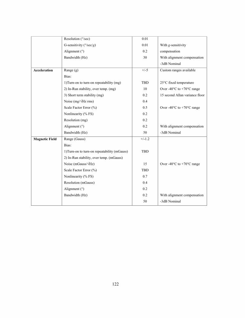
122
Resolution (°/sec)
G-sensitivity (°/sec/g)
Alignment (°)
Bandwidth (Hz)
0.01
0.01
0.2
30
With g-sensitivity
compensation
With alignment compensation
-3dB Nominal
Acceleration Range (g)
Bias:
1)Turn-on to turn-on repeatability (mg)
2) In-Run stability, over temp. (mg)
3) Short term stability (mg)
Noise (mg/√Hz rms)
Scale Factor Error (%)
Nonlinearity (% FS)
Resolution (mg)
Alignment (°)
Bandwidth (Hz)
+/-5
TBD
10
0.2
0.4
0.5
0.2
0.2
0.2
50
Custom ranges available
25°C fixed temperature
Over -40°C to +70°C range
15 second Allan variance floor
Over -40°C to +70°C range
With alignment compensation
-3dB Nominal
Magnetic Field Range (Gauss)
Bias:
1)Turn-on to turn-on repeatability (mGauss)
2) In-Run stability, over temp. (mGauss)
Noise (mGauss/√Hz)
Scale Factor Error (%)
Nonlinearity (% FS)
Resolution (mGauss)
Alignment (°)
Bandwidth (Hz)
+/-1.2
TBD
15
TBD
0.7
0.4
0.2
0.2
50
Over -40°C to +70°C range
With alignment compensation
-3dB Nominal